Angela interviews David Clarence Saturday, Oct 23, 2010 David ...
Upload
khangminh22Category
view
0download
0
To David Makonzi, my husband. Thank you for your patient endurance for all the
time we have been far from each other.
When the Lord brought back
the captives to Zion,
we were like men who dreamed.
Our mouths were filled with
laughter,
our tongues with songs of joy.
Then it was said among the nations,
“The Lord has done great things for them.”
The Lord has done great things for us,
and we are filled with joy.
Those who sow in tears will reap
with songs of joy.
He who goes out weeping,
carrying seed to sow,
will return with songs of joy,
carrying sheaves with him.
(Psalm 126, NIV Bible)


Acknowledgments
A longing fulfilled is sweet to the soul. As a girl in high school I desired to do aBachelors degree in Statistics but I instead did Bachelor of Science with Education,Mathematics and Physics as my teaching subjects. I am grateful to this mathematicalbackground which has led to masters degrees and now PhD in Statistics. Reflectingback whenceforth I have come I simply marvel. The mere term ‘model’ was a mysteryI thought I would never grasp; even worse when categorical variables were involved.But now behold, what seemed a mystery has become a comprehensible and usefultool to provide answers to real problems. Indeed the road to success is not alwaysstraight. I acknowledge support from several people who have enabled me to walkthrough this journey.
My sincere thanks go to my supervisor Prof. Dr. Marc Aerts, to my co-supervisorProf. Dr. Christel Faes and to Prof. Dr. Ziv Shkedy for guiding me and mentoring mein all the work that has led to this PhD. Thank you so very much. There were toughmoments when I felt I missed it but you always led me back on the road. You havebeen a great inspiration to me; a student is not above his teacher, but everyone whois fully trained will be like his teacher (Luke 6:40). Every opportunity and challengehas been a building block to a greater learning and I am grateful to be a part of theworld of statistical/mathematical modellers.
I would like to extend my thanks to the collaborating teams who provided the dataand with whom I have worked to produce publications. Thanks to Dr. Peter Teunis,the biostatistician at the National Institute of Public Health and the Environment(RIVM), Bilthoven, The Netherlands. Thanks to the epidemiologists at the Veterinaryand Agrochemical Research Center in Brussels: Dr. Estelle Meroc, Dr. Sarah Welby,Dr. Koen Mintiens and those I did not have a chance to meet in person. FurthermoreI would like to thank Dr. Lucas Wiessing of the European Monitoring Centre forDrugs and Drug Abuse (EMCDDA), Lisbon, Portugal and Dr. Mirjam Kretzschmarat the Julius Centre for Health Sciences & Primary Care, University Medical Centre
iii

iv
Utrecht, The Netherlands and at the Center for Infectious Disease Control, RIVM,The Netherlands.
I recall my first day in Belgium, Saturday the 14th September 2002, which turnedfrom joy to grief when I arrived at Brussels airport and there was no one to pick meas it was supposed to be. Luckily the good samaritan, Evans from California (who Ilost contact with), led me to the Limburgs Universtair Centrum (LUC) at the time.Then I met Prof. Dr. Noel Veraverbeke who drove me to the student house, carriedmy heavy suitcase to the student room and took me to Spar supermarket to buy somenecessities. My day became bright knowing I was finally at my destination. Thankyou very much Noel and I remain grateful for what you did for me that day. Withtime I got to know many CENSTAT members and I must say it has been a wonderfulexperience at CENSTAT. Thanks to all CENSTAT members for the free and friendlyenvironment to learn and work.
My special thanks go to the D3 group where I first celebrated my birthday. Thenice decorations and gifts for such a special day coupled with the spirit of togethernessmade me feel at home. Many thanks to: Prof. Dr. Ziv Shkedy, Veerle Vandersmissen,Dr. Caroline Beunckens, Suzy Van Sanden, and Arthur Gitome. I would also like tothank Annouschka Laenen who drove me to and from the Spanish classes (for the oneyear I followed the course). Thanks indeed, you saved me walking there especially inthe winter season. To Martine Bernaert and all the Spanish class colleagues, thankyou very much for your friendship. Haha! you gave me a joyful surprise when youcelebrated my 30th birthday in class. Muchas gracias!
It was during the pursuit of this PhD that David and I got married. Our specialthanks go to all who supported us and most especially the friends in Uganda whoworked tirelessly, in our absence, to make our wedding a success. Our deep appreci-ation go to all who attended our wedding. Mwebale nnyo, Mukama abawe omukisaogutaliko buyinike.
I am grateful for the spiritual nourishment I have received over the six years of mystay in Belgium. My heartfelt thanks go to the Evangelische Kerk in Diepenbeek, toThe Same Anointing Ministries in Hasselt and to Christ Centered Church in Leuven.To: Luc and Nicole, and Els Gevaert of the Evangelische Kerk, Seth and CeciliaYeboah, and to the Pastors Grace and Amponsah of The Same Anointing Ministries;thank you, respectively, for your hospitality, kindness, and advice. Pastor & MrsRobinah Kirunda of Revival Tabernacle Ministries in Uganda, you are a real blessingin my life. I have seen God fulfill the promises He spoke to me through you in theyear 2002 and I cannot forget the wonderful moments of prayer, free sharing andencouragement we had at Lungujja. Many thanks indeed and thanks to the members

v
of the Revival Tabernacle Ministries.Just as wisdom is a shelter so money is a shelter (Ecclesiastes 7:12). Without the
financial support from the Vlaamse Interuniversitaire Raad (VLIR) (for the masters)and the Bijzonder Onderzoeksfonds (BOF) “BOF04G01” (for the PhD), all theseexperiences in Belgium would not have happened. More to the academic achievement,I had the opportunity to travel to other nations for conferences or visits and this tome was a superb adventure of the globe. Thank you very much for your generosity.
The name of the Lord, Jesus Christ, be praised for his unfailing love and his won-derful deeds for men.
Harriet Namata
September 15, 2008


Contents
1 Introduction 1
1.1 Research Problem . . . . . . . . . . . . . . . . . . . . . . . . . . . . . 31.2 Modeling Human to Human Infectious Diseases Data . . . . . . . . . . 41.3 Dose-Response Modeling of Food-Borne Infectious Diseases . . . . . . 61.4 Modeling Data on Salmonella Infection in Belgian Chicken Flocks . . 9
I Human to Human Infectious Diseases Data Modeling 13
2 Estimation of the Force of Infection from Current Status Data Using
Generalized Linear Mixed Models 15
2.1 Estimation of Prevalence from Current Status Data . . . . . . . . . . 182.2 Smoothing Binary Data Using GLMM . . . . . . . . . . . . . . . . . . 19
2.2.1 Generalized Linear Mixed Models . . . . . . . . . . . . . . . . . 192.2.2 Penalized Spline Formulation as GLMM . . . . . . . . . . . . . 202.2.3 Parameter Estimation . . . . . . . . . . . . . . . . . . . . . . . 212.2.4 Estimation of the Force of Infection . . . . . . . . . . . . . . . 22
2.3 Data Analysis . . . . . . . . . . . . . . . . . . . . . . . . . . . . . . . . 232.3.1 Bootstrap Confidence Intervals . . . . . . . . . . . . . . . . . . 25
2.4 Simulation . . . . . . . . . . . . . . . . . . . . . . . . . . . . . . . . . . 262.5 Discussion . . . . . . . . . . . . . . . . . . . . . . . . . . . . . . . . . . 32
3 Modeling the Force of Infection for Parvovirus B19 in Europe Using
Penalized Spline Models 39
3.1 Data . . . . . . . . . . . . . . . . . . . . . . . . . . . . . . . . . . . . . 413.2 Estimating the Force of Infection Using Penalized Splines . . . . . . . 43
3.2.1 Simple GLMM Spline Model . . . . . . . . . . . . . . . . . . . 433.2.2 Extension of the Basic Model . . . . . . . . . . . . . . . . . . . 44
vii

viii Contents
3.2.3 Model (3.2) . . . . . . . . . . . . . . . . . . . . . . . . . . . . . 453.2.4 Model (3.3) . . . . . . . . . . . . . . . . . . . . . . . . . . . . . 453.2.5 Model (3.4) . . . . . . . . . . . . . . . . . . . . . . . . . . . . . 453.2.6 Proportional Odds and Proportional Hazard Models . . . . . . 46
3.3 Estimation and Model Selection . . . . . . . . . . . . . . . . . . . . . . 483.3.1 Quasi-Likelihood Estimation . . . . . . . . . . . . . . . . . . . 483.3.2 Hierarchical Bayesian Modeling . . . . . . . . . . . . . . . . . . 49
3.4 Application to the Data . . . . . . . . . . . . . . . . . . . . . . . . . . 503.4.1 Quasi-Likelihood Estimation . . . . . . . . . . . . . . . . . . . 503.4.2 Full Bayesian Approach . . . . . . . . . . . . . . . . . . . . . . 57
3.5 Piecewise Constant Force of Infection . . . . . . . . . . . . . . . . . . 603.6 Discussion and Conclusion . . . . . . . . . . . . . . . . . . . . . . . . . 66
4 Estimation of the Prevalence and Force of Infection of Hepatitis C
Among Injecting Drug Users in Five European Countries 69
4.1 Data and Methods . . . . . . . . . . . . . . . . . . . . . . . . . . . . . 714.1.1 Study Design . . . . . . . . . . . . . . . . . . . . . . . . . . . . 714.1.2 The Exposure Time - The Length of the Injection Career . . . 774.1.3 Statistical Methodology . . . . . . . . . . . . . . . . . . . . . . 79
4.2 Data Analysis . . . . . . . . . . . . . . . . . . . . . . . . . . . . . . . . 814.2.1 Descriptive Analysis . . . . . . . . . . . . . . . . . . . . . . . . 814.2.2 Modeling the Prevalence and Force of Infection . . . . . . . . . 844.2.3 Second Analysis: IDUs With Recent Injecting Career . . . . . 91
4.3 Discussion . . . . . . . . . . . . . . . . . . . . . . . . . . . . . . . . . . 92
II Dose-Response Modeling of Food-Borne Infectious Dis-eases 95
5 Model Averaging in Microbial Risk Assessment Using Modified Frac-
tional Polynomials and Generalized Linear Mixed Models 97
5.1 Microbial Dose-Response Models . . . . . . . . . . . . . . . . . . . . . 995.1.1 A Generic Mechanistic Dose-Response Model . . . . . . . . . . 1005.1.2 Fractional Polynomials . . . . . . . . . . . . . . . . . . . . . . . 104
5.2 Model Averaging Approach . . . . . . . . . . . . . . . . . . . . . . . . 1065.3 Application to Single Strain Data . . . . . . . . . . . . . . . . . . . . . 107
5.3.1 Salmonella Typhi . . . . . . . . . . . . . . . . . . . . . . . . . . 1095.3.2 Campylobacter Jejuni . . . . . . . . . . . . . . . . . . . . . . . 111

Contents ix
5.4 Simulation Study for Single Strain Data . . . . . . . . . . . . . . . . . 116
5.4.1 First Setting . . . . . . . . . . . . . . . . . . . . . . . . . . . . 117
5.4.2 Second Setting . . . . . . . . . . . . . . . . . . . . . . . . . . . 119
5.4.3 To Include Fractional Polynomials or Not . . . . . . . . . . . . 123
5.5 Application to Multi-Strain Data . . . . . . . . . . . . . . . . . . . . . 124
5.6 Simulation Study for Multi-Strain Data . . . . . . . . . . . . . . . . . 131
5.7 Discussion . . . . . . . . . . . . . . . . . . . . . . . . . . . . . . . . . . 134
III Modeling Data on Salmonella Infection in Broiler andLayer Chicken Flocks 137
6 Risk Factor Identification for Salmonella in Belgian Laying Hens 139
6.1 Material and Methods . . . . . . . . . . . . . . . . . . . . . . . . . . . 141
6.1.1 Data Collection . . . . . . . . . . . . . . . . . . . . . . . . . . . 141
6.1.2 Single-Level Analysis . . . . . . . . . . . . . . . . . . . . . . . . 142
6.1.3 Two-Level Analysis . . . . . . . . . . . . . . . . . . . . . . . . . 142
6.1.4 Three-Level Analysis . . . . . . . . . . . . . . . . . . . . . . . . 144
6.2 Results . . . . . . . . . . . . . . . . . . . . . . . . . . . . . . . . . . . . 145
6.2.1 Data Exploration . . . . . . . . . . . . . . . . . . . . . . . . . . 145
6.2.2 Data Analysis . . . . . . . . . . . . . . . . . . . . . . . . . . . . 148
6.3 Discussion . . . . . . . . . . . . . . . . . . . . . . . . . . . . . . . . . . 152
7 Prevalence and Persistence of Salmonella in Belgian Broiler Chicken
Flocks: An Identification of Risk Factors. 155
7.1 Materials and Methods . . . . . . . . . . . . . . . . . . . . . . . . . . . 157
7.1.1 Data Collection . . . . . . . . . . . . . . . . . . . . . . . . . . . 157
7.1.2 Data Description . . . . . . . . . . . . . . . . . . . . . . . . . . 158
7.1.3 Data Analysis . . . . . . . . . . . . . . . . . . . . . . . . . . . . 161
7.2 Results . . . . . . . . . . . . . . . . . . . . . . . . . . . . . . . . . . . . 163
7.2.1 Data Description . . . . . . . . . . . . . . . . . . . . . . . . . . 163
7.2.2 Conditional Analysis . . . . . . . . . . . . . . . . . . . . . . . . 168
7.2.3 Joint Analysis . . . . . . . . . . . . . . . . . . . . . . . . . . . . 173
7.3 Discussion . . . . . . . . . . . . . . . . . . . . . . . . . . . . . . . . . . 175
8 Concluding Remarks and Future Research 179
8.1 Modeling Human to Human Infectious Diseases Data . . . . . . . . . . 179
8.2 Dose-Response Modeling for Food-borne Infectious Diseases . . . . . . 180

x Contents
8.2.1 Single Strain . . . . . . . . . . . . . . . . . . . . . . . . . . . . 1808.2.2 Several Strains . . . . . . . . . . . . . . . . . . . . . . . . . . . 181
8.3 Modeling Data on Salmonella Infection in Broiler and Layer ChickenFlocks . . . . . . . . . . . . . . . . . . . . . . . . . . . . . . . . . . . . 183
References 185
Samenvatting 203

Chapter 1
Introduction
Pathogenic microorganisms, such as bacteria, viruses, parasites or fungi are respon-sible for several infectious diseases that bother human and animal health worldwide(Haas et al. 1999; FAO/WHO, 2003). Infectious diseases can range from the commonillnesses, such as the cold, to deadly illnesses, such as HIV/AIDS. They are referredto as infectious due to their potentiality to be transmitted from one person or speciesto another. Human to human infectious diseases can be spread through the follow-ing ways: sexual transmission e.g. hepatitis B, HIV/AIDS; airborne transmissionthrough inhaling airborne droplets of the organism, which may exist in the air as aresult of a cough or sneeze from an infected person e.g. influenza; blood-borne trans-mission through contact with infected blood, such as through blood transfusions orwhen sharing contaminated needles and syringes e.g. hepatitis B and C, HIV/AIDS;and through direct skin contact with an infected person e.g. measles. Infectious dis-eases, such as malaria, can also be transmitted to humans through insects, such asmosquitoes, which draw blood from an infected person and then bite a healthy person.Food- and water-borne infectious diseases are transmitted to humans by consump-tion of contaminated food and water e.g. typhoid fever. Furthermore consumption offoods of animal origin, particularly eggs, meat and milk products, can lead to zoonoticdiseases (transferred from animals to humans) like Salmonella. Zoonotic diseases canalso be airborne like avian influenza.
Although all these infectious diseases are caused by harmful microorganisms, theliterature on microbiological risk assessment is devoted to food- and waterborne in-fectious pathogens (Haas et al. 1999; FAO/WHO, 2003). However, it can be seen ingeneral that the steps of microbiological risk assessment apply for infectious diseases
1

2 Chapter 1. Introduction
of humans. The first step in microbial risk assessment deals with identifying the in-fectious agent and the associated adverse effect based on various data sources such asclinical literature, clinical microbiologists, case studies, hospitalization studies, labo-ratory animal studies and other epidemiological data. This step can be generalizedto all infectious diseases as the source of the disease must be identified before controland prevention interventions can be established.
In the second step of microbial risk assessment, which is exposure assessment,scientists seek to determine the size and population exposed to a pathogenic microor-ganism, the routes of exposure, the quantities exposed to, duration of exposure andwhether the exposure was continuous or intermittent. While the quantities of ex-posure are often termed as dose for food-borne diseases, they are equivalent to thefrequency of injecting among injecting drug users for human to human infectious dis-eases such as hepatitis C (HCV). Increased doses can occur due to exposure to a singlelarge dose of the pathogen, repeated doses of the pathogen or prolonged duration ofexposure or a cumulative dose that survives in the body. For HCV and sexually trans-mitted diseases, the duration of exposure is the exposure time to the contaminatedobjects or infected persons while for diseases like measles the duration is the age.
The key concept in the third step of microbial risk assessment, which is dose-response assessment, is to evaluate the relationship between the microbial dose andthe adverse effect. Figure 1.1 shows the scatter plots of food-borne disease data (panela) and human to human infectious diseases data (panels b to d). Strong relationshipscan be seen between Salmonella Typhi and log(dose); between HCV seroprevalenceand the frequency of injection among injecting drug users in Czech Republic – permonth or per week or per day; between HCV seroprevalence and the exposure timein Belgium; and between rubella seroprevalence in the UK versus the age of theindividual.
The final step of microbial risk assessment is risk characterization. This step in-tegrates the information from the previous steps in order to estimate the magnitudeof the public health problem in an exposed population taking into account variabilityand uncertainty at each step. For food- and water-borne diseases the quantificationof risk is a function of the hazard and exposure dose. For human to human infectiousdiseases the risk can be expressed in terms of age or number of contacts or exposuretime. The curves for the predicted probabilities added to the scatter plots in Fig-ure 1.1 give an easy-to-comprehend view on the relationship of the exposure variable(horizontal-axis) on the occurrence of the diseases (vertical-axis). An important issuein the risk characterization of human to human infectious diseases considers the ratioof the first derivative of the estimated probability function and the complement of the

1.1. Research Problem 3
1 3 5 7 9
log10(Dose)
0.0
0.2
0.4
0.6
0.8
1.0
prev
alen
ce o
f S. T
yphi
(a)
< 1/m 1-4/m 2-3/m 4-6/week daily > 1/day
Frequency of injection
0.25
0.30
0.35
0.40
HC
V s
erop
reva
lenc
e
(b)
0 10 20 30 40
Age
0.0
0.2
0.4
0.6
0.8
1.0
Rub
ella
ser
opre
vale
nce
(c)
0 10 20 30 40
Exposure time (years)
0.0
0.2
0.4
0.6
0.8
1.0
HC
V s
erop
reva
lenc
e
(d)
Figure 1.1: Scatter plot of the observed and estimated probability of (a) SalmonellaTyphi as a function of dose, (b) hepatitis C against the frequency of injecting (c)rubella as a function of age and (d) hepatitis C as a function of exposure time.
probability to give the rate at which people become infected. The rest of the thesisfocuses on specific risk characterizations as will be discussed further on.
1.1 Research Problem
The main area of work of this thesis was using data and mathematical and/or statis-tical models to estimate risks and trends as well as to identify risk factors associatedwith some bacterial and viral microbial agents in order to enable epidemiologists toimprove the understanding of the epidemiology of these infectious diseases and eval-uate the impact of intervention programmes against the diseases. It weaves togetherdifferent research problems and depending on the data at hand different aspects re-garding the statistical methods are emphasized. The thesis is divided into three

4 Chapter 1. Introduction
parts which deal, respectively, with modeling data on infectious diseases of humans,dose response models for foodborne infectious diseases and identifying risk factors forSalmonella infection in Belgian chicken flocks. How the various modeling techniqueshave been integrated into these parts is explained in the following sections.
1.2 Modeling Human to Human Infectious Diseases
Data
In the first part we analyze cross-sectional current-status data from serological diag-nostics for less to more severe viral infections like rubella, varicella, mumps, parvovirusB19, hepatitis C virus, hepatitis B virus and HIV. For an example, Figure 1.2 depictsthe data sets, for the occurrences of rubella and mumps in the UK and varicella in Bel-gium, with age. There is relevant information represented by the points in the plotsbut it is very difficult to draw any conclusion from this alone. With mathematical orstatistical modeling the data sets can be reduced to summaries that can give insightsin the epidemiology of the disease and that can be used for prediction and can beintegrated in the mathematical modeling of the disease. For a typical childhood infec-tious disease, the flow diagram in Figure 1.3 shows how the individuals move from thesusceptible class (X) at birth, become infected (Y), recover and acquire life-long im-munity (Z). Figure 1.3 represents a basic SIR (Susceptible-Infected-Removed) modelbut more complex models, assuming maternal antibody and a latent period can beused to describe the flow of individuals between the disease stata. One very importantparameter of interest in infectious disease epidemiology is the force of infection `(a),which is the rate at which the susceptible individuals become infected. It is assumedto vary across age groups (discussed further in Part I). The modeling of the force ofinfection can take on parametric models, nonparametric models or semi-parametricmodels. Muench (1934) modeled the force of infection using a constant model whileGriffiths (1974) used the linear model and Grenfell and Anderson (1985) employed amore flexible polynomial model. Shkedy et al. (2006) used fractional polynomials tomodel age dependent force of infection. Hens et al. (2007) illustrates joint modelingof the force of infection for varicella-zoster virus and the parvo B19-virus in Belgiumusing flexible marginal and conditional models. Shkedy et al (2003) proposed to uselocal polynomials as a nonparametric approach. Keiding (1991) proposed modelingthe force of infection using isotonic regression models. Keiding et al (1996) used analternative modeling approach based on natural cubic splines. Nagelkerke et al (1999)estimated the force of infection using a semi-parametric approach via smoothing cu-

1.2. Modeling Human to Human Infectious Diseases Data 5
(a) Rubella
age
sero
prev
alen
ce
0 10 20 30 40
0.0
0.2
0.4
0.6
0.8
1.0
(b) Mumps
age
sero
prev
alen
ce
0 10 20 30 40
0.0
0.2
0.4
0.6
0.8
1.0
(c) Varicella
age
sero
prev
alen
ce
0 10 20 30 40 50
0.0
0.2
0.4
0.6
0.8
1.0
Figure 1.2: Serological dataset: (a) rubella and (b) mumps in the UK and (c) varicellain Belgium.
Birth - X±°²¯
-
?
`(a)Y
?
±°²¯
- Z
?
±°²¯
Susceptible(Years) (Days)
Infected(Life long)Immune
Figure 1.3: Illustration of the SIR model. The individuals are entered into the sus-ceptible class, then move to the infected class and after recovering they move into theimmune class. The force of infection, `(a), will be discussed further in Part I.
bic splines and the proportional hazards model. In Chapter 2 we estimate the forceof infection using nonparametric regression based on penalized regression splines and

6 Chapter 1. Introduction
generalized linear mixed models, with the nonparametric component involving a sin-gle continuous predictor (e.g. age). Chapter 3 extends the nonparametric approachin Chapter 2 with a discrete predictor in various ways and shows the flexibility ofpenalized splines as they relate to proportional odds, proportional hazard models,and constant piecewise force of infection. In Chapter 4, in addition to parametric andnonparametric modeling of the prevalence and force of infection, we investigate riskfactor behaviors associated with hepatitis C virus among injecting drug users in fiveEuropean countries.
1.3 Dose-Response Modeling of Food-Borne Infec-
tious Diseases
Food-borne illness is among the most widespread public health problems and createssocial and economic burdens in addition to human suffering. Figure 1.4 (Haas etal. 1999) shows some of the ways microbes can be transferred from stool to food orwater, which can result in diseases like salmonellosis. Once exposure via ingestion hastaken place the major steps involved in the food-borne disease process are shown inFigure 1.5 (FAO/WHO, 2003). Each ingested organism has a probability of survivingall barriers to reach a target site for growth or multiplication. While infections may beasymptomatic, where a host does not develop any adverse reactions to the infectionand eliminates the pathogens within a limited period of time (i.e. recovers), infectionsmay also lead to symptomatic illness. In a small fraction of ill cases, chronic infectionor sequelae may occur and there may be risk to mortality related to sequelae or acutedisease.
The key concept in developing dose response models is the relation between theactual surviving organisms (the effective dose) and the probability of occurrence ofan adverse event to the host when considering dichotomous responses. This relationhas been described using mathematical and statistical functions based on biologicaland empirical rationales (Haas et al. 1999). The exponential and the Beta-Poissonmodels have received much attention in dose response modeling owing to their bi-ological derivation (Haas et al. 1999). These models fall in the class of hit-theorymodels, which assume that a single infectious microorganism surviving within thehost may result in infection (Teunis et al. 1996). Alternative models, though notwidely used in microbial risk assessment, which assume the existence of a thresholdlevel of pathogens that must be ingested in order for the microorganism to produceinfection or disease are discussed by (Haas et al. 1999). In addition, empirical mod-

1.3. Dose-Response Modeling of Food-Borne Infectious Diseases 7
Figure 1.4: Routes of transmission in the home for fecal-oral microorganisms
IllnessExposure Sequelae
Recovery
Infection
Death
Figure 1.5: The major steps in the foodborne infectious disease process

8 Chapter 1. Introduction
els (primarily for chemical agents), which assume that the population exposed has atolerance distribution for an adverse effect have been used in microbial dose responseassessment (Haas et al. 1999). If the population is exposed to the pathogen at a cer-tain level, all individuals of the population who have a tolerance less or equal to thedosed level will exhibit the adverse effect. Essentially any probability density functionwith support over the positive line can be a tolerance distribution. Despite the useof empirical models they were not regarded as biological plausible (Haas et al. 1999).However, starting from the general mechanistic framework to derive the exponentialand Beta-Poisson models, Kodell et al. (2002) derive the empirical models such asthe log logistic, log probit, the extreme value and other models thus rendering thembiologically plausible. This shows that in essence many functions can be derived thatare flexible enough for dose-response relations. Chapter 5 of part II extends the abovementioned dose response models with modified fractional polynomial models (startingwith the fractional polynomials by Royston and Altman, 1994) that are formulatedto satisfy biological plausibility. However, when extrapolating outside the region ofobserved data, all possible models may predict widely differing results (Coleman andMarks, 1998; Holcomb et al. 1999). This necessitates a selection of the best model ora set of models to use.
The traditional approach was based on one best model selected according to somestatistical criterion for goodness of fit such as the Akaike Information Criterion (AIC),Kullback Information Criterion (KIC) or Deviance Information Criterion (DIC) in thecase of full Bayesian models. This approach, however, ignores the other possible mod-els and one makes statistical inference based on the single selected model. In addition,many different models (as shown in Chapter 5) will usually fit a given data set equallywell and therefore goodness of fit is not a sufficient criterion for model selection. Overthe past decade research in risk assessment has been directed to study and incor-porate uncertainty arising from the alternative dose response models. Buckland etal. (1997) proposed a way to incorporate model uncertainty by averaging across aplausible set of candidate models using Akaike weights and this has been employedby other researchers (Burnham and Anderson, 2002). In Chapter 5 we present thismodel averaging approach to estimate the risks of Salmonella Typhi and Campylobac-ter jejuni at low doses using the proposed modified set of fractional polynomials inaddition to the Beta-Poisson model and the classical empirical models.

1.4. Modeling Data on Salmonella Infection in Belgian Chicken Flocks 9
1.4 Modeling Data on Salmonella Infection in Bel-
gian Chicken Flocks
Salmonella, named after the American veterinary pathologist Daniel Elmer Salmon,was first isolated in 1885 from pigs (Microsoft R© Encarta R©, 2008). The bacteriumis a genus of rod-shaped infectious bacteria that is transmitted to humans throughconsumption of contaminated poultry, eggs, pork and certain other foods and cancause diseases of the intestines. Salmonella Enteritidis is one of the species thatinfects chicken flocks without causing visible disease, and can spread from hen tohen rapidly. The left panel of Figure 1.6 (Microsoft R© Encarta R©, 2008) shows aSalmonella bacterium which can move by means of fine threadlike projections calledflagella. The arrangement of flagella across the surface of the bacterium differs fromspecies to species; they can be present at the ends of the bacterium or all across thebody surface. The right panel of Figure 1.6 shows the Salmonella Enteritidis species(Kunkel, 2007).
Figure 1.6: Left Panel: Salmonella bacterium showing flagella. Right panel:Salmonella Enteritidis - rod prokaryote (bacterium). This zoonotic microorganismcauses salmonellosis (food poisoning) in humans when infected poultry contaminateeggs, poultry meat (which humans ingest).

10 Chapter 1. Introduction
In Belgium, the identification of the flock’s or farm’s Salmonella status is oftentimes based on testing a number of different samples from the same flock or farm,giving rise to correlated data. Such clustered binary responses, disease status in thiscase, also frequently arise in other epidemiologic applications. The scientific objectivesinvolve: (i) modeling the marginal mean responses, such as the probability of disease,and the within-cluster association of the multivariate responses and (ii) modeling thecluster-specific responses and the heterogeneity of clusters. In this regard, statisticalmodels which incorporate and study the clustered type of data are a useful procedure.They are extensions of the well-known logistic regression that is a particular caseof the generalized linear models with binary response data and a logit link function(McCullagh and Nelder, 1989). They are usually classified into marginal (a populationaveraged) and random-effects models. We will briefly describe two marginal models,generalized estimating equations (GEE) and the alternating logistic regression (ALR)models and the general form of random effects models. For details about these modelsthe reader is referred to Liang and Zeger (1986), Carey et al. (1993), Agresti (2002),Molenberghs and Verbeke (2005) and Aerts et al. (2002).
The generalized estimating equations method, originally proposed by Liang andZeger (1986) also outlined by Bobashev and Anthony (1998) is a commonly usedmarginal model for clustered data which accounts for the correlation of a diseasewithin clusters. Let Yij denote the jth response at time point tij(j = 1, . . . , ni) forcluster i(i = 1, . . . , N) with expectation πi and a working covariance matrix Vi. Thiscovariance matrix Vi is an ni × ni matrix where the jth diagonal elements denotethe variance for the jth observation in the ith cluster and the off diagonal elementsspecify the covariance between two different units (j, k) in the ith cluster. Formally,this amounts to
Vi = cov(Yij , Yik) =
πij(1− πij) if j = k
corr(Yij , Yik)× [πij(1− πij)πik(1− πik)]1/2 if j 6= k
where πij = E(Yij = 1). The term corr(Yij , Yij) must be given a working corre-lation pattern in the analysis. Several choices are possible for the working form ofthe covariance matrix, ranging from the most simple assumption of independence(corr(Yij , Yij) = 0 if j 6= k) within clusters to the most complex unstructured form,where all parameters vary. It must be emphasized that estimation of the mean struc-ture is consistent whatever the true correlation structure is, but efficiency is optimal

1.4. Modeling Data on Salmonella Infection in Belgian Chicken Flocks 11
when using an appropriate working covariance structure (Liang and Zeger, 1986). Theintra-cluster correlation, however, is treated as a nuisance with the GEE approach.
The alternating logistic regression (ALR) proposed by Carey et al. (1993) is an-other marginal model that explicitly models the clustering of a disease within clusters.The model yields a readily interpretable statistical index of a disease clustering in theform of a “pairwise odds ratio” (PWOR). In the literal sense, the PWOR reflects howstrongly a disease occurs in clusters. In more technical terms, the PWOR reflectsodds of a disease for a unit in a cluster given that another randomly chosen unit fromthat cluster has a disease, relative to the odds if that randomly chosen unit does nothave a disease. The logarithm of the PWOR can be expressed as a function of anindicator variable coded to show whether units j and k in a pair belong to the sameor different clusters:
log(PWORjk) = αFjk,
where Fjk, takes values 1 or 0, depending on whether the pair (j, k) belongs to thesame cluster. The ALR model, therefore, alternates between estimating the meanstructure using the logistic regression and estimating the disease clustering using thepairwise odds ratio. It should be noted that when the association is of interest, theALR model is preferred to the GEE approach.
The third method incorporates clustering of a disease in clusters through sharedrandom effects. This involves the random components inside the linear predictor ofordinary logistic regression model, i.e random effects logistic regression model
logit(E(Yij |Xij , Zij , ui)) = X ′ijβ + Z ′ijui
where the random effects ui are assumed to vary independently from one cluster toanother according to a common distribution, usually the normal distribution withmean 0 and an unknown variance, σ2. Zij is often a subvector of Xij , which meansthat random effects apply only to a part of the covariates and/or the intercept. Therandom effect variance is interpreted as the variation in logit(πi) between clustersafter having accounted for fixed effects. With an approximate variance for the binaryoutcome the intra-class correlation (ICC) (correlation between two units in the samecluster) can be computed as the sum of variance components of common randomeffects divided by the total variation (fixed effects variation plus random variation).
Part III of this thesis investigates the risk factors for Salmonella in broiler andegg laying chicken flocks in Belgium and since these data are clustered the abovestatistical models have been employed.


Part I
Human to Human Infectious
Diseases Data Modeling
13


Chapter 2
Estimation of the Force of
Infection from Current Status
Data Using Generalized
Linear Mixed Models
The occurrence of infectious diseases, both in industrialized and economically devel-oping countries, cause substantial health and economic impacts. This has provokedthe emergence of various techniques to estimate the disease burden and the impactof interventions aiming to prevent and control the spread of infectious diseases inpopulations.
The use of quantitative methods based on mathematical models to study the trans-mission dynamics of infectious diseases has increased in importance for scientists,policy makers, and health professionals. Many of these models are deterministic andbased on a set of differential equations which describe the course of individuals fromone phase to another. In this chapter, we presume lifelong immunity and negligiblemortality caused by the infection, two commonly made assumptions (Keiding et al.1996; Shkedy et al. 2003). Let q(a, t) denote the fraction of individuals at risk for theinfection at age a and time t. Under the assumptions specified above, the change in
15

16 Chapter 2. Force of Infection from Current Status Data
this fraction can be described by the partial differential equation
∂
∂aq(a, t) +
∂
∂tq(a, t) = −`(a, t)q(a, t), (2.1)
where `(a, t) represents the rate at which susceptible individuals become infected,the force of infection. The natural death rate is assumed to be zero up to the lifeexpectancy and infinity thereafter. In a steady state, that is the time homogeneousform, ∂q(a, t)/∂t = 0, (2.1) reduces to the differential equation
∂
∂aq(a) = −`(a)q(a), (2.2)
which describes the change in the fraction of susceptible individuals with age of theindividual.
The force of infection can be estimated from an age-specific cross-sectional prevalencesample, which is a sample taken at a certain time point and for each of the individualsin the sample the observed information consists of whether the individual has beeninfected or not before his or her age at the test. Assuming that the disease is in asteady state, then the age-dependent force of infection can be modelled according toequation (2.2).
Viewing a cross-sectional serological sample as a special case of current status dataallows using terminology from modeling survival data. This type of data consists ofinformation about the individual’s age and whether or not a specific event occurredbefore the individual’s age at the time of the test. In our setting an event is infectionby a disease. Individuals who experienced the event before age at test are left cen-sored while those who experienced it not before their age at test are right censored.Non-parametric approaches for the estimation of the prevalence and of the force ofinfection, discussed by Keiding (1991) and Keiding et al. (1996) used isotonic re-gression. This method estimates the prevalence, π(a) = 1 − q(a) by a step functionπ(a). For the force of infection, Keiding (1991) suggested a kernel smoothed estimate∫
K{(a− u)/h}/h{1− π(u)}dπ(u) where K is a kernel and h a bandwidth. In orderto avoid the two-step procedure based on isotonic regression, Keiding et al. (1996),used an alternative modeling approach based on natural cubic splines. Nagelkerkeet al. (1999) estimated the force of infection using a semiparametric approach viasmoothing cubic splines and the proportional hazards model. Shkedy et al. (2003)proposed to use local polynomials which simultaneously estimate prevalence and forceof infection. For a given link function, Shkedy et al. (2003) estimated the local forceof infection by `(a) = η′(a)δ{η(a)} where the form of δ is determined by the linkfunction and η(a) is the functional form of the predictor, age, locally approximated

17
by a polynomial of order p. By using the local polynomial method, both π(a) and`(a) are estimated simultaneously as a smooth function of age.
In this chapter, we extend the alternative modeling approach of Keiding et al. (1996)by using penalized splines with truncated polynomial basis and generalized linearmixed models (Ruppert et al., 2003) which can be estimated using the SAS GLIM-MIX procedure and macro. Eilers and Marx (1996) introduced penalized splines as aregression with B-splines penalizing the (q+1)-th order difference in the B-spline coef-ficients, for a B-spline of degree q. The underlying idea of penalized spline smoothingis to fit a smooth curve by using a high dimensional basis but, instead of simple para-metric fitting, a penalized version is pursued to provide a smooth fit. This approachresembles smoothing splines, the major difference being that for smoothing splinesthe dimension of the corresponding spline basis grows with sample size while withpenalized spline smoothing a finite dimensional basis is used. A connection betweensmoothing splines and mixed models is discussed in Verbyla et al. (1999). Not onlydoes penalized spline smoothing permit flexible choices of the spline model, it alsohas strong links to linear mixed models and to penalized quasi-likelihood (PQL) esti-mation in generalized linear mixed models (Ruppert et al., 2003). The smoothing pa-rameter is selected based on the generalized linear mixed model (GLMM) frameworkwhich is equipped with an automatic smoothing parameter choice which correspondsto PQL and restricted maximum likelihood (REML) estimation of the variance com-ponents. A practical advantage for this methodology is that software to implementit is now accessible through statistical packages such as SAS.
The proposed method was applied to serological datasets of rubella and mumpsin the UK and varicella in Belgium (October 1999 to April 2001) shown again inFigure 2.1. The first two datasets were discussed in Whitaker and Farrington (2004)and Shkedy et al. (2003). They consist of 4230 and 8179 individuals for rubella andmumps, respectively, aged 1.5 to 44.5 years old (Figures 2.1(a) and 2.1(b)). Thevaricella dataset contains the serological results of 2027 Belgian individuals togetherwith their age in years, ranging from 1.5 to 49.5 years (Figure 2.1(c)). These diseasesare common airborne childhood infectious diseases spread by droplet and airbornetransmission. This chapter is organized as follows. Section 2.1 sets out on the esti-mation of the prevalence from current status data. We discuss how binary data canbe smoothed using GLMM in Section 2.2. Section 2.3 presents data analyses basedon the proposed approach. The results of simulation studies follow in Section 2.4 and

18 Chapter 2. Force of Infection from Current Status Data
(a) Rubella
age
sero
prev
alen
ce
0 10 20 30 40
0.0
0.2
0.4
0.6
0.8
1.0
(b) Mumps
age
sero
prev
alen
ce
0 10 20 30 40
0.0
0.2
0.4
0.6
0.8
1.0
(c) Varicella
age
sero
prev
alen
ce
0 10 20 30 40 50
0.0
0.2
0.4
0.6
0.8
1.0
Figure 2.1: Serological dataset: (a) rubella and (b) mumps in the UK and (c) varicellain Belgium.
finally a discussion of the results is presented in Section 2.5. The work of this chapterhas been published in Namata et al. (2007).
2.1 Estimation of Prevalence from Current Status
Data
We consider an age-specific cross-sectional prevalence sample of size N and let ai (i =1, 2, . . . , N) be the age of the ith individual. A cross-sectional prevalence sample isa current status sample in which all individuals are censored. The individuals whoexperienced an infection before their age ai at test are left censored while those whodid not experience an infection before their age at test are right censored. Instead of

2.2. Smoothing Binary Data Using GLMM 19
observing the age at infection, we observe a binary response indicator
Yi =
1 if individual i experienced an infection before age ai (left-censored),
0 otherwise (right-censored).
This gives rise to an independent and identically distributed sample (a1, Y1), . . . ,
(aN , YN ). Keiding et al. (1996) estimated the distribution function π(a) = 1 −exp
{∫ a0
0`0(a)da
}, the cumulative probability of being infected by age a as a non-
parametric maximum likelihood estimator which is a step function and the force ofinfection, `0(a) was estimated by natural cubic splines with the smoothing parame-ter chosen by inspection. We propose to semi-parametrically estimate the prevalenceby a smooth curve using penalized splines and generalized linear mixed models, anapproach which automatically selects a smoothing parameter. The force of infectioneasily derives from the calculated derivative of the fitted curve. When there are de-creases in the prevalence the derived force of infection is negative, which would benonsensical from an epidemiological perspective. To ensure positivity of the force ofinfection, we monotonize the prevalence using a pool-adjacent-violators (PAV) algo-rithm proposed by Robertson et al. (1988).
2.2 Smoothing Binary Data Using GLMM
2.2.1 Generalized Linear Mixed Models
Generalized linear mixed models are commonly used as an extension of the generalizedlinear models, formulated for univariate data, since they allow for correlated responsesthrough the inclusion of random-effect terms in the linear component (McCulloch andSearle 2001). The framework can also be used to smooth data (Ruppert et al., 2003;Verbyla et al. 1999). Let us first review the generalized linear mixed model andassociated parameter estimation. Consider the cross-sectional sample (ai, Yi) fromSection 2.1. Let us assume a canonical link function (McCullagh and Nelder, 1989)and no overdispersion, then the GLMM can be written in one-parameter exponentialfamily notation as
f(y|u) = exp[yT (Xβ + Zu)− 1T b(Xβ + Zu) + 1T c(y)
], (2.3)
where X and Z are p-dimensional and q-dimensional vectors of age values ai and ingeneral possibly other variables, 1 is the vector of ones, β is the fixed effects vectorand u is the random effects vector which has the normal density,
f(u) = (2π)−q/2|σ2uI|−1/2 exp
[−1
2uT (σ2
uI)−1u
].

20 Chapter 2. Force of Infection from Current Status Data
The marginal likelihood as a function of (β, σ2u) is given by,
l(β, σ2u) =
∫
<q
f(y|u)f(u)du
= (2π)−q/2|σ2uI|−1/2 exp{1T c(y)}J(β, σ2
u)
with J(β, σ2u) =
∫<q exp{yT (Xβ + Zu)− 1T b(Xβ + Zu)− 1
2uT (σ2
uI)−1u)}du.
Based on a Laplace approximation of J(β, σ2u), the likelihood is approximated by a
quasi-likelihood function which is penalized, to achieve smoothness and numericalstability, by introducing a penalty term, −1/2uT (σ2
uI)−1u, from which the term pe-nalized quasi-likelihood derives. Next, we show how penalized splines can be cast intothe GLMM framework.
2.2.2 Penalized Spline Formulation as GLMM
Suppose that observations yi at values of age ai satisfy the relationship
logit[P (Yi = 1|ai)] = logit[π(ai)] = η(ai), i = 1, 2, · · · , N. (2.4)
The linear predictor η(ai) can be estimated non-parametrically using penalized splinesin the following way. Consider a pth degree spline model with K knots given by
η(ai) = β0 + β1ai + · · ·+ βpapi +
K∑
k=1
uk(ai − tk)p+, (2.5)
with the truncated power basis function defined as
(ai − tk)p+ =
0, ai ≤ tk
(ai − tk)p, ai > tk,(2.6)
where a1 ≤ a2 ≤ · · · ≤ aN and tk denotes the kth knot. In vector form, the meanstructure model for η(ai) becomes
η = Xβ + Zu. (2.7)
Here, η = [ η(a1) · · · η(aN ) ]T , β = [ β0 β1 · · · βp ]T is the vector of fixed
effects and u = [ u1 u2 · · · uk ]T is the vector of random effects and the designmatrices are given by
X =
1 a1 a21 · · · ap
1
1 a2 a22 · · · ap
2
......
......
...
1 aN a2N · · · ap
N
, Z =
(a1 − t1)p+ · · · · · · (a1 − tK)p
+
(a2 − t1)p+ · · · · · · (a2 − tK)p
+
......
......
(aN − t1)p+ · · · · · · (aN − tK)p
+
.

2.2. Smoothing Binary Data Using GLMM 21
Because a large number of knots tk leads to too rough a fit, the nonlinear part Z ispenalized by assuming that the coefficients, u, are random effects and are constrainedto reduce the influence of the knots and hence ensure stable estimation. It is furtherassumed that u ∼ N(0, σ2
uI). These two assumptions provide a strong connectionbetween penalized splines and mixed models. The choice of the knots tk is made ina way that mimics the distribution of the predictor space. Since we only have onepredictor, age, a simple solution proposed by Ruppert et al. (2003) is to select equallyspaced knots based on the quantiles
tk =(
k + 1K + 2
)th,
which is the sample quantile of the unique age values ai, where 1 ≤ k ≤ K. Throughoutthis chapter we employ second degree up to fourth degree penalized splines modelsbecause any linear combination of these spline basis functions will have a continuousfirst derivative and hence smooth estimates for both prevalence and force of infectionwill be obtained. However, for comparison purposes, we include results for linearsplines in Section 2.4 where simulation studies about the sensitivity of the estimatedprevalence and force of infection on the degree of the spline model and the number ofknots taken are performed.
2.2.3 Parameter Estimation
Now, substituting the penalized spline model (2.5) for the linear predictor into (2.3),fully specifies the GLMM. The parameters of (2.3) are estimated by penalized quasi-likelihood (Ruppert et al., 2003) based upon writing it in linear mixed model form:
y∗ = Xβ + Zu + σ−2ε (y − µ) = Xβ + Zu + ε∗, ε∗ ∼ N(0, σ2
ε ) (2.8)
using pseudo-data y∗ as response. Briefly, for given values of (β, σ2u, σ2
ε ), empiricalBayes estimates of u are obtained and substituted into (2.8) and this results intoa pseudo-variable y∗. The linear mixed model is then fit to the pseudo-data toobtain updated values of (β, σ2
u, σ2ε ) which, when re-substituted into the model, yield
updated pseudo-data. This fitting process continues and upon convergence producesPQL estimates of these parameters. We refer to Molenberghs and Verbeke (2005) fora review of this formulation.

22 Chapter 2. Force of Infection from Current Status Data
Estimating the Smoothing Parameter
Smoothing the data using penalized splines requires choosing the value for the smooth-ing parameter, which controls the trade-off between the smoothness and goodness offit of the fitted model. Ruppert et al. (2003) suggest a smoothing parameter withinthe framework of generalized linear mixed models via PQL and REML estimationtechniques. Maximum likelihood can also be used but REML is advantageous as itproduces less biased estimates of the variance components. Thus, smoothing param-eter selection trims down to variance component estimation with a small variance ofrandom effects corresponding to more smoothness of the curve. Therefore the penal-ized spline fitting criterion in (2.8), when divided by the pseudo-error variance, σ2
ε ,
can be written as1σ2
ε
||y∗ −Xβ − Zu||2 +λ2p
σ2ε
uT Iu,
where the ratio σ2u = σ2
ε /λ2p (for a pth degree P-spline) underscores the connectionbetween the smoothing parameter, λ, and variance components. The power of 2p isbased on scale arguments that if the covariate undergoes a transformation, the sametransformation is applied to the smoothing parameter (Ruppert et al. (2003)).
2.2.4 Estimation of the Force of Infection
In this section we discuss the estimation of the force of infection for model with logitlink function. Using the general form for the hazard function in the current statusdata framework, the estimate for the force of infection is given by
ˆ(a) =π′(a)
1− π(a)= η′(a)π(a). (2.9)
For quadratic penalized spline model we have
η(a) = β0 + β1a + β2a2 +
K∑
k=1
uk(a− tk)2+,
and the force of infection is obtained as
ˆ(a) =
[β1 + 2β2a +
K∑
k=1
2uk(a− tk)+
]π(a).
For models with other link functions, one can estimate the force of infection by ˆ(a) =η′(a)δ(η), where δ() is determined by the link function used in the model as discussedby Shkedy et al. (2003).

2.3. Data Analysis 23
2.3 Data Analysis
The proposed approach is applied to three serological data sets: rubella, varicella andmumps. Second degree up to fourth degree spline models are fitted to these datasets with 10 and 20 knots. To the rubella dataset, cubic and fourth-degree splinemodels were fitted but they produced zero estimates for the random effects hencezero random effects variance. The same case applied to the varicella dataset when thefourth degree spline model was fitted. As a result these models were not consideredfurther for rubella and varicella respectively. In this section we are mainly interestedin smooth fit of the force of infection, so we do not consider linear penalized splinessince they produce piecewise constant estimate for the force of infection compared tohigh-degree penalized spline fits. A summary of the models considered together withtheir measure of smoothness are shown in Table 2.1. Models 1(a) and 1(b) representthe 10-knot and 20-knot quadratic penalized spline models for rubella, respectively.To the varicella dataset, quadratic and cubic penalized spline models were fitted andthese are shown by Models 2(a) to 2(d). Finally, to the mumps dataset results aregiven up to fourth-degree penalized splines designated by Models 3(a) to 3(f).
Clearly, from Table 2.1, we see that the random-effects variance gets smaller andsmaller with high-degree penalized spline models which consequently results in largervalues of the smoothing parameter. However, the difference in the smoothness is notexcessive for the different knot locations. Akaike Information Criterion (AIC) in thelast column, for all the data sets, is observed to be smallest for quadratic penalizedspline models with 10 knots which makes them better models relative to the othermodels. Figure 2.2 shows the curve fits to these datasets. It can be observed from theplots that there is not much effect of the number of knots on the estimated prevalenceand force of infection. However, the degree of the penalized spline has some effect.Although the effect cannot be seen on the logit scale, it is present on the scale of inter-est, the force of infection. Figures 2.2(a) and 2.2(b) depict the results on rubella. Forthis dataset, quadratic penalized spline fits were sufficient to obtain smooth estimates.The highest force of infection is estimated at the age of 7.5 afterwhich the force ofinfection declines, then gradually rise again at older ages. Figures 2.2(c) and 2.2(d)pertain to the varicella dataset. Here, two peaks in the estimated force of infectionare exhibited but these slightly differ according to the degree of the penalized splines.With quadratic penalized spline models, the estimated force of infection peaks at theage of 6.5 and 32.5 while for the cubic penalized spline models the peaks occur at theage of 5.5 and 33.5. From age 43.5 onwards the force of infection is constrained tozero to avoid negative forces of infection. The fits to the mumps dataset are shown

24 Chapter 2. Force of Infection from Current Status Data
Tab
le2.
1:M
odel
select
ion
base
don
the
smoo
thin
gpa
ram
eter
λan
dA
kaik
eIn
form
atio
nC
rite
rion
(AIC
).
Dat
aM
odel
knot
sM
odel
Par
amet
ers
Var
ianc
eco
mpo
nent
sλ
AIC
No.
kIn
t=in
terc
ept
σ2 ε
σ2 u
Rub
ella
1a10
Int,
a,a
2,(
a−
t k)2 +
1.00
170.
0000
2514
.148
2064
5.3
1b20
Int,
a,a
2,(
a−
t k)2 +
1.00
170.
0000
1316
.661
2064
5.4
Var
icel
la2a
10In
t,a,a
2,(
a−
t k)2 +
0.98
930.
0001
479.
057
1004
1.1
2b20
Int,
a,a
2,(
a−
t k)2 +
0.98
920.
0000
7810
.612
1004
1.2
2c10
Int,
a,a
2,a
3,(
a−
t k)3 +
0.99
512.
933E
-712
.258
1007
3.7
2d20
Int,
a,a
2,a
3,(
a−
t k)3 +
0.99
511.
533E
-713
.658
1007
3.7
Mum
ps3a
10In
t,a,a
2,(
a−
t k)2 +
0.99
830.
0002
218.
198
4547
0.6
3b20
Int,
a,a
2,(
a−
t k)2 +
0.99
820.
0001
269.
434
4547
2.3
3c10
Int,
a,a
2,a
3,(
a−
t k)3 +
1.00
015.
092E
-711
.191
4548
8.3
3d20
Int,
a,a
2,a
3,(
a−
t k)3 +
1.00
012.
646E
-712
.481
4548
8.1
3e10
Int,
a,a
2,a
3,a
4,(
a−
t k)4 +
1.00
159.
21E
-10
13.4
7645
523.
8
3f20
Int,
a,a
2,a
3,a
4,(
a−
t k)4 +
1.00
154.
83E
-10
14.6
0845
523.
8

2.3. Data Analysis 25
(a) Rubella: Prevalence
Age
P(a
)
0 10 20 30 40
0.0
0.4
0.8
(b) Rubella: Force of Infection
Age
l(a)
0 10 20 30 40
0.0
0.10
0.20
quadratic(10)quadratic(20)
(c) Varicella: Prevalence
Age
P(a
)
0 10 20 30 40 50
0.0
0.4
0.8
(d) Varicella: Force of Infection
Age
l(a)
0 10 20 30 40 500.
00.
100.
20
quadratic(10)quadratic(20)cubic(10)cubic(20)
(e) Mumps: Prevalence
Age
P(a
)
0 10 20 30 40
0.0
0.4
0.8
(f) Mumps: Force of Infection
Age
l(a)
0 10 20 30 40
0.0
0.10
0.25
quadratic(10)quadratic(20)cubic(10)cubic(20)4-th deg(10)4-th deg(20)
Figure 2.2: Prevalence data and estimates for (a) rubella, (c) varicella and (e) mumpsand the estimated force of infection for (b) rubella, (d) varicella and (f) mumps; usingquadratic spline, cubic and/or 4th-degree Penalized splines with 10 and 20 knots.
in Figures 2.2(e) and 2.2(f). The maximum estimated force of infection is estimatedat the age of 5.5 for all models. However, beyond this age, an effect of the degree ofthe penalized splines on the estimated force of infection is seen between the ages of15 and 24 and among adults over 32 years old.
2.3.1 Bootstrap Confidence Intervals
To quantify the variability of the estimated prevalences and forces of infection, weapplied the percentile method of bootstrap confidence intervals, which take α and1 − α percentiles of the bootstrap distribution to define the interval. We sampled,with replacement, B bootstrap samples from the original data, each sample con-taining N pairs (a∗i , Y
∗i ) and obtained 100(1 − 2α)% percentile confidence intervals

26 Chapter 2. Force of Infection from Current Status Data
(ˆ∗(a)[(B+1)α], ˆ∗(a)[(B+1)(1−α)]) , where ˆ∗(a)[(B+1)α] is the (B + 1)αth−order statis-tic of the bootstrap replicated forces of infection ˆ∗
1(a), . . . , ˆ∗B(a). Since the bootstrap
procedure was not constrained, we defined the lower and upper confidence limits tobe max{0, ˆ∗(a)[(B+1)α]} and max{0, ˆ∗(a)[(B+1)(1−α)]}, respectively, as a counterpartto the PAV algorithm in order to avoid negative estimates of forces of infection athigher ages. Because of the presence of small sample sizes at higher age values, theconfidence bounds are very wide. Therefore, to have meaningful graphical results, werestrict the age up to 40.5 years old.
Figure 2.3 shows the estimated probability curves and forces of infection togetherwith their 95% percentile bootstrap confidence intervals for the 10-knot quadratic pe-nalized spline models. Though it appears as if the bootstrap confidence intervals donot differ on the probability scale, this is not so when we consider the derivative scale,the force of infection. We note an increase in the variability around the estimatedforces of infection at older age groups which can be explained by smaller sample sizesat these age levels as mentioned earlier.
2.4 Simulation
The smoothness of the estimated force of infection is oftentimes sensitive to the num-ber of knots and the degree of the penalized spline. To determine whether the numberof knots and the degree of the spline are set to appropriate sizes, different number ofknots and different degrees of penalized splines are used and the results compared todetermine the sensitivity of both the estimated prevalence and force of infection withrespect to these tuning constants. Two simulation studies were conducted, the firstused the sample size at each age value, as the one in the mumps dataset, while thesecond used sample size 200 per age value. The age values used are according to themumps dataset. The true prevalence was taken according to the log-logistic fit to themumps dataset as
π(a) =α1a
α2
1 + α1aα2
and the true force of infection as
`(a) =α2α1a
α2−1
1 + α1aα2,
where α1 is the exponent of the intercept and α2 is the slope obtained from thefitted log-logistic model. The true age at which the maximum force of infectionoccurs is 4.5. There were M = 500 simulated datasets for each simulation study.

2.4. Simulation 27
(a) Prevalence: Rubella
Age
P(a
)
0 10 20 30 40
0.0
0.4
0.8
Estimate95% CIs
(b) Force of infection: Rubella
Age
l(a)
0 10 20 30 40
0.0
0.10
0.25
(c) Prevalence: Varicella
Age
P(a
)
0 10 20 30 40
0.0
0.4
0.8
(d) Force of Infection: Varicella
Age
l(a)
0 10 20 30 400.
00.
20.
40.
6
(e) Prevalence: Mumps
Age
P(a
)
0 10 20 30 40
0.0
0.4
0.8
(f) Force of Infection: Mumps
Age
l(a)
0 10 20 30 40
0.0
0.2
0.4
Figure 2.3: Bootstrap confidence intervals for rubella, varicella and mumps usingquadratic penalized splines with 10 knots: Left hand panels denote prevalence π(a)and right hand panels denote force of infection ˆ(a).
On each data set, generalized linear mixed models were fitted with penalized splinesfrom the second to the fourth-degree and a set of 5, 10 and 20 knots. Using theestimate of prevalence πjK(a), the force of infection `jK(a) at age a for the jth sim-ulation and K knots was estimated according to (2.9). For prevalence and force ofinfection, respectively, the local squared bias is estimated as b2(a) = {¯π(a) − π(a)}2and b2(a) = { ¯(a) − `(a)}2 with ¯π(a) =
∑Mj=1 πj(a)/M and ¯(a) =
∑Mj=1
ˆj(a)/M,
while the local variances are estimated as v(a) =∑M
j=1{πj(a) − ¯π(a)}2/M and
v(a) =∑M
j=1{ˆj(a)− ¯(a)}2/M. Hence, the estimate of the local mean-squared error(MSE) is given by MSE(a) = b2(a) + v(a).Figures 2.4 and 2.5 show the results from the first simulation study. Figure 2.4 showsthe true and estimated average prevalences over all simulations for the second to thefourth degree penalized splines with 5, 10, and 20 knots. The first row shows the

28 Chapter 2. Force of Infection from Current Status Data
a: 5 knots
age
p(a)
0 10 20 30 40
0.2
0.4
0.6
0.8
1.0
b: 10 knots
age
p(a)
0 10 20 30 40
0.2
0.4
0.6
0.8
1.0
c: 20 knots
age
p(a)
0 10 20 30 40
0.2
0.4
0.6
0.8
1.0
truequadraticcubic4th degree
d: 5 knots
age
mse
0 10 20 30 40
0.0
0.00
040.
0008
e: 10 knots
age
mse
0 10 20 30 40
0.0
0.00
020.
0004
0.00
06
f: 20 knots
age
mse
0 10 20 30 40
0.0
0.00
020.
0004
0.00
06quadraticcubic4th degree
Figure 2.4: Simulation results for Prevalence. Upper panels: prevalence, lower panels:mean square error. Sample size at each age equals that of the mumps dataset.
averaged estimate of the prevalences over all simulated data sets versus age. As seenbefore, no clear distinction among the models can be observed on the logit scale.However, when we turn to the mean squared error plots in the second row, the MSEis high for the 5-knot quadratic penalized spline model at ages below 10 years ascompared to other models.
On the other hand, in Figure 2.5, we observe the average estimates of forces ofinfection and their MSEs. Here, slight differences among the models can be seen.In the first row, all models estimated the maximum force of infection at the age 4.5except for the 5-knot quadratic penalized spline model which estimates the maximumat the age of 5.5 years. All models estimate an increase in the force of infection afterthe age of 37.5 but the increase is smaller for quadratic models. Looking at the meansquared error plots in the second row, we see smaller MSEs for quadratic penalized

2.4. Simulation 29
a: 5 knots
age
f.o.i
0 10 20 30 40
0.0
0.1
0.2
0.3
b: 10 knots
age
f.o.i
0 10 20 30 40
0.0
0.1
0.2
0.3
c: 20 knots
age
f.o.i
0 10 20 30 40
0.0
0.1
0.2
0.3
truequadraticcubic4th degree
d: 5 knots
age
mse
0 10 20 30 40
0.0
0.05
0.10
0.15
0.20
e: 10 knots
age
mse
0 10 20 30 40
0.0
0.05
0.10
0.15
0.20
f: 20 knots
age
mse
0 10 20 30 40
0.0
0.05
0.10
0.15
0.20
quadraticcubic4th degree
Figure 2.5: Simulation results for Force of infection. Upper panels: force of infection,lower panels: mean square error. Sample size at each age equals that of the mumpsdataset.
spline models relative to the other models. The results from the second simulationstudy are presented in Figures 2.6 and 2.7. Figure 2.6 shows the averaged estimatesof prevalence and their MSEs. As seen previously, on the logit scale, models cannot bedistinguished. Compared to the results from the previous simulation study, the meansquared errors have slightly increased. Nevertheless, the 5-knot quadratic penalizedspline model still gives high MSE at young ages relative to other models.
Figure 2.7 shows the averaged estimates of force of infection in the first row andtheir mean squared errors in the second row. The 10-knot quadratic and the cubicpenalized spline models estimate the maximum force of infection at the age of 4.5while the rest estimate it at the age of 5.5 years. Although the estimate of the forceof infection still increases at higher ages for all models, quadratic penalized splinemodels give smaller estimates. The MSEs dramatically decrease relative to the resultsof the first simulation study with quadratic penalized spline models still giving the

30 Chapter 2. Force of Infection from Current Status Data
a: 5 knots
age
p(a)
0 10 20 30 40
0.2
0.4
0.6
0.8
1.0
b: 10 knots
age
p(a)
0 10 20 30 40
0.2
0.4
0.6
0.8
1.0
c: 20 knots
age
p(a)
0 10 20 30 40
0.2
0.4
0.6
0.8
1.0
truequadraticcubic4th degree
d: 5 knots
age
mse
0 10 20 30 40
0.0
0.00
050.
0010
0.00
15
e: 10 knots
age
mse
0 10 20 30 40
0.0
0.00
050.
0010
0.00
15
f: 20 knots
age
mse
0 10 20 30 40
0.0
0.00
050.
0010
0.00
15
quadraticcubic4th degree
Figure 2.6: Simulation results for Prevalence. Upper panels: prevalence, lower panels:mean square error. Sample size at each age equals 200.
smallest MSEs. Tables 2.2 and 2.3 show global squared bias, variance and MSEs forall models including linear penalized spline models for comparison purposes. Theseglobal estimates are presented at two age scales: the truncated scale 1.5 to 30.5 andthe full scale 1.5 to 44.5. Table 2.2 shows the results for prevalence. On both agescales, the global MSE is highest for linear models and smallest for fourth degreepenalized spline models. Table 2.3 shows the results of force of infection. On thetruncated age scale the cubic penalized spline models give the smallest global MSEwhile on the full scale global MSE is smallest for the 10-knot linear penalized splinemodel. Nevertheless, results on the full scale also account for small sample sizes athigher age values.

2.4. Simulation 31
a: 5 knots
age
f.o.i
0 10 20 30 40
0.0
0.05
0.15
0.25
b: 10 knots
age
f.o.i
0 10 20 30 40
0.0
0.05
0.15
0.25
c: 20 knots
age
f.o.i
0 10 20 30 40
0.0
0.05
0.15
0.25true
quadraticcubic4th degree
d: 5 knots
age
mse
0 10 20 30 40
0.0
0.01
0.03
0.05
e: 10 knots
age
mse
0 10 20 30 40
0.0
0.01
0.03
0.05
f: 20 knots
age
mse
0 10 20 30 40
0.0
0.01
0.03
0.05
quadraticcubic4th degree
Figure 2.7: Simulation results for Force of infection. Upper panels: force of infection,lower panels: mean square error. Sample size at each age equals 200.
We now examine results from the second simulation study which uses a reasonablylarge sample at each age. Tables 2.4 and 2.5 present the results for prevalence andforce of infection, respectively. The results for prevalence in Table 2.4 still followthe same trend as before, highest global estimates for linear penalized splines andlowest estimates for the fourth-degree spline models. Table 2.5 shows results for forceof infection. On the truncated age scale the fourth-degreee penalized spline modelstill has the lowest global MSE. However, on the full age scale, the quadratic splinemodels, regardless of the number of knots, produce the lowest MSEs relative to othermodels. This agrees with what we see in Figures 2.5 and 2.7. So our observationin Table 2.3, on the full age scale, can be attributed to small sample size. Thus,from the simulation studies conducted, we observe considerable improvements fromlinear to quadratic spline models and from 5 to 10-knots models, but beyond this theimprovements are minor.

32 Chapter 2. Force of Infection from Current Status Data
Table 2.2: Simulation results for prevalence: global simulated squared bias, varianceand mean squared error for linear, quadratic, cubic and 4-th degree penalized splinefits with 5, 10 and 20 knots at two age scales. Sample size at each age equals that ofmumps dataset.
age scale: 1.5 to 30.5 years age scale: 1.5 to 44.5 years
linear quadratic cubic 4th-deg linear quadratic cubic 4th-deg
×10−5 ×10−5 ×10−5 ×10−5 ×10−5 ×10−5 ×10−5 ×10⁻⁵
5 knots b2 59.71 9.20 3.75 3.58 40.71 6.28 2.56 2.45
v 5.32 5.77 6.46 6.35 4.00 4.33 4.84 4.79
MSE 65.04 14.97 10.21 9.93 44.71 10.61 7.40 7.24
10 knots b2 15.46 4.16 4.37 3.45 10.54 2.84 2.99 2.36
v 6.99 6.71 6.32 6.41 5.15 5.00 4.74 4.83
MSE 22.45 10.87 10.69 9.86 15.69 7.84 7.73 7.19
20 knots b2 3.90 4.66 4.33 3.45 2.66 3.18 2.96 2.36
v 7.95 6.65 6.34 6.41 5.82 4.95 4.75 4.83
MSE 11.85 11.31 10.67 9.86 8.48 8.13 7.71 7.19
2.5 Discussion
In this chapter we focussed on estimating the force of infection semi-parametricallyby modeling the functional form of the predictor by penalized splines which werethen fitted with generalized linear mixed models. The data were modelled on thelogit scale and the final model was selected based on AIC. However, estimates on thisscale should be interpreted with caution as it might be tempting to conclude thatestimates were close yet on the actual scale of interest, the derivative scale, they wereless. Indeed, turning to the derivative scale we observed altered estimates for theforces of infection for the different models.
The estimated forces of infection were sensitive to the degree of the spline used and

2.5. Discussion 33
Table 2.3: Simulation results for force of infection: global simulated squared bias,variance and mean squared error for linear, quadratic, cubic and 4-th degree penalizedspline fits with 5, 10 and 20 knots at two age scales. Sample size at each age equalsthat of mumps dataset.
age scale: 1.5 to 30.5 years age scale: 1.5 to 44.5 years
linear quadratic cubic 4th-deg linear quadratic cubic 4th-deg
×10−4 ×10−4 ×10−4 ×10−4 ×10−4 ×10−4 ×10−4 ×10⁻⁴
5 knots b2 38.19 3.87 1.77 1.95 27.49 7.46 19.41 40.93
v 8.66 6.04 5.81 6.20 18.78 27.84 62.76 110.32
MSE 46.85 9.91 7.58 8.15 46.27 35.30 82.17 151.25
10 knots b2 7.76 1.76 2.00 1.84 7.25 8.99 19.52 40.80
v 13.75 7.31 5.87 6.28 23.24 37.46 63.65 109.12
MSE 21.51 9.07 7.87 8.12 30.49 46.44 83.17 149.92
20 knots b2 5.41 1.81 1.99 1.84 6.67 8.96 19.54 40.81
v 16.56 7.15 5.86 6.28 28.70 36.78 63.71 109.11
MSE 21.97 8.96 7.85 8.12 35.37 45.73 83.24 149.92
the number of knots therein. However, as long as the choice of the knots covers therange of the predictor well, not much difference is seen in the estimates. To this end,we visualized only a marginal impact of the number of knots used on the estimatedforces of infection but some effect on the estimates with respect to the degree ofthe spline. Cubic and fourth degree spline models yielded smoother estimates thanquadratic splines but not only do they estimate higher forces of infection at higherages, they also produce very small random effects variances that tend to zero whichapparently suggests that these higher-degree penalized splines might not be necessary.However, the estimates from quadratic penalized spline models were relatively lowerand their smoothness was reasonably sufficient.
Further, although the primary aim of this chapter was not to contrast with paramet-

34 Chapter 2. Force of Infection from Current Status Data
Table 2.4: Simulation results for prevalence: global simulated squared bias, varianceand mean squared error for linear, quadratic, cubic and 4-th degree penalized splinefits with 5,10 and 20 knots at two age scales. Sample size at each age equals 200.
age scale: 1.5 to 30.5 years age scale: 1.5 to 44.5 years
linear quadratic cubic 4th-deg linear quadratic cubic 4th-deg
×10−5 ×10−5 ×10−5 ×10−5 ×10−5 ×10−5 ×10−5 ×10⁻⁵
5 knots b2 64.56 10.45 6.22 4.88 44.02 7.13 4.24 3.33
v 14.98 7.76 8.34 8.05 10.54 5.46 5.87 5.68
MSE 79.54 18.21 14.56 12.93 54.56 12.59 10.11 9.01
10 knots b2 19.18 7.81 6.98 4.94 13.08 5.32 4.76 3.37
v 18.57 8.26 8.12 7.94 13.00 5.81 5.72 5.60
MSE 37.75 16.07 15.10 12.88 26.08 11.13 10.48 8.97
20 knots b2 12.78 8.19 6.97 4.87 8.72 5.59 4.75 3.33
v 19.28 8.19 8.12 8.05 13.49 5.76 5.71 5.69
MSE 32.06 16.38 15.09 12.92 22.21 11.35 10.47 9.02
ric modeling, it is comforting to note that the patterns in our estimates identify withthose of Whitaker and Farrington (2004) for rubella and mumps. The only differencewas seen in the peaks, our semi-parametric approach yielded slightly higher estimatesthan the parametric counterparts, which may be ascribed to the flexibility of thesemi-parametric method.
The variability around the estimated probability curves and forces of infection wasstudied using the percentile bootstrap confidence intervals. Considering computa-tional time constraints, 500 bootstrap samples were considered reasonable. The in-tervals were wider at older age groups for reasons of small sample sizes at these agegroups. Particularly for varicella, the sample sizes were less than 15 from the age of30.5 onwards and indeed this dataset exhibited wider intervals at high ages as com-pared to the rubella and mumps datasets. This variation might also be a consequence

2.5. Discussion 35
Table 2.5: Simulation results for force of infection: global simulated squared bias,variance and mean squared error for linear, quadratic, cubic and 4-th degree penalizedspline fits with 5,10 and 20 knots at two age scales. Sample size at each age equals200.
age scale: 1.5 to 30.5 years age scale: 1.5 to 44.5 years
linear quadratic cubic 4th-deg linear quadratic cubic 4th-deg
×10−4 ×10−4 ×10−4 ×10−4 ×10−4 ×10−4 ×10−4 ×10⁻⁴
5 knots b2 30.02 3.15 2.03 1.88 21.00 3.18 4.17 7.52
v 7.55 4.81 4.70 4.72 13.10 14.02 22.50 33.52
MSE 37.72 7.96 6.73 6.60 34.10 17.20 26.67 41.04
10 knots b2 6.82 2.24 2.23 1.80 5.38 2.89 4.15 7.51
v 11.51 5.27 4.51 4.77 16.92 16.71 21.55 33.53
MSE 18.33 7.51 6.74 6.58 22.30 19.60 25.70 41.04
20 knots b2 4.87 2.27 2.23 1.81 4.31 2.87 4.15 7.50
v 13.56 5.19 4.50 4.78 20.75 16.18 21.58 33.52
MSE 18.43 7.46 6.73 6.59 25.06 19.05 25.73 41.02
of primary varicella infection being a relatively rarer event in adults versus children,than primary rubella or mumps infection.
The non linear mixed procedure NLMIXED also fits generalized linear mixed modelsbut the class of models it can accommodate is more limited. It attempts to max-imize the log likelihood directly by adaptive Gaussian quadrature. If the numberof quadrature points is large enough it gives exact maximum likelihood estimates ofthe parameters but this is only theoretical. Although these are very accurate, thenumber of random effects that can be handled is limited. Also, residual associationcannot be accommodated with the NLMIXED procedure. The GLIMMIX procedureand macro allow for multiple random effects and residual association. A disadvantage

36 Chapter 2. Force of Infection from Current Status Data
is the inaccessibility of the actual likelihood and severe biases that can result for anumber of applications. Nevertheless, we considered PQL approach as implementedin the GLIMMIX macro as our preferred choice.
Alternative approaches to PQL such as the use of standard likelihood to obtain max-imum likelihood estimates and a Bayesian Markov Chain Monte Carlo analysis couldbe employed. However, these methods are substantially more challenging to imple-ment than the GLIMMIX procedure and macro.
The simulation study highlights that the proposed penalized spline-based GLMMmethod exhibits good performance. Therefore, considering the examples of the datasets employed and simulation results, for estimating a smooth curve estimate of forceof infection, we recommend using a quadratic penalized spline with 10 knots whichcan be fitted as suggested using generalized linear mixed models.
Appendix
We fitted our GLMMs using the SAS macro GLIMMIX. However, compared with theGLIMMIX procedure (SAS Institute Inc. 2004), the results obtained were found tobe exactly the same. In this section we show how the GLIMMIX procedure can beused to fit our models. Given the scatterplot vectors x and y and a set of knots tk
the GLMMs were fitted using the SAS code below. The dataset constits of the binaryresponse y, the polynomial components are contained in xlist that forms the designmatrix X and the zlist comprises of the truncated power basis functions (xi − tk)p
+
forming the design matrix Z. As a result the kth column of matrix Z comprises thetruncated power function corresponding to the kth knot. The Toeplitz (1) covariancestructure is used to group together the constructed columns of Z with continuousvariables to have a common variance component.
proc glimmix data=dataset;
model y(event=1)=&xlist / dist=binomial link=logit solution ;
random &zlist/ type=toep(1) solution;
random _residual_/solution;
output out=yhat /allstats;
nloptions tech=nmsimp;
run;
For the model of rubella with quadratic splines with 10 knots we have

2.5. Discussion 37
Standard
Cov Parm Estimate Error
Variance 0.000025 0.000026
Residual (VC) 1.0017 0.02179
Now, the cube of the smoothing parameter is 1.0017/0.000025.


Chapter 3
Modeling the Force of
Infection for Parvovirus B19
in Europe Using Penalized
Spline Models
The previous chapter introduced how to model the prevalence and force of infectionof a disease as a smooth function of a continuous predictor such as age based on pe-nalized splines, which are fitted using the generalized linear mixed model framework.However, apart from age it is possible to include other variables whether discreteor continuous, in the spline model. In this chapter we focus on inclusion of a dis-crete variable and also show the flexibility associated with the spline model based onparvovirus B19 data.
Parvovirus B19 is a virus that commonly (and only) infects humans. It was dis-covered in the 1970’s, while healthy blood donors were being screened for hepatitisB (Cossart et al. 1975). The virus is spread by contact with infected respiratorysecretions (for example, saliva, sputum, or nasal mucus), and from mother to unbornbaby also known as perinatal transmission. Parvovirus B19 infection is common andoccurs worldwide and affects both sex groups. Seroepidemiologic studies from severalcountries show that infection is most common in children aged 6-10 years, but canoccur at any age. The incubation period of the virus varies from 4-20 days frominfection to the development of a characteristic rash or other symptoms. The most
39

40 Chapter 3. Force of Infection for Parvovirus B19
common illness caused by parvovirus B19 infection is called the ‘fifth disease’, a mildrash that occurs most often in children. The ill child typically has a ‘slapped-cheek’rash on the face and a lacy red rash on the trunk and limbs. Once a child recovers fromthe parvovirus infection he or she develops lasting immunity, and is protected againstfuture infection (Anderson et al. 1985). An adult who is infected with parvovirus B19may have no symptoms at all or, may develop a rash, joint pain or swelling or both.Patients who have a compromised immune system, sickle cell anemia and women whoare pregnant are at a greater risk for developing fifth disease (Anderson, 1987; Kochand Adler, 1989). While the disease is generally mild, most studies have focused onrisk factors in pregnant women because of the risk to the fetus (Valeur-Jensen et al.1999).A key epidemiological parameter governing the transmission of infection within agiven population is the force of infection. It is defined as the rate at which a suscepti-ble individual is transferred from the susceptible class to the infection class. A majoreffort has been devoted in the past to model force of infection assuming a constantforce of infection. Empirical evidence of age-related changes in the force of infectionhave been documented for childhood infections (Griffiths, 1974; Anderson and May,1982; Farrington, 1990; Keiding 1991; Shkedy et al. 2003; Shkedy et al. 2006).Serological surveys are a useful source of information about epidemiological parame-ters for infectious diseases. In particular they may be used to estimate contact rates,forces of infection, the reproduction number and the critical vaccination threshold(Farrington et al. 2001; Van Effelterre et al. 2008). These methods require the as-sumption of life-long immunity following initial infection and that the disease is ina steady state (Grenfell and Anderson, 1985). Several approaches were proposed tomodel the prevalence and force of infection for different infectious diseases such asmeasles, mumps, rubella, hepatitis A and varicella. Muench (1934; 1959) consideredmodels in which the force of infection is constant and hence independent of age. Gren-fell and Anderson (1985) used polynomial functions to model age dependent force ofinfection. Farrington (1990), Farrington et al. (2001) and Edmunds et al. (2000)proposed a non-linear model for the prevalence. However, the approach requires priorknowledge about the dependence of the force of infection on age. Shkedy et al. (2006)proposed to model age dependent force of infection from seroprevalence data usingfractional polynomials, a method which provides a variety of different types of rela-tionships between the force of infection and age. Faes et al. (2006a) and Hens et al.(2007) estimated the force of infection using monotone fractional polynomials fromclustered seroprevalence data. Hens et al. (2008) estimated the force of infectionusing fractional polynomials and cubic regression splines for multi-sera data. Shkedy

3.1. Data 41
et al. (2003) proposed to use local polynomials which simultaneously estimate preva-lence and force of infection.In the previous chapter we estimated the force of infection by using penalized splinebasis model fitted by GLMM approach. In the current chapter we extend the basicmodel of the previous chapter and discuss a modeling approach which allows us toinclude other covariates in the model in addition to the host age. In particular thecovariate of primary interest is country. Serological data from five European coun-tries: Belgium, England and Wales, Finland, Italy and Poland will be used. Recently,Mossong et al. (2008) investigated country effect on the force of infection using localpolynomials and piecewise constant models. However, Mossong et al. (2008) esti-mate the force of infection for each country separately. In contrast with Mossong etal. (2008), in this chapter we model both the prevalence and force of infection usingdata from all countries. The GLMMs discussed in this chapter allow us to estimatethe effect of the country by either including a country specific fixed effect or a countryspecific smoother. Section 3.1 presents the data to which apply the proposed methoddiscussed in Section 3.2, is applied. The GLMM with logit and cloglog link functionsare used in order to take possible proportionality into account (i.e., proportional oddsmodel or proportional force of infection model). Section 3.3 describes the model fit-ting procedures and the criteria to select among the models and their application tothe data in Section 3.4. In Section 3.5 we show how the piecewise constant forceof infection can be estimated using penalized splines and finally a discussion of theresults and conclusion are given in Section 3.6. The work of this chapter can be foundin Namata et al. (2008d).
3.1 Data
The data (see Table 3.1) consists of 14070 individuals from five EU countries: Belgium(BE), England and Wales (EW), Finland (FI), Italy (IT) and Poland (PL) collected,respectively, in the years 2001-2003, 1996, 1997-1998, 2003-2004, and 1995-2004. Thedata set contains the individuals’ status of parvovirus B19 infection (outcome=1,if infected and outcome=0, otherwise), their gender and age. Table 3.1 shows thesummary of these data. 4.4% of the data were missing while 0.3% individuals hadnon equitable outcomes. There were 497 individuals older than 65 years. The overallprevalence is 52.1% and it ranges from 41.76% in Finland to 66.02% in Belgium.For Belgium, in particular, there were only 5 individuals above 65 years and theywere seropositive. The presence of only one type of outcome causes the problem of

42 Chapter 3. Force of Infection for Parvovirus B19
Table 3.1: Summary of the Parvovirus B19 data set.
Variable No. No. Equivocal missing No. Effective seropositive
subjects missing results gender >65yrs N % out of N
Response 14070 621 39 2 497 12911 52.10
Gender
female 7232 278 20 281 6675 52.58
male 6836 343 19 255 6236 51.59
Age 14070 621 39 2 497 12911 52.10
Country
BE 3374 276 18 0 5 3075 66.02
EW 3179 343 14 1 106 2715 50.90
FI 2500 0 1 0 107 2392 41.76
IT 2517 2 1 1 139 2374 47.22
PL 2500 0 5 0 140 2355 50.74
inestimable parameters. So in order to avoid this problem, we considered the data setup to age 65 years and also excluded all the missing and non equitable observations.This results in an effective sample size of 12911 individuals. Figure 3.1 shows the fiveseroprevalence samples. Note that the age is grouped in one year intervals and themaximum age is 65 years.

3.2. Estimating the Force of Infection Using Penalized Splines 43
Data: Belgium
Age
P(a
)
0 10 20 30 40 50 60
0.0
0.2
0.4
0.6
0.8
1.0
Data: England & Wales
Age
P(a
)
0 10 20 30 40 50 60
0.0
0.2
0.4
0.6
0.8
1.0
Data: Finland
Age
P(a
)
0 10 20 30 40 50 60
0.0
0.2
0.4
0.6
0.8
1.0
Data: Italy
Age
P(a
)
0 10 20 30 40 50 60
0.0
0.2
0.4
0.6
0.8
1.0
Data: Poland
Age
P(a
)
0 10 20 30 40 50 60
0.0
0.2
0.4
0.6
0.8
1.0
Figure 3.1: Country-specific raw data for the proportions of parvovirus B19 infectionversus age.
3.2 Estimating the Force of Infection Using Penal-
ized Splines
3.2.1 Simple GLMM Spline Model
In the previous chapter we implemented a spline analysis of rubella, mumps andvaricella considering linear, quadratic and cubic spline models with various knots(5, 10 to 20). In the simulation study the penalized quadratic splines emerged asthe best performing regardless of the number of knots. Following this simulationfinding in the previous chapter, we apply 20-knots penalized quadratic spline modelsthroughout this chapter. For a single continuous predictor (age) and a binary responseYi i = 1, . . . , N, which takes the value 1 if the ith individual was infected with B19before age ai, the disease prevalence, π(ai) = P (Yi = 1) can be modeled using the

44 Chapter 3. Force of Infection for Parvovirus B19
GLMM for which the linear predictor is given by
g(π(ai)) = η(a) = β0 + β1ai + β2a2i +
K∑
k=1
uk(ai − tk)2+ (3.1)
with the truncated power basis function defined as
(ai − tk)2+ =
0, ai ≤ tk
(ai − tk)2, ai > tk.
Here, g is the logit link function, uk are random effects for which we assume uk ∼N(0, σ2
u), i.e a common variance component and zero covariances. The parametervector β = (β0, β1, β2) are fixed regression coefficients, and t1 < t2 < · · · < tK
are fixed knots. We considered K = 20 and tk is the sample quantile of age valuescorresponding to probability (k + 1)/(K + 2) but other choices of knots can be used(Namata et al. 2007; Ruppert et al. 2003). In matrix notation the GLMM (3.1) canbe written as
g(π(a)) = Xβ + Zu, u ∼ N [0,G] ,
where X = [1 ai a2i ]1≤i≤N , β = [β0, β1, β2]T , u = [u1, u2, . . . , uK ]T , G = diag(σ2
u1K)and Z =
[(ai − t1)2+ (ai − t2)2+ . . . (ai − tK)2+
]1≤i≤N
for an effective sample size N .Therefore Xβ is the pure polynomial component of the spline and Zu is the componentwith truncated power basis functions. The only covariate included in the GLMM(3.1) is age. In the current study five cross-sectional samples are available and it isof primary interest to include the country, from which the cross-sectional sample wastaken, as a covariate in the model.
3.2.2 Extension of the Basic Model
An advantage of spline modeling is its flexibility. In particular model (3.1) can beextended in several ways to include other predictors from binary to discrete to con-tinuous variables. The predictors can be added additively but also interactive termscan be included. In what follows we discuss some of these extensions. Let wij ,i = 1, · · · , N, j = 1, 2, 3, 4, 5 be an indicator variable given by
wij =
1 if country=j,
0 otherwise.
Here, j = 1 to 5 respectively for Belgium, England and Wales, Finland, Italy andPoland respectively.

3.2. Estimating the Force of Infection Using Penalized Splines 45
3.2.3 Model (3.2)
The second model we consider is a semi-parametric model that allows to add thecountry as a fixed effect into the model. This model assumes that country and ageact additively on the prevalence of B19 on the scale of the linear predictor. For a linkfunction g, the model can be expressed as
g(π(a)) = Xβ + Zu + Wγ, u ∼ N [0,G] , (3.2)
with γ = [γ1, γ2, γ3, γ4, γ5]T , and W = [wi1 wi2 . . . wi5]T while the rest of the com-ponents are given as in (3.1). Note that the country is added to the fixed parametricpart of the model while the dependency on age is modeled nonparametrically by therandom part of the model. The additional term Wγ represents the vertical shiftbetween the five country curves on the scale of the linear predictor.
3.2.4 Model (3.3)
In contrast with model (3.2) which includes country as a fixed effect in the linearpredictor the next model allows for the possibility of country and age interactingwith one another. The effect of age on prevalence in the smooth term is thus allowedto depend upon country. This nonparametric interaction model is denoted as
g(π(ai)) = β0 + β1ai + β2a2i +
5∑
j=1
wij
(K∑
k=1
ujk(ai − tk)2+
), (3.3)
where ujk ∼ N(0, σ2
u). The model can be written as
g(π(a)) = Xβ + Z∗u∗ u∗ ∼ N [0,G∗] ,
with u∗ = [u11, . . . , u
1K , u2
1, . . . , u2K , . . . , u5
1, . . . , u5K ]T , G∗ = diag(σ2
u1K, σ2u1K, . . . ,
σ2u1K) and Z∗ = diag(Z1,Z2, . . . ,Z5). Note that Z∗ is a block diagonal matrix in
which each block consists of the design matrix for the random effects of the j′thcountry. Hence, the model specifies a different smooth function for each subset ofobservations defined by the levels of country by having the random effects indepen-dent from function to function and so there is no implied similarity between theeffects. However, the model assumes the same amount of smoothness for the differentfunctions and as such a constant variance component, σ2
u across the countries.
3.2.5 Model (3.4)
Model (3.4) combines between models (3.2) and (3.3); that is the country effect isentered in the linear predictor and the smooth term depends upon country. This

46 Chapter 3. Force of Infection for Parvovirus B19
gives rise to the semiparametric model
g(π(ai)) = Wγ + β1ai + β2a2i +
5∑
j=1
wij
(K∑
k=1
ujk(ai − tk)2+
), (3.4)
which in matrix notation becomes
g(π(a)) = Wγ + Xβ + Z∗u∗ u∗ ∼ N [0,G∗] .
The design matrices and the coefficients are as defined above for models (3.2) and(3.3). A constant variance component, σ2
u across the countries is assumed.Table 3.2 summarises the different models discussed above. The number of pa-
rameters in model (3.1) is equal to 5: the fixed effects β0, β1 and β2 and the variancecomponents σ2
u and σ2ε . Note that models (3.3a) and (3.4a) have the same mean struc-
tures as models (3.3) and (3.4), respectively. However, these models assume countryspecific smoothing parameter, i.e., G∗ = diag(σ2
u11K, σ2u21K, · · · , σ2
u51K).
Table 3.2: Terms considered for inclusion in the model
Model Terms Smoothing # of model
parameters parameters
(3.1) age1, age2, (age - tk)2+ 1 5
(3.2) age1, age2, country(5 levels), (age - tk)2+ 1 9
(3.3) age1, age2, country(5 levels)*(age - tk)2+ 1 5
(3.3a) age1, age2, country(5 levels)*(age - tk)2+ 5 9
(3.4) age1, age2, country(5 levels), country*(age - tk)2+ 1 9
(3.4a) age1, age2, country(5 levels), country*(age - tk)2+ 5 13
3.2.6 Proportional Odds and Proportional Hazard Models
In the previous section we have described different models to estimate the prevalenceof B19. In this section we derive the force of infection from the estimated prevalencesand investigate the properties of the ratios of the estimated prevalences and forces ofinfection between the country levels. Let us denote the linear predictor as η(a). Forthe logit link function the prevalence can be obtained as
π(a) =eη(a)
1 + eη(a),

3.2. Estimating the Force of Infection Using Penalized Splines 47
and force of infection as (Shkedy et al. 2003)
`(a) = η′(a)π(a).
For the cloglog link function, the prevalence and the force of infection, respectively,are obtained as
π(a) = 1− e−eη(a)and `(a) = η′(a)eη(a).
Using the above equations, the expressions for prevalence and force of infection caneasily be written down for all the models considered. In Table 3.3 we summarise theexpressions for the odds ratio and the ratio of the forces of infection between the j′thcountry and the baseline country for the three models (3.2) to (3.4). These expressions
Table 3.3: Expressions for the ratio of the odds of the prevalences and the ratio of theforces of infection for country j in comparison to Poland, the baseline category formodels (3.2) to (3.4) using logit and cloglog link functions. The expressions considerthe spline models at K knots.
Model link odds(πj)
odds(π5)
`j
`5
(3.2)
logit eγj π2j
π25
cloglog π2j
π25eeXβ+
∑Kk=1 ukZk (eγj−1) eγj
(3.3)
logit e∑K
k=1(ukj−uk5)Zkη′3j(a)
η′35(a)π3j
π35
cloglog π3j
π35eeXβ(e
∑Kk=1 ukjZk−e
∑Kk=1 uk5Zk ) η′3j(a)
η′35(a)e∑K
k=1(ukj−uk5)Zk
(3.4)
logit eγj e∑K
k=1(ukj−uk5)Zkη′4j(a)
η′45(a)π4j
π45
cloglog π4j
π45eeXβ(eγj e
∑Kk=1 ukjZk−e
∑Kk=1 uk5Zk ) η′4j(a)
η′45(a)eγj e
∑Kk=1(ukj−uk5)Zk
display meaningful interpretations of the prevalence and the force of infection betweenany two countries. Let us consider model (3.2). When the logit link function isused, the odds ratio between the j′th country and the baseline country depends

48 Chapter 3. Force of Infection for Parvovirus B19
upon the country effect and it is not dependent on age. The ratio of the forcesof infection (π2j/π25) is age-dependent. For a model with cloglog link the force ofinfection ratio is proportional (exp(γj)) while the odds ratio is age-dependent. Hence,model (3.2) with logit link function implies a proportional odds model while a modelwith cloglog link implies a proportional force of infection model (proportional hazardmodel). The properties of proportional odds or proportional force of infection do notremain when model (3.3) and (3.4) are used. For example the odds ratio for model(3.4) which includes country as a fixed and random effect is eγj e
∑Kk=1(ukj−uk5)Zk
and it depends on age. For the cloglog model, the ratio of the force of infectionis η′4j(a)
η′45(a)eγj e
∑Kk=1(ukj−uk5)Zk . Thus, different model formulations lead to different
interpretations of the odds ratio and the force of infection ratios. This implies thata model selection procedure is needed in order to select the best model among thefitted models. A selection of the best model will allow us to draw conclusions not onlyabout the dependency of the force of infection on age but also on the proportionality.
3.3 Estimation and Model Selection
3.3.1 Quasi-Likelihood Estimation
All the models discussed above were fitted using the SAS procedure GLIMMIX. Un-fortunately a model selection procedure based on the information criteria reportedin GLIMMIX output is not possible. SAS procedure GLIMMIX does not provide alikelihood value for the estimated models, instead a pseudo-likelihood is calculatedand therefore one cannot use the information criteria in GLIMMIX output nor thelikelihood ratio tests. Following Ruppert et al. (2003) we constructed the devianceconditional on the pseudo-likelihood parameter estimates for both β and u,
D(y; π(β, u)) = 2n∑
i=1
{yi log
(yi
πi
)+ (1− yi) log
(1− yi
1− πi
)}. (3.5)
According to Ruppert et al. (2003) the effective number of parameters associatedwith the fit were computed as the trace of the hat matrix as
pD = trace
{(CT WC +
12Λ
)−1
CT WC
}, (3.6)
where C = [X,Z], W = var(y|X, Z,u) and
Λ =
0 0
0 σ2ε cov(u)−1
.

3.3. Estimation and Model Selection 49
The selection between the models based upon the adjusted AIC (Ruppert et al., 2003)is given by
AIC = n−1[D(y; π : Λ) + 2pD] (3.7)
Note that for a given model, significant test for the fixed effects is still valid whenGLIMMIX is used.
3.3.2 Hierarchical Bayesian Modeling
Each of the above mentioned models can be formulated as a hierarchical Bayesianmodel. For example, the prevalence of B19 infection can be estimated for model (3.1)using a hierarchical Bayesian model
yi ∼ Bernoulli(πi) (3.8)
g(πi) = Xβ + Zu (3.9)
β ∼ N(0, 106) and uk ∼ N(0, σ2u) (3.10)
σ−2u ∼ Gamma(10−3, 10−3). (3.11)
In Equation 3.8 we specify the likelihood for the response with πi estimated accordingto 3.9. The equations (3.10) and (3.11) represent the prior and hyperprior distributionfor the parameters in the model, respectively. Following Crainiceanu et al. (2004), anormal prior distribution centered at zero with a standard error of 1000 is consideredto be sufficiently noninformative for the β parameter vector. The parametrizationof the Gamma(a, b) is chosen so that its mean a/b = 1 and its variance is a/b2 =1000. Given data yi and parameters θ = (β,u), where u in turn depends on thehyperparameter σ2
u that is not mentioned in the likelihood, a Bayesian analysis startswith prior probabilities P(β) and P(u|σ2
u) and the likelihood L(y|θ) to compute aposterior probability
P (β,u, σ2u|y) =
L(y|β, u)P (β)P (u|σ2u)P (σ2
u)∑L(y|β, u)P (β)P (u|σ2
u)P (σ2u)
(3.12)
using Markov chain Monte Carlo (MCMC) simulation (Gilks et al., 1996). The valueθ which is the average of the samples of θ is the Bayesian analogue of the maximumlikelihood estimator. For model selection, we use the deviance information criterionproposed by Spiegelhalter et al., (1998, 2002) and also employed by Erkanali et al.,(1999), Rahmann et al. (1999) and Gelfand et al. (2000). Define the deviance asD(θ) = −2log(L(y|θ)). The average of D(θ) over the samples of θ ( i.e. D =Eθ|y[D(θ)]) is a measure of how well the model fits the data; the larger this is,

50 Chapter 3. Force of Infection for Parvovirus B19
the worse the fit. The effective number of parameters of the model is computed aspD = D−D(θ). The larger this is, the easier it is for the model to fit the data. TheDeviance Information Criterion (DIC) is given by
DIC = D + pD = D(θ) + 2pD. (3.13)
The models with smaller DIC indicate better fits than those with larger DIC.
3.4 Application to the Data
3.4.1 Quasi-Likelihood Estimation
The results for selecting between the models fitted with the GLIMMIX procedure arepresented in Table 3.4. The table also shows the deviance, the effective number ofparameters (pD) and the adjusted AIC according to formulas (3.5), (3.6) and (3.7).model (3.1), which corresponds to fitting one smooth function of age to all data forthe five countries simultaneously, compared to all other models, does not appear tofit the data well, yielding a deviance of 15481.88 on 9.99 degrees of freedom (pD) forthe logit model and a deviance of 15486.98 on 8.25 degrees of freedom for the cloglogmodels. Considering the semiparametric model, model (3.2), which specifies lineareffects for country, the penalized quasilikelihood fit of the quadratic spline model yieldsa deviance of 15242.94 on 13.85 df for the logit model and a deviance of 15261.17 on12.18 degrees of freedom for the cloglog model, or a decrease of about 1.5% relativeto the deviances from model (3.1) with both link functions. Among all the fittedmodels, model (3.4a), which (i) allows countries to differ by their intercepts and (ii)specifies a country-by-smooth term interaction with separate smoothing parameters,had the lowest AIC value for both link functions; 1.18199 and 1.18134 for logit andcloglog link functions respectively. Therefore having identified the best fitting model,significance tests can be used to guide what individual estimates remain in the model.
Tables 3.5 and 3.6, respectively, show the estimated pseudo-likelihood coefficientsand corresponding standard errors, for all the fitted models. model (3.4a) shows thatthe intercepts for England & Wales and Italy are not significantly different from that ofPoland (the baseline category) suggesting a common homogeneous effect for England& Wales and Italy and Poland. Since Poland is the baseline category, this is equivalentto testing whether the coefficients γ2 (for England & Wales) and γ4 (for Italy) aresignificantly different from zero i.e., H0 : γ2 = γ4 = 0. For both link functions, areduced model, model (3.5), yielded lower AICs than model (3.4a) implying that we

3.4. Application to the Data 51
Table 3.4: Adjusted AIC and equivalent number of parameters.
logit link cloglog link # of
Model Deviance pD AIC Deviance pD AIC parameters
(3.1) 15481.88 9.98958 1.20067 15486.98 8.24893 1.20080 5
(3.2) 15242.94 13.8530 1.18276 15261.17 12.1835 1.18392 9
(3.3) 15270.76 30.2643 1.18746 15273.70 26.7318 1.18714 5
(3.3a) 15235.20 33.7608 1.18525 15236.55 30.2063 1.18480 9
(3.4) 15203.41 31.1436 1.18238 15202.53 28.6969 1.18193 9
(3.4a) 15196.22 32.2396 1.18199 15192.16 30.0286 1.18134 13
(3.5) 15197.73 30.3544 1.18182 15193.04 28.1962 1.18112 11
cannot reject the null hypothesis that the intercepts for England & Wales, Italy andPoland are equal.

52 Chapter 3. Force of Infection for Parvovirus B19Tab
le3.
5:Pse
udo-
Lik
elih
ood
estim
ates
ofth
epa
ram
eter
sfrom
non-
and
sem
i-pa
ram
etri
cm
odel
sby
mod
elin
gth
epr
obab
ility
ofB19
infe
ctio
nus
ing
the
logi
tlin
kfu
nction
.T
heas
teri
sk*
indi
cate
ssi
gnifi
cant
fixed
effec
ts.
mod
eleff
ect
mod
el(3
.1)
mod
el(3
.2)
mod
el(3
.3)
mod
el(3
.3a)
mod
el(3
.4)
mod
el(3
.4a)
Fix
edEffec
ts
Inte
rcep
t-2
.444
(0.1
64)*
-2.3
84(0
.167
)*-2
.697
(0.1
27)*
-2.6
35(0
.122
)*-2
.641
(0.1
37)*
-2.6
10(0
.138
)*A
ge
age1
0.20
5(0.
067)
*0.
220(
0.06
6)*
0.33
1(0.
037)
*0.
308(
0.03
5)*
0.35
2(0.
032)
*0.
3448
(0.0
330)
*ag
e20.
006(
0.00
8)0.
005(
0.00
8)-0
.007
(0.0
03)*
-0.0
07(0
.003
)*-0
.009
(0.0
03)*
-0.0
08(0
.003
)*C
ountr
y
Bel
gium
0.37
7(0.
062)
*0.
353(
0.12
0)*
0.35
4(0.
120)
*E
ngla
nd&
Wal
es-0
.148
(0.0
63)*
-0.0
82(0
.120
)-0
.078
(0.1
19)
Fin
land
-0.5
32(0
.064
)*-0
.843
(0.1
33)*
-0.9
62(0
.147
)*It
aly
-0.2
03(0
.065
)*-0
.100
(0.1
19)
-0.0
99(0
.119
)Pol
and
base
line
Var
iance
com
pon
ents
σ2 u
4.7E
-5(4
.8E
-5)
4.3E
-5(4
.8E
-5)
2.6E
-5(1
.0E
-5)
1.5E
-5(6
.6E
-6)
σ2 ε
1.00
17(0
.012
5)0.
9998
(0.0
125)
1.00
31(0
.012
5)1.
0015
(0.0
125)
0.99
92(0
.012
5)0.
9990
(0.0
125)
σ2 u1
0.00
138(
0.00
109)
1.5E
-5(1
.5E
-5)
σ2 u2
1.7E
-5(1
.5E
-5)
1.2E
-5(9
.6E
-6)
σ2 u3
1.2E
-5(9
.97E
-6)
5.9E
-5(8
.1E
-5)
σ2 u4
2.1E
-5(2
.1E
-5)
1.5E
-5(1
.2E
-5)
σ2 u5
1.5E
-5(1
.2E
-5)
1.5E
-5(1
.2E
-5)

3.4. Application to the Data 53Tab
le3.
6:Pse
udo-
Lik
elih
ood
estim
ates
ofth
epa
ram
eter
sfrom
non-
and
sem
i-pa
ram
etri
cm
odel
sby
mod
elin
gth
epr
obab
ility
ofB19
infe
ctio
nus
ing
the
com
plem
enta
rylo
glo
glin
kfu
nction
.T
heas
teri
sk*
indi
cate
ssi
gnifi
cant
fixed
effec
ts.
mod
eleff
ect
mod
el(3
.1)
mod
el(3
.2)
mod
el(3
.3)
mod
el(3
.3a)
mod
el(3
.4)
mod
el(3
.4a)
Fix
edEfe
cts
Inte
rcep
t-2
.619
(0.1
32)*
-2.5
50(0
.133
)*-2
.670
(0.1
06)*
-2.6
19(0
.104
)*-2
.598
(0.1
16)*
-2.5
59(0
.117
)*A
age
age1
0.27
2(0.
044)
*0.
277(
0.04
4)*
0.30
7(0.
028)
*0.
285(
0.02
7)*
0.30
9(0.
026)
*0.
301(
0.02
6)*
age2
-0.0
05(0
.005
)-0
.005
(0.0
05)
-0.0
09(0
.002
)*-0
.008
(0.0
02)*
-0.0
09(0
.002
)*-0
.009
(0.0
02)*
Cou
ntr
y
Bel
gium
0.21
8(0.
039)
*0.
310(
0.09
7)*
0.31
5(0.
095)
*E
ngla
nd&
Wal
es-0
.107
(0.0
42)*
-0.0
56(0
.099
)-0
.050
(0.0
98)
Fin
land
-0.3
53(0
.044
)*-0
.668
(0.1
12)*
-0.8
34(0
.131
)*It
aly
-0.1
46(0
.043
)*-0
.057
(0.0
99)
-0.0
54(0
.098
)Pol
and
base
line
Var
iance
com
pon
ents
σ2 u
1.2E
-5(9
.81E
-6)
1.1E
-5(9
.9E
-6)
1.2E
-5(4
.23E
-6)
8.43
E-6
(3.3
1E-6
)σ
2 ε1.
0031
(0.0
125)
1.00
05(0
.012
5)1.
0011
(0.0
125)
0.99
98(0
.012
5)0.
9966
(0.0
124)
0.99
62(0
.012
4)σ
2 u1
0.00
061(
0.00
048)
6.9E
-6(5
.6E
-6)
σ2 u2
8.1E
-6(6
.2E
-6)
7.2E
-6(5
.2E
-6)
σ2 u3
8.6E
-6(6
.4E
-6)
5.6E
-5(6
.9E
-5)
σ2 u4
9.9E
-6(8
.8E
-6)
8.5E
-6(6
.5E
-6)
σ2 u5
6.4E
-6(4
.5E
-6)
7.1E
-6(5
.1E
-6)

54 Chapter 3. Force of Infection for Parvovirus B19
(a) B19 Prevalence
Age
P(a
)
0 10 20 30 40 50 60
0.2
0.4
0.6
0.8
(b) B19 Force of infection
Age
l(a)
0 10 20 30 40 50 60
0.0
0.02
0.04
0.06
0.08
logit linkcloglog link
Figure 3.2: Model (3.1). Fitted curves for prevalence and force of infection for thedata to all five countries simultaneously
Figure 3.2 shows the estimated prevalence and force of infection across all countriesaccording to model (3.1). The force of infection increases until the age of 9 years andthen decreases until 18 years. Between 18 and 28 years the force of infection goes tonegative, due to a corresponding decrease in the prevalence, but it is set to zero inorder to conform with the pool adjacent violaters algorithm (Robertson et al. 1988)because a negative force of infection has no meaning in epidemiology. A second peakis observed at the age of 37 whereafter the force of infection decreases but rises againfrom the mid 50s. Note however that the logit model estimates higher force of infectioncompared to that of the cloglog model. The fitted curves from model (3.2) are shownin Figure 3.3. Belgium has the highest estimate for prevalence and force of infectionwhile Finland showed the lowest estimates for prevalence and force of infection. Thecurves for England & Wales, Italy and Poland are estimated to be close to each other.For all countries the force of infection increases until the peak at the age of around

3.4. Application to the Data 55
(a) B19 Prevalence: logit
Age
P(a
)
0 10 20 30 40 50 60
0.0
0.2
0.4
0.6
0.8
1.0
(b) B19 Force of infection: logit
Age
l(a)
0 10 20 30 40 50 60
0.0
0.04
0.08
0.12
(c) B19 Prevalence: cloglog
Age
P(a
)
0 10 20 30 40 50 60
0.0
0.2
0.4
0.6
0.8
1.0
(d) B19 Force of infection: cloglog
Age
l(a)
0 10 20 30 40 50 60
0.0
0.02
0.04
0.06
0.08
BEEWFIITPL
Figure 3.3: Model (3.2). Estimated prevalence and force of infection for Belgium,England & Wales, Finland, Italy and Poland
9 years then decreases steadily to the ages between 18 and 28 from where it rises toanother peak at age 37 and finally decrease at older age values.
Figure 3.4 shows plots for the estimated curves for prevalence and force of in-fection for the model which assumes a common intercept and equivalent smoothnessfor the different smoothing functions for countries. The first peak of the force ofinfection ranges from age 7 for Finland to age 10 for Belgium. Unlike model (3.2),the second peak from model (3.3) is more clearly pronounced for Poland, England& Wales and Italy than that for Belgium which appears to flatten out. The forceof infection for Finland, however, increases from about the age of 45 years onwards.Figure 3.5, which allows separate intercepts for country and separate smoothness forthe different smoothing functions for countries suggests that a common intercept forPoland, England & Wales and Italy might be reasonable as their curves barely differat young age groups. The first peak of the forces of infection now appears from the

56 Chapter 3. Force of Infection for Parvovirus B19
(a) B19 Prevalence: logit
Age
P(a
)
0 10 20 30 40 50 60
0.0
0.2
0.4
0.6
0.8
1.0
(b) B19 Force of infection: logit
Age
l(a)
0 10 20 30 40 50 60
0.0
0.04
0.08
0.12
(c) B19 Prevalence: cloglog
Age
P(a
)
0 10 20 30 40 50 60
0.0
0.2
0.4
0.6
0.8
1.0
(d) B19 Force of infection: cloglog
Age
l(a)
0 10 20 30 40 50 60
0.0
0.02
0.04
0.06
0.08
BEEWFIITPL
Figure 3.4: Model (3.3). Estimated prevalence and force of infection for Belgium,England & Wales, Finland, Italy and Poland.
age of 8 for England & Wales and Poland to the age of 10 for Finland while the secondpeak appears at the ages of 44, 43 and 40 for Poland, England & Wales and Italyrespectively. Figure 3.6 is the fit when a common intercept for Poland, England &Wales and Italy is allowed for in model (3.5).
In summary we have seen that the force of infection for parvovirus-B19 infectionincreases at young ages until about 10 years. This finding confirms other findings(Gilbert, 2000) that the disease is common in preschool and primary school-agedchildren. Relating to the current countries, the enrolment age in primary school is:6 years in Belgium, 5 years in England and Wales, 7 years in Finland, 6 years inItaly and 7 years in Poland. For secondary school enrolment the ages in years are 12,11, 13, 11 and 13 for the five countries respectively. There is also some suggestionin the data that the force of infection increases among adults in their 30s, meaningthat these adults may have acquired the infection from an infected child at home

3.4. Application to the Data 57
(a) B19 Prevalence: logit
Age
P(a
)
0 10 20 30 40 50 60
0.0
0.2
0.4
0.6
0.8
1.0
(b) B19 Force of infection: logit
Age
l(a)
0 10 20 30 40 50 60
0.0
0.04
0.08
(c) B19 Prevalence: cloglog
Age
P(a
)
0 10 20 30 40 50 60
0.0
0.2
0.4
0.6
0.8
1.0
(d) B19 Force of infection: cloglog
Age
l(a)
0 10 20 30 40 50 60
0.0
0.02
0.04
0.06
0.08
BEEWFIITPL
Figure 3.5: Model (3.4a). Estimated prevalence and force of infection for Belgium,England & Wales, Finland, Italy and Poland
or at occupational exposure such as, primary school teachers and child-care workers(Gilbert, 2000).
3.4.2 Full Bayesian Approach
The models discussed in Section 3.2 were fitted using WinBUGS software based onone chain of several samples, in order to reduce on the computing time. The conver-gence of the Markov chain monte Carlo simulations to the posterior distribution wereinvestigated using Geweke diagnostic. The Geweke diagnostic tests the null hypoth-esis that the Markov chain is in the stationary distribution and produces z-statisticsfor each estimated parameter. Convergence was checked based on various samplesbefore deciding on the final number of samples needed and how many to remove forburn-in. It was found that the β parameters reached their stationary distributionbut the variance component was far from stationarity. We further investigated this

58 Chapter 3. Force of Infection for Parvovirus B19
(a) B19 Prevalence: logit
Age
P(a
)
0 10 20 30 40 50 60
0.0
0.2
0.4
0.6
0.8
1.0
(b) B19 Force of infection: logit
Age
l(a)
0 10 20 30 40 50 60
0.0
0.04
0.08
(c) B19 Prevalence: cloglog
Age
P(a
)
0 10 20 30 40 50 60
0.0
0.2
0.4
0.6
0.8
1.0
(d) B19 Force of infection: cloglog
Age
l(a)
0 10 20 30 40 50 60
0.0
0.02
0.04
0.06
0.08
BEEWFIITPL
Figure 3.6: Model (3.5). Estimated prevalence and force of infection for Belgium,Finland, and for England & Wales, Italy and Poland combined.
using two other prior distributions for the variance components (Crainiceanu et al.2004); the uniform prior on (0,M ], and the uniform prior on [−M, M ] for the log ofσ2
u, where M is very large. However, convergence for all parameters at one time couldnot be achieved. The Bayesian fits were based on a chain of 100000 samples, of whichthe first 10000 were removed as a burn-in period.
Table 3.7 summarizes the DIC differences between the fitted models. Among all themodels, model (3.4a) emerged as the best model as it has the lowest DIC. Note thatthe model is only slightly better than model (3.5) (adjusted AIC equal to 15246.00and 15246.20 respectively). Comparing the results with those of the frequentist ap-proach, we see that the effective number of parameters in the Bayesian framework isalways larger than that of the frequentist (see Figure 3.7). However, this is expectedsince Bayesian inference takes into account the uncertainty of all parameters. Thisinherent additional variability results in larger estimated variance components than

3.4. Application to the Data 59
those obtained with GLIMMIX.
Table 3.7: Measures for the goodness-of-fit and complexity of logit and cloglog Bayesianmodels over 100000 runs with 10000 left out as burn-in.
logit link cloglog link
Model D D(π) pD DIC D D(π) pD DIC
(3.1) 15492.60 15481.90 10.65 15503.20 15576.00 15562.50 13.45 15589.40
(3.2) 15255.20 15241.10 14.11 15269.30 15441.50 15424.90 16.59 15458.10
(3.3) 15273.80 15237.20 36.60 15310.40 15455.80 15424.20 31.57 15487.30
(3.3a) 15270.40 15230.80 39.61 15310.00 15447.70 15410.00 37.68 15485.40
(3.4) 15209.80 15172.20 37.55 15247.30 15354.60 15320.50 34.14 15388.80
(3.4a) 15204.50 15163.00 41.49 15246.00 15219.90 15179.00 40.92 15260.80
(3.5) 15205.30 15164.30 40.94 15246.20 15222.30 15183.50 38.72 15261.00
Figure 3.8 and 3.9 compares the estimated force of infection for the five countriesusing pseudo-likelihood and Bayesian estimation techniques for logit and cloglog linkfunctions respectively for model (3.5), the best model. Also presented in the figures arethe 95% credible intervals for the Bayesian fit. It can be seen that the force of infectionpeaks higher for the Bayesian analysis than the pseudo-likelihood estimate. TheBayesian estimate reveals three peaks of the force of infection for Belgium, Finlandand Italy while the pseudo-likelihood fit reveals two peaks. The credible intervalswiden at higher age values, revealing limited information available at these age points.In general the two methods show, for all the countries, that the forces of infection arein the same direction. A difference in the fits is observed for England & Wales: while,from the age of 55 onwards, the force of infection increases with the Bayesian fit, thepseudo-likelihood fit becomes negative and thus is constrained to zero.

60 Chapter 3. Force of Infection for Parvovirus B19
Pseudo-likelihood pD
Bay
esia
n pD
10 15 20 25 30
1015
2025
3035
40
Adjusted AIC
DIC
1.185 1.190 1.195 1.200
1.18
01.
185
1.19
01.
195
1.20
0
Figure 3.7: Information criteria and pD for the logit link models:Left panel gives theeffective number of parameters obtained for the pseudo-likelihood and full Bayesianapproach. Right panel gives the adjusted AIC and DIC
3.5 Piecewise Constant Force of Infection
In the previous sections the force of infection was assumed to be a smooth functionof age with flexible shape. Interestingly, models with constant, linear and piecewiseconstant force of infection can be easily formulated as GLMM as well. Our startingpoint is a model which assumes a piecewise constant force of infection. In such amodel the force of infection is assumed to be constant within an age group. Considera finite age-classes population (Anderson and May, 1991) in which the population issub divided into K age classes. Let `1, `2, . . . , `K be the force of infection in the ageclasses. The piecewise constant force of infection model is of primary interest sinceit is required for the estimation of the WAIFW (who acquires infection from whom)matrix (Anderson and May, 1991). Becker (1989) considered a model with piecewise

3.5. Piecewise Constant Force of Infection 61
Age
l(a)
0 10 20 30 40 50 60
0.0
0.05
0.10
0.15
Belgium
Age
l(a)
0 10 20 30 40 50 60
0.0
0.05
0.10
0.15
England & Wales
Age
l(a)
0 10 20 30 40 50 60
0.0
0.05
0.10
0.15
Finland
Age
l(a)
0 10 20 30 40 50 60
0.0
0.05
0.10
0.15
Italy
Age
l(a)
0 10 20 30 40 50 60
0.0
0.05
0.10
0.15
Poland
Pseudolikelihood fitBayesian fit95% Credible intervals
Figure 3.8: model (3.5) pseudo-likelihood estimate of force of infection (full line),Bayesian estimate of force of infection (broken line) and 95% credible intervals (dot-ted) using logit link function
constant force of infection of the form
π(a) = exp(− [
ΣK−1k=1 `k(ak − ak−1) + `K(a− aK−1)
]), for aK−1 ≤ a < aK .
(3.14)Note that the piecewise constant model (3.14) was discussed by Becker (1989) as afixed effects model with the number of parameters equal to the number of age classeswhich can be fitted to the data as GLM with log link function. In such a model theprevalence is given by
π(a) = 1− eη(a).
Figure 3.10 shows the linear predictor for the piecewise constant model for a case inwhich the population is divided into three age classes with force of infection equal to

62 Chapter 3. Force of Infection for Parvovirus B19
Age
l(a)
0 10 20 30 40 50 60
0.0
0.05
0.10
0.15
Belgium
Age
l(a)
0 10 20 30 40 50 60
0.0
0.05
0.10
0.15
England & Wales
Age
l(a)
0 10 20 30 40 50 60
0.0
0.05
0.10
0.15
Finland
Age
l(a)
0 10 20 30 40 50 60
0.0
0.05
0.10
0.15
Italy
Age
l(a)
0 10 20 30 40 50 60
0.0
0.05
0.10
0.15
Poland
Pseudolikelihood fitBayesian fit95% Credible intervals
Figure 3.9: model (3.5) pseudo-likelihood estimate of force of infection (full line),Bayesian estimate of force of infection (broken line) and 95% credible intervals (dot-ted) using cloglog link function
`1, `2 and `3, respectively. The linear predictor for this case is given by
η1 = `1a → dη1da = `1, for a < a1,
η2 = `1a1 + `2(a− a1) → dη2da = `2, for a1 ≤ a < a2,
η3 = `1a1 + `2(a2 − a1) + `3(a− a2) → dη3da = `3, for a2 ≤ a < a3.
As illustrated in Figure 3.10 the force of infection is the slope of the linear predictorat each age class. We turn now to formulate the piecewise constant model as a specialcase of a GLMM with a linear penalized spline and a log link. For this model, thelinear predictor is given according to (3.1), for a polynomial of degree one, as
η(a) = β0 + β1a +K∑
k=1
uk(a− tk)+, (3.15)

3.5. Piecewise Constant Force of Infection 63
a1
a2
1
2
3
a1
)(1211
aaa
)()(2312211
aaaaa
a3
a0=0
Figure 3.10: The linear predictor for a model with three age groups.
where the truncated power basis function can be adapted from (3.1). Hence, for apopulation with K age classes, tk = ak. Note the GLMM in (3.15), regardless ofthe number of age classes, consists of 4 parameters: the two fixed effects and thetwo variance components. However, the effective number of parameters is not fixed.Using log link function implies π(a) = 1 − exp(−η(a)). Taking the first derivative ofthe linear predictor with respect to age, the force of infection is obtained as
η1 = β0 + β1a → dη1da
= β1, for a < a1,
η2 = β0 + β1a + u1(a− a1)+ → dη2da
= β1 + u1, for a1 ≤ a < a2,
η3 = β0 + β1a + u1(a− a1)+ + u2(a− a2)+ → dη3da
= β1 + u1 + u2, for a2 ≤ a < a3.
Figure 3.11 shows the linear predictor for the GLMM (3.15). The force of infectionfor the GLMM is the sum of the slopes at each age group. Hence, at the k’th agegroup, the force of infection is given by
`k =π′k(a)
1− πk(a)= η
′(a) = β1 +
i∑
k=1
uk.

64 Chapter 3. Force of Infection for Parvovirus B19
a1
a2
1
a10
a3
u1 u
2
)(1110
aaua
)()(221110
aauaaua
Figure 3.11: GLMM. The linear predictor for a model with three age groups.
The parametrization of the constant piecewise model as GLMM is not uniquefor this specific model but models with constant or linear force of infection can beexpressed as GLMM as well. For all models the linear predictor is given by η(a) =Xβ + Zu.
Table 3.8: Models for the force of infection using GLMM.
Model for Linear Predictor Basis function σ2u link function
the force of infection
Constant β0 + β1a linear σ2u = 0 log
Linear β0 + β1a + β2a2 quadratic σ2
u = 0 log
Piecewise constant Xβ + Zu linear σ2u > 0 log
Flexible Xβ + Zu any σ2u > 0 any

3.5. Piecewise Constant Force of Infection 65
(a) B19 Prevalence
Age
P(a
)
0 10 20 30 40 50 60
0.0
0.2
0.4
0.6
0.8
1.0
(b) B19 Force of infection
Age
l(a)
0 10 20 30 40 50 60
0.0
0.02
0.04
0.06
0.08
0.10
0.12
linear spline: log linkquadratic spline: logit link
Figure 3.12: Estimated prevalence and force of infection for the piecewise constantmodel (full line) and the quadratic spline model (dotted line)
Table 3.8 presents different models for the force of infection and their GLMMrepresentation. The model formulation for a model with constant force of infectionis identical to the constant piecewise model (3.15). The main difference between themodel is the variance of the random effects. The case with σ2
u = 0 implies thatη = β0 + β1a and therefore a constant force of infection. A model with linear forceof infection can be fitted using quadratic penalized spline and a log link function.Similar to the model with constant force of infection, one needs to test if σ2
u = 0 (i.e.η(a) = β0 + β1a + β2a
2).
Figure 3.12 shows the constant piecewise model for B19 in Belgium. Seven ageclasses, [0,3), [3,6), [6,12), [12,18), [18,25), [25,45), and [45,65], according to the schoolstructure of Belgium, were considered with the knots t1 = 3, t2 = 6, t3 = 12, t4 =18, t5 = 25 and t6 = 45. The dotted line in the Figure corresponds to a quadraticspline model using the logit link function and 20 knots. The constant piecewise

66 Chapter 3. Force of Infection for Parvovirus B19
model yielded a deviance of 3428.72 on 5.93 effective number of parameters givingan adjusted AIC of 1.1189. The deviance of the quadratic spline model is 3431.42with 7.56 effective number of parameters yielding a slightly increased adjusted AICof 1.12083.
3.6 Discussion and Conclusion
In this chapter we have discussed the model extension of the simple penalized splinemodel to accommodate a discrete covariate, country in this case. Among the variousmodels considered, the model which allows country-specific intercepts provides usefulinterpretations. Using the logit link function the odds ratios between each countryand the baseline country are proportional, where the exponent of the estimated coun-try effect is the proportionality constant. Applying the complementary log-log linkto the model yields proportional force of infection ratios between each country andthe baseline country and a proportionality constant is the same as that mentionedfor the logit link. An advantage of these additive models is that the effects are sim-ple to summarize and interpret, requiring only a single parameter. In general thisenables comparisons of the prevalences and forces of infection between country cate-gories without having to look at the smooth function of age. However, when differentsmoothing functions are allowed for each country the proportionality feature does nothold and the odds ratio and the force of infection ratios become age-dependent.
The procedure for fitting the models had to be chosen. The method of likelihoodestimation using the NLMIXED SAS procedure required excessive computation anddemanded large amounts of storage for the estimation of the 20 × 20 diagonal co-variance matrix corresponding to the 20 knots. A possible solution was to use thelikelihood approach based on the full Bayesian analysis. The drawback encounteredwith the Bayesian approach was that convergence for all model parameters to theirposterior distributions could not be achieved. However, convergence was consideredsatisfactory since the fixed effects parameters of the spline models attained conver-gence. An alternative strategy to fit the models was the pseudo-likelihood approachimplemented with the GLIMMIX SAS procedure.
Another important point concerned model selection. The model fit statistics re-ported by the GLIMMIX SAS procedure are not recommended to compare betweendifferent models since the pseudo data change each time the mean structure changes.However, we used the pseudo-likelihood estimates to plug them into the hat matrixobtaining the effective number of parameters as the trace of the hat matrix. With the

3.6. Discussion and Conclusion 67
trace and deviance given the pseudo-likelihood estimates, a model selection procedurebased on an adjusted AIC discussed by Ruppert et al. (2003) was employed. Theadjusted AIC model selection criterion was compared with the DIC criterion of theBayesian approach. The two approaches to model selection yielded similar conclu-sions regarding the best model. Moreover, we have shown that the effective numberof parameters are higher for the Bayesian technique than with pseudo-likelihood esti-mation, a finding that can be explained by the added variability into Bayesian modelsthrough prior distribution assignment for each parameter.
We have also shown that the piecewise constant force of infection can be formu-lated as GLMM using linear penalized splines with the log link function. Furthermoreby imposing various constraints other models with constant and linear force of infec-tion can be formulated as penalized spline models, leading to an appreciation of theflexibility of the penalized splines.


Chapter 4
Estimation of the Prevalence
and Force of Infection of
Hepatitis C Among Injecting
Drug Users in Five European
Countries
Unlike the previous chapters which use non- or semi-parametric modeling of the preva-lence and force of infection, this chapter focuses primarily on modeling the prevalenceand the force of infection using parametric models. In addition the estimated preva-lence using the parametric model is compared with another nonparametric approachbased on isotonic regression. The problem of interest in this chapter concerns hepati-tis C virus (HCV) infection among injecting drug users. The hepatitis C virus is theleading cause of known liver diseases in most industrialized countries. It is a commoncause of cirrhosis and hepatocellular carcinoma (HCC) as well as the most commonreason for liver transplantation. At least 170 million people worldwide are believedto be infected with this virus. Following the identification of hepatitis A and hepati-tis B, this disorder was categorized in 1974 as “non-A, non-B hepatitis.” In 1989, thehepatitis C virus was discovered and was found to account for the majority of thosepatients with non-A, non-B hepatitis (Baker 2002). hepatitis C virus (HCV) is an
69

70 Chapter 4. Force of Infection of HCV among IDUs
RNA virus of the Flaviridae family. There are 6 HCV genotypes and more than 50subtypes. These genotypes differ by as much as 30 to 50 percent in their nucleotidesequences. The virus also has a high mutation rate. The extensive genetic hetero-geneity of HCV has important diagnostic and clinical implications, causing difficultiesin vaccine development and the lack of response to therapy (Baker 2002).
HCV transmission occurs primarily through exposure to infected blood. This ex-posure exists in the context of injection drug use (IDU), blood transfusion, solid organtransplantation from infected donors, use of unsafe medical practices, occupationalexposure to infected blood, through birth to an infected mother, multiple heterosexualpartners, and high-risk sexual practices (Baker 2002). Historically, in industrializedcountries, blood transfusions and administration clotting factor concentrates were themost important mode of transmission. However, following the introduction of currentblood screening strategies in the early 1990s, HCV infection via these routes has be-come a rare event in industrialized countries (Matheı et al. 2002). hepatitis C seems tobe acquired rapidly after initiation of drug injection and many people may have beeninfected as a result of occassional experimentation with the drug (Matheı et al. 2002).Once infection has occurred, the virus replicates in the liver and can be detected inthe serum using polymerase chain reaction (PCR) within 1-2 weeks. Detectable anti-body to HCV is present in majority of cases by 12 weeks, though in small proportionthis is delayed or does not occur. The majority of acute infections are asymptomaticor with minor symptoms. Matheı et al. (2002) reported that between 60% and 90%of people acutely infected develop chronic infection, of which an unknown but smallproportion will clear the infection over a period of time.
In context of childhood infectious diseases, the epidemiological quantity of interestis the force of infection, which is the rate at which the susceptible become infected.Under the assumptions of life long immunity and that the disease is in a steady statethe prevalence and the force of infection can be estimated from seroprevalence data(Grenfell and Anderson 1985). Parametric models for the prevalence and the forceof infection of childhood infections estimated from seroprevalence data are discussedby Grenfell and Anderson (1985) who model the force of infection with a polynomialfunction of the host age. Other parametric models fitted within the framework ofgeneralized linear models (GLM) with binomial error (McCullagh and Nelder 1989)were discussed by Becker (1989), Diamond and McDonald (1992) and Keiding et al.(1996) who model with complementary log-log link function in order to parameterizethe prevalence and the force of infection as a Weibull model. Becker (1989) suggestedto model a piecewise constant force of infection by fitting a model with a log link. Inthe case that other covariates, in addition to exposure time, are included in the model,

4.1. Data and Methods 71
Jewel and Van Der Laan (1995) proposed, for current status data, a proportionalhazards model with constant force of infection which can be fitted as a GLM witha complementary log-log link. Grummer-Strawn (1993) discussed two parametricmodels for current status data, the first one being a Weibull proportional hazardsmodel with complementary log-log link and the second being the log logistic modelwith logit link function. For the latter, the proportionality in the model is interpretedas proportional odds. Farrington (1990) and Farrington et al. (2001) proposed a nonlinear model for which the force of infection is restricted to be non negative andapplied the model for measles, mumps and rubella. For childhood infectious diseases,the exposure time is the host age and the prevalence and force of infection are assumedto be age dependent. In the context of hepatitis C, the exposure time is the length ofthe injecting career, i.e., it is the time interval from the age of entering into the riskgroup (the age at first injection) to the age at test, assuming uninterrupted exposure.In addition to the length of the injecting career other behavioral risk factors suchas sharing syringes, sharing injecting paraphernalia and frequency of injecting caninfluence the transmission of HCV and therefore the impact of these risk factors onthe transmission parameters is of primary interest. The aim of the analysis presentedin this chapter is to investigate how the above risk factors, as measured by self reportat the time of interview, are associated with the prevalence and force of infection ofHCV across the six studies. In Section 4.1 we describe the study design, the main riskfactors under investigation and discuss the statistical methodology used in order toinvestigate the associations of the risk factors on both the prevalence and the force ofinfection. Descriptive analysis and statistical models which were used to estimate boththe prevalence and the force of infection are discussed in Section 4.2. The analyses ofthis chapter are available in Namata et al. (2008e).
4.1 Data and Methods
4.1.1 Study Design
Sample Size and Demographics
The data used for the analyses presented in this chapter consists of six seroprevalencesamples of injecting drug users from five European countries: Belgium (N=335), twostudies from the Czech Republic (N=237,754), Italy (N=947), Spain (N=511) andSweden (N=310). Two IDUs sub populations were considered for the analysis: (1)ever injectors, i.e., IDUs who gave an affirmative answer to the question “did you ever

72 Chapter 4. Force of Infection of HCV among IDUs
Table 4.1: Data per study in the given study periods: Sample sizes and prevalence ofHCV.
Ever Recent
Study Injectors Injectors
Study Period N(%HCV+) N(%HCV+)
Belgium 2006 335 (78.2) 97 (85.6)
Czech Republic I 1998-2001 237 (20.7) 185 (18.9)
Czech Republic II 2002-2003 754 (29.8) 661 (30.9)
Italy 2005 947 (76.6)
Spain 2001-2003 511 (73.6) 427 (75.9)
Sweden 2004-2006 310 (86.5)
negativepositive
020
040
060
080
010
00
Response to HCV Infection
Sam
ple
size
per
stu
dy
Belgium Czech Rep I Czech Rep II Italy Spain Sweden
Study
Figure 4.1: Sample size and number of HCV seropositives per study for ever injectors.

4.1. Data and Methods 73
inject drugs” and (2) recent injectors, i.e, IDUs who injected drugs in the last monthbefore the interview. All participants recruited in the studies were ever injectorswhich means that recent injectors are a subset of the ever injectors. It is worthnoting that the Italian and the Swedish studies provided no information for recentinjectors. For more details about these cross-sectional surveys we refer to Sutton etal. (2008). Table 4.1 presents the size of the data for analysis for each study, theperiods in which they were collected and proportions of HCV seropositives for recentand ever injectors. The prevalence of HCV for ever injectors, presented in Table 4.1and Figure 4.1, ranges between 20.7% in the first Czech Republic study to 86.5% inthe Swedish study. In addition to the serological test, all IDUs who participated inthe study were interviewed and information about demographic characteristics andinjecting behavior was collected. Table 4.2 presents the demographic characteristicsof the participants. The average age at interview ranges between 20.1 (SD=4.1) in thefirst study of Czech Republic to 39.2 (SD=7.9) in the Belgian study. The proportionof males among the participants ranges between 22.4% (first study of Czech Republic)to 85.8% in Sweden. Pearson chi square tests for independence (see second row ofTable 4.3) reveal that the proportion of HCV positive across all studies (except thesecond study from the Czech Republic) is equal for males and females. The ageat which the IDUs started their injecting career (the age at first injection) rangesbetween 17.9 (SD=3.2) for the first study of the Czech Republic to 22.7 (SD=7.5)in Belgium. Two analyses were considered. The first analysis includes ever injectorsfrom all studies and in the second only IDUs who were classified as “recent” IDUs wereincluded in the analysis (i.e., from the studies in Belgium, the Czech Republic andSpain). Finally, Figure 4.2 shows the proportion of HCV seropositive as a functionof the length of the injecting career of the ever IDUs and reveals, as expected, anincreasing trend of seropositive proportion with respect to the length of the injectingcareer. In the next section we will investigate this pattern in more detail.
Behavioral risk Factors
• Sharing Syringes
In addition to the length of the injecting career, HCV transmission is associ-ated with behavioral risk factors of the IDUs. It is well documented (Matheı etal. 2006) that IDUs who share syringes, other paraphernalia and have high fre-quency of injecting per day are exposed to a higher risk of infection. Informationabout ever syringe sharing is available in all studies except for Italy. Figure 4.3and Table 4.3 (third row) show the distribution of HCV seropositive for ever

74 Chapter 4. Force of Infection of HCV among IDUs
Tab
le4.
2:D
escr
iptive
stat
istics
ofH
CV
for
dem
ogra
phic
vari
able
s.In
form
atio
nab
outth
eag
eat
first
infe
ctio
nis
notav
aila
ble
inth
ese
cond
stud
yfrom
the
Cze
chRep
ublic
Stud
y
Dem
ogra
phic
Cze
chC
zech
Var
iabl
eB
elgi
umR
epub
licI
Rep
ublic
IIIt
aly
Spai
nSw
eden
Gen
der
Mal
e
N(%
HC
V+
)23
3(8
0.7)
161
(22.
4)49
0(3
2.7)
778
(76.
5)37
6(7
4.7)
233
(85.
8)
Fem
ale
N(%
HC
V+
)10
2(7
2.6)
76(1
7.1)
264
(24.
6)16
4(7
6.8)
135
(70.
4)77
(88.
3)
Age
atIn
terv
iew
mea
n(S
D)
39.2
(7.9
)20
.1(4
.1)
24.6
(6.7
)35
.2(7
.6)
25.9
(3.2
)35
.7(1
0.1)
Age
at1s
tIn
ject
ion
mea
n(S
D)
22.7
(7.5
)17
.9(3
.2)
21.5
(5.2
)19
.4(3
.9)
21.8
(8.7
)

4.1. Data and Methods 750.
00.
20.
40.
60.
81.
0
Seroprevalence of HCV
Ser
opre
vale
nce
BelgiumCzech Rep ICzech Rep IIItalySpainSweden
atmost 1 yr 1-2 years 2-5 years 5-10 years above 10 yrs
Categories of Exposure Time
Figure 4.2: Proportion of HCV seropositive by the length of the injecting career forever injectors.
injectors who share or do not share syringes. For all studies, the prevalence ofHCV among IDUs who report ever sharing syringes is higher than the preva-lence of IDUs who never shared syringes. Pearson chi-square tests indicate thatself reported syringe sharing is a significant risk factor in Belgium, the secondstudy from the Czech Republic and Spain. However, syringe sharing in the pastmonth before the interview is borderline significant for Belgium.
• Sharing Other Paraphernalia
Table 4.3 (fourth row) and Figure 4.3 show the distribution of HCV seropreva-lence among IDUs who ever or never shared other paraphernalia than nee-dles/syringes (for the second study in the Czech Republic, Spain and for Swe-den). The prevalence of HCV for the IDUs who share other paraphernalia isequal to 30.6%, 77.2%, and 92.1% respectively in the three studies. Pearson chi-square tests reveal that self reported sharing of other paraphernalia is significant

76 Chapter 4. Force of Infection of HCV among IDUs
No Yes No Yes No Yes No Yes No Yes
0.0
0.2
0.4
0.6
0.8
1.0
sharing syringes
HC
V s
erop
reva
lenc
e
Belgium Czech Rep. I Czech Rep. II Spain Sweden
No Yes No Yes No Yes
0.0
0.2
0.4
0.6
0.8
1.0
sharing other paraphernalia
HC
V s
erop
reva
lenc
e
Czech Rep. II Spain Sweden
Figure 4.3: Proportion of HCV seropositive by sharing status (No=IDUs who nevershared syringes or other paraphernalia, Yes=IDUs who ever shared).
in the Swedish study.
• Frequency of Injections
Information about the self reported frequency of injections in the last monthbefore the interview is available in the second study for the Czech Republicand in the Spanish study. In both studies the prevalence of HCV reveals anincreasing trend when the number of injections per day increases (see Figure 4.4)and it was found to be a significant risk factor in both studies for ever injectors(last row, Table 4.3).

4.1. Data and Methods 77
< 1/month 1-4/month 2-3/month 4-6/week daily > 1/day
0.0
0.1
0.2
0.3
0.4
Frequency of injecting
HC
V s
erop
reva
lenc
e
Czech Republic II
< weekly 1-6 days/week daily
0.0
0.2
0.4
0.6
0.8
Frequency of injecting
HC
V s
erop
reva
lenc
e
Spain
Figure 4.4: Proportion of HCV seropositive by frequency of injecting in past month.
4.1.2 The Exposure Time - The Length of the Injection Career
The time of exposure is the length of the injecting career and it is considered to bethe length of time (in years) in which the IDUs are in the risk group. The exposuretime is defined as the difference between the age at test and the age at first injection,i.e. we assume a continuous injecting career. For the second study from the CzechRepublic the information about the age at first injection is not available. Thereforethe length of the injecting career is taken as the midpoints of the grouped durationof injection, i.e, midpoints of 1-6 months, 6-12 months, 1-2 years, 2-5 years, 5-10years and more than 10 years. For the last group the length of the injecting career isconsidered to be 10 years. Figure 4.5 presents the proportion of HCV seropositive (leftpanels) when, except for Czech Republic study two, the length of the injecting careeris grouped in time intervals of 1 year. The right panels in Figure 4.5 show the sample

78 Chapter 4. Force of Infection of HCV among IDUs
Tab
le4.
3:D
istr
ibution
ofhep
atitis
Cvi
rus
sero
posi
tivi
tyin
rela
tion
toth
epre
dic
tor
vari
abl
esusi
ng
Pea
rson
chisq
uare
test
ofin
dep
enden
cefo
rfive
studie
s.D
ue
tom
issi
ng
info
rmation
on
cova
riate
s,th
esa
mple
size
sm
ay
notadd
up
toto
talas
inTabl
e4.1
.
Stu
dy
Bel
giu
mC
zech
Rep
IC
zech
Rep
IIIt
aly
Spain
Sw
eden
Vari
able
hcv
+hcv
-P
valu
ehcv
+hcv
-P
valu
ehcv
+hcv
-P
valu
ehcv
+hcv
-P
valu
ehcv
+hcv
-P
valu
ehcv
+hcv
-P
valu
eG
ender
0.0
969
0.3
511
0.0
215
0.9
232
0.3
239
0.5
822
male
188
45
36
125
160
330
595
183
281
95
200
33
fem
ale
74
28
13
63
65
199
126
38
95
40
68
9Syrin
ge
Sharin
g<
.0001
0.5
462
0.0
110
<.0
001
0.1
843
nev
er41
31
316
34
122
185
100
105
21
ever
179
30
46
166
188
394
190
30
163
21
Sharin
goth
er
Paraphenalia
0.4
527
0.2
444
0.0
008
nev
er43
113
219
83
105
28
ever
180
407
149
44
163
14
Syrin
ge
Sharin
gin
last
month
0.0
476
0.4
022
0.4
464
no
200
61
20
65
313
119
yes
20
128
120
38
11
Frequency
ofIn
jecti
on
0.0
017
daily
136
29
1-6
days/
wee
k149
57
less
wee
kly
84
47
Frequency
ofIn
jecti
on
0.0
001
more
tim
esday
42
61
daily
38
55
4-6
tim
esa
wee
k19
57
2-3
tim
es/m
onth
59
111
1-4
tim
es/m
onth
36
142
<once
/m
onth
30
101

4.1. Data and Methods 79
Table 4.4: Mean Exposure time per study and analysis.
Exposure time
Study Ever Recent
Mean (SD) Mean (SD)
Belgium 16.48 (8.78) 16.86 (8.81)
Czech Republic I 2.20 (2.45) 2.31 (2.37)
Czech Republic II 3.60 (3.05) 3.74 (3.08)
Italy 13.87 (7.92)
Spain 6.49 (4.54) 6.47 (4.47)
Sweden 13.89 (12.00)
size at each exposure time. The mean length of the injecting career is presented inTable 4.4. For ever injectors, the mean injecting time ranges from 2.2 years (SD=2.5)in the first Czech Republic study to 16.5 years (SD=8.8) in Belgium. For the recentinjectors information is available for Belgium, the Czech Republic studies and forSpain with mean injecting time ranging from 2.3 (SD=2.4) in the first Czech studyto 16.9 (SD=8.8) in Belgium.
4.1.3 Statistical Methodology
In the analysis discussed below, attention is placed on modeling the prevalence ofseropositive HCV (π(t)) among the IDUs population and the force of infection `(t),which is the rate at which susceptible individuals become infected, both as a functionof the exposure time. The force of infection is defined as `(t)dt=P(infected betweent and t + dt| susceptible at t). Let Λ(t) =
∫ t
0`(t)dt and π(t) the probability to be
infected before exposure time t, then π(t) = 1−exp(−Λ(t)). Consider a cross-sectionalprevalence sample of size N and let ti be the exposure time of the i’th subject. Insteadof observing the exposure time at infection we observe a binary variable Yi such that
Yi =
1 if subject i had experienced infection before exposure time ti,
0 otherwise.(4.1)

80 Chapter 4. Force of Infection of HCV among IDUs
Exposure Time (in years)
Ser
opre
vale
nce
0 10 20 30 40
0.0
0.4
0.8
Seroprevalence of HCV: Belgium
Exposure Time (in years)
num
ber
of in
divi
dual
s
0 10 20 30 40
510
1520
Sample size: Belgium
Exposure Time (in years)
Ser
opre
vale
nce
0 5 10 15
0.0
0.4
0.8
Seroprevalence of HCV: Czech Republic I
Exposure Time (in years)
num
ber
of in
divi
dual
s
0 5 10 15
020
4060
80
Sample size: Czech Republic I
Exposure Time (in years)
Ser
opre
vale
nce
0 2 4 6 8 10
0.2
0.6
Seroprevalence of HCV: Czech Republic II
Exposure Time (in years)
num
ber
of in
divi
dual
s
0 2 4 6 8 10
100
150
200
Sample size: Czech Republic II
Exposure Time (in years)
Ser
opre
vale
nce
0 10 20 30 40
0.2
0.6
1.0
Seroprevalence of HCV: Italy
Exposure Time (in years)
num
ber
of in
divi
dual
s
0 10 20 30 40
010
3050
Sample size: Italy
Exposure Time (in years)
Ser
opre
vale
nce
0 5 10 15
0.4
0.8
Seroprevalence of HCV: Spain
Exposure Time (in years)
num
ber
of in
divi
dual
s
0 5 10 15
1020
3040
Sample size: Spain
Exposure Time (in years)
Ser
opre
vale
nce
0 10 20 30 40
0.0
0.4
0.8
Seroprevalence of HCV: Sweden
Exposure Time (in years)
num
ber
of in
divi
dual
s
0 10 20 30 40
510
1520
Sample size: Sweden
Figure 4.5: Left panels: Proportion of HCV sero positive by exposure time among everinjectors, Right Panels: sample size by exposure time.
the binomial log likelihood is given by
L(β) =N∑
i=1
Yi log {π(ti)}+ (1− Yi) log {1− π(ti)} . (4.2)

4.2. Data Analysis 81
Note that all observations in the sample are either left censored (if the IDU wasinfected before the test) or right censored (if the IDU was infected after the test).In this chapter we follow the parametric approach of Diamond and McDonald (1992)and Keiding et al. (1996) who proposed generalized linear model (McCullagh andNelder, 1989) for the binary data with a linear predictor given by
η(t) = µ + β log(t). (4.3)
A model with complementary log-log link function implies that the prevalence is
π(t) = 1− exp(−αtβ), (4.4)
where α = exp(µ). Note that model (4.4) implies an underlying Weibull distributionin the susceptible class. The force of infection in this model is given by
`(t) = αβtβ−1. (4.5)
In case that other covariates are included in the model the linear predictor becomes
η(t) = log(α) + β log(t) + Zγ, (4.6)
where Z is a design matrix of the risk factors and γ is the parameter vector tobe estimated. The probability to become infected before exposure time t is π(t) =1− exp(−αtβ exp(Zγ)) and the Weibull force of infection in this case is
`(t|Z) = α exp(Zγ)βtβ−1. (4.7)
4.2 Data Analysis
The analysis presented in this section was carried out in three parts. In the firstpart of Section 4.2.1 the association between HCV, HIV and HBV was investigatedusing Pearson chi-square tests for independence. In the second part of the analysis ofSection 4.2.1 multiple logistic regression models were used in order to investigate theinfluence of the behavioral risk factors on the prevalence of HCV. In Section 4.2.2,the Weibull model discussed in Section 4.1.3 is used in order to model the prevalenceand the force of infection for HCV and to assess the impact of the risk factors on boththe prevalence and the force of infection.
4.2.1 Descriptive Analysis
The Prevalence of HCV, HBV and HIV
Typically three diseases: infection with hepatitis C virus, hepatitis B virus and Hu-man Immunodeficiency virus were investigated among injecting drug users for the

82 Chapter 4. Force of Infection of HCV among IDUs
Table 4.5: Testing independence between HCV, HBV and HIV using Pearson chisquare test. Chi square value (P value) are shown.
Study HCV vs HBV HCV vs HIV HBV vs HIV
Belgium 3.23 (0.0724)
Czech Republic I 14.12 (0.0002)
Italy 68.94 (<.0001) 17.35 (<.0001) 23.61 (<.0001)
Spain 16.86 (<.0001) 26.60 (<.0001) 6.88 (0.0087)
Sweden 39.63 (<.0001)
six studies presented in this chapter. However, for the second study from the CzechRepublic there was information only on HCV while for the first study from the CzechRepublic and the Swedish study, information on HIV was not available. Figure 4.6shows the proportions of seropositive IDUs for each of the viruses per study. Amongthe three viruses, HCV had higher prevalence in all studies than HBV and HIV. Theseropositive percentages of both HCV and HBV were lowest for Czech Republic studyone and highest for Sweden.Using the Pearson chi-square tests of independence, the presence of association be-tween the three diseases was examined. Test statistics and p-values are shown inTable 4.5. At a 5% significance level, we notice a highly significant association be-tween all possible pairs of the three diseases (except in the Belgian study). Thisindicates that IDUs who are infected by one of the diseases are more likely to beinfected with the other diseases as well. The measure of the magnitude of this associ-ation was studied using odds ratios. Table 4.6 presents the odds ratios and their 95%confidence intervals. Except in Belgium, the odds ratios are all highly significant (thelower confidence limits are all above one). For interpretation of results, let us considerthe Swedish study and the relation between HCV and HBV. For an injecting druguser, the odds to be infected by both HBV and HCV are 19 times the odds of beingnot infected at all. Similar interpretations apply to the rest of the studies exceptBelgium. The association patterns will not be investigated further in this chapter.For an elaborate discussion about the association patterns and co-infection we referto Shkedy et al. (2008).

4.2. Data Analysis 830
2040
6080
100
% S
erop
ositi
ve
HCVHBVHIV
Belgium Czech Rep I Czech Rep II Italy Spain Sweden
Study
Figure 4.6: Proportion of HCV, HBV and HIV seropositive by study for ever injectors.
Descriptive Analysis of the behavioral risk Factors
The influence of the behavioral risk factors on the prevalence among both “recent”and “ever” injectors was explored using multiple logistic regression models in whichthe dependent variable is the seroprevalence status and the behavioral risk factorswere included as covariates in the models. The odds ratios, their confidence intervalsand p-values are shown in Table 4.7 and 4.8, respectively.We first discuss the results obtained for the first analysis in which the six studieswere included. For the second Czech study, gender, ever sharing of syringes and thefrequency of injecting in the last month were found to be significant risk factors. Theodds of males to be infected with HCV were 1.4 times the odds for women. TheIDUs who ever shared syringes had 1.9 higher odds of infection relative to those whodid not share syringes. IDUs who injected more than once per day had 1.9 odds ofinfection compared to those who injected less than once in a month. For the Italianstudy only age at first injection was significant with the odds of infection lower for

84 Chapter 4. Force of Infection of HCV among IDUs
Table 4.6: Odds Ratios and their confidence intervals between HCV, HBV and HIV .
Study HCV vs HBV HCV vs HIV HBV vs HIV
Belgium 5.31 (0.70 , 40.47)
Czech Republic I 5.15 (2.04 , 13.00)
Italy 5.74 (3.68 , 8.97) 5.68 (2.27 , 14.20) 3.80 (2.15 , 6.73)
Spain 3.70 (1.92 , 7.16) 4.51 (2.45 , 8.31) 1.84 (1.16 , 2.91)
Sweden 18.96 (5.72 , 62.92)
a unit increase in age at first injection. The age at first injection, sharing syringesand the frequency of injecting were significant risk factors for the Spanish study. TheIDUs who shared syringes were about 3 times more at risk for HCV than those whodid not share syringes while those who injected drugs daily were about twice moreat risk than those who injected less weekly. Similar patterns were observed in theBelgian study. IDUs who shared syringes were about 4.2 times higher at risk thanIDUs who did not share syringes. For the Swedish study, sharing other paraphernaliawas the significant risk factor with a risk 3.5 times higher for the IDUs who sharedother paraphernalia than those who did not share other paraphernalia.In the second analysis, only studies for which information about recent injectors isavailable were considered. The analysis shows that frequency of injecting in the lastmonth prior to the interview and age at first injection, respectively, for the secondCzech Republic study and for Spain, are significant risk factors.
4.2.2 Modeling the Prevalence and Force of Infection
Exposure Time
In the first step we consider the Weibull model (4.4) in which the only predictor isthe exposure time. Parameter estimates are shown in Table 4.9 and the predictedmodels for the prevalence are shown in Figure 4.7. Note that the Weibull modelsreveal the same patterns as the non parametric isotonic regression models (Barlowet al. 1972 and Robertson et al. 1988). The force of infection curves are shownin Figure 4.8. The forces of infection for all studies are shown for the whole rangeof exposure time in the left panel. The right panel shows forces of infection up to20 years in order to enable a closer look at earlier exposure times. For the second

4.2. Data Analysis 85
Table 4.7: Ever injectors. Estimated odds ratios, confidence intervals and significancepvalues for risk factors using Logistic regression model.
Belgium Czech Rep I Czech Rep II Italy Spain Sweden
Gender
males vs females 1.95 1.42 1.45 0.92 1.26 0.93
(1.00,3.81) (0.69,2.92) (1.02,2.06) (0.60,1.41) (0.80,2.05) (0.41,2.09)
0.049 0.341 0.041 0.709 0.347 0.857
Age 1st Injection 0.95 1.03 0.97 0.89 1.00
(0.92,0.99) (0.94,1.14) (0.94,0.99) (0.85,0.95) 0.97,1.04)
0.012 0.526 0.032 0.0002 0.906
Sharing Syringes
ever vs never 4.26 1.57 1.92 2.72 0.78
(2.24,8.11) (0.43,5.79) (1.19,3.09) (1.64,4.52) 0.35,1.71)
< .0001 0.498 0.007 0.0001 0.529
Sharing other paraph
ever vs never 0.86 0.97 3.53
(0.55,1.35) (0.60,1.56) (1.56,8.01)
0.508 0.885 0.003
Frequency of Injection
more×/day vs <1/month 1.997
(1.12,3.56)
0.019
daily vs <1/month 1.94
(1.07,3.5)
0.028
4-6×/week vs <1/month 0.900
(0.45,1.78)
0.763
2-3×/month vs <1/month 1.591
(0.94,2.69)
0.084
1-4×/month vs <1/month 0.732
(0.42,1.28)
0.277
Frequency of Injection
daily vs less/week 1.81
(1.01,3.23)
0.047
1-6days vs less/week 1.25
(0.74,2.11)
0.401

86 Chapter 4. Force of Infection of HCV among IDUs
Table 4.8: Recent injectors. Estimated odds ratios, confidence intervals and signifi-cance pvalues for risk factors using Logistic regression model.
Belgium Czech Rep I Czech Rep II Spain
Gender
males vs females 1.06 1.30 1.29 1.23
(0.20 , 5.66) (0.56 , 3.04) (0.89 , 1.85) (0.73 , 2.09)
0.945 0.544 0.170 0.439
Age 1st Injection 0.94 1.03 0.89
(0.86 , 1.01) (0.92 , 1.15) (0.83 , 0.94)
0.103 0.615 0.0001
Syringe Sharing
in past month
yes vs no 4.19 1.05 1.01
(0.48 , 36.80) (0.42 , 2.68) (0.48 , 2.14)
0.196 0.912 0.978
Frequency of Injection
more×/day vs <1/month 2.15
(1.06 , 4.36)
0.034
daily vs <1/month 2.14
(1.05 , 4.38)
0.036
4-6×/week vs <1/month 1.01
(0.46 , 2.23)
0.972
2-3×/month vs <1/month 1.65
(0.85 , 3.21)
0.138
1-4×/month vs <1/month 0.82
(0.41 , 1.63)
0.565
Frequency of Injection
daily vs less/week 1.93
(0.99 , 3.73)
0.053
1-6days vs less/week 1.10
(0.61 , 2.00)
0.748

4.2. Data Analysis 87
Czech study, Belgium, Italy, Spain and Sweden, the force of infection is high in thebeginning of the injecting career and decreases for IDUs with relatively long career.The opposite pattern is revealed for the first Czech study. However, for the first CzechRepublic study, the parameter estimate for the exposure time (β in (4.3)) is equal to1.1272 with 95% confidence interval of (0.75,1.50) which implies that the hypothesisthat β = 1 can not be rejected. Note that a model for which β = 1 implies a constantforce of infection. In this case the Weibull model (4.4) can be rewritten as a modelwith complementary log-log link function implying that the prevalence is
π(t) = 1− exp(−αt) and `(t) = α. (4.8)
The constant force of infection for the first Czech Republic study is shown in Fig-ure 4.8. Likelihood ratio tests, presented in the last row of Table 4.9, between themodel with constant force of infection and the Weibull model indicate that in all otherstudies the Weibull model is to be preferred.

88 Chapter 4. Force of Infection of HCV among IDUs
exposure time (years)
prev
alen
ce
0 10 20 30 40
0.0
0.2
0.4
0.6
0.8
1.0
Belgium
exposure time (years)
prev
alen
ce
0 5 10 15
0.0
0.2
0.4
0.6
0.8
1.0
Czech Republic I
exposure time (years)
prev
alen
ce
0 2 4 6 8 10
0.0
0.2
0.4
0.6
0.8
1.0
Czech Republic II
exposure time (years)
prev
alen
ce
0 10 20 30 40
0.0
0.2
0.4
0.6
0.8
1.0
Italy
exposure time (years)
prev
alen
ce
0 5 10 15
0.0
0.2
0.4
0.6
0.8
1.0
Spain
exposure time (years)
prev
alen
ce
0 10 20 30 40
0.0
0.2
0.4
0.6
0.8
1.0
Sweden
Figure 4.7: Estimated prevalence of HCV by exposure time obtained from the Weibullmodel and isotonic regression (step function).
Including the Risk Factors in the Model
As mentioned in Section 4.1.3 the proportional hazard model (4.6) allows us to includerisk factors and to estimate the impact of a specific risk factor on the transmissionof HCV among the IDUs population. In the second step of the analysis the basicmodel, discussed in the previous section, was adjusted for the risk factors introducedin Section 4.1.1, i.e., age at first injection and gender (all studies, except the secondCzech study), ever sharing syringes (Belgium, Czech Republic, Spain, and Sweden),ever sharing other paraphernalia (Czech Republic second study, Spain and Sweden)and frequency of injecting in the past month before interview (Czech second studyand Spain). The final model for each study is presented in Table 4.9. For all studies,no significant association was found between gender and the prevalence of HCV.
• Age at First Injection
The age at first injection was found to be a non statistically significant risk

4.2. Data Analysis 89Tab
le4.
9:Eve
rin
ject
ors
.Para
met
eres
tim
ate
s(E
st)
and
standard
erro
rs(S
E)
usi
ng
Wei
bull
mod
els.
The
contr
ibution
oflo
g(dura
tion)
toth
eW
eibu
ll
mod
elis
evalu
ate
dby
the
change
indev
iance
(lik
elih
ood
ratio
test
)with
the
χ2
corr
espo
ndin
gto
the
num
ber
oflo
stdeg
rees
offree
dom
.A
p-v
alu
e<
0.0
5
shows
asi
gnifi
cantco
ntr
ibution
oflo
g(dura
tion)
toth
eW
eibu
llm
odel
.
Bel
giu
mC
zech
Rep
IC
zech
Rep
IIIt
aly
Spain
Sw
eden
Basi
cm
odel
Est
(SE
)P
valu
eE
st(S
E)
Pvalu
eE
st(S
E)
Pvalu
eE
st(S
E)
Pvalu
eE
st(S
E)
Pvalu
eE
st(S
E)
Pvalu
eIn
terc
ept
-0.8
5(0
.28)
0.0
02
-2.2
6(0
.25)
0.0
00
-1.8
9(0
.14)
0.0
00
-1.2
0(0
.17)
0.0
00
-0.6
1(0
.13)
0.0
00
-0.2
3(0
.20)
0.2
56
log
Exposu
re0.5
1(0
.10)
0.0
00
1.1
3(0
.19)
0.0
00
0.8
0(0
.08)
0.0
00
0.6
8(0
.07)
0.0
00
0.6
2(0
.07)
0.0
00
0.4
3(0
.08)
0.0
00
Bel
giu
mC
zech
Rep
IC
zech
Rep
IIIt
aly
Spain
Sw
eden
Full
model
Est
(SE
)P
valu
eE
st(S
E)
Pvalu
eE
st(S
E)
Pvalu
eE
st(S
E)
Pvalu
eE
st(S
E)
Pvalu
eE
st(S
E)
Pvalu
eIn
terc
ept
-1.3
3(0
.63)
0.0
34
-2.9
6(1
.06)
0.0
05
-2.0
9(0
.29)
<.0
001
-1.6
4(0
.32)
0.0
00
-1.8
2(0
.59)
0.0
02
-1.9
1(0
.56)
0.0
01
log
Exposu
re0.4
3(0
.14)
0.0
02
1.1
0(0
.19)
0.0
00
0.8
1(0
.09)
<.0
001
0.7
3(0
.07)
0.0
00
0.7
1(0
.10)
<.0
001
0.6
5(0
.11)
0.0
00
gen
der
:m
vs
f0.2
7(0
.17)
0.1
20
0.2
8(0
.33)
0.4
11
0.0
4(0
.16)
0.7
97
-0.1
1(0
.12)
0.3
42
-0.0
7(0
.15)
0.6
37
-0.1
1(0
.19)
0.5
81
age
1st
Inje
ctio
n-0
.001
(0.0
1)
0.9
69
0.0
2(0
.04)
0.6
75
0.0
2(0
.01)
0.0
36
0.0
5(0
.02)
0.0
47
0.0
4(0
.01)
0.0
08
Syri
nge
Shari
ng
0.6
7(0
.19)
0.0
01
0.2
5(0
.62)
0.6
83
0.5
4(0
.22)
0.0
12
0.3
0(0
.14)
0.0
34
0.1
5(0
.21)
0.4
78
Shari
ng
oth
erpara
ph
-0.2
3(0
.20)
0.2
49
-0.0
02
(0.1
4)
0.9
89
0.7
1(0
.21)
0.0
01
Frequency
ofIn
jecti
on
daily
vs
less
/w
eek
0.3
1(0
.17)
0.0
67
1-6
days
vs
less
/w
eek
0.0
2(0
.16)
0.9
12
Frequency
ofIn
jecti
on
more×/
day
vs
<1/m
onth
-0.1
3(0
.25)
0.6
13
daily
vs
<1/m
onth
0.0
5(0
.26)
0.8
46
4-6×/
wee
kvs
<1/m
onth
-0.2
6(0
.31)
0.3
97
2-3×/
month
vs
<1/m
onth
0.1
8(0
.23)
0.4
27
1-4×/
month
vs
<1/m
onth
-0.4
7(0
.26)
0.0
64
Bel
giu
mC
zech
Rep
IC
zech
Rep
IIIt
aly
Spain
Sw
eden
Fin
alm
odel
Est
(SE
)P
valu
eE
st(S
E)
Pvalu
eE
st(S
E)
Pvalu
eE
st(S
E)
Pvalu
eE
st(S
E)
Pvalu
eE
st(S
E)
Pvalu
eIn
terc
ept
-1.1
5(0
.34)
0.0
01
-2.2
6(0
.25)
0.0
00
-2.2
2(0
.21)
0.0
00
-1.7
3(0
.31)
<.0
001
-1.9
0(0
.58)
0.0
01
-1.8
8(0
.52)
0.0
00
log
Exposu
re0.4
4(0
.12)
0.0
00
1.1
3(0
.19)
0.0
00
0.8
2(0
.09)
0.0
00
0.7
3(0
.07)
0.0
00
0.7
0(0
.10)
0.0
00
0.6
4(0
.11)
0.0
00
age
1st
Inje
ctio
n0.0
2(0
.01)
0.0
39
0.0
5(0
.02)
0.0
40
0.0
4(0
.01)
0.0
10
Syri
nge
Shari
ng
0.6
3(0
.19)
0.0
01
0.3
8(0
.19)
0.0
46
0.3
0(0
.13)
0.0
19
shari
ng
oth
erpara
ph
0.8
0(0
.18)
0.0
00
Frequency
ofIn
jecti
on
daily
vs
less
/w
eek
0.3
5(0
.17)
0.0
38
1-6
days
vs
less
/w
eek
0.0
5(0
.16)
0.7
61
Lik
elihood
rati
oTest
Sta
tist
ic&
p-v
alu
e18.7
90.0
00
0.4
50.5
02
5.1
30.0
23
21.0
10.0
00
26.7
00.0
00
37.6
40.0
00

90 Chapter 4. Force of Infection of HCV among IDUs
exposure time (years)
forc
e of
infe
ctio
n
0 10 20 30 40
0.0
0.2
0.4
0.6
0.8
1.0
BelgiumCzech Republic I (W)Czech Republic I (C)Czech Republic IIItalySpainSweden
exposure time (years)
forc
e of
infe
ctio
n
0 5 10 15 20
0.1
0.2
0.3
0.4
0.5
Figure 4.8: Force of infection by exposure time for all studies. W– Weibull model, C–constant force of infection model. The left panel shows the force of infection againstexposure time 0–45 years, the right panel gives the force of infection for 0–20 yearsof exposure.
factor in the Belgian and the first Czech study. Parameter estimates for theage at first injection are equal to 0.019 (SE=0.0093), 0.047 (0.023) and 0.0375(0.0145) for Italy, Spain and Sweden, respectively. This indicates that the forceof infection for IDUs who started to inject at relatively older age is higher thanthe force of infection for IDUs who started to inject at relatively young age.
• Sharing Syringes
Sharing syringes is found to be significant in Spain, Belgium and the secondCzech study. For Spain, the parameter estimate is equal to 0.3 (SE=0.1276)which implies that the force of infection for IDUs who ever shared syringesis 1.34 (exp(0.3)) higher than the force of infection of IDUs who never sharesyringes. In Sweden the force of infection of IDUs who ever shared syringes is

4.2. Data Analysis 91
1.16 times higher than the force of infection of IDUs who never shared syringes,although the parameter estimate is found to be non significant. In Belgium, theforce of infection of IDUs who ever shared syringes is 1.87 (exp(0.6282)) timeshigher than the force of infection of IDUs who never shared syringes. In thesecond Czech study, the force of infection for IDUs who ever shared syringes is1.45 (exp(0.3752)) times higher than the force of infection for IDUs who nevershare syringes.
• Sharing other Paraphernalia
Sharing other paraphernalia is found to be a significant risk factor in Sweden.The force of infection for IDUs who share other injecting materials is 2.22 higherthan the force of infection of IDUs who do not share other paraphernalia.
• The Frequency of Injection
The frequency of injecting is available for Spain and the second Czech study.It was found to be a significant behavioral risk factor in Spain. No significantdifference was found between IDUs who inject 1-6 days per week and those whoinject less days per week. However, the force of infection for IDUs who injecton a daily basis is 1.4 times higher (exp(0.3473)) than the force of infection ofIDUs who inject less days per week.
4.2.3 Second Analysis: IDUs With Recent Injecting Career
Information about recent drug injection (i.e, injecting drugs in the last month beforethe interview) is available in the studies from Belgium, the Czech Republic and Spainand allow us to compare the transmission parameters between the recent and theever injectors (including recent injectors). The number of ever injectors who wererecent injectors can be seen in Table 4.1, 97 out of 335 for Belgium for instance.The model parameter estimates for the four studies of recent injectors are given inTable 4.10. The final model, for the four studies, contains the intercept and theduration of injecting, which is a highly significant as similarly observed in the everinjectors. Since information on recent syringe sharing was not available for the secondCzech study, its effect cannot be compared with that of the ever injectors. The fullmodel for Spain shows marginal significance of the effects for age at first injectionand IDUs who injected drugs on a daily basis relative to those who injected lessdays per week. The parameter estimate for recent syringe sharing changes sign inthe recent analysis although this was non significant. Considering the length of theinjecting career, Figure 4.9 shows the estimated models for both prevalence and force

92 Chapter 4. Force of Infection of HCV among IDUs
of infection, revealing only minor differences between recent and ever injectors. ForBelgium and Spain, we see slight increments of the force of infection for recent relativeto the ever injectors at the beginning of the injecting career but hardly any differencebetween the two as the injecting career gets longer. While the force of infection in thesecond Czech study shows higher force of infection for recent than for ever injectors atshort injecting times, the force of infection is higher for ever than the recent injectorsat longer injecting times. The opposite trend is observed for the first czech study.
4.3 Discussion
Injecting drug users are divided into subgroups according to whether they were everinjectors or recent injectors. In this paper we investigated how the transmission ofHCV is influenced by the risk behavior in the different subpopulations. We haveshown that IDUs who share syringes experience a higher force of infection than IDUswho do not share syringes. Similar patterns were observed for all studies in whichinformation about sharing syringes was available. It is important to mention thateven when sharing syringes was found to be not significant (Czech Republic studyone and Sweden) the same general pattern was observed. Sharing other paraphernalia(available in Sweden) increase significantly the force of infection as well. As expected,the frequency of injection has an impact of the transmission of HCV among IDUs.As the frequency of injection increases, the risk to be infected increases. The resultsobtained from the Spanish study indicate that the force of infection for IDUs withhigh frequency of injection indeed increases.

4.3. Discussion 93Tab
le4.
10:
Rec
entIn
ject
ors.
Par
amet
eres
tim
ates
(Est
)an
dst
anda
rder
rors
(SE)
usin
gW
eibu
llm
odel
s.A
p-va
lue
<0.
05sh
ows
asi
gnifi
cant
cont
ribu
tion
ofth
eva
riab
leto
the
mod
el.
Bel
giu
mC
zech
Rep
IC
zech
Rep
IISpain
Basi
cm
odel
Est
(SE
)P
valu
eE
st(S
E)
Pvalu
eE
st(S
E)
Pvalu
eE
st(S
E)
Pvalu
e
Inte
rcep
t-0
.44
(0.4
7)
0.3
45
-2.5
5(0
.33)
0.0
00
-1.8
2(0
.14)
0.0
00
-0.5
2(0
.14)
0.0
00
log
Exposu
re0.4
6(0
.17)
0.0
08
1.2
5(0
.24)
0.0
00
0.7
6(0
.09)
0.0
00
0.6
0(0
.08)
0.0
00
Bel
giu
mC
zech
Rep
IC
zech
Rep
IISpain
Full
model
Est
imate
(SE
)pvalu
eE
stim
ate
(SE
)pvalu
eE
stim
ate
(SE
)pvalu
eE
stim
ate
(SE
)pvalu
e
Inte
rcep
t-1
.15
(1.1
4)
0.3
16
-3.1
9(1
.06)
0.0
03
-1.8
4(0
.29)
0.0
00
-1.6
5(0
.64)
0.0
10
log
Exposu
re0.6
8(0
.26)
0.0
08
1.2
5(0
.25)
0.0
00
0.7
4(0
.09)
0.0
00
0.7
1(0
.10)
0.0
00
gen
der
:m
vs
f-0
.17
(0.4
4)
0.7
01
0.2
9(0
.39)
0.4
65
-0.0
1(0
.16)
0.9
42
-0.0
2(0
.16)
0.9
09
age
1st
Inje
ctio
n0.0
1(0
.03)
0.8
44
0.0
2(0
.05)
0.7
03
0.0
4(0
.03)
0.0
91
Syri
ngeS
hari
ng(p
ast
month
)1.2
2(0
.68)
0.1
3(0
.45)
0.7
79
0.0
5(0
.17)
0.7
65
Frequency
ofIn
jecti
on
daily
vs
less
/w
eek
0.3
7(0
.20)
0.0
67
1-6
days
vs
less
/w
eek
-0.0
1(0
.19)
0.9
41
Frequency
ofIn
jecti
on
more×/
day
vs
<1/m
onth
0.0
3(0
.31)
0.9
35
daily
vs
<1/m
onth
0.2
2(0
.31)
0.4
89
4-6×/
wee
kvs
<1/m
onth
-0.1
0(0
.35)
0.7
85
2-3×/
month
vs
<1/m
onth
0.3
0(0
.29)
0.3
09
1-4×/
month
vs
<1/m
onth
-0.3
0(0
.31)
0.3
32

94 Chapter 4. Force of Infection of HCV among IDUs
exposure time (years)
prev
alen
ce
0 10 20 30 40
0.0
0.2
0.4
0.6
0.8
1.0
Belgium: prevalence
exposure time (years)
forc
e of
infe
ctio
n
0 10 20 30 40
0.0
0.4
0.8
1.2
Belgium: force of infection
ever injectorrecent injector
exposure time (years)
prev
alen
ce
0 5 10 15
0.0
0.2
0.4
0.6
0.8
1.0
Czech Republic I: prevalence
exposure time (years)
forc
e of
infe
ctio
n
0 5 10 15
0.0
0.05
0.15
0.25
Czech Republic I: force of infection
exposure time (years)
prev
alen
ce
0 2 4 6 8 10
0.0
0.2
0.4
0.6
0.8
1.0
Czech Republic II: prevalence
exposure time (years)
forc
e of
infe
ctio
n
0 2 4 6 8 10
0.0
0.05
0.15
0.25
Czech Republic II: force of infection
exposure time (years)
prev
alen
ce
0 5 10 15
0.0
0.2
0.4
0.6
0.8
1.0
Spain: prevalence
exposure time (years)
forc
e of
infe
ctio
n
0 5 10 15
0.0
0.2
0.4
0.6
0.8
1.0
Spain: force of infection
Figure 4.9: Estimated models for the recent and ever injectors in Belgium (upperpanels), the Czech Republic (middle panels) and Spain (lower panels). Left panels:Prevalence of HCV by exposure time, Right Panels: Force of infection by exposuretime.

Part II
Dose-Response Modeling of
Food-Borne Infectious
Diseases
95


Chapter 5
Model Averaging in Microbial
Risk Assessment Using
Modified Fractional
Polynomials and Generalized
Linear Mixed Models
The data that we have dealt with in the previous part have the common feature thatthey are transmitted from human to human. However, human exposure to microor-ganisms such as yeasts, molds, bacteria, protozoa, helminths (worms) through foodand/or water consumption dictates potential risk of food-borne infection or illness ifsuch microbes survive in the human system. The dose exposed to is a measurementof microorganisms in relation to their ability to cause infection or illness. The unitof measurement of the dose is the colony forming unit (cfu). Ensuring food safetyis directly proportional to a reduction of infectious or toxic food-borne pathogens.This process involves the identification of the microorganisms, how much of the or-ganism an individual is exposed to and the risk associated with a given dosage. Suchrelations have been studied using various dose-response models to estimate risks indiverse range of problems. It is indeed very important to provide unbiased risk esti-mates including uncertainty as much as possible, in order to allow stakeholders (policy
97

98 Chapter 5. Model Averaging in Microbial Risk Assessment
makers, producers, consumers) to assess risks as fairly as possible (given the currentstate of knowledge).With regard to dichotomous responses, a dose-response model is a function describ-ing the relationship between the dose administered and the probability of infectionor disease. In general, any monotonic function which is bounded by zero and oneis a possible function for such dose-response relationship. In the literature, severaldose-response models have been proposed and they can be categorized into mechanis-tically and empirically oriented models. For example, Haas et al. (1999) developed aBeta-Poisson (BP) model from a mechanistic viewpoint where the biological processis readily taken into account. This model, owing to its biological plausibility, has re-ceived much attention in many pathogen dose-response studies (Teunis et al. 1996). Itshould be noted however that several assumptions are made in the biological processwhich can be questioned. Alternatively, so-called empirical models such as the log-logistic (LL), the log-normal (LN) and the extreme value (EV) models have also beenused (Haas et al. 1999). Whichever origin the models may have, the conventional wayto making inferences has largely been dependent on a single chosen model based onsome model selection criterion. Then, one typically proceeds as though that was theonly model and thus discards the other possible models and model uncertainty. Usinga single selected model ignores variation that arises from other competing models andas a result leads to too small standard errors and narrow confidence intervals whichare unrealistically optimistic (Burnham and Anderson, 2002).Instead of proceeding with one single model, one could argue that each model is apossible candidate dose-response model. Buckland et al. (1997) proposed a way ofincorporating the uncertainity that arises from other competitive models by modelaveraging using Akaike Information Criterion (AIC) weights. The better a model,according to a certain selection criterion, the larger the weight given to this model.This approach is further discussed by Burnham and Anderson (2002). In the disci-pline of microbial risk assessment, model averaging has been employed. Bailer et al.(2005) accounted for model uncertainty for experimental studies of quantal responsesusing a Bayesian approach and weighted the models using the Bayesian InformationCriterion (BIC). In the frequentist approach model averaging has been used by Kanget al. (2000) to estimate microbial risk using AIC and by Moon et al. (2005) toestimate effective microbial doses for infection and illness using Kullback InformationCriterion (KIC). In both papers, a mix of the four aforementioned mechanisticallyand empirically oriented models is considered. In this chapter, a further extension ofdose-response modeling is investigated.It is clear that a flexible dose-response model should be used to describe the data

5.1. Microbial Dose-Response Models 99
well. Typically, in the empirically oriented models, a linear dose trend is assumed,which might be too restrictive in the setting of microbial risk assessment. Therefore,we propose to extend the dose-response models by considering fractional polynomialswithin the family of empirical models. While Royston and Altman (1994) proposedthe fractional polynomials as a pre-defined set of (generalized) linear models, wepropose a modified set according to a biological rationale. To account for the model-uncertainty in the extended set of possible dose-response models, we estimate the riskto Salmonella typhi and to Campylobacter jejuni data sets by model averaging.
The rest of this chapter proceeds with a set of plausible models considered in Section5.1, a review of the model averaging approach in Section 5.2 followed by an applicationof the method to human volunteer data sets on Salmonella typhi and Campylobacterjejuni in Section 5.3 and simulation studies in Section 5.4. In Section 5.5 and 5.6 themodel averaging approach is applied to several strains data on Campylobacter jejuniinfection in chicken. A discussion and concluding remarks in Section 5.7 wind up thechapter. The contribution of this chapter to the application of model averaging onsingle-strain data can be found in Namata et al. (2008b).
5.1 Microbial Dose-Response Models
The data for microbial risk assessment can be obtained experimentally where dosegroups are known or as a result of outbreaks in which the exact ingested dose is notknown but can be approximated. The extracted information to study, for instance,dichotomous dose-response relations involves a total number ni of individuals or ani-mals to which a particular dose di of microbes was administered and out of these itis observed that Xi become infected or ill. To translate this process statistically, Xi
is assumed to follow a binomial distribution with parameters ni and π(di), the latterbeing the probability that a subject becomes infected (or ill). Dose-response modelsrefer to models for π(d) as a function of d.
Different dose-response models with one, two, and three parameters have been pro-posed and studied in microbial risk assessment literature (Kodell et al. 2002; Moonet al. 2005). The inclusion of biological processes gave rise to so-called mechanisticmodels of which the Beta-Poisson (BP) model is the most popular and extensivelyused one (e.g., Haas et al. 1999). However, the adequacy of the BP model as auto-matic “default” model has been questioned (Marks et al. 1998). Alternative modelssuch as the so-called log-normal (LN), log-logistic (LL), and the extreme value (EV)model have been suggested (see e.g. Pinsky, 2000). These latter models are standard

100 Chapter 5. Model Averaging in Microbial Risk Assessment
generalized linear models (GLM), used in statistics to analyse binary response data.At first sight, they however seem to lack any biological interpretation.
The purpose of this section is to indicate that many models, such as GLM’s, couldhave a biological interpretation, similar to that of the BP model. A basic concept inapplied statistics states that the true or correct model is never known (or does even notexist) and that all dose-response models are wrong; they are merely approximations(e.g., Burnham and Anderson, 2002). So, the best one can do is to use a goodapproximating model. Now, depending on the setting and the willingness to rely onassumptions or on data or on both, there are three options: i) to select the model inadvance, possibly prior to data collection, only based on biological assumptions (e.g.,the BP model); ii) to select a final model from a set of candidate models; and iii) touse as a final model a weighted average over all or some candidate models. For optionii) and iii) this set of candidate models may be (partly) inspired or based on biologicalknowledge and assumptions. In this chapter we opt for the model averaging approach,since it incorporates explicitly the process of model selection and thus reflects modeluncertainty. A crucial aspect of both options ii) and iii) is the use of a well-definedand rich enough set of candidate models. For that purpose, we consider the familyof fractional polynomials (FP) (Royston and Altman, 1994) and propose a modifiedversion of FP’s, such that they obey some basic biological constraints. These modelstogether with the BP, LN, LL, and EV model will define our set of candidate models.
5.1.1 A Generic Mechanistic Dose-Response Model
So-called mechanistic dose-response models reflect underlying biological processes in-volved in the kinetics of microorganisms in the body of a human or animal host, inorder to determine the proportion that develop an adverse event, owing to exposureto a source containing infectious microorganisms (Haas et al. 1999). The formulationof such models involves different subprocesses.
First of all, let f1 be the probability of ingesting j organisms by an individual, froman exposure source of mean dose d. The second subprocess generates the event thatk out of j organisms survive to initiate infection. Let f2 be the probability of suchan event, where r is the probability of survival of a single pathogenic organism in ahuman host. The total probability that k organisms survive to initiate infectious fociis then given by
f(k|r, d) =∞∑
j=k
f1(j|d)f2(k|j, r). (5.1)
There is uncertainty about the minimal number of surviving organisms, kmin, that

5.1. Microbial Dose-Response Models 101
are needed to initiate infection. For k ≥ 1, denote by f4,k the probability that k
surviving organisms initiate infection. The probability of infection, for a given meandose d, can then be written as
πI(d) =∞∑
k=1
∞∑
j=k
f1(j|d)f2(k|j, r) f4,k
which, when f4,k equals 1 for k ≥ kmin and f4,k is 0 for k < kmin, simplifies to
πI(d) =∞∑
k=kmin
∞∑
j=k
f1(j|d)f2(k|j, r). (5.2)
One can expect different sources of heterogeneity in this approach. The variation inr between hosts and/or between pathogenic organisms can be described by a densityf3(r) over the interval [0,1], leading to the marginal distribution
πI(d) =∫ 1
0
∞∑
k=kmin
∞∑
j=k
f1(j|d)f2(k|j, r) f3(r)dr. (5.3)
Model (5.3) can be considered as a generic mechanistic dose-response model. Differentchoices for f1, f2, f3 and numerical values of kmin, and further assumptions, lead todifferent specific dose-response models. For example, taking f1 to follow a Poissondistribution with mean d, a binomial distribution for f2, a degenerate distribution forf3 (so taking r as fixed), and assuming all parameters in each of these componentsare different (no shared parameters), we get the dose-response model
πI(d) = Γkmin(rd) (5.4)
where Γkmin(rd) is the cumulative distribution of an incomplete gamma distributionwith parameter kmin, evaluated at rd. Taking kmin = 1 leads to the exponentialmodel
πI(d) = 1− exp(−rd). (5.5)
In some situations, choices and assumptions can be verified separately, such as thePoisson assumption in dose verification studies (see e.g. DuPont et al. 1995).
Choosing f1 and f2 and kmin = 1 as above, but now with f3 a beta density, thedose-response relation expressed as a complement of the confluent hypergeometricfunction becomes
πI(d) = 1−1F1(α, α + β,−d) (5.6)

102 Chapter 5. Model Averaging in Microbial Risk Assessment
which Furumoto and Mickey (1967) approximated to the popular BP model
πI(d) = 1−(
1 +d
β
)−α
(5.7)
provided β À α. Teunis and Havelaar (2000) demonstrate that the BP model canproduce results similar to the hypergeometric relation, as long as the conditions givenby Furumoto and Mickey (1967) are fulfilled. But it is also shown that the BP modelmight lead to completely different results, which can even be misleading in case verylittle information is available. See also Teunis et al. (2004).
From the general mechanistic model (5.3) many other models can be derived. Choos-ing f1 as a Poisson random variable with mean µ(d), kmin = 1, f3 as the pointmass distribution I[r=1], and f2 as the point mass distribution I[k=j], we can recoverthe classical models and the fractional polynomials. Taking, respectively, µ(d) =exp(α+β log d), µ(d) = ln(1+exp(α+β log d)) and µ(d) = ln(1/(1−Φ(α+β log d)))leads to the EV, LL and LN models with Φ denoting the standard normal cumulativedistribution function. In a similar way, by replacing the linear predictor in µ(d) thefractional polynomial models introduced in Section 5.1.2 can be reconstructed. Haaset al. (1999) and Kodell et al. (2002) motivated the biological plausibility of the LL,LN and EV model from a completely different angle, namely from their respectivelatent tolerance distribution.
We would like to emphasize that many other models can be derived from equa-tion (5.3) and they can equally be useful in microbial risk assessment. The Poissonmodel and the binomial model for components f1 and f2 are based on an intrinsicassumption of independence and homogeneity. One could as well work with a zero-inflated Poisson, an overdispersed Poisson or even Poisson mixtures for f1, and asimilar story holds for f2. Obviously many other distributions on [0,1] can replace f3.Likewise, kmin can be a probability distribution as long as they are monotone increas-ing (since biologically that probability can not decrease as a function of k). In fact anycumulative distribution function on the integers, having value 0 at k = 0, can play therole. Many choices would however not lead to analytically tractable formula’s. Butany possible model, whatever choice of different distributions in (5.3), has some funda-mental properties in common: no infection in the case when no pathogenic organismsare ingested; the more organisms ingested, the higher the probability of infection; andan extremely high dose exposure always results in infection; or equivalently, assumingthe model is a differentiable function of dose d with derivative π′I(d),
limd→0
πI(d) = 0, (5.8)

5.1. Microbial Dose-Response Models 103
π′I(d) ≥ 0, (5.9)
limd→∞
πI(d) = 1. (5.10)
Properties (5.8) to (5.10) are exactly the properties of a cumulative distribution func-tion on [0,∞), and therefore they can always be written as a GLM (such as theexponential) or a generalized nonlinear model (such as the approximate BP model,
with identity link and predictor(1 + d
β
)−α
. Other examples include again the LL,LN, EV and the fractional polynomial models (Section 5.1.2). In Section 5.3 we il-lustrate that, depending on the application, additional constraints can or should beadded to the minimal set of properties (5.8) to (5.10).
A crucial concept in the theory of multimodel inference is the fact that a “correctmodel” does not exist. Any model is incorrect and merely tries to approximate thetrue process. It is rather a matter of selecting a good approximating model or,in the approach of multimodel inference, to average over a certain subset of goodapproximating models, assigning higher weights to better approximating models. Inthis philosophy it is obviously important to define a rich enough family of candidatemodels. Here, as indicated in Section 5.1.2, the family of fractional polynomials haveshown to be a well-defined and rich family of models. All models considered in thischapter as candidate models are listed in Table 5.1. They are the typical models usedin the literature, the aforementioned BP, LL, LN, EV, extended with a new family offractional polynomial models, as introduced in Section 5.1.2.
Infection versus Illness
Often the data refer to illness rather than to the infection status of the individual.This is the case for the Salmonella typhi data (Hornick et al. 1970) in Table 5.2.These are experimental data on healthy adult volunteers, not exposed previously.Infection was not reported separately, only illness, which was described as developingfever (higher than 103 oF) followed by headaches and abdominal pain. Neverthelessthe BP model is typically used for analyzing such illness data. But since
P (illness|d) = P (illness|infection, d)πI(d),
the BP model loses its direct biological interpretability for estimating the illness proba-bility P (illness|d). Moreover in most cases no data are available on P (illness|infection, d)and little is known in order to build a biologically meaningful parametric model. Inmost cases however, one can assume the probability P (illness|d) to share the samefundamental properties or constraints (5.8), (5.9) and (5.10), namely being monotone

104 Chapter 5. Model Averaging in Microbial Risk Assessment
increasing from 0 to 1, when dose d varies from 0 to ∞ (see e.g. Teunis et al. 1999).This again, even more strongly, motivates the point of view that many statisticalmodels are biologically plausible.
5.1.2 Fractional Polynomials
Other more flexible models like the fractional polynomials can be competitors of theBP, LN, LL and EV commonly used models in microbial risk assessment. Unlikeconventional polynomials that take on positive integer powers (up to the degree beingconsidered), FP’s use powers from a predefined set, P = {−2,−1,−0.5, 0, 0.5, 1, 2, ...,
max(3,m)}, with m the degree of the FP (see below). In principle, other fractional(negative and positive) powers can be considered, but Royston and Altman (1994)illustrated that the above restricted set is sufficient for most practical purposes. Thefamily of fractional polynomials has been shown to be useful in several other, some-what related fields of application, see e.g. Faes et al. (2003, 2006ab), Shkedy et al.(2006), Hens et al. (2007).Fractional polynomials of degree m with powers p1 ≤ p2 ≤ · · · ≤ pm, and in the GLMframework for binary response data, are defined as
g(π(d)) = β0 +m∑
j=1
βjHj(d), (5.11)
where for j = 1, . . . ,m,
Hj(d) =
dpj if pj 6= pj−1,
Hj−1(d) log(d) if pj = pj−1
with p0 = 0 and H0(d) ≡ 1. In (5.11), π denotes the probability on the adverse effectof interest (infection, illness) and g some link function (such as the logit or probitlink). As shown by Royston and Altman (1994), FP’s of degree m higher than 2 arerarely needed in practice.The FP model (5.11) does not automatically satisfy properties (5.8) to (5.10). Firstof all, first order FP’s seem to be less appropriate as a family of candidate models.For example, the model g(π(d)) = β0 + β1d
p1 with p1 > 0, or with p1 < 0 andβ1 > 0, does not obey property (5.8). Property (5.10) does not hold for p1 > 0 andβ1 < 0, or for p1 < 0. Similar issues for the model g(π(d)) = β0 + β1 log(d)p1 . Sinceno unambiguous or clear and consistent constraints on parameters βk and powers p1
guarantee properties (5.8) to (5.10), we do not further consider modifications of firstdegree FP’s. Second degree FP’s however can be modified to satisfy the fundamental

5.1. Microbial Dose-Response Models 105
Table 5.1: Set of candidate dose-response models: BP (approximate Beta-Poisson),LL (log-logistic), LN (log-normal), EV (extreme-value), FPL (FP with logit link),FPN (FP with probit link), FPEV (FP with complementary log-log link). Φ denotesthe standard normal cumulative distribution function. π(d) refers to the illness orinfection probability. The column Subset P shows the admissible values for the powersp1 and p2 from the set P, defining the FP candidate models.
π(d) Parameters Subset P Model
1− (1 + d/β)−α α > 0, β > 0 BP
1/(1 + exp[−(α + β log(d))]) α < 0, β > 0 LL
Φ(α + β log(d)) α < 0, β > 0 LN
1− exp[(− exp(α + β log(d)))] α < 0, β > 0 EV
1/(1 + exp[−(β1(log(d + 1))p1 + β2(log(d + 1))p2 )]) β1 < 0, β2 > 0 p1 < 0, p2 > 0 FPL
Φ(β1(log(d + 1))p1 + β2(log(d + 1))p2 ) β1 < 0, β2 > 0 p1 < 0, p2 > 0 FPN
1− exp[(− exp(β1(log(d + 1))p1 + β2(log(d + 1))p2 ))] β1 < 0, β2 > 0 p1 < 0, p2 > 0 FPEV
properties as follows
g(π(d)) = β1(log(d+1))p1 +β2(log(d+1))p2 with β1, p1 < 0 and β2, p2 > 0 (5.12)
for a given link function g. So, as compared to the original definition of FP’s, thereis no intercept, d is replaced by log(d + 1) and coefficients and powers of both termshave to be opposite in sign. The first term on the rhs of (5.12) guarantees property(5.8), while the second one guarantees property (5.10), and both terms are automat-ically monotone. We will use the typical GLM links: the logit, the probit and thecomplementary log-log link. In the applications and the simulations in the next sec-tions, model (5.12) will be fitted by constrained maximum likelihood, to ensure thatβ1, p1 < 0 and β2, p2 > 0.
An overview of all candidate models considered in this chapter and the functions toderive them are displayed in Table 5.1.2 (for all admissible powers in the set P). Weinclude the “classical” models (Beta-Poisson, log-logistic, log-normal, and extreme-value) and the family (5.12) of modified fractional polynomials of degree 2 with logit,probit and complementary log-log link. Note that all models have the same degreeof complexity (two parameters). This set of candidate models contains a total ofM = 40 models: 4 classical models (BP, LL, LN, EV) and three times 12 FP models(for three different link functions: 3 negative powers, each combined with 4 positivepowers).

106 Chapter 5. Model Averaging in Microbial Risk Assessment
The SAS procedure NLMIXED has been used to fit all models. To improve compu-tational stability, the BP model is reparameterized in terms of mean and variancerelated parameters, using
eu
1 + eu=
α
α + βand ev = α + β. (5.13)
The approach used to calculate confidence intervals for the predicted probabilitieswas to calculate the confidence intervals on the scale of the underlying continuousvariable (i.e., on the log-odds scale or the probit scale or the cloglog scale) and theresulting upper and lower confidence bounds are then converted into probabilitiesusing the logistic distribution, the cumulative distribution function of the standardnormal distribution or a Gompertz distribution. For the BP model, which does not useany of the three link functions, the confidence intervals for the estimated parametersare obtained using a logit-based transformation (shown in the next section).
5.2 Model Averaging Approach
This section recapitulates the necessary formulae for model averaging according toBurnham and Anderson (2002). The set of M plausible candidate models presentedin Section 5.1 is fit to the data and the probability of infection (or illness) π(d) atsome low dose d is estimated for each of the models. Let us denote the estimate for,or better conditional on, model m as πm(d). The ‘unconditional’ estimate for theprobability of infection is defined as (suppressing the specification of the dose level d)
πa =M∑
m=1
wmπm,
with weights
wm =exp(− 1
24m)∑M
h=1 exp(− 124h)
.
So πa is a weighted average of the conditional estimates with weights quantifying therelative importance of the different conditional models. These weights are based onthe AIC differences 4m, defined as the difference between the AIC value of model m
and the AIC value of the ‘best’ model with the lowest AIC value.From Buckland et al. (1997) the estimated variance around the averaged risk estimateis taken as:
var(πa) =
[M∑
m=1
wm
√var(πm) + (πm − πa)2
]2
.

5.3. Application to Single Strain Data 107
This variance estimator is clearly the sum of two components: the conditional sam-pling variance var(πm) of πm given model m and a term for the variation in theestimates across the M models (πm − πa)2. The square root of this sum is thenweighted by the weights wm. This formulation is useful since it accounts for both thewithin and between model variability in estimating the variance of the averaged riskestimate.In order to guarantee that the confidence interval for π(d) is part of the eligible (0,1)range, we first construct a confidence interval [l, u] for the logit transformed param-eter logit(π(d)) = log(π(d)/(1− π(d))) and next transform it back to the probabilityscale using the expit transformation, leading to [el/(1 + el), eu/(1 + eu)]. Since bothtransformations forth and back are monotone one-to-one, the coverage probabilityremains exactly the same (see also Burnham et al. 1987). Using the delta-method tocalculate the standard error of logit(πa) for the construction of the interval [l, u], thefinal large sample confidence interval for π(d) can be written as
[πa
πa + (1− πa)C,
πa
πa + (1− πa)/C
]with C = exp
[zα/2SE(πa)πa(1− πa)
].
5.3 Application to Single Strain Data
In this section, we illustrate the use of the 36 modified fractional polynomials (5.12)along with the four classical models and their model average in order to estimate therisk of illness or infection. In a first study, we use data from Hornick et al. (1970)where the volunteers ingested wild-type Salmonella typhi in 45 mL of milk. The dataare presented in Table 5.2. It includes the dose of pathogenic Salmonella typhi, thetotal number of individuals exposed and the individuals who eventually became ill.Thus, in the first study we investigate the probability of illness due to Salmonella typhiin relation to the ingested dose. A second study, investigates the risk for infection dueto Campylobacter jejuni (Black et al. 1988), with the data presented in Table 5.3. Itincludes the dose of Campylobacter jejuni, the total number of individuals exposed,the individuals infected and the individuals who eventually became ill. Both datasets are also discussed in Teunis et al. (1996).

108 Chapter 5. Model Averaging in Microbial Risk Assessment
Table 5.2: Results of the dose-response experiment (Hornick et al. 1970) forSalmonella typhi Quailes in healthy human subjects. Dose: number of organismsingested. Total: number of subjects at a given dose. Ill: number of subjects withsymptoms of typhoid fever.
Dose (cfu) Total Ill
103 14 0
105 116 32
107 32 16
108 9 8
109 42 40
Table 5.3: Results of the dose-response experiment (Black et al. 1988) for Campy-lobacter jejuni in healthy volunteers. Dose: ingested number of C. jejuni A3249.Total: number of subjects exposed to a given dose. Infected: number of subjects in-fected (excretion of C. jejuni). Ill: number of subjects with gastro-enteric symptoms(fever, vomiting, diarrhea).
Dose (cfu) Total Infected Ill
8 ×10² 10 5 1
8 ×10³ 10 6 1
9 ×10⁴ 13 11 6
8 ×10⁵ 11 8 1
1 ×10⁶ 19 15 2
1 ×10⁸ 5 5 0
1 ×10⁸ 4 4 2

5.3. Application to Single Strain Data 109
5.3.1 Salmonella Typhi
Table 5.4 shows, for Salmonella typhi, the estimated risks at a dose of 100cfu, theirstandard errors and 95% confidence intervals for the 40 fitted models, ordered frombest to least fitting according to AIC goodness-of-fit criterion. The estimated prob-ability of illness due to Salmonella typhi ranges from 7.96×10⁻²² to 0.07407. Thequestion is, on which model should inference be based. Using the Akaike informationcriterion, the relative importance of each model is calculated. One way is to use theestimates from a model that has AIC-weight greater or equal to 0.9 (Haas et al. 1999).However, none of our models meets that criterion and it is unlikely in reality that sucha model would be found. For this data example, the 5 best fitting FPs have somewhathigher weights but still far below 0.9. Instead of selecting one final model, model av-eraging based on all available models (or a selection) can be used. The averaged riskestimate is shown on the last line of Table 5.4 together with its standard errors and95% Wald confidence intervals. The confidence intervals are wider than for individualmodels but this is expected because model averaging incorporates variability betweencompeting models. This uncertainty indicates the importance of model averaging,especially at low doses where we do not have data. This uncertainty is also clearlyvisualised in Figure 5.1. The curves are shown for the BP, LL, LN and EV models aswell as the five best fitting FPs for reasons of clarity of the figure.

110 Chapter 5. Model Averaging in Microbial Risk Assessment
Table 5.4: Salmonella typhi. Estimated probability of illness at dose 100cfu. For theBeta-Poisson and the model averaged(MA) estimates logit-back transformed CIs areused while the other model estimates use CIs back transformed according to theircorresponding link function. Fractional polynomials are denoted as FPlink(powers).
Model wald CIs
Model AIC Weights π(100) SE(π(100)) lower upper
FPEV(−2,3) 20.4273 0.07474 0.00010 0.00012 1.04E-05 0.00103
FPN(−2,3) 20.9307 0.05811 2.13E-09 1.09E-08 2.41E-14 1.27E-05
FPEV(−1,3) 21.1171 0.05294 0.01986 0.00935 0.00787 0.04969
FPN(−1,3) 21.1683 0.05160 0.00489 0.00492 0.00055 0.02851
FPEV(−1,2) 21.2208 0.05026 0.00964 0.00532 0.00326 0.02829
FPEV(−2,2) 21.6446 0.04067 2.87E-05 3.77E-05 2.18E-06 0.00038
FPL(−2,3) 21.7401 0.03877 5.96E-05 8.70E-05 3.41E-06 0.00104
FPEV(−0.5,2) 21.7845 0.03792 0.04254 0.01531 0.02091 0.08553
FPEV(−0.5,1) 21.8671 0.03638 0.01506 0.00735 0.00577 0.03901
FPL(−1,3) 21.9483 0.03494 0.01373 0.00825 0.00420 0.04394
FPN(−1,2) 21.9491 0.03492 0.00058 0.00086 2.34E-05 0.00766
FPN(−0.5,3) 22.0374 0.03341 0.04247 0.02072 0.01494 0.10136
FPEV(−1,1) 22.0668 0.03293 0.00262 0.00187 0.00065 0.01055
EV 22.0954 0.03246 0.04779 0.01626 0.02442 0.09242
FPN(−0.5,2) 22.1012 0.03237 0.01304 0.00948 0.00273 0.04729
FPEV(−0.5,0.5) 22.2591 0.02991 0.00648 0.00386 0.00201 0.02079
FPEV(−0.5,3) 22.4418 0.02730 0.07407 0.02189 0.04127 0.13108
FPL(−0.5,3) 22.6063 0.02514 0.05436 0.02073 0.02541 0.11247
LN 22.7896 0.02294 0.01159 0.00852 0.00239 0.04275
FPEV(−1,0.5) 22.8050 0.02276 0.00094 0.00079 0.00018 0.00492
FPN(−2,2) 22.8445 0.02232 2.94E-13 2.16E-12 2.61E-20 7.74E-08
FPL(−1,2) 22.9265 0.02142 0.00469 0.00344 0.00111 0.01956
FPL(−0.5,2) 23.0040 0.02061 0.02479 0.01204 0.00948 0.06322
FPN(−0.5,1) 23.0333 0.02031 0.00083 0.00112 0.00004 0.00890
Continued on next page

5.3. Application to Single Strain Data 111
Table 5.4 – continued from previous page
Model wald CIs
Model AIC Weights π(100) SE(π(100)) lower upper
FPEV(−2,1) 23.5374 0.01578 3.25E-06 5.16E-06 1.44E-07 7.31E-05
FPN(−1,1) 23.6367 0.01502 4.17E-06 1.12E-05 1.16E-08 0.00044
FPL(−2,2) 23.6483 0.01493 7.17E-06 1.22E-05 2.55E-07 0.00020
LL 23.7942 0.01388 0.02329 0.01128 0.00894 0.05930
FPN(−0.5,0.5) 23.8865 0.01326 5.01E-05 0.00010 5.77E-07 0.00177
FPL(−0.5,1) 24.0609 0.01215 0.00564 0.00389 0.00146 0.02160
FPL(−1,1) 24.5806 0.00937 0.00066 0.00066 0.00009 0.00465
FPEV(−2,0.5) 24.7196 0.00874 6.30E-07 1.15E-06 1.78E-08 2.23E-05
FPN(−1,0.5) 24.8096 0.00836 2.87E-08 1.14E-07 4.49E-12 2.77E-05
FPL(−0.5,0.5) 24.8644 0.00813 0.00168 0.00145 0.00031 0.00905
FPN(−2,1) 25.4658 0.00602 7.96E-22 9.85E-21 9.87E-34 1.20E-12
FPL(−1,0.5) 25.6564 0.00547 0.00014 0.00017 0.00001 0.00151
BP 26.0011 0.00461 0.00070 0.00030 0.00030 0.00162
FPL(−2,1) 26.1635 0.00425 1.81E-07 3.95E-07 2.49E-09 1.31E-05
FPN(−2,0.5) 26.9687 0.00284 6.38E-30 1.11E-28 1.33E-46 4.46E-17
FPL(−2,0.5) 27.5996 0.00207 1.08E-08 2.79E-08 6.71E-11 1.72E-06
MA estimate 0.01285 0.01603 0.00109 0.13404
5.3.2 Campylobacter Jejuni
Applying model averaging over all 40 models on the Campylobacter jejuni data ex-ample, we obtained an averaged risk estimate, at the dose=10cfu, of 0.21281 witha standard error equal to 0.29038 and confidence intervals from 0.00896 to 0.88986.The five best fitting models extended with the “classical” models BP, LL, LN andEV (if not included in the top 5) are shown in Figure 5.2(a). This figure shows somecurves with a peculiar pattern left from the data range. They can be characterised bya steep increase at low dose levels. Based on biological knowledge or expertise suchmodels might be considered as not plausible. Extending the minimal set of criteria

112 Chapter 5. Model Averaging in Microbial Risk Assessment
log10(Dose)
Pro
babi
lity
of Il
lnes
s
0.0
0.2
0.4
0.6
0.8
1.0
1 3 5 7 9
1
1
Observed ResponseFPEV(-2,3)FPN(-2,3)FPEV(-1,3)FPN(-1,3)FPEV(-1,2)EVLNLLBP1
Figure 5.1: Estimated probabilities of illness for the Salmonella typhi data of Table5.2.

5.3. Application to Single Strain Data 113
(5.8), (5.9) and (5.10), such models might be excluded from the initial set of candidatemodels as follows.In addition to (5.8), (5.9) and (5.10), the constraint
π′I(d) ≤ C, for d in some low dose range, (5.14)
controls the increase of the models in the low dose range by excluding all models whosederivatives exceed a certain threshold C in the range. The choice of C depends onthe particular application and should be governed by additional biological expertise.Here we illustrate this idea by applying the threshold C = 0.2 on the dose range from1e-20 to 5 cfu (transformed to log base 10 scale). As a result 14 models are excludedand averaging is restricted to 26 models. Figure 5.2(b) shows the fitted curves of thefive best fitting models, extended with the BP, LN, LL and EV model. Since nowthe EV model is ranked on the fourth position, there is one curve less as comparedto Figure 5.2(a).Table 5.5 shows the estimated risks at a dose of 10cfu, their standard errors and95% confidence intervals for Campylobacter jejuni for the 26 fitted models after therule-out, arranged from best to least fitting according to AIC. In this example, onlysmall differences in AIC are seen, and all models get about the same weight. Theprobability of infection due to Campylobacter jejuni at a dose of 10cfu ranges from4.52×10−11 to 0.3236. By model averaging we obtain an averaged risk estimate of0.089 (last row of Table 5.5), which is about two times less than the averaged riskestimate over all 40 models. The confidence interval based on the model average isstill very wide [0.00248,0.79301] (averaging over all 40 models led to [0.00896, 0.88986]), but it has to account for the (inevitable) high degree of model uncertainty whenextrapolating at low dose levels.
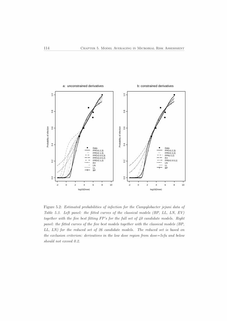
114 Chapter 5. Model Averaging in Microbial Risk Assessment
a: unconstrained derivatives
log10(Dose)
Pro
babi
lity
of in
fect
ion
0.0
0.2
0.4
0.6
0.8
1.0
-2 0 2 4 6 8 10
l
l
l
l
DataFPEV(-2,3)FPEV(-1,3)FPEV(-0.5,3)FPEV(-0.5,2)FPEV(-1,2)EVLNLLBPl
b: constrained derivatives
log10(Dose)
Pro
babi
lity
of in
fect
ion
0.0
0.2
0.4
0.6
0.8
1.0
-2 0 2 4 6 8 10
l
l
l
l
DataFPEV(-2,3)FPEV(-2,2)FPN(-2,2)EVFPEV(-0.5,1)LNLLBPl
Figure 5.2: Estimated probabilities of infection for the Campylobacter jejuni data ofTable 5.3. Left panel: the fitted curves of the classical models (BP, LL, LN, EV)together with the five best fitting FP’s for the full set of 40 candidate models. Rightpanel: the fitted curves of the five best models together with the classical models (BP,LL, LN) for the reduced set of 26 candidate models. The reduced set is based onthe exclusion criterion: derivatives in the low dose region from dose=5cfu and belowshould not exceed 0.2.

5.3. Application to Single Strain Data 115
Table 5.5: Campylobacter jejuni. Estimated probability of infection at dose 10cfu.For the Beta-Poisson and the model averaged(MA) estimates logit-back transformedCIs are used while the other model estimates use CIs back transformed accord-ing to their corresponding link function. Fractional polynomials are denoted asFPlink(powers).
Wald CIs
Model AIC Weights π(10) SE(π(10)) lower upper
FPEV(−2,3) 19.8482 0.05985 0.04804 0.13982 0.00014 1.00000
FPEV(−2,2) 20.1956 0.05031 0.01373 0.04392 2.5E-05 0.99951
FPN(−2,2) 20.2796 0.04824 0.04627 0.28467 5.1E-14 0.99998
EV 20.3201 0.04727 0.32355 0.14222 0.12735 0.67428
FPEV(−0.5,1) 20.4400 0.04452 0.20325 0.15167 0.04303 0.69081
FPL(−2,2) 20.4464 0.04438 0.05259 0.23678 5.0E-06 0.99838
LN 20.5414 0.04232 0.26749 0.17085 0.05072 0.65434
FPEV(−1,1) 20.5778 0.04156 0.08722 0.11266 0.00642 0.72542
FPN(−0.5,1) 20.6301 0.04049 0.15863 0.19185 0.00532 0.71023
LL 20.6902 0.03929 0.26161 0.16551 0.06198 0.65514
FPEV(−0.5,0.5) 20.6943 0.03921 0.12564 0.12056 0.01778 0.63389
FPN(−1,1) 20.7200 0.03871 0.05069 0.13091 2.1E-05 0.79464
FPL(−0.5,1) 20.7747 0.03766 0.15911 0.17442 0.01448 0.70895
FPL(−1,1) 20.8612 0.03607 0.06192 0.11950 0.00117 0.78824
FPEV(−2,1) 20.8765 0.03579 0.00173 0.00636 1.3E-06 0.90770
BP 20.8785 0.03576 0.08640 0.16325 0.00164 0.84489
FPN(−2,1) 20.8927 0.03550 5.99E-6 9.10E-5 8.3E-28 0.98264
FPEV(−1,0.5) 20.8967 0.03543 0.04249 0.06614 0.00192 0.62518
FPN(−0.5,0.5) 20.8970 0.03543 0.05852 0.11247 0.00028 0.62542
FPL(−0.5,0.5) 21.0254 0.03323 0.06983 0.10306 0.00334 0.62726
FPL(−2,1) 21.0299 0.03315 0.00072 0.00390 1.9E-08 0.96585
FPN(−1,0.5) 21.0638 0.03259 0.00602 0.02502 3.6E-08 0.64223
FPL(−1,0.5) 21.1848 0.03068 0.01571 0.03731 0.00014 0.64367
Continued on next page

116 Chapter 5. Model Averaging in Microbial Risk Assessment
Table 5.5 – continued from previous page
Wald CIs
Model AIC Weights π(10) SE(π(10)) lower upper
FPEV(−2,0.5) 21.3155 0.02874 0.00036 0.00146 1.2E-07 0.66425
FPN(−2,0.5) 21.3927 0.02765 4.52E-11 1.10E-9 7.9E-43 0.75888
FPL(−2,0.5) 21.5031 0.02617 2.39E-5 0.00014 1.9E-10 0.75422
MA estimate 0.08900 0.15178 0.00248 0.79301
5.4 Simulation Study for Single Strain Data
In a small simulation study we explore and compare the performance of the estimatedrisk based on three model approaches: each of the 40 candidate models individually,the best fitting model according to AIC (varying from run to run), and by modelaveraging. The model chosen most often by AIC across the simulations was alsomonitored.A total of S = 1000 datasets were generated. For each run, we assume the samedose levels (d) and total number of individuals exposed (n) as those in the Salmonellatyphi data set, and generate the number of ill individuals based on the BP modelor based on a fractional polynomial EV model, with parameters based on the esti-mates from these models fitted on the Salmonella typhi data. In the first setting,the data sets were generated using a BP model taking parameters u = −11.8739and v = 10.2810 in formulas (5.13). In the second setting, the data sets were gen-erated using the cloglog fractional polynomial with powers (p1, p2) = (−1, 3), as oneof the best models in the Salmonella typhi example, with parameters β1 = −18.1425and β2 = 22.5300 × 10⁻⁵. The dose response curves corresponding to both settingsare shown in Figure 5.1. To the 1000 generated samples, we fit the set of 40 can-didate models described earlier, and estimate the risk to Salmonella typhi illness π
at dose=100cfu, for each of the candidate models but also keeping track of the bestfitting model according to AIC. Finally, an averaged risk over the candidate modelsis calculated. We summarize the performance of the different methods by reporting,across the simulations, the average variance of the estimated probability of Salmonellatyphi illness (SE(π∗(100)))2 using model approach ∗, the average length of the 95%confidence intervals and the coverage probability of these intervals. The variability ofthe risk estimate π∗ about its average risk ¯π∗ =
∑Ss=1 π∗s/S over the S simulations

5.4. Simulation Study for Single Strain Data 117
was calculated as σ2(π∗(100)) =∑S
s=1{π∗s− ¯π∗}2/(S−1), while bias = {¯π∗−π} givesthe difference between the average risk estimate and the true risk based on the datagenerating model. The mean-squared error is given by MSE = bias2 + σ2(π∗(100)).
5.4.1 First Setting
Table 5.6 shows the results of the first setting, which uses the BP model as the truemodel. Not all 40 models are shown but the BP, LL, LN and EV, and the mostfrequently selected best fitting model. For this latter model it was observed whichmodel was selected most often by AIC after all runs were finished. The results fromthe best fitting models (BFM) and by model averaging (MA) are shown as well. Notethat the BFM changes from run to run. Estimates based on the BP model have verysmall bias and variance characteristics, as compared with the other models, and acoverage close to 95%, also illustrated by Figure 5.3. Since this model is the truesimulation model, this is not unexpected. But the extremely poor behaviour of mostother models is surprisingly low. Further note that the performances of the LL, LNand EV model are quite similar, indicating that the choice of link function has onlyminor influence on the estimated risk. Figure 5.3 helps to understand these results.The order of the simulation runs on the horizontal scale corresponds to the orderof the corresponding point estimates. So runs leading to smaller estimates are moreto the left side of the horizontal scale (as shown by the solid curve of estimates).The right upper panel of Figure 5.3 shows that the LN tends to overestimate thetrue value. The BFM (lower right panel of Figure 5.3) estimates show smaller biasand smaller variances, showing in some way its adaptive nature, but it also tends tounderestimate the true value for most of the runs. At the right end of the horizontalscale, it exhibits an extremely high variable pattern. This all combines to a verylow coverage of 6.6%. The model which was chosen most often as the best model isthe fractional polynomial logit-model with powers (-2,0.5). Also this model performssurprisingly poorly in terms of coverage. The averaged risk estimate, based on allconsidered models, shows small bias but relatively high variance properties. Butthis model accounts for the variability introduced by the model selection procedure,resulting in wider confidence intervals and a coverage probability of 87% (see Figure5.3). Actually this is also a somewhat disappointing result, but compared to all othermisspecified models it is outstanding.

118 Chapter 5. Model Averaging in Microbial Risk Assessment
Table 5.6: Simulation I results for estimated risk at dose 100cfu. For each model,columns (2) and (3) show the simulation-average of the variance-estimates of theestimated risk and the average confidence interval length respectively. The simulatedcoverage probability of the intervals is shown in column(4). Columns (5), (6) and(7) present the simulated squared bias, variance and mean squared error respectively.The direction of the bias shown by the sign beside the squared bias in column (4).† denotes the data generation model while ‡ shows the most frequently selected bestAIC model. BFM denotes the best fitting models and MA denotes model averaging.
(1) (2) (3) (4) (5) (6) (7)
Model (SE(π∗))2 CIlength coverage (sign)bias2 σ2(π∗) MSE†BP 2.2E-07 0.00172 95.60 (+)7.2E-09 1.5E-07 1.6E-07
LL 0.00020 0.05833 0.00 (+)0.00079 0.00017 0.00097
LN 0.00017 0.05206 5.50 (+)0.00031 0.00013 0.00045
EV 0.00042 0.08205 0.00 (+)0.00399 0.00037 0.00437‡FPL(−2,0.5) 1.5E-12 1.3E-05 0.00 (-)4.8E-07 2.8E-13 4.8E-07
FPL(−2,1) 5.5E-11 6.1E-05 1.20 (-)4.8E-07 1.4E-11 4.8E-07
FPL(−2,2) 9.3E-09 0.00061 25.20 (-)4.4E-07 3.5E-09 4.5E-07
FPL(−2,3) 7.1E-07 0.00329 0.00 (+)0.25271 4.9E-07 0.25271
FPL(−1,0.5) 2.1E-07 0.00245 78.40 (-)1.9E-07 1.1E-07 3.0E-07
FPL(−1,1) 2.0E-06 0.00677 95.00 (+)1.7E-07 1.2E-06 1.4E-06
FPL(−1,2) 3.3E-05 0.02515 20.10 (+)4.1E-05 2.4E-05 6.5E-05
FPL(−1,3) 0.00015 0.05211 0.60 (+)0.00037 0.00012 0.00049
FPL(−0.5,0.5) 6.3E-06 0.01165 76.60 (+)3.2E-06 4.3E-06 7.5E-06
FPL(−0.5,1) 3.4E-05 0.02541 14.70 (+)4.9E-05 2.6E-05 7.5E-05
FPL(−0.5,2) 0.00024 0.06421 0.00 (+)0.00098 0.00021 0.00119
FPL(−0.5,3) 0.00064 0.10095 0.00 (+)0.00460 0.00057 0.00517
FPN(−2,0.5) 1.1E-21 6.6E-08 0.00 (-)4.8E-07 2.0E-23 4.8E-07
FPN(−2,1) 1.1E-17 5.7E-07 0.00 (-)4.8E-07 3.3E-19 4.8E-07
FPN(−2,2) 4.0E-12 3.1E-05 0.80 (-)4.8E-07 3.5E-13 4.8E-07
FPN(−2,3) 6.6E-07 0.00318 0.00 (+)0.25072 0.00101 0.25173
FPN(−1,0.5) 1.0E-09 0.00030 11.10 (-)4.8E-07 1.8E-10 4.8E-07
Continued on next page

5.4. Simulation Study for Single Strain Data 119
Table 5.6 – continued from previous page
(1) (2) (3) (4) (5) (6) (7)
Model (SE(π∗))2 CIlength coverage (sign)bias2 σ2(π∗) MSE
FPN(−1,1) 8.0E-08 0.00177 51.40 (-)4.0E-07 2.4E-08 4.3E-07
FPN(−1,2) 1.1E-05 0.01511 94.50 (+)1.5E-06 6.0E-06 7.6E-06
FPN(−1,3) 0.00011 0.04364 37.00 (+)9.3E-05 7.6E-05 1.7E-04
FPN(−0.5,0.5) 6.7E-07 0.00436 80.60 (-)1.7E-07 2.7E-07 4.4E-07
FPN(−0.5,1) 1.2E-05 0.01534 91.50 (+)2.4E-06 6.8E-06 9.2E-06
FPN(−0.5,2) 0.00022 0.05914 3.30 (+)0.00042 0.00017 0.00060
FPN(−0.5,3) 0.00070 0.10403 0.00 (+)0.00340 0.00061 0.00402
FPEV(−2,0.5) 2.3E-10 9.7E-05 2.00 (-)4.8E-07 8.0E-11 4.8E-07
FPEV(−2,1) 2.0E-09 0.00026 8.70 (-)4.6E-07 8.5E-10 4.6E-07
FPEV(−2,2) 3.8E-08 0.00103 48.30 (-)3.5E-07 2.1E-08 3.7E-07
FPEV(−2,3) 2.3E-07 0.00241 83.00 (-)1.5E-07 1.3E-07 2.8E-07
FPEV(−1,0.5) 3.2E-06 0.00812 82.90 (+)1.5E-06 2.3E-06 3.7E-06
FPEV(−1,1) 1.3E-05 0.01559 28.70 (+)1.7E-05 9.7E-06 2.6E-05
FPEV(−1,2) 7.1E-05 0.03545 0.20 (+)0.00021 5.8E-05 0.00027
FPEV(−1,3) 0.00018 0.05543 0.00 (+)0.00080 0.00015 0.00094
FPEV(−0.5,0.5) 4.0E-05 0.02689 1.60 (+)9.8E-05 3.3E-05 0.00013
FPEV(−0.5,1) 0.00012 0.04453 0.10 (+)0.00048 9.8E-05 0.00058
FPEV(−0.5,2) 0.00039 0.07950 0.00 (+)0.00323 0.00034 0.00357
FPEV(−0.5,3) 0.00069 0.10514 0.00 (+)0.00870 0.00060 0.00930
BFM 9.2E-06 0.00398 6.60 (+)8.5E-07 3.8E-05 3.9E-05
MA 7.8E-05 0.08390 87.10 (+)1.9E-05 2.2E-05 4.1E-05
5.4.2 Second Setting
In a second setting, we study the performance of the different models and of themodel selected and averaged risk estimates again, now with the FPEV(−1,3) modelbeing the true underlying simulation model. Results are summarized in Table 5.7.

120 Chapter 5. Model Averaging in Microbial Risk Assessment
In this setting, the MSE of the BP model is no longer the smallest, and also thecoverage probability is very small as it underestimates the true value most of thetimes (see left upper panel of Figure 5.4). Again, as expected, the data generatingmodel FPEV(−1,3) has the smallest MSE and its coverage probability nicely reachesthe nominal as expected (see right upper panel of Figure 5.4). The best fitting modelhas an average bias similar to that of the BP model, but again, an additional sourceof variability enters the estimation process. The fractional polynomial EV model withpowers (-0.5,3) is chosen most often as the best model but as in the previous settingit exhibits a very low coverage, partly also reflecting a similarly low coverage for theBFM. The averaged risk estimate has a small bias combined with a larger varianceleading to a coverage probability of 97.90.Both simulation settings show that model averaging has a beneficial effect in reducingbias, in accounting for the variability induced by the model selection process, andconsequently in better coverage characteristics.

5.4. Simulation Study for Single Strain Data 121
Table 5.7: Simulation II results for estimated risk at dose 100cfu. For each model,columns (2) and (3) show the simulation-average of the variance-estimates of theestimated risk and the average confidence interval length respectively. The simulatedcoverage probability of the intervals is shown in column(4). Columns (5), (6) and(7) present the simulated squared bias, variance and mean squared error respectively.The direction of the bias shown by the sign beside the squared bias in column (3).† denotes the data generation model while ‡ shows the most frequently selected bestAIC model. BFM denotes the best fitting models and MA denotes model averaging.
(1) (2) (3) (4) (5) (6) (7)
Model (SE(π∗))2 CIlength coverage (sign)bias2 σ2(π∗) MSE
BP 1.5E-06 0.00309 2.40 (-)0.00036 1.1E-06 0.00036
LL 0.00015 0.05118 95.00 (+)2.0E-05 0.00013 0.00015
LN 0.00011 0.04357 89.70 (-)3.2E-05 9.4E-05 0.00013
EV 0.00028 0.06764 34.50 (+)0.00077 0.00026 0.00104
FPL(−2,0.5) 6.9E-10 0.00012 0.00 (-)0.00039 1.8E-10 0.00039
FPL(−2,1) 2.7E-09 0.00022 0.00 (-)0.00039 9.2E-10 0.00039
FPL(−2,2) 4.3E-08 0.00088 0.20 (-)0.00039 2.1E-08 0.00039
FPL(−2,3) 7.3E-07 0.00334 0.00 (+)0.23402 3.6E-07 0.23402
FPL(−1,0.5) 4.1E-07 0.00296 0.80 (-)0.00038 2.7E-07 0.00038
FPL(−1,1) 2.2E-06 0.00672 4.30 (-)0.00035 1.6E-06 0.00035
FPL(−1,2) 2.4E-05 0.02135 49.50 (-)0.00020 1.9E-05 0.00022
FPL(−1,3) 0.00010 0.04246 91.20 (-)2.1E-05 8.6E-05 0.00011
FPL(−0.5,0.5) 6.3E-06 0.01130 14.30 (-)0.00030 4.8E-06 0.00031
FPL(−0.5,1) 2.7E-05 0.02271 56.40 (-)0.00017 2.2E-05 0.00019
FPL(−0.5,2) 0.00017 0.05459 94.10 (+)3.6E-05 0.00015 0.00019
FPL(−0.5,3) 0.00046 0.08608 33.80 (+)0.00119 0.00042 0.00161
FPN(−2,0.5) 7.0E-12 3.9E-05 0.00 (-)0.00039 5.0E-13 0.00039
FPN(−2,1) 3.4E-11 5.1E-05 0.00 (-)0.00039 3.1E-12 0.00039
FPN(−2,2) 1.2E-08 0.00020 0.10 (-)0.00037 0.00026 0.00063
FPN(−2,3) 7.0E-07 0.00328 0.00 (+)0.23410 3.7E-07 0.23410
FPN(−1,0.5) 3.5E-08 0.00081 0.20 (-)0.00039 1.1E-08 0.00039
Continued on next page

122 Chapter 5. Model Averaging in Microbial Risk Assessment
Table 5.7 – continued from previous page
(1) (2) (3) (4) (5) (6) (7)
Model (SE(π∗))2 CIlength coverage (sign)bias2 σ2(π∗) MSE
FPN(−1,1) 2.9E-07 0.00232 1.00 (-)0.00039 1.3E-07 0.00039
FPN(−1,2) 8.4E-06 0.01242 19.80 (-)0.00033 5.6E-06 0.00034
FPN(−1,3) 6.6E-05 0.03346 69.30 (-)0.00016 5.1E-05 0.00021
FPN(−0.5,0.5) 1.3E-06 0.00491 3.80 (-)0.00038 7.1E-07 0.00038
FPN(−0.5,1) 9.9E-06 0.01357 21.60 (-)0.00032 6.9E-06 0.00033
FPN(−0.5,2) 0.00014 0.04760 91.40 (-)1.8E-05 0.00012 0.00013
FPN(−0.5,3) 0.00047 0.08590 70.70 (+)0.00058 0.00043 0.00101
FPEV(−2,0.5) 1.0E-09 0.00014 0.00 (-)0.00039 4.4E-10 0.00039
FPEV(−2,1) 3.5E-09 0.00025 0.00 (-)0.00039 1.9E-09 0.00039
FPEV(−2,2) 3.2E-08 0.00079 0.00 (-)0.00039 2.1E-08 0.00039
FPEV(−2,3) 1.6E-07 0.00178 0.10 (-)0.00039 1.1E-07 0.00039
FPEV(−1,0.5) 2.0E-06 0.00619 2.00 (-)0.00034 1.5E-06 0.00034
FPEV(−1,1) 7.1E-06 0.01155 15.30 (-)0.00028 6.0E-06 0.00028
FPEV(−1,2) 4.0E-05 0.02651 73.50 (-)8.6E-05 3.6E-05 0.00012†FPEV(−1,3) 0.00011 0.04284 95.60 (+)8.7E-07 9.9E-05 9.9E-05
FPEV(−0.5,0.5) 2.3E-05 0.02050 52.90 (-)0.00016 2.0E-05 0.00018
FPEV(−0.5,1) 6.8E-05 0.03442 91.50 (-)1.5E-05 6.2E-05 7.7E-05
FPEV(−0.5,2) 0.00025 0.06440 50.60 (+)0.00052 0.00024 0.00076‡FPEV(−0.5,3) 0.00049 0.08874 4.50 (+)0.00281 0.00047 0.00328
BFM 0.00023 0.05146 35.20 (+)0.00022 0.00101 0.00123
MA 0.00048 0.12179 97.90 (+)0.00002 0.00025 0.00028
In the philosophy that a true and correct model does not exist, or that you willnever know it exactly (which seems the only realistic situation), this simulation alsoshows that not just one single model is appropriate to describe the dose-response rela-tionship of microbial risks, but there exists a whole set of possible models. Fractionalpolynomials are very flexible to estimate the low-dose risk. However, the model selec-

5.4. Simulation Study for Single Strain Data 123
tion procedure induces extra variability that should be accounted for. The averagedrisk estimate gives larger weights to better-fitting models, resulting in a smaller bias.The model selection uncertainty is accounted for in this approach, and a better cover-age probability obtained as illustrated in Figure 5.4. However, from both simulationsettings it was evident that for this particular risk assessment application the coveragepercentages for most of the model fall far below the chosen level of confidence (0.95).The magnitude of inflation of the coverage was certainly surprising to us and is initself a clear warning to be very careful and thoughtful when restricting the analysisto one single model. It certainly motivates the use of different plausible models, atleast as a type of sensitivity analysis, but even better in a multimodel approach suchas model averaging.
5.4.3 To Include Fractional Polynomials or Not
As pointed out before, and clear from the nature of the model averaging approach,the set of candidate models should be rich enough. This section tries to illustratethis point by comparing the results from the data analyses in Section 5.3 and thesimulation results in the previous sections to the corresponding results of model av-eraging over the four classical models only. Let us denote by set one the restrictedset of classical models BP, LL, LN and EV and by set two the modified flexible frac-tional polynomials added to set one. For salmonella typhi example, the averaged riskestimates are 0.029 (SE 0.021 and confidence interval [0.007,0.114]) and 0.01285 (SE0.016 and confidence interval [0.001,0.134]) respectively for set one and two. The riskestimate from set two is reduced to about half that of set one. For campylobacterjejuni example, the averaged risk estimates are 0.2429 (SE 0.180 and confidence in-terval [0.045,0.686]) and 0.089 (SE 0.152 and confidence interval [0.002,0.793]) for setone and two respectively. Including fractional polynomials reduces the estimate toabout 2.5 times from not including them.
For the first simulation setting, with the restricted set one, the true risk estimatewas captured in 38.5% of the runs by the confidence intervals of the averaged riskcompared to 87.1% for set two. Also, the square bias and the variance were higher forset one models than for set two models. In the second simulation setting, averagingover the four models attained a coverage probability of 87.3% versus 97.9% for set two.To this end, we see that using the richer set two, which includes the flexible fractionalpolynomial models, yielded coverage probabilities closer to the nominal 95% level,less biased and more precise risk estimates than set one.

124 Chapter 5. Model Averaging in Microbial Risk Assessment
simulation run
prob
abili
ty (
dose
= 1
00)
0 200 400 600 800 1000
0.0
0.00
40.
008
0.01
2
Beta Poisson
true valuelower 95% limitestimateupper 95% limit
simulation run
prob
abili
ty (
dose
= 1
00)
0 200 400 600 800 1000
0.0
0.05
0.10
0.15
Log Normal
simulation run
prob
abili
ty (
dose
= 1
00)
0 200 400 600 800 1000
0.0
0.00
20.
006
Best Fitting Models
simulation run
prob
abili
ty (
dose
= 1
00)
0 200 400 600 800 1000
0.0
0.05
0.10
0.15
0.20
Model Averaging
Figure 5.3: Simulation I: True probability of S. Typhi based on the Beta Poisson gen-erating model and the estimated probabilities for the Beta Poisson (data generationmodel), the log-normal model, the best fitting models across simulations and the av-eraged risk. The corresponding confidence limits of the estimated risks are shown toillustrate how best they capture the true value.
5.5 Application to Multi-Strain Data
The model averaging approach extends to settings with additional sources of het-eregeneity, within the framework of Generalized Linear Mixed Models (GLMM, seee.g. Molenberghs and Verbeke, 2005). Table 5.8 shows data on Campylobacter je-juni dose exposure for different strains, the total number of chicken exposed and theinfected chicken (Chen et al. 2006). Additionally there is information about the sam-ple, (F)resh or (L)aboratory, whether it originates from (C)hicken or (H)uman andwhether its host is (W)ickman or (L)ohmann.

5.5. Application to Multi-Strain Data 125
simulation run
prob
abili
ty (
dose
= 1
00)
0 200 400 600 800 1000
0.0
0.02
0.04
0.06
0.08
Beta Poisson
true valuelower 95% limitestimateupper 95% limit
simulation run
prob
abili
ty (
dose
= 1
00)
0 200 400 600 800 1000
0.0
0.05
0.10
0.15
FPEV (-1,3)
simulation run
prob
abili
ty (
dose
= 1
00)
0 200 400 600 800 1000
0.0
0.10
0.20
Best Fitting Models
simulation run
prob
abili
ty (
dose
= 1
00)
0 200 400 600 800 1000
0.0
0.10
0.20
Model Averaging
Figure 5.4: Simulation II: True probability of S. Typhi based on FPEV(-1,3) the gen-erating model and the estimated probabilities for the Beta Poisson (taken as standardmodel), the FPEV(-1,3) model, the best fitting models across simulations and the av-eraged risk. The corresponding confidence limits of the estimated risks are shown toillustrate how best they capture the true value.

126 Chapter 5. Model Averaging in Microbial Risk Assessment
Table 5.8: Campylobacter jejuni data in chicken. Isolates. Sample:F(resh)/L(aboratory). Origin: H(uman)/C(hicken). Host: W(ickham)/L(ohmann)
Group Isolate Sample Origin Host Dose Exposed Infected1 480 F H W 10 10 0
480 F H W 1000 10 0480 F H W 100,000 10 10
2 466 F H L 840 8 8466 F H L 8400 7 7
3 P5444 F H L 10,000 10 104 P5623 F H L 5000 10 95 119a F C L 17,000 4 46 121a F C L 11,000 4 47 123a F C L 3500 4 28 UA585 F H W 95 10 10
UA585 F H W 950 10 10UA585 F H W 9500 10 10UA585 F H W 95,000 10 10
9* 93/146 F C W 100 10 093/146 F C W 1000 9 993/146 F C W 100,000 10 10
10* 94/146 F H W 120 10 094/146 F H W 1200 10 1094/146 F H W 12,000 10 10
11* 93175 F C W 28 10 093175 F C W 280 10 1093175 F C W 2800 10 10
12* 0087 F H L 30 10 30087 F H L 300 10 100087 F H L 480 10 100087 F H L 2000 6 60087 F H L 4500 8 80087 F H L 4800 10 100087 F H L 200,000 10 10
13* 81116P F C W 4 10 081116P F C W 40 10 1081116P F C W 40 9 981116P F C W 400 10 1081116P F C W 4000 9 981116P F C W 40,000 10 10
14 R3P F C W 10 10 10R3P F C W 100 10 10
15 81-176 L C W 2000 10 881-176 L C W 2,000,000 10 10
16 81-176 L C L 800 9 881-176 L C L 80,000 10 10
Continued on next page

5.5. Application to Multi-Strain Data 127
Table 5.8 – continued from previous pageGroup Isolate Sample Origin Host Dose Exposed Infected
17 11168 L C W 200,000 10 1018 11168 L C L 2000 10 4
11168 L C L 20,000 10 511168 L C L 200,000 10 711168 L C L 2,000,000 10 9
19 R3 L C W 300 9 6R3 L C W 3000 10 10
20* 81116 L C W 54 8 381116 L C W 540 6 381116 L C W 5400 5 581116 L C W 54,000 6 681116 L C W 250,000 14 14
21* 81116 L C L 35 10 081116 L C L 350 10 681116 L C L 3500 10 881116 L C L 100 10 481116 L C L 1000 10 981116 L C L 10,000 10 1081116 L C L 10,000 10 1081116 L C L 1,000,000 10 10
22 81117 L C L 35,000 10 10
The challenge here is to consider sensible candidate models which correctly account forthe different sources of variability or heterogeneity (different types of isolate, sample,origin, and host) and to extend the model averaging approach over such a family ofcandidate models. In general one can extend models as discussed in the previoussection, with fixed effects and/or random effects. It seems natural to incorporatesample, origin and host (all binary) in the model by fixed effects and isolate by usinga random effect. But for the latter one could also consider a fixed effect. Models withall of the covariates (sample, origin, and host) included as fixed effects and with isolateas fixed or random effect are overparameterized. Indeed, the type of isolate coversmost of the (sample, origin, host)-combinations (except for isolate 81-176, 11168,81116). Moreover for several isolates, there are only observations for one single doselevel, making dose response models with two or more parameters unestimable.
Therefore, to account appropriately for the heterogeneity resulting from differenttypes of isolates, samples, origins and hosts, we considered two approaches: (i) arandom effect for all different combinations of (isolate, sample, origin, host), leadingto a total of 22 different “groups” (as indicated in the first column of Table 5.8); in this

128 Chapter 5. Model Averaging in Microbial Risk Assessment
approach it is possible to fit models with and without type of sample as an additional(fixed) effect in the model (ii) a selection of 7 groups (out of the 22 groups, thosewith group number marked by an asterisk ∗ in the first column), which allows a fullyfixed effects approach (one parameter for each group), again with and without typeof sample as an additional (fixed) effect in the model. Strains with only one or twodose levels together with those that exhibited outlying observations were eliminated.These four families of candidate models corresponds to the four parts of Table 5.9, asdiscussed further on. Because of computational problems and overparameterization,we did not consider fractional polynomial dose response models. Only predictorslinear in dose were considered in what follows.Table 5.9 shows, without and with type of sample (upper and lower part of the tablerespectively), the AIC and the weights of the models fitted to 7 strains (3rd and4th columns) and also the AIC and weights of the models fitted to 22 groups (5thand 6th columns). Using the likelihood ratio test, the type of sample variable wassignificant in the models with an asterisk (*) fit on 7 strains while type of samplewas only significant in the model with † sign fit on 22 groups. This data exampleshows that random effects (RE) models are more flexible than fixed effects modelsand can handle over-parametrization problems. As is clear from the empty cells inthe right upper part of Table 5.9, fixed effects (FE) models could not be fit to the22 groups. The random effects models with type type of sample show no substantialimprovement compared to those without type regardless of the type of grouping used.Most importantly, they all point to the same or similar models.As an illustration, consider the estimation of the probability to be infected at doselevel d = 1, by the models listed in the left upper part of Table 5.9 (7 groups andwithout the type of sample variable). As the weights in the table reveal, some of themodels have very little contribution and so we exclude them for the model averagingexercise. Table 5.10 shows the results for the best five individual models and the modelaveraged estimate for the probability of infection, together with Wald type confidenceintervals. The table mainly shows that the best five models can lead to substantiallydifferent point estimates as well as confidence intervals. In general the model averagedestimates is situated somewhere between the individual model estimates, and themodel averaged confidence intervals tend to be much wider, reflecting the modeluncertainty.For graphical illustration of the different models Figure 5.5 shows fitted dose responsecurves for the best fixed-effects model (FE log-logistic) and the best random-effectsmodel (log-normal random α&β) together with all data of the 7 groups in the twoupper panels, and fitted curves for the five best models, separately for the data of two

5.5. Application to Multi-Strain Data 129
Table 5.9: Multi-strain Campylobacter jejuni data: model fits and AIC-weights usingdata of only 7 groups, and of all 22 groups.
without the type of sample variable
Model random AIC7 weight7 AIC22 weights22
FE LL - 77.32 0.43351
BP FE on u - 79.39 0.15434
LN α & β 79.72 0.13094 154.87 0.47784
FE LN - 79.93 0.11796
LL α & β 80.37 0.09466 154.84 0.48299
EV α & β 81.40 0.05650 159.88 0.03889
FE EV - 84.58 0.01152
LL α 91.40 0.00038 188.65 2.2E-08
BP u 94.14 9.7E-05 169.84 0.00027
LN α 94.47 8.2E-05 194.15 1.4E-09
EV α 100.00 5.2E-06 197.55 2.6E-10
BP v 135.99 7.9E-14 253.30 2.0E-22
BP FE on v - 141.92 4.1E-15
BP u & v 518.83 5.8E-97 177.26 6.5E-06
with the type of sample variable as fixed effect
Model random AIC7 weight7 AIC22 weights22
∗LN α & β 76.85 0.60000 154.68 0.53379∗LL α & β 77.67 0.39953 154.97 0.46359
LL α 92.44 0.00025 188.80 2.1E-08
BP u 94.04 0.00011 169.27 0.00036
LN α 95.41 5.6E-05 194.32 1.3E-09
EV α & β 95.72 4.8E-05 165.62 0.00225
EV α 99.52 7.2E-06 196.97 3.5E-10∗†BP v 129.66 2.1E-12 296.80 7.4E-32
BP u & v 578.32 7.7E-110 182.52 4.8E-07
∗ models fit on 7 groups where the type of sample variable is significant using likelihood ratio test.
† models fit on 22 groups where the type of sample variable was significant.

130 Chapter 5. Model Averaging in Microbial Risk Assessment
groups (group 13 and 21) in the two lower panels.The curves are extrapolated to a dose of 1cfu. The upper panels of Figure 5.5 showsome considerable variability in the fits to the different groups for the log-normalmodel with random intercept and slope compared to the fixed effects model. Thisconclusion was also observed for the other logit random effects model and the log-normal and BP fixed effects models not shown here. In the lower panels of Figure5.5, we observe that the response curves for the five models fit the data quite well,a conclusion also confirmed by the closeness of the model AIC’s. However, despitethe closeness of the AIC’s there is a lot of variability at the lower dose of 1cfu (whichis out of the observed range of dose levels). So, especially for extrapolation, modelaveraging stabilizes the highly variable point estimate, but variability in terms ofmodel uncertainty is still reflected by the wide confidence intervals (see Table 5.10).
Table 5.10: Multi-strain Campylobacter jejuni data. Model specific and model aver-aged estimated probability of Campylobacter jejuni: averaging over five models, thethree best fixed effects models and the two best random effects models without type ofsample. The last two letters added at the end of the strain indicate whether the strainoriginated from (h)uman or (c)hicken and its host is (l)ohmann or (w)ickham.
wald CIsStrain Model AIC Weight π(1) SE(π(1)) lower upper
0087hl FE LL 77.32 0.46543 0.00109 0.00113 0.00014 0.00823BP FE on u 79.39 0.16571 0.01539 0.00594 0.00720 0.03261LN random α & β 79.72 0.14058 7.8E-11 1.9E-09 3.1E-42 0.77942FE LN 79.93 0.12665 9.7E-05 0.00021 7.3E-07 0.00418LL random α & β 80.37 0.10163 9.8E-06 6.0E-05 5.6E-11 0.63004Model Averaged 0.00307 0.00445 0.00018 0.05043
81116Pcw FE LL 77.32 0.46543 0.01429 0.01178 0.00281 0.06946BP FE on u 79.39 0.16571 0.07314 0.02284 0.03917 0.13250LN random α & β 79.72 0.14058 1.0E-07 1.3E-06 1.5E-23 0.32164FE LN 79.93 0.12665 0.01153 0.01325 0.00087 0.07897LL random α & β 80.37 0.10163 9.5E-05 0.00047 6.0E-09 0.60125Model Averaged 0.02024 0.02259 0.00221 0.16152
81116cl FE LL 77.32 0.46543 4.1E-05 5.4E-05 3.0E-06 0.00054BP FE on u 79.39 0.16571 0.00223 0.00073 0.00117 0.00425LN random α & β 79.72 0.14058 0.00028 0.00081 3.4E-07 0.02669FE LN 79.93 0.12665 9.0E-09 3.5E-08 1.9E-12 7.9E-06
Continued on next page

5.6. Simulation Study for Multi-Strain Data 131
Table 5.10 – continued from previous pagewald CIs
Strain Model AIC Weight π(1) SE(π(1)) lower upper
LL random α & β 80.37 0.10163 0.00244 0.00358 0.00014 0.04194Model Averaged 0.00068 0.00120 2.1E-05 0.02147
81116cw FE LL 77.32 0.46543 7.7E-05 0.00011 4.8E-06 0.00124BP FE on u 79.39 0.16571 0.00284 0.00120 0.00124 0.00650LN random α & β 79.72 0.14058 0.00662 0.01964 2.7E-06 0.34367FE LN 79.93 0.12665 1.4E-07 4.8E-07 6.9E-11 5.7E-05LN random α & β 80.37 0.10163 0.01459 0.02560 0.00045 0.32680Model Averaged 0.00292 0.00756 1.8E-05 0.32243
93/146cw FE LL 77.32 0.46543 2.8E-05 4.0E-05 1.6E-06 0.00049BP FE on u 79.39 0.16571 0.00290 0.00121 0.00129 0.00655LN random α & β 79.72 0.14058 1.3E-32 7.0E-31 1.0E-98 0.00229FE LN 79.93 0.12665 5.3E-09 2.3E-08 4.1E-13 9.0E-06LL random α & β 80.37 0.10163 5.7E-10 5.4E-09 5.6E-18 0.05498Model Averaged 0.00049 0.00085 1.7E-05 0.01405
93175cw FE LL 77.32 0.46543 0.00030 0.00036 2.7E-05 0.00325BP FE on u 79.39 0.16571 0.00925 0.00363 0.00428 0.01990LN random α & β 79.72 0.14058 2.7E-25 1.1E-23 3.3E-77 0.01836FE LN 79.93 0.12665 4.8E-06 1.3E-05 8.6E-09 0.00065LL random α & β 80.37 0.10163 7.0E-09 5.8E-08 5.6E-16 0.07878Model Averaged 0.00167 0.00267 7.2E-05 0.03710
94/146hw FE LL 77.32 0.46543 2.1E-05 3.2E-05 1.1E-06 0.00040BP FE on u 79.39 0.16571 0.00265 0.00106 0.00120 0.00582LN random α & β 79.72 0.14058 3.9E-33 2.0E-31 2.8E-96 0.00102FE LN 79.93 0.12665 2.3E-09 1.0E-08 1.2E-13 5.4E-06LL random α & β 80.37 0.10163 5.0E-10 4.6E-09 5.6E-18 0.04208Model Averaged 0.00045 0.00077 1.6E-05 0.01282
5.6 Simulation Study for Multi-Strain Data
This section summarizes the results of a limited simulation study for a multi-strain(or more general a multi-group) setting. We fix the dose levels and the total numberof exposed chicken (n) to that of the Campylobacter jejuni data example and generatethe number of infected chicken from a binomial distribution with parameters n and

132 Chapter 5. Model Averaging in Microbial Risk Assessment
log10(dose)
P(in
fect
ed)
0 1 2 3 4 5 6
0.0
0.2
0.4
0.6
0.8
1.0
FE LL modelFE LL modelFE LL modelFE LL modelFE LL modelFE LL modelFE LL model
log10(dose)
P(in
fect
ed)
0 1 2 3 4 5 6
0.0
0.2
0.4
0.6
0.8
1.0
RE LN modelRE LN modelRE LN modelRE LN modelRE LN modelRE LN modelRE LN model
0087hl81116Pcw81116cl81116cw93/146cw93175cw94/146hw
log10(dose)
P(in
fect
ed)
0 1 2 3 4 5 6
0.0
0.2
0.4
0.6
0.8
1.0
81116Pcw
log10(dose)
P(in
fect
ed)
0 1 2 3 4 5 6
0.0
0.2
0.4
0.6
0.8
1.0
81116cl
FE BPFE LLRE LLFE LNRE LN
Figure 5.5: Estimated Campylobacter jejuni dose-response curves: row 1 shows 7strains using the FE log-logistic model and 2 REs log-normal model and row 2 for fivemodels shown for the‘fresh’ isolate 81116Pcw and ‘Laboratory’ isolate 81116cl

5.6. Simulation Study for Multi-Strain Data 133
p. As probabilities p we take the predicted probabilities from the fixed effects log-logistic model, fitted to the Campylobacter jejuni data. To the simulated data we fitfour models, the fixed and random effects, log-normal and log-logistic models. TheBP model was excluded, due to computational problems. The probability of infectionat dose 1 is estimated from each model, from the AIC selected model and also bymodel averaging. With the generation and fitting process repeated 1000 times, theaverage length and the coverage percentage of confidence intervals, are examined foreach strain.
Figure 5.6 summarizes the simulation results on the confidence intervals. Theperformance characteristics for all models (4 single models, the AIC selected model,and the averaged model) are plotted against the strain numbers (on the horizontalaxes), which are arranged in ascending order of the true probabilities. The graphwith the coverage percentages in the right panel differentiates the different modelsmarkedly: the averaged model shows coverage percentages larger than but close tothose of the true model, the latter as expected being close to 95%. The coverageprobabilities of the other models, the fixed effects log-normal model and the AICselected model are much lower, being low to extremely low on the left end of thescale and increasing to acceptable values at the right end of the scale (correspondingto higher values of the true probabilities). The left panel shows that, compared tothe other models, the length of the confidence intervals produced by the two randomeffects models is much larger than those of the other models. Although this simulationstudy is very limited and many other settings could be considered, it shows that modelselection and model averaging is a crucial issue, also in more complicated settings ofmulti-strain data and random effects models.

134 Chapter 5. Model Averaging in Microbial Risk Assessment
Strain
95%
CI l
engt
h
1 2 3 4 5 6 7
0.0
0.05
0.10
0.15
0.20
0.25
0.30
Strain
cove
rage
(%
)
1 2 3 4 5 6 7
020
4060
8010
0
Model AveragingAIC SelectionFE LLRE LLFE LNRE LN
Figure 5.6: Multi-strain simulation, assuming the fixed effects log-logistic model asthe true model. From left to right: length of 95% confidence intervals and coveragepercentage. The horizontal axes represent the 7 different strains in ascending orderof the true probabilities.
5.7 Discussion
In quantitative risk assessment for microbial pathogens, dose-response assessment isa critical issue. It must be included, health effects are the end-point in any riskassessment. Data are scarce, however. Only few pathogens have been used in clinicalstudies, and even these have been done on a small scale with few volunteers exposedper dose, due to the high costs involved. As a consequence, microbial dose-responsedata often do not contain a great deal of information on the shape of the dose-responserelation, and model choice based entirely on experimental data is not feasible (Teunisand Havelaar 2000). This problem has raised may discussions and several solutionshave been proposed. One could use animals, as these allow, at least in principle,collection of more extensive data sets. However, this chapter also has demonstrated

5.7. Discussion 135
that this may merely give a better insight into the variability involved, not necessarilydecreasing the uncertainty about the shape of the relation. Model averaging hasbeen used before, weighting over an arbitrary collection of mathematical relationsconsidered useful. Reasons for inclusion may range from biological plausibility toflexibility or mere tradition (like threshold models). Here it has been shown thatthe modified fractional polynomials can be derived from the general equation (5.3)thereby potentially extending the family of eligible models a great deal, and providinga natural choice for the collection of models to include in model averaging.As observed in the simulation study, the coverage probabilities of the confidenceintervals of the individual models, the best fitting models and the model averagehighly depend on the generating (true) model. When bias values are high relative tothe variance, the coverage of these intervals considerably fall below the nominal levelof confidence. The bias values for the averaged risk were 10 times higher when onlyaveraging over the four commonly used dose-response models than when fractionalpolynomials were included and as a result the coverage probabilities in the former casewere always below nominal. To this end we recommend model averaging includingthe proposed set (or biological more plausible subset) of fractional polynomials in theset of candidate models.An essential improvement in dose-response assessment is its extension to a hierar-chical framework: like most biological problems, data can frequently be organizedhierarchically. For example several isolates (pure strains of microorganisms separatedfrom a mixed bacterial culture) of a single pathogen species in the same host species,different but related pathogen species in the same host, or a single pathogen isolate inhosts with different levels of immunity. As the purpose of risk assessment usually is topredict risks for an exposed population, dose-response relations should be translatedfrom the special, experimental setting to a more general, unspecified situation. Forinstance, given the different responses to a limited collection of isolates of a pathogen,what would be the response to a newly isolated specimen, of the same type? Fixedeffects models are easy to implement and represent a first solution, but the randommodels, although more complex, use all available data and are more suitable for ex-plicative studies. The generalized linear mixed models (Agresti, 2002; Molenberghsand Verbeke, 2005) allow prediction by using the (joint) distribution of the randomparameters to make exactly this generalization. Our future interest is to extend theseproposed fractional polynomials to investigate dose-response relationships betweenisolates of a single pathogen using generalized linear mixed models and full Bayesianmodels.Further research is needed to go into some issues, like the estimation at very low

136 Chapter 5. Model Averaging in Microbial Risk Assessment
dose levels, especially in case of limited information. Since low dose extrapolationis crucial in risk assessment and the AIC method selects a model regardless of itsintended use, we intend to further investigate selecting a model looking at the (lowerdose) region of interest, by using e.g. the focused information criterion (Claeskensand Hjort, 2003). Another interesting avenue for further research is to investigatebootstrap based alternatives as proposed by Faes et al. (2006b) and Wheeler andBailer (2007).

Part III
Modeling Data on Salmonella
Infection in Broiler and Layer
Chicken Flocks
137


Chapter 6
Risk Factor Identification for
Salmonella in Belgian Laying
Hens
The consumption of foods of animal origin, particularly poultry eggs, can lead totransmission of zoonotic diseases (Salmonella, in this case) from the animals to hu-mans. Salmonellosis constitutes a major public health burden and represents a signif-icant cost in many countries. In Belgium, the disease ranks high among the reportedfood borne illnesses (Collard et al. 2004). Even if the incidence of human salmonellosishas diminished since 1999, in 2004, 9545 cases were reported in the country (EFSA,2006a). As in most of the countries around the world, Belgian Salmonella outbreaksin humans are very often linked to the consumption of contaminated eggs (Daviesand Breslin, 2001; Van Immerseel et al. 2005; Collard et al. 2007). The most fre-quently isolated serotype in layer flocks in the EU as well as in Belgium is SalmonellaEnteritidis which is a non-typhoid non-host adapted serotype with a very wide hostrange (Baird-Parker, 1990; Gast et al. 2005; Quinet, 2005; VAR, 2005; EFSA, 2004).The bacterium infects the eggs by two processes: first by vertical transmission dur-ing the development of the egg within the ovary or its passage through the oviductand secondly by horizontal transmission through trans-shell contamination (Kinde etal. 2000; WHO FAO, 2002; Davies and Breslin, 2003a; Van Immerseel et al. 2005).Vertical transmission is considered to be the major route of egg contamination andshould be controlled by applying sanitary measures at the breeders level (that is, hy-
139

140 Chapter 6. Risk Factors in Belgian Laying Hens
giene practices and eventually vaccination) while horizontal transmission should bereduced by preventing contacts between the layer hens and by cleaning and disinfect-ing the flock’s environment. Salmonella is known for its ability to asymptomaticallyinfect the hen’s oviduct (De Buck et al. 2004a; 2004b). Therefore detection of infectedflocks depends entirely on laboratory analysis. An infected hen may contaminate oneegg out of 200 (Quinet, 2005). Reducing Salmonella flock prevalence results in adirectly proportional reduction in human health risk (Altekruse et al. 1993). Thissuggests that sanitary measures at the flock level contribute to a significant reductionof the risk for salmonellosis due to egg consumption. In Belgium, the layer breedersare not significantly infected, probably due to the many years’ efforts of control atthis level and therefore, it is reasonable to assume that most day-old chicks are freefrom Salmonella when placed on farms (Davies and Breslin, 2001; AFSCA, 2004).The majority of the infections in layer hens seem to be attributed to the persistentcontamination of the farm. Indeed, the presence of Salmonella in the laying houseenvironment has been strongly correlated with the probability that hens will lay con-taminated eggs. Chicken are infected after oral ingestion of the bacteria from theenvironmental sources (for example, contaminated fluff, dust, feed etc) invasion ofthe mucosal epithelial cells, which leads to systemic dissemination and colonization ofthe ovary and oviduct (Henzler et al. 1998; Davies and Breslin, 2003b). The primarycontrol should focus at farm level. Control measures include preventing contacts withcontaminated feed and visitors, wearing house-specific clothing, thorough cleaning anddisinfection of the layer houses, vaccination, rodent control programs. In Belgium,every holding housing more than 5000 hens is required to be sampled for Salmonelladiagnosis 3 weeks before slaughter time. This measure probably has contributed to areduction of the risk for food-borne salmonellosis. However, in 2004, still 27% of thelayer flocks analysed remained positive for Salmonella (AFSCA, 2004). Several riskfactors have been described, but in order to advise the Belgian competent authority(Federal Agency for the safety of the Food Chain) with detailed, practical guidance,an understanding of possible causal factors is essential. The objective of the studyreported here was to investigate the risk factors which are associated with the occur-rence of Salmonella in laying hens in Belgium using data collected for the BaselineStudy on the Prevalence of Salmonella in laying flocks of Gallus gallus f. domesticain the European Union (SANCO/34/2004 and Commission decision 2004/665/EG).Although it would be worthwhile to utilize data from earlier years, the 2005 data setcontained flock information, particularly on some demographic factors and Salmonellavaccination status, which were unavailable for earlier databases. Section 6.1 describeshow the data were obtained and gives the methods used to analyse the data. In Sec-

6.1. Material and Methods 141
tion 6.2, the exploratory results and model fitting results are presented. Section 6.3concludes the chapter with a discussion. A part of the analyses of this chapter arepublished in Namata et al. (2008a).
6.1 Material and Methods
6.1.1 Data Collection
The Belgian part of the Baseline Study on the Prevalence of Salmonella in egg layingflocks of Gallus gallus in the European Union consisted of a cross-sectional studythat covered the year 2005 from February to September in Belgium. The primarysample size providing the number of holdings which had to be tested was calculatedon the basis of a target prevalence of 20%, a confidence level of 95% and an accuracy of3% (Commission decision 2004/665/EG). The population of laying hens was stratifiedaccording to holding size (below 1000, 1000-2999, 3000-4999, 5000-9999, 10000-29999,30000 and more). The number of holdings to be sampled was subsequently distributedproportionally to the number of holdings in each class. In all cases, only one flockper holding was sampled. Seven different samples, two dust samples and five faecalsamples were collected from each selected flock. The dust samples were any of thesetypes: 1) dust from different places in case of barn or free range flocks, 2) dust from eggbelts, 3) dusty material from beneath cages. Faecal samples were any of these types:1) boot swabs which are socks placed over the boots and are sufficiently absorptiveto collect faecal or moist litter samples from the floor surfaces (SANCO/34/2004and Commission decision 2004/665/EG), 2) pooled faecal samples from dip pits, 3)pooled faecal samples from dropping belts, 4) pooled faecal samples from scrapers.The collection of these samples was as follows: There had to be five pooled faecalsamples taken per selected flock. For the pooled faecal samples in cages, there arenormally several stacks of cages within a henhouse. The material from each stackpicked up using a new pair of plastic gloves for each individual sample was includedin each of the five pooled faecal samples of 200-300 grams. For the boot swabs in barnsand free range flocks, each henhouse was divided in sectors of at least 100m that werewalked on with new boot swabs, five pairs of boot swabs per henhouse. Each of thefive pooled samples comprised of faecal material fixed to a pair of boot swabs. Thedust material from beneath cages was obtained from 20 separate locations within ahenhouse using a new pair of plastic gloves for each sample. Finally for the dust fromdifferent places from barns and free range, each dust sample was collected in a 250mlplastic jar or bag ensuring that all parts of the henhouse like from exhaust fan, ledges,

142 Chapter 6. Risk Factors in Belgian Laying Hens
beams etcetera were covered. In order to maximise sensitivity both faecal material(5 out of 7) and dust material from the environment (2 out of 7) were sampled,depending on whether the birds were reared in cages or barns or free-range, in sucha way that the complete farm was represented. The hens were sampled at the end oftheir laying period, within a maximum of 9 weeks before depopulation. Samples weresent within 24 hours to the laboratory. The detection method was as recommended bythe Community Reference Laboratory for Salmonella in Bilthoven, The Netherlands,that is, a modification of ISO 6579:2002. Salmonella isolates were serotyped followingthe Kaufmann-White scheme (Popoff, 2001; VAR, 2005).
The explanatory variables recorded include: region (1= Walloon or 0= Flanders),sampling time (month the flock was sampled: February to September), productiontype (cage or barn/ free range), age (in weeks), flock size (number of hens in theflock considered) and vaccination status against Salmonella (yes, unknown, or no).The flocks were vaccinated against Salmonella enterica, serovar Enteritidis during therearing period (one day to 18-20 weeks) with either a live or inactivated vaccine typealthough for some flocks the vaccine type was not known. The last dose was adminis-tered a few weeks before the onset of laying eggs. The pullets were kept in separatedinstallations on the laying farm considering special conditions like temperature andlight among others.
6.1.2 Single-Level Analysis
In the initial analysis of these Salmonella data we ignore the repeated design of thedata and assume that all observations act independently. With this assumption alogistic regression model
logit(P (Yj = 1) = XTβ (6.1)
can be fitted and risk factors investigated. The probability P (Yj = 1) that thejth sample was positive for Salmonella was predicted as a function of the explanatoryvariables contained in the X design matrix using the logit link function. The estimatesof the model parameters, β were obtained using maximum likelihood estimation.
6.1.3 Two-Level Analysis
This analysis adjusts for the flock level by collapsing observations over samples in eachsample type. The dust response was defined to be Salmonella positive (outcome=1) ifat least one the dust samples was positive otherwise when all of the dust samples werenegative the dust response was negative (outcome=0). Likewise the faeces response

6.1. Material and Methods 143
was taken to be positive (outcome=1) if at least one of the faecal samples was positiveand negative (outcome=0) otherwise. This thus reduces the seven responses recordedper flock to two responses: the ‘dust response’ and the ‘faeces response’.
To explore the data, the frequencies of infected flocks were obtained using thetwo responses separately. Also, since the two outcomes occurred on each flock, itwas important to examine the association between them. This was done using thePearson Chi-square test of independence (FREQUENCY procedure in SAS). Themeasure of this association was examined using the Pearson correlation coefficientusing the SAS CORRELATION procedure. The existence of an association signalsthe necessity for the two outcomes to be modeled jointly. The associations betweeneach of the outcomes and each of the categorical variables were investigated using thePearson chi-Square test of independence (FREQUENCY procedure in SAS). For thecontinuous explanatory variables, the mean values were estimated and compared forthe positive and negative outcome categories.
The data can be analysed by performing separate analyses for the two outcomes,for example, by fitting a logistic model for the dust outcome and another logistic modelfor the faecal outcome. These separate analyses, however, would ignore the correla-tion between the two outcomes. Therefore it is appropriate to use the approacheswhich account for the correlation between the outcomes. We use the two generalapproaches, introduced in chapter one: generalized linear mixed models (GLMM)and marginal models such as the generalized estimating equations (GEE) and thealternating logistic regression model (ALR).
The two-level GLMM to model the probability πis = E(Yis|ui) that the sth sampletype for the ith flock is Salmonella positive conditional on the random effect, ui, forthe ith flock is
logit(πis) = XTβ + ui (6.2)
where ui ∼ N(0, σ2u). Based on the underlying continuous variable coming from a
logistic distribution, with a variance of π2/3, which we substitute for the level 1variance leads to a formulation of the intra-class correlation (ICC) (Browne et al.2005) across flocks as
σ2u
σ2u + π2/3
.
The marginal or population-averaged logistic model is expressed by
logit(πis) = XTβ (6.3)
where πis = E(Yis) is the marginal probability that the sth sample type for the ithflock is a positive case for Salmonella.

144 Chapter 6. Risk Factors in Belgian Laying Hens
The parameters in (6.3) can be estimated using generalized estimating equations,introduced by Liang and Zeger (1986), by quasi-likelihood fitting. Instead of assuminga bivariate binomial distribution for (Yi1, Yi2), the quasi-likelihood method specifies amodel for the means of the marginal distributions of Yi1 and Yi2; a variance functiondescribing how the variance of Yi1 and Yi2 depend on their means; and a pairwisecorrelation, corr(Yi1, Yi2) = ρ between the outcomes. We assume an exchangeableworking correlation structure. Essentially the correlation between the outcomes wasestimated and then used to re-estimate the regression parameters and adjust thestandard errors. An advantage of the GEE model is that the estimates are valid evenif one misspecifies the variance-covariance structure (Agresti, 2002; Molenberghs andVerbeke, 2005).
Alternatively, instead of using the correlation to model the association betweenthe repeated responses, odds ratios can be used and this is accomplished by the ALRmodel.
The GLMM model was fitted using the SAS GLIMMIX procedure while the themarginal models were fitted by the SAS GENMOD procedure. A parsimonious modelwas built based on the single-level logistic model by including one explanatory vari-able (two continuous and four categorical) at a time and the variables that had ap-value less than 0.25 were introduced in the multiple logistic regression models. Astepwise automatic selection procedure was also used to supplement the model selec-tion. The two criteria led to the same model. Along with the selected main factors,their two-way interactions were added to the model. Higher interactions were notconsidered in order to keep a reasonable number of parameters in regard to esti-mation. However, two-way interactions between categorical variables, for instance,production type by vaccination status resulted into observations with only one typeof the outcomes causing difficulties in estimation. The interactions between the cate-gorical and continuous variables posed no estimation problems but were found to benon-significant. Therefore the final model considered eliminated the ‘region’ variableand the interactions.
6.1.4 Three-Level Analysis
The final analysis considers the seven responses by taking into account the samples(level 1) for each sample type (level 2) from each flock (level 3) that were tested forSalmonella. Thus we model the probability, πjis = E(Yjis|ui, uis) that the jth sampleof sample type s for flock i was positive for Salmonella, as
logit(πjis) = XTβ + ui + uis (6.4)

6.2. Results 145
where ui ∼ N(0, σ2u), and uis ∼ N(0, σ2
s). We assume the sample type and flockrandom effects are statistically independent. The formulation of the intra-class cor-relation (ICC) across flocks and sample type, respectively, are estimated as
σ2u
σ2u + σ2
s + π2/3and
σ2u + σ2
s
σ2u + σ2
s + π2/3.
The model was fitted using the SAS GLIMMIX procedure.
6.2 Results
6.2.1 Data Exploration
In total, data were recorded for 148 flocks. In Figure 6.1, we show the numberof flocks that were positive or negative for Salmonella for dust and faecal samples.The numbers at the top of the bars indicate the number of flocks in each categoryon the horizontal axis. Specific to the dust sample type, panels (a) show that in102 flocks none of the dust samples were Salmonella positive whereas 22 flocks hadone positive dust sample and 24 flocks had both dust samples positive. A similarinterpretation follows for the faecal sample type. Grouping the results from panels(a) into Salmonella positive flocks (if at least one sample was Salmonella positive)and Salmonella negative flocks (if all samples were Salmonella negative) producedpanels (b). Considering the dust sample type, for instance, 102 out of 148 flocks wereSalmonella negative while the 46 were positive for Salmonella. The frequencies forthe faecal sample type are interpreted in a similar manner. The Pearson chi-squarestatistic for the association between the two outcome variables was estimated as 66.60(p < 0.001) which rejects the null hypothesis of no association between the dust andfaecal outcomes. The Pearson correlation coefficient between the two outcomes wasobtained as 0.6708 giving an indication of moderate to strong positive association.Table 6.1 shows the distribution of the number of Salmonella positive and negativeflocks for each categorical explanatory variable. Also shown in the table are: thepercentages of all flocks that were positive or negative and the association of eachcategorical variable with the presence of Salmonella using Pearson chi-Square test ofindependence. For both sample types there seems to be significant (p-values < 0.05)associations of production type and Salmonella vaccination status on the occurrenceof Salmonella.
The boxplots in Figure 6.2 show the distributions of the continuous variables withthe responses. The diamond in the box indicates the mean of the variables, the lowerand upper hinges of the box show the 25% and 75% percentiles of the variables, while

146 Chapter 6. Risk Factors in Belgian Laying Hens0
2040
6080
100
(a) Dust
no.o
f flo
cks
102
22 24
0 1 2
positive samples out of 2
020
4060
8010
0
(a) Faeces
no.o
f flo
cks
101
137 6 9 12
0 1 2 3 4 5
positive samples out of 5
020
4060
8010
0
(b) Dust
no.o
f flo
cks
102
46
0 1
probability(positive flock)
020
4060
8010
0
(b) Faeces
no.o
f flo
cks
101
47
0 1
probability(positive flock)
Figure 6.1: Summary of data: Upper panels show Salmonella positive samples out ofthe 2 dust samples and out of the 5 faeces samples. Lower panels define a positiveflock if at least one of the samples in the upper panel was positive.
the line in the box is the median value, the ends of the vertical lines indicate theminimum and maximum variable values. From the figure we observe that for bothage and flock size, the 25% percentile, the median (50% percentile), and the 75%percentile as well as the mean values are higher where Salmonella is present with thedifference more evident for the flock size variable. For the Salmonella positive group,the flocks’ mean age (in weeks) was 74.87 and 76.15 while the mean flock size was21929.22 and 22156.6 for dust and faecal materials respectively. Similarly, for theSalmonella negative group, the mean age was 70.75 and 70.11 while the mean flocksize was 13912.28 and 13727.1 for dust and faecal materials respectively. The meanage and mean flock size were higher for the Salmonella infected flocks than for theuninfected ones, suggesting an increase in risk for Salmonella as the hens get olderand as the flock size increases. The points outside the ends of the vertical lines show

6.2. Results 147
Table 6.1: Frequency of Salmonella positive/negative (+ve/-ve) flocks (percentage ofall 148 flocks) by categorical independent variables and sample type. Association P-values between each categorical variable and the presence/absence of Salmonella usingPearson Chi-Square test are shown.
Dust sample type Faecal sample type
Variable +ve (%) -ve (%) χ2 +ve (%) -ve (%) χ2
P-value P-value
Region 0.9698 0.5598
Flanders 38 (25.68) 84 (56.76) 40 (27.03) 82 (55.41)
Walloon 8 (5.41) 18 (12.16) 7 (4.73) 19 (12.84)
Sampling Month 0.6570 0.4347
February 2 (1.35) 4 (2.70) 3 (2.03) 3 (2.03)
March 4 (2.70) 14 (9.46) 7 (4.73) 11 (7.43)
April 5 (3.38) 16 (10.81) 4 (2.70) 17 (11.49)
May 7 (4.73) 15 (10.14) 9 (6.08) 13 (8.78)
June 12 (8.11) 16 (10.81) 7 (4.73) 21 (14.19)
July 7 (4.73) 10 (6.76) 8 (5.41) 9 (6.08)
August 4 (2.70) 8 (5.41) 3 (2.03) 9 (6.08)
September 5 (3.38) 19 (12.84) 6 (4.05) 18 (12.16)
Production Type <0.0001 0.0002
Cage 45 (30.41) 69 (46.62) 45 (30.41) 69 (46.62)
barn & free range 1 (0.67) 33 (22.30) 2 (1.35) 32 (21.62)
Vaccination Status 0.0260 0.0573
vaccinated 22 (14.86) 68 (45.95) 22 (14.86) 68 (45.95)
unvaccinated 22 (14.86) 26 (17.57) 21 (14.19) 27 (18.24)
status unknown 2 (1.35) 8 (5.41) 4 (2.70) 6 (4.05)
some extreme age and flock size values.

148 Chapter 6. Risk Factors in Belgian Laying Hens20
4060
8010
012
0
0 1
Dust
response
age
(wee
ks)
020
000
6000
0
0 1
Dust
response
flock
siz
e
2040
6080
100
120
0 1
Faeces
response
age
(wee
ks)
020
000
6000
0
0 1
Faeces
response
flock
siz
e
Figure 6.2: Boxplots showing the presence (1) and absence (0) of Salmonella as relatedto the continuous independent variables, age and flock size for the dust samples (row1) and faeces samples (row 2).
6.2.2 Data Analysis
Results from single-level logistic regression model are compared with the GEE andALR models (Table 6.2) and the two-level and three-level GLMM models (Table 6.3).Relative to the multilevel models, the standard errors from the single-level logistic re-gression are much smaller and lead all the predictors to be statistically significant riskfactors for Salmonella. In contrast, neither the GEE nor the ALR nor the GLMMmodels identified a statistically significant vaccination status effect while from theGEE and ALR models there was no significant effect of the sampling month. Re-sults from the GLMM models reveal borderline significant effect for the month ofJuly relative to September. From the two-level models the the effect of age becomesborderline significant but nonsignificant with the three-level GLMM. Except for thetwo-level GLMM, which shows a significant effect of flock size, the other two-level and

6.2. Results 149
three-level model results show borderline significant effects for flock size. Generally,from the three approaches accounting for correlated nature of data, a statistically sig-nificant effect for rearing hens in cages versus barns and free-range systems was found.The estimated population-averaged odds ratio of Salmonella to cage systems relativeto barns and free-range was e2.3434 = 10.41 for GEE and 11.79 for ALR models.
The estimated flock-specific odds ratio of Salmonella to cage systems versus barnsand free range was 14.69 and 14.30 for the two-level and three-level GLMMs respec-tively. The estimated variance of the flock-specific random effects was σu = 2.56 forthe two-level GLMM giving an estimated ICC of 0.437. In contrast the estimated ex-changeable correlation (ICC) was ρ = 0.618 for the model based on GEE. Comparedto the exploratory measure of the Pearson correlation coefficient of 0.6708 that did notaccount for other factors, ρ was slightly lower. Parameters from mixed models andthose from GEE can be compared via the relationship βGLMM ≈ βGEE
√1 + 0.346σ2
u
(Schukken et al. 2003; Kim et al. 2006). This is reflected in the estimates with thetwo-level GLMM estimates being greater in absolute value than the GEE estimates.The three-level analysis shows that the variation in the probability of Salmonella in-fection attributable to flocks is ten times greater than the variation attributable tosample type. This finding raises further issues for studying more explanatory variablesto attempt to explain the variation.

150 Chapter 6. Risk Factors in Belgian Laying Hens
Table 6.2: Comparison of a naive (incorrect) single-level logistic regression model andtwo level logistic regression models fitted with GEE and ALR adjusting for the flocklevel, predicting probability of response.
Logistic GEE ALR
Level(s) Single Two Two
Adjustment None Flock Flock
β (SE) P-value β (SE) P-value β (SE) P-value
Intercept -3.59 (0.51) <.0001 -5.39 (1.55) 0.0005 -5.52 (1.56) 0.0004
Sampling month
February -0.21 (0.34) 0.540 0.23 (1.03) 0.825 0.24 (1.02) 0.814
March -0.56 (0.24) 0.019 -0.04 (0.74) 0.957 -0.02 (0.74) 0.979
April -0.89 (0.25) 0.001 -0.68 (0.80) 0.400 -0.66 (0.80) 0.411
May 0.30 (0.21) 0.162 0.57 (0.78) 0.469 0.57 (0.78) 0.461
June 0.06 (0.18) 0.755 0.39 (0.69) 0.572 0.41 (0.69) 0.557
July 1.03 (0.21) <.0001 1.21 (0.83) 0.144 1.25 (0.84) 0.134
August 0.31 (0.26) 0.228 0.12 (0.93) 0.899 0.14 (0.92) 0.883bSeptember
Production type
Cages 0.96 (0.19) <.0001 2.34 (0.71) 0.001 2.47 (0.71) 0.001bbarns&free range
Vaccination status
vaccinated -0.45 (0.14) 0.001 -0.52 (0.45) 0.247 -0.52 (0.45) 0.244
status unknown 0.31 (0.21) 0.147 -0.17 (0.61) 0.773 -0.20 (0.61) 0.745bunvaccinated
Age
Age 0.02 (0.01) 0.010 0.03 (0.02) 0.090 0.03 (0.02) 0.097
Flock Size
Flock Size 2.1E-5 0.001 3.2E-5 0.076 3.0E-5 0.079
(6.1E-6) (1.7E-5) (1.7E-5)
ρ 0.6176
pairwise log odds 2.88 (0.50) <.0001b denotes the baseline category. The corresponding effects are interpreted relative to
the baseline.

6.2. Results 151
Table 6.3: Two-level GLMM and Three-level GLMM models predicting probability ofresponse.
Levels Two Three
Adjustment Flock Flock and Sample type
β (SE) P-value β (SE) P-value
Intercept -6.14 (1.72) 0.001 -6.27 (1.77) 0.001
Sampling month
February 0.23 (1.17) 0.841 -0.18 (1.24) 0.887
March 0.01 (0.84) 0.991 -0.46 (0.92) 0.618
April -0.77 (0.85) 0.369 -1.06 (0.92) 0.252
May 0.71 (0.87) 0.420 0.54 (0.92) 0.552
June 0.49 (0.78) 0.531 0.30 (0.82) 0.714
July 1.52 (0.88) 0.087 1.71 (0.911) 0.061
August 0.19 (0.98) 0.849 0.54 (1.038) 0.605bSeptember
Production type
Cages 2.69 (0.92) 0.004 2.66 (0.92) 0.004bbarns&free range
Vaccination status
vaccinated -0.63 (0.51) 0.215 -0.89 (0.55) 0.103
status unknown -0.28 (0.94) 0.768 -0.065 (0.99) 0.947bunvaccinated
Age
Age 0.03 (0.02) 0.079 0.02 (0.02) 0.234
Flock Size
Flock Size 3.6E-5 (1.7E-5) 0.034 3.5E-5 (1.8E-5) 0.0530
σ2u(Flock) 2.56 (0.72) 4.21 (0.85)
σ2u(Sample type) 0.41 (0.34)
b denotes the baseline category. The corresponding effects are interpreted relative tothe baseline.

152 Chapter 6. Risk Factors in Belgian Laying Hens
6.3 Discussion
The prevalence of Salmonella in commercial holdings of laying hens in Belgium is rel-atively high, especially when compared to the northern European countries (EFSA,2006b). However, it should be mentioned that Belgium has many laying hens com-pared to neighbouring countries (Quinet, 2005). The European survey was based onenvironmental sampling which is considered to be an accurate and representative in-dicator for the presence of Salmonella in layer flocks and for the probability that henswould lay contaminated eggs (Henzler et al. 1994; Kinde et al. 2005). The persis-tence of the pathogen in the intestinal tract is more important when infection occursin young chicks, since bacterial clearance occurs more efficiently in adults. Geneti-cally distinct lines of hens and various breeds can also be responsible for differencesin the presence of Salmonella in the faeces of a contaminated animal. It is importantto take these factors into account as the duration of this shedding can influence thedetection of Salmonella in the threatening flocks (Kinde et al. 2000; Gast et al. 2005).Environmental sampling is not entirely reliable as it can miss flocks which passed thepeak of infection but which are still producing contaminated eggs (Kinde et al. 1996;Davies and Breslin, 2004; Van Immerseel et al. 2005). The fact that one specifictype of sample would be more contaminated than others helped identify risk factors,for example, a high level of the bacteria in dust (two dust samples positive insteadof one) could point out a problem due to the ventilation system in the hen house ormay be associated with cleaning and disinfection of the house, or with insufficientrodent control. A study from Gast et al. 1998 suggested that infection could, amongother things, occur by oral ingestion of external surfaces contaminated by airbornemovement of Salmonella during the feeding or pecking. From our findings, we sawdifferences in the statistical relations between the response variable and the predictors.
The major risk factor identified from the analyses was rearing flocks in cages com-pared to rearing in barns and free-range systems. The risk of contamination withSalmonella is thought to be higher when eggs are produced in non-cage systems, be-cause of the greater exposure of layers to environmental contamination (Kinde et al.1996; EFSA, 2004). However, in practice, control is not easier in cage layer houses;due to the difficulty to efficiently disinfect the cages and the higher densities of birdswhich produce a larger volume of contaminated faeces and dust (Davies and Breslin,2004). The result of the current study clearly corroborates this finding. In addition,a clear difference was noticed in the proportions of vaccinated hens in the two typesof production systems: 88% of the barn and free-range birds were vaccinated, while

6.3. Discussion 153
only 53% for the cage system poultry. The vaccination variable can act here as a con-founding factor on the apparent association between production type and Salmonellastatus. However, in the description of the sampled population of this present study,we noticed that the proportion of the “barn and free-range” category is relativelysmall (23%). Moreover, the very wide confidence intervals suggest that there mightbe a problem due to sample size.
Most of the studies have proven vaccination to be an important aid to reduceor possibly eliminate Salmonella Enteritidis from laying flocks (Davies and Breslin,2001; 2003b; 2004). In the United Kingdom for instance, most of the laying flockswhich have been implicated in the recent outbreaks of Salmonella Enteritidis in humanbeings were unvaccinated (Davies and Breslin, 2001). In the present analysis vaccina-tion seemed not to have a significant protective effect. In the cases when Salmonellaserovars other than Salmonella enteritidis are present concurrently in flocks vacci-nated for Salmonella enteritidis, then considerably more contamination with theseother Salmonella serovars may occur (Davies and Breslin, 2004). Another explana-tion why vaccination was less effective than expected, is that hens might have beeninfected before the vaccination was completed. Therefore it would have been inter-esting to exploit the period when the flock had been vaccinated as an explanatoryvariable. Such a variable was indeed available in the initial database but we choseto leave it aside for two main reasons. First, since the variables “vaccination status”and “vaccination period” were related to each other, we used only one of them toavoid multicollinearity problems. Second, from the description of the “vaccinationperiod” variable, we had 88 holdings where vaccination was performed at rearing outof the 90 holdings where hens were vaccinated, leaving us with nothing to properlycompare these findings with. Furthermore, effective protection owed to vaccinationmight occur only when the challenge dose is low. It is crucial to keep in mind thatfor vaccination to work effectively, an efficient cleaning and disinfection of layinghouses between successive flocks is compulsory (Davies and Breslin, 2003b; Van denBosch 2003). In this study, other factors like hygiene practices or pest control andtheir potentially confounding effects on the association between vaccination and theprobability of being infected by Salmonella, were not taken into account.
The influence of temperature on the growth of Salmonella in food has been welldocumented. It is known that in all countries the incidence of human salmonellosis ishighest during the summer (Baird-Parker, 1990; CNRSS, 2004; Kovats et al. 2004).Even though a statistically significant effect of the “month” variable is reported fromour study, it is difficult to show the direction of the influence as only the month ofJuly had borderline significance. Mollenhorst et al. 2005 came to the same conclusion.

154 Chapter 6. Risk Factors in Belgian Laying Hens
During the summer season of the year 2003, a large increase of Salmonella infectionswas observed in Belgium and in The Netherlands. This increase could probably beattributed to the extremely hot weather during the summer of 2003. The Dutch study(Van Pelt et al. 2004) showed that a concomitant outbreak of Salmonella and avianinfluenza led to a shortage of eggs on the Dutch market, which was to be compen-sated for with imports, providing a reasonable explanation for this apparent seasonaltrend. This present study showed no evidence of significant differences in the distri-bution of Salmonella among laying flocks according to regional repartition. Again weshould note that the sample repartition is not really equitable, the Walloon holdingsrepresenting only 18%. On the other hand, the number of human salmonellosis casesacross the country is clearly much higher in Flanders. Although the eggs producedin Belgium do not necessarily tend to be consumed locally, the food practices varybetween both regions (CNRSS, 2004; AFSCA, 2006).The impact of the age factor on the occurrence of Salmonella among egg laying flockscannot really be established here, as it ranged from borderline to nonsignificant forthe two and three level analysis.
Finally, other risk factors which were not considered in the present study areimportant to mention. For example, it could be useful to build a model taking intoaccount flock characteristics (type of breed, number of flocks on the farm, multi-agefarm or not), farm management (control of pest access, visitors allowed or not, feedcomposition and feeding practices, drinking water), cleaning and disinfecting practicesrelated with the contamination status of the previous flock in the same hen house(Henzler & Opitz, 1992; Kinde et al. 1996; Shirota et al. 2000; Garber et al. 2003;Liebana et al. 2003; Kinde et al. 2005). Knowing that non-typhoid Salmonellae havevery wide host ranges, it is important to take into consideration all various potentialvectors surrounding the flock.

Chapter 7
Prevalence and Persistence of
Salmonella in Belgian Broiler
Chicken Flocks: An
Identification of Risk Factors.
Broilers are an important source of salmonellosis after eggs, and pork. Salmonellosisis still one of the main causes of infectious food-borne gastroenteritis in humans world-wide (Bouwknegt et al. 2004; Collard et al. 2007; EFSA (European Food Safety Au-thority), 2007). In addition to the health consequences, Salmonella infection also hasa severe economical impact (Collard et al. 2007; World health organisation (WHO),2005). Salmonella spp with about 2600 existing serovars (Coburn et al. 2007), is re-sponsible for human illness and thus causes a real public health issue (Altekruse et al.2006; Collard et al. 2007; Van Immerseel et al. 2005). The symptoms in humans aremost often characterised by the “non typhoid syndrome” which consists of an acuteonset of fever, abdominal pain, nausea, and sometimes vomiting. These symptomsare self limiting in time. Humans become most often infected after consumption ofcontaminated eggs, poultry meat, or pork, or, less frequently bovine meat. In orderto manage the risk to human health it is essential to tackle the problem at the farmlevel to reduce the cross contamination which can occur throughout the food chainprocess (Collard et al. 2007; Van Immerseel et al. 2005). Because animals most oftenare sub-clinically infected the disease tends to spread easily within a herd or flock,
155

156 Chapter 7. Risk Factors in Belgian Broiler Chicken Flocks
and because animals can become intermittent or persistent carriers, it is not easy todetect the prevalence of Salmonella other than by routine sampling for bacteriologytesting (EFSA (European Food Safety Authority), 2007).
Belgium has implemented a Salmonella eradication programme in poultry in ac-cordance with the European legislation 2160/2003 (EU, 2003) in which a vaccinationprogramme has been implemented in breeders and in layers but not in broilers be-cause of the short life expectancy of broilers (42 days) (Anonymous, 2007; EFSA(European Food Safety Authority), 2004a). In broilers, a compulsory sampling, atleast 3 weeks before slaughter, is requested from all farms with more than 5000 birds,as well as from farms who wish to trade their meat. A sanitary certificate is providedto the farm based on the results for Salmonella isolation (Anonymous, 1998; EFSA(European Food Safety Authority), 2004b). These results are requested by the slaugh-terhouses in order to programme their slaughter process, i.e., positive flocks must beslaughtered at the end of the day after slaughtering all negative flocks in order toavoid cross contamination within the slaughterhouse. Afterwards, the slaughterhouseis then thoroughly cleaned and disinfected. All positive farms are recorded in a noti-fication system which exists since the 1st of January 2004 (Anonymous, 2007; EFSA(European Food Safety Authority), 2004b). One day-old chicks are sampled in thebreeding house before being brought to the broiler farm. In Belgium, after a peakof infection in 1999, cases of salmonellosis in humans has been decreasing constantly,probably following vaccination and other sanitary measures implemented in poultrybreeders and layers. In 2005 a total of 4872 human cases caused by Salmonella sppwere registered (AFSCA (Agence Federale pour la securite de la chaine alimentaire),2007; Collard et al. 2007; EFSA (European Food Safety Authority), 2004b; Van Peltet al. 2004).
Both vertical and horizontal transmissions play an important role in the con-tamination of flocks with Salmonella. Introducing only Salmonella-free chicks, e.g.by vaccinating the parental flocks against Salmonella, is an effective way to controlthe vertical transmission but will not prevent contamination of the birds with theenvironment if in addition no hygienic measures are taken simultaneously (Van Im-merseel et al. 2005). Measures to reduce the horizontal transmission include: ensuringSalmonella-free feed and water, effective cleaning and disinfection of the farm, the useof food additives, applying all in all out procedures, appropriate biosecurity measuresagainst animated or unanimated vectors, etcetera. (Anonymous, 2006; Davies andBreslin, 2001, 2004; Garber et al. 2003; Gradel and Rattenborg, 2003; Hald et al.1998; Renwick et al. 1992; Skov et al. 1999; Skov et al. 2004; Van Immerseel etal. 2005; Wales et al. 2007; Wales et al. 2006). A detailed description of the hy-

7.1. Materials and Methods 157
gienic requirements for the farms in Belgium are described in the Belgian legislation(Anonymous, 1998). Even though these sanitary measures have been implementedas mentioned above, the burden of Salmonella infections on farms (mainly broilers)still exist, probably through contamination of the environment. For this purpose, fur-ther investigation of Salmonella on the broiler farms with different flocks in time wasessential. The first objective of the study was to examine the potential risk factorscontributing to Salmonella infection of the current broiler flock on the farm given theSalmonella status of the previous flock. The other objective was to investigate therisk factors associated with the persistence (positive test result for the previous andcurrent flocks) of Salmonella infection on the farm.
Section 7.1 gives the data origins and the methods used to analyse these data. InSection 7.2, the exploratory results and the results from model fitting are presentedand finally follows the discussion in Section 7.3. This work is submitted in Namataet al. (2008c).
7.1 Materials and Methods
7.1.1 Data Collection
The database of the 2005-2006 Belgium Salmonella control programme carried outby the Federal Agency for the Safety of the Food Chain was used to investigate theSalmonella status at the entrance of one-day old broiler chicks and the Salmonellastatus three weeks before slaughter (exit status). All the farms with more than5000 birds and those willing to trade their meat must follow compulsory Salmonellasampling. Samples were taken by the farm owner. The epidemiological unit was abroiler flock. A flock is defined as a group of chicken belonging to the same herd, withthe same sanitary and immune status, reared in the same room or barn, and havingthe following common characteristics: species, category (breeders, production), type(laying, broiler), stage of production (age), sanitary status (Anonymous, 1998, 2007;EFSA (European Food Safety Authority), 2004b). Each flock was sampled on theentrance day and three weeks before slaughter. To obtain the Salmonella status atentrance, day old chicks arriving from the reproduction holding were sampled bycollecting specimens (20 pieces/flock, 5cm/5cm) of the inner lining of their transportboxes. The specimens were taken to the regional laboratory and tested for Salmonella.To obtain the Salmonella status at exit at about three to two weeks before slaughter,faeces samples were sampled by one of the three following sampling methods: 1) apooled sample (60 x 1g) taken with swabs, 2) 60 pooled faecal samples (300 to 600

158 Chapter 7. Risk Factors in Belgian Broiler Chicken Flocks
grams), 3) a pooled sample collected with 2 pairs of overshoes by walking in thebarn. The samples were taken from different places of the barn where the flocksare kept and they were sent to an accredited laboratory within 48 hours accordingto standard norm ISO6579:2002 (Anonymous, 2007; ISO (Commite international denormalisation AW/9), 2002). A flock was considered positive when Salmonella wasisolated from at least one sample and a farm was considered to be persistently positiveif two consecutive flocks were positive on exit occasions. The information on thepotential risk factors was obtained from a checklist questionnaire that was submittedto the different farmers during the 2003 Avian Influenza epidemic and answered on avoluntary basis. The risk factors which were investigated in our study are summarizedin the data description part (Table 7.1). The information in the data set of the 2005-2006 Belgian Salmonella national control program in broilers and that of the dataset identifying the risk factors were linked together using the farms identificationnumbers. The risk factors as well as the entrance Salmonella status for day-old chickscomprise the explanatory variables while the response variable refers to Salmonellastatus at exit. A more elaborate definition of the response variable follows in latersections.
7.1.2 Data Description
The design of the study was longitudinal with multiple observations collected onthe same farms giving rise to correlated data. Table 7.1 shows the description of thevariables that were recorded for the study. The response variables are binary outcomesof presence (outcome=1) or absence (outcome=0) of Salmonella. To get started, thedata were re-structured to have the entrance outcome at a current occasion, theentrance outcome at the previous occasion, the exit outcome at a current occasionand the exit outcome at the previous occasion as separate variables. This impliesthat at least two flocks had to come on a farm thus eliminating farms that hadone flock because they had no previous outcome. The interval in days between theconsecutive flocks was calculated, thus creating a new variable (“duration”), splitinto three categories: less or equal to 6 weeks, between 6 and 12 weeks and over 12weeks. The first objective of this chapter used the exit outcome at a current occasionas the response variable. The previous exit outcome along with the current entranceoutcome and other explanatory variables were used as predictor variables. The currententrance outcome was considered as baseline. For the second objective a new binaryvariable was created and denoted 1 if the current and previous exit outcomes wereboth positive and 0 otherwise. The explanatory variables included continuous and

7.1. Materials and Methods 159
categorical variables.
Table 7.1: Variable descriptions. The binary variables take the value of 1 for a ‘yes’reply to the question and 0 for a ‘no’ reply.
Variable Description VariableName Type
FarmID Identifier for a farm. as givenBroiler houseID Identifier for broiler house. as givenSamplingdate Date the sample was taken. as givenAnalysedate Date the sample was analysed. as givenReferenceID Identifier for a sample. as givenSampletype Type of sample. categoricalEntrance Result positive Salmonella status for one-day binary
old chicks?Exit Result positive Salmonella status for adult broilers binary
before going for slaughter?Province Province the data was obtained. categoricalNumberbroiler- Number of broiler houses on a farm. continuoushousesNumberbroilers Number of broilers at the time of sampling. continuous(Nbroilers)Distance The distance to the nearest poultry holding continuousProduction Type Place where the broilers are reared. categoricalShared materials Are there shared materials in broiler houses? binarySpecies separation Is there separation between birds of different binary
species on a holding?Protection Net Is there a net protecting broilers from wild binary
birds when there is an open air production type?Pre-broilerhouse Is there one bucket to put in feet before binaryDisinfection entering the broiler house?Pre-broilerhouse- Is there a place for changing clothes before binaryhygiene place (HP) entering the broiler house?Broilerhouse HP Is there one place for hygiene per broiler house? binaryHand-wash place Is a place available to wash hands per HP? binaryUndress place Is a place available to undress per HP? binary
Continued on next page

160 Chapter 7. Risk Factors in Belgian Broiler Chicken Flocks
Table 7.1 – continued from previous page
Variable Description VariableName Type
HP Disinfection Is a bucket for disinfection per HP available? binaryVisitors dress Are clean clothes for visitors available? binaryVentilation Is the ventilation mechanic? binaryAll-in All-out Is the flock taken out and the place cleaned for binaryprinciple about 3 days before the next flock is brought in?Cleaning Firm Does an external firm clean the farm? binaryFeed producer Is the feed from an accredited producer? binaryTown water Is the water for drinking and cleaning from town?binaryOutside feeding Do the broilers feed outside? binaryTemporary Workmen Are temporary workmen present on the farm? binaryInternational contactsDo poultry or farmers have contact with foreign binary
poultry or persons?External contacts Do poultry or farmers have contact with external binary
poultry or persons?
The frequencies of the data variables were explored as a check for sparseness. More-over, the associations between each of the categorical predictor variables with theresponses were examined using the Pearson chi square test of independence. A prob-ability value of less than 0.05 leads to rejection of the null hypothesis of independence.Because of the availability of many independent variables per place of hygiene in abroiler house, a study of multicollinearity was imperative. Multicollinearity refers tothe fact that independent variables are correlated with one another (Agresti, 2002;Neter et al., 1996). To check this, Pearson chi square test was used to investigate thepresence of association between any two classification variables while Pearson corre-lation coefficient was used to give an indication of the magnitude of this association.The variables were considered highly associated if their Pearson correlation coefficientwas greater than 0.7. Multicollinearity can have some serious effects on the values ofthe model coefficients. When there is a high degree of multicollinearity, small changesin the data can cause large changes in the values of the coefficients and some variablesmay appear to be completely redundant and may be excluded from the model. Therelation of the continuous variables with the responses was investigated by estimatingthe difference in means between positive and negative Salmonella outcomes at exit.

7.1. Materials and Methods 161
7.1.3 Data Analysis
Like in the previous chapter we considered three statistical methods (also discussedin Chapter one), the random intercept generalized linear mixed model with a logisticlink function and the marginal models: generalized estimating equations (GEE) andalternating logistic regression (ALR), to incorporate and study the clustered typeof data on Salmonella in Belgian broiler chicken flocks’ farms. The analyzes weretwofold: the first analysis uses the current exit outcome conditional on the previousexit outcome as the response variable while the second uses the joint outcome that thecurrent and previous exit outcomes were both positive for Salmonella, as responsevariable.
Conditional Analysis
For each farm i, we distinguished the previous entrance response Y eit as the entrance
response at time t, the current entrance response Y eit+1 as the entrance response at
time t + 1, the previous exit response Y oit as the exit response at time t, and the
current exit response Y oit+1 as the exit response at time t+1. The statistical methods
simultaneously account for clustering and the influence of covariates. For particularvalues of the explanatory variable, Xi = (xi1 . . . xip), we modeled the current exitprobability of Salmonella adjusting for the previous exit outcome and the currententrance response for one-day old chicks as baseline, using the logistic model
logit[P (Y oi t+1 = 1|yo
it, yei t+1)] = β0 + β1y
oit + β2y
ei t+1 +
∑p
βpXip (7.1)
where βp are effects of the p explanatory variables. Here, the GEE method solvesscore equations of a marginal formulation of the likelihood function and uses a work-ing correlation matrix (for our case, the exchangeable structure) to adjust for thecorrelation within clusters. The estimation using ALR is via iterative recalculation ofSalmonella clustering in the form of a pairwise odds ratio (assuming an exchangeablelog odds structure) and logistic regression on the outcomes (Agresti, 2002; Carey etal. 1993).In the GLMM we allowed the intercepts to vary for each farm and modeled the currentexit probability of Salmonella adjusting for the previous exit outcome and the currententrance response Y e
it+1 using the extended logistic model
logit[P (Y oi t+1 = 1|ui)] = β0+β1y
oi t+β2y
ei t+1+
∑p
βpXip+ui, ui ∼ N(0, σ2u). (7.2)
The model describes farm-specific intercepts instead of farm-averaged intercepts. Likein the previous chapter, the intra-class correlation across farms can be calculated as

162 Chapter 7. Risk Factors in Belgian Broiler Chicken Flocks
σ2u/(σ2
u + π2/3). Note that these models are formulated as two-state discrete timeMarkov chains. We refer the reader to Agresti (2002) and Lindsey (1997) for moredetails.
Joint Analysis
The same models as in the conditional analysis are adapted to model the persistence ofSalmonella infection on a farm. We modelled the probability that at two consecutiveoccasions a farm was infected using the marginal models
logit[P (Y oi t = 1, Y o
i t+1 = 1)] = β0 +∑
p
βpXip (7.3)
and the farm-specific model
logit[(P (Y oi t = 1, Y o
i t+1 = 1)|ui] = β0 +∑
p
βpXip + ui, ui ∼ N(0, σ2u). (7.4)
Model Selection
The data constituted more than 20 potential predictor variables (Table 7.1). Selectinga model from all main effects and their two-way or higher interactions often leads toa selection from a very large number of effects and produces a model that overfits thedata. Moreover, when these effects include classification variables with several levels,the number of parameters available for selection is even larger. To determine whatmain effects and interactions to allow, we considered the dependence of each of thevariables on the response and the presence and magnitude of associations betweenpredictor variables in order to avoid multicollinearity problems (see data descriptionin Section 7.1.2). If multicollinearity existed, the choice of the variable to be includedin the model was based on how strong it was related to the responses.
The model was constructed in a way that the response variable depends on thecontinuous variables and classification variables as well as on some two-way inter-actions of these effects. The pre-selected variables from above and their two wayinteractions were entered in the multiple logistic regression model which selected theparsimonious model using the automatic backward selection procedure implementedwith the SAS LOGISTIC procedure. The selected variables using the automaticprocedure were then entered in the multiple logistic GEE model, in the alternatingLogistic model and in the random intercept GLMM model and the models fitted usingthe GENMOD and NLMIXED SAS procedures. The significance of each variable inthe models was examined and if a variable appeared non-significant it was removed

7.2. Results 163
from the model and the model was refitted. The reduced model was compared withthe previous model using Akaike Information Criterion (AIC) for the GLMM modeland using the Quasi under Independence model Criterion (QIC) for the marginalmodels. The smaller the criteria value the better a particular model fits. The QICcriterion proposed by Pan (2001) and further discussed by Hardin and Hilbe (2003)is an analogue to the AIC extending its applicability to quasi-likelihood models. Likethe AIC, the QIC adds a penalty term of twice the number of parameters in the modelto the quasi-likelihood. The final GLMM model was fitted with the GLIMMIX SASprocedure. In the next Section we present the estimated effects of the fitted models.
7.2 Results
This section presents the descriptive results and the results from model fitting. How-ever, it is worth mentioning that when interpreting model fitting results caution mustbe taken with those risk factors involved in higher order interactions since the inter-pretation of effects related to interaction terms involves the description of the effectsof one variable depending on the value of the other variable.
7.2.1 Data Description
A description of all variables used in this chapter is presented in Table 7.1. Thefrequencies, response rates and chi-square association probability values correspondingto the predictor variable categories in regard to both the conditional response (Table7.2) and joint response (Table 7.3) are presented. Because of sparseness of data insome categories of province, we combined the provinces of Brabant Wallon, Hainaut,Liege, Luxembourg and Namur into the Walloon region (denoted 1) and the provincesof Antwerpen, Limburg, Oost-Vlaanderen, Vlaams Brabant and West-Vlaanderen toform the Flanders region (denoted 0). The upper part of the table includes binarypredictor variables. During the period considered (2005-2006) 6824 broilers flockson 723 farms were sampled. Of the 41 one-day old chicks which were positive forsalmonella at the current entry, 19.51% (Table 7.2) resulted positive at the currentexit occasion. Given the 404 flocks that were infected at the previous exit occasion,27.97% were also infected at the current exit occasion (Table 7.2). None of the one-day old chicks were infected at two consecutive entrance occasions. The proportionof broiler flocks that were infected at two consecutive exit occasions was 1.66%.
For the conditional response (Table 7.2), the following variables with chi-square p-values less than 0.05 were observed to be associated with the probability of salmonella

164 Chapter 7. Risk Factors in Belgian Broiler Chicken Flocks
infectivity of a current exit flock: a previous positive Salmonella status at exit, a pos-itive Salmonella status of one-day old chicks of the current flock during entrance,availability of shared materials in broiler houses, having a separation between thedifferent bird species, presence of a hand-wash place, use of an external cleaning firm,having temporary workmen, having poultry or farmers in contacts with foreign poul-try or persons and rearing birds in the Walloon versus Flanders region. For the jointresponse (Table 7.3), we observed the following variables to influence the probabilitythat farms were infected at two consecutive exit occasions: availability of shared ma-terials in broiler houses, separation between different bird species, applying the all-inall-out principle, using an external cleaning firm, having temporary workmen, hav-ing poultry or farmers in contact with foreign poultry or persons, having poultry orfarmers in contact with external poultry or persons, rearing birds in Walloon versusFlanders region and the duration in between consecutive flocks. For the distributionsof conditional and joint responses with the continuous variables (lower panels of Table7.2 and Table 7.3), number of broilers and number of broilerhouses, we see that themean predictor values were higher for the infected flocks relative to the non-infectedones suggesting these variables to be possible risk factors. Also the mean distanceto the nearest poultry holding was smaller for the infected groups than for the non-infected indicating that reduced distance to the nearest poultry holding might be apotential risk factor.
The findings on multicollinearity using Pearson chi square test for independenceshowed highly significant (pvalue < .0001) associations between the pairs of the follow-ing variables: having a hand-wash place per hygiene place (HP), having an undressingplace per HP, availability of a disinfection bucket per HP, presence of visitors specialclothing and feed from accredited producers. Table 7.4 presents their Pearson corre-lation coefficients and they range from 0.72 to 0.84. Feed from accredited producersand use of town water for drinking and cleaning were also highly associated with acorrelation of 0.75. The presence of a hygiene place per broiler house was found tobe associated with presence of the visitors’ special clothing with a correlation of 0.70.Because the presence of a hand wash place per HP was more related to the responses(see χ2 p-values, Table 7.2 and Table 7.3), it was used in substitute of the othersto avoid multicollinearity. Some variables like production type and the number ofbroiler houses were not considered further for the analyzes due to a large portion ofmissingness. Observations for feed from accredited producers and use of town waterfor drinking and cleaning and outside feeding existed for one category of the jointresponse and thus could not be considered for analysis as they would be inestimable.

7.2. Results 165
Table 7.2: Distribution of the conditional response with the study variables basedon 6824 flocks from 723 farms. Percentages (%) of positive flocks out of the flockobservations for the designated categorical variables are shown along with their chi–square association p-values with the response. p-values < 0.05 show significantassociation. The mean values of the continuous predictors are estimated for positiveand negative salmonella status.
Binary category 0 category 1Variable flock Positive flock Positive χ2
observationsflocks(%)observations flock(%) p-value
Previous exit response 6420 3.99 404 27.97 <.0001Current entry response 6783 5.32 41 19.51 <.0001Shared materials 3702 4.38 3122 6.63 <.0001Species separation 6501 5.26 323 8.36 0.0163Protection Net 567 5.64 6257 5.39 0.7950Pre-broilerhouse disinfection 354 4.80 6470 5.44 0.6052Pre-broilerhouse hygieneplace 1096 4.84 5728 5.52 0.3611Broilerhouse HP 447 7.16 6377 5.28 0.0903Handwash place/HP 354 8.47 6470 5.24 0.0088Undressplace/HP 343 7.58 6481 5.29 0.0679HP disinfection 324 4.94 6500 5.43 0.7021Visitors clothing 261 6.13 6563 5.38 0.5985Mechanic ventilation 737 5.56 6087 5.39 0.8431All-in All-out principe 1117 6.09 5707 5.27 0.2716Cleaning firm 5137 5.88 1687 3.97 0.0027Feed producer 232 3.02 6592 5.49 0.1015Town water 326 3.99 6498 5.48 0.2455Outside feeding 6803 5.41 21 4.76 0.8958Temporary workmen 6287 5.22 537 7.64 0.0174International contacts 6652 5.31 172 9.30 0.0222External contacts 5926 5.30 898 6.12 0.3078Region
Walloon(1) vs Flanders(0) 5878 5.78 910 3.08 0.0008
Continued on next page

166 Chapter 7. Risk Factors in Belgian Broiler Chicken Flocks
Table 7.2 – continued from previous page
Categorical flock positive χ2
Variable observationsflocks(%) p-value
Duration (in weeks) 0.2924up to 6 1181 6.186 to 12 4537 5.11more than 12 1106 5.79Production type 0.9096Bio 1 0.00Cage 50 6.00Free range 45 4.44Barn 1789 4.02
Overall Salmonella negative Salmonella positiveContinuous Mean(SD) Flock Mean(SD) Flock Mean(SD)Variable observations observations
Number of broilers 35657.27 6388 35160.57 367 44302.76(23404) (22498.27) (34572.74)
Number broilerhouses 1.8671 4941 1.8438 297 2.2559(1.2630) (1.2463) (1.4618)
Distance to poultryFarm 2.1289 5764 2.1657 317 1.4606(3.2293) (3.2718) (2.2238)
Note: 36, 4939, 69, 1586, 743 respectively, were missing data for region, production type, number of
broilers, number of broilerhouses and distance to nearest holding.

7.2. Results 167
Table 7.3: Distribution of the joint response with the study variables based on6824 flocks from 723 farms. Percentages (%) of positive flocks out of the flockobservations for the designated categorical variables are shown along with their chi–square association p-values with the response. p-values < 0.05 show significantassociation. The mean values of the continuous predictors are estimated for positiveand negative salmonella status.
Binary category 0 category 1Variable flock Positive flock Positive χ2
observationsflocks(%)observations flock(%) p-value
Shared materials 3702 1.19 3122 2.21 0.001Species separation 6501 1.46 323 5.57 <.0001Protection Net 567 0.88 6257 1.73 0.1314pre-broilerhouse disinfection 354 0.85 6470 1.7 0.2209pre-broilerhouse hygieneplace 1096 1.19 5728 1.75 0.1834Broilerhouse HP 447 2.68 6377 1.58 0.0779Handwash place/HP 354 3.95 6470 1.53 0.0005Undressplace/HP 343 3.21 6481 1.57 0.0209HP disinfection 324 1.54 6500 1.66 0.8706Visitors clothing 261 1.92 6563 1.65 0.7374Mechanic ventilation 737 0.81 6087 1.76 0.0579All-in All-out principle 1117 2.78 5707 1.44 0.0013Cleaning firm 5137 1.95 1687 0.77 0.001Feed producer 232 0.00 6592 1.71 0.0443Town water 326 0.00 6498 1.74 0.0164Outside feeding 6803 1.66 21 0.00 0.5515Temporary workmen 6287 1.48 537 3.72 <.0001International contacts 6652 1.56 172 5.23 0.0002External contacts 5926 1.50 898 2.67 0.0104Region
Walloon(1) vs Flanders(0) 5878 1.80 910 0.77 0.0233
Categorical Flock positive χ2
Variable observationsflocks(%) p-value
Duration (in weeks) <.0001up to 6 1181 3.816 to 12 4537 1.28
Continued on next page

168 Chapter 7. Risk Factors in Belgian Broiler Chicken Flocks
Table 7.3 – continued from previous page
more than 12 1106 0.90Production type 0.0609Bio 1 0.00Cage 50 6.00Free range 45 0.00Barn 1789 1.45
Overall Salmonella negative Salmonella positiveContinuous Mean(SD) Flock Mean(SD) Flock Mean(SD)Variable observations observations
Number of broilers 35657.27 6642 35370.45 113 52516.27(23404) (22821.77) (43082.64)
Number broilerhouses 1.8671 5137 1.8491 101 2.7822(1.2630) (1.2405) (1.9058)
Distance to poultryFarm 2.1289 5985 2.1445 96 1.1563(3.2293) (3.2467) (1.5783)
Note: 36, 4939, 69, 1586, 743 respectively, were missing data for region, production type, number of
broilers, number of broilerhouses and distance to nearest holding.
It should be noted that all these results should be considered as indicative thoughnot as formal inferential results, as they did not account for the clustered nature ofthe data. In the next section, models and methods for clustered data as introducedearlier on, will be used to identify risk factors for Salmonella.
7.2.2 Conditional Analysis
The results from the conditional analysis, which investigated the risk factors associ-ated with the probability of Salmonella infection of a current flock at exit from thefarm given the Salmonella status of the previous flock using generalized estimatingequations, alternating logistic regression models and logistic-normal random interceptmodel (GLMM) are presented in Table 7.5. From the three approaches, 15 predictorswere shown to be associated with Salmonella infection of the current broiler flock.One-day old chicks at entrance infected with Salmonella was a highly significant riskfactor for Salmonella to the current flock on the farm. The estimated farm-averagedodds ratios of Salmonella to one-day old chicks were e1.658 = 5.24 and e1.503 = 4.50,respectively for GEE and ALR models while the estimated farm-specific odds ratiowas e1.481 = 4.4 using the GLMM model. Generally, the three approaches produced

7.2. Results 169
Table 7.4: Pearson correlation coefficients for testing independence between any twoof the designated covariates. the pvalue was <.0001 for all combinations rejecting thenull hypothesis of independence. Covariates with a correlation greater than 0.70 wereconsidered to be highly correlated pointing to multicollinearity.
Variable var1 var2 var3 var4 var5 var6 var7
var1: Broilerhouse HP 1.00 0.65 0.68 0.62 0.70 0.63 0.52
var2: Handwash place 1.00 0.78 0.78 0.80 0.80 0.59
var3: Undress place 1.00 0.72 0.81 0.73 0.60
var4: HP disinfection 1.00 0.84 0.84 0.62
var5: Visitors cloth 1.00 0.84 0.70
var6: Feed producer 1.00 0.75
var7: Town water 1.00
similar results in terms of statistical significance. Except for the one-day old chicks’predictor variable, the other predictors were found to interact with each other as theyinfluenced Salmonella infection of the current broiler flock on the farm.
The impact of the Salmonella status of the previous flock on the probability ofSalmonella for the current flock was found to depend, pair wise, on five other factors.From GEE and ALR models, while having a hygiene place for changing clothes beforeentering the broiler house increased the odds for Salmonella for the current flock whenthe previous flock was infected with Salmonella, the existence of the hygiene placedecreased the risk when a previous flock was uninfected. With the GLMM model, thepresence of a hygiene place decreased the odds for Salmonella when the previous flockwas infected, but decreased further when the previous flock was uninfected. Also fromthe GLMM model, the use of mechanic ventilation decreased the odds for Salmonellawhen the previous flock was infected, but the risk decreased further when the previousflock was uninfected. Still, applying the all-in all-out principle or using an externalcleaning firm or introducing a new flock on a farm at least six weeks after the previousflock, decreased the odds for Salmonella when the previous flock was infected, withfurther decrease when the previous flock was not infected.
The effect of the number of broilers on the occurrence of Salmonella to the currentflock given the Salmonella status of the previous flock interacted with five otherpredictors. Separating between birds of different species or having a hygiene place for

170 Chapter 7. Risk Factors in Belgian Broiler Chicken Flocks
changing clothes before entering the broiler house or region of location or employingan external cleaning firm to clean or using temporary workmen, decreased the oddsfor Salmonella when the number of broilers was less or equal to 2SDs from the meannumber of broilers (Nbroilers ≤ 82465) (see Tables 7.2 or 7.3). With this numberof broilers, the odds for Salmonella decreased further when in the Walloon regionthan with the Flanders region. Using the GLMM model, a larger number of broilers(Nbroilers = mean + 3SDs) increased the odds for Salmonella when an external firmcleaned, while from the ALR model this larger number of broilers increased the riskwhen there were temporary workmen. For illustration purposes, the interaction effectof the number of broilers and the external cleaning firm using the GEE model wasderived asLog(odds) = -3.985 + 3.1E-5*Nbroilers - 3.289*(0) + 3.4E-5*Nbroilers*(0) for Firm = 0
Log(odds) = -3.985 + 3.1E-5*Nbroilers - 3.289*(1) + 3.4E-5*Nbroilers*(1) for Firm = 1
The three models also revealed that separating between birds of different speciesor having a hand wash place in the hygiene place; decreased the odds for Salmonellawith a unit increase in the distance to the nearest poultry holding. The GEE and ALRmodels showed that using mechanic ventilation reduced the odds for Salmonella whenthe distance to the nearest poultry holding was increased. While using temporaryworkmen increased the risk for Salmonella when there was a separation between birdsof different species, the odds decreased when birds of different species were separatedand there were no temporary workmen. Similarly, farms located in the Walloonregion had increased odds for Salmonella when there was a separation between birdsof different species, but the odds decreased when there was a separation between birdsof different species for farms located in the Flanders region.
Using an external cleaning firm decreased the odds for Salmonella when therewas a protection net sheltering the broilers from wild birds, but the odds went downfurther when the external firm was employed and the protection net was not available.The presence of a hand wash place decreased the odds for Salmonella when therewere poultry or farmers in contact with external poultry or persons, but absenceof a hand wash place and presence of external contacts led to an increase in theodds for Salmonella. Finally, using an external cleaning firm decreased the odds forSalmonella regardless of the existence of temporary workmen, but the odds decreasedfurther when there were temporary workmen than when they did not exist.
The GLMM model estimated the variance of the farm-specific intercepts as σ2u =
0.6526 giving an estimated intra-class correlation of 0.165. In contrast, the estimatedexchangeable correlation based on GEE was ρ = 0.032. The pairwise exchangeableodds ratio using the ALR was 0.758 and it is highly significant.

7.2. Results 171
Table 7.5: Parameter estimates and their standard errors and their significance p-values from the conditional analysis using GEE and ALR Marginal Models and theRandom intercepts model (GLMM).
Marginal model GEE Marginal model ALR GLMM
β (SE) pvalue β (SE) pvalue β (SE) pvalue
Intercept -3.99(0.44) <.0001 -3.93(0.47) <.0001 -3.99(0.77) <.0001
Main Effects
Previous exit Y ot 1.80 (0.78) 0.0210 1.52(0.85) 0.073 0.32(1.00) 0.7469
Current entry Y et+1 1.66 (0.52) 0.0015 1.50(0.57) 0.008 1.48(0.46) 0.0014
Number of broilers 3.1×10⁻⁵ <.0001 3.1×10⁻⁵ <.0001 3.1×10⁻⁵ 0.0003
(3.7×10⁻⁶) (4.5×10⁻⁶) (8.5×10⁻⁶)
Distance poultryFarm -2.92(0.87) 0.0008 -2.92(0.78) 0.0002 -2.58(1.08) 0.0175
Species separation 2.45 (0.68) 0.0003 2.56(0.65) 0.0001 2.68(0.97) 0.0057
Protection Net -0.77 (0.33) 0.0203 -0.65(0.41) 0.1111 - -
Pre-broilerhouse HP 1.24 (0.32) 0.0001 1.27(0.32) 0.0001 0.97(0.41) 0.0190
Handwash place -0.02 (0.31) 0.9415 -0.04(0.37) 0.9219 -0.70(0.62) 0.2566
Mechanic ventilation -0.03 (0.26) 0.9045 -0.13(0.27) 0.6320 -0.17(0.27) 0.5286
All-in All-out Principle 0.06 (0.24) 0.8101 0.02(0.23) 0.9489 0.01(0.26) 0.983
Cleaning Firm -3.29 (0.91) 0.0003 -2.88(0.97) 0.0029 -0.90(0.37) 0.0143
Temp workmen -0.87 (0.48) 0.0728 -0.83(0.52) 0.1101 -0.48(0.34) 0.1537
External contacts 5.30 (1.73) 0.0021 5.24(1.52) 0.0006 4.38(2.03) 0.0311
Region: Wal vs Fla -0.52 (0.30) 0.0797 -0.49(0.29) 0.0949 0.48(0.50) 0.339
Duration (weeks)
dur1: 6 to 12 0.49 (0.24) 0.0375 0.49(0.24) 0.0406 0.58(0.25) 0.0188
dur2: > 12 0.86 (0.28) 0.0019 0.85(0.28) 0.0022 0.97(0.28) 0.0005
Interaction Effects
PrevY*Pre-broh’seHP 1.90 (0.64) 0.0029 1.47(0.68) 0.0311 1.76(0.69) 0.0103
PrevY*principle -1.36 (0.51) 0.0070 -1.21(0.53) 0.0228 -1.23(0.49) 0.0128
PrevY*Clean’gFirm -1.04 (0.52) 0.0457 - - -1.03(0.47) 0.0268
PrevY*duration
Continued on next page

172 Chapter 7. Risk Factors in Belgian Broiler Chicken Flocks
Table 7.5 – continued from previous page
Marginal model GEE Marginal model ALR GLMM
β (SE) pvalue β (SE) pvalue β (SE) pvalue
prevY*dur1 -0.74 (0.41) 0.0690 -0.73(0.46) 0.1082 -0.97(0.39) <.0129
prevY*dur2 -1.73 (0.69) 0.0118 -1.66(0.81) 0.0399 -1.91(0.58) <.0010
PrevY*MechanicV - - - - 1.54(0.70) 0.0267
Nbros*Species -8.3×10⁻⁵ 0.0012 -8.3×10⁻⁵ 0.0005 -8.0×10⁻⁵ 0.0051
(2.6×10⁻⁵) (2.4×10⁻⁵) (3.0×10⁻⁵)
Nbros*Pre-broh’seHP -3.1×10⁻⁵ <.0001 -3.1×10⁻⁵ <.0001 -2.0×10⁻⁵ 0.0100
(5.5×10⁻⁶) (6.1×10⁻⁶) (9.4×10⁻⁶)
Nbros*Clean’gFirm 3.4×10⁻⁵ <.0001 2.8×10⁻⁵ 0.0008 2.1×10⁻⁵ 0.0066
(8.0×10⁻⁶) (8.4×10⁻⁶) (7.7×10⁻⁶)
Nbros*region - - - - -3.0×10⁻⁵ 0.0339
(1.2×10⁻⁵)
Nbros*Workmen 1.4×10⁻⁵ 0.0114 1.5×10⁻⁵ 0.0140 - -
(5.4×10⁻⁶) (5.9×10⁻⁶)
Distance*Species -1.43 (0.36) 0.0001 -1.38(0.35) 0.0001 -1.38(0.51) 0.0070
Distance*Handwash 2.41 (0.85) 0.0046 2.43 (0.76) 0.0014 2.52(1.09) 0.0202
Distance*MechanicV 0.47 (0.18) 0.0070 0.46 (0.17) 0.0067 - -
Species*Workmen 7.41 (1.48) <.0001 7.12(1.44) <.0001 6.98(1.84) 0.0002
Species*Region 5.05 (1.36) 0.0002 4.86 (1.31) 0.0002 4.21(1.87) 0.0245
Nets*Clean’gFirm 2.02 (0.68) 0.0030 1.71 (0.79) 0.0296 - -
Handwash*External -5.19 (1.73) 0.0027 -5.19(1.53) 0.0007 -4.31(2.05) 0.0352
Clean’gFirm*Workmen -2.39 (0.68) 0.0004 -2.36(0.70) 0.0008 - -
Association Estimates
pairwise ρ 0.03
pairwise OR 0.76(0.17) <.0001
σ2b (Farm) 0.65(0.15)

7.2. Results 173
7.2.3 Joint Analysis
In the joint analysis, we investigated risk factors impacting the probability that twoconsecutive flocks at exit (previous and current) were positive for Salmonella. Theresults are shown in Table 7.6. The persistence of Salmonella on a farm by havingtwo consecutive flocks with positive test results was associated with four variables inaddition to five interaction terms.
Employing an external cleaning firm led to a decrease in the risk for persistentSalmonella. The estimated farm-averaged odds ratios of Salmonella were e−1.645 =0.23 and e−1.222 = 0.29, respectively for GEE and ALR models while the estimatedfarm-specific odds ratio was e−1.076 = 0.34 using the GLMM model. Also, the dura-tion between the consecutive flocks of at least six weeks led to a significant decrease ofthe risk for Salmonella. Furthermore, applying the all-in all-out principle decreasedthe risk for persistent Salmonella infection on a farm. In the GLMM model the effectof the number of broilers did not interact with other variables and it was found to in-crease the risk by a small magnitude but statistically significant (odds ratio=1.000014and confidence interval [1.000001,1.000027]).
The odds for Salmonella decreased with an increase in the number of broilers(Nbroilers ≤ mean + 2SDs) when there were poultry or farmers in contact with ex-ternal poultry or persons, but the odds further decreased when there were no externalcontacts. Also, the odds for Salmonella decreased with an increase in the number ofbroilers for farms located in the Flanders region, but decreased more for farms in theWalloon region. Although the risk for Salmonella decreased with the presence of ahand washing place whether or not there were temporary workmen, the risk decreasedfurther when there were temporary workmen. While having poultry or farmers incontact with foreign poultry or persons increased the risk for Salmonella when therewere temporary workmen, the risk decreased when there were international contactsbut no temporary workmen. Likewise while external contacts increased the odds forSalmonella when there were temporary workmen, external contacts decreased theodds for Salmonella when there were no temporary workmen.
The estimated variance of the farm-specific random effects was σ2u = 3.178 for the
GLMM model giving an estimated intra-class correlation of 0.491. In contrast, theestimated exchangeable correlation was ρ = 0.009 for the model based on GEE. Thedifference in the magnitudes of the parameter estimates from the GLMM models andthose from GEE depends on the estimated random effects variance as shown by therelationship in the previous chapter.

174 Chapter 7. Risk Factors in Belgian Broiler Chicken Flocks
Table 7.6: Parameter estimates and their standard errors and their significance p-values from the joint analysis using GEE and ALR Marginal Models and the Randomintercepts model (GLMM).
Marginal model GEE Marginal model ALR GLMM
Effect β (SE) pvalue β (SE) pvalue β (SE) pvalue
Intercept -4.84 (0.87) <.0001 -5.18 (0.99) <.0001 -5.42(1.08) <.0001
Main Effects
Number of broilers 1.4×10⁻⁵ 0.0082 2.2×10⁻⁵ <.0001 1.4×10⁻⁵ 0.0369
(5.4×10⁻⁶) (5.5×10⁻⁶) (6.8×10⁻⁶)
Handwash place 2.51 (0.94) 0.0075 2.13 (0.98) 0.0286 0.99(1.03) 0.3408
All-in All-out Principle -1.65 (0.61) 0.0071 -1.31 (0.46) 0.0048 - -
Cleaning Firm -1.46 (0.43) 0.0007 -1.22 (0.47) 0.0098 -1.08(0.51) 0.0350
Temp Workmen 3.29 (0.87) 0.0002 3.14 (1.29) 0.0151 4.42(1.57) 0.0048
Int’l contacts -0.23 (0.67) 0.7353 -0.02 (0.83) 0.9774 0.11(1.07) 0.9202
External contacts -2.52 (1.37) 0.0650 0.49 (0.50) 0.3294 - -
Region: Wal vs Fla 2.08 (1.44) 0.1502 1.67 (1.35) 0.2138 - -
Duration(weeks)
6 to 12 -1.01 (0.26) 0.0001 -0.84(0.26) 0.0013 -1.04(0.27) 0.0001
> 12 -1.36 (0.34) 0.0001 -1.28(0.36) 0.0003 -1.45(0.43) 0.0008
Interaction Effects
Nbros*ExtContacts 6.4×10⁻⁵ 0.0011 - - - -
(1.9×10⁻⁵)
Nbros*Region -12.0×10⁻⁵ 0.0001 -12.0×10⁻⁵ <.0001 - -
(3.1×10⁻⁵) (2.5×10⁻⁵)
Handwash*Workmen -11.07 (2.87) 0.0001 -6.81(1.93) 0.0004 -6.31(1.98) 0.0014
Workmen*IntContacts 9.35 (2.44) 0.0001 4.92(1.68) 0.0034 4.670(1.96) 0.0171
Workmen*ExtContacts 4.960 (1.81) 0.0062 3.37(1.32) 0.0107 - -
Association Estimates
pairwise ρ 0.01
pairwise OR 3.19(0.41) <.0001
σ2b (Farm) 3.18 (0.43)

7.3. Discussion 175
7.3 Discussion
The investigations from this study showed that Salmonella infection in broiler chickenflocks involves several risk factors and their interactions. Multivariable logistic regres-sion is a valuable tool to study risk factors in broilers (Chriel et al. 1999; Henken etal. 1992; Skov et al. 1999). In the analyzes presented here we have used generalizedestimated equations (GEE), alternating logistic regression models (ALR) and ran-dom intercept GLMM, extensions of the ordinary logistic regression model to modelcorrelated data, to determine risk factors based on the variables shown in Table 7.1.Salmonella prevalence for current broiler flocks conditional on the Salmonella statusof the previous flock, according to 2005-2006 data, was estimated as 27.9% which israther close to the community observed prevalence of 23.7% in the year 2005 (EU,2005). Using the three modeling approaches, the conditional analysis revealed one-day old chicks infected with Salmonella as an important risk factor to a farm, as alsoobserved in other studies by Kim et al. (2007) and Van Immerseel et al. (2004, 2005).Positive chicks can spread the infection through their faeces and quickly contaminatethe farm. The boxes in which they arrive may constitute a way for introducing theinfection as well (Kim et al. 2007; Renwick et al. 1992; Van Immerseel et al. 2004).Thus the first control measure is having Salmonella free breeding flocks (Bailey, 1993;Bouwknegt et al. 2004; Breytenbach, 2004; Collard et al. 2007; Garber et al. 2003;Skov et al. 1999; Van Immerseel et al. 2005; Van Immerseel et al. 2004). This can beeasily achieved for instance through vaccination of parental lines. In Belgium since afew years, hatcheries have managed to obtain a good control of Salmonella infectioneven though at the time of this study, vaccination was only performed on a voluntarybasis in breeders and in layers. Vaccination on broiler farms is never considered dueto the short life expectancy of broilers and a diverse range of Salmonella serovarsimplicated. Thus vaccination of the broiler breeders is important, and has provenbeing effective in reducing the possibility of human infection through contaminatedpoultry products consumption (Cogan and Humphrey, 2003; Van Immerseel et al.2005). Vaccination is now since June 2007 a legal obligation in Belgium in breedersand in layers (Anonymous, 2007).
The above risk factor is associated with the vertical transmission of Salmonella,but other factors associated with the horizontal transfer of Salmonella, mainly throughthe environment (Breytenbach, 2004; Davies and Breslin, 2003c; Kim et al. 2007;Renwick et al. 1992; Van Immerseel et al. 2004; Wales et al. 2007), were found inthis study. Salmonella’s capability of resisting desiccation, allows it to survive for longperiods in the environment. It has been found to remain for several months in dust
176 Chapter 7. Risk Factors in Belgian Broiler Chicken Flocks
of ventilation filters (Davies and Wray, 1994; Kim et al. 2007; Renwick et al. 1992).A proper cleaning and disinfecting procedure conducted by external firms, especiallytrained for that purpose, seemed to be a major decreasing risk factor in our studyand as proven before (Davies and Breslin, 2001, 2003a; Huneau-Salaun et al. 2007).A sanitary break (i.e. the duration between the previous and current flock of at least6 weeks), or applying the all-in all-out procedure, or using mechanic ventilation, allcontributed as well to reducing the risk of Salmonella to the current flock when theprevious flock was infected.
An increase in risk was observed, according to the conditional analysis using GEEand ALR models, with having a hygiene place to change clothes prior to entering thebroiler house when the previous flock was infected. This suggests that having properbiosecurity measures such as a clean hygiene place before entering a unit is probablynot sufficient enough if a proper maintenance of those rooms is not ensured. Equippingthe barns with individual hygiene places would only be effective if in addition the barnsare equipped with their own individual ventilation systems, and extending biosecuritymeasures to all entering objects such as vehicles, litter, feed, water in order to be fullyeffective (Anonymous, 2006; De Zutter et al. 2001; Hald et al. 2000; Heyndrickx etal. 2002; Huneau-Salaun et al. 2007; Renwick et al. 1992; Wales et al. 2007).Management of those places, such as the cleaning and disinfecting procedure appliedto them must be taken into account as well. Not only is it important to have aneffective cleaning and disinfecting procedure, but also controlling its efficacy (Barkeret al. 2003; Wales et al. 2007; Wales et al. 2006). A crucial element is the choice of theright products. Bacteria can persist in biofilms, which is organic matter accumulating,for instance, in water pipes (Garber et al. 2003; Morgan-Jones, 1980; Renwick et al.1992; Van Immerseel et al. 2004). Chlorine which is often used to disinfect thosesystems does not remove organic matter. Therefore a possible cause of Salmonellapresence could be due to these biolfilms (Alchalabi, 2007; Davies and Breslin, 2003c;Renwick et al. 1992; Ziggity Systems Inc, 2006).
From the joint analysis, studying the persistence of Salmonella on a farm, the mainfactors influencing this outcome were as previously seen in the conditional analysis,i.e., a cleaning and disinfection procedure conducted by an external firm, as well asapplying all-in all-out procedure and at least a period of six weeks of sanitary breakdecreased the risk. A possible explanation for the increase in risk due to the interac-tions of external contacts and international contacts with temporary workmen couldbe an introduction of bacteria through contaminated tools or persons, as previouslyseen in other studies (Hald et al. 2000; Huneau-Salaun et al. 2007).
In conclusion, although a lot of risk factors have been investigated in this study,

7.3. Discussion 177
due to sparseness of data, some of them, had to be omitted such as water, feed,and litter supply and the storing of these supplies. It would be interesting to alsoinclude in future studies the performance of the different ventilation systems, thetemperature in the houses, as these factors have been recognized to greatly influencethe poultry sector performance (Morrow, 2007). Measures against rodents, flies andmanure disposing are key points in controlling the infection and avoiding persistence(Anonymous, 2006; Breytenbach, 2004; Davies et al. 1997; Henken et al. 1992;MacKenzie and Bains, 1976) and therefore should be considered to further enrichthe Belgian database for studying potential risk factors contributing to Salmonellainfection.
It is worth noting that this study was not explicitly designed for the study of riskfactors associated with Salmonella infection but data on risk factors were obtainedfrom the 2003 Avian Influenza check list, filled in on a voluntary basis by the farmowner. Nevertheless, risk factors recognized to play a critical role in avian influenzainfection appear to be the same as those triggering Salmonella infection. Also, thefact that the farm owner was responsible for the filling in of the questionnaire and tocollect samples might highlight a problem of bias in the data. To avoid such bias inthe future it is important to have an independent person filling in the questionnairein a standardized way as well as an independent standardized sampling method inorder to have reliable good quality data.
Accounting for interactions leads to an improved determination of the risk fac-tors that propagate the susceptibility to Salmonella. The epidemiological studiesof Salmonella or other diseases should be designed with interactions in mind. Theconsistency in the results with the three modeling approaches is encouraging andstrengthens their usefulness in identifying risk factors for Salmonella when faced withmany variables and repeated data. These techniques can also handle higher orderinteractions than two-way interactions but these are seldom investigated due to smallsample sizes.


Chapter 8
Concluding Remarks and
Future Research
In this thesis we have focused on modeling binary response data of infectious diseasestransmitted from human to human, from food/water to humans/animals but also fromanimals to humans. The sections below discuss some important issues pertaining toeach part of the thesis.
8.1 Modeling Human to Human Infectious Diseases
Data
In Part I of this research we used an approach to nonparametric modeling basedon penalized splines using truncated power basis (Chapter 2 and 3). The penalizedsplines can be formulated as GLMM where the coefficients of the truncated powerbasis are allowed to vary randomly with an equal variance for each coefficient. It isimportant to realize that although GLMMs are used, the data analysed in Chapter 2and 3 are cross-sectional, that is we have data at only individual level. However, inorder to allow us to estimate the variance of the coefficients of the truncated powerfunctions, we declare a second level with one unit which spans the entire data set.Note that this second level is a non-hierarchical classification.
Future research will be directed to extend the penalized spline model to publichealth problems that take place in the context of a hierarchical structure. Individualsmay belong to one grouping at a given level of hierarchy and the grouping can be a
179

180 Chapter 8. Concluding Remarks and Future Research
source of random variation. For example, for the study of Parvovirus B19 in Chapter3, we can consider these data as clustered by country and instead of having a fixedeffect for country we could treat the country effect as random thus yielding a country-specific P-spline model of the form
g(π) = Xβ + Zu + bj
where g is the link function and bj is the random intercept for country j.GLMM models can be computationally intensive regarding direct calculations of
the intractable integral over random effects in order to maximize the likelihood. Theintegration process can be more difficult with the GLMM fitting of the P-spline modelbecause the dimension of the integral is equivalent to the number of knots and thesecan be as many as even 40. However, while marginal models like generalized esti-mating equations can provide a remedy to the maximum likelihood problem, they arespecific to hierarchical data settings rather than the type of mixed models that arisein smoothing. Therefore, for GLMM fitting of the spline models we used a simpleremedy to the maximum likelihood problem, which uses penalized quasilikelihood,implemented in the SAS procedure GLIMMIX.
The nonparametric modeling presented in Chapter 2 to 4 are known for theirflexibility to capture hidden features of the data but this does not guarantee non de-creasing estimates for prevalence. A nonmonotonic estimate of the prevalence leadsto negative force of infection, which is nonsensical in epidemiology. To ensure mono-tonicity on the probability scale we have used the pool adjacent violater algorithm(PAVA) (Robertson et al. 1988) in the order of ‘smooth then constrain’. That is,we applied the PAVA to the estimated prevalences and the force of infection is set tozero whenever it was negative. However, when model selection is an issue of concern,caution must be taken since the unconstrained predicted probabilities are used tocompute the model deviance and the model selection criteria and these could influ-ence the results. The impact can be removed by carrying out a constrained estimationin the order of ‘constrain then smooth’, which we recommend for future research.
8.2 Dose-Response Modeling for Food-borne Infec-
tious Diseases
8.2.1 Single Strain
In this part we have shown that several models can be derived from the genericmechanistic model (5.3). The derivation of the Beta-Poisson model given by Haas et

8.2. Dose-Response Modeling for Food-borne Infectious Diseases 181
al. (1999) was recapitulated in Chapter 5. Furthermore we derived the log-logistic,log-normal, extreme value models and the modified fractional polynomials. We havecompared all these models for their ability to describe human dose-response data forSalmonella Typhi and Campylobacter jejuni and have found all of them to fit thedata well. That is, none of the models was found to be substantially better than theothers. The risk to Salmonella Typhi for an ingested dose of 100cfu microorganismsestimated from the set of 40 models ranged from 7.96 ×10⁻²² to 0.07407 while therisk to Campylobacter jejuni for a dose of 10cfu microorganisms was estimated fromthe set of models ranged from 4.52×10⁻¹¹ to 0.3236. Clearly, the models vary a lotat low doses. This extreme variation between models at low doses illustrates the needfor more data and the difficulty to generalize the risk estimate in order to developregulations to protect public health. In Chapter 5 we have presented an illustration ofincorporating model uncertainty into the risk estimation process based on the modelaveraging approach suggested by Buckland et al. (1997), where the model-specificrisk estimate is weighted using Akaike weights to obtain an average risk estimate.Furthermore we found that averaging across a set of models that includes the modifiedfractional polynomials yields less biased and more precise risk estimates and attainscoverage probabilities closer to the nominal 95% level compared to the set that doesnot include these fractional polynomials. Moreover model averaging performed betterthan selection of a single model.
Future research will focus on studying the performance of the proposed modifiedfractional polynomials in relation to the commonly used dose-response models usingfull Bayesian analysis.
8.2.2 Several Strains
In Chapter 5, sections 5.5 and 5.6, we have illustrated extrapolation to low dosesfor several strains of Campylobacter jejuni data for chicken using fixed effects andrandom effects models. These models are very important because data often fallinto categories such as strains and one normally wants to control for characteristicsof those categories that might affect the response variable. However, fixed effectsmodels are not without their drawbacks. The fixed effects models may have manycross-sectional units of observations requiring many dummy variables for their specifi-cation. Too many dummy variables may sap the model of sufficient number of degreesof freedom for adequately powerful statistical tests. Moreover, a model with manysuch variables may be plagued with multicollinearity, which increases the standarderrors and thereby drains the model of statistical power to test parameters. With

182 Chapter 8. Concluding Remarks and Future Research
the Campylobacter jejuni data example, the models adjusting for all variables (host,origin, type) contained variables that do not vary within the strains and thereforeparameter estimation was precluded. To over come this problem we partitioned theoriginal strain data into groups according to possible combinations of the variables(origin and host) and proceeded to make analyses based on the formulated groups asthe subjects. Because fixed effects models rely on within-group variation, we needrepeated observations for each group, and a reasonable amount of variation of thepredictor variables within each group. As a result groups with one or two observa-tions were eliminated from the analysis. However, with the groups having at leastthree observations we were faced with the quasi-separation problem, which meansthat some linear combination of the predictor variables can be used to separate thedependent variable’s 1’s versus 0’s and lead maximum likelihood estimates to go toinfinity. As noted by Heinze (1999), separation primarily occurs in small sampleswith several unbalanced and highly predictive covariates, and this can be seen withour current study data set. Firth (1993) developed a procedure to reduce the biasof maximum likelihood estimates and this has proven to provide an ideal solution tomonotone likelihood (Heinze and Schemper, 2002). Heinze and Ploner (2004) presentthe SAS macro, an S-PLUS library and an R package to apply Firth’s procedureto logistic regression. We recommend a deeper look into the separation problem forfuture research.
One potentially significant limitation of fixed effects models is that we cannot as-sess the effect of variables that have little within-group variation. To be able learnabout the effect of a variable that does not show much within-group variation, alter-native models such as random effects models can be used. Random effects modelscan handle all the available data per group. Their disadvantage is that they can becomputationally intensive and thus limit sensitivity analyses via simulations. Fittingthese models using GLIMMIX or NLMIXED SAS procedures requires good startingvalues, which cannot be guaranteed within simulation runs. Random-effects modelsare desirable when there is no a priori knowledge on the strains or when only a fewstrains are expected to comprise a partition of interest.
Another alternative is to use fully Bayesian models where a priori informationon strains is accounted for and summarised by the prior distributions assigned toeach parameter in the model. This will be the focus for further research in order toelaborately compare between fresh isolates and laboratory isolates. A comparison ofthese isolates has been done using only the Beta Poisson model by Chen et al. (2006)but we will extend it to incorporate random effects models and model averaging.
An important aspect worth noting is that we have estimated the probability of

8.3. Modeling Data on Salmonella Infection in Broiler and Layer ChickenFlocks 183
infection for each strain at a common dose. An alternative, which seems to be morereasonable regarding this data set, would be to fix the probability of infection andestimate the infectious dose for each strain or group. The latter estimation appearsto be intriguing because of the widely varying scale of doses for each strain in thecurrent study.
8.3 Modeling Data on Salmonella Infection in Broiler
and Layer Chicken Flocks
In Part III we have studied risk factors for Salmonella in Belgian laying hens andbroiler chicken flocks using three models: the marginal models, generalized estimatingequations and alternating logistic regression model; and the random intercept model.This section presents some points to be considered in the analysis of repeated binarydata. First, depending on the objective of the study, one can choose whether to usemarginal models or random-effects models. If the goal is to study risk factors forSalmonella to a group of farms or at slaughterhouse the marginal models are suitable.However, when the association between repeated measurements is of interest thealternating logistic model is more appropriate than generalized estimating equationswhich treat the association as a nuisance. In contrast, if the goal is to study thefarm risk factors for Salmonella, the random-effects model is more suitable because itallows adjustment on non-observed farm characteristics.
The choice of the structure of the covariance between the repeated responses isimportant. In the marginal models, the inferences on the parameter estimates areasymptotically valid under any assumed structure but it is better to choose a structurecorresponding to the data. In contrast, in the random model, the fixed and randomparameters are simultaneously estimated and the choice of the covariance structureinfluences the final results.
The estimates for the marginal models and the random models differ. Moreover,the interpretation of the estimated parameters is different. In the marginal models,the exponential of an estimated regression parameter is a farm-averaged odds ratio forSalmonella and concerns the sub-group of farms that shares a characteristic relativeto the sub-group of farms not sharing this characteristic. In the random model, theexponential of an estimate is an odds ratio for a farm that has a characteristic relativeto this same farm if it were free of this characteristic.
Marginal models are easy to implement and represent a first solution, but therandom models, although more complex, use all available data and are more suitable

184 Chapter 8. Concluding Remarks and Future Research
for explicative studies.

References
Aerts, M., Geys, H., Molenberghs, G., and Ryan, L.M. (2002). Topics in modellingof Clustered Data. Chapman & Hall.
AFSCA, Agence Federale de la Securite de la Chaine Alimentaire. (2004). Salmonella,rapport annuel 2004.
AFSCA, Agence Federale pour la Securite de la Chaine Alimentaire. (2006). Bul-letin de l’Agence Federale pour la Securite de la Chaine Alimentaire, Mai 2006,4-5.
AFSCA (Agence Federale pour la securite de la chaine alimentaire). (2007). Trendsand Sources report on zoonotic agents in Belgium in 2005.
Agresti, A. (2002). Categorical Data Analysis. Second edition. Wiley, New York.
Alchalabi, D. (2007). Setting up on a small scale: how to design a broiler researchunit. Poultry International, 8–11.
Altekruse, S., Koehler, J., Hickman-Brenner, F., Tauxe, R.V., and Ferris, K. A.(1993). Comparison of Salmonella enteritidis phage types from egg-associatedoutbreaks and implicated laying flocks. Epidemiology and Infection 110(1), 17-22.
Altekruse, S.F., Bauer, N., Chanlongbutra, A., DeSagun, R., Naugle, A., Schlosser,W., Umholtz, R., and White, P. (2006). Salmonella enteritidis in broiler chickens,United States, 2000-2005. Emerging Infectious Disease 12, 1848-1852.
Anderson, L.J. (1987). Role of parvovirus B19 in human disease. The pediatricInfectious Disease Journal, 6, 711-718.
185

186 Bibliography
Anderson M.J., Higgins P.G., Davis L.R., Willman J.S., Jones S.E., Kidd I.M.,Pattison J.R. and Tyrrell D.A. (1985). Experimental parvoviral infection inhumans. J Infect Dis. 152(2), 257-265.
Anderson, R.M., and May, R.M. (1982). Directly transmitted infectious diseases:control by vaccination. Science 215(4536), 1053-1060.
Anderson, R. M., and May, R. M. (1991). Infectious Diseases of Humans. Oxford,U.K. Oxford University Press.
Anonymous. (1998). Arrete ministeriel concernant les modalites d’application del’arrete royal du 10 aout 1998 etablissant certaines conditions pour la qualifica-tion sanitaire des volailles. 19.08.1998 In Moniteur belge, 1-4.
Anonymous. (2006). Salmonella Control in poultry from feed to farm. Workshop,Uppsala. Sweden.
Anonymous. (2007). Arrete Royal relatif a la lutte contre les Salmonelles chez lesvolailles. In Moniteur belge.
Bailer, A.J, Noble, R.B., and Wheeler, M.W. (2005). Model uncertainty and riskestimation for experimental studies of quantal responses. Risk Analysis 25, 292-299.
Bailey, J.S. (1993). Control of Salmonella and Campylobacter in poultry production.A summary of work at Russell Research Center. Poult. Sci.72, 1169-1173.
Baird-Parker, A.C. (1990). Foodborne salmonellosis. Lancet 336, 1231-1235.
Baker, R. (2002). Natural history of hepatitis C. NIH consensus report on hepatitisC Bethesda, Maryland.
Barker, J., Naeeni, M., and Bloomfield, S.F. (2003). The effects of cleaning anddisinfection in reducing Salmonella contamination in a laboratory model kitchen.Journal of Applied Microbiology 95, 1351-1360.
Barlow, R.E., Bartholomew, D.J., Bremner, M.J. and Brunk, H.D. (1972). Statis-tical inference under order restriction, New York: Wiley.
Becker, N.G. (1989). Analysis of infectious disease data. London: Chapman andHall.

Bibliography 187
Black, R.E., Levine, M.M., Clements, M.L., Hughes, T.P., and Blaser, M.J. (1988).Experimental Campylobacter jejuni infections in humans. Journal of InfectiousDiseases, 157(3), 472-479.
Bobashev, G.V, and Anthony, J.C. (1998). Clusters of Marijuana Use in the UnitedStates. American Journal of Epidemiology, 148, 1168-1174
Bouwknegt, M., Dam Deisz, W.D.C., W.J.B., W., Van Pelt, W., Visser, G., andVan de Giessen, A.W. (2004). Surveillance of zooonotic bacteria in farm animalsin the Netherlands. Results from January 1998 until December 2002. RIVM(Netherlands National Institute for Public Health and the Environment), 1-13.
Breytenbach, J.H. (2004). Salmonella control in Poultry. Intervet Internationalb.v., 1-4.
Buckland, S. T, Burnham, K. P, and Augustin, N. H. (1997). Model selection: Anintegral part of inference. Biometrics, 53, 603-618.
Burnham, K. P, and Anderson, D. R. (2002). Model Selection and Multimodel In-ference: A Practical Information-Theoretic Approach. Second Edition. SpringerVerlag, New York.
Burnham, K. P., Anderson, D. R., White, G. C., Brownie, C., and Pollock, K.H. (1987). Design and analysis methods for fish survival experiments based onrelease-recapture. American Fisheries Society, Monograph 5.
Browne, W.J., Subramanian, S.V., Jones, K., and Goldstein, H. (2005). Variancepartitioning in multilevel logistic models that exhibit overdispersion. J.R Statist.Soc.A, 168, 599-613.
Carey, V., Zeger, S.L., and Diggle, P. (1993). Modelling multivariate binary datawith alternating logistic regressions. Biometrika 80, 517-526.
Chen, L., Geys, H., Cawthraw, S., Havelaar, A., and Teunis, P. (2006). Doseresponse for infectivity of several strains of Campylobacter jejuni in chickens.Risk Analysis, 26(6), 16131621.
Chriel, M., Stryhn, H., and Dauphin, G. (1999). Generalised linear mixed modelsanalysis of risk factors for contamination of Danish broiler flocks with Salmonellatyphimurium. Preventive Veterinary Medicine 40, 1-17.
Claeskens, G. and Hjort, N.L. (2003). The Focussed Information Criterion, Journalof the American Statistical Association, 98, 900-916.

188 Bibliography
CNRSS, Centre National de Reference des Salmonella et Shigella, 2004. RapportAnnuel 2004. Institut scientifique de Sante Publique.
Coburn B., Grassl G.A., and Finlay B.B. (2007). Salmonella, the host and disease:a brief review. Immunol. Cell Biol. 85, 112-118.
Cogan T.A., and Humphrey T.J. (2003). The rise and fall of Salmonella Enteritidisin the UK. J. Appl. Microbiol. 94 Suppl, 114S-119S.
Coleman, M. and Marks, H. (1998). Topics in Dose-Response Modelling. Journalof Food Protection, 61(11), 1550-1559.
Collard, J.M., Bertrand, S., Dierick, K., Godard, C., Wildemauwe, C., Vermeersch,K., Duculot, J., F, V.A.N.I., Pasmans, F., Imberechts, H., and Quinet, C. (2007).Drastic decrease of Salmonella Enteritidis isolated from humans in Belgium in2005, shift in phage types and influence on foodborne outbreaks. Epidemiologyand Infection, 1-11.
Collard, J.M., Bertrand, S., Willems, L., Baeyens, D., De Cooman, F., Steenhaut,H., Lattuca, M., Mairiaux, E., Dupont, Y., Godard, C., Wildenauwe, C., andVrints, M. (2004). Human Salmonellosis in Belgium: recent trends and outbreaksin 2003. Proceedings of Belgian symposium on Salmonella research and controlin poultry.
Cossart, Y.E., Field, A.M., Cant, B., and Widdows, D. (1975). Parvovirus-likeparticle in human sera. lancet, 1, 72-73.
Crainineanu, C.M., Ruppert, D., and Wand, M.P. (2004). Bayesian Analysis forPenalized Spline regression Using WinBUGS.
Davies, R., and Breslin, M. (2001). Environmental contamination and detection ofSalmonella enterica serovar enteritidis in laying flocks. Veterinary Record,149(23), 699-704.
Davies, R., and Breslin, M. (2003a). Observations on Salmonella contamination ofcommercial laying farms before and after cleaning and disinfection. VeterinaryRecord 152(10), 283-287.
Davies, R., and Breslin, M. (2003b). Effects of vaccination and other preventivemethods for Salmonella enteritidis on commercial laying chicken farms. Veteri-nary Record 153(22), 673-677.

Bibliography 189
Davies, R.H., and Breslin, M. (2003c). Investigation of Salmonella contaminationand disinfection in farm egg-packing plants. Journal of Applied Microbiology 94,
191-196.
Davies, R. and Breslin, M. (2004). Observations on Salmonella contamination ofeggs from infected commercial laying flocks where vaccination for Salmonellaenterica serovar Enteritidis had been used. Avian Pathology 33(2), 133-144.
Davies R.H., and Wray C. (1994). An approach to reduction of Salmonella infectionin broiler chicken flocks through intensive sampling and identification of cross-contamination hazards in commercial hatcheries. Int. J. Food Microbiol. 24,147-160.
Davies, R.H., Nicholas, R.A., McLaren, I.M., Corkish, J.D., Lanning, D.G., andWray, C. (1997). Bacteriological and serological investigation of persistentSalmonella enteritidis infection in an integrated poultry organisation. VeterinaryMicrobioly 58, 277-293.
De Buck, J., Pasmans, F., Van Immerseel, F., Haesebrouck, F. and Ducatelle, R.(2004a). Tubular glands of the isthmus are the predominant colonization site ofSalmonella Enteritidis in the upper oviduct of laying hens. Poultry Science 83,352-358.
De Buck, J., Van Immerseel, F., Haesebrouck, F., and Ducatelle, R. (2004b). Recentinsights on egg contamination and control. Proceedings of Belgian symposiumon Salmonella research and control in poultry.
De Zutter, L., Herman, L., Heyndrickx, M., Butzler, J.P., and Vanderkerckhove,D. (2001). Studie van Salmonella en Campylobacter kringlopen bij de productievan braadkuikens. In Wetenschappelijke ondersteuning van een prenorminatiefonderzoek in de voedingssector in het kader van een duurzame ontwikkeling.
Diamond, I.D., and McDonald J.M. (1992). Analysis of current-status data. InDemographic Application of Event History Analysis, Trussel J , Hankinson R ,Tiltan J (eds), Chapter 12. Oxford University Press.
Edmunds, W.J., Gay, N.J., Kretzschmar, M., Pebody, R.G and Wachmann, H.(2000). the pre vaccination epidemiology of measles, mumps and rubella inEurope: implications for modelling studies, Epidemiol. Infect., 125, 635-650.
190 Bibliography
EFSA, European Food Safety Authority. (2004). Opinion of the AHW Panel relatedto the Welfare aspects of various systems of keeping laying hens. EFSA Journal197, 1-23.
EFSA (European Food Safety Agency). (2004a). Opinion of the scientific panelon biological hazards on the request from the commission related to the use ofvaccines for the control of Salmonella in poultry. EFSA journals.
EFSA (European Food Safety Agency). (2004b). Trends and sources of zoonosesand zoonotic agents in humans, foodstuffs, animals and feedingstuffs. In Zoonosesmonitoring, 1-30.
EFSA, European Food Safety Authority. (2006a). Trends and sources of zoonoses,zoonotic agents and antimicrobial resistance in the European Union in 2004. TheEFSA Journal 2005, 23-95.
EFSA, European Food Safety Authority. (2006b). Preliminary Report. Analysis ofthe baseline study on the prevalence of Salmonella in laying hen flocks of Gallusgallus. EFSA Journal 81, 1-71.
EFSA (European Food Safety Agency). (2007). Salmonella. In The communitysummary report on trends and sources of zoonoses, zoonotic agents, antimicrobialresistance and foodborne outbreaks in the European Union in 2005 pp. 27-81,215-236/288.
Eilers, P. and Marx, B. (1996). Flexible smoothing with B-splines and penalties,Statistical Science, 11, 89-102.
Erkanali, A., Soyer, R. and Costello, E.J. (1999). Bayesian inference for prevalencein longitudinal two-phase studies, Biometrics 55, 1145-1150.
EU (European Union). (2003). Reglement 2160/2003 Control of Salmonella andother foodborne zoonotic agents.
EU (European Union). (2005). Baseline survey on the prevalence of Salmonella inBroiler flocks of Gallus in the EU.
Faes, C., Geys, H., Aerts, M. and Molenberghs, G. (2003). On the use of fractionalpolynomial predictors for quantitative risk assessment in developmental toxicitystudies. Statistical Modelling, 3, 109-126.

Bibliography 191
Faes, C., Hens, N., Aerts, M., Shkedy, Z., Geys, H., Mintiens, K., Laevens, H. andBoelaert, F. (2006a). Random-effects models for clustered binary data usingmonotone fractional polynomials; with application to the estimation of a herd-specific force of infection. Applied Statistics, 55, 595-613.
Faes, C., Aerts, M., Geys, H., and Molenberghs, G. (2006b). Model Averaging usingFractional Polynomials to Estimate a Safe Level of Exposure. Risk Analysis, 27,111-123.
FAO/WHO. (2003). Hazard characterization for pathogens in food and water:guidelines. Microbiological risk assessment series, no.3. WHO, Geneva, andFAO, Rome. Available at ftp://ftp.fao.org/docrep/fao/006/y4666e/y4666e00.pdf
Farrington, C.P. (1990), Modelling Forces of infection for measles, mumps andrubella. Statist. Med., 9, 953-967.
Farrington, C.P., Kanaan, M.N., and Gay, N.J. (2001). Estimation of the basicreproduction number for infectious diseases from age-stratified serological surveydata (with discussion). Appl. Statist., 50, 251-292.
Firth, D. (1993). Bias reduction of maximum likelihood estimates. Biometrika 80,2738.
Furumoto, W. A, and Mickey, R. (1967). A mathematical model for the infectivity-dilution curve of tobacco mosaic virus: Theoretical considerations. Virology, 32,216-223.
Garber, L., Smeltzer, M., Fedorka-Cray, P., Ladely, S., and Ferris, K. (2003).Salmonella enterica serotype enteritidis in Table Egg Layer House Environmentsand in Mice in U.S. Layer Houses and Associated Risk Factors. Avian Diseases47, 134-143.
Gast, R.K., Guard-Bouldin, J., and Holt, P.S. (2005). The relationship between theduration of fecal shedding and the production of contaminated eggs by layinghens infected with strains of Salmonella enteritidis and Salmonella Heidelberg.Avian Disease 49, 382-386.
Gast, R.K., Mitchell, B.W., Holt, P.S. (1998). Airborne transmission of Salmonellaenteritidis infection between groups of chicks in controlled-environment isolationcabinets. Avian Diseases 42(2), 315-320.

192 Bibliography
Gelfand, A.E., Ecker, M.D.,Chrisiansen, C., Mclaughlin, T.J. and Soumerai, S.B.(2000). Conditional categorical response with application to treatment of acutemyocardial infraction, Applied Statistics 49, 171-186.
Gilbert, G. L. (2000). Parvovirus B19 infection and its significance in pregnancy.Commun. Dis. Intell. 24(Suppl.), 69-71.
Gilks, W.R., Richardson, S., and Spiegelhalter, D.J. (1996). Markov Chain MonteCarlo in Practice. Chapman and Hall, London.
Gradel, K.O., and Rattenborg, E. (2003). A questionnaire-based, retrospective fieldstudy of persistence of Salmonella Enteritidis and Salmonella Typhimurium inDanish broiler houses. Preventive Veterinary Medicine 56, 267-284.
Grenfell, B.T. and Anderson, R.M. (1985). The estimation of age-related rates ofinfection from case notification and serological data, J. Hyg. Camb. 95, 419-436.
Griffiths, D. (1974). A catalytic model of infection for measles. Appl. Statist., 23,330-339.
Grummer-Strawn, L.M. (1993). Regression analysis of current status data: anapplication to breast feeding, Biometrika 72, 527-537.
Haas, C. N, Rose, J. B, and Gerba, C. P. (1999). Quantitative Microbial RiskAssessment. Wiley, New York.
Hald, B., Olsen, A., and Madsen, M. (1998). Typhaea stercorea (Coleoptera: Myce-tophagidae), a carrier of Salmonella enterica serovar Infantis in a Danish broilerhouse. Journal of Economic Entomology 91, 660-664.
Hald, B., Wedderkopp, A., and Madsen, M. (2000). Thermophilic Campylobacterspp. in Danish broiler production: a cross sectional survey and a retrospectiveanalysis of risk factors for the occurence in broiler flocks. Avian pathology 29,
123-131.
Hardin, J.W. and Hilbe, J.M. (2003). Generalized Estimating Equations, Chapman& Hall/CRC: New York.
Heinze, G. (1999). Technical Report 10: The application of Firths procedure to Coxand logistic regression. Department of Medical Computer Sciences, Section ofClinical Biometrics, Vienna University, Vienna.

Bibliography 193
Heinze, G. and Schemper, M. (2002). A solution to the problem of separation inlogistic regression. Statistics in Medicine 21, 24092419.
Heinze, G. and Ploner, M. (2004). Technical Report 2: A SAS macro, S-PLUSlibrary and R package to perform logistic regression without convergence prob-lems. Department of Medical Computer Sciences, Section of Clinical Biometrics,Vienna University, Vienna.
Henken, A.M., Frankena, K., Goelema, J.O., Graat, E.A., and Noordhuizen, J.P.(1992). Multivariate epidemiological approach to salmonellosis in broiler breederflocks. Poultry Science 838-843.
Hens, N.; Aerts, M.; Shkedy, Z.; Theeten, H.; Van Damme, P. and Beutels, P.(2008). Modelling multi-sera data: the estimation of new joint and conditionalepidemiological parameters. Statistics in Medicine, 14, 2651-2664.
Hens, N., Faes, C., Aerts, M., Shkedy, Z., Mintiens, K., Laevens, H. and Boelaert,F. (2007). Handling missingness when modelling the force of infection fromclustered zeroprevalence Data. Journal of Agricultural, Biological and Environ-mental Statistics, 12, 1-16.
Henzler, D.J., Ebel, E., Sanders, J., Kradel, D., and Mason, J. (1994). Salmonellaenteritidis in eggs from commercial chicken layer flocks implicated in humanoutbreaks. Avian Diseases 38(1), 37-43.
Henzler, D.J., Kradel, D.C. and Sischo, W.M. (1998). Management and environ-mental risk factors for Salmonella enteritidis contamination of eggs. Americanjournal of veterinary research 59, 824-829.
Henzler, D. J., and Opitz, H. M. (1992). The role of mice in the epizootiology ofSalmonella enteritidis infection on chicken layer farms. Avian Diseases 36(3),625-631.
Heyndrickx, M., Vandekerchove, D., Herman, L., Rollier, I., Grijspeerdt, K., andDe Zutter, L. (2002). Routes for salmonella contamination of poultry meat: epi-demiological study from hatchery to slaughterhouse. Epidemioly and Infection129, 253-265.
Holcomb, D.L., Smith, M.A., Ware, G.O., Hung, Y.C., Brackett, R.E., and Doyle,M.P. (1999). Comparison of six dose-response models for use with food-bornepathogens. Risk Analysis, 19, 10911100.

194 Bibliography
Hornick, R.B., Greisman, S.E., Woodward, T.E., DuPont, H.L., Dawkins, A.T., andSnyder, M.J. (1970). Typhoid fever: pathogenesis and immunological control.The New England Journal of Medicine 283(13), 686-691.
Huneau-Salaun, A., Denis, M., Balaine, L., and Salvat, G. (2007). Risk factors forCampylobacter spp. colonization in French free-range broiler-chicken flocks atthe end of the indoor rearing period. Preventive Veterinary Medicine 80, 34-48.
ISO (Commite international de normalisation AW/9). (2002). ISO 6579:2002 Mi-crobiology - General guidance on methods for the detection of Salmonella -Amendment 1: Annex D: Detection of Salmonella spp. in animal faeces andin environmental samples from the primary production stage.
Jewell, N.P., and Van Der Leen, M. (1995). Generalizations of current status datawith applications, Lifetime data analysis, 1, 101-109.
Kang, S., Kodell, R. L, and Chen, J. J. (2000). Incorporating Model uncertain-ties along with Data Uncertainties in Microbial Risk Assessment. RegulatoryToxicology and Pharmacology, 32, 68-72.
Keiding, N. (1991). Age-specific incidence and prevalence: a statistical perspective(with discussion). J. R. Statist. Soc. A, 154, 371-412.
Keiding, N., Begtrup. K., Scheike. H.T., and Hasibeder, G. (1996). Estimation fromcurrent-status data in continuous time. Lifetime Data Analysis, 2, 119-129.
Kim, A., Lee, Y.J., Kang, M.S., Kwag, S.I., and Cho, J.K. (2007). Disseminationand tracking of Salmonella spp. in integrated broiler operation. Journal ofVeterinary Science 8, 155-161.
Kim, H-Y., Preisser, J.S., Rozier, R.G., and Valiyaparambil, J.V. (2006). Multilevelanalysis of group-randomized trials with binary outcomes. Community DentOral Epidemiol, 34, 241-251.
Kinde, H., Read, D.H., Chin, R.P., Bickford, A.A., Walker, R.L., Ardans, A., Bre-itmeyer, R.E., Willoughby, D., Little, H.E., Kerr, D., and Gardner, I.A. (1996).Salmonella enteritidis, phase type 4 infection in a commercial layer flock in south-ern California: bacteriologic and epidemiologic findings. Avian Diseases 40(3),665-671.
Kinde, H., Shivaprasad, H.L., Daft, B.M., Read, D.H., Ardans, A., Breitmeyer,R., Rajashekara, G., Nagaraja, K.V., and Gardner, I.A. (2000). Pathologic

Bibliography 195
and bacteriologic findings in 27-week-old commercial laying hens experimentallyinfected with Salmonella enteritidis, phage type 4. Avian Disease 44(2), 239-248.
Kinde, H., Castellan, D.M., Kerr, D., Campbell, J., Breitmeyer, R., and Ardans, A.(2005). Longitudinal Monitoring of Two Commercial Layer Flocks and Their En-vironments for Salmonella Enterrica Serovar Enteritidis and Other Salmonellae.Avian Diseases 49, 189-194.
Koch, W.C. and Adler, S.P. (1989). Human parvovirus B19 infections in women ofchildbearing age and within families. The Prediatric infectious Diseases Journal,8, 83-87.
Kodell, R.L., Kang, S., and Chen, J.J. (2002). Statistical models of health risk dueto microbial contamination of foods. Environmental and Ecological statistics, 9,259-271.
Kovats, R.S., Edwards, S.J., Hajat, S., Armstrong, B.G., Ebi, K.L., and Menne,B. (2004). The effect of temperature on food poisoning: a time-series analysisof salmonellosis in ten European countries. Epidemiology and Infection 132(3),443-453.
Kunkel Dennis Microscopy, Inc. (2007). Electron Microscopy Science Stock Pho-tography. Available at http://www.denniskunkel.com/.
Liang, K.Y., and Zeger, S.L. (1986). Longitudinal Data Analysis Using GeneralizedLinear Models, Biometrika 73, 13-22.
Liebana, E., Garcia-Migura, L., Clouting, C., Clifton-Hadley, F.A., Breslin, M., andDavies, R. H. (2003). Molecular fingerprinting evidence of the contribution ofwildlife vectors in the maintenance of Salmonella Enteritidis infection in layerfarms. Journal of Applied Microbiology 94(6), 1024-1029.
Lindsey, J.K. (1997). Applying Generalized Linear Models. Springer, New York.
MacKenzie, M.A., and Bains, B.S. (1976). Dissemination of Salmonella serotypesfrom raw feed ingredients to chicken carcases. Poultry Science 55, 957-960.
Marks, H.M., Coleman, M.E., Lin, C.J., and Roberts, T. (1998). Topics in microbialrisk assessment;dynamic flow tree process. Risk Analysis, 18, 309-328.

196 Bibliography
Matheı, C., Buntix, F., and Van Damme, P. (2002). Seroprevalence of hepatitisC markers among intravenous drug users in western European countries. Asystematic review J Viral Hepatitis. 9,1-17.
Matheı, C., Shkedy, Z., Denis, B., Kabali, C., Aerts, M., Molenberghs, G., VanDamme, and P.Buntix, F. (2006). Evidence for a substantial role of shearing ofinjecting paraphernalia other then syringes/needles to the spread of hepatitis Camong injecting drug users. Journal of Viral Hepatitis. 13, 560-570.
McCullagh, P. and Nelder, J.A. (1989). Generalized Linear Models. Chapman andHall. New York.
McCulloch, C.E. and Searle, S.R. (2001). Generalized, Linear, and Mixed Models.New York: Wiley.
Microsoft R© Encarta R© Online Encyclopedia. (2008). Salmonella, Available athttp://encarta.msn.com/salmonella.html
Molenberghs, G., and Verbeke, G. (2005). Models for Discrete Longitudinal Data.Springer Verlag, New York.
Mollenhorst, H., van Woudenbergh, C.J., Bokkers, E.G., and De Boer, I.J.M. (2005).Risk factors for Salmonella enteritidis infections in laying hens. Poultry Science84(8), 1308-1313.
Moon, H., Kim, H., Chen, J. J, and Kodell, R. L. (2005). Model averaging usingKullback information criterion in estimating effective doses for microbial infec-tion and illness. Risk Analysis, 25(5), 1147-1159.
Morgan-Jones, S.C. (1980). The occurrence of salmonellae during the rearing ofbroiler birds. Poultry Science 21, 463-470.
Morrow C. (2007). Diseases, Poisons and Toxins.
Mossong, J., Hens, N., Friederichs, V., Davidkin, I., Broman, M., Litwinska, B.,Siennicka, J., Trzcinska, A., Van Damme, P., Beutels, P., Vyse, A., Shkedy, Z.,Aerts, M., Massari, M. and Gabutti, G. (2008). Parvovirus B19 infection in fiveEuropean countries: seroepidemiology, force of infection and maternal risk ofinfection. Epidemiology and infection, 00, 000-000
Muench, H. (1959). Catalytic models in epidemiology. Boston: Harvard UniversityPress.

Bibliography 197
Muench, H. (1934). Derivation of rates from summation data by the catalytic curve,Journal of the American statistical association, March Edition, 25-38.
Nagelkerke, N., Heisterkamp, S., Borgdorff, M., Broekmans, J., and Houwelingen,H.V. (1999). Semi-parametric estimation of age-time specific infection incidencefrom serial prevalence data. Statistics in Medicine, 18, 307-320.
Namata, H., Aerts, M., Faes, C., and Teunis, P. (2008b). Model Averaging inMicrobial Risk Assessment Using Fractional Polynomials. Risk Analysis, 28(4),
891-905.
Namata, H., Meroc, E., Aerts, M., Faes, C., Cortinas, A.J., Imberechts, H., andMintiens, K. (2008a). Salmonella in Belgian laying hens: An identification ofrisk factors. Preventive Veterinary Medicine, 83(3-4), 323-336.
Namata, H., Shkedy, Z., Aerts, M., Faes, C., Hens, N., Van Damme, P., and Beutels,P. (2008d). Modeling the Force of Infection for Parvovirus B19 in Europe UsingPenalized Spline Models. Technical Report.
Namata, H., Shkedy, Z., Aerts, M., Faes, C., Mathei, C., Kretzschmar, M., Wiessing,L., Mravcik, V., Suligoi, B., Norden, L. and Vallejo, F. (2008e). Estimation ofthe Prevalence and Force of Infection of Hepatitis C among Injecting Drug Usersin Five European Countries. Technical Report.
Namata, H., Shkedy, Z., Faes, C, Aerts, M., Molenberghs G., Theeten, H., VanDamme, P. and Beutels, P. (2007). Estimation of the Force of Infection fromCurrent Status Data Using Generalized Linear Mixed Models. Journal of AppliedStatistics, 8, 1-17.
Namata, H., Welby, S., Aerts, M., Faes, C., Cortinas, A.J., Imberechts, H., Vermeer-sch, K., Hooyberghs, J., and Mintiens, K. (2008c). Identification of Risk Fac-tors for the Prevalence and Persistence of Salmonella in Belgian Broiler ChickenFlocks. Preventive Veterinary Medicine, Submitted.
Neter, J., Kutner, M.H., Nachtsheim, C.J., and Wasserman, W. (1996). AppliedLinear Statistical Models (4th Edition). Burr Ridge, IL: Irwin.
Pan, W. (2001). Akaike’s information criterion in generalized estimating equations.Biometrics, 57, 120–125.
Pinsky, P.F. (2000). Assessment of risk from long term exposure to waterbornepathogens. Environmental and Ecological statistics, 7, 155-175.

198 Bibliography
Popoff, M.Y. (2001). Antigenic Formulas of the Salmonella Serovars. 8th edition.WHO Collaborating Centre for Reference and Research on Salmonella. InstitutPasteur. Paris, France.
Quinet, C. (2005). La Salmonellose aviaire, etat des lieux. Arsia infos 20, 1-2.
Rahman, H.J., Wafield, J.C., Stephens, D.A and Falcoz, C. (1999). The bayesiananalysis of pivotal pharmacokinetic study, Statistical methods in medical research28, 195-216.
Renwick, S.A., Irwin, R.J., Clarke, R.C., McNab, W.B., Poppe, C., and McEwen,S.A. (1992). Epidemiological associations between characteristics of registeredbroiler chicken flocks in Canada and the Salmonella culture status of floor litterand drinking water. Canadian Veterinary Journal 33, 449-458.
Robertson, T., Wright, F.T., and Dykstra, R.L. (1988). Order Restricted SatisticalInference. NewYork: Wiley.
Royston, P, and Altman, D. (1994). Regression using fractional polynomials of con-tinuous covariates: parsimonious parametric modelling (with discussion). Ap-plied Statistics, 43, 429-467.
Ruppert, D., Wand, M.P. and Carrol, R.J. (2003). Semiparametric Regression.NewYork: Cambridge University Press.
SAS Institute Inc. (2004). The GLIMMIX Procedure (Experimental). Cary, NC:SAS Institute Inc.
Schukken Y.H., Grohn Y.T., McDermottb B., and McDermottc J.J. (2003). Anal-ysis of correlated discrete observations: background, examples and solutions.Preventive Veterinary Medicine, 59, 223-240.
Shirota, K., Katoh, H., Ito, T., and Otsuki, K. (2000). Salmonella Contaminationin Commercial Layer Feed in Japan. Journal of Veterinary Medicine Science62(7), 789-791.
Shkedy, Z., Aerts, M., Molenberghs, G., Beutels, P., and Damme, P.V. (2006).Modelling age-dependent force of infection from prevalence data using fractionalpolynomials. Statistics in Medicine, 25, 1577-1591.
Shkedy, Z., Aerts, M., Molenberghs, G., Beutels, P., and Damme, P.V. (2003). Mod-elling forces of infection by using monotone local polynomials. Appl. Statist.,52, 469-485.

Bibliography 199
Shkedy, Z., Namata, H., Kasim, A., Maringwa, J.T., Aerts, M., Wiessing, L., Kret-zschmar, M. (2008). Cross Sectional and Longitudinal Evidence for Co-Infectionof HCV and HIV. Technical Report.
Skov, M.N., Angen, O., Chriel, M., Olsen, J.E., and Bisgaard, M. (1999). Risk fac-tors associated with Salmonella enterica serovar typhimurium infection in Danishbroiler flocks. Poultry Science 78, 848-854.
Skov, M.N., Spencer, A.G., Hald, B., Petersen, L., Nauerby, B., Carstensen, B., andMadsen, M. (2004). The role of litter beetles as potential reservoir for Salmonellaenterica and thermophilic Campylobacter spp. between broiler flocks. AvianDisease 48, 9-18.
Spiegelhalter D.J., Best N.G., and Carlin B.P. (1998). Bayesian deviance, the effec-tive number of parameters, and the comparison of arbitrarily complex models,Research report 98-009, Division of Biostatics, University of minisota.
Spiegelhalter D.J., Best N.G., Carlin B.P., and Van der linde, A. (2002). Bayesianmeasures of model complexity and fit. J. R. Statistical Soc. B 64, 1-34.
Sutton, A.J., Hope, V.D., Ncube, F., Mathei, C., Mravcik, V., Sebakova, H., Vallejo,F., Sullgoi, B., Wiessing, L. and Kretzschmar, M. (2008). A comparison betweenthe force of infection estimates for blood-borne viruses in injecting drug userpopulation across the European union - A modeling study. Journal of ViralHepatitis. accepted.
Teunis, P. F. M., and Havelaar, A. H. (2000). The Beta Poisson model is not asingle hit model. Risk Analysis, 20(4), 511-518.
Teunis, P. F. M., Nagelkerke, N. J. D., and Haas, C. N. (1999). dose-responsemodels for infectious gastroenteritis. Risk Analysis. 19(6), 1251-1260.
Teunis, P. F. M., Takumi, K. and Shinagawa, K. (2004). dose-response for infectionby Escherichia coli O157:H7 from outbreak data. Risk Analysis, 24(2), 401-408.
Teunis, P. F. M., Van der Heijden, O. G, Van der Giessen, W. B, and Havelaar, A. H.(1996). The Dose-Response Relation in Human Volunteers for Gastro-intestinalPathogens, Report Nr. 284550002. National Institute of Public Health and theEnvironment (RIVM), Bilthoven, The Netherlands.
Valeur-Jensen, A., Pedersen, C., Westergaard, T., Jensen, I., Lebech, M., Andersen,P., Aaby, P., Pedersen, B. and Melbye, M. (1999). Risk factors for parvovirus

200 Bibliography
B19 infection in pregnancy. Journal of the American Medical Association, 281,1099-1105
Van den Bosch., G. (2003). Vaccination versus treatment: How Europe is tacklingthe eradication of Salmonella. Asian Poultry Magazine, 2-4.
Van Effelterre, T.; Shkedy, Z.; Aerts, M.; Molenberghs, G.; Van Damme, P. andBeutels, P. (2008). Contact patterns and their implied basic reproductive num-bers: an illustration for varicella-zoster virus. Epidemiology and Infection, 00,000-000
Van Immerseel, F., De Buck, J., Boyen, F., Pasmans, F., Bertrand, S., Collard,J.M., Saegerman, C., Hooyberghs, J., Haesebrouck, F., and Ducatelle, R. (2005).Salmonella dans la viande de volaille et dans les oeufs: Un danger pour le consom-mateur qui demande la mise en place d’un programme de lutte efficace. AnnalesMdecine Vtrinaire 149, 34-48.
Van Immerseel, F., De Buck, J., Pasmans, F., Bohez, L., Boyen, F., Haesebrouck,F., and Ducatelle, R. (2004). Intermittent long-term shedding and induction ofcarrier birds after infection of chickens early posthatch with a low or high doseof Salmonella enteritidis. Poultry Science 83, 1911-1916.
Van Pelt W., Mevius D., Stoelhorst H.G., Kovats S., Van de Giessen A.W., WannetW., and Duynhoven Y.T.H.P. (2004). A large increase of Salmonella infectionsin 2003 in the Netherlands: hot summer or side effect of the avian influenzaoutbreak? Eurosurveillance 9(7), 17-19.
VAR, Veterinary and Agrochemical Research Centre, Laboratory of General Bacte-riology. (2005). Salmonella Serotypes analysed at the CODA-CERVA in 2005.Evolution among Poultry, Cattle and Pig isolates from 1992 to 2005 with resultsof Antimicrobial Resistance Testing. VAR Report data 2005.
Verbyla, A.P., Cullis, B.R., Kenward, M.G. and Welham, S.J. (1999). The analysisof designed experiments and longitudinal data by using smoothing splines. Appl.Statist., 48, 269-311.
Wales, A., Breslin, M., Carter, B., Sayers, R., and Davies, R. (2007). A longitudinalstudy of environmental salmonella contamination in caged and free-range layerflocks. Avian Pathology 36, 187-197.

Bibliography 201
Wales, A., Breslin, M., and Davies, R. (2006). Assessment of cleaning and disin-fection in Salmonella-contaminated poultry layer houses using qualitative andsemi-quantitative culture techniques. Vet. Microbiol. 116, 283-293.
Whitaker, H.J. and Farrington, C.P. (2004). Estimation of infectious disease param-eters from serological survey data: the impact of regular epidemics. Statistics inMedicine, 23, 2429-2443.
Wheeler, M.W., and Bailer, A.J. (2007). Properties of Model-Averaged BMDLs:A study of Model Averaging in Dichotomous Response Risk Estimation. RiskAnalysis, 27(3), 659-670.
WHO FAO, World Health Organization, Food and Agriculture Organization of theUnited Nations. (2002). Risk Assessments of Salmonella in eggs and broilerchickens, an interpretative summary. Microbiological Risk Assessment Series 1.
World health organisation (WHO). (2005). Salmonelles multiresitantes, WHO web-site media centre, reference 139, Available on the web athttp://www.who.int/mediacentre/factsheets/fs139/fr/ (november 2007).
Ziggity Systems Inc. (2006). Five common poultry watering myths. World Poultry22, 18.


Samenvatting
Gezondheid is een kostbaar goed voor elk levend wezen, in het bijzonder voor mensen dier. Maar deze gezondheid worden continu blootgesteld aan risico’s. Micro-organismen kunnen schadelijk zijn voor mens en dier, in infectieziekte-terminologiede zogenaamde “gastheer” voor deze organismen. Een infectieziekte kan veroorzaaktworden door verschillende soorten micro-organismen: virussen, bacterin, parasieten enfungi. Ziekten door infectie kunnen varieren van alledaagse, vrij onschadelijke kwaalt-jes, zoals verkoudheden, tot dodelijke ziektes zoals AIDS. Afhankelijk van vele ver-schillende factoren kan een infectieziekte zich verspreiden op verschillende manieren.Infecties kunnen seksueel overdraagbaar zijn, overdraagbaar via de lucht in elkaarsdirecte omgeving, via direct huidcontact, via contact met besmet bloed, maar infec-ties kunnen ook via insecten verspreid worden, alsook via het consumeren van besmetvoedsel en water. In deze thesis worden methoden voor het modeleren van infec-tieziekten voorgesteld en bestudeerd voor infectieziekten die i) overgedragen wordendoor de lucht via bijvoorbeeld druppeltjes vocht, die bij het niezen en hoesten dooreen genfecteerd persoon verspreid worden, ii) via genfecteerd bloed dat druggebruik-ers aan elkaar overdragen, door eenzelfde injectienaald te delen, en iii) het gevolg zijnvan het consumeren van gecontamineerd voedsel.
Deel I van de thesis spitst zich toe op virale infecties zoals rodehond (rubella),bof (mumps), varicella, parvo B19 en hepatitis C. Centraal hierbij staat de zoge-naamde infectiedruk als functie van bijvoorbeeld de leeftijd van het individu. Deinfectiedruk is de kans dat een nog vatbaar persoon met een bepaalde leeftijd ogen-blikkelijk geınfecteerd wordt. Mathematisch kan de infectiedruk afgeleid worden uitde leeftijdsafhankelijke prevalentie van de ziekte. De prevalentie geeft het percentagevan de populatie dat al genfecteerd en niet langer vatbaar is. Deze prevalentie kan opverschillende manieren gemodelleerd worden als functie van de leeftijd. Parametrischemodellen veronderstellen een vooropgesteld functioneel verband tussen de prevalentieen de leeftijd (of een andere maat voor de duur van blootstelling zoals de tijd sinds het
203

204 Samenvatting
begin van het delen van injectienaalden bij drukgebruikers). In Hoofdstuk 4 wordteen zogenaamd Weibull model toegepast voor het modelleren van de prevalentie ende afgeleide infectiedruk voor het hepatitis C virus. Dit Weibull model, gecombineerdmet een logistisch regressiemodel, wordt gebruikt om inzicht te krijgen in factorendie het risico op hepatitis C verhogen (risicofactoren). Bij niet-parametrische mod-ellen wordt het functioneel verband niet vooraf vastgelegd. Dergelijk model is instaat zich aan te passen aan onverwachte patronen in de gegevens. In Hoofdstuk 4wordt het resultaat van een isotoon niet-parametrisch regressiemodel vergeleken meteen parametrisch Weibull model. Beide methoden geven eenzelfde trend aan. InHoofdstuk 2 wordt een andere populaire niet-parametrische methode toegepast opprevalentie-gegevens: de zogenaamde “penalized splines” gerepresenteerd als een ve-ralgemeend lineair gemengd model. Een simulatiestudie toont aan dat kwadratischesplines gebaseerd op 20 knots een betere performantie biedt dan de lineare en cu-bische splines of splines van graad vier. Hoofdstuk 4 wordt de methode uitgebreidtot een semi-parametrische methoden, die parametrische componenten combineertmet niet-parametrische splines. Toegepast op serologische gegevens van vijf Europeselanden, leidt een semiparametrisch model met een logit link tot proportionele oddsratios voor elk land in combinatie met een referentieland. Als echter de cloglog linkwordt gebruikt krijgt men een proportionele infectiedruk voor een land in vergelijkingmet een referentieland. Tenslotte wordt aangetoond dat een constante infectiedruk,een stuksgewijs constante infectiedruk en een lineaire infectiedruk kan geformuleerdworden als een penalized spline model.
Het tweede en derde deel van de thesis handelt over modellen voor bacteriele infec-ties en ziekten. Het is de doelstelling van het tweede deel om te tonen hoe statistischemodellen de response op een nadelig effect van het consumeren van gecontamineerdvoedsel relateren met de hoeveelheid organismen (de dosis). Haas et al. (1999) stellenterecht dat een experiment om rechtstreeks een aanvaardbare kleine dosis bij een aan-vaardbaar klein risico te bepalen praktisch niet haalbaar is, omdat het risico op eenenkele blootstelling zo klein is dat de bepaling ervan een heel groot aantal stud-iesubjecten zou vereisen. Voor dergelijke dosis-respons modellen zijn parametrischemodellen nodig om extrapolatie naar lage dosis met een laag risico mogelijk te maken.In dit deel van de thesis worden twee belangrijke deelgebieden van risico-beoordelingbehandeld: (1) de klasse van mathematische modellen die gebruikt kunnen wordenvoor extrapolatie van hoge naar lage dosis, (2) methoden om de onzekerheid in deschattingen in rekening te brengen. Hoofdstuk 5 draagt bij tot het eerste deelgebiedin de vorm van nieuwe aangepaste fractionele veeltermmodellen. Fractionele veelter-men, in hun oorspronkelijk geıntroduceerd door Royston en Altman (1989) toegepast

Samenvatting 205
op dosis-respons modellen, zijn niet bruikbaar omdat ze kunnen leiden tot een niet-geschikt functioneel verband voor een binaire response (geınfecteerd ja of neen). Meerbepaald dienen dosis-repons modellen aan biologische basisvoorwaarden te voldoen:monotoon stijgend als functie van de dosis en begrensd door 0 en 1. Om aan deze voor-waarden te voldoen, werd een nieuwe klasse van gemodificeerde fractionele veeltermengedefinieerd. In Hoofdstuk 5 worden een hele reeks modellen (40 in totaal) voor hetschatten van risico’s bij lage dosissen voorgesteld. De allereerste vraag is welke mod-ellen echt gebruikt kunnen worden voor deze doeleinden. Traditioneel wordt een besteeindmodel geselecteerd op basis van zogenaamde “goodness-of-fit” criteria, statistis-che maten die aangeven hoe goed de modellen aansluiten bij de data, en nadien wordtinferentie (verklarende statistiek) gebaseerd op dit finaal model; Maar een dergelijkeprocedure houdt geen rekening met de voorafgaande modelselectie procedure en bi-jgevolg ook niet dat andere competitieve modellen quasi dezelfde goodness-of-fit kun-nen vertonen, wat leidt tot een misleidende onderschatting van de standaardfoutenop de schatters. Buckland et al. (1997) introduceerden een manier om de onzekerheidvan dergelijke selectie uit een familie competitieve modellen in rekening te brengen,aan de hand van het uitmiddelen van de modellen op basis van Akaike verschillenen Akaike gewichten. Deze benadering van het uitmiddelen over verschillende mod-ellen werd ook bestudeerd in Burnham and Anderson (2002). Deze methode brengtzowel de onzekerheid omtrent het gebruikte model als de variabiliteit van het schat-ten op basis van gegevens in rekening. Hoofdstuk 5 bestudeert en illustreert hoe degemodificeerde fractionele veeltermen als mogelijke geschikte dosis-respons modellensamen met traditionele dosis-respons modellen zoals het Beta-Poisson model, het log-logistisch, het log-normaal en het extreme waarde model kan toegepast worden omhet risico op ziekte door Salmonella Typhi en op infectie door Campylobacter je-juni infectie te modelleren in gebieden van lage dosissen en hoe de techniek van hetuitmiddelen over al deze modellen in deze context kan toegepast worden.
Daar waar Deel II handelt over de consumptie van gecontamineerd voedsel (bv.gevogelte), richt Deel III zich tot de preventie van de overdracht van bacterien invoedsel naar de mens door de betreffende infectie op het niveau van de boerderijen tecontroleren. Dit laatste deel van de thesis betreft het statistisch ondersteunen van con-trole en preventiemaatregelen tegen infectieziekten bij kippen, in dit geval Salmonella.Het onderzoekt vooral statistische modellen voor de identificatie van potentiele fac-toren die het risico op Salmonella vergroten bij kippen voordat zij bij de consumentbelanden. De gegevens uit dergelijke controle en bewakingssystemen zijn hierarchischgestructureerd. Gegevens binnen een groep kippen zijn gecorreleerd, vervolgens zijngegevens binnen dezelfde boerderij gecorreleerd. Statistische risicomodellen moeten

206 Samenvatting
deze geclusterde structuur in de gegevens correct in rekening brengen. In Hoofd-stuk 6 en 7 worden drie soorten risiciomodellen gebruikt voor de identificatie vanrisicofactoren voor Salmonella bij legkippen en bij braadkippen: marginale modellen,veralgemeende schattingsvergelijkingen waaronder alternerende logistische regressie,en veralgemeende lineaire gemengde modellen. De belangrijkste risicofactor die voorlegkippen werd geındentificeerd is de factor die aangeeft of de groep kippen wordtgehouden in een kooi, of een schuur of in een open ruimte (met een hoger risico voorde kooi). Andere significante factoren waren leeftijd van de groep en omvang vande groep (in beide gevallen een stijgend effect). Een andere analyse in dit laatstedeel betreft factoren die de persistentie van Salmonella bepalen. De aanwezigheid vanwerkkrachten op de boerderij, tijdelijk aanwezig en ook in contact me vreemde enexterne dieren en mensen, is de belangrijkste factor die hiervoor werd geıdentificeerd.
Copyright © 2022 FDOKUMEN