Hydrodynamic flow focusing to study the isolated effects of the flow components

Hydrodynamic flow focusing to study the isolated effects ofthe flow components

Francisco J. Tovar-Lopez a, K. Khoshmanesh b, M. Nasabi a, K. Kalantar–zadeha,Gary Rosengarten c and Arnan Mitchell a

aMMTC, Dept. of Electrical and Computer Engineering, RMIT University,Melbourne, VIC 3001, Australia;

b School of Engineering and IT, Deakin University, Waurn Ponds, VIC 3217, Australia;c School of Mechanical and Manufacturing Engineering, The University of New South Wales

UNSW, Sydney, NSW 2052, Australia;

ABSTRACT

Biological fluids such as blood, proteins and DNA solutions moving within fluidic channels can potentially beexposed to high level of shear, extension or mixed stress, either in vitro such as industrial processing of bloodproducts or in vivo such as ocurrs in some pathological conditions. This exposure to a high level of strain cantrigger some reactions. In most of the cases the nature of the flow is mixed with shear and extensional components.The ability to isolate the effects of each component is critical in order to understand the mechanisms behind thereactions and potentially prevent them. Applying hydrodynamic flow focusing, we present in this investigationthe characterization of microchannels that allow study of the regions of high shear or high extension strain rate.Micro channels were fabricated in polydimethyl siloxane (PDMS) using standard soft-lithography techniqueswith a photolithographically patterned mold. Characterization of the regions with high shear and high extensionstrain rate is presented. Computational Fluid Dynamics (CFD) simulations in three dimensions have beencarried out to gain more detailed local flow information, and the results have been validated experimentally. Acomparison between the numerical models and experiment and is presented. The advantages of microfluidic flowfocusing in the study of the effects of shear and extension strain rates for biological fluids are outlined.

Keywords: Micro fluidics, micro PIV, CFD, micro fabrication, flow focusing.

1. INTRODUCTION

Hydrodynamic flow focusing is a technique that relies on the absence of turbulence and low mixing rates presentat the microscale consisting in confine more than one fluid stream within the same channel. Using this techniqueit is possible to achieve well defined streams delimited by compositions or chemical differences into a microchan-nel. The applications of hydrodynamic flow focusing vary widely. Flow focusing has been recently applied toselectively deposite protein into a channel,1 to measure the viscosity of fluids in a rheometer,2 to microfabricatearrays to steer and refract streams of biomaterials for cells, as hydrodynamic metamaterial,3 or on the other hand,using different viscosity flows as a way to construct opto fluidic waveguides.4 In fluid mechanics, hydrodynamicflow focusing has been applied to micro-PIV as a selective seeding technique. In this application, due to thesmall dimentions present in micro-PIV, the entire flow is illuminated and all the tracer particles are illuminated.Depending on the depth of field used, out of focus particles may also contribute to the measurement limiting thespatial resolution of the technique. In the selective seeding technique, the tracer particles are introduced into thechannel using the focused strem. The width of the sheet can be adjusted according to the resolution using thesheaths streams. In rheology, hydrodynamic focusing has been applied to studing the strain and deformationof a polymer, particulary, to observe the deformation and stretching of DNA molecules under extensional flow.5

Using a combination of sheaths flow on an hyperbolic contraction, the deformation of isolated DNA molecules

Further author information: (Send correspondence to Arnan Mitchell)A.M.: E-mail: [email protected], Telephone: 613 9925 2457F.J.T.L.: E-mail: [email protected]

Biomedical Applications of Micro- and Nanoengineering IV and Complex Systems, edited by Dan V. Nicolau, Guy Metcalfe Proc. of SPIE Vol. 7270, 72700L · © 2008 SPIE · CCC code: 1605-7422/08/$18 · doi: 10.1117/12.813946

Proc. of SPIE Vol. 7270 72700L-12008 SPIE Digital Library -- Subscriber Archive Copy

translation

rotation -=-C) extensior E_,rJ 4

d) shear VL4

Figure 1. Possible types of motion and deformation experienced by an element on a fluid.

under homogeneous extensional flow was observed. In that work, the relaxation time of T2 DNA moleculeswas measured. In this work we take a similar approach to study the strain on viscuous flows confining fluidsin the region of interest to isolate the components of strain that a fluid flow tipically experiences. The studyof the state of stress and strain in a fluid can became very complex if many types of motion and deformationare present, as is often the case. In the case of biological fluids, a better understanding of the deformation thatthe fluid experiences, can level insight to recognizing either potential damage to the cells in biological fluids orphysiological functions driven by mechanical strain.

2. FUNDAMENTALS

In order to study the isolation of the strain components using hydrodynamic flow focusing, the deduction ofthe motion and deformation of an element may experience is presented. The fundamental types of motion ordeformation can be: a) translation, b) rotation, c) extensional strain and d) shear strain, see Figure 1. Usuallyin fluid mechanics, the study of the state of stress and strain for a particle is complicated because all four typesof motion or deformation may occur simultaneously. As we are studying fluids that are in constant motion, themotion and deformation of fluid elements can be expressed in terms of rates. The motions and deformations inFigure 1, are known as the rate of translation or velocity, the rate of rotation or angular velocity, the rate oflinear strain or extensional strain, and the rate of shear strain or shear strain rate. In order for these deformationrates to be useful in the calculation of fluid flows, they are expressed in terms of velocity and its derivatives.Translation and rotation are easily understood since they are commonly observed in the motion of solid particles.A vector is required in order to fully describe the rate of translation in three dimensions. The rate of translationvector is described mathematically as the velocity vector. See Figure 1, insert a. In Cartesian coordinates: Rateof translation vector or velocity.

�V = u�i + v�j + w�k (1)

The rate of rotation (angular velocity) at a point is defined as the average rotation rate of two initially perpen-dicular lines that intersect at that point. The rate of rotation or angular velocity in the xy plane is equal to thetime derivative of the average rotation angle. See Figure 1, insert b. Rate of rotation, or angular velocity in twodimnesions is.

w =12(∂v

∂x− ∂u

∂y) (2)

In three dimensions, the rate of rotation vector is defined as

w =12(∂w

∂y− ∂v

∂z)�i +

12(∂u

∂z− ∂w

∂x)�j +

12(∂v

∂x− ∂u

∂y)�k (3)

The extensional strain rate is defined as the rate if increase in length per unit length. This strain rate dependson the initial orientation or direction, and it cannot be expressed as a scalar or vector quantity. See Figure 1,insert c. In Cartesian coordinates, the extensional strain rate can be expressed as:

εxx =∂u

∂x, εyy =

∂v

∂y, εzz =

∂w

∂z(4)

Proc. of SPIE Vol. 7270 72700L-2

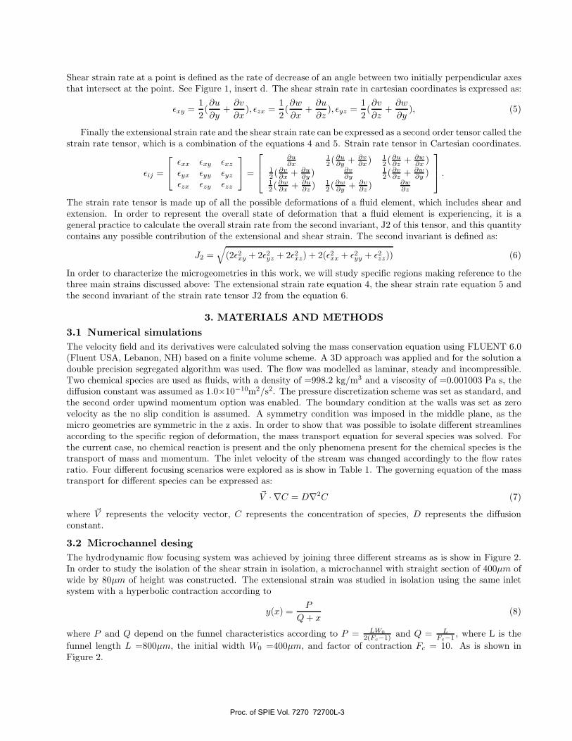
Shear strain rate at a point is defined as the rate of decrease of an angle between two initially perpendicular axesthat intersect at the point. See Figure 1, insert d. The shear strain rate in cartesian coordinates is expressed as:

εxy =12(∂u

∂y+

∂v

∂x), εzx =

12(∂w

∂x+

∂u

∂z), εyz =

12(∂v

∂z+

∂w

∂y), (5)

Finally the extensional strain rate and the shear strain rate can be expressed as a second order tensor called thestrain rate tensor, which is a combination of the equations 4 and 5. Strain rate tensor in Cartesian coordinates.

εij =

⎡⎣

εxx εxy εxz

εyx εyy εyz

εzx εzy εzz

⎤⎦ =

⎡⎢⎣

∂u∂x

12 (∂u

∂y + ∂v∂x ) 1

2 (∂u∂z + ∂w

∂x )12 ( ∂v

∂x + ∂u∂y ) ∂v

∂y12 (∂v

∂z + ∂w∂y )

12 (∂w

∂x + ∂u∂z ) 1

2 (∂w∂y + ∂v

∂z ) ∂w∂z

⎤⎥⎦ .

The strain rate tensor is made up of all the possible deformations of a fluid element, which includes shear andextension. In order to represent the overall state of deformation that a fluid element is experiencing, it is ageneral practice to calculate the overall strain rate from the second invariant, J2 of this tensor, and this quantitycontains any possible contribution of the extensional and shear strain. The second invariant is defined as:

J2 =√

(2ε2xy + 2ε2yz + 2ε2xz) + 2(ε2xx + ε2yy + ε2zz)) (6)

In order to characterize the microgeometries in this work, we will study specific regions making reference to thethree main strains discussed above: The extensional strain rate equation 4, the shear strain rate equation 5 andthe second invariant of the strain rate tensor J2 from the equation 6.

3. MATERIALS AND METHODS3.1 Numerical simulationsThe velocity field and its derivatives were calculated solving the mass conservation equation using FLUENT 6.0(Fluent USA, Lebanon, NH) based on a finite volume scheme. A 3D approach was applied and for the solution adouble precision segregated algorithm was used. The flow was modelled as laminar, steady and incompressible.Two chemical species are used as fluids, with a density of =998.2 kg/m3 and a viscosity of =0.001003 Pa s, thediffusion constant was assumed as 1.0×10−10m2/s2. The pressure discretization scheme was set as standard, andthe second order upwind momentum option was enabled. The boundary condition at the walls was set as zerovelocity as the no slip condition is assumed. A symmetry condition was imposed in the middle plane, as themicro geometries are symmetric in the z axis. In order to show that was possible to isolate different streamlinesaccording to the specific region of deformation, the mass transport equation for several species was solved. Forthe current case, no chemical reaction is present and the only phenomena present for the chemical species is thetransport of mass and momentum. The inlet velocity of the stream was changed accordingly to the flow ratesratio. Four different focusing scenarios were explored as is show in Table 1. The governing equation of the masstransport for different species can be expressed as:

�V · ∇C = D∇2C (7)

where �V represents the velocity vector, C represents the concentration of species, D represents the diffusionconstant.

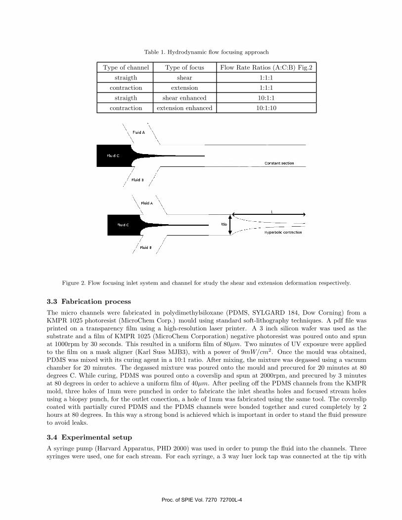
3.2 Microchannel desingThe hydrodynamic flow focusing system was achieved by joining three different streams as is show in Figure 2.In order to study the isolation of the shear strain in isolation, a microchannel with straight section of 400μm ofwide by 80μm of height was constructed. The extensional strain was studied in isolation using the same inletsystem with a hyperbolic contraction according to

y(x) =P

Q + x(8)

where P and Q depend on the funnel characteristics according to P = LW02(Fc−1) and Q = L

Fc−1 , where L is thefunnel length L =800μm, the initial width W0 =400μm, and factor of contraction Fc = 10. As is shown inFigure 2.


7

Fluid B

Constant section

Fluid A

N_____________________________________________ Wo

Hyperbolic contraction

// Fluid B /

L

Table 1. Hydrodynamic flow focusing approach

Type of channel Type of focus Flow Rate Ratios (A:C:B) Fig.2

straigth shear 1:1:1

contraction extension 1:1:1

straigth shear enhanced 10:1:1

contraction extension enhanced 10:1:10

Figure 2. Flow focusing inlet system and channel for study the shear and extension deformation respectively.

3.3 Fabrication process

The micro channels were fabricated in polydimethylsiloxane (PDMS, SYLGARD 184, Dow Corning) from aKMPR 1025 photoresist (MicroChem Corp.) mould using standard soft-lithography techniques. A pdf file wasprinted on a transparency film using a high-resolution laser printer. A 3 inch silicon wafer was used as thesubstrate and a film of KMPR 1025 (MicroChem Corporation) negative photoresist was poured onto and spunat 1000rpm by 30 seconds. This resulted in a uniform film of 80μm. Two minutes of UV exposure were appliedto the film on a mask aligner (Karl Suss MJB3), with a power of 9mW/cm2. Once the mould was obtained,PDMS was mixed with its curing agent in a 10:1 ratio. After mixing, the mixture was degassed using a vacuumchamber for 20 minutes. The degassed mixture was poured onto the mould and precured for 20 minutes at 80degrees C. While curing, PDMS was poured onto a coverslip and spun at 2000rpm, and precured by 3 minutesat 80 degrees in order to achieve a uniform film of 40μm. After peeling off the PDMS channels from the KMPRmold, three holes of 1mm were punched in order to fabricate the inlet sheaths holes and focused stream holesusing a biopsy punch, for the outlet conection, a hole of 1mm was fabricated using the same tool. The coverslipcoated with partially cured PDMS and the PDMS channels were bonded together and cured completely by 2hours at 80 degrees. In this way a strong bond is achieved which is important in order to stand the fluid pressureto avoid leaks.

3.4 Experimental setup

A syringe pump (Harvard Apparatus, PHD 2000) was used in order to pump the fluid into the channels. Threesyringes were used, one for each stream. For each syringe, a 3 way luer lock tap was connected at the tip with


CFDExperiments simulations Pathlines studied Ratio

1:1:1#3

#1 1:1:1

10:1:1#2

10: 1: 10#1

Figure 3. Hydrodynamic flow focusing configuration to isolate the pathlines, previously defined in CFD.

silicone tubing. The connection between the silicone tubing and the inlet of the channels of the hydrodynamicflow focusing system was achieved using a hypodermic needle of 19.5 gauge with the sharp tip removed. Thefirst run of flow was done using three syringes of the same size (3ml) filled with a mixture of water and detergent(Triton 50:2) using a flow rate of 50 μm for 5 minutes in order to remove any air bubbles formed at the walls.Next, taking advantage of the 3 way luer lock tap, the system, already filled with solution was maintained purged,and then the syringe was disconected and filled with either sheath flow (dionised water) or flow (orange couloreddye). For the case of hydroynamic flow focusing with the same ratio (1:1:1), three syringes of the same size wereused (1ml), and the same procedure was followed when the flow focusing was run at different rates (10:10:1)and (10:1:10), using a 10ml syringe accordingly, as is shown in Figure 3. The flow focusing performance on themicrochannel was observed using a microscope (Nikon, Eclipse, TE 2000-U).

A micro resolution particle image velocimetry (PIV) system was used to obtain the velocity profile.6, 7 Thesame procedure of filling the channels with coulored food done above was reproduce for the solution with tracerparticles. The PIV experiments were done using tracer particles of 1μm (Duke Scientific Corp). The microspheres were illuminated with a LED Flasher (LaVision Systems) and the images were captured with a CCDcamera (LaVision Systems) of 1376x1024 pixels connected to an inverted microscope (Nikon TE2000-U), witha 10x objective lens. Double exposure frames were taken and analysed using a cross correlation algorithm. Forall cases a minimum of 100 image pairs were recorded, divided into interrogation areas of 32x32 pixels and thenmaking a second interrogation of 16x16 pixels.


14

10

EE

- micro-PIVCFD

-250 -51I .5']

Channel width [urn]

ISO 250

) )

) ) ) ) ) ) )

r

Figure 4. Velocity profile of the sheaths flows and focused flow. Note that as both fluids have the same viscosity the flowsbehave as a single phase.

0

50

100

150

200

-100 0 100 200 300 400 500 600 700

[1/s

]

Funnel Length micro-m

pathline-1-dx/dypathline-2-dx/dypathline-3-dx/dy

Figure 5. CFD Pathlines studied for the shear deformation on the straigth channel, the correspondant flow focused region,ant the calculated shear strain for the pathlines.

4. RESULTS AND DISCUSSION

4.1 Velocimetry

The velocity profile was taken using micro-PIV for a system of flow rates ratios of 10:1:10, using 1ml/min onthe syringe pump. The same velocity profile was obtained using the CFD simulation. Figure 4 shows thiscomparison. It is observable that the no slip condition is ocurring at the walls and between the sheaths streamsand the flow focused stream which is practically travelling at the same speed of the sheaths fluids, it is observablethat there is a single velocity for both liquids at the interface.

4.2 Pathlines analysis, Shear region

In order to compare the isolation of the fluid in shear strain, three pathlines in different regions accross thechannel of straight section were choosen using CFD as is shown in the Figure 5. Experimentally, using the flowfocusing configuration a stream of fluid was focused on a region close to the calculated pathlines, ajusting theinput flow rates. Once the pathlines were identified, using the results of CFD the rate of shear was explored,


H2

8

E5-a

>2-1-0

0 200 400 600

Funnel Length (lAm]

800

pathllne 1pathllne 2---pathIine 3

0

50

100

150

200

250

300

350

400

-100 0 100 200 300 400 500 600 700

[1/s

]


pathline-1pathline-2pathline-3

Figure 6. Shear of strain rate of the pathlines, which was obtained calculating the second invariant of the strain ratetensor for the pathlines on the straight section.

Figure 7. Pathlines studied for the extensional deformation on the hyperbolic funnel and the velocity along the centerline.

taking εxy = 12 (∂u

∂y + ∂v∂x) for each pathline. The result for the strain in εxy is presented in the Figure 5. The

second invariant of the strain rate tensor for the selected pathlines in the straight channel is presented in theFigure 6, which represents the overall shear rate and is known in CFD codes as the strain rate.

4.3 Pathlines analysis, Extensional region

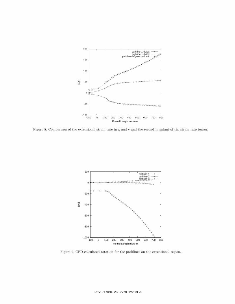
For the isolation of the extensional components, the same pathlines were choosen using a hyperbolic funnel, asis shown in the Figure 7. Once the pathlines were identified, using CFD the velocity along the center line ofthe channel x, was explored. From Figure 7 we can observe that the pathlines 1 and 2 have a similar velocityalong the center line and this one is not exactly constant due three dimensional effects because the channel ischanging of aspect ratio (See discussion of 3D effects on8). As our interest is to study the isolated effects ofthe strain components, we focus now on the pathline 1, which has the more pure extensional effects. Figure 8presents the extensional strain in x and in y as well as the second invariant of the strain rate tensor. Note thatfor du/dx and dv/dy the values are similar both with opposite sign. This is a complimentary way to observe theincompresibility condition because as long as the material is being stretched in x, it must be compressed in y.Notice that the second invariant is basically the vectorial sum of the extensional strain in x and in y. However,as long as the end of the funnel is reached, shear forces in the other planes contribute to the overall strain ratedue to the fact that the aspect ratio of the channel (height/wide) is changing. For the same pathlines in theextensional region, we now explore the rotation as is shown in the Figure 9. Notice that the rotation is a goodway to study whether a particle is experiencing the highest rate of extension. For the pathlines close to thecenterline, the rotation is close to zero and they are experiencing almost pure extension as we discussed in theprevious Figures. The pathline 3 in this image is experiencing the most complex flow studied in this article.


-100

-50

0

50

100

150

200

-100 0 100 200 300 400 500 600 700 800

[1/s

]


pathline-1-du/dxpathline-1-dv/dy

pathline-1-J2-second inv.

Figure 8. Comparison of the extensional strain rate in x and y and the second invariant of the strain rate tensor.

-1000

-800

-600

-400

-200

0

200

-100 0 100 200 300 400 500 600 700 800

[1/s

]



Figure 9. CFD calculated rotation for the pathlines on the extensional region.


0

200

400

600

800

1000

1200

1400

1600

1800

2000

-100 0 100 200 300 400 500 600 700 800 900

[1/s

]



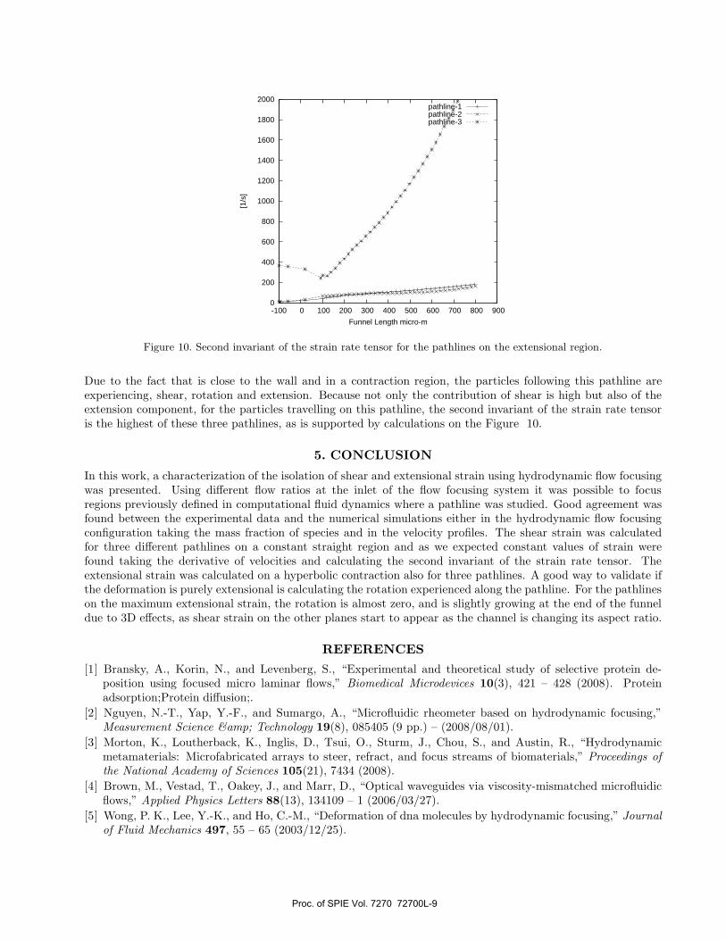
Figure 10. Second invariant of the strain rate tensor for the pathlines on the extensional region.

Due to the fact that is close to the wall and in a contraction region, the particles following this pathline areexperiencing, shear, rotation and extension. Because not only the contribution of shear is high but also of theextension component, for the particles travelling on this pathline, the second invariant of the strain rate tensoris the highest of these three pathlines, as is supported by calculations on the Figure 10.

5. CONCLUSION

In this work, a characterization of the isolation of shear and extensional strain using hydrodynamic flow focusingwas presented. Using different flow ratios at the inlet of the flow focusing system it was possible to focusregions previously defined in computational fluid dynamics where a pathline was studied. Good agreement wasfound between the experimental data and the numerical simulations either in the hydrodynamic flow focusingconfiguration taking the mass fraction of species and in the velocity profiles. The shear strain was calculatedfor three different pathlines on a constant straight region and as we expected constant values of strain werefound taking the derivative of velocities and calculating the second invariant of the strain rate tensor. Theextensional strain was calculated on a hyperbolic contraction also for three pathlines. A good way to validate ifthe deformation is purely extensional is calculating the rotation experienced along the pathline. For the pathlineson the maximum extensional strain, the rotation is almost zero, and is slightly growing at the end of the funneldue to 3D effects, as shear strain on the other planes start to appear as the channel is changing its aspect ratio.

REFERENCES

[1] Bransky, A., Korin, N., and Levenberg, S., “Experimental and theoretical study of selective protein de-position using focused micro laminar flows,” Biomedical Microdevices 10(3), 421 – 428 (2008). Proteinadsorption;Protein diffusion;.

[2] Nguyen, N.-T., Yap, Y.-F., and Sumargo, A., “Microfluidic rheometer based on hydrodynamic focusing,”Measurement Science & Technology 19(8), 085405 (9 pp.) – (2008/08/01).

[3] Morton, K., Loutherback, K., Inglis, D., Tsui, O., Sturm, J., Chou, S., and Austin, R., “Hydrodynamicmetamaterials: Microfabricated arrays to steer, refract, and focus streams of biomaterials,” Proceedings ofthe National Academy of Sciences 105(21), 7434 (2008).

[4] Brown, M., Vestad, T., Oakey, J., and Marr, D., “Optical waveguides via viscosity-mismatched microfluidicflows,” Applied Physics Letters 88(13), 134109 – 1 (2006/03/27).

[5] Wong, P. K., Lee, Y.-K., and Ho, C.-M., “Deformation of dna molecules by hydrodynamic focusing,” Journalof Fluid Mechanics 497, 55 – 65 (2003/12/25).


[6] Meinhart, C., Wereley, S., and Santiago, J., “PIV measurements of a microchannel flow,” Experiments inFluids 27(5), 414–419 (1999).

[7] Santiago, J., Wereley, S., Meinhart, C., Beebe, D., and Adrian, R., “A particle image velocimetry system formicrofluidics,” Experiments in Fluids 25(4), 316–319 (1998).

[8] Oliveira, M., Alves, M., Pinho, F., and McKinley, G., “Viscous flow through microfabricated hyperboliccontractions,” Experiments in Fluids 43(2), 437–451 (2007).


Hydrodynamic flow focusing to study the isolated effects of the flow components

Documents

Transcript of Hydrodynamic flow focusing to study the isolated effects of the flow components