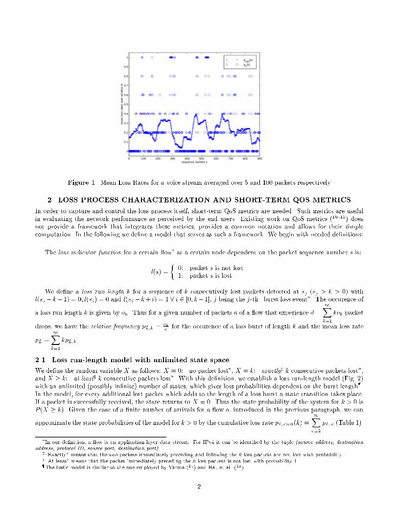
A Framework Model for Packet Loss Metrics Based on LossRunlengths �H. Sanneck and G. CarleGMD Fokus, Kaiserin-Augusta-Allee 31, D-10589 Berlin, GermanyABSTRACTFor the same long-term loss ratio, di�erent loss patterns lead to di�erent application-level Quality of Service (QoS)perceived by the users (short-term QoS). While basic packet loss measures like the mean loss rate are widely usedin the literature, much less work has been devoted to capturing a more detailed characterization of the loss pro-cess. In this paper, we provide means for a comprehensive characterization of loss processes by employing a modelthat captures loss burstiness and distances between loss bursts. Model parameters can be approximated based onrun-lengths of received/lost packets. We show how the model serves as a framework in which packet loss metricsexisting in the literature can be described as model parameters and thus integrated into the loss process characteri-zation. Variations of the model with di�erent complexity are introduced, including the well-known Gilbert model asa special case. Finally we show how our loss characterization can be used by applying it to actual Internet loss traces.Keywords: Packet Loss, Short-Term QoS Metrics, Loss Burstiness, Internet Real-Time Services1. INTRODUCTIONExisting work on Internet Quality of Service (QoS) identi�ed delay, jitter and packet loss as metrics of interest forusers and operators (1). Among these, packet loss is an important metric in the statistically shared environment ofthe Internet, where the demand for a resource (such as bandwidth or bu�er) may exceed the available capacity. Formultimedia applications such as coded audio and video (live or stored), loss may also result from inordinate delay inthe network which causes the play-out deadline of a sample or a frame to be missed. While existing work focuses oncapturing the mean loss (long-term QoS), less emphasis is put on modelling loss distribution (short-term QoS, cf. (2,3)and the references therein). It is important to note that for the same mean loss, di�erent loss patterns can producedi�erent perceptions of QoS, as described in (4{8). Also, as shown by Cidon et al. (6) and Shacham/McKenney (9),many forward error recovery approaches become less e�cient as the loss burstiness increases. Thus, it is important tobe able to capture the actual loss process with suitable (and simple) metrics. As an example, Fig. 1 shows mean lossrates pm(s) for a voice stream versus its sequence number s averaged with a sliding window of �ve and 100 packetsrespectively (p5(s), p100(s)). It can be seen that the distribution of loss rates (and thus the perceptual impact) overa small window size (p5(s)) varies strongly. At the same time, the mean loss rate evaluated over the larger windowsize (p100(s)) varies within a much smaller interval. The mean loss rate calculated over a large time interval is thusnot suitable to reveal di�erences of perceived QoS.Thus, our aim in this paper is to develop a model with the following properties:� possibility of expressing well-known long- and short-term QoS metrics (like e.g. those of the Gilbert model);� adjustable complexity dependent on speci�c application/network requirements, supporting additional metricsfor detailed short-term QoS analysis;� coverage of both loss burstiness, as well as distances between losses.In the following section, we describe a characterization of the loss process, and develop an analytical frameworkusing a model based on loss and no-loss run-lengths. In section 3, we show the applicability of the developed measuresto actual Internet loss traces. Finally, we conclude in Section 4 with a summary and point out directions for futureresearch.� To appear in Proceedings of the SPIE/ACM SIGMM Multimedia Computing and Networking Conference 2000 (MMCN 2000),San Jose, CA, January 2000 1

0 100 200 300 400 500 600 700 800 900

0

0.1

0.2

0.3

0.4

0.5

0.6

0.7

0.8

0.9

1

sequence number s

mea

n lo

ss r

ates

ove

r w

indo

w m

p100

(s)

p5(s)

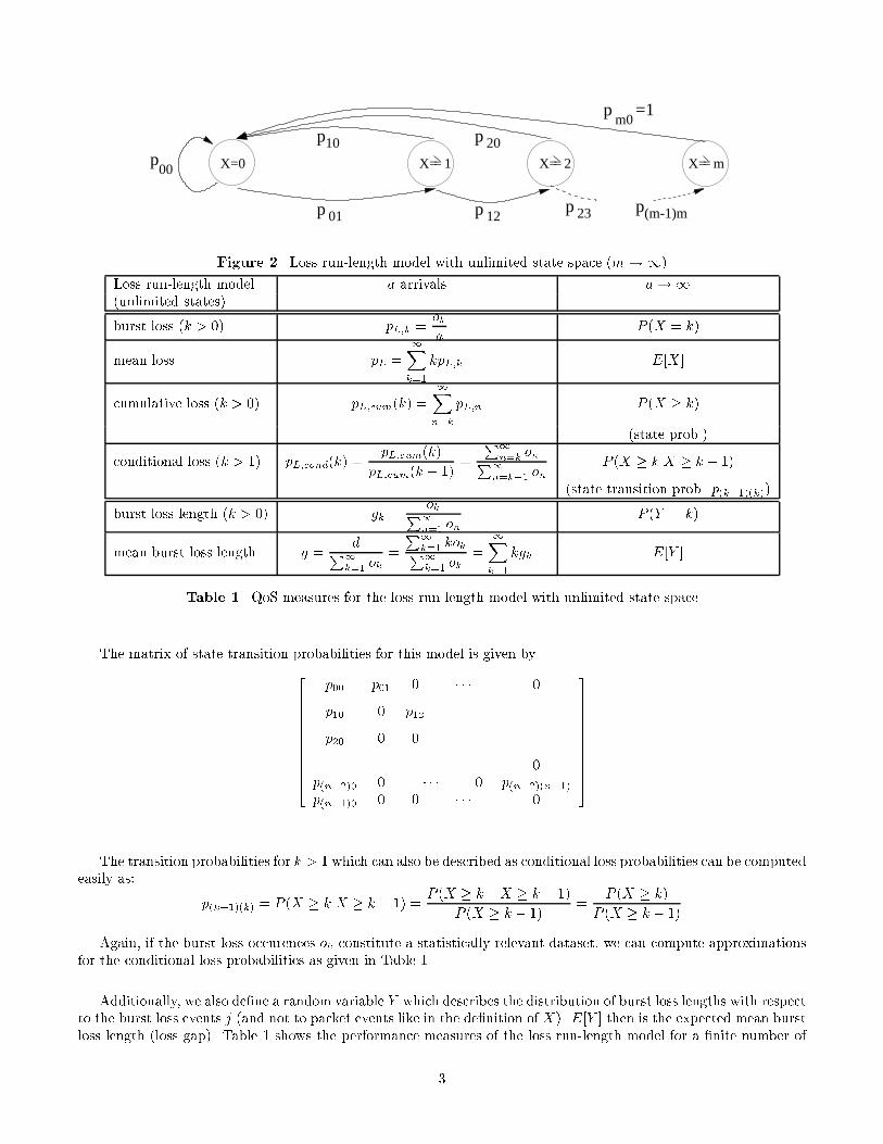
Figure 1. Mean Loss Rates for a voice stream averaged over 5 and 100 packets respectively2. LOSS PROCESS CHARACTERIZATION AND SHORT-TERM QOS METRICSIn order to capture and control the loss process itself, short-term QoS metrics are needed. Such metrics are usefulin evaluating the network performance as perceived by the end users. Existing work on QoS metrics (10{13) doesnot provide a framework that integrates these metrics, provides a common notation and allows for their simplecomputation. In the following we de�ne a model that serves as such a framework. We begin with needed de�nitions:The loss indicator function for a certain owy at a certain node dependent on the packet sequence number s is:l(s) = � 0: packet s is not lost1: packet s is lostWe de�ne a loss run length k for a sequence of k consecutively lost packets detected at sj (sj > k > 0) withl(sj � k� 1) = 0; l(sj) = 0 and l(sj � k+ i) = 1 8 i 2 [0; k� 1], j being the j-th \burst loss event". The occurence ofa loss run length k is given by ok. Thus for a given number of packets a of a ow that experience d = 1Xk=1 kok packetdrops, we have the relative frequency pL;k = oka for the occurence of a loss burst of length k and the mean loss ratepL = 1Xk=1 kpL;k.2.1. Loss run-length model with unlimited state spaceWe de�ne the random variable X as follows: X = 0: \no packet lost", X = k: \exactlyz k consecutive packets lost",and X � k: \at leastx k consecutive packets lost". With this de�nition, we establish a loss run-length model (Fig. 2)with an unlimited (possibly in�nite) number of states, which gives loss probabilities dependent on the burst length{.In the model, for every additional lost packet which adds to the length of a loss burst a state transition takes place.If a packet is successfully received, the state returns to X = 0. Thus the state probability of the system for k > 0 isP (X � k). Given the case of a �nite number of arrivals for a ow a, introduced in the previous paragraph, we canapproximate the state probabilities of the model for k > 0 by the cumulative loss rate pL;cum(k) = 1Xn=k pL;n (Table 1).yIn our de�nition, a ow is an application-layer data stream. For IPv4 it can be identi�ed by the tuple (source address, destinationaddress, protocol ID, source port, destination port).z\Exactly" means that the two packets immediately preceding and following the k lost packets are not lost with probability 1.x\At least" means that the packet immediately preceding the k lost packets is not lost with probability 1.{The basic model is similar to the one employed by Varma (14) and Hsu et al. (15).2

= =X= mX= 2=

20

m0

12 23p

p

p p(m-1)m

p00 X=0

01p

X= 1

p =1

p10

Figure 2. Loss run-length model with unlimited state space (m!1)Loss run-length model a arrivals a!1(unlimited states)burst loss (k > 0) pL;k = oka P (X = k)mean loss pL = 1Xk=1 kpL;k E[X ]cumulative loss (k > 0) pL;cum(k) = 1Xn=k pL;n P (X � k)(state prob.)conditional loss (k > 1) pL;cond(k) = pL;cum(k)pL;cum(k � 1) = P1n=k onP1n=k�1 on P (X � kjX � k � 1)(state transition prob. p(k�1)(k))burst loss length (k > 0) gk = okP1n=1 on P (Y = k)mean burst loss length g = dP1k=1 ok = P1k=1 kokP1k=1 ok = 1Xk=1 kgk E[Y ]Table 1. QoS measures for the loss run-length model with unlimited state spaceThe matrix of state transition probabilities for this model is given by26666666664p00 p01 0 � � � 0p10 0 p12 ...p20 0 0 . . . ...... ... ... . . . 0p(n�2)0 0 � � � 0 p(n�2)(n�1)p(n�1)0 0 0 � � � 0

37777777775The transition probabilities for k > 1 which can also be described as conditional loss probabilities can be computedeasily as: p(k�1)(k) = P (X � kjX � k � 1) = P (X � k \X � k � 1)P (X � k � 1) = P (X � k)P (X � k � 1)Again, if the burst loss occurences ok constitute a statistically relevant dataset, we can compute approximationsfor the conditional loss probabilities as given in Table 1.Additionally, we also de�ne a random variable Y which describes the distribution of burst loss lengths with respectto the burst loss events j (and not to packet events like in the de�nition of X). E[Y ] then is the expected mean burstloss length (loss gap). Table 1 shows the performance measures of the loss run-length model for a �nite number of3

= X= 2=

20

m0

12 23p

p

p

p p(m-1)m

X=0

01p

=p00 p

mmX= 1 X= m

p10

Figure 3. Loss run-length model with limited state space [(m+ 1) states]arrivals a using the loss run length occurences ok, as well as the relation to the transition/state probabilities of themodel (a!1) with the random variables X and Y . The cumulative loss rate for k = 0 is de�ned as the \no loss"case (corresponding to P (X = 0) ):pL;cum(k = 0) = 1� 1Xk=1 pL;cum(k) = 1� 1Xk=1 1Xn=k ona = 1� 1Xk=1 koka = 1� pL2.2. Loss run-length model with limited state spaceTo assess the performance of a network with respect to real-time audio and video applications, a model with a limitednumber of states is su�cient. This is due to the fact that real-time audio and video applications have strict require-ments and cannot use a network service with a signi�cant number of \long" loss bursts. For these applications it isdesirable to use only few model parameters, and to focus on key aspects of the loss process. In addition, memory andcomputational capabilities of the system that performs modelling have to be taken into account (see also paragraph2.6).For these reasons we derive from the basic model a loss run-length model with a �nite number of states (m+1).Fig. 3 shows the Markov chain for the model. Table 2 gives performance measures similar to those in Table 1k,however the state probability for the �nal state m (P (X = m)) and the probability for a transition from state mto state m are added. For 0 < k < m, X = k represents as before \exactly k consecutive packets lost". Due to thelimited memory of the system, the last state X = m is just de�ned as \m consecutive packets lost". Thus P (X = m)can be seen as a measure for the \loss over a window of size m" (independently of actually larger loss run lengths).Figure 4 shows the base measures used to compute the loss run-length based metrics. In Figure 4 (a), each pointindicates whether there was a loss (1) or not (0), representing the loss indicator function. Figure 4 (b) shows the lossrun lengths. Figure 4 also shows some of the state transitions when a given loss trace is applied to a model of eitherm = 2 or m � 4. With m = 2 for a loss burst of length k = 4, the system is three times (k �m+ 1, see Fig. 4 (c))in state 2, and thus two (k �m) transitions m ! m occur. This leads to the computation of pL;m and pL;cond(m)(as approximations for P (X = m) and P (X = mjX = m) respectively) as given in Table 2.Interestingly, Miyata et al. (12) propose precisely pL;m as a performance measure for FEC-based audio applica-tions. This "sliding window" of m consecutively lost packets allows to re ect speci�c applications' constraints, e.g.m can be set to the lowest number of consecutively lost packets for which a complete audio \dropout" is perceivedby a user. Then, larger loss bursts do not have a higher impact and thus do not need to be taken into account withtheir exact size. We extend the above approach by looking at the occurence of a certain number of packets lostwithin the window of length m. This allows e.g. to assess how e�ective FEC protection applied to groups of packetswould be without keeping track of the actual Application Data Unit (ADU) association of the individual packets. Insection 1 we introduced the mean loss rate over a sliding window of length m (pm(s)) which can be de�ned as theconvolution of the analysis window with the loss indicator function (Fig. 5):kThe burst loss length measures are computed as in Table 1 and are therefore not shown.4

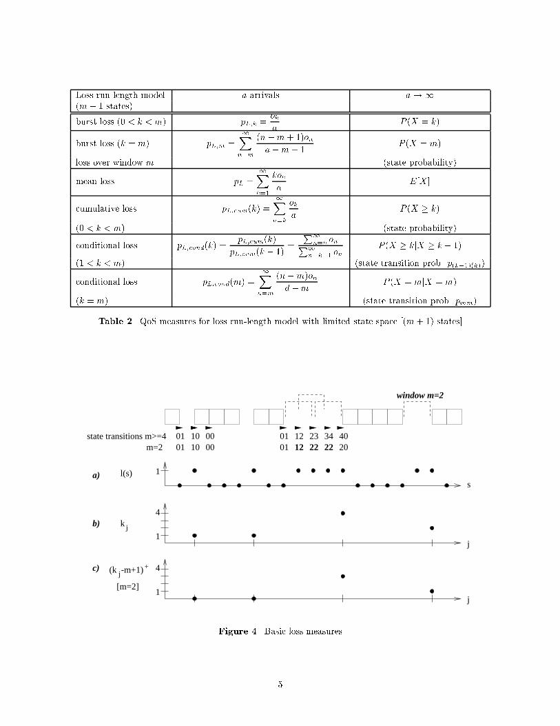
Loss run-length model a arrivals a!1(m+ 1 states)burst loss (0 < k < m) pL;k = oka P (X = k)burst loss (k = m) pL;m = 1Xn=m (n�m+ 1)ona�m+ 1 P (X = m)loss over window m (state probability)mean loss pL = 1Xk=1 koka E[X ]cumulative loss pL;cum(k) = 1Xn=k oka P (X � k)(0 < k < m) (state probability)conditional loss pL;cond(k) = pL;cum(k)pL;cum(k � 1) = P1n=k onP1n=k�1 on P (X � kjX � k � 1)(1 < k < m) (state transition prob. p(k�1)(k))conditional loss pL;cond(m) = 1Xn=m (n�m)ond�m P (X = mjX = m)(k = m) (state transition prob. pmm)Table 2. QoS measures for loss run-length model with limited state space [(m+ 1) states]

k j

01 10 00 01 23 4012 34

1

4

j

[m=2]

j(k -m+1) +c)

window m=2

1

sl(s)a)

j1

4b)

state transitions m>=4m=2 01 10 00 01 22 2012 22

Figure 4. Basic loss measures5

w (s)m

p (s)m

w,m

s

1

1s

1

1

l(s)

m

1

so (k)

a)

b)

c)

5

mk

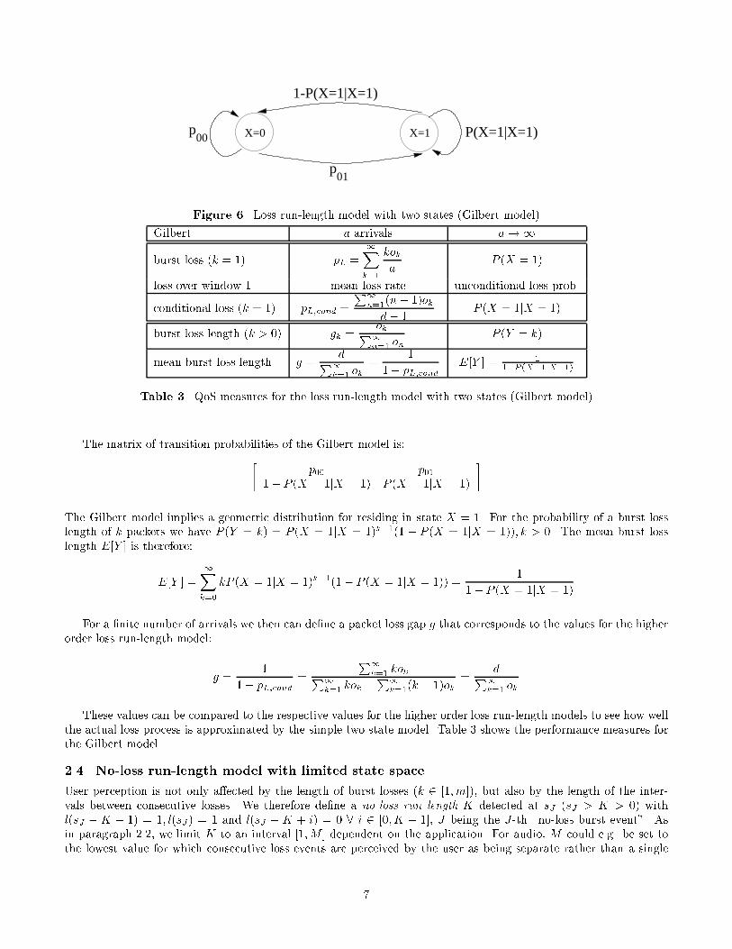
Figure 5. pm(s): mean loss rate over a sliding window of length mpm(s) = l(s) � wm(s)m = aX�=0 l(�)wm(s� �)mThe tradeo� following from the above formula can be described as follows: computing the actual histogram ofpm(s) (solid line in Fig. 5 c) captures the accurate sequential relation of the loss bursts, however makes the measurestill depend on s (this is the approach taken in (16)). When using only the sum of histograms calculated separatelyover each individual loss burst (dashed line Fig. 5 c) some information is lost, however only the tracking of loss burstsk is needed. To describe the latter approach we use ow;m(k) which describes the occurence of k consecutive packetslost within the window of length mow;m(k) = 8>>>><>>>>: (m� k + 1)ok + 2 1Xn=k+1 on: 0 < k < m1Xn=m(n�m+ 1)on: k = mSumming over the weighted ow;m(k) we get in fact the overall mean loss rate (see the Appendix for the proof):mXk=1 kow;m(k)ma = 1Xk=1 koka = pL (1)Similar window-based measures were proposed also in (17{19).2.3. Gilbert ModelFor the special case of a system with a memory of only the previous packet (m = 1), we can use the runlengthdistribution for a simple computation of the parameters of the commonly-used Gilbert model (Fig. 6) to characterizethe loss process (X being the associated random variable with X = 0: \no packet lost", X = 1 \a packet lost").Then the \loss over window m" is equal to the mean loss or unconditional loss probability, and only one conditionalloss probability (transition 1! 1) is de�ned. 6

X=1X=0

p

00p

01

1-P(X=1|X=1)

P(X=1|X=1)

Figure 6. Loss run-length model with two states (Gilbert model)Gilbert a arrivals a!1burst loss (k = 1) pL = 1Xk=1 koka P (X = 1)loss over window 1 mean loss rate unconditional loss prob.conditional loss (k = 1) pL;cond = P1n=1(n� 1)okd� 1 P (X = 1jX = 1)burst loss length (k > 0) gk = okP1n=1 on P (Y = k)mean burst loss length g = dP1k=1 ok = 11� pL;cond E[Y ] = 11�P (X=1jX=1)Table 3. QoS measures for the loss run-length model with two states (Gilbert model)The matrix of transition probabilities of the Gilbert model is:� p00 p011� P (X = 1jX = 1) P (X = 1jX = 1) �The Gilbert model implies a geometric distribution for residing in state X = 1. For the probability of a burst losslength of k packets we have P (Y = k) = P (X = 1jX = 1)k�1(1 � P (X = 1jX = 1)); k > 0. The mean burst losslength E[Y ] is therefore:E[Y ] = 1Xk=0 kP (X = 1jX = 1)k�1(1� P (X = 1jX = 1)) = 11� P (X = 1jX = 1)For a �nite number of arrivals we then can de�ne a packet loss gap g that corresponds to the values for the higherorder loss run-length model:g = 11� pL;cond = P1k=1 kokP1k=1 kok �P1k=1(k � 1)ok = dP1k=1 okThese values can be compared to the respective values for the higher order loss run-length models to see how wellthe actual loss process is approximated by the simple two state model. Table 3 shows the performance measures forthe Gilbert model.2.4. No-loss run-length model with limited state spaceUser perception is not only a�ected by the length of burst losses (k 2 [1;m]), but also by the length of the inter-vals between consecutive losses. We therefore de�ne a no-loss run length K detected at sJ (sJ > K > 0) withl(sJ �K � 1) = 1; l(sJ) = 1 and l(sJ � K + i) = 0 8 i 2 [0;K � 1], J being the J-th \no-loss burst event". Asin paragraph 2.2, we limit K to an interval [1;M ] dependent on the application. For audio, M could e.g. be set tothe lowest value for which consecutive loss events are perceived by the user as being separate rather than a single7

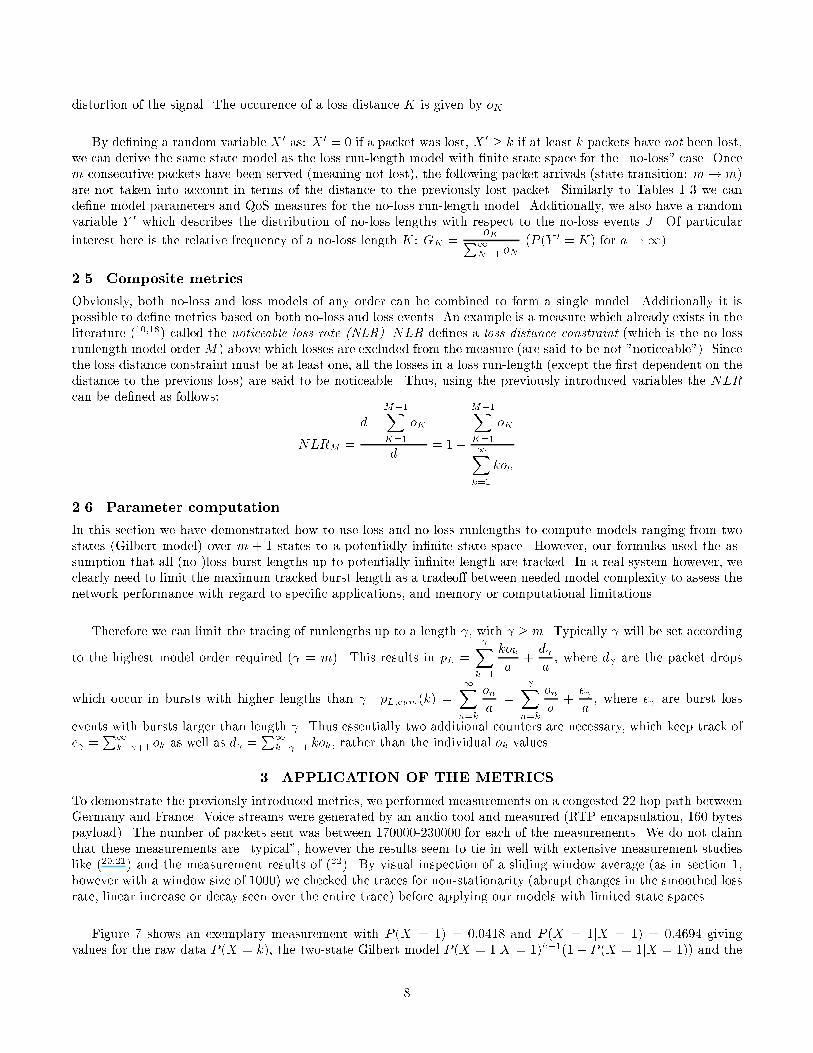
distortion of the signal. The occurence of a loss distance K is given by oK .By de�ning a random variable X 0 as: X 0 = 0 if a packet was lost, X 0 � k if at least k packets have not been lost,we can derive the same state model as the loss run-length model with �nite state space for the \no-loss" case. Oncem consecutive packets have been served (meaning not lost), the following packet arrivals (state transition: m! m)are not taken into account in terms of the distance to the previously lost packet. Similarly to Tables 1-3 we cande�ne model parameters and QoS measures for the no-loss run-length model. Additionally, we also have a randomvariable Y 0 which describes the distribution of no-loss lengths with respect to the no-loss events J . Of particularinterest here is the relative frequency of a no-loss length K: GK = oKP1N=1 oN (P (Y 0 = K) for a!1).2.5. Composite metricsObviously, both no-loss and loss models of any order can be combined to form a single model. Additionally it ispossible to de�ne metrics based on both no-loss and loss events. An example is a measure which already exists in theliterature (10,18) called the noticeable loss rate (NLR). NLR de�nes a loss distance constraint (which is the no-lossrunlength model orderM) above which losses are excluded from the measure (are said to be not "noticeable"). Sincethe loss distance constraint must be at least one, all the losses in a loss run-length (except the �rst dependent on thedistance to the previous loss) are said to be noticeable. Thus, using the previously introduced variables the NLRcan be de�ned as follows: NLRM = d�M�1XK=1 oKd = 1� M�1XK=1 oK1Xk=1 kok2.6. Parameter computationIn this section we have demonstrated how to use loss and no-loss runlengths to compute models ranging from twostates (Gilbert model) over m + 1 states to a potentially in�nite state space. However, our formulas used the as-sumption that all (no-)loss burst lengths up to potentially in�nite length are tracked. In a real system however, weclearly need to limit the maximum tracked burst length as a tradeo� between needed model complexity to assess thenetwork performance with regard to speci�c applications, and memory or computational limitations.Therefore we can limit the tracing of runlengths up to a length , with � m. Typically will be set accordingto the highest model order required ( = m). This results in pL = Xk=1 koka + d a , where d are the packet dropswhich occur in bursts with higher lengths than . pL;cum(k) = 1Xn=k ona = Xn=k ona + e a , where e are burst lossevents with bursts larger than length . Thus essentially two additional counters are necessary, which keep track ofe =P1k= +1 ok as well as d =P1k= +1 kok, rather than the individual ok values.3. APPLICATION OF THE METRICSTo demonstrate the previously introduced metrics, we performed measurements on a congested 22 hop path betweenGermany and France. Voice streams were generated by an audio tool and measured (RTP encapsulation, 160 bytespayload). The number of packets sent was between 170000-230000 for each of the measurements. We do not claimthat these measurements are \typical", however the results seem to tie in well with extensive measurement studieslike (20,21) and the measurement results of (22). By visual inspection of a sliding window average (as in section 1,however with a window size of 1000) we checked the traces for non-stationarity (abrupt changes in the smoothed lossrate, linear increase or decay seen over the entire trace) before applying our models with limited state spaces.Figure 7 shows an exemplary measurement with P (X = 1) = 0:0418 and P (X = 1jX = 1) = 0:4694 givingvalues for the raw data P (X = k), the two-state Gilbert model P (X = 1jX = 1)k�1(1� P (X = 1jX = 1)) and the8

0 5 10 15 20 25 30 35 40 45 50

10−4

10−3

10−2

10−1

100

burs

t pac

ket l

oss

prob

abili

ties

P(.

)

length of loss burst k, length of loss window m

P(X=k)

P(X>=k)

P(X>=k|X>=k−1)

P(X=m)

P(X=1|X=1)k−1(1−P(X=1|X=1))

P(Y=k)

Figure 7. Performance parameters for an example measurement 4state and state transition probabilties for the model with limited (k < m) and unlimited state space. Additionallythe state probability P (X = m) for the model with limited states is given. We see that the probability P (Y = k)to lose exactly k consecutive packets in a burst loss event drops geometrically fast in an interval of approximately[1; 10]. In this case, a loss run-length model con�rms that the loss process is approximated well by the Gilbert modelP (X = 1jX = 1)k�1(1� P (X = 1jX = 1)). For larger bursts (k > 10), the loss burst probabilities are signi�cantlylarger than for the Gilbert model. Thus the loss process in that area is underestimated. However, the absolute valuesof the loss probabilities are several orders of magnitude smaller than for the singleton loss (k = 1) case and do notseem to follow a speci�c distribution. Therefore it is not necessary that this area is considered by a model. Theconditional loss probabilities P (X � kjX � k � 1) increase with increasing loss burst length k, however their valuesare already very close to 1 for k >� 10 and stay there (in the shown area). This means that (as mentioned above)only few burst loss events larger than 10 packets take place and thus models with a higher number of states do notgive much additional information. This can also be seen from the state probability curve P (X � k), where valuesin the mentioned region do not change signi�cantly. Fig. 7 also shows P (X = m), the �nal state probability formodels of order m+1, which gives the probability that all packets within a window of length m are lost. This curveis very close to the "raw data" burst loss probabilities P (X = k) for k > 35, which makes clear that no signi�cantprobability for burst losses larger than that exist, i.e. the data trace contains no "outages".4. CONCLUSIONSIn this paper, we have presented a framework model which integrates both known and novel loss metrics and thusallows to capture the e�ect of loss distribution on continuous media applications. We constructed and parametrizedmodels of di�erent complexity that capture loss characteristics fully or partially, with the well-known Gilbert model9

being a special case of these models. We showed how to directly relate model parameters to runlength-based datatracing. By applying the run-length model to measurement traces of IP voice ows, we demonstrated the tradeo�sbetween accurate multi-parameter modelling and simple but coarse modelling. We conclude that for Internet QoSsupport within applications and gateways an \intermediate model" is needed, which has to be more complex thanthe simple Gilbert model. The needed complexity of such an intermediate model is determined by the applicationrequirements.For future work, the autocorrelation of the loss indicator function, as well as the autocorrelation and compositemetrics like the crosscorrelation function of the loss/no-loss run-lengths (21) remain to be evaluated with regard totheir practical usability and their relation to our model. Furthermore, it seems promising to combine the modelfor loss characterisation presented in this paper with results on user perception of multimedia applications likee.g. in (23,24). This allows a precise and relevant characterisation of application-level QoS based on network levelperformance metrics, and opens a way for novel approaches to QoS support, which enforce certain short-term losscharacteristics (patterns) on the stream rather than looking exclusively at a long-term loss rate (10,25,26).ACKNOWLEDGMENTSWe would like to thank Rajeev Koodli, Nokia Research Center, Boston, for many valuable discussions.REFERENCES1. V. Paxson, G. Almes, J. Mahdavi, and M. Mathis, \Framework for IP performance metrics," RFC, IETF, May1998. ftp://ftp.ietf.org/rfc/rfc2330.txt.2. H. W. Chu and D. H. K. Tsang, \Dynamic bandwidth allocation for VBR video tra�c in ATM networks," inProceedings of ICCCN, pp. 306{312, 1997.3. H. Zhu and V. S. Frost, \In-service monitoring for cell loss Quality of Service violations in ATM networks,"IEEEACM Transactions on Networking 4(2), pp. 240{248, 1996.4. M. Bjorkman, A. Latour-Henner, U. Hansson, and A. Miah, \Controllability and impact of cell loss process inATM networks," in Proceedings of IEEE GLOBECOM, pp. 916{920, 1995.5. J. C. Bolot and A. Vega Garcia, \The case for FEC-based error control for packet audio in the Internet," ACMMultimedia Systems , 1997.6. I. Cidon, A. Khamisy, and M. Sidi, \Analysis of packet loss processes in high-speed networks," IEEE Transactionson Information Theory 39, pp. 98{108, January 1993.7. M. Meky and T. N. Saadawi, \Degradation e�ect of cell loss on speech quality over atm networks," in BroadbandCommunications, IFIP, Chapman and Hall, pp. 259{271, 1996.8. I. E. G. Richardson and M. J. Riley, \Usage parameter control cell loss e�ects on MPEG video," in IEEE ICC,pp. 970{974, 1995.9. N. Shacham and P. McKenney, \Packet recovery in high-speed networks using coding and bu�er management,"in Proceedings ACM SIGCOMM '90, pp. 124{131, (San Francisco, CA), June 1990.10. R. Koodli and C. Krishna, \Noticeable loss: A metric for capturing loss pattern for continous media applica-tions," in Internet Routing and Quality of Service, S. Civanlar, P. Doolan, J. Luciani, R. Onvural, Editors,Proceedings SPIE Vol.3529A, (Boston, MA), November 1998.11. Z. Liu, P. Nain, and D. Towsley, \Bounds on �nite horizon QoS metrics with application to call admission," inProceedings IEEE INFOCOM '96, (San Francisco, CA, USA), April 1996.12. T. Miyata, H. Fukuda, and S. Ono, \New network QoS measures for FEC-based audio applications on theInternet," in Proceedings IEEE IPCCC 1998, pp. 355{362, (Tempe/Phoenix, AZ, USA), February 1998.13. C. Partridge, \A proposed ow speci�cation," RFC 1363, IETF, September 1992.ftp://ftp.ietf.org/rfc/rfc1363.txt.14. V. Varma, \Testing speech coders for usage in wireless communication system," in Proceedings of IEEE SpeechCoding Workshop, pp. 93{94, (Montreal), 1993.15. C. Hsu, A. Ortega, and M. Khansari, \Rate control for robust video transmission over wireless channels," inProceedings of Visual Communications and Image Processing (VCIP), pp. 1200{1211, (San Jose, CA), February1997. 10

16. M. Borella, D. Swider, S. Uludag, and G.Brewster, \Internet packet loss: Measurement and implications forend-to-end QoS," in Proceedings of the International Conference on Parallel Processing, August 1998.17. S. Ono, T. Miyata, and H. Fukuda, \Loss metrics of grouped packets for IPPM," Internet Draft, IETF IPPMWorking Group, August 1998. ftp://ftp.ietf.org/internet-drafts/draft-ono-group-loss-00.txt.18. R. Koodli and R. Ravikanth, \One-way loss pattern sample metrics," Internet Draft, IETF IPPM WorkingGroup, June 1999. ftp://ftp.ietf.org/internet-drafts/draft-ietf-ippm-loss-pattern-01.txt.19. R. Nagarajan, J. Kurose, and D. Towsley, \Finite-horizon statistical Quality-of-Service measures for high speednetworks," J. High Speed Networks , December 1994.20. M. Yajnik, J. Kurose, and D. Towsley, \Packet loss correlation in the MBone multicast network," in ProceedingsIEEE Global Internet 1996 (Jon Crowcroft and Henning Schulzrinne, eds.), pp. 94{99, (London, England),November 1996.21. M. Yajnik, S. Moon, J. Kurose, and D. Towsley, \Measurement and modelling of the temporal dependence inpacket loss," Technical Report 98-78, Department of Computer Science, University of Massachusetts, Amherst,1998.22. J.-C. Bolot, H. Cr�epin, and A. Garcia, \Analysis of audio packet loss in the Internet," in Proceedings of the 5thInternational Workshop on Network and Operating System Support for Digital Audio and Video, pp. 163{174,(Durham, NH), April 1995.23. D. Reininger and R. Izmailov, \Soft quality of service with VBR+ video," in Proceedings of 8th InternationalWorkshop on Packet Video (AVSPN97), (Aberdeen, Scotland), September 1997.24. H. Sanneck and N. Le, \Speech property-based FEC for Internet Telephony applications," in Proceedings of theSPIE/ACM SIGMM Multimedia Computing and Networking Conference 2000 (MMCN 2000), (San Jose, CA),January 2000. ftp://ftp.fokus.gmd.de/pub/glone/papers/Sann0001:Speech-FEC.ps.gz.25. H. Sanneck and G. Carle, \Predictive loss pattern queue management for Internet routers," in Internet Routingand Quality of Service, S. Civanlar, P. Doolan, J. Luciani, R. Onvural, Editors, Proceedings SPIE Vol.3529A,(Boston, MA), November 1998. ftp://ftp.fokus.gmd.de/pub/glone/papers/Sann9811:Predictive.ps.gz.26. H. Sanneck and G. Carle, \A queue management algorithm for intra- ow service di�erentiation in the "beste�ort" Internet," in Proceedings of the Eighth Conference on Computer Communications and Networks (ICCCN'99), (Natick, MA), October 1999. ftp://ftp.fokus.gmd.de/pub/glone/papers/Sann9910:Intra-Flow.ps.gz.AppendixProof of formula 1:mXk=1 kow;m(k)ma == 1ma "m�1Xk=1 k(m� k + 1)ok + 2k 1Xn=k+1 on!+m 1Xn=m(n�m+ 1)on#= 1ma "m�1Xk=1 k(m� k + 1)ok + 2 m�1Xk=1 k m�1Xn=k+1 on + m�1Xk=1 k 1Xn=m on!+m 1Xn=m(n�m+ 1)on#= 1ma "m�1Xk=1 kmok � m�1Xk=1 k(k � 1)ok + 2 m�1Xk=1 k(k � 12 ok + m(m� 1)2 1Xn=m on!+ 1Xn=mnmon �m(m� 1) 1Xn=m on# == m 1Xk=1 kokma = pL11