Title and content - Indian Ecological Society
202
INDIAN JOURNAL OF ECOLOGY Volume 45 Issue-2 June 2018 THE INDIAN ECOLOGICAL SOCIETY ISSN 0304-5250
-
Upload
khangminh22 -
Category
Documents
-
view
2 -
download
0
Transcript of Title and content - Indian Ecological Society

INDIAN JOURNAL OF
ECOLOGYVolume 45 Issue-2 June 2018
THE INDIAN ECOLOGICAL SOCIETY
ISS
N 0304-5250

Registered OfficeCollege of Agriculture, Punjab Agricultural University, Ludhiana – 141 004, Punjab, India
(e-mail : [email protected])
Advisory Board Kamal Vatta S.K. Singh S.K. Gupta Chanda Siddo Atwal B. PateriyaK.S. Verma Asha Dhawan A.S. Panwar S. Dam Roy V.P. Singh
Executive CouncilPresident
A.K. Dhawan
Vice-PresidentsR. Peshin S.K. Bal Murli Dhar G.S. Bhullar
General SecretaryS.K. Chauhan
Joint Secretary-cum-TreasurerVaneet Inder Kaur
CouncillorsA.K. Sharma A. Shukla S. Chakraborti N.K. Thakur
MembersKiran Bains S.K. Saxena Jagdish ChanderR.S. Chandel R. Banyal Ashok Kumar
Editorial BoardChief-EditorS.K. Chauhan
Associate EditorS.S. Walia K. Selvaraj
EditorsR.K. Pannu Harit K. Bal M.A. Bhat K.C. Sharma S. Sarkar Neeraj Gupta Mushtaq A. Wani Harsimran GillChima Njoku Sumedha Bhandari Maninder Kaur Walia Rajinder KumarK.C. Sharma
The Indian Journal of Ecology is an official organ of the Indian Ecological Society and is published six-monthly in June and December. Research papers in all fields of ecology are accepted for publication from the members. The annual and life membership fee is Rs (INR) 700 and Rs 4500, respectively within India and US $ 40 and 700 for overseas. The annual subscription for institutions is Rs 4500 and US $ 150 within India and overseas, respectively. All payments should be in favour of the Indian Ecological Society payable at Ludhiana. KEY LINKS WEBsite:http://indianecologicalsociety.comMembership:http://indianecologicalsociety.com/society/memebership/Manuscript submission:http://indianecologicalsociety.com/society/submit-manuscript/Status of research paper:http://indianecologicalsociety.com/society/paper-status-in-journal-2/Abstracts of research papers:http://indianecologicalsociety.com/society/indian-ecology-journals/
INDIAN ECOLOGICAL SOCIETY
(www.indianecologicalsociety.com)Past resident: A.S. Atwal and G.S.Dhaliwal(Founded 1974, Registration No.: 30588-74)

Degradation of Western Algerian Steppes Lands: Monitoring and Assessment
Indian Journal of Ecology (2018) 45(2): 235-243
Abstract: The Algerian steppes are currently experiencing erosion of natural resources; the situation continues to grow and leads to an
imbalance of local ecosystems. In this investigation, floristic surveys coupled with soil tests were carried out. The phytoecological study
revealed a very strong degradation of the floristic richness and the phytomass with a predominance of the loamy-sand texture and a
disturbance of the parameters studied from one site to another. The monitoring of ecological changes 60 years later shows a decrease in the
number of species and families of 79 and 41% respectively with a disappearance of some facies that are replaced by other indicators of
degradation with less forage value. This regressive dynamic is explained by two essential factors: land use changes and climatic aridity.
Keywords: Steppe, Degradation, Monitoring, Ecological changes
Manuscript Number: NAAS Rating: 4.96
2665
1 2 Fatima Zohra Bahlouli, Abderrezak Djabeur, Abdelkrim Kefifa , Fatiha Arfiand Meriem Kaid-harche
Département de Biotechnologie, Faculté des Sciences de la Nature et de la Vie, Laboratoire des Productions, Valorisations Végétales et Microbiennes (LP2VM), Université des Sciences et de la Technologie d'Oran Mohamed Boudiaf
(USTO'MB), BP 1505 El Mnaouar, Oran 31000, Algeria.1Département de Biologie, Faculté des Sciences, Laboratoire de Biotoxicologie, Pharmacognosie et Valorisation
Biologique des Plantes (LBPVBP), Université de "Dr. Tahar Moulay", BP 138, Saïda 20000, Algeria.2Institue Nationale de la Recherche Forestière, INRF Aïn-Skhouna, Saïda 20000, Algeria.
E-mail: [email protected]
In Algeria, steppes have always been the development
space for sheep farming. They play both an economic role
linked to pastoral activity and an ecological role as a buffer
zone between the Tell and the Sahara. Pastoralism was
considered the most suitable system for steppe lands, which
for a long time ensured the ecological balance in these
environments. This balance has for a long time been assured
by a very rigid harmony between human mobility and the
environment in which he lives (Nedjimi et al 2012). However,
this equilibrium is broken; due to the decrease in the area of
rangelands and the fall in their yields as a result of the
continuous increase in livestock numbers on the one hand
and the extension of clearings at the expense of the best
rangelands on the other hand, thus reducing the forage
resources of the livestock (Nedjraoui 2004). The situation in
these pastoral areas is worrying; the work of Bouazza et al
(2004) on the watershed of El-Aouedj (south-west of Oran)
show that the steppe plant formations are currently entering a
phase of degradation that takes a worrying strong pace. The
steppes at Stipa tenacissima were the most affected by these
changes, they occupied 6.61 per cent of the territory in 1973
to decrease to 2.24 per cent in 1990 and in 2003 they
disappeared completely from the zone. The strongest
regression is recorded in the southern Oran, where in less
than 10 years almost all alfa-nappes have disappeared
(Aidoud et al 2006).
Various factors are mentioned by the authors to explain
the causes of these transformations that have occurred in
recent decades. The profound changes in the management
policies adopted as well as the uses and farming practices
have certainly modified the levels of anthropozoic impacts on
vegetation and environment (Fikri Benbrahim et al 2004,
Aidoud et al 2006, Benabadji et al 2009). However, Benabadji
et al (2009) find that the last five decades have been marked
by a decrease in the amount of rainfall leading to a recurring
drought. Hirche et al (2007) suggest a two-month extension
of the dry season while estimating a decrease in rainfall
amount of 18 to 27 per cent per year on average. The
combined action of man and climate creates a vulnerability of
these ecosystems; the phytogenetic and edaphic resources
are disrupted (Nedjraoui 2011). Any workers documented
that changes that have occurred on the steppe of western
Algeria (Slimani et al 2010, Bencherif 2011, Hasnaoui et al
2014, Hasnaoui and Bouazza 2015, Morsli et al 2016). These
authors confirm the regressive dynamics of steppe plant
formations. The aim of the present paper attempts to outline
the current state of this steppe rangelands by a
phytoecological study followed by a comparative diachronic
analysis, to evaluate the natural resources available, to
assess and monitor the degradation intensity of the study

area on the one hand, and discuss the probable causes of the
changes that have occurred in the other hand. This analysis
could thus highlight the dynamics of this ecosystem.
MATERIAL AND METHODS
Study area: Province of Saïda is located in the western part
of the high plateaus (North -West) of Algeria. It decomposes
respectively from the North to the South in three major areas:
an agricultural area, an agro_pastoral area and a steppe
area. The study area is located in South-eastern part of
department combining two steppe municipalities: Maamora
and Aïn Skhouna (from 34° 30' to 34° 40' North latitude and
from 0° 30' to 0° 50' East longitude, with an elevation ranging
from 995 to 1147m above sea level). The area is
characterized by an annual rainfall relatively low; it is 286 mm -1year . The rainfall pattern is AWSS (autumn, winter, spring,
summer), favourable to vegetative activity despite the length
of the drought period which extends from May to November,
and the cold that extends from December to April. During the
dry season, rainfall amounts do not exceed 90mm. Monthly
average temperatures in winter reach 1 ° C (m) and 36 ° C (M)
in summer. The evapotranspiration ETP is quite important in
the period extending from May to September. The value of
ETP recorded in July equals 173.3 mm and that of August is
163.4 mm (Moulay 2013). The rainfall quotient of Emberger
(Q2) is 28. This allows us to classify the study area in the
semi-arid bioclimatic stages with fresh winter. The soils are
characterized by the presence of accumulation Limestone,
the low organic matter content and high susceptibility to
erosion and degradation D jbaili (1984).
Sampling: Out 90 phyto-ecological surveys with 10
repetitions for each station, executed during the optimum
period of vegetation development, from mid-April to mid-
June of 2012, 2013 and 2014; to obtain the maximum number
of species (especially annuals), according to the Braun-
Blanquet method (1951). The number of stations was
quantified according to the variation in vegetation cover on a
transect line: North-South, which is based on the use of the
Emberger climate index (1955), which revealed large
variations in the North-South direction. The execution of the
surveys is accompanied by the recording of the stationary
characters (Location, altitude, exposure, slope and recovery
rate). The surveys are collected every 200 m depending on
the variability of the vegetation and ecological conditions
such as topography and exposure.
The surface of these surveys must be sufficient to
understand the maximum of plant species (Guinochet 1973).
The delimitation of the plots (sampling and measurement
site) for each survey which characterizes a homoecological
area is of 100 m² (Djebaili 1978) delimited with a rope. The
determination of the taxa for the vegetation was made using
the work of Quézel and Santa (1963) and that of Ozenda
(1977). The biological types were attributed from the work of
Raunkier (1905).
Choice of stations: The choice of stations was guided by
our objective; the stations should best reflect the current state
of the study area. To achieve our objectives we carried out
various field trips which enabled us to characterize an
ecological zoning and; identified three plants structures
(facies): facies to Alfa (Stipa tenacissima L.), facies to white
Wormwood (Artemisia herba alba Asso.) and facies to Sparte
(Lygeum spartum L.). According to the state of vegetation
cover, the facies have been selected to three types: good
state (exclosure), moderately degraded and degraded.
Characterization of vegetation
Specific contribution calculation: To compare the floristic
variation in point of view quantitative of the stations, the sum
served to the calculations of the specific contribution of each
species (Csi) which is defined as the report as a percentage
of its specific frequency (Fsi) to the sum of the frequencies of
all the listed species: Csi = (Fsi/∑Fsi) × 100 or Fsi = (Ni/N) ×
100 (Ni: The number of times where the species i is
encountered; N: The total number of reading points, it is 100
in our case)
Aboveground biomass: The aboveground biomass
measurements were made during the optimum period of
vegetation development and determined by clipping the
perennial and annual species which occupies 1m ? 1m
quadrats for each plots. The determination of the dry matter
(DM) is done to the oven at 105°C until to the constant weight
(during 48h). The aboveground biomass production is
expressed in kg of DM/ha.
Soil sampling and analysis: For the knowledge of the study
area soil, conducted soil profiles (90 soil samples) at the level
of the superficial horizon where the roots exist. The soil
analysis has been devoted to the following parameters: the
texture, according to the method of GRAS (1988) and the
chemical analyzes are carried out using the methods
described in AUBERT (1978), pH in distilled water, electrical
conductivity (Ec), total limestone (CaCO ), organic matter 3
(OM) and the depth of the profile up to the calcareous crust.
Analysis of changes in steppic facies, diachronic study:
For the monitoring of vegetation dynamics over the last sixty
years, the comparative diachronic method was used. This
method takes the oldest state as the starting point for the
observation. The objective is to compare the situation of a
site in an initial state and to assess the changes that occurred
between the two observations. This diachronic study is
based on the work of Dubuit and Simmoneau (1954). A
phytoecological study was conducted on the same sampling
Fatima zohra bahlouli, Abderrezak djabeur, Abdelkrim kefifa, Fatiha arfi and Meriem kaid-harche236
sites of the initial state (Fig.1). For that first by a calibration of
the map of Dubuit and Simmoneau according to the
projection Lembert (North Algerian) was done and then have
georeference the surveys of the old map.
Statistical analysis: In order to confirm the results observed
in the field. The specific contributions of species inter–facies
was compered. The significance of changes between facies
was tested using the nonparametric Friedman. To describe
the both patternplant biomass and soil characteristics of each
facies, the mean (± standard deviation) was calculated for
each above-ground biomass and soil parameter based, on all
observations. Analyzes were carried out using the XLSTAT
software (version 2014 by Addinsoft). Significant differences
for the statistical tests were evaluated at p ≤ 0.05.
RESULTS AND DISCUSSION
Characterization of Vegetation
Analysis of the floristic composition: In the set of surveys
studied, a floristic list of 33 perennial and annual species,
belonging to 28 genera and 12 botanical families was
identified. The 21, 18 and 12 percent belong to the families of
the Asteraceae, Poaceae and Caryophylaceae with
respectively. This order of magnitude is also obtained by
several authors who have worked in this region (Hasnaoui et
al 2015, Saidi et al 2017). The Amaranthaceae are present,
particularly in the Ain Skhouna region with (12%); this is
justified by location of this region near the Chott Echergui.
These plants are Therophytes with 54% and
Chamaephytique with 21%. These results are in agreement
with those obtained by Ghezlaoui et al (2011). These authors
show that the Therophytes and the Chamaephytes are well
adapted to steppe regions. Similarly Kadi-Hanifi et al (1998)
have marked that the predominance of Therophytes is linked
to the accentuation of the aridity outside the increase of
Chamaephytes is linked to the anthropization of the
environment. In addition, Quézel (2000) present the
Therophyzation as a form of resistance to drought, as well as
to the high temperatures of the arid environments and an
ultimate stage of degradation. The geophytes are the less
dominant, they are represented by three species which are:
Stipa tenacissima L., Stipa parviflora Desf. and Muscari
comosum (L.) Miller. Kadi-Hanifi et al (2003) have pointed out
that the rate of Geophytes decreases with the anthropization.
The arborescence stratum is represented by a single species
Atriplex halimus L. (Nanophanerophyte). Kadi Hanifi et al
(2003) confirms that the phanerophytes are always relegated
to the last rank of the biological types in the steppe regions.
Specific Contribution Analysis
Facies to Stipa tenacissima L.: The number of species
decreased from 17 in good state to 13 in moderately
degraded, to only 8 in degraded facies (Fig. 2). More the
palatable species regress more the number of species
indicating degradation and overgrazing appear as Noaea
mucronata (Forssk.) and Peganum harmala L. phenomenon
confirmed by Nedjraoui (2004).
The statistical analysis shows that the difference is
highly significant between facies in good state and the
degraded. On the other hand, it is not significant between the
good state and moderately degraded facies. However, the p-
value between the facies in good state and the moderately
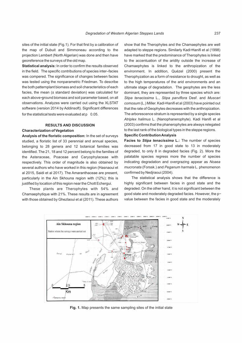
Fig. 1. Map presents the same sampling sites of the initial state
Degradation of Western Algerian Steppes Lands 237

Fig. 2. Photographs showing different types of facies to Stipa tenacissima L: (a), facies to Alfa well growing; (b), facies to Alfa moderately degraded; (c), facies to Alfa degraded. Station of Maamora; province of Saïda; Western Algeria
degraded is relatively high p= 0.7829 (Table 1). We can
deduce that the courses seen in good state show a tendency
to become moderately degraded. However, Slimani et al
(2010) show that the regression of Alfa covers in western
Algeria is mainly due to overgrazing.
Facies to Artemisia herba alba Asso.: The floristic diversity
in the facies to white Wormwood more important than in the
facies to Alfa. The comparative analysis of the specific
contributions show a highly significant difference (Table 1)
between the courses in good state and degraded with a
decrease in Csi of the dominant specie; it's from 70.85 to only
17.06%. It is significant between the good state and
moderately degraded (p = 0.0397) with a decrease from
70.85 to 42.54%. This regression is explained by the
anthropological action (overgrazing and land-use changes)
exercised on the courses (Mahyou et al 2016).
The rise is important and progressive of the two species
indicator of degradation (Noaea mucronata. and Peganum
harmala), in the contributions reached respectively in the
degraded facies 41.82 and 34.04%. The action of the herd on
the courses considerably modifies the floristic composition.
Permanent and uncontrolled pasture thus leads to the
reduction of palatable species, which are replaced by other
species little appetite, usually abandoned by livestock (Kadi
Hanifi 2003). Most of the species are disappeared of the floral
procession in the degraded facies (Figure 3).
Facies to Lygeum spartum L.: The comparative analysis of
the specific contributions shows a very significant difference
between facies in good condition and degraded and shows
significant deference between facies in good condition and
moderately degraded; the decrease in Sparta's contribution
from 70.30 to 38.48% to only 17.92 (Table 1).
A high contribution of peganum harmala was recorded in
the degraded courses (Figure 4) with 63.24%. The
occurrence of P. harmala [a toxic species that develops when
soil nitrate levels are significant (Aimé 1988)] is an indicator
of overgrazing in the area (Benabadjie et al 2009).
Aboveground biomass
Facies to Stipa tenassicima L.: The average of the above-
ground biomass by facies shows that the courses to Alfa in
good state offer a total biomass of 1251 for Alfa and 654 kg
DM / ha for plants association. This result is similar to
Bouchetata and Bouchetata (2005) who estimated that the
above-ground biomass of Alfa is 1254 Kg DM/ha. However, in
the courses moderately degraded and degraded the biomass
present a considerable decline ranging respectively from 707
for Alfa and 242 kg DM/ ha for plants association to 237.8 for
Alfa and 82.2 kg DM/ha for plants association (Figure 5). This
decrease is explained by the result of several factors,
including the irrational management of rangelands and the
introduction of development means and techniques unsuited
to steppe environments. Today, the biomass of the steppe is
constantly decreasing; the comparative analysis of the
Fatima zohra bahlouli, Abderrezak djabeur, Abdelkrim kefifa, Fatiha arfi and Meriem kaid-harche238

Fig. 3. Photographs showing different types of facies to Artemisia herba alba Asso: (a), facies to white Wormwood well growing; (b), facies to white Wormwood moderately degraded; (c), facies to white Wormwood degraded. (a,b), Station of Maamora. (c), Station of Aïn Skhouna, province of Saïda, Western Algeria
Fig. 4. Photographs showing different types of facies to Lygeum Spartum L.: (a), facies to Sparte Well growing; (b), facies to Sparte moderately degraded; (c), facies to Sparte degraded. Station of Aïnskhouna; province of Saïda; Western Algeria
Degradation of Western Algerian Steppes Lands 239

Fig. 5. Total aboveground biomass (mean values ± SD) for each structure and type of facies
results obtained in the different facies studied shows an
alarming regressive dynamic. It should be noted that facies to
Alfa considered in good state are, in fact, under a striking
regression. Indeed, the aboveground biomass estimated by
2100 kg DM / ha in 1976 (Aidoud and Nedjraoui 1992) fell to
1750 kg DM / ha in 1996 (Aidoud and Touffet 1996), to 1500
kg DM / ha in 2001 (Nedjraoui 2002).
Facies to Artemisia herba alba Asso.: The facies in good
state gives an aerial biomass of 3234 kg DM/ha for white
Wormwood. These results are in agreement with those of
Ayad et al (2015) who reported that the total dry matter
biomass of white Wormwood is 3172 kg DM/ha. The
comparison of the biomass calculated in the three facies
highlights the degradation state of these courses, where the
biomass has decreased by 76.46% going from that in good
state to that in degraded (Figure 5). This decrease is due to
overgrazing exerting on the rangelands. According to Li et al
(2011), overgrazing diminishes soil nutrients, which in turn
adversely affects rangeland biomass.
Facies to Lygeum spartum L.: The different measures of
biomass obtained from the three different facies to L. spartum
show a very important variation. The average of the biomass
of Sparte in good state goes from 341.3 to only 103.1kg
DM/ha in the degraded (Figure 5). Heavy grazing intensity
significantly decreased the vegetation height, coverage,
diversity and above-ground biomass (Wei Li et al 2011).
According to Nedjraoui (2002), the steppes to Sparte are little
productive with an annual average production ranging from
300 to 500 kg DM/ha.
The biomass of the plants association is relatively
important in the degraded facies. It represents 45.56% of the
total biomass of the facies. On the other hand, it is 39.60% in
the moderately degraded and 39.84% in good state facies.
The strong pressures on the courses modify the plant
association in a progressive way giving rise to formations rich
in species indicative of degradation with low pastoral values
(cases of Noaea mucronata (frossk), Peganum harmala L.).
Analysis of Soil
Texture: The dominance of the texture sandy loam appears
in 80 stations is 89%. The other texture is of fine loam
appears in 10 stations, be 11% (Table 2). The textures
proportions of samples have a high percentage of the sands
which is in average between 50.5 and 57.1%, and a
significant amount of silt that oscillates between 30.1 and
33.1%. The amount of clay is reduced for the degraded facies
and ranged between 11% and 12.2 %.
Total CaCO : The analysis show low levels of total CaCO , 3 3
with values that ranged between 5.58 and 7.7 % (Table 2).
Benabadji (1996) reported that the CaCO content in steppic 3
soil is related to the nature of the parent rock.
Electrical conductivity: The overall salinity represented by
the electrical conductivity, present low values, ranging
between 0.31and 0.9 mS / cm. these results show that the
soil of the study area is not salty.
pH: The pH varied from 8.29 to 8.54 indicating alkaline soil.
These findings corroborate those of Benabadji et al (2009),
Ghezlaoui et al (2011) and Hasnaoui and Bouazza (2015). In
arid and semi-arid region, pH is alkaline due to cations that
are not leached. Bases are accumulated on the soil surface
because evapotranspiration is greater than precipitation.
Rezaei and Gilkes (2005) suggest that pH values are mainly
affected by the parental material, which varies from place to
place, following rainfall and organic carbon levels.
Organic Matter (OM) and Soil Depth
In facies to Alfa: The decrease in the rate of organic matter
is in correlation with the state of facies. The percentage in
Fatima zohra bahlouli, Abderrezak djabeur, Abdelkrim kefifa, Fatiha arfi and Meriem kaid-harche240

P- Value
Facies A. GS A. MD A. D W. GS W. W. D S. GS S. MD S. D
Alfa GS 1 0,7829 a0,0265
W.Wormwood GS 1 0,039 0,000
Spart GS 1 0,025 < 0,0001
Table 1. Statistical results of specific contribution inter facies
A= Alfa W= white Wormwood S= Spart GS= good state MD= moderately degraded D= degraded
Facies Stipa tenassicima L Artemisia herba alba Asso Lygeum spartum L
sites GS MD D GS MD D GS MD D
Granulometry %
Sand 50.5±2.4 54.9±3.52 56.7±7.29 55.8±2.8 56.7±4.53 57.1±5.12 52.1±5.12 55.8±2,8 56.7±4.53
Silt 31±1.51 33.1±2.99 30.49±7.90 31±3.18 30.3±4.35 31.5±5.78 31.4±5.22 30.2±3.18 30.1±4.35
clay 18.5±1.4 12.8±3.71 11±2.97 13.2±0.35 13±0.23 11.4±0.12 16.5±3.12 14±1.07 12.2±3.28
Type of texture Silt-loam Sandy- Loam
Sandy-Loam
Sandy-Loam
Sandy-Loam
Sandy-Loam
Sandy-Loam
Sandy-Loam
Sandy-Loam
pH 8.29±0.2 8.49±0.34 8.54±0.22 8.32±0.26 8.4±0.27 8.3±0.22 8.34±0.11 8.49±0.15 8.52±0.14
EC mS/cm 0.7±0.06 0.6±0.13 0.33±0.11 0.9±0.29 0.5±0.13 0.55±0.13 0.31±0.2 0.64±0.11 0.76±0.09
CaCO t %3 6.17±1.7 7.7±1.24 5.63±2.2 5.58±1.04 7.15±1.06 5.92±1.7 5.58±1.04 7.15±1.06 5.92±1.7
OM 1.96±0.1 0.62±0.07 0.33±0.07 1.24±0.15 0.61±0.07 0.37±0.14 1.09±0.29 0.47±0.13 0.17±0.12
Depth (cm) 17.6±3.2 12.2±2.4 7.1±1.91 13.6±1.07 12.8±3.28 9.8±3.12 17±2.8 10.7±2.33 7.2±2.1
Table 2. Values of soil physicochemical parameters (mean ± standard deviation) measured in different studied facies.
GS= good state MD= moderately degraded D= degraded EC= electrical conductivity OM= organic matter
average of 1.96 in good state to 0.62 in moderately degraded
to low grades 0.33% in the degraded (Table 2). The reduction
is due to the regression of the rate of vegetation cover
(Benabadji and Bouazza 2002).
In general, soils of steppe are shallow. The different
facies that occupy the steppe zones vary from one zone to
another depending on the planimetry, climate and
environmental conditions. In our case, the rates recorded in
the various samples are variable. This variability depends on
the dominance of Alfa. In sites to Alfa degraded, the depth of
the soil is rather meager, on average of 7.1cm and 12.2cm in
the moderately degraded formations and 17.6 cm in the good
state. The depth parameter varies according to the degree of
degradation due to the impact of wind, runoff. According to
Dengfeng et al (2015) wind and water erosion are among the
most important causes of soil loss. And also to the
degradation or destruction of plant cover who leads to a
disruption of the carbon cycle.
In facies to white wormwood: The organic matter content
for samples of site in good state is on average of 1.24 %. As
for the other two facies (moderately degraded and
degraded), the average values of 0.61 and 0.37 percent
respectively (Table 2). It remains too low. The effects of wind
erosion result primarily in the loss of fine soil particles and soil
organic matter (Zhao et al 2006). The soil depth of 9.8 to 13.6
cm and is lower compared to that of facies to Alfa. The flora of
the facies to Alfa is less important than that of the white
Wormwood facies. Thus the presence of Alfa favours the
conservation of the soils (Hasnaoui and Bouazza 2015).
In facies to Sparte: The analysis show very remarkable low
organic matter, content in moderately degraded and
degraded facies with very low rates of 0.47 and 0.17 %,
respectively. These results are very consistent with those of
Benabadji et al (2009), which explain this by the nature of
steppes with degraded facies, which are feebly productive.
The depth of the soil varies between 7.2 and 17.6 cm. These
values show a regression of one type to another, the soil
truncation is very obvious.
Regressive evolution of facies (analyze of diachronic
study): The diachronic study made it possible to detect the
main changes between 1954 and 2014 which are:
The number of species inventoried goes from 132 in
1954 to 28 in 2014 and is 79% reduction where there are 113
species that no longer appear and 9 new species have
appeared on our inventory. The number of families
inventoried decreased from 29 to only 12 with the
Degradation of Western Algerian Steppes Lands 241

disappearance of 20 families and the appearance of 3 new
ones. According to Debuit and Simmoneau (1954), the facies
to Lygeum spartum L are distinctly individualized on the
South-east of Chott (from 34°15' to 34°20' North latitude and
from 1°1' to 1°6' East longitude). Sixty years later, L. spartum
facies are located on the North-west of Chott (from 34°30' to
34°35' North latitude and from 0°41' to 0°47' East longitude).
The rhizomatous root system of L. spartum facilitates this
extension and seems to be an opportunist species, the
development of which is favored by drought and land
degradation (Hirch et al 2011). Facies to Stipa tenacissima
L. are replaced by facies to Lygeum spartum L. under
association to Artemisia herba alba Asso and the facies to
Artemisia herba alba and Atriplex mauritanica Boiss & Reut.
are replaced by facies to L. spartum under association to
Noaea mucronata Frosk. with the total disappearance of the
Atriplex mauritanica specie. The replacement of dominants
species by L. spartum and other species indicating land
deterioration, a trend observed by other authors (Aidoud et al
2006). However Benabadji et al (2009) reported that the
regression of some species for the benefit of others is due to
climatic and especially anthropogenic factors. According to
Debuis and Simmoneau (1954), the facies to Alfa are fairly
tight to give the impression of a closed settlement appears
like immense meadow called "Alfa Sea". Currently, the Alfa
sites which are in good state (exclosure) do not even exceed
the 60% of the recovery, while the other sites provide 5 to
35% of the recovery. The same phenomenon of decrease in
Alfa cover has been observed in Tunisia (Hanafi and Jauffret
2007). Perennials vegetation is destroyed by anthropical
anarchic action, clearing and grazing, this destruction is also
aggravated by the increase in animal pressure on the
increasingly reduced pastoral areas and by the collection of
plants intended to satisfy culinary and medicinal needs. The
strong decline of Stipa tenacissima L is disturbing, which
presumably assumes its total disappearance in the coming
years. The soil has changed from a silty-clay texture to a
sandy loam texture for the white Wormwood facies. However
the soil of the other facies has changed from a sandy-clay-
loam to a sandy loam texture. Low vegetation cover helps to
explain the importance and increase of wind speed and
frequency (Nouaceur 2008).
CONCLUSION
The analysis of the current state of the study area
reveals a regressive tendency of the pastoral areas and is
accompanied by a worrying decrease in the quality of the
vegetation cover. The increase of formations with indicator
species of degradation, well adapted and of less forage value
is made to the loss of Alfa and Wormwood sites; Formations
more appreciated by the breeders. The edaphic data indicate
the weakness of the elements essential to pedogenesis and
confirm the low biological activity characteristic of the study
area. The diachronic study reveals the degree of regression
of soils and plant species. However, this study showed that
some facies have completely disappeared and are replaced
by others. In addition, the regressive evolution of the white
Wormwood and Alfa steppes results in stages where these
two species are replaced by Sparte and by indicator species
of degradation such as Noaea mucronata and peganum
harmala reflecting overgrazing. This investigation allowed us
to visualize the alarming situation of these rangelands,
indicating an erosion of the natural resources, following the
combined impact of anthropogenic action and climatic
damage; but overgrazing appears to be the major component
of steppe degradation.
ACKNOWLEDGEMENTS
This paper is dedicated to the memory of Morsli Abdslem
who contributed to the work; unfortunately he was deceased
before the article submission. We express our gratitude and
recognition to INRF Ain skhouna to have followed this work
closely. We also thank INRAA Sidi Bel Abbes for the
realization of the soil analyses. We would like to thank Terras
Mouhamed for his help and cooperation in providing
information and to Bahlouli Samia for her support.
REFERENCES
Aidoud A, Le Floc'h E and Le Houérou HN 2006. Les steppes arides du nord de l'Afrique. Sécheresse 17(1–2): 19–30.
Aimé S 1988. Aspects écologiques de la présence de quelques espèces steppiques (Stipa tenacissima, Lygeum spartum, Artemisia herba-alba, Noaea mucronata) en Oranie littorale. Biocénoses 12: 16-24.
Ayad N, Addoune M, Hellal T and Hellal B 2015. Densité et Biomasse de l'armoise blanche (Artemisia herba-alba Asso.) dans la steppe du sud de la wilaya de Tlemcen. Review Ecologie-Environnement 11(1): 80-84.
Benabadji N, Aboura R and Benchouk F 2009. La régression des steppes méditerranéennes : le cas d'un faciès à Lygeum spartum L. d'Oranie (Algérie). Ecologia Mediterranea 35: 75-90.
Benabadji N and Bouazza M 2002. Contribution à l'étude du cortège floristique de la steppe au Sud d'El Aricha (Oranie, Algérie). Science & Technologies. N° spécial D, 11-19p.
Bouchetata T and Bouchetata A 2005. Dégradation des écosystèmes steppiques et stratégies de développement durable. Mise au point méthodologique appliquée à la wilaya de Naama (Algérie). Développement durable et territoires, 12p.
Braun-Blanquet J 1951. Les groupements végétaux de la France Méditerranéenne. C.N.R.S. Paris: 297 p.
Dengfeng T Mingxiang X Yunge Z and Liqian G 2015. Interactions between wind and water erosion change sediment yield and particle distribution under simulated conditions. Journal of Arid Land 7: 590–598.
Djebaili S 1984. Steppe algérienne, phytosociologie et écologie. Office des publications universitaire(OPU), Algiers, Algeria. 182p.
Dubuis A and Simonneau P 1954. Contribution à l'étude de la
Fatima zohra bahlouli, Abderrezak djabeur, Abdelkrim kefifa, Fatiha arfi and Meriem kaid-harche242

végétation de la région d'Aïn Skhouna (chott Chergui oriental). Services Etudes Scientifique Direction Hydraulique Gouvernement Gén. Algérie, Algiers, p 143.
Emberger L 1955. Une classification biogéographique des climats. Recueil des travaux des laboratoires de Botanique. Géologie et Zoologie de la Faculté des Sciences de Montpellier (série Botanique), fascicule 7(11): 3-43.
Ghezlaoui B, Benabadji N, Benmansour D and Merzouk A 2011. Analyse des peuplements végétaux halophytes dans le Chott El-Gharbi (Oranie-Algérie). Acta Botánica Malacitana 36: 113–124.
Haddouche I, Mederbal K and Saidi S 2007. Space analysis and the detection of the changes for the follow-up of the components sand-vegetation in the area of Mecheria (Algeria). Review SFPT 185: 2629.
Hanafi A and Jauffret S 2007. Are long-term vegetation dynamics useful in monitoring and assessing desertification processes in the arid steppe, southern Tunisia. Journal of Arid Environments 72: 557– 572.
Hasnaoui O, Meziane H, Borsali AH and Bouazza M 2014. Evaluation of Characteristics Floristico-Edaphic of the Steppes at Alfa (Stipa tenacissima L.) in the Saida Region (Western Algeria). Open Journal of Ecology 4: 883-891.
Hasnaoui O and Bouazza M 2015. Indicateurs de dégradation des bio-ressources naturelles de l'Algérie occidentale: Cas de la steppe de la wilaya de Saida. Algerian Journal of Arid Environment 5: 63-75.
Hirche A Salamani M Abdellaoui A Benhouhou S and Valderrama J 2011. Landscape changes of desertification in arid areas: the case of south-west Algeria. Environnemental Monitoring and Assessment 18: 403-420.
Kadi-Hanifi-Achour H 1998. L'Alfa en Algérie. Syntaxonomie, relation milieu végétation, Dynamique et perspectives d'avenir. Ph.D.Thesis, Université des Sciences et Technologie Houari Boumediène. Algiers, Algeria. 228 p.
Kadi-Hani f i -Achour H 2003. Diversi té bio logique et phytogéographique des formations à Stipa tenacissima L. de l'Algérie. Revue Sécheresse 14(3): 169–179.
Labani A 2006. Fluctuations climatiques et dynamique de l'occupation de l'espace dans la commune d'Ain El Hadjar (Saïda, Algérie). Revue Sécheresse 17: 391-398.
Le Houérou H N 2005. Problèmes écologiques du développement de l'élevage en région sèche. Revue Sécheresse 16(2): 89-96.
Li XL, Gao J, Brierley G, Qiao YM, Zhang J and Yang YW 2011. Rangeland degradation on the Qinghai-Tibet plateau: implications for rehabilitation. Land Degradation & Development 24: 72–80.
Mahyou H, Tychon B, Balaghi R, Louhaichi M and Mimouni J 2016. A knowledge-based approach for mapping land degradation in the arid rangelands of North Africa. Land Degradation & Development 27(6): 1574-1585.
Morsli A, Hasnaoui O and Arfi F 2016. Evaluation of the Above-Ground Biomass of Steppe Ecosystems According to Their Stage of Degradation: Case of the Area of Ain Skhouna
(Western Algeria). Open Journal of Ecology 6: 235-242.
Moulay A 2013. Contribution à l'étude de la régénération naturelle et artificielle de Stipa tenacissima L. dans la région steppique occidentale (Algérie). Ph.D.Thesis. University of Mascara, Algeria, 172 p.
Nouaceur Z 2008. Apport des images-satellites dans le suivi des nuages de poussières en zones saharienne et sub-saharienne. Revue Télédétectio 8(1): 5–15.
Nedjraoui D 2002. Les ressources pastorales en Algérie. Doc FAO o n l i n e : w w w . f a o . o r g / a g / a g p / a g p c / d o c / counprof/Algeria/Algerie.htm
Nedjraoui D 2002. Evaluation des ressources pastorales des régions steppiques algériennes et définition des indicateurs de dégradation In : Ferchichi A. Réhabilitation des pâturages et des parcours des milieux méditerranéens. Zaragoza : CIHEAM, 2004. p. 2 39 -2 43 (Cahiers Option s Méditerranéennes; n. 62)
Nedjraoui D 2011. Vulnérabilité des écosystèmes steppiques en Algérie. « L'effet du Changement Climatique sur l'élevage et la gestion durable des parcours dans les zones arides et semi-arides du Maghreb ». Université KASDI MERBAH - Ouargla- Algeria, 41-53p.
Quezel P and Santa S 1963. Nouvelle flore de l'Algérie et des régions désertiques méridionales. Paris, CNRS. 2 Tomes, 1170 p.
Quezel P 2000. Réflexions sur l'évolution de la flore et de la végétation au Maghreb méditerranéen. Ibis Press. Paris. 117 p.
Ozenda P 1977. La flore du Sahara. Paris, Éd. CNRS, 622 p.
Raunkier C 1905. “Types Biologiques pour la Géographie Botanique.” In KGL. Danske Videns Kabenes SelsKabs, Farrhandl. pp 347-437.
Rezaei A and Gilkes R 2005. The effects of landscape attributes and plant community on soil chemical properties in rangelands. Geoderma 125: 167–176.
Saidi A, Mehdadi Z, Henni M and Kefifa A 2017. Phytodiversity and Phytogeography of the Artemisia herba alba Asso Steppes in Saida Region (Western Algeria). Journal of Applied Environment. Biological Science 7(7): 1-8.
Slimani H, Aidoud A and Roze F 2010. 30 Years of protection and monitoring of a steppic rangeland undergoing desertification. Journal of Arid Environments 74: 685-691.
Schuman GE, Reeder JD, Manley JT, Hart RH and Manley WA 1999. Impact of grazing management on the carbon and nitrogen balance of a mixed grass rangeland. Ecological Applications 19: 65-71.
Tabet Aoul M 2000. Changement climatique et risques. SOMIGRAF, 1-10.
Wei L, Hai-Zhou H, Zhi-Nan Z and Gao-Lin W 2011. Effects of grazing on the soil properties and C and N storage in relation to biomass allocation in an alpine meadow. Journal of Soil Science and Plant Nutrition 11(4): 27-39.
Zhao HL, Zhou RL, Zhang TH and Zhao XY 2006. Effects of desertification on soil and crop growth properties in Horqin sandy cropland of Inner Mongolia, north China. Soil & Tillage Research 87: 175-185.
Received 24 March, 2018; Accepted 10 May, 2018
Degradation of Western Algerian Steppes Lands 243

Double Harmonization of Transcontinental Allometric Model of Picea spp.
Indian Journal of Ecology (2018) 45(2): 244-252
Abstract: For the first time the trans-Eurasian additive allometric mixed-effects model of tree biomass components (stems, branches,
needles and roots) is designed using the database unique in terms of its volume in a number of 900 model trees of five species of Picea spp.
taken on sample plots within species from natural habitats in Eurasia. The problem of double harmonization of the model was first solved, in
the structure of that two approaches are combined, both in ensuring the principle of additivity of biomass components and in involving into the
model the block of dummy variables localizing it along eco-regions of Eurasia. Trivial model involving the dummy and numeric (stem diameter
at breast height and the tree height) variables in allometric equations without additivity components gives biomass estimates harmonized
according to eco-regions but differing by the absolute value of the mass components only. The fundamental distinction and advantage of the
developed model of double harmonization is that unlike of trivial mixed-effects model, it provides compatibility and difference by eco-regions
not only of absolute values of biomass components, but also of their ratios, i.e. reflects regional traits of biomass component structure.
Keywords: Biosphere role of forests, Biomass component additivity, Mixed-effects model
Manuscript Number: NAAS Rating: 4.96
2666
1,2 2*Vladimir Andreevich Usoltsev , Seyed Omid Reza Shobairi
2and Viktor Petrovich Chasovskikh1Botanical Garden, Russian Academy of Sciences, Ural Branch8 Marta str., 202à, Yekaterinburg-620 144, Russian
Federation.2Ural State Forest Engineering University,Sibirskiitrakt 37, Yekaterinburg-620 100, Russian Federation.
*E-mail: [email protected]
Allometric models of single-tree biomass as a basis of
taxation standards, intended to estimating biological
productivity of forests, are characterized by some
uncertainties, and therefore a problem of harmonization of
regression models, including allometricones, is originated.
The greatest development received at least two methods, or
the two procedures of their harmonization, namely
associated respectively with the introduction of "dummy"
variables and the implementation of principle of additivity of
biomass components. The first method is used to harmonize
the characteristics of equations having a number of separate
levels. For example, the dependency tree biomass upon
stem diameter (P ~ D) in different edaphic conditions will
have different values of the regression coefficients. When
having the aim to harmonize them, in the equation along with
numerical variable (in this case D) a block of artificial
variables (dummy- or indicator variables), that encodes the
equations related to one or another type of forests, is
introduced. There are quite a few works dedicated to
designing such models (Li and Zhang 2010, Fu et al 2012,
Zeng 2015, Usoltsev et al 2017). Lately the equation with a
combination of numerical and dummy variables are included
in the category of mixed-effects models. With respect to the
assessment of tree bitomass, the model that includes a
combination of numerical and dummy variables has the form
(Fu et al 2012). The second method harmonization was
developed in response to the need to harmonize the
equations calculated for different biomass components. This
uncertainty was noted already in the first works devoted to
the evaluation of tree biomass by means of equations
involving the two main dendrometric indicators, namely stem
diameter D and tree height H (Young et al 1964). It is in
violation of the principle of additivity, according to which the
total biomass (stem, branches, foliage, roots), obtained from
component equations, should be equal (but usually not
equal) to the value obtained using the equation for total
biomass.
A special review devoted to the history of development of
regression equations of additive biomass, starting from the
very first works (Kurucz 1969, Kozak 1970), which was
examined two methods of harmonization in terms of
additivity, based on alternative algorithms: respectively "from
particular-to general” and “from general-to particular”
(Usoltsev 2017). The method “from general-to particular”
harmonizating tree biomass components in terms of
additivity was proposed in China (Tang et al 2000, Dong et al
2015). It is based on the principle of disaggregating
(disaggregation model) or on a scheme of three-step
proportional weighting-3SPW. The details of the
disaggregation principle in the sequence "from general - to

particular”, and its advantages in comparison with the
algorithm" from particular - to general" are shown on the
example of Picea spp. and Abies spp. single-trees when
designing the additive generic transcontinental model of
biomass component composition (Usoltsev et al 2017). In the
previous paper (Usoltsev et al 2017) the transcontinental
additive generic model of tree biomass for all species Picea
spp. on overall Eurasia was proposed. In this article on the
example of Picea spp. tree biomass the first attempt is taken
to develop transcontinental allometric model of double
harmonization, the structure of which combines both
approaches that were above mentioned, namely, the
principle of additivity of biomass component composition and
the introduction of "dummy" variables, localizing the additive
model into regions of Eurasia.
MATERIAL AND METHODS
As a basis of the developed models, the database of
single-tree bitomass of woody species in Eurasia is used
(Usoltsev 2016a,b), from which the data are taken in a
number of 900 sample trees of five vicarious species of the
genus Picea spp., namely P. abies (L.) H. Karst., P. obovata
L., P. schrenkiana F. and C.A. Mey., P. jezoensis (S.&Z.)
Carrièr, P. purpurea Masters. They are distributed in seven
eco-regions and marked respectively by seven dummy
variables, from X to X (Table 1). A more detailed description 0 6
of initial data was represented in our previous publication
(Usoltsev 2016a).
The simple allometry P ~ D gives the worst i
approximation to actual data compared with two-factorial
allometry P ~ D, H, where the diameter (D) and tree height i
(H) are included in the equation separately, assuming their
orthogonality in correct planning of the passive experiment
(Nalimov 1971). Accordingly, such two-factorialallometry is
widespread in the studies of the tree biomass structure
(Battulga et al 2013, Li and Zhao 2013, Cai et al 2013,
Usoltsev 2016a). Because the measurations of tree height
compared to stem diameter is considerably more labour-
consuming, regional (Rutishauser et al 2013) or special
mixed-effects models H ~ D are developed, which included
dummy variables coding different tree species or different
site conditions (Valbuena et al 2016). Today, numerous
quantities of H ~ D ratios can be obtained using modern
techniques that combines forest canopy remote sensing data
with terrestrial measurements of trees (Sullivan et al 2017,
Iizuka et al 2018).
Two major mass-forming independent variables as
predictors - stem diameter and tree height - were included in
the allometric tree biomass equation. Attempts to use the
additional independent variables related to tree and/or forest
stand indices show that they either give a negligible increase
of adequacy (Wirth et al 2004), either do not provide it at all
(Fu et al 2016). Nevertheless, biomass allometry in pure
spruce forests of Europe proved misplaced under the
influence of soil conditions (Dutcã et al 2014), and
comparison of allometric biomass models, designed on
actual data of pure spruce stands and mixed spruce-beech
ones, showed significantly lower values in the second case,
at the expense of lesser percentage of the spruce crown in
aboveground biomass (Dutcã et al 2017).
Because the minimum stem diameter at breast height
(DBH) in the compiled database is 0.5-0.6 cm and minimum
height 1.4 m, the traditional allometric relationship of tree
biomass with DBH and tree height is broken as a result of the
shift of taxation diameter up to stem. As a consequence, a
correlation of residual dispersion appears, i.e. there is an
underestimating of all component biomass at the smallest
and most large trees and accordingly is overestimating at
mean trees. This is eliminated by the introduction of variable
(ln D) (ln H), that is statistically significant in all cases
(Usoltsev et al 2017). As in previous studies (Usoltsev
2016a), we do not use as a predictor the so-called “form
Number of trees
359
183
40
276
7
15
Ecoregion* Species Picea spp. Block of dummy variables Tree DBH range, cm
Tree height range, ì
Õ1 Õ2 Õ3 Õ4 Õ5 Õ6
WMÅ P. abies 0 0 0 0 0 0 5.0÷68.0 4.2÷43.0
ÅÐR P. abies 1 0 0 0 0 0 0.6÷51.5 1.5÷32.4
Ur(nat.) P. obovata 0 1 0 0 0 0 3.5÷38.0 3.2÷24.0
Ur(plant.) P. obovata 0 0 1 0 0 0 0.6÷17.4 1.4÷13.5
WS P. obovata 0 0 0 1 0 0 0.5÷6.4 1.5÷6.7
PÒ P. schrenkiana 0 0 0 0 1 0 6.7÷43.5 6.8÷33.4
FE P. jezoensis,P. purpurea 0 0 0 0 0 1 6.7÷30.7 5.8÷20.1 10
Table 1. The scheme of encoding regional pools of Picea tree biomass data with dummy variables
* WME – Western and Middle Europe; ÅÐR – European part of Russia; Ur(nat.) – Ural, natural forests; Ur(plant.) – Ural, plantations; WS – Western Siberia, forest-steppe; PÒ – Pamir-Tien Shan province (Northwest China); FE – Far Eastern province (Primorye and North-East China).
Double Harmonization of Transcontinental Allometric Model of Picea spp. 245
2cylinder” D H, because in its structure at the given diameter
the dependence of biomass upon tree height is “enforced”
positive, whereas when increasing height of trees of equal
diameter the crown biomass is reduced by age and cenotical
features of stands. Hence the worst explanatory ability of
“form cylinder” compared with only DBH that is proven by
numerous studies (Ruiz-Peinado et al 2012, Dong et al
2015,Magalhães and Seifert 2015, Bronisz et al 2016,
Usoltsev 2016a). But the result of evaluating the crown
biomass improves significantly, when along with the “form
cylinder” the crown length index is included into model as the
second predictor, which takes into account the mentioned
features (Parresol 1999, Carvalho and Parresol 2003).
RESULTS AND DISCUSSION
In the first phase of the mentioned double harmonizing
the independent (i.e. not additive) allometric equations are
calculated in our study according to the following order (Table
2 in: Usoltsev et al 2017): first - for total biomass, then - for the
aboveground (intermediate component) and underground
biomass (Step 1), then - for intermediate components - tree
crown and stem above bark (Step 2) and, finally, for the
original (initial) components - needle and branches (Step 3a)
and wood and bark of the stem (Step 3b) according to their
adopted structure
lnP = a+b (lnD)+ c (lnH)+ d (lnD)(lnH)+ Óe X , (2)i i i i i ij j
ãäåi – designation of biomass components: total (t),
aboveground (a), roots (r), tree crown (c), stem above bark
(s), foliage (f), branches (b), stem wood (w) and stem bark
(bk); j – code of dummy variable, from 0 to 6 (Table 1). Óe X – ij j
the block of dummy variables for i–th biomass component of
j–th eco-region. The model (2) after the anti-log circuits has
the formai bi ci di(lnH) ÓeijXj P = e D H D e (3)i
Calculation of coefficients of initial equations (2) is made
using the program of common regression analysis, and their
characteristics are obtained that after correcting on
logarithmic transformation by Baskerville (1972) and
transforming their to the form (3) are shown in the Table 2. All
the regression coefficients for numerical variables in
equations (3) are significant at the level of probability P or 0.95
higher, and the equations are adequate to harvest data.
Structure of additive model proposed by Chinese
researchers (Tang et al 2000, Dong et al 2015), is modified in
accordance with the character traits of research and is
shown in Table 2.
In the second phase of our research, by involving the
regression coefficients of independent equations from Table
2 into the structure of the additive model, presented in Figure
1, we obtain the transcontinental three-step additive model of
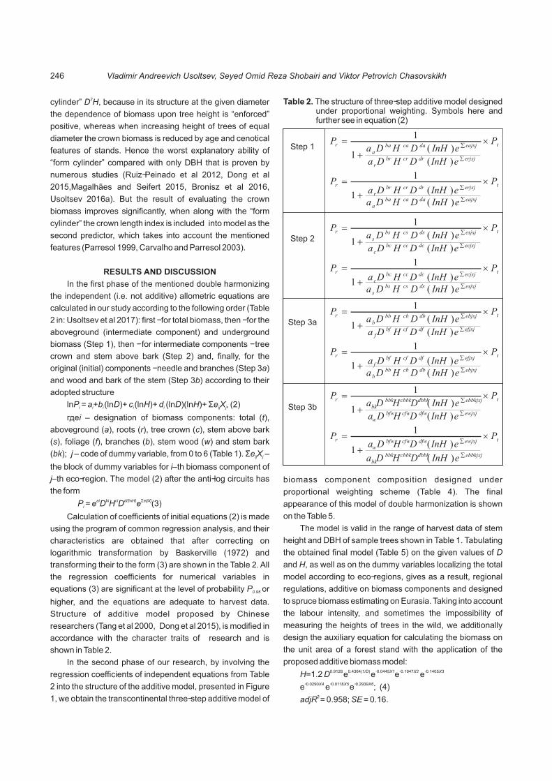
Table 2. The structure of three-step additive model designed under proportional weighting. Symbols here and further see in equation (2)
t
erjxjdrcrbrr
eajxjdacabaa
r P
eInHDHDa
eInHDHDaP ´
+
=
å
å
)(
)(1
1Step 1
Step 2
Step 3à
Step 3b
tr PP ´
+
=erjxjdrcrbr
r eInHDHDa å)(a eajxjdacaba
a eInHDHD å)(1
1
t
ecjxjdcccbcc
esjxjdscsbss
r P
eInHDHDa
eInHDHDaP ´
+
=
å
å
)(
)(1
1
tr PP ´
+
=ecjxjdcccbc
c eInHDHDa å)(a esjxjdscsbs
s eInHDHD å)(1
1
t
efjxjdfcfbff
ebjxjdbcbbbb
r P
eInHDHDa
eInHDHDaP ´
+
=
å
å
)(
)(1
1
tr PP ´
+
=efjxjdfcfbf
f eInHDHDa å)(a ebjxjdbcbbb
b eInHDHD å)(1
1
t
ewjxjdfwcfwbfww
ebbkjxjdbbkcbbkbbkbk
r P
eInHDHDa
eInHDHDaP ´
+
=
å
å
)(
)(1
1
tr PP ´
+
=
1
1ewjxjdfwcfwbfw
w eInHDHDa å)(ebbkjxjdbbkcbbkbbk
bk eInHDHDa å)(
biomass component composition designed under
proportional weighting scheme (Table 4). The final
appearance of this model of double harmonization is shown
on the Table 5.
The model is valid in the range of harvest data of stem
height and DBH of sample trees shown in Table 1. Tabulating
the obtained final model (Table 5) on the given values of D
and H, as well as on the dummy variables localizing the total
model according to eco-regions, gives as a result, regional
regulations, additive on biomass components and designed
to spruce biomass estimating on Eurasia. Taking into account
the labour intensity, and sometimes the impossibility of
measuring the heights of trees in the wild, we additionally
design the auxiliary equation for calculating the biomass on
the unit area of a forest stand with the application of the
proposed additive biomass model:0.9128 0.4364(1/D) -0.0445X1 -0.1947X2 -0.1405X3 H=1.2 D e e e e
-0.0290X4 -0.0118X5 -0.2939X6e e e ; (4)2 adjR = 0.958; SE = 0.16.
Vladimir Andreevich Usoltsev, Seyed Omid Reza Shobairi and Viktor Petrovich Chasovskikh 246

0.9170 0.1114 0.3210(lnH) -0.0837X1 0.0436X2 0.2655X3 0.1163X4 0.0598X5 0.1590X6Pt = 0.5236 D H D e e e e e e
Step 1 Pa= 1 × Pt
1+ 0.9393 -0.1659 0.4236(lnH) 0.3392X1 0.2134X2 0.6642X3 0.8177X4 0.3315X5 0.4874X60.0725 D H D e e e e e e
0.9268 -0.1407 0.3461(lnH) -0.1197X1 0.0390X2 -0.0396X3 -0.2369X4 0.1701X5 0.1364X60.6650 D H D e e e e e e
Pr= 1 × Pt
1+ 0.9268 -0.1407 0.3461(lnH) -0.1197X1 0.0390X2 -0.0396X3 -0.2369X4 0.1701X5 0.1364X60.6650 D H D e e e e e e
0.9393 -0.1659 0.4236(lnH) 0.3392X1 0.2134X2 0.6642X3 0.8177X4 0.3315X5 0.4874X60.0725 D H D e e e e e e
Step 2 Pc= 1 × Pà
1+ 0.6682 0.4936 0.3223(lnH) -0.1357X1 -0.0855X2 -0.2480X3 -0.1305X4 0.1852X5 0.2759X60.2343 D H D e e e e e e
1.6489 -1.1713 0.2887(lnH) 0.0268X1 0.4637X2 0.3302X3 -0.1674X4 0.2536X5 -0.0107X60.4809 D H D e e e e e e
Ps= 1 × Pà
1+ 1.6489 -1.1713 0.2887(lnH) 0.0268X1 0.4637X2 0.3302X3 -0.1674X4 0.2536X5 -0.0107X60.4809 D H D e e e e e e
0.6682 0.4936 0.3223(lnH) -0.1357X1 -0.0855X2 -0.2480X3 -0.1305X4 0.1852X5 0.2759X60.2343 D H D e e e e e e
Step 3à Pf= 1 × Pc
1+ 1.6372 -1.1094 0.2987(lnH) 0.1494X1 0.6184X2 0.3768X3 0.1097X4 0.2840X5 0.3309X60.2054 D H D e e e e e e
1.6561 -1.2510 0.2831(lnH) 0.0115X1 0.3919X2 0.3107X3 -0.3497X4 0.3013X5 -0.3989X60.2817 D H D e e e e e e
Pb= 1 × Pc
1+ 1.6561 -1.2510 0.2831(lnH) 0.0115X1 0.3919X2 0.3107X3 -0.3497X4 0.3013X5 -0.3989X60.2817 D H D e e e e e e
1.6372 -1.1094 0.2987(lnH) 0.1494X1 0.6184X2 0.3768X3 0.1097X4 0.2840X5 0,3309X60.2054 D H D e e e e e e
Step 3b Pw = 1 × Ps
1+ 0.7639 0.1592 0.2944(lnH) 0.0172X1 0.1567X2 -0.0368X3 0.5045X4 0.5520X5 0.7337X60.0441 D H D e e e e e e
0.73410 0.3360 0.3286(lnH) 0.0061X1 -0.1181X2 -0.4134X3 -0.5122X4 0.1427X5 0.1640X60.2484 D H D e e e e e e
Pbk= 1 × Ps
1+ 0.73410 0.3360 0.3286(lnH) 0.0061X1 -0.1181X2 -0.4134X3 -0.5122X4 0.1427X5 0.1640X60.2484 D H D e e e e e e
0.7639 0.1592 0.2944(lnH) 0.0172X1 0.1567X2 -0.0368X3 0.5045X4 0.5520X5 0.7337X60.0441 D H D e e e e e e
Table 4. The additive combination of the original analytical dependencies of component biomass upon tree height and DBH, calculated according to the principle of proportional weighing
Biomasscomponent
Independent variables and regression coefficients of the model 2adjR * SE*
Pt 0.5236 0.9170D 0.1114H 0.3210(lnH)D -0.0837X1e 0.0436X2e 0.2655X3e 0.1163X4e 0.0598X5e 0.1590X6e 0.990 1.19
Step 1
Pa 0.6650 0.9268D -0.1407H 0.3461(lnH)D -0.1197X1e 0.0390X2e -0.0396X3e -0.2369X4e 0.1701X5e 0.1364X6e 0.986 1.26
Pr 0.0725 0.9393D -0.1659H 0.4236(lnH)D 0.3392X1e 0.2134X2e 0.6642X3e 0.8177X4e 0.3315X5e 0.4874X6e 0.975 1.44
Step 2
Pc 0.4809 1.6489D -1.1713H 0.2887(lnH)D 0.0268X1e 0.4637X2e 0.3302X3e -0.1674X4e 0.2536X5e -0.0107X6e 0.930 1.53
Ps 0.2343 0.6682D 0.4936H 0.3223(lnH)D -0.1357X1e -0.0855X2e -0.2480X3e -0.1305X4e 0.1852X5e 0.2759X6e 0.992 1.22
Step 3à
Pf 0.2817 1.6561D -1.2510H 0.2831(lnH)D 0.0115X1e 0.3919X2e 0.3107X3e -0.3497X4e 0.3013X5e -0.3989X6e 0.904 1.62
Pb 0.2054 1.6372D -1.1094H 0.2987(lnH)D 0.1494X1e 0.6184X2e 0.3768X3e 0.1097X4e 0.2840X5e 0.3309X6e 0.887 1.78
Step 3á
Pw 0.2484 0.73414D 0.3360H 0.3286(lnH)D 0.0061X1e -0.1181X2e -0.4134X3e -0.5122X4e 0.1427X5e 0.1640X6e 0.991 1.23
Pbk 0.0441 0.7639D 0.1592H 0.2944(lnH)D 0.0172X1e 0.1567X2e -0.0368X3e 0.5045X4e 0.5520X5e 0.7337X6e 0.976 1.34
Table 3. The characteristic of independent (initial)allometric equations (3).
2*adj R – coefficient of determination adjusted for the number of observations; SE – standard error of equations in the initial dimension P (kg).i
Double Harmonization of Transcontinental Allometric Model of Picea spp. 247

0.9170 0.1114 0.3210(lnH) -0.0837X1 0.0436X2 0.2655X3 0.1163X4 0.0598X5 0.1590X6Pt = 0.5236 D H D e e e e e e
Step 1 Pa= 1 × Pt0.0125 -0.0252 0.0775(lnH) 0.4589X1 0.1744X2 0.7038X3 1.0546X4 0.1614X5 0.3510X61+0.1090 D H D e e e e e e
Pr= 1 × Pt-0.0125 0.0252 -0.0775(lnH) -0.4589X1 -0.1744X2 -0.7038X3 -1.0546X4 -0.1614X5 -0.3510X6 1+9.1724 D H D e e e e e e
Step 2 Pc= 1 × Pà-0.9807 1.6649 0.0336(lnH) -0.1625X1 -0.5492X2 -0.5782X3 0.0369X4 -0.0684X5 0.2866X6 1+0.4872 D H D e e e e e e
Ps= 1 × Pà0.9807 -1.6649 -0.0336(lnH) 0.1625X1 0.5592X2 0.5782X3 -0.0369X4 -0.0684X5 -0.2866X6 1+2.0525 D H D e e e e e e
Step 3à Pf= 1 × Pc-0.0189 0.1416 0.0156(lnH) 0.1379X1 0.2265X2 0.0661X3 0.4594X4 -0.0173X5 0.7298X6 1+0.7291 D H D e e e e e e
Pb= 1 × Pc0.0189 -0.1416 -0.0156(lnH) -0.1379X1 -0.2265X2 -0.0661X3 -0.4594X4 0.0173X5 -0.7298X6 1+1.3715 D H D e e e e e e
Step 3b Pw= 1 × Ps0.0298 -0.1768 -0.0342(lnH) 0.0111X1 0.2748X2 0.3766X3 1.0167X4 0.4093X5 0.5697X6 1+0.1775 D H D e e e e e e
Pbk= 1 × Ps-0.0298 0.1768 0.0342 (lnH) -0.0111X1 -0.2748X2 -0.3766X3 -1.0167X4 -0.4093X5 -0.5697X6 1+5.6326 D H D e e e e e e
Table 5. Three-step trans-Eurasian additive model of component biomass composition of spruce trees rdesigned under proportional weighing scheme
Variable (1/D) is introduced in the model structure (4) for
the allometry correction, broken in small trees due to the shift
of measurement of diameter D in the upper part of the crown.
Because the volume of taxation tables exceeds the format of
journal article, we will focus on analyzing some of regional
characteristics of the spruce biomass structure of equal size
trees on the relevant table fragments (Table 6). Primarily, the
Ural region is of our interest where within the south taiga
subzone we have two pools of sample trees Picea obovata,
data of which were obtained, respectively, in natural stands
and plantations. A comparative analysis of the biomass
structure of equal size trees (within the range of applicability
of the model, as shown in Table 1) showed significant excess
of tree biomass in plantations, namely, total, aboveground
and underground biomass on 24, 14 and 88 percent
respectively. The proportion of needles in the aboveground
biomass varies slightly (13 and 15%, respectively), but the
difference in root: shoot ratio is significant. The latter is in
natural stands and plantations 0.22 and 0.37, respectively.
Spruce trees of two regions adjacent to the Pacific (P.
jezoensis) and Atlantic (P. abies) Oceans differ significantly in
the structure of their biomass: exceeding the first over the
second is for total, aboveground and underground biomass
on 17, 10 and 56percent respectively. The proportion of
needles in the aboveground biomass is 5 and 10 per cent,
respectively, and the root: shoot ratio is 0.26 0.18,
respectively. Structure of tree biomass on two more distant
regions (Pamir-TienShan province and European part of
Russia) and of species growing on their territories (P.
schrenkiana and P. abies respectively) also varies
considerably: the difference between the first and the second
is accounted for to total, aboveground and underground
biomass 15, -9 and 22 per cent, respectively. The root: shoot
ratio equal to 0.21 and 0.29, respectively, and there are no
differences in the proportion of needles in the aboveground
biomass (11%).
It was shown by some researchers (Cunia and Briggs
1984, Reed and Green 1985), that the removal of internal
inconsistency of equations for tree biomass by ensuring their
additivity does not necessarily mean any improvements in
the accuracy of its estimates. Therefore it is necessary to
clear whether adequate an additive model obtained and how
its adequacy characteristics are comparable with those of the
independent equations? To this purpose, the biomass
estimates obtained using independent and additive
equations are compared with observed biomass values in the 2database by calculating the coefficient of determination R
and the root mean squared error RMSE in accordance of the
formulas
Where Y is observed value; Y is predicted value; ? is i i
the mean of N observed values for the same component; p is
the number of model parameters; N is sample size of trees 2involving into calculating R and RMSE.
å
å
=
=
-
--=
N
i ii
N
i ii
YY
YYR
1
2_
1
2_
2
)(
)(1
å=
N - P
-N
i ii YY1
2_
)(RMSE= (5)
Vladimir Andreevich Usoltsev, Seyed Omid Reza Shobairi and Viktor Petrovich Chasovskikh 248

Biomasscomponents
Independent variables and regression coefficients of the model
Pt 0.5236 0.9170D 0.1114H 0.3210(lnH)D -0.0837X1e 0.0436X2e 0.2655X3e 0.1163X4e 0.0598X5e 0.1590X6e
Step 1
Pa 0.4574 0.9133D 0.1438H 0.3054(lnH)D -0.11604X1e 0.0248X2e 0.1955X3e -0.0223X4e 0.0225X5e 0.1004X6e
Pr 0.0731 0.9405D -0.1699H 0.4236(lnH)D 0.3325X1e 0.2130X2e 0.6597X3e 0.8137X4e 0.3313X5e 0.4858X6e
Step 2
Pc 0.3116 1.5201D -0.6013H 0.2170(lnH)D -0.1713X1e 0.4610X2e 0.4770X3e -0.0157X4e -0.3839X5e -0.1722X6e
Ps 0.1985 0.6511D 0.5446H 0.3254(lnH)D -0.1526X1e -0.1169X2e -0.1364X3e 0.0118X4e 0.1396X5e 0.2547X6e
Step 3à
Pf 0.1520 1.6252D -0.8756H 0.2518(lnH)D -0.0288X1e 0.4179X2e 0.8202X3e -0.0278X4e -0.2530X5e -0.5150X6e
Pb 0.1429 1.4219D -0.3226H 0.1818(lnH)D -0.1750X1e 0.6198X2e 0.2591X3e 0.1316X4e -0.3912X5e 0.1427X6e
Step 3b
Pw 0.2484 0.73414D 0.3360H 0.3286(lnH)D 0.0061X1e -0.1181X2e -0.4134X3e -0.5122X4e 0.1427X5e 0.1640X6e
Pbk 0.0441 0.7639D 0.1592H 0.2944(lnH)D 0.0172X1e 0.1567X2e -0.0368X3e 0.5045X4e 0.5520X5e 0.7337X6e
Table 7. The characteristic of "methodized" independent allometric equations (3)
To properly comparing the adequacy of independent and
additive equations, the observed data are given in
comparable condition, i.e. independent equations for all
biomass components are calculated according to the same
data that the additive equation for the total phytomass (where
Biomass components, kg
Ecoregion and the corresponding species of genus Piceaspp.
Ur(plant.)P. obovata
Ur(nat.)P. obovata
FEP. jezoensis,P. purpurea
WMEP. abies
PÒP. schrenkiana
ÅÐRP. abies
Total biomass 96.36 77.19 86.63 73.89 78.45 67.96
Roots 25.80 13.68 17.71 11.32 13.75 15.12
Above-ground 70.56 63.51 68.92 62.58 64.70 52.84
Crown 22.76 20.08 11.51 13.19 14.38 12.63
Needles 10.34 8.33 3.45 6.21 6.83 5.52
Branches 12.42 11.75 8.05 6.98 7.55 7.11
Stem above bark 47.80 43.43 57.41 49.39 50.31 40.21
Stem wood 42.00 38.61 49.16 45.11 44.02 36.69
Stem bark 5.80 4.82 8.25 4.28 6.29 3.52
Table 6. Fragments of the additive biomass (kg) table of trees having DBH of 14 cm and tree height of 14 m in different eco-regions and the corresponding species of genus Picea spp
Indices Biomass components*
Pt Pa Pr Ps Pw Pbk Pc Pb Pf
Independent equations2R 0.950 0.902 0.777 0.898 0.943 0.875 0.728 0.800 0.660
RMSE 69.50 88.34 28.72 77.07 33.38 3.82 22.91 13.96 9.19
Additive equations2R 0.950 0.916 0.786 0.914 0.905 0.844 0.825 0.836 0.631
RMSE 69.70 82.12 28.12 70.99 43.08 4.27 18.38 12.64 9.57
Table 8. The comparison of adequacy indices of independent and additive equations for spruce tree biomass.
2* Designations see equation (2). Bold fonts are components, for which the values of R on the additive models higher than on independent ones, and RMSE values respectively below
were exclude the observations without root data).
Characteristics of such "methodized" equations is given in
the Table 7. The results of the comparison (Table 8) suggest
that the additive equations not only internally consistent, but
also for the most part of components possess the best
Double Harmonization of Transcontinental Allometric Model of Picea spp. 249

Fig
. 1
. T
he
ra
tio o
f o
bse
rve
d v
alu
es
an
d th
e v
alu
es
de
rive
d b
y ca
lcu
latio
n o
n in
de
pe
nd
en
t (a
) a
nd
ad
diti
ve (
b)
mo
de
ls o
f tr
ee
bio
ma
ss.
Vladimir Andreevich Usoltsev, Seyed Omid Reza Shobairi and Viktor Petrovich Chasovskikh 250

indices of adequacy compared with independent equations.
The ratio of observed values and the values derived by
calculation on independent and additive models of tree
biomass (Fig. 4) shows the degree of correlativeness of the
above-mentioned indices and the lack of visible differences
in the structure of residual variance, obtained in two types of
models.
CONCLUSIONS
Thus, for the first time in Russian literature the Trans-
Eurasian additive model of tree biomass of five species of
genus Picea spp. is designed using the unique single-tree
database. The model is harmonized in two ways: It
eliminates the internal contradictions of the component
equations and the total one, and in addition, it takes into
account the regional (and, respectively species)
differences between trees of equal size both in magnitude of
common over ground and underground phytomass and its
component structure. Trivial mixed-effects model involving
the dummy and numeric variables in allometric equations
without component additivity, gives biomass estimates
harmonized according to eco-regions only but differing by
the absolute value of the biomass components (Fu et al
2012). The fundamental distinction and advantage of the
developed model of double harmonization is that unlike of
trivial mixed-effects model, it provides compatibility and
difference by eco-regions not only of absolute values of
biomass fractions, but also of their ratios, i.e. reflects
regional characteristics of biomass component structure.
Thus belied the assertion by Bi et al (2004) that features of
component structure of the additive model on several
separate levels may not be taken into account, resulting in
the harmonized characteristics are possible only for total
biomass. The proposed model and corresponding tables for
estimating tree biomass makes their possible to calculate
spruce stand biomass (t/ha) on Eurasian forests when using
measuring taxation.
ACKNOWLEDGEMENTS
We thank the anonymous referees for their useful
suggestions. This paper is fulfilled according to the programs
of current scientific research of the Ural Forest Engineering
University and Botanical Garden of the Ural Branch of
Russian Academy of Sciences.
REFERENCES
Baskerville GL 1972. Use of logarithmic regression in the estimation of plant biomass. Canadian Journal of Forest Research 2: 49-53.
Battulga P, Tsogtbaatar J, Dulamsuren C and Hauck M 2013. Equations for estimating the above-ground biomass of Larixsibirica in the forest-steppe of Mongolia. Journal of
Forestry Research 24(3): 431- 437.
Bi H, Turner J and Lambert MJ 2004. Additive biomass equations for native eucalypt forest trees of temperate Australia. Trees 18: 467-479.
Bronisz K, Strub M, Cieszewski C, Bijak S, Bronisz A, Tomusiak R, Wojtan R and Zasada M 2016. Empirical equations for estimating aboveground biomass of Betulapendula growing on former farmland in central Poland. Silva Fennica 50(4). Article No. 1559.17 pp.
Cai S, Kang X and Zhang L 2013. Allometric models for aboveground biomass of ten tree species in northeast China. Annals of Forest Research 56(1): 105-122.
Carvalho JP and Parresol BR 2003. Additivity in tree biomass components of Pyrenean oak (Quercus pyrenaica Willd.). Forest Ecology and Management 179: 269-276.
Cunia T and Briggs RD 1984. Forcing additivity of biomass tables: some empirical results. Canadian Journal of Forest Research 14: 376-384.
Dong L, Zhang L and Li F 2015. A three-step proportional weighting system of nonlinear biomass equations. Forest Science 61(1): 35-45.
Dutcã I, Mather R and Iora F 2017.Tree biomass allometry during the early growth of Norway spruce (Piceaabies (L.) Karst) varies between pure stands and mixtures with European beech (Fagus sylvatica L.). Canadian Journal of Forest Research 47(11): 77-84.
Dutcã I, Negru F, Iora F, Mather R, Blujdea V and Ciuva LA 2014. The Influence of Age, Location and Soil Conditions on the Allometry of Young Norway Spruce (Piceaabies L. Karst.) Trees. Notulae Botanicae Horti Agrobotanici Cluj-Napoca 42(2): 579-582.
Fu LY, Zeng WS, Tang SZ, Sharma RP and Li HK 2012. Using linear mixed model and dummy variable model approaches to construct compatible single-tree biomass equations at different scales – A case study for Masson pine in Southern China. Journal of Forest Science 58(3): 101–115.
Fu L, Lei Y, Wang G, Bi H, Tang S and Song X 2016. Comparison of seemingly unrelated regressions with error-invariable models for developing a system of nonlinear additive biomass equations. Trees 30(3): 839–857.
Iizuka K, Yonehara T, Itoh M and Kosugi Y 2018. Estimating tree height and diameter at breast height (DBH) from digital surface models and orthophotos obtained with an unmanned aerial system for a Japanese Cypress (Chamaecyparis obtusa) Forest. Remote Sensing 10(1):13.
Kozak A 1970. Methods for ensuring additivity of biomass components by regression analysis. The Forestry Chronicle 46(5): 402-404.
Kurucz J 1969. Component weights of Douglas-fir, western hemlock, and western red cedar biomass for simulation of amount and distribution of forest fuels. University of British Columbia, Forestry Department, M.F. thesis.116 pp.
Li CM and Zhang HR 2010. Modeling dominant height for Chinese fir plantation using a non-linear mixed-effects modeling approach. Scientia Silvae Sinicae 46: 89–95.
Li H, Zhao P 2013. Improving the accuracy of tree-level aboveground biomass equations with height classification at a large regional scale. Forest Ecology and Management 289: 153–163.
Magalhães TM and Seifert T 2015. Biomass modelling of Androstachys johnsonii Prain: A comparison of three methods to enforce additivity. International Journal of Forestry Research Article ID 878402: 17.
Nalimov VV 1971. Theory of experiment. Moscow: Nauka. 208 pp.
Parresol BR 1999. Assessing tree and stand biomass: a review with examples and critical comparison. Forest Science 45: 573-593.
Reed DD and Green EJ 1985. A method of forcing additivity of
Double Harmonization of Transcontinental Allometric Model of Picea spp. 251
biomass tables when using nonlinear models. Canadian Journal of Forest Research 15: 1184-1187.
Ruiz-Peinado R, Montero G and del Rio M 2012. Biomass models to estimate carbon stocks for hardwood tree species. Forest Systems 21(1): 42-52.
Rutishauser E, Noor'an F, Laumonier Y, Halperin J, Rufi'ieHergoualch K and Verchot L 2013. Generic allometric models including height best estimate forest biomass and carbon stocks in Indonesia. Forest Ecology and Management 307: 219-225.
Sullivan FB, Ducey MJ, Orwig DA, Cook B and Palace MW 2017. Comparison of lidar- and allometry-derived canopy height models in an eastern deciduous forest. Forest Ecology and Management 406: 83-94.
Tang S, Zhang H and Xu H 2000. Study on establish and estimate method of compatible biomass model. Scientia Silvae Sinica 36: 19–27.
Usoltsev VÀ 2016a. Single-tree biomass of forest-forming species in Eurasia: database, climate-related geography, weight tables. Yekaterinburg: Ural State Forest Engineering University. 336 pp. (http://elar.usfeu.ru/handle/ 123456789/5696).
Usoltsev VA 2016b. Single-tree biomass data for remote sensing and ground measuring of Eurasian forests. CD-version in English
and Russian. Yekaterinburg: Ural State Forest Engineering University. (http://elar.usfeu.ru/ handle/123456789/6103).
Usoltsev VÀ 2017. On additive models of tree biomass: some uncertainties and an attempt of their analytical review. Èko-potencial 18(2): 23–46.
Usoltsev VÀ, Voronov MP, Kolchin KV and Azarenok VA 2017. Transcontinental additive allometric model and weight table for estimating spruce tree biomass. AgrarnyiVestnikUrala [Agrarian Bulletin of the Urals] 161(7): 36-45.
Valbuena R, Heiskanen J, Aynekulu E, Pitkänen S and Packalen P 2016.Sensitivity of Above-Ground Biomass Estimates to Height-Diameter Modelling in Mixed-Species West African Woodlands. PLoS/ONE 11(7): e0158198.
Wirth C, Schumacher J and Schulze ED 2004. Generic biomass functions for Norway spruce in Central Europe – a meta-analysis approach toward prediction and uncertainty estimation. Tree Physiology 24: 121-139.
Young HE, Strand L and Altenberger R 1964. Preliminary fresh and dry weight tables for seven tree species in Maine. Maine Agricultural Experiment Station, Technical Bulletin 12. 76 ðp.
Zeng WS 2015. Using nonlinear mixed model and dummy variable model approaches to construct origin-based single tree biomass equations. Trees 29(1): 275-283.
Received 06 April, 2018; Accepted 10 May, 2018
Vladimir Andreevich Usoltsev, Seyed Omid Reza Shobairi and Viktor Petrovich Chasovskikh 252
Habitat Selection for Lemongrass (Cymbopogon citrates Stapf.) Cultivation in Non-Reserve Forests of Southern Western
Ghats, Tamil Nadu, India
Indian Journal of Ecology (2018) 45(2): 253-259
Abstract: In Anaimalais of Western Ghats, the two tribal communities, Pulayar and Muduvar are an integral part of ecosystem. These tribes
did cultivation of lemongrass and distilled oil. After the declaration of Anaimalais as a protective area for biodiversity conservation, they are not
permitted to continue the practice of lemongrass cultivation. However, they are allowed to extract oil from the existing populations, without
adaptingany cultivation practices. Therefore, when rehabilitating thesetribes to other non-reserve forests of adjoining regions, habitats
suitable for lemongrass cultivation with good oil quality similar to that of in Anaimalais must be identified. The present study aims to evaluate
favourable habitat for lemongrass in Udumalpet Range of Anaimalais, among the areas where the lemongrass oil distillation is under practice
by the tribal communities. The results of the study show that among the six sites, Kurumalai and Kulipatti are more favourable for lemongrass
growth and oil yield. Correlation and regression analyses showed that the rainfall, relative humidity, pH, Ca and Mg contents of soil and altitude
are largely determining the biomass production, oil concentration in biomass and citral percent in oil. Therefore, it is suggested to identify
habitats in nearby non-reserved forests with more or less similar climatic conditions, soil pH and nutrients and altitude as in Kurumalai and
Kulipatti for practicing agroforestry by lemongrass cultivation and oil distillation for tribal communities.
Keywords: Lemongrass biomass, Oil and citral contents, The Anaimalais
Manuscript Number: NAAS Rating: 4.96
2667
Sangeeth Thekkan and S. PaulsamyDepartment of Botany, Kongunadu Arts and Science College, Coimbatore – 641 029, India.
E-mail: [email protected]
Anaimalais of Western Ghats, Tamil Nadu (10°13' and
10°31'N and 76°52' and 77°23'E),the unique ecological tract 2covering 958km has an undulating topography and climatic
variation which support a wide variety of flora and fauna. The
two tribal communities viz., Muduvar and Pulayar who inhabit
the reserve forests of this landscape are an integral part of
this ecosystem. These tribes cultivated lemongrass
(Cymbopogon citratus) in fragile areas and rocky slopes until
1970s with good economic returns (Paulsamy et al 2000).
But after the declaration of this region as wildlife sanctuary in
1976, cultivation of any sort has been banned in this region
even for tribals. However, the tribals are permitted to harvest
the existing lemongrass populations for oil extraction in some
localities of Udumulpet Range of Anaimalais without posing
any environmental problem (Paulsamy 2004). For the better
conservation of flora and fauna in recent years no human
activities including lemongrass oil distillation are permitted
and strict legal measures are imposed against violators.
Therefore, to achieve the high degree of species
conservation, the tribal communities may be rehabilitated to
the adjoining non-reserve forests of nearby areas in coarse of
time. For this purpose of rehabilitation, potential areas for
lemongrass cultivation with similar environmental conditions
of certain areas in Udumalpet Range where the lemongrass
production is higher along with better yield and quality of oil
must be identified. As the tribals have vast experience with
lemongrass production and oil extraction, other non-
reserved localities of Anaimalais that have favourable habitat
for better lemongrass cultivation needs to be identified. By
considering these facts, the present study was aimed to
evaluate the best suited habitat among the sites where
lemongrass oil distillation is being made by the tribals in
Udumalpet Range of Anaimalais.
MATERIAL AND METHODS
Study areas: The study was carried out during, June2013-
May, 2014 in six tribal settlement sites in Udumelpet range of
Anaimalais viz., Kodanthur (ca. 4 ha) (10° 300463' N,
77°167928' E), Mavadappu (ca .3 ha) (10° 4234' N, 77°0561'
E), Kulipatti (ca. 4 ha) (10° 437458' N, 77° 051016' E),
Kurumalai (ca.4 ha) (10° 341382' N, 77° 003955' E),
Aattumalai (ca. 5 ha) (10° 40036' N, 77°01464' E) and
Poochikotambarai (ca.5 ha) (10°3746' N, 77°m2144' E),
where the lemongrass oil distillation is practiced by the
tribals. The six study sites of this territorial range are situated
at the altitude, Kodanthur-520m, Mavadappu-690m,
Kulipatti-700m, Kurumalai-740m, Aattumalai-620m and
Poochikotambarai-490m above MSL. The soil of all study

sites was sandy loam with the pH varied between 7.3
(Kodanthur) and 8.8 (Kurumalai) (Table 1). The contents of
nutrients in the soil also showed considerable variation
between the sites studied (Table 5).The climatic data such as
maximum and minimum temperatures, rainfall and relative
humidity were obtained from Kadambarai hydropower
station for Poochikotambarai and Mavadappu, 0.9 km away
from the station, Navamalai hydropower station for Kulipatti,
Kurumalai and Aattumalai which are 0.7, 1.1 and 1.3 km
away from the power station respectively and Amaravathy
Reservoir for Kodanthur, 1.8 km away from the station. Both
south-west monsoon (June-August) and north-east
monsoon (October-November) were effective almost in all
sites studied. The climatic factors were much different
between the study sites during the study period (Fig. 1). The
higher mean annual rainfall of 917 mm was recorded in
Kulipatti site followed by 746mm in Kurumalai, 708 mm in
Mavadappu, 659 mm in Aattumalai, 627 mm in Kodanthur,
and 604 mm in Poochikotambarai. The maximum
temperature varied between 20°C (Kurumalai during
December 2013) and 40°C (Aattumalai during April, 2014)
and that of the minimum ranged between16°C
(Poochikotambarai during December 2013) and 32°C
(Kulipatti during May, 2014). The relative humidity was varied
between 53 per cent (Poochikottambarai during March,
2014) and 86 percent (Kurumalai during October, 2013).
Tribal communities: Among the six study sites, the tribal
community, Muduvar has settlements in Attumalai and
Poochikotambarai with 32 (7 families) and 36 (8 families)
members respectively. In the other four sites viz., Kodanthur,
Mavadappu, Kurumalaiand Kulipatti, the tribal community,
Pulayar numbering 40 (8 families), 92 (12 families), 61 (8
families) and 30 (6 families) respectively are residing. In
addition to the maintenance of lemongrass community by
eradicating dicot weeds and other unwanted monocots,
these two tribal communities are engaged in a host of other
activities like cattle rearing, honey collection, casual labour
for forest department etc.
Soil attributes: Soil samples from A layer (0-10cms) (1kg in 1
each site) in triplicate were collected at all times of harvesting
the lemongrass and mixed thoroughly to obtain composite
sample. Working samples were obtained to analyze the soil
for pH (Ghosh et al 1983), total nitrogen (Jackson 1962),
available phosphorous (Bray and Kurtz 1945) and available
potassium, calcium and magnesium (flame photometric
method, Stanford and English 1949).
Biomass production: The tribals harvested lemongrass
from the study sites6 times during June, August, October and
December of 2013 and February and April of 2014 during the
study period. The harvested grasses were sun dried
adequately for 3-5 days and weighed before oil distillation.
Thus the data on dry weight of total aboveground lemongrass
for the total area of all the sites during different harvesting
times were collected from the tribals. These biomass data of
six harvesting times collected for respective site were pooled
together over a study period to arrive the annual production of
lemongrass (Singh and Yadhava 1974). As the grass was
completely scraped at two months interval, the biomass
harvested at every time is its production in the total area of the
respective site.
Oil yield: The data on oil yield was collected site-wise from
the respective tribal community directly after distillation every
time. Percentage of oil content in biomass was arrived by
using the data on total grass biomass harvested and oil
content (%) available in grass. Oil yield in all harvesting times
in each site were summed to get annual production of lemon
grass oil.
Citral estimation: Oil samples collected from the tribal
communities for each site were analyzed for citral content by
following sodium bisulphate method (Guenther 1972). A 10
ml of oil was taken in a beaker to which 30g sodium
bisulphate and 100 ml distilled water were added. This
mixture was boiled and shaken well for 10 min. After the
formation of a white precipitation, the beaker was dipped in
water bath for 45 min to dissolve the precipitation completely.
Then the beaker was cooled under tap water. The non-citral
portion of the oil separates as an oily layer which has been
measured conveniently in the neck of a cassia flask and there
by determined the citral content of the oil.
Statistical analysis: Statistical significance between the
sites for oil and citral contents were determined using one-
way analysis of variance (SPSS 10.0) and the means were
separated by Duncan's Multiple Range Test (DMRT)
(P<0.05). Correlation coefficients were calculated (SPSS,
1998) to determine the relationships between production
attributes of lemongrass (biomass production, oil content in
biomass and citral percentage in oil) and certain climatic and
soil attributes and attitude. Multiple regression analysis was
used to test the interactive effect of climatic, soil and
altitudinal factors on the production attributes of lemongrass.
RESULTS AND DISCUSSION
The range of minimum and maximum temperatures (16
and 32°C and 20 and 40°C respectively) and annual rain fall
(527-847mm) recorded across the study sites during the
study period of one year indicate the prevalence of suitable
climate for lemongrass cultivation (Nambiar and Matela
2012) in Udumelpet range, the Anaimalais (Fig. 1). The
relative humidity generally ranged between 53 and 86
percent. The soil of all study sites was sandy loam with the pH
Sangeeth Thekkan and S. Paulsamy254
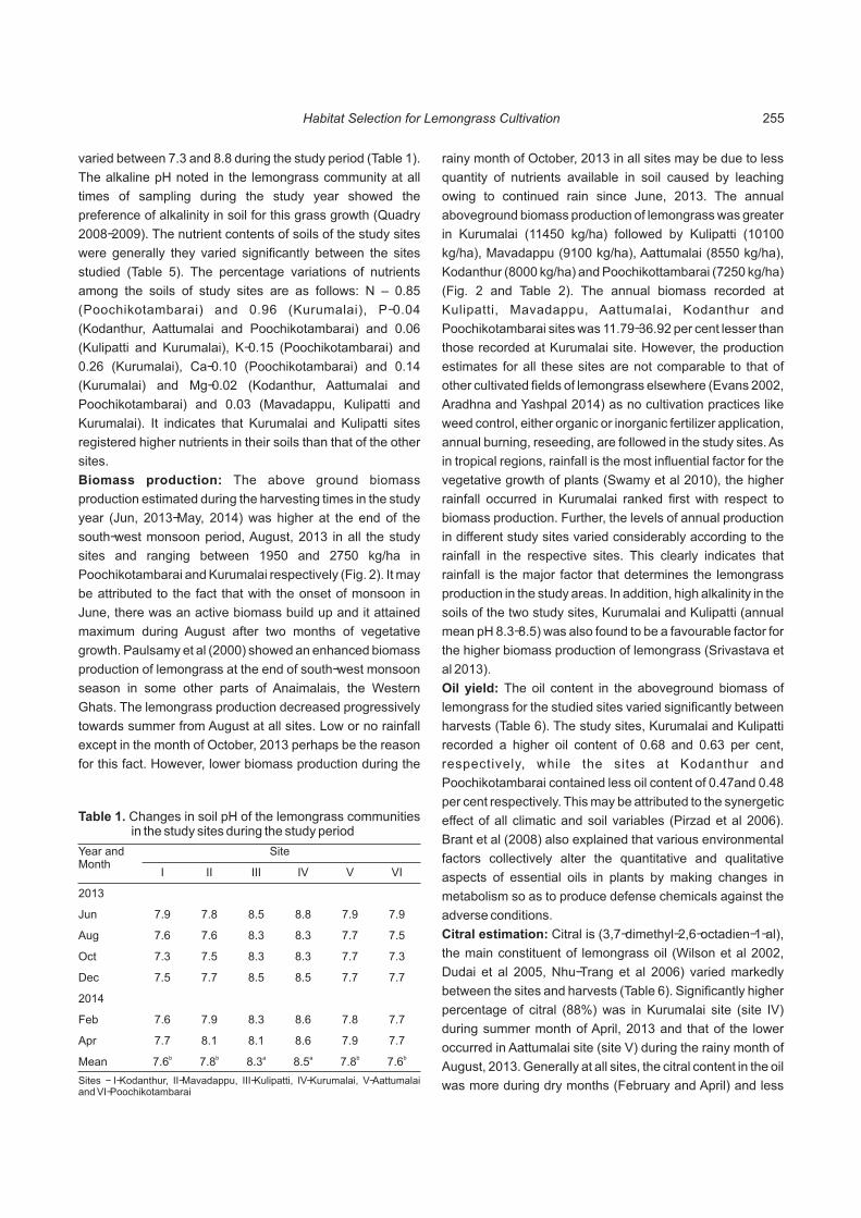
varied between 7.3 and 8.8 during the study period (Table 1).
The alkaline pH noted in the lemongrass community at all
times of sampling during the study year showed the
preference of alkalinity in soil for this grass growth (Quadry
2008-2009). The nutrient contents of soils of the study sites
were generally they varied significantly between the sites
studied (Table 5). The percentage variations of nutrients
among the soils of study sites are as follows: N – 0.85
(Poochikotambarai) and 0.96 (Kurumalai), P-0.04
(Kodanthur, Aattumalai and Poochikotambarai) and 0.06
(Kulipatti and Kurumalai), K-0.15 (Poochikotambarai) and
0.26 (Kurumalai), Ca-0.10 (Poochikotambarai) and 0.14
(Kurumalai) and Mg-0.02 (Kodanthur, Aattumalai and
Poochikotambarai) and 0.03 (Mavadappu, Kulipatti and
Kurumalai). It indicates that Kurumalai and Kulipatti sites
registered higher nutrients in their soils than that of the other
sites.
Biomass production: The above ground biomass
production estimated during the harvesting times in the study
year (Jun, 2013-May, 2014) was higher at the end of the
south-west monsoon period, August, 2013 in all the study
sites and ranging between 1950 and 2750 kg/ha in
Poochikotambarai and Kurumalai respectively (Fig. 2). It may
be attributed to the fact that with the onset of monsoon in
June, there was an active biomass build up and it attained
maximum during August after two months of vegetative
growth. Paulsamy et al (2000) showed an enhanced biomass
production of lemongrass at the end of south-west monsoon
season in some other parts of Anaimalais, the Western
Ghats. The lemongrass production decreased progressively
towards summer from August at all sites. Low or no rainfall
except in the month of October, 2013 perhaps be the reason
for this fact. However, lower biomass production during the
rainy month of October, 2013 in all sites may be due to less
quantity of nutrients available in soil caused by leaching
owing to continued rain since June, 2013. The annual
aboveground biomass production of lemongrass was greater
in Kurumalai (11450 kg/ha) followed by Kulipatti (10100
kg/ha), Mavadappu (9100 kg/ha), Aattumalai (8550 kg/ha),
Kodanthur (8000 kg/ha) and Poochikottambarai (7250 kg/ha)
(Fig. 2 and Table 2). The annual biomass recorded at
Kulipatti, Mavadappu, Aattumalai, Kodanthur and
Poochikotambarai sites was 11.79-36.92 per cent lesser than
those recorded at Kurumalai site. However, the production
estimates for all these sites are not comparable to that of
other cultivated fields of lemongrass elsewhere (Evans 2002,
Aradhna and Yashpal 2014) as no cultivation practices like
weed control, either organic or inorganic fertilizer application,
annual burning, reseeding, are followed in the study sites. As
in tropical regions, rainfall is the most influential factor for the
vegetative growth of plants (Swamy et al 2010), the higher
rainfall occurred in Kurumalai ranked first with respect to
biomass production. Further, the levels of annual production
in different study sites varied considerably according to the
rainfall in the respective sites. This clearly indicates that
rainfall is the major factor that determines the lemongrass
production in the study areas. In addition, high alkalinity in the
soils of the two study sites, Kurumalai and Kulipatti (annual
mean pH 8.3-8.5) was also found to be a favourable factor for
the higher biomass production of lemongrass (Srivastava et
al 2013).
Oil yield: The oil content in the aboveground biomass of
lemongrass for the studied sites varied significantly between
harvests (Table 6). The study sites, Kurumalai and Kulipatti
recorded a higher oil content of 0.68 and 0.63 per cent,
respectively, while the sites at Kodanthur and
Poochikotambarai contained less oil content of 0.47and 0.48
per cent respectively. This may be attributed to the synergetic
effect of all climatic and soil variables (Pirzad et al 2006).
Brant et al (2008) also explained that various environmental
factors collectively alter the quantitative and qualitative
aspects of essential oils in plants by making changes in
metabolism so as to produce defense chemicals against the
adverse conditions.
Citral estimation: Citral is (3,7-dimethyl-2,6-octadien-1-al),
the main constituent of lemongrass oil (Wilson et al 2002,
Dudai et al 2005, Nhu-Trang et al 2006) varied markedly
between the sites and harvests (Table 6). Significantly higher
percentage of citral (88%) was in Kurumalai site (site IV)
during summer month of April, 2013 and that of the lower
occurred in Aattumalai site (site V) during the rainy month of
August, 2013. Generally at all sites, the citral content in the oil
was more during dry months (February and April) and less
Year and Month
Site
I II III IV V VI
2013
Jun 7.9 7.8 8.5 8.8 7.9 7.9
Aug 7.6 7.6 8.3 8.3 7.7 7.5
Oct 7.3 7.5 8.3 8.3 7.7 7.3
Dec 7.5 7.7 8.5 8.5 7.7 7.7
2014
Feb 7.6 7.9 8.3 8.6 7.8 7.7
Apr 7.7 8.1 8.1 8.6 7.9 7.7
Mean b7.6 b7.8 a8.3 a8.5 b7.8 b7.6
Table 1. Changes in soil pH of the lemongrass communities in the study sites during the study period
Sites - I-Kodanthur, II-Mavadappu, III-Kulipatti, IV-Kurumalai, V-Aattumalai and VI-Poochikotambarai
Habitat Selection for Lemongrass Cultivation 255

during wet months (June-October). The mean annual
percentage of citral content was higher in the lemongrass of
Kurumalai site (81.3%), while the lower was determined in
Aatumalai site (76.7%). Alsafar and Al-Hassan (2009)
reiterate that different communities of same macroclimatic
zone exhibit variation in their metabolites according to the
combined action of microclimatic factors. Therefore, the
coupled actions of environmental factors exist in the studied
sites perhaps be the reason for this fact. As the concentration
of oil in the lemongrass biomass at different periods of
harvest varied, the oil production is also varied markedly
between the sites (Table 2). The lemongrass of Kurumalai
(site IV) recorded the highest oil production of 77.8kg/ha/yr
and lowest o f 34.8kg/ha/yr was recorded in
Poochikotambarai (site VI). This was also reflected in the
annual revenue generated from lemongrass oil distillation in
the studied sites (Table 2). The tribal communities at
Kurumalai (site IV) and Kulipatti (site III) sites earned greater
returns of Rs. 1,32,260 and Rs. 1,08,120, respectively
through lemongrass oil extraction. On the other hand, the
tribals at Kodanthur (site I), Poochikotambarai (site VI) and
Attumalai (site V) obtained less economic return due to poor
oil concentration and hence the oil production in their sites.
Statistical analysis: An analysis of data elucidated several
functional relations among the variables of lemongrass
production (biomass, oil yield and citral content) and certain
climatic, soil and altitudinal factors (Table 3). The rainfall and
relative humidity and altitude were positively correlated to
biomass production (r = 0.854 and 0.587, P<0.01 and 0.335,
P<0.05). It is well known that in tropical communities, rainfall
being a limiting factor influences largely on growth and
biomass production (Gunarathne and Perera 2014). Taiz and
Zeiger (2004) explained that high relative humidity favours
stomatal opening which causes free flow of gases for
photosynthesis, results in increasing of biomass production
provided adequate rainfall occurs. The nutrients of soil viz.,
Ca and Mg were also have positive correlations with the
biomass production of lemongrass (r=0.505 and 0.468,
P<0.01). Similar kind of observation on the requirement of
nutrients like Ca and Mg for better growth of Cymbopogon
spp. was made already (Jayalakshmi and Mohanarao 2013,
Singh et al 2014). As the variations in altitude and annual
rainfall in the study sites were directly related to each other, it
is presumed to have the positive correlation between
biomass production and altitude. Other studies have also
demonstrated the positive relation of soil pH to lemongrass
biomass (Jayasinha et al 1999, Paulsamy et al 2000).
Relative humidity was positively correlated to per cent oil
content in lemongrass (r = 0.424, P<0.01). The minimum
temperature was negatively correlated to oil per cent (r = -
Fig. 1. Monthly maximum and minimum temperatures, total rainfall and relative humidity of the study sites in Anaimalais, the Western Ghats for the study period of one year from June, 2013 to May 2014
Sangeeth Thekkan and S. Paulsamy256

0.650, P<0.01). Low temperature generally results in closure
of stomata in plants there by reducing oil volatilization, a
defense mechanism to resist such adverse condition
(Castelo et al 2012). This fact may be the possible reason for
the inverse relationship of low temperature with oil per cent in
lemongrass. The soil pH was positively correlated to the
important chemical constituent of the oil, citral (r = 0.437,
P<0.01). Results of many studies report that alkaline pH
generally enhanced not only the biomass production but also
the chemical constituents of lemongrass oil (Siribel et al
2001). It is evidenced that the citral content determined was
higher in Kurumalai (site IV) (81.3%) and Kulipatti (site III)
(78.7%) where the soil contained significantly higher
alkalinity at all times of sampling during the study period
when compared to other sites (Table 3). Plants growing in
well drained soils like hilly slopes are highly adapted to
alkalinity and may be more sensitive to changes in soil pH by
producing certain secondary metabolites like essential oils
(Evans 1996). This is practically true for lemongrass, which is
known to grow better in alkaline soils (Quadry 2008-2009)
and is producing high citral content in its vegetal parts. The
soil nutrients viz., N, P and K were also positively correlated
to citral per cent (r=0.791, 0.713 and 0.714, P<0.01). These
findings were in conformity with those of Singh et al (2005). In
Pearson's correlation, no significant correlation was found
between biomass production and soil pH, oil per cent in
biomass and rainfall, and citral percentage and minimum
Sites Annual production of lemongrass (kg/ha)
Area of lemon grass community (ha)
*Oil content (%)
Oil production (kg/ha/yr)
**Annual revenue (Rs/total area of grass community)
I 8000 4 0.47 37.6 63920
II 9100 3 0.55 50.0 63750
III 10100 4 0.63 63.6 108120
IV 11450 4 0.68 77.8 132260
V 8550 5 0.53 45.3 96262
VI 7250 5 0.48 34.8 73950
Table 2. Annual biomass production and area of lemongrass community, content and production of oil and revenue generated in the study sites
*Average content in six harvested biomass in an year.**Calculated on basis of average price of oil (Rs. 425/kg) sold by the respective tribal community during the study year, 2013-2014.See Table 1 for details of site
Lemongrass production attributes
Climatic variables Soil variables
Ma.t Mi.t Rf RH pH N P K Ca Mg Alt
Biomass -0.158 -0.276 0.854** 0.587** 0.241 -0.372* -0.234 -0.042 0.505** 0.468** 0.335*
Oilyield -0.2 -0.650** 0.087 0.424** -0.193 -0.323 -0.232 -.383* -0.132 -0.255 -0.152
Citral -0.157 0.287 -0.514** -0.365* 0.437** 0.791** 0.713** 0.714** 0.174 0.078 0.300
Table 3. Correlation coefficient (r) between the variables of lemongrass production and certain environmental factors in Udumalpet range, the Anaimalais
Ma.t – Maximum temperature; Mi.t – Minimum tempertature, Rf – Rain fall; RH – Relative humidity; Atl. – Altitude.**Correlation is significant at 0.01 level, *Correlation is significant at 0.05 level
temperature and altitude. On the other hand the nitrogen
content exhibited negative correlation to biomass production.
Similarly, oil content and citral percentage were negatively
correlated to minimum temperature and soil K content, and
rainfall and relative humidity, respectively. A number of
synergistic effects of climatic, soil and altitudinal factors on
biomass production, oil content and citral percentage in the
oil of lemongrass were detected, but for the sake of brevity,
only the best equations for production variables are
presented (Table 4). Therefore, despite the dominant role
played by the rainfall, relative humidity, soil Ca and Mg
contents and altitude for dry matter production, relative
humidity for oil content and pH, N, P and Kof soil for citral
percentage in oil, the multiple regression analysis showed
relationships involving almost all climatic and soil variables
studied. Previous literature also documents many complex
interactions between climatic and soil factors on growth and
oil yield variables of lemongrass (Paulsamy et al 2000,
Paulsamy 2004).
The present investigation clearly suggests that
lemongrass biomass production oil contents in biomass and
citral percentage in oil are the functions of climatic factors
particularly rainfall and relative humidity, soil nutrients and pH
and altitude but their intensity of influence vary according to
other climatic variables like maximum and minimum
temperatures. Further, the environmental factors that exist in
Kurumalai (site IV) and Kulipatti (site III) are more favorable
Habitat Selection for Lemongrass Cultivation 257

1800
2100
2350 2400
1900
1600
2200
2450 2500
2750
2350
1950
1450
1650
1850
2100
1500
13001250
1400
1600
1850
1300
1100
750
950
1200
1400
900
700550 550 600
950
600 600
0
500
1000
1500
2000
2500
3000
JAN AUG OCT DEC FEB APR
2013 2014
YEAR AND MONTH
Kodanthur Mavadappu Kulipatti
Kurumalai Aattumalai Poochikotambarai
-2B
iom
ass
(g m
)
Fig. 2. Aboveground biomass of lemongrass in the study areas in Anaimalais, the Western Ghats during the sampling months
Lemon grass production attributes Equation r p
Biomass Y= 4947.99 – 42.69 Ma.t + 3.75 Mi.t + 5.13 Rf – 18.96 RH - 0.39 pH –3822.23 N + 896.80 P + 1119.75 K + 14962.50 Ca + 12278.04 Mg - 0.63 alt
R=0.947 0.001
Y= 4828.09 – 39.78 Ma.t + 5.13 Rf – 19.15 RH + 4.58 pH – 3741.02 N + 1088.56 P + 1040.65 K + 14959.22 Ca + 12521.35 Mg - 0.61 alt
R=0.947 0.001
Y= 4945.07 – 42.68 Ma.t + 3.74 Mi.t + 5.13 Rf – 18.96 RH – 3821.46 N + 894.23 P + 1118.11 K + 14958.92 Ca + 12274.85 Mg - 0.63 0.893 alt
R=0.947 0.001
Y= 4882.38 – 43.27 Ma.t + 4.15 Mi.t + 5.12 Rf – 18.71 RH + 2.48 pH – 3753.08 N + 1208.96 K + 14816.21 Ca + 11880.39 Mg – 0.59 alt
R=0.947 0.001
Y= 4742.76 – 43.93 Ma.t + 2.27 Mi.t + 5.19 Rf – 20.93 RH + 15.96 pH – 3436.53 N + 1692.52 P + 15070.18 Ca + 13189.5 Mg – 0.51 alt
R=0.947 0.001
Y= 4785.35 – 44.11 Ma.t + 1.19 Mi.t + 5.24 Rf - 22.31 RH + 1.42 pH – 3307.37 N – 1151.63 P + 476.00 K + 13675.37 Ca + 13357.4 Mg
R=0.948 0.001
Oil yield Y= -1.87 + 0.02 Ma.t – 0.04 Mi.t – 0.00042 Rf + 0.0095 RH + 0.14 pH + 1.72 N – 2.62 P – 1.86 K + 0.85 Ca – 4.03 Mg – 6.30 alt
R=0.917 0.001
Y= – 1.96 + 0.020 Ma.t – 0.037 Mi.t – 0.00041 Rf + 0.0098 RH + 0.15 pH + 1.78 N – 2.98 P – 1.83 K – 3.78 Mg + 2.77 alt
R=0.915 0.001
Y= – 1.89 + 0.02 Ma.t – 0.04 Mi.t – 0.00041 Rf + 0.0092 RH + 0.14 pH + 1.77 N – 2.83 P – 1.93 K + 0.72 Ca – 4.12 Mg
R=0.916 0.001
Citral Y= – 43.68 + 0.37 Ma.t – 0.40 Mi.t – 0.00059 Rf – 0.11 RH + 1.20 pH + 27.59 N + 57.29 P + 20.94 K – 70.74 Ca – 32.40 Mg + 0.012 alt
R=0.872 0.001
Y= 47.84 + 0.25 Ma.t – 0.32 Mi.t – 0.13 RH + 1.15 pH + 28.64 N + 57.14 P + 17.15 K – 78.16 Ca – 22.16 Mg + 0.011 alt
R=0.870 0.001
Y= 43.89 + 0.39 Ma.t – 0.41 Mi.t – 0.0015 Rf – 0.11 RH + 1.10 pH + 27.54 N + 68.28 P + 18.11 K – 73.55 Ca + 0.011 alt
R=0.871 0.001
Table 4. Multiple regression between lemongrass production attributes (biomass production, oil per cent in biomass and citral per cent in oil) and certain environmental variables, maximum and minimum temperatures (Ma.t and Mi.t respectively) rainfall (Rf), relative humidity (RH), soil pH and altitude (alt)
Sangeeth Thekkan and S. Paulsamy258
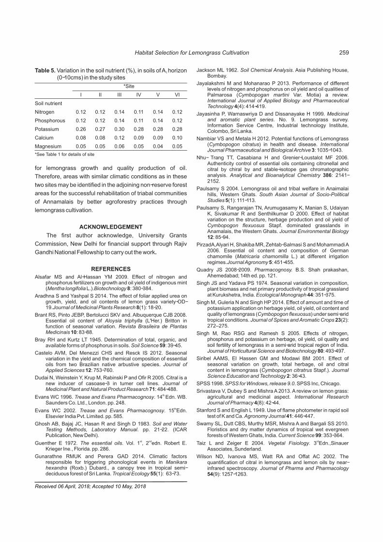
*Site
I II III IV V VI
Soil nutrient
Nitrogen 0.12 0.12 0.14 0.11 0.14 0.12
Phosphorous 0.12 0.12 0.14 0.11 0.14 0.12
Potassium 0.26 0.27 0.30 0.28 0.28 0.28
Calcium 0.08 0.08 0.12 0.09 0.09 0.10
Magnesium 0.05 0.05 0.06 0.05 0.04 0.05
Table 5. Variation in the soil nutrient (%), in soils of A horizon 1
(0-10cms) in the study sites
*See Table 1 for details of site
for lemongrass growth and quality production of oil.
Therefore, areas with similar climatic conditions as in these
two sites may be identified in the adjoining non-reserve forest
areas for the successful rehabilitation of triabal communities
of Annamalais by better agroforestry practices through
lemongrass cultivation.
ACKNOWLEDGEMENT
The first author acknowledge, University Grants
Commission, New Delhi for financial support through Rajiv
Gandhi National Fellowship to carry out the work.
REFERENCES
Alsafar MS and Al-Hassan YM 2009. Effect of nitrogen and phosphorus fertilizers on growth and oil yield of indigenous mint (Mentha longifolia L.).Biotechnology 8: 380-384.
Aradhna S and Yashpal S 2014. The effect of foliar applied urea on growth, yield, and oil contents of lemon grass variety-OD-19.Journal of Medicinal Plants Research 8(1): 18-20.
Brant RS, Pinto JEBP, Bertolucci SKV and. Albuquerque CJB 2008. Essential oil content of Aloysia triphylla (L'Her.) Britton in function of seasonal variation. Revista Brasileira de Plantas Medicinais 10: 83-88.
Bray RH and Kurtz LT 1945. Determination of total, organic, and available forms of phosphorus in soils. Soil Science 59: 39-45.
Castelo AVM, Del Menezzi CHS and Resck IS 2012. Seasonal variation in the yield and the chemical composition of essential oils from two Brazilian native arbustive species. Journal of Applied Sciences 12: 753-760.
Dudai N, Weinstein Y, Krup M, Rabinski P and Ofir R 2005. Citral is a new inducer of casoase-3 in tumer cell lines. Journal of Medicinal Plant and Natural Product Research 71: 484-488.
th Evans WC 1996. Trease and Evans Pharmacognosy. 14 Edn. WB. Saunders Co. Ltd., London. pp. 248.
thEvans WC 2002. Trease and Evans Pharmacognosy. 15 Edn. Elsevier India Pvt. Limited. pp. 585.
Ghosh AB, Bajaj JC, Hasan R and Singh D 1983. Soil and Water Testing Methods, Laboratory Manual. pp. 21-22. (ICAR Publication, New Delhi).
st ndGuenther E 1972. The essential oils. Vol. 1 , 2 edn. Robert E. Krieger Ine., Florida. pp. 286.
Gunarathne RMUK and Perera GAD 2014. Climatic factors responsible for triggering phonological events in Manikara hexandra (Roxb.) Dubard., a canopy tree in tropical semi-deciduous forest of Sri Lanka. Tropical Ecology 55(1): 63-73.
Jackson ML 1962. Soil Chemical Analysis. Asia Publishing House, Bombay.
Jayalakshmi M and Mohanarao P 2013. Performance of different levels of nitrogen and phosphorus on oil yield and oil qualities of Palmarosa (Cymbopogan martini Var. Motia) a review. International Journal of Applied Biology and Pharmaceutical Technology 4(4): 414-419.
Jayasinha P, Warnaswriya D and Dissanayake H 1999. Medicinal and aromatic plant series. No. 9. Lemongrass survey. Information Service Centre, Industrial technology Institute, Colombo, Sri Lanka.
Nambiar VS and Metala H 2012. Potential functions of Lemongrass (Cymbopogon citratus) in health and disease. International Journal Pharmaceutical and Biological Archive 3: 1035-1043.
Nhu- Trang TT, Casabiana H and Grenier-Loustalot MF 2006. Authenticity control of essential oils containing citronellal and citral by chiral by and stable-isotope gas chromatographic analysis. Analytical and Bioanalytical Chemistry 386: 2141-2152.
Paulsamy S 2004. Lemongrass oil and tribal welfare in Anaimalai hills, Western Ghats. South Asian Journal of Socio-Political Studies 5(1): 111-113.
Paulsamy S, Rangarajan TN, Arumugasamy K, Manian S, Udaiyan K, Sivakumar R and Senthilkumar D 2000. Effect of habitat variation on the structure, herbage production and oil yield of Cymbopogon flexuosus Stapf. dominated grasslands in Anamalais, the Western Ghats. Journal Environmental Biology 12: 85-94.
PirzadA,Alyari H, Shakiba MR, Zehtab-Salmasi S and Mohammadi A 2006. Essential oil content and composition of German chamomile (Matricaria chamomilla L.) at different irrigation regimes.Journal Agronomy 5: 451-455.
Quadry JS 2008-2009. Pharmacognosy. B.S. Shah prakashan, Ahemedabad; 14th ed. pp. 121.
Singh JS and Yadava PS 1974. Seasonal variation in composition, plant biomass and net primary productivity of tropical grassland at Kurukshetra, India. Ecological Monograph 44: 351-375.
Singh M, Guleria N and Singh HP 2014. Effect of amount and time of potassium application on herbage yield, oil yield, oil content and quality of lemongrass (Cymbopogon flexuosus) under semi-arid tropical conditions. Journal of Spices and Aromatic Crops 23(2): 272–275.
Singh M, Rao RSG and Ramesh S 2005. Effects of nitrogen, phosphorus and potassium on herbage, oil yield, oil quality and soil fertility of lemongrass in a semi-arid tropical region of India. Journal of Horticultural Science and Biotechnology 80: 493-497.
Siribel AAMS, El Hassen GM and Modawi BM 2001. Effect of seasonal variation on growth, total herbage, oil and citral content in lemongrass (Cymbopogon citratrus Stapf.). Journal Science Education and Technology 2: 36-43.
SPSS 1998. SPSS for Windows, release 9.0. SPSS Inc, Chicago.
Srivastava V, Dubey S and Mishra A 2013. A review on lemon grass: agricultural and medicinal aspect. International Research Journal of Pharmacy 4(8): 42-44.
Stanford S and English L 1949. Use of flame photometer in rapid soil test of K and Ca. Agronomy Journal 41: 446-447.
Swamy SL, Dutt CBS, Murthy MSR, Mishra A and Bargali SS 2010. Floristics and dry matter dynamics of tropical wet evergreen forests of Western Ghats, India. Current Science 99: 353-364.
rdTaiz L and Zeiger E 2004. Vegetal Fisiology. 3 Edn.,Sinauer Associates, Sunderland.
Wilson ND, Ivanova MS, Watt RA and Offat AC 2002. The quantification of citral in lemongrass and lemon oils by near-infrared spectroscopy. Journal of Pharma and Pharmacology 54(9): 1257-1263.
Received 06 April, 2018; Accepted 10 May, 2018
Habitat Selection for Lemongrass Cultivation 259

Pattern of Floristics and Biodiversity of Angiosperms of Purna Wildlife Sanctuary, Mahal, Gujarat
Indian Journal of Ecology (2018) 45 (2): 260-265
Abstract: The present study illustrates the floristic and plant biodiversity resources of Purna Wildlife Sanctuary, Mahal, Dang district, Gujarat
during the period of 2010-2013. A total 70 plant species were recorded which were represented by 46 families and 64 genera. Out of 70
species, 46 tree species, 22 herbs and 2 orchids. The maximum IVI was recorded for Tectona grandis (44.532) and followed by Terminalia
tomentosa, Sterculia urens. Among the herbs species, the highest Shannon-Wiener index was for Nervilia aragoana (0.197). The present
quantitative checklist indicates the potential plant resources of the range which can be used for future biodiversity inventories and species
conservation.
Keywords: Phytosociological, Species richness, IVI, Shannon's diversity index, Purna Wildlife Sanctuary, Mahal, Gujarat
Manuscript Number: 2668NAAS Rating: 4.96
1 2Vikas Kumar, Anjali Tiwari and Bimal S. Desai
2College of Forestry, Navsari Agricultural University, Navsari-396 450, IndiaE-mail: [email protected]
Department of Agriculture, Vivekananda Global University, Jaipur-302 012, India1School of Agricultural Sciences, Jaipur National University, Jaipur-302 017, India
Forest (either pure or artificial) is an important for
biodiversity, environmental and ecological benefits, food
security, soil conservation potential, mitigation of the impact
of climate change and job opportunity in tropics. Large scale
of deforestation, human settlements, agricultural expansion,
pollution, introduces invasive species, and other
infrastructure related to development over the last century
led to a rapid decline of tropical forests throughout the world,
which in turn affected the biodiversity, climate change,
ecological services, soil fauna, soil productivity and the
livelihoods of forest dwelling as well as rural people (Kumar
and Tiwari 2017, Kumar and Tripathi 2017). On the other
hand, lack of technical and scientific infrastructure makes
efforts of sustainable management of these natural
resources extremely difficult (Stock 2010). Jhariya and
Oraon (2012) reported that global biodiversity crisis has
given rise to a growing concern at the prospect of a rapidly
accelerating loss of species, population, domesticated
varieties, medicinal herbs and natural habitats. The need of
the hour is conservation and sustainable use of biodiversity
as an integral component of economic development. All the
species are not equally important but there are only a few
overtopping species which by their bulk and growth modify
the habitat and control the growth of other species of the
community as these species are called dominants. The
immense variety of the climatic, edaphic and altitudinal
variations in this region pay the way for a great range of
ecological habitats for the Gujarat. Gujarat has poor forest
cover (less than 10% forest land of its geographical area) but
it has fairly rich biodiversity (Kumar et al 2013). A major
constraint faced in assessing threat status and ecological
significance of rare, endangered and threatened species is
lack of continuous monitoring over and over again in the
previously explored areas or new areas often referred as
unexplored areas. Thus, species once common remains
common even though population becomes scarce or a rare
species turns common as the forms of rarity are less
understood (Kumar 2015). Understanding species diversity
and distribution patterns is important for helping managers to
evaluate the complexity and resources of these forests. In
this view, objectives of this study was to analyze the patterns
of species richness, species composition for conservation
though best management, so that expansion of the protected
area network can be suggested.
MATERIAL AND METHODS
The investigation was carried out the phytosociological
study of Purna Wildlife Sanctuary, Mahal, Dang district at
Gujarat which is near to Northern zone of Western Ghats (20°
45'-20° 75' N and 73° 04'-73° 07'E) during 2010-2013 (Fig. 1). 0 0The average mean temperature varied from 28 - 36 C and S-
W monsoon brings a humid climate from mid-June to mid-
September while the average rainfall was 130 cm. The land is
drained by rivers and thus is a vast alluvial deposit of black
soil and red loam. Quadrats were laid out to have maximum
representation of different types of vegetation. Selection of
sites for sampling of vegetation was done by random
sampling procedure. Accordingly quadrats of 20 x 20 m for
the tree species and 2 x 2 m plots were laid out randomly for
sampling shrub layer (Fig. 2).
To collect information on ground layer and other
herbaceous species, quadrats of 1 x 1 m size were laid out
within the tree quadrats of all corners and one in center. The
girth at breast height (gbh) of all individuals in each quadrate
was measured for all species of trees and woody climbers (if
it available). All individuals with gbh > 30 cm were considered
as trees (Parthasarathy and Karthikeyan 1997) were
botanically identified by Revision of the Flora of Bombay
Presidency (Blatter and McCann 1926-1935); Flora of
Saurashtra (Santapau 1962); Vegetation of Dangs district
(Jain 1963); Flora of Gujarat state (Shah 1978); Floristic,
phytosociology and ethnobotanical study of Umarpada forest
in South Gujarat (Vashi 1985); this also includes a sketch of
the Flora of Gujarat (Shah et al 1981); and Flora of
Saurashtra Vo. I and II (Bole and Pathak 1988). Basal area of
plants was measured following Philips (1959). The primary
data recorded on number of individuals in a species and girth
was analyzed for secondary attributes like density and
frequency, following standard phyto-sociological methods of
Misra (1968). Relative values were calculated by following
Philips (1959).
Importance Value Index (IVI): Data collected were
subjected to analysis by assessing relative density, relative
frequency and relative dominance. Based on these
parameters, the Importance Value Index (IVI) at species level
was calculated following the method of Cottam and Curtis
(1956). The IVI was calculated following the method of
Cottam and Curtis (1956), Kent and Coker (2001), as:
Density (ni): Number of individuals of the species 'A'
Dominance (D): Sum of the basal areas (at 1.37 m) of
individuals of the same species
Shannon's diversity index: The species richness and
Shannon-Wiener index is used to describe the species
diversity (Whittaker 1972). Species richness (N) was
measured as the absolute number of unique species in each
sample plot; Shanon-Wienner index (H') was calculated
Where, H=Shannon-Wiener index; S= the number of
species; ln = log base and Pi is the relative importance value n
of species.
Simpson's floristic diversity index: The dominance of the
species was computed by using Simpson's index (Simpson,
1949) as under:
Here, pi=the proportion of individuals or the abundance of ththe i species i.e., (ni/N) whereas, S= Number of species in
the plot i=1; ni = Number of individuals of the species i and N=
Total number of individuals in the plot.
RESULTS AND DISCUSSION
The present investigated based three years of study of
Relative density (RD)=Total no. of individuals of species
Total no. of individuals of all speciesX 100
Relative Frequency (RF)=Frequency value of individual species
Sum of frequency value of all speciesX 100
Relative Dominance (RD)=Total basal area of individual species
Sum of total basal area of all speciesX 100
å=
-=-s
i
Pi In PiHWienner indexShanon1
)(
å=
=s
i
piCDSimpson's index0
2)()('
Fig. 1. Geographic map of the study area and dark dot indicate the place of the research area
Pattern of Floristics and Biodiversity of Angiosperms 261
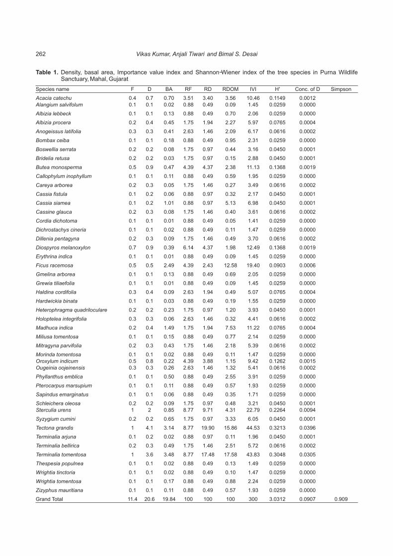
Species name F D BA RF RD RDOM IVI H' Conc. of D Simpson
Acacia catechu 0.4 0.7 0.70 3.51 3.40 3.56 10.46 0.1149 0.0012
Alangium salvifolum 0.1 0.1 0.02 0.88 0.49 0.09 1.45 0.0259 0.0000
Albizia lebbeck 0.1 0.1 0.13 0.88 0.49 0.70 2.06 0.0259 0.0000
Albizia procera 0.2 0.4 0.45 1.75 1.94 2.27 5.97 0.0765 0.0004
Anogeissus latifolia 0.3 0.3 0.41 2.63 1.46 2.09 6.17 0.0616 0.0002
Bombax ceiba 0.1 0.1 0.18 0.88 0.49 0.95 2.31 0.0259 0.0000
Boswellia serrata 0.2 0.2 0.08 1.75 0.97 0.44 3.16 0.0450 0.0001
Bridelia retusa 0.2 0.2 0.03 1.75 0.97 0.15 2.88 0.0450 0.0001
Butea monosperma 0.5 0.9 0.47 4.39 4.37 2.38 11.13 0.1368 0.0019
Callophylum inophyllum 0.1 0.1 0.11 0.88 0.49 0.59 1.95 0.0259 0.0000
Careya arborea 0.2 0.3 0.05 1.75 1.46 0.27 3.49 0.0616 0.0002
Cassia fistula 0.1 0.2 0.06 0.88 0.97 0.32 2.17 0.0450 0.0001
Cassia siamea 0.1 0.2 1.01 0.88 0.97 5.13 6.98 0.0450 0.0001
Cassine glauca 0.2 0.3 0.08 1.75 1.46 0.40 3.61 0.0616 0.0002
Cordia dichotoma 0.1 0.1 0.01 0.88 0.49 0.05 1.41 0.0259 0.0000
Dichrostachys cineria 0.1 0.1 0.02 0.88 0.49 0.11 1.47 0.0259 0.0000
Dillenia pentagyna 0.2 0.3 0.09 1.75 1.46 0.49 3.70 0.0616 0.0002
Diospyros melanoxylon 0.7 0.9 0.39 6.14 4.37 1.98 12.49 0.1368 0.0019
Erythrina indica 0.1 0.1 0.01 0.88 0.49 0.09 1.45 0.0259 0.0000
Ficus racemosa 0.5 0.5 2.49 4.39 2.43 12.58 19.40 0.0903 0.0006
Gmelina arborea 0.1 0.1 0.13 0.88 0.49 0.69 2.05 0.0259 0.0000
Grewia tiliaefolia 0.1 0.1 0.01 0.88 0.49 0.09 1.45 0.0259 0.0000
Haldina cordifolia 0.3 0.4 0.09 2.63 1.94 0.49 5.07 0.0765 0.0004
Hardwickia binata 0.1 0.1 0.03 0.88 0.49 0.19 1.55 0.0259 0.0000
Heterophragma quadriloculare 0.2 0.2 0.23 1.75 0.97 1.20 3.93 0.0450 0.0001
Holoptelea integrifolia 0.3 0.3 0.06 2.63 1.46 0.32 4.41 0.0616 0.0002
Madhuca indica 0.2 0.4 1.49 1.75 1.94 7.53 11.22 0.0765 0.0004
Miliusa tomentosa 0.1 0.1 0.15 0.88 0.49 0.77 2.14 0.0259 0.0000
Mitragyna parvifolia 0.2 0.3 0.43 1.75 1.46 2.18 5.39 0.0616 0.0002
Morinda tomentosa 0.1 0.1 0.02 0.88 0.49 0.11 1.47 0.0259 0.0000
Oroxylum indicum 0.5 0.8 0.22 4.39 3.88 1.15 9.42 0.1262 0.0015
Ougeinia oojeinensis 0.3 0.3 0.26 2.63 1.46 1.32 5.41 0.0616 0.0002
Phyllanthus emblica 0.1 0.1 0.50 0.88 0.49 2.55 3.91 0.0259 0.0000
Pterocarpus marsupium 0.1 0.1 0.11 0.88 0.49 0.57 1.93 0.0259 0.0000
Sapindus emarginatus 0.1 0.1 0.06 0.88 0.49 0.35 1.71 0.0259 0.0000
Schleichera oleosa 0.2 0.2 0.09 1.75 0.97 0.48 3.21 0.0450 0.0001
Sterculia urens 1 2 0.85 8.77 9.71 4.31 22.79 0.2264 0.0094
Syzygium cumini 0.2 0.2 0.65 1.75 0.97 3.33 6.05 0.0450 0.0001
Tectona grandis 1 4.1 3.14 8.77 19.90 15.86 44.53 0.3213 0.0396
Terminalia arjuna 0.1 0.2 0.02 0.88 0.97 0.11 1.96 0.0450 0.0001
Terminalia bellirica 0.2 0.3 0.49 1.75 1.46 2.51 5.72 0.0616 0.0002
Terminalia tomentosa 1 3.6 3.48 8.77 17.48 17.58 43.83 0.3048 0.0305
Thespesia populnea 0.1 0.1 0.02 0.88 0.49 0.13 1.49 0.0259 0.0000
Wrightia tinctoria 0.1 0.1 0.02 0.88 0.49 0.10 1.47 0.0259 0.0000
Wrightia tomentosa 0.1 0.1 0.17 0.88 0.49 0.88 2.24 0.0259 0.0000
Zizyphus mauritiana 0.1 0.1 0.11 0.88 0.49 0.57 1.93 0.0259 0.0000
Grand Total 11.4 20.6 19.84 100 100 100 300 3.0312 0.0907 0.909
Table 1. Density, basal area, Importance value index and Shannon-Wiener index of the tree species in Purna Wildlife Sanctuary, Mahal, Gujarat
Vikas Kumar, Anjali Tiwari and Bimal S. Desai262
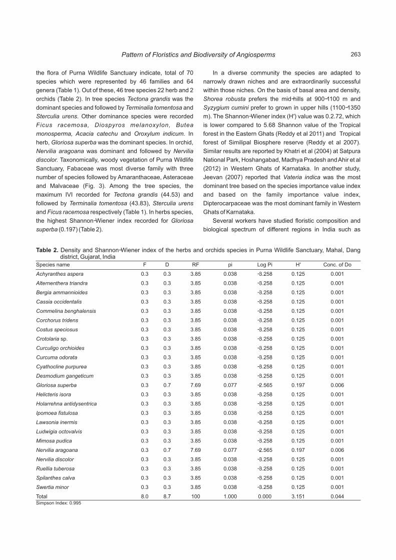
the flora of Purna Wildlife Sanctuary indicate, total of 70
species which were represented by 46 families and 64
genera (Table 1). Out of these, 46 tree species 22 herb and 2
orchids (Table 2). In tree species Tectona grandis was the
dominant species and followed by Terminalia tomentosa and
Sterculia urens. Other dominance species were recorded
Ficus racemosa, Diospyros melanoxylon, Butea
monosperma, Acacia catechu and Oroxylum indicum. In
herb, Gloriosa superba was the dominant species. In orchid,
Nervilia aragoana was dominant and followed by Nervilia
discolor. Taxonomically, woody vegetation of Purna Wildlife
Sanctuary, Fabaceae was most diverse family with three
number of species followed by Amaranthaceae, Asteraceae
and Malvaceae (Fig. 3). Among the tree species, the
maximum IVI recorded for Tectona grandis (44.53) and
followed by Terminalia tomentosa (43.83), Sterculia urens
and Ficus racemosa respectively (Table 1). In herbs species,
the highest Shannon-Wiener index recorded for Gloriosa
superba (0.197) (Table 2).
Species name F D RF pi Log Pi H' Conc. of Do
Achyranthes aspera 0.3 0.3 3.85 0.038 -3.258 0.125 0.001
Alternenthera triandra 0.3 0.3 3.85 0.038 -3.258 0.125 0.001
Bergia ammannioides 0.3 0.3 3.85 0.038 -3.258 0.125 0.001
Cassia occidentalis 0.3 0.3 3.85 0.038 -3.258 0.125 0.001
Commelina benghalensis 0.3 0.3 3.85 0.038 -3.258 0.125 0.001
Corchorus tridens 0.3 0.3 3.85 0.038 -3.258 0.125 0.001
Costus speciosus 0.3 0.3 3.85 0.038 -3.258 0.125 0.001
Crotolaria sp. 0.3 0.3 3.85 0.038 -3.258 0.125 0.001
Curculigo orchioides 0.3 0.3 3.85 0.038 -3.258 0.125 0.001
Curcuma odorata 0.3 0.3 3.85 0.038 -3.258 0.125 0.001
Cyathocline purpurea 0.3 0.3 3.85 0.038 -3.258 0.125 0.001
Desmodium gangeticum 0.3 0.3 3.85 0.038 -3.258 0.125 0.001
Gloriosa superba 0.3 0.7 7.69 0.077 -2.565 0.197 0.006
Helicteris isora 0.3 0.3 3.85 0.038 -3.258 0.125 0.001
Holarrehna antidysentrica 0.3 0.3 3.85 0.038 -3.258 0.125 0.001
Ipomoea fistulosa 0.3 0.3 3.85 0.038 -3.258 0.125 0.001
Lawsonia inermis 0.3 0.3 3.85 0.038 -3.258 0.125 0.001
Ludwigia octovalvis 0.3 0.3 3.85 0.038 -3.258 0.125 0.001
Mimosa pudica 0.3 0.3 3.85 0.038 -3.258 0.125 0.001
Nervilia aragoana 0.3 0.7 7.69 0.077 -2.565 0.197 0.006
Nervilia discolor 0.3 0.3 3.85 0.038 -3.258 0.125 0.001
Ruellia tuberosa 0.3 0.3 3.85 0.038 -3.258 0.125 0.001
Spilanthes calva 0.3 0.3 3.85 0.038 -3.258 0.125 0.001
Swertia minor 0.3 0.3 3.85 0.038 -3.258 0.125 0.001
Total 8.0 8.7 100 1.000 0.000 3.151 0.044
Table 2. Density and Shannon-Wiener index of the herbs and orchids species in Purna Wildlife Sanctuary, Mahal, Dang district, Gujarat, India
Simpson Index: 0.995
In a diverse community the species are adapted to
narrowly drawn niches and are extraordinarily successful
within those niches. On the basis of basal area and density,
Shorea robusta prefers the mid-hills at 900-1100 m and
Syzygium cumini prefer to grown in upper hills (1100-1350
m). The Shannon-Wiener index (H') value was 0.2.72, which
is lower compared to 5.68 Shannon value of the Tropical
forest in the Eastern Ghats (Reddy et al 2011) and Tropical
forest of Similipal Biosphere reserve (Reddy et al 2007).
Similar results are reported by Khatri et al (2004) at Satpura
National Park, Hoshangabad, Madhya Pradesh and Ahir et al
(2012) in Western Ghats of Karnataka. In another study,
Jeevan (2007) reported that Vateria indica was the most
dominant tree based on the species importance value index
and based on the family importance value index,
Dipterocarpaceae was the most dominant family in Western
Ghats of Karnataka.
Several workers have studied floristic composition and
biological spectrum of different regions in India such as
Pattern of Floristics and Biodiversity of Angiosperms 263

Fig. 2. Assessment of phytosociological study through quadrate method
FAMILY
Fig. 3. Family basis of woody vegetation of Purna Wildlife Sanctuary, Mahal, Gujarat
Shukla and Mishra (2006) in Dewghat Forest, UP; Pharswan
et al (2010) in Alpine Medows of Kedavnath; Thakur et al
(2012) in Darlaghat Wild Life Sanctuary, HP.; Sindhuja et al
(2012) in Maruthamalai Hills, Southern Western Ghats;
Sarkar and Devi (2014) in Hollongapar Gibbon Wildlife
Sanctuary, Assam; Chauhan et al (2014) in Madhav National
Park, MP; Sundarapandian and Subbiah (2015) in
Sivagangai district, TN; Kumar and Desai (2016a) in Chikhali
Taluka, Navsari District, Gujarat and Kumar and Desai
(2016b) in Dang district of South Gujarat.
CONCLUSION
Total 70 species (46 tree, 22 herbs and 2 orchids) were
recorded in Purna Wildlife Sanctuary, Mahal, Gujarat during
the period of 2010-2013. The maximum IVI was for Tectona
grandis) and followed by Terminalia tomentosa. Among the
herbs species, the highest Shannon-Wiener index was for
Nervilia aragoana. Apart from physical and ecological
conditions and the natural evolutionary process, the flora
biodiversity has also been greatly influenced by diverse
social-cultural preferences, economic condition, food habit
and needs.
REFERENCES
Ahir KC, Hegde K, Sarkar PK, Maheswarappa V, Hareesh TS and Hegde R 2012. Assessment of Floristic Composition and Population Structure of Coscinium fenestratum in Western Ghats of Karnataka. Second Indian Biodiversity Congress. 9-12 December, 2012. Indian Institute of Science, Bangalore.
Blatter E J and McCann 1926-1935. Revision of the Flora of Bombay Presidency. Journal of Bombay Natural History Society 35: 20-45.
Bole PV and Pathak JM 1988. The Flora of Saurashtra (Asteraceae to Poaccae vol. II and III). BSI. Calcutta.
Chauhan SS, Tiwari A, Sheikh MA and Sharma S 2014. Study on Biological Spectrum of Madhav National Park, Shivpuri, Madhya Pradesh, India. Journal of Biodiversity and Environmental Sciences 4(3): 258-262.
Cottam G and Curtis JT 1956. The use of distance measurements in phytosociological sampling. Ecology 37: 451-460.
Jain SK 1963. Vegetation of Dang district in Gujarat. Bulletin of the Botanical Survey of India 5(3-4): 351-361.
Jeevan K 2007. Distribution and reproductive biology of Vateria indica L. in Central Western Ghats of Karnataka. M.Sc. Thesis, University of Agricultural Sciences, Bangalore.
Jhariya MK and Oraon PR 2012. Analysis of herbaceous diversity in fire affected area of Bhoramdeo Wildlife Sanctuary, Chattisgarh. The Bioscan 7(2): 325-330.
Kent M and Coker P 2001. Vegetation Description and Analysis. A Practical. Approach. Folia Geobotanica 36(1): 101-103.
Khatri PK, Totey NG and Pandey RK 2004. Altitudinal variation in Satpura National Park. Indian Forester 130: 1141-1153.
Kumar V 2015. Impact of non timber forest produces (NTFPs) on food and livelihood security: An economic study of tribal economy in Dang's district of Gujarat, India. International Journal of Agriculture, Environment and Biotechnology 8(2): 387-404.
Kumar V and Desai BS 2016a. Biodiversity and phytosociological analysis of plants around the Chikhali Taluka, Navsari district, Gujarat, India. The Ecoscan 10: 689-696.
Kumar V and Desai BS 2016b. Phytosociological study of Waghai forest range in Dang district, south Gujarat, India. Environment and Bio-sciences. 30(2): 549-553.
Kumar V, Bimal SD and Ajeesh R 2013. Ecology of Rare and Endangered plant species of Dang's Forest, South Gujarat. LAP LAMBERT Academic Publishing, Germany.
Kumar V and Tiwari A 2017. Importance of tropical homegardens agroforestry system. International Journal of Current microbiology and applied sciences 6(9): 1002-1019.
Kumar V and Tripathi AM 2017. Vegetation Composition and Functional Changes of Tropical Homegardens: Prospects and Challenges. In: Gupta, S.K., Panwar, P. and Kaushal, R. (Eds), Agroforestry for increased production and livelihood security. New India Publishing Agency, New Delhi, pp-475-505.
Misra R 1968. Ecological Work Book. Oxford and IBH Publishing Co., New Delhi.
Parthasarathy N and Karthikeyan R 1997. Biodiversity and population density of woody species in a tropical evergreen forest in Courtallum reserve forest, Western Ghats, India. Tropical Ecology 38: 297-306.
Pharswan K, Mehta JP and Subodh 2010. Floristic composition and biological spectrum of vegetation in Alpine Medows of
Vikas Kumar, Anjali Tiwari and Bimal S. Desai264

Kedavnath, Garhwal Himalaya. Nature and Science 8(7): 109-115.
Philips EA 1959. Methods of Vegetation Study. Holt Reinhart and Winston. New York.
Reddy SC, Babar S, Amarnath G and Pattanaik C 2011. Structure and floristic composition of tree stand in tropical forest in the Eastern Ghats of northern Andhra Pradesh, India. Journal of forestry research 22: 491-500.
Reddy SC, Pattanaik C, Mohapatra A and Biswal AK 2007. Phytosociological observations on tree diversity of Tropical forest of similipal biosphere reserve, Orissa, India. Taiwania 52: 352-359.
Santapau H 1962. The Flora of Saurashtra. Part-1. Rajkot, Gujarat.
Sarkar M and Devi A 2014. Assessment of diversity, population structure and regeneration status of tree species in Hollongapar Gibbon Wildlife Sanctuary, Assam, Northeast India. Tropical Plant Research 1(2): 26-36.
Shah GL 1978. Flora of Gujarat state. Sardar Patel University. Vallabh Vidyanagar, Gujarat.
Shah GL, Menon AR and Gopal GV 1981. An account of the ethnobotany of Saurashtra in Gujarat state. (India). Journal of Economic and Taxonomic Botany 29: 173.
Shukla CP and Mishra KN 2006. Floristic composition, biological
spectrum and plant diversity of burnt and unburnt grazing lands of Dewghat Forest, Koraon range (UP). National Academy Science Letters India 29(9-10): 345-349.
Simpson EH 1949. Measurement of diversity. Nature 163: 688.
Sindhuja R, Rajendran A and Jayanthi P 2012. Herbaceous life forms of Maruthamalai Hills. Southern Western Ghats, India. International Journal of Medicinal and Aromatic Plants 2(4): 625-631.
Stork NE 2010. Re-assessing current extinction rates. Biodiversity and Conservation 19: 357-371.
Sundarapandian SM and Subbiah S 2015. Diversity and tree population structure of tropical dry evergreen forests in Sivagangai district of Tamil Nadu, India. Tropical Plant Research 2(1): 36-46.
Thakur M, Santvan V K and Nigam A 2012. Floristic Composition and Biological spectrum of Darlaghat Wild Life Sanctuary, Solan, Himachal Pradesh, India. New York Science Journal 5(12): 1-14.
Vashi BG 1985. Floristic, phytosociology and ethnobotanical study of Umarpada forest in South Gujarat. PhD Thesis, Veer Narmad South Gujarat University, Surat, Gujarat.
Whittaker RH 1972. Evolution and measurement of species diversity. Taxon 21(2-3): 213-251.
Received 16 March, 2018; Accepted 10 May, 2018
Pattern of Floristics and Biodiversity of Angiosperms 265
Habitat Distribution Modelling of Seabuckthorn (Hippophae salicifolia D. Don.) in Sikkim, Eastern Himalaya, India
Indian Journal of Ecology (2018) 45(2): 266-269
Abstract: Seabuckthorn (Hippophae salicifolia) is one of the underutilized plant species having enormous potential for socio-economic
upliftment and sustainable livelihood of rural communities. In Sikkim it grows naturally in Lachen and Lachung valleys of North district and it
has not been explored for economic benefits. Due to its restricted distribution in Sikkim, ecological niche modelling (ENM) was performed to
identify suitable habitat for in-situ conservation through identification of suitable areas and for further reintroduction in its natural habitat. The
model was developed using Maximum Entropy (MaxEnt) distribution modelling algorithm and predicted that the suitable habitats of 2Seabuckthornare restricted to an area of ca. 286 km in Sikkim. The distribution of the potential habitat was strongly influenced by NDVI layer
for October and January, which corresponds to the period of fruiting phenology of the species, thus indicating the importance of fruiting
phenology in determining the distribution of the species. Population status was positively correlated with very high model thresholds at three
locations, confirming the usefulness of the habitat model in population monitoring. Therefore the approach presented here emerge to be quite
promising in predicting the suitable habitat for species with restricted distribution and moreover it can be an effective tool for conservation
planning, monitoring and management of the species.
Keywords: Seabuckthorn, ENM, Conservation, Macro propagation, Protected area
Manuscript Number: NAAS Rating: 4.96
2669
1 2Arun Chettri, Aditya Pradhan, Ghanashyam Sharma , Bharat K. Pradhan *and Dhani Raj Chhetri
Department of Botany, Sikkim University, Sikkim-737 102, India 1The Mountain Institute India, Tadong, Gangtok-737 101, India
2Sikkim Biodiversity Board, Forest, Environment & Wildlife Management Department, Deorali, Gangtok-737 102, India*E-mail: [email protected]
Seabuckthorn (Hippophae salicifolia D. Don) is a thorny,
deciduous shrub (Singh 1998, Nepal et al 2001) belonging to
the family Elaeagnaceae. The species is restricted to the
Himalayan region, between 1500-3500 m asl (Gaur 1999,
Hooker 1894). In India H. salicifolia grows naturally in high
altitude areas of Himachal Pradesh, Jammu and Kashmir,
Uttar Pradesh (Singh et al 1995, Singh 1998) and Sikkim
(Basistha 2001). In Sikkim, the species is found naturally
growing in Lachen and Lachung Valleys of North district
between the altitude of 2700 and 3700 m. Ecological niche
modelling (ENM) also known as species distribution modelling
is a recent tool which uses computer algorithms to generate
predictive maps of species distribution in a geographic space
by correlating the point distributional data with a set of
environmental raster data. Predicting and mapping the
suitable habitat for threatened and endangered species is
critical for monitoring and restoration of their declining native
populations (Kumar and Stohlgren 2009). Species
reintroduction is one such ecological strategy for restoration of
depleted species population reclamation of degraded habitats
and ecosystems (Adhikari et al 2012). To reintroduce and
rehabilitate a threatened species a detailed knowledge of its
potential habitats is essential. Species distribution modelling
or ENM therefore helps to identify the suitable habitats for
reintroduction, and in developing effective species specific
conservation measures. It has been successfully used in
restoring critical habitats and predicting the impact of
environmental and climate change on species and
ecosystems (Brooks et al 2004, Franklin 2009, Giriraj et al
2008, Gogol-Prokurat 2011, Khanum et al 2013).
Identification of suitable habitat is prerequisite for
species restoration programme (Adhikari et al 2012, Pradhan
and Chettri 2017). To achieve such restoration of threatened
species require GIS based techniques like ENM which
reconstructs the niche of a species in an ecological space by
correlating the occurrence points (geographic coordinate)
with a set of environmental variables. The present work was
therefore undertaken with the aim of identifying suitable
habitat for conservation through large scale propagation of
species. Such predicted habitat identified through ENM could
be used for reintroduction of species in near future.
MATERIAL AND METHODS
Species occurrence records: Primary occurrence data
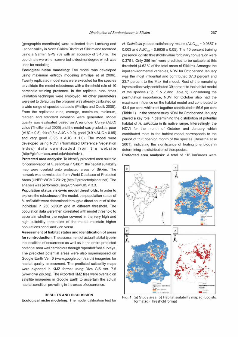
(geographic coordinate) were collected from Lachung and
Lachen valley in North Sikkim District of Sikkim and recorded
using a Garmin GPS 78s with an accuracy of 3-10 m. The
coordinate were then converted to decimal degree which was
used for modeling.
Ecological niche modeling: The model was developed
using maximum entropy modeling (Phillips et al 2006).
Twenty replicated model runs were executed for the species
to validate the model robustness with a threshold rule of 10
percentile training presence. In the replicate runs cross
validation technique were employed. All other parameters
were set to default as the program was already calibrated on
a wide range of species datasets (Phillips and Dudik 2008).
From the replicated runs, average, maximum, minimum,
median and standard deviation were generated. Model
quality was evaluated based on Area under Curve (AUC)
value (Thuiller et al 2005) and the model was graded as: poor
(AUC < 0.8), fair (0.8 < AUC < 0.9), good (0.9 < AUC < 0.95)
and very good (0.95 < AUC < 1.0). The model were
developed using NDVI (Normalized Difference Vegetation
I n d e x ) d a t a d o w n l o a d e d f r o m t h e w e b s i t e
(http://glcf.umiacs.umd.edu/data/ndvi).
Protected area analysis: To identify protected area suitable
for conservation of H. salicifolia in Sikkim, the habitat suitability
map were overlaid onto protected areas of Sikkim. The
network was downloaded from World Database of Protected
Areas (UNEP-WCMC 2012); (http:// protectedplanet.net). The
analysis was performed using Arc View GIS v. 3.3.
Population status vis-à-vis model thresholds: In order to
explore the robustness of the model, the population status of
H. salicifolia were determined through a direct count of all the
individual in 250 x250m grid at different threshold. The
population data were then correlated with model threshold to
ascertain whether the region covered in the very high and
high suitability thresholds of the model maintain higher
populations or not and vice-versa.
Assessment of habitat status and identification of areas
for reintroduction: The assessment of actual habitat type in
the localities of occurrence as well as in the entire predicted
potential area was carried out through repeated filed surveys.
The predicted potential areas were also superimposed on
Google Earth Ver. 6 (www.google.com/earth) imageries for
habitat quality assessment. The predicted suitability maps
were exported in KMZ format using Diva GIS ver. 7.5
(www.diva-gis.org). The exported KMZ files were overlaid on
satellite imageries in Google Earth to ascertain the actual
habitat condition prevailing in the areas of occurrence.
RESULTS AND DISCUSSION
Ecological niche modeling: The model calibration test for
H. Salicifolia yielded satisfactory results (AUC = 0.9857 ± train
0.003 and AUC = 0.9636 ± 0.05). The 10 percent training test
presence logistic thresholds value for binary conversion were 20.3751. Only 286 km were predicted to be suitable at this
threshold (4.62 % of the total areas of Sikkim). Amongst the
input environmental variables, NDVI for October and January
was the most influential and contributed 37.3 percent and
23.7 percent to the Max Ent model. Rest of the remaining
layers collectively contributed 39 percent to the habitat model
of the species (Fig. 1 & 2 and Table 1). Considering the
permutation importance, NDVI for October also had the
maximum influence on the habitat model and contributed to
43.4 per cent, while rest together contributed to 56.6 per cent
(Table 1). In the present study NDVI for October and January
played a key role in determining the distribution of potential
habitat of H. salicifolia in its native range. Interestingly, the
NDVI for the month of October and January which
contributed most to the habitat model corresponds to the
period of fruit ripening month of the species (Basistha et al
2001), indicating the significance of fruiting phenology in
determining the distribution of the species.2Protected area analysis: A total of 116 km areas were
Fig. 1. (a) Study area (b) Habitat suitability map (c) Logistic format (d) Threshold format
Distribution of Seabuckthorn in Sikkim 267

Variable Description of the variable
Percent contribution
Permutation importance
eu1 Month of January 23.7 18.5
eu2 Month of February 4.1 2.5
eu3 Month of March 0.1 0
eu4 Month of April 12.6 2.4
eu5 Month of May 2 0.2
eu6 Month of June 10.5 21.2
eu7 Month of July 0.6 0.1
eu8 Month of August 4.8 8.3
eu9 Month of September 2.9 3.4
eu10 Month of October 37.3 43.4
eu11 Month of November - -
eu12 Month of December 1.5 0.1
Table 1. List of NDVI data used for modeling and contribution to the model
Fig. 2. Result of jackknife test for evaluating the relative contribution of the predictor environmental variables to the habitat model of H. salicifolia in Sikkim
predicted to be suitable in the eight protected area identified
in Sikkim. Kanchenjunga National Park (KNP) had the
highest area predicted to be suitable followed by Singba.
Protected areas viz. Kyongnosla Alpine, Maenam Wildlife
Sanctuary and Kyongnosla extension were unsuitable for
insitu conservation of species (Table 2).
Population and habitat status assessment: Field surveys
for assessing the habitat types of H. salicifolia in the predicted
potential areas revealed that the species occurred
abundantly in riverine area (Riverside) and human
settlement (Table 3). Superimposing the predicted potential
habitat map of the species on Google Earth satellite
imageries revealed, areas with very high and high suitability
for the species were mostly human habitat area along
roadside and river banks. The areas with medium and low
suitability were degraded landslide area with dense
evergreen forest. The areas with low to very low suitability
were open evergreen forest and degraded area (Table 3).
Apart from Lachung and Lachen Valley areas such as
Latong, Talam, Yathang and Lingzah-Tolung in North Sikkim
were identified as suitable for species restoration.
Raising plantlets for propagation: The seeds of
Seabuckthorn were collected from Lachen Valley in North
Sikkim district of Sikkim and were planted in a nursery
(600/150 cm length/breadth) at Lachen at an elevation of
2725m. Out of ca. 1000 seeds planted in the nursery more
than 90 percent of seeds developed into healthy sapling. The
sapling was further distributed amongst the local residents
for restoration of depleting population, through reintroduction
in the natural habitat.
CONCLUSION
The population of seabuckthorn in its natural habitat is
considerably high, however, deforestation through
destruction of forest trees including Seabuckthorn for fuel
and extensive construction of road has led to the depletion of
natural population. At Lachung valley, Seabuckthorn is
mostly dominant in the riverine area. The very high
population density dominated by Sea buckthorn in the
riverside areas unlike in mixed forest areas where the
population were low to moderate. The population data
through direct count in the area predicted through ENM thus
Protected Area IUCN management category
Type of protected area 2Total area (km ) Predicted suitable area 2(Km )
Khangchendzonga National Park II National Park 1784 69
Fambong Lho Wildlife Sanctuary IV Wildlife Sanctuary 51 12
Kyongnosla Alpine Sanctuary IV Sanctuary 31 0
Maenam Wildlife Sanctuary IV Wildlife Sanctuary 35 0
Kyongnosla extension Not Applicable Sanctuary 21 0
Singba Rhododendron Sanctuary Not Reported Sanctuary 57 25
Barsey Rhododendron Sanctuary IV Sanctuary 104 10
2083 116
Table 2. Protected area identified as suitable for insitu conservation (10 % training presence threshold)
Arun Chettri, Aditya Pradhan, Ghanashyam Sharma, Bharat K. Pradhan and Dhani Raj Chhetri268

Occurrence localities
Geographic coordinate Elevation (m asl)
Habitat suitability thresholds
Habitat types identified using high resolution Google Earth satellite imageries
No. of Individuals
Lachung 1 88° 44' 08.00'' E27° 40' 38.42'' N
3524 Very High Riverside area, human settlement 125
Lachung 2 88° 45'0 7.94'' E27° 42' 52.47'' N
3363 Very High Riverside area, human settlement 112
Lachung 3 88° 44' 34.70'' E27° 41' 20.60'' N
3611 Very High Riverside area, human settlement 50
Lachen 1 88° 32' 27.79'' E27° 43' 00.07'' N
3363 Very High Mixed forest, human settlement 25
Lachen 2 88° 32' 44.92'' E27° 43' 08.69'' N
3126 High Mixed forest, human settlement 73
Lachen 4 88° 33' 44.30'' E27° 41' 33.65'' N
3121 Medium Dense evergreen forest, Degraded landslide area
57
Lachen 5 88° 32' 51.16'' E27° 44' 41.02'' N
3034 Low Mixed forest, Degraded landslide area
12
Table 3. Population status and habitat type of H. salicifolia to model thresholds
Habitat suitability thresholds: very low, 0-0.1910; low, 0.1910-0.3820; medium, 0.3820-0.5731; high, 0.5731-0.7641; very high, 0.7641-1
validates the robustness of the model, as it maintains high
population density in the very high and high suitability
threshold and low to moderate population in lower suitability
threshold (Medium and low) areas. Moreover, this study
further provided a considerable lead for development of easy
and effective propagation technique for large scale
propagation of species for further domestication of species
leading to socio-economic upliftment and sustainable
livelihood enhancement in the region.
ACKNOWLEDGEMENT
Financial support received from Ministry of
Environment, Forest and Climate Change, Govt. of India
under NMHS project (No. NMHS/MG-2016/005/8502-7) is
gratefully acknowledged. The authors are also thankful to
Department of Forest, Environment and Wildlife
Management, Govt. of Sikkim for logistic support.
REFERENCES
Adhikari D, Barik SK and Upadhaya K 2012. Habitat distribution modelling for reintroduction of Ilex khasiana Purk., a critically endangered tree species of northeastern India. Ecological Engineering 40: 37-43.
Basistha BC and Adhikari IM 2001. A case study of Hippophae Linn with special reference to agro techniques in the Sikkim Himalayas. In Proceedings of International workshop on Seabuckthorn (February, 2001). New Delhi (India).
Brooks TM, da Fonseca GAB and Rodrigues ASL 2004. Protected areas and species. Conservation Biology 18: 616.
Franklin J 2009. Mapping Species Distributions: Spatial Inference and Prediction. Cambridge University Press. pp. 338.
Gaur RD 1999. Flora of the district Garhwal Northwest Himalaya (with ethno botanical notes).Transmedia, Srinagar Garhwal, India. pp. 811.
Giriraj A, Irfan-Ullah M, Ramesh BR, Karunakaran PV, Jentsch A and Murthy MSR 2008. Mapping the potential distribution of Rhododendron arboreum Sm. ssp. nilagiricum (Zenker) Tagg
(Ericaceae), an endemic plant using ecological niche modeling. Current Science 94: 1605–1612.
Gogol-Prokurat M 2011. Predicting habitat suitability for rare plants at local spatial scales using a species distribution model. Ecological Application 21: 33–47.
Hooker JD 1894. The flora of British India. Dehradun: Bishen Singh Mahendra pal Singh 5: 791.
Khanum R, Mumtaz AS and Kumar S 2013. Predicting impacts of climate change on medicinal asclepiads of Pakistan using Maxent modeling. Acta Oecologica 49: 23-31.
Kumar S and Stohlgren TJ 2009. Maxent modeling for predicting suitable habitat for threatened and endangered tree Canacomyrica monticola in New Caledonia. Journal of Ecology and Natural Environment 1(4): 94-98.
Nepal V, Poudyal DP, Subedi CK, Adhikary K, Dhakal LP and Gupta VN 2001. Proceedings of the International Symposium on the Himalayan Environments: Mountain Sciences and Ecotourism/Biodiversity. pp 72-81.
Pant M, Lal A and Rani A 2014. Hippophae salicifolia D. Don- A plant with multifarious benefits. International Journal of Pharamacy and Pharmaceutical Sciences 6(11): 37-40.
Phillips SJ and Dudík M 2008. Modeling of species distributions with MaxEnt: new extensions and a comprehensive evaluation. Ecography 31: 161–175.
Phillips SJ, Anderson RP and Schapire RE 2006. Maximum entropy modeling of species geographic distributions. Ecological Modelling 190: 231–259.
Pradhan A and Chettri A 2017. Identifying protected areas suitable for conservation of Cycas pectinata Buch.Ham.in Southeast Asia under climate change scenario. International Journal of Ecology and Environmental Sciences 43(2): 129-135.
Singh V 1988. Sea buckthorn a wonder plant of dry temperate Himalayas. Indian Horticulture 43 (2): 6-8.
Singh V, Singh B and Awasthi CP 1995. Distribution, taxonomy and nutritional value of seabuckthorn (Hippophae L.) in dry temperate Himalayas. In: Proc. Int. Workshop Seabuckthorn, Beijing, China, pp. 52-59.
Thuiller W, Richardson DM, Py¡sek P, Midgley GF, Hughes GO and Rouget M 2005. Niche-based modelling as a tool for predicting the risk of alien plant invasions at a global scale.Global Change Biology 11: 2234–2250.
UNEP-WCMC. 2012. Data Standards for the World Database on Protected Areas. UNEP=WCMC. U.K. 15 Pages.
Received 08 April, 2018; Accepted 10 May, 2018
Distribution of Seabuckthorn in Sikkim 269

Effect of Container and Growing Media on Terminalia bellirica Roxb. Seedling Performance under Nursery Conditions
Indian Journal of Ecology (2018) 45(2): 270-275
Abstract: Investigation on the effect of containers (root trainer 250 cc, root trainer 300 cc, polybags 16 x 24 cm-1500cc and polybag 23 x 28
cm-4200cc) and potting media (soil, soil: sand: FYM-1:1:1 and soil: sand:vermicompost-1:1:1 on the growth of Terminalia bellirica was carried
out at Sher-e-Kashmir University of Agricultural Sciences and Technology-Jammu, Chatha, Jammu (India) during 2015-2016. Among the
different container sizes and media, the polybag of 23 x 28 cm size and soil: sand: vermicompost (1:1:1) growing media resulted in significantly
higher seedling height, collar diameter, number of leaves, length of primary root, fresh shoot and root weight, total seedling fresh weight, dry
shoot and root weight, total seedling dry weight, root: shoot ratio and seedling quality. The effect of containers on number of secondary roots
and sturdiness quotient was significant whereas it was non-significant in case of media. The sturdiness quotient decreased with increase in
container size. The effect of interaction of containers x potting media was significant on growth parameters viz. seedling height, number of
leaves, fresh shoot weight, total seedling fresh weight, root: shoot ratio and sturdiness quotient, however, it was non-significant in case of
germination percentage, collar diameter, number of primary roots, fresh shoot weight, dry shoot weight, dry root weight, total seedling dry
weight and seedling quality index. The interaction polybags (23 x 28 cm) x medium (soil: sand: VC-1:1:1) resulted insignificantly higher values
for the most of the studied growth parameters than the remaining interactions. The large sized containers (polybag of 23 x 28 cm) in
combination with soil: sand: VC (1:1:1) media resulted in better growth of T. bellirica seedlings. Thus the seedling of this species should be
grown in polybag (23 x 28 cm) using soil: sand: VC (1:1:1) as growing media to obtain better quality planting stock.
Keywords: Terminalia bellirica, Container size, Potting media, Farm yard manure, Vermicompost, Root trainers, Polybags, Nursery
Manuscript Number: NAAS Rating: 4.96
2670
Kamal Kishor Sood, Fayaz Ahmed and N.S. RainaDivision of Agroforestry, Sher-e-kashmir University of Agricultural Sciences and Technology-Jammu,
Main Campus-Chatha, Jammu-180 009, IndiaE-mail: [email protected]
Terminalia bellirica Roxb. (family Combretaceae), is one
of the important multipurpose trees of Indian subcontinent,
Sri Lanka and South East Asia. It is called “Belric myrobalan”
and also known as “Bahera” in India. Its distribution extends
from 0-1330 m elevation above mean see level. In India it is
generally found in Himalayan tract up to 1200 to 1300 m in
Sal and miscellaneous forest of the subtropical zone. Due to
multifarious uses of T. bellirica is being over-exploited
resulting in shrinkage of its population. Further, collection of
its fruits for medicinal uses also results in its poor
regeneration. Thus, it is necessary to supplement its natural
regeneration through afforestation programme. This would
require production of quality planting stock for afforestation.
During the containerised seedling production, container size,
and growth medium are important determinants of seedling
quality (Tsakaldimi et al 2005, Aghai et al 2014). Hence the
present study was taken to obtain the quality planting stock of
the species. The objective to the study was to standardise
container size and potting media to obtain better quality
seedlings of the species under open nursery conditions.
MATERIAL AND METHODS
Study area: The study was conducted in the Division of
Agroforestry, Sher-e-Kashmir University of Agricultural
Sciences and Technology-Jammu located at Chatha,
Jammu. The experimental site was the subtropical Jammu
region of Jammu and Kashmir state, located at 332 m above o omean sea level with 32 40` N latitude and 74 58` E longitude.
The annual rainfall in the study area ranges from 1000 mm to
1200 mm.
Climate and weather conditions: The weather data
recorded at meteorological observatory of SKUAST-Jammu,
Chatha, during study period (January–October, 2016) are
given in Fig. 1.
Design of experiment: The treatments of the experiment
consisted of different four container sizes root trainer 250 cc,
root trainer 300 cc, polybags 16 cm x 24 cm-1500cc and
polybag 23 x 28 cm-4200cc and three media types: soil, soil:
sand: FYM (1:1:1) and soil: sand: vermicompost (1:1:1).
Each root trainer was in block of 12 cells. The soil of the study
site is sandy loam (Rana and Sood 2012), which was utilised
for the current study. The pH of the study soil was 7.81 and
EC 0.04 ds/m. The available N, P and K was 214 kg/ha, 13.8
kg/ha and 129.8 kg/ha, respectively (Rana 2008). Factorial
CRD (Complete Randomization Design) was used to
conduct the experiment. All the treatments were replicated

thrice. There were 12 plants in a single replication for each
treatment and observations were recorded on nine plant
randomly (three per replication) selected plants per
treatment.
Seed collection: A reconnaissance survey was carried out
at various places in and around the study area to identify
trees bearing sufficient fruits. Three trees were marked and
fruits were collected from these trees in November-
December, 2015. The seeds were extracted by mechanically
breaking the kernel. Seeds were sown in different containers
(containing media in different proportions) in April, 2016.
Before the sowing of seeds, soil was treated with metalaxyl
8% + mancozeb 64% WP (2%) and Imidacloprid (0.7%) to
avoid fungal infection and pest damage to tender seedlings
and light irrigation was provided in the containers after
sowing of seeds. Timely weeding and hoeing was done until
the harvesting of seedlings. Watering of containers was done
as per requirement.
Observations: The observation on germination percentage
was recorded after 40 days of sowing. The seedling height
(cm), collar diameter (mm), number of leaves, length of
primary root (cm), number of secondary roots, fresh shoot
and root weight (g), dry shoot and root weight (g), total
seedling fresh and dry weight (g), root: shoot ratio (dry weight
basis), sturdiness quotient and seedlings quality index were
recorded after six months of sowing of the seedlings. The
fresh shoots and roots of each sampled plant were dried in 0 hot air oven at 65 C in the paper bags for 48 hours to obtain
respective dry weights. Sturdiness quotient was calculated
by using the formula given by Roller (1977).
Seedling Quality Index assessment was made by using
the formula given by Dickson et al (1960).
RESULTS AND DISCUSSION
Effect on germination percentage: The container size
showed a significant effect on seed germination (Table 1).
The maximum germination (38.87%) was observed for seeds
sown in polybag of 23 x 28 cm size, which was statistically at
par with those sown in polybags of 16 x 24 cm size and root
trainer (300 cc) but significantly higher than the remaining
containers (Table 1). The minimum germination (28.69 %)
was in 250 cc root trainer. Potting media also had significant
influence on germination percentage. Maximum germination
(37.46 %) was in soil: sand: vermicompost (1:1:1) whereas
the minimum germination (28.47%) was in soil only. The
effect of interaction of container x potting media on
germination percentage was non-significant (Table 1).
Effect on aboveground growth parameters: Seedling
height, collar diameter, number of leaves, fresh shoot and dry
shoot weight were significantly influenced by containers and
potting media (Table 2).
The maximum seedling height (32.24cm), collar
diameter (8.44 cm), number of leaves (18.55), fresh shoot
weight (16.51g) and dry shoot weights (6.11 g) were in
polybags 23 x 28 cm which were statistically superior to the
remaining containers for the respective parameter. Similarly
the maximum values of all the pre-said parameters were
recorded in soil: sand: VC (1:1:1) and were statistically
superior to respective values in the remaining media (Table
0
50
100
150
200
250
300
350
400
0
50
100
150
200
250
Jan Feb March April May June July Aug Sept Oct
Rain
fall
(m
m)
Tem
per
atu
re(o
C)
an
d R
elati
ve
hu
mid
ity (
%)
Month
Rainfall Relative Humidity MorningRelative Humidity Afternoon Max TempMin Temp
Fig. 1. Daily average temperatures, relative humidity and rainfall
Sturdiness Quotient (S.Q.) =Seedling height (cm)
Collar diameter (mm)
(g)weightdryRoot
(g)weightdryShoot
(mm)seedlingofdiameter(Collar
(cm)seedlingofHeight(g)weightdrySeedling
(Q.I.)IndexQuality+
=
Effect of Container and Growing Media on Terminalia bellirica Roxb. Seedling Performance 271

Media Containers Mean
Root trainer 250 cc Root trainer 300 cc Polybag16cmx24cm Polybag 23cmx28cm
Soil only 25.00(29.88)
27.77(31.74)
27.77(35.14)
33.33(32.15)
28.47(32.22)
Soil: Sand: FYM (1:1:1) 30.55(33.49)
30.55(33.49)
36.10(36.89)
38.88(38.83)
34.02(35.67)
Soil: Sand: VC (1:1:1) 30.53(33.49)
33.33(35.24)
41.60(40.28)
44.40(41.78)
37.46(37.69)
Mean 28.69(32.28)
30.55(33.49)
35.15(37.43)
38.87(37.58)
Figures in parenthesis are transformed (angular) values, FYM : Farm Yard Manure, VC : Vermicompost
CD (p=0.05)
Container =2.75, media=2.38 , container x media = N S
Media Parameter Containers Mean
Root trainer
250 cc
Root trainer
300 cc
Polybag
16cm x 24cm
Polybag
23cm x 28cm
Soil only SH
CLD
NL
FSW
DSW
17.97
3.54
8.22
11.42
2.49
20.45
4.70
11.10
11.40
3.00
24.93
6.06
14.66
13.90
3.92
30.13
7.61
15.44
13.70
4.27
23.37
5.47
12.35
12.60
3.42
Soil: Sand: FYM
(1:1:1)
SH
CLD
NL
FSW
DSW
21.06
4.14
11.37
13.09
3.60
22.50
5.30
13.21
14.07
4.08
26.70
6.47
12.99
15.17
4.78
30.10
8.96
18.66
15.88
6.35
25.09
6.22
14.06
14.55
4.70
Soil: Sand: VC
(1:1:1)
SH
CLD
NL
FSW
DSW
23.10
5.40
14.77
13.82
4.23
26.10
5.96
15.55
14.53
4.33
35.43
7.50
18.44
17.97
5.83
36.50
8.76
21.55
19.96
7.71
30.28
6.90
17.58
16.57
5.52
Mean SH
CLD
NL
FSW
DSW
20.17
4.36
11.45
12.77
3.44
23.01
5.32
13.28
13.32
3.80
29.02
6.67
15.36
15.68
4.84
32.24
8.44
18.55
16.51
6.11
Table 2. Effect of container and potting media on aboveground growth parameters of seedlings of Terminalia bellirica
FYM : Farm Yard Manure, VC : Vermicompost, SH-Seedling height, CLD-Collar Diameter, NL-Number of leaves, FSW-Fresh shoot weight, DSW-Dry shoot weight, N S- Non-significantCD (p=0.05) SH: Container= 1.45, Media= 1.26, Container x Media=2.52CLD: Container= 0.53, Media= 0.45, Container x Media=N SNL: Container= 1.06, Media= 0.92, Container x Media=1.84FSW: Container= 0.83 , Media= 0.72, Container x Media=1.44DSW: Container= 0.60, Media= 0.52, Container x Media= N S
2). However, the interaction container x media showed
significant influence in case of shoot weight, number of
leaves and fresh shoot weight only. The interaction polybag
(23 x 28 cm) x soil: sand: VC (1:1:1) produced tallest seedling
(36.50 cm) which was statistically at par with polybags (16 x
24 cm) x soil: sand: VC (1:1:1) interaction but statistically
superior to remaining interactions.
The interaction polybag (23 x 28 cm) x soil: sand: VC
(1:1:1) resulted maximum number of leaves (21.55), which
was statistically superior to remaining interactions (Table 2).
The interaction polybag (23 x 28 cm)x soil: sand: VC (1:1:1)
also resulted in highest fresh shoot weight (19.96 g/seedling)
which was statistically superior to all other remaining
interactions .
Effect on belowground parameters: The containers
significantly affected all the studies below ground parameters
viz. length of primary root, number of secondary roots, fresh
and dry root weights (Table 3). The polybag 23 x 28 cm
Kamal Kishor Sood, Fayaz Ahmed and N.S.Raina272
Table 1. Effect of container and potting media on germination percentage of T. bellirica seedlings

Media Parameter Containers
Root trainer250 cc
Root trainer300 cc
Polybag16cm x 24cm
Polybag23cm x 28cm
Mean
Soil only LPRNSRFRWDRW
18.5521.223.120.73
19.4721.233.521.27
22.4826.884.752.20
24.1632.225.343.02
21.1625.414.181.80
Soil: Sand: FYM (1:1:1) LPRNSRFRWDRW
20.7421.773.950.73
22.6119.554.331.63
25.7427.776.442.24
27.6934.557.183.10
24.1925.915.471.92
Soil: Sand: VC (1:1:1) LPRNSRFRWDRW
21.0625.114.411.27
23.1420.665.892.21
28.3627.996.742.62
26.9835.447.793.37
26.1327.306.202.37
Mean LPRNSRFRWDRW
21.0622.703.820.91
21.7420.514.581.70
25.5327.315.972.35
26.9834.076.773.16
Table 3. Effect container and potting media on belowground growth parameters of seedlings of Terminalia bellirica
FYM : Farm Yard Manure, VC : Vermicompost, LPR-Length of primary root, NSR-Number of secondary roots, FRW-Fresh root weight, N S – Non-significantCD (p=0.05)LPR: Container= 0.99, Media= 0.86, Container x Media= N S NSR: Container= 1.98, Media= N S, Container x Media= N SFRW: Container= 0.56, Media= 0.48, Container x Media= N SDRW: Container= 0.41, Media= 0.35 , Container x Media= N S
exhibited maximum values of the pre-said parameters which
had statistically higher values than those in the remaining
containers.
The potting media also significantly influenced length of
primary root, fresh and dry weights of roots but the effect was
non-significant in case of number of secondary roots. The
longest primary roots (26.13 cm), highest fresh root weight
(6.20 g) and dry root weight (2.37 g) was in polybags 23 x 28
cm which were statistically superior to respective values in
the remaining containers. The interaction container x media
had no significant effect on all the studied below ground
parameter.
Total seedling fresh and dry weight: Each container size
significantly differed from other with respect to total fresh
weight of the seedlings (Table 4). The effect of containers and
media was significant on total fresh as well as dry weights of
the seedlings (Table 4). Total fresh weight (23.22 g) and total
dry weight (9.22 g) per seedling was maximum in polybags
23 x 28 cm which wee statistically higher than those in the
remaining containers in the respective category. The potting
media were significantly different from each other with
respect to total fresh as well as total dry weight of the
seedlings. The highest seedling fresh weight (22.97 g) and
dry weight (7.87 g) was found in media sand: soil: VC
(1:1:1).The interaction effect of container x media was
significant in case total fresh weight but was non-significant in
case of total dry weight. The interaction polybag (23 x 28 cm)
x soil: sand: VC (1:1:1) had the highest (28.49 g) seedling
fresh weight which was statistically superior to all the
remaining interactions of container sizes and potting media.
Root:shoot ratio: The container size exhibited significant
influence on root:shoot ratio (Table 5). The maximum
root:shoot ratio (0.55) was recorded in polybag 23 x 28 cm
which was statistically higher than remaining sizes. The
root:shoot ratio in each medium was significantly different
from the other. The root: shoot ratio was highest (0.50) in pure
soil which was statistically at par with soil: sand: VC (1:1:1)
but superior to soil: sand: FYM (1:1:1). The interaction effect
with respect to root:shoot ratio was non-significant.
Sturdiness quotient: The container size exhibited a
significant influence on sturdiness quotient (Table 5). The
smallest containers i.e. root trainer (250 cc) had the highest
sturdiness quotient (4.94) which was statistically higher than
that of in the remaining sizes. The media type showed a non-
significant effect on sturdiness quotient. The interaction
container x media also exhibited a significant effect on
sturdiness quotient of seedlings .The sturdiness quotient of
5.27 was highest in root trainer (250 cc) x soil only interaction
which was statistically at par with 5.03 in root trainer (250cc) x
soil: sand: FYM (1:1:1) and polybag (16 x 24cm) x (soil: sand:
FYM, 1:1:1) but superior to remaining interactions (Table 5).
Seedling quality index: The seedling quality index varied
significantly with size of the containers (Table 6). The
seedling quality index of each container size differed
significantly from the other. The seedling quality index
increased from 0.52 in smallest containers (root trainer 250
Effect of Container and Growing Media on Terminalia bellirica Roxb. Seedling Performance 273
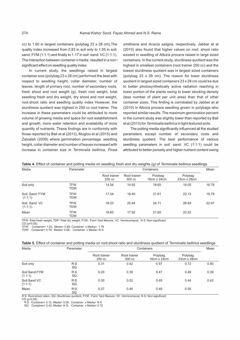
Media Parameter Containers Mean
Root trainer250 cc
Root trainer300 cc
Polybag16cm x 24cm
Polybag23cm x 28cm
Soil only TFWTDW
14.54 14.92 18.65 19.05 16.79
Soil: Sand: FYM (1:1:1)
TFWTDW
17.04 18.40 21.61 22.13 19.79
Soil: Sand: VC (1:1:1)
TFWTDW
18.23 20.44 24.71 28.49 22.97
Mean TFWTDW
16.60 17.92 21.65 23.22
Table 4. Effect of container and potting media on seedling fresh and dry weights (g) of Terminalia bellirica seedlings
TFW- Total fresh weight, TDP- Total dry weight, FYM : Farm Yard Manure, VC :Vermicompost, N S: Non-significantCD (p=0.05)TFW: Container= 1.03, Media= 0.89, Container x Media= 1.79TDW: Container= 0.79, Media= 0.68, Container x Media= N S
Media Parameter Containers Mean
Root trainer250 cc
Root trainer300 cc
Polybag16cm x 24cm
Polybag23cm x 28cm
Soil only R:SSQ
0.31 0.42 0.57 0.72 0.50
Soil:Sand:FYM(1:1:1)
R:SSQ
0.20 0.39 0.47 0.49 0.39
Soil:Sand:VC(1:1:1)
R:SSQ
0.30 0.52 0.45 0.44 0.42
Mean R:SSQ
0.27 0.44 0.49 0.55
Table 5. Effect of container and potting media on root:shoot ratio and sturdiness quotient of Terminalia bellirica seedlings
R:S: Root-shoot ration, SQ- Sturdiness quotient, FYM : Farm Yard Manure, VC :Vermicompost, N S: Non-significantCD (p=0.05) R:S: Container= 0.10, Media= 0.09, Container x Media= N S SQ: Container= 0.42, Media= N S, Container x Media= 0.72
cc) to 1.60 in largest containers (polybag 23 x 28 cm).The
quality index increased from 0.83 in soil only to 1.05 in soil:
sand: FYM (1:1:1) and finally to 1.17 in soil: sand: VC (1:1:1).
The interaction between container x media resulted in a non-
significant effect on seedling quality index.
In current study, the seedlings raised in largest
container size (polybag 23 x 28 cm) performed the best with
respect to seedling height, collar diameter, number of
leaves. length of primary root, number of secondary roots,
fresh shoot and root weight (g), fresh root weight, total
seedling fresh and dry weight, dry shoot and root weight,
root:shoot ratio and seedling quality index However, the
sturdiness quotient was highest in 250 cc root trainer. The
increase in these parameters could be attributed to more
volume of growing media and space for root establishment
and growth, more water retention and availability of more
quantity of nutrients. These findings are in conformity with
those reported by Bali et al (2013), Mugloo et al (2015) and
Zalzaleh (2009) where germination percentage, seedling
height, collar diameter and number of leaves increased with
increase in container size in Terminalia bellirica, Picea
smithiana and Acacia saligna, respectively. Jabbar et al
(2010) also found that higher values on root: shoot ratio
existed in seedling of Albizia procera raised in large sized
containers. In the current study, sturdiness quotient was the
highest in smallest containers (root trainer 250 cc) and the
lowest sturdiness quotient was in largest sized containers
(polybag 23 x 28 cm). The reason for lower sturdiness
quotient in largest sized containers 23 x 28 cm could be due
to better photosynthetically active radiation reaching in
lower portion of the plants owing to lower stocking density
(less number of plant per unit area) than that of other
container sizes. This finding is corrobated by Jabber et al
(2010) in Albizia procera seedling grown in polybags who
reported similar results. The maximum germination percent
in the current study was slightly lower than reported by Bali
et al (2013) for Terminalia bellirica in light textured soils.
The potting media significantly influenced all the studied
parameters except number of secondary roots and
sturdiness quotient. The best performance of various
seedling parameters in soil: sand: VC (1:1:1) could be
attributed to better porosity and higher nutrient content owing
Kamal Kishor Sood, Fayaz Ahmed and N.S. Raina274

to vermicompost in this medium than that of the remaining
media. Similar findings were also reported in case of Acacia
nilotica seedlings by Devaranavadgi et al (2010) in their
experiment at Bijapur (Karnataka).
The interaction effect of container x potting media
showed significant effect on seedling height, number of
leaves, fresh shoot weight, total seedling fresh weight, root
shoot ratio and sturdiness quotient only. The reason could be
attributed to more volume of growing media, higher water
holding capacity coupled with more quantity of nutrients and
space. The results were in accordance with that Chand et al
(2007) in Terminalia tomentosa who reported that addition of
manures in soil media enhance the growth and development
of the seedlings.
CONCLUSIONS
The current study implies that largest sized containers
(polybag 23 x 28 cm) and potting media soil: sand: VC (1:1:1)
should be used to obtain better growth of Terminalia bellirica
to obtain better growth of seedlings under nursery conditions.
Further, studies need to be carried out to find out the out
planting success of the seedling raised using different
container sizes and media.
REFERENCES
Aghai MM, Pinto JR and Davis AS 2014. Container volume and growing density influence western larch (Larix occidentalis Nutt.) seedling development during nursery culture and establishment. New Forests 45: 199–213.
Bali RS, Chauhan DS and Todaria NP 2013. Effect of growing media,
ContainersMedia
Root trainer Root trainer Polybag Polybag
Mean
Soil only 0.36 0.62 1.01 1.35 0.83
Soil: Sand: FYM (1:1:1) 0.50 0.84 1.12 1.75 1.05
Soil: Sand: VC (1:1:1) 0.71 1.03 1.21 1.72 1.17
Mean 0.52 0.83 1.11 1.60
Table 6. Effect container size and type and potting media on seedling quality index of Terminalia bellirica seedlings
FYM : Farm Yard Manure, VC :Vermicompost, N S: Non-significantCD (p=0.05)Container= 0.10, Media= 0.09, Container x Media= N S
nursery beds and containers on seed germination and seedling establishment of Terminalia bellirica (Gaertn.) Roxb., a multipurpose tree. Tropical Ecology 54(1): 59–66.
Chand D, Devar KV and Vikas 2007. Influence of growing media on seedling growth and biomass of laurel (Terminalia tomentosa Heyne ex Roth). The Asian Journal of Soil Science 2(1): 83-85.
Dickson A, Leaf AL, and Hosner JF 1960. Quality appraisal of white spruce and white pine seedling stock in nurseries. Forestry Chronicle 36(1):10-13.
Devaranavadgi SB, Wali SY, Patil SB, Jambagi MB and Kambrekar DN 2010. Effect of nursery mixtures on nutrient content and quality parameters of seedlings of different tree species. International Journal of Agricultural Sciences 6(2): 365–369.
Jabbar F, Ferdousee N, Hossain MK and Rafiq-ul-Hoque ATM 2010. Comparative growth performance of Albizia procera seedlings raised in nursery bed, polybag and root trainers. Australian Journal of Basic and Applied Sciences 4(8): 3038-3042.
Mugloo JA, Khan PA, Mughal AH, Qasir KN, Zaffar SN and Parrey G 2015. Studies on refinement of container size and potting mixture for production of quality Seedlings in Spruce (Piceasmithiana Boiss). Open Journal of Forestry 5: 733-739
Rana, RS 2008. Effect of Cutting Size and Hormonal Application on Growth and Development of Ficus roxburghii Wall. M.Sc. Thesis, Sher-e-kashmir University of Agricultural Sciences and Technology, Jammu.
Rana RS and Sood KK 2012. Effect of cutting diameter and hormonal application on the propagation of Ficus roxburghii Wall. through branch cutting. Annals of Forest Research 55(1): 69-84.
Roller KJ 1977. Suggested minimum standards for container used seedlings in Nova Scotia. Canadian Forest Service, Department of Environment, Information Report M-X-69.
Tsakaldimi M, Zagas T, Tsitsoni T and Ganatsas P 2005. Root morphology, stem growth and field performance of seedlings of two Mediterranean evergreen oak species raised in different container types. Plant Soil 278: 85–93.
Zalzaleh HA 2009. Root and shoot growth of Acacia saligna and Eucalyptus viminalis as influenced by container geometry polybags and root trainers. European Journal of Scientific Research 25(4): 567-573.
Received 02 April, 2018; Accepted 10 May, 2018
Effect of Container and Growing Media on Terminalia bellirica Roxb. Seedling Performance 275

Biomass and Carbon Stocks in Agroforestry Land use System in Sub-tropics of J&K
Indian Journal of Ecology (2018) 45(2): 276-280
Abstract: Biomass, carbon stocks and carbon dioxide equivalent (CO e) in agroforestry land use system was assessed for kandi areas in sub-2
tropics of Jammu & Kashmir. Agri-hoticultural system was the prominent agroforestry land use system in the study area. Mangifera indica gave -1 -1the highest above and below ground biomass (46.19 Mg ha ). The average total biomass in tree component was 14.28 Mg ha , out of which,
the contribution of above ground biomass in tree component was 75.28 percent and 24.78 percent in below ground biomass.. Similarly, carbon -1 -1stocks in tree component were 6.62 Mg ha and the highest were recorded in Mangifera indica (21.28 Mg ha ). The contribution towards
-1 -1carbon stocks of trees and understorey component in agroforestry land use was found to be 6.62 Mg ha (81.23 percent) and 1.47 Mg ha -1(18.17 percent), respectively. The total output from agroforestry land use system towards biomass was 17.62 Mg ha and corresponding
-1carbon stock was 8.09 Mg ha .
Keywords: Agroforestry, Carbon stocks, Carbon dioxide equivalent, Carbon sequestration
Manuscript Number: NAAS Rating: 4.96
2671
Vishal Mahajan, N.S. Raina and L.M. GuptaDivision of Agroforestry, SKUAST-Jammu-180 009, India
E-mail: [email protected]
The role of various land use systems in alleviating the
atmospheric CO concentration and reducing the CO 2 2
emissions or on increasing the carbon sink of forestry and
agroforestry systems has gained momentum in recent years
(Murthy et al 2013). There is substantial interest to increase
the carbon storage potential of terrestrial vegetation through
land use practices such as reforestation, afforestation &
natural regeneration of forests, silvicultural practices and
agroforestry (Canadell et al 2008). Agroforestry land use
system has proved to give positive impact to conventional
agricultural and woody tree production through increase in
productivity, biodiversity, social, economic and ecological
benefit (ICRAF 1995). Agroforestry systems are significantly
important especially when large population depend on land
for their livelihood and food security; and the need for
integrating food production with environmental services
under climate change scenario (Garrity 2004). The biomass
productivity, soil fertility, soil conservation, nutrient cycling,
microclimate improvement and carbon sequestration
potential of an agroforestry system is better than that of a
conventional annual system. The Third Assessment Report
on Climate Change (IPCC 2000) encompasses an
endorsement of the potential for agroforestry to contribute to
increase in carbon stocks in agricultural lands.
The sub-tropics of J&K state is characterized by
presence of kandi region, covering three districts, namely
Jammu, Samba and Kathua. The landscape of kandi area
comprise of undulating topography, steep and irregular
slopes, erodible and low water retentive soils and badly
dissected terrain by numerous gullies with prominent land
use systems of agriculture, horticulture, agroforestry and
forests. The upper portion of kandi (above 500 m) consists of
low hills covered by shrubs and forest, while the lower terrain
has cultivated lands and gully beds. People usually practice
rainfed agriculture, horticulture, agroforestry for their
sustenance and are intrinsically dependent on nearby forests
to meet their energy and fodder requirements. Human
activities such as degradation of forests, perennial
felling/lopping of trees and shrubs for domestic purposes
(especially fuel wood and fodder) and unmanaged
agricultural practices have substantially aggravated the
denudation rate. Also, the literature on carbon sequestration
potential of agroforestry land use systems in kandi belt of
Jammu region is scarce. Thus, the present study was carried
out to assess the biomass, carbon stocks of agroforestry land
use system in kandi region of Jammu sub tropics which
primarily comprised of agri-horticultural system.
MATERIAL AND METHODS
The present study was carried in out in sub-montane
region of the outer Himalayas fringing shivalik hills is
popularly known as bhabar or kandi which stretch between 0 0 0 074 21´ to 75 45´ E longitude and 32 22´ to 32 55´ N latitude.
The total area covered by kandi belt in J&K State is estimated 2to be 811 km , which is primarily located in three districts
namely, Jammu, Samba and Kathua. It is characterized by

10-30 km wide sloping belt extending over approximately
1700 km in length intermittently from Jammu & Kashmir in
west to Teesta River in East (Goyal and Rai 2000). The
inventory of farmers was prepared in all three districts under
study and five farmers for agroforestry land use system were
randomly selected from the inventory in each district. GPS
was used during the field survey exercise to locate the geo-
coordinates and altitude of sampling points. In all, 15
quadrates of 10 m x 10 m (0.01 ha) were used in the study
area. The study was carried out from kharif, 2015 to kharif,
2016. Non-destructive method was for assessment of
biomass and carbon which is more rapid and much larger
area & number of trees can be sampled, thus reducing the
sampling error encountered with the destructive method
(Hairiah et al 2011). The standing biomass and carbon stock
of trees along with the intercrop (understorey component)
was assessed in kandi region of Jammu sub-tropics. Trees
were enumerated and their diameter at breast height (DBH)
and height were measured. The stem volume of trees was
calculated by using basal area (BA), height and form factor.
For standing trees, general form factor of 0.5 was taken
regardless of taper or form (Butterfield and Espinoza 1995).
The stem volume was converted into biomass by using wood -3density (Mg m ) from the available literature (Brown 1997).
Irrespective of size and length, the total number of branches
were counted on each of the sample tree and were
categorized into three parts viz., lower, middle and upper.
Fresh weight of one sampled branch from each group was
recorded separately. The dry weight of branches was
determined (Chidumaya 1990). The fresh leaves segregated
from the harvested branch were weighed and a
representative sample thereof (0.1 kg) was retained to
estimate the dry weight of leaves. Leaves were oven dried to
obtain the constant weight. The below ground biomass of
trees was calculated by using the ratio of below-ground to
above-ground biomass (Mokany et al 2006). The biomass for
intercrop was estimated using 1m x 1m quadrates. The total
herb biomass occurring within the quadrate was cut at the
ground level. The collected samples were weighed, sub-0 0 sampled and taken to the laboratory for oven drying at 65 ± 5
C to obtain the constant dry weight. Carbon concentration in
plants was calculated using combustion method (Negi et al
2003). Oven dried plant components (leaves, bark and wood)
were burnt in electric furnace at 400°C temperature, ash
content (inorganic elements in the form of oxides) left after
burning was weighed and carbon was calculated using the
following equation:
Carbon percent = 100 – (Ash weight+ molecular
weight of O (53.3) in C H O )2 6 12 6
This carbon concentration was converted in to carbon
-1stock (Mg ha ) by multiplying it with the biomass. The
proportion of stem wood used as long-lived wood products as
suggested by Wang and Feng (1995).
Long-lived carbon storage = carbon mass in stem wood
x 42% stem wood put for long term locking
Heat from biomass combustion and carbon storage from -1coal substitution (Mg ha ) was simulated on the basis of
thermal efficiency of biomass (Wang and Feng 1995).Heat
from biomass combustion = [Biomass – (stem wood weight x 9 -10.42)] x 8 x 10 J ton
The estimated carbon stock was converted into CO 2
equivalent by multiplying the carbon stock of 3.67 (AACM
1997 and Van Kooten 1999) for calculating CO assimilation 2
by biomass.
RESULTS AND DISCUSSION
Agroforestry land use system in kandi areas primarily
comprised of fruit tree based systems. The dominant fruit
trees in the study area were Mangifera indica, Litchi
chinensis Phyllanthus emblica, Grewia asiatica (Table 1). -1 -1The average total biomass (14.28 Mg ha ) with 10.75 Mg ha
-1as above ground biomass (AGB) and 3.53 Mg ha as below
ground biomass (BGB) was assimilated in tree component
irrespective of age and sampling site (Table 2).
The data evinced that Mangifera indica possessed the -1highest (37.25 Mg ha ) above ground biomass (AGB) and
-1below ground biomass BGB (8.94 Mg ha ). Similarly, above -1
ground carbon stock (AGCS; 17.21 Mg ha ), below ground -1carbon stock (BGCS; 4.07 Mg ha ) was highest in Mangifera
indica. The carbon sequestered in Mangifera indica was -1 21.28 Mg ha which was highest among all the species. The
lowest value for the same variables was recorded for Litchi
chinensis. Carbon stocks are dependent on biomass. Thus,
higher the biomass accumulation higher will be the carbon
stock. Carbon stock in different carbon pools under study
indicated that vegetation stock i.e., above-ground biomass
contributed the maximum towards aggregate carbon pool
under agroforestry system. Similar results were also reported
by Chauhan et al (2012). The perusal of data showed that
tree component in agroforestry land use system gave -1 maximum biomass to the tune of 14.28 Mg ha (Table 2) and
-1intercrop (understorey) contributed 1.47 Mg ha (Table 4); -1sequestering 6.62 Mg ha carbon from tree component, and -1assimilating 24.30 Mg ha CO e across the agroforestry land 2
use system. The tree component of agroforestry land use
system across the sites had maximum biomass compared to
(Heat of biomass combustion × 0.60 × 0.70)
Carbon storage from coal substitution=9 (18 × 10 )
277Biomass, Carbon Stocks, in Agroforestry, Land use System

Agroforestry system Tree component/species Understorey crop
Agri-Horticulture Citrus reticulata Blanco Triticum aestivum + Zea mays
Litchi chinensis Triticum aestivum + Vigna mungo
Mangifera indica Abelmoschus esculentus + Triticumaestivum
Mangifera indica Zea mays + Triticum aestivum
Emblica officinalis Triticum aestivum + Zea mays
Prunus persica Triticum aestivum + Zea mays
Psidium guajava Curcuma longa
Agri-Horti-pastoral Litchi chinensis Zea mays + perennial grasses
Emblica officinalis Grasses+ Zea mays
Horti-Pastoral Grewia asiatica Grasses
Table 1. Different agroforestry system(s) prevalent in the study area
Species -1Biomass (Mg ha ) Total biomass -1(Mg ha )
-1Carbon stock (Mg ha ) Total carbon sequestered
-1(Mg ha )Above ground
Below ground
Above ground Below ground
Citrus reticulata Blanco 6.25 2.15 8.40 2.75 1.08 3.83
Grewia asiatica 4.10 2.30 6.40 1.83 1.15 2.98
Litchi chinensis 2.37 1.33 3.70 1.09 0.66 1.75
Mangifera indica 37.25 8.94 46.19 17.21 4.07 21.28
Emblica officinalis 6.07 1.70 7.77 2.77 0.85 3.62
Psidium guajava 8.46 4.74 13.20 3.89 2.37 6.26
Average of all species irrespective of age and sampling site
10.75 3.53 14.28 4.92 1.70 6.62
Table 2. Biomass, carbon stocks and carbon sequestered by different tree species in agroforestry land use system
Species CO 2e-1(Mg ha )
long-lived carbon -1storage (Mg ha )
heat from biomass combustion -1(Giga Joules ha )
carbon storage from coal -1substitution (Mg ha )
Grewia asiatica 14.06 0.11 16.98 0.29
Citrus reticulata Blanco 10.94 0.04 9.06 0.15
Litchi chinensis 6.42 0.11 124.91 2.10
Mangifera indica 78.10 2.34 614.49 10.32
Emblica officinalis 13.29 1.62 182.69 3.07
Prunus persica 22.97 0.04 83.84 1.41
Psidium guajava 24.30 0.31 123.61 2.08
Average of all tree species irrespective of diameter class and sampling site
24.30 0.65 165.08 2.77
Table 3. Long-lived carbon storage, heat from biomass combustion, carbon storage from coal substitution and carbon dioxide equivalent (CO e) in tree component of agroforestry land use system2
agriculture component and therefore, the higher carbon
stocks and CO equivalent were removed from the 2
atmosphere as compared to intercrop. Similar results were
also reported by Thakur et al (2011) for shrubs under different
agroforestry systems. The overall average carbon storage -1from coal substitution (Mg ha ) in agroforestry land use
-1system (Table 3) was 2.77 Mg ha . However, the highest
carbon storage from coal substitution among different
species in agroforestry land use was in Mangifera indica -1(10.32 Mg ha ) followed by Psidium guajava and lowest in
Citrus reticulata Blanco. Several workers have reported that
tree incorporation in cropland would result in better net
carbon storage in above and belowground components
(Palm et al 2004, Haile et al 2008, Kumar and Nair 2011).
278 Vishal Mahajan, N.S. Raina and L.M. Gupta

Intercrop/Parameter
Triticum aestivum Zea mays Zingiber officinale Setaria sp. Vigna mungo Average
Biomass -1(Mg ha )
Carbon content
(Mg -1ha )
Biomass (Mg
-1ha )
Carbon content
-1(Mg ha )
Biomass (Mg
-1ha )
Carbon content
(Mg -1ha )
Biomass (Mg
-1ha )
Carbon content
(Mg -1ha )
Biomass (Mg
-1ha )
Carbon content
(Mg -1ha )
Biomass (Mg
-1ha )
Carbon content
(Mg -1ha )
Whole (leaf + stem) biomass
5.73 2.51 3.58 1.53 0.38 0.16 0.54 0.23 0.22 0.1 2.09 0.91
Seed Biomass 1.15 0.5 1.89 0.86 0 0 0 0 0.13 0.06 0.63 0.28
Root/ Rhizome Biomass
1.48 0.68 0.36 0.14 1.09 0.48 0.02 0.01 0.17 0.08 0.62 0.28
Total 8.36 3.69 5.83 2.53 1.47 0.64 0.56 0.24 0.52 0.24 3.35 1.47
Table 4. Biomass and carbon stocks in understorey component of agroforestry land use system
Among the similar ecological conditions, agroforestry
systems were considered to have higher carbon
sequestration potential compared to pasture and crop lands
(Roshetk et al 2002).
Analogous trend (as in case of carbon storage from coal
substitution) was seen for heat from biomass combustion
among the different horticultural species. However, the data
computed for long-lived carbon storage showed the highest -1value for Mangifera indica (2.34 Mg ha ) followed by
officinalis. Among all these species, only ca
has commercial timber value and can fix long lived carbon for
longer duration (70-80 years). For all other species recorded
under study, long lived carbon storage commensurate with
the biological rotation which here may vary from 10 to 30
years except Mangifera indica. The result for carbon dioxide
equivalent showed the maximum assimilation for Mangifera -1indica (78.10 Mg ha ) followed by Psidium guajava. The
understorey component comprised of mainly cereal (wheat
and maize) based intercrop. However, in certain sampling
sites, pulses and grassed were also recorded (Table 4).
The highest biomass and carbon stocks in the
understorey component was in the order Triticum
aestivum>Zea mays >Zingiber officinale> Setaria> Vigna
mungo. Among all the crops, Triticum aestivum had the -1highest biomass (8.36 Mg ha ) and maximum carbon stock
-1(3.69 Mg ha ). However, for understorey component in
agroforestry land use system as a whole, the average -1biomass the intercrop was found to be 3.35 Mg ha and
-1carbon stock of 1.47 Mg ha The average total biomass in .
-1tree component was 14.28 Mg ha , out of which, the
contribution of above ground biomass in tree component was
75.28 percent and 24.78 percent in below ground biomass.
The total contribution of understorey crops in the biomass -1pool was 3.34 Mg ha which was 19.15 percent of the total
agroforestry land use system. Similarly, the contribution
towards carbon stocks of trees and understorey component -1in agroforestry land use was 6.62 Mg ha (81.23 percent) and
Emblica
Mangifera indi
-11.47 Mg ha (18.17 percent), respectively. The total output
from agroforestry land use system as a whole, total biomass -1harnessed was 17.62 Mg ha and corresponding carbon
-1stock was 8.09 Mg ha .
Thus, it is evident from this study that agroforestry plays
important role in livelihood and food security in kandi areas
where dependence on traditional sole cropping is not feasible
due to rainfed farming. Therefore, both tangible and
intangible benefits of agroforestry should be harnessed for
income augmentation.
REFERENCES
AACM, 1997.Greenhouse Challenges/Carbon Sinks Workshop.- A discussion paper, Oct. 1997. Prepared for the greenhouse challenge office, Commonwealth Department of Primary Industries and Energy, Canberra.
Brown S 1996. Present and potential roles of forests in the global climate change debate. Unasylva 185: 3-10.
Brown S1997. Estimating Biomass and Biomass Change of Tropical Forests: A Primer .Volume 134 of FAO forestry paper, Food and Agriculture Organization, 55p.
Butterfield RP and Espinoza MC 1995. Screening trial of 14 tropical hardwoods with an emphasis on species native to Costa Rice: Forth year results. New Forests 9: 135-145.
Canadell JG and Raupach MR 2008. Managing forests for climate change mitigation. Science 320: 1456-1457..
Chauhan S, Sharma R, Sharma SC, Gupta Nand Ritu 2012. Evaluation of poplar (Populus deltoides Bartr. Ex Marsh.) boundary plantation based agri-silvicultural system for wheat-paddy yield and carbon storage. International Journal of Agriculture and Forestry 2: 239-246.
Chidumaya EN 1990. Aboveground woody biomass structure and productivity in a Zambezian Woodl and Forest Ecology and Management 36: 33-46.
Dhyani SK, Ram Newaj and Sharma AP 2009. Agroforestry: its relation with agronomy, challenges and opportunities. Indian Journal of Agronomy 54(3): 249–266.
Garrity DP 2004. Agroforestry and the achievement of the millennium development goals. Agroforestry System 61: 5-17.
Goyal VC and Rai SR 2000. Hydrological problems in the kandi belt of Jammu Region. National Institute of Hydrology, Roorkee, Report No. SR- 1/1999-2000, 69p.
Haile SG, Nair PKR and Nair VD 2008. Carbon storage of different soil-size fractions in Florida silvopastoral systems. Journal of Environmental Quality 37: 1789–1797.
Hairiah K, Dewi S, Agus F, Velarde S, Ekadinata A, Rahayu S and van
279Biomass, Carbon Stocks, in Agroforestry, Land use System

Noordwijk M 2011. Measuring Carbon Stocks Across Land Use Systems: A Manual. Bogor, Indonesia. World Agroforestry Centre (ICRAF), SEA Regional Office, 154p.
International Centre for Research in Agroforestry (ICRAF). (1995). Annual Report, 1995. ICRAF, Nairobi
IPCC 2000. Third Assessment Report of the Intergovernmental Panel on Climate Change. http:// www.ipcc.ch/pub/reports.htm
Kumar BM and Nair PKR 2011. Carbon Sequestration Potential of Agroforestry Systems: opportunity and challenges. Springer Dordrecht Heidelberg London New York, pp. 307.
Mokany K, Raison JR and Prokushkin AS 2006. Critical analysis of root: shoot ratios in terrestrial biomes. Global Change Biology 12: 84-96.
Murthy IK, Gupta M, Tomar S, Munsi M, Tiwari R, Hegde G and Ravindranath NH 2013. Carbon sequestration potential of agroforestry systems in India. Journal of Earth Science & Climatic Change 4: 131.
Negi JDS, Manhas RK and Chauhan PS 2003. Carbon allocation in different components of some tree species of India: A new approach for carbon estimation. Current Science 85(11):1528-
1531.
Palm C, Tomich T, Van Noordwijk M, Vosti S, Alegre J, Gockowski J and Verchot L 2004. Mitigating GHG emissions in the humid tropics: case studies from the Alternatives to Slash and Burn Program (ASB). Environment, Development and Sustainability 6: 145-162.
Roshetk JM, Delaney M, Hairiah K and Purnomosidhi P 2002. Carbon stocks in Indonesian home garden systems: can smallholder systems be targeted for increased carbon storage? American Journal of Alternative Agriculture 17: 138-148.
Thakur NS, Gupta NK and Gupta B 2011.Biomass, carbon Stocks and CO removal by shrubs under different agroforestry 2
systems in Western Himalaya. Indian Journal of Ecology 38: 14-17.
Van Kooten GC 1999.Economic dynamics of tree planting for carbon uptake on marginal agricultural lands. Paper presented at the Canadian Resources and Environmental Economics Study Group Conference, October 2-3. Edmonton, Alberta.
Wang X and Feng Z 1995.Atmospheric carbon sequestration through agroforestry in China. Energy 20(2): 117-121.
Received 30 March, 2018; Accepted 10 May, 2018
280 Vishal Mahajan, N.S. Raina and L.M. Gupta
Rainfall-Runoff Modelling Using Artificial Neural Network and Adaptive Neuro-Fuzzy Inference System
Indian Journal of Ecology (2018) 45(2): 281-285
Abstract: Rainfall is one of the most complicated hydrological process in runoff prediction.
Since it directly affects the design and operation of many water resources structures. The
present study was undertaken to predict runoff for Usri river basin. The Usri river basin is located in Giridih district of Jharkhand with an area of 2about 731.02 km . In this study, two techniques were considered namely artificial neural networks (ANNs) and adaptive neuro-fuzzy inference
th thsystem (ANFIS) to predict runoff. Data of monsoon period (15 June to 30 September) of years 1998-2005 were used for calibration of the
models and data of years 2006-2008 were used for validation of models. The data of rainfall and runoff with three days lag as inputs and current
day runoff as output were used for runoff prediction. The performance of the models were evaluated qualitatively by visual observations and
quantitatively using performance indicators such as root mean square error (RMSE), correlation coefficient (r) and coefficient of efficiency
(CE). It is concluded that the performance of the ANFIS model is better than ANN model for runoff prediction of the study area.
Keywords: Adaptive neuro-fuzzy inference system, Artificial neural networks, Modelling, Rainfall, and Runoff
Development of rainfall-runoff relations in
hydrological modeling is a very important issue.
Manuscript Number: NAAS Rating: 4.96
2672
1* 1Pratibha Kumari, Pravendra Kumar and P.V. SinghG.B. Pant National Institute of Himalayan Environment and Sustainable Development
Himachal Unit, Mohal-Kullu-175 126, India1Department of Soil and Water Conservation Engineering, College of Technology
Govind Ballabh Pant University of Agriculture and Technology, Pantnagar-263 145, India*E-mail: [email protected]
Soil and water are the two important natural resources
and the basic needs for agricultural production. During the
last century, it has been observed that the pressure of
increasing population has led to degradation of these natural
resources. The watershed has prolonged been considered
as the most effective unit for conservation of natural
resources. The need for reliable information on watershed
runoff has got momentum since past decades along with
watershed management programme. The hydrologic
behaviour of watershed in rainfall-runoff conversion
procedure is very typical event which is managed by number
of climatic and topological aspects that differ with both the
time and space.
Hydrological models have been developed since 1930's
for describing the processes of rainfall-runoff in a watershed
fluvial system. Rainfall–runoff models can be categorized as
deterministic, conceptual and parametric models.
Deterministic models describe the rainfall–runoff process
using physical laws of mass and energy transfer. Conceptual
models provide simplified representations of key
hydrological process using a perceived system (such as a
series of interconnected stores and flow pathways).
Parametric models use mathematical transfer functions
(such as multiple linear regression equations) to relate
meteorological variables to runoff. Hydrological models are
further classified as either lumped or distributed. In the recent
years, Artificial Neural Network (ANN), which is basically a
lumped model have been applied successfully to model
complex non-linear input-output relationships (Zhang and
Govindaraju 2000, Singh et al 2013). Adaptive neuro-fuzzy
inference system (ANFIS) which is integration of neural
networks and fuzzy logic has the potential to capture the
benefits of both these fields in a single framework. A fuzzy
rule-based system (FRBS) using the Takagi-Sugeno-Kang
approach has been developed for rainfall-runoff Modeling
(Casper et al 2007). The performance of the ANFIS have
been compared with MLR and found better than MLR for
rainfall-runoff modelling (Singh et al 2016). The present study
has been undertaken to develop rainfall-runoff models using
artificial neural network (ANN) and adaptive neuro-fuzzy
inference system (ANFIS) approaches for Usri river basin, to
validate the formulated models and performance of the
developed models for their comparison.
MATERIAL AND METHODS
Study area: The Usri river basin was selected as study area,
which is the tributary of Barakar river and the Baraka river is
the main tributary of the Damodar River in eastern India. The
Usri river basin is located 13 km east in Giridih district of
Jharkhand that occupies11.74 per cent of the total area. The
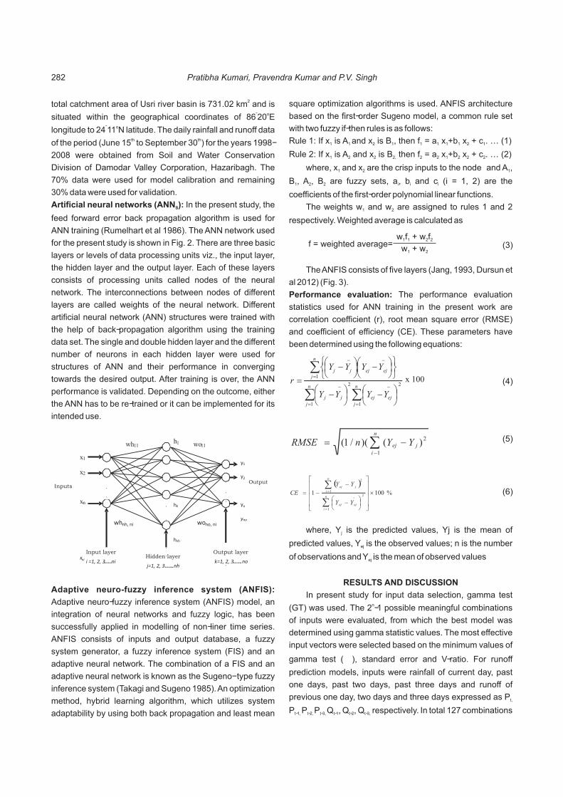
2total catchment area of Usri river basin is 731.02 km and is ? osituated within the geographical coordinates of 86 20 E
? olongitude to 24 11 N latitude. The daily rainfall and runoff data th thof the period (June 15 to September 30 ) for the years 1998-
2008 were obtained from Soil and Water Conservation
Division of Damodar Valley Corporation, Hazaribagh. The
70% data were used for model calibration and remaining
30% data were used for validation.
Artificial neural networks (ANN ): In the present study, the S
feed forward error back propagation algorithm is used for
ANN training (Rumelhart et al 1986). The ANN network used
for the present study is shown in Fig. 2. There are three basic
layers or levels of data processing units viz., the input layer,
the hidden layer and the output layer. Each of these layers
consists of processing units called nodes of the neural
network. The interconnections between nodes of different
layers are called weights of the neural network. Different
artificial neural network (ANN) structures were trained with
the help of back-propagation algorithm using the training
data set. The single and double hidden layer and the different
number of neurons in each hidden layer were used for
structures of ANN and their performance in converging
towards the desired output. After training is over, the ANN
performance is validated. Depending on the outcome, either
the ANN has to be re-trained or it can be implemented for its
intended use.
Adaptive neuro-fuzzy inference system (ANFIS):
Adaptive neuro-fuzzy inference system (ANFIS) model, an
integration of neural networks and fuzzy logic, has been
successfully applied in modelling of non-liner time series.
ANFIS consists of inputs and output database, a fuzzy
system generator, a fuzzy inference system (FIS) and an
adaptive neural network. The combination of a FIS and an
adaptive neural network is known as the Sugeno- type fuzzy
inference system (Takagi and Sugeno 1985). An optimization
method, hybrid learning algorithm, which utilizes system
adaptability by using both back propagation and least mean
square optimization algorithms is used. ANFIS architecture
based on the first-order Sugeno model, a common rule set
with two fuzzy if-then rules is as follows:
Rule 1: If x is A and x is B , then f = a x +b x + c . … (1)1 1 2 1 1 1 1 1 2 1
Rule 2: If x is A and x is B then f = a x +b x + c . … (2)1 2 2 2, 2 2 1 2 2 2
where, x and x are the crisp inputs to the node and A , 1 2 1
B , A , B are fuzzy sets, a , b and c (i = 1, 2) are the 1 2 2 i i i
coefficients of the first-order polynomial linear functions.
The weights w and w are assigned to rules 1 and 2 1 2
respectively. Weighted average is calculated as
The ANFIS consists of five layers (Jang, 1993, Dursun et
al 2012) (Fig. 3).
Performance evaluation: The performance evaluation
statistics used for ANN training in the present work are
correlation coefficient (r), root mean square error (RMSE)
and coefficient of efficiency (CE). These parameters have
been determined using the following equations:
where, Y is the predicted values, Yj is the mean of j
predicted values, Y is the observed values; n is the number ej
of observations and Y is the mean of observed valuesej
RESULTS AND DISCUSSION
In present study for input data selection, gamma test n(GT) was used. The 2 -1 possible meaningful combinations
of inputs were evaluated, from which the best model was
determined using gamma statistic values. The most effective
input vectors were selected based on the minimum values of
gamma test (┌), standard error and V-ratio. For runoff
prediction models, inputs were rainfall of current day, past
one days, past two days, past three days and runoff of
previous one day, two days and three days expressed as Pt,
P P P Q , Q , Q respectively. In total 127 combinations t-1, t-2, t-3, t-1 t-2 t-3,
Inputs
Input layerHidden layer
Output
Output layer
i =1, 2, 3……nij=1, 2, 3 …….nh
k=1, 2, 3…….no
.
.
..
.
y1
y2
yn
x1
x2
xn
h4
h1
hnh
wh11
wo11
whnh, ni
wono, ni
f = weighted average=w f + w f1 1 2 2
w + w1 2(3)
åå
å
= =
--
=
--
÷ø
öçè
æ-÷ø
öçè
æ-
þýü
îíì
÷ø
öçè
æ-÷ø
öçè
æ-
=n
j
n
j
ejejjj
n
jejejjj
YYYY
YYYY
r
1 1
22
1 x 100 (4)
2
1
)()(/1( å-
-=n
i
jej YYnRMSE (5)
( )%1001
1
21
2
´
úúúú
û
ù
êêêê
ë
é
÷ø
öçè
æ-
-
-=
å
å
=
-
=
n
i
ejej
n
i
jej
YY
YY
CE (6)
282 Pratibha Kumari, Pravendra Kumar and P.V. Singh

of these variables were examined for runoff prediction.
Finally, rainfall of current day, previous one day, previous two
days, previous three days, runoff of previous one day, two
days were selected as the prime input variables for runoff
prediction based on gamma test as shown in Table 1. The
ANN models were trained utilizing different number of
neurons in the single and double hidden layers, for training
and testing periods. Log-sigmoid activation function was
used in each hidden layer and pureline used in output layer
and Levenberg-marquardt learning algorithm were used for
maximum 1000 epochs. ANFIS models were developed
using Takagi-Sugeno-Kang type fuzzy inference system with
number of epochs equal to 50 and was used to identify the
one which trains the network more efficiently. Four different
types of membership functions (MFs) were used for ANFIS
networks as: Gaussian, Generalized-bell, Trapezoidal,
Triangular membership function.
The comparative performance of various ANN and
Fig. 2. ANFIS architecture
Input Mask Gamma (Ã) Standard error V-ratio
P P P P Q Q Qt-3, t-2, t-1, t, t-3, t-2, t-1 1111111 0.119 0.0211 0.475
P P P Q Q Qt-2, t-1, t, t-3, t-2 , t-1 0111111 0.143 0.0248 0.572
P P P Q Q Qt-3, t-1, t, t-3, t-2, t-1 1011111 0.123 0.0144 0.492
P P P , Q Q Qt-3, t-2, t, t-3, t-2, t-1 1101111 0.135 0.0228 0.540
P P P Q Q Qt-3, t-2, t-1, t-3, t-2, t-1 1110111 0.171 0.0231 0.684
P P P P Q Qt-3, t-2,, t-1, t, , t-2, t-1 1111011 0.118 0.0172 0.471
P P ,P P Q Qt-3,, t-2 t-1, t, t-3, t-1 1111101 0.124 0.0179 0.493
P P P P Q Qt-3, t-2, t-1, t, t-3, t-2 1111110 0.134 0.0151 0.535
Table 1. Comparison of various models to select the best model for runoff prediction
ANFIS models based on r, RMSE and CE estimation are
given in Table 2 and 3, respectively. During calibration, the
values of r, RMSE and CE for all the developed models vary 3in the range of 0.608 to 0.854, 17.16 to 26.54 m /sec and
45.18 to 73.05 %, respectively and for ANFIS models, these
indices vary in the range of 0.544 to 0.934, 11.80 to 27.74 3m /sec and 29.64 to 87.25% (Table 3). It was concluded
based on the greater values of r, CE and the lower value of
RMSE that ANN model with architecture 6-28-1 and 6-45-45
and ANFIS model gauss 3 are as the best model with
respective technique for the study area than the other
models. The values of r for the best network using ANN(6-28-
1 and 6-45-45-1) and ANFIS (Gauss 3) runoff prediction
models are 0.844, 0.854 and 0.934 for training periods and
0.820, 0.848 and 0.866 for testing, respectively (Table 4). The
RMSE values for the selected network6-28-1remain 17.80 3and 41.04 m /sec and for network 6-45-45-1 are 17.16 and
344.64 m /sec for both the periods and RMSE for ANFIS-
283Rainfall-Runoff Modelling

Networks r 3RMSE (m /sec) CE
6-1-1 0.608 26.54 45.18
6-3-1 0.780 20.79 66.33
6-6-1 0.733 22.55 53.49
6-8-1 0.812 19.30 65.94
6-12-1 0.799 19.86 63.93
6-15-1 0.821 18.90 67.84
6-19-1 0.835 18.26 69.51
6-25-1 0.795 20.11 63.01
6-28-1 0.844 17.80 71.41
6-31-1 0.821 19.16 66.41
6-8-8-1 0.777 20.93 59.93
6-14-14-1 0.766 21.66 57.09
6-35-35-1 0.822 18.91 67.33
6-38-38-1 0.779 20.75 60.63
6-40-40-1 0.842 18.07 70.14
6-45-45-1 0.854 17.16 73.05
6-52-52-1 0.824 18.84 67.52
6-55-55-1 0.710 23.28 50.42
Table 2. Comparison of various ANN models for runoff prediction
Gauss 3 during training and testing periods are 11.80 and 333.79 m /sec . The values of CE for network 6-28-1 are 71.02
and 74.43 % and for network 6-45-45-1 are 73.05 and 69.73
% at the time of both the periods. Similarly, the values of CE
for ANFIS-Gauss 3 are 87.25 and 79.66 % for runoff
prediction models (Table 4). The qualitative assessment of
models were shown in graphical form by plotting the
predicted daily runoff values with the corresponding
y = 0.672x + 4.065
R² = 0.712
0
100
200
300
400
500
600
0 200 400 600
Observed runoff, m3
/sec
3P
red
icte
d r
un
off,
m/s
ec
y = 0.673x + 2.481
R² = 0.673
0
100
200
300
400
500
600
700
800
900
1000
0 200 400 600 800 1000
Pre
dic
ted
ru
no
ff,
m3
/se
c
Observed runoff, m3/sec
Fig. 3. Scatter diagram between observed and predicted runoff using ANN model (6-28-1) during training and testing periods
y = 0.713x + 3.776
R² = 0.731
0
100
200
300
400
500
600
0.00 100.00 200.00 300.00 400.00 500.00 600.00
Pre
dic
ted
ru
no
ff, m
3/se
c
Observed runoff, m3/sec
y = 1.017x + 5.153
R² = 0.724
0
200
400
600
800
1000
0 500 1000
Pre
dic
ted
ru
no
ff, m
3/s
ec
Observed runoff, m3/sec
Fig. 4. Scatter diagram between observed and predicted runoff using ANN model (6-45-45- 1) during training and testing periods
Networks r 3RMSE (m /sec) CE
Gauss (2) 0.870 16.26 75.82
Gauss (3) 0.934 11.80 87.25
Generalized Bell (2) 0.877 15.86 77.00
Generalized Bell (3) 0.930 12.12 86.56
Trapezoidal (2) 0.544 27.74 29.64
Trapezoidal (3) 0.858 16.95 73.71
Triangular (2) 0.872 16.16 76.11
Triangular (3) 0.911 13.61 83.06
Table 3. Comparison of various ANFIS models for runoff prediction
284 Pratibha Kumari, Pravendra Kumar and P.V. Singh
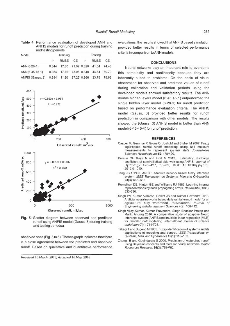
Model Training Testing
r RMSE CE r RMSE CE
ANN(6-28-1) 0.844 17.80 71.02 0.820 41.04 74.43
ANN(6-45-45-1) 0.854 17.16 73.05 0.848 44.64 69.73
ANFIS (Gauss, 3) 0.934 11.80 87.25 0.866 33.79 79.66
Table 4. Performance evaluation of developed ANN and ANFIS models for runoff prediction during training and testing periods
y = 0.860x + 1.934
R² = 0.872
0
100
200
300
400
500
600
0 200 400 600
Observed runoff, m3
/sec
Pre
dic
ted
ru
no
ff, m
3/s
ec
y = 0.899x + 0.906
R² = 0.750
0
200
400
600
800
1000
0 500 1000
Pre
dic
ted
ru
no
ff, m
3/s
ec
Observed runoff, m3/sec
Fig. 5. Scatter diagram between observed and predicted runoff using ANFIS model (Gauss, 3) during training and testing periodsa
observed ones (Fig. 3 to 5). Theses graph indicates that there
is a close agreement between the predicted and observed
runoff. Based on qualitative and quantitative performance
evaluations, the results showed that ANFIS based simulation
provided better results in terms of selected performance
criteria in comparison to ANN models.
CONCLUSIONS
Neural networks play an important role to overcome
this complexity and nonlinearity because they are
inherently suited to problems. On the basis of visual
observation for observed and predicted values of runoff
during calibration and validation periods using the
developed models showed satisfactory results. The ANN
double hidden layers model (6-45-45-1) outperformed the
single hidden layer model (6-28-1) for runoff prediction
based on performance evaluation criteria. The ANFIS
model (Gauss, 3) provided better results for runoff
prediction in comparison with other models. The results
showed the (Gauss, 3) ANFIS model is better than ANN
model (6-45-45-1) for runoff prediction.
REFERENCES
Casper M, Gemmar P, Gronz O, Josht M and Stuber M 2007. Fuzzy logic-based rainfall–runoff modelling using soil moisture measurements to represent system state Journal–des Sciences Hydrologiques 52: 478-490.
Dursun OF, Kaya N and Firat M 2012. Estimating discharge coefficient of semi-elliptical side weir using ANFIS. Journal of Hydrology 426–427, 55–62, DOI: 10.1016/j.jhydrol. 2012.01.010.
Jang JSR 1993. ANFIS: adaptive-network-based fuzzy inference system. IEEE Transaction on Systems, Man and Cybernetics 23(3): 665–685.
Rumelhart DE, Hinton GE and Williams RJ 1986. Learning internal representations by back-propagating errors. Nature 323(6088): 533-536.
Singh PV, Kumar Akhilesh, Rawat JS and Kumar Devendra 2013. Artificial neural networks based daily rainfall-runoff model for an agricultural hilly watershed. International Journal of Engineering and Management Sciences 4(2): 108-112.
Singh Vijay Kumar, Kumar Pravendra, Singh Bhaskar Pratap and Malik, Anurag 2016. A comparative study of adaptive Neuro Inference system (ANFIS) and multiple linear regression (MLR) for rainfall-runoff modelling. International Journal of Science and Nature 7(4): 714-723.
Takagi T and Sugeno M 1985. Fuzzy identification of systems and its applications to modeling and control. IEEE Transactions on Systems, Man, and Cybernetics 15(1): 116–132.
Zhang B and Govindaraju S 2000. Prediction of watershed runoff using Bayesian concepts and modular neural networks. Water Resources Research 36(3): 753-762.
Received 10 March, 2018; Accepted 10 May, 2018
285Rainfall-Runoff Modelling
GIS based Multi-Criteria Decision Making System for Assessment of Landslide Hazard Zones: Case Study
in the Nilgiris, India
Indian Journal of Ecology (2018) 45(2): 286-291
Abstract: Landslides are considered as one of the most common natural hazards occurring in the Nilgiris since immemorial time that leads to
the tremendous loss of human life, property and economy. In this study, landslide hazard zonation (LHZ) map for the Nilgiris district located in
the state of Tamil Nadu, was prepared using various thematic layers such as Precipitation, Slope, Geology, Aspect, Land cover, Distance from
road, Lineament Density, Distance from river, Elevation. The results obtained by adopting analytical hierarchy process (AHP) for updation of
LHZ map found that nearly 52.5% of the total district area falls under risk zone in which 6% of the regions is fall under highly risk zone.
Comparison the LHZ map with the inventory data, data it is found that nearly 90% of the landslides fall under hazardous zone.
Keywords: Analytical hierarchy process, Landslides, Remote Sensing, GIS, Landslide hazard zonation map
Manuscript Number: NAAS Rating: 4.96
2673
*D. Suresh and Kiran YarrakulaCentre for Disaster Mitigation and Management, VIT, Vellore- 632 014, India.
*E-mail: [email protected]
Nilgiris is a part of western ghats situated at the junction
of Tamil Nadu, Karnataka and Kerala at an elevation of 900m
to 2636m above mean sea level. Nilgiris hills plays a major
role in tourism between the months of March and August
every year as it experiences a relative temperature of 21°C 2during summer. Covering an area of 2551 km , the district
receives heavy rainfall between June to August and October
to December. Nilgiris has a long history of disastrous
landslides events across decades and experience landslides
since immemorial time, but the records are available since th19 century. Due to heavy rain in 1824, a huge landslide in the
Kundah hills was recorded. Since then, records are being
maintained for the Nilgiris district for every landslides events.
It is noted that in the Nilgiris both the steep and gentle
slopes have failed across years and the landslides are
spread out in areas that are utilized for various purposes. The
areas of crop cultivation and vegetation is found to
experience large landslides than other areas. The regions of
reserve forest are found to experience less landslides as the
erosion of soil is less in Reserved Forests compared to that of
cultivation areas. The major triggering factor for landslides in
the Nilgiris is the rainfall and deforestation. In Nilgiris,
generally landslides season is in between October and
December .
The landslides in the Nilgiris doesn't have any standard
guidelines which results in consideration of various
parameters for identification of landslides hazard zones.
Remote Sensing and GIS is the advanced technology that
plays a major role in the identification of the hazardous
zones. An attempt has been made in the present study for the
identification of landslide hazard zonation map considering
various parameters such as Precipitation, Slope, Geology,
Aspect, Land cover, Distance from road, Lineament Density,
Distance from river, Elevation. The LHZ map obtained can
help the local authorities in case of disaster event for proper
management and save human lives.
MATERIAL AND METHODS
Description of the study area: The Nilgiris is located
between 76° 14´ E and 77° 02´ E longitude and 11° 10´ N and
11° 42´ N latitude of Tamil Nadu, India (Fig. 1).Charnockite
and pyroxene granulite type of rocks cover the major part of
the district . Lateritic soil and small patches of sandy loam soil
type covers major part of the district. According to the report
from Geological Survey of India, Nilgiris district falls under
judicious landslide hazard zone. Debris type of landslides is
said to occur in major portion of Nilgiris and the major
triggering factor is heavy rainfall. The district receives an
average annual rainfall of 1700mm.
Thematic layers preparation: The spatial dataset was
created in GIS platform with various remote sensing and
collateral data. District boundary was obtained with the help
of SOI Toposheets (58A/6,7,8,10,11,12,14,15) at an
available scale of 1: 50,000. Geology layer was prepared with
the help of Geological Quandrangle Map obtained from
Geological Survey of India at 1: 2,50,000 scale (Fig. 2 (a)).

Fig. 1. Geographical location of the study area
INSAR 3D IMR rainfall was downloaded from MOSDAC and
processed to obtain the rainfall data for the Nilgiris district.
Based on the daily data downloaded it is found that the peak thrainfall was experienced on 4 October, 2017, and the
corresponding data is taken for analysis. The distribution of thrainfall in the Nilgiris district as on 4 October, 2017 (Figure 2
(b)). SRTM DEM (30m) was downloaded from GMTSAR
website for the study area and was processed to obtain
slope, aspect and elevation layers. Figure 2 (c) shows the
DEM of the study area. Generated slope map, aspect map
and elevation map are shown in Figure 2 (d), 2 (e) and 2 (f),
respectively. Using DEM as input, the streams for the study
area was obtained under QGIS Platform (Integrated with
GRASS). The stream segment was classified based on the
distance into di fferent c lasses (Figure 2 (g).
Landuse/Landcover map was obtained for the study area
using Landsat 8 with bhuvan datasets as reference (Figure 2
(h). The roads for the Nilgiris District was obtained from the
SOI toposheet and are classified into five different classes
Figure 2 (i). Using DEM and Landsat 8 Image as reference,
the lineaments for the study area was obtained. Figure 2 (j)
shows the lineament density of the study area. The detailed
methodology adopted with various layers are shown in
Figure 3.
Analytical hierarchy process: One of the most commonly
used method for the assessment of complex problems is the
analytic hierarchy process (AHP) which reflects the
judgement of human thinking by comparison of different
layers with respect to each other (Kayastha et al 2013, Tazik
et al 2014). The parameters are compared and the weights
are normalized based on the sum values and the normalized
matrix is obtained. The eigen vector is also calculated for the
normalized matrix to check the consistency ratio of the
judgement matrix (Subramanian and Ramanathan 2012).
Consistency ratio is calculated to validate the AHP pair-wise
judgement matrix framed. If the values of consistency ratio
are less than 0.1, weightage assigned are to be assumed
correct, therefore the process can be performed easily. In
case the value of consistency ratio is greater than 0.1, the
procedure is to be repeated with new set of values (Alonso
and Lamata 2006). Consistency ratio is calculated by using
the following formula.
Where
CR = Consistency Ratio
CI = Consistency Index
RI = Random Consistency Index = 1.45 (for n = 9)
obtained from Table 1 (Franek and Kresta 2014).
RESULTS AND DISCUSSION
The parameters for the study area namely Precipitation,
Slope, Geology, Aspect, Land cover, Distance from road,
Lineament Density, Distance from river, Elevation were
arranged hierarchically and based on the pair-wise
CI
CRRI
= (1)
n 1 2 3 4 5 6 7 8 9 10
RI 0 0 0.58 0.9 1.12 1.24 1.32 1.41 1.45 1.49
Table 1. Random Index values obtained from Saaty's book
Landslide Hazard Zonation Mapping for the Nilgiris District using AHP 287

Fig. 2. Nilgiris District (a) Geology Map, (b) Rainfall Map, (c) Digital Elevation Model, (d) Slope Map, (e) Aspect Map,(f) Elevation Map, (g) Distance from Rivers, (h) Landuse/Landcover Map, (i) Distance from Roads, (j) Lineament Density
D. Suresh and Kiran Yarrakula288

Weight-decisionmatrix
Precipitation Slope Geology Aspect Land cover
Distancefrom road
Lineament Density
Distancefrom river
Elevation
Precipitation 1 2 2 3 4 3 3 4 7
Slope 1/2 1 3 3 3 4 3 4 7
Geology 1/2 1/3 1 3 2 3 4 4 7
Aspect 1/3 1/3 1/3 1 2 2 1 2 4
Land cover 1/4 1/3 1/2 1/2 1 2 2 2 3
Distance from road 1/3 1/4 1/3 1/2 1/2 1 2 1 4
Lineament density 1/3 1/3 1/4 1 1/2 1/2 1 2 3
Distance from river 1/4 1/4 1/4 1/2 1/2 1 1/2 1 3
Elevation 1/7 1/7 1/7 1/4 1/3 1/4 1/3 1/3 1
Sum 3.63 4.96 7.8 12.75 13.83 16.75 16.83 20.33 38
Table 2. Pair-wise comparison matrix for AHP method
max
-
1
NCI
N
l=
-
9.49 - 90.06125
9 1 CI = =
-
0.061250.04
1.45CR = =
(2)
comparison values are assigned to a scale of 9 for each
parameters. In the present study, rainfall, slope and geology
were treated as strong parameters. The AHP comparison of
all the parameters is shown in Table 2.
The above weights are normalized based on the sum
values and the normalized matrix is obtained. The eigen
vector is also calculated for the normalized matrix to check
the consistency ratio of the judgement matrix. Consistency
ratio is the ratio of consistency index and random consistency
index. Consistency Index is calculated by using the formula,
Fig. 3. Detailed methodology of landslide hazard zonation mapping
In the present study, the consistency ratio 0.04 which is
less than 0.1. So the pair wise comparison is found to be
acceptable. Based on the weights obtained, the overlay
analysis is performed for various layers in QGIS platform.
The weightage obtained using AHP matrix and the
classification for each layer based on criteria and rank age is
shown in Table 3.
CONCLUSIONS
Based on the study, it was found that blocks of Coonor
and Udhagamandalam blocks are very highly sensible to
landslides. Roads network connecting Udhagamandalam
with places like Avvalanche, Manjur and Kundah are also
highly sensitive to landslides. Proper remedies are to be
taken along the roads to reduce the fatalities. Being a tourism
spot, entry can be restricted to the places during the month of
October to December. The main objective is to obtain a
landslide hazard zonation map using AHP technique for the
Landslide Hazard Zonation Mapping for the Nilgiris District using AHP 289

Layer Classification Values Rank Weightage
Slope Very low 0 - 15 1 21.87
Low 15 - 30 3
Moderate 30 - 45 5
High 45 - 60 7
Very high 60 - 80 9
Aspect North 0.00 - 22.50 9 8.92
North-East 22.50 - 67.50 5
East 67.50 - 112.50 1
South-East 112.50 - 157.50 5
South 157.50 - 202.50 7
South-West 202.50 - 247.50 7
West 247.50 - 292.50 5
North-West 292.50 - 337.50 9
North 337.50– 360.00 9
Flat -1.00 1
Lineament density Very low 0 - 25 1 6.32
Low 25 - 50 3
Moderate 50 - 75 5
High 75 - 100 7
Very high 100 - 125 9
Rainfall Very low < 5 1 24.36
Low 5 - 9 3
Moderate 9 - 13 5
High 13 - 17 7
Very high 17 - 21 9
Distance from roads 0 -100 9 6.55
100 - 200 7
200 - 300 5
300 - 400 3
400 - 600 1
Elevation Very low 1 - 530 1 2.3
Low 530 - 990 3
Moderate 990 - 1450 5
High 1450 - 1910 7
Very high 1910 - 2620 9
Distance from rivers 0 -100 9 8.03
100 - 200 7
200 - 300 5
300 - 400 3
400 - 600 1
Landuse/Landcover Settlement 9 4.91
Forest 3
Agricultural 5
Water 1
Scrub land 7
Fallow land 7
Geology Pink Granite and Gneiss 7 16.72
Hornblende – biotite schist and Gneiss 5
Kyanite 5
Quartz 5
Hornblende - biotite gneiss 7
Metaultramafite 3
Charnockite 9
Biotite-hornblende gneiss 7
Total weight 100
Table 3. Weightage obtained for various thematic layers with their classification
D. Suresh and Kiran Yarrakula290

Landslide classification
No. of landslides
Percentage of landslides
Very low 0 0.00
Low 1 1.47
Moderate 6 8.82
High 52 76.47
Very high 9 13.24
Table 4. Comparison of landslides hazard zones and historical landslides data
Fig. 4. Landslide Hazard Zonation map – Nilgiris District
Nilgiris district which can be used by various district
authorities to create awareness among the people.
Periodical updation of the landslide hazard zonation map and
providing periodical awareness can help to reduce the risk of
human life in the Nilgiris District. Based on the study, it is also
recommended to follow multi criteria decision making
analysis such as AHP, Fuzzy logic, etc for updation of LHZ
map.
REFERENCES
Dharmalingam V 2012. Saving the Nilgiri Mountains of South India, Nilgiri Documentation Centre, The Nilgiris.
Ganapathy GP and Hada CL 2012. Landslide hazard mitigation in the Nilgiris district, India – environmental and societal issues. International Journal of Environmental Science and
Development 3(5): 497–500.
Jiri F and Kresta A 2014. Judgment scales and consistency measure in AHP. Procedia Economics and Finance 12(March): 164–73.
Jose Antonio A and Teresa Lamata M 2006. Consistency in the analytic hierarchy process: A new approach. International Journal of Uncertainty, Fuzziness and Knowledge-Based Systems 14(4): 445–459.
Kayastha P, Dhital MR, and De Smedt F 2013. Application of the analytical hierarchy process (AHP) for landslide susceptibility mapping: A case study from the Tinau Watershed, West Nepal. Computers and Geosciences 52: 398-408.
Nachiappan S and Ramanathan R 2012. A review of applications of analytic hierarchy process in operations management. International Journal of Production Economics 138(2): 215–241.
Senthilkumar V, Chandrasekaran SS and Maji VB 2017. Geotechnical characterization and analysis of rainfall-induced 2009 landslide at Marappalam area of Nilgiris district, Tamil Nadu State, India. Landslides 14(5): 1803-1814.
Shanthi S and Elangovan K 2017. Comparison of landslides susceptibility analysis using AHP, SMCE and GIS for Nilgiris district, India. Indian Journal of Geo-Marine Sciences 46(April): 802-814.
Subbu Lakshmi E and KiranYarrakula 2017. Comparative analysis of digital elevation models: A case study around Madduleru River. Indian Journal of Geo-Marine Sciences 46(7): 1339-1351.
Tazik, Esmaeil, Zahra Jahantab, Mohsen Bakhtiari, Abdolali Rezaei and Seyed Kazem Alavipanah 2014. Landslide susceptibility mapping by combining the three methods fuzzy logic, frequency ratio and analytical hierarchy process in dozain basin. International Archives of the Photogrammetry, Remote Sensing and Spatial Information Sciences - ISPRS Archives 40(2W3): 267-272.
Received 18 April, 2018; Accepted 10 May, 2018
Landslide Hazard Zonation Mapping for the Nilgiris District using AHP 291

Weekly Pan-evaporation Simulation using MLP, CANFIS, MLR and Climate-based Models at Pantnagar
Indian Journal of Ecology (2018) 45(2): 292-298
Abstract: This paper explores the potential of multi-layer perceptron (MLP), co-active neuro-fuzzy inference system (CANFIS) and multiple
linear regression (MLR) in simulating weekly pan-evaporation at Pantnagar, located in the foothills of central Himalayan region in Uttarakhand,
India. In this study, a non-linear modelling tool i.e. gamma test (GT) was utilized to identify the most significant input parameters for MLP,
CANFIS and MLR approaches. The simulated pan-evaporation using these techniques was compared with the empirical models such as
Stephens-Stewart (SS) and Griffith (G) based on root mean squared error (RMSE), Nash-Sutcliffe efficiency (NS ) and coefficient of E
correlation (r). The results of comparison revealed that the MLP model performed superior than the CANFIS, MLR, SS and G models in
simulating the weekly pan-evaporation using the available meteorological data for study location.
Keywords: MLP, CANFIS, MLR, Gamma test, Pantnagar
Manuscript Number: NAAS Rating: 4.96
2674
Anurag Malik, Anil Kumar and Priya RaiDepartment of Soil and Water Conservation Engineering, College of Technology,
G.B. Pant University of Agriculture and Technology, Pantnagar-263 145, IndiaE-mail: [email protected]
Evaporation, a major component of hydrologic cycle, is
affected by various meteorological factors, such as air
temperature, relative humidity, solar radiation, wind speed,
and vapour pressure deficit occurring in the nature.
Simulation of evaporation is useful for determining crop water
requirement, irrigation scheduling and sustainable uses of
water resources (Lenters et al 2005). Several studies have
been conducted by various researchers to simulate the
accurate evaporation losses from free water surfaces. In
recent time, black box models have been successfully
applied in hydrological modelling and water resources
management for accurate simulation of pan evaporation
(Sudheer et al 2002, Terzi and Keskin 2005, Kisi 2006, Shiri
and Kisi 2011, Shirgure and Rajput 2012). Keskin et al (2004)
investigated that the fuzzy model and Penman method have
good ability for pan evaporation simulation in Turkey. Piri et al
(2009) applied ANN and neural network autoregressive
exogenous (NNARX) approaches for daily pan evaporation
simulation in arid and semi-arid regions of Iran. Tabari et al
(2010) simulated daily pan evaporation using MLP and non-
linear regression models in Iran, and reported that MLP
model characterized by Delta-Bar-Delta learning algorithm
gave better simulation of daily pan evaporation. Kisi et al
(2012) compared the results of generalized neuro-fuzzy
(GNF) to Penman, SS, and Griffith's models in Arizona, USA.
Results of comparison revealed that the GNF models
performed superior to the Penman, SS and Griffith's models.
Tabari et al (2012) used MLP and CANFIS models to predict
daily pan evaporation in semi-arid region of Iran, and stated
that the MLP model simulate far better than the CANFIS
model in the study area. Malik and Kumar (2015) studied the
potential of ANN, CANFIS and MLR techniques in daily pan
evaporation simulation at Pantnagar, India. The results
revealed that the ANN model performs superior to the
CANFIS and MLR models.
Keeping the above reviews in mind, this study was
conducted with objectives: (i) to select proper input variables
combination for MLP, CANFIS and MLR using gamma test
and their calibration; (ii) to validate the MLP, CANFIS and
MLR models for selected input variables combination; and
(iii) to compared the results obtained by MLP, CANFIS and
MLR models with that of Stephens-Stewart and Griffith
models.
MATERIAL AND METHODS
Study location and data collection: The study was
conducted at Pantnagar with longitude of 79° 31' 0" E and
latitude of 29° 3' 0" N located in Uttarakhand State of India.
The location of study area lies in the Tarai belt situated in the
(Fig. 1) foothills of Indian central Himalayas with an elevation
of 243.8m above mean sea level. It has a sub-humid and sub-
tropical climate with summer season from February to May,
rainy season from June to September, and winter season
from October to January. The mean annual rainfall in the
study region is about 1400 mm. The observed weekly
meteorological data (January, 2004 to December, 2007)
including maximum and minimum air temperatures (T and min
T ) and relative humidity (RH recorded at 7:00 AM in the max max

morning and RH recorded at 2:00 PM in afternoon), wind min
speed (U ), sun-shine hours (SS ) and weekly pan-s h
evaporation (E ) were collected from Crop Research Centre pw
(CRC) observatory at G. B. Pant University of Agriculture and
Technology, Pantnagar, Uttarakhand, India. The total
available dataset was splited into; (i) training dataset: from st stJanuary 1 , 2004 to December 31 , 2006 was used for model
stcalibration; and (ii) testing dataset: from January 1 to stDecember 31 , 2007 was used for model validation. Table 1
gives the details about statistical parameters of training,
testing, and whole datasets. Table 2 represents the cross-
correlation matrix between the input (T , T , RH , RH , max min max min
U and SS ) and output variable (E ).s h pw
Gamma test (GT): The concept of gamma test was first
discovered by Stefansson et al (1997), which was later
modified and used by other researchers (Piri et al 2009).
Gamma test was used to estimate the minimum standard
error for each input-output dataset with continuous nonlinear
models. In order to calculate gamma (Ã), a linear regression
line is constructed as:
y = A Ä + Ã (1)
where, y is the output vector of the regression line, A is
gradient and Ä is the intercept of the regression line. The
value of à is corresponding to the output at Ä = 0. The smaller
value of à (close to zero), is acceptable.
Multi-layer perceptron (MLP): MLP was first introduced by
Haykin (1998). The MLP network with single input and hidden
layers with one output was used in this study. This
environment of MLP was created in Neuro Solutions 5.0
software with error-and-trail procedure.
Co-active neuro-fuzzy inference system (CANFIS): Jang
et al (1997) introduced the concept of CANFIS, which
belongs to a general class of adaptive neuro-fuzzy inference
system. CANFIS has the advantages of both ANN and fuzzy
inference systems in a single frame work. CANFIS includes
fuzzification layer, rule layer, normalization layer,
defuzzification layer and summation layer. The functioning of
each layer was described by (Aytek 2008). The architecture
of CANFIS was decided using trial-and-error method in
Neuro Solutions 5.0 software.
Multiple linear regression (MLR): MLR constructs the
linear correlations between a dependent variable and two or
more independent variables. Mathematically, linear
regression equation (Malik and Kumar, 2015) is written as:
Y = â + â X + â X + ….+ â X (2)0 1 1 2 2 k n
where, Y is the output variable; X , X , .......X are the input 1 2 n
variables; and â â â â are the regression coefficients. 0, 1, 2….. k
Empirical models
Stephens-Stewart (SS) model: Stephens-Stewart (1963)
formulated this model for pan evaporation prediction using
only two climatic variables. Mathematically, SS model can be
written as:
E = R (a + bT ) (3)pw s m
where, a and b are the regression coefficients; R is solar s
-2 -1 oradiation (MJ m day ); and T is mean air temperature ( C).m
Griffith's (G) model: Griffith's (1966) established the
relationship between T and U for estimation of evaporation:m s
E = è +∝T +∝U (4)pw 1 m 2 s
where, è, ∝ and ∝are regression fitting coefficients.1 2
Performance evaluation indices: The performance of MLP,
CANFIS, MLR, SS and G models during calibration and
validation were evaluated using root mean squared error
(RMSE); Nash-Sutcliffe efficiency, NS (Nash-Sutcliffe, E
1970); and coefficient of correlation (r). These indices are
written as:
thwhere, X and Y are the observed and simulated values for i
dataset; N is the total number of observations; x and y are the
mean of observed and simulated values, respectively.
RESULTS AND DISCUSSION
Input variable selection using gamma test: Different
combinations (Table 3) of six input variables (T , T , RH , max min max
RH , U , and SS ) were examined using gamma test to min s h
assess their influence on weekly pan evaporation simulation.
The combination of input variable with the smallest score of Ã
was selected as best input variable combination for weekly
pan evaporation simulation (Piri et al 2009). Using this
criteria, the combination of six variables T , T , RH , max min max
RH , U , SS , with à = 0.497, gradient = 0.009, standard error min s h
= 0.115, V = 0.067 and mask = 111111 was selected as best ratio
input variable combination for weekly pan evaporation
simulation using MLP-5, CANFIS-5 and MLR-5 models.
Simulation of E using MLP-5 model: Several tests were pw
2
1)(
1ii
N
iYX
nRMSE -=å=
(0 < RMSE < ∞) (5)
úúú
û
ù
êêê
ë
é
-
--
å
å
=
=
N
i i
N
i ii
E
XX
YXNS
1
2_
1
2
)(
)(1 (0 < NSE < 1) (6)
úúú
û
ù
êêê
ë
é
--
--=
å å
å
= =
=
N
i
N
i ii
N
i ii
YYXX
YYXXr
1 1
2_
2_
1
__
)()(
))(((-r< 1 < 1) (7)
=
Pan-evaporation Simulation Models 293

Statistical parameters Meteorological variables with their units
Tmax0( C)
Tmin0( C)
RHmax
(%)RHmin
(%)Us
-1(km h )
SSh
(h)Epw
(mm)
Calibration (156 datasets)
Minimum 14.60 3.70 51.00 15.00 1.00 1.00 0.80
Maximum 41.60 27.90 97.00 78.00 19.80 11.30 17.20
Mean 29.69 17.15 84.45 50.59 5.23 7.21 4.46
Standard deviation 5.86 7.08 10.64 16.08 3.38 2.20 2.82
Coefficient of variation 0.19 0.41 0.13 0.32 0.65 0.31 0.63
Skewness -0.36 -0.21 -1.49 -0.40 1.57 -0.48 1.33
Kurtosis -0.34 -1.44 1.32 -0.72 3.03 -0.31 2.46
Validation (52 datasets)
Minimum 17.30 2.60 53.00 8.00 1.70 1.00 1.30
Maximum 40.50 25.50 95.00 84.00 7.70 11.00 10.90
Mean 29.03 16.88 83.58 51.73 4.66 6.40 3.92
Standard deviation 5.22 7.04 9.68 17.99 1.79 2.24 2.33
Coefficient of variation 0.18 0.42 0.12 0.35 0.38 0.35 0.59
Skewness -0.16 -0.32 -1.89 -0.27 0.02 -0.18 1.28
Kurtosis -0.12 -1.22 2.81 -0.56 1.27 -0.25 0.95
Whole (208 datasets)
Minimum 14.60 2.60 51.00 8.00 1.00 1.00 0.80
Maximum 41.60 27.90 97.00 84.00 19.80 11.30 17.20
Mean 29.50 17.08 84.23 50.88 5.09 7.01 4.32
Standard deviation 5.72 7.07 10.41 16.58 3.07 2.24 2.71
Coefficient of variation 0.19 0.41 0.12 0.33 0.60 0.32 0.63
Skewness -0.32 -0.24 -1.56 -0.35 1.67 -0.39 1.36
Kurtosis -0.31 -1.38 1.61 -0.64 4.01 -0.36 2.43
Table 1. Statistical analysis of available dataset at Pantnagar
Fig. 1. Location map of study area
Anurag Malik, Anil Kumar and Priya Rai294

carried out using one and two hidden layers with varying
number of neurons in MLP-5 model, but MLP-5 with 6-8-1
architecture (six input variables, eight neurons, and one
output) was suitable in E simulation for study location. The pw
results of MLP-5 model during validation period gave the
value of RMSE as 0.406 mm/week; NS as 0.969; andras E
0.991 (Table 4). The temporal variation in the observed and
simulated values of E by MLP-5 model are plotted in Fig. 2, pw
which clearly indicates that the observed values match fairly
with simulated values. Their corresponding scatter plot
indicates that the regression line with the coefficient of
2determination R as 0.983 during the validation phase is fairly 0close to the exact line (45 line). It is also revealed that the
regression and exact lines (Fig. 2) cross each other at 5.7
mm/week evaporation rate, which indicates that the
evaporation rate more than 5.7 mm/week are under-
predicted by MLP-5 model covering about 17% data, i.e.
about 83% data are over-predicted.
Simulation of E using CANFIS-5 model: The architecture pw
of CANFIS-5 model was built with two gaussian membership
functions per input, Takagi-Sugeno-Kang fuzzy model,
hyperbolic tangent activation function and delta-bar-delta
Fig. 2. Temporal variation of observed and simulated values of E by MLP-5 model during testing phase and their pw
corresponding scatter plot
Fig. 3. Temporal variation of observed and simulated values of E by CANFIS-5 model during testing phase and their pw
corresponding scatter plot
Pan-evaporation Simulation Models 295

Fig. 4. Temporal variation of observed and simulated values of E by MLR-5 model during testing phase and their pw
corresponding scatter plot
Fig. 5. Temporal variation of observed and simulated values of E by SS model during testing phase and their corresponding pw
scatter plot
learning algorithm. There was non- significant improvement
in the performance of CANFIS-5 model by changing the
number of membership functions. Figure 3 shows the line
diagram (left side) and scatter plot (right side) between
observed and simulated values of E using CANFIS-5 model pw
during validation period. The results of CANFIS model during
validation period gave the value of RMSE as 0.456
mm/week; NS as 0.961; and r as 0.988 (Table 4). The E
simulated values also match closely with the observed 2values of E , and well scattered around the exact line with R pw
as 0.976. It is also revealed that the regression and exact
lines (Fig. 3) cross each other at 6.4 mm/week evaporation
rate, which indicates that the evaporation rate more than 6.4
mm/week are under-predicted by CANFIS-5 model covering
about 13% data i.e. about 87% data are over-predicted.
Simulation of E using MLR-5 model: The results of MLR-pw
5 model during validation period gave the value of RMSE as
0.913 mm/week; NS as 0.846; and r as 0.945 (Table 4). A E
comparison was made in between observed and simulated
values of E by MLR-5 model (Fig. 4) during in validation pw
phase, which indicates a clear difference between the
predicted and observed values. The scatter diagram (left 2side) also clearly indicates that regression line with R as
0.893 is fairly above the exact line throughout the whole
range of the evaporation data, which indicates that MLR-5
model always over-predicts the evaporation rate.
Anurag Malik, Anil Kumar and Priya Rai296

Model Performance evaluation indices
RMSE(mm/week)
NSE r
MLP-5 0.406 0.969 0.991
CANFIS-5 0.456 0.961 0.988
MLR-5 0.913 0.846 0.945
SS 1.399 0.637 0.801
G 1.582 0.537 0.747
Table 4. RMSE, NS and r values for MLP-5, CANFIS-5, E
MLR-5, SS and G models during testing period at Pantnagar
Fig. 6. Temporal variation of observed and simulated values of E by G model during testing phase and their corresponding pw
scatter plot
Simulation of E using SS and G models: Finally, the pw
simulation potential of Stephens-Stewart (SS) and Griffiths
(G) models were assessed (Table 4). Both SS and G models
used different input variables as explained earlier. For SS
model, the results indicated the value of RMSE as 1.399
mm/week; NS as 0.637; and r as 0.801; whereas for G E
model, RMSE was 1.582 mm/week, NS was 0.537, and r E
was 0.747 during the validation period. Figures 5 and 6
illustrate the comparison of observed and simulated values of
E by SS and G models, respectively. It was indicated that pw
the simulated values by SS and G models did not match at all
with the observed values of E . Their corresponding scatter pw
Variables Tmax Tmin RHmax RHmin SSh Us Epw
Tmax 1.0
Tmin 0.778 1.0
RHmax -0.741 -0.343 1.0
RHmin -0.340 0.276 0.691 1.0
SSh 0.523 0.049 -0.562 -0.703 1.0
Us 0.461 0.554 -0.359 0.014 0.056 1.0
Epw 0.856 0.589 -0.872 -0.486 0.479 0.574 1.0
Table 2. Cross-correlation matrix among various input variables at Pantnagar
Models No. Input combinations Gamma test statistics
Gamma (Ã) Gradient SE Vratio Mask
1 Tmax 0.883 0.206 0.096 0.119 100000
2 T , Wmax S 0.634 0.111 0.115 0.086 100001
3 T , RH , Wmax 1 S 0.535 0.028 0.061 0.072 101001
4 T , T , Smax min H 0.554 0.099 0.114 0.075 110010
5 T , T , RH , RH , W , Smax min 1 2 S H 0.497 0.009 0.115 0.067 111111
Table 3. Gamma test results for various combinations of input variables at Pantnagar
Pan-evaporation Simulation Models 297

plots also indicated wide variability between simulated and 2observed values R = 0.642 for SS model, and 0.559 for G
model. The results of comparison among the performances
of MLP-5, CANFIS-5, MLR-5, SS and G models based on
RMSE, NS , and r values during validation phase revealed E
that the MLP-5 model performed better than the CANFIS-5,
MLR-5, SS and G models in simulating the weekly pan
evaporation for study location. These results are in fair
agreement with the results for daily pan evaporation at same
location (Malik and Kumar 2015).
CONCLUSION
The MLP-5 model out-performed in simulating weekly
pan evaporation using six input variables of minimum and
maximum air temperature, minimum and maximum relative
humidity, wind speed and sun-shine hours. It has also been
confirmed that the gamma test has the potential to select
appropriate combination of input variables from a multiple
data set with minimum effort and time. Stephens-Stewart and
Griffith's models were found to be unfit for weekly pan
evaporation simulation at Pantnagar, located in the central
Himalayan region of India.
REFERENCES
Aytek A 2008. Co-active neuro fuzzy inference system for evapotranspiration modelling. Soft Computing 13(7): 691-700.
Griffiths F 1966. Another evaporation formula. Agricultural Meteorology 3(3–4): 257-261.
ndHaykin S 1998. Neural Networks: A Comprehensive Foundation, 2 . Prentice-Hall, Upper Saddle River, New Jersey, pp. 26-32.
Jang JSR, Sun CT and Mizutani E1997. Neuro fuzzy and Soft Computing: A Computational Approach to Learning and Machine Intelligence. Prentice-Hall, NJ, USA, pp. 607.
KeskinME, Terzi O and Taylan D 2004. Fuzzy logic model approaches to daily pan evaporation estimation in western Turkey. Hydrological Sciences Journal 49(6): 1001-1010.
Kisi O 2006. Daily pan evaporation modeling using a neuro-fuzzy computing technique. Journal of Hydrology 329: 636-646.
Kisi O, Ali-Baba AP and Shiri J 2012. Generalized neuro-fuzzy models for estimating daily evaporation values from weather data. Journal of Irrigation and Drainage Engineering 138(4): 349-362.
Lenters JD, Kratz TK and Bowser CJ 2005. Effects of climate variability on lake evaporation: results from a long-term energy budget study of Sparkling Lake, northern Wisconsin (USA). Journal of Hydrology 308: 168-195.
Malik A and Kumar A 2015. Pan evaporation simulation using daily meteorological data by soft computing techniques and multiple linear regression. Water Resources Management 29(6): 1859-1872.
Nash JE and Sutcliffe JV 1970. River flow forecasting through conceptual models: Part 1. A discussion of principles. Journal of Hydrology 10(3): 282-290.
Piri J, Amin S, Moghaddamnia A, Keshavarz A, Han D and Remesan R 2009. Daily pan evaporation modeling in a hot and dry climate. Journal of Hydrologic Engineering 14: 803-812.
Shirgure PS and Rajput GS 2012. Prediction of daily pan evaporation using neural networks models. Scientific Journal of Agricultural 1(5): 126-137.
Shiri J and Kisi O 2011.Application of artificial intelligence to estimate daily pan evaporation using available and estimated climatic data in the Khozestan Province (South western Iran).Journal of Irrigation and Drainage Engineering 137(7): 412-425.
Stefansson A, Koncar N and Jones AJ 1997. A note on the gamma test.Neural Computing and Applications 5:131-133.
Stephens JC and Stewart EH1963. A comparison of procedures for computing evaporation and evapotranspiration. Publication 62, International Association of Scienti?c Hydrology. International Union of Geodynamics and Geophysics, Berkeley, pp.123-133.
Sudheer KP, Gosain AK, Rangan D and Saheb SM 2002. Modeling evaporation using an arti?cial neural network algorithm. Hydrological Processes 16: 3189-3202.
Tabari H, Marofi S and Sabziparvar AA 2010. Estimation of daily pan evaporation using artificial neural network and multivariate nonlinear regression. Irrigation Science 28: 399-406.
Tabari H, Talaee PH and Abghari H 2012. Utility of coactive neuro-fuzzy inference system for pan evaporation modeling in comparison with multilayer perceptron. Meteorology and Atmospheric Physics 116: 147-154.
Terzi O and Keskin ME 2005. Modelling of daily pan evaporation. Journal of Applied Sciences 5(2): 368-372.
Received 13 March, 2018; Accepted 10 May, 2018
Anurag Malik, Anil Kumar and Priya Rai298

Landscape Analysis Using GIS and Remote Sensing For Assessing Spatial Pattern in Forest Fragmentation in Shendurney Wildlife Sanctuary, Western Ghats, India
Indian Journal of Ecology (2018) 45(2): 299-304
Abstract: In this study an attempt is made to assess the forest degradation in Shendurney Wildlife Sanctuary, Western Ghats, India by
evaluating the land use change and by appraising the rates of forest fragmentation. The study was done using two data sets obtained from
Landsat 7 and landsat 8 over a period of fifteen years from 2000 to 2015. The analyses performed in the study includes land use change
analysis. Due to climate change and human interruption the barren land has increased by 19 percent and 17 per cent of land cover reduction in
Semi Deciduous Forest. Fragmentation analysis resulted with increase in non forest area of 13.94 percent, decrease in area of 250-500 ha is
about 168.19% ha and area more than 500 ha is decreased by 15.67% ha. The derived values are then assessed by ground truth, with
reference to random point generated using ArcGIS10.4.2. Cohen's Kappa confers us with in close proximity of our classification scheme,
92.25% ha accuracy for land use classification results and 83.27% of accuracy for fragmentation analysis result. The remote sensing and GIS
reveals that the area of forest under study is affected by the surrounding areas in varying magnitude.
Keywords: Land use change analysis, Fragmentation analysis, Cohen kappa, Western ghats
Manuscript Number: NAAS Rating: 4.96
2675
1S.K. Aditya, V. Smitha Asok, Jenitha Jerome and Rajesh ReghunathAll Saints' College, Thiruvananthapuram-695 007, India
1International and Inter University Centre for Natural Resources Management (IIUCNRM), University of Kerala, Kariavattom, Thiruvananthapuram-695 581, India
E-mail: [email protected]
Forest degradation and fragmentation are perspicuous
but related observable fact. Forest loss is simply the
conversion of forest land to some other land use, but forest
fragmentation occurs when a large region of forest is broken
down, or fragmented, into a collection of smaller patches of
forest habitat (Rajanikumari et al 2017). Large-scale
fragmentation and destruction of indigenous vegetation is a
highly observable outcome of human land-use throughout
the world (Bennett and Sunder 2011). When this occurs,
three interrelated processes take place: a reduction in the
total amount of the original vegetation; subdivision of the
remaining vegetation into fragments, remnants or patches;
and introduction of new forms of land-use to replace
vegetation that is lost. When large continuous forests are
divided and sub divided into smaller blocks forest
fragmentation occurs. All the same, the factor is inevitable in
the up-gradation of the area by roads, agriculture,
urbanization etc (Giriraj et al 2010). This process reduces the
efficacy of forest's function as a habitat for many flora and
fauna. It also reduces the forest's effectiveness in performing
other ecological functions, such as water cycling and air
purification. The extinction rate of endemic plants in
biodiversity hotspots are found to be increasing as a result of
habitat loss and fragmentation (Lugo and Scatena 1995).
Habitat fragmentation and species loss occur in southern
part of Western Ghats as a result of extensive
anthropological activities (Jha et al 2005). Intensive human
pressure is resulting in increased forest fragmentation and
fire frequencies in Western Ghats (Kondapani 2000, Aditya et
al 2016). Forest cover change of Western Ghats region in
Kerala is high due to anthropogenic and natural reasons, and
this leads to forest degradation (Jose 2000).
MATERIAL AND METHODS
The data sets used in the study include Landsat 7 and th rdLandsat 8 images of 7 January 2001 and 23 February 2015
respectively. The major analyses performed in the study
include land use change analysis and fragmentation
analysis, the methodology employed for which are detailed
herein (Figure 1). Shendurney Wildlife Sanctuary, part of
Agasthyamala Biosphere Reserve is a valley of green
splendour acclaimed for its rich biodiversity lying on either
side of the Shendurney River. The total area of the sanctuary 2is 171 km . The major rivers are Shendurney, Kazhuthurutty

Fig. 1. Methodology followed for fragmentation analysis
and Kulathupuzha which join together to form the Kallada
river. The important tributaries are Umayar, Parappar, Uruliar
and Pasmankandamthodu. The Sanctuary is located at 8°48'
N - 8°57' N latitude and 77°4' E - 77°16' E longitude. The
elevation in the sanctuary varies from 800 to 1920m above
MSL with a general slope towards the west. The temperature o ovaries between 20 C and 35 C and the annual rainfall ranges
from 2500 to 5000 mm with an average rainfall of 3000 mm.
The Sanctuary is drained by the Shenduruny River and its
tributaries, Aruviar, Uruliar and Umiar. The Shenduruny River
drains into the Kallada Reservoir, formed by the construction
of dam across Kallada River at Thenmala. The other rivers
that drain into Kallada Reservoir are the Kazhuthurutty and
Kulathupuzha. The underlying rocks are of metamorphic type
consisting of charnockites and other gneisses. In the ridges
and slopes there are intrusions of rocks of granitic nature. In
lesser altitudes, it is also found in varying degrees of
disintegration from hard rock to fine gravel. The soil along the
stream and river banks is of alluvial deposits.
The two images were classified using unsupervised
classification in Erdas Imagine 9.1. The boundary starts at
Thenmala ridge from the north and it passes towards east
through Periyamaruthimalai and Karimalai between the state
boundary of Kerala and Tamil Nadu. From Karimalai the
boundary runs along the Southern boundary of the Division
up to 5 kms and then the boundary between natural forests
and plantation till it reaches the Kallada Reservoir upto the
dam site at its west.
Land use classification: The images were divided into 7
classes namely water body, evergreen forest, semi
evergreen forest, semi deciduous, mixed jungle, grassland,
hilltop/barren land. The results so obtained were confirmed
by ground truthing (using ground control points) for
assessing the reliability of the generated outcome. Moreover
the results were compared with Google Earth images (after
conversion to Kml) and SoI toposheets numbered 58 H1 and
H5 of 1:50000 scale. The results obtained from land use
classification showed that there has been a decrease in
forest cover due to various anthropogenic and physical
factors. The dominating land cover of Shendurney wildlife
sanctuary is tropical evergreen forest followed by west coast
semi evergreen forest. The result from 2001 to 2015 (Figure 2
and 3) shows that there is decrease in the extent of mixed
jungle and deciduous forest and there is drastic increase in
the extent of barren land. This reveals that the forest of
Shendurney wildlife sanctuary has undergone considerable
changes during the period.
RESULTS AND DISCUSSION
The results (Table 1) further indicates that the forest type
during the study period was degrading which means that the
extent of mixed jungle and semi deciduous forest is
decreasing and the extent of evergreen forest and barren
land are slightly increasing. The increase in evergreen
forests might be because of its distance from settlements and
other activities. These forests are at the core zone where
human interference is almost absent. There is a slight
decrease in encroachment / settlement which is due to the
Land cover 2001(ha)
2015 (ha)
Difference Percentage
Water body 551.75 595.25 43.5 7.31
Evergreen 2887.25 3013 125.75 4.17
Semi evergreen 3347.75 3123.5 -224.25 -7.18
Semi deciduous 3310.5 2812.2 -498.25 -17.72
Mixed jungle 3100 2973.5 -126.5 -4.25
Grassland 1961 2039.7 78.75 3.86
Hilltop/barren land 746.5 922.5 176 19.08
Table 1. Areal extent of land use classes in the study
S.K. Aditya, V. Smitha Asok, Jenitha Jerome and Rajesh Reghunath300

Fragmentaion classes 2001(Acres)
2015(Acres)
Differences
Non-forest 7324.52 8510.70 13.94%
Patch 280.33 518.68 45.95%
Edge 3758.59 4324.82 13.09%
Proforated 5799.97 6819.43 14.95%
Core <250 acres 1171.97 1231.25 4.81%
Core 250-500 acres 650.82 242.67 -168.19%
Core >500 acres 19646.91 16985.58 -15.67%
Table 2. Rate of change in fragmentation
loss of settlement area during the construction of dam. The
forest cover type change analysis indicates that the forest
area of this sanctuary is under degradation.
Forest fragmentation: The results obtained (Fig. 4 and 5) so
far revealed the usual pattern of forest fragmentation. LFT
v2.0 classifies a land cover type of interest into 4 main
categories - patch, edge, perforated, and core (Table 2). It
was observed that the small patches which have the
tendency to get fragmented are more inside the study area.
This is visible from the spatial layout obtained. The study area
also showed a trend of perforations inside the thick
vegetation which too has a potential to become fragmented
patches.
The increase in the number and extent of patches,
edges and perforations suggests the increasing tendency of
the study area especially the accessible regions in the wildlife
sanctuary to become more and more fragmented and
isolated. The rates of fragmentation so observed is more in
the dam entrance and settlements regions while the other
regions inside the sanctuary (except core region) possess
tendency of fragmentation. The primary factors of
fragmentation could be classified into different clusters of
Fig. 3. Land use map of Shendurney, 2015
Fig. 4. Fragmentation map of Shendurney, 2001
Fig. 5. Fragmentation map of Shendurney, 2015Fig. 2. Land use map of Shendurney, 2001
Assessing Spatial Pattern in Forest Fragmentation 301

causes like livelihood dependence of local people for timber,
agricultural expansion (plantation), forestry operations,
forest fire and various other infrastructure developments.
Accuracy assessment: Assessment of accuracy was
analysed over both land use land cover classification and
forest fragmentation map resulted using landscape analysis
tool. The Kappa coefficient was introduced to the remote
sensing community in the early 1980s and has become a
extensively used measure for classification accuracy. It was
suggested as a standard by Rosenfield and Fitzpatrick-Lins
(1986). Kappa increase to one as possibility, agreement
decreases and becomes negative as less than chance
agreement occurs. A Kappa of zero occurs when the
agreement between classified data and verification data
equals chance agreement(Congalton et al 1983).
Land use classification analysis: Cohen's Kappa confers
us with in close proximity of our classification scheme and
whether or not we accomplished results better than we would
have attained rigorously by chance (Pareco et al). The
formula for kappa is:
Observed is percentage between number of samples
ground truth and number of random points generated in the
map (Table 3), here both are 50 samples and the percentage
Un
sup
erv
ise
d
Classes Ground truth
Evergreen Semi evergreen
Semi deciduous
Mixed forest
Grassland Hilltop Grand total
Evergreen 18 1 19
Semi Evergreen 7 1 8
Semi-Deciduous 9 9
Mixed Forest 5 5
Grassland 1 4 5
Hilltop 4 4
Grand Total 18 7 11 6 4 4 50
Table 3. Cross matrix of land use classes
Observation-Expected
1-Expected (Equation 1)
Classes
Samples
Evergreen Semi-evergreen
Semi-deciduous
Mixed forest
Grassland Hilltop Total
18 7 11 6 4 4 50
Evergreen 19 342 133 209 114 76 76 950
Semi-evergreen 8 144 56 88 48 32 32 400
Semi-deciduous 9 162 63 99 54 36 36 450
Mixed forest 5 90 35 55 30 20 20 250
Grassland 5 90 35 55 30 20 20 250
Hilltop 4 72 28 44 24 16 16 200
Total 50 900 350 550 300 200 200 2500
Table 4. Product matrix of land use classes
is 100%. Apply the derived values to (Table 3), which is
Then calculated what would be expected based on
chance to apply in (Formula. 2).
The product matrix (Table 4) is the sum of the diagonals:
342+56+99+30+20+20+16=563
The Cumulative Sum is the sum of all the values in the
Product Matrix= 2500
Apply the derived values in (Equation 3)
Hence,
Therefore, Kappa= 92.25%
Forest fragmentation analysis: Cohen's Kappa method is
used to assess the accuracy of Forest Fragmentation Result
with the On field observed details. The following values are
derived from the (Equation 1,2,3) by referring the values from
Observed=Total sample – Error sample
Total sample(Equation 2)
50-350
=0.94
Expected =Product matrix
Cumulative sum of product matrix(Equation 3)
Expected = 563
2560= 22.52%
Kappa = 0.94-0.2252
1-0.2252=0.922561
S.K. Aditya, V. Smitha Asok, Jenitha Jerome and Rajesh Reghunath302

Ground Observed Values
Classes 250-500 acres <250 acres >500 acres Edge Non forest Patch Perforated Grand total
250-500 acres 5 5
<250 acres 13 2 15
>500 acres 20 20
Edge 2 7 1 10
Non forest 1 14 15
Patch 1 15 16
Perforated 1 4 1 6 12
Grand total 7 14 26 7 14 19 6 93
Fo
rest
Fra
gm
en
tatio
n R
esu
lt
Table 5. Cross matrix of forest fragmentation assessment
(Table 5 and 6), which is same way as calculated the
Accuracy assessment of Land Use Classification above.
To least Observed Value = 0.860215054
Product Matrix= 1421
Cumulative Sum of Product Matrix= 8694
Expected Value= 0.16429645
Kappa = 0.832733813
Therefore, Fragmentation analysis result derived using
Landscape Fragmentation Tool (LFT v. 2) is 83.27 % of
accuracy.
CONCLUSION
Increased pressure in the sanctuary particularly in the
tourist zone has resulted in high fragmentation rate leading to
a decline in floral and faunal life. The result also coincides
with the decrease in area for different classes. It is supported
by clear evidences that forest cover decrease is due to illegal
anthropogenic activities and cultivations of agriculture crop
which has supplemented to fragmentation. Deforestation is
mainly attributed to shifting cultivation and commercial
logging of timber in the settlement regions. Changes
between fragments and within fragments, and their
surroundings, involve full consequences of landscape
change. It can be concluded that settlement, tourism, shift
cultivation and over grazing has a role to play in forest
fragmentation.
ACKNOWLEDGEMENT
The authors thankfully acknowledge the financial
assistance extended by the Kerala State Council for Science,
Technology and Environment by way of Student Project
funding which helped in successfully completing the study.
REFERENCES
Aditya SK, Smitha Asok V and Rajesh Reghunath 2016. 'Land Cover Change Analysis in Shendurney Wildlife Sanctuary, Western Ghats, India using Remote Sensing and GIS'. Emergent Life Sciences Research 3: 46-52.
Bennett AF and Suders DA 2011. Habitat fragmentation and landscape change. Sodhi and Ehrlich: Conservation Biology for All. Oxford University Press
Congalton RG, Oderwald R and Mead R 1983. A quantitative method to test for consistency and correctness in photo
Ground observed values
Classes 250-500 acres
<250 acres
>500 acres
Edge Non forest
Patch Perforated Grand total
No of samples 7 14 26 7 14 19 6 93
250-500 acres 5 35 70 130 35 70 95 30 465
<250 acres 15 105 210 390 105 210 285 90 1395
>500 acres 20 140 280 520 140 280 380 120 1860
Edge 10 70 140 260 70 140 190 60 930
Non forest 15 105 210 390 105 210 285 90 1395
Patch 16 112 224 416 112 224 304 96 1488
Perforated 12 84 168 312 84 168 228 72 1116
Grand total 93 651 1302 2418 651 1302 1767 558 8649Fo
rest
Fra
gm
en
tatio
n R
esu
lt
Table 6. Product matrix of forest fragmentation
Assessing Spatial Pattern in Forest Fragmentation 303

interpretation. Photogrammetric Engineering and Remote Sensing 49(1): 69-74.
Giriraj A, Murthy, MSR and Beierkuhnlein C 2010. Evaluating forest fragmentation and its tree community composition in the tropical rain forest of Southern Western Ghats (India) from 1973 to 2004, Environmental Monitoring and Assessment 161: 294.
Jha CS, Goparaju L, Tripathi A, Gharai B, Raghubanshi AS and Singh JS 2005. Forest fragmentation and its impacts on species diversity: An analysis using remote sensing and GIS, Biodiversity and Conservation 14: 1681-1698
Jose SK, Sudhikumar AV, Davis S and Sebastian PA 2000. Preliminary studies on the spider fauna (Arachnida: Araneae) in Parambikulam Wildlife Sanctuary in Western Ghats, Kerala, India. Journal of the Bombay Natural History Society 105(3): 264–273.
Kodandapani N, Cochrane MA and Sukumar R 2000. Conservation threat of increasing fire frequencies in the
Western Ghats, India. Conservation Biology 18: 1553-1561.
Lugo AE and Scatena FN 1995. Ecosystem-level properties of the Luquillo Experimental Forest, with emphasis on the tabonuco forest. In: A E Lugo and C Lowe (editors), Tropical Forests: Management and Ecology. Elsevier, New York, in press.
Rajani Kumari R, Smitha Asok V, Vincent A Ferrer and Parvathi Suresh L 2017. 'Comparitive appraisal on satellite remote sensing data as a utilitarian tool in forest health and fragmentation analysis. International Journal of Innovative Research in Science, Engineering and Technology 6(6): 12184-12194
Rosenfield G and Fitzpatrick-Lins K 1986. A coefficient of agreement as a measure of thematic classification accuracy. Photogrammetric Engineering and Remote Sensing 52(2): 223–227.
Tammy Parece, James Campbell, John McGee 2018. Text book- Remote Sensing in an Arc Map Environment.
Received 18 April, 2018; Accepted 10 May, 2018
S.K. Aditya, V. Smitha Asok, Jenitha Jerome and Rajesh Reghunath304

Harmonization and Comparative Evaluation of Evapotranspiration Estimates in Data Scarce Conditions
Indian Journal of Ecology (2018) 45(2): 305-310
Abstract: For efficient irrigation water management and hydro-meteorological studies at both the field and catchment scales, a need exists to
evaluate the existing evapotranspiration (ET) estimation methods under varied physiographical and data availability conditions. With the
limited availability of meteorological variables at basin-scale in many remote areas, ET estimation is becoming a challenging task. There is a
scope to test the ET methods by FAO-56 PM method, the benchmark method with Hargreaves raw model. All of them were inter-compared by
taking its basin average. Further, FAO-56 PM and Hargreaves raw model were harmonized by daily and monthly correction factor (C ) for five f
year period and was verified by using statistical indicators namely, index of agreement (d) and Pearson correlation coefficient (r) as well as
graphical indicators. The harmonized estimators of less data intensive methods relative to FAO PM provides satisfactory results in all six
stations after applying the correction factor.
Keywords: FAO-56 PM, Hargreaves model, Harmonization
Manuscript Number: NAAS Rating: 4.96
2676
Nikul Kumari and Ankur Srivastava*Department of Civil Engineering, University of Newcastle, Callaghan, NSW 2308, Australia.
*E-mail: [email protected]
Evapotranspiration (ET) has the largest contribution in
the hydrological water balance components, it is necessary
to measure and quantify it under varied data types that
accounts for the meteorological variables, remote sensing
based energy variables and land uses. The ET prediction
plays crucial role in weather and climate forecast, efficient
irrigation water management, agricultural envisions and
other water resources management (National Research
Council 2010). Despite of the necessity of taking decisions
on sectoral water distributions, irrigation scheduling,
groundwater recharge, reservoir management at both the
spatial and temporal scales, ground observations of ET are
still hypothetical (Sheffield et al 2008). The reference ET
(ET ) is estimated in reference to a standard (alfalfa) grass o
surface, 12 cm in average height with a fixed surface
resistance of 70 s/m and albedo of 0.23 (Allen et al 1989).
Now-a-days, the standard FAO-56 ET estimation method
is utilized in various regions (Allen et al 1998) as the
keystone for irrigation system and various other water
supply systems (Srivastava et al 2017). Depending on
varied data availability conditions, different ET estimation
methods exist in the literature which has varied accuracy
levels when compared with the benchmark FAO-56
Penman Monteith method. Evapotranspiration is the
process of returning water back to the atmosphere through
evaporation from open water, soil, and plant surfaces, and
transpiration from plants. Theoretically, evaporation is a
diffusive process that follows the Fick's first law and can be
written as a function of the vapour pressure deficit between
the evaporating surface and overlying air; and the wind
speed. It is accompanied by heat loss from the evaporating
surface in the form of latent heat, that is compensated by
radiative or sensible-heat transfer or by heat transfer from
within the evaporating body to the surface. The importance
of ET in the water cycle and hydrological management, in
addition to the expensive and sensitive measuring
equipment, has led to extensive efforts for modeling the ET
mechanism.
Many methods have been developed, revised, and
proposed for the estimation of ET in different climatic
conditions using different predictor variables and reviewed
the evolution of different types of ET estimation methods.
Belaineh et al (2014) harmonized multiple methods in a
seamless reconstruction of historical Potential
e v a p o t r a n s p i r a t i o n ( P E T ) a n d R e f e r e n c e
evapotranspiration (RET) by quantifying and eliminating
the biases of the simple Hargreaves-Samani method
relative to the more complex and accurate Priestley-Taylor
and Penman-Monteith methods. The common period was
1995-2009. This harmonization process is used to generate
long-term, internally consistent, spatiotemporal databases
of PET and RET. Based on the discussions, the following
research gaps are identified depending on varied data
availability conditions: different ET estimation methods
exist in the literature which has varied accuracy levels when
compared with the FAO-56 Penman Monteith method.

MATERIAL AND METHODS
Description of study area: In order to carry out the framed
objectives, the Kangsabati River basin has been chosen as
the study area. The Kangsabati river basin is located in the 0 0Indian state of West Bengal with 86 00' E and 87 40' E
0 0longitude and 22 20' N and 24 40' N latitude and having an 2area of approximately 5796 km . The Kangsabati river flows
in south-easterly direction before becoming the last
contributing river to the Ganges river in India. The elevation of
the Kangsabati river basin ranges from 19 m to 656 m above
mean sea level. The hilly area is predominantly in the
northeast region of the basin. Paddy is the major crop grown
in the cultivable land. The river basin receives an average
annual rainfall of 1400 mm. Normal rainfall season is for from
June to October. The basin has been traditionally considered
a drought prone basin with erratic rainfall, high summer
temperature, high evapotranspiration rates and low water
holding capacity of the lateritic soil (Saxena 2012). At the
same time, due to high average annual rainfall and hardpan
geology the basin is prone to flood as well. The changes in
the extremes of temperature and precipitation will further
worsen the situation in the basin. There are five rainfall
stations namely, Jhargram, Mohanpur, Kharagpur,
Midnapore, Purulia and Bankura. Daily maximum and
minimum air temperatures data were collected for the period
2011 to 2015. This was used in order calculate the
Hargreaves ET so that is could be used for harmonization.
ET estimation using the FAO-56 Penman-Monteith
equation: The FAO-56 PM equation used for estimating the
reference evapotranspiration is given as (Allen et al 1998)
where R = net solar radiation at the reference grass surface n
-2 -1 -2 -1(MJ m hour ); G = soil heat flux density (MJ m hour ); T = hr
omean hourly air temperature ( C); ?= saturation slope of o -1 ovapour pressure curve at T (kPa C ); e (T )= saturation hr hr
vapour pressure at air temperature T (kPa); u = average hr 2
-1hourly wind speed at 2 m height (m s ); Rh = relative o -1humidity; and ã = psychrometric constant (kPa C ).
ET estimation using the Hargreaves temperature
equation: The Hargreaves temperature equation is one of
the simplest and most accurate equations used to estimate
(ETo) in mm/day (Jensen et al 1997; Zhai et al 2010), which is
expressed as (Hargreaves and Samani 1985)
ET = 0.0023 R (T + 17.8) (2)0 a mean
where R = Extraterrestrial radiation (mm=day), (1 a
2MJ/m /day=0.408 mm=day), T and T are maximum and max min.
minimum temperature.
Harmonization of ET estimates: In this study, the
evapotranspiration estimates using the HS method were
harmonized with FAO PM method to produce unbiased HS
estimators for the six different stations in the given study
area. Harmonization was achieved by computing the mean
biases between HS and FAO-56 PM and. The flowchart Raw
showing the steps involved in harmonization is shown in Fig.
1.
Performance evaluation indicators: The comparison of
model simulated values with the observed values determines
how well a model fits the study area. The graphical
representation of the results could be easily interpreted if
calibration is done for only one watershed at one stream
gauge location. Continuous time series plot of the recorded
and simulated series and a scatter gram of recorded data
plotted against simulated flows were therefore used in this
study for model calibration and validation.
Pearson correlation coefficient: Pearson product-moment
correlation coefficient was obtained by the division of the
covariance of the two variables by the products of the
standard deviations. If there are n observations and n model
simulated values, then the correlation coefficient measure is
used to estimate the correlation between the two:
_ _where P and O are observed and simulated mean value.
The interpretation of the measure is also equally
important. It ranges between +1 to -1. A correlation of +1
show perfectly increasing linear relationship and -1 show a
perfectly decreasing linear relationship, and the values in
between indicates the degree of linear relationship between
modeled and observational data. Whereas, a correlation
coefficient of 0 indicates that there is no linear relationship
between the variables.
Index of agreement: To evaluate each ETo estimation
method, index of agreement (d) are used. The index of
agreement is given by (Willmott 1982)
)34.01(
)]1)(([273
37)(408.0
2
2
u
RhTeuT
GR
EThr
o
hr
n
o ++D
-+
+-D
=g
g(1)
úû
ùêë
é÷÷ø
öççè
æ-å÷
÷ø
öççè
æ-å
úû
ùêë
é --å
=
--
-
_2
1
_2
1
__
1
)()(
)()(
PPOO
PPOO
r
i
n
ii
n
i
ii
n
i (3)
2
1
_ _
2
1
_
)()(
)(
1
ïþ
ïý
ü
ïî
ïí
ì-+-
þýü
îíì
-
-=
å
å
=
=
N
i iiii
N
i ii
OOOP
OP
d (4)
Nikul Kumari and Ankur Srivastava306
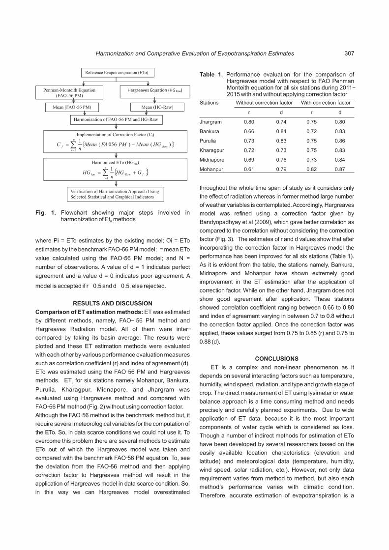
Reference Evapotranspiration (ETo)
Penman-Monteith Equation (FAO-56 PM)
Hargreaves Equation (HGRaw)
Mean (FAO-56 PM)
Mean (HG-Raw)
Harmonization of FAO-56 PM and HG-Raw
Verification of Harmonization Approach Using Selected Statistical and Graphical Indicators
Implementation of Correction Factor (Cf)
Harmonized ETo (HGhm)
{ })()056(1
1Raw
n
if HGMeanPMFAMean
nC -=å
=
{ }fRaw
n
ihm GHG
nHG +=å
=1
1
Fig. 1. Flowchart showing major steps involved in harmonization of Et methods0
where Pi = ETo estimates by the existing model; Oi = ETo
estimates by the benchmark FAO-56 PM model; = mean ETo
value calculated using the FAO-56 PM model; and N =
number of observations. A value of d = 1 indicates perfect
agreement and a value d = 0 indicates poor agreement. A
model is accepted if r ≥ 0.5 and d ≥ 0.5, else rejected.
RESULTS AND DISCUSSION
Comparison of ET estimation methods: ET was estimated
by different methods, namely, FAO- 56 PM method and
Hargreaves Radiation model. All of them were inter-
compared by taking its basin average. The results were
plotted and these ET estimation methods were evaluated
with each other by various performance evaluation measures
such as correlation coefficient (r) and index of agreement (d).
ETo was estimated using the FAO 56 PM and Hargreaves
methods. ET for six stations namely Mohanpur, Bankura, o
Purulia, Kharagpur, Midnapore, and Jhargram was
evaluated using Hargreaves method and compared with
FAO-56 PM method (Fig. 2) without using correction factor.
Although the FAO-56 method is the benchmark method but, it
require several meteorological variables for the computation of
the ETo. So, in data scarce conditions we could not use it. To
overcome this problem there are several methods to estimate
ETo out of which the Hargreaves model was taken and
compared with the benchmark FAO-56 PM equation. To, see
the deviation from the FAO-56 method and then applying
correction factor to Hargreaves method will result in the
application of Hargreaves model in data scarce condition. So,
in this way we can Hargreaves model overestimated
Stations Without correction factor With correction factor
r d r d
Jhargram 0.80 0.74 0.75 0.80
Bankura 0.66 0.84 0.72 0.83
Purulia 0.73 0.83 0.75 0.86
Kharagpur 0.72 0.73 0.75 0.83
Midnapore 0.69 0.76 0.73 0.84
Mohanpur 0.61 0.79 0.82 0.87
Table 1. Performance evaluation for the comparison of Hargreaves model with respect to FAO Penman Monteith equation for all six stations during 2011-2015 with and without applying correction factor
throughout the whole time span of study as it considers only
the effect of radiation whereas in former method large number
of weather variables is contemplated. Accordingly, Hargreaves
model was refined using a correction factor given by
Bandyopadhyay et al (2009), which gave better correlation as
compared to the correlation without considering the correction
factor (Fig. 3). The estimates of r and d values show that after
incorporating the correction factor in Hargreaves model the
performance has been improved for all six stations (Table 1).
As it is evident from the table, the stations namely, Bankura,
Midnapore and Mohanpur have shown extremely good
improvement in the ET estimation after the application of
correction factor. While on the other hand, Jhargram does not
show good agreement after application. These stations
showed correlation coefficient ranging between 0.66 to 0.80
and index of agreement varying in between 0.7 to 0.8 without
the correction factor applied. Once the correction factor was
applied, these values surged from 0.75 to 0.85 (r) and 0.75 to
0.88 (d).
CONCLUSIONS
ET is a complex and non-linear phenomenon as it
depends on several interacting factors such as temperature,
humidity, wind speed, radiation, and type and growth stage of
crop. The direct measurement of ET using lysimeter or water
balance approach is a time consuming method and needs
precisely and carefully planned experiments. Due to wide
application of ET data, because it is the most important
components of water cycle which is considered as loss.
Though a number of indirect methods for estimation of ETo
have been developed by several researchers based on the
easily available location characteristics (elevation and
latitude) and meteorological data (temperature, humidity,
wind speed, solar radiation, etc.). However, not only data
requirement varies from method to method, but also each
method's performance varies with climatic condition.
Therefore, accurate estimation of evapotranspiration is a
Harmonization and Comparative Evaluation of Evapotranspiration Estimates 307

0
2
4
6
8
10
12
0 2 4 6 8 10 12
Ha
rgre
av
es
R
ad
FAO- 56- PM
r = 0.73
d = 0.83
Purulia
0
2
4
6
8
10
12
0 2 4 6 8 10 12
Ha
rgre
av
es
R
ad
FAO- 56 - PM
r = 0.69
d = 0.76
Midnapore
0
2
4
6
8
10
12
0 2 4 6 8 10 12
Ha
rgre
av
es
R
ad
FAO - 56 - PM
r = 0.72
d = 0.73
Kharagpur
0
2
4
6
8
10
12
0 2 4 6 8 10 12
Ha
rgre
av
es
R
ad
r = 0.80
d = 0.74
Jhargram
FAO - 56 - PM
0
2
4
6
8
10
12
0 2 4 6 8 10 12
r = 0.61
d = 0.79
Mohanpur
Ha
rgre
av
es
R
ad
FAO - 56 - PM0
2
4
6
8
10
12
0 2 4 6 8 10 12
Ha
rgre
av
es
R
ad
r = 0.66
d = 0.84
Bankura
FAO - 56 - PM
Fig. 2. Comparison of ETo estimated using Hargreaves model with respect to FAO Penman-Monteith equation for all six stations during 2011-2015 without applying correction factor
challenging task. To overcome this problem a methodology
for evaluating ET was conducted in this study in order to test
the accuracy of limited data based ET estimates. Hargreaves
ET was standardized by using correction factor and
tremendous results was obtained for all the six stations.
Altogether it is an efficient methodology for the water
resources management perspective and for irrigation
scheduling for the crops. Apart from that at catchment-scale
where there is limited data availability for ET calculation
accuracy of harmonized based ET estimation is very useful in
order to estimate the losses.
REFERENCES
Allen RG, Jensen ME, Wright JL and Burman RD 1989. Operational estimates of reference evapotranspiration. Agronomy Journal 81: 650-662.
Allen RG, Pereira LS, Raes D and Smith M 1998. Crop evapotranspiration: Guidelines for computing crop water requirements. FAO Irrigation and Drainage Paper 56, Rome.
Nikul Kumari and Ankur Srivastava308

0
2
4
6
8
10
12
0 2 4 6 8 10 12
Ha
rgre
av
es
R
ad
FAO - 56- PM
r = 0.82
d = 0.87
Mohanpur
0
2
4
6
8
10
12
0 2 4 6 8 10 12
r = 0.72
d = 0.83
Ha
rgre
av
es
R
ad
Bankura
FAO - 56- PM
0
2
4
6
8
10
12
0 2 4 6 8 10 12
Ha
rgre
av
es
R
ad
r = 0.75
d =0.86
Purlia
0
2
4
6
8
10
12
0 2 4 6 8 10 12
Ha
rgre
av
es
R
ad
r = 0.75
d =0.86
Purlia
0
2
4
6
8
10
12
0 2 4 6 8 10 12
Ha
rgre
av
es
R
ad
FAO - 56 - PM
r = 0.75
d = 0.80
Jhargram
FAO - 56- PM FAO - 56- PM
0
2
4
6
8
10
12
0 2 4 6 8 10 12
Ha
rgre
av
es
R
ad
r =0.75
d = 0.83
Kharagpur
FAO - 56- PM
Fig. 3. Comparison of ETo estimated using Hargreaves model with respect to FAO Penman Monteith equation for all six stations during 2011-2015 after applying correction factor
Belaineh G, Sumner D, Carter E and Clapp D 2014. Harmonizing multiple methods for reconstructing historical potential and reference evapotranspiration. Journal of Hydrologic Engineering, ASCE 19(8), doi: 10.1061/(ASCE)HE.1943-5584.0000935,05014006.
Dingman SL 1994. Physical Hydrology. Upper Saddle River, NJ: Prentice Hall.
Hargreaves GH and Samani ZA 1985. Reference crop evapotranspiration from temperature. Applied Engineering in Agriculture 1(2): 96-99.
Jensen DT, Hargreaves GH, Temesgen B and Allen RG 1997.
Computation of ETo under nonideal conditions. Journal Irrigation and Drain Enginnering 123(5): 394-400.
Keune H, Murray AB and Benking H 1991. Harmonization of environmental measurement. Geo Journal 23(3): 249-255.
National Research Council 2010. Assessment of Intraseasonal to Interannual Climate Prediction and Predictability. Washington, DC, National Academies Press, 192pp.
Saxena RP 2012. Impacts of Kangsabati Project, India. In “Impacts of Large Dams: A Global Assessment”, Springer Berlin Heidelberg, pp 277-298.
Sheffield J and Wood EF 2008. Projected changes in drought
Harmonization and Comparative Evaluation of Evapotranspiration Estimates 309

occurrence under future global warming from multi-model, multi-scenario, IPCC AR4 simulations. Climate dynamics 31(1): 79-105.
Srivastava A, Sahoo B, Raghuwanshi NS and Singh R 2017. Evaluation of variable infiltration capacity model and MODIS-Terra satellite-derived grid-scale evapotranspiration in a river basin with tropical monsoon-type climatology. Journal Irrigation and Drainage Engineering (Accepted in Press).
Willmott CJ 1982. Some comments on the evaluation of model performance. Bulletin of the American Meteorological Society
63(11): 1309-1313.
Yeh PJ, Irizarry M and Eltahir EAB 1998. Hydroclimatology of Illinois: a comparison of monthly evaporation estimates based on atmospheric water balance and soil water balance. Journal of Geophyshical Research 103: 19823. http://dx.doi.org/ 10.1029/98JD01721.
Zhai L, Feng Q, Li Q and Xu C 2010. “Comparison and modification of equations for calculating evapotranspiration (ET) with data from Gansu Province, Northwest China.” Irrigation and Drain 59(4): 477-490.
Received 05 March, 2018; Accepted 10 May, 2018
Nikul Kumari and Ankur Srivastava310

Effect of Real Time Nitrogen Management on Productivity of Rice (Oryza sativa L)
Indian Journal of Ecology (2018) 45(2): 311-315
Abstract: The present study was done at farmer field of Katihar district during the two consecutive years 2014 and 2015 to find out the effect of
real time nitrogen management on productivity of rice. The soil is non-calcareous light gray flood plain belongs to the alluvial gangetic plain
(Agro climatic zone II) with normal in physico-chemical properties except fertility status. One of the recently introduced nitrogen management
approach was estimating the leaf nitrogen concentration by the measurement of leaf greenness. The application of nitrogen with the help of 2CLCC significantly increase in yield attributes i.e. plant height, number of tillers, panicle length, filled kernel/plant, productive tiller /m , grain
and straw yield in comparisons to farmers practice. Hence, the B: C ratio increase from 2.08 (farmers practices) to 4.14 where CLCC used for
nitrogen application. Therefore, inexpensive customized leaf color chart (CLCC) has proved quick and reliable tools to decide the time when
nitrogenous fertilizer needs to be applied to the crop. With CLCC, farmers can apply N at the right time, thereby increasing the productivity and
profitability of rice and reduction in nitrogen fertilizer.
Keywords: Rice, CLCC, Nitrogen
Manuscript Number: NAAS Rating: 4.96
2677
1 2Rama Kant Singh,Pankaj Kumar, Pankaj K. Yadav , S.B. Singh and R.N. Singh1Krishi Vigyan Kendra, Katihar-854 105, India; BPSAC, Purnea-854 301, India
2 Bihar Agricultural University, Sabour-813 210, IndiaE-mail: [email protected]
The adequate nutrient supply plays a vital role in soil and
crop management system. Knowing the required nutrients for
all stages of growth and understanding the soil's ability to
supply those needed nutrients are critical to profitable crop
production (Nedunchezhiyan and Laxminarayan 2011).
Increase fertilizer inputs, especially N fertilizer, results in
significant increases in rice crop production (Peng et al 2010).
Nitrogen is the major nutrient limiting the high yield potential of
rice cultivars, Farmers generally apply nitrogenous fertilizer in
several split applications that results in high pest and disease
incidence and serious lodging. Precise application of nitrogen
fertilizer based on plant need and location in the field greatly
improves fertilizer use efficiency in rice. Farmers generally
apply fertilizer N in several split applications, but the number of
splits, amount of N applied per split, and the time of
applications vary substantially. The apparent flexibility of rice
farmers in adjusting the time and amount of fertilizer
application offers potential to synchronize nitrogen application
with the real-time demand of the rice crop (Alam 2005).
Farmers generally apply too much N (and little P and K and
other nutrients) that results in high pest and disease incidence
and serious lodging. The consequence of high N application is
associated with the high pesticide use to control pests, more
expenditure on pesticides, and reduced yield and poor grain
quality due to lodging (Nath et al 2013). Site specific nitrogen
management has the potential to increase fertilizer use
efficiency as well as grain yield in the farmers' fields (Ravi
2007). Precise application of N fertilizer based on plant need
and location in the field greatly improves fertilizer use
efficiency in rice. Farmers generally use leaf color as a visual
and subjective indicator of the rice crop's nitrogen status and
need for N fertilizer application. Leaf color intensity is directly
related to leaf chlorophyll content which, in turn, is related to
leaf N status. The concept is based on results that show a
close link between leaf chlorophyll content and leaf N content
(Nath et al 2013). One of the recently introduced N
management approach was estimating the leaf N
concentration by the measurement of leaf greenness through
CLCC. Among the different tools available to measure the leaf
greenness, the non destructive measurement of leaf green
color intensity using customized leaf color charts (CLCC) is
gaining importance (Kumar and Haefele 2013). The
customized leaf color chart (CLCC) is an easy-to-use and
inexpensive diagnostic tool for monitoring the relative
greenness of a rice leaf as an indicator of the plant N status.
Therefore, a field experiment was conducted to find out the
optimize the right time of nitrogen application on performance
of rice with CLCC tools for increase the productivity and
profitability of rice and reduction the used nitrogen fertilizer.
MATERIAL AND METHODS
An experiment was conducted during kharif 2014-15 at

farmer fields of Katihar adopted by Krishi Vigyan Kendra,
Katihar under Bihar Agriculture University, Sabour,
Bhagalpur. The experiment was in randomized block design
with split plot arrangement in net plot size was 10 x 10 m
having ten replications and three treatments. Nursery of
medium duration rice cultivar Sahbhagi was sown in the first
week of June and transplanted in the age of twenty one
days. The treatment was T -farmer practices (80:40: 20:: N: 1
P: K basal + 50 kg N at 25 DAT+ 50 kg N at 50 DAT), T - RDF 2
(basal 60:60:40 kg N: P: K + 45 kg N at 30 DAT+ 45 kg N at 60
DAT) and T –RDF (basal 60:60:40 NPK + real time 3
application of balance N by using customised leaf colour
chart. The seedlings of rice cultivar Sahbhagi was
transplanted on second week of July with spacing of 20 x 20
cm. The full dose of phosphorous, potash and half dose of
nitrogen were applied at the time of transplanting and
remaining half of nitrogen was top dressed as urea as par
requirement of treatment to correct deficiency of nitrogen.
Data was recorded on leaf color chart with an interval of ten
days, starting from two weeks after transplantation up to
flower initiation. The leaf color chart value for semi dwarf
high yielding rice varieties is 4.0; if the average value fell
below 4.0; nitrogenous fertilizer was top dressed @ 30 kg - 1ha to correct the nitrogen deficiency. The plant height and
tillers were measured at tillering, flowering and harvesting
stages and panicle length, grains per panicles at harvesting
stage. The rice crop was harvested at physiological maturity
stage. After harvesting grains were separated from each
plot and were dried under sun light for three days then
winnowed, cleaned and taken test weight of rice and
computed yield. Straw from each plot was dried under sun
for 10 days and weight was recorded after complete drying.
The benefit cost ratio was worked out after price value of
grain with straw and total cost included in crop cultivation.
The soil samples are collected randomly from all
experimental sites before start the experiment and post
harvest. The important properties of soil samples are
analyzed; organic carbon content was determined by the
Walkley and Black method (1934), available nitrogen was
determined by the alkaline KMNO method (Subbaiah and 4
Asija 1956), available phosphorous (Olsen's method, 1954)
and available potash were determined using 1 N neutral
normal ammonium acetate solution (Tandon 1993), pH and
EC with soil suspension (1:2.5) using electrode (Chopra
and Kanwar 1999). The collected data on different
parameters under the experiment were statistically
analyzed to obtain the level of significance using the
computer MSTAT package program developed by Russel
(1986).
RESULTS AND DISCUSSION
Soil Physico-chemical Properties
pH, EC and Organic carbon: Reduction in electro chemical
properties in farmers practices might be due to continues use
of more amounts of chemical fertilizers over the years
reduced soil pH and EC over applied treatment. This
marginal increase in pH and EC might be due to the
moderating effect of recommended dose of chemical
fertilizers and also less amount of organic matter in treatment
T . The soil organic carbon one of the gracious factor in 1
sustaining agricultural production and also improve physical,
chemical and biological properties of soil. Non significant
improvement of organic carbon content in treatment T might 3
be due to addition of fertilizers that improve the root and shoot
growth might have increase the organic carbon content
(Sharma and Subehia 2014).
Available nitrogen: The significant and positive changes
was observed in available soil nitrogen in T where nitrogen 3
was applied accordance to CLCC and significant negative
relationship in farmer practices with indiscriminate
fertilization at par with T . The higher available nitrogen 2
content which might be due to higher use efficiency of
nitrogen and might be lowest losses of organic and inorganic
nitrogen from soil (Stalin et al 2000). The lowest value of
available nitrogen in T may be due to mining of available 1
nitrogen with continuous cropping without balance
fertilization over the year. The increase was maximum in T 3
where 60:60:40 NPK + real time nitrogen management were
applied. It may be due to sufficient supply of nutrients by
applied NPK fertilizers (Varlakshmi et al 2005).
Available phosphorous: Significant difference in the
available phosphorous of the soil was observed during two
consecutive years after final harvesting of crop (Table 1). The
available P content of the soil was found to be significantly
lower in the treatment T than T and control. The 3 2
phosphorous uptake by the plant increased due to increased
biomass production towards maturity (Table 3). Johnkutty et
al (2000) also documented similar results from increased P
due to higher nitrogen application.
Available potash: Significant variation in the available
potash content of the soil was observed due to application of
different treatments in this study. The decreased available
potash in this treatment might be due to the abundant release
of potash by soil and maximum utilized by plant. Among the
treatment T showed highest available potash utilization. It is 3
possible due to the uses of nitrogen on real time in balanced
amount and its possible due to synergetic effect of nitrogen
on potash and others macro and micro nutrients (Varlakshmi
et al 2005).
Rama Kant Singh, Pankaj Kumar, Pankaj K. Yadav, S.B. Singh and R.N. Singh312
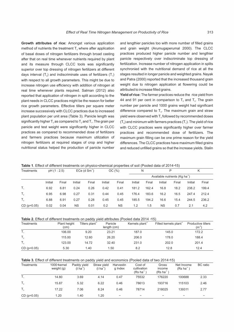
Treatments pH (1 : 2.5) -1ECe (d Sm ) OC (%) N P K
-1Available nutrients (Kg ha )
Initial Final Initial Final Initial Final Initial Final Initial Final Initial Final
T1 6.92 6.81 0.24 0.26 0.42 0.41 181.2 162.4 16.8 18.2 238.2 199.4
T2 6.95 6.98 0.27 0.31 0.44 0.45 176.4 183.6 16.2 16.5 247.4 212.4
T3 6.88 6.91 0.27 0.28 0.45 0.45 185.5 194.2 16.6 15.4 244.5 236.2
CD (p=0.05) 0.02 0.04 NS 0.01 0.2 NS 1.2 1.5 NS 0.7 2.1 4.2
Table 1. Effect of different treatments on physico-chemical properties of soil (Pooled data of 2014-15)
Treatments Plant height (cm)
Tillers plant-1 Panicle length (cm)
Kernels plant-1 Filled kernels plant-1 Productive tillers -2(m )
T1 106.00 9.20 23.21 187.0 145.0 172.2
T2 115.00 12.60 26.20 206.0 178.0 188.4
T3 123.00 14.72 32.40 231.0 202.0 201.4
CD (p=0.05) 5.30 1.40 1.50 8.2 12.8 12.4
Table 2. Effect of different treatments on paddy yield attributes (Pooled data 2014 -15)
Treatments 1000-kernel weight (g)
Paddy yield -1(t ha )
Straw yield-1(t ha )
Harvesting Index
Cost of cultivation (Rs ha )-1
Gross income
(Rs ha )-1
Net Income(Rs ha )-1
BC ratio
T1 14.80 3.69 4.14 0.47 75532 176220 100688 2.33
T2 15.87 5.32 6.22 0.46 78613 193716 115103 2.46
T3 17.22 7.06 8.24 0.46 78714 218025 139311 2.77
CD (p=0.05) 1.20 1.40 1.20 - - - - -
Table 3. Effect of different treatments on paddy yield and economics (Pooled data of two 2014-15)
Growth attributes of rice: Amongst various application
method of nutrients the treatment T where after application 3
of basal doses of nitrogen fertilizers through broad casting
after that on real time whenever nutrients required by plant
and its measure through CLCC tools was significantly
superior over top dressing of nitrogen fertilizers at different
days interval (T ) and indiscriminate uses of fertilizers (T ) 2 1
with respect to all growth parameters. This might be due to
increase nitrogen use efficiency with addition of nitrogen at
real time whenever plants required. Salman (2012) also
reported that application of nitrogen in split according to the
plant needs in CLCC practices might be the reason for better
rice growth parameters. Effective tillers per square meter
increase successively with CLCC practices due to increased
plant population per unit area (Table 3). Panicle length was
significantly higher T as compared to T and T . The grain per 3 2 1
panicle and test weight were significantly higher in CLCC
practices as compared to recommended dose of fertilizers
and farmers practices because maximum utilization of
nitrogen fertilizers at required stages of crop and higher
nutritional status helped the production of panicle number
and lengthier panicles too with more number of filled grains
and grain weight (Arumugaperumal 2000). The CLCC
practices produced higher panicle number and lengthier
panicle respectively over indiscriminate top dressing of
fertilization. Increase number of nitrogen application in splits
synchronied with the nutritional demand of rice at all the
stages resulted in longer panicle and weighted grains. Nayak
and Patra (2000) reported that the increased thousand grain
weight due to nitrogen application at flowering could be
attributed to increase filled grains.
Yield of rice: The farmer practices reduce the rice yield from
44 and 91 per cent in comparison to T and T . The grain 2 3
number per panicle and 1000 grains weight had significant
difference compared to T . The maximum grain and straw 3
yield were observed with T followed by recommended doses 3
(T ) and minimum with farmers practices (T ). The yield of rice 2 1
with CLCC practices were significantly higher over farmer
practices and recommended dose of fertilizers. The
maximum grain filling can be one prime reason for the yield
differences. The CLCC practices have maximum filled grains
and reduced unfilled grains so that the increase yields. Stalin
Effect of Real Time Nitrogen Management on Productivity of Rice 313
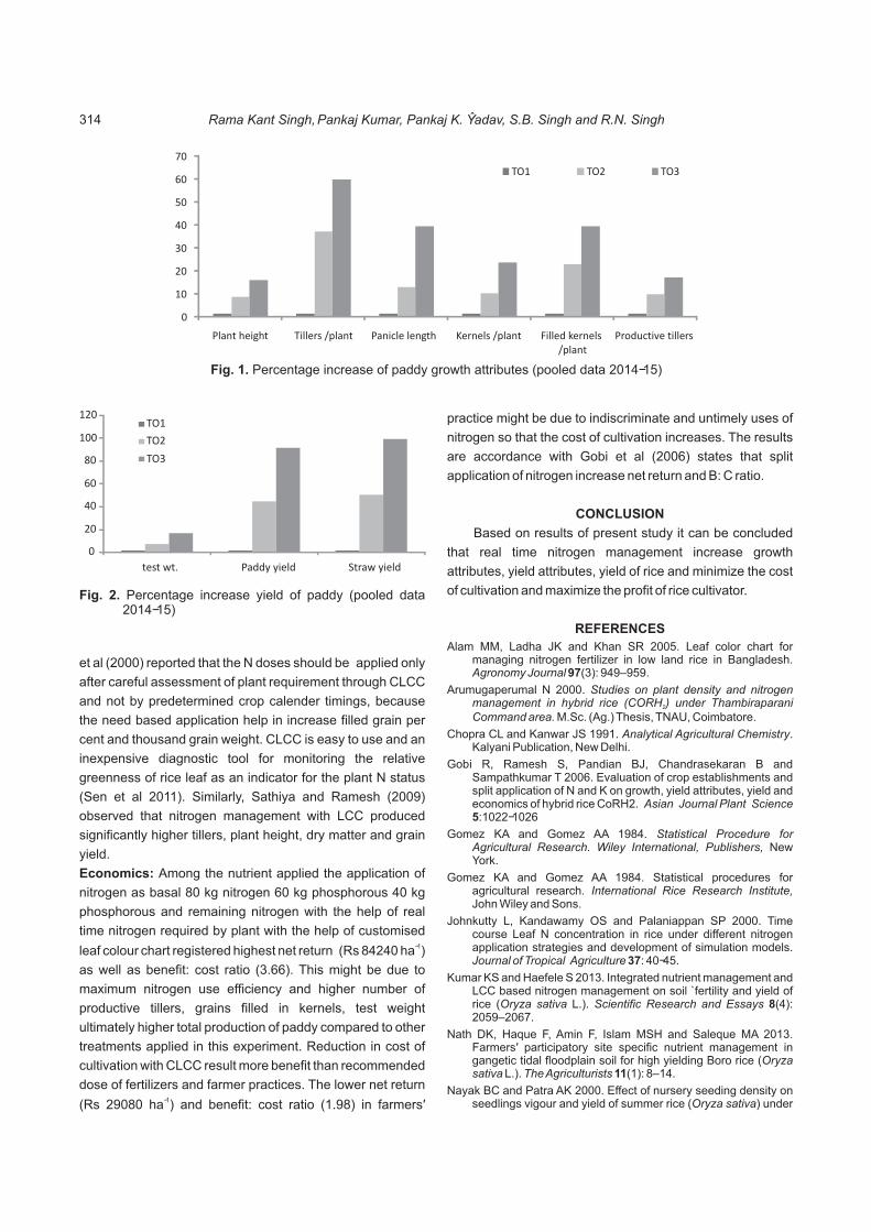
0
20
40
60
80
100
120
test wt. Paddy yield Straw yield
TO1
TO2
TO3
Fig. 2. Percentage increase yield of paddy (pooled data 2014-15)
0
10
20
30
40
50
60
70
Plant height Tillers /plant Panicle length Kernels /plant Filled kernels /plant
Productive tillers
TO1 TO2 TO3
Fig. 1. Percentage increase of paddy growth attributes (pooled data 2014-15)
et al (2000) reported that the N doses should be applied only
after careful assessment of plant requirement through CLCC
and not by predetermined crop calender timings, because
the need based application help in increase filled grain per
cent and thousand grain weight. CLCC is easy to use and an
inexpensive diagnostic tool for monitoring the relative
greenness of rice leaf as an indicator for the plant N status
(Sen et al 2011). Similarly, Sathiya and Ramesh (2009)
observed that nitrogen management with LCC produced
significantly higher tillers, plant height, dry matter and grain
yield.
Economics: Among the nutrient applied the application of
nitrogen as basal 80 kg nitrogen 60 kg phosphorous 40 kg
phosphorous and remaining nitrogen with the help of real
time nitrogen required by plant with the help of customised -1leaf colour chart registered highest net return (Rs 84240 ha )
as well as benefit: cost ratio (3.66). This might be due to
maximum nitrogen use efficiency and higher number of
productive tillers, grains filled in kernels, test weight
ultimately higher total production of paddy compared to other
treatments applied in this experiment. Reduction in cost of
cultivation with CLCC result more benefit than recommended
dose of fertilizers and farmer practices. The lower net return -1(Rs 29080 ha ) and benefit: cost ratio (1.98) in farmers'
practice might be due to indiscriminate and untimely uses of
nitrogen so that the cost of cultivation increases. The results
are accordance with Gobi et al (2006) states that split
application of nitrogen increase net return and B: C ratio.
CONCLUSION
Based on results of present study it can be concluded
that real time nitrogen management increase growth
attributes, yield attributes, yield of rice and minimize the cost
of cultivation and maximize the profit of rice cultivator.
REFERENCES
Alam MM, Ladha JK and Khan SR 2005. Leaf color chart for managing nitrogen fertilizer in low land rice in Bangladesh. Agronomy Journal 97(3): 949–959.
Arumugaperumal N 2000. Studies on plant density and nitrogen management in hybrid rice (CORH ) under Thambiraparani 2
Command area. M.Sc. (Ag.) Thesis, TNAU, Coimbatore.
Chopra CL and Kanwar JS 1991. Analytical Agricultural Chemistry. Kalyani Publication, New Delhi.
Gobi R, Ramesh S, Pandian BJ, Chandrasekaran B and Sampathkumar T 2006. Evaluation of crop establishments and split application of N and K on growth, yield attributes, yield and economics of hybrid rice CoRH2. Asian Journal Plant Science 5:1022-1026
Gomez KA and Gomez AA 1984. Statistical Procedure for Agricultural Research. Wiley International, Publishers, New York.
Gomez KA and Gomez AA 1984. Statistical procedures for agricultural research. International Rice Research Institute, John Wiley and Sons.
Johnkutty L, Kandawamy OS and Palaniappan SP 2000. Time course Leaf N concentration in rice under different nitrogen application strategies and development of simulation models. Journal of Tropical Agriculture 37: 40-45.
Kumar KS and Haefele S 2013. Integrated nutrient management and LCC based nitrogen management on soil `fertility and yield of rice (Oryza sativa L.). Scientific Research and Essays 8(4): 2059–2067.
Nath DK, Haque F, Amin F, Islam MSH and Saleque MA 2013. Farmers' participatory site specific nutrient management in gangetic tidal floodplain soil for high yielding Boro rice (Oryza sativa L.). The Agriculturists 11(1): 8–14.
Nayak BC and Patra AK 2000. Effect of nursery seeding density on seedlings vigour and yield of summer rice (Oryza sativa) under
Rama Kant Singh, Pankaj Kumar, Pankaj K. Yadav, S.B. Singh and R.N. Singh314

varying seedlings rates. Indian Journal Agronomy 45(3): 555-559
Nedunchezhiyan M and Laxminarayan K 2011. Site specific nutrient management for rice. Orissa Review 17: 62–64.
Olsen SR, Cole CV, Watanable FS and Deam LA 1954. Estimation of available phosphorous in soils by extraction with sodium bicarbonate. U.S. Department Agriculture Cire. 939.
Peng S, Buresh RJ and Huang J 2010. Improving nitrogen fertilization in rice by site specific nutrient management. A review,” Agronomy for Sustainable Development 30(3): 649–656.
Peng S, Garcia FV, Laza RC and Cassman KG 1993. Adjustment for specific leaf weight improves chlorophyll meter estimate of leaf nitrogen concentration. Agronomical Journal 85: 987-990.
Ravi S, Ramesh S and Chandrasekaran B 2007. Exploitation of hybrid vigour in rice hybrid (Oryza sativa L.) through green manure and Leaf Colour Chart (LCC) based N application, Asian Journal of Plant Sciences 6(2): 282–287.
Russell D 1986. MSTAT-C package programme. Crop and Soil Science Department, Michigan State University, USA
Sathiya K and Ramesh T 2009. Effect of split application of nitrogen on growth and yield of aerobic rice, Asian Journal of Experimental Sciences 23(1): 303–306.
Sen A, Srivastava VK, Singh MK, Singh RK and Kumar S 2011. Leaf colour chart vis-a-vis nitrogen management in different rice genotypes. American Journal of Plant Sciences 2: 223-236.
Sharma U and Subehia SK 2014. Effect of long term INM of rice (Oryza sativa L.)- Wheat (Triticum astivum L.) productivity and soil properties in North-Western Himalaya. Journal of the Indian Society of Soil Science 62(3): 248-254.
Singh H, Sharma KN, Dhillon GS, Singh T, Singh V, Kumar D and Singh H 2010. On-farm evaluation of real-time nitrogen (RTN) management in rice. Better Crop 94(4): 26-28.
Sripriya S 1993. Studies on the efficacy of humic acid on soil fertility attributes and response of ADT 36 rice. M.Sc. (Ag) Thesis, TNAU, Coimbatore, Tamilnadu, India.
Stalin P, Thiyagarajan TM, Ramanathan S and Subramanian M 2000. Comparing management techniques to optimize fertilizer N application in rice in the Cauvery Delta of Tamil Nadu, India. IRRN 25(2): 25-26.
Subbaiah BV and Asija GL 1956. A rapid method for the estimation of available nitrogen in soil. Current Science 25: 259-260.
Tandon HLS 1993. Methods of analysis of soil, plants, waters and fertilizers. Fertilizers Development and Consultation Organization, New Delhi, India.
Varlakshmi CR, Srinivasmurthy CA and Bhaskar S 2005. Effect of integrated use of organic manure and inorganic fertilizers on organic carbon, available N P and K in sustaining productivity of groundnut-finger millet cropping system. Journal of the Indian Society of Soil Science 53(3): 315-318.
Walkley A and Black IA 1934. An examination of the degtjareff method for determining soil organic matter and a proposed modification of the eronic acid titration methods. Oil Science 37: 29-38.
Witt C, Pasuquin JMCA, Mutters R and Buresh RJ 2005. Leaf color chart for effective nitrogen management in rice, Better Crops 89: 36–39.
Yoseftabar S 2013. Effect of split application of nitrogen fertilizer on leaf color chart values in hybrid rice. International Journal of Biology 5(1): 79-84.
Received 06 March, 2018; Accepted 10 May, 2018
Effect of Real Time Nitrogen Management on Productivity of Rice 315

Effect of Weed Control by Containment and Weeding Frequency on the Growth and Yield of Cucumber in
Abakaliki, Southeastern Nigeria
Indian Journal of Ecology (2018) 45(2): 316-320
Abstract: Growth and yield response of cucumber to weed control by containment technique (plant density and weeding frequency)was
observed in 2014 and 2015 planting seasons at the Ebonyi State University, Abakaliki southeastern Nigeria. The design was a 5x3 factorial
experiment in a randomized complete block design. Factor A was five weeding frequencies [0, 2, 4, 6 and 8 weeks after planting (WAP)], while -1 -1factor B was three plant densities (41,667, 33,333 and 27,778 plants ha ). The highest fresh weed weight (93.62g plot ) was at 0WAP on the
lowest plant density, showing that critical period of weed infestation in cucumber is not localized in this study. Two WAP significantly influenced
growth and yield parameters. The highest plant density (41,667) suppressed weed growth earlier and also gave the highest fruit yield (1.11 kg -1 -1plant ), having a weed suppression ability of 52.86 in2014 and 43.75 per cent in 2015. Eight WAP gave the highest fruit yield (1.17 kg plant ).
-1The highest plant density weeded 2WAP produced 1.60 kg, 1.20 kg at 8WAP and 0.93 kg plant at 0WAP. Therefore, high plant density and a
single weeding at 8WAP will reduce cost of production without adverse effect on growth and yield in cucumber at a zero threat to the
environment. Hence, weed control by containment technique is sustainable and is highly recommended in cucumber production among the
smallholder farmers of developing nations of the world.
Keywords: Containment technique, Plant density, Weeding frequency, Critical weed period
Manuscript Number: NAAS Rating: 4.96
2678
N.L. Aniekwe and C.I. AkabuezeDepartment of Crop Production and Landscape Management,
Ebonyi State University, Abakaliki, PMB 053, Ebonyi State, NigeriaE-mail: [email protected]
The battle against weeds is a never ending one, and its
control is often the costliest agronomic input in terms of the
farmers' time, labour and money. It has been recognized as
the greatest hazard hampering sustainable crop production
and hiking the cost of food supply in developing countries
since man started domesticating plants and animals around
10,000 BC. Weeds are injurious naturally occurring common
or noxious annual, biennial or perennial plants of various
plant families rightly defined as 'plants out of place' in
agricultural systems. They are problem plants which harbor
or serve as alternative hosts to insects and disease
organisms and increasing their damage to crops and harm
the health of animals that may feed on them. Weeds compete
with crops for light, water, nutrients and space thereby
leading to reductions in crop yield and quality or total failure. A
recent estimate showed that weeds account for 37% of the
total annual yield loss in India, varying from as low as 10% to
as high as 100% in certain crop situations and the annual loss
could be nearly 45%. Also, yield reduction of 15-30% was
recorded in wheat, 30-35% in rice, 18-85% in maize,
sorghum, pulses and oilseeds and they also remove on
average 30-40 Kg N, 10-15Kg P O and 20-40 Kg K O/ha 2 5 2
(Das 2008). Weeds may also be parasitic on crops,
poisonous to man and animal, less palatable to animals, poor
in nutrition, its thorns or spines may be injurious, may block
drainage ditches, irrigation channels, railways and roads, but
yet a rich source of medicinal values (Das 2008).
Cucumber (Cucumis sativus L.) is a monoecious plant
(Adetula and Denton 2003) with a chromosome number 2n =
14 (Grubben and Denton 2004). It is a tender annual vine
creeper or climber on stakes or trellises, with indeterminate
or determinate growth habits (Hector et al 2000), being the
most important and popular member of the Cucurbitaceae
family. It is of Indian or Chinese origin and its cultivation dates
back to 5,000 years (Wehner and Guner 2004). It is fourth in
importance after tomato, cabbage and onion in Asia, second
after tomato in Western Europe, less sugary but a good
source of vitamins A, C, K, B6, potassium, magnesium,
phosphorus, copper, manganese, pantothenic acid, caffeic
acid and dietary fibre (Grubben and Denton 2004). Without
herbicides and other control methods, very significant part of
the physical farming process is devoted to weed control, yet
the uncontrolled and unregulated use or misuse of herbicides
when affordable creates health hazards in developing
countries. It is therefore against this backdrop that the effects
of weed control by containment on cucumber growth and
yield was studied in Abakaliki.
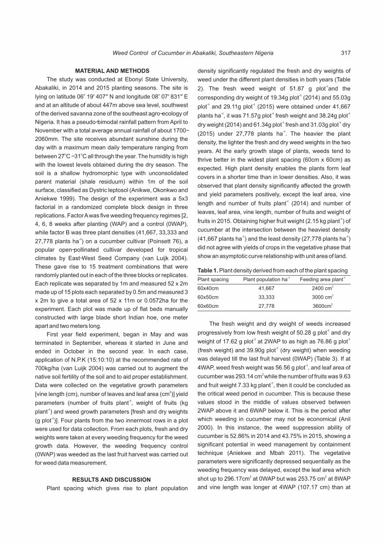
MATERIAL AND METHODS
The study was conducted at Ebonyi State University,
Abakaliki, in 2014 and 2015 planting seasons. The site is o olying on latitude 06 19' 407'' N and longitude 08 07' 831'' E
and at an altitude of about 447m above sea level, southwest
of the derived savanna zone of the southeast agro-ecology of
Nigeria. It has a pseudo-bimodal rainfall pattern from April to
November with a total average annual rainfall of about 1700-
2060mm. The site receives abundant sunshine during the
day with a maximum mean daily temperature ranging from o obetween 27 C - 31 C all through the year. The humidity is high
with the lowest levels obtained during the dry season. The
soil is a shallow hydromorphic type with unconsolidated
parent material (shale residuum) within 1m of the soil
surface, classified as Dystric leptosol (Anikwe, Okonkwo and
Aniekwe 1999). The design of the experiment was a 5x3
factorial in a randomized complete block design in three
replications. Factor A was five weeding frequency regimes [2,
4, 6, 8 weeks after planting (WAP) and a control (0WAP),
while factor B was three plant densities (41,667, 33,333 and -127,778 plants ha ) on a cucumber cultivar (Poinsett 76), a
popular open-pollinated cultivar developed for tropical
climates by East-West Seed Company (van Luijk 2004).
These gave rise to 15 treatment combinations that were
randomly planted out in each of the three blocks or replicates.
Each replicate was separated by 1m and measured 52 x 2m
made up of 15 plots each separated by 0.5m and measured 3
x 2m to give a total area of 52 x 11m or 0.0572ha for the
experiment. Each plot was made up of flat beds manually
constructed with large blade short Indian hoe, one meter
apart and two meters long.
First year field experiment, began in May and was
terminated in September, whereas it started in June and
ended in October in the second year. In each case,
application of N.P.K (15:10:10) at the recommended rate of
700kg/ha (van Luijk 2004) was carried out to augment the
native soil fertility of the soil and to aid proper establishment.
Data were collected on the vegetative growth parameters 2[vine length (cm), number of leaves and leaf area (cm )] yield
-1parameters (number of fruits plant , weight of fruits (kg -1plant ) and weed growth parameters [fresh and dry weights
-1(g plot )]. Four plants from the two innermost rows in a plot
were used for data collection. From each plots, fresh and dry
weights were taken at every weeding frequency for the weed
growth data. However, the weeding frequency control
(0WAP) was weeded as the last fruit harvest was carried out
for weed data measurement.
RESULTS AND DISCUSSION
Plant spacing which gives rise to plant population
density significantly regulated the fresh and dry weights of
weed under the different plant densities in both years (Table -12). The fresh weed weight of 51.87 g plot and the
-1corresponding dry weight of 19.34g plot (2014) and 55.03g -1 -1plot and 29.11g plot (2015) were obtained under 41,667
-1 -1 -1 plants ha , it was 71.57g plot fresh weight and 38.24g plot-1 -1dry weight (2014) and 61.34g plot fresh and 31.03g plot dry -1(2015) under 27,778 plants ha . The heavier the plant
density, the lighter the fresh and dry weed weights in the two
years. At the early growth stage of plants, weeds tend to
thrive better in the widest plant spacing (60cm x 60cm) as
expected. High plant density enables the plants form leaf
covers in a shorter time than in lower densities. Also, it was
observed that plant density significantly affected the growth
and yield parameters positively, except the leaf area, vine -1length and number of fruits plant (2014) and number of
leaves, leaf area, vine length, number of fruits and weight of -1fruits in 2015. Obtaining higher fruit weight (2.15 kg plant ) of
cucumber at the intersection between the heaviest density -1 -1(41,667 plants ha ) and the least density (27,778 plants ha )
did not agree with yields of crops in the vegetative phase that
show an asymptotic curve relationship with unit area of land.
The fresh weight and dry weight of weeds increased -1progressively from low fresh weight of 50.28 g plot and dry
-1 -1weight of 17.62 g plot at 2WAP to as high as 76.86 g plot -1(fresh weight) and 39.90g plot (dry weight) when weeding
was delayed till the last fruit harvest (0WAP) (Table 3). If at -14WAP, weed fresh weight was 56.56 g plot , and leaf area of
2 cucumber was 293.14 cm while the number of fruits was 9.63 -1and fruit weight 7.33 kg plant , then it could be concluded as
the critical weed period in cucumber. This is because these
values stood in the middle of values observed between
2WAP above it and 6WAP below it. This is the period after
which weeding in cucumber may not be economical (Anil
2000). In this instance, the weed suppression ability of
cucumber is 52.86% in 2014 and 43.75% in 2015, showing a
significant potential in weed management by containment
technique (Aniekwe and Mbah 2011). The vegetative
parameters were significantly depressed sequentially as the
weeding frequency was delayed, except the leaf area which 2 2shot up to 296.17cm at 0WAP but was 253.75 cm at 8WAP
and vine length was longer at 4WAP (107.17 cm) than at
Plant spacing -1Plant population ha -1Feeding area plant
60x40cm 41,667 22400 cm
60x50cm 33,333 23000 cm
60x60cm 27,778 23600cm
Table 1. Plant density derived from each of the plant spacing
Weed Control of Cucumber in Abakaliki, Southeastern Nigeria 317

0WAP (89.36 cm) in 2014. In 2015, it was a little bit as
expected but not in a perfect sequence of depression. It was
also evident that delayed weeding till 0WAP did not reduce -1the weight of fruit yield of cucumber being 9.64 kg plant ,
-1while it was 11.11 kg plant at 2WAP in 2014. It is however
difficult to explain why the fruit weight was as low as 5.75kg -1 -1plant at 8WAP but 9.64 kg plant at 0WAP. It may however
-1be suggested that the 9.64 kg plant at 0WAP was a
demonstration of the competitive superiority of cucumber
over weed infestation. But the quantum jump of 11.11 kg -1plant at 2WAP is akin to what was observed in 2015 with
-11.14 kg plant at 2WAP.
Weed growth in a cucumber plot was significantly
influenced by plant density and weeding frequency
interaction on the basis of fresh weed weight in 2014 (Table -14).It showed that the heaviest weed growth (93.62g plot )
was observed on the plots with the lowest plant density -1(27,778 plants ha ) and where weeding was delayed up to
-1the last fruit harvest (0WAP) and at 8WAP (90.39 g plot ). The -1lightest fresh weed weight (32.24 g plot ) was observed on
the plot with the lowest plant population and where weeding
was delayed to 4WAP. On the other hand, heavier fresh weed -1 -1weights (76.86 g plot and 71.57 g plot ) occurred at 0WAP
-1and where plant density was lowest (27,778 plants ha ) -1respectively. The 38.39g plot of fresh weeds observed on
-1the high plant density plot (41,667 plants ha ), 2WAP was in
order as Ngouajio and Mennan (2005) observed that cover
cropping has been a common practice in weed control
management among the smallholder farmers who are
affected by declining workforce. Mbah and Aniekwe (2013)
concluded that cucumber was able to keep weeds in check
while its fruit yield was little affected by weed infestation.
Plant density Fresh weed weight
-1(g plot )
Dry weed weight
-1(g plot )
Number of leaves
Leaf area 2(cm )
Vine length (cm)
Number of -1fruits plant )
Weight of fruits
-1(kg plant )
2014
41,667 51.87 19.34 15.67 286.05 96.28 8.78 1.79
33,333 61.57 29.23 16.42 278.73 86.85 7.75 2.15
27,778 71.57 38.24 17.48 295.03 91.45 7.58 1.59
F-LSD (p<0.05) 9.74 1.78 0.95 29.67 17.62 1.67 0.23
2015
41,667 55.03 29.11 7.65 255.41 79.56 11.40 1.11
33,333 60.12 32.26 7.23 252.64 73.55 8.73 0.97
27,778 61.34 31.03 7.33 247.02 73.60 8.67 0.95
F-LSD (p<0.05) 0.14 0.10 1.00 44.79 12.90 4.97 0.33
Table 2. Effect of plant density on weed growth, growth and yield of cucumber
Weeding frequency Fresh weed weight
-1(g plot )
Dry weed weight
-1(g plot )
Number of -1leaves plant
Leaf area 2(cm )
Vine length (cm)
Number of -1fruits plant
Weight of fruits -1(kg plant )
2014
2WAP 50.28 17.62 21.25 305.50 92.47 7.97 11.11
4WAP 56.56 27.03 18.30 293.14 107.17 9.63 7.33
6WAP 61.96 27.44 16.58 285.14 90.47 8.73 6.42
8WAP 62.70 32.54 15.33 253.75 78.16 6.14 5.75
0WAP 76.86 39.90 11.14 296.14 9.36 7.72 9.64
F-LSD (p<0.05) 16.23 2.30 4.77 38.31 22.74 1.67 0.81
2015
2WAP 52.34 27.12 7.81 226.30 73.08 10.33 1.14
4WAP 53.44 28.14 7.25 247.74 74.64 9.89 1.02
6WAP 59.50 29.33 7.58 270.89 78.28 10.67 0.92
8WAP 67.92 30.24 2.25 288.22 81.78 8.67 1.17
0WAP 75.24 41.40 7.19 225.27 70.08 8.44 0.80
F-LSD (p<0.05) 0.11 0.10 1.65 34.69 9.99 3.85 0.26
Table 3. Effect of weeding frequency on weed growth, growth and yield of cucumber
N.L. Aniekwe and C.I. Akabueze318
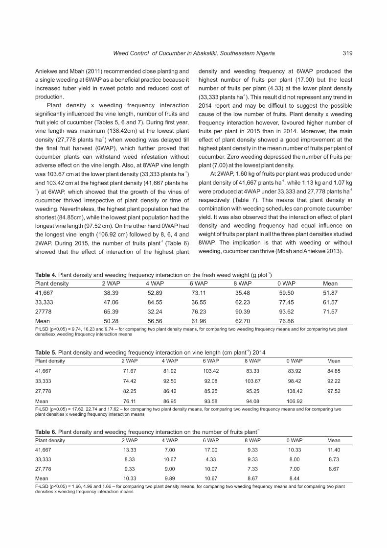
Aniekwe and Mbah (2011) recommended close planting and
a single weeding at 6WAP as a beneficial practice because it
increased tuber yield in sweet potato and reduced cost of
production.
Plant density x weeding frequency interaction
significantly influenced the vine length, number of fruits and
fruit yield of cucumber (Tables 5, 6 and 7). During first year,
vine length was maximum (138.42cm) at the lowest plant -1density (27,778 plants ha ) when weeding was delayed till
the final fruit harvest (0WAP), which further proved that
cucumber plants can withstand weed infestation without
adverse effect on the vine length. Also, at 8WAP vine length -1was 103.67 cm at the lower plant density (33,333 plants ha )
-and 103.42 cm at the highest plant density (41,667 plants ha1) at 6WAP, which showed that the growth of the vines of
cucumber thrived irrespective of plant density or time of
weeding. Nevertheless, the highest plant population had the
shortest (84.85cm), while the lowest plant population had the
longest vine length (97.52 cm). On the other hand 0WAP had
the longest vine length (106.92 cm) followed by 8, 6, 4 and -1 2WAP. During 2015, the number of fruits plant (Table 6)
showed that the effect of interaction of the highest plant
Plant density 2 WAP 4 WAP 6 WAP 8 WAP 0 WAP Mean
41,667 38.39 52.89 73.11 35.48 59.50 51.87
33,333 47.06 84.55 36.55 62.23 77.45 61.57
27778 65.39 32.24 76.23 90.39 93.62 71.57
Mean 50.28 56.56 61.96 62.70 76.86
-1Table 4. Plant density and weeding frequency interaction on the fresh weed weight (g plot )
F-LSD (p<0.05) = 9.74, 16.23 and 9.74 – for comparing two plant density means, for comparing two weeding frequency means and for comparing two plant densitiesx weeding frequency interaction means
Plant density 2 WAP 4 WAP 6 WAP 8 WAP 0 WAP Mean
41,667 71.67 81.92 103.42 83.33 83.92 84.85
33,333 74.42 92.50 92.08 103.67 98.42 92.22
27,778 82.25 86.42 85.25 95.25 138.42 97.52
Mean 76.11 86.95 93.58 94.08 106.92
-1Table 5. Plant density and weeding frequency interaction on vine length (cm plant ) 2014
F-LSD (p<0.05) = 17.62, 22.74 and 17.62 – for comparing two plant density means, for comparing two weeding frequency means and for comparing two plant densities x weeding frequency interaction means
Plant density 2 WAP 4 WAP 6 WAP 8 WAP 0 WAP Mean
41,667 13.33 7.00 17.00 9.33 10.33 11.40
33,333 8.33 10.67 4.33 9.33 8.00 8.73
27,778 9.33 9.00 10.07 7.33 7.00 8.67
Mean 10.33 9.89 10.67 8.67 8.44
Table 6. Plant density and weeding frequency interaction on the number of fruits -1plant
F-LSD (p<0.05) = 1.66, 4.96 and 1.66 – for comparing two plant density means, for comparing two weeding frequency means and for comparing two plant densities x weeding frequency interaction means
density and weeding frequency at 6WAP produced the
highest number of fruits per plant (17.00) but the least
number of fruits per plant (4.33) at the lower plant density -1(33,333 plants ha ). This result did not represent any trend in
2014 report and may be difficult to suggest the possible
cause of the low number of fruits. Plant density x weeding
frequency interaction however, favoured higher number of
fruits per plant in 2015 than in 2014. Moreover, the main
effect of plant density showed a good improvement at the
highest plant density in the mean number of fruits per plant of
cucumber. Zero weeding depressed the number of fruits per
plant (7.00) at the lowest plant density.
At 2WAP, 1.60 kg of fruits per plant was produced under -1plant density of 41,667 plants ha , while 1.13 kg and 1.07 kg
-1were produced at 4WAP under 33,333 and 27,778 plants ha
respectively (Table 7). This means that plant density in
combination with weeding schedules can promote cucumber
yield. It was also observed that the interaction effect of plant
density and weeding frequency had equal influence on
weight of fruits per plant in all the three plant densities studied
8WAP. The implication is that with weeding or without
weeding, cucumber can thrive (Mbah and Aniekwe 2013).
Weed Control of Cucumber in Abakaliki, Southeastern Nigeria 319

Plant density 2 WAP 4 WAP 6 WAP 8 WAP 0 WAP Mean
41,667 1.60 0.87 0.93 1.20 0.93 1.11
33,333 0.67 1.13 0.87 1.17 0.80 0.97
27,778 0.97 1.07 0.90 1.13 0.67 0.95
Mean 1.14 1.02 0.90 1.17 0.80
-1Table 7. Plant density and weeding frequency interaction on the weight of fruits (kg plant ) 2015
F-LSD (p<0.05) = 0.33, 0.26 and 0.33 – for comparing two plant density means, for comparing two weeding frequency means and for comparing two plant densities x weeding frequency interaction means
In view of its growth habit as a creeper as well as a
climber, effects of weeds can relatively be put to a serious
check as a soil cover (un-staked) and as a biological weed
control measure void of environmental disruption and
pollution. This weed control approach (containment) involving
manipulating production factors that favour good crop
establishment, choice of cultivars, land preparation, time of
sowing, crop density and the use of fertilizers proves to be
sustainable. Although, cucumber plants are poor competitors
with weeds at early stages of growth, but can completely cover
the ground within 2WAP for these factors to show significant
interactions on these growth and yield parameters. Some
studies agree that prostrate crops like sweet potato,
cucumber, egusi melon can suppress weeds and reduce early
weeding in maize intercrop (Mbah and Aniekwe 2013) and
plant population trials (Aniekwe and Mbah 2011).
CONCLUSION
In spite of the importance of weed control, there is a
strong reason to do it in an environmental friendly way in view
of the obvious hazards presented by other previous methods,
such as environmental pollution, soil degradation and climate
change. Against this background, biological weed control by
containment is a sustainable alternative to chemical weed
control which is being advocated for in this paper using
cucumber solely or as an intercrop. Apart from controlling
weeds, cucumber provides a suitable source of minerals and
vitamins for man's well being. As high cucumber plant density
and a single weeding at 8WAP will reduce cost of production
without adverse effect on growth and yield in cucumber at a
zero threat to the environment, weed control by containment
technique is sustainable and a recommendable for cucumber
production among the smallholder farmers of developing
nations of the world. Based on this, we highly recommend
that cucumber should be used as an intercrop with cereal
crops that grow erect for effective ground cover, weed
suppression, provision of additional food nutrients and
reduction of cost of production especially in this age of
declining labour force and climate change.
REFERENCES
Adetula O and Denton L 2003. Performance of vegetative and yield accessions of cucumber (Cucumis sativa L),Proceedings of the
st21 annual conference of theHorticultural Society of Nigeria (HORTSON) 10-13 November, 2003.
Aniekwe NL and Mbah MC 2011. Effect of weeding schedules and plant spacings on weed control, growth and yield of sweet potato (Ipomoea batatas (L) Lam) in Abakaliki southeastern, Nigeria, Nigerian Journal of Plant Protection 25(2): 272-279.
Anil S 2000. Time of weed emergence and critical periods in crops, IPM Weed Ecology, Kearney Agricultural Center Bulletin.
Anikwe MAN, Okonkwo CI and Aniekwe NL 1999. The effect of changing land use on selected soil properties in Abakaliki agro-ecological zone, southeastern Nigeria. Journal of Environmental Education and Information 18(1): 78-84.
Das TK 2008. Weed science: Basics and application, Jain Brothers, New Delhi, India, 910pp.
Grubben GHJ and Denton OA (eds.) 2004. Plant resources of tropical Africa: 2 Vegetables, PROTA Foundations, Wageningen, Netherlands/ Backhuys Publishers, Leiden, Netherlands/ CTA, Wageningen, Netherlands, 668 pp.
Hector V, Randall TH and Fakuda S 2000. Field cucumber production guidelines for Hawaii University of Hawaii Cooperative extension service.
Mbah MC and Aniekwe NL 2013. Effect of weed management on the growth and yield of cucumber (Cucumis sativus L) intercropped with maize (Zea mays L) in Southeastern Nigeria, International Multidisciplinary Research Journal 3(2): 23-26.
Ngouajio M and Mennan H 2005. Weed populations and pickling cucumber (Cucumis sativus) yield under summer winter cover crop systems, Crop Protection 24(6): 521-526.
Van Luijk, M N 2004. Cucumissativus L In: Grubben G H J and Denton O A (eds.) Plantresources of tropical Africa: 2 Vegetables, PROTA Foundations, Wageningen, Netherlands/ Backhuys Publishers, Leiden, Netherlands/ CTA, Wageningen, Netherlands, 668 pp.
Wehner TC and Guner N 2004. Growth stage, flowering pattern, yield and harvest dateprediction of four types of cucumber tested at 10 planting dates. Proc. XXVI, Advances invegetable breeding J.D McCreight and E.J. Ryder (eds.) Acta Horticulture 637, ISHS 2004.
Received 31 March, 2018; Accepted 10 May, 2018
N.L. Aniekwe and C.I. Akabueze320

Effects of Paclobutrazol on Growth and Yield Attributes of Groundnut (Arachis hypogaea L.)
Indian Journal of Ecology (2018) 45(2): 321-324
Abstract: A field experiment was carried out to investigate the effect of paclobutrazol (PBZ) as a growth retardant on excessive vegetative
growth and yield of groundnut (Arachis hypogaea L.) at District Seed Farm, under Bidhan Chandra Krishi Viswavidyalaya, Nadia, West Bengal
during kharif season in 2013 and 2014. The experiment was in split-plot with 6 main-plot treatments (PBZ @ 0, 50, 100, 150, 200 and 250ppm)
and 3 sub-plot treatments (single spraying at 30 and 50 days after emergence (DAE) and double spraying at 30 and 50 DAE). During
reproductive stage significantly shorter plants (upto 28% less plant height) were observed due to PBZ application as compared to control. At -2harvest significantly higher dry matter production was recorded from PBZ @ 250ppm (232.1 g m ) and from double spraying at 30 and 50 DAE
-2 -1(231.1 g m ). The number of pod plant and sound mature kernel (%) had showed positive impacts and finally increased the dry pod and haulm -1 -1yield. The maximum dry pod yield was 1745 kg ha and 1610 kg ha with PBZ @ 250ppm and double spraying at 30 and 50 DAE, respectively.
The highest benefit: cost ratio was also from PBZ @ 250ppm and double spraying at 30 and 50 DAE. A highly positive correlation among
different attributes were recorded except plant height which was negatively correlated with other attributes i.e. dry matter production, number -1of pods plant and yield was recorded. Therefore, PBZ @ 250ppm with double spraying had considerable positive influences on number of pod
-1 -1plant , total dry pod yield (Kg ha ) of groundnut as well as on the benefit: cost ratio.
Keywords: Groundnut, Paclobutrazol, Plant height, Dry matter distribution, Yield, Correlation matrix
Manuscript Number: NAAS Rating: 4.96
2679
1Manashi Barman, S.K. Gunri, A.M. Puste and Pankaj DasDepartment of Agronomy, Bidhan Chandra Krishi Viswavidyalaya, Mohanpur, Nadia-741 252, India
1ICAR- Indian Agricultural Statistics Research Institute, New Delhi-110 012, IndiaE-mail: [email protected]
Among the nine oilseeds, groundnut (Arachis hypogaea
L.) is most important in India and takes up a significant place
in the Indian agricultural economy (Madhusudhana 2013).
Despite being a tropical plant, it can be grown in all seasons.
But the main problem during kharif season is the growth of
vegetative parts become rapid which induce the disturbance
in reproductive growth as well as incidence of pest and
diseases. Since its vegetative stage continues along with
reproductive stage, the partition of assimilates is severely
affected with excessive dry matter distribution to stems and
results in low pod yield. For the same reason, yield during
kharif is also lesser than other seasons (Gatan and Gonzales
2015). Considering the above facts application of growth
retardant can be an approach to increase the production of
groundnut by dropping the excess vegetative growth and
proper partitioning of assimilates in the whole plant body
during kharif season. Paclobutrazol (PBZ) [(2RS–3 RS)-1-
4(chlorophenhyl)-4, 4-dimethyl-2-1, 2,4-triazol-1yl-penten-3-
ol], a member of the triazole family encourages different
morphological changes such as shoot inhibition by the
inhibition of gibberellin biosynthesis, increase in the
chlorophyll content and also altered carbohydrate status
(Jaleel et al 2006, Kishorekumar et al 2006). So, PBZ can be
used in order to maintain the balance between vegetative
and reproductive growth by reducing the competition for
assimilate. As a result, more distribution of assimilates to
pods during reproductive stage help in increment of yield
(Arzani and Roosta 2004). Hence, the objective of present
study was to study the effects of different concentrations of
foliar spray of paclobutrazol applied at various times on
growth and yield of groundnut during kharif season.
MATERIAL AND METHODS
The field experiment was carried out at Bidhan Chandra
Krishi Viswavidyalaya, Nadia, West Bengal during kharif
season in the year of 2013 and 2014. The farm is situated at o o23.5 N latitude and 89.0 E longitude with an average altitude
of 9.75 metres above mean sea level. The soil of the
experimental field was alluvial and sandy loam in nature with
good water holding capacity. The fertility status of soil was -almost medium (organic carbon= 0.5%, nitrogen= 231 kg ha
1 -1 -1, phosphorus= 21.63 kg ha and potash= 190.7 kg ha ) and
neutral in reaction (pH= 7.2). The fertilizers were applied as -1per recommended doses (N: P O : K O @ 20: 60: 40 kg ha ).2 5 2
The experimental design, adopted for this research work
was spilt-plot with six different doses of PBZ as main-plot
treatments and three different times of application of PBZ as
sub-plot treatments, which were replicated three times.

Different doses of PBZ were 0, 50, 100, 150, 200 and 250
ppm as T , T T , T , T and T ; the sub-plot treatments were 0 1, 2 3 4 5
viz. single spraying at 30 and 50 days after emergence (DAE)
as S and S , respectively and double spraying at 30 and 50 1 2
DAE (S ). The variety used in this experiment was TG51 3
(Mutant derivatives of TG26 x Chico, Bhaba Atomic
Research Centre, Mumbai) with about 90 days crop duration.
The source of paclobutrazol was CULTAR (23%W/W SC
25% W/V). Different growth attributes such as plant height
(cm) during vegetative stage and reproductive stage i.e. at 45 -2DAE and 75 DAE, respectively; dry matter production (g m )
at 30, 45, 60, 75 DAE and at harvest; number and dry weight
(g) of nodules per plant at 45 and 60 DAE; different yield
attributes like number of pods per plant and sound mature
kernel (%) [Sound mature kernel (%) = {Total weight of
mature kernel (g)/ Total weight of kernel (g)}× 100]; dry pod -1and haulm yields (kg ha ) were recorded during this
experiment. Testing of hypothesis related to correlation
among growth parameters, number of pods per plant and
yield (dry pod and haulm) was implemented by calculating
correlation matrix which was done using software 'R'.
RESULTS AND DISCUSSION
Effect of PBZ on plant height (cm): Application of PBZ in
kharif groundnut had the positive influences to reduce the
plant height (Table 1). With increasing doses of PBZ at 45
DAE, significantly shorter plant height (21.9 cm) (PBZ @ 200
ppm) was statistically at par with PBZ @150 and 250 ppm. In
case of different time of applications of PBZ either single and /
or double spraying at 30 and 50 DAE did not influence the
plant height significantly. The significantly shorter plant
height (45.3 cm) at 75 DAE was with PBZ @ 150 ppm which
was statistically at par with T and T . However there was no 4 5
significant difference in case of double spraying at 30 and 50
DAE (S ) as compared to single sprayings. The inhibition of 3
gibberellin biosynthesis due to PBZ application might have
resulted in declining in plant height. Cheng et al (2006)
showed that by application of PBZ the twig length and stem
height of groundnut were reduced. Sankar et al (2014) also
reported that PBZ treatment decreased the stem length upto
68.53% over control on 80 days after sowing.-2Effect of PBZ on dry matter production (g m ):
Paclobutrazol had no positive influence on dry matter
production at initial stage i.e. at 30 DAE. The dry matter
production at 45 and 60 DAE increased significantly upto the
application of PBZ @ 200ppm, thereafter, decreased with
further increase the doses (PBZ @ 250 ppm) (Table 1). But at
75 DAE and at harvest PBZ upto 250 ppm had the positive
response and significantly maximum dry matter production -2 -2(196.8 g m at 75 DAE and 232.1 g m at harvest) was in the
treatment T . The PBZ @ 150 to 250 ppm were statistically at 5
par among each other and were significantly superior to
control. Double spraying at 30 and 50 DAE (S ) showed the 3
-2significantly higher results at 45 DAE (104.6 g m ) and at -2harvest (231.1 g m ). Despite the reduction in plant height,
the dry matter production was increased and that was might
be as PBZ stimulates the root elongation by inhibiting
gibberellin synthesis and also increases the chlorophyll
content in leaves (Jaleel et al 2006, Kishorekumar et al 2006)
for which more assimilates are produced and partitioned
Treatments Plant height (cm)
-2Dry matter production (g m ) Number of -1nodules plant
Nodule dry -1weight (g) plant
45 DAE
75 DAE
30 DAE
45 DAE
60DAE
75DAE
At harvest
45DAE
60 DAE
45DAE
60DAE
Doses of paclobutrazol (T)
T : control0 30.4 62.8 70.5 93.1 114.5 166.7 194.8 95.3 194.5 0.300 0.491
T : PBZ@50 ppm1 31.3 51.4 71.7 99.0 129.3 162.3 208.3 92.1 167.1 0.304 0.290
T : PBZ @100 ppm2 25.0 45.8 75.1 102.7 136.7 163.2 224.8 101.2 174.2 0.351 0.398
T : PBZ @150 ppm3 24.1 45.3 77.4 103.6 132.3 183.3 225.1 98.7 213.7 0.328 0.432
T : PBZ @200 ppm4 21.9 45.9 75.8 108.1 136.9 185.9 224.3 107.8 203.6 0.316 0.376
T : PBZ @250 ppm5 22.4 48.8 73.6 103.3 135.5 196.8 232.1 112.1 183.3 0.292 0.488
CD (p=0.05) 2.53 4.51 NS 2.60 12.23 19.73 10.52 NS NS NS NS
Time of application (S)
S : single spraying at 30DAE1 25.0 50.65 70.6 89.3 127.0 169.7 208.1 93.7 169.0 0.319 0.349
S : single spraying at 50DAE2 26.8 49.7 74.1 101.2 129.8 178.5 215.5 105.7 206.8 0.321 0.398
S : double spraying at 30 and 50DAE3 25.8 49.55 77.3 104.6 135.8 180.9 231.1 104.2 192.4 0.306 0.490
CD (p=0.05) NS NS NS 1.73 NS NS 7.04 NS NS NS NS
Table 1. Effect of PBZ on growth attributes and nodulation (Pooled over two years)
Manashi Barman, S.K. Gunri, A.M. Puste and Pankaj Das322

Treatments Number of -1pods plant
Sound mature
kernel (%)
-1Yield (kg ha ) B:C ratio
Dry pod
Dry haulm
Doses of paclobutrazol (T)
T0 8.5 86.5 1140 1993 1.62
T1 9.8 87.5 1331 2089 1.78
T2 11.3 87.5 1474 2303 1.91
T3 12.1 87.8 1639 2330 2.05
T4 11.9 87.8 1693 2402 2.06
T5 10.8 87.9 1745 2457 2.06
CD (p=0.05) 1.14 NS 72.5 105.34
Time of application (S)
S1 9.2 86.3 1400 2157 1.79
S2 11.1 88.0 1502 2215 1.92
S3 11.9 88.0 1610 2415 2.03
CD (p=0.05) 1.06 1.45 48.4 70.42
Table 2. Effect of PBZ on yield attributes, yield and B: C ratio (Pooled over two years)
between vegetative and reproductive portions. Kumar et al
(2012) found that PBZ treatments were effective in
shortening plant height along with increasing the number of
stems and stem thickening which finally also contributed to
the total dry matter production. Same result also obtained by
Senoo and Isoda (2003).
Effect of PBZ on number and dry weight of nodules:
There was no significant result of PBZ application on both
number and dry weight (g) of nodules per plant (Table 1). That
means PBZ had no effect on nodulation of plants.
Effect of PBZ on pod number per plant: The significantly
higher pods per plant (12.1) was in PBZ @ 150 ppm, which
was statistically at par with PBZ @ 100 and 200 ppm but
significantly superior to control. In case of time of application
of PBZ, number of pods per plant varied significantly with
double spraying at 30 and 50 DAE (S ). The maximum pod 3
number per plant was in S (11.9) which were statistically at 3
par with S (11.1). The foliar application of PBZ at early stage 2
had no significant influence to increase the pods in groundnut
but at later stage i.e. 50 DAE had the positive response. The
retardation of plant height during reproductive stage might
have resulted in better partitioning of assimilates between
vegetative and reproductive parts which improved the pod
number per plant. Similar finding was attained by other
researchers (Lubis et al 2011, Zhang et al 2013).
Effect of PBZ on sound mature kernel percentage (SMK
%): Due to application of different concentrations of PBZ,
SMK (%) did not vary significantly. But single spraying at 50
DAE (88.0%) as well as double spraying at 30 and 50 DAE
(88.0%) showed significant result. It can be assumed that the
increase in sound mature kernel percentage mainly
depended on the alteration of dry-matter distribution to
kernels due to restrain over stem elongation (Senoo and
Isoda 2003).-1Effect of PBZ on dry pod and dry haulm yield (kg ha ):
Among the different concentrations of PBZ, 250 ppm gave -1significantly higher dry pod yield (1745 kg ha ) which was
statistically at par with PBZ @ 200 ppm. In addition, -1significantly superior dry pod yield (1610 kg ha ) was
observed with the double spraying at 30 DAE and 50 DAE i.e.
S . Therefore, PBZ application at later stages along with early 3
application had positive consequence to increase the pod
yield of groundnut. Lubis et al (2011) and Zhang et al (2013)
also found that PBZ spraying significantly increases pod yield
via increasing the pod number per plant and percentage of
double kernel. Similar kinds of influences of PBZ
concentrations as well as time of applications were observed
for dry haulm yield (aerial portions + roots). Maximum dry -1haulm yield i.e. 2457 and 2415 kg ha were obtained from T 5
in case of doses and S in case of time of applications, 3
respectively. The increase in total dry matter production at
harvesting stage ultimately increased the total dry haulm
yield of plant.
Effect of PBZ on benefit: cost (B: C) ratio: The benefit: cost
was higher in case of PBZ treatments compared to control.
Maximum B: C ratio (2.06) was recorded from both T and T 4 5
treatments and those were 27% more than T . Besides, 0
double spraying of PBZ (S ) presented higher B: C ratio 3
(2.03) than both single treatment i.e. S and S . Despite the 1 2
extra expenditure of higher dose and double application of
PBZ, the B: C ratios were more and that might be due to
additional yield of dry pod and dry haulm in case of the
treatments.
Correlation analysis: In case of different concentrations of
PBZ (Table 3), it can be observed that plant height at 75DAE
was negatively and significantly correlated with other
parameters except with number of pods per plant (r= -0.949)
that was negatively significant at 1% level. Hence, the
reduction in plant height was advantageous to improve the
yield. In addition, positively significant at 1% level correlation
was found regarding dry pod yield with dry matter production
(r= 0.948) and also with dry haulm yield (r= 0.978). For
different times of application of PBZ (Table 4), there was no
significant correlation but plant height was negatively and
highly correlated with other observations. The correlation
result also revealed that dry pod yield had highly positive
correlation with dry matter production at harvest (r= 0.983), -1number of pods plant (r= 0.969), sound mature kernel % (r=
0.858) and dry haulm yield (r= 0.958).
Influences of Paclobutrazol on Growth And Yield of Groundnut 323
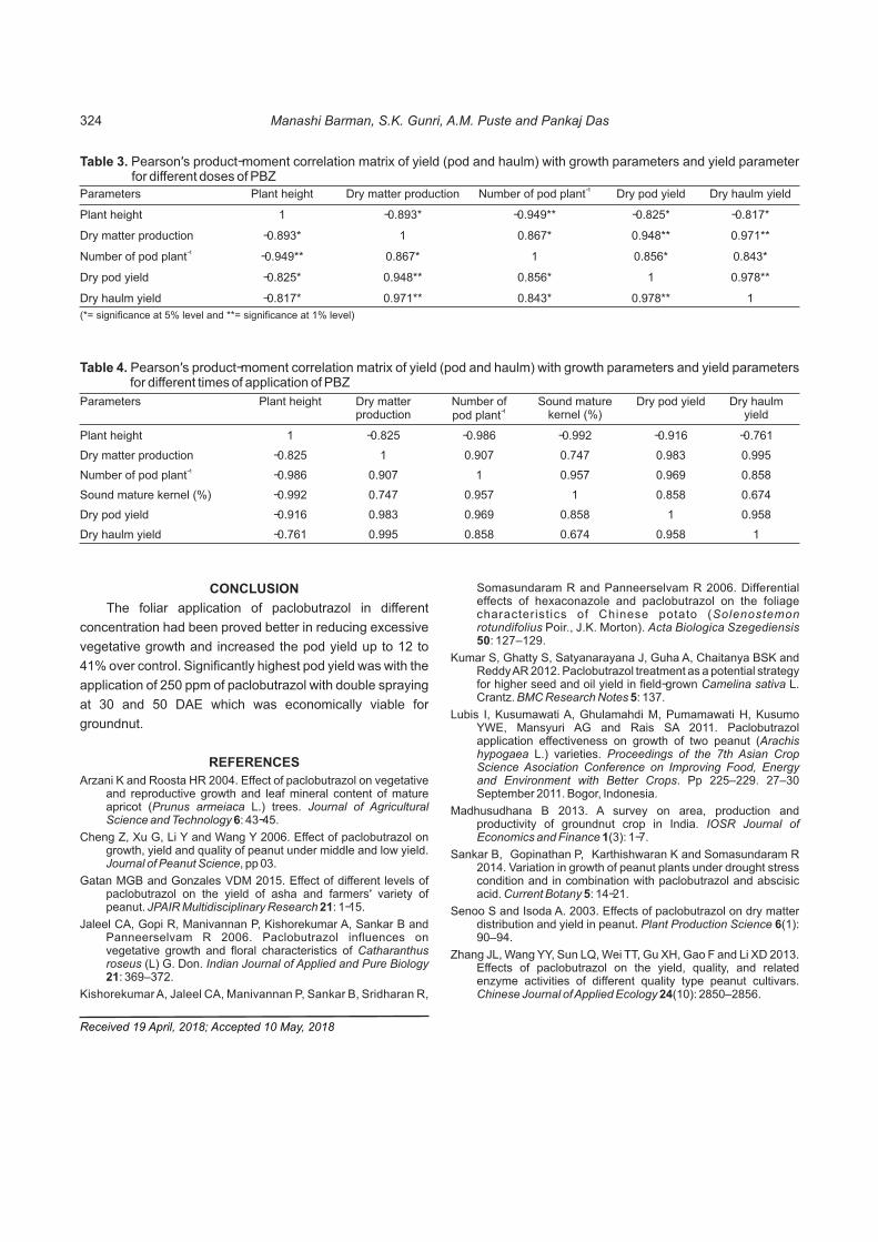
Parameters Plant height Dry matter production -1Number of pod plant Dry pod yield Dry haulm yield
Plant height 1 -0.893* -0.949** -0.825* -0.817*
Dry matter production -0.893* 1 0.867* 0.948** 0.971**
-1Number of pod plant -0.949** 0.867* 1 0.856* 0.843*
Dry pod yield -0.825* 0.948** 0.856* 1 0.978**
Dry haulm yield -0.817* 0.971** 0.843* 0.978** 1
Table 3. Pearson's product-moment correlation matrix of yield (pod and haulm) with growth parameters and yield parameter for different doses of PBZ
(*= significance at 5% level and **= significance at 1% level)
Parameters Plant height Dry matter production
Number of -1pod plant
Sound mature kernel (%)
Dry pod yield Dry haulm yield
Plant height 1 -0.825 -0.986 -0.992 -0.916 -0.761
Dry matter production -0.825 1 0.907 0.747 0.983 0.995-1Number of pod plant -0.986 0.907 1 0.957 0.969 0.858
Sound mature kernel (%) -0.992 0.747 0.957 1 0.858 0.674
Dry pod yield -0.916 0.983 0.969 0.858 1 0.958
Dry haulm yield -0.761 0.995 0.858 0.674 0.958 1
Table 4. Pearson's product-moment correlation matrix of yield (pod and haulm) with growth parameters and yield parameters for different times of application of PBZ
CONCLUSION
The foliar application of paclobutrazol in different
concentration had been proved better in reducing excessive
vegetative growth and increased the pod yield up to 12 to
41% over control. Significantly highest pod yield was with the
application of 250 ppm of paclobutrazol with double spraying
at 30 and 50 DAE which was economically viable for
groundnut.
REFERENCES
Arzani K and Roosta HR 2004. Effect of paclobutrazol on vegetative and reproductive growth and leaf mineral content of mature apricot (Prunus armeiaca L.) trees. Journal of Agricultural Science and Technology 6: 43-45.
Cheng Z, Xu G, Li Y and Wang Y 2006. Effect of paclobutrazol on growth, yield and quality of peanut under middle and low yield. Journal of Peanut Science, pp 03.
Gatan MGB and Gonzales VDM 2015. Effect of different levels of paclobutrazol on the yield of asha and farmers' variety of peanut. JPAIR Multidisciplinary Research 21: 1-15.
Jaleel CA, Gopi R, Manivannan P, Kishorekumar A, Sankar B and Panneerselvam R 2006. Paclobutrazol influences on vegetative growth and floral characteristics of Catharanthus roseus (L) G. Don. Indian Journal of Applied and Pure Biology 21: 369–372.
Kishorekumar A, Jaleel CA, Manivannan P, Sankar B, Sridharan R,
Somasundaram R and Panneerselvam R 2006. Differential effects of hexaconazole and paclobutrazol on the foliage characterist ics of Chinese potato (Solenostemon rotundifolius Poir., J.K. Morton). Acta Biologica Szegediensis 50: 127–129.
Kumar S, Ghatty S, Satyanarayana J, Guha A, Chaitanya BSK and Reddy AR 2012. Paclobutrazol treatment as a potential strategy for higher seed and oil yield in field-grown Camelina sativa L. Crantz. BMC Research Notes 5: 137.
Lubis I, Kusumawati A, Ghulamahdi M, Pumamawati H, Kusumo YWE, Mansyuri AG and Rais SA 2011. Paclobutrazol application effectiveness on growth of two peanut (Arachis hypogaea L.) varieties. Proceedings of the 7th Asian Crop Science Asociation Conference on Improving Food, Energy and Environment with Better Crops. Pp 225–229. 27–30 September 2011. Bogor, Indonesia.
Madhusudhana B 2013. A survey on area, production and productivity of groundnut crop in India. IOSR Journal of Economics and Finance 1(3): 1-7.
Sankar B, Gopinathan P, Karthishwaran K and Somasundaram R 2014. Variation in growth of peanut plants under drought stress condition and in combination with paclobutrazol and abscisic acid. Current Botany 5: 14-21.
Senoo S and Isoda A. 2003. Effects of paclobutrazol on dry matter distribution and yield in peanut. Plant Production Science 6(1): 90–94.
Zhang JL, Wang YY, Sun LQ, Wei TT, Gu XH, Gao F and Li XD 2013. Effects of paclobutrazol on the yield, quality, and related enzyme activities of different quality type peanut cultivars. Chinese Journal of Applied Ecology 24(10): 2850–2856.
Received 19 April, 2018; Accepted 10 May, 2018
Manashi Barman, S.K. Gunri, A.M. Puste and Pankaj Das324

Performance of Groundnut (Arachis hypogaea L) Varieties as Affected by Weeding Frequencies
Indian Journal of Ecology (2018) 45(2): 325-329
Abstract: The field experiment was conducted at Ebonyi State University , Abakaliki during 2014 and 2015 farming seasons to investigate the
effect of weeding regime on the growth and yield of three groundnut varieties. The experiment was laid out in 3 x4 factorial in a randomized
complete block design. The majority of weeds in the experimental site were the broad leaves (dicotyledons), while grasses (monocotyledons)
were in a lesser density. The dominant weeds flora infesting groundnut during growing season were Physalis angulata, Spigelia anthelma and
Cleome viscosa with relative weed density of 27, 21 and 11 per cent, respectively. Samnut 21 produced the lowest number of branches,
number of leaves and days to 50 per cent flowering while Samnut 10 produced the tallesst plant, heaviest pods and seeds, highest number of
seeds and total yield .Weeding at 3 weeks produced the tallest plant, highest leave area index, number of seeds, 100 seed weight and total
yield. The plots without weeding (control) produced the lowest in all the parameters showing that weeds has negative effect on the crop yield.
The result of this research work showed that Samnut 10 with 3 weeks weeding intervals demonstrated highest seed yield and can be
recommended for the farmers in the study area.
Keywords: Groundnut, Dicotyledons weeding, Frequencies, Samnut 21
Manuscript Number: NAAS Rating: 4.96
2680
G.N. Nwokwu, L.G. Ekwu and E.B. UtoboDepartment of Crop Production and Landscape Management, Faculty of Agriculture and Natural Resources Management,
Ebonyi State University, P.M.B 053, Abakaliki, Nigeria. E-mail: [email protected]
Groundnut is a major oil seed crop grown in tropics and
sub-tropic parts of the world. Nigeria is the fourth largest
producer of groundnut after China, India and USA (USDA
2009). It occupies the fourth place among the oil crops in the
world both in area and production next to soybean, sunflower
and cotton (FAO 2015, Garko et al 2015). In United States of - 1America groundnut yield is as high as 3000 kg ha , while the
- 1 average yield in tropical Africa is about 800 kg ha (El Niam et
al 2010). Use of appropriate varieties for a particular ecology
is very vital in groundnut production. Farmers using improved
varieties have derived significant yield gains of 23, 43 and 31
percent over local variets in Mali, Niger and Nigeria,
respectively (ICRISAT 2011). Again, use of aggressive
groundnut varieties can be effective cultural practice for
weed growth suppression. In Nigeria, groundnut yield loss
due to weed infestation could be as high as 51 percent
(Etejere et al 2013). The main problems limiting production of
peanut are poor cultural practices, lack of improved varieties
and inadequate weed management. Page et al (2002)
reported that groundnut cannot compete effectively with
weeds, particularly 3–6 weeks after sowing; therefore, early
removal of weeds is important before flowering and pegging.
The degree of damage caused by the weeds is a function of
their leaf area index (LAI) as compared to the crop they are
competing with (El-Naim and Ahmed 2010). Weed leads to
direct yield losses through competition with the crop for
water, nutrients, lights, space and/or of carbon dioxide. This
degree of damage is mainly a function of their number and
biomass as compared with that of the crop (El Naim et al
2013). Weeds have different competitive abilities which
determines their performance and potential of damage in a
given situations; most important are vigor, growth habit, seed
production, regenerative capacities and time of germination
which is mainly a function of their leaf area index, as
compared with that of the crop (Bedry 2007, Alam 2007).
Weeds constitute a major production problem which
faces farmers in West Africa. In Nigeria, uncontrolled weeds
caused 40-90% yield loss in cereals, 53-60% loss in
legumes, 50-55% loss in oil seeds and 65-91% loss in root
and crops (Etejere et al 2013). Therefore, the objectives of
this study were to investigate the performance of groundnut
varieties as affected by weeding frequencies.
MATERIAL AND METHODS
The field experiments were conducted at Ebonyi State
University, Abakaliki, during the rainy season of 2015 and
2016. The treatments were four weeding frequencies (no
weeding (control), weeding at 3 weeks, weeding at 6 weeks,
and weeding at 9 weeks and three groundnut varieties
(Samnut 10, 11 and 21) which were laid out in 3x 4 factorial
experiment in a randomized complete block design (RCBD)
with three replications. Each replication contained 12 plots

giving a total of 48 plots in the experiment, each plot 2measured 2 x 2 m (4 m ) allowing 0.5 m between adjacent
plots, while 1.0 m separated each replicate. The field was
tilled manually with hoe, while seeds were sown at 2-3 cm
depth at the spacing of 50x50 cm. Weed richness, proportion,
diversity and evenness were calculated using Shannon's
Wiener Diversity Index. Shannon's Wiener Diversity Index
which is represented by H is calculated using the formula : H
= Ó {P(i) x ln P(i)} x -1. The species evenness ranges from
zero to one. The agronomic parameters were also measured
and recorded and were analysed using the General linear
Model in Minitab and the treatment means were compared
using Turkey´s test while the residual effects of treatments
were also tested using Anderson Darling´s test.
RESULTS AND DISCUSSION
The majority of weeds in the experimental site were the
b r o a d l e a v e s ( d i c o t y l e d o n s ) , w h i l e g r a s s e s
(monocotyledons) were found in a lesser density (Table 1).
The dominant weeds flora infesting groundnut during
growing season were Physalis angulata, Spigelia anthelma
and Cleome viscosa with relative weeds density of 27, 21 and
11 percent respectively. Physalis angulata had the highest
frequency of 83, proportion (0.111) and diversity (Table 1).
The lowest frequency (02), proportion (0.027) was of
Dactyloctenium aegyptium. Species richness, evenness
and Shannon Weiner Diversity index for this community were
26, 0.929 and 3.028. This indicate that, the community is
moderately diverse. The diversity of species in a particular
Scientific name Common name Classification Frequency Proportion
Physalis angulata Wildcape gooseberry Broad Leave 83 0.111
Laportea aestuans Tropical nettleweed Broad Leave 32 0.043
Euphorbia heteropylla Spurge weed Broad Leave 26 0.035
Amaranthus spinosis Thorny pig weed Broad Leave 37 0.500
Ageratum conyzoides Goat weed Broad Leave 51 0.068
Commelina benghalensis Wandering jew Broad Leave 45 0.060
Tridax procumbens Tridax Broad Leave 45 0.060
Peporomia pellucida Shiny bush Broad Leave 35 0.047
Cleome viscosa Consumption weed Broad Leave 48 0.064
Solenostemon monostachyus Golden shrimp plant Broad Leave 41 0.055
Scoparia dulcis Broom weed Broad Leave 17 0.023
Spigelia anthelma Worm bush Broad Leave 51 0.068
Senna abtusifolia Sickle pod Broad Leave 46 0.062
Cleome rutidosperma Fringed spider Broad Leave 32 0.043
Aspilia africana Wild sunflowrer Broad Leave 22 0.030
Ghomphrena celosioides Soft khaki weed Broad Leave 27 0.036
Ludwigia abyssinica Water primrose Broad Leave 25 0.034
Kyllinga erecta Creeping sedge Broad Leave 10 0.013
Mariscus altermifolius Angel's wing Sedges 7 0.009
Kyllinga squamulata Asian spike sedge Sedges 18 0.024
Ctperus iria Rice flat sedge Sedges 9 0.012
Cyperuus esculentus Yellow nut sedge Sedges 6 0.008
Fimbristylis littoralis Fringe rush Sedges 15 0.020
Panicum maxmiun Guinea grass Grasses 11 0.015
Dactyloctenium aegyptium Bachelor's button Grasses 2 0.003
Paasspalum scrobiculatum Bahama grass Grasses 4 0.005
Table 1. Weed identification, classification, species richness ,shannon wiener diversity index and eveness in the experimental site
Species richness (X) =26, Shannon Weiner's diversity index H=3.028, Evenness =0.929
G.N. Nwokwu, L.G. Ekwu and E.B. Utobo326

Treatments Plant height(cm)
Numbe rof leaves
Leaf area Index Number of branches
Days to 50% flowering
Variety
Sammaz 10 39.19 b 21.00b 0.69b 5.25b 30.38b
Sammaz 11 38.41c 21.19a 0.74a 5.30a 30.38b
Sammaz 21 39.99a 20.69c 0.72c 5.17c 34.25a
Weeding frequency
Unweeded (Control) 37.01b 17.83d 0.37d 4.46d 30.33c
3 weeks 39.75a 24.50a 0.75a 6.13a 32.25a
6 weeks 40.16a 21.00b 0.70b 5.25b 32.66a
9 weeks 39.85a 20.50c 0.53c 5.12c 31.42b
Table 2. Effect of weeding frequencies on the growth parameters of groundnut varieties
Means followed by same letter (s) within same column and treatment group are notstatistically different at 5% level of probability using Duncan Multiple Range Test (DMRT)
area depends not only on the number of species found but
also in their numbers.
Effect of varieties and weeding frequenices on growth
parameters of groundnut: The varieties used in this
experiment exhibited consistent significance difference in
their growth characters such as plant height, number of
leaves and branches and days to 50 per cent flowering
(Table 2). The tallest plant observed in Samnut 21 is
attributed to its erect growth habit and competition by crops to
intercept greater solar radiation and accumulate greater dry
matter per unit area and per unit time. The widest canopies
observed on plots where samnut 11 were planted indicated
that the variety made adequate use of the soil nutrients to
grow and spread out in conformity with its growth habit. The
increase in the leaf area index, number of branches and
leaves of samnut 10 were attributed to the available nutrients
to crops and its ability to intercept radiation. This is in
agreement with Kamara et al (2011) who reported that
groundnut has the ability to utilize soil nutrients that may be
relatively unavailable to other crops and therefore can make
good use of residual fertility. The variations of the varieties by
days to anthesis and maturity could be attributed to
genotypes differences. The shortening of the days to maturity
promote rapid cell division as reported by Brady and Weil
(2002). Samnut 11 produced the highest leave area index
and the lowest leave area index produced by Samnut 10. The
difference in the mean leaf area index was as a result of the
various varieties which may be attributed to the difference in
the genetic composition of the individual varieties. Variety
had significant effect on number of branches which recorded
its highest at Samnut 11. The lowest number of branches
was produced by samnut 21. There was a deviation as
samnut 21 which had a spreading growth habit had lesser
number of branches while samnut 11 and 10, which have
semi –erect growth habit had higher number of branches.
The result is in agreement with the findings of Ahmad and
Mohammad (1997) who reported that number of branches in
groundnut is a varietal characteristics, controlled largely by
plant genetic factors. The maximum days to 50 per cent
flowering were recorded by Samnut 11.
Weeding at three weeks had a highest plant height.
Weeding facilitates plants to have more resources for growth,
these results agreed with Joshi (2004), Mubarak (2004) and
Bedry (2007) observed that increasing weeding frequency
increased plant height, due to efficient weed control. Weeds
decreased the number of branches per plant. The highest
number of branches per plant was obtained at weeding at
three weeks. This result may be attributed to vigorous plant
with less competition for light, nutrients, and free space in
weed free environment. Increased weeding frequencies
increased leaf area index. This was due to better control of
weeds. The reduced competition and increased availability of
resources like nutrients, soil moisture and light which paved
way for higher leaf area per plant (leaf area index). These
results are conformity with the findings of El Naim et al
(2010).
Effect of variety and weeding frequency on the yield and
yield component of groundnut: The seed yield of the
different varieties was significantly different at the 5 percent
probability (Table 3). Samnut 10 had the higher yield in both
years than Samnut 11 and Samnut 21. Bala et al (2011)
observed that Samnut 10 is inherently higher yielding variety
than Samnut 11 which implies that the variety is more efficient
in the manufacture of assimilate and partitioning of same to
the reproductive sink. This may explain the superiority in
seed yield production of samnut 10 over other varieties as
reported by Kamara et al (2011). Samnut 10 significantly
produced the highest number of pod and pod weight. The
variation in the number of pods per plant were as a result of
the variation in the potential productivity of the groundnut
Performance of Groundnut Varieties under Weeding Frequencies 327

Treatments Pod weight-1(g plant )
Number of seed
Seed weight-1(g plant )
100 Seed weight (g)
Total yeild-1(kg ha )
Variety
Samnut 10 11.94a 65.46a 0.27a 14.44a 1181.25a
Samnut 11 10.06b 54.56b 0.21c 13.75c 984.38b
Samnut 21 9.119c 54.25c 0.23b 14.25b 934.38b
Weeding Frequency
Unweeded (Control) 7.08d 9.83d 0.20b 9.33d 564.58c
3weeks 12.08a 81.92a 0.24a 17.75a 1172.32a
6 weeks 10.42c 81.67b 0.24a 16.25b 1002.08ab
9 weeks 12.00b 58.94c 0.25a 13.25c 993.75ab
Table 3. Effect of weeding frequencies on the yield and yield components of groundnut varieties
Means followed by same letter (s) within same column and treatment group are not statistically different at 5% level of probability using Duncan Multiple Range Test (DMRT)
varieties as reported by Patel et al (2005) who indicated the
spreading and semi-spreading groundnut varieties differ in
their potential productivity. Weeding significantly affected
yield parameters. Weeding at three weeks recorded
significantly the more pod, 100 seed weight, had the highest
number of seeds and total yield while the control treatment
had the least in all the yield parameters. Weeding
significantly affected the 100-kernel weight. Increased
weeding frequencies decreased 100-kernel weight. Weeding
treatments significantly affect the pod yield per plant.
Weeding at three weeks increased pod yield per plant and
improved total yield (t/ha).Weeding increased number of
pods per plant, 100 kernel weight, pods yield per plant and -1final pods yield (ton ha ). This is because hand-weeding
resulted in a better performance of growth and yield
components. Similar results observed by many workers,
Mubarak (2004), Bedry (2007) and Kumar (2009) in
groundnuts and concluded that pod yield increased with
weeding treatments, which encouraged early flowering,
increased flowering, developed higher leaf area index,
increased number of pods and branches per plant and finally
maximized pod yield. Weeding at three weeks resulted in
increased 100-kernel weight. This may be due to better
availability of nutrients and better translocation of
photosynthates from source to sink and may be due to
higher accumulation of photosynthates in the seeds.
Weeding at three weeks had the highest harvest index. This
may be due to better translocation of photosynthates from
source to sink area and may be due to higher accumulation of
photosynthates in the seeds (economical yield).
CONCLUSION
The varieties significantly influenced some of the growth
and yield parameters while weeding regime influenced
almost all the parameters .Samnut 10 with weeding regime at
three weeks produced maximum seed yield which may be
attributed to the varietal characteristics as controlled by
genetic factors on the part of the varieties and reduced
competition for resources and space, efficient dry matter
accumulation for weeding regime.
REFERENCES
Ahmad N and Mohammad R 1997. Evaluation of promising groundnut (Arachis hypogaea) varieties for yield and other characters. Crop and Soil Science 1: 251-260
Alam SM 2007. Weed problems in farming. The DAWN, October 22, 2007. http://www.pakissan.com/english/ news/newsDetail. phpnewsid=15326.
Bala HMB, Ogunela VB, Nkuchinda NC and Tanimu B 2011. Response of two groundnut (Arachis hypogaea L) Varieties to sowing date and NPK fertilizer in a semi arid environment. Yield andyield attributes. Asian Journal of Crop Science 3: 130-140.
Brady NC and Weill RR 2002. The nature and properties of soils (13thed.) Pearson education Ltd., U S A. Pp156-198.
Bedry KA 2007. Effect of weeding regimes on faba bean (Vicia faba L) yield in the Northern State of Sudan University Khartourn . Journal of Agricultural Sciences 15: 220-231.
Cattan P 1998. Flower production and growth in groundnut plants. European Journal of Agronomy 8 (1):13-27.
EL-Naim AM, Abdalrasol O and Ahmed MF 2013. Growth and yield of seed cotton response to plant spacing and weeding frequency under flood irrigation. Journal of Renewable Agriculture 1: 27-32.
El Naim AM and Ahmed SE 2010. Effect of weeding frequencies on growth and yield of two roselle (Hibiscus sabdariffa L) varieties under rainfed. Australia. Journal of Basic Applied Science 4: 4250-4255.
El-Naim AM, Eldoma MA and Abdalla AE 2010. Effect of Weeding frequencies and plant density on vegetative growth characteristics of groundnut (Arachis hypogaea L) in North Kordofan of Sudan. International Journal of Applied Biology and Paceutical Technology 1(3): 1188-1193.
Etejere EO, Olayinka BU and Wuruola AJ 2013. Comparative economic efficacy of different weed control methods in groundnut electronic. Journal of Biological Science (EJBS) 7(2): 10-18.
FAO (Food and Agricultural Organizatiom) 2015. FAO production Yearbook. Vol. 70, Rome Italy.
Garko MS, Mohammed IB, Yakubu AI and. Muhammad ZY 2016.
G.N. Nwokwu, L.G. Ekwu and E.B. Utobo328
Performance of groundnut (Arachis hypogaea L) Varieties as influenced by weed control treatments in Kano State Nigeria. International Journal of Science Technological Resources 5(3): 134-140.
International Crops Research Institute (ICRISAT) 2011. ICRISAT Anual Report. Patuncheru, Andera Pradesh, India. ICRISAT 52pp.
Joshi KR 2004. Effect of time of weeding and levels of N and P, PS fertilizers in the grain yield of Maize. Nepal Agricultural Resources Journal 5: 69-70.
Kamara AY, Ekeleme F, Kwari JD, Omoigui LO and Chikoye D 2011. Phosphorus effects on growth and yield of groundnut varieties in the tropical savannas of Northeast Nigeria. Journal of Tropical Agriculture 49(1-2): 25-30.
Kumar NS 2009. Effect of plant density and weed management practices on the production potential of groundnut (Arachis hypogaea .L). Indian Journal of Agricultural Research 43: 1-5.
Muberak HA 2004. Studies on weed management in irrigated groundnut in Sudan. Ph.D. Thesis faculty of Agricultural Sciences, University of Gezira, Wad Medani, Sudan.
Page WW, Busolo CM, Vander PJA and Chancellor TCB 2002. Recommended groundnut production practices for smallholder farmers in Uganda University of Greenwich. Greenwich London, SE10 9LS.
Patel DP, Murnda GC and Mokidulislam 2005. Dry matter partitioning and yield Performance of HPS groundnut. Division Agronomy ICAR Resources, Indian 30: 156-161.
Ramanatha RV 1988. Botany in groundnut. Indian Council of Agricultural Research, New Delhi. Pp 24-64.
USDA 2009. Foreign Agricultural Sciences, Peanut area, yield and production. www.fas.usda.gov. psdaonline.
Yadava TP and Kumar 1981. Stability analysis for pods yield and maturity in bunch group of groundnut (Arachis hypogeae L). Indian Journal of Agricultural Resources 121: 14-28.
Received 10 April, 2018; Accepted 10 May, 2018
Performance of Groundnut Varieties under Weeding Frequencies 329

Delineation of Rice-wheat Cropped Area using Geo-spatial Techniques
Indian Journal of Ecology (2018) 45(2): 330-336
Abstract: Rice and wheat are the most important food crops of India in term of area, production and consumer preference. India is world's
second largest producer of rice and wheat crop and Punjab, Haryana are the most productive states of rice wheat cropping system. But due to
over exploitation of groundwater resources to irrigate both the crops in these areas, sustainability of rice–wheat cropping is under high threat.
In this paper, rice-wheat cropped area was delineated for Agro Climatic Region (ACR-VI) comprising Punjab, Haryana by using remote
sensing and GIS analysis. Landsat ETM+ and IRS LISS III images were analyzed to delineate area under rice-wheat cropping system during
kharif and Rabi season. Spatial analysis on effective rainfall varied within 230-466 mm during monsoon period in ACR-VI. Based on the rainfall
distribution, groundwater table depth and soil type, potential areas under rice and wheat crops were identified so that most of the crop water
requirement could be met through rainfall and there will be check in use of groundwater to maintain sustainable use of natural resources.
Keywords: Agro Climatic Region-VI, Rice-wheat cropped area, GIS, Remote sensing, Landsat ETM+
Manuscript Number: NAAS Rating: 4.96
2681
1 2Ranu Rani Sethi, A. Sarangi , Amiya Sagar Sahu, K.G. Mandal, R. Aggarwal , 1
K.K. Bandyopadhyay and S.K. AmbastICAR-Indian Institute of Water Management, Bhubaneswar-751 023, India
1ICAR-Indian Agricultural Research Institute, New Delhi-110 014, India2 Punjab Agricultural University, Ludhiana-141 004, India
E mail: [email protected]
Rice and wheat are the major cereals grown all over the
world. In India, rice and wheat production is 103.04 million
tonnes and 94.88 tonnes respectively. Punjab is one of the
most productive states for rice and wheat cropping, which
contributes 12 and 20% to India's rice and wheat production
respectively from only 1.5% of the geographical area. The
expansion of rice–wheat cropping system under the green
revolution turned Punjab and Haryana states into the food
bowl of India, has led to degradation of the natural
environment. More than 90% area in northern states like
Punjab and Haryana is irrigated through groundwater
resources and groundwater decline, rising groundwater table
and salinity is the major concern. Hence sustainability of
rice–wheat cropping system is a big challenge. Global
positioning system (GPS) and geographic information
system (GIS) technologies have been adopted for better
management of land and other resources for sustainable
crop production. Acquiring spatial data in GIS platform and
remote sensing (RS) plays a major role in information
management systems. RS is an accurate, efficient,
economical and reliable technique to prepare a
comprehensive inventory of the natural resources of an area
(Palaniswami et al 2011, Dhanasekarapandian et al 2015).
Many studies demonstrated the effectiveness of using
remotely sensed data as a powerful tool to detect land use
change for critical environmental areas, vegetation dynamics
and urban expansion breakthrough in the method of
acquiring information on land resources, agriculture, forestry,
ocean resources and other studies (Yasodharan et al 2011,
Wulder et al 2012, Crews-Meyer 2004, Laney 2004). The
integration of remote sensing data into monitoring
frameworks has the potential to standardise monitoring
approaches across different spatial scales (Vanden et al
2011). Spectral and contextual information from remote
sensing images and thematic data processed together
resulting in delineation of polygons that is used to support
mapping in field surveys (Schiewe 2002). In object-based
image analysis, region-based multi-resolution segmentation
approach is commonly used. This is a bottom up region-
merging technique in which pixels are merged into
homogeneous land parcel units based on the parameters
defined by homogeneity criteria for different colours and
shapes. However, the algorithms used can lack objective and
reproducible means for defining the parameter values
(Ouyang et al 2011, Tian and Chen 2007). A plethora of
research reports have corroborated the suitability of mapping
and monitoring land cover as an important scientific goal
(Collins et al 2001). Land suitability analysis of Anjarakandi
River basin was carried out using various topographic maps
and satellite imagery. Satellite data from Landsat ETM+ were

used for preparing land use, drainage and contour maps. It
used a weighted overlay methodological approach to
integrate all thematic layers for achieving the designed
objectives (Gopal Krishna and Regil 2014). In this paper,
remote sensing and GIS was used to delineate rice-wheat
coverage areas in ACR-VI region of India and to perform
suitability of rice-wheat cropped area based on soil
properties, cropping pattern and rainfall distribution in ACR-
VI.
MATERIAL AND METHODS
Study area: The study was undertaken in Agro Climatic
Region-VI, which covers the major portion of Punjab and 0 0Haryana state, located between 27.63 N 72.64 E and 32.47
0 0 N 77.59 E and covers the area of 11.4 million ha. Rice during
Kharif and wheat during rabi season are widely grown in this
region. The region has three distinct seasons, viz. winter
(November–March), summer (April–June) and rainy season
(July–October). Average annual rainfall varied within 600-
900mm, out of this 80% occurs during monsoon season of
July–September. The normal annual rainfall is 720 mm in the
Haryana districts and 628 mm in the Punjab districts. The
climate is semi-arid to dry and sub-humid and the soil is
alluvial. Over 80% of the land is sown and over 80% of the
sown area is irrigated (Verma et al 2006).
Remote sensing image analysis: A total of 12 Landsat
ETM+ images with distinctive paths and rows from website
http://glcf.umd.edu for ACR-VI (the states of Punjab and
Haryana) were downloaded for rice area delineation. Out of
12 scenes, acquisition period of three images were in the
month of September 2000 (paddy crowing season) and rest
nine images were for October 2000 (paddy harvesting
season). Similarly, all total 14 IRS LISS III images in January
2012 (8 images) and February 2012 (6 images) were used for
wheat area delineation. ERDAS 9.2 software was used for
data analysis. As acquisition of all the images were not for the
single date so pixel values of each image was different. So
while comparing the images, crop coverage in particular
locations were identified and then analyzed. Then all the
images were processed for mosaicing due to variation in
pixel values and individual districts were clipped out of the
images. False colour composite of band combinations 2,4,7
and 2,3,4 bands of Landsat ETM+ images were considered
for better identifications of land category. For wheat area,
false colour composite was prepared using green, red, and
near infra red bands of the satellites scenes of IRS LISS III
sensor. In order to assist these image interpretation elements
like shape, size, tone, texture, association and pattern were
used. Published crop pattern map developed by Space
Application Centre, Indian Space Research Organization
was used as secondary data to compare the classified
image. All the images were compared to identify the rice
cultivated areas for the months of September and October.
Similarly wheat areas were identified for the month of
January and February. Then delineated rice and wheat areas
were compared with the published report of the state.
GIS (Geographic Information System) analysis:
Topographic maps of Punjab and Haryana were geo
referenced to real World Geodetic Co-ordinate System
(WGS 1984). District wise polygon shape file was generated
to delineate the study area of ACR-VI with attributes
containing the districts name and geographical area. In first
phase, a snapshot was taken from Harmonized world soil
database (HWSD) viewer indicating the ACR-VI boundary
with its all districts boundary. Appropriate soil classes were
selected to cover the entire ACR-VI. The snapshot as image
file was saved and imported to geographic information
system (GIS) interface. With reference to survey of India
(SOI) topo-sheets, the image was geo-referenced, and then
digitized to get a polygon shape file with attributes containing
the soil parameters. The basic soil properties (types) of ACR-
VI were obtained from the HWSD and database was
prepared. Later using the soil texture triangle, soil textural
classes were obtained and map was prepared. Soil texture
map was chosen as first thematic layer for analysis. Then
cropping pattern map of Punjab and Haryana published by
Space Application Centre, Indian Space Research
Organization was taken, geo-referenced and overlaid over
district wise polygon shape file of ACR-VI. The dominant crop
pattern for each district and the same was inserted in the
attribute table of ACR-VI shape file. On this basis, cropping
pattern map was developed. Daily rainfall data of 37 locations
within the ACR-VI was acquired from Indian Meteorological
Department (IMD) for the period from 1994 to 2010. The
mean monthly rainfall depths were calculated for each
location and the monthly effective rainfall depths were
estimated by adopting the USDA SCS method using the FAO
CROPWAT ver. 8.0 software. Rainfall depths occurring
during the pre-monsoon (March, April, May, and June),
monsoon (July, August, September) and post-monsoon
(October, November, December, January and February)
were estimated besides the effective rainfall depths during
these periods. Geographically, to visualise and observe the
distribution pattern over ACR-VI, point shape file was created
importing the coordinates of those 37 locations, attribute
table was created putting the effective rainfall values in the
columns. Interpolation technique was adopted for getting the
values at unknown locations within ACR VI. Krigging
technology was applied to get the effective rainfall range and
their spatial distribution pattern in the study area. Finally,
Delineation of Rice-wheat Cropped Area using Geo-spatial Techniques 331
spatial mapping of effective rainfall was carried out. Then
overlay of thematic layers were performed to identify the
suitability of growing rice and wheat crop in ACR-VI.
RESULTS AND DISCUSSION
Mapping of rice-wheat area using remote sensing image
analysis: Rice-wheat cropping area was delineated for ACR-
VI by using remote sensing and GIS. Landsat ETM+ and IRS
LISS III data with maximum likelihood classifier approach in
image classification were used for delineation of crop
coverage in the study area. It was observed that out of total
area, 2.63 and 1.05 million ha area is under rice in Punjab and
Haryana respectively. In ACR-VI, about 3.68 million ha area
is under rice area (Fig. 1). Similarly wheat area was
delineated for ACR-VI. Resourcesat-2 LISS III data with two
stage classification approach i.e. unsupervised iso-data
followed by maximum likelihood supervised classification
methods were used for delineation of wheat crop coverage
areas. Wheat area was estimated at 3.51 and 2.46 million ha
in Punjab and Haryana respectively. A total of 5.9 million ha
wheat area was delineated in ACR VI region (Fig. 2). Areas
under rice-wheat crop sequence were 2.053 million ha, which
is around 49.06 % of state's total cultivated area. Similarly
combined rice-wheat cultivated areas were estimated at 4.16
million ha (more than 90% of cultivated areas).
Image analysis showed that maximum rice areas were
delineated in Punjab. District wise analysis showed that
Ludhiana and Sangrur districts in the Central Plain Zone
(CPZ) of Punjab showed the maximum areas under rice.
More than 60% of the total cultivated area in the state in the
kharif season is occupied by rice. In sub-montane undulating
zone and undulating plain covering large parts of districts
Ropar, Hoshiarpur, Gurdaspur and Patiala of Punjab state,
rice area has virtually spread to occupy all of the plain land.
Availability of canal and tube well irrigation supplemented by
rain makes large-scale growing of rice quite feasible and
available in the undulating plain zone. Agro climatologically,
the CPZ falls in the low rainfall zone of 400–800 mm. There is
good network of canal system in the state, apart from that
minor irrigation census 2011 showed that Punjab, Haryana
and UP state of India account for 55 per cent of the tube
wells in India. On an average there are 28 tube wells per sq.
km. of net sown area in Punjab alone. The area irrigated by
government canals covers only 29 per cent of the total
irrigated area of the state. On the other hand, net area
irrigated by wells covers 71 per cent of the total irrigated
area of the state. The problem of overexploitation of
groundwater resources is most severe in central Punjab,
usually called sweet water zone and dominated by rice crop
in the kharif season. While the average annual fall in
groundwater table in the central Punjab was about 17 cm
during the 1980s and about 25 cm during the 1990s, it was
alarmingly high at 91 cm per annum during 2000– 2005
(Singh 2011). Analysis revealed that rice and wheat
remained the dominant crops which occupy 57.8 and 64.9%
of total agricultural area, respectively (Choudhury et al 2013).
Similarly, Haryana state is also dominated by rice crop during
the kharif season. Eastern zone of Haryana including districts
of Ambala, Yamunanagar, Kurukshetra, Karnal, Sonipat,
Faridabad, Gurgaon and parts of Rohtak comprises the
major rice-growing area of Haryana. The Kurukshetra-
Karnal-Sonipat-Gurgaon-Faridabad belt is famous for
Basmati rice production. Groundwater quality in this area is
poor and marginal; hence most of the area is dependent on
canal system of irrigation (Narang and Virmani 2001).
Landsat ETM+ satellite image was also used to delineate and
estimate rice crop areas in Haryana state. Remote sensing
and GIS analysis resulted an area of 1051,000 ha under rice
crop, where as the published report indicated an area of
1049,000 ha under rice for the state of Haryana (Sethi et al
2014). In Haryana rice is grown in 18 districts out of 21
districts under irrigated condition only. This has been well
represented in the delineated map of ACR-VI (Table 1).
Satellite image analysis showed that nearly 2626000 ha is
under rice in Punjab, where as published report showed
2611000 ha area is under rice. Similarly, area under rice in
Haryana is 1051,000 ha as per image analysis, whereas it is
1049,000 ha as per the published report.
Hence, there was good agreement on delineation of total
rice area in both the states; however, district wise analysis
showed variation on rice area for these states. Remote
sensing approach was used in other areas for delineating rice
areas. Supervised classification was carried out to make
clusters of pixel values of similar rice crop with same spectral
signature (Dhumal et al 2013). Similarly simplified approach
was used to map rice area in the Indo-Gangetic Basin (IGB)
by combining remotely sensed imagery, national census and
meteorological data. The statistical rice cropped area and
production data were synthesized to calculate district-level
land productivity, which is then further extrapolated to pixel-
level values using MODIS NDVI product based on a crop
dominance map. (Cai and Sharma 2010).
GIS analysis for ACR-VI
Soil analysis: Rice-wheat is the major cropping pattern of
ACR-VI (Fig. 3) followed by cotton-wheat. Mostly, Indo-
Gangetic Plain (IGP) is under continuous deposition of
alluvium from the hills and mountains from both sides of the
plains – the Himalayas in the north and Deccan Plateau in the
south. So, soils of the IGP are Ustochrepts, Aquents,
Naturstalf, and Hapludolls (Tarai region). There are large
Ranu Rani Sethi et al332

lowland patches of heavier soils (silty clay loam to clayey) in
almost all states in the IGP where rice-wheat cropping
system is practiced (Prasad 2007). While delineating soil
map of ACR-VI, all total thirty two numbers of polygons
representing uniform land parcel units were created by
digitization, which comprised of ten number of soil groups.
Major soil groups were presented in Fig. 4 and details of soil
characteristics were shown in Table 2. The sand, silt and clay
percentage varied within 16-89, 6-47 and 5-53 respectively.
The organic carbon content varied within 0.4 to 1.4. The area
is mainly dominated by loamy texture soil. On superimposing
the soil texture map with the cropping pattern map, it was
found that rice-wheat cropping pattern is mainly dominated in
loam soil (Fig. 5). In the loamy soils, the soils were neutral to
alkaline in nature (pH ranged from 6.2 to 8). Organic carbon
content varied within 0.6 to 1.4%. The Leptosol-LP, Lixisol-
LX, Regosol-RG and Cambisol-CM were high in soil organic
carbon content whereas the rest of the soil groups were low
to medium in soil organic carbon content.
GIS Analysis for ACR-VI
Soil analysis: Rice-wheat is the major cropping pattern of
ACR-VI (Fig. 3) followed by cotton-wheat. Mostly, Indo-
Gangetic Plain (IGP) is under continuous deposition of
alluvium from the hills and mountains from both sides of the
plains – the Himalayas in the north and Deccan Plateau in the
south. So, soils of the IGP are Ustochrepts, Aquents,
Naturstalf, and Hapludolls (Tarai region). There are large
lowland patches of heavier soils (silty clay loam to clayey) in
almost all states in the IGP where rice-wheat cropping
system is practiced (Prasad 2007). While delineating soil
map of ACR-VI, all total thirty two numbers of polygons
representing uniform land parcel units were created by
digitization, which comprised of ten number of soil groups.
Major soil groups were presented in Fig. 4 and details of soil
characteristics were shown in Table 2. The sand, silt and clay
percentage varied within 16-89, 6-47 and 5-53 respectively.
The organic carbon content varied within 0.4 to 1.4. The area
is mainly dominated by loamy texture soil. On superimposing
the soil texture map with the cropping pattern map, it was
found that rice-wheat cropping pattern is mainly dominated in
loam soil (Fig. 5). In the loamy soils, the soils were neutral to
alkaline in nature (pH ranged from 6.2 to 8). Organic carbon
content varied within 0.6 to 1.4%. The Leptosol-LP, Lixisol-
LX, Regosol-RG and Cambisol-CM were high in soil organic
carbon content whereas the rest of the soil groups were low
to medium in soil organic carbon content.
Rainfall analysis: Monsoon rainfall varied within 51 to 651
mm in the study area but the rice-wheat areas receive 195 to
484 mm of rainfall with effective rainfall of 156 to 300 mm
(Fig.5). Major crops grown during kharif season in these
areas are rice. Water requirement of kharif rice in Punjab and
Haryana is 730 mm (ENVIS Centre, Punjab 2013). This
showed that maximum water requirement is met through
rainfall if rice is grown in kharif season only. Similarly pre-
monsoon rainfall varies within 0-67 mm with effective rainfall
between 7-64 mm. Post monsoon rainfall varies within 3-32
mm with same amount of effective rainfall. On superimposing
State No. of districts
Area (Govt.records) '000 ha
Area (Imageclassification
analysis) '000 ha
Rice
Punjab 23 2611 2626
Haryana 21 1049 1051
Wheat
Punjab 23 3528 3511
Haryana 21 2522 2464
Table 1. Comparison of rice and wheat cropped area
Id Soil Group Sand (%)
Silt (%)
Clay (%)
Organic carbon content
(% weight)
Bulk density 3(kg/dm )
pH Soil texture
1 Luvisol-LV 81 9 10 0.57 1.41 6.20 Loamy sand
2 Fluvisol-FL 35 47 18 0.60 1.39 8.00 Loam
3 Sand dunes-DS 89 6 5 0.40 1.50 6.40 Sand
4 Calcisol-CL 40 37 23 0.56 1.31 7.90 Loam
5 Solonchak-SC 16 31 53 0.58 1.25 8.30 Clay
6 Leptosol-LP 43 34 23 1.40 1.30 7.60 Loam
7 Arenosol-AR 89 6 5 0.40 1.50 6.40 Sand
8 Lixisol-LX 47 32 21 0.82 1.42 6.20 Loam
9 Regosol-RG 47 34 19 0.97 1.21 6.40 Loam
10 Cambisol-CM 42 36 22 1.00 1.37 6.60 Loam
Table 2. Details of soil characteristics of the study area
Delineation of Rice-wheat Cropped Area using Geo-spatial Techniques 333

Fig. 1. Delineated rice area in Agro-climatic Region VI (Satellite Image Analysis)
Fig. 1. Delineated wheat area in Agro-climatic Region VI (Satellite Image Analysis)
Fig. 3. Major cropping pattern of ACR-VI
Fig. 4. Cropping pattern with soil texture in ACR VI
Fig. 5. Effective rainfall distribution pattern with respect to cropping system
Fig. 6. Status of groundwater table depth in ACR-VI
Ranu Rani Sethi et al334
major cropping pattern of ACR-VI with effective rainfall
distribution, it showed that effective rainfall for rice-wheat
cropping system varied within 230-406, 34-64 and 9-32 mm
during monsoon, pre monsoon and post monsoon season
respectively.
Groundwater table depth: Spatial variation of depth to
water table as per ground water year book in ACR-VI is
presented in Fig. 6. In rice-wheat cropping system maximum
area (24.67 million ha) lies under the water table depth of 10-
20 m followed by 19 million ha under 20-40 m depth to
groundwater (Fig. 6). It has been reported that
overexploitation of groundwater resources is most severe in
central Punjab. The average annual depletion in
groundwater table in the central Punjab was about 17 cm
during the 1980s and about 25 cm during the 1990s; it was
alarmingly high at 91 cm per annum during 2000-2005 (Singh
2011). Out of 142 blocks in the state, water table is declining
in 110 blocks due to over-extraction of water than the
proportionate recharge. By the year 2023, the water table
depth in central Punjab is projected to fall below 21 m in 66 %
area, below 30 m in 34 % area and below 40 m in 7 % area
(Sidhu et al 2010).
CONCLUSION
The rice-wheat area of ACR-VI was mapped through
remote sensing analysis using Landsat ETM+ and IRS
images respectively. There was a good correlation in terms of
quantitative estimation of rice and wheat area between the
analyzed data and the reported information by respective
government departments under the study area. From rice-
wheat delineated areas, the major part of crop water
requirement is not met through rainfall. Hence groundwater is
being extensively used in most part of ACR-VI. Hence choice
of low water requirement crops, appropriate cropping pattern
to fitting the rainfall, improved soil-water-crop management
technologies as well as water saving irrigation methods
should be promoted inorder to sustain the agriculture system
within the limited available water resources.
ACKNOWLEDGEMENT
Authors thank National Agricultural Science Fund
(NASF) of Indian Council of Agricultural Research for
providing financial support for pursuing this research under
the project titled “Decision Support System for Enhancing
Water Productivity of Irrigated Rice-Wheat Cropping
System”.
REFERENCES
Choudhury BU, Sood A, Ray S, Sharma PK and Panigrahy S 2013. Agricultural area diversification and crop water demand
analysis: A remote sensing and GIS approach. J Indian Socierty Remote Sensing 41(1): 71–82.
Collins M, Steiner F and Rrushman M 2001. Land-use suitability analysis in the United states: Historical development and promising technological achievements. Environmental Management 28(5): 611-621.
Crews-Meyer KA 2004. Agricultural landscape change and sustainability in northeast Thailand: Historical patch-level analysis. Agriculture, Ecosystem and Environment 101: 155-169.
Dhanasekarapandian M, Selvan P, Chandran S and Chandramohan K 2015. Land use and land cover dynamic analysis using satellite Remote Sensing and GIS techniques -A case study of Girudhumal river sub basin, Tamilnadu, India. International Journal of Geomatics And Geosciences 5(4).
Dhumal RK, Rajendra Y, Kale KV and Mehrotra SC 2013. Classification of crops from remotely sensed Images: An Overview. International Journal of Engineering Research and Applications 3(3): 758-761.
FAO 1983. Guidelines. Land Evaluation for Rainfed Agriculture. FAO Soils Bulletin No. 52, Rome.
Gopalkrishna GVT and Regil R 2014. Agricultural land suitability analysis of a river basin area using remote sensing and GIS. International Journal of Geospatial Engineering and Technology 1(1): 37- 42.
Lambin EF and Strahler AH 1994. Change-vector analysis in multi temporal space: A tool to detect and categorize land-cover change processes using high temporal resolution satellite data. Remote Sensing of Environment 48: 231–244.
Laney RM 2004. A process-led approach to modelling land change in agricultural landscapes: A case study from Madagascar. Agriculture, Ecosystems and Environment 101: 135-153.
Narang RS and Virmani SM 2001. Rice–wheat cropping systems of the Indo-Gangetic Plain of India. Rice–Wheat Consortium Paper Series 11. RWC, New Delhi, India.
Palaniswami C, Gopalasundaram P and Bhaskaran A 2011. Application of GPS and GIS in Sugarcane Agriculture. Sugar Technology 13(4): 360–365.
Prasad R 2007. Phosphorus Management in the Rice-Wheat Cropping System of the Indo-Gangetic Plains. Better crops-India, 8-11.
Schiewe J 2002. Segmentation of high-resolution remotely sensed data-concepts, applications and problems. International Archives of Photogrammetry and Remote Sensing 34: 380–385.
Serneels S and Lambin EF 2001. Proximate causes of land use change in Narok District, Kenya: A spatial statistical model. Agriculture, Ecosystem & Environment 85: 65-81.
Sethi, RR, Sahu A, Kaledhoknar MJ, Sarangi A, Rani P, Kumar A and Mandal KG 2014. Quantitative determination of rice cultivated areas using geospatial techniques. IOSR Journal of Environmental Science, Toxicology and Food Technology 8(4): 76-81.
Sidhu RS, Vatta K and Dhaliwal HS 2010. Conservation agriculture in Punjab-economic implications of technologies and practices.
65: 413–427.
Singh K 2011. Groundwater depletion in Punjab: measurement and countering strategies. Indian Journal Agriculture Economics 66: 583–589.
Tian J and Chen DM 2007. Optimization in multi-scale segmentation of high resolution satellite images for artificial feature recognition. International Journal of Remote Sensing 28: 4625–4644.
Vanden Borre J, Paelinckx D, Mücher, CA, Kooistra L, Haest B, De Blust G and Schmidt AM 2011. Integrating remote sensing in Natura 2000 habitat monitoring: prospects on the way forward. Journal for Nature Conservation 19: 116–125.
Indian Journal Agriculture Economics
Delineation of Rice-wheat Cropped Area using Geo-spatial Techniques 335

Wulder MA, Masek JG, Cohen WB, Loveland TR and Woodcock CE 2012. Opening the archive: Howfree data has enabled the science and monitoring promise of Landsat. Remote Sensing of Environment 122: 2–10.
Yasodharan S, Balachandar D, Rutharvel MK, Muruganandam R and Kumaraswamy K 2011. Land use/ land cover change detection through using remote sensing and GIS technology-A
case study of St.Thomas Mount Block, Kacheepuram District, Tamilnadu, International Journal of Current Research 3(11): 501-506.
Sharma BR 2010. Integrating remote sensing, census and weather data for as assessment of rice yie;d, water consumption and water productivity in Indo Gangetic river basin. Agricultural Water management 97(2): 302-316.
Received 01 March, 2018; Accepted 10 May, 2018
Ranu Rani Sethi et al336

Effect of Flucetosulfuron on Soil Health in Rice Ecosystem
Indian Journal of Ecology (2018) 45(2): 337-341
Abstract: The present investigation was undertaken to study the impact of the herbicide flucetosulfuron, on soil microbial load during Kharif 0 0 (2016) and Rabi (2016-17) in Kalliyoor Panchayat (8.4455 N and 76.9918 E at an altitude of 29 m above MSL) Kerala, India. Flucetosulfuron
@ 20, 25 and 30 g/ha applied at 2-3, 10-12 and 18-20 days after sowing (DAS) along with two control treatments viz., hand weeding at 20 and
40 DAS and unweeded control comprised the treatments. Microbial count was taken 6 days after spraying the herbicide, using serial dilution
technique. The application of herbicides increased the microbial population in herbicide treated plots which may be because herbicides act as
carbon source for these microorganisms. No significant variation in the microbial population was observed among the herbicidal treatments
and was significantly lower in unweeded control. This indicate that flucetosulfuron is safe to the environment providing healthy and conducive
environment for the microorganisms and the bioindicators of soil quality and health.
Keywords: Earthworms, Flucetosulfuron, New generation herbicides, Soil health, Soil microorganisms
Manuscript Number: NAAS Rating: 4.96
2682
1 2S.R. Arya, Elizabeth K. Syriac, K.S. Meenakumari and Vijayaraghava Kumar1 2Department of Agronomy, Department of Agricultural Microbiology, Department of Agricultural Statistics,
College of Agriculture, Vellayani, Thiruvananthapuram-695 522, IndiaE-mail: [email protected]
Soil health is the capacity of soil to function as a vital living
system, within ecosystem and land use boundaries, to
sustain plant and animal productivity and promote plant and
animal health (Doran and Zeiss 2000). A healthy population
of soil micro and macro organisms can stabilize the
ecological system in soil due to their ability to restore
nutrients to support plant growth (Chauhan et al 2006). The
organisms (bacteria, fungi, actinomycetes, protozoa,
nematodes, earthworm etc.) residing in the soil play
important role in successful functioning of agricultural
ecosystems. Singh and Ghoshal (2012) also reported that for
sustainable agroecosystem, soil microbial biomass and
biological productivity are most essential. Population size of
microorganisms viz., bacteria, fungi and actinomycetes
serves as the bioindicators of the impact of herbicide
application in the agroecosystem (Radosevich et al 2009).
Any change in their populace and activity may affect the
cycling and availability of nutrients which indirectly affect
productivity and other soil functions (Wang et al 2008).
Herbicides have a tremendous role in controlling weeds,
since no viable alternative is presently available to shift the
chemical dependence for weed management in rice (Juraimi
et al 2013). The efficacy of herbicide is evident, but ever
mounting civic concern over the real or perceived impact of
herbicides on public health and environment (Phuong et al
2005) and its effect on soil microbial population (Ayansina
and Osa 2006) has renewed the interest to alternate the use
of herbicide molecules with different mode of action. Among
herbicides, use of low dose, high efficacy herbicides (LDHE)
is becoming more popular due to its high efficacy and
environmental safety. Flucetosulfuron is one of the latest
additions to this array, which is a broad spectrum, systemic
herbicide, inhibiting acetolactase synthase (ALS) enzyme,
thus causing chlorosis of the plant, leading to death of apical
meristems (Paranjape et al 2014). Application of
flucetosulfuron followed by bispyribac sodium (25 g/ha each)
showed excellent control of broad spectrum weeds (WCE-
91-92 %) in wet direct sown and transplanted rice (CRRI,
2013). It is essential to have knowledge of the behavior of
herbicides in the soil to avoid soil pollution and their side
effect on soil macro and micro-organisms. Therefore, in the
present study, an attempt has been made to assess the effect
of flucetosulfuron on soil microbial population i.e., total count
of bacteria, fungi and actinomycetes and earthworm
population under wet seeded system of rice cultivation.
MATERIAL AND METHODS
In order to find out the impact of flucetosulfuron on the
population of soil microbes and earthworm, field
investigations were conducted during Kharif (2016) and Rabi 0 0 (2016-17) in Kalliyoor Panchayat (8.4455 N and 76.9918 E
at an altitude of 29 m above MSL), Kerala, India. A warm,
humid, tropical climate was experienced in the experimental
area. The experiment was laid out in randomised block
design with 12 treatments replicated thrice (Table 1). The soil
was Typic haplaustalf under the order Alfisols. Kanchana

Treatments Before treatment application Six days after treatment application
Kharif (2016) Rabi (2016-17) Kharif (2016) Rabi (2016-17)
T -flucetosulfuron @ 20 g/ha at 2-3 DAS1 4.33 4.67 105.33 (10.27) 82.00 (9.06)
T - flucetosulfuron @ 25 g/ha ,,2 6.33 5.67 101.00 (10.05) 95.67 (9.77)
T - flucetosulfuron @ 30 g/ha ,,3 6.33 5.00 97.00 (9.84) 92.33 (9.60)
T - flucetosulfuron @ 20 g/ha at 10-12DAS4 4.67 5.00 104.33 (10.22) 135.67 (11.65)
T - flucetosulfuron @ 25 g/ha ,,5 5.67 4.67 122.67 (11.07) 136.00 (11.65)
T - flucetosulfuron @ 30 g/ha ,,6 4.67 4.67 90.33 (9.50) 108.00 (10.39)
T - flucetosulfuron @ 20 g/ha at 18-20 DAS7 4 4.33 114.33 (10.70) 112.60 (10.60)
T - flucetosulfuron @ 25 g/ha ,,8 5.67 3.67 111.33 (10.55) 106.67 (10.32)
T - flucetosulfuron @ 30 g/ha ,,9 3.67 4.67 99.33 (9.96) 95.33 (9.76)
T -bispyribac sodium @25 g/ha at 15DAS10 5.67 5.67 97.33 (9.86) 91.00 (9.53)
T -hand weeding at 20 and 40 DAS11 4.67 5.33 52.00 (7.21) 56.33 (7.48)
T -unweeded control12 5.67 4.67 27.67 (5.24) 29.67 (5.43)
CD (p=0.05) NS NS (0.40) (0.67)
6Table 1. Effect of weed management treatments on bacterial population (x 10 cfu/g soil) in soil
cfu- colony forming units. The data were subjected to square root transformation and the values given in parentheses are transformed
(PTB 50), a short duration rice variety, was selected as the
test crop. The size of the experimental plot was 5 m x 4 m
(gross) and 4.7 m x 3.7 m (net). Herbicides were applied on to
the surface of soil using knapsack sprayer with flood jet -1nozzle (spray volume 500 L ha ). The crop was fertilized with
70:35:35 kg/ha N, P and K, where one third N and K and half
P was applied at 15 DAS, one third N and K and half P was
applied at 35 DAS and remaining one third N and K was
applied at 55 DAS. Basal dose of organic manure was
supplied with well decomposed farm yard manure (FYM) with
an analytical value of 0.49, 0.2, and 0.46 % N, P O and K O 2 5 2
respectively. Soil was acidic in reaction, high in organic
carbon (0.83), available phosphorus (25.98 kg/ha) and
available potassium (293.96 kg/ha) and medium in available
nitrogen (291 kg/ha). At the time of sowing, a thin film of water
was maintained in the field and it was gradually increased to 5
cm at tillering and maintained till 2 weeks before harvest. Just
before herbicide application, the field was drained, and
reflooded 48 hours after application. Just before lime
application also the field was drained and was repeatedly
washed 2 days after application. In order to estimate the total
count of bacteria, fungi and actinomycetes in the
experimental plots, soil samples were collected with soil
auger just before herbicide application (JBHA) and 6 days
after herbicide application (DAHA). From each treatment
plot, four samples were collected to a depth of 15 cm and
mixed thoroughly to form a composite sample. The total
count of bacteria, fungi and actinomycetes were assessed by
serial dilution plate technique (Johnson and Curl 1972) using
Nutrient agar, Martin's Rose Bengal agar and Kenknight's
agar respectively. Observations were taken on the colonies
after 24,72 and 168 h for bacteria, fungi and actinomycetes.
Count of earthworm in soil was taken before and after
each field experiment. Before Kharif 2016, one composite
sample was taken by collecting soil randomly from different
parts of the experimental field. After harvest of each crop
earthworm population was enumerated by collecting two
representative samples from each plot. One metre square
wooden frame was used to plot the sampling area. Soil
samples were drawn up to 10 cm depth (Bano and Kale
1991). The soil lumps were broken and the soil was passed
through the fingers to sort out the worms. By passing through
a sieve of 3-4 mm size, the smaller worms were collected.
The worms were then counted.
RESULTS AND DISCUSSION
Microbial population: The herbicide application could result
in significant changes in bacterial population (Table 1). Just
before herbicide application, during both the crop seasons,
the population was non-significant. During Kharif (2016) and
Rabi (2016-17), application of flucetosulfuron @ 25 g/ha at
10-12 DAS recorded the highest bacterial population. During
Kharif (2016), this treatment was on par with its application @
20 g/ha at 18-20 DAS whereas, during Rabi (2016-17), it was
on par with flucetosulfuron @ 20g/ha at 10-12 DAS.
Unweeded control and hand weeding twice recorded
significantly lower bacterial population during both the
seasons though these treatments were not comparable with
each other. The significantly higher bacterial population was
observed in herbicide applied plots. Less inhibitory effect of
sulfonyl urea herbicide on microbial population especially
bacteria was reported by Latha and Gopal (2010). The
S.R. Arya, Elizabeth K. Syriac, K.S. Meenakumari and Vijayaraghava Kumar338

increased microbial population upon herbicide application
might be due to increased supply of nutrients available as
carbon source from the herbicides (Vandana et al 2012, Kaur
et al 2014). Significant differences existed among the
treatments due to herbicide application (Table 2) on fungal
population also. Before herbicide application the fungal
population was non-significant. Similar to the observations
on bacterial population, application of flucetosulfuron @ 25
g/ha at 10-12 DAS recorded the highest fungal population
during both the seasons. However, this treatment was on par
with its application @ 30 g/ha at 10-12 DAS during Kharif
(2016) and during Rabi (2016-17) it was comparable with the
application of flucetosulfuron @ 20 and 25 g/ha at 18-20
DAS. Even though the herbicide applied treatments exhibited
significantly higher fungal population than unweeded control,
these treatments were comparable with the hand weeding
treatment. Baboo et al (2013) reported increased fungal
count in the case of pyrasosulfuron ethyl, a sulfonyl urea th thherbicide, from 7 to 28 day after herbicide application.
Besides this, herbicides can influence fungal count directly or
indirectly by affecting the interaction of fungi with other
microorganisms (Arajuo et al 2003).
The herbicide application exerted significant effect on the
actinomycetes population (Table 3). Before herbicide
application, no significant variation was observed for
actinomycetes population among the treatments. During -1Kharif (2016) flucetosulfuron @ 30 g ha at 2-3 DAS recorded
Treatments Before treatment application
Sixdays after treatment application
Kharif (2016)
Rabi (2016-17)
Kharif (2016)
Rabi (2016-17)
T1 1.00 1.00 13.00 7.33
T2 2.33 1.33 12.33 8.67
T3 1.67 2.33 15.67 6.67
T4 1.33 1.67 12.67 11.67
T5 1.33 2.33 20.33 18.00
T6 1.33 1.67 18.00 7.67
T7 1.33 1.67 15.33 17.67
T8 2.00 2.33 12.33 14.33
T9 1.67 2.00 15.67 12.33
T10 1.00 1.33 13.67 12.33
T11 2.00 1.33 11.67 6.33
T12 1.33 2.00 4.67 2.00
CD (p=0.05) NS NS 3.26 3.72
Table 2. Effect of weed management treatments on fungal 3population (x 10 cfu/g soil) in soil
See Table1 for details
Table 3. Effect of weed management treatments on 4actinomycetes population (x 10 cfu/g soil) in soil
Treatments Before treatment application
Six days after treatment application
Kharif (2016)
Rabi (2016-
Kharif (2016)
Rabi (2016-17)
T1 0.67 1.00 2.33 (1.64)
1.67 (1.46)
T2 0.33 0.67 2.67 (1.77)
3.67 (2.02)
T3 0.67 0.33 3.67 (2.03)
1.67 (1.44)
T4 1.00 1.00 1.33 (1.35)
3.00 (1.84)
T5 1.00 1.00 1.33 (1.35)
2.33 (1.68)
T6 0.67 0.67 2.33 (1.68)
2.00 (1.53)
T7 0.33 0.33 1.33 (1.35)
2.00 (1.56)
T8 0.67 1.00 1.67 (1.44)
2.33 (1.64)
T9 0.33 0.33 1.67 (1.44)
1.67 (1.44)
T10 0.67 1.00 1.67 (1.44)
2.33 (1.68)
T11 0.33 0.33 1.33 (1.35)
1.67 (1.44)
T12 0.33 0.33 0.33 (0.88)
0.33 (0.88)
CD (p=0.05) NS NS 0.46 0.46
See Table1 for details
the highest actinomycetes population, whereas during Rabi
(2016-17), its application @ 25 g/ha at 2-3 DAS recorded the
highest population. Actinomycetes population from the
treatment hand weeding twice was on par with that of
herbicide applied plots during both the seasons. Unweeded
control recorded the lowest population during both the
seasons. Kaur et al (2014) reported that actinomycetes were
less affected as compared to bacteria and fungi and found to
be relatively resistant to herbicides. However, Santric et al
(2016) reported that the effect of herbicide on actinomycetes
population depends on the type of herbicide, application rate,
duration of activity and actinomycete isolate. The constant
population in soil is extremely useful as these microbes play a
major role in the biodegradation of pesticides in the soil
(Yadav 2006).
Enhancement in the bacterial and fungal count at five
days after sowing over the application of azimsulfuron, a
sulfonyl urea herbicide was reported by Nishan (2012) and
Rajagopal (2013). The present study also conforms the
findings of Priya et al (2017) who reported that the increase in
microbial populations might be due to the capability of
utilizing the applied herbicides as carbon source. Bacterial
and fungal population were found significantly and positively
Effect of Flucetosulfuron on Soil Health in Rice Ecosystem 339

Treatments After I crop Before II crop After II crop
T1 6.67 6.67 6.67
T2 5.33 6.67 2.67
T3 5.33 4.00 5.33
T4 8.00 9.33 8.00
T5 9.33 8.00 6.67
T6 6.67 6.67 9.33
T7 8.00 5.33 5.33
T8 4.00 2.67 5.33
T9 6.67 6.67 5.33
T10 5.33 4.00 4.00
T11 5.33 6.67 8.00
T12 10.67 9.33 9.33
CD (p=0.05) NS NS NS
Table 4. Effect of weed management treatments on 2earthworm population in soil (number/m )
See Table1 for details
Parameter Organic Carbon
Kharif (2016) Rabi (2016-17)
Bacterial population 0.531** 0.600**
Fungal population 0.412* 0.510**
Actinomycetes population 0.008 0.230
Earthworm population 0.011 0.082
Table 5. Correlation coefficients of microbial count and earthworm population with organic carbon
**and *- correlation is significant at 0.01 and 0.05 level respectively (2-tailed), n=36
correlated with organic carbon during both the seasons
(Table 5). Even though actinomycetes population exhibited
non-significant correlation with organic carbon content, it
exhibited a positive trend. Islam and Borthakur (2016) also
reported similar results where soil organic carbon was highly
correlated with microbial biomass.
Earthworm population: Critical appraisal of the data (Table
4) revealed that herbicide application did not cause any
significant alterations in the earthworm count before and after
the crop. The earthworm species observed in the
experimental area was Perionyx sansibaricus (Family:
Megascolecidae). Before Kharif (2016) average earthworm
count recorded was 7.33 whereas during Rabi (2016-17)
before the crop the average count was 6.33. After harvest
during Kharif (2016), 6.77 was the average earthworm count
whereas during Rabi (2016-17) after harvest no change was
observed with average count of earthworm. The average
count of earthworm is lower after harvest of Kharif (2016)
crop, compared to its initial count. Dry condition of field at the
time of harvest might be one of the reasons for this reduction.
Even though a slight reduction in the average count of
earthworm could be seen compared to the same before
starting the crop in the field, no alarming reduction due to
herbicide application can be found out in the study. The
results corroborated the findings of Giesy et al (2000) in
which no adverse effects were observed when earthworms
were exposed to glyphosate residues in soil at rates equal to
or greater than labelled rates. Yadav (2006) also observed
that the application of pyrasosulfuron ethyl did not cause any
significant and harmful effect on earthworm population in
wetland rice ecosystem.
CONCLUSION
Flucetosulfuron @ 20, 25 and 30 g/ha applied at 2-3, 10-12
and 18-20 days after sowing (DAS) did not show any inhibitory
effect on microbial population, whereas herbicide application
significantly increase the microbial population. Unweeded
control always reported significantly lower microbial
population and earthworm count and it was not significantly
influenced by any of the treatments. Hence, it can be
concluded that application of flucetosulfuron does not cause
any inhibitory effect on microbial population and earthworm
count irrespective of its dose and time of application.
REFERENCES
Arajuo ASF, Monteiro RTR and Abarkeli RB 2003. Effects of glyphosate on the microbial activity of two Brazilian soils. Chemistry 52: 799-804.
Ayansina ADV and Osa BA 2006. Effect of two commonly used herbicides on soil microflora at two different concentrations. African Journal of Biotechnology 5: 129-132.
Baboo M, Pasayat M, Samal A, Kujur M, Maharana JM and Patel AK 2013. Effect of four herbicides on soil organic carbon microbial biomass-C, enzyme activity and microbial populations in agricultural soils. International Journal of Research in Environmental Science & Technology 3: 100-112.
Bacmaga M, Borowik A, Kucharski J, Tomkiel M and Wyszkowska J 2014. Microbial and enzymatic activity of soil contaminated with a mixture of diflufenican+metsulfuron-methyl+iodosulfuron-methyl-sodium. Environmental Science Pollution Research 22: 643-656.
Bano K and Kale RD 1991. Earthworm fauna of Southern Karnataka, India. In: (eds) Veeresh GK, Rajagopal D and Viraktharnath CA Advances in Management and Conservation of Soil Fauna, Association for promotion of organic farming, Bangalore, pp. 627-633.
Bhimwal JP and Pandey PC 2014. Bio-efficacy of new herbicide molecules for broad spectrum weed control in transplanted rice (Oryza sativa L.). Bioscan 9: 1549-1551.
Chauhan AK, Das A, Kharkwal H, Kharkwal AC and Varma A 2006. Impact of microorganisms on environment and health. In: Chauhan AK and Varma A (eds) Microbes: Health and environment. U.K.
Cochran WC and Cox GH 1965. Experimental Designs. John Wiley and Sons Inc., New York, 225p.
CRRI [Central Rice Research Institute]. 2013. Annual Report 2013-2014. Central Rice Research Institute. Cuttack. 192p.
S.R. Arya, Elizabeth K. Syriac, K.S. Meenakumari and Vijayaraghava Kumar340

Doran JW and Zeiss MR 2000. Soil health and sustainability; managing the biotic component of soil quality. Applied Soil Ecology 15: 2-11.
Giesy JP, Dobson S and Solomon KR 2000. Ecotoxicologicalrisk assessment for roundup herbicide. Reviews of Environmental Contamination and Toxicology 167: 35-120.
Islam NF and Borthakur 2016. Effect of different growth stages on rice crop on soil microbial and enzyme activities. Tropical Plant Research 3: 40-47.
Johnson LF and Curl E A 1972. Methods for Research in the Ecology of Soil-Borne Plant Pathogen. Burgers Publication Co., Minneapolis. 247 p.
Juraimi AS, UddinMd K, Anwar Md P, Mohamed MTM, Ismail MR and Man A 2013. Sustainable weed management in direct seeded rice culture: A review. Australian Journal of Crop Science 7: 989- 1002.
Kaur S, Singh S and Phutela RP 2014. Effect of herbicides on soil microorganisms in direct-seeded rice. Indian Journal of Weed Science 46: 229-233.
LathaP C and Gopal H 2010. Effect of herbicides on fluorescent pseudomonads and spore forming bacilli. Asian Journal of Bioscience 5:211-215.
Nishan M A 2012. Management of water cabbage (Limnocharis flava (L.) buchenau) in wetland rice ecosystem. M.Sc. (Ag) thesis, Kerala Agricultural University, Thrissur, 150 p.
Paranjape K, Gowariker V, Krishnamurthy VN and Gowariker S 2014. The Pesticide Encyclopedia. [e-book]. CABI. p.209. Available at: www.cabi.org/bookshop /book/9781780640143 [30-10-2015].
Phuong LT, Denich M, Vlek PLG and Balasubramanian V 2005. Suppressing weeds in direct seeded lowland rice: effects of methods and rates of seeding. Journal of Agronomy and Crop
Science 191: 185-194.
Priya RS, Chinnuswamy C, Arthanari PM and Janaki P 2017. Microbial and dehydrogenase activity of soil contaminated with herbicide combination in direct seeded rice (Oryza sativa L.). Journal of Entomology & Zoology Studies 5: 1205-1212.
Radosevich SR, Holt J and Ghersa CM 2009. Weed ecology implication for management. John Wiley and Sons, New York. 189p.
Raj SK and Syriac EK 2017. Herbicidal effect on the bio-indicators of soil health- A review. Journal of Applied & Natural Science 9: 2438-2448.
Rajagopal K 2013. Evaluation of new generation herbicides in transplanted Rice (Oryza sativa. L). M.Sc. (Ag) thesis, Kerala Agricultural University, Thrissur, 150p.
Santric L, Radivojevic L, Umiljendic JG, Saric-Krsmanovic M and Durovic-Pejcev R 2016. Effects of herbicides on growth and number of actinomycetes in soil and in vitro. Journal of Pesticides & Phytomedicine (Belgrade) 31: 121–128.
Singh P and Ghoshal N 2012. Variation in total biological productivity and soil microbial biomass in rainfed agro ecosystems: Impact of application of herbicide. Agriculture, Ecosystem & Environment 137: 241-250.
Vandana LJ, Rao PC and Padmaja G 2012. Effect of herbicides and nutrient management on soil enzyme activity. Journal of Rice Research 5: 50-56.
Wang QK, Wang SL and Liu YX 2008. Responses to N and P fertilization in a young Eucalyptus dunnii plantation; microbial properties, enzyme activities, and dissolved organic carbon. Applied Soil Ecology 40: 484-490.
Yadav IP 2006. Bioefficacy and residual effect of new generation herbicide pyrazosulfuron ethyl in transplanted rice. Ph.D. thesis, Kerala Agricultural University, Thrissur, 207p.
Received 16 March, 2018; Accepted 10 May, 2018
Effect of Flucetosulfuron on Soil Health in Rice Ecosystem 341

Towards Unsustainable Resource use in Punjab Agriculture
Indian Journal of Ecology (2018) 45(2): 342-346
Abstract: This paper makes an attempt to develop a composite index to measure sustainability of resource-use for Punjab state.
Sustainability in agriculture has evolved overtime. In present perspective, its definition has been centred on optimal resource-use, maintaining
environment quality. In consequence, the indexis based on three resource components, namely, land, water and air. The data were deployed
on five indicators pertaining to these components from 1970 to 2015. The overall index shows decline in resource sustainability in entire
Punjab. Majorly, districts in central and south-western region have become highly unsustainable overtime. Thus, a regular assessment of
sustainability of resource-use is required and this index can be useful for effective policy decision making. The overall index highlights the
nature of resource sustainability. It raises awareness and understanding of district level differences in sustainability. It aims to trigger
interventions leading to sustainable solutions in agriculture for Punjab.
Keywords: Land productivity, water deficit, air pollutant emissions, unsustainability, Punjab
Manuscript Number: NAAS Rating: 4.96
2683
Garima Taneja, Swati Rawat and Kamal VattaCenters for International Projects Trust, New Delhi, Punjab
E-mail: [email protected]
Natural resources, specifically land, water, soil, climate
and ecosystem services are essentially required for efficient
functioning of agricultural systems. Historically, agricultural
sustainability largely focused on increasing agricultural
productivity; it did not take into account the adverse effects of
rising productivity on the natural resources (Faeth 1993,
Lockeretz 1988, Ruttan 1988). The agricultural sustainability
definition was revisited after the World Commission on
Environment and Development published a report “Our
Common Future”, it proposed a much wider scope of defining
sustainability while including economic, social, political and
ecological dimensions (Brundtland 1987). Later studies
emphasized sustainable agriculture “as enhancing the
environment quality and resource base on which agriculture
depends, is economically viable and enhances the quality of
life for farmers and society as a whole”. Subsequently,
integrated natural resource management was conceived as
the most important component for improving livelihoods,
agro-ecosystem resilience, agricultural productivity and
environmental services particularly for developing countries
(Douglass1984, Allen et al 1991, Pretty 2008).
In India, agriculture plays a dominant role in improving
rural livelihoods and farm incomes. The green revolution
since late-1960s accelerated the cereal production faster
than the rate of population growth during 1965-2000
(Swaminathan 1993; 1996b; 1999). The success of green
revolution was largely visible in the northern parts of India,
particularly Punjab, as the state was able to reap its benefits
more effectively as compared to the other Indian states.
Unfortunately, though, the success came at the expense of
natural resources such as land, water and air and the results,
like depletion of groundwater table, deterioration of soil
quality, stagnating productivity and declining farm incomes,
are clearly visible (Sidhu 2002, Singh 2009, World Bank
2010). These adverse impacts on land, water and air
resources have mostly been assessed subjectively, but
quantification of such impacts, which can be extremely useful
for analysing the status of agricultural sustainability has not
really been explored. The current study addresses the multi-
dimensional nature of sustainability of resources such as
land, water and air in Punjab agriculture by developing a
composite index for all such indicators.
MATERIAL AND METHODS
Study area: The study was carried out for the state of
Punjab, situated between 29°30´- 32°32´´N and 73°55´ -
76°50´´E, with the geographical area of 50,362 sq.km,
accounting for 1.54 per cent of the total geographical area of
the country.
Indicators of resource sustainability: Globally, assessing
the sustainability of natural resources largely examined the
changes in soil fertility, land productivity, water management,
and the use of chemical fertilizers. Within India, several
studies have measured the sustainability of agriculture by
separately using indicators such as productivity, fertilizer
consumption, soil fertility, declining in water depth etc. But,
most of them do not integrate natural resources such as land,
water and air in evaluating the sustainability of agricultural
systems, primarily due to lack of data on appropriate
indicators and unavailability of data at district level. In this

study, we have attempted to evaluate the resource
sustainability by examining the trends of indicators on land,
water and air resources. The list of indicators and
corresponding variables selected for the study has been
listed in Table 1.
Development of resource sustainability index: In this
paper, spatial aspects of resource sustainability have been
emphasized by proposing a composite index of resource
sustainability at the district level. A total of four key indicators
were shortlisted for which sufficient and credible time-series
data were available. The data were obtained from the
Statistical Abstracts of Punjab, were normalized and a
composite index was developed using the Iyengar and
Sudershan method (Iyengar and Sudershan 1982). The
resource sustainability index was estimated for four periods
i.e. triennium ending 1980-82, 1990-92, 2000-02, 2009-11
and 2014-15 to study and compare decadal changes. The
methodology is convenient for the development of composite
index of sustainability.
Let X represent the size or value of the i-th sustainability id
indicator in the d-th district of a state (i=1,2,……m, d
=1,2…..n say). If X is negatively associated with id
sustainability, as for example fertilizer consumption or
cropping intensity is high then the district tends to move
towards unsustainability then it is written as equation 2.1: -
Where Min X and Max X are respectively the minimum id id
and maximum of (X X ……..X ). If however X is positively i1, i2, in i
related to sustainability, then it equation 2.2 is use: -
From equation 2.1 and 2.2 we have obtained scales
values of y which vary from zero to one. From the matrix of id
scaled values, Y = ((y )) we construct a measure for the stage id
of sustainability for different districts as follows: -
Where the w's (0<w<1 and w +w +…….,w =1) are 1 2 m
weights which reflects the relative importance of the
individual indicators.
It is assumed that the weights vary inverse y as the
variation in the respective indicators of development. More,
specifically, we assume: -
The weights were obtained for overall sustainability and
were multiplied with the standardized values and find indices
were obtained for sustainability. The choice of the weights in
this manner ensured that large variation in any one of the
indicators will not dominate the contribution of rest of the
indicators, so that inter-district comparisons are not distorted.
For the purpose of classification, a simple ranking of district
indices (yd) could done, but for more meaningful
characterization of the different stages of sustainability,
suitable fractile classification from an assumed distribution is
needed. The probability distribution which is widely used in
this context is â-distribution. This distribution is defined by
equation 2.6: -
The distribution has two parameters a and b which can
be estimated by comparing the following equation 2.7 and 2.8
(y-m)a-mb = m-y (Equation 2.7)
(1-y)a -yb =0 (Equation 2.8)
Where y is the mean of district indices2 2m = sy + y (Equation 2.9)
2sy is variance of district indices. Once the values of a
and b are obtained, they are distributed with 20% interval and
finally five classes are obtained and districts were ranked
accordingly: (i) least, if 0 <y <z ; (ii) less, if z <y <z ; (iii) d 1 1 d 2
moderate, if z <y <z ; (iv) high, if z <y <z ; and (v) higher, if 2 d 3 3 d 4
z <y <1.4 d
The paper develops an overall resource sustainability
index, land productivity, cropping intensity, fertilizer use,
water deficit and emission index. It indicates that high index
values show lower consumption of resources, whereas lower
index shows higher or greater exploitation of resources.
RESULTS AND DISCUSSION
Land productivity, cropping intensity and fertilizer use
indices: Land productivity has been a dominant indicator of
the agricultural growth and sustainability and is defined
usually as crop output per unit of land (Zhen and Routray
2003, Pretty 2008, Mellor 2001, World Bank 2008). Figure 1
reveals that Punjab had lower land productivity during early
1970s, but it increased considerably after that, slowing down
during 1990s. Districts lying in the central and south-western
region registered further shift towards higher land
productivity during 1990s and 2000s. The index of land
productivity increased tremendously from 0.4 in 1970s to 0.6
in 2000s with slight decline in 2010 (i.e. 0.5). This is mainly
due to stagnant growth in irrigation and cropping intensities
(GOP 2013). However, in 2015 some improvement is seen in
land productivity as more districts showed an increased
yid = Max X – Xid id
Max X – Min Xid id
(Equation 2.1)
yid = X – Xid idMin
Max X – Min Xid id
(Equation 2.2)
yd = w y + w y + ....... + w y (Equation 2.3)1 id 2 2d m md
_
)var( i
iy
kW = (Equation 2.4)
1
1 )var(
1-
=úúû
ù
êêë
éå
i
m
i ywhere k = (Equation 2.5)
f(z) =
a-1 b-1x (1-x)
b(a,b), 0 < x < 1 and a, b >0 (Equation 2.6)
Towards Unsustainable Resource use in Punjab Agriculture 343

Natural resources Indicators Variables
Land Land productivityFertilizer consumptionCropping intensity
Combined yield of Rice-wheat (kg/ha)Fertilizer consumption per unit of land (kg/ha)Ratio of gross cropped area upon net sown area (%)
Water Water demand and supply gap 3Gap between agricultural water demand and supply (m /ha)
Air Crop residue burning emissions Emissions from crop residue burning(tons/ha)
Table 1. Indicators and variables selected for measuring resource sustainability index
Notes: 1.Districts Mansa and Fatehgarh Sahib were created in 1992, hence data of these districts is included in Bathinda and Patiala respectively.2. DistrictsMuktsar, Moga and Nawanshehar were created in 1996, Data of Muktsar and Moga included in Faridkot and that of Nawanshehar in district Jalandhar. 3. Districts Tarn Taran, Nawanshehar and Barnala were created in 2006 hence data of these districts is included in Amritsar, Rupnagar and Patiala, Sangrur district respectively
Fig. 1. Indices of land productivity, cropping intensity and fertilizer consumption
value of the index. Cropping intensity index indicates the
intensification of land resource in the five decades. During
1970s and 1980s almost entire Punjab region was
sustainable. The degree of RW intensification increased in
1990s as almost half of the districts in the region became
unsustainable. By 2000 and 2010, all the districts became
unsustainable as the index declined to 0.449 from 0.7 in
1980s Kapurthala, Ludhiana, Sangrur and Patiala are highly
unsustainable districts, since the cropping intensity remained
more than 190%in the last two decades (Fig. 1). The situation
hasn't seen much change in 2015.
Another important factor affecting the land resource is
the high use of chemical fertilizers. The fertilizer use index
shows aless fertilizer consumption in 1970sand 1980s.
Districts such as Kapurthala and Ludhiana begin to high
fertilizer-use. Butin1990s many of the districts in central
region became potentially unsustainable with index falling to
0.38 from 0.71 (Fig. 1). The trend remained similar in
2000.Post 2000s, use of chemical fertilizers became
tremendously high which resulted in; central region been
entirely shifted from potentially unsustainable to highly
unsustainable categories, index value falling from 0.38 to 0-
0.22 (Fig. 1). A similar trend was visible in 2015, with
Jalandhar, Ludhiana, Fatehgarh Sahib, Patiala and Moga
remained highly unsustainable.
Water resource and Air pollution indices: The water deficit
index indicates the gap between agricultural water demand
and supply. In 1970s, the entire Punjab region seemed
sustainable and by 1980s few districts in central region such
as Ludhiana, Fatehgarh Sahib, Patiala, Sangrur and
Barnalaregistered a decline in sustainability category, with
index value falling from 1 to 0.76 (Fig. 2). In 1990s, districts in
central and south western region shifted towards
unsustainable and potentially unsustainable category.
Ludhiana, Patiala, Fatehgarh Sahib, Firozpur and Fazilika
shifted to unsustainable category, with index declining to
0.54. Kapurthala, Jalandhar, NawanShehar and Mansa
districts shifted to potentially unsustainable category with
index declining to 0.67. A similar trend is visible in 2000s.
While post 2000s, water deficit rose in entire Punjab, with
Garima Taneja, Swati Rawat and Kamal Vatta344

Fig. 2. Indices of water deficit and air pollution
Fig. 3. Resource sustainability index
districts in central region been immensely affected. In 2015,
the gap further aggravated the entire central, south-western
and north-western region became unsustainable with index
declining to 0.54 from 1(Fig. 2).
With rising productivity and amount of crop residue
generated in the state has increased. Since crop residue
burning is the most common farm practice to remove the
residues and prepare the field well on time for the next crop.
The emission index indicates emissions due to crop residue
burning. In 1970s, low crop productivity led to less amount of
residue generation. Due to on farm residue burning was very
less, so were the air pollutant emissions. The index started
rising in 1980s and by 1990s with high use of modern
varieties and farm mechanization, amount of residue
generated on the field increased specifically in the central
region. The emission index value in Ludhiana, Patiala,
Fatehgarh Sahib reached to 0.49 from 0.74. In 2000 and
2010, massive amount of air pollutants were emitted. Again,
the central region became unsustainable in which Ludhiana,
Moga, Sangrur Patiala and were highly unsustainable as the
emission index value ranged from 0-0.496. By 2015, the
number of districts in unsustainable category increased.
Thus, the index for Kapurthala, Firozpur, Fazilka, Faridkot,
Moga, Ludhiana, Jalandhar, Fatehgarh Sahib, Patiala,
Sangrur, Barnala, has seen fall from 0.74 in 1970s to 0.49 in
2015.
Trends in overall resource sustainability: The overall
sustainability index indicates the district-wise resource use of
land, water and air. The highest index value declined from 1
in 1970s to 0.62 in 1990s and further to 0.49 in 2015 (Fig. 3).
A similar trend was seen in the lowest index which decline
from 0.69 in 1970s to0.49 in 2015s. All the districts during
1970s and 1980s were either sustainable or fairly
sustainable. The index was very high ranging from 0.69 to 1
(Fig. 3). In 1990s, the index values considerably declined.
This decade transformed the Punjab story, as it marked the
beginning of unsustainable resource use. It includes different
degrees of sustainability, which is represented in different
clusters of districts in the state. At first, the potentially
unsustainable districts include Firozpur, Fazilka, Amritsar,
Gurdaspur and Pathankot, with index value ranging between
0.57-0.62. Secondly, Sangrur, Patiala, Kapurthala and
Fatehgarh Sahib were unsustainable with index ranging from
0.49-0.57. Lastly, Ludhiana was the only highly
unsustainable district with index value ranging from 0-0.49
(Figure 3).
The districts which were sustainable in the 1990s
became unsustainable in 2000s as indicated by the fall in
index values. Only Hoshiarpur and Rupnagar were fairly
sustainable in 2000s as index value reduced from 0.69 to
0.62. In 2010s, districts in the central regions became critical
with lowest index value ranging from 0 to 0.49. By 2015,
districts in central, south-western and Mandi region became
unsustainable with index falling from 0.68 in 1970 to 0.49 in
Towards Unsustainable Resource use in Punjab Agriculture 345

2015 (Figure 3). Analysis of five decades depicts the march
towards highly unsustainable resource use affecting the
sustainability of agricultural systems. The index directly
points the need for a greater focus on addressing the
sustainability issues in the districtsof Ludhiana, Amritsar,
Kapurthala, Jalandhar, Moga, Sangrur, Firozpur, Faridkot,
Muktsar, Fazilka, Patiala, Gurdaspur and Pathankot.
CONCLUSION
Resource sustainability of Punjab state is critical for the
agricultural economy of India. The assessment of resource
sustainability reveals that green revolution led to gains in
productivity but was practised without adhering to scientific
principles, and hence proved to be detrimental to natural
resources, which are essential for advancement in
productivity. The index reveals the magnitude of damage to
land, water and air resources during the last four decades. In
1970s and 1980s, the extent of resource sustainability was
low. In 2000s and 2015, the sustainability of resources
entered into “overexploitation phase”, resulting in rising cost
of cultivation, stagnation of productivity and farm income.
Moreover, high variability in terms of resource sustainability
was visible among the districts. Around 40% of the districts in
Punjab were found to be highly unsustainable and therefore,
demand greater attention. For improving resource
sustainability, a system should be developed for productivity
enhancement with improvement in soil, water, biodiversity,
atmosphere etc. For this system sustainable agriculture
technologies should be developed enhancing resource
conservation. Along with technological development, regular
monitoring and measurement of resource sustainability is
required at micro level such as district and farm level. The
resource sustainability is an appropriate tool which can be
used for monitoring the sustainability of agriculture systems.
It can be used by the policy makers to identify regions which
require more stringent actions. For better planning for
sustainability, more quantifiable accounting of resources
should be done for achieving long term sustainable
agriculture.
ACKNOWLEDGEMENT
We acknowledge the financial support by United States
Agency for International Development, Washington D.C.,
USA to carry out this research work.
REFERENCES
Allen P, Van dusen D, Lundy J and Gliessman S 1991. Integrating social, environmental and economic issues in sustainable agriculture. American Journal of Alternative Agriculture 6(1): 34-39.
Brundtland GH and World commission on environment and development 1987. Our common future: report of the world commission on environment and development. Oxford university, New York, USA.
Douglass GK 1984. The meanings of agricultural sustainability, pp 1-29. In: Douglass GK(eds). Agricultural Sustainability in a Changing World Order. Boulder CO, West view press.
Faeth P 1993. Evaluating agricultural policy and sustainability of production systems: An economic framework. Journal of Soil and Water Conservation 48(2): 94-99.
G o v e r n m e n t o f P u n j a b ( G O P ) 2 0 1 3 . http://agripb.gov.in/home.php?page=astat.
Iyengar SS and Sudershan PL 1982. A method of classifying regions from multivariate data. Economic and Political Weekly 17(51): 2043-2052.
Lockeretz W 1988. Open questions in sustainable agriculture. American Journal of Alternative Agriculture 3(4): 174-181.
Mellor 2001. Faster more equitable growth. Agriculture, employment multipliers and poverty reduction. Paper prepared for USADD/G/EGAD.
Pretty JN 2008. Agricultural sustainability: concepts, principles and evidence. Philosophical Transactions of the Royal Society B 363(1491): 447-465.
Ruttan VW 1988. Sustainability is not enough. American Journal of Alternative Agriculture 3(2-3): 128-30.
Sidhu HS 2002. Crises in agarain economy in Punjab: Some urgent steps." Economic and Political Weekly 37(30): 3132-38.
Singh K 2009. Act to save groundwater in Punjab: Its impact on water table, electricity subsidy and environment. Agricultural Economics Research Review 22: 365-86.
Swaminathan MS 1993. Wheat revolution: A Dialogue. The Macmillan Company,Chennai, India.
Swaminathan MS 1996b. Sustainable Agriculture: Towards Food Security. M.S. Konark publishers pvt ltd, Delhi, India.
Swaminathan, MS 1999. A Century of Hope: Towards an Era of Harmony with Nature and Freedom from Hunger. East West Books Pvt ltd, Chennai, India.
World Bank 2008. World Development Report: Agriculture for development. World Bank, Washington DC, USA.
World Bank 2010. Deep Wells and prudence: Towards pragmatic action for addressing groundwater exploitation in India. World Bank, Washington DC, USA.
Zhen L and Routray JK 2003. Operational indicators for measuring agricultural sustainability in developing countries. Environmental Management 32(1): 34-36.
Received 09 April, 2018; Accepted 10 May, 2018
Garima Taneja, Swati Rawat and Kamal Vatta346
Water Use Efficiency of Different Mustard Cultivars under Varying Thermal Conditions in Ludhiana, Punjab
Indian Journal of Ecology (2018) 45(2): 347-351
Abstract: A field study was conducted during two consecutive rabi seasons of 2012-13 and 2013-14 to observe the water use efficiency th th(WUE) of mustard varieties, viz, PBR 91, GSL 1 and Hyolla PAC 401 sown on three dates (D1-25 October, D2-5 November and D3-
th15 November). Three water application treatments were applied as per recommendations of package of practices of rabi crops published by
PAU, Ludhiana. Water use efficiency of PBR 91was higher in all the three dates of sowing during both rabi seasons due higher seed and straw
yield. Delayed sowing reduced the yield and yield contributing characters in all the cultivars under all the irrigation levels. Hence, delayed
sowing increased the consumptive water use but decreased the water use efficiency of all the cultivars. The coefficient of determination for
seed yield, straw yield and heat use efficiency was 78 , 84 and 64 per cent, respectively during rabi season 2013-14 and 92, 94 and 46 per cent,
respectively during rabi season 2014-15 when water use efficiency was regressed against these. The relationship was observed to be fairly
positive during both the rabi seasons.
Keywords: Water use efficiency, Mustard crop, Irrigation, Regression
Manuscript Number: NAAS Rating: 4.96
2684
K.K. Gill, Baljeet Kaur and Kavita BhattSchool of Climate Change and Agricultural Meteorology, PAU, Ludhiana-141 004, India
E-mail: [email protected]
Water is essential for crop production because plants
require water for growth and tissue expansion. However,
over 90 per cent of the water required by terrestrial plants is
not 'used' in any biochemical way but lost through
transpiration. (Morison et al 2008). Water use of a crop, with
adequate available soil water supply, is primarily affected by
its canopy and weather conditions (Suyker and Verma 2010).
Water is becoming scarce in the semi-arid areas due to rapid
urbanization and industrialization (Chakraborthy et al 2008).
Water deficit is a major limiting factor for crop production in
the world. Under such constraints, emphasis needs to be
focused on increasing water use efficiency (WUE) of the
crops. This can be possible through proper irrigation
scheduling, i.e., by providing the water as per the crop evapo-
transpiration requirements and at critical growth stages
(Wang et al 2001, Norwood and Dumler 2002 and Kar et al
2005).The concept of crop water use efficiency (WUE),
determined by the ratio between the marketable yield and the
seasonal values of actual evapotranspiration, has become a
suitable tool for analysing the strategies that allow attaining
the best use of water in agriculture.
Rapeseed-mustard crop is sensitive to water shortage. A
substantial rapeseed-mustard area in Rajasthan (82.3%),
Gujarat (98%), Haryana (75.6%), and Punjab (92.4%) is
covered under irrigation. A positive effect of irrigating
rapeseed-mustard at critical stages is observed. Water use
efficiency was highest when irrigation was applied at 0.8
IW:CPE ratio and increased with increasing N rate (Pandey
et al 2004, Parihar 2001). Number of irrigations is important
for working out the most efficient water use by mustard. Kar et
al (2007) observed a significant increase in water use
efficiency of mustard by increasing irrigations from two to
three. Oilseed crops are next to cereals in the agricultural
economy of India being less water requiring and important
source of fats and proteins. The present study was
undertaken to evaluate the water productivity of mustard
varieties under different sowing dates.
MATERIAL AND METHODS
The field experiment was conducted at Punjab
Agricultural University, Ludhiana during Rabi 2013-14 and
2014-15. Ludhiana is situated at 30°54'N latitude, 75°48'E
longitude and at an elevation of 247m above m.s.l. and has
semi-arid climate with hot summer and mild winter seasons.
The soil of the experimental field was sandy loam in texture.
Three varieties namely PBR 91, GSL 1 and Hyolla PAC 401 th thwere sown under three dates of sowing (25 October, 5
thNovember and 15 November) during 2013-14 and 2014-15.
The irrigation and fertilizer dose was applied as per the
recommendation of package of practices provided by PAU,
Ludhiana. The crop received nutrients @40 kg N/ha and 12
kg P2O5/ha. Half of nitrogen and full amount of phosphorus
was applied as a basal dose while the remaining half of
nitrogen was applied 30 days after sowing.

To compute soil water use by the crop, the difference in
soil water retention for the two successive samplings was
taken as soil water use by the crop, assuming that no deep
drainage (or percolation) occurred below the root zone. From
the date of irrigation to the day of next soil moisture sampling,
the daily rate of actual pan evaporation was considered. The
crop consumptive use was calculated by adding the value of
consumptive use of all the crop life cycle interval formula:
CU= Consumptive use of water or seasonal Et (cm) a
ÓCU = Summation of consumptive use of water (cm) of n j
thnumber of crop growth intervals when j is equal to i growth
interval
= Summation of actual open pan evaporation for N
number of irrigation days i.e. between the days of sampling th before and after k irrigation
= Moisture percent on dry weight basis th before and after irrigation application in i layer of soil profile
th ASi = Apparent specific gravity of i layer of soil profile th Di = Depth of i layer of soil (cm)
th E = Effective rainfall (cm) in the j growth intervalRF
0. 6 = Constant for the cooler months (Nov-Feb)
0.7 = Constant for months (March-April and Sept-Oct)
The water use efficiency for seed yield or straw yield was
calculated as seed or straw yield (kg/ha) /total water use
(mm) .
Biometric Parameters2Seed yield: The gross plot size was 8 × 6m , from which the
2net plot area of size 7.5 × 5m was harvested or biomass to
exclude the border row error. Total seed yield from each of the
net plot was recorded after sun drying and threshing of
produce and expressed in kg/ha and straw yield (kg/ha) was
calculated by the formula:
Straw yield = Total weight of harvested material – Seed
weight from each plot
Heat use efficiency: The heat use efficiency was calculated
by using the following formula:
AGDD = Accumulated growing degree days
RESULTS AND DISCUSSIONstDuring 1 date of sowing the variety Hyolla PAC 401
higher water use (336 mm) followed by PBR 91 (Table 1). But nd rd th thduring 2 and 3 date of sowing (5 r and 15 November,
respectively) the water use was higher for GSL 1 followed by
PBR 91 and then Hyolla PAC 401 during rabi season 2013-
14. Similar trend was during rabi season 2014-15. The thaverage water use was higher under15 November sowing
and variety GSL1 i.e. 350.4 mm and 368.9 mm during rabi
season 2013-14 and 2014-15, respectively. The variety PBR
91 had higher water use efficiency for seed and straw (6.7
and 21.2 kg/ha/mm, respectively) as compared to the GSL 1 thand Hyolla PAC 401 under 25 October sowing during rabi
season 2013-14. During rabi season 2014-15, the water use
efficiency was again higher for PBR 91 (seed: 4.2 kg/ha/mm
and straw: 14.5 kg/ha/mm) (Table 2) but it was lower as
compared to rabi season 2013-14 due to reduction in seed
and straw yield because of aberrant weather conditions. th thDuring and 5 December 15 November sowing the straw
water use efficiency was higher for variety Hyolla PAC 401 as
compared to PBR91 and GSL1 during the rabi season 2013-
14 and during rabi season 2014-15, it was higher for PBR 91
(Table 3, 4) whereas PBR91 had higher seed water use
efficiency under all the three dates of sowing during rabi
season 2013-14 and 2014-15. Tesfamariam et al (2010)
observed that well watered control gave highest value of
water use and seed yield. Similar results were observed by
Kingra et al (2012). The water use efficiency was higher
under the conditions where higher yield was produced
indicating the best utilization of available moisture from the
soil profile, while the minimum values of efficiency was found
where less yield was produced.
jC U =0.6 or 0.8
N ni ii
R Fk =1 i -1
M - MEk + x ASi x D i + E
100åå
ni i i
i-1
M - M
100å
N
j
j=1
CU= CUå
N
EkK=1
å
Heat Use Efficiency (kg/ha/°C days)
=Grain or dry matter yield (kg/ha)
AGDD (°C days)
Variety Total Water Use Mean
D1 D2 D3
Rabi season 2013-14
PBR 91 309.0 397.3 341.8 349.4
GSL 1 308.0 402.3 340.8 350.4
Hyolla PAC 401 336.1 331.3 252.0 306.5
Mean 317.7 377.0 311.5
Rabi season 2014-15
PBR 91 312.3 387.0 376.3 358.5
GSL 1 326.2 408.0 372.6 368.9
Hyolla PAC 401 332.9 371.4 312.7 339.0
Mean 323.8 388.8 353.9
Table 1. Total water use by mustard crop under three dates of sowing during Rabi season 2013-14 and 2014-15
K.K. Gill, Baljeet Kaur and Kavita Bhatt348

Regression analyses: The water use efficiency (kg/ha/mm)
was regressed against seed yield (kg/ha), straw yield (kg/ha)
and heat use efficiency (kg/ha/°C days) during rabi season
2013-14 and 2014-15 (Fig. 1-6). The coefficient of 2determination (R ) explained 78 and 94 percent variability
between water use efficiency and seed yield during rabi
season 2013-14 and 2014-15, respectively. Similarly, the
coefficient of determination explained variability between
straw yield and water use efficiency as 84 per cent during
2013-14 and 92 per cent during 2014-15. When water use
Crop variety Total water use Yield Water Use efficiency (kg/ha/mm)
Seed (kg/ha) Straw (kg/ha) Seed Straw
Rabi season 2013-14
PBR 91 309.0 2061.3 6561.4 6.7 21.2
GSL 1 308.0 1810.0 4483.8 5.9 14.6
Hyolla PAC 401 336.1 1800.0 5562.7 5.4 16.6
Rabi season 2013-14
PBR 91 312.3 1301.2 4541.3 4.2 14.5
GSL 1 326.2 1020.4 3114.1 3.1 9.5
Hyolla PAC 401 332.9 934.4 3583.9 2.8 10.8
st thTable 2. Water use efficiency of mustard crop under 1 date of sowing (25 October) during Rabi season 2013-14 and 2014-15
Crop variety Total water use Yield Water Use efficiency (kg/ha/mm)
Seed (kg/ha) Straw (kg/ha) Seed Straw
Rabi season 2013-14
PBR 91 397.3 1921.7 4863.2 4.8 12.2
GSL 1 402.3 1509.0 3058.4 3.8 7.6
Hyolla PAC 401 331.3 1497.9 4623.4 4.5 14.0
Rabi season 2013-14
PBR 91 324.0 948.1 3884.5 2.9 12.0
GSL 1 379.1 787.7 2685.6 2.1 7.1
Hyolla PAC 401 311.9 717.5 2886.4 2.3 9.3
nd thTable 3. Water use efficiency of mustard crop under 2 date of sowing (5 November) during Rabi season 2013-14 and 2014-15
efficiency was regressed against heat use efficiency, the
variability was 64% and 46% as explained by coefficient of
determination during rabi season 2013-14 and 2014-15,
respectively. There was strong positive relationship between
water use efficiency and seed and straw yield during 2013-14
and 2014-15. The relationship was fair and positive between
water use efficiency and heat use efficiency as observed
during rabi season 2013-14 but during rabi season 2014-15,
the relationship was observed to be positive but not enough
strong.
Crop variety Total water use Yield Water Use efficiency (kg/ha/mm)
Seed (kg/ha) Straw (kg/ha) Seed Straw
Rabi season 2013-14
PBR 91 341.8 1296.2 3725.1 3.8 10.9
GSL 1 340.8 1021.5 3388.3 3.0 9.9
Hyolla PAC 401 252.0 918.3 2946.1 3.6 11.7
Rabi season 2013-14
PBR 91 376.3 846.7 3675.8 2.2 9.8
GSL 1 390.2 686.7 2451.4 1.8 6.3
Hyolla PAC 401 322.7 650.0 2685.6 2.0 8.3
rd thTable 4. Water use efficiency of mustard crop under 3 date of sowing (15 November) during Rabi season 2013-14 and 2014-15
Water Use Efficiency of Different Mustard Cultivars under Varying Thermal Conditions 349

y = 292.8x + 186.8R² = 0.782
0.0
500.0
1000.0
1500.0
2000.0
2500.0
0.0 1.0 2.0 3.0 4.0 5.0 6.0 7.0 8.0
See
d y
ield
(kg
/ha
)
Water use efficiency (kg/ha/mm)
Fig. 1. Relationship between seed yield and water use efficiency of mustard crop during rabi season 2013-14
y = 276.5x + 709.8R² = 0.844
01000200030004000500060007000
0 5 10 15 20
Stra
w y
ield
(kg
/ha
)
Water use efficiency kg/ha/mm
Fig. 2. Relationship between straw yield and water use efficiency of mustard crop during rabi season 2013-14
y = 0.188x + 0.181R² = 0.640
0.0
0.2
0.4
0.6
0.8
1.0
1.2
1.4
1.6
0.0 2.0 4.0 6.0 8.0
He
at u
se e
ffic
ien
cy (
kg/h
a/o
C
day
s
Water use efficiency (kg/ha/mm)
Fig. 3. Relationship between heat use efficiency and water use efficiency of mustard crop during rabi season 2013-14
y = 264.9x + 188.1R² = 0.941
0200400600800
100012001400
0 1 2 3 4 5
See
d y
ield
(kg
/ha
)
Water use efficiency (kg/ha/mm)
Fig. 4. Relationship between seed yield and water use efficiency of mustard crop during rabi season 2014-15
y = 263.9x + 709.3R² = 0.921
0
1000
2000
3000
4000
5000
0.0 2.0 4.0 6.0 8.0 10.0 12.0 14.0 16.0Str
aw
yie
ld (
kg
/ha
)
Wtaer use efficiency (kg/ha/mm)
Fig. 5. Relationship between straw yield and water use efficiency of mustard crop during rabi season 2014-15
y = 0.113x + 0.274R² = 0.465
0.00.10.20.30.40.50.60.70.80.9
0 0.5 1 1.5 2 2.5 3 3.5 4 4.5He
at
use
eff
icie
ncy
(k
g/h
a/°
C
da
ys)
Water use efficiency (kg/ha/mm)
Fig. 6. Relationship between heat use efficiency and water use efficiency of mustard crop during rabi season 2014-15
thThus, it can be concluded that normal sown crop (25
October) exhibits higher water use efficiency under varieties
PBR 91, GSL 1 and Hyolla PAC 401 as compared to the
delayed sowing dates. Among varieties, PBR 91 had higher thwater use efficiency for seed under 25 October under both
rabi season 2013-14 and 2014-15 followed by GSL 1 and th thHyolla PAC 401. During 5 and 15 November sowing seed
water use efficiency was somewhat more for GSL 1 than
Hyolla PAC 401. Delayed sowing reduced the yield and yield
contributing characters in all the varieties. Hence, delayed
sowing increased the consumptive water use but decreased
the water use efficiency of all the varieties. Water use
efficiency during rabi season 2014-15 was lower as
compared to rabi season 2013-14 because of aberrant
weather at the time of maturity. Rainfall increased the total
water use but reduced the water use efficiency due to
decrease in seed and straw yield of mustard crop. The
relationship between water use efficiency and seed and
straw yield was also observed to be fairly positive during both
rabi seasons (2013-14 and 2014-15).
REFERENCES
Jin MG, Zhang RQ and Gao YF 1999. Temporal and spatial soil water
K.K. Gill, Baljeet Kaur and Kavita Bhatt350
management: a case study in the Heilongjiang region, PR China. Agriculture Water Management 42: 173-187.
Kar G, Singh R and Verma HN 2005. Phenological based irrigation scheduling and determination of crop coefficient of winter maize in rice fallow of eastern India. Agriculture Water Management 75: 169-183.
Kar G, Kumar A and Marthe M 2007. Water use efficiency and crop coefficients of dry season oilseed crops. Agriculture Water Management 87: 73-82.
Kingra PK and Kaur P 2012. Yield and WUE of Oilseed Brassica sp as Influenced by Irrigation Levels. Journal of Agriculture Physics 12(1):44-53.
Morison JIL, Baker NR, Mullineaux PM and Davies WJ 2008. Improving water use in crop production. Philos Trans Roval Society London B Biological Sciences 363(1491): 639-658.
Norwood CA and Dumler TJ 2002. Transition to dryland agriculture: Limited irrigation vs. dryland corn. Agronomy Journal 94: 310-320.
Pandey N, Tripathi RS and Mittra BN 2004. “N, P and water
management in greengram-rice-mustard cropping system,” Annals of Agricultural Research 25(2): 298-302.
Ghosh RK, Bandopadhyay P and Mukhopadhyay N 1999. Performance of Rapeseed-mustard cultivars under various moisture regimes on the Gangetic Alluvial Plain of West Bengal, Journal of Agronomy and Crop Sciences 173: 5-10.
Parihar SS 2001. Influence of N and irrigation schedule on yield, water use and economics of summer rice. International Journal of Tropical Agriculture 19(4): 157-162.
Suyker AE and Verma SB 2010. Coupling of carbon dioxide and water vapor exchanges of irrigated and rainfed maize-soybean cropping systems and water productivity. Agricultural and Forest Meteorology 150(4): 553-563.
Tesfamarium EH, Annandale JG and Steyn JM 2010. Water stress effects on winter canola growth and yield. Agronomy Journal 102(2): 658-666.
Wang FH, Wang XQ and Sayre K 2004. Conventional flood irrigated flat planting with furrow irrigated raised bed planting for winter wheat in China. Field Crop Research 87: 35-42.
Received 03 April, 2018; Accepted 10 May, 2018
Water Use Efficiency of Different Mustard Cultivars under Varying Thermal Conditions 351

Isolation and Identification of Extremely Halophilic Bacteria Producing Extracellular Hydrolyses from Khur
Indian Journal of Ecology (2018) 45(2):352-357
Abstract: The present study aims to isolate and identify extremely halophilic bacteria producing extracellular hydrolyses from Khur salt lake,
Iran. Soil samples taken from different parts of the lake were cultivated in 20% (W/V) NaCl culture medium. In order to purify the strains, after
colony growth and appearance, pure cultures were collected from single colonies. Bacterial screening led to the identification of 12 extremely
halophilic bacteria. Four strains have the potential to produce a variety of extracellular hydrolytic enzymes. Most produced enzymes were
related to gram-positive Amylase, Cellulase and DNase enzymes and the least amount of enzymes produced by Lipase and Protease, were
grown at temperatures ranging from 34-37°C and pH 7. Four selected strains were identified and sequenced in terms of phylogeny and
molecular characteristics. The studied strains were among the gram-positive bacteria belonging to the Firmicutes phylum, Bacilli order,
Halobacillus and Thalassobacillus genus and showed the highest enzyme diversity in this study. Consequently, these strains, with their
various hydrolytic activities, have a high potential to be used for biotechnological purposes.
Keywords: Biodiversity, Extremely halophilic bacteria, Hydrolytic enzymes
Manuscript Number: NAAS Rating: 4.96
2685
*Elaheh Fallahnezhad Naeini, Manoochehr Sattari Naeini and Marziyeh Noroozi
Department of Microbiology, Naein Branch, Islamic of Azad University, Isfahan, Iran*Email: [email protected]
Iran has different saline environments, such as
hypersaline lakes, where microbial diversity and potential for
producing various hydrolytic enzymes is unknown. These
environments are divided into two parts of saline water and
soil, including mines, deserts, seas, lakes, lagoons, and salt
rivers. Salt lakes contain more than 3 percent salt of different
bacteria that have been developed in order to maintain their
structure and function in accordance with salinity condition in
these environments. Such bacteria are of high importance
and widely used in the production of compounds such as
extracellular enzymes (Rodriguez-Valera 2003, Margesin
and Schinner 2001). Halophilic microorganisms are found
as bacteria, eukaryotes and arches in the environment. One
of the important characteristics of halophilic bacteria is
growth in salt-rich environments with the minimum
contamination risk. Other features of these organisms are
simple food need, the use of different compounds as a source
of carbon and energy, conversion and biological purification
of metal compounds in natural environments, etc., (Nichaus
et al 1999, Ventosa et al 1998). Extremely halophilic bacteria
can be grown in a 20 per cent salinity environment, isolated
from very salty and highly alkaline seas, which can produce
hydrolytic enzymes such as Amylase, Protease, Cellulase,
DNase, Lipase, etc and they can also act at high salt
concentration, high temperature and high pH (Gomez and
Steiner 2004).
Enzymes isolated from extremely halophilic bacteria can
be applied to food supplements, animal feeds, textile
industries, detergents for dry cleaning, leather production,
etc. (Mellado and Ventosa 2003, Birbir and Ilgaz 1996). Soil-
rich environments have been widely distributed in salt lakes,
salt lagoons, and so on, which are good sources of salt and
potash and baking soda. The Great Lakes in Utah, Playa, and
Saline Spring created from underground saline
sedimentation are the examples of hypersaline
environments in the world with a variety of microbial cells and
a source of enzymes adaptable to various salt and pH
concentrations (Noroozi et al 2017). Salt environments have
high osmotic powers and microorganisms must be able to
accept osmolality changes. Preserving the survival of
halophilic microorganisms is the accumulation of low
molecular-weight water soluble compounds to prevent the
harmful effects of salinity on cellular physiology and the loss
of water from these bacteria in salt environments. Amongst
the investigations carried out on the hyprsaline environments
of Iran can point out to study of biodiversity and the
production of hydrolytic enzymes of halophil ic
microorganisms cultivated in the western coast of Lake
Urmia, seasonal lake of Houz-Soltan, salt lake of Aran and
Bidgol, Bakhtegan lake in western Neyriz and Inche Brun
hypersaline lagoon. The principal objective of this research is
to investigate a hypersaline ecosystem (Khur salt lake) in
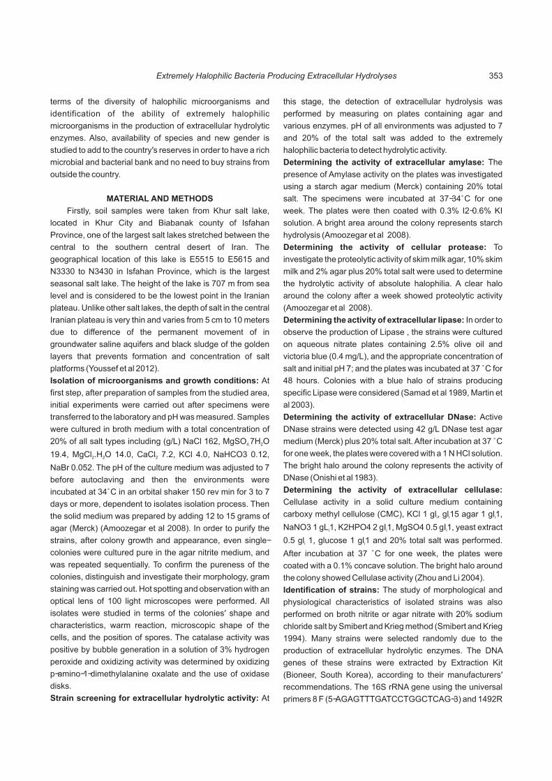
terms of the diversity of halophilic microorganisms and
identification of the ability of extremely halophilic
microorganisms in the production of extracellular hydrolytic
enzymes. Also, availability of species and new gender is
studied to add to the country's reserves in order to have a rich
microbial and bacterial bank and no need to buy strains from
outside the country.
MATERIAL AND METHODS
Firstly, soil samples were taken from Khur salt lake,
located in Khur City and Biabanak county of Isfahan
Province, one of the largest salt lakes stretched between the
central to the southern central desert of Iran. The
geographical location of this lake is E5515 to E5615 and
N3330 to N3430 in Isfahan Province, which is the largest
seasonal salt lake. The height of the lake is 707 m from sea
level and is considered to be the lowest point in the Iranian
plateau. Unlike other salt lakes, the depth of salt in the central
Iranian plateau is very thin and varies from 5 cm to 10 meters
due to difference of the permanent movement of in
groundwater saline aquifers and black sludge of the golden
layers that prevents formation and concentration of salt
platforms (Youssef et al 2012).
Isolation of microorganisms and growth conditions: At
first step, after preparation of samples from the studied area,
initial experiments were carried out after specimens were
transferred to the laboratory and pH was measured. Samples
were cultured in broth medium with a total concentration of
20% of all salt types including (g/L) NaCl 162, MgSO 7H O 4. 2
19.4, MgCl .H O 14.0, CaCl 7.2, KCl 4.0, NaHCO3 0.12, 2 2 2
NaBr 0.052. The pH of the culture medium was adjusted to 7
before autoclaving and then the environments were
incubated at 34°C in an orbital shaker 150 rev min for 3 to 7
days or more, dependent to isolates isolation process. Then
the solid medium was prepared by adding 12 to 15 grams of
agar (Merck) (Amoozegar et al 2008). In order to purify the
strains, after colony growth and appearance, even single-
colonies were cultured pure in the agar nitrite medium, and
was repeated sequentially. To confirm the pureness of the
colonies, distinguish and investigate their morphology, gram
staining was carried out. Hot spotting and observation with an
optical lens of 100 light microscopes were performed. All
isolates were studied in terms of the colonies' shape and
characteristics, warm reaction, microscopic shape of the
cells, and the position of spores. The catalase activity was
positive by bubble generation in a solution of 3% hydrogen
peroxide and oxidizing activity was determined by oxidizing
p-amino-1-dimethylalanine oxalate and the use of oxidase
disks.
Strain screening for extracellular hydrolytic activity: At
this stage, the detection of extracellular hydrolysis was
performed by measuring on plates containing agar and
various enzymes. pH of all environments was adjusted to 7
and 20% of the total salt was added to the extremely
halophilic bacteria to detect hydrolytic activity.
Determining the activity of extracellular amylase: The
presence of Amylase activity on the plates was investigated
using a starch agar medium (Merck) containing 20% total
salt. The specimens were incubated at 37-34°C for one
week. The plates were then coated with 0.3% I2-0.6% KI
solution. A bright area around the colony represents starch
hydrolysis (Amoozegar et al 2008).
Determining the activity of cellular protease: To
investigate the proteolytic activity of skim milk agar, 10% skim
milk and 2% agar plus 20% total salt were used to determine
the hydrolytic activity of absolute halophilia. A clear halo
around the colony after a week showed proteolytic activity
(Amoozegar et al 2008).
Determining the activity of extracellular lipase: In order to
observe the production of Lipase , the strains were cultured
on aqueous nitrate plates containing 2.5% olive oil and
victoria blue (0.4 mg/L), and the appropriate concentration of
salt and initial pH 7; and the plates was incubated at 37 °C for
48 hours. Colonies with a blue halo of strains producing
specific Lipase were considered (Samad et al 1989, Martin et
al 2003).
Determining the activity of extracellular DNase: Active
DNase strains were detected using 42 g/L DNase test agar
medium (Merck) plus 20% total salt. After incubation at 37 °C
for one week, the plates were covered with a 1 N HCl solution.
The bright halo around the colony represents the activity of
DNase (Onishi et al 1983).
Determining the activity of extracellular cellulase:
Cellulase activity in a solid culture medium containing
carboxy methyl cellulose (CMC), KCl 1 gl , gl15 agar 1 gl1, i i i
NaNO3 1 gL1, K2HPO4 2 gI1, MgSO4 0.5 gI1, yeast extract i i i
0.5 gl 1, glucose 1 gl1 and 20% total salt was performed. i i
After incubation at 37 °C for one week, the plates were
coated with a 0.1% concave solution. The bright halo around
the colony showed Cellulase activity (Zhou and Li 2004).
Identification of strains: The study of morphological and
physiological characteristics of isolated strains was also
performed on broth nitrite or agar nitrate with 20% sodium
chloride salt by Smibert and Krieg method (Smibert and Krieg
1994). Many strains were selected randomly due to the
production of extracellular hydrolytic enzymes. The DNA
genes of these strains were extracted by Extraction Kit
(Bioneer, South Korea), according to their manufacturers'
recommendations. The 16S rRNA gene using the universal
primers 8 F (5-AGAGTTTGATCCTGGCTCAG-3) and 1492R
Extremely Halophilic Bacteria Producing Extracellular Hydrolyses 353

(5-CACGGAT CCTACGGGTACCTTGTTACGACTT- 3)
strengthened. One PCR cycler (Biometra) was used for
boosting. The replication reaction took place in a final volume
of 25 liters (Rohban et al 2009).
Following the conditions used to amplify the 16S rRNA
gene, 40 cycles of 94 degrees for 35 seconds, 50 degrees for
30 seconds, 72 degrees for 1.5 minutes, with the final 10
minutes at 72 degrees, were developed. PCR products were
examined on agarose gel using Etidium bromide staining.
Pure PCR products were performed using a purification kit
(Bioneer, South Korea). The pure PCR product was
sequenced in both directions using an automated sequencer
by Seq Lab (Germany). The phylogenic association of
isolates was determined by comparing sequencing data
related to the 16S rRNA gene sequence in the National
Center for Genetic Bank Database for bioinformatics data
through BLAST search.
Phylogenic analysis using MEGA version 5 software
was done by CLUSTAL_X after obtaining balanced levels of
available information from public databases (Thompson et al
1997). The evolutionary two by two distances was calculated
using the correction method and the clusters were carried out
using the neighbor-joining method (Saitou and Nei 1987).
The validity of the tree branches was evaluated using the
Bootstrap analysis algorithm with 1000 times sampling
(Felsenstein 1985).
RESULTS AND DISCUSSION
Isolation of bacterial strains from Khur Salt Lake: Twelve
strains were separated from the studied lake, all of which
were part of extremely halophilic bacteria.
Investigating the activities of hydrolytic enzymes:
Purified strains were investigated for hydrolytic enzymes
activity. Hydrolytic activity of positive tests of extracellular
enzymes in isolated strains is shown in (Fig. 1).
A total of 7, 5, 4.8 and 6 isolates were able to produce
DNase, Cellulase, Amylase, Lipase and Protease,
respectively. 2 strains were also found in a mixture of 5
hydrolytic enzymes. A strain comparison based on the ability
to produce various enzymes is shown in (Table 1).
PCR results: The PCR process was carried out at RENA's
Biotechnology Company. Then, the extracted genome was
evaluated by electrophoresis. The 16S rRNA gene was
replicated. Primers with a length of 1500 were nucleotides.
Phylogenetic studies of selected strains: Based on the
sequencing of 16S rRNA, the examined isolates belonged to
Firmicutes phylum, Bacilli order and include Halobacillus and
Thalassobacillus genus, with 98-96% similarity between
species and strains belonging to this genus. It demonstrates
a significant difference in species level with that species
known in these genus and may be considered in new
species. The phylogenetic tree of the strains is plotted using
the Neighbor joining algorithm and is shown in (Fig. 2).
Extremely halophilic bacteria have high potential to be
used for biotechnology and nanotechnology purposes,
producing industrial compounds such as enzymes,
polymers, pigments, etc., with specific physiological
characteristics (Kaye and Baross 2004). Of the
environmental factors affecting the growth of halophilic
bacteria we can refer to temperature of the culture medium,
which has a significant effect on growth and classification of
the bacteria to halophilic and salt-tolerant bacteria (Margesin
and Schinner 2001, Ventosa et al 1998). Many extremely
halophilic bacteria have extracellular hydrolytic enzymes
such as Amylases, Proteases, Lipase, DNases,
Pulpulanases, Xylanases, Chitinases, Inulinases, and
Cellulases that are highly applicable in various processes
and industries such as food industries, food additives,
Fig. 1. Positive tests for hydrolytic enzymes in isolated strains
DNaseCellulaseAmylaseLipaseProteaseStrains
+++++S1
+++-+S2
+++++S3
--+--S4
----+S5
+-+--S6
--+--S7
+---+S8
----+S10
++++-S12
Table 1. Hydrolytic activity of isolated strains
Elaheh Fallahnezhad Naeini, Manoochehr Sattari Naeini and Marziyeh Noroozi354

chemical industries, and medical sciences. Also, enzymes
that show optimal activity in difficult industrial condition such
as temperature and salts are very important and have high
salt-saturated coatings that are likely required to maintain
their catalytic activity in the environments with low active
water. Also, halophilic microorganisms are considered a
possible source of these enzymes.
Halophilic bacteria have physiological and genetic
properties for success in hypersaline environments. These
features include compatibility with indoor environments,
efficient ion pumps, UV absorbing pigments and acid
proteins that help resistance against osmotic stress and the
effects of salt shrinkage combined with intense sunlight.
Although, nowadays, halophilia applications limit the main
constraint for solvents in cosmetics industries, beta-carotene
and hydrolysis in nutrition and food industries, many new
applications are in development. They include specialized
programs for bacteriophodos in films of halophilia for a
variety of optical nanoscale instruments, including high-
capacity computer storage and for sustainable enzymes for
use as industrial catalysts, some of the ability to work in
organic solvents. The metabolic activities of halophilia are
also used for various environmental programs, such as the
protection of contaminated waste in saline sewage. Some
sub-cellular components, such as polyhydroxyalkaloic
granules and phasolipids, and bioactive compounds such as
halocin, are designed for medical applications. Halophilic
microorganisms' uses are diverse and have significant
commercial opportunities in the chemical, environmental,
biofuel, medical and educational industries (Das sarma et al
2010).
Studies similar to the study conducted by (Sanchez
Porro et al 2003) revealed the prevalence of 5 hydrolytic
enzymes including Amylase, Protease, Lipase, DNase and
Polulanase in moderately halophilic bacterial in saline ponds
in Spain. Besides, (Zavaleta and Cardenas-Fernandez
2007) showed the genetic diversity of 18 moderately
halophilic bacteria producing 3 hydrolytic Amylase, Protease
and Lipase enzymes from Pilluana saline waters in Peru, and
(Moreno et al 2007) demonstrated the biodiversity of
mandatory halophilic bacteria producing 4 hydrolytic
enzymes such as Amylase, Protease, Lipase and DNase in
saline habitats, in Spain. The specificity of this study,
compared to recent works, is that firstly it shows the
prevalence of 5 extracellular hydrolytic enzymes (Amylase,
Protease, Lipase, DNase, carboxymethyl Cellulase) in the
extremely halophilic bacteria in Khur salt lake (the highest
amount of produced enzymes were related to Amylase,
Cellulase, and DNase in gram-positive bacilli and the lowest
amount of produced enzymes were related to Lipase and
Protease). Secondly, the ecological studies in saline water of
Khur salt lake resulted in isolation and identification of some
of the extremely halophilic bacteria with an ability to produce
a mixture of these enzymes. The obtained strains are
considered valuable and can be used for biotechnological
purposes, since no study has been carried out on the
Fig. 2. Neighbor-joining tree for 16s rRNA sequences of Extremely Halophilic Bacteria Producing Extracellular Hydrolyses (hyper saline lake) in Iran and reference strains. The numbers at branching points are bootstrap values based on 1000 replicates. The out group in the tree is the sequence of Salimicrobium haliphilum, Bar, 0.05 substitutions per nucleotide position
Extremely Halophilic Bacteria Producing Extracellular Hydrolyses 355

extremely halophilic bacteria in the study area so far.
Four selected strains, in addition to phenotypic traits,
were identified and sequenced in terms of phylogeny and
molecular characteristics by the 16S rRNA technique, which
included gram positive bacteria belonging to the Halobacillus
and Thalassobacillus genus. In general, among the halophilic
bacteria in terms of enzymes diversity and abundance of
enzymes production is gram positive bacillus. Based on the
results of the present study, most of the gram positive
environmental isolates producing hydrolytic enzymes belong
to the Halobacillus genus. In another study conducted by
(Sanchez Porro 2003) on saline areas in southern Spain, no
strain was isolated from the mentioned genus and some
strains were isolated from Salinivibrio genus, while, in this
study, no strain was isolated from this genus. This could be
attributed to higher concentration of salts in the Khur salt lake.
This bacterium has optimum growth in 2.5-10% NaCl and the
maximum concentration in which it can grow is up to 17%
NaCl, whereas the salt concentration in the studied salt lake is
much higher and reaches 20% salt. (Sanchez Porro 2003),
isolated strains of Chromohalobacter genus in their screening,
while no strain was isolated from this genus this study.
Generally, among the gram-positive bacteria, Halobacillus
bacteria are predominant and are known to be producers of
extracellular hydrolytic enzymes, and most industrial
processes use the species belonging to this genus to produce
industrial enzymes.
Of the features of halophilic microorganisms are
reduced risk of environmental pollution, growth and
proliferation in high salt concentrations, simple dietary
requirements for evolution, and use of various compounds as
a source of carbon and energy compared to other
microorganisms. Other types of extreme conditions such as
high pH, h?? igh or low temperatures, low oxygen availability,
pressure and toxicity of metals due to their abilities,
biodiversity and biotechnology use of halophilic
microorganisms have been interesting for microbiologists.
Most of the environmental isolates producing hydrolytic
enzymes belonged to the gram-positive genus were
especially from the spore gram-positive bacilli. Results were
quite expected due to extreme conditions that predominate in
the studied area because of high salt content as an extreme
factor.
Comparing the results of the present study and other
studies, the researchers found that, in general, the ability to
produce a combination of extracellular hydrolytic enzymes in
gram-positive strains belonged to Firmicutes phylum, Bacilli
order and Halobacillus and Thalassobacillus genus is more
evident, so that identification of such strains in various
industries is valuable.
REFERENCES
Amoozegar MA, Schumann P, Hajighasemi M and Fatemi A 2008. Salinivibrio proteolyticus sp. Nov. A moderately halophilic and proteolytic species from a hypersaline lake in Iran. International Journal of Systematic and Evolutionary Microbiology 58: 1159-1163.
Birbir M and Ilgaz A 1996. Isolation and identification of bacteria adversely affecting hide and leather quality. Journal of the Society of Leather Technologists and Chemists 80:147-153
Das sarma P, Coker JA, Huse V and Das sarma S 2010. Halophiles, industrial applications. Encyclopedia of Industrial Biotechnology 1–43.
Felsenstein J 1985. Confidence limits on phylogenies: an approach using bootstrap. Evolution; International Journal of Organic Evolution 39: 783- 791.
Gomez J and Steiner W 2004. The biocatalytic potential of extremophiles and extremozymes, extremophiles and extremozymes. Food Technology and Biotechnology 2: 223–235.
Kaye JZ and Baross AJ 2004. Synchronous effects of temperature, hydrostatic pressure and salinity on growth, phospholipids profiles, and protein patterns of four Halomonas species isolated from deep see hydrothermal-vent and sea surface environments. Applied and Environmental Microbiology 56: 6220-6229.
Margesin R and Schinner F 2001. Potential of halotolerant and halophilic microorganisms for biotechnology. Extremophiles 5: 73-83.
Martin S, Marquez M, Sanchez-Porro C, Mellado E, Arahal DR and Ventosa A 2003. Marinobacter lipolytic sp. Nov. A novel moderate halophile with lipolytic activity. International Journal of Systematic Evolutionary Microbiology 53: 1383-1387.
Mellado M E and Ventosa A 2003. Biotechnological potential of moderately and extremely halophilic microorganisms. In: Barredo JL (ed) Microorganisms for health care, food and enzyme production. Research Signpost, Kerala 233-256.
Moreno M L, Mellado E, Garcia M T and Ventosa A 2007. Diversity of extreme halophiles producing hydrolytic enzymes in hypersaline habitats, Halophiles-2007 booklet, 59–60.
Nichaus F, Bortoldo C, Kahlor M and Antranikia G 1999. Extremophiles as a source of novel enzymes for industrial application. Applied Microbiology and Biotechnology 51: 711-729.
Noroozi M, Amoozegar MA, Pourbabaee AA, Naghavi NS and Nourmohammadi Z 2017. Evaluation of the moderately halophilic bacteria resistant to mercury from saline soil. Indian Journal of Ecology 44(2): 271-274.
Onish H, Mori T, Takeuchi S, Tani K and Kobayashi T 1983. Halophilic nuclease of a moderately halophilic Bacillus sp. Production purification and characteristics. Applied Environmental Microbiology 45:24–30.
Rodriguez-Valera F 2003. Characteristics and microbial ecology of hypersaline environments. Halophilic Bacteria 1: 3–30.
Rohban R, Amoozegar MA and Ventosa A 2009. Screening and isolation of halophilic bacteria producing extracellular hydrolyses from Howz Soltan Lake, Iran. Journal of Industrial Microbiology and Biotechnology 36: 333-340
Saitou N and Nei M 1987. The neighbor joining method: a new method for reconstructing phylogenetic trees. Molecular Biology and Evolution 4: 406-425.
Samad MYA, Razak CAN, Salleh AB, Zinwan Yunus WM, Ampon K and Basri M 1989. A plate assay for primary screening of Lipase activity. Journal of Microbiological Methods 9: 51–56.
Sanchez Porro C, Mellado E, Bertold C, Antranikian G and Ventosa A 2003. Screening and characterization of the protease cp1 produced by the moderately halophilic bacterium
Elaheh Fallahnezhad Naeini, Manoochehr Sattari Naeini and Marziyeh Noroozi356

pseudoalteromonas sp, strain cp76. Extremophiles 7:221–228
Smibert RM and Krieg NR 1994. Phenotypic characterization. In: Gerhardt P (ed) Methods for general and molecular bacteriology. American Society for Microbiology, Washington, DC, 607–654.
Thompson JD, Gibson TJ, Plefiniak F, Jeanmougin F and Higgins DJ 1997. The clustral X windows interface: Xexible strategies for multiple sequence alignment aided by quality analysis tools. Nucleic Acids Research 24: 4876-4882.
Ventosa A, Nieto JJ and Oren A 1998. Biology of moderately holophilic aerobic bacteria. Microbiology and Molecular Biology Reviews June 62: 504-544.
Youssef NH, Ashlock-Savage KN and Elshahed MS 2012. Phylogenetic diversities and community structure of members of the extremely halophilic Archaea (order Halobacteriales) in multiple saline sediment habitats. Applied and Environmental Microbiology 78: 1332-1344.
Zavaleta AI and Cardenas-Fernandez AM 2007. Diversity of moderately halophilic bacteria producing extracellular hydrolytic enzymes isolated from Pilluana salt brine in Peru. Halophiles Congress Booklet, 50–51.
Zhou H and Li Z 2004. CMCase activity assay as a method for cellulose adsorption analysis. Enzyme and Microbial Technology 35: 455-459.
Received 03 March, 2018; Accepted 10 May, 2018
Extremely Halophilic Bacteria Producing Extracellular Hydrolyses 357

Effect of Silver and Zinc oxide Nanocompound Mixture on Growth and Some Physiological Properties of Sclerotinia sclerotiorum
Indian Journal of Ecology (2018) 45(2): 358-366
Abstract: Laboratory experiments were carried out in at Kerbala University, Iraq to study the effect of silver and zinc oxide nanocompound
(Ag/ZnO) on the sclerotinia sclerotiorum (Lib.) De Bary. A series of experiments were carried out, which included the isolation and diagnosis of
Sclerotinia sclerotiorum, phenotypic and laboratory, and then molecularly using the polymerase chain reaction technique, using ITS4 , ITS1
(Internal transcribed spacer), and the fungal isolates S. sclerotiorum (MMBIRAQ) were recorded for the first time in Iraq National Center for
Biotechnology Information (NCBI) under Entry Numbers (MF167296) at GenBank. the highest percentage of genetic similarity was with the
isolated from Italy, amounting to 99%, while the more distant isolated was from Canada, accounting to 96%.The mixture between Silver and
Zinc oxide nanocompound (Ag/ZnO) was present in the laboratory in terms of 1 nanocompound volume / 50 the volume of the potato dextrose
agar solution before solidation). The results showed that Ag/ZnO had a significant effect on the fungal colony diameter in Potato dextrose agar
(PDA) after 5 and 12 days of inoculation at 50 ìml and the highest volumes. The Ag/ZnO compound caused the disappearance of sclerotia
ranging from 25ìml to 2 ml. The sclerotia mass was 0.04 g. The effect of Ag/ZnO on biomass of Potato dextrose broth (PDB) was significant at
25ìml and the highest volumes. The effect was significant on cell length at 25 ìml and the highest volumes, while the thickness was at 50ìml.
The effects of Ag/ZnO on cell decomposition and destruction were caused by cell wall rupture. The significant difference in the production of
oxalic acid was at the volume of 25 ìml and the highest volumes. The average number of sclerotia in the subsequent generation was 8.88
sclerotia with a diameter of 0.16 cm.
Keywords: Sclerotinia sclerotiorum, Fungal nanotechnology
Manuscript Number: NAAS Rating: 4.96
2686
1Husham A. Mehdi, Ban T. Mohammed and Abbas M. Bashi
Department of Biology, University of Kerbala, Iraq.1Department of Chemistry, Applied Medical Sciences, University of Kerbala, Iraq
E-mail: [email protected]
Sclerotinia sclerotiorum (Lib) De Bary is a plant
pathogen that affects more than 400 plant species in different
stages of growth (Bolland and Hall 1994) . It is considered
that the fungus is difficult to eliminate because of its
production of sclerotia that is resistant to inappropriate
conditions (Mohammed 2012). The sclerotia can resist
drought, heat, fungicides and can remain active. Species
belonging to the Sclerotinia are closely related to the external
appearance and can be distinguished by microscopic
examination or by genetic material DNA (Malvarez et al
2007). Polymerase chain reaction (PCR), is characterized by
rapid, high resolution and sensitivity (Qin et al 2011).
Pesticides are one of the important methods of controlling
and managing plant diseases, which are chemical methods
used for the elimination of various plant pathogens, but this
method has effects due to the continuous use of pesticides,
large amounts of them or their products have deteriorated or
accumulated in the ecosystem, and not all the applied
chemical pesticides reach their targets, but the rest remain in
the soil. All-Naser (2006) found that the benomyl pesticide
with the recommended concentration or the double
concentration had an effect on the fungal groups found in the
rhizosphere area of the bean roots, the effect lasted for two
weeks for the recommended concentration and three weeks
for the multiplier concentration. Nanotechnology has been
introduced as an advanced technology based on the study
and understanding of nanoscience and basic science with
the technological ability to synthesize nanomaterials and
control their internal structure by restructuring and arranging
atoms and molecules to ensure unique and unique products,
so the nanotechnology is one of the most important and in the
forefront fields and fields in chemistry, physics, engineering
and biology (Fouda 2012). The transformation from micro-
particles to nanoparticles occurs in a number of changes in
physical properties, the one of this applications is controlling
plant pathogens, and it has shown many forms of impact on
or against microbes and microscopic organisms (Clement
and Jarrett 1994). Silver ion showed a safe control of plant
pathogens compared with the pesticides (Park et al 2006).
Transgenic nanoparticles have also been used to control
pathogens properly compared to fungicides, such as
nanoparticles of Ag-SiO , which have the inhibitory activity of 2
Botrytis cinerea (Yamamoto 2001). Zinc oxide powder
showed an inhibitory effect on fungi and bacteria) (Sawai and

Yoshikawa 2004). The aim of this study was to reduce using a
conventional chemical pesticide and to reduce pollution.
MATERIAL AND METHODS
Samples Collection: The stems of the infected eggplant
plants were collected from farms GPS 32°47'25.9"N
44°23'57.5"E based on the phenotypic symptoms and initial
diagnosis. The sclerotia were washed with normal water and
then sterile by immersing them for 3 minutes with 6%
commercial chlorax solution, washed several times with
sterile distilled water and dried on sterile filter sheets
(Mohammed 2001).
Diagnosis the fungus S. sclerotiorum according to
method of earlier workers (Khon 19679, Tariq et al 1985,
Saharan and Mehta 2008). The DNA was extracted using the
Cat No: FAPGK100 extraction kit processed by Taiwan-
China Favorgen. DNA purity was determined by applying the
following formula described by William and others (1997):
DNA purity= the amount of absorbance at wavelength of 260
nm. The amount of absorbance at wavelength of 280 nm. The
polymerase chain reaction test (PCM PreMix, Cat. No. K-
2012) was conducted by the Korean company Bioneer. The
polymerase chain reaction was performed with a volume of
20 microliter and containing 1 microliter of all the frontal
initiators (5'- TCCGTAGGTGAACCTGCGG-3': ITS1) and
posterior (5'-TCCTCCGCTTATTGATATGCI-3': ITS4) . After
completing the specimen transfer on gel layer, examine the
gel containing the DNA packets under UV trans illumination
and take photos. The PCR products were sent to the Korean
company Microgen for the determination of the nucleotide
sequence and in the front and rear directions of the multiply
products of the fungal isolates. The nucleotide sequences
are analyzed using the Basic Local Alignment Search Tool
(BLAST) to compare the data available at the National Center
for Biotechnology Information (NCBI), which belong to the
same isolate and internationally recognized.
Cultivate the sclerotia S. sclerotiorum: One sclerotia was
planted in the middle of a petri dish containing a medium of
chloramphenicol 250 mg / L. After five days of incubation at
20 + 2 ° C, and before the new sclerotia formed, the dish was
divided into cubed pieces for the propagation of fungus on the
wheat grain media as described in Mohammed (2001) to
produce as many sclerotia as possible.
Preparation of Ag/ZnO: The compound was prepared
according to the modified Kunde et al (2016) method. The
compound consists of the combination of silver nanoparticles
with zinc nanoparticles, as the followings:-
Solution 1: Weight of 29.7 g of zinc nitrate, and add 167 ml of
ethanol to zinc nitrate and 2 ml of ethylene chloral to the
solution made of zinc and ethanol.
Solution 2: Weight of 4.2 g of silver nitrate and dissolved in
100 ml distilled water.
Solution 3: Add 0.6 ml of HNO3 to 26 mL distilled water
Weight of 5 g of Polyvinylpyrrolidone (PVP).
The solution 1 was placed on the magnetic mixer and
shaking well, then the solution 3 was added to it with the
continues shaking. After that, solution No. 2 was distilled into
the solution of 1 + 3, after which 5 g of PVP was added, At 120
° C until obtained a third of the solution. The resulting solution
is a stock of nanoparticle. The concentration of Nano-silver is
32.8 mg/ml and the concentration of Nano-zinc oxide is 323
mg/ml, from which the subsequent concentrations are
obtained by adding different volumes of 1, 2, 0.7, 0.5, 0.3 and
0.1 ml, 50 µ ml, 25 µ ml to 50 ml from the medium (Table 1).
Attributes studied: Sclerotinia sclerotiorum diagnosis using
traditional method and molecular properties as well as
sequencing of fungi and its registration in the World Genomic
Bank was done. The properties of nanoparticles prepared by
FTIR Infrared Spectrometer, AFM Atomic Force Microscopy,
SEM, Electron Microscope Scanner, U.V. visibale
Spectroscopy of Visible and Ultraviolet Radiation
Spectroscopy. Ag/Zn Nanocompound are evaluated for the
growth of the sclerotinia sclerotiorum using different sizes
using the following media:
Solid PDA: The following characteristics were studied
The vegetative growth of Sclerotinia sclerotiorum in term of
diameter of the fungal colony (cm) after 5and 12 days from
inoculation, the percentage of inhibition using the equation of
Kim and his group (2012). [Inhibition Rate (%) = R-r/ R,
R=the growth in the control dish, r= the growth in the
treatment], the number and mass (g) of sclerotia grown on
PDA after 12 days of inoculation, the Microscopic parameters
Concentrat ion of Nano- compoundAg/Zn) mg / ml)
Volume used in media
25mlµ
50mlµ
0.1ml
0.3ml
0.5ml
0.7ml
1ml
2ml
Ag 0.820 1.640 3.280 9.800 16.400 22.960 32.800 65.600
ZnO 8.075 16.150 32.300 96.900 161.500 226.100 323.000 646.000
Table 1. Concentrations of nanocompound (Ag/Zn) mg / ml) based on the volume used in the medium Concentrations of nanocompound (Ag/Zn) mg / ml) based on the volume used in the medium
Effect of Silver and Zinc Oxide Nanocompound Mixture on Sclerotinia sclerotiorum 359

of mycelium treatment with Ag/ZnO after 12 days of
inoculation and the vitality of the pathogen produce from
Ag/ZnO treated fungus in terms of number and weight of
resulting sclerotia .
Liquid PDB: The following characteristics were studied: The
mean of fungal biomass (g) after 12 days of inoculation,
using the modified Asha et al (2006) and Navale et al (2015),
Estimation of oxalic acid produced by fungi in liquid media
(mg/l) after 12 days of inoculation (Bateman and Beer (1965).
RESULTS AND DISCUSSION
The fungus is microscopically dependent on the nature
and form of sterile mycelium as applied to the taxonomic keys
contained in Saharan and Mehta (2008), Tariq and his group
(1985) and Kohn (1979). As identified by Mohammed and
Almothafer (2013) and ALmasody (2015). The results of DNA
extraction of S. sclerotiorum isolation and the use of
polymerase chain reaction, used internal transcribed spacer
(ITS4) and ITS1, showed that it is similar to the same isolates
identified by Mohammed and Almothafer (2013) and
ALmasody (2015), although the sequence of the prefixes
used in the two studies are different, but they are similar to the
same isolates (Figure 1).
The fungal isolation was recorded in the name S.
sclerotiorum MMBIRAQ fungi the first time in Iraq at the
National Center for Biotechnology Information (NCBI) under
the Accession number MF167296 in GenBank. The results
revealed that the isolated S. sclerotiorum MMBIRAQ isolated
in this study is a new isolation previously unknown in the
world. The results of the Nucleotide Sequence Analysis of the
amplification DNA bundle and using the BLAST program and
comparing them with the data available at the National
Center for Biotechnology Information (NCBI), showed that
isolating the S. sclerotiorum. is the highest genetic resemble
isolated from S. sclerotiorum isolated from Japan (Accession
number: LC318723) of 99%, while the most genetically
divergent isolated was from S. sclerotiorum isolated from
Canada (KF859935: Accession number number) of 96%.
Other isolates gave homozygous ratios ranging from 96-99%
with isolated S. sclerotiorum isolates in this study from
Babylon (Figure 2, Table 2).
Ag / ZnO characteristics of prepared compound
By FTIR: The Nano-silver at package 875 after the
dissociation of glucose as a result of giving electrons of the
material reduces the conversion of silver from ion to metal
after taking the electrons and comes the role of the installer to
be formed in the form of balls. Note that the package between
703-666 represents the vibration of nanoparticles To
demonstrate the composition of nanoparticles on the
difference of the reduced factor, silver nanoparticles appear
in different sizes and diameters (Sun 2013, Rycenga et al
2011, Sakamoto et al 2009) (Figure 3).
By AFM: The results of the microscopic examination by the
atomic force microscope in Fig. 4, show that the obtained
compounds are nanoparticles and possess the
characteristics of the nanoparticles through the rise of the
nanoparticle and its fear. This is shown by the microscopic
atomic force, where the heights and sizes of nanoparticles
varied according to the reduced factor (Van Hyning and
Zukoski1998).
By electron microscope SEM scanner: The electron
microscopy shows forms of nanoparticles of different
diameters according to the reduced factor (Fig 5). The
nanoparticle mix with the zinc oxide is shown in the shape of
its silver heart and its zinc form (Ferreira da Silva et al 2011,
Rogers et al 2012, Alarcon et al 2012).
Optical and ultraviolet radiation spectroscopy: By
examining the resulting nanoparticles with ultraviolet-visible
light, Figure 6 appears package locations for nanotubes by
the wavelength of maximum absorption. Thus, showing the
wavelength of the wavelength of light falling on the surface of
nanoparticles with their free electrons orbiting the surface of
Fig. 1. Electrolysis of Cellulose Gel for DNA Complications by PCR of S. sclerotiorum isolated from Babylon province.
M = DNA ladder marker 1Kpb; P= product
Husham A. Mehdi, Ban T. Mohammed and Abbas M. Bashi360

Fig. 2. The nucleotide sequence of the DNA (PCR-amplified product) from S. sclerotiorum isolated from some farms in Babylon province, which is characterized by PCR
the nanoscale to show Plasmon, which turns the metal
surface electrons to give a bundle in the ultraviolet light (Kadir
et al 2005).
Fig. 3. Ag/ZnO characteristics compound by FTIR
Fungus Isolate or strain name Origin The most similar sequence in GenBank database
GenBank accession Sequence similarly (%)
S. sclerotiorum *MMBIRAQ Iraq MF167296 100
S. sclerotiorum MuNi-339 Japan LC318723 99
S. sclerotiorum 3Sd Italy EU627005 99
S. sclerotiorum SSAG01 India KT281863 99
S. sclerotiorum 1 Chile KF148604 99
S. sclerotiorum CAF-11011 Republic of Korea KX951645 99
S. sclerotiorum SS5 USA KF545319 98
S. sclerotiorum DB 090720091 Italy GQ375746 98
S. sclerotiorum CR 45 Iran KY694474 98
S. sclerotiorum SQC-000 China KY750530 98
S. sclerotiorum CXL 14041906 China KX781301 98
S. sclerotiorum SK-8 China KJ576850 98
S. sclerotiorum CBS-537.77 Japan AB926090 97
S. sclerotiorum Wb560 Austria AF455413 97
S. sclerotiorum F0675 Japan AB693927 97
S. sclerotiorum Wb560 Austria AF455413 96
S. sclerotiorum - Canada KF859934 96
S. sclerotiorum - Canada KF859935 96
Table 2. Comparison of the neoclutidosis ratios of S.sclerotiorum isolates from Babylon province and other isolates of the same fungus registered globally at the National Biotechnology Information Center (NCBI)
* Isolation of S.sclerotiorum isolated in this study from a farm in Babylon province
Evaluation of the Ag / ZnO nanocompound on the PDA:
The Ag / ZnO nanocompound affected the fungus in terms of
growth and phenotypic shape of the fungal colony (Table 3).
That the Ag / ZnO nanocompound had a significant effect on
the fungal colony diameter. After 5 and 12 days of inoculation
at 50 ìml the highest volumes, leading to slow and distorted
growth (Fig. 7). The shape of the colony in the media was
characterized by its distorted shape and uneven growth, as
well as irregular and curvilinear edges (Fig. 7). The growth
distinguished by 25 ìml being close to the control form, 50 ìml
was a distorted and irregular growth, so at 0.1 ml and 0.3 ml,
the spinning form was spread out and far from the PDA. The
Ag / ZnO nanocompound compound was not affected by the
Effect of Silver and Zinc Oxide Nanocompound Mixture on Sclerotinia sclerotiorum 361
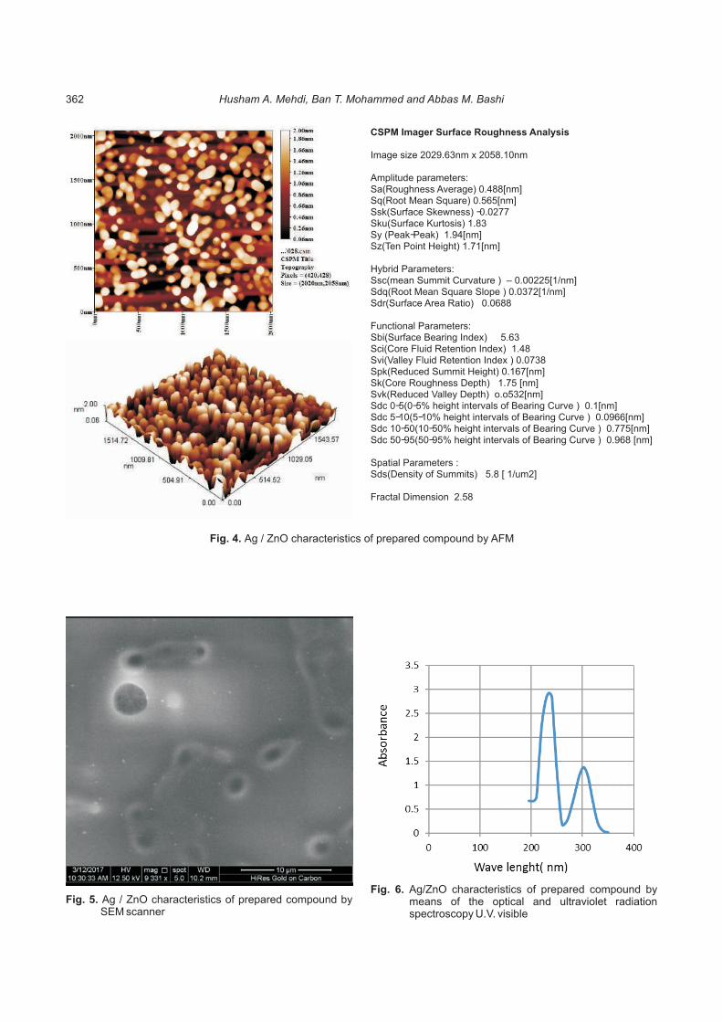
Fig. 5. Ag / ZnO characteristics of prepared compound by SEM scanner
Fig. 6. Ag/ZnO characteristics of prepared compound by means of the optical and ultraviolet radiation spectroscopy U.V. visible
CSPM Imager Surface Roughness Analysis
Image size 2029.63nm x 2058.10nm
Amplitude parameters:Sa(Roughness Average) 0.488[nm]Sq(Root Mean Square) 0.565[nm]Ssk(Surface Skewness) -0.0277Sku(Surface Kurtosis) 1.83Sy (Peak-Peak) 1.94[nm]Sz(Ten Point Height) 1.71[nm]
Hybrid Parameters:Ssc(mean Summit Curvature ) – 0.00225[1/nm]Sdq(Root Mean Square Slope ) 0.0372[1/nm]Sdr(Surface Area Ratio) 0.0688
Functional Parameters:Sbi(Surface Bearing Index) 5.63Sci(Core Fluid Retention Index) 1.48Svi(Valley Fluid Retention Index ) 0.0738Spk(Reduced Summit Height) 0.167[nm]Sk(Core Roughness Depth) 1.75 [nm]Svk(Reduced Valley Depth) o.o532[nm]Sdc 0-5(0-5% height intervals of Bearing Curve ) 0.1[nm]Sdc 5-10(5-10% height intervals of Bearing Curve ) 0.0966[nm]Sdc 10-50(10-50% height intervals of Bearing Curve ) 0.775[nm]Sdc 50-95(50-95% height intervals of Bearing Curve ) 0.968 [nm]
Spatial Parameters :Sds(Density of Summits) 5.8 [ 1/um2]
Fractal Dimension 2.58
Fig. 4. Ag / ZnO characteristics of prepared compound by AFM
Husham A. Mehdi, Ban T. Mohammed and Abbas M. Bashi362
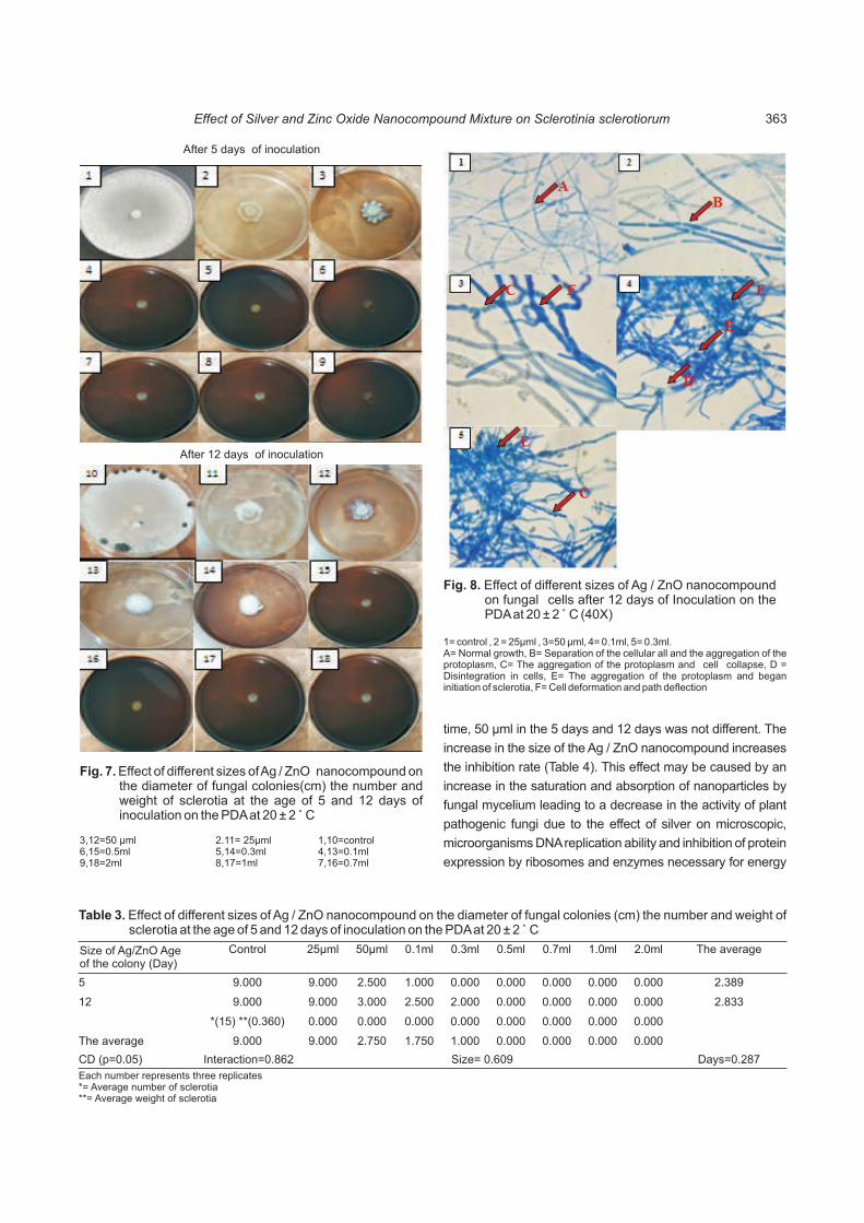
After 5 days of inoculation
After 12 days of inoculation
Fig. 7. Effect of different sizes of Ag / ZnO nanocompound on the diameter of fungal colonies(cm) the number and weight of sclerotia at the age of 5 and 12 days of inoculation on the PDA at 20 ± 2 ° C
3,12=50 µml6,15=0.5ml9,18=2ml
2.11= 25µml5,14=0.3ml8,17=1ml
1,10=control4,13=0.1ml7,16=0.7ml
Fig. 8. Effect of different sizes of Ag / ZnO nanocompound on fungal cells after 12 days of Inoculation on the PDA at 20 ± 2 ° C (40X)
1= control , 2 = 25µml , 3=50 µml, 4= 0.1ml, 5= 0.3ml.A= Normal growth, B= Separation of the cellular all and the aggregation of the protoplasm, C= The aggregation of the protoplasm and cell collapse, D = Disintegration in cells, E= The aggregation of the protoplasm and began initiation of sclerotia, F= Cell deformation and path deflection
time, 50 ìml in the 5 days and 12 days was not different. The
increase in the size of the Ag / ZnO nanocompound increases
the inhibition rate (Table 4). This effect may be caused by an
increase in the saturation and absorption of nanoparticles by
fungal mycelium leading to a decrease in the activity of plant
pathogenic fungi due to the effect of silver on microscopic,
microorganisms DNA replication ability and inhibition of protein
expression by ribosomes and enzymes necessary for energy
Control 25µml 50µml 0.1ml 0.3ml 0.5ml 0.7ml 1.0ml 2.0ml The average
5 9.000 9.000 2.500 1.000 0.000 0.000 0.000 0.000 0.000 2.389
12 9.000 9.000 3.000 2.500 2.000 0.000 0.000 0.000 0.000 2.833
*(15) **(0.360) 0.000 0.000 0.000 0.000 0.000 0.000 0.000 0.000
The average 9.000 9.000 2.750 1.750 1.000 0.000 0.000 0.000 0.000
CD (p=0.05) Interaction=0.862 Size= 0.609 Days=0.287
Table 3. Effect of different sizes of Ag / ZnO nanocompound on the diameter of fungal colonies (cm) the number and weight of sclerotia at the age of 5 and 12 days of inoculation on the PDA at 20 ± 2 ° C
Each number represents three replicates*= Average number of sclerotia**= Average weight of sclerotia
Size of Ag/ZnO Age of the colony (Day)
Effect of Silver and Zinc Oxide Nanocompound Mixture on Sclerotinia sclerotiorum 363

Control
80.000
LSD0.05
9.34
1.139
Average
17.720
1.440
2ml
0.000
0.000
1ml
0.000
0.000
0.7ml
0.000
0.000
0.5ml
0.000
0.000
0.3ml
10.000
2.000
0.1 ml
10.000
2.000
25µml
32.500
3.0002.000
50 µml
27.000
4.000
Width=1.139Length=9.340
Volume of Ag/ZnOcharacteristicstudy
Average length of hypha (mµ)
Average width of hypha (mµ)
LSD (0.05)
Table 4. Effect of different sizes of Ag / ZnO nanocompound on the length and width of the mycelium (µm) at the age of 12 days of inoculation on the PDA at 20 ± 2 ° C
Each number represents three replicates
Volume of Ag/ZnO characteristic study
Control 25µml 50µml 0.1ml 0.3ml 0.5ml 0.7ml 1.0ml 2.0ml The average
number of clerotia 15.000 11.000 20.000 13.000 20.000 0.000 0.000 0.000 0.000 8.770
12 0.330 0.300 0.230 0.330 0.300 0.000 0.000 0.000 0.000 0.350
LSD 0.05 Average number of sclerotia=2.491
Average diameter of = 0.118 sclerotia (cm)
Table 5. Effect of different sizes of Ag / ZnO nanocompound on the Average number of Sclerotia and Average diameter of sclerotia (cm) in the subsequent generation at the age of 12 days of inoculation on the PDA at 20 ± 2°C
Each number represents three replicates
Volumes of Ag/ZnOcharacteristic
Average of Biomass (gm)
Average number of sclerotia
Average diameter of sclerotia (mm)
LSD0.05
0.127
2.491
0.118
1.127
Average
0.132
8.770
0.350
1.677
2ml
0.000
0.000
0.000
0.000
1ml
0.000
0.000
0.000
0.000
0.7ml
0.000
0.000
0.000
0.000
0.5ml
0.000
0.000
0.000
0.000
0.3ml
0.150
20.000
0.300
1.265
0.1 ml
0.160
13.000
0.330
2.280
50 µml
0.180
20.000
0.230
2.790
25µml
0.240
11.000
0.300
3.180
Control
0.460
15.000
0.330
5.580Average product of oxalic acid (ppm)
Table 6. Effect of different sizes of Ag / ZnO nanocompound on the fungal biomass rate (gm), the number, diameter of the sclerotia (mm), and the rate of oxalic acid (ppm) production at 12 days of inoculation on PDB at 20 ± 2° C
Each number represents three replicates
production (Yamanaka et al 200, Feng et al 2000). These
results were identical to Kim's et al (2012). The effect was
significant on mycelium length at 25 ìml and the highest sizes,
while the width was at 50ìml (Table 4).
Figure 8 and Table 4, showed that the effect of different
sizes of Ag / ZnO nanocompound on fungal cells after 12
days of inoculation on a PDA, this effect is between
separation of the cellular wall, aggregation of the protoplasm,
cell collapse, disintegration in cells, cell deformation and
path deflection and began initiation of sclerotia, is the
important phenomenon to survival the fungus over
inappropriate circumstances and this is the main cause to
regrowth the fungus during the subsequent generation. The
average number of sclerotia in the subsequent generation
was 8.77 sclerotia with a diameter of 0.35 cm (Table 5). This
experiment may open up horizons for the effect of other
nancompounds that may have an effect on later generations
of the second generation, or that repeated treatment with
nanoparticles may conceal the sclerotia of the fungus without
fear of a mutation, due to the effect of silver on several vital
processes in the fungus making the role of mutation or
nanoparticle resistance is completely excluded (Herrera et al
2001, Wright et al1999).
Evaluation of the Ag / ZnO nanocompound on the PDB:
There was a significant at 25ìml the highest volumes until
0.5ml Ag / ZnO nanocompound and the highest there were no
growth (Table 6).
The Ag / ZnO nanocompound caused the significant
decrease number of sclerotia, and disappear in the volumes
ranging from 0.5 ml to 2 ml. The Ag / ZnO nanocompound
effects in cell decomposition and destruction were caused by
cell wall rupture. The production of oxalic acid also showed a
significant decrease in the production of acid with increasing
sizes of Ag / ZnO nanocompound. However, it is shown
Husham A. Mehdi, Ban T. Mohammed and Abbas M. Bashi364
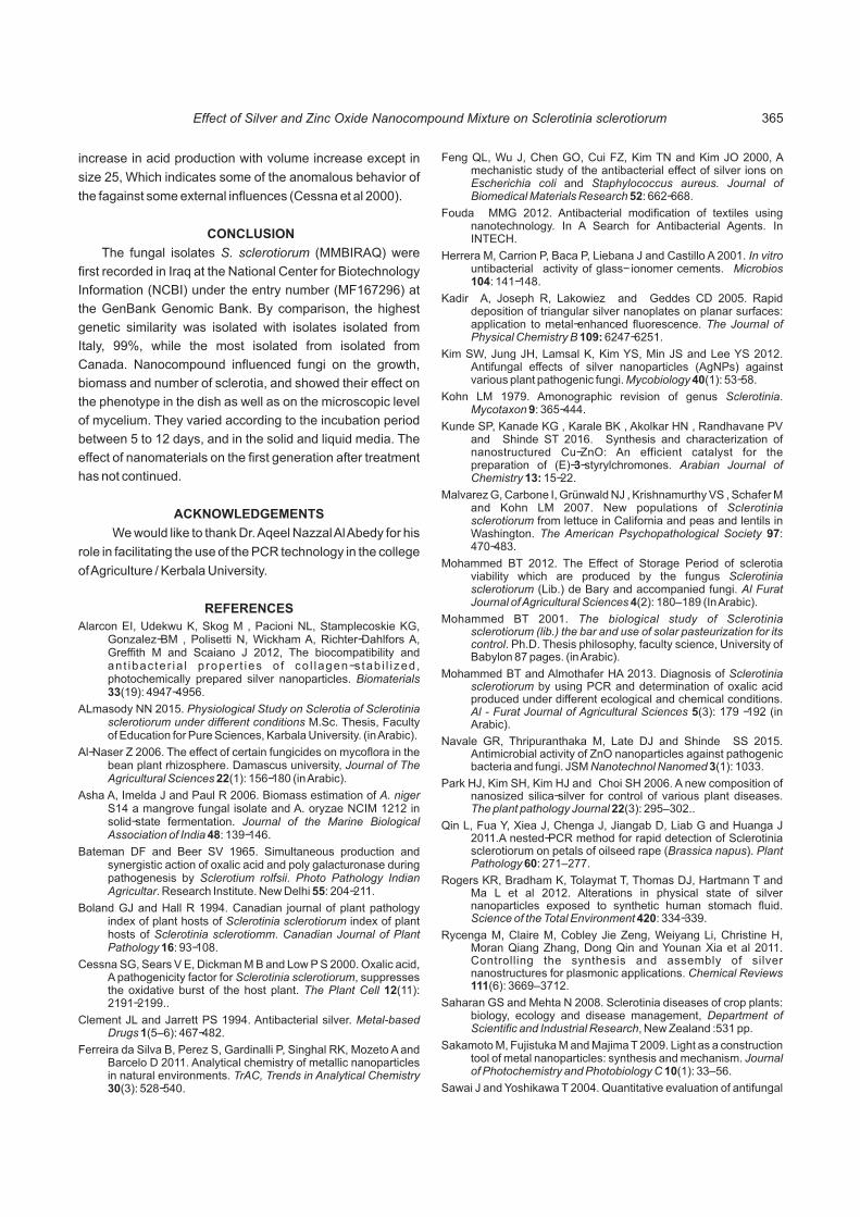
increase in acid production with volume increase except in
size 25, Which indicates some of the anomalous behavior of
the fagainst some external influences (Cessna et al 2000).
CONCLUSION
The fungal isolates S. sclerotiorum (MMBIRAQ) were
first recorded in Iraq at the National Center for Biotechnology
Information (NCBI) under the entry number (MF167296) at
the GenBank Genomic Bank. By comparison, the highest
genetic similarity was isolated with isolates isolated from
Italy, 99%, while the most isolated from isolated from
Canada. Nanocompound influenced fungi on the growth,
biomass and number of sclerotia, and showed their effect on
the phenotype in the dish as well as on the microscopic level
of mycelium. They varied according to the incubation period
between 5 to 12 days, and in the solid and liquid media. The
effect of nanomaterials on the first generation after treatment
has not continued.
ACKNOWLEDGEMENTS
We would like to thank Dr. Aqeel Nazzal Al Abedy for his
role in facilitating the use of the PCR technology in the college
of Agriculture / Kerbala University.
REFERENCES
Alarcon EI, Udekwu K, Skog M , Pacioni NL, Stamplecoskie KG, Gonzalez-BM , Polisetti N, Wickham A, Richter-Dahlfors A, Greffith M and Scaiano J 2012, The biocompatibility and an t ibac ter ia l p roper t ies o f co l lagen-s tab i l i zed , photochemically prepared silver nanoparticles. Biomaterials 33(19): 4947-4956.
ALmasody NN 2015. Physiological Study on Sclerotia of Sclerotinia sclerotiorum under different conditions M.Sc. Thesis, Faculty of Education for Pure Sciences, Karbala University. (in Arabic).
Al-Naser Z 2006. The effect of certain fungicides on mycoflora in the bean plant rhizosphere. Damascus university, Journal of The Agricultural Sciences 22(1): 156-180 (in Arabic).
Asha A, Imelda J and Paul R 2006. Biomass estimation of A. niger S14 a mangrove fungal isolate and A. oryzae NCIM 1212 in solid-state fermentation. Journal of the Marine Biological Association of India 48: 139-146.
Bateman DF and Beer SV 1965. Simultaneous production and synergistic action of oxalic acid and poly galacturonase during pathogenesis by Sclerotium rolfsii. Photo Pathology Indian Agricultar. Research Institute. New Delhi 55: 204-211.
Boland GJ and Hall R 1994. Canadian journal of plant pathology index of plant hosts of Sclerotinia sclerotiorum index of plant hosts of Sclerotinia sclerotiomm. Canadian Journal of Plant Pathology 16: 93-108.
Cessna SG, Sears V E, Dickman M B and Low P S 2000. Oxalic acid, A pathogenicity factor for Sclerotinia sclerotiorum, suppresses the oxidative burst of the host plant. The Plant Cell 12(11): 2191-2199..
Clement JL and Jarrett PS 1994. Antibacterial silver. Metal-based Drugs 1(5–6): 467-482.
Ferreira da Silva B, Perez S, Gardinalli P, Singhal RK, Mozeto A and Barcelo D 2011. Analytical chemistry of metallic nanoparticles in natural environments. TrAC, Trends in Analytical Chemistry 30(3): 528-540.
Feng QL, Wu J, Chen GO, Cui FZ, Kim TN and Kim JO 2000, A mechanistic study of the antibacterial effect of silver ions on Escherichia coli and Staphylococcus aureus. Journal of Biomedical Materials Research 52: 662-668.
Fouda MMG 2012. Antibacterial modification of textiles using nanotechnology. In A Search for Antibacterial Agents. In INTECH.
Herrera M, Carrion P, Baca P, Liebana J and Castillo A 2001. In vitro untibacterial activity of glass- ionomer cements. Microbios 104: 141-148.
Kadir A, Joseph R, Lakowiez and Geddes CD 2005. Rapid deposition of triangular silver nanoplates on planar surfaces: application to metal-enhanced fluorescence. The Journal of Physical Chemistry B 109: 6247-6251.
Kim SW, Jung JH, Lamsal K, Kim YS, Min JS and Lee YS 2012. Antifungal effects of silver nanoparticles (AgNPs) against various plant pathogenic fungi. Mycobiology 40(1): 53-58.
Kohn LM 1979. Amonographic revision of genus Sclerotinia. Mycotaxon 9: 365-444.
Kunde SP, Kanade KG , Karale BK , Akolkar HN , Randhavane PV and Shinde ST 2016. Synthesis and characterization of nanostructured Cu-ZnO: An efficient catalyst for the preparation of (E)-3-styrylchromones. Arabian Journal of Chemistry 13: 15-22.
Malvarez G, Carbone I, Grünwald NJ , Krishnamurthy VS , Schafer M and Kohn LM 2007. New populations of Sclerotinia sclerotiorum from lettuce in California and peas and lentils in Washington. The American Psychopathological Society 97: 470-483.
Mohammed BT 2012. The Effect of Storage Period of sclerotia viability which are produced by the fungus Sclerotinia sclerotiorum (Lib.) de Bary and accompanied fungi. Al Furat Journal of Agricultural Sciences 4(2): 180–189 (In Arabic).
Mohammed BT 2001. The biological study of Sclerotinia sclerotiorum (lib.) the bar and use of solar pasteurization for its control. Ph.D. Thesis philosophy, faculty science, University of Babylon 87 pages. (in Arabic).
Mohammed BT and Almothafer HA 2013. Diagnosis of Sclerotinia sclerotiorum by using PCR and determination of oxalic acid produced under different ecological and chemical conditions. Al - Furat Journal of Agricultural Sciences 5(3): 179 -192 (in Arabic).
Navale GR, Thripuranthaka M, Late DJ and Shinde SS 2015. Antimicrobial activity of ZnO nanoparticles against pathogenic bacteria and fungi. JSM Nanotechnol Nanomed 3(1): 1033.
Park HJ, Kim SH, Kim HJ and Choi SH 2006. A new composition of nanosized silica-silver for control of various plant diseases. The plant pathology Journal 22(3): 295–302..
Qin L, Fua Y, Xiea J, Chenga J, Jiangab D, Liab G and Huanga J 2011.A nested-PCR method for rapid detection of Sclerotinia sclerotiorum on petals of oilseed rape (Brassica napus). Plant Pathology 60: 271–277.
Rogers KR, Bradham K, Tolaymat T, Thomas DJ, Hartmann T and Ma L et al 2012. Alterations in physical state of silver nanoparticles exposed to synthetic human stomach fluid. Science of the Total Environment 420: 334-339.
Rycenga M, Claire M, Cobley Jie Zeng, Weiyang Li, Christine H, Moran Qiang Zhang, Dong Qin and Younan Xia et al 2011. Controlling the synthesis and assembly of silver nanostructures for plasmonic applications. Chemical Reviews 111(6): 3669–3712.
Saharan GS and Mehta N 2008. Sclerotinia diseases of crop plants: biology, ecology and disease management, Department of Scientific and Industrial Research, New Zealand :531 pp.
Sakamoto M, Fujistuka M and Majima T 2009. Light as a construction tool of metal nanoparticles: synthesis and mechanism. Journal of Photochemistry and Photobiology C 10(1): 33–56.
Sawai J and Yoshikawa T 2004. Quantitative evaluation of antifungal
Effect of Silver and Zinc Oxide Nanocompound Mixture on Sclerotinia sclerotiorum 365

activity of metallic oxide powders (MgO, CaO and ZnO) by an indirect conductimetric assay. Journal of Applied Microbiology 96(4): 803-809.
Sun Y 2013. Controlled synthesis of colloidal silver nanoparticles in organic solutions: empirical rules for nucleation engineering. Chemical Society Reviews 42: 2497-2511.
Tariq VN, Gutteridge CS and Jeffries P 1985. Comparative studies of cultural and biochemical characteristics used for distinguishing species within Sclerotinia, Transactions of the British Mycological Society 84(3): 381-397.
Van Hyning DL and Zukoski CF 1998. Formation mechanisms and aggregation behavior of borohydride reduced silver particles. Langmuir 14: 7034-7040.
William WW, Mackey K and Chomczynski P 1997. Effect of pH and ionic strength on the spectrophotometric assessment of nucleic acid purity. Biotechniques 22: 474-481.
Wright JB, Lam K, Hansen D and Burrell RE 1999. Efficacy of topical silver against fungal burn wound pathogens. American Journal of Infectus Control 27: 344-350.
Yamanaka M, Hara K and Kudo J 2005,.Bactericidal actions of a silver ion solution on Escherichia coli, studied by energyfiltering transmission electron microscopy and proteomic analysis. Applied Environ Microbiology71: 7589-7593.
Yamamoto O 2001. Influence of particle size on the antibacterial activity of zinc oxide. International Journal of Inorganic Materials 3(7): 643–646.
Received 31 March, 2018; Accepted 10 May, 2018
Husham A. Mehdi, Ban T. Mohammed and Abbas M. Bashi366

Incidence of Blossom Midge, Contarinia maculipennis Felt on Jasmine (Jasminum sambac L.) and its Natural Enemies
in Tamil Nadu
Indian Journal of Ecology (2018) 45(2): 367-372
Abstract: Jasmine blossom midge (Contarinia maculipennis Felt Cecidomyiidae, Diptera) was found to be the serious pest posing severe
threat to flower yield. Field surveys indicated the presence of the pest in the surveyed region in varying intensity with maximum incidence in
Madurai ( %), Ramanathapuram (33.62 %) and Tirunelveli ( 34.27 33.19 %) respectively. Coccinellid predators like Cheilomenes sexmaculata,
C. transversalis, Scymnus sp., C. septumpunctata, Brumus suturalis, Illeis cincta and Chilocorus sp. were present in the jasmine ecosystem
with a mean population of 3.1 per plant. Neuropteran predators, Chrysoperla zastrowi sillemi and Mallada boninensis were found with a mean
population of 2.2 per plant. A wide range of preying mantises and spiders with a mean population of 3.8 and 4.3 per cent, respectively was
present. A dipteran predator, Systasis dasyneurae played a vital role in natural suppression of the pest. Native weeds and flowering plants like
Parthenium hysterophorus, Rosa sp., Nerium oleander, Vernonia cinera, Datura metal, Lantana camara, Tagetus erecta, Ipomea carnea,
Helianthus annus and Coriandrum sativum provide nectar to the adult stages of the predators in jasmine ecosystem.
Keywords: Jasmine, Blossom midge, Pink discolouration, Systasis sp., Coccinellid, Chrysopid, Spider, Preying mantises
Manuscript Number: NAAS Rating: 4.96
2687
I. Merlin Kamala Department of Agricultural Entomology, Tamil Nadu Agricultural University, Coimbatore - 641 003, India
E-mail: [email protected]
Jasmine is cultivated in an area of more than 8,000 ha
with an annual production of flowers worth Rs. 80-100 million
in India. Tamil Nadu is the leading producer of jasmine in the
country with an annual production of 77, 247 tonnes in an
area of 9,360 ha (Prakash and Muniandi 2014, Thakur et al
2014). The production of jasmine is affected by various
factors, among which, insect pests are the most devasting
factor. The major pests affecting jasmine are jasmine bud
worm (Hendecasis duplifascialus Hampson), blossom midge
(Contarinia maculipennis Felt), leaf webworm (Nausinea
geometralis Guenee), gallery worm (Elasmopalpus
jasminophagus Hampson), leaf roller (Glyphodes unionalis
Hubner.) and the two spotted mite (Tetranychus urticae
Koch.). Of these, budworm and blossom midge gain major
economic importance, as they cause excessive damage to
the buds. Blossom midge has attained the status of a major
pest causing severe economic loss by reducing the
marketable quality of the flowers. In case of severe
infestations, buds dry prematurely leading to bud drop or
blossom drop, thereby the marketable quantity of the flowers
are greatly reduced. The pteromalid, Systasis dasyneurae
Mani (Pteromalidae, Hymenoptera) is a general midge
predator found in different agro-ecosystems (Parnell 1983). It
has the potential to prey on the larval stages of midges. The
larvae of this wasp parasitizes the midge larvae in the buds,
attaching to the midges and extracting body fluids from its
host. Each wasp larva can destroy 3-4 midge larvae (Pruthi
1937). Level of predation of late instar midge larvae can
exceed 50 per cent (Ahmad and Mani 1939).
Lady bird beetles and green lace wings were reported
to feed on the egg and larval stages of the insect pests
(Dixon 2000). Spiders as carnivorous arthropods, consume
a large number of larvae present in jasmine ecosystem
including midge maggots (Rajeshwaran et al 2005).
Preying mantises play an important role in the environment
as an efficient predator. Studying the identity, intensity of
infestation of the pest and the natural enemies associated is
a pre requisite to develop the management strategy.
Classical biological control involving the utilization of host -
specific parasitoids requires the information on the native
natural enemies involved with them. The present study was
aimed at studying the intensity of damage caused by
blossom midge and documenting the various natural
enemies associated with them in different jasmine growing
region of Tamil Nadu.
MATERIAL AND METHODS
Roving survey: Roving surveys were conducted during
June-August 2015 around ten major jasmine growing
Southern districts of Tamil Nadu viz., Kanyakumari,
Ti rune lve l i , Tut icor in , Vi rudhunagar, Madura i ,
Ramanathapuram, Theni Dindigul, Erode and Coimbatore

districts to study the incidence of blossom midge and the
natural enemies associated with them.
Blossom midge incidence: In each district, 10 jasmine
gardens were randomly selected and the per cent incidence
of blossom midge was recorded by counting the pink
discoloured buds with shriveled budstalks and total number
of buds per plant. The number of maggots present per plant
was also recorded. The observations were recorded at
fortnightly interval for six months from June- December,
2016.
Natural enemies associated with blossom midge: The
population of natural enemies viz., predators and parasitoids
that were seen actively moving near the infested buds from
ten randomly selected plants were observed and recorded.
The pink infested buds were collected in small containers and
brought to lab and maintained to check for any
predator /paras i to id emergence. The co l lec ted
predators/parasitoids from ten randomly selected plants
were reared still adult stage to confirm the identity of the
natural enemies. The flowering plants and weeds in and
around the jasmine gardens were observed and recorded for
the activity of parasitoids/predators.
Taxonomic identification of natural enemies of
blossom midge: Field collected predators were killed
using ethyl acetate, preserved as dry mounts and identified
using standard taxonomic keys. The identity was confirmed
by the repository collection of natural enemies maintained
at Insect Systematic Laboratory, Department of
Entomology, Tamil Nadu Agricultural University
Coimbatore. The emerged parasitoids from parasitized
larvae as well as pink infested buds were collected and
preserved in 70 per cent ethanol and sent to Division of
Systematics, National Bureau of Agricultural Insect
Resources (NBAIR), Bengaluru.
RESULTS AND DISCUSSION
The incidence of blossom midge was noticed in all the
ten districts of Tamil Nadu. The jasmine growing regions of
Tamil Nadu showed slight to heavier infestation of blossom
midge However, the incidence was maximum in Madurai
distr ict recording 34.27 per cent, fol lowed by
Ramanathapuram, Tirunelveli, Kanyakumari and
Thootukudi. The lowest per cent incidence was recorded in
Erode and Dindugal. Similar trend was noticed in the number
of pink discoloured buds/ plant with Madurai recording the
maximum number of 19.10 buds/plant followed by Tirunelveli
with 14.80 buds/plant. The variations in blossom midge
incidence in the study locations may be due to the interplay of
various biotic and abiotic factors that influence the pest
population.
A specific midge predator, Systasis dasyneurae was
recorded in all the jasmine gardens surveyed (Fig. 1). The
larva of Systasis dasyneurae is a carnivorous predator of
dipteran maggots (Fig. 2). The adult predators oviposit a
single egg, in tip of the jasmine flower bud (Fig. 3). The
emerging larvae feed on the midge maggots present inside
the bud, pupate inside the buds and the adults emerge from
the buds after being dried and fall off. The Systasis
dasyneurae adults prefer to oviposit in buds with midge eggs.
This clearly depicts the specific predatory role of Systasis
dasyneurae to midge maggots. The Systasis larvae was
present abundantly in pink discoloured buds, which reveals
that the predator sense the olfactory stimuli of either the bud
volailes due to damage of its prey or the kairomomal odours
from midge body. The herbivore induced volatiles might be
the reason for the oviposition of predators in midge damaged
buds.
The saturated hydrocarbons, linalool, naphthalene,
azulene, methyl salicylate, methyl anthranilate, alpha
farnescene, phenol and naphthalene are emitted from midge
damaged buds (Merlin Kamala et al 2017). The potent
natural enemy attractant, allyl isothiocyanate were also
emitted from midge damaged buds in volatile form. The
attraction of Systasis dasyneurae in olfactometer showed a
positive response to midge damaged bud extracts (Merlin
kamala 2017). Hence, the field collected pink discoloured
shrivelled buds of jasmine were kept in plastic containers for
predator emergence. More number of predators emerged
from buds collected from Madurai, followed by Tirunelveli,
Kanyakumari, Dindugal and Erode. Systasis sp., as a potent
predator of jasmine blossom midge was reported by David et
al 1991.
The coccinellids observed in jasmine ecosystem ranged
from 1.66 to 6.00/plant (Table 3) with a mean number of 3.1
/plant (Table 4). Ramanathapuram recorded the highest
population of ladybird beetles. The different coccinellids
observed in jasmine ecosystem were Cheilomenes
sexmaculata (Fabricius), Scymnus coccivora (Fabricius), C.
transversalis (Fabricius), C. septumpunctata (Linnaeus), C.
repanda (Fabricius),Brumus suturalis (Fabricius), Illeis
cincta (Fabricius), Chilocorus sp. and Propylea dissecta
(Mulsant).
Chrysopid predators identified during the survey were
Chrysoperla zastrowii sillemi and Mallada bonensis with a
mean number of 2.2/plant (Table 3). The number of
chrysopids ranged from 1.00-4.33 / plant including both
grubs and adults in the different regions surveyed with the
highest number recorded in Dindugal (Table 2). The various
lifestages of chrysopids were invariably observed in many
jasmine gardens with the eggs oviposited in the undersurface
368 I. Merlin Kamala
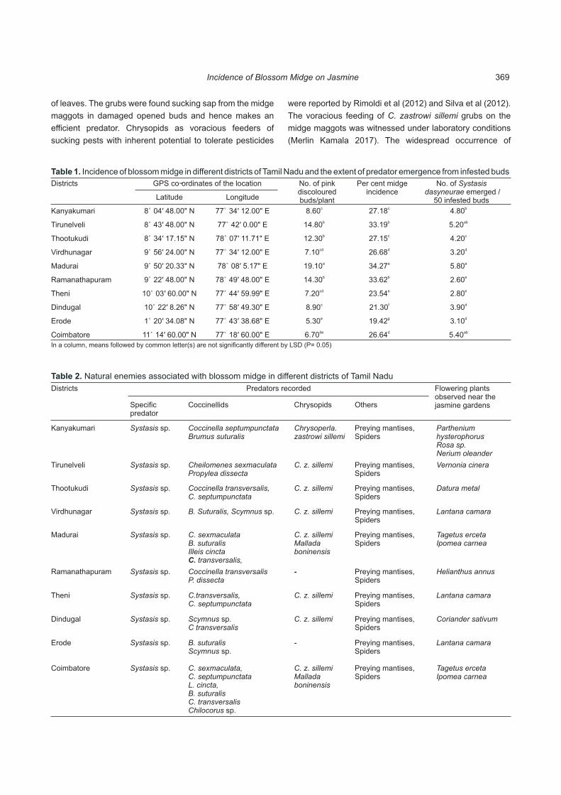
Districts Predators recorded Flowering plants observed near the jasmine gardensSpecific
predatorCoccinellids Chrysopids Others
Kanyakumari Systasis sp. Coccinella septumpunctata Brumus suturalis
Chrysoperla. zastrowi sillemi
Preying mantises, Spiders
Parthenium hysterophorusRosa sp.Nerium oleander
Tirunelveli Systasis sp. Cheilomenes sexmaculata Propylea dissecta
C. z. sillemi Preying mantises, Spiders
Vernonia cinera
Thootukudi Systasis sp. Coccinella transversalis, C. septumpunctata
C. z. sillemi Preying mantises, Spiders
Datura metal
Virdhunagar Systasis sp. B. Suturalis, Scymnus sp. C. z. sillemi Preying mantises, Spiders
Lantana camara
Madurai Systasis sp. C. sexmaculata B. suturalis Illeis cincta C. transversalis,
C. z. sillemiMallada boninensis
Preying mantises, Spiders
Tagetus erceta Ipomea carnea
Ramanathapuram Systasis sp. Coccinella transversalis P. dissecta
- Preying mantises, Spiders
Helianthus annus
Theni Systasis sp. C.transversalis, C. septumpunctata
C. z. sillemi Preying mantises, Spiders
Lantana camara
Dindugal Systasis sp. Scymnus sp. C transversalis
C. z. sillemi Preying mantises, Spiders
Coriander sativum
Erode Systasis sp. B. suturalis Scymnus sp.
- Preying mantises, Spiders
Lantana camara
Coimbatore Systasis sp. C. sexmaculata, C. septumpunctata L. cincta, B. suturalis C. transversalisChilocorus sp.
C. z. sillemiMallada boninensis
Preying mantises, Spiders
Tagetus erceta Ipomea carnea
Table 2. Natural enemies associated with blossom midge in different districts of Tamil Nadu
Districts GPS co-ordinates of the location No. of pink discoloured buds/plant
Per cent midge incidence
No. of Systasis dasyneurae emerged /
50 infested budsLatitude Longitude
Kanyakumari 8° 04' 48.00" N 77° 34' 12.00" E c8.60 c27.18 b4.80
Tirunelveli 8° 43' 48.00" N 77° 42' 0.00" E b14.80 b33.19 ab5.20
Thootukudi 8° 34' 17.15" N 78° 07' 11.71" E b12.30 c27.15 c4.20
Virdhunagar 9° 56' 24.00" N 77° 34' 12.00" E cd7.10 d26.68 d3.20
Madurai 9° 50' 20.33" N 78° 08' 5.17" E a19.10 a34.27 a5.80
Ramanathapuram 9° 22' 48.00" N 78° 49' 48.00" E b14.30 b33.62 e2.60
Theni 10° 03' 60.00" N 77° 44' 59.99" E cd7.20 e23.54 e2.80
Dindugal 10° 22' 8.26" N 77° 58' 49.30" E c8.90 f21.30 d3.90
Erode 1° 20' 34.08" N 77° 43' 38.68" E e5.30 g19.42 d3.10
Coimbatore 11° 14' 60.00" N 77° 18' 60.00" E de6.70 d26.64 ab5.40
In a column, means followed by common letter(s) are not significantly different by LSD (P= 0.05)
Table 1. Incidence of blossom midge in different districts of Tamil Nadu and the extent of predator emergence from infested buds
of leaves. The grubs were found sucking sap from the midge
maggots in damaged opened buds and hence makes an
efficient predator. Chrysopids as voracious feeders of
sucking pests with inherent potential to tolerate pesticides
were reported by Rimoldi et al (2012) and Silva et al (2012).
The voracious feeding of C. zastrowi sillemi grubs on the
midge maggots was witnessed under laboratory conditions
(Merlin Kamala 2017). The widespread occurrence of
369Incidence of Blossom Midge on Jasmine

District Coccinellids Chrysopids Preying mantises
Spiders
Kanyakumari c3.66 d1.23 b4.33 b4.33
Tirunelveli c3.33 d1.00 c3.33 a5.33
Thootukudi d2.00 c2.00 c3.66 c3.66
Virdhunagar c3.33 c2.00 a5.33 d2.33
Madurai d2.33 c2.33 c3.66 b4.33
Ramanathapuram a5.33 d1.33 c3.66 b4.66
Theni d2.66 c2.33 d2.66 a5.33
Dindugal b4.33 a4.33 c3.00 c3.66
Erode e1.66 b3.33 d2.33 cd3.00
Coimbatore d2.34 c2.00 a5.66 a5.66
Table 3. Incidence of generalist predators in jasmine ecosystem
In a column, means followed by common letter(s) are not significantly different by LSD (P= 0.05)
Predators observed Species of predators in decreasing trend Mean number of predator/plant
Pteromalid Systasis dasyneurae 4.1
Coccinellids Cheilomenes sexmaculata > Coccinella transversalis> Scymnus sp. > Coccinella septumpunctata > Brumus suturali > Illeis cincta > Chilocorus sp.
3.1
Chrysopids Chrysoperla zastrowi sillemi > Mallada boninensis 2.2
Preying mantises Mantis religiosa > Odontomantis micans> Creobroter pictipennis > Creobroter urbana > Euantisa pulchra > Hestiasula sp.
3.8
Spiders Oxyopes javanus > Plexippus paykulli >Thyene imperialis >Telamonia dimidiata > Hyllus semicupreus > Thomisus projectus >Neoscona mukherjee > Olios milleti > Peucetia viridana
4.3
Table 4. Incidence and species complex of predators during the study
Fig. 1. Systasis dasyneurae adult
Fig. 2. Systasis dasyneurae larva
Fig. 3. Adult Systasis dasyneurae ovipositing on jasmine flowerbud
coccinellids and chrysopids in habiting diverse habits can be
utilized for pest management in jasmine. Preying mantis
predators recorded were Mantis religiosa (Linnaeus),
Creobroter urbana (Fabricius), Euantisa pulchra (Fabricius),
Empusca pennata (Thunberg), Gongylus gongylodes
(Linnaeus), Creobroter urbana (Fabricius), C. pictipennis
(Wood-Mason), Odontomantis micans (Saussure),
Hestiasula brunneriana (Saussure), Amorphoscelis sp., and
Thesprotia sp. with the mean of 3.8/ plant (Table 2, 4). The
number of preying mantises ranged from 2.66 to 5.66 / plant
with the highest number recorded in Coimbatore (Table 3).
Their predatory role can be utilized in effective management
of jasmine blossom midge.
A variety of spiders were found in jasmine plant leaves,
twigs, trunk as well as flower and buds, preying jasmine
pests. Spiders belonging to different families viz.,
araenidae, clubionidae, theridi idae, l inyphiidae,
miturgidae, oxyopidae, salt icidae, sparassidae,
tetragnathidae, thomisidae, ulaboridae etc. were
encountered in different region of Tamil Nadu. The
predominant spiders observed being Argiope anasuja
(Thorell), Neoscona theisi (Walkckenaeur), Neoscona
mukherjee (Tikader), Olios milleti (Pocock), Chikunia nigra
(O. Pickward-Cambridge), Pisaura putiana (Barion and
Litsinger), Peutica viridana (Stoliczka ), Oxyopes javanus
(Thorell), Oxyopes birmanicus (Thorell), Oxyopes shweta
(Tikader), Phintella vitata (C.L.Koch), Myrmaplata
370 I. Merlin Kamala

plataleoides (O. Pickard-Cambridge), Plexippus paykulli
(Audouin), Telamonia dimidiata (Simon), Telamonia
dimidiata (Simon), Rhene danieli (Tikader), Carrhotus
viduus (C.L.Koch ), Thyene imperialis (Rossi), Hyllus
semicupreus (Simon), Thomisus projectus (Tikader ),
Araneus sp., Heteropoda sp., Theridion sp., Uthina sp.,
Clubiona sp., Cheiracanthium sp., Bavia sp., and
Misumena sp. The mean number of spiders observed was
4.3/plant (Table 4). Different species of spiders belonging to
different families were seen actively preying pests of
jasmine including blossom midge maggots. Prey searching
ability, wide host range, ease in multiplication and
polyphagous in nature make them as a potential predator in
biological pest suppression (Rajeshwaran et al 2005). The
positive response of spiders in naturally managing pests
can be utilized in biological control and care should be taken
to use safer and compatible insecticides that may not harm
them. Flower spiders that fondly live on flowers were
noticed to feed on midge maggots. A pteromalid parasitoid,
Pteromalus sp., was emerging from the pink discoloured
buds. Pteromalus sp. is a potential parasitoid of dipteran
maggots especially fruit fly maggots (Cavaloro 1982). But
its parasitic role on blossom midge of Jasmine was not
defined. Pteromalus sp., as a parasitoid was reported in rice
ecosystem (Catling and Islam 2013).
The flowering plants like Parthenium hysterophorus,
Rosa sp., Nerium oleander, Tagetus erecta and Helianthus
annus as well as native weeds like Vernonia cinera, Datura
metal, Lantana camara, Ipomea carnea, and Coriandrum
sativum were noticed in and around jasmine gardens, which
provide nectar to the adult stages of the predators in jasmine
ecosystem. The highest activity of the natural enemies may
be due to the ample supply of nectar to the adult stages of the
predators by the adjacent necariferous crops. The adult
natural enemes in jasmine ecosystem were survived by the
pollen and nectar from flowering plants as feed and the
foliage for shelter and overwintering. The positive influence in
increasing the population of beneficials in the jasmine
gardens by growing nectariferous crops was reported Altieri
and Nicholls (2004).
CONCLUSION
The present survey projected blossom midge of
jasmine, C. maculipennis as the major pest infesting jasmine
in all the major jasmine growing tracks of Tamil Nadu. The
pest was associated with a rich pool of natural enemies that
provide natural suppression of blossom midge of jasmine.
These natural enemies need to be conserved by raising
flowering plants in and around jasmine gardens to support
adult predators and parasitoids as a source of nectar during
the period of scarce availability of target hosts. The strategic
planning with safer insecticides for management of blossom
midge to preserve the native natural enemies in jasmine
gardens needs priority.
ACKNOWLEDGEMENT
The financial assistance provided by UGC, Government
India, awarding Maulana Azad fellowship to pursue Ph.D. in
Agricultural Entomology at Tamil Nadu Agricultural
University, Coimbatore is gratefully acknowledged for the
senior author. The authors are also thankful to ICAR- NBAIR-
Division of Insect Systematics, National Bureau of
Agricultural Insect Resources, Bengaluru, for identification of
natural enemies.
REFERENCES
Ahmad T and Mani MS 1939. Two new chalcidoid parasites of the linseed midge, Dasyneura lini Barnas. Indian Journal of Agricultural Sciences 9: 531-539.
Altieri MA and Letourneau DK 1982. Vegetation management and biological control in agroecosystems. Crop Protection 1: 405-430
Altieri MA and Nicholls CI 2004. Biodiversity and pest management in agroecosystems. Haworth Press, New York.
Baliddawa CW 1985. Plant species diversity and crop pest control: an analytical review. Insect Science Application 6: 479-487.
Catling D and Islam Z 2013. Diversity and seasonal fluctuations of arthropod fauna in Bangladesh deepwater. Bangladesh Rice Journal 17(1&2): 75-104.
Cavaloro 1982. Fruit flies of economic importance. Balekma Publishers. Netherlands.
David PMM, Hanifa AM and Natarajan S 1991. Evaluation of some insecticides and neem oil against jasmine blossom midge, Contarinia sp. Madras Agricultural Journal 78: 82-84.
Dixon AFG 2000. Insect-Predator Prey Dynamics. Ladybird beetles and biological control. Cambridge University Press, Cambridge.
Merlin Kamala I 2017. Studies on diversity, bioecology and integrated management of major pests of jasmine (Jasminum sambac L.). Ph.D. thesis submitted to Tamil Nadu Agricultural University.
Merlin Kamala I, Chinniah C, Kennedy JS, Kalyana Sundaram M and Suganthy M 2017. Identification of saturated hydrocarbons from Jasmine (Jasminum sambac L.) buds damaged by blossom midge, Contarinia maculipennis Felt through GC-MS Analysis. Applied Ecology and Environmental Sciences 5(1): 10-18.
Neelima Y 2005. Bioecology and management of jasmine pests. M.Sc. (Ag.) Thesis submitted to Acharya N.G. Ranga Agricultural University.
Parnell 1963. http://www.nhm.ac.uk/our-science/data/chalcidoids/ pteromalidae2.html.
Prakash K and Muniyandi B 2014. Application of ARIMA model for forecasting production of jasmine flower in Madurai district of Tamil Nadu, India. American International Journal of Research in Humanities, Arts and Social Sciences 6(3): 279-285.
Pruthi HS 1937. Three decades of agricultural research at the Institute, (d) Insects. Sci. Repts. Imp. Agric. Res. Inst, New Dehli. Pp.75.
Rajeswaran J, Duraimurugan P and Shanmugam PS 2005. Role of spiders in agriculture and horticulture ecosystem. Journal of
371Incidence of Blossom Midge on Jasmine

Food, Agriculture and Environment 3(3&4) : 147-152.
Rimoldi F, Schneider MI and Ronce AE 2012. Short and long term effects of endosulfan, cypermethrin, spinosad and methoxyfenozide on adults of Chrysoperla externa (Neuroptera; Chrysopidae). Journal of Economic Entomology 105: 1982-1987.
Silva RA, Carvalho GA, Carvalho CF and Silva DB 2012. Effects of pesticides on eggs of Chrysoperla externa (Neuroptera: Chrysopidae) and consequences on subsequent development. Colombian Entomology 38: 58-63.
Thakur A, Naqvi SMA, Aske DK and Sainkhediya 2014. Study of some ethno medicinal plants used by tribals of Alirajpur, Madhya Pradesh, India. Journal of Agriculture and Forestry Science 2(4): 9-12.
Vanitha J 2001. Management of major pests of Jasmine (Jasminum spp.) with special reference to botanicals and biological control. M.Sc. Thesis. Submitted to Tamil Nadu Agricultural University.
Received 02 April, 2018; Accepted 10 May, 2018
372 I. Merlin Kamala
Multivariate Analysis of Water Quality Parameters in the Seasonal Wetland Ecosystem
Indian Journal of Ecology (2018) 45(2): 373-379
Abstract: Diversity and distribution of aquatic plants, water birds and their relationship of water parameters were investigated from seasonal
wetlands of Ramanathapuram district, Tamilnadu, India. Three sampling stations such as Thamaraikulam, Manankudi and Pudhumadam
were selected to present study. Fifteen aquatic macro floras representing 12 families, 7 classes and 9 orders were recorded. Out of these, 7
were submerged, 6 rooted floating weeds, and only one species of floating weed and rooted macrophytes. Twenty nine species of water birds
with representing 13 families and 7 orders were recorded from two different habitats such as aquatic habitat and shrubby habits. Anhinga
melanogaster, Threskiornis melanocephalus and Mycteria leucocephala are near threatened species. Myriophyllum spicatum L, Hydrilla
verticillata, Nymphaea nouchali Burm.f, Ceratophyllum demersum L, Lemna minor L, Marsilea quadrifolia L, Patamogeton nodosus poix, and
Najas minor are under IUCN categories especially least concern and IUCN population trend also recorded and a variety of plants and aquatic
birds are also reported from this ecosystem.
Keywords: Seasonal wetland, Water quality, Aquatic flora, Water birds, IUCN Threatened species
Manuscript Number: NAAS Rating: 4.96
2688
1S. Rameshkumar and Kalidos RadhakrishnanDepartment of Environmental Sciences, School of Energy, Environment and Natural resources, Madurai Kamaraj
University, Madurai-625 021, India1Fisheries College and Research Institute, Tamil Nadu Fisheries University, Tuticorin-628 008, India
E-mail: [email protected]
Wetlands are important element to biological diversity
and ecosystem functions. This utility performance was
determined by hydrological factors (Banner and MacKenzie
2000). In natural environment, wetlands provides essential
habitat for many wildlife such as fishes, animals, birds,
amphibians, plants (both macro and micro floras) and
addition to this, it provides feed and breeding wildlife animals
particularly to avifauna (Hernandez and Mitsch 2007).
Aquatic plants can also influences the abiotic factors and
biota at across multiple tropic levels as providing habitat and
food (Norlin et al 2005). The abiotic factors are the most
common factors for growth of micro and macro flora that form
the base of the biological food chain. The wetlands with
higher tropic states generally supports more aquatic birds,
since these environments usually have an abundance of
plants and animals that can be used for food and shelter by
aquatic birds. Present day, importance of wetlands has been
considerably focused due to rich potential production,
untapped resources and fruitful nourishment resources for
many other organisms. In many countries, wetland
biodiversity is serious threat from anthropogenic activities,
including unsustainable harvesting of wetland resources,
industrial pollution, poisoning, agricultural runoff, siltation
and the introduction of exotic and invasive species into
wetland ecosystems (HMGN/MFSC 2002, Baral and Inskipp
2005). In present study, the macrophyte flora and water birds
distribution of a wetland ecosystem which consists of two
entirely different habitats (fresh water habitats and shrubby
habitats), are investigated to identify the different plant and
avifaunal communities are present in the aquatic ecosystems
and environmental factors that influence their abundance
and distribution of flora and avifauna in seasonal wetlands of
Tamilnadu, India
MATERIAL AND METHODS
Study area: Tharavai wetland is one of the important and
largest seasonal wetland ecosystems in Ramanathapuram
district of Tamil Nadu, India. It originating from
Regunathapuram village near in Ramanathapuram town and
it has a length of 35 – 40 km and breath of 100 to 200 m up to
Pirappanvalasai village. Then it flows in small channel (30-
40m breath) and finally ends in Palk Bay coast. The total area
of wetland ecosystem is 2425.6 hectares (245.5 sq. km). A
total stretch of 15 km distances of Tharavai wetland located
along the coastal vil lages like Thamarikkulam,
Ammapattinam, Pudumadam, Nariyurani, Katukkavalasai,
Notchiyurani and Manankudi. Among this, three sampling
sites such as Manankudi, Pudumadam and Thamarikkulam
were selected to study the status of physicochemical
parameters and its influences on diversity of aquatic
macrophytes. Station1 is the Thamaraikulam (10°23.484N;
077°.57.134E) located 2.5 km away from Pudhumadam
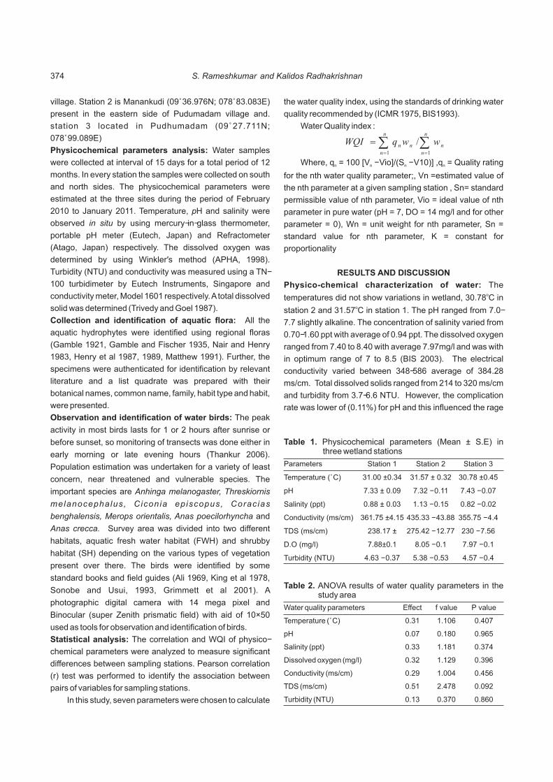
village. Station 2 is Manankudi (09°36.976N; 078°83.083E)
present in the eastern side of Pudumadam village and.
station 3 located in Pudhumadam (09°27.711N;
078°99.089E)
Physicochemical parameters analysis: Water samples
were collected at interval of 15 days for a total period of 12
months. In every station the samples were collected on south
and north sides. The physicochemical parameters were
estimated at the three sites during the period of February
2010 to January 2011. Temperature, pH and salinity were
observed in situ by using mercury-in-glass thermometer,
portable pH meter (Eutech, Japan) and Refractometer
(Atago, Japan) respectively. The dissolved oxygen was
determined by using Winkler's method (APHA, 1998).
Turbidity (NTU) and conductivity was measured using a TN-
100 turbidimeter by Eutech Instruments, Singapore and
conductivity meter, Model 1601 respectively. A total dissolved
solid was determined (Trivedy and Goel 1987).
Collection and identification of aquatic flora: All the
aquatic hydrophytes were identified using regional floras
(Gamble 1921, Gamble and Fischer 1935, Nair and Henry
1983, Henry et al 1987, 1989, Matthew 1991). Further, the
specimens were authenticated for identification by relevant
literature and a list quadrate was prepared with their
botanical names, common name, family, habit type and habit,
were presented.
Observation and identification of water birds: The peak
activity in most birds lasts for 1 or 2 hours after sunrise or
before sunset, so monitoring of transects was done either in
early morning or late evening hours (Thankur 2006).
Population estimation was undertaken for a variety of least
concern, near threatened and vulnerable species. The
important species are Anhinga melanogaster, Threskiornis
melanocephalus, Ciconia episcopus, Coracias
benghalensis, Merops orientalis, Anas poecilorhyncha and
Anas crecca. Survey area was divided into two different
habitats, aquatic fresh water habitat (FWH) and shrubby
habitat (SH) depending on the various types of vegetation
present over there. The birds were identified by some
standard books and field guides (Ali 1969, King et al 1978,
Sonobe and Usui, 1993, Grimmett et al 2001). A
photographic digital camera with 14 mega pixel and
Binocular (super Zenith prismatic field) with aid of 10×50
used as tools for observation and identification of birds.
Statistical analysis: The correlation and WQI of physico-
chemical parameters were analyzed to measure significant
differences between sampling stations. Pearson correlation
(r) test was performed to identify the association between
pairs of variables for sampling stations.
In this study, seven parameters were chosen to calculate
the water quality index, using the standards of drinking water
quality recommended by (ICMR 1975, BIS1993).
Water Quality index :
Where, q = 100 [V - Vio]/(S - V10)] ,q = Quality rating n n n n
for the nth water quality parameter;, Vn =estimated value of
the nth parameter at a given sampling station , Sn= standard
permissible value of nth parameter, Vio = ideal value of nth
parameter in pure water (pH = 7, DO = 14 mg/l and for other
parameter = 0), Wn = unit weight for nth parameter, Sn =
standard value for nth parameter, K = constant for
proportionality
RESULTS AND DISCUSSION
Physico-chemical characterization of water: The otemperatures did not show variations in wetland, 30.78 C in
ostation 2 and 31.57 C in station 1. The pH ranged from 7.0-
7.7 slightly alkaline. The concentration of salinity varied from
0.70-1.60 ppt with average of 0.94 ppt. The dissolved oxygen
ranged from 7.40 to 8.40 with average 7.97mg/l and was with
in optimum range of 7 to 8.5 (BIS 2003). The electrical
conductivity varied between 348-586 average of 384.28
ms/cm. Total dissolved solids ranged from 214 to 320 ms/cm
and turbidity from 3.7-6.6 NTU. However, the complication
rate was lower of (0.11%) for pH and this influenced the rage
Parameters Station 1 Station 2 Station 3
Temperature (°C) 31.00 ±0.34 31.57 ± 0.32 30.78 ±0.45
pH 7.33 ± 0.09 7.32 - 0.11 7.43 - 0.07
Salinity (ppt) 0.88 ± 0.03 1.13 - 0.15 0.82 - 0.02
Conductivity (ms/cm) 361.75 ±4.15 435.33 - 43.88 355.75 - 4.4
TDS (ms/cm) 238.17 ± 275.42 - 12.77 230 - 7.56
D.O (mg/l) 7.88±0.1 8.05 - 0.1 7.97 - 0.1
Turbidity (NTU) 4.63 - 0.37 5.38 - 0.53 4.57 - 0.4
Table 1. Physicochemical parameters (Mean ± S.E) in three wetland stations
Water quality parameters Effect f value P value
Temperature (°C) 0.31 1.106 0.407
pH 0.07 0.180 0.965
Salinity (ppt) 0.33 1.181 0.374
Dissolved oxygen (mg/l) 0.32 1.129 0.396
Conductivity (ms/cm) 0.29 1.004 0.456
TDS (ms/cm) 0.51 2.478 0.092
Turbidity (NTU) 0.13 0.370 0.860
Table 2. ANOVA results of water quality parameters in the study area
åå==
=n
n
n
n
n
nn wwqWQI11
/
S. Rameshkumar and Kalidos Radhakrishnan374

Parameters Standard value (s )n
Unit weight
(w )n
Station-1 Station-2 Station-3
Observed value
Quality rating (q )n
W qn n Observed value
Quality rating (q )n
W qn n Observed value
Quality rating (q )n
W qn n
Ph 6.5 – 8.5 0.2190 7.32 21.33 4.67 7.43 28.89 6.33 7.33 22.22 4.87
D.O (mg/l) 5 0.3723 8.05 66.11 24.61 7.97 67.04 24.96 7.88 67.96 25.30
Conductivity (ms/cm) 300 0.3710 435.33 145.11 53.84 355.75 118.58 43.99 361.75 120.58 44.74
TDS (ms/cm) 500 0.0037 275.42 55.08 0.20 230.00 46.00 0.17 238.17 47.63 0.18
Range of water quality 0.9660 83.32 75.45 75.08
Table 3. Water quality index (WQI) of the seasonal wetland ecosystem
Parameters Temperature (°C)
pH Salinity (ppt)
D.O (mg/l)
Conductivity (ms/cm)
TDS (ms/cm)
Turbidity (NTU)
Species nos.
Temperature (°C) 1
pH -0.325 1
Salinity (ppt) 0.628 -0.64 1
D.O (mg/l) -0.04 -0.139 0.433 1
Conductivity (ms/cm) 0.58 -0.575 .987** 0.526 1
TDS (ms/cm) 0.638 -0.654 .987** 0.513 .989** 1
Turbidity (NTU) 0.475 -0.574 .975** 0.474 .984** .956** 1
Species nos. -0.482 0.211 -0.803 -0.515 -.877* -.824* -.858* 1
Table 4. Pearson correlation coefficients matrix between the physic-chemical parameters of and species distribution
* Correlation is significant at the 0.05 and ** at 0.01 level (2-tailed).
of individual parameters. The level of dissolved oxygen
standardizes the distribution pattern of flora and fauna
(Kotadiya Nikesh and Acharya 2014). The BIS/ ICMR
reported that, the dissolved oxygen of 5mg/l is optimum.
Water quality index has been used to evaluate status of
wetland water quality through water quality index (Chatterji
and Raziuddin 2002, Rameshkumar and Rajaram 2016). In
the present study, water quality was very poor in all three
stations (WQI >76). This finding was confirmed by some
previous study (Thakor et al 2011, Jena et al 2013,
Korgaonkar et al 2014). More human activities were altering
and deteriorate water qualities on these wetlands than other
kinds. The status of water quality in these study sites are
given in (Table 3). The salinity was positively correlated with
electrical conductivity, total dissolved solids and turbidity.
Similarly the conductivity correlated positively with TDS and
turbidity (Table 4). The number of species was correlated
significantly negative with all physic-chemical parameters
except pH, but the electrical conductivity, total dissolved
solids and turbidity. This indicated that, the total number of
species decreased with increased electrical conductivity,
turbidity and total dissolved solids in wetland ecosystem. The
pH was correlated negatively with all physico-chemical
parameters but was statistically not significant.
Distribution and abundance of aquatic macrophytes :
The Ceratophyllum demersum L. Egeria densa planch,
Lemna minor L. Marsilea quadrifolia L., Patamogeton
nodosus poix, Nymphaea nouchali Burm.f, Nymphaea
odorata Aiton, Nelumbo nucifera Gaertn, Myriophyllum
spicatum L, Hydrilla verticillata, Chara globularis, Sagittaria
guyanensis, Isoetus ribaria, Eichornia crassipes kunth, and
Najas minor were recorded (Table 5). The highest number of
12 plant species was observed in Station 1 whereas the
minimum of 7 species were recorded at station 2. The
variations of species distribution were based on the physico
chemical and environmental parameters. Present study
revealed that, most of the wetland covered by submerged
macrophytes (7 species) and rooted floating weeds (6
species) than those of floating weed (1 species.) and rooted
macrophytes (1 species). Adhishwar and Choudhary (2013)
observed 137 macrophytes belong to 50 families. With
respect to water quality changes in water chemistry has been
considered to exert influence in the distribution of many
aquatic plant species (Engelhardt and Ritchie 2001, Lentz-
Cipollini and Dunson 2006).
In wetland, macro vegetation have imperative role in
determining the limno-biological environment (Das et al
2009) that can reflected in taxonomic composition of plants
Multivariate Analysis of Water Quality Parameters 375
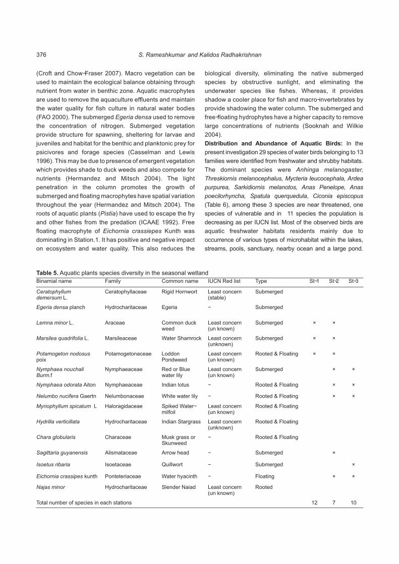
Binamial name Family Common name IUCN Red list Type St-1 St-2 St-3
Ceratophyllum demersum L.
Ceratophyllaceae Rigid Hornwort Least concern (stable)
Submerged
Egeria densa planch Hydrocharitaceae Egeria - Submerged
Lemna minor L. Araceae Common duck weed
Least concern (un known)
Submerged × ×
Marsilea quadrifolia L. Marsileaceae Water Shamrock Least concern (unknown)
Submerged × ×
Potamogeton nodosus poix
Potamogetonaceae Loddon Pondweed
Least concern (un known)
Rooted & Floating × ×
Nymphaea nouchali Burm.f
Nymphaeaceae Red or Blue water lily
Least concern (un known)
Submerged × ×
Nymphaea odorata Aiton Nymphaeaceae Indian lotus - Rooted & Floating × ×
Nelumbo nucifera Gaertn Nelumbonaceae White water lily - Rooted & Floating × ×
Myriophyllum spicatum L Haloragidaceae Spiked Water-milfoil
Least concern (un known)
Rooted & Floating
Hydrilla verticillata Hydrocharitaceae Indian Stargrass Least concern (unknown)
Rooted & Floating
Chara globularis Characeae Musk grass or Skunweed
- Rooted & Floating
Sagittaria guyanensis Alismataceae Arrow head - Submerged ×
Isoetus ribaria Isoetaceae Quillwort - Submerged ×
Eichornia crassipes kunth Ponteteriaceae Water hyacinth - Floating × ×
Najas minor Hydrocharitaceae Slender Naiad Least concern (un known)
Rooted
Total number of species in each stations 12 7 10
Table 5. Aquatic plants species diversity in the seasonal wetland
(Croft and Chow-Fraser 2007). Macro vegetation can be
used to maintain the ecological balance obtaining through
nutrient from water in benthic zone. Aquatic macrophytes
are used to remove the aquaculture effluents and maintain
the water quality for fish culture in natural water bodies
(FAO 2000). The submerged Egeria densa used to remove
the concentration of nitrogen. Submerged vegetation
provide structure for spawning, sheltering for larvae and
juveniles and habitat for the benthic and planktonic prey for
psicivores and forage species (Casselman and Lewis
1996). This may be due to presence of emergent vegetation
which provides shade to duck weeds and also compete for
nutrients (Hermandez and Mitsch 2004). The light
penetration in the column promotes the growth of
submerged and floating macrophytes have spatial variation
throughout the year (Hermandez and Mitsch 2004). The
roots of aquatic plants (Pistia) have used to escape the fry
and other fishes from the predation (ICAAE 1992). Free
floating macrophyte of Eichornia crassiepes Kunth was
dominating in Station.1. It has positive and negative impact
on ecosystem and water quality. This also reduces the
biological diversity, eliminating the native submerged
species by obstructive sunlight, and eliminating the
underwater species like fishes. Whereas, it provides
shadow a cooler place for fish and macro-invertebrates by
provide shadowing the water column. The submerged and
free-floating hydrophytes have a higher capacity to remove
large concentrations of nutrients (Sooknah and Wilkie
2004).
Distribution and Abundance of Aquatic Birds: In the
present investigation 29 species of water birds belonging to 13
families were identified from freshwater and shrubby habitats.
The dominant species were Anhinga melanogaster,
Threskiornis melanocephalus, Mycteria leucocephala, Ardea
purpurea, Sarkidiornis melanotos, Anas Penelope, Anas
poecilorhyncha, Spatula querquedula, Ciconia episcopus
(Table 6), among these 3 species are near threatened, one
species of vulnerable and in 11 species the population is
decreasing as per IUCN list. Most of the observed birds are
aquatic freshwater habitats residents mainly due to
occurrence of various types of microhabitat within the lakes,
streams, pools, sanctuary, nearby ocean and a large pond.
S. Rameshkumar and Kalidos Radhakrishnan376

Binomial name Family Common name IUCN Red list Habitat St-1 St-2 St-3
Anhinga melanogaster Anhingidae Oriental Darter Near threatened (decreasing)
AqH ×
Phalacrocorax niger Phalacrocoracidae Little Cormorant Least concern (Unknown)
AqH
Phalacrocorax carbo Phalacrocoracidae Great Cormorant Least concern (increasing)
AqH × ×
Tachybaptus ruficollis Podicipedidae Little grebe Least concern (decreasing)
AqH ×
Ardea cinerea Ardeidae Grey Heron Least concern (Unknown)
AqH/SH × ×
Ardea purpurea Ardeidae Purple Heron Least concern (decreasing)
AqH/SH ×
Ardea alba Ardeidae (Great White Egret Least concern (Unknown)
AqH/SH × ×
Sarkidiornis melanotos Anatidae African Comb Duck Least concern (decreasing)
AqH/SH × ×
Nettapus coromandelianus
Anatidae Cotton Pygmy-goose Least concern (stable)
AqH/SH × ×
Anas penelope Anatidae Eurasian Wigeon Least concern (decreasing)
AqH/SH ×
Anas poecilorhyncha Anatidae Indian Spot-Billed Duck Least concern (decreasing)
AqH/SH × ×
Spatula querquedula Anatidae Garganey Least concern (decreasing)
AqH/SH × ×
Anas crecca Anatidae Common Teal Least concern (Unknown)
AqH/SH × ×
Ciconia episcopus Ciconiidae Asian Woollyneck Vulnerable (decreasing)
AqH/SH × ×
Merops phillippinus Meropidae Blue-tailed Bee-eater - AqH/SH
Halcyon smyrnensis Alcedinidae White-breasted Kingfisher
Least concern (Increasing)
AqH/SH ×
Egretta garzetta Ardeidae Little Egret Least concern (Increasing)
AqH
Mesophoyx intermedia Ardeidae Median Egret - AqH/SH
Bubulcus ibis Ardeidae Cattle Egret Least concern (Increasing)
AqH/SH ×
Ardeola grayii Ardeidae Indian pond-heron Least concern (Unknown)
AqH/SH ×
Tringa ochropus Charadriidae Green Sandpiper Least concern (Stable) SH/AqH × ×
Tringa glareola Charadriidae Wood Sandpiper Least concern (Stable)
SH/AqH
Himantopus himantopus Recurvirostridae Black-winged Stilt Least concern (Increasing)
SH/AqH
Rostratula benghalensis Rostratulidae Greater painted-Snipe Least concern (decreasing)
SH/AqH ×
Threskiornis melanocephalus
Threskiornithidae Black-headed Ibis) Near threatened (decreasing)
AqH × ×
Mycteria leucocephala Ciconiidae Painted Stork Near threatened (decreasing)
AqH/SH
Merops orientalis Meropidae Asian Green Bee-eater Least concern (Increasing)
AqH/SH × ×
Coracias benghalensis Coraciidae Indian Roller Least concern (Increasing)
AqH/SH
Alcedo atthis Alcedinidae Common Kingfisher Least concern (unknown)
AqH/SH ×
Total number of species in each stations 21 19 14
Table 6. Diversity of aquatic birds in the seasonal wetland ecosystem
AqH: Aquatic habitat, SH: Shrubby habitat
Multivariate Analysis of Water Quality Parameters 377

Due to the abundance of variety of plant and avifaunal
communities are occurring in environment which is very
favourable for bird conservation in this part of the wetlands.
Water birds tend to be highly mobile in winter, moving to other
areas in response to factors such as cold weather and
changes in water levels and in food resources (Kershaw and
Cranswick 2003). The present study concludes that wetlands
are serious threat to biodiversity due to waste from agricultural
waste, domestic, sewage effluents, fishing waste etc. During
monsoon (October-December) and post monsoon (January-
March) seasons many water birds are migrating from various
parts. Hence, the conservation and management strategy is
important to protect wetland ecosystem.
REFERENCES
Adhishwar AK and Choudhary SK 2013. Diversity of macrophytic species of gogabil lake wetland in Katihar, Bihar, India. Ecological Environment and Conservation 19: 1165-1172.
Ali S 1969. The Book of Indian Birds (8th edition). Bombay Natural History Society, Bombay, India.
APHA 1998. Standard methods for the examination of water and wastewater (Edition 20th). Washington, DC: American Public Health Association.
Banner A and Mac Kenzie W 2000. The ecology of wetland ecosystem. 45 Extension note. Ministry of forest research program. British Columbia.
Baral HS and Inskipp C 2005. Important Bird Areas in Nepal: Key Sites for Conservation. Bird Conservation Nepal and Bird Life International, Kathmandu and Cambridge.
BIS 1993. Standards of water for drinking and other purposes Bureau of Indian Standards, New Delhi.
Bureau of Indian Standards (BIS) 2003. 10500, Manak Bhavan, New Delhi, India.
Casselman JM and Lewis CA 1996. Habitat requirements of northern pike (Esoxlucius). Canadian Journal of Fisheries and Aquatic Sciences 53: 161–174.
Catling PM, Freedman B, Stewart C, Kerekes JJ and Lefkovitch LP 1986. Aquatic plants of acid lakes in Kejimkujik National Park, Nova Scotia; floristic composition and relation to water chemistry. Canadian Journal of Botany 64: 724-729.
Chaterjee C and Razuddin M 2002. Determination of Water Quality Index (W.Q.I.) of a degraded river in Asanil Industrial area, Ranigunj, Burdwan, West Bengal. Nature Environment and Pollution Technology 1: 181-189.
Chee WL and Vitt DH 1989. The vegetation, surface water chemistry and peat chemistry of moderate-rich fens in central Alberat, Canada. Wetlands 9: 227-261.
Croft VM and Chow-Fraser P 2007. Use and Development of the wetland macrophyte index to detect water quality impairment in fish habitat of Great lakes coastal marshes. Journal of Great Lakes Research 33: 172–197.
Cohen J 1988. Statistical Power Analysis for the Behavioral ndSciences (2 edition). Lawrence Erlbaum Associates,
publishers. New Jersey.
Colle DE and Shireman JV 1980. Coefficients of condition for largemouth bass, bluegill and redearsunfish in hydrilla-infested lakes. Transactions of the American Fisheries Society 109: 521-531.
Das SK, Biswas F and Roy S 2009. Study of hydrophytes in some lentic water bodies in West Bengal, India. Ecoprint 16: 9-13.
Engelhardt K and Ritchie M 2001. Effects of macrophyte species
richness on wetland ecosystem functioning and services. Nature 411: 687–689.
FAO 2000. Crops and drops: making the best use of water for agriculture. FAO Advance Edition. Rome.
Gamble JS and Fischer CEC 1921-35. Flora of the Presidency of Madras. 3 Vols. London: Adlard and Son Ltd. 2017p.
Grimmett R, Inskipp C and Inskipp T 2001. Birds of the Indian Subcontinent. (Revised reprint 2001), Christopher Helm, London.
Hernandez ME and Mitsch WJ 2004. Deepwater macrophytes and water quality in two experimental wetlands at Olentangy River Wetland Research Park.
Hernandez ME and Mitsch WJ 2007. De-nitrification in created riverine wetlands: Influence of hydrology and season. Ecological Engineering 30: 78-88.
Henry AN, Kumari GR and Chitra V 1987. Flora of Tamil Nadu, India. Series I: Analysis. Volume 2. Coimbatore: Botanical Survey of India. p258.
Henry AN, Chitra V and Balakrishnan NP 1989. Flora of Tamil Nadu, India. Series II: Analysis. Volume 3. Coimbatore: Botanical Survey of India. p171.
HMGN/MFSC 2002. Nepal Biodiversity Strategy. Ministry of Forests and Soil Conservation, His Majesty's Government of Nepal, Kathmandu.
ICAAE 1992. Introduction to fish culture in ponds. International Centre for Aquaculture and Aquatic Environments, Auburn University, Alabama.
ICMR 1975. Manual of Standards of Quality for Drinking Water Supplies. Indian Council of Medical Research. Special Report No. 44: 27.
Jena V, Dixit S and Gupta S 2013. Assessment of water quality index of industrial area surface water samples. International Journal of Chem Tech Research 5: 278-283.
Kershaw M and Cranswick PA 2003. Deriving population estimates for wintering wildfowl in Great Britain. Ornis Hungarica 12-13: 75-87.
King B, Woodcock M and Disckinson EC 1978. A field guide to the birds of South-east Asia. Collins, St. Jame's Pa-lace, London.
Korgaonkar DS, Bharamal DL and Koli YJ 2014. Determination of water quality index in Annapurna river in Devgad Taluka, district Sindhudurg, Maharashtra. An International Quarterly Journal of Biology and Life sciences 2: 1268-1273.
Kotadiya Nikesh G and Acharya CA 2014. An assessment of lake water quality index of Manipu lake of district Ahmedabad, Gujarat. International Journal of Scientific Research Vol.III, Issue.
Kricher JC 1975. Diversity in two wintering bird communities: possible weather effects. Auk 92: 766-777.
Lentz-Cipollini KA and Dunson WA 2006. Abiotic features of seasonal pond habitat and effects on endangered northeastern Bulrush, Scirpus ancistrochaetus Schuyler, in Central Pennsylvania. Castanea 71: 272-281.
Matthew KM 1991. An excursion Flora of Central Tamil Nadu. Tamil Nadu: Thiruchirappalli, Rapinat Herbarium. 682p.
Nair NC and Henry AN 1983. Flora of Tamil Nadu, India. Series I: Analysis. Volume1. Coimbatore: Botanical Survey of India.
Norlin JI, Bayley SE and Ross LCM 2005. Submerged macrophytes, zooplankton and the predominance of low- over high-chlorophyll states in western boreal, shallow-water wetlands. Freshwater Biology 50: 868-881.
Powell GVN 1987. Habitat use by wading birds in a semitropical estuary: implications of hydrography. Auk 104: 740-749.
Rameshkumar S and Rajaram 2016. Assessment of physicochemical parameters to diversity and distribution of aquatic macrophytes in seasonal wetlands through water quality index approach. Conference Abstracts, The 10th
S. Rameshkumar and Kalidos Radhakrishnan378

INTECOL International Wetlands Conference Hotspots of Biodiversity and Ecosystem Services under Global Changes September 19-24pp.
Sooknah RD and Wilkie AC 2004. Nutrient removal by floating aquatic macrophytes cultured in anaerobically flushed dairy manure wastewater. Ecology Engineering 22: 27–42.
Sonobe K and Usui S 1993. A field guide to the water birds of Asia. Wildlife Bird Society of Japan, Tokyo.
Thakor FJ, Bhol DK, Pandya SN and Chauhan NB 2011. Water quality index (W.Q.I.) of Periyej lake district, Kheda – Gujarat. Current World Environment 6: 225-231.
Thankur ML 2006. Ph.D. thesis, Himachal Pradesh University, Shimla, India. pp-306
Trivedy RK and Goel PK 1987. Chemical and Biological methods for water pollution studies. Environmental Publications, Karad, India. pp1-34.
Received 20 March, 2018; Accepted 10 May, 2018
Multivariate Analysis of Water Quality Parameters 379

Evaluation of Groundwater Quality by Using Water Quality Index Near Magnesite Mines, Salem District, Tamilnadu, India
Indian Journal of Ecology (2018) 45(2): 380-383
Abstract: The present investigation meant to assess the water quality for the groundwater of around Magnesite Mines in Salem District. For
ascertaining the WQI, the parameter considered were pH, total hardness, calcium, magnesium, chloride, sulfate, total dissolved solids,
sodium, total alkalinity. All the physic-chemical parameters of groundwater samples were within the highest desirable limit as per WHO. The
WQI varied from 55.45 to 81.29.In Sengaradu, Gollapatti, Vinayakampatti the WQI was higher due to convergence of magnesium, sulphate
and chloride in the groundwater. A significant negative correlation was observed between calcium and sulphate, sodium and total alkalinity.
Keywords: Groundwater, Magnesite mines, Chemical characteristics, Water quality index, Correlation
Manuscript Number: 2689NAAS Rating: 4.96
1P.S. Kumar and P. BalamuruganDepartment of Civil Engineering, University College of Engineering, Ariyalur Campus, Ariyalur-621 704, India
1 Department of Civil Engineering, Dhirajlal Gandhi College of Technology, Salem-636 309, IndiaE-mail: [email protected]
Groundwater assumes a critical part in Indian
horticulture. The appropriateness of water system water
relies on many elements counting the nature of water, soil
sort and salt resilience qualities of the plants, atmosphere
and waste qualities of the dirt (Michael 1990). Groundwater
dependably contains little measure of solvent salts broke
down in it. The sorts and qualities of these salts rely on the
hotspots for revive of the groundwater and the strata through
which it streams. The abundance amount of solvent salts
might be unsafe for some products. Subsequently, for a
superior comprehension of science of groundwater it is
extremely fundamental to legitimately assess groundwater
quality for water system reason. Paddy crops, vegetables,
foods grown from the ground crops are the normal rural
deliver of the general population in the contemplate zone
(Abdoliman Amouei et al 2012). The waterway and tank
waters are not accessible at many places in the investigation
zone or in the event that if accessible, they are not ready to
supply sufficient water for flooding crops even at basic
phases of harvest development (Adelekan et al 2011). Under
these conditions, the groundwater turns into the primary
wellspring of irrigation. Geochemical forms in groundwater
include the association of nation rocks with water, prompting
the improvement of auxiliary mineral stages. The standards
administering the synthetic attributes of groundwater are
very much archived in many parts of the world
(HadiHajizadesh et al 2011, Hariharan et al 2010, Mahadev
et al 2010). This paper examines the conceivable concoction
forms of groundwater shake collaboration in hard shake
landscape. Geographic Information System (GIS) has risen
as a capable innovation of guideline, for look into, and for
building the stature of projects have directed GIS-based
examination and understanding of groundwater quality
information.
MATERIAL AND METHODS
Study Area: Salem in Tamil Nadu, South India, is the center
of essential hard-headed industry in the nation. Magnesite,
the main crude material for fundamental refractory and
additionally calcined Magnesia, is being mined from three
huge and a few little mines situated in Salem. The ultramarine 2complex of Salem spreads over a region of 30 km and is
known as the Chalk Hills area. It is the archive of both
obstinate and non-recalcitrant evaluations of magnesite.
Salem area is limited by Villupuram locale in the east; Erode
region in the west and Dharmapuri region in the north and
Namakkal region in the south. The area lies between o o o o11 21'30"N to 11 59'00"N Latitude, 77 38'00" E to 78 50'00"E
2Longitude and has a flying degree of 5245 km . The normal o otemperatures run from 37 C to 43 C. The normal precipitation
for the area is 972.3mm. Normal annual rainfall over the
district varies from 800 to 1600mm.(Arulmozhi et al 2017).
The WQI has been computed by using standards of drinking
water quality recommended by the world health organization
(WHO), Bureau of Indian Standards (BIS) and Indian Council
for Medical Research (ICMR). The major three steps are
followed to compute the water quality index for the water
samples.
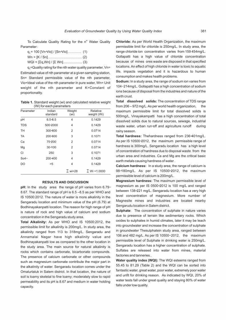
thTo Calculate Quality Rating for the n Water Quality
Parameter:
q = 100 [Vn-Vio] / [Sn-Vio]………… (1)n
Wn = [K / Sn]………………………… (2)
WQI = [Óq Wn] / [Ó Wn]…………….. (3)n
q =Quality rating for the nth water quality parameter, Vn= n
Estimated value of nth parameter at a given sampling station,
Sn= Standard permissible value of the nth parameter,
Vio=Ideal value of the nth parameter in pure water, Wn= Unit
weight of the nth parameter and K=Constant of
proportionality.
RESULTS AND DISCUSSION
pH: In the study area the range of pH varies from 6.79-
8.67. The standard range of pH is 6.5 –8.5 as per WHO and
IS 10500:2012. The nature of water is more alkalinity in the
Sengaradu location and minimum value of the pH (6.79) at
Bodhinayakanpatti location. The reason for high range of pH
is nature of rock and high value of calcium and sodium
concentration in the Sengaradu study area.
Total Alkalinity: As per WHO and IS 10500:2012, the
permissible limit for alkalinity is 200mg/L. In study area, the
alkalinity ranged from 113 to 318mg/L. Sengaradu and
Annamalai Nagar have high alkalinity value and
Bodhinayakanpatti low as compared to the other location in
the study area. The main source for natural alkalinity is
rocks which contains carbonate, bicarbonate compounds.
The presence of calcium carbonate or other compounds
such as magnesium carbonate contribute the major part in
the alkalinity of water. Sengaradu location comes under the
Omalurtaluk in Salem district. In that location, the nature of
soil is loamy skeletal to fine loamy; moderately slow to rapid
permeability and its pH is 8.67 and medium in water holding
capacity.
Chloride: As per World Health Organization, the maximum
permissible limit for chloride is 250mg/L. In study area, the
range chloride ion concentration varies from 159 454mg/L.
Gollapatti has a high value of chloride concentration
because of mines ores waste are disposed in that specified
locations. An effect of high chloride in water is toxic to aquatic
life, impacts vegetation and it is hazardous to human
consumption and makes health problems.
Sodium: In a study area, the range of sodium ion varies from
104- 214mg/L. Gollapatti has a high concentration of sodium
ions because of disposal from the industries and nature of the
earth crust.
Total dissolved solids: The concentration of TDS range
from 206 – 972 mg/L. As per world health organization, the
maximum permissible limit for total dissolved solids is
500mg/L. Vinayakampatti has a high concentration of total
dissolved solids due to natural sources, sewage, industrial
waste water, urban run-off and agriculture runoff during
rainy season.
Total hardness: Thehardness ranged from 236-401mg/L.
As per IS 10500-2012, the maximum permissible range of
hardness is 300mg/L. Sengaradu location has a high level
of concentration of hardness due to disposal waste from the
urban area and industries. Ca and Mg are the critical basic
earth metals causing hardness of water .
Calcium hardness: In a study area, the range of calcium is
98-180mg/L. As per IS 10500-2012, the maximum
permissible level of calcium is 200mg/L.
Magnesium hardness: The maximum permissible level of
magnesium as per IS 0500-2012 is 100 mg/L and ranged
between 138-221 mg/L. Sengaradu location has a very high
level concentration of magnesium. More number of
Magnesite mines and industries are located nearby
Sengarudu location in Salem district.
Sulphate: The concentration of sulphate in nature varies
due to presence of terrain like sedimentary rocks. Which
oxides to sulphates in humid climates, later it may be leach
into groundwater and increase the concentration of sulphate
in groundwater Thesulphatein study area, ranged between
106 and 482 mg/L. As per IS 10500- 2012, the maximum
permissible level of Sulphate in drinking water is 250mg/L.
Sengaradu location has a higher concentration of sulphate.
Sulfates are released into water from mines, material
factories and tanneries..
Water quality index (WQI): The WQI esteems ranged from
55.45 to 81.29 (Table 2) and the WQI can be sorted into
fantastic water, great water, poor water, extremely poor water
and unfit for drinking reason. As indicated by WQI, 20% of
water tests fall under great quality and staying 80% of water
falls under low quality.
Parameter Indianstandard
Weight(wi)
Relativeweight (Wi)
pH 6.5-8.5 4 0.1429
TDS 500-2000 4 0.1429
TH 300-600 2 0.0714
TA 200-600 3 0.1071
Ca 75-200 2 0.0714
Mg 30-100 2 0.0714
Cl 250 3 0.1071
So4- 200-400 4 0.1429
DO >5 4 0.1429
∑wi=28 ∑Wi =1.0000
Table 1. Standard weight (wi) and calculated relative weight (Wi) for each parameters
Evaluation of Groundwater Quality by Using Water Quality Index 381

Sample station Latitude Longitude pH TA Cl TDS T H Ca Mg SO4- Na WQI
Adivaram 11.706058 78.179088 6.5 100 180 150 150 100 70 200 168 46.57
Ayyamperumalpatti 11.67771 78.082812 7.8 184 337 621 244 184 102 375 143 73.29
Chettichavadi 11.724912 78.15621 8.14 304 376 489 359 304 160 189 151 75.21
Karuppur 11.716306 78.087567 7.23 121 209 647 302 121 131 248 176 63.59
Gollapatti (pudur) 11.319183 77.79568 7.09 148 454 509 354 148 157 307 214 78.05
Kundur 11.747975 78.199441 8.16 278 273.9 451 378 278 169 170 158 70.16
Sengaradu 11.747699 78.138529 8.67 318 211 372 401 318 180 293 176 74.15
Vinayakampatti 11.724362 78.166434 8.14 278 377 972 332 278 146 301 164 81.29
Muniyappankovil 11.6269541 78.118495 7.1 187 329.8 343 298 187 129 407 152 72.88
Vellakkalpatti 11.468867 78.264831 6.9 159 240 472 382 159 171 379 104 72.5
Mettupatti 11.667368 78.311561 6.5 150 159.8 150 200 150 110 159 105 45.81
Daivanagar 11.738116 78.155626 6.9 100 150 140 136 100 76 198 134 43.64
Suramangalam 11.675316 78.120673 7 152 178 146 148 152 94 180 125 46.49
ATCnagar 11.693233 78.161246 7.31 140 159 262 381 140 171 221 183 62.16
Annamalainagar 11.681879 78.172118 8.2 318 284.9 148.8 348 318 154 189.6 135 68.55
Bodhinayakanpatti 11.424797 78.242788 6.79 113 248 482 438 113 199 106 183 65.43
Pasuvakkal 11.693206 78.086436 8.1 286 246 321 282 286 122 482 163 75.05
Mungilpadi 11.639105 78.852362 8.02 298 176 464 301 298 131 361 148 69.77
Karuppur East 11.706254 78.152422 7.23 121 209 647 302 121 131 248 176 63.74
Ayyamperumalpatti North 11.69124 78.212354 7.8 184 337 621 244 184 102 375 143 73.29
Table 2. Physic-Chemical parameter of groundwater samples
Factual analysis: Statistical Package for Social Science
(SPSS Ver.13) was utilized to establish out the statistical
examination for groundwater in an examination zone. In
measurable test were essential measurements like mean,
middle and standard deviation is ascertained to know the
synthetic parameters which are digressing from the Bureau
pH TDS TH TA CA MG CL SO4 NA
Mean 7.48 420.39 299 196.95 135.25 163.75 256.77 269.43 155.05
Median 7.27 457.5 302 171.5 131 171 243 248 155
Std.Dev 0.64 220.8 88.08 79.85 35.46 54.05 86.74 100.6 27.04
Max 8.67 972 438 318 199 239 454 482 214
Min 6.5 140 136 100 70 54 150 106 104
Indian.Std 8.5 500 300 200 75 30 250 250 200
Table 4. Statistics analysis for Ground water samples
WQI values Percentage ofstudy area (%)
Quality
0-25 0 Excellent water
25-50 20 Good water
50-75 80 Poor water
75-100 - Very poor water
>100 - Unfit for drinking
Table 3.Status of groundwater sample for study area of Indian Standard for drinking reason. In an examination
territory, mean, middle, standard deviation for all parameters
were observed and 90% of the areas are inside the points of
confinement of BIS for drinking reason (Table 5). Connection
investigation measures the cozy connection between the
concoction parameters of the water tests. In this
investigation, the esteem go between +1 to - 1 and it
demonstrates the ideal connection between the two
parameters (Table 6).
CONCLUSION
According to, IS 10500-2012, Sengaradu, Gollapatti,
Vinayakampatti areas has a high grouping of concoction
parameters. As per WQI, 20 percent of water sample fall under
good quality water and 80 percent under low quality. The high
P.S. Kumar and P. Balamurugan382

Parameter pH TDS TH TA Ca Mg Cl SO -4 NA
pH 1
TDS 0.34 1
TH 0.42 0.4 1
TA 0.9 0.14 0.4 1
Ca 0.34 0.28 0.65 0.36 1
Mg 0.46 0.46 0.58 0.41 0.32 1
-Cl 0.34 0.56 0.35 0.31 0.26 0.4 1
4-SO 0.31 0.32 0.01 0.26 -0.1 0.93 0.31 1
Na 0.14 0.33 0.42 -0.06 0.35 0.45 0.3 -0.02 1
Table 5. Correlation coefficient matrix of groundwater quality
estimation of WQI at this ar eais due to higher magnesium,
chloride and sulfate and calcium in the groundwater.
Sengaradu, Gollapatti, Vinayakampatti area needs essential
treatment like sedimentation, coagulation, flocculation before
.The industrial effluents and agricultural disposals must be
treated before pumping into the river system.
REFERENCES
Abdoliman Amouei, Amir Hossein Mahvi, Ali Akbar Mohammadi, Seiedeh Horieh Fallah, Hossen Ali Asgharnia and Ali Akbar Khafajeh 2012. Physical and chemical quality assessment of potable ground water in rural areas of Khaf, Iran, World Application Sciences Journal 18: 693-697.
Adelekan BA and Abegudne KD 2011. Heavy metal contamination of soil and groundwater at automobile mechanic villages in Ibadan, Nigeria. International Journal Physical Science 6: 1045-1048.
Arulmozhi S and Prince Arulraj G 2017. “Rainfall variation and frequency analysis study on salem district tamilnadu” Indian Journal of Geo Marine Science 46(01): 213-218.
Balamurugan P and Kumar PS 2016. “Quality of ground water assessment in Salem district using GIS Techniques”. Advances in Natural and Applied Science 10(3): 22-31.
Bureau ofIndian Standards 2012. Drinking water specification IS:10500
Gagik Badalians Gholikandi, Skineh Haddadi, Emad Dehghanifard and Hamid Reza Tashayouie 2012. Assessment of surface water resources quality in Tehran province, Iran. Desalination and Water Treatment 37: 8-20.
HadiHajizadeh Namaghi, Gholamhossein Karami and Saeed Saadat 2011. A study on chemical properties of ground water and soil in ophiolitic rocks in Firuzabad, east of Shahrood, Iran: with emphasis to heavy metal contamination. Environ Monit Assess 174: 573-583.
Hariharan, SH, Chandaluri Subba Rao and Srinivasa Rao B 2010. Determination of water quality index of some areas in Guntur
district, Andra Pradesh, International Journal of Applied Biology and Pharmaceutical Technology 1: 79.
Kumar PS and Periyasamy M 2017. Monitorning of groundwater quality for domestic and irrigation purpose in Nillakottai Block, Dindigul District, Tamilnadu, India. Ecology, Environment and Conservation 23(3):1751-1755.
Magesh NS, Krishnakumar S, Chandrasekar N and John Prince Soundranayagam 20??. Groundwater quality assessment using WQI and GIS techniques, Dindigul district, Tamil Nadu, India”, Arabian Journal of Geosciences 6(11): 4179-4189.
Mahadev J, Syed Akhel Ahmed and Belgali SL 2010. Analysis of seasonal variation in water quality of Cauvery and Kabini rivers with respect to physic-chemical parameters and calcium carbonate saturation index. Journal of Applied Geo Chemistry 12: 224-230.
Mahadevaswamy G et al 2011. Groundwater quality studies in Nanjangud Taluk, Mysore District, and Karnataka, India. International Journal of Environmental Sciences 1(7):
Mufidal-Hadithi 2012. Application of water quality index to assess suitability of groundwater quality for drinking purpose in Ratmao-Pathri Raowatershed, Haridwar district, India. American Journal of Scientific and Industrial Research 3(6): 395-402.
Nirmala B et al 2012. Seasonal Variations of Physico-Chemical Characteristics of Groundwater Samples of Mysore City, Karanataka, India. International Research Journal of Environment Sciences 1(4): 43-49.
Rahman A 2008. A GIS based DRASTIC model for assessing groundwater vulnerability in shallow aquifer in Aligarh, India
Ramakrishnaiah CR, Sadashivaiah C and Ranganna G 2009. Assessment of water quality index for the groundwater in tumkertaluk, Karnataka state, India. E-Journal of Chemistry 6(2): 523-30.
Ravisankar N 2004. Study of groundwater quality in tsunami affected areas of Sirkazhitaluk, Nagapattinam district, Tamil Nadu, India, Centre for Water Resources, Anna University, and Chennai.
WHO (World health Organization) 1993. Guidelines for drinking ndwater quality, 2 edition, 1993, Vol1,pp187-190.
Received 16 March, 2018; Accepted 10 May, 2018
Evaluation of Groundwater Quality by Using Water Quality Index 383
Water Quality Index Assessment of Domestic Water Supplies in System Tank
Indian Journal of Ecology (2018) 45(2): 384-387
Abstract: The study was confined toa system tank zone of River Noyyal in Coimbatore. The ground water and surface water of the monsoon
and post–monsoon seasons were analyzed for various physico-chemical parameters. The Parametric Water Quality values in the respective
units of measurement were found to be in the IS permissible ranges prescribed for EC (3to15dS/m), pH(6.2to 6.8), Total dissolved salts (500 t0
2000) and sulphates (200 to 400). The overall quality indices for both surface and ground water were arrived at in a gradation system of
weightage limits from 1 to 5, as less hazardous to severely hazardous status. The indices established the values in the moderate range of 2.3 to
3.8, suggesting the feasibility of quality sustained domestic water supplies.
Keywords: System Tank, Water Quality Index, Parametric Index, pH, EC, Turbidity, Hardness, Alkalinity, domestic water supplies
Manuscript Number: NAAS Rating: 4.96
2690
S. Ragunath and M. Lenin SundarDepartment of Civil Engineering, KPR Institute of Engineering and Technology, Coimbatore- 641 407, India,
Department of Civil Engineering, Sri Krishna College of Engineering and Technology, Coimbatore-641 042, IndiaE-mail: [email protected]
Surface water reserves such as the tanks and
subterranean aquifers embedded with dug wells and bore
wells store the rainwater for the diversified usage in their
vicinity viz., irrigation, domestic and industrial water supplies
in an ingenious way of roaster based rotational distribution
through open channels and pipeline networks (Debels et al
2005,Giridharan et al 2010). By and large, the system tanks
constructed at various zones of Coimbatore were primarily
envisaged to cater to the irrigation needs of agricultural crops
in their downstream command areas. However, over the past
twenty years this scenario has undergone dramatic changes
partly due to extensive urbanization and intensive
industrialisation as well. Eventually the agricultural land area
has diminished drastically and got converted into real estate
pockets. In response to this impulse the agricultural needs
also got decreased but the domestic and industrial water
requirements got exponentially shotup. Hence the paradigm
shift of transforming agricultural requirements of the water
towards domestic water supplies has become inevitable.
Mostly we resort to a conjunctive use of surface and
groundwater storage that is also responsible for spatial and
temporal water quality changes in accordance with the
contaminant solute transport (Kannel et al 2007, WHO 2008,
Sener et al 2017). However, a qualitative scrutiny of the water
in storage and that reaching the groundwater aquifers is
indispensible. Hence it could be impeccable if the existing
water distribution schedule can be modified to suit the
dominating domestic water needs compared to the barest
minimum agricultural water requirements. By way of
incorporating suitable mechanical filtration systems and
disinfection schedules assured domestic water supplies at
desirable quality level can be accomplished.
Besides, the sustainability of extracting and using both
surface and groundwater from the system tank storage and
dispersion zone needs extensive investigation. System tanks
or non-system tanks do contribute to the aquifer recharge
covering a certain radius of influence both on the
downstream side and upstream side of storage indicated the
well water level fluctuations (Subramani et al 2005) . The
present investigation was contemplated to include nodal
point water samplings related to the surface storage of water
in the tank and well water in the vicinity. Based on these
quality indices focused for domestic water supplies, the
appropriate filtration and disinfection units can be designed
and installed (Horton 1965).
MATERIAL AND METHODS
Study area: The Noyyal river stretch proliferating and
meandering through Coimbatore region encompasses 21
Anaikuts and 31 Tanks, of which 8 system tanks are located
within Coimbatore city urban viz.,Narasampathi tank,
Krisnampathi tank, Selvampathi tank, Kumarasamy tank,
Selvasindhamani tank, UkkadamPeriyakulam tank,
Valankulam tank and Singanallur tank. The study was
however limited only to UkkadamPeriyakulam tank that is
knitted to the downstream reach of the Noyyal River feeding
where the concentrated dumping of pollutants and
contaminants along the stream flows gushing into the tank

water spread pose a severe threat on the surface and
groundwater water qualities. The latitude of Coimbatore,
Tamil Nadu (a State of India) is 11.017363, and the longitude
is 76.958885. (GPS coordinates of 11° 1' 2.5068'' N and 76°
57' 31.9860'' E.). The experimental observations were made
during the monsoon season (June-Nov, 2016) and during the
non-monsoon (December-May, 2016) following the Indian
Standards procedures in sample collection and analysis.
Sample sites and status of pollution: The primary data
collected includes the laboratory analysis results for the
water samples collected along the stretch of the
UkkadamPeriyakulam tank. Secondary data such as rainfall,
water quality, groundwater level, lithology, and aquifer
parameters were obtained from state surface water and
groundwater board. Four sampling sites were selected
randomly by considering the domestic, agricultural and
industrial factions. The ground water and surface water of the
pre- monsoon/summer (March-June), monsoon (July-
November) and post–monsoon (December-February)
seasons were analyzed for various physico-chemical
parameters in line with parametric considerations for 5
samples per parameter. The results were compared with the
drinking water standards / guidelines by Indian Standards (IS
10500:2012) and World Health Organization (WHO 2008).
The water quality indexing was done based on the weights
affixed to these parameters and the overall index was taken
as a weighted mean value of all the independent parametric
water quality indices (Brown et al 1970).
The relative severity grading has been done on 1 to 5
grade scale in which <1 is hazard free or low, (>1to 2) is
medium, (>2 to 3) is high, (>3 to 4) is severe and (>4) is
critical. These gradations followed by the parametric Water
Quality Indices obtained are discussed as follows. In case of
Total Alkalinity (TA) the following gradation grouping was
done:
The grouping was done for total hardness (TH) as
mentioned below:
In case of electrical conductivity status assessment the
following criteria was used:
The classified as mentioned below
For the status of dissolved oxygen levels indicating the
relative contaminant levels, the following IS gradation was
reckoned:
RESULTS AND DISCUSSION
The distinctive effects on physio-chemical characteristic
variations between the monsoon season contaminant dumps
and the post-monsoon season residuals were not so distinct
(Table1). However, marked differences was observed during
the pre-monsoon water table depletion phase. As regards the
colour and odour both surface and groundwater samples
exhibited satisfactory appearance from clear to slight grey
waters and not much of odour diffusion in the vicinity during
the monsoon season and the variations were within the
quality criteria as agreeable by the IS or WHO guidelines.
Hence the weights for these two parameters were reckoned
as unity without much error.
Water Quality Indices (WQI): Parametric Water Quality
Indices within the stipulated ranges on a 5 grade system
suggested and the overall Water Quality indices for the
monsoon and non-monsoon seasons. The weighted mean
values of the parametric pre-monsoon (WQI) for the surface t
water was 4.6 and for groundwater 3.6. The same for
monsoon quality rating were registered at 3.8 and 3.2,
respectively. The corresponding values for the post-monsoon
sampling were 3.2 for surface water and 2.5 for groundwater.
Turbidity: The respective parametric indices of turbidity for
monsoon season were 81.4and 77.48 NTU. During post-
monsoon season were declined to 76.33 and 74.30 NTU
respectively.
Total Dissolved Solids (TDS): The weighted mean values
of the parametric pre-monsoon (WQI) for the surface water t
was 1.9 and for the groundwater1.4. The same for monsoon
and post-monsoon quality rating were registered
respectively at 1.
TA, mg/l <200 200 – 400
400 – 600
600 –800
> 800
Hazard rating
Low Medium High Severe Critical
Weight 1 2 3 4 5
TH, mg/l <200 200 – 400
400 – 600
600 -800
> 800
Hazard rating
Low Medium High Severe Critical
Weight 1 2 3 4 5
EC, dS/m < 3 3 – 6 6 - 9 9 - 12 12 - 15
Hazard rating Low Medium high severe critical
Weight 1 2 3 4 5
Cl, mg/l <200 200 – 400
400 – 600
600 -800
> 800
Hazard rating
Low Medium
High Severe Critical
Weight 1 2 3 4 5
DO, mg/l <2 2 – 4 4 – 6 6 -8 > 8
Hazard rating Critical Severe High Medium Low
Weight 5 4 3 2 1
Water Quality Index Assessment of Domestic Water 385
Electrical Conductivity (EC): By and large the level of
contaminant concentration in domestic or irrigation or
industrial waters are limited in the EC range of 3 to 15 dS/m.
However, the tested values of EC fluctuated from 2 to 6 dS/m
close range. Hence, the weight ranges were stipulated as
indicated in the methodology.
On this gradation criterion, the WQI during pre-monsoon
period was reckoned as 2.8 for surface water and 1.8 for
groundwater. During monsoon season the WQI were
obtained as 1.2 for surface water and 1.1 for groundwater.
However, during the post-monsoon season the WQI values
were obtained as 1.3 for surface water and 1.8 for
groundwater.
pH: A perusal of the pH values from the tables suggests that
the pH is well within the prescribed range of 6.5 to 8.5 as per
IS or WHO guidelines in relation to the relative
salinity/alkalinity/neutral levels. Hence, the parametric
(WQI) is taken as 1 irrespective of the monsoon or post pH
monsoon or pre-monsoon seasons for the surface and
groundwater sampling.
Total alkalinity (TA): The level of contaminant concentration
in surface and groundwater sampling irrespective of the
monsoon are contained well within the IS prescribed TA
range of 200 - 600 mg/l. The parametric indices of total
alkalinity for monsoon season stood at 378.46 mg/l for
surface water and 430.00 mg/l for the groundwater. In the
same line, the parametric indices of TA for the post-monsoon
season were reckoned to be 359.15 mg/l and 308.13 mg/l
respectively.
On this gradation criterion, the WQI during pre-monsoon
period was reckoned as 4.5 for surface water and 3.9 for
groundwater. During monsoon season the values of WQI
were obtained as 3.4 for surface water and 3.1 for
groundwater. However, during the post-monsoon season the
WQI values were obtained as 4.5 for surface water and 3.1
for groundwater.
Total Hardness (TH): The parametric indices of total
hardness for monsoon season were 628.21 mg/l for surface
water and that for the groundwater at 596.67 mg/l. The
same indices of TH for the post-monsoon season were
reckoned to be 563.33 mg/l and 571.00 mg/l respectively.
Even as during the monsoon rains and catchment inflows
the surface and ground waters are getting softened, the
receding water table during the post monsoon dry spells
may again impart hardness to the fluctuating waters. The
TH indexing is slightly deviating from TA, with the same
permissible range of 200-600 mg/l. The observed test
values of the samples are also showing a trend of variations
similar to that of TA, but some sample values exceeding
upto 900mg/l.By this gradation criterion, the WQI during
pre-monsoon period was reckoned as 3.6 for surface water
and 3.4 for groundwater. During monsoon season the
values of WQI were obtained as 3.7 for surface water and
3.4 for groundwater. However, during the post-monsoon
season the WQI values were obtained as 3.9 for surface
water and 3.6 for groundwater.
Chlorides (Cl): Based on the gradation criterion, the WQI
during pre-monsoon period was reckoned as 2.6 for surface
water and 2.4 for groundwater. During monsoon season the
values of WQI were obtained as 1.5 for surface water and 1.5
for groundwater. However, during the post-monsoon season
the WQI values were obtained as 1.6 for surface water and
1.8 for groundwater.
Sulphate (SO ): WHO suggests a limiting value of 500, IS 4
10500:2012 prescribes the range from 200 to 400 mg/l. The
values for pre-monsoon, monsoon and post monsoon
Parameter Pre - Monsoon Monsoon Post Monsoon
Surface water Ground water Surface water Ground water Surface water ground water
Turbidity 4.6 3.6 3.8 3.2 3.2 2.5
Total dissolved salts 1.9 1.4 1 1 1 1
EC 2.8 1.8 1.2 1.1 1.3 1.8
pH 1.5 1.3 1 1 1 1
Total alkalinity 4.5 3.9 3.4 3.1 4.5 3.1
Total hardness 3.6 3.4 3.7 3.4 3.9 3.6
Chlorides 2.6 2.4 1.5 1.5 1.6 1.8
Sulphates 1 1 1 1 1 1
Dissolved oxygen 5.2 5.2 4.3 4.2 5.4 5.1
Overall index 3.15 2.75 2.35 2.32 2.42 2.31
Overall hazard rating High to severe Medium to high Medium to high Medium to high Medium to high Medium to high
Table 1. Parametric water quality indices
S. Ragunath and M. Lenin Sundar386

situations indicated less than 200mg/l only. Hence, the
parametric water quality (WQI) in the study area confined is sul
taken as 1 irrespective of surface or groundwater sampling
Dissolved Oxygen: By the traditional quality standards
prescribed by Thomann and Miller (1987) the saturated
solubility of Oxygen in water at 1 atm. pressure and an °ambient temperature of 20 C is 9.09mg/l with zero chloride
concentration. However, it is a bit red-signalling to observe
that the contamination levels have impaired both surface and
groundwater qualities with DO alarmingly less than 3 mg/l
only irrespective of whether monsoon and post monsoon
seasons. They have also prescribed optimum levels in the
range of 5 mg/l to 8 mg/l for the survival base to fish and other
water borne entities. Hence, the following weight factor
distribution in the reverse grade order was made. On the
gradation criterion indicated in the methodology for DO
status, the WQI during pre-monsoon period was 5.2 for both
surface water and groundwater. During monsoon season.
the values of WQI were obtained as 4.3 for surface water and
4.2 for groundwater. However, during the post-monsoon
season the WQI values were obtained as 5.4 for surface
water and 5.1 for groundwater.
.
CONCLUSIONS
The dissolved oxygen status was low for both surface
and groundwater irrespective of the monsoon and non-
monsoon phases falling below the safe recoverable range
6.5 to 9 mg/L. The Electrical Conductivity criterion for
irrigation and drinking water suitability was in the safe range
of 2 to 6 dS/m as against the permissible range of 3 to 15dS/m
irrespective of the seasons. The pH was also within safe
neutral range of 6.8 to 7.2 indicating the suitability for crop
production and domestic water usage. Chloride
concentration for drinking water usage was out of safe range
indicating the need for dilution. Sulphate content was well
within the safe water quality range of 5.1 to 5.4 only against
the prescribed limit of 500.
REFERENCES
Brown RM, McClelland NI, Deininger RA and Tozer RG 1970. A water quality index – do we dare? Water Sewer Works 117: 339-343.
Debels P, Fýgueroa R., Urrutia R, Barra R and Niell X 2005. Evaluation of water quality in the Chilla'n river (Central Chile) using physicochemical parameters and a modified water quality index. Environment Monitor Assessment 110: 301-322.
Giridharan L, Venugopal T and Jayaprakash M 2010. Identification and evaluation of hydrogeochemical processes on river Cooum, South India. Environment Monitor Assessment 162: 277-289.
Horton RK. 1965. An index number systemfor rating water quality. Jouranl Water Pollution Control Federation 37(3): 300-306.
Kannel PR, Lee S, Lee YS, Kanel SR and Khan SP. 2007. Application of water quality indices and dissolved oxygen as indicators for river water classification and urban impact assessment. Environment Monitor Assessment 132: 93-110
ªener 2017. Evaluation of water quality using water quality index (WQI) method and GIS in Aksu River (SW-Turkey) / Scientific Total Environment 584–585 : 131-144.
Subramani T, Elango L, Srinivasalu S and Marikio T.2005.Geological setting and groundwater chemistry in Chithar River basin, Tamil Nadu, India. Journal Indian. Minearals 39:108-119.
Thomann RV and. Muller JA 1987. Principles of surface Water Quality Modelling and control, (Harper and Row, New York),
WHO 2008. Guidelines for Drinking-Water Quality, World Health Organization, Geneva, Switzerland.
Received 04 April, 2018; Accepted 10 May, 2018
Water Quality Index Assessment of Domestic Water 387

Removal of Chromium (VI) from Aqueous Solution using Azolla Caroliniana as Adsorbent
Indian Journal of Ecology (2018) 45(2): 388-392
Abstract: In this study, the batch removal of Cr (VI) ion from aqueous solution using Azolla caroliniana is investigated. The biosorption
capacity of Azolla caroliniana strongly depends on the pH and the maximum Cr (VI) sorption capacities of Azolla species was obtained at pH 2.
Equilibrium uptake of Cr (VI) increased with increase of Cr (VI) concentration of biomass up to 10mg -5omg/l at pH 2. The maximum Cr (VI)
uptake is acquired using 0.3mm size of particles of Azolla. The maximum monolayer adsorption capacity from the Langmuir isotherm model is
obtained as 110 mg/g. The maximum efficiency of chromium removal using Azolla caroliniana was 73.6 percent.
Key words: Azolla caroliniana, Biosorption, Cr (VI), pH, Contact time, Concentration
Manuscript Number: NAAS Rating: 4.96
2691
S. Evany Nithya, A. Sabeek Mohamed and R. VijiUniversity College of Engineering- BIT Campus, Anna University, Tiruchirappalli-620 024, India
E-mail: [email protected]
Anthropogenic activities have contaminated the water
bodies throughout the world (Babu et al 2008). The major
source of pollutants is industrial effluent and the discharge of
industrial effluents in to the ecosystem poses a serious threat
to human health, plants and animals. Inorganic waste present
in industrial effluent like heavy metals has led to disastrous
consequences to the ecosystem as they cannot be degraded,
highly toxic and have carcinogenic effect (Vetriselvi et al 2015).
Due to these harmful effects and its persistence in nature, the
removal of these heavy metals from the waste becomes
essential. If these heavy metals are not removed prior to its
discharge to the environment it will enter the food chain and
will finally accumulate in large quantity in human body. The
chemical – intensive industries discharge large amount of
heavy metal contaminated waste such as Cu, Cr, Cd, Ni, As
and Zn. These heavy metals can be removed from the
inorganic effluent by using conventional treatment processes
such as chemical precipitation, electro dialysis, coagulation
reverse osmosis, ion exchange and electrochemical removal
(Nimmala et al 2014). But these methods have significant
drawbacks like incomplete removal and production of toxic
sludge. Recently, alternative methods have evolved for
removal and recovery of the heavy metals. These methods are
based on biological methods of removal of metals. The
biosorption process is transfer of ions from solution phase
(dissolved species to be sorbent) to solid phase (biosorbent).
The major advantages of biosorption technology are their
effectiveness in reducing the concentration of heavy metal
ions and the use of inexpensive biosorbent materials. Cr(VI) or
chromate is a toxic form of chromium metal and rarely occurs
naturally (Samson et al 2016). The hexavalent chromium is
highly toxic and most commonly produced by industrial
processes (Heena Gupta et al 2016). Cr(VI) species are more
mobile and is considered acutely toxic and human carcinogen.
Therefore, there is currently a need for new, innovative and
cost effective methods for the removal of toxic substances
from the waste water. The use of natural product as biosorbent
has been widely investigated as a replacement for current
costly methods of removing heavy metals from industrial
effluent (Tabrez et al 2017). In this study, the batch removal of
Cr (VI) ion from aqueous solution is carried out using Azolla
caroliniana. The effect of dosage, pH, contact time, adsorbent
concentration and metal ion/adsorbent ratio are also studied.
MATERIAL AND METHODS
Biomass: The raw biomass of Azolla caroliniana was
collected from contaminated water bodies in Mallippattinam
at Thanjore district, Tamilnadu. The biomass was washed
with tap water to remove the impurities. The cleaned biomass
was then sun dried for 3 days. Dry biomass was milled and
sieved. An average of 0.3mm particles size of biomass was
used for biosorption experiments.
Preparation of Cr (VI) solutions: All the chemicals used
were of analytical grade. A stock solution of 1000mgL-1 of Cr
(VI) was prepared by dissolving 2.8287 g (99.9%) potassium
dichromate in 1000mL of solution. This solution was then
diluted as required to obtain the standard solutions10-50 mg
L-1 of Cr (VI). pH adjustment was carried out by 0.1N HCl and
0.1 N NaOH.
Measurement of Cr (VI) concentration in aqueous
solutions: In the present study, di-pheynl carbazide method
was used for the analysis of Cr (VI) in the solution which only

measures the amount of Cr (VI). This method has been
reportedly used in many studies for analysis of Cr (VI) at low
pH. The concentration of Cr (VI) ions in the effluent was
determined spectrophotometrically by developing a purple-
violet color with 1,5-diphenyl carbazide in acidic solution as a
complexing agent. The absorbance of the purple-violet
colored solution was read at 540 nm after 20 min.
Batch experiments: The sorption of Cr(VI) on Azolla
caroliniana was studied by batch technique. The general
method used for this study is described as follows: The
experiment was conducted in 250 ml borosil conical flasks
containing 100ml of Cr (VI) aqueous solution at desired level
of each component at the beginning of the adsorption. The
flasks were agitated on a shaker at a150 rpm constant
shaking rate for 60 min to ensure equilibrium is reached. In
batch experiments pH, contact time and adsorption capacity
studies of Azolla biomass were conducted. About 0.4g of
Azolla caroliniana biomass was allowed to contact with
Cr(VI) solution in the pH range of 2- 6 under the shaking
condition and room temperature to study the effect of ph on
Cr(VI) sorption. Next, Azolla biomass was allowed to contact
with Cr(VI) solution for a certain period of time 15, 30, 45, 60
and 75 minutes condition to find the optimum time for
effective sorption. The favorable pH condition and optimum
time for Azolla biomass to adsorb Cr(VI) were then applied to
study the adsorption capacity by varying the concentration of
Cr(VI) from 10 to 50 mgL-1.
The amount of Cr (VI) adsorbed by the Azolla
Caroliniana dry biomass at equilibrium q and the percentage e
removal of Cr (VI) (sorption efficiency in %) are calculated
using the following
where, q is the adsorption capacity at equilibrium in mg e
- 1g , C and C are the initial and equilibrium concentration of 0 e
- 1Cr (VI) in mg L , V is the volume of Cr (VI) solution in ml and m
is the total amount of Azolla caroliniana biomass in gm.
Isotherm study: The adsorption isotherm study is a
fundamental study which yields certain values of co-efficient.
These values are used to quantitatively describe the
interaction between the adsorbate and adsorbent in a solid –
liquid adsorption system. The applicability of newer
adsorbents is established only by studying the distribution of
adsorbate molecules between adsorbent and solution. In this
context, Langmuir and Freundlich Adsorption models were
used to study the distribution of Cr (VI) ions between the
absorbent and solution. The equilibrium adsorption data
were fitted in to respective isotherm equation (Namasivayam
et al 1995). Freundlich adsorption model assumes that
adsorption takes place on a heterogeneous surface and it is
not restricted to the formation of the monolayer. The linear
form of the Freundlich relationship in given as,
Log(q ) = Log K + 1/n (Log C )e F e
The constants, K and 1/n, indicates the adsorption F
capacity and intensity of adsorption respectively. q the e
amount of Cr (VI) adsorbed per weight of Azolla biomass and
Ce is the concentration of the adsorbate in equilibrium in the
liquid phase.
Langmuir adsorption isotherm assumes that the
adsorption occurs at a definite localized homogenous site
and holds a single adsorbent molecule (monolayer). The
linearized Langmuir adsorption isotherm is given by,
1/( q ) = 1/q + 1/K .q Ce m A m e
Where
q = the amount of Cr (VI) adsorbed per weight of Azolla e
biomass, C =Equilibrium concentration of adsorbate, K and e A
q are constants , K = Rate of adsorption, q = Maximum m A m
adsorption capacity to form a monolayer.
The Langmuir isotherm can be expressed in terms of a
dimensionless separation factor R is defined asL,
R = 1/(1+ K .C ) = 0.917L A o
Where C = Initial concentration, R = Separation o L
factor
Value of R predict whether the adsorption process is L
favorable or unfavorable. If the R value is between 0 and 1 L
(0<R <1) then the adsorption process is favorable and if R >1 L L
then the adsorption process is unfavorable.
RESULTS AND DISCUSSION
Effect of pH on Cr(VI) ion removal: Biosorption capacity
decreased with an increase in the pH, maximum adsorption
being observed at a pH of 2 (Fig 1). It is well known that the
dominant form of Cr(VI) at this pH is HCrO4-. Increasing the
pH will shift the concentration of HCrO4- to other forms such
as CrO4- and Cr2O7- (Popuri et al 2007). This clearly shows
that the active form of Cr (VI) that can be preferentially
adsorbed by A. caroliniana biomass is HCrO4-2.
Effect of biomass on Cr(VI) ion removal: The removal
percentage of Cr(VI) as a function of adsorbent is shown in
Figure 1. The percentage of adsorption increases rapidly up
to 0.8 g/ 100 mL metal solution and after that reaches
saturation level. It is apparent that the removal percentage of
Cr(VI) increased rapidly with increasing algal biomass due to
the greater availability of more adsorption sites on surface.
The decrease in the adsorption rate at higher concentration is
mainly to the decrease in the active sites due to partial
m
VCeCogmgqe
)()/(
-=
100
)(% ´
-=
Co
CeCoof adsorbiton
Removal of Chromium (VI) from Aqueous Solution 389

0
20
40
60
80
2 3 4 5 6
pH
60
62
64
66
68
0.2 0.4 0.6 0.8 1
Dosage
56
60
64
68
72
15 30 45 60 75
Time
0
20
40
60
80
10 20 30 40 50
Initial concentration
Fig. 1. Effect of different parameters on percent Cr(VI) ion absorbed
- 4
- 3
- 2
- 1
0
0.47 0.475 0.48 0.485 0.49 0.495
qe
Ce
Fig. 2. Freundlich isotherm Fig. 3. Langmuir isotherm
aggregation of adsorbent.
Effect of contact time on Cr(VI) ion removal : The
biosorption was rapid during the first 15 mins and after 15 min
increase in the adsorption rate was not well pronounced. The
adsorption process attained saturation in 60 mins, which was
selected as optimum contact time. The rapid removal of
Cr(VI) from the solution during the first 15 min is attributed to
the presence of more active sites on the surface of the
adsorbent ( Fig. 1).
Effect of initial Cr(VI) concentration on Cr(VI) ion
S. Evany Nithya, A. Sabeek Mohamed and R. Viji390

Adsorbent Qmax
(mg/g)pH References
Wool 41.1 2 Dakiky et al 2002
Olive cake 33.44 2 Dakiky et al 2002
Saw dust 15.82 2 Dakiky et al 2002
Almond 10.61 2 Dakiky et al 2002
Pine needles 7.08 2 Dakiky et al 2002
Coal 6.78 2 Dakiky et al 2002
Azadirachta indica leaf powder
7.43 2 Venkateswarlu et al 2007
Annona Squamosa Peel Powder
7.87 2 Krishnaa et al 2013
Citrus Limetta peel 250 2 Saha et al 2013
Unmodified groundnut shell
90 2 Samson et al 2016
Modified groundnut shell
131 2 Samson et al 2016
Azolla caroliniana 110 2 Present study
Table 1. Comparison of adsorption capacities of Azolla caroliniana with other adsorbents for Cr (VI)
removal: When the Cr (VI) concentration is lower, the initial
number of moles of metal ions is less compared to the
available surface area and subsequently the adsorption
process becomes independent of the initial Cr(VI) ions
concentrations. However, when the Cr (VI) concentration is
higher, the site available for adsorption is less therefore the
removal of metal ion depends on the initial concentration.
The rate of adsorption increases as the concentration of
Cr(VI) ions increases from 10 to 50 mg/L. This is attributed to
the fact that the site available for adsorption at the initial stage
is more and if the Cr(VI) ions concentration is suf?ciently
large at this stage, the adsorbent surface is rapidly filled by
the metal ions. The removal percentage of Cr(VI) as a
function of initial Cr(VI) concentration (Fig. 1).
Isotherm Study: To evaluate the Freundlich constants, a
logarithmic plot of Ce Vs q was made and a linear e
2relationship was found to exists with a R value of 0.963 (Fig. 22). The R value is greater than 0.95 which indicates the
applicability of this model for this study (Shadreck et al 2013).
The value of K and 1/n are 0.0025 and 0.241, F
respectively. The value of 1/n is closer to zero which shows
that the surface has becomes more heterogeneous. It is also
a positive value which indicates a favorable adsorption
process. A graph of 1/C Vs 1/( q ) was plotted for Langmuir e e
adsorption isotherm and it follows a linear path as shown in 2the figure 3. The correlation coefficient R value is found to be
0.978 which is very much closer to 1 indicating that Cr (VI)
adsorbtion follows the Langmuir adsorption isotherm.
The maximum monolayer adsorption capacity of Azolla
biomass is 110. This show that Cr (VI) has affinity towards
Azolla biomass. The values of Langmuir isotherm constants -5K and q were 5.818 x 10 and 110. In this study, R value is A m L
0.997 which is between 0 and 1 and indicates that the
adsorption process is favorable.
Comparison of Cr (VI) adsorption of different
adsorbents: The adsorption capacity of previously reported
adsorbents was compared with the present research. The
maximum adsorption capacity of Azolla caroliniana at pH 2 is
comparatively higher than most of the reported adsorbent
(Table 1). The results of this study clearly indicate that Azolla
caroliniana can be used as an effective adsorbent to remove
the Cr (VI) from aqueous solution. However Citrus Limetta
peel and Modified groundnut shell showed higher maximum
adsorption capacities of 250 and 131 respectively at a pH of 2.
CONCLUSION
The present research presents Azolla caroliniana dry
biomass as adsorbent for effective removal of Cr (VI) ion from
the aqueous solution. The removal efficiency was dependent
on contact time, initial concentration and pH. Biosorption
capacity decreased with an increase in the pH, maximum
adsorption being observed at a pH of 2. The percent removal
of Cr (VI) rapidly increased for the first 15min while increasing
the contact time, the percentage removal became constant
after lapse of 60minutes. Therefore, the optimum contact
time for Azolla biomass was 60 minutes. The percentage
removal was constant after 0.8 grams of concentration of
Azolla caroliniana. The optimum dosage for Azolla biomass
was concluded as 0.8grams/100ml at a pH of 2. The
maximum efficiency of chromium removal using Azolla
caroliniana was 73.6%. This elucidates that dry biomass of
Azolla caroliniana can be effectively used as an adsorbent
from the removal chromium ions from the aqueous solution.
REFERENCES
Azam Sadat Delbari and Kulkarni DK 2013. Assessing heavy metal pollution in agricultural soil in Pune, Maharashtra, India. Indian Journal of Ecology 40:119-122.
Babu BV and Gupta S 2008. Removal of Cr(VI) from wastewater using activated tamarind seeds as an adsorbent. Journal of Environmental Engineering Sciences 7: 553–557.
Dakiky M, Khamis M, Manassra A and Mereb M 2002. Selective adsorption of chromium(VI) in industrial wastewater using low-cost abundantly available adsorbents. Advances in Environmental Research 6:533-540.
Heena Gupta KR, Sharma, Shabir Ahmad Rather and Chander Lekha 2016. Sharma Effect of Chromium on Lantana camara L. Extract treated wood species. Indian Journal of Ecology 43: 229-232.
Krishnaa D and Padma Sreeb R 2013. Removal of chromium from aqueous solution by Custard Apple (Annona Squamosa) Peel powder as adsorbent. International Journal of Applied Science and Engineering 11: 171-194.
Namasivayam C and Yamuna RT 1995. Adsorption of Ž. Chromium VI by a low-cost adsorbent: biogas residual slurry.
Removal of Chromium (VI) from Aqueous Solution 391

Chemosphere 30:561-578.
Nimmala Anvesh Reddy R, Lakshmipathy R and Sarada NC 2014. Application of Citrullus lanatus rind as biosorbent for removal of trivalent chromium from aqueous solution. Alexandria Engineering Journal 53: 969-975.
Popur SR, Jammala A, Reddy KVNS and Abburi K 2007. Biosorption of hexavalent chromium using tamarind (Tamarindus indica) fruit shell: a comparative study. Electronic Journal of Biotechnology 10: 358-367.
Saha Indrajit, Aniruddha Ghosh, Sumanta K and Bidyut Saha 2013. Removal of hexavalent chromium from water by adsorption on mosambi (Citrus limetta) peel. Research on Chemical Intermediates 39: 2245–2257.
Samson O and Adedibu C 2016. Removal of hexavalent chromium from aqueous solutions by adsorption on modi?ed groundnut hull. Beni-suef University Journal of Basic and Applied
Sciences 5: 377–388.
Shadreck Mandina, Fidelis Chigondo, Munyaradzi Shumba, Benias Chomunorwa Nyamunda and Edith Sebata 2013. Removal of chromium (VI) from aqueous solution using chemically modified orange (Citrus cinensis) peel. IOSR Journal of Applied Chemistry 6: 66-75.
Tabrez A, Momina Nazir, Imran Ali and Ajeet Kumar 2017. Removal of Chromium (VI) from aqueous solution using guar gum-nano zinc oxide biocomposite adsorbent. Arabian Journal of Chemistry 10: S2388-S2398.
Venkateswarlu P, Ratnam MV, Rao DS and Rao MV 2007. Removal of chromium from an aqueous solution using Azadirachta indica (neem) leaf powder as an adsorbent. International Journal of Physical Sciences 2:188-195.
Vetriselvi V and Jaya Santhi R 2015. Redox polymer as an adsorbent for the removal of chromium (VI) and lead (II) from the tannery effluents. Water Resources and Industry 10: 39-52.
Received 02 April, 2018; Accepted 10 May, 2018
S. Evany Nithya, A. Sabeek Mohamed and R. Viji392

Feathers of Feral Pigeons (Columbia livia) as Bioindicator for Heavy Metals Pollution in Jaipur, India
Indian Journal of Ecology (2018) 45(2): 393-396
Abstract: Biological indicators are used to ascertain and monitor the health and functioning of ecosystem. This study investigates whether
feral pigeons (Columbia livia) can be used as bioindicators for heavy metal pollution in an urban environment. The concentrations of copper
(Cu), cadmium (Cd), lead (Pb) and zinc (Zn) were analysed in the contour feathers of pigeons. The average range concentration of Cu was
7.05 to 9.07 ppm, Cd was below the range of 0.02 to 2.02 ppm, Pb was 2.37 to 3.0 ppm and Zn was in range of 27.14 to 35.13 ppm. There was
no significant difference between the concentrations of metals between various sites. Feathers reflect the body burden of metals and also can
be used as a non-invasive tool for indicating the metals concentration of pigeons which indirectly indicates the metal pollution of an
environment.
Keywords: Feathers, Heavy metals, Urban environment, Feral pigeon, Non-invasive
Manuscript Number: NAAS Rating: 4.96
2692
Varsha GuptaDepartment of Microbiology, JECRC University, Jaipur-303 905, India
E-mail: [email protected]
Heavy metal pollution has been an increasing problem in
the last decade. Although the threat that heavy metals pose
to the environment and its ecosystems have been know
because of previous research only a few measures were
undertaken to reduce the release of heavy metals into the
environment. All metals with a density higher than 5 g/cm3
are called heavy metals. For example iron, copper, lead,
cadmium, mercury, zinc, nickel and manganese (Vashishat
and Kler 2014). Some of these metals like Copper and Zinc
are essential micronutrients and therefore a limited amount
of them is required within the body. In general heavy metals
are persistent, highly accumulative and in certain
concentrations toxic. To assess the pollution of the
environment bioindicators have become an essential
method. Many species have been proposed as suitable
bioindicators but especially birds have become a general
favourite since they are at a high trophic in the food web and
tend to be more sensitive to environmental pollution than
other vertebrates (Vashishat and Kler 2014). The diet of birds
is very diverse the content of heavy metals in their bodies,
therefore, reflects the contamination of their entire territory
(Adout et al 2007). When deciding on a species of bird for a
bioindicator it is necessary to use common species with a
wide distribution in order to prevent further stress to an
already endangered species. Another advantage of using
species that is adapted to different habitats is the possibility
of a comparison between different environments.
The feral pigeon (Columbia livia) is one of the most
abundant species in the urban environment and it is known
for its exceeding good adaptation to an anthropogenic
environment. Therefore, it is self-evident to think of the feral
pigeon as a possible species for a bioindicator. Previous
studies have also shown that pigeons tend to stay in a fixed
territory which offers the possibility of studying local effects
(Frantz et al 2012). If birds are used as a bioindicator two
general types of tools can be used for the analysis. Invasive
tools, which include the analysis of internal organs such as
liver and kidney or non-invasive tools where only fecal matter,
egg shells or feathers are used. In this study a non-invasive
tool was used in order to preserve the life of the pigeon.
Feathers are metabolically inert after formation, so for those
avian species with well known moult schedules, the analyses
of specific individual feathers provide unique chemical
information. There are several advantages for feather as
monitoring units, first, they are easy to obtain and can be
observed for a long period, so feather is useful for long when
large number of samples are needed. The aim of the study is
to investigate feathers of feral pigeon are suitable
bioindicator of metal pollution in urban environment.
MATERIAL AND METHODS
Collection of samples: Feral pigeon feathers were collected
from several sights within and outside of Jaipur. The 5 sites
within Jaipur were Malviya Nagar, Albert Hall, on the roadside
close to Albert Hall, near Hawa Mahal and behind Hawa
Mahal. On all sites except the one at Albert Hall the pigeons
received food from the people. The site outside of Jaipur was
located at the campus of JECRC University in the industrial

area of Sitapura. No food was provided for the pigeons there.
All types of contour feathers were collected.
Treatment of samples: Samples had been collected in
paper bags from 6 different sites for each site 15-20 samples
were used. After the collection the feathers were washed first
with normal water and afterwards again with distilled water.
They were air-dried overnight between two sheets of filter
paper. To reduce the remaining amount of water they were
also dried in an oven for 30 min at 50°C. Afterwards the
feathers were cut into small pieces with a scissor. Then for
each site samples each weighing 0.1 g were put into test-
tubes. For the digestion of the feathers 1 ml of 70%
concentrated nitric acid was added to each tube and the
tubes were placed in a hot water bath with 100°C for 90
minutes. Then 0.5 ml of 30 % hydrogen peroxide was added
to neutralize the solution and the tubes were heated in the
water bath for another 30 minutes. The solution was then
transferred to plastic tubes and diluted with deionized water
to a total volume of 10 ml.
Heavy metal analysis: The samples were analysed with an
AA500 atomic absorption spectrometer (AAS). The
concentration of cadmium, copper, lead and zinc were
analysed at 228.8 nm, 324.7 nm, 217.0 nm and 213.9 nm
respective wavelengths. The mean concentration of the
metal was calculated in parts per million (ppm) by the
following formula:
Dilution factor = 25 ml, dry weight of sample = 0.1 g
RESULTS AND DISCUSSION
Lead: The lead concentrations in the feathers were similar
Concentration [ppm] = Mean of AAS readings x Dilution factor[ml]
Weight of Sample [g]
Malviya Nagar Albert Hall Albert Hall-roadside Hawa Mahal-Near Hawa Mahal-behind JECRC University
LeadZincCopper
40.000
35.000
30.000
25.000
20.000
15.000
10.000
5.000
0.000
Pb, Zn & Cu concentrations [ppm]
Fig. 1. Comparision of lead, zinc and copper concentrations in ppm at six sites of Jaipur
for all sites. The lowest concentration of 2.5 ppm was found at
Albert Hall, the highest concentration of 3.0 ppm was found in
the sample from JECRC University (Table 1).
Zinc: The concentrations of Zinc in the feathers were higher
than the lead concentrations. The highest concentration of
Zinc was in the feathers at Malviya Nagar, 35.130 ppm and the
lowest behind Hawa Mahal 27.140 ppm (Table 1). There are
no differences between the concentrations from different sites.
Copper: The concentrations of copper were even lower than
the concentrations zinc but still higher than the levels of lead.
The highest concentration of copper, 9.070 ppm was in the
sample at Malviya Nagar. The lowest concentration of 7.050
ppm was at JECRC University Campus (Table 1). The
concentrations of copper are very similar at all six sites.
Cadmium: The analysis with the AAS could not detect
absorption of cadmium. The working range of the AA500
atomic absorption was 0.02-2.20 ppm.
The metal with the highest concentration in the feathers
was zinc, followed by copper and lead. Cadmium was not
detectable at any of the six sites investigated. There were
only minor differences between the concentrations of the
three metals at the six sites. The levels of heavy metals are in
accordance with results from previous research. In Israel
lead levels of 0.29 µg/g were in the control group and of 10.3
µg/g were in industrial areas (Adout et al 2007). The levels
measured in Jaipur are in the middle of that range and fit the
results for an urban environment. The same applies for the
concentration of copper and zinc (Table 1).
Other studies support the results for cadmium obtained
here. In Paris, 0.08 µg/g concentrations of cadmium were in
urban areas (Frantz et al 2012). In the city of Santa Cruz on
Tenerife the cadmium levels were at 0.0231 µg/g wet weight
Varsha Gupta394

Site (number of samples) Concentration (ppm± S.D)
Copper (Cu) Cadmium (Cd) Lead (Pb) Zinc (Zn)
Malviya Nagar (11) 9.070 ± 4.609 ND 2.750 ± 0.031 35.130 ± 16.619
Albert Hal l(15) 7.640 ± 4.732 ND 2.500 ± 0.023 28.510 ± 14.976
Albert Hall – Road (10) 8.435 ± 2.479 ND 2.375 ± 0.117 27.370 ± 12.171
Hawa Mahal – Near (13) 8.515 ± 3.867 ND 2.875 ± 0.131 32.695 ± 14.699
Hawa Mahal – Behind (16) 7.760 ± 3.740 ND 2.625 ± 0.119 27.140 ± 14.039
JECRC University Campus (18) 7.050 ± 4.792 ND 3.000 ± 0.084 34.775 ± 14.696
Table 1. Concentration of copper, cadmium, lead and zinc in feathers of feral pigeon (Columba livia) for different sites of Jaipur
*ND- Not detectable below 0.02-2.02 ppm
(Torres et al 2010). This is very close to the lower end of the
working range of 0.02 ppm in this study. Therefore, it might be
realistic to find values below 0.02 ppm in an urban
environment. In addition, the concentration for copper 9.607
µg/g wet weight and 2.696 µg/g wet weight for lead measured
at Santa Cruz (Torres et al 2010) are again very similar to
results obtain for the sites in Jaipur (Table 1).
Only the concentrations of zinc obtained in Jaipur are
considerably lower than those reported in most of the
previous research like 204.80 µg/g in Paris (Frantz et al
2012) and 144.9 µg/g wet weight in Santa Cruz de Tenerife
(Torres et al 2010). Similar levels of heavy metals were also
found in other bird species. In the feathers of sparrow hawks
(Accipiter nisus), little owls (Athene nocta) and barn owls
(Tyto alba) from Belgium concentrations of 0.05-0.33 ppm for
cadmium, 0.606-9.13 ppm for copper, 2.51-9.9 ppm for lead
and 23.8-74 ppm for zinc were found (Dauwe et al 2003).
Another study from Egypt found concentrations of 7.070
ppm copper in the moorhen and 10.29 ppm in little grebe
(Salah-Eldein et al 2012) which are very similar to the
concentrations measured in the feathers of the feral pigeons
(compare Table 1). The results are also in line with a recent
study analysing the concentration of heavy metals in
vegetables around Jaipur. Although the ranges are very wide,
the levels ranging from 1.40-71.06 ppm for lead, 0.61-34.48
ppm for cadmium, 0.39-187.26 ppm for zinc (Kumar and
Verma 2014) fit the results. An analysis of the soil and air
pollution at the sites of the feathers would be necessary for an
in-depth comparison. In addition, the food provided for the
pigeons at the five sites needs to be analysed. In order to
determine the uptake of heavy metals by the pigeon the
concentration of heavy metals that is potentially available to
pigeons needs to be investigated. That means the
concentration of the metals in the habitat of the pigeons
would have to be analysed for a more detailed comparison.
Another fact that should be taken into account, concerning
the concentration of lead, is the mandatory introduction of
unleaded gasoline in India in 2000. There might have been a
strong decrease in the contamination with lead due to this
measure. Although a study from South Korea opposes that
theory and found that levels of lead have been remaining at
the same levels as in 1991 although in South Korea unleaded
gasoline was introduced in 1993 (Nam and Lee 2006).
On the other hand, there are also previous results using
feathers of feral pigeons, which could not identify differences
in the concentrations among the locations (Begum & Sehrin
2013). This alludes to the assumption that studying local
effects might depend entirely on the sites that are examined.
Therefore, the difference in the environmental concentration
of heavy metals in the six sites investigated in the present
study might have been too small and therefore no significant
differences appeared in the concentrations in the feathers of
the pigeons. This theory is likely since four of the six sites
were rather close to each other and in the same area of
Jaipur. The old city of Jaipur is an urban area with lots of
traffic. The site on the outskirts of Jaipur, Malviya Nagar is
close to a very big highway. Because of that, it might face the
same amount of pollution as the sites in the city centre.
Finally, the site at JECRC University is far outside of Jaipur
and there is not much traffic in the area but it is located in the
Sitapura Industrial area. The pollution originating from the
industry might account for the concentrations of heavy
metals. Additionally the Pigeons were not fed at the
University and the diet must therefore, vary greatly in
comparison to the other sites of Jaipur
CONCLUSION
The analysing metal content of feral pigeon feathers
provides an authentic, non-invasive tool for indicating
environmental changes like pollution which increases the
metal burden of the environment. Feather is a representing
structure of pigeon body in which metals deposition occurs
through inhalation and ingestion than after absorption into
blood. So feather can be used as internal body organ in this
case. Therefore, they can be used as non-invasive
bioindicators of metal pollution
Feathers of Feral Pigeons as Bioindicator for Heavy Metals Pollution 395

REFERENCES
Adout A, Hawlena D, Maman R, Paz-Tal O and Karpas Z 2007. Determination of trace elements in pigeon and raven feathers by ICPMS. International Journal of Mass Spectrometry 267: 109–116.
Begum A and Sehrin S 2013. Levels of heavy metals in different tissues of pigeon (Columba livia) of Bangladesh for safety assessment for human consumption. Bangladesh Pharmaceutical Journal 16: 81-87.
Dauwe T, Pixton R, Blust R and Eens M 2003. Variation of heavy metals within and among feathers of birds of prey: effects of molt and external contamination. Environmental Pollution 124: 429-436.
Frantz A, Pottier M, Karimi B, Corbel H, Aubry E, Haussy C, Gasparini J and Castrec-Rouelle M 2012. Contrasting levels of heavy metals in the feathers of urban pigeons from close habitats suggest limited movements at a restricted scale. Environmental Pollution 168: 23-28.
Kumar A and Verma P 2014. Determination of Cadmium, Zinc and Lead in Vegetables in Jaipur (India). Journal of Environmental Science and Engineering 56: 41-44.
Nam DH and Lee DP 2006. Monitoring for Pb and Cd pollution using feral pigeons in rural, urban and industrial environments of Korea. Science of the Total Environment 357: 288-295.
Salah-Eldein AM, Gamal-Eldein MA and Mohamadeen LI 2012. Resident wild birds as bio-indicator for some heavy metals pollution in Lake Manzala. Suez Canal Veterinary Medical Journal 17: 109-121.
Torres J, Foronda P, Eira C, Miquel J and Feliu C 2010. Trace Element Concentrations in Raillietina micracantha in Comparison to Its Definitive Host, the Feral Pigeon Columba livia in Santa Cruz de Tenerife (Canary Archipelago, Spain). Archives of Environmental Contamination and Toxicology 58:176-182.
Vashishat N and Kler TK 2014. Birds as bioindicators of heavy metal pollution. Agrolook April-June:1-6.
Received 02 April, 2018; Accepted 10 May, 2018
Varsha Gupta396
Zoning and Trends of LGP Sowing Period in North-west India under Changing Climate using GIS
Indian Journal of Ecology (2018) 45(2): 397-401
Abstract: A study was conducted to quantify trends, variability and spatial distribution of length of growing period (LGP) in north-west India.
For this purpose more than 30 years daily data on rainfall, maximum and minimum temperatures was collected from twenty two different
agrometeorological stations situated in NW India. The map of north-west India was digitized and four LGP zones (<120 days, 120-180 days,
180-240 days and >240 days) were delineated using GIS. Growing period increased toward centre both from south and north end of the study
area. Trends in LGP for different meteorological stations, hills, plains and north-west India were evaluated using trend analysis. Among
stations the normal length of growing period was maximum for Manali and Ranichauri (365 days) and lowest for Ganganagar (59 days). The
normal LGP for annual was 299.5, 151.9 and 191.9 days with coefficient variation of 17.5, 38.3 and 45.4 per cent for effective growing season
normal LGP was 184, 73 and 103 days with coefficient variation of 45.5, 60.2 and 25.4 per cent and for dormant season it was 116, 78 and 89
days with coefficient variation of 25.4, 42.3 and 40.4per cent for hills, plains and north-west India, respectively. The
Keywords: GIS, Length of Growing period, North-west India, Trend analysis, Zoning
highest LGP was observed
in hills followed by plains and north-west India. A non-significant increasing trend was observed in rainfall, PET and LGP over north-west India.
Manuscript Number: 2693NAAS Rating: 4.96
Mohan Singh, Satish Kumar Bhardwaj and AdityaDepartment of Environmental Science
Dr. YS Parmar University of Horticulture and Forestry, Nauni-173 230, India [email protected]:
The concept of the growing period is essential to crop
ecological zoning and provides a way of including
seasonality in land resource appraisal. Crops grow best in
locations where the optimum climatic conditions and
sufficient growing period is available. It was assumed that
during the length growing period (LGP) the monthly rainfall
had to be at least 50 per cent of potential evapotranspiration
(PET) and that the mean daily temperature had to exceed
5°C.LGP is an important variable determining carbon
assimilation and evapotranspiration from vegetation and
soils (Euskirchen et al 2006) at same time it is also an
important constraint on agricultural productivity, particularly
in colder climate (Olesen et al 2002). Probably the first
serious attempt to use computers help to integrate climate,
soil and plant information in order to determine agro-
ecological zones throughout the world was that reported by
Ghaffari et al (2000).
Under the global warming scenarios the changes in
temperatures have shifted phenological phases, life spans
and affected crop yields (Chmielewski et al 2011, Jangra and
Singh 2011). Changes in the length of the growing season
can have both positive and negative effects on the yield and
prices of particular crops. Overall, warming is expected to
have negative effects on yields of major crops, but at some
individual locations may have beneficial effects (IPCC 2014).
The season tends to end by about 10-12 days earlier per
decade leaving long term impacts on agriculture and
horticulture production (Baul and McDonald 2015). Length of
growing period has been shown to increase by 4-6 days for
every degree increase in annual average air temperature
(White et al 1999). Kunkel (2014) reported that the average
length of the growing season in USA has increased by nearly
two weeks since the beginning of the 20th century and it has
increased more rapidly in the West than in the East. Length of
the growing period (LGP) is a very important concept to
assess the crop production potential of a particular locality.
Keeping the importance of the length of growing period for
growing of different crops, the present study was undertaken
with the objectives to delineate different LGP zones and its
trend in north-west India which may be very useful for the
growers in the selection of crops and varieties to enhance cro
pproduction.
MATERIAL AND METHODS
Study sites: Twenty two meteorological stations, Srinagar,
Jammu (Jammu and Kashmir), Manali, Shimla, Palampur,
Solan (Himachal Pradesh), Ranichauri (Utrakhand),
Ludhiana, Bathinda, Patiala (Punjab) Chandigarh, Ambala,
Karnal, Rohtak, Sirsa, Hisar, Bawal, Narnaul (Haryana)
Delhi, Sriganganagar, Jaipur (Rajasthan) Saharanpur and in

Uttar Pradesh located in north-west India were selected for
the study. The experimental site was the north-west India, 0 0which approximately is located between 26 40' to 37 10' N
0 0latitude and between 72 50' and 81 00' E longitudes. The
altitude of area varies between 200 to 8600 meters above
mean sea level. Total area of the site is approximately 5 lakh
square km out of this 1000 thousand hectare is covered
under the fruit crops. It has geographic features like the cold
desert, the coldest place on the earth (Akbar et al 2013), the
Higher Himalaya, the Middle Himalaya, the Lower Himalaya,
the Shiwalik hills, semi desert sandy plain and the Aravali
range and the hot Thar Desert.
The geographical information (latitude, longitude and
altitude) of all the stations is given in Table 1. Based on the
altitude, the study area was divided >1000 meters as hills
(Srinagar, Manali, Shimla, Palampur, Solan and Ranichauri)
and < 1000 m as Plains (Jammu, Chandigarh, Ambala,
Saharanpur, Delhi, Karnal, Patiala, Ludhiana, Rohtak,
Bathinda, Hisar, Sirsa, Bawal, Narnaul, Ganganagar and
Jaipur).
Data collected: Daily rainfall and maximum and minimum
temperature data of twenty two locationsfor the year 1980 to
2014 and at Srinagar, Palampur, Ranichauri, Ranichauri,
Sirsa, Bawal from 1985 to 2014, respectively were used for
the study. These data were collected from India
Meteorological Department, Central Research Institutes for
Dry Land Agriculture (CRIDA), revenue department and state
agricultural universities.
Calculation of PET: The Thornthwaite method (1948) was
used for estimation of PET a PET = 1.6 (10T/l) (D/12) (N/30)
For a month consisting 30 days and 12 hours a day,
the above equation can be written as: a E = 1.6(10T/I)
Where, E = Unadjusted PET, cm/month, T = Mean air
temp °C, I = Annual heat index. It is the summation of 12 1.514 values of monthly heat indices i.i = (T/5) ,
a = an empirical exponent computed by an expression
given as,-7 3 -5 2 -2a = 6.75x10 I -7.71x10 I +1.79x10 I + 0.49239
For daily computation the equation is modified as:PET
= (KxEx10)/30 (mm/day)
Where, K = Adjustment factor
Length of growing period: Long-term weekly data on
rainfall and potential evapotranspiration (PET) were
analyzed for calculation of length of growing period (LGP).
The LGP is the period in days during a year when rainfall (P)
exceeds half the potential evapotranspiration plus a period
required to evapotranspiration assured estimated stored
moisture (S) (Higgins and Kassam 1981). Lengths of growing
period in individual years were calculated using Excel
spreadsheet for the period of time that P + S exceeds 0.5
PET. The yields of many common crops decline markedly if
the soil moisture falls below this level (Doorenbos an Kassam
1979). The soil moisture storage capacity was assumed to be
uniform throughout the state, because a particular soil type
was scattered irrespective of rainfall and PET zones. The
LGP excludes any period in which the temperature is below o5 C unfavorable for crop growth. The LGP is the period in
days during a year when rainfall exceeds half the potential
evapotranspiration plus a period during which half of PET is
met by assured estimated stored moisture (Higgins and
Kassam 1981). Following formula was used:
LGP = d(P ≥ PET/2) + 2ASM/PET
Where, d = day and ASM= Assured stored soil moisture
Calculation of statistical measures: Statistical measures
like normal (long period average) standard deviation,
coefficient of variation, slope and regression coefficient were
computed using 'OP Stat” software from daily rainfall and
potential evapotranspiration data of more than 30 years at
each station. Monthly annual and seasonal statistical
measures were computed for each station, hills, plains and
north-west India, respectively
Station Latitude Longitude Altitude (m)
Srinagar 34.09 74.79 1600
Manali 32.27 77.17 2050
Shimla 31.11 77.17 2397
Palampur 32.12 76.53 1219
Solan 30.92 77.12 1600
Ranichauri 30.06 78.99 1950
Jammu 32.73 74.87 327
Chandigarh 30.75 76.78 321
Ambala 30.38 76.78 264
Saharanpur 29.96 77.54 268
Delhi 28.62 77.21 216
Karnal 29.69 76.98 245
Patiala 30.34 76.38 350
Ludhiana 30.91 75.85 244
Rohtak 28.89 76.57 220
Bathinda 30.23 74.95 201
Hisar 29.15 75.71 215
Sirsa 29.53 75.01 205
Bawal 28.08 76.58 266
Narnaul 28.01 76.01 308
Ganganagar 29.92 73.88 178
Jaipur 26.91 75.81 431
Table 1. Geographical information of different meteorological stations
1-6 represents hill and rest plains division
Mohan Singh, Satish Kumar Bhardwaj and Aditya398

Preparation of LGP maps: LGP map was prepared in the
GIS environment using Arc GIS 10.1with following steps:
1. The hard copy of the map of the study area was
digitized and shape file was created.
2. NW India polygon shape file was selected.
3. The latitude-longitude values of each of 22 points
were find out and converted to degree-decimal
format to enter in GIS.
4. The coverage file (point) was then generated from
the location data in Arc info GIS.
5. The thermal and LGP data entered as attribute table
and attached/joined to the point file already
generated.
6. Then the point file was interpolated by GIS tools and
converted to raster format by krigging/radial basis
interpolation function.
RESULTS AND DISCUSSION
Length of growing period (LGP): The rainfall and PET was
showing anon-significant increasing trend in north-west India
(Fig. 1) with a rate 5.5 and 1.6 mm per year, respectively. The
annual normal length of growing period was 299.5 days for
hills, 151.9 days for plains and 191.9 days for north-west
India with coefficient of variation of 17.5, 38.3 and 45.4 per
cent, respectively. The normal length of growing period for
effective growing season was 184 days for hills, 73 days for
plains and 103 days for north-west India with coefficient
variation of 45.5, 60.2 and 25.4 per cent and for dormant
season, it was116,78 and 89 days with coefficient variation of
25.4, 42.3 and 40.4 per cent for hills, plains and north-west
India, respectively. The coefficient of variation was more
during effective growing season as compared to the dormant
season (Table 1). A growing period of more than 300 days
was available at Manali, Palampur, Solan and Ranichauri,
between 300-200 days at Srinagar, Shimla, Jammu,
Chandigarh, Patiala, Saharanpur, between 200-100 days at
Ambala, Delhi, Karnal, Ludhiana, Rohtak, Bathinda, Bawal,
Narnaul and less than 100 days at Sirsa, Ganganagar and
Jaipur, respectively (Fig. 2). The longest growing period of
365 days was observed at Manali and shortest of 59 days at
Ganganagar.
Spatial distribution of LGP: Length of the growing period
(LGP), a concept introduced by the UN Food and Agriculture
Organization, to assess the crop production potential of a
particular locality. It is very useful as it describes an area
within which rainfall and temperature conditions are suitable
for crop growth for a given number of days in the year.
Growing periods were computed based on availability of
water for raising crops in different parts of the study area oexcluding areas having temperature less than 5 C and are
depicted in Fig. 3. Based on water availability to meet the half
of the crop water demand, the study area was divided into
four growing zones. Growing period of 3 month was observed
in both south-west to north-east and increased up to 8
months toward central part of study area. Cold desert, Kargil
and upper Himalayan part of Jammu and Kashmir in north-
east and arid hot desert in south-west comprised of less than
120 days LGP (Map 4.5.5). A part of south-west Uttar
Pradesh, central Haryana, central Punjab and south-west
Jammu and Kashmir comprised 120-180 days. South-
western Uttar Pradesh, northern Haryana and Punjab and
south-western Jammu and Kashmir comprised 180-240
days. A growing period of more than 240 days was available
in some parts of Uttar Pradesh touching Utrakhand, whole of
the Utrakhand, Himachal Pradesh and Jammu areas of
Jammu and Kashmir except Lahau land Spiti of Himachal
Pradesh.
Length of the growing period (LGP) is a very important
concept to assess the crop production potential of a particular
locality. Kunkel et al (2014) provided a complete description
of the analytical procedures used to determine length of
growing period (LGP) and trends. Based on water availability
to meet the half of the crop water demand, the study area was
divided into four growing zones(<120 days, 120-180 days,
180-240 days and >240 days) depicted in Map 2. Growing
period of 3 months was observed in both south-west to north-
east ends and increased up to 8 months toward central part of
study area. Cold desert, Kargil and upper Himalayan part of
Jammu and Kashmir in north-east and arid hot desert in
south-west comprised of less than 120 days LGP having
limited crop production as Fischer et al (2009) reported that a
length of growing period shorter than 120 days at any area or
locality was considered to pose a sever constraints in
agricultural production system. A part of south-west Uttar
Pradesh, central Haryana, central Punjab and south-west
Jammu and Kashmir comprised 120-180 days and having
moderate constraints to crop production (Fischer et al 2009,
Singh and Bhatia 2011). South-western Uttar Pradesh,
northern Haryana and Punjab and south-western Jammu
and Kashmir comprised 180-240 days. A growing period of
more than 240 days was available in some parts of Uttar
Pradesh touching Utrakhand, whole of the Utrakhand,
Himachal Pradesh and Jammu areas of Jammu and Kashmir
except Lahaul and Spiti of Himachal Pradesh having the
prospects of good crop production.
Bal et al (2009) computed the length of growing period
for agro-ecological zones of entire state of Punjab depicting
the constraints and prospects of crop production in the state
in changing climate. Similar study was carried out by Sehgal
et al (1992) for India. Climate changes between now and the
Zoning and Trend of Sowing Period in North-west India 399
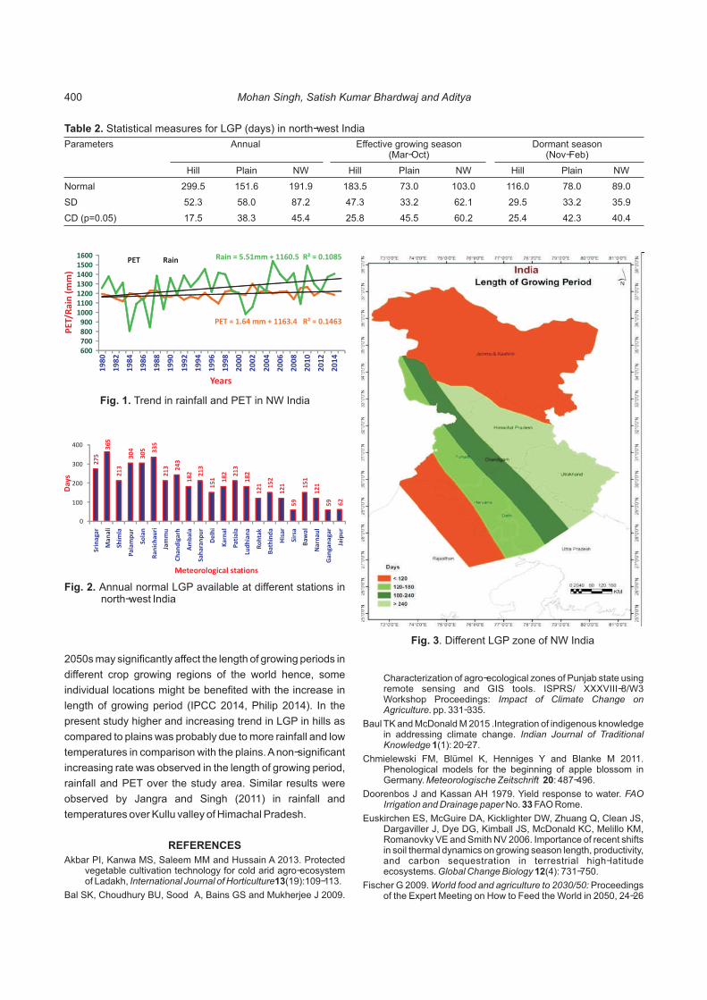
Parameters Annual Effective growing season(Mar-Oct)
Dormant season(Nov-Feb)
Hill Plain NW Hill Plain NW Hill Plain NW
Normal 299.5 151.6 191.9 183.5 73.0 103.0 116.0 78.0 89.0
SD 52.3 58.0 87.2 47.3 33.2 62.1 29.5 33.2 35.9
CD (p=0.05) 17.5 38.3 45.4 25.8 45.5 60.2 25.4 42.3 40.4
Table 2. Statistical measures for LGP (days) in north-west India
2050s may significantly affect the length of growing periods in
different crop growing regions of the world hence, some
individual locations might be benefited with the increase in
length of growing period (IPCC 2014, Philip 2014). In the
present study higher and increasing trend in LGP in hills as
compared to plains was probably due to more rainfall and low
temperatures in comparison with the plains. A non-significant
increasing rate was observed in the length of growing period,
rainfall and PET over the study area. Similar results were
observed by Jangra and Singh (2011) in rainfall and
temperatures over Kullu valley of Himachal Pradesh.
REFERENCES
Akbar PI, Kanwa MS, Saleem MM and Hussain A 2013. Protected vegetable cultivation technology for cold arid agro-ecosystem of Ladakh, International Journal of Horticulture13(19):109-113.
Bal SK, Choudhury BU, Sood A, Bains GS and Mukherjee J 2009.
Characterization of agro-ecological zones of Punjab state using remote sensing and GIS tools. ISPRS/ XXXVIII-8/W3 Workshop Proceedings: Impact of Climate Change on Agriculture. pp. 331-335.
Baul TK and McDonald M 2015 .Integration of indigenous knowledge in addressing climate change. Indian Journal of Traditional Knowledge 1(1): 20-27.
Chmielewski FM, Blümel K, Henniges Y and Blanke M 2011. Phenological models for the beginning of apple blossom in Germany. Meteorologische Zeitschrift 20: 487-496.
Doorenbos J and Kassan AH 1979. Yield response to water. FAO Irrigation and Drainage paper No. 33 FAO Rome.
Euskirchen ES, McGuire DA, Kicklighter DW, Zhuang Q, Clean JS, Dargaviller J, Dye DG, Kimball JS, McDonald KC, Melillo KM, Romanovky VE and Smith NV 2006. Importance of recent shifts in soil thermal dynamics on growing season length, productivity, and carbon sequestration in terrestrial high-latitude ecosystems. Global Change Biology 12(4): 731-750.
Fischer G 2009. World food and agriculture to 2030/50: Proceedings of the Expert Meeting on How to Feed the World in 2050, 24-26
Mohan Singh, Satish Kumar Bhardwaj and Aditya400
PET = 1.64 mm + 1163.4 R² = 0.1463
Rain = 5.51mm + 1160.5 R² = 0.1085
600700800900
1000110012001300140015001600
19
80
19
82
19
84
19
86
19
88
19
90
19
92
19
94
19
96
19
98
20
00
20
02
20
04
20
06
20
08
20
10
20
12
20
14
PET
/Rai
n (
mm
)
Years
PET Rain
Fig. 1. Trend in rainfall and PET in NW India
27
5
36
5
21
3
30
4
30
5 33
5
21
3 24
3
18
2 21
3
15
1 18
2 21
3
18
2
12
1 15
2
12
1
59
15
1
12
1
59 62
0
100
200
300
400
Srin
agar
Man
ali
Shim
la
Pal
amp
ur
Sola
n
Ran
ich
auri
Jam
mu
Ch
and
igar
h
Am
bal
a
Sah
aran
pu
r
De
lhi
Kar
nal
Pat
iala
Lud
hia
na
Ro
hta
k
Bat
hin
da
His
ar
Sirs
a
Baw
al
Nar
nau
l
Gan
gan
agar
Jaip
ur
Day
s
Meteorological stations
Fig. 2. Annual normal LGP available at different stations in north-west India
Fig. 3. Different LGP zone of NW India

June 2009. Food and Agriculture Organization of the United Nations, Rome, Italy. Available online at ftp://ftp.fao.org/
Ghaffari A, Cook HF and Lee HC 2000. Integrating climate, soil and crop information: a land suitability study using GIS. 4th International Conference on Integrating GIS and Environmental M o d e l i n g . h t t p : / / w w w. c o l o r a d o . e d u / r e s e a r c h /cires/banff/pubpapers/129/
Higgins GM and Kassam AH 1981. The FAO agro-ecological zone approach to determination of land potential. Pedologie 31: 147-68
IPCC 2014.. Climate change 2014: Impacts, adaptation, and vulnerability. Working Group II contribution to the IPCC Fifth Assessment Report. Cambridge, United Kingdom: Cambridge University Press. www.ipcc.ch/report/ar5/wg2.
Jangra S and Singh M 2011. Analysis of rainfall and temperatures for climatic trend in Kullu valley. Mausam 62(1): 77-84.
Kunkel KE 2014. Update to data originally published in: Kunkel KE, DR Easterling, K Hubbard and K Redmond. 2004. Temporal variations in frost-free season in the United States: 1895–2000. Geophysical Research Letters 31: L03201.
Olesen JE and Bindi M 2002. Consequences of climate change for European agricultural productivity, land use and policy. European Journal of Agronomy 16(4): 239-262.
Philip T 2014. Impacts of Climate Change on Length of Growing Period, Atlas of African Agriculture Research and Development: Revealing Agriculture's Place in Africa, International Food Policy Research Institute (IFPRI).
Sehgal JL, Mandal DK, Mandal C and Vadivelu S 1992. Agro-ecological Regions of India. Publication 24. NBSS and LUP (ICAR), Nagpur, India.
Singh M and Bhatia HS 2011. Thermal time requirement for phenophases of apple genotypes in Kullu valley. Journal of Agrometeorology 13(1): 46-49.
Thornthwaite CW 1948. An approach toward a rational classification of climate.Geographical Review 38(1): 55-94
White MA, SW Running, PE Thornton 1999. The impact of growing-season length variability on carbon assimilation and evapotranspiration over 88 years in the eastern US deciduous forest. International Journal of Biometeorology 42(3): 139-145.
Received 16 February, 2017; Accepted 10 April, 2017
Zoning and Trend of Sowing Period in North-west India 401

Effect of Different Drying Techniques on Quality of Red Chilli Powder
Indian Journal of Ecology (2018) 45(2): 402-405
Abstract: The experiments were carried out to analyze the effect of sun drying, improved sun drying and mechanical drying at 50, 60 and 70ºC
on different quality parameters of red chilli powder namely ascorbic acid, capsaicin content, colouring matter and oleoresin content. Whole and
slit chillies were used for the experiments. Mechanical drying at 50ºC showed the best quality in terms of all the quality parameters after every
drying technique. Quality of the product reduced significantly during sun drying and mechanical drying at 70ºC. Improved sun drying technique
was much better than sun drying technique in terms of different quality parameters.
Keywords: Ascorbic Acid, Capsaicin Content, Colouring Matter, Drying Techniques, Oleoresin Content, Physical Treatment, Red Chillies
Manuscript Number: 2694NAAS Rating: 4.96
2Shuchi Gupta, S.R. Sharma, T.C. Mittal, S.K. Jindal and S.K. Gupta1Department of Processing and Food Engineering, Department of Vegetable Science
2Training Unit, Punjab Agricultural University, Ludhiana - 141 004, IndiaE-mail: [email protected]
Pepper is an important agricultural crop of India due its
economic importance and for the nutritional value of its fruits
that are an excellent source of natural colours and
antioxidant compounds (Nevarro et al 2006). Different fruit
characteristics like pungency, colour, shape, flavor, size, and
their uses are used to classify the peppers In Asian cuisines
dried chilli (Capsicum annuum L.) is one of the most widely
used spice product as condiments for flavoring and colouring
(Jitbunjerdku and Kijroongrojana 2007, Toontom et al 2010).
A number of different parameters such as colour, hotness,
ascorbic acid content and volatile flavor compounds are used
to assess the quality of dried chilli (Wang et al 2009, Yaldiz et
al 2010). Traditionally, sun drying was used to obtain the
dried chilli and to reduce the moisture content of chilli to 10-
15% approximately 7-20 days are needed depending on the
weather conditions (Oberoi et al 2005). Currently for drying
chilli, hot air drying is popular method due to a relatively short
drying time, uniform heating and more hygienic
characteristics. The temperature for this method ranges from 045 to 70 C (approximately 10% of moisture content), and
takes about 20 hours (Díaz-Maroto et al 2003, Berke and
Shieh 2001).
Sun drying technique is not a time effective technique, is
extremely weather dependent and has the problem of
contamination with dust, soil and insects. While the
mechanical drying technique is not a cost effective technique
and leads to serious injuries such as the worsening of the
taste, colour and nutritional content of the product, decline in
the density and water absorbance capacity and shifting of the
solutes from the internal part of the drying material to the
surface, due to high drying temperature. Keeping the above
problems, present work was focused on modifying the sun
drying technique in order to minimize the problems
associated with the sun drying technique and then comparing
it with the other drying techniques in terms of their effect on
the quality of red chilli powder.
MATERIAL AND METHODS
Raw material and sample preparation: The fresh red
chillies of variety Punjab Sandhoori were procured from the
Vegetable Farm of Department of Vegetable Science, PAU
Ludhiana and were thoroughly sorted and graded. Green and
partially red chillies were separated and discarded. The
cleaned product was then weighed and was given physical
treatment of slitting to half of the lot and making two lots as
whole and slit chillies. Initial moisture content of the chillies
was determined by standard oven drying method (AOAC,
1975) and chillies were dried using following techniques.
Sun drying: The drying was carried out under sun and
samples were placed on perforated trays placed on the
floors.
Improved sun drying: The drying was carried out under sun
and samples were placed on a perforated wire mess table
raised from the ground by about 2.5 ft (Fig. 1). The improved
sun drying method was used to provide a better flow of air
through the sample as compared to traditional sun drying
method where the chillies were placed on the floor. This could
result in relatively faster drying.
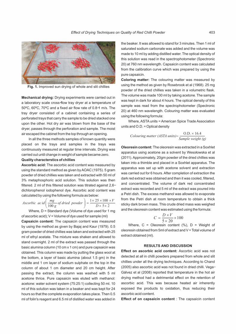
25
100251
100 ´́
´́´=÷÷
ø
öççè
æ
D
Vderof dried pow
g
mgidAscorbic ac
Colouring matter (ASTA units)O.D. ́ 16.4
=Sample weight (g)
100
205´
´
´=
VDC
Fig. 1. Improved sun drying of whole and slit chillies
Mechanical drying: Drying experiments were carried out in
a laboratory scale cross-flow tray dryer at a temperature of
50ºC, 60ºC, 70ºC and a fixed air flow rate of 0.8-1 m/s. The
tray dryer consisted of a cabinet containing a series of
perforated trays that carry the sample to be dried stacked one
upon the other. Hot dry air was blown from the base of the
dryer, passes through the perforation and sample. The moist
air escaped the cabinet from the top through an opening.
In all the three methods samples of known quantity were
placed on the trays and samples in the trays was
continuously measured at regular time intervals. Drying was
carried out until change in weight of sample became zero.
Quality characterstics of chillies
Ascorbic acid: The ascorbic acid content was measured by
using the standard method as given by AOAC (1975). 5 gram
powder of dried chillies was taken and extracted with 50 ml of
3% metaphosphoric acid solution. This solution was then
filtered. 2 ml of this filtered solution was titrated against 2,6-
dichlorophenol iodophenol dye. Ascorbic acid content was
calculated by using the following formula as below:
Where, D = Standard dye (Volume of dye used for 1 mg
of ascorbic acid); V = Volume of dye used for sample (ml)
Capsaicin content: The capsaicin content was measured
by using the method as given by Bajaj and Kaur (1979). 0.5
gram powder of dried chillies was taken and extracted with 25
ml of ethyl acetate. The mixture was shaken and allowed to
stand overnight. 2 ml of the extract was passed through the
basic alumina column (10 cm x 1 cm) and pure capsaicin was
obtained. This column was made by putting the glass wool at
the bottom, a layer of basic alumina (about 1.5 gm) in the
middle and 1 cm layer of sodium sulphate on the top in the
column of about 1 cm diameter and 20 cm height. After
passing the extract, the column was washed with 5 ml
acetone thrice. Pure capsaicin was eluted with methanol:
acetone: water solvent system (75:25:1) collecting 50 ml. 10
ml of this solution was taken in a beaker and was kept for 24
hours so that the complete evaporation takes place. Then 0.5
ml of folin's reagent and 6.5 ml of distilled water was added in
the beaker. It was allowed to stand for 3 minutes. Then 1 ml of
saturated sodium carbonate was added and the volume was
made to 10 ml by adding distilled water. The optical density of
this solution was read in the spectrophotometer (Spectronic
20) at 760 nm wavelength. Capsaicin content was calculated
from the calibration curve which was prepared by using the
pure capsaicin.
Coloring matter: The colouring matter was measured by
using the method as given by Rosebrook et al (1968). 25 mg
powder of the dried chillies was taken in a volumetric flask.
The volume was made 100 ml by taking acetone. The sample
was kept in dark for about 4 hours. The optical density of this
sample was read from the spectrophotometer (Spectronic
20) at 460 nm wavelength. Colouring matter was evaluated
using the following formula:
Where, ASTA units = American Spice Trade Association
units and O.D. = Optical density
Oleoresin content: The oleoresin was extracted in a Soxhlet
apparatus using acetone as a solvent by Weso³owska et al
(2011). Approximately, 20gm powder of the dried chillies was
taken into a thimble and placed in a Soxhlet apparatus. The
apparatus was set up with acetone solvent and extraction
was carried out for 6 hours. After completion of extraction the
dark red extract was obtained and then it was cooled, filtered,
and concentrated. The volume of dark red concentrated
extract was recorded and 5 ml of the extract was poured into
a Petri dish. The excess methanol was allowed to evaporate
from the Petri dish at room temperature to obtain a thick
sticky dark brown mass. This crude dried mass was weighed
and the oleoresin content was estimated using the formula:
Where, C = Oleoresin content (%), D = Weight of
oleoresin obtained from 5ml of extract and V = Total volume of
extract obtained (ml).
RESULTS AND DISCUSSION
Effect on ascorbic acid content: Ascorbic acid was not
detected at all in chilli powders prepared from whole and slit
chillies under all the drying techniques. According to Chand
(2005) also ascorbic acid was not found in dried chilli. Vega-
Gálvez et al (2008) reported that temperature in the hot air
drying method had a detrimental effect on the retention of
ascorbic acid. This was because heated air inherently
exposed the products to oxidation, thus reducing their
ascorbic acid content.
Effect of on capsaicin content : The capsaicin content
Effect of Drying Techniques on Quality of Red Chilli Powder 403

Drying technique Capsaicin content (%) Colouring matter (ASTA units) Oleoresin content (%)
Whole Slit Whole Slit Whole Slit
Sun drying 0.69 ± 0.14 0.65 ± 0.04 50.02 ± 3.47 41.82 ± 1.15 13.26 ± 0.62 11.35 ± 1.62
Improved sun drying 0.86 ± 0.02 0.75 ± 0.04 77.08 ± 2.31 67.24 ± 2.31 13.70 ± 0.28 12.36 ± 0.14
Mechanical drying
At 50ºC 0.95 ± 0.04 0.89 ± 0.04 95.94 ± 1.15 84.46 ± 3.47 15.63 ± 0.11 13.44 ± 0.07
At 60ºC 0.91 ± 0.04 0.86 ± 0.02 91.02 ± 1.15 90.2 ± 2.31 14.60 ± 0.21 12.52 ± 0.45
At 70ºC 0.73 ± 0.04 0.72 ± 0.02 63.14 ± 1.15 58.22 ± 1.15 12.68 ± 0.21 11.74 ± 0.33
Table 1. Effect of different drying techniques on different quality parameters
varied between 0.65 to 0.95% on chilli powder basis (Table
1). Higher capsaicin content was observed for whole chillies
than slit chillies. This variation on the basis of physical
treatment given was found to be statistically significant (p≤
0.05). Themaximum capsaicin content was found in red 0chilli dried by mechanical drying at 50 C followed by
0mechanical drying at 60 C and improved sun drying. Red 0chilli dried by mechanical drying at 70 C had lesser
capsaicin content than that dried by improved sun drying
but more than that dried by sun drying. This variation on the
basis of drying technique used was found to be statistically
significant (p≤0.05).
If the interaction between these two factors is found out
statistically, i.e. the effect of both the factors (physical
treatment and the drying technique) together is considered
on the capsaicin content, the interaction between these two
factors was found to be statistically non significant (p≤0.05).
Kaleemullah and Kailappan (2005) observed that as the
drying air temperature increased from 50 to 65°C the average
capsaicin content of dried chillies decreased. According to
Chand (2005) quality of the product reduced significantly
when the temperature was 70ºC.
Effect on colouring matter: The colouring matter varied
between 41.82 to 95.94 ASTA (American Spice Trade
Association units) on chilli powder basis, (Table 1). In case of
whole chillies, the maximum colouring matter was found in red 0chilli dried by mechanical drying at 60 C followed by
0mechanical drying at 50 C and improved sun drying. Red chilli 0dried by mechanical drying at 70 C had lesser colouring matter
than that dried by improved sun drying but more than that dried
by sun drying. In case of slit chillies, the maximum colouring
matter was found in red chilli dried by mechanical drying at 0 050 C followed by mechanical drying at 60 C and improved sun
0drying. Red chilli dried by mechanical drying at 70 C had lesser
colouring matter than that dried by improved sun drying but
more than that dried by sun drying. This variation was found to
be statistically significant (p≤0.05) of the physical treatment
given. This variation was found to be statistically significant (p≤
0.05) of the drying technique used as well.
If the interaction between these two factors is found out
statistically, i.e. the effect of both the factors (physical
treatment and the drying technique) together is considered
on the colouring matter, the interaction between these two
factors was found to be statistically significant (p≤0.05).
Mangaraj et al (2001) also observed that punched
chillies lost some colour over unpunched chillies. Sigge et al
(2003) also revealed that colour was adversely affected by
temperature during dehydration and loss was more
prominent at higher temperature (70°C and 75°C). Chand
(2005) also observed that the quality of the product reduced
significantly when the chillies were dried mechanically with
70ºC air temperature.
Effect on oleoresin content: The oleoresin content varied
between 11.35 to 15.63% on chilli powder basis (Table 1).
Higher oleoresin content was observed for whole chillies than
slit chillies. This variation on the basis of physical treatment
given was found to be statistically significant (p≤0.05). Sun
dried chillies had lesser oleoresin content as compared to
improved sun dried chillies and mechanically dried chillies.
Mechanical dried chillies at 70ºC had the minimum oleoresin
content, followed by mechanical dried chillies at 60ºC
whereas mechanical dried chillies at 50ºC had the maximum
oleoresin content out of all the mechanically dried chillies.
This variation on the basis of drying technique used was
found to be statistically significant (p≤0.05)
If the interaction between these two factors is found out
statistically, i.e. the effect of both the factors (physical
treatment and the drying technique) together is considered
on the oleoresin content, the interaction between these two
factors was found to be statistically non significant (p≤0.05).
Kalpana (2003) also showed that shade drying followed
by electrical tray drying retained higher oleoresin yield as
compared to other drying techniques.
CONCLUSION
Mechanical drying technique at 50ºC was the best drying
technique in terms of quality parameters followed by
Shuchi Gupta, S.R. Sharma, T.C. Mittal, S.K. Jindal and S.K. Gupta404
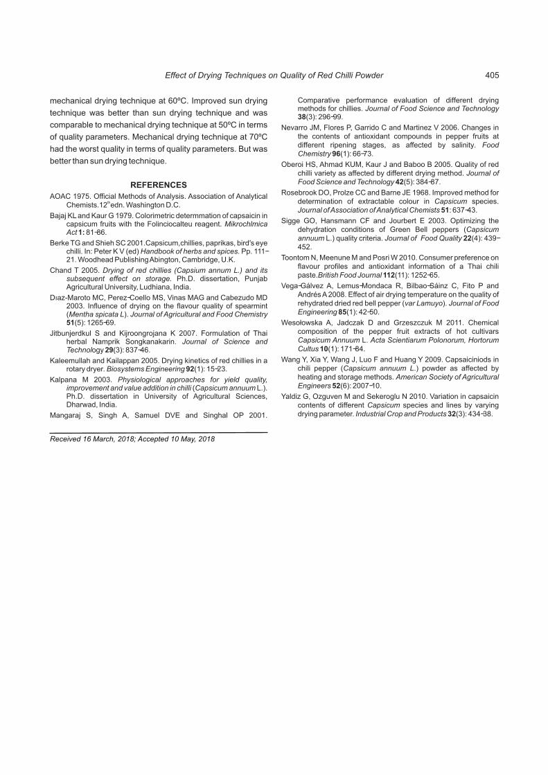
Received 16 March, 2018; Accepted 10 May, 2018
mechanical drying technique at 60ºC. Improved sun drying
technique was better than sun drying technique and was
comparable to mechanical drying technique at 50ºC in terms
of quality parameters. Mechanical drying technique at 70ºC
had the worst quality in terms of quality parameters. But was
better than sun drying technique.
REFERENCES
AOAC 1975. Official Methods of Analysis. Association of Analytical thChemists.12 edn. Washington D.C.
Bajaj KL and Kaur G 1979. Colorimetric determmation of capsaicin in capsicum fruits with the Folinciocalteu reagent. Mikrochlmica Act 1: 81-86.
Berke TG and Shieh SC 2001.Capsicum,chillies, paprikas, bird's eye chilli. In: Peter K V (ed) Handbook of herbs and spices. Pp. 111-21. Woodhead Publishing Abington, Cambridge, U.K.
Chand T 2005. Drying of red chillies (Capsium annum L.) and its subsequent effect on storage. Ph.D. dissertation, Punjab Agricultural University, Ludhiana, India.
Dýaz-Maroto MC, Perez-Coello MS, Vinas MAG and Cabezudo MD 2003. Influence of drying on the flavour quality of spearmint (Mentha spicata L). Journal of Agricultural and Food Chemistry 51(5): 1265-69.
Jitbunjerdkul S and Kijroongrojana K 2007. Formulation of Thai herbal Namprik Songkanakarin. Journal of Science and Technology 29(3): 837-46.
Kaleemullah and Kailappan 2005. Drying kinetics of red chillies in a rotary dryer. Biosystems Engineering 92(1): 15-23.
Kalpana M 2003. Physiological approaches for yield quality, improvement and value addition in chilli (Capsicum annuum L.). Ph.D. dissertation in University of Agricultural Sciences, Dharwad, India.
Mangaraj S, Singh A, Samuel DVE and Singhal OP 2001.
Comparative performance evaluation of different drying methods for chillies. Journal of Food Science and Technology 38(3): 296-99.
Nevarro JM, Flores P, Garrido C and Martinez V 2006. Changes in the contents of antioxidant compounds in pepper fruits at different ripening stages, as affected by salinity. Food Chemistry 96(1): 66-73.
Oberoi HS, Ahmad KUM, Kaur J and Baboo B 2005. Quality of red chilli variety as affected by different drying method. Journal of Food Science and Technology 42(5): 384-87.
Rosebrook DO, Prolze CC and Barne JE 1968. Improved method for determination of extractable colour in Capsicum species. Journal of Association of Analytical Chemists 51: 637-43.
Sigge GO, Hansmann CF and Jourbert E 2003. Optimizing the dehydration conditions of Green Bell peppers (Capsicum annuum L.) quality criteria. Journal of Food Quality 22(4): 439-452.
Toontom N, Meenune M and Posri W 2010. Consumer preference on flavour profiles and antioxidant information of a Thai chili paste.British Food Journal 112(11): 1252-65.
Vega-Gálvez A, Lemus-Mondaca R, Bilbao-Sáinz C, Fito P and Andrés A 2008. Effect of air drying temperature on the quality of rehydrated dried red bell pepper (var Lamuyo). Journal of Food Engineering 85(1): 42-50.
Weso³owska A, Jadczak D and Grzeszczuk M 2011. Chemical composition of the pepper fruit extracts of hot cultivars Capsicum Annuum L. Acta Scientiarum Polonorum, Hortorum Cultus 10(1): 171-84.
Wang Y, Xia Y, Wang J, Luo F and Huang Y 2009. Capsaiciniods in chili pepper (Capsicum annuum L.) powder as affected by heating and storage methods. American Society of Agricultural Engineers 52(6): 2007-10.
Yaldiz G, Ozguven M and Sekeroglu N 2010. Variation in capsaicin contents of different Capsicum species and lines by varying drying parameter. Industrial Crop and Products 32(3): 434-38.
Effect of Drying Techniques on Quality of Red Chilli Powder 405

Assessing and Prioritizing Training Needs of Shrimp Farmers of Palghar District, Maharashtra
Indian Journal of Ecology (2018) 45(2): 406-410
Abstract: Study was conducted with the objective of assessing and prioritizing training needs of shrimp farmers of Palghar district in
Maharashtra. Palghar ranks first in terms of shrimp production and number of shrimp farms. Out of 65 registered shrimp farmers in Palghar
district, information was collected from 55 shrimp farmers. An expert group of 30 comprising of academicians, extension workers, aqua feed
industry representatives, government officials and progressive shrimp farmers were asked to locate potential training areas from the ten heads
of Best Management Practices (BMPs) and also suggest any other training areas. A total of 40 potential training areas were suggested
amongst which 11 were related to BMPs and 29 were outside the framework of BMPs. Importance Weightage (IW) was computed for the
training areas and the score ranged from 0 to 1. Training areas which had IW score of 0.5 or more were selected and thus 22 areas were
identified. Using Borich Need Assessment Model, shrimp farmers were asked to rate these 22 training areas on a 5 point Likert scale for their
perceived importance and competency. Mean Weighted Discrepancy Score (MWDS) was computed to rank and prioritize the training areas.
MWDS was highest for training areas viz. shrimp diseases, symptoms, identification, prevention and management, nursery system and
management, feeding management, use of biosecurity measures and farming with biofloc technology and thus were prioritised. Training
needs assessment has revealed that farmers prioritized six training areas from specific ten frameworks of BMPs. In addition, four training
areas not in the framework of BMPs were also given high priority. It is concluded that to design any capacity development programme, it is
necessary to do training need assessment with reference to importance and competency and training areas should be accordingly prioritized.
Keywords: Training needs, Shrimp farmers, Prioritizing, Need assessment model, Palghar district
Manuscript Number: NAAS Rating: 4.96
2695
Sandesh Patil and Arpita Sharma* Fisheries Economics, Extension and Statistics Division
ICAR-Central Institute of Fisheries Education, Versova, Mumbai - 400 061, India*E-mail: [email protected]
Among various fish production enterprises, shrimp
farming provide gainful employment and steady income to
fish farmers. Shrimp aquaculture is one of the fastest growing
forms of aquaculture but has witnessed many ups and downs
during 1990 - 2000. Shrimp farming industry was at its peak
around 1991 throughout India, but saw its decline mainly due
to the White Spot Syndrome Virus (WSSV) disease,
However, in 2008, Government of India permitted use of
Specific Pathogen Free (SPF) stock of Litopenaeus
vannamei for culture. This resulted in revival of shrimp
farming along the coast of Andhra Pradesh, Maharashtra as
well as other states. Maharashtra state has about 52,001 ha
of potential brackish water area all along its coastline and
adjacent creeks. Out of this area, 10,400 ha is reported to be
suitable for shrimp farming as per the survey conducted by
Government of Maharashtra in 2008. However, only 1356 ha
is used for shrimp farming as per MPEDA (2016) and 9044 ha
area is left which can be utilized for shrimp farming. Per
hectare shrimp productivity of Maharashtra is 4.51
MT/ha/year, whereas national average is 6.87 MT/ha/year.
With a gap of 2.36MT/ha/year there is of improvement in the
five coastal districts i.e., Palghar, Thane, Raigad, Ratnagiri
and Sindhudurg.
Amongst these districts, Palghar ranks first in shrimp
farming area and total shrimp production. Here the total area
under shrimp farming is 733 ha and shrimp production is
2710 tons. However, per hectare shrimp production in
Palghar district is 3.69 tons/ha which is less that the state
average of 4.73 tons/ha. Ratnagiri district has highest per
hectare shrimp production of 6.56 MT/ha/year DoF (2016). It
is clear that Palghar district has relatively less average and
thus there are gaps which need to be addressed.
In a study by Gawde et al (2006) done in Ratnagiri and
Sindhudurg districts, it has been reported that lack of
awareness being one of the main reasons for non-adoption of
certain good management practices by shrimp farmers for
which training is needed. Studies performed in east and west
coasts of India by Kumaran et al (2017) have also reported
that there is a need for trained shrimp farmers regarding the
Best Management Practices (BMPs) to achieve sustainable
production. From the study done by Basavakumar and
Yaliger (2000) in Karnataka it is clear that trainings have
helped shrimp farmers to acquire more knowledge on
technical aspects and has resulted in achieving higher

production for farmers. By this review, it is clear that training is
an important component for adoption of BMPs. To have
sustainable shrimp farming, it is necessary that shrimp
farmers have necessary skills to adopt the BMPs. Thus, there
is a need to assess on which specific areas of BMPs and
other fields, shrimp farmers need trainings. Accordingly a
study was done with the objective of assessing and
prioritizing the training needs of shrimp farmers of Palghar
district, Maharashtra.
MATERIAL AND METHODS
Maharashtra has five coastal districts, out of which
Palghar district ranks first in terms of shrimp production and
number of shrimp farms (MPEDA 2016). Out of 65 registered
shrimp farmers in Palghar district, information was collected
through an interview schedule from 55 shrimp farmers from
three coastal tehsils namely Vasai, Palghar and Dahanu.
With reference to training need assessment BMPs were
taken as a broad framework to locate the training areas for
shrimp farmers. Coastal Aquaculture Authority (CAA) has
provided guidelines for shrimp farmers and has framed
BMPs. BMPs have 10 sub frame works i.e. site selection and
construction, preparation of shrimp farms, water quality
management, seed selection and stocking, feed and feed
management, health management, use of chemicals and
drugs, harvest and post-harvest management, waste water
management and farm hygiene and management. An expert
group of 30 comprising of academicians, extension workers,
aqua feed industry representatives, government officials and
progressive shrimp farmers were asked to locate potential
training areas from the ten heads of BMPs. They were also
asked to suggest additional training areas other than those
listed in BMPs. A total of 40 potential training areas were
suggested by the experts in which 11 were related to BMPs
and 29 were listed outside the framework of BMPs. Based on
this, all the potential training areas were listed. These training
areas were scored on a five point Likert scale on how
important they were perceived to achieve sustainable
production. The five point continuum scale were very
important, important, somewhat important, little important
and not important with scores of 4, 3, 2, 1 and 0, respectively.
Further Importance weightage (IW) was computed as the
ratio of actual total score obtained to the maximum
obtainable total score. Thus IW ranged from 0 to 1.
Kendall's coefficient of concordance (W) was used to
test the hypothesis if the experts were in agreement among
sets of rankings. Value of W was 0.65 which was acceptable.
As per Siegel (1989) if perfect agreement exists between
experts W equals 1 and if maximum disagreement exists
then W equals to 0.
The training areas, which had IW score of 0.5 or more
were selected as important and thus 22 training areas were
identified. Within the framework of BMPs, 11 training areas
scored more than 0.5 which are listed here. Under the head
"site selection and construction", the training area suggested
was site specific approach in selection, design and
construction of shrimp farm. Under "farm preparation", pond
preparation and pre-stocking management was the area
identified. Under "water quality management", water quality
and pond bottom management was the area suggested.
Seed selection, packing, transportation, acclimatization and
stocking was the area suggested under the head "seed
selection and stocking". Under the head, "feed and feed
management", feeding management was the training area
identified. In "health management", shrimp diseases,
symptoms, identification, prevention and management was
the area identified. Use of drugs and chemicals during culture
was the training located by experts. Under the head, "harvest
and post harvest", two training areas viz. harvesting
techniques and post harvest handling of farmed shrimps
were identified. In "waste water management", effluent and
solid waste management was the area identified. Farm
hygiene and management was also a training area identified.
In addition to these, other training areas apart from those
listed in BMPs which scored high on importance were shrimp
nursery system, biosecurity measures, use of biofloc
technology, marketing management, human resource
management, project formulation, climate change and
shrimp farming, schemes and policies for shrimp farming,
ICT based trainings and aeration system in shrimp farming.
Borich Need Assessment Model (1980) was used to assess
the farmers perceived level of importance for each training
area and their competency in that field. Using this model,
training needs of shrimp farmers were prioritized. Shrimp
farmers were asked to rate these 22 training areas with
respect to how important it was perceived by them on a five
point Likert scale (0 : not important and 4: extremely
important). Similarly, each training area was rated with
respect to how the shrimp farmers perceived their
competency on it. Five point Likert scale (0: not competent to
4: extremely competent) was used.
Reliability of the scales was tested using test-retest
method. The scale was administered to 15 farmers and then
repeated after 15 days. Reliability coefficient which is a
measure of how consistent the results are over time was
found to be 0.80 and 0.85 respectively for two scales, and
thus the same were considered reliable (Webb et al 2006).
Mean Weighted Discrepancy Score (MWDS) was
calculated to rank and prioritize the training areas as follows.
Discrepancy score (DS) = I - C
Assessing and Prioritizing Training Needs of Shrimp Farmers 407
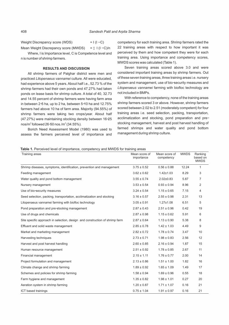
Weight Discrepancy score (WDS) = I (I - C)
Mean Weight Discrepancy score (MWDS) = ∑ I (I - C)/n
Where, I is Importance level, C is Competence level and
n is number of shrimp farmers.
RESULTS AND DISCUSSION
All shrimp farmers of Palghar district were men and
practiced Litopenaeus vannamei culture. All were educated,
had experience above 5 years. About half i.e., 52.73 % of the
shrimp farmers had their own ponds and 47.27% had taken
ponds on lease basis for shrimp culture. A total of 40, 32.73
and 14.55 percent of shrimp farmers were having farm area
in between 2-5 ha, up to 2 ha, between 5-10 ha and 12.75%
farmers had above 10 ha of farm area. Majority (94.55%) of
shrimp farmers were taking two crops/year. About half
(47.27%) were maintaining stocking density between 16-25 2 2nos/m followed 26-50 nos./m (34.55%).
Borich Need Assessment Model (1980) was used to
assess the farmers perceived level of importance and
Training areas Mean score of importance
Mean score of competency
MWDS Ranking based on MWDS
Shrimp diseases, symptoms, identification, prevention and management 3.75 ± 0.52 0.56 ± 0.88 12.24 1
Feeding management 3.62 ± 0.62 1.42±1.03 8.29 3
Water quality and pond bottom management 3.55 ± 0.74 2.02±0.83 5.87 7
Nursery management 3.53 ± 0.54 0.93 ± 0.94 8.96 2
Use of bio-security measures 3.24 ± 0.54 1.15 ± 0.65 7.15 4
Seed selection, packing, transportation, acclimatization and stocking 3.16 ± 0.57 2.55 ± 0.98 2.31 13
Litopenaeus vannamei farming with biofloc technology 3.05 ± 0.91 1.27±1.08 6.51 5
Pond preparation and pre-stocking management 2.87 ± 0.43 2.51 ± 0.96 0.42 19
Use of drugs and chemicals 2.87 ± 0.98 1.15 ± 0.62 5.91 6
Site specific approach in selection, design and construction of shrimp farm 2.87 ± 0.64 1.13 ± 0.90 5.38 8
Effluent and solid waste management 2.85 ± 0.78 1.42 ± 1.03 4.49 9
Market and marketing management 2.82 ± 0.72 1.78 ± 0.74 3.47 10
Harvesting techniques 2.73 ± 0.71 1.98 ± 0.83 2.56 12
Harvest and post harvest handling 2.60 ± 0.85 2.16 ± 0.94 1.87 15
Human resource management 2.51 ± 0.92 1.78 ± 0.85 2.67 11
Financial management 2.15 ± 1.11 1.76 ± 0.77 2.00 14
Project formulation and management 2.13 ± 0.86 1.51 ± 1.00 1.82 16
Climate change and shrimp farming 1.89 ± 0.92 1.65 ± 1.09 1.49 17
Schemes and policies for shrimp farming 1.58 ± 0.94 1.69 ± 0.96 0.55 18
Farm hygiene and management 1.35 ± 0.82 1.98 ± 1.01 0.27 20
Aeration system in shrimp farming 1.20 ± 0.87 1.71 ± 1.07 0.16 21
ICT based trainings 0.75 ± 1.04 1.91 ± 0.97 0.16 21
Table 1. Perceived level of importance, competency and MWDS for training areas
competency for each training area. Shrimp farmers rated the
22 training areas with respect to how important it was
perceived by them and how competent they were for each
training area. Using importance and competency scores,
MWDS scores was calculated (Table 1).
Seven training areas scored above 3.0 and were
considered important training areas by shrimp farmers. Out
of these seven training areas, three training areas i.e. nursery
system and management, use of bio-security measures and
Litopenaeus vannamei farming with biofloc technology are
not included in BMPs.
With reference to competency, none of the training areas
shrimp farmers scored 3 or above. However, shrimp farmers
scored between 2.02 to 2.51 (moderately competent) for four
training areas i.e. seed selection, packing, transportation,
acclimatization and stocking, pond preparation and pre-
stocking management, harvest and post harvest handling of
farmed shrimps and water quality and pond bottom
management during shrimp culture.
Sandesh Patil and Arpita Sharma408
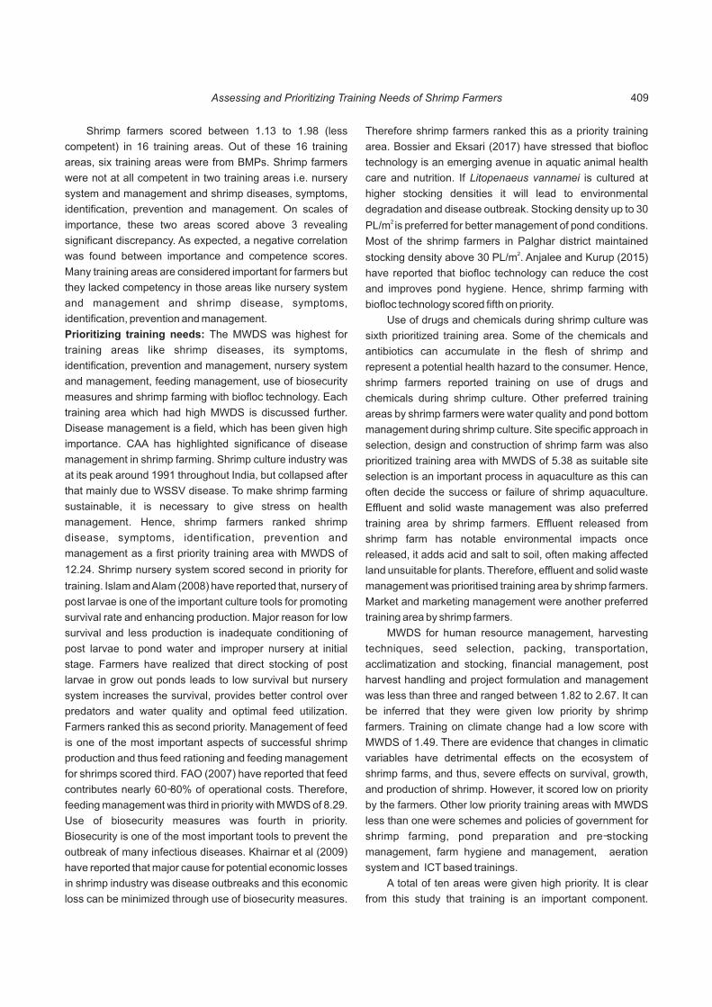
Shrimp farmers scored between 1.13 to 1.98 (less
competent) in 16 training areas. Out of these 16 training
areas, six training areas were from BMPs. Shrimp farmers
were not at all competent in two training areas i.e. nursery
system and management and shrimp diseases, symptoms,
identification, prevention and management. On scales of
importance, these two areas scored above 3 revealing
significant discrepancy. As expected, a negative correlation
was found between importance and competence scores.
Many training areas are considered important for farmers but
they lacked competency in those areas like nursery system
and management and shrimp disease, symptoms,
identification, prevention and management.
Prioritizing training needs: The MWDS was highest for
training areas like shrimp diseases, its symptoms,
identification, prevention and management, nursery system
and management, feeding management, use of biosecurity
measures and shrimp farming with biofloc technology. Each
training area which had high MWDS is discussed further.
Disease management is a field, which has been given high
importance. CAA has highlighted significance of disease
management in shrimp farming. Shrimp culture industry was
at its peak around 1991 throughout India, but collapsed after
that mainly due to WSSV disease. To make shrimp farming
sustainable, it is necessary to give stress on health
management. Hence, shrimp farmers ranked shrimp
disease, symptoms, identification, prevention and
management as a first priority training area with MWDS of
12.24. Shrimp nursery system scored second in priority for
training. Islam and Alam (2008) have reported that, nursery of
post larvae is one of the important culture tools for promoting
survival rate and enhancing production. Major reason for low
survival and less production is inadequate conditioning of
post larvae to pond water and improper nursery at initial
stage. Farmers have realized that direct stocking of post
larvae in grow out ponds leads to low survival but nursery
system increases the survival, provides better control over
predators and water quality and optimal feed utilization.
Farmers ranked this as second priority. Management of feed
is one of the most important aspects of successful shrimp
production and thus feed rationing and feeding management
for shrimps scored third. FAO (2007) have reported that feed
contributes nearly 60-80% of operational costs. Therefore,
feeding management was third in priority with MWDS of 8.29.
Use of biosecurity measures was fourth in priority.
Biosecurity is one of the most important tools to prevent the
outbreak of many infectious diseases. Khairnar et al (2009)
have reported that major cause for potential economic losses
in shrimp industry was disease outbreaks and this economic
loss can be minimized through use of biosecurity measures.
Therefore shrimp farmers ranked this as a priority training
area. Bossier and Eksari (2017) have stressed that biofloc
technology is an emerging avenue in aquatic animal health
care and nutrition. If Litopenaeus vannamei is cultured at
higher stocking densities it will lead to environmental
degradation and disease outbreak. Stocking density up to 30 2 PL/m is preferred for better management of pond conditions.
Most of the shrimp farmers in Palghar district maintained 2stocking density above 30 PL/m . Anjalee and Kurup (2015)
have reported that biofloc technology can reduce the cost
and improves pond hygiene. Hence, shrimp farming with
biofloc technology scored fifth on priority.
Use of drugs and chemicals during shrimp culture was
sixth prioritized training area. Some of the chemicals and
antibiotics can accumulate in the flesh of shrimp and
represent a potential health hazard to the consumer. Hence,
shrimp farmers reported training on use of drugs and
chemicals during shrimp culture. Other preferred training
areas by shrimp farmers were water quality and pond bottom
management during shrimp culture. Site specific approach in
selection, design and construction of shrimp farm was also
prioritized training area with MWDS of 5.38 as suitable site
selection is an important process in aquaculture as this can
often decide the success or failure of shrimp aquaculture.
Effluent and solid waste management was also preferred
training area by shrimp farmers. Effluent released from
shrimp farm has notable environmental impacts once
released, it adds acid and salt to soil, often making affected
land unsuitable for plants. Therefore, effluent and solid waste
management was prioritised training area by shrimp farmers.
Market and marketing management were another preferred
training area by shrimp farmers.
MWDS for human resource management, harvesting
techniques, seed selection, packing, transportation,
acclimatization and stocking, financial management, post
harvest handling and project formulation and management
was less than three and ranged between 1.82 to 2.67. It can
be inferred that they were given low priority by shrimp
farmers. Training on climate change had a low score with
MWDS of 1.49. There are evidence that changes in climatic
variables have detrimental effects on the ecosystem of
shrimp farms, and thus, severe effects on survival, growth,
and production of shrimp. However, it scored low on priority
by the farmers. Other low priority training areas with MWDS
less than one were schemes and policies of government for
shrimp farming, pond preparation and pre-stocking
management, farm hygiene and management, aeration
system and ICT based trainings.
A total of ten areas were given high priority. It is clear
from this study that training is an important component.
Assessing and Prioritizing Training Needs of Shrimp Farmers 409
Training needs assessment has revealed that farmers
prioritized six training areas from specific ten frameworks of
BMPs. In addition, four training areas not in the framework of
BMPs were also given high priority.
CONCLUSIONS
To design any capacity development programme, it is
necessary to do training need assessment with reference to
the importance as perceived by experts and the farmers. In
addition, it is necessary to study the competency level of the
farmers in the important training areas. Based on the
importance and competency level, training areas should be
prioritized. The institutes / organizations responsible for
conducting training programmes should have this database
and these needs to be updated from time to time. Certain
training area considered to be important by experts scored low
in farmers priority. To avoid this disconnect, it is necessary that
information has to be collected at field level from farmers. In
case experts feel that in some areas like farm hygiene and
management training is necessary, then importance of subject
needs to be taught to shrimp farmers. The shrimp diseases,
symptoms, identification, prevention and management,
nursery system and management, feed rationing and feeding
management, use of biosecurity measures and shrimp
farming with biofloc technology are prioritized training need.
The study has also revealed that along with some areas of
BMPs farmers also need training on new technologies like
biofloc, biosecurity, nursery management etc.
REFERENCES
Anjaleedevi CA and Kurup BM 2015. Biofloc Technology: An Overview and its application in animal food industry.
International Journal of Fisheries and Aquaculture Sciences 5(1): 1-20.
Basavakumar KV and Yaligar MD 2000. Impact of training on knowledge and opinion of trainees on brackishwater prawn farming. Karnataka Journal of Agriculture Sciences 13(3): 707-711.
Borich GD 1980. A needs assessment model for conducting follow-up studies. Journal of Teaching Education 31(1): 39-42.
Bossier P and Eksari J 2017. Biofloc technology application in aquaculture to support sustainable development goals. Microbial Biotechnology 10(5): 1012-1016.
CAA 2010. Guidelines for sustainable shrimp farming. CAA, Government of India, Ministry of Agriculture.
DoF 2016. Fish production report-2015-16, Department of Fisheries, Government of Maharashtra.
FAO 2007. Economics of aquaculture feeding practices in selected Asian countries. FAO Fisheries Technical Paper No. 505. Rome.
Gawade MM, Chandge MS and Shirdhankar MM 2006. Adoption of improved aquaculture practices by the farmers of the south Konkan region, Maharashtra, India. Journal of Agriculture and Social Research 6(2): 1-8.
Islam ML and Alam MJ 2008. Impact of in pond nursery of shrimp (Penaeus monodon) post larvae on the survival rate and production under modified improved culture sytem. Progressive Agriculture 19(2): 167-175.
Khairnar SO, Mali K, Kapse P, Deshmukh A and Solanki B 2009. Biosecurity: Its application in shrimp farming. Online review article on Aquafind.com
Kumaran M, Ravisankar T, Anand PR, Vimala D and Balasubramanian CP 2017. Knowledge level of shrimp farmers on better management practices (BMPs) of Penaeus vannmei farming: a comparative assessment of east and west coasts of India. Indian Journal of Fisheries 64(3): 93-99.
MPEDA 2016. Annual Report 2015-16, Marine Product Export Development Authority (MPEDA), Kochi, Kerala.
Siegel S 1989. Non parametric statistics for the behavioral sciences (1st ed.), New York, NY: McGraw-Hill.
Webb NM, Shavelson RJ and Haertel EH 2006. Reliability coefficients and generalizability theory. Handbook of Statistics 26: 4-42.
Received 23 March, 2018; Accepted 10 May, 2018
Sandesh Patil and Arpita Sharma410

Assessment of Nutrition Knowledge of Elite Athletes and their Coaches in Punjab
Indian Journal of Ecology (2018) 45(2): 411-418
Abstract: Research study for the assessment of nutrition knowledge of 120 (16-25 years) elite athletes and their coaches, selected from 5
universities and participating in 4 sports viz. hockey, athletics, badminton and lawn tennis was carried out. The knowledge, attitude and
practice (KAP) score of athletes along with the KAP score of coaches regarding sports nutrition was assessed. A statistically significant
difference was observed in the KAP score of male and female athletes of hockey and lawn tennis. However, the KAP score of overall male and
female athletes was observed to be statistically non-significant. Majority of coaches (96.7%) had no formal training in sports nutrition and 90%
of them had no access to registered dietician. KAP score data of the coaches revealed that 10% had excellent KAP score; 53% had a very good
score; 30% had good KAP and 6.7% had average to poor score. A positive significant (p≤0.05) correlation between KAP score of coaches and
their years of experience was observed. KAP score of athletes had a significantly positive correlation with the KAP score of coaches.
Keywords: Elite athletes, Knowledge Attitude and Practice (KAP) score, Nutrient intake
Manuscript Number: NAAS Rating: 4.96
2696
Aditi Sewak and Neerja SinglaDepartment of Food and Nutrition, Punjab Agricultural University, Ludhiana-141 004, India
E-mail: [email protected]
An elite athlete is defined as one who has previously or
currently competed as a state player, varsity player
(individual or team), a professional player or a national or
international level player. Nutrition, from decades, has been
recognized to play an important role in attaining high level of
achievements in sports (Alexopoulas and Frazier 2012).
According Purcell (2013), adequate calorie intake, ample
hydration and timing of meals is desirable to maintain lean
tissue mass and an optimal athletic performance. Inadequate
calorie intake leads to a condition in which the body uses fat
and lean tissue mass as fuel, resulting in loss of muscle
mass, thus compromising strength and endurance. There
has been a direct correlation between healthy food choices
and an athlete's nutrition knowledge and it was revealed that
majority of athlete population had a dearth of basic nutrition
knowledge (Dunn et al 2007, Supriya and Ramaswami
2013). Delivering nutrition education resulted in a significant
increase in sports nutrition knowledge accompanied by
increased intake of energy, carbohydrates and protein
(Burns et al 2004, Rodriguez et al 2009, Walsh et al 2011,
Valliant et al 2012, Devlin and Belski 2015). The educational
resources for low income community athletes are less,
resulting in insufficient knowledge about nutrition and sports
supplements (Peerkhan and Srinivasan 2010). Participation
in various competitions and tournaments increases nutrition
knowledge of athletes as they gain experience in their sport.
The nutrition knowledge of athletes pursuing physical
education course at their institutions is better. A majority of
athletes also highlighted the importance of breakfast (Aziz et
al 2010). Assessing knowledge of coaches regarding
nutrition is important, as coaches are the first persons dealing
with sportspersons. Coaches often receive nutrition
knowledge from other coaches, their experiences and self-
involvements in sports and competitions (Reade et al 2008).
On the other hand, athletes considered coaches as their
main source of sports nutrition knowledge (Sajber et al 2013).
Dissemination of incorrect information regarding nutrition by
professionals whose sports nutrition knowledge is deficient is
a matter of concern. (McGehee et al 2012). Hence, in the
present study, an attempt was made to obtain data regarding
the objective of assessing the nutrition knowledge level of the
selected athletes and coaches.
MATERIAL AND METHODS
The present study was conducted in five universities of
Punjab namely, Punjab Agricultural University, Ludhiana,
Guru Angad Dev Veterinary and Animal Sciences University,
Ludhiana, Punjab University, Chandigarh, Guru Nanak Dev
University, Amritsar and Punjabi University, Patiala.
Selection of subjects: A total of one hundred and twenty
elite athletes (30 in each category) falling in the age-group of
16-25 years and their coaches (total 30 combined from all
categories) were selected (Fig. 1) from five universities of
Punjab who were participating in hockey, athletics,
badminton and lawn Tennis.
The selection of subjects was independent of gender.

Fig. 1. Selection of subjects
The athletes for the above mentioned sports were selected
on the basis of their participation in state or national level
tournaments such as open state, open national, inter-varsity
and inter-agri.
Collection of data
General information of athletes and coaches: The
information regarding general profile of subjects, socio-
economic status of family, family composition, dietary habits,
food intake on daily basis, pattern of physical activity and
information pertaining to health and lifestyle of the athletes
while information in addition to general profile and social and
family composition, access to nutrition information and
nutrition expert at personal or university level to coaches
were collected.
Assessment of knowledge, attitude and practice (kap)
score of athletes and coaches: The knowledge, attitude
and practice (KAP) regarding role of nutrition in sports and its
dietary management by the athletes and their coaches was
assessed using KAP questionnaire which was distributed
among selected one hundred and twenty athletes pursuing
four different sports and also among selected thirty coaches
who were providing coaching in the above mentioned sports.
Classification of knowledge, attitude and practice (kap)
score of athletes and coaches: The scores of the athletes
were categorized into excellent, very good, good and
average to poor. Athletes scoring 30-35 were ranked as
excellent, score of 25-29 was ranked very good, score of 20-
24 was good and less than 20 was ranked as poor. The
maximum score was taken to be 35.
RESULTS AND DISCUSSION
General profile: Majority of athletes belonged to nuclear
family especially female athletes with 4 to 8 members in the
family. Among these a major proportion (74.2%) of athletes
belonged to high income group with a greater mainstream of
males (81.5%). A majority of athletes (75.8%) were
participating at national level, especially all the athletes of
hockey. Furthermore, athletes used to spend 0-2 hours
(34.1%) and 4-6 hours (34.2%) per day in workout while a
very few (3.3%) male athletes, especially those pursuing
athletics and lawn tennis spent 6-8 hours a day in workout. A
considerable number of male and female athletes (50.8 and
65.5%) from all the sports in the study experienced feeling of
fatigue specifically after their morning training session. Junk
food consumption was found common among majority
(87.3%) of female athletes, but the frequency of consumption
was low i.e. once or twice a week.
Majority of athletes (53.3%) were non-vegetarian
comprising males of athletics (71.4%) and males of
badminton (92.8%). It also came into prominence that major
fraction of selected athletes (66.7%) did not skip meals to
maintain weight, which may be considered common among
female athletes. Fifty-six percent female athletes rejected the
notion of skipping meals, particularly female athletes (87.5%)
of lawn tennis.
Knowledge, attitude and practice (KAP) of athletes
knowledge: The knowledge score revealed no significant
difference between all the male and female athletes of the
selected sports with a good overall knowledge score
Aditi Sewak and Neerja Singla412

Characteristics Hockey Athletics Badminton Lawn tennis Total (%) Total (%)
Male(n=8)
Female(n=22)
Male(n=21)
Female(n=9)
Male(n=14)
Female(n=16)
Male(n=22)
Female(n=8)
Male(n=65
Female(n=55)
N=120
Family Size
Nuclear 6 (75) 18 (81.9) 12 (57.1) 6 (66.7) 13 (92.8) 11 (68.8) 18 (81.8) 8 (100) 75.4 78.2 76.7
Joint 2 (25) 4 (18.2) 9 (42.9) 3 (33.3) 1 (7.14) 5 (31.3) 4(18.2) 0 24.6 21.8 23.3
Family composition
Small (<4) 2 (25) 0 1 (4.76) 1 (11) 2 (14.3) 0 1(4.5) 1(12.5) 9.2 3.6 6.7
Medium (4 to 8)
6 (75) 18 (81.9) 16 (76.2) 7 (77.8) 12 (85.7) 11(68.8) 21(95.5) 7(87.5) 84.6 78.2 81.7
Large (>8) 0 4 (18.2) 4 (19) 1 (11) 0 0 0 0 6.2 9.1 7.5
Family income (Rs/ annum)
Low (upto 50,000/-)
0 3 (13.6) 0 0 0 0 0 0 0 5.5 2.5
Medium (50,000 to 2,50,000/-)
2 (25) 2 (9.1) 3 (14.3) 2 (22.2) 1 (7.1) 8 (50) 6 (27.3) 4 (50) 16.9 29.1 23.3
High (>2,50,000/-)
6 (75) 17 (77.3) 18 (85.7) 7 (77.8) 13 (92.8) 8 (50) 16 (72.7) 4 (50) 81.5 65.5 74.2
Level of participation
State 0 0 12 (57.1) 3 (33.3) 4 (28.6) 5 (31.3) 4 (18.2) 1 (12.5) 30.8 16.6 24.2
National 8 (100) 22 (100) 9 (42.9) 6 (66.7) 10 (71.4) 11 (68.8) 18 (81.8) 7 (87.5) 69.2 83.6 75.8
Time spent in workout (in hours)
0-2 1 (12.5) 8 (36.4) 4 (19.0) 6 (66.7) 6 (42.9) 7 (43.8) 7 (31.8) 2 (25) 27.7 41.8 34.1
2-4 3 (37.5) 2 (9.1) 8 (38.1) 1 (11) 2 (14.3) 3 (18.8) 9 (40.9) 6 (75) 33.8 21.8 28.3
4-6 4 (50) 12 (54.5) 7 (33.3) 2 (22.2) 6 (42.9) 6 (25) 4 (18.2) 0 32.3 36.4 34.2
6-8 0 0 2 (9.5) 0 0 0 2(9.1) 0 6.15 0 3.3
Feeling of fatigue
Yes 4 (50) 16 (72.7) 15 (71.4) 6 (66.7) 3 (21.4) 9 (56.3) 11 (50) 5 (62.5) 50.8 65.5 57.5
No 4 (50) 6 (27.3) 6 (28.6) 3 (33.3) 11(78.6) 7 (43.8) 11 (50) 3 (37.5) 49.2 34.5 42.5
Junk Food
Yes 2 (25) 18 (81.8) 14 (66.7) 8 (88.9) 12 (85.7) 14 (87.5) 15 (68.2) 8 (100) 66.2 87.3 75.8
No 6 (75) 4 (18.9) 7 (33.3) 1 (11) 2 (14.3) 2 (12.5) 7 (31.8) 0 33.8 12.7 24.2
Food habits
Vegetarian 6 (75) 16 (72.7) 5 (23.8) 5 (55.6) 1 (7.1) 8 (50) 9 (40.9) 4 (50) 32.3 60 45
Ovo-Lactovegetarian
0 0 1 (4.76) 0 0 1 (6.3) 0 0 1.5 1.8 1.7
Non-vegetarian 2 (25) 6 (27.3) 15 (71.4) 4 (44.4) 13 (92.8) 7 (43.8) 13 (59.1) 4 (50) 66.2 38.2 53.3
skipping meals
Yes 4 (50) 15 (68.9) 7 (33.3) 3 (33.3) 5(35.7) 5 (31.3) 1(4.5) 1(12.5) 26.2 43.6 34.2
No 4 (50) 7 (31.8) 14 (66.7) 6 (66.7) 9 (64.3) 11 (68.8) 21 (95.5) 7 (87.5) 73.8 56.4 66.7
Table 1. General profile of the athletes
*Figures in parenthesis represent percentages
(71.2%). However, Kong (2009) observed higher knowledge
score of female as compared to their male counterparts.
Attitude: The attitude of elite athletes regarding sports
nutrition revealed statistically significant higher score of male
athletes of hockey as compared to female while male and
female athletes of other sports did not exhibit any significant
difference with an average overall score (62%).
Practice: The practice score in male and female athletes of
Assessment of Nutrition Knowledge 413
Particulars Hockey Athletics Badminton Lawn tennis Total
Male Female t-value Male Female t-value Male Female t-value Male Female t-value Male Female t-value
Knowledge 11 10.3 NS1.2 10.4 9.7 NS1.4 9.1 9.8 NS0.8 9.7 10.7 NS0.8 10.05 10.1 NS0.9
Attitude 6.12 4.3 3.2* 5.0 5.7 NS0.9 6.8 7.4 NS0.3 7.2 6.8 NS0.8 6.28 6.05 NS0.1
Practice 8.12 8.2 NS0.1 9 7.1 3.3* 8.1 8.4 NS0.4 7.4 9 2.2* 8.17 8.18 NS0.0
KAP score 25.3 22.9 1.9* 24.3 22.4 NS1.5 24 25.6 NS1.2 24.3 26.5 2.7* 24.5 24.4 NS0.1
Table 2. Knowledge, attitude and practice score of athletes
Values are Mean, *Significant at 5% level, NS-non significant
Particulars Total Score
Hockey Athletics Badminton Lawn tennis Total (%) Total (%)
Male(n=8)
Female(n=22)
Male(n=21)
Female(n=9)
Male(n=14)
Female(n=16)
Male(n=22)
Female(n=8)
Male(n=65)
Female(n=55) N=120
Knowledge 14 78.6 73.7 74.3 69.3 65 70 69.3 76.4 71.8 72.1 71.2
Attitude 10 61.3 43 50 57 68 74 72 68 63 61 62
Practice 11 73.8 74.5 81.8 64.5 73.6 76.4 67.3 81.8 74.3 74.4 74.3
KAP Score 35 72.1 65.4 69.4 64 68.6 73.1 69.4 75.7 70 69.7 69.9
Table 3. Knowledge, attitude and practice score of athletes (%)
KAP Hockey Athletics Badminton Lawn tennis Total Total
Male(n=8)
Female(n=22)
Male(n=21)
Female(n=9)
Male(n=14)
Female(n=16)
Male(n=22)
Female(n=8)
Male(n=65)
Female(n=55)
N=120
Excellent(30-35)
1 (12.5)
0 3 (14.3)
0 0 0 1 (4.5)
0 5 (7.7)
0 5 (4.2)
Very good( 25-29)
5 (62.5)
5 (22.7)
6 (28.6)
1 (11.1)
3 (21.4)
7 (43.8)
3 (13.6)
4 (50)
17 (25.2)
17 (30.9)
34 (28.3)
Good(20-24)
2(25)
14 (63.6)
10 (47.6)
4 (44.4)
6(42.9)
4 (66.7)
14 (63.6)
2 (25)
32 (49.2)
24 (43.6)
56 (46.7)
Average to poor(Score:< 20)
0 3 (13.6)
2 (9.5)
2 (22.2)
5 (35.7)
5 (31.3)
4 (18.2) 2 (25)
11 (16.9)
12 (21.8)
23 (19.2)
Table 4. Classification of KAP level of athletes
*Figures in parenthesis represent percentages
athletics as well as lawn tennis showed a statistically
significant difference, where male athletes of athletics scored
higher as compared to their female counterparts whereas,
female athletes of lawn tennis scored higher as compared to
male athletes of lawn tennis. The athletes of other two sports
did not show any significant difference between males and
females. The overall male athletes and female athletes
showed non-significant difference.
KAP score: The overall KAP score exhibited a significant
difference between male and female athletes particularly
among athletes of hockey and lawn tennis because of their
significant difference in practices regarding sports nutrition. A
similar result was observed where male athletes of hockey
scored higher compared to their female counterparts,
whereas female athletes of lawn tennis scored higher KAP
score than male athletes. The difference between overall
male and female athletes was observed to be statistically
non-significant. Also, the overall percent KAP marks of a total
of 120 athletes were found to be good (69.9%). Low mean
KAP scores of both male and female adolescent cricketers
were also reported by Sobana (2016) and suggested a
necessity for continuous nutrition education particularly
through a sports nutritionist.
Classification of KAP level of athletes
The athletes were categorized into having excellent,
very good, good, average to poor KAP regarding sports
nutrition on the basis of their achieved scores (Table 4), which
revealed that overall a few fraction of athletes (4.2%) had
excellent KAP score which comprised male athletes of
hockey, athletics and lawn tennis (12.5, 14.3 and 4.5% resp.)
and no female athlete fell in this category. Twenty-five
percent of male athletes had very good KAP score while
30.9% of female athletes secured very good knowledge
score.
A significant proportion of athletes (46.7%) had good
nutrition KAP score comprising male athletes and female
athletes (49.2 and 43.6%). The highest percentage (63.6 and
66.7%) of athletes who scored good KAP score were female
Aditi Sewak and Neerja Singla414
Characteristics Hockey (n=7) Athletics (n=5) Badminton (n=8) Lawn tennis (n=10) Total (N=30)
Family size
Nuclear 4 (57.1) 2 (40) 5 (62.5) 6 (60) 17 (56.7)
Joint 3 (42.9) 3 (60) 3 (37.5) 4 (40) 13 (43.3)
Family composition
Small (<4) 1 (14.3) 0 1 (12.5) 3 (30) 5 (16.7)
Medium (4 to 8) 5 (71.4) 4 (80) 6 (75) 6 (60) 21 (70)
Large (>8) 1 (20) 1 (12.5) 1 (10) 3 (10)
Family income (Rs/ annum)
Medium (50,000-2,50,000/-) 3 (42.9) 5 (100) 6 (75) 5 (50) 19 (63.3)
High (>2,50,000/-) 4 (57.1) 0 2 (25) 5 (50) 11 (36.7)
Years of coaching
< 10 years (1) 3 (42.9) 1 (20) 4 (50) 8 (80) 16 (53.3)
10-20 years (2) 2 (28.6) 4 (80) 2 (25) 2 (20) 10 (33.3)
>20 years (3) 2 (28.6) 0 2 (25) 0 4 (13.3)
Level of education
Matric (0)
10+2 (1) 2 (28.6) 1 (20) 1 (12.5) 3 (30) 7 (23.3)
UG degree (2) 1 (14.3) 3 (60) 3 (37.5) 6 (60) 13 (43.3)
PG degree (3) 4 (57.1) 1 (20) 4 (50) 1 (10) 10 (33.3)
Table 6. General profile of coaches
*Figures in parenthesis represent percentages
athletes of hockey and badminton respectively while majority
of male athletes of lawn tennis (63.6%) scored good KAP
score. Nineteen percent of the total athletes scored an
average KAP score including male and female athletes (16.9
and 21.8%).
Comparison of KAP score of athletes of various sports:
There was statistically significant difference in KAP score of
hockey and badminton, athletics and badminton and
athletics and lawn tennis (Table 5). A significant difference in
nutritional knowledge between athletes of different fields of
sport was also reported by Mardani et al (2017).
General profile of coaches: The general information of the
coaches is given in Table 6 and 7. It was revealed that
majority of total coaches (56.7%) from all the sports belonged
to nuclear family while a significant fraction of them (43.3%)
belonged to joint family. Seventy percent of all the coaches
had medium family consisting of 4 to 8 members. Sixty-three
percent coaches fall in medium income group and several
(36.7%) belonged to high income group. The majority of
coaches (53.3%) had an experience of < 10 years, 10 to 20
years (33.3%) and an experience of > 20 years (13.3%)
which included substantial proportion of hockey and
badminton coaches (28.6 and 25%). Majority of the coaches
(43.3%) were undergraduate while others were post-
graduate and 10+2 (33.3 and 23.3%) (Table 6).
Majority of coaches did not have any formal training
regarding sports nutrition (96.7%). Only a few of the
Sport-1 Sport-2 t-value
Hockey 23.5
Athletics 23.7
NS0.3
Badminton 21.5
1.9*
Lawn Tennis 21.4
NS1.54
Athletics 23.8
Badminton 21.5
2.03*
Lawn Tennis 21.4
1.69*
Badminton 21.5
Lawn Tennis 21.4
NS0.07
Table 5. Comparison of KAP score of athletes of various sports
*Significant at 5% levelNS-Non-significant
badminton coaches (12.5%) had formal training of one year
duration. Ninety percent of sports coaches did not have an
access to dietitian or nutritionist, while only a little proportion
of coaches (3.3%) had this service which included hockey
and lawn tennis coaches (14.3 and 20%). Seven percent of
dietitians available were post-graduate while a few (3.3%)
had diploma in nutrition. Majority of coaches revealed that
they themselves were the major source of dissemination of
sports nutrition knowledge to their athletes (70%) while other
sources included parents, magazine or internet, books,
media and doctor etc. Study of Zinn et al (2006) further
supports the argument stating that a major proportion of
Assessment of Nutrition Knowledge 415
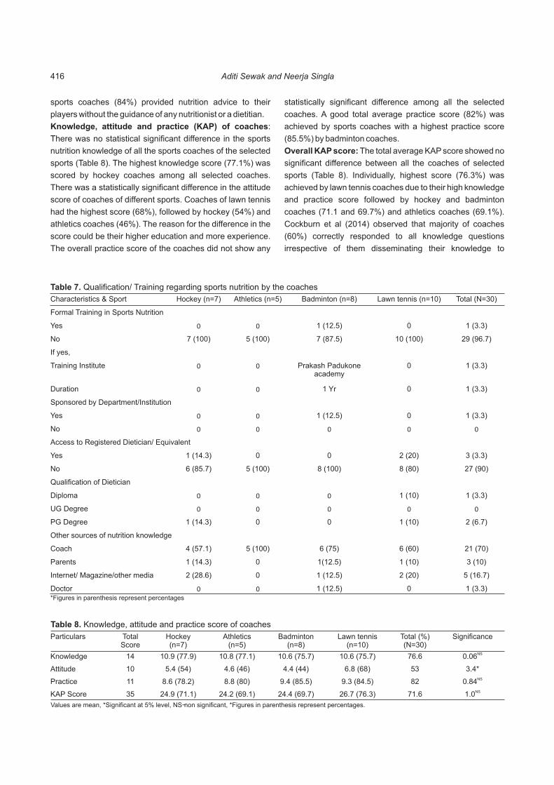
Particulars TotalScore
Hockey(n=7)
Athletics(n=5)
Badminton (n=8)
Lawn tennis (n=10)
Total (%)(N=30)
Significance
Knowledge 14 10.9 (77.9) 10.8 (77.1) 10.6 (75.7) 10.6 (75.7) 76.6 NS0.06
Attitude 10 5.4 (54) 4.6 (46) 4.4 (44) 6.8 (68) 53 3.4*
Practice 11 8.6 (78.2) 8.8 (80) 9.4 (85.5) 9.3 (84.5) 82 NS0.84
KAP Score 35 24.9 (71.1) 24.2 (69.1) 24.4 (69.7) 26.7 (76.3) 71.6 NS1.0
Table 8. Knowledge, attitude and practice score of coaches
Values are mean, *Significant at 5% level, NS-non significant, *Figures in parenthesis represent percentages.
Characteristics & Sport Hockey (n=7) Athletics (n=5) Badminton (n=8) Lawn tennis (n=10) Total (N=30)
Formal Training in Sports Nutrition
Yes 0 0 1 (12.5) 0 1 (3.3)
No 7 (100) 5 (100) 7 (87.5) 10 (100) 29 (96.7)
If yes,
Training Institute 0 0 Prakash Padukone academy
0 1 (3.3)
Duration 0 0 1 Yr 0 1 (3.3)
Sponsored by Department/Institution
Yes 0 0 1 (12.5) 0 1 (3.3)
No 0 0 0 0 0
Access to Registered Dietician/ Equivalent
Yes 1 (14.3) 0 0 2 (20) 3 (3.3)
No 6 (85.7) 5 (100) 8 (100) 8 (80) 27 (90)
Qualification of Dietician
Diploma 0 0 0 1 (10) 1 (3.3)
UG Degree 0 0 0 0 0
PG Degree 1 (14.3) 0 0 1 (10) 2 (6.7)
Other sources of nutrition knowledge
Coach 4 (57.1) 5 (100) 6 (75) 6 (60) 21 (70)
Parents 1 (14.3) 0 1(12.5) 1 (10) 3 (10)
Internet/ Magazine/other media 2 (28.6) 0 1 (12.5) 2 (20) 5 (16.7)
Doctor 0 0 1 (12.5) 0 1 (3.3)
Table 7. Qualification/ Training regarding sports nutrition by the coaches
*Figures in parenthesis represent percentages
sports coaches (84%) provided nutrition advice to their
players without the guidance of any nutritionist or a dietitian.
Knowledge, attitude and practice (KAP) of coaches:
There was no statistical significant difference in the sports
nutrition knowledge of all the sports coaches of the selected
sports (Table 8). The highest knowledge score (77.1%) was
scored by hockey coaches among all selected coaches.
There was a statistically significant difference in the attitude
score of coaches of different sports. Coaches of lawn tennis
had the highest score (68%), followed by hockey (54%) and
athletics coaches (46%). The reason for the difference in the
score could be their higher education and more experience.
The overall practice score of the coaches did not show any
statistically significant difference among all the selected
coaches. A good total average practice score (82%) was
achieved by sports coaches with a highest practice score
(85.5%) by badminton coaches.
Overall KAP score: The total average KAP score showed no
significant difference between all the coaches of selected
sports (Table 8). Individually, highest score (76.3%) was
achieved by lawn tennis coaches due to their high knowledge
and practice score followed by hockey and badminton
coaches (71.1 and 69.7%) and athletics coaches (69.1%).
Cockburn et al (2014) observed that majority of coaches
(60%) correctly responded to all knowledge questions
irrespective of them disseminating their knowledge to
Aditi Sewak and Neerja Singla416

athletes or not. In this study it was also revealed that the
coaches who had attended formal nutrition training scored
higher than those who did not have.
Classification of KAP level of coaches: Only a few
coaches (10%) had excellent sports nutrition knowledge,
attitude and practice score. Fifty-three percent of coaches
were having very good while a significant fraction (30%) had
good KAP. Very less proportion of coaches (6.7%) had
average to poor knowledge, attitude and practice towards
sports nutrition.
Correlations of KAP scores of coaches with other
factors: KAP score of coaches was non-significantly
correlated with their qualification. However, a positively
significant correlation (p≤0.05) was observed with the years
of experience, indicating that as the experience of the
coaches increases, they tend to acquire more knowledge.
Furthermore, KAP score of athletes had a significantly (p≤
0.05) positive correlation with the KAP score of coaches
which associates well with the earlier finding of this study that
coaches are the main source of nutrition knowledge for their
athletes. Correlation of KAP score of coaches and athletes
with other factors has been displayed in Table 10.
KAP Total Score (35) Hockey (n=7) Athletics (n=5) Badminton (n=8) Lawn Tennis (n=10) Total (N=30)
Excellent (30-35) 1 (12.5) 2 (20) 3 (10)
Very Good (25-29) 4 (57.1) 2 (40) 3 (37.5) 7 (70) 16 (53.3)
Good (20-24) 3 (42.9) 3 (60) 3 (37.5) 0 9 (30)
Average to Poor (< 20) 0 0 1 (12.5) 1 (10) 2 (6.7)
Table 9. Classification of KAP level of coaches
*Figures in parenthesis represent percentages
Factor-1 Factor-2 Correlation coefficient (r)
KAP score of coaches Qualification of coaches NS0.20
KAP score of coaches Sports experience of coaches 0.74*
KAP score of coaches KAP score of athletes 0.79*
Table 10. Correlation of KAP score of coaches and athletes with other factors
*Significant at 5% level, NS-Non-significant
The overall KAP score of all the male and female
athletes did not show any significant difference. Majority of
selected coaches (96.7%) had no formal training in sports
nutrition while ninety percent of them did not have any access
to registered dietician or equivalent. Furthermore, the
coaches stated self as the chief source of nutrition
information to their athletes with their KAP score being
positively correlated with their experience and KAP score of
athletes. Coaches are observed to be the primary source of
nutrition knowledge for the athletes; hence their functional
efficiency needs to be enhanced by providing them formal
trainings regarding sports nutrition. Hence, there should be a
provision of sports nutritionists/dietician in sports
departments and universities of the country.
REFERENCES
Alexopoulas Y and Frazier DM (eds) 2012. Krause's food and the nutrition care process. Pp 507. Elsiever Saunders, USA.
Azizi MRN, Farhad M, Maryam M and Mina K 2010. A study of nutritional knowledge and attitudes of elite college athletes in Iran. Brazilian Journal of Biomotricity 4: 105-112.
Burns RD, MS, Schiller MR, Merrick MA and Wolf KN 2004. Intercollegiate student athlete use of nutritional supplements and the role of athletic trainers and dieticians in nutrition counselling. Journal of American Dietetic Association 104: 246-249.
Dunn D, Turner LW and Denny G 2007. Nutrition knowledge and attitudes of college athletes. Sports Journal 10: 45-52.
Cockburn E, Fortune A, Briggs M and Rumbold P 2014. Nutrition knowledge of UK coaches. Nutrients 6: 1442-1453.
Devlin BL and Belski R 2015. Exploring general and sports nutrition and food knowledge in elite male Australian athletes. International Journal of Sport Nutrition and Exercise Metabolism 25: 225-232.
Jessri M, Jessri M, RashidKhani B and Zinn C 2010. Evaluation of Iranian college athletes' sport nutrition knowledge. International Journal of Sport Nutrition and Exercise Metabolism 20: 257-263.
Kong L 2009. Survey of knowledge, attitudes, practices on sports nutrition among excellent athletes in Sichuan province. Modern
0
10
20
30
40
50
60
KA
P S
core KAP Athletes
KAP Coaches
r = 0.79
Assessment of Nutrition Knowledge 417

Preventive Medicine 5: 49.
Mardani M, Bazgir B, Bazgir AB, Mansurnezhad H and Rezapour M 2017. Nutritional knowledge and behavior of professional athletes in khorramabad. Journal of Life Sciences 11: 65-73.
McGehee TMT, Pritchett KL, Zippel D, Minton DM, Cellamare A and Sibilia M 2012. Sports nutrition knowledge among collegiate athletes, coaches, athletic trainers, and strength and conditioning specialists. Journal of Athletic Training 47: 205-211.
Peerkhan N and Srinivasan V 2010. Nutrition knowledge, attitude and practice of college sportspersons. Asian Journal of Sports Medicine 1: 93-100.
Purcell LK 2013. Sports nutrition for young athletes. Journal of Paediatrics and Child Health 18: 200-202.
Reade I, Rodgers W and Spriggs K 2008. New ideas for high performance coaches: a case study of knowledge transfer in sport science. International Journal of Sports Science and Coaching 3: 335-354.
Rodriguez NR, DiMacro NM and Langley S 2009. American Dietetic Association; Dieticians of Canada and the American college of sports medicine: nutrition and athletic performance. Journal of American Dietetic Association 109: 509-527.
Sajber D, Rodek J, Escalante Y, Olujic D and Sekulic D 2013. Sport
nutrition and doping factors in swimming; parallel analysis among athletes and coaches. Collegium Antropologicum 2: 179-186.
Sobana RM 2016. Sports nutritional knowledge, attitude and practice of adolescent cricket players. International Education and Research Journal 2: 129-131.
Supriya V and Ramaswami L 2013. Knowledge, attitude and dietary practices of track and field athletic men and women aged 18-22 Years. International Jounal of Innovative Research and Development 2: 399-404.
Turrell G and Kavanagh AM 2006. Socio-economic pathways to diet: modelling the association between socio-economic position and food purchasing behaviour. Public Health Nutrition 9: 375–383.
Valliant MW, Emplaincourt HP, Wenzel RK and Garner BH 2012. Nutrition education by a registered dietician improves dietary intake and nutrition knowledge of NCAA female volleyball team. Nutrients 4: 506-516.
Walsh M, Cartwright L, Corish C, Sugrue S and Martin RW 2011. The body composition, nutritional knowledge, attitudes, behaviours, and future education needs of senior school boy rugby players in Ireland. International Journal of Sport Nutrition and Exercise Metabolism 21: 365-376.
Received 03 March, 2018; Accepted 10 May, 2018
Aditi Sewak and Neerja Singla418

Fixed-Bed Biosorption of Nitrate using Tamarind Fruit Shells
Indian Journal of Ecology (2018) 45(2): 419-424
Abstract: This study focuses the removal of nitrate (NO ?) from the concocted water environment using Tamarind Fruit Shell (TFS) with Fixed 3
Bed Reactor (FBR) system under room temperature. The settled bed ponders secured the huge analyses, such as, eneration of breakthrough
curvess (counting the impacts of beginning NO3? fixation, TFS size, and stream rate) and bed-profundity benefit time (BDST) approach. From
the FBR studies, the pattern of breakthrough curves were almost similar and consistent, but marginally deviated from the typical S-shaped
curve. The breakthrough time was inversely proportionate to flow rate, initial NO ? concentration and size of TFS, but directly proportionate to 3
bed depth. The head loss problem was not encountered in any of the fixed-bed studies. The biosorptive capacity of TFS in FBR was
approximately 7 to 8 times higher than those in CMBR studies. BDST approach was highly suitable for NO ? removal by TFS; and yielded 3
higher bed efficiency of 99%. The biosorptive capacity of TFS was shown to be directly proportionate to the initial NO ? concentration (N = 3 o
0.09C ).o
Keywords: Nitrate, Tamarind Fruit Shell, Fixed Bed Reactor, Bed-depth Service Time, Biosorptive Capacity
Manuscript Number: 2697NAAS Rating: 4.96
1M. Senthil Rajan and R. Saraswathi
Department of Civil Engineering, Dr. N.G.P Institute of Technology, Coimbatore-641 048, India 1Associate Professor, Department of Civil Engineering, CIT, Coimbatore-641 014, India
E-mail: [email protected]
The ground and surface water were highly contaminated
due to toxic pollutants like inorganic anions, metal ions and
synthetic xenobiotic etc due to industrialization. Among the
large number of inorganic species, nitrate (NO ?) is 3
challenging and hectic problem that has to be tackled in an
indigenous manner. Because of its inadequate holding with
soil grid and moderately high dissolvability in water, the
elevated amounts of NO3? in consumable water is accounted
for to be capable in causing numerous natural and general
wellbeing dangers like eutrophication, methamoglobinemia,
soundness of live stocks (counting dairy cattle), growth of
nutritious channel and cyanosis among kids. According to the
Seems to be: 10500-1995 proposal, the most extreme
allowable utmost for NO3? in drinking water is 50 to 45
mg/l.Significant efforts has been taken in recent years to
remove NO ? from water using various biological and 3
physiochemical processes such as denitrification, reverse
osmosis, ion exchange and electrodialysis etc. The slower
reduction rate, complexity in process and expensive nature
of above said processes made the researchers still anxious
to overcome this problem. Amith and Sillanpaa (2011)
usedsorption for the evacuation of F-, bromate, perchlorate,
and arsenate, from water; in view of its accommodation,
simple task, straightforwardness of outline and well-suited for
low to direct convergences of sorbates (under 100 mg/l),
recuperation and recovery of spent sorbent.
Even though biosorption is quite popular and effective in
removing NO ? (concentrations less than 25 mg/l) from water 3
environment; in so far, no specific biosorbent was emerged
as overall successful due to certain disadvantages like: their
local availability, occurrence in varied size ranges, availability
of certain diversified functional groups, pore size and its
distribution, poor mechanical strength, handling and
operational difficulties, practicability at real time applications,
presence of other competitive species and complete
understanding of sorption mechanism. So, there is a
continuous search to choose an appropriate biosorbent to
effectively Sorb NO ? from various aqueous phases. In this 3
direction, the Tamarind Fruit Shell (TFS) was first time
investigated as novel biosorbent in removing NO ? from 3
concocted water spiked with 10 to 100 mg/l of NO ?, in CMBR 3
system (Prabhu 2012). The current study proposes to
develop a fixed-bed correlation models in removing NO ? by 3
TFS as biosorbent through various factors like flow-rate,
initial sorbate concentration, biosorbent sizes, and bed-
depths on breakthrough of No ?.3
MATERIAL AND METHODS
Biosorbent: The TFS was obtained from Erode District,
Tamilnadu, India and pounded to various sizes by going
through I.S strainers, for example, 1.41 mm, 0.71 mm, 0.5
mm and 0.32 mm individually. It was altogether washed in
refined water to expel remote materials and broiler dried to a
temperature of 110° C for 10 hours, at that point cooled in the
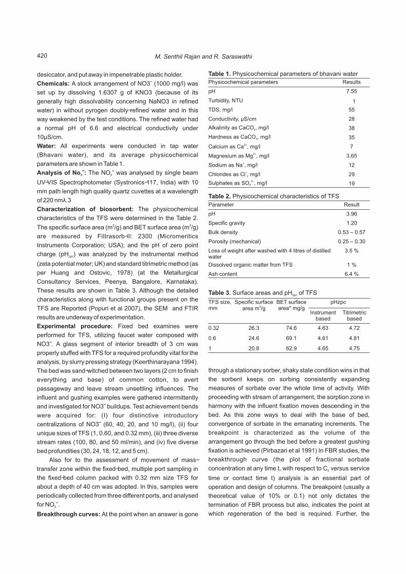
desiccator, and put away in impenetrable plastic holder.
Chemicals: A stock arrangement of NO3? (1000 mg/l) was
set up by dissolving 1.6307 g of KNO3 (because of its
generally high dissolvability concerning NaNO3 in refined
water) in without pyrogen doubly-refined water and in this
way weakened by the test conditions. The refined water had
a normal pH of 6.6 and electrical conductivity under
10µS/cm.
Water: All experiments were conducted in tap water
(Bhavani water), and its average physicochemical
parameters are shown in Table 1.
Analysis of No ?: The NO ? was analysed by single beam 3 3
UV-VIS Spectrophotometer (Systronics-117, India) with 10
mm path length high quality quartz cuvettes at a wavelength
of 220 nmë.3
Characterization of biosorbent: The physicochemical
characteristics of the TFS were determined in the Table 2. 2 2The specific surface area (m /g) and BET surface area (m /g)
are measured by Filtrasorb-II: 2300 (Micromeritics
Instruments Corporation; USA); and the pH of zero point
charge (pH ) was analyzed by the instrumental method zpc
(zeta potential meter; UK) and standard titrimetric method (as
per Huang and Ostovic, 1978) (at the Metallurgical
Consultancy Services, Peenya, Bangalore, Karnataka).
These results are shown in Table 3. Although the detailed
characteristics along with functional groups present on the
TFS are Reported (Popuri et al 2007), the SEM and FTIR
results are underway of experimentation.
Experimental procedure: Fixed bed examines were
performed for TFS, utilizing faucet water composed with
NO3?. A glass segment of interior breadth of 3 cm was
properly stuffed with TFS for a required profundity vital for the
analysis, by slurry pressing strategy (Keerthinarayana 1994).
The bed was sand-witched between two layers (2 cm to finish
everything and base) of common cotton, to avert
passageway and leave stream unsettling influences. The
influent and gushing examples were gathered intermittently
and investigated for NO3? buildups. Test achievement bends
were acquired for: (I) four distinctive introductory
centralizations of NO3? (60, 40, 20, and 10 mg/l), (ii) four
unique sizes of TFS (1, 0.60, and 0.32 mm), (iii) three diverse
stream rates (100, 80, and 50 ml/min), and (iv) five diverse
bed profundities (30, 24, 18, 12, and 5 cm).
Also for to the assessment of movement of mass-
transfer zone within the fixed-bed, multiple port sampling in
the fixed-bed column packed with 0.32 mm size TFS for
about a depth of 40 cm was adopted. In this, samples were
periodically collected from three different ports, and analysed
for NO ?.3
Breakthrough curves: At the point when an answer is gone
Physicochemical parameters Results
pH 7.55
Turbidity, NTU ≤ 1
TDS, mg/l 55
Conductivity, µS/cm 28
Alkalinity as CaCO , mg/l3 38
Hardness as CaCO , mg/l3 352+Calcium as Ca , mg/l 7
2+Magnesium as Mg , mg/l 3.65+Sodium as Na , mg/l 12
–Chlorides as Cl , mg/l 292–Sulphates as SO , mg/l4 19
Table 1. Physicochemical parameters of bhavani water
Parameter Result
pH 3.96
Specific gravity 1.20
Bulk density 0.53 – 0.57
Porosity (mechanical) 0.25 – 0.30
Loss of weight after washed with 4 litres of distilled water
3.5 %
Dissolved organic matter from TFS 1 %
Ash content 6.4 %
Table 2. Physicochemical characteristics of TFS
TFS size,mm
Specific surface 2area m /g
BET surfacearea* mg/g
pHzpc
Instrumentbased
Titrimetricbased
0.32 26.3 74.6 4.63 4.72
0.6 24.6 69.1 4.61 4.81
1 20.8 62.9 4.65 4.75
Table 3. Surface areas and pH of TFSzpc
through a stationary sorber, shaky state condition wins in that
the sorbent keeps on sorbing consistently expanding
measures of sorbate over the whole time of activity. With
proceeding with stream of arrangement, the sorption zone in
harmony with the influent fixation moves descending in the
bed. As this zone ways to deal with the base of bed,
convergence of sorbate in the emanating increments. The
breakpoint is characterized as the volume of the
arrangement go through the bed before a greatest gushing
fixation is achieved (Pirbazari et al 1991) In FBR studies, the
breakthrough curve (the plot of fractional sorbate
concentration at any time t, with respect to C versus service 0
time or contact time t) analysis is an essential part of
operation and design of columns. The breakpoint (usually a
theoretical value of 10% or 0.1) not only dictates the
termination of FBR process but also, indicates the point at
which regeneration of the bed is required. Further, the
M. Senthil Rajan and R. Saraswathi420

mFw /1µ (7)
appearance of breakpoint in any FBR system depends on
several factors like flow rate, sorbent size, sorbate
concentration, bed depth, pH, temperature, nature of
isotherm and others.
In order to appropriately select the flow rates in different
FBR studies, effluent flow measurements were adopted as
per Geresh (2009), for different sizes of TFS of depth 30 cm.
It was seen that at 5 and 60 cm depths of water above the
bed, the effluent flows varied between 95 and 213 ml/min (for
0.32 mm size), and 224 and 320 ml/min (for 0.6 mm size).
Since effluent flow rate was critical, even at 30 cm depth of
TFS of size 0.13 mm, an appropriate flow rate of 50 ml/min
was fixed in biosorption of NO ? by different sizes in FBR.3
RESULTS AND DISCUSSION
Breakthrough curves based on bed depth and service
time: Dale et al (1946) determined the bed depth, which is
hypothetically adequate to counteract entrance of focus in
overabundance of C at zero time, is characterized as basic b
bed profundity and is resolved from when t=0
Where, t = service time, h; v = linear flow rate, cm/h; Z = 3depth of bed, cm; K = rate constant, cm /mg/h; N = sorptive 0
3 3capacity, mg/cm ; C = influent concentration, mg/cm ; and C 0 b
= allowable effluent concentration (breakthrough 3concentration), mg/cm .From Eq. 1, sorptive capacity N can 0
be determined from the slope of a linear plot t versus Z. The
rate constant K is then computed from the intercept of this
plot:
Hutchins (1973) exhibited an adjustment to
Bohart- Adams condition which requires just three settled
bed tests to gather the vital information. This is called bed
profundity benefit time (BDST) approach. Then, the
Bohart- Adams equation (Eq. 1) can be expressed as
t = aZ + b (3)
Where a is slope = N /(C v) and b is intercept = -0 0
1/KC ln[C /C -1]. 0 0
The design parameters calculated according to BDST
TFS bed through which the liquid concentration approach
represented the biosorption of fluctuates from 95 to 1.7% of
the feed focus, and afterward this zone is planned by the
even separation between these two lines in the BDST plot
(Fig. 5). From Figs. 1-3, it is seen that the breakthrough
curves of NO ? sorption by TFS for various depths and 3
operating at various flow rates are almost similar. But, the two
lines in the BDST plot (Fig. 5) were not parallel. So, the depth
of biosorption zone of 21 cm was assessed based on
average distance between the two lines (at the center). The
respective equations for the two straight lines are:
t = 10.6Z + 4.8 (at 1.7 % saturation) (4)
t = 13.5Z + 174.2 (at 95 % saturation) (5)
The Table 4 shows the respective slopes and intercepts,
for various flow rates.3 2For the given flow rate 4.24 m /m /h, the new slope was
calculated by the average slope of the two lines (12.05
min/cm) and as:
The service time t, acquired from BDST configuration
was essentially higher than trial leap forward time and
ascertained bed effectiveness was as high as 95%, despite
the fact that the achievement bends were not sharp after the
break-point.
Bed performance with different flow rates: Based on the
results of Fig. 1-3, a plot of service time versus bed saturation
at breakthrough was dawn. The data points are slightly
scattered (due to a particular point with 75 min and 43.15%),
even though the existence of linearity in the original BDST
model (Fig. 6). Further, this was also due to the variations of
slope between 5.4 and 10.6 min/cm for the respective flows
of 100 ml/min and 50 ml/min (as per Fig. 4). The service time
is inversely proportional to the flow rate through the bed, for
all the bed depths. In this regard, two prominent effects (Lee
et al 2000) can be seen with respect to the mechanism of
NO ? on TFS. Firstly, the higher stream rate diminishes the 3
outer film mass-exchange opposition at the surface of TFS in
view of the extra speed shear, in this manner decreasing the
film thickness. Also, the habitation time of the influent inside
the bed diminishes with higher stream rates. Along these
lines, the NO3? particles have less time to infiltrate and
diffuse into the focal point of TFS. In spite of very scanty
availability of literature pertaining to NO ? removals from the 3
biosorbents by aqueous phase, a fair comparison was made 6+with the biosorption of single-component Cr onto PATFS
(Ramakrishnan 2010) in which, the BDST model could show
almost similar correlation of results with the present
investigation. In concise, the effect of flow rate on bed
performance (BDST slope = m) can be related as per Eq.7.
]1[ 0
0
0 -=bC
CIn
KN
vZ (1)
]1[
1 0
0
--=bC
CIn
KCb (2)
)(
2
112
w
w
F
Faa = (6)
Fixed-Bed Biosorption of Nitrate 421
Flow Rate,ml/min
Bed Saturation, %
1.7 % 95 %
Slope Intercept Slope Intercept
50 10.6 4.8 13.5 174.2
80 7.05 -0.9 13.4 96
100 5.4 4.8 13.95 25.1
Table 4. Values of slope and intercept for different flow rates
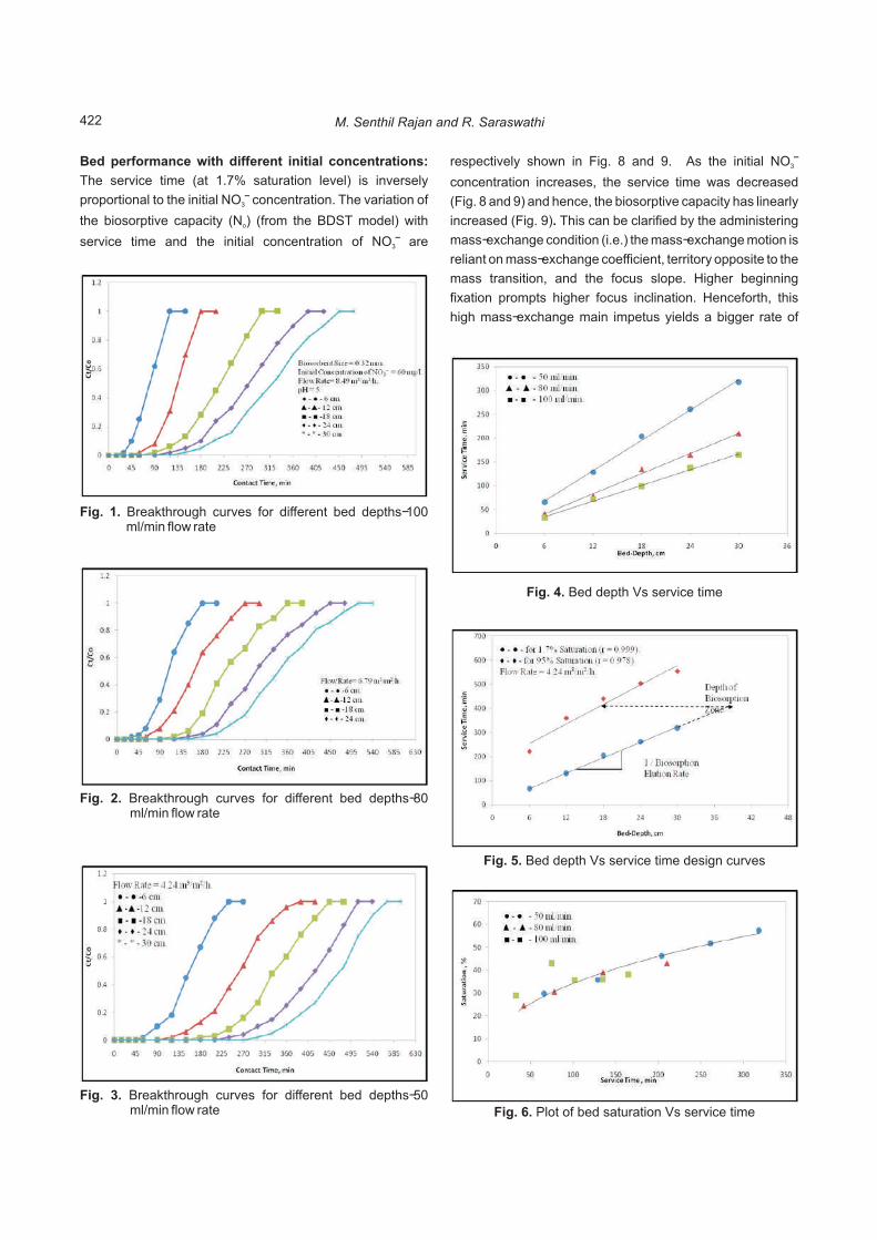
Bed performance with different initial concentrations:
The service time (at 1.7% saturation level) is inversely
proportional to the initial NO ? concentration. The variation of 3
the biosorptive capacity (N ) (from the BDST model) with o
service time and the initial concentration of NO ? are 3
Fig. 1. Breakthrough curves for different bed depths-100 ml/min flow rate
Fig. 2. Breakthrough curves for different bed depths-80 ml/min flow rate
Fig. 3. Breakthrough curves for different bed depths-50 ml/min flow rate
422 M. Senthil Rajan and R. Saraswathi
Fig. 4. Bed depth Vs service time
Fig. 5. Bed depth Vs service time design curves
Fig. 6. Plot of bed saturation Vs service time
respectively shown in Fig. 8 and 9. As the initial NO ? 3
concentration increases, the service time was decreased
(Fig. 8 and 9) and hence, the biosorptive capacity has linearly
increased (Fig. 9). This can be clarified by the administering
mass-exchange condition (i.e.) the mass-exchange motion is
reliant on mass-exchange coefficient, territory opposite to the
mass transition, and the focus slope. Higher beginning
fixation prompts higher focus inclination. Henceforth, this
high mass-exchange main impetus yields a bigger rate of

Fig. 8. Plot of biosorptive capacity Vs service time
Fig. 9. Plot of biosorptive capacity Vs initial concentrations of No3
progress in bed limit regarding administration time of the
beds. Further, a relationship was developed between initial
concentration of NO ? and biosorptive capacity of NO ? and 3 3
shown in Eq. 8.
N = 0.09C (8)o o
Bed performance with different particle sizes: The
423Fixed-Bed Biosorption of Nitrate
Fig. 7. Performance of TFS column for different initial -concentrations of NO3
Fig. 10. Performance of TFS column for different particle sizes
biosorbent size in FBR operation not only affects the bed
porosity, but also greatly influences the flow rate it can be
seen that the service time (at 1.7% saturation level) is
increased with decrease in the geometric mean particle size.
Since experimental Reynolds number (R ) varied between e
0.39 and 1.21 (with sphericity constant, ö = 0.9, ñ = 1000 w
3 3kg/m , v = 1.18×10¯ m/s, particle sizes; 0.32, 0.60, and 1 3 2mm, and µ = 0.88×10¯ Ns/m ) shown in Fig.10, the Wilson
and Geankoplis correlation model (Geankoplis, 1993) (for R e
between 0.0016 and 55) can be used to explain the effect of
particle size on NO ? removal in FBR. As per the model;3
2/3J = (1.09×R - )/å (9)d e
Where, J is the mass-transfer factor (dimensionless) d
and å is the bed void fraction or bed porosity (dimensionless). ¯1From Eq. 9, the J value varies from 2.04å (for 0.32 mm size) d
¯1to 0.96å (for 1 mm size). As the bed porosity decreases with
decrease in size of TFS, the respective J values will increase d
marginally (although the actual bed porosity was not
available or not measured), and hence, bed capacity of TFS 6+is increased. This was in accordance with the removal of Cr
by PATFS in FBR (Ramakrishnan 2010).
CONCLUSION
Based on the investigation relating to the biosorption of
NO3? by TFS in FBR frameworks, The TFS is a decent
biosorbent in expelling NO3? from fluid stage and exceedingly
appropriate in FBR frameworks, for all size ranges between
0.32 and 1 mm. In all fixed bed studies, the pattern of the
breakthrough curves is fairly different with respect to a typical
S-shaped curve and the biosorption of NO ? by TFS can be 3
best explained by BDST model. The head loss and swelling of
TFS particles are insignificant during the fixed bed studies
hence the biosorptive capacity of TFS is directly proportional
to the initial feed concentration of No ?3

REFERENCES
Amith Bhatnagar and Milka Sillanpaa 2011.A review of emerging adsorbents for nitrate removal from water. Chemical Engineering Journal 168: 493-504.
Bohart GS and Adams EQ 1920. Some aspects of the behavior of charcoal with respect to chlorine. Journal of the American Chemical Society 42: 523-544.
Cengeloglu Y, Tor A, Ersoz M and Arslan G 2006. Removal of nitrate from aqueous solution by using red mud. Separation and PurificationTechnology 51: 374-378.
Chatterjee S and Woo SH2009. The removal of nitrate from aqueous solutions by chitosan hydrogel beads. Journal of Hazard Mater 164: 1012-1018.
Demiral H and Gunduzoglu G 2010. Removal of nitrate from aqueous solutions by activated carbon prepared from sugar beet bagasse. Bioresource Technology 101: 1675-1680.
Geankoplis CJ 1993. Transport process and unit operations. Printice- Hall, NJ.
Geresh M 2009. Biosorption of malachite green from aqueous phase by FBR. M.E Thesis Submitted to Anna University (Chennai), CIT, Coimbatore.
Hassan ML, Kassem NF and El-Kader AHA 2010. Novel Zr(IV)/sugar beet pulp composite for removal of sulfate and nitrate anions. Journal of Applied Polymer Science 117: 2205-2212.
Hutchins RA 1973. Designing fixed bed adsorbed for wastewater treatment. American Journal of Chemical Engineering 80: 133. IS: 10500, 1992.Drinking water standards of India.
Jaafari K, Ruiz T, Elmaleh S, Coma J and Benkhouja K 2004. Simulation of a fixed bed adsorber packed with protonated cross-linked chitosan gel beads to remove nitrate from contaminated water. Chemical Engineering Journal 99: 153-160.
Karimi M, Entezari MH and Chamsaz M 2010. Sorption studies of nitrate ion by a modified Beet residue in the presence and absce of ultrasound. Ultrasonic Sonochemistry (ULTRASON
SONOCHEM) 17: 711-717.
Keerthinarayana S 1994. Sorption of lindane from water environment by wood charcoal. Ph.D. Thesis Submitted to IIT, Kharagpur, W.B., India.
Namasivayam and Höll WH 2005. Quaternized biomass as an anion exchanger for the removal of nitrate and other anions from water. Journal of Chemical Technology and Biotechnology 80:164-168.
Orlando US, Baes AU, Nishijima W and Okada M 2002. A new procedure to produce lignocellulosic anion exchangers from agricultural waste materials. Biorecourse Technology 83: 195-198.
Öztürk N and Bekta TE 2004. Nitrate removal from aqueous solution by adsorption onto various materials. Journal of Hazard Mater 112: 155-162.
ÖzcanAhin MS and Özcan AS 2005. Adsorption of nitrate ions onto sepiolite and surfactant-modified sepiolite. Adsorption Science Technology 23: 323-333.
Pirzabari M, Badriyha BN, and Milnter RJ 1991. GAC adsorber design for removal of chlorinated pesticides, Journal of Environmental Engineering Division, ASCE 117(1): 80-100.
Popuri SR, Jammala A and Abburi K 2007. Biosorption of Hexavalent chromium using tamarind (Tamarind indica) Shell-a comparative study. Electronic Journal of Biotechnology 10.
Senthil Rajan M, Prabhu P and Keerthinarayana S 2017. Biosorption kinetices of nitrate onto tamrind fruit shells. Asian Journal of Research in Social Sciences and Humanities 6: 1-12.
Wang Y, Gao BY, Yue WW and Yue QY 2007. Preparation and utilization of wheat straw anionic sorbent for the removal of nitrate from aqueous solution. Journal of Environmental science 19: 1305-1310.
Wang Y, Gao BY, Yue WW and Yue QY 2007. Adsorption kinetics of nitrate from aqueous solutions onto modified wheat residue. colloids surface. Physicochemical Engineering Aspects 308: 1-5.
Received 08 April, 2018; Accepted 10 May, 2018
424 M. Senthil Rajan and R. Saraswathi

Genetic Diversity for Yield and Its Attributes in Barley (Hordeum vulgare L.) under Irrigated Condition
Indian Journal of Ecology (2018) 45(2): 425-429
Abstract: Genetic diversity among 87 barley genotypes comprised of two and six row types was carried out for 10 characters using 2Mahalanobis D statistics. All the genotypes were assigned into eight distinct clusters depending upon the similarity in the expression of their
genetic divergence. Maximum number of genotypes were grouped in cluster VI (20) followed by cluster VII (15), IV (13), III (12), VIII (10), II (8)
and clusters V and I had six and three genotypes, respectively. Highest intra- cluster distance was observed for cluster V (3.360) followed by
cluster VI (3.312) and cluster VII (3.304) whereas it was recorded minimum for cluster VIII (2.553).The average inter-cluster distance was
found to be highest between the cluster I and VII (6.722) followed by between cluster I and VIII (5.534) while the lowest inter-cluster distance
was observed between clusters III and IV. The contribution of number of grains per spike was maximum (32.24%) towards divergence out of 10
characters studied, followed by 1000-grain weight (24.73%), plant height (13.79%), days to heading (8.26%) and number of tillers per meter
row (7.38%), whereas the remaining characters contributed very little to diversity. The improvement in six rowed barley could be achieved
through the use genotypes assigned in clusters I and II, whereas the genotypes which contained in cluster VI might be considered as potential
parents for two rowed barley to obtain high heterotic response and consequently better segregants for grain yield.
Keywords: Genetic diversity, Barley, Cluster
Manuscript Number: NAAS Rating: 4.96
2698
Yogender Kumar, Naveen Kumar and Suman DeviWheat and Barley Section,Department of Genetics and Plant Breeding
CCS Haryana Agricultural University, Hisar-125 004, IndiaE-mail: [email protected]
Barley (Hordeum vulgare L.), cereal plant of the grass
family Poaceae and is edible grain. It is the fourth largest
grain crop globally, after wheat, rice, and corn grown in a
variety of environments. Commonly used in breads, soups,
stews, and health products, though it is primarily grown as
animal fodder and as a source of malt for alcoholic
beverages, especially beer. Because of its hardiness, in
many countries around the world, it is often considered the
only possible rainfed cereal crop under low input and
stressful environment. In India, the area under barley is
around 0.69 million hectares with the production and -1productivity of 1.78 million tons and 2580 kg ha ,
respectively. Haryana state achieved a productivity level of -13475 kg ha on 40,000 hectares (Anonymous 2017).
Genetic diversity is essential for genetic improvement of
a given crops. If the information on genetic diversity is not
enough to utilize, the available genetic diversity study should
be crucial (Addisu and Shumet 2015). The clustering of
parents based on genetic diversity is a pre-requisite for a
successful hybrid breeding program. The use of diverse
parents gives better opportunities to a breeder for selection
and development of superior varieties (Singh et al 2013).
Criteria for the estimation of genetic diversity can be different:
pedigree records, morphological traits, biochemical markers
and molecular markers (Eshghi and Akhundova 2010).
According to Muhe and Assefa (2011), knowledge of the
genetic diversity and agronomic potential of barley landraces
in variable environments is an important task to design
strategic utilization of germplasm. High magnitude of genetic
association may be due to pleiotropy rather than linkage. By
improving the characters which are directly and positively
correlated with yield will ultimately improve the yield (Singh et
al 2014). The information on genetic diversity would be useful
for selection parameters to plan crosses and maximize the
use of genetic diversity and expression of heterosis in barley
breeding program for yield improvement (Yadav et al 2015).
The present study, therefore, was undertaken with the
aim of examining the magnitude of genetic diversity and
characters contributing to divergence among barley
genotypes.
MATERIAL AND METHODS
The experimental material consisted of 87 diverse
genotypes including 47 two rowed and 40 six rowed barley.
The material was evaluated in randomized block design with
three replications at CCS Haryana Agricultural University,
Hisar during rabi 2016-17. Each genotype was grown in six 2rows with a plot size of 5 x 1.38 m . Recommended package
of practices were followed to raise the good crop. The
observations were recorded for 10 quantitative traits viz.,

days to heading, days to maturity, plant height (cm), ear
length (cm), number of tillers per meter row, number of grains
per spike, 1000-grain weight (g), harvest index (%), biological
yield (kg/plot) and grain yield (kg/plot). Five randomly
selected competitive plants in each replication were recorded
for all the traits under study except of days to heading, days to
maturity, biological yield and grain yield which were recorded
on plot basis. Further, the value of harvest index was
calculated as per the formula given by Donald and Humblin
(1976).
The mean performance of each genotype was embayed
for statistical analysis. Analysis of variance to test the
significance for each character was carried out as per
methodology given by Panse and Sukhatme (1967). To
quantify genetic divergence between any two genotypes or 2group of genotypes, Mahalanobis' D statistics (1936) as
described by Rao (1952) was used and the genotypes were
grouped into different clusters on the basis of Ward's
minimum variance method (Spark 1973).
RESULTS AND DISCUSSION
Significant differences were observed among the
genotypes for all the character studied indicating
considerable amount of variability among them. Genetic 2divergence (D ) is the basis of variability and helps to craft the
designed genotypes as per the requirement. Based on the
results of cluster analysis, 87 genotypes were grouped into
eight clusters in such a way that the genotypes within a 2cluster had a small D values than those of in between the
clusters. The cluster membership profile (Table 1 and Fig.1)
revealed that cluster VI had the largest number of genotypes
(20) followed by cluster VII (15), IV (13) and cluster III (12),
while the cluster I was smallest with three genotype only. The
clustering pattern showed that two rowed genotypes got
distributed in three clusters viz., cluster VI, VII and VIII except
two genotypes namely BH 16-36 and BH 16-39. Singh et al
(2013) also studied the genetic divergence among 108 barley
germplasm collections on the basis of 10 quantitative
characters and grouped the genotypes into 11 clusters
revealing the presence of considerable amount of genetic
diversity in the material.
The inter-cluster distance was higher than the intra-
cluster, indicating wide genetic diversity among the
genotypes (Table 2 and Fig. 2). The maximum intra-cluster
distance was recorded for clusters V (3.360) followed by
cluster VI (3.312) and cluster VII (3.304). On the other hand,
minimum intra-cluster distance (2.553) was observed in
cluster VIII. It was reported that genotypes within the cluster
with high degree of divergence would produce more
desirable breeding materials for achieving maximum genetic
advance (Singh et al 2014).
The highest inter-cluster distance was observed
between clusters I and VII (6.722) followed by between
clusters I and VIII (5.534) whereas it was minimum between
clusters III and IV. The inter-cluster values that indicated
close relationship were to be considered that hybridization
among the genotypes of these clusters would not provide
good levels of segregation. It is well recognized that greater
the distance between clusters, wider the genetic diversity
would be between the genotypes. Therefore, highly
divergent genotypes would produce a broad spectrum of
segregation in the subsequent generations enabling further
Clusters Genotypes No. of genotypes
I BH 10-11 (1), BH393 (41), BH 16-40 (81) 3
II BH 12-46 (4), BH 7-35 (19), BH 15-02 (14), BH 16-44 (85), BH 946 (38), BH 7-34 (18), BH 15-06 (25), BH 15-07 (15) 8
III BH 13-22 (6), BH 14-44 (23), BH 15-30 (17), BH 16-10 (51), BH 16-43 (84), BH 15-39 (33), BH 14-01 (8), BH 14-13 (11), BH 15-37 (31), BH 14-42 (13), BH 15-25 (30), BH 16-45 (86)
12
IV BH 15-16 (28), BH 16-18 (59), BH 16-20 (61), BH 16-33 (74), BH 902 (37), BH 16-06 (47), BH 16-07 (48), BH 16-42 (83), BH 16-13 (54), BH 16-11 (52), BH 16-30 (71), BH 16-17 (58), BH 16-29 (70)
13
V BH 10-03 (34), BH 16-38 (79), BH 16-36 (77), BH 16-39 (80), BH 16-37 (78), BH 16-41 (82) 6
VI BH 12-29 (3), BH 15-17 (16), BH 15-11 (26), BH 16-34 (75), BH 16-35 (76), DWRB 92 (40), BH 16-12 (53), BH 14-07 (10), BH 14-25 (12), BH 10-30 (2), BH 14-17 (20), BH 15-05 (24), DWRUB 52 (39), BH 14-43 (22), BH 16-25 (66), BH 14-06 (9), DWRB 101 (35), BH 885 (36), BH 16-21 (62), BH 15-38 (32)
20
VII BH 13-20 (5), BH 16-19 (60), BH 15-24 (29), BH 16-05 (46), BH 13-26 (7), BH 14-40 (21), BH 15-12 (27), BH 16-27 (68), BH 16-08 (49), BH 16-24 (65), BH 16-26 (67), BH 16-31 (72), BH 16-03 (44), BH 16-32 (73), BH 16-04 (45)
15
VIII BH 16-01 (42), BH 16-22 (63), BH 16-15 (56), BH 16-14 (55), BH 16-16 (57), BH 16-46 (87), BH 16-23 (64), BH 16-28 (69), BH 16-02 (43), BH 16-09 (50)
10
Table 1. Cluster membership profile of different genotypes
Values in parenthesis indicates serial number of genotypes
Yogender Kumar, Naveen Kumar and Suman Devi426

selection and improvement. The hybrids developed from the
selected genotypes within the limit of compatibility of these
clusters may produce desirable transgressive segregants of
high magnitude of heterosis. Manjunatha et al (2007),
Shakhatreh et al (2010), Ebrahim et al (2015), Yadav et al
(2015) also found similar results of diversity in barley.
The eight clusters showed considerable differences in
mean values for the characters under study (Table 3). Cluster
I comprised of three genotypes, exhibited minimum number
of days to head and maturity, shortest plant height and ear
length, and had moderately high cluster means for grain yield
as well as harvest index. The genetic distance value of these
genotypes was 2.653. Cluster II consisted of 8 genotypes
including national check variety BH 946, characterized by
high 1000-grain weight among the clusters had six rowed
genotypes with highest grain yield and biological yield. The
genotypes of this cluster showed genetic distance of 2.995.
Fig. 1. Clustering by Ward's minimum variance method
Clusters I II III IV V VI VII VIII
I 2.653 4.156 4.972 5.129 4.844 4.768 6.722 5.534
II 2.995 4.194 3.809 4.860 4.262 5.281 5.282
III 3.002 3.568 4.219 4.965 4.641 4.884
IV 3.109 4.565 4.823 4.419 4.715
V 3.360 5.142 5.492 5.365
VI 3.312 4.539 4.026
VII 3.304 3.908
VIII 2.553
Table 2. Estimates of intra-and inter-cluster distances
Diagonal: Intra-cluster distances; Off-diagonal: Inter-cluster distances
Cluster III had 12 genotypes having characteristic features of
highest number of grains per spike, lowest 1000-grain weight
with highest number of days to head. The genetic distance
value of these genotypes was 3.002.
Cluster IV, contained 13 genotypes including national
check BH 902, recorded moderately high number of days to
maturity and plant height with minimum number of tillers per
meter row. The genetic distance value of these genotypes
was 3.109. Six genotypes constituted cluster V and
characterized by high number of tillers per meter row among
the clusters having six row type barley, highest harvest index
with minimum biological yield. Maximum genetic distance
(3.360) was observed between genotypes of this cluster. The
clusters VI, VII and VIII were assigned with two row barley
genotypes. Cluster VI which consisted of 20 genotypes being
largest one included national check varieties viz., DWRUB
52, DWRB 101, DWRB 92 and BH 885, exhibited maximum
Genetic Diversity in Barley 427

Characters Clusters
I II III IV V VI VII VIII
Days to heading 77.11 80.96 84.39 81.59 84.33 80.47 83.93 78.87
Days to maturity 118.11 122.50 122.53 124.77 123.44 121.33 124.80 120.47
Plant height (cm) 83.67 103.29 97.64 108.26 88.22 97.47 110.73 106.10
Ear length (cm) 5.97 6.29 6.92 6.45 6.78 6.37 7.01 7.15
No. of tillers per meter row 97.33 95.75 97.44 90.67 98.94 132.13 125.64 125.30
No. of grains per spike 63.68 61.17 65.79 63.64 50.79 24.37 26.71 25.27
1000-grain wt. (g) 40.13 44.36 37.84 43.04 39.46 50.39 51.08 52.29
Grain yield (kg/plot) 2.75 3.11 2.22 2.29 2.15 2.69 2.03 1.85
Biological yield (kg/plot) 7.93 9.33 8.71 8.47 6.13 8.79 8.70 7.66
Harvest index (%) 35.09 33.75 25.65 27.36 35.42 31.21 23.33 24.49
Table 3. Average performance of different clusters for yield and its attributes in barley
number of tillers per meter row, highest grain yield, biological
yield as well as harvest index among two rowed clusters.
The genotypes of this cluster showed genetic distance of
3.312.
Cluster VII had 15 genotypes was responsible for
maximum number of days to mature and also showed
highest plant height. The genotypes of this cluster showed
genetic distance of 3.304. Cluster VIII contained 10
genotypes observed with highest ear length, 1000-grain
weight and had lowest grain yield with genetic distance of
2.553. Several genetic diversity studies have been
conducted on barley based on quantitative traits in order to
select genetically distant parents for hybridization (Sharma et
Characters Desirable genotypes
Days to heading (Early) Six rowed: BH 393, BH 10-11, BH -35, BH 16-40Two rowed: BH 14-06, BH 16-09
Days to maturity (Early) Six rowed: BH 10-11, BH 393, BH 13-22Two rowed: BH 16-23, BH 16-09, BH 16-22
Plant height (Medium Dwarf)
Six rowed: BH 16-40, BH 10-03, BH 393, BH 10-11, BH 13-22Two rowed: BH 16-35, BH 16-36, DWRB 92, BH 14-06, BH 10-30, DWRUB 52, BH 14-25, BH 14-17
Ear length (cm) Six rowed: BH 14-44, BH 16-37, BH 13-22Two rowed: BH 14-40, BH 16-36, BH 13-26, BH 16-19, BH 16-12
No. of tillers per meter row Six rowed: BH 12-46, BH 7-35, BH 16-29, BH 15-25Two rowed: BH 14-40, BH 14-07, DWRB 92, BH 14-25, BH 10-30
No. of grains per spike Six rowed: BH 15-30, BH 13-22, BH 16-43, BH 16-17Two rowed: BH 13-20, BH 16-19, BH 16-28, BH 14-40
1000-grain wt. (g) Six rowed: BH 15-06, BH 15-02, BH 7-34, BH 15-07Two rowed: BH 16-09, DWRB 92, BH 16-12, BH 15-11
Grain yield (kg/plot) Six rowed: BH 15-07, BH 15-06, BH 946, BH 15-02, BH 393, BH 7-34, BH 7-35, BH 16-44Two rowed: BH 14-17, BH 14-07, BH 10-30, BH 16-12, DWRUB 52, DWRB 92, BH 14-25, BH 13-26
Biological yield (kg/plot) Six rowed: BH 15-07, BH 14-13, BH 902, BH 15-06Two rowed: DWRUB 52, BH 15-05, BH 13-26, BH 14-40, BH 15-12
Harvest index (%) Six rowed: BH 946, BH 16-40, BH 16-38, BH 15-02, BH 10-03Two rowed: BH 16-35, BH 10-30, BH 16-36, BH 14-17
Table 5. Diverse and superior genotypes with desirable traits selected from different clusters
Source Times stranked 1
Contribution towards divergence (%)
Days to heading 309 8.26
Days to maturity 151 4.04
Plant height (cm) 516 13.79
Ear length (cm) 54 1.44
No. of tillers per meter row 276 7.38
No. of grains per spike 1206 32.24
1000-grain wt. (g) 925 24.73
Grain yield (kg/plot) 162 4.33
Biological yield (kg/plot) 133 3.56
Harvest index (%) 9 0.24
Table 4. Contribution of different characters towards divergence
Yogender Kumar, Naveen Kumar and Suman Devi428

Fig. 2. Euclidean Distances in barley genotypes
al 2014, Dyulgerova et al 2016, Sarkar et al 2014).
Out of 10 traits studied, contribution of number of grains
per spike towards divergence was maximum (32.24%)
followed by 1000-grain weight (24.73%), plant height
(13.79%) and days to heading (8.26%), whereas, the
remaining traits like number of tillers per meter row (7.38%),
grain yield (4.33%), days to maturity (4.04%), biological yield
(3.56%), ear length (1.44%) and harvest index (0.24%)
contributed very little to divergence (Table 4).The
contribution of various characters towards the expression of
genetic divergence should be taken into account as a
criterion for choosing parents for crossing programme for the
improvement in such characters. Similar findings have also
been corroborated by Singh et al (2014) in barley. Hailu et al
(2016) also showed the presence of high genetic divergence
among barley genotypes based on cluster and principal
component analyses for breeding strategies. Most diverse
and superior genotypes with desirable traits selected from
different clusters are represented in Table 5.
Therefore, it can be concluded that clusters I and II for six
rowed and cluster VI for two rowed might be considered
desirable for selecting genotypes which may be used as
promising parents for hybridization. The genotypes, which
fall in these clusters could be used in crossing programme to
obtain high heterotic response and thus better segregants in
subsequent generations for higher grain yield in barley.
REFERENCES
Addisu F and Shumet T 2015. Variability, heritability and genetic
advance for some yield and yield related traits in barley (Hordeum vulgare L.) landraces in Ethiopia. International Journal of Plant Breeding and Genetics 9(2): 68-76.
Anonymous 2017. Progress report of All India Coordinated Wheat and Barley Improvement Project 2016-17, Project Director's Report. Ed. G.P. Singh, ICAR-Indian Institute of Wheat and Barley Research, Karnal, India, pp: 87.
Donald CM and Humblin J 1976. The biological yield and harvest index of cereals as agronomic and plant breeding criteria. Advances in Agronomy 28: 361-405.
Dyulgerova B, Dimova D and Valcheva D 2016. Genetic diversity in six rowed winter barley (Hordeum sativum Jess., ssp. vulgare L.) genotypes. Bulgarian Journal of Agricultural Sciences 22(1): 114-118.
Ebrahim S, Shiferaw E and Hailu F 2015. Evaluation of genetic diversity in barley (Hordeum vulgare L.) from Wollo high land areas using agro-morphological traits and hordein. African Journal of Biotechnology 14(22): 1886-1896.
Eshghi R and Akhundova E 2010. Genetic diversity in hulless barley based on agro morphological traits and RAPD markers and comparison with storage protein analysis. African Journal of Agricultural Research 5: 97-107.
Hailu A, Alamerew A, Nigussie M and Assefa E 2016. Study of genetic diversity in different genotypes of barley (Hordeum vulgare L.) based on cluster and principal component analysis. Agricultural Science Research Journal 6(2): 31-42.
Mahalanobis PC 1936. On the generalized distance in statistics. Proceedings of the National Institute of Sciences of India 2: 49-55.
Manjunatha T, Bisht IS, Bhat KV and Singh BP 2007.Genetic diversity in barley (Hordeum vulgare L. ssp. vulgare) landraces from Uttaranchal Himalaya of India. Genetic Resources and Crop Evolution 54:55-65.
Muhe K and Assefa A 2011. Diversity and agronomic potential of Barley (Hordeum vulgare L.) landraces in variable production system, Ethiopia. World Journal of Agricultural Sciences 7(5): 599-603.
Panse VG and Sukhatme PV 1967. Statistical Methods for ndAgricultural Workers, 2 Ed. ICAR, New Delhi, India, pp: 381.
2Rao CR 1952. D analysis. In: Advanced Statistical Methods in Biometrical Research. John Wiley and Sons Inc., New York, pp. 357-363.
Sarkar B, Sarkar A, Sharma RC, Verma RPS and Sharma I 2014. Genetic diversity in barley (Hordeum vulgare) for traits associated with feed and forage purposes. Indian Journal of Agricultural Sciences 84(5): 102-107.
Shakhatreh Y, Haddad N, Alrababah M, Grando S and Ceccarelli S 2010. Phenotypic diversity in wild barley (Hordeum vulgare L. ssp. spontaneum (C. Koch) Thell.) accessions collected in Jordan. Genetic Resources and Crop Evolution 57: 131-146.
Sharma A, Joshi N, Cheema BS, Jindal MM and Singh S 2014. Assessment of genetic diversity in barley (Hordeum vulgare L.). Journal of Research PAU 51(2): 105-108.
Singh SK, Verma PN, Singh L, Ali T and Prasad KD 2014. Variability and divergence analysis in barley (H. vulgare L.) under irrigated condition. Trends in Biosciences 7(6): 452-456.
Spark DN 1973. Euclidean cluster analysis.Algorithm As 58. Applied Statistics 22(1): 126-130.
Yadav SK, Singh AK and Malik R 2015. Genetic diversity analysis based on morphological traits and microsatellite markers in barley (Hordeum vulgare L.). Indian Journal of Agricultural Sciences 85(10):1285-1292.
Singh M, Vishwakarma SR and Singh AP 2013. Genetic divergence in barley. Progressive Research 8(2): 230-232.
Received 26 April, 2018; Accepted 10 May, 2018
Genetic Diversity in Barley 429

Quality Evaluation of Elephant Foot Yam (Amorphophallus paeoniifolius Dennst- Nicolson) Cultivars during
Growth and Development
Indian Journal of Ecology (2018) 45(2): 430-432
Abstract: Eleven cultivars of elephant foot yam were evaluated and variability was observed at monthly intervals within the cultivars. In cv.
NDA-9 and AC-28 amount of dry was more at 100 and 250 DAP respectively. The TSS was higher in cultivar NDA-9 and BCA-5 and BCA-2
and total sugar in BCA-5 and BCA-2 .The range of titrable acidity was 0.064-0.160 % at different stages during growth and development.
Significant increase was in dry weight, total soluble solids, total sugar and titrable acidity during growth and development period at monthly
intervals.
Keywords: Elephant foot yam, Cultivar, TSS, TS, Acidity
Manuscript Number: NAAS Rating: 4.96
2699
1 2Amit Kumar Singh, Arvind Kumar Chaurasiya and Surajit MitraDepartment of Horticulture, Rani Lakshmi Bai Central Agricultural University, Jhansi-284 003, India
1North Eastern Hills University Tura, Meghalaya-794002, India2Bidhan Chandra Krishi Viswavidyalaya Mohanpur, Nadia-741 252, India
E-mail: [email protected]
Amorphophallus paeoniifolius Dennst-Nicolson known
as Elephant foot yam is a highly potential tropical tuber crop
of Areace family (Jansen et al 1996). It is regarded as “King
of tuber crops” due to its higher biological efficiency as a
food producer and possesses higher productivity in a short
growing season as well as confers high returns
(Nedunchezhiyan 2014, Singh et al 2017). Root and tubers
are the most important food crops since time immemorial in
the tropics and subtropics (Behera et al 2009). The tubers
are rich in nutrients and is a natural product that is high in -1fiber, rich in potassium, calcium (50 mg g ), phosphorus (34
-1 -1mg g ) vitamin A (260 IU g ), vitamin B6, as well as with trace
minerals like selenium, zinc and copper It is difficult to
ascertain whether the tubers can be relied upon as good
sources of minerals because of the presence of anti-
nutrition substances (oxalate), which render the minerals,
in them unavailable to the consumers (Onwuka 2005).
These corms are consumed by many people as a food and
widely used in many ayurvedic preparations (Angayarkanni
et al 2007) because it contains different bioactive
components like alkaloids, flavonoids, phenols, vitamins,
minerals etc. (Dey et al 2010). For this study, elephant foot
yam cultivars were evaluated for horticultural and nutritional
parameters, to provide information to the breeders to
develop desirable cultivars having a high yield and a better
nutritional profile.
MATERIAL AND METHODS
Collection of samples: The experiments were carried out at
Bidhan Chandra Krishi Viswavidyalaya, India during 2010-
2012 with a view to analyze the physico-chemical
characteristics of fresh harvested corms of elephant foot yam
at monthly intervals. Eleven cultivars of elephant foot yam
were procured from state agricultural universities and
research institutes under the Indian council of agricultural
research, India and cultivated at horticultural research station
Mondouri, BCKV, India. The samples were collected in the
month of December and stored at ambient condition, while th thplanting has been done at 5 and 16 of April 2011 and 2012,
respectively. The monthly data was recorded from 100 days
after planting to 250 DAP. Climatically the region located at O O23.5 N latitude and 89 E longitudes with an altitude of 9.75
m above mean sea level. The soil was a slightly acidic (pH
6.5) with sandy loam and climatic condition was tropical
humid with rainfall of 0.00 to 264.00 mm, temperature O Omaximum 37.59 C and minimum 9.62 C along with RH (%)
96.87 to 36.74 (Annual average).
Physico-chemical analysis: The physic-chemical traits of
elephant foot yam were recorded from 10 randomly selected
plants from each replication in both year at monthly intervals
during growth and development by mentioned methods viz.,
total sugar (Moorthy and Padmaja 2002), total soluble solids
by Pocket refractometer, titrable acidity by titration method

Cultivars Dry Weight (%) OTSS ( Brix)
100 130 160 190 220 250 100 130 160 190 220 250
BCA-1 19.15 22.50 26.74 29.36 35.83 36.70 6.00 7.10 7.40 7.90 8.40 8.50
BCA-2 18.53 20.29 22.54 23.89 27.09 27.90 5.40 5.70 6.50 6.90 7.30 7.50
BCA-4 17.49 18.95 24.84 27.92 29.45 30.81 4.90 5.60 7.40 8.00 8.50 8.70
BCA-5 20.49 20.75 25.33 29.74 31.33 33.24 5.10 6.00 6.80 8.30 8.70 8.90
BCA-6 19.64 19.95 23.04 23.95 27.32 29.33 5.20 5.90 7.30 7.90 8.20 8.40
NDA-4 20.41 22.13 26.19 29.28 33.15 35.50 5.80 6.30 6.80 7.70 8.10 8.30
NDA-5 19.41 19.60 20.25 23.95 25.55 26.56 5.70 6.10 7.00 8.00 8.40 8.60
NDA-9 21.11 22.45 25.11 29.44 32.98 34.73 6.50 7.00 7.60 8.20 8.70 8.80
AC-28 20.02 20.73 26.66 30.08 35.52 38.82 5.10 5.70 6.10 6.50 7.30 7.40
IGAM-1 19.56 22.64 27.16 29.12 33.06 34.29 5.30 5.90 7.00 7.80 8.60 8.80
Gajendra 19.32 20.26 24.51 26.36 27.64 29.74 5.80 6.20 7.00 7.50 8.20 8.30
Mean 19.56 20.93 24.76 27.56 30.81 32.51 5.50 6.10 7.00 7.70 8.20 8.40
CD (p=0.05) CD (p=0.05)
C 1.84 1.87 1.82 1.84 1.87 1.61 1.15 1.10 1.21 1.09 1.41 1.14
Y 0.78 0.80 0.78 0.78 0.79 0.69 0.49 0.47 0.52 0.46 0.63 0.48
CY 2.60 2.65 2.58 2.60 2.64 2.28 1.63 1.56 1.72 1.54 2.00 1.61
Table 1. Changes in dry weight and TSS contents in elephant foot yam corms in different cultivars
Days after planting
Cultivars Total Sugar (%) Titrable Acidity (%)
100* 130 160 190 220 250 100 130 160 190 220 250
BCA-1 0.54 0.95 1.04 1.29 1.53 1.58 0.088 0.110 0.122 0.130 0.140 0.150
BCA-2 0.68 0.95 1.17 1.40 1.66 1.69 0.096 0.114 0.125 0.132 0.139 0.148
BCA-4 0.56 0.78 1.04 1.23 1.60 1.64 0.064 0.098 0.114 0.122 0.131 0.143
BCA-5 0.68 0.87 1.04 1.24 1.53 1.56 0.096 0.113 0.124 0.132 0.140 0.150
BCA-6 0.57 0.89 1.03 1.25 1.54 1.58 0.096 0.118 0.128 0.136 0.141 0.153
NDA-4 0.61 0.90 1.00 1.22 1.48 1.51 0.080 0.102 0.112 0.119 0.126 0.137
NDA-5 0.53 0.88 0.98 1.19 1.33 1.35 0.096 0.113 0.124 0.132 0.141 0.152
NDA-9 0.61 0.85 1.01 1.25 1.63 1.67 0.096 0.099 0.109 0.118 0.127 0.141
AC-28 0.60 0.72 0.94 1.21 1.46 1.50 0.096 0.135 0.125 0.133 0.140 0.152
IGAM-1 0.50 0.82 0.98 1.30 1.35 1.40 0.080 0.097 0.108 0.122 0.129 0.131
Gajendra 0.61 0.79 0.93 1.18 1.59 1.63 0.109 0.123 0.132 0.139 0.146 0.160
Mean 0.59 0.85 1.01 1.25 1.52 1.55 0.091 0.109 0.120 0.128 0.136 0.147
CD (p=0.05) CD (p=0.05)
C 0.35 0.26 0.38 0.35 0.39 0.36 0.03 0.04 0.03 0.03 0.03 0.03
Y 0.15 0.11 0.16 0.15 0.16 0.15 0.01 0.02 0.01 0.01 0.01 0.01
CY 0.49 0.36 0.54 0.49 0.55 0.51 0.04 0.05 0.04 0.04 0.04 0.04
Table 2. Changes in total sugar (%) and titrable acidity (%) contents in elephant foot yam corms in different cultivars
Days after planting
(AOAC 1990) and dry weight by total moisture content of
fresh corms weighing 100 g was calculated from loss in Oweight during drying at 70 C for 48 hrs.
RESULTS AND DISCUSSION
Dry Weight: Dry weight content of corm was significantly
influenced by cultivars during maturity stages (Table 1). In
cultivar NDA-9 and AC-28 dry matter contents were 21.11
and 38.82 % at 100 DAP and 250 DAP ,respectively. The
lowest amount was in cultivar BCA-4 (17.49 %) and NDA-5
(26.56 %) at 100 and 250 DAP respectively. A wide range of
dry weight content was also observed by Panja et al 2017 in
elephant foot yam corms during storage. OTotal soluble solids: The total soluble solids (TSS Brix)
content of elephant foot yam corms increased throughout the
growing periods in both the years. The highest TSS content
Quality Evaluation of Elephant Foot Yam Cultivars during Growth and Development 431
O Owere in cultivar NDA-9 (6.5 Brix) and BCA-5 (8.9 Brix) at
100 DAP and 250 DAP respectively. While, cultivar BCA-4 O O(4.9 Brix) and AC-28 (7.4 Brix) content lowest amount of
TSS at 100 and 250 DAP respectively (Table 1). The increase
in TSS might be due to depletion of moisture in the form of
water from elephant foot yam corms during growth and
development stage. A similar finding was reported by Shirke
et al (2002) in sweet potato.
Total sugar: Cultivars also produced significant effect on
total sugar and it showed a increasing trend from 100 days
after planting to 250 DAP. The highest total sugar content
was in cultivar BCA-2 and BCA-5 (0.68 % each) at 100 DAP,
while in BCA-2 (1.69 %) at 250 DAP (Table 2). The lowest
total sugar content was in cultivar NDA. It could be due to
hydrolysis of polysaccharides. The increase in total sugar
was reported by Panja et al 2017 in elephant foot yam corms
during storage from harvest to 90 days of storage.
Acidity: There was a continuous increase in the acid content
of corm during growth and development in both years (Table
2). The highest content of titrable acidity was in cultivar
Gajendra at 100 and 250 DAP (0.109 and 0.160 %
respectively). The lowest content of titrable acidity was in
cultivar BCA-4 (0.064 %) and IGAM-1 (0.131 %) at 100 and
250 DAP, respectively. Panja et al (2017) reported similar
trends in elephant foot yam corms during storage. The NDA-
9, AC-28 and BCA-5 were best performing cultivars among
the eleven cultivars during research period.
REFERENCES
Angayarkanni J, Ram Kumar KM, Poornima T and Priyadarshini U 2007. Cytotoxic activity of Amorphophallus paeoniifolius tuber extracts in vitro. American-Eurasian Journal of Agriculture & Environment Science 2(4): 395-398.
AOAC 1990. Official methods of analysis of the association of official analytical chemists. Washington. D.C.
Behera KK, Maharana T, Sahoo S and Prusti A. 2009. Biochemical quantification of protein, fat, starch, crude fibre, ash and dry matter content in different collection and greater yam (Dioscorea alata L.) found in Orissa. Nature and Science 7: 24-32.
Bonte DRLa, Picha DH, Johnson HA and La Bonte DR 2000.
Carbohydrate related changes in sweet potato storage roots during development. Journal of American Society of Horticultural Science 125(2): 200-204.
Damodaran T, Sudha R, Srivastava R C, Damodaran, V and Banu S. 2008. Elephant foot yam – A potential crop for livelihood and nutritional security of the Andaman and Nicobar Islands. In: Palaniswami, M.S., Anil, S.R., Sajeev., M.S., Unnikrishnan, M., Singh., P.P., and Choudhary, B.C (Eds.). National Seminar on Amorphophallus: Innovative technologies. Abstract Book: Status Papers and Extended Summary. Thiruvananthapuram: Central Tuber Crops Research Institute, pp, 68-74.
Dey YN, De S and Ghosh AK 2010. Anti-inflammatory activity of methanolic extracts of Amorphophallus paeoniifolius and its possible mechanism. International Journal of Pharma and Biosciences 1(3): 1-8.
Jansen PCM, Wilk CV and Hetterscheid WLA 1996. Amorphophallus Blume ex Decaisne.In M. Flach and F. Rumawas (Eds.). PROSEA 9: Plant Yielding Non- seed Carbohydrates. Backhuys Publ. Leiden pp 45--50.
Kamiloglu O 2011. Influence of some cultural practices on yield, fruit quality and individual anthocyanins of table grape cv. 'HorozKarasi'. Journal of Animal and Plant Sciences 21(2): 240-245.
Moorthy SN and Padmaja GA 2002. Rapid titrimetric method for the determination of starch content of cassava tubers. Journal of Root Crops 28: 30--37.
Nedunchezhiyan M 2014. Production potential of intercropping spices in elephant foot yam (Amorphophallus paeoniifolius). Indian Journal of Agronomy 59: 596-601.
Onwuka L 2005. Food analysis and instrumentation. Theory and practice, University press, Anambra. pp140-156.
Panja P, Thakur PK and Mitra S 2017. Changes in the biochemical constituents of elephant foot yam (Amorphophallus paeoniifolius (Dennst.) Nicolson) corms during ambient storage. Indian Journal of Ecology 44(5): 465-469.
Sankaran M, Singh N P, Nedunchezhiyan M, Santosh R and Datt C 2008. Amorphophallus muelleri Blume (Arecae): An edible species of elephant foot yam in tribal areas of Tripura. Aroideana 31: 125-128.
Shirke AM, Joshi JD, Manjareker RG, Mali PC and Khandekar RG 2002. Studies on growth, yield and physiochemical changes in sweet potato tubers during growth and development. Journal of Root Crops 28(2): 42-46.
Singh AK, Chaurasiya AK and Mitra S 2016. Assessment of nutritional composition in elephant foot yam (Amorphophallus paeoniifolius Dennst- Nicolson) cultivars. International Journal of Food Studies 6: 146-157.
Singh AK, Chaurasiya AK and Mitra S 2017. Assessment of Anti-nutritional changes in elephant foot yam (Amorphophallus paeoniifolius Dennst- Nicolson) cultivars. Vegetable Science 44 (2): 57-61.
Received 16 February, 2018; Accepted 20 April, 2018
Amit Kumar Singh, Arvind Kumar Chaurasiya and Surajit Mitra432
2686 Effect of Silver and Zinc oxide Nanocompound Mixture on Growth and Some Physiological Properties of 358Sclerotinia sclerotiorumHusham A. Mehdi, Ban T. Mohammed and Abbas M. Bashi
2687 Incidence of Blossom Midge, Contarinia maculipennis Felt on Jasmine (Jasminum sambac L.) 367 and its Natural Enemies in Tamil NaduI. Merlin Kamala
2688 Multivariate Analysis of Water Quality Parameters in the Seasonal Wetland Ecosystem 373S. Rameshkumar and Kalidos Radhakrishnan
2689 Evaluation of Groundwater Quality by using Water Quality Index Near Magnesite Mines, Salem District, 380Tamil Nadu, IndiaP.S. Kumar and P. Balamurugan
2690 Water Quality Index Assessment of Domestic Water Supplies in System Tank 384S. Ragunath and M. Lenin Sundar
2691 Removal of Chromium (VI) from Aqueous Solution using Azolla Caroliniana as Adsorbent 388S. Evany Nithya, A. Sabeek Mohamed and R. Viji
2692 Feathers of Feral Pigeons (Columbia livia) as Bioindicator for Heavy Metals Pollution in Jaipur, India 393Varsha Gupta
2693 Zoning and Trends of LGP Sowing Period in North-west India under Changing Climate using GIS 397Mohan Singh, Satish Kumar Bhardwaj and Aditya
2694 Effect of Different Drying Techniques on Quality of Red Chilli Powder 402Shuchi Gupta, S.R. Sharma, T.C. Mittal, S.K. Jindal and S.K. Gupta
2695 Assessing and Prioritizing Training Needs of Shrimp Farmers of Palghar District, Maharashtra 406Sandesh Patil and Arpita Sharma
2696 Assessment of Nutrition Knowledge of Elite Athletes and their Coaches in Punjab 411Aditi Sewak and Neerja Singla
2697 Fixed-Bed Biosorption of Nitrate using Tamarind Fruit Shells 419M. Senthil Rajan and R. Saraswathi
2698 Genetic Diversity for Yield and Its Attributes in Barley (Hordeum vulgare L.) under Irrigated Condition 425Yogender Kumar, Naveen Kumar and Suman Devi
2699 Quality Evaluation of Elephant Foot Yam (Amorphophallus paeoniifolius Dennst- Nicolson) Cultivars during 430Growth and DevelopmentAmit Kumar Singh, Arvind Kumar Chaurasiya and Surajit Mitra
CONTENTS
1Indian Journal
of EcologyIndian Journal of Ecology (2018) 45(2)
2665 Degradation of Western Algerian Steppes Lands: Monitoring and Assessment 235Fatima Zohra Bahlouli, Abderrezak Djabeur, Abdelkrim Kefifa, Fatiha Arfi and Meriem Kaid-harche
2666 Double Harmonization of Transcontinental Allometric Model of Picea spp. 244Vladimir Andreevich Usoltsev, Seyed Omid Reza Shobairiand Viktor Petrovich Chasovskikh
2667 Habitat Selection for Lemongrass (Cymbopogon citrates Stapf.) Cultivation in Non-Reserve Forests of 253Southern Western Ghats, Tamil Nadu, IndiaSangeeth Thekkan and S. Paulsamy
2668 Pattern of Floristics and Biodiversity of Angiosperms of Purna Wildlife Sanctuary, Mahal, Gujarat 260Vikas Kumar, Anjali Tiwari and Bimal S. Desai
2669 Habitat Distribution Modelling of Seabuckthorn (Hippophae salicifolia D. Don.) in Sikkim, Eastern 266Himalaya, IndiaArun Chettri, Aditya Pradhan, Ghanashyam Sharma, Bharat K. Pradhan and Dhani Raj Chhetri
2670 Effect of Container and Growing Media on Terminalia bellirica Roxb. Seedling Performance under Nursery 270ConditionsKamal Kishor Sood, Fayaz Ahmed and N.S. Raina
2671 Biomass and Carbon Stocks in Agroforestry Land use System in Sub-tropics of J&K 276Vishal Mahajan, N.S. Raina and L.M. Gupta
2672 Rainfall-Runoff Modelling Using Artificial Neural Network and Adaptive Neuro-Fuzzy Inference System 281Pratibha Kumari, Pravendra Kumar and P.V. Singh
2673 GIS based Multi-Criteria Decision Making System for Assessment of Landslide Hazard Zones: Case 286 Study in the Nilgiris, IndiaD. Suresh and Kiran Yarrakula
2674 Weekly Pan-evaporation Simulation using MLP, CANFIS, MLR and Climate-based Models at Pantnagar 292Anurag Malik, Anil Kumar and Priya Rai
2675 Landscape Analysis Using GIS and Remote Sensing for Assessing Spatial Pattern in Forest Fragmentation 299 in Shendurney Wildlife Sanctuary, Western Ghats, IndiaS.K. Aditya, V. Smitha Asok, Jenitha Jerome and Rajesh Reghunath
2676 Harmonization and Comparative Evaluation of Evapotranspiration Estimates in Data Scarce Conditions 305Nikul Kumari and Ankur Srivastava
2677 Effect of Real Time Nitrogen Management on Productivity of Rice (Oryza sativa L) 311Rama Kant Singh, Pankaj Kumar, Pankaj K. Yadav, S.B. Singh and R.N. Singh
2678 Effect of Weed Control by Containment and Weeding Frequency on the Growth and Yield of Cucumber in 316Abakaliki, Southeastern NigeriaN.L. Aniekwe and C.I. Akabueze
2679 Effects of Paclobutrazol on Growth and Yield Attributes of Groundnut (Arachis hypogaea L.) 321Manashi Barman, S.K. Gunri, A.M. Puste and Pankaj Das
2680 Performance of Groundnut (Arachis hypogaea L) Varieties as Affected by Weeding Frequencies 325G.N. Nwokwu, L.G. Ekwu and E.B. Utobo
2681 Delineation of Rice-wheat Cropped Area using Geo-spatial Techniques 330Ranu Rani Sethi, A. Sarangi, Amiya Sagar Sahu, K.G. Mandal, R. Aggarwal, K.K. Bandyopadhyay and S.K. Ambast
2682 Effect of Flucetosulfuron on Soil Health in Rice Ecosystem 337S.R. Arya, Elizabeth K. Syriac, K.S. Meenakumari and Vijayaraghava Kumar
2683 Towards Unsustainable Resource use in Punjab Agriculture 342Garima Taneja, Swati Rawat and Kamal Vatta
2684 Water Use Efficiency of Different Mustard Cultivars under Varying Thermal Conditions in Ludhiana, Punjab 347K.K. Gill, Baljeet Kaur and Kavita Bhatt
2685 Isolation and Identification of Extremely Halophilic Bacteria Producing Extracellular Hydrolyses from Khur 352Elaheh Fallahnezhad Naeini, Manoochehr Sattari Naeini and Marziyeh Noroozi
CONTENTS
Date of Publication 01.06.2018