
Title 48(3).cdr - Indian Ecological Society
294
INDIAN JOURNAL OF Volume 48 Issue-4 THE INDIAN ECOLOGICAL SOCIETY August 2021
-
Upload
khangminh22 -
Category
Documents
-
view
1 -
download
0
Transcript of Title 48(3).cdr - Indian Ecological Society

INDIAN JOURNAL OF
Volume 48 Issue-4
THE INDIAN ECOLOGICAL SOCIETY
August 2021

Registered OfficeCollege of Agriculture, Punjab Agricultural University, Ludhiana – 141 004, Punjab, India
(e-mail : [email protected])
Advisory Board Kamal Vatta Chanda Siddo Atwal K.S. Verma Asha Dhawan
Executive Council
PresidentA.K. Dhawan
Vice-Presidents R. Peshin S.K. Bal G.S. Bhullar
General SecretaryS.K. Chauhan
Joint Secretary-cum-TreasurerVaneet Inder Kaur
Councillors A.K. Sharma R.S. Chandel R. Banyal N.K. Thakur
Editorial Board
Managing-EditorA.K. Dhawan
Chief-EditorAnil Sood
Associate Editor S.S. Walia K. Selvaraj
Editors Neeraj Gupta Sumedha Bhandari Maninder K. Walia Rajinder Kumar Subhra Mishra A.M. Tripathi Harsimran Gill Hasan S.A. Jawad
The Indian Journal of Ecology is an official organ of the Indian Ecological Society and is published bimonthly in February, April, June, August, October and December. Research papers in all fields of ecology are accepted for publication from the members. The annual and life membership fee is Rs (INR) 800 and Rs 8000, respectively within India and US $ 100 and 350 for overseas. The annual subscription for institutions is Rs 6000 and US $ 300 within India and overseas, respectively. All payments should be in favour of the Indian Ecological Society payable at Ludhiana. See details at web site. The manuscript registration is Rs 500.KEY LINKS WEBwebsite:http://indianecologicalsociety.comMembership:http://indianecologicalsociety.com/society/memebership/Manuscript submission:http://indianecologicalsociety.com/society/submit-manuscript/Status of research paper:http://indianecologicalsociety.com/society/paper-status-in-journal-2/Abstracts of research papers:http://indianecologicalsociety.com/society/indian-ecology-journals/Full journal: http://indianecologicalsociety.com/society/full-journals/
THE INDIAN ECOLOGICAL SOCIETY
(www.indianecologicalsociety.com)Past President: A.S. Atwal and G.S.Dhaliwal(Founded 1974, Registration No.: 30588-74)
See detailed regarding editorial board at web site

Intercomparison of Trend Analysis using Multi Satellite Precipitation Products and Gauge Measurements
Indian Journal of Ecology (2021) 48(4): 955-963Manuscript Number: 3316
NAAS Rating: 5.79
Abstract: This study evaluates the capability of four multi-satellite precipitation products using gridded rain gauge data collected by India Meteorological Department (IMD) for the period of 2000–2018 at monthly scale with the spatial resolution (0.25° × 0.25°). The gridded precipitation datasets are compared for all districts of Andhra Pradesh region. TRMM, CHIRPS, PERSIANN, and MSWEP datasets accuracy for the districts are measured by comparing with IMD using mean absolute error (MAE), root mean square error (RMSE) and correlation coefficient (CC). To evaluate the data pattern, the Mann-Kendall (MK) test is applied, and magnitude of change is detected by Sen's Slope using all datasets for annual and seasonal time periods. The monthly Correlation Coefficient between these Satellite datasets and IMD has shown above 0.80. CHIRPS and TMPA are better comparable to gauge-based precipitation than any other datasets. The annual and monsoon trend pattern for TMPA, CHIRPS, PERSIANN and MSWEP matched with IMD data in the coastal and northwest districts. The products of TMPA and CHIRPS showed better performance relative to IMD than MSWEP and PERSIANN, thus suitable for use in hydrometeorological studies in the data-scarce area of the state.
Keywords: Precipitation, IMD, TRMM, CHIRPS, MSWEP, Trend analysis
A.S. Suchithra and Sunny Agarwal*
Department of Civil Engineering, Koneru Lakshmaiah Education FoundationDeemed to be University, A.P. Guntur-522 502, India
*E-mail: [email protected]
Rainfall is one of the most important climatic element
which helps in planning and management of water resources
and it links directly to forestry, agriculture, disaster
management, preparedness and its mitigation measures.
Consequently, authentic rainfall data are vital for model
correction, validation and prediction of various natural
phenomenons. Generally, rainfall trend series is calculated
by utilizing historical data, which are conventionally recorded
from rain -gauge stations (Agarwal and Kumar 2020 2021).
Rainfall time series for any site may be either point data or
gridded data. In many parts of the world, acquiring station
data is challenging due to various technical reasons and
sometimes it is expensive, mainly in arid regions where
precipitation is limited. Satellite rainfall products get
prominent importance for global and local hydrologic studies
(Xue et al 2013). Each product has its specific benefits and
constraints. In India, Gauge-based precipitation has limited
network in several parts of the country (e.g., Himalayas),
although over some region gauges are widely distributed
(Bandyopadhyay et al 2018). In India, TRMM multi satellite
rainfall products were compared with gauge data and
observed TMPA gave better performance than other multi
satellite rainfall product (Prakash et al 2014, 2015b, 2016).
TMPA rainfall products are consistent and applied for
hydrological modeling with high spatial and temporal
resolution. (Tawde and Singh 2015) studied TMPA 3B42 v7
rainfall products with the IMD dataset with spatial resolution
of 0.5° for the Western Ghats of India. (Nair and Indu 2017)
observed MSWEP precipitation product matched with IMD
daily rainfall over India. (Shen et al 2020) compared the
global performance of CHIRPS and CHIRP at monthly scale
against the gauge based GPCC. Massari et al (2017)
evaluated global performance of satellite products without
gauge observations. Kumar et al (2019) estimated the
weekly rainfall over India using different satellite products
and rain gauge satellite merged products compared with IMD
gridded data. Kumar et al (2015) compared IMD data with
satellite data product with spatial resolution of 1° × 1° from
2000 to 2010. Mondal et al (2018) compared rainfall trend
pattern of CMORPH, PERSIANN-CDR, MSWEP, TMPA
against IMD gridded data with 0.25° × 0.25° spatial resolution
at monthly scale for major river basins of India. Numerous
studies evaluated trend pattern of precipitation based on
point observations from rainfall station (Sonali and Kumar
2013). However, rainfall trend findings dealing with satellite-
based products are comparatively limited (Kumar and Jain
2010, Rathore et al 2013). Waghaye et al (2018) studied the
rainfall trend in different regions of Andhra Pradesh and
Telangana using station data. Patakamuri et al (2020)
evaluated rainfall homogeneity, trend and its pattern for

Anantapur, Andhra Pradesh state using station data. Man-
Kendall (MK) test is used for identifying trend in many
studies. Nonparametric test is considered advantageous
over parametric test Goyal (2014). Valli et al (2013)
identifying the Monthly, Seasonal, and Annual distributions,
variations, and trends in ten AP districts using a 30-year
database of monthly precipitation. Rainfall trend pattern of
Andhra Pradesh evaluated using station data for various
studies, but no such past studies used multi satellite
precipitation product for Trend analysis. The aim of the
present study is to analyze and compare the trend pattern of
TMPA, CHIRPS, PERSIANN-CDR, and MSWEP rainfall
products with 0.25° × 0.25° gauge based IMD data for district
of Andhra Pradesh state.
MATERIAL AND METHODS
The study area, Andhra Pradesh, state of India, located
between 12°41' and 19.07°N Latitude and 77° and 84°40'E
Longitude (Fig. 1), the south - eastern region of subcontinent.
It is surrounded by Indian state of Chhattisgarh, Orissa,
Telangana in the north, Karnataka in the west, Tamil Nadu in
the south. Study area covers 1,62,968 sq. km which is 4.96%
of the geological area of the country. The environment of the
region is usually hot and humid. During summer, the daily
temperature is higher than 30 °C and even exceeding 40 °C
in central part of state. During winter (October to February),
the climate is cold, and this is when the state attracts most of
its tourists. The temperature ranging from 13°C to 30 °C in
winter. Annual precipitation of coastal region is 1000 to 1200
mm, but half of the precipitation is occurring in western
region. In north eastern mountains precipitation exceed 1200
m which can be as high as 1400 mm. Maximum elevation and
average elevation of Study area is 2514 m and 239 m (Fig. 2).
This study analysed four types of seasonal variability, pre-
monsoon (March–May), monsoon (June–September), post-
monsoon (October-December), and winter (January-
February).
Ground reference datasets: IMD daily gridded rainfall
dataset with spatial resolution of 0.25° covering longer period
of 118 years (1901-2018) is arranged in 135x129 grid points.
This gridded data is made from daily rainfall events and
stored using Shepard method at the National Data Centre,
IMD, Pune which uses rainfall records of 6955 Rain gauge
stations. Out of these rain gauges, 547 are from IMD
observatory stations, 494 are under the Hydro-meteorology
program, 74 from under Agriculture meteorological stations
while rest are various rainfall reporting stations provided by
the State Government of India (Pai et al 2014). Earlier
versions of IMD data are IMD3, IMD2, IMD1 which is Fig. 2. Elevation map of Andhra Pradesh State
Fig. 1. IMD grid points with 0.25 spatial resolution
developed during the period 1971-2005 (6076 rain gauges),
1901-2004 (1380 rain gauges) and 1951-2007 (2140 rain
gauges) with spatial resolution of 0.5° × 0.5° and 1° × 1°
across India. In this study, version of data used is IMD4 which
is accessible in Net CDF format and processed using Grads
software. The gridded data (0.25° × 0.25°) is directly
956 A.S. Suchithra and Sunny Agarwal

n
GSMAE
iini
1
n
i ii GSn
RMSE1
2)(1
n
i
n
I ii
iini
SSGG
SSGGCC
1 1
22
1
)()(
))((
projected on District of Andhra Pradesh shapefile and the
average of that gridded district data is used of the analysis.
IMD monthly data is reference data for comparison of
multisatellite precipitation product.
Satellite-based Precipitation Dataset
TRMM: The TRMM is considered as a Low Earth Orbit (LEO)
satellite primarily used to study the physical features of
tropical and sub-tropical precipitation. Two types of products
are included in version 7 of TMPA, the real-time version
(3B42RTV7) and the gauge-adjusted post-real-time
research product (3B42V7) having spatial resolution of 0.25°
× 0.25°. Data is available from 1998 to present in 3 hours
duration (3B42_v7), daily (3B42RT_v7) and monthly
(3B43_v7) temporal resolution. By combining the results of
different multiple geostationary satellites and ground-based
precipitation data, the TMPA dataset is developed (Huffman
et a. 2007). In this study, Monthly(3B43_v7) Precipitation
product downloaded in the Tag Image File Format (TIFF) of
0.25° × 0.25° resolution.
CHIRPS: It is a more than 35 years quasi-global (50°S -
50°N) rainfall data set, at a very high spatial resolution 0.05° ×
0.05° and provides daily, Pentadal and monthly temporal
outputs for the period of 1981 to present. The CHIRPS
product is developed through blending USGS and U.S.
Interior Department (Funk et al 2015) for trend analysis and
monitoring of seasonal droughts. It relies on precipitation
dependent on InfraRed (IR). Numerous studies showed the
purpose of CHIRPS precipitation dataset around the globe.
In the present study, the monthly CHIRPS version 2.0 from
2000 to 2018 is used. CHIRPS data were resampled from
0.05° × 0.05 to 0.25° × 0.25 to ensure homogeneity with other
precipitation products.
PERSIANN-CDR: It is released by the Centre for
Hydrometeorology and Remote Sensing (CHRS) at the
University of California, Irvine which provides daily rainfall
estimates at 0.25° for the latitude band 60°S to 60°N over the
period of 1983 to present. It is produced from the PERSIANN
algorithm using GridSat-B1 infrared data and adjusted using
the Global Precipitation Climatology Project (GPCP) monthly
product to maintain uniformity of the two datasets at 2.5-
degree monthly scale throughout the entire record. Using
Artificial Neural Network, the algorithm converts InfraRed IR
information into rain rate. The purpose of this product is to
resolve the need for a reliable, long-term, high-resolution and
global precipitation dataset.
MSWEP: Multi-Source Weighted-Ensemble Precipitation
(MSWEP) is historical precipitation dataset (1979–2019) with a
3-hourly temporal and 0.1° spatial resolution globally, enabling
trend and drought assessment. This product considers data from
the comparative merits of satellite infrared and microwave
precipitation estimates, rain gauge observations and
reanalysis products (Beck et al 2017a). This product is
demonstrated as one of the best performers, during the
recent assessment of 22 precipitation products over global
scale using rain gauge and hydrological modelling (Beck et al
2017b). This data is validated using observation from nearly
70,000 gauges and hydrological modeling for 9000
catchments, with daily gauge corrections globally.
Precipitation data from IMD (ground based) and TRMM,
CHIRPS, PERSIANN, and MSWEP (Satellite based) are
processed for thirteen districts of Andhra Pradesh from 2000
to 2018 grid wise. All data sets are up to 2018 except MSWEP
which is accessible only till 2017. Resampling is done for
MSWEP and CHIRPS Precipitation products at 0.25° to
maintain homogeneity of all datasets.
To assess the performance of Multisatellite precipitation
products with IMD gridded data, three indices are evaluated
using root mean square error (RMSE), Mean Absolute Error
(MAE) and correlation coefficient (CC). RMSE is used to
measure average error in magnitude. Lesser values of
RMSE show better fit. To evaluate the agreement between
satellite-based precipitation and rain-gauge observations,
CC is used. The value of the CC is from -1 to +1. The value of
+1 indicates a perfect positive fit. If there is no linear
correlation, CC is close to zero. The mean absolute error
(MAE) is used to represent the average magnitude of the
error. These assessment metrics were calculated as follows:
Here, S represents satellite product and G represents i i
IMD Gauge based product, S and G are respective mean and
n is the number of observations. The non-parametric trend
analysis method, Mann–Kendall (MK) is applied using
precipitation datasets for the annual and seasonal time
series to detect the actual pattern of change from 2000 to
2018. Sen's Slope estimator test used to estimate the
magnitude of change (Fig 3)..
RESULTS AND DISCUSSION
The MSWEP product mostly underestimates all
957Trend Analysis using Multi Satellite Precipitation Products and Gauge Measurements

Fig. 3. Comparative study of precipitation products
datasets in all districts except for Srikakulam and
Vizianagaram. Anantapur, Guntur, Kurnool, Chittoor,
Srikakulam, Kurnool, East Godavari and Vizianagaram, have
shown similarity between TMPA and PERSIANN products
while the districts of Krishna and Prakasham has no similarity
between these two datasets (Fig 4). There is less variation .
between TMPA, PERSIANN, and CHIRPS in districts of East
Godavari, West Godavari, Visakhapatnam, Vizianagaram. In
the northeast part of Andhra Pradesh, the average
precipitation (Fig 5) and standard deviation (Fig. 6) of all .
Fig. 4. Annual precipitation for all datasets district wise
958 A.S. Suchithra and Sunny Agarwal

Fig. 5. Average annual precipitation of IMD, TMPA, CHIRPS, PERSIANN and MSWEP datasets
Fig. 6. Standard Deviation of annual precipitation for IMD, TMPA, CHIRPS, PERSIANN and MSWEP
datasets are high except in Anantapur, Y.S.R Kadapa,
Kurnool and Chittoor. Compared to other datasets, MSWEP
reported lower mean precipitation and standard deviation in
most of the districts. In most of the districts, comparisons to
other datasets, PERSIANN reported greater mean rainfall
and standard deviation.
From June to October, all data sets showed, higher
precipitation compared with the rest of the year. For almost all
months except November and December, TRMM
exaggerated the IMD dataset (Fig 7). MSWEP underrated .
the measurements of the IMD in all the months apart from
May. PERSIANN-CDR has exaggerated the measurements
of the IMD for almost all months except November,
December, and January. CHIRPS underrated the IMD
measurements in all months except June, July, and August.
High RMSE is observed around the eastern north region Figure 8.
The monthly Correlation Coefficient between TMPA,
PERSIANN, CHIRPS, and IMD showed CC of above 0.80 in
all districts of Andhra Pradesh (Fig 10). Correlation .
coefficient of MSWEP showed the same pattern in all the
Districts expect Kurnool. TRMM, MSWEP better correlated
with IMD data than other datasets. High MAE values
observed coastal part of the state, Srikakulam, Nellore,
Prakasam, East Godavari, West Godavari, Visakhapatnam (Fig. 9).
The districts with the higher RMSE and MAE are mostly
located in the areas with precipitation range 1045 mm to 1170
mm.
For all datasets, the MK (Mann-Kendall) test is carried
out to evaluate trend patterns and their levels of significance
(Z-statistic) (Fig 11). Annual and Monsoon, positive and .
negative patterns conforming with the Z-statistic values
(significant or non-significant). In some districts, West
Godavari, East Godavari, Visakhapatnam a positive
significant trend is observed along the eastern border of the
upper part of the state. In many of these districts, the pre-
monsoon season showed a negative and positive non-
significant precipitation trend. During the post-monsoon
season, positive non -significant trend is only observed in the
Kadapa and Kurnool. In the monsoon season positive
significant trend is observed for West Godavari in IMD
datasets while East Godavari and Visakhapatnam showing
positive trend in TRMM. Major Districts of Andhra Pradesh
showed non-significant Negative trend for all datasets.
Sen's slope test is done for all precipitation datasets
Figure 12. The annual and monsoon magnitude of slope
indicated increasing trend in the Srikakulam and
Visakhapatnam in all datasets. In Rayalaseema region
(Anantapur, Kurnool, YSR Kadapa and Chittoor), decreasing
trend was observed in all datasets expect CHIRPS. During Fig. 7. Monthly average precipitation of IMD and satellite
datasets (2000–2018)
959Trend Analysis using Multi Satellite Precipitation Products and Gauge Measurements
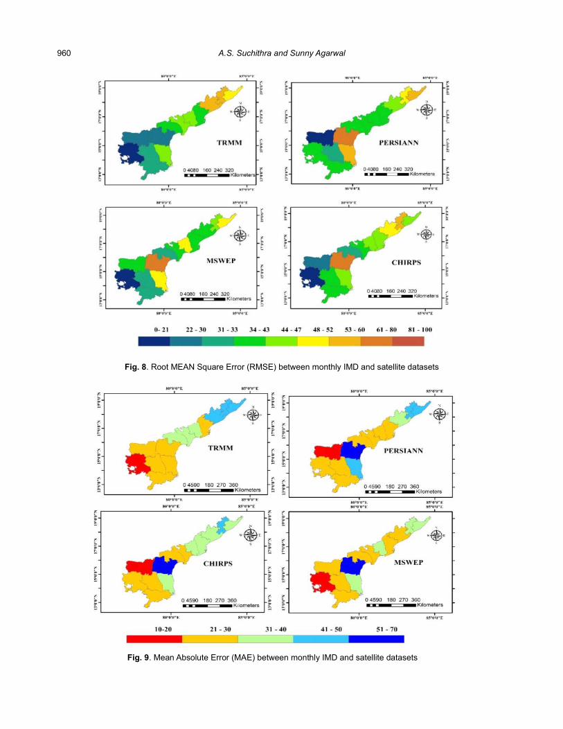
Fig. 8. Root MEAN Square Error (RMSE) between monthly IMD and satellite datasets
Fig. 9. Mean Absolute Error (MAE) between monthly IMD and satellite datasets
960 A.S. Suchithra and Sunny Agarwal

Fig. 10. Correlation Coefficient (CC) between monthly IMD and satellite datasets
Fig. 11. Annual and seasonal Z-statistics values for satellite and IMD precipitation datasets (A=Annual, B=Monsoon, C=Post-Monsoon, D=Pre-Monsoon, E=Winter)
961Trend Analysis using Multi Satellite Precipitation Products and Gauge Measurements

Fig. 12. Annual and seasonal Sen's Slope values for satellite and IMD Precipitation datasets (A=Annual, B=Monsoon, C=Post-Monsoon, D=Pre-Monsoon, E=Winter)
the pre-monsoon season, a similar pattern of increase and
decrease in magnitude of Slope is found for IMD, TMPA, and
CHIRPS datasets. During the post-monsoon and winter
season, maximum areas showed decrease in magnitude of
Slope for all datasets.
The reliability of satellite products with respect to
ground-based data, the correlation coefficient and the root
mean square error are used (Kundu et al 2017a). TMPA and
IMD relationship, districts of Visakhapatnam and Krishna
indicated lower CC and Visakhapatnam, Vizianagaram &
Srikakulam higher RMSE which are in East Northern parts of
Andhra Pradesh. The average RMSE of 40.6 mm (minimum),
MAE of 24.1 mm (minimum) and CC of 0.918 (maximum) for
TMPA and IMD datasets for entire A.P., implying highest
relevance between these two datasets. Average RMSE of
51.7 mm (maximum), MAE of 33.6 (maximum) and CC of
0.89 (minimum), for PERSIANN for entire Andhra Pradesh
indicating the lowest relevance between these two datasets.
The MSWEP dataset showed lower RMSE and higher CC
(48.1mm and 0.905) than the PERSIANN dataset (51.7 mm
and 0.903) which is like other study done by (Mondal et al
2018). Highest similarity for annual and monsoon analysis
between CHIRPS and IMD (69.23%) while PERSIANN
shows minimum similarity between IMD (38.46%). The
TRMM and MSWEP both gave the same percentage of
matched data with IMD (about 61.5%). TRMM demonstrated
better trend analysis results in the post-monsoon, pre-
monsoon, winter (76.9%) and monsoon seasons (53.8%)
relative to IMD. The similar trend between IMD and other
datasets varied from 38.46% (MSWEP in monsoon) to 76.9%
(TMPA in post-monsoon, Pre-monsoon and Winter). All
datasets in coastal Andhra Pradesh generally showed an
increasing trend, while the central and northern parts of
Andhra Pradesh showed a decreasing trend using the MK
method from 2000 to 2018.The precipitation trend indicated
almost decrease in trend for districts of Andhra Pradesh.
CONCLUSION
CHIRPS and TMPA are better compared to gauge-based
precipitation estimates than MSWEP for all districts of
Andhra Pradesh, which is clear from higher correlation (CC),
lower Mean Absolute Error (MAE) and Root Mean Square
Error (RMSE). The products of TMPA and CHIRPS showed
better performance relative to IMD than MSWEP and
PERSIANN based on accuracy, thus suitable for use in
hydrometeorological studies in the data scarce area of the
state. The trend analysis implied small variations among the
TRMM, CHIRPS, and MSWEP data. However, MSWEP
dataset showed best similarity to IMD in annual and monsoon
trend analysis. These three satellite products are more
reliable for use in ungauged areas and in complex terrain
where measurement of in situ precipitation is scarce. In
962 A.S. Suchithra and Sunny Agarwal

addition, multi-satellite precipitation products were finally
reprocessed with some enhancements and published the
revised version, which ultimately needs to be thoroughly
tested before being implemented into any application.
REFERENCESAgarwal S and Kumar S 2020. Urban flood modeling using SWMM
for historical and future extreme rainfall events under climate change scenario. (11): 48-53.Indian Journal of Ecology 47
Agarwal S and Kumar S 2021. Intensity duration frequency curve generation using historical and future downscaled rainfall data. Indian Journal of Ecology 48 (1): 275-280.
Bandyopadhyay A, Nengzouzam G, Singh WR, Hangsing N and Bhadra A 2018. Comparison of various re-analyses gridded data with observed data from meteorological stations over India. EPiC Series in Engineering 3 : 190-198.
Beck HE, Van Dijk AIJM, Levizzani V, Schellekens J, Miralles DG, Martens B and de Roo A 2017a. MSWEP: 3-hourly 0.25° global gridded precipitation (1979-2015) by merging gauge, satellite, and reanalysis data. : Hydrology and Earth System Science 1589-615.
Beck HE, Vergopolan N, Pan M, Levizzani V, Van Dijk AIJM, Weedon GP, Brocca L, Pappenberger F, Huffman GJ and Wood EF 2017b. Global-scale evaluation of 22 precipitation datasets using gauge observations and hydrological modeling. Hydrology and Earth System Science 21: 6201-6217.
Funk C, Peterson P, Landsfeld M, Pedreros D, Verdin J, Shukla S and Michaelsen J 2015. The climate hazards infrared precipitation with stations-a new environmental record for monitoring extremes. (1): 1-21.Scientific data 2
Goyal MK 2014. Statistical analysis of long-term trends of rainfall during 1901-2002 at Assam, India. Water Resources Management : 1501-1515.28
Huffman GJ, Bolvin DT, Nelkin EJ, Wolff DB, Adler RF, Gu G and Stocker EF 2007. The TRMM Multisatellite Precipitation Analysis (TMPA): Quasi-global, multiyear, combined-sensor precipitation estimates at fine scales. Journal of Hydrometeorology 8 (1): 38-55.
Kumar P, Kishtawal CM and Pal PK 2014. Impact of satellite rainfall assimilation on weather research and forecasting model predictions over the Indian region. Journal of Geophysical Research: Atmospheres 119 (5): 2017-2031.
Kumar V and Jain SK 2010. Trends in rainfall amount and number of rainy days in river basins of India (1951-2004). Hydrology Research 42 (4): 290-306.
Kundu S, Khare D and Mondal A 2017. Interrelationship of rainfall, temperature and reference evapotranspiration trends and their net response to the climate change in Central India. Theoretical and Applied Climatology 130 (3): 879-900.
Massari C, Crow W and Brocca L 2017. An assessment of the performance of global rainfall estimates without ground-based observations. (9): Hydrology and Earth System Sciences 214347-4361.
Mondal A, Lakshmi V and Hashemi H 2018. Intercomparison of trend analysis of multisatellite monthly precipitation products and gauge measurements for river basins of India. Journal of Hydrology 565 : 779-790.
Nair AS and Indu J 2017. Performance assessment of multi-source weighted-ensemble precipitation (MSWEP) product over India. Climate 5 (1): 2-21.
Pai DS, Sridhar L, Rajeevan M, Sreejith OP, Satbhai NS and Mukhopadhyay B 2014. Development of a new high spatial resolution (0.25× 0.25) long period (1901-2010) daily gridded rainfall data set over India and its comparison with existing data sets over the region. (1): 1-18.Mausam 65
Patakamuri SK, Muthiah K and Sridhar V 2020. Long-term homogeneity, trend, and change-point analysis of rainfall in the arid district of ananthapuramu, Andhra Pradesh State, India. Water 12 (1): 211-222.
Pombo S and de Oliveira RP 2015. Evaluation of extreme precipitation estimates from TRMM in Angola. Journal of Hydrology 523 : 663-679.
Prakash S, Sathiyamoorthy V, Mahesh C and Gairola RM 2014. An evaluation of highresolution multisatellite rainfall products over the Indian monsoon region. International Journal Remote Sensing 35 : 3018-3035.
Prakash S, Mitra AK, AghaKouchak A and Pai DS 2015a. Error characterization of TRMM multisatellite precipitation analysis (TMPA-3B42) products over India for different seasons. Journal of Hydrology 529 : 1302-1312.
Prakash S, Mitra AK and Pai DS 2015b. Comparing two high-resolution gauge-adjusted multisatellite rainfall products over India for the southwest monsoon period. Meteorology Application 22 : 689-702.
Prakash S, Mitra AK, Rajagopal EN and Pai DS 2016. Assessment of TRMM-based TMPA-3B42 and GSMaP precipitation products over India for the peak southwest monsoon season. International Journal Climatology 36 : 1614-1631.
Rathore LS, Attri SD and Jaswal AK 2013. State level climate change t rends in India . Meteorological Monograph No. ESSO/IMD/EMRC/02/2013. New Delhi, India: India Meteorological Department.
Singh A K, Tripathi JN, Singh KK, Singh V and Sateesh M 2019. Comparison of different satellite-derived rainfall products with IMD gridded data over Indian meteorological subdivisions during Indian Summer Monsoon (ISM) 2016 at weekly temporal resolution. : 1371-1379.Journal of Hydrology 575
Sonali P and Kumar DN 2013. Review of trend detection methods and their application to detect temperature changes in India. Journal of Hydrology 476 : 212-227.
Sunilkumar K, Narayana Rao T, Saikranthi K and Purnachandra Rao M 2015. Comprehensive evaluation of multisatellite precipitation estimates over India using gridded rainfall data. Journal of Geophysical Research Atmospheres 120 (17): 8987-9005.
Tawde SA and Singh C 2015. Investigation of orographic features influencing spatial distribution of rainfall over the Western Ghats of India using satellite data. International Journal of Climatology35(9): 2280-2293.
Valli M Sree KS and Krishna IVM 2013. Analysis of precipitation concentration index and rainfall prediction in various agro-climatic zones of Andhra Pradesh, India. International Research Journal Environmental Sci 2ence (5): 53-61.
Waghaye AM, Rajwade YA, Randhe RD and Kumari N 2018. Trend analysis and change point detection of rainfall of Andhra Pradesh and Telangana, India. Journal of Agrometeorology20(2): 160-163.
Xue X, Hong Y, Limaye AS, Gourley JJ, Huffman GJ, Khan SI and Chen S 2013. Statistical and hydrological evaluation of TRMM-based Multi-satellite Precipitation Analysis over the Wangchu Basin of Bhutan: Are the latest satellite precipitation products 3B42V7 ready for use in ungauged basins? Journal of Hydrology 499 : 91-99.
Received 22 May, 2021; Accepted 31 July, 2021
963Trend Analysis using Multi Satellite Precipitation Products and Gauge Measurements

Impacts of Land Use/Land Cover on Surface Temperature and Soil Moisture in the Region of Nagavali Basin
Indian Journal of Ecology (2021) 48(4): 964-969Manuscript Number: 3317
NAAS Rating: 5.79
Abstract: The land use/land cover (LULC) has the major impact on various hydro-meteorological parameters. The present study focuses on the influence of LULC changes on surface temperature and soil moisture for the Nagavali basin, India. In the present study, LULC was prepared from Landsat series of data with maximum likelihood image classification algorithm. The land surface temperature (LST) estimated from the thermal infrared band of Landsat data using radiative transfer equation. The soil moisture index estimated from the scatter data feature space of normalized difference vegetation index (NDVI) and surface temperature. The result of the study confirms the LULC has the significant impact on surface temperature and soil moisture. Land surface temperature drastically increased from the year 1990 to the year 2017. Soil moisture content calculated for each class of LULC and the results showed that the hilly and vegetative terrain has higher moisture content than low lying region.
Keywords: Nagavali basin, Land use/land cover, Land surface temperature, Soil moisture index, Temperature vegetation dryness index
P.M. Thameemul Hajaj and Kiran Yarrakula1*
School of Civil Engineering, Vellore Institute of Technology, Vellore-632 014, India1Department of Civil Engineering, Ghani Khan Choudhury Institute of Engineering & Technology, Malda-732 141, India
*E-mail: [email protected]
To study the anthropological influence on the natural
environment and ecosystem, land use/land cover (LULC)
provides important information about the changes in the land
surface. The LULC changes impact on surface parameters
include roughness, albedo, temperature, visible light
radiation, precipitation, and vegetation coverage. In addition
to the surface parameter, LULC transforms the typical
hydrological process and its element primarily
evapotranspiration, runoff, infiltration and subsurface flow
(Wagner et al 2016, Mohaideen and Varija 2018). The
classification of LULC can be performed using both visual
interpretation and digital processing techniques with satellite
remote sensing image. Individual classes of LULC contribute
temperature changes. The changes in LULC depict a strong
correlation with the increasing land surface temperature
(LST). Thermal infrared remote sensing plays a major role to
extract the LST and the information of surface thermal
condition. The soil moisture aspects can be inferred well from
the relation of surface thermal range and vegetation index
space, which commonly used in soil moisture reversal
models in recent years. Temperature vegetation dryness
index (TVDI) is the dryness index generally used for
assessing soil moisture and which is based on the
interrelationship of vegetation indices and temperature of
land estimated regional crop yield with TVDI and authors
concluded that crop yield estimation from TVDI shows better
than the yield estimation obtained from vegetation index
monitored soil moisture based on vegetation index and
surface temperature space for Southwest China from the
multispectral image and concluded that TVDI has the
stronger association with soil moisture at 3.9 inches.
Analyzed agriculture drought based LST-VI Feature Space
for Anantapur, India and they concluded that drought
classification for the year 2016 shows 40percent of the area
under severe and moderate drought and remaining area
under normal and no drought. Estimated impacts of LULC on
gross primary production (GPP) of urban vegetation for
Wuhan, China and results showed that the greatest GPP loss
caused where the crop land transforms to settlement and the
greatest GPP gain happened due to the transformation of
cropland to forest. There are plenty of researches discussing
about the impact LST and NDVI on LULC. The present study
analyzed TVDI and LST impact on LULC due to the limited
availability of the research. In this research, soil moisture
influence on each land cover studied under different
temperature condition. In the present study, the main
objective is to quantify the land use influence on surface
temperature and soil moisture index in the region of Nagavali
Basin.
MATERIAL AND METHODS
Description of study area: Nagavali basin of southern India
selected as study are located between 18 16'N to 19 31'N o o
latitude and 82 53'E to 83 55'E longitude (Fig. 1). The areal o o
extent of the Nagavali basin is 8397 km . The major 2
reservoirs are Vottigedda, Totapalli, Narayanpur, and

Madduvalasa. The study area receives an annual rainfall of
about 703.4mm.
Data description: Remote sensing satellite data used to
prepare LULC include the Landsat Series (OLI/TIRS, ETM+,
and TM) of 30 m resolution for the years 1990, 2002, and
2017 (Table 1). Landsat TM is a multispectral sensor working
in visible and infrared (IR) electromagnetic spectrum.
Landsat ETM+ introduced all the features of TM with the
addition of 15 m resolution panchromatic band and 60 m
resolution thermal band. The Landsat TM has the thermal
band of resolution 120 m. The Landsat OLI/TIRS has all the
feature of TM and ETM+ with thermal band acquired at 100
m. The thermal band obtained from all the three sensors
resampled to 30 m in the delivered product.
Land cover/land use classification: The LULC map
generated from Landsat group of remotely sensed data using
maximum likelihood image classification method (Prabu and
Dar 2018).The survey of India topo sheets taken as reference
data for classifying Landsat images into seven classes which
are settlements, water bodies, wasteland, current fallow,
cropland, forest, and plantation. The maximum likelihood
algorithm operating based on the principle of Bayes theorem
of decision making. The methodology for estimating the
likelihood ( ) based on the equation 1.D
Satellite data Spatial resolution of optical band (m)
Spatial resolution of thermal band (m)
Scene (path, row) Time of acquisition
Landsat TM 30 120 (141, 47) April, 1990
Landsat ETM+ 30 60 (141, 47) May, 2002
Landsat OLI/TIRS 30 100 (141, 47) May, 2017
Table 1. Data specification of the Landsat imageries
Fig. 1. Geographical setting of the study area
ln ( ) [ 0 .5 0 ln ( c o v ) ] [ 0 .5( )K K KD a X X ( co v 1)( ) ] (1)K KT X X
Where, is known classes and is unknown X XK
measurement vector coming under known classes.
The accuracy of the image classification assessed
based on the overall accuracy and kappa coefficient.
According to Congalton (1991) theoretical description of the
image assessment methods are detailed as follow:
Overall Accuracy
Kappa Coefficient
where is the number of observations in row and x iii
column (the diagonal elements), is the number of rows in i r
the matrix, is the number of observations, and and are N x x+i i+
the marginal totals of row and column respectively.r i
Normalized difference vegetation index (NDVI)
estimation: NDVI is the threshold of vegetation which
related to spectral reflectance of the Earth surface feature.
The threshold value of NDVI ranges from -1 to +1 (Singh et al
2016, Vaani and Porchelvan 2017). The NDVI values scaled
from minimum (bare soil) to maximum fractional vegetation
cover. The NDVI defined as:
Where and represent near-infrared band (NIR) λ λNIR RED
and red band from the visible spectrum respectively.
Land surface temperature quantification: Satellite data
offer the possibility for estimating LST all over the places in
the world with good temporal and spatial resolution. The
thermal infrared (TIR) band of satellite sensor related to LST
through the radiative transfer equation (Li et al 2013). Three
steps involved in the calculation of LST, the initial step
involves the transformation of digital number (DN) values to
radiance, and the second step involves the calculation of
brightness temperature. Finally, conversion of resultant
temperature from the unit of Kelvin to Degree Celsius
Overall Accuracy (2) 1
1 r
iii
xN
Kappa Coefficient (3)1 1
2
1
r r
iii i
r
i
N x
N
(x )i i x x
(x )i i x x
NIR RED
NIR RED
NDVI
965Impacts of Land Use/Land Cover on Surface Temperature and Soil Moisture

TIRL MF AF (5)
2
1
(K)
ln 1
KT
KL
(Chokkavarapu and Mandla 2018). It described as:
T( C) = T (K) – 273 (7)O Where, L is spectral radiance of the top of the λ
atmosphere, is thermal infrared band of satellite image, λTIR
MF AFis the multiplicative factor of thermal band, is the
additive factor of thermal band, and are specific K K1 2
conversion constants of thermal band, (K) is temperature in T
Kelvin, and ( C) is temperature in Degree Celsius. The T o
common factors affect the LST are (i) sensor noise and error
are the strong influence on LST, (ii) due to the presence of
atmosphere between the sensor and surface, affects the
quality of radiance measurement in radiometer, (iii) to avoid
the uncertainty in LST, analysis was done in clear sky data.
Soil moisture index: The soil moisture index is a threshold
index which indicates the presence of moisture content in the
soil. The soil moisture condition can estimate from the
relation of temperature vegetation dryness index. TVDI
provides the effective indication of land moisture and is
computed based on NDVI-LST feature space. The TVDI
calculation method commonly called as triangle method
because the scatter of LST and NDVI is the triangular shape
in feature space (Przeździecki et al 2018). Fig. 2 shows the
schematic definition of soil moisture index. The line CE in Fig.
2 is dry edge and the line DE is the wet edge. The lower
moisture and transpiration capacity nearer to the dry edge
and the capacity of moisture and transpiration become higher
at the wet edge. According to the TVDI defined as:
\Where, is the maximum surface temperature with the TMAX
function of the dry edge at NDVI-LST feature space with
linear fitting parameter and . is the function of the a b TMAX MAX MIN
wet edge at the triangular plot in feature space which
represents the minimum surface temperature of each pixel
with the coefficient of linear regression parameters ( anda MIN
bMIN). Figure 2 also defines the threshold value of TVDI ranges
between 0 and 1. The value closer to the zero indicates
moisture and the threshold value nearer to the 1 indicates
dryness.
The method assumes that the LST for the given NDVI
--
MIN
MAX MIN
T TTVDI
T T
MAX MAX MAXT a b NDVI
MIN MIN MINT a b NDVI
happened due to the variation in soil moisture rather than the
canopy temperature, atmospheric pressure, and air
temperature.
RESULTS AND DISCUSSION
The settlement cover increased from 1990 (58 km ) to 2
2017 (427 km ). The surface area of the water bodies in the 2
basin decreased from 1990 (154 km ) to 2002 (48 km ). After 2 2
the construction of several reservoirs in the Nagavali basin,
water surface area increased in the year 2017 (305 km ). 2
Wasteland of the study area decreased on the year 2002
(481 km ) from the year 1990 (877 km ), because of growth of 2 2
small shrubs in the study area on the year 2002 some part of
wasteland comes under the vegetation classes. The
increase in crop cover of the year 2002 confirms the
wasteland and fallow land conversion. In 2017, wasteland
increased to 980 km . The cropland of the year 1990 (2006 2
km ) increased during monsoon season in the year 2
2002(3567 km ) which shows satisfactory rainfall received in 2
the basin. In 2017, the cropland area dropped to 1812 km . 2
Due to infrastructural developmental activities, forest covers
gradually decreasing from year 1990 (3279 km ) to the year 2
2017 (2155 km ).2
The mean temperature of all land cover feature
gradually increases from the years 1990 to 2017, it reveals
climate change scenario (Fig. 3, 4). The forest area received
lower temperature compared to another surface feature. The
settlement, water bodies, wasteland, and fallow land receive
the maximum and almost nearly equal range of temperature
with 0.5 C variation. The temperature range of cropland and o
plantation is less than settlement, water bodies, wasteland,
and fallow land and greater than forest cover temperature.
The results of the present study prove vegetation cover
receives a lesser amount of temperature compared to other
surface features.
Fig. 2. Soil moisture index (CE is dry edge and the line DE is the wet edge)
966 P.M. Thameemul Hajaj and Kiran Yarrakula

Fig. 3. LULC of the Nagavali Basin on (a) April, 1990, (b) May, 2002, and (c) May, 2017
Fig. 4. Trend of LULC changes for the years 1990, 2002, and 2017
Fig. 5. LST map of the Nagavali Basin on (a) 1990, (b) 2002, and (c) 2017
Fig. 6. Temperature changes for LULC of the years 1990, 2002, and 2017
967Impacts of Land Use/Land Cover on Surface Temperature and Soil Moisture

Fig. 7. Soil moisture index (TVDI) map of the Nagavali Basin on the years (a) 1990, (b) 2002, and (c) 2017
The threshold value of the soil moisture index ranges
from 0 to 1 (Fig. 7). The value close to zero and 1 indicates the
presence of good and poor quantity moisture. The overall
mean of soil moisture in the years 1990, 2002, and 2017 are
Year Name of the satellite image
Overall accuracy of classification (%)
Kappa statistics
1990 Landsat TM 78.37 0.7364
2002 Landsat ETM+ 76.83 0.6957
2017 Landsat OLI/TIRS 79.52 0.7160
Table 2. Assessment of accuracy for the classified images
0.52063, 0.53881, and 0.4002, respectively. The forest area
is having the presence of higher soil moisture compared to
other feature. The, hilly and forest cover regions having good
moisture presence compared to low lying areas.
CONCLUSION
Remote sensing is a viable tool to predict climate change
impact in Earth surface. The prepared LULC show the trend
of surface feature changes from the year 1990 to the year
2017. The forest covers decreasing whiles the settlement
increasing. The water surface area decreased from the year
1990 to the year 2002.After the construction of Jhanjavati
reservoir in 2001 and Thotapalli barrage construction was in
between 2003 and2015, water surface increased in 2017.
The result confirms the majority of the changes in land
surface happening due to anthropogenic activities. The
results of the surface temperature map showed from the year
1990 to 2017 confirms the climate change scenario slowly
occurred in Nagavali basin. The presence of higher soil
moisture range and the lower surface temperature at
vegetation feature compared to other features showed the
possibility to maintain the surface temperature and soil
moisture index by the mass plantation.
REFERENCESBarsi JA, LeeK, Kvaran G, Markham BL and Pedelty JA 2014. The
spectral response of the Landsat-8 operational land image. Remote Sensing 6: 10232-10251.
Chokkavarapu N, Kummamuru PK and Mandla VR 2018. Estimation of land use land cover change relationship with normalized difference vegetation index (NDVI) different method and land surface temperature (LST). (1):Indian Journal of Ecology 45 178-182.
Congalton RG 1991. A review of assessing the accuracy of classifications of remotely sensed data. Remote Sensing of Environment 37: 35-46.
Holzman ME, Rivas R and Piccolo MC 2014.Estimating soil moisture and the relationship with crop yield using surface temperature and vegetation index. International Journal of Applied Earth Observation and Geoinformation 28:181-192.
Li Y, Kun Yang and Rong Yang 2015. Land surface temperature estimation from remote sensing data - a case study in Kun Ming city, In: 2015, 23rd International Conference on GeoinformaticsIEEE,1-6
Li Z, Tang B, Wu H, Ren H, Yan G, Wan Z, Trigo IFand Sobrino JA2013.Satellite-derived land surface temperature: Current status and perspectives. : Remote Sensing of Environment 13114-37.
Liu S, Du W, Su H, Wang S and Guan Q 2018. Quantifying Impacts of land-use/cover change on urban vegetation gross primary production: A case study of Wuhan, China, : 714.Sustainability 10
Mohaideen MMD and Varija K 2018. Improved vegetation parameterization for hydrological model and assessment of land cover change impacts on flow regime of the Upper Bhima basin, India. : 697-715. Acta Geophys 66
Prabu P and Dar MA 2018. Land-use/cover change in Coimbatore urban area (Tamil Nadu, India ): A remote sensing and GIS-based study. Environmental Monitoring and Assessment 190: 1-14.
968 P.M. Thameemul Hajaj and Kiran Yarrakula

Przeździecki K, Zawadzki J and Miatkowski Z 2018. Use of the temperature–vegetation dryness index for remote sensing grassland moisture conditions in the vicinity of a lignite open-cast mine. 623.Environment and Earth Science 77:
Sandholt I, Rasmussen K and Andersen J 2002. A simple interpretation of the suface temperature/vegetation index space for the assessment of surface moisture stress. Remote Sensing of Environment 79: 213-224.
Singh N, Kala S, Kumar D, Chatterjee RC, Panigrahi DC and Chaudhary SK 2018. Impact of land use dynamics on land surface temperature in Jharia coalfield, 2018 4th Int Conf Recent Adv Inf Technol 1-6.
Singh RP, Singh N, Singh S and MukherjeeS 2016. Normalized difference vegetation index (NDVI) based classification to assess the change in land use/land cover (LULC) in lower Assam, India. International Journal Advance Remote Sening GIS 5: 1963-1970.
Srivastava PK, Han D, Rico-Ramirez MA and Bray MTJ 2012. Selection of classification techniques for land use/land cover change investigation. : 1250-1265. Advance Sp Res 50
Subbu Lakshmi E and Yarrakula K 2016. Monitoring land use land cover changes using remote sensing and gis techniques : A case study around Papagni River, Andhra Pradesh, India. Indian Journal of Ecology 43: 383-387.
Tao H, Xing J, Zhou H, Xing C, Guojing L, Lei C and Junhua Li 2018. Impacts of land use and land cover change on regional meteorology and air quality over the Beijing-Tianjin-Hebei region, China. : 9-21. Atmos Environment 189
USGS 2016. Landsat Missions, United States Geol Surv, 5–8.
Vaani N and Porchelvan P 2017. GISbased agricultural drought assessment for the State of Tamilnadu, India using vegetation condition index (VCI). International Journal Civil Engineering Technology 8: 1185-1194.
Vani V and Mandla VR 2018. Agriculture drought analysis using remote sensing based on NDVI-LST Feature Space. Indian Journal of Ecology 45: 6-10.
Wagner PD, Bhallamudi SM, Narasimhan B, Kantakumar LN, Sudheer KP, Kumar S, Schneider K and Fiener P 2016. Dynamic integration of land use changes in a hydrologic assessment of a rapidly developing Indian catchment. Science and Total Environment 539: 153-164.
Warnasuriya TWS 2015. Mapping land-use pattern using image processing techniques for medium resolution satellite data: Case study in Matara District, Sri Lanka. International Conference Advance ICT Emergering Reg 106-111.
Zhang F, Zhang LW, Shi JJ and Huang JF 2014. Soil moisture monitoring based on land surface temperature-vegetation index space derived from MODIS Data. : 450-460.Pedosphere 24
Received 24 April, 2021; Accepted 08 August, 2021
969Impacts of Land Use/Land Cover on Surface Temperature and Soil Moisture

Remote Sensing Planet Images Application in Mapping the Status of Tropical Forests: A Case Research in Kontum Province, Vietnam
Indian Journal of Ecology (2021) 48(4): 970-976Manuscript Number: 3318
NAAS Rating: 5.79
Abstract: This paper describes the process of creating a forest status map in Kon Tum province using Planet satellite images captured in December 2020 and the image interpretation keys belonged to 14 land cover types. With the aid of eCognition Developer software the satellite images were segmented into 30 896 objects and the forest status map was established with an accuracy of 82%, the Kappa coefficient is .0 801. The total forest area in Kon Tum is 621,356.05 hectares, including 547759 37 hectares of natural forests (88%) and 73596 68 hectares . . .of planted forests (12%). The results of the article are good references for studies on satellite image application in forest classification, forest management and forest monitoring.
Keywords: Satellite image, Planet, stratified random, Random forest method, Cnfusion matrix
Nguyen Dang Hoi, Ngo Trung Dung, Nguyen Quoc Khanh, Dang Hung Cuong , 1
Kolesnikov Sergey Ilyich and1 Ha Dang Toan 2
Institute of Tropical Ecology, Vietnam - Russia Tropical Centre 63 Nguyen Van Huyen Str., Cau Giay District, , Hanoi, Vietnam, 11353
1Academy of Biology and Biotechnology D.I. Ivanovsky, Southern Federal University, 194/1 Stachki Avenue, Sovetsky District, Rostov-on-Don, Russia, 344090
2Vietnam-Hungary Industrial University, 16 Huu Nghi Str., Son Tay District, Hanoi, Vietnam, 12712E-mail: [email protected]
Forest ecosystems cover approximately 31% of land
surface in the world, with a total forest area of approximately
4 billion hectares . Sustainable (United Nations 2017)
development and management of forest resources is
required not only to meet the needs of present but also future
generations. Meeting those needs is on the basis of close
and harmonious coordination between economic growth,
ensuring social progress and environmental protection (Hien
2020). Remote sensing technology and Geographic
Information System (GIS) are considered very effective tools
in forest resource management and protection. GIS is a
supporting system for collecting, storing, retrieving,
analyzing and displaying spatial and non-spatial data
(Oyebade et al 2012). The application of GIS technology for
forest management began in the early 1990s . (Ahmad 2008)
Up to now, the application of remote sensing and GIS in forest
resource management and protection has been used in most
countries, from Europe to Asia, America, and Africa
(Kolosvary and Corbley 1998, Peddi 2010, Freddy et al 2014,
Devaraj and Yarrakula 2018, Tuyen et al 2019, Oettel and
Lapin 2020, Sonowal 2020).
In Vietnam, the application of remote sensing in forest
classification is one of the priority tasks and is conducted
regularly in many provinces, through research programs at
different levels of management, including the province
Kontum (eCognition 2004). Kontum is a province in the
Central Highlands of Vietnam. The vegetation cover here is
the typical forest ecosystem of the tropical monsoon
mountainous and plateaus (Congalton and Green 1999). The
Vietnamese government's forest inventory projects in
Kontum province used images satellite SPOT to create
status maps of the forest (Cuong et al 2021). In addition, the
program "Survey, assessment and monitoring of national
forest resources in the period 2016-2020" of the Vietnamese
Ministry of Agriculture and Rural Development used Sentinel
2 satellite medium resolution images to establish current
status maps of the forest.
Determination of forest status by remote sensing
method depends on the interpretation key. The interpretation
key is the concept showing the arrangement of image
elements, detailed characteristics of the object forming a
whole in the macro space (Karakış et al 2006, Genuer and
Poggi 2020). Therefore, image resolution plays an important
role in the establishment of forest maps since they specify the
granularity of the selected interpretation keys. Planet satellite
imagery has a medium spatial-resolution (4.7m) but has a
high time-resolution due to the daily shooting cycle, provided
free charge to users for learning and research purposes (Mai
and Nguyen 2017). With their superior parameters, the
Planet satellite imagery offers significantly higher value than
the popular non-commercial satellite images commonly used
for forest status mapping such as Landsat 8 (spatial
resolution of 30 m, shooting cycle 15 days) or Setinel 2
(spatial resolution of 10 m, shooting cycle of 5 days). In this
research, we use satellite imagery of Planet to create a forest
status map of the area in Kontum province. The results of
image interpretation are to compare advantages and
disadvantages of Planet images with SPOT or Setinel
images.
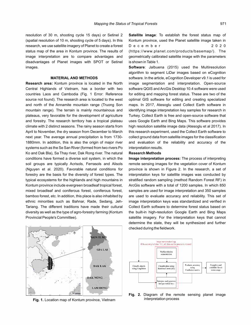
MATERIAL AND METHODS
Research area: Kontum province is located in the North
Central Highlands of Vietnam, has a border with two
countries Laos and Cambodia (Fig. 1 Error: Reference
source not found). The research area is located to the west
and north of the Annamite mountain range (Truong Son
mountain range). The terrain is mainly mountainous and
plateaus, very favorable for the development of agriculture
and forestry. The research territory has a tropical plateau
climate with 2 distinct seasons. The rainy season starts from
April to November, the dry season from December to March
next year. The average annual precipitation is from 1730-
1880mm. In addition, this is also the origin of major river
systems such as the Se San River (formed from two rivers Po
Ko and Dak Bla), Sa Thay river, Dak Rong river. The natural
conditions have formed a diverse soil system, in which the
soil groups are typically Acrisols, Ferrasols and Alisols
(Nguyen et al. 2020). Favorable natural conditions for
forestry are the basis for the diversity of forest types. The
typical ecosystems for the highlands and high mountains in
Kontum province include evergreen broadleaf tropical forest,
mixed broadleaf and coniferous forest, coniferous forest,
bamboo forest, etc. In addition, this place is also inhabited by
ethnic minorities such as Bahnar, Rade, Sedang, Jeh-
Tariang. The different traditions have made their cultural
diversity as well as the type of agro-forestry farming (Kontum
Provincial People's Committee).
Fig. 1. Location map of Kontum province, Vietnam
Satellite image: To establish the forest status map of
Kontum province, used the Planet satellite image taken in
D e c e m b e r 2 0 2 0
(https://www.planet.com/products/basemap/). The
geometrically calibrated satellite image with the parameters
is shown in Table 1 .
Software: Jalbuena (2015) used the Multiresolution
algorithm to segment LiDar images based on eCognition
software. In the article, eCognition Developer v9.1 is used for
image segmentation and interpretation. Open-source
software QGIS and ArcGis Desktop 10.4 software were used
for editing and mapping forest status. These are two of the
optimal GIS software for editing and creating specialized
maps. In 2017, Atesoglu used Collect Earth software in
identifying image interpretation key samples for research in
Turkey. Collect Earth is free and open-source software that
uses Google Earth and Bing Maps This software provides .
high resolution satellite image data . In (Atesoglu et al 2017)
this research experiment, used the Collect Earth software to
collect ground data from satellite images for the classification
and evaluation of the reliability and accuracy of the
interpretation results.
Research Methods
Image interpretation process: The process of interpreting
remote sensing images for the vegetation cover of Kontum
province is shown in Figure 2. In the research, a set of
interpretation keys for satellite images was conducted by
stratified random sampling in (method Random Forest RF)
ArcGis software with a total of 1200 samples. In which 850
samples are used for image interpretation and 350 samples
are used to evaluate accuracy and reliability. This set of
image interpretation keys was standardized and verified in
Collect Earth software to determine forest status based on
the built-in high-resolution Google Earth and Bing Maps
satellite imagery. For the interpretation keys that cannot
determine the state, they will be synthesized and further
checked during the fieldwork.
Fig. 2. Diagram of the remote sensing planet image interpretation process
971Mapping the Status of Tropical Forests

Image attribute Description
Visual bands 3 color (Red, Blue, Green)-band natural
Ground sample distance 4.7m x 4.7m (at reference altitude 475 km)
Pixel size (orthorectified) 3125 m
Bitdepth 8-bit
Image geometry correction Sensor-related effects are corrected using sensor telemetry and a sensor model.Spacecraft-related effects are corrected using attitude telemetry and best available ephemeris data.Orthorectified using GCPs and fine DEMs (30 m to 90 m posting) to <10 m RMSE positional accuracy
Positional accuracy Less than 10m RMSE
Color enhancement Enhanced for visual use and corrected for sun angle
Image coordinates WGS 84, zone 48N
Table 1. Parameters of the Planet satellite image taken in December 2020 for Kontum province
c
ccwh
n
lh
)(
)(
12
11
iiri
iiriij
ri
XXN
XXXNK
A mandatory requirement when determining the status
for these 1200 image interpretation key samples is that they
must be independently performed by a minimum of two
experts. Experts synthesize and reject distorted patterns,
using only highly reliable image interpretation keys. This is a
very important and decisive step to the accuracy of the
interpretation process. he image interpretation key is T
entered into eCognition software to implement the
Multiresolution segmentation algorithm. This is the algorithm
proposed by Baatz and used to group areas with similar
pixels and neighboring points into objects by considering
uniformity criteria (Baatz and Schape 2000). Kavzoglu
(2014) showed that segmentation creates objects by
grouping similar spectral properties on an image.
Multiresolution segmentation is a bottom up region-merging
technique starting with one-pixel objects. The purpose of this
technique is to divide an image into sections that are strongly
correlated with the objects or areas in the image. Segment
images are used to determine the position of objects and the
boundaries between them (Kavzoglu and Yildiz 2014). In
numerous subsequent steps, smaller image objects are
merged into larger ones. Throughout this pairwise clustering
process, the underlying optimization procedure minimizes
the weighted heterogeneity of resulting image objects, “ ”nh
where is the size of a segment and an arbitrary “ ” “ ”n h
definition of heterogeneity. In each step, that pair of adjacent
image objects is merged which stands for the smallest growth
of the defined heterogeneity. If the smallest growth exceeds
the threshold defined by the scale parameter, the process
stops . Spectral or color heterogeneity is (eCognition 2004)
described as:
Heterogeneity as deviation from a compact shape is
described by the ratio of the de facto border length and the “ ”l
square root of the number of pixels forming this image object
(Karakış et al 2006):
According to Genuer (2020), the determination of the
state after image segmentation is done by the Random
Forest (RF) method in eCognition Developer. This is a
comprehensive method of machine learning for performing
classification, regression, and other tasks that operate by
constructing a multitude of decision trees at training time and
outputting the class that is the mode of the classes
(classification) or mean/average prediction (regression) of
the individual trees (Genuer and Poggi 2020).
To check the results of image interpretation, a random
selection method was used. Each forest state will have a
minimum of 10 control points. After that, the current situation
was verified by field survey and compared with interpretation
results. In the case where the accuracy is less than 75%, it is
necessary to re-check the procedure and the method of
taking the interpretation key to improve the correct value (Mai
and Nguyen 2017). This process requires constructing of
confusion matrix between classification results and control
samples and evaluation of Kappa coefficient . (K) According
to Congalton and Green (1999), this matrix is the most
effective method to evaluate accuracy is to evaluate overall
accuracy user accuracy and producer accuracy The Kappa , .
coefficient is used as a measure of classification accuracy.
These are the utility coefficients of all the elements from the
confusion matrix. It is the fundamental difference between
the real difference in the deviation error of the matrix and the
total change indicated by the row and column (Mai and
Nguyen 2017). The formula for determining the Kappa
coefficient is as follows:
Where: r = Number of columns in the image matrix X = ; ii
972 Nguyen Dang Hoi et al

number of pixels observed in row and column (on the main i i
diagonal) X = Total Pixel observed in row X = total pixel ; ;i+ ii +
observed in column N = the total number of pixels observed i;
in the image matrix. The value of the Kappa coefficient is
usually between 0 and 1. If within this range the accuracy of
the classification is accepted. According to the US Geology
Department, the Kappa coefficient has 3 groups of values:
K>0.8: high accuracy; 0.4<K<0.8: moderate accuracy; and
K<0.4: low accuracy.
RESULTS AND DISCUSSION
Interpretation keys: Based on the interpretation results on
the Collect Earth software, the key samples with low reliability
interpretation were excluded. Selected interpretation keys
include 800 samples (eliminated 50 samples) for image
interpretation and 299 samples (eliminated 51 samples) for
verification (Fig. 3). According to Kavzoglu (2014) and Tran
(2011), the number of key samples has met the requirements
for interpretation for the area of Kontum province (Tran and
Nguyen 2011, Kavzoglu and Yildiz 2014) After processing, .
interpretation keys were obtained for forest types including:
Fig. .3 Sample locations for interpretation and verification keys
(1) Evergreen broadleaf forest with good quality (93
samples); (2) Evergreen broadleaf forest with medium quality
(104 samples); (3) Evergreen broadleaf forest with poor
quality (58 samples); (4) Recovering evergreen broadleaf
forest (79 samples); (5) Deciduous forest (10 samples); (6)
Bamboo forest (47 samples); (7) Mixed trees and bamboo
forest (73 samples); (8) Coniferous forest (33 samples); (9)
Mixed broadleaf and coniferous forest (25 samples); (10)
Plantation forest (85 samples); (11) Vacant land (57
samples); (12) Water surface (25 samples); (13) Residential
area (18 samples); (14) Agricultural land samples(93 ).
Results evaluate the accuracy of : Overall accuracy of the
interpretation results reached 82% and the coefficient Kappa
K . Deviations appear much in interpretation key = 0 801.
numbers from 1 to 4, with producer accuracy ranging from
71% to 73% (Table 2). These are the keys for evergreen
broadleaf forests, which are all difficult to interpret and
confuse with each other. Key numbers 9 and 14 have the
highest accuracy (94% and 92% producer accuracy). Other
interpretation keys (numbers 7, 8, 10, 11, 12) all have
relatively high accuracy (89 – 90% producer accuracy).
Establish forest map of Kontum province: From the
results of satellite image interpretation, the forest status map
of Kon Tum province in 2020 was established (Fig. 4). The
Fig. 4. Forest status map of Kontum province in 2020 established from planet remote sensing image data
973Mapping the Status of Tropical Forests

Ground truth Evaluation
1 2 3 4 5 6 7 8 9 10 11 12 13 14 Total Useraccuracy Producer accuracy
Total
1 21 5 26 81% 72% 82%
2 4 20 1 1 26 77% 71%
3 1 1 18 1 21 86% 72%
4 2 1 3 19 25 76% 73%
5 1 1 14 2 18 78% 78%
6 1 12 1 1 15 80% 75%
7 1 1 1 18 1 22 82% 90%
8 1 1 1 1 17 1 22 77% 89%
9 1 1 1 15 1 19 79% 94%
10 1 1 16 18 89% 89%
11 1 1 1 17 1 21 81% 89%
12 17 2 19 89% 89%
13 1 17 2 20 85% 81%
14 1 1 1 1 23 27 85% 92%
Total 29 28 25 26 18 16 20 19 16 18 19 19 21 25 299
Table .2 The confusion matrix between the classification results and the control key sample
vegetation cover of Kon um province has several forest types t
representing the monsoon tropical climate: plateau
evergreen broadleaf tropical forest, deciduous forest
(dipterocarp forest), coniferous forest, mixed and broadleaf
bamboo forest, mixed broadleaf and coniferous forest.
According to Table 3, the total area of vegetation cover
including natural forest and plantation forest is 621 356.05
hectares. which, natural forest area is 547 759.37 hectares In
(88%), plantation forest area is 73 596.68 hectares (12%). Of
the natural forest types, evergreen broadleaf tropical forest
occupies the largest area with 387472.09 hectares, over 70%
of the total Kontum natural forest area. Mixed broadleaf and
coniferous forests also cover a large area, with about 14% of
the total natural forest area. The typical forest type for the
high mountains in Kontum province is coniferous forest with
an area of 30 143.05 ha, accounting for 5.5% of the total
natural forest area.
To evaluate the quality of remote sensing Planet images,
the results were compared with the data on the forest status
map using SPOT and Sentinel 2 remote sensing images in
the “Vietnam National Forest Inventory and Monitoring
Program” (Fig. 5). The SPOT remote sensing image
interpretation results are the official results used by the
Ministry of Agriculture and Rural Development to statistic the
forest area in Vietnam. The comparison results show that the
deviation of remote sensing images for different forest types is
small. According to Planet image, the natural forest area is
about 56%, plantation forest accounts for about 8% and non-Fig. 5. Comparing forest status map data using different
types of remote sensing images
forest land is about 36%. This result is equivalent to the
results of SPOT image interpretation (58%, 8% and 34%,
respectively). Forest status data using remote sensing Planet
image is more accurate than image Sentinel 2. For the results
of forest status according to photo Sentinel 2, natural forest
area is about 70%, plantation forest accounts for 3% and non-
forest land about 27%. This result is much different from forest
inventory data using SPOT remote sensing image. According
to photo Sentinel 2, the result of natural forest area difference
is 12%, plantation forest is 5% and non-forest land is 7% of
total area compared to published forest inventory data.
The use of free charged remote sensing Planet image
gives similar results when compared with forest inventory
974 Nguyen Dang Hoi et al

Interpretation key codes
Forest types Area (hectares) Interpretation key codes
Forest types Area (hectares)
I Natural forest 547 759.37 II Plantation forest 73 596.68
1 Evergreen broadleaf forest with good quality 87 667.46 10 Plantation forest 73 596.68
2 Evergreen broadleaf forest with medium quality 73 793.95 III Non-forest land 349 437.21
3 Evergreen broadleaf forest with poor quality 55 412.59 11 Vacant land 155 109.66
4 Recovering evergreen broadleaf forest 170 598.09 12 Water surface 14 862.45
5 Deciduous forest 2 067.18 13 Residential area 38 140.01
6 Bamboo forest 17 476.10 14 Agricultural land 141 325.09
7 Mixed broafleaf and bamboo forest 76 126.63 Total 970 793.26
8 Coniferous forest 30 143.05
9 Mixed broadleaf and coniferous forest 34 471.33
Table 3. Statistics of forest types of Kontum province based on map established from remote sensing Planet image in 2020
data using paid SPOT satellite image. This is considered a
new direction in the mapping of forest status with free satellite
image source, bringing high reliability in forest classification,
management and protection.
CONCLUSION
In a total of 1200 interpretation keys, after removing the
samples that do not meet the accuracy, the research team
used 800 samples for image interpretation and 299 samples
for verification. The interpretation keys for mapping forest
status of Kon Tum province includes 14 types of forest
statuses, of which 10 types of forest and 4 types of non-
forest. After interpretation, the results of evaluating the
accuracy and reliability by the confusion matrix reached the
overall accuracy of 82%, the Kappa coefficient reached
0,801. All remote sensing images of the study area are
divided into 30896 subjects. Based on the state of the
decoding key set, these objects are classified into 14 different
types of forest state with the help of eCognition Developer
software based on the Random Forest classification method.
The forest status map of Kon Tum province has been
successfully developed with a total forest area of 621 356.05
hectares. In which natural forest area is 547 759.37 hectares
(88%) and plantation forest area is 73 596.68 hectares
(12%). High accuracy and K coefficient shows the feasibility
and practical application of the research. The research
results contribute to improving the application of remote
sensing to develop forest status maps. Remote sensing
Planet image is important data serving forest status mapping
and assessment of forest changes over time. This is an
important document in the management, conservation and
development of forest resources.
ACKNOWLEDGEMENTS
The authors would like to thank the Board of Director-
Generals of the Vietnamese - Russian Tropical Center for
administrative support. This study was funded by project
“Researching structure and function of tropical forest
ecosystems for conservation, restoration and sustainable
use” (E.1.2).
REFERENCESAhmad F 2008. GIS application for forest management in drylands of
Pakistan. Journal of Food, Agriculture and Environment 6(2): 388-392
Atesoglu A, rslan , ılmaz , Arıkan Yildiz 2017. A M Y M Y and SMonitoring of Dryland in Turkey using collect earth. Afyon Kocatepe University Journal of Science and Engineering : 17252-261.
Baatz M and Schape 2000. Multiresolution segmentation: an A optimization approach for high quality multi-scale image segmentation, pp.12-23. In: Strobl J, Blaschke T and Griesbner G (eds), Angewandte Geographische Proceedings ofInformationsverarbeitung XII, Wichmann Verlag, Karlsruhe, Germany.
Congalton RG and Green 1999. K Assessing the accuracy of remotely sensed data: Principles and practices, Lewis Publishers Boca Raton, FL, USA, , p 348.
Cuong ND, Michael and Volker 2021. Land use spatial K Moptimization for sustainable wood utilization at the regional level: A case study from Vietnam. (2): 245.Forests 12
Devaraj S and Yarrakula 2018. GIS based Multi-criteria decision Kmaking system for assessment of landslide hazard zones: Case study in the Nilgiris, India. : 286-Indian Journal of Ecology 45291.
eCognition 2004 User Guide 4, Definiens Imaging GmbH..
Freddy A, Tennyson , Samraj and Roy 2014. Land use land S D Acover change detection using remote sensing and geographical information system in Pathri Reserve forest, Uttarakhand, India, pp. 353-365. In: Mathur P P (eds), Contemporary Topics in Life Sciences, Narendra Publishing House, India.
Genuer R and Poggi 2020. Random Forests wit R J M , Springer Nature, Switzerland, p98.
Hien P 2020. Forest management meeting the requirements for sustainable development in Vietnam. Public Administration Research 9 : 15-27.
Jalbuena RL, Peralta RV and Tamondong AM 2015. Object-based image analysis for mangroves extraction using Lidar datasets and orthophoto. pp. 1-8. In: Asian Association on Remote Sensing (eds), Proceedings of 36th Asian Conference on
975Mapping the Status of Tropical Forests

Remote Sensing: Fostering Resilient Growth in Asia , Manila, Philippines.
Karakış S, Marangoz A and Buyuksalih G 2006. Analysis of segmentation parameters in ecognition software using high resolution quickbird ms imagery. pp. 1-4. In: International Society for Photogrammetry and Remote Sensinh (eds), ISPRS Workshop on Topographic Mapping from Space (with Special Emphasis on Small Satellites), Ankara, Turkey.
Kavzoglu T and Yildiz M 2014. Parameter-based performance analysis of object-based image analysis using aerial and quikbird-2 images. ISPRS Annals of the Photogrammetry, Remote Sensing and Spatial Information Sciences 2(7): 31-37.
Kolosvary R and Corbley KP 1998. Forest management with GIS. Industry taps image processing and GIS to earn green certification. : 27-29.GIM-Feature 12
Kontum Provincial People's Committee. General report on socio-economic of Kontum province in 2020. Kontum, Vietnam. (in Vietnamese)
Mai TT and Nguyen HH 2017. Usinh multi-spectral LANDSAT imageries to quantify changes in the extents of mangroves in Quang Yen township, Quang Ninh province Journal of forestry . science and technology 3 : 101-112 (in Vietnamese)
Nguyen DH, Dang HC, Kolesnikov SI, Ngo TD and Minnikova TV 2020. Plants diversity and forest structure differentiation by elevation in Ngoc Linh mountain range, Kon Tum province, Vietnam. Scientific Notes of V.I. Vernadsky Crimean Federal University. Biology. Chemistry 6 (72): 165-181.
Oettel J and Lapin K 2020. Linking forest management and biodiversity indicators to strengthen sustainable forest management in Europe. 122.Ecological Indicators
Oyebade BA, Aiyeloja AA and Aigbe HI 2012. Geographical Information System (GIS) Applications in Forest Resource Assessment and Management. pp: 38-45. In: Agbeja BO, Lameed GA, Adesoye PO, Omole AO Ojo M (eds), and Third Biennial National Conference of the Forest and Forest Products Society of Nigeria, Ibadan, Nigeria.
Peddi A 2010. Development of Geospatial Decision Support System fo r Forest Management using Gis and remoteSensing. pp: 2. , 38th COSPAR Scientific AssemblyBremen, Germany.
Sonowal C 2020. Community involvement in forest management: A social analysis of joint forest management in Maharashtra, India. : 148-166.Journal of human ecology 72
Tran QB and Nguyen HH 2011. Applying spot-5 satellite imagines to establish forest resource map for forest inventory and forest change detection. Journal of Agriculture and Rural Development 05 : 77-85. (in Vietnamese)
Tuyen TT, Yen HPH, Thuy HT, Thanh NTT, Quoc NK, Prakash I and Pham BT 2019. Agricultural land suitability analysis for Yen Khe Hills (Nghe An, Vietnam) using Analytic Hierarchy Process (AHP) Combined with Geographic Information Systems (GIS). Indian Journal of Ecology 46 (3): 445-454.
United Nations 2017. . The Sustainable Development Goals ReportUnited Nations, New York, USA.
Received 07May, 2021; Accepted 20 July, 2021
976 Nguyen Dang Hoi et al

Groundwater Vulnerability Assessment by Using Drastic and God Methods
Indian Journal of Ecology (2021) 48(4): 977-981Manuscript Number: 3319
NAAS Rating: 5.79
Abstract: Vulnerability of groundwater to pollution was investigated for the optimum decision to provide the best options for stakeholders to use the suitable lands for plants and crop cover, in addition to establishing factories and industrial development areas based on the results of vulnerability maps. The aim was to choose the best method of assessment groundwater vulnerability in Teeb area, Missan province, and south of Iraq. Two models DRASTIC and GOD of vulnerability maps are analyzed using GIS techniques. DRASTIC vulnerability index (DVI) is computed as the weighted sum overlay of the seven layers. The final result of DRASTIC map ranges from 60 to 139, which represent very low to medium while the GOD vulnerability Index (GVI) is based on three parameters. GVI ranges from 0 to 1. The output of GOD map ranges from 0 to 0.6, which represent very low to high. The DRASTIC method includes three classes, for which the low class dominated most of the study area by 80.29% of the total area, while the GOD method represented four classes (very low, low, medium and high), the medium is the most prevalent in the study area with 54.12 % of the total area. Pearson correlation coefficient for DRASTIC and GOD were 73.05 and 49.79 per cent respectively. Therefore, the DRASTIC method is better for representing the vulnerability groundwater for contamination than the GOD method.
Keywords: Groundwater vulnerability, DRASTIC, GOD, GIS
Ali H. Al-Aboodi , Husham T. Ibrahim and Tagreed Hameed Khlif
College of Engineering, University of Basrah, IraqE-mail:[email protected]
The concept of the vulnerability of groundwater to
contamination in its broader perspective indicates the extent
to which the aquifer can be contaminated with pollutants on
the earth's surface and arrival to the aquifer system
(Agyemang 2017). If its arrival is easy, this indicates the high
vulnerability of groundwater and on the contrary the low
vulnerability indicates the difficulty of the arrival of pollutants
due to the presence of natural factors provide relatively good
protection. Groundwater as an important and supportive
resource for surface water, which is declining due to high
temperatures, increased evaporation rates in summer and
reduced rainfall in winter, in addition to the policies of
neighbor countries to construct dams on river sources, This
in turn enhances the importance of groundwater and the
ability to manage it in the best way. In recent decades,
measures to protect this important resource through
methods of assessing groundwater, are considered which in
turn give optimal decision to decision makers on urbanization
or the construction of sewage plants or agricultural land that
would degrade the quality of groundwater. The assessment
of groundwater vulnerabilities is carried out by Geographical
Information System (GIS)-based qualitative methods,
process-based methods and statistical methods. GIS-based
qualitative methods include GOD, DRASTIC, SINTACS,
EPIK, AVI, PI and GLA In this study, qualitative methods .
such as DRASTIC and GOD are adopted (Ghazavi and
Ebrahimi 2015). The study aim is to assess the groundwater
vulnerability by choosing the best methods to be more
realistic for management of the pollution of the area.
MATERIAL AND METHODS
Study area: The study area is located in the northeastern
part of Missan Governorate, which constitutes an area
estimated at 2450 km out of the governorate's area of 16072 2
km . It represents the strategic depth of the Amara city, center 2
of Missan Governorate. It is bordered to the north-east by the
Iranian mountains, to the west by the administrative borders
of Ali-Gharbi district, and to the south by Hor Al-Sanaf
between longitudinal-line (47 39 11″- 47 55 1″) and latitude-° ' ° '
line (32 29′ 47″- 31 58 16″). Mostly, the study area is ° ° '
characterized by its plain nature and the cultivated crops
include wheat and barley based on economic return. For
irrigation depends on the rainwater of wet seasons and on the
wells in the dry seasons. Despite the existence of two rivers,
Teeb and Duriage rivers, the receding of waters level,
especially in the summer the attention must be paid to assess
the vulnerability of groundwater for optimal management.
DRASTIC and GOD which are used in this study to
identify the most prone area to pollution and comparison
between two methods to choose the best one in real
representation of the area pollution represented by the nitrate
concentration (Machdar et al 2018 and Oroji 2018).
Drastic method: This method adopts seven layers, each
layer represents the first letter of it, and each layer has its own

rate ranging from 1 to 10, while the weight for each layer
ranges from 1 to 5 representing developed by the US
Environmental Protection Agency (USEPA) by (Aller et al
1987). The DRASTIC Vulnerability Index (DVI) is obtained
from the assemblage of the rate and weight for each of the
seven parameters according to the following linear equation.
DVI=D x D + R x R + A x A + S x S + T x T + I x I + C x C r w r w r w r w r w r w r w
(1)
Where D , R , A , S , T , I C are rating for the depth to r r r r r r ^ r
water table, aquifer recharge, aquifer media, the soil media,
topographic (slop), vadose zone, and hydraulic conductivity.
D , R , A , S , T , I C are weights assigned to the depth to w w w w w w ^ w
water table, aquifer recharge, aquifer media, soil media,
topography, vadose zone, and hydraulic conductivity.
The required data are calculated from different sources
such as field work, well logs, soil survey and geological maps
and hydro-geologic reports available in Groundwater
Directorate in Missan province 35 selected wells were
measured by the sounder device. The depth ranged from
(zero to twenty-nine meter). There groundwater recharge is
calculated with WetSpass model (Salih 2020). By finding an
average of the 12 input layers for each month and analyzing
the resulting layer through the technique within the GIS
environment. WetSpass model reduces uncertainty and
reliability not only for spatial distribution of recharge but also
Parameters Units Range Rating Percentage Relative weight
Depth to groundwater m 0-1.5 10 1` 5
1.5-4.5 9 6
4.5-9 7 71
9-15 5 18
15-23 3 3
23-29 2 1
Net recharge mm/year < 50 1 100 4
Aquifer media Sand & Gravel 8 70 3
Shale 6 30
Soil media - Sand 9 45 2
Sandy Loam 6 3
Loamy Sand 7 52
Topography % 0-2 10 86 1
2-6 9 11
6-12 5 2
12-18 3 1
Impact of Vadose Zone - Gravel 9 1 5
Sand&Gravel 8 6
Sand 7 74
Silt/ Clay 3 19
Hydraulic onductivityc m/day Less than 4 1 31 3
4.0 -12 2 69
Table 1. Parameters used in drastic
for hydraulic conductivity and ultimately simulate the
transport of pollutants. All the recharge values ranges from
(zero to sixteen mm/year) which are less than 50 mm/year so
it is classified as one rating.
Based on the geological map of the basin and drilling
well logs to produce spatial variation of the aquifer media
shows that two classes in the study area sand and gravel and
shale. Twenty Soil samples are collected from the al-Teeb
area randomly distributed and at a depth of 30 cm and tested
by Hydrometer test. Soils are classified to three types (sand,
sandy loam and loamy sand). The topography of the area
refers to the slope of the surface area by per cent.
Topographic map is constructed from digital elevation model
(DEM) with accuracy of (30 m). Four classes of topographic
map range from 0-2, 2-6, 6-12, 12-18 per cent as in Aller
tables. Low slope (0-2) % is occupied most study area by
(86%) as rated 10 which more potential of groundwater
pollution. Remaining slopes (2-6, 6-12,12-18) are occupied
low percentage of study area by (11%, 2% and 1%)
respectively. Four segments of vadose zone are (sand,
gravel, sand & gravel, and clay) classes. Hydraulic
conductivity varies (2.19 to 12.87 m/day) as shown in Table 1,
Figure 1.
God method: This method was advanced in England by
(Foster 1987) is a swift estimate of groundwater vulnerability
978 Ali H. Al-Aboodi , Husham T. Ibrahim and Tagreed Hameed Khlif

as a result of its reliance on three hydrogeological
parameters of any study area and represents abbreviated
three characters GOD, here G represents groundwater
occurrence, O lithology of unsaturated zone (overall aquifer
class), and D r aquifer depth .
GVI = G x O x D (2) r r r
Where the symbol r is the rating of the three parameters
mentioned above. The ratings used for the parameters range
from 0 to 1 (Table 2, Fig. 2).
RESULTS AND DISCUSSION
The final vulnerability DRASTIC and GOD maps are
illustrated Figure 3 and 4, respectively. DRASTIC map shows
three classes ranges from very low to medium which scores
ranged from 60 to 139, respectively, (Fig. 5). The final
vulnerability map is obtained by the DRASTIC technique that
varies from (60 to 139) (Fig. 3). About 80.29% of study area is
classified under low vulnerability; the remaining 7.84 and
11.87% are under very low and moderate vulnerability
respectively (Table 3). The DRASTIC parameters mean
shows that the highest contribution to the vulnerability index
is made by slope and soil media (mean = 10) followed by
aquifer media by (mean = 7.40) and depth (mean= 6.58).
Hydraulic conductivity and recharge mean of 1.69 and 1,
respectively contribute lowest to the contamination of
groundwater. The coefficient of variations indicates a high
contribution to the variation of vulnerability index is made by
hydraulic conductivity (27 %), then by vadose zone (26%)
(Table 4). GOD vulnerability map depicts four classes ranges
from very low to high which represents scores from 0.0 to 0.6
(Fig. 6). Medium vulnerability zone is dominated in study area
occupied by 54.12% of area while the low vulnerability area
was occupied by 44.32% and high vulnerability area
represents the remaining percentage of study area (Table 5).
The means shows that groundwater occurrence and depth to
groundwater were the highest by mean of 0.8. Then over all
lithology mean was 0.58. The coefficient of variations shows
that groundwater occurrence is higher than other parameters
by 20%, followed by overall lithology 14% and the remaining
represents 8.5% depth groundwater (Table 6). There is no
fixed model that meets all the requirements of the
hydrological environments due to the different nature and
study area. The model must therefore be adjusted to suit the
needs of the study area. The choice of the right model
depends on several factors, the most important of which is
the availability of data, hydrological setting and the final use
of the map. Nitrate concentration was used to verify the
accuracy of groundwater risk map as a basis for comparison
between different models where Pearson coefficient was
employed for this purpose. Pearson's correlation coefficients
Parameters Range Rating Percentage
Groundwater occurrence
Unconfined 1 83
Semi-confined 0.3 16
Confined 0.2 1
Overlaying lithology Unconsolidated sediment 0.4 17
Consolidates dense rocks 0.7 81
0.8 2
Depth to groundwater (m)
<2 1 1
2-5 0.9 21
5-10 0.8 44
10-20 0.7 31
20-50 0.6 3
Table 2. Parameters used in GOD method
Fig. 1. The range and rating of parameters used in DRASTIC method
979Groundwater Vulnerability Assessment by Using Drastic and God Methods

Fig. 2. Parameters of GOD methods
Fig. 3. DRASTIC parameters
Fig. 4. GOD parameters
Fig. 5. DRASTIC vulnerability map
Fig. 6. GOD vulnerability map
for comparing each vulnerability map with the rate of nitrate
concentration as spatial distribution map was 73.05and
49.79 per cent for DRASTIC and GOD, respectively.
DRASTIC vulnerability map appears more interconnected
than GOD and represented the best technique for evaluating
vulnerability map in the study area which can be
recommended (Fig. 7).
980 Ali H. Al-Aboodi , Husham T. Ibrahim and Tagreed Hameed Khlif

Vulnerability zone From To Area (Km )2 Percent
Very low 60 100 190.17 7.84
Low 100 125 1948.5 80.29
Medium 125 139 288 11.87
Table 3. Percentage of each zone of DRASTIC vulnerability
Parameters Weights Minimum Maximum Mean SD Cv (%)
D 5 2 10 6.58 1.25 19
R 4 1 1 1 0 0
A 3 6 8 7.4 0.92 12
S 2 3 10 10 0 0
T 1 3 10 10 0 0
I 5 3 9 6.3 1.63 26
C 3 1 2 1.69 0.46 27
Table 4. Statistical analysis of the seven parameters
Vulnerability zone From To Area (Km )2 Percent
Very low 00 0.1 7.21 0.29
Low 0.1 0.3 1086.18 44.32
Medium 0.3 0.5 1326.4 54.12
High 0.5 0.6 31.98 1.3
Table 5. Percentage of each zone of GOD vulnerability
Parameters Minimum Maximum Mean SD Cv
G 0.2 1 0.8 0.16 20
O 0.3 0.9 0.58 0.08 14
D 0.6 1 0.8 0.068 8.5
Table 6. . Statistical analysis of the GOD parameters
20
40
60
80
0
50
100
150
2 3 4 5 6 7 8 9 10 11 12 13
DVI NO3 mg/l
0
0.1
0.2
0.3
0.4
0.5
0.6
0
10
20
30
40
50
60
70
1 2 3 4 5 6 7 8 9 10 11 12 13
NO3 mg/l GOD
Fig. 7. Spatial variability of nitrate
Received 01 May, 2021; Accepted 20 July, 2021
CONCLUSION
DRASTIC technique that varies from 60 to 139. The area
under low vulnerability was 80.29 prevent followed by 7.84
and 11.87 per cent under very low and moderate
vulnerability respectively while the final vulnerability map
obtained by the GOD technique t varies from 0.0 to 0.6. About
54.12% of study area is classified under moderate
vulnerability, the remaining 44.32% and 1.3% are under low
and very low vulnerability, respectively. Pearson's correlation
coefficients for comparing each vulnerability map with the
rate of Nitrate concentration as spatial distribution map as
follows 73.05, 49.79 per cent for DRASTIC and GOD,
respectively. So, that DRASTIC is the best technique for
evaluating Vulnerability map is recommended in the study
area.
REFERENCESAgyemang A 2017. Vulnerability Assessment of Groundwater to NO3
Contamination Using GIS, DRASTIC Model and Geostatistical Analysis. A thesis presented to the Department of Geosciences East Tennessee State University. Electronic Theses and Dissertations. Paper 3264. https://dc.etsu.edu/etd/3264.
Aller L, Bennett T, Lehr JH, Petty RJ and Hackett G 1987. DRASTIC: A standardized system for evaluation groundwater pollution potential using hydro-geologic setting. EPA-600/2-87-035. Ada, Oklahoma: U.S. Environmental Protection Agency. 228.
Foster SSD 1987. Fundamental concepts in aquifer vulnerability, pollution risk and protection strategy. Proceedings International Conference VSGP. Noordwijk, The Netherlands.
Ghazavi R. and Ebrahimi Z 2015. Assessing groundwater vulnerability to contamination in an arid environment using DRASTIC and GOD models. International Journal of Environment Science and Technology. Islamic Azad University (IAU) : 2909-2918.12
Houan H, Wang J and Teng Y 2012. Assessment and validation of groundwater vulnerability to nitrate based on a modified DRASTIC model: A case study in Jilin city of northeast China. Science Total Environment 440 : 14-23.
Machdar I, Zulfikar T, Rinaldi W and Alfiansyah Y 2018. Assessment of groundwater vulnerability using DRASTIC Model and GIS: A case study of two sub-districts in Banda Aceh city, Indonesia. IOP Conf. Series: Materials Science and Engineering : 334012032.
Oroji B 2018a.Groundwater vulnerability assessment using GIS-based DRASTIC and GOD in the Asadabad plain. Journal of Materials and Environmental Sciences 9 (6): 1809-1816.
Oroji B 2018b. Assessing groundwater vulnerability by pollution mapping in Iran: Case study Hamadan-Bahar plain. Geophysical International 57 (3): 161-174.
Salih AH 2020. Estimation of Spatial Groundwater Recharge Using Wets pass Model in Teeb Area, Missan Province. M.Sc. dissertation presented to the University of Basrah.
981Groundwater Vulnerability Assessment by Using Drastic and God Methods

Flood Vulnerability Mapping using Frequency Ratio Model and Dempster Shafer Theory: A Case Study on Devikulam and
Udumbanchola aluks of dukki istrict, Kerala, IndiaT L D
Indian Journal of Ecology (2021) 48(4): 982-989Manuscript Number: 3320
NAAS Rating: 5.79
Abstract: Each year floods triggered by heavy monsoon rains have displaced millions of people in India, Nepal and Bangladesh in the north and Kerala in south. Vulnerability helps us to find the degree to which the area is susceptible to flooding. In this study flood vulnerability mapping was done for Devikulam and Udumbanchola taluks of Idukki district in Kerala state. The factor taken for this study are land use, drainage density, lineament density, soil, slope, rainfall, geology and geomorphology. Thematic maps of these factors were prepared from satellite images and field data using ARCGIS 10.5. Frequency ratio model and Dempster Shafer Theory were used to map the vulnerability of flood in the taluks of Idukki district. The flood vulnerability map of the region was divided in to low, medium, high and very high vulnerable area by using both the models. The results of the models were validated using the past flood occurred locations. 24.92% of the study area falls under very high flood susceptibility region and 25.75% of the area falls under high flood susceptibility region. Frequency ratio provided 75% prediction accuracy and Dempster Shafer Theory showed higher prediction accuracy (80%). These results obtained can be used for the planning and management of the areas vulnerable to floods and prevent flood-induced damage.
Keywords: Rainfall, Slope, Soil, Flood, Remote sensing and GIS
S. Evany Nithya, Jeno Blessy and R. VijiUniversity College of Engineering - BIT Campus, Anna University, Tiruchirappalli-620 024, India
E-mail: [email protected]
The flood is an inevitable phenomenon which occurs
over a period displacing millions of people every year. During
a heavy rainfall event, the flood plain as well as its
surrounding area is covered by the water which rises above
the normal bed. This mainly occurs due to the rapid increase
in the amount of flow discharge in a river (Ahmed 2013).
Flood hazard can be classified in to primary hazards that
occur due to contact with water, secondary effects that occur
because of the flooding. The hazards have many aspects like
structural and erosion damage, contamination of food and
water, disruption of socio-economic activity, communication,
loss of life and property (Ellakkia 2020). India embraces flood
event during every monsoon period and suffers from
irrecoverable damages. India is considered as one of the
worst flood affected country. Kerala receives heavy rainfall
during the monsoon which causes flooding in the local
region. On 16 August 2018, kerala was severely flooded due
to unusually high rainfall during the monsoon season and 35
out of 54 dams had to be opened due to heavy rainfall,
flooding local low-lying areas. Over 483 people died and
about a million were excavated. Idukki is one of the districts in
kerala which receives high rainfall during the monsoon.
Idukki received about 129.80 mm rainfall. It was estimated
that 161 properties including houses were buried under
landslides and 400 houses were completely destroyed.
Devikulam and Udumbanchola taluks are the worst affected
taluks in Idukki district.Hence assessing the probability of
flooding and susceptibility of Kerala to flood hazard has
become a vital part of development and planning. The
purpose of this research work is to identify the flood
vulnerable area in Devikulam and Udumbanchola taluks of
Idukki district. In natural hazard modelling different
qualitative or quantitative approaches are used. Different
researchers had used different ecological modelling
approaches to map the vulnerability of flood prone areas
such as frequency ratio ( et al 201 ), support vector 5Tehrany
machine (Tehrany et al 201 ), artificial neural network (Vijay 8
et al 2016) and fuzzy analytical hierarchy process (Pratibha
et al 2018). This study aims to generate accurate flood
vulnerability mapping using frequency ratio and Dempster
Shafer model.
MATERIAL AND METHODS
Study area: Kerala is a southern state of Indian located in the
southwestern Malabar Coast. The study areas of this
research work are Devikulam and Udumbanchola taluks,
Idukki District, Kerala. Both the taluks are the worst affected
taluks by the flood and is located between North latitudes
9º16' 30” and 10º21'00”, East longitudes 76º 38' 00” and
77º24'30”. Both the taluk has a notably diverse flora and
fauna. The base map for the study area is extracted from the
topo sheet map obtained from Survey of India (Fig. 1).

Fig. 1. Base map of the study area
Flood inventory: A flood inventory map was created by
mapping the flood location in Devikulam and Udumbanchola
taluk using documentary sources and field survey and was
divided in to two groups training and testing. The training set
of data is used for the flood conditioning layers which were
considered dependent factor. The test data set is used for the
purpose of validation of the result.
Flood conditioning factors: In this study a total of eight
parameters were considered for flood susceptibility mapping
such as land use, geology, geomorphology, drainage density
slope, soil, lineament density and rainfall intensity. The
spatial data base related to these conditioning factors was
compiled. After preparing the data base all the conditioning
factors were transformed in to grid data base. Topographic
map of high precision has direct impact on the output of the
modelling (Tehran 201 ). The digital elevation model is y 5
used to obtain the conditioning factors like slope and
drainage. Quantile method is used to classify these
conditioning factors. The slope is finally divided into 5 classes
as very low, low, medium, high and very high. Drainage
density can be defined as the total length of all the streams
and a river in a drainage basin divided by the total area of the
drainage basin and was classified as very low, low, medium,
high and very high. Geology map is generated by the data
collected from Geological Survey of India. This map shows
the rock formation present in the study area. The maximum
area is covered by peninsular gneissic and khondalite rock
and lesser by acidic rock. Lineament data was generated
from LISS IV and created from SRTM DEM. The study area
includes structural and geomorphic lineament. Lineament
density is calculated from the extracted lineament lines and
was classified using quantile method into five classes very
low, low, medium, high and very high. Rainfall is the important
hydrological element contributing to the flood event. The
rainfall data is collected from Indian Meteorological
Department Trivandrum. The records of monthly rainfall were
obtained from 3 rain gauge stations namely Devikulam,
Udumbanchola and Idukki. The rainfall map was prepared by
using ArcGIS with 2018 rainfall data. Rainfall map is
categorized into five classes very low, low, medium, high and
very high. Soil map shows surface property of study area.
Soil map was obtained from soil survey of India (SSI). Study
area is mostly covered by clay.
The drainage lines were delineated from an accurate
topographic map and was used to calculate the drainage
density and is also classified using the quantile method in to
five classes very low, low, medium, high and very high. Land
use map of this study area is generated from LISS IV satellite
image. The study area is divided into five categories such as
water body, forest, agriculture, built-up and scrubland. The
62 percent of the study area is covered by agriculture and
forest area. Built up area covers 21% of the study area.
Statistical Analysis
Frequency ratio model: Frequency ratio model is applied to
evaluate the flood vulnerability of the study area. The spatial
relationship between the past flood occurred locations and a
set of flood conditioning factors is assessed using this model.
The frequency ratio model for the study area is carried out as
a ratio of the probability of presence or absence of flood
occurrence for each conditioning factor. Ratio value greater
than one indicates that there is strong relationship between
the conditioning factor and the probability of occurrences of
the flood and ratio value less than 1 indicates the relationship
between the conditioning factor and the probability of
occurrences of the flood is week (Sarkar et al 2020).
Where, N = Number of pixels in each flood conditioning pi
factor class
N = Total Number of all pixels in the study area
N = Number of flood pixels in each flood conditioning fp
i
factor class
N = Total number of all flood pixels in the study area.f
Dempster-Shafer theory of evidence model: In the study
ffp
i
pi
NN
NNFR
/
/
983Flood Vulnerability Mapping

)()(
)()(
)()(
LNAN
ELNEN
)(LN
ELNT
ijij
ijEijp
ijp
ijp
ET
ETBel
)(
)(
)()(
)()()()(
)()()(
LNAN
ELnENLNAN
)( LN
ELNLNT
ijij
ijEijp
ijp
ijp
ET
ETDis
)(
)(
area, the four series of mass functions of Dempster-Shafer
theory of evidence which are namely Belief (Bel), Disbelief
(Dis), uncertainty (Unc) and plausibility (Pls) were calculated
using the below functions. The properties of these functions
are explained as below:
Bel(H) ≤ Pls(H) (2)
Pls(H) = 1 – Bel(H) (3)
Where, H indicates the negative form of H and Belief H
indicates the Disbelief function. The difference between
Belief and Plausibility gives the degree of uncertainty. The
clear details of the basic equations needed to establish the
evidential belief mass functions and the equations are given
below from equation 4 to equation 13. These equations of
mass functions quantify the relationship between flood
occurred locations and the factors controlling the flooding
event in the study area. The algorithm of likelihood ratio
function is used in this model.
If i number of conditioning factors are considered in a
study area then each layer will have evidence E for the target i
proposition T . If E is the evidence of the j class attribute of a P ijth
particular conditioning factor then the likelihood ratio which
supports the positive target proposition is given by the
equation below
Where, N (L) is the total number of flooded location, N
(L∩ E ) is number of flooded locations occurred in E , N (E ) is ij ij ij
the number of pixels in E and N (A) is the total number of ij
pixels in the study area.
The belief function is given by the .equation below
Equation 6 is used to calculate the likelihood ratio for the
opposite target proposition. The disbelief function is derived
from the equation 7. The equation 8 gives the disbelief
function.
Plausibility function is calculated from the equation 8.
The uncertainty function is the difference between the
plausibility function and the belief function. From the equation
8 and 9 it is clear that sum of the belief, uncertainty and
disbelief is equal to one. The value of belief and plausibility
ranges from 0 to 1.
Pls = 1− Dis (8)
Unc = Pls – Bel (9)
After calculating the four mass functions for all the
conditioning factors considered the Dempster's rule of
combination is used to estimate the integrated mass
functions (Dempster 1968). The combination rule used in this
research work to combine two conditioning factors A and B is
given below
X denotes each conditioning factor considered in this
study. Normalization factor which is also known as the
degree of conflict is represented as . George and pal 1996 β
defined as an expression used to measure the degree of β
conflict between the pieces of evidence. The mathematical
expression of given belowβ
β A B A B = 1 - Bel Dis – Dis Bel (14)
RESULT AND DISCUSSION
Frequency ratio model: The frequency ratio analysis was
able to derive the relationship between the flood occurrences
and the classes of each conditioning factors. Slope is cited as
the most influencing factor in flood studies (Mojaddadi et al
2017, Tehrany et al 2018). The medium slope region shows
high frequency ratio of 1.879, which indicates that the
medium slope regions have high probability of flooding event.
The very high slope region showed the lowest probability
(0.697) of flooding event. Similarly, the area with medium
drainage density showed high frequency ratio (2.154)
indicating high probability of flood. The rainfall intensity is the
important conditioning factor to predict the flooding event. In
this research work area with high rainfall intensity shows the
highest frequency ratio of 1.887. The area with Gravelly clay
soil has high frequency ratio of 1.021 and Gravelly loam type
soil showed zero probability for flooding event. Region with
Charnokite rock showed highest probability for the flooding
event with the frequency ratio value of 1.535 and migmatite
type of geology had the lowest probability for the flooding
Bel Bel + Bel Unc + Bel Unc A B A B B ABel =x (10)
β
Dis Dis + Dis Unc + Dis Unc A B A B B ADis (11)x =
β
Unc Unc A BUnc (12)x =
β
Pls = Unc + Bel (13)x x x
984 S. Evany Nithya, Jeno Blessy and R. Viji

event with the frequency ratio of 0.624. The dissected middle
plateau has the highest frequency ratio of 1.468 in the
geomorphologic conditioning factor. The land use and land
cover has a strong relationship with the probability of
occurrence of flooding. The land with vegetation cover has
the lowest frequency ratio i.e. agricultural land and scrubland
has the lowest frequency ratio of 0.765 and 0.899
respectively. This proves that the vegetation cover controls
the rapid flow of the water and there by decreases the
potential of flooding over that area. On contrary, the barren
and built up region show high frequency ratio. The built up
area is mostly covered by the impervious layer and there is no
possibility for infiltration which makes the region more
susceptible to flooding. The flood vulnerability map
Fig. 2. Thematic layers: Rainfall map, slope map, geology map, geomorphology map, soil map, drainage density, lineament density, land-use / land-cover
generated using frequency ratio model is presented in Figure
3.
Dempster-Shafer theory of evidence model: The
Dempster Shafer Theory is used to analyze the area for flood
vulnerability. The accuracy of the Dempster Shafer Theory is
greatly enhanced by the uniqueness of this model to predict
the uncertainty using the uncertainty mass function (Evany et
al 2018). From the result it is found that the factors which has
high belief function value has the low disbelief function value
and vice versa. The region with high belief function value and
low disbelief function value has the highest probability for the
occurrence of flood. The region with medium slope has high
belief value of 0.301 i.e high probability for flooding event.
Similarly, the area with medium drainage density showed
985Flood Vulnerability Mapping

Category No. of pixels
Pixel (%)
No .of flood location
Flood location
(%)
Frequency ratio
Dempster shafer mass functions
Belief Disbelief Uncertainity Plausibility
Slope
Very low 60538 2.67 1 2 0.749 0.240 0.195 0.566 0.806
Low 158574 7.01 4 8 1.143 0.183 0.195 0.622 0.806
Medium 337449 14.90 14 28 1.879 0.301 0.167 0.532 0.833
High 667976 29.49 15 30 1.020 0.163 0.196 0.641 0.804
Very high 1039628 45.91 16 32 0.697 0.112 0.248 0.64 0.752
Drainage density
Very low 7294 43.27 16 32 0.739 0.143 0.236 0.621 0.764
Low 4451 26.40 10 20 0.756 0.147 0.214 0.639 0.786
Medium 2348 13.93 15 30 2.154 0.419 0.160 0.421 0.84
High 2027 12.02 9 18 1.497 0.291 0.184 0.525 0.816
Very high 734 43.55 0 0 0 0 0.206 0.794 0.794
Lineament density
Very low 23794 60.62 24 48 0.792 0.194 0.257 0.549 0.743
Low 8962 22.83 19 38 1.667 0.408 0.156 0.436 0.844
Medium 3663 9.33 6 12 1.286 0.316 0.188 0.496 0.812
High 2343 5.96 1 2 1.626 0.083 0.203 0.714 0.797
Very high 486 1.23 0 0 0 0 0.197 0.803 0.803
RainfalL
Very low 763 4.5 2 4 0.889 0.154 0.199 0.647 0.801
Low 903 5.3 5 10 1.887 0.327 0.189 0.484 0.811
Medium 1756 10.41 6 12 1.153 0.200 0.195 0.605 0.805
High 8500 50.4 24 48 0.952 0.165 0.208 0.627 0.792
Very high 4932 29.26 13 26 0.889 0.154 0.208 0.638 0.792
Soil
Clay 16167 94.01 48 96 1.021 0.278 0.146 0.576 0.854
Water body 231 1.34 1 2 1.538 0.419 0.214 0.367 0.786
Loam 90 0.52 0 0 0 0 0.212 0.788 0.788
Gravelly clay 317 1.84 1 2 1.087 0.303 0.214 0.482 0.786
Gravelly loam 392 2.28 0 0 0 0 0.215 0.785 0.785
Geology
Charnockite rocks 4481 26.06 20 40 1.535 0.317 0.135 0.548 0.865
Migmatite 2752 16.01 5 10 0.624 0.129 0.178 0.693 0.822
Khondalite rocks 3255 18.93 12 24 1.268 0.262 0.156 0.582 0.844
Acidic rocks 460 2.6 1 2 0.769 0.154 0.167 0.679 0.833
Peninsular rocks 6168 35.88 12 24 0.668 0.138 0.197 0.665 0.803
Water body 73 0.4 0 0 0 0 0.167 0.833 0.833
Geomorphology
Denudation hills 11112 64.84 25 50 0.771 0.149 0.228 0.623 0.772
Water Body 73 0.4 0 0 0 0 0.161 0.839 0.839
Dissected middle plateau 2803 16.35 12 24 1.468 0.284 0.145 0.571 0.855
Valley (denudation hill) 1803 10.52 7 14 1.331 0.258 0.154 0.588 0.846
Valley 1290 7.5 6 12 1.6 0.309 0.152 0.539 0.848
River Channel 56 0.3 0 0 0 0 0.162 0.84 0.84
Land use/Land cover
Water Body 244435 10.37 7 14 1.35 0.202 0.190 0.608 0.81
Forest 824056 34.97 16 32 0.915 0.137 0.207 0.656 0.793
Agriculture 677294 28.74 11 22 0.765 0.115 0.217 0.668 0.783
Built-up 496598 21.07 9 18 2.854 0.434 0.206 0.666 0.794
Scrubland 113890 4.83 7 14 0.899 0.128 0.179 0.387 0.821
Table 1. Results of FR and DS theory foreach flood conditioning factors
986 S. Evany Nithya, Jeno Blessy and R. Viji

high belief value of 0.419 and low disbelief value of 0.16
revealing a strong relationship between the flooding and
medium drainage density. When the mass functions were
calculated for the lineament density the region with low
lineament density showed high belief of 0.408 and low
disbelief of 0.156. This output indicates that the area with low
lineament density has high probability for the occurrence of
flooding event. The area with gravelly clay soil has high belief
value indicating high probability for flooding event. When
geology of the area was analysed, the results were similar to
the frequency ration model i.e charnokite rock showed high
probability for flooding event with high belief value of 0.317
and low disbelief value of 0.135. In case of land use / land
cover the results were similar to frequency ratio model i.e. the
agricultural land has low belief value and high disbelief
indicating that land covered with vegetation is an effective
method for flood mitigation. The belief function map is most
appropriate map in evaluating flood vulnerability
assessment. The belief values are series of continuous
values that ranges from (1.62-3.144). This index predicts the
probability of occurrence of flooding for the considered set of
conditioning factors and it is classified into 4 classes as low,
medium, high and very high using quantile method. Thus the
map representing the belief mass function of the entire
conditioning factors gives the flood vulnerability assessment Fig. 3. Flood vulnerability assessment map derived using frequency ratio model
Fig. 4. Belief map, disbelief map, plausibility map and uncertainty map
Fig. 5. Flood vulnerability assessment map derived using Dempster Shafer Theory
987Flood Vulnerability Mapping

Flood vulnerabilityIndex
Flood occurrence location in case of
FR
Flood occurrence location in case of
FR (%)
Cumulativeflood occurrence
(%)
Flood occurrence in case of DS
Flood occurrence location in case of
DS (%)
Cumulative flood occurrence (%)
0-0.1 1 5 100 1 5 100
0.1-0.2 1 5 95 1 5 95
0.2-0.3 2 10 90 1 5 90
0.3-0.4 1 5 80 1 5 85
0.4-0.5 1 5 75 2 10 80
0.5-0.6 3 15 70 3 15 70
0.6-0.7 2 10 55 2 10 55
0.7-0.8 1 5 45 1 5 45
0.8-0.9 3 15 40 4 20 40
0.9-1.0 5 25 25 4 20 20
Table 2. Validation of flood vulnerability assessment
map. The flood vulnerability map produced using Dempster
Shafer is shown in Figure 5.
Validation: Validation is an important part of the analysis to
find the prediction accuracy of the models. In order to find the
prediction accuracy initially the flood vulnerability index of the
Frequency Ratio and Dempster shafer model are converted
into values between 0 to 1 using linear Fuzzy Membership
function for the purpose of comparison. After the conversion
of values from 0 to 1, the values are classified into ten classes
with an interval 0.1. Then validation is performed using the
flood inventory map. The percentage of occurrence of flood in
each class is calculation and shown in 3.Table
The cumulative percentage of flood occurrence for the
vulnerability index is calculated for both the frequency ratio
model and Dempster Shafer Theory model. Then the flood
location data set separated for the validation purpose was
overlaid on the flood susceptibility map generated using
frequency ratio method and Dempster Shafer Theory model
to analyze the accuracy of the results. In frequency ratio
method 75 percentage of the flood locations were in the
region with high susceptibility to flood. Similarly in case of
Dempster Shafer Theory model 80 percentages of the flood
locations were in the region with high susceptibility to flood.
These results prove that the Dempster Shafer Theory is more
accurate than the frequency ratio model with an accuracy
rate of 80%. One of the drawbacks of the frequency ratio
model is that it a bivariate statistical analysis i.e it only
evaluates the impact of each class of the conditioning factors
to the flooding event and it does not correlate the relationship
among the factors themselves. Dempster Shafer Theory
performs both the bivariate and multivariate statistical
analysis at the same time. Therefore it produces high
accuracies compared to the frequency ratio model. This
proposed Dempster Shafer Theory is being used by the
researchers in different natural hazard domains to derive the
susceptibility map and provided promising results
(Thimmaiah et al 2019). The flood susceptibility map
provides reasonably accurate results and can be used in
hydrological studies and disaster management.
CONCLUSION
Flood is one of the major disasters faced by the human
society for many decades. Different strategies and methods
have been followed to mitigate and control flooding. The
evaluation of the flood vulnerability is a nonlinear and tough
problem. Many researchers have followed different
mathematical model to evaluate the flood vulnerability map.
The flood vulnerability mapping was carried out for the study
area using Dempster Shafer frequency ratio method and
Theory. The generated results were validated to check the
accuracy of the output. The frequency ratio model has an
accuracy of 75% and the Dempster Shafer Theory model has
80% accuracy. The highest prediction rate was achieved
using , suggesting that this Dempster Shafer Theory
technique is more capable of identifying the flood vulnerable
region accurately compared to the other technique. These
results can be used by the disaster management authorities
to formulate an effective mitigation programme for flood
management in Devikulam and Udumbanchola taluks of
idukki district.
REFERENCESAhmed CF and Kranthi N 2013. Flood vulnerability assessment
using geospatial techniques: Chennai, India. Indian Journal of Science Technology 11 (6): 1-13.
Ellakkia V and Amit BM 2020. Short-term flood forecasting using ensemble learning (4): 943-948.. Indian Journal of Ecology 47
Evany NS and Jeeva J 2018. Groundwater potential mapping using dempster - shafer theory of evidence for Tiruvannamalai District India. (3): 542-549.Indian Journal of Ecology 45
988 S. Evany Nithya, Jeno Blessy and R. Viji

Mojaddadi H, Pradhan B, Nampak H, Ahmad N and Ghazali AH 2017. Ensemble machine-learning-based geospatial approach for flood risk assessment using multi-sensor remote-sensing data and GIS. : 1080-1102.Geomatic Natural Hazard Risk 8
Pratibha K, Pravendra K and Singh PV 2018. Rainfall-runoff modelling using artificial neural network and adaptive neuro-fuzzy inference system. (2): 281-Indian Journal of Ecology 45285.
Sarkar D and Mondal P 2020. Flood vulnerability mapping using frequency ratio (FR) model: A case study on Kulik river basin, Indo-Bangladesh Barind region. (1): 3.Applied Water Science 10
Tehrany MS and Lalit K 2018. The application of a Dempster–Shafer-based evidential belief function in flood susceptibility mapping and comparison with frequency ratio and logistic regression
methods. (490).Environmental Earth Sciences 77
Tehrany MS, Pradhan B and Jebur MN 2015. Flood susceptibility analysis and its verification using a novel ensemble support vector machine and frequency ratio method. Stochastic Environmental Research and Risk Assessment 29 (4): 1149-1165.
Thimmaiah GN, Sepideh TP, Omid G, Hejar S and Thomas B 2019. Landslide susceptibility mapping for Austria using geons and optimization with the dempster-shafer theory. Applied Science9(24): 5393, 1-20.
Vijay KS, Pravendra K and Bhaskar PS 2016. Rainfall-runoff modeling using artificial neural networks (ANNs) and multiple linear regression (MLR) techniques 436 442. Indian Journal of Ecology 43 (2): 436-442.
Received 01 May, 2021; Accepted 20 July, 2021
989Flood Vulnerability Mapping

Use of Remote Sensing and GIS techniques in Monitoring of Land Use/ Land Cover Changes: Case Study of Kanaan area of
Diyala Province, Central Iraq
Indian Journal of Ecology (2021) 48(4): 990-994Manuscript Number: 3321
NAAS Rating: 5.79
Abstract: This study was conducted on the floor coverings in the Kanaan area of Diyala province, central Iraq, between latitudes 44 39ʹ 23.47 º
'- 45º 02 ʹ 39.81 and33º 28ʹ 29.47 33º 42ʹ 37.51 an area of 993.506 km . The field survey was based on ground observation points. Two ʺ ʺ 2 ــʺ
satellite data the first for the Landsat 7 sensor ETM + (row 37 and path 168) captured on 18/4/2009 and the second satellite Landsat 8 sensor OLI_TIRS (row 37 and path 168) captured on 2/3/2019 was used. The results were classified as unsupervised on the spatial data. The result of the classification showed that 5 plant coverings, including forest and orchard trees, exploited agricultural land, unexploited agricultural land, buildings and Constructions, and barren land. They were identified and compared with land control 75 points. The classification and evaluation of the satellite data were based on the error matrix. The percentage of each category and the whole plan were 81 and 86% in 2009 and 2019 respectively. Respectively, and reached a clear deterioration of the vegetation cover by 34.53% or equivalent area of 79. 884 km , and an 2
increase in the area of agricultural land by 67,895 km (26.35%) during the study period.2
Keywords: Vegetation degradation, Land coverings, Remote sensing, GIS
Ahmed Bahjat Khalaf and Mohammed Younis Al-alaf1
Depertement of Soil and Water Resources, College of Agriculture, University of Diyala, Iraq. Depertement of Forestry, College of Agriculture, University of Mousl,Iraq1
E-mail: [email protected]
Land use change / land cover is an important factor
environmental and ecological change (Sharjee et al 2016)
and must differentiate between floor coverings and uses of
land, the Land cover intended all natural and human
phenomena that spread over a surface area, either land use
means Land use manifestations arising from human
activities (Mathewos and Bewuketu 2018, Ranjeet et al
2018), which necessitates the continuation of their
monitoring and follow-up of their developers to develop their
management and investment programs in remote sensing
and geographic information systems (GIS) systems to
achieve this because the data of these technologies are
accurate, comprehensive, spectral and time-critical
(Selassie 2018, Shivangi et al 2018, Shanmugapriya et al
2019).
Aidoo et al (2019) in Tarkwa west of Ghana detected the
change in floor coverings using satellite images of the
satellite Landsat 7 for the period 1991-2008 and concluded
that the buildings and barren land increased by 25%, while
land, dense vegetation, land scattered plants and shrubs
decreased by 17, 5 and 28%, respectively. Maggie et al
(2019) in Dedza in Malawi detected the change in floor
coverings using satellite images of the satellite Landsat 7 for
the period 1995-2015 and concluded that forests and water
bodies and wetlands of agricultural land dropped significantly
while the urban areas of arid land and significantly increased
between 1995 and 2015. Biswajit et al (2018) monitored the
change in land cover and land use in study found that urban,
agricultural and forest areas are the major groups that have
changed through natural and human activities. Ali and
Muhammad (2016) mentioned that the remote sensing is
very effective and useful tool for use in the study of
covariance time for the types of floor coverings The study on
floor coverings for the province of Baghdad to detect changes
for the years 1976, 1990 and 2014, indicated that there is an
increase of urban areas versus vegetation. Because LUCC
changes are attributed to human activities as one of the main
factors of local, regional and global environmental changes
and LULC studies are vital in enhancing understanding and
monitoring environmental change. This study aims to use
remote sensing and GIS techniques to prepare land cover
classification maps in the Canaan region and the amount of
change in it.
MATERIAL AND METHODS
Study area: The study area was determined by field visits
using the GPS Test program and compared to the
coordinates of the study with the GPS (Global Positioning
System), as readings matched 100%, after determining the
study area, which reached an area of 993.506 km . The 30 2
random samples were selected and geographical
coordinates, was adopted from two satellite images first

Landsat 7 sensor + ETM captured on April 18, 2009 (row 37,
path 168) and the second Landsat 8 OLI_TIRS grade sensor
(row 37 ,path 168) captured on 2/3/2019 (Fig. 1)
Processing of satellite images: Erdas Imagine V.14 to
geometric correction and radiometric correction for satellite
images was used, for spatial accuracy 15 m, the channels or
bands (1-7) and (2-8) were combined for Landsat 7 and
Landsat 8 respectively. After that, the study area was cut and
using ArcMap 10.3.1 A map of the study area was prepared
and as shown in (Fig. 2)
Fieldwork: For field work, a set of random control points was
randomly assigned to the study area (the simplest and most
widely used method for producing classification maps for
floor coverings). Obtained through several visits and field
surveys for the study site and using the GPS Test program by
selecting 30 samples (5 samples per class) using the
stratified method and each layer representing a class of floor
coverings in the Kanaan area (Emad et al 2014). The sample
area of 15 max 15 m according to the spatial accuracy of the
satellite image, standing in the middle of the sample and take
their geographical coordinates to represent the ground
control points for these samples.
Land cover classification map: The satellite maps of
Landsat 7 and Landsat 8 were adopted for the purpose of
finding land items in the study area, relying on the Erdas
Imagine V. 14 software in the unsupervised classification
method. The final product of this iterative process is a set of
layers that the interpreter may wish to merge together or a
group of those that he wishes to divide subsequent (Dawod
2015), In this study, five varieties were obtained for different
land coverings, including vegetation cover (forest and
orchard trees),unexploited agricultural land, exploited
agricultural land, buildings and constructions, and barren
land. For better distinguish the varieties, used ArcMap 10.3.1
to filter and filter Majority (Fig. 3).
RESULTS AND DISCUSSION
Using the unsupervised Classification method, two
satellite data were classified. after verification . The items
were found to be identical to those in the area. These items
included vegetation cover (forest trees and orchards),
unexploited agricultural land, exploited agricultural land,
buildings and constructions and barren land. Pixels for each
category and area of coverage in Canaan after the filtration
process were obtained (Table 1). There was a decline and
decrease in the area of vegetation cover and unused
agricultural land by 79,884 and 21,806 km and 34.53, 8.59% 2
respectively, while there was an average increase in the area
of land undergrowth 8,476 km , and a significant increase in 2
the area of cultivated agricultural lands, buildings and
constructions 67,895 and 25,318 km , and 26.35 and 16.54% 2
respectively .
Changes in the characteristics of land use and
vegetation cover between 2009 and 2019 show changes of
land use as well as the environmental impacts that have led
to significant variation in both categories. Both categories
include the same land types and land cover[vegetation
cover( forest trees and orchards), unexploited agricultural
land, exploited agricultural land, buildings and constructions
and barren land]. The area of change in land use and plant
cover during the two periods was estimated. The analysis of
changes in land use, indicate that can increase the
understanding of the changes occurring during the two
periods. The overall change in each category of species that
emerged in the region, whereas some of these varieties have
changed significantly (vegetation and unexploited
agricultural land) have lost part of their area while other
varieties have increased their area (Table 1). The vegetation
cover and the unexploited agricultural land lost 79,884 km 2
and 21,806 km . There was a decrease in vegetation and 2
excessive cutting and overgrazing or poor exploited so that
the areas of the rest of the varieties, especially exploited
agricultural land exploited and buildings and constructions
increased at the expense of the area of vegetation and
unexploited agricultural land. There is deterioration in land
use and the transformation of plant coverings in lower level of
991Monitoring of Land Use/ Land Cover Changes
Category 2009 2019 Amount of change / km2
Percentage change
Number of pixels Area km 2 Number of pixels Area km 2
Vegetation cover 1028144 231.332 673106 151.449 -79.884 34.53
Unexploited agricultural land 1128253 253.857 1031339 232.051 -21.806 8.59
Exploited agricultural land 1145015 257.628 1446770 325.523 67.895 26.35
Buildingsand Constructions 680259 153.058 792785 178.377 25.318 16.54
Barren lands 433907 97.629 471578 106.105 8.476 8.68
Total 4415580 993.506 4415580 993.506 0.000
Table 1. Number of pixels units for floor coverings of the study area in Canaan for each category and area

Fig. 3. Classified satellite data for land coverings in the Canaan area A (2009), B (2019)
A B
992 Ahmed Bahjat Khalaf and Mohammed Younis Al-alaf
Fig. 1. Area in Canaan is part of the satellite's Landsat 7 (2009), Landsat 8 (2019) (upper Fig.) and Diyala Governorate (lower Fig.)
A B
Fig. 2. Studied area in Canaan is part of the satellite A (Landsat 7 2009) and B (Landsat 8 2019)
use , the increase in the area of exploited agricultural land
due to the availability of water significantly as a result of the
amount of heavy rains in the winter of 2019, which led to the
farmers to use more agricultural land compared to 2009.
There should be an effort to develop and by reducing
unproductive land and exploiting it as arable land for other
purposes (Abed El Hay et al 2016).
The loss and gain on plant cover or other items shows
that there is a regular change of these two periods. The
change indicates that there are two directions. The first trend:
represents the development of performance or work in the
exploitation of agricultural sites that can be exploited for the
production of different agricultural crops and the cultivation of
land and barren land to productive land. The second trend is
that there was deterioration in the vegetation due to the loss
of part of the area in favor of the other covers. To make sure

that there were significant differences between the two study
periods, used the chi-square test with calculated scale of
12.26 which is greater than the value of the scale of 3.84
(0.05 level) indicating that there are statistically significant
differences between the periods.
Rating accuracy: The process of evaluating the accuracy of
the classification of the elements of the different spatial
statement is particularly important to the classification of
vegetation covers and land classification. Through this
accuracy can determine the compatibility of the classification
with these covers, and the possibility of reliance on the map
prepared and used in the future. The random sampling
method was used to evaluate the classification accuracy of
plant coverings in the Kanaan area by taking 75 (15 points
per category) ground adjustment points to determine this
accuracy. The accuracy of the classified data (2009 and 2019
) was (81 and 86%, respectively, indicating that the overall
rating accuracy of each of the above categories is good. The
ratio to 2000 was high for all cultivars for vegetation (100%)
and the lowest (77%) for barren land. The highest value
(93%) was for the exploited agricultural lands for the 2009
and 2019, and the lowest was for the unexploited agricultural
land (73%) and vegetation cover for the 2009 map The lowest
(80%) or the 2019 was also for the unexploited agricultural
land and vegetation cover. and is acceptable for the
evaluation of Classification Accuracy (McCoy 2005). When
using the Kappa statistical scale, a classification accuracy
Category Vegetation cover Exploited agricultural land
Unexploited agricultural land
Buildings and constructions
Barren lands Total
Vegetation cover 12 0 1 1 1 15
Exploited agricultural land 0 14 1 0 0 15
Unexploited agricultural land 1 1 12 1 0 15
Buildings and Constructions 1 0 1 13 0 15
Barren lands 1 0 0 0 14 15
Total 15 15 15 15 15 75
Accuracy ( )% 0.80 0.93 0.80 0.86 0.93 0.86
Table 3. Accuracy of the classification map prepared by Landsat 2019
993Monitoring of Land Use/ Land Cover Changes
Category Vegetation cover Exploited agricultural land
Unexploited agricultural land
Buildings and constructions
Barren lands Total
Vegetation cover 11 1 1 1 1 15
Exploited agricultural land 1 14 0 0 0 15
Unexploited agricultural land 1 0 11 2 1 15
Buildings and Constructions 1 0 2 12 0 15
Barren lands 1 0 1 0 13 15
Total 15 15 15 15 15 75
Accuracy ( )% 0.73 0.93 0.73 0.80 0.86 0.81
Table 2. Accuracy of the classification map prepared by Landsat 2009
Category 2009 2019
Vegetation cover 0.82 0.81
Exploited agricultural land 0.89 0.93
Unexploited agricultural land 0.80 0.79
Buildings and constructions 0.82 0.85
Barren lands 0.83 0.82
Accuracy % 0.83 0.84
Table 4. Kappa 's statistical value of 2009 and 2019
was 0.83 and 0.84 for the years 2009 and 2019, respectively,
This is in agreement with Al-Nakhshabandi (2013) and
Selassie 2018). To estimate the coverage of each category,
the DOT GRID METHOD was used in Arc GIS V 10.3 by
creating a layer of points and dropping it on the classified
satellite data (Table 5)
The highest coverage for 2009 and 2019 was for
agricultural land 26 and 33%, respectively, and the lowest for
vegetation and barren land and this corresponds to the reality
in terms of areas, but there was decline in vegetation (Table
1). This indicates a decrease in the area of vegetation cover
due to over-exploitation, poor and unscientific exploitation,
and the conversion of green spaces into residential lands, or
cutting of the vegetation which turns barren land (Inyoman et
al 2018) .There is an increase in the area of buildings and
barren land is, and increase in exploited agricultural land in
exchange for a decrease in unexploited agricultural land is

Category 2009 2019 Percentage change
Number of points Percentage Number of points Percentage
Vegetation cover 69 23 45 15 -8
Exploited agricultural land 76 26 97 33 9
Unexploited agricultural land 75 26 69 23 -3
Buildings and constructions 45 15 53 18 3
Barren lands 29 10 32 11 1
Total 295 100 295 100
Table 5. Percentage of the distribution of floor coverings for the study area in Kanaan
not exploited and to exploit the latter and converted to
exploited agricultural land by farmers because of the
availability of arable water due to abundance rain in the
winter season .
CONCLUSION
There was change in vegetation cover and untapped
agricultural land in favor of other land coverings, deterioration
of the vegetation cover by 34.53% or equivalent area of 79.
884 km2, and an increase in the area of agricultural land by
67,895 km2 by 26.35 % during the study period,. The use of
remote sensing techniques and geographic information
systems is very important in interpreting the results through
different programs.
REFERENCESAbd El hay A, El Sayed A and Megahed H 2016. Land Use/Land
cover change detection and classification using remote sensing and GIS Techniques: A Case Study at Siwa Oasis, Northwestern Desert of Egypt. International Journal of Advanced Remote Sensing and GIS 5 (1): 1649-1661.
Al-Nakhshabandi A 2013. Managing the turul resources in Zawita forests using the remote sensing and geographical information systems. M.Sc. thesis. Mosul University, college of Agriculture, Iraq.
Ali R, and Muhaimeed S 2016. The study of temporal changes on land cover/land prevailing in Baghdad governorate using RS and GIS. (3): 846-The Iraqi Journal of Agricultural Sciences 47855.
Aidoo A, Annan B and Adu O 2019. Remote sensing and gis-assisted approach for land cover change detection with respect to elevation: A case study In Tarkwa, Western Region Of Ghana. The International Journal of Engineering and Science (IJES) 7(10): 61-67.
Biswajit N, Zheng N and Singh P 2018. Land use and land cover changes, and environment and risk evaluation of Dujiangyan City (SW China) using remote sensing and GIS techniques. Sustainability 10 (12): 2-32.
Received 15 April, 2021; Accepted 20 July, 2021
994 Ahmed Bahjat Khalaf and Mohammed Younis Al-alaf
Dawod. M 2015. Fundamentals and Applications of Remote Sensing. Cairo press. Egypt. p 219. (In Arabic).
Emad T, Walaa A and Wafa Y 2014. Ministry of Statistics Science.Higher Education and Scientific Research. Board of Technical Education. The Republic of Iraq, p 154. (In Arabic).
Inyoman S, Takahiro O and Nurweda P 2018. Estimation of green land to urban change based on cellular automats(CA) method in Singaraja city and its surrounding areas. International Journal of Environment 2and Geosciences (1): 1-8
Mathewos M, and Haile B 2018. Land-use/cover change analysis using Remote Sensing techniques in the landscape of Majang Zone of Gambella Region, Ethiopia. African Journal of Environmental Science and Technology :12 (4) 141-149.
Maggie G, Joel O Nerhene D and Adeola M 2019. multi-temporal analysis of land use and land cover change detection for Dedza District of Malawi using geospatial techniques. International Journal of Applied Engineering Research 14, (5): 1151-1162
McCoy R 2005. . The Gifford Field Methods in Remote SensingPress. New York. USA. p159
Ranjeet KS, Manmohan S Shailendra K Debjeet P Nimisha T and Shekhar R 2018. Land use/land cover change detection analysis using remote sensing and GIS of Dhanbad district, India. (2): 1-12. Eurasian Journal of Forest Science 6
Selassie MD 2018. Monitoring of Land use/cover change using remote sensing and GIS techniques: A case study of Loliondo game controlled area, Tanzania. Treands Journal of Science Research 3 (1): 18-32.
Shanmugapriya P, Rathika S Ramesh T and Janaki P 2019. Applications of remote sensing in agriculture: A review. International Journal of Current Microbiology and Applied Sciences 8 (1): 2270-2283.
Sharjee M, Zahir A, Mateeul H and Ghuri B 2016. Monitoring and predicting landuse/landcover change using an integrated markov chain and multilayer perceptron models: A case study of Sahiwal Tehsil. (2): 43-59 . Journal of GeoSpace Science 1
Shivangi S, Phool K and Singh M 2018. Remote sensing and GIS techniques for sustainable land resource management and planning. International Refereed Journal of Engineering and Science 7 (1): 11-24.
Uriel J, Santiago N and Ludivina B 2017. Assessment of land use-cover changes and successional stages of vegetation in the natural protected area Altas Cumbres, Northeastern Mexico, Using Landsat Satellite Imagery. (7): 1-32.Remote Sensing 9

Analysis of Land Surface Temperature based on NDVI in Basavana Bagewadi
Indian Journal of Ecology (2021) 48(4): 995-1000Manuscript Number: 3322
NAAS Rating: 5.79
Abstract: The present study is carried out in Basavana Bagewadi taluk of Bijapur district, which is well known for experiencing fluctuations in temperature over years. Comparison of LST derived from Landsat with respect to NDVI and MODIS LST data for 12 years (2005 to 2017), is carried out in the present study. Based on the study, it is found that the region experiences hot climatic conditions during summer with the mean temperature of 40 . Comparison of the LST obtained from Landsat and MODIS datasets experiences a variation of 5 to 7 with the ℃ ℃ ℃considered data products. The variation experienced is due to the comparison of finer and coarser resolution products.
Keywords: Land surface temperature, NDVI, MODIS, Emissivity
D. Suresh, M. Geetha Priya and B. Vaishnavi1 2*
Department of Civil Engineering, Saveetha Engineering College, Chennai 602 105, India- 1Centre For Incubation, Innovation, Research and Consultancy (CIIRC)
Jyothy Institute of Technology, Bangalore-560 082, India2CHRIST (Deemed to be University), Bengaluru-560029, India
*E-mail: [email protected]
One of the significant parameters which affects variety of
applications such as urban climate, hydrological cycle,
climate change and vegetation monitoring is, land surface
temperature (LST) ), which plays a crucial role in land
applications and is directly related to the transportation of
heat between the atmosphere and the surface (Vlassova et al
2014, Reddy et al 2019). LST is a key parameter of the earth
surface as it involves in processing energy and water
exchange with atmosphere (Yu et al 2014) and is the
measure of the emitted heat from the features associated
with the earth surface (Ramachandra et al 2012). LST is also
essential for various flood studies (Vaishnavi et al 2020).
Land surface temperature varies spatially due to the non-
homogeneity of land cover features. The other method of
predicting LST accurately is ground measurements but it is
time consuming, expensive and requires large human effort
(Suresh and Yarrakula 2020a, b). Remote sensing satellites
with the integration of thermal infrared bands paved way for
obtaining LST information at regional and global scale
without having any contact with the ground (Lakshmi et al
2016). Landsat ETM+ and OLI/TIRS are built with thermal
bands with a resolution of 60m (ETM+) and 100m (OLI/TIRS)
(Suresh and Yarrakula 2018).Various methods have been
developed for the estimation of LST since the availability of
Landsat images. The methodology adopted in the present
study for the estimation of LST from Landsat images is the
Algorithm for Automated Mapping of Land Surface
Temperature developed by USGS that utilises red band, near
infrared (NIR) band and thermal infrared (TIR) bands. In
Landsat 8 Thermal Infrared band 10 was used to derive LST
as the TIRS band 11 is not reliable due to its larger calibration
(Ramachandra et al 2012). The Present study is carried out
with an objective to understand the varying temperature in
Basavana Bagewadi Taluk and the study the variation of LST
obtained from Landsat and MODIS datasets.
MATERIAL AND METHODS
Study area: Basavana Bagewadi Taluk, Bijapur District is
located in the northern part of Karnataka state lies between
16.44⁰N and 16.59⁰N latitude and 75.88⁰E and 75.99⁰E
longitude. Lying at an elevation of around 607m above mean
sea level, the town receives an average annual rainfall of
685mm. The region experiences cold winter with
temperature fall less than 19⁰C and very hot summer with the
rise in temperature over 45⁰C. Figure 1 shows the
geographical location of the study area.
The Survey of India (SOI) toposheets of scale 1:50000
were obtained for the study area and georeferenced. In QGIS
Georeferencer platform. The base map and the taluk
boundary are extracted from the georeferenced toposheets.
Landsat 7 and 8 dataset are downloaded from USGS earth
explorer from the year 2005 to 2017 and the data is pre-
processed and layer stacked using Semi-Automatic
Classification Plugin (SCP tool). Proportional vegetation is
calculated with the obtained NDVI using which the land
surface emissivity (LSE) is derived. The estimation of LST
with Landsat 7 and Landsat 8 datasets with the combination
of thermal bands. Normalized Difference Vegetation Index

Fig. 1. Study area - Basavana Bagewadi Taluk, Bijapur istrictd
(NDVI) and Land Surface Emissivity (LSE) were estimated
using the visible and near infrared bands. With the obtained
NDVI, LSE and thermal band, LST was estimated and the
results obtained were compared with the Moderate
Resolution Imaging Spectroradiometer (MODIS) data to
study the efficiency of the MODIS data in Indian conditions
(Table 1, Fig. 2).
Land surface temperature estimation: The radiative skin
temperature of the land surface measured by using the
remote sensing sensors (Lakshmi et al 2016, Suresh et al
2016).
Where,
BT = Thermal Band at ⁰C
λ= Wavelength of Thermal Band
Year Landsat satellite Sensor Resolution Path Row Date
2017 Landsat-8 OLI/TIRS 30 145 49 01.05.2017
2016 Landsat-8 OLI/TIRS 30 145 49 28.04.2016
2015 Landsat-8 OLI/TIRS 30 145 49 26.04.2015
2014 Landsat-8 OLI/TIRS 30 145 49 07.04.2014
2013 Landsat-7 ETM+ 30 145 49 27.03.2013
2012 Landsat-7 ETM+ 30 145 49 25.04.2012
2011 Landsat-7 ETM+ 30 145 49 22.03.2011
2010 Landsat-7 ETM+ 30 145 49 19.03.2010
2009 Landsat-7 ETM+ 30 145 49 16.03.2009
2008 Landsat-7 ETM+ 30 145 49 13.03.2008
2007 Landsat-7 ETM+ 30 145 49 11.03.2007
2006 Landsat-7 ETM+ 30 145 49 24.03.2006
2005 Landsat-7 ETM+ 30 145 49 21.03.2005
Table 1. Dataset used in the present study
)(*)/*[1( eInBT
BTLST
h = Plank's constant
c = Velocity of light
s = Boltzmann constant
e = Emissivity
RESULTS AND DISCUSSION
The Landsat Dataset for the study area are downloaded
and re-projected to WGS84 (EPSG: 4326). DN values of the
downloaded datasets are converted to spectral radiances
and the NDVI is calculated using red and near infrared bands.
Comparison of NDVI and LST is carried out by plotting a
random of 1000 points across the study area and extracting
the corresponding NDVI and LST values from 2005 to 2017.
The values of the sampling points are extracted and Mean is
calculated. The comparison of the mean LST and NDVI are
shown in Figure 3-5.
mK
sch 14388
10*38.110*3*10*626.6*
23
834
Thermal Band Red BandNear infrared
Band
Conversion of DN values to
Spectral Radiance
Conversion of Spectral
Radiance to Brightness
Temperature
Calculation of NDVI
Determination of LSE
Calculation of Proportional
Vegetation Cover
LST Estimation
Comparison of Land Surface Temperature
MODIS LST
Data
Fig. 2. Methodology adopted in the present study
996 D. Suresh, M. Geetha Priya and B. Vaishnavi

Fig. 3. NDVI map for the year 2005 to 2017
997Land Surface Temperature based on NDVI

Fig. 4. LST map for the year 2005 to 2017
998 D. Suresh, M. Geetha Priya and B. Vaishnavi

Date of acquisitionlandsat images
Land surface temperature
NDVI
Min (⁰C) Max (⁰C) Min Max
01.05.2017 32.90 44.25 -0.16 0.57
28.04.2016 25.19 47.10 -0.18 0.51
26.04.2015 25.41 45.01 -0.15 0.53
07.04.2014 25.37 46.13 -0.18 0.50
27.03.2013 23.56 46.17 -0.54 0.30
25.04.2012 23.74 40.03 -0.49 0.17
22.03.2011 23.73 40.27 -0.37 0.46
19.03.2010 23.55 45.42 -0.37 0.46
16.03.2009 22.98 44.46 -0.38 0.58
13.03.2008 14.41 39.54 -0.65 0.54
11.03.2007 22.70 43.48 -0.59 0.36
24.03.2006 23.27 49.92 -0.61 0.45
21.03.2005 23.27 48.07 -0.56 0.43
Table 2. Minimum and maximum values of LST and NDVI from 2005 to 2017
Fig. 5. Comparison of LST and NDVI from 2005 to 2017 (1000 sampling points)
Comparison of MODIS and Landsat derived LST from 2005 to 2013
2005 2006 2007 2008 2009 2010 2011 2012 20130
10
20
30
40
50
60Landsat MODIS
Years
Fig. 6. Comparison of MODIS and Landsat LST from 2005 to 2013 (500 sampling points)
Based on the LST obtained from the datasets it is
observed that the study area experiences a hot weather
during summer which varies between 40 to 45 , where a ℃ ℃
drop in the temperature of 2 is experienced since a peak ℃
temperature of 50 is experienced in 2006. NDVI values ℃
obtained for the study area clearly indicates the wide spread
vegetation variation between 2005 to 2017 within the study
area. NDVI values indicates an increase in the vegetation in
the region since a sudden fall in the values are experienced in
2012. The presence of the perennial river Krishna supplies
water for vegetation within the surrounding regions
encouraging vegetation and based on the study carried out it
is evident that there is a fall in the temperature from 2005 and
2017. Comparison of NDVI and LST results prove that the
management of water within the taluk has improved across
decades resulting in fall of temperature and increase in the
vegetation.
MODIS and Landsat are the products widely used for
LST studies and the MODIS data at 1km resolution is used in
the present study for comparison. The MODIS data for the
study area is not available for the years (2014 to 2017) due to
the error in the data. A comparison of LST obtained from
MODIS and Landsat was performed by plotting around 500
points randomly around the study area (based on the pixel
reliability of MODIS data) and the correlation between LST
from Landsat and MODIS was found. Figure 6 shows the
comparison of mean LST of MODIS and Landsat from the
year 2005 to 2013. The correlation and Standard deviation
between the datasets are provided in Table 3. Based on the
comparison between the datasets, it is clearly evident that
there is a huge correlation between the MODIS and Landsat
datasets for all the 500 sampling locations with the year 2012
as an exception and a linear variation of 5 C to 5 C is O O
experienced. The variation between the MODIS and Landsat
999Land Surface Temperature based on NDVI

Correlation Standard deviation
2005 0.78 5.96
2006 0.75 5.32
2007 0.71 5.15
2008 0.71 6.87
2009 0.78 5.72
2010 0.71 6.20
2011 0.74 6.02
2012 0.084 12.61
2013 0.79 5.56
Table 3. Correlation and Standard Deviation between Landsat and MODIS derived LST
derived datasets are experienced due to the processing
techniques and it is suggested to use a scaling factor of 5 C O
for the LST datasets obtained from MODIS data and use the
same for analysis in the future.
CONCLUSION
The area of Basavana Bagewadi Taluk experiences an
average LST of above 35⁰C during summer. The temperature
increases simultaneously since 2014 crossing 40⁰C making
the area warmer and uncomfortable for the people residing in
the location. It is recommended to the Government to take
necessary actions during summer to save the locality from
heat waves. Management of water resources indicates the
development of vegetation in the region and is also found that
the LST values is constant for a decade and less compared to
the highest recorded temperature of 505 C. Further O
measures has to be taken to provide better livelihood to the
farmers and to support the localities during summer season.
There was a variation of around 5⁰C to 7⁰C the MODIS LST is
not reliable in the particular study area as it has a variation of
around 5⁰C to 7⁰C and it is recommended to consider a
scaling factor over the region to utilise the MODIS datasets at
larger scale.
REFERENCESSuresh D and Yarrakula K 2018. GIS based Multi-Criteria Decision
Making System for Assessment of Landslide Hazard Zones: Case Study in the Nilgiris, India, (2): Indian Journal Ecology 45286-291.
Lakshmi ES and Yarrakula K 2016. Monitoring land use land cover changes using remote sensing and GIS techniques : A case study around Papagni River, Andhra Pradesh, India. Indian Journal of Ecology 43: 383-387.
Ramachandra TV, Aithal BH, and Durgappa Sanna D 2012. Land surface temperature analysis in an urbanising landscape through multi-resolution data. Journal Space Science and. Technolology 1(1): 110.
Reddy KR, Devaraj S, Biradar S, Yarrakula K and Srinivas Kumar K 2019. Spatial distribution of land use/ land cover analysis in Hanamkonda taluk, Telangana: A case study, Indian Journal of Geo-Marine Science (11): 1761-1768.48
Rozenstein O, Qin ZY, Derimian and Karnieli A 2014. Derivation of land surface temperature for landsat-8 TIRS using a split window algorithm. (4): 5768-5780.Sensors (Switzerland) 14
Suresh S, Ajay SV, and Mani K 2016. Mountain landscape of Devikulam Taluk using landsat 8 data International Journal of Research in Engineering and Technology (1): 92965
Suresh D and Yarrakula K 2020a. Assessment of topographical and atmospheric errors in Sentinel 1 derived DInSAR. Geocarto International. pp 117.
Suresh D and Yarrakula K 2020b. Evaluation of Sentinel 1 derived and open access Digital Elevation Model products in mountainous areas of Western Ghats, India. Arabian Journal of Geosciences. pp 117.
Vaishnavi B, Kiran Yarrakula and Karthikeyan J 2020. Flood inundation mapping of lower Godavari River basin using remote sensing and GIS. (1): 30-35Indian Journal of Ecology 47
Vlassova L, Perez-Cabello F, Nieto H, Martín P, Riaño D and La Riva JD 2014. Assessment of methods for land surface temperature retrieval from landsat-5 TM images applicable to multiscale tree-grass ecosystem modeling. (5): 4345-Remote Sensing 64368.
Yu X, Guo X, and Wu Z 2014. Land surface temperature retrieval from landsat 8 TIRS-comparison between radiative transfer equation-based method, split window algorithm and single channel method. (10): 9829-9852.Remote Sensensing 6
Received 20 April, 2021; Accepted 09 August, 2021
1000 D. Suresh, M. Geetha Priya and B. Vaishnavi

Assessment of Sedimentation in Maithon Reservoir using Remote Sensing and GIS
Indian Journal of Ecology (2021) 48(4): 1001-1004Manuscript Number: 3323
NAAS Rating: 5.79
Abstract: Multipurpose reservoir plays a vital role in water resources development; at the same time sedimentation in these reservoirs causes hurdle in water resources management. In this study, reservoir capacity and sedimentation survey of Maithon reservoir was done with the help of remote sensing and GIS. The water spread area of the reservoir was calculated using per-pixel classification technique using Landsat data images between 2018 to 2019 and then capacity of reservoir was calculated using prismoidal formula at different elevation. It was observed that capacity of reservoirs was decreased to 441.93 MCM in 2019 as compared to 611.3 MCM in 1994 as reported by central water commission. Assessment revealed 6.7 MCM/year is the loss of capacity during the last 25 years; which is due to sedimentation in the reservoir. The study shows that reservoir water spread area and sediment deposited was effectively estimated using remote sensing and GIS, which may act as time saving process as compared to manual based survey in future.
Keywords: Reservoir, Sedimentation, Remote sensing, Maithon, Landsat
P. Santhoshi and Sanjeet Kumar*Department of Civil Engineering, Koneru Lakshmaiah Education Foundation
Deemed to be University, Guntur-522 502, India*E-mail: [email protected]
Conservation and management of water, is essential for
sustainable development of any region. Multipurpose
reservoirs are constructed across the rivers for the storage of
water for different purpose like flood control, irrigation,
hydropower generation, and water supply for industrial and
domestic uses (Balaji and Kumar 2018). But these purposes
fail due to the heavy sedimentation because of high soil
erosion from the catchment of the reservoir (Kumar et al
2018, Yadav and Satyannarayana 2020), which lead to
decrease in capacity and increase in water spread are which
leads to flooding, high evaporation, change in water quality
(Asadi et al 2017) and this all lead to great loss, by which
these projects are constructed. Capacity of reservoirs is
gradually reducing due to silting and hence sedimentation of
reservoir is of great concern to all the water resources
development projects around the world. Silting not only
occurs in the dead storage but also encroaches into live
storage capacity, which has long and short-range impact on
the functioning of the project and economics (Schiefer et al
2013). Correct assessment of the sedimentation rate is
essential for assessing useful life of the reservoir as well as
optimum reservoir operation schedule. It was established
that the live storage of reservoir is getting reduced due to
siltation, a systematic effort has been made by various
departments/organizations to evaluate the capacity of
reservoirs. Faced with the high temporal and spatial
variability of rainfall (Reshma et al 2018, Kumar et 2018),
more than 3000 major and medium river valley projects have
been constructed in India to tap the available water resources
to serve various conservation purposes and to control
flooding. In view of the limited availability of good storage
sites because of topographical constraints, it is important that
the live storage capacity of existing reservoirs be preserved
as much as possible. Impact of sedimentation in
multipurpose reservoir is more significant than that on others.
In some of the reservoirs, the sedimentation rate is high as
compared to the sedimentation rate considered at the
planning stage. Many of the reservoirs in India are losing
capacity at the rate of 0.2 to 1.0 percent annually. Therefore,
it has become necessary that the surveys should be
conducted in all the existing reservoirs for ascertaining
siltation rate and their useful life. Sedimentation adversely
affects planning for long term utilization of reservoir capacity
for irrigation, power generation, drinking water supply and
flood moderation.
There are several methods which have been used in
past to determine the amount of sediment in reservoirs, such
as hydrography (Furnans and Austin 2008), mathematical
and computer models (Wu et al 2012, Reshma et al 2017),
hydrometry (Heidarnejad et al 2006), bathymetric survey
(Haregeweyn et al 2012). But, these methods are time taken
and costly, which cannot be affordable by everyone. Remote
sensing and GIS are the latest methods which is very helpful
in solving many problems like assessment of land use and
land cover change (Selvaraj and Saravanan 2019), water
quality (Gurijala et al 2019, Sujatha et al 2019), soil erosion,

hypsometric analysis (Malik and Kumar 2019) Flood
(Vaishnavi et al 2020, Kesanapalli et al 2018) drought
(Agarwal et al 2019), Climate (Dabbakuti and Ratnam 2017),
groundwater monitoring (Vinothkanna et al 2020), landslides
(Chandrasekaran et al 2020) in recent year as studied by
many researcher's around the world. The present study is
taken with the objective of assessment of sedimentation in
Maithon reservoir using remote sensing and GIS.
MATERIAL AND METHODS
Study area: Maithon Dam is built across river Barakar, the
main tributary of Damodar River and it is located 48 km from
Dhanbad District, the state of Jharkhand (Fig. 1) India during
1957. The reservoir is situated between lat. 23°51´01´´ N and
long. 86°46´40´´ E. Dam has composite structure of earth,
concrete and masonry. The reservoir water spread area at
full reservoir level (FRL) is 99.55 Sq.km. The catchment area
is 6391.74 sq. km. The reservoir volume is 441.64 M.m 3
(utilizable) and 1093.54 Mm (gross). The reservoir is multi-3
purpose used for supply water for irrigation, Hydropower,
domestic, industrial and for recreation facilities.
Data used: For the study Landsat_OLI8 data collected from
USGS Explorer. The Landsat 8 scene size is 185-km-cross-
track-by-180-km-along-track and the spacecraft altitude is
about 705 km. The Landsat 8 satellite images of different
dates between 2018 to 2019 was Downloaded (29-May-19,
27-Apr-19, 02-Apr-19, 17-Mar-19, 06-Feb-19, 09-Nov-18,
24-Oct-18, 01-Oct-18). The reservoir sedimentation and
capacity survey reports; carried by CWC, India; were
obtained from the Reservoir Operation Department, DVC,
Maithon, Jharkhand and CWC Asansol, West Bengal, India.
Methodology: The changes in the water spread could be
accurately estimated by analysing the areal spread of the
reservoir at different elevations over a period of time using
the satellite image data for per-pixel approaches have been
used in this study to extract the water spread area of the
reservoir. Estimated water spread areas were used in a
simple volume estimation formula to compute the storage
capacity of the reservoir. Water reflects most of the visible
wavelengths, but the energy at the near-infrared (NIR)
wavelength is almost absorbed by the water, thus providing a
significant contrast between land and water in the NIR
images. This contrast helps in extracting the water spread
area of the reservoir. Among these procedures, the band
threshold approach is a relatively easy and valid method for
identifying the water body. It has also been suggested that
this per-pixel based approach can give acceptable estimates
of the area of the water body if the NIR band is used.
Therefore, in the per-pixel based approach, the band
threshold technique was adopted to extract the water pixels
that correspond to various water levels of the reservoir by
using ENVI 4.3 software. Water levels of the reservoir are
collected for years 2018 to 2019. The maximum and
minimum levels and their difference with respect to FRL and
MDDL respectively for each year from 2018 to 2019 are given
in Table 1. Landsat-8OLI was used with resolution of 30m has
been used for the analysis (Fig. 2).
Computation of capacity and sedimentation: Traditionally
the reservoir volume between two consecutive reservoir
water levels was computed using the Prismoidal formula, the
Simpson or the Trapezoidal formula. Of these, the
trapezoidal formula has been most widely used for the
computation of volume in Indian reservoirs. In this study the
volume between two consecutive reservoir water levels was
computed using the following trapezoidal formula:
V=(h/3) (A1+A2+√(A1*A2) (1)
Where V is the reservoir capacity between two
successive elevation h1 and h2. h is the elevation difference
(h1-h2), A1 and A2 are area of reservoir water spread at
Date Elevation(m)
WSA(Sq.km)
Cumulativecapacity (MCM)
Revised capacity(MCM)
29-May-19 137.74 26.05 137.84 137.84
27-Apr-19 138.2 27.82 150.23 213.91
02-Apr-19 139.2 32.76 180.48 242.33
17-Mar-19 140.06 33.1 208.80 270.75
06-Feb-19 141.97 34.5 273.36 350.69
9-Nov-18 142.69 36.7 298.99 361.98
24-Oct-18 144.22 39.4 357.19 472.19
01-Oct-18 146.3 42.1 441.93 611.3
Table 1. Water spread area and cumulative capacity of reservoir at different elevation
Fig. 1. Location of the maithon reservoir, Jharkhand, India
1002 P. Santhoshi and Sanjeet Kumar

Fig. 2. Flowchart showing estimation of reservoir sedimentation
Fig. 3. Change in water spread area of the reservoir during water year 2018-2019
Fig. 4. Comparison of original capacity 1994 and revised capacity 2019
elevation at h1 and h2. The volumes computed (using
equation1) between different water levels (i.e., from
minimum draw down level (MDDL) to full reservoir level
(FRL)) were added together to calculate the cumulative or
storage capacity of the reservoir by using above formula. The
difference in storage capacity between any two periods
produces the amount of sedimentation deposited in the
reservoir. The annual rate of sedimentation could be arrived
by dividing the total amount of sediment deposited during that
period.
RESULTS AND DISCUSSION
Landsat 8 data with 16-bit unsigned integer format with
grey level varies from 0 to 65536. The minimum DN values of
the water spread area are 198, 224, 294, 318, 408, 420, 462
and 488 for the images pertaining to the month May, April,
March, February, November, and October respectively was
used for the estimation of water spread area and capacity of
the reservoir. The periphery of the reservoir contains low
water depth and due to the presence of mixed pixels they
exhibit maximum DN values. The maximum DN values used
to extract the water spread area are 1116, 1330, 1488, 1504,
1512, 1515, 1526 and 1558 pertaining to the images in the
chronological order. The locations of these pixels in the water
spread area were also verified, and showed that the pixels
with low DN were located in the deeper and central portion of
the water spread area of the reservoir. The analysis of DN
values of the water body show that the pixel value increases
towards the periphery of the water body and the border pixels
contain the maximum DN. The total number of water pixels
that were extracted was multiplied by the area (30 m x 30 m)
of a single pixel to compute the water spread area. The same
technique was adopted to convert the extracted pixels into
the water spread area in all the eight images used in this
study. The Figure 3 images are the outputs arrived from ENVI
4.3 software, which is extracted water pixels from NIR band
of the different water levels with corresponding water spread
areas respectively. By observing the outputs in the figure, it
was observed that from 2018 June to 2019 June the water
spread area of the reservoir was gradually decreased due to
siltation of reservoir from the last decades. It leads to reduce
the storage capacity of the reservoir (Table 1). The below
Figure 4 shows the variation between the original and revised
capacity of the Maithon reservoir.
The reservoir capacity thus computed is 441.93 MCM at
1003Assessment of Sedimentation in Maithon Reservoir

the elevation of 146.3 m. The capacity reported by the project
authority is 611.3 MCM based on the physical survey of the
reservoir 1994 (CWC, 2002). During the span of 25 years i.e.,
from 1993-94 to 2018-2019, it is observed that about 169.37
MCM of sediments have deposited in the reservoir, the
annual rate being 6.77 MCM per year. The revised elevation
capacity curve is prepared from Table 1 and compared with
the curve based on the hydrographic survey of the reservoir
during 1993-94, and shown in Figure 4.
CONCLUSION
Sedimentation in reservoirs is aggravated year by year
due to frequent floods, soil erosion, deforestation and change
in land cover pattern in the catchment. It was observed that
capacity of maithon reservoir decrease in last 25 years with a
rate of 6.7 MCM/year during 1994 to 2019. The storage
capacity between 1994 to 2019 decreased by 27.7% with
compared to the original capacity of the reservoir based on
the hydrographic survey of the reservoir during 1993-94.
Overall, these types studies provide real time assessment,
cost and time effective estimation of the live capacity of the
reservoirs.
REFERENCESAgarwal S, Patil JP, Goyal VC and Singh A 2019. Assessment of
Water Supply–Demand Using Water Evaluation and Planning (WEAP) Model for Ur River Watershed, Madhya Pradesh, India. Journal of The Institution of Engineers (India): Series A 100 (1): 21-32.
Asadi SS, Kumar MS, Sree BR and Sujatha M 2017. Remote sensing and GIS based water quality estimation for Thimmapally watershed. International Journal of Civil Engineering and Technology 8 (8): 1626-1635.
Balaji B and Kumar S 2018. Dam break analysis of Kalyani dam using HEC-RAS. International Journal of Civil Engineering and Technology 9 (5): 372-380.
Chandrasekaran R, Kumar PS and Nayak N 2020. Application of remote sensing and GIS in conventional weightage modelling for landslide hazard 464 zonations (LHZ) in Nilgiri District, Tamil Nadu, India. (3): 464-469.Indian Journal of Ecology 46
Dabbakuti JRKK and Ratnam DV 2017. Modeling and analysis of GPS-TEC low latitude climatology during the 24th solar cycle using empirical orthogonal functions, Advances in Space Research 60 (80): 1751-1764.
Furnans J and Austin B 2008. Hydrographic survey methods for determining reservoir volume. Environmental Modelling and Software 23 : 139-146.
Gurijala A Asadi SS Chandra DS 2019. Estimation of water
excellence of Himayat sagar and Osmansagar lakes in Hyderabad: A model study. International Journal of Recent Technology and Engineering 76 C2: 575-579.
Haregeweyn N, Melesse B, Tsunekawa A, Tsubo M, Meshesha D and Balana BB 2012. Reservoir sedimentation and its mitigating strategies: a case study of Angereb reservoir (NW Ethiopia). Journal of Soils Sediments 12 : 291-305.
Heidarnejad M, Golmaee SH, Mosaedi A and Ahmadi MZ 2006. Estimation of sediment volume in Karaj Dam reservoir (Iran) by hydrometry method and a comparison with hydrography method. (3): 233-239.Lake and Reservoir Management 22
Kesanapalli SK, Konda RR and Pitta SK 2018. Planning and estimation of water grid in sub basin of Gundlakamma River, Andhra Pradesh, India: A Model study. International Journal of Civil Engineering and Technology 9 (6): 162-171.
Kumar PS, Praveen TV, Prasad MA and Rao PS 2018. Identification of critical erosion prone areas and computation of sediment yield using remote sensing and GIS: A case study on Sarada river basin. Journal of The Institution of Engineers (India): Series A 99 (4): 719-728.
Malik A and Kumar A 2019. Use of GIS for hypsometric (area-elevation) analysis of Gagas Watershed (Uttarakhand). Indian Journal of Ecology 46 (3): 481-485.
Reshma T, Reddy KVDP and Agilan V 2017. Single- and two- step optimization of infiltration parameters and Manning's roughness coefficients for a watershed using a multi-objective genetic algorithm. (1): 53-60.ISH Journal of Hydraulic Engineering 24
Reshma T, Reddy KVDP and Agilan V 2018. Parameters optimization using fuzzy rule based multi-objective genetic algorithm for an event based rainfall-runoff model. Water Resources Management 32 : 1501-1516.
Selvaraj A and Saravanan S 2019. Tree-based classification of mangrove forest using hyperspectral remote sensing data. Indian Journal of Ecology 46 (4): 691-696.
Schiefer E, Petticrew EL, Immell R, Hassan MA and Sonderegger DL 2013. Land use and climate change impacts on lake sedimentation rates in western. Canada. : 61-Anthropocene 371.
Sujatha M, Satyanarayana T and Asadi SS 2019. Spatial distribution analysis on groundwater quality of sarada river basin, Visakhapatnam, AP, India. International Journal of Recent Technology and Engineering 76 C2: 747-751.
Vaishnavi B, Yarrakula K and Karthikeyan J 2020. Flood inundation mapping of lower Godavari river basin using remote sensing and GIS. (1): 30-35.Indian Journal of Ecology 47
Vinothkanna S, Rajee R and Senthilraja K 2020. Assessing ground water quality for the suitability of irrigation in Dindigul District, Tamil Nadu. India, (1): 23-29.Indian Journal of Ecology 47
Wu CH, Chen CN, Tsai CH and Tsai CT 2012. Estimating sediment deposition volume in a reservoir using the physiographic soil erosion-deposition model. International Journal of Sediment Research 27 : 362-377.
Yadav A and Satyannarayana P 2020. Multi-objective genetic algorithm optimization of artificial neural network for estimating suspended sediment yield in Mahanadi River basin, India. International Journal of River Basin Management 18 (2): 207-2015.
Received 12 May, 2021; Accepted 31 July, 2021
1004 P. Santhoshi and Sanjeet Kumar

Prioritization of Sub-Watersheds in the Arasalar-Palavar Region using Sediment Production Rate (SPR)
Indian Journal of Ecology (2021) 48(0): 1005-1010Manuscript Number: 3324
NAAS Rating: 5.79
Abstract: In this study, the sub watersheds of Arasalar Palavar region were prioritized based on Sediment Production Rate (SPR) evaluated using Jose and Das model. The primary Arasalar Palavar watershed region is subdivided into eight sub-watersheds such as APR1a, APR2b, APR3c, APR4d, APR5e, APR6f, APR7g and APR8h. SRTM open source data was used for delineating the streamlines over the study area. The linear aspect parameters such as form factor, circularity ratio and compactness coefficient of the watershed are used to calculate the sediment production rate. SPR value ranges from 0.00097764 to 3.009953769 ha-m/100 sq-km/year for the study area and is lesser than other watersheds, implying that the Arasalar Palavar basin is an elongated one.
Keywords: Watershed, Sediment Production Rate (SPR), Jose and Das model, SRTM
Rajesh Kumar V. and M. RamarajGeospatial Technologies, WET IC, L&T Construction, Manappakkam, Chennai-600 089, India
E-mail: [email protected]
As part of a watershed management program,
especially for large watersheds, it may not be possible to
covenant with the entire basin using existing land treatment
measures. The categorizations of particular areas or sub-
watersheds in a significant watershed area are known as
prioritization of watersheds. Followed by the effective
watershed prioritization process, it is mandatory to organize
a sub-watershed management plan for each primary sub-
watershed to reduce natural and anthropogenic menaces
and to conserve precious resources. Morphometric Analysis
(MA) and Sediment Production Rate (SPR) are the two
different methods using in the prioritization of sub-
watersheds. In emerging nations, land management
sustainability and water resource development are at risk
from soil erosion and sediment-related issues (Maryam et al
2016). These issues result in water storage capacity loss in
watersheds, damage to water reservoirs and dams, and
pollution of surface waters (Ninija 2017). Therefore,
appropriate watershed planning and management are
needed to maintain and enhance the resource productivity,
mainly through optimal land use in threatened areas. The
shape of the watershed influences the rate of soil erosion and
sediment production, which controls the runoff time required
to focus at the outlet and the drainage configuration of a
micro-watershed (Jha et al 2012). The functions of remote
sensing and GIS technologies provide wide applications over
water resource management plans, especially on watershed
characterization and prioritization. The development of water
resource technology depends on the factors such as annual
rainfall, terrain, soil type, drainage, land use/land cover, and
their variability playing a vital role in identifying opt places for
water conservation (Ashish et al 2011).
Many studies described the prioritization of watershed
over various areas elaborately. Zende et al (2018) used the
grade model to determine sediment yield from the Agrani
river basin using geospatial technologies. All India Soil and
Land Use Survey (AISLUS) method was adopted to calculate
the Sediment Yield index from 15 sub-watershed regions
(Ashish et al 2011). The Game theory prioritized the
watershed in Gorganroud and Qareh Sou watersheds in
Golestan Province, northern Iran. The principle component
analysis classified 37 independent factors into 7 components
(Gajbhiye et al 2017). Aher et al (2014) used a novel
Weighted Sum Analysis (WSA) technique developed for
ranking of each hydrological unit concerning the weights
obtained from morphometric parameters to prioritize the
watershed in semi-arid regions in India. Jha et al (2012) used
the Jose das model to estimate the sediment production rate
concerning morphometric characteristics in the region of
Umbaniun micro-watershed in Meghalaya having an area
about 3951.18 ha. The satellite-derived DEM used to retrieve
morphometric parameters such as bifurcation ratio, form
factor, circularity ratio, elongation ratio, drainage density,
stream frequency, and drainage texture sub-watershed
integrating with land use/land cover, soil, and slope
information to determine the sediment yield. Based on the
highest to lowest morphological parameters value, the
watershed ranking has been assigned accordingly (Pandey
et al. 2011). Hamed Noori et al (2016), conducted a study in
the region of two sub-basins of Dez Watershed, Iran. The two

models named Modified Pacific Southwest Inter-Agency
Committee (MPSIAC) and Erosion Potential Method (EPM)
were used to estimate the sediment yield and concluded that
the EPM model performance was astonishing. Suresh et al
(2004) prioritized the watershed using sediment production
rate in the Tarai basin. The sediment production rate in this
area varies from 2.45 to 11 ha-m/100 km /year. Kumar and 2
Kumar (2011) judiciously compared the parameter results in
the 'importance matrix' depend on a scale of importance
intensities. An attempt to prioritize and characterize the
watershed in the central west part of the Subernarekha basin
made using the composite suitability index method.
Sediment production Rate (SPR) and runoff estimate the
morphological parameters present in the particular
watershed region. The derived value of SPR and runoff rate
gives the watershed the restrained quantity of sediment
produced yearly with the enormous runoff occurred due to
high relief and steeper slopes (Fuzal et al 2015). The
Weighted Sum Analysis (WSA) and field data and remote
sensing data worked together in the GIS platform to estimate
soil erosion's susceptibility. The new model developed WSA-
SPR prioritized the watershed into low, deficient, moderate,
and high-level categories (Ajaykumar et al 2018). Singh
(2017) used Snyder's synthetic unit hydrograph method to
prioritize the watershed in Dangri River watershed,
Panchkula District, Haryana. The resulting image from this
method compared with the morphometric analysis and land
use/cover analysis, and it is found from this study that
Snyder's synthetic unit hydrograph is an enhanced method,
as it is easier to use and fewer data exhaustive. The principal
component analysis intended for the redundancy of
morphometric parameters helps prioritize watersheds in the
Shakkar River Catchment (Gajbhiye et al 2017). Das (2014)
conducted a study in Haharo sub-catchment in the Damodar
catchment of the upper Damodar valley area with 565 km 2
involving four watersheds in Jharkhand State in eastern
India, derived a map that contains topographical information
helps in fixing of priority of watershed. Sreenivasulu Vemu
(2012), used USLE to estimate sediment yield at the river
Indravati catchment outlet. Mohammad Ezz-Aldeen et al
(2018) assessed the annual runoff and sediment loads of the
Dokan Dam watershed using the soil and water assessment
tool (SWAT) model. The objectives of this study are to
prioritize Arasalar-Palavar watershed using Jose and Das
model.
MATERIAL AND METHODS
Study area: "Arasalar – Palavar watershed" lies between the
geographical coordinates of 11˚05′00″ N and 12˚00′00″ N
latitudes and longitudes of 79˚15′00″ E and 79˚55′00″ E along
the coastal region of Cauvery delta ( . 1). The topo sheets Fig
numbered 58M/8, 11, 12, 15, 16 and 58N/1, 5, 9, 13 were
used. The Cauvery distributaries named Arasalar, Palavar,
and Cauvery are covered in this study area. The Palavar river
separated into the pudumanniyar and uppanar river in the
area of Kabisthalam. The maximum amount of rainfall was
recorded during the monsoon period from October to
November. The infiltrated groundwater to the aquifers is the
source of groundwater recharge. The temperature of this
region varies from 35 to 40˚C in summer and 25to 35˚C in
winter. Brick clays, seashells, ilmenite, and garnet sands are
the major minerals found in this region. The alluvial and
tertiary deposits are the highly distributed soil in this study
area. The watershed data from the Institute of Remote
sensing, Chennai helps in the extraction of the exact study
area. SRTM DEM open source data from the USGS website
was used for delineating the streamlines. ENVI 5.5 was used
to retrieve the streamlines in the study area. The geometric
properties of watershed like area and perimeter were derived
using GIS.
Drainage system analysis of watersheds: DEM-derived
streamlines of the watershed shows a dendritic drainage
pattern. The drainage system network was created and
validated using ArcGIS environment with SOI topographic
sheets as base. Sub-watershed boundaries were digitized
based on the water divide line obtained from the watershed
raster layer retrieved from SRTM in the Arc Hydro toolbox of
the ARC GIS environment. The methodology used for the
study is shown as flowchart ( . 2).Fig
Estimation of Sediment Production Rate (SPR): SPR is
the volume of sediment produced per unit drainage area per
unit time. In this study, the formula estimated by Jose and das
(1982) was used to calculate SPR.
Fig. 1. Study area
1006 Rajesh Kumar V. and M. Ramaraj

Fig. 3. Linear spects of atersheda w
log(SPR) = 4919.80 + 48.64 log (100 + R ) - 1337.77 log f
(100+R ) – 1165.65 log ( 100 + C )c c
Where, SPR = Sediment production rate, R = Form f
factor,R = Circularity ratio,C = Compactness Co-efficientc c
SPR model can be adopted when the land use/cover,
soil, and slope information is not available. It is time saving
compared to the Sediment Yield Index (SYI) and Universal
Soil Loss Equation (USLE) methods that require various
datasets and about giving weightage. The various
geomorphic parameters and sediment production rate were
estimated.
Prioritization of watershed: The erosion risk assessment
factors such as linear and areal aspects called morphometric
parameters are likely used to prioritize the sub-watersheds.
Form Factor (R ):f Form factor represents the shape of the
basin. It is calculated as the ratio of the basin area (A) to the
square of basin length (L ). Nominal values of form factor b
direct a more lengthened shape of the basin, while significant
values indicate its affinity to be circular (Aher et al 2014).
Circularity Ratio (R ):c The circulatory ratio is estimated as
the ratio of basin's (A) area to circle area (A ) having a c
circumference equal to basin's perimeter. As the basin shape
approaches a circle, the circulatory ratio approaches unity.
Fig. 2. Methodology
Various hydro-geological parameters like land usages, relief,
and drainage patterns signify the Rc of the watershed
Compactness Co-efficient (Cc): Compactness co-efficient
is calculated as the ratio between basin perimeter and
perimeter of a circle to the same watershed area (Horton,
1945). It derives the relationship between actual hydrologic
basins to the same circular basin having the same area as the
hydrologic basin. In this study, the prioritization of all sub-
watersheds in the Arasanar- Palavar was obtained by
estimating the sediment production rate through linear
parameters values. The sub-watershed with the minimum
SPR value is specified as the highest priority.
RESULTS AND DISCUSSION
Form factor: The form factor values ranges from 0.095867
to 0.960938, with the mean value of 0.3473765.
Circularity ratio (R ): c Rc values in this watershed range from
0.1648 to 0.8094, with a mean value of 0.5218.
Compactness co-efficient (C ):c c C values are in this sub
watershed region ranges from 1.1115 to 2.4636 with a mean
value of 1.4219. 3 shows the graphical representation Figure
of linear aspects concerning micro level watershed.
The watershed (4B1A4) is divided into 8 sub-
watersheds such as APR1a, APR2b, APR3c, APR4d,
APR5e, APR6f, APR7g and APR8h (Fig. 1). For all the 8 sub-
watersheds, the Sediments Production Rate (SPR) was
estimated using linear aspect parameters. The calculated
values of SPR ranges from 0.00097764 to 3.009953769 ha-
m/100 sq-km/year. The highest value of SPR found in the
Cauvery-Manniyar subwatershed and the lowest value of
1007Sub-Watersheds in the Arasalar-Palavar Region

Fig. 4. Arasalar-Kuttimannar sub-watershed Fig. 5. Tirumalairajanar-Mudikondar division
Fig. 6. Nattar-Vanjiyar division Fig. 7. Virasolanar-Nandalar division
Fig. 8. Cauvery-Manniyar division Fig. 9. Manniyar-Uppanar division
Fig. 10. Cauvery-Palavar division
1008 Rajesh Kumar V. and M. Ramaraj

Sub-watershed Mini-watersheds(No)
Micro-watersheds
(No)
Micro-watershed under priority 1
(No)
Micro-watershed under priority 2
(No)
Micro-watershed under priority 3
(No)
Arasalar-Kuttimannarsub-watershed (APR1a ) 12 33 4 21 8
Tirumalairajanar-Mudikondar division (APR2b ) 13 35 3 22 10
Nattar-Vanjiyar (APR3c ) 14 43 5 23 15
Virasolanar-Nandalar division (APR4d) 11 30 2 23 5
Manajalar Uppanar (APR5e) 9 29 3 23 3
Cauvery-Manniyar division (APR6f) 15 45 3 36 6
Manniyar-Uppanar (APR7g) 12 33 2 28 3
Cauvery-Palavar (APR8h) 12 38 5 26 7
Table 1. Sub watersheds and their priority at micro-level
SPR found in the Tirumalairajanar-Mudikondar sub-
watershed. Since the values of linear parameters are
compared with other drainage basin values and found to be
less, it can be concluded that the basin is elongated. The
watershed having the highest sediment production rate,
given lower priority. There are total 27 micro watersheds,
falling in priority 1 classified as per the highest SPR which
requires continuous water and soil conservation
measurement. The number of micro watershed falling in
priority 2 is higher than micro watershed falling in priority 1
and 2 i.e., 202 which may not require the continuos
monitoring as preference given to priority 1. Total 57 micro
watersheds are falling in priority 3. Based on the priority
levels assigned by SPR, the gully portion could be canned
with appropriate structural and vegetative measures. In
accordance with the size of gullies, small and medium sized
gullies selected for constructing confinement dams to store
the strom runoff in order to prevent the problem of floods
(Suresh et al 2004). The maps were prepared using
Structural Query Language (SQL) process ( . 4-10). At Fig
every micro-level watershed, watershed prioritization is done
based on Sediment Production Rate (SPR) model. Based on
sediment production rate, the prioritization of watershed is
sorted into three classes such as high SPR (priority 1),
moderate SPR (priority 2) and low SPR (priority 3). The
details of the sub watersheds and their priority at micro-level
is shown in 1.Table
CONCLUSIONS
The study summarizes a sensible method adopted to
prioritize sub-watershed using the SPR model (Jose and
Das) in the Arasalar-Palavar watershed (4B1A4) region.
According to the priority levels measured, the watershed
adoption supported some effective structural and vegetative
measures to maintain uniformity. The micro level watersheds
having a higher sediment production rate would be given
priority. This SPR model dominates when land use/land
cover, soil, slope information of the sub watershed is not
readily available in hand. Based on the prioritization level,
proper conservation and engineering structures must be
suggested and proposed for cropping system based on the
water resources generated or sustainable use of natural
resource like water, urgent need for environmental
conservation, and sub watershed management surrounding
communities, if necessary.
REFERENCESAjaykumar K. Kadam, Jaweed TH, Kalea SS, Umrikar BN and
Sankhuad RN 2018. Identification of erosion-prone areas using modified morphometric prioritization method and sediment production rate: A remote sensing and GIS approach. Geomatics, Natural Hazards and Risk 10 (1): 986-1006.
Das D 2014. Identification of erosion prone areas by morphometric analysis using GIS. Journal Institution Engineering India Service A 95(1): 61-74.
Fuzal Ahmed and Srinivasa Rao K 2015. Geomorphometric analysis for estimation of sediment production rate and run-off in Tuirini Watershed, Mizoram, India. International Journal of Remote Sensing Applications (IJRSA) 5: 67-77.
Hamed Noori, Seyed Mostafa Siadat Mousavi and Barat Mojaradi 2016. Assessment of sediment yield using RS and GIS at two sub-basins of Dez Watershed,Iran. International Soil and Water Conservation Research 7 : 1-8.
Jha PN and Rymbai LK 2012. Estimation of sediment production rate of the Umbaniun Micro-watershed, Meghalaya, India. Journal of Geography and Regional Planning 5(11): 293-297.
Kumar B and Kumar U 2011. Micro watershed characterization and prioritization using geomatics technology for natural resources management. International Journal of Geomatics and Geosciences 1(4): 789-802.
Maryam Adhami and Seyed Hamidreza Sadeghi 2016. Sub-watershed prioritization based on sediment yield using game theory. (B): 977-987.Journal of Hydrology 541
Mohammad Ezz-Aldeen, Rebwar Hassan, Ammar Ali, Nadhir Al-Ansari and Sven Knutsson 2018. Watershed sediment and its effect on storage capacity: Case study of Dokan Dam reservoir. Water 10: 1-16.
Pandey A, Behra S, Pandey RP and Singh RP 2011. Application of GIS for watershed prioritization and management: a case study. International Journal of Environmental Science Development & Monitoring 2(1): 25-42.
Suresh M, Sudhakar S, Tiwari KN and Chowdary VM 2004. Prioritization of watersheds using morphometric parameters
1009Sub-Watersheds in the Arasalar-Palavar Region

and assessment of surface water potential using remote sensing. (3): Journal of the Indian Society of Remote Sensing 32249-259.
Aher PD, Adinarayana J and Gorantiwar SD 2014. Quantification of morphometric characterization and prioritization for management planning in semi-arid tropics of India: A remote sensing and GIS approach. : 850-860.Journal of Hydrology 511
Ninija Merina R 2017. Evaluation of sediment using GIS approach in Southern Tamilnadu, India. (2): Indian Journal of Ecology 44179-184.
Gajbhiye S, Sharma SK and Chandrashekhar Meshram 2014. Prioritization of watershed through sediment yield index using RS and GIS approach. International Journal of u- and e-
Service, Science and Technology 7 (6): 47-60.
Singh N and Singh KK 2017. Geomorphological analysis and prioritization of sub-watersheds using Snyder's synthetic unit hydrograph method. (1): 275-283.Applied Water Science 7
Sreenivasulu Vemu and Udaya Bhaskar Pinnamaneni 2012. Sediment yield estimation and prioritization of watershed using remote sensing and GIS. International Archives of the Photogrammetry, Remote Sensing and Spatial Information Sciences 8 XXXIX-B : 529-533.
Zende AM, Patil RA and Bhosale GM 2018. Sediment yield estimation and soil conservation measures for Agrani River Basin using geospatial techniques. : 550-Science Direct 5556.
Received 25 May, 2021; Accepted 20 July, 2021
1010 Rajesh Kumar V. and M. Ramaraj

Appraisal of Groundwater Potential Zonation Mapping in Coastal Track of Cuddalore District using Geospatial
Techniques in Tamil Nadu India
Indian Journal of Ecology (2021) 48(4): 1011-1018Manuscript Number: 3325
NAAS Rating: 5.79
Abstract: The study area covers an area of 1774 km , which primarily depends on groundwater due to rapid urbanization and industrialization 2
other than agriculture and aquaculture activities in the last two decades. Hence the present study aims to isolate the groundwater potential possible zones using the geospatial techniques. Weightage index values and rank has been assigned based on the significance and water holding capacity of the individual feature through linear equation method. Remote sensing and (GIS) have been used to integrate the eight thematic layers like Lithology, geomorphology, soil, land use/land cover, lineament density, drainage density and slope of the study area for delineating the groundwater potential zone through Weightage index overlay analysis (WIOA) technique. The groundwater potential zone has been divided into five classes such as very high, high, medium, low and very low. The results were more correlated with the water level of the study region. The final map of the area was demarcated by four different zones of groundwater prospects, viz., very high, (19.38% of the area), high (44.50 % of the area), moderate (30% of the area) low (4.83% of the area), and very low (1.35% of area). The hydro geomorphological units, such as alluvial plain, low slope area, and land occupied by urbanization, are prospective zones for groundwater occurrence in the study area. The proper augmentation and management are needed through proper planning in groundwater resource development and management.
Keywords: Groundwater Potential Zonation (GWPZ), Remote Sensing, GIS, WIOA, Cuddalore
R. Ayyandurai and S. VenkateswaranDepartment of Geology, Periyar University, Salem-636 011, India
E-mail: [email protected]
In the 21st century, groundwater is an unavoidable source
for agriculture, aquaculture, industries, drinking, and domestic
uses in the non-rainy season, due to unexpected population
growth, industrialization, and urbanization, the groundwater is
under observation because of improper prediction and
management (Prasad et al 2008, Saranya and Saravanan
2020). Hence, it is necessary to study the way to isolate the
groundwater potential zones and its proper management of
this natural resource on small scale and as well as big scale,
especially the developing country like India it is necessary to
isolate the potential zones with scientific methods (Magesh et
al 2012, Ayyandurai et al 2016 Groundwater occurrence in ).
our country is highly uneven due to diversified topographical,
geological and climatological variations. The occurrences of
groundwater are varying due to the types of aquifer such as
primary aquifer (sedimentary rocks) and secondary aquifers
(hard rocks) (Arkoprovo et al 2012, Lakshmi and Kumar 2018).
The groundwater exploration is more in sedimentary terrains
than hard rock mainly because of its needy in many ways. So, it
has to be quantitative and isolate with scientific and advance
techniques (Gupta et al 2018, Gebrie and Getachew 2019).
Geospatial technology is a key technique for this type of study
in this modern era due to more advance and error less results
(Aneesh and Deka 2015). Remote sensing and GIS are an
effective tool for groundwater resources studies both in
quantitative and qualitative with a specific scientific method like
weightage index overlay analysis (WIOA) (Selvam et al 2015,
Deepa et al 2016, Ghosh et al 2016) The analysis of the study .
area will be in both large scale and small scale. One of the
greatest advantage of using remote sensing and GIS for
hydrological investigations and monitoring is its ability to
generate information in spatial and temporal domain, which is
very crucial for successful analysis, prediction and validation
(Arivalagan et al 2014, Gnanachandrasamy et al 2018,
Aggarwal et al 2019, Benjmel et al 2020, Saranya and
Saravanan 2020). The present study has been attempted
similar in the coastal part of Cuddalore district, Tamil Nadu,
India by using all the necessary thematic layers and WIOA
techniques to isolate the groundwater potential zone for
necessary action like water resources management in the
study area.
MATERIAL AND METHODS
Study area: The study area is located in the coastal part of
Cuddalore district, Tamil Nadu, India, which is lies between
the latitude of 11°12'20.67” to 11°52'48.79” N and longitude of
79°29'25.06” to 79°48'41.70” E with an area of 1772.4 km2
(Fig. 1). Cuddalore is one of the industrial districts in the

country due to its resources and larger coastal part. The
study area is exists in the east coast of India in semi-arid
climatic condition. The temperature and rainfall vary with
respect to monsoon and non-monsoon seasons. The 70% of
the total rainfall is from the north east monsoon due to huge
numbers of cyclones from Bay of Bengal, which is receives at
the rate of 1446.3 mm per annum. There are four major rivers
Coleroon, Vellar, Gadilam and Ponnaiyar along with
backwater estuaries like Planar and Pitchavaram mangroves
contains unconsolidated quaternary shallow alluvium
aquifer, which is present up to 30 m below ground level
(CGWB 2009). Fishing, aquaculture farms, and small-scale
industries are dominant economic sources other than
agriculture. The groundwater is the predominant source for
the above said works along with rapid population and
urbanization growth.
Methodology: The step-wise detailed methodology has
been presented in Figure 2. The study area map has been
prepared using survey of India topo sheet (58
M/10,11,12,14,15) with a scale of 1:50000, secondary data,
and satellite images by digitizing through ArcGIS 9.3.1
software. The thematic maps such as drainage, drainage
density, l ineament, l ineament density, geology,
geomorphology, land use land cover, soil, and slope have
been prepared from the source data, which is collected from
the Geological Survey of India, soil survey of India, Landsat
imageries and other secondary sources. Each layer is
discussed in detail with respect to groundwater resources
and chances. The weightage has been assigned for each
layer of all the themes, which is integrated together after the
weightage assigned by Weightage Index Overlay Analysis
(WIOA) techniques. Each raster has been evaluated in the
ArcGIS platform, which is used to predict the groundwater
potential zone with more accuracy in nature. The
groundwater potential zones have been classified into
different zones, and the predicted zones are recommended
for water resources management and artificial recharge
processes.
RESULTS AND DISCUSSION
In general, the thematic layers have been discussed in
detail and the weightage has been assigned for each theme
of all the layers based on the groundwater holding capacity
and recharge rates. Finally, the weightage has been
integrated and the groundwater potential has been isolated
and the necessary recommendation has been made in the
medium and poor zones respectively, which has been
explained in detail in the result and discussion.
Geology: The study area geology features have been
generated from geology map of the Cuddalore district, which
Fig. 1. Study area
Fig. 2. Methodology
is prepared by geological survey of India, published in the
year of 2001. Geological features are present up to 5 m
through entire study area. The study region confined by
sedimentary formations representing quaternary age and
validated during field visit. Geologically it is covered eight
formations such as clay, clay black, and clay with sandstone,
laterite (ferricrete), sand with clay and shells, sand/clay
admixture, sandy clay and silt with sand (Fig. 3). The area
and percentage of each parameter have been representing
in Table 1. Among eight features, three features are
1012 R. Ayyandurai and S. Venkateswaran

Thematic layers Features Area (Km )2 Percentage
Geology Clay 759.70 42.82
Clay black 399.20 22.50
Clay and sandstone 552.36 31.13
Laterite (ferric rete) 8.50 0.47
Sand, clay and shells 13.93 0.78
Sand/clay admixture 30.70 1.73
Sandy clay 0.07 0.01
Sand and silt 7.92 0.44
Geomorphology Alluvial plain 712.81 40.10
Coastal plain 304.27 17.15
Flood plain 143 8.06
Pedi plain 362.20 20.41
Up land 250.16 14.10
Land use /Land cover
Agricultural land 1385.86 78.12
Built land 177.63 10.01
Forest 5.43 0.30
Waste land 82.02 4.62
Water 121.17 6.83
Soil Alfisols 746.03 41.99
Inceptisols 218.43 12.31
Entisols 210.99 11.89
Vertisols 594.03 33.48
Slope Less than 1 degree 1367.06 77.06
1 to 5 degree 394.63 22.24
5 to 10 degree 6.99 0.39
10 to 15 degree 1.60 0.09
Greater than 15 Degree
0.35 0.01
Lineament density
Less than 0.2 902.56 50.93
0.2 to 0.5 37.07 2.09
Greater than 0.5 832.16 46.98
Drainage density
Less than 0.5 980.34 55.52
0.5 to 1 615.35 34.73
Greater than 1 176.75 9.75
Table 1. Details for different thematic layers
predominantly covered by such as Clay (759.7 km ), black 2
clay (399.2 km ) and clay with sandstone (552.4 km ) and 2 2
other features are occurring as small patches in the
predominant features such as laterite (ferricrete) (8.5 km ), 2
sand with clay and shells (13.93 km ), sand/clay admixture 2
(30.7 km ), sandy clay (0.07 km ) and silt with sand (7.9 km ). 2 2 2
Clays are observed along the south western and north
western part of the study area with low top soil permeability.
Black clays are noted along the coastal track of the study
area and sandstone with clays are present along the Middle
Western part of the study region and all formation are
embedded within this geological parameter as a patch.
Geomorphology: The geomorphic features of the study
area have been imported from BHUVAN - 2015 (sources:
Indian Space Research Organization (ISRO) and is covered
by five geomorphic features such as alluvial plain, coastal
plain, flood plain, pedi plain and upland (Fig. 4). The
predominant geomorphic feature is the alluvial plain
observed with an area of 712.81 km . The alluvial plains are 2
formed due to fluvial and river actions in the study area. The
coastal plain is noted along the coastal track and which is
created by sea action and covered an area of 304.27 km . 2
Pedi plains are present along the Middle Western part with an
area of 362.2 km . Uplands are observed northern part of the 2
study domain with an Areal extant of 250.16 km . Flood plains 2
are made due to flood action on the river courses, which is
representing an area of 143.0 km .2
Land use land cover: The land use and land cover features
are essential for proper planning and environmental
management activities in the study area. The land use and
land cover map (Fig. 5) has been created from Indian Remote
Sensing Satellite P6 series (IRS- P6), Linear Imaging and
Self Scanning Sensor (LISS - III) satellite data product with a
resolution of 23.5m, geo-referenced in Arc GIS 10.1. LULC
for the study area have been classified type I such as
Agricultural land, build up land, forest, waste land and water
bodies (Table 1). About 78.12% of the study area is covered
by agricultural land, which includes crop land (wet and dry),
plantation and fallow lands. Built up lands representing 10.01
% of the total study area is associated with cities, towns, rural
settlements, villages and industrial zones. Minor features like
water bodies (6.83 %), waste land (4.62 %), and forest (0.30
%). Water bodies were present throughout the study area as
a lake, pond, river, channels and back waters. Waste lands
are in the form of barren land and wetland.
Soil: The soil types in the study area are classified into four
as per the United States Department of Agriculture (USDA)
classification such as alfisols, entisols, inceptisols and
vertisols (Fig. 6). Alfisols were covering major portion of the
study area, which representing 746.03 km of the total area 2
(Table 1) and were rich in aluminum and distributed in the
northern part of the study domain. Vertisols are occupied an
area of 594.03 km and represents 33.48% of the total area. 2
The vertisols are observed along the southern part of the
study area and made up of clay fragments and have wide and
deep cracks during dry season and sticky during wet season.
Inceptisols are noted with different rate infiltrations based on
the mixing of clay content in the formation. The inceptisols
are noted along the central region of the study area with an
area of 218.44 km , which represents 12.31% of the total 2
study area. Entisols are present along the coastal part of the
study area, which is made up of sand. The entisols are
covered to an area of 210.99 km that representing 11.89% of 2
the total study area.
Slope: The slope of the study area ranged from 0 to 18
1013Mapping of Groundwater Potential Zonation

Fig. 3. Geology map of the study area Fig. 4. Geomorphology map of the study area
Fig. 5. Land use / Land cover map of the study areaFig. 6. Soil map of the study area
1014 R. Ayyandurai and S. Venkateswaran

degree, which is classified into five types such as less than 1
degree, 1 to 5 degree, 5 to 10 degree, 10 to 15 degree and
greater than 15 degrees. About 77% area noted the slope
range is less than 1 degree (Fig. 7). The area and percentage
of the slope covered area representing in Table 1.
Drainage and drainage density: The study area presents
on the coastal track and crisscrossed by numerous rivers,
streams, irrigational tanks and canals. Major streams like
Ponnaiyar, Gadilam, Uppanar, Vellar and Coleroon were
flowing in the order of north to south and all the rivers are
draining from west to east (Fig. 8). The drainage density is
important factor because of its impacts on lineaments, faults,
joints and fractures, which play a key role in groundwater
recharge, flow direction and movement. Drainage density is
calculated from following equation (Horton 1932);
Drainage density = (LWS/AWS)
Where, LWS = total length of streams in watershed,
AWS = area of the watershed
The estimated drainage density in the study area as
drainage density (Fig. 9) is the sum of all the streams order
length per unit drainage area (km km ) and is a measure of -2
proximity of channels. The drainage density has been
classified into three classes and it is varied from less than 0.5,
0.5 to 1.0 and greater than 1.0 km km covers an area of -2
980.34 km , 615.35 km and 176.75 km respectively. The 2 2 2,
moderate and higher drainage density has been noted in the
northern part of the study area and the southern part of the
study area represents the poor drainage density due to lesser
slope and flat elevation.
Lineament and lineament density: Lineaments are defined
as a long linear natural feature, which includes, zones of
faults, fractures and joints etc., lineaments are rich with
secondary porosity and permeability and good tank for
groundwater storage. The geology map, satellite imageries
and field data help to identify the lineament features in the
study area (Fig. 10). Lineaments control the groundwater
quantity. The length is differing from few meters to kilometers
and locating in the north south and east west direction. Along
the lineaments and around the lineaments are influencing the
groundwater recharge. Lineament-length density (Ld); total
length of all recorded lineaments divided by the area under
study. The lineament density is divided into three classes
such as less than 0.2, 0.2 to 0.5 and greater than 0.5 km/km 2
covers an area of 902.56 km , 37.67 km and 832.16 km , 2 2 2
respectively. The moderate and higher linear density were
enhancing the groundwater recharge rate rather than low
density (Fig. 11).
Weightage index overlay analysis (WIOA): The presence
of groundwater in the aquifer is mainly controlled by geology
(lithology), geomorphology, land use land cover, soil, slope,
lineament, drainage and density. In the study area each
layers depends on the different features, which is controlling
the groundwater recharge and discharge rate in nature
(Selvam et al 2015). The present study mainly focusing
seven layers such as geology, geomorphology, land use land
cover, soil, slope, drainage density and lineament density.
The rank and weightage have been assigned based on
their role in the groundwater potential zones. Rank has been
assigned from 1 to 4 in which, 1 indicate the good or high
potential, 2 and 3 represents the moderate potential and 4
represents the poor potential in nature. The weightage for all
the features assigned higher to lower (4 to 1) based on the
high to low potential (Magesh et al. 2012, Prakash and
Venkateswaran 2014). Higher weightage represents good
potential and lower weightages represent the lower potential
(Table 2). The weightage and rank have been assigned in the
ArcGIS platform, all the files (geology, geomorphology, land
use and land cover, soil, slope, drainage density and
lineament density) were integrated in the same platform to
find out the potential zone (Fig.12).
Layer Features Rank Weightage Index
Total weightage
Geology Sand and SiltSand/Clay admixtureClay Clay (Black) Clay and sandstone Laterite Sand, clay and shellsSandy Clay
13442122
42113433
21
Geomorphology
Alluvial plainCoastal plainFlood plainPedi plainUpland
11113
44442
18
LU/LC Agriculture landBuilt up landForest Waste landWater bodies
14221
41334
15
Soil AlfisolsInceptsolsEntisolsVertisols
2113
3442
13
Slope Less Than 11 to 55 to 1010 to 15Greater Than 15
12223
43332
15
Lineament Density
Less Than 0.20.2 to 0.5Greater Than 0.5
321
234
9
Drainage Density
Less Than 0.50.5 to 1Greater Than 1
123
432
9
Sum of Weightage 100
Table 2. Rank and weightage of individual parameters for groundwater potential zone
1015Mapping of Groundwater Potential Zonation

Fig. 7. Slope map of the study area Fig. 8. Drainage map of the study area
Fig. 9. Drainage density map of the study areaFig. 10. Lineament map of the study area
1016 R. Ayyandurai and S. Venkateswaran

Groundwater potential zone (GWPZ): The groundwater
potential zone for the present study has been demarcated
(Fig. 13). The GWPZ has been classified into five classes
such as very high (343.52 km ), high (789.60 km ), moderate 2 2
Fig. 11. Lineament density map of the study area Fig. 13. Groundwater potential zone map of the study area
Fig. 12. Schematic representations of WIOA for GWPZ
(532.24 km ), low (85.84 km ) and very low (23.97 km ) (Table 2 2 2
3). The very high and high groundwater potential zones were
representing 63.86% of the study area, which mainly
contains the high weightages and 36.14% of the study area
1017Mapping of Groundwater Potential Zonation

Category Area (Sq.km) Area (%)
Very low 23.97 1.32
Low 85.84 4.82
Moderate 532.24 30.00
High 789.60 44.50
Very high 343.92 19.36
Table 3. Categories of groundwater potential zone
groundwater potential zones were representing moderate to
very low potential zones. The groundwater potential zones
were validated by field investigation in the study area, which
represents shallow water level in the high and very high
GWPZ and the deeper water levels were present in the
moderate and low GWPZ in nature. The moderate to low
groundwater potential zones are recommended for artificial
recharge structures and water resources management for
the enhancing of recharge to increasing the possible GWPZ
and shallow water level.
CONCLUSION
The present study was attempted to isolate the
groundwater potential zones in the coastal part of cuddalore
district in the Tamil Nadu, India. The weightage and rank has
been assigned for all the layers and the layers are integrated
in the ArcGIS platform through weightage index overlay
analysis techniques. The groundwater potential zones were
controlled by the geology, geomorphology, land use land
cover, soil, slope, lineament and drainage density features.
63.86% of the study area comes under the high to very high
classes and the rest of 36.14% study area represents the
moderate to low GWPZ. The water resources and
management practices are recommended for the less
potential zones to develop and enhance the recharge zones.
ACKNOWLEDGEMENTS
The authors wish to express their gratitude to the
University Grants Commission (UGC) for and DST-FIST for
the necessary financial support to carry out this research
study.
REFERENCESAggarwal M, Saravanan S, Jennifer JJ and Abijith D 2019 Advances
in remote sensing and geo informatics applications Springer,. New York.
Aneesh R and Deka PC 2015. Groundwater potential recharge zonation of Bengaluru urban district a GIS based analytic hierarchy process (AHP) technique approach. International Advanced Research Journal in Science, Engineering and Technology 2 : 129-136.
Arivalagan S, Kiruthika AM and Sureshbabu S 2014. Delineation of groundwater potential zones using Rs and Gis techniques: A case study for eastern part of Krishnagiri district. Tamil nadu.
International Journal of Advance Research in Science and Engineering 3(3): 51-59.
Arkoprovo B, Adarsa J and Prakash SS 2012. Delineation of groundwater potential zones using satellite remote sensing and geographic information system techniques: A case study from Ganjam district, Orissa. India Research Journal of Recent Sciences 1: 59.
Ayyandurai R, Venkateswaran S, Deepa S, Kannan R and Vijay Prabhu M 2016. Groundwater prospective zone mapping using remote sensing and GIS techniques: A case study from the Gadilam River Basin, Tamil Nadu, India. : Earth Science 9440386-40391.
Benjmel K, Fouad Amraoui, Said Boutaleb, Mohammed Ouchchen, Amine Tahiri and Amine Touab 2020. Mapping of groundwater potential zones in crystalline terrain using remote sensing, GIS techniques, and multicriteria data analysis (Case of the Ighrem Region, Western Anti-Atlas, Morocco). : 471.Water 12
Deepa S, Venkateswaran. S, Ayyandurai R, Kannan Ra and Vijay Prabhu M 2016. Groundwater recharge potential zones mapping in upper Manimuktha Sub basin Vellar river Tamil Nadu India using GIS and remote sensing techniques. Modeling Earth Systems and Environment 2: 137.
Gebrie T and Getachew G 2019. Journal of Hydrology: Regional studies groundwater potential assessment using GIS and remote sensing: A case study of Guna tana landscape, upper Blue Nile Basin. : 100610. Ethiopia Journal Hydrology Reg Studies 24
Gnanachandrasamy G, Yongzhang Zhou, Bagyaraj M, Venkatramanan S, Ramkumar T and Shugong Wang 2018. Remote Sensing and GIS based groundwater potential zone mapping in Ariyalur District, Tamil Nadu. Journal of Geological Society of India 92 : 484-490.
Ghosh Prasanta Kumar, Bandyopadhyay Sujay and Jana Narayan Chandra 2016. Mapping of groundwater potential zones in hard rock terrain using geoinformatics: a case of Kumari watershed in western part of West Bengal. Model Earth System Environment2: 1.
Gupta D, Yadav S, Tyagi D and Tomar L 2018. Multi-criteria decision analysis for identifying of groundwater potential sites in Haridwar : 9-15. 3
Horton RE 1932. Drainage basin characteristics. Trans. American Geophyics Un . pp. 350-361.
Lakshmi SV and Kumar KS 2018. Identification of groundwater potential zones in kancheepuram using remote sensing and GIS. (17): International Journal Pure Applied Mathematics 1193185-3194.
Magesh NS, Chandrasekar N and John Prince Soundranayagam. 2012. Delineation of groundwater potential zones in Theni district, Tamil Nadu, using remote sensing, GIS and MIF techniques. (2): 189-196.Geoscience Frontiers 3
Prakash R and Venkateswaran S 2014. Demarcation of site specific groundwater recharge structures in Manimuktha Sub Basin, Viluppuram District using GIS techniques. Environment Geo Chimica Acta 1 (2): 147-152.
Prasad RK, Mondal NC, Banerjee P, Nandakumar MV and Singh VS 2008. Deciphering potential groundwater zone in hard rock through the application of GIS. (3): Environmental Geology 55467-475.
Saranya T and Saravanan S 2020. Groundwater potential zone mapping using analytical hierarchy process (AHP) and GIS for Kancheepuram District, Tamilnadu, India. Modeling Earth Systems and Environment 6 : 1105-1122.
Selvam S, Magesh NS, Chidambaram S, Rajamanickam M and Sashikkumar MC 2015. A GIS based identification of groundwater recharge potential zones using RS and IF technique: A case study in Ottapidaram taluk, Tuticorin district Tamil Nadu. : 3785-3799.Environmental Earth Science 73
Received 22 April, 2021; Accepted 10 July, 2021
1018 R. Ayyandurai and S. Venkateswaran

Reproductive Phenology and Productivity Pattern of Moghaniain Sal Forest of Gorakhpur, India
Indian Journal of Ecology (2021) 48(4): 1019-1025Manuscript Number: 3326
NAAS Rating: 5.79
Abstract: The congeneric species of genus [ (Benth.) Kuntze, (Roxb.) L., (L.) Ktze. and Moghania M. chappar M. bracteata M. lineata M. prostrata Roxb.] are the common understorey associates of sal forest of Gorakhpur Forest Division, India. The main objective of the paper is to determine the phenological pattern and productivity of different congeneric species of facing different level of disturbance. The Moghaniaflowering peak is closely follows the fruiting peak. In general, peak of fruit maturation did not coincide significantly for any two species. The result shows that peak bloom of species other than overlapped to a considerable degree. Total number of seeds per plant was M. prostrata highest for . Number of seeds and their germination was comparatively greater in experimental pot condition than in field M. chappar –condition. The total as well as above ground biomass of conspecific species of differ significantly (P<0.01) among the species as Moghaniaevident from ANOVA test. The two species, and can provide good understorey cover even in presence of M. chappar M. bracteataconsiderable disturbance and thus supports the flora and fauna of the disturbed forests. A deeper understanding of reproductive phenology and productivity pattern on long term study at species level is very essential for the maintenance of ecosystem attributes in disturbed sal forest.
Keywords: Phenology, Flowering, Fruiting, Disturbance, Productivity, , Sal forest Moghania
Sanjay Kumar PandeyDepartment of Botany, D.A.V. PG College, Buxipur, Gorakhpur-273 001, India
E-mail: [email protected]
Phenology includes the periodicity or timing of recurring
biological activities like seed germination, leafing, flowering,
fruiting, seed setting for survival and evolutionary success of
many plant species. The overlapping and adjustment of
phenophases of different species in nature for the efficient
utilization of seed dispersal agents are important for niche
differentiation in a forest ecosystem (Shukla and
Ramakrishnan 1982). The phenosequence and the span of
flowering and fruiting during the annual life cycle of a
perennial plant is a manifestation of its adaptive strategy to
the seasonal climatic condition (Sakai 2001). Several biotic
and abiotic environmental conditions such as precipitation,
fluctuation in temperature, pollinators and competitors have
played a significant role in timing of various phenological
activities (Murali and Sukumar 1994, Sundarapandian et al
2005, Gordienko and Sokolov 2009, Nanda et al 2014). The
studies on reproductive phenology are not only important in
understanding community attributes but also the functioning
of forest ecosystem (Tesfaye et al 2011). Variations in
phenophases among individuals of the same species or
different species have been linked to environmental
perturbations. The number of fruits produced by a plant at
any one time is determined by competition for the plant
resources among metabolic sinks concerned with growth
maintenance and reproduction (Nakar and Jadeja 2015,
Chaurasia and Shukla 2016). The reproductive phenology in
sal forest is not self-regulatory and often depends on
vegetative phenology and environmental constrains.
Availability of resources such as light intensity and moisture
content regulate the reproductive events in forest (Aravind et
al 2013), which in turn determines the availability of
resources for local fauna. Several studies have described the
relationship between flowering and fruiting times among the
species in a community and a few studies have examined this
relationship among conspecific individuals (Bhat and Murali
2001, Singh and Kushwaha 2006).
Level of disturbance plays a crucial role in biomass
allocation pattern. They are the important factor affecting
plant growth strategies and architecture pattern of terrestrial
plants worldwide (Christopher et al 2000, Bond and Midgley
2001). Sexual reproduction and asexual propagation are the
two major means of regeneration in many perennials but the
species of harsh environment are known to regenerate by
non- seed methods (Pandey and Shukla 2019). Several
studies on the biomass and allocation pattern of perennial
are available (Mensah et al 2016, Pandey and Shukla 2019)
and few studies have also examined the influence of
disturbance regimes on the demographic and life history
traits of individual species (Saha and Howe 2003, Chaturvedi
et al 2011). However, study carried out by Pandey and Shukla
(2018) demonstrated that under disturbance, resprouts were
favoured because of their ability to persist in more
competitive environment. The regional forest of Gorakhpur
division is composed of different communities with a number

of leguminous and non-leguminous associates. The species
-level studies on the adaptation of common woody legumes
to the environment in terms of phonological periodicity is
quite meager (Pandey 2000, Mauro et al 2014) and the
available studies consider mostly non-leguminous woody
plants. To disclose the structural organization and various
resources of forest community it is essential to understand
the phonological activities and productivity pattern in it.
Keeping this in mind, the main objectives of the of the present
study were to (i) illustrate the seasonal pattern of flowering
and fruiting of genus in regional sal forest and (ii) Moghania
effect of disturbance on aboveground and belowground
productivity in congeneric species under different Moghania
disturbance levels.
MATERIAL AND METHODS
The study was conducted in Gorakhpur Forest Division
(between 27° 05′ and 27° 40′ N latitudes and 83° 30′ and 84°
E longitudes at an altitude of 95 m) in eastern Uttar Pradesh,
India. The division, however, consisted mostly of plantation
forest of sal ( Gaertn.) planted mainly through Shorea robusta
the ' ' (Champion and Seth 1968). The climate taungya system
of the region is seasonal and sub-tropical. The total average
annual rainfall is about 1814 mm, 87% of which occurs during
the wet summer or monsoon season (July–October). The
monthly rainfall is less than 100 mm. The mean maximum
temperature during wet summer, winter and dry summer is
35, 27 and 39.8°C, while the mean minimum temperature is
26, 12 and 34.8°C, respectively (Pandey and Shukla 2003).
Reproductive phenology: MoghaniaIndividuals of four
species occurring within a mature sal- dominated forest (50
±5 yrs) were identified. The proportion of individuals
undergoing reproductive activity was accounted for each
species. The phonological observations were made during
June 2016 to May 2017 at weekly to fortnight intervals. 40
individuals undergoing flowering, were marked for each
species to observe the demography of reproductive units.
The number of inflorescence stalk (peduncle) per individuals,
number of flower per cm of peduncle and proportion of
abortive buds, flowers and fruits were accounted. The
percent fruit set and seed set and ratio of aborted vs. mature
seeds were also observed. Occasionally new plants were
chosen when census plant got damaged. The phenophases
considered, were flowering (flower bud and full bloom) and
fruiting (fruit development, ripening and fall). The span of
each discrete reproductive activities were measured by
marking the units upto fruit fall stage. F-test were carried out
to know the level of significance of relationship between
longevity of flower and fruits of different species. The fate of
different reproductive unites in field conditions ware
compared with that under experimental conditions in the form
of pot culture.
Productivity pattern: The standing biomass was measured
on per individual basis at the end of the active growth phase.
A set of 5- replicates of different species of which Moghania
represented different age series (from 1 to 6 year) and
sequence of maturity status were excavated with their root
intact. The excavated individuals were carefully washed with
fine jet of water. The biomass of the harvested individuals
was sorted out into their root, stem, leaf and inflorescences.
The sampled individuals were dried at 80± 2ºC to constant
weight. The dry weight of respective component was
obtained and summed to get above ground, belowground
and total biomass. The leaves and branches senescing and
falling during growth, were also accounted for estimating
aboveground and belowground productivity. The productivity
was determined as the sum of positive changes in biomass in
successive age series. The annual change in an individual
biomass (∆B) was estimated as B – B , where n, is the age (n-1)n
in year and B in the biomass of an individual and was taken as
annual biomass accumulation (Rawat and Singh 1988).
Some inaccuracies were involved in the estimation of
belowground production due to difficulties in the estimation of
death, decay and consumption of fine roots. The above set of
productivity estimation was made in stands facing high,
moderate and low level of disturbances (Pandey 2000).
RESULTS AND DISCUSSION
Features of reproductive units and phenology:
Phenophase depends on environmental conditions of the
study area and are species specific (Aravind et al 2013).
Extended duration flowering commonly produce fewer
flowers per day as in the case of . and M bracteata M.
chappar. The latter two species showed quite steady and
extended flowering event. Such extended flowering has also
been reported in many other understory species of tropical
forests (Sundarapandian et al 2005). The different
management, time of anthesis, size and colour of flower on
congeneric species may reduce the competition (Mitchell et
al 2009). was recurrent flowerer and along with M. lineata M.
prostrata had small bright-coloured flowers with easily
accessible nectar and pollen suited to be visited by the small
and day active pollinator. The overlapping and displacement
of flowering and fruiting phases among the woody species of
the genus was quite variable (Fig. 1) The species Moghania .
started germination/ sprouting after first shower of rain in mid-
June and continued extension growth, branching and leaf
production until the emergence of inflorescence checked
further vegetative growth. Among the different Moghania
species, peak flowering was much earlier in prostrate than
1020 Sanjay Kumar Pandey

Fig. 1. Percent number of total individuals bearing flowers/ fruits in different months of the year in four shrubby species of Moghania
other species. The flowering activity of and M. bracteata M.
chappar was comparatively more extended and the peak
flowering occurred in January and March, respectively. M.
lineata, however, was found to be a recurrent flowerer. In
addition to seasonal bloom, flower buds were also apparent
at some auxillary positions on the senescing inflorescence
stalk. The second peak of the flowering event in M. lineata
synchronized with the only peak in . Evidently, M. chappar M.
chappar was the last to come into bloom and continued its
flowering up to May. The peak bloom of species other than M.
prostrata overlapped to a considerable degree. The different
Attributes Moghania chappar Moghania bracteata Moghania lineata Moghania prostrata
Inflorescence Axillary raceme. On longer peduncle
Axillary branched raceme on shorter peduncle
Raceme, sub- sessile flowers on short peduncle
Raceme, sessile flowers packed on dense fox tail type inflorescence
Flowering pattern Acropetal Acropetal Almost simultaneous Amphipetal
Recurrence of flowering
Once, extended(Feb- Mar)
Once, extended(Jan- Feb)
Recurrent (Oct and Mar) Once (Aug- Sept)Purple violet
Flower colour Yellowish white Creamy white Pink to violet Purplish violet
Change in flower colour
White- yellowish white light brown
Yellow- creamy white dull brown
Pink- violet- brown Pink violet- blue- bluish yellow- yellow
Bract,shape and flower colour
Cordate, yellowish green in young, salmon brown when mature
Deeply cordate, persistent green, reddish- green when young
Minute linear scariose, dry, stiff, membranous
Membranous pubescent, gray silky out- side, deciduous, soft, brown
Pod and seeds Brownish black with two seeds of black green shades
Brown, two seeds of black- brown colour
Glabrescent with two ovoid seeds
Pods quickly dehisces, seeds two, with brown or bluish- black shining
Table 1. General feature of inflorescence, flower, fruit and seed of four congeneric species of Moghania
features of reproductive units of four woody species of
Moghania are illustrated in Table 1.
Like a few species congeners as studied by Nakar and
Jadeja (2015) and shared almost the M. chappar lineata
same temporal windows for reproduction. and M. prostrata
M. bracteata, however, showed considerable displacement
in flowering time with little overlap. However, flowering
periodicity has evolved as an adaptation to an annual leafless
period and the time required for the fruit to develop (Singh
and Kushwaha 2006). The proximate mechanism behind the
differences in flowering period involves the differences in
response to seasonal rain fall and in rates of inflorescence
maturation. On the other hand onset of flowering, however,
has been reported to be initiated by three major physical
factors of the environmental photoperiod, temperature and
moisture (Sakai 2001). The event of flowering was followed
by the usual process of development and maturation of fruits.
In general, peak of fruit maturation did not coincide
significantly for any two species. March to May was the most
suitable period of fruit maturation for species other than M.
prostrata, which had its peak fruiting during October.
Demography of reproductive units from flower bud to
seed germination stages: Flower morphology, flower
colour and nectar reward makes the species insect-
pollinated a condition found also in these woody species of
Moghania. Longevity of flowers determines the probability
and the number of times a flower will be visited pollinator.
Species which flower early would have invested more
resources in flowers and hence have shorter flower to fruit
duration (Murali and Sukumar 1994) as is the case with M.
lineata M. prostrata and . Studies have reported more than
one peak of flowering and fruiting in wet forest and only one
peak in early wet season in seasonal dry forests (Bhat and
Murali 2001). The individual flowers of and M. chappar M.
bracteata showed greater longevity than that of other two
1021Reproductive Phenology and Productivity Pattern of Moghania in Sal Forest

Parameters M. chappar M. bracteata M. lineata M. prostrata
Inflorescence length (cm) 11 ± 2.3 9.0 ± 1.7 5.1 ± 1.4 7.8 ± 2.8
Flower density cm flower stalk-1 2.3 ± 0.6 2.4 ± 0.4 5.9 ± 1.7 11.6 ± 2.6
No. of inflorescence plant-1 34 ± 7.5 21.3 ± 4 9.2 ± 3.4 6.3 ± 2.1
No. of flowering buds inflorescence-1 35.5 ± 7.5 28 ± 6.1 40.1 ± 8.4 90.5 ± 18.3
No. of flowering buds plant-1 1200 ± 121 609 ± 97 368 ± 86 570 ± 109
No. of flowers plant-1 860 ± 136 460 ± 88 277 ± 57 453 ± 83
No. of flowering buds aborted plant-1 340 ± 77(28.3 %)
149 ± 42(24.5%)
91 ± 19(32.8%)
117 ± 22(23.7%)
No. of flowers aborted plant-1 198 ± 34(23%)
128 ± 30(27.8%)
121 ± 37(43.6%)
125 ± 44(29.8%)
No. of mature fruits plant-1 527 ± 39 258 ± 27 178 ± 16 272 ± 22
Fruit set (%) 79.6 77.7 80.5 86
No. of fruits aborted plant-1 146 ± 17(27.7%)
108 ± 14(41.2%)
93 ± 9(52.3%)
44 ± 6(16.2%)
Seeds set (%) 72.3 50.8 47.8 83.8
Total no. of seeds plant-1 723 ± 64 247 ± 31 153 ± 19 413 ± 56
No. of viable seeds plant-1 610 ± 41(84.4%)
194 ± 22(78.5%)
97 ± 11(63.4%)
73 ± 7(17.7%)
No. of non- viable seeds plant-1 113 ± 17(15.6%)
53 ± 7(21.5%)
56 ± 6(36.6%)
3 ± 1(4.1%)
Table 2. Demography of reproductive units of four congeneric speciesMoghania
species. It has been argued that the longevity of individual
flower affects the, total number of flowers opening at any one
time which may in turn affect the level of out- crossing and the
effectiveness of overall floral display in attracting pollinators
(Khan et al 2005, Mitchell et al 2009). The number of
reproductive units and percent abortion of flower bud, bud,
flower, fruits and seed and percentage of fruit set and seed
set was derived on per individual basis during the
reproductive phase. The inflorescence length was maximum
for and minimum for . The number of M. chappar M. lineata
flowers per cm peduncle length varied greatly for different
species (11.6 ± 2.6 for . and between 2 to 3 for M prostrata
chappar bracteataand ). The number of inflorescence per
plant was greater for followed byM. chappar M. bracteata
and and lowest for . The number of flower M. lineata prostrata
buds per inflorescence was highest for (90.5 ± M. prostrata
18.3) and minimum for (28 ± 6.1). The M. bracteata
percentage of flower bud aborting was maximum for M.
lineata prostrata (32.8) and minimum for (23.8). The per cent
number of flower aborted, was highest for and M. lineata
lowest for . The number of mature fruits was highest chappar
for and gradually decreased from prostate, M. chappar M.
bracteata M. lineata,to respectively.
Synchrony in phonological event like flowering and
fruiting may satiate seed predators or attract opportunistic
seed dispersing animals (Freitas and Bolmgren 2008). In
general, phenological results indicate that span of flowering
and fruiting overlap is shorter enough to allow the species of
Moghania to extensively share the same pollinators and seed
dispersers without experiencing serious interspecific
competition. Such inferences have also been drawn by a few
other workers (Sundarapandian et al 2005, Aravind et al
2013). The percent fruit set was, however, minimum for
bracteata prostrata (77.7%) and maximum for (86%). Fruit
abortion was maximum for and minimum for M. lineata M.
prostrata M. bracteata (16.2%). 41.2% of the total fruits of
aborted at different stages. The proportion of seed set was
similar for (50.8%) and (47.8%) but was bracteata M. lineata
much greater for (83.8%). Total number of seeds prostrata
per plant was highest for (Table 2). The longevity of chappar
an individual flower or fruit widely varied for different species
of . Flowers and fruits of were retained Moghania M. prostrata
only for shortest period as compared to other species. The
longevity of flower and of fruits was highest for M. bracteata
and was average for (Table 3a). Analysis of variance lineata
for the longevity of flower and of fruits within the species and
between the species was significantly different even at 1% P-
level (Table 3b).
Fate of reproductive units: There were significant
differences in the fate of reproductive units between the field
condition and experimental pot condition. In general, greater
damage at successive reproductive stages was observed in
field condition. Number of seeds and their germination was
comparatively greater in experimental pot condition than in
1022 Sanjay Kumar Pandey

Source of variance Degree of freedom Longevity of flowers Longevity of fruits
Mean sum of squares
F- ratio Mean sum of squares
F- ratio
Within the species (Between columns) 3 102 20.0* 13 0.43
Between the species (Between rows) 3 337 66.1* 316 10.36*
Residual 9 5.1 30.5
Total 15
Table 3b. Analysis of variance (F- value) for longevity of flowers (in hours) and of longevity of fruits (in day) of different congeneric species of Moghania
*Significant at 1% P-level
Species Average longevity of flowers (Hours)
Average longevity of fruits (days)
M. chappar 34.5 ± 4.3 32.0 ± 5.2
M. bracteata 41.5 ± 7.2 38.0 ± 7.9
M. lineata 32.0 ± 6.0 24.0 ± 3.3
M. prostrata 19.5 ± 3.9 17.5 ± 2.7
Table 3a. Longevity of flowers (in hours) and of fruits (in day) of different congeneric species of Moghania
field –condition. produced much greater number M. prostrata
of seeds than other species but its germination percentage
was quite low. Under experimental pot condition the percent
viable seeds decreased from tochappar, bracteata, lineata
prostrata respectively. The maximum seed germination,
however, was observed in and minimum in M. bracteata
prostrata (Fig. 2). Under field condition the crucial
reproductive stage spanned from fruit to seed germination.
Maximum percentage of seed set and fruit set was observed
in followed by . However, in case of M. prostrata chappar
lineata bracteata and the percentage of seed set was
considerably higher but fruit set was very low. Fate of
reproductive units is severely affected in field condition
probably because of heat stress and other disturbances
(Saha and Howe 2003). A considerable higher percentage of
fruit set and seed set in (as compared to chappar bracteata
and ) may be one of the factors responsible for its lineata
growth across much wider range. However, legume seeds
are known to be highly proteinacious and often form the
principal food source of several vital fauna of a forest
community (Pandey 2000).
Though the aggregation pattern of bud or flower is
species- specific but their density (number per cm stalk
length) has been found to be affected by light intensity
(Shukla and Pandey 1991). The abortion of buds, flowers and
fruits have been assumed to be of various adaptive and
evolutionary significance (Palupi et al 2010, Uma Shankar
2012). In general higher the life forms, greater was the
abortion of buds and of flowers as compared to that of fruit.
The number of buds produced by plant is related to vigour of
mother plant and climatic conditions. The number of buds is
strongly correlated within populations with the number of
vegetative shoots produced on the same plants during the
pre-reproductive session. This suggests that plants
predominantly match their resources in initial adjustment of
the number of inflorescences produced (Harder and
Prusinkiewicz 2013). By contrast, at the next developmental
stage the number of flowers produced within each
inflorescence showed little variability in control vs. field-
condition. Some regulation is evident at the next two stage of
development. Initiation of numerous fruits, followed by
abortion of many of very flexible strategy, as the plants can
compensate for uncertainties in the pollination of flowers.
The early loss of fruits to predation or fluctuations in the
amount of resource available for reproduction is not
predictable at the time of flower initiation (Aravind et al 2013).
Productivity pattern: MoghaniaThe , an iteroparous shrub
had a large amount of below-ground biomass. This
belowground storage helps them in survival during
unfavourable dry summer. The abundance of such species,
which can survive the hot summer in the form of underground
storage may be the result of selection in significantly
disturbed environment (Pandey and Shukla 2018). In
general, the above ground shoot biomass grows maximum at
moderate level of disturbance due to effective remains of leaf
area are due to lesser competition at ground level. The total
biomass showed significant difference (P<0.01) among
disturbance level as evident from F-test (F- value was > 19 at
df 2 for each congeneric species). Aboveground productivity
(log value) was highest at moderate level of disturbance for
species other than which showed its maximum prostrata,
only at low disturbance. had similar aboveground M. chappar
biomass at low or high disturbance upto 4 year plant age (Fig.
3). and showed marked difference in M. lineata bracteata
aboveground productivity between the low and high level of
difference. In general, the aboveground productivity
increased upto 4 year irrespective of disturbance level.
Belowground productivity showed no clear- cut pattern with
1023Reproductive Phenology and Productivity Pattern of Moghania in Sal Forest

Fig. 2. Fate of reproductive units from flower bud to seed germination stage (FB, flower buds; FL, flowers; FR, fruits; S, seeds; VS, viable seeds; and G, seed germination %) under field and experimental conditions
respect to degree of disturbance, but for and M. chappar
lineata M. , it was better at moderate disturbance. The
breateata prostrata and showed greater belowground
productivity at low disturbance. High disturbance caused
much lower belowground production in all the species
except , for which it was better at low M. bracteata
disturbance. Studying the productivity in terms of biomass
extraction is useful in planning the proper forest management
strategy and information on reproductive phenology is helpful
in predicting the interaction of flora and fauna in changing
stochastic environment.
CONCLUSION
Phenological behaviour of a species is its adaptation to
the surrounding environment. The present study revealed
that the productivity pattern and reproductive phenology of
congeneric species are adaptations to the heterogeneous
environment. The mechanisms behind the difference in
flowering and fruiting are probably due to the local
Fig. 3. Pattern of change in aboveground and belowground productivity in four species along the age Moghaniaseries at three different disturbance levels
1024 Sanjay Kumar Pandey

disturbances. In general, flowering in was Moghania
seasonal and segregated spatially as well as temporally. To
understand the effect of disturbance on reproductive
phenology, however, long term studies including more
environmental factors are required to understand their sal
forest stability.
ACKNOWLEDGEMENTS
I am thankful to the my mentor Prof RP Shukla, Ex.
Head, Department of Botany for providing laboratory facilities
and forest officers of Gorakhpur Forest Division for their
active cooperation in the field. I am also thankful to Dr Satish
Kumar Rai for assisting in field observation.
REFERENCESAravind NA, Ganeshaiah KN and Shaanker RU 2013. Indian
monsoons shape dispersal phenology of plants. Biological Letter 9 : 20130675.
Bhat DM and Murali KS 2001. Phenology of understorey species of tropical moist forest of Western Ghats region of Uttara Kannada district in South India. : 799-805.Current Science 81
Bond WJ and Midgley JJ 2001. Ecology of sprouting in woody plants: the persistence niche. : 45-Trends in Ecology and Evolution 1651.
Champion HG and Seth SK 1968. . General silviculture for IndiaPublication Branch, Department of Printing and Stationary Government of India, Delhi.
Chaturvedi RK, Raghubanshi AS and Singh JS 2011. Plant functional traits with particular reference to tropical deciduous forest: a review. : 963-981.Journal of Bioscience 36
Chaurasia B and Shukla RP 2016. Changes in reproductive phenology and sex ratio of Linn. growing in sal Trewia nudifloraforest of north-eastern Uttar Pradesh, India. Tropical Ecology57: 89-99.
Christopher JP, Condit R, Hubbell SP and Foster RB 2000. The demographics of resprouting in tree and shrub species of a moist tropical forest. b: 765-777.Journal of Ecology 88
Freitas L and Bolmgren K 2008. Synchrony is more than overlap: measuring phenological synchronization considering time length and intensity. : 721-724.Revista Brasil Bot 31
Gordienko NS and Sokolov LV 2009. Analysis of long-term changes in the dates of seasonal phenomena in plants and insects of the Il'men Reserve as related to climatic factors. Russian Journal of Ecology 40 : 86-92.
Harder LD and Prusinliewicz P 2013. The interplay between inflorescence development and function as the crucible of architectural diversity. : 1477-1493. Annals of Botany 112
Khan ML, Bhuyan P and Tripathi RS 2005. Effects of forest disturbance on fruit set, seed dispersal and predation of rudraksh ( Roxb.) in northeast India. Elaeocarpus ganitrusCurrent Science 88 : 133-142.
Mauro RP, Sortino O, Dipasqale M and Mauromicale G 2014. Phenological and growth response of legume cover crops to shading. : 917-931.Journal of Agriculture Science 152
Mensah S, Glele Kakaı R and Seifert T 2016. Patterns of biomass allocation between foliage and woody structure: The effects of tree size and specific functional traits. : 49-60.Ann For Res 59
Mitchell RJ, Flanagan RJ, Brown BJ, Waser NM and Karron JD 2009. New frontiers in competition for pollination. Annals of Botany103: 1403-1413.
Murali KS and Sukumar R 1994. Reproductive phenology of a tropical dry forest in Mudumalai, Southern India. Journal of Ecology 82 : 759-767.
Nakar RN and Jadeja BA 2015. Flowering and fruiting phenology of some herbs, shrubs and undershrubs from Girnar reserve forest, Gujarat, India. : 111-118.Current Science 108
Nanda A, Suresh HS and Krishnamurthy YL 2014. Phenology of a tropical dry deciduous forest of Bhadra wildlife sanctuary, southern India. : 1-12.Ecol Pro 3
Palupi ER, Owens JN, Sadjad S, Sudarsono and Solihin DD 2010. The importance of fruit set, fruit abortion, and pollination success in fruit production of teak ( ). Tectona grandis Canadian Journal of Forest Research 40 : 2204-2214.
Pandey SK 2000. Population status and regeneration strategy of some perennial legumes in plantation forests of N.-E. UP. Ph.D. Thesis, University of Gorakhpur, Gorakhpur, India
Pandey SK and Shukla RP 2003. Plant diversity in managed sal ( Gaertn.) forests of Gorakhpur, India: Species Shorea robustacomposition, regeneration and conservation. Biodiversity and Conservation 12 : 2295-2319.
Pandey SK and Shukla RP 2018. Plant population structure and species diversity status at two disturbance regimes within mixed forests and sal forests of Gorakhpur, India. International Journal of Ecology and Environmental Science 44 : 43-58.
Pandey SK and Shukla RP 2019. Effect of disturbance on population structure, regeneration and conservation of Moghania chapparin sal forests of Gorakhpur, India. : 337-349.Tropical Ecology 60
Rawat YS and Singh JS 1988. Structure and function of Oak forests in central Himalaya, I. Dry matter dynamics. Annals of Botany62: 397-411.
Saha S and Howe HF 2003. Species composition and fire in a dry deciduous forest. : 3118-3123.Ecology 84
Sakai S 2001. Phenological diversity in tropical forests. Population Ecology 43 : 77-86.
Shukla RP and Pandey UN 1991. On the reproductive phenology and sex ratio of Muell. Arg. Mallotus philippensis Current Science 61 : 354-356.
Shukla RP and Ramakrishnan PS 1982. Phenology of trees in a sub- tropical humid forest in North Eastern India. : 103-Vegetatio 49109.
Singh KP and Kushwaha CP 2006. Diversity of flowering and fruiting phenology of trees in a tropical deciduous forest in India. Annals of Botany 97 : 265-276.
Sundarapandian SM, Chandrasekaran S and Swamy PS 2005. Phenological behaviour of selected tree species in tropical forests at Kodayar in the Western Ghats, Tamil Nadu, India. Current Science 88 : 805-810.
Tesfaye G, Teketay D, Fetene M and Beck E 2011. Phenology of seven indigenous tree species in a dry afromontane forest, southern Ethiopia. : 229-241.Tropical Ecology 52
Uma Shankar 2012. Effect of seed abortion and seed storage on germination and seedling growth in Aquilaria malaccensisLamk. (Thymelaeaceae). : 596-604.Current Science 102
Received 15 May, 2021; Accepted 20 July, 2021
1025Reproductive Phenology and Productivity Pattern of Moghania in Sal Forest

Impact of Different Agroforestry Systems on Depth Wise Distribution of Physico- hemical Properties and Soil Carbon C
Stock in North-West India
Indian Journal of Ecology (2021) 48(4): 1026-1031Manuscript Number:3327
NAAS Rating: 5.79
Abstract: The present study compares the physico-chemical properties and carbon in soil under different agroforestry systems ( + Populuswheat and + wheat) and sole wheat mono cropping at different depths at Shahbad (Kurukshetra). 224.75±4.53 kg ha of available Eucalyptus -1
nitrogen was reported in + wheat agroforestry system, while highest soil organic carbon (1.17±0.04%), soil organic matter Eucalyptus(2.01±0.06%) and soil organic carbon stock (29.17±0.84 Mg ha ) was reported in s + wheat agroforestry system. Results support the -1 Populuhypothesis that adoption of the agroforestry system would be ecologically beneficial over sole cropping systems since adopting groforestry apractices can increase profitability, marketability, and most importantly, sustainability.farmers
Keywords: Agroforestry, Agronomy, Carbon stock, , Populus Eucalyptus
Rahul Arya, Pooja Arora , Gaurav Rawal , Ajay Kumar Mishra and Smita Chaudhry1* 1 2 1
1CSIR- National Physical Laboratory, Dr. K.S. Krishnan Road, New Delhi , India-110 0121Institute of Environmental Studies, Kurukshetra University, Kurukshetra , India-136 119
2Sustainable Impact Platform, International Rice Research Institute (IRRI), Bhubaneswar , India-751 007*E-mail: [email protected]
A six-fold increase in the Indian population from 200
million to 1200 million has resulted in significant change in
land use during 1800-2010 (Arya et al 2018, Tian et al 2014).
Enormous pressure of population has led to a rapid loss of
natural resources. In developing countries, drastic
population growth, industrial growth, rapid deforestation,
urbanization, and vehicular activities lead to increased
atmospheric temperature through the tricking of a definite
wavelength of energy in the atmosphere (Kumar et al 2019,
Mishra et al 2013). To maintain the ecological balance and
natural biogeochemical cycling, we need to explore viable
options for reducing atmospheric stresses. Trees act as a
sink of CO by fixing carbon through photosynthesis and 2
storage of excess carbon pools as biomass. The entire CO 2
sink/sources relation in forest, change with time as tree
grows, die and degrade. The most promising management
for CO mitigation is reforestation, agroforestry + natural 2
reforestation (Kumar et al 2018, Chaudhari et al 2014, Arora
and Chaudhry 2014, Sharma et al 2016). Developing trees in
urban areas can be a latent contributor in dropping down the
concentration of CO in the atmosphere by its accumulation 2
in the form of biomass (Arya et al 2018, Giri et al 2018,
Chavan 2010).
North-West India witnessed a green revolution in the
1970s by increasing the agriculture area and extensive use of
fertilizers and pesticides with a mono cropping system. As a
repercussion of the green revolution, the soil of this area is
now facing the challenges of salt accumulation and soil
degradation, which now need to be restored for sustainable
growth and livelihood. Agroforestry is the intermixing of trees
and shrub into the crop and/or animal yield system to create
environmental, economic, and social benefits. It is a useful
strategy for carbon sequestration for climate change
mitigation under the CDM of the Kyoto Protocol (IPCC 2007,
Nair 2007). Agroforestry may control soil erosion, act as a
windbreaker, maintains and improve soil fertility, control
weeds, fencing, and carbon sink in soil by their function of
service (Arya et al 2018, Sarangle et al 2018, Gupta et al
2009, Nair et al 2009).
Poplar/ (Popular-wheat and/or Rice + Eucalyptus
Eucalyptus + wheat and /or rice) agroforestry systems have
been found economically viable as well as more sustainable
than other cropping rotation and monocropping system with
good soil health, physicochemical properties (Arora and
Chaudhry 2017, 2015, Chauhan et al 2015, Sharma et al
2016). The present study was carried out to determine the
variation among the physico-chemical properties, nutrient
availability, and carbon status in soil under agroforestry
system of + wheat, + wheat, and sole Eucalyptus Populus
wheat mono-cropping system.
MATERIAL AND METHODS
Site description: The study was carried out in the Shahbad
town of Kurukshetra District in NW Haryana, India, which lies
on the Western Bank of the river Yamuna (Fig. 1). The district
is a portion of the Ganga-Indus (Indo-Gangetic) plains and

has a well-spread grid of the Western Yamuna canal. Three
different land uses viz. + wheat, Poplar + wheat, Eucalyptus
and sole wheat were sampled for analysis of soil properties.
Soil sampling: Soil samples were collected from two
agroforestry and one agronomy system at three soil depths
i.e., 0-20cm (surface soil), 20-40cm (subsurface soil), and
40-60cm (deep soil) using a soil auger in a zig-zag manner.
During the collection of samples, the superior cover of litter
was carefully wiped out; collected samples were mixed
thoroughly to form a composite sample. The moist soil
samples were air-dried and passed through a 2-mm sieve for
the removal of plant debris and larger particles and were
used for the subsequent chemical analyses.
Physicochemical analysis: Soil moisture was determined
by the gravimetric method, Bulk density by soil core method
(Blake and Hartage 1986). Soil pH and Electrical conductivity
(soil: water, 1:2) was determined by following standard
methods (Jackson 1967). Soil respiration, Available
Nitrogen, Exchangeable Calcium, Magnesium, Chloride
were determined by alkali absorption, Kjeldahal distillation,
Versanate titration, and Argentometric methods,
respectively. SOC was determined by Walkley and Black's
method (Jackson 1967). Soil texture analysis was
accomplished by the International Pipette Method (Baruah
and Barthakur 1999).
Soil organic carbon stock calculation: The total carbon
stock was calculated by following the method of Batjes
(1996). The total SOC stock was calculated using the
equation:
C stock in soil (Mg ha C content ( g ) × BD (g cm ) × Soil = k-1 -1 -3)
depth (m)
Statistical analysis: Statistical analysis of data was
computed for each parameter for the interpretation of the
results.
RESULTS AND DISCUSSION
Physicochemical properties: The variations in physic -o
chemical properties of the soil of the three studied systems
Fig. 1. Location map of the sampling site
are presented in Table 1. Sole cropping land-use system of
wheat recorded higher soil moisture content i.e., 26.91%
while + wheat-based agroforestry system Eucalyptus
recorded minimum soil moisture content i.e., 13.13%. In
Eucalyptus+ wheat based land use practice, surface soil had
higher moisture content (13.46%) followed by subsurface
soil. In the case of + wheat agroforestry system, Populus
surface soil had higher moisture content (22.06%); however,
subsurface soil had the lowest moisture content (17.14%). In
the sole wheat system, the highest moisture content was
observed in the deep soil layer followed by surface soil.
Agroforestry system of +wheat had minimum BD Eucalyptus
(1.21 mg m ) while +wheat based agroforestry -3 Populus
system had maximum BD (1.33 mg m ). Bulk density -3
increased from top to bottom with soil depth in all three
systems.
Soil pH in all the three land-use systems, varied from
6.80 to 8.73. Sole wheat based agronomy system had
recorded maximum pH i.e., 8.73. However, + wheat Populus
based agroforestry land use had a minimum pH i.e., 6.80. In
all the three systems, the highest soil pH was observed in the
deep soil layer. EC of soil water suspension ranged from 0.15
to 0.76 dS m with maximum EC value observed in + -1 Populus
wheat based agroforestry system followed by the sole wheat
agronomy system and +wheat agroforestry. The Eucalyptus
maximum value of electric conductivity was reported in al
subsurface soil in all the three systems. Soil respiration or CO 2
evolution varied from 29.10 per ha day to 107.07 per ha/day -1
in all the land-use systems. Higher CO evolution i.e., 107.07 2
per ha/day, was recorded in the sole wheat mono-cropping
system and minimum CO evolution i.e., 29.10 per ha day 2
-1
was observed in s + wheat agroforestry system. The Populu
rate of soil respiration decreased down the depth in all three
study sites. Available nitrogen varied from 172.48 to 224.75
kg ha being highest in + wheat based land-use -1 Eucalyptus
system and lowest in s + wheat based land use Populu
practice. The available nitrogen content was observed to be
decreasing down the depth of all three systems.
1027Agroforestry Systems

0
0.2
0.4
0.6
0.8
1
1.2
1.4
Eucalyptus+Wheat Sole Wheat Poplar + Wheat
Cropping System
0-20 cm
20-40 cm
40-60 cm
Fig. 2. Soil organic carbon (%) of different systems
Exchangeable cations & anions in the soil: Exchangeable
calcium varied from 0.26 meq l to 2.03 meq l . Sole wheat -1 -1
based land use practice recorded maximum calcium i.e.,
2.03 meq/l while +wheat land use practice recorded Populus
minimum calcium i.e., 0.26 meq l . The results revealed that -1
calcium content increased down the depth all the three land-
use practices under study exchangeable magnesium ranged
from 1.05 to 2.81meq/l being the highest in sole wheat
practice and lowest in + wheat based agroforestry Populus
system. The magnesium content increased from top to
bottom with soil depth in all the land-use practices. The
chloride content in soil ranged from 1.93 to 5.87 mg l in all -1
three land-use systems. The highest amount of chloride
content was observed in + wheat based agroforestry Populus
practice while the lowest amount was observed in
Eucalyptus+ wheat based land use practice (Table 2).
Soil organic carbon (SOC): Soil organic carbon varied from
0.37% to 1.17% in the three different land-use systems.
Populus+ wheat based agroforestry system showed a
maximum SOC (1.17%) followed by + wheat Eucalyptus
based agroforestry system (0.72%) and sole wheat
agronomy system (0.37%). In all the three systems, the SOC
showed a decreasing trend down the soil depth (Fig. 2).
Soil organic matter (SOM): Soil organic matter followed the
same trend as in the case of SOC. It was observed to be
Parameters Soil depth (cm) Types of system
Eucalyptus+Wheat Agroforestry system
Poplar+Wheat Agroforestry system
Sole Wheat Agronomy
Moisture (%) 0-20 13.46± 0.07 22.06± 0.19 25.23± 0.40
20-40 13.21± 0.15 17.14± 0.65 13.83± 0.17
40-60 13.13± 0.02 17.61± 0.07 26.91± 0.37
Bulk density (mg m )-3 0-20 1.21± 0.01 1.25± 0.00 1.27± 0.01
20-40 1.22± 0.01 1.29± 0.00 1.27± 0.02
40-60 1.23± 0.01 1.33± 0.01 1.30± 0.01
Soil pH 0-20 7.39 ± 0.00 6.80± 0.10 8.36± 0.03
20-40 7.25± 0.00 6.90± 0.00 8.33± 0.25
40-60 7.61± 0.00 7.00± 0.00 8.73± 0.08
Electrical conductivity (dS m )-1
0-20 0.15± 0.00 0.50± 0.01 0.52± 0.01
20-40 0.17± 0.00 0.76± 0.00 0.56± 0.01
40-60 0.15± 0.00 0.65± 0.00 0.60± 0.01
Soil respiration(per ha day )-1
0-20 39.43± 2.45 51.43± 3.33 107.07± 1.27
20-40 35.77± 1.42 39.50± 0.75 37.20± 2.23
40-60 30.07± 2.54 29.10± 1.51 29.63± 1.11
Nitrogen (kg ha )-1 0-20 224.75± 4.53 222.13± 4.53 198.61± 11.98
20-40 214.29± 55.07 211.68± 0.00 201.23± 4.53
40-60 188.16± 7.84 172.48± 0.00 198.61± 22.63
Table 1. Physico-Chemical properties of the soil of different agriculture system. The values after ± represent the error
varying from 0.64% to 2.01%. + wheat based Populus
agroforestry system had higher SOM i.e., 2.01%, whereas,
sole wheat agronomy system had lower SOM i.e., 0.64%.
The surface layer of all the three land-use practices recorded
the higher soil organic matter while a deep layer of all the
systems recorded lowest soil organic matter (Fig. 3).
Soil organic carbon stock: Carbon stocks varied from 9.63
Mg ha to 29.17 Mg ha . + wheat based agroforestry -1 -1 Populus
system had maximum soil carbon stocks (29.17 Mg ha ), and -1
sole wheat system had minimum carbon stocks i.e., 9.63 Mg
ha (Fig. 4).-1
1028 Rahul Arya, Pooja Arora, Gaurav Rawal, Ajay Kumar Mishra and Smita Chaudhry

0
0.5
1
1.5
2
2.5
Eucalyptus+Wheat Sole Wheat Poplar + Wheat
Cropping System
0-20 cm
20-40 cm
40-60 cm
Fig. 3. Soil organic matter (%) from different systems
0 5 10 15 20 25 30 35
0-20
20-40
40-60
Carbon stock (Mg C ha )-1
Sole wheat Eucalyptus+wheat Populus +wheat
Fig. 4. Soil organic carbon stock (Mg ha ) from different -1
systems
Total inorganic carbon (TIC): Total inorganic carbon
ranged from 0.08% to 0.17%. TIC was recorded highest in
Eucalyptus+ wheat based agroforestry system i.e., 0.17 %,
while minimum TIC has recorded in + wheat system Populus
i.e., 0.08%. TIC was observed to be increasing with soil depth
in all the land-use practices (Fig. 5).
Aggregate associated carbon: Associated carbon with
meso-aggregates varied from 0.34% to 0.58% being highest
in + wheat based land-use system and lowest in Populus
Sole Wheat based land use practice, associated carbon with
0.00 0.02 0.04 0.06 0.08 0.10 0.12 0.14 0.16 0.18 0.20
0-20
20-40
40-60
Sole wheat Eucalyptus+wheat Populus +wheat
Fig. 5. Total inorganic carbon (%) of the different systems
micro aggregates varied from 0.55% to 0.65 % being highest
in + wheat based land-use system and lowest in Populus
Eucalyptus + wheat based land-use system, associated
carbon with sand & silt varied from 0.67% to 0.84%, wherein
highest carbon was noticed in + wheat based land-Populus
use system and lowest in + wheat based land-use Eucalyptus
system and associated carbon with coarse macro
aggregates varied from 0.32% to 0.52% being highest in
Populus + wheat based land-use system and lowest in sole
wheat based land-use system (Fig. 6-8)
Soil moisture content declined with depth in both
agroforestry systems. The upper layer and surface layer of
Fig. 6. Aggregate associated carbon under agroforestry and agronomy system above up to 20 cm depth
Fig. 7. Aggregate associated carbon under agroforestry and agronomy system up to 40 cm depth
Fig. 8. Aggregate associated carbon under different land-use system above up to 60 cm depth
1029Agroforestry Systems

Parameters Soil depth (cm) Types of system
Eucalyptus+Wheat Agroforestry system
Poplar+Wheat Agroforestry system
Sole Wheat Agronomy
Calcium (meq l ) -1 0-20 0.31±0.01 0.26 ±0.02 1.21±0.01
20-40 0.51±0.01 0.51±0.02 1.44±0.05
40-60 0.84±0.01 0.65±0.02 2.03±0.03
Magnesium (meq l )-1 0-20 1.40±0.52 1.05±0.01 2.00±0.00
20-40 1.28±0.07 1.30 ±0.00 2.23±0.02
40-60 1.64±0.00 1.43 ±0.02 2.81±0.02
Chloride (mg l ) -1 0-20 3.33±0.23 4.14 ±0.22 3.07±0.23
20-40 1.93±0.12 4.67±0.23 4.15±0.22
40-60 4.05±0.08 5.87±0.23 4.81±0.02
Table 2. Exchangeable cations and anions of the soil. The values after ± represent the error
soil showed higher moisture content. It may be due to the
reason that vegetated land uses are expected to have
comparatively healthy soil characteristics that may affect
both the soil infiltration and water holding capacities;
however, high moisture content was noticed in the
subsurface layer of soil in sole wheat agronomy system. It
might be owed to leaching of irrigation water and high rate of
infiltration due to absence of more vegetation, weak water
holding capacity, etc. Bulk density increased from top to
bottom with soil depth. The bulk density depends on several
factors such as compaction, consolidation, and amount of
SOC present in the soil, but it is highly correlated to the
organic carbon content (Morisada et al 2004).
No consistent trends were observed in Soil pH and EC;
however, a higher value of pH of the upper layer might be due
to leaching and accumulation of basic ions in the deep layer
of the soil profile. Production of organic acids by exudating
and decomposing leaf, root, debris, and litter in soil profile
may cause the lower pH agroforestry plantation compared to
the sole wheat mono-cropping system. Soil respiration or
CO evolution was observed to be declining with soil depth in 2
all the three land-use systems. This may be attributed to low
microbial activity in deep soil (Fang and Moncrieff 2005).
Various factors such as soil temperature, moisture, site
productivity, soil physico-chemical properties and soil
microbial communities have been reported to greatly
influence the rates of soil respiration in the form of CO loss 2
(Arora and Chaudhry 2017, Chauhan et al 2018).
Available nitrogen also showed a declining trend down
the soil depth in both agroforestry systems; however, the
upper layer and subsurface layer of sole wheat agronomy
system were noticed to have almost similar value for
available nitrogen and surface layer of soil was noticed with a
higher content of available nitrogen. Application of fertilizers,
soil organic matter quality, temperature, and soil water
availability, might have contributed to an increased level of
available nitrogen in all land-use systems. Exchangeable
ions were observed to increase with soil depth in all the three
land-use systems. However, the surface layer of soil in the
Eucalyptus + wheat agroforestry system noticed the lowest
calcium and chloride content. A positive build-up of
Exchangeable ions might be possible due to parent material.
The soil carbon viz, soil organic carbon (SOC), soil
organic matter (SOM), carbon stock (CS), and total inorganic
carbon was found highest in agroforestry land-use practices
status, and it might be due to the more organic matter in the
soil, more leaf litterfall, more decomposition than the
agricultural field, whereas in the agricultural field, SOC
depended on nature and types of crop, leaf foliage, and
supply of inputs. Many studies have reported that tree
plantations have a marked potential for carbon sequestration
by improving soil structure, soil aggregation, and increasing
soil carbon (Arya et al 2018, Giri et al 2018, Gupta et al 2009,
Arora and Chaudhry 2015, 2014).
CONCLUSION
Soil properties are substantially altered in the soil profile
by agroforestry system. Higher soil carbon dynamic build-up
(soil organic carbon, soil organic matter, soil organic carbon
stock) has been observed in both agroforestry systems
compared to the wheat mono-cropping. Agroforestry
practices have an immense potential for carbon
sequestration and other multiple benefits such as soil quality
indexing, biomass build-up, and environmental services of
carbon elimination from the atmosphere. The agroforestry
system thus can be considered as a sustainable land-use
system for environmental and biological productivity by
meeting the objective of sustainable development and
sustainable agriculture in context of changing climate.
REFERENCESArora P and Chaudhry S 2014. Carbon sequestration in tree
1030 Rahul Arya, Pooja Arora, Gaurav Rawal, Ajay Kumar Mishra and Smita Chaudhry

plantations at Kurukshetra in Northern India. American International Journal of Research in Formal, Applied and Natural Sciences 5(1): 65-70.
Arora P and Chaudhry S 2015. Carbon sequestration potential of Populus deltoides plantation under social forestry scheme in Kurukshetra, Haryana in Northern India. Journal of Materials and Environmental Science 6 (3): 713-720.
Arora P and Chaudhry S 2017. Dependency of rate of soil respiration on soil parameters and climatic factors in different tree plantations at Kurukshetra, India. (3): 573-Tropical Ecology 58581.
Arya R, Mishra AK and Chaudhry S 2018. Variation in Soil Properties and Carbon Stocks under Roadside Plantation and Rice-Wheat Cropping System in North Western Haryana, India. International Journal of Current Microbiology and Applied Sciences 7 (4): 1939-1949.
Chaudhari SK, Kumar P, Singh K, Mishra AK, Rai P, Singh R and Sharma DK 2014. Aggregate fractions and organic carbon dynamics in partially reclaimed sodic soils growing Eucalyptus tereticornis Journal of Soil Salinity and Water Quality 6. (2): 96-100.
Chauhan SK, Saini KS, A 2015. Saralch HS, Rani S and Verma
Wheat and barley crop performance under different sowing methods under poplar based agroforestry system. Indian Journal of Ecology 42 (2): 528-530.
Chauhan SK, Singh S, Sharma S, Vashist BB, Sharma R and Saralch HS 2018. Soil health (physical, chemical and biological) status under short rotation tree plantations on riverain soils. Journal of Pharmacognosy and Phytochemistry 7 (5): 1599-1605.
Chavan BL 2010. Sequestered standing carbon stock in selective tree species grown in University campus at Aurangabad, Maharashtra, India. International Journal of E n g i n e e r i n g Science and Technology 2 (7): 3003-3007.
Fang C and Moncrieff JB 2005. The variation of soil microbial respiration with depth in relation to soil carbon composition. Plant and Soil 268 : 243-253.
Giri A, Kumar G, Arya R, Mishra S and Mishra A K 2018. Carbon sequestration in Populus deltoides based agroforestry system in Northern India. International Journal of Chemical Studies
7(1): 2184-2188.
Gupta N, Kukal SS, Bawa SS and Dhaliwal GS 2009. Soil organic carbon and aggregation under poplar based agroforestry system in relation to tree age and soil type. Agroforest Systems76(1): 27-35.
IPCC 2007. Mitigation of climate change. Intergovernmental Panel on Climate Change.
Kumar G, Giri A, Arya R, Tyagi R, Mishra S, Mishra AK and Datta J 2019. Multifaceted applications of different parts of Moringa species: Review of present status and future potentials. International Journal of Chemical Studies 7(2): 835-842.
Kumar P, Mishra AK, Chaudhari SK, Basak N, Rai P, Singh K, Singh R, Pandey CB and Sharma DK 2018. Carbon pools and nutrient dynamics under based agroforestry system Eucalyptusin semi-arid region of North-West India. Journal of the Indian Society of Soil Science 66 (2):188.
Mishra AK, Singh J, Kumar V, Srivastava R and Srivastava S 2013. Standing carbon stock estimation in different tree species grown in dry tropical forests of Vindhyan highland, Mirzapur, India. (2): 401-407.Ecology, Environment and Conservation 19
Morisada K, Ono K and Kanomata H 2004. Organic carbon stock in forest soils in Japan. (1-2): 21-32.Geoderma 119
Nair PR 2007. The coming of age of agroforestry. Journal of the Science of Food and Agriculture 87(9): 1613-1619.
Nair PKR, Kumar BM and Nair VD 2009. Agroforestry as a strategy for carbon sequestration. Journal of Plant Nutrition and Soil Science 172 (1): 10-23.
Sarangle S, Rajasekaran A, Benbi DK and Chauhan SK 2018. Biomass and carbon stock, carbon sequestration potential under selected land use systems in Punjab. Forestry Research and Engineering: International Journal 8 (2): 75-80.
Sharma R, Chauhan SK and Tripathi AM. 2016. Carbon sequestration potential in agroforestry system in India: An analysis for carbon project. (4): 631-Agroforestry Systems 90644.
Tian H, Banger K, Bo T and Dadhwal VK 2014. History of land use in India during 1880-2010: Large-scale land transformations reconstructed from satellite data and historical archives. Global and Planetary Change 121 : 78-88.
Received 13 May, 2021; Accepted 20 July, 2021
1031Agroforestry Systems

Variability in Stone Characters and Early Progeny Performance of Selected Genotypes from Northern Western Melia dubia
Ghats of India
Indian Journal of Ecology (2021) 48(4): 1032-1038Manuscript Number: 3328
NAAS Rating: 5.79
Abstract: Variability in stone characters and early offspring performance at nursery stage was evaluated in twenty Candidate Plus Trees (CPTs) of selected from Northern Western Ghats of India. Aged drupes were gathered during February-March, 2014-15 and sown Melia dubiain nursery to contemplate the degree of inconstancy. Analysis of variance uncovered significant variations among the genotypes. CPTs namely NAU-9, NAU-12 and NAU-17 recorded predominance in stone morpho-metric characters, germination efficiency and early progeny performance markers under examination. Genetic variability analysis exhibited higher phenotypic coefficient of variation (PCV) with little variation to genotypic coefficient of variation (GCV) for all the characters under scrutiny whereas heritability (broad sense) ranged from 40.46 to 98.04% and genetic advancement per cent (GA%) from 6.98 to 85.81. Germination capacity of stones and seedling dry weight were the two strong heritable characters of interest which showed the higher PCV, GCV, heritability and GA% while stone length recorded lower esteems. Strong correlation among stone weight, germination capacity and seedling vigour and quality were established in this study. In addition to, twenty genotypes organized themselves in to four clusters based on similarity in characters as revealed by cluster analysis. In our examination, group III, accommodating offspring of NAU-9, NAU-12 and NAU-17 were predominant in mean stone and progeny performance characteristics. This investigation recommended the consideration of these principal genotypes for mass augmentation of quality planting material for improved farm productivity and further genetic advancement.
Keywords: Melia dubia, Malabar neem, Variability, Stone, Progeny performance
R.S. Chauhan, D.B. Jadeja , N.S. Thakur and S.K. Jha1 1
Department of Forest Biology &Tree Improvement, Department of Silviculture and Agroforestry 1
College of Forestry, Navsari Agricultural University, Navsari-396 450. IndiaE-mail: [email protected]
Melia dubia, commonly known by its trade name
'Malabar Neem' is a tall and straight tree, native to moist
localities and topical forests distributed in eastern Himalayas,
Assam, Khasi hills and Western Ghats (Troup 1921). It goes
up to 30 m in height, 9 m of clear bole and 1.2 to 1.5 m
diameter at breast height. has gained the M. dubia
recognition as a fast growing, industrially as well as
medicinally important multipurpose tree species in the recent
years. Wood of has been proved to be a M. dubia
distinguished and highly suitable raw material for plywood
and veneer industry industries (Uday et al 2011), paper and
pulp industries (Parthiban et al 2009, 2019) and power
generation plants (Sarvanan et al 2013). In addition to wood,
almost every products of this species are being known
equally important. Extract of bark, fruits and leaves are the
source of essential oil and many compounds proven to be
effective against wide range of human pathogen
(Malarvannan et al 2009) and insects (Yasodha et al 2012).
Leaves and fruit pulp of are rich source of mineral M dubia
elements, crude protein, crude lipid and vitamins that serve
as excellent fodder for livestock (Leela et al 2016, Sukhadiya
et al 2020).
M. dubia is also considered as an model agroforestry
tree with no allelopathic effects on understorey crops (Thakur
et al 2017, Parmar et al 2019). Although this species has
came up on Indian farms as an indigenous alternate to
Eucalypts and Poplar based agroforestry but access to high
quality planting stock is still constraint to farmers unlike these
exotic short rotation productive crops. To bridge the gap,
committed and constant efforts are being made for selection
and screening of germplasm by some workers in Tamil Nadu
(Kumar et al 2013), Uttarakhand (Kumar et al 2013) and
Telangana (Warrier et al 2018) of Indian states but to the best
of our knowledge natural germplasm available in northern
most tip of Western Ghats remains untouched. Therefore, in
a row, maiden efforts have been made to explore naturally
growing population of Malabar Neem in the southern part of
Gujarat, India (Chauhan et al 2018) and as an extension, this
study being undertaken to screen the genetic variation
available in locally adaptive population of at nursery M. dubia
stage with a view to select potential germplasm for
developing quality planting material and further tree breeding
initiatives.
MATERIAL AND METHODS
Experimental site: Present study was undertaken in plant

nursery of College of Forestry, Navsari Agricultural
University, Navsari ( ). 20° 95' N and 73° 90' E; altitude of 10 m
Experimental site experiences hot and humid tropical climate
with an average annual temperature of 27 C (Max. 31 C - o o
Min. 22 C) and rainfall of 1555 mm. o
Experimental material and procedure: Ripened drupes
were collected from the selected candidate plus trees (CPTs)
of , from different places covering three districts of M. dubia
South Gujarat region of Indian state which falls in Northern
Western Ghats (Chauhan et al 201 ) (Table 1 and Fig. 1). 9
Collected drupes were depulped manually and dried in
shade. Stones were sown in germination trays filled with
sterilized sand in shade. Watering was done daily by rose
can. After germination, young seedlings of different
genotypes were pricked out and transplanted into poly bags
of size 10 × 20 cm containing soil, sand and farm yard
manure (2:1:1). Seedlings were kept under shade net,
watered regularly and subsequently used for growth and
biomass study.
Data collection and layout: For the evaluation of seed
morphological traits, 50 stones (bony endocarp + seeds), in
thrice, from each genotype were chosen. Length and width of
stones were measured by using digital vernier calliper.
Similarly, 50 stones were weighed and extrapolated to
calculate the 100 stone weight in gram (g). Number of seeds
per stone was verified by making a vertical cut to hard
endocarp with the help of handy saw. Chambers either
having seeds or not were counted and expressed as number
of locules per stone whereas healthy seeds having compact
Tree code (Accession number) District Altitudinal variation
NAU-01, NAU-02, NAU-03 NAU-04, NAU-05, NAU-06, NAU-07, NAU-08, NAU-09 and NAU-10 Valsad 87-387
NAU-11, NAU-12, NAU-13, NAU-14 and NAU-15 The Dangs 127-150
NAU-16, NAU-17, NAU-18, NAU-19 and NAU-20 Narmada 340-437
Table 1. Regional details of selected Candidate Plus Trees (CPTs) of in Northern Western GhatsM. dubia
Fig. 1. Location map of seed source of in Northern Western Ghats of IndiaM. dubia
mass were only considered to count number of seeds per
drupe. Seed filling per cent was estimated by using the
formula: Seed filling (%) = (Average number of seeds per
stone/Average number of locules per stone) X100.
The experiment for evaluation of germination potential
was laid out in Completely Randomized Design (CRD) with
four replications of 100 stones in each. Emergence of
plumule above the was taken as the criteria of media
germination and recorded daily up to 75 days from the day of
sowing. Cumulative number of germinates was used to
calculate germination per cent by the formula: Germination
(%) = (Number of normal seeds germinated/Number of
seeds sown) X 100. For assessment of seedling growth,
biomass and vigour characteristics, three replications of 5
seedlings each, were used. Monthly seedling growth
observations were recorded up to six months after sowing.
Shoot height was recorded from the collar region to the apex
of leading shoot by using measuring tape. Root length was
recorded from the collar region to the tip of main root. Collar
diameter was measured with the help of digital calliper. For
biomass parameters, plants were carefully uprooted and
washed with water and oven dried at 80 C. Weight of dried 0
root, stem and leaves were taken separately by using
electronic top pan balance. Seedling vigour index (SVI) was
calculated by the formula: SVI=Mean seedling height (cm) x
Mean germination (%) (Abdul-Baki and Anderson 1973) and
Seedling Quality Index (SQI) was calculated based mean
growth and biomass observations i.e. SQI=Total dry weight
of seedling (g)/(Final height of seedling/ Final collar diameter)
1033Melia dubia Genotypes from Northern Western Ghats of India

Stone traits Growth, biomass and vigour traits
Accession No.
Stonelength(mm)
Stone width(mm)
100 Stone weight
(g)
Seed filling(%)
Seed germinati
on (%)
Shoot height (cm)
Collar diameter
(mm)
Root length(cm)
Dry biomass of
seedling (g)
Seedling VigourIndex
Seedling QualityIndex
NAU-1 21.16bcdefg 11.95bcdef 162.97fg 71.78bcd 24.87fgh 94.71 cd 7.87cde 16.64fghi 10.38 h 2070.99 f 0.67 fgh
NAU-2 21.80bcde 12.40abcde 189.85cde 74.22abc 33.63cde 80.49efgh 8.63bc 19.62bcd 16.58 c 3228.59 d 1.37 ab
NAU-3 21.19bcdefg 12.57abcd 173.23efg 74.29abc 31.44 e 95.84bcd 8.20bcd 19.37 cd 12.02 f 3258.11 d 0.72 fg
NAU-4 19.02i 11.22ef 136.31i 51.66 f 17.37 j 74.82fgh 6.53 f 14.97i 8.78i 873.50ij 0.69 fg
NAU-5 20.29cdefghi 12.29abcde 173.61efg 60.30 def 26.34fg 77.11fgh 7.53 def 17.14fgh 9.19i 1941.32fg 0.75 ef
NAU-6 21.95bc 12.31abcde 170.56fg 76.71abc 32.10 de 89.09 de 8.17bcd 19.12 de 11.71fg 3137.92 d 0.88 e
NAU-7 21.89bcd 13.22 ab 195.01 cd 75.14abc 34.74bcd 83.64ef 8.43bcd 21.49 a 14.31 e 3448.05 d 1.13 cd
NAU-8 21.09bcdefgh 11.76cdef 178.37 def 58.60ef 23.32 hi 76.30fgh 7.00ef 16.01ghi 6.90 j 1572.71gh 0.49 ij
NAU-9 24.37 a 13.21 ab 228.79 a 77.43abc 37.00 ab 115.01 a 9.80 a 21.23 ab 19.78 a 5119.57 a 1.37 ab
NAU-10 22.03bc 12.32abcde 160.33fg 72.83bc 27.61 f 94.55 cd 8.37bcd 18.40 def 15.47 d 2523.05 e 1.09 d
NAU-11 19.55fghi 11.00 f 158.55gh 60.25 def 15.54 j 81.08efg 7.53 def 14.87i 6.82 j 769.70 j 0.46 ij
NAU-12 22.70 ab 13.25 a 206.20bc 86.00 a 38.05 a 103.76bc 9.70 a 21.20 ab 19.83 a 4868.61 ab 1.50 a
NAU-13 19.21 hi 11.16ef 133.86i 57.34ef 16.87 j 79.43fgh 6.60 f 15.34 hi 6.14 j 886.33ij 0.39 j
NAU-14 20.92bcdefgh 10.70 f 141.82 hi 68.90cde 26.82fg 74.52fgh 7.93cde 17.31efg 8.73i 2055.68 f 0.75 ef
NAU-15 22.80 ab 12.90abc 215.23 ab 82.32 ab 34.89bcd 95.01 cd 8.50bcd 21.13abc 15.09 de 3986.20 c 1.14 cd
NAU-16 21.38bcdef 12.38abcde 160.28fg 72.18bcd 31.12 e 94.67 cd 8.07bcd 17.35efg 12.70 f 3103.62 d 0.82 ef
NAU-17 22.22 b 11.15ef 203.93bc 75.37abc 35.96abc 104.39 b 9.10 ab 22.20 a 18.60 b 4515.61 b 1.26 bc
NAU-18 20.02defghi 11.91cdef 167.80fg 67.65cde 24.48ghi 92.99 d 8.10bcd 16.91fgh 10.83gh 2015.58 f 0.74 ef
NAU-19 19.95efghi 11.30 def 136.53i 53.37 f 21.51i 72.07gh 7.50 def 16.24ghi 6.76 j 1269.38 hi 0.52 hij
NAU-20 19.40ghi 11.66cdef 128.77i 57.37ef 18.12 j 71.39 h 6.50 f 16.03ghi 8.18i 898.03ij 0.58 ghi
Table 2. Variation in stone and progeny traits of selected CPTs of M. dubia in Northern Western Ghats
+ [Final shoot + leaves dry weight / Final root dry weight
(g)])(Dickson et al 1960).
Statistical analysis: The data gathered were subjected to
statistical analysis following Completely Randomised Design
(CRD). To understand the significance of difference among
stones and progenies traits of selected genotypes, analysis
of variance (ANOVA) and Duncan Multiple Range Test
(DMRT) was done with Web Agri Stat Package (WASP 2.0)
available online. Genetic estimations, correlation matrix,
path analysis and k-means clustering were worked out with
the help of online statistical package OPSTAT as per
Sheoran et al (1998).
RESULTS AND DISCUSSION
Stone traits and early progeny performance: Source
variation studies are necessary to screen the naturally
available genetic variation to select the best planting material
for higher production and to select suitable genotypes for
future breeding programmes (Aigbe et al 2016). The study
evinced that there was significant (P ≤ 0.05) variation among
selected CPTs or genotypes for stone morphometric traits
(Table 2). Stone length ranged from 24.37 to 19.02 mm, stone
width from 13.25 to 10.70 mm, 100 stones weight from
228.79 to 128.77 g and seed filling per cent from 86.00 to
51.66 % among genotypes. Maximum stone length and 100
stones weight was measured in NAU-9, whereas maximum
stone diameter and per cent seed filling was observed in
NAU-12. The results exhibited that variation in germination
per cent (38.05-15.54%) among stones of 20 CPTs (Table 2).
Highest germination capacity (38.05%) was recorded in
stones of NAU-12, which was at par with NAU-9 (37.00).
Significant variation in early growth and biomass
performance indicators (at 6 months after sowing) too, was
recorded among progenies of selected CPTs (Table 2). Shoot
height ranged from 115.01 to 71.39 cm, collar diameter from
9.80 to 6.50 mm, root length from 21.49 to 14.87 cm and
seedling dry biomass from 19.83 to 6.76 g. Maximum shoot
height and collar diameter was recorded in progeny of NAU-
9, whereas highest mean root length was attained by
progeny of NAU- 17 at par with NAU-7(21.49 cm). Maximum
seedling dry biomass (19.83 g) was attained by progeny of
NAU-12, at par with NAU-9 (19.78 g). When it comes to
overall progeny performance (combining two or more
important growth and biomass characters), NAU-9 recorded
1034 R.S. Chauhan, D.B. Jadeja, N.S. Thakur and S.K. Jha

statistically highest seedling vigour index (5119.57) which
was at par with NAU-12 (4868.61), whereas NAU-12
recorded maximum seedling quality index (1.50), which was
on par with NAU-9 (1.37). The variability recorded in stone
morphology among the individuals might be due to multiple
factors. Potential genetic difference among the individuals
could be one of the reasons and second may be the
differences in micro-site environmental as well as edaphic
factors in which the mother trees grow (Kołodziejek 2017).
Role of water availability, mineral nutrition, temperature
difference experienced by parents at time of seed the
development and maturation, governing seed size, mass and
seed fillings are well understood and archived (Gutterman
2000, Luzuriaga et al 2006). Variation amongst the
genotypes for germination, growth and biomass characters
are assumed to appearance of genotypic effect of parents in
progeny, considering alike growing environment and inputs
(Shu et al 2012). Above findings are in line with the
investigations of Sehgal et al (1995) in chir pine, Loha et al
(2006) in Meena et al (2014) Chauhan et al Cordia africana,
(2018) in and Vasav et al (2011) in Melia azedarach
Pongamina pinnata.
Genetic variability analysis: The genetic parameters are
helpful tools for predicting amount of gain from the selection
of genetic material. In the present study, phenotypic
coefficient of variation was found at higher side with little
variation to genotypic coefficient for all the characters studied
(Table 3). Germination capacity of the stones exhibited the
maximum phenotypic and genotypic coefficient of variation
(46.25 and 43.89 %), followed by seedling dry weight (37.50
and 37.13%) while, the minimum was recorded for stone
length (7.96 and 5.73%), respectively. Heritability (broad-
sense) was maximum for seedling dry weight (98.04)
followed by germination percentage (90.07), whereas,
minimum heritability (broad sense) was exhibited by stone
Characters Coefficient of variation (%) Heritability (%) GA % of Means
Genotypic Phenotypic
Stone length 5.73 7.96 51.77 8.49Stone width 5.33 8.38 40.46 6.98
100 Stone weight 16.27 17.48 86.70 31.21
Seed filling (%) 12.71 14.57 76.01 22.82
Germination (%) 43.89 46.25 90.07 85.81
Shoot height 13.50 14.92 81.89 25.16
Collar diameter 10.64 13.39 63.19 17.43
Root length 12.68 13.98 82.25 23.69
Seedling dry weight 37.13 37.50 98.04 75.73
Table 3. Genetic estimates of stone morphometry and progeny traits in M. dubia
diameter, (40.46). Similarly, maximum genetic gain was
observed in germination percentage (85.81%) followed by
seedling dry weight (75.73) while, the minimum was recorded
in stone diameter (8.49%). Revelation of higher magnitude of
phenotypic coefficient of variation as compared to genetic
coefficient of variation with little difference for all the
characters under scrutiny demonstrated nearly equal
influence of genotypic and environmental factors controlling
the expression of traits. Germination percentage was found
to shown higher amount of genotypic coefficient of variation,
indicating that this character is considerably under the
influence of genetic design of the mother tree as confirmed in
Jatropha curcus by Ginwal et al (2005). Thus, seed
germination could be reliable markers to assist early
phenotypic selection. Further, in general agreement of
Kaushik et al (2019), higher heritability coupled with genetic
advance for traits like seedling dry weight and germination
confirms that substantial amount of genetic gain could be
obtained by exploiting these traits through selection and
improvement.
Characters association studies: Correlation studies are
important tools used to determine prevalence and
relationships among variables, and to forecast events from
current data and knowledge (Curtis et al 2016). Correlation
matrix revealed positive inter and intra correlations among
stone traits, seed germination and seedling growth and
biomass characters (Table 4). Strong positive intra-
correlation was detected among stone morphometric traits.
Stones weight was positively correlated with stone length
(r=0.652), seed filling per cent (r=0.557) and stone width
(r=0.501). It indicates that, these traits are influential to
decide the seed mass. Further, correlation matrix also
suggested positive correlation between stone traits and
germination percentage (Table 4). Germination capacity of
seeds was found having strong positive significant
1035Melia dubia Genotypes from Northern Western Ghats of India
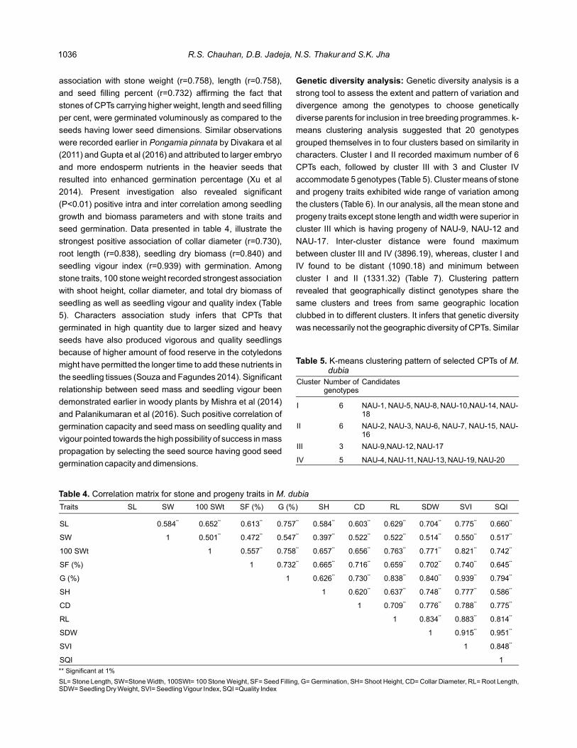
Traits SL SW 100 SWt SF (%) G (%) SH CD RL SDW SVI SQI
SL 0.584** 0.652** 0.613** 0.757** 0.584** 0.603** 0.629** 0.704** 0.775** 0.660**
SW 1 0.501** 0.472** 0.547** 0.397** 0.522** 0.522** 0.514** 0.550** 0.517**
100 SWt 1 0.557** 0.758** 0.657** 0.656** 0.763** 0.771** 0.821** 0.742**
SF (%) 1 0.732** 0.665** 0.716** 0.659** 0.702** 0.740** 0.645**
G (%) 1 0.626** 0.730** 0.838** 0.840** 0.939** 0.794**
SH 1 0.620** 0.637** 0.748** 0.777** 0.586**
CD 1 0.709** 0.776** 0.788** 0.775**
RL 1 0.834** 0.883** 0.814**
SDW 1 0.915** 0.951**
SVI 1 0.848**
SQI 1
Table 4. Correlation matrix for stone and progeny traits in M. dubia
** Significant at 1%
SL= Stone Length, SW=Stone Width, 100SWt= 100 Stone Weight, SF= Seed Filling, G= Germination, SH= Shoot Height, CD= Collar Diameter, RL= Root Length, SDW= Seedling Dry Weight, SVI= Seedling Vigour Index, SQI =Quality Index
Cluster Number of genotypes
Candidates
I 6 NAU-1, NAU-5, NAU-8, NAU-10,NAU-14, NAU-18
II 6 NAU-2, NAU-3, NAU-6, NAU-7, NAU-15, NAU-16
III 3 NAU-9,NAU-12, NAU-17
IV 5 NAU-4, NAU-11, NAU-13, NAU-19, NAU-20
Table 5. K-means clustering pattern of selected CPTs of M. dubia
association with stone weight (r=0.758), length (r=0.758),
and seed filling percent (r=0.732) affirming the fact that
stones of CPTs carrying higher weight, length and seed filling
per cent, were germinated as compared to the voluminously
seeds having lower seed dimensions. Similar observations
were recorded earlier in by Divakara et al Pongamia pinnata
(2011) and Gupta et al (2016) and attributed to larger embryo
and more endosperm nutrients in the heavier seeds that
resulted into enhanced germination percentage (Xu et al
2014). Present investigation also revealed significant
(P<0.01) positive intra and inter correlation among seedling
growth and biomass parameters and with stone traits and
seed germination. Data presented in table 4, illustrate the
strongest positive association of collar diameter (r=0.730),
root length (r=0.838) dry biomass (r=0.840) and , seedling
seedling vigour index (r=0.939) with germination. Among
stone traits, 100 stone weight recorded strongest association
with shoot height, collar diameter, and total dry biomass of
seedling as well as seedling vigour and quality index (Table
5). Characters association study infers that CPTs that
germinated in high quantity due to larger sized and heavy
seeds have also produced vigorous and quality seedlings
because of higher amount of food reserve in the cotyledons
might have permitted the longer time to add these nutrients in
the seedling tissues (Souza and Fagundes 2014). Significant
relationship between seed mass and seedling vigour been
demonstrated earlier in woody plants by Mishra et al (2014)
and Palanikumaran et al (2016). Such positive correlation of
germination capacity and seed mass on seedling quality and
vigour pointed towards the high possibility of success in mass
propagation by selecting the seed source having good seed
germination capacity and dimensions.
Genetic diversity analysis: Genetic diversity analysis is a
strong tool to assess the extent and pattern of variation and
divergence among the genotypes to choose genetically
diverse parents for inclusion in tree breeding programmes. k-
means clustering analysis suggested that 20 genotypes
grouped themselves in to four clusters based on similarity in
characters. Cluster I and II recorded maximum number of 6
CPTs each, followed by cluster III with 3 and Cluster IV
accommodate 5 genotypes (Table 5). Cluster means of stone
and progeny traits exhibited wide range of variation among
the clusters (Table 6). In our analysis, all the mean stone and
progeny traits except stone length and width were superior in
cluster III which is having progeny of NAU-9, NAU-12 and
NAU-17. Inter-cluster distance were found maximum
between cluster III and IV (3896.19), whereas, cluster I and
IV found to be distant (1090.18) and minimum between
cluster I and II (1331.32) (Table 7). Clustering pattern
revealed that geographically distinct genotypes share the
same clusters and trees from same geographic location
clubbed in to different clusters. It infers that genetic diversity
was necessarily not the geographic diversity of CPTs. Similar
1036 R.S. Chauhan, D.B. Jadeja, N.S. Thakur and S.K. Jha

Cluster SL SW 100 SWt SF (%) G (%) SH CD RL SDW SVI QI
I 21.74 13.36 138.98 81.85 33.38 85.03 7.80 17.07 10.25 2029.89 0.75
II 21.13 12.63 184.03 75.88 32.97 89.79 8.33 19.68 13.74 3360.42 1.01
III 20.42 12.54 212.97 79.76 36.99 107.72 9.53 21.54 19.40 4834.60 1.38
IV 16.66 11.27 138.80 55.97 17.88 75.76 6.93 15.49 7.34 939.39 0.53
Table 6. Cluster mean values for stone and progeny traits in accession of M. dubia
Cluster No. I II III IV
I 0 1,331.32 2,805.80 1,090.98
II 0 1,474.60 2,421.64
III 0 3,896.19
IV 0
Table 7. Inter cluster distance in accession of M. dubia
conclusions were made by Jaisankar et al (2014) and
Pavithra et al (201 ). Wide inter-cluster distance between 3
cluster III and IV signify the importance of these CPTs for
being chosen as potential candidates for tree breeding and
hybridization programmes.
CONCLUSION
Current investigation recorded superiority of CPTs like
NAU-9, NAU-12 and NAU-17 over other candidates on stone
morphological qualities, progeny growth, vigour and biomass
ascribes thus, recommending the inclusion of these
accessions for mass production of quality planting material.
Additionally, traits like stone mass, seed filling percent,
germination capacity and seedling dry biomass are attention
worthy for early selection of genotypes and further
improvement in progeny.
ACKNOWLEDGEMENT
Authors are grateful to authorities of Navsari Agricultural
University for providing all the facilities, logistics and
approvals to conduct the study.
REFERENCESAbdul-Baki AA and Anderson JD 1973. Vigour determination in
soyabean seed by multiple criteria. : 630-633.Crop Science 13
Aigbe HI, Fredrick C and Omokhua GE 2016. Effect of seed source on germination and early seedling growth of Heinsia crinita(Afzel.) G. Taylor. (3): 180-185. Applied Tropical Agriculture 21
Chauhan RS, Jadeja DB, Thakur NS, Jha SK and Sankanur MS2018. Selection of candidate plus trees (CPTs) of Malabar neem ( Cav.) for enhancement of farm productivity in South Melia dubia Gujarat. International Journal of Current Microbiology and Applied Science 7(5): 3582-3592.
Chauhan RS, Thakur NS, Gunaga RP, Bhuva D and Jadeja DB 2019. Assessment of germination attributes in candidate plus trees (CPTs) of Malabar neem ( Cav.). Melia dubia Indian Journal of Ecology 46(2): 335-339.
Chauhan SK, Dhakad AK and Sharma R 2018. Growth dynamics of different half-sib families of Linn. Melia azedarach PLoS ONE
13(11): e0207121. https:/ /doi.org/10.1371/ journal. pone.0207121.
Curtis EA, Comiskey C and Dempsey O 2016. Importance and use of correlational research. (6): 20-25. Nurse Researcher 23
Dickson A, Leaf AL and Hosner JF 1960. Quality appraisal of white spruce and white pine seedling stock in nurseries. The Forestry Chronicle 36 (1): 10-13.
Divakara BN and Das R 2011. Variability and divergence in Pongamia pinnata Journal for further use in tree improvement. of Forestry Research 22(2): 193-200.
Ginwal HS, Phartyal SS, Rawat PS and Srivastava RL 2005. Seed source variation in morphology, germination and seedling growth of Linn. in Central IndiaJatropha curcas . Silvae Genetica 54(2): 76-80.
Gupta G, Handa A K, Ajit and Maurya D 2016. Variation in seed and seedling traits of (9): Pongamia pinnata. The Indian Forester 149852-857.
Gutterman Y 2000. Maternal effects on seeds during development. The Ecology of Regeneration in Plant Communities. CABI publishing, UK, pp.59-84.
Jaisankar I, Sankaran M, Singh DR and Damodaran V 2014. Genetic variability and divergence studies in pod and seed traits of Pongamia pinnata (L.) Pierre. accessions in Bay Islands.Journal of Forestry Research 25 (2): 351-358.
Johnson HW, Robinson HF and Comstock RE 1955. Estimates of genetic and environmental variability in soybeans. Agronomy Journal 47 : 314-318.
Kaushik N, Deswal RPS, Jakhar V and Arya S 2019. Variation in eed sand eedling traits of Mahaneem ( roxb.) s Ailanthus excelsaInternational Journal of Genetics 11 (12): 674-679.
Kołodziejek J 2017. Effect of seed position and soil nutrients on seed mass, germination and seedling growth in Peucedanum oreoselinum Scientific Reports 7 (Apiaceae). : 1959.
Kumar A, Dobhal S, Sharma S, Ahmed N and Rawat US 2013. Genetic screening and improvement of Willd. Melia compositaAnnals of Forestry 21 (2): 189-196.
Kumar P, Parthiban KT and Saravanan V 2013. Genetic variations among open pollinated families of selected better trees in Melia dubia Research Journal of Recent Science 2. : 189-194.
Leela G, Dayana J, Monisha S, Irudaya I, Anitha A and Rosaline J V 2016. Studies on phytochemical, nutritional analysis and screening of biological activities of leaf in vitro Melia dubiaextract. International Journal of Scientific and Engineering Research 7 (8): 56-68.
Loha A, Mulualem T, Demel T, Kenneth L and Aders F 2006. Provenance variation in seed morphometric traits, germination, and seedling growth of Lam. : Cordia africana New Forests 3271-86.
Luzuriaga AL, Escudero A and Pe´rez GF 2006. Environmental maternal effects on seed morphology and germination in Sinapis arvensis Weed Research 46 (Cruciferae). : 163-174.
Malarvannan S, Giridharan R, Sekar S, Prabavathy VR and Sudha N 2009. Ovicidal activity of crude extracts of few traditional plants against (Hubner) (Noctuidae: Helicoverpa armigeraLepidoptera). (1): 64-71. Journal of Biopesticides 2
Meena H, Kumar A, Sharma R, Chauhan SK and Bhargava KM 2014. Genetic variation for growth and yield parameters in half-
1037Melia dubia Genotypes from Northern Western Ghats of India

sib progenies of (Linn.). Melia azedarach Turkish J Agri and Forestry 38 (4): 531-539.
Mishra Y, Rawat R, Rana PK, Sonkar MK and Mohammad N 2014. Effect of seed mass on emergence and seedling development in Pterocarpus marsupium Journal of Forestry Research 25 Roxb. : 415.
Palanikumaran B, Parthiban KT, Sekar I, Umarani R and Amirtham D 2016. Variability studies for seed and seedling traits in Pongamia pinnata . Electronic Journal of Plant (L.) Pierre at Tamil NaduBreeding 7(3): 657-665.
Parmar AG, Thakur NS and Gunaga RP 2019. Cav. leaf Melia dubialitter allelochemicals have ephemeral allelopathic proclivity. Agroforestry Systems 93 (4): 1347-1360.
Parthiban KT, Akilesh KB, Seenivasan R, Kamala K and Govinda RM 2009. Integrating in agroforestry farms as an Melia dubia alternate pulpwood species. Asia Pacific Agroforstry News Letter 34 : 3-4.
Parthiban KT, Chauhan SK and Jude Sudhagar 2019 Malabar . neem, Genetic resources, silviculture and Melia dubia-economics, Agrobios New Delhi.
Pavithra HR, Gowda B, Prasanna KT and Shivanna MB 2013. Pod and seed traits in candidate plus trees of (L.) Pongamia pinnata Pierre from southern Penninsular India in relation to provenance variation and genetic variability. Journal of Crop Science and Biotechnology 24(2): 201-203.
Saravanan V, Parthiban KT, Kumar P, Anbu PV and Ganesh P 2013. Evaluation of fuel wood properties of Cav. at Melia dubia different age gradation. Research Journal of Agriculture and Forestry Sciences 1 (6): 8-11.
Sehgal RN, Chauhan SK and Dhall SP 1995. Half-sib progeny evaluation of chir pine. (2): 61-62.Silvae Genetica 44
Sheoran OP, Tonk DS, Kaushik LS, Hasija RC and Pannu RS 1998. Statistical Software Package for Agricultural Research Workers. Recent Advances in information theory, Statistics & Computer Applications by DS Hooda and RC Hasija Department of Mathematics Statistics, CCS HAU, Hisar, pp.139-143.
Shu X, Yang X and Yang Z 2012. Variation in seed and seedling traits among fifteen chinese provenances of . Magnolia officinalis
Notulae Botanicae Horti Agrobotanici Cluj-Napoca (2): 274-40283.
Souza ML and Fagundes M 2014. Seed size as key factor in germination and seedling development of Copaifera langsdorffii (Fabaceae). 2566-2573. American Journal of Plant Sciences 5:
Sukhadiya ML, Thakur NS, Patel VR, Gunaga RP, Kharadi VB, Tyagi KK and Singh S. 2020. Cav. drupe pulp: a new Melia dubia alternate livestock feed resource. Range Management and Agroforestry 40(2): 299-305.
Thakur NS, Kumar D and Gunaga RP 2017. Transient allelopathic propensity of Willd. leaf litter on chickpea (Melia composita Cicer arietinum Indian Journal of Ecology 44L.). (5): 443-450.
Troup RS 1921. Silviculture of Indian Trees, Clarendon Press, London, : 152p 3
Uday DN, Dhanapal S and Pandey C 2011. Suitability of Melia dubia(Malabar neem wood) for plywood manufacture. Journal of Indian Acadmy of Wood Science 8 (2): 207-211.
Vasav VP, Narkhede SS, Rane AD, Gunaga RP and Bhave SG 2011. Evaluation of progenies of candidate plus trees of Pongamia pinnata (L.) Pierre. for seed germination and seedling vigour. Current Science 100 (4): 465-467.
Warrier KCS, Raja JL and Warrier RR 2018. Genetic divergence in fruit and stone traits of Cav. in India. Melia dubia International Journal of Genetics 10 (10): 530-533.
WASP Web Agri Stat Package 2.0, ICAR-Central Coastal -Agricultural research Institute, Goa database (online) available at https://www.ccari.res.in/wasp2.0/index.php
Xu J, Li W, Zhang C, Liu W and Du G 2014. Variation in seed germination of 134 common species on the eastern tibetan plateau: phylogenetic, life history and environmental correlates. PLoS ONE 9 ! (6): 1-13.
Yasodha D, Manimegalai M, Binu K S and Vijayakumar K 2012. Larvicidal effect of seed extract against the malarial Melia dubiafever mosquito, . Culex quinquefasciatus Current Biotica5(1):102-106.
Zobel BJ and Talbert J 1984. John Wiley Applied tree improvement. & Sons, Inc., New York.
Received 22 April, 2021; Accepted 09 August, 2021
1038 R.S. Chauhan, D.B. Jadeja, N.S. Thakur and S.K. Jha

Local Forest Institution and Participation of Local Communities:A Study in Bankura (South) Forest Division in West Bengal, India
Indian Journal of Ecology (2021) 48(0): 1039-1046Manuscript Number: 3329
NAAS Rating: 5.79
Abstract: The local institutions like forest protection committee are working with forest department to protect forest governance under Participatory forest management. The paper attempts to construct participation index in the planning, implementation and monitoring stages across ten villages of Bankura (South) forest division of West Bengal. The paper examines whether there is any impact on change in forest area last ten years across villages. The paper also attempts to estimate the factors responsible for community participation in forest management programme at local level. This paper is based on primary data collected from 228 households in the Ranibandh range under Bankura (south) forest division of West Bengal, in the month of January, 2020. A multi stage sampling technique and questionnaire method have been used for data collection. The result of the paper shows that participation index is found to be 0.47and planning, implementation and monitoring indices are 0.478, 0.589 and 0.342respectively. There is no deforestation across ten villages in Ranibandh range on account of participation of the community. The level of participation is influenced by caste, sex, age, landholdings, monitoring and occupation. The paper has an important policy implication for sustainable forest management.
Keywords: Participation index, Planning index, Implementation index, Monitoring index, Forest protection committee, Sustainable forest management
Payal Ghosh and Jyotish Prakash Basu
Department of Economics, West Bengal State University, Barasat, Kolkata-700126, IndiaE-mail: [email protected]
The environmental resources particularly forests play an
important role in local and global context. It also plays to
maintain ecological balance, soil erosion, climate change
and it is also essential for development of rural economy.
Forest provides various goods and services for domestic
purpose as well as industrial purpose. Now-a-days forests
are deteriorated gradually due to human activities. The aim of
sustainable forest management is to maintain and enhance
the economic, social and environmental value of all types of
forest resources for the benefit of present and future
generations (UN 2008, Resolution 62/98). The good quality
of forest governance is necessary condition for the decrease
in deforestation and long term carbon storage globally
(Umemiya et al 2010). The probability of degradation of a
forest declines and regeneration of forest increases with
more involvement of local people or local institution (Chhatre
and Agrawal 2008). A fundamental assumption is that forest
user's people has given an opportunity to participate in
decision-making process about forest resource
management, and they properly manage and use the
resources in a sustainable way (Shrestha and McManus
2008). Decentralised theory states that local people or
institutions take better decision than centralised authorities
because they have clear knowledge about forest resources
and management (Tacconi 2007). Many developing
countries have revised their forest policies. Many African and
South Asian countries have merged local communities or
institutions in the management of forest resources through a
Participatory Forest Management (PFM) approach
(Schreckenberg et al 2006). PFM is an approach to forest
management where local communities are living in and
around the forests together to make decisions in all forest
management process like planning, implementing,
monitoring and evaluation process. PFM is always for the
people, of the people and by the people who lives around the
forest and also other people who live far away from forest
(Karki 2003).
The institutions at the local level are common Forest
Management groups, Van Panchayat, Joint forest
Management Committee, Traditional Village Level
institutions or Village Councils and Forest Protection
Committee(in West Bengal) etc. In West Bengal there are
4262 numbers of joint forest management committees
having total membership of 496998.The JFMCs covering or
protecting 563344.134 ha forest area in West Bengal. The
SC and ST communities constitute near about 55% of
members in the JFMCs (State Report, 2017-18). People
participation depends on the socio-economic condition of the
people around the forest and other institutional factors. The
main objective of community forest programme is to get
forest products for their subsistence, socio-economic
development of the people and conservation of forest

resources. If people are assured that they are getting benefits
from forests, they will more involve in forest protection and
management activities. Accessibility is the another key factor
to grow people's interest in involving or participating in forest
management (Yogesh 2014).Participation of people in forest
management process means planning, implementing,
monitoring, decision making and evaluation of any
programme. People's participation in forest management
programme is a key to success local communities'
development (Tadesse et al 2017). Given the above
backdrop, the objectives of the paper are twofold. First is to
construct community participation index of the local
communities in the Bankura (South) forest Division, West
Bengal. Second is to estimate the factors influencing forest
participation of the local communities.
MATERIAL AND METHODS
Study area: The study has been conducted in the district of
Bankura in West Bengal (Fig. 1). It is situated in south-
western side of the West Bengal. Approximately 90% to 92%
people live in rural areas (Census 2011). The forest divisions
of Bankura district is divided into three: Bankura South,
Bankura North and Panchet Division. The study is conducted
in the Bankura (South) forest division which comprises of
twelve (12) range offices. These offices are Bankura, Indpur,
Kamalpur, Khatra, Hirbundh, Simlapal, Pirragari, Sarenga,
Fig. 1. Map of Bankura district of West Bengal, India
Source: http://www.westbengalforest.gov.in/upload/forest_map
Motgoda, Fulkushma, Ranibandh and Jhilimili. We have
chosen Ranibandh range in our study on the basis of highest
forest protection area. According to state forest report,
Ranibandh range area comes under highest forest protection
(Table 1). It is situated 60 kms to the south of Bankura town.
The major component of its demography is tribal population.
Data Collection: The present study, which is based on the
primary data, is collected from Ranibandh range office in
Bankura (south) forest division in the district of Bankura,
West Bengal. A multistage sampling technique has been
followed. The field survey is carried out in the month of
January, 2020. We adopted a questionnaire method to
collect data from head of the households. Ten JFM villages
are selected under Ranibandh range purposively. After the
selection of villages, 20% of households from each villages
are randomly selected. Thus, total number of sample
households consist of 228. The name of the villages and the
name of the forest protection committees are same. The
sample villages and sample households are shown in Table
2.
Analytical methods: The forest protection committees
(FPCs) are the local institution at the village level under joint
forest management (JFM) programme. Forest protection
committee comprises two bodies. One is executive body of
consists of 5-10 members and other is general body consists
of all adult members of the households. All members follow
the government rules but executive committee members can
formulate some other rules and regulations for forest
protection. Some decisions are approved in the meeting in
presence of general members of the committee. Executive
Division Range office Beat office No. of FPC
Protected area ha)(
Bankura (South Division)
Bankura 3 47 3230.45
Indpur 4 63 4310.72
Kamalpur 3 28 1670.82
Khatra 4 104 4277.64
Hirbundh 3 36 1922.18
Simlapal 3 53 4238.46
Pirragari 3 53 4004.42
Sarenga 3 50 4648.03
Motgoda 3 63 3032.1
Fulkushma 3 38 3993.09
Ranibandh 4 55 5418.94
Jhilimili 2 24 3350.23
Total 12 38 614 44097.08
Table 1. Details of range office, beat office, FPC and area under protection by FPC
Source: Bankura forest division
1040 Payal Ghosh and Jyotish Prakash Basu

committee members encourage general members to
participate in the forest protection programme regularly.
Participation index: People's participation in forest
protection programme is measured by the participation
index. Participation index value is the average of three
indices (i.e., planning index, implementation index and
Main indicator Sub-indicator Descriptions
Participation index Planning index Forest boundary demarcation Yes=1,No=2,Don't Know=3
Identifying forest users
Participatory forest resource assessment
Forest management committee election
Encouraging others to participate
Developing forest management by laws
Preparing forest management plan
Approval of forest management agreement
Implementation index Reforestation of degraded forest areas Yes=1,No=2,Don't Know=3
Planting of fruit bearing trees such as mahua & mango
Planting trees & management
Nursery establishment
Beekeeping
Forest fire fighting
Attending meetings
Participations in knowledge & skill developing training
Monitoring index Follow ups forest managements by law Yes=1,No=2,Don't Know=3
Helps forest patrols
Detecting of illegal activities
Supervise forest management plan implementation
Forest boundary maintenance
Table 3. Description of main and sub-indicators of participation index
Source: Author's calculation from primary data
Name of the sample villages
Total number of households
No. of sample households (20% of the households)
Kamo 163 33
Makhnu 85 17
Barapatcha 50 10
Jamgeria 130 26
Dhankura 114 22
Kadmagarh 120 24
Kalabani 120 24
Bagdiha 40 08
Mitham 186 38
Mahadebsinan 130 26
Total households 1138 228
Table 2. Number of sample households
Source: Author's calculation from primary data
monitoring index). For evaluating index values of planning,
implementation and monitoring, each main indicator is sub-
divided into five or more indicators. Each and every
household are asked to respond their views in three Likert
type of scale in which Yes=1, No=2, don't know=3 is assumed
on all indicators' statement (Table 3). In forest planning index,
we take the responses from the households whether the
households under forest protection committee at local level
participate in the different planning like forest boundary
demarcation, identifying forest user, participatory forest
resource assessment, forest management committee
election, encouraging others to participate, preparing forest
management plan, developing forest management by laws
and approval of forest management agreement.
For implementation index, we take the responses from
the households whether the households were involved in any
reforestation programme of degraded forest areas, planting
any fruit trees such as Mahua and Mango, planting trees and
management, any nursery establishment, beekeeping,
forest fire fighting programme, attending meetings and
participate in any knowledge and skill developing training.
For the construction of the monitoring index, we take the
1041Local Forest Institution and Participation of Local Communities

responses from the households whether they were following
up forest management by law, helping forest patrols,
protection of illegal logging, supervising forest management
plan implementation and helping in maintaining forest
boundary.
In order to formulate the index values we need to
normalize value of each indicator for each household. The
normalized value lies between '0' and '1'. '0' means minimum
and '1' means maximum value. This normalization procedure
is followed by the methodology of Human Development
Index (UNDP-2006). After normalizing procedure, we get the
index value. For evaluating the index value we take the
average of all indicators. Participation index is calculated as:
Par t ic ipa t i on index= 1 / 3 [P lann ing in dex
+Implementation index +Monitoring index]
Linear regression model: Linear Regression Model is used
to estimate the factor responsible for participation index in the
Bankura (south) forest division of West Bengal.
Model specification: In order to identify socio-economic
and other determinants that influence the level of a forest
user's participation at house level in participatory forest
management (PFM) programme, the linear model is
employed. Therefore, we specify a linear model is as follows:
Y X X X X X X X X X=α+β +β +β +β +β +β +β +β +βi 1 1i 2 2i 3 3i 4 4i 5 5i 6 6i 7 7i 8 8i 9
9i 10 10i i+β +εX …………… (1)
Where Y is the Participation Index (PI) of the ith i
households as the dependent.
X = Caste of the household head (SC= 1, ST=2, 1i
OBC=3 and GEN = 4)
X = ex of the household head (Male = 1, Female = 0)2i S
X = Age of head of households3i
X = Occupation of the head of the households4i
X = Educational index5i
X = Distance from home to forest (in km)6i
X = Land holdings (in acres)7i
X = Monitoring Index8i
X = Cooperation of forest department9i
X = Monthly forest income as percentage of total 10i
income (in Rs)
εi = random disturbance term
RESULTS AND DISCUSSION
The value of the participation, planning, implementation
and monitoring indices are presented in Table 4. The value of
the participation index of the households as a whole Bankura
south forest division is 0.470 shown in Table 4. The value of
the planning index, implementation index and monitoring
index as a whole Bankura south forest division are
respectively 0.478, 0.589 and 0.342 (Table 4). The positive
and higher value of the indices means higher participation of
the households. The value of the implementation index is
highest as whole in the Bankura south forest division. The
value of the participation index across ten villages is shown in
the Table 5 and Figure 2. The high value of forest
management committee election index (0.814) means
households are more involved in choosing of forest
protection committee member. The value of attending
meeting is highest in implementation index (0.908). The
value of reporting illegal activities are 0.833 under monitoring
index. So that involvement of local communities against
illegal activities is found to be highest in monitoring index
(Table 4). The value of the planning, implementation and
monitoring indices are shown in Table 5 and Figure 3. The
value of the participation index is highest in the village
Kadmagarh (0.593) followed by Dhankura (0.549), Makhnu
(0.484), Kamo (0.479) and so on. The lowest participation
index is in the village Kalabani (0.369). The value of planning,
monitoring, and implementation indices are also low in the
village Kalabani. That means participation of the villagers are
very low in the village Kalabani. The value of planning index is
highest in the village Dhankura (0.568) followed by
Kadmagarh (0.565), Jamgeria (0.488), Kamo (0.487) and so
on. The value of the implementation index is highest in the
village Dhankura (0.656) followed by Kadmagarh (0.646),
Kamo (0.623) and so on. The value of the monitoring index is
0.000
0.100
0.200
0.300
0.400
0.500
0.600
0.700
Particiaption Index
Fig. 2. Village wise participation index in Ranibandh range, Bankura (south) forest division
0.0000.1000.2000.3000.4000.5000.6000.700 Planning Index Implementation Monitoring Index
Fig 3.. Village wise planning, implementation and monitoring indices in Ranibandh range
1042 Payal Ghosh and Jyotish Prakash Basu

Village Participation index Planning index Implementation index monitoring index
Kamo 0.479 (4) 0.487 (4) 0.623 (3) 0.327 (5)
Makhnu 0.484 (3) 0.412 (9) 0.599 (6) 0.441 (2)
Bagdiha 0.413 (9) 0.430 (8) 0.547 (8) 0.263 (8)
Mitham 0.467 (5) 0.469 (5) 0.609 (4) 0.324 (6)
Jamgeria 0.435 (7) 0.488 (3) 0.567 (7) 0.250 (9)
Barapatcha 0.458 (6) 0.463 (6) 0.600 (5) 0.310 (7)
Mahadebsinan 0.422 (8) 0.397 (10) 0.526 (9) 0.342 (4)
Kadmagarh 0.593 (1) 0.565 (2) 0.646 (2) 0.567 (1)
Kalabani 0.369 (10) 0.461 (7) 0.487 (10) 0.158 (10)
Dhankura 0.549 (2) 0.568 (1) 0.656 (1) 0.423 (3)
Table 5. Value of the indices across sample villages
Source: Author's calculationFNote: igures in () indicate rank
highest in the village Kadmagarh (0.567) followed by Makhnu
(0.441), Dhankura (0.423), and Mahadebsinan (0.342) and
so on. The value of all indices are approximately high in the
village Dhankura (Table 5).
Planning index Forest boundary demarcation 0.318
Identifying forest users 0.450
Participatory forest resource assessment 0.439
Forest management committee election 0.814
Encouraging others to Participate 0.636
Preparing forest management plan 0.373
Developing forest management by laws 0.404
Approval of forest management agreement 0.395
Planning index 0.478
Implementation index Reforestation of degraded forest areas 0.443
Planting of fruit bearing trees such as mahua & mango 0.669
Planting trees & management 0.689
Nursery establishment 0.487
Beekeeping 0.456
Forest fire fighting 0.779
Attending meetings 0.908
Participations in knowledge & skill developing training 0.283
Implementation index 0.589
Monitoring index Follow ups forest managements by law 0.184
Forest patrols 0.252
Reporting of illegal activities 0.833
Supervise forest management plan implementation 0.167
Forest boundary maintenance 0.272
Monitoring index 0.342
Participation index 0.470
Table 4. Value of the main index and sub-indices
Source: Author's calculation from primary data
Table 6 shows that there is no loss of forest cover across
the ten villages since last 10 years (Basu 2020). Fifty per cent
(50%) of the villages show a positive change in forest cover
and the rest shows no changes in forest cover. This result
1043Local Forest Institution and Participation of Local Communities

Name of villages
Forest cover (ha) in 2007-08
Forest cover (ha) in 2016-17
Change of forest cover over 10
years (ha)
Kamo 100 100.23 +0.23
Makhnu 148.62 154.25 +5.63
Bagdiha 46 47 +1.00
Kalabani 223.15 297.493 +74.343
Kadmagarh 146.49 146.49 0
Dhankura 93.096 93.096 0
Mitham 139.09 139.09 0
Mahadebsinan 305.88 313 +7.12
Jamgeria 50.65 50.65 0
Barapatcha 401 401 0
Table 6. Changes of forest cover in sample villages over 10 years
Source: Basu 2020( )
Variable Mean Standard deviation Minimum Maximum
Caste 0.5919662 0.3251945 0.09091 2
Sex 0.2348242 0.1330276 0 1
Age of the head of households 12.95238 6.433973 3.57143 60
Occupation of the head of households 0.5245739 0.3697685 0 2
Educational Index** 0.0589485 0.0401625 0 0.175926
Distance from home to forest 0.1003041 0.0891117 0 0.333333
Land holdings (in acres) 0.22865 0.2213052 0 1.322314
Monitoring Index 0.0905462 0.0797923 0 0.6
Cooperation 0.2443637 0.1256245 0 1
Monthly forest income as percentage of total income (in Rs) 6.938153 5.385894 0 41.86047
Table 7. Basic statistics of independent variables of Bankura (South) forest division
Source: Author's calculation**Education index of the households is measured on the basis of UNDP methodology, where Education Index (EI) = (MYSI+EYSI)/2. MYSI is the mean years of schooling index and EYSI is the expected years of schooling index. Due to Heteroscadisity problem, we divided the regression model by total households' members. Total households' members is an explanatory variable
shows that there is no deforestation because of more
participation of local community in forest management (i.e.,
planning, implementing and monitoring) programme (Table
6).
Estimation of factors affecting participation: In order to
estimate the factors that influence forest user's participation
in forest management programme, we have taken linear
regression model. The independent variables and their basic
statistics are shown in Table 7. The dependent variable is the
participation index. The Result of linear regression are given
in the Table 8.
From the Table 8, we find that the model is overall
significant as indicated by the value of F statistics. The value
of F statistic is F= 164.71. Regression analysis shows that
various demographic, social, economic and environmental
related factor influence the level of local people's
participation in joint forest management programme. Here
forest user's participation is taken as the dependent variable
where as social, economic, environmental factors are taken
as explanatory (independent) variable like caste of
households' head (SC= 1, ST= 2, GEN= 3, OTH= 4), sex of
households' head (male= 1, female= 0), occupation of
households' head, distance between home and forest (in
km), educational index, total land holdings of the households
(in acre) etc. Some other factors which also influence
people's participation but are not taken into the model
because of their irrelevance to our study. 88.36% of the total
variation in the response or dependent variable (PI) is
explained by the variation in the given all explanatory
(independent) variables. On the other hand 87.82% of the
total variation in the dependent variable (PI) is explained by
fitted regression model (equation). It means both values of R 2
and adj R is moderate. It can be concluded that all given 2
independent variables of people's participation in forest
protection and management activities are at satisfactory
level. Out of the 10 independent variables tested in the
regression model, six variables are proved statistically
significant either at 1%, 5% or 10% probability level.
The regression result shows that there is a positive and
significant relation between caste and participation of the
forest users'. It implies that upper caste communities' people
participate more in the joint forest management programme
than the schedule and tribal communities. This means upper
caste people participate more in planning, implementation
and monitoring programme of forest resources which is done
in collaboration with forest department. Gender of the
households' head is positive and significantly associated with
1044 Payal Ghosh and Jyotish Prakash Basu

Independent variable Bankura forest division
Coefficient SE t
Caste 0.0225 0.008 2.74
Sex 0.0719 0.021 3.38
Age of the head of households 0.0026 0.000 5.60
Occupation of the head of households 0.0148 0.007 2.05
Educational Index 0.0260 0.046 0.57
Distance from home to forest 0.0239 0.021 1.14
Land holdings (in acres) 0.0154 0.008 1.82
Monitoring Index 0.5484 0.030 18.22
Cooperation -0.0119 0.024 -0.49
Monthly forest income as percentage of total income (in Rs) -0.0003 0.000 -0.69
Constant -0.0005 0.005 -0.10
F(10, 217)=164.71,Prob > F=0.000, R-squared= 0.8836,Adj R-squared= 0.8782,Root MSE=0.02565
Table 8. Results of linear regression model of participation in Bankura (south) forest division
Source: Author's calculation
the level of participation of the households. This means that
male participants are more in decision making, planning and
monitoring process. There is a positive and significant
relation between age of households' head and level of
participation. This implies that aged people are involved
more in forest management programme. That means aged
person or more experienced persons are mainly participate
in this planning, monitoring and implementing process. There
is a positive and significant relation between occupation of
the households' head and level of participation. There is a
positive but insignificant relation of distance from home to
forest and level of participation. There is also insignificant
relation between level of education and participation. There
is positive and significant relation between total land holdings
and level of participation of the households. Large land
holders are participate more in the forest management
programme. There is a positive and significant impact of
monitoring on participation index shown in table 8. This
means, if monitoring process such as reporting of illegal
activities, supervising forest management plan
implementation, following up forest management by law,
forest patrolling, maintaining of forest boundaries is
evaluated properly there will be a positive result in forest
management programme and conservation of resources.
Hence monitoring process is an important path for evaluation
of participation. The participation of the households also
depends upon other factors which are not taken in account.
Some villagers says that committee does not involved them
in this programme. Participation also depends on the
occupation of the other family member in a family, number of
livestock keeping and structure of the market etc.
CONCLUSIONS
The study has attempted to examine the level of
people's participation in natural resource management like
forests. People who are highly dependent upon forests and
forest product for their livelihoods, they participate more in
forest management programme. The result shows that
participation of the households is measured by index value.
Participation index is comprised of planning index,
monitoring index and implementation index. The value of the
participation index is found to be 0.470. The value of
planning, implementation and monitoring indices are found to
be 0.478, 0.589 and 0.342 respectively. In planning index,
people's participation in forest management committee
election is found to be highest (0.814). In implementation
index people's participation is found to be highest in
attending meetings (0.908). In monitoring index local,
communities contribution is found to be highest in reporting of
illegal activity (0.833) and lowest in supervising forest
management plan implementation (0.167). There is no
deforestation across ten villages in Ranibandh range in
Bankura (south) forest division due to more participation of
the local communities or forest users' communities.
The nature and level of participation is highly determined
by caste, sex, age of the head of households, monitoring,
total land holdings, and occupation of households. In this
paper we find that local people and institutions like forest
protection committee play a significant role for forest
protection and management process. This study supports
the change of centralized process into decentralized
process. There is more involvement of forest users'
communities in every stage of forest management to ensure
1045Local Forest Institution and Participation of Local Communities

the better livelihood opportunities for forest dependent
people or communities and sustainable forest management.
REFERENCESChhatre A and Agrawal A 2008. Forest commons and local
enforcement. Proceedings of the National Academy of Sciences 105 (36): 13286-13291.
Government of India 2011. District Census Abstract, Bankura District, Department of Census Operations, Kolkata.
Government of India 2011. District Census Hand book, Bankura District, Department of Census Operations, Kolkata.
Government of West Bengal, State Forest Report, 2006-2007,2011-12,2015-16,2017-18,2019
India's State of the Forest Report (ISFR). 2015, 2017, 2019.
Basu JP 2020. Community-based Institution, Forest Enforcement Index and Forest Governance An Empirical study in Bankura (South) Forest Division in West Bengal, India. ISSN: 2321-8819 (Online) 2348-7186 (Print) 8(9), September, 2020, Asian Journal of Multidisciplinary Studies 8 (9) September, 2020
Karki M 2003. Joint and community forest in South Asia: Lesson learned road blocks and future prospects, Paper presented at the . Peshawar, July 30-Joint Forest Management in Pakistan31, 2003.
Schreckenberg K, Luttrell C and Moss C 2006. Participatory forest management: An overview: Forest policy and environment programme: grey literature. March 2006 ODI UK.
Available from https://www.odi.org/sites/odi.org.uk/files/odi-assets/publications- opinion-files/3781.pdf
Shrestha KK and McManus P 2008. The politics of community participation in natural resource management: essons from Lcommunity forestry in Nepal. : 135-146.Aust Forest 71
Solomon Tadesse, Muluneh Woldetsadik and Feyera Senbeta 2017. Forest users' level of participation in a participatory forest management program in southwestern Ethiopia. Forest Science and Technology 13 (4): 164-173.
Tacconi L 2007. Decentralization, forests and livelihoods: heory Tand narrative. : 338-348.Global Environmental Change 17
Tadesse S, Woldetsadik M and Senbeta F 2017. Forest users' level of participation in a participatory forest management program in southwestern Ethiopia. Forest Science and Technology 13(4): 164-173.
Umemiya C, Rametsteiner E and Kraxner F 2010. Quantifying the impact of the quality of governance on deforestation. Environmental Science & Policy DOI 10.1016/j.envsci.2010.07.002 .
UNDP 2006. United Nations Human development report Development Program, h t t p : / / h d r. un dp . o r g /h dr 20 06 / statistics/
UN 2008. Non-legality binding instrument on all types of forests. U.N general Assembly sixty-second session second committee Agenda Item 54. A/RES/62/98. 31 January 2008.
Yogesh Ranjit 2014. Determinants of people's participation in forest protection and management: A study in Kaski, Nepal. Economic Journal of Development Issues 17 & 18 (1-2): 21-28.
Received 22 May, 2021; Accepted 20 July, 2021
1046 Payal Ghosh and Jyotish Prakash Basu

Effect of Integrated Nutrient Management on Seedling Growth and Biomass of Sandalwood ( L.)Santalum album
Indian Journal of Ecology (2021) 48(4): 1047-1050Manuscript Number: 3330
NAAS Rating: 5.79
Abstract: The investigation was undertaken with as host plant and 12 INM treatments of different organic, inorganic, Leucaena leucocephalabiofertilizers and their combinations application along with control for sandal wood growth and biomass. Among different integrated nutrient management treatments, seedling height, collar diameter, number of leaves per plant, fresh and dry weight of shoot, leaves and whole plant were recorded maximum in 1 g of NPK and vermi-compost @ 25 g seedling . Moreover, fresh and dry weight of root and root length were -1
registered maximum in vermi-compost @ 50 g seedling . The seedlings without integrated nutrient treatment were poorest for all parameters -1
under study. However, root: shoot ratio was noted maximum in vermin seedling .-compost @ 25 g -1
Keywords: ,Sandalwood INM, Growth, Biomass, NPK, Biofertilizers, Vermicompost
Govind, V.M. Prajapati and M.B. TandelDepartment of Silviculture and Agroforestry, College of Forestry, ACHF, NAU, Navsari-396 450, India
E-mail:[email protected]
Santalum album (Sandalwood) is considered in India to
be a practical agroforestry species. Among the sixteen species
of the economically important genus , Santalum Santalum
album . L or Indian Sandalwood is highly prized for its scented
heartwood. The heartwood yields oil which is commercially
known as East Indian Sandalwood oil. The oil is also used in
indigenous medicine, while the wood is used in the religious
rituals of Hindus, Buddhists and Muslims. It is sometimes
grown as an ornamental and as a low branching windbreak,
while its leaves provide green manure. Sandalwood plants can
live autographically (without parasitizing a host) up to
maximum of one year and for subsequent growth an intimate
association with roots of a host plant through haustoria is
essential (Radomiljac 1998). Artificial regeneration is achieved
by dibbling seeds in pits, sowing on mounds and trenching
around mother trees for wounding the roots for inducing root
sucker production. Planting of nursery raised, vegetatively
multiplied and tissue culture raised seedlings are also in
practice (Rai and Kulkarni 1986). However, because it is very
slow growing, taking up to 40 years to develop its heartwood
fully, the tree has been overexploited and has become
endangered in the wild. It is desirable not to clean-weed all-
round the Sandalwood seedlings, as the roots form haustorial
connections with adjoining weed growth. Integrated Nutrient
Management (INM) system aims at achieving efficient use of
chemical fertilizers in conjunction with organic manures. It also
maintains the soil fertility for sustaining increased crop
productivity through optimizing all possible sources, organic
and inorganic, of plant nutrients required for crop growth and
quality in an integrated manner, appropriate to each cropping
system and farming situation in its ecological, social and
economic possibilities (Roy 1986). Seedlings are not growing
well during its seedling growth because of lack of proper
nutrition to it. There is a need of providing the appropriate
nutrition to the seedlings of Sandalwood in the nursery. There
are so many sources of nutrients in integrated nutrient
management and from that best integrated nutrient application
we can find from this experiment. For this reasons, this
experiment was designed to check the best nutrient for S.
album seedling.
MATERIAL AND METHODS
The present investigation was carried out at Net House
Complex, College of Forestry (ACHF), Navsari Agricultural
University, Navsari during year 2018-19. The experiment
comprised of twelve different combinations of organic,
inorganic and biofertilizers along with control (Table 1). All
polybags were filled with soil, sand and FYM in the ratio of
1:1:1. Seeds of Sandalwood were treated with 500 ppm GA 3
for 24 hours. After GA treatment seeds were sown in sand 3
bed. After good germination of seed in sand bed, averaged
heighted plants were selected for seedling growth
experiment. Then seedlings of Sandalwood (Santalum
album L.) were transplanted in to different nutrients treated
polythene bags. Leucaena ( ) was Leucaena leucocephala
used as a common host plant. The bio-fertilizer like
Phosphobacteria and was inoculated in Azospirillium
polybags as per the treatments. Vermicompost powdered
thoroughly and applied in polybags as per the treatments.
NPK applied through chemical fertilizer as per treatments.

The observations were recorded for growth and biomass of
sandalwood seedlings. Five plants randomly selected for
taking observations of every treatment in all the three
repetitions and the observation were recorded at monthly
interval for seedling height, collar diameter and number of
leaves/plant, while other parameters root length, fresh viz.
and dry weight of leaves, shoot and root, root: shoot ratio
were recorded after 6 months. The different parameters were
subjected to the statistical analysis by using variance
technique as described by Panse and Sukhatme (1967).
RESULTS AND DISCUSSION
The findings of research revealed that application of
various INM treatment combinations on Sandalwood
seedling at nursery stage significantly increased the growth
parameters (seedling height, collar diameter, number of
leaves and root length), fresh and dry biomass and root:
shoot ratio. A constant increased in all parameters and
variation among different treatments was observed during
study period (30 to 180 days after transplanting).
Growth parameters: During growing period (from 30 to 180
days) all monthly observed parameters (seedling height,
collar diameter and number of leaves) found increased in 1.0
g of NPK + Vermicompost @ 25 g seedling . Among all INM -1
treatments at the end of experiment, application of 1.0 g of
NPK + Vermicompost @ 25 g seedling recorded highest -1
seedling height (28.47 cm), collar diameter (3.26 cm) and
number of leaves (16.27) (Table 2). This might be due to
prompt release of nutrients by the application of inorganic
fertilizers (NPK) and thereafter slow and continuous release
of nutrients by vermicompost, these together also ensures in
increase in release of micronutrients. Nitrogen plays an
important role in increasing the seedling height as it plays
direct role in formation of proteins. It is also an integral part of
chlorophyll, which is primary absorber of light energy needed
for photosynthesis. This might have led to increased
production of photosynthesis and its distribution into root and
shoot portion resulting in higher plant height and collar
diameter. Korwar et al (2005) reported that the growth of
Aonla increased by the various source of nutrients such as
organic and inorganic source of nutrients. Similar results
were also reported by Lamani et al (2001), Sumbli and
Koppad (2013), Mishra and Channabasappa, (2013),
Somashekar and Channabasappa, (2015), Atik et al (2015).
For number of leaves similar result was found by Manikanta
et al (2016) in Simarouba glauca.
Maximum root length (21.45 cm) was recorded in
Vermicompost @ 50 g / seedling (Table 2). The probable
reason for this might be more porosity offered by higher
proportion of vermicompost as compared to other
Treatment Treatment details
T0 Soil : Sand : FYM ( 1:1:1 )
T1 1.0 g of NPK seedling-1
T2 2.0 g of NPK seedling-1
T3 Vermicompost @ 25 g seedling-1
T4 Vermicompost @ 50 g seedling-1
T5 Azospirillum @ 5 g seedling-1
T6 Azospirillum @ 10 g seedling-1
T7 Phosphobacteria@ 5 g seedling-1
T8 Phosphobacteria@ 10 g seedling-1
T9 Azospirillum @ 5 g seedling + Phosphobacteria@ 5 g -1
seedling-1
T10 1.0 g of NPK seedling + Vermicompost @ 25 g -1
seedling-1
T11 Vermicompost @ 25 g seedling + Azospirillum @ 5 g -1
seedling-1
T12 Vermicompost @ 25 g seedling + Phosphobacteria@ -1
5 g seedling-1
Table 1. Treatment details
Treatments Seedling height(cm)
Collar diameter
(mm)
Number of leaves
Root length(cm)
T0 22.80 2.39 9.53 16.93
T1 28.20 3.20 15.10 18.43
T2 28.23 3.24 16.00 18.97
T3 26.53 2.99 14.07 21.36
T4 26.60 3.02 14.13 21.45
T5 23.13 2.71 11.00 19.18
T6 23.27 2.85 11.40 19.43
T7 24.87 2.90 12.07 19.84
T8 26.07 2.91 12.27 20.13
T9 26.27 2.98 13.40 20.25
T10 28.47 3.26 16.27 20.33
T11 27.80 3.09 14.27 20.53
T12 28.00 3.11 14.33 20.95
S. Em.+ 0.691 0.087 0.32 0.394
CD (p=0.05) 1.97 0.24 0.93 1.12
CV % 4.57 5.08 4.24 3.44
Table 2. Effect of integrated nutrient management on growth parameters of L. seedlings at 180 Santalum album DAT
treatments. This result is supported by Biradar et al (1988).
Vijayanathan et al (2005), who reported maximum root length
with application of vermicompost at 100 g seedling in -1
Pongamia pinnata seedlings.
Fresh and dry biomass: Biomass parameters such as fresh
and dry weight of leaves, shoot, root, and whole plant were
1048 Govind, V.M. Prajapati and M.B. Tandel

Treatments Fresh weight (g) Dry weight (g)
Leaves Shoot Root Whole plant Leaves Shoot Root Whole plant
T0 3.00 0.58 0.41 3.98 0.39 0.25 0.11 0.75
T1 4.14 1.05 0.50 5.69 0.71 0.53 0.18 1.42
T2 4.24 1.08 0.52 5.84 0.73 0.54 0.20 1.47
T3 3.66 0.83 0.81 5.30 0.60 0.39 0.34 1.33
T4 3.80 0.85 0.85 5.50 0.64 0.43 0.35 1.43
T5 3.10 0.60 0.53 4.23 0.45 0.27 0.21 0.92
T6 3.13 0.66 0.55 4.34 0.48 0.30 0.22 1.00
T7 3.34 0.69 0.60 4.63 0.49 0.34 0.23 1.06
T8 3.43 0.73 0.65 4.80 0.52 0.41 0.25 1.18
T9 3.48 0.82 0.69 4.99 0.56 0.42 0.27 1.25
T10 4.32 1.15 0.71 6.18 0.75 0.55 0.31 1.61
T11 3.92 0.90 0.74 5.56 0.66 0.41 0.32 1.39
T12 4.03 0.97 0.79 5.79 0.69 0.48 0.33 1.50
S. Em.+ 0.054 0.028 0.019 0.058 0.010 0.013 0.008 0.018
CD (p=0.05) 0.15 0.08 0.05 0.16 0.02 0.03 0.02 0.05
CV % 2.56 5.83 5.33 1.97 2.98 5.70 5.45 2.57
Table 3. Effect of integrated nutrient management on fresh and dry biomass of L. seedlings at 180 DATSantalum album
recorded at 180 DAP. Maximum fresh weight of leaves (4.32
g), shoot (1.15 g) and whole plant (6.18 g) as well as dry
weight of leaves (0.75 g), shoot (0.55 g) and whole plant
(1.61g) were observed in 25 g Vermicompost along with 1g
NPK (Table 3). This might be due to application of NPK
fertilizers. Nitrogen application might have influenced
chlorophyll formation in the plants, which lead to improve the
photosynthetic activity which resulted in vigorous vegetative
growth and ultimately development of plant. The similar
results were also found by Huda et al (2007) and Khamis et al
(2015). The highest fresh weight (0.85 g) and dry weight
(0.35 g) of root were found in treatment having Vermicompost
@ 50g (Table 3). The probable reason for this might be more
porosity offered by higher proportion of vermicompost which
0.46
0.340.37
0.870.81 0.79
0.720.68
0.62 0.65 0.55
0.780.69
0
0.1
0.2
0.3
0.4
0.5
0.6
0.7
0.8
0.9
1
T0 T1 T2 T3 T4 T5 T6 T7 T8 T9 T10 T11 T12
S.Em.+ 0.032CD @ 5% 0.09CV % 8.87
Root : shoot ratio
Fig. 1. Effect of integrated nutrient management on root: shoot ratio of L. seedlingsSantalum album
ultimately increased aeration and finally growth of root as
compared to other treatments. The same result was also
recorded by Sujata and Manjappa (2014).
Root: shoot ratio: Maximum root-shoot ratio (0.87) was
recorded in treatment having Vermicompost at 25 g seedling -1
whereas minimum root: shoot ratio was noted in treatment of
1.0 g of NPK / Seedling (Fig. 1). This result was supported by
Ashraf et al (2017).
CONCLUSION
From the forgoing investigation, it is concluded that
among different integrated nutrient treatments to
Sandalwood seedlings, 1.0 g of NPK + Vermicompost @ 25 g
seedling significantly influenced seedling height, collar -1
diameter, number of leaves per plant, fresh and dry weight of
shoot, leaves and whole plant. The next best integrated
nutrient treatments were 2.0 g of NPK / seedling, 1.0 g of NPK
/ seedling, Vermicompost @ 25 g seedling + -1
Phosphobacteria@ 5 g/seedling and Vermicompost @ 25 g
seedling + Azospirillum @ 5 g/seedling. -1
REFERENCESAshraf AN, Zulkefly S, Adekunle SM and Samad MYA 2017. Growth
and biomass yield of oil palm ( ) seedlings as Elaeis guineensisinfluenced by different rates of vermicompost. European Journal of Engineering Research and Science 2 (8): 17-21.
Atik A, Yılmaz B and Asla F 2015. Effects of three different concentrations of vermicompost on the growth in 2+0 aged seedlings of Anatolian black pine. International Journal of Agriculture, Forestry and Fisheries 3 (2): 25-31.
Biradar AP, Devaranavadagi SB, Teggelli RG, Balikai RA,
1049Integrated Nutrient Management in Sandalwood

Nandagundi JM and Vastrad SM 1988. Effect of vermicompost as potting media mixture on growth and vigour of neem seedling ( ). : Azadirachta indica Advanced Forest Research in India 1884-87.
Huda SMS, Sujauddin M, Shafinat S and Uddin SM 2007. Effects of phosphorus and potassium addition on growth and nodulation of in the nursery. . Dalbergia sissoo Journal of Forest Research18(4): 279-282.
Khamis MH, Atia MG and Ali HM 2007. Impact of nitrogen and phosphorus sources on growth efficiency of Melia Azedarachand in Wadi El Natrun, Egypt. Populus euphratica Journal of Forest Products and Industries 2 (5): 13-19.
Korwar GR, Pratibha G, Ravi V, and Palanikumar D 2005. Influence of organics and inorganics on growth, yield of aonla (Emblica officinalis Indian Journal of ) and soil quality in semi-arid tropics.Agricultural Sciences 76 (8): 457-461.
Lamani VK, Patil SK and Manjunath GO 2001. Growth of Acacia auriculiformis Karnataka as influenced by N, P and K fertilizer.Journal of Agricultural Science 17(4): 872-874.
Manikantha MV, Shivaprasad D, Lamani N, Swamy S, Kotresh KR and Dasar GV 2016. Effect of moisture conservation in-situ measures and application of organic manures on soil properties in plantation. Simarouba glauca International Academy of Ecology and Environmental Sciences 6 (3): 84-96.
Mishra RK and Channabasappa KS 2013. Effect of integrated nutrient management on Tectona grandis (Linn. f.) with special reference to biofertilizers. M.Sc. (Fort.) Thesis, University of Agricultural Science. Dharwad, Karnataka (India).
Panse VG and Sukhatme PV 1967. Statistical method for agriculture
worker. Indian council of Agriculture. New Delhi.
Radomiljac A 1998. The influence of pot host species, seedling age and supplementary nursery nutrition on Santalum albumplantation establishment within the Ord river irrigation area. Forest Ecological Management 102 : 193-201.
Rai SN and Kulkarni HD 1986. Sandalwood plantations. In Plantations Crops Vol I. Opportunities and constraints. Edited by H. C. Srivastava, Bharatendu Vatsya, and K. K. G. Menon. Oxford and IBH Publishing Co., New Delhi. 295-300.
Roy RN 1986. FAO, fertilizer programme with special reference to integrated plant nutrition system. Fertilizer in agricultural development. Krishak Bharati Cooperative Limited, New Delhi, India. pp149-169.
Somashekar J and Channabasappa KS 2015. Influence of spacing and fertilizer levels on biomass production of Salacia chinensisLinn. (2): 298-Karnataka Journal of Agricultural Science 28300.
Sujata VN and Manjappa K 2014. Standardization of nursery techniques in Melia azedarach L. M.Sc. (Fort.) Thesis,University of Agricultural Science. Dharwad, Karnataka (India).
Sumbli S and Koppad, AG 2013. Effect of moisture in-situconservation structures and application of manures and fertilizer on growth of . Acacia auriculiformis Karnataka Journal of Agricultural Science 26(4): 528-533.
Vijayanathan M. Kumar G and Gopi D 2005. Influence of vermin products on growth and biomass production of tree borne oil seedlings of pongam ( ). Pongamia pinnata Journal of Non Timber Forest Products 12 (3): 161-165.
Received 21 May, 2021; Accepted 20 July, 2021
1050 Govind, V.M. Prajapati and M.B. Tandel

Effect of Different Growing Media on the Performance of Teak ( Linn.) Stump in NurseryTectona grandis
Indian Journal of Ecology (2021) 48(4): 1051-1055Manuscript Number: 3331
NAAS Rating: 5.79
Abstract: A study was undertaken to analyse the effect of different growing media using soil, sand, FYM, sawdust and vermicompost in different proportion to optimize the sprouting and growth of behaviour of teak ( Linn.) stump in nursery condition. Stumps of 13 - Tectona grandis 18 mm collar diameter, 2.5 cm shoot and 12.5 cm root were selected and raised in the polybags of 6” x 12” in size containing fifteen combinations of growing media under nursery condition for 150 days. Experiment revealed that vermicompost: sand: soil (1:1:1), sawdust: soil: vermicompost (1:1:1) and soil: sand: FYM (1:1:1) showed 100% sprouting indicating better sprouting possibility than solo media like FYM (96%), sawdust (95.67%) and sand (95%). Both the collar diameter and height was highest (14.47 mm and 107.91 cm) in vermicompost: sand: soil (1:1:1), which was strongly at par with vermicompost: sand (1:1) (14.04 mm and 105.42 cm), whereas the lowest collar diameter (7.53 mm) and height (53.55 cm) was recorded in sawdust and sawdust: soil (1:1), respectively. At the end of 150 days of growth, sturdiness quotient in each and every growing media except sawdust: soil: FYM (1:1:1) was cross the limit (6.0) signalling that further the growth of seedlings in the container lead to risk on survival and growth in the field.
Keywords: Tectona grandis, Stump, Growing media, Sprouting, Collar diameter
Mihir Ranjan Panda, Devbratha Pradhan and Amarendra Nath Dey*Department of Forestry, Uttar Banga Krishi Viswavidyalaya, West Bengal- 736 165, India
*E-mail: [email protected]
Teak ( Linn.) is one of the most important Tectona grandis
tree species of tropical regions and distributed from the
longitudes of 73 E to 104 30' E (Troup 1921, Mahaphol o o
1954). It is indigenous in both peninsulas of India, in north-
eastern drier parts of Java and in other islands of Indian
Archipelago (Brandis 1906). Its natural habitat lies between
10 N and 25 N latitudes with altitudinal range up to 1300 m o o
above sea level on the Indian subcontinent and in South East
Asia, especially in India, Burma, Thailand, Cambodia,
Vietnam and Indonesia. It is accounted as the most highly-
valued hardwood due to the dimensional stability, quality,
attractiveness, workability and durability of its heartwood
(Bishop 1999 and Bermejo et al 2003). It is one of the most
widely grown hardwood timber species in the globe,
increasing subsequently from 2.25 million ha to 6.0 million
hectares (Ball et al 1999, Bhat and Hwan 2004). It is
preferably grown in the areas having at mean annual
temperature varies from 14º-36ºC and annual rainfall ranges
from 600 to 4000 mm, but mostly prefer contrasting dry and
wet seasons with a wide range of climatic and edaphic
conditions (Orwa et al 2009). It prefers to grow in deep, fertile,
well-drained soil with a degree of neutral to slightly alkaline
pH (Luna 1996).
Teak plants are generally raised either by seeds or
stumps or vegetative means as grafting, layering and branch
cutting. Teak plant raised from stump has been adopted as a
standard practice since 1932 because of its high success in
adaptability (Champion and Pant 1932) in comparison to the
other methods. Stump refers to root- shoot cutting of the
seedling. Quick sprouting ability and vigorous growth of teak
stump may encourage the rapid restoration of forest cover in
the gaps after timber extraction or cyclone damage
(Bellingham et al 1994, Riswan and Kartwawinata 1991). The
growth behaviour of seedlings is an important parameter to
ascertain its superiority for its successful establishment in
any plantation programme which depends upon its genetic
make up of parent trees well as environment particularly
edaphic and climatic condition. Rapid early growth of
seedlings in nursery enables them for early establishment in
field. Application of mineral nutrition during establishment of
seedlings may increase their growth rate (Ruaysoongnern et
al 1984). To get better seedlings for achieving higher
productivity, seedlings are either to be fertilized or raised with
using proper growing media in nursery. This practice is now
quite common for nursery man because the healthy
seedlings usually develop sturdy root system and grow
successfully after transplanting. Also it takes shorter time
than the actual length of time required for trees to attain
plantable size (Stockeler 1960). Though, a number of works
on the growth performance of forest seedlings with the
application of different growing media or potting mixtures in
nursery have been carried out by different workers as Guleria
(2006), Mhango et al (2008), Sondarva et al (2017) and
Vidyasagaran and Kumar (2017). But the effect of growing

media on growth performance of stump has not been fully
studied. Thus, the present study is emphasized on the
application of easily available different growing media for
raising quality seedlings of teak through stumps in the
nursery.
MATERIAL AND METHODS
Study area: The present investigation was carried out in the
central nursery of the Department of Forestry, Uttar Banga
Krishi Viswavidyalaya in 2019-2020. The site was located at
26°23'47.8"N latitude and 89°23'16.2"E longitude. The
climate was mostly dominated by humid subtropical over the
region and soil was alluvial sandy loam with acidic in nature.
Media and stump preparation: Stumps of 13-18 mm collar
diameter, 2.5 cm shoot and 12.5 cm root were selected and
raised in the polybags of 6” x 12” in size containing different
growing media under nursery condition for propagation. The
growing media used were nursery soil, farm yard manure
(FYM), vermicompost and saw dust in different proportion.
The nursery soils were collected 2-3 weeks before
conducting the experiment. Then the soils were air-dried and
sieved to remove stones, pellets and other foreign materials.
The polybags were filled with soil, FYM, vermicompost and
saw dust mixture in different ratio.
Experimental layout: The present study was carried out
using complete randomized design with 15 treatments in
three replications and fifty stumps were taken in each
replication. The experimental designs were, T : Sand; T : 1 2
Soil; T : FYM; T : Soil: Sand (1:1); T : Sand: FYM (1:1); T : 3 4 5 6
Soil: FYM (1:1); T : Sand: Soil: FYM (1:1:1); T : Sand: Soil: 7 8
FYM (1:2:1); T : Sawdust; T : Sawdust: Soil (1:1); T : 9 10 11
Sawdust: Soil: FYM (1:1:1); T : Sawdust: Soil: 12
Vermicompost (1:1:1); T : Vermicompost; T : 1 3 1 4
Vermicompost: Sand (1:1) and T : Vermicompost: Sand: Soil 15
(1:1:1). Seedlings were weeded and irrigated as and when
required. At the end of 30 days, data on sprouting percentage
and time taken for complete sprouting were recorded, where
the observations on growth attributes of seedlings i.e. collar
diameter, shoot height and Sturdiness Quotient (S.Q.) as per
Thomson (1985) were assessed at monthly interval up to the
age of five months of the seedlings.
RESULTS AND DISCUSSION
Sprouting: The results pertaining to sprouting percentage
and time taken for completion of sprouting are presented in
Table 1. The mean sprouting percentage and time taken for
completion of sprouting in the different growing media was
significantly different (p < 0.05). Irrespective of the growing
media, the sprouting of teak stumps was varied between
93.33 to 100% with an average value of 97.40%. Highest
Treatments Sprouting (%)
Time taken for complete
sprouting (days)
T : Sand1 95.00cde 16.67abcd
T : Soil2 94.33de 17.67ab
T : FYM3 96.00bcde 13.67defg
T : Soil: Sand (1:1)4 98.00abc 15.67abcdef
T : Sand: FYM (1:1)5 98.67ab 16.00abcdef
T : Soil: FYM (1:1)6 97.33abcd 17.33ab
T : Sand: Soil: FYM (1:1:1)7 100.00a 15.00bcdefg
T : Sand: Soil: FYM (1:2:1)8 98.67ab 13.33efg
T : Sawdust9 95.67bcde 18.67a
T : Sawdust: Soil (1:1)10 98.00abc 16.33abcde
T : Sawdust: Soil: FYM (1:1:1)11 98.67ab 14.00cdefg
T : Sawdust: Soil: Vermicompost (1:1:1)12 100.00a 12.00g
T : Vermicompost13 93.33e 17.33ab
T : Vermicompost: Sand (1:1)14 97.33abcd 17.00abc
T : Vermicompost: Sand: Soil (1:1:1)15 100.00a 13.00fg
Mean 97.40 15.58
SEm± 1.26 1.13
CD (p=0.05) 3.64 3.25
Table 1. Effect of growing media on sprouting and time for completion of sprouting
sprouting (100%) was occurred in media of vermicompost:
sand: soil (1:1:1), soil: sand: FYM (1:1:1) and sawdust: soil:
vermicompost (1:1:1) whereas the sole vermicompost (T ) 13
showed the lowest (93.33%) sprouting followed by soil
(94.33%), which may be due to more compactness and
binding property with highest Ca content in vermicompost
and acidic nature of soil (Nurhidayati et al 2017). In case of
solo growing media, FYM had recorded highest (96%)
sprouting followed by sawdust (95.67%) and sand (95%),
which was quite similar with studies in for Terminalia bellirica
the FYM (Bali et al 2013). Sood and Ram (2019) assessed
that soil: sand: vermicompost (1:1:1) was showed
significantly higher germination than that of soil: sand: FYM
(1:1:1) in . This result is closely agreement Oroxylum indicum
with the findings of Billah et al (2015) and Khadijah et al
(2020).
The longest time span (18.67 days) for complete
sprouting was recorded in sawdust followed by soil (17.67
days) which was strongly at par the same value of 17.33 days
in both vermicompost and soil: FYM (1:1), whereas, the
shortest time span (12 days) was exhibited in T : sawdust: 12
soil: vermicompost (1:1:1). The growing media as
vermicompost: sand: soil (1:1:1), FYM, sand: soil: FYM
(1:2:1) and sawdust: soil: FYM (1:1:1) with respect to the
1052 Mihir Ranjan Panda, Devbratha Pradhan and Amarendra Nath Dey

Treatments 30 days 60 days 90 days 120 days 150 days
Collar diameter
(mm)
Height (cm)
Collar diameter
(mm)
Height (cm)
Collar diameter
(mm)
Height (cm)
Collar diameter
(mm)
Height (cm)
Collar diameter
(mm)
Height (cm)
T : Sand1 3.19ef 12.52h 4.43f 19.13f 6.44efg 21.06hi 7.49de 30.83gh 8.54def 61.83g
T : Soil2 4.02a 17.20f 5.73cd 26.84cd 8.41bcd 31.48def 8.66de 42.13de 10.79cd 91.13cd
T : FYM3 4.20a 19.40cd 6.00c 29.76ab 9.07ab 38.82a 11.20ab 49.56abc 13.96a 101.02ab
T : Soil: Sand (1:1)4 3.28de 15.42g 4.58ef 22.35e 6.58efg 26.45fg 8.58de 35.39fg 10.57cde 78.62ef
T : Sand: FYM (1:1)5 3.79b 17.22f 5.45d 26.01d 7.68cde 35.58bcd 8.82cd 48.20bcd 10.97bcd 95.41bc
T : Soil: FYM (1:1)6 4.09a 19.16cd 5.85cd 28.81bc 8.77abc 37.08bc 10.90b 48.81abc 13.95a 100.16ab
T : Sand: Soil: FYM (1:1:1)7 3.70bc 20.79b 6.51ab 31.16ab 8.76abc 38.88ab 11.22ab 53.75ab 13.55ab 102.81ab
T : Sand: Soil: FYM (1:2:1)8 3.55cd 17.66ef 5.74cd 28.92bc 7.29def 37.08bc 10.69bc 45.74cd 12.41abc 85.74de
T : Sawdust9 2.96f 10.79ij 3.82g 12.77h 5.94g 17.35i 6.94de 24.59i 7.93ef 53.55g
T : Sawdust: Soil (1:1)10 3.01ef 10.25j 3.92g 13.71h 6.24fg 16.23i 6.88e 25.41hi 7.53f 55.41g
T : Sawdust: Soil: FYM (1:1:1)11 3.11ef 11.33ij 4.57ef 16.40g 7.53cdef 24.99gh 10.90b 39.11ef 12.88abc 74.11f
T : Sawdust: Soil: Vermicompost 12
(1:1:1)3.98ab 11.67hi 4.89e 16.69g 7.62cde 29.38efg 8.71cde 34.98fg 10.54cde 75.62f
T : Vermicompost13 3.06ef 18.44de 6.08bc 29.96ab 9.30ab 32.96cde 12.33ab 45.63cde 14.33a 103.40ab
T : Vermicompost: Sand (1:1)14 4.08a 19.97bc 5.83cd 30.85ab 9.05ab 39.39ab 11.21ab 53.76ab 14.04a 105.42a
T : Vermicompost: Sand: Soil 15
(1:1:1)3.78bc 22.63a 6.61a 31.55a 9.99a 42.41a 12.94a 55.06a 14.47a 107.91a
SEm± 0.10 0.38 0.15 0.82 0.45 1.71 0.66 2.26 0.94 3.00
CD (p=0.05) 0.28 1.08 0.44 2.38 1.31 4.93 1.90 6.54 2.72 8.66
Table 2. Effect of different growing media on collar diameter and height growth of teak seedlings
number of days taken for complete sprouting was not
significantly different with each other. This study is strong
agreement with Bharadwaj (2014) in The Carrica papaya.
higher N content in vermicompost may readily available in
composite mixture than sole media which influenced the
germination period (Lazcano 2010).
Growth parameter: The collar diameter and height growth of
teak seedlings was significantly different (p < 0.05) among
the different growing media treatments (Table 2). Both the
collar diameter and height showed an increasing trend
throughout the study period. After 30days, the highest (4.20
mm) collar diameter growth was recorded in sole FYM (T ), 3
which was strongly at par with 4.09, 4.08 and 4.02 mm in soil:
FYM (1:1), vermicompost: sand (1:1) and sole soil (T ), 2
respectively and the lowest (2.96 mm) was showed in sole
sawdust (T ) at par with 3.01, 3.06, 3.11 and 3.19 mm in 9
sawdust: soil (1:1), vermicompost, sawdust: soil: FYM (1:1:1)
and sand, respectively. The treatment, vermicompost: sand:
soil (1:1:1) was recorded the highest collar diameter in 60, 90,
120 and 150 days respectively, whereas the lowest (3.82 and
5.94 mm) had in sawdust at 60 and 90 days of growth and T : 10
sawdust: soil (1:1) showed the lowest (6.88 and 7.53 mm) at
the end of 120 and 150 days growth, respectively among the
different media compositions. Height growth was ranged
from 10.25 to 22.63 cm, 12.77 to 31.55 cm, 16.23 to 42.41
cm, 24.59 to 55.06 cm and 53.55 to 107.91 cm at 30, 60, 90,
120 and 150 days of growth, respectively. The height growth
was found to be highest in vermicompost: sand: soil (1:1:1) in
all growth period whereas the sole growing media sawdust
(T )pronounced lowest height growth except 30 and 90 days 9
of growth of seedling which was found in T : sawdust: soil 10
(1:1). Among the treatments, Vermicompost and FYM were
the best performing as sole growing media in both collar
diameter and height, while sawdust and sand was the worst
ones. Overall, the composite potting mixture performed
better than the sole media. The media vermicompost: sand:
soil (1:1:1) was statistically superior to all other growing
media with highest increment in height and collar diameter
which well in line with Sood and Ram (2019) in Oroxylum
indicum. In one hand, vermicompost was not only improved
the soil health but also promoted plant growth and seed
germination as well (Shafique et al 2021) because of higher
microbial load (Emperor and Kumar 2015) while sawdust
was recorded lowest seedling growth in height and root collar
diameter in seedlings (Ashiono 2017) due to slow rate of
decomposition and temporary depression in nitrogen release
tendency (Garner 2014).
Sturdiness quotient: At 30 days of growth, the sturdiness
1053Effect of Growing Media on Teak Stump

0.00
2.00
4.00
6.00
8.00
10.00T1: Sand
T2:Soil
T3:FYM
T4: Soil: Sand (1:1)
T5: Sand: FYM (1:1)
T6: SOIL: FYM (1:1)
T7: Sand: Soil: FYM (1:1:1)
T8: Sand: Soil: FYM (1:2:1)
T9: Sawdust
T10: Sawdust: Soil (1:1)
T11: Sawdust: Soil: FYM (1:1:1)
T12: Sawdust: Soil: Vermicompost
(1:1:1)
T13: Vermicompost
T14: Vermicompost:
Sand (1:1)
T15: Vermicompost:
Sand: Soil (1:1:1)
306090120150Limit
Fig. 1. Sturdiness quotient of teak seedling in different growing media
quotient was higher (6.00) in vermicompost and
vermicompost: sand: soil (1:1:1) followed by 5.62 in soil:
sand: FYM (1:1:1) indicating optimum height growth in the
seedlings (Fig. 1). But later stage up to 120 days all the plants
grow were below the limit of 6.00, indicating more diameter
growth and better survival in extreme conditions. At the end of
150 days of sowing plants raised in each and every media
except sawdust: soil: FYM (1:1:1) was cross the limit
simultaneously and put a signal that further growth in
container lead to risk on survival and growth in the field
condition. Sturdiness quotient above six was an indication of
physiological imbalance inducing tall spindly seedlings while
in reverse there was difficulty in seedling establishment
(Jaenicke 1999). Compost growing media was produced
seedlings with significantly higher sturdiness quotient as
compared to both soil and sand due to the effect of organic
carbon and nitrogen availability of the media (Kihara 2002).
CONCLUSION
The sprouting of teak stumps were varied between
93.33 to 100% with 12 to 18.67 days for complete
germination. Vermicompost: sand: soil (1:1:1) and sawdust:
soil: vermicompost (1:1:1) showed highest sprouting (100%)
as well as shortest time span for completion of sprouting.
Though, soil: sand: FYM (1:1:1) had 100% sprouting
percentage but it took more time than soil: sand: FYM (1:2:1)
for completion of sprouting. The result obtained from
composite media mixture showed highest sprouting and less
sprouting period significantly in comparison to solo media. All
the vermicompost combinations specially T : vermicompost: 15
sand: soil (1:1:1) along with sand: soil: FYM (1:1:1) gave the
best seedling growth (collar diameter and height) while all the
potting mix with sawdust (T ) gave significantly poor results. 9
In sole media, vermicompost (T ) and FYM (T ) were the best 13 3
performing while sawdust (T ) and sand (T ) were the poor 9 1
performing media for seedling growth. Irrespective of
growing media, seedlings of 120 days gave optimum result
with adequate physiological balance and assurance for
better survival as per the sturdiness quotient.
REFERENCESAshiono FA, Wangechi HK and Kinyanjui MJ 2017. Effects of
sawdust, forest soil and cow dung mixtures on growth characteristics of blue gum ( ) seedlings in Eucalyptus salignaSouth Kinangop Forest, Nyandarua, Kenya. Open Journal of Forestry 7: 373-387.
Bali RS, Chauhan DS and Todaria NP 2013. Effect of growing media, nursery beds and containers on seed germination and seedling establishment of (Gaertn.) Roxb., a Terminalia bellirica multipurpose tree. (1): 59-66. Tropical Ecology 54
Ball JB, Pandey D and Hirai S 1999. Global overview of teak plantations. Regional seminar on site, technology and productivity of teak plantations. Chiang Mai, Thailand
Bellingham PJ, Tanner EVJ and Healey JR 1994. Sprouting of trees in Jamaican montane forests after a hurricane. Journal of Ecology 82 : 747-758.
Bermejo I, Isabel Canellas I, Miguel AS 2003. Growth and yield models for teak plantations in Costa Rica. Forest Ecology and Management 189 : 97-110.
Bharadwaj RL 2014. Effect of growing media on seedling germination and seedling growth of papava cv. Red lady. African Journal of Plant Science 8 (4): 178-184.
Bhat KM and Hwan OM 2004. Teak growers unite. ITTO Tropical Forest Update 14 (1):3-5.
Billah MAS, Kawsar MH, Titu AP, Pavel MAA and Masum KM 2015. Effect of pre-sowing treatments on seed germination of Tectona grandis International Journal of Bioinformatics and Biomedical , Engineering 1(1): 37-42.
Bishop P 1999. 100 Woods: A guide to popular timbers of the world. The Crowood, London, England.
Brandis D. 1906 . Archibald Constable and Company.Indian Trees
Champion HG and Pant BD 1932. The use of stumps (root and shoot cuttings) in artificial regeneration. : Indian Forest Records 16147-235.
Emperor GN and Kumar K 2015. Microbial population and activity on vermicompost of and in Eudrilus eugeniae Eisenia fetidadifferent concentrations of tea waste with cow dung and kitchen waste mixture. International Journal of Current Microbiology and Applied Science 4 (10): 496-507.
Garner E 2014. Sawdust as a mulch and soil amendment for Rhododendrons and Azaleas. In: Roberts AN and Bulletin ARS (eds). : 58. Journal American Rhododendron Society 5
Guleria V 2006. Effect of farm yard manure application on the growth and nutrient dynamics of Merr. under nursery Albiziz chinensis conditions. (2): International Journal of Agricultural Science 2599-600.
Jaenicke H 1999. Good tree nursery practises: Practical guidelines for research nurseries . ICRAF, Nairobi, Kenya.
Khadijah MD, Amina AY and Lawan GM 2020. Evaluation of the effect of different growing media on emergence and seedling growth of Pawpaw ( )Carica papaya Journal of Agriculture and Veterinary Science 13(6): 27-35.
Kihara J 2002. Effects of tree nursery growing media and farmers' management techniques on seedling quality in Mount Kenya region. Masters' Thesis, Department of Environmental Foundation, Kenyatta University.
Lazcano C, Sampedro L, Zas R and Domínguez J 2010 Vermicompost enhances germination of the maritime pine (Pinus pinaster New Forests Ait.) DOI: 10.1007/s11056-009-9178-z.
1054 Mihir Ranjan Panda, Devbratha Pradhan and Amarendra Nath Dey

Luna R K 1996. . International Book Distributors, Plantation TreesDehradun, India.
Mahapol S 1954. Teak in Thailand, Royal Forest Department, Thailand 31.16:
Mhango J, Akinnifesi FK, Mng'omba SA and Sileshi G 2008. Effect of growing medium on early growth and survival of Uapaca kirkiana African Journal of Müell Arg. seedlings in Malawi Biotechnology 7 (13): 2197-2202.
Nurhidayati, Ali U and Murwani I 2017. Chemical composition of vermicompost made from organic wastes through the vermicomposting and composting with the addition of fish meal and egg shells flour. Journal of Pure and Applied Chemistry Research 6 (2): 127-136.
Orwa C, Mutua A, Kindt R, Jamnadass R and Simons A 2009. Agroforestree database: A tree reference and selection guide version 4.0. World Agroforestry Centre, Nairobi, Kenya.
Riswan S and Kartwawinata K 1991. Regeneration after disturbance in a lowland dipterocarp forest in East Kalimantan, Indonesia, pp. 295-301. In: Gomez- Pompa A, Whitemore T C and Hadley M (eds) . Man and Rain Forest Regeneration and ManagementBiosphere Series 6.UNESCO, Paris.
Ruaysoongnern SH, Shelton M and Edwards SDG 1984. The influence of time, combined nitrogen supply and Rhizobium strain on growth, nodulation and nitrogen status of Leucaena leucocephala Seventh Australian Legume c.v. cunningham. Nodulation Conference. Australian Institute of Agricultural science Occasional Publication No. 12.
Shafique I, Andleeb S, Aftab MS, Naeem F, Ali S, Yahya S, Ahmed F,
Tabasum T, Sultan T, Shahid B, Khan AH, Islam G, Abbasi WA 2021. Efficiency of cow dung based vermi-compost on seed germination and plant growth parameters of Tagetes erectus(Marigold) 7: e05895. https://doi.org/10.1016/j.Heliyon heliyon.2020.e05895
Sondarva RL, Prajapati VM, Mehta ND, Bhusara J and Bhatt BK 2017. Effect of various growing media on early seedling growth in (Desr.) A. Juss. Khaya senegalensis International Journal of Current Microbiology and Applied Science 6 (12): 3290-3294.
Sood KK and Ram J 2019. Growth and development of seedlings in relation to container size and potting media under nursery conditions in : A multipurpose medicinal plant Oroxylum indicumIndian Journal of Ecology 46(1): 143-148.
Stockeler G 1960. Recent advances in plant nutritional Research and potential application in the field of forest fertilization in Indian context: A preview. 521-530.Indian Forester
Thomson BE 1985. Seedling morphological evaluation: What you can tell by looking, pp 59-71. In: ML Duryea (eds) Evaluating seedling quality: Principles, procedures and predictive abilities of major tests. Forest Research Laboratory, Oregon State University, Corvallis.
Troup RS 1921. . Clarendon Press, The Siliviculture of Indian TreesOxford.
Vidyasagaran K and Kumar V 2017. Evaluation of municipal garbage as a component of potting media for economically important timber species seedlings for afforestation in tropics Journal of Environmental Biology 38 : 7-14.
Received 15 April, 2021; Accepted 30 July, 2021
1055Effect of Growing Media on Teak Stump

Assessment of Tree Species Composition and Diversity of Core and Buffer Zones in Pualreng Wildlife Sanctuary, Mizoram, India
Indian Journal of Ecology (2021) 48(4): 1056-1061Manuscript Number: 3332
NAAS Rating: 5.79
Abstract: This study aims to scrutinize tree species composition and diversity in the tropical forest of Pualreng Wildlife Sanctuary which was evaluated by randomly laying 60 quadrats (10m x 10m) each in the core and buffer zones. Total of 109 tree species ( ≥5 cm dbh) belonging to 41 families were recorded in the study area where Fabaceae family accounts for the highest number of species followed by Malvaceae and Lauraceae. In the Buffer Zone, 71 species belonging to 63 genera and 32 families were documented while in Core zone, 94 species belonging to 77 genera and 40 families were recorded. Shannon-Weiner's Species Diversity Index (H' = 4.2) and Margalef's Index for Species Richness (R = 12.38) indicate higher values in the Core Zone but the Simpson's dominance index value (D = 0.02) was low. Pielou's Evenness Index (E = 0.6862) was slightly higher in buffer zone. Results obtained revealed high biodiversity in the study area. The study provides data for the management of protected areas and shows the potential of in situ method in the conservation of preserved areas. Keywords: Composition, Diversity, Buffer zone, Core zone
P.C. Vanlalnunpuia, S.T. Lalzarzovi, P.C. Lalbiaknii and Joney Vanlalnunpuii Pachuau1 2
Department of Environmental Science, Department of Botany, Mizoram University, Aizawl-796 004, India1
2Department of Botany, Government Champhai College, Champhai-796 321, IndiaE-mail: [email protected]
Biodiversity refers to the degree of variations of all life
forms along with their distribution patterns and comprises all
living species of plants, animals, microorganisms, and the
ecosystems on which they occur (Uno et al 2001). The
patterns of distribution and ecomorph of a species can well
be delineated by observing various ecological attributes in
which the instructions can be used for proper framing and
management for global anthropogeny and ecological
catastrophe (Nayak and Sahoo 2020). Tropical forests
account for about 52% of the global total forest, therefore in
terms of biodiversity, they exhibit the highest diversities.
Tropical forests provide many ecosystem services such as
upholding habitats for plants and animals; play a key role in
sustainable development and climate change (Anbarashan
and Parthasarathy 2013). Deterioration of forests mainly on
account of anthropogenic activities had led to critical losses
in biodiversity (Sodhi et al 2009). Numerical studies on
vegetation are of paramount importance to comprehend
ecosystem dynamics as it recounts the vegetation in terms of
floristic composition and diversity. The constant monitoring of
diversity should be prolonged for conserving species and
habitat diversity since tree species are dominant life forms
(Attua and Pabi 2013). An important step made towards
conserving tropical forests is the formation of strictly
protected core zones, where species and their habitats are
secured (Bruner et al 2001), and the surrounding as buffer
zones where mild impact forest use intensity is assumed.
This method can strengthen the conservation value of
protected areas while providing some forest products for the
fringing villages (DeFries et al 2005). The state of Mizoram
has 8 wildlife sanctuaries and 2 national parks comprising a
total of 1240.75 sq. km area i.e. 5.9% of the total
geographical area of the state. It is located in the north-
eastern region of India which is characterized by high rainfall
and provides beneficial conditions for vegetation. Mizoram
occurs in the Indo-Burma biodiversity hotspot having a great
number of endemic species which are under serious threat.
Forests within Mizoram suffer from deforestation due to
extensive anthropogenic disturbances such as collection of
timber, livelihood dependency of forest-dwelling populations
and jhum cultivation to support the increasing population. So
far, no research has been conducted to identify and evaluate
the diversity of trees in this sanctuary, hence this study aims
to first acknowledge tree species composition in the study
area, then identify and compare tree species diversity
between buffer and core zones.
MATERIAL AND METHODS
The study was conducted in the tropical forest of
Pualreng Wildlife Sanctuary located in Kolasib district of
Mizoram which lies between 24 6'35”-24 14'16'21”' North o o
Latitude and 92 50' 17.6” -92 54'2.64” East longitude. It o o
covers an area of 50 sq. km. which contains a rich ecosystem
of flora and fauna. The altitude ranges from 260 m to 750 m
and the fringing villages include N. Hlimen, Thingthelh,
Bukpui, Palsang, Zohmun and N. Khawdungsei. The climatic

condition is very mild and pleasant, during summer the
temperature ranges between 20°C-30 C and in winter it o
ranges between 10°C-20 C having a mean annual rainfall of o
2000 mm-3900 mm (Sharma et al 2013). Activities such as
logging, hunting and gathering of non-timber forest products
(NTFPs) are prohibited in core zone. However, during
fieldwork, some signs of logging and collecting of NTFPs
were observed. Agriculture through jhum cultivation (slash-
and-burn) is the main economic activity of the fringing
villages. As a result, much vegetation in the buffer zones was
degraded by the local individuals due to the expanding
agricultural lands led by an increase in population.
The composition and diversity of the tree species in the
study area were assessed by random sampling method in
each zone. The quadrat size was set at 10m x 10m for all the
plots. A total of 120 quadrats were laid, 60 quadrats in each
conservation zone. All individual trees having a diameter ≥5
cm at breast height were identified, measured and recorded.
Tree species were identified in their local or commercial
name at the species level with the help of local people who
are experienced in the vegetation of the region. These trees
were later confirmed with herbarium present in the Mizoram
University and herbarium of the Botanical Survey of India
(BSI), Eastern circle, Shillong and counter checked using
various regional floras (Kanjilal et al 1934-1940,
Lalramnghinglova 2003, Sawmliana 2009, Singh et al 2002).
Unidentified tree species were collected and identified with
the help of experts at Mizoram University. The core and buffer
zones were identified and shown in Fig . Diversity ure 1
indices can be utilized to gain information about the
community structure along with the rarity or commonness of
species. Comparison of indices between two types of
habitats can be done through these diversity indices (Kent
and Coker 1992). Species diversity and indices were
determined following the works of Misra (1968), Mueller-
Dombois and Ellenberg (1974).
RESULTS AND DISCUSSION
Floristic composition: In the study area, a total of 109 tree
species belonging to 41 families were identified. Fabaceae
was the most dominant family with 11 species, followed by
Malvaceae and Lauraceae with 7 species each. In core zone,
94 species of trees were documented belonging to 77 genera
and 40 families while in buffer zone, 71 species of trees
belonging to 63 genera and 32 families were identified. The
number of species in core zone is comparable to Phawngpui
National Park, Mizoram (84 species) (Malsawmsanga and
Lalramnghinglova 2011) while buffer zone is more
comparable to Hollongapar Gibbon Wildlife Sanctuary,
Assam (75 tree species) (Sarkar and Devi 2014). However,
Fig. 1. Core and buffer zones of Pualreng wildlife sanctuary
number of species present in both zones is significantly lower
than those reported by Sailo (2013) at Lengteng wildlife
sanctuary, Mizoram having 128 species and 127 species at
Nongkhyllem wildlife sanctuary, Meghalaya by Thapa et al
(2011). In both zones, Fabaceae with 8 species each was the
most dominant family followed by Lauraceae (7 species) in
core zone and Lauraceae, Malvaceae, Meliaceae and
Rubiaceae (5 species each) in buffer zone. Tree species
composition was much higher in core zone as compared to
buffer zone which indicated the importance and beneficial
effect of area enclosure on tree species composition. Kibret
(2008) observed species diversity may be depleted in buffer
zones as compared to core zones since less protection is
provided for tree species in buffer zones so they are more
vulnerable to disturbance by animals or humans. This
suggests that individuals in buffer zones are harvested by
local residents for firewood, house construction, or clearing
for agricultural lands.
Species diversity, evenness and richness: The diversity
was higher in core zone (4.2) as compared to buffer zone
(3.9). Diversity index tends to be higher in tropical forests
1057Tree Species Composition and Diversity of Core and Buffer Zones in PWS

Core Zone Buffer Zone
Name of peciess Family Name of peciess Family
Acer laevigatum Wall. Sapindaceae Acrocarpus fraxinifolius Arn. Fabaceae
Albizia chinensis (Osbeck) Merr. Fabaceae Aglaia edulis (Rox.) Wall. MeliaceaeAlbizia procera (Roxb.) Benth. Fabaceae Albizia procera (Roxb.) Benth. Fabaceae
Alseodaphne petiolaris (Meisn.) Hook. fil. Lauraceae Alseodaphne petiolaris (Meisn.) Hook. fil. Lauraceae
Anthocephalus chinensis (Roxb.) Miq. Rubiaceae Anogeissus acuminate (Roxb. ex DC.) Wall. ex Guill. and Perr.
Combretaceae
Aporosa octandra (Buch.-Ham. Ex D.Don) Vickery Phyllanthaceae Anthocephalus chinensis (Roxb.) Miq. Rubiaceae
Ardisia polycephala Wall. Ex A.DC. Primulaceae Aporosa octandra (Buch.-Ham. Ex D. Don) Vickery
Phyllanthaceae
Artocarpus chama Buch.-Ham. Moraceae Ardisia polycephala Wall. Ex A.DC. Primulaceae
Artocarpus lacucha Roxb. Moraceae Baccaurea ramiflora Lour. Phyllanthaceae
Baccaurea ramiflora Lour. Phyllanthaceae Bauhinia variegate L. FabaceaeBauhinia variegate L. Fabaceae Bischofia javanica Blume Phyllanthaceae
Bischofia javanica Blume Phyllanthaceae Bombax ceiba L. Malvaceae
Bombax ceiba L. Malvaceae Calliandra umbrosa (Wall.) Benth. FabaceaeBombax insigne Wall. Malvaceae Callicarpa arborea Roxb. Lamiaceae
Callicarpa arborea Roxb. Lamiaceae Canarium strictum Roxb. Burseraceae
Calophyllum polyanthum Wall. ex Choisy Calophyllaceae Carallia brachiate (Lour.) Merr. RhizophoraceaeCanarium strictum Roxb. Burseraceae Cassia javanica L. Fabaceae
Carallia brachiate (Lour.) Merr. Rhizophoraceae Castanopsis indica (Roxb. ex Lindl.) Fagaceae
Cassia javanica L. Fabaceae Castanopsis lanceifolia (Oerst.) FagaceaeCastanopsis indica (Roxb. ex Lindl.) Fagaceae Celtis australis L. Cannabaceae
Castanopsis lanceifolia (Oerst.) Fagaceae Chrysophyllum lanceolatum (Blume) A.DC. Sapotaceae
Castanopsis tribuloides (Sm.) A.DC. Fagaceae Chukrasia velutina (M. Roemer) King MeliaceaeCeltis australis L. Cannabaceae Cinnamomum tamala (Buch.-Ham.) Lauraceae
Chukrasia velutina (M. Roemer) King Meliaceae Colona floribunda (Kurz) Craib Malvaceae
Cinnamomum tamala (Buch.-Ham.) Lauraceae Cordia dichotoma G. Forst. CordiaceaeCordia dichotoma G. Forst. Cordiaceae Diospyros malabarica (Desr.) Kostel. Ebenaceae
Derris robusta (DC.)Benth. Fabaceae Diospyros stricta Hort. ex Loudon Ebenaceae
Diospyros lanceifolia Roxb. Ebenaceae Duabanga grandiflora (Roxb. ex DC.) Walp. LythraceaeDiospyros stricta Hort. ex Loudon Ebenaceae Dysoxylum binectariferum Hiern. Meliaceae
Drimycarpus racemosus (Roxb.) Hook.fil. Anacardiaceae Dysoxylum gobara (Buch.-Ham.) Merr. Meliaceae
Duabanga grandiflora (Roxb. ex DC.) Walp. Lythraceae Emblica officinalis L. PhyllanthaceaeDysoxylum gobara (Buch.-Ham.) Merr. Meliaceae Erythrina stricta Roxb. Fabaceae
Elaeocarpus lanceifolius Roxb. Elaeocarpaceae Ficus retusa L. Moraceae
Emblica officinalis L. Phyllanthaceae Flacourtia jangomas (Lour.) Rauesch. SalicaceaeErythrina stricta Roxb. Fabaceae Garcinia anomala Planch. and Triana Clusiaceae
Ficus benjamina L. Moraceae Garcinia pedunculata Roxb. Clusiaceae
Ficus racemosa L. Moraceae Garuga floribunda (King ex W. Smith) Kalkman
Burseraceae
Flacourtia jangomas (Lour.) Rauesch. Salicaceae Garuga pinnata Roxb. Burseraceae
Garcinia anomala Planch. and Triana Clusiaceae Gmelina arborea Roxb. LamiaceaeGarcinia sopsopia (Buch.-Ham.) Mabb. Clusiaceae Helicia robusta (Roxb.) R. Br. ex Wall. Proteaceae
Garcinia xanthochymus Hook. f. Clusiaceae Heritiera papilio Bedd. Malvaceae
Garuga pinnata Roxb. Burseraceae Hibiscus macrophyllus Roxb. ex Hornem. MalvaceaeGlochidion khasicum (Müll.Arg.) Hook.f. Phyllanthaceae Holigarna longifolia Buch.-Ham. ex Roxb. Anacardiaceae
Gmelina arborea Roxb. Lamiaceae Hydnocarpus kurzii (King) Warb. Achariaceae
Gmelina oblongifolia Roxb. Lamiaceae Litsea cubeba (Lour.) Pers. LauraceaeHelicia excels (Roxb.) Blume Proteaceae Litsea monopetala (Roxb. ex Baker) Pers. Lauraceae
Helicia robusta (Roxb.) R. Br. ex Wall. Proteaceae Macaranga denticulate (Blume) Müll.Arg. Euphorbiaceae
Heritiera papilio Bedd. Malvaceae Macaranga indica Wight EuphorbiaceaeHoligarna longifolia Buch.-Ham. ex Roxb. Anacardiaceae Mesua ferrea L. Calophyllaceae
Hydnocarpus kurzii (King) Warb. Achariaceae Michelia champaca L. Magnoliaceae
Table 1. Floristic composition of core and buffer zones
Cont...
1058 P.C. Vanlalnunpuia, S.T. Lalzarzovi, P.C. Lalbiaknii and Joney Vanlalnunpuii Pachuau

Table 1. Floristic composition of core and buffer zonesCore Zone Buffer Zone
Name of peciess Family Name of peciess Family
Knema erratica (Hook.fil. and Thomson) J. Sinclair Myristicaceae Michelia oblonga Wall. ex Hook.f. and Thomson
Magnoliaceae
Lithocarpus elegans (Blume) Hatus. ex Soepadmo Fagaceae Mitragyna diversifolia (Wall. ex G.Don) Havil. RubiaceaeLitsea cubeba (Lour.) Pers. Lauraceae Neonauclea purpurea (Roxb.) Merr. RubiaceaeLitsea monopetala (Roxb. ex Baker) Pers. Lauraceae Nyssa javanica (Blume) Wangerin NyssaceaeMacaranga denticulate (Blume) Müll.Arg. Euphorbiaceae Ostodes paniculata Blume EuphorbiaceaeMacaranga indica Wight Euphorbiaceae Palaquium polyanthum (Wall. ex G.Don)
Baill.Sapotaceae
Machilus japonica Siebold and Zucc. Lauraceae Parkia timoriana (DC.)Merr. FabaceaeMacropanax dispermus (Blume) Kuntze Araliaceae Persea minutiflora Kosterm. LauraceaeMagnolia hodgsonii (Hook.f. and Thomson) H.Keng Magnoliaceae Polyalthia jenkinsii (Hook. f. and Thomson) AnnonaceaeMesua ferrea L. Calophyllaceae Protium serratum (Wall. ex Colebr.) Engl. BurseraceaeMichelia champaca L. Magnoliaceae Pterospermum acerifolium (L.) Willd. MalvaceaeMichelia oblonga Wall. ex Hook.f. and Thomson Magnoliaceae Randia wallichii Hook. f. RubiaceaeMitragyna diversifolia (Wall. ex G.Don) Havil. Rubiaceae Sapium baccatum Roxb. EuphorbiaceaeNyssa javanica (Blume) Wangerin Nyssaceae Saraca asoca (Roxb.) Willd. FabaceaeOroxylum indicum (L.) Benth. ex Kurz Bignoniaceae Schima wallichii (DC.) Korth. TheaceaeOstodes paniculata Blume Euphorbiaceae Spondias pinnata (L.f.) Kurz. AnacardiaceaeParkia timoriana (DC.)Merr. Fabaceae Syzygium cumini (L.) Skeels MyrtaceaePersea minutiflora Kosterm. Lauraceae Tetrameles nudiflora R. Br. TetramelaceaePhoebe attenuate (Nees) Nees Lauraceae Toona ciliata M. Roem. MeliaceaePodocarpus neriifolius D.Don Podocarpaceae Wendlandia grandis (Hook.f.) Cowan RubiaceaePolyalthia jenkinsii (Hook. f. and Thomson) Annonaceae Zanthoxylum rhetsa (Roxb.) DC. RutaceaeProtium serratum (Wall. ex Colebr.) Engl. BurseraceaePrunus ceylanica (Wight) Miq. RosaceaePterospermum acerifolium (L.) Willd. MalvaceaeRandia wallichii Hook. f. RubiaceaeSapium baccatum Roxb. EuphorbiaceaeSaurauia punduana Wall. ActinidiaceaeSchima wallichii (DC.) Korth. TheaceaeSophora wightii Baker FabaceaeSpondias pinnata (L.f.) Kurz. AnacardiaceaeSterculia villosa Roxb. MalvaceaeStereospermum colais (Buch.-Ham. ex Dillwyn) Mabb.
Bignoniaceae
Stereospermum neuranthum Kurz. BignoniaceaeSyzygium cumini (L.) Skeels MyrtaceaeTerminalia crenulata Roth CombretaceaeTerminalia myriocarpa Van Heurck and Müll. Arg. CombretaceaeTetrameles nudiflora R. Br. TetramelaceaeToona ciliata M. Roem. MeliaceaeUlmus lanceifolia Roxb. UlmaceaeVitex heterophylla L. LamiaceaeVitex peduncularis Wall. ex Schauer LamiaceaeWalsura robusta Roxb. MeliaceaeWendlandia grandis (Hook.f.) Cowan RubiaceaeZanthoxylum rhetsa (Roxb.) DC. Rutaceae
where it has been reported to vary from 3.6 to 5.4 for tree
species (Knight 1975). The diversity index of both zones
points towards the higher range reported for tropical forests
of the Indian sub-continent having a range of 0.67-4.86
(Kumar et al 2010, Panda et al 2013). In Indian forests,
diversity index (H') ranges between 0.83-4.1 (Vishalakshi
1995) so the value of diversity index in both zones indicates
high diversity of tree species in the study areas. However,
diversity index of both zones was lower than those recorded
by Giriraji et al (2008) in the tropical forest of Western Ghats
but higher than those indices recorded earlier workers
(Sundarapandian and Swamy 2000, Rao et al 2011,
1059Tree Species Composition and Diversity of Core and Buffer Zones in PWS

Malsawmsanga 2011). It is more comparable to that of the
tropical moist forest of Reiek (Devi et al 2018). A lower value
of Simpson's dominance index was observed in the core
zone (0.02) than the buffer zone (0.03). The tropical forests of
India reported Simpson's index in the range of 0.03-0.92
(Bhuyan et al 2003, Nath et al 2005, Devi and Yadava 2006,
Deb and Sundriyal 2011, Kushwaha and Nandy 2012) so the
dominance index of the study area tends towards the lower
range reported for other tropical forests.
Pielou's evenness index revealed that species were
more uniformly distributed in buffer zone (E = 0.6862) as
compared to core zone with a value of 0.6814. This showed
that there was little difference between the two zones
suggesting an even distribution of species in the study area.
Evenness index of the study is comparable to 0.584 - 0.898
reported from tropical mountain cloud forest in Yunnan,
South Western China by Shi and Zhu (2009). Margalef's
index of species richness is higher in core zone (12.38)
compared to the buffer zone (10.0). The values are
comparable to 9 -19 recorded by Bhatt and Bankoti (2016)
and fall within the range of 4.3 – 14.73 as reported by Sagar
and Singh (2004).
CONCLUSION
The study exhibits that the forests of Pualreng wildlife
sanctuary are rich in terms of floristic composition where a
total of 109 tree species were identified in the study area in
which 94 species of trees occur in core zone and seventy one
species of trees were identified in the buffer zone. The lower
values of diversity indices are observed in the buffer zone
due to the increasing anthropogenic pressure such as
logging, collection of NTFPs and jhum cultivation for
agricultural lands. Many rare and endangered species of
trees were identified within the study area however due to
higher frequency of disturbances in buffer zone these rare
species are under more stress which could lead to a
reduction of such rare species. The present study will provide
primary information for better management plans and
monitoring of tree species in the future.
Diversity Indices Core Zone Buffer Zone Overall
H' 4.2 3.9 4.3
E 0.6814 0.6862 0.6518
D 0.02 0.03 0.02
R 12.38 10 13.53
Number of species 94 71 109
Table 2. Diversity indices estimated for core and buffer zone of the study area
H' = Shannon-Weiner diversity index; E = Pielou's evenness index; D = Simpson's dominance index; R = Margalef's index of species richness
ACKNOWLEDGEMENT
The first author thanks University Grant Commission
(UGC), Government of India for financial assistance.
REFERENCESAnbarashan M and Parthasarathy N 2013. Tree diversity of tropical
dry evergreen forests dominated by single or mixed species on the Coromandel coast of India. (2): 79-190.Tropical Ecology 54
Attua EM and Pabi O 2013. Tree species composition, richness and diversity in the northern forest-savanna ecotone of Ghana. Journal of Applied Biosciences 69 : 5437-5448.
Bhatt A and Bankoti NS 2016. Analysis of forest vegetation in Pithoragarh Kumaun Himalayas, Uttrakhand, India. International Journal of Current Microbiology and Applied Science 5 (2): 784-793.
Bhuyan P, Khan ML and Tripathi RS 2003. Tree diversity and population structure in undisturbed and human-impacted stands of tropical wet evergreen forest in Arunachal Pradesh, Eastern Himalayas, India. (8): Biodiversity and Conservation 121753-1773.
Bruner AG, Gullison RE, Rice RE and da Fonseca GAB 2001. Effectiveness of parks in protecting tropical biodiversity. Science 291 (5501): 125-128.
Deb P and Sundriyal RC 2011. Vegetation dynamics of an old-growth lowland tropical rainforest in North-east India: Species composition and stand heterogeneity. International Journal of Biodiversity and Conservation 3 (9): 405-430.
DeFries R, Hansen A, Newton AC and Hansen MC 2005. Increasing isolation of protected areas in tropical forests over the past twenty years. (1): 19-26.Ecological Applications 15
Devi LN, Singha D and Tripathi SK 2018. Tree species composition and diversity in tropical moist forests of Mizoram, Northeast India. (3): 454-461.Indian Journal of Ecology 45
Devi LS and Yadava PS 2006. Floristic diversity assessment and vegetation analysis of tropical Semi-evergreen forest of Manipur, north east India. (1): 89-98. Tropical Ecology 47
Giriraji A, Ramesh MSR and Ramesh BR 2008. Vegetation composition, structure and patterns of diversity : A case study from the tropical wet evergreen forest of the Western Ghats, India. (3): 447-468.Edinburgh Journal of Botany 65
Kanjilal UN, Kanjilal PC, Das A, De RN and Bor NL 1934-1940. Flora of Assam. Vols. 1-5. Government Press, Shillong, India.
Kent M and Coker P 1992. Vegetation description and analysis: A practical approach. Belhaven Press, London, England, 363p.
Kibret M 2008. Enclosure as a viable option for rehabilitation of degraded lands and biodivesrsity conservation: the case of Kallu Woreda South Wello, M.Sc Thesis, Addis Ababa University, Ethiopia.
Knight DH 1975. A phytosociological analysis of species rich tropical forest on Barro-Colorado Island: Panama. Ecological Monographs 45 (3): 259-289.
Kumar JIN, Kumar RN, Bhoi RK and Sajish PR 2010. Tree species diversity and soil nutrient status in three sites of tropical dry deciduous forest of western India. (2): Tropical Ecology 51273-279.
Kushwaha SPS and Nandy S 2012. Species diversity and community structure in sal ( ) forests of two Shorea robustadifferent rainfall regimes in West Bengal, India. Biodiversity and Conservation 21 (5): 1215-1228.
Lalramnghinglova H 1997. A Handbook of Common Trees of Mizoram, K. Lalhnuna, Zarkawt, India, 100p.
Malsawmsanga A 2011. Studies on Plant diversity of Phawngpui national park in Lawngtlai District of Mizoram. Ph.D. Thesis. Mizoram University, Mizoram, India.
Malsawmsanga A and Lalramnghinglova H 2011. Assessment of
1060 P.C. Vanlalnunpuia, S.T. Lalzarzovi, P.C. Lalbiaknii and Joney Vanlalnunpuii Pachuau

plant species richness of Phawngpui National Park in Lawngtlai District of Mizoram, India. (2): 292-303.Pleione 5
Misra R 1968. , IBH Publishing Co., Calcutta, Ecology WorkbookIndia, 244p.
Mueller-Dombois D and Ellenberg H 1974. Aims and Methods in Vegetation Ecology, John Wiley and Sons, New York, USA, 547p.
Nath PC, Arunachalam A, Khan ML, Arunachalam K and Barbhuiya AR 2005. Vegetation analysis and tree population structure of tropical wet evergreen forests in and around Namdapha National Park, Northeast India. Biodiversity and Conservation14(9): 2109-2135.
Nayak S and Sahoo UK 2020. Tree diversity and ecological status of Madhuca latifolia Indian (Roxb.) J.F. Macbr in forests of Odisha. Journal of Ecology 47 (1): 138-149.
Panda PC, Mahapatra AK, Acharya PK and Debata AK 2013. Plant diversity in tropical deciduous forests of Eastern Ghats, India: A landscape level assessment. International Journal of Biodiversity Conservation 5 (10): 625-639.
Rao R, Suresh B, Reddy S, Reddy M, Rao S, Sunitha S and Ganeshaiah KN 2011. Sacred groves in southern Eastern Ghats, India: Are they better managed then forest reserves. Tropical Ecology 52 (1): 79-90.
Sagar R and Singh JS 2004. Tree density, basal area and species diversity in a disturbed dry tropical forest of northern India: Implications for conservation. Environmental Conservation33(3): 256-262.
Sailo GL 2013. Assessment of tree diversity and distribution pattern in Lengteng wildlife sanctuary of Mizoram, India. Ph.D. Thesis. Mizoram University, Mizoram, India.
Sarkar M and Devi A 2014. Assessment of diversity, population structure and regeneration status of tree species in Hollongapar Gibbon Wildlife Sanctuary, Assam, Northeast India. (2): 26-36.Tropical Plant Research 1
Sawmliana M 2009. , LV Art, Chanmari, India, Forester's Field Guide155p.
Sharma S, Singh SK and Kumar R 2013. Pteridophytic flora of Pualreng Wildlife Sanctuary, Kolasib; Mizoram. Annals of Forestry 21 (2): 219-226.
Shi JP and Zhu H 2009. Tree species composition and diversity of tropical mountain cloud forest in the Yunnan, South Western China. (1): 83-92.Ecological Research 24
Singh MP, Singh BS and Dey S 2002. , Vol-I, Shiva Flora of MizoramOffset Press, Dehra Dun, India, 54p.
Sodhi NS, Lee TM, Koh LP and Brook BW 2009. A meta-analysis of the impact of anthropogenic forest disturbance on Southeast Asia's biotas. (1): 103-109.Biotropica 41
Sundarapandian SM and Swamy PS 2000. Forest ecosystem structure and composition along the altitudinal gradient in the Western Ghats, South India. Journal of Tropical Forest Science12(1): 104-123.
Thapa N, Upadhaya K, Baishya R and Barik SK 2011. Effect of plantation on plant diversity and soil status of tropical forest ecosystems in Meghalaya, Northeast India. International Journal of Ecology and Environmental Sciences 37 (1): 61-73.
Uno G, Storey R and Moore R 2001. , The Principles of BotanyMcGraw-Hill Companies, Inc., New York, USA, 563p.
Vishalakshi N 1995. Vegetation analysis of two tropical dry evergreen forest in southern India. (1): 117-Tropical Ecology 36127.
Received 02 May, 2021; Accepted 20 July, 2021
1061Tree Species Composition and Diversity of Core and Buffer Zones in PWS

Climate Change and Habitat Adaptability of (J. Madhuca longifolia Koenig ex L.) J.F. Macbr.: An Endangered Tree Species of High
Socio-Economic Significance to Tribal Community of Eastern India
Indian Journal of Ecology (2021) 48(4): 1062-1067Manuscript Number: 3333
NAAS Rating: 5.79
Abstract: M. longifolia (J. Koenig ex L.) J.F. Macbr., also known as Mahua, is facing issues of gradual depletion and poor regeneration due to overexploitation and climate change. Present study highlights the distribution of suitable habitats of under the varying climatic M. longifoliaconditions in eastern India using Maxen . At present about ~ 29,550.29 Km area possesses suitable habitat for the distribution of t 2 M. longifoliain the eastern region, with prominent distribution in Jharkhand comprising ~ 72% of total suitable area followed by Chhattisgarh with ~ 17 % area. The future projections for the year 2050 indicated an increase in suitable habitat area in the range of ~1.2- 2.7% with southward shifting but the pattern of distribution is getting confined to a narrower geographical range as compared to the existing extent. Variable Bio_3 (isothermality) followed by elevation was the major predictor variable in limiting the distribution of for the present as well as future M. longifolia climatic scenario. The outcome of the study provides an insight on suitable habitats of and promotion and conservation strategies M. longifoliaon predicted areas shall enable better growth scenario and contribute towards socioeconomic upliftment of tribal communities in the region.
Keywords: Climate change, Habitat, , Maxent, Tribal communityM. longifolia
Sanjoy Garai, Ashish Ranjan, SK Mujibar Rahaman, Masjuda Khatun, Raj Kumar, Basant Kumar, Shambhu Nath Mishra and Sharad Tiwari*
Institute of Forest Productivity, Lalgutwa, Ranchi-835 303, India*E-mail: [email protected]
The 27 percent of total population of India, depend on
non-timber forest products (NTFPs) for subsistence and
livelihood support with an annual turnover of about Rs.60000
Million Rupees (Bhattacharya and Hayat 2009, Malhotra and
Bhattacharya 2010).One of the major NTFP tree species of
eastern India, J. Koenig ex L.) J.F. Madhuca longifolia (
Macbr., belongs to family and generally referred Sapotaceae
to as the butternut tree or Mahua (Ramadan et al 2006) is
widely distributed in India, Sri Lanka and Nepal under dry
tropical and subtropical climatic conditions (Saluja et al
2011). It is an important multipurpose tree species that
provides livelihood support to tribal populations and is widely
used by them in various ceremonies and festivals (Bisht et al
2018). The branches of are symbolized and M. longifolia
regarded as the witness of the marriage in tribal communities
(Kala, 2011). The plant possesses antibacterial, analgesic,
antidiabetic, anticarcinogenic, wound healing, Nephro and
hepatoprotective properties (Devi and Sangeetha 2016). M.
longifolia flowers, fruits and leaves are edible (Fern 2014)
and oil extracted from its seed is used for the manufacture of
soaps and candles and is a remedy for seed pests and
diseases (Orwa et al 2009). In ChotaNagpur plateau, Shorea
robusta M. longifolia seeds boiled with flowers used as a
substitute for grain staples by the tribals (Sunita et al 2013).
The nectar produced by flowers is an excellent M. longifolia
and valuable source of feeding for honey bees in the periods
of scarcity (Singh and Upadhyay 2008). The forests,
especially NTFPs have been overexploited to the various
demands of the growing population, in this process the
distribution and population of several plant species have
been reduced to such an extent that if conservation
interventions are not taken, some of these may face
extinction. The extremely poor regeneration of in M. longifolia
natural forests, burning of forest floor, sometime cutting of
bark of old trees to facilitate collection of flower M. longifolia
during summer in the natural forest are several examples
prevailing destructive harvesting practices (Mishra and Teki
2007). Such unsustainable practices coupled with
overexploitation and degrading habitats are major factors
leading to reduced resources of this important tree species
and has been put in endangered category by the IUCN (Gopi
et al 2018). Further, the climate change has also impacted
the distribution range of species (Gomez-Ruiz and Lacher Jr
2019) and has necessitated the need to understand the
habitat adaptability response of species with reference to
varying climatic conditions. Habitat suitability models have
emerged as one of major tools to study the habitat distribution
pattern of various species due to varying climatic conditions
and have been attempted by many research groups (Edenius
and Mikusiński 2006). Numerous studies undertaken using
habitat suitability modelling tools, suggests that the climate
change has emerged as one of the major factors leading to

shifts in habitats of various species (Mishra et al 2021,
Weiskopf et al 2020), depleted resources (Singh and Singh
2012), altered forest composition (Keenan 2015) and
compromised ecosystems (Bellard et al 2012).
The present study is an important endeavor to assess
the response of to varying climatic conditions M. longifolia
across varied agro-climatic zones of eastern India using
Maxent. The study was taken up with the objectives to assess
the present distribution range of in eastern M. longifolia
India , investigate the species response to climate change by
2050 and examine the change in potential suitable habitats of
M. longifolia due to the climate change.
MATERIAL AND METHODS
Study area: The study area lies between 17° 46' 56.49" N to
27° 31' 17.88" N and 80° 14' 39.27" E to 89° 52' 27.11" E
encompassing major states of eastern region including
Chhattisgarh, Bihar, Jharkhand, West Bengal and Odisha.
The total geographic area of the present study is 553526 Sq
Km, Odisha cover largest area of the study that is 155707 Sq
Km, followed by Chhattisgarh (135194 Km ), Bihar (94163 2
Km ), West Bengal (88752 Km ) and Jharkhand (79714 Km ). 2 2 2
The study area is mostly tribal dominated and the major
population of the area depends on forests to meet livelihood
support in their day to day life.
Occurrence data: The occurrence data was collected
through a field survey and also from GBIF (Global
Biodiversity Information Facility) web site (https://www.
gbif.org/). The field survey to Chhattisgarh, Bihar, Jharkhand
and Odisha was conducted during the year 2018-19 across
all seasons for the collection of occurrence data of M.
longifolia.
Environmental data: In the present study we used 19
Bioclimatic variable layers acquired from the Worldclim site
(www.worldclim.org) at a spatial resolution of 30 arc seconds
(~1 × 1 km resolution) (Fick and Hijmans 2017). Aspect and
slope layers were derived from Shuttle Radar Topography
Mission (SRTM) digital elevation model (DEM) acquired from
USGS (https://earthexplorer.usgs.gov).The soil layer for the
study area was derived from FAO soi l maps
(http://www.fao.org/geonetwork/srv). Different climate layers
for the year 2050, representing RCP 2.6, RCP 4.5, RCP 6.0,
and RCP 8.5 (Navarro-Racines et al 2020) were acquired
from Climate Change, Agriculture and Food Security data
portal (www.ccafs_climate.org) and used GCM model IPSL-
CM5A-LR (Dufresne et al 2013). These RCP datasets are
statistically downscaled for regional studies using Delta
method (Van Vuuren et al 2011).
Model training and evaluation: The Maxent 3.4.1 version
(Phillips et al 2021) was for the analysis of the most employed
probable distribution area of Maxent due to its M. longifolia.
robustness and accuracy is preferred and applied by various
research groups to study the impact of climate change on
species habitat (Qin et al 2017, Gebrewahid et al 2020,
Ghosh et al 2021, Rawat et al 2020, Dasari et al 2020). The
species occurrence file in .csv format, along with bioclimatic
and geographical data layers in ASCII format were in entered
Maxent. The training and test data were set at a ratio of 75:25
and background dataset points were set to 10,000 with 10
replicates.
Model performance: M. The species distribution map of
longifolia was modelled for the present as well as for the year
2050 under different RCP scenarios, RCP 2.6, RCP 4.5, i.e.,
RCP 6.0 and RCP 8.5. The model performance and accuracy
analysis are as under:
Receiver operating curve (ROC) analysis: The area under
receiver operating characteristics curve (AUC/ROC)
determines the efficiency of the model and ROC curve value
close to 1 suggests excellent performance (Hajian-Tilaki
2013). The average test AUC under the present climatic
scenario (2020), was 0.858 (Fig. 2a). For future scenario,
depending upon RCP, AUC ranges between ~ 0.83-0.88 (Fig.
2 (b-e))
Jackknife test: Jackknife test deduce the most significant
contributor variable (Fig. 3 (a-e)) and the test indicates that
bioclimatic variable Bio_3 followed by elevation contributing
most in the model fitting for the current climatic conditions as
well as for the year 2050 across all the RCPs.
Fig. 1. Process flow diagram of the study
1063Climate Change and Habitat Adaptability of Madhuca longifolia

Fig. 2. AUC Curve for the year Fig (a) 2020 and Fig (b-e) 2050 under different RCPs 2.6, 4.5, 6.0 and 8.5i.e.
Fig. 3. Jackknife test gain result on AUC for the year Fig (a) 2020 and Fig (b-e) 2050 for different RCP Scenario 2.6, 4.5, 6.0 i.e. and 8.5
Fig. 4. Habitat suitability map of in eastern IndiaM longifolia . for the year (a) 2020 and (b-e) 2050 under RCP 2.6, 4.5, 6.0 and 8.5
RESULTS AND DISCUSSION
Projected habitat suitability maps of M. longifolia: The
most probable suitable habitat area of for the M. longifolia
year 2020 and 2050 under different RCP scenarios is
displayed through Figure 4(a-e). The area distribution
statistics show that the suitable habitat area will increase by
2050 across all RCPs with maximum expansion to ~35000
Km in suitability range under RCP 8.5 as compared to 2
present calculated area ~ 29550.29 Km (Fig. 5). The current 2
distribution pattern show wide distribution of in M. longifolia
the region, with dominance in the state of Jharkhand
~21627.39 Km , followed by Chhattisgarh ~5102.07 Km and 2 2
to some extent in West Bengal ~1469.67 Km . The 2
projections for the year 2050 exhibited traits of clumped
increase in suitable habitat confined to Jharkhand,
Chhattisgarh and Odisha, where the suitable habitat area
may increase maximum up to ~26219.54 Km , ~6880.91 Km 2 2
and ~1885.80 Km respectively. In contrast, the study 2
exhibited three to four times decrease in suitable habitat
areas for West Bengal and Bihar and it may reduce to
~228.58 Km and ~202.21 Km as compared to present 2 2
statistics of ~1469.67 Km and ~793.44 Km respectively. 2 2
The results for the year 2020 exhibits that the distribution
of is mostly dominated in the state of Jharkhand M. longifolia
which is having about ~73% of total suitable habitat area
followed by Chhattisgarh with about ~17% area. Study
1064 Sanjoy Garai et al

Year Scenario Bihar CG Jharkhand Odisha West Bengal
2020 Current 793.44 5102.07 21627.39 507.72 1469.67
2050 RCP 2.6 231.51 6189.30 23624.55 687.21 1052.80
RCP 4.5 202.21 5384.87 24796.76 492.33 1274.05
RCP 6.0 405.15 5873.53 23993.06 1282.84 228.58
RCP 8.5 248.36 6880.91 26219.54 1885.80 397.09
Table 1. Projected suitable habitat area (in Km ) of for the year 2020 and 2050 under different RCPs2 M. longifolia
Fig. 5. Projected distribution of suitable habitats of M. longifolia in eastern India for 2020 and 2050 under different RCPs
revealed that at present only ~1.72 % of suitable habitat area
exists in Odisha. Field surveys revealed wide distribution of
M. longifolia exists in forest landscape with associated
species like Shorea robusta, Terminalia bellirica, Boswellia
serrata Lagerstroemia parviflora. and The distribution was
also found along road side as well as private lands The .
observation was in agreement with earlier report that M.
longifolia trees can be found in natural landscape, revenue,
under private land holding class (Mishra and Padhan, 2013).
The predictor variable study showed that Bioclimatic
variable Bio_3 (isothermality) followed by variable elevation
was the most significant contributor variable in limiting the
distribution of for the year 2020 as well as for M. longifolia
2050 across all RCPs except for RCP 8.5, where elevation
was the major contributing factor followed by Bio_3. The
outcome of the study revealed that the elevation zone upto
1200 m was more congenial to the suitable habitat for s M.
longifolia in the study area and field surveys also confirmed
this pattern of occurrence. This supports one of the earlier
studies that reported the distribution of upto M. longifolia
1200-1800 m in the marginal areas of arid tropical and
subtropical forests of India (Orwa et al 2009). The projections
for the year 2050 indicated further expansion in suitable
habitat area in the region with overall gain in the range of ~1.2
- 2.7%. The state wise analysis for the year 2050 exhibited an
increase in suitable habitat areas in Jharkhand, CG and
Odisha across all RCPs but in contrast the area is projected
to be decreasing in Bihar and West Bengal. The pattern
suggested that by 2050 although the overall suitable habitat
area of is increasing in the region but this M. longifolia
increase is getting confined to a comparatively narrow
geographical range as compared to existing geographical
extent. The study exhibits contraction in spatial extent of
distribution with distribution area getting confined from
northern and eastern part with southward shifting of the
habitat. This is in sync with a study that reported southward
shifting of by 2050 due to the climate change B. Monosperma
(Tiwari et al 2021). A study carried out in eastern US to assess
response of habitat distribution of 125 number of tree species
to climate change showed that the habitat range for most of
the species were shifting towards the north east, but some of
the species including Acer pensylvanicum L., Prunus
pensylvanica and Sorbus americana showed southward
shifting (Iverson et al 2019). The projected shift in habitat
endorses the fact that in future, the species habitats would
shift due to the climate change (Tiwari et al 2021, Rajpoot et
al 2020). The study showed decrease in suitable habitat
areas particularly in the state of West Bengal and Bihar in
future. Thus conservation interventions of in M. longiolia
these states need to be initiated on priority basis.
M. longifolia carries great medicinal, edible as well as
cultural significance for the tribal community living in the
region but due to the economical value of its seeds and
flowers is under anthropogenic stress (Hegde et al 2018). A
single tree of , contributes to about Rs 1500/- M. longifolia
annually from its flowers and seeds (Kohli 2018).
Considering the socio-economic importance of this species
and its ecological adaptability , the promotion characteristics
strategy in the wasteland, community land and as
agroforestry practices can be adopted. Many parts of the
region particularly Chhattisgarh and Odisha face severe
drought issues and being a drought resistance M. longifolia
species (Bisht et al 2018) can be a good option in such areas.
The increased resource base of and other M. longifolia
similar multipurpose tree species having edible and
medicinal significance shall also support promotion of small
scale industries, enabling employment opportunities to the
marginal population living in this region as well as help to
1065Climate Change and Habitat Adaptability of Madhuca longifolia

address the issue of large scale migration of labours from this
part for employment.
A well defined strategy to promote mixed plantation of M.
longifloia and other similar native species shall support the
balance in uniform distribution of natives across varied
geographical extent, providing much needed support
towards increased forest cover, livelihood support to the
marginal population living in the vicinity of forests as well as
shelter to a wide category of faunal community.
CONCLUSION
The present study highlights the distribution and habitat
adaptability of in eastern region characteristics M. longifolia
under the varying climatic conditions. The outcome of the
study revealed prominent distribution of exists in M. longifoia
Jharkhand, CG and West Bengal. The future projections for
the year 2050 indicated a decrease in geographical extent
from the northern and eastern part of the study area with a
southward shift of the suitable habitat. Study indicated that in
future the distribution range of is getting confined M. longifolia
to a narrower range due to the climate change as compared
to the existing distribution extent. A well planned
conservation strategy in vulnerable states and promotion in
the line of suitable habitat zones as predicted by the study
shall support the optimum growth and increase in the
resources of in the region. Further, the M. longifolia
promotion of small scale industries based on M. longifolia
and other similar NTFP tree species need to be encouraged
to promote socio-economic upliftment of marginal tribal
communities, strengthen rural economy and enable better
employment opportunities in the eastern region of the
country.
ACKNOWLEDGEMENT
Authors acknowledge the data access services from
W o r l d c l i m s i t e ( w w w. w o r l d c l i m . o r g ) , FA O
http://www.fao.org/geonetwork/srv) and Climate Change,
A g r i c u l t u r e a n d F o o d S e c u r i t y d a t a p o r t a l
(www.ccafs_climate.org) for various data layers used in the
study. Authors extend thanks to Dr N Kulkarni, Director, IFP,
Ranchi for his support during the study.
REFERENCESBellard C, Bertelsmeier C, Leadley P, Thuiller W and Courchamp F
2012. Impacts of climate change on the future of biodiversity. Ecology Letters 15 (4): 365-377.
Bhattacharya P and Hayat SF 2009. Sustainable NTFP Management for Livelihood and Income Generation of Tribal Communities: A case from Madhya Pradesh, India. (in) Non timber Forest Products: Conservation Management and Policy in the Tropics. Ed. By Shaanker R. Uma, Ankita J. Hiremath, Gladwin C. joseph & Nitin D. Rai. Published by ATTREE & University of Agriculture Science, Bangalore:21-34.
Bisht VN, Solanki VK and Dalal N 2018. Mahua an important Indian species: A review. Journal of Pharmacognosy and Phytochemistry 7 (2) 3414-3418.
Dasari R, Narendra M, Gopi K and Ravali B 2020. MAXENT Modeling and Mapping of Passer domesticus Species Distribution in Guntur Region. : 64-Indian Journal of Ecology 4770.
Devi N and Sangeetha A 2016. Madhucal latifolia (Sapotaceae): A review of its phytochemcial and pharmacological profile. International Journal of Pharma and Bio Sciences 7 (4): 106-114.
Dufresne JL, Foujols MA, Denvil S 2013. Climate change projections using the IPSL-CM5 Earth System Model: from CMIP3 to CMIP5. : 2123–2165. Clim Dyn 40
Edenius L and Mikusiński G 2006. Utility of habitat suitability models as biodiversity assessment tools in forest management. Scandinavian Journal of Forest Research 21 (S7): 62-72.
FAO 2020. Digital Soil Map of the World. http://www.fao.org/soils-portal/soil-survey/soil-maps-and-databases/faounesco-soil-map-of-the-world/en/accessed on 10th august 2020.
Fern K 2014. Madhuca longifolia. . Useful Tropical Plants Databasehttp://tropical.theferns.info. Accessed 25 July 2021.th
Fick SE and Hijmans RJ 2017. WorldClim 2: new 1km spatial resolution climate surfaces for global land areas. International Journal of Climatology 37 (12): 4302-4315.
Gebrewahid Y, Abrehe S, Meresa E, Eyasu G, Abay K, Gebreab G, Kidanemariam K, Adissu G, Abreha G and Darcha G 2020. Current and future predicting potential areas of Oxytenanthera abyssinica (A. Richard) using MaxEnt model under climate change in Northern Ethiopia (1): 1-15. . Ecological Processes 9
GBIF 2021. . Internet source: Occurrence data of M. longifoliahttps://www.gbif.org/ Acquired on 01 January 2021.
Ghosh BG, Garai S, Rahaman SKM, Khatun M, Mohammad N, Mishra Y, Ranjan A and Tiwari S 2021. Assessing potential habitat distribution range of the endangered tree species Pterocarpus marsupium Roxb. Under the climate change scenario in India, Trees, Forests and People 6:https://doi.org/10.1016/j.tfp.2021.100124.
Gómez-Ruiz EP and Lacher Jr TE 2019. Climate change, range shifts, and the disruption of a pollinator-plant complex. Scientific reports 9 (1): 1-10.
Gopi DK, Mattummal R, Narayana SKK and Parameswaran S 2018. IUCN Red Listed Medicinal Plants of Siddha. Journal of Medical Research 1 (1): 15-22.
Hajian-Tilaki K 2013. Receiver operating characteristic (ROC) curve analysis for medical diagnostic test evaluation. Caspian Journal of Internal Medicine 4 (2): 627.
Hegde HT, Gunaga RP, Thakur NS, Jha SK and Dobriyal MJ 2018. Population structure and regeneration of mahua (Madhuca longifolia var. latifolia (Roxb.) A. Chev.) in disturbed and undisturbed sites. (4): 724-727.Indian Journal of Ecology 45
Iverson LR, Peters P, Prasad M and Matthews SN 2019. Analysis of climate change impacts on tree species of the eastern US: Results of DISTRIB-II modelling. 10: 302. doi: Forests10.3390/f10040302.
Kala CP 2011. Indigenous uses and sustainable harvesting of trees by local people in the Pachmarhi Biosphere Reserve of India. International Journal of Medicinal and Aromatic Plants 1 (2): 153-161.
Keenan RJ 2015. Climate change impacts and adaptation in forest management: A review. : 145-167. Annals of Forest Science 72
Kohli D 2018. . The spirit of mahua (livemint.com). The spirit of MintAccessed on 28th Feb, 2021.
Malhotra K C and Bhattacharya P 2010. . Forest and LivelihoodPublished by CESS, Hyderabad:246.
Mishra M and Teki S 2007. Present harvesting practices of Siali leaves (Bauhinia vahlii) and its impact on plant density and
1066Sanjoy Garai et al

regeneration in the natural forest of three districts of Orissa state. (2): 12-24.Journal of Tropical Forestry 23
Mishra S and Padhan S 2013. Madhuca Longifolia (Sapotaceae): A review of its traditional uses and nutritional properties. International Journal of Humanities and Social Science Invention 2 (5): 30-36.
Mishra SN, Kumar D, Kumar B and Tiwari S 2021. Assessing impact of varying climatic conditions on distribution of Buchanania Cochinchinensis in Jharkhand using species distribution modelling approach, Current Research in Environmental Sustainability 3. https://doi.org/10.1016/j.crsust.2021.100025.
Navarro-Racines C, Tarapues J, Thornton P, Jarvis A and Ramirez-Villegas J 2020. High-resolution and bias-corrected CMIP5 projections for climate change impact assessments. Science Data 7 : 7. doi: 10.1038/s41597-019-0343-8.
Orwa C, Mutua A, Kindt R, Jamnadass R and Simons A 2009. Agroforestree Database: A tree reference and selection guide. Version 4.
Qin A, Liu B, Guo Q, Bussmann RW, Ma F, Jian Z, Xu G and Pei S 2017. Maxent modeling for predicting impacts of climate change on the potential distribution of Thuja sutchuenensis Franch., an extremely endangered conifer from southwestern China. : 139-146. Global Ecology and Conservation 10
Rajpoot R, Adhikari D, Verma S, Saikia P, Kumar A, Grant KR, Dayanandan A, Kumar A, Khare PK and Khan ML 2020. Climate models predict a divergent future for the medicinal tree Boswellia serrata Roxb. in India. Global Ecology and Conservation 23 :p.e01040.
Ramadan MF, Sharanabasappa G, Paramjyothi S, Seshagiri M and Moersel JT 2006. Profile and levels of fatty acids and bioactive constituents in mahua butter from fruit-seeds of buttercup tree [Madhucalongifolia (Koenig)]. European Food Research Technology 222 (5): 710-718.
Rawat N, Mishra AP, Chandra N, Painuly V, Negi GS, Bisht MPS and
Purohi S 2021. MaxEnt modeling for predicting the potential distribution of Jones. in Chakrata Forest Valeriana jatamansiDivision of Garhwal Himalaya. (2): Indian Journal of Ecology 48367-372.
Saluja MS, Sangameswaran B, Hura IS, Sharma A, Gupta SK and Chaturvedi M 2011. In Vitro cytotoxic activity of leaves of Madhucalongifolia against Ehrlich Ascites Carcinoma (EAC) cell lines, International journal of drug discovery and herbal research (IJDDHR) 1 (2): 55-57.
Singh BR and Singh O 2012. Study of impacts of global warming on climate change: Rise in sea level and disaster frequency. Global warming-impacts and future perspective. DOI: 10.5772/50464.
Singh RP and Upadhyay SK 2008. The beneficial effects of feeding mahua ( Roxb.) flower syrup to honey bee (Bassia latifolia Apis mellifera Journal of ) colonies during periods of dearth. Apiculture Research 47(4): 261-264.
Sunita M and Sarojini P 2013. (Sapotaceae): A Madhuca Longifoliareview of its traditional uses and nutritional properties. International Journal of Humanities Social Science Invention 2 (5): 30-36.
Tiwari S, Ghosh BG, Vaidya SN, Rahaman Sk M, hatun M, Garai S, Saikia P and Kumar A 2021. Modelling potentially suitable lac cultivation zones of Butea monosperma to promote livelihood security in rural India. : 1-8 https://doi.org/10.1007/Vegetos . s42535-021-00222-0.
Van Vuuren, DP, Edmonds J, Kainuma M, Riahi K, Thomson A, Hibbard K, Hurtt GC, Kram T, Krey V and Lamarque JF 2011. The representative concentration pathways: An overview. Climatic Change 109 (1–2): 5.
Weiskopf SR, Rubenstein MA, Crozier LG, Gaichas S, Griffis R, Halofsky JE and Whyte KP 2020. Climate change effects on biodiversity, ecosystems, ecosystem services, and natural resource management in the United States. Science of the Total Environment 733 : 137782.
Received 03 May, 2021; Accepted 20 July, 2021
1067Climate Change and Habitat Adaptability of Madhuca longifolia

Quantitative Analysis of Elements in Efficacious Some Medicinal Plants by Using ICPMS and IRMS Method
Indian Journal of Ecology (2021) 48(4): 1068-1074Manuscript Number: 3334
NAAS Rating: 5.79
Abstract: Determination of chemical composition and element profile of medicinal plants used as pharmaceutical agents and herbal products is very important for understanding their beneficial and therapeutic value. The study aims to carry out a Quantitative elemental analysis of leaves of five efficacious medicinal plants of Bhilai in Chhattisgarh, India by using Inductively Coupled Plasma Mass Spectrometry (ICPMS) and Isotope Ratio Mass Spectrometry (IRMS) methods. The elements found in the dried leaf samples of Clitoria ternatea,Calotropis gigantea, Mentha Arvensis, Aegle marmelos Catharanthus roseus and were Fe, Co, Cu Cr, Mn, Zn, Se, Mo, As, Cd, Ni and Pb. To verify the precision of the proposed spectrophotometric techniques, standard reference material is used. The Pearson Correlation analysis method is used for the interpretation of the elements analysed. The investigation results confirm that the leaves of selected medicinal plants as a potential source of twelve elements, that are essential for the nutrition and health of human beings. The results obtained in this study will be useful for herbal medicine, alternative medicine and herbal products to ensure the standard.
Keywords: Elemental analysis, Herbal medicine, ICP-MS, IRMS, Medicinal plant, Pearson correlation
Reena V. Mathai, Jayati Chatterjee Mitra and Santosh Kumar Sar1
Department of Chemistry, Dr CV Raman University, Kota, Bilaspur-495 113, India1Department of Applied Chemistry, Bhilai Institute of Technology, Durg-490 001, India
E-mail: [email protected]
Medicinal plants play a vital role in promoting and
maintaining a healthy life. The application of medicinal plants
from ancient times may be reasoned for the emergence of
modern medicine (Esther et al 2020). Herbal medicines are
used for maintaining good health, preventing diseases and
cure ailments. The therapeutic value of these medicinal
plants is due to the chemical constituents in them that
develop a specific physiological action in human beings
(Mishra et al 2018). The use of plant-based medicines to
prevent and cure many human ailments is enhancing day by
day around the world because of high effectiveness, easy
availability, low cost and negligible toxicity as side effects and
proving to be a good al ternate for synthetic
chemotherapeutic agents (Rani et al 2016). Elements show
significant function in the production of the phytochemicals
found in medicinal plants which accounts for their medicinal
value and toxic nature. For better metabolic growth and good
health, the human body needs both metallic and non-metallic
elements within certain permitted levels. Natural food fulfils
the nutritional requirements of the body. It is taken in the form
of fruits, roots, seeds, nuts, and leaves provided by plants
which are consumed as a major dietary source for both trace
and essential elements (Ngigi and Muraguri 2019). The
quantitative analysis of various elements present in plants
and their concentrations is important as it determines the
pharmacological properties and effectiveness of the
medicinal plants used in treating various ailments and in the
production of herbal drugs. known as Clitoria ternatea
'Aprajita or Butterfly Pea' is a medicinal plant of the family
Fabaceae commonly used in Ayurveda medicines. It has
been used as a sedative agent, memory enhancer,
antidepressant, anticonvulsant, anti-stress, tranquillizing
and anxiolytic for centuries (Md. Bakhtiar et al 2017).
Calotropis gigantea is a commonly seen weed plant known
as 'giant milk' belongs to the family Asclepiadaceae and is
known for its various therapeutic properties and used in the
treatment of disorders such as bronchial asthma, rheumatoid
arthritis, diabetes mellitus and nervous disorders(Dhivya and
Manimegalai 2016). Linn belongs to the Mentha arvensis
family Lamiaceae and is an edible and aromatic herb
commonly found throughout the year. Mentha shows
antimicrobial, antiviral, anti-allergic, anti-inflammatory, anti-
cancer and insecticidal activity and extensively used in
pharmaceutical, cosmetic and flavouring industries(Md
Nauman and Saleem 2016). an indigenous Aegle marmelos
plant that belongs to the family Rutaceae, commonly known
as 'bael' and is used in curing cardiac disorders, dysentery,
diarrhoea, fever, inflammation, diabetes and pain. The
pharmacological properties of the plant leaf include
antipyretic, antioxidant, anticancer, anti-hyperglycemic, anti-
inflammatory and analgesic properties (Jadhav et al 2017).
Catharanthus roseus is an evergreen shrub commonly called
Madagascar periwinkle. It belongs to Apocynaceae family
and shows anti-cancer properties due to the presence of

alkaloids such as vincristine and vinblastine. The different
parts of the plant are used for treating various ailments like
corns, eczema, psoriasis, sores, epilepsy, dermatitis,
ringworm, malaria, tumours and used as an antidiabetic,
antihypertensive and antioxidant and for curing Alzheimer's
disease (Aziz et al 2016).
Many studies have been carried out to explore the action
of organic components in medicinal plants. The awareness of
the effects of essential and trace elements in the cure of
various diseases has less noted. In addition to
phytochemicals, macro and trace elements in medicinal
plants also play a vital role in the prevention of various
diseases, in physiological activities and as cofactors in the
metabolism of enzymes in human beings. The excess or
insufficiency of these elements is also responsible for toxicity
in plants (Jyothsna et al 2020). Thus, the present study focus
on the estimation of elements in the selected plant leaves by
ICP-MS and IRMS spectroscopic methods to determine the
concentration of major and trace elements present in the five
selected medicinal plants which are used for the cure and
prevention of various ailments.
MATERIAL AND METHODS
Preparation of ample: s The leaves of selected five plants
(Fig. 1) were collected in May from the Bhilai region in
Chhattisgarh, India. The list of selected medicinal plants
used for elemental analysis and their medicinal use is
illustrated in (Table 1). The leaves were cleaned thoroughly in
tap water and distilled water, dried in the shade at room
temperature and then ground in a grinder to make a fine
powder. The leaf powder sieved using a standard sieve and a
grain size of less than 100 m was used for further μ
determinations. All apparatus and glassware were cleaned
thoroughly with 10% nitric acid and rinsed with double
distilled water.
Botanical name Family name Common name Medicinal use
Clitoria ternatea Fabaceae Butterfly pea Used to treat various disorders such as body aches, common cold, cough, asthma, infections, urogenital disorders, eradication of intestinal worms (anthelmintic) and as an antidote to animal stings
Calotropis gigantea Asclepiadaceae Giant milkweed, crown flower
Used to cure disorders such as diabetes mellitus, rheumatoid arthritis, bronchial asthma and nervous disorders
Mentha Arvensis Lamiaceae Mint Used as a medicinal herb to treat belly ache, chest pains, Fever, diabetes, constipation, skin infections and Urinary disease
Aegle marmelos Rutaceae Stone apple, Bael
Used in treating diarrhoea, dysentery, stomach ache, thyroid-related disorders, as a cardiac stimulant, anaemia, fractures, swollen joints, typhoid, coma, colitis, bleeding sores, and cramps
Catharanthus roseus Apocyanaceae Madagascar periwinkle
Used in the treatment of lymphocytic cancer, Wilkins's cancer, reticulum cell tumour, Hodgkin's disease, biliary disorders, jaundice, dysentery, diabetes and diarrhoea
Table 1. Medicinal plants used for elemental analysis and their medicinal use
Clitoria ternatea Calotropis gigantea Mentha arvensis
Aegle marmelos Catharanthus roseus
Fig. 1. Medicinal plants analysed for essential and trace elements
Instrumentation: Inductively coupled plasma mass
spectrometry (ICP-MS) has emerged as a new and powerful
technique for isotope and element analysis as it comprises
plasma, a high-temperature ionization source (8000 K)
quadruple mass spectrometer (MS) analyser, the sensitive
rapid scanning detector and an exclusive interface. In a
single analysis, elements can be measured in concentration
terms from ppb to ppm-level. The advantages of ICP-MS
includes broad linear range, extreme sensitivity, minor
elemental interference, requires only minimal sample size,
lower detection limits and it provides fast and automated
multi-elemental analyses with negligible interference of
chemical components contained in the sample or on the
individual element recoveries (Jianquan et al 2006).The ICP-
MS system, an Agilent 7500 cx model, Tokyo, Japan, was
applied for simultaneous multi-element detection is used in
the present study. The operating conditions of the ICP-MS
instrument are illustrated in (Table 2). The stable isotope
carbon ratios (13C/12C) of the five selected plant samples
1069Quantitative Analysis of Elements in Efficacious Medicinal Plants Some

Parameters Specifications
Nebulizer Glass concentric
RF generator 1,550 W
Carrier gas 0.90 L min -1
Makeup gas flow rate 0.23 L min -1
Spray chamber temperature 2 °C
Cones Ni
Uptake time 20 sec
Stabilization time 60 sec
Helium flow rate 5 mL min -1
KED 2V
Sample depth 8.0 mm
Integration time[sec] 0.1 sec point -1
Number of replicates 3
Table 2. Operating conditions of ICP-MS
were measured using a mass spectrometer, Delta V Plus
IRMS isotope ratio mass spectrometer (Thermo Electron
Corporation, Germany) interphase with a combustion device,
Flash EA 1112 via TC/EA gas control unit (Thermo Finnegan,
Germany).
Determination of element concentration with ICP MS: -The di-acid digestion method was used for the elemental
analysis. 300 mg of dried, leaf powder of each plant sample
was taken in a 100 ml volumetric flask and mixed with the acid
mixture [(3:1 mixtures of nitric acid (HNO ) and hydrogen 3
peroxide (H O )]. The mixture heated at a higher temperature 2 2
till the volume reduced to almost 3 ml. The mixture is kept for
cooling then added 20 ml of distilled water and filtered
through Whatman No. 41. The above mixture was then,
taken for the determination of elements by using an ICP- MS
spectrophotometer.
Determination of carbon isotope ratio by IRMS: The
stable isotope carbon ratios (13C/12C) of the five selected
plant samples were measured using a Delta V Plus IRMS
isotope ratio mass spectrometer (Thermo Electron
Corporation, Germany) interphase with a combustion device,
Flash EA 1112 via TC/EA gas control unit (Thermo Finnegan,
Germany). To determine the 13C, samples of the dry leaves δ
were weighed and then encapsulated samples were first
combusted in an oxidation tube and the sample is then
placed in a chamber in which reduction is carried out where
nitrous oxides are converted into nitrogen and excess
oxygen is also removed. Each sample was analysed three
times.
RESULT AND DISCUSSION
Quantitative analysis of elements in five selected
medicinal plants: Using ICPMS, twelve elements present in
five selected medicinal plant leaves were determined and the
mean elemental concentrations of iron (Fe), cobalt (Co),
copper (Cu), chromium (Cr), manganese (Mn), zinc (Zn),
selenium (Se), molybdenum (Mo), arsenic (As), cadmium
(Cd), nickel (Ni) and lead (Pb) The validity of were measured.
the method is tested by using standard reference material.
The result reveals that the elemental concentrations of plant
leaves detected by the ICPMS method follows the standard
Plant Cr Mn Fe Co Ni Cu Zn As Se Mo Cd Pb
Clitoria ternatea 0.011 0.119 3.838 0.0014 0.0056 0.0759 0.2092 0.0093 0.0155 0.085 0.0004 0.01
Calotropis gigantea 0.0289 0.894 10.3 0.0067 0.0203 0.0934 0.6471 0.0073 0.0197 0.148 0.0011 0.007
Mentha arvensis 0.0345 4.371 83.88 0.1703 0.0814 0.0463 0.8931 0.06 0.0589 0.344 0.0011 0.01
Aegle marmelos 0.0094 11.34 2.095 0.0223 0.0173 0.0153 0.2321 0.0018 0.0362 0.068 0.0004 0.013
Catharanthus roseus 0.0132 0.184 3.534 0.0035 0.0088 0.2593 0.3707 0.0024 0.0029 0.055 0.0005 0.015
Table 3. Mean lemental concentration (in ppm) in the selected medicinal plantse
approved values. The mean concentrations (in ppm) of
elements found in five selected medicinal plant leaves are
shown in (Table 3). The elements detected and their
concentrations (ppm) are shown respectively in (Fig. 2).
Elemental Analysis
Iron (Fe): The concentration of iron was found to be in the
highest concentration in (83.88 ppm) Mentha arvensis
followed by with 10.3 ppm and least in C. gigantea A.
marmelos (2.095 ppm). The permissible amount of iron in the
diet is 10-60 mg per day. The deficiency of iron may result in
risks like anemia, depression, poor immunity and problems in
adverse pregnancy whereas a high dose of iron in the diet
may aggravate the risk of cancer in the colorectal and liver
( ).Pingale et al 2017
Copper (Cu): The mean concentration of copper in selected
plants was maximum in (0.259 ppm) and lowest in C. roseus
A. armelos having (0.0153) ppm. The permitted intake of
copper in the diet is 1.5 to 3.0 mg per day in an adult. The lack
of a proper amount of copper in diet may result in Meknes
syndrome, neutropenia condition and weakened growth,
particularly in children. When copper is taken in excess it may
cause neurological problems such as Alzheimer's disease,
Wilson's disease, discolouration of hair and skin (Pingale et
al 2017).
1070 Reena V. Mathai, Jayati Chatterjee Mitra and Santosh Kumar Sar

Clitoria ternatea Calotropis gigantea Mentha arvensis
Aegle marmelos Catharanthus roseus
Fig. 2. Concentration of elements (ppm) in selected plants leaves
Manganese (Mn): The concentration of Mn is considerably
high in (11.34 ppm) followed by A. marmelos M. arvensis
(4.84 ppm) and lowest in (0.0119 ppm). C. ternatea
Manganese is very important for the metabolism of
carbohydrates and protein, in blood coagulation and the
treatment of diabetes. The inadequate intake of Mn results in
cardiovascular diseases, skeletal ailments and effects in a
male and female reproductive system whereas its higher
dosage may lead to adverse effects on the brain and lungs,
cause neurological problems such as Parkinson's disease
(Jyothsna et al 2020).
Nickel (Ni): In the present investigation, less than 1 ppm Ni
concentration was in all the samples of leaves. C. ernatea
leaves contain the lowest Ni concentration ( 0.0056 ppm) and
the highest concentration was of (0.0814 Mentha arvensis
ppm).The permissible limit for Ni is given to be 1.63 mg/kg
(WHO 2007) in edible plants. However, for medicinal plants,
no such limits were given. Nickel is essential in insulin
production, skin and healthy bone. The health problems like
high blood pressure, cardiovascular problems, neurological
problems and lung cancer is increased due to high exposure
to Nickel. The deficiency of Nickel may cause the liver
disorder. The absorption of Nickel in the body is very low
hence induced toxicity by Nickel in the human body is
rare( ).Varhan et al 2019
Cobalt (Co): In the human body, cobalt is required in a trace
amount. The mean concentration of cobalt in all selected
plant leaves was less than 1ppm. contain the M. arvensis
highest amount of 0.173 ppm and the lowest was in C.
ternatea C.gigantea, A. marmelos and C. (0.0014 ppm).
roseus contained only a trace amount of cobalt. Generally,
Cobalt is used for the treatment of various cancers and also
used in patients having anemia. If given in a higher dose may
increase the risk of coronary diseases. The permissible limit
for Cd in edible plants is 200 µg/kg, as reported by the World
Health Organization ( ). The Cd levels of all Varhan et al 2019
selected five samples were found to be below the stated
WHO limits.
Zinc (Zn): Zinc content in the plant leaves analyzed ranged
from 0.2-0.8 ppm. Leaves of shows the Mentha arvensis
highest Zn (0.089 ppm) and lowest was in (0.209 C. ternatea
ppm). The zinc levels of all selected sample were below the
permissible limits of 27.40 mg/kg. Zinc is a significant part of
insulin in the body and it is known to enhance the activity of
insulin in diabetic people. It enhances the immune response
in the body. The lack of Zn may result in health problems such
1071Quantitative Analysis of Elements in Efficacious Medicinal Plants Some

as reduction of growth, loss of hair, skin rash and night
blindness ( ). Pingale et al 2017
Chromium (Cr): Chromium content in the plant leaves
samples varied from 0.011 to 0.0345 in C. ternatea,
Calotropis gigantean and M.arvensis, respectively.
Chromium is used in curing ailments such as
hypercholesterolemia and diabetes mellitus. The trivalent
chromium (Cr 3+) is essential for human metabolism but the
(Cr6+) is reported to have toxic effects on human beings. The
deficiency of Cr may lead to disorders like diabetes,
hyperglycemia and atherosclerosis. The human body
requires chromium in a very trace amount. It causes
damages to the kidney, lung and liver if taken for a long
duration ( ). Zhang et al 2013
Molybdenum (Mo): The amount of molybdenum in the five
selected medicinal plant leaves ranged from 0.055 -0.344
ppm being maximum in and least in . It is Mentha C. roseus
observed that Mo is present in these selected plant leaves in
trace amounts. Molybdenum is considered a significant
element in diet that is required for the synthesis of amino
acids. If taken 10-15 mg/day for a long time, may lead to an
enhanced concentration of uric acid in the blood. Intake of
meals with a high dose of molybdenum content may result in
lower-limb Osteoporosis ( ).Anal and Chase 2016
Lead (Pb):The permissible limit given by WHO, 2007 for lead
is (10 mg/kg).The levels of lead in all the selected plant leaf
samples were below the permitted limits. Lead is a highly
toxic heavy environmental metal pollutant. Even a minimum
amount of lead in the human body causes various health
damages and can affect the central nervous, cardiovascular
and especially the immune systems
Cadmium (Cd): In the present investigation, the content of
cadmium is found to be a very negligible amount, in all five
selected samples. The content of cadmium in all five plant
species is lower than the permissible level of heavy elements
as a daily intake. The concentration of Cd was 0.0004 ppm in
C.ternatea A. marmelos C. gigantea and and , 0.0011 ppm in ,
M. arvensis C. roseus and 0.0005 ppm in respectively. Cd is
known to be toxic and reported as a high-risk factor to public
health in general. Cadmium in food has inherent toxicity and
accumulation in the food chain. The reported permitted level
as stated by WHO for cadmium is 0.2 to 0.81 ppm. The
accumulation of Cadmium in flora and fauna has been
observed to be with a half-life of around 25-30 years
( . Giuseppe et al 2020)
Selenium (Se): In mammals, selenium provides several
significant physiological actions like fertility, metabolism of
thyroid hormone and the immune system (Nikolay et al
2021).It possesses anti-inflammatory, antioxidant and
immunological properties. Se deficiency contributes to heart
diseases. The requirement of Se for an adult is 0.02-0.2
mg/day ( The selenium Frontasyeva et al 2014).
concentration in selected plant samples analyzed was in
traces.
Arsenic (As): Studies show that globally people are exposed
to arsenic toxicity by environmental factors of about 0.33 ppb
to 2500 ppb concentration (Eva et al 2020).The accumulation
of arsenic in cell, tissues and inhibit the metabolic activities of
the cellular enzyme. High intake of As ingestion is found to
cause health problems such as cancer, cardiac problems,
diabetes mellitus, cerebrovascular disease and circulatory
problems( .In the present investigation, the Alam et al 2019)
content of Arsenic is found to be a very negligible amount, in
all the five selected medicinal plants. The content of As in all
the plant species was less than permitted daily intake of a
heavy element.
Correlations: In the present study, Pearson correlation
analysis was applied for 12 elements detected in five
selected medicinal plants and the relationship between these
plants is determined (Table 4). According to statistical
analysis principles, if the value of correlation coefficient, r is
near (+1) or (-1), then it indicates a high level of a relationship
between two variables, if r=0 means no relationship between
them and if correlation coefficient, r > 0.7 they are strongly
correlated. The correlation between two different parameters
is moderate if the value of r is between 0.5 and 0.7.The
variables increase and decrease simultaneously and show a
direct relationship if the correlations are positive. The
significant strong positive correlation coefficients were
between MP1 and MP2(r= 0.998), MP1 and MP3 (r= 0.999)
and between MP1 and MP5 (r=0.997), whereas very low
correlation is found between MP1 and MP4 .The MP2 and
MP1, MP2 and MP3, MP2 and MP5 show significant and high
correlations and less significant correlation coefficient was
between MP2 and MP4.The correlation coefficients between
MP3 were positive for MP1 MP2 and MP5). There was
significant strong and positive correlation between MP5 and
the rest MP1, MP2 and MP3. Results showed moderate
positive correlation coefficients between MP4 and MP1,
MP2, MP3 and MP5. (MP1= , MP2= , C. ternatea C. gigantea
MP3= , MP4= , MP5= ). M. arvensis A. marmelos C. roseus
The strong positive correlation among the samples indicates
that they are closely associated and reveals that the
existence or non-existence of one element affects to a
greater extent the other and thus suggest their origin and
characteristic properties.
IRMS Analysis: Isotope Ratio Mass Spectrometry (IRMS) is
an advanced spectroscopic technique using stable isotopes
to get information about the chemical, biological and
geographical origins of substances. The source of an organic
1072 Reena V. Mathai, Jayati Chatterjee Mitra and Santosh Kumar Sar

substance can be determined from the relative stable
isotopic abundances of the elements from which the
substance is comprised. This method is generally used to
measure the isotopic ratios of elements such as carbon,
hydrogen, oxygen, sulphur, and nitrogen. The stable isotope
ratio of a particular substance is expressed as a ratio relative
to an internationally accepted reference standard. The stable
isotope ratios (13C/12C) are given in the delta ( ) notation δ
and calculated against the international standard.
The following formula is used for calculation:
MP1 MP2 MP3 MP4 MP5
Plant Pearson Correlation 1 0.998** 0.999** 0.112 0.997**
Clitoria ternatea Sig. (2-tailed) 0.000 0.000 0.730 0.000
N 12 12 12 12 12
Pearson Correlation 0.998** 1 0.998** 0.169 0.996**
Calotropis gigantea Sig. (2-tailed) 0.000 0.000 0.599 0.000
N 12 12 12 12 12
Pearson Correlation 0.999** 0.998** 1 0.141 0.994**
Mentha arvensis Sig. (2-tailed) 0.000 0.000 0.662 0.000
N 12 12 12 12 12
Pearson Correlation 0.112 0.169 0.141 1 0.124
Aegle marmelos Sig. (2-tailed) 0.730 0.599 0.662 0.702
N 12 12 12 12 12
Pearson Correlation 0.997** 0.996** 0.994** 0.124 1
Catharanthus roseus Sig. (2-tailed) 0.000 0.000 0.000 0.702
N 12 12 12 12 12
Table 4. Correlation analysis of plant samples
**Correlation is significant at the 0.01 level
Weight d 13C/12C CID Avg SD
Clitoria ternatea 110 -30.919 20.2916 20.30443 0.382612
118 -30.946 20.31726
114 -30.236 19.6421
Calotropis gigantea 147 -30.05 19.46507 19.23508 0.407514
97 -29.567 19.00508
118 -29.197 18.65241
Mentha arvensis 145 -29.037 18.49982 18.5127 0.846355
155 -29.064 18.52557
106 -27.516 17.04694
Aegle marmelos 134 -27.471 17.00389 16.91585 0.091327
155 -27.287 16.82782
150 -27.335 16.87376
Catharanthus roseus 155 -27.387 16.92352 16.90916 0.059228
108 -27.357 16.89481
160 -27.268 16.80963
Table 5. Analysis of carbon isotope ratios of samples by IRMS
100)1(13
R sampleC
R standard
Where R is the isotope ratio of the sample and sample
R is the isotope ratio of the international standard. The standard
values of delta are expressed in units “per mil” .If value is δ
positive it means that the sample contains more of the heavy
isotope than the standard value whereas a negative value of
δ reveals that the sample contains less heavy isotope than
the standards. In the present study, it is found that all the five
selected medicinal plant samples show negative values δ
indicating a less heavy isotope than the standard (Table 5).
CONCLUSION
The present investigation concludes that the selected
1073Quantitative Analysis of Elements in Efficacious Medicinal Plants Some

five medicinal plants contain twelve essential elements such
as Fe, Co, Cu Cr, Mn, Zn, Se, Mo, As, Cd, Ni and Pb required
by the human body to sustain good health. Among the
essential trace elements detected, Mentha arvenesis leaves
has the highest concentration of Fe with 83.3ppm followed by
10.3 ppm in and 4.37ppm in Calotropis gigantea Aegle
marmelos whereas Mn was highest in Aegle marmelos
leaves with 11.3 ppm and 4.37 ppm in Mentha arvensis.
These results indicate that these plants are rich source of
essential trace element. Cadmium (Cd) and Lead (Pb) has a
negligible concentration in all plants. The essential elements
and trace elements found in the analysed medicinal plants
are within the permissible limits given by FAO & WHO. Toxic
element measurements were found to be below the
permissible level. The plant to plant correlation with the
elemental concentration done with Pearson correlation
coefficient values that are significant at 0.01 levels was
evaluated. MP1, MP2, MP3, and MP5 are strongly positively
correlated with each other. While MP4 shows moderate
correlations with other plant samples. The conclusion of the
correlation coefficient studied in this study might be a useful
evaluation tool for medicinal plant breeders when functioning
for a particular character. The carbon isotope ratio values
measured by IRMS technique for selected medicinal plants in
the present investigation will be very helpful to find the
essential elements and adulterants in crude drug. Thus the
elemental fingerprint of plants generated by ICPMS and
IRMS in the current investigation can be applied for the
identification and quality control of herbal dosage prepared
from these plants. The results of present study confirm that
selected plant leaves are very good sources of twelve vital
elements which can be used as a safer drug and a promising
source of alternative medicines.
REFERENCESAlam MZ, Hoque MA, Ahammed GJ, McGee R and Carpenter-Boggs
L 2019. Arsenic accumulation in lentil ( ) Lens culinarisgenotypes and risk associated with the consumption of grains. Scientific Reports 9: 1-9.
Anal JMH and Chase P 2016. Trace elements analysis in some medicinal plants using graphite furnace atomic absorption spectroscopy. : 247-Environmental Engineering Research 21255.
Aziz S, Saha K, Sultana N, Nur HP, Ahsan MA, Ahmed and Hossain MK 2016.Comparative studies of elemental composition in leaves and flowers of growing in Catharanthus roseusBangladesh. : Asian Pacific Journal of Tropical Biomedicine 650-54.
Dhivya R and Manimegalai K 2016. Phytochemical screening and analysis of active secondary metabolites present in the ethanolic extract of leaves using Gc-ms Calotropis giganteatechnique. World Journal of Pharmacy and Pharmaceutical Sciences 5 (10): 1510-1523.
Esther S, Jose A, Garrido-Cardenas and Francisco M 2020.
Worldwide research trends on medicinal plants. International Journal of Environmental Research and Public Health 17 (10): 3376.
Eva AA, Ricardo Lira Jr, and Walter TK 2020. Chronic exposure to Arsenite enhances influenza virus infection in cultured cells. Journal of Applied Toxicology 40 (4): 458-469.
Frontasyeva MV, Nyamsuren B, Nanzad T, Baasanjav J and Sergey SP 2014. Investigation of elemental content of some medicinal plants from Mongolia. International Journal of Medicinal Plants, Photon 106 : 481-492.
Giuseppe Genchi, Maria Stefania S, Graziantonio Lauria, Alessia Carocci and Alessia C 2020. The Effects of Cadmium Toxicity. International Journal of Environmental Research and Public Health 17(11): 3782.
Jadhav MG, Pawar SS and Deokar TG 2017. Determination of elemental and morphological properties of (L) Aegle marmelosby FTIR and FESEM technique. Research Journal of Recent Sciences 6 : 40-45.
Jianquan H, Xin Hu, Junren Z, Kexin Li, Ying Y and Xianbin Xu 2006. The application of inductively coupled plasma mass spectrometry in pharmaceutical and biomedical analysis. Journal of Pharmaceutical and Biomedical Analysis 40 : 227-234.
Jyothsna S, Manjula G, Suthari S and Nageswara RAS 2020.Qualitative elemental analysis of selected potential anti-asthmatic medicinal plant taxa using EDXRF technique. Heliyon 6: e03260.
Md. Bakhtiar L, Nigar Sultana M, Eleas J, Md. Abdur Rahman and Ismail H 2017. Phytochemistry and pharmacological activities of Clitoria ternatea. International Journal of Natural and Social Sciences 4 (1): 01-10.
Md Nauman and Saleem MI 2016. Podina (Mentha arvensis):Transformation from food additive to multifunctional medicine. ISSN 2455-ARC Journal of Pharmaceutical Sciences1538.
Mishra P, Yadav KS and Shrivastava P 2018. Comparative qualitative and quantitative phytochemical analysis of Calotropis giganteaand Roots. Calotropis procera Journal of Drug Delivery and Therapeutics 8 : 179-184.
Nikolay S, Evgenii D, Bastian B and Bernhard M 2021. Selenium at the neural barriers: A review. : Frontiers in Neuroscience 15630016.
Ngigi AN and Muraguri BM 2019. ICP-OES determination of essential and non-essential elements in Moringa oleifera, Salvia hispanicaand . : e00165.Linum usitatissimum Scientific African 6
Pingale SS, Manohar GC and Nirmala RK 2017. Elemental analysis of leaves. Caesalpinia bonducella International Research Journal of Pharmacy ISSN 2230-8407.
Rani N, Sharma S and Sharma M 2016. Phytochemical analysis of Meizotropis pellita by FTIR and UV- VIS spectrophotometer. Indian Journal of Science and Technology 9 : 1-4.
Tschinkel PFS, Melo ESP, Pereira HS, Silva KRN, Arakaki DG, Lima NV, Fernandes MR, Leite LCS, Melo ESP, Melnikov P, Espindola PR, De Souza ID, Nascimento VA, Júnior JLR, Geronimo ACR, Dos Reis FJM and Nascimento VA 2020. The hazardous level of heavy metals in different medicinal plants and their decoctions in water: A public health problem in Brazil. BioMed Research International doi.org/10.1155/2020 /1465051.
Varhan Oral E, Tokul-Ölmez Ö, Yener, İ, Firat M, Tunay Z, Terzioğlu P, Aydin F and Öztürk M and Ertaş A 2019.Trace elemental analysis of allium species by inductively coupled plasma-mass spectrometry (ICP-MS) with multivariate chemometrics. Analytical Letters 52: 320-336.
Zhang G, Yanxin Z, Fengjun L, Jianya L, Jianqiang L and Zhang C 2013. Determination of essential and toxic elements in Cordyceps kyushuensis Kawam by inductively coupled plasma mass spectrometry. Journal of Pharmaceutical and Biomedical Analysis 72 : 172-176.
Received 27 April, 2021; Accepted 30 July, 2021
1074 Reena V. Mathai, Jayati Chatterjee Mitra and Santosh Kumar Sar

Asiatic Black Bear ( ) Activity Pattern and Ursus thibetanusHuman-Black Bear Conflict in the Nanda Devi Biosphere
Reserve, Western Himalaya, India
Indian Journal of Ecology (2021) 48(4): 1075-1082Manuscript Number: 3335
NAAS Rating: 5.79
Abstract: Asiatic black bear ( )-human conflicts and its activity in buffer and transition zone of Nanda Devi Biosphere Reserve Ursus thibetanus(NDBR), Uttarakhand, India was assessed, based on semi-structured interviews with villagers during 2016-2018. The 65% of villagers depended on forest products and 80% crop depredation was by black bear agricultural field situated near to bear habitat. The three types of black bear-human conflicts recorded from NDBR were crop depredation, livestock depredation and attacks on humans. From these crop depredations (80%), most of the crop depredations were on maize (91%) in agricultural crops and apple (88%) in orchard crop. Maximum observations were recorded for prematurity stage (69.23 %) and followed by maturity stage (23.08 %). A total of 82 cases of attacks by black bear on livestock were reported, of these, 57 (49 on cattle and 8 on sheep/goat) were killed in the night shelters, 16 were killed in the forest while grazing. The 24 attacks were on humans, out of them mauling was 87% and rest were killed and maximum in autumn attacks were season (62.50%), dawn and dusk time (58.33%), in agricultural fields (58.33%), on head and face (37.50%) of body. The improvement in traditional crop protection measures, improvement in night shelters and proper disposal of home waste material and regular monitoring of high conflict zone with wildlife management team is recommended. These protection measures will improve problem with black bears and to get in local villagers support for black bear conservation.
Keywords: Asiatic black bear, Conflict, Livestock depredation, Management, Protection
Vijay Kumar Yadav, D.S. Chauhan and P.C. Lakhera1 2
Department of Forestry, Mewar University, Gangrar, Chittorgarh-312 901, India1Department of Forestry and Natural Resources HNB Garhwal University, Srinagar-Garhwal-246 174, India,
²Department of Biotechnology, HNB Garhwal University, Srinagar-Garhwal-246 174, IndiaE-mail: [email protected]
Conflict between Asiatic black bears ( ) Ursus thibetanus
and humans span a diverse array of geographic and human
demographic contexts. Bears typically compete with humans
directly for food, space, cover and security. Human food has
been reported throughout their range as the most attractive
leading to bear–human conflict (Bargali et al 2005,
Fredriksson 2005, Smith et al 2005, Mordo et al 2008, Yadav
et al 2009). Throughout the range of Asiatic black bear
conflict with humans occurs in the Indian Himalayas
(Stubblefield and Shrestha 2007, Honda et al 2009). In Asia
black bear receives more public attention than some other
large mammals, due to its conflicts occurs frequently with
villagers living close to black bear habitat (Liu et al 2011).
Asiatic black bears are very good in memories, can locate
seasonally available cultivated crops in and around their
habitats. Agricultural crops and orchards provide nutritious
food for bears. If once bears identify crops, which are rich
source of energy, they visit regularly to depredate the same
agricultural field or orchard (Hashimoto et al 2003).
In the Himalayan landscape Asiatic black bear–human
conflict has been reported in the past too, but in the recent
years severity of such conflicts have increased
(Sathyakumar and Choudhury 2007). Main reasons behind
these conflicts may be due to disturbance of bear habitats
and changes in land use pattern, such as expansion of
agricultural field or orchards and encroachment, as well as
increased human development activities and increasing
human population surrounding bear habitats (Sathyakumar
and Choudhury 2007). Black bears are also known to
depredate on livestock, leading to economic losses to local
communities and attack on humans (Charoo et al 2011).
Therefore, if species legally protected, damages to
agricultural fields, livestock or property, people think that they
are at a disadvantage against these species and they prefer
illegal ways of dealing with these problems (Wani 2014). As
human population increasing and extending towards wildlife
habitats, so natural territory of wildlife is displaced. The
overlapping population density of wild animals and humans
increasing their interaction with each other, it results increase
in physical conflict. Degradation of habitat, lack of food
resources, trade of bear body parts and increased conflict
with humans (Bargali 2003, Bargali et al 2005) are among the
main reasons posing serious threat to the bear population in
the country as well as in their entire distribution range. Bear

populations usually require large habitat for their survival and
usually compete directly with humans for resources such as
security, food, space and cover. Almost all bears may
depredate or injure livestock, depredate agricultural or
horticultural crops and directly competes with humans
(Chauhan 2004). Some traditional methods used by people
to threat black bear to reduce crop depredation and cattle
lifting by black bears in NDBR includes crackers, drumming
on empty metal canister, use of guard dogs, burning of red
chilies, barbed wire fencing and golliwogs. Black bear-
human conflict occurs in NDBR but there has been no
investigation on this till date. Therefore, we investigated the
magnitude of black bear-human conflict in NDBR.
MATERIAL AND METHODS
Study area: The study was conducted in the Nanda Devi
Biosphere Reserve (NDBR), lies between 30 05'-31 02'N o o
Latitude, 79 12'-80 19'E Longitude, located in the state of o o
Uttarakhand, India, falls in the biogeographically classified
zone, 2B (Rodgers et al 2000). The reserve is spread over
Chamoli district in Garhwal region and Bageshwar and
Pithoragarh districts in Kumaun region of the Uttarakhand
State. The NDBR with an area of 6020.43 km is comprised of 2
two core zones i.e., Nanda Devi National Park, 630 km ; 2
Valley of Flowers National Park, 87.5 km ; surrounded by a 2
buffer and a transition zone. Both the core zones have been
recognized as World Heritage Site by UNESCO. Human
habitations are absent inside the core zones but buffer zone
having 47 and transition zone having 33 villages with six
villages in the immediate after of the core zones. Settlements
(small townships and villages), agricultural land (terrace
farms), orchards, plantation and developmental areas or
human modified landscapes are available in the region. Most
of the flora and fauna in the NDBR is native and endemic.
Methodology
In fo rma l i nte rv iews us ing semi -s t ructured
questionnaires were carried out in the villages located in the
buffer zone and transition zone of NDBR since September
2016 to July 2018. Interviews with villagers were mostly
based on interaction basis; however, all the information was
recorded in the pre-designed formats. In each village, by
adopting participatory rural appraisal (PRA) techniques
(Charoo et al 2011) and stratified sampling of households
was adopted by compiling census data of village households.
Based on economic status of households, the government of
India has classified into 2 groups: below poverty line (BPL)
and above poverty line (APL) - families have less than and
more than 1.5 lakh INR annual incomes (Department of
Food, Civil Supplies & Consumer Affairs, Government of
Uttarakhand 2019). In villages adjoining NDBR landscape,
families in APL or BPL are in equal proportions. Five families
(households) were sampled in each village, 3 from group
exceeded 50% of the population in that village (Charoo et al
2011).
The information on black bear encounters with villagers
(number, place and time), cropping pattern, crop
depredation, livestock depredation, attacks on humans,
protection measures and forest dependency (fuel
wood/fodder collection and livestock grazing) was recorded
from each family interviewed. The presence of black bear in
the crop fields were verified with the help of forest officials
and villagers. Field investigations (direct and indirect
observation) were also conducted for recording crop
depredation (n = 78) on different growth stages, livestock
depredation and human casualties. The black bear-human
conflicts were categorized in three categories as crop
depredation, attacks on humans and livestock depredation.
The data on crop depredation sites (crop type, part eaten,
stage of the crop and month) and approximate distance
(<500 m to >1000 m) from the nearest bear habitat and
altitude (<2000 m to > 3000 m) were recorded. Data of black
bear attacks on humans, that includes month, time and
location as reported by the victim, family members of the
victim or a witness were recorded. For livestock depredation
cases, location, time and month were recorded.
RESULTS AND DISCUSSION
A total of 157 respondents were interviewed in Nanda
Devi Biosphere Reserve. About 65% of respondents
recorded the dependence on forest products and about 52%
were below poverty line. Black bear-human conflicts were
recorded most intense near to bear habitats (Fig. 5) and in the
altitudinal range between 2000-2500 m (Fig. 1 & 6). The most
conflict cases were recorded between human and black bear
from the months of March to December (Table 1).
Crop depredation: In NDBR region, villagers were
producing seasonal crops such as Zea mays, Vigna
unguiculata, Eleusine coracana, Phaseolus vulgaris,
Solanum tuberosum, Cucumis sativus, Cucurbita pepo, etc.
and fruits like Malus pumila, Juglans regia, Prunus
armeniaca, Prunus persica, Prunus domestica, Morus spp.,
etc. About 80 percent villagers living near black bear habitats
were more prone to crop depredation by black bear. Most of
the crop depredations were on maize (91%) in agricultural
crops and apple (88%) in orchard crop (Fig. 2). The crop
depredation was observed at germination, flowering,
prematurity and maturity stages of plants. During field survey
crop depredation mainly recorded at prematurity stage
(69.23 %) and followed by maturity stage (23.08 %). The crop
depredation by black bear was maximum at prematurity
1076 Vijay Kumar Yadav, D.S. Chauhan and P.C. Lakhera

Fig. 1. Study area (NDBR) with activity and conflict details
stage (84.08 %) and followed by maturity stage (68.79 %) as
villagers said. Results showed similar trend to field
observations as well as people's perception with commonly
depredated crops by black bear (agricultural crop - maize,
frenchbean, cowpea, potato, finger millet, cucumber and
pumpkin; orchard crops - apple, walnut, apricot, peach, plum
and mulberry) (Fig. 2 & 3). There was no crop depredation at
germination stage during field observations.
Crop depredation by black bear recorded maximum in
the morning time (86.62 %) and followed by night time (71.34
%) (Fig. 4). Agricultural fields closer to black bear habitats
were more prone to depredation than those further away.
Seasons Months Crop depredation (%) Livestock depredation (%)
Monthly incidence
Seasonal incidence
Monthly incidence
Incidence Seasonal incidence (%)
Cattle Goat/Sheep
Winter December 7.64 7.64 7.64 7.64 - 7.64
January 0 - - -
February 0 - - -
Spring March 2.55 7.01 2.55 1.27 1.27 6.37
April 4.46 3.82 3.18 0.64
Summer May 5.73 40.76 3.18 2.55 - 15.29
June 7.64 4.46 2.55 1.27
July 11.46 5.73 2.55 0.64
August 15.92 4.46 3.18 2.55
Autumn September 20.38 44.59 5.10 5.10 - 22.93
October 14.01 6.37 7.01 0.64
November 10.19 8.92 10.19 -
Mean±SD 13.08±9.97 39.25±32.14 6.83±4.84 5.92±4.93 0.92±1.24 13.06±7.67
Table 1. Asiatic black bear crop depredation and livestock depredation in different months and seasons in NDBR, India, as reported by respondents (n = 157)
y = 0.008x 5 - 0.256x 4 + 2.775x 3 - 12.22x 2 + 17.82x + 82.20R² = 0.929
0102030405060708090
100
Agricultural Crops Orchard Crops
Fig. 2. Crop depredation by Asiatic black bear ( Ursus thibetanus) in NDBR (n = 157) since 2016 to 2018; polynomial line: trend line
1077Asiatic Black Bear (Ursus thibetanus) Activity Pattern and Human-Black Bear

0 2.557.69
28.03
69.23
84.08
23.08
68.79
0102030405060708090
Field observation (n=78) People's perceptions (n=157)
Stages of crop depredaton
Germination FloweringPrematurity Maturity
Fig. 3. Stages of crop depredation by Asiatic black bear ( ) in NDBR between 2016-2018Ursus thibetanus
0102030405060708090
100
Morning Noon Evening Night
Time of crop depredation
Fig. 4. People's perception (n=157) about time of crop depredation by black bear in NDBR; polynomial line: trend line
y = -8.280x 3 + 96.17x 2 - 312.1x + 310.8R² = 1
y = 7.006x 2 - 52.22x + 105.1R² = 1
0
10
20
30
40
50
60
70
< 500 m 500 - 1000 m > 1000 m
Distance from forest
Fig. 5. Asiatic black bear crop depredation–human conflict by distance from forest in NDBR India, as reported by respondents to a survey (n = 157); polynomial line: trend line
Maximum crop depredation (60 %) in agricultural fields
occurs close proximity to the black bear < 500 m from the
habitat (Fig. 5). Crop depredation by altitudes ranges from
less than 2000 m to more than 3000 m. Maximum crop
Attacks on livestock Attacks on livestock (%)
Body parts of attacks Head 7.32
Neck 32.93
Stomach 13.41
Hump 46.34
Mean±SD 20.50±14.71
Attacks on animals Cow 51.22
Bull 24.39
Buffalo Female 10.98
Goat/Sheep 13.41
Mean±SD 20.5±15.11
Stage of attacks Calf 14.63
During pregnancy 34.15
After birth 24.39
Normal 26.83
Mean±SD 20.5±6.61
Table 2. Attack on livestock by Asiatic black bear in NDBR, India, as reported by respondents to a survey (n = 82)
depredation (56 %) recorded between 2000-2500 m altitudes
and followed by between 2500-3000 m altitudes (35 %) (Fig.
1 & 6).
Autumn season had the maximum number of crop
depredation cases (44.59 %) followed by summer, winter,
and spring (Table 1). The maximum cases of crop
depredations (62 %) occurred in July, August, September
and October. During November, there were few cases of crop
depredation (10.19 %) and the cases declined as autumn
progressed, with only 7.64 % of cases reported in December
(winter) (Table1). The villagers were using protection
measures for against the black bear conflict or crop
depredation. The most commonly used measure to repel
black bear was use of fire crackers (84.71 %) followed by
drumming on empty metal canisters, use of barbed wire
fencing, golliwogs, guard dogs and burning of red chilies with
cow dung (Fig. 7).
Livestock depredation: A total of 82 attacks by black bear
on livestock were reported during the study period since
August, 2016 to July, 2018. Of these, 57 (49 cattle and 8
sheep/goat) were killed in the livestock night shelters, 16
were killed in the forest while grazing and others in villages or
fields. The livestock depredation occurred maximum in the
November month (8.92%) of the year and autumn season
(22.93%) (Table 1 & Fig. 8). The attacks on livestock
recorded maximum for cows (24.39%), on hump portion
(46.34%) it might be due to availability of fat content in the
hump and during pregnancy (34.15%) (Yadav et al. 2018;
Yadav et al 2019)(Table 2).
1078 Vijay Kumar Yadav, D.S. Chauhan and P.C. Lakhera

y = 9.023x 3 - 88.21x 2 + 248.6x - 160.5R² = 1
0
10
20
30
40
50
60
< 2000 m 2001 -2500 m 2501 -3000 m > 3001 m
Altitudes
Fig. 6. Asiatic black bear crop depredation–human conflict by altitudes in NDBR India, as reported by respondents to a survey (n = 157); polynomial line: trend line
y = -4.140x 4 + 56.28x3 - 253.7x 2 + 413.0x - 126.9R² = 0.997
0102030405060708090
100
Fire crackers Empty metal canisters
Barbed wire fencing
Golliwogs Guard dogs Burning of red chilies
Protection measure to repel black bear
Fig. 7. Protection measures used by villagers to repel black bear in NDBR, India, as reported by respondents to a survey (n = 157); polynomial line: trend line
y = -0.000x 6 + 0.009x 5 - 0.112x 4 + 0.549x3 - 1.056x 2 + 1.541x - 1.090R² = 0.950
-10123456789
10
Winter Spring Summer Autumn Winter
Fig. 8. Livestock depredation by Asiatic black bear in different months and seasons in NDBR, India, as reported by respondents to a survey (n = 157), polynomial line: trend line
Attacks on humans: Asiatic black bear attacks on humans
were occurred from March to December. There were 24
attacks on humans, out of them 87% mauling and rest killing
(13%) occurred during study period. Most of the attacks were
recorded on male (62%) and followed by female (38%).
Maximum attacks were occurred during autumn season
(62.50%), followed by summer and winter (16.67%) and
spring season (4.17%) (Fig. 9). The higher attacks were in
dawn and dusk time (58.33%), followed by in night time and
during day time. Most attacks (58.33%) were occurred when
people working in agricultural fields and villages, followed by
in the forest, near to water sources and near to den site of
black bear.
Attacks on different body parts of humans were also
1079Asiatic Black Bear (Ursus thibetanus) Activity Pattern and Human-Black Bear

y = 0.001x 6 - 0.068x 5 + 1.011x 4 - 7.011x 3 + 23.46x2 - 34.14x + 16.73R² = 0.828
-5
0
5
10
15
20
25
30
Winter Spring Summer Autumn Winter
Fig. 9. Human casualties due to Asiatic black bear attacks in different months and seasons in NDBR, India, as reported during survey (n = 24), polynomial line: trend line
recorded. Maximum attacks were on head and face
(37.50%), followed by stomach and back, chest and arms,
and least on hips and legs, (Table 3). Black bear attacks on
humans are the most serious trouble of all the types of black
bear-human conflicts. The periods of black bear-human
conflict correspond to the periods of increased intensive
human activity: mostly cultivation of crops occurred between
May to December, and increases human movement in
summer and autumn probably made humans vulnerable to
bear attacks (Charoo et al 2011). During interviews, villagers
claimed that black bears were more active in crop field during
dawn and dusk, resulted more fatalities between these hours
(58.33%) (Table 3). A remarkable factor contributing to this
condition is the growth of human population and expanding
development of habitat along the wild land, urban interface.
Black bear-human conflicts have been reported to be
increasing in the recent past years. For example, in
Uttarakhand, black bears accounted for 28.5% of 540 attacks
on humans by large carnivores between 1991 and 2001. Of
these attacks, 9% resulted in a human fatality (Chauhan
2004). The high levels of conflicts between black bears and
humans have been reported at the interface of wild and
developed areas, under such circumstances humans are
expected to be at more risk (Honda et al 2009). Charoo (2009)
also stated that, most of the incidents were reported with
villagers living at the edge of forests. The incidences of
conflicts between humans-black bears have increased
because fragmentation of bear habitats and transformation of
forested areas to farmland has increased (Charoo et al 2011).
The continuous presence of humans in black bear habitats
might have also increased the incidences of conflicts in forests
area. Main reason of human–black bear conflicts is
competition for food resources and space (Trent 2010, Charoo
et al 2011). Conflict increasing between humans and bears
due to fragmentation of bears habitats with adjacent human
habitations and croplands or orchards (Bargali et al 2005).
About 80 percent villages that were living near black
bear habitats were more prone to crop depredation by black
bear in NDBR. Agricultural fields surrounding to forest area
accidentally attracts bear with nutritious food. Black bear
locates seasonally available cultivated crops around its
habitat; they have an excellent memory (Wani 2014).
Recently changes in agricultural practices near to these high-
density bear habitats from low crops to orchards changes
aggregate the problem of crop depredation, causes to big
economic losses for farmers (Choudhury et al 2008).
Livestock depredation by black bears is not uncommon and
may become a serious problem. Black bears are known to
depredate on livestock in night shelters or during grazing in
its habitat (Charoo et al 2011, Yadav et al 2009, 2018, Yadav
2020). Such encounters happen because of the habit of
villagers to store harvested honey & fruits in their cattle shed.
Economically losses in the form of livestock depredation or
crop depredation results in retaliatory killing of bears and
therefore has serious implications for bear conservation.
During study period death of a black bear was reported due to
feeding on poisonous food material in Pandukeshwar beat of
NDBR . Attraction of bears for human food sources are a
secondary effect of attacks on humans (Yadav et al 2020).
Black bear attacks on humans are the most serious trouble of
all the types of black bear-human conflicts. The periods of
black bear-human conflict correspond to the periods of
1080 Vijay Kumar Yadav, D.S. Chauhan and P.C. Lakhera

increased intensive human activity: mostly cultivation of
crops occurred between May to December, and increases
human movement in summer and autumn probably made
humans vulnerable to bear attacks (Charoo et al 2011).
During interviews, villagers claimed that black bears were
more active in crop field during dawn and dusk, resulted more
fatalities between these hours. A remarkable factor
contributing to this condition is the growth of human
population and expanding development of habitat along the
wild land, urban interface.
CONCLUSIONS
The study indicates that the urgency of management of
black bear-human conflict in the NDBR. A fully equipped, well
trained and motivated conflict management team comprised
of wildlife staff, veterinarian and staff of related departments
should be constituted. Human home waste is the main
reason of attraction of black bear towards villages, so proper
disposal techniques for waste material should be adopted.
Simultaneously plantation of fruiting plant in the bear habitat
should be required so that bear attraction towards
agricultural field may reduce. Maximum livestock
depredation incidences were recorded at night shelters in
villages, we recommend to villagers for strengthening of
Attacks on humans (n=24) Attacks on humans (%)
Seasons of attacks Spring 4.17
Summer 16.67
Autumn 62.50
Winter 16.67
Mean±SD 6±6.16
Time of attacks Dawn & dusk 58.33
Night 29.17
Day 12.50
Mean±SD 8±5.57
Place of attacks Near to den 8.33
Crop fields and villages 58.33
Near to water source 12.50
In the forest 20.83
Mean±SD 6±5.48
Body parts of attacks Head & face 37.50
Chest & arms 20.83
Stomach & back 25.00
Hips & legs 16.67
Mean±SD 6±2.16
Table 3. Asiatic black bear attacks on humans in NDBR, India, as reported during survey (n = 24)
doors, windows and other weaker portions of the shelters to
reduce loss from depredation by black bears. Findings of the
study shows that attacks of black bear on humans might be
reduced through extension campaign that make villagers
aware that they are mainly vulnerable to attacks of black bear
when they are alone during dawn and dusk in the agricultural
field and forest; that they could reduce the risk of attacks by
black bear by giving safe passage to black bears they
encounter and when they are alone should never try to scare
off black bear. We suggested villagers to watch their
agricultural field with proper lighting and cooperatively using
crackers and drumming on empty metal canisters without
harming the black bear to reduce the loss.
ACKNOWLEDGEMENT
Authors are thankful to University Grants Commission,
New Delhi for financial support under the scheme of Rajiv
Gandhi National Fellowship. Thanks, are also due to Chief
Wildlife Warden, Uttarakhand and, Director NDBR,
Uttarakhand (India) for granting permission and providing
necessary help and cooperation for this study.
REFERENCESBargali HS 2003. Ecology of the problematic sloth bear (Melursus
ursinus) and mitigation of human-bear conflicts in North Bilaspur forest division, Madhya Pradesh. Ph.D. Thesis, Saurashtra University, Rajkot, India.
Bargali HS, Akhtar N and Chauhan NPS 2005. Characteristics of sloth bear attacks and human casualties in North Bilaspur forest division, Chhattisgarh, India. (2): 263-267.Ursus 16
Charoo SA 2009. Asiatic black bear human conflicts around Dachigam National Park, Kashmir. Ph.D. Thesis, Wildlife Institute of India, Uttarakhand, India.
Charoo SA, Sharma LK and Sathyakumar S 2011. Asiatic black bear-human interactions around Dachigam National Park, Kashmir, India. : 106 113.Ursus 22 -
Chauhan NPS 2004. Black bear-human conflicts in Garhwal and Kumaon Hills Uttaranchal, India. Poster presentation at the Fifteenth International Conference on Bear Research and Management. San Diego, California, USA, 8-13 February 2004 (Abstract).
Choudhury S, Ali M, Mudashir T, Ahmad NS, Sofi MN, Mughal I, Sharma UJ, Srivastava AK and Kaul R 2008. Predator alert-Attacks on humans by leopards and Asiatic black bear in the Kashmir valley-Analysis of case studies and spatial patterns of elevated conflict. New Delhi, India.Wildlife Trust of India,
Department of Food, Civil Supplies & Consumer Affairs, Government of Uttarakhand 2019. http://fcs.uk.gov.in/pages/display/96-issuance-of-new-ration-cards. Access on 6.06.2019.
Fredriksson G 2005. Human-sun bear conflicts in East Kalimantan, Indonesian Borneo. : 130-137.Ursus 16
Hashimoto Y, Kaji M, Sawada H and Takatsuki S 2003. Five year ‐study on the autumn food habits of the Asiatic black bear in relation to nut production. : 485 492.Ecological Research 18 -
Honda T, Yoshida Y and Nagaike T 2009. Predictive risk model and map of human-Asiatic black bear contact in Yamanashi Prefecture, central Japan. : 77-84.Mammal Study 34
Liu F, McShea WJ, Garshelis DL, Zhu X, Wang D and Shao L 2011. Human-wildlife conflicts influence attitudes but not necessarily
1081Asiatic Black Bear (Ursus thibetanus) Activity Pattern and Human-Black Bear

behaviors: Factors driving the poaching of bears in China. Biological Conservation 144 - : 538 547.
Mordo BS, Breck WS, Wilson RK and Theobald MD 2008. Spatio-temporal distribution of black bear-human conflicts in Colorado, USA. : 1853-1862.Journal of Wildlife Management 72
Rodgers WA, Panwar HS and Mathur VB 2000. Wildlife Protected Area Network in India: A review. Wildlife Institute of India.
Sathyakumar S and Choudhury A 2007. Distribution and status of the Asiatic black bear in India. Journal of Bombay Natural History Society 104(3): 316-323.
Smith TS, Herrero S and Debruyn TD 2005. Alaskan brown bears, humans, and habituation. : 1-10.Ursus 16
Stubblefield CH and Shrestha M 2007. Status of Asiatic black bears in protected areas of Nepal and the effects of political turmoil. Ursus 18 : 101-108.
Trent J A 2010. Ecology, habitat use and conservation of Asiatic black bear in Min Mountains of Sichuan Province, China, Ph.D. Thesis, Virginia Polytechnic Institute and State University.
Wani NR 2014. Himalayan Black bear-human conflict, conservation and management strategies in Kashmir valley: A review. Asian Journal of iological and ife cienceB L S 3 (1): 1-5.
Yadav BP, Sathyakumar S and Bhatta SR 2009. Assessment of Asiatic black bear (Ursus thibetanus) Human conflicts at Dhorpatan Hunting Reserve, Nepal. A report submitted to the International Association for Bear Research and Management, USA.
Yadav VK, Chauhan DS, Lakhera PC and Sathyakumar S 2018. Study of Asiatic black bear ( )-human conflict in Ursus thibetanusNanda Devi Biosphere Reserve, Uttarakhand. In 12th
Uttarakhand . State Science and Technology Congress 2017-18In Environmental Science and Forestry, held on March, 7-9, 2018 at Dehradun, India.
Yadav VK, Chauhan DS and Lakhera PC 2019. Occurrence and feeding habit of Asiatic black bear ( ) in Nanda Ursus thibetanusDevi biosphere reserve, Uttarakhand, India. Journal of Entomology and Zoology Studies 7 (3): 1650-1656.
Yadav VK, Chauhan DS and Lakhera PC 2020. Diet and feeding habit of Asiatic black bear ( ) in Nanda Devi Ursus thibetanusBiosphere Reserve, Uttarakhand, India. Ecology, Environment and Conservation 26 : S299-S305.
Yadav VK 2020. Study of Asiatic Black Bear (Ursus thibetanus) habitat and human-black bear conflict in Nanda Devi Biosphere Reserve, Uttarakhand. Ph.D. Thesis, H.N.B. Garhwal University, Srinagar-Garhwal, Uttarakhand, India.
Received 15 April, 2021; Accepted 30 July, 2021
1082 Vijay Kumar Yadav, D.S. Chauhan and P.C. Lakhera

Assessment of Arsenic Induced Oxidative Damage and Modulation of Antioxidant Defence System in Tomato
Indian Journal of Ecology (2021) 48(4): 1083-1089Manuscript Number: 3336
NAAS Rating: 5.79
Abstract: Arsenic (As) is proved to be phytotoxic for growth and development of plants. After uptake by plants causes cell membrane damage, inhibition cellular functions, oxidative damage, and even cell death. As exposure results in the generation of ROS (reactive oxygen species) such as superoxide radical, hydroxyl radical and hydrogen peroxide which can directly damage proteins, amino acids and nucleic acids. It can also cause peroxidation of membrane lipids. Being a strong oxidizing agent, ROS induces oxidative stress which results degradation of biomolecules and finally cell death. To cope with oxidative stress plants induce their antioxidant defence system which leads to the synthesis of enzymatic and non-enzymatic antioxidants such as superoxide dismutase (SOD), catalase (CAT) and glutathione-S-transferase (GST), ascorbate (AsA) and glutathione (GSH). In addition, phytohormones also play important role to inhibit oxidative stress-induced cell death. Increased concentrations of phytohormones were observed in response to treatment. It has been concluded that the induction of oxidative stress is the main process underlying As phytotoxicity. The present investigation portrays a general idea about phytotoxic effect of As in terms of oxidative damage and its regulation in tomato plants.
Keywords: Antioxidants, Arsenic, Oxidative stress, Phytohormones, Phytotoxicity
Shraddha Rai and Arvind Kumar SinghDepartment of Botany, T.D.P.G. College, V.B.S. Purvanchal University, Jaunpur-222 002, India
E-mail: [email protected]
Arsenic (As) is a non-essential and toxic metalloid for all
life forms including plants (Armendariz et al 2016, Afzal et al
2018). In nature As exists in both organic and inorganic
forms, out of which the latter is predominantly present in the
environment, particularly as arsenite (As III) and arsenate
(As V) (Armendariz et al 2016). Arsenate is a chemical
analogue of phosphate, so it is absorbed through high affinity
phosphate uptake systems, whereas, As (III) is taken up via
aquaglyceroporins (Chandrakar et al 2016). Arsenite is 100-
fold more toxic than Arsenate, due to its strong affinity
towards -SH groups of proteins leading to disturbance of
structure and functions, which ultimately results in death of
plants. As phytotoxicity may assess by observing several
morphological symptoms such as wilting of leaves, inhibition
of root and shoot length, leaf chlorosis and necrosis, violate
leaf color decrease or complete loss of root hairs, damage to
epidermal cells and cortex (Singh et al 2007), degradation of
thylakoid membranes (Li et al 2006) and finally cell death. As
phytotoxicity leads to oxidative stress which is induced by
overproduction of reactive oxygen species (ROS), such as,
superoxide anion (O ˉ), hydroxyl radical (OH˙) and hydrogen 2
peroxide (H O ), resulting in oxidative damage imposing 2 2
array of irreparable injuries to the plants (Flora 2011, Kaur et
al 2012, Syu et al 2019). The ROS can react and
deteriorate/damage all sorts of cellular macromolecules like
lipids, carbohydrates, proteins and nucleic acids (Parkhey et
al 2014a, Gaba et al 2018). Moreover, lipid peroxidation can
also be initiated enzymatically by lipoxygenase (LOX) as a
result of oxidative stress and is believed to be a critical factor
for inhibition of growth and development in plants exposed to
heavy metals (Mostofa and Fujita 2013). In order to combat
against oxidative burst (excessive production of ROS) and to
protect the cells from oxidative damage, plant cells possess a
complex network of defence system, which includes both
enzymatic and non-enzymatic components (Chandra and
Keshavkant 2016, Chandrakar et al 2016, Kumar and Trivedi
2018, Wang et al 2020). The enzymatic component
comprises superoxide dismutase (SOD), catalase (CAT),
guaiacol peroxidase (POD) and ascorbate peroxidase (APX)
(Dong et al 2014). Non-enzymatic component includes low
molecular weight anti-oxidants, such as, -tocopherol, α
proline, ascorbate, glutathione and phenolic compounds
(Raza et al 2014, Singh et al 2015b). The very first line of
defence for the detoxification of cellular ROS is made by SOD
antioxidative enzyme (Keshavkant and Naithani 2001). SOD
is one of the metalloenzymes that convert two O ˙ˉ radicals 2
into H O and O (Keshavkant and Naithani 2001). CAT and 2 2 2
POD catalyzes the breakdown of H O (Chandra and 2 2
Keshavkant 2016). Although, CAT is apparently absent in the
chloroplasts, H O may be detoxified in a reaction catalyzed 2 2
by an ascorbate-specific peroxidase through the ascorbate-
glutathione cycle (Chandrakar et al 2016). Phytohormones
salicylic acid (SA) and ethylene have been considerably
recognized as signal molecules involved in plant's defense

mechanisms by modulating both physiological and
biochemical processes (Odjegba 2012, Dong et al 2015). SA
enhances accumulation of proline thereby minimizes
phytotoxic effects of abiotic stressors (Mostofa and Fujita
2013). Previous researches demonstrated that protection of
plants from oxidative damage by SA is intimately linked with
an enhanced antioxidant defence system (Parkhey et al
2014b). In the light of above information, the present study
was carried out to probe As-induced oxidative
deterioration/damage and its regulation by modulation of
antioxidant defence system in a well-known model plant,
tomato.
MATERIALS AND METHODS
Plant material and growth conditions: The tomato seeds
were obtained from Indian Institute of Vegetable Research
(IIVR), Varanasi for proposed experiments. Tomato plants
were grown in controlled greenhouse condition of 14 h light
and 10 h dark at 27 ± 0.5°C.
Hydroponic culture development: The tomato seeds were
germinated in Petri dishes containing moist blotting paper in
a growth chamber under controlled condition. The seedlings
were then placed in a container of 2 L capacity having Knop's
medium prepared by 6 mmol L KNO , 4 mmol L KH PO , -1 -13 2 4
500 µmol L MgSO .7H O, 500 µmol L Na C H O .2H O, 100 -1 -14 2 3 6 5 7 2
µmol L FeCl , 1 mmol L CaCl .2H O, 50 µmol L H BO , 10 -1 -1 -13 2 2 3 3
µmol L MnCl .4H O, 0.9 µmol L ZnSO .7H O, 2 µmol L -1 -1 -1
2 2 4 2
NaMoO .2H O, 0.4 µmol L CuSO .5H O, and 0.2 µmol L 4 2 4 2-1 -1
CoCl .6H O at pH 5.5-5.8. pH of the solution was adjusted 2 2
using 1N NaOH and 1N HCL. After 3-4 weeks, the tomato
plants were ready to use for As treatment to assess expected
outcomes.
As treatment to tomato plants: Treatment of As was given
directly to the roots of hydroponically grown tomato plants in
triplicate manner. Different arsenic concentrations were
prepared by using NaAsO (sodium arsenite). Tomato plants 2
were treated with various concentrations of As and plants
without arsenic treatment were kept as control. To assess the
phytotoxic effect of As the plants were harvested at 0, 12, 24,
36, 48, 72 and 96 h after treatment and cut at the root-shoot
junction. The roots and shoots were washed, weighed, and
dried at 65 C to a constant weight for estimation of As o
accumulation.
Determination of ROS generation: The following methods
were used to assess the phytotoxic effect of As on the ROS
generation in tomato leaf tissues.
DAB staining to detect H O accumulation :2 2 For DAB
staining, As-treated leaves were cut with razor blade 1 cm
above the base of the petiole and immediately placed in a
beaker containing 1 mg/ml 3,3′-diaminobenzidine
hydrochloric acid (DAB-HCl), at pH 5.6 followed by their
incubation in a humid growth chamber for 8 h in dark
condition. The leaves were adjusted in vertical position with 5
mm of the basal part dipped into the DAB solution. After
proper uptake of DAB stain, the leaves were cleared in boiling
solution of 96% ethanol, and examined under microscope.
Accumulation of H O was visualized as a reddish-brown 2 2
coloration in leaf tissue.
Estimation of H O level: 2 2 2 2Production of H O was estimated
as per the method of Sagisaka (1976). The treated and
control plant leaf tissues were ground in a cold solution of 5%
trichloroacetic acid (TCA) by using mortar and pestle and
centrifuged at 17,000g for 10 min at 0°C. According to this
method a reaction mixture was prepared by using 1.6 ml of
supernatant, 0.4 ml of 50% TCA, 0.4 ml of ferrous ammonium
sulphate, and 0.2 ml of potassium thiocyanate. The
absorbance was estimated spectrophotometrically at 480 nm
after 15 min of incubation. The amount of H O was measured 2 2
by plotting a calibration curve prepared with known
concentrations of H O .2 2
Estimation of lipid peroxidation: Lipid peroxidation was
estimated by measuring the amount of malondialdehyde
(MDA) according to the method of Heath and Packer (1968).
The treated and control leaves were cut into small pieces and
ground with pestle and motor after the addition of 1 ml of 0.1%
cold TCA. The samples were then centrifuged at 10,000g for
20 min at room temperature. A reaction mixture was prepared
by adding 1 ml supernatant, 1 ml 20% TCA containing 0.5%
thiobarbituric acid and 0.01 ml 4% butylated hydroxyl toluene
solution in ethanol into a new tube and incubated at 96°C for
35 min. The tubes were then placed on ice bath for 5 min
followed by centrifugation at 10,000g for 5 min. Finally,
absorbance of the supernatant was noted at 532 nm and
corrected for non-specific turbidity by subtracting the
absorbance recorded at 600 nm. The MDA concentration
was calculated with the help of its molar extinction coefficient
(156 mmol L cm which was expressed as µM/g FW.-1 -1)
Production of phytohormones: The following methods
were used to assess the production of phytohormones in the
tomato plant tissues under arsenic treatment condition.
Ethylene production assay: For ethylene production the
method of Lund et al (1998) was followed. The treated and
control leaves of tomato plants were excised and placed in
test tubes for 1/2h to allow the escape of wound ethylene.
After this, the tubes were sealed for 2 h for the collection of
gaseous sample. Analysis of ethylene content was done on
gas chromatograph (Model CP-3800 GC, Varian, Inc. CA,
USA) equipped with flame ionization detector (FID) and a
column (CP-Pora PLOT Q, 25 m × 0.32 mm) packed with
fused silica. One ml gas sample was injected into the GC
1084 Shraddha Rai and Arvind Kumar Singh

column using a Hamilton gastight syringe (Model: 701 RN)
for the measurement of ethylene content. The temperature of
the column, injector and detector were adjusted at 110°C,
130°C and 130°C, respectively. Nitrogen gas at a flow rate of
30 ml/min was set as the carrier in the column. The ethylene
production was quantified by comparing with standard curve
prepared by using standard ethylene gas (SSG, Alltech Asso.
Inc., USA).
Salicylic acid production assay: Production of SA was
measured by following method of Gil and Martínez-Merino
(2007) as SA reacts with ferric chloride to form coloured (blue
or violet) complexes. To determine SA content, 0.2 g leaf
tissues (control and treated) were homogenized with mortar
and pestle in 2 ml of distilled water. The homogenate was
then centrifuged well at 10000g for 15 min. In a fresh tube, 2
ml of the supernatant was added to 1 ml of 0.1% aqueous
solution of FeCl . The colour (blue/violet) development is the 3
indication of the presence of salicylic acid. Then absorbance
of the sample solution was recorded spectrophotometrically
at 540 nm. Concentration of the SA in the solution was
calculated by comparing with standard curve.
Assessment of antioxidative enzyme activities : For the
determination of antioxidative enzyme activities, the leaves
were homogenized (1:5 w/v) in 1 M NaCl in 50 mM potassium
phosphate buffer (pH 7.0) containing 1% polyvinyl
pyrrolidone (PVP) and 1 mM EDTA. For the assay of
Ascorbate peroxidase activity (APX), leaf extracts were
prepared in the same medium containing 1 mM sodium
ascorbate. After centrifugation of homogenate, the
supernatant was used as an enzyme extract to assay
superoxide dismutase (SOD), catalase (CAT), APX, and
peroxidase (POX) activities.
Protein content: The protein content was estimated by the
method of Bradford (1976), with standard curves prepared
with the help of bovine serum albumin (Sigma).
Superoxide dismutase (SOD) activity: Assay of SOD
activity was done spectrometrically according to the method
of Beauchamp and Fridovich (1971) which based on the
inhibition of the photochemical reduction of NBT. An assay
mixture was prepared by adding 50 mM potassium
phosphate buffer (pH 7.8), 13 mM L-methionine, 75 M NBT, μ
0.1 mM EDTA, 2 M riboflavin and enzyme extract. At last μ
riboflavin was added and the reaction was started by placing
the tubes under two 15 W fluorescent lamps. The reaction
was terminated by removal from the light source after 10 min.
Non-illuminated and illuminated tubes without enzyme
extract served as control. The absorbance was recorded at
560 nm. The volume of enzyme extract corresponding to
50% inhibition of the reaction was considered as one unit of
enzyme activity for the calculation of SOD activity.
Catalase (CAT) activity: Assay of CAT activity was
performed spectrophotometrically as per the method of
Dhindsa et al (1981). The assay mixture contained 50 mM
potassium phosphate buffer (pH 7.0), 15 mM H O and 2 2
enzyme extract. The decomposition of H O (absorbance 2 2
coefficient of 45.2/mM cm) was measured at 240 nm at 25°C.
Ascorbate peroxidase (APX) activity: Assay of APX
activity was based on the oxidation of ascorbate to
dehydroascorbate at 265 nm (an absorbance coefficient of
13.7/mM cm) according to the method of Nakano and Asada
(1981). The assay mixture was prepared by adding 50 mM
potassium phosphate buffer (pH 7.0), 0.25 mM sodium
ascorbate, 25 M H O and enzyme extract. Reaction was μ 2 2
started by addition of H O . The rates were corrected for the 2 2
non-enzymatic oxidation of ascorbate by the inclusion of
reaction mixture without enzyme extract.
Peroxidase (POX) activity: Assay of POX activity was
performed as per the modified method of Manoranjan and
Dinabandhu (1976). POX was determined by measuring the
oxidation of 4 mM guaiacol at 470 nm ( = 22.6 mM cm ) in ε -1 -1
50 mM potassium phosphate buffer (pH 6.5), following
addition of 1 mM H O . The oxidation of guaiacol was 2 2
calculated by the increase of absorbance of 470 nm. The
increase in A produced by H O breakdown was noted per 470 2 2
min. The activity of POX was expressed as enzyme unit
(U)/mg protein, where 1 U of POX activity was defined as an
increase of 0.01 in the readings per minute.
Experimental design and statistical analyses of data:
The experimental was in completely randomized block
design. All the experiments were carried out in triplicates and
were repeated two times. Statistical analysis was done using
Duncan's Multiple Range Test (Duncan 1955).
RESULTS AND DISCUSSION
As-induced cell death in tomato root: After 96 h of As
treatment significant amount of cell death was observed this
was increased with increasing concentration of As (Fig. 1).
The maximum cell death was induced by 5 ppm of As
concentration as assessed by Evans blue staining method.
At ppm also showed similar amount of cell death. Hence, 7 As
the 5 ppm concentration of As was selected for further
experiments to assess its phytotoxicity in tomato plant parts.
Similar phytotoxic concentration of arsenic was used by
Mishra et al (2011) to induce oxidative stress and modulation
of antioxidant defence system in rice seedlings (Mishra and
Dubey 2006). Cao et al (2004) also reported that greater As
concentration in plants causes greater oxidative stress.
As-induced oxidative burst (H O production) 2 2 Tomato
leaves treated with As showed enhanced H O production. 2 2
The increase in H O generation was time-dependent. The 2 2
1085Arsenic Induced Oxidative Damage in Tomato

0
0.005
0.01
0.015
0.02
0.025
0.03
0.035
0.04
0.045
0 1 2 3 4 5 7Concentration of As (ppm)
**
**
** *
Fig 1. . Cell death in the leaves of tomato plant treated with various concentrations of As after 96 h (O.D., Optical density)
Mean ± standard error. * indicates that values are significantly different (p<0.05)
0
1
2
3
4
5
6
0 12 24 36 48 72 96
Time (h)
Control
As - treated
Fig 2. . H O production in the roots of tomato plants treated 2 2
with As
Mean ± standard error. * indicates that values are significantly different (p<0.05)
*
**
** *
0
5
10
15
20
25
30
35
40
0 12 24 36 48 72 96Time (h)
ControlAs-treated
Fig 3.. Lipid peroxidation in the roots of tomato plants treated with As
Mean ± standard error. * indicates that values are significantly different (p<0.05)
*
**
* * *
level of H O started to increase gradually after arsenic 2 2
exposure that reached to maximum at 72 h and then declined
(Fig. 2). Low basal level of H O was observed in control 2 2
leaves. Enhanced level of H O in As-treated tomato leaves 2 2
showed prevalence of ROS in tomato plants under exposure
to As. Similar results were reported by Hartey-Whitaker et al
(2001) and Srivastava and Sharma (2013).
Effect of As on membrane lipid peroxidation: The level of
MDA, the final decomposition product of lipid peroxidation in
the leaves of tomato plants treated with As, was significantly
different in all samplings as compared to the control leaves
(Fig. 3). MDA accumulation in leaves was increased
gradually up to 48 h after As exposure and then declined. The
result suggests that As-induced production of ROS which
leads to increased lipid peroxidation.
Effect of As on phytohormone production: Production of
some phytohormones such as ethylene and SA was
investigated following the treatment of As to the leaves of
hydroponically grown tomato plants. The significant increase
in ethylene evolution was measured after As treatment in
comparison to control leaves. As triggered ethylene
production in tomato leaves after exposure. Initially, ethylene
evolution was slower but increased rapidly after As exposure
and reached at peak at 24 h, then decreased afterword (Fig. 4
A). SA is a major phenylpropanoid compound whose
synthesis is triggered by various stressors. In this study, SA
production started to increase after As treatment which
reached to maximum at 24 h and declined thereafter (Fig. 4
B). These phytohormones (ethylene and SA) play an
important role in the process of cell death after As treatment
(Lund et al 1998).
Induction of antioxidative enzymes after As exposure:
The significant increase in SOD activity was observed after
As treatment as compared to control. SOD activity increased
after As exposure in the leaf tissue up to 48 h and declined
thereafter (Fig. 5A). Result shows that increased SOD
activity acts as first line of defence which catalysed the
dismutation of superoxide radicals to H O (Qureshi et al 2 2
2005, Diwan et al 2008). CAT activity in the leaves of As-
treated plants increased gradually and reached at peak after
48 h of treatment (Fig. 5B). However, it was less significantly
higher in comparison to control at all the samplings. It was
observed that CAT activity did not participate actively in H O2 2
reduction. Similar pattern has been reported earlier in
response to other heavy metals stresses (Wu et al 2003,
Diwan et al 2007). APX activity As treated leaf tissue was
significantly higher as compared to control throughout all
samplings (Fig. 5C). Increase in APX activity suggested a
role of APX in the detoxification of H O and its up-regulation 2 2
under As-induced oxidative stress as established earlier with
reference to other heavy metals (Qureshi et al 2005, Israr et
al 2006, Diwan et al 2008). Significant increase in POX
1086 Shraddha Rai and Arvind Kumar Singh

Fig. 4. (A) Effect of As treatment on phytohormone production in tomato roots. Ethylene production in the roots of tomato plant treated with As, and SA production in the roots of tomato plant treated with As. (B)
0
0.5
1
1.5
2
2.5
3
3.5
4
0 12 24 36 48 72 96Time (h)
Control
As -treated
0
10
20
30
40
50
60
70
80
0 12 24 36 48 72 96Time (h)
Control
As -treated
A B
Mean ± standard error. * indicates that values are significantly different (p<0.05)
*
*
*
**
* *
*
*
** * * *
0
2
4
6
8
10
12
0 12 24 36 48 72 96Time (h)
0
0.5
1
1.5
2
2.5
0 12 24 36 48 72 96Time (h)
0
2
4
6
8
10
12
0 12 24 36 48 72 96
Time (h)
Control
As -treatedControl
As - treated
Control
As -treated
A B
C
Fig. 5. (A) Activities of antioxidative enzymes in the roots of tomato plant treated with As. Effect of As treatment on enzymatic activity of SOD in tomato roots, Effect of As treatment on enzymatic activity of CAT in tomato roots, Effect of As (B) (C) treatment on enzymatic activity of APX in tomato roots, Effect of As treatment on enzymatic activity of POX in tomato (D) roots.
Mean ± standard error. * indicates that values are significantly different (p<0.05)
0
2
4
6
8
10
12
14
16
18
0 12 24 36 48 72 96
Time (h)
Control
As -treated
D
**
* ** * *
*
*
*
* * * *
*
*
*
** * *
*
*
**
** *
1087Arsenic Induced Oxidative Damage in Tomato

activity was measured in As-treated leaf tissue. POX activity
was assayed with guaiacol. Its activity increased gradually up
to 2 or 3 days after As exposure as compared to control (Fig.
5D). Plant peroxidases exist in a variety of isoforms that use
different electron donors and may play different functions.
Enhanced activity of POX enzyme on As exposure suggests
their protective role under As phytotoxicity. (Probst et al 2009,
Talukdar 2012b).
CONCLUSION
As-induced phytotoxicity was evident with inhibition
plant growth and development. As exposure resulted an
enormous oxidative burst in leaf tissues of tomato plants. The
oxidative burst i.e. generation of large quantities of ROS like
hydrogen peroxide is one of the earliest responses of plant
cells under heavy metal stress. Overproduction of ROS
imposed an oxidative stress in plant cells which resulted
oxidative damage of membrane lipid. Thus, As-induced
oxidative burst is evident from increased lipid peroxidation.
To cope with As toxicity plants developed a cellular strategy
involving activation of antioxidative defence system. Results
demonstrate that evolution of some phytohormones viz.
ethylene and SA provokes oxidative burst, while ROS
stimulates their production. In this way these signalling
molecules induce each other's production, thus amplifying
the initial signal, ultimately resulting in to plant cell death. In
the present study, a concomitant enhancement in ROS
production, the down regulation of the antioxidant enzyme
activities and increased lipid peroxidation were crucial for the
onset of cell death in tomato plants which proved phytotoxic
nature of As metalloid.
REFERENCESAdriano DC 1986. , Trace element in the terrestrial environment
Springer-Verlag, New York.
Afzal B, Hussain I and Farooqi A 2018. Arsenic in paddy soils and potential health risk. Environmental Pollution of Paddy Soils, Springer, Cham, pp. 151-163.
Armendariz AL, Talano MA, Travaglia C, Re-inoso H, Oller ALW and Agostini E 2016. Ar-senic toxicity in soybean seedlings and their attenuation mechanisms. Plant Physiology and Biochemistry98: 119-127.
Beauchamp C and Fridovich I 1971. Superoxide dismutase: improved assays and assay applicable to acrylamide gels. Annual Review of Plant Physiology and Plant Molecular Biology 44: 276-287.
Bradford MM 1976. A rapid and sensitive method for the quantitation of microgram quantities of protein utilizing the principle of protein-dye binding. : 248-254.Analytical Biochemistry 72
Cao X, Ma LQ and Tu C 2004. Antioxidative responses to arsenic in the arsenic hyperaccumulator Chinese brake fern ( Pteris vittataL.). : 317-325.Environmental Pollution 128
Chandra J and Keshavkant S 2016. Physiological and biochemical changes during seed development and maturation in Madhuca latifolia Bangladesh Journal of Botany 45 Roxb. : 335-343.
Chandrakar V, Naithani SC and Keshavkant S 2016. Arsenic-
induced metabolic disturbances and their mitigation mechanisms in crop plants: A review. : 367-377.Biologia 71
Dhindsa RS, Plumb-Dhindsa P and Thorpe TA 1981. Leaf senescence: correlated with increased levels of membrane permeability and lipid peroxidation, and decreased levels of superoxide dismutase and catalase. Journal of Experimental Botany 32 : 93-101.
Diwan H, Ahmad A and Iqbal M 2008. Genotypic variation in the phytoremediation potential of Indian mustard for chromium. Environmental Management 41 (5): 734-741.
Dong YJ, Jinc SS, Liu S, Xu LL and Kong J 2014. Effects of exogenous nitric oxide on growth of cotton seedlings under NaCl stress. : 1-Journal of Soil Science and Plant Nutrition 1413.
Dong YJ, Wang ZL, Zhang JW, Liu S, He ZL and He MR 2015. Interaction effects of nitric oxide and salicylic acid in alleviating salt stress of L. Gossypium hirsutum Journal of Soil Science and Plant Nutrition 15 : 561-573.
Duncan DB 1955. Multiple range and multiple F tests. : Biometrics 111-42.
Flora SJS 2011. Arsenic-induced oxidative stress and its reversibility. Free Radical Biology and Medicine 51 : 257-281.
Gaba R, Gupta N and Jindal SK 2018. Effect of seed treatment on seed germination and vigour parameters in seeds subjected to salt stress in tomato ( L.). Solanum lycopersicum Indian Journal of Ecology 45 (4): 892-894.
Gil MJ and Martínez-Merino V 2007. Determination of the free salicylic acid concentration in aspirin by forming Fe +3
complexes. 1-7 (www.iupac.org/Medicinal Chemistry publications/cd/medicinal_chemistry).
Gomez KA and Gomez AA 1984. Statistical Procedures for Agricultural Research nd, 2 edn, John Wiley and sons Inc London, UK p 13-175.
Halliwell B and Gutteridge MC 1984. Oxygen toxicity, oxygen radicals, transition metals and disease. Biochemical Journal219: 1-14.
Hartley-Whitaker J, Ainsworth G and Meharg AA 2001. Copper and arsenate-induced oxidative stress in L. clones Holcus lanatuswith differential sensitivity. : 713-Plant Cell and Environment 24722.
Heath RL and Packer L 1968. Photoperoxidation in isolated chloroplasts. I. Kinetics and stoichiometry of fatty acid peroxidation. : Archives of Biochemistry and Biophysics 125189-198.
Israr M, Sahl SV and Jain J 2006. Cadmium accumulation and antioxidative responses in the . Sesbania drumondliallusArchives of Environmental Contamination and Toxicology 50 : 121-127.
Kaur S, Singh HP, Batish DR, Negi A, Mahajan P, Rana S and Kohli RK 2012. As inhibits radicle emergence and elongation in Phaseolus aureusby altering starch-metabolizing enzymes vis-à-vis disruption of oxidative metabolism. Biological Trace Element Research 146 : 360-368.
Keshavkant S and Naithani SC 2001. Chilling-induced oxidative stress in young sal seedlings. : Acta Physiologiae Plantarum 23457-466.
Kumar S and Trivedi PK 2018. Glutathione S-transferases: role in combating abiotic stresses including arsenic detoxification in plants. : 751.Frontiers in Plant Science 9
Li WX, Chen TB, Huang ZC, Lei M and Liao XY 2006. Effect of arsenic on chloroplast ultrastructure and calcium distribution in arsenic hyperaccumulator L. : Pteris vittata Chemosphere 62803-809.
Lund ST, Stall RE and Klee HJ 1998. Ethylene regulates the susceptible response to pathogen infection in tomato. Plant Cell10: 371-382.
Manoranjan K and Dinabandhu M 1976. Catalase, peroxidase, and
1088 Shraddha Rai and Arvind Kumar Singh

polyphenoloxidase activities during rice leaf senescence. Plant Physiology : 315-319.57
Mishra S, Jha AB and Dubey RS 2011. Arsenite treatment induces oxidative stress, upregulates antioxidant system, and causes phytochelatin synthesis in rice seedlings. : Protoplasma 248565-577.
Mostofa MG and Fujita M 2013. Salicylic acid alleviates copper toxicity in rice ( L.) seed-lings by up-regulating Oryza sativaantioxidative and glyoxalase systems. : 959-Ecotoxicology 22973.
Nakano Y and Asada K 1981. Hydrogen peroxide is scavenged by ascorbate-specific peroxidase in spinach chloroplasts. Plant and Cell Physiology 22 : 867-880.
Odjegba VJ 2012. Exogenous salicylic acid alleviates arsenic toxicity in Arabidopsis thaliana. Indian Journal of Innovations and Developments 7 : 515-522.
Parkhey S, Naithani SC and Keshavkant S 2014a. Protein metabolism during natural ageing in desiccating recalcitrant seeds of . : Shorea robusta Acta Physiologiae Plantarum 361649-1659.
Parkhey S, Tandan M and Keshavkant S 2014b. Salicylic acid and acquisition of desiccation toler-ance in seeds. Pisum sativumBiotechnology 13 : 217-225.
Prasad TK 1996. Mechanisms of chilling-induced oxidative stress injury and tolerance in developing maize seedlings: Changes in antioxidant system, oxidation of proteins and lipids, and protease activities. : 1017-1026.The Plant Journal 10
Qureshi MI, Israr M Abdin MZ and Iqbal M 2005. Responses of Artemisia annua L. to lead and salt-induced oxidative stress. Environmental and Experimental Botany 53 : 185-193.
Raza MAS, Saleem MF, Shah GM, Khan IH and Raza A 2014. Exogenous application of glycinebetaine and potassium for improving water relations and grain yield of wheat under drought. : 348-Journal of Soil Science and Plant Nutrition 14364.
Sagisaka S 1976. The occurence of peroxide in a perennial plant, Populus gelrica Plant Physiology 57. : 308-309.
Singh HP, Batish DR, Kohali RK and Arora K 2007. Arsenic-induced root growth inhibition in mung bean ( Roxb.) Phaseolus aureusis due to oxidative stress resulting from enhanced lipid peroxidation. : 65-73.Plant Growth Regulation 53
Singh M, Singh VP, Dubey G and Prasad SM 2015b. Exogenous proline application amelio-rates toxic effects of arsenate in Solanum melongena Ecotoxicology and L. seedlings. Environmental Safety 117 : 164-173.
Syu CH, Wu PR, Lee CH, Juang KW and Lee DY 2019. Arsenic phytotoxicity and accumulation in rice seedlings grown in arsenic-contaminated soils as influenced by the characteristics of organic matter amendments and soils. Journal of Plant Nutrition and Soil Science 182 (1): 60-71.
Talukdar D 2012b. Ascorbate deficient semi-dwarf mutant of asfL1 Lathyrus sativus exhibits alterations in antioxidant defence. Biologia Plantarum 56 (4): 675-682.
Wang C, Zheng L, Tang Z, Sun S, Ma JF, Huang XY and Zhao FJ 2020. OASTL-A1 functions as a cytosolic cysteine synthase and affects arsenic tolerance in rice. Journal of Experimental Botany 71 . . https://doi.org/10.1093/jxb/eraa113
Wu FB, Zhang GP and Dominy P 2003. Four barley genotypes respond differently to cadmium: lipid peroxidation and activities of antioxidant capacity. Environmental and Experimental Botany 50 : 67-78.
Received 07 June, 2021; Accepted 10 August, 2021
1089Arsenic Induced Oxidative Damage in Tomato

Screening Blackgram ( VarietiesVigna mungo (L.) Hepper) for Shade Tolerance in Coconut Gardens of Southern Laterites of Kerala
Indian Journal of Ecology (2021) 48(4): 1090-1093Manuscript Number: 3337
NAAS Rating: 5.79
Abstract: A field experiment was conducted to examine the prospects of blackgram cultivation in coconut garden as an intercrop during Rabi2019. Twelve promising blackgram varieties with three cultures were evaluated for their yield performance and shade tolerance in coconut garden with palms aged above 40 years experiencing a light intensity between 40-46.5 Klux. Results of the study revealed that the performance varied significantly with respect to yield attributes and yield among the varieties and cultures. Sumanjana and culture 4.6.1 flowered much early compared to other varieties (34 days) and higher number of pods per plant was in DBGV-5 (23.67) which was on par with Sumanjana, VBN - 6, VBN - 5 and CO - 6. The variety DBGV-5 recorded superior yield attributes and yield (1183.33 kg ha ) followed by VBN - 5 -1
(916.67 kg ha ) and Sumanjana (906.67 kg ha ) under shaded situations in coconut garden. The study identified DBGV - 5, Sumanjana and -1 -1
VBN - 5 as promising varieties for intercropping in partially shaded situation in coconut garden with superior yield attributes.
Keywords: Blackgram, Coconut garden, Partial shade, Varieties, Yield attributes
A.P. Pooja, M. Ameena and JosephJiji 1
Department of Agronomy, College of Agriculture, Kerala Agricultural University VellayaniThiruvananthapuram-695 522, India
1Department of Plant Breeding and Genetics, College of , Kerala Agricultural UniversityAgricultureVellanikkara, Thrissur-680 656, India
E-mail: [email protected]
Blackgram [ (L.) Hepper] is an important Vigna mungo
crop among the premier pulse crops and considered as third
important pulse crop in India, covering an area of 5.03 million
ha accounting for 17.32 per cent of the total acreage, and
constitutes only 14.12 per cent of the total pulse production of
the country. In Kerala, blackgram is mainly cultivated under
rainfed condition in rice fallows during summer season, fit
well in intercropping, crop rotation and crop mixture and can
be included in any cropping system practiced in the tropics. In
Kerala, coconut gardens account for 7.9 lakhs ha with a
production of 5473 million tonnes and offer an opportunity for
expanding its cultivation as inter crop. In ccoconut
plantations of above 40 years, light transmission increases
about 50 per cent which makes growing of intercrops
possible in the interspaces. The active root zone of coconut is
confined only to 25 per cent of the available land area. So, the
interspaces in coconut garden can be effectively utilized for
growing blackgram. To obtain maximum yield under low light,
selection of suitable varieties plays an important role in
intercropping. Different varieties respond differently to
shading stress in terms of morpho-physiology as well as yield
(Pooja et al 2021). Since horizontal expansion of cultivation
of pulses is not possible during any of the seasons, increase
in pulses production can be achieved by intercropping.
Growing short duration pulses in the coconut garden has
numerous advantages like utilization of available space in
between coconut palms, additional income to the farmers,
enhancing the soil fertility and ensuring food and nutritional
security. Being a favourable short duration pulse crop,
blackgram survives better in all seasons either as sole,
intercrop or catch crop. The present study was undertaken to
evaluate the performance of blackgram varieties for yield and
shade tolerance in partially shaded situation in coconut
garden in the southern laterites of Kerala.
MATERIAL AND METHODS
The field experiment was carried out in season of Rabi
2019 with cropping period extending from October to January
at College of Agriculture, Vellayani, Kerala, India located at 8o
25' 46” N latitude, 76 59' 24” E longitude and altitude of 29 m o
above the mean sea level. The region enjoys a humid tropical
climate experiencing temperature of 26.9 to 42.2 C and o
relative humidity of 89%. A total of 244.5 mm rainfall was
received in 105 days with an average weekly evaporation of
33.89 mm during the cropping period. Seeds of 12 promising
blackgram varieties along with 3 cultures were collected from
different research stations of South India and evaluated for
their yield performance and shade tolerance in coconut
garden experiencing a light intensity between 40-46.5 Klux.
The varieties were, Sumanjana, DU -1, DBGV - 5, VBN - 5,
VBN - 6, VBN - 8, Rashmi, CO - 6, TAU - 1, TAU - 2, Blackgold
and AKU - 15 (Table 1). The three cultures tested were 4.5.8

Variety Selection/Parentage Year of release
Duration(days)
Yield(kg ha )-1
Remarks Seed source
TAU 1 T 9 x UM 196 1985 65-70 1000-1200 Bold seed, fast growth PDKV, Akola
TAU 2 T 9 x U 196 1993 70 1000 Purplish black pods, seeds bold PDKV, Akola
Sumanjana Pure line selection from Co Bg9
2000 75 933 Suited to summer rice fallows of Thiruvananthapuram
COH, Vellanikkara, Thrissur
AKU 15 TAU 1 x Pant U 31 2006 65-83 1000-1200 Kharif, tolerant to powdery mildew PDKV, Akola
VBN 5 CO 4 x PDU 102 2007 65-70 836 Hairy pods, 100 grain weight - 4 g, moderately resistant to yellow mosaic virus
NPRC, Vamban, TNAU
DU 1 TAU 1 x 169 2008 75-80 1000-1200 Suited to paddy fallows, tolerant to stem fly
UAS Dharwad
CO 6 DU 2 x VB 20 2010 60-65 733 Moderately resistant to yellow mosaic virus
COA, Vellayani
Rashmi LBG 17 x UG 201 80-85 1000 Hairy pods, protein 20-25% UAS, Bangalore
VBN 6 VBN 1 x UK 17 2011 65-70 850 Hairy pods, synchronized pod maturity, moderately resistant to yellow mosaic virus
NPRC, Vamban, TNAU
DBGV 5 TAU 1 x LBG 20 2012 82-85 1200 Moderately resistant to yellow mosaic virus
UAS Dharwad
VBN 8 VBN 3 / VBN 04-008 2016 65-75 900 Non shattering, synchronous maturity, protein content - 21.9 %, arabinose content - 7.5%
NPRC, Vamban, TNAU
Blackgold AKU- 10 -1 2016 70-75 1000-1100 Tolerant to powdery mildew PDKV, Akola
Table 1. Characteristics of blackgram varieties used for screening for shade tolerance
(T-9 x Rusami), 4.5.18 (T-9 x Rusami) and 4.6.1 (T-9 x
Rusami). Coconut garden in the farm with palms above 40
years age planted at a spacing of 7.6m x 7.6m was selected
for screening the varieties. The plots were laid out in
randomized block design replicated thrice. From the base of
the palm, two-meter radius was left to avoid interruption from
coconut roots so that growth and development of intercrop
was unaffected. Hence in between two coconut palms, 3.6 m
space was utilized for sowing blackgram. Land in between
the palms was thoroughly ploughed, micro plots of 1.5 m2
were taken and applied lime @ 250 kg ha . The shade level in -1
coconut garden was assessed using light meter and ranged
from 40-46.5 klux which was 58.5-65% less solar irradiance
than that of open conditions. Photo-synthetically active
radiation (PAR) was also measured at monthly interval which
ranged from 4.41 to 10.01 µmoles m . Well decomposed -2
farmyard manure was incorporated at the rate of 20 t ha as -1
basal dose. The recommended nutrients (20:30:30 kg N:
P O : K O ha ) was given through urea, rock phosphate and 2 5 2-1
muriate of potash (KAU, 2016). Half the dose of N, full P and
K were given as basal and the remaining half dose of N was
given as two foliar spray at 15 and 30 days after sowing
(DAS). Two weedings were done at 15 and 30 DAS with
irrigation provided on alternate days. All the varieties reached
maturity within a range of 80-100 days. A total of three
pickings were taken and the observations of sample plants
were recorded. Comparative yield percentage was based on
the yield potential under open condition for each variety.
RESULTS AND DISCSSION
Assessment of yield attributes and yield under shaded
condition: There was significant difference among the
varieties and cultures tested with respect to days to 50%
flowering, number of pods per plant, 100 seed weight and
seed yield. The variety Sumanjana and the culture 4.6.1
flowered much early compared to other varieties with 34 days
to reach 50% flowering. The variety DBGV - 5 which reached
50% flowering at 36 DAS was on par with Sumanjana and
culture 4.6.1. TAU - 2 took the maximum number of days
(43.33) to reach 50% flowering and was on par with VBN- 5,
VBN -6, DU -1 and Rashmi. Among all the varieties and
cultures tested, DBGV - 5 produced the highest number of
pods per plant (23.67) and on par with Sumanjana, VBN - 5,
VBN - 6 and CO - 6 under shade. Varietal difference did not
show a remarkable influence on length of pod and number of
seeds per pod. However, 100 seed weight was an important
yield determining character of each variety and culture. The
culture 4.6.1 produced bold seeds with the highest 100 seed
weight (5.06) and was at par with DBGV - 5, DU - 1,
1091Screening Blackgram Varieties for Shade Tolerance in Coconut Garden

Blackgold, TAU - 1 and AKU - 15 under coconut garden.
The observation on seed yield per plant was highest in
DBGV-2 (5.44 g) followed by VBN 5 (4.44 g) and Sumanjana
(4.40 g). This might be due to the highest number of pods per
plant produced by the respective varieties (Table 2). DBGV -
5 with a seed yield of 1183.33 kg ha was superior to rest -1
(Table 2) followed by VBN - 5 (916.67 kg ha ) and Sumanjana -1
(906.67 kg ha ). Higher number of pods per plant (23.67) in -1
DBGV-5 attributed to the highest seed yield of the variety.
Higher yield obtained from Sumanjana could be related to its
suitability to Thiruvananthapuram, Kerala condition (KAU
2016). Interestingly, yield of VBN-5 was higher than the yield
under open condition (109.65%) while that of DBGV-5 and
Sumanjana were 98.61 and 97.18 percentage of the average
yield recorded under open field conditions. The better
performance of these varieties in coconut garden could
largely be connected to its efficiency in capturing the solar
Treatments (variety)
Days to 50% flowering
Number of pods plant-1
Average length of pod (cm)
Number of seeds per pod
100 seed weight
Seed yield per plant (g)
Seed yield kg ha-1
Sumanjana 34.33 20.55 4.34 6.67 4.13 4.40 906.67
DU -1 41.67 16.65 4.48 7.10 4.70 3.19 583.33
DBGV - 5 36.33 23.67 4.41 6.54 5.01 5.44 1183.33
Culture 4.6.1 34.33 17.75 4.39 6.44 5.06 3.84 756.67
Culture 4.5.8 38.00 12.70 4.33 6.50 3.85 2.16 310.00
Culture 4.5.18 43.00 17.30 4.22 7.11 4.02 3.39 636.67
VBN - 6 42.33 20.45 4.58 7.33 4.29 4.20 853.33
VBN - 8 39.67 14.65 4.35 6.89 3.93 4.06 816.67
VBN - 5 42.67 22.00 4.36 6.66 4.46 4.44 916.67
TAU - 2 43.33 18.40 4.48 6.67 4.587 3.53 673.33
Rashmi 43.00 20.80 4.45 7.00 4.497 3.59 690.00
CO - 6 37.67 22.55 4.54 7.00 4.403 4.03 863.33
Blackgold 38.67 16.83 4.48 6.93 4.96 3.88 766.67
TAU - 1 38.33 17.16 4.48 6.67 4.887 4.03 806.67
AKU - 15 36.67 17.67 4.29 7.12 4.837 4.24 806.67
CD (p=0.05) 2.15 4.92 NS NS 0.422 0.78 209.520
Table 2. Effect of treatments (varieties and cultures) on yield attributes
Particulars Days to 50% flowering
Number of pods per plant
Average length of pod
Number of seeds per pod
100 seed weight
Sees yield per plant
Seed yield
Days to 50% flowering 1
Number of pods per plant 0.0215 1
Average length of pod 0.087 0.159 1
Number of seeds per pod 0.350* 0.180 0.133 1
100 seed weight 0.171 0.157 0.068 0.264 1
Seed yield per plant -0.245 0.510** 0.150 -0.132 0.232 1
Seed yield -0.245 0.519** 0.149 -0.131 0.232 0.998** 1
Table 3. Effect of correlation of yield attributes and yield
*Significant at 1% **Significant at 5%
radiation (55%) not intercepted by the canopy. This indicate
that light intensity levels in the interspaces in coconut
gardens was sufficient to drive photosynthesis and related
physiological processes in shade tolerant varieties. The
number of pods per plant and seed yield were highly
correlated with a correlation coefficient of 0.519 indicating a
significant positive association between seed yield with pods
per plant and 100 seed weight (Table 3) and in line with the
results of Sohel et al (2016) and Sushmitharaj et al (2018).
However, days to 50% flowering and seed yield showed
negative correlation of -0.245 which implied that, early
flowering promotes better flowering and pod formation
thereby higher yield. Similar observations were made by
Hemalatha et al (2017) in blackgram.
CONCLUSION
Among the varieties and cultures tested for yield and
1092 A.P. Pooja, M. Ameena and JosephJiji

shade tolerance in coconut gardens with 40-46.5 klux light
intensity, the study identified DBGV - 5, Sumanjana and VBN
- 5 as the most performing ones. DBGV - 5 recorded the
highest seed yield (1183.33 kg ha ) in shaded condition -1
prevailed in coconut garden followed by VBN - 5 and
Sumanjana, confirming its capacity to perform better under
the shade levels in Southern lateritic soils of Kerala.
Considering the yield performance, DBGV - 5, VBN -5 and
Sumanjana could be recommended as the suitable varieties
for inter cropping in shaded situations of coconut garden
above 40 years of age.
REFERENCESHemalatha SL and Lal GM 2017. Study on genetic variability and
correlation in blackgram ( L. Hepper). Vigna mungo Journal of Pharmacognosy and Phytochemistry 6 (4): 674-676
KAU [Kerala Agricultural University] 2016. Package of Practices Recommendations: Crops th(15 Ed.). Kerala Agricultural University, Thrissur.
Pooja AP, Ameena M, Joseph J, and Arunjith P 2021. Identification of low light tolerant blackgram varieties with respect to morpho-physiology and yield. DOI: 10.18805/LR-Legume Research.4683.
Sohel MH, Miah MR, Mohiuddin SJ, Islam AKMS, Rahman MM and Haque MA 2016. Correlation and path coefficient analysis of blackgram ( L.). Vigna mungo Journal of Bioscience and Agriculture Research 7 (2): 621-629.
Sushmitharaj DV, Shoba D and Pillai MA 2018. Genetic variability and correlation studies in blackgram ( [L.] Vigna mungoHepper) with reference to YMV resistance. International Journal of Current Microbiology and Applied Sciences 6: 2849-2856.
Received 04 May, 2021; Accepted 20 July, 2021
1093Screening Blackgram Varieties for Shade Tolerance in Coconut Garden

Effect of Injecting Soils with Lime and Gypsum by Sawdust Extract and the Wetting and Drying Cycles on Physical
Properties and Phosphorous Behavior in the Soil
Manuscript Number: 3338NAAS Rating: 5.79
Abstract: A laboratory study was conducted on undisturbed soil samples taken from a depth of 0-12 cm, collected from different desert areas in lime and gypsum percentages, devoid of agricultural use in the western Anbar Governorate. The organic extract of sawdust (EOM) was added at 10% of the extract equivalent to the percentage of dry organic matter from the dry soil weight for all samples of the study soil. Nine wetting and drying cycles were performed with a 3-day incubation of samples after each wetting and drying cycle. There was significant increase in the mean weighted diameter (MWD) at fast wetting (flood) by increasing the percentage of gypsum. The significant increase in gypsum soil was by 8.02% compared to calcareous soil, and the presence of a significant increase in the mean weighted diameter at slow wetting by increasing the lime percentage. Further significant increase in calcareous soil by 15.20 and 10.77%, respectively, compared to soils with a close percentage of lime and gypsum and gypsum soil. The wetting cycles as well as the succession of wetting and drying cycles had a significant effect on decreasing the dispersion ratio, as the highest decrease ratio was 45.88% in the ninth cycle compared to the first cycle. Moreover there was no significant effect of lime and gypsum on the amount of available phosphorus by adding 10% of sawdust extract.
Keywords: Available phosphorus, Calcareous soil, Gypsum soil, Soil structure
Omar S.M. Al-Fahdaw and Wathib S.S. Al-Nuaymy Department Soil and Water Resources Sciences, College of Agriculture, University of Anbar, Iraq
E-mail: [email protected]
Indian Journal of Ecology (2021) 48 (4): 1094-1101
A large part of the Iraqi land suffers from the problem of
deterioration and low percentage of organic matter as a result
of weak vegetation cover due to the prevailing climatic
conditions such as high temperature and lack of rainfall. Soil
high level of salinity, as a result of irrigation with poor quality
water and not using water properly. Therefore, it is necessary
to add organic matter to the soil to improve its properties in
general and to reduce the deterioration of the Iraqi soil
structure. The presence of organic matter in the soil is a major
factor affecting soil properties. Humic substances in the soil
improve its structure and increasing its stability of aggregates
by connecting soil particles, improving its porosity. The,
distributing water and air increasing the soil's ability to retain
moisture and providing suitable conditions for the growth of
the roots, thus increasing nutrient absorption by the roots.
Furthermore, organic matter has an effective role in covering
soil particles and reducing rapid wetting due to its
containment of hydrophobic substances such as humates. In
addition, organic materials can provide some nutrients such
as nitrogen, carbon, and phosphorus and contribute to
increasing the biological activity in the soil better than
industrial fertilizers. The organic acids work to dissolve some
compounds inside the soil and releasing most of the
nutrients. However, this research aims to identify the effect of
wetting and drying cycles with 10% sawdust extract injection
to soil samples with different lime and gypsum ratios on the
stability of aggregates and some physical and chemical
properties.
MATERIAL AND METHODS
Sawdust was collected from several carpentry factories
in Ramadi city, Anbar Governorate, sieved through 0.5 mm
sieve to obtain very fine sawdust to increase the speed of s
decomposition. The 70 kg of fine sawdust was subjected to
the process of aerobic decomposition by placing the sawdust
in a pile on polyethylene pieces, then, 2% nitrogen was
added to the sawdust in the form of N (46% urea) (Sarheed
2013). The compost was mixed with sawdust, moistened with
water by a drizzle, and then covered with polyethylene in
order to raise temperature and to provide suitable conditions
for decomposition by the microorganisms. Furthermore, the
pile was flipping manually and moistened every 3 days until
the original sawdust becomes difficult to identify. The
temperature of the pile was measured continuously, the
temperature was decreased from 65 to 45 ° C, and this
decrease was considered as a sign to ending the
decomposition process. However, the decomposition period
lasted 4 months and the decomposing material was spread to
air dry for 4 days. Undisturbed soil samples were collected
from different desert areas devoid of agricultural use located
to the west of the Anbar governorate in which a previous
study was conducted (Al-Nuaymy et al 2013), by using

cylinders made of PVC, with a diameter of 10 cm and a height
of 12 cm. These cylinders were folded at one end to facilitate
the process of entering the soil by using a hydraulic press,
after the cylinder was implanted and was raised from the soil,
then the soil is removed from the tip of the cylinder that was
implanted in the soil by a sharp tool. In addition, the cylinder is
covered on both sides by caps. After that, the cylinders were
placed in plastic boxes with inflexible walls, and then the gaps
between the cylinders were filled by foam. The samples
analysed for physical and chemical properties (Table 1). The
soil samples were wetted with the capillary action by placing
the cylinders on a sand column of 0.5 mm particle size and
the column length 20 cm above the water surface. The water
column was fixed with a Macloren bottle, where the wetting
process continued to the point of saturation (about 16 hours).
The samples treated with organic matter extract were left to
lose their water until they reached a lower level of the field
capacity, and the amount of required extract solution was
estimated to be added to the soil by injection. The extract of
organic matter was injected in an amount equivalent to the
amount of the organic matter in the soils, and all treatments
were incubated at a temperature of 22 ° C for three days
(Smucker et al 2007).
Then, the cylinders were removed and placed on the
ground horizontally to be air-dried for three days. Three
replicates were prepared for all soil treatments for analyzed
where the soil cylinders are cut from opposite sides in half
lengthwise by melting the plastic with a knife heated to a high
temperature. Besides, the sample is placed on sieves 9.5, 4,
and 2 mm with their natural moisture after air-drying and are
sifted and air-dried at a laboratory temperature of 25°C1 and
prepared for analysis. The Mean weighted diameter (MWD)
was estimated by taking 25 g from soil aggregates on the 4
mm sieve and to estimate passersby through a 9.5 mm sieve
the MWD (Yoder 1936) and modified (Van Bavel 1950) using
a wet sieving device manufactured according to the
specifications of the device mentioned (Kemper et al 1986)
and consisting of five sieves in the order 0.25-0.5-1-2-4-9.5
mm. The samples are wetted in two technique, the first is to
flooding the soil suddenly for 5 minutes, then turn the device
on for 10 minutes, and then transfer the soil quantitatively to
boxes made of aluminum of known weight and place in an
oven at a temperature of 105°C. The samples were exposed
to water vapor by placing a sieve with a hole of 4 mm diameter
above a cylindrical water tank in the second technique. The
tank height was 210 mm and its diameter is 180 mm, two-
thirds of it was filled with water, after which the sieve was
covered. The same diameter as the sieve with a hole in the
middle of a diameter of 50 mm, a cylinder height of 10 cm is
placed on it to insert soil aggregates and calculate MWD from
the equation below
Finally, the dispersion ratio was estimated, by taking 10
g of soil passing through a 2 mm sieve, then it is placed in a
volumetric cylinder with a capacity of one liter and then
completing the volume to a liter with distilled water. The
shaking the contents of the cylinder was done by using the
plunger and leaving the suspension for some time, and then
the volume of soil aggregates was calculated using Stokes'
law. The process is repeated by taking 10 g of soil passing
through a 2 mm sieve, then, an analysis of particle sizes was
performed, by removing the organic matter using (H O ), 2 2
removing the salts using distilled water, and dispersing the
soil aggregates using the dispersion solution, then the
dispersion ratio was calculated according to the following
equation
Where
Silt (%)+ clay (w) are the percentage of clay and silt in
distilled water without adding a dispersion solution.
Silt (%)+ clay (g) is the percentage of clay and silt with
the addition of the dispersion solution.
RESULTS AND DISCUSSION
Effect of lime and gypsum in the soil with the addition of
10% of the extract equivalent of sawdust in the MWDf at
the fast wetting: The wetting and drying cycles increased
significantly the MWDf, and the increase ranged between
10% for the second cycle and 41.81% for the ninth cycle
compared to the first cycle (Table 2). Further, the mean
weighted diameter increased gradually ranged between
3.21% for the third cycle and 26.83% for the ninth cycle
compared to the second cycle. There was also a significant
increase in MWDf and ranged between 4.76 and 18.64%
from the fourth to the ninth cycle, respectively, compared to
the fourth cycle. Likewise, the ninth cycle had a significant
effect in MWDf, with increasing percentages of 18.55, 21.04,
and 15.73 compared to the fifth, sixth, and seventh cycle,
respectively. It is also evident that MWDf decreased
insignificantly in the eighth cycle compared to the seventh
session, as the decrease percentage reached 2.48. The
increase in MWDf is attributed to the effect of humic acids
resulting from the decomposition of sawdust. These acids
bind the soil particles to each other upon drying while
allowing the aggregates to expand when they absorb water
again in the next wetting process. As well as, the incubation
n
i
ixwiMWD1
1......
DR = (2)% Silt + clay (without remove)
% Silt + clay (with remove)
1095Effect of Injecting Soils with Lime and Gypsum in soil

Sample Silt (g kg )-1 Clay (g kg )-1
Sand (g kg )-1
Texture Elect conduct. ds m-1
Bulk density Mg kg -1
pH Gypsum (g kg )-1
Lime (g kg )-1
Organic matter in soil aggregates (g kg )-1
FG1 40.7 48.7 10.6 Silty clay loam
7.3 1.37 8.12 19.9 61.52 5.5
BG2 57.3 8.9 33.8 4.8 1.34 7.62 21.8 34.37 10.7
CG3 30.6 10.9 58.6 14.33 1.33 7.96 56.8 12.64 3.4
Table 1. Physical and chemical characteristics of the study soil, as FG represents calcareous soils, BG represents soils with 1 2
converging lime and gypsum percentage, and CG represents gypsum soil3
Soil type 1 2 3 4 5 6 7 8 9 Average soil type
Lime 0.5113 0.5804 0.5408 0.5679 06103 0.4541 0.5318 0.3850 0.5785 0.5289
Lime and Gypsum 0.4754 0.4793 0.5350 0.53551 0.5583 0.5612 0.5646 0.5878 0.6903 0.5541
Gypsum 0.4139 0.4937 0.5273 0.5353 0.5071 0.6259 0.6198 0.7010 0.7175 0.5713
Average soil type 0.4669 0.5178 0.5344 0.5461 0.5585 0.547 0.5721 0.5579 0.6621
L.S.D (p=0.05) Soil type = 0.06203 Interaction = 0.10744 DW cycle = 0.03581
Table 2. Effect of different percentages of lime and gypsum in the soil when adding 10% of the extract equivalent of sawdust in (MWD) at the fast wetting by water vapor
period, growth, and reproduction of microorganisms at each
wetting and drying cycle. There was a significant difference
between the soil types in MWDf by the method of fast wetting
(Fig. 1b). Gypsum soil (lime less than 15% and gypsum more
than 25%) showed the highest increase in the mean
weighted diameter, with an increase of 8.02% over
calcareous soils (lime more than 25% and gypsum less than
15%). The increase in MWDf at gypsum soil is due to the role
of organic acids in covering gypsum grains preventing water
from reaching and reducing their solubility during the wetting
period. Further, the role of acids resulting from the
decomposition of organic matter increases the binding
between gypsum granules. There was a significant effect of
the interaction between the wetting and drying cycles and the
soil types with different gypsum and lime percentages (Table
2). However, the gypsum soils and soils with converging lime
and gypsum percentage showed an increase in MWDf in the
fast wetting method with increasing wetting and drying cycles
until the ninth cycle. There was a great difference in the
response of the (MWD) with the wetting cycles in different
types of soils with different lime and gypsum percentage.
Similarly, the highest (MWD) was in the gypsum soil at the
ninth cycle with an increase of 73.35 and 45.33% compared
to the first and second cycle respectively, while calcareous
soils (lime more than 25% and gypsum less than 15%)
recorded the lowest (MWD) in the eighth cycle, with a
decrease of 24.70%. The reason for an increase in the
gypsum soil is due to the presence of calcium sulfate that
changes the microbial activity by changing the level of soil
acidity and releasing calcium ions during the wetting process,
which leads to the formation of complex compounds (clay -
calcium - organic matter). Besides, the deficiency is due to
the calcium ion shared between calcium carbonate and
calcium sulfate, which had a negative effect on MWDf. The
addition of organic acids increased the (MWD) significantly.
Moreover, the interaction between organic components and
carbonates present in calcareous soils leads to the formation
of organic carbon bonds ( ).Kartani et al 2011
The wetting and drying cycles at slow wetting has a
significant effect on the (MWD), as the (MWD) increased by
two percentages of 16.78 and 6.83% in the eighth and ninth
cycle, respectively, compared to the first cycle (Table 3).
DW cycleSoil type
1 2 3 4 5 6 7 8 9 Average soil type
Lime 4.1720 4.1420 4.0230 4.0540 3.594 3.2370 2.9320 4.2990 3.0470 3.7220
Lime and gypsum 2.9370 3.2290 3.2250 3.2390 3.0220 2.8470 3.4420 3.4630 3.6720 3.2310
Gypsum 2.9940 3.0780 3.0690 3.1380 3.0850 3.4200 3.3470 4.0380 4.0740 3.3600
Average soil type 3.3680 3.483 3.4390 3.4770 3.2340 3.1680 3.2400 3.9330 3.5980
L.S.D Soil type = 0.3128 Interaction = 0.9385 DW cycle = 0.5419
Table 3. Effect of the difference in lime and gypsum percentage in the soil and the DW cycles when adding 10% of the extract equivalent of sawdust on the MWD (mm) by the slow wetting
1096 Omar S.M. Al-Fahdaw and Watheb S.S. Al-Nuaymy

Though the values were not significantly affected in the other
wetting and drying cycles compared to the first cycle, and it
was also evident that the (MWD) decreased insignificantly in
the fifth, sixth, and seventh cycles compared to the second
cycle, as the decrease percentage reached 7.15, 9.94 and
6.98%, respectively. The eighth cycle had a significant effect
on the (MWD), with an increasing percentage of 21.61,
24.15, and 21.39%, compared to the fifth, sixth, and seventh
cycle, respectively. As for the rest of the cycles from the
second to the seventh and the ninth cycle, it did not have a
significant effect, and the reason for this increase in the
(MWD) is attributed to the positive and effective role of the
wetting and drying cycles in the formation of soil aggregates.
As well as, an increasing its stability with the addition of
organic matter, as the wetting and drying cycles increase the
organic carbon, and maintain it inside the soil aggregates,
increase the activity of microorganisms. Likewise, the
formation of secretions and fungal hyphae, which positively
affect the soil aggregates because of its action as a bonding
material between soil particles (Rahman et al 2017, 2018).
There was significant difference in the (MWD) at slow
wetting for the soil samples and significant decrease of 15.20
and 10.77% in soils was observed with converging lime and
gypsum percentage and gypsum soils in order compared to
calcareous soils. There was no significant difference
between soils with converging lime and gypsum percentage
and gypsum soils, and the reason for the decrease may be
the increase in positive charges resulting from the increase of
calcium ions Ca more than the negative charges on the clay + 2
particles, which leads to less aggregation between soil
particles (Tayel et al 2010). The increase in the (MWD) in
slow wetting by steam compared to fast wetting by flood may
be due to the homogeneity of wetting distribution of the
samples at wetting by steam by capillary action. The water
steam will condense in the pores of soil aggregates at
approximately the same time. There was no difference in the
expansion and swelling of the soil aggregate parts during
wetting, while allowing the gradual exit of air. The absence of
air explosions inside the aggregates, which leads to the
absence of breakage of the aggregates during wetting and
the constant distribution of the aggregates and the strong soil
aggregates is not affected, as opposed to fast wetting (Al-
Nuaymy and Al-Hadithi 2014, Carrizo et al 2015). The
significant effect of interaction within the first cycle was
observed as soils with converging lime and gypsum
percentage and gypsum soils, recorded a decrease of 36.78
and 34.17%, respectively, compared to calcareous soil.
Moreover, the ninth session also had a significant effect, as
gypsum soil recorded a percentage of an increase of 33.70
compared to calcareous soils, while there was no significant
difference when soils with converging lime and gypsum
percentage and gypsum soils. The reason for this increase in
calcareous soils is attributed to the increase in the binding
between mineral components of the soil and calcium ions
resulting from calcium carbonate due to the action of acids in
the soil solution, which leads to an increase in the formation
of aggregates. The microorganisms secretions also play
significant role in increasing the binding of soil particles. In
gypsum soils is due to the formation of bonds resulting from
microbial activity due to the availability of appropriate
conditions during the incubation period along with the role of
organic acids (humic and fulvic) in the organic extract by
interacting with the calcium ions a already present in the + 2
soil and resulted from calcium sulfate, which contributes to
increasing the MWD (Norambuena et al 2014).
The succession of the wetting and drying cycles had a
significant effect on the dispersion ratios, as the decrease in
the dispersion ratio for the third to ninth cycles reached 3.35,
17.46, 20.55, 12.82, 35.88 38.98, 45.88%, respectively,
compared to the first cycle (Table 4). The decrease is due to
an increase in binding factors and an increase in organic
carbon, which led to an increase in the stability of aggregates
with an increase in MWD ( Table 2) as a result of adding
organic extract and increasing microbial activities (Han et al
2010). There was significant increase in the dispersion ratio
for soils with a converging lime and gypsum percentage and
gypsum soils compared to calcareous soils (14.02 and
8.54%, respectively), which was due to the decrease in the
DW cycleSoil type
1 2 3 4 5 6 7 8 9 Average soil type
Lime 0.5904 0.5473 0.5427 0.4520 0.4220 0.4997 0.43285 0.3786 0.3110 0.4635
Lime and Gypsum 0.6408 0.5893 0.5637 0.4867 0.4900 0.3150 0.4867 0.5107 0.3737 0.5285
Gypsum 0.6465 0.6977 0.6663 0.5750 0.5450 0.4843 0.3327 0.2720 0.3080 0.5031
Average soil type 0.6259 0.6114 0.5909 0.5046 0.4857 0.5330 0.4159 0.3875 0.3309
L.S.D Soil type = 0.04502 Interaction = 0.13505 DW cycle = 0.0.7797
Table 4. Effect of the difference in lime and gypsum percentage in the soil and DW cycles when adding 10% of the extract equivalent of sawdust on the dispersion ratio (%)
1097Effect of Injecting Soils with Lime and Gypsum in soil

MWD. This can also be due the role of acids in increasing the
acidity of the soil and decomposition of calcium carbonate,
which is highly soluble in acids and low solubility in water,
which leads to breaking the bonds and dispersing the soil
particles, as the lime bind the fine soil parts. The increase is
can also be attributed to the large role of indirect calcium
carbonate in stabilizing organic carbon in calcareous soils
through its direct role in stabilizing soil aggregates through
the binding of calcium ions with organic carbon, preventing
consumption and increasing protection by microbes. The
decrease may be because calcium carbonate increases the
biological activity and activates its role in the mineralization
process of the organic matter, which leads to the loss of Co , a 2
decrease in the organic carbon accumulation, and
consequently the instability of aggregates (Paradelo et al
2015). There was significant effect of the interaction, as it
showed a gradual decrease in the dispersion ratio from the
second to the fifth cycle and for all types of soils. The
significant difference in the decreasing values of the
dispersion ratio from the sixth to the ninth cycle with different
soil type was observed as the gypsum soil recorded the
highest decrease percentage in the eighth cycle (57.93%),
while soils with converging lime and gypsum percentage
recorded the lowest decrease percentage in the sixth cycle
(2.58%). This is due to improved soil structure and increased
stability of aggregates (Table 4). Han (1995) pointed out by
explaining the reason for the decrease in the interaction of
calcium ions with negatively charged humic acids during the
succession of wetting and drying processes that form
complexes that may contribute to reducing the dispersion of
particles. The establishment of a strong correlation between
the soil particles, as well as the succession of wetting and
drying processes that transfer the binding agents from points
within the soil and its deposition on the contacts between soil
particles, depending on the organic matter, soil type and the
amount of biomass was observed (Albalasmeh et al 2014).
There was no significant effect of the wetting and drying
cycles in available phosphorus (Table 5) except for the third
DW cycleSoil type
1 2 3 4 5 6 7 8 9 Average soil type
Lime 71 496 48 501 355 189 161 188 119 236
Lime and Gypsum 264 30 265 276 438 253 171 115 291 234
Gypsum 496 352 230 48 324 62 490 310 294 290
Average soil type 277 293 181 275 372 168 274 205 238
L.S.D Soil type = 91.8 Interaction =275.5 DW cycle = 159.1
Table 5. Effect of the difference in lime and gypsum percentage in the soil and the DW cycles when adding 10% of the extract equivalent of sawdust on the available phosphorous (mg per kg soil)
and fifth cycles. There was significant increase for
phosphorus for the fifth cycle by 105% compared to the third
cycle. However, the amount of available phosphorus
decreased by 121 and 81.00% for the sixth and eighth cycles,
respectively, compared to the fifth cycles, where the reason
for phosphorus deficiency is attributed to the fixation of
available phosphorus within the microbial cells after re-
wetting (Yevdokimov et al 2016). The increase or decrease in
available phosphorous after each wetting cycle may be due
to the difference in the microbes type prevailing in the soil,
bacteria or fungi, or both, and the size microbes formed in the
soil at each wetting and drying cycle (Dinh et al 2017). The
amount of available phosphorus increased significantly by
85.68% for gypsum soil, in the first cycle, compared to a
calcareous soil (Table 5). Besides, the amount of available
phosphorus increased significantly by 46.77% at gypsum
soil, compared to soils with converging lime and gypsum
percentage. There was no significant difference between
soils with converging lime and gypsum percentage and
calcareous soils, as the second, fourth, fifth, and sixth wetting
cycles affected at gypsum soil compared to a calcareous soil.
However, the increase in the amount of available
phosphorous may be due to the binding the available
phosphorous by releasing high amounts of (soil organic
matter) SOM resulting from Humic acids, which is complex
with the resulting Ca and thus reducing the phosphorous 2
binding energy in the soil (Tolanur et al 2003). There was
significant increase in the amount of available phosphorus in
calcareous soils in the second, fourth and fifth wetting and
drying cycles by 85.6, 85.83 and 80%, respectively,
compared to the first cycle (Table 5). The significant decrease
was observed for phosphorus and percentage ranged
between 61.89-90.32 from the third to the ninth cycle
compared to the second cycle, except for the fourth and fifth
cycles. It was also evident that there was a significant
increase in the fourth and fifth cycles by a percentage of
90.41 and 86.47, respectively, compared to the third cycle.
There was a decrease in the amount of available
1098 Omar S.M. Al-Fahdaw and Watheb S.S. Al-Nuaymy

phosphorous for the sixth, seventh and ninth wetting cycles
by percentages reached 62.27, 67.86, and 76.24,
respectively, compared to the fourth cycle. The last five
wetting cycles had no significant effect and the deficiency of
available phosphorus in calcareous soils is due to the
occurrence of some adsorption, sedimentation. The
stabilization reactions was due to the high degree of reaction
that changes the state of phosphorous in the soil from
available to stabilize, which reduces the readiness of
phosphorus in the soil. The addition of sawdust solution
improves the ability of soil to retain water and reduces its
ability to release available elements (Zhang et al 2020), while
the increase is due to the killing and accumulation of
microbial cell as a result of soil compaction that destroys the
microorganisms inside the soil during the drying process.
The re-decomposition during the wetting process,
transformed the organic phosphorus into available
phosphorus in the soil (Khan et al 2019). The soils with
converging lime and gypsum percentage indicated no
significant effect except for the second and fifth cycles, as
there was significant increase in the amount of available
phosphorus for the fifth cycle by 93.15% compared to the
second cycle. The amount of available phosphorus
decreased by 73.74% for the eighth cycle compared to the
fifth cycle. There was a significant decrease in the amount of
available phosphorus in the gypsum soil for the fourth and
sixth cycles of 90.32 and 87.5% compared to the first cycle,
and the same two cycles decreased by 86.36 and 82.38%
compared to the second cycle. Despite the amount of
available phosphorus for the fifth and seventh cycles
increased by 85.18 and 90.20% compared to the fourth cycle
and the amount of available phosphorus for the seventh cycle
increased by 87.34% compared to the sixth cycle. For the
third, fifth, seventh, eighth, and ninth wetting cycles did not
significantly affect, and the increase is due to role of organic
acids in regulating the degree of reaction of the gypsum soil
reducing the sedimentation. In addition to the adsorption
processes that occur to phosphorous in the soil as a result of
gathering out the exchange sites in soil colloids, and their
effective role in the increasing biological activity. Besides
their contribution to the production of the phosphatase
enzyme, which works to dissolving phosphorous-containing
compounds in the soil and increase the available
phosphorus (Shafi and Sharif 2019).
Scanning electron microscope analysis of soil: The
calcareous soils at the fourth cycle, showed the presence of
light-colored soil aggregates that may be due to the presence
of microorganisms (Fig. 1 FD ). The repeated wetting and 4
drying cycles from the appropriate conditions of water and
food increased the percentage of oxygen necessary for its
growth (Dorner et al 2012). However, the picture BD 4
represents the treatment of soils with converging lime and
gypsum percentage for the fourth cycle. There is a wide
convexity in the form of big aggregates with smooth edges
whose structure appears in the form of mass and lamellar,
with clear and large gaps between the aggregates. The CD 4
represents the treatment of gypsum soil for the fourth cycle
and indicate that there are many aggregates of uniform
shape, the gradient in size, with a lamellar and granular
structure, with smooth edges and few clear pores. The FD , 8
Fig. 2, represents the treatment of calcareous soils at the
eighth wetting and drying cycle, where the aggregates had a
mass structure and the pores were more clearly compared to
the picture FD respectively, and it was also observed that 4
there was more clear granularity with different sizes. The BD 8
also represent the treatment of soils with converging lime
and gypsum percentage for the eighth cycle, in which the
presence of granularity appears in a small number. Also the
presence of fungi aggregate is widely observed as white
color (Alnuaymy and Al-Alousi 2016). The Fig 2, CD , 8
represents the treatment of gypsum soil in the eighth cycle,
the presence of large granules with the growth of fungi on
BD4FD4CD4
Fig. 1. Images taken with a fine-scanning electron microscope of soil samples treated in the equivalent of 10% of the equivalent extract of sawdust after the end of second wetting and drying cycle, as FD represents calcareous soil treatment, BD 4 4
soil treatment of converging lime and gypsum percentage and CD gypsum soil treatment4
1099Effect of Injecting Soils with Lime and Gypsum in soil

some aggregates and the presence of a large number of
pores more clearly. This may be to the high MWD. The
increase in aggregates formation is attributed to the role of
wetting and drying cycles on the transfer and spread of binder
materials such as secretions resulting from a biological
activity from inside the soil, Besides sedimentation between
contact points for soil particles where colloidal substances
act as an effective adhesive to connect between soil
particles. Further, the role of the incubation period and the
availability of appropriate conditions of water, food, air and
the addition of organic matter, as well as the presence of a
high percentage of calcium carbonate originally in the soil
have led to encouraging the growth of fungi and microbial
groups and the formation of stable aggregations. Finally, it
was also found that the type of soil and the type and quantity
of organic matter has an effect on the formation of
aggregates, and this was observed through accurate
imaging of the studied samples using an environmental
scanning electron microscope (ESEM) (Albalasmeh et al
2014).
CONCLUSION
The sawdust extract played a positive role in improving
the MWD of gypsum soils more than calcareous soils.
Besides, the wetting and drying cycles had the clear effect of
increasing the MWD upon fast wetting (flood) and reducing
the dispersion ratio of both types of gypsum and lime soils,
and it increased the formation of soil aggregates and the
formation of fungus. The sequence of wetting cycles was
positively improved with the addition of 10% of the equivalent
extract of sawdust. The increase in the number of wetting
cycles has increased the levels of available phosphorus in
the soil. for The phosphorous contents differ with types of
soils in their ability to release available phosphorous
according to the different number of wetting cycles, and that
gypsum soils are abler to increase content of available
phosphorus, starting from the first wetting cycle upwards.
CD8 BD8FD8
Fig. 2. Images taken with a micro-scanning electron microscope of soil samples treated in the equivalent of 10% of the equivalent extract of sawdust after the end of the eighth wetting and drying cycle, as FD 8 represents calcareous soil treatment, BD 8 soil with converting lime and gypsum percentage treatment and CD 8 gypsum soil treatment
REFERENCESAl-Nuaymy WSS Al-Alousi AMS and 2016. The effect of injecting
organic residues extracts into the soil on some physical properties of the soil. Anbar Journal of Agricultural Sciences14(2): 1-14.
Albalasmeh AA and Ghezzehei TA 2014. The interplay between soil drying and root exudation in rhizosheath development. Plant and Soil (1-2): 739-751. 374
Al-Nuaymy WSS and Al-Hadithi EKH 2014. Evaluation of aggregate stability of some Iraqi western desert soils 2- Relationship between mean weight diameter and some soil Properties. Anbar Journal of Agricultural Sciences (1): 1-18. 11
Baohuna GU and Harvey ED 1993. Dispersion and aggregation of soils as influenced by organic and inorganic polymers. Soil Science Society America Journal 57 . : 709-716
Carrizo ME, Alesso CA, Cosentino D and Imhoff S 2015. Aggregation agents and structural stability in soils with different texture and organic carbon contents. (1):75-82.Scientia Agricola 72
Dinh MV, Guhr A, Spohn M and Matzner E 2017. Release of phosphorus from soil bacterial and fungal biomass following drying/rewetting. : 1-7.Soil Biology and Biochemistry 110
Dorner J, Dec D, Feest E, Vasquez N and Díaz M 2012. Dynamics of soil structure and pore functions of a volcanic ash soil under tillage. : 52-60.Soil Tilled Research 125
Han KH, Ha SG and Jang BC 2010. Aggregate stability and soil carbon storage as affected by different land use practices. Proc. Int. Workshop Evaluation and Sustainable Management of Soil Carbon Sequestration in Asian Countries. Bogor, Indonesia Sept. . 28-29, 2010
Han YM 1995. An Experimental Study on Reconsolidation Pressures Induced by Desiccation. In: Proceedings of 10 Asian Regional th
Conference on Soil Mechanics and Foundation Beijing, p 21–24.
Kartani, AKO and Tae SEHM 2011. Effect of bio-fertilization with mosseae Glomus, organic fertilization of humic acid, and chemical fertilizers in some growth properties of maize growing in gypsum soil. Fifth Scientific Conference of the Faculty of Agriculture. The University of Tikrit. For the period 26-27 April.
Kemper WD and Rosenau RC 1986. Aggregate stability and size distribution. Methods of soil analysis: Part 1 Physical and mineralogical methods 5 : 425-442.
Khan SU, Hooda PS, Blackwell MS and Busquets R 2019. Microbial biomass responses to soil drying- rewetting and phosphorus leaching. : 133.Frontiers in Environmental Science 7
Norambuena M, Neaman A, Schiappacasse MC and Salgado E 2014. Effect of liquid humus and calcium sulphate on soil aggregation. Journal of Soil Science and Plant Nutrition14(3):701-709.
Paradelo R, Virto I and Chenu C 2015. Net effect of liming on soil organic carbon stocks: a review. Agriculture, Ecosystems &
1100 Omar S.M. Al-Fahdaw and Watheb S.S. Al-Nuaymy

Environment :98-107.202
Rahman MT, Guo ZC, Zhang ZB, Zhou H and Peng XH 2018. Wetting and drying cycles improving aggregation and associated C stabilization differently after straw or biochar incorporated into a Vertisol. :28-36.Soil and Tillage Research 175
Rahman MT, Zhu QH, Zhang ZB, Zhou H and Peng X 2017. The roles of organic amendments and microbial community in the improvement of soil structure of a Vertisol. Applied soil ecology111:84-93.
Sarheed BR 2013. Preparation of Natural Chelating Fertilizers for Zinc and Iron and Studying Their Behavior in Soil and Their Effect on Yield of Cucumber Cucumis sativus L. Under Greenhouse Conditions. PhD thesis - College of Agriculture - Anbar University.
Shafi MI and Sharif M 2019. Soil Extractable Phosphorus Contents as Affected by Phosphatic Fertilizer Sources Applied with Different Levels of Humic Acid. journal.sja/2019/35.4. 1084.1093.
Shafi MI and Sharif M 2019. Soil extractable phosphorus contents as affected by phosphatic fertilizer sources applied with different levels of humic acid. (4):1084-Sarhad Journal of Agriculture 351093.
Smucker AJM, Eun-Jin P and Sula BWJ 2007. Glucose additions to aggregates subjected to drying/wetting cycles promote carbon sequestration and aggregate stability. Soil Biological and
Biochemical 39 : 2758–2768.
Tayel MY, El-Hady MA and Eldardiry EI 2010. Soil structure affected by some soil characteristics. American-Eurasian Journal of Agricultural and Environmental Science (6):705-711.7
Tolanur S and Badanur VP 2003. Changes in organic carbon, available nitrogen, phosphorus, and potassium under integrated use of organic manure, green manure, and fertilizers on sustaining productivity of pearl millet–pigeon pea system and fertility of an inceptisol. Journal of the Indian Society of Soil Science (1): 37-41.51
Van Bavel CHM 1950. Mean weight-diameter of soil aggregates as a statistical index of aggregation 1. Soil Science Society of America Journal (C):20-23.14
Yevdokimov I, Larionova A and Blagodatskaya E 2016. Microbial immobilization of phosphorus in soils exposed to drying-rewetting and freeze-thawing cycles. Biology and Fertility of Soils (5):685-696.52
Yoder RE 1936. A direct method of aggregate analysis of soils and a study of the physical nature of erosion losses 1. Agronomy Journal (5):337-351.28
Zhang X, Liu Y, Lu P and Zhang M 2020. Preparation and properties of hydrogel based on sawdust cellulose for environmentally friendly slow-release fertilizers. Green Processing and Synthesis (1):139-152.9
Received 21 April, 2021; Accepted 20 July, 2021
1101Effect of Injecting Soils with Lime and Gypsum in soil

Analysis of Physical Composition and Nutrient Content of Decomposed Municipal Solid Waste in Fonko Town of Analemo
District, Southern Ethiopia
Indian Journal of Ecology (2021) 48(4): 1102-1105Manuscript Number: 3339
NAAS Rating: 5.79
Abstract: The aim of the present study was to determine the physical composition and status of major nutrient content in the solid waste for waste management practices. Ten randomly collected municipal solid waste samples (10 kilograms) were mixed together and to get a composite sample and then it was spread on a polythene sheet and sorted into different categories for the analysis of physical components in the municipal solid waste. For physic -chemical, major nutrient content, and heavy metal analysis, one kilogram of randomly collected decomposed solid waste was collected from a bottom layer in the dumping site. The physical composition in the solid waste revealed the presence of food, ash, yard, paper, plastic, glasses, and metal waste. Among the identified physical composition of municipal solid waste showed the highest proposition of food waste (43.07%) followed by ash content (16.9%) and paper waste (15.5%). Therefore, the municipal solid waste contains more percentage of bio-degradable waste (85.71%). The electrical conductivity (EC) was 1.58 ds/m, pH is 6.23, and moisture content was 46.44% inthe municipal solid waste. The major nutrient content analysis revealed the presence of a sufficient quantity of organic carbon, total nitrogen, phosphorus, and potassium in the municipal solid waste. The heavy metal in the study area indicated the presence of copper, zinc, iron, manganese, lead, chromium, and nickel. Among the selected heavy metals iron showed the highest quantity in the study area next to zinc and copper. The analysis of physico-chemical and major nutrient content in the municipal solid waste indicates that favorable conditions as well as good source of nutrients for which can be used as organic fertilizer or soil alteration to the composting process.
Keywords: Physical composition, Nutrient content, Municipal solid waste, Fonko town
Abebe Markos, Abebe Aschalew and Rejila Manikandan*School of Natural Resources Management and Environmental Sciences
College of Agriculture and Environmental Sciences, Haramaya University, Haramaya, Dire Dawa, Ethiopia*E-mail: [email protected]
Solid waste is a serious environmental problem in both
developing and underdeveloped countries. Inadequate
management of solid waste leads to problems that impair
human and animal health and ultimately result in economic,
environmental, and biological losses (Ramachandra et al
2018).An efficient system for MSW management requires a
good knowledge of the characterization of solid wastes to be
disposed of. The recoverable matter, as well as selection and
functioning of collection and transportation equipment,
energy transformation, mostly related to the physical
composition of solid wastes and design of proper disposal
methods (Rishi Rana et al 2018). Most of developing
countries have newly started refining their municipal solid
waste management practices. The physical composition
includes food and drink cans, plastic containers, scrap metal,
and plastic bags. Depending on the characteristic threats
connected with its physical and chemical properties, solid
waste can be categorized as either hazardous or non-
hazardous. Hazardous (harmful) waste possesses potential
threats to the environment. Substances such as toxic,
infectious, and corrosive are classified as hazardous. Those
wastes do not possess hazardous characteristics
considered as non-hazardous wastes and are not harmful to
people and the environment. Rapid population growth and
expanding urbanization have caused a drastic increase in
municipal solid waste generation and the variety of waste
composition (Ramachandra et al 2018). Municipal solid
waste (MSW) consists of all types of solid waste generated
by households and commercial establishments and
collected usually by local government bodies (Jasir Mushtaq
et al 2020) Established countries are able to accomplish the
several types of waste to an acceptable level, opposing to
developing nations like Ethiopia which are still harassed to
deal with the problem of proper management of solid wastes.
Moreover, the current proportion of urbanization municipal
solid waste assortment, transportation, and dumping has
been a major problem of municipalities in most of the
Ethiopian cities significant amount of research work has
been conducted on solid waste management in Ethiopia
(Abiot et al 2012, Feleke 2015). For sustainable
management of this waste, it is very important to know the
physical and chemical composition of the waste for the waste
management practices. Therefore, the present study was
carried out to determine the Physical composition, physic-

chemical, and major nutrient content in the municipal solid
waste.
MATERIAL AND METHODS
Study area: Fanko is one of the capital towns of the Analemo
District in the Hadiya Zone of the Southern, Nations,
Nationalities, and Peoples' Region of Ethiopia. It is located
between 70 15' 47'' to 80 08' 32'' North latitude and 37041'55''
to 380 18' 25'' East longitude and it is bordered on the
southwest by Lemo , on the north by the Silte zone, woreda
and on the southeast by Shashogo woreda. The study area is
situated at about 130 km northwest of the regional town
Hawassa and 230 km from Addis Ababa, to through the
asphalt road from Addis Ababa to the Hosanna town that
passes via towns of, Wolait Sodo, Arbminch, Ethiopia.
Collection of municipal solid waste for physical
composite: Ten sample sites were selected from the bottom
layer (decomposed) of the municipal solid waste dumping
site in the study area and were mixed together and to get a
composite sample. The composite sample was dried on the
polythene sheath and was subjected to further analysis.
Physico chemical composition of decomposed
municipal solid waste: Fifty grams of fresh compost
samples of food and yard waste were weighed and dried at
105°C for 24hr. After this sample was removed from the oven
and cooled indesiccators for 30min and weighed. The
percentage moisture was calculated. For the pH estimation
10 grams of the sample was placed in a flask; to this 500 ml,
distilled water was added and stirred for 3 to 5minutes. The
mixtures were allowed to settle for 5 minutes and pH was
measured by using a pH meter with a glass electrode
(Philippe and Culot 2009).The Electrical conductivity of a 1:1
aqueous extract was measured and the reading was
corrected to conductivity at 25ºC sample saturation with
chemical method (Rhoades 1996).
Nutrient content in decomposed municipal solid waste:
Total nitrogen content was analyzed using the Kjeldahl
digestion (Hogarh 2012) and total organic carbon content in
the samples by Walkley and Black (1934). Total phosphorus
in compost samples requires conversion of insoluble
phosphates to soluble forms by digestion with a mixture of
nitric acid and sulphuric acid. The total potassium and
phosphorus contents in compost are estimated by
conversion of insoluble potassium/phosphorus to soluble
forms by digestion with a mixture of nitric acid and sulphuric
acid. The potassium content in the solution was estimated
with a flame photometer (Hogarh 2012) and phosphorus by
spectrophotometer.
RESULTS AND DISCUSSION
Physical composition of municipal solid waste: The
physical composition of the municipal solid waste from
different sources was identified (Table 1). The major
dominant sources of municipal solid waste in the study area
were residential, commercial and institutional area. The
physical composition revealed the presence of food, ash,
yard, paper, plastic, glasses, and metal waste. The food
waste showed the highest percentage (50.8%) in the
residential areas followed by commercial and institutional
areas. However, ash content was not observed in the
institutional area. In addition to this more yard waste (11.7%)
was observed in the residential areas. In high proposition
paper waste (34.3%) was observed in the institutional area
and least (2.3%) in a residential area. Moreover, plastic glass
and metal waste were observed more in the institutional
areas followed by commercial.
Among the identified physical composition of municipal
solid waste showed the highest proposition of food waste
(43.07%) followed by ash content (16.9%) and paper waste
(15.5%). The municipal solid waste contains more
percentage of bio-degradable waste (85.71%). The inorganic
fraction accounts for 14.30 %. This indicates that the
Fig. 1. Location map of Fonko town
Composition Residential (%)
Commercial (%)
Institutional (%)
Average (%)
Food 50.8 47.21 31.2 43.07
Ash 26.7 24 - 16.9
Yard 11.7 9 10 10.23
Paper 2.3 9.89 34.3 15.5
Plastic 3.5 4.5 14 7.33
Glasses 1.5 2.6 4.2 2.77
Metal 1.5 1.2 4 2.23
Others 2 1.6 2.3 1.97
Total 100 100 100 100
Table 1. Physical composition of municipal solid waste from different sources
1103Physical Composition and Nutrient Content in Decomposed Municipal Solid Waste

Parameters Average value
Moisture content 46.44 %
pH value 6.23
Electrical conductivity 1.58 ds/m
Table 2. Physico chemical composition of decomposed municipal solid waste
Parameters Average value
Organic Carbon (%) 38.2
Total nitrogen (%) 1.29
Phosphorous ppm 5587.93
Potassium ppm 7034.90
Table 3. Major nutrient composition of decomposed municipal solid waste
composition of organic waste was dominated by food waste
(mixed). It mainly includes leftover food residue, vegetable
waste, leaves, and decayed vegetables, The finding was
similar to study conducted in Hosanna town in Ethiopia
(Endalu and Habtamu 2014) and Numan town in Nigeria
(Abubakar et al 2018).
Physico chemical characterization of decomposed
municipal solid waste: The average moisture content in the
study areas was 46.44%. The large quantity of moisture in
the garbage is mainly contributed by cooked waste material.
The results were somewhat similar to that reported by Jasir
Mushtaq et al (2020) and recommend a moisture range of 45-
65%. The moisture content of the wastes was very important
for degradation rate, landfills, and leachate quality was
determined. The specific physicochemical properties and
biological material being composted to contribute to the
optimum moisture content. Compost with low moisture
content (<35%) may be too dry and dusty and irritating when
handled. Compost with too high moisture content (>65%) can
become too clumpy and difficult to transport which will limit its
chances of being advertised as a quality product. The pH
value of municipal solid waste in Fonko town was 6.23. In
comparison to another finding, there was not as much
variation in the pH content of the samples. Rawat et al (2013)
observed pH values of the composite 5.5-8.5. The pH level
was an important parameter in the composting process. It
affects microbial activities during composting microbial
activities become limited when the pH was outside the
optimal range (Chen et al. 2015). The electrical conductivity
(EC) was 1.58 ds/m in municipal solid waste. The EC
indicates the total salt content of compost reflecting the
quality of compost to be used as a fertilizer (Awasthi et al
2014). The electrical conductivity of compost was dependent
on the amount of the soluble salts present in it, the lower EC
of the MSW decreased the concentration of salt present in
the food waste as a result of degradation of organic matter
that results in the release of bases and nutrient content. High
salinity levels (when suspended solids concentrations are
greater than 10-15) can be toxic to plants (Giacomo Luigi et al
2019)
Nutrient content in decomposed municipal solid waste:
The total organic carbon of MSW samples was 38.2%
(Gautam et al 2010) also observed high concentration of
carbon in MSW (38%), The total nitrogen content in the study
area of the MSW was 1.29% Abebe (2015). This finding also
observed 0.7 to 1.8 % of the nitrogen in MSW compost may
contain N on a dry weight basis. The concentration and
availability of nitrogen in compost were very important to
assess when considering its agronomic value. Nitrogen was
an essential nutrient for successful plant production. The
phosphorous concentration of compost samples was
5587.93 ppm. This finding was comparable to the other in
Ethio-highland and ZK farms (Abebe 2015). Phosphorous
was also an important nutrient for plant growth. The higher
the content of the phosphorus in compost and this indicated
the greater fertilizer value of the compost in the study area. As
the levels of these elements were generally higher,
application rates might be required when they are to be used
for soil fertilization (Hogarh 2012). The total Potassium was
7034.90 ppm. Potassium was highly soluble in the wastes
was one of the macronutrients that were required by plants in
large amount for growth and development. Potassium in its
available form in compost exists as K O (Sudharsan 2013). 2
Therefore, potassium was leached easily. The insoluble
potassium salts can be solubilized by the decomposition of
the wastes (Rawat et al 2013). Moreover, Vidyasagaran and
Vikas Kumar (2017) reported that use of municipal garbage
for the growth nursery plant showed the highest growth
parameters. This indicates that municipal solid waste contain
good source of nutrient content for plant growth and
development.
Heavy metal content in decomposed municipal solid
waste: Heavy metals such as copper, zinc, iron, manganese,
lead, chromium, and nickel were analyzed (Table 4). Among
the selected heavy metals zinc was maximum followed by
copper and iron highest quantity in the study area next to zinc
and copper. The least quantity of heavy metal was
manganese and nickel.
Anjanapriya and Lalitha (2016) observed that
concentrations of heavy metals such as copper, zinc, iron,
manganese, lead, chromium, and nickel in decompose
municipal solid waste did not exceed the limits when
compared with Indian and USEPA standard. The presence of
lead (Pb), cadmium (Cd), copper (Cu), and nickel (Ni) is
1104 Abebe Markos, Abebe Aschalew and Rejila Manikandan

potentially toxic to plants and animals and get accumulated in
the food chain. Zinc (Zn) is a necessary micronutrient for
plants but at a high level is phytotoxic and might reduce the
fertility of the land. In addition to this, Omer et al (2021)
reported that presence of more concentration of heavy metal
nearby solid waste dumping site water sample. Therefore,
continuous dumping of wastes can disturb natural soil
physical, chemical, and biological characteristics, pollute
groundwater, and causes a hazardous impact on human
health.
CONCLUSIONS
The physical composition of municipal solid waste
showed the major component of the wastes was organic or
biodegradable waste which accounts for about 85.7% of the
average value within 7 days, which was an easily degradable
and relatively very low concentration of toxic materials.
Organic waste was dominated by food waste. The inorganic
fraction accounts for 14.3 %. Physicochemical properties of
municipal solid waste were analyzed, moisture content, pH
and electrical conductivity showed the value of 46.44, 6.23,
and 1.58ds/m respectively. The major nutrient content
revealed the presence of a sufficient quantity of organic
carbon, total nitrogen, phosphorus, and potassium. This
study also exposed the presence of heavy metals such as
copper, zinc, iron, manganese, lead, chromium, and nickel.
Among this highest value was observed for iron followed by
zinc and copper. The analysis of physico-chemical and major
nutrient content in the municipal solid waste indicates that
good sources of nutrients for which can be used as organic
fertilizer or soil alteration to the composting process.
REFERENCESAbebe B, Worku L, Triest L and Kloos H 2015. Urban impact on
ecological integrity of nearby rivers in developing countries: The Borkena River in highland Ethiopia. Environmental Monitoring and Assessment 153: 461-476.
Abiot Abera, Akhila SN and Zuberi MI 2012. Household solid waste
Parameters Average value
Copper (ppm) 195
Zinc (ppm) 160
Iron (g kg )-1 530
Manganese (ppm) 23
Lead (ppm) 25
Chromium (ppm) 40
Nickel (ppm) 12
Table 4. Heavy metal composition of decomposed municipal solid waste
generation rate and physical composition analysis: Case of Hosaina city, SNNPRS, Ethiopia. Municipal Solid Waste Dump Site. 62-69.International Journal of Science and Research 5:
Abubakar A Barnabas MH and Tank BM 2018. The physico-chemical composition and energy recovery potentials of municipal solid waste generated in Numan Town, North-Eastern Nigeria. Energy and Power Engineering 10: 475-485.
Anjanapriya S Lalitha S 2016. Impacts of heavy metals in soil profile of surrounding municipal solid waste dumping site. International Journal of Science and Research 5: 554-557.
Awasthi MK Pandey AK Khan J Bundela PS Wong JWC and Selvam A 2014. Evaluation of thermophilic fungal consortium for organic municipal solid waste composting. Bio Resource Technology 168 : 214-221.
Chen Z, Zhang S Went Q and Zhang J. 2015. Effect of aeration rate on composting of penicillin mycelia degradation. Journal of Environmental Sciences 37: 172-178.
Endalu Lemma and Habtom Tekilu 2014.Characterization and disposal of municipal solid waste, case study, Hosanna town. American Journal of Environmental Engineering 4: 162-168.
FelekeAmare 2015. Solid Waste Management practice and challenges in Durame Town, KembataTambaro Zone, in SNNPR State. M.Sc. thesis submitted to the School of Graduate studies, Addis Ababa University.
Gautam SP Bundela PS Pandey AK Awasthi MK and Sarsaiya S 2010. Composting of municipal solid waste of Jabalpur City. Global Journal of Environmental Research 4: 43-46.
Giacomo Luigi Petretto Pietro Paolo Urgeghe Daniele and Massa
Sara Melito 2019. Effect of salinity (NaCl) on plant growth, nutrient content, and glucosinolate hydrolysis products trends in rocket genotypes. : Plant Physiology and Biochemistry 14130-39.
Hogarh JN 2012. Chemical and biological characteristics of some marketed solid waste composts in Ghana. Doctoral dissertation, University of Ghana.
Jasir Mushtaq Abdul Quayoom Dar and Naved Ashan 2020. Physio-chemical characterization of municipal solid waste and its management in high-altitude urban areas of North-Western Himalayas. 151-Waste Disposal and Sustainable Energy 2: 160
Omer A, Elamin AG, Elfadil and Abdelelah M Elhassan 2021. Analysis of heavy metals concentrations in water samples nearby Wadafiea dumpsite of solid waste in the Khartoum North, Sudan. (3): 784-788Indian Journal of Ecology 48
Philippe F and Culot M 2009. Household solid waste generation and characteristics in Cape Haitian city. Republic of Haiti. Resources, Conservation and Recycling 54: 73-78.
Ramachandra TV Bharath HA Kulkarni Gand Han SS 2018. Municipal solid waste: Generation, composition and GHG emissions in Bangalore, India. Renewable and Sustainable Energy Reviews 82: 1122-1136.
Rawat A Ramanathan T and Kuriakose M 2013. Characterization of municipal solid waste compost from selected Indian cities. A case study for its sustainable utilization. Journal of Environmental Protection 4: 163-171.
Rishi Rana Rajiv Ganguly and Ashok Kumar Gupta 2018. Physico-chemical characterization of municipal solid waste from Tricity region of Northern India: A case study. Journal of Material Cycle and Waste Management 20 : 678-689
Sudharsan VV and Kalamdhad AS 2013. Composting of Municipal Solid Waste (MSW) mixed with cattle manure. International Journal of Environmental Sciences 2: 2068-2079.
Vidyasagaran K and Vikas Kumar 2017. Use of municipal garbage as potting media in nursery production of Ailanthus triphysa (Dennst.) Alst on Seedlings. (1): Indian Journal of Ecology 4454-57.
Received 05 May, 2021; Accepted 14 July, 2021
1105Physical Composition and Nutrient Content in Decomposed Municipal Solid Waste

Influence of Agronomic Management Practices on Rhizosphere Microbial Biodiversity in Coleus [ Plectranthus rotundifolius
(Poir.) J.K. Morton]
Indian Journal of Ecology (2021) 48(4): 1106-1110Manuscript Number: 3340
NAAS Rating: 5.79
Abstract: An investigation was conducted at, College of Agriculture, Vellayani, Thiruvananthapuram, Kerala to assess the influence of method of planting, nutrient management practice with consortium biofertilizer (INM) and growth promoters in coleus on the diversity of microbiome population in rhizosphere. The experiment was laid out in split plot design with five main plots and six subplot treatments, replicated four times. The main plot treatments included five methods of planting and six sub plot treatments involving combinations of two nutrient management practice and three growth promoter. The population of microbes ( , , Azospirillum lipoferum Azotobactor chroococcum Bacillus megaterium, Bacillus sporothermodurans , fungi and actinomycetes) among the methods of planting were higher in raised beds planted at a closer spacing (30 cm x 15 cm) and the crop management practice of manuring with 60:30:120 kg NPK ha + PGPR Mix 1 @ 2 per cent, irrespective of the -1
growth promoter applied. Highest counts were recorded for bacteria and, the genera was most prominent. The Bacillus sporothermoduransinteraction effect of main plot and subplot treatments revealed higher population of microorganisms in bed planting with closer spacing, nutrient management practice of 60:30:120 kg NPK ha + PGPR Mix 1 and irrespective of the growth promoter.-1
Keywords: Coleus, Growth promoters, Planting method, Microbes, Nutrient management, Rhizhosphere
Arunjith P. and Sheeba Rebecca IsaacDepartment of Agronomy, College of Agriculture, Vellayani, Thiruvananthapuram-695 522, India
E-mail: [email protected]
Rhizosphere is a dynamic system controlled by the
combined effects of soil properties, plants characteristics and
the interactions of plant roots with microorganisms and the
surrounding soil (Bowen and Rovira 1999). Soil properties,
especially the biological properties in the rhizosphere soil,
are markedly different from the bulk soil. Plant roots secrete
a wide range of organic compounds in the rhizospheric
region which act as food source for microbial communities to
increase microorganism density and other activities in the
rhizospheric region compared to bulk soil (Kushwaha et al
2020). This assumes significance in crop production as the
rhizospheric microbial activities to a large extent govern root
growth, nutrient uptake, mobilisation and performance of the
crop. Schmidt et al (2019) observed that the crop rhizosphere
microbial communities are greatly influenced by crop
management practices. The rhizosphere has a unique
biophysical and biogeochemical environment shaped by
plant roots in their interdependent and dynamic interaction
with soil microbial communities (Canto et al 2020). Coleus
[ (Poir.) J.K. Morton] is cultivated in Plectranthus rotundifolius
many parts of the world for its edible tubers. The proper
agronomic management practices including land
preparation, optimum planting time, crop geometry, plant
population, nutrient and weed management paly significant
role in higher productivity (Kabir et al 2004, John et al 2016,
Nedunchezhiyan et al 2018). The importance of microbial
activity in soil governing the nutrient availability and
favourable soil properties influencing crop growth and yields
have also been documented (Nedunchezhiyan et al 2018).
Nevertheless, research works on the influence of the
management practices on the rhizospheric microbial
diversity that would have contributed to the better yields have
been less explored. Schmidt et al (2019) mentioned that
agricultural management practices such as fertilization and
tillage shape microbial communities in bulk soil, but little is
known about how these practices affect the rhizospheric
composition. Inoculation with rhizobacteria apparently
caused changes in the microflora colonizing the roots and
stolons, which in turn brought about a better growth and yield
and would have immense significance in a crop like coleus as
this is a tuber crop and the economic part, roots. In this
background, the paper attempts to assess the microbial
diversity in the rhizosphere soil in coleus raised under
different agronomic management practices in the southern
laterites of Kerala, India.
MATERIAL AND METHODS
The field experiment was conducted College of at
Agriculture, Vellayani, and Thiruvanathpuram, Kerala,
India located at 8.5 N latitude and 76.9 E longitude and 29 o o
m above mean sea level (MSL), during October 2019 to
February 2020. The soil of the experimental site was sandy
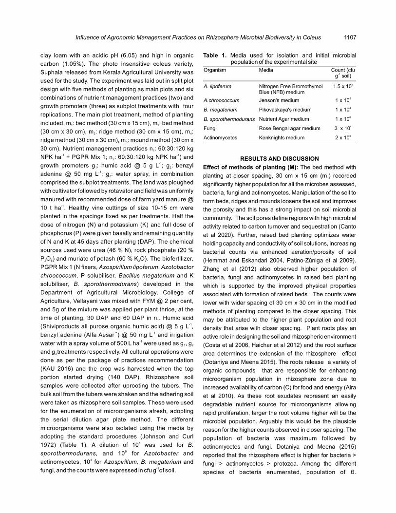
clay loam with an acidic pH (6.05) and high in organic
carbon (1.05%). The photo insensitive coleus variety,
Suphala released from Kerala Agricultural University was
used for the study. The experiment was laid out in split plot
design with five methods of planting as main plots and six
combinations of nutrient management practices (two) and
growth promoters (three) as subplot treatments with four
replications. The main plot treatment, method of planting
included, m : bed method (30 cm x 15 cm), m : bed method 1 2
(30 cm x 30 cm), m : ridge method (30 cm x 15 cm), m : 3 4
ridge method (30 cm x 30 cm), m : mound method (30 cm x 5
30 cm). Nutrient management practices n : 60:30:120 kg 1
NPK ha + PGPR Mix 1; n : 60:30:120 kg NPK ha ) and -1 -12
growth promoters g : humic acid @ 5 g L ; g : benzyl 1 2
-1
adenine @ 50 mg L ; g : water spray, in combination -13
comprised the subplot treatments. The land was ploughed
with cultivator followed by rotavator and field was uniformly
manured with recommended dose of farm yard manure @
10 t ha .-1 Healthy vine cuttings of size 10-15 cm were
planted in the spacings fixed as per treatments. Half the
dose of nitrogen (N) and potassium (K) and full dose of
phosphorus (P) were given basally and remaining quantity
of N and K at 45 days after planting (DAP). The chemical
sources used were urea (46 % N), rock phosphate (20 %
P O ) and muriate of potash (60 % K O). 2 5 2 The biofertilizer,
PGPR Mix 1 (N fixers, , Azospirillum lipoferum Azotobactor
chroococcum Bacillus megaterium, P solubiliser, and K
solubiliser, ) developed in the B. sporothermodurans
Department of Agricultural Microbiology, College of
Agriculture, Vellayani was mixed with FYM @ 2 per cent,
and 5g of the mixture was applied per plant thrice, at the
time of planting, 30 DAP and 60 DAP in n . Humic acid 1
(Shiviproducts all purose organic humic acid) @ 5 g L , -1
benzyl adenine (Alfa Aesar ) @ 50 mg L and irrigation ™ -1
water with a spray volume of 500 L ha were used as g , g -11 2
and g treatments respectively. All cultural operations were 3
done as per the package of practices recommendation
(KAU 2016) and the crop was harvested when the top
portion started (140 DAP). drying Rhizosphere soil
samples were collected after uprooting the tubers. The
bulk soil from the tubers were shaken and the adhering soil
were taken as rhizosphere soil samples. These were used
for the enumeration of microorganisms afresh, adopting
the serial dilution agar plate method. The different
microorganisms were also isolated using the media by
adopting the standard procedures (Johnson and Curl
1972) (Table 1). A dilution of 10 was used for 6 B.
sporothermodurans Azotobacter , and 10 for 5 and
actinomycetes, 10 for 4 Azospirillum, B. megaterium and
fungi, and the counts were expressed in cfu g of soil. -1
Organism Media Count (cfu g soil)-1
A lipoferum. Nitrogen Free Bromothymol Blue (NFB) medium
1.5 x 10⁴
A.chroococcum Jenson's medium 1 x 10⁵
B. megaterium Pikovaskaya's medium 1 x 10⁴
B sporothermodurans. Nutrient Agar medium 1 x 10⁶
Fungi Rose Bengal agar medium 3 x 10⁴
Actinomycetes Kenknights medium 2 x 10⁵
Table 1. Media used for isolation and initial microbial population of the experimental site
RESULTS AND DISCUSSION
Effect of methods of planting (M): The bed method with
planting at closer spacing, 30 cm x 15 cm (m ) recorded 1
significantly higher population for all the microbes assessed,
bacteria, fungi and actinomycetes. Manipulation of the soil to
form beds, ridges and mounds loosens the soil and improves
the porosity and this has a strong impact on soil microbial
community. The soil pores define regions with high microbial
activity related to carbon turnover and sequestration (Canto
et al 2020). Further, raised bed planting optimizes water
holding capacity and conductivity of soil solutions, increasing
bacterial counts via enhanced aeration/porosity of soil
(Hemmat and Eskandari 2004, Patino-Zúniga et al 2009).
Zhang et al (2012) also observed higher population of
bacteria, fungi and actinomycetes in raised bed planting
which is supported by the improved physical properties
associated with formation of raised beds. The counts were
lower with wider spacing of 30 cm x 30 cm in the modified
methods of planting compared to the closer spacing. This
may be attributed to the higher plant population and root
density that arise with closer spacing. Plant roots play an
active role in designing the soil and rhizospheric environment
(Costa et al 2006, Haichar et al 2012) and the root surface
area determines the extension of the rhizosphere effect
(Dotaniya and Meena 2015). The roots release a variety of
organic compounds that are responsible for enhancing
microorganism population in rhizosphere zone due to
increased availability of carbon (C) for food and energy (Aira
et al 2010). As these root exudates represent an easily
degradable nutrient source for microorganisms allowing
rapid proliferation, larger the root volume higher will be the
microbial population. Arguably this would be the plausible
reason for the higher counts observed in closer spacing. The
population of bacteria was maximum followed by
actinomycetes and fungi. Dotaniya and Meena (2015)
reported that the rhizosphere effect is higher for bacteria >
fungi > actinomycetes > protozoa. Among the different
species of bacteria enumerated, population of .B
1107Influence of Agronomic Management Practices on Rhizosphere Microbial Biodiversity in Coleus

Treatment A lipoferum. (10 )4
A. chroococcum (10 )5
B. megaterium (10 )4 B sporothermodurans. (10 )6
Fungi (10 )4 Actinomycetes (10 )5
Methods of planting
m1 7.25 5.50 4.88 2.67 13.08 6.92
m2 3.83 4.33 2.83 2.04 9.33 4.17
m3 5.62 5.75 3.88 2.75 10.46 4.21
m4 2.79 3.42 1.71 1.54 4.83 3.25
m5 2.96 2.38 2.25 1.75 9.38 4.17
CD (p=0.05) 0.33 0.38 0.28 0.46 0.39 0.37
Nutrient management x growth promoter
n g1 1 5.55 5.60 4.5 2.75 12.65 4.95
n g1 2 5.75 5.70 4.65 2.70 12.85 5.15
n g1 3 5.50 5.45 4.45 2.70 12.75 4.90
n g2 1 3.35 2.85 1.6 1.65 6.00 4.05
n g2 2 3.45 3.10 1.75 1.55 6.20 4.15
n g2 3 3.35 2.95 1.7 1.55 6.05 4.05
CD (p=0.05) 0.28 0.32 0.34 0.30 0.42 0.52
Table 2. Effect of methods of planting and combination of nutrient management and growth promoter on microbial count (cfu g -1
soil)
sporothermodurans 3 was highest in ridge planting (m ) with a
spacing of 30 x 15 cm (2.75 x 10 ) and on par with bed method 6
with the same spacing (2.67 x 10 ). The populations of 6 A.
lipoferum B. megaterium 4 -1(7.25 x 10 cfu g soil) and (4.88 x
10 cfu g soil) were superior in bed method of planting with 4 -1
lower spacing (m ) followed by ridge planting (m ) with a 1 3
spacing of 30 x 15 cm. Ridge and mound methods with
planting at 30 cm x 30 cm spacing (m and m respectively) 4 5
recorded lower populations of and were on par Azospirillum
whereas the lowest count of was enumerated B. megaterium
in the ridge method with spacing of 30 cm x 30 cm. The similar
trend of higher counts of in bed and ridge method of planting
with lower spacing of 30 cm x 15 cm were recorded for A.
chroococcum, 5 5 the population being 5.50 x 10 and 5.75 x 10
cfu g soil in m and m respectively. Fungal (13.08 x 10 cfu -1 41 3
g soil) and actinomycete (6.9 x 10 cfu g soil) populations -1 5 -1
were significantly the highest in bed method of planting with
lower spacing of 30 cm x 15 cm (m ) followed by ridge 1
planting with a spacing of 30 cm x 15 cm (m ) in the case of 3
fungi. The lowest counts of fungi and actinomycetes were
recorded in m , ridge method (30 cm x 30 cm). The variations 4
in specific species also followed the same trend as the total
counts, confirming that the closer spacing was primarily
responsible for the increased counts.
Effect of nutrient management and growth promoter (N x
G): The combination of nutrient management and growth
promoter registered significant influence on microbial
population. Irrespective of the growth promoters, all the
treatments which involved an integrated nutrient (INM)
package, 60:30:120 kg NPK ha + biofertilizer, PGPR Mix 1 -1
recorded the highest population of all microbes enumerated
under study. The results corroborate the findings of
Vijendrakumar et al (2014) and Gopi et al (2020).
Vijendrakumar et al (2014) observed that dual and triple
inoculation of biofertilizers resulted in maximum counts in soil
with respect to both beneficial and general microflora. The
lowest population of microbes was recorded in plots without
PGPR mix 1. It is apparent that the N fixers, P and K
solubilisers in the consortium biofertilizer augmented the
microbiome in the rhizosphere. In addition the better nutrient
availability, uptake and hence the growth and photosynthetic
efficiency with INM would resulted in proliferated root growth,
exudation of organic substances that enhanced microbial
activities. Photosynthates are comprised mainly of carbon
compounds, electrons, protons, water, and inorganic ions,
which all enter the rhizosphere as root exudates (Olanrewaju
et al 2019). .
Interaction effect of methods of planting, nutrient
management and growth promoter (M x N x G): The
interaction methods of planting and combination of effect of
nutrient management and growth promoter on the count of
microbial population as significant. The population of w
Azospirillum 4 -1 (9.50 x 10 cfu g soil) was highest in
combination, bed method (30 cm x 15 cm) + 60:30:120 kg
NPK ha + PGPR Mix 1 and benzyl adenine spray (m n g -1
1 1 2)
and on par with m n g and m n g (9.25x10 cfu g soil). The 1 1 1 1 1 34 -1
1108 Arunjith P. and Sheeba Rebecca Isaac

Treatments A lipoferum. (10 )4 A.chroococcum (10 )5
B. megaterium (10 )4
B sporothermodurans. (10 )6
Fungi (10 )4 Actinomycetes (10 )5
m n g1 1 1 9.25 7.50 6.25 3.50 16.25 6.50
m n g1 1 2 9.50 7.50 6.50 3.75 16.25 7.00
m n g1 1 3 9.25 7.25 6.25 3.75 16.50 6.75
m n g1 2 1 5.25 3.50 3.25 1.75 9.75 7.00
m n g1 2 2 5.25 3.75 3.50 1.50 10.00 7.00
m n g1 2 3 5.00 3.50 3.50 1.75 9.75 7.25
m n g2 1 1 5.25 5.50 4.25 2.75 11.25 5.25
m n g2 1 2 5.50 5.75 4.50 2.75 11.50 4.50
m n g2 1 3 5.25 5.25 4.25 2.50 11.25 4.50
m n g2 2 1 2.25 3.00 1.25 1.50 7.25 3.75
m n g2 2 2 2.50 3.25 1.50 1.25 7.50 3.50
m n g2 2 3 2.25 3.25 1.25 1.50 7.25 3.50
m n g3 1 1 6.00 7.25 6.25 3.25 15.25 4.25
m n g3 1 2 6.25 7.50 6.50 3.25 15.50 4.50
m n g3 1 3 6.00 7.25 6.25 3.00 15.25 4.25
m n g3 2 1 5.25 4.00 1.25 2.25 5.50 4.00
m n g3 2 2 5.00 4.25 1.50 2.50 5.75 4.25
m n g3 2 3 5.25 4.25 1.50 2.25 5.50 4.00
m n g4 1 1 3.50 4.50 2.25 2.00 6.25 3.00
m n g4 1 2 3.50 4.75 2.50 1.75 6.50 3.50
m n g4 1 3 3.25 4.25 2.25 2.00 6.25 3.25
m n g4 2 1 2.00 2.25 1.00 1.25 3.25 3.25
m n g4 2 2 2.25 2.50 1.25 1.25 3.50 3.25
m n g4 2 3 2.25 2.25 1.00 1.00 3.25 3.25
m n g5 1 1 3.75 3.25 3.50 2.25 14.25 5.75
m n g5 1 2 4.00 3.00 3.25 2.00 14.50 6.25
m n g5 1 3 3.75 3.25 3.25 2.25 14.50 5.75
m n g5 2 1 2.00 1.50 1.25 1.50 4.25 2.25
m n g5 2 2 2.25 1.75 1.00 1.25 4.25 2.75
m n g5 2 3 2.00 1.50 1.25 1.25 4.50 2.25
CD (p=0.05) 0.63 0.74 0.77 0.69 0.96 1.18
Table 3. Interaction effect of methods of planting and combination of nutrient management and growth promoter on microbial count ( cfu g of soil)-1
closer spacing, INM and foliar spray (growth promoter/ water
spray) recorded higher counts of in both bed Azotobatcter
and ridge method of planting. The values ranged between
7.25 to 7.50 x 10 cfu g soil. The . 5 -1 Bacillus B megateriumsp.
and also recorded similar trends B. sporothermodurans
indicating the superiority of closer spacing, INM and foliar
spray in enhancing beneficial bacteria in the root zone. The
highest counts of fungi (16.5 x 10 cfu g soil) were 4 -1
combination m n g which was on par with m n g and m n g . 1 1 3 1 1 1 1 1 2
In actinomycetes, m n g recorded the highest count of 7.25 1 2 3
x 10 cfu g soil, but was on par with the treatments 5 -1
comprising of bed method of planting with lesser spacing (30
cm x cm), irrespective nutrient and growth promoter along 15
with m n g The higher microbial counts in bed method of 5 1 2.
planting (30 cm x 15 cm) with 60:30:120 kg NPK ha + PGPR -1
Mix 1 is a reflection of the individual effects in combination.
The favourable environment for root and canopy spread
would have enhanced the rhizodeposits and created a niche
for microbial activity. The microbes help plants to grow and
function more effectively by increasing plant pathogen
1109Influence of Agronomic Management Practices on Rhizosphere Microbial Biodiversity in Coleus

resistance, retain more water, take up and utilize more
nutrients and, in general, increase their growth (Olanrewaju
et al 2019). The microbiota vary with the root exudates and
other rhizodeposits secreted by plants (Moe 2013). C and 3
C plants show variations in the types of exudates released 4
into the rhizosphere, with C plants are reported to exude 3
more carbohydrates and organic carbons (Nabais et al 2011)
and C plants, higher numbers of organic acids and amino 4
acids compared to C plants. Coleus is a C plant and 3 3
microbes that have affinity for the mannose, maltose, and
ribose sugars are more prominent in its rhizosphere.
Augmentation with PGPR Mix I contributed to the increased
microbial activity in the rhizosphere. The mutualistic relation
the co-exists in the soil-plant- microbe interface regulates
and induces responses in the rhizosphere which ultimately
governs organic matter decomposition, nutrient acquisition,
biotic and abiotic stress tolerance in the crop plants.
CONCLUSIONS
The agronomic management practice for a favourable
rhizosphere manipulation in coleus would include a land
preparation of raised beds with planting at a spacing of 30 cm
x 15 cm, manuring with the nutrient dose of 60:30:120 kg
NPK ha + PGPR Mix 1 @ 2% with 5 g per plant and -1
irrespective of growth promoter spray.
REFERENCESAira M, Gómez-Brandón M, Lazcano C, Bååth E and Domínguez J
2010. Plant genotype strongly modifies the structure and growth of maize rhizosphere microbial communities. Soil Biology and Biochemistry (12): 2276-2281.42
Bowen GD and Rovira AD 1999. The rhizosphere and its management to improve plant growth. Advances in Agronomy66:1-102.
Costa R, Götz M, Mrotzek N, Lottmann J, Berg G and Smalla, K 2006. Effects of site and plant species on rhizosphere community structure as revealed by molecular analysis of microbial guilds. (2): 236-249.FEMS Microbiology Ecology 56
De la Fuente Canto C, Simonin M, King E, Moulin L, Bennett MJ, Castrillo G and Laplaze, L 2020. An extended root phenotype: The rhizosphere, its formation and impacts on plant fitness. The Plant Journal 103(3): 951-964.
Dotaniya ML and Meena VD 2015. Rhizosphere effect on nutrient availability in soil and its uptake by plants: a review. Proceedings of the National Academy of Sciences, India Section B: Biological Sciences (1):1-12.85
Gopi GK, Meenakumari KS, Anith KN, Nysanth NS and Subha P 2020. Application of liquid formulation of a mixture of plant growth promoting rhizobacteria helps reduce the use of
chemical fertilizers in Amaranthus ( L.). Amaranthus tricolorRhizosphere 100212.15:
Haichar FEZ, Roncato MA and Achouak W 2012. Stable isotope probing of bacterial community structure and gene expression in the rhizosphere of Arabidopsis thaliana. FEMS Microbiology Ecology (2): 291-302. 81
Hemmat A and Eskandari I 2004. Conservation tillage practices for winter wheat fallow farming in the temperate continental climate of northwestern Iran. : 123-133. Field Crops Research 89
John KS, George J, Beegum SS and Shivay YS 2016. Soil fertility and nutrient management in tropical tuber crops: An overview. Indian Journal of Agronomy 61 (3): 263-273.
Johnson LF and Curl EA 1972. Methods for research on the ecology of soil-borne plant pathogens. Minneapolis, Burgess.
Kabir MH, Alam MK, Hossain MM, Hossain MJ 2004. Yield performance of whole-tuber and cut-piece planting of potato. Tropical Science 44 : 16-19.
KAU [Kerala Agricultural University] 2016. Package of Practices Recommendations: Crops th(15 Ed.). Kerala Agricultural University, Thrissur.
Kushwaha RK, Rodrigues V, Kumar V, Patel H, Raina M and Kumar D 2020. Soil microbes-medicinal plants interactions: ecological diversity and future prospect. In Varma A, Tripathi S and Prasad R (eds) (pp. 263-286). Plant Microbe SymbiosisSpringer, Cham.
Moe LA 2013. Amino acids in the rhizosphere: From plants to microbes. (9): 1692-1705.American Journal of Botany 100
Nabais C, Labuto G, Gonçalves S, Buscardo E, Semensatto D, Nogueira ARA and Freitas H 2011. Effect of root age on the allocation of metals, amino acids and sugars in different cell fractions of the perennial grass (bahiagrass). Paspalum notatumPlant Physiology and Biochemistry (12): 1442-1447. 49
Nedunchezhiyan M, Laxminarayana K and Chauhan VBS 2018. Soil microbial activities and yield of elephant foot yam as influenced by weed management practices in alfisols. International Journal of Vegetable Science (6): 583-596.24
Olanrewaju OS, Ayangbenro AS, Glick BR and Babalola OO 2019. Plant health: Feedback effect of root exudates-rhizobiome interactions. (3): Applied Microbiology and Biotechnology 1031155-1166.
Pati ˜no-Zú˜ Niga L, Ceja-Navarro JA, Govaerts B, Luna-Guido M, Sayre KD and Dendooven L 2009. The effect of different tillage and residue management practices on soil characteristics, inorganic N dynamics and emissions of N O, CO and CH in the 2 2 4
central highlands of Mexico: a laboratory study. Plant Soil 314: 231-241.
Schmidt JE, Vannette RL, Igwe A, Blundell R, Casteel CL and Gaudin AC 2019. Effects of agricultural management on rhizosphere microbial structure and function in processing tomato plants. Applied and Environmental Microbiology 85 (16): 123-130.
Vijendrakumar RC, Sreeramu BS, Shankarappal TH, Santhosh KV, Mallikarjuna AP and Umesha, K 2014. Effect of liquid bio fertilizers on growth, yield and survival of seedlings in garden rue ( Linn.). : 171-175.Ruta graveolens Plant Archives 14
Zhang X, Ma L, Gilliam FS, Wang Q and Li C 2012. Effects of raised-bed planting for enhanced summer maize yield on rhizosphere soil microbial functional groups and enzyme activity in Henan Province, China. : 28-37.Field Crops Research 130
Received 24 April, 2021; Accepted 20 July, 2021
1110 Arunjith P. and Sheeba Rebecca Isaac

Influence of Organic Formulations as Foliar Sprays on Yield Attributing Traits of Onion ( L.)Allium cepa
Indian Journal of Ecology (2021) 48(4): 1111-1114Manuscript Number: 3341
NAAS Rating: 5.79
Abstract: The present investigations with five promising onion varieties of Haryana region were selected viz. Pusa Riddhi, Pusa Madhavi, NHRDF Red, Pusa Red and AGLR were conducted for yield potential. Three organic formulations were applied as pre- harvest spray viz. ,neem based formulation (Besara), Panchgavya, (bio shield) and Control (water). Organic formulations sprayed as foliar Trichoderma viride application at the interval of fifteen days on pre-harvest gave better results in yield and yield attributing characters of onion as compared to control condition. Panchgavya applications resulted in maximum plant height, number of leaves, bulb diameter and bulb weight irresptives of onion varieties. Among the onion varieties Pusa Riddhi exhibited maximum plant height, number of leaves, bulb diameter and bulb weight. Minimum response was in onion varieties treated with Trichoderma viride.
Keywords: Onion, Organic formulations, Varieties, Yield attributes
Vinay Kumar and Prabhat Kumar Singh1
Department of Genetics and Plant Breeding, Lovely Professional University, Phagwara, Jalandhar-144 113, India1Department of Genetics and Plant Breeding, MSSSoA, Centurion University of Technology and Management
Paralakhemundi-761 211, IndiaE-mail: [email protected]
Onion ( L.) is one of the oldest bulbous crops Allium cepa
known to mankind and consumed worldwide in various
cooked and raw forms. It is one of the most important
commercial horticultural vegetable crops and is of global
commercial importance. It is grown in almost all part of the
world and believed to be originated in central Asia (Kukanoor
2005). India ranks second in the production of onions next to
china and contribute about 19.25% of total world production
(FAO 2018).The other leading onion producing countries
apart from china and India are United States of America,
Turkey and Pakistan. In the year 2017-18, India exported
about 1588985 MT of fresh onion to the world amounting to
479.32 million USD. The major export destination included
Bangladesh, Sri Lanka, Malaysia, UAE and Nepal (APEDA
2018). It is also reported that productivity of India (14.35 t ha ) -1
is 5 times less compared to Republic of Korea (66.16 t ha ), 4 -1
times less than USA (56.13 t ha ), Spain (55.21 t ha ), -1 -1
Netherland (51.64 t ha ) and Myanmar (46.64 t ha ) -1 -1
(Chengappa et al 2012). The conventional methods of
fertilization and application of inorganic chemicals have
helped in both i.e. the bulb yield and the bulb quality. But, in
India the routine management practice appear to be
incapable of maintaining yield over the long period. The
steady reduction of soil fertility and occurrence of several
nutrient deficiencies in onion field has led to the reduced
onion production (Sharma et al 2003).
In past few years, organic agriculture is getting hold of
movement in India (Gopal 2015) due to individual as well as
group efforts to protect environment and contamination of
farm produce from use of chemical fertilizers and pesticides.
Since, Onion is a bulbous crop and is capable of scavenging
heavy metals from soil or contaminated irrigation water,
applied chemicals etc., poses severe health hazard. It is
really crucial to develop ecological and eco-friendly noble
agricultural practices through organic resources based on
scientific facts so that safe and hygienic production of onion
crop could be achieved (Worthington 1998, Kannaiyan
2000). During the past ten years a gradual shift in affinity
towards organically grown produce has been noticed and as
a result of which demand of organically grown onion has also
been seen increasing (Naik et al 2014). Presently, India is
ranked 10 among the countries in terms of area under th
organic certification. India produced approximately 1.24
million MT of certified organic products in all varieties of foods
(APEDA 2018). Since, State of Haryana is among top 10
leading onion producing states of the country, an attempt was
made through this study to evaluate quality of five major
promising onion varieties of Haryana region (Pusa Riddhi,
Pusa Madhavi, NHRDF Red, Pusa Red and AGLR) and
effect of different organic formulations (applied as foliar
sprays during growth period) on quality and yield.
MATERIAL AND METHODS
Present investigation conducted at National Institute of
Food Technology Entrepreneurship and Management
(NIFTEM), Sonepat, Haryana during seasons of 2014-Rabi

16. Seedlings of five indigenous varieties of onion obtained
from regional station IARI, Karnal, Haryana (Pusa Riddhi,
Pusa Madhavi) and from regional station National
Horticulture Research and Development Foundation
(NHRDF), Karnal, Haryana (NHRDF Red, Pusa Red and
AGLR) were used as experimental materials. The field
experiment was conducted in randomized block design
(RBD) with three replications. The seedlings were planted in
plot size of 10 m x 4 m. with plant to plant spacing of 10 cm
and row to row spacing 15 cm.
Four different treatments Neem based formulation viz.
(Besara) @20 ml L , Panchgavya @100ml L , -1 -1 Trichoderma
viride -1(Bio Shield) @50g L and untreated control were
subjected in form of foliar spray to all the varieties in
replicated mode. The organic formulations mentioned as
above were applied at four different intervals of times as pre-
harvest foliar sprays using hand sprayer. First spray applied
at 30 days to transplanting and subsequently remaining three
sprays given at 15 days interval (45, 60 and 75 days). The
dosage of respective organic formulation to be applied was
finalized as suggested by (Compant et al. 2019).
RESULTS AND DISCUSSION
Plant height: There was significant difference in plant height
of different onion cultivars due to application of organic
formulation and different onion varieties. Pusa Riddhi
exhibited maximum plant followed by Pusa Red. The
application of panchgavya had significant impact on plant
height on all varieties. The maximum plant height was in
Pusa Riddhi (45.85cm) followed by Pusa Red and NHRDF
Red. The least impact on plant height of onion varieties was
observed with the application of . All onion Trichoderma viride
varieties were responsive towards application of panchgavya
and neem based formulation and recorded significant
increase in plant height as compared to control. The increase
on plant height due to application of panchgavya was also
Treatments [A] Plant height (cm) of onion varieties [B]
Pusa Madhavi Pusa Riddhi Pusa Red NHRDF Red AG LR Mean
Control 40.80 (10.30) 44.38 (13.17) 42.33 (12.23) 41.36 (8.09) 40.50 (6.30) 41.87 (10.02)
Neem based formulation 41.54 (11.42) 46.10 (14.43) 44.17 (13.14) 42.34 (9.09) 41.09 (7.79) 43.05 (11.18)
Panchgavya 42.40 (13.45) 48.36 (17.06) 45.25 (14.81) 43.09 (10.30) 42.92 (8.38) 44.41 (12.80)
Trichoderma viride 40.84 (10.36) 44.58 (13.14) 42.45 (12.53) 41.52 (8.14) 40.62 (6.46) 42.00 (10.13)
Mean 41.40 (11.39) 45.85 (14.52) 43.55 (13.18) 42.08 (8.90) 41.29 (7.23)
CD (p=0.05) Treatments [A] Varieties [B] Interaction [A x B]
0.02 (0.01) 0.01 (0.01) 0.02 (0.03)
Table 1. Impact of foliar spray of organic formulations on plant height (cm) and number of leaves plant * of selected onion -1
varieties
*No. of leaves plant in parentheses-1
reported by Kumar and Neeraj (2015) in onion and Kumar et
al (2020) in legume. The increase of plant height may be due
to better nutrient uptake and metabolization efficiency
resulting in increased cell division and enhancement of cell
size.
Number of leaves per plant: The results showed that
irrespective of treatments, among various onion varieties the
maximum number of leaves per plant was observed in Pusa
Riddhi (14.52) on overall mean basis (Table 1). Maximum
number of leaves among varieties applied with panchgavya.
Pusa Riddhi exhibited highest number of leaves (17.06)
followed by Pusa Red which was significantly higher as
compared to other treatments. Even under control condition,
maximum number of leaves per plant was recorded in Pusa
Riddhi (13.17) followed by Pusa Red (12.23), which were
higher and statistically significant as compared to number of
leaves in AGLR (6.30). No major difference was observed in
onion varieties applied with and control. The T. viride
application of neem based formulation was second best
treatment as compared to and control. Trichoderma viride
Similar results regarding more number of leaves per plant
were recorded by Selvaraj (2003) and Choudhary et al
(2017) while working with panchgavya and neem based
formulations.
Bulb diameter: The results in Table 2 irrespective of
treatments, on overall mean basis showed that Pusa Riddhi
had highest bulb diameter (45.71mm) followed by Pusa Red
(42.50mm), NHRDF red (41.32mm). The smallest bulbs
were observed in AGLR (38.29mm). Even under control
condition, maximum bulb diameter was recorded in Pusa
Riddhi (44.50mm) followed by Pusa Red (41.80mm). Among
various treatments applied, on over all mean basis, the
maximum bulb diameter (irrespective of varieties) was
observed in onion bulbs treated with panchgavya
(43.38mm).
This was slightly higher as compared to other treatments
1112 Vinay Kumar and Prabhat Kumar Singh

Treatments [A] Bulb diameter (mm) of onion varieties [B]
Pusa Madhavi Pusa Riddhi Pusa Red NHRDF Red AG LR Mean
Control 39.89 (86.33) 44.50 (89.34) 41.80 (87.87) 40.85 (80.54) 37.65 (72.17) 40.94 (83.27)
Neem based formulation 40.09 (87.46) 45.46 (90.77) 42.17 (87.67) 41.06 (81.21) 37.84 (72.15) 41.32 (83.91)
Panchgavya 41.86 (88.60) 48.15 (92.34) 44.07 (89.15) 42.51 (88.67) 39.90 (73.60) 43.38 (86.47)
Trichoderma viride 39.95 (86.51) 44.72 (89.22) 41.96 (87.29) 40.84 (80.76) 37.76 (72.30) 41.05 (83.21)
Mean 40.45 (87.23) 45.71 (90.42) 42.50 (88.00) 41.32 (82.80) 38.29 (72.65)
CD (p=0.05) Treatments [A] Varieties [B] Interaction [A x B]
0.02 (0.38) 0.02 (0.53) 0.05 (0.86)
Table 2. Impact of foliar spray of organic formulations on Bulb diameter (mm) and bulb weight* (g) of selected onion varieties
*bulb weight in parentheses
and control. The least bulb diameter irrespective of
treatments was observed in control (40.94mm). Among
various varieties, maximum bulb diameter was observed with
panchgavya application in Pusa Riddhi (48.15mm) followed
by Neem extract (45.46mm), which more than control
(44.50mm). Similarly, in Pusa Red, application of
panchgavya gave maximum diameter (44.07mm) followed
by application of Neem based formulation (42.17mm), which
was more than control (41.80mm). The least impact on bulb
diameter of onion bulb was observed with application of
Trichoderma viride in all the varieties which was more or less
same as that of control. The results are in accordance with
the finding of Kondappa et al (2009) and Manna et al (2016) in
chilli with different organic formulations.
Bulb weight: There was increase in bulb weight as a result of
application of various organic formulations as compared to
control (Table 2). Maximum bulb weight was recorded with
application of panchgavya. Irrespective of treatments, Pusa
Riddhi had maximum mean bulb weight (90.42gm) on overall
mean basis followed by in Pusa Red (88.00gm), Pusa
Madhavi (87.23gm). The minimum bulb weight was observed
in AGLR (72.65gm). The maximum bulb weight was
observed in all the selected onion varieties as result of
panchgavya application, however, the maximum bulb weight
was recorded in Pusa Riddhi (92.34gm) followed by 89.15gm
in Pusa Red. Pusa Madhavi, NHRDF Red showed similar
weight with panchgavya application (i.e. 88.60gm and
88.67gm, respectively). The results obtained with the
application of panchgavya in all the varieties were higher and
differences were statistically significant as compared to
control and application. The results also Trichoderma viride
showed that there was about 10% increase in bulb weight in
NHRDF Red (88.67gm) with panchgavya application as
compared to control (80.54gm). Similar finding on increase in
weight of onion bulb have also been reported by other
researchers working with onion (Boyhan et al 2001, Meena
2017).
CONCLUSION
Pusa Riddhi had maximum overall mean value for plant
height, number of leaves per plant, bulb diameter and bulb
weight and appeared as the best performing variety under
the given organic treatment. Among numerous treatments
applied, irrespective of varieties, Panchgavya exhibited
better growth as compared to other treatments including
control for all the attributing characters under study. On
contrary, irrespective of genotypes Trichoderma viride
showed minimum response towards all the characters
studied.
REFERENCESAPEDA 2018. Agricultural and Processed Food Products Export
D e v e l o p m e n t A u t h o r i t y ( A P E D A ) D a t a b a s e (www.apeda.gov.in).
Boyhan GE, Randle WM, Purvis AC, Lewis PM, Linton DO, Torrance RL, and Curry DE 2001. Evaluation of growth stimulants on short-day onions. (1): 38-42.Hort-Technology 11
Chengappa PG, Manjunatha AV, Vikas D and Khalil S 2012. Competitive assessment of onion markets in India. Institute for social and economic change. Competition commission of India, 1-81.
Choudhary GL, Choudhary SK, Singh SK, Kaushik MK and Bazaya BR 2017. Effect of panchagavya on quality, nutrient content and nutrient uptake of organic blackgram ( L.). Vigna mungo Journal of Pharmacognosy and Phytochemistry 6 (5): 1572-1575.
Compant S, Samad A, Faist H and Sessitsch A 2019. A review on the plant microbiome 2019. Ecology, functions, and emerging trends in microbial application. Journal of Advanced Research1(19):29-37.
FAO 2018. Onion Production. Food and Agriculture Organization (FAO) of the United Nations, FAOSTAT. http://faostat.fao.org.
Gopal J 2015. Onion research in India: status and challenges. Progressive Horticulture 47 (1): 1-19
Kannaiyan K 2000. Bio fertilizers Key factors in organic farming. The Hindu survey of Indian agriculture, 165-173.
Kondapa D, Radder BM, Patil PL, Hebsur NS and Alagundagi SC 2009. Effect of integrated nutrient management on growth, yield and economics of chilli (cv. Byadgi dabbi) in a vertisol. Karnataka Journal of Agricultural Sciences 22 (2): 438-440.
Kukanoor L 2005. Postharvest studies in onion cv. N.53. PhD Thesis, University of Agricultural Sciences Dharwad, India.
Kumar S, Sharma SB, Nongrum MM, Singh TR, Kumari N and Rozar KP 2020. Effect of pre-sowing treatments on the
1113Influence of Organic Formulations on Yield Attributing Traits of Onion

germination of five legume species and their tolerance to desiccation. (1): 102-108Indian Journal of Ecology 47
Kumar V and Neeraj 2015. Evaluation of the performance of onion varieties in response to organic cultivation. International Journal of advance Research 3 (9): 1558-1562.
Manna D and Maity TK 2016. Growth, yield and bulb quality of onion ( L.) in response to foliar application of boron and Allium cepazinc. (3): 438-441.Journal of Plant Nutrition 39
Meena KR 2017. Effect of organic manures, biofertilizers and micronutrients on growth, yield and quality of onion ( Allium cepaL.). (2): 236-241.International Journal of Agricultural Sciences 13
Naik VR, Patel PB and Patel BK 2014. Study on effect of different organics on yield and quality of organically grown onion. The
Bioscan 9 (4): 1499-1503.
Selvaraj N 2003. Report on the work done on organic farming at Horticultural Research Station. In: Panchagavya- Boon to Organic Farming. Eds. (4): Asian Journal of Plant Sciences 9215-220.
Sharma RP, Datt N and Sharma PK 2003. Combined application of nitrogen, phosphorus, potassium and farmyard manure in onion ( L.) under high hills, dry temperate conditions Allium cepaof north-western Himalayas. Indian Journal of Agricultural Science 73 (4): 225-227.
Worthington V 1998. Effect of agricultural methods on nutritional quality: A comparison of organic with conventional crops. Alternative Therapies 4 (1): 58-69.
Received 03 July, 2021; Accepted 31 July, 2021
1114 Vinay Kumar and Prabhat Kumar Singh
Influence of Foliar Application of Nano-Zinc and Iron Fertilizers on Growth and Yield of Bell Pepper ( L.)Capsicum annuum
Indian Journal of Ecology (2021) 48(4): 1115-1119Manuscript Number: 3342
NAAS Rating: 5.79
Abstract: A field experiment in the autumn 2019 was conducted to investigate the combined effect of foliar spraying with nano zinc and iron fertilizers on growth and yield of bell 0, 1.5, 3, and 4.5 g. The spraying with nano-Fe and nano-zinc at 3 g l resulted in significant increase in -1
plant height, the number of branches, leaf area, dry weight, leaf content of chlorophyll, nitrogen, phosphorus, and potassium, number of fruits, fruit weight and total yield. The iron and zinc nano at 3 g l + 3 g l had significant effect on all the above traits. Nano-fertilizers as a foliar -1 -1
application enhanced the growth and yield of bell pepper with a higher uptake of nutrients.
Keywords: Bell pepper, Micronutrient, Nano fertilizers, Fe and Zn
Hassan Hadi Alkarawi and Sana Qasim Hasan
Al-Mussaib Technical College ,Al-Furat Al-Awast Technical University, Babylon, IraqE-mail: [email protected]
Pepper is cultivated in Iraq with the traditional method at
the beginning of spring under field conditions and the
protected method at the beginning of autumn. Fertility can
improve by adding organic and inorganic fertilizers to the soil.
Nanotechnology improves soil fertility and crop production
while minimizing environmental impact. Improving food
security and environmental sustainability in agricultural
systems requires an integrated approach to managing soil
fertility, ensuring that crop production is minimizing the
depletion of nutrient stocks in the soil. Using nanotechnologies
in agriculture helps to improve soil fertility practices, supporting
the intensification of crop production and the conservation of
natural resources. Soil fertility can by improved through nano
fertilizers that add organic matter to the soil, which leads to
improved soil structure and contributes to creating healthy and
fertile soils, or by spraying foliar fertilizers, to compensate for
the losses resulting from plant uptake and other processes of
the crops through improved nutrient use (Ziogas et al 2020).
Using foliar nutrients is a complementary method of soil
fertilization, which addresses the shortage of one of the
important nutrients for plant growth (Singh et al 2017). The
most important objectives of agricultural policy are to improve
production and increase the number of agricultural products, in
order to meet the needs of the ever-growing population.
Among these technologies, nanotechnology has the potential
to revolutionize agricultural systems, biomedicine,
environmental engineering, safety, security, and energy
conversion (Taran et al 2021, Kaphle et al 2018). The aim of
this research was to determine the effect of foliar application of
two types of iron and zinc nano fertilizers and their effect on the
indicators of vegetative growth and yield of bell pepper.
MATERIAL AND METHODS
The experiments were conducted in a non-heated
plastic house at Al-Mussaib Technical College during the
autumn 2019to observe the effect of foliar spraying with nano
zinc and iron fertilizers on growth and yield of bell pepper
(Yolo Wonder cultivar). The study included two factors, first
factor included four concentrations of iron nano fertilizer (0,
1.5, 3, and 4.5 g l ) and the second factor included four -1
concentrations of the zinc nano fertilizer (0, 1.5, 3, and 4.5 g l-
1). The spraying was done five times at 20 days interval.
Control treatment was sprayed with water only. The spraying
was done in the morning and until the complete wetness for
the plants, which is preceded by irrigation of the seedlings
before one day .The irrigation prior to spraying reduces the
concentration of the solutes in the leaf cells because of the
water entering and increasing the swelling, thus opening the
stone which increases the permeability of the spraying
solution ions to the leaf cells (Schjoerring et al 2019). The
recommended cultivation practices were followed as per the
vegetable production guide, 2013. The experimental design
was randomized complete block design with three replicates
test. All statistical tests were performed with the program R
2.15.0 (Team RC 2017). The mineral fertilizer was added with
an average of 250 kg ha of ammonium sulfate and 150 kg ha 1 1
of triple superphosphate in two batches during the vegetative
and flowering stage. Random samples were collected from
the soil field of the Bell pepper from three areas with a depth
of 0-30 cm. The samples were mixed well and analyzed to
determine the physicochemical traits according to standard
methods (Jackson 1958) (Table 1).
After completion of the experiment, the data on various

Traits Value Unit
Electrical conductivity 2.7 ds.S-1
pH 7.1 --
Organic matter 9.5 g kg soil-1
Interchangeable capacity 16.92 Cmol.kg soil-1
Calcium carbonate 18.3 g kg soil-1
Nitrogen 23.5 Cmol.kg soil-1
Phosphorus 4.9
Potassium 67.9
Apparent density 1.42 μg m-3
Sand 601.6 g kg soil-1
Silt 241.3
Clay 157.1
Soil texture Loamy sand soil
Table 1. Physical and chemical traits of the soil used in the experiment
Fe (g l )-1 Plant length (cm) Average Number of fruit branches per plant Average
Zinc (mg l )-1 Zinc (mg l )-1
0 1.5 3 4.5 0 1.5 3 4.5
0 53.7 77.2 98.5 96.3 81.34 2.8 3.5 4.6 3.9 3.7
1.5 79.4 89.5 101.6 97.4 91.98 4.7 5.0 6.2 5.5 5.35
3 102.3 106.9 110.9 103.3 105.85 5.9 6.3 6.9 6.6 6.43
4.5 97.5 101.9 106.2 105.5 102.93 4.5 5.5 6.4 6.8 5.80
Average 83.23 93.88 104.45 100.63 4.48 5.08 6.03 5.7
LSD (0.05) Fe Zn Interaction 7.48 7.48 13.56
Fe Zn Interaction 0.41 0.41 0.76
Table 2. Effect of foliar application of nano fertilizer on plant height and number of branches
parameter was recorded from six plants which included plant
height and stem height was measured to the apical meristem,
number of branches per plant, leaf area, dry weight of plants
(dried at 70-75 °C in an electric oven and until the weight is
stable), number of fruits and fruit weight, and total yield of
plant . Nitrogen in leaves was estimated using macro or micro
Kjeldahl technique method (Jackson 1958), phosphorus by
using the acid, ammonium oxalate extraction method (Olsen
and Sommers 1982) and potassium by using a Flame
photometer. Vitamin C content was estimated with the
method of Horwitz et al (1970).
RESULTS AND DISCUSSION
Plant height (cm) and number of branches: The plant
height and the number of fruit branches differ significantly in
different treatments. Maximum plant height and number of
fruit branches (105.85 cm and 6.43 branches, respectively)
were in nano solution of iron and zinc at a concentration of 3
ml l , compared to the control (81.43 cm and 3.7 branches, -1
respectively) (Table 2). The spraying of the zinc nano at
different levels led to a significant increase in these two traits
(110.9 cm and 6.9 branches, respectively). The lowest
average for these two traits was in control. There was no
significant differences between the two factors (3 g l ) and -1
(4.5 g l ) for both elements and both traits. The interaction -1
treatment (spraying fertilizers at a level of 3 g l Fe + 3 g l Zn) -1 -1
resulted in the maximum plant height and the number of
branches (. The lowest average of these two traits was in
control.
Leaf area and the dry weight of the plant: There were
significant differences between the spraying levels for the
iron Nano on leaf area and the dry weight, with spraying at 3 g
l . The average number of leaves in the seedling and the leaf -1
area were 25.48 dm and 108.9 g, respectively compared to 2
the control treatment (spraying with add water) (19.05 dm 2
and 92.23 g, respectively) (Table 3). Spraying with the nano
zinc at different levels led to a significant increase in leaf area
and the dry weight (24.33 dm , 112.72 g), compared to the 2
control treatment. With the addition of nano zinc at 3 and 4.5 g
l there is no difference between them in both traits. The -1
interaction between the two factors had a significant effect on
the increase in the average leaf area and dry weight. The e
spraying t with a mixture of the two fertilizers (nano iron 3 g l -1
+ nano zinc 3 g l ) gave maximum leaf area and the dry -1
weight (26.3 dm and 121.2 g, respectively). 2
Phosphorus and potassium content in leaves (%):
The differences were significant between the spraying levels
of the nano iron solution on phosphorus and potassium in the
leaves (%) and spraying treatment at 3g l gave the highest -1
phosphorus and potassium in the leaves o (0.67, 1.99%,
respectively) as compared to the control (0.51, 1.44%,
respectively) (Table 4). The spraying with the nano zinc
fertilizer at 3 g resulted in increase in the percentage of 1
phosphorus in the leaves (0.66%) and spray nano zinc
fertilizer at 4.5 g L was significant in the t content of -1
1116 Hassan Hadi Alkarawi and Sana Qasim Hasan

Fe (g l )-1 Phosphorus (%) Average Potassium (%) Average
Zinc (mg l )-1 Zinc (mg l )-1
0 1.5 3 4.5 0 1.5 3 4.5
0 0.38 0.47 0.60 0.62 0.51 1.32 1.39 1.47 1.60 1.44
1.5 0.50 0.61 0.66 0.63 0.60 1.39 1.46 1.68 1.64 1.53
3 0.63 0.69 0.70 0.68 0.67 1.73 1.83 2.27 2.15 1.99
4.5 0.65 0.66 0.68 0.67 0.66 1.59 1.70 2.17 2.16 1.90
Average 0.53 0.60 0.66 0.64 1.50 1.59 1.88 1.89
LSD (0.05) Fe Zn Interaction 0.04 0.04 0.07
Fe Zn Interaction 0.28 0.28 0.52
Table 4. Effect of foliar application of nano fertilizer on phosphorus and potassium content in leaves
Fe (g l )-1 Number of fruits per plant Average Fruit weight (g) Average
Zinc (mg l )-1 Zinc (mg l )-1
0 1.5 3 4.5 0 1.5 3 4.5
0 23.8 27.5 29.8 28.5 27.4 78.6 82.2 88.3 89.4 84.63
1.5 26.3 28.8 32.9 31.4 29.85 80.6 85.6 90.2 91.2 86.9
3 28.9 32.4 35.6 33.6 32.63 89.4 94.2 109.5 105.8 99.73
4.5 29.5 30.2 33.2 34.0 31.73 90.6 93.3 107.7 106.7 99.58
Average 27.13 29.73 32.88 31.88 84.80 88.83 98.93 98.28
LSD (0.05) Fe Zn Interaction 1.07 1.07 1.75
Fe Zn Interaction 7.62 7.62 14.20
Table 5. Effect of foliar application of nano fertilizer on fruit number and fruit weight
Fe (g l )-1 Leaf area (dm )2 Average Dry weight for the total vegetative (g ) Average
Zinc (mg l )-1 Zinc (mg l )-1
0 1.5 3 4.5 0 1.5 3 4.5
0 17.4 18.6 19.7 20.5 19.05 76.7 92.9 95.9 96.4 90.55
1.5 21.6 22.8 25.6 23.9 23.48 85.9 90.0 115.7 111.8 100.85
3 24.8 25.4 26.3 25.4 25.48 96.3 98.6 121.2 119.5 108.9
4.5 22.7 24.2 25.7 25.1 24.43 95.3 97.8 118.1 109.8 105.25
Average 21.63 22.75 24.33 23.72 88.55 94.83 112.72 109.37
LSD (0.05) Fe Zn Interaction 1.08 1.08 1.76
Fe Zn Interaction 7.68 7.68 14.22
Table 3. Effect of foliar application of nano fertilizer on a leaf area and dry weight of total plant
potassium with highest averages of 1.89% as compared to
the control . The interaction between the two factors had a
significant effect on the increase in the average leaves'
content from the phosphorus and potassium. The interaction
of spraying with a mixture of the two fertilizers (3 g l Fe + 3 g l-1 -
1 Zn) gave the highest average of leaves content from the
phosphorus and potassium (0.70, 2.27%, respectively).
Number of fruits and weight: There were significant
differences between the spraying levels for the iron nano for
the number of fruits per plant and the average weight of fruit
at a concentration of 3 g l (32.36, 99.73g, respectively) -1
compared to the control (27.4 fruits, 84.63 g respectively).
Spraying zinc Nano fertilizer at 3 g l led to a significant -1
number of fruits per plant (Table 5). The interaction between
the two factors had a significant effect on the increase in the
average number of fruits per plant and the average weight of
fruit. The interaction treatment spraying with iron nano at a
level of 3 g l and zinc nano at level 3 g l (35.6 fruits and -1 -1
1117Growth and Yield of Bell Pepper

Fe (g l )-1 Total yield (kg plant )-1 Average Vitamin C (mg kg )-1 Average
Zinc (mg l )-1 Zinc (mg l )-1
0 1.5 3 4.5 0 1.5 3 4.5
0 1.63 1.99 2.28 2.56 2.11 12.73 13.15 13.36 13.21 13.11
1.5 2.01 2.18 2.99 2.70 2.47 13.24 13.45 14.24 13.85 13.69
3 2.39 2.89 3.58 3.27 3.03 14.92 15.34 15.72 15.39 15.34
4.5 2.44 2.72 3.35 3.31 2.96 13.33 13.52 14.71 13.82 13.84
Average 2.11 2.44 3.05 2.96 13.55 13.86 14.5 14.06
LSD (0.05) Fe Zn Interaction 0.23 0.23 0.42
Fe Zn Interaction 0.88 0.88 1.11
Table 6. Effect of nano fertilizer in the average of the total plant yield and vitamin C
Fe (g l )-1 Total yield (kg plant )-1 Average Vitamin C (mg kg )-1 Average
Zinc (mg l )-1 Zinc (mg l )-1
0 1.5 3 4.5 0 1.5 3 4.5
0 4.50 4.55 4.74 4.63 4.60 4.74 4.76 5.11 5.92 5.13
1.5 4.59 4.95 5.19 5.09 4.95 5.26 5.33 6.98 6.72 6.07
3 4.97 5.16 5.89 5.41 5.36 8.54 9.24 10.58 9.51 9.47
4.5 4.91 4.92 5.67 5.33 5.21 7.03 7.12 8.44 7.45 7.51
Average 4.74 4.89 5.37 5.11 6.39 6.61 7.77 7.4
LSD (0.05) Fe Zn Interaction 0.26 0.26 0.49
Fe Zn Interaction 0.92 0.92 1.24
Table 7. Effect of the nano fertilizer on the total sugars and carotenoids
109.5 g, respectively) had a significant difference.
Plant yield and vitamin C: The differences were significant
between the spraying levels for the iron and zinc nano
solution in the total yield and vitamin C The spraying
treatment of iron nano at 3 ml l gave the highest average of -1
the total yield and vitamin C (3.03 kg, 15.34 mg kg -1)
compared to the control (2.11 kg plant , 13.11mg kg ) (Table -1 -1
6). The addition of spraying of zinc nano at different levels
resulted in significant increase in yield and vitamin C (3.05 kg
per plant, 14.5 mg per kg . The lowest average for these traits )
was at the treatment without spraying with the two fertilizers.
Total sugars and carotenoids: There were significant
differences between the spraying levels for the iron nano for
the total sugars and carotenoids at a concentration of 3 g l -1
(5.36%, 9.47 mg kg , respectively) as compared to the -1
control (4.60%, 5.13 mg kg , respectively). Spraying zinc -1
nano fertilizer at 3 g l ) led to a significant increase of the total -1
sugars and carotenoids (Table 7). The addition of spraying of
zinc Nano at different levels led to a significant increase in
these two traits above (The lowest average for these two
traits was in without spraying with the two fertilizers. The
interaction between the two factors had a significant effect on
the increase in the average of total sugars and the
carotenoids.
These factors (spraying with the two types of Nano
fertilizers (iron and zinc) affected significantly all indicators of
vegetative and flowering growth. The level of spraying 3 g l ) -1
for the two fertilizers sequentially significantly excelled in plant
height, the number of branches, leaf area, dry weight, leaf
content of chlorophyll, percentage of nitrogen, phosphorus,
and potassium in the leaves. This reason may be because of
iron is a necessary element for plant growth and development
(Rui et al 2016). Iron also contributes many of bio-processes
including the production of amino acids, metabolism, and
enzymes that help to increase cellular divisions and increase
the activity of enzymes against the process of oxidation and
this leads to the organization of plant growth and the
promotion of activity, which reflects the increase in the
indicators of vegetative growth of the plant. Foliar application
of nano iron resulted in a significant improvement in growth
and yield, which might be attributed to increased
photosynthetic activity and increased production and
accumulation of carbohydrates. It contributes to the promotion
of energy transfer and metabolism and increased cell division,
These results were positively reflected with the increase in
plant height averages, the number of branches, leaf area, and
concentration of phosphorus and potassium in leaf tissue and
fruits and were observed by many authors (Jadczak et al
2010, Nair et al 2011, Zaki et al 2013).The increase in the
number of fruit branches with use foliar fertilization leaf with
iron nano can be an attribute that the iron component reduces
the auxins that promote the growth of the apical growth and
1118 Hassan Hadi Alkarawi and Sana Qasim Hasan

therefore plant tends from more fruit branches. Nechitailo et al
(2018) observed similar results on growth indices of bell
pepper. The significant effect of zinc nano in the indicators of
the vegetative growth can also be attributed to in the amino's
formation acid tryptophan and formation of the growth
regulator IAA, which affects the increase of cell division and
promotes the activity of cell membranes and division and
many of the biological reactions (Guo et al 2011). The
significant increase in the number of fruits and their weight
and total yield because of the spraying of the two types of
Nano which may be attributed to the role of nano-nutrients (Fe
and Zinc) in the synthesis and activation of many enzymes
necessary for the Bio-processes in the plant and control the
hormonal balance of the plant and this is the increase in the
indicators of vegetative growth (Zhao et al 2019).
CONCLUSION
This study unraveled the factors affecting the response of
Bell pepper to nano foliar application. The iron and zinc nano
fertilizers had a significant effect on the indicators of growth
and yield of Bell pepper. However, the iron nano fertilizer
alone or combined with the addition of zinc nano fertilizers at
the stages of growth could be useful in improving vegetative
growth, quality and yield of bell pepper.
REFERENCESAbdul-Jabbar G 2012. Effect of foliar nutrition on the growth and yield
of sweet pepper L.(carisma cultivar). Capsicum annuum Al-Furat Journal of Agricultural Sciences 3 (2): 57-62.
Afshar I, Haghighi AR and Shirazi M 2014. Comparison arison the effect of spraying different amounts of nano zinc oxide and zinc oxide on wheat (3): 688-693.. IJPAES 4
Amiri A, Baninasab B, Ghobadi C and Khoshgoftarmanesh AH 2016. Zinc soil application enhances photosynthetic capacity and antioxidant enzyme activities in almond seedlings affected by salinity stress. (2): 267-274.Photosynthetica 54
Barker AV and Stratton ML 2015. Chapter11 Iron, pp: 399-426. In Barker AV and Pilbeam DJ (eds): . Handbook of Plant NutritionSecond Edition. CRC Press, Taylor and Francis Group, London. New York.
Blake GR and Hartge KH 1965. Methods of soil analysis. Part I, American Society of Agronomy. Madison, Wisconsin, USA.
Burman U, Saini M and Kumar P 2013. Effect of zinc oxide nanoparticles on growth and antioxidant system of chickpea seedlings. (4): 605-Toxicological & Environmental Chemistry 95612.
Gajc-Wolska J, Mazur K, Niedzińska M, Kowalczyk K and Żołnierczyk P 2018. The influence of foliar fertilizers on the quality and yield of sweet pepper ( L.). Capsicum annuum Folia Horticulturae 30 (2): 183-190.
Guo B, Abbasi BH, Zeb A, Xu LL and Wei YH 2011. Thidiazuron: A multi-dimensional plant growth regulator. African Journal of Biotechnology 10 (45): 8984-9000.
Horwitz W, Chichilo P and Reynolds H 1970. Official methods of analysis of the Association of Official Analytical Chemists.
Official methods of analysis of the Association of Official Analytical Chemists.
Izadi Y and Modares Sanavey SA 2018. Effect of nano iron and manganese fertilizers on mung bean growth and yield in water deficit stress condition. Iranian Journal Field Crops Research16(3): 651-664.
Jackson ML 1958 . Hall Inc, Englewood . Chemical analysis prenticecliffs, N.J, England.
Jadczak D, Grzeszczuk M and Kosecka P 2017. Quality characteristics and content of mineral components in fruit of some cultivars of sweet pepper ( L.). Capsicum annuum Journal of Elementology 15 (3): 509-515.
Kaphle A, Navya PN, Umapathi A and Daima HK 2018. Nanomaterials for agriculture, food and environment: applications, toxicity and regulation. Environmental Chemistry Letters 16 (1): 43-58.
Nadi E, Aynehband A and Mojaddam M 2013. Effect of nano-iron chelate fertilizer on grain yield, protein percent and chlorophyll content of Faba bean ( L.). Vicia faba International Journal of Biosciences 3 (9): 267-272.
Nair SH, Nair BG, Maekawa TY, Yoshida and Kumar DS 2011. Nano particulate material delivery to plants. (3): Plant Science 179154-163.
Nechitailo GS, Bogoslovskaya OA, Ol'khovskaya IP and Glushchenko NN 2018. Influence of iron, zinc, and copper nanoparticles on some growth indices of pepper plants. Nanotechnologies in Russia 13 (3-4): 161-167.
Olsen SR and Sommers LE 1982 Phosphorus, pp. 403-430. In: AL Page et al. (ed.) Agron. Monogr. Methods of soil analysis. Part 2.9. ASA and SSSA, Madison, WI, USA.
Rui M, Ma C, Hao Y, Guo J, Rui, Y, Tang X, Zhao Q, Fan X Zhang Z, Hou T and Zhu S 2016. Iron oxide nanoparticles as a potential iron fertilizer for peanut ( ). Arachis hypogaea Frontiers in Plant Science 7 (815): 1-10.
Schjoerring JK, Cakmak I and White PJ 2019. Plant nutrition and soil fertility: Synergies for acquiring global green growth and sustainable development. : 1-6.Plant Soil 434
Singh DG, Chirag P, Prakash MH, Prakasha MG and Vishwajith K 2017. Nano-fertilizers is a new way to increase nutrients use efficiency in crop production. International Journal of Agriculture Sciences 9 (7): 3831-3833.
Siva GV and Benita LFJ 2016. Iron oxide nanoparticles promotes agronomic traits of ginger ( Rosc.). Zingiber officinaleInternational Journal of Advanced Research in Biological Sciences 3 (3): 230-237.
Taran M, Safaei M, Karimi N and Almasi A 2021. Benefits and application of nanotechnology in environmental science: An overview. (1): Biointerface Research in Applied Chemistry 117860-7870.
Team RC 2017. A language and environment for statistical computing R Foundation for Statistical Computing Department of Agronomy, Faculty of Agriculture of the University of the Free State. .Vienna, Austria. www. R-project. org
Zaki N, Hakmaoui A, Ouatmane A and Fernandez-Trujillo JP 2013. Quality characteristics of Moroccan sweet paprika (Capsicum annuum Food Science and L.) at different sampling times. Technology 33 (3): 577-585.
Zhao H, Liu M, Chen Y, Lu J, Li H, Qiao S, Nechitaylo GS, Bogoslovskaya OA, Olkhovskaya IP and Glushchenko NN 2019. Pepper plants response to metal nanoparticles and chitosan in nutrient media. Australian Journal of Crop Science13(3): 433.
Ziogas V,Michailidis M, Karagiannis E, Tanou G and Molassiotis A 2020. Manipulating fruit quality through foliar nutrition. Fruit Crops 21. Elsevier : 401-417.
Received 03 May, 2021; Accepted 31 July, 2021
1119Growth and Yield of Bell Pepper

Assessment of Physico-chemical Parameters and Water Quality Index of Bhavanisagar Reservoir, Tamil Nadu
Indian Journal of Ecology (2021) 48(4): 1120-1123Manuscript Number: 3343
NAAS Rating: 5.79
Abstract: The present study employs the technique of WQI to provide the overall quality of water. The evaluation of physico-chemical parameters values were within or below permissible limits which was also confirmed by WQI indicated that the water of the reservoir was oligotrophic in nature and an ideal source for drinking and irrigation purposes. The adequate nutritional load of the water would suffice a balanced growth of micro and macro organisms and provides a well-balanced and sustained aquatic ecosystem.
Keywords: Water quality, Quality assessment, WQI, Physico-chemical parameters, Bhavanisagar reservoir
C. Rojamadhuvanthi, M. Harsita and P.B. Harathi
Department of Zoology, PSGR Krishnammal College for Women, Coimbatore-641 004, India*E-mail: [email protected]
Dynamic function of an ecosystem is determined by the
water availability of the region. About 3/4 of the world's total th
surface is covered by water in which 1.2% is surface water
which is used for human consumption. In India, monsoon
prevails from June – September, which is mainly fed by
Southwest and Northeast monsoon with average rainfall of
4000 billion cubic meters from which only 18% can be used
for conventional purposes (Panda 2011). This sudden influx
of periodic water supply to the system causes a change
which may result in flood. Reservoirs are artificial catchment
built across perennial or long season stream for multi –
variant purpose i.e. man – made surface impoundment
impeding water flow, for irrigation, fisheries, flood control and
hydro – electric power supply. According to the area covered
the reservoirs are classified as small, medium and large.
India has 19,370 reservoirs consisting of 3,153,366 ha area
of the region, out of which Tamil Nadu accounts for holding
large number of small reservoirs. The inflow and outflow of
the water to the reservoirs alters the reservoir ecosystem
from natural ecosystem which is a distinct feature of
reservoir. The surface flow of rainwater obstructed by the
reservoir, act as a source of potable water after various
treatments. The variation of reservoir ecosystem from the
natural environment alters hydrological properties, deviating
from the natural environment may be compatible or
incompatible depends on the quality of water determining
parameters. The quality must be checked to prevent
deterioration of water availability for the human consumption.
Rapid industrialization and urbanization results in
deterioration of the water quality making the water unfit for
human consumption and domestic purposes. Periodic
assessment of the analytical parameters is essential for
protection, preservation and utilization of water resources. In
a water quality study, analytical parameters vary according to
the purpose of study and function of water body (Sawant et al
2013). Physical and chemical parameters are the quality
determinants of a water body. Water Quality Index (WQI) is a
suitable method to assess the quality of surface water,
through determining the relative weight of analytical
parameters in terms of concentration (Tyagi et al 2013, Bora
et al 2017). The present study gives a detailed analysis of
physico-chemical parameters to assess the water quality and
WQI is calculated.
MATERIAL AND METHODS
Study area: Bhavanisagar Dam located at latitude 11°28' N
and longitude 77°06' E, is constructed below the confluence
of River Moyer and River Bhavani of Tamil Nadu. The
reservoir is built 280.2 m above the Mean Sea Level (MSL).
The height of the reservoir is about 40 meters (120ft) and the
capacity is about 32.8 TMC (Thousand Million Cubic). Heavy
rainfall in the study area is during low-pressure depressions
and cyclones during the northeast monsoon period. The dam
is fed by both Southwest and Northeast monsoon. The
amount of rainfall is about 621mm (458 mm during monsoon
and 163mm during in non-monsoon months) and the higher
is towards coast.
Sampling method: Water samples were collected on
fortnight intervals from June 2019 - October 2019. Surface
sampling were done at two sampling points of latitude and
longitude 11°28'14"N 77°06'52"E named as S1 and
11°28'15"N 77°06'49"E named as S2. Sterilized polyethylene
bottles of one litre capacity were used for collecting samples.
Three samples for each sampling point were taken for

concordance and the average is calculated. Dissolved
oxygen, pH and temperature were carried out at the
collection site, other parameters and heavy metals were
analysed in laboratory using the standard procedure given by
Bureau of Indian Standards (BIS) (IS 3025-42 1992) (IS
3025-34 1998) (IS 3025-41 1992) (IS 3025-47 1994) (IS
3025-49 1994) (IS 3025-52 2003). Standard limits were set in
reference with WHO and BIS.
WQI assessment: Weighted arithmetic water quality index
(WAWQI) method was employed to determine the WQI.
Commonly used 10 water quality parameters were
considered to determine the quality of water. The water
quality rating as per WAWQI method is given in Table 1. The
calculation of WQI was made by using the following equation:
WQI = ∑Q W / ∑Wi i i
The quality rating scale (Q) for each parameter is i
calculated by using this expression
Q = 100[(V-V / S-V )]i i o i o
Where,
V is estimated concentration of ith parameter in the i
analysed water
WQI aluev Rating of water quality Grading
0-25 Excellent water quality A
26-50 Good water quality B
51-75 Poor water quality C
76-100 Very poor water quality D
Above 100 Unsuitable for drinking purpose E
Table 1. Water quality rating as per WAWQI method
Parameters (mg l )-1 June July August September October Permissible limits (mg l )-1
BIS WHO
pH 8.1±0.1 8.2±0.1 8.6±0.1 8.5±0.1 8.5±0.1 6.5-8.5 6.5 - 9.5
Temperature 28±1.8 29.2±0.9 28±1.4 29.5±0.5 29.2±0.9 - -
Total dissolved solids 48.2±5.7 78.6±5.8 62.2±13.0 45.7±2.7 44.5±1.4 500-2000 500 - 1000
Total suspended solids 0.2±0.08 0.7±0.2 0.3±0.1 0.1±0.05 0.1±0.09 - -
Total solids 49.7±2.0 50±6.7 62.9±18.0 54.5±4.0 50.2±2.0 - -
Chloride 17.5±3.0 23.6±5.0 16.8±3.3 21.3±4.9 15±3.0 250 200
Total alkalinity 35±15.0 46±7.5 41.2±16.0 25±7.0 37.5±11.0 200 100
DO 3.3±0.1 3.7±0.3 3.6±0.1 5.0±0.7 4±0.5 4 -6 4 - 6
Sulphate 2.3±2.0 4.8±0.6 2.0±2.3 0 0 200 250
Total hardness 32.5±10.0 34±12.0 35±5.7 31.2±8.5 35±9.0 200 500
Sodium 0.1±0.0 0.09±0.1 0.3±0.3 0 0 180 200
Calcium 7.8±1.0 6.0±3.0 8.3±5.0 5.5±1.9 10±4 75 75
Magnesium 6.5±1.0 7.7±2.2 2.2±0.2 4.1±0.2 0 30 50
Nitrate BDL 45 50
Phosphorus BDL - -
Table 2. Estimated physico-chemical parameters of water sample from June - October, 2019
V is the ideal value of this parameter in pure watero
V = 0 (except pH = 7.0 and Dissolved Oxygen = 14.6 o
mg/l)
S is recommended standard value of ith parameter.i
The unit weight (W) for each water quality parameter is i
calculated by using the following formula:
W= K/Si i
Where,
K = proportionality constant and can be also calculated
by using the following equation:
K= 1/ ∑ (1/S) i
RESULTS AND DISCUSSION
The water quality was assessed considering the
physico- chemical parameters and overall rating was given
by Weighted Arithmetic Water Quality Indices (WAWQI) are
tabulated in Table 2 & 3.
Physical parameters: The pH in water samples ranges from
8.1-8.6 indicate the alkaline nature of water. But the basic
nature increased and fluctuated from 8.3-8.7 from August till
October due to the influence of rain water by the dilution of the
chemical parameters. The temperature range was from 28°C
to 29°C. The color variation during the study period was
significant, the transition from transparent to greenish color
occurred during September and October signifies an
elevated amount of chlorophyll content due to the increase in
primary producers of water due to nutrient input from rains
(Pires et al 2017).
Chemical parameters: Total dissolved solids were maximum
1121Assessment of Physico-chemical Parameters and Water Quality Index

Parameters Common weighing factor Quality rating for sampling months
Jun July August September October
pH 0.0359 220.0 240.0 320.0 300.0 300.0
TDS 0.0005 9.6 15.7 12.4 9.1 8.9
TA 0.0022 29.2 38.5 34.3 20.8 31.3
TH 0.0009 10.8 11.3 11.7 10.4 11.7
NO3 0.0060 - - - - -
Cl 0.0011 7.0 9.4 6.7 8.5 6.0
Fe 0.8981 - - - - -
SO4 0.0013 1.2 2.4 1.0 - -
DO 0.0539 117.7 113.5 114.6 99.5 110.4
WQI 14.3 14.8 17.7 16.2 16.8
Table 3. WQI rating for sampling months - June – October, 2019
during July and August but the TDS levels remained constant
during June, September and October. The variation was due
to dilution of water in reservoir by rain water. The average
range of TDS was from 44.5 mg l -78.6 mg l . A corresponding -1 -1
increase in Total suspended solids were observed with
increase TDS by 0.7 mg l during July. The highest value of -1
both parameters signifies the inflow of water fed by monsoon.
The maximum value of alkalinity was recorded during July
with an average range of 25 mg l - 47 mg l . The high value -1 -1
may indicate the process of weathering in the reservoir during
high temperature. The above phenomenon was observed by
Singh et al (2005) at Gomathi River, India. The DO ranged
from 3.3 mg l - 5.0 mg l . The highest value corresponds to the -1 -1
increase in the oxygen production in post – monsoon period.
The increase in DO during September was due to the easy
exchange of air between the atmosphere and water surface.
The lowest value of 3.3mg/l was observed during June due to
the effects of high temperature. The concentration of calcium
and the magnesium ions present in the form of Mg and Ca 2+ 2+
in water determines the total hardness. The total hardness
was between 32.5 mg l and 35 mg l . Similar results were -1 -1
observed by Ramteke (2013) in Savithri reservoir,
Maharashtra. The values obtained from the analysis for the
total hardness indicates that the water is soft and lies between
the ranges of 0 mg l -75 mg l . The average range of -1 -1
magnesium was between 6.5 mg l and 7.7 mg l . The -1 -1
magnesium was either very low or in BDL. Chloride
constitutes the salt taste of water. The highest and lowest
values of chloride were observed in S1 during July and
October was 28.6 mg l and 10.6 mg l , respectively are less -1 -1
than the permissible limits indicating the soft nature of water
(Asok et al 2014). The concentration of heavy metals was in
Below Detectable Level (BDL) which indicates that the water
is free from pollutants and suitable for irrigation and for
drinking purposes. Similar studies were made by Semy et al
(2019) at Tsurang River, Nagaland; Rahmanian et al (2015) at
State of Perek, Malaysia and Abhishek et al (2020) at Rohtak,
Haryana.
The estimated values of physico-chemical parameters
were lower than permissible limits, indicate a very less
nutritional load – a characteristic feature of Oligotrophic
water. Walker et al (2007) in a special report entitled
“Nutrients in Lakes and Reservoir” states: The oligotrophic
water supports a very limited source for the survival of
biological components where one or more macronutrients
(Nitrogen, Phosphorus and Carbon) are absent and
enhances water quality for drinking and irrigation purposes.
Moreover, reservoir exhibits very low variability in its
parameters and nutritional load due to its dynamic nature.
The movement of water from higher gradient to lower
gradient (Reservoir) limits the flow of nutrients to the lower
gradient and hence a less nutritional load is obtained from the
watershed areas. Anthropogenic activities and domestic
wastes can induce certain organic, inorganic substances and
heavy metals to the water which might contribute to the
nutrient availability and when released in excess leads to
eutrophication and pollution of the water. Data generated
from our study depicts that the DO level of the Bhavanisagar
reservoir and BDL of phosphorus supports the oligotrophic
nature of water also the absence of eutrophication and BDL
of heavy metals indicates the water is suitable for human
consumption and irrigation.
WQI is commonly used for the detection and evaluation
of water pollution. WQI were determined for the two samples
during the study period by considering 9 parameters.
According to the water quality rating status the value at the
two sampling stations were between the range of 0-25. This
indicates that overall water quality during the time period of
1122 C. Rojamadhuvanthi, M. Harsita and P.B. Harathi

June-October was suitable for drinking and irrigation. The
quality status though deteriorated during the month of
August, September and October the range was within the
level of excellent. The variation was due to influence of
rainfall over water.
CONCLUSION
Bhavanisagar reservoir is a catchment of flood waters
from the watershed areas that are not frequently accessed by
humans. Hence, anthropogenic intervention, domestic
wastes and other chemical effluents are absent or very less
due to which the nutritional content is checked. The lower
nutrition load signifies the oligotrophic nature of water,
sustains a stable aquatic ecosystem which do not lead to
algal bloom and eutrophication. The physico-chemical
assessment and WQI method used to determine the quality
of water indicates that the water quality is excellent for the
consumption and for the purpose of irrigation. As the water in
the reservoir is used for drinking and irrigation purposes the
values are ideal for the both purposes.
ACKNOWLEDGEMENT
Authors extend our sincere gratitude for the fund
provided by DBT (Star College Scheme) for the chemical
analysis conducted.
REFERENCES Abhishek Nandal, Naveen Kaushik, Yadav SS, Rao AS, Neetu Singh
and Gulia SS 2020. Water quality assessment of pond water of Kalanaur block, Rohtak, Haryana. Indian Journal of Ecology 47 (1): 1-6.
Asok SV and Thomas J 2014. Spatial evaluation of pond water quality using Gis: A study from Athiyannoor block Panchayath, Thiruvananthapuram, Kerala, India. International Journal of Scientific and Research Publications 5 (10): 1-5.
Bora M and Goswami DC 2017. Water quality assessment in terms of water quality index (WQI): Case study of the Kolong River, Assam, India. (6): 3125-3135.Applied Water Science 7
IS 3025 1992, Reaffirmed 2009: Method of Sampling and Test (physical and chemical) for Water and Wastewater, Part 42: Copper (First Revision). ICS 13.060.50.
IS 3025-34 1988: Methods of sampling and test (physical and chemical) for water and wastewater, Part 34: Nitrogen [CHD 32: Environmental Protection and Waste Management]
IS 3025-41 1992: Methods of sampling and test (physical and chemical) for water and wastewater, Part 41: Cadmium [CHD 32: Environmental Protection and Waste Management]
IS 3025-47 1994: Methods of Sampling and Test (physical and chemical) for Water and Wastewater, Part 47: Lead [CHD 32: Environmental Protection and Waste Management].
IS 3025-49 1994: Methods of sampling and test (physical and chemical) for water and wastewater, Part 49: Zinc [CHD 32: Environmental Protection and Waste Management].
IS 3025-52 2003: Methods of Sampling and Test (physical and chemical) for Water and Wastewater, Part 52: Chromium [CHD 32: Environmental Protection and Waste Management].
Panda R 2011. A growing concern: How soon will India run out of water? (2): 135. Journal of Global Health 1
Pires APF, Leal J, Da S and Peeters ETHM 2017. Rainfall changes affect the algae dominance in tank bromeliad ecosystems. PLOS ONE 12 (4): e0175436.
Rahmanian N, Ali SHB, Homayoonfar M, Ali NJ, Rehan M, Sadef Y and Nizami AS 2015. Analysis of physiochemical parameters to evaluate the drinking water quality in the state of Perak, Malaysia. : 1-10.Journal of Chemistry 185
Ramteke KK 2013. Assessment of seasonal variations of water quality parameters of Savitri Reservoir, Poladpur, Raigad District, Maharashtra. (4): 1337-1342.Assessment 8
Sawant R and Chavan N 2013. Water quality status of Mahagaon reservoir from Gadhinglaj tahsil from Maharashtra. International Journal of Science, Environment and Technology 2 (6): 1196-1204.
Semy K and Singh MR 2019. Assessment on the water quality of Tsurang river, Nagaland Affected by coal mining drainage. Indian Journal of Ecology (4): 845-849.46
Singh KP, Malik A and Sinha S 2005. Water quality assessment and apportionment of pollution sources of Gomti river ( India ) using multivariate statistical techniques: A case study. Analytica Chimica Acta 538 (1-2): 355-374.
Walker JL, Younos TM, and Zipper CE 2007. Nutrients in lakes and reservoirs: A literature review for use in nutrient criteria development. Virginia Water Resource Research Center (VWRRC) - Special Report, 122p.
WHO 2007. , 4 edition, World Guidelines for drinking-water quality th
Health Organisation, Geneva.
Received 27 April, 2021; Accepted 31 July, 2021
1123Assessment of Physico-chemical Parameters and Water Quality Index

Analysis of Nitrate Contamination of Water in Deeg District -Bharatpur (Rajasthan), India
Indian Journal of Ecology (2021) 48(4): 1124-1127Manuscript Number: 3344
NAAS Rating: 5.79
Abstract: The occurrence of high nitrate levels in groundwater has to be recognized as a threat to humans and animals. In the present investigation, an attempt has been made to understand the nitrate toxicity and evaluation of seasonal changes in the concentration of nitrate in town Deeg (Bharatpur). A comparison with ISI standard shows that all the samples of ground water (hand pump and well) exhibit nitrate content very much higher in all seasons. Nitrate was minimum in post-monsoon somewhat higher in pre-monsoon and highest in monsoon season. The water was severely polluted and unfit for human consumption for drinking and bathing at all location in all seasons. In hand pump water of Kaman road high nitrate (376.97ppm) was recorded as compared to other samples during monsoon season. All instances of nitrate pollution are related to anthropogenic sources can be managed to reduce or eliminate nitrogen inputs and for protecting groundwater resources.
Keyword: Town Deeg, Nitrate, Seasonal variation, Ground water
Sunder SinghDepartment of Zoology (Hydrobiology lab), M.S.J. Govt. College, Bharatpur-321 001, India
E-mail: [email protected]
Water quality is affected by a wide range of natural and
human influences and most important of the natural
influences are geological, hydrological and climatic. Although
water may be available in adequate quantities, its unsuitable
quality limits the uses. Although the natural ecosystem is in
harmony with natural water quality, any significant changes in
water quality will usually due to disruptive influence of
ecosystem. Water pollution can be analysed by the changes
in physical, chemical and biological properties like colour,
organic/inorganic contents and microbial load (Kumari et al
2008). The source of this waste could be raw sewage,
chemicals, trash, or fertilizer. Water pollution has severe
consequences, since less than 3% of the earth contains
water that is potable or safe for drinking. When a source of
drinking water becomes contaminated with untreated
sewage can spread diseases through the water like
Giardiasis, a diarrheal disease caused by a parasitic
protozoa, (Kumari et al 2008).Water pollution Giardia lamblia
also occurs when water is contaminated with fertilizer
(nitrified and phosphoralized). These added nutrients in the
water can cause eutrophication which promotes excessive
growth of algae and aquatic plants. Water pollution is also
due to trash and chemicals that are dumped into a body of
water.
The groundwater quality deterioration can be attributed
broadly to two mechanisms, anthropogenic and geogenic
during the last two decades, nitrate (NO3) contamination in
groundwater has become serious issue. Nitrate, nitrite
(NO2), ammonia (NH3), and organically bound forms of
nitrogen (Org-N) are of concern for water resource
management around the globe. Ground water is the major
source of water supply for urban and rural areas. The
evaluation of ground water quantity and quality is very
important since the physical and chemical characteristics of
ground water determine its suitability for agricultural,
industrial and domestic uses (Singh 2016, 2019). Although
degradation of water quality is almost invariably the result of
human activities. Certain natural phenomena can result in
water quality falling below that required for particular
purposes. Natural events such as torrential rainfall and
hurricanes lead to excessive erosion and landslides, which in
turn increase the content of suspended material in affected
rivers and lakes. Seasonal overturn of the water in some
lakes can bring water with little or no dissolved oxygen to the
surface. Such natural events may be frequent or occasional.
Permanent natural conditions in some areas may make
water unfit for drinking or for specific uses, such as irrigation.
Common examples of this are the salination of surface
waters through evaporation in arid and semi–arid regions
and the high salt content of some ground waters under
certain geological conditions (Omezuruike et al 2008). Safe
drinking water is the basic need of the people. The residents
of town Deeg do not totally depend on ground and PHED
water supply scheme, for drinking purpose they fetch water
from the wells and hand pumps at some places situated
sometimes at far off places is being used for drinking purpose
without any treatment. The main objective of the present
investigations is to assess and identify the quality of well,

hand pump, pond and PHED supply water with the reference
of nitrate.
MATERIAL AND METHODS
Collection of water samples: The samples were collected
during pre-monsoon (February to May), monsoon (June to
September) and post-monsoon season (October to
January). Four samples from Hand pump, well, PHED and
pond water from study areas (Nagar road, Goverdhan road,
Jal mahal and Kaman road) were collected. Samples were
analyzed by standard methods (APHA 2005, WHO 2011) and
compared ISI standards (2012). pH and turbidity were
determined on spot by portable water analyzer kit model no.
METZ–302M while the other parameters were determined in
the laboratory within 24 hours of sampling. Nitrate was
measured by phenoldisulfonic acid method (rubbing method)
using spectrophotometer.
RESULTS AND DISCUSSION
The concentration of NO ranged in between 6.60 to 3
376.97 ppm. Content of nitrate has been observed in the
present study show higher values in hand pump and well
water and within the permissible limit in ponds and PHED
supply water in all area and seasons as prescribed by ISI (45
Area Type of water Pre monsoon season Monsoon season Post monsoon season
Nagar Road (A) Hand pump 219.00± 0.06 246 ± 0.99 125.5 ± 0.98
Goverdhan Road (B) Well 209.00± 0.02 233± 0.98 142.65 ± 0.07
PHED supply 25.6 ± 0.05 43 ± 0.48 44.5 ± 0.07
Pond 7.6 ± 0.05 28.34 ± 0.63 22.46 ± 0.38
Hand pump (W )1 210 ± 0.04 241 ± 0.98 115.25 ± 0.38
Well (W )2 210.06 ± 0.05 233 ± 0.88 82.67 ± 0.07
PHED supply (W )3 47 ± 0.05 85 ± 0.13 40.75 ± 0.39
Jal Mahal (C)Kaman Road (D)
Pond (W )4 6.6 ± 0.05 43 ± 0.23 42.62 ± 0.20
Hand pump (W )1 209 ± 0.06 225 ± 0.14 115.25 ± 0.04
Well (W )2 217 ± 0.04 248 ± 0.98 125.25 ± 0.38
PHED supply (W )3 25.6 ± 0.06 35.9 ± 0.07 12.65 ± 0.07
Pond (W )4 6.7 ± 0.05 27.9 ± 0.08 35.5 ± 0.07
Hand pump (W )1 220 ± 0.04 376.97 ± 0.08 325.75 ± 0.48
Well (W )2 212.02 ± 0.03 247 ± 0.38 142.65 ± 0.07
PHED supply (W )3 26.7 ± 0.06 49.5 ± 0.34 45.25± 0.08
AreaNagar Road (A)Goverdhan Road (B)
Pond (W )4 44 ± 0.05 39 ± 0.36 42.62± 0.49
Type of water Pre monsoon season Monsoon season Post monsoon season
Hand pump 219.00± 0.06 246 ± 0.99 125.5 ± 0.98
Well 209.00± 0.02 233± 0.98 142.65 ± 0.07
PHED supply 25.6 ± 0.05 43 ± 0.48 44.5 ± 0.07
Pond 7.6 ± 0.05 28.34 ± 0.63 22.46 ± 0.38
Hand pump (W )1 210 ± 0.04 241 ± 0.98 115.25 ± 0.38
Well (W )2 210.06 ± 0.05 233 ± 0.88 82.67 ± 0.07
Jal Mahal (C)Kaman Road (D)
PHED supply (W )3 47 ± 0.05 85 ± 0.13 40.75 ± 0.39
Pond (W )4 6.6 ± 0.05 43 ± 0.23 42.62 ± 0.20
Hand pump (W )1 209 ± 0.06 225 ± 0.14 115.25 ± 0.04
Well (W )2 217 ± 0.04 248 ± 0.98 125.25 ± 0.38
PHED supply (W )3 25.6 ± 0.06 35.9 ± 0.07 12.65 ± 0.07
Pond (W )4 6.7 ± 0.05 27.9 ± 0.08 35.5 ± 0.07
Hand pump (W )1 220 ± 0.04 376.97 ± 0.08 325.75 ± 0.48
Well (W )2 212.02 ± 0.03 247 ± 0.38 142.65 ± 0.07
Table 1. Nitrate (NO ) of water of town Deeg (Bharatpur) Rajasthan (mg L )3– -1
(Mean ± S.E)Permissible limits: Min.: 45.00 mg l-1
1125Nitrate Contamination of Water

ppm) (Table 1).
Pre-monsoon season: All the samples of ground water
(hand pump and well) exhibit nitrate content moderate higher
as compared to ISI standards in pre-monsoon season.
Monsoon season: Water samples of hand pump and well
exhibit nitrate content very much higher as compared to ISI
standards in monsoon season. Alarming positions with
regards to nitrate value (376.97 ppm) in the hand pump water
of Kaman road as compared to other samples during
monsoon season. Nitrate in PHED water supply water was
also moderately high in Goverdhan area of present study.
Post-monsoon season: All the samples of ground water
(hand pump and well) exhibit nitrate content very much
higher and PHED water supply water was also moderately
high in Goverdhan area as compared to ISI standards in post-
monsoon season except pond water. Chandrashekar et al
(2005) observed that nitrate was minimum in post-monsoon
sand higher in pre-monsoon and highest in monsoon season.
The high levels of nitrate in the ground water in monsoon
season in the present study may be due to the deposition of
organic matter of human and animal waste, industrial
effluents, manure from livestock, seepage of sewage through
drainage system and deposition of municipal and domestic
waste around the water resources. Some ground water
naturally have high nitrate and further become more
contaminated by percolation of runoff and wastes into the
aquifer (Kalyani et al 2018, Nasseem and Shive 2019).
Batheja et al (2009) observed high nitrate in water as a result
of leguminous crops. The ability of NO to enter well water 3
depends on the type of soil and bedrock present and on the
depth and construction of the well. If there is excessive
rainfall or over irrigation, nitrate will be leached below the
plants root zone and may eventually reach ground water. In
the soil bacteria convert various forms of nitrogen to nitrate.
Nitrate is highly leachable and readily moves with water
through the soil profile because of the low capacity of soil to
retain nitrate which leads to an increase in nitrate content in
ground water (Abhishek et al 2020, Kannan et al 2005). NO 3
in ground water may result from naturally occurring sources
of nitrogen (Sairendri et al 2019, Ragunath and Sunder
2018). Further, in the nearby areas of town Deeg there are
croplands, where a very rich crop of mustard every year
forms the major part of livelihood of the people of that area.
Since, mustard is a leguminous plant (fix nitrogen into
nitrate), the possibility of high nitrate due to this
leguminaceae crop cannot be ruled out (Batheja et al 2009).
The elevated levels of nitrate in ground water have also
been reported by earlier workers (Garg et al 2008, Kumar et
al 2008, Gupta and Singh 2009). The decreased value of
nitrate in pre and post-monsoon may be attributed to the
biological utilization and absorption of nitrate into the
sediment (Rajaram et al 2005, Tatwat and Chandel 2007).
CONCLUSIONS
The ground water of town Deeg contain very high
amount of nitrate which renders the water unsuitable for
drinking purpose. All the samples of ground water (hand
pump and well) exhibit very much high nitrate content.
However, an alarming position with regards to nitrate value
(376.97 ppm) in hand pump water of Kaman road observed.
The ground water of town Deeg contain very high amount of
nitrate which renders the water unsuitable for drinking
purpose.
REFERENCESAbhishek N, Naveen K, Yadav SS, Rao AS, Neetu S and Gulia SS
2020. Water quality of pond water of Kanpur block, Rothay Haryana. (1): 1-6.Indian Journal of Ecology 47
APHA 2005. Standard methods for the examination of water and waste waters. 21 Edn. Washington, DC, USA.st
Batheja K, Sinha AK and Seth G 2009. Studies on water Treatment for removal of Nitrate. Asian Journal of Experimental Sciences 23(1): 61-66.
Chandrashekar JS, Babu KL and Somashekar RK 2005. Impact of urbanization on Bellandur Lake, Bangalore: A case study. Journal of Environmental Biology 24(3): 223-227.
Garg DF, Kaur R, Chand D, Mehta SK and Singh RV 2008. Analysis of water quality of Bharatpur area in post-monsoon season. Rasayan Journal of Chemistry 1(4): 743-750.
Gupta BK and Singh S 2009. Ground water quality of town Deeg in district Bharatpur, Rajasthan, India: A physico–chemical analysis pp. 296-297. LK Dadhich, Fatima Sultana, S In: Gupta, P Saxena, J Kaur, N Rajpoot (eds), Proceeding of National Conference on Environmental Health Hazards held on December 17-18, 2009, Govt. College Kota Rajasthan, India.
ISI 2012. – 10500: drafts Indian Indian standards Institutionsstandards specification (SecondRevision).
Kalyani S, Ramesh C and Balbinder S 2018. Water quality of fresh water pond ecosystem under sub temperate conditions of Palampur, Himachal Pradesh. (4): Indian Journal of Ecology 45774-777.
Kannan V, Ramesh R and Kumar CS 2005. Study on ground water characteristics and the effects of discharged effluents from textile units at Karur, Tamilnadu. Journal Environmental Biology 26(2): 269-272.
Kumar S, Gupta RK and Gorani AC 2008. Nitrate pollution in dug well water of Putki-Balihari Colliery area of Dhanbad district (Jharkhand). (1): Asian Journal of Experimental Sciences 22161-164.
Kumari S, Mehta A, Shukla S, John J and Mehta P 2008. Biodegradation potential of the selected bacterial strains isolated from Sagarlake. Asian Journal of Experimental Sciences 22(1): 43-48.
Nasseem A and Shive PR 2019. Physicochemical analysis of ground water for irrigation and drinking purposes around Moth block of Jhansi district, Uttar Pradesh India. Indian Journal of Ecology 46(2): 260-289.
Omezuruike OL, Adejoye OD, Ogunnusi TA, Fajobi EA and Shittu O B 2008. Microbiological and physic-chemical analysis of different water samples used for domestic purposes in Abeokuta and Ojota. Lagos State, Nigeria. African Journal of Biotechnology 7(5): 617-621.
Ragunath S and Sunder ML 2018. Water quality assessment of
1126 Sunder Singh

domestic water supply system tank. Indian Journal of Ecology 45(2): 381-384.
Rajaram R, Srinivasan M and Rajasagar M 2005. Seasonal distribution of physico-chemical parameters in effluent discharge area of upper estuary, Cuddalore, South East Coast. Indian Journal of Environmental Biology 26(2): 291-297.
Singh S 2019. Hydrochemistry types of groundwater of Town Deeg (Bharatpur) Rajasthan: Correlation with adverse health effects and control measures. (1): Journal Asian Resonance 854-59.
Singh S 2016. Monitoring of toxic chemical elements in drinking water and their impact on human health. (3): Journal Research 2271-278.
Sairendri M, Mratunjay J and Malaya KM 2019. Seasonal variation of physic-chemical parameter of Chilika lagoon, East coast of India. (4): 641-643.Indian Journal of Ecology 46
Tatwat R and Chandel CPS 2007. Characterization of quality and suitability of ground water of Jaipur city for the multipurpose uses. (4): 681-685.Journal Pollution Research 26
WHO 2011. , Geneva. 4 Ed.THGuidelines for drinking water quality
Received 20 April, 2021; Accepted 31 July, 2021
1127Nitrate Contamination of Water

Nutrient Release Pattern in Soil Incubated with Fly Ash, Inorganic Fertilizers and Organic Manures
Indian Journal of Ecology (2021) 48(4): 1128-1133Manuscript Number: 3345
NAAS Rating: 5.79
Abstract: An incubation experiment was conducted to assess the nutrient release pattern in soil added with fly ash, inorganic fertilizers and organic manures. The fly ash was procured from Mettur thermal power station. The pH of fly ash was neutral to slightly alkaline and contains nutrients such as P, K, Ca, Mg, Fe, Mn, Zn and Cu. Since it was poor in nitrogen and organic carbon content, organic manures were added as supplement. Fly ash applied as a basal dose @ 20 t ha with three manures farm yard manure (FYM @ 12.5 t ha ), green leaf manure -1 -1viz.,(GLM @ 6.25 t ha ) and humic acid (HA @ 37.5 litres ha ). Period of the incubation study was for two months. Destructive soil sample from -1 -1
each set of container was taken for analysis at weekly intervals and analyzed for pH, electrical conductivity (EC) and available macro nutrients (N P K). No change in the pH, EC, N, P and K were recorded during the first three weeks. There was no significant change in pH and EC after the third week of incubation. Prominent changes were recorded at 6 week of incubation study with respect to soil available nitrogen and th
phosphorus, and for soil available K noticeable changes were observed at 4 week of incubation. Maximum release of NPK was in the soil th
treated with fly ash @ 20 t ha and GLM @ 6.25 t ha along with recommended dose of fertilizers (RDF). The available macro nutrients -1 -1
released during the period were found to be statistically significant.
Keywords: Soil incubation, Fly ash, FYM, GLM, HA, pH, EC, Available macro nutrients
K. Theresa, S. Sheeba and J. Vimalin Hena1 2
Karunya Institute of Technology and Sciences, Coimbatore-641 114, India1Department of Soil Science and Agricultural Chemistry, Tamil Nadu Agricultural University, Coimbatore-641 003, India
2Department of Microbiology, Karunya Institute of Technology and Sciences, Coimbatore-641 11, IndiaE-mail: [email protected]
Fly ash is a noncombustible mineral matter in coal,
which is thermally altered as it goes through the combustion
process and is a fine powdered waste that contains partially
or completely burnt or unburnt particles of carbon released as
a byproduct from coal based thermal power stations
(Gautama et al 2012). The total quantity of fly ash generated
during 2019-20 was 256 million tonnes and it was expected to
reach 400 million tonnes at the end of 2030. About 40,000 ha
of land are required for the construction of ash ponds for
dumping 250 million tonnes of fly ash (Dived and Jain 2014).
Indian coals, though low in sulfur, contain higher amount of
ash (about 35-45 %), hence the fly ash generated in huge
quantities from the thermal power plants. Many technologies
have been developed for gainful utilization and safe
management of fly ash. Fly ash was moved from “hazardous
industrial waste” to “waste material” category during the year
2000 and during November 2009, it became a saleable
commodity (Jambhulkar et al 2018, Senapathi 2011). Use of
fly ash in agriculture provides a feasible alternative for its safe
disposal to improve the soil environment and enhances the
crop productivity (Rao et al 2020, Gond et al 2013). Fly-ash
has great potentiality in agriculture due to its efficacy in
modification of soil health and crop performance. The high
concentration of nutrient elements (P, K, Na, Zn, Ca, Mg and
Fe) in fly-ash increases the yield of many agricultural crops
(Ahmaruzzaman 2010). But compared to other sectors, the
use of fly-ash in agriculture is limited. Fly ash is being utilized
in many sectors namely cement industries, brick making,
road and building construction and agriculture. Compared to
other sectors utilization of fly ash in agriculture was only 2 per
cent (Basu et al 2009, Kishor et al 2010). Fly ash is an
amorphous ferro-alumino-silicate mineral that contains
essential nutrient elements required for plant growth except
nitrogen and organic carbon (Tiwari et al 2016). However, a
proper management strategy has to be developed to abate
the land pollution from the dumping of fly ash. Hence, with the
view of effective use of fly ash in agriculture, the present
experiment was initiated to study the nutrient release from fly
ash with the combined addition of organic manures.
MATERIAL AND METHODS
Laboratory incubation study was conducted in silt loam
soil to assess the nutrient releasing pattern of N, P, K from
native and applied sources fly ash, farm yard manure viz.,
FYM, green leaf manure (GLM) and humic acid (HA). The
experiment was conducted with two factor completely
randomized factorial design with three replications. Factor A
comprised of fly ash (FA) @20 t ha applied along with -1

organic manures namely., - farm yard manure (FYM), humic
acid (HA) and green leaf manure (GLM - was Glyricidia
added). The main plot treatments were: M - FA alone; M - FA 0 1
+FYM (12.5 t ha ); M - Fly ash + HA (15 liters ac ) and M - -1 -12 3
Fly ash + GLM (@ 6.25 t ha ). Factor B comprised of fertilizer -1
treatments as listed: S - No Fertilizer; S - 100 % RDF 0 1
(100:50:50) kg NPK + ZnSO @ 25 kg ha + FeSO @ 50 kg 4 4 -1
ha ); S - NP + ZnSO + FeSO ; S - NP + 50% K + ZnSO + -12 4 4 3 4
FeSO ; S - NPK + ZnSO ; S - NPK + FeSO ; S - NPK.4 4 4 5 4 6
Preparation of soil medium: The soil was collected from the
Field no. 9E of KVK, Tirur. Polythene containers each with a
capacity of 100 ml were used for conducting incubation study.
Totally 840 numbers were used for entire experiment.
Application of fly ash, FYM, GLM and humic acid: Fly ash
@ 20 t ha was added to the total quantity of soil and mixed -1
thoroughly. After mixing, the soil was separated into four
equal parts, for one part humic acid was added, for the
second FYM was applied, GLM was added to the third part
and the fourth part was kept as control. Required quantity of
water was added to maintain the soil moisture at field
capacity throughout the period of incubation (2 months).
Soil analysis for releasing pattern of nutrients: Each one
of the four sets of soil treated with fly ash and other organics
was filled in 10 sets of containers, each set consists of 84
numbers (7 treatments and 3 replications). Destructive
sample from each set of container was utilized for analysis at
weekly intervals. Samples were estimated for pH, EC and
available N, P, K as per the standard procedures.
RESULTS AND DISCUSSION
Characteristics of fly ash: Fly ash was analysed for total N,
P, K, micro nutrients and heavy metal content. The total N
content of the fly ash was very low (0.04%). The total P and K
content in fly ash were (0.22%) and (0.51%) was
comparatively high among three macro nutrients. DTPA
extractable micro nutrients Zn, Fe, Cu and Mn recorded viz.,
as 6.8, 17.0, 1.5 and 1.3 mg kg , respectively. The heavy -1
metal content, Cr, P b and Cd was recorded as 2.1, 2.6 and
1.1 mg kg , respectively. -1
Initial characteristics of soil: The composite soil collected
from field was slightly alkaline in reaction and non saline. The
textural analysis revealed that it is silty clay loam in nature.
The physical properties bulk density, particle density, viz.,
porosity and water holding capacity were 1.35 (Mg m ), 2.64 -3
(Mg m ), 47.3 per cent and 40.1 per cent, respectively. The -3
organic carbon status was medium and the exchange
reactions of soil in respect of cations were 13.4 cmol (p ) kg . + -1
Available nutrient status of soil with respect to N, P and K
showed high K, medium P and low N.
Nutrient composition of the manures: FYM recorded 0.97
per cent of N, 0.58 per cent of P and 0.72 per cent of K. GLM
(Glyricidia) was recorded high K (4.6%) followed by N (2.76
%) and P (0.28 %), NPK content in HA were 3.5, 1.5 and 2.1
per cent, respectively.
Change in soil reaction (pH): Initial pH of the soil ranged
from 8.0 to 8.4. During the I two weeks, no change in the pH ST
was observed. After 30 days the pH starts declining up to 7.9.
The fall in pH was more in fly ash + GLM than in fly ash alone
treatment. As the incubation prolonged to 60 days the pH had
fallen to the initial pH level (Table 1). The pH of soil has
slightly increased with the addition of fly ash. This may be
attributed to the reaction of CaO present in the fly ash with soil
water and atmospheric CO as the incubation was conducted 2
in an open system. Similar results were reported by (Dash
Treatments Initial IV weekth IX weekth
M0 M1 M2 M3 Mean M0 M1 M2 M3 Mean M0 M1 M2 M3 Mean
F0 8.2 8.2 8.1 8.4 8.23 8.0 8.0 8.0 7.9 7.98 8.2 8.2 8.1 8.3 8.20
F1 8.3 8.4 8.4 8.3 8.35 8.1 8.1 8.2 8.1 8.13 8.2 8.3 8.2 8.3 8.25
F2 8.4 8.4 8.4 8.2 8.35 8.0 8.0 8.2 8.1 8.08 8.3 8.1 8.1 8.2 8.18
F3 8.3 8.3 8.2 8.3 8.28 8.0 7.9 7.9 8.2 8.00 8.2 8.3 8.2 8.2 8.23
F4 8.3 8.3 8.2 8.2 8.25 8.0 7.8 7.9 8.1 7.95 8.2 8.1 8.1 8.1 8.13
F5 8.2 8.2 8.0 8.1 8.13 7.9 7.8 8.1 8.1 7.98 8.1 8.1 8.0 8.1 8.08
F6 8.1 8.1 8.1 8.1 8.10 7.8 7.8 7.9 8.0 7.88 8.1 8.0 8.1 8.1 8.08
Mean 8.26 8.27 8.20 8.23 8.24 7.97 7.91 8.03 8.07 8.00 8.19 8.16 8.11 8.18 8.16
CD (P = 0.05
M 0.06 0.0 0.05
F 0.08 0.09 0.0
M×S 0.17 0.18 NS
Table 1. Effect of fly ash, manures and fertilizers on soil reaction at different periods of incubation
1129Nutrient Release Pattern in Soil Incubated with Fly Ash

Treatments Initial IV weekth IX weekth
M0 M1 M2 M3 Mean M0 M1 M2 M3 Mean M0 M1 M2 M3 Mean
F0 0.51 0.50 0.50 0.52 0.50 0.62 0.52 0.51 0.55 0.55 0.52 0.50 0.50 0.55 0.52
F1 0.61 0.51 0.49 0.59 0.55 0.65 0.56 0.56 0.61 0.59 0.60 0.52 0.51 0.60 0.56
F2 0.62 0.61 0.56 0.66 0.61 0.66 0.64 0.61 0.66 0.64 0.62 0.62 0.61 0.66 0.63
F3 0.67 0.68 0.59 0.64 0.65 0.71 0.72 0.61 0.66 0.67 0.61 0.67 0.60 0.65 0.63
F4 0.56 0.62 0.61 0.49 0.57 0.59 0.66 0.61 0.55 0.60 0.55 0.63 0.63 0.52 0.58
F5 0.60 0.58 0.59 0.55 0.58 0.64 0.61 0.60 0.58 0.61 0.60 0.61 0.61 0.55 0.59
F6 0.58 0.60 0.57 0.60 0.59 0.61 0.62 0.59 0.58 0.60 0.60 0.60 0.61 0.60 0.60
Mean 0.59 0.58 0.55 0.58 0.58 0.64 0.62 0.58 0.60 0.61 0.58 0.59 0.58 0.59 0.58
CD (P = 0.05)
M 0.01 0.01 0.007
F 0.01 0.01 0.02
M×S 0.03 0.02 NS
Table 2. Effect of fly ash, manures and fertilizers on electrical conductivity (dS m ) at different periods of incubation-1
and Sahoo 2017, Jambhulkar et al 2018). The degree of
change in soil pH upon the addition of fly ash generally
depends on the pH of fly ash and soil, buffering capacity of
soil and the amount of CaO, MgO, and Al SiO present in fly 2 5
ash (Truter et al 2005, Schonegger et al 2018). Fly ash might
contain considerable amounts of silicate minerals such as
mullet, which in principle can take up H and helps to +
neutralize the pH through the formation of silisic acid. Thus,
dissolving even a small quantity of silicate minerals with fly
ash application would broadly increase the soil pH
(Jankowski et al 2006, Panda and Biswal 2018). The decline
and stability could be ascribed to the formation of stable
carbonates of Ca and Mg (Table 1d). The atmospheric CO in 2
the absence of organic manures and CO evolved from the 2
decomposing organic manures would have facilitated the
formation of stable carbonates and thus resulting in the
stability of pH with time (Sahu et al 2017, Yakubu et al 2018).
The magnitude of reduction in the pH was more in fly ash and
organic manure incubated soils. The results indicated that fly
ash by virtue of the presence of Ca, Mg and Na oxides would
raise the pH of the soil (Ribeiro et al 2018). Adding fly ash with
manures to a highly buffered soil might not affect the soil pH
very much.
Change in soil salinity (EC): The initial values of EC in the
fly ash, manure and fertilizers treated soil ranged from 0.51
to 0.66 dS m (Table 2). Significant increase in the soil -1
salinity was with the application of fly ash along with organic
manures. During the initial week of incubation study,
changes in the soil salinity were recorded were small. In the
4 week of incubation period, the EC increased from 0.58 to th
0.72 dS m (Table 2). Thereafter, a gradual decrease in the -1
pH was recorded in the proceeding weeks and it became
stable at the end of the incubation period. At the end of the
incubation period the EC was 0.50 to 0.66 dS m . Increase in -1
the soil salinity with the addition of fly ash may be attributed
to the dissolution of salts from fly ash and added manures.
This dissolution of salts might raise the ionic concentration in
the soil solution. The results were in accordance with the
findings of Prita and Alka (2012). Since fly ash is rich in
soluble salts, its soil application might tend to increase soil
EC (Tsadilas et al 2002), which could be undesirable.
However, in some cases, the soil EC was decreased due to
fly ash application (Sinha and Gupta 2005). The decrease in
soil EC in these cases were attributed to the precipitation of
the soluble compounds in the ash amended soils. In general,
it could be said that fly ash application to soils is not likely to
increase EC to harmful levels for most agricultural crops,
unless fly ash is applied in excessive amounts (Sahu et al
2007).
Release and availability of nitrogen in soil: Initially the
available N content of fly ash alone, fly ash + FYM, fly ash +
HA and fly ash + GLM treated soil were 116.2, 131.7, 122 and
134.3 mg kg , respectively (Table 3). Addition of fly ash, -1
manures and fertilizers showed an increase in the status of
available N content at 6 week of incubation period. The th
available N content of 119, 136.8, 125.5 and 143.2 mg kg-1
was recorded in fly ash alone, fly ash + FYM, fly ash + HA and
fly ash + GLM, respectively on 6 week (Table 3). After that th
decline in the status of soil available N was observed (Table
3a-3d). Though there was a decline in the available soil N
status as the period of incubation proceeded, the effect of fly
ash and organic manures on increasing available N content
in the treated soil was found to be statistically significant. Fly
ash is a poor source of N. Combined application of fly ash
1130 K. Theresa, S. Sheeba and J. Vimalin Hena

with manures and fertilizers increased the nitrogen
availability in soil. The sole addition of fly ash with poor N and
C contents might not be a good source to improve soil fertility
with respect to available N (Sajwan et al 2003). Conjoint
addition of fly ash and organics can be recommended to
provide the necessary nutrients, moisture, aeration, energy
and conducive C: N ratio and this could facilitate better biotic
activities and release of available N. The fly ash combined
with GLM and RDF showed better results in improving the
nitrogen content of soil compared to the other treatment
combinations. Similar results were reported by Ondrasek et
al (2021).
Release and availability of phosphorus in soil : Soil
treated with fly ash alone, fly ash + FYM, fly ash + HA and fly
Treatments Initial IV weekth IX weekth
M0 M1 M2 M3 Mean M0 M1 M2 M3 Mean M0 M1 M2 M3 Mean
F0 10.4 11.5 11.1 12.0 11.2 11.1 12.8 12.4 13.3 12.4 11.0 12.0 12.1 13.0 12.0
F1 10.9 11.9 11.4 12.4 11.6 11.9 13.8 13.0 13.9 13.1 11.7 13.5 12.8 13.4 12.9
F2 10.7 11.9 11.3 12.3 11.6 11.8 13.6 13.0 13.8 13.0 11.7 13.5 12.8 13.4 12.8
F3 10.8 11.7 11.3 12.3 11.5 11.8 13.5 12.8 13.7 12.9 11.7 13.3 12.6 13.3 12.7
F4 10.7 11.7 11.3 12.2 11.5 11.6 13.4 12.7 13.7 12.8 11.6 13.3 12.4 13.2 12.6
F5 10.7 11.7 11.2 12.2 11.4 11.5 13.5 12.7 13.7 12.8 11.4 13.1 12.4 13.2 12.5
F6 10.5 11.7 11.2 12.1 11.4 11.5 13.0 12.6 13.6 12.6 11.2 12.9 12.3 13.1 12.3
Mean 10.7 11.7 11.2 12.2 11.5 11.6 13.4 12.7 13.7 12.8 11.5 13.1 12.5 13.2 12.6
CD (P = 0.05)
M 0.04 0.08 0.06
F 0.05 0.11 0.07
M×S NS 23 0.15
Table 4. Effect of fly ash, manures and fertilizers on NaHCO3 extractable P (mg kg ) release at different periods of incubation-1
Treatments Initial IV weekth IX weekth
M0 M1 M2 M3 Mean M0 M1 M2 M3 Mean M0 M1 M2 M3 Mean
F0 112.6 129.3 120.0 131.0 123.2 114.0 136.6 123.0 138.3 128.0 113.3 136.3 125.3 136.0 127.7
F1 119.3 133.6 123.0 137.6 128.4 121.0 139.0 126.3 146.3 133.1 123.0 139.3 127.6 144.3 133.5
F2 118.0 133.0 123.6 136.6 127.8 123.3 138.3 127.3 144.3 133.3 123.3 138.0 127.6 142.3 132.8
F3 117.3 132.3 123.6 135.6 127.2 120.0 136.3 126.3 145.0 131.9 121.0 137.0 126.6 143.2 132.0
F4 116.3 131.6 121.3 134.0 125.8 118.0 134.6 126.0 143.3 130.5 120.0 137.0 126.6 142..0 131.2
F5 115.6 131.3 121.3 133.3 125.4 118.3 135.0 124.0 143.0 130.0 119.3 137.3 125.0 141.3 130.7
F6 114.6 130.6 121.3 132.3 124.7 118.6 138 125.6 142.3 131.1 119.6 136.3 125.3 140.3 130.4
Mean 116.2 131.7 122.0 134.3 126.1 119.0 136.8 125.5 143.2 131.1 119.9 137.3 123.6 135.7 131.2
CD (P = 0.05)
M 0.45 0.66 0.56
F 0.60 0.87 0.74
M×S 1.21 1.74 NS
Table 3. Effect of fly ash, manures and fertilizers on KMnO N (mg kg ) release at different periods of incubation4-1
ash + GLM recorded the initial available P as 10.7, 11.7, 11.2
and 12.2 mg kg , respectively (Table 4). Increasing pattern in -1
available P was recorded on 6 week of incubation. After 6 th th
week of incubation period, the fly ash, organic manure and
fertilizer treated soil showed decline in the P availability as
the period of incubation advanced. At the end of the period
the P content was recorded as 11.5, 13.1, 1.5 and 13.2 mg kg-
1 (Table 4). However the effect of fly ash and organic manures
on increasing available P in the treated soils was found to be
statistically significant, as compared to the initial available P
status. Conjoint application of fly ash and organics had
marked influence on P availability. The synergistic effect of
combined addition and the contribution of P from the organic
sources might have resulted in the marked enhancement of P
1131Nutrient Release Pattern in Soil Incubated with Fly Ash

Treatments Initial IV weekth IX weekth
M0 M1 M2 M3 Mean M0 M1 M2 M3 Mean M0 M1 M2 M3 Mean
F0 175.0 189.3 183.3 186.1 183.4 182.3 195.6 192.0 188.4 189.6 179.6 193.6 190.3 188.6 188.0
F1 183.3 194.6 188.6 210.0 194.1 191.0 206.0 203.6 214.6 203.8 185.3 202.0 197.3 212.6 199.3
F2 182.6 191.0 186.3 205.3 191.3 185.0 196.3 193.0 206.4 195.2 184.0 199.0 192.6 205.6 195.3
F3 181.6 194.3 187.3 207.1 192.6 189.0 202.0 199.3 212.6 200.7 185.3 200.0 194.6 210.8 197.7
F4 179.6 193.0 186.3 202.1 190.3 188.3 199.0 196.3 204.3 197.0 184.0 198.3 192.6 200.7 193.9
F5 179.0 192.3 186.0 203.4 190.2 186.0 199.3 196.0 201.4 195.7 183.3 197.3 192.3 200.5 193.4
F6 178.3 190.6 184.6 193.4 186.7 186.3 197.6 195.6 194.1 193.4 182.0 195.3 191.0 190.1 189.6
Mean 179.9 192.1 186 201.1 189.8 186.8 199.4 196.5 203.1 196.5 183.3 19.9 191.3 201.3 193.9
CD (P = 0.05)
M 0.7 0.8 0.5
F 0.9 1.0 0.7
M×S 1.9 2.1 NS
Table 5. Effect of fly ash, manures and fertilizers on NH OAc extractable K (mg kg ) release at different periods of incubation4-1
availability in the soils (Ondrasek et al 2021). The increased
P availability was in the highest order with the combined
addition of organics with fly ash at 20 t ha indicating higher -1
levels of fly ash would result in higher p availability whatever
may be the soil type. The organic acids would have hastened
the solubility of fly ash P and thus adding more to the
available P pool (Schonegger et al 2018, Hong et al 2018,
Sharma and Kalra 2005). Increase in P release during the
study was noticed from 15 day onwards and it reached to the th
maximum on 45 day of incubation. The availability tends to th
decline after 45 days and it might be attributed to the
reversion of available P into soluble form. Results clearly
showed that fly ash either as such or in combination with
organic manures could improve the P availability of the soil.
The results were corroborated with the earlier findings of
Seshadri et al (2013).
Release and availability of potassium in soil: Regarding K
availability, the initial soil available K status was recorded as
179.9, 192.1, 186 and 206.2 mg kg in fly ash alone, fly ash + -1
FYM, fly ash + HA and fly ash + GLM treated soil respectively
(Table 5). Available K content did not show any changes
during the first four weeks, the increase in the K was
observed at 4 week (Table 5). Application of fly ash + GLM th
recorded the highest K content of 211.9 mg kg and the least -1
was registered in the fly ash alone treated soil (186.8 mg kg ). -1
The availability of K was found to increase with the manurial
addition along with fly ash. The availability was reduced
significantly as the period of incubation advanced 60 days
(Table 5). With respect to the interaction effect of fly ash,
manures and fertilizers the highest K content was recorded in
fly ash + GLM and RDF on 4 week. At the end of the th
incubation period the K content was decline to 183.3, 197.9,
193 and 211 mg kg in fly ash alone, fly ash + FYM, fly ash + -1
HA and fly ash + GLM treated soil respectively. Addition of fly
ash enhanced the available K content in soil. Application of
organics along with fly ash added good amount of K to soil. As
the incubation period advanced, decline in the K content was
observed and the reduction could due to the mobilization of
Ca from the added sources which might have affected the
release of K (Ashfaque and Inam 2019). This trend explains
the possible fixation of K in the soils, when the concentration
of K increased due to the additive effect of fly ash and
organics. Khan and Khan (1996) reported the highest
available K in soil treated with fly ash within 15 days of
incubation and thereafter a decline up to 5 week was th
noticed. Those changes might be attributed to the dynamic
nature of K-fixation and release as pointed out by Sarwar et al
(2008).
CONCLUSION
The present study reveals that soil reaction and
electrical conductivity did not show any negative impact in
soil with the addition of the fly ash. Available nutrient release
was high in the soil treated with fly ash @ 20 t ha and GLM @ -1
6.25 t ha along with RDF. With respect to available NPK -1
content, the nutrient release was observed up to 40 days for
N, P and 30 days for K in the incubation experiment. When
these findings are taken to the field crop, it will enhance the
nutrient content and uptake besides improving the post-
harvest soil nutrients status.
ACKNOWLEDGEMENT
This study was supported by a grant of Department of
Science and Technology.
1132 K. Theresa, S. Sheeba and J. Vimalin Hena

REFERENCESAhmaruzzaman M 2010. A review on the utilization of fly ash.
Progress in Energy and Combustion Science 3 : 327-363.
Ashfaque F and Inam A 2019. Interactive effect of potassium and fly ash: a soil conditioner on metal accumulation, physiological and biochemical traits of mustard ( L.). Brassica junceaEnvironmental Science and Pollution Research 26 (8): 7847-7862.
Basu M, Pande M, Bhadoria PB and Mahapatra SC 2009. Potential fly-ash utilization in agriculture: A global review. Progress in Natural Science 19 (10): 1173-1186.
Bhoyar SM 1998. Effect of fly ash application on micronutrient status of black soil in multiple cropping systems. Ph.D. Thesis, Dr. P.D.K., Akola.
Dash S and Sahoo S 2017. Effect of fly ash amendment on growth of mustard. International Journal of Applied Environmental Sciences 12 (9): 1617-1629.
Dwivedi A and Jain MK 2014. Fly ash–waste management and overview: A review. Recent Research in Science and Technology 6 (1): 30-35.
Gautam S, Singh A and Singh J 2012. Effect of fly ash amended soil on growth and yield of Indian mustard ( ). Brassica junceaAdvances in Bioresearch 3(4): 39-45.
Gond DP, Singh S, Pal A and Tewary BK 2013. Growth, yield and metal residues in grown in fly ash Solanum melongenaamended soils. (3): 539-Journal of Environmental Biology 34544.
Hong C, Su Y and Lu S 2018. Phosphorus availability changes in acidic soils amended with biochar, fly ash, and lime determined by diffusive gradients in thin films (DGT) technique. Environmental Science and Pollution Research 25 (30): 30547-30556.
Jambhulkar HP, Shaikh SM and Kumar MS 2018. Fly ash toxicity, emerging issues and possible implications for its exploitation in agriculture; Indian scenario: A review. : 333-Chemosphere 213344.
Jankowski J, Ward CR, French D and Groves S 2006. Mobility of trace elements from selected Australian fly ashes and its potential impact on aquatic ecosystems. : Fuel Research 85243-256.
Khan RK and Khan MW 1996. The effect of fly ash on plant growth and yield of tomato. : 105-111.Environmental Pollution 92
Kishor P, Ghosh AK and Kumar D 2010. Use of fly ash in agriculture: A way to improve soil fertility and its productivity. Asian Journal of Agricultural Research 4 (1): 1-4.
Ondrasek G, Zovko M, Kranjcec F, Savic R, Romic D and Rengel Z 2021. Wood biomass fly ash ameliorates acidic, low-nutrient hydromorphic soil and reduces metal accumulation in maize. Journal of Cleaner Production 283 : 124650.
Panda RB and Biswal T 2018. Impact of fly ash on soil properties and productivity. International Journal of Agriculture, Environment and Biotechnology 11 (2): 275-283.
Prita P and Alka C 2012. Effect of fly ash on reproductive biology of oil yielding plant. Global Journal of Bio-Science and Biotechnology1(2): 175-177.
Rao CS, Lakshmi CS, Tripathi V, Dubey RK, Rani YS and Gangaiah B 2020. Fly ash and its utilization in Indian agriculture: constraints and opportunities. In circular economy and fly ash management Singapore. : 46., Springer 27
Ribeiro JP, Tarelho L and Gomes AP 2018. Incorporation of biomass fly ash and biological sludge in the soil: effects along the soil profile and in the leachate water. Journal of Soils and Sediments18(5): 2023-2031.
Sahu G, Bag AG, Chatterjee N and Mukherjee A 2017. Potential use of fly ash in agriculture: A way to improve soil health. Journal of Pharmacognosy and Phytochemistry 6 (6): 873-880.
Sahu G, Bag AG, Chatterjee N and Mukherjee A 2017. Potential use of flyash in agriculture: A way to improve soil health. Journal of Pharmacognosy and Phytochemistry 6 (6): 873-880.
Sajwan KS, Paramasivam S, Alva AK, Adriano DC and Hooda PS 2003. Assessing the feasibility of land application of fly ash, sewage sludge and their mixtures. Advances in Environmental Research 8: 77-91.
Sarwar G, Hussain N, Schmeisky H, and Muhammad S 2008. Effect of various organic residues for enhancing rice-wheat production under normal soil conditions. (5): 2107-Journal of Botany 402113.
Schonegger D, Gomez-Brandon M, Mazzier T, Insam H, Hermanns R, Leijenhorst E, Bardelli T and Juarez MF 2018. Phosphorus fertilising potential of fly ash and effects on soil microbiota and crop. : 262-270.Resources, Conservation and Recycling 134
Seshadri B, Bolan NS and Kunhikrishnan A 2013. Effect of clean coal combustion products in reducing soluble phosphorus in soil I. Adsorption study. : 1524.Water, Air, Soil and Pollution 224
Senapati MR 2011. Fly ash from thermal power plants–waste management and overview. : 1791-1794.Current Science 25
Sharma SK and Kalra N 2005. Fly ash characteristics and its incorporation effects on germination of maize and rice. Journal of Scientific and Industrial Research 60 : 951-952.
Sinha S and Gupta AK 2005. Translocation of metals from fly ash amended soil in the plant of L. Ritz: Effect Seabania cannabina on antioxidants. : 1204-1214. Chemosphere 61
Tisdale SL, Nelson WL and Beaton JD 1985. Soil fertility and fertilizers. Macmillan Publishing Company, New York, USA.
Tiwari MK, Bajpai S and Dewangan UK 2016. Fly ash utilization: A brief review in Indian context. International Research Journal of Engineering and Technology 3(4): 2395-0056.
Truter WF, Rethman NF, Potgieter CE and Kruger RA 2005. The international scenarios on the use of fly ash in agriculture: a synopsis. Proceedings fly ash India, International congress. Technical Session, XII. FAUP, TIFAC, DST, New Delhi, p. 1-10.
Tsadilas CD, Samaras V, Kazai P and Sgouras J 2002. Fly ash and sewage sludge application on an acid soil and their influence on some soil properties and wheat biomass production. In: Proceedings of the 2002, vol. III. International soil conservation organization, Beijing, China. 118-123.
Yakubu Y, Zhou J, Ping D, Shu Z and Chen Y 2018. Effects of pH dynamics on solidification/stabilization of municipal solid waste incineration fly ash. : Journal of Environmental Management 207243-248.
Received 25 April, 2021; Accepted 10 July, 2021
1133Nutrient Release Pattern in Soil Incubated with Fly Ash

Evaluation of the Efficiency of the Northern Project for the Water Purification and Transport, in Al-Dour City, Salahaldin, Iraq
Indian Journal of Ecology (2021) 48(4): 1134-1139Manuscript Number: 3346
NAAS Rating: 5.79
Abstract: The study was conducted to evaluate the efficiency of the northern project for water purification and transport in Al-Dour City, based on the of physical tests and chemical analyses in addition to pollution Indicators Water Quality Index (WQI), and Heavy Metal Pollution Index (HPI). Water samples were collected from four sites: Tigris River water (Intakes), sedimentation basins, after passing through the filtration unit, and house water. Laboratory work included the physiochemical properties of water: EC, TDS, TH, Tur., Alk and pH. It also included chemical analyses for samples: Cations (Ca, Mg, Na, and K), Anions (SO , HCO ,Cl, and NO ) and Heavy Metals, such as: Fe, Co, Zn, Cu, Mn, Cd, and 4 3 3
Pb. Accuracy of chemical analyses were calculated using the Ionic Balance Equation. The results of the analyses were compared with the limits and specifications proposed by the Iraqi standard (IQS), World Health Organization (WHO), and Canadian Specifications. The concentrations of the major Ions (Cations and Anions) were within the permissible limits, while the Heavy Metals were within the permissible limits except Iron and Cadmium. Water Quality Index WQI), it was found that the water quality was not acceptable for drinking in River, and Filtrations basin, and ( was very poor in Sedimentation basin, and poor in Houses. Heavy Metal Pollution Index (HPI), was low in River and Sedimentation basin and medium in Filtrations basin and Houses. In general, the efficiency of the project was acceptable, but required chemical treatments to remove heavy metals, suspended contaminated sediments, and impurities in addition to the disposal of unacceptable turbidity.
Keywords: Al-Dour, Heavy metals, Standard specification, Pollution indicators
Ehab Mohammad Amen and Ayad Abdullah Khalaf1
Applied Geology Department, Science College,1Natural Resources Research Center (NRRC), Tikrit University, Tikrit, Iraq
E-mail: [email protected]
Fresh water is vital to life and yet it is a finite resource and
of all the water on earth, just 3% is fresh water, (Souilmi and
Tahraoui 2021). Many water resources are polluted due to
variable reasons. The United Nations reports that the use of
contaminated water leads to the death of a child every eight
seconds (Montana et al 2013). Water quality depends mainly
on the physical and chemical properties and determines the
suitability of use of this water. Accordingly, water standards
have been developed for the purpose of determining their
suitability for different uses, (WHO 2011). The constant
variability in the chemical composition of river water is very
important for water purification and distribution for different
uses. The quality of raw water treatment varies as much as
the quality of water sources, which leads to the use of
scientific and practical methods to reducing and minimizing
the impact of pollutants that may exist in an unacceptable
proportions and thus control pollution, therefore, interest in
studies related to the evaluation of the water efficiency
purification projects relationship with human life. The aim of
study was to evaluate the efficiency by assessing the water
quality before entering the first station comparing with
international and local standards to determine their suitability
for human drinking.
Study area: The study area is located in Al-Dour City,
Salauldin Governorate, Iraq, that longitude (43º 46" 21`) E
and latitude (34º 29" 43`) N, it represents the northern water
purification project (Fig. 1).
Detailed description of the project: The project is 70
meters away from Tigris River, it was established in 1978.
Project area about 15000 m , and design capacity 500 m 2 3
hour . The project consists of the following units (Fig. 2).-1
Intake: It is located on the Tigris River to draw water with
special pumps and delivered it to sediment basin.
Main pumps: The four main pumps, two of them are to draw
water from the river to the project and two are working to push
the water into the city, and operates a maximum capacity 500
m hour .3 -1
Pipelines: Parallel lines of diameter 12 inches, to transport
raw water from the intake to the sedimentation basins,
filtrations basins, and final tank.
Sediments basin: This units contain two circular basins
inside the project, each consisting of three basins, in this
station, chlorine is added (primary chlorination).
Filtrations basin: This include four the sand filters type and
add chlorine to the water (final chlorination).
Final tank: It is the main tank for storing treated water and is
located inside the project then the water is pumped to the
network. Finally, treated water from the final tank is

transported by lines of 30 cm diameter pipes to the city.
MATERIAL AND METHODS
The necessary water samples were taken before and
after treatment from four stations: Intake (Tigris River water),
sedimentation basins, after passing through the filtration unit,
and then from house water. Physiochemical test, total
dissolved solids, pH, electrical conductivity, turbidity and total
hardness, of water samples was collected from the project
and analyzed at, Department of Chemical Engineering, and
of Central laboratory, in Tikrit University. Chemical analysis,
included: Cations: sodium (Na , potassium (K , calcium +) +)
(Ca , and magnesium (Mg , and Anions such as chloride ++) ++)
(Cl) , sulfate (SO ), bicarbonates (HCO ) and nitrate (NO ), - = - -
4 3 3
and heavy metals (Fe, Co, Zn, Cu, Mn, Cd, and Pb). Accuracy
(A) was calculated to show the accuracy of chemical analysis
using Ionic balance equation (Hem 1985).
E% = ( r. Cat – r. Ani/r. Cat+ r. Ani)*100Σ Σ Σ
A = 100 – E%
Where:
E%: Percentage of error.
Fig. 1. Location map of the study area
Fig. 2. Main project units
Σ r. Cat: Total concentrations of Cations in units epm.
Σ r. Ani: Total concentrations of Anions in units epm.
Where concentrations of ions in epm.
The international and local specifications and
parameters of human drinking (IQS 2009, WHO 2017,
Canada 2017), were used to determine the suitability of water
and thus evaluate the efficiency of the project.
Pollution indicators were used as the final criterion in
evaluating the efficiency of the project work. pollution
indicators were:
1. Water quality index (WQI): calculated by equations of
Cristina et al (2014).
2. Heavy metal pollution index (HPI): calculated by
equations of Ameh and Akpah (2011).
RESULTS AND DISCUSSION
Physical tests: The results of the physical tests are shown in
Table 3.
Electrical conductivity (EC): The variation of conductivity
gives important information about the evolution of water
quality. The EC in the stations of was in range of 489-500
μ.s/cm (Fig. 3). Accordingly Detay classification, water
samples are classified as having moderately mineralized
water (Table 1).
Total dissolved solid (TDS): TDS concentrations are
varied, determined by the geological structure, the different
solubility of rock materials, and the time it takes for water to
come into contact with the rocks. TDS values ranged
between 267-312 ppm, (Fig. 3). According on Todd 2005 and
Klimentove 1983 classification the station water was Fresh
water (Table 2).
Total Hardness (TH): In the Stations, TH ranged between
220 to 277 ppm (Fig. 3). Hard type based on Boyd
classification of Boyd 2000.
Turbidity (Tur) : In the Project stations of the Turbidity ranged
between 6.71-15 NTU.
Alkalinity (Alk): The main source of carbon dioxide that
produces alkalinity in water is the CO gas fraction of the 2
atmosphere, or the atmospheric gases present in the dirt
(Towfik and Hammadi 2020). Alk values showed a range of
134- 162 ppm.
pH: In most of standards pH must be between 6.5 to 8.5. In
the stations the pH value was 7.3 to 7.7. The pH is affected by
several factors, including temperature, the presence of
calcium carbonate and plants, as the photosynthesis process
reduces the amount of carbon dioxide and causes an
increase in pH.
Temperature (T): It was between 34 to 39 Cº. Water
temperature directly touches many of its physiochemical
characteristics. .
1135Evaluation of the Efficiency of the Northern Project for Water Purification and Transport

EC ( cm )μS -1 Mineralization
<100 Very weakly mineralized water (granite terrains)
100-200 Weakly mineralized water
200-400 Slightly mineralized water (limestone terrains)
400-600 Moderately mineralized water
600-1000 Highly mineralized water
>1000 Excessively mineralized water range
Table 1. Relation between EC and mineralization (Detay 1997)
Water class Todd, 2005 Klimentove, 1983
Super - 200
Fresh Water <1000 200 – 1000
Slightly saline 1000 – 3000 1000 – 3000
Brackish Water 3000 – 10000 3000 – 10000
Saline Water 10000-35000 10000 – 35000
Brine > 35000 > 35000
Table 2. Todd and Klimentove water classification
050
100150200250300350400450500
River Sed. Basin Filtr. Basin HousesStations
EC ms/cm
TDS ppm
TH ppm
Fig. 3. Concentrations of EC, TDS, and TH in the stations
Stations ECμ.s cm-1
TDSppm
T.Hppm
TurNTU
Alkppm
pH TCº
River 500 312 257 14.60 162 7.7 34
Sedimentation Basin 496 302 220 7.45 147 7.6 37
Filtration Basin 497 297 243 15 134 7.6 34
Houses 489 267 277 6.71 159 7.3 39
Table 3. hysiochemical properties of water samplesP
Stations Units Cations Anions Accuracy %
Ca++ Mg++ Na+ K+ SO4
= HCO3
- Cl- NO3
-
River ppm 95 4.65 15 8.22 22.5 98.45 138 4.54 97%
epm 4.47 0.38 0.65 0.20 0.47 1.61 3.89 0.07
Sedimentation Basin ppm 83 3.01 16.7 8 28.6 94.77 112 3.5 98%
epm 4.14 0.25 0.73 0.20 0.60 1.55 3.16 0.06
Filtration Basin ppm 93 2.5 5.65 6.25 16.8 101.25 92 4.99 95%
epm 4.64 0.21 0.25 0.15 0.35 1.66 2.60 0.08
Houses ppm 80 18.7 7.18 6.1 19.7 97.32 120 6.52 96%
epm 3.99 1.54 0.31 0.15 0.41 1.60 3.39 0.1
Table 4. Chemical analyses ( ) of water samplescations, anions
Chemical Analyses
Cations: The results of Cations are shown in Table 4 and
Figure 4.
Calcium (Ca ):+2 The concentrations varied between 80 to 95
ppm. Calcium was dominant cation which separately
accounted for of the total cations. The relatively high values
of Calcium in the study area are attributed to the presence of
dissolution of some sedimentary minerals, such as calcite,
dolomite, anhydrite, and gypsum. Most Calcium in surface
water comes from streams flowing over limestone, gypsum,
and other calcium-containing rocks and minerals.
Evaporates rocks containing gypsum and anhydrite are also
most important sources of calcium soluble in water
Magnesium (Mg ):+2 Mg value was between 2.5 and 18.7
ppm.
Sodium (Na ):+ Sodium values of the study area varied from
5.65 to16.7 ppm.
Potassium (K ):+ Rivers generally contains about 2-10 ppm
potassium. Potassium is highly soluble, therefore it is not
easily removed from water except by ion exchange (Filippin
et al 2008). The concentrations varied between 6.1 to 8.22
ppm.
Anions: The results of Anions are shown in Table 4 and
Figure 5.
Sulfate (SO4-2): Sulfate concentration in the water samples of
the study area ranged between 16.8 to 28.6 ppm.
Sedimentary rocks such as gypsum and anhydrite represent
an important source of sulfate (Todd 2005). Other sources for
sulfate include agricultural and industrial activities (Obiefuna
and Sheriff 2011).
Bicarbonate (HCO3
-): Its concentrations ranged between
94.77 to 101.25 ppm, which is within the permissible limits.
The little increase in HCO can be attributed to the effect of 3-
CO in the atmosphere and in soil and carbonate rock 2
solutions. In addition, the process of respiration and decay of
plants after their death, CO is released.2
Chloride (Cl-): The Chloride concentration in the stations
1136 Ehab Mohammad Amen and Ayad Abdullah Khalaf

was between 92 to 138 ppm. High concentration of Cl , -
because chloride content is increased in water by
evaporation and salts chloride has high solubility, such as
Halite. Thus, the falling rain (even if a few) dissolves chloride
salts and increases water content. Cl with HCO were - -
3
dominant Anions which separately accounted for of the total
Anions.
Nitrate (NO )3-1 : Nitrate value ranged 3.5 to 6.5 ppm, which is
within the permissible limits. In general, nitrate is a very small
percentage in the Tigris River water.
Heavy metals: The concentrations of Heavy metals were
found for the water samples: Fe, Co, Zn, Cu, Mn, Cd, and Pb,
Figure 6, and Table 5. Most of the concentrations were within
its acceptable limits except Fe and Cd.
0102030405060708090
100
River Sed. Basin Filtr. Basin HousesStations
Ca
Mg
Na
K
Fig. 4. Concentrations of cations in the stations
0
20
40
60
80
100
120
140
River Sed. Basin Filtr. Basin HousesStations
So4
HCO3
Cl
NO3
Fig. 5. Concentrations of anions in the stations
00.050.1
0.150.2
0.250.3
0.350.4
River Sed. Basin Filtr. Basin HouseStations
FeCoZnCuMnCdPb
Fig. 6. Concentrations of eavy metals in the stationsh
Station Fe Co Zn Cu Mn Cd Pb
River 0. 21 0.001 0.04 0.008 0.031 0.02 0.01
Sedimentation Basin 0.08 Nil 0.021 0.007 0.002 0.03 0.011
Filtration Basin 0.09 Nil 0.029 0.002 0.002 0.07 0.001
House 0.41 0.002 0.02 Nil 0.007 0.04 0.01
Table 5. Heavy metals concentrations (ppm) of water stations
Types Parameters (ppm)
WHO 2017
Canada2017
IQS2009
Physio-chemical
TDS 600 500 1000
pH 8.5 6.5-8.5 6.5- 8.5
T.H. 500 500 500
Tur. (NTU) 5 -- 5
Cations Ca++ 100 -- 150++Mg 125 -- 100
Na+ 200 200 200
K+ 12* -- --
Anions SO4
= 250 ≤ 500 400
HCO3 350* -- --
Cl- 250 250 350
NO3
- 50 45 50
Heavy metals Cu2+ 2 1 1
Pb2+ 0.01 0.01 0.01
Fe2+ 0.3* ≤ 0.3 0.3
Zn2+ 3 ≤ 5 3
Cd2+ 0.003 0.005 0.003
CO2+ 0.002 -- --
Pb 0.01 0.01 0.01
Table 6. Standards (international and local) for drinking water
* WHO 2006
The potential contamination of river waters with Heavy
metals is very harmful due to their non-biodegradable
nature, long biological half-lives and their potential to
Name of stations Water Quality Index (WQI)
River 155.947
Sedimentation Basin 91.012
Filtration Basin 154.281
Houses 71.030
Not acceptable for drinking, Very Poor type, Poor type
Table 7. Water quality index (WQI) in the project stations
* Brown et al 1972): If Classification of water Quality Index (WQI) ( WQI 25 >Excellent type, 26-50 Good type, 51-75 Poor type, 76-100 Very Poor type, and <100 Not acceptable for drinking
1137Evaluation of the Efficiency of the Northern Project for Water Purification and Transport

Name of stations Heavy Metal Pollution Index (HPI)
River 8.4715
Sedimentation Basin 11.9155
Filtration Basin 24.349
Houses 19.4575
Low pollution, Medium pollution
Table 8. Heavy Metal Pollution Index (HPI) in the four water samples
* Classification of (Tiwari et al 2015): If Heavy Metal Pollution Index (HPI) HPI > <15 15-30 Medium pollution, and 30 High pollutionLow pollution,
accumulate in different body part, (Khanna et al 2011). The
natural sources of Heavy metals are the weathering of the
rocks and soil. Pollution of the natural environment by heavy
metals is a universal problem because these metals are
indestructible and most of them have toxic effects on living
organisms, when permissible concentration levels are
exceeded (Mmolawa et al 2011).
After comparing physiochemical and chemical analysis
results, (Table 3, 4) with the international and local
specifications (Table 6), and all parameters were within the
permissible limits except the turbidity was more than 5 NTU.
From Comparing the results of the heavy elements most of
them were within the permissible limits except for increase of
Iron (Fe), and Cadmium (Cd). The concentration of iron was
within the permissible limits in the first three stations and
exceeded the limit after the arrival of water from the project to
the houses, and this indicates that there is corrosion in the
water transmission network.
Pollution Indicators
Water quality index WQI): ( The Water Quality Index for the
water samples of the project was classified based on the
Brown classification which depends on the physicochemical
properties of water, and water quality was not acceptable for
drinking in River, and Filtration basin, and very poor in
Sedimentation basin, and poor in Houses (Table 7).
Heavy metal pollution index (HPI): This indicator was
calculated based on the classification of Tiwari et al 2015.
The pollution level was low in the River, and Sedimentation
basin, and it was Medium pollution level in Filtration basin
and Houses (Table 8).
CONCLUSIONS
Based on the analyses results, it was found that raw
water (Tigris River water) is generally good for treatment and
processing of water suitable for human use. After comparing
the physiochemical test results with international and local
standards and specifications, it was found that within the
permissible limits except Turbidity. The chemical analyses
results (Cations and Anions) were all within the permissible
limits for human drinking. From Comparing the results of the
Heavy Metals concentrations with the specifications, it was
found that most of the elements were within the permissible
limits except for a noticeable increase of Iron (Fe), and
Cadmium (Cd). Iron increased content and the crossing of
the permissible limit at the fourth station (water houses)
reflects the inefficiency of the water pipeline network. Water
Quality Index (WQI) it was found that the water quality was
not acceptable for drinking in River, and Filtration basin, and
was very poor in Sedimentation basin, and poor in Houses.
Heavy Metal Pollution Index (HPI), was low in River, and
Sedimentation basin, and Medium pollution level in Filtration
basin and Houses. In general, this study showed acceptable
efficiency of the project to filter and treat water except the
turbidity and increase of Iron and Cadmium. We recommend,
attention to the chemical unit treatment in the project and to
provide the plant with integrated units and devices for the
purpose of avoiding the increase of heavy metals and
suspended contaminated sediments. In addition to the use of
anti- corrosion pipes and tanks to improve the water transport
and storage network to maintain water quality. Finally, a
periodic cleaning of water treatment basins and tanks for the
purpose of getting rid of turbidity and contaminated
sediments.
ACKNOWLEDGEMENTS
The authors would like to thank Natural Resources
Research Center (NRRC), Tikrit University to cooperation
and helping also providing financial support to complete our
article.
REFERENCESAmeh E and Akpah F 2011. Heavy metal pollution indexing and
multivariate statistical evaluation of hydro geochemistry of River PovPov in Itakpe Iron-Ore mining area, Kogi State, Nigeria. (1): 33-46.Advance Applied Science Research 2
Boyd CE 2000. . Klwer Academic Water Quality an Introductionpublishers, USA: P 330.
Brown RM, McCleiland NJ, Deininger RA and Connor MF 1972. A water quality index-crashing the psychological barrier. In: Jenkis, S.H. (Ed.) Proc. International. Conference on Water Pollution Research Jerusalem 6: 787-797.
Cristina RI, Ioana P, Carmen R and Ozunu A 2014. Water quality index for assessment of drinking water sources from Medias Town,Sibiu County. : Aerul si Apa. Componente ale Mediului 1424-31.
Detay M 1997. Water wells implementation, maintenance and restoration, John Wiley & Sons, London, p 379.
Federal-Provincial-Territorial Committee on Drinking Water 2017. Guidelines for Canadian Drinking Water Quality Summary Table. Health Canada, 22p.
Filippin LI, Vercelino R, Marroni NP and Xavier RM 2008. Redox signalling and the inflammatory response in rheumatoid arthritis. (3): 415-Clinical and Experimental Immunology 152422.
Hem JD 1985. Study and Interpretation of The Chemical Survey.
1138 Ehab Mohammad Amen and Ayad Abdullah Khalaf

Water Supply Paper 2254, P 246.
Iraqi Quality Standard, (IQS) 2009. Iraq Standard of Drinking Water No.417, Second Modification.
Khanna S, Kapoor P, Pillai K and Vohora D2011. Homocysteine in neurological disease: a marker or a cause? CNS & Neurological Disorders-Drug Targets (Formerly Current Drug Targets-CNS & Neurological Disorders) 10(3): 361-369.
Klimentove P 1983. , Mir. Publ., Moscow (English General HydrologyTranlation) p 239.
Mmolawa KB, Likuku AS and Gaboutioeloe GK 2011. Assessment of heavy metal pollution in soils along major roadside areas in Botswana. African Journal of Environmental Science and Technology 5(3): 186-196.
Montana M, Camacho A, Serrano I, Devesa R, Matia L and Valles I2013. Removal of radionuclides in drinking water by membrane treatment using ultrafiltration reverse osmosis and EDR, ELSEVER. (5): 86- 92.Desalination 12
Obiefuna GI and Sheriff A 2011. Assessment of shallow ground water quality of Pindiga Gombe Area, Yola Area, NE, Nigeria for irrigation and domestic purposes. Research Journal of Environmental and Earth Science 3(2): 131-141.
Souilmi F and Tahraoui S 2021. Assessment of spatial and seasonal water quality variation of the upstream and downstream of OumEr-rabia River in Morocco. Indian Journal of Ecology 48(1): 47-51.
Tiwari, AK, De MM, Singh PK and Mahato MK 2015. Evaluation of surface water quality by using GIS and a heavy metal pollution index (HPI) model in a coal mining area, India. Bulletin of Environmental Contamination and Toxicology 95(3): 304-310.
Todd DK 2005. y. 2nd Ed. John Wiley & Sons, Groundwater hydrologUSA,535p.
Towfik SM and Hammadi AJ 2020. Water quality of groundwater in selected wells in Zubairarea, Basra city.Iraqi Journal of Science 61(6): 1370-1382.
World Health Organization (WHO) 2006. Guidelines, drinking water quality (2nd ed.). Vol. II. Geneva, 951p.
World Health Organization (WHO) 2011. Guidelines for Drinking Water Quality, 4th ed, Geneva, Switzerland,541p.
World Health Organization (WHO) 2017. Guidelines for Drinking-water Quality. 4th ed, incorporating the first addendum. Brazil, World Health Organization, 518p.
Received 02 April, 2021; Accepted 20 July, 2021
1139Evaluation of the Efficiency of the Northern Project for Water Purification and Transport

Study on Bioaccumulation and Translocation of Trace Metals by and from Selected , Eichhornia crassipes Pistia stratiotes
Fresh Water Ecosystems of Goa
Indian Journal of Ecology (2021) 48(4): 1140-1143Manuscript Number: 3347
NAAS Rating: 5.79
Abstract: Aquatic species show different capacities for metal uptake and can accumulate trace metals in roots, stems and/or leaves thereby improving the lake ecosystems. Present study compares the trace metal bioaccumulation and translocation capabilities of two aquatic macrophytes viz. and from selected fresh water bodies of Goa Trace metals from water were extracted Eichhornia crassipes, Pistia stratiotes . using APDC (ammonium pyrorolidene dithio carbamate) and MIBK (methyl isobutyl ketone). Root and shoot samples of selected macrophytes were digested using nitric acid and were aspirated for detection of trace metals using Atomic Absorption Spectrophotometer. Metal concentration in water except Zinc, exceeded the drinking water limits prescribed by WHO. Lotus lake was more contaminated as compared to Curtorim lake as far as trace metal concentration is concerned. Aquatic macrophytes showed absorption of trace metals in the following order for - Fe>Cu>Mn>Zn>Ni>Pb and for Cu>Mn>Fe> Zn>Pb>Ni. Absorbed metals were accumulated and translocated E. crassipes P. stratiotes – in the plant body. Differences in bioaccumulation and translocation factor (BAF and TF) indicate the preferential accumulation/uptake and translocation of metals due to morphological and anatomical peculiarities of selected species. Both aquatic plants have rapid growth rate, high biomass yield, show uptake of a large amount of trace metals, the ability to transport metals in aboveground parts of plants is high, so also the mechanism to tolerate metal toxicity is very high. Environmental factors like pH, solar radiation and nutrient availability greatly influence phytoremediation potential and growth of these plants. BAF and TF were higher than 1 in most of the metals analyzed in case of both the species thus proving to be highly potential for phytoremediation of aquatic bodies contaminated with trace metals.
Keywords: Trace metals, Phytoremediation, Bioaccumulation and translocation factor, Eichhornia crassipes, Pistia stratiotes
Ranjita U. Sawaiker and Bernard Felinov RodriguesDepartment of Botany, Goa University, Goa-403 206, India
E-mail: [email protected]
Aquatic ecosystems are heavily influenced by human
activity over the years. Many industrial and mining processes
cause trace metal pollution, which contaminate fresh water
systems and become a hazard to human health Delbari and (
Kulkarni 2013, Kumar and Balamurugan 2018,
Mohanakavitha et al 2019 . Colonization of macrophytes on )
water or sediments polluted with trace metals and their role in
transportation of metals is very important. Submerged,
emergent and free-floating aquatic macrophytes are known
to accumulate and bioconcentrate trace metals from the
water, producing an internal concentration several fold
greater than their surroundings (Lu et al 2010). Many of the
aquatic macrophytes are potential scavengers of trace
metals from water (Ugya et al 2015). The present
investigation was planned and executed to understand the
potential of macrophytes and as a E. crassipes P. stratiotes
biological filter of the aquatic environment.
MATERIAL AND METHODS
Study has been carried by selecting two water bodies
from South Goa district in viz; Lotus and Curtorim Lakes.
Lotus lake is situated between 15.2 N Latitude and 73.9 E o o
Longitude at Benaulim in Salcete taluka. The lake is polluted
and has abundant growth of aquatic weeds. Curtorim Lake is
situated between 15.2 N Latitude and 74.0 E Longitude at o o
Curtorim in Salcete taluka. Lake is a source of irrigation for
paddy crop (Fig. 1). Water and plant samples were collected
during pre-monsoon, monsoon and post Monsoon seasons.
Trace metals Fe, Mn, Cu, Ni, Zn and Pb were analyzed viz.,
from water and aquatic plants using standard protocols.
Sample collection, preparation and analysis: Sterile
plastic containers (washed with detergent, later with 1:1 nitric
acid and rinsed with deionized water) of one litre capacity
were used sample collection. Samples were acidified by
adding few drops of concentrated HNO After transportation 3.
to laboratory it was filtered using 0.45 microns pore
(Millipore) filter. From this 500 ml of water sample was taken
in 1000 ml separating funnel and pH was adjusted to 4-5 with
dilute NH . Trace metals from water were extracted using 3
APDC (ammonium pyrorolidene dithio carbamate) and MIBK
(methyl isobutyl ketone) (APHA, 2012). Ten ml of APDC and
15 ml MIBK was added to sample and mixture was shaken for
two minutes. The two phases were allowed to separate after
15-30 minutes. Upper organic layer was drained into 100ml

separating funnel (ensuring that MIBK extract was free from
water sample). The procedure was continued by adding 5 ml
APDC and 10 ml MIBK to water sample and the contents
were transferred in a separating funnel. The contents were
shaken again for 2 minutes and both the extracts were
combined. Aquatic plants were handpicked from the habitat
that is Lotus and Curtorim Lakes and washed with lake water
carefully. For estimation of trace metals, roots and shoots of
E. crassipes P. stratiotes and were separated, washed in
distilled water and dried at 70 C in hot air oven for 48 hours. º
Dried samples were homogenized and ground to yield fine
powder. Nitric acid digestion method was followed for
extraction of trace metals from plants (Zheljazkov and
Nielson 1996). One gram of powdered sample was taken to
which 10 ml of concentrated HNO was added. The sample 3
was heated for 45 minutes at 90 C, and then the temperature º
was increased to 150 C at which the sample was boiled for at º
least 8 hours until a clear solution was obtained.
Concentrated HNO (5 ml) was added thrice to the sample. 3
Digestion was carried out until the volume was reduced to 1
ml. After cooling, 5 ml of 1% HNO was added to the sample. 3
The solution was filtered using Whatman No. 42 filter paper
and transferred to a 25 ml volumetric flask by adding milique
water. The digested sample solutions were aspirated for
trace metals using Atomic Absorption Spectrophotometer
after ensuring the technicalities as per standard procedures
(APHA, 2012). Average values of three replicates were taken
for all detections. The BAF and TF were calculated as
follows:
BAF= Metal concentration in plant tissue / Metal
concentration in water (Klavins et al 1998).
TF= Metal concentration in root / Metal concentration in
shoot (Wu and Sun 1998).
Fig. 1. Location of study sites
RESULTS AND DISCUSSION
There were significant differences in the trace metal
concentration in both the water bodies. Aquatic plants always
develop extensive root and shoot system which help them to
accumulate contaminants in their body. The metal
concentration in water and plants is depicted in Table 1 and 2.
The concentration of analyzed metals in water was
compared with the drinking water limits prescribed by WHO
2008 (Table 2).
Iron content in water ranged from 0.42 to 8.61 ppm. It
exceeding the WHO (2008) drinking water limit. Iron
concentration in plants ranged from 0.37 to 12.36 ppm. E.
crassipes P. roots showed more accumulation compared to
stratiotes roots while it ranged from 0.04 to 4.29 ppm, in
shoots of Total concentration of Fe was higher E. crassipies.
in . Manganese in water ranged from 0.004 to E. crassipes
0.60 ppm which exceeded WHO drinking water limit. It was
higher in Curtorim Lake than in lowest at Lotus Lake.
Manganese concentration ranged from 0.37 to 2.65 ppm in ,
root and from 0.02 to 0.34 ppm in shoots The highest .
concentration was in . Copper concentration in P. stratiotes
water varied from 0.014 to 1.72 ppm, which was more than
the WHO limit for drinking water and ranged from 0.01 to 3.06
ppm in roots while it varied from BDL to 0.40 ppm in the
shoots. Highest concentration of Cu was in P. stratiotes
followed by . Nickel concentration in water varied E. crassipes
from BDL to 1.40 ppm exceeding the WHO limit and ranged
from BDL to 1.10 ppm in roots and from BDL to 0.06 ppm in
shoots. Highest concentration of Ni was in Zinc E. crassipes.
in water ranged from BDL to 2.52 ppm. However the
concentration was lower than WHO limit. It ranged from 0.01
to 1.31 ppm in the roots while it varied from BDL to 0.71 ppm,
in shoots. Highest Zn concentration was in and E. crassipes
P. stratiotes. Lead in water ranged from BDL to 0.32 ppm
which was higher than WHO drinking water limit. Lead
concentration BDL to 0.74 ppm in roots and BDL to 0.51 ppm
in shoots and was in . Metal highest E. crassipes
concentration in selected macrophytes was in the following
order for – Fe>Cu>Mn>Zn>Ni>Pb and for E. crassipes P.
stratiotes – Cu>Mn>Fe> Zn>Pb>Ni
Earlier workers suggested that and E. crassipes P.
stratiotes are hyper accumulators and can be applied for the
remediation of surface waters (Jindal and Kauri 2000, Syed
et al 2010, Qin Lu et al 2011, Ndeda and Manohar 2014).
Because and have quick growth E. crassipes P. stratiotes
rate, high biomass yield, they uptake of a large amount of
trace metals. The ability to transport metals in aboveground
parts of plant is high, so also the mechanism to tolerate metal
toxicity is very high. Environmental factors like pH, solar
radiation and nutrient availability greatly influence
1141Bioaccumulation and Translocation of Trace Metals

Metal Pre - monsoon Monsoon Post - monsoon
Water Eichhornia(Root)
Eichhornia(Shoot)
Water Eichhornia(Root)
Eichhornia(Shoot)
Water Eichhornia(Root)
Eichhornia(Shoot)
Fe 1.03 7.32 0.37 1.35 1.19 0.16 8.61 12.36 4.29
Mn 0.22 0.43 0.30 0.22 1.22 0.09 0.004 1.40 0.02
Cu BDL 0.01 BDL 1.72 0.20 0.01 0.014 2.25 0.31
Ni BDL BDL BDL 1.32 0.29 0.05 BDL 1.10 0.06
Zn BDL 0.01 BDL 2.52 1.00 0.30 1.69 1.31 0.49
Pb 0.27 0.41 0.01 0.32 0.05 0.02 BDL 0.74 0.51
Table 1. Concentration of trace metals in water in Lotus Lake and phytoaccumulation by Eichhornia crassipes
Legend : BDL = below detectable level; Fe - Iron, Mn - Manganese, Cu - Copper, Ni -Nickel, Zn - Zinc, Pb – Lead; units -ppmAll values are mean of three readings
Metal Pre - monsoon Monsoon Post - monsoon Maximum permissible limitin water (WHO, 2008) (mg l )-1
Water Pistia(Root)
Pistia(Shoot)
Water Pistia(Root)
Pistia(Shoot)
Water Pistia(Root)
Pistia(Shoot)
Fe 0.42 0.37 0.04 3.10 1.04 0.59 3.31 2.01 1.26 0.30
Mn BDL 0.92 0.34 0.40 0.37 0.06 0.60 2.65 1.06 0.10
Cu BDL 3.06 0.40 1.47 2.45 0.10 0.018 0.08 0.01 0.05
Ni BDL 0.04 0.01 1.40 BDL BDL BDL BDL BDL 0.05
Zn 0.65 0.49 0.30 0.90 0.31 0.16 0.26 0.25 0.04 5.00
Pb 0.21 0.10 0.02 0.20 BDL BDL BDL BDL BDL 0.05
Table 2. Trace metal concentration (water) in Curtorim Lake and phytoaccumulation by Pistia stratiotes
See Table 1 for details
phytoremediation potential and growth of the plant.
Bioaccumulation and translocation factor (BAF): The
absorption of metals depends upon the degree and extent of
exposure of the water body to anthropogenic activities, size
of the water body, amount of rainfall, life cycle of an exposed
plant species, besides light intensity, oxygen and even the
age of the sampled plant from that particular sampling point
(Siriwan et al 2006). Bioaccumulation factor for analyzed
metals was: Fe - Mn - Eichhornia > Pistia; Eichhornia > Pistia;
Cu - Ni - Zn -Pistia > Eichhornia; Eichhornia > Pistia; Pistia >
Eichhornia; Eichhornia Pistia. > Pb - Both aquatic plants
growing in the study area exhibited variations in trace metal
concentrations due to their internal tolerance mechanism
and internal detoxification. Metal uptake was more during dry
season compared to monsoon. Temperature and pH played
an important role in the metal up-take and can be attributed to
elevated temperatures in dry season that enhances evapo-
transpiration which transports metals at a faster rate from the
soil solution to root, steam and leaf. Low water pH during dry
season increased metal bioavailability in hydrophytes. Both
the aquatic plants showed difference in translocation of
accumulated metals. TF for analyzed metals was in following
order:
Fe - Mn - Cu - Pistia > Eichhornia; Eichhornia >Pistia;
Eichhornia > Pistia; Ni Pistia > Eichhornia; Eichhornia > - Zn -
Pistia Eichhornia > Pistia; Pb -
Active transport of trace metals in free-floating aquatic
plants occurs from the roots, from where metals are
transferred to other parts of the plant body. Passive transport
is associated with plant body and pollution medium. In
passive transport, heavy metals mainly accumulate in upper
parts of the plant body. and are the E. crassipes P. stratiotes
most frequently used free-floating plants for the remediation
of trace metals (Tabinda et al 2018). has the E. crassipes
advanced tendency of remediating different pollutants like
organic material, trace metals and removal of nutrients. P.
stratiotes possesses extraordinary tolerance for extensive
range of pH and temperature. Extension and proliferation of
water lettuce occured with the production of daughter plants
and also produced seeds which remained present in water
and their germination occured during the wet seasons
because of which it is an excellent contender for the
phytoremediation ( . Yanquan et al (2005) Forni et al 2006)
reported that when the TF value is greater than 1, the plants
are considered as whereas when TF accumulator species
value is less than 1 the plants are considered as excluder
species. Akinbile and Yusoff (2012) observed differences in
TF values thereby indicating the preferential accumulation/
1142 Ranjita U. Sawaiker and Bernard Felinov Rodrigues

uptake and it translocation of metals due to morphological
and anatomical peculiarities of the species and also
inf luences of e levated temperature enhancing
evapotranspiration and low pH during dry season.
CONCLUSION
Fresh water bodies provide number of environmental
benefits like replenishing ground water; preserve
biodiversity, opportunities for recreation and tourism, source
of irrigation, supply water for drinking purpose, besides
others. Present study revealed that with exception of zinc; the
concentration of all other trace metals exceeded the drinking
water limits prescribed by WHO (2008). Lotus lake was more
contaminated as compared to Curtorim lake as far as trace
metal concentration is concerned. In a small state like Goa,
discharge of nutrient loads into fresh water bodies has
increased resulting in the degradation of fresh water bodies.
In order to restore the lakes and to mitigate bad conditions
phytoremediation technique can be effectively used. The
selected macrophytes showed bioaccumulation and
translocation of analyzed metals. Maximum absorption was
observed in roots compared to shoots in both the
macrophytes. Both BAF and TF were higher than 1 in
selected metal accumulator species and thus proves to be
useful potential for phytoremediation of metal polluted
aquatic bodies.
REFERENCESAkinbile CO and Yusoff MS 2012. Water hyacinth (Eichhornia
crassipes Pistia stratiotes) and lettuce ( ) effectiveness in aquaculture wastewater treatment in Malaysia. International Journal of Phytoremediation 14: 201-211.
APHA 2012. Standard Methods for Examination of Water and
Metal Eichhornia crassipes Pistia stratiotes
BAF TF BAF TF
Fe 2.33 2.88 0.77 1.59
Mn 7.86 1.43 5.40 2.50
Cu 4.12 7.25 5.22 7.65
Ni 1.14 5.80 0.03 4.00
Zn 0.73 1.40 0.85 1.63
Pb 2.94 1.45 2.48 5.00
Table 3. Bioaccumulation and translocation factor of selected macrophytes
Wastewater. American Public Health Association. Washington, D C.
Delbari AS and Kulkarni DK 2013. Assessing heavy metal pollution in agricultural soil in Pune. (1): 119-Indian Journal of Ecology 40122.
Forni C, Patrizi C and Migliore L 2006. Floating aquatic macrophytes as a decontamination tool for antimicrobial drugs. Soil and Water Pollution Monitoring, Protection and Remediation; 3-23 pp.
Jindal R and Kaur B 2000. Effect of heavy metal toxicity on the productivity of a freshwater ecosystem. Indian Journal of Ecology 27 (1): 27-32.
Klavins M, Briede A, Parele A, Rodinov V and Klavina I 1998. Metal accumulation in sediments and benthic invertebrates in lakes of Latvia. (15): 3043-3053.Chemosphere 36
Kumar PS and Balamurugan P 2018. Evaluation of ground water quality by using water quality index near magnesite mines, Salem District, Tamil Nadu. (2): Indian Journal of Ecology 45380-383.
Lu Q, He ZL, Graetz DA, Stoffella PJ and Yang X 2010. Phytoremediation to remove nutrients and improve eutrophic stormwaters using water lettuce ( L.). Pistia stratiotes Environmental Science and Pollution Research 17 : 84-96.
Mohanakavitha T, Divahar R, Meenambal T and Keredin T 2019. Assessment of water quality of surface water in Kalingarayan canal for heavy metal pollution, Tamil Nadu. Indian Journal of Ecology 46 (1): 49-54.
Ndeda LA and Manohar S 2014. Bio concentration factor and translocation ability of heavy metals within different habitats of hydrophytes in Nairobi Dam, Kenya. Journal of Environmental Science, Toxicology and Food Technology 8 (5): 42-45.
Qin Lu, Zhenli L, Donald A, Peter J and Stoffella XY 2011. Uptake and distribution of metals by water lettuce ( L.) Pistia stratiotesEnvironmental Science and Pollution Research 18 (6): 978-986.
Siriwan P, Maleeya K, Prayad P and Suchart U 2006. Toxicity and bioaccumulation of cadmium and lead in Salvinia cucullata. Journal of Environmental Biology 27(4): 645-652.
Syed TH, Tariq M and Salman AM 2010. Phytoremediation technologies for Ni++ by water hyacinth. African Journal of Biotechnology 9 (50): 8648-8660.
Tabinda A,Yasar A, Iqbal A and Irfan R 2018. Phytoremediation potential of and to remove Pistia stratiotes Eichhornia crassipeschromium and copper. (9): 1-16.Environmental Technology 41
Ugya YA, Tijjani SI and Salisu MT 2015. The use of to Pistia stratiotesremove some heavy metals from Romi Stream: A case study of Kaduna refinery and petrochemical company polluted stream. Journal of Environmental Science, Toxicology and Food Technology 9(1): 48-51.
WHO (World Health Organization) 2008. Guidelines for Drinking-water Quality Fourth Edition, Geneva, Switzerland.
Wu FY and Sun EJ 1998. Effects of copper, zinc, nickel, chromium and lead on the growth of water convolvulus in water culture. Environmental Protection 21 (1): 63 - 72.
Yanqun Z, Yuan, L, Jianjun, C, Haiyan C, Li Q and Schvartz C 2005. Hyper-accumulation of Pb, Zn and Cd in herbaceous grown on lead-zinc mining area in Yunnan. China. Environmental International 31 : 755-762.
Zheljazkov D and Nielson NE 1996. Effect of heavy metals on peppermint and corn mint. : 59-66.Plant Soil 178
Received 24 April, 2021; Accepted 30 July, 2021
1143Bioaccumulation and Translocation of Trace Metals

Site Suitability Analysis for Development of Decentralized Solid Waste Processing unit for Coimbatore City, South India
Indian Journal of Ecology (2021) 48(4): 1144-1148Manuscript Number: 3348
NAAS Rating: 5.79
Abstract: The decentralized solid waste management will provide a comprehensive solution to the waste management challenges due to improper segregation of recyclable waste, unavailability of infrastructure to handle huge amount of waste generation. The Coimbatore city is one of the developing cities in Tamilnadu which produces about 1000 tons of municipal solid waste per day with 60% of wet waste and 40% of dry waste processed at one processing unit site at Vellalore, Coimbatore city. In this research the suitable site for solid waste processing unit for north zone region of Coimbatore is found by using GIS tool and weighted overlay analysis. Primary thematic layers were considered weights are assigned and analysed by weighted overlay analysis. The results are justified and screened under categories as highly suitable, high to moderately suitable, moderately suitable, poorly suitable and not suitable. It is found that 2 sqkm is highly suitable and 10 sqkm is high to moderately suitable for solid waste processing unit. The suitability map shows the availability of land for solid waste processing unit.
Keywords: Site suitability, Weighted overlay analysis, Solid waste management, Decentralized processing unit, North zone
P. Poornima and R. NithyaAvinashilingam Institute for Home Science and Higher Education
School of Engineering, Coimbatore-641 043, IndiaE-mail: [email protected]
The urban development and industrialization in a city is
for well being of the society and people but the solid waste
management should also compete along with the
development of country in order to improve the living
standard and quality of life of population. The solid waste
disposal management is influenced by many factors like
financial environmental and political consideration (Central
public health and environmental engineering organization,
June 2018). Many research have identified factors
influencing the elements of waste management system. Site
selection for solid waste disposal involves in depth
investigation with respect to many parameter like population,
land use land cover, drainage density, soil type, slope factor
and many. The time taken by each type of waste for
degrading varies according to the individual characteristics of
each waste. The decentralized waste management system
can rely on more effective recycle, reuse and recover
operations (City Report on Coimbatore solid waste
management project under JNNURM,2013). Land suitability
analysis can be done for different purpose like agricultural
suitability, sewage treatment plant ,urban development and
dump yard location in which the agricultural land suitability
analysis has a profitable impact to the public (Tran Thi Tuyen
et al 2019). GIS combined with various techniques weightage
modeling, AHP and MCDA gives a concrete output for
suitability analysis. Weighted overlay analysis is more
suitable for landslide analysis and zonation hazard land were
detected using weightage modeling (Chandrasekaran et al
2019). In hierarchy of solid waste management system the
landfill is the least preferred option in order to decrease the
dumping of waste. The effective decentralized processing
unit can no doubt reduce the unscientific dumping of waste in
landfill.
Enormous literature on decentralized solid waste
management by different approach is being analysed in other
cities (Shoukr Quarani et al 2018.) Design and study for
composting process site can help to reduce the major organic
waste produced by public (Satty 2008). The selection of site
for solid waste processing unit by traditional means with
available disaggregated data may end in unscientific and
poor output hence using GIS tool helps to resolve the
decision making issue and can suggest suitable site for
installing solid waste processing unit. In the present research
the Coimbatore city is taken as study area to arrive suitable
site for installing decentralized solid waste processing unit.
MATERIAL AND METHODS
The study area lies in the geographic latitude and
longitude of 11º01'06''N and 76º58'21''E respectively. The
present population of the city is approximately 13 lakhs For
administrative purpose the Coimbatore city is divided into five
zones North Zone, South Zone, East Zone, West Zone and
Central Zone. For the present study north zone of
Coimbatore is analyzed for development of processing unit
for solid waste.
In the present study, an attempt is made to identify the

Fig. 1. Study area
suitable land for development of decentralized processing
unit, for achieving this research eleven predominant factors
are considered they are land use, geomorphology, geology,
soil, lineament density, groundwater depth, distance from
water bodies, road density, distance from railway track, slope
(degree) and drainage density. The essential base map
prepared from India toposheet. IRS P6 LISS III image to get
land use, geomorphology, and lineament and water body
extraction.
The SRTM DEM 90 m resolution satellite data utilized for
preparation of slope map. Geological features and soil
information are prepared from GIS 1998 and Soil survey of
India map respectively. Ground water depth is measured
from field at 43 spots and ground water levels also referred
from previous research papers. Distance measurement is
done by buffer tool the distance from water bodies and
distance from railway track are prepared using buffer tool.
The road information digitized from toposheet and road
density map generated using ArcGIS tool. The railway track
information also gathered from toposheet. The drainage line
digitized from India toposheet and drainage density was
generated from ArcGIS tool.
Land use: The land use was prepared with five major
classification namely agriculture, commercial educational,
industrial and residential use. The ranking is given according
to the most preferable and least preferable land use. The
agricultural land cannot be used for the processing unit plant
since it is more sensitive to ecological system. The ranking is
done according to the land use and overall score weightage
for land use criteria is 14.
Geomorphology: The present map is classified into seven
major classifications as structural hills, pediplain weathered,
pediment buried, bazada, colluvial fan, flood plain, inselberg
complex in which structural hills are least preferred due to
hilly terrain. The flood plain is nearer to the river flow and the
region is more prompt to flood. Therefore the buried pediment
is more suitable due to its infiltration feature and the ranking is
done accordingly the overall score weightage for
geomorphology criteria is 10.
Geology: In present study the geology of the study area is
classified as granite, granitoid gneiss, hornblende biotite
gneiss, quartz vein, sand and silt, sandstone and shale, and
ultrabasic rocks. The preferable and essential feature of earth
is permeable accordingly the presence of sand and silt is
given priority in ranking and the overall score weightage for
geology criteria is 12.
Soil: The study area has different soil types namely Alfisols,
Entisols, Inceptisols, Vertosols,and reserve forest, vertisols
category is more suitable for the treatment unit next to
vertisols inceptisols,can also accepted as preferable option
Ranking is done according to the importance the particular
feature and their influence. The overall score weightage for
soil criteria is 9.
Lineament: The study area with less lineament density is
most preferable for the installation of processing unit
.Lineament density of range 0-0.20 km km is most -2
preferable and ranked as 1 for this present study. The overall
score weightage for lineament criteria is 9.
Groundwater depth: The study area is classified into five
categories in ranges varies from 4m to 16m.The site can be
chosen based on the depth of ground water level maximum
depth is preferred for disposal site. The ranking is done with
high ground water depth as 1, because the below ground
level increases the proximity to contamination decreases.
The overall score weightage for ground water depth criteria is
10.
Distance from water bodies: Therefore the ranking is done
for five classification which ranges from 250m to 1000m and
the rank 1 is given for greater than 1000m value and which is
most preferred zone for installation of processing unit. The
overall score weightage for distance from water bodies is 12.
Road density: According to the guidelines and
recommendation of MSW rules the low road density zones
are most preferable for the solid waste disposal and
processing unit. The ranks are assigned with most preferred
rank 1 for least road density and rank 5 for high road density.
1145Site Suitability Analysis for Development of Solid Waste Processing Unit

The overall score weightage for road density is 5.
Slope: Therefore the design of a sanitary engineer will be
effective if the slope is flat or gentle. The slope map is
prepared with SRTM DEM 90M resolution satellite depth and
slope map is classified into five categories as 0 to 0.99,0.99-
4.28,4.28-11.28,11.28-20.71,20.71-36.56 the lower slope
values is given as rank 1 and the steeper slope values is
given as rank 1 and the steeper slope value is given as higher
rank. Since the steeper slope are less preferred. The overall
score weightage for slope criteria is 7.
Distances from railway track: The allocation of site for solid
waste processing unit influences the solid waste
management of whole city. Hence it is necessary to consider
the development as a part of town planning. For any town
planning development activities it is compulsory to study the
existing location of other infrastructure of city, in this list the
railway track is also major factor to be considered for
allocating the location for solid waste processing unit. The
solid waste guidelines says that the railway track should be
away from 500m hence the higher rank is given for the
greater distance to arrive the suitable land. The overall score
weightage for distance from railway track criteria is 6.
Drainage density: The drainage density of the area is
represented in unit Km km , which is the key to calculate the 2
surface run off and the low density reflects lesser surface run
off. The site for solid waste processing unit should have
lesser drainage density because hindrance of surface run off
may lead to flood in that region. Hence the area with lesser
density is most suitable for installing solid waste processing
unit therefore the ranking is done as per preference level. The
drainage density is classified under five ranges 0-0.35, 0.99-
1.67, 0.35-0.99, 1.67-2.80, 2.80-4.82 and ranking done
accordingly. The overall score weightage for drainage
density criteria is 6.
Weighted overlay analyses: The weighted overlay analysis
was performed on a GIS platform to identify the suitable
location for solid waste processing unit. The prepared
various thematic maps such as land use, geomorphology,
geology, soil, lineament, groundwater table, water bodies,
road, railway track, slope and drainage were used for
weighted overlay analysis. Based upon the importance of the
each feature ranks and weight has been assigned (Table 1).
In a weighted overlay analysis, as per ARC GIS weighted
overlay tool the evaluation scale represents the range of
suitability the value at one of scale represent one extreme of
suitability the value at other end represent other extreme.
The weight assigned ranges from 5 to 15 and ranks assigned
ranges from 1 to 5. Weighted overlay analysis is performed to
identify the suitable site in north zone of Coimbatore city.
Thematic maps: The thematic maps of eleven selected
Parameter Class Rank Weight
Land use Agricultural use 3 14
Commercial use 4
Educational use 1
Industrial use 2
Residential use 2
Geomorphology Structural Hills 4 10
Pediplain Weathered 1
Pediment buried 1
Bazada 5
Colluvial fan 2
Flood Plain 2
Inselberg Complex 4
Geology Granite 4 12
Granitoid gneiss 4
Hornblende biotite gneiss 4
Quartz vein 5
Sand and silt 1
Sandstone and shale 1
Ultrabasic rocks 3
Soil Alfisols 4 9
Entisols 3
Inceptisols 2
Vertisols 1
Reserve Forest 5
Lineament 0-0.20 km/sq.km 5 9
0.20-0.57 4
0.57-0.94 3
0.94-1.52 2
1.52-2.65 1
Ground water depth
4.29-7.46 5 10
7.46-8.84 4
8.94-10.11 3
10.11-11.73 2
11.73-16.09 1
Distance from water bodies
> 1000 m 1 12
750-1000 m 2
500-750 m 3
250-500 m 4
< 250 m 5
Road Density 0-.0.88 km/sq.km 1 5
0.88-2.50 2
2.50-4.75 3
4.75-8.41 4
8.41-13.37 5
Table 1. Weighted overlay analysis parameters and weights
Cont...
1146 P. Poornima and R. Nithya

Parameter Class Rank Weight
Distance from railway track
> 1000 m 1 6
750-1000 m 2
500-750 m 3
250-500 m 4
< 250 m 5
Slope 0-0.99 1 7
0.99-4.28 2
4.28-11.28 3
11.28-20.71 4
20.71-36.56 5
Drainage Density 0-0.35 km/sq.km 1 6
0.99-1.67 2
0.35-0.99 3
1.67-2.80 4
2.80-4.82 5
Table 1. Weighted overlay analysis parameters and weights
Criteria Area in Sq Km % Area
Highly suitable 2 3.80
High to moderately suitable 10 18.90
Moderately suitable 24 45.30
Poorly suitable 12 22.64
Not suitable 5 9.43
Table 2. Site suitability analysis output for processing unit for north zone
Title Dimension (m) Area (Sqm)
Composting yard 131 X 57 7467
Vehicle zone 57 X 69 3933
Screening machine 43 X 69 2967
Baling 131 X 22 2882
Shredder 131 X 21 2751
Total area (In Sqm) 20000 Sqm
Table 3. Processing unit design
Fig. 2. Land use map Fig. 3. Geomorphology map
Fig. 4. Ground water depth map Fig. 5. Slope map
criteria are created for the present study analysis in which the
land use map, geomorphology map, groundwater depth map
and slope map are shown below. Likewise other maps are
prepared and analysis is done to arrive suitability map for
north zone of Coimbatore city.
Fig. 6. Site suitability map for North Zone
1147Site Suitability Analysis for Development of Solid Waste Processing Unit

RESULTS AND DISCUSSION
The site suitability map of decentralized processing unit
for north zone of Coimbatore city was obtained by using Arc
view GIS Software (Fig. 6).The parameters considered are
land use, geomorphology, geology, soil, lineatment, ground
water depth, distance from water bodies, road network
density, slope, railway tract and drainage density. Ranking
are given according to highly suitable, high to moderately
suitable, moderately suitable and not suitable. The weights of
the parameter ranges from 5 to 14.Using weighted overlay
analysis and GIS the suitability map is arrived and it reveals
that 2 km of land is highly suitable, 10 km high to moderately 2 2
suitable, 24 km of land is moderately suitable, 12 sqkm of 2
land is poorly suitable, and 5 km of land is not suitable area 2
for the decentralized solid waste processing unit.
The theoretical design of processing unit with all
essential Process arrived and it is found that 20000sqm area
is required for the processing unit, which shows that the land
availability is sufficient for the processing unit (Table 3).
CONCLUSIONS
The integrated weighted overlay analysis of eleven
thematic layers suggested 2 sq km of area is more suitable,
10 sqkm of area is high to moderately suitable, for installing
decentralized solid waste processing unit.
REFERENCESAlanbari MA, Al-Ansari N and Jasim HK 2014. GIS and multicriteria
decision analysis for landfill site selection in Al-Hashimyah Qadaa. (5): 282-304.Natural Science 6
Chandrasekaran R, Kumar PS and Nibedita Nayak 2019. Application of remote sensing and GIS in conventional weightage modelling for landslide hazard zonations (LHZ) in Nilgiri District, Tamil Nadu. India. (3): 464-469.Indian Journal of Ecology 46
City Report on Coimbatore solid waste management project under JNNURM-July 2013. Ministry of urban Development
.Government of India.
Deepa K and Krishnaveni M 2012. Suitable Site selection of decentralized treatment plant using multi criteria approach in GIS. (4): 254-260.Journal of Geographic information System 21
Demesouka OE, Vavatsikos AP and Anagnostopoulos KP 2013. Suitability analysis for siting MSW landfills and its multi-criteria spatial decision support system method implementation and case study. (5): 1190-1206.Waste Management 33
Eskandari M, Homaee M, Mahmoodi S and Pazira E 2013. Integrating GIS and AHP for municipal solid waste landfill site selection. (4): Journal of Basic and Applied Scientific Research 3588-595.
Jesudas A, Kavya RN, Janani M and Muthu Mithra M 2019. Development of an integrated and sustainable model for solid waste management in an urban environment. International Journal of Engineering and Advanced Technology 8 (5): 2249-8958.
Makan A, Malamis D, Assobhei O, Loizidou M, and Mountadar M 2012. Multi-criteria decision analysis for the selection of the most suitable landfill site: case of Azemmour, Morocco, International Journal of Management Science and Engineering Management 7(2): 96-109.
Mohamedsherm AA and Gebresilassie MA 2014. Application of GIS and remote sensing in solid waste disposal site selection in Wukro Town, Tigray, Ethiopia. International Archives of the Photogrammetry, Remote Sensing and Spatial Information Sciences 11(2): 6-8.
Nas B, Cay T, Iscan F and Berktay A 2010. Selection of MSW landfill site for Konya Turkey using GIS and multi-criteria evaluation. Environmental Monitoring and Assessment 160(1): 491-500.
Tran Thi Tuyen, Hoang Phan Hai Yen, Hoang Thi Thuy, Nguyen Thi Trang Thanh, Nguyen Kim Quoc, Indra Prakash and Binh Thai Pham.2019. Agricultural land suitability analysis for Yen Khe hills using analytic hierarchy process (AHP) combined with geographic information systems (GIS). Indian journal of Ecology 46 (3): 4445-4454.
Satty TL 2008. Decision making with AHP. International Journal of Service Sciences 1 (1): 83-98.
Shoukr Quarani Aziz, Imad Ali Omar and Jwansabah Mustafa 2018. Design and study for composting processing site.International Journal of Engineering Inventions 7(9): 09-18.
Srimathi N, Sathish Kumar V and Elangovan K 2015. Land suitability analysis for urban planning using GIS for Coimbatore city. International Journal of Applied Engineering Research 10(62): 356-363.
Received 12 May, 2021; Accepted 30 July, 2021
1148 P. Poornima and R. Nithya

Analysis of Groundwater Quality of Haridwar Region by Application of Nemerow Pollution Index Method
Indian Journal of Ecology (2021) 48(4): 1149-1154Manuscript Number: 3349
NAAS Rating: 5.79
Abstract: The study was done for determining the pollution contributing parameters in the groundwater quality of water in Haridwar district. The physico-chemical parameters were taken into consideration and based on the study, 10.53% of the water samples were clean, 84.21% under slightly polluted and 5.26% under moderately polluted. The parameters total dissolved solid, total hardness and electrical conductivity exceeds the permissible limits as per guidelines given by Bureau of Indian Standard (BIS), World Health Organisation (WHO) and Indian Council of Medical Research (ICMR). The pollution index of the area ranged between 0.99 to 4.32. In Bahadrabad, Bhagwanpur and Laksar block, proper waste water sewage management should be taken in order to limit the contagion of contaminant with the ground water. Keywords: Water quality, Physio-chemical parameter, Nemerrow comprehensive pollution index
Shekhar Singh, Sonali Kumara and Vinod KumarGovind Ballabh Pant University of Agriculture and Technology, Pantnagar-263 145, India
E-mail: [email protected]
Ground water quality monitoring is an effort to generate
information on chemical composition of water on a regional
scale and the assessment of the suitability of water for
various purposes, through representative sampling in
different hydro geological units (Abbasnia et al 2019). The
quality of surface water and the groundwater is a major
concern in India. In the upper reaches, water quality is fit for
human consumption, agricultural use but as one goes
towards the lower reaches the quality goes on decreasing
(Al-Omran et al 2015, Tiwari and Nayak 2002). The
overexploitation of surface water and dumping of pollutants
into the source put pressure on the groundwater resources
and necessary to preserve groundwater resources from
pollution. Earlier studies indicated that the water of the river
Ganga is polluted due to industrial effluents, religious
activities, and agricultural waste (Mishra 2010, Sharma et al
2014). Inorganic waste such as heavy metals contributes a
lot to degradation because of its diligent nature (Rai et al
2010, Giri and Singh 2014), to manage the demand for water
for domestic, agricultural, and industrial use preventive
measures must be taken to ensure the suitability of the
resources. The purpose of the study was to scrutinize the
physio-chemical properties of the shallow groundwater of
Haridwar district to quantify the extent of pollution and to
identify the parameter(s) responsible for the pollution.
MATERIAL AND METHODS
Study area and data collection: Haridwar district lies in the
south-western part of Uttrakhand state. The water samples
was collected over the Haridwar district & block-wise details
of sampling location are given in Table 1 and collected
samples was sealed to prevent them from contamination and
were carried to Laboratory for Physio-chemical analysis. The
parameters such as color, odor, taste, and pH were tested at
the time of sampling and by pocket digital pH meter while the
others such as electrical conductivity, total dissolved solids,
total hardness, alkalinity, nitrate, turbidity, magnesium,
calcium, and chloride was analyzed by titration method,
Spectrophotometer and flame photometry (APHA 1985).
Water quality: For determining the water quality of Haridwar
district, the examined data were judged against different
standards given by different agencies such as BIS (BIS
2012), WHO (WHO 2004- 2011) and ICMR (ICMR1975). For
determining the water quality index, the weighted index
method (Brown et al 1970, Parmar and Parmar 2010,
Adimalla and Qian 2019) was used and the calculation was
done using the following equation:
Where, WQI=Water Quality Index, Q = Water Quality r
Rating. W = Relative Weight of r parameter.rth
Where, U = Lab tested value, U= Ideal pure water (0 for a i
all parameters except 7 for pH and 14.6mg/l for DO) and S= i
Standard permissible value.
100
1
1
n
rr
n
rrr
W
WQWQI
100 (2)
)(
)(
ii
ia
r US
UUQ

k= proportionality constant, which can determine by
using:
1 2
1
1 1 1..........
n
k
S S S
Name of block Location(s) Longitude Latitude
Bahadrabad Khedki 78.03 29.92
Bahadrabad 78.06 29.92
Kankhal-d 78.12 29.93
Kisanpur 78.13 29.88
Shahpur 78.14 29.80
Chandighat Bridge 78.16 29.95
Kangri (Shyampur) 78.18 29.90
Sajanpur Pili 78.19 29.85
Gaindi Khanta 78.25 29.79
Ahmadpur Chidiya 78.28 29.75
Roorkee Iqbalpur-d 77.8 29.88
Nanheda 77.81 29.89
Puhana 77.84 29.92
Imlikhera 77.90 29.93
Jhanjheri (Landhora) 77.93 29.81
Kaliyar 77.94 29.92
Dhanauri 77.95 29.94
Jainpur (Belada) 77.96 29.89
Jamalpur-Daulatpur 77.98 29.94
Narsan Sahranpur Road 77.76 29.81
Gurukul Road 77.78 29.80
Jataul 77.79 29.79
Sadholi 77.79 29.77
Ramnagar 77.8 29.73
Tikola Kalan 77.81 29.71
Narsan 77.85 29.7
Dhayanki 77.85 29.73
Manglour 77.87 29.79
Jhabreda-1d 77.74 29.82
Jhabreda-2 77.77 29.81
Bhagwanpur Rahmatpur Flavada 77.74 29.82
Sirchandi 77.76 29.94
Chudiala-d 77.78 29.92
Chanchak 77.78 29.95
Bhagwanpur Road 77.79 29.96
Raipur 77.8 29.95
Laksar Rasulpur Bakkal 77.99 29.78
Laksar 78.03 29.76
Khanpur Nil
Table 1. Distribution of sampling locations in different blocks
The standard permissible values and unit weight of the
parameters by different agencies are listed in Table 2.
Nemerow pollution index: Nemerow's pollution index is an
index that gives quick results based on the status of water
and concept was given by Nemerow and Sumitomo in 1970
and is used for determining the pollution index as described
below in eq. 5:
Where, P= Nemerow's pollution index of the i parameter; ith
C= Concentration of the i parameter; and L= Allowable limit i ith
of the i parameter.th
The value for Nemerow's pollution index (NPI) was unit
less as the units of both the parameters were the same. If the
value of NPI exceeds 1, it signifies the presence of impurities
in water (Dawood 2017 and Jie 2012). For determining the
Nemerow comprehensive Pollution Index, the following
relationship was used as shown in eq. 6:
Where,
P=Nemerow comprehensive pollution index, N= Total
number of water quality parameters, P= Nemerow's pollution i
index of the i parameter and (P) = maximum value of th
i max
pollution index.
According to the Nemerow comprehensive Pollution
Index, the classification of water based on its quality is given
in Table 3.
RESULTS AND DISCUSSION
Physio-chemical parameters: Total Hardness, electrical
conductivity and alkalinity were beyond the permissible limit
Parameters Standard values (S )n Unit weight (W)
pH 6.5-8.5 0.2190
Electrical conductivity 300 0.317
Total dissolved solid 500 0.0037
Nitrate 45 0.0412
Total hardness 300 0.0062
Calcium 75 0.025
Magnesium 30 0.061
Chloride 250 0.0074
Alkalinity 120 0.0155
Table 2. Standard values and unit weight of the parameters
100 (5)
)(
)(
i
i
r L
CP
2
)(1 2
2
1Maxi
n
ii PP
nP
1150 Shekhar Singh, Sonali Kumara and Vinod Kumar
W = (3)r
kSn

Parameters Mean Std. Dev
Color - -Odorphy - -Taste - -pH 7.50 0.32Electrical conductivity 591.8 244.43Total dissolved solid 310.81 141.65Turbidity 2.43 1.57Nitrate 1.44 4.24Sodium 35.01 21.83Alkalinity 366.12 136.43Total hardness 525.5 286.71Chloride 41.41 24.89Calcium 65.95 17.53Magnesium 27.15 8.73
Table 4. Descriptive statistical analysis of groundwater sample data
Nemerow's comprehensive pollution index (P)
Water class
<0.80 Clean
0.80-2.50 Slightly polluted
2.50-4.25 Moderately polluted
4.25-7.20 Heavily polluted
>7.20 Seriously polluted
Table 3. Classification of water-based on Nemerow comprehensive Pollution Index
Block's name Location (s) Nemerow pollution index
pH EC TDS Alkalinity Cl TH Mg Ca Nitrate Turbidi Avg. Max. P
Bahadrabad Khedki 0.91 0.82 0.33 1.00 0.10 1.40 0.50 0.29 0.01 0.40 0.58 1.40 1.07
Bahadrabad 0.98 0.71 0.29 0.98 0.09 1.30 0.31 0.24 0.01 0.20 0.51 1.30 0.99
Kankhal-d 0.99 0.69 0.28 0.90 0.08 1.45 0.33 0.20 0.01 0.40 0.53 1.45 1.09
Kisanpur 0.93 3.85 1.56 1.48 0.37 3.22 0.42 0.69 0.01 1.00 1.35 3.85 2.89
Shahpur 0.89 2.66 1.07 1.45 0.19 1.65 0.69 0.48 0.08 0.24 0.93 2.66 1.99
Chandighat Bridge 0.93 1.25 0.51 1.28 0.11 1.35 0.31 0.25 0.01 0.60 0.66 1.35 1.06
Kangri (Shyampur) 0.90 1.63 0.70 1.65 0.11 6.00 0.33 0.25 0.02 0.28 1.18 6.00 4.32
Sajanpur Pili 0.99 2.82 1.16 2.45 0.23 0.95 0.59 0.35 0.01 0.20 0.97 2.82 2.1
Gaindi Khanta 0.98 1.88 0.76 2.23 0.13 1.00 0.36 0.33 0.01 0.32 0.80 2.23 1.67
Ahmadpur Chidiya 0.99 1.57 0.63 1.83 0.09 1.65 0.75 0.40 0.03 0.60 0.85 1.83 1.42
Roorkee Iqbalpur-d 0.90 2.30 0.93 2.28 0.14 2.85 0.29 0.55 0.01 0.38 1.06 2.85 2.15
Nanheda 0.93 1.35 0.55 1.60 0.09 3.50 0.80 0.55 0.01 0.20 0.96 3.50 2.57
Puhana 0.89 1.52 0.61 1.63 0.09 2.60 0.45 0.58 0.01 0.54 0.89 2.60 1.94
Imlikhera 1.01 1.33 0.54 1.73 0.11 1.88 0.29 0.36 0.04 0.40 0.77 1.88 1.43
Jhanjheri (Landhora) 0.96 1.41 0.57 1.55 0.09 4.30 0.66 0.94 0.01 0.28 1.08 4.30 3.13
Kaliyar 0.95 1.89 0.76 2.00 0.12 1.20 0.53 0.59 0.01 0.46 0.85 2.00 1.54
Dhanauri 0.91 1.51 0.62 2.55 0.31 2.00 0.65 0.32 0.01 0.30 0.92 2.55 1.92
Jainpur (Belada) 0.90 1.77 0.71 2.03 0.09 4.27 0.51 0.44 0.01 1.36 1.21 4.27 3.14
Jamalpur-Daulatpur 0.89 2.35 0.96 2.70 0.15 1.20 0.55 0.21 0.01 0.60 0.96 2.70 2.03
Narsan Sahranpur Road 0.93 2.17 0.98 2.00 0.11 2.15 0.37 0.76 0.03 0.20 0.97 2.17 1.68
Gurukul Road 0.90 2.55 1.03 2.30 0.24 1.90 0.42 0.53 0.00 0.20 1.01 2.55 1.94
Jataul 0.98 0.70 0.29 0.65 0.14 1.80 0.70 0.45 0.14 1.46 0.72 1.80 1.37
Sadholi 0.90 1.51 0.61 1.38 0.12 2.88 0.48 0.38 0.23 0.34 0.86 2.88 2.12
Ramnagar 0.89 1.41 0.57 1.38 0.12 1.80 0.80 0.58 0.21 0.36 0.79 1.80 1.39
Tikola Kalan 0.99 1.20 0.49 1.25 0.09 5.00 0.45 0.41 0.11 0.32 1.02 5.00 3.61
Narsan 0.90 2.74 1.11 1.40 0.34 3.20 0.55 0.62 0.38 0.50 1.17 3.20 2.41
Dhayanki 0.91 1.95 0.79 1.68 0.22 2.00 1.26 0.44 0.01 0.32 0.96 2.00 1.57
Manglour 0.90 2.45 0.99 2.58 0.15 2.25 0.74 0.52 0.01 0.80 1.14 2.58 1.99
Jhabreda-1d 0.90 1.64 0.66 1.50 0.12 3.35 0.42 0.68 0.47 0.60 1.03 3.35 2.48
Jhabreda-2 0.93 3.91 1.58 3.15 0.56 3.20 0.41 0.59 0.47 0.60 1.54 3.91 2.97
Bhagwanpur Rahmatpur Flavada 0.98 2.93 1.18 2.68 0.35 2.30 0.62 0.48 0.01 1.38 1.29 2.93 2.26
Sirchandi 0.96 1.69 0.71 1.75 0.15 1.75 0.42 0.42 0.01 0.20 0.81 1.75 1.36
Chudiala-d 0.91 3.03 1.24 3.63 0.11 3.40 0.70 0.48 0.01 0.80 1.43 3.63 2.76
Chanchak 0.91 1.55 0.63 2.18 0.13 3.75 1.06 0.57 0.01 0.20 1.10 3.75 2.76
Bhagwanpur Road 1.01 2.06 0.82 2.38 0.11 1.60 0.54 0.43 0.02 0.60 0.96 2.38 1.81
Raipur 0.99 1.15 0.47 1.60 0.54 3.15 0.91 0.40 0.01 1.00 1.02 3.15 2.34
Laksar Rasulpur Bakkal 0.96 2.32 0.93 2.75 0.19 4.30 0.45 0.59 0.01 0.32 1.28 4.30 3.17
Laksar 0.98 2.36 0.96 2.38 0.17 2.15 0.76 0.80 0.07 1.40 1.20 2.38 1.88
Table 5. Nemerrow comprehensive pollution index
given by different standard agencies such as ICMR, WHO &
BIS (Table 2).
Nemerow pollution index: None of the samples lies under
1151Groundwater Quality of Haridwar Region

P< 0.80, which indicates the quality of water ranged from
slightly polluted to heavily polluted. Water quality of river
Ganga of Haridwar district was suitable for domestic and
irrigation purpose except for the rainy season due to rise in
Block's name Location(s) Pollution contributing parameters (NPI Values)
Bahadrabad Khedki Alkalinity (1.0), TH (1.40)
Bahadrabad TH (1.30)
Kankhal-d TH (1.45)
Kisanpur EC (3.85), TDS (1.56) Alkalinity (1.48), TH (3.22)
Shahpur EC (2.66), TDS (1.07), Alkalinity (1.45), TH (1.65)
Chandighat Bridge EC (1.25), Alkalinity (1.28), TH (1.35)
Kangri (Shyampur) EC (1.63), Alkalinity (1.65), TH (6.0)
Sajanpur Pili EC (2.82), TDS (1.16), Alkalinity (2.45)
Gaindi Khanta EC (1.88), Alkalinity (2.23), TH (1.0)
Ahmadpur Chidiya EC (1.57), Alkalinity (1.83), TH (1.65)
Roorkee Iqbalpur-d EC (2.30), Alkalinity (2.25), TH (2.85)
Nanheda EC (1.35), Alkalinity (1.60), TH (3.50)
Puhana EC (1.52), Alkalinity (1.63), TH (2.60)
Imlikhera pH (1.01), EC (1.33), Alkalinity (1.73), TH (1.88)
Jhanjheri (Landhora) EC (1.41), Alkalinity (1.55), TH (4.30)
Kaliyar EC (1.89), Alkalinity (2.0), TH (1.20)
Dhanauri EC (1.51), Alkalinity (2.55), TH (2.0)
Jainpur (Belada) EC (1.77), Alkalinity (2.03), TH (4.27)
Jamalpur-Daulatpur EC (2.35), Alkalinity (2.70), TH (1.20)
Narsan Sahranpur Road EC (2.17), Alkalinity (2.00), TH (2.15)
Gurukul Road EC (2.55), TDS (1.03), Alkalinity (2.30), TH (1.90)
Jataul TH (1.80)
Sadholi EC (1.51), Alkalinity (1.38), TH (2.88)
Ramnagar EC (1.41), Alkalinity (1.38), TH (1.80)
Tikola Kalan EC (1.20), Alkalinity (1.25), TH (5.0)
Narsan EC (2.74), TDS (1.11), Alkalinity (1.40), TH (3.20)
Dhayanki EC (1.95), Alkalinity (1.68), TH (2.00)
Manglour EC (2.45), Alkalinity (2.58), TH (2.25)
Jhabreda-1d EC (1.64), Alkalinity (1.50), TH (3.35)
Jhabreda-2 EC (3.91), Alkalinity (1.58), TH (3.20)
Bhagwanpur Rahmatpur Flavada EC (2.93), TDS (1.18), Alkalinity (2.68), TH (2.30)
Sirchandi EC (1.69), Alkalinity (1.75), TH (1.75)
Chudiala-d EC (3.03), TDS (1.24), Alkalinity (3.63), TH (3.40)
Chanchak EC (1.55), Alkalinity (2.18), TH (3.75), Mg (1.06), Turbidity (1.10)
Bhagwanpur Road pH (1.01), EC (2.06), Alkalinity (2.38), TH (1.60)
Raipur EC (1.15), Alkalinity (1.60), TH (3.15), Turbidity (1.0)
Laksar Rasulpur Bakkal EC (2.32), Alkalinity (2.75), TH (4.30)
Laksar EC (2.36), Alkalinity (2.38), TH (2.15)
Khanpur Nil
Table 6. Pollution contributing parameters
the concentration of EC and TDS (Joshi et al 2009, Chauhan
and Singh 2010, Bhuiyan et al 2015). In Roorkee, Laksar, and
Bhagwanpur block, pollution was high due the level of
concentration of the pollution contributing parameters are
1152 Shekhar Singh, Sonali Kumara and Vinod Kumar

also high leading to anthropogenic contribution to the
groundwater (Table 5).
Based on the Nemerrow comprehensive pollution index
value the pollution contributing parameters to the areaswere
EC, TDS, Alkalinity and TH (Table 6). This is because of the
shallow aquifer getting contaminated mainly due to urban
and agricultural waste water. The areas i.e. Chandighat
Bridge, Kankhal-d, Bahadrabad, Khedki, Imlikhera, Raipur,
Naheda, Jatual and Tikola Kalan were less polluted areas.
The entry of industrial effluents from the Bhagwanpur and
Lasar block should be restricted to the river flow in order to
have a proper management in the groundwater quality in the
district
The data partially indicates that the main parameters that
are contributing to the pollution in the groundwater were EC,
Alkalinity, Total Hardness, and TDS (Table 5). This is because
the shallow aquifer getting contaminated mainly due to urban
and agricultural wastewater. Only 10.53, 84.21 and 5.26% of
the water samples were clean, slightly pollutedand
moderately polluted. The Bhagwanpur block and some parts
of Narsan blocks are highly polluted. The Bahadrabad block
of the Haridwar district was the lowest polluted area. The
sources of pollution in these areas were effluent from
industries, agricultural chemicals, and fertilizers that drains
out by agricultural runoffcand sewage waste (Semwal and
Jangwan 2009, Caliman et al 2011).
CONCLUSIONS
The greater deviation in the concentration of alkalinity,
electrical conductivity and total hardness were observed by
comparing with the standard values recommended by
different agencies which obviously explained the aptness of
intake of water. The negative value for alkalinity electrical
conductivity and total hardness were recorded which means
parameters crossed the permissible limits leading to
deterioration of groundwater quality. The results of Numerow
Comprehensive Pollution Index also indicated that 10.53%
samples were under clean category and 84.21% of samples
come under slightly polluted category. For enhancing the
Water class Nemerow comprehensive pollution index
Percent samples
Clean <0.80 10.53
Slightly polluted 0.80-2.50 84.21
Moderately polluted 2.50-4.25 5.26
Heavily polluted 4.25-7.20 -
Seriously polluted ˃ 7.20 -
Total 100.00
Table 7. Classification of water-based on Nemerow comprehensive pollution index
better groundwater quality in the study area, the results
suggested that the use of fertilizer and crop manure in the
fields should be reduced. The discharge of industrial
effluents into waterways should regulate properly. Thus,
water can be consumed for drinking and also for irrigation
purposes before taking proper treatment for the pollutants.
REFERENCESAbbasnia A, Yousefi N, Mahvi AH, Nabizadeh R, Radfard M, Yousefi
M and Alimohammadi M 2019. Evaluation of groundwater quality using water quality index and its suitability for assessing water for drinking and irrigation purposes: A case study of Sistan and Baluchistan province (Iran). Human and Ecological Risk Assessment: An International Journal 25 (4): 988-1005.
Adimalla N and Qian H 2019. Groundwater quality evaluation using water quality index (WQI) for drinking purposes and human health risk (HHR) assessment in an agricultural region of Nanganur, south India. Ecotoxicology and Environmental Safety 176 : 153-161.
Al-Omran A, Al-Barakah F, Altuquq A, Aly A and Nadeem M 2015. Drinking water quality assessment and water quality index of Riyadh, Saudi Arabia. Water Quality Research Journal of Canada 50(3): 287-296.
APHA 1985: Standard Methods for Examination of Water and Wastewater, 20th Edition American Public Health Association. Washington D. C.
Bhuiyan MAH, Dampare SB, Islam MA and Suzuki S 2015. Source apportionment and pollution evaluation of heavy metals in water and sediments of Buriganga River, Bangladesh, using multivariate analysis and pollution evaluation indices. Environmental monitoring and assessment (1): 1-21.187
BIS 2012 , New Delhi, . Bureau of Indian Standards for Drinking water2-3.
Brown RM, McClelland NI, Deininger RA and Tozer RG 1970. Water quality index-do we dare. (10): 339-Water Sewage Works 117343.
Caliman FA, Robu BM and Smaranda C 2011. Soil and groundwater cleanup benefits and limits of emerging technologies. Clean Technologies and Environmental Policy 13(2): 241-268.
Chauhan A and Singh S 2010. Evaluation of Ganga water for drinking purpose by water quality index at Rishikesh, Uttarakhand, India. (9): 53-61.Report and Opinion 2
Dawood AS 2017. Using of Nemerow's pollution index (NPI) for water quality assessment of some Basrah marshes, south of Iraq. Journal of Babylon University, Engineering Sciences 25(5): 1708-1720.
Giri S and Singh AK 2014. Assessment of surface water quality using heavy metal pollution index in Subarnarekha River, India. Water Quality, Exposure and Health 5 : 173-182.
Indian Council of Medical Research 1975. Manual of quality of drinking water supply, special report series no: 44. New Delhi.
Jie C, Qing L and Hui Q 2012. Application of improved Nemerow index method based on entropy weight for groundwater quality evaluation. International Journal of Environmental Sciences2(3): 1284.
Joshi DM, Kumar A and Agrawal N 2009. Assessment of the irrigation water quality of river Ganga in Haridwar district. Rasayan Journal of Chemistry 2 (2): 285-292.
Mishra A 2010. Assessment of water quality using principal component analysis: a case study of the river Ganges. Journal of Water Chemistry and Technology (4): 227-234.32
Nemerow NL and Sumitomo H 1970. Benefits of water quality enhancement. Report No. 16110 DAJ, U. S. Environmental Protection Agency. Syracuse University, Syracuse, New York, United States.
1153Groundwater Quality of Haridwar Region

Parmar K and Parmar V 2010. Evaluation of water quality index for drinking purposes of river Subernarekha in Singhbhum District. International Journal of Environmental Sciences 1(1): 77-81.
Rai PK, Mishra A and Tripathi BD 2010. Heavy metal and microbial pollution of the river Ganga: A case study of water quality at Varanasi. (4): Aquatic Ecosystem Health and Management 13352-361.
Semwal N and Jangwan JS 2009. Major ion chemistry of river Bhagirathi and river Kosi in the Uttarakhand Himalaya. International Journal of Chemical Sciences 7 (2): 607-616.
Sharma P, Meher PK, Kumar A, Gautam YP and Mishra KP 2014. Changes in water quality index of Ganges river at different locations in Allahabad. Sustainability of Water Quality and Ecology : 67-76.3
Tiwari TN and Nayak S 2002. Water quality index for the groundwater of Sambalpur town. Environmental Pollution Research. New Delhi: APH Publication Corporation 971.
WHO 2004: Guidelines for Groundwater quality. VL, Geneva.
WHO 2011: Guidelines for drinking water quality-fourth edition. Geneva, Switzerland.
Received 24 April, 2021; Accepted 30 July, 2021
1154 Shekhar Singh, Sonali Kumara and Vinod Kumar

Ichthyofaunal Migration Causes Realized Niche Amplification Leading to Habitat Adaptation and Speciation in Rivers of
Bengal Delta
Indian Journal of Ecology (2021) 48(4): 1155-1164Manuscript Number: 3350
NAAS Rating: 5.79
Abstract: Investigations of thirteen rivers of Southern Bengal delta- India, reveal that high precipitation years create functionally significant interconnections among them to facilitate average ichthyofaunal population rise by 22 %, biodiversity amplification (richness, equitability, diversity indices by 28.29%, 12%, 15.41% respectively and decrease in concentration of dominance by 50%), along with intensified inter-riverine fish migration, than the low precipitation years. Annual average rainfall explains 88% variability in fish count rise within a polynomial relationship, and average rise amounts to 34% across the rivers. In low rainfall years, many migrated species disappear indicating their incapability to reproduce in other habitat conditions. Species depletion percentage ranges from 6.4 to 34.9 across the rivers, with an average depletion of 8%. Species number also differs between high and low precipitation years in each river. Some rivers act as sources and some as sinks for these migrated species. They survive temporarily in sinks, but reproduce only in sources ensuring temporary availability in rivers beyond their ecological amplitude. Such recurring phenomena may have led to habitat adaptations and diversification. High rainfall years trigger realized niche expansion beyond fundamental niche in some ichthyofaunal populations through flood induced river interconnectivity and habitat homogeneity during intense monsoo . n
Keywords: - , Ecotype, Fish-diversity, Habitat adaptation Interconnected- Rivers, Migration
Arpita Rakshit and Sovan Roy ⃰1
Department of Zoology, Seth Anandram Jaipuria College, Kolkata-700 005, India1West Bengal State Council of Science & Technology, Department of Science and Technology and Biotechnology
Kolkata-700 064, India*E-mail: [email protected]
Variations induced by natural heterogeneity create
bio-diversified ecosystems and such variations across and
within populations of coexisting species affect regional
diversity pattern (Pereira et al 2018). Diversity pattern is a
dynamic component of fish communities and the latter's
structure and functions are comprised of both migrant and
resident species in a river. This can be an important reference
to assess and restore the ecological integrity of that river
(Schmutz et al 2000). Ecological integrity in lotic functions
can be maintained through spatially and temporally
coordinated, dynamic life supporting mechanisms (Roy
2011) and other survival strategies. However, aquatic
ecosystem's integrity is imperiled due to anthropogenic
activities for which many perennial rivers have shifted to
intermittent conditions (Datry et al 2011, Oliveira et al 2018).
This corresponds to retrogression of the river-water and its
aquatic communities. Aquatic ecosystems however, tend to
restore stability through many ways. An important way is
community succession (Hershkovitz and Gasith 2013)
mediated through migration and adaptation. This can be
facilitated by extra influx of water as spatial, seasonal, and
intra plus inter-riverine migrations of invader species are
facilitated by increasing homogeneity among rivers during
monsoonal flooding (Thomaz et al 2007). Stability is also
brought through configurative alterations in the composition
of fish communities relating to niche apportionments
avoiding any biodiversity loss (Soares et al 2017).
Hypothesis tested here is whether intensified monsoonal
rainfall and drought periods influence the fish species
distribution through niche manipulation in the network of
fresh water lotic and associated lentic ecosystems of Bengal
delta.
MATERIAL AND METHODS
Study area: The study sites are within geographical co-
ordinates of 22°18´ to 24°10´N latitude and 86°32´ to 89°09´
E longitude, in the lower Ganga delta of West Bengal in India,
supporting a large tract of deciduous Sal ( ) Shorea robusta
dominating forests, habitations, industries, mines,
agricultural lands on a mixed terrain of lateritic soil in western
part of Bengal delta and alluvial in the eastern Gangetic plane
(Fig. 1).
Seasonal climate persists such as rainy (mid June to
September), winter (November to February) and summer
(April to Mid June). October and March demarcate transition
periods between rainy and winter and winter and summer

Fig. 1. Study sites on lower Gangetic Bengal delta. Ghatal (1), Gadiara(2), Mukutmanipur (3), Khirpai (4), Ranibandh (5), Khatra (6), Dudhkundi (7), Mahisadal (8), Shyamsundarpur (9), Gopiballavpur (10), Kolaghat(11), Deulti (12), Birbhanpur(13), Amta(14), K e t u g r a m ( 1 5 ) , K e n d u l i ( 1 6 ) , S u r i ( 1 7 ) , Sundarpur(18), Nabadwip(19), Bandel(20), Panihati (21), Krishnanagar (22), Tehatta(23), Ranaghat (24), Birnagar (25), Hasnabad(26), Basirhat(27). Modified from Google-Map
seasons respectively. Annually seven to eight months are
dry. Remaining months are wet due to South West
monsoonal precipitation. Rainy season encounters about 76
per cent of annual precipitation creating recurring flood. The
average rainfall is around 1420 to 1425 mm per year. Mean
maximum temperature is below 22 C in December and ◦
January and rises to about 28 C in February, 34 C in March, ◦ ◦
and 38 C in April- May.◦
Riverine system of lower Ganga delta: Thirteen principal
rivers of the lower Ganga river basin (23371 sq km) in the
state of West Bengal (Fig. 1) have been investigated within
freshwater zone characterized by less than 0.05 % of
dissolved salts (Cavin 2017). These rivers include
Bhagirathi/ Hooghly (R1), Ajay (R2), Mayurakshi (R3),
Jalangi (R4), Churni (R5), Ichhamati (R6), Damodar (R7),
Darakeswar (R8), Shilabati (R9), Rupnarayan (R10),
Kongsabati (R11), Keleghai (R12), Subarnarekha (R13).
Sampling: Twenty-seven fish landing regions (two landing
regions per river), (Fig. 1) were selected one each by and
l a rge a t u ps t ream an d down st re am, exc ep t
Hooghly/Bhagirathi where three landing regions were
sampled for being the central and the largest river. A single
sample ) was the addition of total catches by a group of 7 (n
fishermen in two replicates in one morning only up to 3 PM,
made from an area of 100 m (a single quadrate) within the 2
aquatic body. Altogether five samples per season were taken
into consideration at each landing region for fish counts
(means ten quadrats). It means ten samples were added up
per season for two landing zones of each river for three
seasons indicating thirty samples (sixty quadrats) annually
(winter, summer and rainy) for each river. There were 45
samples for 3 landing regions in case of Hooghly. Quadrates
were also placed on river associated lentic bodies and
agricultural lands during flood and inundation. Fish were
subject to identification. Worth mentioning that accurate
sampling was difficult in Hooghly and many other lotic
continuums in a condition of ever-present spatial and
temporal variations in water quality and consequent habitat
quality induced heterogenous clustering of Ichthyofauna
(Aarts and Nienhuis 2003, Souilmi and Tahraoui, 2021).
Depth could also be excessive at many places.
1450 mm was considered as the midpoint of average
annual precipitation (calculated from 15 years data from
different locations). Years with rainfall below this average
were marked 'Below Average Annual Precipitation' (BAAP),
(altogether 6 years) and years with rainfall above this
average were marked 'Above Average Annual Precipitation'
(AAAP), (altogether 6 years) to provide a logical
representation of the data. 3 years data had been discarded
as the average rainfall values were close to annual average,
either at higher or lower (within ± 20 mm S.E.) side.
Diversity analysis: Diversity indices were calculated
consulting Roy (2003), Fedor and Zvarikova (2019).
Standard indices such as Equitability Index, Concentration of
Dominance, Index of Diversity and Species Richness Index,
were calculated as follows:
Equitability Index (Es)
S = Number of species;
n =Number of individuals of the most abundant species.i
n = Number of individuals of the least abundant species.s
Concentration of dominance (Cd)
n = Proportion of individuals of the species measured as i ith
number of individuals of each species in all quadrats.
N= Total number of individuals of all species.
si nn
SEs
loglog
log
2
1
s
n
i
iN
nCd
1156 Arpita Rakshit and Sovan Roy

Index of diversity (D)
N = Total number of individuals of all species.
n Total number of individuals of each species in all i =
quadrats.
Species richness index (d)
S = Number of species.
N = Number of individuals of all species.
Indices have been represented as relative per cent
values to compare AAAP (Above Average Annual
Precipitation) and BAAP (Below Average Annual
Precipitation) effects. Models have also been obtained by
fitting these indices in polynomial equations. Dominance
Diversity curves (species importance curve/ DD curve) were
drawn in accordance with Roy, 2003. DD curves were
represented as log values of annual average fish count of
each species (Total average fish count for 6 AAAP years and
6 BAAP years plotted separately for each river per 30 × 100
m quadrate) on axis of a semi logarithmic scale with each 2 Y
species arranged on axis in an order of most to least X
abundance.
Statistical analysis: Shapiro-Wilk Normality test and
Polynomial modeling were conducted using Past 3.14
statistical software, Graph Pad Prism 5 Statistical Software
and Microsoft Excel 7.
RESULTS AND DISCUSSION
Fish population and number of species: Out of 137 fish
species recorded, 36 species are common to all rivers in both
AAAP and BAAP years and 101 species are uncommon. In
many rivers they have never appeared in samples and in
some of the rivers they are available in AAAP years only
(Table 2). However, increase in number of species in AAAP
years has been variable. Average numbers of species
available in each river in AAAP and BAAP years are given in
)1(
)1(
ii nn
NND
N
Sd
log
1
Diversity indices Years R1 R2 R3 R4 R5 R6 R7 R8 R9 R10 R11 R12 R13
Equitability index: Es
AAAP 53.16 50.88 50.88 52.51 69.34 51.55 53.47 53.42 50.81 53.52 50.64 52.91 52.79
BAAP 46.84 49.12 49.12 47.49 30.66 48.45 46.53 46.58 49.19 46.48 49.36 47.09 47.21
Concentration of dominance: Cd
AAAP 50.00 50.00 50.00 50.00 42.86 50.00 33.33 40.00 50.00 50.00 40.00 50.00 50.00
BAAP 50.00 50.00 50.00 50.00 57.14 50.00 66.67 60.00 50.00 50.00 60.00 50.00 50.00
Index of diversity: D
AAAP 50.26 50.51 53.36 50.02 51.36 52.61 50.44 52.96 52.08 51.46 50.61 50.77 51.22
BAAP 49.74 49.49 46.64 49.98 48.64 47.39 49.56 47.04 47.92 48.54 49.39 49.23 48.78
Species richness index: d
AAAP 57.85 52.41 51.92 55.41 52.13 52.13 51.66 52.38 55.79 58.63 59.47 59.61 60.49
BAAP 42.15 47.59 48.08 44.59 47.87 47.87 48.34 47.62 44.21 41.37 40.53 40.39 39.51
Table 1. River wise ichthyofaunal dominance- diversity indices, expressed as relative percentage for AAAP & BAAP years
Figure 2. Subarnarekha (R 13) has a maximum of 125
species in AAAP years and a minimum number of 117
species in BAAP years and is highest among all rivers. Ajay
(R2), with lowest number of species among all rivers, has a
maximum number of 64 species in AAAP years and 47
species in BAAP years (Fig. 2). The difference in number of
fish species in AAAP and BAAP years was significant.
However, the same difference due to sites (rivers) were
insignificant and this indicates that no conclusion should be
drawn regarding the exact number of species in any specific
river as there is high degree of mixing during flood,
heterogeneous clustering and habitat specific adaptations
etc. This is further supported by the non-correlated
polynomial relationships between average population of
Fig. 2. Average no. of fish species (Mean ± Data error.) in AAAP and BAAP years ( ) Y available in each river arranged on as R1, R2, R3 and so on. Values X axisare joined along the sites by fragmented lines to represent treatments only; otherwise axis Xrepresents static values of each river. Data are dynamic along axis onlyY
1157Ichthyofaunal Migration in Rivers of Bengal Delta

Fish species R 1 R 2 R 3 R 4 R 5 R 6 R 7 R 8 R 9 R 10 R 11 R 12 R 13
Ailia coila + + + + + ● ● + + + +
Anguilla bengalensis bengalensis + + + + + ● + + + +
Aorichthys seenghala + ● + + + + ● ● ● + + + +
Aplocheilus panchax ● ● ● ● + + + + + ● + + +
Apocryptes macrolepis +
A.s cantoris + + ●
Arius platystomus ● ● + +
Badis badis + ● ● ● ● ● + + +
Bagarius bagarius ● + + + + + + ● + + +
B.s yarrelli + + ● + + +
Barbonymus gonionotus ● ● ●
Barilius barila ● ● + + + ● ● ●
B.us bendelisis ● ● + ● ● + +
Botia birdi ● ● + + +
Botialo hachata ● + ● + ● + + +
Chagunius chagunio ● ● + + +
Channa marulius + ● ● ● ● ● + + + + + + +
C. gachua + ● ● ● + + + + + + +
Chanda nama + ● ● + + + + + + +
C.a Psedoambassis /Parambassis( ) ranga
● ● ● ● ● ● + + + + + + +
Chela laubuca + + + + + ● + ● ● + + + +
Cirrhinus reba + + + + + + + + + + +
Clupiso magarua + + + + ● ● ● +
Colisa fasciata ● ● ● + ● ● + + + ● ● + +
C.sa lalia ● ● ● ● ● + + + ● ● + +
Coiliarama carati + ● ● ● + + + +
Corica soborna + + + + ● ● ●
Crossocheilus latiuslatius + ● ● + ● + + + + +
Ctenopharyngodon idella + + + + + + + + + +
Cynoglossus lingua + + + + + + + + + +
C.us puncticeps ● ● ● + + + +
Danio rerio ● + + + +
Devarioa equipinnatus + + + + + + +
Devario devario ● + + + + + + + + +
Eleotris fusca ● + + + +
Eleutheronematetra dactylum + ● +
Erethistes pussillus ● + +
Escualosa thoracata ● ● + ● ●
Esomus danricus + + + + + + + ● + + + + +
Eutropiichthys vacha + + + + ● + + +
Gambusia affinis ● + ● + ●
Garra mullya ● ● + +
Table 2. River-wise availability of 101 fish species in samples ('+' = species present in both AAAP and BAAP years' samples; '●' = species appeared in AAAP years only)
Cont...
1158 Arpita Rakshit and Sovan Roy

Fish species R 1 R 2 R 3 R 4 R 5 R 6 R 7 R 8 R 9 R 10 R 11 R 12 R 13
Gagata cenia + ● ● ● + + + + +
Gonialo samanmina + ● ● + + ● ● ● + + + ● ●
Gudusia chapra ● ● + + + + + + + +
Hara hara ● + + + +
Labeo angra ● ● ● +
L. boga + + + + + +
L. dero ● ● ● ● + + + + + + +
L. gonius ● + + + ● + + + + +
Lates calcarifer ● + + + + ● ● ● + + + +
Lepidocephalus guntea + + + ● + + + + +
Liza parsia + +
L.a tade ● ● + + + + +
Macrognathus aculeatus + + + + ● ● + + + + + + +
M. aral ● ● + ● ● + + +
M. armatus + + ● + ● ● + + + + + + +
Monopterus cuchia ● ● ● ● ● ● + +
Mugil cephalus + ● ● ● + + +
Mystus cavasius + ● + ● ● + + + ● + +
M.us gulio + ● ● + + ● ● ● ● ● ● ●
Nandus nandus + ● ● + + ● + + + + ● + +
Gogangra viridescens ● + + +
Nibea soldado +
Neotropius atherinoides ● + +
Odontamblyo pusrubicundus ● + ●
Ompokbi maculatus + ● ● ● + +
Ompok pabda + + + + + + +
O. pabo ● + + + + ● + +
Oryzias melanostigma + +
Osteobrama cotio + ● ● + + + ● + ● ● + + +
Otolithoides biauritus ● ● + + +
Puntius saranas arana ● ● + ● ● +
P. phutunio ● ● ● ● ● + + + + + + + +
P. conchonius ● ● ● + + + + + + + +
Pama pama ● + + +
Pangasius pangasius ● ● ● + + + + + + + + + +
Panna microdon ● ● +
Parambassis lala ● ● ● + + +
Pisodonophis boro ● ● ● ● +
Plotosus canius ●
Polycanthus fasciatus ● ● + + + +
Polynemus paradiseus + + + + ● + + + +
Prionobutis koilomatodon +
Table 2. River-wise availability of 101 fish species in samples ('+' = species present in both AAAP and BAAP years' samples; '●' = species appeared in AAAP years only)
Cont...
1159Ichthyofaunal Migration in Rivers of Bengal Delta

Fish species R 1 R 2 R 3 R 4 R 5 R 6 R 7 R 8 R 9 R 10 R 11 R 12 R 13
Pseudeutropius atherinoides ● ● ● ● ● ● ● +
Pseudapocryptes elongatus ● + + + ●
Rhino mugilcorsula + ● + + + + + ●
Rita rita + + + ● + ● + + + + + + +
Salmosto mabacaila + ● ● + ● ● + + + ● ●
S. maphulophulo ● ● + ● ● + + + +
Securico lagora + ● + + + ● ● ● ● + + + +
Setipinna phasa + + + + + + + ●
S.a taty ● ● ● ●
Sillaginopsis panijus + ● +
Tenulosa ilisha ● ● + + + ● + +
Teraponjar bua ● ● +
Tetraodon cutcutia ● + + + + + + + +
T. fluviatilis ● + + + + + + + +
Thryssaha miltonii +
Trichogaster fasciata + ● ● + + + + + + + + + +
T.r labiosa ● + +
Table 2. River-wise availability of 101 fish species in samples ('+' = species present in both AAAP and BAAP years' samples; '●' = species appeared in AAAP years only)
ichthyofauna in 30 X 100 m area per year in each river ( ) 2 X
and maximum number of available fish species in each river
( ) in both AAAP and BAAP years (Fig. 3). A large portion of Y
Ichhamati (R6) flows through Bangladesh; data collected
from this river in West Bengal however, do not represent the
holistic diversity status of the river.
Figure 4 shows that AAAP years show significantly
greater fish counts in almost all rivers. Average rise in annual
fish count values across the rivers was 22 per cent from
BAAP to AAAP years, with a minimum of 8 per cent in
Rupnarayan to a maximum of 34 per cent in Hooghly River.
' ' of significance revealed that average fish Pooled t test
counts of AAAP and BAAP years in each of the thirteen rivers
were statistically different (p <0.01 to 0.05).
Fish diversity observations: Dominance diversity curves
(Fig. 5 a, b) indicate that species dominance increases during
BAAP years whereas species equitability is enhanced in
AAAP years (as represented by Steeper DD curves in BAAP
years) in almost all rivers. Curve shows that maximum
number of species available in a single river is 117 in BAAP
years and this value is 125 in AAAP years. Higher average
indices values encountered across all rivers in terms of
equitability, diversity and richness are 1.12, 36.62, and 17.23
respectively during the AAAP years compared to 0.95, 31.73
and 13.43 respectively in BAAP years. There is a
simultaneous higher average concentration of dominance
index in BAAP years (0.03) than AAAP years (0.02). This
Fig. 3. Polynomial relationships between populations (average fish counts per 30 100 m y ) of X 2 -1
ichthyofauna in each river ( ) and the maximum Xnumber of available species in each river ( ) in a Yyear in AAAP (a) and BAAP (b) years
Fig. 4. Six year's annual average fish counts (±1S.E.) separately for 'AAAP' & 'BAAP' years in 30 X 100 m 2
area
1160 Arpita Rakshit and Sovan Roy

Fig. 5a . : Dominance Diversity Curves of all rivers in 'AAAP' years (horizontal Axis): Species Xsequence in the order of most to least abundance; (vertical Axis): Log number of Y individuals of each species (log of total annual fish counts represented as an average fish count per 30 X 100 m y )2 -1
phenomenon is supported by the negative polynomial
relationships (Fig. 6 a, b) between the index of diversity ( ) X
and the index of dominance ( ) in both AAAP and BAAP Y
years across all rivers. Increased intensity of dominance
indicates implosion of overall diversity, and this is more
intensified in BAAP years as the relationship is significant but
the same relationship is insignificant in AAAP years
indicating nullification of species dominance effect due to
increased habitat homogeneity. Species richness index ( ) Y
has significant positive polynomial relationship with the index
of diversity ( ) (Fig 7a, b), in both AAAP ( = 0.957) and BAAP X r
( ) years, indicating that species richness increases r = 0.985
irrespective of equitability with the amplification of
ichthyofaunal diversity, as the same relationships between
the index of diversity and equitability have been insignificant.
Coefficient of determination ( ) indicates that overall r2
ichthyofaunal diversity explains 91 and 97 per cent variability
in the species richness in AAAP and BAAP years respectively
(Fig. 7a, b).
Rainfall and ichthyofaunal population: Fish counts from
all rivers representing populations corresponding to annual
average precipitations per 30 X 100 m area per year have 2
been put to Shapiro- Wilk Normality test, to reveal that in both
AAAP ( = 0.95,) and BAAP ( = 0.90) years distributions of w w
ichthyofaunal populations never significantly deviate from
Normal Distributions and consequently the pooled up values
for both the treatments have been analysed through
polynomial regression equation (Fig. 8). A significant positive
polynomial relationship ( ) between annual average r = 0.938
rainfall ( ) and log values of total fish counts per year ( ) X Y
indicate a significant rise in fish population across all the
rivers with the increase in rainfall. An overall significant 88 per
cent of the variations in fish population can be attributed to
variations in the quantity of precipitations as reflected by the
coefficient of determination ( ). Remaining 12 per cent r2
variations can be considered due to other reasons.
Population and diversity amplification during high
monsoon years: Significantly greater fish counts during
AAAP years than the BAAP years (Fig. 4) (average rise by
22%) indicate higher population due to more conducive
homogeneous habitat condition. Fish population counts,
diversity etc. have increased in all lotic bodies with the
1161Ichthyofaunal Migration in Rivers of Bengal Delta

Fig. 5b. Dominance Diversity Curves of all rivers in 'BAAP' years; (horizontal Axis): XSpecies sequence in the order of most to least abundance; (vertical Axis): Log Y number of individuals of each species (log of total annual fish counts represented as an average fish count per 30 X 100 m y )2 -1
Fig. 6a, b: Negative significantly correlated polynomial relationships between the index of diversity ( ) Xand concentration of dominance ( ) in both YAAAP (a) and BAAP (b) years
Fig. 7a, b: Polynomial relationship between the index of diversity ( ) and species richness index ( ), X Yacross the rivers in AAAP (a) and BAAP (b) years
increase in precipitation. Average values for species richness
index, equitability index and diversity index have amplified by
28.29, 12, 15.41 per cents respectively, whereas index of
concentration of dominance has decreased by more or less,
50 per cent from BAAP to AAAP years across the rivers.
Variations in the turnover of aquatic community composition
between wet and dry years are influenced by the variations in
intensity of hydrological perturbations (Hershkovitz and
Gasith 2013). The annual average rainfall has an influence
over 88 per cent variability in fish counts across the rivers
during study period without considering AAAP and BAAP
treatments (Fig. 8). All these signify that monsoon is the
triggering factor to rejuvenate both, ichthyofaunal diversity
and populations in all lotic systems.
Rivers turn into biodiversity sources and sinks: Some
species have appeared in samples from many of the rivers in
high monsoonal rainfall years only (AAAP years) (Table 2,
Fig. 2), although these species appeared in many other rivers
1162 Arpita Rakshit and Sovan Roy

Fig. 8. Polynomial relationship between the annual rainfalls represented in mm
throughout the study period in all the years (both AAAP and
BAAP). High average monsoonal precipitation mediated
recurring floods at variable intensity determine ichthyofaunal
compositions of rivers through rejuvenating interconnections
and easy migration routes among them essential to conserve
biodiversity (Datry et al 2011, Arthington 2012, Oliveira et al
2018). Floods increase similarity among aquatic habitats
(Thomaz et al 2007) explaining increase in dissimilarity
during low rainfall years among rivers. Many of these
migrated species seldom reproduce in the migrated rivers.
They disappear during dry years as well as in dry seasons
within a year, when rivers are not functionally interconnected.
The degree of disappearance of number of species has
ranged from 6.4 per cent to 34.9 per cent across the rivers
during BAAP years, with an average depletion of 8 per cent
(Fig 2), indicating that in some rivers the percentage of
disappearance is very high. Repeated appearances and
disappearances of species within a complex of co-existing
ichthyofaunal taxa, may have led to habitat adaptations as
new ecotypes or varieties and subsequently new species.
This observation is supported as the index of diversity
explains a significant 91 (AAAP) and 97 (BAAP) per cent
variability in species richness index (Fig. 7a, b), irrespective
of any significant influence on species equitability index.
Repeated changes in overall fish diversity and richness
without affecting equitability indicate that many species are
yet to establish permanently in these repeatedly
retrogressive rivers supporting vulnerable fish communities.
This also suggests for spontaneous phenotypic and
genotypic variations in fish species in face of high instability
and vulnerability during low monsoonal years as evidenced
by co-existing137 species with multiple subspecies, varieties
belonging to 91 genera. Phenotypic plasticity, standing
genetic variations and newly derived mutations have been
the prime adaptive potentials of freshwater fish with limited
dispersal abilities to avoid extinctions due to natural stresses
(Smith et al 2013). Transitions between discrete freshwater
habitats, ecological transitions within habitats, extrinsic
abiotic and intrinsic autecological constraints have profound
influence on speciation and fish bio-diversification.
High rainfall triggers niche expansion in fish
populations mediated through migration. Realized niche of
many migrated fish species transcends their own
fundamental niche (found in both originating and recipient
rivers but seldom reproduce in recipient rivers) to temporarily
survive beyond their ecological amplitude. Carmona et al
(2016) describe that as a probabilistic hyper-volume niche
can be an important parameter to quantify functional diversity
components of an ecosystem.
CONCLUSIONS
Availability of a number of fish varieties in different rivers
is mediated through reversible explosion and implosion of
their niche spaces triggered by monsoonal rainfall. Existing
aquatic communities oscillate between pre-climax and post-
climax states depending on concentrations of monsoonal
rainfall. High monsoonal precipitation with additional water
supply rejuvenates connections between rivers and triggers
amplification of ichthyofaunal population (represented by fish
counts) and improvement of diversity parameters through
reproduction, and inter-riverine migration. Constrained niche
of migrated fish species in some rivers appears to amplify
beyond their fundamental niche due to migration. Recurring
appearances and disappearances of migrating species due
to aquatic constraints in long term may have led to the
formation of existing high fish diversity through habitat
adaptations.
ACKNOWLEDGEMENTS
Financial support was rendered by the Council of
Scientific and Industrial Research-India to Dr. Sovan Roy
during the initial parts of this investigation. Dr Arpita Rakshit
received a funding support from the Department of Higher
Education, Govt. of West Bengal at the later part of the
investigation.
REFERENCESAarts BGW and Nienhuis PH 2003. Fish zonations and guilds as the
basis for assessment of ecological integrity of large rivers. Hydrobiologia 500 : 157-178.
Arthington AH 2012. Environmental flows: Saving rivers in the third millennium . Berkley, C.A. University of California Press.
Carmona CP, Bello FD, Mason NWH and Leps J 2016. Traits without
1163Ichthyofaunal Migration in Rivers of Bengal Delta

borders: Integrating functional diversity across scales. Trends in Ecology and Evolution 31 : 382-394.
Cavin L 2017. Freshwater Fishes: 250 million years of evolutionary History, ISTE Press Ltd./ Elsevier Ltd. U.K. p214.
Datry T, Arsco DB and Sabater HS 2011. Recent perspectives on temporary river ecology. : 453 -457.Aquatic Sciences 73
Fedor P and Zvarikova M 2019. Conservation ecology: Biodiversity Indices, pp 337-46. In: Faith B (eds). . Encyclopedia of EcologyElsevier, Oxford.
Hershkovitz Y and Gasith A 2013. Resistance, resilience and community dynamics in Mediterranean-climate streams. Hydrobiologia 719 : 59-75.
Oliveira AG, Baumgartner MT, Gomes LC, Dias RM and Agostinho AA 2018. Long term effects of flow regulations by dams simplify fish functional diversity. (3): 1-13.Fresh Water Biology 63
Pereira RC, Rudolf VHW, Sonza FL, Araujo MS and Prugh L 2018. Drivers of individual niche variation in coexisting species. Journal of Animal Ecology 88 : 1452-1464.
Roy S 2003. Environmental Science: A comprehensive treatise on Ecology and Environment, Publishing Syndicate, Kolkata, India, p 624.
Roy S 2011. Seasonally and Spatially Coordinated Strategy of Detritus Conservation and Use in the World's Largest Mangrove Ecosystem. : 63-71.Proceedings of the Zoological Society 64
Schmutz S, Kaufmann M, Vogel B, Jungwirth J and Muhar S 2000. A multi-level concept for fish-based, river-type-specific assessment of ecological integrity. : 279-289.Dev. Hydrobiology 149
Smith S, Bernatchez L and Beheregaray LB 2013. RNA–Seq analysis reveals extensive transcriptional plasticity to temperature stress in a fresh water fish species. : 375. BMC Genomics 14
Soares BE, Cabral GL, Estrella F and Caramaschi EL 2017. Two –Decade remaining effects of Bauxite Tailings on the Fish Taxonomic Structure of a clear-water floodplain lake in Central Amazon (Batala Lake, Para State, Brazil). Oecologia Australis27(3): 311-322.
Souilmi F and Tahraoui S 2021. Assessment of spatial and seasonal water quality variation of the upstream and downstream of Oum Er-rabia River in Morocco. (1): 47-Indian Journal of Ecology 4851.
Thomaz SM, Bini LM and Bozelli RL 2007. Floods increase similarity among aquatic habitats in river floodplain systems. Hydrobiologia579: 1-13.
Received 30 April, 2021; Accepted 31 July, 2021
1164 Arpita Rakshit and Sovan Roy

Feeding Habits of an Endemic Bagrid Catfish, Mystus oculatusfrom Western Ghats of India
Indian Journal of Ecology (2021) 48(4): 1165-1168Manuscript Number: 3351
NAAS Rating: 5.79
Abstract: bThe diet composition and feeding ecology of a agrid freshwater cat fish, , endemic to the Western Ghats Mystus oculatusregion of South India was studied from October 2018 to September 2019. The gut contents of 363 specimens with a total length ranging from 56 to 129 mm were collected from Chalakudy river of Kerala. The mean relative length of gut (RLG) recorded was 0.32. Lowest feeding intensity and GaSI was noticed during the breeding season while highest feeding activity during pre-spawning months. Index of relative importance showed that crustaceans (37.97%) were the most preferred food item in the gut followed by insects (13.97%), fish body parts and scales (11.77% . ) and rotifers (10.6%) The results of the gut content analysis revealed that the species exhibits a carnivorous and euryphagous feeding habit. The present investigation provides a clear idea about the role of this endemic species in the Chalakudy river food web.
Keywords: , Bagrid cat fish, Feeding ecology, Carnivorous Mystus oculatus
C.R. Renjithkumar K. Roshn and iDepartment of Aquatic Environment Management
Kerala University of Fisheries and Ocean Studies (KUFOS), Kochi-682 506, IndiaE-mail: [email protected]
Mystus oculatus commonly known as Malabar mystus is
a agrid freshwater catfish endemic to the Western Ghats b
biodiversity hotspot of India (Froese and Pauly 2019,
Suryavamshi and Shivanna 2020). The species is reported
from lowland rivers, wetlands and estuaries of Kerala as well
as Tamil Nadu (Raghavan and Ali 2011). prefers M. oculatus
pool and riffle habitats with gravelly or sandy bottom (Kurup
2005). The species is used as food fish by local fishers for
their daily diet and recently the fish has entered in to
ornamental fish trade (Haniffa 2009). Population of M.
oculatus has declined due to various threats like sand mining,
pollution from domestic and industrial waste, eutrophication,
destructive fishing practices and reclamation of wetlands
(Raghavan and Ali 2011).
Food web exploration is one of the most prime areas in
community structure research (Prasad and Ali 2008). The
environment plays an important role in deciding the nature of
food of an organism and fishes are highly adaptable in their
feeding habits (Manorama and Ramanujam 2017). The
bagrid catfishes under genus constitute a very Mystus
important fish group having highly nutritional significance.
Dietary habit of some species of cat fishes has been Mystus
characterised as omnivorous (Begum et al 2008, Mitu and
Alam 2016) or carnivorous (Gupta and Banerjee 2014,
Chattopadhyay et al 2014). However, no studies exist
informing the diet composition of from Mystus oculatus
natural waters. Hence, aim of the present study was to
investigate the feeding intensity, gastrosomatic index, index
of relative importance, relative length of gut of M. oculatus
which will be helpful in planning required steps for and
conservation of this endemic species in its natural habitats.
MATERIAL AND METHODS
Study are: Chalakudy River is the fifth longest river (144 km)
of Kerala originates from the Anamalai hills of Western Ghats
mountain ranges- a global biodiversity hotspot of India. The
major tributaries of the river are Parambikulam, Kuriarkutti,
Sholayar, Karappara and Anakkayam. The river drains
through the highland, midland and lowland areas and its
merges with the Periyar river at Elanthikara before draining to
Arabian Sea. The total drainage area of the river is 1704 km²
out of this 1404 km² lies in Kerala and the rest 300 km² in
Tamil Nadu.
Sample collection: A total of 363 samples were collected at
monthly intervals between October 2018 to September 2019
using seine nets (5-8 mm) and gill nets (15-25 mm) from
Chalakudy River of state Kerala, India. Collected fishes were
cleaned and wiped out for further analysis. The specimens
were measured for total length (TL) to the nearest 0.1 cm
using a vernier caliper and body weight (BW) to the nearest
0.1 g using an electronic balance. The size of the specimens
varied from 56 to 129 mm of TL and 2.88 to 18.24 g in BW. To
investigate the feeding habits, the guts of the sampled fish
were dissected out and preserved in 10% formalin solution to
prevent further breakdown of the gut contents. The total
length, weight and fullness of the guts were recorded. The gut

contents of fishes were further analyzed in the laboratory and
each food item was identified to the lowest taxonomic level
using stereomicroscope.
Feeding intensity: The intensity of feeding was recorded
based on the state of distension of gut and the amount of food
contained therein. The guts were visually categorized as
empty,poor ( / full), medium( / full), good ( / full) and heavy 1 1 34 2 4
(full) stomachs depending upon the degree of fulness and the
amount of food contained in them. Feeding intensity (FI) was
then calculated from: FI = 100N N , where N is the number F T F-1
of specimens with full stomachs and N is the total number of T
specimens examined (Sreeraj et al 2006).
Gastrosomatic index (GaSI): The gastrosomatic index
(GaSI) was calculated to investigate monthly variation in
feeding intensity following Singh et al (2018).
GaSI = (Weight of the gut/Total weight of the fish) × 100.
Relative length of gut (RLG): Relative length of gut (RLG),
i.e., the ratio between gut length and body length and was
calculated following Al-Hussaini (1949).
RLG = Total Length of the gut/Total length of the fish
Index of relative importance (IRI) Feeding habits were
determined by using Index of relative importance (IRI)
(Pinkas et al 1971, Hyslop 1980) (1) the frequency of
occurrence (% ), (2) the numerical percentage (% ), (3) the F N
volumetric percentage (% ), V
Indices were calculated for each stomach as follows:
%N N/ Ni total = × 100
N i Ni total is the number of prey (th), is the total number of
prey items
% = / × 100V V Vi total
V i Vi total is the mass of prey (th), and is the volume of prey
items
% = / x 100F A Ni
A i Ni is the number of fish with prey (th) in their stomach,
is the total number of fish with stomach contents
IRI = ( +% ) ×%%N V F
IRI was converted into a percentage and expressed as
% IRI.
RESULTS AND DISCUSSION
Feeding intensity: The highest percentage of full
stomachs was during April (53.12%) and lowest in June
(12.12%) (Fig. 1). Among the 363 guts observed, 114
(31.4%) fishes were recorded with full stomachs. Poor
feeding activity was reported in breeding season (May-
September) of and high feeding during post and M. oculatus
pre- spawning periods (October-April) (Dominic 2014). The
low feeding activity during spawning season may be that
body cavity would be occupied with fully developed gonads,
limiting the space in the stomach for intake of food (Sh et al
2020). The fish feeds more voraciously because of higher
energy demand associated with gonad development during
the spawning stage. Seasonal variations in the feeding
intensity in fishes are influenced not only by the maturation of
gonads but also reduced availability of prey items in the
environment (Ghanbarzadesh et al 2014).
Gastro-somatic index (GaSI): The minimum and maximum
GaSI values were noticed during June (1.8) and February
(3.25) respectively (Fig. 2). High feeding activity was noticed
in November to April, while low feeding activity was observed
during May-September. The low feeding activity during the
spawning season may be attributed to completely developed
gonads, permitting limited space in the abdominal cavity for
intake of food. The intensity in food intake was increased
after spawning and the reason is that fishes need more food
and energy for their growth and development. Similar kind of
observation on low GaSI value during the breeding season
has been observed earlier in other cat fishes like Mystus
tengara (Gupta and Banerjee 2014).
Relative length of gut (RLG): The observed average
relative gut length (RLG) value in was very low M. oculatus
(0.32) confirming the species as highly carnivorous in feeding
habit. Structure of alimentary canal and intestine morphology
of fishes has a direct bearing on the nature of food consumed
by the fish (Karachle and Stergiou 2010). The gut length of
herbivorous fishes is larger than that of omnivorous and
Oct Nov Dec Jan Feb Mar Apr May Jun Jul Aug Sep0
10
20
30
40
50
60
Months
Fig. 1. Monthly variation in feeding intensity of M. oculatusfrom Chalakudy River based on proportion of individuals with full stomachs
October No-vember
De-cember
January Feb-ruary
March April May June July August Sep-tember
0
0.5
1
1.5
2
2.5
3
3.5
Months
Fig. 2. Monthly variation in GaSI of from M. oculatusChalakudy river
1166 C.R. Renjithkumar K. Roshn and i

Food items October November December January February March April May June July August September
Crustaceans 35.64 40.85 38.84 38.99 44.87 43.15 41.22 41.70 34.96 32.89 29.87 32.66
Insects 16.57 17.58 16.35 15.82 12.52 13.43 12.31 11.91 11.40 13.03 12.60 14.15
Fish body parts and scales
9.84 9.35 9.09 9.70 13.04 15.98 15.84 16.43 12.79 9.37 10.09 9.71
Rotifers 13.65 11.23 11.58 10.36 8.13 7.80 7.14 6.74 10.54 13.16 13.25 13.61
Mollusks 3.09 3.53 3.58 3.13 2.12 2.28 3.31 3.25 5.22 5.67 6.28 6.40
Plant matter 3.91 4.67 5.68 5.60 4.69 3.60 5.06 5.96 6.52 6.18 6.98 4.91
Bacillariophyceae 5.69 3.74 4.54 4.82 3.98 2.32 3.86 3.79 5.21 5.94 5.23 4.32
Chlorophyceae 3.17 2.58 3.18 3.53 3.24 2.50 3.27 3.85 4.62 6.61 6.68 6.11
Annelids 2.76 1.78 2.56 2.91 1.48 1.96 1.92 2.53 3.52 3.12 4.27 3.65
Mud and miscellaneous items
5.69 4.67 4.60 5.15 5.92 6.99 6.07 3.85 5.22 4.02 4.75 4.48
Table 1. Index of relative importance of food items in from Chalakudy riverM. oculatus
carnivorous fishes (Padmakumar et al 2009). Dasgupta
(2004) reported that average RLG of 0.70 for carnivorous
fishes, 1.37 for omnivorous, 3.70 for planktivorous and 4.77
for herbivorous fishes.
Index of relative importance (IRI): Gut content analysis
revealed that crustaceans were the most abundant prey
group among the food classes with IRI of 37.97 per cent
followed by insects (13.97%), fish body parts and scales
(11.77% ) and rotifers (10.6%). Highest percentage
composition of crustaceans was recorded (Table 1) in
February (44.87%) and the lowest during August (29.87%).
Percentage composition of insects was highest in November
(17.58%) and lowest in June (11.4%). The occurrence of fish
parts and scales was observed all-round the year with
maximum value during the month of March (15.98%) and
minimum value in December (9.09%). Percentage of rotifers
was recorded high during October (13.65%) and low in May
(6.74%). Environment and season plays an important role in
the distribution of food organism in different habitats of
tropical regions and such differences in the availability of prey
items in the habitats are reflected in diet composition of fishes
(Mukherjee et al 2016, Bhakta et al 2019). In rainy seasons,
runoff transport organic matter and other nutrients in to the
river, which enrich these environments (Konan et al 2014).
Scales, gills and bone parts of juveniles of small fishes
could be identified as important fish parts in the guts of M.
oculatus. Scale eating is a common habit among other
species of cat fishes in tropical fresh water habitats. presence
of fish scales and crustaceans in the stomach of M. oculatus
may be related to the differential digestive property of specific
prey items. Crustaceans and fish scales and gills resist
digestion and are reported to be identifiable in fish guts over a
long period when compared to many other food items (Raja
and Perumal 201 ).8 The presence of sand in the stomachs
examined is probably due to accidental ingestion when
taking from the food from river bed but may also contribute
the grinding and digestion of food items. The sub terminal
mouth of the fish assists benthophagic feeding nature in M.
oculatus.
The present study revealed that species is categorized
as a carnivorous feeder as the gut contains more than 80% of
animal matter. The carnivorous feeding nature was also
reported in other species like, (Mystus M. cavasius Krishna
Rao 2007), Chattopadhyay et al 2014M. vittatus ( ), M.
armatus M. gulio (Gupta and Banerjee 2014) (Sabbir et and
al 2017). fed a wide range of prey items ranging M. oculatus
from planktons to invertebrates and hence could be called as
euryphagous feeder as already reported in other bagrid cat
fishes like , and Hemibagrus punctatus Mystus gulio M.
tengra (Gupta and Banerjee 2014, Karna et al 2016, Raja and
Perumal 2018). The pharyngeal teeth of some catfishes have
specialized in structure which will help for feeding on live prey
such as crustaceans, insects, fishes, rotifers etc (Inasu et al
1997). The present study agrees with the above greatly
report as feed mainly on these live organisms.M. oculatus
CONCLUSION
Mystus oculatus exhibited a carnivorous and
euryphagous feeding habit. Crustaceans (37.97%) were the
most preferred food followed by insects (13.97%), fish body
parts and scales (11.77% .) and rotifers (10.6%) Lowest
feeding intensity was during the breeding season (May-
September) while highest feeding activity was recorded
during pre-spawning months (October-April). The intensity in
food intake was increased after spawning as fishes need
more food and energy for their growth and development
during this period. Presence of fish scales, bones and
crustaceans in the stomach of M. oculatus may be related to
1167Feeding abits of Mystus oculatusH

the differential digestion of specific prey items. The sub
terminal mouth of the fish assists benthophagic feeding
nature. The study helps to understand the trophic role of fish
in relation to other fish species in this ecosystem.
ACKNOWLEDGEMENT
The authors acknowledge the funding support of the
Kerala State council for Science & Technology (KSCSTE),
Thiruvanthapuram, Kerala. The authors are also thankful to
local fishers for assisting in collection of fish samples.
REFERENCESAl-Hussaini AH 1949. On the functional morphology of the alimentary
tract of some fish in relation to difference in their feeding habits: anatomy and histology. Quarterly Journal of Microscopical Science 90 :109-139.
Begum M, Alam MJ, Islam MA and Pal HK 2008. On the food and feeding habit of an estuarine catfish, Mystus gulio (Hamilton) in the south-west coast of Bangladesh. University Journal of Zoology, Rajshahi University 27: 91-94.
Bhakta D, Das SK, Das BK, Nagesh TS and Behera S 2019. Food and feeding habits of (Hamilton, 1822) Otolithoides pamaoccurring from Hooghly-Matlah estuary of West Bengal, India. Regional Studies in Marine Science 32 : 1-10.
Chattopadhyay S, Nandi S and Saikia SK 2014. Mouth morphometry and architecture of freshwater cat fish Bloch Mystus vittatus (1974) (Siluriformes, Bagridae) in relation to its feeding habit. Journal of Scientific Research 6(1): 169-174.
Dasgupta M 2004. Relative length of the gut of some freshwater fishes of West Bengal in relation to food and feeding habits. Indian Journal of Fisheries 51 : 381-384.
Dominic DA 2014. Biodiversity and survival of indigenous ornamental fishes of Keecheri Puzhakkal river systems of Kerala with emphasis on handling and packing stress in Etroplus maculatus, Mahatma Gandhi University, Kerala, India.
Froese R and Pauly D 2019. . World Wide Web electronic Fish Basepublication. www.fishbase.org, (12/2019)
Ghanbarzadeh M, Soofiani NM, Keivany Y and Motlagh TSA 2014. Feeding habits of the king soldier bream, Argyrops spinifer (Forssk_al 1775) (Perciformes: Sparidae), in the northern Persian Gulf. (3): 485-489.Journal of Applied Ichthyology 30
Gupta S and Banerjee S 2014. Food and feeding habit of a freshwater catfish, (Siluriformes: Bagridae) Mystus tengara Journal of Ichthyology 54(9): 742-748.
Haniffa 2009. Native catfish culture: A technology package for fish farmers. (3): 22-24.Aquaculture Asia Magazine XIV
Hyslop EJ 1980. Stomach contents analysis: A review of methods and their application. : 411-429.Journal of Fish Biology 17
Inasu ND, Shiny TV and Kurian M 1997. Pharyngeal teeth and their role in the feeding biology of some teleost catfishes. Journal of Life Science 2 : 1-7.
Karachle PK and Stergiou KI 2010. Intestine morphometrics: A compilation and analysis of bibliographic data. Acta Ichthyologica et Piscatoria 40 (1): 45-54.
Karna SK, Mohapatro D, Guru BC and Panda S 2016. Composition of natural foods of long whiskers catfish, Mystus gulio
(Hamilton, 1822) from Chilika lake. (2): 20-27.e-planet 14
Konan AY, Bamba M, Koné T 2014. Aspects qualitatifs et quantitatifs de l'alimentation de (Siluriformes; Clariidae) Clarias buettikoferi dans la forêt des marais Tanoé-Ehy (Côte d'Ivoire). Cybium 38(1): 61-68.
Krishna Rao DS 2007. Biology of the catfish, Mystus cavasius(Ham.), in the Hemavathi reservoir (Cauvery river system, Karnataka). (1): Journal of Inland Fisheries Society of India 3935-39.
Kurup BM 2005. Germplasm inventory evaluation and gene banking of freshwater fishes. Project report, NBFGR (ICAR).
Manorama M and Ramanujam SN 2017. Diet of threatened fish Pethia shalynius (Yazdani and Talukdar 1975) in the Umiam river, Northeast India. : 38-49.Asian Fisheries Science 30
Mitu NR and Alam MM 2016. Feeding ecology of a bagrid catfish, Mystus tengara (Hamilton 1822) in the Tanore wetland of Rajshahi, North-western Bangladesh. Journal of Applied Ichthyology 32 : 448-455.
Mukherjee M, Suresh VR, Manna RK, Panda D, Sharm AP and Pati MK 2016. Dietary preference and feeding ecology of Bloch's gizzard shad, 373-Nematalosa nasus. Journal Ichthyology 56: 382.
Padmakumar KG, Bindu L, Sreerekha PS and Joseph N 2009 Food and feeding habits of the golden catfish, Horabagrus brachysoma Indian Journal of Fisheries 56 (Gunther). (2): 139-142
Prasad G and Ali PHA 2008. Morphology of the diet in the gut of threatened yellow catfish (Gunther Horabagrus brachysoma1864) at two life stages. : Fish Physiology and Biochemistry 34385-389.
Pinkas L, Oliphant MS and Iverson ILK 1971. Food habits of albacore, Bluefin tuna, and bonito in California waters. Fish Bulletin 152 : 105.
Raja M and Perumal P 2018. Food and feeding habits of critically endangered bagrid catfish (Jerdon, Hemibagrus punctatus 1862) (Teleostei: Bagridae) in the Cauvery river, South India. Iranian Journal of Ichthyology 5(2): 1-10.
Raghavan R and Ali A 2011. . Mystus oculatus The IUCN Red List of Threatened Species 2011: e.T172454A6895409. h ttps:/ /dx.do i .org/10.2305/IUCN.UK.2011 1.RLTS. T172454A6895409.en. Downloaded on 06 September 2020
Sabbir W, Mondal B, Das M, Md Khan N and Sultana T 2017. Biological aspect of Nona Tengra ( ) in Khulna Mystus gulioRegion, South West Bangladesh. Journal of Biomaterials1(1):19–24.
Sh AK, Shalloof, Alaa M, El-Far and Aly W 2020. Feeding habits and trophic levels of cichlid species in tropical reservoir, Lake Nasser, Egypt. : 159-Egyptian Journal of Aquatic Research 46165.
Singh A, Datta SN and Singh A 2018. Biometric characteristic of giant river- cat fish (Sykes,1839) from Harike Aorichthys seenghalawetland- A Ramsar site. (3): 627-Indian Journal of Ecology 45631.
Sreeraj N, Raghavan R and Prasad G 2006. The diet of Horabagrus brachysoma (Gunther), an endangered bagrid catfish from Lake Vembanad (South India). : 637-Journal of Fish Biology 69642.
Suryavamshi LG and Shivanna MB 2020. Diversity and antibacterial activity of endophytic fungi In . F.- Memecylon umbellatum BurmA medicinal plant in the western ghats of Karnataka, India. Indian Journal of Ecology 47 (1): 171-180.
Received 30 April, 2021; Accepted 31 July, 2021
1168 C.R. Renjithkumar K. Roshn and i

Screening and Biochemical Characterization of PHB Producing Bacterium Isolated from Marine Sample
Indian Journal of Ecology (2021) 48(4): 1169-1172Manuscript Number: 3352
NAAS Rating: 5.79
Abstract: The increasing importance of the non-degradable plastics has emerged as one of the major concerns. For this, research is being ventured from the existing reserve to produce bio plastics on the basis of biodegradability properties. A thermoplastic is both biodegradable and environmental friendly, as well as biocompatible is Poly-hydroxy butyrate. Present study focused on identification of potential polyhydroxybutyrate producing bacterial strains from marine soil sample collected from Bapatla, Guntur District. Ten bacterial isolates were identified through Sudan Black staining, out of which RR25 observed to be potential for PHB production. Biochemical characterization was performed for preliminary identification of isolate and was sp. Biopolymer obtained from the isolate was characterized by FTIR and BacillusDSC. The biopolymer compared with standard and identified as polyhydroxtbutyratye.
Keywords: Biopolymer, sp, Polyhydroxtbutyratye, FT-IR, DSC Bacillus
A. Ranganadha Reddy Department of Biotechnology, Vignan's Foundation for Science
Technology & Research Vadlamudi, Guntur-522 213, India, E-mail: [email protected]
Sustainability, environmental concerns and green
chemistry in the coming years will played a vital role in
developing the next generation of materials, products and
processes. There has been a steady decline in the petroleum
assets and landfill space due to the tenacity of different
plastics in the environment. Enormous amounts of waste,
which is difficult to decompose, and greenhouse gases are
generated by both the production and after life remediation of
plastics, which cause various kinds of health hazard
problems in humans (Chen et al 2012, Vijetha et al 2020,
Raviteja et al 2020). Plastic is naturally resistant to
degradation due to the molecular size which is up to 1, 50,000
dalton. In order to displace this ever increasing waste o
plastic, a potential material could be bioplastic, which can be
equally utilized in all applications and its degradability with
time is the major merit of bioplastic over synthetic plastic.
Bioplastics, in some cases are non-immunogenic in nature
and this can be utilized for designing medical implants and
devices. The physico-chemical properties of bioplastics are
similar to that of synthetic polymers, with an added
advantage of being degradable under normal environmental
conditions. A lot of interest for scientists and researchers has
been created by biodegradable polymers such as PLA
(polylactic acid), PHA (polyhyrdoxyalkanoates), PHB
(Polyhydroxtbutyratye) and cellophane. PHAs can be
purified from bacteria, which have the ability to accumulate
bioplastics under stress conditions in these forms (Chen
2009). PHA is normally produced as a polymer containing
103-104 monomers. This accumulates in the bacterial
inclusion size of 0.2-0.5 µm in diameter. Depending upon the
various groups and their position on the main chain, PHA
consists of different classes and has approximately 150
different constituents (Loo et al 2007).The current study
involved screening of bacteria that produce PHB and the
characterization of PHB which is produced for the quality.
MATERIAL AND METHODS
Sample collection: Soil samples were collected from
Bapatla, Guntur district (Costal Region of Andhra Pradesh)
with coordinates of 15° 53' 47.8392'' N and 80° 27' GPS
37.5624'' E. The samples were stored in sterile plastic bags
at 4 C and were transferred to laboratory. o
Isolation of PHB producing bacteria: One gram of costal
soil sample was collected and pure colonies of bacterial
isolates were obtained by serial dilution pour plate technique
on nutrient agar medium using L shaped spreader. All the
petriplate were incubated at 37°C for 24-48 hours and
bacterial colonies with unique characteristic features were
maintained as pure cultures on agar slants and preserved at
4°C.
Morphological analysis of bacterial isolates: Pure
bacterial colonies were characterized for colour, form,
elevat ion, margin etc. Bacterial isolates were
morphologically analysed on the basis of staining and cell
morphology using microscope. The staining of isolate was
done and analysed for the cell size, arrangement, form,
shape and pattern of the isolated strain. Methylene blue was
used as simple staining dye as per standard procedure.. The

isolates were further screened for PHB accumulation by
Sudan black B staining with standard procedure.
PHB extraction from bacterial isolates: PHB extraction
from bacterial isolates was carried by centrifugation of10 mL
of bacterial culture (10000 rpm/15 min.) and pellet was
digested with sodium solution at 37 C for 1 hrs. The mixture o
was further centrifuged at 5000 rpm for 15 min and washed
with distilled phosphate buffer saline, water, acetone and
methanol respectively. After washing, the pellet was
dissolved in 5 ml of boiling chloroform and kept for complete
evaporation to obtain PHB crystal. The sample was identified
by Polyhydroxtbutyratye assay
Characterization of PHB: The extracted PHB was
characterized by FTIR and DSC analysis.
FTIR analysis: FTIR transmits infrared radiation between
10,000 and 100cm , which receive and pass through such -1
radiation. The radiation absorbed is converted into rotating or
vibrational energy by the sample. The received image on the
sensor generally shows a profile of the sample, from 4000
cm to 400 cm . 1mg of the PHB sample and 10mg of spectral -1 -1
pure anhydrous potassium bromide crystal was formed into
pellet for IR analysis.
DSC analysis: The crystallization temperature (Tc), melting
temperature (Tm), and glass transition temperature (Tg)
were determined by using Differential Scanning Calorimeter.
Extracted Biopolymer sample was encapsulated in
aluminium crucible and heated in a temperature range from -
50 C to 400 C at the rate of 10 C/min. Melting temperature o o o
was recorded at the peak of the melting endotherm (Kulkarni
et al 2010).
RESULTS AND DISCUSSION
Isolation and screening of PHB producing colonies: Out
of 30 bacterial isolates screened for PHB production, 10
isolates screened positive after preliminary screening.
Bacterial isolates that appeared bluish white under UV were
selected as potential PHB producers. Among the 10 isolates
which were subjected to secondary screening isolate RR25
was highly potential for PHB production (Table 1) and was
selected for further studies. Andhra Pradesh has a vast
coastal region of 1000kms, Bapatla, Guntur district was
explored for collecting marine soil sample. In this sp. Bacillus
RR25 strain which was isolated successfully is highly
potential for PHB production (Fig. 1).
Screening of isolate RR25 by Sudan Black B: Bacterial
isolate RR25 screened positive to Sudan Black B (0.3 gm in
100ml of 70% ethanol) as shown in Figure 2 when observed
under Olympus microscope at 100x.
PHB assay by Law and Slepecky method: The bacterial
isolates viz., RR03, RR05, RR06, RR08, RR12, RR15,
RR16, RR18, RR25 and RR28 showed considerable amount
of PHB accumulation as shown in Table 1. The bacterial
isolate RR25 was considered for further studies as it
produced maximum yield of PHB. PHB assay using
concentrated H SO is based upon quantitative conversion of 2 4
PHB to crotonic acid under boiling conditions (Fig. 3).
A B
RR25
Fig. 1. PHB producing positive colony a) pure colony of RR25 b) Gram staining
A
RR25
B
PHB
Fig. 2. PHB positive Colony a) bacterial isolate RR25 b) Sudan Black B staining
Control RR25
Fig. 3. PHB assay of bacterial isolate RR25 by Law and Slepecky method
1170 A. Ranganadha Reddy
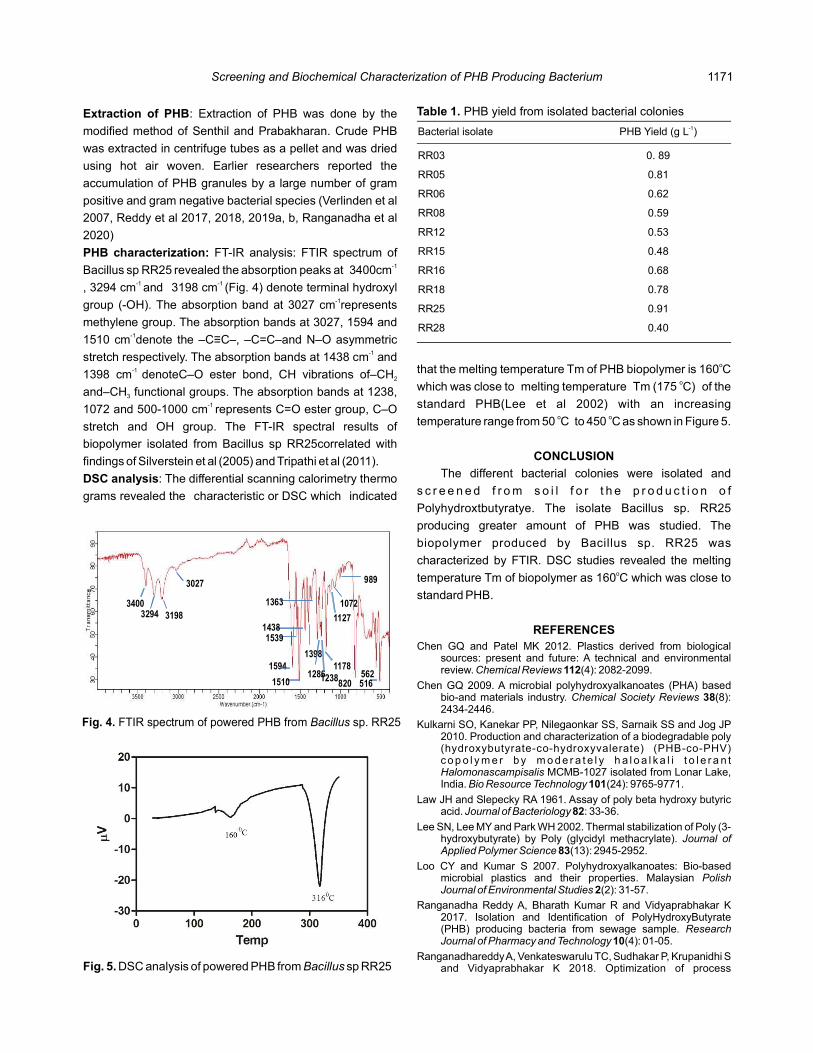
Bacterial isolate PHB Yield (g L )-1
RR03 0. 89
RR05 0.81
RR06 0.62
RR08 0.59
RR12 0.53
RR15 0.48
RR16 0.68
RR18 0.78
RR25 0.91
RR28 0.40
Table 1. PHB yield from isolated bacterial colonies
34003294 3198
3027
1594
1510
15391438
1398
1363
128612381178
1127
1072
820
989
562516
Fig. 4. FTIR spectrum of powered PHB from sp. RR25 Bacillus
Fig. 5. DSC analysis of powered PHB from sp RR25Bacillus
Extraction of PHB: Extraction of PHB was done by the
modified method of Senthil and Prabakharan. Crude PHB
was extracted in centrifuge tubes as a pellet and was dried
using hot air woven. Earlier researchers reported the
accumulation of PHB granules by a large number of gram
positive and gram negative bacterial species (Verlinden et al
2007, Reddy et al 2017, 2018, 2019a, b, Ranganadha et al
2020)
PHB characterization: FT-IR analysis: FTIR spectrum of
Bacillus sp RR25 revealed the absorption peaks at 3400cm-1
, 3294 cm and 3198 cm (Fig. 4) denote terminal hydroxyl -1 -1
group (-OH). The absorption band at 3027 cm represents -1
methylene group. The absorption bands at 3027, 1594 and
1510 cm denote the –C≡C–, –C=C–and N–O asymmetric -1
stretch respectively. The absorption bands at 1438 cm and -1
1398 cm denoteC–O ester bond, CH vibrations of–CH-1
2
and–CH functional groups. The absorption bands at 1238, 3
1072 and 500-1000 cm represents C=O ester group, C–O -1
stretch and OH group. The FT-IR spectral results of
biopolymer isolated from Bacillus sp RR25correlated with
findings of Silverstein et al (2005) and Tripathi et al (2011).
DSC analysis: The differential scanning calorimetry thermo
grams revealed the characteristic or DSC which indicated
that the melting temperature Tm of PHB biopolymer is 160 C o
which was close to melting temperature Tm (175 C) of the o
standard PHB(Lee et al 2002) with an increasing
temperature range from 50 C to 450 C as shown in Figure 5.o o
CONCLUSION
The different bacterial colonies were isolated and
s c r e e n e d f r o m s o i l f o r t h e p r o d u c t i o n o f
Polyhydroxtbutyratye. The isolate Bacillus sp. RR25
producing greater amount of PHB was studied. The
biopolymer produced by Bacillus sp. RR25 was
characterized by FTIR. DSC studies revealed the melting
temperature Tm of biopolymer as 160 C which was close to o
standard PHB.
REFERENCESChen GQ and Patel MK 2012. Plastics derived from biological
sources: present and future: A technical and environmental review. (4): 2082-2099. Chemical Reviews 112
Chen GQ 2009. A microbial polyhydroxyalkanoates (PHA) based bio-and materials industry. (8): Chemical Society Reviews 382434-2446.
Kulkarni SO, Kanekar PP, Nilegaonkar SS, Sarnaik SS and Jog JP 2010. Production and characterization of a biodegradable poly (hydroxybutyrate-co-hydroxyvalerate) (PHB-co-PHV) c o p o l y m e r b y m o d e r a t e l y h a l o a l k a l i t o l e r a n t Halomonascampisalis MCMB-1027 isolated from Lonar Lake, India. (24): 9765-9771.Bio Resource Technology 101
Law JH and Slepecky RA 1961. Assay of poly beta hydroxy butyric acid. : 33-36.Journal of Bacteriology 82
Lee SN, Lee MY and Park WH 2002. Thermal stabilization of Poly (3-hydroxybutyrate) by Poly (glycidyl methacrylate). Journal of Applied Polymer Science 83(13): 2945-2952.
Loo CY and Kumar S 2007. Polyhydroxyalkanoates: Bio-based microbial plastics and their properties. Malaysian Polish Journal of Environmental Studies 2(2): 31-57.
Ranganadha Reddy A, Bharath Kumar R and Vidyaprabhakar K 2017. Isolation and Identification of PolyHydroxyButyrate (PHB) producing bacteria from sewage sample. Research Journal of Pharmacy and Technology 10(4): 01-05.
Ranganadhareddy A, Venkateswarulu TC, Sudhakar P, Krupanidhi S and Vidyaprabhakar K 2018. Optimization of process
1171Screening and Biochemical Characterization of PHB Producing Bacterium

parameters for polyhydroxy butyrate production from isolated Acinetobacter nosocomialis RR20 through submerged fermentation. Current Trends in Biotechnology and Pharmacy 12(2): 16-25.
Ranganadha Reddy A, Krupanidhi S, Venkateswarulu TC, Bharathkumar R, Sudhakar P and Vidyaprabhakar K 2019a. Molecular characterization of a biopolymer producing bacterium isolated from sewage sample. Current Trends in Biotechnology and Pharmacy 13(3): 325-335.
Ranganadhareddy A, Abrahampeele K, Krupanidhi S, Prabhakar KV and Venkateswaru lu TC 2019b . Product ion o f Polyhydroxybutyrate from RR20 Acinetobacter nosocomialisstrain using modified mineral salt medium: A statistical approach. International Journal of Environment Science and Technology 16(10): 6447-6452.
Ranganadha Reddy A, Prabhakar KV, Venkateswarulu TC, Krupanidhi S, Nazneen Bobby Md, Abraham Peele K, Sudhakar P and Vijetha P 2020. Statistical optimization of PolyHydroxy Butyrate (PHB) production by novel Acinetobacter nosocomialisRR20 strain using response surface methodology. Current Trends in Biotechnology and Pharmacy 14(1): 62-69.
Raviteja KE, Abraham Peele K, Venkateswarulu TC, Vijetha P, Krupanidhi S and Ranganadha Reddy A 2020. Computational modeling of chitinase (CsCHIO) protein from Chitiniphilus shinanonensis Indian Journal of Ecology 47. (1): 151-153.
Senthil KB and Prabakharan G 2006. Production of PHB (bioplastic) using bio-effluent as substrate by . Alcaligenes eutrophus Indian Journal of Biotechnology 5 : 76-79.
Silverstein MR, Francis WX and David KJ 2005. Spectrometric Identification of Organic Compounds th, 7 edition. Johnwiley and Sons, Inc., Newyork.
Tripathi AD and Srivastava SK 2011. Kinetic study of biopolymer (PHB) synthesis in sp.in submerged fermentation Alcaligenesprocess using TEM. Journal of Polymers and Environment 19(3): 732-738.
Verlinden RA, Hill DJ, Kenward MA, William CD and Radecka I 2007. Bacterial synthesis of biodegradable polyhydroxyalkanoates. Journal of Applied Microbiology 102(6): 1437-1449.
Vijetha P, Ranganadha Reddy A and Sumalatha B 2020. Sorption and desorption studies for the removal of bentazone using biochar amended soil. (1): 128-Indian Journal of Ecology 47131.
Received 07 May, 2021; Accepted 09 August, 2021
1172 A. Ranganadha Reddy

Micro Comparative Study on Diversity of Ants Species (Hymenoptera: Formicidae) in Goa
Indian Journal of Ecology (2021) 48(4): 1173-1183Manuscript Number: 3353
NAAS Rating: 5.79
Abstract: The study examined the diversity and density of ant species of Carmel College campus, Nuvem, Salcete Goa, as there was no adequate information relating to ant faunal diversity of this region, from July 2006 to April 2007. The ants were collected using various standard methods. The result showed that a total of 9202 individuals were collected from the study area. The sampled specimens represented 37 species belonging to 20 genera and six subfamilies. The most diverse subfamily in relation to species was Myrmicinae with 12 species, followed by subfamily Formicinae with eleven, Ponerinae with seven and Pseudomyrmicinae with four species. Less diversity was found in subfamily Dorylinae with just two species and Dolichoderinae with only one species. In the generic trend, eight genera were in subfamily Myrmicinae while five in Formicinae, four in Ponerinae and just one genus each in Dolichoderinae, Dorylinae and Pseudomyrmicinae. This study has yielded valuable information of ant diversity in this region as well as on the campus of Carmel College of Arts, Science and Commerce for Women. An effort was made to compare the findings of this study with that of a similar study conducted almost ten years later (2015-2016) in the same study area. The results showed a remarkable difference with four subfamilies, 13 genera and 17 species.
Keywords: Diversity, Density, Undisturbed areas, Disturbed areas, Formicidae
Maria Lizanne A.C. and Maria AlvaresCarmel College of Arts, Science & Commerce for Women, Nuvem, Salcette Goa-403 713, India
E-mail: [email protected]
There is a steadfast curiosity in the number of species in
native communities, because they are the necessary units of
biodiversity. Many studies report on change in species
richness but the interest of conservation biologists is to
examine whether species richness changes with extensive
use of land, history or degree of landscape fragmentation,
change in topography and whether richness changes over
time. There are numerous reasons for selecting ants as a
survey taxon in research studies. Ants along with other
invertebrate taxa are included in biodiversity studies because
of their great diversity and quick response to even a minor
environmental change. In most of the terrestrial ecosystems
ants are a noticeable presence, and they are among the most
frequently studied terrestrial invertebrates. They are mostly
scavengers and predators, and have large impact on soil
formation, seed predation and its dispersal, and invertebrate
community structure (Lach et al 2010, Del Toro et al 2012,
Guénard 2013). They are predominantly good candidates for
observing community changes that may occur due to climate
change or fragmentation of habitats. They add up to a
cumulative 15-25% total terrestrial animal biomass (Schultz
and McGlynn 2000, Krushelnycky et al 2005). The success of
ants in many different environments is credited to their social
organization and capacity to adapt to nearly any habitat,
procure food resources and defend them (Keller and Gordon
2009). Due to the mutualistic behavior of ants with both flora
and other fauna, they are considered as efficient biological
and ecological indicators and are one of the nine projected
indicators of the ecosystem (Underwood and Fisher 2006).
Presence of ants is observed at all levels of the terrestrial
food webs (Pfeiffer et al 2013). Nearly 12,500 of an estimated
22,000 ant species have been described (Bolton et al 2006,
Philip 2007). Formicidae contains 21 subfamilies and 283
genera and about 12,500 living ant species. India has known
ant fauna of 828 species in 100 genera and 10 subfamilies.
About 66 species belonging to 32 genera have been reported
from Goa which includes Daman and Diu (Bharti et al 2016).
Ants act as ecosystem engineers and are efficient
decomposers and thus play an important role in soil fertility
and nutrient cycling. Considering the importance of ants in
ecological communities, the present investigation was
undertaken to fill in the lacuna in the existing knowledge of
ant diversity in the state of Goa.
MATERIAL AND METHODS
Study area: The field work was conducted on the campus of
Carmel College of Arts, Science and Commerce for Women,
Nuvem, Salcete Goa, covering 14.16 ha of land. It is situated
in Nuvem village (Lat. N 15° 18' 42.5772", Long. E 73° 56'
41.2764"), a suburban area, which is located three
kilometers away from Margao city. This region is a
biologically diverse and productive habitat of native flora and
fauna because of its pristine nature and most of the area
being undisturbed as it is a private property. This study was

conducted from July 2006 to April 2007 and survey included
undisturbed and disturbed areas that covered study sites like
various transects of the hill top and scrub areas that are
hardly visited (undisturbed areas) (Fig. 1) and vehicle parking
areas, roadside, botanical garden, library which are
frequently visited (disturbed areas) (Fig. 2).
Habitat characterization: The campus, with an area of
14.16 ha, has a diverse biota. Predominant vegetation of the
campus is scrub jungle mixed with cashew, mango, acacia,
eucalyptus and wild deciduous trees. The hilltop has scrub
mixed with grassy patches. The built-up area has more
ornamental shrubs and also includes trees like Peltophorum
pterocarpus K a oelreuteria paniculatand . The ground layer is
rich in seasonal herbaceous flora especially during the
monsoon. The most dominant angiosperm families in the
campus are Acanthaceae, Apocynaceae, Asteraceae,
Araceae, Euphorbiaceae, Fabaceae, Poaceae, Rubiaceae
and Verbenaceae.
Ant sampling method: Ant sampling was done from July
2006 to April 2007. Five different standard ant sampling
collection methods were employed in the collection of ants: a)
hand collection b) pitfall trap method, c) Tullgren funnel
method, d) bait method and e) beat sheet method. Ants were
mostly collected during daytime. Field information (date,
time, habitat and locality) was recorded at the time of
collection. The collected ants were brought to the laboratory
Carmel
College
Fig. 1. Undisturbed areas of the campus
Fig. 2. Disturbed areas of the campus
of the Department of Zoology, Carmel College for
identification, labeling and preservation.
Hand collection (all-out search) method: Larger, slow
moving ants were either hand-picked or picked up with the
fine brush dipped in 70% alcohol (ethanol) then dropped into
a collecting bottle containing 70% alcohol. Collections were
also made from soil nests, foraging columns and ants found
on trees.
Pitfall trap method: A small container three-quarters full of
water containing detergent was placed in a hole in the ground
with the rim of the container level with the surface. Ants that
fell into the container were collected after 24 hours. They
were transferred to collecting bottles containing 70% alcohol
and later washed in saline to remove dust particles and other
debris, then plain water to remove the excess saline.
Cleaned ants were placed into containers with 70% alcohol
for preservation.
Tullgren funnel method: Leaf litter from shady areas was
collected in polythene bags and carried to the laboratory. The
litter was then placed in the mouth of a broad funnel with a 40-
watt bulb for heat and light. Ants moving downward fell into a
beaker containing 70% alcohol.
Bait method: Baits such as honey, coconut pieces, sugar,
jaggery and cooked rice were used to attract ants. The baits
were on the ground, tree trunks, shrubs, and other likely
places. Ants attracted to these baits were immediately
collected and preserved in 70% alcohol.
Beat sheet method: An open umbrella was placed upside
down under a tree and the low-hanging branches of the tree
above the open umbrella were gently shaken. Ants that fell
into the open umbrella were either hand-picked or collected
with a brush dipped in 70% alcohol and preserved in vials of
70% alcohol.
Identification: Ant specimens that were dry-mounted were
studied and identified directly under a stereozoom
LABOMED CZM4 and MOTIC B SERIES B1 220 ASC
microscopes. Smaller ants were temporarily mounted on
microscope slides of 1mm thickness, in a drop of glycerin and
then identified. Specimens were identified to subfamily using
the identification keys given by Narendra and Kumar (2006).
The species were identified with keys in Bingham (1903),
Bolton (1995), Plowes and Patrock (2000), Bolton et al. 2006,
Chavan and Patkar 2014 and AntWeb (2020). After
identification, cross checking was done with the images
avai lable at ht tp :/ /www.antbase.net / index.html.
Identifications were further confirmed with keys in Hölldobler
and Wilson (1990). Diversity Indices as such as Shannon
Weaver, Simpson's Index and Evenness were calculated
using PAST statistical software Version 2.7. A reference
collection was maintained in the Zoology Museum of Carmel
1174 Maria Lizanne A.C. and Maria Alvares

College of Arts, Science and Commerce for Women, Nuvem,
Salcette Goa.
Labeling: Permanently preserved specimens were labeled
with identification and data labels. The data labels include
information about the date and time of collection, name of the
collector, the habitat and the locality.
Mounting and dry preservation: After identification, ants
were removed from the alcohol and dried in a petri dish with
the help of a light source. Before mounting, specimens were
relaxed by remoistening them in xylene to soften the tissues
in order to facilitate the adherence of the specimen onto the
paper. And body parts of taxonomic significance were
repositioned.
Wet preservation: Ants not dry-mounted on points were
preserved species wise in separate vials of 70% alcohol. All
vials had labels containing complete field information
(locality, date and time of collection, name of the collector,
habitat) and specimen identity.
RESULTS AND DISCUSSION:
Six subfamilies of ant fauna have been reported from
Goa that includes Daman and Diu namely Dolichoderinae,
Dorylinae, Formicinae, Myrmicinae, Ponerinae and
Pseudomyrmicinae. In this study ant species were recorded
from six subfamilies that included 37 species and 20 genera
(Table 1). Species distribution among the subfamilies was
more even. The distribution of species in the subfamilies
showed a dominance of Myrmicinae with 12 species (32.5%)
followed by Formicinae, Ponerinae, Pseudomyrmicinae,
Dorylinae and Dolichoderinae (Table 2). In the generic trend,
subfamily Myrmicinae showed dominance of eight (40%)
genera, followed by Formicinae five (25%), Ponerinae four
(20%). The remaining three subfamilies were recorded with
only one genus each (5%) (Table 2). A total of 32 (86.48%)
and 24 (64.86%) ant species were identified from the
undisturbed and disturbed areas respectively (Tables 3 and
4). Of the 37 ant species, 19 (51.35%) species were present
in both the study areas undisturbed as well as disturbed,
while 13 (35.13%) species were exclusively in the
undisturbed areas and only five (13.51%) species were
exclusively found in the disturbed areas (Tables 3 and 4).
Species , Tapinoma melanocephalum Camponotus
irritans, Camponotus radiatus Pheidole grayi Pheidole , and
sharpi were not reported from the undisturbed areas while
Cerapachys aitkenii, Cerapachys biroi, Aphaenogaster
beccarii, Aphaenogaster feae, Meranoplus bicolor,
Bothroponera henryi, Bothroponera sulcata, Diacamma
ceylonense, D. rugosum Tetraponera and the species were
absent from the disturbed areas (Tables 3 and 4). The total
number of ants collected from the undisturbed areas (4766)
Biological name Common name
Dolichoderinae
Tapinoma melanocephalum (Fabricius, 1793)
Odour Ant (Ghost Ant)
Dorylinae
Cerapachys aitkenii (Forel,1900) Red Cannibal Ant
C. biroi (Forel, 1907) Ant-raiding Ant
Formicinae
Anoplolepis gracilipes (Smith, 1857) Yellow Crazy Ant
Camponotus angusticollis (Jerdon, 1851) Long Neck Sugar Ant
C. compressus (Fabricius, 1878) Common Godzilla Ant
C. irritans (Smith, 1857) Giant Honey Ant
C. parius (Emery, 1889)
C. radiatus (Forel, 1892) Carpenter Ant
C. sericeus (Fabricius, 1798) Golden Black Ant
Oecophylla smaragdina (Fabricius, 1775) Weaver Ant
Paratrechina longicornis (Latreille, 1802) Black Crazy Ant
Polyrhachis exercita (Emery, 1889)
P. illaudata (Walker, 1859)
Myrmicinae
Aphaenogaster beccarii (Emery, 1887) Long-legged Hunchback Ant
A. feae (Emery, 1889)
Crematogaster rothneyi (Mayr, 1879) Common Acrobat Ant
C. subnuda (Mayr, 1879) Common Broad Acrobat Ant
Meranoplus bicolor (Guerin-Meneville, 1844)
Shield Ant
Monomorium atomum (Forel, 1902)
M. pharaonis (Linnaeus, 1758) Pharao's Ant
Myrmicaria brunnea (Saunders, 1842) Short-legged Hunchback Ant
Pheidole grayi (Forel, 1902)
P. sharpi (Forel, 1902)
Solenopsis geminata (Fabricius, 1804) Common Red Fire Ant
Tetramorium wroughtonii (Forel, 1902)
Ponerinae
Bothroponera henryi (Donisthorpe, 1942)
B. sulcata (Mayr, 1867)
Diacammaceylonense (Emery, 1897) Queenless Ant
D. rugosum (Le Guillou, 1842) Lesser Striated Bispinous Ant
Leptogenys diminuta (Smith, 1857)
L. processionalis (Jerdon, 1851) Procession Ant
Odontomachus haematodus (Linnaeus, 1758)
Greater Trap-jaw Ant
Pseudomyrmicinae
Tetraponera aitkenii (Forel, 1902) Slender Ants
T. allaborans (Walker, 1859) Polished Leaf-border Ant
T. nigra (Jerdon, 1851)
T. rufonigra (Jerdon, 1851) Arboreal Bicolored Ant
Total Subfamilies - 06 Genus - 20 Species - 37
Table 1. Checklist of ants collected from Carmel College campus
1175Micro Comparative Study on Diversity of Ants Species

Subfamily Genera Percentage Species Percentage
Dolichoderinae 01 5 01 2.7
Dorylinae 01 5 02 5
Formicinae 05 25 11 29.7
Myrmicinae 08 40 12 32.5
Ponerinae 04 20 07 18.9
Pseudomyrmicinae 01 5 04 10.8
Total 20 37
Table 2. Total number and percentage of genera and species per subfamily
Biological name Study areas
Undisturbed Disturbed
DolichoderinaeTapinoma melanocephalum +DorylinaeCerapachys aitkenii +C. biroi +FormicinaeAnoplolepis gracilipes + +Camponotus angusticollis + +C. compressus + +C. irritans +C. parius + +C. radiatus +C. sericeus + +Oecophylla smaragdina + +Paratrechina longicornis + +Polyrhachis exercita + +P. illaudata + +MyrmicinaeAphaenogaster beccarii +A. feae +Crematogaster rothneyi + +C. subnuda + +Meranoplus bicolor +Monomorium atomum + +M. pharaonis + +Myrmicaria brunnea + +Pheidole grayi +P. sharpi +Solenopsis geminata + +Tetramorium wroughtonii + +PonerinaeBothroponera henryi +B. sulcata +Diacammaceylonense +D. rugosum +Leptogenys diminuta + +L. processionalis + +Odontomachus haematodus + +PseudomyrmicinaeTetraponera aitkenii +T. allaborans +T. nigra +T. rufonigra +
Table 3. Distribution of the presence of the ant species in the two study areas
Study areas Species present Percentage
Undisturbed areas 32 86.48
Disturbed areas 24 64.86
Common –Undisturbed areas & disturbed areas)
19 51.35
Only in undisturbed areas 13 35.13
Only in disturbed areas 05 13.51
Table 4. Presence and percentage of the distribution of ant species in the two study areas
was more compared to the disturbed areas (4436) (Tables 5
and 7). In undisturbed areas, subfamily Myrmicinae was
more speciose (10 species) and the least was subfamily
Dorylinae with only two species whereas in the disturbed
areas it was subfamily Formicinae that was more diverse with
eleven species and the least was Dolichoderinae with just
one (Table 9). In undisturbed areas subfamily Dolichoderinae
was absent while in disturbed areas subfamilies Dorylinae
and Pseudomyrmicinae were not represented (Table 9). In
undisturbed areas, subfamily Formicinae recorded
maximum number of individuals (2360), followed by
subfamily Myrmicinae, Ponerinae, Dorylinae and minimum
was in subfamily Pseudomyrmicinae (148) (Tables 5 and 6).
The monthly variation of the ant subfamilies in the
undisturbed areas is represented in Table 5. Subfamily
Dolichoderinae was not represented in the undisturbed
areas.
In the disturbed areas, the same trend was observed
with subfamily Formicinae representing the maximum
number of individuals (2485) followed by subfamily
Myrmicinae (1633) and the least were observed in subfamily
Ponerinae (156). Subfamily Dolichoderinae was represented
with 162 species in the disturbed areas while no individuals
were recorded in sub fami l ies Dory l inae and
Pseudomyrmicinae in the disturbed areas (Tables 7 and 8).
The three abundant species in the undisturbed areas were
from subfamily Formicinae, (406), Anoplolepis gracilipes
Oecophylla smaragdina Camponotus compressus (336) and
(292) while in the disturbed areas, the abundant species
were also from the subfamily Formicinae, Anoplolepis
gracilipes Oecophylla smaragdina (391), (369) and
Camponotus radiates (314) (Table 5 and 7). Overall the
subfamily Formicinae had the maximum number of ant
species (4845) in the college campus in both the undisturbed
and disturbed areas (Table 7). Of the 11 species recorded in
this subfamily, is the commonest in the Anoplolepis gracilipes
college campus both in the undisturbed areas (406) and in
the disturbed areas (391) with a total of 797.
Altogether total number of species recorded in the study
sites was 37 where 32 (86.48%) species were found in the
1176 Maria Lizanne A.C. and Maria Alvares

Species Undisturbed study areas (JULY 2006 – APRIL 2007) Total A
JUL AUG SEP OCT NOV DEC JAN FEB MAR APR
Dolichoderinae
Tapinoma melanocephalum - - - - - - - - - - -
Dorylinae
Cerapachys aitkenii - 08 11 11 13 12 13 15 15 16 114
Cerapachys biroi 04 08 10 11 10 13 12 14 14 16 112
Total A 04 16 21 22 23 25 25 29 29 32 226
Formicinae
Anoplolepis gracilipes 16 26 28 30 35 37 49 57 60 68 406
Camponotus angusticollis - - 20 24 30 37 37 40 41 44 273
Camponotus compressus - 15 21 27 27 35 39 41 42 45 292
Camponotus irritans - - - - - - - - - - -
Camponotus parius - 12 17 22 24 26 31 33 36 38 239
Camponotus radiatus - - - - - - - - - - -
Camponotus sericeus - - - 19 24 27 33 35 39 42 219
Oecophylla smaragdina - 09 13 20 28 37 45 59 63 62 336
Paratrechina longicornis 06 11 16 21 27 32 35 39 42 44 273
Polyrhachis exercita - - 07 10 14 15 20 23 27 34 150
Polyrhachis illaudata - - 09 09 15 22 27 28 30 32 172
Total B 22 73 131 182 224 268 316 355 380 409 2360
Myrmicinae
Aphaenogaster beccarii - - 04 05 06 05 06 06 07 07 46
Aphaenogaster feae - - - 04 05 07 07 06 06 07 42
Crematogaster rothneyi 03 05 05 10 12 15 15 21 25 28 139
Crematogaster subnuda 04 04 04 09 09 11 15 17 21 25 119
Meranoplus bicolor - - - 05 08 12 14 17 22 27 105
Monomorium atomum 07 11 10 11 12 12 18 21 26 30 158
Monomorium pharaonis 06 09 12 13 15 18 21 24 26 29 173
Myrmicaria brunnea - - 05 09 12 12 13 15 15 13 94
Pheidole grayi - - - - - - - - - - -
Pheidole sharpi - - - - - - - - - - -
Solenopsis geminata - 09 13 16 20 23 28 33 37 41 220
Tetramorium wroughtonii 04 10 10 14 17 17 17 19 21 24 153
Total C 24 48 63 96 116 132 154 179 206 231 1249
Ponerinae
Bothroponera henryi - 09 12 25 28 32 15 15 10 05 151
Bothroponera sulcata - - 05 11 20 29 25 21 14 08 133
Diacammaceylonense 05 07 07 13 16 23 29 31 33 30 194
Diacamma rugosum 07 11 09 15 21 24 26 26 30 27 196
Leptogenys diminuta - - 03 03 07 10 11 09 - - 43
Leptogenys processionalis - - 02 02 08 07 11 09 - - 39
Odontomachus haematodus - - - 03 05 08 08 03 - - 27
Total D 12 27 38 72 105 133 125 114 87 70 783
Pseudomyrmicinae
Tetraponera aitkenii - - 04 04 03 02 02 01 - - 16
Tetraponera allaborans - - 12 10 10 07 04 02 - - 45
Tetraponera nigra - - - 09 06 06 05 02 02 - 30
Tetraponera rufonigra - - 12 12 10 09 07 05 02 - 57
Total E 28 35 29 24 18 10 04 148
GRAND TOTAL = (A+B+C+D+E) = 226+2360+1249+783+148 4766
Table 5. Total number of ants collected from the undisturbed areas month wise from July 2006 to April 2007
1177Micro Comparative Study on Diversity of Ants Species

Undusturbed areas
Subfamilies Total number of ants
Dolichoderinae 0
Dorylinae 226
Formicinae 2360
Myrmicinae 1249
Ponerinae 783
Pseudomyrmicinae 148
Total 4766
Table 6. Total number of ants per subfamily in undisturbed areas
undisturbed areas and 24 (64.86%) were recorded in the
disturbed areas (Table 4). In the undisturbed areas
subfamilies Dorylinae, Ponerinae and Pseudomyrmicinae
were represented 100% and subfamily Dolichoderinae was
not represented at all while in the disturbed areas subfamilies
Dolichoderinae and Formicinae were represented 100%
while Dorylinae and Pseudomyrmicinae were not
represented at all (Table 9). Mayr, 1861 was Camponotus
represented by six species, of which (292 C. compressus
individuals) and (273 individuals) in the C. angusticollis
undisturbed areas and (217) and (216) C. irritans C. sericeus
in the disturbed areas were remarkably found in most of the
sites with maximum number (Tables 5 & 7). Individuals of
Oecophylla smaragdina (336 & 369) in the undisturbed and
disturbed areas respectively, a species with arboreal nests,
was dominant on tree trunks. (406 Anoplolepis gracilipes
&391) in the undisturbed and disturbed areas respectively
were especially abundant in cool, moist places under leaf
litter at the base of the trees. Species Mayr Camponotus
1861, Fabricius 1775, Smith 1857, Oecophylla Anoplolepis
Myrmicaria Solenopsis Saunders1842, Fabricius 1804,
Monomorium Diacamma Linnaeus,1758, Le Guillou, 1842,
Pachycondyla Leptogenysdonisthorpe 1942 and Jerdon,
1851 were found throughout the study period and recorded
from most of the study sites of the undisturbed and disturbed
areas (Table 5 and 7).
Shannon-Wiener diversity index value (H') for
undisturbed areas (3.25) was slightly higher than that of
disturbed areas (3.03). Value of Simpson's index (D) for
undisturbed areas was 0.044 while for disturbed areas is
0.053. Evenness values were more or less the same for both
the areas, undisturbed (0.94) and disturbed (0.95). Species
richness and abundance from both the areas were
significantly different (Table 10). An attempt was made to
compare the findings of this study and a study conducted
almost ten years later in the same campus and in the same
study sites with the same parameters. A remarkable
difference was observed in the results. The study of 2015-
2016 resulted in documenting and identifying four
subfamilies, with 13 genera and 15 species in the
undisturbed areas and seven genera and ten species in the
disturbed. A few species were unidentified. The study of
2006-2007 had recorded six subfamilies with 18 genera and
32 species in the undisturbed areas and 14 genera and 24
species in the disturbed areas. Subfamilies Dolichoderinae
and Dorylinae and genera Pheidole were not represented in
2015-2016 study (Table 11 & 12). Ants can be effectively
used as indicator species as they respond to any alteration in
the surrounding environment. They can also be effectively
used to study landscape disturbance and species diversity
(Paknia and Pfeiffer 2011). Thus, understanding the impact
of habitat loss on myrmecofaunal diversity and density is a
necessity. The collection and documentation of ants can give
a good insight into the regional diversity and can be used in
developing a regional checklist or an reference collection of
an educational institution. It can also be considered as a
document of faunal representation and any variation or
decline in numbers can be taken as an indicator of an
environment undergoing alteration as a result of human
activity or natural forces. The species richness, diversity and
density were less in the disturbed areas as compared to the
undisturbed during both the study periods. This could be due
to habitat destruction and increase in disturbance by various
anthropogenic activities. Related studies on diversity of ants,
butterflies and birds have shown that species richness and
density decreases with increase in habitat disturbance
(Ingalhallikar et al. 2000-2001, Kunte 2000-2001, Pachpor
and Ghodke 2000-2001). Many studies have recorded that
habitat degradation; disturbance and fragmentation have
damaging impact on ant diversity and abundance where
undisturbed areas or forests have higher species richness
than those in the disturbed habitats (Watt et al 2002).
The undisturbed areas of the campus had abundant and
diverse vegetation and hence showed a greater diversity of
ant species than the disturbed areas where vegetation was
not dense. During 2006-2007, the campus had more diversity
and density of ant species than when it was conducted in
2016-2017 in both the undisturbed and disturbed areas. The
undisturbed areas had various types of trees and plants in
2006-2007 which were felled for construction and campus
expansion along with concrete pavers over the years. The
plantation of acacia trees in the undisturbed areas during the
gap of ten years of the study periods could be the cause of
decrease in species richness and abundance during the
study period of 2015-2016. Thus habitat variables such as
dense canopy cover of foliage and abundant litter content in
the soil can provide a suitable habitation for ants. This is
1178 Maria Lizanne A.C. and Maria Alvares

Species Disturbed study area (JULY 2006 – APRIL 2007) TotalB
TotalA+B
JUL AUG SEP OCT NOV DEC JAN FEB MAR APR
Dolichoderinae
Tapinoma melanocephalum - 06 10 15 15 21 24 23 23 25 162
Total A 06 10 15 15 21 24 23 23 25 162 162
Dorylinae
Cerapachys aitkenii - - - - - - - - - - -
Cerapachys biroi - - - - - - - - - - -
Total B - - - - - - - - - - - 226
Formicinae
Anoplolepis gracilipes 07 12 19 29 35 43 48 55 67 76 391
Camponotus angusticollis - 03 07 07 09 12 12 11 11 10 82
Camponotus compressus 10 13 15 17 20 22 25 25 23 23 193
Camponotus irritans 05 09 12 17 23 26 29 31 32 33 ! 217
Camponotus parius - 04 08 11 14 17 21 21 27 25 148
Camponotus radiatus 11 14 19 23 28 33 37 42 52 55 314
Camponotus sericeus - 10 10 15 16 22 28 34 38 43 216
Oecophylla smaragdina 07 11 17 27 33 41 46 51 63 73 369
Paratrechina longicornis - 10 15 21 27 32 37 37 31 29 239
Polyrhachis exercita 03 09 11 11 15 16 22 24 25 25 161
Polyrhachis illaudata 03 07 12 15 17 17 21 22 21 20 155
Total C 46 102 145 193 237 281 326 353 390 412 2485 4845
Myrmicinae
Aphaenogaster beccarii - - - - - - - - - - -
Aphaenogaster feae - - - - - - - - - - -
Crematogaster rothneyi 07 11 15 22 27 32 36 41 42 44 277
Crematogaster subnuda 05 12 17 25 31 34 39 42 44 41 290
Meranoplus bicolor - - - - - - - - - - -
Monomorium atomum - 06 10 15 13 25 27 31 33 33 193
Monomorium pharaonis - 07 12 14 17 20 23 27 30 29 179
Myrmicaria brunnea - - - 02 05 03 07 08 09 09 43
Pheidole grayi 02 05 09 12 14 17 13 10 07 07 96
Pheidole sharpi 02 27 07 10 15 19 16 14 12 09 131
Solenopsis geminata - 04 13 27 31 37 39 40 41 43 275
Tetramorium wroughtonii - - 09 13 17 21 25 23 21 20 149
Total D 16 72 92 140 170 208 225 236 239 235 1633 2882
Ponerinae
Bothroponera henryi - - - - - - - - - - -
Bothroponera sulcata - - - - - - - - - - -
Diacammaceylonense - - - - - - - - - - -
Diacamma rugosum - - - - - - - - - - -
Leptogenys diminuta - - - 04 07 09 11 08 06 04 49
Leptogenys processionalis - - - 03 07 10 08 07 05 04 44
Odontomachus haematodus - - - - 10 12 15 11 09 06 63
Total E - - - 07 24 31 34 26 20 14 156 939
Pseudomyrmicinae
Tetraponera aitkenii - - - - - - - - - - -
Tetraponera allaborans - - - - - - - - - - -
Tetraponera nigra - - - - - - - - - - -
Tetraponera rufonigra - - - - - - - - - - -
Total F - - - - - - - - - - - 148
GRAND TOTAL = (A+C+D+E) = 162+2485 +1633+156 4436 9202
Table 7. Total number of ants collected from the disturbed areas month wise from July 2006 to April 2007
1179Micro Comparative Study on Diversity of Ants Species

Subfamilies Total number of ants
Dolichoderinae 162
Dorylinae 0
Formicinae 2485
Myrmicinae 1633
Ponerinae 156
Pseudomyrmicinae 0
Total 4436
Table 8. Total number of ants per subfamily in disturbed areas
Subfamily Total number of species Ant species present in the study areas
Undisturbed Percentage Disturbed Percentage
Dolichoderinae 01 0 0 01 100
Dorylinae 02 02 100 0 0
Formicinae 11 09 81.81 11 100
Myrmicinae 12 10 83.33 09 75
Ponerinae 07 07 100 03 42.85
Pseudomyrmicinae 04 04 100 0 0
Total 37 32 86.48 24 64.86
Table 9. Total number of ants per subfamily in undisturbed and disturbed areas
Subfamily Study site
Undisturbed Disturbed
Dolichoderinae 0 (0) 1 (162)
Dorylinae 2 (226) 0 (0)
Formicinae 9 (2360) 11 (2485)
Myrmicinae 10 (1249) 9 (1633)
Ponerinae 7 (783) 3 (939)
Pseudomyrmicinae 4 (148) 0 (0)
Abundance 4766 4436
Species Richness 32 24
Simpson's Index 0.0442 0.0531
Shannon Weaver diversity 3.2520 3.0342
Evenness 0.9383 0.9547
Table 10. Abundance, Species richness, Simpson's Index, Shannon Weaver diversity and Evenness of the species of the subfamilies in undisturbed and disturbed areas
Figures in the bracket indicate abundance of ants
because habitat complexity and heterogeneity was high in
the undisturbed areas as compared to disturbed areas.
Habitat intricacy provides hiding, nesting and foraging
grounds to the many species of ants. Bharti et al (2016)
reported that the most species ant genus is with Camponotus
83 named species which is one tenth of the total known
Indian species. In this study too Camponotus was
represented with six species. Similarly, in terms of species
richness, the subfamily Myrmicinae is the most species in
India which was also the findings in this study with 12
species. The distribution and diversity of ants can be credited
to biotic or abiotic factors, human impacts or habitat structure
which was also found in this study where with more human
intervention and impact over the years on the natural habitat
there was decline in the species richness and abundance
during the study period of 2016-2017 (Armbrecht et al 2004,
Philpott et al 2010, Wittman et al 2010). The diversity and
density of arboreal ants can be directly connected to the
presence, quality and quantity of resources available from
the trees, such as extrafloral nectaries and presence of
trophobiont arthropods along with other nitrogen-rich
sources (Yanoviak and Kaspari 2000, Schoereder et al
2010). This was also observed in the present study in
undisturbed areas with more dense vegetation which had
more species than the disturbed areas.
The decline observed in the ant species richness clearly
states that habitat destruction does play a major role in
species decrease in number and diversity. Overall relative
abundance of Myrmicinae from disturbed sites was more
because species of Myrmicinae might have high possibility to
adjust to fluctuating environmental conditions and also found
in different types of habitats worldwide. Andersen (2000)
classified subfamily Myrmicinae as generalized Myrmecinae
(GM) among the functional groups. Savitha et al (2008) also
recorded similar results.
CONCLUSION
Study conducted on the ant diversity on the campus in
2015-2016 by D'Sa et al. (2015-2016) reports only four
subfamilies which is a clear indication of decrease in the ant
fauna. The rich diversity and density of the ant species
documented in the study conducted in 2006-2007 may be
1180 Maria Lizanne A.C. and Maria Alvares

Subfamily Biological name Undisturbed areas Disturbed areas
2006-2007 2015-2016 2006-2007 2015-2016
Dolichoderinae Tapinoma melanocephalum - - + -
Dorylinae Cerapachys aitkenii + - - -
C. biroi + - - -
Formicinae Anoplolepis gracilipes + + + +
Camponotus angusticollis + + + +
C. compressus + + + +
C. irritans - - + +
C. parius + - + -
C. radiatus - - + +
C. sericeus + - + -
Oecophylla smaragdina + + + +
Paratrechina longicornis + + + +
Polyrhachis exercita + - + -
P. illaudata + - + -
Myrmicinae Aphaenogaster beccarii + + - -
A. feae + - - -
Crematogaster rothneyi + - + -
C. subnuda + - + -
Meranoplus bicolor + + - -
Monomorium atomum + - + -
M. pharaonis + - + -
Myrmicaria brunnea + + + +
Pheidole grayi - - + -
P. sharpi - - + -
Solenopsis geminata + + + -
Tetramorium wroughtonii + - + -
Ponerinae Bothroponera henryi + + - -
B. sulcata + - - -
Diacammaceylonense + - - -
D. rugosum + + - -
Leptogenys diminuta + - + -
L. processionalis + + + +
Odontomachus haematodus + + + +
Pseudomyrmicinae Tetraponera aitkenii + - - -
T. allaborans + + - -
T. nigra + - - -
T.rufonigra + + - -
Total 32 15 24 10
Table 11. Ant species recorded in the subfamilies in 2006–2007 and 2015–2016 in the undisturbed and disturbed areas
+ = present; - = absent
1181Micro Comparative Study on Diversity of Ants Species

Subfamilies Total number of genera Total number of species
2006-2007 2015-2016 2006-2007 2015-2016
U. A. D. A. U. A. D. A. U. A. D.A. U. A. D. A.
Dolichoderinae 0 01 0 0 0 01 0 0
Dorylinae 01 0 0 0 02 0 0 0
Formicinae 05 05 04 04 09 11 05 07
Myrmicinae 07 06 04 01 10 09 04 01
Ponerinae 04 02 04 02 07 03 04 02
Pseudomyrmicinae 01 0 01 0 04 0 02 0
Total 18 14 13 07 32 24 15 10U.A. = Undisturbed Areas D.A. = Disturbed Areas
Table 12. Number of genera and species recorded in the subfamilies in 2006–2007 and 2015–2016 in the undisturbed and disturbed areas
because of satisfactory nesting sites, dense and varied
vegetation and along with availability of food as well as high
foraging capacity on the Carmel College campus. The major
findings of both the studies is the species Odontomachus
haematodus, typically referred to as 'Greater Trap-Jaw Ant'
belonging to the morphologically primitive subfamily
Ponerinae. This ant has the second fastest moving and
effective predatory appendages (Patek et al 2006) in the
animal Kingdom after the dracula ant ( ). A Mystrium camillae
local to South America is now by far the most frequent
species in the rural regions nesting in decaying logs and
branches at the ground. The same were the finding in this
study as Carmel College campus comes under rural areas
and most of it is undisturbed. Investigation of ant species on
the Carmel College campus clearly indicates the richness of
ant fauna in the village and in turn in the state. The study had
recorded 37 species belonging to 20 genera and six
subfamilies in 2006-2007. Subfamily Myrmicinae was
dominant in genera as well as species. This study will yield
valuable information of ant diversity to fill in the lacuna of
invertebrate fauna in the state of Goa.
REFERENCESAndersen AN 2000. A global ecology of rainforest ants: functional
groups in relation to environmental stress and disturbance, pp 25-34. In: Agosti D, Majer J D, Alonso L E and Schultz TR (eds). Ants: Standard Methods for Measuring and Monitoring Biodiversity.
Armbrecht I, Perfecto I and Vandermeer J 2004. Enigmatic biodiversity correlations: Ant diversity responds to diverse resources. : 284-286.Science 304
AntWeb Version 8.41. California Academy of Science, online at https://www.antweb.org. Accessed 12 October 2020.
Bharti H, Guénard B, Bharti M and Economo EP 2016. An updated checklist of the ants of India with their specific distributions in Indian states (Hymenoptera, Formicidae). : 1-83. ZooKeys 551
Bingham CT 1903. The Fauna of British India, including Ceylon and Burma. In: Blanford W T (eds) Hymenoptera, - Vol II, Ants and Cuckoo-wasps.
Bolton B, Alpert G, Ward P and Naskrecki P 2006. Bolton's Catalogue of Ants of the World 1758-2005 (CD).
Bolton B 1995. . Harward A new general catalogue of ants of the worldUniversity Press: London.
Chavan RJ and Patkar NB 2014. Diversity of ants (Hymenoptera: Formicidae) from undisturbed and disturbed habitats of Great Indian Bustard Wildlife Sanctuary, (M. S.), India. International Journal of Scientific Research 3 (12): 398-400.
Del Toro I, Ribbons RR and Pelini SL 2012. The little things that run the world revisited: A review of ant-mediated ecosystem services and disservices (Hymenoptera: Formicidae). Myrmecological News 17 : 133-146.
D'sa V, Coutinho F, Naik D and Xavier NF 2015-2016. Myrmecofaunal diversity of Carmel College campus: A preliminary study (Unpublished).
Guénard B 2013. An overview of the species and ecological diversity of ants. In: . John Wiley & Sons, Encyclopedia of Life SciencesLtd: Chichester.
Hölldobler B and Wilson EO 1990. . Cambridge, MA: The AntsHarvard University Press, p. 732.
Ingalhallikar S, Purandare R, Nalavade S and Dhole S 2000-2001. Avifauna around Pune. : Journal of Ecological Society 13&1459-70
Keller L and Gordon E 2009. . Oxford University The lives of antsPress. London, p. 252.
Kunte K 2000-2001. Butterfly diversity of Pune city along human impact gradient. : 40-45.Journal of Ecological Society 13&14
Krushelnycky P D, Loope L L and Reimer N J 2005. The ecology, policy, and management of ants in Hawaii. Proceedings of the Hawaiian Entomological Society 1-25.37:
Lach L, Parr CL and Abbott KL 2010. . Oxford: Oxford Ant EcologyUniversity Press.
Narendra A and Sunil KM 2006. On a trail with ants: a handbook of the ants of peninsular India. Self-published, p193.
Pachpor T and Ghodke Y 2000-2001. Ant genera distribution across Pune city. : 18-22. Journal of Ecological Society 13 and 14
Paknia O and Pfeiffer M 2011. Steppe versus desert: Multi-scale spatial patterns in diversity of ant communities in Iran. Insect Conservation and Diversity 4 : 297–306.
Patek SN, Baio JE, Fisher BL and Suarez AV 2006. “Multifunctionality and mechanical origins: Ballistic jaw propulsion in trap-jaw ants” (PDF). Proceedings of the National Academy of Sciences 103 (34): 12787-12792.
Pfeiffer M, Mezger D and Dyckmans J 2013. Trophic ecology of tropical leaf litter ants (Hymenoptera: Formicidae): A stable isotope study in four types of Bornean rain forest.
1182 Maria Lizanne A.C. and Maria Alvares

Myrmecological News 19 : 31-41.
Philip SJ 2007. Phylogeny, classification and species-level taxonomy of ants (Hymenoptera: Formicidae). : Zootaxa 1668549-563.
Philpott SM, Perfecto I, Armbrecht I and Parr CL 2010. Ant diversity and function in disturbed and changing habitats pp137–157 In: Lach, L, Parr C. L. and Abbott, K. (eds.) .Ant Ecology
Plowes NJR and Patrock R 2000. A field key to the ants (Hymenoptera, Formicidae) found at Brackenridge Field Laboratories, Austin, Travis County, Texas. 20 pp. http://www.sbs.utexas.edu/bio373l/docs/ants/antkey.pdf. Accessed 18 October 2020.
Savitha S, Barve N and Davidar P 2008. Response of ants to disturbance gradients in and around Bangalore, India. Tropical Ecology 49 (2): 235-243.
Schultz TR and McGlynn TP 2000. A global ecology of rainforest ants: functional groups in relation to environmental stress and disturbance, pp. 35-44. In: Agosti D, Majer JD, Alonso LE and Schultz TR (eds). Ants: Standard Methods for Measuring and
Monitoring Biodiversity.
Schoereder JH, Sobrinho TG, Madureira MS, Ribas CR and Oliveira PS 2010. The arboreal ant community visiting extraforal nectaries in the Neotropical cerrado savana. Terrestrial Arthropod Reviews 3 : 3-27.
Underwood EC and Fisher BL 2006. The role of ants in conservation monitoring: If, when and how. (2): Biological Conservation 132166-182.
Watanasit S and Bickel TO 2000. Diversity of ants from Ton Nga Chang Wildlife Sanctuary, Sonfkhla, Thailand. pp. 187-194.
Watt AD, Stork NE and Bolton B 2002. The diversity of ant in relation to forest disturbance and plantation establishment in southern Cameroon. :18-30. Journal of Applied Ecology 39
Wittman SE, Sanders NJ, Ellison AM, Jules ES, Ratchford JS and Gotelli NJ 2010. Species interactions and thermal constraints on ant community structure. : 551-559.Oikos 119
Yanoviak SP and Kaspari M 2000. Community structure and the habitat template: Ants in the tropical forest canopy and litter. Oikos 89: 259-266.
Received 02 May, 2021; Accepted 20 July, 2021
1183Micro Comparative Study on Diversity of Ants Species

Comparison of Terrestrial Beetles in Cultivated and Natural Ecosystem of Semi-Arid Region of Morocco
Indian Journal of Ecology (2021) 48(4): 1184-1190Manuscript Number: 3354
NAAS Rating: 5.79
Abstract: The present study highlights the presence of terrestrial beetles in three locations of the semi-arid region of northeastern Morocco, more precisely the geographical area of Sidi Kacem. The objective is to establish an inventory of beetles species residing in cultivated and natural areas of the region. Sight hunting, trapping and are three methods used to collect the different Mowing of herbaceous vegetationspecies. The results obtained revealed the presence of 1443 specimens, divided into 53 species belonging to 14 families. The specific richness, abundance, and Shannon index of beetles species were significantly higher along the undisturbed area, while the cultivated area has a lower population density reflecting the stability of the former biotope.
Keywords: Natural Steppe area, Cultivated zone, Coleoptera, diversity
H. El Harche, R. Fegrouche , G. Chavanon , D. Ghailoule , A. Benhoussa , M. Arahou , 1 2 3 1 4
and M. FadliUniversity Ibn Tofail, Faculty of Sciences, Department of Biology, Laboratory of Plant, Animal and AgroIndustry
Productions, Kenitra, Morocco1Mohammed V University in Rabat, Faculty of Sciences , Laboratory of Biodiversity
Ecology, and Genome,Morocco2University Mohamed Premier, Faculté des Sciences, Département de Biologie, Oujda, Morocco
3Forestry Research Center, Department of Water and Forests, Rabat, Morocco4Mohammed V University, Scientific Institute, Laboratory of Zoology, Rabat, Morocco
E-mail: [email protected]
The study of terrestrial beetles has long been the subject
of several research to improve the biodiversity of this
particular group of insects. For North Africa (Morocco,
Algeria, Tunisia & Triplotitania) there are a number of
published studies on beetles (Gaubil 1849, Chevrolat 1861,
Bedel 1895, Peyerimhoff 1927, 1933). Similarly, specific
catalogs for Tunisia were created (Normad 1935). Generally,
in Morocco, beetles are relatively well known (Escalera1914,
Antoine 1955 -1962, Kocher 1956-1963). These insects
constitute a group of species that has an important agronomic
role (Haloti et al 2006). However, studies on beetles in the arid
and semi-arid region of Morocco are still limited, with an
exception of a few studies conducted by earlier workers
.(Chavanon et al 1995, Zitouni and Chavanon 1996 2000
2005, Arahou 2008, Hajji Hour et al 2011, Bouraada et al
2015, Castro-Arrazola 2018). In the region of Sidi Kacem
revealed the presence of Coprophagous Scarabidae (Haloti
et al 2006). The region is subject to an imbalance due to the
massive use of fertilizers and pesticides by farmers to protect
crops, which consequently affects the presence and diversity
of insects (Dakkak et al 2016). The beetles of Northern Africa
agroecosystems are poorly known (Dajoz2002). In Morocco,
no information is available concerning beetles composition in
cultivated areas. The objective of the present study is to
contribute to a deeper knowledge of the beetle population in
the agroecosystems of the Sidi Kacem region, especially
carabid beetles which are excellent bioindicators, and
compare beetles assemblages between both areas. Thus, to
assess the beetle assemblages, several indices were
calculated for a natural area along with two cultivated areas,
including abundance (N), diversity of the Shannon-Weiner
index H and equitability E.
MATERIAL AND METHODS
Study area: The Sidi Kacem region is in northeastern
Morocco at an altitude of 142m, longitude 4°90'E and latitude
34°03'N respectively. The region is characterized by a semi-
arid climate with an average annual precipitation of 76mm, an
average annual temperature of 17.31 °C and an average
annual humidity of 77% (MERRA-2 2016). The zonal soil is a
silty clay soil covering about 75% of the study area
(FAO/UNESCO 2003).
In present studies, 3 stations were selected (Fig.1) in
based primarily for their differences in vegetation cover and
these also represents the most dominant crops in the
region.
Station 1: 34°12'35.5"N - 5°42'31.8"E. Located at the south-
east of the entrance of the town of Sidi Kacem, 2 km from

Fig. 1. Geographic location of study area and stations of Sidi Kacem
station 2 and 3 km from station 3. It is classified as field of
beans ( ) (Fabaceae).Vicia faba
Station 2: 34°14'41.5"N - 5°42'14.9"E. Located 2 km from
Station 1 and 6 km from station 3; it is classified as a soft
wheat ( ) (Poaceae) field.Triticum aestivum
Station 3: 34°13'50.5"N -5°42'14.7"E. This is a natural
steppe. The dominant plant species are: Nicotiana glauca
(Solanaceae) (Apiaceae),, Ferula communis Cynara humilis
L (Asteraceae) and (Apiaceae). Ammi visnaga ,
Methodology: Beetles were sampled using sweep nets,
pitfall traps, and direct observation of the study area.
Samples were collected twice a month, resulting in 24
samples for 2019. The effectiveness of this method has been
demonstrated by earlier workers (Southwood 1968,
Greenslade 1973, Benkhellil 1991, Porcelli and Pizza2007).
The captured specimens were collected, labeled and
identified with a maximum magnification of x35 and several
identification keys such as: French carabid fauna (Jeannel
1941, 1942), Moroccan carabid beetles (Antoine 1955 to
1962), Scarabaeidae: Fauna of North Africa (Baraud1985).
For validation Antoine's collection at the Scientific Institute of
Rabat (Morocco) and the National Museum of Natural History
of Paris (France) were consulted. The collected data were
transferred to MS Excel for further statistical validation.
Data Analysis: To determine biodiversity, various ecological
indices and statistical analyses were used. The description
and evaluation is based on 2 variables specific richness and
abundance Twoindexes were used to (Grall and Hily 2003).
characterize the structure of beetle stand, The Shannon
diversity index (H) and evenness indices (E).
Specific richness: The total richness of a biocenosis
corresponds to the totality of the species that make it up
(Ramade 2003).
Relative abundance (AR%): Relative abundance is the
percentage of individuals of a species (ni) in relation to the
total number of individuals (N) as mentioned in
eq.1.(Frontier 1983).
AR = ni / N x 100 (eq.1)
Shannon-Weaver Diversity (H'): This index is considered to
be the best way to reflect diversity (Blondel et al 1973).
According to Dajoz (2008), Shannon's diversity index (H') is
expressed as mentioned in eq.2.
H' = - ∑ qi log2 qi (eq.2).
H': diversity index expressed in bit units
qi: relative frequency of species i in relation to individuals
in the stand as a whole
Log2: logarithm based on 2.
Equitability index (E): Equitability or evenness index (E) is
the relationship between diversity H' and maximum diversity
H' max as mentioned in eq.3 (Blondel, 1975).
E = H' / H'max (eq.3)
E: is the regularity index
H': is the Shannon diversity index expressed in bits
H' max: is the index of the maximum diversity expressed
in bit.
RESULTS AND DISCUSSION
Differences between the cultivated and the natural
area:The total number of individuals collected during the 24
sampling campaigns are 1443 specimens divided into 53
species belonging to 14 families. 765 specimens belonging
to 39 species were captured in natural area (station 3), the
cultivated area (station 1 and 2), out of which 243 specimens
belongs to 23 species and 435 specimens belong to 34
species (Fig 2). respectfully Magagula (2003), observed that .
the diversity is higher in natural habitats than cultivation
243
435
765
23 34 39
0
100
200
300
400
500
600
700
800
900
Station 1 Station 2 Station 3
Abundance Species richness
Fig. 2. Abundance and species richness caught at each station
1185Terrestrial Beetles in Cultivated and Natural Ecosystem

areas which is consistent with results mentioned before.
The most abundant beetles in the natural area are
mainlyDasytes terminalis, Pterostichus globosus, Silpha
tristis and Pachychila salzmanni whereas in the cultivated
area, the dominant species are Rhagonycha fulva, Cantharis
coronata, Oedemera simplex Thanatophilus sinuatus and
(Table1) and Carabidae was dominating species. This is
probably related partially to the texture of the soil that affects
the richness of species and the abundance of specimens.
Dajoz (2002) also observed that the ground beetle, are
abundant fin silty or clay soils. The comparison between the
two biotopes revealed differences in the beetle fauna which
could be related to the soil humidity conditions and density of
vegetation. The richness and stability of this population may
vary due to agricultural activities (Benton et al 2003, Burkle et
al 2013). As a result, in cultivated area (1 and 2), there is a
significant reduction in stands presumably to the methods
used in agriculture during this season (harvesting, stubble
burning, and plowing). These negative traits affect species
diversity (Foley et al 2005). In addition to the use of pesticides
which has an intensively negative effect on soil organisms
reducing both their abundance and diversity (Degtjarenko
2016). Serrano et al 2005) also concluded that agricultural (
practices can cause disturbances in beetle assemblages.
The density of vegetation, the availability of habitats, and
food resources in the area play a major role in these
abundances (Barbosa et al 2002).
Composition of the coleoptera fauna: The results show a
strong dominance of the Carabidae family (40.12%),
followed by the Tenebrionidae (23.63%) and, Silphidae
(12.61%). The other families didn't exceed by 6% when
compared to rest.
Station 3 with 39 species has the highest species
richness. Carabidae are dominant with 22 species (46%
specimens). They are followed by Tenebrionidae 2 species
(21% specimens) and finally, Silphidae 2 species (14%
specimens). Other families had negligible concentration of
specimens
Station 2 comes in 2 place along with 34 species. The nd
principal families are Carabidae, Tenebrionidae, Silphidae
and Cantharidae with 16 species (34% specimens), 2
species (22% specimens), 1 species (13% specimens) and
finally 2 species (12% specimens).
Station 1 has been the lowest with only 23 species.
Carabidae dominate with 11 species (38% specimens). They
are followed by Tenebrionidae 2 species (33% specimens)
and Cantharidae 2 species (8% specimens).
The species which have a wide distribution are:
Pterostichus globosus ( ) dominates with Quensel 1806
(20.93% specimens), followed by Pachychila salzmanni
( ) (19.96%), (Thanatophilus sinuatusSolier 1835 Fabricius
1775 (Illiger 1798) This ) (6.86%) and ( (5.75%). Silpha tristis
dominance may be partially related to the period of activity of
these species which is associated with their reproductive
cycle that allows them to be active for two or three seasons in
the year The number and diversity of beetles are also .
strongly related to the density of the vegetation cover and the
climatic conditions (Magura et al 2001, Standberg et al 2005).
According to Cardwell et al (1994),mentioned thathigher
density of vegetation means a longer period of soil humidity
which favors a great abundance of beetles.
Monthly variations of abundance and species richness
at the 3 stations: Insects depend mostly on the temperature
of their living environment to perform all their vital biological
functions such as feeding, reproduction, movement and
growth (Faurie et al 2003). These physiological constraints
related to temperature force them to be active during certain
times of the year and become inactive during others. The
number of beetle species varies between 8 and 30 (Table 2).
The highest wasis in May with 30 species and the lowest in
September & October with 8 species only. The results were
obtained represent that spring has the highest number with
591 specimens (approximately 56% of the total) and
consecutively represents the most favorable period for
beetles; while on the contrary, autumn is the worst period with
157 specimens d (13% of the total) The total monthly
abundance varies over time. It fluctuates between 44
specimens in September and 229 specimens in May. During
the study period, the highest abundance occurs in spring
(March, April & May). The strongest species distribution was
observed in the spring (April & May) and start of summer
(June). These values are probably related to the high
presence of certain species such as Pterostichus globosus
(Quensel 1806) (Gyllenhal 1808),, Cantharis coronate
Coccinellase ptempunctata Pachychila (Linnaeus 1758),
salzmanni , Silpha tristis (Solier 1835) and (Illiger 1778).
Spring can even be the time period of emergence for these
species. From July temperature reached 40° C with the result
the abundance and the specific richness are beginning to
decline This is due to anthropogenic activity during the .
summer (harvest season) and the decrease in plant density
during the summer season. This loss of vegetation leads to
changes in the hygrothermal conditions of the soil leading to
the disappearance of several families of beetles that
otherwise prefer humidity (Petremand 2015).
The lowest abundances appear in autumn (September-
October), then numbers gradually increase from November
(Fig 3). This variation is probably due to the emergence of .
certain species Germar 1823). like (Calathus circumseptus
The lowest values of beetles occur from late summer
1186 H. El Harche et al

Families Species Stations
Station 3 Station 2 Station 1
N AR (%) N AR (%) N AR (%)
Malachiidae Malachius lusitanicus (Erichson 1840) 2 0.26 4 0.92 0 0.00Charopus rotundatus (Erichson 1840) 2 0.26 6 1.38 0 0.00
Meloidae Lagorina sericea (Waltl 1835) 1 0.13 0 0.00 0 0.00Dasytidae Psilothrix viridicoerulae (Geoffroy 1785) 10 1.31 4 0.92 0 0.00
Dasytes terminalis (Jacquelin du Val 1863) 60 7.84 3 0.69 0 0.00Lobonyx aeneus (Fabricius 1787) 0 0.00 10 2.30 0 0.00
Staphylinidae Philonthus laminatus (Creutzer 1799) 1 0.13 0 0.00 0 0.00Ocypus olens (Muller 1764) 0 0.00 1 0.23 0 0.00
Carabidae Calathus circumseptus (Germar 1823) 8 1.05 7 1.61 5 2.06Scybalicus oblongiusculus (Dejean 1829) 33 4.31 6 1.38 13 5.35Pterostichus globosus (Quensel 1806) 171 22.35 82 18.85 49 20.16Pterostichus elongatus (Duftschmid 1812) 9 1.18 7 1.61 0 0.00Chlaenius chrysocephalus (Rossi 1790) 5 0.65 0 0.00 4 1.65Chlaenius cyaneus (Brullé 1835) 1 0.13 0 0.00 0 0.00Licinus punctatulus (Fabricius 1792) 9 1.18 0 0.00 2 0.82Brachinus immaculicornis (Dejean 1826) 16 2.09 0 0.00 0 0.00Brachinus efflans (Dejean 1830) 19 2.48 0 0.00 0 0.00Brachinus angustatus (Dejean 1831) 21 2.75 8 1.84 0 0.00Brachinus crepitans (Linnaeus 1758) 21 2.75 5 1.15 0 0.00Siagona rufipes (Fabricius 1792) 6 0.78 0 0.00 0 0.00Laemostenus complanatus (Dejean 1828) 0 0.00 1 0.23 0 0.00Parophonus hispanus (Rambur 1838) 2 0.26 0 0.00 0 0.00Poecilus decipiens (Waltl 1835) 0 0.00 2 0.46 0 0.00Carabus rugosus rugosus (Fabricius 1775) 0 0.00 1 0.23 1 0.41Graniger cordicollis (Audinet Serville 1821) 3 0.39 3 0.69 2 0.82Chlaeniellus olivieri (Crotch 1871) 1 0.13 0 0.00 0 0.00Scarites terricola pacifus (Bonelli 1813) 4 0.52 4 0.92 7 2.88Dixus clypeatus (Rossi 1790) 0 0.00 2 0.46 0 0.00Dixus sphaerocephalus (Olivier 1795) 0 0.00 2 0.46 0 0.00Chlaenius decipiens (L.Dufour 1820) 7 0.92 6 1.38 0 0.00Demetrias atricapillus (Linnaeus 1758) 0 0.00 0 0.00 4 1.65Carterus dama (Rossi 1792) 0 0.00 2 0.46 0 0.00Acinopus sabulosus (Fabricius 1792) 8 1.05 10 2.30 0 0.00Ditomus tricuspidatus (Fabricius 1792) 2 0.26 1 0.23 0 0.00Tschitscherinellus cordatus (Dejean 1825) 1 0.13 0 0.00 5 2.06Harpalus neglectus (Audinet Serville 1821) 1 0.13 0 0.00 0 0.00Poecilus purpurascens (Dejean 1828) 6 0.78 2 0.46 2 0.82
Cantharidae Cantharis coronata (Gyllenhal 1808) 14 1.83 26 5.98 15 6.17Rhagonycha fulva (Scopoli 1763) 4 0.52 30 6.90 5 2.06
Coccinellidae Coccinella septempunctata (Linnaeus 1758) 40 5.23 31 7.13 9 3.70Dermestidae Dermestes frischii (Linnaeus 1758) 2 0.26 0 0.00 0 0.00Chrysomelidae Chrysolina bankii (Fabricius 1775) 4 0.52 7 1.61 4 1.65
Chrysolina diluta (Germar 1823) 0 0.00 2 0.46 0 0.00Chrysolina affinis (Fabricius 1787) 1 0.13 0 0.00 0 0.00Lachnaia vicina (Lacordaire 1848) 0 0.00 0 0.00 1 0.41
Silphidae Silpha tristis (Illiger 1798) 83 10.85 0 0.00 0 0.00Thanatophilus sinuatus (Fabricius 1775) 25 3.27 59 13.56 15 6.17
Tenebrionidae Pachychila salzmanni (Solier 1835) 139 18.17 83 19.08 66 27.16Gastrhaema rufiventris (Walt 1835) 22 2.88 16 3.68 15 6.17
Curculionidae Lixus algirus (Scopoli 1763) 0 0.00 1 0.23 1 0.41Scarabaeidae Oxythyrea funesta (Poda 1761) 0 0.00 1 0.23 2 0.82
Aethiessa floralis (Fabricius 1787) 1 0.13 0 0.00 0 0.00Gymnopleurus sturmi (Macleay 1821) 0 0.00 0 0.00 2 0.82
Oedemeridae Oedemera simplex (Linnaeus 1767) 0 0.00 0 0.00 14 5.7614 53 765 435 243
Table 1. Abundance of species caught at each station
N: number of individuals, AR%: relative abundance
1187Terrestrial Beetles in Cultivated and Natural Ecosystem

(August), autumn (September, October and November) to
initial days of winter (December) before gradually increasing
until peak May (Fig. 3).
In terms of species activity most populations are active in
the spring and early summer when the soil is humidified by
rains and the temperature is high enough. The same
observation has been made by studying the activity rhythms
of beetles in Cyrenaic (Libya) by Paarmann (1970) and
Yaacobi et al 2007) on arid ecosystems stands. Brandmayr (
and Zetto-Brandmayr (1986) also made similar observations
on the arid grasslands of Sicily, with significant beetle activity
in the spring while decrease during summer (July-August). It
is found that in natural habitats; beetles disappear from late
June until September. This inactivity is probably due to the
nature of the soil which tends to dry out quickly resulting in the
disappearance of many plants followed by various beetles
(Petremand 2015) Temperature is a vital factor in the .
distribution of beetles in a habitat (Judas et al 2002). It
remains one of the determining factors in the activity of these
set of insects, which are heterothermic organisms However,
their abundance is mainly determined by their life cycle
because the periods of reproduction differ from species to
species, manifested by emergences at specified periods
(Larochelle and Lariviere 2003).
Shannon-Weaver diversity index (H') and the equitability
index (E): To make a comparison of the three stations
calculated the Shannon-Weaver H' index and the equitability
index (E) (Fig 4) for each station. The calculated values allow .
to have a general idea of the distribution of species according
to the environment variation. When the H' value is high the
population is considered to be diversified, while when one or
more species dominate strongly the index stays low (Gobat
Seasons Month Abundance Specific richness
T°C/month
Spring March 172 17 18
April 190 23 20
May 229 30 22.5
Summer June 211 19 26
July 154 13 29.5
August 62 10 32.5
Autumn September 44 8 27
October 49 8 24
November 64 9 20.5
Winter December 76 10 175
January 90 12 14.5
February 102 14 17
Table 2. Temporal variation of species richness and abundance across the three stations (2019)
0
5
10
15
20
25
30
35
0
50
100
150
200
250AbundanceSpecific RichnessT°C/month
Fig. 3. Monthly variation of abundance and species richness at different stations
3.883.31 3.14
5.17 5.094.52
0.75 0.65 0.69
0
1
2
3
4
5
6
Station 3 Station 2 Station 1
H' Hmax E
Fig. 4. Shannon indices (H'), H max and equitability (E)
et al 2010).The station 3 has the highest diversity and
equitability indices (H' - 3.88 & E - 0.75 followed by station 2
(H' - 3.31 & E - 0.65) and station 1 (H'- 3.14 & E - 0.69). The
high values of H' are explained by the fact that all three
stations have a diversified beetles population. This is
confirmed by the Equitability Index (E), whose values are
also high at the three stations reflecting the absence of highly
dominant species ().
The Shannon-Weaver (H') and equitability (E) indices is
used to assess the diversification and ecological balance of
environments. Relatively higher habitat stability is found in
the natural station (station 3), due to a more stable
environment which is absence of anthropogenic activities
(Magagula 2003). The low values of Shannon and equitability
index in cultivated areas (station1 and 2) reflects differences
in vegetation density between the three station, due the
impact of certain anthropogenic factors, like the use of
pesticides. However, despite the variant pressures in these
stations, indices show that all three environments are
ecologically balanced.
CONCLUSION
Based on the results obtained, can conclude that the
1188 H. El Harche et al

order of beetles is very diverse in the geographical area of
Sidi Kacem. Comparing the natural and cultivated areas, it is
observed that these have a lower number of species and
specimens. These values are probably due to anthropogenic
factors (agricultural practices, fertilizer use) that cause
disturbances in beetles assemblages (Serrano et al 2005).
Fifty-three species of beetles were collected from the three
selected biotopes and highlighted the importance of the
seasonal factor in the variability of species abundance and
biodiversity over time. It is shown that some species are
absent from areas exposed to strong anthropic action
(station 2 and 3). Keeping them in these areas limits overly
destructive agricultural practices. It is also desirable to
continue long-term and periodic research that can offer new
data on the Coleoptera species. Consequently, additional
efforts need to be made to obtain more information on the
spatial distribution of the Coleopteran species in all
agroecosystems of the Sidi Kacem region to significantly
understand the endemic species, rare or endangered
requiring conservation. Finally, because of their often
relatively easy diversity and determination, beetles appear to
be a good tool to study population changes in anthropogenic
habitats.
REFERENCESAntoine M 1955-1962. Carabid beetles of Morocco. Mémoire de la
Société des Sciences Naturelles et Physiques du Maroc. Zoologie, nouvelle série, 1st part: 1955, n° 1, 1-177; 2nd part: 1957, n° 3, 178-314; 3rd part: 1959, n° 6, 315-465; 4th part: 1961, n° 8, 466-537; 5th part: 1962, n° 9, 538-692.
Arahou M 2008. Catalog of the entomofauna of the Holm Oak of the Middle Atlas (Morocco). Documents de l'Institut Scientifique, Rabat, n° 22, 36 p. and 1 plate
Barbosa MG, Fonseca CR, Hammond PM and Stork NE 2002. Diversity and similarity among habitats based on the serrapilheira of a land floresta in the Central Amazon. Monografıas Tercer Milenio. vol. 2, Sociedad Entomologica Aragonesa, SEA, Zaragoza: 69-83.
Baraud J 1985. Coleoptera Scarabaeoidea: Fauna of North Africa, from Morocco to the Sinai. Encyclopédie Entomologique, n° 46, Lechevalier Ed, Paris, 652 p.
Bedel L 1895. Catalog raisonné des coléoptères du nord de l'Afrique (Maroc, Algérie, Tunisie et Tripolitaine) with notes on the fauna of the Canary Islands and Madeira. 1st part. Publication of the Entomological Society of France, 402 p.
Benkhellil M 1991. Harvesting and trapping techniques used in terrestrial entomology. Ed. Office des publications universitaires, Algiers, 60 p.
Benton TG, Vickery JA and Wilson JD 2003. Farmland biodiversity: Is habitat heterogeneity the key . Trends in Ecology & Evolution 18: 182-188.
Blondel J 1975 . L'analyse des peuplements d'oiseaux, éléments d'un diagnostic écologique. La méthode des échantillonnages fréquentiels progressifs (E.F.P.). Vol. Rev. Ecol. (Terre et vie),XXIX(4).
Bouraada K, Chavanon G and Essafi M 2015. Commented catalog of mobile dune beetles of the northern fringe and eastern region of Morocco. Revue Marocaine des Sciences Agronomiques et Vétérinaires (1): 53-59. 3
Brandmayr P and Zetto-Brandmayr T 1986. Phenology of ground beetles and its ecological significance in some of the main habitat types of southern Europe. In: Den Boer, P., Luff, M.L., Mossakowski, D. & Weber, F. : Carabid Beetles: Their Adaptations and Dymamics. pp. 195-220. Gustav Fischer (Ed). Stuttgart, New York.
Burkle LA, Marlin JC and Knight TM 2013. Plant-pollinator interactions over 120 years: loss of species, co-occurrence, and function. (6127): 1611-1615.Science 339
Butterfied J 1997. Carabid community succession during the forestry cycle in conifer plantations. : 614-625. Ecography 20
Cardwell C, Hassall M and White P 1994. Effects of headland management on carabid beetle communities in Breckland cereal fields. : 50-62.Pedobiologia 38
Castro-Arrazola I, de Hortal J, Moretti M and Sánchez-Piñero F 2018. Spatial and temporal variations of aridity shape dung beetle assemblages towards the Sahara Desert : 5210.6
Chavanon G, Rahhou I and Chavanon L 1995. Etudes sur la basse Moulouya (Oriental Morocco). 4: The carabics of the banks of the wadi Zeghzel. Monthly bulletin of the Société linnéenne de Lyon 64 (4): 188-192.
Chevrolat LA 1861. Descriptions of New Beetles of Algeria. Revue et Magasin de Zoologie (2) 13, pp. 118-126, 147-155, 205-208, 264-270 and 306-312.
Dajoz R 2002. Carabid and Tenebrionid Beetles: Ecology and Biology. Lavoisier Tec & Doc, London, Paris, New York. 522 p.
Dajoz R 2008- La biodiversité « l'avenir de la planète et de l'homme ». Ed. Ellipses. Paris, 302 p.
Dakkak A, El Berbria I, Petavyb, AF, Bouéc F, Bouslikhanea M, Fassi Fihria O, Welburnd S and Ducrotoy MJ 2016. Echinococcus granulosus infection in dogs in Sidi Kacem Province (North-West Morocco). : 26-32.Acta Tropica 165
Degtjarenko P 2016. Impacts of alkaline dust pollution on biodiversity of plants and lichens: from communities to genetic diversity. Ph.D., University of Tartu, Estonia, 47 p.
Foley JA, DeFries R, Asner GP, Barford C, Bonan G and Snyder PK 2005. Global consequences of land use. (5734): Science 309570-574.
FAO/UNE SCO 2003. Food and Agriculture Organization of the United Nations Version 3.6. Completed January 2003. The Digital Soil Map Of The World Fao/Unesco. 1995.
Faurie C, Ferra C, Medori P, Devaux J and Hemptinne JL 2003. E Ed. Lavoisier, Paris, cologie approche scientifique et pratique.407 p.
Frontier S 1983. Stratégie d'échantillonnage en écologie. Ed. Masson, Paris, (n°17), 494 p.
Gaubil J 1849. Catalog synonymique des coléoptères d'Europe et d'Algérie, Maison Ed., Paris, 297 p.
Gobat JM, Aragno M and Matthey W 2010. The living soil: Basic pedology, soil biology. 3rd revised and expanded edition. Presses Polytechniques et Universitaires Romandes, Lausanne , 820 p.
Grall J and Hily C 2003. Treatment of situational data (Wildlife). Ifremer.fr/Rebint/ Fiche Technique 102003-01.Doc. , 12 p.
Greenslade PJM 1973. Sampling ants with pitfall traps: digging-in effects. Insectes Sociaux 20: 343-353.
Hajji Hour R, Chenfour D, Janati-Idrissi A and Haloti S 2011. Evaluation of the biodiversity of Coprophagous Scarabéides and their seasonal evolution in the Moyenne Moulouya Plateau (Morocco). Bulletin de la Société Entomologique de Muhlouse 67: 1-13.
Haloti S, Janati-Idrissi A, Chergui H and Lumaret JP 2006. Structure of communities of Scarabéides coprophages in northwestern Morocco (Coleoptera, Scarabaeoidea). Bulletin de l'Institut Scientifique, Rabat section Sciences de la Vie , : 25-34. 28
Jeannel R 1941. Faune de France, Coléoptères Carabiques. Iière partie. Eds. Paul Lechevalier et fils, Paris: 571. 1-
1189Terrestrial Beetles in Cultivated and Natural Ecosystem

Jeannel R 1942. Faune de France, Coléoptères Carabiques. 2nd part. Paul Lechevalier et fils, Paris: 573-1173.
Judas M, Dornieden K and Strothmann U 2002. Distribution patterns of carabid beetle species at the landscape level. Journal of Biogeography 29: 249-508.
Kocher L 1956-1963. Commented catalog of beetles of Morocco. Travaux de l'Institut scientifique chérifien, Rabat, series Zoologie, 1956a, fasc. III : Malacodermes - Serricornes, n° 8, 153 p.; 1956b, fasc. IV : Clavicornes et groupes voisins, n°11, 136p.; 1956c, fasc. V : Hétéromères (Ténébrionides excepés), n°10, 107p.; 1958a, fasc. II: Hydrocanthares, Palpicornes, Brachélytres,n°14,246p;1958b, fasc. VI: Ténébrionides, n°12,185p.; 1958c, fasc. VII: Lamellicornes, n°16, 83p.; 1958d, fasc. VIII: Phytophages, n°19, 172p.; 1961, fasc. IX: Rhynchophores, n°24, 263p.; 1963, fasc. I: Carabidae, n° 27, 170 p.
Lalonde O 2011. Evaluation of the relative abundance and species richness of ground beetles associated with different cropping systems and tillage. Ph.D. thesis, Université de Laval, Quebec City, 95 p.
Larochelle A and Lariviere MC 2003. A natural history of the ground beetles (Coleoptera: Carabidae) of American North of Mexico. Ed. Pensoft Publications, 583 p.
Legender L and Legender P 1984. Digital ecology - the multiple processing of ecological data. Volume I, 2nd edition. Ed. Masson, Paris et les Presses de l'Université du Québec, 260 p.
Magagula CN 2003. Change in carabid beetle diversity within a fragmented agricultural landscape. African Journal of Ecology41: 23-30.
Magura T, Othmeresz B and Molnar T 2001. Forest edge and diversity: carabids along forest-grassland transects. Biodiversity and Conservation10: 287-300.
Normand H 1935. Contribution to the catalog of Coleoptera de Tunisie. Bulletin de la Société d'Histoire Naturelle de l'Afrique du Nord 26: 86-304.
Paarmann W 1970. Studies on the annual rhythmicity of ground beetles (Coleoptera, Carabidae) in Cyrenaica (Lybia, North Africa). (Berlin) : 325-333. Oecologia 5
Petremand G 2015. Agricultural practices and biodiversity: impact of grapevine grassing on auxiliary entomofauna (Diptera: Syrphidae, Coleoptera: Carabidae). Maitrise Universitaire en Sciences de l'Environnement, University of Geneva, 109 p.
Peyerimhoff P 1927. Study on the systematics of North African Beetles. I: The Pachychila (Tenebrionidae). : 1-57.L'Abeille 34
Peyerimhoff P 1933. Description of Four Tenebrionidae from the Central Sahara. Bulletin of the Natural History Society of North Africa 24 (9): 344-356.
Porcelli F and Pizza M 2007. Potenziamento and dimplentation of the toxicological database of soil and derived products. In: Usodegliin di catoribiologici per la valutazione indiretta del grado di contaminazione. Ministery of Environment, Italy, 54 p.
Ramade F 2003. Ed. Ecological elements - Fundamental ecology.Durand. Paris. 690 p.
Stairs M 1914. The Coleopterous of Morocco. Works of the National Museum of Natural Sciences of Madrid. , n° 11, Zoological Series553 p.
Serrano J, Ruiz C, Andujar C and Lencina JL 2005. Land use and ground beetle assemblages in the National Park of Cabañeros, Central Spain (Coleoptera: Carabidae). In: Lövei, G., Toft, S. Eds.: European Carabidology. Proceedings of the 11th European Carabidologists's Meeting. DIAS Report Plant Production Danish Institute of Agricultural Sciences14, : 275-289.
Southwood TRE 1968. Insect Abundance. Symposia of the Royal Entomological Society of London.Blackwell Scientific Publications, Oxford 4: 2-25.
Standberg B, Pedersen, MB and Elmegaard N 2005. Weed and arthropod populations in conventional and genetically modified herbicide-tolerant fodder beet fields. Agriculture, Ecosystems and Environment 105: 243-253.
Yaacobi G, Ziv Y and Rosenzwerg ML 2007. Effect of the interactive scale-dependent variable on beetle diversity in a semi-arid agricultural landscape. Ecology : 687-703. 22
Zitouni N and Chavanon G 1996. Phases de colonization des berges de deux dayas du Maroc oriental durant leur mise en eau automnale: cas des coléoptères carabiques. Ecologia Mediterranea 22(1-2): 63-75.
Zitouni N and Chavanon G 2000. Seasonal variation in the Caraboidea population of the banks of the reservoir of the Sidi Yahya hill dam (Eastern Morocco). Proceedings of the Institut Agronomique et Vétérinaire (Morocco) 20(2): 109-114.
Zitouni N and Chavanon G 2005. Mobility of the riparian community of a daya in eastern Morocco. : 79-85.Mésogée 61
Received 21 April, 2021; Accepted 30 July, 2021
1190 H. El Harche et al

Invitro Toxicity of Pendimethalin using Ciliate Protozoa Paramecium caudatum Blepharisma intermedium and
Indian Journal of Ecology (2021) 48(4): 1191-1197Manuscript Number: 3355
NAAS Rating: 5.79
Abstract: The herbicide pendimethalin was tested for its ability to induce cytological, physiological and genotoxic changes in selected ciliates Paramecium caudatum Blepharisma intermedium and . Different concentrations of pendimethalin were administered to both the test organisms in acute toxicity studies for 3 hours and threshold. LC and LC values were derived using probit analysis. The calculated LC were 50 100 50
to be 15ppm and 34.67 ppm for and respectively. The selected sub lethal concentrations of pendimethalin to P. caudatum B. intermedium, Paramecium (2, 3, 4 and 5 ppm) and Blepharisma (4, 6, 8 and 10 ppm) induced significant decrease in contractile vacuole and food vacuole activity with that of controls which is concentration dependent. The changes in shape, size and structure of macronucleus were noticed in both the test organisms under pesticide stress. Rod shaped, vacuolated, fragmented, uneven division and karyolysis were the different changes observed in the macronucleus. The bioassay experiments revealed that the is more sensitive than the and could P. caudatum B. intermedium be used as complementary model in assessing cytotoxic potential of pendimethalin in invitro studies.
Keywords: Pendimethalin, Ciliate protozoa, Acute toxicity studies, Pesticide stress
Nageswara Rao Amanchi and G. ArchanaOsmania University, Hyderabad, Telangana-500 007, India
E-mail: [email protected]
The freshwater ecosystem comprises of diverse
habitats and organisms, which include ponds, lakes, rivers,
streams and their associated flora and fauna from unicellular
to multicellular (Walter and Whiles 2020). The protozoa are a
diverse group with several unicellular organisms commonly
found in any zooplankton community. Zooplanktons are
strongly influenced by several external climatic factors;
therefore, they have been used as bio-indicators to observe
and analyze the changes in ecosystem since beginning (Li et
al 2000, Jyoti et al 2013). Among other zooplankton, ciliate
protozoan communities are effective in sensing the changes
in the water quality (Dias et al 2008). Earlier study indicated
that the ciliates are efficient quality bio indicators of
freshwater ecosystems and can be used in biomonitoring of
streams, lakes and reservoirs under different levels of
anthropogenic impact (Madoni and Romeo 2006, Dias et al
2008 and Gerhardt et al 2010). Alternatively, freshwater
ciliates are also used as valuable tools for ecotoxicological
and sub cellular studies, providing chance to study the
individual cells as they possess definite characters of
individual cells and of complete organism (Vilas Boas et al
2020).
Pesticides have played a major role in the drastic
increase of agricultural yield in India, however many of these
pesticides may be harmful to non-target organisms through
surface run-off from the treated area (Banshtu and Patyal
2017). Pendimethalin is a dinitroaniline group of herbicides
and widely used as pre-emergent herbicide to eliminate
annual grasses and broadleaf weeds. It is applied on various
crops such as wheat, rice, maize, soybean, cabbage, potato,
asparagus, carrot etc. and act as a microtubular disruptor in
target species and inhibits the growth of shoot and root of
plants by preventing the cell division and cell elongation
(Vighi et al 2017). The bioassay studies are reliable
approaches to determine acute and chronic effects of any
toxicant and the suitability of organisms is determined by the
substances to be assessed and the sensitivity of the
organism (Bae and Park 2014, Shubhajit and Nimai 2021). In
this context, and were used as P. caudatum B. intermedium
test species to evaluate toxic effects of pendimethalin, and a
comparison was made.
MATERIAL AND METHODS
Test compound: Pendamil is a commercial grade
insecticide containing 33.90% pendimethalin, manufactured
by Insecticides India Limited, Gujarat, India was used in the
study. Stock solution and experimental concentrations of
pendimethalin were prepared as recommended by APHA
(2017).
Organisms selected for the present studies: P. caudatum
were isolated from the freshwater samples collected from
various water bodies in Hyderabad, Telangana, India. Pure
line stock culture of was supplied from B. intermedium
Carolina Biological suppliers, NC, USA and sub cultured and
maintained in the laboratory for experimental studies.
Culturing ciliates: Test organisms were cultured separately

using hay infusion and distilled water in 1:1 ratio at room
temperature. Boiled okra was added as nutrient supplement
for Paramecia and two grains of boiled wheat for B
intermedium P. . Dilution technique was used to isolate
caudatum and pure line cultures were developed. Sterile
conditions were maintained in all experiments.
Acute toxicity tests: These tests were conducted for 3 hr
duration to assess the immediate response under
pendimethalin stress as suggested by Apostol (1973) and
0.5ml concentration of pesticide solution was added to 4.5ml
culture medium containing 50 organisms in a cavity block to
achieve desired concentration of pendimathalin. Three
observations were made for all test concentrations and
controls were maintained simultaneously with the same
number of organisms. Counting of number of organisms was
done for every 10mins interval for the first 1hr and then for
every 20mins interval during the next 2hrs with the help of
binocular microscope. LC value was derived using probit 50
analysis.
Contractile vacuole activity: Marsot and Couillard (1973)
method was used to study the contractile vacuole activity. 25
organisms of each type were exposed to different sub lethal
concentrations such as 5, 10, 15 and 20 ppm for P. caudatum
and for , 12, 18, 24 and 30ppm for 15min. Five B. intermedium
replicates and controls were maintained. Observations were
recorded on the cells in each concentration and the rate of
pulsation for each individual was calculated and compared
with the control.
Food vacuole activity: Test organisms were exposed for 1hr
to different concentrations of pendimethalin. 25 treated
ciliates were mixed with 3% India ink and kept for 10min. Ten
organisms from each concentration were taken and
immobilized on protamine coated slides for further studies.
Preparation of India ink and counting of food vacuoles were
done by the method suggested by Bozzone (2000).
Macronuclear aberration studies: Both the ciliate species
were treated with different sub lethal concentrations of
pendimethalin for 1hr. From each exposed group a drop of
culture medium (100 organisms) was placed on the slide and
air dried. Ten experimental sets were maintained and a total
of 1000 organisms were considered from each concentration
for calculating the percent abnormalities. Nuclear staining
was done by Feulgen fast green technique as suggested by
Rizzo and Nooden (1973). Cells were fixed in carnoy's
fixative. The cells were hydrolyzed first briefly in 1N Hcl at
room temperature and washed in distilled water. Hydrolysis
was followed by transfer of slides into Schiff's reagent and
incubated for 1 hr. The cells were immersed in three changes
of sodium metabisulfite solution, again rinsed with distilled
water, dehydrated in graded alcohols, cleared in xylene and
mounted in DPX. These slides were observed under
binocular microscope at 200X magnification initially and
different nuclear changes were recorded.
RESULTS AND DISCUSSION
Acute toxicity studies: The behaviour and morphology of
Paramecium caudatum was normal in lower concentrations
(up to 5ppm) of pendimethalin for 3hr duration. The
movement was changed at above 5ppm concentrations
where initially showed fast and rotation P. caudatum
movements and after few min the movement became weak,
sluggish and all the Paramecia were aggregated towards the
corner of the cavity block. The morphological alterations
such as shortening of longitudinal axis, oval shape
deformities, enlargement of cell size, appearance of large
protoplasmic vacuoles and darkening of protoplasm were
observed at above 10ppm concentrations in concentration
dependent manner (Plate 1). Leaking out of cytoplasm and
immediate cell death was recorded at 30ppm and this
concentration was considered as LC . LC value was 100 50
derived from probit analysis which was 15 ppm (Fig. 1).
When exposed to different concentration of B. intermedium
pendimethalin 10ppm and below concentrations showed no
behavioural and structural changes. Jerky and abnormal
ciliary strokes were observed at above 10ppm
concentrations. Cytopathological changes were noticed in B.
intermedium when treated with 32, 58 and 70ppm of
pendimethalin. Complete cell lysis and instant cell death of B.
intermedium was observed at 88ppm concentration. The
LC value from probit analysis (Fig. 2) for 50 B. intermedium
exposed to pendimethalin was 34.67 ppm. The 4, 6, 8 and
10ppm were selected as sub lethal concentrations for further
studies.
Fig. 1. LC of exposed to different 50 Paramecium caudatum concentrations of pendimethalin
1192 Nageswara Rao Amanchi and G. Archana

N Mean Std. Deviation 95% Confidence Interval for mean Minimum Maximum
Lower Bound Upper Bound
Control 5 4.8 0.44721 4.2447 5.3553 4 5
2ppm 5 3.3 0.67082 2.4671 4.1329 2.5 4
3ppm 5 2.6 0.41833 2.0806 3.1194 2 3
4ppm 5 2 0.35355 1.561 2.439 1.5 2.5
5ppm 5 1.6 0.41833 1.0806 2.1194 1 2
Total 25 2.86 1.22916 2.3526 3.3674 1 5
Table 1. Contractile vacuole activity of different concentrations of Pendimethalin exposed for 15 min Paramecium caudatum
One-way ANOVA: F = 35.289; P˂ 0.054,20
Fig. 2. LC of exposed to different 50 Blepharisma intermedium concentrations of pendimethalin
Similar alterations were also reported by several authors
with different toxicants. Nageswara Rao (2010) observed
that when higher concentrations of Azadiractin was
administered to , weak and irregular ciliary Oxytricha fallax
movements were observed and after a few minutes
organisms were dead. Invitro observations of Masood et al
(2008) revealed that the weak movements were the first
observable change in exposed to 135 ppm of P. caudatum
carbofuran. Darkening of cytoplasm, deformed cell structure
and total lysis of organisms occurred immediately at 320
ppm. Nageswara Rao (2011) observed that cellular activity in
O. fallax P. caudatum and increased at higher concentrations
(1000 mg l ) of monocrotophos in 5min exposure due to -1
pesticide stress but no data available on pendimethalin
toxicity in ciliates and limited data is available using higher
animals. Ahmad et al (2018) reported that the hepatocytes of
exposed rats to lower concentration of pendimethalin
exhibited the appearance of hyperplasia and swelling but the
appearance of pyknotic nuclei, activated kupffer cells,
leukocyte infiltrations and large cytoplasmic vacuolization
were very prominent at the middle and highest
concentrations. Nabela et al (2011) observed abnormal
swimming movement, weak and dark colouration of skin in
Oreochromis niloticus 50 exposed to 10 and 5% of LC (0.355
mg/l and 0.177 mg/l) of pendimethalin for an exposure of 96
hrs.
Activity of contractile vacuole: The significant variation
with respect to pulsations per minute in contractile vacuole
activity in different treatment groups and control was
observed. Different test concentrations (2, 3, 4 and 5 ppm) of
pendimethalin caused retardation in pulsations per minute in
P. caudatum (Table 1). Highest negative impact on pulsations
per minute was observed in 5 ppm exposed for 15min with
66.66% decrease in pulsations over control, followed by 4, 3
and 2 ppm. Similarly, significant inhibitory effect in contractile
vacuole activity of was also recorded in all B. intermedium
sub lethal concentrations (4, 6, 8 and 10ppm) of
pendimethalin (Table 2). Maximum inhibition in pulsations
per min was observed in 10ppm concentration exposed for
15 min with 62.5% decrease and minimum inhibition was in 4
ppm with 29% decrease.
The contractile vacuole activity in under P. caudatum
sub lethal concentrations of delfin diminished the vacuolar
output in time and concentration dependent manner
(Nageswara Rao and Masood 2008). Similarly, Shubham
Singh and Tejashree (2014) observed inhibitory effect of
dimethoate on pulsatory vacuole in Paramecium. Focus-
Ultra caused a concentration dependent reduction in
pulsations in (Ouissem et al 2016). Stock et al P. tetraurelia
(2002) stressed on the point that the pressure developed at
the pulsatory vacuole membrane might be responsible for the
pressure required for the discharge of water content from
vacuole through pulsatory vacuole pore. The expulsion
frequency of pulsatory vacuole might be changed or
influenced by exterior factors. It was further concluded that
the contractile vacuole fluid osmolarity is constantly
hypertonic to the cytoplasm, and the osmolarity of the
cytoplasm is constantly hypertonic to the osmolarity of
surroundings. When the surrounding osmolarity increases
immediate reduction in the rate of water exclusion was
1193Invitro Toxicity of Pendimethalin using Ciliate Protozoa

observed. In the present study pendimethalin might have
altered the ionic composition of external environment which
resulted in inhibition of contractile vacuole activity.
Activity of food vacuole: Concentration dependent
inhibition in food vacuole activity of was P. caudatum
recorded in different concentrations (3, 4 and 5ppm) of
pendimethalin (Table 3). Maximum reduction in food vacuole
formation was in 5ppm exposure for 1hr with mean 4.5 with
58% reduction as compared to control. The food vacuole
activity of has shown significant difference B. intermedium
with respect to different concentrations of pendimethalin
(Table 4). Maximum inhibition in food vacuole activity was in
10 ppm with 55 % reduction over control.
The present results are in consistent with those of
Nageswara Rao and Masood (2008), where significant
N Mean Std. Deviation 95% Confidence Interval for mean Minimum Maximum
Lower Bound Upper Bound
Control 5 2.4 0.54772 1.7199 3.0801 2 3
4ppm 5 1.7 0.27386 1.36 2.04 1.5 2
6ppm 5 1.3 0.27386 0.96 1.64 1 1.5
8ppm 5 1.2 0.27386 0.86 1.54 1 1.5
10ppm 5 0.9 0.22361 0.6224 1.1776 0.5 1
Total 25 1.5 0.61237 1.2472 1.7528 0.5 3
One-way ANOVA: F = 14.565; P˂ 0.054,20
Table 2. Contractile vacuole activity of under different concentrations of Pendimethalin exposed for Blepharisma intermedium15 min
N Mean Std. Deviation 95% Confidence Interval for mean Minimum Maximum
Lower Bound Upper Bound
Control 10 10.8 1.22927 9.9206 11.6794 9 12
3ppm 10 7.6 0.96609 6.9089 8.2911 6 9
4ppm 10 5.8 0.91894 5.1426 6.4574 4 7
5ppm 10 4.5 0.84984 3.8921 5.1079 4 6
Total 40 7.175 2.58087 6.3496 8.0004 4 12
One-way ANOVA: F = 74.352; P˂ 0.053,36
Table 3. Changes in food vacuole formation in under different concentrations of Pendimethalin for 1 hrParamecium caudatum
N Mean Std. Deviation 95% Confidence Interval for mean Minimum Maximum
Lower Bound Upper Bound
Control 10 10 1.56347 8.8816 11.1184 8 12
6ppm 10 7.8 0.78881 7.2357 8.3643 7 9
8ppm 10 6.5 0.70711 5.9942 7.0058 5 7
10ppm 10 4.5 0.70711 3.9942 5.0058 4 6
Total 40 7.2 2.24408 6.4823 7.9177 4 12
One-way ANOVA: F = 74.352; P˂ 0.053,36
Table 4. Changes in food vacuole formation in under different concentrations of Pendimethalin for 1 hrBlepharisma intermedium
inhibitory effect in phagocytosis of was noticed P. caudatum
at 100ppm of delfin and it was stated that the reduction in
phagocytosis may be due to damge to cell membrane and
ciliary structure. Ouissem et al (2016) reported that the
alterations in food vacuole formation in ciliates under stress
conditions caused by various pesticides and it was also
concluded that the changes in external environment,
reduced the ability of cytostome contractions, which in turn
causes diminish in food vacuole number. Pendimethalin
induces changes in the fluidity of any cell (Ahmad and Ahmad
2016, Khaled et al 2016 and Ahmad et al 2017). Changes in
the fluidity also known to cause alterations in the
phagocytosis. So this could be the reason for the retardation
in the food vacuole formation as addition of pendimethalin to
the surroundings of ciliate protozoa which might have lead to
1194 Nageswara Rao Amanchi and G. Archana

N Mean Std. Deviation 95% Confidence Interval for mean Minimum Maximum
Lower Bound Upper Bound
Control 10 3 0.4714 2.6628 3.3372 2 4
2ppm 10 20.3 1.25167 19.4046 21.1954 19 22
3ppm 10 34.7 0.94868 34.0214 35.3786 34 36
4ppm 10 48.2 1.13529 47.3879 49.0121 47 50
5ppm 10 63 1.33333 62.0462 63.9538 60 65
Total 50 33.84 21.17407 27.8224 39.8576 2 65
One-way ANOVA: F = 4759.949 P˂ 0.054,45
Table 5. Induction of macronuclear aberrations in exposed to different concentrations of Paramecium caudatumPendimethalin for 1hr.
N Mean Std. Deviation 95% Confidence Interval for mean Minimum Maximum
Lower Bound Upper Bound
Control 10 5.9 0.56765 5.4939 6.3061 5 7
4ppm 10 27.7 1.05935 26.9422 28.4578 26 29
6ppm 10 36.7 1.76698 35.436 37.964 34 39
8ppm 10 42.1 1.79196 40.8181 43.3819 39 44
10ppm 10 52.3 1.56702 51.179 53.421 50 55
Total 50 32.94 15.91227 28.4178 37.4622 5 55
One-way ANOVA: F = 1504.241 P˂ 0.054,45
Table 6. Induction of macronuclear aberrations in exposed to different concentrations of Blepharisma intermediumPendimethalin for 1hr
alteration in pH in the culture medium and consequently
modified the food vacuole activity.
Macronuclear aberration studies: P. caudatum When and
B. intermedium exposed to different sub lethal
concentrations of pendimethalin and concentration
dependent increase in the total abnormalities in
macronucleus was observed. The nuclear aberrations were
categorized into rod shaped, unevenly divided, vacuolated,
fragmented, karyolysed and other deformities (Table 5 &
Plate 2). Significance difference between mean scores of
different treatment groups of pendimethalin was observed
and P-value of total percent abnormal forms in macronucleus
of was 0.00. Highest total abnormal forms were P. caudatum
in 5ppm with 63% and lowest were in 2ppm with 20.3%. In B.
intermedium, highest total abnormalities were in 10ppm with
52.3% and lowest were in 4ppm with 27.7% (Table 6 & Plate
3). Fragmented and rod shaped nuclei observed at lower
concentration and vacuolization, unevenly divided and
karyolysed nuclei at higher concentrations. The results were
highly significant in inducing macronuclear changes in both
P. caudatum B. intermedium and and the findings were
closely related with that of Masood et al (2008) where
carbofuran induced deformities were recorded in Paramecia
at 100, 210 and 280 ppm for 1hr. Martin et al (2005) also
reported macronuclear chromatin condensation and
nucleolar fusion in , and C. steinii C. elongata D. revoluta
exposed to different concentrations of Cd and Zn for 24 hr.
Malathion LC dose (0.22ppm) at an exposure of 24 hr 50
induced nuclear changes like chromatin condensation and
shrinkage in the longitudinal axis of macronucleus in
Tetrahymena (Ashish et al 2016). In a comparative
assessment of glyphosate, pendimethalin and diquat against
mouse bone marrow cells, pendimethalin induced significant
micronuclei and chromosomal abberations (Dimitrov et al
2006). Ahmad and Ahmad (2016) reported erythrocytic
nuclear abnormalities and micronuclei formation at 0.9, 1.8
and 2.7 mg/L of pendimethalin in after 24 Channa punctatus
to 96 hr exposure. Pendimethalin is known to cause oxidative
stress which could ultimately lead to DNA damage in the cells
(Olusegun et al 2019). The reason for macronuclear
deformaties in test species could be due to amplification of
genetic material as a result of oxidative stress caused by
pendimethalin.
1195Invitro Toxicity of Pendimethalin using Ciliate Protozoa

(A) Oval shape deformity at 15ppm (B) Blacking of cytoplasm at 20ppm
(c) Blebbing & blacking of cytoplasm j at 25ppm
(D) Oozing out of cell contents at 30ppm
Plate 1. Cytopathological deformities in Paramecium caudatum exposed to different concentrations of Pendimethalin (200X)
(A) Control (B) Rod shaped and enlarged nucleus at 3ppm
(C) Karyolysed & Fragmented nucleus at 5ppm
Plate 2. Pendimethalin induced nuclear changes in Paramecium caudatum exposed for one hour (200X)
(D) vacuolization at 6ppm.
(E) Karyolysisat 10ppm
(B) Folded nucleus at 4ppm
(C) Marginalization at 6ppm
(A) Control
(F) Fragmentation at 8ppm
Plate 3. Pendimethalin induced nuclear changes in Blepharisma intermedium exposed for one hour (200X)
CONCLUSIONS
Pendimethalin caused significant damage to cell
structure, morphology, internal organelles and their function.
The simplicity, low cost and less time span for the
experimental procedure enable these tests to be applied in
pollution research and water quality assessment.
Pendimethalin is relatively more toxic to than P. caudatum B.
intermedium. Both the test species identified to be useful
models for basic toxicity studies replacing higher animal
models.
ACKNOWLEDGEMENTS
This reasearch work received financial assistance by
BSR-UGC.
REFERENCESAhmad I and Ahmad M 2016. Freshwater fish, , as Channa punctatus
a model for Pendimethalin genotoxicity testing: A new approach towards aquatic environmental contaminants. Environmental Toxicology 31 (11): 1520-1529.
Ahmad Irshad Md, Faraz Z Mohd, Mehjbeen J and Ahmad Masood 2018. Pendimethalin induced oxidative stress, DNA damage and activation of anti-inflammatory and apoptotic markers in male rats. : 17139.Scientific Reports 8
Ahmad Irshad Md, Usman A and Ahmad M 2017. Computational study involving identification of endocrine disrupting potential of herbicides: Its implication in TDS and cancer progression in CRPC patients. : 395-403.Chemosphere 173
APHA 2017. Standard Methods for the Examination of Water and Wastewater, 23rd edition, Washington DC, USA, American Public Health Association.
Apostol S 1973. A bioassay of toxicity using protozoa in the study of
1196 Nageswara Rao Amanchi and G. Archana

aquatic environment pollution and its prevention. Environmental Research 6 (4): 365-372.
Ashish C, Jeeva S A, Sripoorna S, Sankar M, Vikas A, Renu G, Seema M and Ravi T 2016. Evaluation of the cytotoxic effect of pesticide malathion on freshwater ciliate, sp. DU TetmemenaJournal of Undergraduate Research and Innovation 2 (1): 20-30.
Bae MJ and Park YS 2014. Biological early warning system based on the responses of aquatic organisms to disturbances: A review. Science of The Total Environment 1: 466-467: 635-649.
Banshtu T and Patyal SK 2017. Dissipation of pre-mix chlorpyrifos and cypermethrin in cauliflower grown under mid hill conditions of Himachal Pradesh. (2): 385-Indian Journal of Ecology 44389.
Bozzone DM 2000. Investigating Phagocytosis in Tetrahymena. An experimental system suitable for introductory and advanced instruction. (2): 136-139.The American Biology Teacher 62
Dias RJP, Wieloch AH and D'Agosto M 2008. The influence of environmental characteristics on the distribution of ciliates (Protozoa, Ciliophora) in an urban stream of southeast Brazil. Brazilian Journal of Biology 68 (2): 287-295.
Dimitrov BD, Gadeva PG, Benova DK and Bineva MV 2006. Comparative genotoxicity of the herbicides Roundup, Stomp and Reglone in plant and mammalian test systems. Mutagenesis 21 (6): 375-382.
Gerhardt A, Ud-Daula A and Schramm K W 2010. spp. Tetrahymena(Protista, Ciliophora) as test species in rapid multi level ecotoxicity tests. (4): 271-280.Acta Protozoologica 49
Jyoti R, Subhash CP and Subrata P 2013. Phyto and Zooplankton Composition and its Relation to Water Quality Status of Parashari River in Vidisha, Madhya Pradesh. Indian Journal of Ecology 40(2): 224-228
Khaled A, Osman, Ahmed KS, Maher SS and Ahmed SA 2016. Oxidative stress and pharmacokinetics of pendimethalin in female rats. (6): 1-6.Journal of Clinical Toxicology 6
Li M, Gargett A and Denman K 2000. What determines seasonal and interannual variability of phytoplankton and zooplankton in strongly estuarine systems? Estuarine, Coastal and Shelf Science 50(4): 467-488.
Madoni P and Romeo GM 2006. Acute toxicity of heavy metals towards freshwater ciliated protists. Environmental Pollution141(1): 1-7
Marsot P and Couillard P 1973. The use of protamine coated slides for immobilizing protozoa (1): 105-. Journal of Protozoology 20106.
Martin AG, Borniquel S, Díaz S, Ortega R and Gutiérrez JC 2005. Ultrastructural alterations in ciliated protozoa under heavy metal exposure. (2): 119-126.Cell Biology International 29
Masood MH, Nageswara Rao A, Solanki VR and Mohan B 2008. Low cost microbioassay test for assessing cytopathological and physiological responses of ciliate model Paramecium
caudatum Pesticide Biochemistry to carbofuran pesticide. Physiology 90 (1): 66-70.
Nabela I, Rasha MR and Iman E 2011. Assessment of Stomp (Pendimethalin) toxicity on . Oreochromis niloticus Journal of American Science 7 (10): 568-576.
Nageswara Rao A 2010. A low cost microbiotest for screening behavioural and ecotoxicological responses of Paramecium caudatum Oxytricha fallax Advances in and to Azadirachtin. Applied Science Research 1 (2): 124-131.
Nageswara Rao A 2011. Acute Toxicity and Cytogenetic Effects of Monocrotophos in and Paramecium Caudatum Oxytricha Fallax. Indian Journal of Fundamental and Applied Life Sciences 1 (3): 65-70.
Nageswara Rao A and Masood MH 2008. Cytotoxic effects of Delfin insecticide ( ) on Cell behaviour, Bacillus thuringiensisPhagocytosis, Contractile vacuole activity and Macronucleus in a protozoan ciliate . Paramecium caudatum African journal of Biotechnology 7(15): 2637-2643.
Olusegun KA, Felix AA, Dasola TF, Abimbola A and Adedoja DW 2019. Oxidative stress and inflammation following sub lethal oral exposure of cypermethrin in rats: mitigating potential of epicatechin. : 5(8): 02274.Heliyon 9
Ouissem M, Houria B, Zoubir A, Rima A, Hadjer O, Amel A, Sana B and Mohamed RD 2016. Effects of Cycloxydim on population growth, Phagocytosis, contractile vacuole activity and antioxidant responses in the Freshwater ciliate (Paramecium tetraaurelia Research journal of Environmental Toxicology). 10(2): 115-125.
Rizzo PJ and Nooden LD 1973. Isolation and chemical composition of dinoflagellate nuclei. (5): 666-Journal of Protozoology 20672.
Shubhajit S and Nimai CS 2021. Study on Acute Toxicity of Bifenthrin to Linn. (2): 545-Clarias batrachus Indian Journal of Ecology 48548.
Shubham Singh T and Tejashree S 2014. Effect of Neurotoxic Insecticide Dimethoate on Unicellular Freshwater Protozoan Ciliate SpParamecium . International Research Journal of Biological Sciences 3 (5): 62-66.
Stock C, Gronline HK, Allen RD and Naitoh Y 2002. Osmoregulation in Paramecium: In situ ion gradients permit water to cascade through the cytosol to the contractile vacuole. Journal of Cell Science 115 (11): 2339-48.
Vighi M, Matthies M and Solomon KR 2017. Critical assessment of pendimethalin in terms of persistence, bioaccumulation, toxicity, and potential for long range transport. Journal of Toxicology and Environmental Health 20, Part B (1): 1-21.
Vilas-Boas JA, Cardoso SJ, Senra MVX, Rico A and Dias RJP 2020. Ciliates as model organisms for the ecotoxicological risk assessment of heavy metals: A meta–analysis. Ecotoxicology and Environmental Safety 199 : 110669.
Walter KD and Whiles MR 2020. (Third edition), Freshwater EcologyAcademic Press : 723-764.8
Received 22 April, 2021; Accepted 30 July, 2021
1197Invitro Toxicity of Pendimethalin using Ciliate Protozoa

Insecticidal Activity of L. Essential Oil against Lantana camarathe Stored Wheat Pest, (Herbst) Tribolium castaneum
(Coleoptera: Tenebrionidae)
Indian Journal of Ecology (2021) 48(4): 1198-1202Manuscript Number: 3356
NAAS Rating: 5.79
Abstract: This study was conducted to determine the insecticidal activity of (Verbenaceae) essential oil against adults of Lantana camaraTribolium castaneum L. camara. Chemical composition of essential oil isolated by hydrodistillation from the aerial part of was analyzed by GC-MS. 1H-Cycloprop [E]-Azulène (19.23%), Methanophtalène (15.49%) and Caryophyllèneoxide (11.77%) were the main constituents. The results indicate that essential oil of the aerial part of shows toxic effects against adults of . The LD and LD of the aerial L. camara T. castaneum 50 90
part of against of was 89.83 and 193.37 µl at 120 hours exposure. The maximum mortality caused by the L. camara T. castaneum adults extracted essential oil was 93.33% at 120 hours exposure at 200 µl. The LT values were respectively 22.52 hours in dose 200 µl for 50 T. castaneum .adults
Keywords: Insecticidal activity, Essential oil, Lantana camara, Tribolium castaneum
Karahacane and Kaci Zakia Tahar Faculty of Nature and Life Sciences and Earth Sciences, Research Laboratory "Water-Rock-Plants", University Djillali
Bounaama, KhemisMiliana, Wilaya of Ain Defla, 44225, Republic of AlgeriaE-mail: [email protected]
Wheat is the most important cereal crop in the world and
consumption is progressively increasing from one year to
another, reaching 763, 92 million tons in 2020 and 46.25
million tons in North Africa (USDA 2021). In Algeria, cereals,
particularly wheat and its derivatives, constitute the essential
needs of the food system. Its consumption reached 10.35
million tons in 2016 (FAS 2017). To ensure a steady supply to
consumers, storage of wheat has become a necessity. But
unfortunately, during its conservation many pest cause
economic loos, mainly insects. The largest losses are caused
by different species of Coleoptera and Lepidoptera (Waongo
et al 2013, Sankara et al 2017). Post-harvest losses caused
by pests of stored food products were estimated to be up to
9% in developed countries and up to 20% or more in
developing countries (Phillips and Throne 2010). Currently,
the means of protecting post-harvest wheat stocks are
increasingly based on the use of chemical pesticides .
Unfortunately, these chemicals are very toxic to the
environment and especially to human health (Mondedji et al
2015, Agboyi et al 2016) . To overcome the toxicity problems
several studies are focused on the use of natural plant based
products ( 2014, Popovic et al 2014, Zhu et al Ben Jemâa
2017, Wang et al 2019). (Herbst, 1997), T. castaneum
considered as an important insect pest, causing damage in
the stored wheat ( Abdullahi et al 2018, Skourti et al 2020,
Hashem et al 2020). The main objective of this study is to
determine the chemical composition of and to L. camara
evaluate its insecticidal activity on hich is T. castaneum, w
considered one of the major pests in Algerian wheat stocks.
MATERIAL AND METHODS
Plant material: L. camaraAerial part of (Verbenaceae) was
collected in the Khemis Miliana region, province of Ain Defla,
(Algeria) during March and April 2018. The plant was dried by
hot oven under low temperature.
Extraction process of essential oil: An amount of 50 g of
plant material (aerial part) is placed in a one-liter flask, filled
with distilled water at 1/3 of its capacity. The mixture is heated
in heater balloon. The evaporated water, bringing with it the
constituents of the essential oil which are then channeled into
condenser and refrigerated to liquefy at a temperature
ranging from 17°C to 22°C. The oil which floats on the surface
of the distillation water is recovered in a dropping funnel. The
essential oil was packaged in (2 ml eppendorf) tubes and
stored in refrigerator at a temperature of 5°C prior to use in
tests.
The chemical analysis of the essential oil of L. camara
was carried out using the GCMS apparatus coupled to the
mass spectrometer GCMS (TQ8030NC W/O-RP
SHIMADZU CORPORATION) equipped with an RxiR- 5 MS
column (30 m x 0.32 mm, 0.25 µm i.d., 1 µm film thickness).
The injector temperature was 250°C. Oven temperature
used was holding at 40°C for 2 min, heating to 250°C at
3°C/min and keeping the temperature constant at 250°C for 8
min. Helium was used as a carrier gas at a contact flow of 1.0
ml/min and an injection volume of 0.3 µl was employed. The
MS scan parameters included electron impact ionisation
voltage of 70 eV, a mass range of 40-500 m/z. Identification of

the components of essential oils according to Adams and
Sparkman (2007).
Yield of essential oil: L. camara The yield of essential oil of
was calculated by taking into account the mass of extracted
essential oil in relation to the used mass of the plant material
(Afnor 1992).
Culture of the insect: T. castaneumParent adults of were
obtained from stock cultures maintained at laboratory to
obtain the larvae and adults necessary for the bioassays
Insects were maintained in breeding room under of the
conditions 27±1°C and 60±5% relative humidity (RH)
(Mahmoudvand et al 2011) adults of 8 - 15 . T. castaneum
days were used for inhalation toxicity tests.
Inhalation toxicity: The doses used in experiments were:
50, 100, 150 and 200 l of pure oil, selected after several μ
preliminary tests. Insecticidal tests by inhalation of essential
oils were carried out in Petri dishes of 95.37 cm .3
Experimental protocol: Tests were carried out on ten
individuals on non-sexed adults. These are placed in Petri
dishes hermetically sealed with parafilm instead of the glass
jars (Najem et al 2020). The crude essential oils (4 doses),
placed on a filter paper, were placed in a 7 cm volume 3
capsule, covered with aluminum and closed with a piece of
tulle. There was no contact between the insects and the
essential oil. Killed insects were counted on Petri dishes
every 24 hours, till 120 hours after treatment.
Analysis results: 50 90 To calculate the DL and the DL and the
TL and the TL , we have transformed the doses and times 50 90
into decimal logarithms and the percentage values of
mortality corrected to probit (Finney 1971). These
transformations allow us obtaining equations of linear
regression of the type: Y = ax + b.
Y: probit of corrected mortality. x: logarithm of dose or
time. a: slope. b: constant value. The corrected mortality
calculated according to the Abbott formula (1925):
MC: Corrected mortality percentage (%), NIM: Number
of dead insects in the treated population, NIMT: Number of
dead insects in the control population.
Statistical analysis: The variance analyse at two
classification factor (Dagnelie 1975) was performed using
the software statistics. The main factor was the treatment
dose with 4 levels (and the second factor was the exposure
time with five levels). The regression curves were done using
the Microsoft Office Excel 2007 software.
RESULTS AND DISCUSSION
Yield in essential oil: Lantana The yield of essential oils of
camara obtained from the aerial part was 0.20%. This value
MC% =(NIM-NIMT)
(NTI-NIMT)x 100
seems almost identical to Sousa et al (2012) and Jawonisi
and Adoga (2013) with values 0.18% and 0.19% respectively.
Badasa et al (2014) in Ethiopia and Nascimento et al (2020)
in Ivory Coast observed higher yields of 0.36 and 1.55%.
Chemical analysis of essential oil: L. camara The
chemical analysis of essential oil of showed about L. camara
33 components of which 3 are predominant 1H-Cycloprop [E]
- Azulene, methanophthalene and caryophyllene oxide with
respective 29.23, 15.49 and 12.10% and rest of elements are
in the form of traces (Table 1). The chemical composition of
fresh natural leaves of essential oil, harvested in L. camara
Compounds Percent
2,3-Dihydroindole-4-ol-2-one,5,7-dibromo-3,3-dimethyl- 0.21
Phellandrène alpha 0.19
1,4 cyclohexadiène 0.82
Camphène 0.06
M-Mentha-4,8-diene 3.01
1-octen-3-ol 0.12
Bicyclo [4.1.0] heptane 0.05
Vinylamylcarbinol 1.47
Thujene alpha 0.40
Octanal 0.05
Limonène 0.84
1,3,7-octatriene 0.04
3-octen-5-yne 0.78
4-Thujanol 0.23
Cyclohexène 0.30
1,6 octadien 0.40
Isovelerate 0.05
Trans hydrate sabinène 0.06
Humulène 0.87
Alpha-Cubibène 0.11
Copaene 0.68
ELEMEN 0.50
1H-Cycloprop [E]- Azulène 29.23
Methanophtalène 15.49
Longifolene 1.79
Cedrene 1.89
Nerolidol A CIS 0.15
Viridiflorol 1.30
AZULENE 3.21
Beta-copaen-4, alpha-ol 2.07
Verbenol 0.34
Aromadendrenoxide-(1) 0.46
Caryophylleneoxide 12.10
Traces 20.73
Total identified 79.27
Table 1. Chemical analysis of the essential oil obtained from the aerial part of L. camara
1199Bioactivity of Lantana camara L. Essential Oil against Tribolium castaneum (Herbst)

Time Mean mortality ± SE (%)
Control Dose 1 Dose 2 Dose 3 Dose 4
24h 0 0 16.66±11.55 40±10.00 60±10.00
48h 0 3.33±5.77 33.33±5.77 66.66±5.77 63.33±5.77
72h 0 10±10.00 46.66±5.77 60±10.00 73.33±5.77
96h 0 16.66±11.55 53.33±5.77 66.66±5.77 86.66±5.77
120h 0 16.66±5.77 56.66±5.77 73.33±5.77 93.33±5.77
Table 2. Daily mean mortality of c adults treated T. astaneumwith essential oilL. camara
SE: Standard error
Time Doses
50 µl 100µl 150µl 200µl
24 h 0.00H 16.66G 60CD 60,00CD
48 h 0.00H 33.33F 66,66BC 63,33BCD
72 h 10.00GH 46.66E 60,00CD 73,33B
96 h 6.66GH 53.33DE 66,66BC 86,66A
120 h 13.33G 56.66CDE 73,33B 93,33A
Table 3. Response of adult mortality to dose T. castaneumand time factors
Dosages Mortality (%)
Mean± SE (%)5 CM (%)6 PM (%)7 Lg D8
After 96 hours of exposure time
D1 16,66±11.55 16,66 4,0364 1.69
D2 53,33±5.77 53,33 5,0866 2
D3 66,66±5.77 66,66 5,4298 2.17
D4 86,66±5.77 86,66 6,4821 2.30
After 120 hours of exposure time
D1 16,66±5.77 16,66 4,0364 1.69
D2 53,33±5.77 53,33 5,0866 2
D3 66,66±5.77 66,66 5,4298 2.17
D4 86,66±5.77 86,66 6,4821 2.30
Table 4. Decimal logarithms of doses and probits of mortality rates for D1, D2, D3 and D4 of essential L. camaraoil applied by inhalation to adults after T. castaneum96 h and 120 h exposure
1 5 6 7 8Control, Standard error, Corrected mortality, Probit of mortality, Decimal logarithm of doses
Bangladesh shows the majority compounds, caryophyllene
(13.57%), Alpha-caryophyllene (11.76%), germacrene D
(10.88%), Isocaryophyllene (9.59%), y-muurolene (6.85%)
andy-elemene (5.65%) (Chowdhury et al 2007). Tesch et al
(2011) identified 33 compounds. The major components
were germacrene D (31%), followed by beta-caryophyllene
(14.8%), a-phellandrene (6.7%), Limonene (5.7%) and 1.8
cinéole (5.2%). Khan et al (2015) found other components in
the essential oil from leaves. The major L. camara
components are cis-3-hexene-1-ol (11.3%), 1-octen-3-ol
(8.7%), spathulenol (8.6%), caryophyllene oxide (7.5%) and
1-hexanol (5.8%). According to Nea et al (2020),
hydrodistilled essential oils of are dominated by L. camara
sesquiterpenes such as (E) - -caryophyllene and -β α
humulene.
The mean mortality of adults of treated by T. castaneum
inhalation with essential oil during the five L. camara
exposure times (Table 2). T. castaneumMortality of adults
was 60% in dose 3 and dose 4 in the first day of observation
and then increased to 93.33% during the 5 day with dose 4) th
(Table 3). Rajashekar et al (2014) observed that the leaves of
L. camara act by inhibiting the acetylcholinesterase of insects
of stored commodities such as , Sitophilus oryzae T.
castaneum Callosobruchus chinensisand .
Toxicity of the essential oil: 50 90The LD and LD values of the
essential oil of are obtained from equation of linear L. camara
regression calculated after exposure time of 96 and 120 h
(Table 4) (Fig. 1).
The lethal doses obtained in adult with T. castaneum L.
camara essential oil are 93.40 l for the LD and l for μ μ50 206.50
Fig. 1. Linear regression T1 and T2 of adult mortality of T. castaneum L.camara per dose of essential oil ( l) 96 μand 120 h after exposure time of treatment
the DL after 96 hours of exposure and respectively 89.83 l 90 μ
and 193.37 l after 120 hours (Table 5) (Fig. 1). The lethal μ
doses are 89.83 l [82.33 - 98.00] for LD and 193.37 l μ μ50
[163.67 - 252.41] (Table 5) for LD after 120 hours of 90
treatment. In Egypt according to Abdelgaleil et al (2008), the
toxicity against adults of LD was 29.47 l/l. In T. castaneum 50 μ
Bihar India, were also found highly effective as compare to
untreated control at 0.1- 0.2- 0.3 and 0.4 percent against T.
1200 Karahacane and Kaci Zakia Tahar

Fig. 2. Efficacy of the different doses, D1, D2, D3 and D4 of the essential oil of on the adults of . L. camara T castaneum
Doses R-Equa1 INT2 SL3 LT (h)50
4 R2
50 µl yD1=5.841x-7.177 -7.477 5.841 136.80 87
100µl yD2=1.688x+1.729 1.729 1.688 86.63 99%
150µl yD3=1.081x+3.358 3.358 1.081 33.02 79%
200µl yD4=1.730x+2.660 1.730 1.730 22.52 81%
Table 6. Different equations from the linear regression relating to the calculation of LT of each dose of essential oil 50 L. camaraobtained from aerial part
Significant at P<0.05, Regession Equation, Intercept, Slop, Chemical concentration that kills 50% of a sample population1 2 3 4
ExpT1 R-Equa2 INT3 SL4 LD (µl)50
5 LD (µl)90
6 R2
96 h yT1=3.715x-2.320 –2.509 3.715 93.40 206.50 97%
(85.35-102.21) (173.76-272.04)
120 h YT2=3.844x-2.509 –2.320 3.844 89.83 193.37 97%
(82.33-98.00) (163.67-252.41)
Table 5. Probit analysis of inhalation toxicity data of aerial part essential oil against adults 96 and 120 h L. camara T. castaneum after exposure time
Significant at P<0.051 2 3 4 5 6Exposure time, Regression equation in time 1 and 2, Intercept, Slop, Chemical concentration that kills 50% of sample population, Chemical concentration that kills 90% of sample population
castaneum Sitophilus oryzae Rhyzoperta dominica , and
(Kumar and Pandey 2021). The essential oils of on L. camara
adults of and indicated low S. oryzae T. castaneum
insecticidal activity by fumigation with LD of 0.22 mg/cm50
2
(Sousa and Costa 2012). Extracts of with a L. camara
dichloromethane solvent on adults of and gave T. castaneum
a strong repulsive action of 62% with an LD of 53 mg/g after 50
24 h of treatment (Kalita and Bhola 2014). The essential
thymol component of L. camara essential oil has strong
insecticidal activity against . (Nea et al 2020). S granarius
Rajashekar et al (2013) isolated a natural bioactive molecule
from leaves named Coumaran. The latter is highly L. camara
toxic and can control insects such as at Tribolium castaneum
an LC50 of only 0.27 µl/l. The best lethal times (LT ) obtained 50
for the essential oil of the aerial part are respectively 22.52
hours in dose 4 and 33.02 hours in dose 3 (Table 6, Fig. 2).
CONCLUSION
The essential oil of the plant , obtained from L. camara
the aerial part, has an insecticidal effect and that the insect T.
castaneum was sensitive to inhalation tests. These results
suggested that oil could be used as a potential L. camara
control agent for T. castaneum.
REFERENCESAbbott WS 1925. A method of computing the effectiveness of an
insecticide. (2): 265-267.Journal of Economic Entomology 18
Abdelgaleil SAM, Abbassy MA, Belal ASH and Abdel-Rasoul MAA 2008. Bioactivity of two constituents isolated from the essential oil of L. (13): Artemisia judaica Bioresource Technology 995947-5950.
Abdullahi, G, Muhamad R, Dzolkifli O, Sinniah and UR 2018. Damage potential of (Herbst) (Coleoptera: Tribolium castaneumTenebrionidae) on cocoa beans: Effect of initial adult population density and post infestation storage time. Journal of Stored Products Research 75 : 1-9.
Adams RP and Sparkman OD 2007. Review of identification of essential oil components by gas chromatography/mass spectrometry. Journal of the American Society for Mass Spectrometry 18(4): 803-806.
Afnor N 1992. , Recueil des Normes Françaises: Huiles EssentiellesAFNOR, Paris.
Agboyi LK, Ketoh GK, Martin T, Glitho IA and Tamo M 2016. Pesticide
1201Bioactivity of Lantana camara L. Essential Oil against Tribolium castaneum (Herbst)

resistance in (Lepidoptera: Plutellidae) Plutella xylostellapopulations from Togo and Benin. International Journal of Tropical Insect Science 36(4): 204-210.
Badasa S, Bufebo T, Derbe TW and Mariam Y 2014. Physico-chemical analysis of essential oil of L. of Lantana camaraMekelle, Ethiopia. World Journal of Pharmacy and Pharmaceutical Sciences 3 (10): 1349-1357.
Ben Jemâa JM 2014. Essential oil as a source of bioactive constituents for the control of insect pests of economic importance in Tunisia. Journal of Medicinal and Aromatic Plants3: 1-7.
Chowdhury JU, Nandi NC and Bhuiyan MNI 2007. Chemical composition of leaf essential oil of L. from Lantana camaraBengladesh. Bangladesh Journal of Botany (2): 193-194.36
Dagnelie P 1975. . Les presses Théories et méthodes statistiquesagronomiques de Gembloux : 245-249.2
FAS 2017. Foreign agricultural servises: Grain: world markets and trad. Reportes: Unites states Department of Agriculture, p 59.
Finney DJ 1971. , 2 edition. ndStatistical method in biological assayLondon, Griffin, p 333.
Hashem AS, Ramadan MM, Abdel-Hady AA, Sut S, Maggi F and Dall'Acqua S 2020. Essential Oil Pimpinella anisumNanoemulsion Toxicity against Shedding Tribolium castaneumLight on Its Interactions with Aspartate Aminotransferase and Alanine Aminotransferase by Molecular Docking. Journal Molecules 25 (20): 4841.
Jawonisi IO and Adoga GI 2013. Chemical constituents of essential oil of L. Leaves. Lantana camara British Journal of Pharmacology and Toxicology 4 : 155-157.
Kalita S and Bhola RK 2014. Repellency and toxicity of some plant extracts against (Herbst). Tribolium castaneum Global Journal for Research Analysis 6 (3): 2277-8160
Khan M, Mahmood A and Althothlan HZ 2015. Characterization of leaves and flowers volatile costituents of Lantana camaragrowing in central region of Saoudi Arabica. Arabian Journal of Chemestry 9 (6): 764-774.
Kumar R and Pandey PS 2021. Insecticidal activity of essential oils against three stored product beetles in stored wheat. Journal of Entomology and Zoology 9 (1): 387-389.
Mahmoudvand M, Abbasipour H, Basij M, Hosseinpour MH, Rastegar F and Nasiri MB 2011. Fumigant toxicity of some essential oils on adults of some stored-product pests. Chilean Journal of Agricultural Research 71 (1): 83-89.
Mondedji AD, Nyamador WS, Amevoin K, Adéoti R, Abbey GA, Ketoh GK and Glitho IA 2015. Analyse de quelques aspects du système de production légumière et perception des producteurs de l'utilisation d'extraits botaniques dans la gestion des insectes ravageurs des cultures maraîchères au Sud du Togo. International Journal of Biological and Chemical Sciences 9(1): 98-107.
Najem M, Bammou M, Bachiri L, Bouiamrine EH, Ibijbijen J and Nassiri L 2020. Ruta chalepensis L. Essential Oil Has a Biological Potential for a Natural Fight against the Pest of Stored Foodstuffs: Herbst. Tribolium castaneum Complementary and Alternative Medicine, p 11.
Nascimento LFA, Blank AF, de Sá Filho, JCF, Pereira KLG, Nizio DAC, Arrigoni-Blank MF, de Oliveira AMS and de Souza VT 2020. Morphoagronomic characterization of L. . Lantana camara
Germplasm. (4): 1211-1222. Biosciences Journal Uberlândia 36
Nea F, Kambiri DA, Genva M, Tanoh EA, Wognin EL, Martin H, Brostaux Y, Toni F, Lognay GC and Fauconnier 2020. Composition, Seasonal Variation, and Biological Activities of Lantana camara Journal . Essential Oils from Côte d'IvoireMolécules 25 (10): 2400.
Phillips TW and Throne JE 2010. Biorational approaches to managing stored-product insects. Annual Review of Entomology 55: 375-397.
Popovic Z, Kostic M, Popovic S, and Skoric S 2014. Bioactivities of essential oils from Basil and Sage to L. Sitophilus oryzaeBiotechnology and Biotechnology Equipment 20 (1): 36-40.
Rajashekar Y, Kumar HV, Ravindra KV and Bakthavatsalam N 2013. Isolation and characterization of biofumigant from leaves of Lantana camara . for control of stored grain insect pestsIndustrial Crops and Products 51 : 224-228.
Rajashekar Y, Ravindra KV and Bakthavatsalam N 2014. Leaves of Lantana camara Linn (Verbenaceae) as a potential insecticide for the management of three species of stored grain insect control. Journal of Food Science and Technology (11): 3494-513499.
Sankara F, Sanou AG , Antoine W , Somda M, Toé P and Somda I 2017. Pratique paysanne post récolte du maïs dans la région des Hauts-Bassins du Burkina Faso. Journal of Animal and Plant Sciences (1): 5274-5288.33
Skourti A, Kavallieratos NG, and Papanikolaou NE 2020. How Is Fitness of (Herbst) (Coleoptera: Tribolium castaneumTenebrionidae) Affected When Different Developmental Stages Are exposed to Chlorfenapyr? (8): 542. 11Journal Insects
Sousa EO, Almeida TS, Menezes IR, Rodrigues FF, Campos AR, Lima SG and de Costa JG 2012. Chemical composition of essential oil of L. (Verbenaceae) and Lantana camarasynergistic effect of the aminoglycosides gentamicin and amikacin. (2): 144-150.Natural Products Research 6
Sousa EO and Costa JGM 2012. Genus : Chemical aspects Lantanaand biological activities. Revista Brasileira de Farmacognosia Journal 22(5): 1155-1180.
Tesch NR, Mora F, Rojas L, Diaz T, Velasco J, Yánez C, Rios N, Carmona J and Pasquale S 2011. Chemical composition and bacterial activity of the essential oil of L. Lantana camaraJournal Natural Products Communication (7): 1031-1035.6
USDA 2021. United States. Department of Agriculture. National Agricultural Statistics Services: Crop Production-Anal, Grains Stocks, Rice stocks, Cotton Ginnings, Winter Whest Seeding and January Crop Production, p 40.
Wang Y, Zhang LT, Feng YX, Zhang D, Guo SS, Pang X, Geng ZF, Xi C and Du SS 2019. Comparative evaluation of the chemical composition and bioactivities of essential oils from four spice plants (Lauraceae) against stored-product insects. Industrial Crops and Products 140: 1-11.
Waongo A, Yamkoulga M, Dabire-Binso CL, Ba MN et Sanon A 2013. Conservation post-récolte des céréales en zone sud-soudanienne du Burkina Faso: Perception paysanne et évaluation des stocks. International Journal of Biology and Chemistry Sciences (3):1157-1167.7
Zhu XK, Guo SS, Zhang Z, Chen ZY, Zhou YX and Du SS 2017. Insecticidal activities of the essential oil from Alpinia zerumbetleaves against in storageTribolium castaneum Journal Plant . Protection 6 :151-155.
Received 05 April, 2021; Accepted 20 July, 2021
1202 Karahacane and Kaci Zakia Tahar

Taxonomic Studies and Seasonal Variations in Density of Fresh Water Leech (Nesemann, 2007) Inhabiting Erpobdella bhatiai
Torrential Hill Stream in Greater Himalayas
Indian Journal of Ecology (2021) 48(4): 1203-1208Manuscript Number: 3357
NAAS Rating: 5.79
Abstract: Present study encompasses the taxonomic characteristics of a freshwater predatory leech, and variations in its Erpobdella bhatiaipopulation density in relation to various physico-chemical attributes of habitat. A comparison of its morpho-taxonomic characters with other congeneric species has been done. A detailed and close examination of about 30-35 adult specimens revealed that absence of proboscis, presence of long V-shaped myognaths, multiple testis sacs per somite, and absence of post caeca, accessory male and female pores are genus characters. The length and shape of atrium, atrial horns, 2.5 annuli between gonopores and three post anal annuli are species characters for identification. Highest density value was found in winter (21.6) and lowest in summer (3.3). A strong negative correlation of density with temperature, FCO and positive correlation with chloride ions indicated this species to be tolerant to low temperature and good 2
indicator of chlorides.
Keywords: Taxonomy, Leech, , Greater HimalayasErpobdella bhatiai
Suneha Uttam and Seema LangerDepartment of Zoology, University of Jammu, Jammu-180 006, India
E-mail: [email protected]
Leeches are placed under class clitellata following
phylogenetic analysis (Borda and Siddall 2004). Freshwater
leeches have been evolved from terrestrial forms and play a
crucial role as food of higher predators, as predators of small
aquatic benthic organisms and as sanguivorous parasite.
About 700 species of leeches have been reported all over the
world till date. Out of a total number of seven hundred, 55
species belonging to freshwater leeches have been reported
from India so far (Mandal and Mishra 2017). Leeches have
remained one of the most ignored groups in terms of studying
taxonomy in North-India for almost two decades. Latest
information with regard to diversity of leeches in Jammu
region, (J&K) dates back to 1983, when Chandra (1983)
reported a total of 4 species belonging to family Erpobdellidae.
The detailed taxonomic account however, has not been given
in that document and therefore, has led to the incorrect
information regarding its classification. The three species
Herpobdelloidea lateroculata, Nematobdella indica, and
Barbronia weberi are now classified under family Salifidae
(Nesemann et al 2004) due to the presence of accessory
copulatory pores and pharyngeal stylets in the oral cavity and
therefore, only one species, , collected Erpobdella octoculata
along Doda road, Bhaderwah, actually belongs to family
Erpobdellidae. No other survey has been conducted later on in
that area. The present species has also been collected from
the same type locality and identified as . Erpobdella bhatiai
Presently reported work has emanated after a lapse of more
than four decades and aims to address the wide lacuna in our
existing information regarding the taxonomy, diversity and
distribution of this vital group of organisms from North-
Western region in the Great Himalayas.
The animal under study was described for the E. bhatiai
first time from Dal lake Floating Gardens, Srinagar by
Nesemann et al (2007). Only diagnosis and differential
diagnosis with was made in the description. E. octoculata
Neither the detailed taxonomic account nor the habit and
habitat of the species were described at that time. After its
first description, not even a single document has been
reported with respect to the detailed taxonomy, habit, habitat,
life history or population structure of in relation to E. bhatiai
habitat changes. Leeches of genus have natural Erpobdella
potential to be used as biomonitoring agent for assessing the
levels of polychlorinated biphenyls, a harmful pollutant of
water bodies (Macova et al 2009). The capability of E.
octoculata, a congeneric species of the studied leech, to
accumulate trace metals in their tissues was well explored by
Friese et al (2003). Such studies indicate the importance of
these small organisms in biomonitoring and bioremediation.
It, therefore, becomes necessary to explore this very aspect
of leeches in detail and for this, knowledge about its accurate
taxonomy and ecology becomes a prime requisite. The
present study is an effort to study the detailed taxonomy,
habitat description, seasonal variation of in relation E. bhatiai
to variations in physico-chemical parameters of the Neeru

nullah flowing in the torrential terrains of Bhaderwah, the part
of Greater Himalayas.
MATERIAL AND METHODS
Study area: The study was conducted in Neeru nullah
traversing a small village Dharaija (elevation of 1683m) in
Bhaderwah town (32°58 N- 75°43 E), UT of Jammu and ′ ′
Kashmir in North-Western Himalayas. Neeru nullah is a
perennial torrential hill stream with very fast flowing water
and is the main lifeline for local residents. It originates from
Kailash lake, locally known as Kablas kund (3900m), located
in Mountain Kailash range. After traversing about 35 km in
north-west direction, it merges in the Chenab River near Pul
Doda. It has gravel bottom and many boulders are present in
the stream. The area experiences four distinct seasons in a
year winter (mid November- February), spring (late i.e.,
February-April), summer (May to August), autumn
(September – mid November).
Sampling technique and analysis of physico-chemical
parameters: Leeches were collected using forceps from
underside of stones, crevices in boulders, under degrading
leaves and by sieving the sediments and were brought live
and reared in laboratory conditions. Fresh specimens were
used for investigating taxonomical characters. Leeches were
narcotized by adding chloroform to water. After the leech has
ceased responding to touch, it is taken out and excess
mucous was removed by passing it between fingers. These
are then fixed in 10% formalin overnight and preserved in
70% ethyl alcohol. Preserved specimens were washed in
distilled water and dipped in glycerol for about 24 hours to
enhance the visibility of viscera before dissection.
Specimens were photographed, analysed morphometrically
and dissected under Olympus SZ61 stereomicroscope.
Identification was done using Thorp and Lovell (2019), and
confirmed using Nesemann et al (2007). A total of nine
physico-chemical parameters air temperature (AT), viz.
water temperature (WT), water pH, dissolved oxygen (DO),
free carbon dioxide (FCO ), bicarbonates (HCO ), chloride 2 3-
ions (Cl ), calcium ions (Ca ) and magnesium ions (Mg ) - 2+ 2+
were estimated from the selected water body in different
seasons during the study period 2019-202 using A.P.H.A 0
(2000). Seasonal variations in density of leech during study
period were calculated using quadrant method and impact of
various physico-chemical parameters on its density were
determined using Pearson correlation. Data was analysed
using SPSS 17.0 version.
RESULTS AND DISCUSSION
Taxonomy of Erpobdella bhatiai
Habitat and distribution: Leeches were found attached to
underside of stones (not smaller than 10cm), degrading
leaves, and to the crevices on the bottom of boulders lying
mostly near the bank of streams. They prefer stones with
smooth surface. Some specimens were also collected from
seasonal ditches in paddy fields attached to weeds and
embedded in sediments. Other macro-invertebrates found in
the vicinity were , trichopteran larva and psephenidae larva
few specimens of sp. It is mostly found in higher Lymnaea
altitudes of North-western Himalayas. Bhatia (1939) reported
it from Pahlgam and Kaimul (7500 feet). Soota (1956)
collected it from Srinagar, and misidentified it to be
Erpobdella octoculata. Later Nesemann et al (2007)
described the new species , collected from Erpobdella bhatiai
Dal lake Floating Gardens, Srinagar (1470m).
Morphological observations: These are based on close
examination of about 30-35 adult specimens. Small to
medium sized leech with an average length of about 27mm,
when extended reach about 60mm in length; maximum mid-
body width is 0.5mm. Body is elongated, cylindrical, with
tapering ends (anterior end more tapering than posterior
end). Colour is olive green below clitellum and dark coloured
anteriorly with two dark longitudinal stripes (slightly irregular)
running throughout the dorsum with very less inter-stripe
distance (Fig. 1). Ventral side is non-pigmented. Clitellum is
well marked in breeding adults. Mid-body somite is
quinquannulate with b6 sl ight ly more widened
(b1=b2=a2=b5<b6) with a light furrow in each annulus.
Dorsum has numerous pale sensillary papillae on it which are
hard to see with naked eyes and appear only as pale spots on
dorsum. a2 annulus of each somite has a transverse row of
10-15 spots whereas other annuli of somite have irregular
arrangement of papillae. Oral sucker is ventrally directed,
mouth occupy entire sucker cavity, lack jaws and is armed
with muscular pharyngeal ridges. Pharynx is strepsilamatous
and extends upto about 1/4 of body length. Oral cavity has th
three V shaped pseudognaths alternating with pharyngeal -
ridges. Post caeca are absent. Four pairs of equal sized
conspicuous eyes are present, arranged in two groups
consisting of two pairs each. One group of cephalic eyes
directed anteriorly, arranged in parabolic arc. First pair is
present in II annuli and second pair on the furrow of II/III.
Second group is of labial eyes which are directed slightly to
the lateral side and present on IVa2. Posterior sucker is
directed ventrally and attached to body by a small
constriction called pedicel. Dorsally it has 7-8 bright radiating
stripes which indicate fused somites. It is hermaphrodite.
Gonopores are present ventrally separated by two and half
annuli and in rare cases by three annuli. Male gonopore is
present in XIIb2 (in first case) or on XIIb1/b2 (second case)
while female pore is constant in furrow of XIIb5/b6 (Fig. 2).
1204 Suneha Uttam and Seema Langer

XII
Figure 1
Figure 2
Figure 5
Figure 4
Figure 3
Figure 6
Fig 1 Fig 2.. .. Adult of . Camera lucida diagram showing ventral side of leech to depict the location of male Erpobdella bhatiaiand female gonopores (scale bar 0.2 mm). . Camera lucida diagram of atrium (scale bar 1mm). Camera - Fig 3 - Fig 4.. .lucida diagram of lateral view of atrium (scale bar 1mm). Camera lucida diagram of four eyed cocoon (Scale bar- Fig 5. -.1mm). Empty cocoon (scale bar 1mm)Fig 6. - .
Multiple testis sacs are present per somite arranged in
clusters. Spermatic ducts are highly undulated, and extend
upto somite XI before entering to atrial cornua resulting in
pre atrial loops. Anus is situated on the furrow XXVa2. Three -
post anal annuli are present. Cocoon is oval oblong, light - -
brown enclosing four juveniles, and is found cemented to
stones (Fig. 5 6).-
Differential diagnosis: The sole morphological character
that predicts the phylogenetic relationship among
erpobdellids is the number of labial eyes (Siddall 2002). The
species like , , , E. octoculata E. subviridis E. bykowski E.
obscura E. dubia E. parva E. testacea E. japonica, , , , ,
E.villnensis E. bhatiai and are closely related as all of them
possess 2 pairs of labial eyes. A comparative account of
morphological characters between these species is also
depicted in Table 1. Character that can be used for differential
diagnosis of is the number of annuli between E. bhatiai
gonopores. The species , , and E. octoculata E. bhatiai E.
japonica are separable from other erpobdellids in having
same number of annuli between gonopores. The three
mentioned species have male pore located in annulus,
female pore in furrow and both are separated by 2.5 annuli.
Further is differentiated from and E. japonica E.octoculata E.
bhatiai due to comparatively large body length and dorsum
colour. and have close resemblance E.octoculata E. bhatiai
to each other due to the same body colouration and dot
patterns. The latter species can be differentiated from each
other by comparing body length, shape of atrium and length
of ovisacs. Body length of is comparatively shorter E. bhatiai
than . Atrium is 0.5 neurosomite (ns) long which E. octoculata
is small in comparison to where it is 1 ns long. E.octoculata
Atrial horns are thick, curved, directed medially (Fig. 3 4), -
whereas, it is goat horned, directed anteriorly in . E.octoculata
Angle between atrial horns and atrial body is acute in
E.bhatiai E. octoculata whereas it is almost right in case of .
Ovisacs are above 5 ns long in while it is only E.octoculata,
about 3.5 ns long in present species. The animal under study
bears close resemblance to , but is identified to E. octoculata
be based on above findings.E. bhatiai
Seasonal variations in density: Average density of leeches
reported was 10.2 individuals/m which is much close to what 2
reported by Mushatq (2014) in (13 E. octoculata
individuals/m ). The leech density was highest in early winter 2
and lowest in summer, following the trend winter > spring >
autumn > summer (Table 2). The air and water temperature
throughout the study period varied from 6.2°C 24.9°C and -
5.1°C 21.3°C, respectively. Temperature was negatively -
correlated with DO which ranged from 6.1 10.7 mg/l - i.e.,
lowest in summer and highest in winter. The results are in
accordance with Palaq et al (2020) and in contradiction to
1205Taxonomic Studies and Seasonal Variations of Fresh Water Leech

Seasons AT(°C)
WT(°C)
pH DO(mg l )-1
FCO2
(mg l )-1HCO3
-
(mg l )-1Ca2+
(mg l )-1Mg2+
(mg l )-1Cl-
(mg l )-1Density(ind/m )2
Winter 6.20 5.10 8.17 10.70 2.10 32.50 9.10 2.10 2.12 21.6
Spring 12.20 10.90 7.60 8.40 4.30 21.30 5.70 1.37 1.91 10.6
Summer 24.90 21.30 7.90 6.10 7.00 16.20 6.10 1.62 1.11 3.3
Autumn 16.50 15.00 8.00 7.40 6.40 29.20 8.94 2.21 2.00 5.3
Table 2. Seasonal variation in physico-chemical parameters of perennial torrential stream and density of , in Erpobdella bhatiaiNeeru nullah (2019 2020)-
Parameters E. subviridis
(Nesemann and
Neubert 1994)
E. bykowski
(Nesemann and
Neubert 1999)
E. obscura (Klemm 1982)
E. dubia (Klemm 1982)
E. parva (Klemm 1982)
E. testacea (Nesemann
and Neubert 1999)
E. octoculata
(Moore 1924)
E. japonica (Nesemann
1995)
E. villnensis
(Nesemann and
Neubert 1999)
E. bhatiai Present species
Average size 80mm 80-140mm 100mm 20-60mm 25-30mm 40mm 30-70mm 55mm 45mm 27mm
Dorsum colour
Brown Whitish red or pink
Greenish brown
Greenish Unpigmented/ smoky
gray
Orange-brown
Greenish yellow to red brown
Dark brown/
yellowish brown/ reddish brown
Dark reddish
brown to black
Olive green
Mid-dorsal stripe
+ - - + - + + + + +
Spots - - + + - / + + + +
Position of male gonopore
furrow Furrow Furrow Annulus Annulus furrow Annulus Annulus Furrow Annulus
Position of female gonopore
Furrow Furrow furrow Furrow furrow Furrow furrow furrow furrow furrow
Annuli between gonopore
6-9 2 2 3.5-4 3.5 4 2.5-3.5 2.5 3 2.5
Ovarian sac length
/ / / / / / >5ns 4ns / 3.5ns
Angle between atrial body and horns
obtuse Right acute Right right acute right right Right acute
Table 1. Comparative morphology of with other related species of Erpobdella bhatiai Erpobdella
(/ indicates that information is not available)
Yousuf and Jamila (2018) who reported highest values of DO
during spring in Dal Lake as lentic water bodies freeze in the
area due to harsh winter and uptake of air are possible only
when it melts in spring. Density of leeches have a strong
negative correlation with temperature (r = 0.963, 0.976). In - -
winter, leeches were highly abundant in December, but
exclusively absent in January and February because of
extreme cold temperature which ceases their metabolic
activities. During these months, only cocoons are found
attached to stones in natural water conditions, but in
laboratory condi t ions where temperature was
complimentary, adults continued to survive and even laid
cocoons in early February. Mushatq (2014) also observed
complete absence of leech during harsh winter E. octoculata
months in basins of Dal lake. A strong negative correlation of
density with FCO (r = 0.966) is witnessed as increase in 2 -
FCO leads to anoxia, and hence death of individuals which is 2
probably a reason that accounts for low density values during
summer and autumn seasons (Table 2). A slight high positive
correlation was found between chlorine (r = 0.795) and
density of leeches (Table 3). Macova et al (2009) concluded
that leeches have a tendency to accumulate high levels of
polychlorinated biphenyl compounds in their tissues which
are otherwise harmful for many other aquatic animals such
as fishes. Owing to their ability to tolerate high levels of
chlorine, leeches act as good indicators of chlorinated
1206 Suneha Uttam and Seema Langer

AT WT pH DO FCO2 HCO3
- Ca2+ Mg2+ Cl- Density
AT r = 1
WT r = 0.998** 1
p value 0.002
pH r = -0.245 -0.267 1
p value 0.755 0.733
DO r = -0.972* -0.985* 0.386 1
p value 0.028 0.015 0.614
FCO2 r = 0.941 0.962* -0.269 -0.981* 1
p value 0.059 0.038 0.731 0.019
HCO3
- r= -0.410 -0.415 0.958* 0.494 -0.347 1
p value 0.590 0.585 0.042 0.506 0.653
Ca2+ r = -0.486 -0.475 0.861 0.514 -0.345 0.970* 1
p value 0.514 0.525 0.139 0.486 0.655 0.030
Mg2+ r = -0.277 -0.264 0.875 0.311 -0.132 0.956* 0.974* 1
p value 0.723 0.736 0.125 0.689 0.868 0.044 0.026
Cl- r = -0.894 -0.862 0.226 0.789 -0.689 0.472 0.629 0.470 1
p value 0.106 0.138 0.774 0.211 0.311 0.528 0.371 0.530
Density r = -0.963* -0.976* 0.452 0.997** -0.966* 0.559 0.575 0.380 0.795 1
p value 0.037 0.024 0.548 0.003 0.034 0.441 0.425 0.620 0.004
*,** Correlation is significant at the 0.05 level and 0.01 level (2-tailed) respectively.
Table 3. -Pearson correlation between Physico chemical parameters and density of leech collected from Erpobdella bhatiai Neeru nullah
compounds. The details regarding the physiological
implication of chloride levels in their body however, needs
further investigations. Calcium and magnesium ions reveal a
weak positive correlation with density of leeches (Table 3).
Due to lack of bony endoskeleton and exoskeleton
(shell/carapace), leeches are not much dependent on
calcium for their growth. But still small amount of calcium is
required by leeches for signal transmission via glial cells
(Lohr and Deitmar 2006). Since magnesium is essential for
many biochemical reactions occurring inside body of
animals, this slight positive correlation of density with Mg (r = 2+
0.380) is evident and justified.
Leech density increased from summer (3.3
individuals/m ) to winter (21.6 individuals/m ). High density 2 2
can be correlated with diverse type of food organisms which
are abundantly and readily available in the form of many
dormant insect cocoons, snails, water penny beetle larva
found attached to stones during winter. For a predatory and
not a very active swimmer, as the leeches are, such
conditions are particularly favourable for adults that are
about to lay cocoons and whose food requirements at this
particular stage are at the peak. This may also be due to less
anthropogenic activities in winter which are restricted due to
heavy snowfall in the area. Lowest density in summer
season may be due to an increase in the water column as
during this season, due to melting of ice, water level
increases leading to flooded conditions. This in turn results
in a fall in levels of O in benthic zones as compared to 2
surface layers of water. Benthic habitat, therefore
temporarily becomes unfavourable for these organisms due
to a shift in physico-chemical attributes of this particular
zone (benthic). Leeches, being benthic in nature, ecological
parameters (particularly low oxygen) no more remain in
their favour. The increased water flow in streams causes
small stones to move along with water current and as
leeches remain attached to stones for most of the time,
therefore, a fraction of their population is also flushed along
with moving stones which in turn accounts for a decline in
the population of leeches during summer months. A
comparatively high density of leeches in spring (10.6
individuals/m ) is due to the appearance of favourable 2
conditions in spring. Advent of spring season coincides with
arrival of favourable ecological conditions (particularly
temperature marks an increase which in turn facilitates
hatching of cocoons). It is worth mentioning here that more
than 60% of the population recorded during spring
comprises of juveniles indicating the extent of contribution
made by newly hatched cocoons.
1207Taxonomic Studies and Seasonal Variations of Fresh Water Leech

CONCLUSION
The study highlights the identification features of fresh
water leech and is a first report on its density E. bhatiai
variations in relation to changing physico-chemical
parameters. Leeches when placed in glycerol for 24 hours
before dissection showed better visibility of viscera and thus
eased identification process. showed close E. bhatiai
resemblance with in morphology and can be E. octoculata
differentiated from it in having an acute angle between atrial
horns and atrial body and about 3.5 ns long ovisacs. Density
was positively correlated with pH, DO, Ca , Mg and Cl and 2+ 2+ -
negatively correlated with temperature and FCO . A positive 2
correlation of density with chlorine strengthens its future
potential use in biomonitoring of our natural water bodies as it
is a good indicator of chlorinated compounds.
ACKNOWLEDGEMENTS
The first author is thankful to Council of Scientific and
Industrial Research (CSIR) for providing financial assistance
in form of JRF.
REFERENCESAPHA 2000. Standard methods of examination of water and waste
water: 20 edition. : 2737 2792.th Choice Reviews Online 37 -
Bhatia ML 1939. On some leeches from the Dal Lake, Kashmir. University of the Punjab Lahore, Department of Zoology: Bulletin 2 -:1 17.
Borda E and Siddall ME 2004. Arhynchobdellida (Annelida: Oligochaeta: Hirudinida): phylogenetic relationships and evolution. : 213 225. Molecular Phylogenetics and Evolution 30 -
Chandra M 1983. The leech fauna of Jammu region of Jammu and Kashmir state, India. : Records of Zoological Survey of India 81289 298.-
Friese K, Frommichen R, Witter B and Muller H 2003. Determination of trace metals in the freshwater leech of Erpobdella octoculatathe Elbe river-evaluation of the analytical protocol. Acta hydrochimica et Hydrobiologica 31 - - (4 5): 346 355.
Klemm DJ 1982. , Leeches (Annelida: Hirudinea) of North AmericaEnvironmental Protection Agency, Cincinnati, Ohio, EPA-600/3-82-025.
Lohr C and Deitmer JW 2006. Calcium signaling in invertebrate glial cells. : 642-649.Glia 54
Macova S, Harustiakova D, Kolarova J, Machova J, Zlabek V, Vykusova B, Randak T, Velisek J, Poleszczuk G, Hajslova J, Pulkrabova J and Svobodova Z 2009. Leeches as Sensor-bioindicators of River Contamination by PCBs. Sensors (Basel)9 -(3): 1807 1820.
Mandal CK and Mishra SS 2017 Annelida: Hirudinea (Leeches), pp 187 197. In: Chandra K, Gopi KC, Rao DV, Valarmathi K and -Alfred JRB (eds). Current status of Freshwater Faunal Diversity in India. Director, Zoological Survey of India, Kolkata.
Moore JP 1924. Notes on some Asiatic Leeches. Principally from China, Kashmir, and British India. Proceedings of the Academy of Natural Sciences of Philadelphia 76 - : 343 388.
Mushatq B 2014. Variation in Macrozoobenthos community in Various Basins of Dal Lake Srinagar, Kashmir. Ph.D. Dissertation, Barkatullah University, Bhopal, India.
Nesemann H and Neubert E 1994. New data to the leeches of the subfamily Trochetinae (Hirudinea, Erpobdellidae). Miscellanea Zoologica Hungarica 9 -: 19 28.
Nesemann H 1995. On the morphology and taxonomy of Asian leeches (Hirudinea: Erpobdellidae, Salifidae). Acta Zoologica Academiae Scientiarum Hungaricae 41 - (3): 165 182.
Nesemann H, Sharma G and Sinha RK 2004. Aquatic annelida (Polychaeta, Oligochaeta, Hirudinea) of the Ganga river and adjacent water bodies in Patna (India: Bihar), with description of a a new leech species (Family Salifidae). Annalen des Naturhistorischen Museums in Wien 105 -(B): 139 187.
Nesemann H, Sharma S and Sharma G 2007 Order Hirudinea, pp. 170-263. In: Nesemann H, Sharma S, Sharma G, Khanal SN; Pradhan B, Shah DN, Tachamo RD (eds). Aquatic Invertebrates of the Ganga River System (Mollusca, Annelida, Crustacea [in part]), Vol. 1. Chandi Media Pvt. Ltd, Kathmandu.
Palaq, Langer S and Ahmad F 2020. Taxonomic and ecological studies on trematode parasite Euclinostomum heterostomum(Clinostomidae: Euclinostominae) from freshwater fishes of river Tawi of Jammu Region (J&K). Indian Journal of Ecology47 -(4): 1111 1117.
Soota TD 1956. Fauna of Kashmir valley: Leeches. Records of the Indian Museum 54 - - (1 2): 1 4.
Thorp JH. and Lovell LL 2019. , pp 360-518. Introduction to AnnelidaIn: Rogers DC and Thorp JH (eds). Keys to Palaearctic Fauna, Thorp and Covich's Freshwater Invertebrates th, Vol. IV, 4 Edition, Elsevier: Academic Press, New York.
Yousuf AR and Jamila I 2018. Seasonal variations in physicochemical characteristics of Dal lake, Kashmir. Indian Journal of Ecology 45(1): 33-43.
Received 03 June, 2021; Accepted 20 July, 2021
1208 Suneha Uttam and Seema Langer

Levels and Pattern of Consumption Expenditure of Non-Farm Households in Rural Punjab
Indian Journal of Ecology (2021) 48(4): 1209-1216Manuscript Number: 3358
NAAS Rating: 5.79
Abstract: The present paper deals with consumption pattern of 440 rural non-farm households, sampled from 44 villages of all 22 districts of Punjab. A household member, on an average, spends around a half of the monthly consumption expenditure on food items and slightly less than half of the percent of its total consumption expenditure per month on non-food items. Among the food items, more than two-fifth of the total expenditure was spent on milk and milk products. Among the non-food items, around one-fourth of the expenditure was on education which was a good sign for human development. However, it was observed that the total consumption expenditure was unevenly distributed among the various groups. The bottom ten per cent household members has only less than one-twentieth share of total per capita consumption expenditure. The upper most ten per cent household members share less than one-fourth of the total per capita consumption expenditure, which shows inequality prevailing among the rural non-farm categories. The absolute level of per capita expenditure on all items of consumption was fairly higher for the service category households as compared with those of self-employment category households.
Keywords: Self-Employed category, Service category, Consumption pattern, Food items, Non-food items
Aman Rani Jasdeep Singh Toor and Department of Economics, Punjabi University, Patiala- 47 002, India
E-mail: [email protected]
There was changing in the consumption expenditure
from traditional food items to non-food items from 1973.
Traditional food items were dominated by cereals among
other changes higher expenditure on beverages and milk
and milk products. Similarly, in non-food expenditure
consumption on goods and services has risen, these include
educational and medical expenses (Gupta 2016). Among
various households in rural Kerala, casual labour in
agriculture and non-agriculture has the lowest living
standard. On the other hand, the regular wage/salary earning
and self-employed in agriculture enjoys a much better
lifestyle (Biji 2017). The living pattern of the people has been
changing, which reflected in the change in the consumption
pattern of the rural people, especially the youth and with
changes in the consumption pattern, the cropping pattern
also changes. The relative importance of cereals and non-
cereal crops was changed and also change in the
occupational structure of rural household due to the high
income in others sectors (non-farm sector). With the passage
of time, non-farm activities were becoming the alternative
source of livelihood for the rural people (Pal and Biswas
2011). The activities related to fishing and hunting, animal
husbandry, forestry and logging form the part of the
agriculture sector, are commonly included in the non-farm
sector. Other rural non-farm economic activities consist of
wide-ranging various traditional and modern manufacturing
activities, mining and quarrying, construction, trading,
transport storage and communication, hoteling and those are
rendering community and personal services (Dave and Dave
2012). A study conducted by IEG (2015) has found that the
small unit at the village level and was operated by a single
person, engaging family members, provide employment
opportunities in the absence of more profitable alternatives,
and constitute secondary sources of income (IEG 2015). The
present paper focuses up on the levels and pattern of
consumption expenditure of non-farm households in rural
Punjab.
MATERIAL AND METHODS
The sample of 440 non-farm households (10 from each
sampled village was taken from 44 sampled villages located
in all 22 districts of Punjab, considering the geographical
spread of the region as well as keeping the
representativeness of the sample. Two villages have been
selected from each of the districts, one located relatively near
the main city (preferably the district headquarter) and the
other one situated comparatively far away from the same city.
For the collection of the data, two villages each have been
selected from the all the 22 districts of Punjab, one near to the
city (less than 12 km. away) and the other far from the city
(more than 12 km. away). The data was collected in the year
of 2015 by field survey in rural Punjab. The present study was
based on the primary data, a well-structured schedule was
used for collecting information about the sampled
households. The selected villages were spread all over the
agro-climatic regions of the state. For calculation and

analysis the data, simple average, percentage, t test and
Ginni coefficient has used.
RESULTS AND DISCUSSION
Total monthly per capita consumption expenditure - on
average, sampled households spends Rs. 1971.99 per
capita monthly for full filling its own needs. Out of this,
average monthly per capita expenditure on food items was
Rs. 987 and on non-food items were Rs. 985. Across all the
22 categories, the maximum average monthly consumption
expenditure of Rs. 2858 was observed in the households of
the Public Administration and Defense (SRPD) household
category, followed by Human Health and Social Work
(SRHS) household category and the minimum per capita
average monthly consumption expenditure for transportation
and storage (SETS) household category.
Food items: On an average, household spends Rs. 987 on
monthly consumption of food items. The maximum per capita
monthly expenditure on food items was of Rs. 1474 by the
other Service (SROS) household category, followed by of Fig.
Abbreviation Household category
SE Self-Employed
SEAF Self-Employed in Accommodation and Food Service related RNFAs
SECT Self-Employed in Construction related RNFAs
SEMF Self-Employed in Manufacturing related RNFAs
SEPT Self-Employedin Professional, Scientific and Technical related RNFAs
SETR Self-Employed in Wholesale andRetail Trade; Repair of Motor Vehicles and Motorcycles related RNFAs
SETS Self-Employed in Transportation and Storage related RNFAs
SR Service Category
SRAF Service in Accommodation and Food Service related RNFAs
SRAR Service in Arts, Entertainment and Recreation related RNFAs
SRAS Service in Administrative and Support Service related RNFAs
SRCT Service in Construction related RNFAs
SRED Service in Education related RNFAs
SRFI Service in Financial and Insurance related RNFAs
SRHS Service in Human Health and Social Work related RNFAs
SRIC Service in Information and Communication related RNFAs
SRMF Service in Manufacturing related RNFAs
SROS Service in Other Service related RNFAs
SRPD Service in Public Administration and Defense; Compulsory Social Security related RNFAs
SRPT Service in Professional, Scientific and Technical related RNFAs
SRRE Service in Real Estate related RNFAs
SRTR Service in Wholesale and Retail Trade; Repair of Motor Vehicles and Motorcycles related RNFAs
SRTS Service in Transportation and Storage related RNFAs
SRWS Service in Water Supply; Sewerage, Waste Management, and Remediation related RNFAs
Table 1. Category classification according to the national industrial classification (NIC)
1210 Aman Rani Jasdeep Singh Toor and

RNFACategories
Food Items Non-food items Total monthly consumption
SEAF 1107 495 1601
SECT 958 891 1849
SEMF 942 844 1786
SEPT 828 740 1568
SETR 958 1002 1960
SETS 606 588 1193
SE 900 760 1660
SRAF 1301 685 1986
SRAR 1129 690 1819
SRAS 982 1116 2098
SRCT 860 632 1493
SRED 1176 1281 2457
SRFI 1013 895 1909
SRHS 1262 1391 2653
SRIC 1038 1015 2053
SRMF 906 1077 1983
SROS 1474 922 2396
SRPD 1286 1572 2858
SRPT 1171 998 2169
SRRE 1026 655 1681
SRTR 1052 829 1881
SRTS 984 1024 2008
SRWS 760 549 1308
SR 1089 958 2047
Total Sample 987 985 1972
Table 2. Per Capita monthly consumption pattern(in Rs.)
accommodation and food service (SRAF) household
followed by public administration and defense (SRPD). The
50 per cent of it's average monthly consumption expenditure
on food items.
Non-food items: The per capita monthly consumption
expenditure on non-food was Rs. 985. The maximum per
capita monthly expenditure on non-food items by SRPD of
Rs. 1572 followed SRHS category. Percentage-wise, a
person, on an average, spends 49.9 per cent of its total
consumption expenditure per month on non-food items.
Prasad (2015) observed that the households spent majority
of their income on food, followed by nonfood items, medicine
and education. The results show almost equal distribution of
expenditure between food and non-food items. This, in way,
reflects that people were investing more in household's
assets and enjoying a better standard of life.
Per capita monthly consumption expenditure of food
items by the sampled households: Total per capita
monthly expenditure on food items was Rs. 987 per month.
The maximum 41.9 per cent were spent on milk and milk
products, followed by 22.5 per cent on vegetables and 11.8
per cent on wheat. This reflect the economic well-being of our
sample households as more the per capita monthly
expenditure on milk and milk products, vegetables and wheat
means a more nutritious and healthy food, was enjoyed by
rural non-farm households. In the self-employed category,
total per capita monthly expenditure on food items was Rs.
900 per month and 39.6 per cent was spent on milk and milk
products, followed by on vegetables with 23.6 per cent. In
service category, total per capita monthly expenditure on
food items was Rs. 1089.per month with maximum of 45.6
per cent on milk and milk products, followed by vegetables
with 21.2 per cent. Across the categories, the maximum total
per capita monthly consumption expenditure was of the
household category of Other Services (SROS), followed by
(SRAF), (SRPD) and lowest expenditure by (SEPT), and
followed by (SRWS) and (SETS). Gupta (2016) and
Kharwade (2017) support the present study that in rural area,
food consumption was more for cereals, pulses, milk and milk
products and sugars. Toor (2015) also observed maximum
were spent on milk and milk products, followed by on wheat.
The absolute level of per capita expenditure on all items of
consumption was fairly higher for the service category
households as compared with those of self-employed
category households. The total per capita expenditure, were
higher for service category households as compared to self-
employed category households.
Per capita monthly consumption expenditure of non-food
items: There was on an average Rs. 985 per capita monthly
expenditure on the consumption of non-food items. Out of this,
maximum expenditure of 23.8 per cent was on education
which was a good sign for human development. This was
followed by 18.9 percent on fuel and lighting and 16.1 per cent
on health and medicine. Gupta (2016) observed that the
contribution of miscellaneous goods and services and durable
goods which has increased significantly in rural areas. The
share of fuel and light and pan and tobacco and intoxicants
has decreased in rural areas. Rao (2015) concluded that the
people with higher incomes may spend relatively more on
children's education, to shape their future in a better way.
Educational and health consciousness were on the upward
movement in rural areas. Biji (2017) observed that people
spend more on durable goods, medicine and conveyance
were second and third largest expenditure in rural Kerala.
A minimum expenditure was on rent and on purchase of
some durable purchased in one year preceding the survey.
1211Levels and Pattern of Consumption Expenditure of Non-Farm Households

RNFA Wheat Pulses Rice Pickles Sweets Beverages Non-veg
Bread etc.
Fand FD
Sand S
Veg Tea Oil Milk and M.
products
Sugar Total value
SEAF 124 30 11 8 14 16 0 24 32 3 269 33 30 472 40 1107
SECT 105 35 13 4 17 15 2 16 15 4 244 45 24 382 38 958
SEMF 116 35 10 8 17 15 6 17 16 3 211 31 22 391 44 942
SEPT 119 37 9 6 13 13 3 15 10 3 190 29 24 319 40 828
SETR 111 36 11 7 18 21 8 19 18 4 221 33 23 389 44 958
SETS 109 27 6 2 11 13 5 15 9 4 142 22 16 189 39 606SE 114 33 10 6 15 15 4 18 17 3 213 32 23 357 41 900
% (12.7) (3.7) (1.1) (0.6) (1.7) (1.7) (0.4) (2.0) (1.8) (0.4) (23.6) (3.6) (2.6) (39.6) (4.5) (100)
SRAF 97 47 12 3 28 22 7 31 15 4 264 40 23 659 50 1301
SRAR 88 40 10 13 25 25 0 25 38 4 228 30 23 532 50 1129
SRAS 121 35 11 6 17 17 6 23 21 4 217 33 22 408 42 982
SRCT 109 34 9 6 14 11 5 16 14 3 198 29 20 355 38 860
SRED 113 40 12 7 19 18 5 26 30 4 263 33 22 534 51 1176
SRFI 98 36 10 8 30 20 1 26 26 4 216 35 22 441 43 1013
SRHS 125 37 12 8 23 22 8 28 35 5 274 38 22 581 46 1261
SRIC 93 32 10 12 18 18 4 20 6 3 250 24 24 487 36 1038
SRMF 114 35 11 6 16 13 3 15 12 4 208 33 24 371 43 906
SROS 117 40 13 17 28 28 17 33 33 5 222 40 30 811 40 1474
SRPD 143 37 10 10 30 28 13 32 33 4 268 35 30 569 45 1286
SRPT 122 35 10 7 26 24 5 29 32 4 260 30 23 526 39 1171
SRRE 116 30 10 5 21 19 7 21 21 2 178 19 23 520 34 1026
SRTR 137 37 14 6 19 19 5 20 22 4 276 32 26 390 47 1052
SRTS 115 37 11 7 15 18 7 18 21 4 204 29 20 435 41 984
SRWS 93 28 10 7 15 19 0 16 5 3 175 25 15 317 33 760
SR 113 36 11 8 21 20 6 24 23 4 231 32 23 496 42 1089
% (10.3) (3.3) (1.0) (0.7) (2.0) (1.8) (0.5) (2.2) (2.1) (0.3) (21.2) (2.9) (2.1) (45.6) (3.9) (100)
Total Sampled
116 36 11 7 18 18 6 20 19 4 222 32 23 414 43 987
% (11.8) (3.6) (1.1) (0.7) (1.8) (1.8) (0.6) (2.0) (2.0) (0.4) (22.5) (3.2) (2.3) (41.9) (4.3) (100)
Table 3. Per capita monthly consumption pattern of food items (in Rs.)
The increasing spending on non-food items by sample
households showing the improving levels of livings of rural
non-farm households. Toor (2015) found that in rural area
maximum expenditure of income was on transportation for
commuting their workplace followed by on purchase of some
durable item and the expenditure on education. In the self-
employed category total per capita monthly expenditure on ,
non-food items was worth Rs. 759 per month and maximum
expenditure of Rs. 181 was in education, followed by Rs. 140
on fuel and lightning. In service category, total per capita
monthly expenditure on non-food items was Rs. 958.3 per
month and a highest expenditure was on fuel and lighting,
followed by on education .Overall, share of all commodity
groups in the total per capita expenditure, were higher for
service category households as compared to self-employed
category households, except share of education which was
slightly high for self-employed category. In self-employed as
well as service category signifies the consumption
reorientations ushered in by the expanding levels of
household incomes. The percentage share of non-food items
has also been increasing which shows the better standard of
living of rural households.
Comparison between consumption pattern of self-
employment and service categories: Most of the food-
items such as cereals, gram and pulses, salt and spices were
regularly consumed. There were other items such as clothing
1212 Aman Rani Jasdeep Singh Toor and

Categories Edu DurableGood
Socialceremonies
EN CT Rand M
HR CS Comm.
HC(NI)
C/TC I and D
Footwear
Sand D
Toiletries
Personal
FandL CandB
Total value
SEAF 37 0 12 38 13 7 0 14 26 12 92 6 36 11 5 33 71 82 495
SECT 324 0 14 51 14 11 0 16 29 52 24 14 41 16 7 32 160 87 891
SEMF 214 1 12 29 11 54 0 15 29 84 30 5 42 13 5 33 175 91 844
SEPT 100 0 14 22 11 9 2 13 19 211 19 0 39 12 6 27 154 82 740
SETR 301 2 14 30 11 19 0 16 27 156 34 5 44 13 6 37 192 95 1002
SETS 112 2 29 17 9 30 0 11 23 93 42 5 27 9 4 22 91 62 588
SE 181 1 16 31 12 22 0 14 26 101 40 6 38 12 5 31 141 83 760
% (23.9) (0.1) (2.1) (4.1) (1.5) (2.8) (0.03) (1.9) (3.4) (13.3) (5.3) (0.8) (5.0) (1.6) (0.7) (4.0) (18.5) (10.9) (100)
SRAF 42 0 14 54 16 10 0 18 25 38 21 7 49 17 7 49 208 111 685
SRAR 0 0 25 38 10 10 0 15 75 25 125 21 63 13 6 52 88 125 690
SRAS 343 2 13 31 11 9 4 15 32 228 43 6 43 13 5 33 193 92 1116
SRCT 65 0 10 29 12 40 1 13 23 122 21 4 38 11 6 36 116 85 632
SRED 382 6 17 37 13 9 4 17 43 252 40 8 48 12 7 40 241 105 1281
SRFI 151 0 41 43 11 33 0 15 40 87 61 9 63 14 7 44 143 134 895
SRHS 380 4 21 49 11 10 0 20 39 235 56 10 59 14 8 44 298 134 1391
SRIC 0 0 8 28 10 46 0 28 70 63 67 0 42 15 6 33 500 100 1015
SRMF 140 1 15 30 12 349 2 15 22 138 20 4 43 12 5 39 151 80 1077
SROS 33 0 14 67 21 14 0 19 33 33 22 28 69 19 7 42 333 167 922
SRPD 482 5 32 39 12 176 0 23 38 169 48 14 53 15 10 62 272 122 1572
SRPT 149 1 24 31 10 8 0 16 42 157 49 13 52 14 9 43 265 116 998
SRRE 128 8 16 20 9 7 0 14 26 59 18 7 48 11 6 36 154 90 655
SRTR 181 0 13 36 13 11 0 18 22 129 22 2 43 17 7 36 184 95 829
SRTS 203 0 16 33 13 19 3 17 30 285 43 7 40 12 7 34 172 91 1024
SRWS 142 0 7 42 11 7 0 14 17 54 14 2 43 11 5 33 68 80 549
SR 176 2 18 38 12 47 1 17 36 130 42 9 50 14 7 41 212 108 958
% (18.4) (0.2) (1.9) (3.9) (1.3) (4.9) (0.1) (1.8) (3.7) (13.5) (4.4) (0.9) (5.2) (1.4) (0.7) (4.3) (22.1) (11.2) (100)
Total Sample
235 2 16 32 12 63 1 16 29 158 34 6 44 13 6 38 186 95 985
% (23.8) (0.2) (1.6) (3.2) (1.2) (6.4) (0.1) (1.6) (2.9) (16.1) (3.5) (0.6) (4.5) (1.3) (0.6) (3.8) (18.9) (9.7) (100)
Table 4. Per capita monthly consumption expenditure of non-food items (in Rs.)
and bedding, footwear, etc., which were not regularly
purchased and hence, the number of positive respondents in
their case was markedly less among the total sample
households. Similarly, expenditure on durable goods,
marriage and other social ceremonies was not incurred as
regularly as on food items. In both the categories, in case of
food items, maximum expenditure was on milk and milk
products, vegetables and wheat. The minimum amount was
spent on salts, non-vegetarian items and pickles. In case of
non-food items, total per capita monthly expenditure on non-
food items was worth Rs. 759 per month in the self-employed
category. The maximum expenditure was on education, fuel
and lighting, health and medicines and minimum expenditure
was on rent for the residential accommodation and on
purchase of some durable goods in one year preceding the
survey. In service category, total per capita monthly
expenditure on non-food items was Rs. 958 per month. The
highest expenditure was on fuel and lighting, education,
health and medicines. On lower side, the minimum
expenditure was on rent for the residential accommodation
and purchase of some durable goods
Monthly average propensity to consume among the
sampled RNFA households: The APC was less than one for
all the categories except SEPT and SRIC which indicate that
sampled households have the capacity to save some
income. The overall APC for all categories was less than unity
1213Levels and Pattern of Consumption Expenditure of Non-Farm Households

Per Capita expenditure SE SR Total sampled t-Test
Items Average Percent Average Percent Average Percent
Food Items
Wheat 114 12.7 113 10.3 116 11.8 0.19
Pulses 33 3.7 36 3.3 36 3.6 -1.37
Rice 10 1.1 11 1 11 1.1 -1.02
Pickles 6 0.6 8 0.7 7 0.7 -1.67
Sweets 15 1.7 21 2 18 1.8 -2.64*
Beverages 15 1.7 20 1.8 18 1.8 -2.24*
Non-veg 4 0.4 6 0.5 6 0.6 -0.929
Biscuits and bread etc. 18 2 24 2.2 20 2 -2.31*
Fruits 17 1.8 23 2.1 19 2 -1.25
Salt and spices 3 0.4 4 0.3 4 0.4 -8.09
Vegetables 213 23.6 231 21.2 222 22.5 -1.06
Tea 32 3.6 32 2.9 32 3.2 0.128
Edible oil 23 2.6 23 2.1 23 2.3 0.086
Milk and milk products 357 39.6 496 45.6 414 41.9 -2.45*
Sugar 41 4.5 42 3.9 43 4.3 -0.67
Sub Total 900 100 1089 100 987 100 -2.18*
Non-food Items
Education 181 23.9 176 18.4 235 23.8 0.076
Durable good 1 0.1 2 0.2 2 0.2 -0.77
Ceremonies 16 2.1 18 1.9 16 1.6 -0.507
Entertainment 31 4.1 38 3.9 32 3.2 -1.22
Consumer tax (Road cess, chowkidari tax, municipal rates, other taxes)
12 1.5 12 1.3 12 1.2 -0.543
Repair and Maintenance 22 2.8 47 4.9 63 6.4 -0.679
House Rent 0 0.03 1 0.1 1 0.1 -0.831
Consumer Services (Services of driver, coachman, cleaner, cobbler, blacksmith, unskilled labourers, etc.)
14 1.9 17 1.8 16 1.6 -1.83*
Communication 26 3.4 36 3.7 29 2.9 -1.54
Health care facilities and medicine 101 13.3 130 13.5 158 16.1 -0.723
Communication and conveyance 40 5.3 42 4.4 34 3.5 -0.137
Intoxicant and drugs 6 0.8 9 0.9 6 0.6 -0.947
Footwear 38 5 50 5.2 44 4.5 -2.88*
Soap and detergent 12 1.6 14 1.4 13 1.3 -1.18
Toiletries 5 0.7 7 0.7 6 0.6 -1.98*
Personal 31 4 41 4.3 38 3.8 -2.89*
Fuel and lightening 141 18.5 212 22.1 186 18.9 -1.54
Cloth and bedding 83 10.9 108 11.2 95 9.7 -2.39*
Sub total 760 100 958 100 985 100 -1.55
Total sampled 1660 - 2047 - 1972 - -2.16*
Table 5. Comparison between self-employment and service categories
1214 Aman Rani Jasdeep Singh Toor and

RNFA categories Saving (S) APC=C/Y
SEAF 2248.72 0.772
SECT 5023.39 0.652
SEMF 1011.55 0.909
SEPT -625.29 1.097
SETR 121.19 0.987
SETS 1144.92 0.853
SE 1487.5 0.850
SRAF 4053.33 0.686
SRAR 6481.33 0.529
SRAS 3283.42 0.751
SRCT 4118.09 0.662
SRED 13530.43 0.471
SRFI 6644.06 0.540
SRHS 11792.85 0.494
SRIC -2515.75 1.325
SRMF 1353.98 0.875
SROS 7311.67 0.496
SRPD 16892.02 0.430
SRPT 20198.52 0.357
SRRE 12925.31 0.450
SRTR 902.16 0.901
SRTS 6186.82 0.611
SRWS 274.83 0.969
SR 7089.6 0.575
Total sampled 4260.82 0.693
Table 6. Average monthly propensity to consume among the sampled RNFA households
Y=Average income level, C=Average consumption expenditure, S=Average saving level, APC=Average propensity to consume (C/Y
(0.693) i.e. around 70 per cent. Out of the 22 categories, only
2 categories have negative savings. Rest of the categories
have positive savings, which shows higher level of income
earned and the better employment opportunities available in
the rural non-farm sector. There were more savings in service
category and less saving in self-employed category, in
relation to the level of average income. The accrual of
savings in service category was directly attributable to higher
income which was made possible due to better employment
opportunities in the non-farm sectors.
Chand et al (2017) analysed that the service sector in
rural areas witnessed deceleration in output as well as
employment after 2004-05and was due to increased reliance
of rural consumers on service providers located in urban
areas. Kadrolkar (2014) pointed that self-employed units
were employing both hired and family labourers. Only 50% of
the self-employed units have sustained for 5 years. Thus,
modern service sector are more income generating, in
comparison to the self-employed sector.
Distribution of per capita consumption expenditure of
RNFA: Ginni coefficient was used to analyze the level of
inequality prevailing among the sampled household. The
total consumption expenditure was unevenly distributed
among the various docile groups. The bottom 10 per cent
household members have only 4.04 per cent share of total
per capita consumption expenditure.
Furthermore, comparing the shares of bottom and top 50
per cent household members' share in total consumption
expenditure, the bottom 50 per cent household members
account only 30.64 per cent of total per capita consumption
expenditure, whereas top 50 per cent get more than double
the share, i.e. 69.36 per cent of total per capita consumption,
Cumulative percentage persons Remaining categories
All sampled categories
SEMF SEPT SETR SRAS SRCT SRMF SRPD SRPT SRTS SRED SRHS SRTR
10 5.15 4.42 4.0 2.62 5.40 3.73 3.28 2.99 3.76 1.48 3.56 3.0 7.37 4.04
20 11.37 9.76 9.3 6.83 11.84 8.74 7.02 9.07 8.22 5.18 9.20 6.4 16.44 9.40
30 18.53 15.61 15.2 11.92 19.44 14.26 11.66 15.62 12.96 9.0 15.68 10.3 23.20 15.72
40 26.26 22.33 22.0 18.63 28.22 20.44 17.63 24.40 20.41 13.3 22.31 14.4 35.82 22.76
50 34.97 29.71 29.7 25.93 37.44 26.98 23.92 34.42 28.80 18.3 29.55 18.7 45.19 30.64
60 44.64 38.24 38.6 34.54 47.38 33.72 31.18 44.81 37.98 24.2 37.55 31.2 55.22 39.86
70 56.05 46.94 48.5 44.19 58.16 40.89 38.74 55.56 48.67 36.5 45.66 45.1 66.80 50.38
80 69.34 56.62 59.9 55.05 70.02 49.53 51.19 66.88 61.23 52.5 53.91 60.4 77.06 62.23
90 82.26 68.64 73.4 69.08 83.81 63.67 64.94 81.02 78.52 74.3 74.08 77.8 90.20 76.5
100 100 100 100 100 100 100 100 100 100 100 100 100 100 100
Ginni Coefficient
0.20 0.31 0.29 0.36 0.17 0.37 0.40 0.23 0.29 0.43 0.31 0.37 0.065 0.276
Table 7. Distribution of per capita consumption expenditure of RNFAs
1215Levels and Pattern of Consumption Expenditure of Non-Farm Households

which shows a highly inequitable distribution of consumption
expenditure among the sampled non-farm household
members. Nearly half of the consumption expenditure was
shared by around 70 per cent of the bottom household
members and remaining half of the consumption expenditure
was shared by top 30 per cent of the persons only. For all the
sampled non-farm household categories, the Gini coefficient
was 0.276. Hence, it can be concluded that a high degree of
inequality exists among the sampled household members as
far as distribution of consumption among them was
concerned.
CONCLUSIONS
The absolute level of per capita expenditure on all items of
consumption was fairly higher for the service category
households as compared with those of self-employment
category households. Across all the 22 categories, the
maximum average monthly consumption expenditure was
observed in the households of the Public Administration and
Defense (SRPD) household category, followed by Human
Health and Social Work (SRHS) household category. The
minimum per capita average monthly consumption
expenditure was observed for transportation and storage
(SETS) and water supply (SRWS) household category. A
person, on an average, spends a half of average monthly
expenditure on food. Hence, it can be concluded that
inequality exists among the sampled household members as
far as distribution of consumption among them was
concerned.
REFERENCESBiji K Sebastian 2017. Dynamics of consumption expenditure of rural
households in Kerala. Ph.D. Dissertation, Mahatma Gandhi University, Kerala, India.
Chand Ramesh, Srivastava SK and Jaspal Singh 2017. Changing structure of rural economy of india implications for employment and growth. National Institution for Transforming India NITI Aayog, discussion paper, pp. 23-25.
Dave D and Dave R 2012. Role of non-farm sector in rural development. (7): 7-Journal of Research in Arts and Education 116.
Gupta Sonika and Kalpana Singh 2016. An analysis of changing rural-urban consumption pattern in India. IOSR Journal of Humanities and Social Science 21 (9): 66-69.
IEG 2015. Growing the rural non-farm economy to alleviate poverty: An ieg evaluation of world bank group support 2004-2014. Approach Paper, World Bank Group 1 (2): 9-14.
Kadrolkar Vilas Mohan 2014. Self-employment generation in rural economy: a study of skill generation programme. Training and Development Journal 4(1): 29-36 ·
Kharwade Aruna Ramchandra 2017. Nutritional Status of urban and rural female farm laboures. Ph.D. Dissertation, Swami Ramanand Teerth Marathwada University, Nanded, India.
Pal Dipti Prakash and Biswas Mausumi Datta 2010. Diversification of farm and non-farm sectors and structural transformation of rural economy. 19 international Input-Output Conference, th
Alexandria, Virginia, USA, 4-5.
Prasad Tamarada Sriram 2015. Impact of Mahatma Gandhi national rural employment guarantee scheme MGNREGA on poverty asset creation and agriculture sustainability. Ph.D. Dissertation, Acharya Nagarjuna University, Guntur, India.
Tandel DR andr Varsha K 2016. A case study of the growth and challenges of non-farm activities in Gujarat. IOSR Journal of Economics and Finance 7 (6): 73-79.
Toor Jasdeep Singh 2015. Consumption pattern of rural households involved in non-farm activities in Punjab. Diviner12(3): 31-44.
Received 21 April, 2021; Accepted 09 August, 2021
1216 Aman Rani Jasdeep Singh Toor and

Does India Achieve Agenda 2030 Targets: A Multiple Lens Analysis
Indian Journal of Ecology (2021) 48(4): 1217-1225Manuscript Number: 3359
NAAS Rating: 5.79
Abstract: The study compares three most prominent methods to measure Sustainable Development Goals performance at the country and state-level. By using indicator approach and statistical weight method, performance of State and Union Territories was assessed towards Sustainable Development. The study results suggest a strong discrepancy in existing methods, depending on the chosen indicators and methods applied, states can receive substantially different relative evaluations. The differential results highlight the constraints and opportunities for States/UTs that are lagged behind the national targets. Out of 36 States/UTs 14 are show relatively decline social status compare to 2018 in 2019.Our findings suggest that several SDG indicators could be refined in term of their wording, and their underlying objective could be further clarified. The findings also point out potential pitfalls in interpreting progress on the SDGs, since different evaluation methods can lead to different conclusions. Lack of progress in attaining any one of these latter goals, such as climate action may on its own be sufficient to constrain future progress towards all other SDGs.
Keywords: SDGI Index, Differential methodologies, Regional analysis, Sustainable development
Surendra Singh JatavDepartment of Economics, Babasaheb Bhimrao Ambedkar University, Lucknow-226 025, India
E-mail: [email protected]
The Sustainable Development Goals (SDGs) is a fitting
framework that calls attention to the challenges to a
sustainable future and organizes individual and collective
responses (United Nations 2018). The overall picture of the
SDGs is a set of goals; all are seriously relevant and needed
as guidance for attaining Sustainable Development
(UNIRISD 2016). India, home to one-sixth of all humanity, is
recognizant of its role and responsibility in working towards a
sustainable future of the planet and all its life (UNDP 2019).
The SDG India Index (SDGII), in this direction, provides a
holistic assessment of status, challenges, and opportunities
in the path of Sustainable Development. The SDGII- 2018
and SDGII- 2019 reveal that States belonging to the
Himalayan region is least performing, except Himachal
Pradesh, while tate belonging to plains regions are the s s
front runners. A significant improvement in goal- 6 is largely
driven by the success of the in 'Swatch Bharat Abhiyaan'
eliminating open defecation. Improvement in goal- 7 can be
credited to the extensive coverage of LPG for households
and saturation of electricity connections. The progress
recorded under goal- 9 can be largely attributed to the
improvement in rural road coverage, and higher mobile and
internet penetration. However, when we see India's commitment towards Agenda 2030 by a critical lens, we find
that in 2019, India's score has 60 out of 100. With social and
economic obstacles, Goals; No Poverty, Zero Hunger and
Good Health & Well-being are to be dealing with a holistic
socioeconomic development initiative. In India, more than
20% of the population is living under extreme poverty without
any social protection programme (NITI Aayog 2019).
As far as health status is concern, more than 60% of
women finds hardship to get any maternity benefits, 40%of
children aged under five are stunted, and 50% of pregnant
women are anaemic(NFHS 2016).Similarly, Goals; Clean
Water and Sanitation and Affordable and Clean Energy are
proactively deal with health. The recent report of National
Sample Survey Organization (NSSO 2016) highlights that
the major source of drinking water has (untreated hand pump
water), i.e., about 42.9% of rural population using hand pump
as a principle source of drinking water. Further, about 18.01%
of the Development Blocks (administrative unit) in the
country are over-exploited to ground water (NITI Aayog
2019). As far as goal; affordable and clean energy is concern,
India's total primary energy demand is expected to grow by
63% by 2030, while India's contribution to world energy-
related carbon dioxide (CO ) emission is also expected to rise 2
from 6.7% to 10%. The lack of sufficient human resources,
capabilities and funds for supporting renewable energy is a
critical challenge. Further, expanding the supply of electricity
at a faster rate to meet the current and future demands of
industry, commerce, and households is another challenge
(NITI Aayog 2019).
Aforesaid, evidences reveal that the India needs a
holistic approach to deal with inadequate access to resource,
poverty, unemployment and energy demand in such a way,
where each and every actor has their own targets and

accountability to achieve the targets within a time-frame for
Sustainable Development. The present study aims to
compares three most prominent methods to measure SDGs
performance at the country and state level. Study highlights
crucial weaknesses that should be addressed to provide a
context-dependent analysis to measure SDGs performance.
The study results suggest a strong discrepancy in existing
methods, depending on the chosen indicators and methods
applied, states can receive substantially different relative
evaluations. The remainder of the paper is organized as
follows. Section 1 highlights the nexus of natural disasters and
sustainable development goals (SDGs); Section 2 provides
methods and material compassing data and analytical tools
used; Section 3 presents the results of the study, while Section
4 summarizes conclusion and policy implications.
MATERIAL AND METHODS
The present study uses secondary data obtained from
the National Institution for Transforming India (NITI Aayog)
for the years, i.e., 2018 and 2019. In order to coordinate all
the SDGs effects at the national and sub-national levels, NITI
Aayog acts as the nodal institution in India. At the same time,
owing to the federal structure of the country, the States/
Union Territories play a significant role in ensuring the
success of the SDG agenda. Withholding 17% world's
population, India is facing multiple challenges in several
sectors of development, be it health, nutrition, education,
sanitation, and infrastructure. Therefore, to track the
progress, identifying priority areas, facilitate peer learning,
highlight data gaps, and promote healthy competition among
the actors, a “Sustainable Development Goals India-Index
(SDGII)” was developed for 2018 and 2019. The SDGII- 2018
was the first effort by the Government of India and perhaps
anywhere globally to rank sub-national governments by
computing composite index on SDGs. It is constructed using
62 indicators, covers 54 targets across 13 goals out of 17
SDGs (leaving out Goals 12, 13, 14, and 17). The SDG India
Index is intended to provide a holistic view on the social,
economic and environmental status of the country and its
States and UTs.
Estimation Method: The SDGII- 2018 and 2019 were
developed using equal weights methodology to assess the
status and performance of tate and Union Territories (UTs), s s
which is not a correct methodology. India has diverse
socioeconomic and demographical profile, and even access
of sanitation, affordable energy also inadequately distributed
across the States and UTs. In other words, equal weights
provides biased results. Hence, the present study has given
judicious weights using statistical techniques (Table 1).
Further, SDGs reclassified into three mainstream SDGs, are
i.e., social, economic and environmental (Table 2). The
modified methodology can help in identifying human
populations at major risks, and as a result, resources can be
targeted towards those most in need. These goals are
selected as representatives of focal policy objective, and a
stepwise method for addressing livelihood security,
development linkages, and the economic, social and
environmental dimensions (Singh and Nayak 2020). Using
Iyenger and Sudharshan (1982) and Singh (2020)
methodology, indicators were first normalized to the scale of
zero (0) and one (1), premised on their functional relationship
with the dimension. The indicator has positive relationship
with SDGs, then equation (1) was employed.
Where, Y is the index for the i indicator related with jijth th
State, K is the actual/observed value of i indicator for the jij
th th
State, Max (X ) and Min (X ) is the maximum and minimum ij ij
value of i indicator among all the L (I= 1………36) States, th
respectively. If the indicator has negative functional
relationship with SDG, then equation 2 was employed.
Weight
The assignment of appropriate weight for different
components is an important issue in the construction of an
index. Therefore, using equation (3 & 4), weights were
calculated.
Where, 'W' denotes the weight, Var (Cid) is variance of i
Y Weight is multiply in the index value calculated in equation ij
1 or 2 as follows.
Z is the index score for the j State; W is the weight j ith
corresponding to i indicator; k is the total number of th
indicators; and W is the summation of weights. The index Σki i
value close to zero (0) shows lower Sustainable
Development status and the index value close to one (1)
shows higher Sustainable Development.
RESULTS AND DISCUSSION
The validation of index has foremost task for framing
development policies. Hence, this sudy compares
)()(
)(
ijij
ijij
ij XMinXMax
XMinKY
)()(
)(
ijkij
ijijij XMinXMax
KXMaxY
]
)([
CidVar
KWi
]
)(
1
1[
1
CidVar
K
ni
iki
iijki
j W
WYZ
*
1218 Surendra Singh Jatav

Sub- components
Indicators Direction Sub-componentweight (%)
No poverty Population living below National Poverty line (%) Negative 10
Households with any usual member covered by any health scheme or health insurance (%) Positive
Persons provided employment as a percentage of persons who demanded employment under MGNREGA (%)
Positive
Proportion of the population (out of total eligible population) receiving social protection benefits under Maternity Benefit
Positive
Zero hunger Ratio of rural households covered under public distribution system to rural households where monthly income of highest earning member is less than Rs.5,000
Positive 10
Children under age 5 years who are stunted (%) Negative
Pregnant women aged 15-49 years who are anaemic (11.0g/dl) (%) Negative
Rice, wheat and coarse cereals produced annually per unit area (Kg/Ha) Positive
Good health-being
Maternal Mortality Ratio Negative 10
Under-five mortality rate per 1,000 live births Negative
Children aged 12-23 months fully immunized (BCG, Measles and three doses of Pentavalent vaccine) (%)
Positive
Annual notification of Tuberculosis cases per 1 lakh population Negative
Number of governmental physicians, nurses and midwives per 1,00,000 population Positive
Quality Adjusted Net Enrolment Ratio at Elementary (Class 1-8) and Secondary (Class 9-10) school (%) Positive 5
Correct responses on Learning Outcomes in Language, Mathematics and EVS for Class 5 students (%)
Positive
Correct responses on Learning Outcomes in Language, Mathematics, Science and Social Science for Class 8 students (%)
Positive
Children in the age group of 6-13 who are out of school (%) Negative
Average Annual Drop-out rate at secondary level (%) Negative
School teachers professionally qualified (%) Positive
Elementary and secondary schools with Pupil Teacher Ratio less than/equal to 30 (%) Negative
Gender equality
Sex Ratio at Birth (female per 1000 male) Positive 5
Average female to male ratio of average wages/salaries received per day by regular wage/salaried employees of age 15-59 for rural and urban
Positive
Married women aged 15-49 who have ever experienced spousal violence (%) Negative
Seats won by women in the general elections to state legislative assembly (%)
Ratio of Female Labour force participation rate to Male Labour force participation rate Positive
Women in the age group of 15-49 years using modern methods of family planning (%) Positive
Clean water and sanitation
Population having safe and adequate drinking water in rural areas (%) Positive 10
Rural households with individual household toilets (%) Positive
Districts verified to be Open Defecation Free (%) Positive
Installed sewage treatment capacity as a proportion of sewage created in urban areas (%) Positive
Annual ground water withdrawal against net annual availability (%) Positive
Affordable andclean
Households electrified (%) Positive 5
Households using Clean Cooking Fuel (%) Positive
Renewable share of installed generating capacity (%) Positive
Decent work andeconomic
Annual growth rate of GDP per capita (at constant price of 2011-12) Positive 5
Average unemployment rate per 1000 persons for males and females Negative
Households with a bank account (%) Positive
Number of ATMs per 1,00,000 population Positive
Table 1. Indicators and sub-components, weight assigned for ndicators and ub-components for Sustainable Development i sGoals Index
Cont...
1219Does India Achieve Agenda 2030 Targets

Sub- components Indicators Direction Sub-componentweight (%)
Industry, innovationand infrastructure
Targeted habitations connected by all-weather roads under Pradhan Mantri Gram SadakYojana (%)
Positive 10
Number of mobile connections per 100 persons in rural and urban area (Mobile Tele density) Positive
Number of Internet Subscribers per 100 population Positive
Gram Panchayats covered under Bharat Net (%) Positive
Reduced inequality
Palma Ratio of Household Expenditure in Urban India Positive 4
Palma Ratio of Household Expenditure in Rural India Positive
Ratio of Transgender Labour force participation rate to Male Labour force participation rate Positive
Scheduled Caste Sub Plan fund utilised (%) Positive
Tribal Sub Plan fund utilised (%) Positive
Sustainable citiesandcommunications
Houses completed under PMAY as a percentage of net demand assessment for houses Positive 8
Urban households living in slums (%) Negative
Wards with 100% door to door waste collection (%) Positive
Waste processed (%) Positive
Life on land Total land area covered under forest (%) Positive 10
Decadal change in extent of water bodies within forests from 2005 to 2015 (%) Positive
Change in forest area from 2015 to 2017 (%) Negative
Change in estimated population of wild elephants over 5-year period (%) Negative
Peace, justice andstrong institutions
Reported murders per 1 lakh population Negative 8
Reported cognizable crimes against children per 1 lakh population Negative
Estimated number of courts per 10 Lakh persons Negative
Estimated reported corruption crimes per 10 million population Negative
Births registered (%) Positive
Population covered under Aadhaar (%) Positive
Table 1. Indicators and sub-components, weight assigned for ndicators and ub-components for Sustainable Development i sGoals Index
Source: Author's Calculations, 2020. Note: Negative indicates negative relationship with SDGI and positive indicates positive relationship with SDGI.
Indicator Sub- components Direction Sub-componentweight (%)
Economic No poverty Positive 34
Zero hunger Positive
Good health and weil-being Positive
Decent work and economic growth Positive
Industry, innovation and infrastructure Positive
Environmental Clean water and sanitation Positive 23
Affordable and clean energy Positive
Life on land Positive
Social Quality education Positive 43
Gender equality Positive
Reduced inequality Positive
Sustainable cities and communities Positive
Peace, justice and strong Institutions Positive
Table 2. Indicators and sub-components, weight assigned for indicators and sub-components for Sustainable Development Goals Index
Source: Author's stimation, 2020e
1220 Surendra Singh Jatav

)()(
)('
xMinxMax
xMinxx
)()(
)('
xMinxMax
xxMaxx
)(CidVar
KWi
]
)(
1
1[
1
CidVar
K
ni
100*
)()(
)min('
xMinxT
xxx
100*
)()max(
)(1['
xTx
xTxx
100*
)()(
)('
xMinxMax
xMinxx
100*
)()(
)('
xMinxMax
xMaxx
]
)([
CidVar
KWi
]
)(
1
1[
1
CidVar
K
ni
Direction Iyenger and Sudarshan (1982) NITI Aayog Methodology Modified Methodology
1 2 3
Positive
Negative
Weight Equal weight for all indicators
Range 0-1 0-100 0-100
Final indexing Summation Arithmetic Mean Arithmetic Mean
Table 3. Deferent ethodologies of ndexingm i
methodologies evolved over a period of time (Table 3). Each
methodology has its own implications. Firstly, Iyenger and
Sudarshan (1982) were determined the functional
relationship of a respective indicator with targeted index
(column 1). They have developed a scientific method to
calculate weight for respective indicator. Secondly, NITI
Aayog, was developed a new methodology by introducing T
function (targeted value) keeping in consideration of Agenda
2030 (column 2). Further, Aayog uses equal weight to all
indicators and uses the arithmetic mean for the final
composite index.
However, the validity of aforesaid methods always
questioned. There are five major research gaps were
identified that questioned the validity of Indices of SDGII as
follows. First, the index does not measure indicators of SDG
17 owing to the unavailability of suitable data at the State/UT
level. Second, the indicators and data from State/UT
statistical systems and non-government sources have not
been included, to ensure data comparability and uniformity
across them. Third, assigning equal weights to the indicators.
Fourth, mismatched in the indicators, viz., 62 in SDGII- 2018,
and 100 in SDGII- 2019. Lastly, for some indicators, data for
all States/UTs are not available. Hence, we have developed a
new innovative methodology. Our methodology has features
of both previous methodologies: (i) scientific weight for each
indicator, (ii) use of the arithmetic mean for final indexing, and
(iii) index value ranges between 0-100 (column 3).
Validation of Sustainable Development Goals India
Index (SDGII)
This section compares the performance of States and
UTs by combing all 13 SDGs and 62 indicators (Table 4). The
Source: Author's calculation, 2020
composite indices revealed that Himachal Pradesh was
topped on the position, while Uttar Pradesh was bottomed as
per the NITI Aayog method. However, the calculated results
from Iyenger and Sudarshan (1982) method revealed that
Kerala has a secure top position (rank 1), while Meghalaya
remains the bottom line. While, the present study's results
also revealed that Kerala has the top position, while Assam
remains the bottom line. The differential results highlight the
drawbacks of the methodology used by NITI Aayog.
Tracking the Performance of SDG India Index
Though, the SDGII- 2018 and SDGII- 2019 are not
comparable. Because in SDGII- 2018, 62 indicators and 13
goals were undertaken, while in SDGII- 2019, 100 indicators
and 16 goals undertaken. Table 5 highlights the comparative
performance of India's commitment to sustainable
development by 2030. The composite score for India
improved, from 57 in 2018 to 60 in 2019. This indicated that
the country has overall progressed forward in its journey
towards achieving the SDGs. Five Goals drive the positive
push: Goal- 6(clean water and sanitation), Goal- 7
(affordable and clean energy), Goals- 9 (industry, innovation,
and infrastructure), Goal- 15 (life on land) and Goal- 16
(peace, justice, and strong institutions), where India has
scored between 65 and 99. Goals; Zero Hunger and Gender
Equality demand special attention, as the overall country
score is below 50.
As far as the performance of State/UTs is concern, the
top three states in overall improvement deserve special
attention, viz., Uttar Pradesh, Odisha, and Sikkim. Uttar
Pradesh had improved its overall score from 42 in 2018 to 55
in 2019, and it is the highest gainer. The biggest improvement
1221Does India Achieve Agenda 2030 Targets

State Iyenger and Sudarshan (1982)
Rank NITI Aayog method
Rank Modified method Rank
Kerala 0.464 1 69 2 51 1
Manipur 0.370 12 59 17 44 2
Chandigarh 0.426 2 68 3 44 3
Tamil Nadu 0.391 6 66 4 43 4
Mizoram 0.377 9 59 16 43 5
Karnataka 0.395 5 64 9 43 6
Pondicherry 0.376 10 65 5 43 7
Goa 0.406 3 64 6 43 8
Himachal Pradesh 0.397 4 69 1 43 9
Gujarat 0.368 14 64 7 42 10
Punjab 0.386 7 60 15 41 11
Uttarakhand 0.379 8 60 14 41 12
Chhattisgarh 0.366 16 58 20 41 13
Tripura 0.362 18 55 25 41 14
Maharashtra 0.367 15 64 10 40 15
Haryana 0.359 21 55 26 40 16
Rajasthan 0.363 17 59 18 40 17
Arunachal Pradesh 0.362 20 51 32 40 18
A & N Islands 0.373 11 58 19 39 19
West Bengal 0.353 23 56 24 39 20
Sikkim 0.354 22 58 21 39 21
Andhra Pradesh 0.362 19 64 8 38 22
Delhi 0.369 13 62 12 38 23
Daman and Diu 0.352 24 63 11 37 24
Jharkhand 0.335 29 50 33 37 25
Madhya Pradesh 0.337 26 52 29 37 26
Odisha 0.337 27 51 30 36 27
Lakshadweep 0.330 31 57 22 36 28
Telangana 0.334 30 61 13 36 29
Jammu and Kashmir 0.341 25 53 27 36 30
Meghalaya 0.305 36 52 28 35 31
Nagaland 0.314 34 51 31 35 32
Bihar 0.318 33 48 35 34 33
Uttar Pradesh 0.321 32 42 36 34 34
D & N Haveli 0.335 28 57 23 34 35
Assam 0.312 35 49 34 34 36
India 0.361 57 39
Table 4. Comparison of NITI Aayog, Iyenger and Sudarshanand modified methodologies
Source: Author's Calculation 2020( )
has been in Goal-7 (affordable and clean energy), where the
jump has been by 40 points. Scores in Goal- 6 (clean water
and sanitation) and Goal- 9 (industry, innovation, and
infrastructure) have climbed by 39 and 34 points,
respectively. Further, Odisha stands second in overall
improvement, with an increase of 7 points, from 51 to 58.
1222 Surendra Singh Jatav

States/UTs 2018 Rank 2019 Rank
Andhra Pradesh 64 8 67 4
Arunachal Pradesh 51 32 53 34
Assam 49 34 55 31
Bihar 48 35 50 36
Chhattisgarh 58 20 56 29
Goa 64 6 65 9
Gujarat 64 7 64 11
Haryana 55 26 57 26
Himachal Pradesh 69 1 69 3
Jharkhand 50 33 53 34
Karnataka 64 9 66 7
Kerala 69 2 70 1
Madhya Pradesh 52 29 58 23
Maharashtra 64 10 64 11
Manipur 59 17 60 20
Meghalaya 52 28 54 33
Mizoram 59 16 56 29
Nagaland 51 31 57 26
Odisha 51 30 58 23
Punjab 60 15 62 16
Rajasthan 59 18 57 26
Sikkim 58 21 65 9
Tamil Nadu 66 4 67 4
Telangana 61 13 67 4
Tripura 55 25 58 23
Uttar Pradesh 42 36 55 31
Uttarakhand 60 14 64 11
West Bengal 56 24 60 20
A and N Islands 58 19 61 17
Chandigarh 68 3 70 1
D and N Haveli 57 23 63 14
Daman and Diu 63 11 61 17
Delhi 62 12 61 17
Jammu and Kashmir 53 27 59 22
Lakshadweep 57 22 63 14
Pondicherry 65 5 66 7
India 57 60
Target 100 100
Table 5. Performance of SDG India Index
Source: Author's Calculation, 2020
Goal- 9 (Industry, Innovation, and Infrastructure) has
contributed most to the rise with a jump of 40 points. Goal- 6
and 7 follow, with an increase of 39 and 27 points,
respectively.
Sikkim is the third-best State in overall improvement:
from a score of 58 to that of 65, indicating an increase by 7
points. The State has achieved commendable improvement
in goal- 7 where it has recorded an increase by 55 points. In
goal- 9, Sikkim has made a jump of 26 points. Performance in
goal- 11 (sustainable cities and communities) has been by 18
points, which is the third biggest contributor to Sikkim's
improvement.
Identifying Vulnerable Areas: Social, Economic and
Environmental Perspective
In order to understand the extent and dimensions, the
present study asserts here that an important starting point for
this is a reconceptualization of the current SDG framework,
whereby the environmental goals, i.e., 6, 7 & 15, are
recognized as a necessary precondition for achieving
sustainable development. While a comprehensive list of
goals, i.e., 1, 2, 3, 8 & 9 (economic development) has helped
the SDGs become more precise and quantifiable than their
Millennium Development Goals (MDGs) predecessors. The
goals, i.e., 4, 5, 10, 11 & 16, highlight the social status of the
society. The SDGs cover multidimensional issues in which
Healthy Ecosystems; Clean Energy; Food Security; Water
Security; Lives and Livelihood; and Governing for
Sustainability are equally mobilizing to achieve steady
economic growth. Healthy ecosystems support these
development areas analogously to a tree whose branches
depend upon its roots for survival and growth; serving the
branches and trunk from the roots of a tree necessarily seals
its fate. In much the same way, we assert that social and
economic goals cannot be attained wholly independent from
their environmental underpinning.
Table 6 depicts that two (2) Union Territories
(Pondicherry and Chandigarh) and one (1) State (Himachal
Pradesh) is the best performer among the States/UTs.
Pondicherry ranked first in economic development, while
Chandigarh ranked topped in environmental protection. As
far as social development is concern, Himachal Pradesh
ranked first among the States. The differential results
highlight the constraints and opportunities for States/UTs
that are lagged behind the national targets. Out of 36
States/UTs 14 are show relatively decline social status
compare to 2018 in 2019.Similarly, 25 states show relatively
decline economic status compare to 2018 in 2019. Finally,
environmental status broughtin limelight past 30 years. It
was observed that all 36 States/UTs reported decline in
environmental status.
1223Does India Achieve Agenda 2030 Targets

States/UTs Economic Environmental Social
2018 2019 2018 2019 2018 2019
Andhra Pradesh 65 59 89 56 56 62
Arunachal Pradesh 47 47 78 45 47 49
Assam 48 46 79 40 47 50
Bihar 43 44 66 39 49 49
Chhattisgarh 47 45 82 58 55 59
Goa 61 59 90 57 59 63
Gujarat 63 59 81 60 61 60
Haryana 60 56 66 43 57 52
Himachal Pradesh 63 59 79 63 75 71
Jharkhand 49 42 76 42 53 56
Karnataka 55 61 88 57 60 59
Kerala 74 72 82 49 66 67
Madhya Pradesh 45 41 83 53 57 51
Maharashtra 57 56 87 59 59 62
Manipur 49 58 86 46 57 58
Meghalaya 49 53 74 36 49 53
Mizoram 49 52 79 54 52 60
Nagaland 41 40 80 45 51 57
Odisha 55 49 78 42 51 51
Punjab 63 61 74 47 61 58
Rajasthan 50 54 71 44 59 63
Sikkim 57 48 92 56 63 57
Tamil Nadu 65 66 90 57 61 58
Telangana 59 54 88 50 65 64
Tripura 58 54 71 39 47 58
Uttar Pradesh 46 40 73 33 52 43
Uttarakhand 59 51 88 58 60 60
West Bengal 60 56 76 46 54 53
A and N Islands 44 43 81 53 63 66
Chandigarh 63 58 92 70 66 64
D and N Haveli 60 35 90 68 55 57
Daman and Diu 55 48 89 67 58 62
Delhi 65 67 80 48 57 56
Jammu and Kashmir 54 50 78 46 51 51
Lakshadweep 43 43 71 65 55 54
Pondicherry 68 77 73 39 68 62
India 55 52 75 51 58 55
Target 100 100 100 100 100 100
Table 6. Differential erformance of SDGsp
Source: Author's calculation, 2020
1224 Surendra Singh Jatav

CONCLUSION
This paper began by asking how useful the SDGs are
informing country and sub-national-level empirical analysis
across the key dimensions, viz., social, economic and
environment. We compare the mainstream methodologies
and came out the reliable, easy to use robust methodology to
track the progress of India's Sustainable Development
journey. We have collected a reliable literature from
mainstream online databases to identifying the obstacles
and opportunities to achieve Agenda 2030. A total 62
indicators and 13 goals were compared at sub-national (i.e.,
state) levels using 2018 and 2019 data. The study results
suggest a strong discrepancy in existing methods,
depending on the chosen indicators and methods applied,
states can receive substantially different relative evaluations.
The differential results highlight the constraints and
opportunities for States/UTs that are lagged behind the
national targets. Out of 36 States/UTs 14 are show relatively
decline social status compare to 2018 in 2019. As far as
policy implications are concern, our findings suggest that
several SDG indicators could be refined in term of their
wording, and their underlying objective could be further
clarified. The findings also point out potential pitfalls in
interpreting progress on the SDGs, since different evaluation
methods can lead to different conclusions. Lack of progress
in attaining any one of these latter goals, such as climate
action may on its own be sufficient to constrain future
progress towards all other SDGs.
Overall progress has occurred simultaneously towards
goals that are largely associated with “economic” or “social”
aims, whereas there has been less success in attaining
“environmental” SDGs. The decline in environmental goals
may constrain or undermine progress towards achieving
sustainable development, even with improvement in
economic and social goals in the future. Long-term data are
not available for most of the indicators which are necessary
for more accurate projections of future trends. This would
simply create homogeneous outline and access at national
level. For the same reason, we were unable to perform any
statistical analysis. In future, analysis and freely available
data at state and district level should be prepared and
maintained, both for general awareness and scientific
research purposes. Also, enough data should be generated
to redesign policy framework or restructure governance in
accordance with scientific findings.
REFERENCESIyengar NS and Sudarshan P 1982. A method of classifying regions
from multivariate data. (51): Economic and Political Weekly 172047-2052.
NFHS 2016. , International Institute of Population District Fact SheetStudies, Mumbai, India.
NITI Aayog 2019. S . National DG India Index & Dashboard 2019-20Institute for Transforming India, New Delhi.
NSSO 2016. , Situation Assessment of Agricultural HouseholdsNational Sample Survey of India, Ministry of Statistics and Programme Implementation, Government of India, New Delhi.
Singh S 2020. Bridging the gap between biophysical and social vulnerability in rural India: A community livelihood vulnerability approach. (2): 1-24.Area Development and Policy 5
Singh S and Sanatan N 2020. Development of sustainable livelihood security index for different agro-climatic zones of Uttar Pradesh, India. (1): 1-22.Journal of Rural Development 39
UN 201 . The sustainable development goals report. United 8Nations, Geneva.
UNDP 201 . Sustainable Development Goals. United Nations 9Development Programme. New York, United State of America.
UNIRISD 2016. The least developed countries report 2016: The path to graduation and beyond: making the most of the process. New York and Geneva: United Nations.
Received 17 May, 2021; Accepted 20 July, 2021
1225Does India Achieve Agenda 2030 Targets

Using as Natural Low-Cost Biosorbent for Imperata cylindericaRapid and Efficient Removal of Zinc(II) Ions from Aqueous Solutions
Indian Journal of Ecology (2021) 48(4): 1226-1232Manuscript Number: 3360
NAAS Rating: 5.79
Abstract: Zinc in lower quantities is considered as toxic affecting on the human health. The was collected from the Imperata cylindericafarmland abandoned as agricultural waste as an adsorbent to Zinc(II) ions adsorption from aqueous solution by utilizing Fourier transforms infrared spectroscopy, EDX spectra and electron microscopic scanning (SEM) of cylinderica. Simulating aqueous solution was used in batch experiments, the tests completed in ideal statuses of pH, initial Zinc (II) ions concentration, contact time and adsorbent dosage. The Langmuir, Freundlich, Temkin and Harkins-Henderson isotherm models were tested and isotherm models constants (which represented the adsorption efficiency) were 0.99, 0.95, 0.92 and 0.94, respectively. The Langmuir model was more suitable for describing the adsorption process than the other models. The kinetics results were, 0.989 for Pseudo-first-order, 0.947 for Pseudo-second order, 0.969 for Intra particle diffusion study and 0.905 for the Elovich model. Pseudo-first-order kinetic equation best described the kinetics of the reaction. The thermodynamics study affect temperature changes on the parameters of thermodynamic like change in free energy (∆G°), enthalpy (∆H°) and n entropy (∆S°). The study indicates that is an appropriate adsorbent to rid Zinc ions from wastewater. Imperata cylinderica
Keywords: Adsorption, , Isotherm, Kinetics, Thermodynamic, Zinc(II) ionsImperata Cylinderica
Mohammed Jaafar Ali Alatabe and Nagam Obaid Kariem
College of Engineering, University of Mustansaryah, Bab-Al-Mu'adhem, Baghdad, IraqE-mail: [email protected]
Many toxic heavy metals have been discharged into the
environment as industrial wastes, causing serious soil and
water pollution. Discharging the heavy metal to aquatic
ecology occur from different sources like plastics effluents,
pesticides, fertilizers uses, microelectronics, textiles
industry, wood preservatives industries producing, metal
smelters and tanning industries. The bed rock also consists
of the toxic metals. Many industries containing oil refining,
textile industry, metal plating facilities, electroplating, mining
operations, pigments and dyes manufacturing, fertilizer, and
batteries produce heavy metals. There are toxic pollutants
from heavy metals in industrial aqueous solutions like
copper, lead and zinc and key contaminant the groundwater.
Plants and animals needs the zinc element in high
concentration and is toxic at ≥3000ppm and act as animals
poison and photosynthesis impairment, chlorosis of leaf and
inhibition of root growth in plants . Acid Mine drainage effluent
wastewater contain zinc ions, natural zinc ores in addition to
municipal discharges of wastewater treatment, galvanizing
factories, and galvanized structures leachate also contribute
Zinc pollution. Thus, zinc rid from industrial wastewater is
most significant.
Conventional processes that used to remove the zinc
ions from wastewater were very costly and inefficient in low
quantities of zinc in solution. Chemical precipitation is most
significant process using to remove or reduce the metal
concentrations in industrial wastewater followed by ion-
exchange, electro dialysis and ultra-filtration. Different
researches have removed the toxic metal ions by use
biological and physicochemical processes. The main factor
to select the adsorbent substances is the cost. Generally,
assume that adsorbent should be natural available, by-
product, waste substance from agriculture or industrial
activities and low-cost. There are many low-cost materials
used for adsorption Zinc ions like, Bagasse fly ash natural ,
zeolite, purified carbon nanotubes, synthetic nanocrystalline
akaganéite pulp waste, succinyl-grafted chitosan, Faba
bean. In the present work, as a novel Imperata cylinderica
and natural plant adsorbent, examined for the removal of
Zinc (II) ions from aqueous solutions.
MATERIAL AND METHODS
Procedure: From roadsides in Baghdad city and the
abandoned farmland was collected the Imperata cylinderica
as agricultural waste and was washed, dried, crushed and
milled to mesh size between 150-210 µm for experimental
using. The predetermined amount of zinc chloride was
dissolving in 1 L of distilled water, prepared a typical solution
of Zinc (II). For preparation of the required concentration
samples, diluting the stock solution used in experiments was
done. Utilizing 1 M NaOH or 1 M HCl for adjusted the pH of
the experimental solutions. By atomic absorption

spectrophotometer (Varian AA220) was determined
concentration of residual zinc (II) in the liquid solution. The
chemicals utilized were of analytical grade. Firstly, 100 ml of a
prepared solution containing Zn(II) ions was used to study
the ability of a to adsorb Zn(II) ions from solution. I. cylinderic
The factors investigated were the dose of adsorbent (1,5,10
and 50 g), temperature (25,35,45 and 55 °C), the contact
time (10,40,60and 90 min) and pH of the solution (2,4,6 and
7). The rotational speed of the mixer was 200 rpm. The
adsorption process of Zn(II) ions needs to optimal design and
it's so significant side in adsorption development. Analyzing
statistical optimization to calculate the experimental data by
developing the general model of adsorption.
Adsorption capacity: q The adsorption capacity in(mg/g)
was calculated from the difference between the initial
concentration(c ) and equilibrium adsorbate compound o
concentration(c ) in (mg/l), which is as follows the e : e quation
M V is the adsorbent dosage (g) and is the solution volume
(L).
The Zn (II) ions removal percentage can be calculated as
follows:
V (C0- Ce)
Mq= (1)
C0- Ce
C0
× 100(%) Zn (II) ions removal= (2)
Fig. 1. Fourier transforms infrared spectroscopy and EDX spectra of I. cylinderica
Fig. 2. Scanning Electron Microscopic (SEM) of Imperata cylinderica
RESULTS AND DISCUSSION
Fourier transforms infrared spectroscopy (FT-IR) and
Energy Disperse X-ray spectra (EDX) investigation: The
FT-IR spectra images of the EDX spectra Imperata
cylinderica Fig were recorded ( . 1). The medium length and
two peaks observed at 2,916 cm and 2849 cm are −1 −1
attributed to the presence of the C-H asymmetrical stretching
and symmetrical stretching respectively. The peak at
1731.91 cm was assigned to C=O stretching of the −1
carboxylate group, 1462 cm is related to C=C stretching of −1
the alkenes group. The SEM spectrum chart showed a white
region that represents Imperata cylinderica contain a high
percentage of Si, also EDX chart notice is so interesting. The
best method for elements identify onto the adsorbent surface
is by EDX. The surface existence Si, O, and C I. cylinderica
ions that certain through the tops 1.7, 0.5, and 0.2 ke.V
respectively,.
Scanning Electron Microscopic (SEM) investigations:
The SEM images for the Imperata cylinderica surface are
shown in 2. It can be considered as a porous Figure
adsorbent and has an irregular and rough surface with many
creases
Effect of pH: Generally, the changes in the solution pH were
effect on the metal ions adsorption, due to the activity of
protons and ions. The pH changes effect on the Zn (II) ions
1227Rapid and Efficient Removal of Zinc(II) Ions from Aqueous Solutions

1 2 3 4 5 6 7 8 9 1075
80
85
90
95
100
105
pHFig. 3. Effect of pH on Zn(II) ions adsorption efficiency onto
Imperata cylinderica
20 25 30 35 40 45 50 55 60 650
0.2
0.4
0.6
0.8
1
Temperature (oC)
Fig. 4. Effect of temperature on Zn (II) ions removal at adsorbent (dose= 5 g/100ml, t= 60 min)
adsorption by as adsorbent material. The I. cylinderica
solution pH changing affected slightly on the Zn(II) ions
adsorption ( . 3). At pH=4, the adsorption of Zn(II) ions was Fig
increased slightly to 98.8%, then pH<4 decreases slightly.
When the solution pH between 5 to 6.5, the adsorption
percentage relatively was constant between 98.8% to 99%,
but at pH = 7 the adsorption efficiency decreasing to less than
95% because the Zn (II) ions started to precipitate that mean
the Zn (II) ions converted to the solid-state at pH≤7.
Effect of Temperature: The increase in system temperature
causes increase the solubility of the Zn (II) ions in wastewater
and correspondingly, removal of Zn (II) ions would increase.
Effect of adsorbent dose: The removal of Zn (II) ions
increased with increasing adsorbent dosage and attained a
maximum value (100%) at an adsorbent dosage of 0.753
g/100 ml ( . 5). The phenomenon is associated with an Fig
increase in available binding sites for adsorption in higher
sorbent dosage, but sorption capacity decreases with an
increase in sorbent dosage.
Effect of contact time: The Zn(II) ions removal increased
with contact time. The rapid adsorption in the first 5 to 30
minutes can be attributed to the increased availability of
vacant surface sites at the initial stages. The optimal contact
time was 45 minutes. The adsorption rapidly occurs and
normally controlled by the diffusion process from the bulk to
the surface.
Isotherms Models for Adsorption: Describing of
mathematical isotherms models for adsorption are the
species of adsorbate distribution of through the solid phase
and the liquid phase, there are series of hypotheses which
regarded to the homogeneity/ heterogeneity of the solid
surface, covering type, and the adsorbate reaction
possibility. The models were tested in this study as following:
Langmuir model
where K (dm /g) and a (dm /mg) represent Langmuir l l3 3
constants
Freundlich mode q = a Ce f ebf (4)
a (mg/g ) indicates the multilayer adsorption capacity f
and b an empirical parameter related to the intensity of f
adsorption.
Temkin isotherm model
q =RT/b lnAC (5) e e
Here (RT/b)= B(j/mol ), which is Temkin constant, A
(l/g) is the equilibrium binding constant, R is the universal gas
constant and T(K) is absolute solution temperature
Harkins-Henderson Model
n H-H and K are isotherm constants.
From the above isotherm models the results were
obtained, the linearized form of Langmuir, Freundlich,
Temkin, and Harkins-Henderson isotherm models, using
equations (3), (4), (5) and (6) respectively, were analyzed
using Microsoft Excel Software to find the isotherm
constants. These constants presented in 1, indicate Table
that the regression correlation coefficient (R ) of the 2
Langmuir equation (R =0.998) is more linear when 2
compared with that of other equations, implying that the
adsorption isotherm data are well fitted by the Langmuir
isotherm. 7 shows the experimental curve and Figure
isotherm model curves.
The fact that the Langmuir isotherm fits the experimental
data very well. The adsorption is single-layer and the
maximum adsorption corresponds to a saturated monolayer
of Zn (II) molecules on the surface, the energy of I. cylinderica
adsorption is constant, and there is no transmigration of Zn
(II) in the plane of the surface. The hypothesis of Langmuir
isotherm model depends on there are a limited active sites
distributed on the adsorbent surface homogeneously. The
affinity of active sites is same to a monomolecular layer
qe= (3)
Kl Ce
1+alCe
qe= (6)
K H- H1/ n
ce1/ n
1228 Mohammed Jaafar Ali Alatabe and Nagam Obaid Kariem

adsorption and no reaction between adsorbed molecules.
Adsorption Kinetics: The kinetics of adsorption describes
the rate at which adsorbate is adsorbed on the adsorbent.
The adsorption kinetics is required for selecting optimum
0 0.1 0.2 0.3 0.4 0.5 0.6 0.7 0.80
0.10.20.30.40.50.60.70.80.9
1
Adsorpent dose (g)
Fig. 5. Effect of adsorbent dose on Zn(II) ions removal (t=60 min, T=45 C)o
0 10 20 30 40 50 60 70 80 90 100 1100
20
40
60
80
100
120
Time (min)
Fig. 6. Effect of contact time on Zn(II) ions removal (dose= 5 g/100 ml, T= 45 C)o
0 10 20 30 40 50 600
1
2
3
4
5
6
7
8
q experimental
q langmuir
q freundlich
q temkin
q Harkins
Ce (ppm)
Fig. 7. Adsorption isotherm of Zn(II) ions adsorbed onto I. cylinderica
operating conditions for the full- scale batch process. It is also
helpful for the prediction of the adsorption rate, giving
important information for designing and modeling the
process. Several kinetic models are used to analyze
adsorption kinetics data. The models were tested in this
study as following:
Pseudo-first-order kinetic model. proposed by Lagergren.
Log(qe-qt)= logqe–k t/2.303 (7)1
qe (mg/g) and q (mg/g) are adsorption capacity at t
equilibrium and at time t respectively. k is the rate constant of 1
pseudo first-order adsorption (min ).-1
- Pseudo-second- . order kinetic model
Where k is the rate constant of adsorption, g/(mg.min).s
- Intra particle diffusion study..
q= k t + C (9)t id1/2
Where k and C are the intra-particle diffusion rate id
constant.
- Elovich model.
q = 1/ ln ( ) + 1/ ln t (10)t β α β β
Where, is the initial biosorption rate (mg/g min) and is α β
related to the extent of surface coverage and the activation
energy for chemisorption (g/mg).
The kinetic models indicated the instantaneous
adsorption of the batch process was investigated using four
different models. These kinetic models included the pseudo-
first-order, pseudo-second-order, intra-particle diffusion, and
Elovich models. The experimental results were employed to
derive the kinetic parameters using these models. The
contacts for these models were obtained using Microsoft
Excel Software. The 2 shows the results of these Table
analysis and represent the Figures. 8, 9, 10 and 11
adsorption capacity with the fitted model. (Fig. 8) represents
the relation of log (qe-qt) and time for pseudo-first-order
model, (Fig. 9) represents the relation of (time/qt) and time for
pseudo-second-order model (Fig. 10) represents the relation
dqt
dt= k (q - q ) (8)s e t
2
Isotherms Parameters Values
Langmuir qL
KL
R2
0.1251.140.99
Freundlich bf
aF
R2
0.651.670.95
Temkin BAR2
0.8832.500.92
Harkins-Henderson nKH-H
R2
1.2292.150.94
Table 1. Isotherm models constants
1229Rapid and Efficient Removal of Zinc(II) Ions from Aqueous Solutions

Isotherms Parameters Values
Pseudo-first orderEquation (7)
qe
K1
R2
145.70.03540.989
Pseudo-Second OrderEquation (8)
qe
Ks
R2
0.6351.9550.947
Intra-Particle DiffusionEquation (9)
Kid
CR2
0.9450.4550.969
ElovichEquation (10)
αβR2
2.5590.4870.905
Table 2. Kinetic models constants for the adsorption of oil onto I. cylinderica
of qt and (time)0.5 for intra-particle diffusion model, and (Fig.
11) represents the relation of qt and pn (time) for Elovich
model. By comparing the correlation coefficient (R ) values of 2
each curve for all five models it seems that the kinetics of Zn
(II) ions adsorption onto Imperata cylinderica was found to be
0 5 10 15 20 25 30 35 40 45 50
-2.6
-2.55
-2.5
-2.45
-2.4
-2.35
-2.3
-2.25
-2.2
-2.15
f(x) = − 0.009504352218096 x − 2.15322507557625R² = 0.984247596781031
t (min)
Fig. 8. Pseudo-first-order adsorption kinetics of Zn(II) ions onto I. cylinderica
0 5 10 15 20 25 30 35 40 45 500
1
2
3
4
5
6
7
f(x) = 0.107591277593755 x + 1.8236213614125R² = 0.938166844051146
t (min)
Fig. 9. Pseudo-second-order adsorption kinetics of Zn(II) ions onto aI. cylinderic
2 2.5 3 3.5 4 4.5 5 5.5 6 6.5 70
1
2
3
4
5
6
7
R² = 0.979817763578657
f(x) = 0.967378937665468 x + 0.474319367344757
t^0.5 (min)
Fig. 10. Intra particle adsorption kinetics of Zn(II) ions onto I. cylinderica
1 1.5 2 2.5 3 3.5 40
1
2
3
4
5
6
7
8
f(x) = 1.94283729765396 x − 0.775953778409345R² = 0.912116713921237
lnt
Fig. 11. Elovich model for adsorption kinetics of Zn(II) ions onto I. cylinderca
0.003 0.0031 0.0032 0.0033 0.0034
0
0.05
0.1
0.15
0.2
0.25
0.3 f(x) = 755.813953488451 x − 2.24941860465143R² = 0.9825581395349
1/T (1/K)
Fig. 12. Thermodynamic Parameters for Zn(II) ions adsorption onto I. cylinderica
fitted with a pseudo-first-order model more than other
models.
Thermodynamic observations: Observed the effect of Zn
(II) ions adsorption on the temperature, temperature ranging
from 20 to 60 °C. Thermodynamic parameters such as Gibbs
energy change (∆G°), standard enthalpy change (∆H°) and
1230 Mohammed Jaafar Ali Alatabe and Nagam Obaid Kariem

standard entropy change (∆S°) were dcalculate :
From Equ.(11) and Equ. (12) obtained:
According to Equation (13), ( H°) and ( S°) parameters Δ Δ
can be calculated from the slope and intercept of a plot of
linK versus 1/T, respectively ( . 12)c Fig
The parameters of thermodynamic can present insight
into the mechanism and type of an adsorption process.
Values of free energy change ∆G° are negative confirming
that oil adsorption is spontaneous and thermodynamically
favorable since ∆G° became more negative with an increase
in temperature (-0.27,-0.39 and-0.63KJ/mol) at 25,35 and
55C respectively, indicating the higher adsorption capacity o
result high driving force at a higher temperature. ∆H°in
positive value that indicates the adsorption reaction
endothermic (0.756 KJ/mol.). A little but positive value of ∆S°
(0.0225 KJ/mol.K) in the temperature range 20-60°C, during
Zn(II) ions adsorption several of water molecules were
displace therefore increase the solid-solution interface
randomness suggested .
CONCLUSIONS
Imperata cylinderica was effective in adsorption Zn (II)
ions from wastewater. The Langmuir model equation fits the
experimental data for equilibrium isotherm of Zinc (II) ions
removal more than other model equations. The pseudo-first-
order adsorption is predominant for the kinetics study. The
thermodynamics study effect temperature changes on the
thermodynamic parameters such as standard free energy
change (∆G°), standard enthalpy change (∆H°) and standard
entropy change (∆S°).
ACKNOWLEDGMENT
The authors are thankful to the technical support of
Environmental Engineering Department, Al-Mustansiriyah
University for giving their investigative services.
REFERENCESAlatabe MJA and Hussein AA 2018. Adsorption of nickel ions from
aqueaus solution using natural clay. Al-Nahrain Journal for Engineering Sciences 21(2): 223-229.
Alatabe MJA 2018. Adsorption of copper (II) ions from aqueous solution onto activated carbon prepared from cane papyrus. Pollution 4(4): 649-662.
Alatabe MJA and Hussein AA 2021. Utilization of low-cost adsorbents for the adsorption process of chromium ions. IOP Conference Series: Materials Science and Engineering 1076(1): 12095.
Alobaidi KH, Oraibi AG, Yahya HN and Al-Obaidi JR 2020.
RTIinG o
ooo STHG
RTH
RS
Koo
clin
Phytoremediation of zinc ion using faba bean plant in Vicia faba vitro. (4): 965-968.Indian Journal of Ecology 47
Alyüz B and Veli S 2009. Kinetics and equilibrium studies for the removal of nickel and zinc from aqueous solutions by ion exchange resins. (1–3): Journal of Hazardous Materials 167482-488.Bains K, Kaur H and Bajwa NK 2019. Iron and zinc status of adult women from low income rural families of Punjab, India. (4): 933-937.Indian Journal of Ecology 46
Burakov AE, Galunin EV, Burakova IV, Kucherova AE, Agarwal S, Tkachev AG and Gupta VK 2018. Adsorption of heavy metals on conventional and nanostructured materials for wastewater treatment purposes: A review. Ecotoxicology and Environmental Safety 148: 702-712.
Cheung CW, Porter JF and McKay G 2000. Elovich equation and modified second order equation for sorption of cadmium ions onto bone char. Journal of Chemical Technology & Biotechnology 75(11): 963-970.
Chien SH and Clayton WR 1980. Application of Elovich equation to the kinetics of phosphate release and sorption in soils 1. Soil Science Society of America Journal 44(2): 265-268.
Deliyanni EA, Peleka EN and Matis KA 2007. Removal of zinc ion from water by sorption onto iron-based nanoadsorbent. Journal of Hazardous Materials 141(1): 176-184.
Estrada JA and Flory SL 2015. Cogongrass ( a) Imperata cylindricinvasions in the US: mechanisms, impacts, and threats to biodiversity. : 1-10.Global Ecology and Conservation 3
Freundlich HMF 1906. Over the adsorption in solution. Journal Physical Chemistry 57(385471): 1100-1107.
Gupta VK and Sharma S 2003. Removal of zinc from aqueous solutions using bagasse fly ash: A low cost adsorbent. Industrial & Engineering Chemistry Research 42(25): 6619-6624.
Hadi HJ, Al-zobai KMM and Alatabe MJA 2020. Oil removal from produced water using Imperata cylindrica as low-cost adsorbent. (3): Current Applied Science and Technology 20494-511.
Hagan DL, Jose S and Lin CH 2013. Allelopathic exudates of cogongrass (I a): implications for the mperata cylindricperformance of native pine savanna plant species in the southeastern US. (2): 312-322.Journal of Chemical Ecology 39
Ho YS and McKay G 1999. Pseudo-second order model for sorption processes. (5): 451-465.Process Biochemistry 34
Hussein AA and Alatabe MJA 2019. Remediation of lead-contaminated soil, using clean energy in combination with electro-kinetic methods. (4): 859-869.Pollution 5
Innocenzi V, Prisciandaro M, Tortora F, di Celso GM and Vegliò F 2018. Treatment of WEEE industrial wastewaters: Removal of yttrium and zinc by means of micellar enhanced ultra filtration. Waste Management 74: 393-403.
Jaafar Alatabe M 2018. A novel approach for adsorption of copper (II) Ions from wastewater using cane papyrus. International Journal of Integrated Engineering 10(1): 96-102.
Kyzas GZ, Siafaka PI, Pavlidou EG, Chrissafis KJ and Bikiaris DN 2015. Synthesis and adsorption application of succinyl-grafted chitosan for the simultaneous removal of zinc and cationic dye from binary hazardous mixtures. Chemical Engineering Journal 259: 438-448.
Lagergren SK 1898. About the theory of so-called adsorption of soluble substances. : 1-Sven. Vetenskapsakad. Handingarl 2439.
Langmuir I 1916. The constitution and fundamental properties of solids and liquids. Part I. Solids. Journal of the American Chemical Society 38(11): 2221-2295.
Lee S, Maken S, Jang JH, Park K and Park JW 2006. Development of physicochemical nitrogen removal process for high strength industrial wastewater. (5): 975-980.Water Research 40
Liu, Y. (2009). Is the free energy change of adsorption correctly calculated? (7): Journal of Chemical & Engineering Data 541981-1985.
1231Rapid and Efficient Removal of Zinc(II) Ions from Aqueous Solutions

Lu C, Chiu H and Liu C 2006. Removal of zinc (II) from aqueous solution by purified carbon nanotubes: kinetics and equilibrium studies. (8): Industrial & Engineering Chemistry Research 452850-2855.
Alatabe MJA and Hussein AA 2017. Isotherm and kinetics studies, adsorption of chromium (III) Ions from wastewater using cane papyrus. International Journal of Scientific Research in Science, Engineering and Technology 3(6): 676-686.
McGrath SP, Lombi E, Gray CW, Caille N Dunham SJ and Zhao FJ 2006. Field evaluation of Cd and Zn phytoextraction potential by the hyperaccumulators Thlaspi caerulescens and Arabidopsis halleri. (1): 115-125.Environmental Pollution 141
Perić J, Trgo M and Medvidović NV 2004. Removal of zinc, copper and lead by natural zeolite: A comparison of adsorption isotherms. (7): 1893-1899.Water Research 38
Prakash P, Hemalatha M and Joseph M 2019. Influence of zinc nutrition and green leaf manuring on dry matter yield, nutrient uptake and economics of rice cultivation. Indian Journal of Ecology 46(1): 65-69.
Rajczykowski K and Loska K 2018. Stimulation of heavy metal adsorption process by using a strong magnetic field. Water, Air
& Soil Pollution 229(1): 20.Sampranpiboon P, Charnkeitkong P and Feng X 2014. Equilibrium isotherm models for adsorption of zinc (II) ion from aqueous solution on pulp waste. WSEAS Transactions on Environment and Development 10: 35-47.
Simonin JP and Bouté J 2016. Intraparticle diffusion-adsorption model to describe liquid/solid adsorption kinetics. Revista Mexicana de Ingeniería Química 15(1): 161-173.
Trautwig AN, Eckhardt LG, Loewenstein NJ, Hoeksema JD, Carter EA and Nadel RL 2017. Cogongrass (Imperata cylindrica) Affects Above-and Belowground Processes in Commercial Loblolly Pine (Pinus taeda) Stands. (1): 10-Forest Science 6316.
Vadi M, Abbasi M, Zakeri M and JAFARI YB 2010. Application of the Freundlich Langmuir Temkin and Harkins-Jura adsorption isotherms for some amino acids and amino acids complexation with manganese ion (II) on carbon nanotube. Journal of Physical & Theoretical Chemistry IAU Iran 7(2): 95-104
Zwain HM, Vakili M and Dahlan I 2014. Waste material adsorbents for zinc removal from wastewater: A comprehensive review. International Journal of Chemical Engineering 2014 Article ID 347912, 13 pages http://dx.doi.org/10.1155/2014/347912.
Received 20 April, 2021; Accepted 31 July, 2021
1232 Mohammed Jaafar Ali Alatabe and Nagam Obaid Kariem

Performance of Serrated Sickle and Pedal Operated Paddy Thresher for Harvesting of Paddy by Hill Farm Women
Indian Journal of Ecology (2021) 48(4): 1233-1236Manuscript Number: 3361
NAAS Rating: 5.79
Abstract: Harvesting is perceived as a drudgery prone task in agriculture domain. Manual harvesting of paddy accumulates high physical strain and fatigue during peak seasonal period causing drudgery in farm women. The present study was planned for mechanized intervention of paddy harvesting and to compare and assess the economics and rate of drudgery among farm women in traditional and mechanized paddy harvesting practices using serrated sickle and pedal operated paddy thresher. Efficiency of paddy harvesting increased by using serrated sickle, as one farm women could harvest paddy with an output of 104.6 m hr using serrated sickle and 87.8 m hr through traditional/local 2 -1 2 -1
sickle. 100% of the respondents reported serrated sickle as a comfortable tool for harvesting paddy with experience of less fatigue. Farm women were satisfied with pedal operated paddy thresher as it was easy to handle and to operate by them, was light in weight and could be easily carried from one terraced field to another. Most of the cultivated land in hilly area is under terraced farming and under the category of small and marginal farmers whose threshing requirements are less and can be met with this low cost thresher.
Keywords: Paddy harvesting, Serrated sickle, Paddy thresher, Performance, Farm women
Radhna Gupta and Rakesh Kumar Gupta Department of Agricultural Engineering, COA, Himachal Pradesh Agriculture University
Palampur-176 062, IndiaE-mail: [email protected]
In India, women play a significant and crucial role in
agricultural activities and women work force in agriculture
and allied sectors is estimated to be around 92 million which
amounts to 40 per cent of the total rural workers in the country
(Singh et al 2007). Various studies on women in agriculture
point to the fact that women are generally employed in the
operations which are either not mechanized or least
mechanized and involve a lot of drudgery. Most of the
activities are not only drudgerious but time consuming also
so, a farm woman suffers a lot of drudgery while performing
operations (Srinath et al 2010). The most drudgery prone
activities experienced by women in various farm operations
are sowing, harvesting, threshing, manuring, weeding and
intercultural operations. During the activities, they adapt
awkward body posture due to which their physiological
workload increases and also they faces many types of
musculo-skeletal problems as a result the efficiency of
women to work decreases to a greater extent. Harvesting is
perceived as a drudgery prone task in agriculture domain. It
accumulates load of work on farmwomen during peak
seasonal period of work. The work environment and the tools
used by women in agriculture are also some of the important
reasons to lower down the productivity and increase in health
hazards. Poor posture and tool design can increase the
discomfort of both healthy as well as less fit individuals.
Majority of harvesting of paddy by farm women is done by
local sickles made by local artisans using bending and
squatting postures for a long time (Patel et al 2013). The
ordinary sickle being used for harvesting is very simple and
the design has not been changed for years. The sickles are
very rough to handle and gives poor working efficiency and
serrated sickle for harvesting purpose is lesser in weight,
easy to handle and also saves harvesting time. The serrated
sickle consists of a steel blade with special serration and a
special handle that makes operation of the sickle easy and
comfortable compared to the traditional sickle. The good
quality steel used and the special serration gives a cutting
tooth profile that easily cuts both dry and wet crops. The
special shape of the handle gives protection of fingers from
getting rubbed to the soil or stubbles.
Women are the backbone of agriculture in Himachal and
about 80% of the field work in agriculture, from sowing to
harvesting and in addition post-harvest management and
dairy management is also done by women farmers. The rice
cultivation activities are usually performed by women who
suffer with high physical strain and fatigue during various
operations. These agricultural operations are time and
energy consuming and therefore the farm women are
needed to be mechanized appropriately for increasing their
productivity, income and reducing the drudgery involved in
various agricultural activities. By promoting mechanization,
the work and work environment can be improved,
physiological workload can be reduced and efficiency/work
output can be improved significantly. Therefore, it becomes

imperative to empower farm women with scientific
knowledge and gender friendly appropriate technology
based on principles of ergonomics to bridge the gap in
access to appropriate technology to reduce drudgery, ill
health, stress, enhance efficiency, productivity, better health
and satisfaction. Keeping this in view, the present study was
planned for mechanized intervention of paddy harvesting
and to compare and assess the economics and the rate of
drudgery among farm women in paddy harvesting practices
using serrated sickle and pedal operated paddy thresher.
MATERIAL AND METHODS
To evaluate the paddy harvesting activity through
ergonomic point of view, thirty farm women were divided into
two groups. One group (n=15) was allowed to use the desi
ordinary sickle whereas another group (n=15) was provided
with serrated sickle. Healthy farm women involved in paddy
cultivation for a long time were selected randomly. The
investigation was carried out in October. Similarly, healthy
farm women actively engaged in threshing activity were
selected at random to conduct both operations viz. manual
beating of paddy and by the use of pedal operated paddy
thresher (n=15 per group). The respondents were trained in
operation of the tools before start of the actual experiment. All
the subjects were right handed, physically fit and were not
suffering from any physical abnormalities to perform the
selected activity. These tools were studied for their
productivity, comfort ability and as drudgery reducing tools by
comparing them with traditional methods. The subjects were
allowed to take sufficient rest before starting the activity.
Subjects were asked to perform the action for a time period of
20 minutes and their physiological parameters were noted
down. After completing the task for scheduled time, subjects
were given adequate rest so that all the physiological
parameters regained to their resting level. The resting heart
rate (HR ) of the subjects was measured at rest and 15 rest
minute prior to conducting the experiment. The heart rate of
the subjects was measured by polar heart rate monitor.
During and after continuous work operation, working heart
rate (HR work) and recovery heart rate were measured.
Based on these values, energy expenditure was worked out
(Singh et al 2007). Based on the energy expenditure values,
the categorization of the work was done (Nag et al 1980).
Muscular stress during the performance of the activity was
measured by recording the incidence of pain perceived by
the subjects from the body map indicating different parts of
the body.
RESULTS AND DISCUSSION
Inventory of all agricultural tasks suggests harvesting as
one of the most drudgery prone task with high energy cost,
thereby making it amenable to ergonomic interventions in
terms of improved technologies to relieve women from high
energy demands, time spent, associated drudgery and ill
health (Patel et al 2013). The local sickle was heavy in
weight, had wider width of blade which had more concavity
than the improved sickle. The serrated sickle had effective
handle length and diameter with more cutting surface and
was lighter in weight. Heart rate at rest (beats/min) was
73.91and 72.54 for local sickle and serrated sickle group
respectively (Table 2). In this order, heart rate at work was as
112.45 and 100.84 beats/min when paddy was harvested for
a total given time of twenty minutes. The average energy
expenditure of farm women was 16.02 for traditional sickle
and 14.15 for serrated sickle. The efficiency of paddy
harvesting increased by using serrated sickle, as one farm
women could harvest paddy with an output of 104.6 m hr2 -1
using serrated sickle and 87.8 m hr through traditional/local 2 -1
sickle (Table 3). Reduced concavity and enhanced cutting
surface of the sickle improved harvesting proficiency. The
100% of the respondents reported serrated sickle as a
Particulars Dimensions of sickles (mm)
Serrated Local
Base plate for blade of sickle 52 15
Maximum width of blade 28 32
Blade thickness 2 1.5
Cutting surface 254 220
Outer length of blade 287 270
Concavity of blade 32 50
Sickle length 370 320
Maximum handle length 145 120
Effective handle length 122 90
Maximum handle diameter 34 15
Length of ferrule 22 40
Size of sickle 240 185
Weight (g) 163 190
Table 1!!. Dimensions of studied sickles
Ergonomic assessment Local sickle Serrated sickle
HR (beats min )rest
-1 73.91 72.54
HR (beats min )work
-1 112.45 100.84
Average energy expenditure 16.02 14.15
Musculoskeletal problems Pain in lower back, wrist/hands and
shoulders
Mild pain in right arm initially
Table 2 . Ergonomic assessment of serrated vs local sickle
1234 Radhna Gupta and Rakesh Kumar Gupta

Tools Easy ripg Comfortable Decrease in angle bend
Less pain in muscle
Less fatigue Area coveredm /hr2
Local sickle No. 11 9 10 9 9 87.8
% 73.33 60 66.66 60 60
Serrated sickle No. 13 15 12 13 14 104.6
% 86.66 100 80 86.66 93.33
Table 3 . Ergonomic appraisal of serrated vs local sickle n=15 each( )
Ergonomic assessment
Traditional method Pedal operated paddy thresher
HR (beats min )rest
-1 75.37 72.54
HR (beats min )work
-1 116.22 112.84
Musculoskeletal problems
Pain in wrist/hands, shoulders and back
Mild pain in operating feet and legs
Table 4 ! . Ergonomic assessment of traditional method vs pedal operated paddy thresher
Particulars Traditional method
Pedal operated paddy thresher
Moisture content of grain, db (%) 15.8-16.6 15.6 to 17.2
Capacity of threshing kg hr( )-1 25 -30 35-40
Threshing efficiency % ( ) 96 94 to 96
Labour requirement man-h q( )-1 8 6
Cost of operation Rs q( )-1 320 240
Table 5! ! . Performance evaluation of thresher
comfortable tool for harvesting paddy with experience of less
fatigue (93.33%). The 86.66% supported it for having easy
grip for its effective handle length and diameter and causing
less pain in muscle due to light weight and work efficiency
and the decrease in angle bend (80%). The serrated sickle
provided safety to the farm women due to its better
construction that reduced musculoskeletal discomforts. G te i
and Agarwal (2000) concluded that improved sickle with
serrated edge reduced drudgery of farm women by about
16.5% as compared to local sickle for harvesting wheat crop.
Apart from that, it is necessary to maintain proper posture
while performing any agricultural operation that reduces the
shifting of body gravity and thereby tension of involved
muscles.
Farm women reported that though they were habitual in
using the local sickle for fodder and crop harvesting but when
asked to assess, they could feel mild pain in lower back,
wrist/hands and shoulders which may be due to its heavier
weight and the impact or pulling action as against sawing
action by serrated one. The respondents added that use of
serrated sickle initially caused mild pain in right arm initially
which may be due to use of new tool. It required time to adjust
with it. They were satisfied with the serrated sickle due to its
comfort level of usage and increased efficiency of the new
tool in terms of ergonomic design, field capacity and
balanced mode of working. The design of traditional sickle is
not comfortable for the user as sometimes the fingers as well
as lower portion of the hand get rubbed with the soil and
cause pain. On the other hand, the design of serrated sickle is
farmer friendly and does not result in any damage to the
worker. Hence, it reduces the drudgery amongst the farm
women while working in the fields. In addition, ordinary sickle
requires its grinding more frequently which wastes time as
well as money whereas serrated sickle does not require it at
all.
In many parts of the state, paddy grains are still threshed
manually by beating or by use of animal treading followed by
winnowing. It is slow and drudgery oriented process. With the
use of a paddy thresher, paddy threshing in hills could be
mechanized. Besides, the drudgery involved in threshing of
paddy could also be reduced. Therefore, a pedal operated
paddy thresher is of great significance for hilly farmers to
mechanize paddy crop for threshing of the paddy at farmers'
field as it saves time, labour and cost. The overall dimensions
(L×W×H) of pedal operated paddy thresher used in the
present investigation were 80x79x95 cm. The threshing
drum was of size -47x35 cm (length x diameter) and the
weight of the thresher was 36.25 kg.
Fifteen farm women subjects were randomly selected
for ergonomical assessment of traditional method of paddy
threshing as well as for paddy thresher. Before doing the
operation, mean heart rate of the subjects at rest was 75.37
and 72.54 beats/min for traditional and mechanised
threshing and while doing the activity it was recorded as
116.22 and 112.84 beats/min, respectively (Table 4). During
the threshing of paddy, one person was engaged for
supplying the crop bundles to the person operating the
thresher. During threshing, pedal operation is continuous,
one leg on the pedal and the other leg on the is placed
ground. In addition to that, the operator keeps on spreading
the crop bundle on the threshing drum so that ear heads get
detached. This requires suitable hand orientation to keep the
crop spreading. The body parts discomfort was mainly due to
1235Performance of errated ickle and edal perated addy hresherS S P O P T

bending posture adopted while beating of paddy crop bundle
whereas in case of manually operated paddy thresher
discomfort was maximum in lower leg due to pedalling and
feeding the crop in bent posture. The farmers were quite
enthusiastic in working on it as it required no fuel in any form.
However, they required time for acclimatization to the new
machine. They were satisfied with the thresher as it was easy
to handle. It was light weight as compared to the power
operated paddy thresher and could be easily carried from
one terraced field to another. Farm women could also
operate it easily. Most of the cultivated land in hilly area is
under terraced farming and under the category of small and
marginal farmers whose threshing requirements are less and
can be met with this low cost thresher.
CONCLUSION
The use of serrated sickle and pedal operated pedal
thresher by the farm women is desirable for harvesting and threshing of paddy due to the fact that they reduces drudgery on one hand and saves time and money on the other hand. Hence, such improved technologies need to be demonstrated on a large scale among the rural farm women.
REFERENCESGite LP and Agarwal N 2000. Ergonomical comparison of local and
improved sickle for wheat harvesting by women workers. Agricultural Engineering Today 24 (3): 7-12.
Nag PK, Sebastian, NC and Maulankar MG 1980. Occupational workload of Indian agriculture workers. : 91-102.Ergonomics 23
Patel HS, Kher AO and Bariya MK 2013. Use of improved sickle for drudgery reduction in farmwomen of Gir-Somnath District of Gujarat. : 109-112.Journal of Krishi Vigyan 3
Singh SP, Gite LP, Agarwal N and Majumdar J 2007. Women friendly improved farm tools and equipment. CIAE, Bhopal.
Srinath K, Dash HK, Agarwal S, Tripathy A, Lopamudra P and Pattanaik S. 2010. Drudgery reduction and women friendly farm tools and equipment. . Directorate of Technical Bulletin 16Research on Women in Agriculture (ICAR) Bhubaneswar. pp 2.
Received 23 April, 2021; Accepted 31 July, 2021
1236 Radhna Gupta and Rakesh Kumar Gupta

Bioeconomic Appraisal of Wheat and Black Gram under Peach, Apricot and Pear based Agroforestry System
Indian Journal of Ecology (2021) 48(4): 1237-1239Manuscript Number: 3362
NAAS Rating: 5.79
Abstract: Land-use options for sustainable livelihood security were generally taken into consideration in this study. The experiment was laid out in randomized block design (factorial) with five treatments Recommended fertilizer, FYM, vermicompost, Jeevamrut and no manure that were applied after treatment) under four different systems (Peach, Apricot, Pear and open system ), replicated thrice. The results in general indicated that maximum cost of cultivation (Rs 39475.74 ha ) incurred in practice, where wheat was grown under pear tree. Maximum net -1
return (Rs 19108.06 ha ) was obtained in wheat when recommended dose of fertilizer was used in peach tree. The application of -1
vermicompost resulted in higher cost of cultivation under peach based agroforestry system. Highest B:C ratio (5.08) was observed under peach tree in wheat.
Shivani Sharma, C.L.Thakur and Aruna MehtaDepartment of Silviculture and Agroforestry
Dr YS Parmar University of Horticulture and Forestry, Nauni, Solan-173 230, IndiaE-mail: [email protected]
On one hand agri-horti system is emerging as one of the
viable and sustainable option to fulfill the ever increasing
demand of food to human and fodder to livestock whereas on
the other hand it is also treated as an opportunity to
maximize the land cover under trees. This system is an
improvised indigenous intercropping system in India and
can significantly increases the return per unit area and time
by full utilization of the growing season. The total production,
output and return from land can be enhanced Agri-
horticulture system mainly by choice of short duration crops
between the alleys of fruit crops (Dhillon et al 2012). Fruit
tree based agro forestry system involves intentional and
simultaneous association of perennial fruit trees with annual
or perennial crops on the same land unit. These systems
enjoy high demand and popularity among producers
worldwide because of relatively short juvenile (pre-
production) phase of fruit trees, high market value of
products and the contribution of fruits to household dietary
needs (Sangwan et al 2015). Lands with low nutritional
status can be exploited for establishing orchards, thus
making agricultural systems economically viable. It also
generates better employment opportunities for landless
labours and small/marginal farmers. Generally, the systems
are economically rewarding with high benefit-to-cost ratios
and total system-productivity in fruit tree + annual mixed
systems remaining high.
MATERIAL AND METHODS
Study area: he experimental farm of Department of T
Silviculture and Agroforestry, Dr. Y. S. Parmar University of
Horticulture and Forestry, Nauni, Solan (H.P.) is located in the
mid-hill zone of Himachal Pradesh at 30° 51' N latitude and
76° 11' E longitude, with an elevation of 1200 m above mean
sea level having slope of 7-8 per cent.
Experimental methodology: The experiment comprised of
five treatments with three replications and was laid out in
randomized block design . Peach var. nectarine (Prunus
persica Prunus armeniaca Pyrus ), Apricot ( ) and Pear (
communis) in East to West direction at a distance of 9m x 4m
were used as a tree component for the experiment. The
spacing of 20cm for wheat and 30cm for black gram was
maintained for consecutive two years Sowing was done in .
the month of July for black gram and in December for wheat.
Light irrigations were given after sowing to facilitate the
germination. The experimental plots were maintained
properly and kept free from weeds. FYM, Vermi-compost and
other chemical fertilizers were evenly spread and mixed with
the soil before sowing. Thereafter, wasJeevamrut (5%)
applied as foliar application on nitrogen equivalent basis after
the 15 days of sowing. Data for different parameters were
collected after harvesting.
Analytical technique: The entire data of the present study
were statistically analyzed by using analysis of variance
(ANOVA) for Randomized Block Design (RBD) in
accordance with the procedure outlined by Gomez and
Gomez (1984), where effects exhibited significance at 5 per
cent level of probability and then critical difference (CD) was
calculated.

The cost of cultivation of medicinal and aromatic plant
and harvest of its produce was worked out on the basis of net
cropped area per hectare. The requirements of labour and
mechanical power for different operations such as ploughing,
harrowing, weeding and harvesting were calculated per
hectare as per the rates prevalent at experimental farm. Cost
of inputs such as seeds, farm yard manure and Jeevamrut
was calculated based on the actual amounts applied to the
land use system. Similarly, cost of cultivation of trees (Prunus
armeniaca Prunus persica and ) and harvest of its produce
was computed with respect to variable cost involved in
harvesting of fruits on per hectare basis during the year of
study. The prevailing local market prices were used to
convert yield of medicinal and aromatic plant into gross return
in rupees per hectare. Gross returns were obtained by
multiplying the quantity of produce with the prevailing prices
in the market.
Net returns were worked out by subtracting the cost of
cultivation from the gross returns.
Net return (Rs. ha ) = Gross returns - Cost of cultivation-1
The net returns per rupee invested ratio were calculated
as per following formula:
Net returns = Benefit cost ratio/Cost of cultivation (Rs. ha )-1
RESULTS AND DISCUSSION
The economics of different agroforestry system
consisting of wheat and black gram as intercrop was
calculated. The cost of cultivation, gross return and net
returns of four different agroforestry systems was determined
separately in the presence and absence of trees to know the
economic profitability of tree-crop combination. The
economics of four systems showed that the maximum cost of
cultivation (Rs 39475.74 ha ) incurred in treatment T under -13
pear based agroforestry system. The maximum net return
(Rs 19108.06 ha ) was obtained when recommended dose -1
of fertilizer was used under peach tree. The application of
recommended dose of fertilizers resulted in higher gross
return (Rs 53277 ha ) under peach based agroforestry -1
system. Highest (5.08) B:C ratio was observed under peach
tree; where no manure was applied. However, for black gram
the highest cost of cultivation (Rs 35236.51 ha ) under pear -1
based agroforestry system with the application of farm yard
manure. Net return for black gram was reported maximum
(Rs 14218.80 ha ) for the treatment T under peach based -14
agroforestry system. The highest cost of cultivation (Rs
41787 ha ) was recorded in treatment T under pear tree. B:C -11
ratio was recorded maximum (5.05) under peach based
Particulars Peach based agroforestry system
Gross return from intercrop (Rs ha )-1
Cost of cultivation (Rs ha )-1
Net return from intercrop (Rs ha )-1
Net return from tree (Rs ha )-1
Total net return from AGF system (Rs ha )-1
BC ratio
Wheat Black gram
Wheat Black gram
Wheat Black gram
Wheat Black gram Wheat Black gram
Wheat Black gram
T1 53277 35634.6 34168.94 28891.11 19108.06 6743.49 126047.863 131325.692 145155.93 138069.18 4.25 4.78
T2 45906 34917.25 36266.80 30933.95 9639.20 3983.30 111734.304 117067.152 121373.51 121050.45 3.35 3.91
T3 50127 34168.5 38198.88 28637.66 11928.12 5530.84 109677.571 119238.787 121605.69 124769.62 3.18 4.36
T4 37464 31884.3 26659.89 23904.11 10804.11 7980.19 90078.9917 92834.7745 100883.10 100814.97 3.78 4.22
T5 23902 26979.2 22085.46 22630.15 1816.54 4349.05 110409.178 109864.485 112225.72 114213.53 5.08 5.05
Table 1. Bioeconomic appraisal of and under Peach based agroforestry systemTriticum aestivum Vigna mungo
Particulars Apricot based agroforestry system
Gross return from intercrop (Rs ha )-1
Cost of cultivation (Rs ha )-1
Net return from intercrop (Rs ha )-1
Net return from tree (Rs ha )-1
Total net return from AGF system (Rs ha )-1
BC ratio
Wheat Black gram
Wheat Black gram
Wheat Black gram
Wheat Black gram Wheat Black gram
Wheat Black gram
T1 50540 37674 35375.97 29009.21 15164.03 8664.79 39040.077 45406.845 54204.10 54071.64 1.53 1.86
T2 44441 36133.2 36516.33 32576.39 7924.67 3556.81 63403.108 67343.054 71327.78 70899.87 1.95 2.18
T3 49343 37200.6 38719.17 29429.58 10623.83 7771.02 55142.285 64431.874 65766.12 72202.90 1.70 2.45
T4 38665 35944.2 26384.92 24407.20 12280.08 11537.00 46410.675 48388.398 58690.75 59925.40 2.22 2.46
T5 26676 26838 22790.42 23041.63 3885.58 3796.37 59644.785 59393.574 63530.37 63189.95 2.79 2.74
Table 2. Bioeconomic appraisal of and under Apricot based agroforestry systemTriticum aestivum Vigna mungo
1238 Shivani Sharma, C.L.Thakur and Aruna Mehta

Particulars Pear based agroforestry system
Gross return from intercrop (Rs ha )-1
Cost of cultivation (Rs ha )-1
Net return from intercrop (Rs ha )-1
Net return from tree (Rs ha )-1
Total net return from AGF system (Rs ha-
BC ratio
Wheat Black gram
Wheat Black gram
Wheat Black gram
Wheat Black gram Wheat Black gram
Wheat Black gram
T1 52136 41787 34961.30 30400.70 17174.70 11386.30 35091.99855 31868.90005 52266.70 43255.20 1.49 1.42
T2 46645 39902.4 37353.66 35236.51 9291.34 4665.89 35067.98975 29138.28616 44359.33 33804.17 1.19 0.96
T3 51224 41106.6 39475.74 29986.74 11748.26 11119.86 48402.50642 48127.26208 60150.76 59247.12 1.52 1.98
T4 42351 40235.4 27592.75 26016.60 14758.25 14218.80 44427.24716 35200.40282 59185.49 49419.21 2.14 1.90
T5 29811 27771.9 23860.49 24205.50 5950.51 3566.40 48602.70642 37388.21542 54553.21 40954.61 2.29 1.69
Table 3. Bioeconomic appraisal of and under Pear based agroforestry systemTriticum aestivum Vigna mungo
Particulars Sole crop
Gross return (Rs ha )-1
Cost of cultivation (Rs ha )-1
Net return (Rs ha )-1
BC ratio
T1 90439.7 61151.19 29288.51 1.48
T2 82214.8 66430.03 15784.77 1.24
T3 88584.1 64927.69 23656.41 1.36
T4 77450.3 47665.14 29785.16 1.62
T5 57412.75 42696.76 14715.99 1.34
Table 4. Bioeconomic appraisal of wheat and gram based system (sole crop)
agroforestry system when no manure was applied.
Kareemulla et al (2012) and Dhillon and Chauhan (2012)
recorded higher BCR under agroforestry system as
compared to conventional crop rotation. Fruit based
agroforestry systems were more profitable as compared to
sole cropping. Dutt and Thakur (2004) reported that net
returns were more under agroforestry system combining the
returns from both intercrop and tree as compared to sole
crop. B:C ratio exclusive of tree yield was found to be
maximum in Jeevamrut. Kasbe et al (2009) also reported that
application of jeevamrutha is one of the cheap and efficient
organic substitutes for other organic manures like
vermicompost in integrated approach for high crop yield and
profitability, besides improving the nutrient status of soil.
Results found are in line with Meena (2008), Nayak (2011)
and Thakur (2018). Hence, it proves that carrying out tree
canopy management activities like lopping not only increase
crop yield but also gives economic returns leading to
increased B:C ratio from the system.
CONCLUSION
The study revealed that agroforestry systems were
found to be more profitable as compared to sole crop. On the
basis of these findings, it can be concluded that although
wheat and black gram underperformed in agroforestry
systems but due to high net returns for systems, crops can be
grown successfully under fruit tree based agroforestry
systems.
REFERENCESNayak A 2014. Impact of variable pruning intensities, fertilizer doses
and seed rate on crop yield and wood production under Dalbergia sissoo Roxb. based agrisilviculture system. M.Sc. Thesis. Department of Forestry. Jawaharlal Nehru Krishi Vishwa Vidyalalya, Jabalpur.178 p.
Dhillon WS and Chauhan SK 2012. Crop yield and economic evaluation of an agri-horti- silvicultural system. Indian Journal of Ecology (2): 310-312.39
Dhillon WS, Chauhan SK, Jabeen N, Singh C and Singh N 2012. Growth performance of intercropping system components and nutrient status of soil under horti-silvicultural system. International Journal of Environment and Resource (1): 31-38.1
Dutt V and Thakur PS 2004. Bio-economics of cropping systems combining medicinal and aromatic herbs with commercial timber tree species. 1-7.Indian Journal of Soil Conservation 6:
Gomez LA and Gomez AA 1984. Statistical Procedure for Agricultural Research. John Wiley and Sons, Singapore. p. 680
Kareemulla K, Rizvi RH, Kumar K, Dwivedi RP and Singh R 2012. Poplar agroforestry systems of western Uttar Pradesh in northern India: Socioeconomic analysis. Forests, Tree and Livelihood 15: 375-381.
Kasbe SS, Mukund J and Bhaskar S 2009. Characterization of farmer's jeevamrutha formulations with respect to Aerobic rice. Mysore Journal of Agricultural Sciences 43(3): 570-573.
Meena 2008. Effect of different pruning intensities and doses of fertilizers on the growth and productivity of wheat under agri-silviculture (Shisham+Wheat) practice. M.Sc. Thesis (Agronomy), College of Agriculture, JNKVV, Jabalpur: pp 52-55.
Nayak H 2011. Differential responses of pruning on growth and yield of paddy under Dalbergia sissoo Roxb.based agrisilviculture system. M.Sc. Thesis. Department of Forestry. Jawaharlal Nehru Krishi Vishwa Vidyalalya, Jabalpur,178 p.
Thakur P 2018. Performance of Phaseolus vulgaris (Pencil bean var. Shreya) under peach based agroforestry system. M.Sc. Thesis. Department of Silviculture and Agroforestry. Dr. Y.S. Parmar University of Horticulture and Forestry. pp. 65-70.
Sangwan AK, Dhillon WS, Singh H, Singh NP, Chauhan SK and Gill PPS 2015. Influence of horti-silviculture combinations on pre-bearing growth and physiological parameters of pear. Indian Journal of Horticulture (1): 21-27.72
Received 20 April, 2021; Accepted 31 July, 2021
1239Economics of different Agri-Horticulture systems

Social Behaviour of Chital ( ) in Kota Zoo and In Axis Axis Mukandra Hills Tiger Reserve, India
Indian Journal of Ecology (2021) 48(4): 1240-1242Manuscript Number: 3363
NAAS Rating: 5.79
Abstract: Social behaviour of the chital ( ) or spotted deer includes grooming, play, antagonistic, and reproductive behaviour. The Axis axiscomparative study was conducted in captivity and in the wild, using scan sampling technique to examine the effect of captivity on social behaviour. Captive animals interacted more with each other in the confined habitat. Hence, social behaviour frequency among all diurnal activities was found almost twice in captivity as compared to wild. Grooming was the principal social act in both research sites, but with an enhanced prevalence in captivity. Play activity of fawns was also more recurrent in captivity, as there was no risk of predation by predators. Chital showed increased antagonistic behaviour in captivity, because of close association and more struggle for feed, area, and partner. Reproductive behaviour was more common during summer in both research sites but Chital was a less seasonal breeder in wild as fawns were reported throughout the year in wild. Thus, social behaviour patterns differed between habitats depending upon their adaptation in behaviour strategies. Overall captive Chital was found more social than their wild counterparts.
Keywords: Antagonistic, Captivity, Grooming, Reproductive, Wild
Rajendra Singh RajawatDepartment of Zoology, Government College, Kota-324 008, India
E-mail: [email protected]
Chital ( ) or spotted deer is an inhabitant of the Axis axis
Indian subcontinent and prefers damp and dry deciduous
forest and live, small groups and represents fission-fusion or
fluid group formation (Bagchi et al 2008, Ramesh et al 2012)
with a home range of 1.5-2.0 km. As in most of the cervids, a
matriarchal leadership strategy is typical in chital. Chital
formed a bulk of ungulate biomass in the wild (Bagchi et al
2004, Dave 2008). It has proven chital important herbivores
in the food chain. Chital-Tiger relationship is a prey-predator
relationship and plays a crucial part in the ecosystem.
Besides, being a natural grazer, it feeds upon grasses, fallen
leaves, and browse in monsoon, winter, and summer
respectively (Chandra 2013). Chital has great adaptability to
the different habitats, and it flourishes with high reproductive
fitness there. Comparative research on the social behaviour
of chital in captivity and in wild was conducted to explore the
effect of confinement. Mukandra Hills Tiger Reserve
(MHTR) covers a 759.99 km in the south-east (semi-arid) 2
Rajasthan (India) with Sub-tropical Dry Deciduous Forest
(Sultana 2007, Nama et al 2013, Khan 2015). Kota Zoo (KZ)
is a mini zoo in Kota (Rajasthan), with a considerably small
enclosure for Chital.
MATERIAL AND METHODS
The study was conducted from October 2017 to
September 2018 and observed the study animals from dawn
to dusk for continuously one week in every month and
competed thus 12 schedules in each research area with
equal distribution in every season (winter, summer and
monsoon). Direct visual observations collected information
using a scan sampling technique (Mathur 2005). A Nikon
binocular and Canon camera were used for observation and
photographs. An elaborate check sheet was used to note the
social activities at a regular interval of every 10 minutes.
Social behaviour was categorized into four categories:
antagonistic, reproductive, grooming and playing.
Antagonistic behaviour is a sign of aggression in individuals
of a group and reproductive behaviour includes activities
related to breeding. Grooming includes muzzling, scratching,
and licking by antlers or legs. Play activities (rapid striking,
zigzag running, kicking, and jumping) were usually
performed by fawns.
RESULTS AND DISCUSSION
The mean group size for chital in wild and captivity was
9.44 and 69.25, respectively. There were 41.98 males and
49.34 fawn per 100 females in wild and 83.33 males and 68.5
fawns per 100 females in captivity. Thus, population structure
showed a skewed female sex ratio in wild. Group and age-
sex composition influenced social behaviour in both research
sites. In wild, chital mostly formed small groups whereas, in
captivity, chital were in a single large herd, enclosed in a
Fenced enclosure. There were 1304 and 679 social activity
frequencies observed during the study in KZ and MHTR,
respectively. Thus, the social activity frequency was
observed almost double in captivity (15.09%) as compared to

wild (7.85%) among all activities from dawn to dusk. Animals
performed more social activities in captivity because they
were in close association. Hence, they showed increased
interaction because of more competition for food, space, and
partner.
Antagonistic behaviour: Sparring among sub-adult males
and biting followed by pushing among females were the
major antagonistic activities. Fighting was exceptionally
more frequent in the wild, because of the territorial tendency
among adult males.
Reproductive behaviour: There was no adverse effect of
captivity on the reproductive behaviour of the study animal.
During rut Antler rubbing, Pawing/thrashing and preaching
were frequent in hard antlered males. Chital males usually
sniff female's urine and vagina to know her receptiveness for
mating. Males usually followed the female and attempted to
force for mating. These were the sign of reproductive
behaviour because of the increased hormonal level and peak
breeding was in summer.
Grooming: Grooming mainly performs the function of
cleaning of coat from dirt or parasites or it may be regardless
of any specific purpose. Animals of all age-sex performed
grooming as a major social activity. It also strengthens the
mother-infant relationship.
Play behaviour: Fawns mostly showed playing in
association with mothers in the wild and in a group of fawns in
captivity. Thus, there was a notable disparity in the pattern of
social behaviour in imprisonment and natural habitat (Fig. 1,
Table 1 and 2). Seasonal variation: The significant
differences in social behaviour were observed during the
three seasons in captivity. Thus, the chital was a less
seasonal breeder in the wild. The social activity were
significantly different between captivity and wild during
winter) and summer (but there was no significant difference
during the monsoon ( 3).Table
Diurnal variation: In captivity, social activities were most
frequent in the evening and least frequent during noon. In the
0100200300400500600700800
Antagonistic Reproductive Grooming Playing
Social Activities
Social behaviour in KZ and in MHTR
KZ MHTR
Fig. 1. Comparison of observed social activities frequency in KZ and MHTR
Social activity KZ MHTR
Antagonistic behaviour
Head up display 9 3
Head down display 8 3
Present threat 6 2
Antler threat 7 2
Pawing & thrashing 5 3
Preaching 2 1
Antler rubbing 60 11
Body rubbing 8 6
Sparring 130 54
Fighting 10 14
Circle & parallel walk 20 2
Chasing 3 2
Biting & pushing 80 18
Nudging 49 21
Reproductive behaviour
Marking 1 1
Following 19 9
Driving 1 1
Sniffing 53 9
Flehmen 15 8
Mounting 5 4
Matting call 6 5
Copulation 5 4
Grooming 756 485
Playing 46 11
Table 1. Social activity frequency in KZ and in MHTR
Chi-Square tests Value df Asymp. Sig. (2-sided)
Pearson Chi-Square 70.304 23 .000
Likelihood ratio 76.172 23 .000
Linear-by-linear association 28.554 1 .000
Table 2. Social behaviour in KZ and in MHTR
Season Winter Summer Monsoon
KZ 13.61 19.96 7.7
MHTR 6.31 7.77 9.47
Table 3. Social ehaviour during different season in KZ and bMHTR (%)
Time session KZ % MHTR %
Morning 5.92 2.51
Noon 3.12 2.75
Evening 6.04 2.59
Table 4. Temporal distribution of frequency percentage of social activity among all diurnal activities
1241Social Behaviour of Chital

evening sub-adult males performed sparring and fawn
performed the play as a major social activity. In wild, during
noontime, social activities frequency was maximum,
because of more grazing during the morning and evening
hours. There was a significant difference in social activity
between morning, evening and noon in captivity (and in wild
( 4). Table
CONCLUSIONS
Chital in captivity showed increased social behaviour
because of the large herd in limited space. Overcrowding
produced more aggression in captive animals. The higher
reproduction rate in captivity proved higher adaptability of the
chital to a distinctive habitat. The animals were busy feeding
in the forest at dawn and dusk, so were socially less active.
The animal in the forest spent a majority of time in search of
food, so less time remained left for social activity.
ACKNOWLEDGMENTS
Authors are grateful to officials of the forest department
for granting research permission and their help during
fieldwork.
REFERENCESBagchi S, Goyal SP and Sankar K 2004. Herbivore density and
biomass in a semi-arid tropical dry deciduous forest of western India. : 475-478.Journal of Tropical Ecology 20
Bagchi S, Goyal SP and Sankar K 2008. Social organisation and population structure of ungulates in a dry tropical forest in Western India. : 44-49.Mammalia 72
Chandra S 2013. Indian Ungulate Biodiversity Conservation under Captivity and Wild , , Lap Lambert Academic PublishingDuetschland, Germany, p 140.
Dave CV 2008. Ph.D. Ecology of Chital (Axis axis) in Gir.Dissertation, Saurashtra University, Rajkot, India.
Khan S 2015. Study on Sympatric herbivores (Sambhar, Chital and Nilgai) with special reference to conservation strategies in Darrah wild Sanctuary, Rajasthan, India. Ph.D. Dissertation, University of Kota, Kota, India.
Mathur R 2005. , Rastogi Publication, Meerut, Animal BehaviourIndia, 672p.
Nama KS, Meena HM, Lal G and Kumar S 2013. Dietary composition of Leopard ( ) in Mukandra Hills National Panthera pardus fuscaPark, Kota, Rajasthan, India. International Journal of Pure and Applied Bioscience 1 (6): 72-76.
Ramesh T, Sankar K, Qureshi Q and Kalle R 2012. Group size, sex and age composition of Chital ( ) and Sambar (Axis axis Cervus unicolor Mammalian Biology 77). : 53-59.
Sultana F 2007. A study of the faunal diversity of Darrah Sanctuary of Hadoti region in Rajasthan. Ph.D. Dissertation, University of Kota, Kota, India.
Received 06 June, 2021; Accepted 20 July, 2021
1242 Rajendra Singh Rajawat


3354 Comparison of Terrestrial Beetles in Cultivated and Natural Ecosystem of Semi-Arid Region of MoroccoH. El Harche, R. Fegrouche, G. Chavanon, D. Ghailoule, A. Benhoussa, M. Arahou, and M. Fadli
1184
3355 Invitro Toxicity of Pendimethalin using Ciliate Protozoa andParamecium caudatum Blepharisma intermediumNageswara Rao Amanchi and G. Archana
1191
3356 Insecticidal Activity of L. Essential Oil against the Stored Wheat Pest, Lantana camara Tribolium castaneum (Herbst) (Coleoptera: Tenebrionidae)Karahacane Tahar and Kaci Zakia
1198
3357 Taxonomic Studies and Seasonal Variations in Density of Fresh Water Leech Erpobdella bhatiai(Nesemann, 007) Inhabiting Torrential Hill Stream in Greater HimalayasSuneha Uttam and Seema Langer
1203
3358 Levels and Pattern of Consumption Expenditure of Non-Farm Households in Rural PunjabAman Rani and Jasdeep Singh Toor
1209
3359 Does India Achieve Agenda 00 Targets: A Multiple Lens AnalysisSurendra Singh Jatav
1217
3360 Using as Natural Low-Cost Biosorbent for Rapid and Efficient Removal of Zinc(II) Ions from Imperata cylindericaAqueous Solutions Mohammed Jaafar Ali Alatabe and Nagam Obaid Kariem
1226
3361 Performance of Serrated Sickle and Pedal Operated Paddy Thresher for Harvesting of Paddy by Hill Farm WomenRadhna Gupta and Rakesh Kumar Gupta
1233
3362 Bioeconomic Appraisal of Wheat and Black Gram under Peach, Apricot and Pear based Agroforestry SystemShivani Sharma, C.L.Thakur and Aruna Mehta
1237
3363 Social Behaviour of Chital ( ) in Kota Zoo and In Mukandra Hills Tiger Reserve, IndiaAxis AxisRajendra Singh Rajawat
1240
CONTENTS

CONTENTS
3334 Quantitative Analysis of Elements in Some Efficacious Medicinal Plants by Using ICPMS and IRMS MethodReena V. Mathai, Jayati Chatterjee Mitra and Santosh Kumar Sar
1068
3335 Asiatic Black Bear ( ) Activity Pattern and Human-Black Bear Conflict in the Nanda Devi Ursus thibetanusBiosphere Reserve, Western Himalaya, IndiaVijay Kumar Yadav, D.S. Chauhan and P.C. Lakhera
1075
3336 Assessment of Arsenic Induced Oxidative Damage and Modulation of Antioxidant Defence System in TomatoShraddha Rai and Arvind Kumar Singh
1083
3337 Screening Blackgram ( (L.) Hepper) Varieties for Shade Tolerance in Coconut Gardens of Vigna mungoSouthern Laterites of KeralaA.P. Pooja, M. Ameena and Jiji Joseph
1090
3338 Effect of Injecting Soils with Lime and Gypsum by Sawdust Extract and the Wetting and Drying Cycles on Physical Properties and Phosphorous Behavior in the SoilOmar S.M. Al-Fahdaw and Watheb S.S. Al-Nuaymy
1094
3339 Analysis of Physical Composition and Nutrient Content in Decomposed Municipal Solid Waste in Fonko Town of Analemo District, Southern EthiopiaAbebe Markos, Abebe Aschalew and Rejila Manikandan
1102
3340 Influence of Agronomic Management Practices on Rhizosphere Microbial Biodiversity in Coleus [ (Poir.) J.K. Morton]Plectranthus rotundifoliusArunjith P. and Sheeba Rebecca Isaac
1106
3341 Influence of Organic Formulations as Foliar Sprays on Yield Attributing Traits of Onion ( L.)Allium cepaVinay Kumar and Prabhat Kumar Singh
1111
3342 Influence of Foliar Application of Nano-Zinc and Iron Fertilizers on Growth and Yield of Bell Pepper ( L.)Capsicum annuumHassan Hadi Alkarawi and Sana Qasim Hasan
1115
3343 Assessment of Physico-chemical Parameters and Water Quality Index of Bhavanisagar Reservoir, Tamil NaduC. Rojamadhuvanthi, M. Harsita and P.B. Harathi
1120
3344 Analysis of Nitrate Contamination of Water in Deeg District -Bharatpur (Rajasthan), IndiaSunder Singh
1124
3345 Nutrient Release Pattern in Soil Incubated with Fly Ash, Inorganic Fertilizers and Organic ManuresK. Theresa, S. Sheeba and J. Vimalin Hena
1128
3346 Evaluation of the Efficiency of the Northern Project for the Water Purification and Transport, in Al-Dour City, Salahaldin, IraqEhab Mohammad Amen and Ayad Abdullah Khalaf
1134
3347 Study on Bioaccumulation and Translocation of Trace Metals by, and Eichhornia crassipes Pistia stratiotes from Selected Fresh Water Ecosystems of GoaRanjita U. Sawaiker and Bernard Felinov Rodrigues
1140
3348 Site Suitability Analysis for Development of Decentralized Solid Waste Processing unit for Coimbatore City, South IndiaP. Poornima and R. Nithya
1144
3349 Analysis of Groundwater Quality of Haridwar Region by Application of Nemerow Pollution Index MethodShekhar Singh, Sonali Kumara and Vinod Kumar
1149
3350 Ichthyofaunal Migration Causes Realized Niche Amplification Leading to Habitat Adaptation and Speciation in Rivers of Bengal DeltaArpita Rakshit and Sovan Roy
1155
3351 Feeding Habits of an Endemic Bagrid Catfish, from Western Ghats of IndiaMystus oculatusC.R. Renjithkumar and K. Roshni
1165
3352 Screening and Biochemical Characterization of PHB Producing Bacterium Isolated from Marine SampleA. Ranganadha Reddy
1169
3353 Micro Comparative Study on Diversity of Ants Species (Hymenoptera: Formicidae) in GoaMaria Lizanne A.C. and Maria Alvares
1173

1Indian Journalof EcologyIndian Journal of Ecology (2021) 48(4)
CONTENTS
Date of Publication 30.08.2021
3316 Intercomparison of Trend Analysis using Multi Satellite Precipitation Products and Gauge MeasurementsA.S. Suchithra and Sunny Agarwal
955
3317 Impacts of Land Use/Land Cover on Surface Temperature and Soil Moisture in the Region of Nagavali BasinP.M. Thameemul Hajaj and Kiran Yarrakula
964
3318 Remote Sensing Planet Images Application in Mapping the Status of Tropical Forests: A Case Research in Kontum Province, VietnamNguyen Dang Hoi, Ngo Trung Dung, Nguyen Quoc Khanh, Dang Hung Cuong, Kolesnikov Sergey Ilyich and Ha Dang Toan
970
3319 Groundwater Vulnerability Assessment by Using Drastic and God MethodsAli H. Al-Aboodi , Husham T. Ibrahim and Tagreed Hameed Khlif
977
3320 Flood Vulnerability Mapping using Frequency Ratio Model and Dempster Shafer Theory: A Case Study on Devikulam and Udumbanchola Taluks of Ldukki District, Kerala, IndiaS. Evany Nithya, Jeno Blessy and R. Viji
982
3321 Use of Remote Sensing and GIS techniques in Monitoring of Land Use/ Land Cover Changes: Case Study of Kanaan area of Diyala Province, Central IraqAhmed Bahjat Khalaf and Mohammed Younis Al-alaf
990
3322 Analysis of Land Surface Temperature based on NDVI in Basavana BagewadiD. Suresh, M. Geetha Priya and B. Vaishnavi
995
3323 Assessment of Sedimentation in Maithon Reservoir using Remote Sensing and GISP. Santhoshi and Sanjeet Kumar
1001
3324 Prioritization of Sub-Watersheds in the Arasalar-Palavar Region using Sediment Production Rate (SPR)Rajesh Kumar V. and M. Ramaraj
1005
3325 Appraisal of Groundwater Potential Zonation Mapping in Coastal Track of Cuddalore District using Geospatial Techniques in Tamil Nadu IndiaR. Ayyandurai and S. Venkateswaran
1011
3326 Reproductive Phenology and Productivity Pattern of in Sal Forest of Gorakhpur, IndiaMoghaniaSanjay Kumar Pandey
1019
3327 Impact of Different Agroforestry Systems on Depth Wise Distribution of Physico-Chemical Properties and Soil Carbon Stock in North-West IndiaRahul Arya, Pooja Arora, Gaurav Rawal, Ajay Kumar Mishra and Smita Chaudhry
1026
3328 Variability in Stone Characters and Early Progeny Performance of Selected Genotypes from Melia dubiaNorthern Western Ghats of IndiaR.S. Chauhan, D.B. Jadeja, N.S. Thakur and S.K. Jha
1032
3329 Local Forest Institution and Participation of Local Communities: A Study in Bankura (South) Forest Division in West Bengal, IndiaPayal Ghosh and Jyotish Prakash Basu
1039
3330 Effect of Integrated Nutrient Management on Seedling Growth and Biomass of Sandalwood (Santalum album L.)Govind, V.M. Prajapati and M.B. Tandel
1047
3331 Effect of Different Growing Media on the Performance of Teak ( Linn.) Stump in NurseryTectona grandisMihir Ranjan Panda, Devbratha Pradhan and Amarendra Nath Dey
1051
3332 Assessment of Tree Species Composition and Diversity of Core and Buffer Zones in Pualreng Wildlife Sanctuary, Mizoram, IndiaP.C. Vanlalnunpuia, S.T. Lalzarzovi, P.C. Lalbiaknii and Joney Vanlalnunpuii Pachuau
1056
3333 Climate Change and Habitat Adaptability of (J. Koenig ex L.) J.F. Macbr.: An Madhuca longifoliaEndangered Tree Species of High Socio-Economic Significance to Tribal Community of Eastern IndiaSanjoy Garai, Ashish Ranjan, SK Mujibar Rahaman, Masjuda Khatun, Raj Kumar, Basant Kumar, Shambhu Nath Mishra and Sharad Tiwari
1062