Accepted Manuscript

Titania’s radius and an upper limit on its atmosphere from theSeptember 8, 2001 stellar occultation

T. Widemann et al.

PII: S0019-1035(08)00340-0DOI: 10.1016/j.icarus.2008.09.011Reference: YICAR 8771

To appear in: Icarus

Received date: 14 April 2008Revised date: 1 August 2008Accepted date: 22 September 2008

Please cite this article as: T. Widemann et al., Titania’s radius and an upper limit on its atmosphere fromthe September 8, 2001 stellar occultation, Icarus (2008), doi: 10.1016/j.icarus.2008.09.011

This is a PDF file of an unedited manuscript that has been accepted for publication. As a service toour customers we are providing this early version of the manuscript. The manuscript will undergocopyediting, typesetting, and review of the resulting proof before it is published in its final form. Pleasenote that during the production process errors may be discovered which could affect the content, and alllegal disclaimers that apply to the journal pertain.

ACCEP

TED M

ANUSC

RIPT

ACCEPTED MANUSCRIPT

Accepted version - October 17, 2008

Titania’s radius and an upper limit on its atmosphere

from the September 8, 2001 stellar occultation

T. Widemann1, B. Sicardy1,2

R. Dusser3, C. Martinez4, W. Beisker5, E. Bredner5, D. Dunham6, P. Maley7

E. Lellouch1, J.-E. Arlot8, J. Berthier8, F. Colas8, W.B. Hubbard9, R. Hill9, J. Lecacheux1, J.-F.Lecampion10, S. Pau1, M. Rapaport10, F. Roques1, W. Thuillot8

C. R. Hills11, A.J. Elliott12, R. Miles12, T. Platt13, C. Cremaschini14, P. Dubreuil15, C.Cavadore16, C. Demeautis16, P. Henriquet17, O. Labrevoir17, G. Rau18, J.-F. Coliac19, J.Piraux20, Ch. Marlot21, C. Marlot21, F. Gorry21, C. Sire21, B. Bayle22, E. Simian23, A.M.

Blommers24, J. Fulgence25, C. Leyrat26, C. Sauzeaud26, B. Stephanus26, T.Rafaelli27, C. Buil28,R. Delmas28, V. Desnoux28, C. Jasinski28, A. Klotz28, D. Marchais28, M. Rieugnie29, G.Bouderand30, J.-P. Cazard30, C. Lambin30, P.O. Pujat30, F. Schwartz30, P. Burlot31, P.

Langlais31, S. Rivaud31, E. Brochard32, Ph. Dupouy33, M. Lavayssiere33, O. Chaptal34, K.Daiffallah35, C. Clarasso-Llauger36, J. Aloy Domenech36, M. Gabalda-Sanchez36, X.

Otazu-Porter36, D. Fernandez37, E. Masana37, A. Ardanuy38, R. Casas38, J.A. Ros38, F.Casarramona38, C. Schnabel38, A. Roca38, C. Labordena38, O. Canales-Moreno39, V. Ferrer40, L.

Rivas41, J.L. Ortiz42, J. Fernandez-Arozena43, L.L. Martın-Rodrıguez43 A. Cidadao44, P.Coelho44, P. Figuereido44, R. Goncalves44, C. Marciano44, R. Nunes44, P. Re44, C. Saraiva44, F.

Tonel44, J. Clerigo45, C. Oliveira45, C. Reis45, B.M. Ewen-Smith46, S. Ward46, D. Ford46 J.Goncalves47, J. Porto47, J. Laurindo Sobrinho48, F. Teodoro de Gois48, M. Joaquim48, J. Afonso

da Silva Mendes48, E. van Ballegoij24, R. Jones49, H. Callender49, W. Sutherland49, S.Bumgarner6, M. Imbert50, B. Mitchell50, J. Lockhart50, W. Barrow50, D. Cornwall50, A. Arnal51,G. Eleizalde51, A. Valencia51, V. Ladino52, T. Lizardo52, C. Guillen52, G. Sanchez52, A. Pena52, S.

Radaelli52, J. Santiago52, K. Vieira52, H. Mendt53, P. Rosenzweig54, O. Naranjo54, O.Contreras54, F. Dıaz54, E. Guzman54, F. Moreno54, L. Omar Porras54, E. Recalde55, M.

Mascaro55, C. Birnbaum56, R. Cosias57, E. Lopez57, E. Pallo57, R. Percz57, D. Pulupa57, X.Simbana57, A. Yajamın57, P. Rodas58, H. Denzau5, M. Kretlow5, P. Valdes Sada59, R.

Hernandez59, A. Hernandez60, B. Wilson61, E. Castro62, J.M. Winkel24

Accepted for publication in Icarus, MS I10463Manuscript pages : 30Tables : 5 ; Figures : 17

ACCEP

TED M

ANUSC

RIPT

ACCEPTED MANUSCRIPT

– 2 –

Correspondence and requests for materials should be addressed to :T. Widemann (thomas.widemann@obspm.fr)LESIA, Observatoire de Paris, UMR CNRS 8109, 92195 Meudon cedex, France

ACCEP

TED M

ANUSC

RIPT

ACCEPTED MANUSCRIPT

– 3 –

1Observatoire de Paris, LESIA, 5, place Jules Janssen, 92195 Meudon cedex, France

2Universite Pierre et Marie Curie et Institut Universitaire de France

3European Asteroidal Occultation Network (EAON), France

4Instituto Superior de Ciencias Astronomicas,

& Liga Iberoamericana de Astronomıa, Buenos Aires, Argentina

5International Occultation Timing Association, European Section (IOTA/ES),

Bartold-Knaust-Strasse 8, 30459 Hannover, Germany

6International Occultation Timing Association (IOTA), PO Box 6356, Kent, WA 98064-6356, USA

7IOTA, 4535 Cedar Ridge Trail, Houston Texas 77059 USA

8Observatoire de Paris, IMCCE, 77 Av. Denfert-Rochereau, 75014 Paris, France

9Lunar and Planetary Laboratory, University of Arizona, Tucson, AZ 85721, USA

10Observatoire de Bordeaux, 2, rue de l’Observatoire, BP 89, 33270 Floirac, France

11Simoco Digital System, Cambridge, United Kingdom

12British Astronomical Association, Asteroids and Remote Planets Section,

Lower Earley, Reading, RG6 4AZ, United Kingdom

13Binfield, United Kingdom

14Pompiano, Brescia, Italy

1506790 Aspremont, France

16Observatoire du Tim, Chemin La Chapelle, 04700 Puimichel, France

17Centre d’astronomie, 04870 St-Michel l’Observatoire, France

18Observatoire de Haute-Provence/CNRS,

04870 St-Michel l’Observatoire, France

19Observatoire Farigourette, 13012 Marseille, France

20Clos des Orfeuilles, 13012 Marseille, France

21La Garde d’Apt, 84390 Saint Christol, France

2213300 Salon, France

2313310 St Martin de Crau, France

24Dutch Occultation Association, Boerenweg 32, NL 5944 EK Arcen, The Netherlands

25Nımes, France

26Observatoire du College de l’Etang de l’Or, UAI 180, 34130 Mauguio, France

27Observatoire de Malibert, St Chinian, France

28Association des Utilisateurs de Detecteurs Electroniques (AUDE),

c/o F. Colas, 45, Av. Reille, 75014 Paris

29Observatoire de Saint Caprais, Tarn, France

30Observatoire Jolimont, 1 avenue Camille-Flammarion, 31500 Toulouse, France

ACCEP

TED M

ANUSC

RIPT

ACCEPTED MANUSCRIPT

– 4 –

31Societe d’Astronomie Populaire Poitevine (SAPP), France

32St Savinien sur Charente, France

33Observatoire de Dax, 40100 Dax, France

34Fort de France, Martinique, France

35Algiers, Algeria

36Agrupacion Astronomica de Barcelona, Carrer Arago 141-143, 2-E, 08015 Barcelona, Spain

37Dept. d’Astronomia i Meteorologia, IEEC-Universitat de Barcelona, Av. Diagonal 647, 08028 Barcelona, Spain

38Agrupacion Astronomica de Sabadell, C. Prat de la Riba, s/n, Apdo 50, Sabadell (Barcelona), Spain

39Zaragoza, Spain

40Riba-Roja de Turia, Spain

4146016 Tavernes Blanques, Spain

42Instituto de Astrofısica de Andalucıa, Apdo. 3004, 18080 Granada, Spain

43Asociacion Astronomica de la Palma (AAP), Canary Island, Spain

44Associacao Portuguesa de Astronomos Amadores (APAA), Portugal

45Associacao Nacional de Observacao Astronomica (ANOA), Portugal

46Centro de Observacao Astronomica no Algarve (COAA), Poio, 8500 Portimao, Portugal

47Nucleo Acoriano da Associacao Portuguesa de Astronomos Amadores (NAAPAA), Acores, Portugal

48Funchal, Madeira, Portugal

49Barbados Astronomical Society, Harry Bayley Observatory,

Bridgetown, St Michael, Barbados

50Trinidad & Tobago Astronomical Society, Trinidad & Tobago

51Observatorio Arval, Caracas, Venezuela

52Asociacion Larense de Astronomıa (ALDA), Barquisimeto,

Lara, Venezuela

53Maracaibo, Zulia, Venezuela

54Universidad de Los Andes, Facultad de Ciencias,

5101, Merida, Venezuela

55Cumbaya, 1722 Quito, Ecuador

56Cite des Sciences et de l’Industrie, 75930 Paris, France

57Observatorio Astronomico de Quito, Parque de la Alameda,

PO Box 17-01-165, Quito, Ecuador

58Cuenca, Ecuador

59Universidad de Monterrey, Departamento de Fısica y

Matematicas, Av. I. Morones Prieto, 4500 Pte., San Pedro Garza Garcıa, N.L. 66238, Mexico

60Asociacion Panamena de Aficionados de la Astronomia,

ACCEP

TED M

ANUSC

RIPT

ACCEPTED MANUSCRIPT

– 5 –

ABSTRACT

On September 8, 2001 around 2h UT, the largest Uranian moon, Titania, occultedHipparcos star 106829 (alias SAO 164538, a V=7.2, K0 III star). This was the first-everobserved occultation by this satellite, a rare event as Titania subtends only 0.11 arcsecon the sky. The star’s unusual brightness allowed many observers, both amateurs orprofessionals, to monitor this unique event, providing fifty-seven occultations chordsover three continents, all reported here.

Selecting the best 27 occultation chords, and assuming a circular limb, we deriveTitania’s radius: RT = 788.4 ± 0.6 km (1-σ error bar). This implies a density ofρ = 1.711±0.005 g cm−3 using the value GM = (2.343±0.006)×1011 m3 sec−2 derivedby Taylor (1998). We do not detect any significant difference between equatorial andpolar radii, in the limit req − rpo = −1.3 ± 2.1 km, in agreement with Voyager limbimage retrieval during the 1986 flyby.

Titania’s offset with respect to the DE405 + URA027 (based on GUST86 theory)ephemeris is derived : ΔαT cos(δT ) = −108 ± 13 mas and ΔδT = −62 ± 7 mas (ICRFJ2000.0 system). Most of this offset is attributable to a Uranus’ barycentric offsetwith respect to DE405, that we estimate to be : ΔαU cos(δU ) = −100 ± 25 mas andΔδU = −85±25 mas at the moment of occultation. This offset is confirmed by anotherTitania stellar occultation observed on August 1st, 2003, which provides an offset ofΔαT cos(δT ) = −127 ± 20 mas and ΔδT = −97 ± 13 mas for the satellite.

The combined ingress and egress data do not show any significant hint for atmo-spheric refraction, allowing us to set surface pressure limits at the level of 10-20 nbar.More specifically, we find an upper limit of 13 nbar (1-σ level) at 70 K and 17 nbar at80 K, for a putative isothermal CO2 atmosphere. We also provide an upper limit of 8nbar for a possible CH4 atmosphere, and 22 nbar for pure N2, again at the 1-σ level.

We finally constrain the stellar size using the time-resolved star disappearance andreappearance at ingress and egress. We find an angular diameter of 0.54 ± 0.03 mas(corresponding to 7.5 ± 0.4 km projected at Titania). With a distance of 170 ± 25parsecs, this corresponds to a radius of 9.8 ± 0.2 solar radii for HIP 106829, typical ofa K0 III giant.

Subject headings: Occultations ; Uranus, satellites ; Satellites, shapes ; Satellites, dy-namics ; Ices ; Satellites, atmospheres

Panama

61George Observatory, Brazos Bend State Park,

Houston TX 77030, USA

62Universidad Autonoma de Nuevo Leon, Facultad de

Ciencias Fısico Matematicas, Av. Universidad s/n, Ciudad Universitaria,

San Nicolas de los Garza, N.L. 66451 Mexico

ACCEP

TED M

ANUSC

RIPT

ACCEPTED MANUSCRIPT

– 6 –

1. Introduction

Among the various techniques used to probe the physical properties of distant objects in thesolar system, ground-based stellar occultations are especially powerful. They provide kilometricaccuracies or better on sizes and shapes, and may reveal tenuous atmospheres down to a few tensof nbar, as stellar rays are differentially refracted by a possible rarefied gas near the surface. OnSeptember 8, 2001 the bright (V=7.2) Hipparcos-catalog star HIP 106829 – a K0 III giant – wasocculted by Titania, the largest Uranian satellite (Table 1), which angular diameter subtends 0.11arcsec only on the sky. This rare event was independently predicted by Jean Meeus (Belgium) in1999 and later by one of us (Claudio Martinez, Argentina) in 2001.

A great variety of observations were made using both small portable telescopes and larger, fixedinstruments. The brightness of HIP 106829 allowed an exceptionally high number of observers togather timings for the event, and light curves for some of them, using a wide variety of acquisitionsystems and timing techniques ; proper motion and parallax measurements in Hipparcos and Tycho-2 catalogs provided prediction of the stellar position in the International Celestial Reference System(ICRS) at the time of event. More than eighty reports from about seventy stations were gathered,spanning Western Europe, various islands in the northern Atlantic ocean and Caribbean region, aswell as several countries in North and South America (Figures 1-3 and Table 2).

The main goals of the observations were to (i) determine Titania’s radius and possible oblate-ness ; (ii) determine Titania’s offset with respect to the DE405 + URA027 ephemeris ; (iii) to searchfor an atmosphere aroud Titania, or derive significant constraints (upper limits) on an atmosphere.

Another important and unique aspect of this observation is that our determination of Titania’sradius can be compared to remote sensing observations by the Voyager spacecraft during its January1986 flyby. It allows us to validate a ground-based method for which a sub-kilometric accuracyis usually claimed. We determine an upper limit for a pure CO2 atmosphere, along with otherpossible gaseous constituents (CH4 and N2) on Titania.

We finally address the ability of the occultation technique to probe tenuous atmospheres downto the ∼ 10 nb level or below in distant solar system objects. As pressure levels detected duringrefractive occultations are inversely proportional to distances, we discuss how this method wouldquantitatively apply to the detection and characterization of atmospheres of trans-Neptunian ob-jects at a few nanobar levels.

After a presentation and discussion of observing and timing techniques and limitations (Section2), we derive the stellar diameter in Section 3, as a few stations could record individual images ofthe star as it disappeared (ingress) and re- appeared (egress) from behind Titanias limb. Titania’soffset with respect to the DE405 + URA027 ephemeris is given in Section 4. Titania’ size and anupper limit for its oblateness is provided in Section 5. Upper limits for various types of atmospheresare given in Section 6, before concluding remarks in Section 7.

ACCEP

TED M

ANUSC

RIPT

ACCEPTED MANUSCRIPT

– 7 –

2. Occultation chords

2.1. Circumstances of the event

The observation of this occultation was attempted from more than seventy ground-based sta-tions, totalizing more than eighty reports (Table 2). Note that not all stations actually recordedthe event, due to weather conditions, technical problems, or being out of the shadow path. Fig-ure 1 shows a post-event reconstruction of Titania’s shadow trajectory on Earth. Titania’s shadowwas cast on Earth’s night side at a velocity of 20.92 km s−1 in the plane of the sky, yielding fora maximum possible duration about 75 s. The shadow first swept at low elevation over denselypopulated areas of Western Europe: France, UK, Italy, Portugal, Spain, and Portugal/Madeira;Northern Africa: Morocco, Algeria, and Spain/Canary Islands (Figure 2). It was then visible athigh elevation from the Caribbean: Aruba, Barbados, France/Martinique, Trinidad and Tobago,and finally South America: Ecuador, Venezuela, while being attempted from North America: Mex-ico and USA (Figure 3). The Moon was not visible in the sky at that moment, thus causing nointerference with observations.

Among the 70 or so observing stations, nine were clouded out: Quito (Ecuador), Pompiano(Italy), Madeira and Funchal (Portugal), Santa Margarita (Trinidad), Merida and other threeamateur stations in Venezuela. Six were outside the shadow: Algiers (Algeria), Monterrey (Mexico),Greenbelt (USA), Temara (Morocco), Granada and Canary Islands (Spain) see Table 2.

Among all stations, the highest elevation recording was at Cerro El Bueran near Cuenca(Ecuador) at 3987 m altitude, followed by Llano del Hato (Merida, Venezuela) at 3600 m, andPic du Midi (France), at 2878 m. Lowest elevation was sea level. The largest telescope werePic-du-Midi (France) 1.05-m, followed by Observatoire de Haute-Provence (France) 1-m and 0.8-m,Merida (Venezuela) 0.6-m which was clouded out, and Sabadell-1 (Spain) 0.5-m, while the Granada(Spain) 0.4-m telescope was outside the shadow. A historical refractor telescope built in 1873, the23.8-cm Mertz refractor in downtown Quito (Ecuador) was also set up for this observation, but wasunfortunately clouded out.

2.2. Recording modes

As a wide range of telescope diameters had been used from 1.05-m (France/Pic-du-Midi) toa mere 5-cm (Venezuela/Maracaibo), as well as a large variety of camera devices, acquisition andtiming methods, including visual and audio. Only a selection of observations turned out to berelevant for astrometry and limb fitting measurements, among which an even smaller selectionconsisted in extended lightcurves. A reliable method to constrain astrometry and limb shape of theocculting body is to combine frame by frame analysis and absolute timing capability. Frame byframe acquisition are provided by low-noise CCD cameras from various groups or vendors, such asIOC cameras by IOTA (International Occultation and Timing Association), Audine-series cameras

ACCEP

TED M

ANUSC

RIPT

ACCEPTED MANUSCRIPT

– 8 –

by AUDE (Association des Utilisateurs de Detecteurs Electroniques), ST-series cameras by SBIG(Santa Barbara Instrument Group), among others, and in some cases, analog video tapes (Table 2).

The timing methods were either GPS-based, internet/internal PC clock, visual or audio (about25 stations) consisting in either stopwatch visual synchronization to a radio signal (DCF-77 orlocal/national radio), or audio recording of time signal or beeps, on the acquisition VHS tape ora separate audio recorder with observer’s commentary. Absolute timing must be provided by aGlobal Positioning System (GPS), or an NTP server (Matsuda 1996), directly connected to the fileacquisition/recording device or to the PC clock time. Direct reading from the internet, withoutsuch precautions, should be avoided even for relative time measurements. Table 2 provides ingressand egress times, the observer’s position in terrestrial coordinates, telescope diameter, acquisitioninstrument, visual recording and timing methods for each individual station.

ACCEP

TED M

ANUSC

RIPT

ACCEPTED MANUSCRIPT

– 9 –

3. Star properties

To reconstruct the geometry of the event we need (1) the position of the star at epoch, (2)Titania’s ephemeris, (3) the observers’ geocentric coordinates and (4) the timings of the occultation(star ingress and egress) at each station. These timings allow us to reconstruct the 2-D geometry ofthe stellar occultation by Titania’s disk in the sky plane, and provide the offset between Titania’sactual position and its calculated ephemeris.

3.1. Star position

The ICRS position for star HIP 106829 is provided by the Vizier site (Ochsenbein et al. 2000).This star is not documented as either variable nor multiple in the Hipparcos catalog. Its ICRSposition at Hipparcos epoch (1991.25) is α = 324.55809702◦, δ = −14.91006013◦ with error of0.8 and 0.6 milli-arcsec (mas), respectively. The Hipparcos catalog provides a proper motion ofμα cos(δ) = 27.703± 1.314 mas year−1 and μδ = 29.5± 0.72 mas year−1, while the Tycho 2 cataloggives μα cos(δ) = 28.251±0.827 mas year−1 and μδ = 29.5±0.8 mas year−1. Weighing those propermotions according to errors, we obtain a total motion of Δα cos(δ)pm = 295.516 ± 7.368 mas andΔδpm = 310.290±5.629 mas between the Hipparcos epoch and the date of occultation (2001.7683).

The annual parallax of the star, from Hipparcos, is π” = 5.89±0.91 mas (Perryman et al. 1997).This yields a further correction of Δα cos(δ)par = −2.294± 0.354 mas and Δδpar = −0.838± 0.130mas, and finally: {

α = 324.55817850◦ ± [Δα cos(δ) = 7.4mas]δ = −14.90997417◦ ± [Δδ = 5.7mas],

(1)

where the uncertainties essentially come from the propagation of the proper motion error between1991.25 and 2001. At the distance of Titania, D = 2.8504×109 km (Table 1), one arcsec correspondsto 13,819 km. Thus, the error bars quoted above correspond to distances of ∼100 km in the planeof the sky.

3.2. Stellar diameter

A few stations could record individual images of the star as it disappeared (ingress) and re-appeared (egress) from behind Titania’s limb. We have selected the four best light curves in termsof timing accuracy, namely Salinas-1 (0.25-m) and Salinas-2 (0.20-m) in Ecuador, Arikok in Arubaisland (0.20-m), and Portimao-1 in Portugal (0.25-m). All four datasets were collected with IOCcameras. An example of lightcurve, obtained with the 25-cm reflector at Salinas-1, is displayed inFigure 4.

Individual fits to each gradual decrease and increase in star intensity have been performedfor each of those experiments, providing eight timings (Table 2). Those times correspond to the

ACCEP

TED M

ANUSC

RIPT

ACCEPTED MANUSCRIPT

– 10 –

instant when the center of the stellar disk intersects Titania’ limb. Prior to the fit, the datawere normalized between zero (Titania’ flux only) and unity (flux of Titania plus star outsideoccultation). The fits include the following steps : (1) Fresnel diffraction by a point-like source atdistance D = 2.8504 × 109 km from the observer are generated. The numerical scheme used togenerate this diffraction pattern is described in details in Roques et al. (1987). Because the IOC’swere used in clear (no filter) mode, convolution with the camera bandwidth were performed. Theresulting diffraction pattern is shown in Figure 5, see the thin upper curve ; (2) this profile wasconvolved by a 2-D stellar disk, taking into account limb darkening. The limb darkening profile wastaken from Claret (2000), who provides a four-parameter model for the stellar disk specific intensityI: I(μ) = 1−∑4

k=1 ak(1−μk/2), where μ = cos(γ), and γ is the the angle between the line of sightand the intensity emerging from the stellar surface. Note that the intensity is arbitrarily normalizedto unity for μ = 1. For a K0 giant star (effective temperature Teff = 4750 K), this author gives: a1,2,3,4 = 0.6699, -0.7671, 1.6405, -0.6607, respectively ; (3) a final convolution accounts for theinstrumental response, namely the fact that each data point actually represents the number ofphotons received during a finite time step Δt. Examples of such fits to the Salinas-1, Salinas-2 andArikok lightcurves are shown in Figure 6.

The ingress/egress timings are derived from the classical minimization of:

χ2 =∑ (Φi,obs − Φi,cal)2

σ2i

, (2)

where Φ is the flux, “i” refers to the ith data point, “obs” refers to observations, “cal” refers tocalculated, and σi is the expected 1-σ error of the ith data point. The latter is estimated fromthe signal fluctuations observed during a typical time interval of 2 mn around the event. Quotedformal errors on timings correspond to an increase of Δχ2 = χ2−χ2

min = 1 with respect to the bestobtained value, χ2

min, the so-called 1-σ level, or more precisely, the 68.3% confidence level (Press etal. 1986).

In order to derive the stellar size, we need to align all the eight profiles along a common radialscale. To do so, we force the extremities of the four chords to lie on a common circle, with areference radius RT,occ = 788.4 km corresponding to Titania’s best fit value later determined inSection 5. This reference radius is arbitrary since small timing errors and/or topographic featuresalong Titania’s limb may induce radial scatter at the km-level. This procedure is valid, however,as long as we are interested in the local behavior of the light curve during ingress and egress of thestar.

Figure 5 shows the data points plotted versus distance to Titania’s shadow center. As notedbefore, the thin upper line shows the diffraction profile expected from a point-like star (but afterconvolution by the receptor bandwidth). Note that the main fringe has a width at half maximumof about 1 km. This is expected from the classical expression of the Fresnel scale, LF =

√λD/2,

where λ is the wavelength of observation and D is the distance to Titania. Thus, LF varies from0.9 to 1.1 km when λ varies from 0.6 to 0.9 μm (the typical coverage of IOC cameras), yielding the

ACCEP

TED M

ANUSC

RIPT

ACCEPTED MANUSCRIPT

– 11 –

kilometric scale quoted above.

A χ2 minimization similar to that of Eq. 1 provides the best fit stellar diameter projected atTitania, D� = 7.5± 0.4 km, corresponding to an angular diameter of 0.54± 0.03 mas. The quotederror bar corresponds again to a variation Δχ2 = 1 above the best fit.

Thus, the occultation pattern is dominated by stellar diameter, not by diffraction. Note,however that the formal error bars on ingress/egress times are of the order of 0.010-0.035 sec, cor-responding to radial errors of 0.1-0.7 km depending on the star velocity perpendicular to Titania’slimb. Thus, and at least for stations where individual images are available, sub-km radial errorscan be achieved.

The stellar diameter obtained here can be compared to independent estimations, e.g. usingthe formulae of van Belle (1999). The magnitudes provided by the Simbad astronomical database(Wenger et al. 2000) are mB = 8.24, mV = 7.20, mJ = 5.45, mH = 4.90, mK = 4.75, from whichwe get an angular diameter of 0.59 mas, with typical errors of 10-20%. This is compatible with ourdetermination, although with a larger error bar. The annual parallax of the star is 5.89± 0.91 mas(Perryman et al. 1997), corresponding to a distance of 170± 25 parsecs. Hence, our determinationof the angular diameter yields a stellar radius of 9.8± 0.2 solar radii, where most of the error barscomes from the error on the annual parallax. This radius is typical of a K0 III giant star, for whichlogR/R� = +1.2 (Allen 1976).

ACCEP

TED M

ANUSC

RIPT

ACCEPTED MANUSCRIPT

– 12 –

4. Titania’s ephemeris offset

4.1. The September 8, 2001 occultation event

We first determine Titania’s predicted position for the September 8, 2001 event with Horizonsephemeris provided by NASA’s Jet Propulsion Laboratory (Giorgini et al. 1996). The on-lineephemeris is a combination of the DE405 motion of Uranus, and the URA027 satellite analyticalephemeris derived from the GUST86 theory (Laskar & Jacobson 1987). As indicated in Table 1,it provides (i) the latitude of sub-Earth point at 02:00 UT (8 September 2001), B = -24.2◦ (IAUconvention), (ii) Titania’s north pole position angle, P = 260.4◦, with respect to the local J2000.0celestial North, and (iii) the longitude of sub-Earth point, 343.5◦ (Earth and the Sun being about1.2◦ apart as seen from Uranus). This allows us to reconstruct Titania’s orientation in the skyplane, identify the meridian facing Uranus, as shown on Figure 7, and associate a titaniacentriclatitude to each ingress and egress occultation point, see Table 3. Note that the sub-occultationpoints provided in Table 3 represent a subset of the full dataset, as explained below.

Titania’s south pole was visible from Earth in the celestial East direction. As the Uraniansystem was moving westward in the sky at the time of occultation, the star ingress occurred in thenorthern Titania hemisphere, close to equatorial and mid-northern latitudes (Figures 7 et sequ.).Egress occurred in the southern Titania hemisphere, at higher planetocentric latitudes than duringingress, in fact near the satellite’s south polar region. Because the titaniacentric elevation of theobserver is B = -24.2◦, the occultation could probe latitudes between +65.8◦ and -65.8◦.

Titania’s offset is derived from a subset of ingress and egress times provided in Table 2. Eachtime gives the position of the observer in Titania’s shadow at ingress or egress, once the starposition at epoch is established (Eq. 1). Titania’s motion in right ascension and declination isinterpolated using a second-order polynomial, fitting twenty position steps calculated every minuteand bracketting the event.

Practically, and owing to the wide variety of methods used here (CCD imaging, video, driftscan,visual, etc...), we have to establish selection criteria on the timings provided by the observing teams,in order to derive an accurate ephemeris offset through limb fitting.

We start with all the occultation chords provided in Table 2, using all possible timings at facevalue. The resulting fifty-seven chords are shown in Figure 7. Some of them have clearly wrongdurations, due to various kinds of errors (wrong time base, confusions due to the nearby, brighterUranus, especially for visual observations, etc...). Several chords appear to have correct durations,though, but are shifted in time due to errors in absolute time setup (due e.g. to delays of internetclocks, personal reaction timelags from manual stopwatch, misprints when writing reports, etc...).It is impossible to retrieve the exact origin of all those time shifts, and of course, to correct themafterwards. Such chords may be of interest, though, as their durations are correct to within afraction of a second, i.e. a few kilometers in length. As such they can be included in a circular fitto Titania’s limb, as described in the next Section.

ACCEP

TED M

ANUSC

RIPT

ACCEPTED MANUSCRIPT

– 13 –

Thus, we have shifted all the chords along the direction of motion, so that all the chords havea common mediatrix1. If Titania’s limb is circular and all the relative timings are correct, then allthe extremities of the chords should lie on a common circle, after this procedure has been applied.Because of timing errors, as alluded to just before, and also due to possible topographic featuresalong the limb, radial residuals Δr = ri,obs − rref with respect to a common circle of radius rref

are observed.

To proceed forward, we have selected chords which have a residual radial dispersion Δr < ±10 km. This corresponds to an error of 0.5 to 2 sec in chord duration, depending on the observer’slocation projected on Titania’s limb. The 10-km limit is of course arbitrary, but it appears thatthe most deviant chords are also those which are derived from either one, or a combination ofthe following observing circumstances : (i) smaller instruments (less that 15 cm in diameter), (ii)large time steps (no fraction of seconds available), (iii) documented problems, and/or (iv) visualobservations, for which post-occultation corrections are impossible to make.2

This step eliminates 14 chords, leaving us with 43 chords, shown in Figure 8. The circle fittedto the chord extremities has been obtained iteratively. First we fit a circle to the chord extremities,then we shift the chords so that all their mediatrixes coincide with the circle diameter perpendicularto stellar motion, repeating that operation till the circle center varies by less than one kilometer.Once this is achieved, we obtain Titania’s offset with respect to its predicted position.

This offset, readily visible in Figure 8, amounts to Δf = −1493 km (sign meaning towardcelestial west) and Δg = −862 km (toward celestial south). The internal accuracy of this offset isless than ∼ 10 km, after the selection criterium on Δr for the 43 chords, described before. Thiscorresponds to less than one milli-arc-second (1 mas = 13.8 km at Titania’s distance) and thusnegligible compared to the accuracy on the star position of Δα cos(δ) = 7.4 mas and Δδ = 5.7mas, see Eq. 1. In other words, the error bars on the offset is dominated by error bars on the starposition, and not by the accuracy of our fit. With a range of 2.8504× 109 km, Titania’s offset withrespect to the DE405 + GUST86 prediction amounts to:{

ΔαT cos(δT ) = −108 ± 7 masΔδT = −62 ± 6 mas.

(3)

Part of this offset is due to a general offset of Uranus barycenter with respect to DE405, and part isdue to an offset in Titania’s motion around Uranus. To find out which of Uranus’ or Titania’s offsetsprevail, let us consider some alternative ephemerides to DE405 and GUST86. While GUST86 was

1The mediatrix of two points in a plane is the line equidistant to those two points.

2Two stations, however, have large radial residuals, while good accuracy is expected since ingress and egress

timings come from video tapes with 0.15 to 0.35m telescopes. They are the Almerim station (Portugal), withΔt =

1.55 s corresponding to radial residual Δr = −28.8 km, for an expected error ≤ 0.1 s, and Sabadell-2 0.15m station

(Spain), with Δt = 2.04 s and Δr = −20.4 km, for a claimed accuracy of 0.2 s. No explanation has been given for

these large residuals.

ACCEP

TED M

ANUSC

RIPT

ACCEPTED MANUSCRIPT

– 14 –

fitted to observations made from 1911 to 1986, a new theory (“LA07”) has been fitted to morerecent observations made from 1948 to 2003 (including Voyager observations) for better predictingthe mutual events of 2007, see Lainey (2008).

Titania’s position with respect to Uranus on September 8, 2001 at 02h UT, as given byGUST86, is: X = 11.0532 arcsec and Y = 11.4900 arcsec, eastward and northward of Uranus ICRSJ2000.0 position, respectively. A new theory LA07 gives X = 11.0456 arcsec and Y = 11.5130arcsec. This yields a difference LA07 - GUST86= -8 mas and +23 mas in right ascension anddeclination, respectively, with typical accuracy of 20-25 mas. This indicates that the offset givenabove (Eq. 3) is dominated by Uranus barycentric offset. Taking the LA07 theory as reference,our astrometric reconstruction discussed above yields the following Uranus offset, in the sense [ouroccultation observation minus DE405] of :{

ΔαU cos(δU ) = −100 ± 25 masΔδU = −85 ± 25 mas.

(4)

A survey made at the Bordeaux meridian transit circle actually shows that Uranus’ offsetaveraged over several months around September 2001 amounts to: ΔαU cos(δU ) = −98 ± 10 masand ΔδU = −122 ± 10 mas, see Arlot et al. (2008). This is fully consistent with our result in rightascension (difference of +2 mas with respect to our result), while the difference is barely significantin declination (difference of -37 mas).

We may finally compare the DE405 ephemeris with the newly released IMCCE ephemeris“INPOP06” (Fienga et al. 2008), which improves Uranus ephemeris. We have, in the sense [INPOP- DE405] : ΔαU cos(δU ) = −66 mas ΔδU = −75 mas. There is now a barely significant difference(+34 mas) in right ascension when compared to our result, and a fully consistent offset in declination(difference +10 mas with our result).

4.2. Additional offset constraints from the Aug. 1, 2003 event

We have a confirmation of this systematic offset from another stellar occultation by Titania,observed on August 1st, 2003 (Figure 9). The star involved, TYC 5806-696-1 (V=10.3) has thefollowing ICRF position at epoch, α = 333.9773096◦ ± 20 mas and δ = −11.6156551◦ ± 13 mas(Table 1) with proper motion taken into account as for HIP 106829 on September 8, 2001, but notannual parallax, which is too small to be measured. The 2003 event was observed from two sites, inMexico and USA, see Table 4 for locations, instrument characteristics and timings. With these twochords, we obtain a radius for Titania of 787.3 km, i.e. 1.1 km smaller than the radius obtainedlater in this paper, but with an uncertainty of ∼4 km, vs. a fraction of km obtained with theSeptember 2001 event. So, this occultation does not improve our radius determination presentedin the next Section. However, the timing of the event is reliable enough to provide a significantTitania offset of −127± 20 mas and −97± 13 mas, where error bars come again from uncertainties

ACCEP

TED M

ANUSC

RIPT

ACCEPTED MANUSCRIPT

– 15 –

on the star position. This offset is fully consistent in right ascension with the offset obtained in2001 (see Eq. 3), and barely larger – in absolute value – in declination. This difference remainsmarginal, however, when compared to error bars.

In summary, the offset established for the Sep. 8, 2001 occultation and confirmed by the Aug.1, 2003 occultation is probably a manifestation of Uranus’ offset slowly varying over years withrespect to the DE405 ephemeris for the main part, and from Titania’s uranocentric orbit for asmall part.

ACCEP

TED M

ANUSC

RIPT

ACCEPTED MANUSCRIPT

– 16 –

5. Titania’s size and upper limit on oblateness

The next step of our analysis involves further selection among observed chords, in order toincrease the accuracy on Titania’s size and shape. We keep the observations for which (i) frameby frame data acquisition and timing capability is provided, using a CCD or a video/camcorderequipment and (ii) visual observations and timings reported with radial residuals consistent withΔr < ± 5 km, allowing us to obtain an improved timing of the star ingress and egress. Consequently,we eliminate timings obtained from drift scans observations, as the time interval during which thestellar trail disappears is actually affected by the point spread function (PSF). For instance, theoccultation durations derived from the two IOC cameras at Salinas 1-2 (Ecuador) agree with eachother to within 0.005 sec, while the drift scan observation made at the same site (Salinas-3, Ecuador)shows a large discrepancy of 1.8 sec, see Table 2, corresponding in that case to a difference in chordlength of about 30 km. Although it might be possible to correct the effect of PSF convolution inthe occultation length, even in that case, estimation of error bars would be problematical.

We noticed that the radial dispersion of the chord extremities show a marked concentrationin an interval Δr = ± 5 km (Figure 10), with some outliers between 5 and 10 km, that we havewithdrawn from the fit. We therefore retained Δr < ± 5 km as a selection criterium for thelimb fitting analysis. All outliers, from the previous selection of 43 stations, except two, are fromvisual observations, for which it is now impossible to assess the degree of confidence. For thetwo remaining stations excluded with that method, Observatoire de Haute Provence (France) andOeiras (Portugal), no satisfactory explanations have been given for their larger radial residuals.3 Incontrast, we kept 13 visual observations reported by experienced observers for which we estimatean accuracy of about 0.2-0.3 sec for the occultation duration (even if the absolute timing may beoff by much more than that, as detailed in Table 3). To support why the remaining visual timingsmay equal the relative accuracy of frame-by-frame recording, on can note in Figure 11 that manyremaining visual chords (shown in black solid) are far away from shadow center, which may reducesignificantly the projected star velocity perpendicular to the limb down to 6-14 km sec−1, dependingon the chord. Consequently, typical errors of 0.2-0.3 translate into radial residuals of typically 1-4 km, i.e. less than the 5-km limit we used to discriminate the CCD or video frame-by-frameobservations for limb fitting, as explained above.

5.1. Circular fit

Twenty-seven occultation chords are finally kept for a circular limb fit. They consist in a totalof 13 visual timing observations, 9 video recordings and 5 CCD recordings, plotted on Figure 11and listed in Table 3. A first point to note is that even with the stations with the best timingaccuracies, the radial residuals to a circular fit are quite larger than the expected accuracy of each

3Δr = +5.0 and -8.8 km, respectively.

ACCEP

TED M

ANUSC

RIPT

ACCEPTED MANUSCRIPT

– 17 –

measurements. For instance, the Salinas-1, Salinas-2, Arikok, Pic du Midi and Portimao-1 chordextremities have formal radial accuracies of 0.1 to 0.4 km, while the observed radial residuals havevalues of Δr = ±2 km.

This indicates either that we grossly underestimate our error bars, or that this dispersion hasa physical origin, not accounted for by our circular fit. This will be discussed later, but we canalready mention here that images taken by the Voyager spacecraft in 1986 show typical r.m.s.limb radial dispersions of ±1 km, with peak to peak amplitudes of ±3 km (Thomas 1988). Ourr.m.s. residuals of Δr = ±2 km are thus consistent with the Voyager images and are typical ofwhat may be expected from the satellite topography itself, characterized by scarps 2-4 km highand an uneven crust. In other words, the pseudo random radial fluctuations that we observe arelikely to be dominated by Titania’s topography, not by the uncertainties on the durations of our 27selected chords. There are only two stations for which the error bars exceed the typical limb radialdispersion, namely the Ponta Delgada (Azores Island, Portugal) and Marinha Grande (mainlandPortugal) sites. Their timing accuracy is announced at ± 0.3 and ± 0.5 seconds, respectively,translating into radial accuracy of 3.1 and 4.1 km, respectively.

We now proceed to a circular fit to the extremities of the 27 selected chords. The free parame-ters of the fit are Titania’s radius, RT,occ, and the location of shadow center, as given by the offset(Δf,Δg). We define the χ2 of the fit as:

χ2 =54∑i=1

(ri,obs − RT,occ)2

σ2i

(5)

where the ri,obs’s are the 54 radii of the 27 chords extremities.

We will assume that the error σ2i attached to each chord length is imposed by Titania’s to-

pography. Our best circular fit to the 27 selected chords then yields a radius RT,occ = 788.4 km,with a dispersion of 1.6 km (Figure 11). Since we shifted the chords prior to the fit so that theyhave a common mediatrix, the two extremities of a given chord have the same radius, by definition.Consequently, there are actually N = 27 independent data points, while the fit has M = 3 adjustedparameters (RT,occ, Δf and Δg), so that the expected minimum value of χ2 is the number ofdegrees of freedom, χ2

min = ν = N − M = 24.

This value is obtained for σi = 2.29 km, a value that we keep for our error bar determination,except for the Ponta Delgada and Marinha Grande chords, for which we take 3.1 and 4.1 km, asexplained before. Exploring the effect of fixed values of RT,occ on χ2, while keeping Δf and Δg

as free parameters, we obtain the so-called 1-σ error bar (68.3% confidence level) for RT,occ, suchthat Δχ2 = χ2 − χ2

min = 1 (Press et al. 1986) :

RT,occ = 788.4 ± 0.6 km. (6)

This radius is fully compatible with the value derived by Thomas (1988) from the Voyager

ACCEP

TED M

ANUSC

RIPT

ACCEPTED MANUSCRIPT

– 18 –

images RT,Voy = 788.9 ± 1.8 km. This latter value is actually an average of seven limb profiles,none of them being a priori the one that we observed during the occultation.

We finally derive a mean density ρ = 1.711±0.005 g cm−3 for Titania, based on Taylor (1998)estimate of GM = 2.343× 1011 m3 sec−2 (Table 1). It lies within previously published value usingVoyager’s radius RT,Voy = 788.9 ± 1.8 (Thomas 1988) and improves by a factor of 10 the value ofρ = 1.71 ± 0.05 g cm−3 by Jacobson et al. (1992). This density represents a silicate to ice ratio of∼0.5 (Brown et al. 1991), a much higher silicate fraction than the satellites of Saturn, in agreementwith the observed relative depletion of surface ice in the Uranian system, that we discuss in Section6.

5.2. Upper limit on oblateness

Estimating the satellite oblateness is hampered by the fact we have shifted the occulting chordsin time, so that they have a common mediatrix. In doing so, we impose the radial residuals to bethe same at each extremity of a given chord, i.e. at two different latitudes. This tends to mix upany low frequency pattern present along the limb. This effect is visible in Figure 12, where thepoints come by pairs with same radii.

However, we may give a rough estimation for the upper limit on oblateness in a simplifiedsituation, namely assuming that Titania is an ellipsoid of revolution, with smaller axis aligned withits pole. At lowest order in oblateness f = (req − rpo)/req, where req (resp. rpo) is the equatorial(resp. polar) radius, the limb shape is given by r = req[1−f sin2 φ], where r is the radius at latitudeφ. This limb profile is an even function of φ, so that the points of Figure 12 can be all folded inthe interval [0◦,90◦]. Furthermore, each pair of point corresponding to one chord can be replacedby a unique point with same radial residual, at a latitude which is the average of the latitudes ofthe two points.

Figure 13 shows the result of this operation. When the function req[1 − f sin2 φ] is fitted tothese data points, the overall radial residual is decreased. However, since one new free parameteris added (namely, the oblateness f), the χ2 per degree of freedom of the fit actually increases,showing that no significant oblateness is detected in our data set. More precisely, we obtain anequator to pole difference of req − rpo = −1.3 ± 2.1 km, while the equatorial radius remains closeto the circular fit value, req = 788.0 ± 0.9 km.

A rough estimation of the oblateness f of a slowly rotating fluid satellite is given by f ∼ q

(Murray & Dermott 1999), where q is the dimentionless rotational factor q = (4π2R3)/(GMP 2) ∼1.5 × 10−4, using the GM and rotation period P = 8.706 days (Table 1). This would imply adifference req − rpo ∼ 0.1 km, i.e., about 10 times smaller than the upper limit for req − rpo

derived above from our data set. This finding is in agreement with Voyager limb image analysisby Thomas (1988) who find no observational evidence for oblateness. Another attempt was madein our analysis, assuming that Titania is elongated along the line joining the satellite to the planet

ACCEP

TED M

ANUSC

RIPT

ACCEPTED MANUSCRIPT

– 19 –

(i.e. along the suburanian point labelled “SU” in Figure 7). In this case, however, all the sub-occultation points along the limb lie between 63◦ and 90◦ away from the point SU. This is a toonarrow interval to yield any significant constraint on a possible elongation towards Uranus. Otherdirections of elongation might be possible, but the shifts of the chords described earlier makeimpossible a detection of such distortions.

Note that without absolute timing shifts discussed before, we would have reached a muchmore stringent upper limit for Titania’s oblateness. This is a strong argument for the importanceof getting absolute timing accuracy at the 0.1-sec level or less.

ACCEP

TED M

ANUSC

RIPT

ACCEPTED MANUSCRIPT

– 20 –

6. Limits on an atmosphere around Titania

In this section, we use the occultation data to constrain the existence of an atmosphere aroundTitania. Potential origins for such an atmosphere include (i) solar-induced ice sublimation, which isstrongly dependent on the surface temperature (ii) outgassing associated with hot-spot cryovolcan-ism. As discussed hereafter, the high sensitivity of occultation lightcurves to vertical refractivityvariations allows us to derive significant constraints (upper limits) on an atmosphere.

6.1. Derivation of an initial atmospheric limit based on radius

A remarkable feature of this particular event, is the fact that we can directly compare aground-based observation with remote sensing observations from a nearby spacecraft. The excellentagreement between the two results is a strong illustration of the power of ground-based observations,for which kilometric accuracies or better can be reached.

We used the Voyager radius of RT,Voy = 788.9 ± 1.8 km as a reference as its value derived byThomas (1988) results from images acquired during the 1986 flyby with no detectable atmosphericeffect on the limb at close range. The difference of radii derived from our experiment and fromVoyager is ΔR = RT,occ − RT,Voy = −0.5 ± 1.9 km is not significant, but can nevertheless be usedto set an upper limit of a faint atmosphere around Titania4. Such a tenuous atmosphere couldactually refract the stellar rays, reducing the shadow radius at Earth, with respect to the actualradius. This effect is illustrated in Figure 14, where various occultation profiles are generated,assuming isothermal (T = 70 K) CO2 atmospheres with surface pressures of 0, 50, 100, 150 and200 nbar. Those profiles are obtained by ray tracing, using a procedure described in details bySicardy et al. (2006). The upper limit for the difference between Voyager ’s and our measurement,ΔR ≤ 2.4 km sets a 1-σ upper limit of ps = 45 nbar for the surface pressure of such a CO2

atmosphere. One must be careful, however, that we did not observe the same limb as Voyager did,and that difference of 3-4 km are still possible, depending on the geometry of observation (Thomas1988). So, a value of ps = 70 nbar seems a safer 1-σ upper limit for a CO2 atmosphere at T = 70 K,based on the upper limit of apparent shrinking of Titania’s mean radius, see Figure 14. A tighterupper limit for an atmosphere around Uranus’ largest moon can be inferred from the stellar fluxrefracted prior to, and after the stellar occultation by Titania’s limb, as we examine in the nextsubsection.

4Ray bending by Titania’s gravitational mass, due to general relativity, amounts to only 50 meters or so at the

Earth’s distance, and is thus irrelevant at our level of accuracy.

ACCEP

TED M

ANUSC

RIPT

ACCEPTED MANUSCRIPT

– 21 –

6.2. Upper limits on the surface pressure based on lightcurves

Interpreting stellar occultation lightcurves in terms of atmospheric properties requires an as-sumption on its composition. A sublimation atmosphere reflects the composition of the surface.Near infrared spectroscopy has demonstrated the presence of water ice (e.g. Grundy et al. 1999 forthe most recent study) and carbon dioxide (Grundy et al. 2006) on the surface of Titania (and Ariel,Umbriel and Oberon, with no detected CO2 on Oberon). While H2O ice is clearly involatile, CO2

ice stability against sublimation over the course of a seasonal cycle of Titania can be considered.As shown by Grundy et al. (2006), its vapor pressure of about pCO2 = 1.6× 10−4 nbar for a meansurface temperature of T = 70 K is sufficient to induce significant sublimation-condensation cyclesand seasonal redistribution.

We thus consider a CO2 atmosphere as our baseline case. Deriving a constraint on the surfacepressure requires the knowledge of carbon dioxide molecular refractivity (Table 1) and an assump-tion on the vertical temperature profile. We assumed isothermal atmospheres at temperaturesof 60, 70, and 80 K. These are in the range of (i) the H2O ice temperatures measured from thenear-IR spectra (Grundy et al. 1999) and (ii) the mean 20-μm brightness temperature (70 ± 7 K)determined by Brown et al. (1982). Due to the very small pressures involved, the atmosphere mustbe transparent to surface thermal radiation, so we did not consider tropospheric or mesosphericcooling. With a surface gravity of 0.38 m s−2, the assumed surface temperatures correspond topressure scale heights of 30, 34, and 39 km respectively.

To perform model fitting we have combined the stellar fluxes observed in four of our IOCdatasets in Arikok (Aruba), Salinas-1 and -2 (Ecuador) and Portimao-1(Portugal). All data pointswith r > 792 km were included in the fit, to the limit of significant signal drop due to partialoccultation of the stellar disk by the limb, so the star remains essentially unocculted. Ingress andegress measurements were folded over, and data sets from different stations were separately fitted,taking into account their individual noise levels. The synthetic lightcurves were obtained by raytracing, see Sicardy et al. (2006) for details. We calculate the χ2 while keeping CO2 ground pressureas free parameter, and determine the upper limit at 1-σ error bar (68.3% confidence level) so thatΔχ2 = χ2 −χ2

min = 1. For a pure CO2 isothermal atmosphere with T = 60 K, we find a maximumsurface pressure p = 9 nbar. The corresponding atmospheric column density is 0.132 cm-amagat.The 1-σ pressure upper limit is 13 nbar for T = 70K, and p = 17 nbar for T = 80 K (Table 5).Figure 15 illustrates the effect on the light curve of an isothermal, T = 80 K pure CO2 atmosphere.In this figure, the shaded area shows the difference between this upper-limit of 1-σ and an airlessmodel. As the contribution to errors of each data point depends not only of its uncertainty, but alsoon the relative velocity of the star, perpendicularly to the limb, we have binned the folded-over datafrom the four stations at constant radius intervals Δr ∼ 20 km. Note that the binning has beenperformed for plotting purposes only in order to readily reflect the contribution of each lightcurveto the atmospheric detection (Figure 15).

We explored the possibility of other, more volatile, constituents, namely CH4 and N2. Al-

ACCEP

TED M

ANUSC

RIPT

ACCEPTED MANUSCRIPT

– 22 –

though such compounds are unlikely to be present as a permanent, stratified atmosphere giventhe unstability of their surface frosts (see below), they could be temporarily present as possibleproducts of outgassing associated with internal heating and cryovolcanism. For a pure CH4 atmo-sphere, we assumed a “Pluto-like” stratosphere, produced by absorption of solar near-IR radiation.For definiteness, we adopted a temperature profile increasing from T = 70 K at the surface to anisothermal T = 110 K above 20 km. The resulting scale height is H = 95 km at the surface. Inthis case, the 1-σ detection upper limit is p = 8 nbar (Figure 16), corresponding to an atmosphericcolumn density of 0.44 cm-amagat. For a pure N2 atmosphere, assumed isothermal at 70 K (scaleheight H = 55 km), we find an upper limit p = 22 nbar with a corresponding atmospheric columndensity of 0.55 cm-amagat (Figure 17). On Figures 15 − 17, we have included as a smooth dottedline, the expected lightcurve for a detection event at 3-σ (p = 18 nbar for CH4, p = 27 nbar forCO2 with T = 80 K, p = 46 nbar for N2). Results are summarized in Table 5.

6.3. Discussion

As detailed above, we determine 1-σ upper limits of an atmosphere around Titania at thelevel of 10-20 nbar. Is it physically significant ? For a sublimation equilibrium atmosphere, theequilibrium pressure is a very steep function of the temperature. Based on saturation laws describedby Brown and Ziegler (1980), CO2 vapor pressure pCO2 is orders of magnitude below our derivedsurface pressure upper limits at T = 70 K. However, the surface temperature may be locallyhigher than this mean value. For example, Hanel et al. (1986) have measured maximum, sub-solar,temperatures of 86 ± 1 K and 84 ± 1 K at Miranda and Ariel from Voyager 2/IRIS measurements.Although no values are reported for Titania in that paper, even slightly higher values may beexpected because Titania’s Bond albedo may be slightly lower (0.15 ± 0.02) than Miranda’s (0.18± 0.05) and Ariel’s (0.20 ± 0.04), see Helfenstein et al. (1988) and Buratti et al. (1990). In fact,the maximum surface temperature that can be expected on Titania is given by the instantaneousequilibrium with solar input, as :

T =(

Φ0(1 − AB)εBσr2

h

)1/4

(7)

where Φ0 is the solar constant, AB is Bond’s bolometric albedo, rh is the distance to the Sun, σ

is Stefan-Boltzmann’s constant and εB is the bolometric emissivity. With εB = 0.9, the maximumpossible temperature on Titania is 88.6 K. At this extreme temperature, pCO2 = 2.9 nbar (Brownand Ziegler 1980), still a factor of 3-6 lower than the upper limit provided by our measurement.Thus, it is not surprising that we are unable to detect an equilibrium CO2 atmosphere aroundTitania. We note also that the Voyager measurements were acquired at southern summer solstice,which is the period of maximum surface temperatures (in polar regions).

The situation is very different for N2 and CH4, for which an equilibrium pressure of ∼10 nbaris reached for temperatures as low as 29 K and 38 K, respectively. However, the problem is ratherthat Titania is too small to retain N2 or CH4 ices against a massive thermal evaporation, given their

ACCEP

TED M

ANUSC

RIPT

ACCEPTED MANUSCRIPT

– 23 –

high volatility (Jeans escape is proportional to equilibrium vapor pressure). Schaller and Brown(2007a) have recently examined the volatile loss and retention on distant icy (Kuiper Belt) SolarSystem objects. They find that a ∼ 800 km object is able to retain its volatiles (N2, CH4, CO)over the age of the Solar System only if its “equivalent” temperature (essentially their periheliontemperature) is less than ∼ 30 K. Clearly, an equilibrium atmosphere of N2 and CH4 is not expectedon Titania, consistent with the absence of features due to their ices in its near-infrared spectrum.

Although the above arguments seem to rule out a significant sublimation atmosphere on Ti-tania, there remains, in principle, the possibility of a plume-like atmosphere, similar to Enceladus’– where the above discussion would apply as well. In Enceladus’ southern pole plume, Cassini/INMS measurements have indeed revealed the presence of volatile and involatile species, namely91 % H2O, 4 % N2, 3 % CO2 and 1.6 % CH4 , with a total pressure in the range 10−1 − 10−4

nbar (Waite et al. 2006). Another estimate of gas density within the plume was obtained fromthe stellar occultation of γ Orionis on July 14, 2005, observed with Cassini UVIS (Hansen et al.2006), showing evidence for water vapor absorption, with a slant abundance of 1.5 × 1016 cm−2,and an exponential decline of slant column abundance versus altitude with a scale length of 80 km.From this, a ∼ 9 × 1015 cm−2 vertical column and a ∼ 109 cm−3 surface density can be roughlyestimated.

Converting this into a surface pressure would require an assumption on the unknown gastemperature, but for a gas temperature in the range 100 - 1000 K, the above numbers typicallyindicate a 0.01 − 0.1 nbar atmosphere. This remains significantly less than our upper limits.Titania’s surface is poorly constrained by its geological features : comparison with other majorUranian satellites suggests it was globally resurfaced up to 2 Ga ago (Croft & Soderblom (1991),see also Fig. 10 in Zahnle et al. (2003)). Crystalline water deposits may be considered as a possibleindicator of recent heating episodes (e.g. Jewitt & Luu (2004)), and relatively high destruction andloss rates of CO2 ice suggest a possible recent or ongoing source (Grundy et al. 2006). However, thepresence of CO2 ice does not seem to correlate with less-cratered, younger regions and no convincingevidence can be found for outgassing activity. This is opposed to Enceladus, where an age of 10-100million years is estimated for the southern polar region (Porco et al. 2006), and probably even muchyounger for the “Tiger stripes” features from which the plume seems to originate.

In summary, the non-detection of an atmosphere of Titania is not surprising. However, oursearch demonstrates the power of the occultation technique to probe atmospheres down to pressurelevels of ∼10 nbar, much more tenuous than on Pluto or Triton, by typical factors of 103. Thisis promising in view of the detection of volatile ices on several trans-Neptunian objects (TNO’s).Methane has been clealy detected on dwarf planets Eris, e.g. Licandro et al. (2006b), Makemakeformerly known as 2005 FY9 (Licandro et al. 2006a), and recently on Quaoar (Schaller and Brown2007b), while the presence of N2 on Eris is indirectly suggested (Licandro et al. 2006b; Dumas etal. 2007). At a current distance of 43 AU, and with its large size (1260 ± 190 km) which makesits ices marginally stable over the age of the Solar System (Schaller and Brown 2007a), Quaoarappears to be a promising occultation target for an atmosphere.

ACCEP

TED M

ANUSC

RIPT

ACCEPTED MANUSCRIPT

– 24 –

On a longer term, a monitoring of TNO atmospheres might reveal a seasonal variability dueto sublimation-condensation exchanges, as has been observed on Pluto (Elliot et al. 2003; Sicardyet al. 2003; Elliot et al. 2007) and perhaps Triton (Elliot et al. 2000). Remembering also thatpressure levels detected during refractive occultations are inversely proportional to distances, andconsidering that better signal to noise ratios than obtained in this work can be reached, it appearsthat atmospheres at the nanobar level can be detected for trans-Neptunian objects, using themethod described in this paper.

ACCEP

TED M

ANUSC

RIPT

ACCEPTED MANUSCRIPT

– 25 –

7. Conclusions

The 8 September 2001 stellar occultation by Titania provides a newly determined radius forTitania, RT = 788.4± 0.6 km (1-σ error bar), in agreement with the Voyager limb image retrievalwhich gave RT = 788.9± 1.8 km (Thomas 1988). Our value, combined to the mass GM = 2.343×1011 m3 sec−2 given by Taylor (1998), yields a density of ρ = 1.711±0.005 g cm−3. This representsa silicate to ice ratio of ∼0.5 (Brown et al. 1991), a much higher silicate fraction than the satellitesof Saturn, indicating a relative depletion of surface ice in the Uranian satellites. No oblateness isdetected, down to a limit of req−rpo = −1.3±2.1 km for the difference between equatorial and polarradii, again in agreement with Voyager results. Our measurements demonstrate the capabilities ofstellar occultations to retrieve kilometric or better accuracies for the size of objects in the outersolar system.

HIP 106829 angular diameter is derived : 0.54 ± 0.03 mas, corresponding to 9.8 ± 0.2 solarradii, typical of a K0 III giant star.

The offset of Titania with respect to the DE405 + URA027 (GUST86 theory) is found to beΔαT cos(δT ) = −108 ± 13 mas and ΔδT = −62 ± 7 mas, in the ICRF J2000.0 reference frame. onSept. 8, 2001, 2:00 UT. This is mainly attributable to an offset in Uranus barycentric ephemeris,that we estimate to ΔαU cos(δU ) = −100 ± 25 mas and ΔδU = −85 ± 25 mas. Another Ti-tania occultation observed on August 1st, 2003, confirms this finding, as it yields an offet ofΔαT cos(δT ) = −127 ± 20 mas and ΔδT = −97 ± 13 for the satellite.

Our analysis allows to set upper limits to an atmosphere for Titania, at the level of 10-20nbar for CO2, CH4 or N2 atmospheres. Although an atmosphere around Titania was not expected,this is 3 orders of magnitude less than the currently observed pressures on Pluto and Triton. Aspressure levels detected during refractive occultations are inversely proportional to distances, theupper limits obtained on Titania open promising perspectives to constrain atmospheres of trans-Neptunian objects at a few nanobars level, as developed in this paper.

ACCEP

TED M

ANUSC

RIPT

ACCEPTED MANUSCRIPT

– 26 –

Acknowledgments. We thank Amanda A. S. Gulbis and an anonymous referee for extensiveand constructive comments on the first version of this paper. We wish to thank Francis Kahn,director of the Institut de Recherche pour le Developpement (IRD) at Quito, Ecuador, for logisticsand advice. This paper is dedicated to the memory of Raymond Dusser, who passed away onSeptember 8th, 2006, five years exactly after the event described here. Raymond actively partic-ipated to this campaign, and played a huge role in collecting results and connecting many of thepeople involved in this event. We vividly remember his crisp and cheerful comments on occultationissues, and others, that he used to send to many of us, over many years.

ACCEP

TED M

ANUSC

RIPT

ACCEPTED MANUSCRIPT

– 27 –

REFERENCES

Allen, C.W. 1976, Astrophysical Quantities, London: Athlone (3rd edition), p. 209.

Arlot, J.-E., Dourneau, G. & Le Campion, J.F. 2008, An analysis of Bordeaux meridian transitcircle observations of planets and satellites (1997-2007), A&A, 484, 869-877

Brown Jr, G. N. & Ziegler, W.T. 1980, Vapor pressure and heats of vaporization and sublimationof liquids and solids of interest in cryogenics below 1-atm pressure, Adv. Cryogen. Eng. 25,662-670

Brown, R.H., Cruikshank, D.P. & Morrison D. 1982, Diameters and albedos of satellites of Uranus,Nature, 300, 423-425

Brown, R.H. & Cruikshank, D.P. 1983, The Uranian satellites Surface compositions and oppositionbrightness surges, Icarus, 55, 83-92

Brown, R.H., Johnson, T.V., Synnott, S., Anderson, J.D., Jacobson, R.A., Dermott, S.F. andThomas, P.C. 1991, Physical properties of the Uranian satellites, Uranus, Bergstrahl, Miner& Matthews Eds., Univ. of Arizona Press : Tucson, pp. 513-527

Buratti, B., Wong, F., & Mosher, J. 1990, Surface properties and photometry of the Uraniansatellites, Icarus, 84, 203-214

Claret, A. 2000, A new non-linear limb-darkening law for LTE stellar atmosphere models : Calcu-lations for -5.0 < log[M/H] < +1, 2000 K < Teff < 50000 K, at several surface gravities,A&A, 363, 1081

Croft, S.K. & Soderblom, L.A. 1991, Geology of the Uranian Satellites, Uranus, Bergstrahl, Miner& Matthews Eds., Univ. of Arizona Press : Tucson, pp. 561-628.

Dumas, C., Merlin, F., Barucci, M. A., de Bergh, C., Hainault, O., Guilbert, A., Vernazza, P. &Doressoundiram, A. 2007, Surface composition of the largest dwarf planet 136199 Eris (2003UB313), A&A, 471, 331-334.

Elliot, J. L., Person, M. J., McDonald, S. W., Buie, M. W., Dunham, E. W., Millis, R. L.,Nye, R.A., Olkin, C. B., Wasserman, L. H., Young, L. A. & 8 coauthors, 2000, The Prediction andObservation of the 1997 July 18 Stellar Occultation by Triton: More Evidence for Distortionand Increasing Pressure in Triton’s Atmosphere, Icarus, 148, 347-369

Elliot, J.L., A. Ates, A., Babcock, B.A., Bosh, A.S, Buie, M.W. et al. 2003, The recent expansionof Pluto′s atmosphere, Nature, 424, 165-168

Elliot, J. L., Person, M. J., Gulbis, A. A. S., Souza, S. P., Adams, E. R., Babcock, B. A., Gangestad,J. W., Jaskot, A. E., Kramer, E. A., Pasachoff, J. M., Pike, R. E., Zuluaga, C. A., Bosh,A. S., Dieters, S. W., Francis, P. J., Giles, A. B., Greenhill, J. G., Lade, B., Lucas, R. &Ramm, D. J. 2007, Changes in Pluto’s Atmosphere: 1988-2006, AJ, 134, 1-13

ACCEP

TED M

ANUSC

RIPT

ACCEPTED MANUSCRIPT

– 28 –

Fienga, A., Manche, H., Laskar, J. & Gastineau, M. 2008, INPOP06: a new numerical planetaryephemeris, A&A, 477, 315-327

Giorgini J.D., Yeomans D.K., Chamberlin A.B., Chodas P.W., Jacobson R.A., Keesey M.S., LieskeJ.H., Ostro S.J., Standish E.M., & Wimberly R.N. 1996, JPL HORIZONS On-Line SolarSystem Data and Ephemeris Computation Service, Bull. Am. Astron. Soc., 28(3), 1158.JPL/Horizons website as of Jul. 1, 2008 : http://ssd.jpl.nasa.gov/horizons.html .

Grundy et al. 1999, Near-Infrared Spectra of Icy Outer Solar System Surfaces: Remote Determi-nation of H2O Ice Temperatures, Icarus, 142, 536-549

Grundy, W.M., Young, L.A., Spencer, J.R., Johnson, R.E., Young, E.F. & Buie, M.W. 2006,Distributions of H2O and CO2 ices on Ariel, Umbriel, Titania, and Oberon from IRTF/SpeXobservations, Icarus, 184, 543-555

Hanel, R., Conrath, B., Flasar, F.M., Kunde, V., Maguire, W., Pearl, J., Pirraglia, J., Samuel-son, R., Cruikshank, D., Gautier, D., Gierasch, P., Horn, L., & Schulte, P. 1986, Infraredobservations of the Uranian system, Science, 233, 70-74

Hansen, C.J., Esposito, L., Stewart, A.I.F., Colwell, J., Hendrix, A., Pryor, W., Shemansky, D. &R. West 2006, Enceladus’ Water Vapor Plume, Science, 311, 1422-1425

Helfenstein, P., Ververka, J. & Thomas, P. C 1988, Uranus satellites - Hapke parameters fromVoyager disk-integrated photometry, Icarus, 74, 231-239

Jacobson, R.A., Campbell, J.K., Taylor, A.H. & Synnott, S.P. 1992, The masses of Uranus andits major satellites from Voyager tracking data and Earth-based Uranian satellite data, AJ,103, 2068-2078

Jewitt, D.C. and Luu, J. 2004, Crystalline water ice on the Kuiper belt object (50000) Quaoar,Nature, 432, 731-733.

Johnson, T.V., Brown, R.H. & Pollack, J.B. 1987, Uranus satellites − Densities and composition,J. Geophys. Res., 92, 14884-14894

Lainey, V. 2008, Planet. Space Sci., submitted.

Laskar, J., & Jacobson, R.A. 1987, GUST86 - an analytical ephemeris of the Uranian satellites,A&A, 188, 212-224

Licandro, J., di Fabrizio, L., Pinilla-Alonso, N., de Leon, J., & Oliva, E. 2006a, The methane icerich surface of large TNO 2005 FY9 : a Pluto-twin in the trans-Neptunian belt?, A&ALett.,445, L35-L38.

Licandro, J., Grundy, W.M., Pinilla-Alonso, N., & Leisy, P. 2006b, Visible spectroscopy of 2003UB313 : evidence for N2 ice on the surface of the largest TNO?, A&ALett., 458, L5-L8.

ACCEP

TED M

ANUSC

RIPT

ACCEPTED MANUSCRIPT

– 29 –

Matsuda, K. 1996, Time keeping office and NTP servers, Astron. Her., Vol. 89, N◦5, pp. 210-215.Network Time Protocol website as of Jul. 1, 2008 : http://www.ntp.org

Murray, C.D., & Dermott, S.F. 1999, Solar System Dynamics (Cambridge University Press)

Ochsenbein F., Bauer P., & Marcout J. 2000, A&AS, 143, 221. Vizier website as of Jul. 1, 2008 :http://vizier.u-strasbg.fr

Perryman M.A.C., et al. 1997, The Hipparcos Catalogue, A&A, 323, L49-L52

Porco, C.C., Helfenstein, P., Thomas, P.C., Ingersoll, A.P., et al 2006, Cassini Observes the ActiveSouth Pole of Enceladus, Science, 311, 1393.

Press, W. H., Flannery, B. P., Teukolsky, S A., & Vetterling, W. T. 1986, Numerical Recipes(Cambridge University Press)

Roques, F., Moncuquet, M., & Sicardy, B. 1987, Stellar occultations by small bodies : diffractioneffects, AJ, 93, 1549-1558

Schaller, E.L. & Brown, M.E. 2007a, Volatile loss and retention on Kuiper Belt Objects, ApJ, 659,L61-L64

Schaller, E.L. & Brown, M.E. 2007b, Detection of Methane on Kuiper Belt Object (50000) Quaoar,ApJ, 670, L49-L51

Sicardy, B., Widemann, T., Lellouch, E., Veillet, C., Cuillandre, J.-C et al. 2003, Large ChangesIn Pluto’s Atmosphere As Revealed By Recent Stellar Occultations, Nature, 424, 168-170

Sicardy, B., Colas, F., Widemann, T., Bellucci, A., Beisker, W., Kretlow, M., Ferri, F., Lacour, S.,Lecacheux, J., Lellouch, E., Pau, S., Renner, S. et al. 2006, The two Titan stellar occultationsof 14 November 2003, J. Geophys. Res., Volume 111, Issue E11, E11S91.

Taylor, D.B. 1998, Ephemerides of the five major Uranian satellites by numerical integration, A&A,330, 362-374

Thomas, P.C. 1988, Radii, shapes, and topography of the satellites of Uranus from limb coordinates,Icarus, 73, 427-441

van Belle, G.T. 1999, Predicting stellar angular sizes, Publ. Astron. Soc. Pac., 111, 1515-1523

Waite, J. H., Combi, M. R., Ip, W.-H., Cravens, T. E., McNutt, R. L., Kasprzak, W., Yelle, R.,Luhmann, J. et al. 2006, Cassini Ion and Neutral Mass Spectrometer : Enceladus PlumeComposition and Structure, Science, 311,1419-1422

Washburn, E. W. 1930, International Critical Tables of Numerical Data : Physics, Chemistry &Technology. Vol. 7, McGraw-Hill, New York, 11

ACCEP

TED M

ANUSC

RIPT

ACCEPTED MANUSCRIPT

– 30 –

Wenger, M., Ochsenbein, F., Egret, D., Dubois, P., Bonnarel, F., Borde, S., Genova, F., Jasniewicz,G., Laloe, S, Lesteven, S. & Monier, R. 2000, The SIMBAD astronomical database. The CDSreference database for astronomical objects, A&AS, 143, 9-22. Simbad website as of Jul. 1,2008 : http://simbad.u-strasbg.fr

Zahnle, K, Schenk, P. Levison, & H., Dones, L. 2003, Cratering rates in the outer Solar System,Icarus, 163, 263-289

This preprint was prepared with the AAS LATEX macros v5.2.

ACCEP

TED M

ANUSC

RIPT

ACCEPTED MANUSCRIPT

– 31 –

Table 1. Various parameters adopted in this paper.

Titania physical properties

Gravitational constant G = 6.67259 × 10−11 m3 kg−1 sec−2

Titania’s massa GM = (2.343 ± 0.006) × 1011 m3 sec−2

Rotation perioda P = 8.706 days

Bond albedob AB = 0.15 ± 0.02

Stellar occultations geometry

Sept. 8, 2001 02:00 UT

Distancec (km) 2.8504 × 109 km

North pole position angle P = 260.4◦

Sub-observer latitude B = −24.17◦

Sub-observer longitude L = 343.5◦

Star position at epoch (ICRF) α = 324.55817850◦ ± 7.4 mas

δ = −14.90997417◦ ± 5.7 mas

Aug. 1, 2003 04:28 UT

Distance (km) 2.8557 × 109 km

North pole position angle P = 257.6◦

Sub-observer latitude B = −15.67◦

Sub-observer longitude L = 164.3◦

Star position at epoch (ICRF) α = 333.9773096◦ ± 20 mas

δ = −11.6156551◦ ± 13 mas

Atmospheric refractivity modeling

Carbon dioxide molecular mass μ = 7.308 × 10−26 kg

Carbon dioxide molecular refractivitye KCO2 = 1.566 × 10−23 cm3 molecule−1

Methane molecular mass μ = 2.664 × 10−26 kg

Methane molecular refractivitye KCH4 = 1.549 × 10−23 cm3 molecule−1

Nitrogen molecular mass μ = 4.652 × 10−26 kg

Nitrogen molecular refractivitye KN2 = 1.023 × 10−23+

(5.888 × 10−26/λ2μm) cm3 molecule−1

aTaylor (1998)

bBuratti et al. (1990)

cyields a scale of 13,819 km at Titania per arcsec on the sky

dPerryman et al. (1997)

eWashburn (1930)

Note. — Mass determination using fixed J2 solution 4 from Taylor (1998).

ACCEP

TED M

ANUSC

RIPT

ACCEPTED MANUSCRIPT

– 32 –

Table 2. Circumstances and timings of September 8, 2001 occultation of HIP 106829 by Titania,ordered by country of observing stations/datasets and event chronology from Northeast to

Southwest.

Site name Lat.(d:m:s) Ingress UT Telescope Observers

Lon.(d:m:s) Egress UT Instrument/Receptor

Alt. (m) Cycle time Timing ref. and remarks

United Kingdom

Teversham b 52:12:06 N 01:54:29.75 R 0.16m Newt. C. R. Hills

00:11:30 E 01:55:40-43.0 Audio recording MSF

10 m vis. & observer’s commentary

Worth Hill Obs., 50:35:52.9 N 01:54:29.08±0.03 R 0.25m S/C A.J. Elliott

Bournemouth b,c, d 02:01:50.5 W 01:55:42.11±0.03 Vid.

140 m 0.04 sec DCF-77

Binfield b 51:25:26 N 01:54:30 r 0.25m Yolo off-axis R. Miles

00:47:19.45 W 01:55:41 timings Junghans T. Platt

73 m vis. “Mega” radio

Italy

Pompiano, 45:26:14.2 N clouded out R 0.2m S/C C. Cremaschini

Brescia 09:59:30.3 E n.a.

94 m n.a.

France

Calern, Obs. 43:44:54 N 01:54:28 R 0.2m S/C P. Dubreuil

Cote d’Azur b,c 06:55:36 E 01:55:05 Aud. CCD

1270 m n.a. PC time from internet

Puimichel b,c 43:58:53.1 N 01:54:19.7±0.4 n.a. C. Cavadore,

06:02:10.0 E 01:55:05.8±0.4 Audine, drift scan C. Demeautis

680 m n.a. bad seeing (10”)

Obs. Haute 43:55:46 N 01:54:21 R 0.8m + R 0.6m W. Thuillot,

Provence b,c 05:42:45 E 01:55:07 CCD & vid. P. Henriquet,

650 m 0.04 sec SVHS recorder O. Labrevoir,

No data on R 0.6m G. Rau

Marseille b,c 43:18:28 N 01:54:26 R 0.26m, Newt. J.F. Coliac

05:24:53 E 01:55:05 radio-piloted video

90 m 0.04 s & comments

Les Orfeuilles, 43:18:57 N 01:54:25.3±0.2 R 0.2m S/C, micro-calculator J. Piraux

Marseille b,c, d 05:27:55 E 01:55:03.5±0.2 HP71 calibrated with speaking

180 m vis. clock and DCF 77

ACCEP

TED M

ANUSC

RIPT

ACCEPTED MANUSCRIPT

– 33 –

Table 2—Continued

Site name Lat.(d:m:s) Ingress UT Telescope Observers

Lon.(d:m:s) Egress UT Instrument/Receptor

Alt. (m) Cycle time Timing ref. and remarks

Notre Dame de 44:00:11.2 N 01:54:21.087 R 0.08m F. Gorry,

Lamaron, 05:04:05.4 E 01:55:07.765 Vid., digital camcorder C. Marlot,

Plateau d’Albion b 1090 m 0.040 sec Speaking clock, tape recorder, Ch. Marlot,

Stopwatch, beep every 10 sec C. Sire

Salon b,c 43:36:00 Ne 01:54:25 R 0.2m S/C B. Bayle

05:06:00 E 01:55:09 Webcam Compro PS39

40 m 0.04 s DCF77 timing

St Martin 43:38:00 Ne 01:54:25 R 0.2m S/C E. Simian

de Crau b,c 04:49:00 E 01:55:12 Radio clock,

20 m vis. accuracy 1 sec

St Maurice de 44:00:36 N 01:54:20.9 R 0.2m S/C A.M. Blommers

Cazevieille b,c, d 04:14:06 E 01:55:12.7 DCF77, stopwatch

190 m vis.

Nımes b 43:48:05 N 01:54:22 R 0.114m Newt. J. Fulgence

04:14:05 E 01:55:18 Speaking clock, stopwatch,

170 m vis. tape recorder

Obs. de 43:34:07 N 01:54:180 R 0.305m S/C LX200 C. Leyrat,

Mauguio b,c 03:57:07 E 01:55:070 CCD KaF400 C. Sauzeaud,

n.a. 0.015 sec Time set on internet B. Stephanus

Obs. Malibert, 43:26:48 N 01:54:28 R 0.15m Mak-Cass. T. Rafaelli

Pezenas b,c 03:22:46 E 01:55:17 Speaking clock

n.a. vis.

Guitalens b 43:38:34.7 N 01:54:22.6 4 x R 0.2m S/C, C. Buil, R. Delmas,

02:02:11.2 E 01:55:18.9 Four Audine cameras, drift scan V. Desnoux,

148 m n.a. DCF 77 C. Jasinski, A. Klotz,

D. Marchais

Rabastens 43:49:00 Ne duration r 0.4m M. Rieugnie

01:43:00 E 59 sec n.a.

(approx.) vis.

Obs. Jolimont 43:36:43 N n.a. n.a. G. Bouderand,

Toulouse 01:27:46 E 01:55:15 Partly cloudy J.-P.Cazard, C. Lambin,

189 m n.a. P.O. Pujat, F. Schwartz

ACCEP

TED M

ANUSC

RIPT

ACCEPTED MANUSCRIPT

– 34 –

Table 2—Continued

Site name Lat.(d:m:s) Ingress UT Telescope Observers

Lon.(d:m:s) Egress UT Instrument/Receptor

Alt. (m) Cycle time Timing ref. and remarks

Chatellerault b,c, d 46:50:21.0 N 01:54:19.9 r 0.1m, E. Bredner

00:34:02.9 E 01:55:33.1 stopwatch DCF,

131 m vis. synchro : Cuno inserter

Poitiers 46:35:00 Ne no data n.a. J. Berthier

00:20:00 E

(approx.)

St Maurice 46:22:00 N 01:54:20.9±0.2 R 0.12m Newt. P. Langlais,

la Clouere b 00:30:00 E 00:55:12.7±0.2 S. Rivaud,

120 m vis. P. Burlot

St Savinien 45:53:26.5 N 01:54:24.20 R 0.2m S/C E. Brochard

sur Charente b,c 00:38:58.0 W 01:55:36.03 Aud. KAF 401E

30 m 0.1 sec NTP server, poor absolute

accuracy (several sec)

Bordeaux b 44:50:07 N 01:54:21 R 0.6m, J.-F. Lecampion,

00:31:42 W 01:55:27 CCD camera M. Rapaport

73 m 4.5 sec

Pic du Midi b,c, d 42:56:12 N 01:54:23.046±0.02 R 1.0m, J. Lecacheux

00:08:32 E 01:55:20.606±0.02 vid. & CCD (not used here)

2870 m 0.17 sec GPS timing

Obs. de Dax b 43:41:36.4 N Missed Ingress R 0.32m Newt. Ph. Dupouy,

01:01:49.8 W 01:55:34.70 Aud. CCD M. Lavayssiere

11 m n.a. DCF 77 timing

Fort de France b,c 14:37:04 N 01:58:12.9 r 0.09m O. Chaptal

61:04:57 W 01:59:26.5

n.a. vis.

Algeria

Algiers 36:45:00 N no event R 0.114m Newt. K. Daiffallah

03:20:00 E from 01:47

200 m to 02:19, vis.

Morocco

Les Sables d’Or 33:55:07.4 N no events for R 0.06m R. Dusser

Temara 06:58:08.6 W several mn DCF 77 and short wave

ACCEP

TED M

ANUSC

RIPT

ACCEPTED MANUSCRIPT

– 35 –

Table 2—Continued

Site name Lat.(d:m:s) Ingress UT Telescope Observers

Lon.(d:m:s) Egress UT Instrument/Receptor

Alt. (m) Cycle time Timing ref. and remarks

6 m around 01:55, vis. receptor, tape & stopwatch

Spain

Alella b,c, d 41:29:02.3 N 01:54:29.03±0.1 R 0.24m S/C C. Clarasso-Llauger

02:18:01.8 E 01:55:00.04±0.1 vid. + CCD, stopwatch,

45 m 0.04 sec 10MHz signals

Barcelona-1 b,c, d 41:25:18.9 N 01:54:31.9±0.2 R 0.258m Dobson D. Fernandez

02:12:10.0 E 01:55:01.6±0.2 stopwatch

60 m vis. DCF77

Barcelona-2.1, 41:23:32.4 N 01:54:31.7±0.2 R 0.21m Newt. J. Aloy-Domenech

L’Ordal b,c, d 01:52:48.0 E 01:55:03.4±0.2 stopwatch,

540 m vis. DCF77

Barcelona-2.2, 41:23:32.4 N 01:54:31.7±0.2 R 0.203m Newt. M. Gabalda-Sanchez

L’Ordal b,c, d 01:52:48.0 E 01:55:03.5±0.2 stopwatch + DCF77

540 m vis.

Barcelona-2.3, 41:23:32.4 N 01:54:31.5±0.2 R 0.21m Newt. X. Otazu-Porter

L’Ordal b,c, d 01:52:48.0 E 01:55:03.3±0.2 stopwatch + DCF77

540 m vis.

Barcelona-3 b,c, d 41:23:06.4 N 01:54:32.2±0.2 R 0.1m Newt. E. Masana

02:08:16.0 E 01:55:02.0±0.2 stopwatch

60 m vis. & radio signal

Esplugues 41:22:38 N n.a. R 0.20m F. Casarramona

de Llobregat b 02:05:37 E 01:54:59.8 CCD Cookbook, drift scan

120 m Manual set up of PC clock

St Esteve 41:29:41.5 N 01:54:30.8±0.2 R 0.2m Newt. C. Schnabel

Sesrovires b,c, d 01:52:25.7 E 01:55:04.2±0.2 tape + DCF77

180 m vis.

Obs. AAS 41:33:03 N 01:54:30.865±0.1 R 0.5m R. Casas, J.A. Ros

Sabadell-1 b,c, d 02:05:29 E 01:55:03.825±0.1 IOC, manual set up

231 m 0.25 sec of PC clock

Obs. AAS 41:33:03 N 01:54:31.2 R 0.15m Newt., webcam, A. Ardanuy

Sabadell-2 b 02:05:29 E 01:54:59.6 manual set up of PC

231 m 0.2 sec clock with time beeps

ACCEP

TED M

ANUSC

RIPT

ACCEPTED MANUSCRIPT

– 36 –

Table 2—Continued

Site name Lat.(d:m:s) Ingress UT Telescope Observers

Lon.(d:m:s) Egress UT Instrument/Receptor

Alt. (m) Cycle time Timing ref. and remarks

Hortoneda b,c, d 42:14:49 N 01:54:23.2±0.2 R 0.203m Newt. A. Roca

01:02:35 E 01:55:11.0±0.2 stopwatch, time-signal

1001 m vis. from RNE1 station

Castellon b,c, d 40:00:31.5 N 01:54:40.3±0.2 R 0.2m S/C & C. Labordena

00:01:48.2 W 01:54:59.6±0.2 video, DCF77

85 m vis.

Zaragoza b,c, d 41:37:29.4 N 01:54:27.6±0.2 R 0.12m Newt. O. Canales-Moreno

01:02:30.5 W 01:55:18.7±0.2 stopwatch, time-signal

330 m vis. from RNE1 station

Cerro 39:47:41 N 01:54:39.9±0.2 R 0.2m Newt. L. Rivas, V. Ferrer

Los Molinos, 00:41:24 W 01:55:01.5±0.2 stop watch and tape

Alcublas b,c, d 903 m vis.

Granada 37:10:54 N no event R 0.4m & R 0.25m J.L. Ortiz

03:23:05 W from 01:50:08 CCD surveillance

n.a. to 02:02:37 video camera

Roque de los 28:45:44 N no event R 0.125m Newt., J. Fernandez-Arozena,

Muchachos, 17:52:42 W from 1:52 R 0.2m S/C & R 0.25m L.L. Martın-Rodrıguez

Canaries Island 2333 m to 2:03, vis.

Portugal

Linhaceira, 39:31:22.6 N 01:54:36.35±0.02 R 0.25m Newt. R. Goncalves

Tomar b,c, d 08:23:01.5 W 01:55:37.39±0.02 low-light vid. with AGC,

90 m 0.04 sec VHS, DCF 77

Almeirim b 39:10:50 N 01:54 37.7 R 0.25m C. Reis

08:34:58 W 01:55:34.0 Webcam + PC

10 m 0.04 sec Antennal timing

Marinha 39:45:00 Ne 01:54:36.98±0.5 R 0.4m S/C J. Clerigo

Grande b,c, d 09:01:58.8 W 01:55:41.31±0.5 vid.

30 m 0.04 sec timing from internet

Alvito b,c, d 38:11:01.8 N 01:54:40.0±0.08 R 0.25m S/C, vid., C. Oliveira

08:06:11.0 W 01:55:30.8±0.08 PAL system, PC Compaq

50 m 0.04 sec 10 MHz times signal

ACCEP

TED M

ANUSC

RIPT

ACCEPTED MANUSCRIPT

– 37 –

Table 2—Continued

Site name Lat.(d:m:s) Ingress UT Telescope Observers

Lon.(d:m:s) Egress UT Instrument/Receptor

Alt. (m) Cycle time Timing ref. and remarks

Alcacer 38:21:38.9 N 01:54:41 R 0.2m S/C, stopwatch C. Marciano

do Sal b,c 08:28:33 W 01:55:34 timing origin n.a.

25 m vis.

Setubal b,c 38:30 Ne 01:54:36.5 R 0.25m S/C, CCD, R. Nunes, P. Coelho

08:55 W 01:55:33.0 timing origin n.a.

40 m 1/15 sec

Carcavelos b,c 38:41:11.4 N 01:54:42 R 0.25m S/C, CCD, C. Saraiva,

09:20:44.5 W 01:55:41 GPS P. Figueiredo

56 m 0.1 s

Oeiras b,c 38:41:07 N 01:54:36 R 0.25m SC, SBIG’s ST-237 A. Cidadao

09:19:25 W 01:55:34 refrigerated CCD

50 m 1/3.325 sec

Portimao-1 a,b,c, d 37:08:28.7 N 01:54:45.611±0.035 R 0.25m S/C H. Denzau,

0.25m 08:37:33.2 W 01:55:27.831±0.035 IOC, TC 245 chip P. Re, F. Tonel

64 m ±0.27 sec (fitted) DCF 77

COAA Algarve, b,c, d 37:11:24.6 N 01:54:44.84±0.06 R 0.2m Newt. B.M. Ewen-Smith,

Portimao-2 08:36:01.8 W 01:55:27.72±0.06 low-light vid., AVI S. Ward, D. Ford

65 m 1/14.995 sec 60kHz timing, soundtrack

Espada 32:38:15.3 N clouded out R 0.35m S/C R. Hill, W.B. Hubbard,

Station, 16:56:07.8 W J. Laurindo Sobrinho,

Funchal, 35 m F. Teodoro de Gois,

Madeira J. Afonso da Silva

Mendes, M. Joaquim

Ponta 37:44:38 N 01:55:18.25±0.30 R 0.3m S/C J. Goncalves,

Delgada, 25:40:38 W 01:56:31.15±0.30 vid. & PC, J. Porto

Acores b,c, d 50 m 0.04 s DCF 77

United States of America

Greenbelt, 38:59:10.1 N no R 0.2m S/C D. Dunham

Maryland 76:52:09.9 W event vid.

53 m

Aruba

Arikok a,b,c, d 12:29:55.6 N 01:58:59.140±0.005 R 0.2m S/C T. Widemann

ACCEP

TED M

ANUSC

RIPT

ACCEPTED MANUSCRIPT

– 38 –

Table 2—Continued

Site name Lat.(d:m:s) Ingress UT Telescope Observers

Lon.(d:m:s) Egress UT Instrument/Receptor

Alt. (m) Cycle time Timing ref. and remarks

0.20m 69:55:34.1 W 02:00:08.680±0.005 IOC, TC245 chip

99 m ±0.110 sec (fitted) GPS time

Wela b 12:29:00.5 N 01:59:00.1 R 0.318m Dobson E. van Ballegoij

69:57:49.6 W 02:00:11.3 Colorado time-signal

30 m vis. station 15 MHz, stopwatch,

cassette recorder

Barbados

Bridgetown b 13:05:07 N 01:58:14.4 R 0.35m S/C, WWV time R. Jones,

59:35:10 W 01:59:22.9 signal radio station, H. Callender,

74 m vis. tape recorder W. Sutherland

Trinidad & Tobago

Santa n.a. clouded out R 0.2m S/C S. Bumgarner

Margarita, n.a. CCD

Trinidad n.a.

Arnosvale, 11:13:54 N duration: R 0.3m S/C, CCD w/increased M. Imbert,

Tobago 60:45:42 W 70.9 sec gain, Trinidad & Tobago B. Mitchell,

100 m Astron. Society’s J. Lockhart,

VHS video recorder W. Barrow,

D. Cornwall

Venezuela

Obs. ARVAL, 10:30:08.6 N 01:58:50.00±0.05 R 0.125m S/C, PC23C, A. Arnal,

Caracas b,c, d 66:50:39.4 W 02:00:04.73±0.05 camera VHS tape G. Eleizalde,

915 m 1/30 sec (SP speed) A. Valencia

Casetejas 10:04:44.91 N clouded out n.a. A. Pena,

69:14:54.86 W S. Radaelli

465 m

Tamaca 10:09:43.25 N clouded out n.a. J. Santiago,

69:19:02.88 W K. Vieira

595 m

Bobares 1 b,c 10:16:19.5 N 01:59:00.25 R 0.275m S/C V. Ladino,

69:27:20.52 W 02:00:13.50 T. Lizardo,

620 m vis. P. Maley,

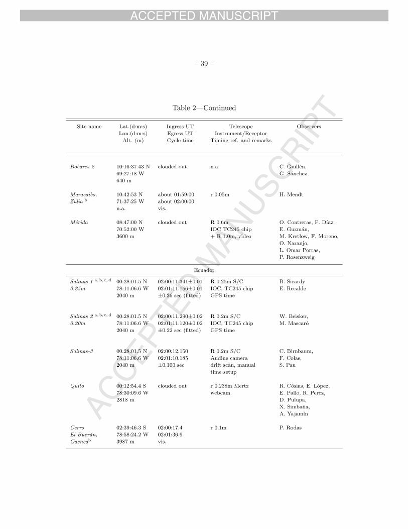
ACCEP

TED M

ANUSC

RIPT

ACCEPTED MANUSCRIPT

– 39 –

Table 2—Continued

Site name Lat.(d:m:s) Ingress UT Telescope Observers

Lon.(d:m:s) Egress UT Instrument/Receptor

Alt. (m) Cycle time Timing ref. and remarks

Bobares 2 10:16:37.43 N clouded out n.a. C. Guillen,

69:27:18 W G. Sanchez

640 m

Maracaibo, 10:42:53 N about 01:59:00 r 0.05m H. Mendt

Zulia b 71:37:25 W about 02:00:00

n.a. vis.

Merida 08:47:00 N clouded out R 0.6m O. Contreras, F. Dıaz,

70:52:00 W IOC TC245 chip E. Guzman,

3600 m + R 1.0m, video M. Kretlow, F. Moreno,

O. Naranjo,

L. Omar Porras,

P. Rosenzweig

Ecuador

Salinas 1 a,b,c, d 00:28:01.5 N 02:00:11.341±0.01 R 0.25m S/C B. Sicardy

0.25m 78:11:06.6 W 02:01:11.166±0.01 IOC, TC245 chip E. Recalde

2040 m ±0.26 sec (fitted) GPS time

Salinas 2 a,b,c, d 00:28:01.5 N 02:00:11.290±0.02 R 0.2m S/C W. Beisker,

0.20m 78:11:06.6 W 02:01:11.120±0.02 IOC, TC245 chip M. Mascaro

2040 m ±0.22 sec (fitted) GPS time

Salinas-3 00:28:01.5 N 02:00:12.150 R 0.2m S/C C. Birnbaum,

78:11:06.6 W 02:01:10.185 Audine camera F. Colas,

2040 m ±0.100 sec drift scan, manual S. Pau

time setup

Quito 00:12:54.4 S clouded out r 0.238m Mertz R. Cosias, E. Lopez,

78:30:09.6 W webcam E. Pallo, R. Percz,

2818 m D. Pulupa,

X. Simbana,

A. Yajamın

Cerro 02:39:46.3 S 02:00:17.4 r 0.1m P. Rodas

El Bueran, 78:58:24.2 W 02:01:36.9

Cuencab 3987 m vis.

ACCEP

TED M

ANUSC

RIPT

ACCEPTED MANUSCRIPT

– 40 –

Table 2—Continued

Site name Lat.(d:m:s) Ingress UT Telescope Observers

Lon.(d:m:s) Egress UT Instrument/Receptor

Alt. (m) Cycle time Timing ref. and remarks

Mexico

Monterrey 25:38:36 N no event R 0.175m P. Valdes Sada

100:22:26 W from 01:51 Astrovid camera

659 m to 02:05

aThe four stations/datasets used for stellar diameter (Section 3) and atmospheric model

fitting (Section 6). Quoted error bars are formal errors from diffraction limb fitting and

are at most 0.035 s. Larger, systematic errors on absolute timing may be present at the ±0.3 s level (see text).

bThe fifty-seven stations with reported timings (shown in Figure 7). Error bars at these

stations are those reported by observers and have not been modified by us.

cThe forty-three stations with Δr = ri,obs − rref ≤ 10 km used for Titania’s ephemeris

offset using time-shifted chords (Section 4 and Figure 8)

dThe twenty-seven stations used for Titania’s size and oblateness through limb fitting

(Section 5, fit parameters listed in Table 3). Among them are thirteen visual observations

made by experienced observers, for which we estimate an accuracy of about 0.2-0.3 sec

eUndocumented site or one or more observer’s coordinates at ± 1 arcmin error level.

Note. — Abbreviations and acronyms : Cycle time = Recording time resolution ;

Telescope : R = reflector ; r = refractor ; Newt. = Newton ; S/C = Schmidt-Cassegrain ;

Instrument/Receptor : IOC = Iota camera, Aud. = Audine camera, SBIG = Sbig camera,

Vid. = video/camcorder, Vis. = Visual ; Timing source/reference : MSF (or NPL) = UK

60 kHz time signal, DCF77 = Germany 77.5kHz time signal, WWVB = NIST 60 kHz time

signal, Colorado ; n.a. = not available/specified.

ACCEPTED MANUSCRIPT

AC

CE

PT

ED

MA

NU

SC

RIP

T

–41

–Table 3. Circular fit to 27 selected chords, Sep. 8, 2001 event. The free parameters of the fit are Titania’s radius, RT,occ, and

the location of shadow center, as given by the offset Δf,Δg (see text).

Ingress Egress

Sitea Rec.b Δtc Latituded fe ge Latituded fe ge C/Af Δrg

(sec) (deg) (km) (km) (deg) (km) (km) (km) (km)

Arikok, 0.2m ccd +0.093 +65.7 -2275.3 -957.8 -45.4 -973.7 -271.1 +279.6 -1.37

Worth Hill, 0.25m vid. +0.243 +65.6 -2261.0 -1044.5 -50.4 -911.6 -330.2 +197.3 -0.05

Ponta D., 0.3m vid. -0.531 +65.3 -2251.7 -1068.2 -52.0 -894.8 -354.1 +170.2 -3.17

Caracas, 0.125m vid. -2.520 +59.5 -2184.4 -1248.3 -61.1 -784.9 -510.7 -020.1 +2.74

Chatellerault, 0.1m vis. -0.378 +50.4 -2078.3 -1393.4 -65.6 -725.7 -678.1 -196.8 +1.57

Marinha G., 0.4m vid. -0.415 +36.7 -1898.8 -1540.1 -62.5 -705.7 -911.3 -411.4 +1.56

Linhaceira, 0.25m vid. +0.235 +33.0 -1846.4 -1565.3 -60.3 -714.5 -968.7 -458.1 -1.48

Salinas-1, 0.25m ccd -0.381 +32.0 -1833.6 -1573.5 -59.8 -714.6 -981.7 -470.4 +0.25

Salinas-2, 0.2m ccd -0.333 +32.0 -1833.7 -1573.5 -59.8 -714.6 -981.6 -470.4 +0.29

Pic du Midi, 1m vid. +0.290 +28.8 -1787.4 -1595.3 -57.5 -722.8 -1033.0 -511.6 +1.66

St Maurice Caz., 0.2m vis. -0.153 +23.2 -1705.3 -1619.9 -53.2 -748.5 -1114.1 -571.5 -1.21

Zaragoza, 0.12m vis. -0.018 +22.6 -1696.0 -1624.5 -52.6 -750.3 -1125.3 -580.3 +0.78

Alvito, 0.25m vid. +0.455 +22.4 -1693.2 -1626.1 -52.4 -751.0 -1129.7 -583.4 +1.59

Hortoneda, 0.203m vis. +2.808 +19.7 -1652.6 -1631.8 -50.2 -768.6 -1165.0 -606.9 -2.02

COAA, 0.2m vid. +0.402 +15.5 -1590.6 -1643.3 -46.5 -794.9 -1224.2 -646.5 -0.81

Portimao-1, 0.25m ccd +0.007 +15.0 -1583.0 -1642.8 -46.0 -799.6 -1230.2 -649.6 -2.19

Orfeuilles, 0.2m vis. -0.431 +11.5 -1529.6 -1647.1 -43.0 -824.9 -1274.6 -677.7 -2.04

St Esteve, 0.2m vis. +0.265 +07.8 -1473.4 -1648.6 -39.5 -855.8 -1322.5 -705.5 -1.09

Sabadell-1, 0.5m ccd +0.097 +07.4 -1467.7 -1649.5 -39.1 -858.3 -1327.6 -708.9 -0.08

Barcelona-2.1, 0.21m vis. +0.091 +06.5 -1453.4 -1648.5 -38.3 -867.2 -1338.9 -714.7 -0.49

Barcelona-2.2, 0.203m vis. +0.041 +06.5 -1454.3 -1649.0 -38.3 -866.3 -1338.4 -714.7 -0.04

Barcelona-2.3, 0.21m vis. +0.241 +06.5 -1454.3 -1649.0 -38.3 -866.3 -1338.4 -714.7 -0.05

Alella, 0.24m vid. +2.492 +05.8 -1443.1 -1652.4 -37.6 -869.8 -1349.6 -722.9 +4.01

Barcelona-1, 0.258m vis. +0.384 +04.9 -1430.2 -1647.5 -36.8 -881.0 -1357.5 -724.7 +0.12

Barcelona-3, 0.1m vis. +0.111 +04.9 -1430.8 -1648.7 -36.9 -879.8 -1357.7 -725.4 +1.24

Alcublas, 0.2m vis. +0.255 -01.0 -1341.9 -1634.4 -31.1 -942.1 -1423.4 -754.3 -0.77

Castellon, 0.2m vis. -0.046 -02.7 -1316.8 -1630.1 -29.5 -959.7 -1441.7 -762.3 +0.31

ACCEPTED MANUSCRIPT

AC

CE

PT

ED

MA

NU

SC

RIP

T

–42

–aSee Table 2. Chords have been sorted in order of decreasing closest approach (C/A) distances. This corresponds from top to

bottom in Figure 11.

bType of recording mode : CCD, vid.= video or vis.= visual.

cApplied time shift, see text for details.

dSub-occultation titaniacentric latitude.

ePosition in sky plane, see Figure 11.

fClosest approach to shadow center. Positive means observer North of shadow center, negative otherwise.

gRadial residual to circular fit (plotted in Figure 12).

Note. — Best fitting circle radius RT = 788.4 km, center : fc = −1494.1 km, gc = −861.6 km, r.m.s. radial dispersion : 1.58 km,

no oblateness detected. See text, Section 5 for details.

ACCEP

TED M

ANUSC

RIPT

ACCEPTED MANUSCRIPT

– 43 –

Table 4. Titania occultation, August 1, 2003, circumstances and timings. Same abbreviations asin Table 2.

Site name Lat.(d:m:s) Ingress UT Telescope Observers

Lon.(d:m:s) Egress UT Instrument/Receptor

Alt. (m) Cycle time Timing ref. and remarks

Mexico

Observatorio 25:54:51.5 N 04:28:08.49±0.05 R 0.3m S/C, Astrovid P. Valdes Sada,

UANL 100:08:35.6 W 04:29:22.01±0.03 video with R. Hernandez,

385 m ±0.05/0.03 sec GPS time insertion E. Castro

United States of America

George 29:22:30 N 04:27:53±1 R 0.9m S/C, A. Hernandez

Observatory 95:35:37 W 04:28:53±1 video with P. Maley

24 m ±1 sec WWVB time signal B. Wilson

ACCEP

TED M

ANUSC

RIPT

ACCEPTED MANUSCRIPT

– 44 –

Table 5. Modelling results for Titania’s atmosphere surface pressure at equilibrium, withdetection upper limits in standard deviation units for CO2, CH4 and N2.

gas (dz/dT)z T(z > 20km) surface scale height surface pressure column density

(K km−1) (K) (km) upper limit (nb) (cm-amagat)

CO2 0 60 30 1-σ 9 0.132

3-σ 20 0.293

CO2 0 70 35 1-σ 13 0.193

3-σ 28 0.410

CO2 0 80 40 1-σ 17 0.257

3-σ 37 0.549

CH4 2 110 95 1-σ 8 0.436

3-σ 18 0.954

N2 0 70 55 1-σ 22 0.550

3-σ 46 1.150

ACCEP

TED M

ANUSC

RIPT

ACCEPTED MANUSCRIPT

– 45 –

Fig. 1.— Path of Titania’s shadow on Earth on September 8, 2001, according to the post-occultationanalysis presented in this paper. Motion is from upper right to lower left. The darker grey zoneis for night time (Sun below -18◦ with respect to local horizon), lighter grey is for astronomicaltwilight (Sun between 0◦ and -18◦ below local horizon) and white is for day time. Dots along thecenterline are plotted every minute. This is where the event duration was maximum, about 72sec. The green star symbols indicate all the stations reported in Table 2, among which fifty-sevenreported timings. The event was observed at low elevation from France, UK, Italy, Spain, Morocco,Portugal around 1:55 UT, and near zenith in the Caribbean region (Barbados, Tobago, Aruba) andfrom Northern South-America (Ecuador, Venezuela); around 2:00 UT.

ACCEP

TED M

ANUSC

RIPT

ACCEPTED MANUSCRIPT

– 46 –

Fig. 2.— Enlargement of Figure 1. Titania’s shadow over Europe and Africa observing stations.Green star symbols are for stations where observations were attempted and/or achieved, Red starsymbols mark the subset of twenty-seven stations used for limb fitting (Section 5). See Table 2 forcircumstances and timings, and Table 3 for limb fitting data.

ACCEP

TED M

ANUSC

RIPT

ACCEPTED MANUSCRIPT

– 47 –

Fig. 3.— Same as Figure 2, for Central and South America. See Table 2 for circumstances andtimings, and Table 3 for limb fitting data.

ACCEP

TED M

ANUSC

RIPT

ACCEPTED MANUSCRIPT

– 48 –

Fig. 4.— Example of a light curve, obtained with the 0.25m reflector at Salinas. All data pointsare shown, with a cycle time of 0.26 sec, see Table 2. The flux from the star (plus the much fainterTitania) has been divided by a running average (over 5 sec) of Uranus’ flux, in order to correct forlow frequency sky transparency variations. Finally, the data have been normalized between zero(Titania only) and unity (full stellar + Titania flux).

ACCEP

TED M

ANUSC

RIPT

ACCEPTED MANUSCRIPT

– 49 –

Fig. 5.— Fit the stellar diameter from the Salinas-1 0.25m (squares), Salinas-2 0.20m (bullets),Arikok 0.20m (triangles) and Portimao-1 0.25m (crosses) light curves (see Table 2). Data arenormalized between 0 (no star) and 1 (full signal). The vertical dotted line is the location of anedge at 788.4 km, corresponding to the Titania radius obtained in this paper. The upper thin curveis shifted vertically by +0.6 for better viewing, and shows the expected diffraction pattern froma point-like source. Thin lines superimposed to the data are best fits with stellar diameter takeninto account. They are slightly different from each other, as the response of each instrument varieswith integration time. See text for details.

ACCEP

TED M

ANUSC

RIPT

ACCEPTED MANUSCRIPT

– 50 –

Fig. 6.— Upper panel: Fit to the Arikok, Aruba, ingress and egress light curves (solid line). Thetriangles are the individual data points, while the open circles are from a best fit model, takinginto account diffraction, stellar diameter and instrumental response, see text for details. Besidesproviding the stellar diameter, see Figure 5, the fit yields the stellar half-light times at disappearanceand re-appearance, and associated error bars, see Table 2. Lower panel: The same for the Salinas-10.25m reflector data, where the square are individual data points, see also Figure 4. On both plots,note the discontinuity in time at the vertical dotted line, in order for the light curves to fit into thefigure. Also, note the better sampling of the Arikok light curve, due to a smaller cycle time (0.11sec vs. 0.26 sec, see Table 2).

ACCEP

TED M

ANUSC

RIPT

ACCEPTED MANUSCRIPT

– 51 –

Fig. 7.— Fifty-seven occultation chords with reported timings (Table 2). The origin “O” of thediagram is located at the expected center of Titania’s disk in ICRS J2000.0 coordinates, as derivedfrom the star position predicted at time of event (Eq. 1) and DE405+URA027 Titania ephemeris.The arrow indicates the direction of motion in the sky plane. The horizontal and vertical barsare aligned with the local celestial ICRS J2000.0 N-S and E-W directions, respectively, and havelengths of 1000 km, with celestial North up and celestial East left. The scale is 13,819 km perarcsec. Label “S” stands for Titania’s south pole (IAU convention). Meridians and parallels onTitania’s globe are plotted every 15◦, with thicker lines delineating Titania’s equator and origin oflongitudes (the meridian facing Uranus). The intersection of this meridian with Titania’s equatordefines the sub-Uranus point on Titania, labelled “SU”. Sub-observer latitude at Titania is -24.2◦,and north pole position angle is 260.4◦, see Table 1. An offset with respect to the expected Titania’sposition is clearly visible, see Section 4. The circle surrounding the chords is the best circular fitto Titania’s limb (Section 5).

ACCEP

TED M

ANUSC

RIPT

ACCEPTED MANUSCRIPT

– 52 –

Fig. 8.— Same as Figure 7, but limited to the forty-three stations with radial residual Δr =r − rref ≤ 10 km used for Titania’s ephemeris offset determination (Table 2 and Section 4). Thiscorresponds to an error of 0.5 to 2 sec in chord duration, depending on the observer’s locationprojected on the limb. The occultation chords have also been displaced along their own directionso that they share the same mediatrix. This is equivalent to applying a time shift to each ofthose stations, to compensate for their absolute timing error, see text for details. The offset inICRS J2000.0 celestial coordinates, between Titania’s expected position (globe at upper left) andobserved position is Δα cos(δ) = −108± 13 mas and Δδ = −62± 7 mas. Like in Figure 7 the circlesurrounding the chords is the best circular fit to Titania’s limb.

ACCEP

TED M

ANUSC

RIPT

ACCEPTED MANUSCRIPT

– 53 –

Fig. 9.— The two occultation chords derived from the additional timings provided by the Aug. 1,2003 occultation (see Table 4) and used for an additional offset constraint to Titania’s ephemerisposition. The Figure shows Titania’s orientation and direction of motion in the sky plane in ICRSJ2000.0 coordinates. Label ”S” is Titania’s south pole ; titaniacentric meridians and parallelsare plotted every 15◦. ”AU” designates the anti-suburanian meridian at longitude 180◦, as primemeridian is on the far side. See text, Section 4 for details.

ACCEP

TED M

ANUSC

RIPT

ACCEPTED MANUSCRIPT

– 54 –

Fig. 10.— Histogram of radial residuals for our best circular fit to both extremities of the twenty-seven occultations chords of see Fig. 11, reported in Table 3. Our fitted Titania’s radius, RT,occ =788.4 ± 0.6 km, is shown as a black dot with associated error bars, just below the value derivedfrom Voyager images, RT,Voy = 788.9 ± 1.8 (Thomas 1988). Most of the dispersion seen in thishistogram is likely to be caused by topographic features along Titania’s limb, see Section 5, ¶5.1.

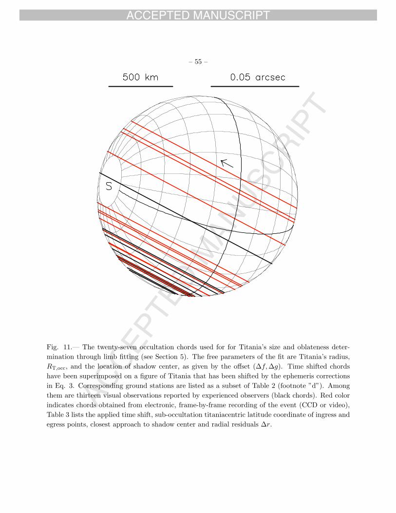
ACCEP

TED M

ANUSC

RIPT

ACCEPTED MANUSCRIPT

– 55 –

Fig. 11.— The twenty-seven occultation chords used for for Titania’s size and oblateness deter-mination through limb fitting (see Section 5). The free parameters of the fit are Titania’s radius,RT,occ, and the location of shadow center, as given by the offset (Δf,Δg). Time shifted chordshave been superimposed on a figure of Titania that has been shifted by the ephemeris correctionsin Eq. 3. Corresponding ground stations are listed as a subset of Table 2 (footnote ”d”). Amongthem are thirteen visual observations reported by experienced observers (black chords). Red colorindicates chords obtained from electronic, frame-by-frame recording of the event (CCD or video),Table 3 lists the applied time shift, sub-occultation titaniacentric latitude coordinate of ingress andegress points, closest approach to shadow center and radial residuals Δr.

ACCEP

TED M

ANUSC

RIPT

ACCEPTED MANUSCRIPT

– 56 –

Fig. 12.— Upper limit on Titania’s oblateness.− Residuals of the best circular fit to the 27 occul-tation chords shown in Figure 11. X-axis is the titaniacentric latitude, with South pole on the leftand North pole on the right, from -90◦ to +90◦. Y-axis is the distance to Titania’s shadow center.The dotted horizontal line corresponds to the radius of our best circular fit, RT,occ = 788.4±0.6 km,with its error bar (±0.6 km, shaded rectangle). Bullets indicate the ingress and egress distancesri,obs versus sub-occultation latitude on Titania, after each 27 chords has been shifted in absolutetime so they have a common mediatrix. This explains why the points come by pairs (ingress atright and egress at left) with the same distance to shadow center imposing their extremities tohave the same radial residuals with respect to a reference circle. The vertical lines marks themaximum latitudes (±65.8◦) reachable during the occultation, due to the titaniacentric elevationB = −24.2◦ of the observers during the Sept. 8, 2001 event. Solid bullets are from the 14 stationswith an electronic record of the event (CCD or video), while open bullets are from the 13 bestvisual observations, see Section 5.

ACCEP

TED M

ANUSC

RIPT

ACCEPTED MANUSCRIPT

– 57 –

Fig. 13.— Same as Fig. 12, after plotting all latitudes in absolute value, and averaging them overingress and egress values. The thicker line corresponds to the upper limit of an oblate limb of theform r = req[1− f sin2 φ], with a difference between equatorial and polar radius of req − rpo = +0.8km. The thin line is the upper limit of a prolate limb, with req − rpo = −3.4 km. See text fordetails.

ACCEP

TED M

ANUSC

RIPT

ACCEPTED MANUSCRIPT

– 58 –

Fig. 14.— Examples of shrinkings of Titania’s shadow radius due to ray bending by a model CO2

isothermal atmosphere (T = 70 K) with surface pressures of 0, 50, 100, 150, 200 nbar, in orderof decreasing line thicknesses, see also labels above each curve. The model takes into account thesmoothing by a 0.51 mas diameter star (but does not account for diffraction effects), and assumesthe radius derived from Voyager images, 788.9 km (Thomas 1988). The Voyager radius and ourown measurement are shown by black dots with associated error bars at the top. The dotted lineis the diffracting model which best fits our data, see Fig. 5. For this particular model (CO2 atT=70K), we find that Titania’s apparent radius decreases by about 0.056 km per nbar added tothe surface pressure. The stellar drop just prior to the occultation by Titania’s limb amounts toabout 1.1 × 10−3 per nbar. For instance, a 200 nbar atmosphere shrinks the radius by about 11.2km, and causes a drop of 22% by the time the star reaches the satellite limb. See text, Section 6,¶6.1.

ACCEP

TED M

ANUSC

RIPT

ACCEPTED MANUSCRIPT

– 59 –

Fig. 15.— Same as Fig. 5, but at different scales, to illustrate the effect of a faint atmosphere onthe light curves. Symbols are the same as in Fig. 5, namely Salinas-1 0.25m (squares), Salinas-20.20m (bullets), Arikok 0.20m (triangles) and Portimao-1 0.25m (crosses). For each of the fourlightcurves, the before-ingress and after-egress data points have been folded over and binned over∼ 20 km vertical bins, in order to take into account the relative velocity of the star perpendicularlyto each limb, so that the radial sampling Δr is constant at each station on the plot. In this waythe actual contribution of stations to vertical sampling can be assessed, although the fit to modelwas performed on actual data points. The point on left (Portimao) corresponds to the stellar dropbehind Titania’s limb at r < 792 km (those data points were not included in the fit). The dottedvertical line corresponds to our estimate of Titania’s radius best value of 788.4 km. The smoothsolid line is the 1-σ upper limit for the fit of actual data points to a CO2 isothermal (T = 80 K)model atmosphere, with a surface pressure of 17 nbar. The dotted line is the 3-σ upper limit (p= 27 nbar). The shaded area shows the difference between this model and an airless model. SeeTable 5 and text for details.

ACCEP

TED M

ANUSC

RIPT

ACCEPTED MANUSCRIPT

– 60 –

Fig. 16.— Same as Fig. 15, but for methane. The smooth solid line is the 1-σ upper limit for aheated CH4 atmosphere with T = 70 K at surface level and T = 110 K above 20 km, with a surfacepressure of 8 nbar. The shaded area shows the difference between this model and an airless model,while the dotted line shows the 3-σ upper limit (p = 18 nbar) for comparison. See Table 5 and textfor details.

ACCEP

TED M

ANUSC

RIPT

ACCEPTED MANUSCRIPT

– 61 –

Fig. 17.— Same as Fig. 16, but for an isothermal, T = 70 K N2 atmosphere. The 1-σ upper limitis 22 nbar, corresponding to 0.550 cm-amagat (solid line) while the 3-σ upper limit corresponds top = 46 nbar or 1.150 cm-amagat (dotted line).