Time-Aware Test Suite Prioritization

Kristen R. WalcottMary Lou Soffa

Department of Computer ScienceUniversity of Virginia

{walcott, soffa}@cs.virginia.edu

Gregory M. KapfhammerRobert S. Roos

Department of Computer ScienceAllegheny College

{gkapfham, rroos}@allegheny.edu

ABSTRACTRegression test prioritization is often performed in a timeconstrained execution environment in which testing only oc-curs for a fixed time period. For example, many organiza-tions rely upon nightly building and regression testing oftheir applications every time source code changes are com-mitted to a version control repository. This paper presentsa regression test prioritization technique that uses a geneticalgorithm to reorder test suites in light of testing time con-straints. Experiment results indicate that our prioritiza-tion approach frequently yields higher average percentageof faults detected (APFD) values, for two case study appli-cations, when basic block level coverage is used instead ofmethod level coverage. The experiments also reveal funda-mental trade-offs in the performance of time-aware prioriti-zation. This paper shows that our prioritization techniqueis appropriate for many regression testing environments andexplains how the baseline approach can be extended to op-erate in additional time constrained testing circumstances.

Categories and Subject DescriptorsD.2.5 [Software Engineering]: Testing and Debugging—Testing tools

General TermsVerification, Experimentation

Keywordstest prioritization, coverage testing, genetic algorithms

1. INTRODUCTIONAfter a software application experiences changes in the

form of bug fixes or the addition of functionality, regressiontesting is used to ensure that changes to the program donot negatively impact its correctness. However, regressiontesting can be prohibitively expensive, particularly with re-spect to time [13], and thus accounts for as much as half thecost of software maintenance [14, 24]. In one example, an

Permission to make digital or hard copies of all or part of this work forpersonal or classroom use is granted without fee provided that copies arenot made or distributed for profit or commercial advantage and that copiesbear this notice and the full citation on the first page. To copy otherwise, torepublish, to post on servers or to redistribute to lists, requires prior specificpermission and/or a fee.ISSTA’06, July 17–20, 2006, Portland, Maine, USA.Copyright 2006 ACM 1-59593-263-1/06/0007 ...$5.00.

industrial collaborator reported that for one of its productsof approximately 20,000 lines of code, the entire test suiterequired seven weeks to run [8]. Since there is usually a lim-ited amount of time allowed for testing [19], prioritizationtechniques can be used to reorder the test suite to increasethe rate of fault detection earlier in test execution [8, 24].However, no existing approach to prioritization incorporatesa testing time budget.

As frequent rebuilding and regression testing gain in pop-ularity, the need for a time constraint aware prioritizationtechnique grows. For example, popular software systems likePlanetLab [3] and MonetDB [2] use nightly builds, which in-clude building, linking, and unit testing of the software [19].New software development processes such as extreme pro-gramming also promote a short development and testing cy-cle and frequent execution of fast test cases [23]. Therefore,there is a clear need for a prioritization technique that hasthe potential to be more effective when a test suite’s allowedexecution time is known, particularly when that executiontime is short. This paper shows that if the maximum timeallotted for execution of the test cases is known in advance,a more effective prioritization can be produced.

The time constrained test case prioritization problem canbe reduced to the NP-complete zero/one knapsack problem[10, 24], which can often be efficiently approximated with agenetic algorithm (GA) heuristic search technique [6]. Justas genetic algorithms have been effectively used in other soft-ware engineering and programming language problems suchas test generation [22], program transformation [9], and soft-ware maintenance resource allocation [5], this paper demon-strates that they also prove to be effective in creating timeconstrained test prioritizations. We present a technique thatprioritizes regression test suites so that the new ordering (i)will always run within a given time limit and (ii) will havethe highest possible potential for defect detection based onderived coverage information. This paper also provides em-pirical evidence that the produced prioritizations on averagehave significantly higher fault detection rates than randomor more simplistic prioritizations, like the initial order ora reverse reordering. In summary, the important contribu-tions of this paper are as follows:

1. A technique that uses a genetic algorithm to prioritizea regression test suite that will be run within a timeconstrained execution environment (Section 2 and Sec-tion 3).

2. An empirical evaluation of the effectiveness of the re-sulting prioritizations in relation to (i) GA-producedprioritizations using different parameters, (ii) the ini-

tial test suite ordering, (iii) the reverse of the initialtest suite ordering, (iv) random test suite prioritiza-tions, and (v) fault-aware prioritizations, showing thatthe GA-produced prioritizations are superior to theother test suite reorderings (Section 4).

3. An empirical evaluation of the time and space over-heads of our approach. This evaluation reveals thatthe technique is especially applicable when (i) there isa fixed set of time constraints, (ii) prioritization occursinfrequently, or (iii) the time constraint is particularlysmall (Section 4).

4. A discussion of enhancements to the baseline approachthat reduce the time overhead required to perform pri-oritization and extend the technique’s applicability toother time constrained testing situations (Section 5).

2. TIME-AWARE TEST PRIORITIZATIONCHALLENGES

Test prioritization schemes typically create a single re-ordering of the test suite that can be executed after manysubsequent changes to the program under test [7, 24]. Testcase prioritization techniques reorder the execution of a testsuite in an attempt to ensure that defects are revealed earlierin the test execution phase. If testing must be terminatedearly, a reordered test suite can also be more effective atfinding faults than one that was not prioritized [24]. Prob-lem 1 defines the time-aware test case prioritization problem.Intuitively, a test tuple σ earns a better fitness if it has agreater potential for fault detection and can execute withinthe user specified time budget.

Problem 1. (Time-Aware Test Suite Prioritization)Given: (i) A test suite, T , (ii) the collection of all permu-tations of elements of the power set of permutations of T ,perms(2T ), (iii) the time budget, tmax, and (iv) two func-tions from perms(2T ) to the real numbers, time and fit.Problem: Find the test tuple σmax ∈ perms(2T ) such thattime(σmax) ≤ tmax and ∀σ′ ∈ perms(2T ) where σmax 6=σ′ and time(σ′) ≤ tmax, fit(σmax) > fit(σ′).

In Problem 1, perms(2T ) represents the set of all possi-ble tuples and subtuples of T . When the function time isapplied to any of these tuples, it yields the execution timeof that tuple. The function fit is applied to any such tu-ple and returns a fitness value for that ordering. Withoutloss of generality, we assume that an awarded higher fitnessis preferable to a lower fitness. In this paper, the func-tion fit quantifies a test tuple’s incremental rate of faultdetection. Our technique considers the potential for faultdetection and the time overhead of each test case in orderto evaluate whether the test suite achieves its potential atthe fastest rate possible.

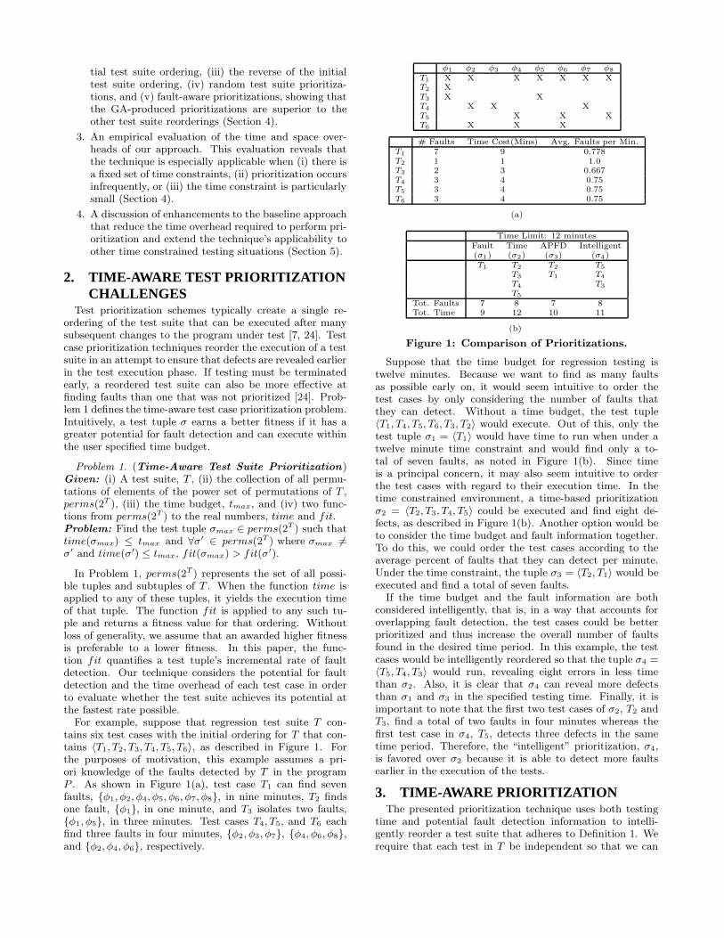
For example, suppose that regression test suite T con-tains six test cases with the initial ordering for T that con-tains 〈T1, T2, T3, T4, T5, T6〉, as described in Figure 1. Forthe purposes of motivation, this example assumes a pri-ori knowledge of the faults detected by T in the programP . As shown in Figure 1(a), test case T1 can find sevenfaults, {φ1, φ2, φ4, φ5, φ6, φ7, φ8}, in nine minutes, T2 findsone fault, {φ1}, in one minute, and T3 isolates two faults,{φ1, φ5}, in three minutes. Test cases T4, T5, and T6 eachfind three faults in four minutes, {φ2, φ3, φ7}, {φ4, φ6, φ8},and {φ2, φ4, φ6}, respectively.

φ1 φ2 φ3 φ4 φ5 φ6 φ7 φ8

T1 X X X X X X XT2 XT3 X XT4 X X XT5 X X XT6 X X X

# Faults Time Cost(Mins) Avg. Faults per Min.T1 7 9 0.778T2 1 1 1.0T3 2 3 0.667T4 3 4 0.75T5 3 4 0.75T6 3 4 0.75

(a)

Time Limit: 12 minutesFault Time APFD Intelligent(σ1) (σ2) (σ3) (σ4)T1 T2 T2 T5

T3 T1 T4

T4 T3

T5

Tot. Faults 7 8 7 8Tot. Time 9 12 10 11

(b)

Figure 1: Comparison of Prioritizations.

Suppose that the time budget for regression testing istwelve minutes. Because we want to find as many faultsas possible early on, it would seem intuitive to order thetest cases by only considering the number of faults thatthey can detect. Without a time budget, the test tuple〈T1, T4, T5, T6, T3, T2〉 would execute. Out of this, only thetest tuple σ1 = 〈T1〉 would have time to run when under atwelve minute time constraint and would find only a to-tal of seven faults, as noted in Figure 1(b). Since timeis a principal concern, it may also seem intuitive to orderthe test cases with regard to their execution time. In thetime constrained environment, a time-based prioritizationσ2 = 〈T2, T3, T4, T5〉 could be executed and find eight de-fects, as described in Figure 1(b). Another option would beto consider the time budget and fault information together.To do this, we could order the test cases according to theaverage percent of faults that they can detect per minute.Under the time constraint, the tuple σ3 = 〈T2, T1〉 would beexecuted and find a total of seven faults.

If the time budget and the fault information are bothconsidered intelligently, that is, in a way that accounts foroverlapping fault detection, the test cases could be betterprioritized and thus increase the overall number of faultsfound in the desired time period. In this example, the testcases would be intelligently reordered so that the tuple σ4 =〈T5, T4, T3〉 would run, revealing eight errors in less timethan σ2. Also, it is clear that σ4 can reveal more defectsthan σ1 and σ3 in the specified testing time. Finally, it isimportant to note that the first two test cases of σ2, T2 andT3, find a total of two faults in four minutes whereas thefirst test case in σ4, T5, detects three defects in the sametime period. Therefore, the “intelligent” prioritization, σ4,is favored over σ2 because it is able to detect more faultsearlier in the execution of the tests.

3. TIME-AWARE PRIORITIZATIONThe presented prioritization technique uses both testing

time and potential fault detection information to intelli-gently reorder a test suite that adheres to Definition 1. Werequire that each test in T be independent so that we can

guarantee that for all Ti ∈ 〈T1, . . . , Tn〉, ∆i−1 = ∆0, andthus there are no test execution ordering dependencies [14].This requirement enables our prioritization algorithm to re-order the tests in any sequence that maximizes the suite’sability to isolate defects.

Definition 1. A test suite T is a triple〈∆0, 〈T1, . . . , Tn〉 , 〈∆1, . . . , ∆n〉〉, consisting of an ini-tial test state, ∆0, a test case sequence 〈T1, . . . , Tn〉 forsome initial state ∆0, and expected test states 〈∆1, . . . , ∆n〉where ∆i = Ti(∆i−1) for i = 1, . . . , n.

3.1 OverviewA genetic algorithm is used to solve Problem 1. First, the

execution time of each test case is recorded. Because a timeconstraint could be very short, test case execution timesmust be exact in order to properly prioritize. Care is takento ensure that only the execution time of the test case wasincluded in the recorded time and not that of class loading.Timing information additionally includes any initializationand shutdown time required by a test. For example, if Ti

requires an open a network connection, this is performed be-fore test execution and is added into Ti’s overall executiontime. Similarly, the shutdown time of Ti could include a sub-stantial amount of time to store ∆i for subsequent analysisafter testing. Inclusion of initialization and shutdown timeis necessary because these operations can greatly increasethe execution time required by the test case.

The program P and each Ti ∈ 〈T1, . . . , Tn〉 are inputinto the genetic algorithm, along with the following userspecified parameters: (i) s, maximum number of candidatetest tuples generated during an iteration, (ii) gmax, maxi-mum number of iterations, (iii) pt, percent of the executiontime of T allowed by the time budget, (iv) pc, crossoverprobability, (v) pm, mutation probability, (vi) pa, additionprobability, (vii) pd, the deletion probability, (viii) tc, thetest adequacy criterion, and (ix) w, the program coverageweight. We require that all probabilities and percentagespt, pc, pm, pa, pd ∈ [0, 1]. The genetic algorithm uses heuris-tic search to solve Problem 1 and to identify the test tupleσmax ∈ perms(2T ) that is likely to have the fastest rate offault detection in the provided time limit. In general, anyσj ∈ perms(2T ) has the form σj = 〈Ti, . . . , Tu〉 where u ≤ n.

3.2 Genetic AlgorithmThe GAPrioritize algorithm in Figure 2 performs test

case prioritization on T based on a given time constraintpt, as desired by Problem 1. On line 1, this algorithm cal-culates pt percent of the total time of T , and stores thevalue in tmax, the maximum execution time for a tuple. Inthe loop beginning on line 3, the algorithm creates a setR0 containing s random test tuples σ from perms(2T ) thatcan be executed in tmax time. R0 is the first generationof s potential solutions to Problem 1. Once a set of testtuples is created, coverage information, which is explainedin Section 3.2.1, is used by the CalcF itness(P, σj , pt, tc, w)method on line 10. The CalcF itness(P, σj , pt, tc, w) methodis discussed in Section 3.2.2, and it is used to determine the“goodness” of σj . To simplify the notation, we denote Fj

the fitness value of σj , where Fj = fit(P, σj , tc, w). We alsouse F = 〈F1, F2, . . . , Fs〉 to denote the tuple of fitnesses foreach σj ∈ Rg , 0 ≤ g ≤ gmax.

The SelectTwoBest(Rg, F ) method on line 11 chooses thetwo best test tuples in Rg to be elements in the next gener-

Algorithm GAPrioritize(P, T, s, gmax, pt, pc, pm, pa, pd, tc, w)

Input: Program P

Test suite T

Number of tuples to be created per iteration s

Maximum iterations gmax

Percent of total test suite time pt

Crossover probability pc

Mutation probability pm

Addition probability pa

Deletion probability pd

Test adequacy criteria tc

Program coverage weight w

Output: Maximum fitness tuple Fmax ∈ F in set σmax

1. tmax ← pt ×Pn

i=0time(〈Ti〉)

2. R0 ← ∅3. repeat

4. R0 ← R0 ∪ {CreateRandomIndividual(T, pt)}5. until |R0| = s

6. g← 0;7. repeat

8. F ← ∅9. for σj ∈ Rg

10. F ← F ∪ {CalcF itness(P, σj , pt, tc, w)}11. Rg+1 ← SelectTwoBest(Rg, F )12. repeat

13. σk, σl ← SelectParents(Rg, F )14. σq, σr ← ApplyCrossover(pc, σk, σl)15. σq ← ApplyMutation(pm, σq)16. σr ← ApplyMutation(pm, σr)17. σq ← AddAdditionalTests(T,pa, σq)18. σr ← AddAdditionalTests(T, pa, σr)19. σq ← DeleteATest(pd, σq)20. σr ← DeleteATest(pd, σr)21. Rg+1 ← Rg+1 ∪ {σq} ∪ {σr}22. until |Rg+1| = s

23. g ← g + 124. until g > gmax

25. σmax ← FindMaxFitnessTuple(Rg−1, F )26. return σmax

Figure 2: The GA Prioritization Algorithm.

ation Rg+1 of test tuples. The two best tuples are chosen inorder to guarantee that Rg+1 has at least one “good” pair.It is important to carry these highly fit tuples into Rg+1

as they are in Rg because they are most likely very closeto exceeding tmax. Any slight change to these test tuplescould cause them to require too much execution time, thusinvalidating them. Since the GA is trying to identify oneparticular test tuple, this elitist selection technique ensuresthat the best tuple in Rg survives on to Rg+1 [11].

On line 13, SelectParents(Rg, F ) identifies pairs of tuples{σk, σl} from Rg through a roulette wheel selection tech-nique based on a probability proportional to |F |. The fitnessvalues are normalized in relation to the rest of the test tupleset by multiplying each Fj ∈ F by a fixed number, so thatthe sum of all fitness values equals one [11]. The test tuplesare then sorted by descending fitness values, and accumu-lated normalized fitness values are calculated. A randomnumber r ∈ [0, 1] is next generated, and the first individ-ual whose accumulated normalized value is greater than orequal to r is selected. This selection method is repeated un-til enough tuples are selected to fill the set Rg+1. Candidatetest tuples with higher fitnesses are therefore less likely to

be eliminated, but a few with lower fitness have a chance tobe used in the test tuple set as well [11].

The ApplyCrossover(pc, σk, σl) method on line 14 maymerge the pair {σk, σl} to create two potentially newtuples {σq , σr} based on pc, a user given crossoverprobability, as explained in Section 3.2.3. Each tu-ple in the pair {σq , σr} may then be mutated basedon pm, a user provided mutation probability, as de-scribed in Section 3.2.4. Finally, Section 3.2.5 explainshow a new test case may be added or deleted fromσq or σr using the AddAdditionalTests(T, pa, σr) andDeleteATest(pd, σr) methods. The crossover operator ex-changes subsequences of the test tuples, and the mutationoperator only mutates single elements. Test case additionand deletion are needed because no other operator allowsfor a change in the number of test cases in a test tuple.

After each of these modifications have been made to theoriginal pair, both tuples σq and σr are entered into Rg+1,as seen on line 21. The same transformations are appliedto all pairs selected by the SelectParents(Rg, F ) methoduntil Rg+1 contains s test tuples. In total, gmax sets of s

test tuples are iteratively created in this fashion as specifiedin Figure 2 on lines 7–24. When the final set Rgmax hasbeen created, the test tuple with the greatest fitness, σmax,is determined on line 25. This tuple is guaranteed to be thetuple with the highest fitness out of all g sets of size s.

3.2.1 Test CoverageSince it is very rare for a tester to know the location of

all faults in P prior to testing, the prioritization techniquemust estimate how likely a test is to find defects, whichfactors into the function fit of Problem 1. Recall that thefunction fit yields the fitness of the tuple σj based on itspotential for fault detection and its time consumption. As itis impossible to reveal a fault without executing the faultycode, the percent of code covered by a test suite is used todetermine the suite’s potential. In this paper, two forms oftest adequacy criteria tc are considered: (i) method coverageand (ii) block coverage [7, 14, 25]. A method is coveredwhen it has been entered. A basic block, a sequence ofinstructions without any jumps or jump targets, is coveredwhen it is entered for the first time. Because several highlevel language source statements can be in the same basicblock, it is sensible to keep track of basic blocks rather thanindividual statements at the time of execution [7, 25].

Our genetic algorithm accepts coverage information basedon the code covered in an application by an entire test suite.As noted by Kessis et al., this is the form that many toolssuch as Clover [15], Jazz [20], and Emma [25] produce. Thepresented prioritization approach can reorder a test suitewithout requiring coverage information on a per-test basis.While the genetic algorithm handles the common case, itscalculation of test tuple fitness could be enhanced to usecoverage information on a per-test basis, similar to [7]. In-formation revealing the impact of a test case Ti’s test cov-erage on any other test case’s coverage would also furtherimprove the performance of the fitness function. This andother enhancements are explained in Section 5.

3.2.2 Fitness FunctionThe CalcF itness(P, σj , pt, tc, w) method on line 10 uses

fit(P, σj , tc, w) to calculate fitness. The fitness function,represented by fit in Problem 1, assigns each test tuple a

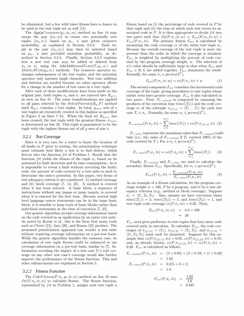
fitness based on (i) the percentage of code covered in P bythat tuple and (ii) the time at which each test covers its as-sociated code in P . It is then appropriate to divide fit intotwo parts such that fit(P, σj , tc, w) = Fpri(P, σj , tc, w) +Fsec(P, σj , tc). The primary fitness Fpri is calculated bymeasuring the code coverage cc of the entire test tuple σj .Because the overall coverage of the test tuple is more im-portant than the order in which the coverage is attained,Fpri is weighted by multiplying the percent of code cov-ered by the program coverage weight, w. The selection ofw’s value should be sufficiently large so that when Fpri andFsec ∈ [0, 1] are added together, Fpri dominates the result.Formally, for some σj ∈ perms(2T ),

Fpri(P, σj , tc, w) = cc(P, σj , tc)×w (1)

The second component Fsec considers the incremental codecoverage of the tuple, giving precedence to test tuples whoseearlier tests have greater coverage. Fsec is also calculated intwo parts. First, Fs−actual is computed by summing theproducts of the execution time time(〈Ti〉) and the code cov-erage cc of the subtuple σj{1,i} = 〈T1 . . . Ti〉 for each test

case Ti ∈ σj . Formally, for some σj ∈ perms(2T ),

Fs−actual(P, σj , tc) =

|σj |X

i=1

time(〈Ti〉)× cc(P, σj{1,i}, tc) (2)

Fs−max represents the maximum value that Fs−actual couldtake (i.e., the value of Fs−actual if T1 covered 100% of thecode covered by T .) For a σj ∈ perms(2T ),

Fs−max(P, σj , tc) = cc(P, σj , tc)×

|σj |X

i=1

time(〈Ti〉) (3)

Finally, Fs−actual and Fs−max are used to calculate thesecondary fitness Fsec. Specifically, for σj ∈ perms(2T ),

Fsec(P, σj , tc) =Fs−actual(P, σj , tc)

Fs−max(P, σj , tc)(4)

As an example of a fitness calculation, let the program cov-erage weight w = 100, P be a program, and tc be a test ad-equacy criterion (e.g., method or block coverage). Supposeσj = 〈T1, T2, T3〉. Also, assume we have execution timestime(〈T1〉) = 5, time(〈T2〉) = 3, and time(〈T3〉) = 1, andtest tuple code coverage cc(P, σj , tc) = 0.20. Then,

Fpri(P, σj , tc, w) = 0.2 × 100

= 20

Fsec next gives preference to test tuples that have more codecovered early in execution. To calculate Fsec, the code cov-erages of σj{1,1} = 〈T1〉, σj{1,2} = 〈T1, T2〉, and σj{1,3} =〈T1, T2, T3〉 must each be measured. Suppose for this ex-ample that cc(P, σj{1,1}, tc) = 0.05, cc(P, σj{1,2}, tc) = 0.19,and, as already known, cc(P, σj{1,3}, tc) = cc(P, σj , tc) =0.20. Fsec is calculated as follows,

Fs−actual(P, σj , tc) = (5× 0.05) + (3× 0.19) + (1 × 0.20)

= 1.02

Fs−max(P, σj , tc) = 0.2(5 + 3 + 1)

= 1.8

Fsec(P, σj , tc) =1.02

1.8= 0.567

Figure 3: Crossover with Random Crossover Point.

Adding Fpri and Fsec gives the total fitness value Fj of σj .Therefore, in this example,

fit(P, σj , tc, w) = Fpri(P, σj , tc, w) + Fsec(P, σj , tc)

= 20 + 0.567

= 20.567

If a test tuple execution time time(σj) is greater thanthe time budget tmax, Fj is automatically set to -1 by theCalcF itness(P, σj , pt, tc, w) method. Because such a tupleviolates the execution time constraint, it cannot be a so-lution and thus receives the worst fitness possible. While atuple σj with Fj = −1 could simply not be added to the nextgeneration Rg+1, populations with individuals that have afitness of -1 can actually be favorable. Since the “optimal”test tuple prioritization likely teeters on the edge of exceed-ing the designated time budget, any slight change to a σj

with Fj = −1 could create a new valid test tuple. Therefore,some σj ’s with Fj = −1 are maintained in the next gener-ation. If the test tuple execution time time(σj) <= tmax,Equations 1–4 are used.

3.2.3 CrossoverCrossover is used to vary test tuples from one test tu-

ple set to the next through recombination. It is unlikelythat the new test tuples after recombination will be iden-tical to a particular parent tuple. As explained in the in-troduction to Section 3.2, pairs of test tuples {σk, σl} areselected out of Rg. The ApplyCrossover(pc, σk, σl) methodperforms crossover to create two potentially new hybrid testtuples from {σk, σl}. First, a random number r1 ∈ [0, 1]is generated. If r1 is less than the user provided value forpc, the crossover operator is applied. Otherwise, the parentindividuals are unchanged and await the next step, muta-tion. If crossover is to occur, the ApplyCrossover(pc, σk, σl)method on line 14 selects another random number r2 ∈[0, min(|σk|, |σl|)] as the crossover point, where |σk| and |σl|are the number of test cases in σk and σl, respectively. Thesubsequences before and after the crossover point are thenexchanged to produce two new offspring, as seen in Figure 3.

If crossover causes two of the same test cases to be inthe same test tuple, another random test not in the currenttuple is selected from T instead of including the duplicatedtest case. Although a test case may be run more than oncein a test suite with all independent test cases, there is rarelya benefit to executing it again. We assume that multipleexecutions of a test case will produce the same results andthat there is no benefit to multiple execution. However, theApplyCrossover method can be easily reconfigured to allowfor duplicate test cases if there is a testing benefit. If thenew tuple already includes all tests, no additions are made.

3.2.4 MutationThe use of the ApplyMutation(pm, σj) method on lines 15

and 16 of Figure 2 also provides a way to add variation to a

Figure 4: Mutation of a Test Tuple.

new population. The new test tuple is identical to the priorparent tuple except that one or more changes may be madeto the new tuple’s test cases. All test tuples that are selectedon line 13 are first considered for crossover. Then they aresubject to mutation at each test case position with a smalluser specified mutation probability pm. If a random numberr3 ∈ [0, 1] is generated such that r3 is less than pm for testcase Ti, a new test not included in the current test tuple israndomly selected from T to replace Ti, as demonstrated forT2 in Figure 4(a). Figure 4(b) also shows that if there areno unused tests in T when T9 is chosen for mutation, thetest tuple is still mutated. Instead of replacing the test witha random test, the test to be mutated is swapped with thetest case that succeeds it.

3.2.5 Addition and DeletionTest cases can also be added to or deleted from the test

tuples using the AddAdditionalTests(T,pa, σj) method onlines 17 and 18 or the DeleteATest(pd, σj) method on lines19 and 20. As in messy genetic algorithms [12], the sets oftuples Rg must be allowed to grow beyond the initial set R0.Addition and deletion ability permits such growth. Whilethe crossover operator exchanges subsequences, it does notincrease the number of test cases within an individual. Sim-ilarly, the mutation operator only mutates single elementsat each index within the test tuple. Although addition anddeletion operations are necessary, they should be performedinfrequently so as to not violate the principle of the geneticalgorithm. If a random number r4 ∈ [0, 1] is generated suchthat r4 < pa, a random test case is removed from the indi-vidual. If another random number r5 ∈ [0, 1] is generatedand r5 < pd, a random test case not yet executed in theindividual is added to the end of the test sequence.

4. EMPIRICAL EVALUATIONThe primary goal of this paper’s empirical study is to

identify and evaluate the challenges that are associated withtime-aware test suite prioritization. We implemented the

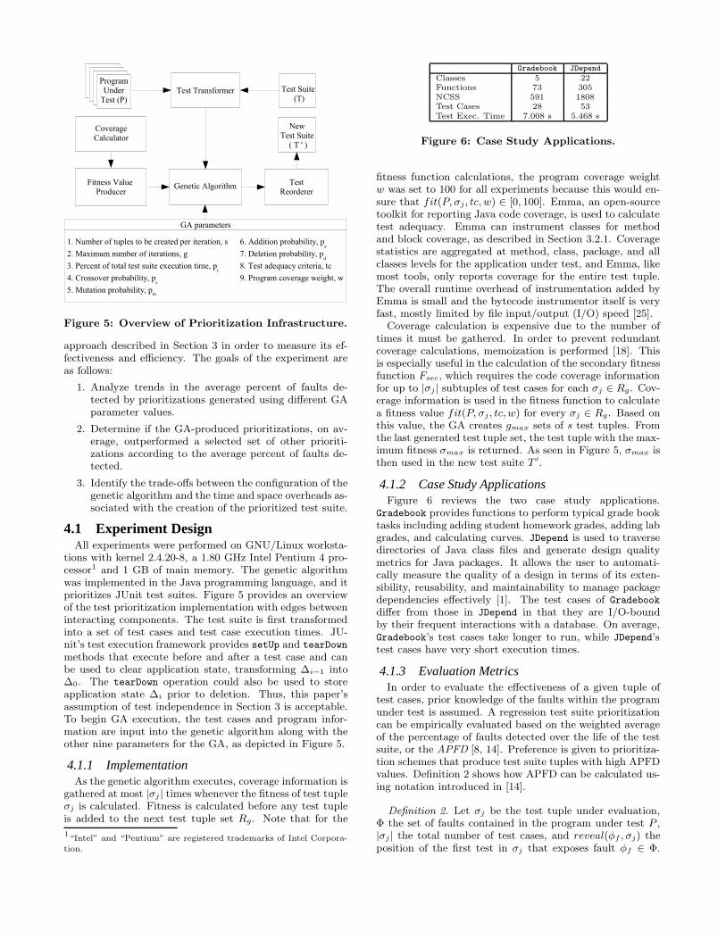
Figure 5: Overview of Prioritization Infrastructure.

approach described in Section 3 in order to measure its ef-fectiveness and efficiency. The goals of the experiment areas follows:

1. Analyze trends in the average percent of faults de-tected by prioritizations generated using different GAparameter values.

2. Determine if the GA-produced prioritizations, on av-erage, outperformed a selected set of other prioriti-zations according to the average percent of faults de-tected.

3. Identify the trade-offs between the configuration of thegenetic algorithm and the time and space overheads as-sociated with the creation of the prioritized test suite.

4.1 Experiment DesignAll experiments were performed on GNU/Linux worksta-

tions with kernel 2.4.20-8, a 1.80 GHz Intel Pentium 4 pro-cessor1 and 1 GB of main memory. The genetic algorithmwas implemented in the Java programming language, and itprioritizes JUnit test suites. Figure 5 provides an overviewof the test prioritization implementation with edges betweeninteracting components. The test suite is first transformedinto a set of test cases and test case execution times. JU-nit’s test execution framework provides setUp and tearDown

methods that execute before and after a test case and canbe used to clear application state, transforming ∆i−1 into∆0. The tearDown operation could also be used to storeapplication state ∆i prior to deletion. Thus, this paper’sassumption of test independence in Section 3 is acceptable.To begin GA execution, the test cases and program infor-mation are input into the genetic algorithm along with theother nine parameters for the GA, as depicted in Figure 5.

4.1.1 ImplementationAs the genetic algorithm executes, coverage information is

gathered at most |σj | times whenever the fitness of test tupleσj is calculated. Fitness is calculated before any test tupleis added to the next test tuple set Rg. Note that for the

1“Intel” and “Pentium” are registered trademarks of Intel Corpora-

tion.

Gradebook JDepend

Classes 5 22Functions 73 305NCSS 591 1808Test Cases 28 53Test Exec. Time 7.008 s 5.468 s

Figure 6: Case Study Applications.

fitness function calculations, the program coverage weightw was set to 100 for all experiments because this would en-sure that fit(P, σj , tc, w) ∈ [0, 100]. Emma, an open-sourcetoolkit for reporting Java code coverage, is used to calculatetest adequacy. Emma can instrument classes for methodand block coverage, as described in Section 3.2.1. Coveragestatistics are aggregated at method, class, package, and allclasses levels for the application under test, and Emma, likemost tools, only reports coverage for the entire test tuple.The overall runtime overhead of instrumentation added byEmma is small and the bytecode instrumentor itself is veryfast, mostly limited by file input/output (I/O) speed [25].

Coverage calculation is expensive due to the number oftimes it must be gathered. In order to prevent redundantcoverage calculations, memoization is performed [18]. Thisis especially useful in the calculation of the secondary fitnessfunction Fsec, which requires the code coverage informationfor up to |σj | subtuples of test cases for each σj ∈ Rg . Cov-erage information is used in the fitness function to calculatea fitness value fit(P, σj , tc, w) for every σj ∈ Rg. Based onthis value, the GA creates gmax sets of s test tuples. Fromthe last generated test tuple set, the test tuple with the max-imum fitness σmax is returned. As seen in Figure 5, σmax isthen used in the new test suite T ′.

4.1.2 Case Study ApplicationsFigure 6 reviews the two case study applications.

Gradebook provides functions to perform typical grade booktasks including adding student homework grades, adding labgrades, and calculating curves. JDepend is used to traversedirectories of Java class files and generate design qualitymetrics for Java packages. It allows the user to automati-cally measure the quality of a design in terms of its exten-sibility, reusability, and maintainability to manage packagedependencies effectively [1]. The test cases of Gradebook

differ from those in JDepend in that they are I/O-boundby their frequent interactions with a database. On average,Gradebook’s test cases take longer to run, while JDepend’stest cases have very short execution times.

4.1.3 Evaluation MetricsIn order to evaluate the effectiveness of a given tuple of

test cases, prior knowledge of the faults within the programunder test is assumed. A regression test suite prioritizationcan be empirically evaluated based on the weighted averageof the percentage of faults detected over the life of the testsuite, or the APFD [8, 14]. Preference is given to prioritiza-tion schemes that produce test suite tuples with high APFDvalues. Definition 2 shows how APFD can be calculated us-ing notation introduced in [14].

Definition 2. Let σj be the test tuple under evaluation,Φ the set of faults contained in the program under test P ,|σj | the total number of test cases, and reveal(φf , σj) theposition of the first test in σj that exposes fault φf ∈ Φ.

Faults Test CasesT1 T2 T3 T4 T5 T6 T7

φ1 X Xφ2 Xφ3 X Xφ4 Xφ5 X X

Table 1: Faults Detected by T = 〈T1, . . . , T7〉.

Then APFD(σj , P, Φ) ∈ [ −1

2|σj |, 1] can be defined as

APFD(σj , P, Φ) = 1 −

P

φf ∈Φreveal(φf , σj)

|σj ||Φ|+

1

2|σj |.

Since σj is a subtuple of T , it may contain fewer testcases than T . Moreover, σj may not be able to detect alldefects. Therefore, we define reveal(φf , σj) = |σj | + 1 if afault φf was not found by any test case in σj . This wouldcause a prioritized test suite tuple that finds few faults topossibly have a negative APFD. Suites finding few faults arepenalized in this way. For example, suppose that we have thetest suite T = 〈T1, . . . , T7〉 and we know that the tests detectfaults Φ = {φ1, . . . , φ5} in P according to Table 1. Considerthe two prioritized test tuples σ1 = 〈T3, T2, T1, T6, T4〉 andσ2 = 〈T1, T5, T2, T4〉. Incorporating the data from Table 1into the APFD equation yields

APFD(σ1, P, Φ) = 1 −3 + 1 + 2 + 5 + 2

5× 5+

1

2× 5= 0.58

and

APFD(σ2, P, Φ) = 1−1 + 5 + 3 + 4 + 3

4× 5+

1

2 × 4= 0.325

Note that σ2 is penalized because it fails to find φ2. Accord-ing to the APFD metric, σ1 with APFD(σ1, P, Φ) = 0.58has a better percentage of fault detection than σ2 withAPFD(σ2, P, Φ) = 0.325 and is therefore more desirable.

To evaluate the efficiency of our approach, time and spaceoverheads are analyzed by using a Linux process trackingtool. This tool supports the calculation of peak memory useand the total user and system time required to prioritizethe test suite. The time overhead comprises user and sys-tem time overheads, where total time equals user time plussystem time. User time includes the total time spent in usermode executing the process or its children, whereas systemtime incorporates the time that the operating system spendsperforming program services such as executing system calls.

4.2 Experiments and ResultsExperiments were run in order to analyze (i) the effec-

tiveness and the efficiency of the parameterized genetic al-gorithm and (ii) the effectiveness of the genetic algorithmin relation to random, initial ordering, reverse ordering, andfault-aware prioritizations. For all experiments, the result-ing test tuples were run on programs that were seeded withfaults using Jester [21]. Each source file in JDepend andGradebook was seeded with faults multiple times as deter-mined by a mutation configuration file, which contains valuesubstitutions. For example, ‘+’ is replaced by ‘-’, ‘>’ is re-placed by ‘<’, and so on [21]. 40 errors that could be foundby at least one Ti ∈ T were randomly selected for each ap-plication. 25, 50, and 75% of the 40 possible mutations wereseeded into each program P , where the larger mutation setswere supersets of the smaller mutation sets.

GA parametersP Gradebook, JDepend(gmax, s) (25, 60), (50, 30), (75, 15)pt 0.25, 0.50, 0.75pc 0.7pm 0.1pa 0.02pd 0.02tc method, blockw 100

Table 2: Parameters used in GA Configurations.

Block MethodGradebook 0.638993 0.573982JDepend 0.715984 0.630298

Table 3: Gradebook and JDepend APFD Values.

4.2.1 GA Effectiveness and EfficiencyThe first experiment compares the GA execution results

and overheads when different GA parameter configurationsare used. The genetic algorithms were run with the pa-rameters described in Table 2. In order to run all possibleconfigurations, 36 experiments were completed: 18 usingGradebook and 18 using JDepend. Thirty-six identical com-puters were used, each running one trial with one uniqueconfiguration. For example, one computer ran a genetic al-gorithm on the test suite T of the Gradebook application cal-culating gmax = 25 generations of tuple sets, each of whichcontained s = 60 test tuples. In this configuration, the pri-oritization was created to be run with pt = 0.25, requiringsolution test tuples to execute within 25% of the total ex-ecution time of T , and fitness was measured using methodcoverage.

Effectiveness. As observed in Table 3, on average, theprioritizations created with fitnesses based on block cover-age outperformed those developed with fitnesses based onmethod coverage. In Gradebook, use of block coverage pro-duced APFD values 11.32% greater than the use of methodcoverage, and in JDepend, block coverage APFD values in-creased by 13.59% over method coverage due to block cov-erage’s finer level of granularity.

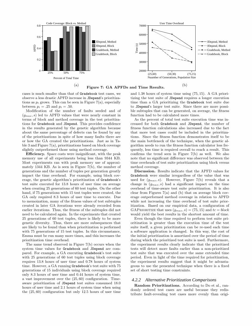
As the time budget is increased, the APFD values in-crease as well for both Gradebook and JDepend, although theamount of increase for a JDepend prioritization is less thanthat of the Gradebook prioritizations. This trend, which isdue to the nature of the applications’ test cases, can be ob-served in Figure 7(a). The Gradebook test cases that findthe most faults take a significantly longer time to executethan the test cases of JDepend. A few other short tests existin Gradebook’s test suite, but these are not the most crucialtest cases in terms of defect detection. Thus, fewer influen-tial Gradebook test cases can be executed within a shortertime budget of 25%. When pt is increased to 50%, the ma-jority of the test cases that find the most faults are able tobe run within the time budget, which greatly increases testtuple APFD values. An increase to pt = 0.75 allows for theinclusion of the shorter, less useful test cases.

Since these new test cases are unlikely to find many newfaults, changes to the overall APFD of the test tuples are mi-nor. JDepend’s test cases all have very short execution times,and many of them cover about the same amount of code. Asin Gradebook, the longer running JDepend test cases gener-ally detect more faults than the shorter tests. However,because the execution time difference between JDepend test

Code Coverage: Block vs. Method

25% 50% 75%

Percent of Total Time

0

0.2

0.4

0.6

0.8

APF

D

JDepend, Method

JDepend, Block

Gradebook, Method

Gradebook, Block

(a)

User Time Overhead

(25,60) (50,30) (75,15)Nuumber of Generations, Population Size

20000

30000

40000

50000

60000

70000

Tim

e (s

)

JDepend, Method

JDepend, Block

Gradebook, Method

Gradebook, Block

(b)Figure 7: GA APFDs and Time Results.

cases is much smaller than that of Gradebook test cases, weobserve a less drastic APFD increase in JDepend’s prioritiza-tions as pt grows. This can be seen in Figure 7(a), especiallybetween pt = .25 and pt = .50.

Modification of the number of faults seeded and of(gmax, s) led to APFD values that were nearly constant interms of block and method coverage in the test prioritiza-tions for Gradebook and JDepend. This provides confidencein the results generated by the genetic algorithm becauseabout the same percentage of defects can be found by anyof the prioritizations in spite of how many faults there areor how the GA created the prioritizations. Just as in Ta-ble 3 and Figure 7(a), prioritizations based on block coverageslightly outperformed those using method coverage.

Efficiency. Space costs were insignificant, with the peakmemory use of all experiments being less than 9344 KB.Most experiments ran with peak memory use of approxi-mately 1344 KB. As is seen in Figure 7(b), the number ofgenerations and the number of tuples per generation greatlyimpact the time overhead. For example, using block cov-erage, the genetic algorithm’s prioritization of Gradebook’stest suite executed for 13.8 hours of user time on averagewhen creating 25 generations of 60 test tuples. On the otherhand, if 75 generations with 15 test tuples were created, theGA only required 8.3 hours of user time to execute. Dueto memoization, many of the fitness values of test subtuplescreated in later GA iterations were already recorded fromearlier iterations. Thus, the fitness of the subtuples did notneed to be calculated again. In the experiments that created25 generations of 60 test tuples, there is likely to be moregenetic diversity. Thus, there are more subsequences thatare likely to be found than when prioritization is performedwith 75 generations of 15 test tuples. In this circumstance,Emma must be run many more times, and this increases theprioritization time overhead.

The same trend observed in Figure 7(b) occurs when thesystem time values for Gradebook and JDepend are com-pared. For example, a GA executing Gradebook’s test suitewith 25 generations of 60 test tuples using block coveragerequires 13.8 hours of user time and 0.78 hours of systemtime. However, a GA running Gradebook’s test suite with 75generations of 15 individuals using block coverage requiredonly 8.3 hours of user time and 0.44 hours of system time,a vast improvement over the (25, 60) configuration. Time-aware prioritization of JDepend test suites consumed 18.0hours of user time and 2.1 hours of system time when usingthe (25, 60) configuration but only 12.5 hours of user time

and 1.38 hours of system time using (75, 15). A GA priori-tizing the test suite of JDepend requires a longer executiontime than a GA prioritizing the Gradebook test suite dueto JDepend’s larger test suite. Since there are more possi-ble subtuples that can be generated, on average, the fitnessfunction had to be calculated more times.

As the percent of total test suite execution time was in-creased for both Gradebook and JDepend, the number offitness function calculations also increased due to the factthat more test cases could be included in the prioritiza-tions. Since the fitness function demonstrates itself to bethe main bottleneck of the technique, when the genetic al-gorithm needs to run the fitness function calculator less fre-quently, less time is required overall to reach a result. Thisconfirms the trend seen in Figure 7(b) as well. We alsonote that no significant difference was observed between thetime overheads of test suite prioritization using block versusmethod coverage.

Discussion. Results indicate that the APFD values forGradebook were similar irregardless of the value that wasused for (gmax, s). However, Figure 7(b) reveals that achange in (gmax, s) had a significant impact on the timeoverhead of time-aware test suite prioritization. It is alsoclear from Figures 7(a) and (b) that on average block cov-erage outperformed method coverage in relation to APFDwhile not increasing the time overhead of test suite prior-itization. Based on our empirical data, a configuration ofGAPrioritize that uses (gmax, s) = (75, 15) and tc = block

would yield the best results in the shortest amount of time.Even though the time required to perform test suite pri-

oritization is greater than the execution time of the testsuite itself, a given prioritization can be re-used each timea software application is changed. In this way, the cost ofthe initial prioritization is amortized over the period of timeduring which the prioritized test suite is used. Furthermore,the experiment results clearly indicate that the prioritizedtests will detect more faults earlier than a non-prioritizedtest suite that was executed over the same extended timeperiod. Even in light of the time required for prioritization,the experiment results suggest that it might be advanta-geous to use the presented technique when there is a fixedset of short testing time constraints.

4.2.2 Alternative Prioritization ComparisonsRandom Prioritizations. According to Do et al., ran-

domly ordered test cases are useful because they redis-tribute fault-revealing test cases more evenly than origi-

Gradebook Prioritization: GA vs. Random

(25%,10)(50%,10)

(75%,10)(25%,20)

(50%,20)(75%,20)

(25%,30)(50%,30)

(75%,30)

(Percent of Total Time, Number of Faults)

-0.5

0

0.5A

PFD GA Tuple

Random Tuple

(a)

JDepend Prioritization: GA vs. Random

(25%,10)(50%,10)

(75%,10)(25%,20)

(50%,20)(75%,20)

(25%,30)(50%,30)

(75%,30)

(Percent of Total Time, Number of Faults)

0

0.5

APF

D GA Tuple

Random Tuple

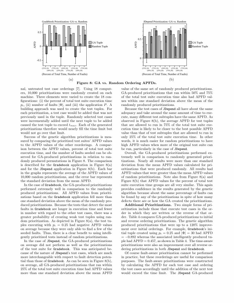
(b)Figure 8: GA vs. Random Ordering APFDs.

nal, untreated test case orderings [7]. Using 18 comput-ers, 10,000 prioritizations were randomly created on eachmachine. Three elements were varied to create the 18 con-figurations: (i) the percent of total test suite execution timept, (ii) number of faults |Φ|, and (iii) the application P . Abuilding approach was used to create the test tuples. Foreach prioritization, a test case would be added that was notpreviously used in the tuple. Randomly selected test caseswere incrementally added until the next tuple to be addedcaused the test tuple to exceed tmax. Each of the generatedprioritizations therefore would nearly fill the time limit butwould not go over that limit.

Success of the genetic algorithm prioritizations is mea-sured by comparing the prioritized test suites’ APFD valuesto the APFD values of the other reorderings. A compar-ison between the APFD values, percent of total test suiteexecution time, and the number of faults seeded can be ob-served for GA-produced prioritizations in relation to ran-domly produced permutations in Figure 8. The comparisonis described for the Gradebook application in Figure 8(a)and for the JDepend application in Figure 8(b). Each barin the graphs represents the average of the APFD values of10,000 random prioritizations, and the error bar representsthe standard deviation from the mean APFD.

In the case of Gradebook, the GA-produced prioritizationsperformed extremely well in comparison to the randomlyproduced prioritizations. All APFD values from prioriti-zations based on the Gradebook application fell more thanone standard deviation above the mean of the randomly pro-duced prioritizations. Because the tests that detect the mostfaults in Gradebook are longer in execution time and fewerin number with regard to the other test cases, there was agreater probability of creating weak test tuples using ran-dom prioritization. As depicted in Figure 8(a), the test tu-ples executing with pt = 0.25 had negative APFD valueson average because they were only able to find a few of theseeded faults. Thus, there is a clear benefit to using intelli-gently prioritized tests instead of random prioritizations.

In the case of JDepend, the GA-produced prioritizationson average did not perform as well as the prioritizationsof the test suite for Gradebook. This was anticipated be-cause of the nature of JDepend’s test cases, which are muchmore interchangeable with respect to fault detection poten-tial than those of Gradebook. As can be seen in Figure 8(b),on average, all GA-produced prioritizations that ran within25% of the total test suite execution time had APFD valuesmore than one standard deviation above the mean APFD

value of the same set of randomly produced prioritizations.GA-produced prioritizations that ran within 50% and 75%of the total test suite execution time also had APFD val-ues within one standard deviation above the mean of therandomly produced prioritizations.

Because the test cases of JDepend all have about the sameadequacy and take around the same amount of time to exe-cute, many different test subtuples have the same APFD. Asobserved in Figure 8(b), the average APFD for test tuplesthat are allowed to run in 75% of the total test suite exe-cution time is likely to be closer to the best possible APFDvalue than that of test subtuples that are allowed to run inonly 25% of the total test suite execution time. In otherwords, it is much easier for random prioritizations to havehigh APFD values when more of the original test suite canbe run, particularly in the case of JDepend.

Overall, the GA-produced prioritizations performed ex-tremely well in comparison to randomly generated priori-tizations. Nearly all results were more than one standarddeviation from the mean APFD values calculated for pri-oritizations that were produced randomly. All results hadAPFD values that were greater than the mean APFD valuesof random prioritizations. Note also from Figure 8(a) andFigure 8(b) that APFD values for the percent of total testsuite execution time groups are all very similar. This againprovides confidence in the results generated by the geneticalgorithm because about the same percentage of faults canbe found by any of the prioritizations in spite of how manydefects there are or how the GA created the prioritizations.

Additional Prioritizations. Two simple forms of pri-oritization include those that execute test cases in the or-der in which they are written or the reverse of that or-der. Table 4 compares GA-produced prioritizations to initialand reverse ordering prioritizations. The genetic algorithmproduced prioritizations that were up to a 120% improve-ment over initial orderings. For example, Gradebook’s ini-tial tuple created using pt = 0.25 and |Φ| = 30 had APFD= −0.892 whereas the associated intelligently produced tu-ple had APFD = 0.457, as shown in Table 4. The time-awareprioritizations were also an improvement over all reverse or-dering prioritizations in both JDepend and Gradebook.

Of course fault-aware prioritization cannot be performedin practice, but these reorderings are useful for comparisonpurposes. The fault-aware prioritizations were constructedby calculating the APFD for each test case and orderingthe test cases accordingly until the addition of the next testwould exceed the time limit. The JDepend GA-produced

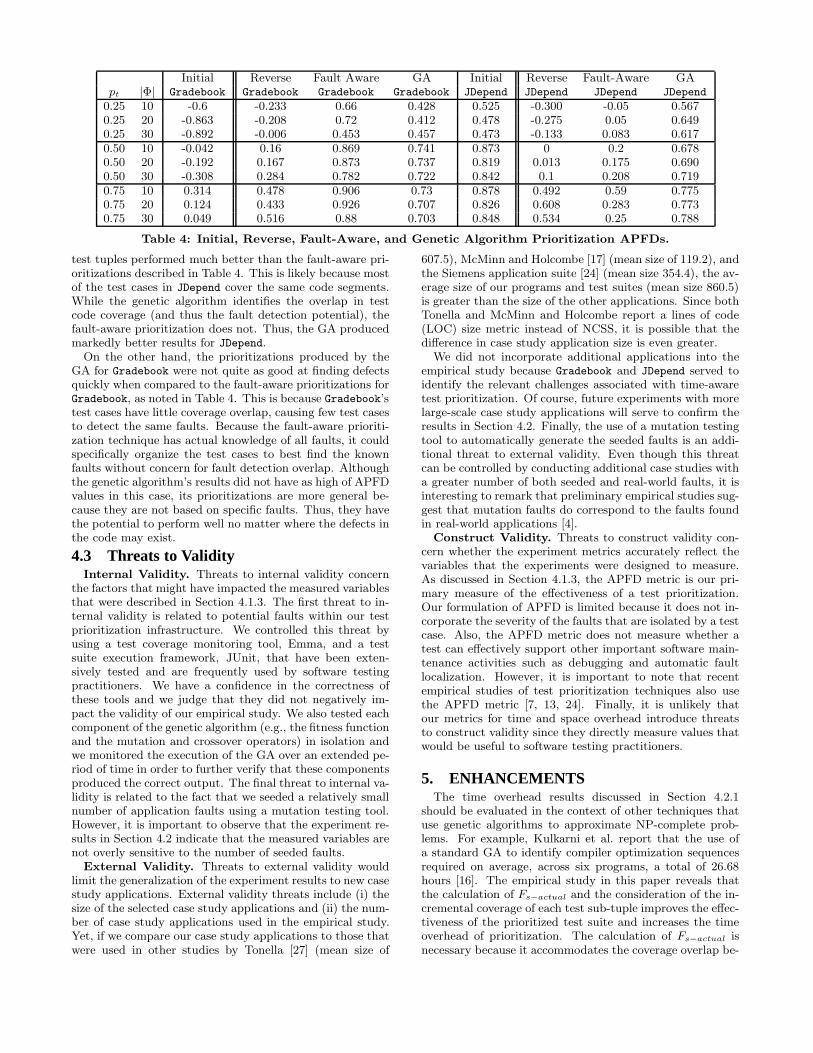
Initial Reverse Fault Aware GA Initial Reverse Fault-Aware GApt |Φ| Gradebook Gradebook Gradebook Gradebook JDepend JDepend JDepend JDepend

0.25 10 -0.6 -0.233 0.66 0.428 0.525 -0.300 -0.05 0.5670.25 20 -0.863 -0.208 0.72 0.412 0.478 -0.275 0.05 0.6490.25 30 -0.892 -0.006 0.453 0.457 0.473 -0.133 0.083 0.6170.50 10 -0.042 0.16 0.869 0.741 0.873 0 0.2 0.6780.50 20 -0.192 0.167 0.873 0.737 0.819 0.013 0.175 0.6900.50 30 -0.308 0.284 0.782 0.722 0.842 0.1 0.208 0.7190.75 10 0.314 0.478 0.906 0.73 0.878 0.492 0.59 0.7750.75 20 0.124 0.433 0.926 0.707 0.826 0.608 0.283 0.7730.75 30 0.049 0.516 0.88 0.703 0.848 0.534 0.25 0.788

Table 4: Initial, Reverse, Fault-Aware, and Genetic Algorithm Prioritization APFDs.

test tuples performed much better than the fault-aware pri-oritizations described in Table 4. This is likely because mostof the test cases in JDepend cover the same code segments.While the genetic algorithm identifies the overlap in testcode coverage (and thus the fault detection potential), thefault-aware prioritization does not. Thus, the GA producedmarkedly better results for JDepend.

On the other hand, the prioritizations produced by theGA for Gradebook were not quite as good at finding defectsquickly when compared to the fault-aware prioritizations forGradebook, as noted in Table 4. This is because Gradebook’stest cases have little coverage overlap, causing few test casesto detect the same faults. Because the fault-aware prioriti-zation technique has actual knowledge of all faults, it couldspecifically organize the test cases to best find the knownfaults without concern for fault detection overlap. Althoughthe genetic algorithm’s results did not have as high of APFDvalues in this case, its prioritizations are more general be-cause they are not based on specific faults. Thus, they havethe potential to perform well no matter where the defects inthe code may exist.

4.3 Threats to ValidityInternal Validity. Threats to internal validity concern

the factors that might have impacted the measured variablesthat were described in Section 4.1.3. The first threat to in-ternal validity is related to potential faults within our testprioritization infrastructure. We controlled this threat byusing a test coverage monitoring tool, Emma, and a testsuite execution framework, JUnit, that have been exten-sively tested and are frequently used by software testingpractitioners. We have a confidence in the correctness ofthese tools and we judge that they did not negatively im-pact the validity of our empirical study. We also tested eachcomponent of the genetic algorithm (e.g., the fitness functionand the mutation and crossover operators) in isolation andwe monitored the execution of the GA over an extended pe-riod of time in order to further verify that these componentsproduced the correct output. The final threat to internal va-lidity is related to the fact that we seeded a relatively smallnumber of application faults using a mutation testing tool.However, it is important to observe that the experiment re-sults in Section 4.2 indicate that the measured variables arenot overly sensitive to the number of seeded faults.

External Validity. Threats to external validity wouldlimit the generalization of the experiment results to new casestudy applications. External validity threats include (i) thesize of the selected case study applications and (ii) the num-ber of case study applications used in the empirical study.Yet, if we compare our case study applications to those thatwere used in other studies by Tonella [27] (mean size of

607.5), McMinn and Holcombe [17] (mean size of 119.2), andthe Siemens application suite [24] (mean size 354.4), the av-erage size of our programs and test suites (mean size 860.5)is greater than the size of the other applications. Since bothTonella and McMinn and Holcombe report a lines of code(LOC) size metric instead of NCSS, it is possible that thedifference in case study application size is even greater.

We did not incorporate additional applications into theempirical study because Gradebook and JDepend served toidentify the relevant challenges associated with time-awaretest prioritization. Of course, future experiments with morelarge-scale case study applications will serve to confirm theresults in Section 4.2. Finally, the use of a mutation testingtool to automatically generate the seeded faults is an addi-tional threat to external validity. Even though this threatcan be controlled by conducting additional case studies witha greater number of both seeded and real-world faults, it isinteresting to remark that preliminary empirical studies sug-gest that mutation faults do correspond to the faults foundin real-world applications [4].

Construct Validity. Threats to construct validity con-cern whether the experiment metrics accurately reflect thevariables that the experiments were designed to measure.As discussed in Section 4.1.3, the APFD metric is our pri-mary measure of the effectiveness of a test prioritization.Our formulation of APFD is limited because it does not in-corporate the severity of the faults that are isolated by a testcase. Also, the APFD metric does not measure whether atest can effectively support other important software main-tenance activities such as debugging and automatic faultlocalization. However, it is important to note that recentempirical studies of test prioritization techniques also usethe APFD metric [7, 13, 24]. Finally, it is unlikely thatour metrics for time and space overhead introduce threatsto construct validity since they directly measure values thatwould be useful to software testing practitioners.

5. ENHANCEMENTSThe time overhead results discussed in Section 4.2.1

should be evaluated in the context of other techniques thatuse genetic algorithms to approximate NP-complete prob-lems. For example, Kulkarni et al. report that the use ofa standard GA to identify compiler optimization sequencesrequired on average, across six programs, a total of 26.68hours [16]. The empirical study in this paper reveals thatthe calculation of Fs−actual and the consideration of the in-cremental coverage of each test sub-tuple improves the effec-tiveness of the prioritized test suite and increases the timeoverhead of prioritization. The calculation of Fs−actual isnecessary because it accommodates the coverage overlap be-

tween the individual tests. If T was initially reduced in orderto remove the majority of test coverage overlap and coveragewas reported on a per-test basis, Treduce could be prioritizedusing the presented approach and the modified fitness func-tion Fit described in Equation 5. The fitness of test tupleσj could be calculated with Fit whenever time(σj) ≤ tmax

and if σj exceeds the testing time limit we require thatFit(P, σj , tc) = 0.

Fit(P, σj , tc) =

|σj |X

i=1

cc(P, Ti, tc)

time(〈Ti〉)(5)

Since Fit does not need to consider the incremental codecoverage of the σj that was derived from Treduce, wejudge that it will significantly decrease the time overheadof GAPrioritize. The performance of the baseline fit-ness function fit can also be improved if test suite re-duction is not desirable because of concerns about dimin-ishing the suite’s potential to reveal faults. For example,during the calculation of Fs−actual, each computation oftime(〈Ti〉)× cc(P, σj{1,i}, tc) could be performed on a sepa-rate computer. If test execution histories are available, fit

could be modified to focus on tests that have recently re-vealed faults. When test prioritization has been previouslyperformed, the fitness of test tuple σmax can be recordedand all subsequent executions of GAPrioritize could beterminated when the algorithm generates a tuple that hasfitness greater than the prior σmax.

6. RELATED WORKThere are many existing approaches to regression test pri-

oritization that focus on the coverage of or modifications tothe structural entities within the program under test [7, 8,24, 26]. Yet, none of these prioritization schemes explicitlyconsider the testing time budget like the time-aware tech-nique presented in this paper. Similar to our approach, El-baum et al. and Rothermel et al. focus on general regressiontest prioritization and the identification of a single test casereordering that will increase the effectiveness of regressiontesting over many subsequent changes to the program [8,24]. Do et al. present an empirical study of the effective-ness of test prioritization in a testing environment that usesJUnit [7]. This paper is also related to our work becauseDo et al.’s prioritization technique uses coverage informa-tion at the method and block levels. Recent research byMemon et al. implicitly assumes that testing is constrainedby the amount of time available in an evening [19]. Whiletheir infrastructure is highly automated, it does not directlyconsider the time constraint and thus cannot guarantee thattesting will complete in the allotted time.

7. CONCLUSIONS AND FUTURE WORKThis paper describes a time-aware test suite prioritiza-

tion technique. Experimental analysis demonstrates thatour approach can create time-aware prioritizations that sig-nificantly outperform other prioritization techniques. Forone case study application, our technique created prioriti-zations that, on average, had up to a 120% improvement inAPFD over other prioritizations. This paper identifies andevaluates the challenges associated with time-aware prioriti-zation. We also explain ways to reduce the time overhead ofprioritization. In future work, we intend to examine the en-hancements to our approach that are discussed in Section 5.These improvements to our algorithm have the potential toincrease the applicability of the presented technique.

8. REFERENCES[1] http://www.clarkware.com/software/JDepend.html.

[2] http://monetdb.cwi.nl/.

[3] http://www.planet-lab.org/.

[4] J. H. Andrews, L. C. Briand, and Y. Labiche. Is mutation anappropriate tool for testing experiments? In Proc. of 27thICSE, pages 402–411, 2005.

[5] G. Antoniol, M. D. Penta, and M. Harman. Search-basedtechniques applied to optimization of project planning for amassive maintenance project. In Proc. of the 21st ICSM, pages240–249, Washington, DC, USA, 2005.

[6] P. Chu and J. Beasley. A genetic algorithm for themultidimensional knapsack problem. Journal of Heuristics,4(1):63–86, 1998.

[7] H. Do, G. Rothermel, and A. Kinneer. Empirical studies of testcase prioritization in a JUnit testing environment. In Proc. of15th ISSRE, pages 113–124, 2004.

[8] S. Elbaum, A. G. Malishevsky, and G. Rothermel. Test caseprioritization: A family of empirical studies. IEEE Trans.Softw. Eng., 28(2):159–182, 2002.

[9] D. Fatiregun, M. Harman, and R. M. Hierons. Evolvingtransformation sequences using genetic algorithms. In Proc. of

4th SCAM, pages 66–75, 2004.

[10] M. R. Garey and D. S. Johnson. Computers and Intractability:

A Guide to the Theory of NP-Completeness. W. H. Freeman& Co., New York, NY, USA, 1979.

[11] D. E. Goldberg. The Design of Innovation: Lessons from andfor Competent Genetic Algorithms. Addison-Wesley, Reading,MA, 2002.

[12] D. E. Goldberg, B. Korb, and K. Deb. Messy geneticalgorithms: Motivation, analysis, and first results. ComplexSystems, 3(5):493–530, 1989.

[13] T. L. Graves, M. J. Harrold, J.-M. Kim, A. Porter, andG. Rothermel. An empirical study of regression test selectiontechniques. ACM Trans. on Softw. Eng. and Meth., 10(2),2001.

[14] G. M. Kapfhammer. Software testing. In The ComputerScience Handbook, chapter 105. CRC Press, Boca Raton, FL,second edition, 2004.

[15] M. Kessis, Y. Ledru, and G. Vandome. Experiences in coveragetesting of a Java middleware. In Proc. of 5th SEM, pages39–45, 2005.

[16] P. A. Kulkarni, S. R. Hines, D. B. Whalley, J. D. Hiser, J. W.Davidson, and D. L. Jones. Fast and efficient searches foreffective optimization-phase sequences. ACM Trans. Archit.Code Optim., 2(2):165–198, 2005.

[17] P. McMinn and M. Holcombe. Evolutionary testing ofstate-based programs. In Proc. of GECCO, pages 1013–1020,2005.

[18] P. McNamee and M. Hall. Developing a tool for memoizingfunctions in C++. ACM SIGPLAN Not., 33(8):17–22, 1998.

[19] A. Memon, I. Banerjee, N. Hashmi, and A. Nagarajan. DART:A framework for regression testing “nightly/daily builds” ofGUI applications. In Proc. of ICSM, 2003.

[20] J. Misurda, J. Clause, J. L. Reed, P. Gandra, B. R. Childers,and M. L. Soffa. Jazz: A tool for demand-driven structuraltesting. In Proc. of 14th CC, 2005.

[21] I. Moore. Jester- a JUnit test tester. In Proc. of 2nd XP, pages84–87, 2001.

[22] R. P. Pargas, M. J. Harrold, and R. R. Peck. Test-datageneration using genetic algorithms. Soft. Testing, Verif. and

Rel., 9(4):263–282, 1999.

[23] C. Poole and J. W. Huisman. Using extreme programming in amaintenance environment. IEEE Softw., 18(6):42–50, 2001.

[24] G. Rothermel, R. J. Untch, and C. Chu. Prioritizing test casesfor regression testing. IEEE Trans. on Softw. Eng.,27(10):929–948, 2001.

[25] V. Roubtsov. Emma: a free java code coverage tool.http://emma.sourceforge.net/index.html, March 2005.

[26] A. Srivastava and J. Thiagarajan. Effectively prioritizing testsin development environment. In Proc. of ISSTA, pages 97–106,2002.

[27] P. Tonella. Evolutionary testing of classes. In Proc. of ISSTA,pages 119–128, 2004.