Integrated Urban System and Energy Consumption Model: Residential Buildings
Upload
khangminh22Category
view
1download
0
Time Series Analysis on Energy
Consumption Data
Inaugural-Dissertation
zur
Erlangung des Doktorgrades der
Mathematisch-Naturwissenschaftlichen Fakultät
der Heinrich-Heine-Universität Düsseldorf
vorgelegt von
Christian Bock
aus Düsseldorf
Düsseldorf, Oktober 2019

aus dem Institut für Informatik der
Heinrich-Heine-Universität Düsseldorf
Gedruckt mit der Genehmigung derMathematisch-Naturwissenschaftlichen Fakultät derHeinrich-Heine-Universität Düsseldorf
Referent: Prof. Dr. Stefan Conrad
Koreferent: Prof. Dr. Martin Mauve
Tag der mündlichen Prüfung: 20. Dezember 2019

i
Ich versichere an Eides Statt, dass die Dissertation von mir selbstständig und ohneunzulässige fremde Hilfe unter Beachtung der "Grundsätze zur Sicherung guter wis-senschaftlicher Praxis an der Heinrich-Heine-Universität Düsseldorf" erstellt wordenist.
Die Dissertation wurde in der vorgelegten oder in ähnlicher Form noch bei keineranderen Institution eingereicht. Ich habe bisher keine erfolglosen Promotionsversucheunternommen.
Düsseldorf, den 22. Oktober 2019Christian Bock

ii

Danksagung
Als erstes danke ich meinem Doktorvater und Erstgutachter Prof. Dr. Stefan Conradfür die Möglichkeit, Teil seines Teams der wissenschaftlichen Mitarbeiter und Dok-toranden zu sein. In den fünf Jahren, die ich an meiner Promotion gearbeitet habe,hat er mir ein angenehmes Umfeld für den wissenschaftlichen Austausch geboten. Erist stets sehr an meiner Forschung interessiert gewesen, hat immer ein offenes Ohrfür meine Fragen gehabt und hat stets mit wertvollem und hilfreichem Feedback zumGelingen dieser Doktorarbeit beigetragen. Darüber hinaus danke ich Prof. Dr. MartinMauve für sein Interesse an meiner Arbeit und seine Bereitschaft, als Zweitgutachterzu fungieren.
Des Weiteren danke ich allen Personen, die diese Arbeit direkt oder indirekt the-matisch unterstützt haben, darunter Martin Dziwisch, Jan Hoppenkamps, ChristianKretschmann und Jan Sträter. Für ihre kostbare Hilfestellung bei Fragen zum ThemaClustering danke ich darüber hinaus Dr. Ludmila Himmelspach. Nicht unerwähntbleiben darf außerdem die exzellente technische und administrative Unterstützung,wofür ich insbesondere Sabine Freese und ganz besonders unserem Systemadministra-tor Guido Königstein danke. Für weiteren technischen Support und die Bereitstellungvon Berechnungsinfrastruktur bedanke ich mich beim Zentrum für Informations- undMedientechnologie (ZIM). Außerdem bedanke ich mich bei meinen Forschungskollegenfür die stets konstruktiven Gespräche bei unseren Forschungstreffen, darunter Alexan-der Askinadze, Kirill Bogomasov, Daniel Braun, Janine Golov, Dr. Matthias Liebeck,Julia Romberg, Dr. Michael Singhof und Martha Tatusch.
Selbstverständlich bedanke ich mich ebenfalls bei meiner Familie und Bekannten,insbesondere bei meinen Eltern Martina und Michael, dafür dass sie mir das Studiumermöglicht haben und für die unermüdliche emotionale Unterstützung, sowie bei meinerNachbarin Anneliese Kaiser dafür, dass sie mir stets wie eine Oma zur Seite stand.
iii

iv

Abstract
Nowadays, electronic devices are used in almost all aspects of everyday lives. Examplesfor these are computer, radios, television, light bulbs, domestic appliances and electriccars will possibly play a bigger part in the near future. Due to the enormous comfortand gain in efficiency these kinds of devices contribute during both spare time and in aprofessional environment, it is not possible to imagine one without the other. To enablethe usage of these devices a whole industry branch has been created with the task toguarantee the supply of electrical energy almost everywhere. As a consequence of this,a complex electricity grid emerged. In order for the electricity grid to function properly,many roles such as energy producers, grid operators, energy providers, accounting gridcoordinator and imbalance energy providers need to cooperate hitchlessly.Since the supply of electrical energy needs to be ensured at all times, energy providersface the responsible and difficult task of forecasting the actual energy consumptionof their customers in advance in order for energy producers to adjust the productionaccordingly. For this purpose, current business processes rely on so called load profileswhich are statistical models that yield a good estimate for the total energy demand ofall customers based on a set of assumptions about them. Traditionally, these assump-tions about the customers are very vague, for example because the electricity metersof customers are read by the energy provider approximately only once per year in con-junction with the yearly accounting of electricity expenses, which does not allow todifferentiate between uniform and peak consumption.As a consequence of the increasing availability of intelligent metering devices, so calledSmart Meter, it is progressively feasible to read the actual energy consumption of in-dividual customers in real-time and transmit the data as a time series. This enables avariety of possible applications such as target-group-specific tariffs, where the prices canbe adjusted in real-time, simplification of customer change processes or pointing outcost-saving opportunities for the customer by visualizing his or her consumption behav-ior. In addition to this, Smart Metering devices allow for the usage of algorithms thathelp to semi-automatically extract potentially useful knowledge from these datasets.These algorithms are part of the research area Knowledge Discovery in Databases. Theyare often employed if the data to be processed is too big or too complex for a manualanalysis. The extraction of useful knowledge from consumption time series gatheredby means of Smart Metering devices is the main topic of this thesis.
v

vi

Zusammenfassung
In fast allen Bereichen des Alltags werden heutzutage elektrische Geräte eingesetzt.Beispiele hierfür sind Computer, Radios, Fernseher, Glühbirnen, Haushaltsgeräte undin naher Zukunft möglicherweise auch flächendeckend E-Autos. Aufgrund des enormenKomforts und der Produktivitätssteigerung, die derartige Geräte sowohl zur Freizeitals auch im beruflichen Umfeld beitragen, sind sie kaum noch wegzudenken. Um dieNutzung dieser Geräte zu ermöglichen, ist ein ganzer Industriezweig entstanden, umdie Versorgung mit elektrischer Energie nahezu überall zu garantieren. Im Zuge dessenist ein komplexes Stromnetz entstanden, für dessen Funktionieren zahlreiche Rollenwie die des Energieproduzenten, Netzbetreibers, Energielieferanten, Bilanzkreiskoordi-nators und Regelenergieanbieters reibungslos ineinander greifen müssen.Da die Versorgung mit elektrischer Energie zu jedem Zeitpunkt sichergestellt sein muss,stehen Energielieferanten vor der verantwortungsvollen und schwierigen Aufgabe, denStrombedarf seiner Kunden möglichst akkurat vorherzusagen, damit Energieproduzen-ten ihre Produktion entsprechend optimal regulieren können. Hierfür kommen sogenannte Lastprofile zum Einsatz, das heißt statistische Modelle, welche anhand vongetroffenen Annahmen über die Kunden eine Schätzung für den Gesamtverbrauch derKunden ermöglichen. Traditionell sind diese Annahmen über den Kunden sehr vage,da beispielsweise der Stromzähler der Kunden nur etwa einmal im Jahr im Rahmender jährlichen Stromkostenabrechnung abgelesen wird, wodurch keine Unterscheidungzwischen gleichmäßigem Stromverbrauch und Lastspitzen möglich ist.Durch den wachsenden Ausbau von intelligenten Stromzählern, so genannter SmartMeter, ist es zunehmend umsetzbar, unter anderem den tatsächlichen Stromverbrauchder einzelnen Kunden in Echtzeit auszulesen und als Zeitreihe zu übertragen. Dies er-möglicht eine Vielzahl von Möglichkeiten, beispielsweise zielgruppenorientierte Tarife,deren Preise in Echtzeit angepasst werden können, eine Verschlankung von Kunden-wechselprozessen oder das Aufzeigen von Einsparmöglichkeiten gegenüber dem Kundendurch Visualisieren dessen Verbrauchsverhaltens. Darüber hinaus erlauben Smart Me-ter die Verwendung von Algorithmen, die dabei helfen, semi-automatisch potentiellnützliches Wissen aus den dabei entstehenden Datenmengen zu extrahieren. Diese Al-gorithmen sind Komponenten des Themengebiets Knowledge Discovery in Databasesund werden häufig angewandt, wenn die zu untersuchenden Daten zu groß für einemanuelle Analyse sind; die Extraktion von nützlichem Wissen aus den durch SmartMeter erhobenen Verbrauchszeitreihen ist Hauptbestandteil dieser Arbeit.
vii

viii
Contents
1 Introduction 11.1 Motivation . . . . . . . . . . . . . . . . . . . . . . . . . . . . . . . . . . 11.2 Knowledge Discovery . . . . . . . . . . . . . . . . . . . . . . . . . . . . 2
1.2.1 Overview of the KDD process . . . . . . . . . . . . . . . . . . . 31.2.2 Clustering Analysis . . . . . . . . . . . . . . . . . . . . . . . . . 51.2.3 Dissimilarity measurements for time series . . . . . . . . . . . . 9
1.3 Contributions . . . . . . . . . . . . . . . . . . . . . . . . . . . . . . . . 111.4 Outline of this work . . . . . . . . . . . . . . . . . . . . . . . . . . . . . 12
2 Background 132.1 Overview of the electricity grid . . . . . . . . . . . . . . . . . . . . . . 132.2 Current challenges of energy providers . . . . . . . . . . . . . . . . . . 162.3 Structure and purpose of load profiles . . . . . . . . . . . . . . . . . . . 18
3 Knowledge Discovery in the energy economy 273.1 Impact on consumers . . . . . . . . . . . . . . . . . . . . . . . . . . . . 27
3.1.1 Financial benefit and influence on consumer behavior . . . . . . 303.1.2 Data privacy . . . . . . . . . . . . . . . . . . . . . . . . . . . . 32
3.1.2.1 De-pseudonymisation of customers . . . . . . . . . . . 333.1.2.2 Differential privacy in a Smart Metering environment . 353.1.2.3 Data reduction and data economy . . . . . . . . . . . 36
3.1.3 Photovoltaic systems . . . . . . . . . . . . . . . . . . . . . . . . 383.2 Impact on the electricity grid . . . . . . . . . . . . . . . . . . . . . . . 393.3 Impact on energy providers . . . . . . . . . . . . . . . . . . . . . . . . 46
3.3.1 Extraction of customer insight . . . . . . . . . . . . . . . . . . . 463.3.2 Installation of intelligent metering systems . . . . . . . . . . . . 48
3.3.2.1 Prediction of household properties . . . . . . . . . . . 483.3.2.2 Creation of target-group-specific tariffs . . . . . . . . . 513.3.2.3 Forecast of the energy consumption . . . . . . . . . . . 54
4 Clustering using Smart Meter Data 574.1 Description of datasets . . . . . . . . . . . . . . . . . . . . . . . . . . . 574.2 Assessment of clustering quality . . . . . . . . . . . . . . . . . . . . . . 60
4.2.1 Partition Coefficient . . . . . . . . . . . . . . . . . . . . . . . . 614.2.2 Compactness & Separation by Xie & Beni . . . . . . . . . . . . 614.2.3 Compactness & Separation by Bouguessa, Wang & Sun . . . . . 62
ix

x CONTENTS
4.2.4 Fuzzy Hypervolume and Partition Density . . . . . . . . . . . . 644.2.5 Silhouette Coefficient . . . . . . . . . . . . . . . . . . . . . . . . 654.2.6 Average Clustering Uniqueness . . . . . . . . . . . . . . . . . . . 65
4.3 Framework for generating load profiles . . . . . . . . . . . . . . . . . . 664.3.1 Day-type segmentation . . . . . . . . . . . . . . . . . . . . . . . 664.3.2 Identification of typical consumption patterns . . . . . . . . . . 684.3.3 Compilation of load profiles . . . . . . . . . . . . . . . . . . . . 694.3.4 Assessment of load profiles . . . . . . . . . . . . . . . . . . . . . 70
4.4 Evaluation . . . . . . . . . . . . . . . . . . . . . . . . . . . . . . . . . . 714.4.1 Evaluation using the Euclidean distance . . . . . . . . . . . . . 72
4.4.1.1 Experimental Setup . . . . . . . . . . . . . . . . . . . 724.4.1.2 Results . . . . . . . . . . . . . . . . . . . . . . . . . . 73
4.4.2 Evaluation using the Manhattan distance . . . . . . . . . . . . . 764.4.2.1 Experimental Setup . . . . . . . . . . . . . . . . . . . 764.4.2.2 Results . . . . . . . . . . . . . . . . . . . . . . . . . . 78
4.4.3 Evaluation using the exponential Manhattan distance . . . . . . 814.4.3.1 Experimental Setup . . . . . . . . . . . . . . . . . . . 814.4.3.2 Results . . . . . . . . . . . . . . . . . . . . . . . . . . 84
4.4.4 Evaluation using weighted clustering . . . . . . . . . . . . . . . 844.4.4.1 Experimental Setup . . . . . . . . . . . . . . . . . . . 844.4.4.2 Results . . . . . . . . . . . . . . . . . . . . . . . . . . 88
5 Online Clustering using Smart Meter Data 935.1 Motivation . . . . . . . . . . . . . . . . . . . . . . . . . . . . . . . . . . 935.2 Related Work . . . . . . . . . . . . . . . . . . . . . . . . . . . . . . . . 945.3 Building load profiles using Online Clustering . . . . . . . . . . . . . . 965.4 Evaluation . . . . . . . . . . . . . . . . . . . . . . . . . . . . . . . . . . 98
5.4.1 Experimental Setup . . . . . . . . . . . . . . . . . . . . . . . . . 985.4.2 Results . . . . . . . . . . . . . . . . . . . . . . . . . . . . . . . . 100
6 Summary 1036.1 Conclusions . . . . . . . . . . . . . . . . . . . . . . . . . . . . . . . . . 1036.2 Future Work . . . . . . . . . . . . . . . . . . . . . . . . . . . . . . . . . 104
References 107
List of Figures 121
List of Tables 127
List of Own Publications 129

1Introduction
1.1 Motivation
One of the most important achievements of humanity is the ability to gather, store anddistribute energy. This feat has enabled the Industrial Revolution in the 18-th centuryand the ongoing Digital Revolution that has started in the 20-th century, thus layingthe foundation for the lifestyle of modern society. Though the comforts of modernelectrical devices, such as televisions or smartphones, as well as technologies like theInternet, have drastically changed the habits of citizens and the business models ofcompanies in industrialized countries, these luxuries are typically taken for granted inour day-to-day life, with the average citizen putting very little thought into the innerworkings of the energy infrastructure these achievements are based on. When one bearsthe importance of the security of the energy supply in mind, it is noteworthy that theenergy economy has taken a backseat until the end of the 20-th century.Ever since then, the energy market has begun to significantly change over the courseof the following decades. For example, legislators have postulated an expansion in theusage of renewable energies, partly to decrease the carbon footprint of the country andpartly in an effort to prepare for the increasing shortage of fossil fuels in the future.This has involuntarily let market participants to continously rethink the way of howthe energy production and distribution are planned and carried out. Likewise, end-consumers have become more sensitized by the media to reduce their personal carbonfootprint. Complementary, end-consumers have progressively been provided financialincentives to install and use personal renewable electricity generation plants such asphotovoltaic systems. In addition, because of the liberalization of the energy marketin the European Union, the increasing competitive pressure as a consequence thereof,as well as due to policies to adopt digitization and promote energy efficiency, marketparticipants in the energy economy are compelled to engage with new technologies toprevent missing out on potentially valueable knowledge [Hay+14].One of the new technologies that legislators in particular have placed high expecta-tions in are Intelligent Metering Systems, which are commonly referred to as Smart
1

2 1. INTRODUCTION
01
234
456
123
567
789
34, kWh
Smart Meter Gateway
000000002211774488,99 kWkWhh000021748,9 kWh
1234567890
Smart Meter
000000002211774488,99 kWkWhh000021748,9 kWh
1234567890
Smart Meter
000000002211774488,99 kWkWhh000021748,9 kWh
1234567890
Smart Meter
Hydroelectric
Power Stations
Coal
Power Stations
Nuclear
Power Stations
bilateral trading and wholesale,
mostly in local markets
Wind
Power Stations
Production
New technologies change the
composition of energy☆
Dezentralized production☆
Infrequently available
capacities☆
Regional Markets - Centralization
Traditional electricity meterIntelligent Metering Systems /
„Smart Metering“
Today Prospective
Energy is delivered from the producer
to the end consumerbidirectional flow of energy
Coal Power Stations
with CCS
Solar
Power Stations
Core changes
DistributionSmart Metering and Smart
Grids enable flexible flow of
energy both to and from the
end consumer
☆
Metering
Yearly, manual reading no
longer required by the consumer☆
Digitalized Measurements☆
Amount of customer data
increases drastically☆
Differentiation between
consistent consumption and
peak in demand possible
☆
Marketing
Smart Metering enables new
business opportunities☆
Customer produces own energy☆
TradingNecessity for more sophisticated
trading strategies due to
increased complexity
☆
Figure 1.1: Overview of the transformation of the electricity grid due to digitizationand growing deployment of Intelligent Metering Systems. Adapted from [EK13] withsome assets taken from [Wik].
Meter. Though the base functionality of Intelligent Metering Systems consists of al-lowing the frequent remote reading of the meter by the electricity grid operator, govern-ments recommend that Smart Metering devices also support advanced tariff systemsand remote control of the supply and energy flow [Com12]. This prospective couldenable the electricity grid to be transformed into a complex network, where devicessemi-automatically coordinate themselves and make use of a more flexible demand-side according to user-defined parameters, dynamically scheduling tasks in an effort toincrease overall energy efficiency, expand the integration of renewable energy sourcesas well as reduce costs for both energy market participants and end-consumers. Thistransformation of the electricity grid is also visualized in figure 1.1.
With the energy economy facing ambitious goals, this thesis presents means toaddress the upcoming challenges for the energy economy and end-consumers. In doingso, we lay the focus on approaches to extract useful knowledge from energy consumptiontime series yielded by employing Smart Metering devices. In preparation for this, wegive a brief introduction into the concept of Knowledge Discovery in Databases andrelevant techniques in the following section.
1.2 Knowledge Discovery
Over the last decades, advances in computing and storage technology has allowed for adrastic expansion of the collection of data. The term data corresponds to arbitrary setsof information recorded by an organization or an individual. In the past, the reasons
1.2. KNOWLEDGE DISCOVERY 3
0
50
100
150
200
Database
Target
Data
Preprocessed
Data
Patterns
Transformed
Data Knowledge
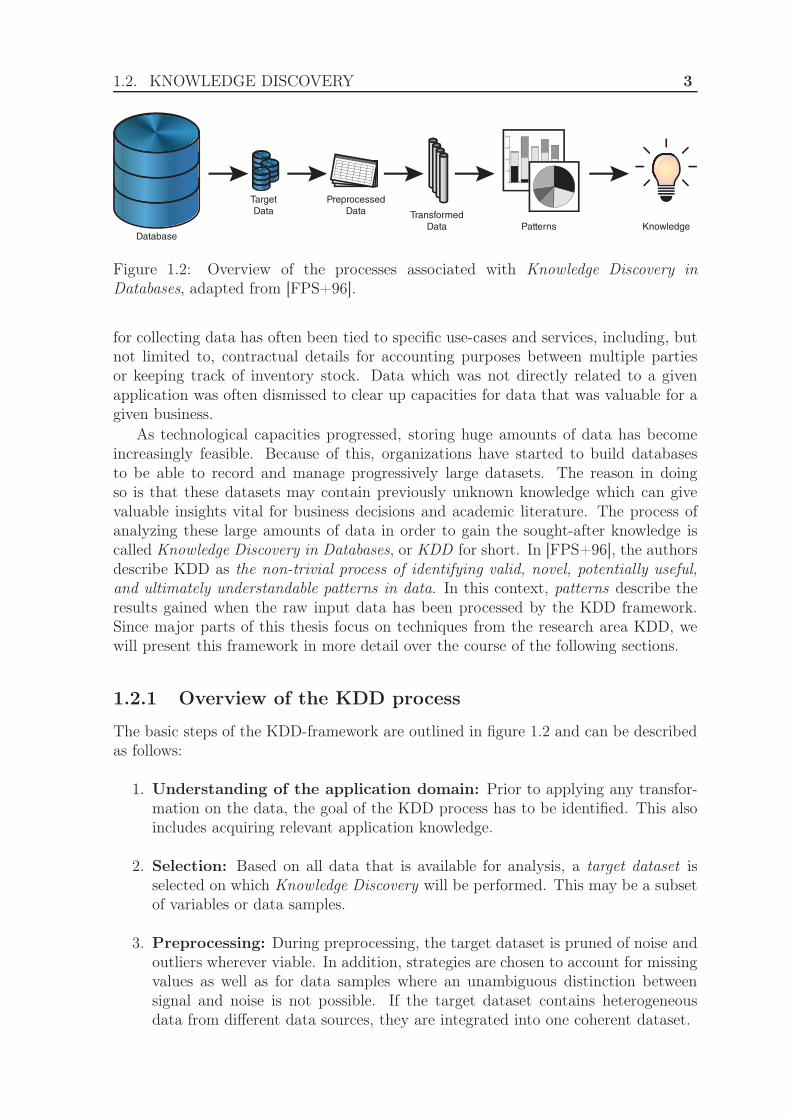
Figure 1.2: Overview of the processes associated with Knowledge Discovery inDatabases, adapted from [FPS+96].
for collecting data has often been tied to specific use-cases and services, including, butnot limited to, contractual details for accounting purposes between multiple partiesor keeping track of inventory stock. Data which was not directly related to a givenapplication was often dismissed to clear up capacities for data that was valuable for agiven business.
As technological capacities progressed, storing huge amounts of data has becomeincreasingly feasible. Because of this, organizations have started to build databasesto be able to record and manage progressively large datasets. The reason in doingso is that these datasets may contain previously unknown knowledge which can givevaluable insights vital for business decisions and academic literature. The process ofanalyzing these large amounts of data in order to gain the sought-after knowledge iscalled Knowledge Discovery in Databases, or KDD for short. In [FPS+96], the authorsdescribe KDD as the non-trivial process of identifying valid, novel, potentially useful,and ultimately understandable patterns in data. In this context, patterns describe theresults gained when the raw input data has been processed by the KDD framework.Since major parts of this thesis focus on techniques from the research area KDD, wewill present this framework in more detail over the course of the following sections.
1.2.1 Overview of the KDD process
The basic steps of the KDD-framework are outlined in figure 1.2 and can be describedas follows:
1. Understanding of the application domain: Prior to applying any transfor-mation on the data, the goal of the KDD process has to be identified. This alsoincludes acquiring relevant application knowledge.
2. Selection: Based on all data that is available for analysis, a target dataset isselected on which Knowledge Discovery will be performed. This may be a subsetof variables or data samples.
3. Preprocessing: During preprocessing, the target dataset is pruned of noise andoutliers wherever viable. In addition, strategies are chosen to account for missingvalues as well as for data samples where an unambiguous distinction betweensignal and noise is not possible. If the target dataset contains heterogeneousdata from different data sources, they are integrated into one coherent dataset.
4 1. INTRODUCTION
4. Transformation: In compliance with the goal of the KDD process and theknowledge about the application requirements, useful features adequate for rep-resenting the dataset are defined. If deemed appropriate, dimensionality reduc-tion or transformation is applied on the preprocessed data to exclude variablesof lesser importance or to achieve an invariant representation of the dataset.
5. Data Mining: After the dataset has been transformed, a fitting Data Miningalgorithm, such as clustering, regression, classification, etc., is chosen and appliedto extract the desired patterns from the data.
6. Interpretation / Evaluation: The discovered patterns are analyzed, visualizedand documented. The insight achieved is consolidated with previously gainedknowledge.
The goals and tools of KDD make it a strongly interconnected field of research com-bining statistics, maschine learning and databases [ES00]. Although the KDD processas illustrated above is often presented as a pipeline of processes, Knowledge Dicoveryis to be understood as an iterative process, where during each step the user may optto restart the process at an earlier stage. Using this procedure, parameters can bechanged if necessary and emerging complications can be avoided. Depending on thecomplexity of the task, many iterations are required to achieve acceptable results.
Albeit the term Data Mining is only one step in the KDD process, it is often usedinterchangeably with KDD itself. This is because Data Mining is often seen as thecore part of KDD, even though the results, and thus the success, of Data Mining arereliant on the proper execution of all previous steps. Depending on the concrete typeof data that is being analyzed, different Data Mining techniques are used to carry outthat task. The most common of these techniques include the following [ES00]:
• Clustering: The goal of clustering is to partition a given dataset into groupscalled clusters. The segmentation is processed under the optimization constraintthat data objects belonging to the same cluster should be as similar as possiblewhile data objects belonging to different clusters should be as dissimilar as possi-ble. Because clustering algorithms do not rely on labeled or precategorized dataobjects, clustering belongs to the branch of machine learning called UnsupervisedLearning. Since major parts of this thesis are utilizing clustering techniques wegive a more thorough introduction to clustering in section 1.2.2.
• Classification: Given a set of classes and data objects where their membershipto a class is known, classification is about training a model to learn to assign aclass to data objects of which the class memberships are unknown. Unlike withclustering, the categories or classes need to be defined ahead of time, which iswhy classification belongs to the branch of machine learning called SupervisedLearning.
• Association Rules: Association Rule Mining is about finding associations in aset of transactions. Associations describe common or strong correlations betweenitems. These correlation may be of the form if A and B then C, which is typicallynotated as A,B → C.
1.2. KNOWLEDGE DISCOVERY 5
• Generalization: The goal of generalization is to describe the dataset in a morecompact way. This may be achieved by aggregating multiple attributes or byreducing the number of data objects in the dataset.
For each of the Data Mining techniques as outlined above, there are numerous algo-rithms for the analyst to choose from. Each algorithm has its strengths and weaknesseswhich must be taken into consideration when selecting an algorithm for a concrete DataMining task; e.g. data objects with categorical attributes require different handlingthan strictly numerical data.
Although Knowledge Discovery in Databases is a very well-known and reliableframework in the field of Data Analytics, other guidelines [Mül+16] and variationsof KDD have emerged in recent years. While these modifications of KDD maintainthe core concepts outlined above, they shift the focus of the discovery process more to-wards the interests of businesses and decision-making processes. One example for sucha variation of KDD is CRoss-Industry Standard Process for Data Mining (CRISP-DM)[She00]. The main innovations of CRISP-DM compared to KDD are an additionalstep named Deployment which comes after the Evaluation as well as two separatesteps called Business Understanding and Data Understanding for what was unified asUnderstanding of the application domain in KDD.
1.2.2 Clustering Analysis
Clustering is one of the main techniques used as part of the KDD process when it comesto analyzing a large dataset. It is used as a means to segment the elements of a givendataset into groups, such that elements which have been assigned to the same groupare as similar to each other as possible while at the same time elements belonging todifferent groups are as dissimilar as possible. What makes clustering a very versatiletechnique in the KDD process is the fact that it does not rely on data that is alreadylabeled or categorized and instead mainly relies on a way to quantize the dissimilarityfor each pair of elements in the dataset and parameters specific to the chosen clusteringalgorithm. As each clustering algorithm has different characteristics, the concretealgorithm is typically chosen depending on the application task it is supposed to solve.Among the most important categories of clustering algorithms are the following:
• Partitioning Clustering: Clustering methods belonging to this category seg-ment the data objects into a predefined number of groups which is usually givenas a parameter for the algorithm. The segmentation can either be crisp, meaninga data object belongs to exactly one cluster, or fuzzy, meaning a data objectbelongs partially to multiple clusters depending on the membership degree of thedata object to each cluster. Some representatives of this category of clusteringalgorithms are K-Means [Mac+67], Fuzzy-C-Means [Bez81], Gustafson-Kessel[GK78; BVK02], Fuzzy-Maximum-Likelihood-Estimation [GG89] and ISODATA[BH65; BD75].
• Density-based Clustering: While partitioning clustering algorithms segmentthe dataset into a number of clusters which is usually predetermined by a pa-rameter given by the user, density-based clustering works by defining clustersas dense regions of data objects in the feature space separated by non-dense re-gions. Density-based methods usually do not require the number of clusters as
6 1. INTRODUCTION
an input parameter, but a means to decide if a given data element is part of adense region. A popular representative of this category of clustering algorithmsis DBSCAN [Est+96].
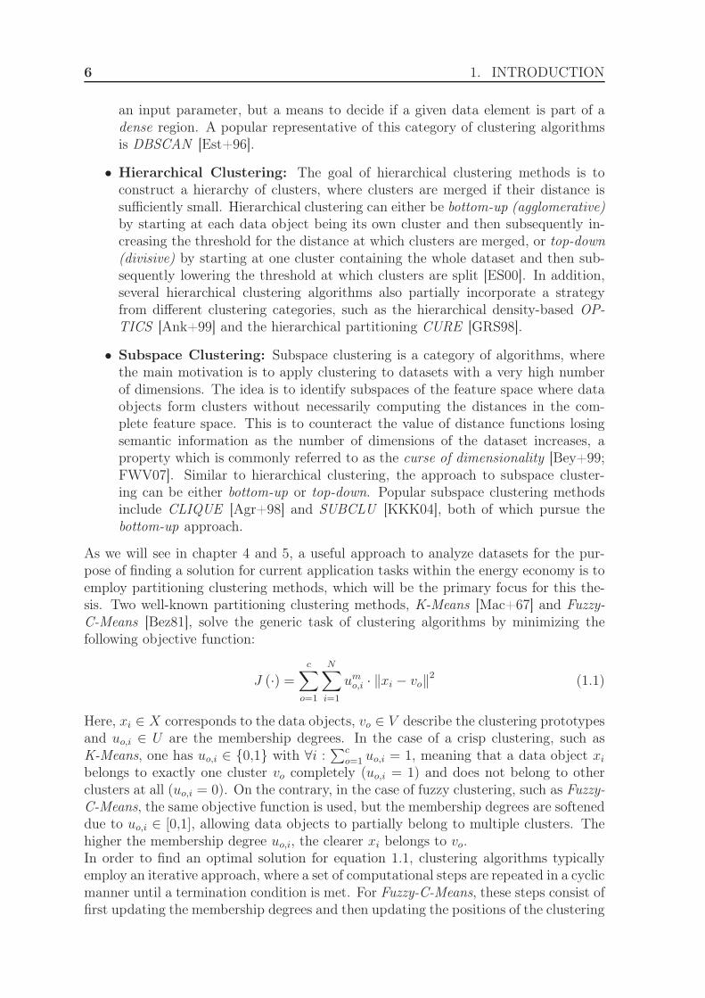
• Hierarchical Clustering: The goal of hierarchical clustering methods is toconstruct a hierarchy of clusters, where clusters are merged if their distance issufficiently small. Hierarchical clustering can either be bottom-up (agglomerative)by starting at each data object being its own cluster and then subsequently in-creasing the threshold for the distance at which clusters are merged, or top-down(divisive) by starting at one cluster containing the whole dataset and then sub-sequently lowering the threshold at which clusters are split [ES00]. In addition,several hierarchical clustering algorithms also partially incorporate a strategyfrom different clustering categories, such as the hierarchical density-based OP-TICS [Ank+99] and the hierarchical partitioning CURE [GRS98].
• Subspace Clustering: Subspace clustering is a category of algorithms, wherethe main motivation is to apply clustering to datasets with a very high numberof dimensions. The idea is to identify subspaces of the feature space where dataobjects form clusters without necessarily computing the distances in the com-plete feature space. This is to counteract the value of distance functions losingsemantic information as the number of dimensions of the dataset increases, aproperty which is commonly referred to as the curse of dimensionality [Bey+99;FWV07]. Similar to hierarchical clustering, the approach to subspace cluster-ing can be either bottom-up or top-down. Popular subspace clustering methodsinclude CLIQUE [Agr+98] and SUBCLU [KKK04], both of which pursue thebottom-up approach.
As we will see in chapter 4 and 5, a useful approach to analyze datasets for the pur-pose of finding a solution for current application tasks within the energy economy is toemploy partitioning clustering methods, which will be the primary focus for this the-sis. Two well-known partitioning clustering methods, K-Means [Mac+67] and Fuzzy-C-Means [Bez81], solve the generic task of clustering algorithms by minimizing thefollowing objective function:
J (·) =c
∑
o=1
N∑
i=1
umo,i · ‖xi − vo‖
2 (1.1)
Here, xi ∈ X corresponds to the data objects, vo ∈ V describe the clustering prototypesand uo,i ∈ U are the membership degrees. In the case of a crisp clustering, such asK-Means, one has uo,i ∈ {0,1} with ∀i :
∑c
o=1 uo,i = 1, meaning that a data object xi
belongs to exactly one cluster vo completely (uo,i = 1) and does not belong to otherclusters at all (uo,i = 0). On the contrary, in the case of fuzzy clustering, such as Fuzzy-C-Means, the same objective function is used, but the membership degrees are softeneddue to uo,i ∈ [0,1], allowing data objects to partially belong to multiple clusters. Thehigher the membership degree uo,i, the clearer xi belongs to vo.In order to find an optimal solution for equation 1.1, clustering algorithms typicallyemploy an iterative approach, where a set of computational steps are repeated in a cyclicmanner until a termination condition is met. For Fuzzy-C-Means, these steps consist offirst updating the membership degrees and then updating the positions of the clustering

1.2. KNOWLEDGE DISCOVERY 7
Algorithm 1 Fuzzy-C-MeansInput: X,m, ǫ, cOutput: set of all clustering prototypes V , matrix containing the membership degrees
U1: Generate initial clustering prototypes V (0) =
(
v(0)0 , . . . , v
(0)c
)
2: r ← 03: repeat
4: U (r+1) ←
u(r+1)1,1 . . . u
(r+1)1,N
.... . .
...u(r+1)c,1 . . . u
(r+1)c,N
with u
(r+1)o,i :=
dist2
1−m
(
xi,v(r)o
)
∑co′=1
dist2
1−m
(
xi,v(r)
o′
)
5: V (r+1) ←(
v(r+1)0 , . . . , v
(r+1)c
)
with v(r+1)o :=
∑Ni=1
(
u(r+1)o,i
)m
·xi
∑Ni=1
(
u(r+1)o,i
)m
6: r ← r + 17: until ‖V (r+1) − V (r)‖ < ǫ8: return V, U
prototypes. This procedure has the advantage of being easily implementable and thushighly practical. In contrast, one disadvantage of this approach lies in the dependencyfor the starting configuration of the clustering prototypes, causing the algorithm tosometimes terminate in a local optimum which might be far off the global optimum forthe objective function. Algorithm 1 presents the general form of Fuzzy-C-Means. Inliterature, the termination condition of Fuzzy-C-Means is very commonly expressed asthe algorithm continuing indefinitely until the change of the clustering segmentationcompared to the prior iteration no longer exceeds a given threshold ǫ as seen in line 7of algorithm 1, but implementations often also support the algorithm terminating aftera user-specified maximum number of iterations, either as an additional or a surrogatetermination condition for ‖V (r+1) − V (r)‖ < ǫ.
While the quality of the results of the clustering process does depend on parame-ters specific to the clustering process, such as the initial starting configuration for theclustering prototypes, the quality of the input dataset also plays a major role, whichis of particular importance if the dataset is based on real-world circumstances, as op-posed to synthetic datasets. This is due to the fact that when recording real-worldevents or objects, external factors may impact the collection of data in a negative way,for example through inaccuracies in the measuring equipment or during preprocessing,technical failures that have occured during the transmission of data, as well as someaspects being outright unknown, for example because of survey participants not an-swering some questions in a poll. This, among possibly other reasons, may cause thedataset to contain missing values. The underlying principle for the absence of a valuein the data is referred to as a missing-data mechanism. In general, there are threemechanisms for missing values [LR02]:
• Missing At Random (MAR): If the data is missing at random, then thismeans that the probability of a given value to be missing is dependent on theobserved data, but not on the missing attribute value itself. More formally, thevalues are missing at random if the following condition is met:
f(M |X, φ) = f(M |Xobs, φ) ∀Xmis, φ (1.2)

8 1. INTRODUCTION
Here, M = (mi,n) indicate whether the n-th attribute of the i-th data object isavailable (mi,n = 0) or missing (mi,n = 1). Furthermore, Xobs denotes the set ofobserved values, Xmis represents the set of missing values, X = Xobs ∪ Xmis isthe entire dataset and φ are unknown parameters.
• Missing Completely At Random (MCAR): If the data is missing completelyat random, then the availability or absence of values does depend neither on theobserved values Xobs nor the unobserved values Xmis:
f(M |X, φ) = f(M |φ) ∀X, φ (1.3)
• Not Missing At Random (NMAR): The mechanism of missing values isnot missing at random if the probability of a given value being unobserved isdependent on the missing value itself.
While the failure mechanism for missing values is usually not known in advance for real-world datasets, the failure mechanism can have a significant influence on the qualityof the resulting clustering segmentation [HC10b; HC10a]. In order to probe whichmissing-data mechanism is present for a given dataset, tests based on statistics can beapplied; to test for NMAR and MAR, the one-sample test and two-sample test can beused, respectively [WB05], while a test based on the χ2 test is presented in [Lit88] forMCAR.After learning which failure mechanism is present, an analyst may decide on whichmethod is applied to process the data as good as possible while keeping the applicationtask in mind. In general, there are three approaches to handle missing values in thedataset [LR02]:
• Adaption of analysis methods: One way to accommodate for missing valuesin the dataset is to modify the methods that are part of the Knowledge Dis-covery in Databases process. This can happen by estimating missing data priorto applying Data Mining methods but still differentiate between estimated andmeasured data during analysis, or by extending the definition of computationalmethods that access the data tuples so that they can be applied even if the tuplescontain missing values.
• Complete-Case Analysis: Possibly the simplest approach in processing adataset that contains missing values is to remove all data tuples that are partiallyunobserved and to analyze only the data tuples that have been observed com-pletely. This approach is particularly tempting if the amount of missing values isrelatively small. It should be noted however that while this approach is uncriticalif the mechanism that let to the occurrence of missing values is MCAR, it canlead to wrong conclusions if the mechanism is NMAR.
• Imputation of missing values: This technique works by replacing missingvalues in the dataset with values that are typically derived from observed data.The chosen method to assign a value to fields that are unobserved can be verysimple, such as computing the arithmetic mean or median, but also includesarbitrary elaborate methods as long as they are deemed adequate for the givenapplication by an analyst. After missing values are replaced with imputed values,these values are treated as measured data, meaning that data analysis can beperformed normally without the need to further account for missing values.

1.2. KNOWLEDGE DISCOVERY 9
One of the major drawbacks of Complete-Case Analysis is that it artificially reducesthe size of the dataset. Similarily, imputation of missing values can majorly skew theresults of the analysis depending on the amount of unobserved data and the concreteimputational method used. As for adaption of analysis methods, while this methodologydoes not alter the input dataset, the choice of how the data mining algorithm is modifiedcan still have a tremendous impact on the final analysis result. Some approaches on howFuzzy-C-Means, as presented in algorithm 1, can be modified to work with datasetscontaining missing values are presented in [HB01; SL01], while their impact on theclustering quality is investigated and discussed in [HC10a; HHC11].
1.2.3 Dissimilarity measurements for time series
Though clustering methods are a useful tool to find patterns in data, they are primarilydesigned for static data, meaning datasets which are presented as a set of tuples whosefeatures do not evolve over time. This usually makes applying clustering on time seriesdata a non-trivial task. As [Lia05] mentions, further care should be taken in regardas to whether the measured values are discrete or continuous, sampled uniformly ornon-uniformly, univariate or multivariate and whether or not the time series are ofequal length. Depending on the dataset and the application task, the analyst mayopt to modify the function to evaluate the dissimilarity between two data objects toa measure more appropriate for time series. That way, existing clustering algorithmscan be used without further modifications. Another possibility would be to convert thetime series data or extract features from them in a way such that existing clusteringalgorithms can handle the resulting data. Over the course of this section, we focus onthe first two categories and present examples for dissimilarity measures for time seriesas well as feature extraction techniques that can help analyze unknown time series.
When trying to evaluate the dissimilarity of two given time series, the most simplecase is when both time series are of equal length. In that case, the Lp-norm, sometimesalso called the Minkowski distance, can be used. It is defined as follows:
dist (a, b) =
(
∑
n
|an − bn|p
)1p
(1.4)
For p = 2, equation 1.4 results in the well-known euclidean distance. However, de-pending on the application task, the Lp-norm may be unsuitable to compare the giventime series. For example, the time series may be of unequal length, the values of thetime series may have different means and variances, or the time series may have localcompressions and stretchings.
In order to circumvent the problems outlined above, it is often desirable to mathe-matically capture the human perception of the shape of a given time series and usethat to compare the data objects in the dataset instead of focusing on the actual mea-sured values directly; this is the basic idea behind Shape Definition Language (SDL)[Agr+95]. Here, an expert first defines an alphabet Σ. The symbols contained inΣ describe the shape of a portion of the time series, for example ascending, stronglyascending or descending. Before analysis, a time series is then encoded using the cor-responding symbols of Σ. Due to the concept, the choice of the alphabet stronglyinfluences which curve shapes can be detected at all, but also if a time series represen-tation by a sequence of symbols is unique. Once such a representation by sequence of
10 1. INTRODUCTION
(a) (b)
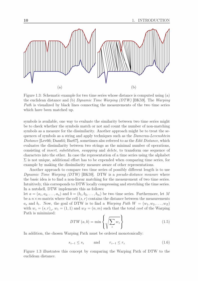
Figure 1.3: Schematic example for two time series whose distance is computed using (a)the euclidean distance and (b) Dynamic Time Warping (DTW) [BK59]. The WarpingPath is visualized by black lines connecting the measurements of the two time serieswhich have been matched up.
symbols is available, one way to evaluate the similarity between two time series mightbe to check whether the symbols match or not and count the number of non-matchingsymbols as a measure for the dissimilarity. Another approach might be to treat the se-quences of symbols as a string and apply techniques such as the Damerau-LevenshteinDistance [Lev66; Dam64; Bar07], sometimes also referred to as the Edit Distance, whichevaluates the dissimilarity between two strings as the minimal number of operations,consisting of insert, substitution, swapping and delete, to transform one sequence ofcharacters into the other. In case the representation of a time series using the alphabetΣ is not unique, additional effort has to be expended when comparing time series, forexample by making the dissimilarity measure aware of other representations.
Another approach to compare two time series of possibly different length is to useDynamic Time Warping (DTW) [BK59]. DTW is a pseudo-distance measure wherethe basic idea is to find a non-linear matching for the measurement of two time series.Intuitively, this corresponds to DTW locally compressing and stretching the time series.In a nutshell, DTW implements this as follows:let a = (a1, a2, . . . , an) and b = (b1, b2, . . . , bm) be two time series. Furthermore, let Mbe a n×m-matrix where the cell (s, r) contains the distance between the measurementsas and br. Now, the goal of DTW is to find a Warping Path W = (w1, w2, . . . , wZ)with wz = (s, r)z, w1 = (1, 1) and wZ = (n,m) such that the total cost of the WarpingPath is minimized:
DTW (a, b) = min
√
∑
z
wz
(1.5)
In addition, the chosen Warping Path must be ordered monotonically:
sz−1 ≤ sz and rz−1 ≤ rz (1.6)
Figure 1.3 illustrates this concept by comparing the Warping Path of DTW to theeuclidean distance.
1.3. CONTRIBUTIONS 11
(a) (b)
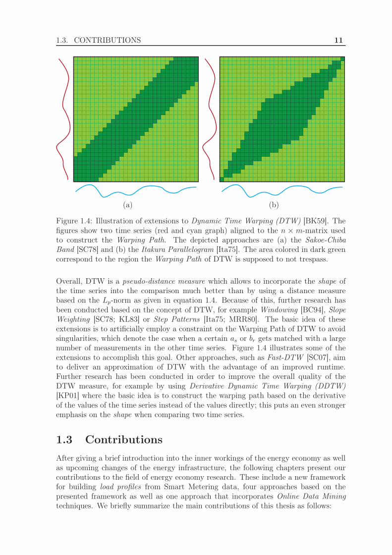
Figure 1.4: Illustration of extensions to Dynamic Time Warping (DTW) [BK59]. Thefigures show two time series (red and cyan graph) aligned to the n × m-matrix usedto construct the Warping Path. The depicted approaches are (a) the Sakoe-ChibaBand [SC78] and (b) the Itakura Parallelogram [Ita75]. The area colored in dark greencorrespond to the region the Warping Path of DTW is supposed to not trespass.
Overall, DTW is a pseudo-distance measure which allows to incorporate the shape ofthe time series into the comparison much better than by using a distance measurebased on the Lp-norm as given in equation 1.4. Because of this, further research hasbeen conducted based on the concept of DTW, for example Windowing [BC94], SlopeWeighting [SC78; KL83] or Step Patterns [Ita75; MRR80]. The basic idea of theseextensions is to artificially employ a constraint on the Warping Path of DTW to avoidsingularities, which denote the case when a certain as or br gets matched with a largenumber of measurements in the other time series. Figure 1.4 illustrates some of theextensions to accomplish this goal. Other approaches, such as Fast-DTW [SC07], aimto deliver an approximation of DTW with the advantage of an improved runtime.Further research has been conducted in order to improve the overall quality of theDTW measure, for example by using Derivative Dynamic Time Warping (DDTW)[KP01] where the basic idea is to construct the warping path based on the derivativeof the values of the time series instead of the values directly; this puts an even strongeremphasis on the shape when comparing two time series.
1.3 Contributions
After giving a brief introduction into the inner workings of the energy economy as wellas upcoming changes of the energy infrastructure, the following chapters present ourcontributions to the field of energy economy research. These include a new frameworkfor building load profiles from Smart Metering data, four approaches based on thepresented framework as well as one approach that incorporates Online Data Miningtechniques. We briefly summarize the main contributions of this thesis as follows:

12 1. INTRODUCTION
• We present a framework that describes a methodology to construct load profilesusing Smart Metering data. This framework sets itself apart from other proposalsby constructing load profiles as energy consumptions forecast models that adhereto current business processes within the energy economy, thus being easy to adoptby the industry [Boc16; Boc17; Boc18].
• Another contribution of this work are the experimental evaluation of four ap-proaches based on the framework introduced in [Boc16; Boc17; Boc18] usingreal-world datasets. Two of these approaches have been presented in [Boc17;Boc18] while the other two are new.
• Lastly, we propose a new approach that combines the advantage of building loadprofiles that are easy to adopt due to the load profiles being built with existingbusiness processes in mind with Online Data Mining techniques. This allowsthe load profiles to become sensitive to changing customer behavior without theneed to restart the entire KDD workflow from scratch. In addition to loweringcomputational requirements, this approach gives the analyst the opportunity tochoose the optimal amount of history to include in the analysis, therefore fine-tuning the performance of the forecast models.
1.4 Outline of this work
The rest of this thesis is structured as follows. In chapter 2, we introduce the basicconcepts and business processes in the energy economy. This includes the generalsetup of the electricity grid, day-to-day challenges of a market participant as well asthe basic structure of load profiles, a common technique to forecast the energy demandof consumers.We expand on this foundation in chapter 3, where we present and discuss approachesfrom academic literature based on the concept of Knowledge Discovery in Databasesfor gaining useful insight both from the perspective of an end-consumer and an energyprovider. We also outline some of the upcoming changes to the electricity infrastructureitself.In chapter 4, we introduce a framework to construct load profiles using Smart Meteringtime series in an effort to tackle the challenges energy providers face. In addition,we also present an experimental evaluation of our framework using real-world data.Chapter 5 then further builds upon this framework by introducing the concept ofOnline Data Mining techniques to help keep load profiles up-to-date with changes inconsumer behavior as new Smart Metering data becomes available.Finally, chapter 6 concludes this thesis with a short summary and a brief discussion ofpotential future work.

2Background
During major parts of this thesis, the main focus of our attention are approaches tocurrent challenges in the energy economy involving time series data. For this purposeit is important to understand the requirements and procedures of business processeswhich are in practice today as well as the general setup of the electricity grid. Becauseof this, we give an introduction to the fundamentals of these areas over the course ofthis chapter, which is to be understood as the first step in the process of KnowledgeDiscovery in Databases, where relevant application knowledge is collected in order togain a sufficient understanding of the application domain. The overview we give in thefollowing sections concerns current challenges of utility companies and energy providersas well as approaches implemented at present in the industry to tackle these problems;we introduce the state-of-the-art in academic literature in later chapters of this thesis.For the most part, the business processes presented in this chapter primarily relate toelectricity companies in Germany; however it is possible that processes in other regionsare also affected.
2.1 Overview of the electricity grid
One of the most fundamental requirements within the energy economy is the construc-tion and maintenance of infrastructure which allows producers to deliver energy tothe consumers. At the same time, the infrastructure must account for physical laws,imposing certain constraints on the way energy can be distributed. To overcome thesetechnical limitations, engineers have elected to build the electricity grid using a tieredstructure of different voltage levels, for which an overview is given in figure 2.1. Themain idea of using different voltage levels for the various abstract layers of the electric-ity grid is that in order to deliver energy across large distances, high voltage lanes arepreferable. This is due to the fact that increasing the voltage allows for a decrease ofthe electric current, which helps in reducing the amount of grid losses due to the cablesheating up. At the same time, high voltage lanes require more sophisticated isolationto prevent short circuits caused by arcing. This makes them impractical to use all
13
14 2. BACKGROUND
Hydroelectric Power
Stations
Coal Power Stations
Nuclear Power Stations
Industrial and mid-
sized Power Stations
Industrial
Consumers Transregional
Operating Reserve
Regional
Operating Reserve
Industrial
Consumers
Industrial
Consumers
City Power Grid
Urban Power Stations
Solar Power Stations
Wind Power Stations
Railway
Extra-High Voltage
In europe mostly
220 kV or 380 kV☆
Wide area transmission
incl. across national borders
☆
High Voltage
In europe mostly
from 60 kV up to 150 kV☆
Conurbations with energy
requirements up to 100 MW
☆
Medium Voltage
In europe mostly
from 1 kV up to 35 kV☆
Rural and urban regions☆Hospitals and factories☆
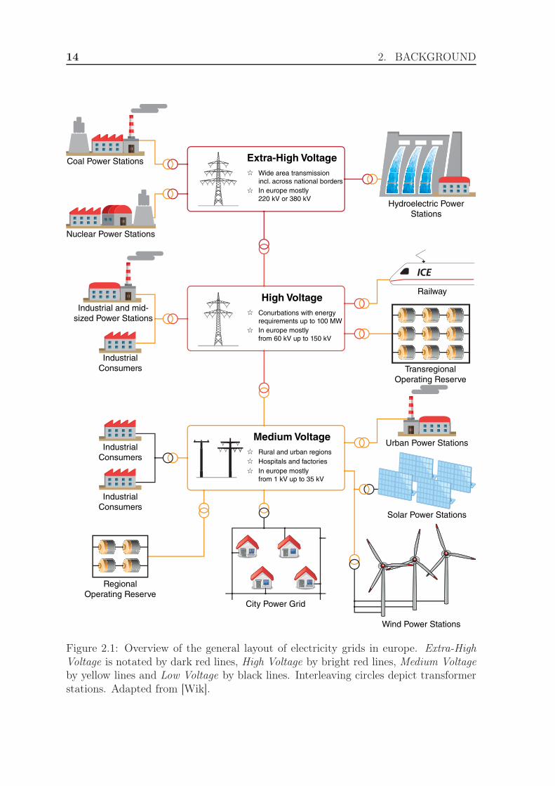
Figure 2.1: Overview of the general layout of electricity grids in europe. Extra-HighVoltage is notated by dark red lines, High Voltage by bright red lines, Medium Voltageby yellow lines and Low Voltage by black lines. Interleaving circles depict transformerstations. Adapted from [Wik].

2.1. OVERVIEW OF THE ELECTRICITY GRID 15
the way up to the house or building complex of the customer, particularly in denselypopulated areas, where a lack of space between cables might lead to short circuits incase the cable isolation is damaged.In general, the higher the voltage, the larger the area that part of the electricity gridaims to cover. While small, urban power stations usually reside in the medium volt-age network, transregional power stations with a large energy output are typicallyconnected to the high voltage or extra-high voltage network.
Until the end of the 1990s, public utility companies had been responsible for bothoperating and maintaining the electricity grid as well as managing corporate sales.That is, utility companies were purposefully given a monopoly for the region they hadbeen responsible for. This had begun to change with the Directive 96/92 of the Eu-ropean Parliament [Par96], which has laid the foundation for the liberalization of theenergy market. In the case of Germany, the liberalization was legally finalized as partof the "Gesetz zur Neuregelung des Energiewirtschaftsrechts" (Law for the revision ofthe energy economy rights) [Bun98] in 1998.Since the liberalization of the energy market, consumers are able to freely choose theirenergy provider, allowing for grid operators and third party energy providers to bein direct competition with each other. At the same time, even when customers havechosen a third party to be their energy provider, physical lane circuitry still requiredcustomers to be served by their local utility company. In order to prevent unfair ad-vantages for the utility company, the liberalization of the energy market also requiredutility companies to have their grid operation department and their marketing depart-ment to function separately and independently. Because of this, customers are able tomandate the energy provider of their choice and pay only an electricity bill accordingto the prices of their chosen energy provider, while the physical delivery of energy isstill conducted by their corresponding local utility company.As a consequence of customers from different regions being able to require their lo-cal grid operator to cooperate with an arbitrary third party energy provider, therehas been a need for business processes of all grid operators and energy providers tobe compatible to one another to satisfy legal obligations. In Germany, this stan-dardization has been the task of the BDEW, which is short for "Bundesverband derEnergie- und Wasserwirtschaft" (Federal association of the energy and water economy).For the electricity market, the applicable policy for the business processes themselvesis the "Marktregeln für die Durchführung der Bilanzkreisabrechnung Strom" (MaBiS)[Bun13], while the technical format for the market communication is documented as asubset of the UN/EDIFACT standard called EDI@Energy [EDI].Since business processes and market communication are standardized, notable changesare only possible by new revisions of the MaBiS standard, which are then requiredby all market participants in Germany to be implemented almost simultaneously, withrespect to an adequate transition period. Depending on the concrete implementationof the MaBiS standard, changes can be very complex and costly. Because of this, wewill present some of the most important challenges of energy providers and currentsolutions within the confinements of the MaBiS standard in the following sections.

16 2. BACKGROUND
2.2 Current challenges of energy providers
The most important task of energy providers is to ensure the security of the energysupply, laying down an indispensable necessity of the very foundation of modern so-ciety. In order to achieve this goal, it is essential to predict the aggregated energyconsumption time series of all customers, that is, the amount of energy the customerbase as a whole consume at a given point in time, as accurately as possible. On thebasis of this forecasted consumption time series, energy providers allocate productioncapacities from energy producers at an early stage, giving energy producers enoughlead time to ramp production up or down so that energy is injected into the electricitygrid exactly according to the consumption time series predicted and announced by theenergy provider. This procedure is necessary due to the fact that adjusting the pro-duction rate of energy takes time, which is dependent on the type of the power station.While hydroelectric power stations can adjust their production within seconds, mostother power plants, such as coal or nuclear power stations, require a startup time ofmultiple hours up to several days. Because energy is conserved in a closed system,special precautions need to be taken to protect sensitive industrial and consumer elec-tronics from damages caused by undervoltage or overvoltage. This is one of the reasonswhy the electricity grid need to be balanced at all times, thus requiring the forecastof the total energy consumption compiled by the energy providers need to match theactual consumption as closely as possible, with deviations by overestimating and un-derestimating the actual load being equally undesirable.However, since the consumption forecast by energy providers is, by definition, merelyan estimate of the future actual consumption, forecast errors are inevitable. Theseforecast errors require adjustments in real-time, which is referred to by the industry asimbalance energy or operating reserve, in order to keep the electricity grid balanced.Any technology that is able to both absorb and provide energy within seconds canfunction as imbalance energy, such as parallel-connected batteries at large-scale orpump-driven water containers which store and retrieve energy by converting betweenelectricity and potential energy. Due to their limited availability, their increased wearand tear because of constant readjusting, their reduced energy efficiency in order to pri-oritize response time, as well as their importance to keep the electricity grid balanced,imbalance energy is usually much more financially volatile than regular energy. On anabstract level, imbalance energy can be understood as a battery which aims to stayat 50 percent charge status and is installed between energy producers and consumers;depending on whether the energy provider has under- or overestimated the actual totalenergy load of customers, the battery charges or discharges accordingly to make up forthe difference. As depicted in figure 2.1, based on whether the provider of imbalanceenergy is regional or transregional, the provider typically resides in either the mediumvoltage or high voltage electricity grid.
In order to minimize the amount of imbalance energy that has to be injected intoor extracted from the electricity grid, the forecast models used by energy providersneed to both be accurate and provide long-term predictions about the consumptionbehavior of customers. This enables the energy providers to take a long view on theirfuture buy-in of energy, allowing for more attractive terms in cooperation with energyproducers. As a rule of thumb, the more uniformly and smoothly the total energyconsumption changes, the easier it is both to adjust to those changes by requiring less

2.2. CURRENT CHALLENGES OF ENERGY PROVIDERS 17
imbalance energy and to forecast the energy consumption beforehand. While for mostof the time, prices for imbalance energy are one order of magnitude more cost-intensivethan regular energy, in cases where the operating reserve is almost depleted, but alsofor other reasons, it is possible for the prices of imbalance energy to be multiple ordersof magnitude higher than for regular energy. For example, on the 17th October 2017,the prices of imbalance energy have reached an all-time high with a price of 24.455,05 eper MWh of energy, a huge step up compared to the prices of regular energy which aretypically within the price range of 30 to 60 e per MWh of energy for Day-Ahead Auc-tions, causing controlling authorities to intervene [Bun18]. As a consequence thereof,sudden, abrupt changes in the total energy consumption time series which cause im-balance energy to be used are generally undesirable to energy providers due to thefinancial risk associated with them.In practice however, the total energy consumption is only known in hindsight and elec-tricity meters of customers are usually read only once per year as part of the annualaccounting. Although the total energy consumption time series is in fact the only re-quirement of energy providers in order to plan the future buy-in of energy, the absenceof detailed knowledge about the consumption behavior of customers leads to the ab-sence of knowledge about consumption causes of which the total energy consumptiontime series is composed of. In particular, since in most cases only one meter readingfrom each customer is available per year, there is no way of differentiating between uni-form and peak consumption. Aside from one annual meter reading, in most cases theenergy provider only knows contractual details about the customer such as his or hername and the full postal address. High resolution measurements of the consumptionbehavior of individual customers as well as an intensive, continuous communicationso to cater to their specific needs are often economically justifiable only for very largecustomers, that is, customers with an annual consumption of at least 100.000 kWh ofenergy.The resulting lack of insight about the consumption behavior of customers is in starkcontrast to the amount of information that online merchants and service providers, aswell as retailers using campaigns such as Payback, have gathered on their customers,which can then be analyzed using techniques such as Association Rule Mining that onemay derive customer habits and preferences [Sch12]. Although, for billing purposes,having only one meter reading per year is sufficient, assuming that the retail energyprice is constant, differentiating between uniform and peak consumption is necessaryto plan the buy-in of energy and avoid imbalance energy as much as possible. It shouldbe noted however that even if the past consumption behavior of a given customer isknown, his or her behavior might change the following day. For example, it is intu-itively plausible for employed end-consumers to have a different daily routine, and thusa different consumption behavior, on a working day than during the weekend. Thisfactor can possibly cause the base load to change significantly or for some load peaks tonot occur at all, occur pronounced differently or at different times of the day. Further-more, customers can genuinely differ in their consumer behavior due to the customerspracticing different hobbies, having made different lifestyle decisions, being either asingle or a family household, being a low income or a high income household, or beingeither an end-consumer of a business, among other factors. The accurate handling ofthe superimposition of all distinct unknown requirements of all customers is one of themain challenges of an energy provider when planning the future buy-in of energy. The

18 2. BACKGROUND
goal of finding a feasible solution to this problem is a core component of this thesis.For this purpose, we introduce the concept of load profiles in the following section.Currently, load profiles are the main tool of energy providers in order to tackle theproblem of forecasting the energy consumption. Based on this, we will then elaborateon our optimization approach in chapter 4 and 5 of this thesis.
2.3 Structure and purpose of load profiles
The forecast of the energy consumption and thus the planning of the future buy-inof energy in order to overcome the difficulties outlined in the previous section is typ-ically achieved using so called load profiles. Load profiles are designed to offer a wayto differentiate between uniform and peak consumption along with the possibility tocope with variable daily routines of customers. To accomplish this goal, additionalknowledge about customers or, if such knowledge is not available, additional assump-tions about customers need to be incorporated. Over the course of this section, wewill give an overview of the mechanics of SLP load profiles, the standard forecastmodel of the energy economy as outlined by the "Marktregeln für die Durchführungder Bilanzkreisabrechnung Strom" (MaBiS) industry policy [Bun13].
In essence, load profiles consist of a set of customer groups and a segmentation ofall calendar days for a year into so called day-types as well as a consumption patternfor each combination of a customer group and a day-type. The basic idea here is thatwhile customer groups offer a way to address the needs of distinct customers, such asbusinesses having different use-cases and energy requirements than home consumers,day-types allow to define temporal intervals during which the consumption behaviorof customer is significantly different than for other day-types. What is important tonote here is that load profiles, as implemented by the energy economy, have a strictperiodicity of 1 year. Because of this, special events that happen more rarely than1 year or events whose appointed date is not known 1 year in advance, but whichpossibly have a significant influence on the consumption behavior of customers, suchas the FIFA World Cup or other major sports events, can not be modeled using loadprofiles. Figure 2.2 depicts some of the Standard Load Profiles as provided by theBDEW. As shown in figure 2.2 and in compliance with intuitive understanding, privatehouseholds and businesses have significantly different consumption behaviors. Whilethe industrial load profile G0 expects the energy consumption of businesses to stronglycorrelate with business hours, the consumption of private households is much morespread out according to the load profile H0, with two noticeable consumption peaksat noon and in the evening and a drop in energy consumption during the afternoon.By assigning a load profile to each customer, energy providers do not presume thatevery customer behaves exactly as expected by the consumption pattern of the loadprofile; instead, energy provider merely assume the consumption pattern of a givenload profile to be representative for all customer assigned to that customer group, withdeviations between individual customers and the consumption pattern of their assignedload profile to balance out.
It should be noted however that the load profile themselves are normalized, meaningthey do not directly predict the amount of energy required by a given customer, butmerely the expected consumption behavior. In order to derive an actual forecast fora given customer, load profiles require additional external input in the form of the

2.3. STRUCTURE AND PURPOSE OF LOAD PROFILES 19
Working day Saturday Sunday and Holiday
00:00 03:00 06:00 09:00 12:00 15:00 18:00 21:000.00
0.05
0.10
0.15
0.20
0.25
Time
Ener
gy
consu
mpti
on@k
WhD
(a)
Working day Saturday Sunday and Holiday
00:00 03:00 06:00 09:00 12:00 15:00 18:00 21:000.00
0.05
0.10
0.15
0.20
0.25
Time
Ener
gy
consu
mpti
on@k
WhD
(b)
Figure 2.2: Overview of the Standard Load Profiles (a) H0 (household profile) and (b)G0 (general purpose industrial profile) from the BDEW, valid only during summer.The time series shown are normalized and describe the expected consumption behaviorfor the day-types Working day, Saturday and Sunday and Holiday.
so called Year Consumption Forecast (YCF). The Year Consumption Forecast is acustomer-specific property assigned by the energy provider and equals to the amountof energy the corresponding customer is expected to consume over the course of 1 year.Since the energy provider does know 1 meter reading per year of every customer as partof the annual accounting, most energy providers derive the Year Consumption Forecastof their customers for the following year by computing the actual energy consumptionof the previous year as follows:
Y CF2016 = actual total consumption in 2015
= reading (01.01.2016)− reading (01.01.2015)(2.1)
Even though the formula in equation 2.1 is possibly the most used method to define aYear Consumption Forecast, depending on the choice of the individual energy provider,other options for the definition of a Year Consumption Forecast can be used. Forexample, instead of using just the actual energy consumption of a given customer ofthe previous year as a prediction for the energy consumption of the same customer ofthe following year, a weighted average over the last couple of years can be used. Inaddition, without loss of generality, equation 2.1 can also be applied if energy providersopt to perform the meter reading not at the beginning of the year, but rather performthe meter reading of all customers over the course of the year in a staggered manner.If both the load profile and the Year Consumption Forecast of a customer are known,the forecast of that customer’s energy consumption Ei (t) is computed as follows:
Ei (t) = Y CF i ·Enormalized profile (t)
1.000.000 kWh(2.2)
The denominator of 1.000.000 kWh in equation 2.2 is a consequence of the load pro-files being normalized; according to [Bun13], load profiles have to be tuned so thatEnormalized profile (t) adds up to 1.000.000 kWh over the course of a year chosen by theauthors of the load profile. Subsequently, however, the normalization of a load profile
20 2. BACKGROUND
...
Meter reading
Time
Meter reading
on 01.01.2016
+ YCF of
customer
01.01.2016 02.01.2016 03.01.2016 04.01.2016 05.01.2016 31.12.2016
Working day Saturday Sunday and Holiday
Meter reading
on 01.01.2016
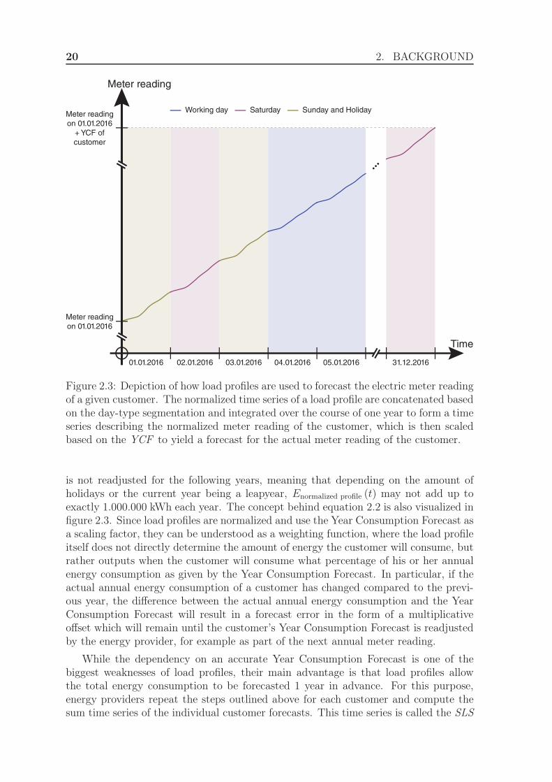
Figure 2.3: Depiction of how load profiles are used to forecast the electric meter readingof a given customer. The normalized time series of a load profile are concatenated basedon the day-type segmentation and integrated over the course of one year to form a timeseries describing the normalized meter reading of the customer, which is then scaledbased on the YCF to yield a forecast for the actual meter reading of the customer.
is not readjusted for the following years, meaning that depending on the amount ofholidays or the current year being a leapyear, Enormalized profile (t) may not add up toexactly 1.000.000 kWh each year. The concept behind equation 2.2 is also visualized infigure 2.3. Since load profiles are normalized and use the Year Consumption Forecast asa scaling factor, they can be understood as a weighting function, where the load profileitself does not directly determine the amount of energy the customer will consume, butrather outputs when the customer will consume what percentage of his or her annualenergy consumption as given by the Year Consumption Forecast. In particular, if theactual annual energy consumption of a customer has changed compared to the previ-ous year, the difference between the actual annual energy consumption and the YearConsumption Forecast will result in a forecast error in the form of a multiplicativeoffset which will remain until the customer’s Year Consumption Forecast is readjustedby the energy provider, for example as part of the next annual meter reading.
While the dependency on an accurate Year Consumption Forecast is one of thebiggest weaknesses of load profiles, their main advantage is that load profiles allowthe total energy consumption to be forecasted 1 year in advance. For this purpose,energy providers repeat the steps outlined above for each customer and compute thesum time series of the individual customer forecasts. This time series is called the SLS
2.3. STRUCTURE AND PURPOSE OF LOAD PROFILES 21
... ... ...
Customer 1
Customer 2
Customer N
Householdprofile
Householdprofile
Industrial profile
YCFCustomer 1
YCFCustomer 2
YCFCustomer N
Daily forecast for Customer 1
Daily forecast for Customer 2
Daily forecast for Customer N
Total energy consumption
(“SLS“ time series)
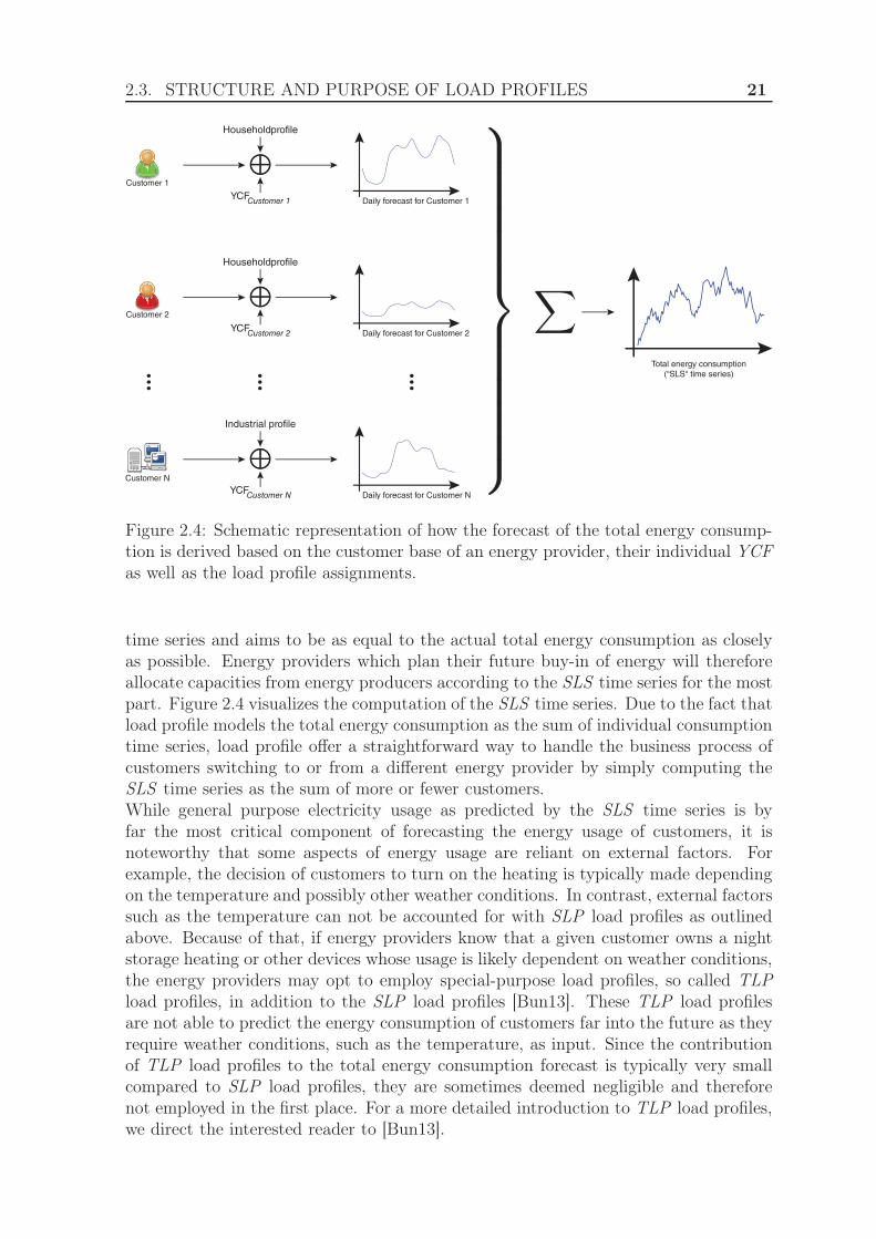
Figure 2.4: Schematic representation of how the forecast of the total energy consump-tion is derived based on the customer base of an energy provider, their individual YCFas well as the load profile assignments.
time series and aims to be as equal to the actual total energy consumption as closelyas possible. Energy providers which plan their future buy-in of energy will thereforeallocate capacities from energy producers according to the SLS time series for the mostpart. Figure 2.4 visualizes the computation of the SLS time series. Due to the fact thatload profile models the total energy consumption as the sum of individual consumptiontime series, load profile offer a straightforward way to handle the business process ofcustomers switching to or from a different energy provider by simply computing theSLS time series as the sum of more or fewer customers.While general purpose electricity usage as predicted by the SLS time series is byfar the most critical component of forecasting the energy usage of customers, it isnoteworthy that some aspects of energy usage are reliant on external factors. Forexample, the decision of customers to turn on the heating is typically made dependingon the temperature and possibly other weather conditions. In contrast, external factorssuch as the temperature can not be accounted for with SLP load profiles as outlinedabove. Because of that, if energy providers know that a given customer owns a nightstorage heating or other devices whose usage is likely dependent on weather conditions,the energy providers may opt to employ special-purpose load profiles, so called TLPload profiles, in addition to the SLP load profiles [Bun13]. These TLP load profilesare not able to predict the energy consumption of customers far into the future as theyrequire weather conditions, such as the temperature, as input. Since the contributionof TLP load profiles to the total energy consumption forecast is typically very smallcompared to SLP load profiles, they are sometimes deemed negligible and thereforenot employed in the first place. For a more detailed introduction to TLP load profiles,we direct the interested reader to [Bun13].

22 2. BACKGROUND
Up to this point we described how load profiles work in helping to forecast theenergy demand of customers, assuming they are chosen carefully and contain day-typeand customer group segmentations that accurately represent the customer behaviors.Traditionally however, energy providers do not have detailed, up-to-date knowledgeabout their customers to ponder what load profile best suits a given end-consumer ofbusiness. Instead, the segmentation of customer groups has been based on conjectures;for example, it seems intuitively plausible that private households and businesses havedifferent energy requirements, causing a segmentation of private households and busi-nesses in different customer groups to likely be reasonable. In the case of Germany,most energy providers use the Standard Load Profiles as published by the BDEW,which have been ordered from the academic chair for energy economy of the Branden-burg University of Technology during the 1990s [Mei+99]. To compile the StandardLoad Profiles, the researchers of [Mei+99] resorted to field measurements of approxi-mately 1.500 low voltage customers in cooperation with a selection of energy providers.Some of the resulting load profiles are shown in figure 2.2. As for the day-type seg-mentation, the Standard Load Profiles differentiate between working day, saturday andsunday and soliday for each of the seasons summer, winter and interim period, withthe corresponding customer groups being introduced in table 2.1. According to theresearchers, the Standard Load Profiles are applicable to customers with an annualconsumption up to 30.000 kWh or a peak demand of 30 kW of energy [FT00], but areoften used for customers with an annual consumption up to 100.000 kWh.In addition to the concept of day-types and customer groups, the Standard Load Pro-files also define a so called dynamization function. The idea behind such a function isto account for reoccurring patterns in the total energy consumption time series with aperiodicity of 1 year, such as the sine-shaped patterns visible in the datasets introducedin section 4.1. In the case of the Standard Load Profiles, the dynamization functionproposed by the BDEW is as follows:
DynFactor (doy) =− 3,92 · 10−10 · (doy)4 + 3,2 · 10−7 · (doy)3
− 7,02 · 10−5 · (doy)2 + 2,1 · 10−3 · (doy) + 1,24(2.3)
Here, doy corresponds to the day of year. By incorporating a dynamization functioninto the forecast of the energy consumption, energy providers are able to continuouslydistribute the energy allocation over the course of a year, increasing the energy al-location during winter and at the same time decreasing the energy allocation duringsummer. As a consequence, succeeding calendar days can have slightly different energyforecasts even if they belong to the same day-type. Thus, if a dynamization function isused, equation 2.2 is modified as follows:
Ei (t) = Y CF i · DynFactor (doy (t)) ·Enormalized profile (t)
1.000.000 kWh(2.4)
In principle, an energy provider may choose their preferred dynamization functionfreely, as the determined dynamization function is broadcasted to other market par-ticipants as part of the normal market communication [Bun06]. When deciding for adynamization function however, it is important to tune it such that the average valueof the dynamization function over the course of a whole year is equal to 1 to avoid theoverall amount of energy allocated, as predicted by the sum of the Year ConsumptionForecasts of the customers, from being distorted.

2.3. STRUCTURE AND PURPOSE OF LOAD PROFILES 23
Profile Description Target audience
H0Private households, but also minor
commercial needs
End-consumers, commercial agents,not applicable to thermal heat
pumps and thermal storage heatingdevices
G0General purpose industrial profile,defined as a weighted mean of all
commercial customers
Assigned if none of the profiles G1to G6 apply
G1Industrial profile for businesses
which operate on weekdays from 8to 18 o’clock
Offices, workshops, kindergartens,public administration facilities,
doctor’s office
G2Industrial profile for businesses
which operate mostly during theevening
Street lights, gas stations, eveningrestaurants and recreational
facilities (if their peak consumptionis not during the weekend)
G3
Industrial profile for continuous,relatively uniform demand,
including a noticeable, continuouspeak demand
Purification plants, drinking waterpumps, communal facilities in
residential complexes, cold storagewarehouses
G4Industrial profile for businesseswhich are mostly dependent on
business hoursShops, hairdresser
G5
Industrial profile for bakeries withbakehouses which typically start
operating at 3 o’clock duringweekdays and at midnight on
saturdays
Bakeries with bakehouse
G6Industrial profile for businesses
with a strong consumption focusduring weekends
Youth clubs, cinemas, restaurants,petrol stations
L0General purpose agricultural
profile, defined as a weighted meanof all agricultural customers
Assigned if the energy providerdoes not differentiate between
agricultural customers according tothe profiles L1 and L2
L1Agricultural profile for dairy farms
and sideline stockbreedingbusinesses
Dairy farms, sideline stockbreedingsfarms
L2Agricultural profile for businesseswith a mixture of household and
farming
Assigned if neither L1 nortime-of-the-day-independent
industrial profiles apply
Table 2.1: Overview of the BDEW Standard Load Profiles used by most German energyproviders and their common use-cases as defined in [Mei+99; FT00].

24 2. BACKGROUND
January February March April May June July
August September October November December
0
5
10
15
20
Figure 2.5: Comparison of the ratios of the absolute difference between the actualconsumption and the predicted load yielded when using the BDEW Standard LoadProfiles to the actual consumption in percent for 10 randomly selected energy providersin Germany. The monthly ratios shown correspond to the year 2017. The energyproviders are sorted ascendingly according to their yearly average deviation ratio.
Although the Standard Load Profiles as published by the BDEW have played avital role in securing the stability of the energy supply since they have come into ef-fect, studies have shown that, at least for the load profiles for the gas economy, thecurrent load profile have become an increasingly bad model to forecast the energy de-mand of customers [Roo+14]. Possible reasons for this trend include social changesas well as technological advances in recent years. In the case of the BDEW StandardLoad Profiles, an evaluation of the performance of the load profiles can be done usingfreely available data in accordance with disclosure requirements for energy providersexceeding a certain size due to the "Verordnung über den Zugang zu Elektrizitätsver-sorgungsnetzen" (Electricity Supply Grid Access Act) [Jus05]. Using a random sampleof energy providers, depicted in figure 2.5, the data suggests that in practice the loadprofiles yield an average forecast error of approximately 12,21 percent in relation tothe actual total energy consumption. Other researchers mention a forecast error 13,67percent using the BDEW Standard Load Profiles [SM17]. Though regional and possi-bly other factors likely play an important part in whether load profiles fit one customerbase better than the other, in general there is the risk of the accuracy of the StandardLoad Profiles to worsen in the future due to upcoming changes in the consumptionbehavior of customers, for example by an increase in electromobility, unless adequatecountermeasures are taken [Wüs17b; Wüs17a]. Aside from gathering new data to ad-just existing consumption patterns of load profiles it begs the question whether thesegmentation of day-types and customer groups themselves should be reconsidered.For example, [Sil+05; Chi+01] indicate that customers may have very different con-sumption behaviors even within the same industry branch. Their research suggest thatcategory based customer groups, such as the industrial load profiles G0 till G6 intable 2.1, are deprecated and should be replaced by macro categories such as residen-tial, industrial, commercial, electric lighting or traction [Chi12]. Due to the growingavailability of Smart Metering technology and increasing computational power, thisissue can be tackled using techniques from Knowledge Discovery in Databases. Whenevaluating segmentations of day-types, it is important to recall that load profiles aredesigned to primarily forecast the total energy demand as accurate as possible. Thus,a good day-type segmentation partitions the calendar days such that the daily total en-ergy demand of calendar days belonging to the same day-type are as similar as possible

2.3. STRUCTURE AND PURPOSE OF LOAD PROFILES 25
while aiming to make the total energy demand on calendar days belonging to differentday-types as dissimilar as possible. Analogous, and in accordance with intuitive un-derstanding, the same argument holds true for customer groups. The task descriptionfor such a good segmentation closely coincides with the goal of generic clustering algo-rithms as we have introduced in section 1.2.2. In chapter 4 and 5, we will get back tothis problem and present solutions approaches.

26 2. BACKGROUND

3Knowledge Discovery in the
energy economy
Knowledge Discovery in Databases (KDD) is applied in many areas of academic re-search and decision-making processes in order to analyze huge amounts of data. Insection 1.2, we have given an introduction to the principles of the KDD-process. Overthe course of this chapter, we present concrete approaches from academic literatureon how data collected by the growing digitization can be used as a chance for bothutility companies and consumers via KDD-techniques. In doing so, we focus on 3 mainaspects in the energy economy in conjunction with digitization while at the same timekeeping the requirements as outlined in chapter 2 in mind:
• Savings benefiting consumers, especially through a more energy-aware usage ofelectricity, resulting in a reduction of energy cost.
• Modifications of the electricity grid itself (smart grid), which is of particularinterest with regard to electric vehicles as this technology puts enormous stresson the energy infrastructure which currently is not designed to be able to handlesuch a task [Wüs17b; Wüs17a].
• Optimizations benefiting energy providers by being able to better plan their buy-in of energy as well as improving tariff offerings according to customer behavior.
Although we present and discuss the aspects of digitization mentioned above in separatesections of this chapter depending on the entity affected most by these changes, theyare not to be understood as isolated modules as each aspect involuntarily influencesthe other aspects in their goals and methods.
3.1 Impact on consumers
End-consumers primarily participate in the digitization of the energy economy throughthe integration of Photovoltaic Systems, but also via the installation of Intelligent
27

28 3. KNOWLEDGE DISCOVERY IN THE ENERGY ECONOMY
01
234
456
123
567
789
34, kWh
Smart Meter Gateway
000000002211774488,99 kkWWhh000021748,9 kWh
1234567890
Smart Meter
000000002211774488,99 kkWWhh000021748,9 kWh
1234567890
Smart Meter
000000002211774488,99 kkWWhh000021748,9 kWh
1234567890
Smart Meter
000021748,9 kWh
1234567890
Smart Meter
Traditional
electricity meter
mechanical electricity meter,
able to measure the
consumption of energy
☆
unable to be read remotely☆
Modern
Metering Device
digital electricity meter, able
to measure and store the
consumption of energy
☆
unable to be read remotely☆
Intelligent
Metering System
consisting of one or more
Smart Meter devices that are
directly connected to a
Smart-Meter-Gateway
☆
integrated rights management☆able to process and transmit
measurements
☆
Figure 3.1: Comparison of capabilities of traditional electricity meters against ModernMetering Devices and Intelligent Metering Systems.
Metering Systems, the latter of which consist of one or more Modern Metering Devicesand one Smart Meter Gateway per building complex. Although the term Smart Meterhas become an accepted usage for the umbrella term covering all aspects of digitizedmetering, technically it merely describes Modern Metering Devices. Modern MeteringDevices are solely able to measure and store the amount of energy consumed and donot possess any capabilities involving a sophisticated network stack, to manage accesscontrol lists or to process the gathered data. To provide these missing functionalities,one or more Modern Metering Devices are required to be directly connected to a SmartMeter Gateway, which are multitenant devices and allow for remote servicing. Thisenables even big apartment buildings to be managed by a single Smart Meter Gateway.The combination of one Smart Meter Gateway and possibly multiple Modern MeteringDevices is called an Intelligent Metering System. Figure 3.1 provides an overview ofthis set of facts.
To guarantee that Smart Metering devices are rolled out in a timely manner, theEuropean Parliament has enacted that at least 80 percent of all consumers must beequipped with Intelligent Metering Systems by the year 2020 provided that studiesdeem the rollout to be economically reasonable [Par09]. One of the main motivationsbehind the rollout of Smart Metering devices from a consumer standpoint is to improvethe amount of information readily available to consumers about their energy consump-tion behavior. Traditionally, end-consumers have next to no information about theirenergy consumption behavior aside from their yearly consumption in the form of anannual account on their electricity bill. With consumers only knowing their yearlyconsumption, they have hardly any way to critically question their own consumptionbehavior. Therefore, some of the main benefits of Smart Metering for consumers areto raise awareness for their own consumption behavior, to identify major consumptionappliances and to increase customer comfort. Ways to accomplish this include the visu-

3.1. IMPACT ON CONSUMERS 29
alization of the customers energy usage in real-time, the possibility of individual tariffofferings tailored to the specific needs of the consumer, faster rate conversions, shorterbilling cycles as well as less reading errors and thus less customer complains throughautomated remote readings. In the case of Germany, the rollout of Smart Meteringdevices is regulated by law through the "Gesetz zur Digitalisierung der Energiewende"(Law for the digitization of the energy transformation) [Wir16; Ene16] as well as the"Messstellenbetriebsgesetz" (Law for the operation of metering points) [Jus16] whichare implementations of the EU guidelines 2015/1535 [Par15] and 2006/32 [Par06].
Even though the digitization of the energy economy offers great benefits for theend-consumer, they come with a lot of risks attached, some of which are as follows:
• Since Smart Meter Gateways are essentially general purpose computers, theyimpose the risk of being hacked by a malicious entity, possibly causing a hugefinancial loss for the targeted consumer by corrupting the measurements trans-mitted to the energy provider or by cutting off the energy supply entirely.
• Because Intelligent Metering Systems by design allow for high resolution mea-surements of the energy consumption, they also allow for detailed insights intothe lifestyle habits of the consumer, including, but not limited to, deducing thetime when he or she usually leaves the house or determining the period when thecustomer has gone on holiday, which is of particular interest to burglars.
• If the typical behavior of each individual customer is known, the energy providermay opt to offer financial incentives (or penalties) to urge the customer to changehis or her consumption behavior in a certain way, by which the consumer mightfeel being patronized.
In contrast to these fears of customer advocates are statutory provisions such as arti-cle 8 of the Convention for the Protection of Human Rights and Fundamental Freedomsby the Council of Europe which warrant the right of privacy to each individual [Eur50].These requirements constitute a great responsibility for legislators, market participantsand device manufacturers to be mindful of data and device security as well as privacydemands. The security aspect so far has been countered by requiring all parties partici-pating in controlling Intelligent Metering Systems to be certified according to ISO/EIC27001 [Sta13] as mandated by §25 of the aforementioned "Messstellenbetriebsgesetz"[Jus16]. In addition, market participants are required to secure all communication re-garding Smart Metering devices by using cryptographic functions compliant with thetechnical guidelines BSI TR-03109-2 and BSI TR-03109-1 [Sic].
Even though the requirements as described above cover the most important crit-icisms of Intelligent Metering Systems, we will discuss the privacy aspects in moredetail in section 3.1.2. In that section we will also present examples on why the se-curity and data privacy controversy is by no means conclusively clarified and shouldbe openly discussed further in order to prevent the failure of Smart Metering due toconsumer mistrust. Additionally, we will present some of the possibilities on how theend-consumer can benefit from the digitization of the electricity grid in the followingsections.

30 3. KNOWLEDGE DISCOVERY IN THE ENERGY ECONOMY
3.1.1 Financial benefit and influence on consumer behavior
Aside from the criticisms of Smart Metering mentioned at the beginning of this chapter,one of the main concerns of consumers is an increase in cost for energy providers, whichis then passed on to their customers. Possible reasons for energy providers to claim anincrease in their operating costs include the acquisition costs of the Smart Meteringdevices themselves, the labor costs associated with the physical installation in thehomes of the consumers as well as the perpetual costs for operating and maintainingthe devices. In order to protect end-consumers from being faced with unreasonablyhigh additional costs because of Intelligent Metering Systems, §31 of the German law"Messstellenbetriebsgesetz" (Law for the operation of metering points) [Jus16] dictatesa limit on how much energy providers may charge annually to cover all costs relatedto Smart Metering. The costs are tiered according to the customer’s total energyconsumption per year. For typical private households (up to 10.000 kWh per year),customers have to expect an initial increase in cost ranging from 23 to 100 e peryear. While doing so, legislators anticipate that the main increase in cost originatesfrom upfront one-time payments, namely device acquisition and deployment. Oncethese one-time payments have been amortized, advocates expect the benefits of SmartMetering to outweigh the ongoing costs for operation and maintenance, causing theconsumer to see a decrease in energy cost compared to prior of the installation of theIntelligent Metering System.
In order to verify that Smart Metering is profitable for the end-consumer in thelong run and to quantize that financial benefit, several countries have launched pilotprojects and auditors compiled cost-benefit analyses [EK13]. In the case of Germany,auditors estimated in 2013 that 68 percent of all customers can realistically be equippedwith either Intelligent Meter Systems or Modern Metering devices by the year 2022via an average annual cost of 58 e for consumers outfitted with the new technology.This scenario estimates that approximately one third of installations of Smart Meteringdevices will be Intelligent Metering Systems and two thirds will be Modern Meteringdevices. Since Modern Metering devices are relatively cheap compared to IntelligentMetering Systems, consumers can be offered to just have an Modern Metering deviceinstalled which may later straightforwardly be upgraded to an Intelligent MeteringSystem. This constitutes an economic alternative for customers who do not put em-phasis on being connected to the external communication infrastructure. Altogether,this strategy for the rollout of Smart Metering devices would require energy providersto perform a mixed calculation, where at first the providers accept financial deficitsby underselling the devices to keep the economic burden for end-consumers low. Incontrast, energy providers save money as Smart Metering devices are able to coverfunctionality required by some renewable energy power plants which would otherwisedepend upon a further expansion of capacities within the energy grid. Thus, the overallnet capital value of the Smart Metering rollout according to this scenario is estimatedto be positive 1,5 billion e with the period under review being from the year 2012 until2032, a strong signal in the eyes of Smart Metering advocates.
In addition to the cost-benefit analysis for Germany, the authors of [EK13] alsopresent Smart Metering pilot projects in 6 european countries, the most importantkey figures of which have been summarized in table 3.1. In all countries that are partof this study, the net benefit of the end-consumer is positive, with the average netbenefit per consumer being approximately 70 e. It is noteworthy however, that the

3.1. IMPACT ON CONSUMERS 31
Country Rollout period # metering points Consumer net benefit
Great Britain 2014− 2019 27 million 3.042 million eIreland 2015− 2019 2,2 million 179 million eItaly 2001− 2011 32 million N/A
France 2013− 2018 35 million 100− 700 million eNetherlands 2014− 2020 7,7 million 770 million e
Sweden 2006− 2009 5,1 million 230 million e
Table 3.1: Overview of the Smart Metering pilot projects in different european coun-tries. Adapted from [EK13].
statistical dispersion of the net benefit per consumer is very high, possibly dependingon demographic and region-specific factors, which makes it difficult to derive the netbenefit of consumers in other countries or even to conclude that the net benefit ofconsumers in other regions will be positive at all.
Aside from the pilot projects mentioned above which mainly focus on the overall costbenefit of the consumer, there have been studies which concentrate on if and how theconsumer changes his or her behavior when being provided with certain information.For instance, in [Deg+13] the authors have randomly segmented study participantsin Switzerland into groups, each group consisting of roughly 1200 participants. Eachgroup has been provided with one of the following:
• No additional information at all (control group).
• Fine-grained consumption information about the customer’s own energy con-sumption via the installation of Smart Metering devices.
• Free energy counseling to highlight possibilities for the customers to save energy.
• Fine-grained consumption information about the energy consumption of a mutu-ally assigned, group-internal partner.
• Fine-grained consumption information about the customer’s own energy con-sumption as well as information about the energy consumption of a mutuallyassigned, group-internal partner via the installation of Smart Metering devices.
Comparisons with the control group have shown that the mere installation of SmartMetering devices has caused a lasting reduction of the energy consumption of roughly3,2 percent which approximately corresponds to 0,2 kWh per day. The field mea-surements have also demonstrated that customers with Smart Metering devices partlyshift their energy consumption into off-peak tariff periods, for example during the night,causing their consumption during the evening hours, where the peak load period takesplace, to drop by as much as 8 percent. The consumption behaviors of the customersthemselves however has not changed, for example by watching less television, meaningthat information provided by Smart Metering helps to improve the efficient usage ofenergy without diminishing the customer’s quality of life. At the same time, assuminga constant electricity price of 0,36 e per kWh, the end-consumer is able to save roughly0,07 e per day, or 26,28 e annually. In addition to these savings gained by reducing theamount of energy consumed, the aforementioned shifting of consumption into off-peak
32 3. KNOWLEDGE DISCOVERY IN THE ENERGY ECONOMY
tariff periods likely causes the financial gain to be notably greater, possibly resultingin an overall net benefit more in line with the findings of the pilot project describedin table 3.1. The precise amount of money that can be saved by shifting consumptiondepends on the off-peak tariff terms negotiated between the energy provider and theend-consumer. Other sources of information however, such as free energy counselingor information about the energy consumption of a mutually assigned, group-internalpartner has not shown to have a significant and lasting impact on the consumptionbehavior.
3.1.2 Data privacy
Data privacy is a very important and sensitive subject for many end-consumers, withdata collected by the energy economy being no exception. On the one hand thisencompasses the granularity as well as the sheer amount of data being gathered, butalso how the data is being processed and transmitted, for example whether or notthe data is encrypted while transferred. In addition, since most data collected andprocessed within the energy economy, as well as by Smart Metering devices because ofthe planned digitization, are inherently sensitive personal information, the presence ofdata protection concepts will become more and more important for market participants.For example, the German energy provider Yellow Strom was awarded the negativeaward BigBrother 2008 in the category technology because of its intent to install SmartMetering devices in the homes of its customers without developing an adequate dataprotection concept first [Ren08].
To protect end-consumers from unauthorized usage of their data, German legisla-tors have decided and pronounced via §25 of the "Messstellenbetriebsgesetz" [Jus16]that all market participants that come into contact with Intelligent Metering Systemsand data gathered from them must be certified according to ISO/EIC 27001 [Sta13].Furthermore, Smart Metering devices must use cryptographic functions compliant withthe technical guidelines BSI TR-03109-2 and BSI TR-03109-1 [Sic] to secure all com-munication. This marks an important step to protect consumer rights and to preventmisuse of data. Malicious exploitation of sensible personal information including dataabout the consumption behavior makes end-consumers vulnerable to a great extend. IfSmart Metering data were to fall into the wrong hands or if legal obstacles are set inap-propriately low, the possible ramifications include, but are not limited to, the following[MRT12]:
• Burglars could deduce from the absence of energy consumption over a sufficientlylong period that the home of their potential target is currently uninhabited.
• Stalkers would obtain a new tool to monitor their victims.
• Law enforcement authorities could easily check whether or not a subject hadindeed been at home at the time of the crime.
• Insurance companies would be able to abruptly adjust the tariffs of customerswho behave in a way the insurance company deems unpleasant, for example bykeeping some devices switched on when leaving the house.
The more fine-grained the consumption data of a customer is, the more informationabout the consumer can be derived from it and the more invasive these deductions

3.1. IMPACT ON CONSUMERS 33
become, up to a highly personalized profile describing the customers behavior patternsand family status.
3.1.2.1 De-pseudonymisation of customers
In section 3.3, we will discuss approaches on how household properties and lifestylehabits of end-consumers can be deduced by analyzing sensitive personal informationsuch as consumption time series measured by Smart Metering devices. To prevent anal-yses of customer data for unauthorized purposes, some energy providers implementtechnical safety mechanisms in addition to the data protection guidelines mandatedby law. One of the mechanisms is to store consumption data and personal affiliationseparate. In this case, the matching table between the pseudonym and the real cus-tomer identity is kept confidential by the energy provider. Thus, in the event of theconsumption data becoming compromised, the idea is for an attacker to only retrieveconsumption data with random labeling, making it harder for the malicious party toderive the true identity of a potential victim. This safety measure is often reinforcedby re-scrambling the labels of the consumption data regularly, for example once eachmonth. Even though this is a well-meant approach to increase customer safety, aca-demic literature has demonstrated a variety of attack vectors, which the authors havecalled linking by behavior anomaly and linking by behavior pattern [JJR11]:
• Linking by behavior anomaly: This attack vector is applicable if two distinctdata sources (with different pseudonymisation) are available. The time intervalsof these data sources must be overlapping and within these overlapping timeintervals the same anomaly must occur in both data sets. An anomaly refersto any action by the consumer which leaves a rare, possibly unique signaturepattern in the energy consumption time series, for example a craftsman executinga particular assignment or character-specific changes in consumption behaviorduring holidays.
• Linking by behavior pattern: This attack vector can be employed if thepseudonymisation of the data has changes, for example if the customer changeshis or her energy provider or the time series labels get re-scrambling as partof data privacy efforts. The idea behind this approach is that the behaviors ofcustomers fundamentally do not change, making lifestyle habits such as earlyrising recognizable even if the data labels are altered.
In order to de-pseudonymize a given customer, different techniques are employed toperform the attacks briefly described above. For this purpose, let Fi = fi,1, . . . , fi,nbe the Smart Metering consumption time series of the i-th customer with n calendardays of data available. Furthermore, let fi,l = (mi,l,1, . . . , mi,l,H) describe the individualmeasurements for the l-th calendar day with H total measurements per day.To perform the Linking by behavior anomaly attack, every fi,l is mapped into a binaryfeature space, visualized by a g×H grid, where for each time of the day a g-dimensionalvector is used to tier the continuous consumption values into discrete bins of ranges.For example, if the resolution of the Smart Metering time series is 1 measurementper hour (which equates to H = 24), with the highest consumption reading of anycustomer being less than 2.000 Wh and the user specifies g = 100, then the feature spacecorresponds to a 2.400-dimensional binary vector φ (fi,l), where each measurement
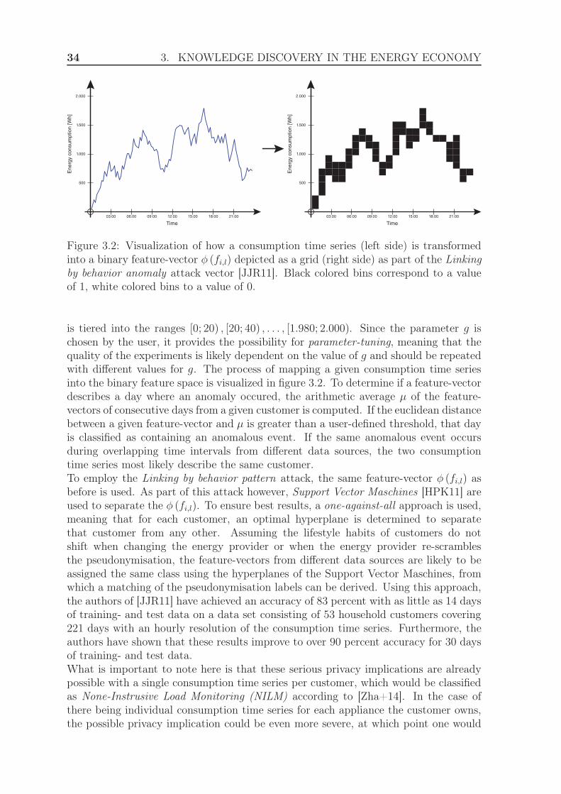
34 3. KNOWLEDGE DISCOVERY IN THE ENERGY ECONOMY
2.000
03:00 06:00 09:00 12:00 15:00
500
18:00 21:00
1.500
1.000
2.000
03:00 06:00 09:00 12:00 15:00
500
18:00 21:00
1.500
1.000
Time
En
erg
y c
on
su
mp
tio
n [
Wh
]
Time
En
erg
y c
on
su
mp
tio
n [
Wh
]
Figure 3.2: Visualization of how a consumption time series (left side) is transformedinto a binary feature-vector φ (fi,l) depicted as a grid (right side) as part of the Linkingby behavior anomaly attack vector [JJR11]. Black colored bins correspond to a valueof 1, white colored bins to a value of 0.
is tiered into the ranges [0; 20) , [20; 40) , . . . , [1.980; 2.000). Since the parameter g ischosen by the user, it provides the possibility for parameter-tuning, meaning that thequality of the experiments is likely dependent on the value of g and should be repeatedwith different values for g. The process of mapping a given consumption time seriesinto the binary feature space is visualized in figure 3.2. To determine if a feature-vectordescribes a day where an anomaly occured, the arithmetic average µ of the feature-vectors of consecutive days from a given customer is computed. If the euclidean distancebetween a given feature-vector and µ is greater than a user-defined threshold, that dayis classified as containing an anomalous event. If the same anomalous event occursduring overlapping time intervals from different data sources, the two consumptiontime series most likely describe the same customer.To employ the Linking by behavior pattern attack, the same feature-vector φ (fi,l) asbefore is used. As part of this attack however, Support Vector Maschines [HPK11] areused to separate the φ (fi,l). To ensure best results, a one-against-all approach is used,meaning that for each customer, an optimal hyperplane is determined to separatethat customer from any other. Assuming the lifestyle habits of customers do notshift when changing the energy provider or when the energy provider re-scramblesthe pseudonymisation, the feature-vectors from different data sources are likely to beassigned the same class using the hyperplanes of the Support Vector Maschines, fromwhich a matching of the pseudonymisation labels can be derived. Using this approach,the authors of [JJR11] have achieved an accuracy of 83 percent with as little as 14 daysof training- and test data on a data set consisting of 53 household customers covering221 days with an hourly resolution of the consumption time series. Furthermore, theauthors have shown that these results improve to over 90 percent accuracy for 30 daysof training- and test data.What is important to note here is that these serious privacy implications are alreadypossible with a single consumption time series per customer, which would be classifiedas None-Instrusive Load Monitoring (NILM) according to [Zha+14]. In the case ofthere being individual consumption time series for each appliance the customer owns,the possible privacy implication could be even more severe, at which point one would

3.1. IMPACT ON CONSUMERS 35
refer to this practice as Instrusive Load Monitoring (ILM).
3.1.2.2 Differential privacy in a Smart Metering environment
Overall, even though the dataset used by the experiments in section 3.1.2.1 is relativelysmall, it shows how privacy-invasive KDD-techniques can be and thus how importantcompliance with data protection guidelines is to maintain customer trust. Possibleways to make unauthorized de-pseudonymisation more difficult for an attacker is todrastically lower the resolution of the consumption time series, for example by onlystoring one measurement per day, or to re-scramble the labels much more frequently.Other possibilities to preserve consumer privacy include methods to smooth out theconsumption time series or to mask the consumption pattern with noise in order tominimize the amount of meaningful information that can be extracted from the data,for example by employing Battery-based Load Hiding (BLH), which is sometimes alsocalled Load Signature Moderator (LSM) [Zha+14]. In this scenario, the consumerdecides to install a battery at home to act as a buffer between the actual energyconsumption caused by household peripherals and the consumption time series recordedby the electricity meter. The basic idea here is that since the battery does not alterthe total amount of energy consumed, it does not hamper the ability of the energyprovider regarding billing purposes. It is however able to charge and discharge inorder to mask sensitive consumption behavior, restricted only by physical limitationsgiven by the chemistry of the battery. This chemistry of the battery determines themaximum amount of privacy it can provide, given by its maximum capacity as wellas its maximum charge and discharge rate. To accomplish its task, the battery mayprovide the user the option of several strategies to hide the consumption behavior.These strategies determine what the battery aims the consumption time series to looklike "to the outside world" and how it may behave when the battery charge approachesits maximum or minimum.One such strategy is what the authors of [Zha+14] have called the Best Effort strategy.Here, the battery produces artificial load peaks (by charging the battery) when theactual demand is low in order to discharge and thus mask or mitigate actual peak loadscaused by peripherals of the consumer. In essence, the Best Effort strategy correspondsto a low-pass filter, where the battery tries to maintain the externally visible load asbeing constant as much as possible. However, since the battery comes with physicallimitations such as a maximum capacity and maximum charge or discharge rate, usagepatterns that push the battery to its limits will cause the externally visible load toonce again contain private information. Overall, the authors of [Zha+14] have shownthat the Best Effort strategy does not provide differential privacy [Dwo06].Differential privacy or more specifically ǫ-differential privacy [Dwo06] is a statisticalconcept that measures the amount of private information that is exposed if a databaseis asked a given query. To ensure the disclosed information about a private individualdoes not exceed a user-defined threshold, random noise is added to the result of queries.The amount of noise added depends on the selectivity of the query. As a rule of thumb,the more specific a query is, the more noise needs to be added to retain the desiredminimum privacy for all individuals in the database. More formally, given two datasetD1 and D2 which differ at most in one element, a randomized function K provides

36 3. KNOWLEDGE DISCOVERY IN THE ENERGY ECONOMY
ǫ-differential privacy if for all S ∈ Range (K) the following condition is met [Dwo06]:
Pr [K (D1) ∈ S] ≤ eǫ × Pr [K (D2) ∈ S] (3.1)
In simplified terms, this means the difference of the query-results that would emergeif a single piece of information about an individual was part of the dataset or not (de-noted by the hypothetical datasets D1 and D2) must remain smaller than a user-definedthreshold. This is achieved by not evaluating the query on the actual datasets D1 andD2, but on K (D1) and K (D2), which corresponds to adding noise to the datasets byapplying a randomized function K. If K is chosen carefully, this concept provides prov-able privacy in statistic queries.In order to translate this concept on the problem of preserving ǫ-differential privacy ina scenario where a Smart Metering device queries the energy consumed in regular in-tervals, the authors of [Zha+14] propose for the battery to periodically chose a randomvalue of the binomial distribution B
(
n, 12
)
− n2, where n corresponds to a sufficiently
large number, at least as large as the number of queries on the dataset, but withinthe physical limitations given by the chemistry of the battery. Following that, the bat-tery charges with a rate according to the chosen value if it is positive, or analogouslydischarges if the value is negative. Since the expected value of the aforementioned bi-nomial distribution is 0, the overall charge of the battery is expected to stay the same,meaning that the battery is able to provide this privacy measure indefinitely.Overall, the authors of [Zha+14] have presented an effective means to counteract espi-onage or profiling of customers by deliberately distorting the energy extracted from theenergy grid by the end-consumer. Since these methods are about random charging ordischarging of a battery with an expected value of 0, this distortions even themselvesout if used by a sufficiently large user base, meaning this privacy measure does nothamper the energy providers duty to maintain the stability of the energy grid. How-ever, a possible weakness of this procedure emerges if there is no consumption at allcaused by the user over a sufficiently long period, for example if the consumer has goneon holiday. In that case, depending on the strength of the battery, the noise it canprovide might be unable to mask that the average consumption has decreased by suchan amount. Because of that, the absence of the user might still be visible under somecircumstances, which constitutes some valuable information for burglars.
3.1.2.3 Data reduction and data economy
Another approach for privacy is presented in [MRT12]. Here, the authors debatewhether the data can remain mostly local while still providing the benefits of havingSmart Metering devices installed, eliminating the need for anonymization in the firstplace. For this purpose, several applications of Smart Metering data are discussed,which we will present hereafter.The primary application of the energy provider, where having access to Smart Meteringdata of consumers is a technical necessity, is improving load balancing and the buy-inof energy from the energy producers. One way of improving the buy-in of energy usingSmart Metering data is by analyzing the data to build load profiles (see section 2.3),for example by performing the experiments we present in chapter 4 and 5. In essence,the authors of [MRT12] argue that while this utilization of the data is ultimately le-gitimate, with the benefits outweighing the data privacy concerns, it might suffice to
3.1. IMPACT ON CONSUMERS 37
be content with just using anonymized consumption time series gathered on an en-tirely voluntary basis. Among satisfied customers, this would simplify legal questionsif energy providers plan to engage the services of cloud providers to put up with theamount of computing power required to apply KDD-techniques to these huge amountsof data.Another aspect where having high resolution consumption data available is advanta-geous is Demand Reduction. For this purpose, Smart Metering devices usually providethe end user with up-to-date consumption statistics via a build-in display, a smart-phone or web application. Using this data, users can get an idea of their consumption,identify high consumption devices and thus specifically focus on reduce their demand.Since smartphone or web applications can work within the local home network of theuser, the data does not need to be transferred into the cloud. If the Intelligent MeteringSystem does offer Remote Feedback, meaning that data processing does happen in thecloud, the protection of the user’s data privacy can consist of Remote Feedback beingentirely optional, meaning that no data is transmitted outside of the user’s home unlessthe user explicitly consents. This facet of Remote Feedback is primarily relevant if theuser is either living alone or consists of a family, where mutual trust can be assumed.However, if a building complex hosts a shared apartment or something similar, evenlocal-only feedback can give undesirable deep insights into private matters. In this sce-nario, a solution might be to allow local feedback only based on aggregated data, suchas half-hourly or hourly resolution, which limits the amount of critical information interms of data-protection law that can be extracted from such data.Lastly, the authors of [MRT12] discuss the extensive aspect of Demand Response inthe context of data privacy. Although we present this subject as the last facet ofthis chapter, it is by far the most significant. This is a consequence of the fact thatSmart Metering is considered the great hope of politics for end-consumers to voluntar-ily adjust their consumption behavior. For example, the Directive 2009/72/EC of theEuropean Parliament [Par09] describes Intelligent Metering Systems as the best possi-bility to provide energy management services and innovative pricing formulas in orderto promote energy efficiency. As a consequence, [Par09] recommends the wide-spreadroll-out of Smart Metering devices so that they shall assist the active participation ofconsumers in the electricity supply market. Notably, the active participation of con-sumers raises the question of which data must necessarily be made available publiclyto the market for this purpose and what the benefits for the consumers are. One of themost relevant aspects for consumers are price advantages. Here, the likely most sim-ple, but also most privacy-unfriendly approach would be to transmit the consumptiontime series in its highest available resolution to the energy provider. Subsequently, theenergy provider could apply Time-Of-Use Pricing (TOU), meaning that the energyprice is not constant, but rather dynamically calculated based on customer-specificagreements, the total load of the energy grid, the time of the day and possibly otherfactors. This scenario is consistent with the European Commission Recommendation2012/148/EU [Com12], which describes remote reading of meters as a key function-ality and advocates the support for advanced tariff systems. A more privacy-friendlyapproach to dynamically handle different tariffs consists of the Intelligent MeteringSystem managing separate meters for each tariff. In this case, capable Intelligent Me-tering Systems require only the time intervals describing which tariff is valid at a giventime to be told by the energy provider. At the end of the accounting period, only

38 3. KNOWLEDGE DISCOVERY IN THE ENERGY ECONOMY
the cumulative total consumptions readings per tariffs need to be submitted to theenergy provider. Additionally, if the Intelligent Metering Systems is able to processdynamic pricing tables published by energy provider, invoicing can be done completelylocal from a technical standpoint. In this last case, privacy concerns can be avoidedcompletely as the energy provider only learns about the total invoice amount. Thisconcept of keeping data local also corresponds to the suggestion of [JJR11] to preventde-pseudonymisation as much as possible.
3.1.3 Photovoltaic systems
In 2014, the European Commission has stated that at least 27 percent of the energyconsumed should be produced by renewable energy sources by the year 2030 [Com14].This strong commitment towards renewable energies can also be considered as a signalfor investors as it has been feared that investments would level off through 2020 if notstimulated and backed up by corresponding long-term policies [Age14]. Due to techno-logical advances in an effort to make solar power plants more economically sustainable,the price of energy produced by photovoltaic systems continues to decrease: in 2018,a tender for a 300 megawatts solar power plant was won in Saudi Arabia at a price of0,0234 US-Dollars per kWh [WS18]. Even though this project corresponds to a rolloutat a rather large scale, a photovoltaic system can also be economically reasonable fora home consumer without the user being aware of that fact. Because general energyprices are expected to increase over time due to the growing scarceness of fossil fuels,it becomes increasingly important for consumers to have the benefits of photovoltaicsystems presented to them. This amplifies the incentive of end-consumers to considerto invest in photovoltaic systems even today. However, one huge challenge for the wide-spread adoption of photovoltaic systems is that the economic potential differs greatlyper customer, which greatly hampers the consumers ability of making an informedchoice. This is, among others factors, because of the different east-west orientationof the roofs, foreground objects casting shadows on the roof, roof inclination and rooftype. Since the factors are often unknown to private individuals, the assessment ofeconomic feasibility often requires a costly on-site meeting with a professional.
To avoid having to perform large-scale, yet detailed assessments for accurate simula-tions, some approaches settle with using commonly available statistics like typical sizesof buildings, population density or gross domestic product to evaluate the economicfeasibility of photovoltaic systems [Löd+10], while other methods include using smallrandom samples which are then extrapolated to the size of whole regions [Ord+10].While these approaches are useful for politics and investors to get a rough idea whichcountries or regions of countries to subsidize or invest in, it is of little help for individ-ual home consumers to decide whether or not the installation of photovoltaic systemsis reasonable for them.
In order to overcome this difficulty, research has started to include freely availablegeospatial information systems, also referred to as Volunteered Geographic Information(VGI), as a source of data. In [Hop+17], the authors make use of these services,especially OpenStreetMap, to build a Data Mining based decision support system tohelp predict the solar energy potential of customers. The idea here is to resolve theaddress of a customer into coordinates using OpenStreetMap and then to derive thefloor area AF by choosing the nearest building polygon for the address coordinates. By

3.2. IMPACT ON THE ELECTRICITY GRID 39
assuming a gabled roof with an inclination angle of α = 35◦ for all homes, which is themost common roof type according to the authors, the usable area Ac for photovoltaicsystems can be calculated as:
Ac =1
2·
AF
cos (α)(3.2)
In conjunction with the roof orientation angle β, which can be derived using the ori-entation of the polygons from OpenStreetMap, as well as historical solar radiationand temperature data, an estimate for the solar energy potential can be given. Theimplementation of these semantics can be simplified using purpose-built software li-braries such as solaR [Lam12], a framework written in the statistical programminglanguage R to perform calculations involving photovoltaic energy, sun geometry andsolar radiation.
While the procedure outlined above is a good approach for end-consumers to get afirst impression about their solar energy potential, it is noteworthy that the estimateis highly dependent on the accuracy of the geospatial data used. Furthermore, theapproach does not take into consideration that only parts of the roof may be usabledue to roof windows, chimneys, antennas or foreground obstacles casting shadows.In this regard, computer ray-tracing simulations in 3 urban sites in Switzerland haveshown that the average usable area of the roofs for photovoltaic systems is rangingfrom 49 to 95 percent [WNP10]. In addition, evaluations of this OpenStreetMap-based approach with validation data in 3 German cities have shown that the averagedeviation in estimating the usable roof area is −9,6m2 for private households, meaningthat the OpenStreetMap-based approach tends to underestimate the usable area. Withthe absolute deviation for gabled roofs being 20,14m2, this corresponds to an averageprediction error of 27 percent. However, since this approach assumes gabled roofs withan inclination angle of α = 35◦ for all buildings, the estimation error is much higherfor non-gabled roofs. Overall, the OpenStreetMap-based approach achieves an averageestimation error of 55,15 percent when considering all roof types of private homes.
In conclusion, the main strength of this approach lies in the fact that VGI-data iswidely available in contrast to more accurate cartographic material, however cautionshould be exercised when estimating the photovoltaic potential of an end-consumerwhose roof type is unknown. If more accurate Geographical Information System (GIS)data is available, errors in the rooftop estimation of approximately 15 percent canbe achieved [WNP10]. With that said, due to the wide availability of VGI-data, theOpenStreetMap-based approach presented in this section poses a means of a quick andapproximative preselection, for example to identify regions where more precise, butalso more expensive, measurements might be profitable.
3.2 Impact on the electricity grid
Due to the growing digitization within the energy economy, changes to the way energyis delivered to consumers have become mandatory in order to accommodate the plansfor the installation of Intelligent Metering Systems as a consequence thereof. Thesechanges to the electricity grid are described by the umbrella term Smart Grid. Theterm Smart Grid was first characterized by the US Energy Independence and SecurityAct of 2007 [Con07], which lists the following requirements for Smart Grids:

40 3. KNOWLEDGE DISCOVERY IN THE ENERGY ECONOMY
1. Increased use of digital information and controls technology to improve reliability,security and efficiency of the electric grid
2. Dynamic optimization of grid operations and resources with full cyber-security
3. Deployment and integration of distributed resources and generation, includingrenewable resources
4. Development and incorporation of demand response, demand-side resources andenergy-efficiency resources
5. Deployment of smart technologies (real-time, automated, interactive technologiesthat optimize the physical operation of appliances and consumer devices) for me-tering, communications concerning grid operations and status, and distributionautomation
6. Integration of smart appliances and consumer devices
7. Deployment and integration of advanced electricity storage and peak-shavingtechnologies, including plug-in electric and hybrid electric vehicles, and thermal-storage air conditioning
8. Provision to consumers of timely information and control options
9. Development of standards for communication and interoperability of appliancesand equipment connected to the electric grid, including the infrastructure servingthe grid
10. Identification and lowering of unreasonable or unnecessary barriers to adoptionof smart grid technologies, practices and services
The implementation of these properties requires a transformation of the electricity gridwith profound effects on the way energy is produced, traded, distributed and measured.An overview of these changes has been given in figure 1.1 in section 1.1 of this thesis.The way of how the concept of a Smart Grid will transform the energy supply andforce energy providers, which to date have had next to nothing to do in terms of BigData, to rethink their business practices, is part of active research. Among other topics,current research is concerned with processing huge amount of data in the cloud, loadclassification and short-term load forecasting with respect to security policies [DKK15]as well as means to predict technical failures [RW+12].
One of the main advantages of the digitization of the electricity grid is that itallows for technologies that can not be facilitated in a conventional electricity grid.An example for this are electric cars : current electric cars have batteries ranging incapacity from 16 to 53 kWh and consume as much as 7 to 10 kWh of energy to drive adistance of 50 to 65 kilometers. In order to charge these cars in a reasonable amount oftime, for example between 3 and 4 hours, electric outlets from 6,6 to 16 kW of powerare required [IA09]. However, this means that when an end-consumer charges his orher electric car, the overall energy consumption of that customer more than doubles forthe duration the car is charging [IA09]. Depending on the distance a given customerhas driven during the day, this can cause high peak amounts of energy to be needed tobe injected into the electricity grid in order to ensure the stability of the energy supply.

3.2. IMPACT ON THE ELECTRICITY GRID 41
On a larger scale, this can lead to problems when the electricity grid is not designedto handle the use-case of a significant proportion of customers switching to electriccars [IA09; Wüs17b; Wüs17a], providing the necessity of practical solutions to enableelectric cars and other high-power household appliances to use energy in a staggeredmanner.
One inconvenient property of customer behavior for energy providers is when theconsumption occurs in bursts in contrast to a more steady load. This is due to the factthat high peaks of energy load, such as the load generated by charging electric cars,are generally difficult to predict accurately and thus can not be properly accountedfor when energy providers are planning their future buy-in of energy, instead requiringcost-intensive real-time adjustments as soon as a peak load becomes apparent. Theseadjustments typically are executed by using imbalance energy, which we have intro-duced in more detail in section 2.2. Due to the financial risk imbalance energy poses,energy providers generally aim to smooth out the overall load on the electricity gridas much as possible. One way to quantize how abrupt the short-term adjustmentsneed to be is to compute the Peak-To-Average Ratio (PAR) which [Moh+10] definedas follows:
PAR =Lpeak
Lavg
=H ·maxh∈H Lh
∑
h∈H Lh
=H ·maxh∈H
∑
i∈N lhi∑
h∈H
∑
i∈N lhi(3.3)
Here, N corresponds to the total number of customers and lhi describes the amountof energy the i-th customer has consumed at the time h ∈ H , {1, . . . , H}. Sincethe PAR is computed per day, the value for H is equal to 24 in case the energy timeseries have an hourly resolution. The smaller the value of PAR, the more uniform theconsumption can be characterized.
With the development of the Smart Grid, several technologies have emerged inorder to alter the overall shape of the consumption time series:
• Demand-Side Management (DSM): This term describes any model whichincentivizes the consumer to become more energy efficient in the long term, forexample by lighting retrofits, building automation upgrades, re-commissioning,improvements to Heating, Ventilation and Air Conditioning (HVAC), variablefrequency drives, etc [Alg+15], as well as other measures to reduce the Peak-To-Average Ratio without introducing external causes such as dynamic pricingmodels.
• Demand Response (DR): This term covers any models to encourage the enduser to make short-term adjustments in his or her energy demand. This is typ-ically achieved by creating financial incentives in the form of dynamic, but pre-determined pricing models, for example by offering more attractive prices duringtimes where the overall energy consumption is low and more expensive prices dur-ing peak load times. This latter model is sometimes referred to as Time-Of-UsePricing (TOU) [WL11; Str08; AE08].
• Direct Load Control (DLC): This term describes a subcategory of DemandResponse, in which the reaction to dynamic tariffs including the control of someelectronic appliances, for example the act of turning them off or on, is carried outdirectly by the energy provider. The degree to which energy providers assumecontrol over the devices is negotiated with the customer beforehand [Alg+15].

42 3. KNOWLEDGE DISCOVERY IN THE ENERGY ECONOMY
DLC is most frequently applied in conjunction with air conditioning systems andthermal heat pumps [AE08]. While DLC is a simple and cost-effective meansfor energy providers to shape the overall energy load of large institutions, wherethe consumption behavior is primarily dictated by the business practices, end-consumers might reject this patronization as being privacy-invasive and intrusive[RV08].
The application of these models have been tried in pilot projects over the last years.For example, in the USA, Demand Response using dynamic pricing models have beendeployed [SL07], more specifically Real-Time Pricing (RTP) and Critical-Peak Pricing(CPP), which are variations of the more general Time-Of-Use Pricing (TOU) [WL11].However, in order not to lose large industrial customers, these models where offeredon a voluntary basis. As [SL07] mentions, the primary motivation to roll out dynamicpricing models have been customer retention for enterprises seeking a way to optimizetheir electricity bill; peak management was of far lesser importance to energy providers.The success and amount of savings for customers through dynamic pricing models, suchas RTP or CPP, strongly depend on the elasticity of demand of the customer. In [SL07],the authors describe an elasticity of −0,2 as meaning that a price increase of 10 percentwill cause the customer to reduce his energy demand by 2 percent. Participants optingfor RTP with an elasticity of −0,1 have achieved a reduction in their invoicing amountof between 3,51 and 6,52 percent, with the overall peak power being lowered by between14,0 and 24,5 percent [SL07].A similar success could be observed in the case-study of a library [Alg+15], where themanagers of the library and the energy provider agreed upon deploying Direct LoadControl. In exchange for direct or short-term control of Heating, Ventilation and AirConditioning equipment, the energy provider has agreed on a price discount in theamount of 3 e per MWh. This method caused the amount of energy consumed to bereduced by 4 percent as well as financial savings of 7 percent annually.
Another way for customers to increase their elasticity of demand is by installing abattery to buffer energy locally. In section 3.1.2.2, we have introduced this concept asBattery-based Load Hiding (BLH) to help protect user privacy. In this case however,the basic idea is for the battery to charge during low-price time slots and to dischargewhen energy prices are high. This process could possibly be automated by equippingthe batteries with a network interface, analogous to Intelligent Metering Systems (seesection 3.1), which could enable the battery to query current prices. Subsequently,it would be possible for the battery to autonomously learn to classify prices as low,average and high by computing the average price over a sufficiently long time period,thus decide on its own when to charge and when to discharge. Alternatively, thecharging and discharging of the battery of the customer could be executed by theenergy provider as part of Direct Load Control. In this case, the user participates inthe energy market as a supplier for imbalance energy and would be entitled to claim afinancial compensation from the energy provider depending on the amount of batterycapacity allocated. Using this technology, the end user could automatically benefit fromfluctuating prices and thus amortize the acquisition cost of the battery without anycompromises in lifestyle habits. Depending on the functionality the battery providesand the demand of the customer, an optimal balance for the end user between a financialgain by utilization of dynamic pricing models and means to protect user privacy, suchas the ones presented in section 3.1.2, is arrangeable.

3.2. IMPACT ON THE ELECTRICITY GRID 43
Further research has been conducted on Intelligent Load Management using coolingsystems and refrigeration plants [GP11]. The idea here is to suspend or lower coolingactivities from time to time and to play on thermal inertia to prevent defrosting ofchilled goods. By also taking Demand-Side Management into account, cooling systemscan be used to supply imbalance energy, albeit to a lesser extend.However, using the example of the Model City Mannheim from 2013 [And13], it hasbeen revealed that large, industrial consumers are missing the necessary communica-tions infrastructure between refrigeration plants and control instances to participatein an intelligent, decentralized Smart Grid. Instead, a unidirectional communicationof price data from the energy provider to the customer has taken place, with the cus-tomer manually deciding on which measures to adopt. Overall, this likely results inindustrial customers, which store chilled goods and thus are liable to strict legal tem-perature policies, to deem such measures as being especially risky and intrusive fortheir core business. One of the main reasons for this is that decision makers often lackthe necessary experience to give a sufficiently accurate estimation for the cost-benefitratio.
To counteract the intrusive aspect of Direct Load Control mentioned above, tech-nologies have emerged that offer specifying a declarative objective, but the means tooptimize that objective is automated. For that purpose, techniques like Dynamic Pro-gramming [RV08] and Binary Particle Swarm Optimization [PSM09] can be used. Oneexample for specifying a declarative objective is when a customer configures a targetroom temperature for the air conditioner, as well as an allowed deviation from saidtarget temperature, but leaves the actual implementation to the devices as part ofhome automation. In that case these devices may semi-autonomously carry out theirassigned task with intervention from the energy provider being limited to the usagerestrictions as given by the temperature deviation tolerated by the customer.However, in order for Demand-Side Management to work in a home automation en-vironment, agreements between smart home devices or energy providers have to takeplace to some extend. If smart home devices such as air conditioners were to act fullyautonomous, the main basis of decisionmaking for when to start or stop heating orcooling is the current room temperature. This leads to an event what the authorsof [RV08] have called the cold load pickup phenomenon. This anomaly occurs if thedevices cause a sudden surge in energy consumption when they turn themselves onafter they have been turned off for a while. In general, if no coordination betweendevices takes place, this phenomenon could cause huge energy load peaks, which is theopposite of what Demand-Side Management methods are trying to achieve. One so-lution for this problem involves Dynamic Programming, meaning that air conditioningdevices are being turned on and off in a cyclic and staggered manner, so that the overallenergy consumption stays constant or increases / decreases as uniformly as possible,while at the same time preferring devices being turned on where the difference betweenthe target and actual temperature is greatest [RV08].In addition to the agreements between devices mentioned above by smart home equip-ment explicitly communicating with the devices of the customer’s neighbors, the Intel-ligent Metering Systems could be designed to allow for measuring voltage fluctuationsin addition to the energy consumption [MRT12]. From the point of view of an energyprovider, keeping the electricity grid balanced is of utmost importance. With localvoltage readings known, this allows for quick and precise diagnoses of potential prob-

44 3. KNOWLEDGE DISCOVERY IN THE ENERGY ECONOMY
Prices
Load
Prices
Load
Price
s
Load
Price
s
Load
Price
sLoad
Price
sLoad
(a)
PricesDesired
Aggregate Load
(b)
Figure 3.3: Overview of Demand-Side Management strategies focusing on (a) individualinteractions between the energy provider and each customer and (b) the Smart Gridwith enabled communication between the customers and the energy provider. Adaptedfrom [Moh+10] with some assets taken from [Wik].
lems, which ultimately helps in reducing customer complaints and minimizing customerminutes lost. In addition, knowing local voltage readings enables the energy providerto identify problem areas, meaning areas where consumption shaping measures such asDirect Load Control most urgently need to be taken. At the same time, since voltagemeasurements at the house connection are region-specific, not customer-specific, andthus do not allow to deduce private activities of the consumer, no privacy protectionmeasures such as the ones presented in section 3.1.2 need to be put in place.
Another way for the consumer to specify a declarative intent for smart home devicesto implement is an Energy Consumption Scheduler (ECS) [Moh+10]. The idea hereis that, for the example of electric vehicles, most customers are indifferent to whenexactly the car is being charged, as long as it is sufficiently charged the next time itis needed. Thus, ECS allows for the consumer to specify a time interval for when thevehicle can be charged; the actual charging time can then either be dictated by theenergy provider or agreed upon by neighboring smart home devices so that charginghappens in a staggered manner with the goal for the energy provider being to avoidproblematic peak loads and for the end-consumer to benefit from financial incentivesdue to Demand Response programs. This idea is not limited to electric vehicles, but canalso be extended to include other high-power household appliances such as intelligentwashing machines and dishwashers [And13].
Overall, assuming the necessary communication infrastructure for both consumersand energy providers is in place, DSM programs are commonly employed using one oftwo strategies, which are illustrated in figure 3.3. The topology in figure 3.3 (a) is morecommonly used in RTP programs, but also puts more stress on the energy provideras the provider has to individually communicate with each customer [Moh+10]. Incontrast, the topology in figure 3.3 (b) frees the energy provider of almost all coordi-nation efforts and instead allows the provider to focus on giving financial incentivesto shape the aggregated energy load to more directly impact the PAR introduced inequation 3.3. Although the scenario in figure 3.3 (b) requires some interactions be-tween smart home devices of the customer, these interactions can be automated using

3.2. IMPACT ON THE ELECTRICITY GRID 45
bidirectional digital communication.In order for a set of customers to reach an agreement using a decentralized topologysuch as in figure 3.3 (b), a distributed mechanism based on game-theory is proposedin [Moh+10]. Here, as a preliminary step, the ECS distinguishes between shiftable andnon-shiftable household appliances. Shiftable appliances, such as electric vehicles ordishwashers, allow for flexible scheduling of their energy consumption, in contrast tonon-shiftable appliances, such as refrigerators or lights, of which the user expects tobe switched on permanently or on-demand. By knowing which devices are shiftable,as well as their required energy and the scheduling interval that the customer toleratesfor each device, it is possible for an Intelligent Metering System to derive a set of con-sumption scheduling plans Xi for all connected household appliances.Finally, the goal for the Intelligent Metering System is to minimize the PAR usingthe best scheduling plan among the set of feasible consumption scheduling plans it hascalculated earlier. The best schedule xi ∈ Xi for a given customer then corresponds tothe solution for the following optimization problem:
minimizexi∈Xi
=
H∑
h=1
Ch ·
xhi +
∑
i′∈N\{i}
lhi′
(3.4)
Here, xi corresponds to a scheduling plan from the set of all possible consumptionscheduling plans Xi for the i-th customer, with xh
i describing the scheduled consumptionat the time h. Furthermore, Ch describes the cost function announced by the energyprovider, meaning the price per energy unit, which is assumed to be only dependenton the total amount of energy the energy provider has to ingest into the electricitygrid. Lastly,
∑
i′∈N\{i} lhi′ describes the sum of the announced energy schedules by all
consumer other than the i-th customer.Since the optimization problem 3.4 only contains local variables of a given customer,its solution can be locally computed by the Intelligent Metering System. As shown in[Moh+10], the solution for the optimization problem 3.4 exists and is unique assumingthat Ch is monotone increasing and strictly convex. In that case, the solution to theoptimization problem 3.4 corresponds to the most cost-effective scheduling plan for agiven customer and at the same time forms a Nash equilibrium with the most cost-effective scheduling plans of the other customers, where no customer benefits if theydeviate from their best schedule or provide inaccurate information to mislead otherconsumers.While the strategy presented in [Moh+10] is an interesting approach to incentivizecollaboration of intelligent appliances in a Smart Grid environment in a decentralizedway, relieving energy providers in the process, its main disadvantage is that it requiresall xh
i to be predictable accurately and the lhi of all customers to be known by all othercustomers in order to compute
∑
i′∈N\{i} lhi′ , giving rise to valid concerns with respect
to privacy. While the authors of [Moh+10] argue that announcing lhi publicly does notdisclose details about the energy consumption, this is not the case, as we have discussedin section 3.1.2 of this thesis. One possible solution for this problem is a hybrid of bothtopologies depicted in figure 3.3, where all customers send their preferred xh
i as lhi to theenergy provider using an encrypted communication channel; the energy provider thenaggregates all energy schedules by computing
∑
i∈N lhi , which is then broadcasted toall consumers. Each customer can then individually solve his or her own optimization
46 3. KNOWLEDGE DISCOVERY IN THE ENERGY ECONOMY
problem 3.4 by computing:
∑
i′∈N\{i}
lhi′ = −xhi +
∑
i∈N
lhi (3.5)
Since xhi is known only by the i-th customer and the energy provider, no other customer
i′ ∈ N \ {i} is able to derive lhi from the broadcast of the energy provider. While thissolution centralizes the problem to some degree and necessitates the energy providerto be a trusted party with regard to privacy, its role would be limited to aggregatingthe individual lhi and broadcasting the result, which still requires less effort from theenergy provider than a fully centralized topology.
3.3 Impact on energy providers
The primary ways for energy providers to improve are by achieving a higher predictabil-ity for their buy-in of energy as well as lowering costs for electricity grid infrastructure.The first aspect can be accomplished by gaining a better understanding of customerneeds or by optimizing existing internal processes. In addition, new technologies suchas Smart Metering enable shaping of the consumption behavior using techniques likeDirect Load Control as introduced in section 3.2, which allows for shifting energy con-sumption into periods of lower demand, thus making it possible for the electricity gridto not be designed for maximum load at all times, ultimately lowering infrastructurecosts. At the same time, legal obligations and requirements of the energy market, suchas the ones presented in chapter 2, must be kept in mind. Over the course of thissection, we will introduce some of the most important goals of energy providers as wellas discuss typical strategies from academic literature on how to achieve these goals.
3.3.1 Extraction of customer insight
One way for energy provider to gain information about customers aside from contrac-tual data consists of conducting customer surveys, in addition to employing a CustomerEngagement Portal. This often is a central part of marketing strategies to better under-stand customer requirements which in turn enables the energy provider to adjust tariffoffers and internal processes accordingly. In order to yield a representative statistic ofthe whole customer basis, in most cases it is necessary for the energy provider to incen-tivize participation in these surveys. Such incentives to increase participation mightbe discounts for upcoming billing cycles or perks in cooperation with other companies.
However, even when survey participation is incentivized, it is very rare for the ma-jority, let alone the entirety, of customers to partake. Thus, businesses usually seekways to deduce information on customers who have not partaken in surveys by extrap-olating insight gained from users who have voluntarily provided their information. Oneway to apply this approach on customers of energy providers is presented in [HSK16].The idea here is to use supervised machine learning to build a model for householdcharacteristics from survey data. As a data basis, the authors have used data of 3.986customers of an energy provider in Switzerland who have voluntarily entered their datain a Customer Engagement Portal. In total, said energy provider delivers electricityto 10.482 customers, meaning that the overall participation rate is approximately 38

3.3. IMPACT ON ENERGY PROVIDERS 47
percent. Among the features that have been gathered as part of the survey to trainthe model are the following [HSK16]:
• Household Type: A categorical attribute which describes whether the customerlives in a house or an apartment.
• Living Area: An attribute which corresponds to the living area of the customer.In the dataset, the living area of the customers cover a range from 10m2 to5.443m2. Although the living area of customers is given in the dataset as anumerical attribute, the authors have converted it into a categorical attribute bydefining the ranges 0m2−95m2, 95m2−145m2 and 145m2− inf as class borders,which are motivated on 33 percent and 66 percent quartiles.
• Number Of Residents: An attribute which describes the number of peopleliving in the corresponding house or apartment. Similar to the feature-attributeLiving Area, this attribute has been converted to a categorical attribute by defin-ing a set of ranges to serve as class borders. During their research, the authorshave experimented with multiple set of ranges. Overall, the class border ranges1, 2, 3− 5 and > 5 have yielded the best results.
• Logarithmic Average Daily Consumption: This numerical attribute corre-sponds to the logarithmic value of the ratio of the total amount of energy con-sumed divided by the number of days where energy consumption took place. Thelogarithmic transformation is applied to achieve a more symmetric distributionof this attribute in the dataset.
• Relative Consumption Trend: This attribute corresponds to the linear re-gression of the customers consumption over the last 4 years.
• Z-Score In Neighborhood: An attribute which describes the Z-Score of thecustomer’s attribute Logarithmic Average Daily Consumption within the cus-tomer’s neighborhood. The Z-Score corresponds to the number of standard devi-ations of a data tuple xi from the expected value of the distribution. The Z-Scoreis calculated as follows: zi =
xi−xσ
In addition to the features described above, the authors of [HSK16] have used 66 ge-ographical features derived from Volunteered Geographic Information (VGI) sources,namely OpenStreetMap and GeoNames.org, such as the distance of the home of thecustomer to the nearest city center with up to 1.000, 5.000 or 15.000 inhabitants. Toincrease the accuracy of the model, some of the attributes have been pruned usingcorrelation-based feature selection [Hal99] to reduce the number of dimensions. Thebasic idea of correlation-based feature selection is that an attribute is useful for amodel if and only if that feature is predictive of or correlates with the class, but thefeatures themselves are uncorrelated among each other.With this setup, the best results have been achieved using Random Forest classification[Bre01], followed up closely by Support Vector Maschines [HPK11], using 5-fold crossvalidation [Sto74]. In simplified terms, Random Forest classification works by indepen-dently generating random decision trees with weak correlation and then employing amajority vote on a per-feature-vector basis to assign the class which the feature-vectorgot most often classified to by the generated decision trees. By including VGI sources
48 3. KNOWLEDGE DISCOVERY IN THE ENERGY ECONOMY
for the evaluation, the authors achieved accuracies from 49,4 and 68,7 percent. Formost business cases of energy providers, this accuracies are good enough to then justifytargeted marketing campaigns for personalized tariff offerings. If VGI data is left outor not available, the accuracy of the feature Household Type drops by 12,7 percent andthe accuracy of Living Area drops by 7,0 percent.
3.3.2 Installation of intelligent metering systems
One of the major upcoming technical advancements in the energy economy are SmartMetering devices, which enable fine-grained measurements of the energy consumptionas well as corresponding data processing and transmission. In previous sections ofthis chapter as well as figure 1.1 in section 1.1, we have outlined the most importantchanges brought by Smart Metering technology. With historical consumption timeseries for each customer of the energy provider present, this allows for the employmentof time series analysis or other appropriate techniques to help classify a customer orto find reoccurring patterns in the data, but also to assess the influence of plants forthe production of renewable energy such as photovoltaic systems (see section 3.1.3).The latter is particularly important since photovoltaic systems make the customer apartially self supporter, this causes deviations between the expected consumption bythe energy provider, for which the energy provider has prepared for, and the actualconsumption of the customer (see section 2.2).
Due to the fact that the data gathered by Intelligent Metering Systems and possi-bly other smart home devices are progressively complex and vast, technologies whichallow for the extraction of useful knowledge from such data are becoming increasinglysignificant. Such useful knowledge can include models which allow for a more accurateprediction of the upcoming energy consumption of a customer, thus helping the energyprovider to manage the tasks outlined in section 2.2, but also ways to help identify tar-get audiences for which custom tariff offers might be financially attractive while stillcovering their use-cases as good as possible. Over the course of the following sections,we will introduce some approaches from academic literature to help achieve this goal.
3.3.2.1 Prediction of household properties
The main motivation of energy providers for seeking to know certain properties of theircustomers is that it allows for targeted ad campaigns and custom tariff offerings, whichcustomers might deem more relevant for their use-cases. Very often, the underlyingdata for such analyses is gathered by executing expensive customers surveys as we havediscussed in section 3.3.1. Due to the emerging Smart Metering technology however,customer properties can also be extracted by examining customer behavior patternsfrom energy consumption time series. Since time series data is fundamentally differentfrom survey data, which is often in the form of multiple-choice questions, the datarequires a different approach to be processed expediently.
One approach to segment private households is presented in [VVS16], which is spe-cial in that it uses the CER-Dataset [CER] for analysis, as it consists of both SmartMetering time series as well as survey data for most of the corresponding households.Using this dataset, the approach focuses on Data Mining techniques by classifying thecustomers using features derived from the Smart Metering time series, while using the

3.3. IMPACT ON ENERGY PROVIDERS 49
survey data as Ground Truth to assess the results for households not part of the train-ing data. To train a classification model, [VVS16] relies on Support Vector Maschines[HPK11] while employing 10-fold cross validation [Sto74] using features such as theratio of the average daily consumption compared to the daily maximum consumption orratio of the daily minimum consumption compared to the daily maximum consumptionto assign classes to the households in the categories income (high or low), education(superior or non-superior) and children (present or not present). Using this setup, theauthors of [VVS16] have achieved accuracies of 63 percent for the category income,63 percent for education and 69 percent for children. When assessing the quality ofthese results, it is important to recall that the categories in the experiments are bi-nary, meaning that accuracies from 63 to 69 percent pose only marginal to moderateimprovements compared to random guessing.A similar approach is presented in [Hop+16]. Like [VVS16], the authors aim to pre-dict properties of private households using classification techniques on Smart Meteringdata, specifically the CER-Dataset [CER]. In addition to [VVS16] however, whichonly uses 8 features for their method, [Hop+16] defines a total of 88 features andemploys feature-selection methods, such as correlation-based feature selection [Hal99]and Kolmogorov-Smirnov Test based feature selection [Lop11], to prune redundant andunnecessary features. Within the scope of the experiments in [Hop+16], the authorshave noted that including feature-selection methods improves classification accuracy byapproximately 8 percent. A much smaller influence on classification accuracy has beenthe choice of the classification algorithm itself, with Support Vector Machines [HPK11]yielding an on average only 2 percent higher accuracy than k-Nearest-Neighbor [ES00;HPK11], which has been the other classification algorithm tested. Overall, the averageclassification accuracy achieved using Support Vector Machines and feature-selectionmethods is approximately 60 percent, which is slightly lower than the experimentsshown in [VVS16], even though the same dataset is used. However, the main influenceon classification accuracy has been the choice of class borders, as the authors haveshown by also repeating their experiments using different definitions for said class bor-ders. For example, the experiments have yielded an accuracy of 50 percent for the classage of the house when using the definition old =̂ > 30 years and new =̂ ≤ 30 years,while yielding an accuracy of 80 percent when using the definition old =̂ > 10 yearsand new =̂ ≤ 10 years, which indicates a strong influence of the choice of class borderson the accuracy of the results. Another point of criticism is that the experiments in[Hop+16] have been conducted using only 1 week of consumption time series out of the76 weeks available from the CER-Dataset. While the authors claim that the week theyused is noise-free and without public holidays as well as average weather conditions,the assumption that this 1 week is representative for all consumers, meaning that noend-consumers are gone on holiday during this period or have other unusual eventsdisturbing their normal daily routines, is still hard to justify.
One aspect that has not been part of the experimental evaluation of the aforemen-tioned research of [VVS16; Hop+16] is the influence of the granularity of the data onthe performance of the Data Mining algorithm. With that in mind, it is importantto note that, as an energy provider, requiring a particular minimum resolution of theconsumption time series from the Intelligent Metering System means carefully balanc-ing business interests with the privacy concerns of customers, as we have mentioned insection 3.1.2.3. This aspect of data resolution has been examined in further research.
50 3. KNOWLEDGE DISCOVERY IN THE ENERGY ECONOMY
In [Sod+17; HSS18] for example, the authors pursue the same goal of predicting privatehousehold properties using Smart Metering data, while also assessing the impact of theresolution of the time series on the classification accuracy. In both publications, theauthors have used a Smart Metering dataset from a Swiss energy provider with 9.000customers containing time series data for 1 year, of which 527 customers have partici-pated in a voluntary online survey. However, due to the fact that not all customers havefully answered the online survey, 40 percent of these 527 customers had to be prunedfrom the dataset, so that approximately only data from 316 customers have been usedfor the experimental evaluation in both [Sod+17; HSS18]. The basic approach in bothpublications is very similar to [VVS16; Hop+16] in that the authors define classifica-tion features according to the Smart Metering time series, use the categories of thesurvey data as Ground Truth, such as age of appliances with the possible values new/ average / old and cooking type with the possible values electric / not electric, andutilize cross validation [Sto74] to segment the data into training and test datasets. Themain novelty of [Sod+17], besides the aforementioned evaluation of the influence of thegranularity of the time series data on the performance of the Data Mining algorithm,is that [Sod+17] also assesses the influence of the choice of the classification algorithmby repeating the experiments using Support Vector Maschines [HPK11], k-Nearest-Neighbor [ES00; HPK11], AdaBoost [HPK11] as well as Random Forrest [Bre01] andNaïve Bayes [ES00; HPK11] classification. In contrast to [Sod+17], [HSS18] does notmention the usage of feature-selection methods and only uses Random Forrest clas-sification, but includes multiweek -classification, where the experiments are not onlyconducted using a single week of Smart Metering data like in [Hop+16; Sod+17], butall weeks in the dataset are classified individually; the resulting class predictions arethen aggregated by computing the average of the confidence values over all weeks.As for the results, the authors of [Sod+17] have achieved an average accuracy of 70percent in their experiments, with Random Forrest classifiers yielding the best resultsin 7 out of 11 cases. In doing so, the granularity of the data has been a critical fac-tor for the classification performance, with the accuracy significantly worsening whenswitching from hourly Smart Metering time series to daily measurements. In general,the performance is better the higher the resolution of the time series data is, howeverwith the accuracy only marginally improving beyond hourly resolution. Furthermore,in [HSS18], the authors have shown that employing multiweek -classification signifi-cantly improves accuracy over only using singular weeks for most classes, althoughthe accuracy strongly depends on the number of weeks used. While heating relatedattributes, such as water heating type, space heating type, heat pump and solar instal-lation, have been found to be very accurately classifiable using Smart Metering timeseries, the performance of some other attributes, such as age of appliances, cookingtype and efficiency measures, has been only marginally better than random guessing.As in [Sod+17], the authors of [HSS18] have found that, for most attributes, higherresolution time series yield better accuracies; the accuracy of some attributes however,such as solar Installation, has even got worse when using data at a higher resolutionthan daily.Overall, while the basic approach in [Sod+17; HSS18] seems very promising, it has tobe noted that only approximately 316 out of 9.000 customers have been used duringthe evaluation in both publications, which suggests a strong selection bias due to thesmall sample size, as the authors themselves have noted. In addition, the experiments

3.3. IMPACT ON ENERGY PROVIDERS 51
have been conducted using data only from one urban energy provider, which also con-stitutes a regional bias. This causes the conclusions of the experiments to likely notbe generally valid and possibly need to be repeated if statements for the classificationperformance of the customer behavior in more heterogeneous datasets are required. Toaddress the selection bias of the dataset, it might have been desirable to first performclustering on the Smart Metering data of all 9.000 customers, possibly using one ofthe algorithms presented in section 1.2.2, and then to examine if the customers whohave participated in the online survey evenly distribute themselves on all clusters orif survey participants are over- or underrepresented in some clusters. With respect tothe fact that less than 4 percent of the customer base of the Swiss energy provider hasbeen considered during experimental analysis by the authors and depending on howmisrepresented some clusters would be with regard to survey participants, it wouldhave given the reader a better sense for how strong the selection bias and thus howrepresentative the results of the experimental evaluation of the dataset actually are.
3.3.2.2 Creation of target-group-specific tariffs
The creation of target-group-specific tariffs is often carried out by marketing sales-men after sufficient information about potentially interested customers is available.For energy providers, this information about customers typically comes in the form ofhousehold properties which can be gathered as part of customer surveys or by ana-lyzing Smart Metering time series as we have outlined in the preceding section. Veryoften however, it is desirable to have the Data Mining algorithm output the targetgroup segmentation directly, either instead of or in conjunction with outputting dis-covered and potentially relevant household properties. For this purpose, research haspredominantly applied clustering techniques to identify such target groups.
One such clustering-based approach is presented in [Rod+03]. Here, the authorsuse K-Means [Mac+67], a well-known partitioning clustering algorithm which we haveintroduced in for detail in section 1.2.2, Kohonen Self-Organized Maps [Koh89] as wellas a combination of both to segment consumption time series as means to identifytariff groups. Since customers may or may not behave very similar in terms of energyconsumption, the careful choice of the metric which is used to evaluate the dissimilar-ity of energy consumers to segment the data tuples is paramount. For this purpose,the authors have opted to use a distance function based on the well-known EuclideanDistance and to normalize all energy consumption time series by dividing all measure-ment by the peak value of the corresponding customer to accommodate for customerswhose consumption behaviors differ by a scaling factor. To convert consumption timeseries into tuples in order to be able to apply the Euclidean Distance, the time seriesof each customer is split at midnight to form a feature-vector si,a =
(
s1i , s2i , . . . , s
Hi
)
.Here, H describes the number of measurement per day. Since consumption time seriesin the energy economy are typically recorded in either 60-, 30- or 15-minute intervals,H equals 24, 48 or 96, respectively. Overall, the number of si,a feature-vectors for thei-th customer corresponds to the number of calendar days a for which consumptionmeasurements are available. Using a dataset containing 165 customer covering a timespan of 6 months of consumption as well as corresponding contractual data of thecustomers, the authors have found a poor correlation between contractual details andcluster membership, indicating that contractual details are not suitable for tariff groupsegmentation.
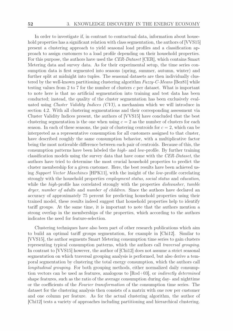
52 3. KNOWLEDGE DISCOVERY IN THE ENERGY ECONOMY
In order to investigate if, in contrast to contractual data, information about house-hold properties has a significant relation with class segmentation, the authors of [VVS15]present a clustering approach to yield seasonal load profiles and a classification ap-proach to assign customers to a load profile depending on their household properties.For this purpose, the authors have used the CER-Dataset [CER], which contains SmartMetering data and survey data. As for their experimental setup, the time series con-sumption data is first segmented into seasons (spring, summer, autumn, winter) andfurther split at midnight into tuples. The seasonal datasets are then individually clus-tered by the well-known partitioning clustering algorithm Fuzzy-C-Means [Bez81] whiletesting values from 2 to 7 for the number of clusters c per dataset. What is importantto note here is that no artificial segmentation into training and test data has beenconducted; instead, the quality of the cluster segmentation has been exclusively eval-uated using Cluster Validity Indices (CVI), a mechanism which we will introduce insection 4.2. With all clustering segmentations and their corresponding assessment viaCluster Validity Indices present, the authors of [VVS15] have concluded that the bestclustering segmentation is the one when using c = 2 as the number of clusters for eachseason. In each of these seasons, the pair of clustering centroids for c = 2, which can beinterpreted as a representative consumption for all customers assigned to that cluster,have described roughly the same consumption behavior, with a multiplicative factorbeing the most noticeable difference between each pair of centroids. Because of this, theconsumption patterns have been labeled the high- and low -profile. By further trainingclassification models using the survey data that have come with the CER-Dataset, theauthors have tried to determine the most crucial household properties to predict thecluster membership for a given customer. Here, the best results have been achieved us-ing Support Vector Maschines [HPK11], with the insight of the low -profile correlatingstrongly with the household properties employment status, social status and education,while the high-profile has correlated strongly with the properties dishwasher, tumbledryer, number of adults and number of children. Since the authors have declared anaccuracy of approximately 75 percent for predicting household properties using theirtrained model, these results indeed suggest that household properties help to identifytariff groups. At the same time, it is important to note that the authors mention astrong overlap in the memberships of the properties, which according to the authorsindicates the need for feature-selection.
Clustering techniques have also been part of other research publications which aimto build an optimal tariff groups segmentation, for example in [Chi12]. Similar to[VVS15], the author segments Smart Metering consumption time series to gain clustersrepresenting typical consumption patterns, which the authors call traversal grouping.In contrast to [VVS15] however, the author of [Chi12] does not assume a strict seasonalsegmentation on which traversal grouping analysis is performed, but also derive a tem-poral segmentation by clustering the total energy consumption, which the authors calllongitudinal grouping. For both grouping methods, either normalized daily consump-tion vectors can be used as features, analogous to [Rod+03], or indirectly determinedshape features, such as the ratio of the average consumption during day- and nighttimeor the coefficients of the Fourier transformation of the consumption time series. Thedataset for the clustering analysis then consists of a matrix with one row per customerand one column per feature. As for the actual clustering algorithm, the author of[Chi12] tests a variety of approaches including partitioning and hierarchical clustering.
3.3. IMPACT ON ENERGY PROVIDERS 53
All these techniques have in common that for the purpose of identifying target groups,only the memberships values are of interest, even if the clustering algorithm used out-puts clustering prototypes as it is the case by K-Means [Mac+67] or Fuzzy-C-Means[Bez81] for example. This combination of longitudinal grouping and traversal groupinghas been tested by the author with a dataset containing consumption time series of400 customers with a resolution of one measurement every 15 minutes for one repre-sentative working day during the interim period. The best results, according to theCluster Validity Indices used to assess the quality of the clustering segmentation, aredependent on the specific goal of the process; in order to identify and exclude outliers,hierarchical clustering in conjunction with the Single-Linkage-Criterion has achievedthe best results, whereas K-Means and Fuzzy-C-Means have been deemed suitable if adirect segmentation of consumption data into target groups is desirable.
Another approach, with focuses on a Mixed Fuzzy Clustering method [Fer+15] toincorporate both Smart Metering time series and household properties for target groupsegmentation, is presented in [Sch+15]. Contrary to the previously mentioned researchof [VVS15], which uses household properties in a classification mechanism followingthe clustering step, the authors of [Sch+15] use these household properties directly aspart of the clustering step. For this purpose, the authors consider the Smart Meteringdata as time-dependent data, whereas the household properties are considered time-independent data, such as consumer income, age and number of residents.The basic idea of Mixed Fuzzy Clustering is to compute clustering prototypes for thetime-independent attributes and for each timeslot of the time-dependent data inde-pendently using Fuzzy-C-Means [Bez81] and then to deduce a clustering segmentationof the complete dataset from these clustering prototypes using an adequate distancefunction. More specifically, the r time-independent attributes for the i-th customer arenotated as a vector
xsi =
(
xsi,1, . . . , x
si,r
)
(3.6)
where the superscript s indicates the time-independent attributes. Similarly, the time-dependent data is notated as a matrix X t
i as follows:
X ti =
xti,1,1 xt
i,1,2 . . . xti,1,p
xti,2,1 xt
i,2,2 . . . xti,2,p
......
. . ....
xti,q,1 xt
i,q,2 . . . xti,q,p
(3.7)
Here, p corresponds to the number of time-dependent attributes and q describes thenumber of measurements for each attribute for the i-th customer. The o-th clusteringprototype of the time-independent attributes is then computed as
vso =
∑n
i=1 umo,i · x
si
∑n
i=1 umo,i
(3.8)
while the o-th clustering prototype of the time-dependent attributes is given as
vto,k =
∑n
i=1 umo,i · x
ti,k
∑n
i=1 umo,i
(3.9)
for the k-th time-dependent attribute. Similar to X ti , the clustering prototypes vto,k
belong to the matrix V to . Once the individual vso and vto,k are known, the clustering

54 3. KNOWLEDGE DISCOVERY IN THE ENERGY ECONOMY
segmentation for the complete dataset is then given as
uo,i =1
∑c
b=1
(
d2λ(vso,V
to ,xi)
d2λ(vsb ,V t
b,xi)
)2
m−1
(3.10)
using
d2λ(
vso, Vto , xi
)
= ‖vso − xsi‖
2 + λ
p∑
k=1
δ(
vto,k, xti,k
)
(3.11)
where λ corresponds to a user-defined weight for the time-dependent data and δ repre-sents the euclidean distance. Analogous to Fuzzy-C-Means as presented in section 1.2.2,the computation of V t
o , V s and the membership matrix uo,i ∈ U is repeated in a loopuntil the changes of U compared to the previous iteration are less than a user-definedthreshold ǫ.Overall, [Sch+15] presents an interesting concept using Mixed Fuzzy Clustering [Fer+15]to process both time-dependent and time-independent data. However, due to the factthat each clustering is performed individually per timeslot, it requires the dataset to becomplete and can not be applied unaltered if the data contains missing values in eitherthe time-dependent or time-independent attributes. Since time-independent attributesin the form of survey data typically is, if at all, available only in very limited quantities,and since missing values can occur in the time-dependent data due to technical failures,only a very small portion of the customer base can be processed using this approachin a real-world scenario. Because of this, Mixed Fuzzy Clustering is likely best suitedto find common interests of consumers for target-group-specific tariff offerings since,in contrast to the forecast of the energy consumption of consumers, it is not criticalfor all customers to be included in this processing technique. Alternatively, it mightbe desirable for Mixed Fuzzy Clustering to adapt techniques to allow data containingmissing values to be processed, as the authors of [HB01; SL01] have presented in thecase of Fuzzy-C-Means. Another possibility would be to apply methods to predictmissing information about household properties using available Smart Metering data,such as the ones presented in section 3.3.2.1, and then to use Mixed Fuzzy Cluster-ing on the original household properties in conjunction with the conclusions drawn byclassifying previously unknown properties. Depending on the set of features used totrain a classifier to carry out this task, the features can be meaningfully defined even ifthe Smart Metering time series contain missing values. This idea outlines a potentialstarting point for further research.
3.3.2.3 Forecast of the energy consumption
The forecast of the total energy consumption of their customers is one of the mostimportant aspects of the task of energy providers to keep the electricity grid balancedin terms of energy injection by the energy producers and withdrawal by the customers.This is due to the fact that energy providers need a bit of lead time to announce theexpected energy demand to the energy producers. Knowing the expected energy loadin advance enables to ensure that necessary capacities are allocated and the energy isinjected into the electricity grid exactly when it is needed by the consumers. We havegiven a more detailed introduction into this topic in section 2.2; in this section, we
3.3. IMPACT ON ENERGY PROVIDERS 55
present some approaches from academic literature on how to more accurately predictthe energy load of customers in order to plan the energy providers buy-in of energymore efficiently.
One way of improving the forecast of the energy consumption for energy providersis by building upon existing technology for how this task is currently being dealt withby the industry. As of this writing, most energy providers in Germany use the BDEWStandard Load Profiles [Mei+99; FT00], a consumption forecast model which we haveintroduced in section 2.3 in more detail. However, these load profiles, having beencompiled during the end of the 1990s, have not been adjusted to recent advances intechnology. Because of this, they are considered to be an increasingly bad model toforecast the energy load of customers [Roo+14]. With the upcoming broad availabilityof Intelligent Metering Systems and corresponding high resolution consumption timeseries, research has been conducted to build better prediction models to help energyproviders maintain the security of the energy supply.The approach presented in [SM17] tries to achieve this goal by slightly altering theshape of the BDEW Standard Load Profiles by utilizing Smart Metering data. Toaccomplish this, the authors use two datasets. The first dataset is a total consumptiontime series of an energy provider for the year 2012 until 2015, from which disturbingfactors, such as grid losses, have been manually subtracted. As a result, the total con-sumption time series only of the customers who have a load profile assigned remains,which corresponds to what we have introduced and referred to as the SLS time series insection 2.3. This SLS time series can be seen as the sum of an unknown consumptiontime series containing only private households and an unknown consumption time se-ries containing only industrial customers. The second dataset contains Smart Meteringdata for the years 2012 until 2014. In their analysis, the authors of [SM17] have keptmost of the structures from the BDEW Standard Load Profile in place, including theset of day-types and the concept of a dynamization function. To derive a new householdload profile from the first dataset, the authors have used the original industrial loadprofile G0 from the BDEW to yield an approximation for the unknown consumptiontime series containing only private households. This approximation is then processedaccording to the original approach of the creators of the BDEW Standard Load Pro-files [Mei+99; FT00]. In simplified terms, this means that the time series have beengrouped according to the day-type segmentation; for each day-type, the representativeconsumption pattern for the load profile is then given by computing the average con-sumption per time of day of the corresponding time series data. Similarly, the loadprofiles for the second dataset are built by aggregating the individual Smart Meteringtime series to a household time series and an industrial time series. These two timeseries are then further processed analogous to [Mei+99; FT00] to yield a new householdload profile and a new industrial load profile akin to the BDEW profiles H0 and G0,respectively.During the experimental evaluation, the authors claim a deviation between the actualenergy load and the load predicted using these new load profiles of roughly 3 percent,which is an excellent result compared to the BDEW Standard Load Profiles typicallyachieving a forecast error of 12 to 13 percent as we have shown in figure 2.5. In addition,the authors have demonstrated that their load profiles as well as their dynamizationfunctions significantly differ from the existing BDEW Standard Load Profiles, whichcould indicate both the consumers having changed their consumption behavior over

56 3. KNOWLEDGE DISCOVERY IN THE ENERGY ECONOMY
the last decades or a selection bias caused by the input dataset. In fact, very littleinformation over the dataset is provided apart from the fact that the dataset contains0,6 percent of all industrial customers, which strongly reinforces the suspicion of aselection bias in the input data. If this circumstance would be confirmed, then thealgorithm might not have had to struggle to consolidate the requirements of industrialcustomers of different industry branches, allowing a single load profile to yield excellentresults due to the homogeneity of the dataset. With regard to future research, sincethe basic idea of this approach is very akin to [Mei+99; FT00], testing it with a moreheterogeneous dataset might give more insight on whether the customer behaviors haveindeed significantly changed over the last decades.
Instead of relying on established methodology for generating load profiles to forecastthe energy demand, Data Mining techniques can also be used in a slightly alteredfashion to process Smart Metering time series to create a model which is only distantlyrelated to the concept of load profiles. For example, the authors of [ALB13] maintainthe concept of customer group and day-types, but make use of an autoregressive modelAR (1) to be able to long-term forecast the energy load. More specifically, the expectedenergy demand of a given customer group at a given time ct is modeled as follows:
ct =∑
d
ad ·Dtd
∑
m
ad,m ·Dtm
∑
h
ad,m,h ·Dth + ǫt (3.12)
Here, the coefficients a of the model are dependent on the day-type (subscript d), month(subscript m) and the time of day (subscript h) and are determined by the AR (1)model. The variables Dt
d ∈ {0, 1}, Dtm ∈ {0, 1} and Dt
h ∈ {0, 1} in equation 3.12 arebinary and equal 1 if and only if a given time, notated by the superscript t, belongsto the corresponding day-type, month or time of day. While this is a simple modelbased on statistics, it is a straightforward way for energy providers to make long-termpredictions and planning, either instead of, or in conjunction with, existing modelsbased on load profiles.

4Clustering using Smart Meter
Data
With the increasing availability of Smart Metering devices, it has become progressivelyeasier for energy providers to optimize business processes by improving customer under-standing using techniques from the field of Knowledge Discovery in Databases (KDD).Among the most important business processes of energy providers are marketing strate-gies, such as tariff optimization and customer loyalty programs, as well as negotiationswith market participants to allocate resources from energy producers.For the latter aspect, energy providers rely on forecast models to plan for their futurebuy-in of energy. These forecast models employed by energy providers come in theform of load profiles. Due to policies by controlling authorities mandating the usageof load profiles, and since changes to the concept of load profiles may, depending onthe implementation used by the energy providers, require a high amount of man-powerto realize, we have opted to adhere to the existing specification as introduced in sec-tion 2.3. Thus, over the course of this chapter, we will present approaches that utilizeKDD-techniques and Smart Metering data to build load profiles. By maintaining theexisting concept of load profiles, it is not only significantly easier for the energy providerto adopt the resulting models, but it also allows to satisfy regulatory requirements suchas the guideline to announce load profiles to all market participants at least 3 monthsprior to their usage [Bun13], meaning that the forecast models need to yield predictionswith acceptable error rates many months in advance.
4.1 Description of datasets
To evaluate the performance of our approach to generate load profiles, which we willpresent in section 4.3, we have used three real-world datasets containing Smart Meter-ing time series. These datasets have been visualized in figure 4.1.
The first dataset, which we will refer to as the HHU-Dataset, contains data for 7793distinct customers. The data covers a time period of 65 months with a resolution of
57
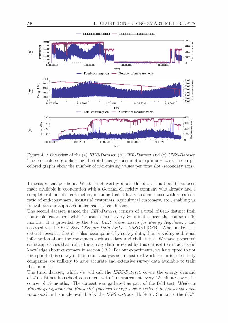
58 4. CLUSTERING USING SMART METER DATA
(a)
����� ��������� ��� �� ���������
���������� ���������� ��������� ����������
����
����
����
����
����
���
� ��
������[��]
�
����
����
���
����
#��� ���������
(b)
(c)
Figure 4.1: Overview of the (a) HHU-Dataset, (b) CER-Dataset and (c) IZES-Dataset.The blue colored graphs show the total energy consumption (primary axis); the purplecolored graphs show the number of non-missing values per time slot (secondary axis).
1 measurement per hour. What is noteworthy about this dataset is that it has beenmade available in cooperation with a German electricity company who already had acomplete rollout of smart meters, meaning that it has a customer base with a realisticratio of end-consumers, industrial customers, agricultural customers, etc., enabling usto evaluate our approach under realistic conditions.The second dataset, named the CER-Dataset, consists of a total of 6445 distinct Irishhousehold customers with 1 measurement every 30 minutes over the course of 16months. It is provided by the Irish CER (Commission for Energy Regulation) andaccessed via the Irish Social Science Data Archive (ISSDA) [CER]. What makes thisdataset special is that it is also accompanied by survey data, thus providing additionalinformation about the consumers such as salary and civil status. We have presentedsome approaches that utilize the survey data provided by this dataset to extract usefulknowledge about customers in section 3.3.2. For our experiments, we have opted to notincorporate this survey data into our analysis as in most real-world scenarios electricitycompanies are unlikely to have accurate and extensive survey data available to traintheir models.The third dataset, which we will call the IZES-Dataset, covers the energy demandof 416 distinct household consumers with 1 measurement every 15 minutes over thecourse of 19 months. The dataset was gathered as part of the field test "ModerneEnergiesparsysteme im Haushalt" (modern energy saving systems in household envi-ronments) and is made available by the IZES institute [Hof+12]. Similar to the CER-
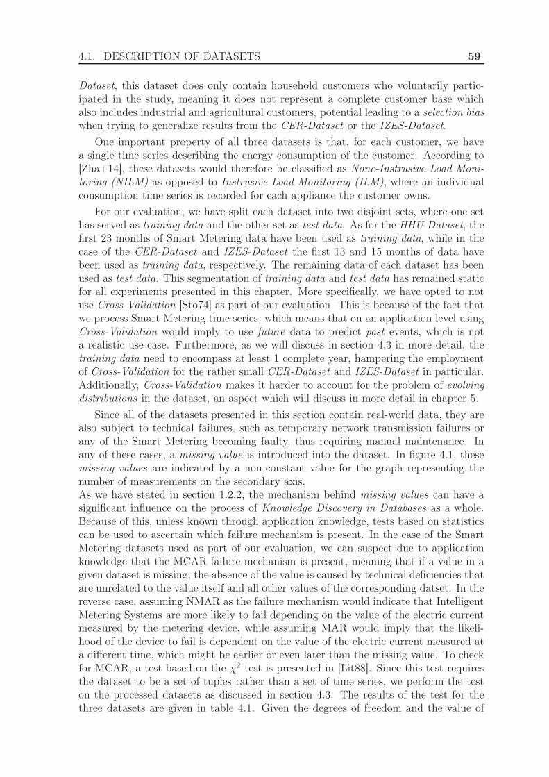
4.1. DESCRIPTION OF DATASETS 59
Dataset, this dataset does only contain household customers who voluntarily partic-ipated in the study, meaning it does not represent a complete customer base whichalso includes industrial and agricultural customers, potential leading to a selection biaswhen trying to generalize results from the CER-Dataset or the IZES-Dataset.
One important property of all three datasets is that, for each customer, we havea single time series describing the energy consumption of the customer. According to[Zha+14], these datasets would therefore be classified as None-Instrusive Load Moni-toring (NILM) as opposed to Instrusive Load Monitoring (ILM), where an individualconsumption time series is recorded for each appliance the customer owns.
For our evaluation, we have split each dataset into two disjoint sets, where one sethas served as training data and the other set as test data. As for the HHU-Dataset, thefirst 23 months of Smart Metering data have been used as training data, while in thecase of the CER-Dataset and IZES-Dataset the first 13 and 15 months of data havebeen used as training data, respectively. The remaining data of each dataset has beenused as test data. This segmentation of training data and test data has remained staticfor all experiments presented in this chapter. More specifically, we have opted to notuse Cross-Validation [Sto74] as part of our evaluation. This is because of the fact thatwe process Smart Metering time series, which means that on an application level usingCross-Validation would imply to use future data to predict past events, which is nota realistic use-case. Furthermore, as we will discuss in section 4.3 in more detail, thetraining data need to encompass at least 1 complete year, hampering the employmentof Cross-Validation for the rather small CER-Dataset and IZES-Dataset in particular.Additionally, Cross-Validation makes it harder to account for the problem of evolvingdistributions in the dataset, an aspect which will discuss in more detail in chapter 5.
Since all of the datasets presented in this section contain real-world data, they arealso subject to technical failures, such as temporary network transmission failures orany of the Smart Metering becoming faulty, thus requiring manual maintenance. Inany of these cases, a missing value is introduced into the dataset. In figure 4.1, thesemissing values are indicated by a non-constant value for the graph representing thenumber of measurements on the secondary axis.As we have stated in section 1.2.2, the mechanism behind missing values can have asignificant influence on the process of Knowledge Discovery in Databases as a whole.Because of this, unless known through application knowledge, tests based on statisticscan be used to ascertain which failure mechanism is present. In the case of the SmartMetering datasets used as part of our evaluation, we can suspect due to applicationknowledge that the MCAR failure mechanism is present, meaning that if a value in agiven dataset is missing, the absence of the value is caused by technical deficiencies thatare unrelated to the value itself and all other values of the corresponding datset. In thereverse case, assuming NMAR as the failure mechanism would indicate that IntelligentMetering Systems are more likely to fail depending on the value of the electric currentmeasured by the metering device, while assuming MAR would imply that the likeli-hood of the device to fail is dependent on the value of the electric current measured ata different time, which might be earlier or even later than the missing value. To checkfor MCAR, a test based on the χ2 test is presented in [Lit88]. Since this test requiresthe dataset to be a set of tuples rather than a set of time series, we perform the teston the processed datasets as discussed in section 4.3. The results of the test for thethree datasets are given in table 4.1. Given the degrees of freedom and the value of
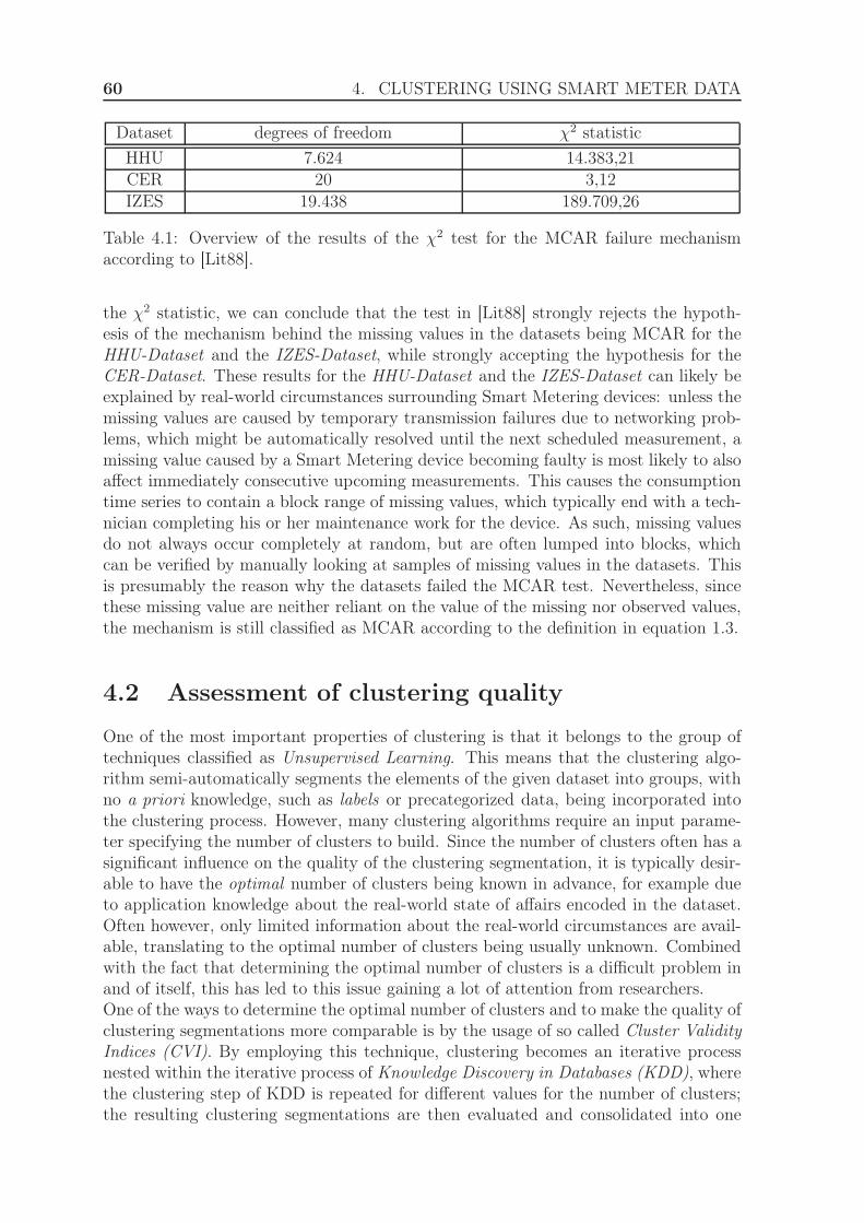
60 4. CLUSTERING USING SMART METER DATA
Dataset degrees of freedom χ2 statistic
HHU 7.624 14.383,21CER 20 3,12
IZES 19.438 189.709,26
Table 4.1: Overview of the results of the χ2 test for the MCAR failure mechanismaccording to [Lit88].
the χ2 statistic, we can conclude that the test in [Lit88] strongly rejects the hypoth-esis of the mechanism behind the missing values in the datasets being MCAR for theHHU-Dataset and the IZES-Dataset, while strongly accepting the hypothesis for theCER-Dataset. These results for the HHU-Dataset and the IZES-Dataset can likely beexplained by real-world circumstances surrounding Smart Metering devices: unless themissing values are caused by temporary transmission failures due to networking prob-lems, which might be automatically resolved until the next scheduled measurement, amissing value caused by a Smart Metering device becoming faulty is most likely to alsoaffect immediately consecutive upcoming measurements. This causes the consumptiontime series to contain a block range of missing values, which typically end with a tech-nician completing his or her maintenance work for the device. As such, missing valuesdo not always occur completely at random, but are often lumped into blocks, whichcan be verified by manually looking at samples of missing values in the datasets. Thisis presumably the reason why the datasets failed the MCAR test. Nevertheless, sincethese missing value are neither reliant on the value of the missing nor observed values,the mechanism is still classified as MCAR according to the definition in equation 1.3.
4.2 Assessment of clustering quality
One of the most important properties of clustering is that it belongs to the group oftechniques classified as Unsupervised Learning. This means that the clustering algo-rithm semi-automatically segments the elements of the given dataset into groups, withno a priori knowledge, such as labels or precategorized data, being incorporated intothe clustering process. However, many clustering algorithms require an input parame-ter specifying the number of clusters to build. Since the number of clusters often has asignificant influence on the quality of the clustering segmentation, it is typically desir-able to have the optimal number of clusters being known in advance, for example dueto application knowledge about the real-world state of affairs encoded in the dataset.Often however, only limited information about the real-world circumstances are avail-able, translating to the optimal number of clusters being usually unknown. Combinedwith the fact that determining the optimal number of clusters is a difficult problem inand of itself, this has led to this issue gaining a lot of attention from researchers.One of the ways to determine the optimal number of clusters and to make the quality ofclustering segmentations more comparable is by the usage of so called Cluster ValidityIndices (CVI). By employing this technique, clustering becomes an iterative processnested within the iterative process of Knowledge Discovery in Databases (KDD), wherethe clustering step of KDD is repeated for different values for the number of clusters;the resulting clustering segmentations are then evaluated and consolidated into one

4.2. ASSESSMENT OF CLUSTERING QUALITY 61
key figure per clustering segmentation. By tracking the evolution of the key figure of agiven Cluster Validity Index for different values for the number of clusters, the optimalnumber of clusters can be determined as the number of clusters where the key figureof the CVI has reached a global optimum over all tested numbers of clusters. In doingso, each CVI focuses on different aspects of the clustering segmentation, for examplerewarding uniqueness in cluster assignment or incentivizing the creation of compactand well-separated clusters. As such, each CVI has different strengths and weaknessesin coping with overlapping, heterogeneous shaped or hierarchically structured clusters.Over the course of this section, we will introduce some common Cluster Validity Indicesfor Fuzzy Clustering often used to assess the quality of a clustering segmentation.
4.2.1 Partition Coefficient
The Partition Coefficient (PC) [Bez74] evaluates a given clustering segmentation basedon the membership degrees uo,i of each data tuple to each clustering prototype and isdefined as follows:
VPC (U, c) =1
N
c∑
o=1
N∑
i=1
u2o,i (4.1)
According to this CVI, the best clustering partitioning is the one where all tuples havebeen unambiguously assigned to a given clustering prototype, which translates to thememberships of all tuples being equal to 1 for one clustering prototype and 0 for allother prototypes since uo,i ∈ [0,1]. In that case, VPC = 1.However, the worst clustering segmentation, according to this CVI, is present if alltuples belong to all clustering prototypes equally, which due to the Fuzzy Clusteringproperty ∀i :
∑c
o=1 uo,i = 1 is the case if ∀o, i : uo,i =1c
and thus VPC = 1c. Because of
this, VPC has a range of[
1c, 1]
.Due to the fact that the range of VPC is dependent on the number of clusters c, the
CVI is biased towards a smaller value for c. To overcome this issue, the NormalizedPartition Coefficient (NPC) has been proposed [Bac78; Rou78]:
VNPC (U, c) = 1−c
c− 1(1− VPC (U, c)) = 1−
c
c− 1
(
1−1
N
c∑
o=1
N∑
i=1
u2o,i
)
(4.2)
Unlike VPC , the range of VNPC is [0, 1] regardless of the value of c. Like VPC, a highervalue of VNPC indicates a better cluster segmentation.
While both VPC and VNPC are rather simple CVIs, possibly their biggest flaw is theproperty to yield good results only when the dataset consists of spherical and clearlyseparated clusters, or else the optimal number of clusters is very often underestimated[BWS06; Him16].
4.2.2 Compactness & Separation by Xie & Beni
The Xie-Beni (XB) Index [XB91] works by consulting the original objective of genericclustering algorithms, which instructs the algorithm to find a clustering segmentationso that data tuples belonging to the same cluster are as similar as possible while datatuples belonging to different clusters are as dissimilar as possible. For this purpose, theXie-Beni Index uses two key figures to evaluate how good the clustering algorithm has

62 4. CLUSTERING USING SMART METER DATA
solved the objective criterion. The first key figure, called the Compactness, describeshow similar data tuples are compared to their assigned clustering prototype:
CompXB (U,X, V ) =J
N=
∑c
o=1
∑N
i=1 u2o,i ‖xi − vo‖
2
N(4.3)
The connection of the Compactness to the objective function of clustering algorithmsis also illustrated by the fact that CompXB (U,X, V ) incorporates J (·), which corre-sponds to the objective function of Fuzzy-C-Means as described in equation 1.1. Be-cause clustering algorithms strive to minimize the objective function, a good clusteringsegmentation according to this CVI is achieved when the Compactness is minimizedas well.The second key figure expresses the dissimilarity of clusters and is called the Separation:
SepXB (V ) = min1≤o,o′≤c
o6=o′
‖vo − vo′‖2 (4.4)
Since clustering algorithms aim to maximize the dissimilarity of each pair of clusters,a high value for the Separation signalizes a good clustering segmentation.
To aggregate both key figures, the Xie-Beni Index VXB is defined as the ratio of theCompactness and the Separation:
VXB (U,X, V ) =CompXB
SepXB
=
∑c
o=1
∑N
i=1 u2o,i ‖xi − vo‖
2
N min1≤o,o′≤co6=o′
‖vo − vo′‖2 (4.5)
For the experiments presented in section 4.4 however, the definition of VXB asgiven in equation 4.5 can not be used because the value of the CVI is dependent onthe values of the data tuples xi, which are partially unavailable if the dataset containsmissing values. To handle this issue, we employ a modified definition of VXB where theeuclidean distance between xi and vo is replaced by their partial distance as describedby [HHC11]. The resulting modified definition of VXB is as follows:
VXB (U,X, V ) =
∑c
o=1
∑N
i=1 u2o,i
h∑h
n=1 Ii,n(xi,n−vo,n)2
∑hn=1 Ii,n
N min1≤o,o′≤co6=o′
‖vo − vo′‖2
with Ii,n =
{
1 if xi,n is not a missing value
0 else
(4.6)
Although the design of VXB is well thought out due to its definition being closelyinspired by the objective function of clustering algorithms, it can be formally shownthat the value of the CVI is monotonously decreasing when increasing the number ofclusters c, which the authors of the CVI themselves have pointed out [XB91].
4.2.3 Compactness & Separation by Bouguessa, Wang & Sun
The idea behind the Bouguessa-Wang-Sun (BWS) Index [BWS06] is very similar tothe Xie-Beni Index in that the Bouguessa-Wang-Sun Index also assesses the qualityof the clustering segmentation by evaluating the ratio between two key figures called

4.2. ASSESSMENT OF CLUSTERING QUALITY 63
Compactness and Separation. However, in contrast to VXB, VBWS is defined as theratio of Separation divided by Compactness as opposed to VXB where it is the otherway around:
VBWS (U, V,X) =SepBWS
CompBWS
(4.7)
Thus, a good clustering partition according to this CVI is characterized by a value forVBWS which is as large as possible. The Separation of VBWS is based on the between-cluster fuzzy scatter matrix SB:
SepBWS (U,X, V ) = trace (SB)
with SB =c
∑
o=1
N∑
i=1
umo,i (vo − x) (vo − x)⊤
(4.8)
Here, x is the means of all data tuples xi. A large value for SepBWS indicates that thefuzzy clusters are well-separated. Similar to the Separation SepBWS, the CompactnessCompBWS is also based on the trace of matrices, more specifically the fuzzy covariancematrices for each cluster:
CompBWS (U,X, V ) =c
∑
o=1
trace (Covo)
with Covo =
∑N
i=1 umo,i (xi − vo) (xi − vo)
⊤
∑N
i=1 umo,i
(4.9)
Due to the CVIs definition of Compactness and Separation, particularly by itsinclusion of the fuzzy covariance matrices, VBWS aims to perform well if the clusterspartially overlap or differ in their size, shape and density. In experiments with bothsynthetic and real-world datasets, VBWS has achieved above-average results [BWS06;Him16].However, because VBWS is dependent on the value of the data tuples xi, the originaldefinition of VBWS is undefined if there are missing values present in the dataset.Because of this, for our experiments, we employ a modified definition of this CVIaccording to [HCC12]:
Covo(p,l) =
∑N
i=1 umo,i · Ii,p · Ii,l (xi,p − vo,p) (xi,l − vo,l)
⊤
∑N
i=1 umo,i · Ii,p · Ii,l
, 1 < p, l < h
with Ii,n =
{
1 if xi,n is not a missing value
0 else
(4.10)
In equation 4.10, Covo(p,l) describes a modified version for the fuzzy covariance matricesused to compute the Compactness in equation 4.9. To compute the Separation of VBWS,only the definition of x in equation 4.8 is altered:
x =
∑N
i=1 Ii,n · xi,n∑N
i=1 Ii,nwith Ii,n =
{
1 if xi,n is not a missing value
0 else(4.11)

64 4. CLUSTERING USING SMART METER DATA
4.2.4 Fuzzy Hypervolume and Partition Density
Fuzzy Hypervolume (FH) [GG89] is a CVI that incentivizes the creation of clusterswith minimal volumes. In doing so, the volume of a cluster is measured based on thefuzzy covariance matrix:
VFH (U,X, V ) =c
∑
o=1
√
det (Covo) (4.12)
The definition for the fuzzy covariance matrices we have employed is given in equa-tion 4.10, which converges to the definition of Covo as in equation 4.9 in the absence ofmissing values in the dataset. Similar to VBWS, by incorporating the fuzzy covariancematrices of each cluster, VFH is able to recognize non-spherical, partially overlappingclusters with varying size, shape and density. Since the idea of VFH is to build clusterswith minimal volumes, a good clustering segmentation is achieved when this CVI isminimized.
One disadvantage of VFH is that, by design, clusters are rated solely on their volume,discouraging the formation of large clusters. Thus, the authors of [GG89] propose theconcept of Partition Density (PD):
VPD (U,X, V ) =Z
VFH (U,X, V )
with Z =
c∑
o=1
N∑
i=1
uo,i ∀xi ∈{
xi
∣
∣
∣(xi − vo)
⊤ Cov−1o (xi − vo) < 1
}
(4.13)
Here, the term Z is described by the authors of [GG89] as the sum of central members.A central member as in equation 4.13 is a data tuple whose radius to the correspondingclustering prototype is less than one standard deviation of the overall size of the clusteras given by the fuzzy covariance matrix. The more massive each cluster is, that is,the more central members each cluster has and the higher the membership degree ofeach central member to said cluster is, the higher the value Z. Using Z, the authors of[GG89] aim to overcome the weakness of VFH favoring clusters with minimal volumesand instead reward the formation of large clusters if they are sufficiently massive.As in the case of VXB and VBWS, the definition of VPD might be undefined if the datasetcontains missing values as equation 4.13 accesses the values of xi directly. Because ofthis, we have used an adaptation for our experiments according to an idea introducedin [HHC11]:
Z =c
∑
o=1
N∑
i=1
uo,i ∀xi ∈
xi
∣
∣
∣
∣
∣
∣
∣
∣
∣
∣
∣
h
(
Ii,1(xi,1−vo,1)..
Ii,h(xi,h−vo,h)
)⊤
Cov−1o
(
Ii,1(xi,1−vo,1)..
Ii,h(xi,h−vo,h)
)
∑h
n=1 Ii,n< 1
with Ii,n =
{
1 if xi,n is not a missing value
0 else
(4.14)

4.2. ASSESSMENT OF CLUSTERING QUALITY 65
4.2.5 Silhouette Coefficient
Another well-known indicator for evaluating the quality of a clustering segmentationis the Silhouette Coefficient (SC) [Rou87; KR90; ES00]. The idea behind this indexis to incorporate the distance function used during the clustering process to rate howunambiguous each data tuple belongs to their assigned cluster. For this purpose, theSilhouette Coefficient VSC defines two utility functions:
a (i) =1
|Co| − 1
∑
xi,xi′∈Co
i6=i′
dist (xi, xi′) (4.15)
b (i) = mino′ 6=o
1
|Co′|
∑
xi∈Co
xi′∈Co′
dist (xi, xi′) (4.16)
Here, Co is derived from the fuzzy memberships uo,i and describes the set of data tuplesxi which have been assigned to the o-th cluster. While a (i) can be vividly describedas the average distance of xi to other members of the same cluster, b (i) describes theaverage distance of xi to members of its "neighbor" cluster.With both equation 4.15 and 4.16, the Silhouette Coefficient VSC is defined as follows:
VSC (U,X) =1
∑c
o=1 |Co|
c∑
o=1
∑
xi∈Co
b (i)− a (i)
max (a (i) , b (i))(4.17)
The range of VSC is [−1, 1], whereas a value closer to 1 means that, for most datatuples, the average distance of each data tuple to members of its "neighbor" cluster,expressed by b (i), is much larger than the average distance each data tuple to othermembers of their assigned cluster, expressed by a (i). Thus, a value of approximately1 signifies a good cluster segmentation, where most data tuples unambiguously belongto the cluster they have been assigned to according to the dissimilarity measure of theclustering process.
4.2.6 Average Clustering Uniqueness
One difficulty in using the Silhouette Coefficient (SC) [Rou87; KR90; ES00] introducedin section 4.2.5 arises when applying VSC on increasingly large datasets. Due to the factthat VSC is defined as the average of the b(i)−a(i)
max(a(i),b(i))for all data tuples xi, it is required
to compute the distances between each pair of data tuples dist (xi, xi′) with i 6= i′. Thisis because for all i 6= i′, the term dist (xi, xi′) is either part of a (i) as in equation 4.15if both xi and xi′ belong to the same cluster or part of b (i) as in equation 4.16 todetermine which of the other clusters is the "neighbor" cluster. Overall, this results ina time complexity of O (N 2) to compute VSC , where N is the number of data tuplesin the dataset. This causes VSC to become infeasible to compute when the dataset issufficiently large.To counteract this issue, we introduce a new CVI in this section, which we will referto as Average Clustering Uniqueness (ACU), which is based on the idea behind VSC .For this purpose, we redefine the utility functions a (i) and b (i) as follows:
a (i) = dist (xi, vo) , xi ∈ Co (4.18)

66 4. CLUSTERING USING SMART METER DATA
b (i) = mino′ 6=o
dist (xi, vo′) , xi ∈ Co (4.19)
As in section 4.2.5, Co describes the set of data tuples belonging to the o-th cluster,represented by the clustering prototype vo. We then define the Average ClusteringUniqueness VACU as follows:
VACU (U,X, V ) =1
∑c
o=1 |Co|
∑
xi
b (i)− a (i)
max (a (i) , b (i))(4.20)
Though very similar to VSC, the VACU is based on the distance to the clustering proto-types vo instead of the set of data tuples assigned to the o-th cluster. This causes thetime complexity of VACU to be O (N · c), where N corresponds to the total numberof data tuples and c is equal to the number of clustering prototypes. Since one hasc ≪ N in a typical clustering scenario, VACU can be used as an efficient approximationof VSC in cases where the clusters are known to be of spherical shape.
4.3 Framework for generating load profiles
Due to the design of load profiles as introduced in section 2.3, the construction ofsuch load profiles consists of several steps which are processed in sequence. On a highlevel, these steps conform to our previous work [Boc16; Boc17; Boc18] and can besummarized as follows:
1. Day-type segmentation: As the first step in the construction of load profiles,the optimal number of day-types as well as their segmentation onto the individualcalendar days are determined.
2. Identification of typical consumption patterns: For each day-type, identifycustomer groups and derive one representative consumption pattern for eachcustomer group.
3. Compilation of load profiles: Compile the load profiles by combining theresults from the previous steps and assign a load profile to each customer.
4.3.1 Day-type segmentation
For determining a good day-type segmentation, the most crucial aspect is to identifygroups of calendar days on which the total energy consumption of customers is suffi-ciently similar. Since load profiles are used by energy providers to forecast the totalenergy demand as accurately as possible, the careful choice of an optimal day-typesegmentation is arguably the most crucial factor in achieving that goal. That is, if it isplausible to assume that the total energy demand of customers does not significantlydiffer on two or more given calendar days, there is no reason to use a different dailyforecast, even if that forecast does not satisfy the actual consumption of individualcustomers.To derive a good day-type segmentation during our experimental evaluation introducedin section 4.4, we have opted to first construct a new time series X = {x1, x2, ..., xT}

4.3. FRAMEWORK FOR GENERATING LOAD PROFILES 67
00:00 06:00 12:00 18:00 00:00 06:00 12:00 18:00 00:00 06:00 12:00 18:000.00
0.05
0.10
0.15
0.20
...
Energ
y c
onsum
ption [kW
h]
Time series X
Figure 4.2: Visualization of how the Dataset D is constructed from the time series Xby splitting the time series into tuples at the start of a new calendar day.
for each point in time tj , 1 ≤ j ≤ T using the individual customer’s Smart Meteringtime series si,j ∈ Si, 1 ≤ i ≤ N, 1 ≤ j ≤ T as follows:
xj :=1
Nj · DynFactor (tj)
N∑
i=1
si,jYCF i,j
(4.21)
Here, N corresponds to the total number of distinct customers and Nj is equal tothe number of measurements available for tj . The distinction between N and Nj isnecessary so as to not distort X when missing values are present in the data or whencustomers leave or join to or from other energy providers. The term YCF i,j standsfor the Year Consumption Forecast assigned to the i-th customer, represented by hisor her Smart Metering time series Si, for the year that tj belongs to. The optionalterm DynFactor (tj) corresponds to the dynamization function evaluated at tj; in thecase that no dynamization function is used, the term is omitted. What is importantto note here is that si,j describes the amount of energy consumed since the previousmeasurement si,j−1, not the cumulative consumption such as the meter reading. Al-though it is technically possible to record and process si,j as power (kilowatts) insteadof energy (kilowatthours), this requires correction terms in order to work properly withthe concept of the Year Consumption Forecast. Thus, for equation 4.21 and following,we notate si,j and related terms as energy. In a nutshell, X can be described as anaverage time series of the normalized Smart Metering time series of all customers.
We then construct dataset D using X as follows:
D :=
{
dl := (xj , ..., xj+H−1)
∣
∣
∣
∣
∀a with 1 ≤ j ≤ a ≤ j +H − 1 ≤ T :ta belongs to the l-th calendar day
}
(4.22)
Here, H corresponds to the number of measurements per day. In general, each tupledl corresponds to a slice of the time series X containing data for one calendar day. Indoing so, we account for application knowledge, which states it is reasonable to thinkof Smart Metering time series not as an atomic data source, but as a set of tuples,where each tuple describes the consumption time series of a single calendar day. SinceSmart Metering time series typically have a resolution of one measurement every 15,30 or 60 minutes, each dl corresponds to a 96-, 48- or 24-tuple, respectively. Figure 4.2visualizes how the dl are derived using X.
As the second to final step in deriving a good day-type segmentation, we applyclustering on the dataset D. In principle, an arbitrary clustering algorithm can be em-ployed for this task, such as the one presented in section 1.2.2. However, it is important

68 4. CLUSTERING USING SMART METER DATA
to recall that the goal of this step is to group calendar days where the customer base asa whole behaves as similar as possible. Even if the consumption behaviors of consumersvary widely only in a few number of dimensions, these differences contribute to the fi-nancial risk associated with imbalance energy. Because of this, even if ellipsoid clustersor clusters of other shapes were to be recognizable in the data, a further segmenta-tion of such ellipsoid clusters into multiple spherical clusters is more desirable whenincorporating application knowledge. Thus, the chosen clustering algorithm shoulddiscourage the formation of non-spherical clusters. This requirement removes some al-gorithms from being considered, for example density-based clustering algorithms suchas DBSCAN [Est+96], which are able to identify clusters of arbitrary shape. For ourexperiments, we have opted to use Fuzzy-C-Means [Bez81], a partitioning clustering al-gorithm with the tendency to recognize only spherical clusters [BWS06]. Additionally,Fuzzy-C-Means has the advantage of being a well-known and comparatively simple al-gorithm, which helps us in creating an approach with low computational requirementsthat is easy for energy providers to adopt and can be feasibly employed locally with-out relying on cloud computing service providers where compliance with data privacypolicies are often a concern.
Once a good clustering segmentation is available, a day-type segmentation can bededuced by knowing which dl got assigned to the same cluster and which calendardays each dl represents. Starting out from this, an analyst examines regularities in theclustering segmentation, therefore deriving rulesets to classify future calendar days. Atthe same time, the analyst has to keep the strict periodicity of load profiles of 1 yearin mind. That is, if for example multiple years of Smart Metering time series are beinganalyzed and a cluster only appears in a single year, the analyst has to take a closelook at the corresponding calendar days. If the suspicion of these calendar days beingan outlier day-type solidifies, for example caused by major sport events such as theFIFA World Cup, the analyst has to prune these calendar days from the evaluationand decide on appropriate replacement day-types. For the same reason, the size of thetraining data has to cover at least 1 year of continuous data to ensure that each dayof year is present during analysis.
4.3.2 Identification of typical consumption patterns
The identification of typical consumption patterns is carried out after the day-typesegmentation is finalized. With the set of day-types known, the goal of this process isto find representative consumption patterns for groups of customers for each day-type.Since load profiles expect the consumption pattern to represent all customers associatedto the same customer group as a whole rather than individually, the same consumptionpatterns can be used as long as it matches the total energy consumption as accuratelyas possible. As a result of the identification of typical consumption patterns takingplace after the day-type segmentation, it is already known which calendar days exhibita sufficiently similar total energy consumption, namely all calendar days assigned tothe same day-type. Because of this, our goal for this step is to look at the SmartMetering time series for each day individually in order to deduce day-type-specificconsumption patterns for each customer. For this purpose, let Kn, 1 ≤ n ≤ L be thesets of day-types from section 4.3.1 where each Kn consists of the corresponding tj .
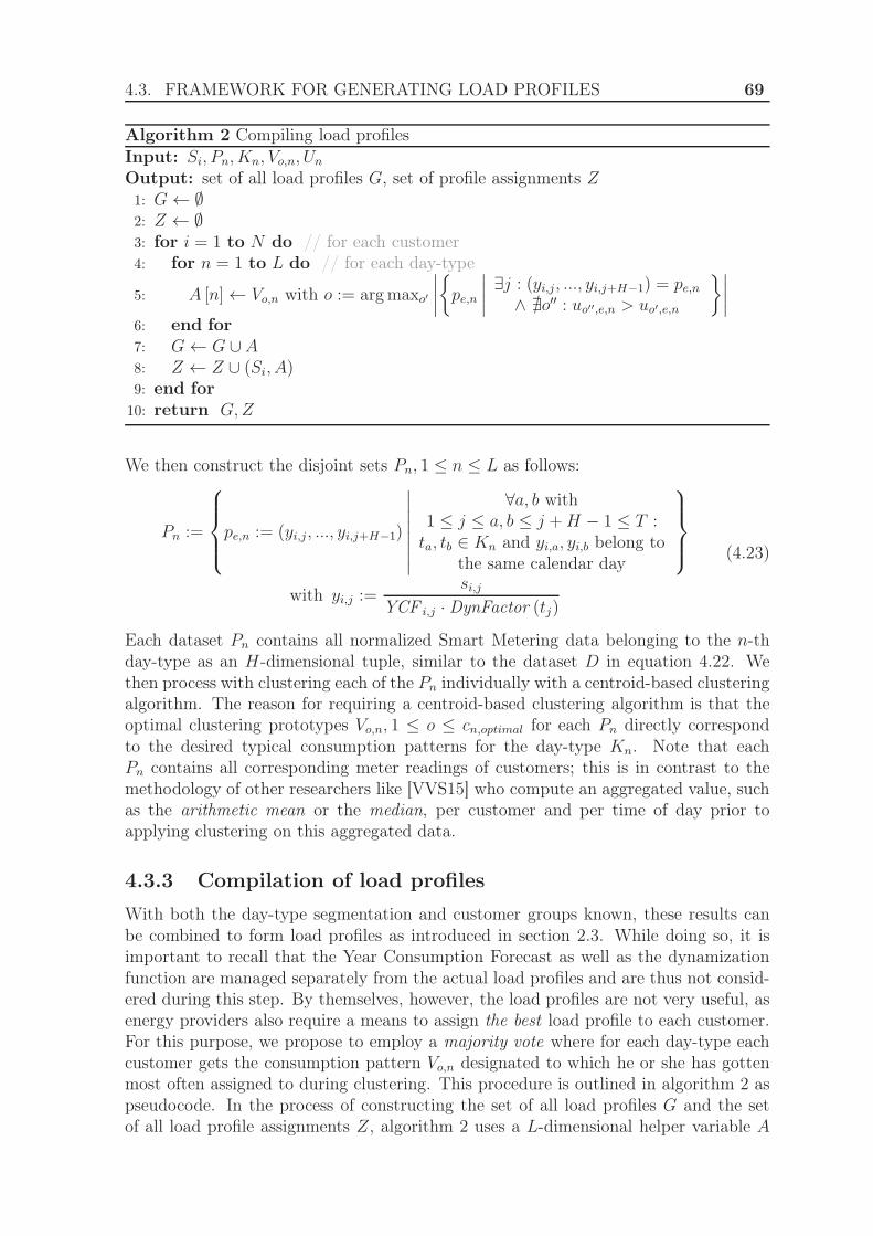
4.3. FRAMEWORK FOR GENERATING LOAD PROFILES 69
Algorithm 2 Compiling load profilesInput: Si, Pn, Kn, Vo,n, Un
Output: set of all load profiles G, set of profile assignments Z1: G ← ∅2: Z ← ∅3: for i = 1 to N do // for each customer4: for n = 1 to L do // for each day-type
5: A [n] ← Vo,n with o := argmaxo′
∣
∣
∣
∣
{
pe,n
∣
∣
∣
∣
∃j : (yi,j, ..., yi,j+H−1) = pe,n∧ ∄o′′ : uo′′,e,n > uo′,e,n
}∣
∣
∣
∣
6: end for7: G ← G ∪ A8: Z ← Z ∪ (Si, A)9: end for
10: return G,Z
We then construct the disjoint sets Pn, 1 ≤ n ≤ L as follows:
Pn :=
pe,n := (yi,j, ..., yi,j+H−1)
∣
∣
∣
∣
∣
∣
∣
∣
∀a, b with1 ≤ j ≤ a, b ≤ j +H − 1 ≤ T :ta, tb ∈ Kn and yi,a, yi,b belong to
the same calendar day
with yi,j :=si,j
YCF i,j · DynFactor (tj)
(4.23)
Each dataset Pn contains all normalized Smart Metering data belonging to the n-thday-type as an H-dimensional tuple, similar to the dataset D in equation 4.22. Wethen process with clustering each of the Pn individually with a centroid-based clusteringalgorithm. The reason for requiring a centroid-based clustering algorithm is that theoptimal clustering prototypes Vo,n, 1 ≤ o ≤ cn,optimal for each Pn directly correspondto the desired typical consumption patterns for the day-type Kn. Note that eachPn contains all corresponding meter readings of customers; this is in contrast to themethodology of other researchers like [VVS15] who compute an aggregated value, suchas the arithmetic mean or the median, per customer and per time of day prior toapplying clustering on this aggregated data.
4.3.3 Compilation of load profiles
With both the day-type segmentation and customer groups known, these results canbe combined to form load profiles as introduced in section 2.3. While doing so, it isimportant to recall that the Year Consumption Forecast as well as the dynamizationfunction are managed separately from the actual load profiles and are thus not consid-ered during this step. By themselves, however, the load profiles are not very useful, asenergy providers also require a means to assign the best load profile to each customer.For this purpose, we propose to employ a majority vote where for each day-type eachcustomer gets the consumption pattern Vo,n designated to which he or she has gottenmost often assigned to during clustering. This procedure is outlined in algorithm 2 aspseudocode. In the process of constructing the set of all load profiles G and the setof all load profile assignments Z, algorithm 2 uses a L-dimensional helper variable A

70 4. CLUSTERING USING SMART METER DATA
where A [n] stores the optimal consumption pattern for the current customer for theday-type Kn.
4.3.4 Assessment of load profiles
For the most part, we evaluate the load profiles generated during our experimentsin section 4.4 according to the real-world requirements and policies as outlined insection 2.3. Even so, minor adjustments still need to be made in order to accommodatefor the fact that our experiments are synthetic.
One of those adjustments concerns the customer-specific Year Consumption Fore-cast. Usually, energy providers assign each customer their total energy consumptionof the past year as the estimated energy consumption for the upcoming year. In caseswhere no past year consumption is available, for example as it is the case for newcustomers, a default value is chosen for the first year. For our experiments, adheringto this procedure would result in rendering the first year of each of the datasets un-usable as the Year Consumption Forecast would be undefined, severely reducing theavailable training and test data. Because of this, for our experiments, we have opted tochange equation 2.1 so that the Year Consumption Forecast of a given year for a givencustomer is equal to his or her actual total energy consumption for the same year:
Y CF2016 = actual total consumption in 2016
= reading (01.01.2017)− reading (01.01.2016)(4.24)
Though this handling with regard to the Year Consumption Forecast introduces aminor inaccuracy compared to the real-world usage of load profiles, it helps us intaking full advantage of the complete data that is made available to us. Similarly, ifthe consumption time series for a given customer does not start at the beginning ofthe calendar year or terminates before the end of the year, for example because theconsumer has joined another energy provider as a new customer in the middle of theyear or because the dataset itself starts on a date other than the beginning of the year,we extrapolate the Year Consumption Forecast for a given customer by computinghis or her total energy consumption and multiply it by the number of calendar dayswhere measurements should be available divided by the number of calendar days wheremeasurements are actually available for said customer.
Another adjustment when evaluating the performance of the load profiles is ac-counted for by the fact that our datasets contain missing values. In a real-worldscenario, by monitoring the load on the electricity grid, the total energy consumptionis accurately known by the energy provider in hindsight. Due to customers consumingenergy continuously even if some individual Smart Meter readings are unavailable dueto transmission errors or technical failures in the Intelligent Metering Systems, theactual total energy consumption is higher than the sum of available Smart Meteringmeasurements per time slot. In contrast, for our experiments the total energy con-sumption time series is simulated to be equal to the sum of available Smart Meteringmeasurements per time slot. Because of this, to prevent the presence of missing val-ues from skewing the accuracy of our evaluation, we omit the value of a consumptionforecast if we were to compare the forecasted value to a missing value in the SmartMetering time series for a given customer and time slot; in other words, we assess theaccuracy of load profiles only for customers and time slots where the actual data does

4.4. EVALUATION 71
not contain a missing value. This procedure also elegantly allows us to cope with theproblem of consumers leaving or joining the energy provider by assuming missing valuesbefore the customer joins as a new customer or after the customer has left the energyprovider. As such, if there is no consumption data available for a given customer in thetraining data and is only observed in the test data, for example because said customerhas only recently joined the energy provider as a new customer, the customer is omit-ted from the assessment of the load profiles completely. In a real-world scenario, newcustomers could possibly be accounted for by legacy load profiles until enough SmartMetering data is available to classify them to an existing load profile that better suitstheir consumption behavior.
With both the load profile forecast known, we are able to assess the accuracy ofthe forecast by comparing them to the actual total energy consumption. To make theperformance of load profiles comparable when evaluating energy providers of differentsizes, it is expedient to look at the relative forecast error, defined as the ratio of theabsolute difference between the actual energy consumption and the predicted loadyielded when using the load profiles to the actual consumption:
relative forecast error =|forecast − actual demand|
actual demand(4.25)
During our experimental evaluation, we grade the performance of the load profilesaccording to their relative forecast error. As a baseline, the BDEW Standard LoadProfiles typically achieve an average relative forecast error of approximately 12 to 14percent as shown in figure 2.5.
Due to the method of how the load profiles are built, they serve two purposes. Onthe one hand, they can be used to forecast the actual energy demand in accordancewith the requirements of energy providers as discussed in section 2.3. On the otherhand, knowing which customer has gotten assigned to which load profile aids in deriv-ing target-group-specific tariff offers, akin to the approaches presented in section 3.3.2where this is the main goal. The reason why load profile assignments can be useful forcompiling such tariff offers is because, by definition, all customers which have gottenassigned to the same load profile have exhibited roughly the same consumption behav-ior, meaning that one can assume those customers have the very similar requirementsregarding energy consumption and might be interested in the same tariff offers. Assuch, an energy provider might decide to conduct a poll only for a small sample ofcustomers from each set of customers per load profile and extrapolate the poll resultsto gather data for decision making processes. In the case of the experiments presentedover the course of this chapter, we will focus on assessing the load profiles accordingto the relative forecast error of the forecast of the actual total energy demand.
4.4 Evaluation
Over the course of the following sections we present the evaluation results for the frame-work presented in section 4.3 as a means to predict the actual total energy consumptionof the customers. In doing so, each section introduces and evaluates concretizations orslight modifications to the base framework.
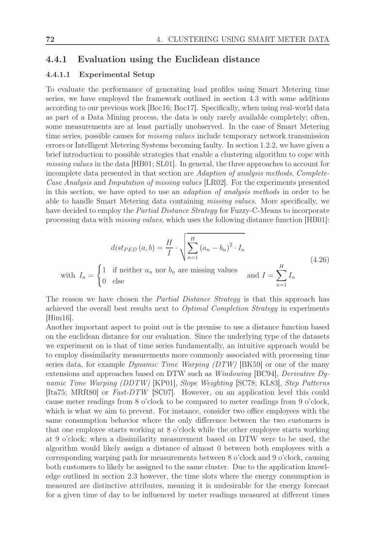
72 4. CLUSTERING USING SMART METER DATA
4.4.1 Evaluation using the Euclidean distance
4.4.1.1 Experimental Setup
To evaluate the performance of generating load profiles using Smart Metering timeseries, we have employed the framework outlined in section 4.3 with some additionsaccording to our previous work [Boc16; Boc17]. Specifically, when using real-world dataas part of a Data Mining process, the data is only rarely available completely; often,some measurements are at least partially unobserved. In the case of Smart Meteringtime series, possible causes for missing values include temporary network transmissionerrors or Intelligent Metering Systems becoming faulty. In section 1.2.2, we have given abrief introduction to possible strategies that enable a clustering algorithm to cope withmissing values in the data [HB01; SL01]. In general, the three approaches to account forincomplete data presented in that section are Adaption of analysis methods, Complete-Case Analysis and Imputation of missing values [LR02]. For the experiments presentedin this section, we have opted to use an adaption of analysis methods in order to beable to handle Smart Metering data containing missing values. More specifically, wehave decided to employ the Partial Distance Strategy for Fuzzy-C-Means to incorporateprocessing data with missing values, which uses the following distance function [HB01]:
distPED (a, b) =H
I·
√
√
√
√
H∑
n=1
(an − bn)2 · In
with In =
{
1 if neither an nor bn are missing values
0 elseand I =
H∑
n=1
In
(4.26)
The reason we have chosen the Partial Distance Strategy is that this approach hasachieved the overall best results next to Optimal Completion Strategy in experiments[Him16].Another important aspect to point out is the premise to use a distance function basedon the euclidean distance for our evaluation. Since the underlying type of the datasetswe experiment on is that of time series fundamentally, an intuitive approach would beto employ dissimilarity measurements more commonly associated with processing timeseries data, for example Dynamic Time Warping (DTW) [BK59] or one of the manyextensions and approaches based on DTW such as Windowing [BC94], Derivative Dy-namic Time Warping (DDTW) [KP01], Slope Weighting [SC78; KL83], Step Patterns[Ita75; MRR80] or Fast-DTW [SC07]. However, on an application level this couldcause meter readings from 8 o’clock to be compared to meter readings from 9 o’clock,which is what we aim to prevent. For instance, consider two office employees with thesame consumption behavior where the only difference between the two customers isthat one employee starts working at 8 o’clock while the other employee starts workingat 9 o’clock; when a dissimilarity measurement based on DTW were to be used, thealgorithm would likely assign a distance of almost 0 between both employees with acorresponding warping path for measurements between 8 o’clock and 9 o’clock, causingboth customers to likely be assigned to the same cluster. Due to the application knowl-edge outlined in section 2.3 however, the time slots where the energy consumption ismeasured are distinctive attributes, meaning it is undesirable for the energy forecastfor a given time of day to be influenced by meter readings measured at different times
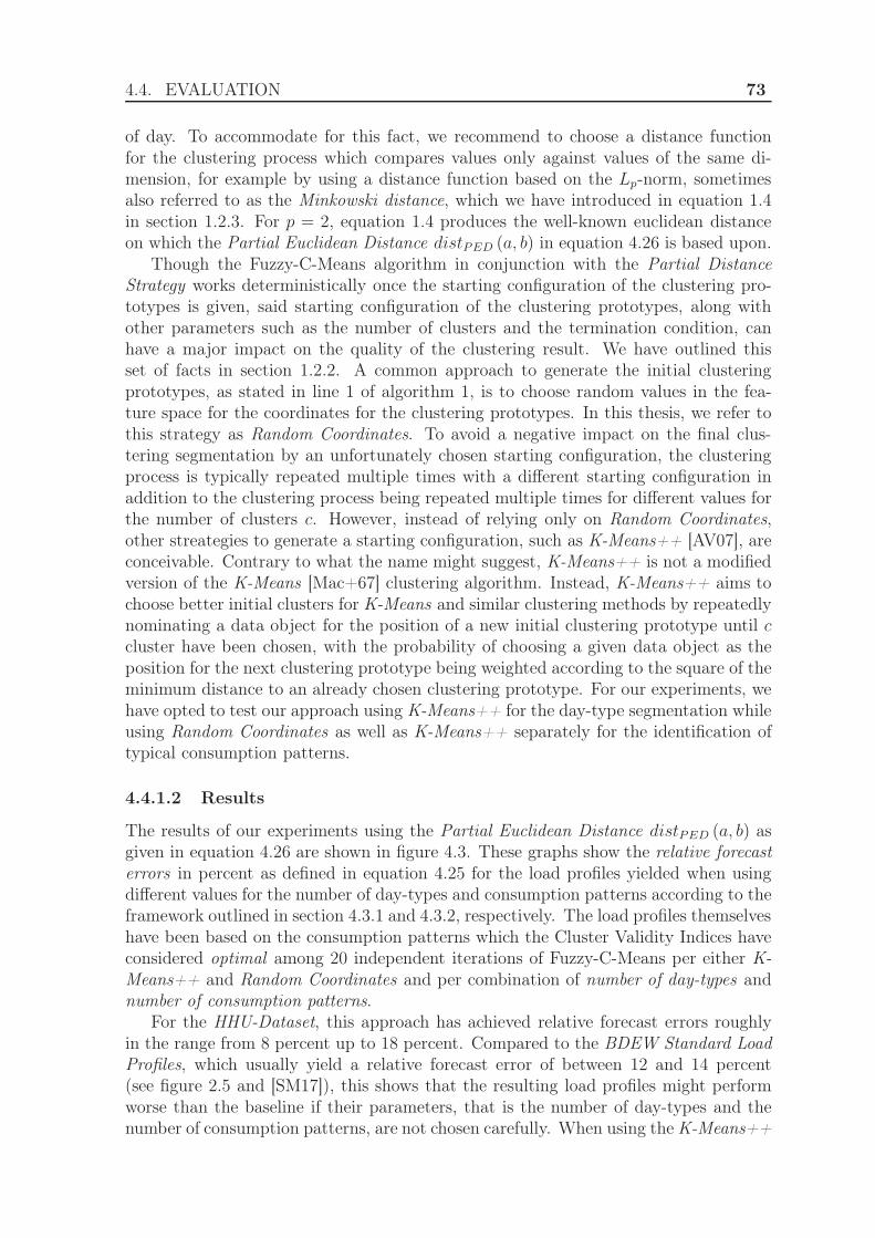
4.4. EVALUATION 73
of day. To accommodate for this fact, we recommend to choose a distance functionfor the clustering process which compares values only against values of the same di-mension, for example by using a distance function based on the Lp-norm, sometimesalso referred to as the Minkowski distance, which we have introduced in equation 1.4in section 1.2.3. For p = 2, equation 1.4 produces the well-known euclidean distanceon which the Partial Euclidean Distance distPED (a, b) in equation 4.26 is based upon.
Though the Fuzzy-C-Means algorithm in conjunction with the Partial DistanceStrategy works deterministically once the starting configuration of the clustering pro-totypes is given, said starting configuration of the clustering prototypes, along withother parameters such as the number of clusters and the termination condition, canhave a major impact on the quality of the clustering result. We have outlined thisset of facts in section 1.2.2. A common approach to generate the initial clusteringprototypes, as stated in line 1 of algorithm 1, is to choose random values in the fea-ture space for the coordinates for the clustering prototypes. In this thesis, we refer tothis strategy as Random Coordinates. To avoid a negative impact on the final clus-tering segmentation by an unfortunately chosen starting configuration, the clusteringprocess is typically repeated multiple times with a different starting configuration inaddition to the clustering process being repeated multiple times for different values forthe number of clusters c. However, instead of relying only on Random Coordinates,other streategies to generate a starting configuration, such as K-Means++ [AV07], areconceivable. Contrary to what the name might suggest, K-Means++ is not a modifiedversion of the K-Means [Mac+67] clustering algorithm. Instead, K-Means++ aims tochoose better initial clusters for K-Means and similar clustering methods by repeatedlynominating a data object for the position of a new initial clustering prototype until ccluster have been chosen, with the probability of choosing a given data object as theposition for the next clustering prototype being weighted according to the square of theminimum distance to an already chosen clustering prototype. For our experiments, wehave opted to test our approach using K-Means++ for the day-type segmentation whileusing Random Coordinates as well as K-Means++ separately for the identification oftypical consumption patterns.
4.4.1.2 Results
The results of our experiments using the Partial Euclidean Distance distPED (a, b) asgiven in equation 4.26 are shown in figure 4.3. These graphs show the relative forecasterrors in percent as defined in equation 4.25 for the load profiles yielded when usingdifferent values for the number of day-types and consumption patterns according to theframework outlined in section 4.3.1 and 4.3.2, respectively. The load profiles themselveshave been based on the consumption patterns which the Cluster Validity Indices haveconsidered optimal among 20 independent iterations of Fuzzy-C-Means per either K-Means++ and Random Coordinates and per combination of number of day-types andnumber of consumption patterns.
For the HHU-Dataset, this approach has achieved relative forecast errors roughlyin the range from 8 percent up to 18 percent. Compared to the BDEW Standard LoadProfiles, which usually yield a relative forecast error of between 12 and 14 percent(see figure 2.5 and [SM17]), this shows that the resulting load profiles might performworse than the baseline if their parameters, that is the number of day-types and thenumber of consumption patterns, are not chosen carefully. When using the K-Means++
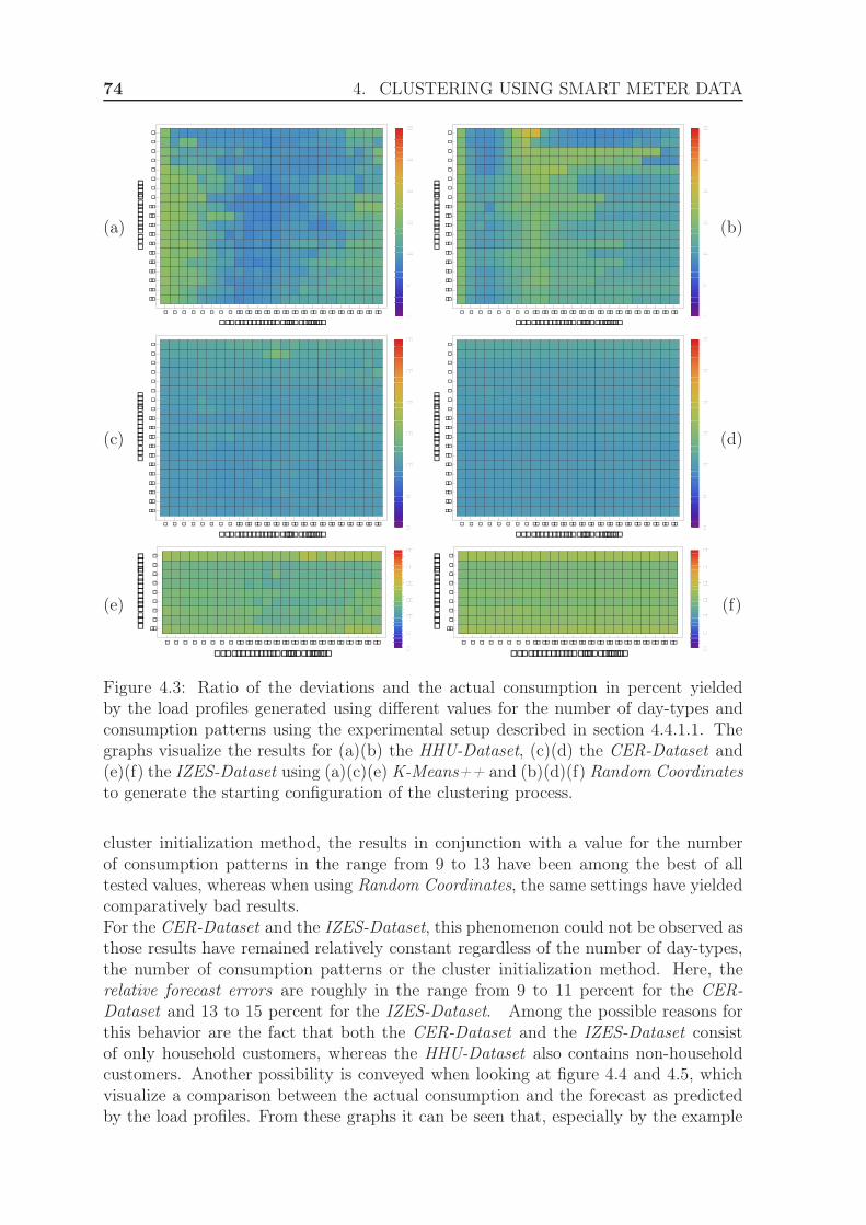
74 4. CLUSTERING USING SMART METER DATA
(a)
� � � � � � � � � � � � � � � � � � �� �� �� ��
�
�
�
�
�
�
�
�
�
�
�
�
�
�
�
�
�
������ �� ����� �� �� ���
����������� ��
0
5
10
15
20
25
30
� � � � � � � � � � � � � � � � � � �� �� �� ��
�
�
�
�
�
�
�
�
�
�
�
�
�
�
�
�
�
������ �� ����� �� �� ���
����������� ��
0
5
10
15
20
25
30
(b)
(c)
� � � � � � � � � � � � � � � � � � �� �� �� ��
�
�
�
�
�
�
�
�
�
�
�
�
�
�
�
�
�
������ �� ����� �� �� ���
����������� ��
0
5
10
15
20
25
30
� � � � � � � � � � � � � � � � � � �� �� �� ��
�
�
�
�
�
�
�
�
�
�
�
�
�
�
�
�
�
������ �� ����� �� �� ���
����������� ��
0
5
10
15
20
25
30
(d)
(e)
� � � � � � � � � � � � � � � � � � �� �� �� ��
�
�
�
�
�
�
�
�
������ �� ����� �� �� ���
����������� ��
0
5
10
15
20
25
30
� � � � � � � � � � � � � � � � � � �� �� �� ��
�
�
�
�
�
�
�
�
������ �� ����� �� �� ���
����������� ��
0
5
10
15
20
25
30
(f)
Figure 4.3: Ratio of the deviations and the actual consumption in percent yieldedby the load profiles generated using different values for the number of day-types andconsumption patterns using the experimental setup described in section 4.4.1.1. Thegraphs visualize the results for (a)(b) the HHU-Dataset, (c)(d) the CER-Dataset and(e)(f) the IZES-Dataset using (a)(c)(e) K-Means++ and (b)(d)(f) Random Coordinatesto generate the starting configuration of the clustering process.
cluster initialization method, the results in conjunction with a value for the numberof consumption patterns in the range from 9 to 13 have been among the best of alltested values, whereas when using Random Coordinates, the same settings have yieldedcomparatively bad results.For the CER-Dataset and the IZES-Dataset, this phenomenon could not be observed asthose results have remained relatively constant regardless of the number of day-types,the number of consumption patterns or the cluster initialization method. Here, therelative forecast errors are roughly in the range from 9 to 11 percent for the CER-Dataset and 13 to 15 percent for the IZES-Dataset. Among the possible reasons forthis behavior are the fact that both the CER-Dataset and the IZES-Dataset consistof only household customers, whereas the HHU-Dataset also contains non-householdcustomers. Another possibility is conveyed when looking at figure 4.4 and 4.5, whichvisualize a comparison between the actual consumption and the forecast as predictedby the load profiles. From these graphs it can be seen that, especially by the example
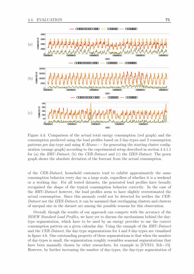
4.4. EVALUATION 75
(a)
������ ��������� ������ ���������
���������� ���������� ���������� ���������� ���������� �����������
����
���
���
����
� ��
������[��]
(b)
������ ��������� ������ ���������
���������� ���������� ���������� ���������� ���������� �����������
����
�����
�����
�����
��
������[��]
(c)
������ ��������� ������ ���������
���������� ���������� ���������� ���������� ����������
�
���
��
���
��
��
������[��]
Figure 4.4: Comparison of the actual total energy consumption (red graph) and theconsumption predicted using the load profiles based on 2 day-types and 2 consumptionpatterns per day-type and using K-Means++ for generating the starting cluster config-uration (orange graph) according to the experimental setup described in section 4.4.1.1for (a) the HHU-Dataset, (b) the CER-Dataset and (c) the IZES-Dataset. The greengraph shows the absolute deviation of the forecast from the actual consumption.
of the CER-Dataset, household customers tend to exhibit approximately the sameconsumption behavior every day on a large scale, regardless of whether it is a weekendor a working day. For all tested datasets, the generated load profiles have broadlyrecognized the shape of the typical consumption behavior correctly. In the case ofthe HHU-Dataset however, the load profiles seem to have slightly overestimated theactual consumption. Since this anomaly could not be detected for neither the CER-Dataset nor the IZES-Dataset, it can be assumed that overlapping clusters and clustersof unequal size in the dataset are among the possible reasons for this observation.
Overall, though the results of our approach can compete with the accuracy of theBDEW Standard Load Profiles, we have yet to discuss the mechanisms behind the day-type segmentation, which have to be used by an energy provider to use the correctconsumption pattern on a given calendar day. Using the example of the HHU-Datasetand the CER-Dataset, the day-type segmentations for 4 and 8 day-types are visualizedin figure 4.6. One outstanding property of these segmentations is that when the numberof day-types is small, the segmentation roughly resembles seasonal segmentations thathave been manually chosen by other researchers, for example in [VVS15; Sch+15].However, by further increasing the number of day-types, the day-type segmentation of

76 4. CLUSTERING USING SMART METER DATA
(a)
������ ��������� ������ ���������
���������� ���������� ���������� ���������� ���������� �����������
����
���
���
����
� ��
������[��]
(b)
������ ��������� ������ ���������
���������� ���������� ���������� ���������� ���������� �����������
����
�����
�����
�����
��
������[��]
(c)
������ ��������� ������ ���������
���������� ���������� ���������� ���������� ����������
�
���
��
���
��
��
������[��]
Figure 4.5: Comparison of the actual total energy consumption (red graph) and the con-sumption predicted using the load profiles based on 10 day-types and 25 consumptionpatterns per day-type and using K-Means++ for generating the starting cluster config-uration (orange graph) according to the experimental setup described in section 4.4.1.1for (a) the HHU-Dataset, (b) the CER-Dataset and (c) the IZES-Dataset. The greengraph shows the absolute deviation of the forecast from the actual consumption.
the datasets start to resemble that of a threshold filter, where the total energy consumedon a given calendar day has a more significant impact on the day-type classification thanthe shape of the consumption as a result of the behavior of customers. Since real-worldconsumption time series, such as the ones presented as part of our evaluation, tendto have seasonal patterns with a recognizable peak near the end of a year, modifyingour approach to take advantage of the regularity of these patterns is a promisingoptimization which we will pursue in the following sections.
4.4.2 Evaluation using the Manhattan distance
4.4.2.1 Experimental Setup
Some of the main aspects we want to take advantage of in order to further improveupon the approach presented in section 4.4.1 are the regular and often sine-like patternsthat become visible when looking at the total energy consumption of real-world SmartMetering datasets. For this purpose, we can make use of the fact that the specificationof load profiles includes the concept of a dynamization function, a tool that allows tomodel and thus exclude the recurrent patterns during the analysis. The idea behind this
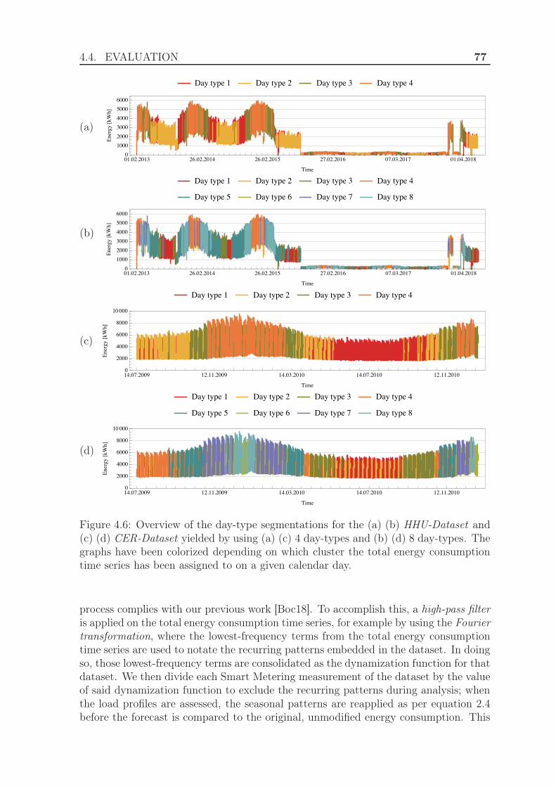
4.4. EVALUATION 77
(a) []
(b) []
(c) []
(d) []
Figure 4.6: Overview of the day-type segmentations for the (a) (b) HHU-Dataset and(c) (d) CER-Dataset yielded by using (a) (c) 4 day-types and (b) (d) 8 day-types. Thegraphs have been colorized depending on which cluster the total energy consumptiontime series has been assigned to on a given calendar day.
process complies with our previous work [Boc18]. To accomplish this, a high-pass filteris applied on the total energy consumption time series, for example by using the Fouriertransformation, where the lowest-frequency terms from the total energy consumptiontime series are used to notate the recurring patterns embedded in the dataset. In doingso, those lowest-frequency terms are consolidated as the dynamization function for thatdataset. We then divide each Smart Metering measurement of the dataset by the valueof said dynamization function to exclude the recurring patterns during analysis; whenthe load profiles are assessed, the seasonal patterns are reapplied as per equation 2.4before the forecast is compared to the original, unmodified energy consumption. This

78 4. CLUSTERING USING SMART METER DATA
allows the clustering process to focus on the shape of the daily consumption time seriesas opposed to being mostly influenced by the energy offset. As a consequence of thisprocedure, each energy provider may extract a unique dynamization function from thedata of their customer base. However, since the dynamization function is already partof the normal market communication the interoperability between energy providers isguaranteed where necessary [Bun06].Though the usage of a high-pass filter to derive a dynamization function has the po-tential to improve the clustering process, the resulting load profiles are more likelyto be region-specific since the dynamization function might encode recurring patternsunique to the underlying customer base. As experiments such as [SM17] have shown,region-specific load profiles can differ from the BDEW Standard Load Profiles quitesignificantly, tough more extensive evaluation is required to distinguish whether thesedifferences are caused mainly due to region-specific factors or changes in the customerbehavior over time. Complementary to this, [HRR14] mentions that region-specificload profiles have the potential to significantly improve upon non-region-specific loadprofiles. Because of this, energy providers seeking to minimize imbalance energy maywant to acknowledge a dynamization function as well as associated load profiles asbeing region-specific, causing them to use the forecasting models of a different region ifthey gain a new customer from said foreign region. For the datasets used in our evalu-ation, no regional information about the customer is present. Thus, we have opted toassume that all customers of a given dataset belong to the same region.In addition to the adoption of a dynamization function, we also modified the origi-nal Partial Distance Strategy to be based on the manhattan distance rather than theeuclidean distance:
distPMD (a, b) =H
I·
H∑
n=1
|an − bn| · In
with In =
{
1 if neither an nor bn are missing values
0 elseand I =
H∑
n=1
In
(4.27)
We refer to this distance measure as the Partial Manhattan Distance distPMD (a, b).Our motivation behind this change is to make the clustering process more sensitiveto the imbalance energy which we have introduced in section 2.2, as imbalance energycan be modeled as the manhattan distance between the actual consumption and theforecast time series.Additional, similar to our setup described in section 4.4.1.1, we have opted to use K-Means++ [AV07] for the day-type segmentation while employing Random Coordinatesas well as K-Means++ separately for the identification of typical consumption patterns.
4.4.2.2 Results
The first step in conducting the experiments as outlined above involved applying theFourier transformation on each dataset. The resulting dynamization functions arevisualized in figure 4.7. For the HHU-Dataset, the dynamization function has beentrained according to the Smart Metering data for the year 2014 and can be expressedas
DynFactorHHU (doy) = 1 + 0,23654 cos
(
2π · doy
365
)
+ 0,05169 sin
(
2π · doy
365
)
(4.28)
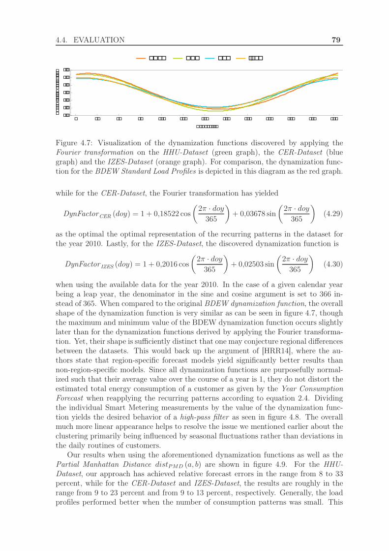
4.4. EVALUATION 79
���� ��� ��� ��
� �� �� �� ��� ��� ��� ��� �� �� ��� ��� �����
���
���
���
���
���
���
� � �� �� �
������������� ����
Figure 4.7: Visualization of the dynamization functions discovered by applying theFourier transformation on the HHU-Dataset (green graph), the CER-Dataset (bluegraph) and the IZES-Dataset (orange graph). For comparison, the dynamization func-tion for the BDEW Standard Load Profiles is depicted in this diagram as the red graph.
while for the CER-Dataset, the Fourier transformation has yielded
DynFactorCER (doy) = 1 + 0,18522 cos
(
2π · doy
365
)
+ 0,03678 sin
(
2π · doy
365
)
(4.29)
as the optimal the optimal representation of the recurring patterns in the dataset forthe year 2010. Lastly, for the IZES-Dataset, the discovered dynamization function is
DynFactor IZES (doy) = 1 + 0,2016 cos
(
2π · doy
365
)
+ 0,02503 sin
(
2π · doy
365
)
(4.30)
when using the available data for the year 2010. In the case of a given calendar yearbeing a leap year, the denominator in the sine and cosine argument is set to 366 in-stead of 365. When compared to the original BDEW dynamization function, the overallshape of the dynamization function is very similar as can be seen in figure 4.7, thoughthe maximum and minimum value of the BDEW dynamization function occurs slightlylater than for the dynamization functions derived by applying the Fourier transforma-tion. Yet, their shape is sufficiently distinct that one may conjecture regional differencesbetween the datasets. This would back up the argument of [HRR14], where the au-thors state that region-specific forecast models yield significantly better results thannon-region-specific models. Since all dynamization functions are purposefully normal-ized such that their average value over the course of a year is 1, they do not distort theestimated total energy consumption of a customer as given by the Year ConsumptionForecast when reapplying the recurring patterns according to equation 2.4. Dividingthe individual Smart Metering measurements by the value of the dynamization func-tion yields the desired behavior of a high-pass filter as seen in figure 4.8. The overallmuch more linear appearance helps to resolve the issue we mentioned earlier about theclustering primarily being influenced by seasonal fluctuations rather than deviations inthe daily routines of customers.
Our results when using the aforementioned dynamization functions as well as thePartial Manhattan Distance distPMD (a, b) are shown in figure 4.9. For the HHU-Dataset, our approach has achieved relative forecast errors in the range from 8 to 33percent, while for the CER-Dataset and IZES-Dataset, the results are roughly in therange from 9 to 23 percent and from 9 to 13 percent, respectively. Generally, the loadprofiles performed better when the number of consumption patterns was small. This
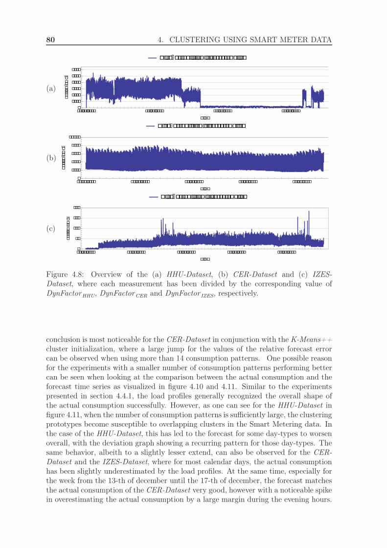
80 4. CLUSTERING USING SMART METER DATA
(a)
����-���� ���� �� ����������
���������� ���������� ��������� ����������
����
����
����
����
����
���
� ��
������[��]
(b)
����-���� ���� �� ����������
���������� ���������� ���������� ���������� �����������
����
����
���
���
�����
�� �
������[��]
(c)
����-���� ���� �� ����������
���������� ���������� ���������� ���������� �����������
��
���
���
���
��
������[��]
Figure 4.8: Overview of the (a) HHU-Dataset, (b) CER-Dataset and (c) IZES-Dataset, where each measurement has been divided by the corresponding value ofDynFactorHHU, DynFactorCER and DynFactor IZES, respectively.
conclusion is most noticeable for the CER-Dataset in conjunction with the K-Means++cluster initialization, where a large jump for the values of the relative forecast errorcan be observed when using more than 14 consumption patterns. One possible reasonfor the experiments with a smaller number of consumption patterns performing bettercan be seen when looking at the comparison between the actual consumption and theforecast time series as visualized in figure 4.10 and 4.11. Similar to the experimentspresented in section 4.4.1, the load profiles generally recognized the overall shape ofthe actual consumption successfully. However, as one can see for the HHU-Dataset infigure 4.11, when the number of consumption patterns is sufficiently large, the clusteringprototypes become susceptible to overlapping clusters in the Smart Metering data. Inthe case of the HHU-Dataset, this has led to the forecast for some day-types to worsenoverall, with the deviation graph showing a recurring pattern for those day-types. Thesame behavior, albeith to a slightly lesser extend, can also be observed for the CER-Dataset and the IZES-Dataset, where for most calendar days, the actual consumptionhas been slightly underestimated by the load profiles. At the same time, especially forthe week from the 13-th of december until the 17-th of december, the forecast matchesthe actual consumption of the CER-Dataset very good, however with a noticeable spikein overestimating the actual consumption by a large margin during the evening hours.

4.4. EVALUATION 81
(a)
� � � � � � � � � � � � � � � � � � �� �� �� ��
�
�
�
�
�
�
�
�
�
�
�
�
�
�
�
�
�
������ �� ����� �� �� ���
����������� ��
0
5
10
15
20
25
30
� � � � � � � � � � � � � � � � � � �� �� �� ��
�
�
�
�
�
�
�
�
�
�
�
�
�
�
�
�
�
������ �� ����� �� �� ���
����������� ��
0
5
10
15
20
25
30
(b)
(c)
� � � � � � � � � � � � � � � � � � �� �� �� ��
�
�
�
�
�
�
�
�
�
�
�
�
�
�
�
�
�
������ �� ����� �� �� ���
����������� ��
0
5
10
15
20
25
30
� � � � � � � � � � � � � � � � � � �� �� �� ��
�
�
�
�
�
�
�
�
�
�
�
�
�
�
�
�
�
������ �� ����� �� �� ���
����������� ��
0
5
10
15
20
25
30
(d)
(e)
� � � � � � � � � � � � � � � � � � �� �� �� ��
�
�
�
�
�
�
�
�
������ �� ����� �� �� ���
����������� ��
0
5
10
15
20
25
30
� � � � � � � � � � � � � � � � � � �� �� �� ��
�
�
�
�
�
�
�
�
������ �� ����� �� �� ���
����������� ��
0
5
10
15
20
25
30
(f)
Figure 4.9: Ratio of the deviations and the actual consumption in percent yieldedby the load profiles generated using different values for the number of day-types andconsumption patterns using the experimental setup described in section 4.4.2.1. Thegraphs visualize the results for (a)(b) the HHU-Dataset, (c)(d) the CER-Dataset and(e)(f) the IZES-Dataset using (a)(c)(e) K-Means++ and (b)(d)(f) Random Coordinatesto generate the starting configuration of the clustering process.
4.4.3 Evaluation using the exponential Manhattan distance
4.4.3.1 Experimental Setup
As mentioned in section 2.2, one of the most important criterions for energy providerswhen assessing the performance of forecast models is minimizing the amount of im-balance energy caused by them. Notably, unexpected spikes in energy consumptionare more undesirable than misvalued uniform consumption due to the financial riskinvolved. The evaluation of our experiments in the previous sections has shown thatwhile the algorithm successfully identified the overall shape of the consumption, thedeviation graphs have shown recurring patterns as well as imbalance energy spikes inthe evening hours. One possible explanation for imbalance energy spikes in the eveninghours is that the tuples in the dataset match during daytime and the deviations duringthe evening hours do not warrant splitting the tuples into separate clusters. Because of
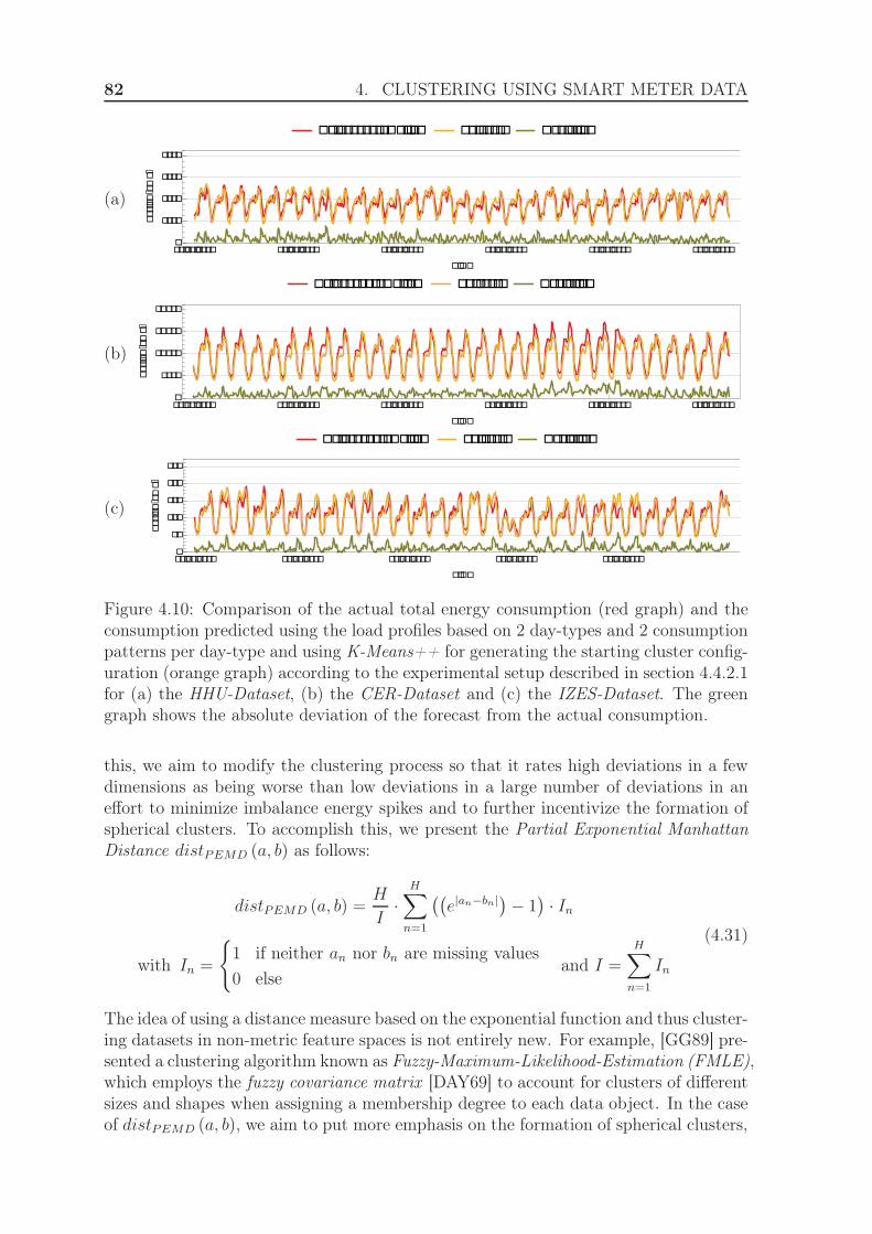
82 4. CLUSTERING USING SMART METER DATA
(a)
������ ��������� ������ ���������
���������� ���������� ���������� ���������� ���������� �����������
����
���
���
����
� ��
������[��]
(b)
������ ��������� ������ ���������
���������� ���������� ���������� ���������� ���������� �����������
����
�����
�����
�����
��
������[��]
(c)
������ ��������� ������ ���������
���������� ���������� ���������� ���������� ����������
�
���
��
���
��
��
������[��]
Figure 4.10: Comparison of the actual total energy consumption (red graph) and theconsumption predicted using the load profiles based on 2 day-types and 2 consumptionpatterns per day-type and using K-Means++ for generating the starting cluster config-uration (orange graph) according to the experimental setup described in section 4.4.2.1for (a) the HHU-Dataset, (b) the CER-Dataset and (c) the IZES-Dataset. The greengraph shows the absolute deviation of the forecast from the actual consumption.
this, we aim to modify the clustering process so that it rates high deviations in a fewdimensions as being worse than low deviations in a large number of deviations in aneffort to minimize imbalance energy spikes and to further incentivize the formation ofspherical clusters. To accomplish this, we present the Partial Exponential ManhattanDistance distPEMD (a, b) as follows:
distPEMD (a, b) =H
I·
H∑
n=1
((
e|an−bn|)
− 1)
· In
with In =
{
1 if neither an nor bn are missing values
0 elseand I =
H∑
n=1
In
(4.31)
The idea of using a distance measure based on the exponential function and thus cluster-ing datasets in non-metric feature spaces is not entirely new. For example, [GG89] pre-sented a clustering algorithm known as Fuzzy-Maximum-Likelihood-Estimation (FMLE),which employs the fuzzy covariance matrix [DAY69] to account for clusters of differentsizes and shapes when assigning a membership degree to each data object. In the caseof distPEMD (a, b), we aim to put more emphasis on the formation of spherical clusters,
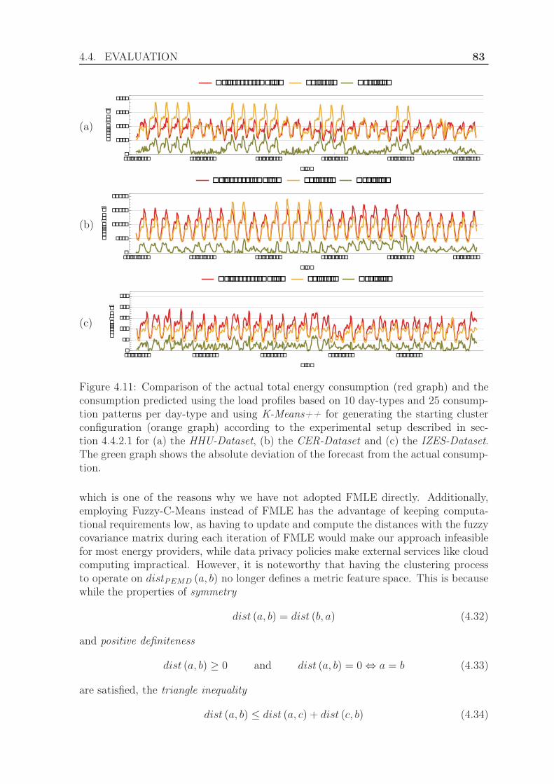
4.4. EVALUATION 83
(a)
������ ��������� ������ ���������
���������� ���������� ���������� ���������� ���������� �����������
����
���
���
����
� ��
������[��]
(b)
������ ��������� ������ ���������
���������� ���������� ���������� ���������� ���������� �����������
����
�����
�����
�����
��
������[��]
(c)
������ ��������� ������ ���������
���������� ���������� ���������� ���������� ����������
�
���
��
���
��
��
������[��]
Figure 4.11: Comparison of the actual total energy consumption (red graph) and theconsumption predicted using the load profiles based on 10 day-types and 25 consump-tion patterns per day-type and using K-Means++ for generating the starting clusterconfiguration (orange graph) according to the experimental setup described in sec-tion 4.4.2.1 for (a) the HHU-Dataset, (b) the CER-Dataset and (c) the IZES-Dataset.The green graph shows the absolute deviation of the forecast from the actual consump-tion.
which is one of the reasons why we have not adopted FMLE directly. Additionally,employing Fuzzy-C-Means instead of FMLE has the advantage of keeping computa-tional requirements low, as having to update and compute the distances with the fuzzycovariance matrix during each iteration of FMLE would make our approach infeasiblefor most energy providers, while data privacy policies make external services like cloudcomputing impractical. However, it is noteworthy that having the clustering processto operate on distPEMD (a, b) no longer defines a metric feature space. This is becausewhile the properties of symmetry
dist (a, b) = dist (b, a) (4.32)
and positive definiteness
dist (a, b) ≥ 0 and dist (a, b) = 0 ⇔ a = b (4.33)
are satisfied, the triangle inequality
dist (a, b) ≤ dist (a, c) + dist (c, b) (4.34)

84 4. CLUSTERING USING SMART METER DATA
is violated. As a one-dimensional counterexample for this, consider the case of a = 1,b = 7 and c = 4:
distPEMD (a, b) = e6 − 1 � 2 · e3 − 2 = distPEMD (a, c) + distPEMD (c, b) (4.35)
One may suspect that, due to both methods using a distance measure based on theexponential function, a lot of properties that are applicable to FMLE also apply to aclustering process based on distPEMD (a, b). For example, [GG89] stresses the impor-tance of a good starting configuration for FMLE as the algorithm quickly converges toa local optimum in a narrow region.In addition to the Partial Exponential Manhattan Distance distPEMD (a, b), we haveemployed the same dynamization functions as in section 4.4.2 as well as both K-Means++ [AV07] and Random Coordinates to generate the starting configuration ofthe clustering process when identifying typical consumption pattern, while using K-Means++ during the day-type segmentation.
4.4.3.2 Results
The results of our experiments when using the Partial Exponential Manhattan DistancedistPEMD (a, b) are visualized in figure 4.12.
One apparent property when comparing these results with the ones presented infigure 4.9 is that the overall performance of the load profiles is roughly the same: forthe HHU-Dataset, the approach based on the Partial Exponential Manhattan DistancedistPEMD (a, b) has achieved relative forecast errors from 8 to 33 percent. Similarly, forthe CER-Dataset the results are roughly in the range from 9 to 16 percent, while forthe IZES-Dataset, the results for the relative forecast errors range from 9 to 13 percent.Though the results have improved only marginally for the HHU-Dataset and the IZES-Dataset, the results for the CER-Dataset have improved noticeable when using a largevalue for the number of consumption patterns. As such, the stronger incentive of theclustering process to build spherical clusters appears to be a plausible explanation forthe increase in performance. Aside from that, the results fall in line with the loadprofiles from the experiments presented in section 4.4.2 as can be seen when comparingfigure 4.13 and 4.14 with the results from figure 4.10 and 4.11. However, since the loadprofiles presented in this section have not eliminated some of the problems with thePartial Manhattan Distance distPMD (a, b) such as the peaks in the relative forecasterror during the evening hours as visualized in figure 4.11, it can be assumed that astronger emphasis on the formation of spherical clusters is not sufficient to improve theoverall quality of the resulting load profiles.
4.4.4 Evaluation using weighted clustering
4.4.4.1 Experimental Setup
Some of the areas where the load profiles presented in the previous sections can beimproved the most are the peculiar offsets, where the overall shape of the consumptionhas been predicted accurately, but multiplicative scalars between the actual consump-tion and the forecast either during whole calendar days or during short time periodshave caused a large amount of imbalance energy. These offsets for whole calendardays can be seen in figure 4.14 (a), for example. Since these offsets only occur during
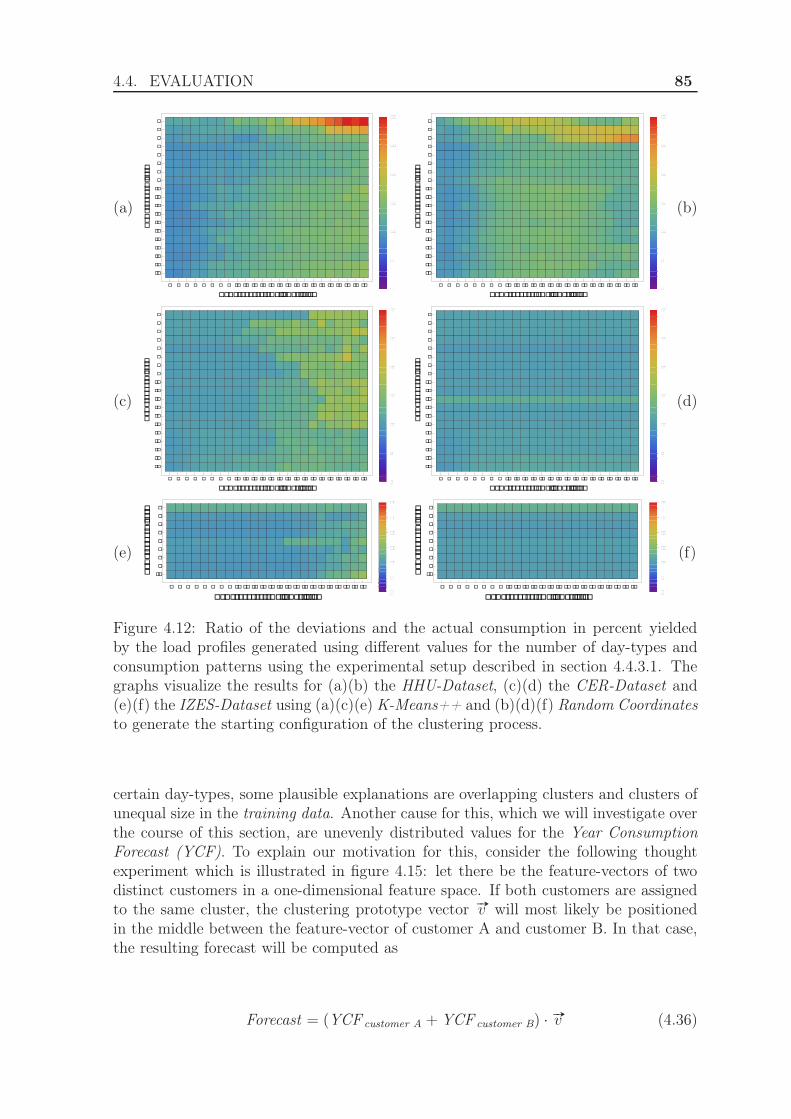
4.4. EVALUATION 85
(a)
� � � � � � � � � � � � � � � � � � �� �� �� ��
�
�
�
�
�
�
�
�
�
�
�
�
�
�
�
�
�
������ �� ����� �� �� ���
����������� ��
0
5
10
15
20
25
30
� � � � � � � � � � � � � � � � � � �� �� �� ��
�
�
�
�
�
�
�
�
�
�
�
�
�
�
�
�
�
������ �� ����� �� �� ���
����������� ��
0
5
10
15
20
25
30
(b)
(c)
� � � � � � � � � � � � � � � � � � �� �� �� ��
�
�
�
�
�
�
�
�
�
�
�
�
�
�
�
�
�
������ �� ����� �� �� ���
����������� ��
0
5
10
15
20
25
30
� � � � � � � � � � � � � � � � � � �� �� �� ��
�
�
�
�
�
�
�
�
�
�
�
�
�
�
�
�
�
������ �� ����� �� �� ���
����������� ��
0
5
10
15
20
25
30
(d)
(e)
� � � � � � � � � � � � � � � � � � �� �� �� ��
�
�
�
�
�
�
�
�
������ �� ����� �� �� ���
����������� ��
0
5
10
15
20
25
30
� � � � � � � � � � � � � � � � � � �� �� �� ��
�
�
�
�
�
�
�
�
������ �� ����� �� �� ���
����������� ��
0
5
10
15
20
25
30
(f)
Figure 4.12: Ratio of the deviations and the actual consumption in percent yieldedby the load profiles generated using different values for the number of day-types andconsumption patterns using the experimental setup described in section 4.4.3.1. Thegraphs visualize the results for (a)(b) the HHU-Dataset, (c)(d) the CER-Dataset and(e)(f) the IZES-Dataset using (a)(c)(e) K-Means++ and (b)(d)(f) Random Coordinatesto generate the starting configuration of the clustering process.
certain day-types, some plausible explanations are overlapping clusters and clusters ofunequal size in the training data. Another cause for this, which we will investigate overthe course of this section, are unevenly distributed values for the Year ConsumptionForecast (YCF). To explain our motivation for this, consider the following thoughtexperiment which is illustrated in figure 4.15: let there be the feature-vectors of twodistinct customers in a one-dimensional feature space. If both customers are assignedto the same cluster, the clustering prototype vector #»v will most likely be positionedin the middle between the feature-vector of customer A and customer B. In that case,the resulting forecast will be computed as
Forecast = (YCF customer A + YCF customer B) ·#»v (4.36)
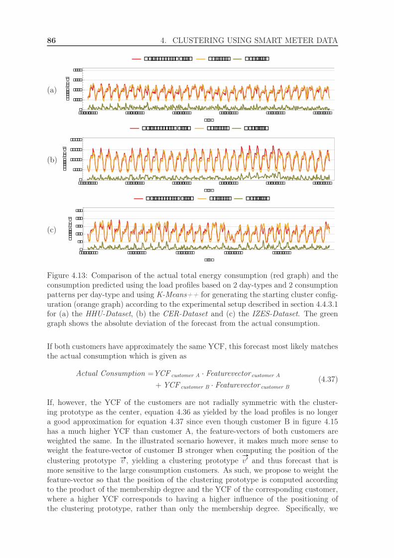
86 4. CLUSTERING USING SMART METER DATA
(a)
������ ��������� ������ ���������
���������� ���������� ���������� ���������� ���������� �����������
����
���
���
����
� ��
������[��]
(b)
������ ��������� ������ ���������
���������� ���������� ���������� ���������� ���������� �����������
����
�����
�����
�����
��
������[��]
(c)
������ ��������� ������ ���������
���������� ���������� ���������� ���������� ����������
�
���
��
���
��
��
������[��]
Figure 4.13: Comparison of the actual total energy consumption (red graph) and theconsumption predicted using the load profiles based on 2 day-types and 2 consumptionpatterns per day-type and using K-Means++ for generating the starting cluster config-uration (orange graph) according to the experimental setup described in section 4.4.3.1for (a) the HHU-Dataset, (b) the CER-Dataset and (c) the IZES-Dataset. The greengraph shows the absolute deviation of the forecast from the actual consumption.
If both customers have approximately the same YCF, this forecast most likely matchesthe actual consumption which is given as
Actual Consumption =YCF customer A · Featurevectorcustomer A
+ YCF customer B · Featurevector customer B
(4.37)
If, however, the YCF of the customers are not radially symmetric with the cluster-ing prototype as the center, equation 4.36 as yielded by the load profiles is no longera good approximation for equation 4.37 since even though customer B in figure 4.15has a much higher YCF than customer A, the feature-vectors of both customers areweighted the same. In the illustrated scenario however, it makes much more sense toweight the feature-vector of customer B stronger when computing the position of theclustering prototype #»v , yielding a clustering prototype
#»
v′ and thus forecast that ismore sensitive to the large consumption customers. As such, we propose to weight thefeature-vector so that the position of the clustering prototype is computed accordingto the product of the membership degree and the YCF of the corresponding customer,where a higher YCF corresponds to having a higher influence of the positioning ofthe clustering prototype, rather than only the membership degree. Specifically, we
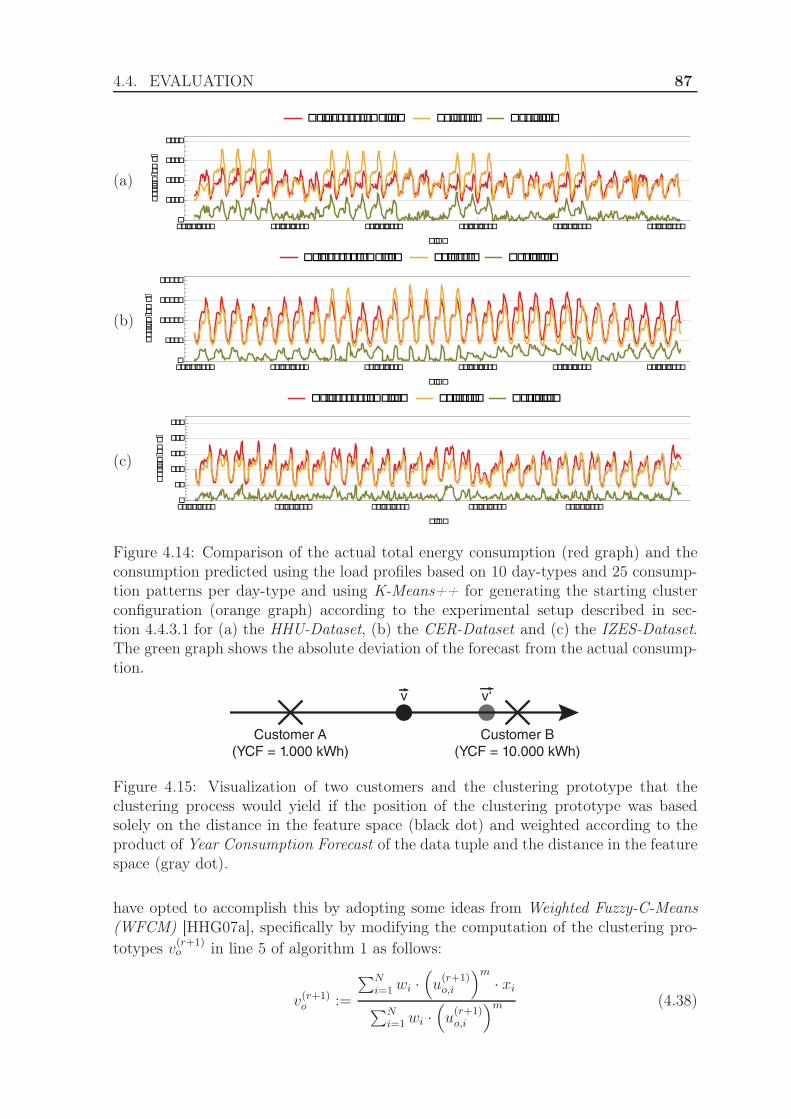
4.4. EVALUATION 87
(a)
������ ��������� ������ ���������
���������� ���������� ���������� ���������� ���������� �����������
����
���
���
����
� ��
������[��]
(b)
������ ��������� ������ ���������
���������� ���������� ���������� ���������� ���������� �����������
����
�����
�����
�����
��
������[��]
(c)
������ ��������� ������ ���������
���������� ���������� ���������� ���������� ����������
�
���
��
���
��
��
������[��]
Figure 4.14: Comparison of the actual total energy consumption (red graph) and theconsumption predicted using the load profiles based on 10 day-types and 25 consump-tion patterns per day-type and using K-Means++ for generating the starting clusterconfiguration (orange graph) according to the experimental setup described in sec-tion 4.4.3.1 for (a) the HHU-Dataset, (b) the CER-Dataset and (c) the IZES-Dataset.The green graph shows the absolute deviation of the forecast from the actual consump-tion.
Customer A
(YCF = 1.000 kWh)
Customer B
(YCF = 10.000 kWh)
v v‘
Figure 4.15: Visualization of two customers and the clustering prototype that theclustering process would yield if the position of the clustering prototype was basedsolely on the distance in the feature space (black dot) and weighted according to theproduct of Year Consumption Forecast of the data tuple and the distance in the featurespace (gray dot).
have opted to accomplish this by adopting some ideas from Weighted Fuzzy-C-Means(WFCM) [HHG07a], specifically by modifying the computation of the clustering pro-totypes v
(r+1)o in line 5 of algorithm 1 as follows:
v(r+1)o :=
∑N
i=1 wi ·(
u(r+1)o,i
)m
· xi
∑N
i=1wi ·(
u(r+1)o,i
)m (4.38)
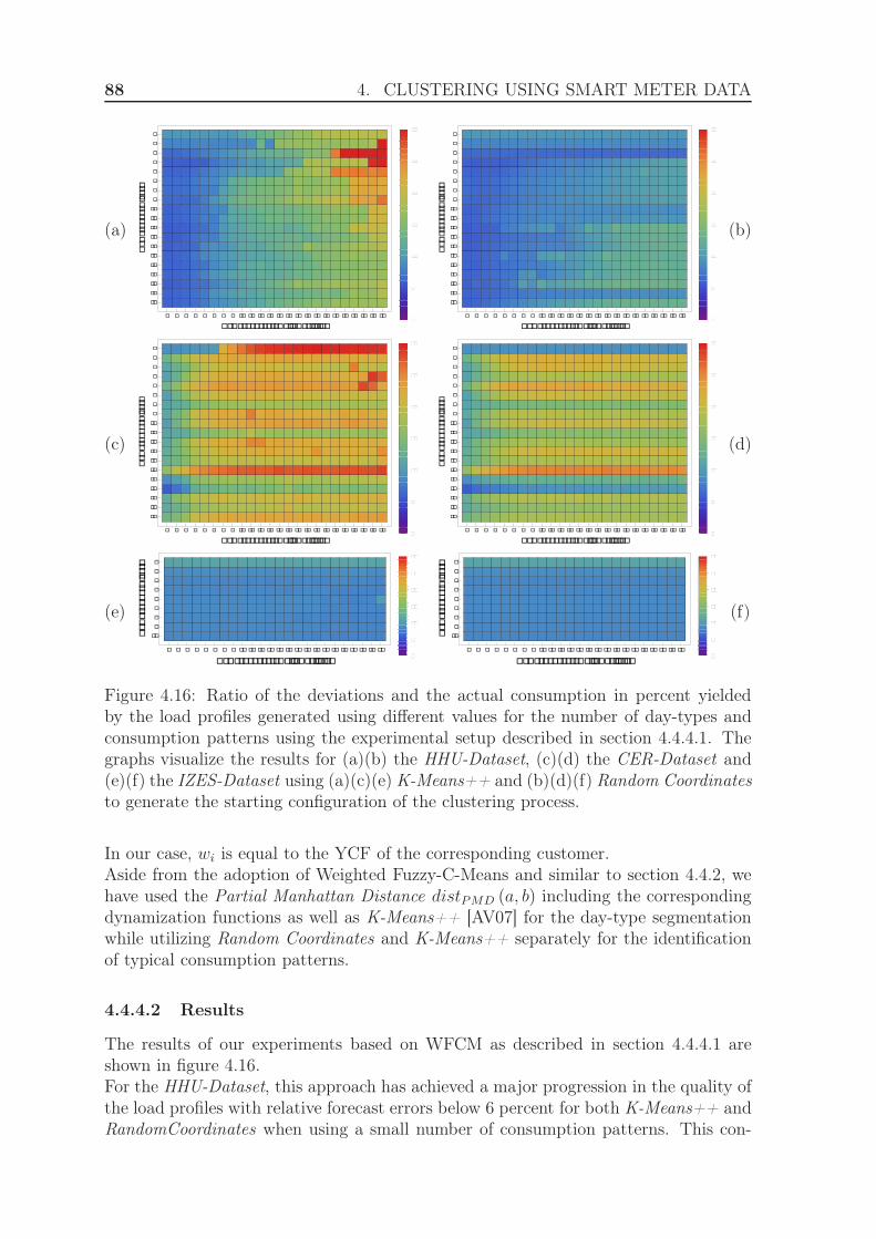
88 4. CLUSTERING USING SMART METER DATA
(a)
� � � � � � � � � � � � � � � � � � �� �� �� ��
�
�
�
�
�
�
�
�
�
�
�
�
�
�
�
�
�
������ �� ����� �� �� ���
����������� ��
0
5
10
15
20
25
30
� � � � � � � � � � � � � � � � � � �� �� �� ��
�
�
�
�
�
�
�
�
�
�
�
�
�
�
�
�
�
������ �� ����� �� �� ���
����������� ��
0
5
10
15
20
25
30
(b)
(c)
� � � � � � � � � � � � � � � � � � �� �� �� ��
�
�
�
�
�
�
�
�
�
�
�
�
�
�
�
�
�
������ �� ����� �� �� ���
����������� ��
0
5
10
15
20
25
30
� � � � � � � � � � � � � � � � � � �� �� �� ��
�
�
�
�
�
�
�
�
�
�
�
�
�
�
�
�
�
������ �� ����� �� �� ���
����������� ��
0
5
10
15
20
25
30
(d)
(e)
� � � � � � � � � � � � � � � � � � �� �� �� ��
�
�
�
�
�
�
�
�
������ �� ����� �� �� ���
����������� ��
0
5
10
15
20
25
30
� � � � � � � � � � � � � � � � � � �� �� �� ��
�
�
�
�
�
�
�
�
������ �� ����� �� �� ���
����������� ��
0
5
10
15
20
25
30
(f)
Figure 4.16: Ratio of the deviations and the actual consumption in percent yieldedby the load profiles generated using different values for the number of day-types andconsumption patterns using the experimental setup described in section 4.4.4.1. Thegraphs visualize the results for (a)(b) the HHU-Dataset, (c)(d) the CER-Dataset and(e)(f) the IZES-Dataset using (a)(c)(e) K-Means++ and (b)(d)(f) Random Coordinatesto generate the starting configuration of the clustering process.
In our case, wi is equal to the YCF of the corresponding customer.Aside from the adoption of Weighted Fuzzy-C-Means and similar to section 4.4.2, wehave used the Partial Manhattan Distance distPMD (a, b) including the correspondingdynamization functions as well as K-Means++ [AV07] for the day-type segmentationwhile utilizing Random Coordinates and K-Means++ separately for the identificationof typical consumption patterns.
4.4.4.2 Results
The results of our experiments based on WFCM as described in section 4.4.4.1 areshown in figure 4.16.For the HHU-Dataset, this approach has achieved a major progression in the quality ofthe load profiles with relative forecast errors below 6 percent for both K-Means++ andRandomCoordinates when using a small number of consumption patterns. This con-
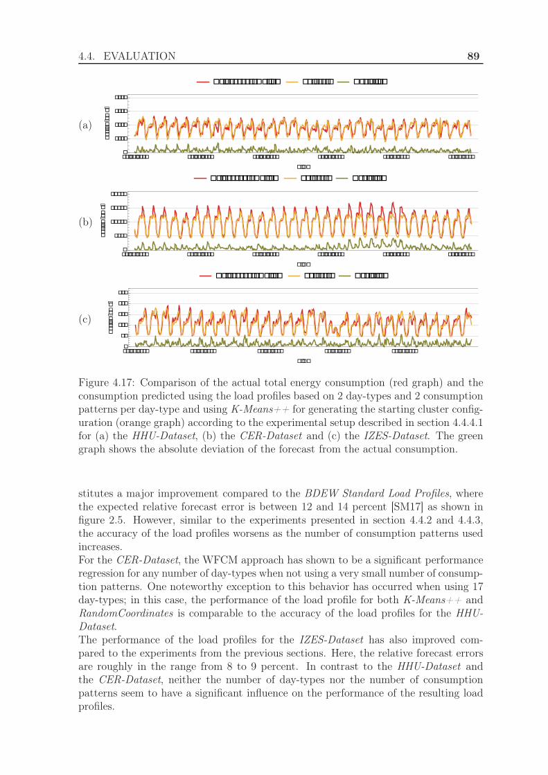
4.4. EVALUATION 89
(a)
������ ��������� ������ ���������
���������� ���������� ���������� ���������� ���������� �����������
����
���
���
����
� ��
������[��]
(b)
������ ��������� ������ ���������
���������� ���������� ���������� ���������� ���������� �����������
����
�����
�����
�����
��
������[��]
(c)
������ ��������� ������ ���������
���������� ���������� ���������� ���������� ����������
�
���
��
���
��
��
������[��]
Figure 4.17: Comparison of the actual total energy consumption (red graph) and theconsumption predicted using the load profiles based on 2 day-types and 2 consumptionpatterns per day-type and using K-Means++ for generating the starting cluster config-uration (orange graph) according to the experimental setup described in section 4.4.4.1for (a) the HHU-Dataset, (b) the CER-Dataset and (c) the IZES-Dataset. The greengraph shows the absolute deviation of the forecast from the actual consumption.
stitutes a major improvement compared to the BDEW Standard Load Profiles, wherethe expected relative forecast error is between 12 and 14 percent [SM17] as shown infigure 2.5. However, similar to the experiments presented in section 4.4.2 and 4.4.3,the accuracy of the load profiles worsens as the number of consumption patterns usedincreases.For the CER-Dataset, the WFCM approach has shown to be a significant performanceregression for any number of day-types when not using a very small number of consump-tion patterns. One noteworthy exception to this behavior has occurred when using 17day-types; in this case, the performance of the load profile for both K-Means++ andRandomCoordinates is comparable to the accuracy of the load profiles for the HHU-Dataset.The performance of the load profiles for the IZES-Dataset has also improved com-pared to the experiments from the previous sections. Here, the relative forecast errorsare roughly in the range from 8 to 9 percent. In contrast to the HHU-Dataset andthe CER-Dataset, neither the number of day-types nor the number of consumptionpatterns seem to have a significant influence on the performance of the resulting loadprofiles.
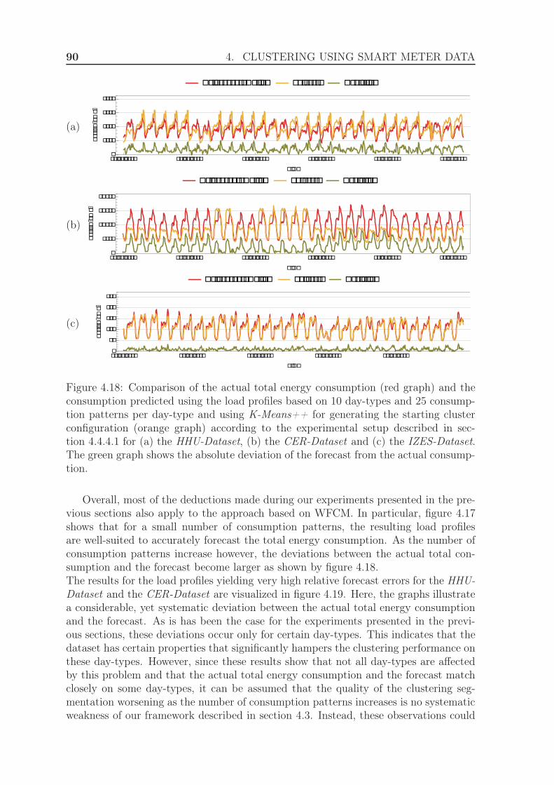
90 4. CLUSTERING USING SMART METER DATA
(a)
������ ��������� ������ ���������
���������� ���������� ���������� ���������� ���������� �����������
����
���
���
����
� ��
������[��]
(b)
������ ��������� ������ ���������
���������� ���������� ���������� ���������� ���������� �����������
����
�����
�����
�����
��
������[��]
(c)
������ ��������� ������ ���������
���������� ���������� ���������� ���������� ����������
�
���
��
���
��
��
������[��]
Figure 4.18: Comparison of the actual total energy consumption (red graph) and theconsumption predicted using the load profiles based on 10 day-types and 25 consump-tion patterns per day-type and using K-Means++ for generating the starting clusterconfiguration (orange graph) according to the experimental setup described in sec-tion 4.4.4.1 for (a) the HHU-Dataset, (b) the CER-Dataset and (c) the IZES-Dataset.The green graph shows the absolute deviation of the forecast from the actual consump-tion.
Overall, most of the deductions made during our experiments presented in the pre-vious sections also apply to the approach based on WFCM. In particular, figure 4.17shows that for a small number of consumption patterns, the resulting load profilesare well-suited to accurately forecast the total energy consumption. As the number ofconsumption patterns increase however, the deviations between the actual total con-sumption and the forecast become larger as shown by figure 4.18.The results for the load profiles yielding very high relative forecast errors for the HHU-Dataset and the CER-Dataset are visualized in figure 4.19. Here, the graphs illustratea considerable, yet systematic deviation between the actual total energy consumptionand the forecast. As is has been the case for the experiments presented in the previ-ous sections, these deviations occur only for certain day-types. This indicates that thedataset has certain properties that significantly hampers the clustering performance onthese day-types. However, since these results show that not all day-types are affectedby this problem and that the actual total energy consumption and the forecast matchclosely on some day-types, it can be assumed that the quality of the clustering seg-mentation worsening as the number of consumption patterns increases is no systematicweakness of our framework described in section 4.3. Instead, these observations could
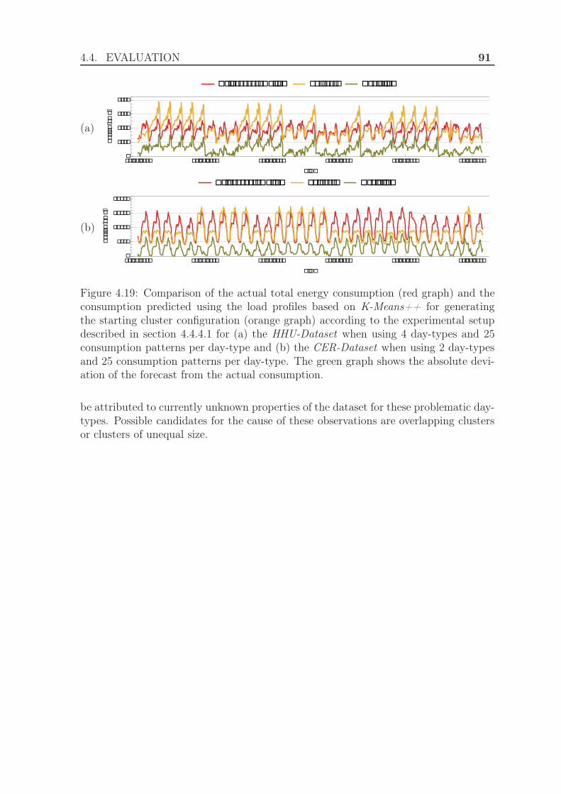
4.4. EVALUATION 91
(a)
������ ��������� ������ ���������
���������� ���������� ���������� ���������� ���������� �����������
����
���
���
����
� ��
������[��]
(b)
������ ��������� ������ ���������
���������� ���������� ���������� ���������� ���������� �����������
����
�����
�����
�����
��
������[��]
Figure 4.19: Comparison of the actual total energy consumption (red graph) and theconsumption predicted using the load profiles based on K-Means++ for generatingthe starting cluster configuration (orange graph) according to the experimental setupdescribed in section 4.4.4.1 for (a) the HHU-Dataset when using 4 day-types and 25consumption patterns per day-type and (b) the CER-Dataset when using 2 day-typesand 25 consumption patterns per day-type. The green graph shows the absolute devi-ation of the forecast from the actual consumption.
be attributed to currently unknown properties of the dataset for these problematic day-types. Possible candidates for the cause of these observations are overlapping clustersor clusters of unequal size.

92 4. CLUSTERING USING SMART METER DATA
5Online Clustering using Smart
Meter Data
One important property of load profiles is the ability to predict the energy consumptionof customers many months in advance. If the consumption behavior changes over time,maintaining acceptable forecast results is a non-trivial task. In this chapter, we addressthe problem of keeping load profiles up-to-date in the event of the consumption behaviorof customers not being constant.
5.1 Motivation
When utilizing Smart Metering data to build load profiles as the foundation to planthe future buy-in of energy, one important aspect for energy providers is that, in a real-world scenario, there is a constant stream of new Smart Metering data. This new SmartMetering data possibly hints at a change in customer behavior or allows to fine-tune ex-isting forecast models. Unless load profiles are kept up-to-date, their performance canworsen over time as it has been the case for the gas economy [Roo+14]. Additionally,experimental evaluations such as in [SM17] have shown that region-specific load profilesmay significantly differ from the existing BDEW Standard Load Profiles even thoughthe same methodlogy has been used to build them. This can indicate that either theenergy consumption is influenced by region-specific factors or that the consumptionbehavior of customers have changed over time. Since the technological advancementsof society are not expected to slow down anytime soon, it can be assumed that thecustomer behavior will also change over time, thus creating the necessity to keep theforecast models up-to-date to enable energy providers to fulfill their duties outlinedin section 2.2. However, frameworks such as the one presented in chapter 4 usuallyrequire to rebuild the forecast models from scratch, which can be a time consumingprocess depending on the computational equipment available to energy providers. Be-cause of this, energy providers would need to strike a balance between their interestin modernizing the load profiles and waiting until enough new Smart Metering data is
93
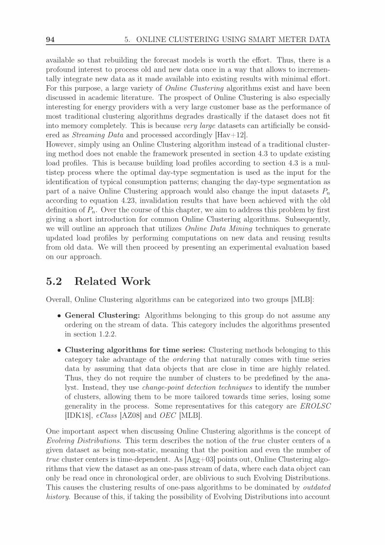
94 5. ONLINE CLUSTERING USING SMART METER DATA
available so that rebuilding the forecast models is worth the effort. Thus, there is aprofound interest to process old and new data once in a way that allows to incremen-tally integrate new data as it made available into existing results with minimal effort.For this purpose, a large variety of Online Clustering algorithms exist and have beendiscussed in academic literature. The prospect of Online Clustering is also especiallyinteresting for energy providers with a very large customer base as the performance ofmost traditional clustering algorithms degrades drastically if the dataset does not fitinto memory completely. This is because very large datasets can artificially be consid-ered as Streaming Data and processed accordingly [Hav+12].However, simply using an Online Clustering algorithm instead of a traditional cluster-ing method does not enable the framework presented in section 4.3 to update existingload profiles. This is because building load profiles according to section 4.3 is a mul-tistep process where the optimal day-type segmentation is used as the input for theidentification of typical consumption patterns; changing the day-type segmentation aspart of a naive Online Clustering approach would also change the input datasets Pn
according to equation 4.23, invalidation results that have been achieved with the olddefinition of Pn. Over the course of this chapter, we aim to address this problem by firstgiving a short introduction for common Online Clustering algorithms. Subsequently,we will outline an approach that utilizes Online Data Mining techniques to generateupdated load profiles by performing computations on new data and reusing resultsfrom old data. We will then proceed by presenting an experimental evaluation basedon our approach.
5.2 Related Work
Overall, Online Clustering algorithms can be categorized into two groups [MLB]:
• General Clustering: Algorithms belonging to this group do not assume anyordering on the stream of data. This category includes the algorithms presentedin section 1.2.2.
• Clustering algorithms for time series: Clustering methods belonging to thiscategory take advantage of the ordering that naturally comes with time seriesdata by assuming that data objects that are close in time are highly related.Thus, they do not require the number of clusters to be predefined by the ana-lyst. Instead, they use change-point detection techniques to identify the numberof clusters, allowing them to be more tailored towards time series, losing somegenerality in the process. Some representatives for this category are EROLSC[IDK18], eClass [AZ08] and OEC [MLB].
One important aspect when discussing Online Clustering algorithms is the concept ofEvolving Distributions. This term describes the notion of the true cluster centers of agiven dataset as being non-static, meaning that the position and even the number oftrue cluster centers is time-dependent. As [Agg+03] points out, Online Clustering algo-rithms that view the dataset as an one-pass stream of data, where each data object canonly be read once in chronological order, are oblivious to such Evolving Distributions.This causes the clustering results of one-pass algorithms to be dominated by outdatedhistory. Because of this, if taking the possibility of Evolving Distributions into account

5.2. RELATED WORK 95
when clustering Smart Metering data, for example caused by current or upcoming tech-nological advancements such as electric vehicles, one-pass clustering algorithms are notthe best choice. In addition, many one-pass clustering algorithms such as Single-PassFuzzy-C-Means (spFCM) [HHG07b] or LOCALSEARCH [OCa+02] require the datato be processed in a random order, notably meaning the tuples are scrambled non-chronologically prior to the analysis. Other algorithms, such as random sampling plusextension Fuzzy-C-Means (rseFCM) [Hav+12], process only a random subset of thedata and generalize the findings onto the complete dataset. Because of this, the ap-plicable use-case of one-pass clustering algorithms is to scale clustering algorithms tovery large datasets, rather than clustering streaming data [Agg+03].In the case of analysing Smart Metering time series, processing the data chronologicallyis highly desirable as this represents a realistic use-case of how an energy provider willwant to handle the data in an effort to adapt to new trends that have a significantimpact on the consumption behavior of customers in a timely manner. To counter-act the drawbacks of one-pass clustering algorithms, [Agg+03] introduces the conceptof micro-cluster as part of the CluStream framework to aggregate data chunks parti-tioned by time and compare them within a user-specified time window. The basic ideaof this approach has also been used in [Cao+] as part of the DenStream algorithm,a method that uses the density-based DBSCAN [Est+96], allowing the approach toidentify clusters of arbitrary shapes.
Another approach for clustering streaming data is presented in [HHG07a]. Here,the authors assume that the data arrives in chunks, meaning that nj data objects getrecorded at the time tj . In particular, even though data objects may be recorded at anarbitrary point in time in a real-world scenario, all data objects recorded at the timet ∈ (tj−1, tj] are assigned to the j-th chunk of data, treating them as if all data objectssimultaneously arrived at time tj . The basic idea is to then apply clustering on thefirst chunk of data and compute the clustering weights for each clustering prototypeaccording to
wo =
n1∑
i=1
uo,i , 1 ≤ o ≤ c (5.1)
Afterwards, the j-th chunk of data is processed by using a dataset comprised of theclustering prototypes which have resulted from the clustering process of the (j − 1)-thchunk of data in addition to the nj data objects of the j-th chunk of data. Here,Weighted Fuzzy-C-Means (WFCM) is used to cluster the data, which is equal to al-gorithm 1 except for line 5 which is replaced by equation 4.38. While the weight ofthe clustering prototypes from processing the previous chunk of data, which are nowtreated as normal data objects, is given in equation 5.1, the actual data objects getassigned a weight of 1. In doing so, WFCM optimizes a different objective functionthan the original Fuzzy-C-Means, which is given as follows:
J (·) =c
∑
o=1
N∑
i=1
wi · umo,i · ‖xi − vo‖
2 (5.2)
Since the cluster weights are computed according to the membership degrees, theirweights do not accumulate indefinitely over several chunks of data, meaning thatWFCM will not become insensitive to Evolving Distributions over time. As [HHG07a]emphasizes, this is one of the main differences compared to LOCALSEARCH [OCa+02].
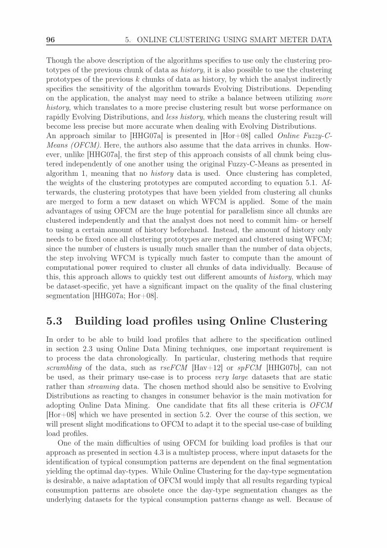
96 5. ONLINE CLUSTERING USING SMART METER DATA
Though the above description of the algorithms specifies to use only the clustering pro-totypes of the previous chunk of data as history, it is also possible to use the clusteringprototypes of the previous k chunks of data as history, by which the analyst indirectlyspecifies the sensitivity of the algorithm towards Evolving Distributions. Dependingon the application, the analyst may need to strike a balance between utilizing morehistory, which translates to a more precise clustering result but worse performance onrapidly Evolving Distributions, and less history, which means the clustering result willbecome less precise but more accurate when dealing with Evolving Distributions.An approach similar to [HHG07a] is presented in [Hor+08] called Online Fuzzy-C-Means (OFCM). Here, the authors also assume that the data arrives in chunks. How-ever, unlike [HHG07a], the first step of this approach consists of all chunk being clus-tered independently of one another using the original Fuzzy-C-Means as presented inalgorithm 1, meaning that no history data is used. Once clustering has completed,the weights of the clustering prototypes are computed according to equation 5.1. Af-terwards, the clustering prototypes that have been yielded from clustering all chunksare merged to form a new dataset on which WFCM is applied. Some of the mainadvantages of using OFCM are the huge potential for parallelism since all chunks areclustered independently and that the analyst does not need to commit him- or herselfto using a certain amount of history beforehand. Instead, the amount of history onlyneeds to be fixed once all clustering prototypes are merged and clustered using WFCM;since the number of clusters is usually much smaller than the number of data objects,the step involving WFCM is typically much faster to compute than the amount ofcomputational power required to cluster all chunks of data individually. Because ofthis, this approach allows to quickly test out different amounts of history, which maybe dataset-specific, yet have a significant impact on the quality of the final clusteringsegmentation [HHG07a; Hor+08].
5.3 Building load profiles using Online Clustering
In order to be able to build load profiles that adhere to the specification outlinedin section 2.3 using Online Data Mining techniques, one important requirement isto process the data chronologically. In particular, clustering methods that requirescrambling of the data, such as rseFCM [Hav+12] or spFCM [HHG07b], can notbe used, as their primary use-case is to process very large datasets that are staticrather than streaming data. The chosen method should also be sensitive to EvolvingDistributions as reacting to changes in consumer behavior is the main motivation foradopting Online Data Mining. One candidate that fits all these criteria is OFCM[Hor+08] which we have presented in section 5.2. Over the course of this section, wewill present slight modifications to OFCM to adapt it to the special use-case of buildingload profiles.
One of the main difficulties of using OFCM for building load profiles is that ourapproach as presented in section 4.3 is a multistep process, where input datasets for theidentification of typical consumption patterns are dependent on the final segmentationyielding the optimal day-types. While Online Clustering for the day-type segmentationis desirable, a naive adaptation of OFCM would imply that all results regarding typicalconsumption patterns are obsolete once the day-type segmentation changes as theunderlying datasets for the typical consumption patterns change as well. Because of

5.3. BUILDING LOAD PROFILES USING ONLINE CLUSTERING 97
this, the naive approach would be to keep the day-type segmentation static and useStreaming Clustering algorithms only to fine-tune the expected consumption behaviorof customers towards emerging trends by processing newly arriving Smart Meteringdata. In this scenario, the chunks of the dataset as described by the OFCM approach[Hor+08] would be predefined by gathering all data consecutively belonging to a givenday-type, similar to Pn as given in equation 4.23. As the final step of OFCM, for eachday-type the weighted clustering prototypes of all chunks within a user-specified timehorizon are clustered using WFCM to yield the clustering prototypes to build the loadprofiles with. By varying the time horizon used for WFCM, the algorithm can be tunedby an analyst to include the optimal amount of history.Though the naive approach as described above has the disadvantage of not being ableto alter the day-type segmentation afterwards, exactly this property can be desirablefor energy providers in some scenarios. This is because, depending on the financialresources available to said energy provider, a steady change in the clustering prototypesof the day-type segmentation means perpetual effort for the analyst to derive newrules to classify future calendar days. Especially for very small energy providers thisis typically not affordable personnel-wise in the long-term.
In order to be able to both have the day-type segmentation as well as the charac-teristics of the consumption patterns change over time while using OFCM, we proposethe following approach:
1. As the first step, we propose to split the entire dataset into partitions, where eachpartition contains the consumption data for a given calendar day. This meansthat after this step, we have an amount of dataset partitions equal to the numberof distinct calendar days for which Smart Metering data is available. Similar tothe original OFCM algorithm, each of these chunks is then independently clus-tered using the original Fuzzy-C-Means algorithm. In particular, these clusteringprocesses take place without regard to any day-type segmentation. When newSmart Metering data becomes available, the new data also gets split into parti-tions and is clustered independently using the original Fuzzy-C-Means algorithmwhile keeping the already clustered partitions unchanged.
2. Since the day-type segmentation utilizes only the aggregated total energy con-sumption for all calendar days as input, its computational requirements are neg-ligible and can thus be performed unaltered according to section 4.3.1. This isdone as the second step of our proposed approach. In particular, this means thateach time new Smart Metering data is made available and the load profiles areto be reevaluated, the process of finding an optimal day-type segmentation isstarted from scratch. To prevent outdated history from having an influence onthe day-type segmentation, it is reasonable to only use data from the most recentyears as the input dataset.
3. For each day-type identified during the second step, all weighted clustering pro-totypes of the independently clustered dataset partitions during the first stepbelonging to the corresponding calendar days are consolidated and clustered us-ing WFCM; this corresponds to the final step of the OFCM algorithm. Similar tothe day-type segmentation, only data from recent years should be used to preventthe end result from being influenced by outdated history. The exact amount of

98 5. ONLINE CLUSTERING USING SMART METER DATA
history to use is for the analyst to decide. In addition, since WFCM is appliedonly on clustering prototypes instead of complete datasets, the computational re-quirements are insignificant compared to section 4.3.2 and can thus be performedfrom scratch each time the load profiles are to be updated.
4. Once both the day-type segmentation and the consumption patterns are known,the load profiles are compiled and assigned to customers according to section 4.3.3.
One important aspect to think about is how the algorithm as described above will dealwith new customers joining or existing customers leaving the energy provider. In thecase of an existing customer leaving the energy provider for another, the forecast gen-erated for that customer by the load provider is no longer used, adequately reducingthe total energy forecast in the process. Over time, the influence of the lost customeron the characteristics of the remaining load profiles will diminish since they are pur-posefully designed to phase out outdated history. If, on the other hand, a new customerjoins the energy provider, the new customer can not immediately get an optimal loadprofile assigned since the necessary Smart Metering data to make that decision is notavailable. In that case, one possible approach would be to use the legacy BDEW Stan-dard Load Profiles for the new customer for the time being until at least one year ofSmart Metering data has been accumulated. During that time, the algorithm as de-scribed above is executed normally, meaning that the consumption patterns and theday-type segmentation become progressively influenced by the consumption behaviorof the new customer, but the load profile assignment for the new customer is ignored.Once enough representative data has been gathered for the new customer, the newload profiles for the new customer is activated. From that point onward, the customeris then treated as an existing customer.
5.4 Evaluation
In this section we will present the evaluation of the approach outlined in section 5.3.We will start by introducing the dataset used for this evaluation, which is a subset ofthe HHU-Dataset introduced in section 4.1, as well as by describing the segmentationof the dataset into training data and test data. We then proceed by explaining howwe plan to simulate the passing of time, that is, making new Smart Metering dataavailable, and how the segmentation of the dataset into training data and test data ischanged as a result. Afterwards, we show and discuss the results of our experimentalsetup.
5.4.1 Experimental Setup
To evaluate the performance of the approach as presented in section 5.3, we have takena subset of the dataset we have introduced as the HHU-Dataset in section 4.1. Thissubset, which is visualized in figure 5.1, consists of a total of 383 distinct customersand, like the original HHU-Dataset, covers a period of 65 months with a resolution of 1measurement per hour. We have specifically decided for this dataset because the timeperiods that the CER-Dataset and the IZES-Dataset cover are too small to be used forevaluating this approach. At the same time, the subset of the HHU-Dataset we havechosen contains customers for which data is continuously available most of the time.
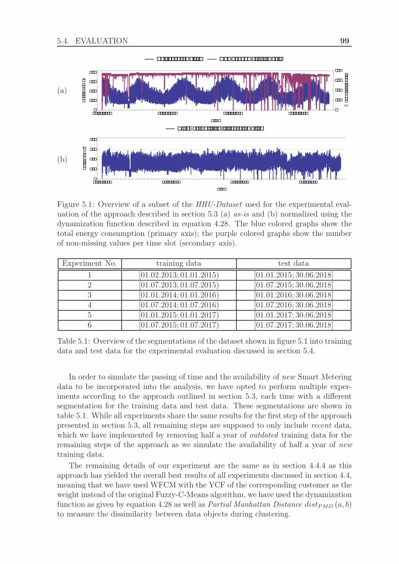
5.4. EVALUATION 99
(a)
����� ��������� ��� �� ���������
���������� ���������� ��������� ����������
���
���
���
���
�� �
������[��]
�
���
���
���
���
#��� ���������
(b)
����-���� ���� �� ����������
���������� ���������� ��������� ����������
���
���
���
���
�� �
������[��]
Figure 5.1: Overview of a subset of the HHU-Dataset used for the experimental eval-uation of the approach described in section 5.3 (a) as-is and (b) normalized using thedynamization function described in equation 4.28. The blue colored graphs show thetotal energy consumption (primary axis); the purple colored graphs show the numberof non-missing values per time slot (secondary axis).
Experiment No. training data test data
1 [01.02.2013; 01.01.2015) [01.01.2015; 30.06.2018]2 [01.07.2013; 01.07.2015) [01.07.2015; 30.06.2018]
3 [01.01.2014; 01.01.2016) [01.01.2016; 30.06.2018]4 [01.07.2014; 01.07.2016) [01.07.2016; 30.06.2018]
5 [01.01.2015; 01.01.2017) [01.01.2017; 30.06.2018]6 [01.07.2015; 01.07.2017) [01.07.2017; 30.06.2018]
Table 5.1: Overview of the segmentations of the dataset shown in figure 5.1 into trainingdata and test data for the experimental evaluation discussed in section 5.4.
In order to simulate the passing of time and the availability of new Smart Meteringdata to be incorporated into the analysis, we have opted to perform multiple exper-iments according to the approach outlined in section 5.3, each time with a differentsegmentation for the training data and test data. These segmentations are shown intable 5.1. While all experiments share the same results for the first step of the approachpresented in section 5.3, all remaining steps are supposed to only include recent data,which we have implemented by removing half a year of outdated training data for theremaining steps of the approach as we simulate the availability of half a year of newtraining data.
The remaining details of our experiment are the same as in section 4.4.4 as thisapproach has yielded the overall best results of all experiments discussed in section 4.4,meaning that we have used WFCM with the YCF of the corresponding customer as theweight instead of the original Fuzzy-C-Means algorithm, we have used the dynamizationfunction as given by equation 4.28 as well as Partial Manhattan Distance distPMD (a, b)to measure the dissimilarity between data objects during clustering.
100 5. ONLINE CLUSTERING USING SMART METER DATA
(a)
� � � � � � � � � � � � � � � � � � �� �� �� ��
�
�
�
�
�
�
�
�
�
�
�
�
�
�
�
�
�
������ �� ����� �� �� ���
����������� ��
0
5
10
15
20
25
30
� � � � � � � � � � � � � � � � � � �� �� �� ��
�
�
�
�
�
�
�
�
�
�
�
�
�
�
�
�
�
������ �� ����� �� �� ���
����������� ��
0
5
10
15
20
25
30
(b)
(c)
� � � � � � � � � � � � � � � � � � �� �� �� ��
�
�
�
�
�
�
�
�
�
�
�
�
�
�
�
�
�
������ �� ����� �� �� ���
����������� ��
0
5
10
15
20
25
30
� � � � � � � � � � � � � � � � � � �� �� �� ��
�
�
�
�
�
�
�
�
�
�
�
�
�
�
�
�
�
������ �� ����� �� �� ���
����������� ��
0
5
10
15
20
25
30
(d)
(e)
� � � � � � � � � � � � � � � � � � �� �� �� ��
�
�
�
�
�
�
�
�
�
�
�
�
�
�
�
�
�
������ �� ����� �� �� ���
����������� ��
0
5
10
15
20
25
30
� � � � � � � � � � � � � � � � � � �� �� �� ��
�
�
�
�
�
�
�
�
�
�
�
�
�
�
�
�
�
������ �� ����� �� �� ���
����������� ��
0
5
10
15
20
25
30
(f)
Figure 5.2: Ratio of the deviations and the actual consumption in percent yielded bythe load profiles generated using different values for the number of day-types and con-sumption patterns using the experimental setup described in section 5.3. The graphsvisualize the results for the dataset depicted in figure 5.1 using K-Means++ to gener-ate the starting configuration of the clustering process. The results shown correspondto (a) Experiment No. 1, (b) Experiment No. 2, (c) Experiment No. 3, (d) Experi-ment No. 4, (e) Experiment No. 5 and (f) Experiment No. 6 as outlined in table 5.1.
5.4.2 Results
The results of our experiments using Online Data Mining techniques as described insection 5.3 are visualized in figure 5.2 and 5.3.One striking observation when looking at the results is the influence of the strat-egy to generate the starting configuration of the clustering prototypes. When usingK-Means++ [AV07], the resulting load profiles perform much better in terms of therelative forecast errors, which are roughly in the range from 10 up to 20 percent forthe tested dataset. In contrast, the relative forecast errors when using Random Co-
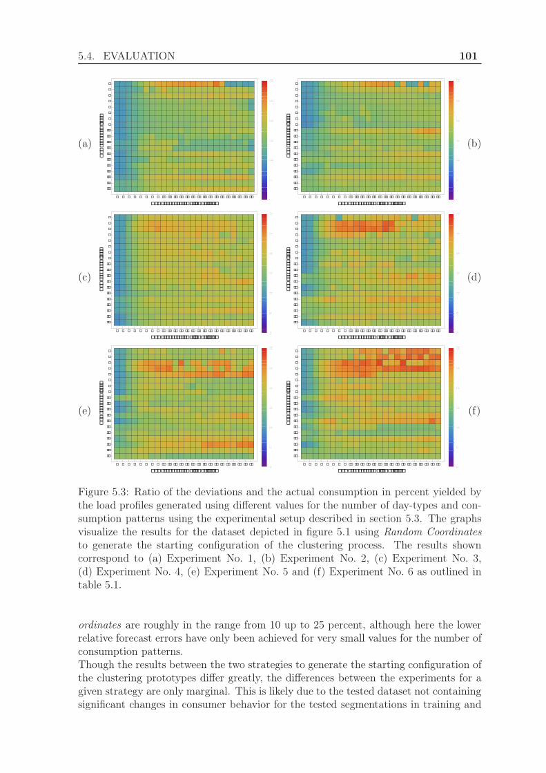
5.4. EVALUATION 101
(a)
� � � � � � � � � � � � � � � � � � �� �� �� ��
�
�
�
�
�
�
�
�
�
�
�
�
�
�
�
�
�
������ �� ����� �� �� ���
����������� ��
0
5
10
15
20
25
30
� � � � � � � � � � � � � � � � � � �� �� �� ��
�
�
�
�
�
�
�
�
�
�
�
�
�
�
�
�
�
������ �� ����� �� �� ���
����������� ��
0
5
10
15
20
25
30
(b)
(c)
� � � � � � � � � � � � � � � � � � �� �� �� ��
�
�
�
�
�
�
�
�
�
�
�
�
�
�
�
�
�
������ �� ����� �� �� ���
����������� ��
0
5
10
15
20
25
30
� � � � � � � � � � � � � � � � � � �� �� �� ��
�
�
�
�
�
�
�
�
�
�
�
�
�
�
�
�
�
������ �� ����� �� �� ���
����������� ��
0
5
10
15
20
25
30
(d)
(e)
� � � � � � � � � � � � � � � � � � �� �� �� ��
�
�
�
�
�
�
�
�
�
�
�
�
�
�
�
�
�
������ �� ����� �� �� ���
����������� ��
0
5
10
15
20
25
30
� � � � � � � � � � � � � � � � � � �� �� �� ��
�
�
�
�
�
�
�
�
�
�
�
�
�
�
�
�
�
������ �� ����� �� �� ���
����������� ��
0
5
10
15
20
25
30
(f)
Figure 5.3: Ratio of the deviations and the actual consumption in percent yielded bythe load profiles generated using different values for the number of day-types and con-sumption patterns using the experimental setup described in section 5.3. The graphsvisualize the results for the dataset depicted in figure 5.1 using Random Coordinatesto generate the starting configuration of the clustering process. The results showncorrespond to (a) Experiment No. 1, (b) Experiment No. 2, (c) Experiment No. 3,(d) Experiment No. 4, (e) Experiment No. 5 and (f) Experiment No. 6 as outlined intable 5.1.
ordinates are roughly in the range from 10 up to 25 percent, although here the lowerrelative forecast errors have only been achieved for very small values for the number ofconsumption patterns.Though the results between the two strategies to generate the starting configuration ofthe clustering prototypes differ greatly, the differences between the experiments for agiven strategy are only marginal. This is likely due to the tested dataset not containingsignificant changes in consumer behavior for the tested segmentations in training and

102 5. ONLINE CLUSTERING USING SMART METER DATA
test data.Overall, the results show a slight regression in the quality of the resulting load profilescompared to the experimental evaluation discussed in section 4.4. Similar to the resultsfor the HHU-Dataset on which the dataset for this experimental evaluation is basedon, overlapping clusters and clusters of different sizes are among the possible reasonsfor the performance of the load profiles. For this reason, more research is necessaryto achieve relative forecast errors similar to the experimental evaluation outlined insection 4.4.4.

6Summary
This chapter represents the conclusion of the thesis. In section 6.1, we summarize thecontributions of this thesis and describe the results of addressed problems. We thendiscuss starting points for future research in section 6.2.
6.1 Conclusions
The energy economy is one of the most crucial preconditions for enabling the lifestyle ofmodern society. As such, structural changes to the energy market face the challenge ofincreasing efficiency while maintaining uptime and fault tolerance of the security of theenergy supply. With data analysis methods having gained increased importance fol-lowing the possibility to store and process huge amounts of data, new technologies suchas Intelligent Metering Systems have made it conceivable to employ techniques fromthe research area Knowledge Discovery in Databases to optimize business processes.
In this thesis, we have laid the focus on extracting useful knowledge from SmartMetering time series. For this purpose, in chapter 2, we have given a small introduc-tion into some basic concepts relevant to market participants in the energy economy.In doing so, we have put emphasis on how the security of the energy supply is beingorganized, particularly with respect to forecasting the energy demand of customersusing load profiles. As it has turned out, load profiles are a very simple yet effectivemeans to forecast the total energy demand of customers. They work by segmenting thecustomer base into groups, where it is assumed that the differences in individuals con-sumption behavior of the same customer group will balance themselves out comparedto the representative consumption pattern specific for the given customer group.
Furthermore, in chapter 3, we have presented some approaches from academic litera-ture on how Knowledge Discovery in Databases techniques can be used in an IntelligentMetering System environment and discussed their implications concerning consumerprivacy. While pilot projects within the context of the studies shown in this thesisso far have all resulted in a positive net benefit for the end consumer, other researchwork has revealed attack vectors on the lifestyle habits of consumers even if the data
103

104 6. SUMMARY
is partly pseudonymized, raising valid concerns for data privacy. To counteract theseconcerns, data gathered by Intelligent Metering Systems should be kept locally as muchas possible and privacy techniques such as data reduction should be employed wherethe transmission of information can not be avoided.Additionally, technologies such as Demand-Side Management or Demand Response arelikely to play an essential role in enabling the widespread usage of electric vehicles andother high-power household appliances such as intelligent washing machines and dish-washers. At the same time, Smart Metering devices with Demand Response capabilitiescan also help to semi-automatically reduce the energy bills of end consumers by beingaware of volatile energy prices and scheduling household appliances accordingly.For energy providers, Intelligent Metering Systems pose the possibility of learning morecharacteristics about their consumers. This information in turn can then be used tooptimize business processes, for example by identifying common traits within groupsof customers and creating new target-group-specific tariffs as a consequence.
Another very important task of energy providers that can be improved by employingIntelligent Metering Systems is to forecast the total energy demand of customers inorder to plan the future buy-in of energy, which we have addressed in chapter 4 and 5of this thesis. In chapter 4, we have introduced and evaluated several approachesbased on a common framework to construct load profiles, an established model topredict customer consumption behavior. With the baseline relative forecast error ofexisting load profiles approximately being in the range from 12 to 13 percent, we havemanaged to achieve relative forecast errors below 6 percent, a significant increase inthe forecasting quality of the models. By further combining the ability to generate loadprofiles with Online Data Mining techniques as discussed in chapter 5 of this thesis, wehave been able to show that it is possible to keep load profiles updated and maintainlow relative forecast errors even in the event of the consumption behavior of customerschanging over time.
6.2 Future Work
In this thesis we have proposed multiple clustering approaches for building load profilesusing Smart Metering data. While the experimental evaluation has shown promisingresults under certain conditions that can help to significantly improve on the existingStandard Load Profiles currently in use by the industry, there is still potential forthe relative forecast errors of the load profiles constructed using our framework to beimproved upon. For example, our experiments have shown that increasing the numberof consumption patterns actually worsens the performance of the corresponding loadprofiles. One possible explanation for this observation might be the datasets containingclusters with varying sizes and shapes, which is a situation that Fuzzy-C-Means doesnot handle very well. In order to help process datasets that have data with thisproperty, it might be worth considering to use Fuzzy-Maximum-Likelihood-Estimation(FMLE) [GG89], a clustering approach which incorporates the fuzzy covariance matrix[DAY69] to handle clusters of different sizes and shapes.
Another possible area for future research concerns the number of dimensions usedduring analysis. During our experimental evaluation, we have always used the highestavailable resolution of the time series per dataset since the load profiles have to have aquarter-hourly resolution in a real-world scenario as mentioned in chapter 2. However,
6.2. FUTURE WORK 105
dimensionality reduction might further help in constructing better performing loadprofiles by counteracting the effects of the curse of dimensionality [Bey+99; FWV07],a term we have introduced in section 1.2.2. Approaches that might help with thisproblem include:
• To reduce the number of dimensions during analysis, it might be desirable todownscale the resolution of the time series, e.g. to an hourly resolution. Oncethe analysis is complete and load profiles have been constructed, the consumptionpatterns used can be scaled back up to quarter-hourly resolution using techniquessuch as cubic spline interpolation.
• Another way to reduce the number of dimensions without downscaling the timeseries is to split the tuples used during clustering into several groups, for exampleby having the first group containing only the data from midnight to 8 o’clock,the second group containing only data from 8 o’clock to 16 o’clock and the lastgroup containing data from 16 o’clock to midnight. The framework as describedin section 4.3 could then be applied to each of these groups individually so thatin the end, the load profile for a given customer consists of a set of smallerload profiles, where one of these smaller load profiles describes the expectedconsumption behavior from midnight to 8 o’clock, the second smaller load profilesdescribes the consumption behavior from 8 o’clock to 16 o’clock and the lastsmaller load profiles describes the behavior from 16 o’clock to midnight. A similaridea in association with tariff groups segmentation has been described in [Chi12;Chi+03].
If the energy provider has detailed knowledge about which customers have a photo-voltaic system installed, including its size and degree of efficiency, the energy providermight decide to use historic weather data to compute a theoretical SLS time series foreach customer that would have arisen as a result of the customer not having a photo-voltaic system installed. Depending on the capabilities of the installed Smart Meteringdevice, this feature might already be available to an energy provider without resortingto error-prone estimates based on weather data. If possible, the energy provider mightwant to build the load profiles used to forecast the energy demand according to thoseconsumption-only SLS time series, while at the same time using weather prognosis datato compute a correction term to be applied onto the forecast generated by the resultingload profiles in order to yield the actual energy the customer is likely to extract fromthe electricity grid.

106 6. SUMMARY

Bibliography
[AE08] M.H. Albadi and E.F. El-Saadany. “A summary of demand response inelectricity markets”. In: Electric Power Systems Research 78.11 (2008),pp. 1989–1996. issn: 0378-7796. doi: 10.1016/j.epsr.2008.04.002.
[Age14] International Energy Agency. Policy uncertainty threatens to slow renew-able energy momentum. https://www.iea.org/newsroom/news/2014/a
ugust/policy-uncertainty-threatens-to-slow-renewable-energy-
momentum.html. Aug. 2014.
[Agg+03] Charu C. Aggarwal et al. “A Framework for Clustering Evolving DataStreams”. In: Proceedings 2003 {VLDB} Conference. Ed. by Johann-Christoph Freytag et al. San Francisco: Morgan Kaufmann, 2003, pp. 81–92. isbn: 978-0-12-722442-8. doi: 10.1016/B978-012722442-8/50016-1.
[Agr+95] Rakesh Agrawal et al. “Querying Shapes of Histories”. In: Proceedings of the21th International Conference on Very Large Data Bases. VLDB ’95. SanFrancisco, CA, USA: Morgan Kaufmann Publishers Inc., 1995, pp. 502–514. isbn: 1-55860-379-4. url: http://dl.acm.org/citation.cfm?id=645921.673157.
[Agr+98] Rakesh Agrawal et al. “Automatic Subspace Clustering of High Dimen-sional Data for Data Mining Applications”. In: SIGMOD Rec. 27.2 (June1998), pp. 94–105. issn: 0163-5808. doi: 10.1145/276305.276314.
[ALB13] F.M. Andersen, H.V. Larsen, and T.K. Boomsma. “Long-term fore-casting of hourly electricity load: Identification of consumptionprofiles and segmentation of customers”. In: Energy Conversionand Management 68 (2013), pp. 244–252. issn: 0196-8904. doi:10.1016/j.enconman.2013.01.018.
[Alg+15] Hugo Algarvio et al. “Electricity Usage Efficiency in Large Build-ings: DSM Measures and Preliminary Simulations of DR Programs ina Public Library”. In: Highlights of Practical Applications of Agents,Multi-Agent Systems, and Sustainability - The PAAMS Collection: In-ternational Workshops of PAAMS 2015, Salamanca, Spain, June 3-4,2015. Proceedings. Ed. by Javier Bajo et al. Cham: Springer Inter-national Publishing, 2015, pp. 249–259. isbn: 978-3-319-19033-4. doi:10.1007/978-3-319-19033-4_21.
[And13] Andreas Kießling. Modellstadt Mannheim (moma) - Abschlussbericht. July2013. url: https://www.ifeu.de/projekt/modellstadt-mannheim/.
107
108 BIBLIOGRAPHY
[Ank+99] Mihael Ankerst et al. “OPTICS: Ordering Points to Identify the ClusteringStructure”. In: SIGMOD Rec. 28.2 (June 1999), pp. 49–60. issn: 0163-5808.doi: 10.1145/304181.304187.
[AV07] David Arthur and Sergei Vassilvitskii. “K-means++: The Advantages ofCareful Seeding”. In: Proceedings of the Eighteenth Annual ACM-SIAMSymposium on Discrete Algorithms. SODA ’07. New Orleans, Louisiana:Society for Industrial and Applied Mathematics, 2007, pp. 1027–1035.isbn: 978-0-898716-24-5. url: http://dl.acm.org/citation.cfm?id=1283383.1283494.
[AZ08] Plamen P. Angelov and Xiaowei Zhou. “Evolving Fuzzy-Rule-BasedClassifiers From Data Streams”. In: IEEE Transactions on FuzzySystems 16.6 (Dec. 2008), pp. 1462–1475. issn: 1063-6706. doi:10.1109/TFUZZ.2008.925904.
[Bac78] Eric Backer. “Cluster analysis by optimal decomposition of induced fuzzysets”. PhD thesis. TU Delft, Delft University of Technology, 1978.
[Bar07] Gregory V. Bard. “Spelling-error Tolerant, Order-independent Pass-phrases via the Damerau-levenshtein String-edit Distance Metric”. In: Pro-ceedings of the Fifth Australasian Symposium on ACSW Frontiers - Vol-ume 68. ACSW ’07. Ballarat, Australia: Australian Computer Society, Inc.,2007, pp. 117–124. isbn: 1-920-68285-X. url: http://dl.acm.org/citation.cfm?id=1274531.1274545.
[BC94] Donald J Berndt and James Clifford. “Using dynamic time warping to findpatterns in time series”. In: KDD workshop. Vol. 10. 16. Seattle, WA. 1994,pp. 359–370.
[BD75] J. C. Bezdek and J. C. Dunn. “Optimal Fuzzy Partitions: A Heuristicfor Estimating the Parameters in a Mixture of Normal Distributions”. In:IEEE Transactions on Computers C-24.8 (Aug. 1975), pp. 835–838. issn:0018-9340. doi: 10.1109/T-C.1975.224317.
[Bey+99] Kevin Beyer et al. “When Is “Nearest Neighbor” Meaningful?” In: DatabaseTheory — ICDT’99. Ed. by Catriel Beeri and Peter Buneman. Berlin,Heidelberg: Springer Berlin Heidelberg, 1999, pp. 217–235. isbn: 978-3-540-49257-3.
[Bez74] J. C. Bezdek. “Numerical taxonomy with fuzzy sets”. In: Journal ofMathematical Biology 1.1 (May 1974), pp. 57–71. issn: 1432-1416. doi:10.1007/BF02339490.
[Bez81] James C. Bezdek. “Objective Function Clustering”. In: PatternRecognition with Fuzzy Objective Function Algorithms. Boston,MA: Springer US, 1981, pp. 43–93. isbn: 978-1-4757-0450-1. doi:10.1007/978-1-4757-0450-1_3.
[BH65] GH Ball and DJ Hall. “ISODATA, a novel technique for data analysis andpattern classification”. In: Standford Res. Inst., Menlo Park, CA (1965).
[BK59] R. Bellman and R. Kalaba. “On adaptive control processes”. In: IRE Trans-actions on Automatic Control 4.2 (Nov. 1959), pp. 1–9. issn: 0096-199X.doi: 10.1109/TAC.1959.1104847.

BIBLIOGRAPHY 109
[Boc16] Christian Bock. “Clustering-Ansatz zur Erstellung von Lastprofilen zurVorhersage des Stromverbrauchs”. In: Proceedings of the 28th GI-WorkshopGrundlagen von Datenbanken (GvDB 2016). Ed. by Lena Wiese, Hen-drik Bitzmann, and Tim Waage. Nörten Hardenberg, Germany: CEUR-Workshop Proceedings, Vol. 1594, May 2016, pp. 21–26. url: http://ceur-ws.org/Vol-1594/.
[Boc17] Christian Bock. “Generating Load Profiles Using Smart Metering TimeSeries”. In: Advances in Fuzzy Logic and Technology 2017: Proceedingsof: EUSFLAT-2017 – The 10th Conference of the European Society forFuzzy Logic and Technology, September 11–15, 2017, Warsaw, PolandIWIFSGN’2017 – The Sixteenth International Workshop on Intuitionis-tic Fuzzy Sets and Generalized Nets, September 13–15, 2017, Warsaw,Poland, Volume 1. Ed. by Janusz Kacprzyk et al. Cham: Springer In-ternational Publishing, 2017, pp. 211–223. isbn: 978-3-319-66830-7. doi:10.1007/978-3-319-66830-7_20.
[Boc18] Christian Bock. “Forecasting Energy Demand by Clustering Smart Meter-ing Time Series”. In: Information Processing and Management of Uncer-tainty in Knowledge-Based Systems. Theory and Foundations. Ed. by JesúsMedina et al. Cham: Springer International Publishing, 2018, pp. 431–442.isbn: 978-3-319-91473-2. doi: 10.1007/978-3-319-91473-2_37.
[Bre01] Leo Breiman. “Random Forests”. In: Machine Learning 45.1 (Oct. 2001),pp. 5–32. issn: 1573-0565. doi: 10.1023/A:1010933404324.
[Bun06] Bundesnetzagentur. Richtlinie Datenaustausch und Mengenbilanzierung(DuM). 2006. url: https://www.bundesnetzagentur.de/DE/Service-Funktionen/Beschlusskammern/1_GZ/BK6-GZ/2007/2007_0001bis0999
/2007_001bis099/BK6-07-002/BK6-07-002_RichtlinieDatenaustaus
chundId8623doc_bf.html.
[Bun13] Bundesnetzagentur, Beschlusskammer 6. Marktregeln für die Durch-führung der Bilanzkreisabrechnung Strom (MaBiS). 2013. url: https://www.bundesnetzagentur.de/DE/Service-Funktionen/Beschlusskamme
rn/BK06/BK6_71_Bilanzabr/08%20achte%20Mitteilung/AchteMitteil
ung.html?nn=872140.
[Bun18] Bundesnetzagentur. Festlegungsverfahren zur Änderung der Ausschrei-bungsbedingungen und Veröffentlichungspflichten von Minutenreserve(BK6-18-020). 2018. url: https://www.bundesnetzagentur.de/DE/Service-Funktionen/Beschlusskammern/1_GZ/BK6-GZ/2018/2018_0001bi
s0999/BK6-18-020/BK6-18-020_Beschluss_vom_08_05_2018.html?nn
=269594.
[Bun98] Bundesanzeiger. Gesetz zur Neuregelung des Energiewirtschaftsrechts. http://www.bgbl.de/xaver/bgbl/start.xav?startbk=Bundesanzeiger_
BGBl&jumpTo=bgbl198s0730.pdf. Apr. 1998.
[BVK02] R. Babuka, P. J. van der Veen, and U. Kaymak. “Improved covariance es-timation for Gustafson-Kessel clustering”. In: Fuzzy Systems, 2002. FUZZ-IEEE’02. Proceedings of the 2002 IEEE International Conference on.Vol. 2. 2002, pp. 1081–1085. doi: 10.1109/FUZZ.2002.1006654.

110 BIBLIOGRAPHY
[BWS06] Mohamed Bouguessa, Shengrui Wang, and Haojun Sun. “An objective ap-proach to cluster validation”. In: Pattern Recognition Letters 27.13 (2006),pp. 1419–1430. issn: 0167-8655. doi: 10.1016/j.patrec.2006.01.015.
[Cao+] Feng Cao et al. “Density-Based Clustering over an Evolving Data Streamwith Noise”. In: Proceedings of the 2006 SIAM International Conferenceon Data Mining, pp. 328–339. doi: 10.1137/1.9781611972764.29.
[CER] CER – The Commission for Energy Regulation. Accessed via the IrishSocial Science Data Archive. http://www.ucd.ie/issda.
[Chi+01] Gianfranco Chicco et al. “Electric energy customer characterisationfor developing dedicated market strategies”. In: 2001 IEEE PortoPower Tech Proceedings (Cat. No.01EX502). Vol. 1. Sept. 2001. doi:10.1109/PTC.2001.964627.
[Chi+03] Gianfranco Chicco et al. “Customer characterization options for improvingthe tariff offer”. In: IEEE Transactions on Power Systems 18.1 (Jan. 2003),pp. 381–387. issn: 0885-8950. doi: 10.1109/TPWRS.2002.807085.
[Chi12] Gianfranco Chicco. “Overview and performance assessment of the cluster-ing methods for electrical load pattern grouping”. In: Energy 42.1 (2012).8th World Energy System Conference, WESC 2010, pp. 68–80. issn: 0360-5442. doi: 10.1016/j.energy.2011.12.031.
[Com12] European Commission. 2012/148/EU: Commission Recommendation of 9March 2012 on preparations for the roll-out of smart metering systems. http://data.europa.eu/eli/reco/2012/148/oj. Mar. 2012.
[Com14] European Commission. 2030 climate and energy policy framework. https://ec.europa.eu/clima/policies/strategies/2030_en. Oct. 2014.
[Con07] 110th United States Congress. Energy Independence and SecurityAct. https://www.epa.gov/laws-regulations/summary-energy-independence-and-security-act. Dec. 2007.
[Dam64] Fred J. Damerau. “A Technique for Computer Detection and Correction ofSpelling Errors”. In: Commun. ACM 7.3 (Mar. 1964), pp. 171–176. issn:0001-0782. doi: 10.1145/363958.363994.
[DAY69] N. E. DAY. “Estimating the components of a mixture of nor-mal distributions”. In: Biometrika 56.3 (1969), pp. 463–474. doi:10.1093/biomet/56.3.463.
[Deg+13] Kathrin Degen et al. “Smart Metering, Beratung oder Sozialer Vergleich -Was beeinflusst den Elektrizitätsverbrauch?” In: (July 2013).
[DKK15] Panagiotis D. Diamantoulakis, Vasilios M. Kapinas, and George K. Kara-giannidis. “Big Data Analytics for Dynamic Energy Management in SmartGrids”. In: CoRR abs/1504.02424 (2015). url: http://arxiv.org/abs/1504.02424.
[Dwo06] Cynthia Dwork. “Differential Privacy”. In: Automata, Languages andProgramming. Ed. by Michele Bugliesi et al. Berlin, Heidelberg:Springer Berlin Heidelberg, 2006, pp. 1–12. isbn: 978-3-540-35908-1. doi:10.1007/11787006_1.

BIBLIOGRAPHY 111
[EDI] EDI@Energy. url: https://www.edi-energy.de.
[EK13] Helmut Edelmann and Thomas Kästner. Kosten-Nutzen-Analyse füreinen flächendeckenden Einsatz intelligenter Zähler. Graf-Adolf-Platz 15,40213 Düsseldorf, Deutschland, July 2013. url: https://www.bmwi.de/Redaktion/DE/Publikationen/Studien/kosten-nutzen-analyse-fue
r-flaechendeckenden-einsatz-intelligenterzaehler.html.
[Ene16] Bundesverband der Energie- und Wasserwirtschaft (BDEW). Position-spapier: Umsetzung Gesetz zur Digitalisierung der Energiewende. https://www.bdew.de/service/stellungnahmen/positionspapier-umsetzun
g-gesetz-digitalisierung-energiewende/. May 2016.
[ES00] Martin Ester and Jörg Sander. Knowledge Discovery in Databases:Techniken und Anwendungen. Springer Berlin Heidelberg, 2000. isbn:9783540673286. doi: 10.1007/978-3-642-58331-5.
[Est+96] Martin Ester et al. “A density-based algorithm for discovering clusters inlarge spatial databases with noise.” In: Kdd. Vol. 96. 34. 1996, pp. 226–231.
[Eur50] Council of Europe. Convention for the Protection of Human Rights andFundamental Freedoms. https://www.coe.int/en/web/conventions/full-list/-/conventions/treaty/005. Nov. 1950.
[Fer+15] Marta C. Ferreira et al. “Fuzzy modeling based on Mixed Fuzzy Clus-tering for health care applications”. In: 2015 IEEE International Con-ference on Fuzzy Systems (FUZZ-IEEE). Aug. 2015, pp. 1–5. doi:10.1109/FUZZ-IEEE.2015.7338028.
[FPS+96] Usama M Fayyad, Gregory Piatetsky-Shapiro, Padhraic Smyth, et al.“Knowledge Discovery and Data Mining: Towards a Unifying Framework.”In: KDD. Vol. 96. 1996, pp. 82–88.
[FT00] Christian Fünfgeld and Remo Tiedemann. Anwendung der Repräsenta-tiven VDEW-Lastprofile step - by - step. Tech. rep. VDEW-MaterialienM-05/2000, Frankfurt. Brandenburgische Technische Universität Cottbus,Lehrstuhl für Energiewirtschaft, 2000.
[FWV07] Damien François, Vincent Wertz, and Michel Verleysen. “The Con-centration of Fractional Distances”. In: IEEE Transactions on Knowl-edge & Data Engineering 19 (2007), pp. 873–886. issn: 1041-4347. doi:10.1109/TKDE.2007.1037.
[GG89] I. Gath and A.B. Geva. “Unsupervised Optimal Fuzzy Clustering”. In:IEEE Transactions on Pattern Analysis and Machine Intelligence 11(1989), pp. 773–780. issn: 0162-8828.
[GK78] D. E. Gustafson and W. C. Kessel. “Fuzzy clustering with a fuzzy covari-ance matrix”. In: 1978 IEEE Conference on Decision and Control includingthe 17th Symposium on Adaptive Processes. Jan. 1978, pp. 761–766. doi:10.1109/CDC.1978.268028.
[GP11] Arne Grein and Martin Pehnt. “Load management for refrigeration sys-tems: Potentials and barriers”. In: Energy Policy 39.9 (2011), pp. 5598–5608. issn: 0301-4215. doi: 10.1016/j.enpol.2011.04.040.

112 BIBLIOGRAPHY
[GRS98] Sudipto Guha, Rajeev Rastogi, and Kyuseok Shim. “CURE: An EfficientClustering Algorithm for Large Databases”. In: SIGMOD Rec. 27.2 (June1998), pp. 73–84. issn: 0163-5808. doi: 10.1145/276305.276312.
[Hal99] Mark Andrew Hall. “Correlation-based Feature Selection for MachineLearning”. PhD thesis. 1999.
[Hav+12] Timothy Havens et al. “Fuzzy c-Means Algorithms for Very Large Data”.In: 20 (Dec. 2012), pp. 1130–1146.
[Hay+14] Marian Hayn et al. “Electricity load profiles in Europe: The importance ofhousehold segmentation”. In: Energy Research & Social Science 3 (2014),pp. 30–45. issn: 2214-6296. doi: 10.1016/j.erss.2014.07.002.
[HB01] R. J. Hathaway and J. C. Bezdek. “Fuzzy c-means clustering of incom-plete data”. In: IEEE Transactions on Systems, Man, and Cybernetics,Part B (Cybernetics) 31.5 (Oct. 2001), pp. 735–744. issn: 1083-4419. doi:10.1109/3477.956035.
[HC10a] Ludmila Himmelspach and Stefan Conrad. “Clustering approaches for datawith missing values: Comparison and evaluation”. In: 2010 5th Interna-tional Conference on Digital Information Management, ICDIM 2010. Aug.2010, pp. 19–28. doi: 10.1109/ICDIM.2010.5664691.
[HC10b] Ludmila Himmelspach and Stefan Conrad. “Fuzzy Clustering of In-complete Data Based on Cluster Dispersion”. In: Computational In-telligence for Knowledge-Based Systems Design. Ed. by Eyke Hüller-meier, Rudolf Kruse, and Frank Hoffmann. Berlin, Heidelberg: SpringerBerlin Heidelberg, 2010, pp. 59–68. isbn: 978-3-642-14049-5. doi:10.1007/978-3-642-14049-5_7.
[HCC12] Ludmila Himmelspach, João Paulo Carvalho, and Stefan Conrad. “OnCluster Validity for Fuzzy Clustering of Incomplete Data”. In: Scalable Un-certainty Management. Ed. by Eyke Hüllermeier et al. Berlin, Heidelberg:Springer Berlin Heidelberg, 2012, pp. 612–618. isbn: 978-3-642-33362-0.doi: 10.1007/978-3-642-33362-0_50.
[HHC11] Ludmila Himmelspach, Daniel Hommers, and Stefan Conrad. “ClusterTendency Assessment for Fuzzy Clustering of Incomplete Data”. In: Pro-ceedings of the 7th conference of the European Society for Fuzzy Logic andTechnology. Atlantis Press, Aug. 2011, pp. 290–297. isbn: 978-90-78677-00-0. doi: 10.2991/eusflat.2011.136.
[HHG07a] P. Hore, L. O. Hall, and D. B. Goldgof. “A fuzzy c means variant forclustering evolving data streams”. In: 2007 IEEE International Confer-ence on Systems, Man and Cybernetics. Oct. 2007, pp. 360–365. doi:10.1109/ICSMC.2007.4413710.
[HHG07b] P. Hore, L. O. Hall, and D. B. Goldgof. “Single Pass Fuzzy C Means”. In:2007 IEEE International Fuzzy Systems Conference. July 2007, pp. 1–7.doi: 10.1109/FUZZY.2007.4295372.
[Him16] Ludmila Himmelspach. “Fuzzy Clustering of Incomplete Data”. PhD thesis.Heinrich-Heine-University, Institute of Computer Science, 2016.

BIBLIOGRAPHY 113
[Hof+12] Patrick Hoffman et al. Praxistest “Moderne Energiesparsysteme imHaushalt”. Altenkesseler Straße 17, D-66115 Saarbrücken, Germany, 2012.
[Hop+16] Konstantin Hopf et al. “Feature extraction and filtering for household clas-sification based on smart electricity meter data”. In: Computer Science -Research and Development 31.3 (Aug. 2016), pp. 141–148. issn: 1865-2042.doi: 10.1007/s00450-014-0294-4.
[Hop+17] Konstantin Hopf et al. “A Decision Support System for PhotovoltaicPotential Estimation”. In: Proceedings of the 1st International Confer-ence on Internet of Things and Machine Learning. IML ’17. Liverpool,United Kingdom: ACM, 2017, 3:1–3:10. isbn: 978-1-4503-5243-7. doi:10.1145/3109761.3109764.
[Hor+08] P. Hore et al. “Online fuzzy c means”. In: NAFIPS 2008 - 2008 AnnualMeeting of the North American Fuzzy Information Processing Society. May2008, pp. 1–5. doi: 10.1109/NAFIPS.2008.4531233.
[HPK11] Jiawei Han, Jian Pei, and Micheline Kamber. Data mining: concepts andtechniques. Elsevier, 2011. isbn: 9780123814791.
[HRR14] Michael Hinterstocker, Serafin von Roon, and Marina Rau. “Bewertung deraktuellen Standardlastprofile Österreichs und Analyse zukünftiger Anpas-sungsmöglichkeiten im Strommarkt”. In: Proc. 2014 13. Symposium En-ergieinnovation. 2014.
[HSK16] Konstantin Hopf, Mariya Sodenkamp, and Ilya Kozlovskiy. “Energy DataAnalytics For Improved Residential Service Quality And Energy Effi-ciency”. In: ENERGY (2016). url: http://aisel.aisnet.org/ecis2016_rip/73.
[HSS18] Konstantin Hopf, Mariya Sodenkamp, and Thorsten Staake. “Enhanc-ing energy efficiency in the residential sector with smart meter dataanalytics”. In: Electronic Markets (Mar. 2018). issn: 1422-8890. doi:10.1007/s12525-018-0290-9.
[IA09] Ali Ipakchi and Farrokh Albuyeh. “Grid of the future”. In: IEEE Powerand Energy Magazine 7.2 (Mar. 2009), pp. 52–62. issn: 1540-7977. doi:10.1109/MPE.2008.931384.
[IDK18] Omar A. Ibrahim, Yizhuo Du, and James Keller. “Robust On-Line Stream-ing Clustering”. In: Information Processing and Management of Uncer-tainty in Knowledge-Based Systems. Theory and Foundations. Ed. by JesúsMedina et al. Cham: Springer International Publishing, 2018, pp. 467–478.isbn: 978-3-319-91473-2. doi: 10.1007/978-3-319-91473-2_40.
[Ita75] F. Itakura. “Minimum prediction residual principle applied to speechrecognition”. In: IEEE Transactions on Acoustics, Speech, and Sig-nal Processing 23.1 (Feb. 1975), pp. 67–72. issn: 0096-3518. doi:10.1109/TASSP.1975.1162641.
[JJR11] Marek Jawurek, Martin Johns, and Konrad Rieck. “Smart Metering De-pseudonymization”. In: Proceedings of the 27th Annual Computer SecurityApplications Conference. ACSAC ’11. Orlando, Florida, USA: ACM, 2011,pp. 227–236. isbn: 978-1-4503-0672-0. doi: 10.1145/2076732.2076764.

114 BIBLIOGRAPHY
[Jus05] Bundesministerium der Justiz und für Verbraucherschutz. Strom-netzzugangsverordnung: Verordnung über den Zugang zu Elektriz-itätsversorgungsnetzen. https://www.gesetze-im-internet.de/stromn
zv/. July 2005.
[Jus16] Bundesministerium der Justiz und für Verbraucherschutz. Gesetz über denMessstellenbetrieb und die Datenkommunikation in intelligenten Energien-etzen. https://www.gesetze-im-internet.de/messbg/. Aug. 2016.
[KKK04] Karin Kailing, Hans-Peter Kriegel, and Peer Kröger. “Density-ConnectedSubspace Clustering for High-Dimensional Data”. In: Proceedings of the2004 SIAM International Conference on Data Mining. 2004, pp. 246–256.doi: 10.1137/1.9781611972740.23.
[KL83] Joseph B. Kruskal and Mark Liberman. “The symmetric time-warpingproblem: From continuous to discrete”. In: (Jan. 1983).
[Koh89] Teuvo Kohonen. Self-Organization and Associative Memory. 3rd ed.Springer Series in Information Sciences 8. Springer-Verlag Berlin Heidel-berg, 1989. isbn: 978-3-540-51387-2,978-3-642-88163-3.
[KP01] Eamonn J. Keogh and Michael J. Pazzani. “Derivative Dynamic TimeWarping”. In: Proceedings of the 2001 SIAM International Conference onData Mining. 2001, pp. 1–11. doi: 10.1137/1.9781611972719.1.
[KR90] Leonard Kaufman and Peter J. Rousseeuw. Finding Groups in Data:An Introduction to Cluster Analysis. John Wiley & Sons, 1990. isbn:9780471878766. doi: 10.1002/9780470316801.
[Lam12] Oscar Perpiñan Lamigueiro. “solaR: Solar Radiation and Photovoltaic Sys-tems with R”. In: Journal of Statistical Software 50.9 (Aug. 2012), pp. 1–32. url: http://oa.upm.es/20821/.
[Lev66] Vladimir Iosifovich Levenshtein. “Binary codes capable of correcting dele-tions, insertions and reversals.” In: Soviet Physics Doklady 10.8 (Feb.1966). Doklady Akademii Nauk SSSR, V163 No4 845-848 1965, pp. 707–710.
[Lia05] T. Warren Liao. “Clustering of time series data — a survey”. In: Pat-tern Recognition 38.11 (2005), pp. 1857–1874. issn: 0031-3203. doi:10.1016/j.patcog.2005.01.025.
[Lit88] Roderick J. A. Little. “A Test of Missing Completely at Ran-dom for Multivariate Data with Missing Values”. In: Journal of theAmerican Statistical Association 83.404 (1988), pp. 1198–1202. doi:10.1080/01621459.1988.10478722.
[Löd+10] Martin Lödl et al. “Abschätzung des Photovoltaik-Potentials aufDachflächen in Deutschland”. In: 11. Symposium Energieinnovation „AlteZiele–Neue Wege “. 2010.
[Lop11] Raul H. C. Lopes. “Kolmogorov-Smirnov Test”. In: International Ency-clopedia of Statistical Science. Ed. by Miodrag Lovric. Berlin, Heidelberg:Springer Berlin Heidelberg, 2011, pp. 718–720. isbn: 978-3-642-04898-2.doi: 10.1007/978-3-642-04898-2_326.

BIBLIOGRAPHY 115
[LR02] Roderick J. A. Little and Donald B. Rubin. Statistical Analysis with Miss-ing Data, Second Edition. New York: John Wiley & Sons, 2002. isbn:978-0-471-18386-0. doi: 10.1002/9781119013563.
[Mac+67] James MacQueen et al. “Some methods for classification and analysis ofmultivariate observations”. In: Proceedings of the fifth Berkeley symposiumon mathematical statistics and probability. Vol. 1. 14. Oakland, CA, USA.1967, pp. 281–297.
[Mei+99] Hermann Meier et al. Repräsentative VDEW-Lastprofile. Tech. rep.VDEW-Materialien M-32/99, Frankfurt. Brandenburgische TechnischeUniversität Cottbus, Lehrstuhl für Energiewirtschaft, 1999.
[MLB] Masud Moshtaghi, Christopher Leckie, and James C. Bezdek. “On-line Clustering of Multivariate Time-series”. In: Proceedings of the 2016SIAM International Conference on Data Mining, pp. 360–368. doi:10.1137/1.9781611974348.41.
[Moh+10] A. H. Mohsenian-Rad et al. “Autonomous Demand-Side ManagementBased on Game-Theoretic Energy Consumption Scheduling for the Fu-ture Smart Grid”. In: IEEE Transactions on Smart Grid 1.3 (Dec. 2010),pp. 320–331. issn: 1949-3053. doi: 10.1109/TSG.2010.2089069.
[MRR80] C. Myers, L. Rabiner, and A. Rosenberg. “Performance tradeoffs in dy-namic time warping algorithms for isolated word recognition”. In: IEEETransactions on Acoustics, Speech, and Signal Processing 28.6 (Dec. 1980),pp. 623–635. issn: 0096-3518. doi: 10.1109/TASSP.1980.1163491.
[MRT12] Eoghan McKenna, Ian Richardson, and Murray Thomson. “Smart me-ter data: Balancing consumer privacy concerns with legitimate ap-plications”. In: Energy Policy 41 (2012). Modeling Transport (En-ergy) Demand and Policies, pp. 807–814. issn: 0301-4215. doi:10.1016/j.enpol.2011.11.049.
[Mül+16] Oliver Müller et al. “Utilizing big data analytics for information systemsresearch: challenges, promises and guidelines”. In: European Journal of In-formation Systems 25.4 (2016), pp. 289–302. doi: 10.1057/ejis.2016.2.
[OCa+02] Liadan O’Callaghan et al. “Streaming-data algorithms for high-qualityclustering”. In: Proceedings 18th International Conference on Data En-gineering. Feb. 2002, pp. 685–694. doi: 10.1109/ICDE.2002.994785.
[Ord+10] J. Ordóñez et al. “Analysis of the photovoltaic solar energy capacity ofresidential rooftops in Andalusia (Spain)”. In: Renewable and Sustain-able Energy Reviews 14.7 (2010), pp. 2122–2130. issn: 1364-0321. doi:10.1016/j.rser.2010.01.001.
[Par06] European Parliament. Directive 2006/32/EC of the European Parliamentand of the Council of 5 April 2006 on energy end-use efficiency and energyservices and repealing and repealing Council Directive 93/76/EEC. http://data.europa.eu/eli/dir/2006/32/oj. Apr. 2006.

116 BIBLIOGRAPHY
[Par09] European Parliament. Directive 2009/72/EC of the European Parliamentand of the Council of 13 July 2009 concerning common rules for the in-ternal market in electricity and repealing Directive 2003/54/EC. http://data.europa.eu/eli/dir/2009/72/oj. Aug. 2009.
[Par15] European Parliament. Directive (EU) 2015/1535 of the European Parlia-ment and of the Council of 9 September 2015 laying down a procedurefor the provision of information in the field of technical regulations and ofrules on Information Society services (codification). http://data.europa.eu/eli/dir/2015/1535/oj. Sept. 2015.
[Par96] European Parliament. Directive 96/92/EC of the European Parliamentand of the Council of 19 December 1996 concerning common rules for theinternal market in electricity. http://data.europa.eu/eli/dir/1996/92/oj. Dec. 1996.
[PSM09] Michael Angelo A. Pedrasa, Ted D. Spooner, and Iain F. MacGill.“Scheduling of Demand Side Resources Using Binary Particle Swarm Op-timization”. In: IEEE Transactions on Power Systems 24.3 (Aug. 2009),pp. 1173–1181. issn: 0885-8950. doi: 10.1109/TPWRS.2009.2021219.
[Ren08] Rena Tangens. BigBrotherAward 2008 in der Kategorie “Technik”. Tech.rep. BigBrotherAwards, 2008. url: https://bigbrotherawards.de/2008/technik-yello-strom.
[Rod+03] Fátima Rodrigues et al. “Machine Learning and Data Mining in PatternRecognition: Third International Conference, MLDM 2003 Leipzig, Ger-many, July 5–7, 2003 Proceedings”. In: ed. by Petra Perner and AzrielRosenfeld. Berlin, Heidelberg: Springer Berlin Heidelberg, 2003. Chap. AComparative Analysis of Clustering Algorithms Applied to Load Profiling,pp. 73–85. isbn: 978-3-540-45065-8. doi: 10.1007/3-540-45065-3_7.
[Roo+14] Serafin von Roon et al. Statusbericht zum StandardlastprofilverfahrenGas. https://www.ffegmbh.de/kompetenzen/system-markt-analysen
/508-statusbericht-standardlastprofile-gas. Am Blütenanger 71,80995 München, Deutschland, Nov. 2014.
[Rou78] Marc Roubens. “Pattern classification problems and fuzzy sets”. In:Fuzzy Sets and Systems 1.4 (1978), pp. 239–253. issn: 0165-0114. doi:10.1016/0165-0114(78)90016-7.
[Rou87] Peter J. Rousseeuw. “Silhouettes: A graphical aid to the interpreta-tion and validation of cluster analysis”. In: Journal of Computationaland Applied Mathematics 20 (1987), pp. 53–65. issn: 0377-0427. doi:10.1016/0377-0427(87)90125-7.
[RV08] B. Ramanathan and V. Vittal. “A Framework for Evaluation of AdvancedDirect Load Control With Minimum Disruption”. In: IEEE Transactionson Power Systems 23.4 (Nov. 2008), pp. 1681–1688. issn: 0885-8950. doi:10.1109/TPWRS.2008.2004732.
[RW+12] C. Rudin, D. Waltz, et al. “Machine Learning for the New York CityPower Grid”. In: IEEE Trans. Pattern Anal. Mach. Intell. 34.2 (Feb. 2012),pp. 328–345. issn: 0162-8828. doi: 10.1109/TPAMI.2011.108.

BIBLIOGRAPHY 117
[SC07] Stan Salvador and Philip Chan. “Toward Accurate Dynamic Time Warpingin Linear Time and Space”. In: Intell. Data Anal. 11.5 (Oct. 2007), pp. 561–580. issn: 1088-467X. url: http://dl.acm.org/citation.cfm?id=1367985.1367993.
[SC78] H. Sakoe and S. Chiba. “Dynamic programming algorithm optimizationfor spoken word recognition”. In: IEEE Transactions on Acoustics, Speech,and Signal Processing 26.1 (Feb. 1978), pp. 43–49. issn: 0096-3518. doi:10.1109/TASSP.1978.1163055.
[Sch+15] Hanna Schäfer et al. “Analysing the segmentation of energy con-sumers using mixed fuzzy clustering”. In: 2015 IEEE International Con-ference on Fuzzy Systems (FUZZ-IEEE). Aug. 2015, pp. 1–7. doi:10.1109/FUZZ-IEEE.2015.7338120.
[Sch12] Tim Schlüter. “Knowledge Discovery from Time Series”. PhD thesis.Heinrich-Heine-University, Institute of Computer Science, 2012.
[She00] Colin Shearer. “The CRISP-DM model: the new blueprint for data mining”.In: Journal of Data Warehouse 5.4 (2000), pp. 13–22.
[Sic] Bundesamt für Sicherheit in der Informationstechnik. BSI TR-03109 Tech-nische Vorgaben für intelligente Messsysteme und deren sicherer Be-trieb. https://www.bsi.bund.de/DE/Publikationen/TechnischeRichtlinien/tr03109/index_htm.html.
[Sil+05] Vera Silva et al. “An Electric Energy Consumer CharacterizationFramework Based on Data Mining Techniques”. In: Power Sys-tems, IEEE Transactions on 20 (June 2005), pp. 596–602. doi:10.1109/TPWRS.2005.846234.
[SL01] Manish Sarkar and Tze-Yun Leong. “Fuzzy K-Means Clustering with Miss-ing Values”. In: Proceedings of American Medical Informatics AssociationAnnual Fall Symposium (AMIA). 2001, pp. 588–592.
[SL07] Kathleen Spees and Lester B. Lave. “Demand Response and ElectricityMarket Efficiency”. In: The Electricity Journal 20.3 (2007), pp. 69–85.issn: 1040-6190. doi: 10.1016/j.tej.2007.01.006.
[SM17] D. Scholz and F. Müsgens. “How to improve standard load profiles: Up-dating, regionalization and smart meter data”. In: 2017 14th InternationalConference on the European Energy Market (EEM). June 2017, pp. 1–6.doi: 10.1109/EEM.2017.7981939.
[Sod+17] Mariya A. Sodenkamp et al. “Smart Meter Data Analytics for EnhancedEnergy Efficiency in the Residential Sector”. In: Towards Thought Leader-ship in Digital Transformation: 13. Internationale Tagung Wirtschaftsin-formatik, WI 2017, St.Gallen, Switzerland, February 12-15, 2017. Ed. byJan Marco Leimeister and Walter Brenner. 2017. url: http://aisel.aisnet.org/wi2017/track12/paper/10.
[Sta13] International Organization for Standardization (ISO). ISO/IEC27001:2013. BIBC II, Chemin de Blandonnet 8, CP 401, 1214 Vernier,Geneva, Switzerland, 2013.

118 BIBLIOGRAPHY
[Sto74] M. Stone. “Cross-Validatory Choice and Assessment of Statistical Predic-tions”. In: Journal of the Royal Statistical Society. Series B (Methodologi-cal) 36.2 (1974), pp. 111–147. issn: 00359246. url: http://www.jstor.org/stable/2984809.
[Str08] Goran Strbac. “Demand side management: Benefits and challenges”. In:Energy Policy 36.12 (2008). Foresight Sustainable Energy Managementand the Built Environment Project, pp. 4419–4426. issn: 0301-4215. doi:10.1016/j.enpol.2008.09.030.
[VVS15] Joaquim P. L. Viegas, Susana M. Vieira, and João M. C. Sousa. “Fuzzyclustering and prediction of electricity demand based on household char-acteristics”. In: 2015 Conference of the International Fuzzy Systems Asso-ciation and the European Society for Fuzzy Logic and Technology (IFSA-EUSFLAT-15), Gijón, Spain., June 30, 2015. Ed. by José M. Alonso,Humberto Bustince, and Marek Reformat. Atlantis Press, 2015. isbn: 978-94-62520-77-6.
[VVS16] Joaquim L. Viegas, Susana M. Vieira, and João M. C. Sousa. “Min-ing Consumer Characteristics from Smart Metering Data throughFuzzy Modelling”. In: Information Processing and Management of Un-certainty in Knowledge-Based Systems: 16th International Conference,IPMU 2016, Eindhoven, The Netherlands, June 20-24, 2016, Proceed-ings, Part I. Ed. by Paulo Joao Carvalho et al. Cham: Springer Inter-national Publishing, 2016, pp. 562–573. isbn: 978-3-319-40596-4. doi:10.1007/978-3-319-40596-4_47.
[WB05] Christel Weiß and Peter Bucsky. Basiswissen Medizinische Statistik.Springer-Verlag Berlin Heidelberg, 2005. isbn: 978-3-540-28549-6. doi:10.1007/3-540-28549-0.
[Wik] Wikipedia. Stromversorgung. https://de.wikipedia.org/wiki/Datei:
Stromversorgung.svg.
[Wir16] Bundesministerium für Wirtschaft und Energie. Gesetz zur Digitalisierungder Energiewende. Aug. 2016. url: https://www.bmwi.de/Redaktion/DE/Downloads/Gesetz/gesetz-zur-digitalisierung-der-energiewen
de.html.
[WL11] Zhimin Wang and Furong Li. “Critical peak pricing tariff design for massconsumers in Great Britain”. In: 2011 IEEE Power and Energy SocietyGeneral Meeting. July 2011, pp. 1–6. doi: 10.1109/PES.2011.6039603.
[WNP10] L.K. Wiginton, H.T. Nguyen, and J.M. Pearce. “Quantifying rooftopsolar photovoltaic potential for regional renewable energy pol-icy”. In: Computers, Environment and Urban Systems 34.4 (2010).Geospatial Cyberinfrastructure, pp. 345–357. issn: 0198-9715. doi:10.1016/j.compenvurbsys.2010.01.001.
[WS18] James Watson and Michael Schmela. Global Market Outlook 2018-2022.Tech. rep. Solar Power Europe, 2018. url: http://www.solarpowereurope.org/global-market-outlook-2018-2022/.

BIBLIOGRAPHY 119
[Wüs17a] Christian Wüst. “Blackout im Parkhaus”. In: DER SPIEGEL 43 (Oct.2017), pp. 116–117.
[Wüs17b] Christian Wüst. “Strom-Illusionen”. In: DER SPIEGEL 34 (Aug. 2017),pp. 118–120.
[XB91] Xuanli Lisa Xie and Gerardo Beni. “A Validity Measure for Fuzzy Clus-tering”. In: IEEE Trans. Pattern Anal. Mach. Intell. 13.8 (Aug. 1991),pp. 841–847. issn: 0162-8828.
[Zha+14] Jing Zhao et al. “Achieving differential privacy of data disclosurein the smart grid”. In: IEEE INFOCOM 2014 - IEEE Confer-ence on Computer Communications. Apr. 2014, pp. 504–512. doi:10.1109/INFOCOM.2014.6847974.

120 BIBLIOGRAPHY

List of Figures
1.1 Overview of the transformation of the electricity grid due to digitizationand growing deployment of Intelligent Metering Systems. Adapted from[EK13] with some assets taken from [Wik]. . . . . . . . . . . . . . . . . 2
1.2 Overview of the processes associated with Knowledge Discovery in Databases,adapted from [FPS+96]. . . . . . . . . . . . . . . . . . . . . . . . . . . 3
1.3 Schematic example for two time series whose distance is computed us-ing (a) the euclidean distance and (b) Dynamic Time Warping (DTW)[BK59]. The Warping Path is visualized by black lines connecting themeasurements of the two time series which have been matched up. . . . 10
1.4 Illustration of extensions to Dynamic Time Warping (DTW) [BK59].The figures show two time series (red and cyan graph) aligned to the n×m-matrix used to construct the Warping Path. The depicted approachesare (a) the Sakoe-Chiba Band [SC78] and (b) the Itakura Parallelogram[Ita75]. The area colored in dark green correspond to the region theWarping Path of DTW is supposed to not trespass. . . . . . . . . . . . 11
2.1 Overview of the general layout of electricity grids in europe. Extra-High Voltage is notated by dark red lines, High Voltage by bright redlines, Medium Voltage by yellow lines and Low Voltage by black lines.Interleaving circles depict transformer stations. Adapted from [Wik]. . 14
2.2 Overview of the Standard Load Profiles (a) H0 (household profile) and(b) G0 (general purpose industrial profile) from the BDEW, valid onlyduring summer. The time series shown are normalized and describe theexpected consumption behavior for the day-types Working day, Saturdayand Sunday and Holiday. . . . . . . . . . . . . . . . . . . . . . . . . . . 19
2.3 Depiction of how load profiles are used to forecast the electric meterreading of a given customer. The normalized time series of a load profileare concatenated based on the day-type segmentation and integratedover the course of one year to form a time series describing the normal-ized meter reading of the customer, which is then scaled based on theYCF to yield a forecast for the actual meter reading of the customer. . 20
2.4 Schematic representation of how the forecast of the total energy con-sumption is derived based on the customer base of an energy provider,their individual YCF as well as the load profile assignments. . . . . . . 21
121

122 LIST OF FIGURES
2.5 Comparison of the ratios of the absolute difference between the actualconsumption and the predicted load yielded when using the BDEWStandard Load Profiles to the actual consumption in percent for 10 ran-domly selected energy providers in Germany. The monthly ratios showncorrespond to the year 2017. The energy providers are sorted ascend-ingly according to their yearly average deviation ratio. . . . . . . . . . 24
3.1 Comparison of capabilities of traditional electricity meters against Mod-ern Metering Devices and Intelligent Metering Systems. . . . . . . . . . 28
3.2 Visualization of how a consumption time series (left side) is transformedinto a binary feature-vector φ (fi,l) depicted as a grid (right side) as partof the Linking by behavior anomaly attack vector [JJR11]. Black coloredbins correspond to a value of 1, white colored bins to a value of 0. . . . 34
3.3 Overview of Demand-Side Management strategies focusing on (a) indi-vidual interactions between the energy provider and each customer and(b) the Smart Grid with enabled communication between the customersand the energy provider. Adapted from [Moh+10] with some assetstaken from [Wik]. . . . . . . . . . . . . . . . . . . . . . . . . . . . . . . 44
4.1 Overview of the (a) HHU-Dataset, (b) CER-Dataset and (c) IZES-Dataset. The blue colored graphs show the total energy consumption(primary axis); the purple colored graphs show the number of non-missing values per time slot (secondary axis). . . . . . . . . . . . . . . 58
4.2 Visualization of how the Dataset D is constructed from the time seriesX by splitting the time series into tuples at the start of a new calendarday. . . . . . . . . . . . . . . . . . . . . . . . . . . . . . . . . . . . . . 67
4.3 Ratio of the deviations and the actual consumption in percent yieldedby the load profiles generated using different values for the number ofday-types and consumption patterns using the experimental setup de-scribed in section 4.4.1.1. The graphs visualize the results for (a)(b)the HHU-Dataset, (c)(d) the CER-Dataset and (e)(f) the IZES-Datasetusing (a)(c)(e) K-Means++ and (b)(d)(f) Random Coordinates to gen-erate the starting configuration of the clustering process. . . . . . . . . 74
4.4 Comparison of the actual total energy consumption (red graph) and theconsumption predicted using the load profiles based on 2 day-types and2 consumption patterns per day-type and using K-Means++ for gener-ating the starting cluster configuration (orange graph) according to theexperimental setup described in section 4.4.1.1 for (a) the HHU-Dataset,(b) the CER-Dataset and (c) the IZES-Dataset. The green graph showsthe absolute deviation of the forecast from the actual consumption. . . 75
4.5 Comparison of the actual total energy consumption (red graph) and theconsumption predicted using the load profiles based on 10 day-types and25 consumption patterns per day-type and using K-Means++ for gener-ating the starting cluster configuration (orange graph) according to theexperimental setup described in section 4.4.1.1 for (a) the HHU-Dataset,(b) the CER-Dataset and (c) the IZES-Dataset. The green graph showsthe absolute deviation of the forecast from the actual consumption. . . 76

LIST OF FIGURES 123
4.6 Overview of the day-type segmentations for the (a) (b) HHU-Datasetand (c) (d) CER-Dataset yielded by using (a) (c) 4 day-types and(b) (d) 8 day-types. The graphs have been colorized depending on whichcluster the total energy consumption time series has been assigned to ona given calendar day. . . . . . . . . . . . . . . . . . . . . . . . . . . . . 77
4.7 Visualization of the dynamization functions discovered by applying theFourier transformation on the HHU-Dataset (green graph), the CER-Dataset (blue graph) and the IZES-Dataset (orange graph). For compar-ison, the dynamization function for the BDEW Standard Load Profilesis depicted in this diagram as the red graph. . . . . . . . . . . . . . . . 79
4.8 Overview of the (a) HHU-Dataset, (b) CER-Dataset and (c) IZES-Dataset, where each measurement has been divided by the correspondingvalue of DynFactorHHU, DynFactorCER and DynFactor IZES, respectively. 80
4.9 Ratio of the deviations and the actual consumption in percent yieldedby the load profiles generated using different values for the number ofday-types and consumption patterns using the experimental setup de-scribed in section 4.4.2.1. The graphs visualize the results for (a)(b)the HHU-Dataset, (c)(d) the CER-Dataset and (e)(f) the IZES-Datasetusing (a)(c)(e) K-Means++ and (b)(d)(f) Random Coordinates to gen-erate the starting configuration of the clustering process. . . . . . . . . 81
4.10 Comparison of the actual total energy consumption (red graph) and theconsumption predicted using the load profiles based on 2 day-types and2 consumption patterns per day-type and using K-Means++ for gener-ating the starting cluster configuration (orange graph) according to theexperimental setup described in section 4.4.2.1 for (a) the HHU-Dataset,(b) the CER-Dataset and (c) the IZES-Dataset. The green graph showsthe absolute deviation of the forecast from the actual consumption. . . 82
4.11 Comparison of the actual total energy consumption (red graph) and theconsumption predicted using the load profiles based on 10 day-types and25 consumption patterns per day-type and using K-Means++ for gener-ating the starting cluster configuration (orange graph) according to theexperimental setup described in section 4.4.2.1 for (a) the HHU-Dataset,(b) the CER-Dataset and (c) the IZES-Dataset. The green graph showsthe absolute deviation of the forecast from the actual consumption. . . 83
4.12 Ratio of the deviations and the actual consumption in percent yieldedby the load profiles generated using different values for the number ofday-types and consumption patterns using the experimental setup de-scribed in section 4.4.3.1. The graphs visualize the results for (a)(b)the HHU-Dataset, (c)(d) the CER-Dataset and (e)(f) the IZES-Datasetusing (a)(c)(e) K-Means++ and (b)(d)(f) Random Coordinates to gen-erate the starting configuration of the clustering process. . . . . . . . . 85

124 LIST OF FIGURES
4.13 Comparison of the actual total energy consumption (red graph) and theconsumption predicted using the load profiles based on 2 day-types and2 consumption patterns per day-type and using K-Means++ for gener-ating the starting cluster configuration (orange graph) according to theexperimental setup described in section 4.4.3.1 for (a) the HHU-Dataset,(b) the CER-Dataset and (c) the IZES-Dataset. The green graph showsthe absolute deviation of the forecast from the actual consumption. . . 86
4.14 Comparison of the actual total energy consumption (red graph) and theconsumption predicted using the load profiles based on 10 day-types and25 consumption patterns per day-type and using K-Means++ for gener-ating the starting cluster configuration (orange graph) according to theexperimental setup described in section 4.4.3.1 for (a) the HHU-Dataset,(b) the CER-Dataset and (c) the IZES-Dataset. The green graph showsthe absolute deviation of the forecast from the actual consumption. . . 87
4.15 Visualization of two customers and the clustering prototype that theclustering process would yield if the position of the clustering prototypewas based solely on the distance in the feature space (black dot) andweighted according to the product of Year Consumption Forecast of thedata tuple and the distance in the feature space (gray dot). . . . . . . . 87
4.16 Ratio of the deviations and the actual consumption in percent yieldedby the load profiles generated using different values for the number ofday-types and consumption patterns using the experimental setup de-scribed in section 4.4.4.1. The graphs visualize the results for (a)(b)the HHU-Dataset, (c)(d) the CER-Dataset and (e)(f) the IZES-Datasetusing (a)(c)(e) K-Means++ and (b)(d)(f) Random Coordinates to gen-erate the starting configuration of the clustering process. . . . . . . . . 88
4.17 Comparison of the actual total energy consumption (red graph) and theconsumption predicted using the load profiles based on 2 day-types and2 consumption patterns per day-type and using K-Means++ for gener-ating the starting cluster configuration (orange graph) according to theexperimental setup described in section 4.4.4.1 for (a) the HHU-Dataset,(b) the CER-Dataset and (c) the IZES-Dataset. The green graph showsthe absolute deviation of the forecast from the actual consumption. . . 89
4.18 Comparison of the actual total energy consumption (red graph) and theconsumption predicted using the load profiles based on 10 day-types and25 consumption patterns per day-type and using K-Means++ for gener-ating the starting cluster configuration (orange graph) according to theexperimental setup described in section 4.4.4.1 for (a) the HHU-Dataset,(b) the CER-Dataset and (c) the IZES-Dataset. The green graph showsthe absolute deviation of the forecast from the actual consumption. . . 90

LIST OF FIGURES 125
4.19 Comparison of the actual total energy consumption (red graph) and theconsumption predicted using the load profiles based on K-Means++ forgenerating the starting cluster configuration (orange graph) accordingto the experimental setup described in section 4.4.4.1 for (a) the HHU-Dataset when using 4 day-types and 25 consumption patterns per day-type and (b) the CER-Dataset when using 2 day-types and 25 con-sumption patterns per day-type. The green graph shows the absolutedeviation of the forecast from the actual consumption. . . . . . . . . . 91
5.1 Overview of a subset of the HHU-Dataset used for the experimentalevaluation of the approach described in section 5.3 (a) as-is and (b)normalized using the dynamization function described in equation 4.28.The blue colored graphs show the total energy consumption (primaryaxis); the purple colored graphs show the number of non-missing valuesper time slot (secondary axis). . . . . . . . . . . . . . . . . . . . . . . . 99
5.2 Ratio of the deviations and the actual consumption in percent yieldedby the load profiles generated using different values for the number ofday-types and consumption patterns using the experimental setup de-scribed in section 5.3. The graphs visualize the results for the datasetdepicted in figure 5.1 using K-Means++ to generate the starting con-figuration of the clustering process. The results shown correspond to(a) Experiment No. 1, (b) Experiment No. 2, (c) Experiment No. 3,(d) Experiment No. 4, (e) Experiment No. 5 and (f) Experiment No. 6as outlined in table 5.1. . . . . . . . . . . . . . . . . . . . . . . . . . . . 100
5.3 Ratio of the deviations and the actual consumption in percent yieldedby the load profiles generated using different values for the number ofday-types and consumption patterns using the experimental setup de-scribed in section 5.3. The graphs visualize the results for the datasetdepicted in figure 5.1 using Random Coordinates to generate the startingconfiguration of the clustering process. The results shown correspondto (a) Experiment No. 1, (b) Experiment No. 2, (c) Experiment No. 3,(d) Experiment No. 4, (e) Experiment No. 5 and (f) Experiment No. 6as outlined in table 5.1. . . . . . . . . . . . . . . . . . . . . . . . . . . . 101

126 LIST OF FIGURES

List of Tables
2.1 Overview of the BDEW Standard Load Profiles used by most Germanenergy providers and their common use-cases as defined in [Mei+99;FT00]. . . . . . . . . . . . . . . . . . . . . . . . . . . . . . . . . . . . . 23
3.1 Overview of the Smart Metering pilot projects in different europeancountries. Adapted from [EK13]. . . . . . . . . . . . . . . . . . . . . . 31
4.1 Overview of the results of the χ2 test for the MCAR failure mechanismaccording to [Lit88]. . . . . . . . . . . . . . . . . . . . . . . . . . . . . 60
5.1 Overview of the segmentations of the dataset shown in figure 5.1 intotraining data and test data for the experimental evaluation discussed insection 5.4. . . . . . . . . . . . . . . . . . . . . . . . . . . . . . . . . . 99
127

128 LIST OF TABLES

List of Own Publications
[Boc16] Christian Bock. “Clustering-Ansatz zur Erstellung von Lastprofilen zurVorhersage des Stromverbrauchs”. In: Proceedings of the 28th GI-WorkshopGrundlagen von Datenbanken (GvDB 2016). Ed. by Lena Wiese, Hen-drik Bitzmann, and Tim Waage. Nörten Hardenberg, Germany: CEUR-Workshop Proceedings, Vol. 1594, May 2016, pp. 21–26. url: http://ceur-ws.org/Vol-1594/.
[Boc17] Christian Bock. “Generating Load Profiles Using Smart Metering TimeSeries”. In: Advances in Fuzzy Logic and Technology 2017: Proceedingsof: EUSFLAT-2017 – The 10th Conference of the European Society forFuzzy Logic and Technology, September 11–15, 2017, Warsaw, PolandIWIFSGN’2017 – The Sixteenth International Workshop on Intuitionis-tic Fuzzy Sets and Generalized Nets, September 13–15, 2017, Warsaw,Poland, Volume 1. Ed. by Janusz Kacprzyk et al. Cham: Springer In-ternational Publishing, 2017, pp. 211–223. isbn: 978-3-319-66830-7. doi:10.1007/978-3-319-66830-7_20.
[Boc18] Christian Bock. “Forecasting Energy Demand by Clustering Smart Meter-ing Time Series”. In: Information Processing and Management of Uncer-tainty in Knowledge-Based Systems. Theory and Foundations. Ed. by JesúsMedina et al. Cham: Springer International Publishing, 2018, pp. 431–442.isbn: 978-3-319-91473-2. doi: 10.1007/978-3-319-91473-2_37.
129
Copyright © 2022 FDOKUMEN