arX

iv:0

903.

1305

v1 [

hep-

th]

6 M

ar 2

009

Exact solution for the energy density inside a one-dimensional non-static cavity with

an arbitrary initial field state

Danilo T. Alves1, Edney R. Granhen2, Hector O. Silva1 and Mateus G. Lima1

(1) - Faculdade de Fısica, Universidade Federal do Para, 66075-110, Belem, PA, Brazil(2) - Centro Brasileiro de Pesquisas Fısicas, Rua Dr. Xavier Sigaud, 150, 22290-180, Rio de Janeiro, RJ, Brazil

(Dated: March 6, 2009)

We study the exact solution for the energy density of a real massless scalar field in a two-dimensional spacetime, inside a non-static cavity with an arbitrary initial field state, taking intoaccount the Neumann and Dirichlet boundary conditions. This work generalizes the exact solutionproposed by Cole and Schieve in the context of the Dirichlet boundary condition and vacuum asthe initial state. We investigate diagonal states, examining the vacuum and thermal field as par-ticular cases. We also study non-diagonal initial field states, taking as examples the coherent andSchrodinger cat states.

PACS numbers: 42.50.Lc, 12.20.Ds, 03.70.+k

I. INTRODUCTION

The first works investigating the quantum problemof the radiation generated by moving mirrors in vac-uum where published in the 1970s decade (see Refs.[1, 2, 3, 4]). Moore [1], in the context of a real masslessscalar field in a two dimensional spacetime, investigatedthe radiation generated in a cavity with a moving bound-ary. Imposing Dirichlet boundary condition to the fieldand also a prescribed law for the movement of a bound-ary, Moore obtained an exact formula for the expectedvalue of the energy-momentum tensor, assuming the ini-tial field state as the vacuum. The field solution obtainedby Moore is given in terms of a functional equation, usu-ally called Moore’s equation (which was obtained inde-pendently by Vesnitskii [5]), for which there is no generaltechnique of analytical solution. Law [6] obtained anexact analytic solution for the Moore equation for a par-ticular resonant movement of the boundary (see also Ref.[7]). Cole and Schieve [8] proposed a numerical method tosolve exactly the Moore equation for a general law of mo-tion of the boundary. Approximate analytical solutionsof the Moore equation were also obtained, for instance, byDodonov-Klimov-Nikonov [9] and Dalvit-Mazzitelli [10].With different approaches from those adopted by Moore[1] and Fulling-Davies [2], perturbative methods wheredeveloped to solve the problem of a quantum field in thepresence of a single moving boundary [11] and also inoscillating cavities [12].

The first works studying the problem of particle cre-ation by moving mirrors with initial states different fromvacuum were also published about thirty years ago [3],showing that the presence of real particles in the ini-tial state amplifies the phenomenon of particle creation.Considering a thermal bath as the “in” field state, the dy-namical Casimir effect has been investigated for the caseof a single mirror [13, 14, 15], and also for an oscillatingcavity [9, 14, 16]. The coherent state as initial field statehas been considered for one moving boundary in Refs.[15, 17, 18, 19], and the superposition of coherent satesin connection to the investigation of decoherence via the

dynamical Casimir effect [20]. Squeezed states have alsobeen considered by three of the present authors [15].

Recently, several works have also investigated the in-fluence of different boundary conditions on the dynam-ical Casimir effect [15, 17, 21, 22]. In this context, itwas showed that, for the single mirror problem, Dirichletand Neumann boundary conditions yield the same energydensity radiated when the initial field state is symmetri-cal under time translations [15, 17].

In the present work we investigate the time evolutionof the energy density for a real massless scalar field ina two-dimensional spacetime, inside a non-static cavity,considering both the Dirichlet and Neumann boundaryconditions. We extend to an arbitrary initial field statethe exact method for calculating the energy density pro-posed by Cole and Schieve [8, 23] in the context of theDirichlet boundary condition and vacuum as the initialstate. Considering an arbitrary initial field state, weshow that the energy density in a given point of the space-time can be obtained by tracing back a sequence of nulllines, connecting the value of the energy density at thegiven spacetime point to a certain known value of theenergy at a point in the “static zone”, where the initialfield modes are not affected by the perturbation causedby the boundary motion. We investigate diagonal states(for which the static energy density is invariant undertime translation), examining in particular the vacuumand thermal field states. We also study non-diagonal ini-tial field states (in this case the static energy density isnot invariant under time translation), investigating thecoherent and the Schrodinger cat states.

The paper is organized as follows. In Sec. II, consider-ing Neumann and Dirichlet boundary conditions and alsoan arbitrary initial field state, we write the field solutionand the energy density in the non-static cavity, general-izing the formula found in the literature [1, 2], which isvalid for the Dirichlet boundary condition and vacuum asthe initial field state. In Sec. III we discuss the energydensity in the static situation. In Sec. IV we obtain theenergy density in the non-static situation given in termsof the static energy density. In Sec. V we summarize our

2

main results.

II. ENERGY DENSITY: EXACT FORMULAS

Let us start considering the field satisfying the Klein-Gordon equation (we assume throughout this paper ~ =c = kB = 1):

(

∂2t − ∂2

x

)

ψ (t, x) = 0, and obeyingconditions imposed at the static boundary located atx = 0, and also at the moving boundary’s position atx = L(t), where L(t) is a prescribed law for the mov-ing boundary with L(t < 0) = L0, where L0 is thelength of the cavity in the static situation. We con-sider four types of boundary conditions. The Dirichlet-Neumann (DN) boundary condition imposes Dirichletcondition at the static boundary, whereas the spacederivative of the field taken in the instantaneously co-moving Lorentz frame vanishes at the moving boundary’sposition (Neumann condition): ∂x′ψ′(t′, x′)|boundary =0. Using the appropriate Lorentz transformation, thisboundary condition can be written in terms of quan-tities in the laboratory inertial frame as follows:

∂x′ψ′ (t′, x′) =h“

L(t)∂t + ∂x

”

ψ (t, x)i˛

˛

˛

x=L(t)= 0. The

Neumann-Neumann (NN) boundary condition imposes

[∂xψ (t, x)]|x=0 = 0 and

h“

L(t)∂t + ∂x

”

ψ (t, x)i˛

˛

˛

x=L(t)= 0.

The Neumann-Dirichlet (ND) boundary condition im-poses [∂xψ (t, x)]|

x=0 = 0 and ψ (t, L(t)) = 0, whereasthe Dirichlet-Dirichlet (DD) boundary condition imposesψ (t, 0) = 0, and ψ (t, L(t)) = 0. Considering the procedureadopted in Refs. [1, 2], the field in the cavity can beobtained by exploiting the conformal invariance of theKlein-Gordon equation. The field operator, solution ofthe wave equation, is given by:

ψ(t, x) = λ[A+Bψ(0) (t, x)]+

∞∑

n=1−2β

[anψn (t, x) +H.c.] ,

(1)where ψ(0) = [R(v) +R(u)] /2 [24], and the field modesψn(t, x) are given by:

ψn(t, x) =1

√

4(n+ β)π

[

γ ϕ(β)n (v) + γ∗ ϕ(β)

n (u)]

, (2)

with ϕ(β)n (z) = e−i(n+β)πR(z), u = t − x, v = t + x, and

R satisfying Moore’s functional equation:

R[t+ L(t)] −R[t− L(t)] = 2. (3)

The operators A and B satisfy the commutation rules[

A, B]

= i,[

A, an

]

=[

B, an

]

= 0 [24]. In Eqs. (1)

and (2) we introduce a notation which enables us to putinto a single formula the solutions for the four boundaryconditions considered in the present work. In this sense,for λ = γ = 1 and β = 0, Eqs. (1) and (2) give the NNsolution. The other three possible situations are recov-ered if we consider λ = 0 and: β = 0 and γ = i for the

DD case; β = 1/2 and γ = i for the DN case; β = 1/2and γ = 1 for the ND case.

Heareafter, considering the Heisenberg picture, we areinterested in the averages 〈...〉 taken over any initial field

state annihilated by B. In this context, we will write theexact formulas for the expected value of the energy den-sity operator T = 〈T00(t, x)〉. We can split T , writing:

T = Tvac + Tnon-vac, (4)

where

T vac =π|γ|2

4

∞∑

n=1−2β

(n+ β)[

R′2(v) +R′2(u)]

(5)

and

T non-vac = T〈a†a〉 + T〈aa〉, (6)

with

T〈a†a〉 = g1(v) + g1(u), (7)

T〈aa〉 = g2(v) + g2(u), (8)

g1(z) =π |γ|2

2

∞∑

n,n′=1−2β

√

(n+ β) (n′ + β)

× Re{

ei(n−n′)πR(z) [R′ (z)]2 ⟨

a†nan′

⟩

}

, (9)

g2(z) = −πγ2

2

∞∑

n,n′=1−2β

√

(n+ β) (n′ + β)

× Re{

e−i(n+n′+2β)πR(z) [R′ (z)]2

×〈anan′〉} . (10)

The term T vac is the local energy density related to thevacuum state, which is divergent. Following Ref. [2],we adopt the point-splitting regularization method andobtain T vac (now redefined) as the renormalized localenergy density:

T vac = −f(v) − f(u), (11)

where

f =|γ|2

24π

{

R′′′

R′−

3

2

(

R′′

R′

)2

+ π2

[

1

2− 3(β − β2)

]

R′2

}

.

(12)In the above equation the derivatives are taken with re-spect to the argument of the R function.

We can also write the non-vacuum part of the energydensity in the analogous notation:

T non-vac = −g(v) − g(u), (13)

3

where g = −(g1 + g2). Note that T vac and T〈a†a〉 de-

pend on |γ|2, which has the same value for the consideredboundary conditions. On the other hand T〈aa〉 depends

on γ2, which can differ by a sign, depending on the situ-ation. For further analysis, it is useful to write:

T = −h(v) − h(u), (14)

where

h = f + g. (15)

III. STATIC SITUATION

Let us first examine the formulas in the preceding sec-tion for the static situation t ≤ 0, when the Moore equa-tion is reduced to R(t + L0) − R(t − L0) = 2 . For thiscase the function R is given by [1]:

R(z) = z/L0. (16)

The functions f , g, g1 and g2, now relabeled, respectively,

as f (s), g(s), g(s)1 and g

(s)2 , are given by:

f (s) =|γ|2π

24L20

[

1

2− 3(β − β2)

]

, (17)

g(s) = −(g(s)1 + g

(s)2 ), (18)

g(s)1 (z) =

π |γ|2

2L20

∞∑

n,n′=1−2β

√

(n+ β) (n′ + β)

× Re{

ei(n−n′)πz/L0

⟨

a†nan′

⟩

}

, (19)

g(s)2 (z) = −

πγ2

2L20

∞∑

n,n′=1−2β

√

(n+ β) (n′ + β)

× Re{

e−i(n+n′+2β)πz/L0 〈anan′〉}

. (20)

Note that f (s) is a constant and T vac (in this case theCasimir energy density and relabeled as T cas) is suchthat (see Refs. [24, 25]):

T DDcas = T NN

cas = −π

24L20

, T DNcas = T ND

cas =π

48L20

, (21)

where the superscripts DD, NN, DN and ND mean thetypes of boundary conditions considered in the calcula-tions. Note that, for mixed boundary conditions (in thiscase ND or DN), the Casimir energy is positive, origi-nating a repulsive Casimir force (see Ref. [26]). On theother hand, g(s) is, in general, spacetime dependent, whatimplies that T〈a†a〉 and T〈aa〉, in this static situation re-

labeled respectively as T(s)

〈a†a〉and T

(s)〈aa〉, are functions of

the spacetime variables. Despite the fact that T(s)

〈a†a〉and

T(s)〈aa〉 can depend on time, from the principle of energy

conservation the total energy is a constant in time forthe static situation. In fact, for an arbitrary initial fieldstate, the integration of Eqs. (19) and (20) yields:

∫ L0

0

T(s)

〈a†a〉dx =

∞∑

n=1−2β

ωnNn, (22)

∫ L0

0

T(s)〈aa〉 dx = 0, (23)

where ωn = π(n+ β)/L0, and Nn =⟨

a†nan

⟩

is the initialmean number of particles in the nth mode. Then, for

the static cavity, the function T(s)〈aa〉 can give contribution

for the spacetime behavior of the energy density T (nowrelabeled as T (s)), but not for the total energy stored

in the cavity. The total static energy E(s) =∫ L0

0T (s)dx

can be written as E(s) = Ecas +∑

n ωnNn, where Ecas =∫ L0

0T cas dx. Observe that, for a static cavity, for any

initial field state considered, we have: E(s)ND = E(s)DN

and E(s)DD = E(s)NN.For the initial field states such that the density matrix

is diagonal in the Fock basis, so that 〈anan′〉 = 0 and⟨

a†nan′

⟩

= Nnδnn′ [19], we have:

g(s)2 (z) = 0, ∂z[g

(s)1 (z)] = 0, ∂z [h

(s)(z)] = 0, g(s) ≤ 0,(24)

leading to an uniform energy density in the static zone,which is invariant under time translation. For this casewe have:

T (s) DD = T (s) NN, T (s) DN = T (s) ND. (25)

This extends the equalities T DDcas = T NN

cas and T DDcas =

T NNcas , showed in Eqs. (21), from the vacuum to any other

diagonal field state.For initial field states with the density matrix having

nonzero off-diagonal elements, the function g(s) can havespacetime dependence, what leads to an energy densitynon-invariant under time translation. For two cavitieswith different boundary conditions, but the same lengthL0 and values for

⟨

a†nan′

⟩

we have:

T(s) DD〈a†a〉

= T(s) NN〈a†a〉

, T(s) DN〈a†a〉

= T(s) ND〈a†a〉

. (26)

On the other hand, for the same values of 〈anan′〉, weget:

T(s) DD〈aa〉 = −T

(s) NN〈aa〉 , T

(s) DN〈aa〉 = −T

(s) ND〈aa〉 . (27)

However, different and suitable choices for 〈anan′〉, forinstance 〈anan′〉1 and 〈anan′〉2 can produce:

T(s) DD〈aa〉

1

= T(s) NN〈aa〉

2

, T(s) DN〈aa〉

1

= T(s) ND〈aa〉

2

, (28)

as showed in Sec. IVB, Eq. (59).

4

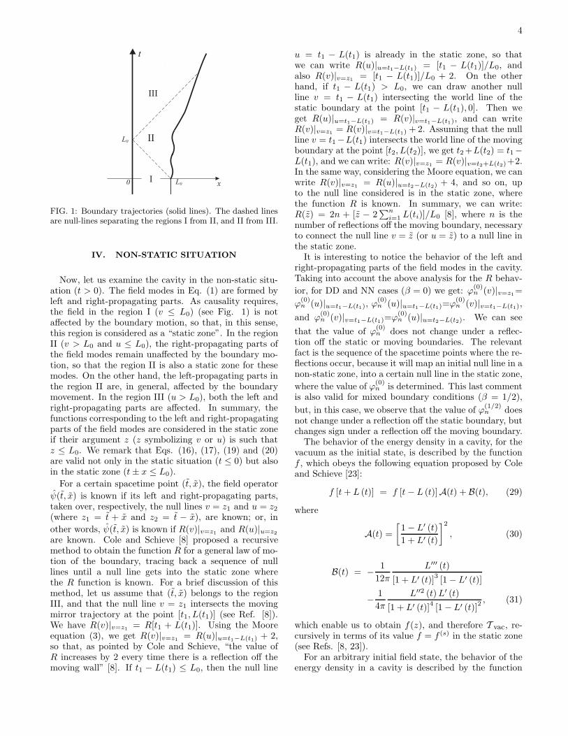
FIG. 1: Boundary trajectories (solid lines). The dashed linesare null-lines separating the regions I from II, and II from III.

IV. NON-STATIC SITUATION

Now, let us examine the cavity in the non-static situ-ation (t > 0). The field modes in Eq. (1) are formed byleft and right-propagating parts. As causality requires,the field in the region I (v ≤ L0) (see Fig. 1) is notaffected by the boundary motion, so that, in this sense,this region is considered as a “static zone”. In the regionII (v > L0 and u ≤ L0), the right-propagating parts ofthe field modes remain unaffected by the boundary mo-tion, so that the region II is also a static zone for thesemodes. On the other hand, the left-propagating parts inthe region II are, in general, affected by the boundarymovement. In the region III (u > L0), both the left andright-propagating parts are affected. In summary, thefunctions corresponding to the left and right-propagatingparts of the field modes are considered in the static zoneif their argument z (z symbolizing v or u) is such thatz ≤ L0. We remark that Eqs. (16), (17), (19) and (20)are valid not only in the static situation (t ≤ 0) but alsoin the static zone (t± x ≤ L0).

For a certain spacetime point (t, x), the field operator

ψ(t, x) is known if its left and right-propagating parts,taken over, respectively, the null lines v = z1 and u = z2(where z1 = t + x and z2 = t − x), are known; or, in

other words, ψ(t, x) is known if R(v)|v=z1and R(u)|u=z2

are known. Cole and Schieve [8] proposed a recursivemethod to obtain the function R for a general law of mo-tion of the boundary, tracing back a sequence of nulllines until a null line gets into the static zone wherethe R function is known. For a brief discussion of thismethod, let us assume that (t, x) belongs to the regionIII, and that the null line v = z1 intersects the movingmirror trajectory at the point [t1, L(t1)] (see Ref. [8]).We have R(v)|v=z1

= R[t1 + L(t1)]. Using the Mooreequation (3), we get R(v)|v=z1

= R(u)|u=t1−L(t1) + 2,so that, as pointed by Cole and Schieve, “the value ofR increases by 2 every time there is a reflection off themoving wall” [8]. If t1 − L(t1) ≤ L0, then the null line

u = t1 − L(t1) is already in the static zone, so thatwe can write R(u)|u=t1−L(t1) = [t1 − L(t1)]/L0, andalso R(v)|v=z1

= [t1 − L(t1)]/L0 + 2. On the otherhand, if t1 − L(t1) > L0, we can draw another nullline v = t1 − L(t1) intersecting the world line of thestatic boundary at the point [t1 − L(t1), 0]. Then weget R(u)|u=t1−L(t1) = R(v)|v=t1−L(t1), and can writeR(v)|v=z1

= R(v)|v=t1−L(t1) + 2. Assuming that the nullline v = t1−L(t1) intersects the world line of the movingboundary at the point [t2, L(t2)], we get t2 +L(t2) = t1−L(t1), and we can write: R(v)|v=z1

= R(v)|v=t2+L(t2)+2.In the same way, considering the Moore equation, we canwrite R(v)|v=z1

= R(u)|u=t2−L(t2) + 4, and so on, upto the null line considered is in the static zone, wherethe function R is known. In summary, we can write:R(z) = 2n + [z − 2

∑ni=1 L(ti)]/L0 [8], where n is the

number of reflections off the moving boundary, necessaryto connect the null line v = z (or u = z) to a null line inthe static zone.

It is interesting to notice the behavior of the left andright-propagating parts of the field modes in the cavity.Taking into account the above analysis for the R behav-

ior, for DD and NN cases (β = 0) we get: ϕ(0)n (v)|v=z1

=

ϕ(0)n (u)|u=t1−L(t1), ϕ

(0)n (u)|u=t1−L(t1)=ϕ

(0)n (v)|v=t1−L(t1),

and ϕ(0)n (v)|v=t1−L(t1)=ϕ

(0)n (u)|u=t2−L(t2). We can see

that the value of ϕ(0)n does not change under a reflec-

tion off the static or moving boundaries. The relevantfact is the sequence of the spacetime points where the re-flections occur, because it will map an initial null line in anon-static zone, into a certain null line in the static zone,

where the value of ϕ(0)n is determined. This last comment

is also valid for mixed boundary conditions (β = 1/2),

but, in this case, we observe that the value of ϕ(1/2)n does

not change under a reflection off the static boundary, butchanges sign under a reflection off the moving boundary.

The behavior of the energy density in a cavity, for thevacuum as the initial state, is described by the functionf , which obeys the following equation proposed by Coleand Schieve [23]:

f [t+ L (t)] = f [t− L (t)]A(t) + B(t), (29)

where

A(t) =

[

1 − L′ (t)

1 + L′ (t)

]2

, (30)

B(t) = −1

12π

L′′′ (t)

[1 + L′ (t)]3[1 − L′ (t)]

−1

4π

L′′2 (t)L′ (t)

[1 + L′ (t)]4 [1 − L′ (t)]2, (31)

which enable us to obtain f(z), and therefore T vac, re-cursively in terms of its value f = f (s) in the static zone(see Refs. [8, 23]).

For an arbitrary initial field state, the behavior of theenergy density in a cavity is described by the function

5

f (related to the vacuum part) and a new function g(related to the non-vacuum part) proposed in the presentpaper. For the latter one, from Eqs. (3), (9) and (10) weobtain the following equation:

g [t+ L (t)] = g [t− L (t)]A(t), (32)

which enable us to get g(z), and therefore T non-vac, re-cursively in terms of its value g(z) = g(s)(z) in the staticzone.

Now, for a complete analysis involving vacuum andnon-vacuum parts, let us write the equation for the func-tion h (Eq. (14)) as follows:

h [t+ L (t)] = h [t− L (t)]A(t) + B(t). (33)

The procedure to find h(z), solving recursively the Eq.(33), starts by setting z = t1 + L (t1) and tracing thenull line v = t1 + L (t1). From Eq. (33), after the firstreflection traced back on the moving boundary, we getthe relation h(z) = h [t1 − L (t1)]A(t1) + B(t1). Now, asexplained above, we set t1 − L (t1) = t2 + L (t2), and,after the second reflection on the moving boundary, weget:

h(z) = h [t2 − L (t2)]A(t2)A(t1) + B(t2)A(t1) + B(t1).

This process goes on, up to a null line gets into a staticzone, where h = h(s) = f (s) + g(s) is known. At the end,we get:

h(z) = h(s)(z)A(z) + B(z), (34)

where:

h(s)(z) = f (s) + g(s)[z(z)], (35)

A(z) = Πni=1A(ti), (36)

B(z) = B(tn)Πn−1i=1 A(ti) + B(tn−1)Π

n−2i=1 A(ti)

+...+ B(t2)A(t1) + B(t1). (37)

The number n of reflections and the sequence of in-stants t1, ...tn depend on z. In Eq. (35), we havez(z) = tn − L(tn). From this process, we observe thatthe value of f does not change under a reflection off thestatic boundary, but it changes under a reflection off themoving boundary, as expected. We also note, from Eq.(33), that the function h, after a reflection, changes inthe same way for all boundary conditions considered inthe present work (for the same boundary motion). We

remark that, in Eq. (34), the functions A and B dependonly on the law of motion of the moving mirror, whereasall the dependence on the boundary conditions consid-ered in the present paper, and on the initial field state,are stored in the static region function h(s)(z). We also

observe that, for a generic law of motion, A and B aredifferent functions, with the following properties:

A(z) > 0 ∀ z, A(z < L0) = 1, B(z < L0) = 0, (38)

which are directly obtained from Eqs. (30) and (31).The energy density T can be given as in Eq. (4), but

now with the parts Tvac and Tnon-vac rewritten as:

Tvac = −f (s)[

A(u) + A(v)]

− B(u) − B(v), (39)

Tnon-vac = −g(s)[z(u)]A(u) − g(s)[z(v)]A(v). (40)

The instantaneous force acting on the moving bound-ary, in this two-dimensional model, is given by T (t, L(t)).From Eqs. (14), (39) and (40) we see that two cavitieswith different boundary conditions and the same initiallength L0, presenting different vacuum and non-vacuumcontributions for their initial energy densities, but withthe same total energy density T (s) in the static zone, fora same (but arbitrary) law of motion will always exhibitidentical evolutions in time for their energy densities T .

A. Diagonal states

Now, let us analyze and compare the behavior of Tvac,Tnon-vac and T for the initial field states for which thedensity matrix is diagonal in the Fock basis. From Eqs.(24) and (40) we obtain:

Tnon-vac = −g(s)[

A(u) + A(v)]

, (41)

where g(s) is a constant factor. From Eqs. (39) and (41)we can see that all spacetime dependence in T comesfrom A and B. For this case we have:

T DD = T NN, T DN = T ND. (42)

Since Eq. (42) is valid for any law of motion, it gen-eralizes the Eq. (25), and because it is also valid forany diagonal state, it extends the conclusion obtained inRef. [22], where formulas correspondent to Eq. (42) wereobtained just considering the vacuum as the initial fieldstate.

The total energy stored in the cavity as a function

of time can be written as E(t) =∫ L(t)

0 T (t, x) dx. Fordiagonal initial states, we have:

E(t) = −h(s)F1(t) −F2(t), (43)

where F1(t) =∫ L(t)

0

[

A(u) + A(v)]

dx and F2(t) =∫ L(t)

0

[

B(u) + B(v)]

dx. We emphasize that F1 and F2

depend only on the law of motion of the boundary,whereas all dependence on the initial field state or typeof boundary condition is stored in the coefficient h(s).

Since the functions A and B are, in general, differentone from the other, we conclude that Tvac, Tnon-vac andT exhibit, in general, different structures. On the otherhand, one could ask about the conditions under whichTvac, Tnon-vac and T would exhibit the same structure

6

(the same curve apart from a positive scale factor or anadditive constant) so that, for instance, if there are peaksand valleys they would be at the same positions in thecavity. One condition is provided by laws of motion forwhich B(z) and A(z) have a linear relation as given by:

B(z) = k1A(z) + k2, (44)

where k1 e k2 are constants. From the properties in Eq.(38), we get k1 = −k2, resulting:

B(z) = k1[A(z) − 1]. (45)

From (39), (40) and (45), we get:

Tvac = −(f (s) + k1)[A(u) + A(v)] + 2k1, (46)

Tnon-vac = −g(s)[A(u) + A(v)], (47)

T = −(f (s) + g(s) + k1)[A(u) + A(v)] + 2k1. (48)

In the energy densities showed in Eqs. (46)-(48), if

the constant factors multiplying A(u) + A(v) are dif-ferent from zero and have the same sign, as the ratioσ(z) = B(z)/[A(z) − 1] becomes more approximatelyequal to a constant value k1, more the structures of Tvac,Tnon-vac and T become similar one to the other. Next,we exemplify these situations in the context of the vac-uum and thermal field, which are examples of a diagonalinitial field states.

For the thermal state we take into account that〈a†nan′〉 = δnn′n(n, β) and 〈anan′〉 = 〈a†na

†n′〉 = 0, where

n (n, β) = 1/(e(n+β)/T − 1), with the Boltzmann con-stant (kB) equal to 1. For this initial state, the energydensity T non-vac, now relabeled as TT , is given by:

TT =π|γ|2

2L20

G(β, T )[

A(u) + A(v)]

, (49)

where G(β, T ) =∑∞

n=1−2β

[

(n+ β)/(e(n+β)/T − 1)]

plays the role of a scale factor. Since G(1/2, T ) > G(0, T )(see Fig. 2), for T > 0 we have:

TTmixed > TT

non-mixed, (50)

where the superscript “mixed” means ND or DN cases,whereas “non-mixed” means NN or DD cases.

Note that if we set up two different cavities, one ofthem with non-mixed and the other one with mixedboundary conditions, both with a thermal field as theinitial state with temperatures given, respectively, by T1

and T2 such that G(1/2, T2) − G(0, T1) = −1/16, we getfor both cases the same initial configurations of energydensities in the static zone. Then for a same arbitrarylaw of motion for both cavities, they will exhibit the sametime evolutions for the energy densities T (and hence thesame force acting on the boundaries). An interesting caseoccurs if we set up T1 ≈ 0.34 and T2 = 0. In this case we

0.5 1 1.5 2T

1

2

3

4

5

6

G(

)β,T

FIG. 2: Plot of G(β, T ). The solid curve corresponds toG(1/2, T ), whereas the dashed one to G(0, T ).

obtain that the static and dynamical Casimir effect forthe vacuum state in the mixed case (where the Casimirstatic force is repulsive) is mimicked by the non-mixedcase with the mentioned specific temperature.

Let us now investigate a particular movement de-scribed by:

L (t) = L0

[

1 + ε sin

(

pπt

L0

)]

, (51)

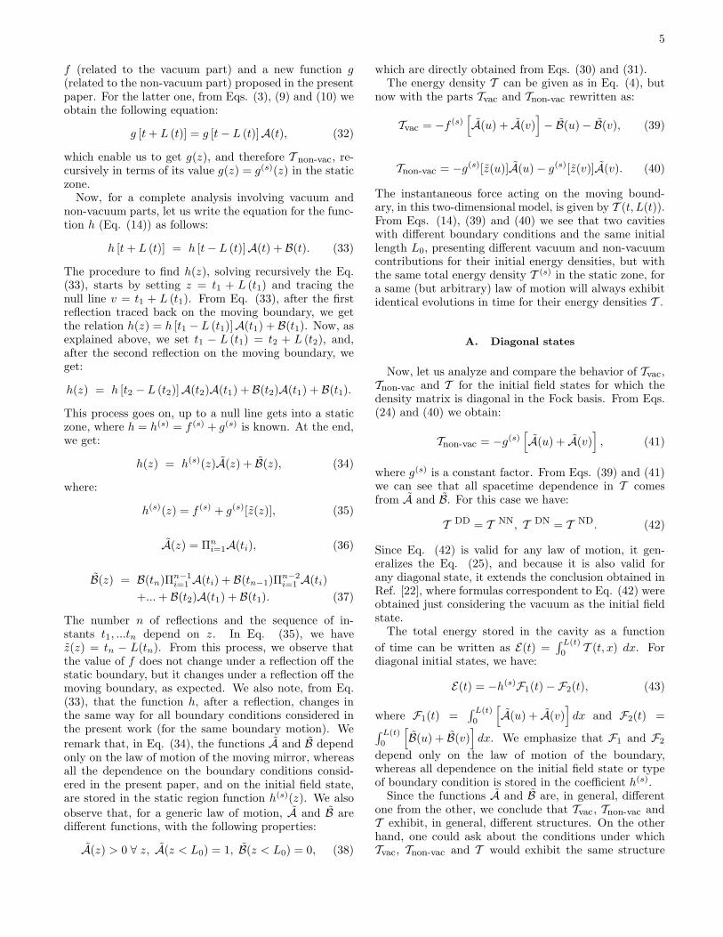
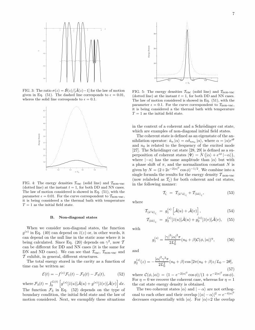
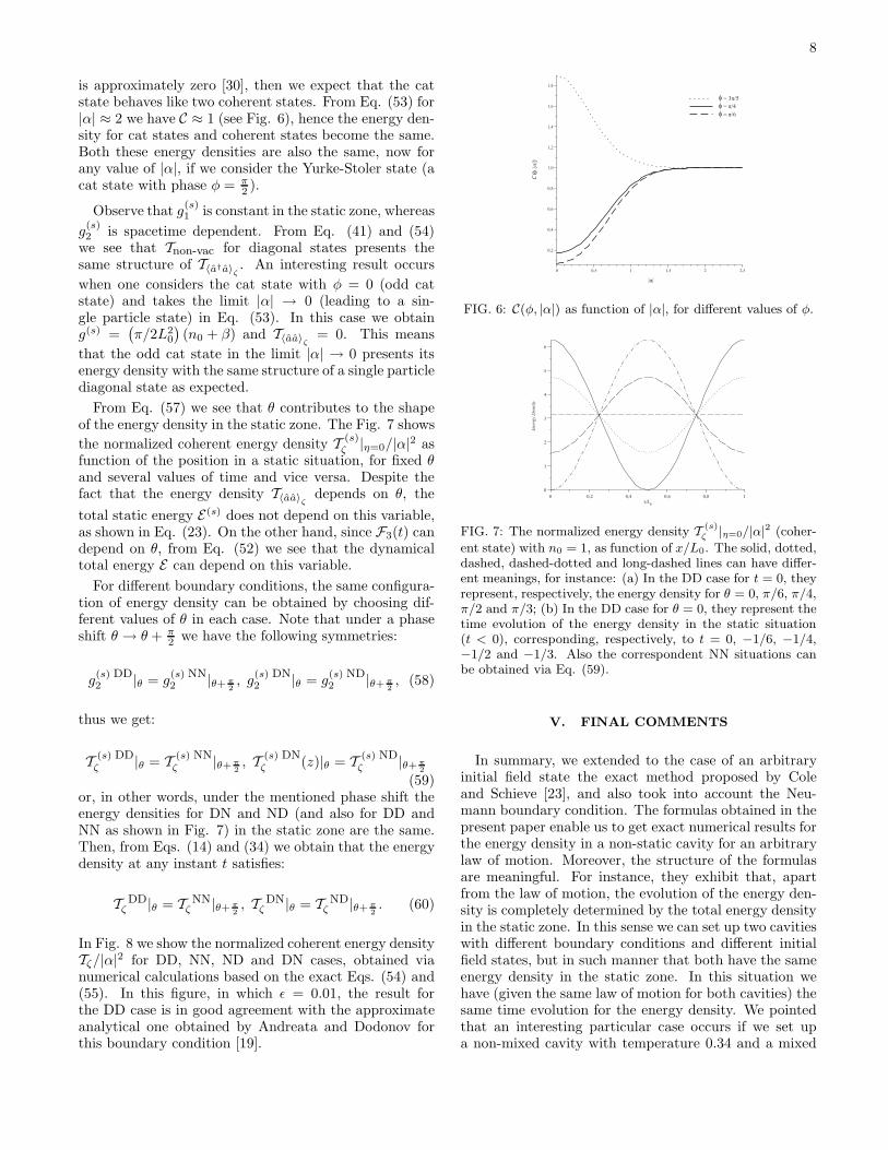
where L0 = 1, p = 2 and ǫ is a dimensionless parame-ter. This oscillatory boundary motion is investigated inseveral papers (see, for instance, Refs. [9, 19]). In thesepapers the calculations were developed in the context ofanalytical approximate methods, considering small am-plitudes of oscillation (|ǫ| ≪ 1). Here, we investigate thelaw of motion in Eq. (51) for ǫ = 0.01 and ǫ = 0.1. Theformer value is in better agreement with the condition|ǫ| ≪ 1 than the latter one. Our intention now is to ver-ify, from an exact point of view, the similarity betweenthe structures of Tvac, Tnon-vac and T for both valuesof ǫ. In Fig. 3 we plot the ratio σ for the two values:ǫ = 0.01 and ǫ = 0.1. We observe that the ratio σ ismore approximately constant for ǫ = 0.01 (dashed line)than for ǫ = 0.1 (solid line), so that, since f (s) + k1 < 0and g(s) ≤ 0, we expect that Tvac, Tnon-vac and T exhibitmore similarity for the former than for the latter valueof ǫ, for any diagonal initial state or any of the boundaryconditions considered in the present paper. In fact, thisis what can be visualized in Figs. 4 and 5, where we showTvac (dotted lines) and Tnon-vac (solid lines) for the lawof motion (51) and the thermal bath with temperatureT = 1 as the diagonal initial field state. In Fig. 4, forthe case ǫ = 0.01, both dotted and solid lines have theirminimum and maximum values at the same positions, aspredicted by the approximate analytical approach con-sidered by Andreata and Dodonov [19], which was basedon ǫ≪ 1. On the other hand, in Fig. 5 (case ǫ = 0.1), ifcompared to the dotted line, the solid line has additionalmaximum points at x = 0.28 and x = 0.72, and also addi-tional minimum points at x = 0.42 and x = 0.58, so thatdifferences between the structures of Tvac and Tnon-vac

start to become more evident.

7

t

s

FIG. 3: The ratio σ(z) = B(z)/[A(z)−1] for the law of motiongiven in Eq. (51). The dashed line corresponds to ǫ = 0.01,wheres the solid line corresponds to ǫ = 0.1.

x / L0

Ener

gy

Den

sity

FIG. 4: The energy densities Tvac (solid line) and Tnon-vac

(dotted line) at the instant t = 1, for both DD and NN cases.The law of motion considered is showed in Eq. (51), with theparameter ǫ = 0.01. For the curve correspondent to Tnon-vac,it is being considered a the thermal bath with temperatureT = 1 as the initial field state.

B. Non-diagonal states

When we consider non-diagonal states, the functiong(s) in Eq. (40) can depend on z(z) or, in other words, itcan depend on the null line in the static zone where it isbeing calculated. Since Eq. (20) depends on γ2, now Tcan be different for DD and NN cases (it is the same forDN and ND cases). We can see that Tvac, Tnon-vac andT exhibit, in general, different structures.

The total energy stored in the cavity as a function oftime can be written as:

E(t) = −f (s)F1(t) −F2(t) −F3(t), (52)

where F3(t) =∫ L(t)

0

[

g(s)[z(u)]A(u) + g(s)[z(v)]A(v)]

dx.

The function F3 in Eq. (52) depends on the type ofboundary condition, the initial field state and the law ofmotion considered. Next, we exemplify these situations

x / L0

En

erg

y D

ensi

ty

FIG. 5: The energy densities Tvac (solid line) and Tnon-vac

(dotted line) at the instant t = 1, for both DD and NN cases.The law of motion considered is showed in Eq. (51), with theparameter ǫ = 0.1. For the curve correspondent to Tnon-vac,it is being considered a the thermal bath with temperatureT = 1 as the initial field state.

in the context of a coherent and a Schrodinger cat state,which are examples of non-diagonal initial field states.

The coherent state is defined as an eigenstate of the an-nihilation operator: an |α〉 = αδnn0

|α〉, where α = |α|eiθ

and n0 is related to the frequency of the excited mode[27]. The Schrodinger cat state [28, 29] is defined as a su-perposition of coherent states |Ψ〉 = N

(

|α〉 + eiφ |−α〉)

,where |−α〉 has the same amplitude than |α〉 but witha phase shift of π, and the normalization constant N is

given by N = (2+2e−2|α|2 cosφ)−1/2. We combine into asingle formula the results for the energy density T non-vac

(now relabeled as Tζ) for both coherent and cat states,in the following manner:

Tζ = T〈a†a〉ζ

+ T〈aa〉ζ, (53)

where

T〈a†a〉ζ

= g(s)1

[

A(u) + A(v)]

, (54)

T〈aa〉ζ

= g(s)2 [z(u)]A(u) + g

(s)2 [z(v)]A(v), (55)

with

g(s)1 =

|γ|2|α|2π

2L20

(n0 + β)C(φ, |α|)η , (56)

and

g(s)2 (z) = −

|α|2γ2π

2L20

(n0 + β) cos [2π(n0 + β)z/L0 − 2θ],

(57)

where C(φ, |α|) = (1 − e−2|α|2 cosφ)/(1 + e−2|α|2 cosφ).For η = 0 we recover the coherent case, whereas for η = 1the cat state energy density is obtained.

The two coherent states |α〉 and | −α〉 are not orthog-

onal to each other and their overlap |〈α| −α〉|2 = e−4|α|2

decreases exponentially with |α|. For |α|=2 the overlap

8

is approximately zero [30], then we expect that the catstate behaves like two coherent states. From Eq. (53) for|α| ≈ 2 we have C ≈ 1 (see Fig. 6), hence the energy den-sity for cat states and coherent states become the same.Both these energy densities are also the same, now forany value of |α|, if we consider the Yurke-Stoler state (acat state with phase φ = π

2 ).

Observe that g(s)1 is constant in the static zone, whereas

g(s)2 is spacetime dependent. From Eq. (41) and (54)

we see that Tnon-vac for diagonal states presents thesame structure of T〈a†a〉ζ

. An interesting result occurs

when one considers the cat state with φ = 0 (odd catstate) and takes the limit |α| → 0 (leading to a sin-gle particle state) in Eq. (53). In this case we obtaing(s) =

(

π/2L20

)

(n0 + β) and T〈aa〉ζ

= 0. This means

that the odd cat state in the limit |α| → 0 presents itsenergy density with the same structure of a single particlediagonal state as expected.

From Eq. (57) we see that θ contributes to the shapeof the energy density in the static zone. The Fig. 7 shows

the normalized coherent energy density T(s)

ζ |η=0/|α|2 asfunction of the position in a static situation, for fixed θand several values of time and vice versa. Despite thefact that the energy density T〈aa〉

ζdepends on θ, the

total static energy E(s) does not depend on this variable,as shown in Eq. (23). On the other hand, since F3(t) candepend on θ, from Eq. (52) we see that the dynamicaltotal energy E can depend on this variable.

For different boundary conditions, the same configura-tion of energy density can be obtained by choosing dif-ferent values of θ in each case. Note that under a phaseshift θ → θ + π

2 we have the following symmetries:

g(s) DD2 |θ = g

(s) NN2 |θ+ π

2, g

(s) DN2 |θ = g

(s) ND2 |θ+ π

2, (58)

thus we get:

T(s) DD

ζ |θ = T(s) NN

ζ |θ+ π2, T

(s) DNζ (z)|θ = T

(s) NDζ |θ+π

2

(59)or, in other words, under the mentioned phase shift theenergy densities for DN and ND (and also for DD andNN as shown in Fig. 7) in the static zone are the same.Then, from Eqs. (14) and (34) we obtain that the energydensity at any instant t satisfies:

T DDζ |θ = T NN

ζ |θ+ π2, T DN

ζ |θ = T NDζ |θ+ π

2. (60)

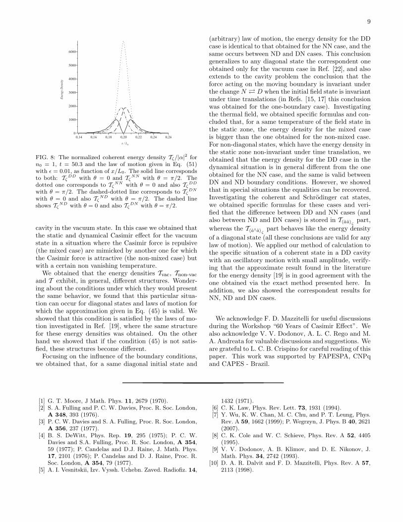
In Fig. 8 we show the normalized coherent energy densityTζ/|α|2 for DD, NN, ND and DN cases, obtained vianumerical calculations based on the exact Eqs. (54) and(55). In this figure, in which ǫ = 0.01, the result forthe DD case is in good agreement with the approximateanalytical one obtained by Andreata and Dodonov forthis boundary condition [19].

FIG. 6: C(φ, |α|) as function of |α|, for different values of φ.

FIG. 7: The normalized energy density T(s)

ζ |η=0/|α|2 (coher-

ent state) with n0 = 1, as function of x/L0. The solid, dotted,dashed, dashed-dotted and long-dashed lines can have differ-ent meanings, for instance: (a) In the DD case for t = 0, theyrepresent, respectively, the energy density for θ = 0, π/6, π/4,π/2 and π/3; (b) In the DD case for θ = 0, they represent thetime evolution of the energy density in the static situation(t < 0), corresponding, respectively, to t = 0, −1/6, −1/4,−1/2 and −1/3. Also the correspondent NN situations canbe obtained via Eq. (59).

V. FINAL COMMENTS

In summary, we extended to the case of an arbitraryinitial field state the exact method proposed by Coleand Schieve [23], and also took into account the Neu-mann boundary condition. The formulas obtained in thepresent paper enable us to get exact numerical results forthe energy density in a non-static cavity for an arbitrarylaw of motion. Moreover, the structure of the formulasare meaningful. For instance, they exhibit that, apartfrom the law of motion, the evolution of the energy den-sity is completely determined by the total energy densityin the static zone. In this sense we can set up two cavitieswith different boundary conditions and different initialfield states, but in such manner that both have the sameenergy density in the static zone. In this situation wehave (given the same law of motion for both cavities) thesame time evolution for the energy density. We pointedthat an interesting particular case occurs if we set upa non-mixed cavity with temperature 0.34 and a mixed

9

x / L0

Ener

gy

Den

sity

FIG. 8: The normalized coherent energy density Tζ/|α|2 for

n0 = 1, t = 50.3 and the law of motion given in Eq. (51)with ǫ = 0.01, as function of x/L0. The solid line correspondsto both: Tζ

DD with θ = 0 and TζNN with θ = π/2. The

dotted one corresponds to TζNN with θ = 0 and also Tζ

DD

with θ = π/2. The dashed-dotted line corresponds to TζDN

with θ = 0 and also TζND with θ = π/2. The dashed line

shows TζND with θ = 0 and also Tζ

DN with θ = π/2.

cavity in the vacuum state. In this case we obtained thatthe static and dynamical Casimir effect for the vacuumstate in a situation where the Casimir force is repulsive(the mixed case) are mimicked by another one for whichthe Casimir force is attractive (the non-mixed case) butwith a certain non vanishing temperature.

We obtained that the energy densities Tvac, Tnon-vac

and T exhibit, in general, different structures. Wonder-ing about the conditions under which they would presentthe same behavior, we found that this particular situa-tion can occur for diagonal states and laws of motion forwhich the approximation given in Eq. (45) is valid. Weshowed that this condition is satisfied by the laws of mo-tion investigated in Ref. [19], where the same structurefor these energy densities was obtained. On the otherhand we showed that if the condition (45) is not satis-fied, these structures become different.

Focusing on the influence of the boundary conditions,we obtained that, for a same diagonal initial state and

(arbitrary) law of motion, the energy density for the DDcase is identical to that obtained for the NN case, and thesame occurs between ND and DN cases. This conclusiongeneralizes to any diagonal state the correspondent oneobtained only for the vacuum case in Ref. [22], and alsoextends to the cavity problem the conclusion that theforce acting on the moving boundary is invariant underthe change N ⇄ D when the initial field state is invariantunder time translations (in Refs. [15, 17] this conclusionwas obtained for the one-boundary case). Investigatingthe thermal field, we obtained specific formulas and con-cluded that, for a same temperature of the field state inthe static zone, the energy density for the mixed caseis bigger than the one obtained for the non-mixed case.For non-diagonal states, which have the energy density inthe static zone non-invariant under time translation, weobtained that the energy density for the DD case in thedynamical situation is in general different from the oneobtained for the NN case, and the same is valid betweenDN and ND boundary conditions. However, we showedthat in special situations the equalities can be recovered.Investigating the coherent and Schrodinger cat states,we obtained specific formulas for these cases and veri-fied that the difference between DD and NN cases (andalso between ND and DN cases) is stored in T〈aa〉

ζpart,

whereas the T〈a†a〉ζ

part behaves like the energy density

of a diagonal state (all these conclusions are valid for anylaw of motion). We applied our method of calculation tothe specific situation of a coherent state in a DD cavitywith an oscillatory motion with small amplitude, verify-ing that the approximate result found in the literaturefor the energy density [19] is in good agreement with theone obtained via the exact method presented here. Inaddition, we also showed the correspondent results forNN, ND and DN cases.

We acknowledge F. D. Mazzitelli for useful discussionsduring the Workshop “60 Years of Casimir Effect”. Wealso acknowledge V. V. Dodonov, A. L. C. Rego and M.A. Andreata for valuable discussions and suggestions. Weare grateful to L. C. B. Crispino for careful reading of thispaper. This work was supported by FAPESPA, CNPqand CAPES - Brazil.

[1] G. T. Moore, J Math. Phys. 11, 2679 (1970).[2] S. A. Fulling and P. C. W. Davies, Proc. R. Soc. London,

A 348, 393 (1976).[3] P. C. W. Davies and S. A. Fulling, Proc. R. Soc. London,

A 356, 237 (1977).[4] B. S. DeWitt, Phys. Rep. 19, 295 (1975); P. C. W.

Davies and S.A. Fulling, Proc. R. Soc. London, A 354,59 (1977); P. Candelas and D.J. Raine, J. Math. Phys.17, 2101 (1976); P. Candelas and D. J. Raine, Proc. R.Soc. London, A 354, 79 (1977).

[5] A. I. Vesnitskii, Izv. Vyssh. Uchebn. Zaved. Radiofiz. 14,

1432 (1971).[6] C. K. Law, Phys. Rev. Lett. 73, 1931 (1994).[7] Y. Wu, K. W. Chan, M. C. Chu, and P. T. Leung, Phys.

Rev. A 59, 1662 (1999); P. Wegrzyn, J. Phys. B 40, 2621(2007).

[8] C. K. Cole and W. C. Schieve, Phys. Rev. A 52, 4405(1995).

[9] V. V. Dodonov, A. B. Klimov, and D. E. Nikonov, J.Math. Phys. 34, 2742 (1993).

[10] D. A. R. Dalvit and F. D. Mazzitelli, Phys. Rev. A 57,2113 (1998).

10

[11] L. H. Ford and A. Vilenkin, Phys. Rev. D 25, 2569(1982); P. A. Maia Neto, J. Phys. A 27, 2167 (1994);P. A. Maia Neto and L. A. S. Machado, Phys. Rev. A54, 3420 (1996).

[12] M. Razavy and J. Terning, Phys. Rev. D 31, 307 (1985);G. Calucci, J. Phys. A 25, 3873 (1992); C. K. Law, Phys.Rev. A 49, 433 (1994); C. K. Law, Phys. Rev. A 51, 2537(1995); V. V. Dodonov and A. B. Klimov, Phys. Rev. A,53, 2664 (1996); D. F. Mundarain and P. A. Maia Neto,Phys. Rev. A 57, 1379 (1998).

[13] M. T. Jaekel and S. Reynaud, J. Phys. I (France) 3, 339(1993); M. T. Jaekel and S. Reynaud, Phys. Lett. A 172,319 (1993); L. A. S. Machado, P. A. Maia Neto, and C.Farina, Phys. Rev. D 66, 105016 (2002).

[14] G. Plunien, R. Schutzhold, and G. Soff, Phys. Rev. Lett.84, 1882 (2000).

[15] D. T. Alves, E. R. Granhen and M. G. Lima, Phys. Rev.D 77, 125001 (2008).

[16] J. Hui, S. Qing-Yun, and W. Jian-Sheng, Phys. Lett.A 268, 174 (2000); R. Schutzhold, G. Plunien, and G.Soff, Phys. Rev. A 65, 043820 (2002); G. Schaller, R.Schutzhold, G. Plunien, and G. Soff, Phys. Rev. A 66,023812 (2002).

[17] D. T. Alves, C. Farina, and P. A. Maia Neto, J. Phys. A36, 11333 (2003).

[18] V. V. Dodonov, A. Klimov, and V. I. Man’ko, Phys. Lett.A 149, 225 (1990).

[19] M. A. Andreata and V. V. Dodonov, J. Phys. A 33, 3209(2000).

[20] V. V. Dodonov, M. A. Andreata, and S. S. Mizrahi, J.Opt. B: Quantum Semiclass. Opt. 7 S468 (2005); D. A.R. Dalvit and P. A. Maia Neto, Phys. Rev. Lett 84, 798(2000).

[21] M. Montazeri and M. F. Miri, Phys. Rev. A 71, 063814(2005); D. T. Alves, C. Farina, and E. R. Granhen, ibid.73, 063818 (2006); B. Mintz, C. Farina, P. A. M. Neto,and R. B. Rodrigues, J. Phys. A 39, 6559 (2006); J.Sarabadani and M. F. Miri, ibid. 75, 055802 (2007).

[22] D. T. Alves and E. R. Granhen, Phys. Rev. A 77, 015808(2008).

[23] C. K. Cole and W. C. Schieve, Phys. Rev. A 64, 023813(2001).

[24] D. A. R. Dalvit, F. D. Mazzitelli, and O. Millan, J. Phys.A 39, 6261 (2006).

[25] T. H. Boyer, Am. J. Phys. 71, 990 (2003).[26] T. H. Boyer, Phys. Rev. A 9, 2078 (1974).[27] R. J. Glauber, Phys. Rev. 131 6, 2766 (1963); R. J.

Glauber, Phys. Rev. Letters. 10 84 (1963)[28] E. Schrodinger, Naturwissensheften 23, 807 (1935); C.

C. Gerry and P. L. Knight, Am. J. Phys. 65, 964 (1997).[29] H. Jeong, A. P. Lund, and T. C. Ralph, Phys. Rev. A

72, 013801 (2005).[30] H. Jeong and T. C. Ralph, quant-ph/0509137 (2005).