arX

iv:a

stro

-ph/

9903

165v

1 1

1 M

ar 1

999

Time Evolution of Galaxy Formation

and Bias in Cosmological Simulations

Michael Blanton, Renyue Cen,

Jeremiah P. Ostriker, Michael A. Strauss

Princeton University Observatory, Princeton, NJ 08544

blanton, cen, jpo, strauss@astro.princeton.edu

and

Max Tegmark

Institute for Advanced Study, Princeton, NJ 08540

max@sns.ias.edu

ABSTRACT

The clustering of galaxies relative to the underlying mass distribution declines with cosmic

time for three reasons. First, nonlinear peaks become less rare events as the density field evolves.

Second, the densest regions stop forming new galaxies because their gas becomes too hot to

cool and collapse. Third, after galaxies form, they are subject to the same gravitational forces

as the dark matter, and thus they tend to trace the dark matter distibution more closely with

time; in this sense, they are gravitationally “debiased.” In order to illustrate these effects, we

perform a large-scale hydrodynamic cosmological simulation of a ΛCDM model with Ω0 = 0.37

and examine the statistics of δ∗(r, z), the density field of recently formed galaxies at position r

and redshift z. We find that the bias of recently formed galaxies b∗ ≡ 〈δ2∗〉

1/2/〈δ2〉

1/2, where

δ is the mass overdensity, evolves from b∗ ∼ 4.5 at z = 3 to b∗ ∼ 1 at z = 0, on 8 h−1 Mpc

comoving scales. The correlation coefficient r∗ ≡ 〈δδ∗〉/〈δ2〉

1/2〈δ2

∗〉1/2

evolves from r∗ ∼ 0.9 at

z = 3 to r∗ ∼ 0.25 at z = 0. That is, as gas in the universe heats up and prevents star formation,

the star-forming galaxies become poorer tracers of the mass density field. We show that the

linear continuity equation is a good approximation for describing the gravitational debiasing,

even on nonlinear scales. The most interesting observational consequence of the simulations

is that the linear regression of the galaxy formation density field on the galaxy density field,

b∗gr∗g = 〈δ∗δg〉/〈δ2g〉, evolves from about 0.9 at z = 1 to 0.35 at z = 0. Measuring this evolution,

which should be possible using the Sloan Digital Sky Survey, would place constraints on models

for galaxy formation. In addition, we evaluate the effects of the evolution of galaxy formation

on estimates of Ω from cluster mass-to-light ratios, finding that while Ω(z) increases with z, the

estimated Ωest(z) actually decreases. This effect is due to the combination of galaxy bias and

the relative fading of cluster galaxies with respect to field galaxies. Finally, these effects provide

a possible explanation for the Butcher-Oemler effect, the excess of blue galaxies in clusters at

redshift z ∼ 0.5.

– 2 –

1. Motivation

Recent observations of the evolution of galaxy clustering have explored both the regime z <∼ 1, and

have probed the distribution of galaxies at z ≈ 3. The low-redshift works include a wide-field (4 × 4)

I-selected angular sample (Postman et al. 1998), Canada-France Redshift Survey galaxies with redshifts

between 0 < z < 1.3 (Le Fevre et al. 1996), the Hubble Deep Field (Connolly, Szalay, & Brunner 1998),

field galaxies from the Canadian Network for Observational Cosmology (CNOC) survey (Shepherd et

al. 1997), the Hawaii K-selected redshift survey (Carlberg et al. 1997), and a redshift survey performed on

the Palomar 200-inch telescope (Small et al. 1999). The results of these surveys are still rather discrepant;

they don’t yet give a consistent picture for how galaxy clustering evolves with time. The evolution of the

relative clustering of old and and young galaxies is also of interest, because it yields direct information on

where galaxy formation occurs as a function of redshift. Le Fevre et al. (1996) made a simple attempt at

measuring this evolution by separating their sample by color. They found that red and blue galaxies have

comparable correlation amplitudes at z > 0.5, although red galaxies are more clustered today, by a factor

of about 1.5 (in agreement with other local estimates, such as Davis & Geller 1976, Giovanelli, Haynes, &

Chincarini 1986, Santiago & Strauss 1992, Loveday et al. 1995, Loveday et al. 1996, Hermit et al. 1996, and

Guzzo et al. 1997). The evolution of the density-morphology relation in clusters also contains information

about where galaxies form as a function of redshift, showing that at z ∼ 0.5 there is significantly more star

formation in clusters than there is today (Butcher & Oemler 1978, 1984; Couch & Sharples 1987; Dressler

& Gunn 1992; Couch et al. 1994; Oemler, Dressler, & Butcher 1997; Dressler et al. 1997; Poggianti et al.

1999).

Measurements of the clustering of Lyman-break objects (LBOs) at z ∼ 3 (Steidel et al. 1998) give a

more unambiguous indication of the evolution in clustering. In particular, measurements of the amplitude

of counts-in-cells fluctuations (Adelberger et al. 1998) or the angular autocorrelation function (Giavalisco

et al. 1998) suggest that galaxies were as strongly clustered in comoving coordinates at z ∼ 3 as they

are today. If the LBOs are unbiased tracers of the mass density field, these results contradict the widely

accepted gravitational instability (GI) model for the formation of large-scale structure, unless one assumes

an unacceptably low value of Ω0 in order to prevent the growth of the clustering of galaxies between z = 3

and today. Therefore, the objects observed at high redshift are probably more highly “biased” tracers of the

mass density field than are galaxies today. That is, they have a high value of bg ≡ σg/σ, where σg ≡ 〈δ2g〉

1/2

is the rms galaxy density fluctuation and σ ≡ 〈δ2〉1/2

is the rms mass fluctuation. The counts-in-cells

analysis of Adelberger et al. (1998) suggests that at z = 3 the bias of LBOs is bg ∼ 2b0 (for Ω0 = 0.2,

ΩΛ = 0), bg ∼ 4b0 (for Ω0 = 0.3, ΩΛ = 0.7), or bg ∼ 6b0 (for Ω0 = 1), where b0 is the bias of galaxies today.

How does the observed clustering since z ≈ 3 relate to the underlying mass density fluctuations? From a

theoretical perspective, the bias decreases with time because of three effects. First, at early times, collapsed

objects are likely to be in the highest peaks of the density field, since one needs a dense enough clump

of baryons in order to start forming stars. Such high-σ peaks are highly biased tracers of the underlying

density field (Doroshkevich 1970; Kaiser 1984; Bardeen et al. 1986; Bond et al. 1991; Mo & White 1996).

As time progresses, lower peaks in the density field begin to form galaxies, which are less biased tracers of

the mass density field. Second, the very densest regions soon become filled with shock-heated, virialized

gas which does not easily cool and collapse to form galaxies (Blanton et al. 1999). These two effects cause a

shift of galaxy formation to lower density regions of the universe. This shift is evident in the real universe:

young galaxies are not found in clusters at z = 0. To keep track of these effects, we define the bias b∗ and

– 3 –

correlation coefficient r∗ of galaxy formation as

b∗ ≡〈δ2

∗〉1/2

〈δ2〉1/2

and r∗ ≡〈δ∗δ〉

〈δ2∗〉

1/2〈δ2〉

1/2, (1)

where δ ≡ ρ/〈ρ〉 − 1 is the overdensity of mass and δ∗ ≡ ρ∗/〈ρ∗〉 − 1 is the overdensity field of “recently

formed” galaxies, each defined at some smoothing scale. By “recently formed,” we mean material that has

collapsed and formed stars within the last 0.5 Gyrs. Alternatively, one can consider δ∗ as the overdensity

field of galaxies weighted by the star formation rate in each — for the purposes of this paper we consider

the formation of a galaxy equivalent to the formation of stars within it. As functions of redshift, b∗(z) and

r∗(z) are essentially differential quantities which keep track of where stars are forming at each epoch. They

both decrease with time for the reasons stated above. Predictions of b∗(z) and r∗(z) are complementary

to predictions of the star formation rate as a function of redshift (Madau et al. 1996; Nagamine, Cen &

Ostriker 1999; Somerville & Primack 1998; Baugh et al. 1998); whereas those studies examine when galaxies

form, we examine where they form.

The third effect is that after galaxies form, they are subject to the same gravitational physics as the

dark matter; thus, the two distributions become more and more alike, debiasing the galaxies gravitationally

(Fry 1996; Tegmark & Peebles 1998; see Section 4). The history of b∗(z) and r∗(z) convolved with effects of

gravitational debiasing determines the history of the bias of all galaxies, quantified as

bg ≡〈δ2

g〉1/2

〈δ2〉1/2

and rg ≡〈δgδ〉

〈δ2g〉

1/2〈δ2〉

1/2, (2)

where δg ≡ ρg/〈ρg〉 − 1 is the overdensity of galaxies. Here, bg(z) and rg(z) are integral quantities, which

refer to the entire population of galaxies. Until recently, most papers on this subject have considered only

the effect of bias (bg) on large-scale structure statistics. However, observational and theoretical arguments

suggest that scatter in the relationship between galaxies and mass may also be important (Tegmark &

Bromley 1998; Blanton et al. 1999); treating the relationship as purely deterministic when analyzing

peculiar velocity surveys or redshift-space distortions of the power spectrum can produce observational

inconsistencies (Pen 1998; Dekel & Lahav 1998). Thus, even at lowest order, these treatments need to

include consideration of the correlation coefficient rg.

Finally, we will also define the cross-correlation of all galaxies and of young galaxies as

b∗g ≡〈δ2

∗〉1/2

〈δ2g〉

1/2and r∗g ≡

〈δ∗δg〉

〈δ2∗〉

1/2〈δ2

g〉1/2

. (3)

These quantities are important because they are potentially observable, by comparing number-weighted

and star-formation weighted galaxy density fields.

Previous theoretical efforts have focused on the evolution of the clustering of all galaxies, or equivalently,

the evolution of the integral quantities bg(z) and rg(z). There has been notable success in this vein in

explaining the nature of the LBOs. In the peaks-biasing formalism, the halo mass of collapsed objects

determines both their number density and their clustering strength (Doroshkevich 1970; Kaiser 1984;

Bardeen et al. 1986; Bond et al. 1991; Mo & White 1996); interestingly, halos with masses > 1012M⊙

at z = 3 have both a number density and clustering strength similar to those of LBOs, in reasonable

cosmologies (Adelberger et al. 1998), a result verified by N -body simulations (Wechsler et al. 1998;

Kravtsov & Klypin 1998). This fact is reflected in the results for high-redshift clustering of semi-analytic

– 4 –

galaxy formation models, which also find that galaxies at z ∼ 3 are highly biased (Kauffmann, Nusser, &

Steinmetz 1997; Kauffmann et al. 1999; Somerville, Primack & Faber 1998; Baugh et al. 1998). Furthermore,

hydrodynamic simulations using simple criteria for galaxy formation (Evrard, Summers, & Davis 1994;

Katz, Hernquist, & Weinberg 1998; Cen & Ostriker 1998a) find that the distribution of galaxies at z = 3

is indeed biased with respect to the mass distribution, and that the clustering strength of galaxies depends

only weakly on redshift.

While the issue of bg(z) and rg(z) is the one which observations are currently best-suited to address,

perhaps other statistics can constrain the nature of galaxy formation more powerfully. After all, the

fundamental prediction of theories for galaxy formation, such as ours and such as the semi-analytic models

mentioned above, is the location of star formation as a function of time. Important information about

galaxy formation may be lost if one examines only the integral quantities, which have been affected by the

entire history of galaxy formation convolved with their subsequent gravitational evolution. Therefore, we

focus here on the evolution of the large-scale clustering of galaxy formation, defined as the formation of the

galaxy’s constituent stars — that is, the evolution of b∗ and r∗. Now is an opportune time to investigate

such questions, since large redshift and angular surveys which can examine this and related properties of

galaxies are imminent.

In this paper, we measure the clustering of galaxy formation in the hydrodynamical simulations of

Cen & Ostriker (1998a), which we describe in Section 2. In Section 3, we consider the properties of galaxy

formation in these simulations as a function of time, studying the first two effects discussed above and

the redshift dependence of b∗ and r∗. In Section 4, we discuss the gravitational debiasing, the third effect

mentioned above. In Section 5, we discuss observable effects of the trends in galaxy formation found in the

simulations. Especially important is the strong evolution of the cross-correlation between the star-formation

weighted density field and the galaxy density field; this evolution should be observable with surveys such as

the Sloan Digital Sky Survey (SDSS; Gunn & Weinberg 1995). In addition, the evolution of the location of

galaxy formation in the universe may be related to the observed Butcher-Oemler effect and may affect the

mass-to-light ratios of clusters. We conclude in Section 6.

2. Simulations

The work of Ostriker & Steinhardt (1995) motivated the choice of a flat cold dark matter cosmology for

the simulation used in this paper, with Ω0 = 0.37, ΩΛ = 0.63, and Ωb = 0.049. Recent observations of high

redshift supernovae have lent support to the picture of a flat, low-density universe (Perlmutter et al. 1997;

Garnavich et al. 1998). Great uncertainty remains, however, and future work along the lines of this paper

will need to address different cosmologies. The Hubble constant was set to H0 = 100 h km s−1 Mpc−1,

with h = 0.7. The primordial perturbations were adiabatic and random phase, with a power spectrum

slope of n = 0.95 and amplitudes such that σ8 = 0.8 for the dark matter at z = 0, at which time the

age of the universe is 12.7 Gyrs. We use a periodic box 100 h−1 Mpc on a side, with 5123 grid cells and

2563 dark matter particles. Thus, the dark matter mass resolution is about 5 × 109 h−1 M⊙ and the grid

cell size is ∼ 0.2 h−1 Mpc. The smallest smoothing length we consider is a 1 h−1 Mpc radius top hat,

which is considerably larger than a cell size. On these scales and larger, the relevant gravitational and

hydrodynamical physics are correctly handled. On the other hand, subgrid effects such as the fine grain

structure of the gas and star formation may influence large-scale properties of the galaxy distribution. As

we describe here, we handle these effects using crude, but plausible, rules.

– 5 –

Cen & Ostriker (1998a) describe the hydrodynamic code in detail; it is similar to but greatly improved

over that of Cen & Ostriker (1992a,b). The simulations are Eulerian on a Cartesian grid and use the

Total Variation Diminishing method with a shock-capturing scheme (Jameson 1989). In addition, the code

accounts for cooling processes and incorporates a heuristic galaxy formation criterion, whose essence is as

follows: if a cell’s density is high enough, if the cooling time of the gas in it is shorter than its dynamical

time, if it contains greater than the Jeans mass, and if the flow around that cell is converging, it will have

stars forming inside of it. The code turns the baryonic fluid component into collisionless stellar particles

(hereafter “galaxy particles”) at a rate proportional to mb/tdyn, where mb is the mass of gas in the cells

and tdyn is the local dynamical time. These galaxy particles subsequently contribute to metal production

and the background ionizing UV radiation. This algorithm is essentially the same as that used by Katz,

Hernquist, & Weinberg (1992) and Gnedin (1996a,b). The masses of these galaxy particles range from

about 106 to 109 M⊙. Thus, many galaxy particles are contained in what would correspond to a single

luminous galaxy in the real universe. However, rather than grouping the particles into galaxies, in this

paper we simply define a galaxy mass density field from the distribution of galaxy particles themselves.

More details concerning the galaxy formation criteria and their consequences are given in Appendix A.

We will examine the results of the simulations at four output times: z = 3, z = 1, z = 0.5 and

z = 0. At each output time, we will consider the properties both of all the galaxy particles and of those

galaxy particles formed within the previous 0.5 Gyrs. We will take these “recently” formed particles to be

representative of the properties of galaxy formation at that output time, and label their overdensity field

δ∗ ≡ ρ∗/〈ρ∗〉 − 1, the “galaxy formation density field.”

3. Time dependence of Galaxy Formation

In this section, we study the relationship between the mass density, the gas temperature, and the

galaxy formation density fields at each epoch. We will show the evolution of the the quantities b∗ and r∗with redshift, and demonstrate that this evolution is largely due to the changing relationship between mass

density and temperature.

Let us begin by considering the evolution of the temperature and mass density fields as a function of

redshift. At each of our four output times, we smooth the fields with a top hat of 1 h−1 Mpc comoving

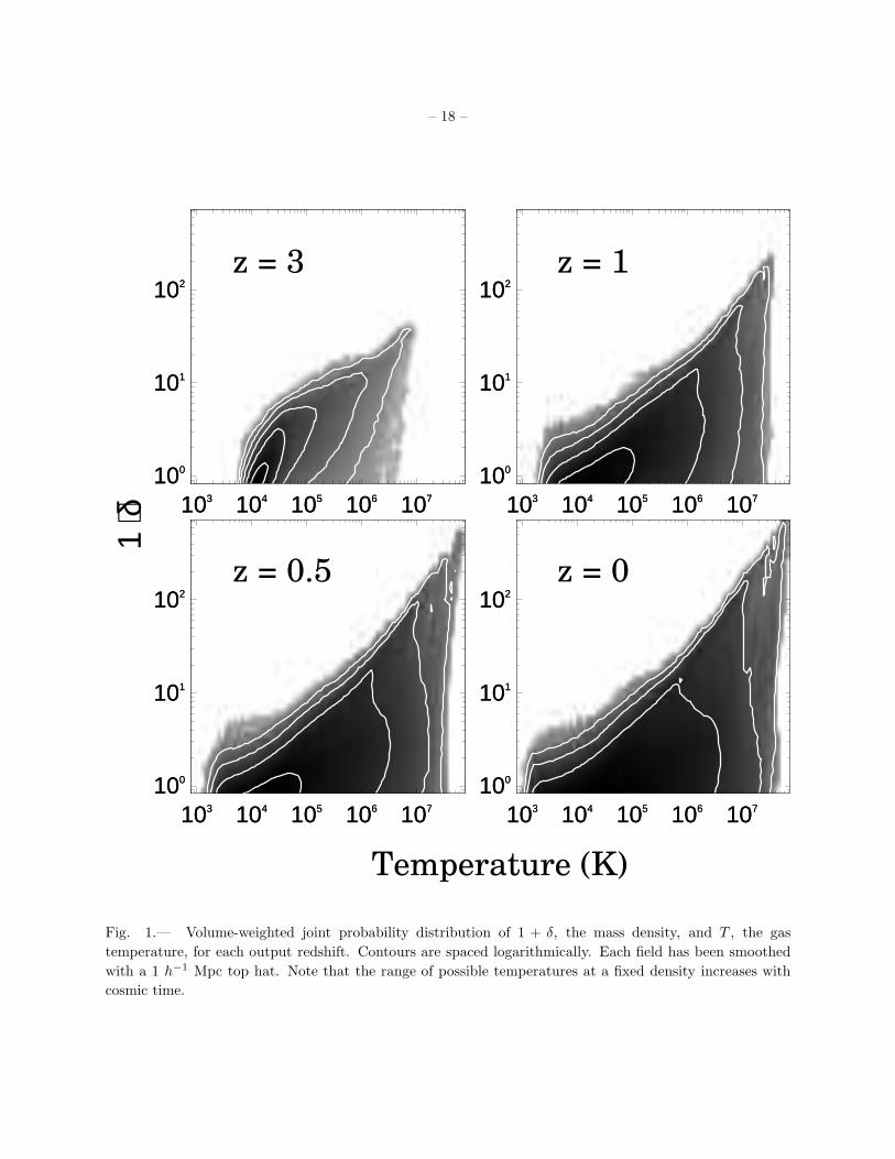
radius. In Figure 1 we show the joint distribution of 1 + δ, the normalized mass density, and T , the gas

temperature, as a function of redshift. We could instead have considered the distribution of 1 + δb, the

baryonic density; the results would have been nearly identical, because the dark matter and baryonic

overdensities are closely related on these scales. Most of the gas, that is, does not cool, fall to the central

parts of galaxies, and form stars, but instead follows the same distribution as the dark matter (Cen &

Ostriker 1998b). As the universe evolves, the variance in density increases. In addition, as gas falls into the

potential wells, it shocks and heats up to the virial temperature necessary to support itself in the potential

well, raising the average temperature of gas in the universe. Thus, volume elements above the mean density

move up and to the right on this diagram. These results are consistent with previous work with the same

code (for instance, Cen, Gnedin, & Ostriker 1993) and with other codes (for a summary, see Kang et

al. 1994). Note that on 1 h−1 Mpc scales, the importance of cooling physics to the gas temperature is not

immediately apparent; in Appendix A, we show this same figure at the scale of a single cell, which shows

quite clearly the effects of including the radiative physics of the gas.

We now consider the equivalent plot for the galaxy formation density field. Figure 2 shows the

– 6 –

conditional mean of the galaxy formation density field 1 + δ∗ as a function of 1 + δ and T : 〈1 + δ∗|1 + δ, T 〉.

At any fixed density, the star formation rate declines as temperature rises. It is clear that the densest

regions cannot cool and collapse at late times because they are too hot. To illustrate what Figure 2

implies about the relationship between galaxy formation and mass density, Figure 3 shows the conditional

probability P (1 + δ∗|1 + δ) as the logarithmic grey scale and the conditional mean 〈1 + δ∗|1 + δ〉 as the

solid line. The dashed lines are 1σ limits around the mean. At high redshift, the high density regions are

still cool enough to have clumps of gas in them cooling quickly; in this sense, the temperature on these

scales is not particularly important, making the relationship between galaxy formation and mass density

close to deterministic. At low redshift, many regions become too hot to form new galaxies; in particular,

galaxy formation is completely quenched in the densest regions, causing a turnover in 〈1 + δ∗|1 + δ〉. In

addition, at low redshifts, the galaxy formation rate depends strongly on temperature, adding scatter to

the relationship between galaxy formation and mass (Blanton et al. 1999).

The most obvious consequence of this evolution is that the bias of galaxy formation is a strong function

of time. Figure 4 shows b∗ and r∗ (defined in Section 1) as a function of redshift for top hat smoothing

radii of R = 1 and R = 8 h−1 Mpc. The bias of galaxy formation b∗ is clearly a strong function of redshift,

especially at small scales. The decrease in the bias is due to the fact that the galaxy formation has moved

to lower σ peaks and out of the hottest (and densest) regions of the universe, as described in Section 1.

We can compare these results to those of the peaks-bias formalism for the bias of dark matter haloes.

If we assume that the distribution of galaxy formation is traced by M > 1012 M⊙ halos (that is, halos

with typical bright galaxy masses) which have just collapsed, then according to the peaks-bias formalism

(Doroshkevich 1970; Kaiser 1984; Bardeen et al. 1986; Bond et al. 1991; Mo & White 1996), the bias of

mass in such halos with respect to the general mass density field is:

b∗(z) = 1 +δc

σ2(M, z), (4)

where δc ∼ 1.7 is the linear overdensity of a sphere which collapses exactly at the redshift of observation,

and σ(M, z) is the rms mass fluctuation on scales corresponding to mass M , again at the redshift of the

observations. Note that this formula differs from the standard one for the bias of all halos which have

collapsed before redshift z. The dotted line in the upper panel of Figure 4 shows the resulting bias. Thus,

the prediction for b∗ of the pure halo bias model is not much different from that of our hydrodynamic

model on large scales, even though the former does not include all the physical effects of the latter. That

is, measuring b∗(z) alone cannot easily distinguish the two models.

More interesting is the evolution of the correlation coefficient r∗ as a function of redshift, shown in

the lower panel of Figure 4. At all scales, the correlation coefficient falls precipitously for z < 1, when the

densest regions become too hot to form new galaxies. On the other hand, in the case of peaks-biasing, Mo

& White (1996) find a scaling between the halo and mass cross- and autocorrelations that implies r∗ ∼ 1

on large scales at all redshifts1. This is an important difference between the predictions of the models of

Mo & White (1996) and ours, which is presumably due to the more realistic physics used in our model.

Semi-analytic models can predict the evolution of r∗; it will be interesting to see how dependent this statistic

is to the details of the galaxy formation model. We discuss a way to get a handle on r∗ observationally in

Section 5.

1On scales of 1 h−1 Mpc, things are more complicated, because 1012 M⊙ halos so close together actually overlap in Lagrangian

space — see Sheth & Lemson 1998.

– 7 –

4. Gravitational Evolution of Bias

After galaxies form, they fall into potential wells under the influence of gravity. Because the acceleration

on galaxies is the same as that on the dark matter, this gravitational evolution after formation will tend

to bring both the bias bg and the correlation coefficient rg closer to unity, as described by Fry (1996)

and Tegmark & Peebles (1998). The evolution of the bias, then, is determined by the properties of

forming galaxies (outlined in the previous section) and how those properties evolve after formation.

Here we investigate this process and show that the linear approximations of Fry (1996) and Tegmark &

Peebles (1998) describe this evolution well, even in the nonlinear regime.

4.1. Evolution of the Clustering of Coeval Galaxies

Fry (1996) and Tegmark & Peebles (1998) rely on the continuity equation to study the evolution of the

density field of galaxies formed at a given epoch. In this subsection, subscript c will refer to this coeval set

of galaxies. Both galaxies and mass satisfy the same equation, which is to first order

δ + ∇ · v = 0, (5)

assuming that galaxies are neither created nor destroyed. Since we are dealing with a coeval set of galaxies,

they cannot be created by definition. Although it is possible to disrupt or merge galaxies in dense regions

(Kravtsov & Klypin 1998), we are following the stellar mass density in this paper, not the galaxy number

density, and thus do not consider these effects.

Assuming that there is no velocity bias between the volume-weighted velocity fields of mass and of

galaxies (which is borne out by the simulations), it follows that δ = δc. This statement means that on

linearly scaled plots of δc against δ, volume elements are constrained to evolve along 45 lines. We test this

prediction on 30 h−1 Mpc top hat scales, which should be close to linear, in Figure 5. Here we consider

a burst of galaxies formed at z = 1. The solid lines are 〈δc|δ〉 at z = 1, z = 0.5 and z = 0. The dashed

lines are the predictions extrapolated from z = 1 as above, to z = 0.5 and z = 0, respectively. Notice use

the growth factor of mass, σ(z = 0)/σ(z = 1), which on these scales is close to its linear theory value, to

determine ∆δ, and assume that ∆δc is the same. Evidently the linear continuity equation works on these

scales. We also test this prediction on the nonlinear scale of 1 h−1 Mpc in Figure 6. We find that it works

extremely well in the range 3 < δ < 100; in higher and lower density regions, nonlinear corrections to

Equation (5) are clearly important.

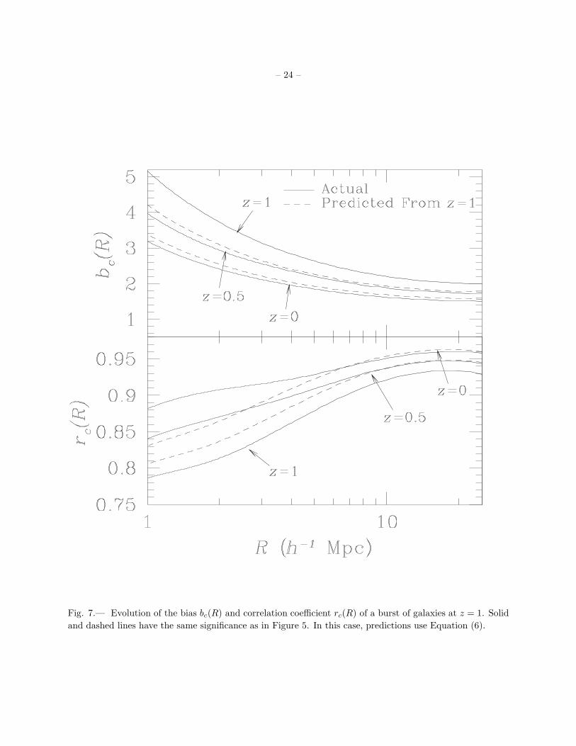
Tegmark & Peebles (1998) use the continuity equation to make further predictions about the bias

properties of coeval galaxies. In particular, given a “bias at birth” of bc(z0) and a “correlation coefficient at

birth” of rc(z0), one can express bc(z) and rc(z) in terms of the linear growth factor relative to the epoch of

birth D(z)/D0:

bc(z)rc(z) = 1 +bc(z0)rc(z0) − 1

D(z)/D0

b2c(z) =

[

(1 − D(z)/D0)2 − 2(1 − D(z)/D0)bc(z0)rc(z0) + b2

c(z0)]

(D(z)/D0)2(6)

In Figure 7 we show as the solid lines the values of bc and rc for the burst of galaxies at z = 1, at each output

time. The dashed lines are the predictions based on z = 1 for the results at z = 0.5 and z = 0. Notice that

on small scales, the prediction for bc remains extremely good. For rc, the linear prediction underestimates

– 8 –

the degree to which galaxies and mass become correlated on small scales; essentially, nonlinearities enhance

the rate at which initial conditions are forgotten.

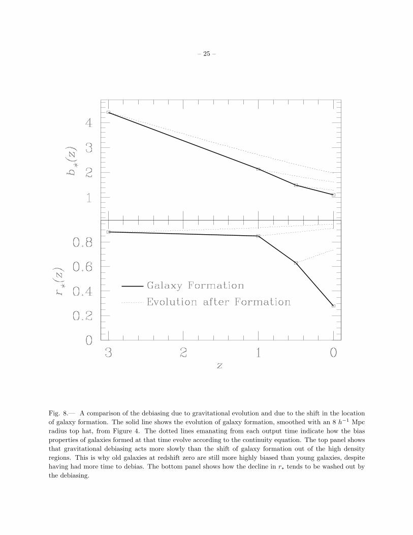
We can compare the effects of debiasing to the decline in the correlation between galaxy formation and

mass with redshift. In Figure 8 we show b∗(z) and r∗(z) at 8 h−1 Mpc scales, from Figure 4, as the solid

lines. The dotted lines originating at each output redshift show how the galaxies formed at that redshift

would evolve according the continuity equation. Naturally, bc(z) declines while rc(z) rises. Note that b∗(z)

falls more quickly than debiasing can occur, which is why old galaxies at redshift zero are still more highly

biased than young galaxies (Blanton et al. 1999), despite having had more time to debias.

4.2. Evolution of the Clustering of the Full Galaxy Population

These results show that the decrease in the bias of the galaxy density field with time found by Cen

& Ostriker (1998a) must be partly due to gravitational debiasing (described in this section) as well as the

decrease in b∗ (described in Section 3). We investigate this process here by showing the evolution of the

bias of all the galaxies in Figure 9 as the solid lines, for a tophat smoothing of 8 h−1 Mpc. The evolution of

the bias of galaxy formation, from Figure 4, is shown as the dashed lines. Notice that bg(z) and b∗(z) are

nearly the same, even though rg(z) and r∗(z) differ considerably; r∗(z) plummets after z = 1, while rg(z)

remains close to unity. About half the star formation in the simulation occurs at z < 1. Although this

recent star formation has a low r∗, and is thus poorly correlated with the mass distribution, this has little

effect on rg, partly due to the gravitational debiasing.

Using the approximations of Tegmark & Peebles (1998), we can reconstruct bg(z) and rg(z) from the

properties of galaxy formation as a function of redshift. We get equations similar to those of equation (6),

now integrated over the star formation history:

bg(z)rg(z) = 1 +1

D(z)G(z)

∫

dz′ [b∗(z′)r∗(z

′) − 1]D(z′)dG

dz′,

b2g(z) = b2

g(z)r2g(z) +

s2

σ2, (7)

where D(z) is the linear growth factor, G(z) is the cumulative mass of stars formed by redshift z, and σ

is the rms mass fluctuation. Calculating bg(z) requires first evaluating bg(z)rg(z) substituting it into the

expression given. In the second term, the quantity s2 is defined as:

s2 ≡1

G2(z)

∫

dz′dG′

dz′

∫

dG′′ dG′′

dz′′〈δ⊥(z′)δ⊥(z′′)〉, (8)

where δ⊥ ≡ δ∗ − b∗r∗δ is the component of the galaxy formation field which is uncorrelated with the

local density.2 These equations are simply a result of applying the continuity equation (Equation 5) to

the case of continuous star formation, rather than an instantaneous burst, as in Equation (6). Figure 9

shows bg(z), rg(z), and bg(z)rg(z) for all galaxies reconstructed from the properties of our galaxy formation

fields. bg(z)rg(z) represents the linear regression of the galaxy density on the mass density. Note that the

reconstruction of this quantity is quite accurate; on the other hand, the reconstructions of bg(z) and rg(z)

separately, which require knowledge of 〈δ⊥(z′)δ⊥(z′′)〉, have significant errors. These errors are mostly due

2Note that the definition of b∗ in Tegmark & Peebles (1998) is equivalent to our quantity b∗r∗.

– 9 –

to the poor time resolution of our output.3 The continuity equation will prove useful to future theoretical

and observational work, as we discuss in Section 6.

5. Observing the Evolution of Galaxy Formation

Here we discuss the observational consequences of the evolution of the spatial distribution of galaxy

formation. First, we consider observable properties of the star formation density field. Second, we consider

the resulting properties of galaxy clusters.

5.1. Star Formation Density Field

We noticed in the last section that the correlation coefficient between star forming galaxies and mass

should decrease considerably with time. We cannot currently observe this decrease directly in the real

universe.4 However, from Figure 9 we note that the galaxy distribution as a whole does correlate well with

the mass, in the sense that rg(z) ∼ 1 at all redshifts. Therefore, we should be able to detect the evolution

of r∗(z) by cross-correlating galaxy formation with the distribution of all galaxies. In Figure 10 we plot

b∗g ≡ σ∗/σg and r∗g ≡ 〈δ∗δg〉/σ∗σg between the galaxy formation density field and all galaxies as a function

of redshift, at 8 h−1 Mpc scales. While the evolution in b∗g is rather weak, the evolution in r∗g is striking,

and should be observable.

Observationally, measuring this correlation will require mapping the density field of star formation in

the universe, which has not yet been done. Given that the fundamental prediction of galaxy formation

models is the location of star formation as a function of time, such a map would be extremely useful. The

spectral coverage of the Las Campanas Redshift Survey (LCRS) includes a star formation indicator ([OII]

equivalent widths; Schectman et al. 1996; Hashimoto et al. 1998); thus, one can measure this correlation

at low redshift using this data. Using the LCRS, Tegmark & Bromley (1998) have addressed a related

question by measuring the correlation between the distributions of early and late spectral types (as classified

by Bromley et al. 1998); they found r ∼ 0.4–0.7, in qualitative agreement with our findings here, if one

makes a correspondence between spectral type and star formation rate. They can calculate r because

they understand the properties of their errors, which are due to Poisson statistics; however, in the case of

measuring spectral lines to determine the star formation rate in a galaxy, the errors are much greater and

more poorly understood. Therefore, since δg is likely to be much better determined than δ∗, the quantity

of interest will not be r∗g, but the combination b∗gr∗g = 〈δ∗δg〉/σ2g , which is the linear regression of star

formation density on galaxy density and is independent of σ∗. Future redshift surveys such as the SDSS will

probe redshifts as high as z ∼ 0.2—0.3 and will have spectral coverage which will include measures of star

formation such as [OII] and Hα. Figure 9 indicates that b∗gr∗g ∼ 0.35 at z = 0 and b∗gr∗g ∼ 0.5 at z = 0.25

(linearly interpolating between z = 0 and z = 0.5), a difference that should be measureable. A cautionary

note is that the linear interpolation in this range may not be accurate, and that simulations with finer time

3The results of these simulations take large amounts of disk space, and thus when they were run we did not attempt to store

more than a handful of output times. It would be impractical to rerun the simulations again for the sole purpose of obtaining

more output redshifts.

4Weak lensing studies (Mellier 1999) and peculiar velocity surveys (Strauss & Willick 1995) do probe the mass distribution

and may prove useful for studying the evolution of bg(z) and rg(z) directly.

– 10 –

resolution are necessary to make more solid predictions.

In addition, the SDSS photometric survey will probe to even higher redshift. Using the multiband

photometry, one will be able to produce estimates both of redshift and of spectral type. These measurements

will allow a calculation of the angular cross-correlation of galaxies of different types or colors as a function

of redshift out to z ∼ 0.5—1; Figure 10 shows that this evolution should be strong. The drawback to this

approach is that one cannot make a quantitative comparison between our models and the cross-correlations

of galaxies of different colors, because we can not yet reliably identify individual galaxies in the simulations

and because there is not a one-to-one correspondence between galaxy color and ages. Needless to say, the

observational question is still worth asking, because quantitative comparisons will be possible in the future

using hydrodynamical simulations at higher resolution, and are even possible today using semi-analytic

models (Kauffmann et al. 1999; Somerville, Primack & Faber 1998; Baugh et al. 1998).

5.2. Clusters of Galaxies

The measurement of b∗g and r∗g directly in the field is not possible given current data. However, the

observed evolution of galaxy properties in clusters does give us a handle on the evolution of the distribution

of galaxy formation. Here, we investigate cluster properties in the simulations. First, we describe the effect

of the clustering of galaxy formation on cluster mass-to-light ratios, and how that subsequently affects

estimates of Ω based on mass-to-light ratios. Second, we discuss the Butcher-Oemler (1978, 1984) effect.

We select the three objects in the simulation with the largest velocity dispersions, whose properties are

listed in Tables 1 and 2 at redshifts z = 0.5 and z = 0. This number of clusters of such masses in the

volume of the simulations is roughly consistent with observations (Bahcall 1998). Clusters #2 and #3 are

about 5 h−1 Mpc away from each other at z = 0, and have a relative velocity of 1000 km s−1 almost directly

towards each other; thus, they will merge in the next 5 Gyrs.

To calculate mass-to-light ratios, we must calculate the luminosity associated with each galaxy particle.

There are two steps: first, we assign a model for the star formation history to each particle; then, given

that star formation history, we use spectral synthesis results provided by Bruzual & Charlot (1993, 1998)

to follow the evolution of their rest-frame luminosities in B, V , and K. The simplest model for the star

formation history of a single particle is that its entire mass forms stars immediately, the instantaneous

burst (IB) approximation. However, it is unrealistic to expect that all of the star formation will occur

immediately; at minimum, it will at least a dynamical time for gas to collapse from the size of a resolution

element to the size of a galaxy. Thus, we also consider an alternative model based on the work of Eggen,

Lynden-Bell, & Sandage (1962; hereafter ELS), which spreads the star formation out over the local

dynamical time. We assign a star formation rate of

dm∗

dt=

mp

tdyn

t

tdyn

e−t/tdyn , (9)

to each particle, where mp is the mass of the galaxy particle and tdyn is the local dynamical time at the

location of the particle at the time it was formed. The evolution of the mass-to-light ratios of clusters are

qualitatively the same for both the IB and ELS models; the evolution of the B −V colors of cluster galaxies

does differ somewhat between the models, as described below.

We can calculate the mass-to-light ratios of these clusters in the B-band, ΥB ≡ (M/LB)/(M⊙/L⊙,B),

and compare them to the critical mass-to-light ratio ΥB,c necessary to close the universe. We do the same

in the V and K-bands, and show the results in Tables 1 and 2 at redshifts z = 0 and z = 0.5, respectively.

– 11 –

An observer in the simulated universe would thus estimate Ωest(z = 0) ≡ ΥB/ΥB,c ≈ 0.4–0.5 based on

cluster mass-to-light ratios, not far from the correct value for the simulation (Ω0 = 0.37). The galaxy bias,

which causes Ω0,est to underestimate Ω0 by a factor of about 1.6, is partially cancelled by the relative fading

of the light of the older cluster galaxies with respect to the younger field galaxies. The bias effect (as we

have shown above) increases in importance with redshift, while the differential fading of cluster galaxies

decreases in importance. Thus, in the simulations, the cluster mass-to-light ratio estimates of Ωest(z)

decrease with redshift, even though Ω(z) itself increases. We find similar results for analyses performed in

V and K, which we also list in Tables 1 and 2. For the ELS star formation model, the mass-to-light ratios

are all higher, but the estimated values for Ω and their redshift dependence do not change substantially.

Carlberg et al. (1996) studied 16 X-ray selected clusters between z ∼ 0.2 and 0.5, in the K-corrected

r-band. Their estimate of Ω(z ≈ 0.3) = 0.29 ± 0.06 is not far from what observers in our simulation would

conclude for that redshift, Ω(z ≈ 0.3) ≈ 0.38, using V -band luminosities. However, the correct value in the

simulations is Ω(z = 0.3) = 0.56. Carlberg et al. (1996) found no statistically significant dependence of

either Υr or Υr,c on redshift, but their errors are large enough to be consistent with the level of evolution

of these quantities seen in the simulations. We caution, therefore, that estimates of Ω0 from cluster

mass-to-light ratios can be affected by bias, by the differential fading between the cluster galaxies and the

field galaxies, and by the evolution of both these quantities with redshift.

As an aside, Tables 1 and 2 also show that Ω0 estimated from the baryonic mass in each cluster,

ΩbMtot/Mbaryons, is biased slightly high. This effect occurs because of the slight antibias (5 – 10%) of

baryons with respect to mass at low redshift (due, presumably, to shocking and outflows in the gas which

prevent baryons from flowing into the potential wells as efficiently as dark matter does). This result is

consistent with previous work (Evrard 1990; Cen & Ostriker 1993; White et al. 1993; Lubin et al. 1996).

Measuring Mbaryons is possible in the clusters because the gas is hot enough to be visible in X-rays; the main

difficulty is in measuring Ωb, which is generally based on high-redshift deuterium abundance measurements

(e.g., Burles & Tytler 1998) and Big Bang nucleosynthesis calculations (e.g., Schramm & Turner 1998). The

fact that the baryon mass in clusters is closely related to the total mass makes this method of estimating

Ω0 less prone to the complications of hydrodynamics, galaxy formation, and stellar evolution than using

mass-to-light ratios.

From the results of Section 3, we expect that cluster galaxies at z = 0.5 should be younger and bluer

than cluster galaxies at z = 0. Does this account for the Butcher-Oemler effect — the existence of a blue

tail in the distribution of B − V colors of cluster galaxies at z ∼ 0.5 (Butcher & Oemler 1978, 1984)?

The simplest approach to this question is to ask whether the mass ratio of recently formed galaxies to all

galaxies in the cluster changes from z = 0 to z = 1. Figure 11 shows the distribution of formation times

of galaxy particles in each cluster at z = 0 and at z = 0.5, assuming the IB model of star formation. For

comparison, the thick histogram shows the star formation history of the whole box. At both z = 0 and at

z = 0.5, there has been no star formation in the previous 1 Gyr in any cluster. On the other hand, the more

realistic ELS model allows star formation to persist somewhat longer. Figure 12 illustrates this effect by

showing the fraction of the stars in the clusters formed in the previous 0.5, 1. and 2 Gyrs at z = 0, z = 0.5,

and z = 1, now using the ELS model. For comparison, we show the same curves for the whole box. Clearly,

the fraction of young stars increases with redshift more quickly in the clusters than in the field. This is

qualitatively in agreement with the observed Butcher-Oemler effect.

We can look at the problem in a more observational context by calculating the B − V colors of cluster

galaxies as a function of redshift. Following Butcher & Oemler (1978, 1984), we define the quantity fb (the

“blue fraction” of galaxies) to be the fraction of mass in galaxy particles whose colors are more than 0.2

– 12 –

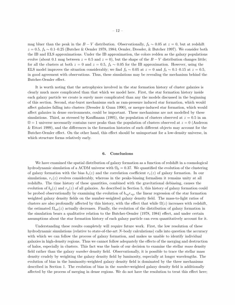
mag bluer than the peak in the B − V distribution. Observationally, fb ∼ 0.05 at z = 0, but at redshift

z = 0.5, fb ∼ 0.1–0.25 (Butcher & Oemler 1978, 1984; Oemler, Dressler, & Butcher 1997). We consider both

the IB and ELS approximations. Under the IB approximation, the colors redden as the galaxy populations

evolve (about 0.1 mag between z = 0.5 and z = 0), but the shape of the B − V distribution changes little;

for all the clusters at both z = 0 and z = 0.5, fb ∼ 0.05 for the IB approximation. However, using the

ELS model improves the situation considerably; we find fb ∼ 0.05 at z = 0 and fb ∼ 0.1–0.15 at z = 0.5,

in good agreement with observations. Thus, these simulations may be revealing the mechanism behind the

Butcher-Oemler effect.

It is worth noting that the astrophysics involved in the star formation history of cluster galaxies is

clearly much more complicated than that which we model here. First, the star formation history inside

each galaxy particle we create is surely more complicated than any the models discussed in the beginning

of this section. Second, star-burst mechanisms such as ram-pressure induced star formation, which would

affect galaxies falling into clusters (Dressler & Gunn 1990), or merger-induced star formation, which would

affect galaxies in dense environments, could be important. These mechanisms are not modelled by these

simulations. Third, as stressed by Kauffmann (1995), the population of clusters observed at z = 0.5 in an

Ω = 1 universe necessarily contains rarer peaks than the population of clusters observed at z = 0 (Andreon

& Ettori 1999), and the differences in the formation histories of such different objects may account for the

Butcher-Oemler effect. On the other hand, this effect should be unimportant for a low-density universe, in

which structure forms relatively early.

6. Conclusions

We have examined the spatial distribution of galaxy formation as a function of redshift in a cosmological

hydrodynamic simulation of a ΛCDM universe with Ω0 = 0.37. We quantified the evolution of the clustering

of galaxy formation with the bias b∗(z) and the correlation coefficient r∗(z) of galaxy formation. In our

simulations, r∗(z) evolves considerably, whereas in the peaks-biasing formalism it remains unity at all

redshifts. The time history of these quantities, combined with the gravitational debiasing, causes the

evolution of bg(z) and rg(z) of all galaxies. As described in Section 5, this history of galaxy formation could

be probed observationally by examining the evolution of b∗gr∗g, the linear regression of the star formation

weighted galaxy density fields on the number-weighted galaxy density field. The mass-to-light ratios of

clusters are also profoundly affected by this history, with the effect that while Ω(z) increases with redshift,

the estimated Ωest(z) actually decreases. Finally, the evolution of the distribution of galaxy formation in

the simulation bears a qualitative relation to the Butcher-Oemler (1978, 1984) effect, and under certain

assumptions about the star formation history of each galaxy particle can even quantitatively account for it.

Understanding these results completely will require future work. First, the low resolution of these

hydrodynamic simulations (relative to state-of-the-art N -body calculations) calls into question the accuracy

with which we can follow the process of galaxy formation, and makes us unable to identify individual

galaxies in high-density regions. Thus we cannot follow adequately the effects of the merging and destruction

of halos, especially in clusters. This fact was the basis of our decision to examine the stellar mass density

field rather than the galaxy number density field. Observationally, it is possible to trace the stellar mass

density crudely by weighting the galaxy density field by luminosity, especially at longer wavelengths. The

evolution of bias in the luminosity-weighted galaxy density field is dominated by the three mechanisms

described in Section 1. The evolution of bias in the number-weighted galaxy density field is additionally

affected by the process of merging in dense regions. We do not have the resolution to treat this effect here;

– 13 –

Kravtsov & Klypin (1998) explore this using a high-resolution N -body code.

Equally important is to explore the dependence of the evolution of b∗(z) and r∗(z) on cosmology. As we

saw in Section 3, their evolution was dominated by the evolution of the density-temperature relationship;

as this relationship and its time-dependence varies from cosmology to cosmology, we expect b∗(z) and r∗(z)

to vary as well. Just as important is the uncertainty in the star formation model used, whose properties

are evidently rather important in determining the clustering and correlation properties of the galaxies.

Furthermore, understanding the statistical properties of galaxy clusters in the simulations will require more

realizations than the single one we present. Finally, larger volumes than we simulate will be necessary to

compare our results to the large redshift surveys, such as the SDSS, currently in progress.

Since these simulations are expensive and time-consuming to run, we would like to find less expensive

ways of increasing the volume of parameter space and real space which we investigate. It may be

possible to capture the important aspects of the hydrodynamic code by using much less expensive N -body

simulations. One way to do so is to determine the relationship between galaxy density, mass density,

and velocity dispersion at z = 0, and simply apply that relation to the output of an N -body code at

redshift zero, as suggested by Blanton et al. (1999). However, the final relationship between galaxies,

mass, and temperature will depend both on the time evolution of the mass-temperature relationship, and

the gravitational debiasing. For instance, if all galaxies form at high redshift, galaxies will have had time

to debias completely. To take into account such effects explicitly, we want to apply a galaxy formation

criterion at each time step, and follow the gravitational evolution of the resulting galaxies to find the final

distribution at z = 0. If one could do so, one could run large volume dark matter simulations, in which

one formed galaxies in much the same way as they form here. Motivated by Figure 2, we propose applying

our measured 〈δ∗|δ, T 〉 on 1 h−1 Mpc scales in order to form galaxies in such an N -body simulation, using

the local dark-matter velocity dispersion or the local potential as a proxy for temperature. This approach

assumes only that the dependence of galaxy formation on local density and local temperature is not a

strong function of cosmology. This method would be similar in spirit to, but simpler than, the semi-analytic

models which have been implemented in the past.

The results of Section 4 suggest a simple way of exploring the effects of changing the galaxy formation

criteria in such N -body simulations, or for that matter in the hydrodynamical simulations themselves,

as long as one is content with studying second moments and with ignoring the effects of the feedback of

star formation. Given more output times than we have available from these simulations, one can simply

determine the location of galaxy formation at each time step – after the fact – and use Equation (7) to

propagate the results to z = 0, or to whichever redshift one wants. Thus, one could easily examine the

effects that varying the galaxy formation criteria would have. Compared to rerunning the full simulation,

it is computationally cheap to determine the properties of δ∗ at each redshift (given the galaxy formation

model) and then to reconstruct the evolution of bg(z) and rg(z).

The continuity equation may also prove useful in comparing observations to models. For instance,

large, deep, angular surveys in multiple bands, such as the SDSS, will permit the cross-correlation of

different galaxy types as a function of redshift, using photometry to estimate both redshift and galaxy type

(Connolly, Szalay, & Brunner 1998). If one properly accounts for the evolution of stellar colors, one will be

able to test the hypothesis that two galaxy types both obey the continuity equation. The sense and degree

of any discrepancy will shed light on whether one type of galaxy merges to form another, or whether new

galaxies of a specific type are forming.

Estimates of the star formation rate as a function of redshift are now possible (Madau et al. 1996).

– 14 –

Perhaps the next interesting observational goal is to study the evolution of the clustering of star formation.

The Butcher-Oemler effect tells us something about the evolution of star formation in dense regions, but it

is necessary to understand the corresponding evolution in the field, as well. The correlation of star-forming

galaxies at different redshifts with the full galaxy population may be a more sensitive discriminant between

galaxy formation models than measures of the clustering of all galaxies.

This work was supported in part by the grants NAG5-2759, NAG5-6034, AST93-18185, AST96-16901,

and the Princeton University Research Board. MAS acknowledges the additional support of Research

Corporation. MT is supported by the Hubble Fellowship HF-01084.01-96A from STScI, operated by AURA,

Inc., under NASA contract NAS5-26555. We would like to thank James E. Gunn, Chris McKee, Kentaro

Nagamine, and David N. Spergel for useful discussions, as well as Stephane Charlot for kindly providing his

spectral synthesis results.

A. Understanding Galaxy Formation in the Simulation

The conditions required for galaxy formation in each cell of the simulation are:

δ > 5.5,

mb > mJ ≡ G−3/2ρ−1/2

b C3

[

1 +δd + 1

δb + 1

Ωd

Ωb

]−3/2

,

tcool < tdyn ≡

√

3π

32Gρ, and

∇ · v < 0. (A1)

The subscript b refers to the baryonic matter; the subscript d refers to the collisionless dark matter. In

words, these criteria say that the overdensity must be reasonably high, the mass in the cell must be greater

than the Jeans mass, the gas must be cooling faster than the local dynamical time, and the flow must be

converging. Assuming that the time scale for collapse is the dynamical time, we transfer mass from the gas

to collisionless particles at the rate:∆m∗

∆t=

mb

t∗. (A2)

where t∗ = tdyn if tdyn > 100 Myrs and t∗ = 100 Myrs if tdyn > 100 Myrs.

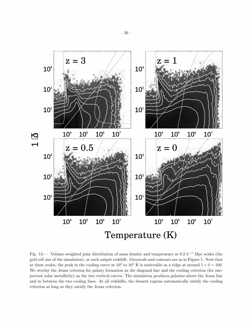
To understand the effects of these criteria, consider Figure 13, which shows the distribution of 1+ δ and

T at the scale of a single cell at each redshift. We show the Jeans mass criterion as the diagonal grey line

(points to the left are Jeans unstable), and the cooling criterion (for one-percent solar metallicity gas) as

the curved grey lines (points in between the lines can cool efficiently). For these purposes we have assumed

δb = δ, γ = 5/3, and µ = mH . Note that at high densities, satisfying the Jeans criterion automatically

satisfies the cooling criterion. At high redshifts, there is a fair amount of gas which appears to have cooled

into this regime, at 104–105 K and at relatively high densities. As the density fields evolve, the densest

regions become hotter, making it more difficult for the gas there to cool enough to allow galaxy formation.

REFERENCES

Adelberger, K., Steidel, C., Giavalisco, M., Dickinson, M., Pettini, M., & Kellogg, M. 1998, ApJ, 505, 543

– 15 –

Andreon, S., & Ettori, S. 1999, preprint (astro-ph/9901137)

Bahcall, N. A. 1998, in Formation of Structure in the Universe Winter School, ed. J. P. Ostriker & A. Dekel

(Cambridge: Cambridge University Press), 135

Bardeen, J. M., Bond, J. R., Kaiser, N., & Szalay, A. S., 1986, ApJ, 304, 15

Baugh, C. M., Cole, S., Frenk, C. S., & Lacey, C. G. 1998, ApJ, 498, 504

Blanton, M., Cen, R., Ostriker, J. P., & Strauss, M. A. 1999, ApJ, in press (astro-ph/9807029)

Bond, J. R., Cole, S., Efstathiou, G., & Kaiser, N. 1991, ApJ, 379, 440

Bromley, B. C., Press, W. H., Lin, H., & Kirshner, R. P. 1998, ApJ, 505, 25

Bruzual, A. G., & Charlot, S. 1993, ApJ, 405, 538

Bruzual, A. G., & Charlot, S. 1998, in preparation

Burles, S., & Tytler, D. 1998, ApJ, 507, 732

Butcher, H. R., & Oemler, A. 1978, ApJ, 219, 18

Butcher, H. R., & Oemler, A. 1984, ApJ, 285, 426

Carlberg, R. G., Yee, H. K. C., Ellingson, E., Abraham, R., Gravel, P., Morris, S., & Pritchet, C. J. 1996,

ApJ, 462, 32

Carlberg, R. G., Cowie, L. L., Songaila, A., & Hu, E. M. 1997, ApJ, 484, 538

Cen, R., Gnedin, N. Y., & Ostriker, J. P. 1993, ApJ, 417, 387

Cen, R., & Ostriker, J. P. 1992a, ApJ, 393, 22

Cen, R., & Ostriker, J. P. 1992b, ApJ, 399, L113

Cen, R., & Ostriker, J. P. 1993, ApJ, 417, 415

Cen, R., & Ostriker, J. P. 1998a, preprint (astro-ph/9809370)

Cen, R., & Ostriker, J. P. 1998b, submitted to Science (astro-ph/9806281)

Connolly, A. J., Szalay, A. S., & Brunner, R. J. 1998, ApJ, 499, 125

Couch, W. J., Ellis, R. S., Sharples, R. M., & Smail, I. 1994, ApJ, 430, 121

Couch, W. J., & Sharples, R. M. 1987, MNRAS, 229, 423

Davis, M., & Geller, M. J. 1976, ApJ, 208, 13

Dekel, A. & Lahav, O. 1998, preprint (astro-ph/9806193)

Doroshkevich, A. G. 1970, Astrophysica, 6, 320

Dressler, A., & Gunn, J. E. 1990, in Evolution of the Universe of Galaxies: Proceedings of the Edwin Hubble

Centennial Symposium, (San Francisco: Astronomical Society of the Pacific), 200

– 16 –

Dressler, A., & Gunn, J. E. 1992, ApJS, 78, 1

Dressler, A., Oemler, A., Couch, W. J., Smail, I., Ellis, R. S., Barger, A., Butcher. H., & Poggianti,

B. M. 1997, ApJ, 490, 577

Eggen, O. J., Lynden-Bell, D., & Sandage, A. R. 1962, ApJ, 136, 748

Evrard, A. E. 1990, ApJ, 363, 349

Evrard, A. E., Summers, F. J., & Davis, M. 1994, ApJ, 422, 11

Fry, J. N. 1996, ApJ, 461, L65

Garnavich, P. M. et al. 1998, ApJ, 509, 74

Giavalisco, M., Steidel, C. C., Adelberger, K. L., Dickinson, M. E., Pettini, M., Kellogg, M. 1998, ApJ, 506,

543

Giovanelli, R., Haynes, M. P., & Chincarini, G. L. 1986, ApJ, 300, 77

Gnedin, N. Y. 1996a, ApJ, 456, 1

Gnedin, N. Y. 1996b, ApJ, 456, 34

Gunn, J. E., & Weinberg, D. H. 1995, in Wide-Field Spectroscopy and the Distant Universe, ed. S. J. Maddox

& A. Aragon-Salamanca (Singapore: World Scientific), 3

Guzzo, L., Strauss, M. A., Fisher, K. B., Giovanelli, R., & Haynes, M. P. 1997, ApJ, 489, 37

Hashimoto, Y., Oemler, A., Lin H., & Tucker, D. L. 1998, ApJ, 499, 589

Hermit, S., Santiago, B. X., Lahav, O., Strauss, M. A., Davis, M., Dressler, A., & Huchra, J. P. 1996,

MNRAS, 283, 709

Jameson, A. 1989, Science, 245, 361

Kaiser, N. 1984, ApJ, 284, L9

Kang, H., Ostriker, J. P., Cen, R., Ryu, D., Hernquist, L., Evrard, A. E., Bryan, G. L., & Norman,

M. L. 1994, ApJ, 430, 83

Katz, N., Hernquist, L., & Weinberg, D. H. 1992, ApJ, 399, L109

Katz, N., Hernquist, L., & Weinberg, D. H. 1998, preprint (astro-ph/9806257)

Kauffmann, G. 1995, MNRAS, 274, 153

Kauffmann, G., Colberg, J. M., Diaferio, A., & White S. D. M. 1999, MNRAS, 303, 188

Kauffmann, G., Nusser, A., & Steinmetz, M. 1997, MNRAS, 286, 795

Kravtsov, A. V. & Klypin, A. A. 1998, preprint (astro-ph/9812311)

Le Fevre, O., Hudon, D., Lilly, S. J., Crampton, D., Hammer, F., & Tresse, L. 1996, ApJ, 461, 534

Loveday, J., Efstathiou, G., Maddox, S. J., & Peterson, B. A. 1997, ApJ, 442, 457

– 17 –

Loveday, J., Efstathiou, G., Maddox, S. J., & Peterson, B. A. 1996, ApJ, 468, 1

Lubin, L. M., Cen, R., Bahcall, N. A., & Ostriker, J. P. 1996, ApJ, 460, 10

Madau, P., Ferguson, H. C., Dickinson, M. E., Giavalisco, M., Steidel, C. C., & Fruchter, A. 1996, MNRAS,

283, 1388

Mellier, Y. 1999, preprint (astro-ph/9812172)

Mo, H.J., & White, S.D.M. 1996, MNRAS, 282, 347

Nagamine, K., Cen, R., & Ostriker, J. P. 1999, preprint (astro-ph/9902372)

Oemler, A., Dressler, A., & Butcher, H. R. 1997, ApJ, 474, 561

Ostriker, J. P., & Steinhardt, P. J. 1995, Nature, 377, 600

Pen, U.-L. 1998, ApJ, 504, 601

Perlmutter, S., et al. 1997, ApJ, 483, 565

Poggianti, B. M., Smail, I., Dressler, A., Couch, W. J., Barger, A. J., Butcher, H., Ellis, R. S., & Oemler,

A. 1999, preprint (astro-ph/9901264)

Postman, M., Lauer, T. R., Szapudi, I., & Oegerle, W. 1998, ApJ, 506, 33

Santiago, B. X. & Strauss, M. A. 1992, ApJ, 387, 9

Shectman, S. A., Landy, S. D., Oemler, A., Tucker, D. L., Lin, H., Kirshner, R. P., & Schechter, P. L. 1996,

ApJ, 470, 172

Schramm, D. N., & Turner, M. S. 1998, RMP, 70, 303

Sheth, R. K. & Lemson, G. 1998, preprint (astro-ph/9808138)

Shepherd, C. W., Carlberg, R. G., Yee, H. K. C., & Ellingson, E. 1997, ApJ, 479, 82

Small, T. A., Ma, C.-P., Sargent, W. L. W., & Hamilton, D. 1999, preprint (astro-ph/9901194)

Somerville, R. S., Primack, J. R., & Faber, S. M. 1998, preprint (astro-ph/9806228)

Somerville, R. S., & Primack, J. R. 1998, preprint (astro-ph/9811001)

Steidel, C. C., Adelberger, K. L., Dickinson, M., Giavalisco, M., Pettini, M., & Kellogg, M. 1998, ApJ, 492,

428

Strauss, M. A., & Willick, J.A. 1995, Phys. Rep., 261, 271

Tegmark, M., & Bromley, B. 1998, preprint (astro-ph/9809324)

Tegmark, M., & Peebles, P. J. E. 1998, ApJ, 500, L79

Wechsler, R. H., Gross, M. A. K., Primack, J. R., Blumenthal, G. R., & Dekel, A. 1998, ApJ, 506, 19

White, S. D. M., Navarro, J. F., Evrard, A. E., & Frenk, C. S. 1993, Nature, 366, 429

This preprint was prepared with the AAS LATEX macros v4.0.

– 18 –

103 104 105 106 107

100

101

102

103 104 105 106 107

100

101

102

103 104 105 106 107

100

101

102

103 104 105 106 107

100

101

102

103 104 105 106 107

100

101

102

103 104 105 106 107

100

101

102

103 104 105 106 107

100

101

102

103 104 105 106 107

100

101

102

z = 3 z = 1

z = 0.5 z = 0

Temperature (K)

1 +

δ

Fig. 1.— Volume-weighted joint probability distribution of 1 + δ, the mass density, and T , the gas

temperature, for each output redshift. Contours are spaced logarithmically. Each field has been smoothed

with a 1 h−1 Mpc top hat. Note that the range of possible temperatures at a fixed density increases with

cosmic time.

– 19 –

103 104 105 106 107

100

101

102

103 104 105 106 107

100

101

102

103 104 105 106 107

100

101

102

103 104 105 106 107

100

101

102

103 104 105 106 107

100

101

102

103 104 105 106 107

100

101

102

103 104 105 106 107

100

101

102

103 104 105 106 107

100

101

102

z = 3 z = 1

z = 0.5 z = 0

Temperature (K)

1 +

δ

Fig. 2.— The average rate of galaxy formation, 1+δ∗, as a function of 1+δ and T , for each output redshift.

Each field has been smoothed with a 1 h−1 Mpc top hat. We measure the local rate of galaxy formation

by examining the density distribution of “recently-formed” galaxy particles; that is, those formed in the

previous 0.5 Gyrs. Contours are spaced logarithmically. Note that at any given density, the star formation

declines with increasing temperature. As the densest regions become too hot to cool and collapse, they no

longer become preferred sites for galaxy formation, which move to the relatively less dense regions of the

universe.

– 20 –

100 101 102 103

100

101

102

103

100 101 102 103

100

101

102

103

100 101 102 103

100

101

102

103

100 101 102 103

100

101

102

103

100 101 102 103

100

101

102

103

100 101 102 103

100

101

102

103

100 101 102 103

100

101

102

103

100 101 102 103

100

101

102

103

z = 3 z = 1

z = 0.5 z = 0

1 +

δ *

1 + δ

Fig. 3.— Conditional probability P (1 + δ∗|1 + δ) at each of four redshifts. Greyscale stretch is logarithmic.

Each field has been smoothed with a 1 h−1 Mpc top hat. Solid line is the conditional mean 〈1 + δ∗|1 + δ〉;

dashed lines are 1σ limits around that mean. Note that at later times there is increasing stochasticity and

a turnover in 〈1 + δ∗|1 + δ〉 at high density. While in Blanton et al. (1999) we showed where galaxies of

different ages ended up at z = 0, here we show instead where galaxies form at each redshift.

– 21 –

Fig. 4.— The redshift evolution of the bias b∗(z) ≡ σ∗/σ (top) and the correlation coefficient r∗(z) ≡

〈δδ∗〉/σσ∗ (bottom) “at birth,” for top hat smoothing scales of 1 h−1 Mpc and 8 h−1 Mpc. There is a strong

trend with redshift. We also show, as the dotted lines, the peaks-bias prediction for b∗(z) and r∗(z) on large

scales, for M > 1012M⊙. Note that r∗(z) does not evolve at all in the peaks-biasing model.

– 22 –

Fig. 5.— Evolution of a burst of galaxies at z = 1, smoothed on 30 h−1 Mpc scales. The solid lines show

the conditional mean galaxy density given the mass density, at z = 1, z = 0.5 and z = 0. The dashed lines

show the predictions at z = 0.5 and z = 0 given the results at z = 1, according to the rule that ∆δc = ∆δ.

– 23 –

Fig. 6.— Same as Figure 5, now smoothed on 1 h−1 Mpc scales and plotted on a logarithmic scale.

Predictions are good in the regime: 3 < δ < 100.

– 24 –

Fig. 7.— Evolution of the bias bc(R) and correlation coefficient rc(R) of a burst of galaxies at z = 1. Solid

and dashed lines have the same significance as in Figure 5. In this case, predictions use Equation (6).

– 25 –

Fig. 8.— A comparison of the debiasing due to gravitational evolution and due to the shift in the location

of galaxy formation. The solid line shows the evolution of galaxy formation, smoothed with an 8 h−1 Mpc

radius top hat, from Figure 4. The dotted lines emanating from each output time indicate how the bias

properties of galaxies formed at that time evolve according to the continuity equation. The top panel shows

that gravitational debiasing acts more slowly than the shift of galaxy formation out of the high density

regions. This is why old galaxies at redshift zero are still more highly biased than young galaxies, despite

having had more time to debias. The bottom panel shows how the decline in r∗ tends to be washed out by

the debiasing.

– 26 –

Fig. 9.— Evolution of the bias bg(z), correlation coefficient rg(z), and the combination bg(z)rg(z) of all

galaxies on 8 h−1 Mpc tophat scales. Solid line is measured from the simulations. Dotted line is the

reconstruction according to Equation (7). The reconstruction suffers from the poor time sampling of our

output. The dashed lines are the corresponding quantities for the recently-formed galaxies at each redshift,

as in Figure 4.

– 27 –

Fig. 10.— Bias b∗g(z) ≡ σ∗/σg, correlation coefficient r∗g(z) ≡ 〈δ∗δg〉/σ∗σg, and the linear regression

b∗gr∗g of the galaxy formation density field on the density field of all galaxies as a function of redshift. We

show results for 1 h−1 Mpc and 8 h−1 Mpc radius tophat smoothing. The dotted lines are the peaks-bias

predictions for the same quantities on large scales, comparing the bias of the mass in recently formed halos

> 1012M⊙ to that of all halos > 1012M⊙.

– 28 –

Fig. 11.— Star-formation history in clusters at z = 0 (thin solid line) and z = 0.5 (thin dotted line).

Note that most star formation is complete in these clusters long before the universe is 7.8 Gyrs old, which

corresponds to z = 0.5 (shown as the vertical dashed line). For this reason, there is no excess of blue galaxies

at z = 0.5, although there may be at somewhat higher redshifts. For comparison, we show the star formation

history of the full box as the thick solid line. This figure assume the instantaneous burst (IB) approximation.

– 29 –

Fig. 12.— Mass fraction of recently formed stars in the clusters (solid lines) and in the whole box (dashed

lines), using the ELS star formation model described in the text. We show results for stars formed in the

previous 0.5, 1, and 2 Gyrs. In each case, the rapid decline in the clusters compared to the field is evident.

– 30 –

104 105 106 107

101

102

103

104 105 106 107

101

102

103

104 105 106 107

101

102

103

104 105 106 107

101

102

103

104 105 106 107

101

102

103

104 105 106 107

101

102

103

104 105 106 107

101

102

103

104 105 106 107

101

102

103

z = 3 z = 1

z = 0.5 z = 0

Temperature (K)

1 +

δ

Fig. 13.— Volume-weighted joint distribution of mass density and temperature at 0.2 h−1 Mpc scales (the

grid cell size of the simulation), at each output redshift. Greyscale and contours are as in Figure 1. Note that

at these scales, the peak in the cooling curve at 104 to 105 K is noticeable as a ridge at around 1 + δ ∼ 100.

We overlay the Jeans criterion for galaxy formation as the diagonal line and the cooling criterion (for one-

percent solar metallicity) as the two vertical curves. The simulation produces galaxies above the Jeans line

and in between the two cooling lines. At all redshifts, the densest regions automatically satisfy the cooling

criterion as long as they satisfy the Jeans criterion.

– 31 –

Table 1. Clusters at z = 0, at which time Ω = 0.37.

Mtot (h−1 M⊙) 〈v2〉1/2

(km/s) ΥB/ΥB,c ΥV /ΥV,c ΥK/ΥK,c Ωb0Mtot/Mbaryons

#1 9.847× 1014 1076.505 0.414 0.366 0.316 0.390

#2 7.919× 1014 951.378 0.442 0.401 0.359 0.401

#3 5.448× 1014 832.657 0.535 0.498 0.481 0.409

Table 2. Clusters at z = 0.5, at which time Ω = 0.66.

Mtot (h−1 M⊙) 〈v2〉1/2

(km/s) ΥB/ΥB,c ΥV /ΥV,c ΥK/ΥK,c Ωb0Mtot/Mbaryons

#1 2.698× 1014 751.243 0.321 0.275 0.231 0.716

#2 6.468× 1014 1135.564 0.451 0.390 0.321 0.719

#3 3.839× 1014 815.936 0.397 0.349 0.304 0.663