Time-course analysis of genome-wide gene expression data from hormone-responsive human breast cancer...

BioMed CentralBMC Bioinformatics

ss
Open AcceResearchTime-course analysis of genome-wide gene expression data from hormone-responsive human breast cancer cellsMargherita Mutarelli1,2,3, Luigi Cicatiello1,3, Lorenzo Ferraro1, Olì MV Grober1,3, Maria Ravo1, Angelo M Facchiano2, Claudia Angelini4 and Alessandro Weisz*1,3
Address: 1Department of General Pathology - Second University of Napoli, Napoli, Italy, 2Institute of Food Sciences, National Research Council (ISA-CNR), Avellino, Italy, 3AIRC Naples Oncogenomics Center, Napoli, Italy and 4Institute of Applied Calculus, National Research Council (IAC-CNR) Napoli, Italy

Email: Margherita Mutarelli - [email protected]; Luigi Cicatiello - [email protected]; Lorenzo Ferraro - [email protected]; Olì MV Grober - [email protected]; Maria Ravo - [email protected]; Angelo M Facchiano - [email protected]; Claudia Angelini - [email protected]; Alessandro Weisz* - [email protected]

* Corresponding author

AbstractBackground: Microarray experiments enable simultaneous measurement of the expression levels of virtually alltranscripts present in cells, thereby providing a ‘molecular picture’ of the cell state. On the other hand, the genomicresponses to a pharmacological or hormonal stimulus are dynamic molecular processes, where time influences geneactivity and expression. The potential use of the statistical analysis of microarray data in time series has not been fullyexploited so far, due to the fact that only few methods are available which take into proper account temporalrelationships between samples.

Results: We compared here four different methods to analyze data derived from a time course mRNA expressionprofiling experiment which consisted in the study of the effects of estrogen on hormone-responsive human breast cancercells. Gene expression was monitored with the innovative Illumina BeadArray platform, which includes an average of 30-40 replicates for each probe sequence randomly distributed on the chip surface. We present and discuss the resultsobtained by applying to these datasets different statistical methods for serial gene expression analysis. The influence ofthe normalization algorithm applied on data and of different parameter or threshold choices for the selection ofdifferentially expressed transcripts has also been evaluated. In most cases, the selection was found fairly robust withrespect to changes in parameters and type of normalization. We then identified which genes showed an expressionprofile significantly affected by the hormonal treatment over time. The final list of differentially expressed genesunderwent cluster analysis of functional type, to identify groups of genes with similar regulation dynamics.

Conclusions: Several methods for processing time series gene expression data are presented, including evaluation ofbenefits and drawbacks of the different methods applied. The resulting protocol for data analysis was applied tocharacterization of the gene expression changes induced by estrogen in human breast cancer ZR-75.1 cells over an entirecell cycle.

from Italian Society of Bioinformatics (BITS): Annual Meeting 2007Naples, Italy. 26-28 April 2007

Published: 26 March 2008

BMC Bioinformatics 2008, 9(Suppl 2):S12 doi:10.1186/1471-2105-9-S2-S12

<supplement> <title> <p>Italian Society of Bioinformatics (BITS): Annual Meeting 2007</p> </title> <editor>Graziano Pesole</editor> <note>Research</note> </supplement>

This article is available from: http://www.biomedcentral.com/1471-2105/9/S2/S12

© 2008 Mutarelli et al.; licensee BioMed Central Ltd. This is an open access article distributed under the terms of the Creative Commons Attribution License (http://creativecommons.org/licenses/by/2.0), which permits unrestricted use, distribution, and reproduction in any medium, provided the original work is properly cited.

of 14(page number not for citation purposes)

http://www.biomedcentral.com/1471-2105/9/S2/S12

http://creativecommons.org/licenses/by/2.0

http://www.biomedcentral.com/

http://www.biomedcentral.com/info/about/charter/

BMC Bioinformatics 2008, 9(Suppl 2):S12 http://www.biomedcentral.com/1471-2105/9/S2/S12

BackgroundEstrogens (E2) are key regulators in many biological proc-esses, along with a highly recognized role in breast cancerwhere they control key cellular functions by diffusingthrough the cell membrane and interacting with the estro-gen receptors (ERs), transcription factors which play animportant role in controlling multiple cellular processesmainly via changes in the expression of selected genes [1-3]. Complexity of the cellular responses to estrogen andtheir receptors can ideally be investigated only with com-prehensive analytical approaches, including in particulargene expression profiling with microarrays [4,5]. Thesetechnologies allow to assess at genome-wide scale changesin gene activity resulting, for example, from hormonaland pharmacological treatments or pathological anddivergent physiological conditions. As changes in geneexpression are driven by a dynamic process, the influenceof time should not be neglected, but the use of this tech-nique to study kinetics of gene expression changes has notbeen fully exploited yet. Indeed, few statistical methodsare available which enable to fully evaluate time series.Most of the methods to identify differentially expressedgenes adapt classical techniques originally designed forstatic experiments. This ‘static’ approaches have the disad-vantage of not taking into account temporal relationshipamong samples, leading to results that are often invariantunder permutation of the values representing differenttime points, thus ignoring the biological causality whichcan be inferred from the temporal response. They do notaccurately consider the existing temporal structure in thedata which can have as consequence a falsely calculatedsignificance of the genes.

For example, the popular microarray analysis packageSAM (Significance Analysis of Microarrays) [6] wasrecently adapted to handle time course data, by consider-ing different time points as distinct groups; the ANOVA[7] approach can also be applied to time course experi-ments by treating the time variable as a particular experi-mental factor and other methods [8-10], including thelimma package [11] which uses linear models, follow sim-ilar approaches.

On the other hand, most classical time series algorithms,mainly used for signal processing, are quite rigid, includ-ing requirement of a large number of time-points, uni-form sampling intervals and absence of replicated ormissing data-points, which microarray experiments rarelymeet.

Recently the time variable is starting to be much moreconsidered in the analysis of regulation of gene expres-sion, leading to new developments in the area of analysisof time-course microarray [12,13]. Due to the constraintsin microarray data structure, however, the problem of

detecting and estimating gene expression profilesbecomes extremely challenging and robust statisticalmethodologies are still missing. On the other hand, veryfew large scale comparisons are available in order to illus-trate benefits and drawbacks of current methodologies.

With the aim of setting up a workflow adapted for timecourse experiments, we tested the available methods tai-lored for time series analysis and established an analysisprotocol to be used in subsequent experiments. The firstmethod we considered introduces the time variablethrough a gene expression response curve which isexpanded over the polynomial or B-spline basis with thecoefficients estimated by the least squares procedure [14](implemented in the software EDGE - Extraction of Differ-ential Gene Expression [15]). The second method uses anovel multivariate empirical Bayes approach to rankgenes in the order of interest from longitudinal replicatedmicroarray time course experiments [16] (implementedin the Bioconductor [17] package timecourse). However,this last method does not consider time curves from afunctional point of view, neither provides any cut-off toselect statistically significant genes. The third method is afunctional Bayesian approach in which each gene expres-sion temporal profile is estimated globally by expandingit over an orthogonal basis [18] (implemented in the soft-ware BATS - Bayesian Analysis of Time Series [19]).

Our aim here, rather than to propose new methodologies,is to provide a detailed comparison of different methodswhich can be used as suitable protocol for analysis of timecourse gene expression data from microarray experiments.

MethodsCell-lines cultures and array hybridizationsHuman estrogen-responsive breast cancer cells (ZR-75.1)cultured in steroid-free medium for 4 days were stimu-lated with a mitogenic dose (10nM) of 17β-estradiol andRNA was extracted before or after 1, 2, 4, 6, 8, 12, 16, 20,24, 28 and 32 hours hormonal stimulation. Cells werecollected from multiple parallel cultures and pooledbefore RNA extraction as described before [4]. Hybridiza-tion reactions were performed with Illumina Human WG-6 BeadChips following manufacturer's protocols, induplicate for each sample, except the reference sample(before stimulation - 0h) which was in quadruplicate andthe 4h sample in triplicate. In the Illumina arrays the oli-gonucleotides are attached to microbeads which are thenput onto microarrays using a random self-assembly mech-anism [20]. Also, due to the small dimension of the beads,each bead-type (representing one probe for a total of46713 sequences) is present in a number of the order of ≈30-40 copies, thus providing an internal technical replica-tion that other platforms usually lack. In the presentpaper, we use the term ‘probe’ and ‘bead’ indifferently,



since in each case we use as signal the mean value of eachbead population of signals present on the array.

The complete datasets will be submitted to the publicrepository of microarray data ArrayExpress upon publica-tion.

Pre-processingFive different normalization algorithms were applied ondata, three of them present in the chip manufacturer'sanalysis software BeadStudio and two of them performedusing R/Bioconductor statistical environment [17,21].The average method simply adjusts the intensities of eachsignal so that the average signal of each array becomes thesame. The rank invariant is very similar, the only differ-ence is that the scaling factor is calculated only on a subsetof rank-invariant genes and not on all genes [22]. Thecubic spline is the only non-linear method present in theBeadStudio software, similar to an existing algorithm [23]and described in the software manual [22]. The quantilemethod [24] acts to uniform the quantile distribution ofeach array signal population and is widely used as stand-ard in single-channel arrays [25]; it is available throughthe R/Bioconductor packages affy [26] or limma [11] andmany other popular analysis software. Lumi[27] is a newmethod especially designed for Illumina BeadChips,based on a modification of the variance stabilizing nor-malization algorithm [28] to make use of the bead stand-ard deviation associated to each signal, only available inthis microarray platform.

After normalization, probe signals were checked for detec-tion against negative controls with a BeadStudio internalalgorithm and missing values were introduced to replacesignals under the detection limit. Probes in which the ref-erence sample had less than 3 out of 4 detected signalswere filtered out. Then log2 transformation was appliedon data, except in the case of lumi which uses its own var-iance stabilizing transformation. Ratios of each signalagainst the average reference signal were calculated andprobes with more than 15% missing values of the result-ing time series were filtered out.

Time series analysisThe following sections contain a brief description of themethods used in this paper to perform the statistical anal-ysis of a microarray experiment made in the course oftime. For a detailed description of each method, we referthe reader to each method's reference. Some preliminaryconsiderations are however necessary: the number of timepoints t(j), j = 1,…, n at which each sample is taken is rela-tively small (n ≈ 10) and the experimental design is notgenerally regular, with very few replicates at each timepoint (ki

(j) = 0,…, K, K = 1, 2 or 3); on the other hand avery large number of genes (N ≈ 104) are simultaneously

measured, some data points might be missing due to tech-nical error and the noise is usually not gaussian.

Sliding window analysisWe first extracted a list of differentially expressed genes ateach time-point using the internal DiffScore test of Bead-Studio software [22] by using thresholds of different strin-gency (a DiffScore of 20 and 30, correspondingrespectively to a p-value of 0.01 and 0.001 of the underly-ing statistical test). We denoted as ‘differentiallyexpressed’ genes those which were selected at least in threeconsecutive time-points. The limits of this procedure arethe lack of statistical formalization and the fact that thefixed window does not account for irregularly spaced gridassigning to all points the same weight.

EDGEThe method proposed in Storey et al. [14] apply both tolongitudinal and independent data. For each gene theeffect of the treatment is modeled as a mathematical func-tion and expanded over the polynomial or p-dimensionalB-spline basis [s1 (t),…, sp(t)]. In our case data are not trulylongitudinal since the biological source is a cell line, cul-tured in parallel, under identical and controlled condi-tions, hence the method is applied in its simplifiedversion.

Let be the relative expression level of the gene i in the

kth replicates at the jth time point t(j) where there are i =

1,…, N genes and j = 1,…, n time points,

replicates for time point. The relative observed geneexpression values are then modeled by

where µi(t(j)) is the (unknown) relative expression timecurve for gene i evaluated at time t(j) and can be written interms of a p-dimensional linear basis [s1(t),…, sp(t)]:

where, β0,i is the intercept term, p is the same for all genes

(it is assumed to be known and in practice it is preliminar-ily estimated from the data or it can be provided by the

user), and are modeled as independent random vari-

ables with mean zero and gene dependent variance .

Under this setup the interest is to test the null hypothesis

H0,i that μi(t) = 0 against the alternative H1,i formulated

under the general parametrization μi(t) = βi,1s1(t) + βi,

2s2(t) + … + βi,psp(t) with some non zero coefficients. To

assess differentially expressed genes, the goodness of

zij k,

k kij= ( )1,...,

z tij k

ij

ij k, ,= +( )( )μ ζ

μ β β β βi i i i i p pt s t s st t( ) ( ) ( ) ( )= + + + +0 1 1 2 2, , , ,...

ζij k,

σi2



model fit under the null hypothesis is compared to thatunder the alternative hypothesis, by calculating for gene ia F statistic similar to the one used in ANOVA:

where is the sum of squares of the residuals obtained

from the null model, and from the alternative model.

However, Storey et al. [14] do not impose assumption ofnormality: the distribution of these statistics is treated asunknown and studied via bootstrap [29], which mayrequire high computational cost. Finally, to account forthe multiplicity of comparisons, the most significantcurves are selected by controlling q-values using an FDR-like procedure [30].

This method is implemented in the user-friendly softwareEDGE [15]. We used the software with default parametersetting (increasing the number of iterations to 1000 inorder to reduce the problem of the granularity of the p-val-ues and to obtain more stable lists) and q-value thresholdsof 0.01 and 0.001. The ‘K nearest neighbor’ (KNN)method [31] is provided to impute missing values, sincethe method itself does not account for missing data. Inorder to separate the effect of the method from the proce-dure to impute the missing values, we repeated the analy-sis both by filtering out all the genes with missingobservations and by using the KNN method to imputethem.

timecourseThis method applies the novel multivariate empiricalBayes approach described in Tai et al. [16] to rank genes inthe order of interest from longitudinal replicated microar-ray time course experiments. Similarly to Storey et al. [14],timecourse can be applied both to the ‘one-sample’ and‘two-sample’ case, however in the last case it is applicableonly to data sets with identical time grids. On the otherhand, differently from Storey et al. [14] where both longi-tudinal and independent sampling designs are accountedor from Angelini et al. [18] where only the independentsampling is considered, this method is designed for datawhere replicates are biologically meaningful, for examplewhen a full series of time-points is drawn from the sameindividual (i.e., truly longitudinal). Indeed, biologicalsamples are treated under the ‘fixed effects’ rather than the‘random effects’ design model. Hence, since in this con-text one replicate is a full time curve (i.e, vector of size n),missing data are not allowed and the same number ofarrays is required at any time point. On the other hand,different number of replicates are allowed between differ-ent genes.

For each gene i and individual k the n-dimensional vector

of observations on the grid t(1),…,t(n)

is assumed to be conditionally independently drawn froma multivariate n-variate normal distribution with

unknown mean μi and covariance matrix Σi, i.e.,

The method only seeks a statistic for ranking genes in theorder of evidence against a null hypothesis and does notattempt to find a threshold to select the significant genes.The null hypothesis corresponding to a gene mean expres-sion level being zero is defined as H0,i: μi = 0, Σi > 0 andthe alternative as H1,i : μi ≠ 0, Σi < 0. An N-dimensionalindicator random variable I is defined to reflect the statusof the genes:

with a Bernoulli distribution with success probability ω, 0< ω < 1. The multivariate hierarchical Bayesian model isbuilt by elicitating the following priors:

where η > 0 is a scale parameter, ν > 0 and ν Λ < 0 are thedegrees of freedom and scale matrix, respectively. Sinceconjugate priors are elicited on the unknown parameters,all computations for the posterior distributions and theform of the statistics are carried out in a analytical form.Moreover, the hyper-parameters, whose amount howeverincreases with the number of time points, can be esti-mated from the data.

Finally, the Hotelling T2-statistic is calculated and used torank genes when the same number of replicates are avail-able for all genes, while the M B-statistics is used when thenumber of replicates is not equal for all genes [16]. Forfurther details on the statistics and on parameters estima-tion, we refer the interested reader to the original refer-ence. Here we only note that, due to the way the datamodel was conceived, the quantitative information aboutthe time measurements is not explicitly used by thismethod. The method is implemented in the timecourse R/Bioconductor package [32]. We applied the method usingthe first two replicates per time point, since the number ofreplicates has to be the same along the time curve. Alsosince missing values are not allowed, we repeated theanalysis both by filtering out all the genes with missing

FSS SS

SSii i

i

= −0 1

1,

SSi0

SSi1

zik

ik

i nk T

z z=( ), ,, ,1 …

zik

i i n i iN| , ,μ μ∑ ∼ ∑( )

Iii

i

H

H= ⎧

⎨⎩

1

01, ,if is true

if is true, 0,

μμ μμi i i n i i i i

i

I N I| , , | , ,...,∑∑ ∑∑ ∑∑

∑∑

= =−( ) ( )1 0 0 01∼ ∼

∼

0 η δand

Inv-Wisharrtν νΛΛ( )( )−1



observations and by using a KNN algorithm implementa-tion present in R [33].

BATSBATS (Bayesian Analysis of Time Series) software [19] is anewly-developed user friendly tool which implements thefunctional Bayesian approach described in Angelini et al.[18]. Although independently developed, the methodappears to be a compromise between EDGE and time-course. Indeed, similarly to EDGE, the method treatsrecords as functional data, thus preserving causality andtaking into account the temporal nature of data. Similarlyto timecourse, the Bayesian approach is applied in themethod at all stages of analysis, but the priors are elicitedon the space of the function coefficients, hence the timevariable enters in the model in explicit form trough thedesign matrix.

BATS is designed for data consisting of the records on Ngenes and describing the difference in gene expression lev-els between treatment and control in a context of inde-pendent sampling time course experiment. A gene recordis defined as a vector of size Mi, containing all the meas-

urements available for gene i. Each record is modeled as a

noisy measurement of a function μi(t) at a time point t(j)

∈ [0, T] as in equation (1) where for each gene i, its expres-

sion profile μi(t) is expanded into series over some stand-

ard orthonormal basis [φ0(t) φ1(t) ··· φLi(t)] on [0,T]

(Legendre polynomials or Fourier basis are implementedin the software, however any other bases can be theoreti-

cally considered) of gene specific degree 0 ≤ Li ≤ Lmax with

coefficients :

Similar to EDGE, the objective is to identify the genesshowing different functional expressions between treat-

ment and control (i.e. μi(t) ≠ 0), and additionally to

explicitly evaluate the effect of the treatment (i.e., estimate

), which in EDGE is hidden in the model but it

could be obtained by least squares fit of (1) under model(2). Following Angelini et al. [18], genes are treated asconditionally independent and modeled as

in which Di is the block design matrix, the j-row of which

is the block vector [φ0(tj) φ1(tj) ··· φLi(tj)] replicated

times;

and

are, respectively, the

column vectors of all measurements for gene i, the coeffi-

cients of μi(t) in the chosen basis, and random errors. The

following hierarchical model is imposed on the data:

All parameters in the model are treated either as randomvariables or as nuisance parameters that are recoveredfrom data. Noise variance σ2 is assumed to be random, σ2

˜ ρ(σ2) in order to account for possibly non-Gaussianerrors which are quite common in microarray experi-ments.

Three different Bayesian models are contained in BATSproviding the user a more flexible theoretical set-up toaccommodate various types of error distributions,namely, all scale mixtures of a normal distribution: delta-

type prior , the inverse Gamma prior

ρ(σ2) = IG(γ, b) and the exponential type prior

which lead to normal, Student T

and double-exponential errors, respectively. The choice ofdifferentially expressed genes is made on the basis ofBayes Factors which are used for multiplicity control andare computed using the procedure described by Abramov-ich et al. [34]. Once significant genes are detected, the

coefficients and, subsequently, the curve are

estimated by the posterior means. Hyperparameters π0

and , γ, b or μ are estimated from the data, or can be

entered as known by the user. Gene specific parameters

and Li are estimated by maximizing the marginal like-

lihood P(zi) and the posterior mean or mode of P(LiZi),

respectively.

The advantage of the Bayesian model described above isthat since all priors are conjugate (see [18] for details), allposterior inference can be carried out analytically withvery efficient computations.

The method is used for simultaneous estimation of thecurves, as well as for ranking the curves (genes) accordingto their significance level. Moreover, significance testing

C l Lil

i( ) =, , ,0

μ φi t tcil

ll

Li

( ) ( )==∑ ( ) .

0

μi t( )

z D ci i i i= + ζ

kji

z ci i ik

in

in k T

i i iL T

z z z z n ic c= =( ) ( )1 1 1 1 01, , , ,... , , , ... , , ...,

ζ ζ ζ ζ ζi i ik

in

in k T

n=( )1 1 1 11, , , ,, ..., , , , ...,

z c

c

D c Ii i i

i

i i

i i ML

L

L

N

Li| , ,

| ,

,

,

σ

σ

σ

λ

2

2

2∼∼∼

( )

Truncated Poisson mmax

, , ,

( )

( )+ −( ) ( )−π δ π σ τ0 02 2 10 0 1 0… N i iQ

ρ σ δ σ σ2 202( )= −( )

ρ σ μσ μσ2 1 22

( )= − −c Mi e /

( )cil μi t( )

σ02

τi2



of the curves is carried out by controlling the multiplicityof comparisons from a Bayesian perspective [34], provid-ing an automatic cut-off. We performed the analysis byusing two error models (the normal and the double-expo-nential) and a range of values of the parameter λ, whichinfluences the prior degree of the polynomial curve esti-mated for each gene.

Simulations

To compare performances of EDGE, timecourse and BATS,we carried out a small simulation study by generating datawith the Simulation utility of BATS. We generated data tomimic the structure of the real data set described above,

with N = 10000, n = 11 and for all j = 1, …, 11

except . In the data sets generated, 1000 or 2000

genes were randomly chosen to be “differentiallyexpressed”, corresponding respectively to 10 % or 20 % ofthe total number of genes. The first scenario correspond toa case where relatively few genes are involved in the proc-ess, the second to a more strong respondence to the treat-ment. The values of 1000 and 2000 where chosen fromthe prior belief on behavior of the real data experiments.The remaining 9000 or 8000 curves were set to identicalzero.

For each significant curve, the Simulation utility samples

the degree of the polynomial from a discrete uniform

distribution in [1, Lmax], with Lmax = 6 (in contrast to the

truncated Poisson that is used in fitting the model). Poly-nomials of degree zero are excluded since a nonzero con-stant signal is questionable from a biological point ofview. Coefficients ci where randomly sampled from

. Matrix Qi is set to

where νi ∼ U([0,1]) and

was sampled uniformly in order to produce the signal-

to-noise ratio (SNR) in the interval between 2 and 6.Under this set up we can mimic both weak and strong sig-nals and different signal regularity (which is notaccounted explicitly by any of the models). Furthermore,since is known that noise on microarray date has heaviertails than gaussian, we performed simulations under three

scenarios of i.i.d. noise: normal N(0, σ2) and Student Twith 5 or 3 degrees of freedom (indicated as T5 and T3,respectively). Student noise was rescaled to have the same

variance σ2 of the normal case (σ = 0.33, the estimatedvalue for the real data set).

In addition, very large values (with a threshold of 5) werefiltered out and substituted with missing values, mimick-ing real data preprocessing where unreliable values areeliminated.

For each kind of noise and number of true signals we gen-erated 5 data-set, averaging the results. Analysis of simu-lated data was performed with the three methods with thesame choice of parameters used in the real data analysis:EDGE q-value 0.01 and 0.001; BATS error model normaland double exponential and λ = 9 and λ = 12; with time-course we chose the first genes in the ranked list corre-sponding to the same number of the genes selected byBATS on the same dataset, to evaluate the number of falsepositives and false negatives.

Cluster analysisCluster analysis on the final list of gene profiles signifi-cantly affected by estrogen stimulation was performedusing a Bayesian functional based software, Splinecluster[35]. The method proposes a hierarchical clusterapproach, where the number of cluster is automaticallyselected by maximizing the marginal distribution. How-ever, it is recommended both for computational and forpractical point of view to apply the method only on therelevant subset of genes, instead of the whole dataset ofgenes. Here, similarly to BATS, the gene profiles are alsorepresented by expansions over a certain basis and thenormal-inverse gamma prior is imposed on the unknowncoefficients. The number of clusters and cluster participa-tion are also treated as random, leading to a full Bayesianmodel. Since the method does not address many of theissues which we treat in the Results and discussion Sec-tion, we processed the selected data matrix by filtering outmissing data points and by averaging the replicates at eachtime point.

Results and discussionExperimental design of the experiment and its implicationsWe present the analysis performed on a time series ofmicroarray data from breast cancer cells treated with estro-gens. Our experimental design is formalized in a ‘onesample’ statistical model with a time series, in which rep-licated arrays for each time-point are technical replicates,with no special relationships between each other. We alsohave unequally spaced sampling intervals (1h betweenthe first two time-points, 2h till the time-point of 8h and4h till the end of the series) and 2 replicates at each time-point, except one case (4h) in which we have 3 replicates.This data structure has quite common features in microar-ray experimental designs: a number of replicates barelysufficient to get statistically significant results, unequalnumber of replicates which may be due to technical needsor reasons of biological interest. For example, the higherdetail in the first part of the curve reflects a greater interest

kij = 2

ki4 3=

Litrue

N i i0 2 2 1,σ τ Q−( )Qi i

i i iL= ( )diag 1 22 2 2ν ν ν, , ...,

τi2



from a biological point of view in the earlier responses tohormone treatment with respect to the rest of the timeseries. Some difficulties may arise in analyzing data pre-senting features like these, both for a static analysisapproach and with a longitudinal method. In fact, for astatic method of comparison treated/non treated, per-formed point-by-point, the number of replicates of indi-vidual time-points is lower than the required minimum ofmost standard tests. This limited number of replicates isjustified by the time-series analysis: since we are interestedin the whole profile, we don't need absolute precision ineach time point comparison but rather we need to takeadvantage of the temporal structure of the data and use allinformation available along the time in order to makeappropriate and robust inference.

Pre-processingWe evaluated the effect of different normalization algo-rithms in terms of overlap between the selected gene listsproduced with the time-series analysis methods used.After inspection of normalized data, the cubic splinemethod was discarded since the data produced was notcorrectly normalized between the arrays (see Additionalfile 1), thus requiring further manipulation on data thatwe decided not to apply. The better overlap was notedbetween quantile and lumi normalization, with averagebeing the best performing algorithm among the onespresent in BeadStudio software.

After the filtering step, the genes left for the analysis were9593, of which 1261 (13.2%) had between 1 and 4 miss-ing values.

Time series analysisSliding window analysisThis method is quite naive and is presented just to have astatic counterpart to compare with the other methods. Wechose to apply it only to data normalized with BeadStudioalgorithms, thus representing an analysis performed with

the only help of the chip manufacturer's software. Weapplied the internal differential analysis algorithm whichuses the bead standard deviation in the error model, thusmaking it possible to analyze data with only 2 replicatesfor each time-point, as in our case, unlike a standard t-test.Results of the analysis with this and the other methods arereported in Table 1. We noted a fairly good robustness tonormalization effects (75-80% overlap among theselected gene lists). Although being a very simple proce-dure, we obtained results which were comparable to othermethods having more appropriate assumptions (60-70%with EDGE and BATS). However, we also have to pointout that, by considering a window of three time pointsregardless of time interval between them, we are incor-rectly treating unequally spaced times with the sameweight in the analysis. It can nevertheless be useful todetect local changes in the expression.

EDGEEDGE is distributed as a stand-alone software and,although relying on R [21], it silently uses it in the back-ground, so that the user does not need to know the lan-guage to use it but only interacts with a graphicalinterface. It also has some useful utilities to inspect theinput data, such as the possibility to make boxplots, tocheck the presence of missing data and to impute themwith the KNN algorithm. The results are highly robust tochanging normalizations (80-96% overlap among all thefour methods) except for the case of rank invariant nor-malization, with which the number of significant genesdrops unexpectedly with respect to the others. Weobtained similar results both by filtering out missing dataand by imputing them. As compared with the other meth-ods, on real data EDGE selects a surprisingly much longerlist of genes (Table 1). Moreover, we observed that, eventhough we increased the number of permutations, due tothe granularity problem, genes with the same q-value aretoo many, since for example the first 67 (average norm.),44 (lumi) or 85 (quantiles) genes all result as ‘first rank’

Table 1: Comparison of the selected gene lists obtained with different methods of selection. Numbers indicate the genes obtained by pairwise intersection of different methods of selection. In bold are the selected gene lists for each method.

Sliding window 201

Sliding window 301

EDGE 0.012 EDGE 0.0012 BATS #13 BATS #24 timecourse 10005 timecourse 15005

Sliding window 201 1563 997 1126 667 903 1069 140 209Sliding window 301 997 825 540 690 797 85 128EDGE 0.012 2595 1145 936 1086 232 343EDGE 0.0012 1145 590 659 104 154BATS #13 1478 1397 157 157BATS #24 1660 232 243timecourse 10005 1000 1000timecourse 15005 1500

1DiffScore threshold. 2q-value threshold. 3Error model = normal, λ=12. 4Error model = double-exponential, λ=9. 5Number of ranked genes selected.



genes with the same q-value. To reduce granularity oneshould further increase the number of permutations, butthen as a consequence the computational cost would alsoincrease, thus making the method less convenient to use.

timecoursetimecourse [32] is a package distributed with Bioconductor[17], thus requiring knowledge of the statistical environ-ment R [21], which is both an advantage for those familiarwith this language, since it is very quick to install and usenew packages, but it can be unfriendly for biologists. Sim-ilarly to EDGE, we found very similar results both whenfiltering out genes with missing observations and whenimputing them. This method only ranks in order of signif-icance the input gene list without providing an automaticor suggested cut-off to determine which genes are signifi-cant. For this reason, on real data we selected the first1000 and 1500 genes of the rank ordered lists to compareresults among normalizations and with the other meth-ods. Surprisingly, we found a very low overlap bothbetween the ordered lists prepared with different normal-izations and with lists produced with other methods(Table 1). It is worth mentioning that our dataset containsonly technical (indistinguishable) replicates, thus themethod could not take advantage of the replicate identifi-cation, nonetheless the difference with the other methodsand above all between data normalized with differentmethods is difficult to explain.

BATSBATS is also distributed as a stand-alone software with agraphical and friendly interface, as, although written inMatlab [36] it does not require the use of Matlab. Selec-tion was found robust with respect to changes in parame-ters (85-90% genes common to all the combinationsused) and type of normalization (74-82%, with a loweroverlap for the rank invariant). BATS has also some graph-ical utilities to plot, filter data and compare resulting listsand is the only method which allows to save the estimatedprofile for the selected genes for further use (Figure 1). Asthe result on the ‘one sample’ problem, the techniqueallows different number of basis functions for each curve,which improves the fits, it does not require to pre-deter-mine the most significant genes to select the dimension ofthe fit and avoids a computer intensive evaluation of thep-values via bootstrap. Furthermore, by using the Bayesianformulation in combination with the functionalapproach it can successfully handle various technical dif-ficulties which arise in microarray time-course experi-ments such as a small number of observations available,non-uniform sampling intervals, presence of missing dataor multiple data as well as temporal dependence betweenobservations for each gene, which are not completelyaddressed by the above mentioned methods. On the other

hand, current version of the BATS method cannot beapplied to the ‘two sample’ case.

Comparison of methodsSimulation studyTables 2 and 3 summarize results with the simulated data-sets. In particular, for any group of datasets it is reportedthe average number of rejected hypotheses, i.e. genesdeclared differentially expressed, the average number ofthe correctly rejected hypotheses, the false discovery rate,estimated as the average proportion of the falsely rejectedhypotheses over the total number of rejected hypotheses,and the false negative rate, estimated as the average pro-portion of the significant curves not detected over thenumber of not rejected hypothesis. As already stated, sincetimecourse does not provide any cut-off point, for the sakeof comparison we cut the ranked list on the same numberof significant genes as in BATS with default parameterschoice. We can say that all methods have good perform-ances under all the simulated datasets, with BATS provid-ing more accurate results (both in terms of FDR and FNR)than the other methods. However, we have to note thatthe simulated datasets were generated according to severalof the BATS model assumptions. On the other hand itdoes not exists an accepted standard dataset of microarraytime course to be used as benchmark, neither a way to per-form a blind experiment, or a well established set of syn-thetic test functions as in non parametric regression.Different methods account for different biological infor-mation and are valid under different assumptions, whilethe various amount of different interactions and sourcesof error that can affect the data can often change the per-formance of a given method from a simulated case to thereal data application.

For what concerns EDGE, we observe a quite conservativebehavior (it has a higher FNR with respect the other meth-ods) which is not preserved on the analysis of real data.This might be due to the bootstrap technique applied toestimate the parameters.

In the case of timecourse, we note a higher consistency withthe other methods, in spite of its strikingly differentresults when applied on real data. It is not surprising toobserve that the methods performed differently on realdata with respect to simulated data, since any simulationhas implicit assumptions which may or may not be veri-fied on experimental datasets. Apparently, a more irregu-lar noise distribution on real data has arisen oppositeproblems to EDGE and timecourse in detecting geneexpression signals over the noise, while on the contrary itdoes not affect the performance of BATS significantly.




Expression kinetics of representative estrogen-responsive genesFigure 1Expression kinetics of representative estrogen-responsive genes. Green lines represent the estimated profiles gener-ated by BATS for each gene and crosses show the actual data of replicates.

Table 2: Simulation study. Datasets generated with 1000 true signals, with three different noise models. Results were averaged over 5 datasets.

Noise model N Noise model T5 Noise model T3

Method Rej.4 Corr.5 FDR6 FNR7 Rej.4 Corr.5 FDR6 FNR7 Rej.4 Corr.5 FDR6 FNR7

EDGE1 0.01 383.8 382.4 0.004 0.064 405.6 403.4 0.005 0.062 462.6 460.8 0.004 0.057EDGE1 0.001 207.8 207.4 0.002 0.081 183.6 183.6 0.000 0.083 187 187 0.000 0.083timecourse2 775.6 733.4 0.054 0.029 794.4 690.6 0.131 0.034 869.8 733.4 0.157 0.029BATS3 N, 9 775.6 775.6 0.000 0.024 794.4 782.6 0.015 0.024 869.8 803.4 0.076 0.022BATS3 N, 12 775.4 775.4 0.000 0.024 794.2 782.4 0.015 0.024 869 802.6 0.076 0.022BATS3 D, 9 753.2 753.2 0.000 0.027 774.8 762.8 0.015 0.026 875.4 793.4 0.094 0.023BATS3 D, 12 745.8 745.8 0.000 0.027 768.4 756.4 0.016 0.026 871.6 789.2 0.095 0.023

1q-value threshold.2Number of rejected chosen equal to the case of BATS (N,9), for comparison purpose.3Error model N = normal, D = double-exponential, the indicated number is the value of λ.4Rej. (Rejected) = average number of genes declared differentially expressed.5Corr. (Correct) = average number of the correctly rejected hypotheses.6FDR (False Discovery Rate) = average proportion of falsely rejected hypotheses over the total number of rejected hypotheses.7FNR (False Negative Rate) = average proportion of false negatives over the total number of not rejected hypotheses.


Real data analysisWhen several methods are compared on experimentaldata, there is no clear and well accepted way to compareperformance of each approach and the final choice usu-ally depends upon several considerations. We thus firstinvestigated the robustness of each procedure in terms ofuser selected parameters and different normalization pro-cedures (data not shown). In Table 1 are reported theresults relative to the gene lists selected by each of the pro-cedures described above, all normalized according to theaverage method. As shown, the less rigorous sliding win-dow approach as well as EDGE and BATS have a satisfyingoverlap among the gene list they select. We then consid-ered the different methods from a statistical point of view,analyzing benefits and drawbacks.

Sliding windows is of course the less statistically rigorous,it does not take into account unequally spaced time pointsor missing data nor provides a global measure of signifi-cance for the whole time series. On the other hand, this isvery intuitive and computationally inexpensive, and maybe useful to detect local changes.

EDGE, on the other hand, suffers for the problem of thegranularity of p-values which can be only partially solvedby increasing the number of iterations, although at theprice of a high computational cost, which can becomeprohibitive for large dataset. Moreover, the choice of anappropriate threshold may become problematic, sincesmall changes lead to remarkable differences in theselected gene lists. Furthermore, EDGE assumes the samedegree in the functional expansion of each gene and, as aconsequence, it may lack in adaptation. It has, however,the merit of being the first tool to formalize the problemof selection by a functional approach.

timecourse is mainly designed for a slightly different prob-lem, hence its use in the context considered here does notallow to take complete advantage of the methods itself.Moreover, similarly to EDGE, timecourse does not accountfor missing data, requiring the user to filter out incom-plete datasets, missing time points, or to force the user toemploy preliminary procedures in order to impute them.Furthermore, this method does not provide an automaticcut-off for selecting significant genes, nor uses the quanti-tative ‘time’ information in an explicit way.

Hence, we found BATS more appropriate for this experi-mental setting, since it automatically accounts for varioustechnical difficulties which arise in microarray time courseexperiments, such as limited number of observations, nonuniform sampling intervals or missing/multiple records,all conditions which are not completely addressed by theabove mentioned alternative methods. Moreover, sinceBATS does not require bootstrap and posterior inferencecan be evaluated in closed form, and it is applicable alsoto the larger datasets that are becoming more widely useddue to microarray technology improvements and diffu-sion. Furthermore, it has the merit of providing an esti-mate of the significant expression profile, which is notexplicitly provided by any of the other methods, whilebeing also very flexible, capable of handling gene specificvariance and, using the Bayesian paradigm, allowing bet-ter adaptation of the estimates to the underlying data.

Cluster analysisThe biological model selected for this study is based onthe responsiveness of human breast cancer ZR-75.1 cellsto stimulation with estrogen, since it is well known thatunder these conditions the hormone evokes in the cellcomplex, timed gene regulation events that result in cellcycle progression and inhibition of cell death [3,4] and

Table 3: Simulation study. Datasets generated with 2000 true signals, with three different noise models. Results were averaged over 5 datasets.

Noise model N Noise model T5 Noise model T3

Method Rej.4 Corr.5 FDR6 FNR7 Rej.4 Corr.5 FDR6 FNR7 Rej.4 Corr.5 FDR6 FNR7

EDGE1 0.01 928.4 921.8 0.007 0.119 953.4 948 0.006 0.1163 1054.6 1048.2 0.006 0.106EDGE1 0.001 519.6 519.6 0.000 0.156 526 526 0.000 0.1556 544.6 544.6 0.000 0.154timecourse2 1386 1380 0.004 0.072 1396 1319 0.055 0.0791 1461 1384 0.052 0.072BATS3 N, 9 1385.8 1385.8 0.000 0.071 1395.8 1391 0.003 0.0708 1460.6 1435 0.018 0.066BATS3 N, 12 1382 1382 0.000 0.072 1393.4 1388.6 0.003 0.0710 1459.6 1433 0.018 0.066BATS3 D, 9 1386 1386 0.000 0.071 1407.2 1403.4 0.003 0.0694 1510.2 1477.4 0.022 0.062BATS3 D, 12 1368.2 1368.2 0.000 0.073 1384.2 1380.4 0.003 0.0719 1489.8 1457 0.022 0.064

1q-value threshold.2Number of rejected chosen equal to the case of BATS (N,9), for comparison purpose.3Error model N = normal, D = double-exponential, the indicated number is the value of λ.4Rej. (Rejected) = average number of genes declared differentially expressed.5Corr. (Correct) = average number of the correctly rejected hypotheses.6FDR (False Discovery Rate) = average proportion of falsely rejected hypotheses over the total number of rejected hypotheses.7FNR (False Negative Rate) = average proportion of false negatives over the total number of not rejected hypotheses.



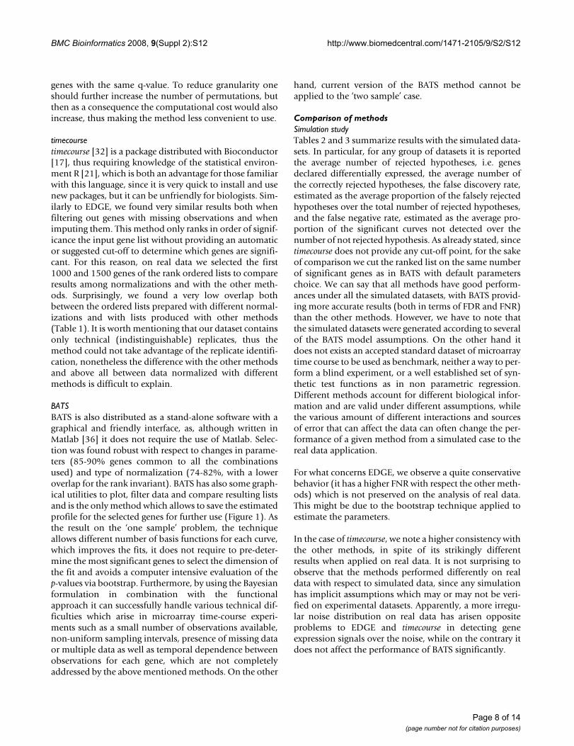
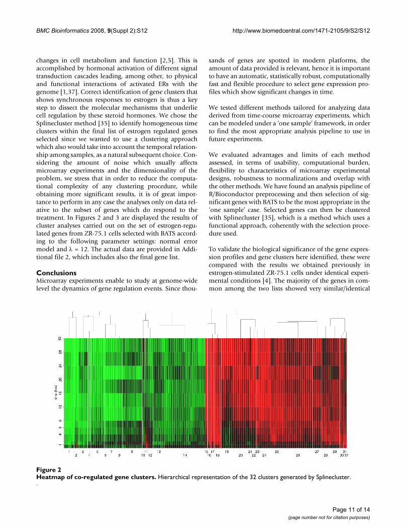
changes in cell metabolism and function [2,5]. This isaccomplished by hormonal activation of different signaltransduction cascades leading, among other, to physicaland functional interactions of activated ERs with thegenome [1,37]. Correct identification of gene clusters thatshows synchronous responses to estrogen is thus a keystep to dissect the molecular mechanisms that underliecell regulation by these steroid hormones. We chose theSplinecluster method [35] to identify homogeneous timeclusters within the final list of estrogen regulated genesselected since we wanted to use a clustering approachwhich also would take into account the temporal relation-ship among samples, as a natural subsequent choice. Con-sidering the amount of noise which usually affectsmicroarray experiments and the dimensionality of theproblem, we stress that in order to reduce the computa-tional complexity of any clustering procedure, whileobtaining more significant results, it is of great impor-tance to perform in any case the analyses only on data rel-ative to the subset of genes which do respond to thetreatment. In Figures 2 and 3 are displayed the results ofcluster analyses carried out on the set of estrogen-regu-lated genes from ZR-75.1 cells selected with BATS accord-ing to the following parameter settings: normal errormodel and λ = 12. The actual data are provided in Addi-tional file 2, which includes also the final gene list.

ConclusionsMicroarray experiments enable to study at genome-widelevel the dynamics of gene regulation events. Since thou-

sands of genes are spotted in modern platforms, theamount of data provided is relevant, hence it is importantto have an automatic, statistically robust, computationallyfast and flexible procedure to select gene expression pro-files which show significant changes in time.

We tested different methods tailored for analyzing dataderived from time-course microarray experiments, whichcan be modeled under a ‘one sample’ framework, in orderto find the most appropriate analysis pipeline to use infuture experiments.

We evaluated advantages and limits of each methodassessed, in terms of usability, computational burden,flexibility to characteristics of microarray experimentaldesigns, robustness to normalizations and overlap withthe other methods. We have found an analysis pipeline ofR/Bioconductor preprocessing and then selection of sig-nificant genes with BATS to be the most appropriate in the‘one sample’ case. Selected genes can then be clusteredwith Splinecluster [35], which is a method which uses afunctional approach, coherently with the selection proce-dure used.

To validate the biological significance of the gene expres-sion profiles and gene clusters here identified, these werecompared with the results we obtained previously inestrogen-stimulated ZR-75.1 cells under identical experi-mental conditions [4]. The majority of the genes in com-mon among the two lists showed very similar/identical

Heatmap of co-regulated gene clustersFigure 2Heatmap of co-regulated gene clusters. Hierarchical representation of the 32 clusters generated by Splinecluster.

� �




Cluster profilesFigure 3Cluster profiles. Blue lines show each cluster average profile.

0 5 10 15 20 25 30

−2−1

01

2

time (hrs)

log2

rat

io

Cluster 1 (54 obsns.)

●

●●

●

●

●●

●

●

●

●

●

●●

●

●

● ●

●

●

●

●

● ●●

●

●

●

●

●

●

●

●

●

●

●

●●

●

●

●

●

●

●

●

●

●

●

●

●

●

●

●

●

●

●

●

●

●● ●

●

● ● ●

●

●

●

●

●

●

●

●● ●

●

●

●

● ●

●

●

●●

●

●

●

●

●

●

●

●

●

●●

● ●

●

●

●

●●

●

●

●

●

●

●●

●

●

●

●

●

●

●●

● ● ●

●

●

●●

●

●

●●

●

●●

●

●

●

●

●

●

●

●●

●

●

●

●

●

●

●

●

●

●

● ●

●

●

●

●

●

●

●

●

●

●● ●

●

●

●

●

● ●

●

●

● ●●

●

●

●

●

●

●

●

●

● ●

●

●

●

● ●

●

●

●

●

●●

●

●

●

●

●●

●●

●

●

● ●

●

●

●

●

●

●

● ●

● ● ●

●

●

●●

●

●

●●

●

●●

●

●

●

●

●

●

●

●

●

●

●

●

●

●

●

●

●

●●

● ●●

●

●

●

●

●●

●

●

● ● ●

●

●

●●

●

●

● ●

●

●

●

●

●

●

●●

●

●

●

●

●●

●

● ●●

●

●

●

●

●●

●

●

●

●

●

●

●●

●

●●

●

●

●

●

●

●

●

● ●

●

●

●

●

●

●

●

●●

●

●

●● ●

●

●

● ●

●

●

●

●

● ●

●

●

●

●

●

●

●

●

●

●

●

●

●

●

●

●

●

●

● ●

●● ●

●

●

● ●●

●

●●

●

●

●

●

●

●●

●

●

● ●

●

●

●

●

●

●

●

●

●

●

●

●

●

●

●

●

●●

●

●

●

●

●●

●

●

●●

●

●●

● ●

●

●●

●

● ●●

●●

●

● ●

●

●

●

●

● ● ●●

●

●

●

●

●

●

●

●

●

●

● ● ● ●

● ●●

●

●

●

● ●

●● ●

●

●●

●

●●

●● ●

● ●

●

●●

●

●

●● ● ●

●

●

●●

●

●

●

●

●●

●●

●

●● ●

●

●

●●

● ●

●●

●

● ●

●

●●

●● ● ●

●

●

●●

●

●

●●

● ●●

●

●

●

●

●

●●

● ●

●●

●

● ●●

●

●

● ●

●●

●

●●

●

●

●

●

●

● ● ●●

●

● ●

●

●

●

●●

●

●●

●

●

●

●

●

●

●

●

●

● ●

●

●

●

●

●

●

● ●

● ●

●●

●

●●

0 5 10 15 20 25 30

−2−1

01

2

time (hrs)

log2

rat

io


●

●●

●

●

●

●●

●

●

●

●

●

● ●

●

●●

●

●

●

●

●

●

●

●

●

●●

●

●

● ●

●

●

●●

●●

●●

●

● ●

●

●●

●●

●

●● ●

●●

●

●●

●● ●

●●

●

●

●

●

● ●●

● ●

● ●●

●●

●

●● ●

●

●

●●

●●

●

●

● ●●

●

●

●

●

●

●

●

●

●●

● ●

● ●

●●

●

●

●

●

● ●

●●

● ●

●

●

●

●

●

● ●

●

●

●●

●

●

●

●

●

●●

●

●●

●

●

●

●

●

●

●

●

●

●

●

●

●

●

●

●

●

●

●●

●

●

●●

●●

● ●

● ●

●

●

●

● ●

● ●

●

●

●

●

●

●

●

●●

● ●

●

●

●

●

●

●

●

● ●

● ●

●

●

●

●

● ●

●

●

●

●

●

●

●

●

●

●

●

●

●● ●

●

●

●

●●

●

●

●

●

● ● ●

● ●

●●

●

●

●●

●

●●

0 5 10 15 20 25 30

−2−1

01

2

time (hrs)

log2

rat

io


●

● ● ● ●

●

●

●

●

●

●

●

●

● ●● ● ●

●

●●

●

●

●

● ●

●

●●

●

●

●

●

●

●

●

●●

●

●

● ● ●●

●

●

●

● ●

●●

●

● ●

●

●

●

●

●

●

● ●

●

●●

●

●

●

●

●

●

●

●

● ●

●

●

●

●

●

●●

●●

●●

●

●

●

●

● ●

●

●

●

●

●

●

●

●

●

●

●

●

●●

●

●●

●● ●●

●

● ●

●●

●●

●

● ●

●

●

● ● ●

●

●●

●

●

●

●

●

●

●

●

●

●

●

●

●

●●

● ●●

●

●

●

● ●

●

●

●

● ●

●

●

●

●

●

●

●

●

●

●●

●●

●●

●

●

●

●●

●

●

● ●

●●

●

●

●

● ●● ●

● ●●

●

●

●

●

● ●

●●

●

●

●

●

●

●

●

● ●

● ●

●

●

●●

●

●

●

● ●

●

●●

●

●●

●

●

●

● ●

●●

● ●

● ● ●

●

●● ●

●

●

●

●

●●

●

●

● ●●

●

●

●●

● ● ●

●

●

●

●

●

●

●

●

● ● ●

●

●● ●

●

●

●●

●

●

●

●

●

●●

● ●

●●

● ●●

●

●

●

●●

●●

●

●

●

●

●

●

●

●

●

●●

●

●

●● ●

●

●

●●

●

●

●

●●

●

●

●

●

●●

●

●●

●● ●

●

●

●

●

●

●

●●

●

●

●

●

●

●●

●

●

● ●

● ●

●

●

●●

●●

●

●

●

●

●

●

●

●

●

●

●

●

●●

● ●

●

●

●● ●

●

● ●

●●

●

●

●

●

●●

●

●

●

●

●●

●

●

●

● ●

●● ●

●

●●

●

●

● ●

●

●

●

●● ●

●

●

●

●

● ●●

●

●●

● ●

●

●

●

●●

● ●

● ●

●

●

●

●

●

●

● ●

●●

●

●

●

●●

●●

●

●●

●

●

● ●

●

●

● ●

● ●

●

●

●●

●

●

●

●●

●

●

●

●

●

●

● ●

●●

●

●

●● ●

●

●

●

●

●

●

●

●

●

●

●●

●●

●

●

●

●●

● ●

●● ●

●

●

●

●

●

●

●

●●

●●

● ●

●

0 5 10 15 20 25 30

−2−1

01

2

time (hrs)

log2

rat

io


●

●

● ●

●

●

●●

●●

●

●

●

●●

●●

●●

● ●●

●

●●

●

● ● ● ●

●

● ●

●

●

●

●● ● ●

●

●

●

●

●

●

● ●● ●

●

● ●● ●

●

●

●

●

●●

● ●

●

● ●

●

●

●

●● ●

●

●

●

● ●

●

●

● ●

●●

● ●

●

●●

●

●

●●

● ●

●

●

●

● ●

●

● ●●

● ●

● ●●

●

●

●

●

●●

● ●

●

●

●

●

●

●

●

●

●● ● ● ●

●●

●

●●

●●

● ●● ●

●● ●

●

●

●

●

●

●●

●

●●

●

●

●

●●

●

●● ●

●

●●

●

●●

●

●

● ● ●

● ●

●

0 5 10 15 20 25 30

−2−1

01

2

time (hrs)

log2

rat

io


●

● ●

●

●

●

●

●

●

●●

●●

●

●

●●

●

●● ●

●

●● ●

●●

●

●

● ●

● ●

●

●

● ●●

●●

● ●

●●

●

●

●

●●

●

●● ●

●●

●

●

●

● ● ●

●

● ●

●

●

●

●

●

●

●

●

● ●

●

●

●

●●

● ●

●

●

● ●

●

●

●

● ●

● ●

●

●●

●

●● ●

●

●

●●

●

●

● ● ●

●●

●

●

●

●● ●

●

●

●●

●

●

● ●

●●

●● ● ● ●

●

●

●

●

●● ●

●●

●

● ●

●

●●

●●

● ●●

●

● ●

●

● ●

●●

● ●

●

●

●●

●

●●

● ●●

●

● ●

●

●

●

●

●● ●

●

●●

● ● ●

●

●

● ●

●

●●

●

●

●●

●

●●

●●

●

●●

●

●●

●

●

● ●

● ●

● ●

●

●

●

●

●●

●

● ●

● ●

●

●

●

●

● ●

● ● ●

●

●● ●

●

●

●

●

●●

●

●● ● ●

●

●

●

● ●●

●

●

●

●

● ●

● ●●

●● ● ●

●

●●

●

●● ●

●

● ● ●

●● ●

●

●

● ●

●

●●

●

●

●

●

●

●●

● ●

●●

●

●

●● ●

●●

●

●●

●

● ● ●●

●

●

●

●

●●

● ●

●

●

● ●

●

● ●

● ● ●

●●

●●

●

●

●

●● ● ●

● ●● ●

●

●

●●

●

● ●●

● ●● ●

●

●

● ●

●

●

●●

●● ●

●

●●

●●

●

●●

●●

●

●

●

● ●●

●

● ● ●

●

●

●

●

●●

●

●

●● ● ●

●

●

● ●

●●

●

●●

●

●●

●

●

● ●

●●

● ● ●●

●

●

●

●

●

●

●●

●

● ●

●

●●

●

●

●●

●

● ●●

●

●●

●

●● ●

● ●●

●

●

●●

●●

● ●

● ● ●●

●

● ●

●

●●

●

●●

● ● ●

● ● ●

●

●

●

●

●

● ●

●

●

●

●●

●

●

● ●

●

● ●

●●

● ●●

●

●●

●

● ●

●

●

●

●●

●●

● ●●

●

●

●

●●

●

●

●

●

●

● ●

●

● ● ●

●

●

●● ●

●

●

●

● ● ● ●●

●

●

●

●●

●

●● ●

●●

● ●

●● ●

●

●● ●

●●

●●

●

●●

●

● ●●

● ●

●● ●

●

●

●●

●●

●● ●

●

●

●

●

●

●

●

● ● ●

●

●●

●

●

●

● ●

● ●

●● ●

●

●

●

●

●●

●●

●

●

●●

● ●

● ●

●●

●

● ●

● ●●

●

●

●

●

●

●

●

●

●

●

●●

● ●●

● ●

●●

●

●

●●

●

●

●

●

●

● ● ●

●

●

●

● ●

● ● ●

●

● ●

●

●

●

●●

● ●●

●

●

●

●

● ●

● ●

●●

●

●

●●

●

●

●

●

●

●

●

●

●

●

●

●●

●

●

●

●

●

●

●●

●

●

●

●

●●

●●

●

●

●

●

●

●

●

●

● ●

●●

●

● ● ●

● ●

●

●

●

●

●●

● ●

●

●

●

0 5 10 15 20 25 30

−2−1

01

2

time (hrs)

log2

rat

io


● ●

●● ●

●

●

●

●

● ●

● ●

●● ●

●

●

●

●

●

●

● ●●

● ●

●

●

●

●

●

●

●

●

●

● ●

●

●

●

●

●

●

●●

●

●

●

●

●

●

●

●

●

●●

●

●●

●

●

●

●

●

●

●

●

●

●

●

● ●

●

●

●

●

●

●

●

● ●

●●

●

●

●

●

●

●

●

●●

● ●

●

●

●

●

● ●

●

●

●

● ●

●

●

●

●

● ●

● ●

●

●●

●

●

●

●

●●

●

●●

●

●

●

●

●

●

0 5 10 15 20 25 30

−2−1

01

2

time (hrs)

log2

rat

io


●

●

● ●

●

● ●●

●

●

●

●

●

●

●

●

●

●

●

●

●

●

●

●

●

●●

●

●

●

●

●

●

●

●

●

●●

●

●

●

●

●

●

●

●

●

● ●

●

●

●

●

●

●

●

●●

● ●

●

●

●

●

●

●

●

●●

●●

●

●

●

●

●

●

●

●

●

● ●

●●

●

●

●●

●

●

●● ●

●●

●

●

●

●

●●

●

●●

●

●

●

●

●

●

●

●

●

●

●

●

●

●

●

●●

●

●

●

●

●

●●

●

●

●

●

● ●

●

●●

●●

●

●

●

●

●

●

●● ●

●●

●

●

●

●

●

●

●● ●

●●

●

●

●●

●

●

● ● ●

●

●

●

●

●●

●

●

●

●●

● ●

●

●

●●

●

●

●

●●

●●

●

●

●

●

●

●

●

●

●

●

●

●

●

● ●

●●

●

● ●

●

●

●

●

●

●

●●

●

● ●

●

●

●

●

●

●

●● ●

●●

● ●

●

●

●

●

●

●

●●

●

●

●

●

●

●

●

●

●

●

● ●

●●

●

●

●

●

●

●

●● ●

● ●

●

●

●

●

●

●

●

● ●

●

●

●

●

●

●

●

●

●

●●

●●

●

●

●

●

●

●

●

●●

●●

●

●

●

●

●

●●

● ●

●●

●

●

●

●

●

●

●

●

●

●

●

●

●

● ●

●

●

●

●

●

● ●

●

●

● ●

●● ●

● ●

●●

●

●

●●

●

●

●●

●

●

●

●

●

●

●

●

●

●● ●

●

●

●

●

●●

●

●

● ● ●

●

●

●

●

● ●

●

●

●●

●

●

●

●

●

●

●

●

●

●● ●

●

●●

●

● ●

●

●

●

● ●

●●

●

●

●

●

●

●

●

●

●

●

●

●

●

●

●

●

●

●

● ●

●●

●

●

●

●

●

●

●

● ●

●

●

●

●

●

●

●

●

●

● ●

●

●

●

●

●

●

●

●

● ●

●

●

●

●

●

●

●

●

●●

●●

●

●

●

●

●●

●●

●● ●

●

●

●

●

●

●

●

● ●

●●

● ●

●●

●

●

●●

●

●

●

●

●

●

●

●

●

●

●●

●●

●●

●

●

●

●

● ●●

●

●

●●

●

●

●

●

●

● ●

● ●

●●

●

●

●

●

●

●●

●●

●

●

●

●

●

●

●●

●

● ●

● ●

●

●

●

●

0 5 10 15 20 25 30

−2−1

01

2

time (hrs)

log2

rat

io


●

●

●

● ●

●●

●

●

●

●

●

●

●

●

●

●●

●

●

●●

●

●

●●

●

●

●

●

●

●●

●

●

●

●●

●●

●

●

●

●

●

●

●●

●

●●

●

●

●●

●

●

●●

●

● ●

●

●

●●

●●

● ● ●

●

●

●

●

●

●

●

●

●

●

●

●●

●

●

●

●

●

●

●

●

●

●

●

●

●

● ●

●●

●●

●

●●

●

●

● ●

●

●

●● ●

● ●

●

●

●●

●

●

●

● ●

●

●

●

●

●

●

● ● ●

●●

●●

●

●

●

●

● ●●

●●

●●

●

●

●

●

●

●

●

●●

●

●

●

●

●●

●

●

●

●●

●

●

●

●

●

●

●

●

●● ●

●

●

●

●

●

●

●

●

● ●●

● ●

●

●

● ●

●

●

●

●

●

●

●

●

●

● ●

●

●

● ● ●

●●

●

●

●

●

●

●

●

●

●

● ●

●

●

●

●

●

●

●

●

●

● ●

●

●

●

●

●

●

● ● ●

●

●

●

●

● ●

●●

●●

●

●●

●

●

● ●

●●

●

●

●

●

●

●

●

● ●

●

●

●

●●

●

●

●

●

●

●

●

●

●●

●

●

●

●

●

●●

● ● ●

●

●

●

●

●

●

●

●

●

●

● ●●

●

●

●

●

●●

● ●

●

●●

●

●

●

●

●●

●●

●

●

●

●

●

●

●

●

●

0 5 10 15 20 25 30

−2−1

01

2

time (hrs)

log2

rat

io


●

●

●

●

●

●

●

●

●

●

●

●

●

● ●●

●●

●

●

●

●●

●●

● ●

●

● ●

●

●

●

●

● ●

●●

●

●

●

●

●

●●

●●

●

●

●

●

●

●

●

●●

●

●

●●

●

●

●

●

●

●

●

●

●

●

●

●

●

●

●

●●

●

●

●●

●

●

●

●

●

●

●

●

●●

●

●

●

●

●

●

●

●

●

●

● ●●

●

●●

●

● ●●

●

●

●

●

●

●

●

●

●

●●

● ●●

●

●●

●

●

●

●

●

●

● ● ●

●●

●

●

●

●

●

●

● ● ●

●

●

●

●

●

●

●

●

●●

●

●

●

●

●

●●

●

●●

●● ●

●

●

●●

●

●

●

● ●

●

●●

●●

●

●●

●

●●

●

●●

●

●

●

●

●

●

●

●

●

●

● ●

●●

●

●

●

●● ●

●

●

●

●●

●

● ● ●●

●

●

● ●

●

● ●

● ●

●●

● ● ●

●

●

●

●

●●

● ●●

●● ●

●

● ●

●

●

●

●●

● ●

●

●

●●

●

●

●●

●●

●

●

●

●●

●

●

●●

●

●

● ●

●

●

●

● ●

●

●●

●●

●

●

●

●

● ●●

●●

●●

●

●

●

●

● ●

●

●●

● ●●

●

●

●

● ●

●●

●

●

●●

●

●

●

● ●

●

●

●

●

●●

●

●

●

●●

●●

●

● ●

●

●

●

●

●

● ●

●●

●

● ●●

●

●

●

● ●

●

●

●●

●

●

●

●

●

●●

●

●

●

●

●

●

●●

●●

●●

●

●

●●

●

●

●

●

●

●

●

●

●

●

●

●

● ●●

●●

● ●

●

●

●

●

●

●

●

●●

● ●

●

●

●

●

● ●

●

● ●

●

●

●

●

●

●

●

●

●

● ●

●

●

●

●

●

●

●

●

●

●●

●

●

●

●●

●

●

●

●

●●

●●

●●

●

●

●●

●

●●

● ●

●●

●

●

●●

●●

●

●●

●

●

●

●

●

●●

●●

●●

●●

●

●

●

●

●

●●

●

●

●

●

●

●

●

●

●● ●

●●

●

●

●

●

●●

●

●●

● ●

● ●

●

●

●

●

●●

●

●●

●●

●

●

●

●

●

●

●

●●

● ●

●

●

●

●

●●

●●

●

● ●

●●

●

●

●

●●

●

●

●●

●

●

●

●

●

● ●

●●

●●

●

●

●

●

●

●

●●

●

●●

●

●

●

●

●

●

●● ●

●●

●

●

●

●

● ●

● ●●

●●

●

●

●

●

●

●●

●●

●

●

●

●

●

●

●

●

●● ●

● ●

●

●

●

●

●

●

●●

●

● ●

●

●

●

●

●

●●

● ●

●

●

●

●

●

●

●

●

● ●●

●●

●

●

●

●

●●

●

●●

●●

●

●

●

●

●

● ●

●

●●

● ●

●

●

●

●

●●

●●

●

●●

●

● ●

●●

● ●●

●

● ●●

●

●●

● ●●

● ●●

●

●

●

●

●

●

●

● ●

●

●

●

●

●

●

●

●●

●●

●● ● ●

●●

●

●

● ●

●

●

●

●

●

●

●

●

●●

●●

● ●

●

●

●

●

●●

●

●

●

●

●●

●

● ●

●

●

●

●●

●

●●

●

●

●

●

●●

● ●

● ●

●

●

●

●

●●

●

● ●

●●

●

●

●

●

●● ●

●

●

●

●

●

●

●

●

●

● ●

●●

●●

●

●

●

●

●

●

●

●

●

● ●

●

●

●

●

●

● ●

●

●

●

●

●

●

●

●

●

●●

● ●

●

●

●

●

●

●

●

●

●●

●

●●

●

●

●

●

●

●

●

●

●

●

●

●

●

●●

●

●

●

●

●

●

●

●

●

●

●

●

●

● ● ●

●

● ●

●

● ●

●

●

● ●●

●

●

●

●

● ●

●

●

●●

●

●●

●

●

●

●

●

●●

●

●

●●

●

●

● ●

●

●

●●

●

● ●

●

●

● ●

●

●

●

●

●

●●

●

●

●

●

●

●

● ●

●

●●

●

●

● ●●

●

●

●●

●

● ●

●

● ●●

●●

● ●

●

● ●

●

● ●●

●

● ●●

●●

●

●

● ●

●

●●

●●

●●

●

●

●●

●

●●

●

●

● ●

●

●

●

●●

●● ●

●

●●

●

●

●

●

●

● ●

● ●

●

●

●

●

●●

●

●● ● ●

●●

●

●

●

●●

●● ● ●

●

●

●

●

●

●

●●

●● ●

●

●

●

●

●

●

●

●●

●

●

● ●

●

●

●

●

●

●

● ●

●

● ●

●

●

●

●

0 5 10 15 20 25 30

−2−1

01

2

time (hrs)

log2

rat

io


●

●

●● ●

●●

●

●

●

●

●●

●

●

●

●

●

●

●●

●

●

●

●

●

●

●

●●

● ●

●

●

●

●●

●

●●

●

●

●

●●

●

● ●

●●

●

●

●

● ●

●

●

● ●● ●

●

●

●

●

●●

●

●

●● ● ● ●

●

●

●●

●●

●

● ●

● ●

● ● ●

●

● ● ● ●● ●

●

●

●●●

●● ●

●●

●

●

● ● ●

●

● ●

●

●●

●

●

●

● ●

●●

●

●

●

●

●●

●

●

●

0 5 10 15 20 25 30

−2−1

01

2

time (hrs)lo

g2 r

atio


●

●

●●

●

●

●

● ●

●●

●

●

●●

●

●

●

●

●● ●

●

●

●

●

●

●

●●

●● ●

●

● ● ●

●

●

●

●

●●

●

●●

●

●

●●

●●

●

●●

● ●

●●

●

●

●

●●

● ●

●

●

●

●

●●

● ●

●

● ●

●

●

●

●

●

●

● ● ● ●

●

●

●

●

●

●●

●●

●

● ●

●

●

●

●

● ●

●

●

●●

●

●

●

●

●

●●

●● ●

●

●

●

●

●●

●

●

● ●●

●●

●

●

●

● ● ● ●

●

●

●

●

●

●

●

●

●

●

●

●●

●

●

●

●

● ●

●

●● ●

●

●

●

●

●

●●

●

●

●

●

●

●

●

0 5 10 15 20 25 30

−2−1

01

2

time (hrs)

log2

rat

io


●

● ●●

●

●

●●

●

●●

●

●

●●

● ●

● ●

●

●

●

● ●●

●●

●

●●

●●

●

● ●●

●● ●

● ● ●

●●

●● ● ●

● ●

●● ●

●●

●●

●●

● ●

●●

●

●

●

●

●

●● ● ●

● ● ●

●

●

● ●

●●

●

●

●●

●

●

●

● ● ●●

●●

●● ●

●

●

●

●●

● ● ●

●●

●

●

●

●

●

●

●

●

● ● ●

●●

●

●

●

●

●

●●

●●

●

●●

●

●●

● ●

●

●●

●

●

●

●

●

●●

●

●●

●●

●

●

●

●● ●

●

●

●

●

●●

●

●●

●●

●

●

●

●●

●

●

●●

●●

● ● ●

● ●

● ●

●● ●

●

● ● ●

●●

●●

● ● ● ●

●

● ●

● ● ●

●

●●

● ●●

● ●

●●

● ●

●●

●

●●

●●

●

●

●

●

●

●● ●

● ●

●● ●

●

●

●● ● ● ●

●●

●

●

●

●

●●

●

● ●

● ●

●● ● ●

●

●

● ●

● ●●

● ●● ●

●

●●

● ● ●

●

●

●

●●

●

●● ● ●

●●

●

●

●

●

●

●

● ●●

●●

●

●

●●

●

●●

●●

●

● ●

●

●

●

0 5 10 15 20 25 30

−2−1

01

2

time (hrs)

log2

rat

io


●●

●

● ●●

●●

●●

●

●

●●

●●

●

●

●

●● ●

●● ●

● ●

●

●

●

●●

●

●

●●

●

●

● ●●

● ●

●

●

● ● ●

●

●●

●

●

●

●

●

● ●●

●

● ● ●

●

●

●

●

●● ●

●

●

●

●●

●

●

●

●

● ● ●●

●

●

● ●

●

●●

●● ●

●●

●

●

●

●

●

●

● ●●

●● ●

●

●●

●

●

● ●●

●● ●

●

● ●

●

●

●

●

●●

●

●

●

●

●

●

●●

●●

●

●

●

●

●●

●

● ●●

●●

●

● ●●

●

●

●●

●

●

● ●

●

●

●●

●

● ●●

●

●●

●●

● ●

●

●

● ● ● ● ●●

●

● ●

●

●

●

● ●

●●

●

●

●

●

●

●

●● ●

●

●

●

●

●

●

●

●

●

● ●

●

●

●●

●

●

●

● ●●

●

●

●

●

●

●●

●

●● ● ●

●

●

●

●

●

●

●

●

● ● ●

●

●

●●

●●

●

● ● ●

●

●

●●

●

● ●

●

● ●

●● ●

●

●●

●

●●

●

●

● ●

● ● ●●

●

●

●

●

●

●● ●

●● ●

●●

●

●●

●● ●

● ●●

●

●

●

●

●●

● ●

●

● ●● ●

●

●●

● ●

● ●

● ● ●

●

●

●

●

●

●

●●

●

●

●

●●●

●

●●

●

●

●●

●

●

●

●

●

●

●

●●

●●

●

●

●

●

●

●

●

●

●

●●

●

●

●

●

●

●

●

●

● ●

● ●

●

●

●

●

● ●

●●

●●

●

●

●

●

●

● ● ●

●

● ●

●

●

●●

●

●

●

●

●● ●

●●

●

●

●

● ●

●●

● ● ●

●

●

●

●●

●

●●

● ●●

●

●

●

● ●

●

●

●

●

●

●

●

● ●●

●

● ●●

●

●

●

●

●

●● ●

●●

●

●

●

●

●

●●

●

●●

● ●

●

●

●

●

● ●

●

●

●

●●

●

●

●

●

●● ● ● ●

●

●

●●

●

●

●

●

●

●●

● ● ●

●

●

●

●

●

●●

●

●●

●

●

●

●

●

●

●

● ●

●

●

●●

●

●

●

●

●

●●

●●

● ●

●

●

●● ●

●●

●

●

●● ●

●

● ● ●

● ●● ●

●

● ●

●

●

●● ●

●●

●

● ●

●●

●

●

●

● ●●

●

●●

●

●

●

●●

●●

● ●

● ●

●

●

● ●●

●● ●

●

●●

●

●

●

●

●

● ●

●

●

●●

●

●

● ●

●

●

●

● ●

●

●

●

●

●● ●

●

●

●

● ● ●

●

●

●●

●

●

●

●

●

●

●

●

●

●

●

●

●●

●

●

●

●

●

●

●

●

●●

●

●

● ●

●

●●

0 5 10 15 20 25 30

−2−1

01

2

time (hrs)

log2

rat

io


●

●

●

●

●

●●

●

●

●

●

●

●

●

●●

● ●● ●

●●

●

●

●

●

●●

●

●●

●●

●

●

●

●●

●● ●

●●

●

●

● ●● ●

●

●

● ●

●

●

●

● ●

●

● ● ●

●

●

● ●

●

●●

●

●●

● ●

●

●

●

●

● ●

●

●● ● ●

●

●●

●

●

● ●

● ●●

●●

● ●

●

●

● ●

● ●

●

●

●● ●

●

● ●●

●●

●

● ● ● ●

●

●

●

● ●

●● ● ●

● ●

●

●●

●●

● ●●

●

●●

●

●

●

●●

●

●●

●

●●

●

●

●

● ●

●

●

●

●

●●

●●

●● ●

●

●

●

●

●

●

●

●

●● ●

●●

●●

● ●

●

● ● ●●

●

●●

● ● ●

●

●

●

● ● ●●

●

●●

●

●●

●

● ●

●●

●●

● ●

● ●

●●

● ●

●

● ●

●●

●

●

●

● ●

●

●●

●

● ●

●●

● ● ● ●●

●

● ●

●

●

●

●

●●

●● ●

● ● ●

●

●

●

● ●

●

●●

● ●●

●●

●

●

●●

● ●

●

●

●

●

●

●●

●

●●

●

●

●●

●

●

●

●

●●

●●

●

● ●

●

●

●

● ● ●

●

●

●●

●

●

●

●

●

●●

● ●

●

●

●

●

●●

●●

●● ●

● ●

●

●● ●

●

● ●●

●●

●

●

●●

● ●

●

● ●

●

●●

●

●

●● ●

●●

●●

●

●●

●

●

●

●

●●

●●

●

●

●

●

● ● ●

●●

●

●●

●●

●

●

●

●●

●

●

●

● ● ●

●

●●

● ● ●● ●

●●

●

●●

● ●● ●

●●

●● ●

●

●

● ●●

●

●

●

●● ●

●

●

●

●●

● ●●

●

●●

●●

●

● ● ● ● ●

●

●●

●

● ●

● ●

●

●

●

●

●●

●

●

●

●

● ●

●●

●

●

●

●

●● ● ●

●● ●

● ●

●

●

●

● ● ●● ● ● ●

●

●

●

●

●●

●●

●

●●

●●

●

●

●

● ●

●

●

●●

●

●

●

●

● ●● ●

●

●

●

●

●

●

●●

●

●

●

●

●

● ●

●

●

●

●

● ●● ● ●

●

●●

●

●●

●●

●●

● ●●

●

●

●●

● ● ● ●●

●

●

●

●

●

●●

●●

● ●

●

●

●

●

●●

● ●●

●●

●

●

●

●

●●

● ●●

●●

●

●

●

●

●

●●

●●

●

●

●

● ●

●

●

● ●●

●

● ●

●

●

●

●

●●

● ●●

●●

●●

●

●

●● ● ●

● ●●

●

●

●

●

●●

●●

●● ●

●

●

●

●

●●

● ●

●●

●

●

●

●

●

●

● ● ●●

● ●

●

●●

●●

●●

● ●

● ●

●

● ●

●

● ●

●●

●

● ●

●

●●

●

●●

● ●

●

● ●

●

● ●

●

●

● ●●

●

●●

●

● ●

●●

● ● ● ●

● ●

●

●●

●

●●

● ● ●●

●

● ●

●

●

●

●●

●● ●

●●

● ●

●

● ●●

●

●● ●

●

●●

●

●

●

●

●

●●

● ●

●●

● ●

● ● ●● ● ●

●

●●

●●

●●

● ●● ●

●●

●

●

●

●● ●

●●

●

●

● ●

●

●

● ●●

●●

●

●

●●

●

●● ●

● ●●

●

●

●●

●

●●

●

●●

●

●

●

●

●

●

●●

●●

● ● ●●

●●

●

●● ●

● ● ●● ●

●

●

●

●●

●

●

●●

●

●

●

●

●

●

●

●●

●

●

● ●

● ●

● ●

●

●●

● ● ●●

●

●

●●

● ●●

●

●●

●● ●

● ●

●●

●● ● ●

●

●

●●

●

● ●●

●

●●

●

●●

●

●

●● ● ●

●

●

●●

●

●

●

● ●●

●

● ● ●

●

●

●●

●

●

●

●

●●

●

●●

●●

●

●●

●● ●

●

●

●

●

●●

●●

● ● ●

●●

●

● ●●

● ●

●● ● ●

●

●

● ●

●● ●

●

● ●●

●

●

●

● ●

● ●●

● ● ●

●

●

●

●

● ●● ●

●●

●

●

●

● ●

●●

● ●●

●

●

●

●

●

●● ●

●

●

●

●●

● ●

●

●

●

●●

●● ● ●

●

●

●

●●

●

●

●

● ●

●●

●

●

● ●

●●

● ● ●

●

●

●

●

●●

●●

● ●●

●

●

●

●

● ●●

●

●●

●

●●

●

●

●●

●

●

●

●

●

●

●

●

●

●●

●●

●

●

●●

●

●

●

●

●● ●

●

●●

●●

●

●

●

●

●● ●

●

●●

●

●

●

● ●●

●●

●●

●●

●

● ●

● ● ●

●● ●

●

●●

●●

●

● ●

●●

●

● ●●

●

● ●● ●

●

●●

● ●

●

●

●

●●

●

●●

●●

●

●

●

● ● ●

●●

●● ●

●

●

●

● ●●

●●

●●

● ●

●

● ●●

●

●

●●

●

●

●

●

● ●

● ●●

●

●

●●

●

●

●

● ●●

●

●

●

●●

●

●

●●

●● ● ● ●

● ●●

●

●

●●

●● ●

●● ● ●

●

●

● ●

●● ●

●●

● ●

●

●

●

●

●● ● ● ● ● ●

●

●

●

● ●●

●●

●

●● ●

●

●

●●

●

●

●

● ●●

●

●

● ●●

●●

●

● ●

●●

●

●

● ● ●●

● ● ●● ●

●

●

●●

●

● ●●

●

● ●

●

●●

●●

●

●

●

●

●

●

●

●

● ● ● ●

●●

● ●

●

●

●

●

●● ●

● ●

●

●●

●

●

●

●

●

●

●

●

●

● ●

●

●

●

● ●

●

●

●

●

●

●

●

●

●

●●

●

●●

●

●

●

● ● ●

●●

● ●●

●●

●

●

●●

● ●

● ●

●

● ●

●

●●

●

●●

●

●

●

● ● ●

●●

●●

●

●

●

● ●

●

●

●●

● ●●

●

●

●

●

● ●

●●

●● ● ●

●

● ●

●

●●

●●

●

● ● ●

●● ● ●

●

●

●

●●

●

●●

●

●

●●

●

●

● ●●

●

●

● ●

●

● ●

● ●

●

●

●

●

●

● ●

● ●

●●

●

●●

●

●

●

●

● ●

● ●

●● ● ● ●

●●

●●

●●

● ●

● ● ●● ●

●●

● ●

●

●● ●

● ●●

●●

●●

●

●●

●●

●●

● ●

●●

●● ● ● ●

●

●

●●

●

●●

●●

●● ●

●

●●

●

●●

●●

●

●

●

●

● ●

●● ●

● ●

●●

●

●

●

●

●●

●● ●

●

● ●●

●

●

●

●

● ● ● ● ●●

●

●●

●●

●● ●

●

● ● ●

●

●

●

●

● ●

● ●

●● ●

●●

● ●

●●

●

● ●

●

●

●

● ●

●● ● ●

●

● ●

●

●●

● ●

●

●● ●

●●

●

● ●

●●

● ●

●●

●

●●

●

●

● ● ●●

●●

● ● ●

●●

●

●

●●

● ●

● ● ●

●

●

● ● ●● ●

●

●● ●

●

●

●●

●

●●

●●

●

●

●●

● ●● ●

●● ●

● ●

●●

● ●● ●

●●

● ●●

●● ● ●

●●

●●

●●

●

●

●

●

●●

●

●● ●

●●

● ●

● ● ●●

●●

●

●

●

●●

●●

●● ●

●

●

●●

●●

● ●

●

●●

●

●

● ●

● ●

●●

●●

● ●

●

●●

● ●

●● ●

●●

●

●

● ●

● ● ●●

● ●

●●

●●

●

●●

●● ●

●

●

●●

●

●

●

●

● ●

●●

●

●

●

●

●

●

●

●

●●

●

●

● ●

●

●

●

●●

●●

●

●

●

●

●

●

●

●

●● ●

●

● ●

●

● ●

●

● ● ●●

●

●●

●

●●

●

●

●

●●

●

● ●

●

● ●

●

●

● ●

●

●

●●

●

●

●

●

●

●●

● ●

●●

●

●●

●

●

●●

● ●

●●

●●

●

●

● ●

●●

●

●●

●

● ●

●●

●●

●●

● ●●

●

●

●

●

●

● ●●

●

●●

●

●

●

●

● ● ●●

●●

●

● ●

●

●

●

●●

●

●●

●

●●

●

●●

●

●●

● ●●

●●

●● ●

●●

●

●●

●

●●

●

● ●

●

●

●

● ●●

●

●

●

●● ●

●

●

●●

●

●

●

●

●

● ●● ●

●●

●

●

●

●

● ●● ● ●

●●

●

●●

●

●

●

●●

●

●

●●

● ●

●

●●

●● ●

● ●

●

●●

●

● ●●

●

●

● ●

●

●●

●

● ●●

●

●

●

●

●

●

●

●

● ● ●● ●

● ● ●

● ●

●

●●

●●

● ●

● ●● ●

●

● ●● ●

●

●● ●

●

●

●

●●

● ●

●

●●

●

●

●

●

●

●

●

●

●

● ●●

●●

● ● ●

●

● ●●

●

●

●

●

●

●

●

● ●

●

●●

●

● ●

●

● ●●

●●

●

●●

●

●

● ● ●

●

●●

●

●●

●●

● ●●

● ●

●

●

● ●

●

●

●

●

● ●

●

●●

● ●● ●

●

●

●

● ●●

●

●●

●

●

● ●

●●

● ●

●

●●

●

●

0 5 10 15 20 25 30

−2−1

01

2

time (hrs)

log2

rat

io


●

●

●

● ●

●● ●

●

●

●

●●

●

●●

●

●●

●

●

●

●

●

●●

●

●●

●● ●

●

●

●

●

●

●

● ●●

●

●

●

●

●

●

●

●

●

●

●

● ● ●

● ●

●

●●

● ● ●

●

●●

●

●

●

●●

●

●

●

●● ●

●

●

●

●

●

●

●

●

●

●

●

● ●

●●

●

●●

●

●

●

●

●

●

●●

●●

●●

●

● ●

●

●

●

●

●

●

● ●

●

●●

●

●

●●

●

●

●

●

●

●

●

0 5 10 15 20 25 30

−2−1

01

2

time (hrs)

log2

rat

io


●

●

●

● ●●

●

●●

●●

●

●

●

●

●

●

●●

● ●

●

●

●

●●

● ●

● ●●

●

●

●

●

●

●

● ●

●●

●

●

●

●

●

●

● ●●

● ●●

● ●

●

●

●

●

●●

●

●●

●

●

●

●

●●

●

●

●

●

●● ●

● ●

●

●●

●●

●

●●

●

● ●

●●

●

● ●

●

●

●

●

●

●●

●

●

●

●

●

●

● ●

●

●●

●

●●

● ●

●

●●

●

● ●● ●

● ●●

●

●

●

●

●

● ●

●●

●

●

●

●

●

●

● ●●

●

●

●

●

●

●

●

●

●

●● ● ●

● ●

●

●

●

●

●●

●● ●

●

● ●

●

●

●

●

●

●

● ●●

● ● ●●●

●

●

●

● ● ●

●

●●

●

●

●

●●

●

●

●

●

●

●

●

0 5 10 15 20 25 30

−2−1

01

2

time (hrs)

log2

rat

io


●

●

●●

●

● ●●

●

●

●

●

●

●

● ●

●●

●●

●

●

●

●

●● ● ●

●●

●

● ●

●

●

●

● ●

●● ● ●

●●

●

●

● ● ●

● ●

●●

●●

●●

●

●●

●

● ●

●

●

●

● ●

●●

●

● ● ●

●

●

●

● ●

●● ●

●● ●

●

●

●

●●

● ●

●● ● ●

●

●●

●

●

● ●

●● ● ● ● ● ●

●

●

●

●

●● ●

●● ●

●

●

●

●

● ● ●

●

●●

●●

●●

●

●

●●

●

● ●

●

●

●

●

●●

● ●

●

● ● ●●

●● ●

●

●●

●

●

●●

●

0 5 10 15 20 25 30

−2−1

01

2

time (hrs)

log2

rat

io


●●

●

● ●●

●

●

●

●●

●

● ●

●●

●●

●

●●

●

●●

●

●

● ●●

● ●

●

●

●

●

●● ●

●

●●

●

●●●

●

●

● ●

●

●

●

●

●

●

●

●● ●

●

●●

●

●●

●

●

●●

● ●

● ●

●

●●

●

●●

● ● ●

●

●●

● ● ●

●

●● ● ●

● ●

● ● ●

●

●

● ●

●●

●●

●

●

●●

●

●

●●

●

● ●●

●●

●

●

●●

●●

●

●

● ●●

●

●

●

●

●

●● ●

●

● ●

●

●

●

●

●

●● ●

● ●

●●

●

●

● ●● ●

●

●

●

●

●

●

● ●

●●

●

●●

●

●

●

●

●

●

●

●●

●

●

● ● ●

●

●● ● ●

●●

● ●

●

●

●

● ●●

●

●

●●

●

●

●●

● ●●

●

●

●

●

●

●

●

●

● ●

●● ●

●

●●

●

●

●

●

●

●

●

●

● ●●

●●

●

●

●●

●●

● ●●

●

●

●

●

●

●●

●●

●

●

●

●●

●

●●

●

●

●●

● ●

●

●

●

● ●

●●

●

●

●

● ●

●

●

●●

●●

●

●●

●

●

●

●

●

●●

●

●

●

●

● ●

●● ● ●

●

●

● ●

●

●●●

●

●

●

●●

● ●

●

●

●

●

●

●

●

●

● ●

● ● ● ●●

●

●

●

●●

●

●●

●

●

● ●

●

●

● ●

●

●●

●

●

●

●

● ●

● ● ●

●

●

● ●

●

●

●

●●

● ●

● ● ●

●

●

●

●●

●

●●

●

●

●

●

●●

●●

●

● ●

●

●

●

●

0 5 10 15 20 25 30

−2−1

01

2

time (hrs)

log2

rat

io


●

●

● ●●

●

●

●

●●

●

●●

●●

●

●●

●

●

●

●

● ●

●●

●

● ● ●

●

●

●

●

●●

● ●

● ●

●

●

●

●

●●

●● ●

●●

●

●●

●

●●

●●

●

●●

●

●

● ●

● ●

● ●●

●●

●

●

● ●

●

●

●

●●

●●

●

●●

●

●

●● ●

●

●

●

●

● ●

●

●●

● ●●

●●

●

●

●

●

●●

● ●

●

●●

●

●

●●

●●

● ●

●

● ● ●

●

●●

●●

●●

● ●

● ●

●

● ●

●

● ●●

●

●

● ●

●

● ●

● ●

●●

●

●

●●

● ●

●

● ●

● ●

●

●●

●

●

●

●

●

●● ●

●

● ●●

●●

●

●●

● ●

●

● ●

●

● ●

●

●●

●

● ●

●

●● ●

●

●

● ●●

● ●

●

●●

●

● ●

●

●● ●

●

●

●

●●

●

●

●

●

●

●

●●

●

●

●

● ●

●

●

●

●●

●●

●

●●

●

●

●

●

●●

●

● ●

●

●

●

●● ●

●

●

●

●

●

●

●

●

●

●● ●

●●

●

●

●

●●

●●

●

●

●

●

●

●

●

●

●

●

●

●

●

●

●●

●

●

●●

●

●

●● ●

●● ●

●

●

●

●

●

●●

●

●

●

●

● ●●

● ● ● ●

●

●● ●

●

●

●

● ●

●● ●

● ●

●

● ●

●

●●

● ● ●

●

●

●

●

●●

●

●

● ●●

●

●●

●

● ●

● ● ● ●●

● ● ●

●

●

●

●●

● ● ●

●●

●

●

●

●

●

●

●

● ●

●

●

●●

● ●

●

● ●

●

●

●●

●

●

●●

●

●

● ●● ●

● ●●

●

●

●

●● ●

●

●

●

●

●

●

●

●

●●

●●

●

●

●

●

● ●

●●

● ● ●

●

●

●

●

●

●

● ●

●● ●

●

●●

●● ●

●

●

●●

●

●

●●

●

●

●

●

● ●

●

●●

●

●

●

● ●

●

●●

●●

●

●●

●

●●

●● ● ● ●

●

●

●

●

●

●

●

●

●●

●

●

●

●

●

●

●

●

●

●●

●●

●

●

●

● ●

●

●

●●

●●

●

●●

●

●

●

●

●●

●

●

●●

●

●

●

●

●

●

● ●●

● ●

●

●●

●

●

●

●

●

●

●●

●

●●

●

●●

●

●

●

● ●

●

●

●

●

●

●

●

● ●

●

●

●

●

●

●

●

●●

●

●

●

●

●

●

●

●

●

● ●

●

●

●

●

●

●

●

●

●●

●

●

●

●

●

●

●

●

●

●

●●

●

●

●●

●

●

●

0 5 10 15 20 25 30

−2−1

01

2

time (hrs)

log2

rat

io


●●

● ●●

●

●●

●

● ●

●

●

●● ●

●

● ●

●●

●

●

●

●

●

●

●

● ●

●

● ●

●

●

● ●●

●

●●

●

●

●

●

●

●●

●

●● ●

●

● ●

● ●

● ●

●

●

●●

●

●●

● ●● ●

●

●

●

●

● ●●

●

●

●

●

●

● ●

●

●

● ●

●

●

●●

●

●

●●

●

●●

●

●

●

●●

● ●●

●

●●

●

●

●

● ●

● ●

●●

● ●

●● ●

● ●

●● ●

●

●●

●

●

●●

●●

●●

●● ●

●●

●●

●●

●

●

●

●

●

●● ● ●

● ●

●●

●

●

●

●

●

●●

●

●●

●

●

●

●

●●

●●

●

● ●● ●

●

●

●

●

●

●●

● ●

●●

●

●

●

●

● ●

●

●

● ●●

●

●

●●

● ●●

●

●●

●● ●

●●

●

●

● ●●

●●

●

●

●●

●●

●●

●●

●

● ●

● ●

● ●

●

● ●

● ● ●●

●

●●

●

●

●●

●

●

●●

●

●●

●

●

● ● ●

●

● ●

●● ●

●

●

●

●● ● ●

●

●

●●

● ●

● ● ●●

●

●

● ●

●

● ●

●

●

●●

●

●

●

●● ●

●●

●●

●● ●

●●

● ●

●

●

●

●

● ●

●

● ●

●

●●

● ●

●

●

●

●

● ● ●●

●

●●

●

●

●●

● ●●

●●

● ●●

●●

●

●●

●● ●

●●

●

●

●

●

● ●●

● ●

●

●

●

●

●

●

●

●

●

●●

● ●●

●● ●

●● ●

● ●

●

●

●● ● ●

●

●

●●

●

●●

● ● ●

●

●

●●

●

●

●●

●

●

●

●

●●

● ●

●●

●

●

●

●

●

●

●

●●

●

●

● ●

●

●●

●

●●

●

●● ●

●

●

● ●

●●

●

●

●

●●

●● ● ●

●●

● ●

●

●●

● ● ●

●

●

●

● ●

●● ●

●

● ● ●

●●

● ●

● ●

●

●

●

●

●

● ●

●●

●

● ●●

●

●

●

●● ●

●

●

●●

●

●

● ●

●●

● ● ●

●●

● ●● ●

● ●●

●●

● ● ●

●

●●

●● ● ●

●

●●

●

●

● ●

●●

●● ●

●● ●

●

● ●

●●

●●

●

● ● ●

●

●●

●

●●

●

●

● ● ●●

●

●●● ● ●

●

●

●

●● ●

●

●●

● ●●

●

●

●●

●●

●●

●●

●

●

●

●

●●

●

●● ●

● ●

●

● ●

●●

●

● ●●

● ● ●

●

●

●

●

●

● ●●

●●

●

●

●

● ●

●

●

● ●●

●●

●

●

● ●

●

●●

●

●● ●

● ●●

●

●

●● ● ●

●● ●

●●

●

●

● ● ● ●●

●

●

●●

●

●

●

●

● ●●

●

●● ●

●

●

●

●

● ●●

●

●

●

●

●

●

●●

● ●

●

●

●

●

●

●

●

● ● ●●

●

● ● ●

●

●

●

●●

●

●

● ●

●●

●●

●

●

●● ●

●

●●

●

●

●

●

●● ●

●

●●

●

●

●

● ●

●●

●●

●

●

●●

●

●●

● ●●

● ●

●

●

●●

●●

●●

●

●

●

●

●

●●

●

●

●

●

●●

●

●●

●

●

● ●

●

● ● ●

●

●●

● ●

●●

●

●

●●

●

●

●

●

●

●●

●

●

● ● ●

●

●

●

● ●

●

●

● ●● ●

●●

●

●

●

●

●

●● ●

●

●●

●

●●

●

●

● ●● ●

●● ●

●

● ●

●

●

●●

●●

●●

●

● ●

●

●

● ●

●

●● ●

●

●

●

●

●

● ●●

●

● ●

●●

●

●

●

● ●

●

●

●

●

●

●

●

●

●

●

● ●

● ●●

● ●

●

●● ●

●●

●

●

●

●

●

●

0 5 10 15 20 25 30

−2−1

01

2

time (hrs)

log2

rat

io


● ●

●

●

●

● ●

●

●

●●

●●

●

●

●

● ●

●

●

●●

●

●

●

● ●

●

●●

●

●

●

●

●

●

●

●

●

●● ●

● ●

●

●

●

●

●

●● ●

●

●

●

●

●

●

●

●

● ●

●●

●●●

●

●

●

●

●●

●●

●

●●

●

●

●

●●

● ●

●●

●

●

●●

●

●●

●

●

●

●●

●

●

●●

●●

●

●

●●

●

●●

●

●●

●

●●

●

●

●●

●

●

●

●

●

● ● ●

●

●

●

●●

●

● ●

●

●

●●

●

0 5 10 15 20 25 30

−2−1

01

2

time (hrs)

log2

rat

io


●

● ●

●

●

●

● ●

●

●

●

●●

●●

●

●

●

●

●

●

●

●

● ●●

●

●

● ●● ●

●

●● ●

●●

●

●

●

●

●

●

● ●

●

●

●

●

●

●

●

●

●

●● ●

●

●

●

●●

●

●

●

●

●● ●

●

● ●

●

● ●

●

●● ●

● ●

●

●●

● ●

●

●

● ●

●

●

●● ●

●

● ●

●

●

●

●

●

● ●●

●●

●

●

●

●

●●

●● ●

●

●●

●●

● ●

●

●

●

●

● ● ●

●●

●

●

●

●● ●

●●

●

●● ●

●

●

●● ●

● ●

●

●●

●

●

●

●

● ●●

●

●

●●

●●

●

●

●

●

● ●

●

●

●

●

●

●

●

●

●

●

●●

● ●●

●●

●

●●

● ●●

●

●

●●

●

●

●●

●●

●

●

●

●

●●

●

●

●

●

●●

●●

●

●●

●

●

●

●

●

●

●

● ●●

●●

●●

●

● ●

●

●

●●

●●

●●

●

●●

●

●●

●

●

●

●

●

●

●

●

●

●

●

●

●

●

●

●

●

●

●

0 5 10 15 20 25 30

−2−1

01

2

time (hrs)

log2

rat

io


●

●

●

●

●

●

●

●

●

●

●

●

●●

●●

●

● ●

●

● ●

●

●●

● ●

●

●

●

●

●

●

●

●

●

●

●●

●

●

●

●

●

●

●●

●

●

●

●

●

●

●

●

●

● ●

●

●

●

●●

●

●●

●

●

●

●

●

●

●●

●

●●

●

●●

●

●●

●●

●

●●

●

● ●

●

●

●

● ●

●

● ●

●

● ●

●

●

●

●

●

●

●

●

●

● ●

●

●

●

●

●

●

●

●

0 5 10 15 20 25 30

−2−1

01

2

time (hrs)

log2

rat

io


●

●

●

●

●

●●

●

●

●

●

●

●

●

●

●

●

●

● ●

●●

●

●

●

●

●

● ●

● ●

● ●

●

● ●●

●

●

●

●

●

● ●

●

●

●

●●

● ● ●

●

●●

●

●

●

●●

● ● ●●

●

●

●

●

●

●

●●

●

●●

●

●

●

● ● ●● ●

●●

●

●

●

● ●

●

●

●●

●

●

●●

●

●

● ●

● ●●

●

●

●

●

●

● ●

●●

●

●

●

●

●

●

●

●●

●

●

●

●

● ●

●

●

●

●

●

●●

●

●●

●●

●

●

●

●

●

●

●

● ●●

● ● ●

●●

●

●

● ●

●

●

●●

●

●●

●●

●

●●

●●

● ●

●

●

●●

●

●

●

● ●

●●

●

●

●

●●

● ●

●

●●

●

● ●

●●

●

●● ● ●

●

●

●●

●●

●

●

●●

●●

●

● ●

●

●●

●● ● ●

●●

● ●

●●

●

●● ●

●

●

●

●●

●

● ●

●● ●

●

●

●

●

●

●●

●

●

●● ●

●●

● ●

●● ●

●

●●

●

●●

● ●

●●

●

●

●

●●

● ●

●

●

● ●

●●

● ●

●

● ●

● ●

● ●

●

●

●

●● ● ●

● ●

● ●●

● ●

●●

● ●

● ●

●● ●

● ●

● ●

●

●

●●

●

●●

●●

●●

● ●

● ●

●

●

●●

●● ●

●

●

●

●

●●

●

●

● ●●

●

●

● ●

● ● ●

●

●

●

●●

●

● ●

● ●●

●

●

●

● ●

●

●

●

●●

●

● ●

●

●

● ●

●●

● ●

●

●● ●

● ● ●

● ●

●●

●●

●

●● ●

●

●●

● ●●

●

●

●

● ●

●

●●

●●

● ●

●

●

●● ●

●

●

● ●

●●

●

●

●●

●

●●

● ●

●

●●

●

●

●

●

●●

●●

●●

●

●

● ●●

●●

● ●

●●

●

●

● ● ●

● ●

●

●

●

● ●

●

●

●●

● ●

●● ●

●

●

● ●

●

●

● ●

● ●●

●

●

● ●● ●

●

●

●● ●

●

●●

● ●

●

●

●

●● ●

●● ●

●

●●

● ●

●

● ●

● ●● ●

● ●

● ●

● ● ●

●

●

● ● ● ●

● ●

●●

●●

●

●

●●

●

●●

●●

●●

●● ● ●

●

●

● ●●

●

●

● ● ●●

●

●

●

● ●● ●

● ●

●

●

●

● ●●

●

●●

●● ●

● ●

● ●●

●

●

●●

●

●●

●

●

● ●●

●●

●

●

●

● ●

●

●

●

●●

●●

●

●

●●

●

●

●

●● ●

●

●

●

●●

●●

●●

●● ●

●

●

●

●

●●

●

●

●●

●

●

●

●

●

●

●

●

●

● ●

●●

●

●

●

0 5 10 15 20 25 30

−2−1

01

2

time (hrs)

log2

rat

io


●●

● ● ●●

●●

● ●

●● ●

●

● ●●

●●

●

●●●

●

● ●●

●●

●

●

●

●

●●

● ● ● ●●

●

●

● ●● ●

●

●● ● ●

●●

●

●

●

●

●

●

●

●

●●

●

● ●●

●

●

●●

●

● ●●

●

●●

●

●

● ●

●

● ●●

●

●

●

●

●●

● ●●

●●

● ●

●

●

●

●●

●●

●●

●●

●

●●

●●

●● ●

●

● ●●

●

● ● ● ●●

● ●

●●

●

●

● ●●

●●

●●

● ●●

●

● ●●

●

● ● ●●

●

●

●

● ● ●

●

●●

●

●

●● ●

●●

●●

●

●

●

●●

●

●

●● ●

● ●

●

●

● ●●

●

●

●● ●

●

●●

●●

●

●

● ● ● ● ●●

● ●

●

●

●

●

●●

●● ●

●

● ●

●

●

●

● ●

●

●

●

●● ●

●

●

●

● ● ●

●

● ●

●●

●

●

●●

●●

●●

●

●●

●

●

●

● ●●

●

● ●●

●

●

●

●

●●

●

●●

●●

●●

●

● ●● ● ●

●● ●

●

●

●

●●

●●

●●

●

●

●

●

●

●

●

●●

●

●

●

●●

●

●

●● ●

●

●●

●

●

●

●

●

● ● ●● ●

●

●●

●

●

●

●

●●

● ●

●

●

●

●

● ●

● ●

●

● ●

●

●

● ●

● ●

●

●

●

● ●●

●

●

●

●●

● ●

● ●

●

●

●

●

●

●●

● ●

●● ● ●

● ●

●

●

●

●●

●

●●

●●

●

●

● ●

●

●●

● ● ●●

●●

● ●

●

●

●

●

●

●●

●●

● ●

●

●● ●

● ●●

●●

●

●

●●

●●

●●

●

●

●

●

●

● ● ●

● ●

●●

●●

●

●

●

●

●

●

● ●●

● ●

●

● ●● ●

●●

●

●

● ●

● ●

●

●●

●● ●

●

●●

●●

●● ● ● ●

●●

●●

●

●

● ●

●

●●

●

●

●

●

●●

●●

● ● ●

●

●

●

●

●

● ●

●●

●●

●

●●

●

● ●

● ●●

●●

●

●

●●

●●

●

●●

●●

● ●

●

●

●●

●

● ●

●● ● ●

●

●

● ●

●●

●●

● ●

●

● ●

●

●

●

● ●

●

●● ●

●●

● ●

●● ●

●●

●●

●

●

● ●

●●

●

●

● ●●

● ●

●●

●● ●

●

● ●

●

●

●

● ●●

●

●

●

● ●

● ●●

●

●

●

● ● ● ●

●

●

●●

●●

●

● ●

●

● ●●

●●

●●

●

●●

●●

●●

●

●

●●

●●

●

●

●

●

●●

●

●

●

●●

●

●

● ●

●

●●

●●

●

●●

●●

●●

●●

●

●

●

●●

●●

●●

●●

●

●

●

●

● ●

● ●●

●

●

●

●

●●

●

● ●

●

●

●

●

●●

● ●● ●

●

● ● ●●

●●

●● ●

●

●

● ● ●

●

●

●

● ●

● ● ●

●

●

●

●

0 5 10 15 20 25 30

−2−1

01

2

time (hrs)

log2

rat

io


●

●

●

● ●● ●

● ●

● ●●

●●

● ●

● ●

●●

●

●

●

●●

●

● ●●

●●

●

●

●●

●●

●●

● ●●

●

●

● ● ●●

● ● ● ● ●

●

●

●●

●●

●

● ●

●●

●

●

●●

● ● ● ● ●

● ●●

●

● ●

● ●

● ● ●

● ●●

●

● ●

● ●

●● ●

● ●

●

●

● ●

● ●

●

●●

●●

●

●

●●

●

● ● ● ● ●

●

●

●

●●

● ●●

●

●●

● ● ●

●

●

●

●

●

●

●

●

●

●●

●●

● ●

●●

●

●●

●

●● ●

●

● ●

●

●

●

● ●

●

●

●●

● ● ●

●

●

●●

●

● ●● ●

●● ● ● ●

●

●●

●

●

●● ● ●

●●

●●●

●

●●

● ●

● ● ●

●

●

● ●

●●

●

●

●●

●

●●

●

●

●

●●

●

●●

●

●●

● ●

●

●

●

●●

● ●

●

●●●

●● ●

● ●

●

●●

●

● ●

● ●●

●

● ●

●

●●

●●

●● ●

●

●●

●

● ●

●●

●● ●

●

●●

●

●●

● ●

●●

●●

●

●

●

●●

●

●

●

● ●

●●

●

●

● ●

● ●

●

●

●

●

●●

●

●●

●

●

● ● ●●

●● ●

●

●

● ●

● ●

● ●

● ●●

●

●

●

●

●●

●

●●

●●

●●

●

●

●● ●

●● ● ●

●

●

●●

●● ●

●●

●●

●

●

● ●

●● ●

●

●●

●●

●

●●

●

● ●

●●

● ●●

●

●●

●

●●

● ●●

●● ●

● ●

●

● ●

●●

●●

● ●

●

●

● ● ●

●

●●

●

● ●

● ●

● ●

●

●●

●●

●●

●●

● ● ●

●

●●

●

●●

● ●

●●

●

●

●●

●

● ●

●●

● ●

●● ●

● ●

●●

●

●

●

●

●● ● ●

●

●●

● ●

●

●

●● ● ●

●

● ●

●

●

●● ●

● ●

●

●

●●

● ●

●● ●

●

● ●●

●●

● ●

● ● ●

● ●

●

●

●●

●

●

●

●●

●● ●

●

●

●

●

●

●

●●

●

●

● ●●

●

● ●

● ●

●

● ● ●

●

●

●

●●

●●

●

● ●

●

● ●

●

●

●

●●

●

● ●

●

●

●

●

●

●

●

●●

●●

●

●

●

●

●

●

●

● ●

●

● ●

●●

●●

●

● ● ●

●●

●

●● ●

●●

● ● ● ●

●

●

●●

●

●

●

●

●

● ● ●

●

●●

●

●

●

●

● ● ●●

●

● ●●

● ●

●●

●●

●

●

●

●

●

●●

●

● ●

● ●

●

●

●

●

●●

●●

●●

●

●

●

●

●

●

●

●● ●

●●

●

●

●

●

●

●

●●

●●

● ●●

●

●

●●

●●

●●

● ●●

●

●

●

●

●● ● ●

●

●

●

●

●

●●

● ●● ● ●

●

●●

●

● ●

●

● ● ●●

●

●

●

●

●●

● ●

● ● ●

●

●

●

●

●●

● ●

●●

●

●

●

●

●

● ●●

●●

●●

●

●

● ●

● ●● ●

●● ●

●

●

●

●

● ●

●●

● ●●

● ● ●●

●●

●● ●

●

●●

●

●

●

●●

● ●●

● ●●

●

●

●

● ●

● ●●

●●

●

● ●●

● ●●

● ●● ● ●

●

●

●

●

●

● ●

● ● ●●

●

●

●

● ●●

●

●● ●

● ●

●

●

●●

●●

●

●

●●

●

●

●

●● ●

● ● ●●

● ●

●●

●

●

●●

● ●

●

●

●

●●● ● ●

●●

●

●●

●

●

●

●

●

● ●

●● ● ●

●

●

●

●●

● ● ●●

● ●

● ● ●

●

●

●●

● ●

●

●

●●

●

●

●

●

● ●

● ● ●●

●

●

●●

● ●

●

●

●

●

●

●

●●

●

● ●

●●

● ●●

●

●

● ●

●●

●

●●

●

●●

●

●●

●

●●

●

●● ●

●

●

●

●

●●

●●

● ● ●

●●

●

●

●

● ● ● ●

● ●

●

●●

●●

●

●

●●

●

●

●

●

● ●●

● ● ●

●

●

● ●

●

●● ●

●● ●

●●

● ●

●

● ● ● ●

●●

●

●

● ●●

●

●●

●

● ●

●

●

●

●

●

● ● ●●

●

●●

● ● ●

●

● ●

●● ●

● ● ●

●

●

●

●●

●● ●

● ●●

●● ●

●●

● ●

●●

● ●

●

●●

●●

●●

●

●

●

●●

●

●

●●

●● ●

● ●● ● ●

●

●

●

● ●● ●

●●

● ●●

●

● ● ●

● ●

●●

● ●

●

●

●●

●

●●

● ●●

● ●

●

●●

●●

●

●

●

● ● ●

●

●●

●

●

● ● ●● ● ●

●●

● ●

● ●

●●

●

● ●

●●

●●

●

●●

●

●

●●

●

●●

●

●

●

●

●

●● ●

●

●

●●

● ●

● ●

●

● ●

●

●●

●● ●

● ●●

●

●

●

●

●●

●

● ●●

● ●●

●

● ●

●●

●●

●●

●●

●

●

● ●

●

● ● ●●

●

●

●

●

●●

●●

●

●

●

●●

●●

●

●●

●

●● ●

●●

●

●

● ●●

● ● ●●

●

●

●●

● ●

●

●● ●

●●

●

●●

● ●

●

●

●● ●

●●

●●

●●

●

● ● ●

●

●●

● ●

●● ●

● ● ●

●

●●

●

●

●

●

●● ● ●

●

● ●

●●

● ●●

●

● ● ●

● ●

●●

●●

●

●

●

●

●●

●

● ●

● ●

● ● ●●

●●

●

●●

● ●

●●

●●

●

●●

●●

●●

●

●●

●

●

● ●

●

●

●●

●

●●

●

●

● ●

●●

●●

● ●

●

●

●●

●

● ●

●

● ●

●●

● ● ● ●

●●

● ●●

●● ●

●

● ●

●

●

●

● ●

● ●

●●

●

●

●●

●●

●●

● ● ●

●

●

●

●

●

●

●

●●

●●

●●

●●

● ●

●●

● ●

●

●

●

●

●

●● ●

● ●● ●

●

●

●

●

●●

●●

●●

●●

●

●●

● ● ●

● ●

●●

●

●

● ●

●●

●

●

●

●●

●●

● ●

●●

●● ●

●

●

●

●●

●

● ●●

●●

●

●

●

●

●●

●●

●

●●

● ●

●

●

●

●

●● ●

● ● ●

●

●

●

● ●

●

●

●●

●●

●

●

●

●

●

●

●

●● ● ●

●

●●

● ●

●● ●

●

●

●●

●●

●●

●

●

●

●●

● ●

●●

0 5 10 15 20 25 30

−2−1

01

2

time (hrs)

log2

rat

io


●

●

●●

●

●

●●

●

●

●

●

● ● ●

●

●

●●

●

●●

●

● ● ● ●

●

● ●

●

●

●

●

●●

●

●

●

●

●

●

● ●

● ●

●

● ●● ●

●

●

●

●

●●

●●

●

●

● ●

●

●

●

●

●● ●

●

●●

●

●

●●

●

●

●● ●

● ●

●

●

● ●

●

●● ● ●

●

●

●●

●●

●

●●

● ●

● ●●

●●

●

●

● ●●

●

●●

●

●

●

●

●

●●

●●

●

● ● ●

●●

●

●

● ● ●●

● ●

●●

●

●

●● ●

● ●●

●

●

● ●

●

●●

●● ● ●

●

●

●●

●

●

●

● ●

●●

●

●

● ●

●

●

● ●

●

●

●

●

●

●

●

●

●●

●●

●

●●

●

●

●

●

● ●

●

●

●●

●

●

●

●

●●

●●

●●

●

●

●

●●

●●

●●

● ●

●●

●

●

●

●

● ● ●

●

●

●●

●

●●

● ●●

●

●

●

●●

●

● ●

●

● ● ●

● ●

●●

●

●●

●

● ●●

●

●

●●

●

●●

● ●●

●

●●

●●

●

●●

●

● ●

●● ●

●●

●●

●

●

●●

● ● ●

●

●

●

●

●

●

●●

● ●●

●

● ●

●

●

●

●●

●

●●

●

●

●

●●

●

● ●

● ●●

●●

●

●●

●

● ●● ● ●

●

●

●

●●

●●

● ●● ●

●

●

●

●●

●

● ●●

●

●

● ●

●

●

●

●

● ● ● ●

●

● ●

●

●

●

●

●

●●

●●

●●

●●

●

●

●●

●

●

●

●

●

●

● ●

●● ●

●

● ●

●

●●

●

●

●

● ● ●

●

●

●●

●

●

●

●

●

●

●●

●

●

●

●

●

●

●

●

●

● ●

●

● ●

●

●●

●

●

●

● ●

●

● ●

●

●

●

●

●

● ●●

●

●

●

● ●

●

●●

●

●●

●

●●

●

●

●

●

● ●

●

●

●

● ●

●

●

●

●

●

●●

●

●●

● ●

● ●

●

●

● ●

●

●

●

●

●

●

●

0 5 10 15 20 25 30

−2−1

01

2

time (hrs)

log2

rat

io


●

●

● ● ●

●

●

●

●

●●

●

●

●

●

●

●

●●

●

●●

● ●

●

●●

●

●

●●

● ●

●

●

●●

● ●●

●●

●

●● ●

●

●

●●

●

●

●

●

●

●●

● ● ●

●

●

●●

●

●●

●

● ●●

●

●

● ●

●

●●

●

● ● ●●

●

●●

●●

●

●

●

●●

●●

● ●

●●

●

●

●●

●● ●

●●

●●

●

●

●● ● ● ●

●●

●●

●●

● ●

● ●●

● ●

● ●●●

●●

●●

●● ●

●●●

●

●● ●

●

●

●

●

●●

●●

●● ●

●

●● ●

●●●

●

●

●● ●

● ● ●

●

●

●●

●

●● ●

●●

●●

●

●

●

●

●● ●

●

●

●

● ●

●

●

●●

●

●

●●

●

●●●

●

●●

● ●

●●

● ●

●●

●

●

●

●

●

● ● ●

● ●●

●

●●

●●

●

●●

●

●●

●

●●

●●

●

●

●●

●

●

●

●

● ●●

●

●

●

●

●●

●

●

●● ●

● ●●

●●

●

● ● ●●

●

●

●

●●

●

●

●

●● ●

● ● ●

●●

●

●

●

● ● ●●

●

●● ●

●

●

●●

●●

●●

●●

●●

●

●●

●●

●

●

●● ●

●

●

● ● ● ●● ● ●

● ●

●

●

●

●

● ● ●

● ●

●

●

●●

●

●

● ● ●

● ●●

●

●

●

●

●

●

●

●●

●

●

●●

●

●

●

●●

● ●

●

●

● ●

●

●

●● ●

●●

●

●

●

●

●

●●

●●

●●

●

●●

●

●

●

●● ● ●

●

● ●

● ●

●

●

●

●● ●

●

●●

●●

●

●

●

● ●●

● ●● ●

●●

●●

● ●●

●●

●

●

●●

●● ●

●

●

● ●●

●●

●

● ●

●●

●

●

●●

●●●

● ●

●● ● ●

●

●

●●

0 5 10 15 20 25 30

−2−1

01

2

time (hrs)

log2

rat

io


●

●

●●

●

●

●●

●

●

●

●

●

●●

●

●

●●

●

●

●

●

●

●●

●

●

●

●

●

●

●

●

●

●●

●

●

● ●

●

●

●

●

● ●●

●

●

●

●

●

●●

●

●

●●

●

●●

●

●

● ●

●

●

●●

●

●●

● ● ● ●

●

●●

●●

●●

● ●●

●

●

●

● ●

●

●

●●

●

●

●

●

●

●● ●

●

●

●

●

●

●

●

●

●●

●

●

●●

●

●

●

●

●●

● ●

●

●

●

●

●

●

●

●

● ●

●

●

●●

●

● ●

●

●

●●

●

●

● ●

●

● ●

●

● ●●

●●

●

● ●

●●

●

●●

●●

●

●

●

●

● ●

●

●

● ● ●

●

●●

● ●●

●

●

●● ●

●●

●

●●

●

●

●

● ● ●

●

● ●

●

●●

●

●

●

●●

●

●

●

●●

●

●

●

●●

●

●

● ●

●

●●

●

●

●●

●

●

●

●

●

● ●

●

●●

●●

● ●●

●

● ●

●

●

●● ●

●

●●

●

●

●●

●

●

●●

●●

●

●

●●

●

●●

● ●

●

●●

●

●●

●

●

●

● ●

●●

●

●

●●

●

●

● ●●

● ●●

●

●●

●

●

●

● ●●

●●

●●

●

●

●

●

●●

●● ●

●

●

●

●

●

●●

●

●●

●

●

●●

●

●●

●

●

●

● ●

●

●

●

●

●

● ●

●

●●

●

●

●

●

●

●●

●● ●

●

●

●●

●

●

●

●

● ●

●

●●

●

● ●

●

●●

●

●

●

●●

●

●

●

●

●

●

●

●

●●

●

● ●●

●

●

●●

●

●●

●

●●

●

●●

●

●

●

●

●

●

●

●●

●

●●

●●

●●

●

●

●

●

●

● ● ●●

● ●

●

●

●●

●

●

●

●●

● ●

● ●

●

●

●

●

●●

●

●

● ●

●

●

●

●

●

● ●●

● ●●

●

●●

●

●●

●● ●

●●

●

● ●

●

●

●

● ●

● ●

●

●

●●

●

●● ●

●

● ● ●

●

● ●

●

●

● ●●

● ●

● ●

●●

●

●

●●

●

●

●

●

●●

●

●

●

●

● ●

●

●

●

●

●

●●

●

●

● ●

●

●●

●

●

●

0 5 10 15 20 25 30

−2−1

01

2

time (hrs)

log2

rat

io


●

●

● ●

●

●● ● ●

● ●●

●

●● ● ●

●●

● ●●

●

●

●

●

●

● ●

●

● ●

●●

●

●

●●

●

●

● ●

●●

●

●● ●

●● ●

●

●

●

●

● ● ●

●●

● ●

●

●●

●

●

●

●

● ●● ●

●

●● ●

● ●

●

●●

●●

●

●

●

●●

●●

●● ●

●

●

●

● ●

● ●

●

●●

● ●●

● ●

●

●

●●

● ●●

●●

●

● ●

● ●●

●● ● ●

●

●

●

●●

●

●

● ●● ● ●

●

●●

●

●

●●

●●

● ●

●

● ●

●

●

●

●●

● ●

●

●

●

●

●

●

●

●●

●

●●

●

● ●

●

●

●

●

●

●● ●

●

●

●

●●

●

●

●●

●

● ●

●

●

●●

●

● ● ●

●

●●

●●

●

●

●

● ●● ●

●

●

● ●

●

●

●● ● ● ●

●

●● ●

●

●

●● ●

● ● ●

●

● ●

0 5 10 15 20 25 30

−2−1

01

2

time (hrs)

log2

rat

io


●

●

●●

●

●

● ●

●

●

●

●

●

●

●

●●

●

●●

●

●

●

●

●

●

●

●

●●

●

●

●

●

●

●

●

●● ●

● ●

●●

●

●

●

●●

●●

●

●● ●

●

●

●

●●

●●

●● ●

●

●

●

●

●

●

●

●

●

● ●

●

●●

●●

●

●●

●

●●

●●

●

●●

●

●

●● ●

●

●

●

●

●

●

●●

●

● ●

●

●

●

●

●

● ●

●

●

●

●

●●

0 5 10 15 20 25 30

−2−1

01

2

time (hrs)

log2

rat

io


●

●

●

● ●

●

●

●

●

● ●

●

●

●

●● ●

●

●

● ●

●

●

●

●

● ●

●

●

● ●● ●


pattern of expression. This is evident, for example, whencomparing in Additional file 2 and Cicatiello et al. [4] thedata relative to: EGR1 (early growth response 1: cluster 1),ZNF217 (zinc finger protein 217: cluster 1), MYC (c-myc:cluster 32), FOS (c-fos: cluster 32), TFF1 (trefoil factor 1:cluster 17), CCND1 (cyclin D1: cluster 18), CCNA2 (cyc-lin A2: cluster 19) and CCNB1 (cyclin B1: cluster 19). Allthese genes are known target of ERs, while their activityrelates to regulation of cell cycle phasing. The pattern ofinduction/repression of these genes by estrogen over time(see also Figure 1), as identified with the method heredescribed, perfectly corresponds to their known biologicalrole in these cells, providing a strong biological confirma-tion of the reliability of the gene selection method pro-posed.

Competing interestsThe authors declare that they have no competing interests.

Authors' contributionsMM participated in the conception and design of thestudy, performed the statistical analyses and participatedin drafting the manuscript. LC, LF and MR carried out themicroarray experiments and participated in data analyses.OMVG contributed to the statistical analyses and to man-uscript drafting. AMF and CA participated in the concep-tion and design of the study and supervised the analyses.AW coordinated the project, participated in conceptionand design of the study and participated in drafting andfinalization of the manuscript. All authors read andapproved the final manuscript.

Additional material

AcknowledgementsResearch supported by: MIUR (PRIN 2005063915_003 and 2006069030_003), UE (CRESCENDO IP, contract nr. LSHM-CT2005-018652), Second University of Napoli, CNR-Bioinformatics Project, Onco-proteomics Project Conv.n.527B/2A/10 and AIRC (Italian Association for

Cancer Research), Ph.D. Programs: ‘Pathology of Cellular Signal Transduc-tion’ of the Second University of Naples (OMVG) and ‘Toxicology, Oncol-ogy and Molecular Pathology’ of the University of Cagliari (MR).

This article has been published as part of BMC Bioinformatics Volume 9 Sup-plement 2, 2008: Italian Society of Bioinformatics (BITS): Annual Meeting 2007. The full contents of the supplement are available online at http://www.biomedcentral.com/1471-2105/9?issue=S2

References1. Weisz A: Estrogen regulated genes. In Handbook of Experimental

Pharmacology, Volume 135/I: Estrogens and Antiestrogens Edited by: Oet-tel M, Schillinger E. Berlin-Heidelberg-New York: Springer Verlag;1999:127-151.

2. Weisz A: New insights on estrogen action from gene expres-sion profiling. In Signal Transduction and Neoplastic Transformation inEndocrine Systems: Molecular mechanisms and clinical aspects, Volume211 Roma: Atti dei Convegni Lincei, Bardi; 2005:143-153.

3. Weisz A, Addeo R, Altucci L, Battista T, Boccia V, Cancemi M, Cica-tiello L, Germano D, Mancini A, Pacilio C, Bresciani F: Molecularmechanisms for estrogen control of cell cycle progressionduring G1. In Sex Steroid Hormone Action Edited by: Edited byKuramoto H, Gurpide E, Tokyo. Churchill Livingstone Japan; 1996:1-16.

4. Cicatiello L, Scafoglio C, Altucci L, Cancemi M, Natoli G, Facchiano A,Iazzetti G, Calogero R, Biglia N, De Bortoli M, Sfiligol C, Sismondi P,Bresciani F, Weisz A: A genomic view of estrogen actions inhuman breast cancer cells by expression profiling of the hor-mone-responsive transcriptome. J Mol Endocrinol 2004,32:719-775.

5. Scafoglio C, Ambrosino C, Cicatiello L, Altucci L, Ardovino M, Bon-tempo P, Medici N, Molinari AM, Nebbioso A, Facchiano A, CalogeroR, Elkon R, Menini N, Ponzone R, Biglia N, Sismondi P, De Bortoli M,Weisz A: Comparative gene expression profiling reveals par-tially overlapping but distinct genomic actions of differentantiestrogens in human breast cancer cells. J. Cell. Biochem.2006, 98:1163-1184.

6. Tusher V, Tibshirani R, Chu C: Significance analysis of microar-rays applied to the ionizing radiation response. Proc Natl AcadSci U S A 2001, 98:5116-5121.

7. Kerr MK, Martin M, Churchill GA: Analysis of variance for geneexpression microarray data. J Comput Biol 2000, 7:819-837.

8. Park T, Yi SG, Lee S, Lee SY, Yoo DH, Ahn JI, Lee YS: Statisticaltests for identifying differentially expressed genes in timecourse microarray experiments. Bioinformatics 2003,19:694-703.

9. Conesa A, Nueda MJ, Ferrer A, Talon M: MaSigPro: a method toidentify significantly differential expression profiles in time-course microarray-experiments. Bioinformatics 2006,22:1096-1102.

10. Di Camillo B, Sanchez-Cabo F, Toffolo G, Nair SK, Trajanosky Z,Cobelli C: A quantization method based on threshold optimi-zation for microarray short time series. BMC Bioinformatics2005, 6(Suppl 4):S11.

11. Smyth GK: Limma: linear models for microarray data. Bioinfor-matics and Computational Biology Solutions using R and Bioconductor2005:397-420.

12. De Hoon MJL, Imoto S, Miyano S: Statistical analysis of a smallset of time-ordered gene expression data using linearsplines. Bioinformatics 2002, 18:1477-1485.

13. Bar-Joseph Z: Analyzing time series gene expression data. Bio-informatics 2004, 20:2493-2503.

14. Storey JD, Xiao W, Leek JT, Tompkins RG, Davis RW: Significanceanalysis of time course microarray experiments. Proc NatlAcad Sci U S A 2005, 102:12837-12842.

15. Leek J, Monsen E, Dabney A, Storey J: EDGE: extraction and anal-ysis of differential gene expression. Bioinformatics 2006,22:507-508.

16. Tai YC, Speed TP: A multivariate empirical Bayes statistic forreplicated microarray time course data. Ann Statist 2006,34:2387-2412.

17. Gentleman R, Carey V, Bates D, Bolstad B, Dettling M, Dudoit S, EllisB, Gautier L, Ge Y, Gentry J, Hornik K, Hothorn T, Huber W, IacusS, Irizarry R, Leisch F, Li C, Maechler M, Rossini A, Sawitzki G, SmithC, Smyth G, Tierney L, Yang JYH, Zhang J: Bioconductor: open

Additional file 1: Normalization boxplotsBoxplots of normalized data after filtering and log-transformation.Click here for file[http://www.biomedcentral.com/content/supplementary/1471-2105-9-S2-S12-S1.pdf]

Additional file 2: Selected gene listSelected gene list corresponding to the cluster analysis shown in Figure 2 and 3. Each gene is accompanied by its measured signal over time (data shows average log2 ratios, normalized with quantile method). Genes with one or more missing points are listed at the bottom, since the clustering software could not include them in the analysis.Click here for file[http://www.biomedcentral.com/content/supplementary/1471-2105-9-S2-S12-S2.xls]


http://www.biomedcentral.com/content/supplementary/1471-2105-9-S2-S12-S1.pdf

http://www.biomedcentral.com/content/supplementary/1471-2105-9-S2-S12-S2.xls

http://www.biomedcentral.com/1471-2105/9?issue=S2

http://www.biomedcentral.com/1471-2105/9?issue=S2

http://www.ncbi.nlm.nih.gov/entrez/query.fcgi?cmd=Retrieve&db=PubMed&dopt=Abstract&list_uids=15171711




























Publish with BioMed Central and every scientist can read your work free of charge

"BioMed Central will be the most significant development for disseminating the results of biomedical research in our lifetime."

Sir Paul Nurse, Cancer Research UK

Your research papers will be:

available free of charge to the entire biomedical community

peer reviewed and published immediately upon acceptance

cited in PubMed and archived on PubMed Central

yours — you keep the copyright

Submit your manuscript here:http://www.biomedcentral.com/info/publishing_adv.asp

BioMedcentral

software development for computational biology and bioin-formatics. Genome Biol 2004, 5:R80-R80.

18. Angelini C, De Canditiis D, Mutarelli M, Pensky M: A BayesianApproach to Estimation and Testing in Time-course Micro-array Experiments. Stat Appl Genet Mol Biol 2007, 6():Article24.

19. Angelini C, Cutillo L, De Canditiis D, Mutarelli M, Pensky M: BATS:a Bayesian user-friendly software for Analyzing Time Seriesmicroarray experiments. Rapp. Tech. IAC-CNR 331-07 2007.

20. Gunderson KL, Kruglyak S, Graige MS, Garcia F, Kermani BG, ZhaoC, Che D, Dickinson T, Wickham E, Bierle J, Doucet D, Milewski M,Yang R, Siegmund C, Haas J, Zhou L, Oliphant A, Fan J, Barnard S,Chee MS: Decoding randomly ordered DNA arrays. GenomeRes. 2004, 14:870-877.

21. Everitt B, Hothorn T: A Handbook of Statistical Analyses UsingR. In In Genome Res. Boca Raton, FL: Chapman & Hall/CRC 2006. [http://cran.r-project.org/web/packages/HSAUR/index.html]. [ISBN 1-584-88539-4].

22. Illumina Inc. In BeadStudio User Guide San Diego, USA 2004; 2005.[http://www.illumina.com]. [Doc. 11179632 Rev. B].

23. Workman C, Jensen L, Jarmer H, Berka R, Gautier L, Nielser H, SaxildH, Nielsen C, Brunak S, Knudsen S: A new non-linear normaliza-tion method for reducing variability in DNA microarrayexperiments. Genome Biol 2002, 3:research0048-research0048.

24. Bolstad BM, Irizarry RA, Astrand M, Speed TP: A comparison ofnormalization methods for high density oligonucleotidearray data based on bias and variance. Bioinformatics 2003,19:185-193.

25. Barnes M, Freudenberg J, Thompson S, Aronow B, Pavlidis P: Exper-imental comparison and cross-validation of the Affymetrixand Illumina gene expression analysis platforms. Nucleic AcidsRes 2005, 33:5914-5923.

26. Gautier L, Cope L, Bolstad BM, Irizarry RA: affy-analysis ofAffymetrix GeneChip data at the probe level. Bioinformatics2004, 20:307-315.

27. Du P, Kibbe W, Lin S: Using lumi, a package processing IlluminaMicroarray. 2007 [http://www.bioconductor.org]. Bioconductorpackage

28. Huber W, von Heydebreck A, Sultmann H, Poustka A, Vingron M:Variance Stabilization Applied to Microarray Data Calibra-tion and to the Quantification of Differential Expression. Bio-informatics 2002, 18(Suppl 1):S96-S104.

29. Efron B, Tibshirani R: An Introduction to the Bootstrap Boca Raton, FL:Chapman and Hall; 1993.

30. Storey J, Tibshirani R: Statistical significance for genomewidestudies. Proc Natl Acad Sci U S A 2003, 100:9440-9445.

31. Troyanskaya O, Cantor M, Sherlock G, Brown P, Hastie T, TibshiraniR, Botstein D, Altman RB: Missing value estimation methods forDNA microarrays. Bioinformatics 2001, 17:520-525.

32. Tai Y, Speed T: Statistical analysis of microarray time coursedata. In DNA Microarrays Edited by: Edited by Nuber U. Taylor and Fran-cis; 2005. [ISBN 9780415358668]

33. Hastie T, Tibshirani R, Sherlock G, Eisen M, Brown P, Botstein D:Imputing Missing Data for Gene Expression Arrays. StanfordUniversity Statistics Department Technical report 1999. [http://www-stat.stanford.edu/~hastie/Papers/missing.pdf].

34. Abramovich F, Angelini C: Bayesian Maximum a Posteriori Mul-tiple Testing Procedure. Sankhya - The Indian Journal of Statistics2006, 68:436-460.

35. Heard N, Holmes C, Stephen D: A quantitative study of generegulation involved in the Immune response of AnophelineMosquitoes: An application of Bayesian hierarchical cluster-ing of curves. J. Amer. Stat. Soc. 2006, 101:18-29.

36. The MathWorks I. In Getting Started with MATLAB 7 The Math-Works, Inc., Natick, USA 2007. [http://www.mathworks.com]

37. Cicatiello L, Addeo R, Sasso AR, Altucci L, Belsito Petrizzi V, BorgoR, Cancemi M, Caporali S, Caristi S, Scafoglio C, Teti D, Bresciani F,Perillo B, Weisz A: Estrogens promote persistent G1 activationof the CCND1 gene by inducing transcriptional de-repres-sion via c-Jun/c-Fos/ER complex assembly to a distal regula-tory element and recruitment of cyclin D1 to its own genepromoter. Mol. Cell. Biol. 2004, 24:7260-7274.








http://cran.r-project.org/web/packages/HSAUR/index.html

http://cran.r-project.org/web/packages/HSAUR/index.html

http://www.illumina.com












http://www.bioconductor.org








http://www-stat.stanford.edu/~hastie/Papers/missing.pdf

http://www-stat.stanford.edu/~hastie/Papers/missing.pdf

http://www.mathworks.com





http://www.biomedcentral.com/info/publishing_adv.asp


Time-course analysis of genome-wide gene expression data from hormone-responsive human breast cancer...

Documents

Transcript of Time-course analysis of genome-wide gene expression data from hormone-responsive human breast cancer...