Structural Behaviour of Cold Formed Stainless Steel Bolted ...
Upload
khangminh22Category
view
2download
0
This document is downloaded from DR‑NTU (https://dr.ntu.edu.sg)Nanyang Technological University, Singapore.
Tightening and loosening of bolted joint
Tanra, Ivan
2013
Tanra, I. (2013). Tightening and loosening of bolted joint. Doctoral thesis, NanyangTechnological University, Singapore.
https://hdl.handle.net/10356/54895
https://doi.org/10.32657/10356/54895
Downloaded on 26 Jan 2022 11:12:29 SGT

TIGHTENING AND LOOSENING OF BOLTED JOINT
IVAN TANRA
SCHOOL OF MECHANICAL AND AEROSPACE
ENGINEERING
2013
Tig
hten
ing a
nd
Lo
osen
ing
of B
olted
Jo
int
20
13
Iva
n T
an
ra

TIGHTENING AND LOOSENING OF
BOLTED JOINT
Ivan Tanra
School of Mechanical and Aerospace Engineering
A thesis submitted to the Nanyang Technological University in
partial fulfilment of the requirement for the degree of
Doctor of Philosophy
2013
Iva
n T
an
ra

Abstract
i
ABSTRACT
A bolted joint is a common joint encountered in mechanical structures or machine
design. Its tightness is important in order to secure the structure or machine it is
attached to. A proper tightness is installed at a bolted joint to resist static and
dynamic loading it is subjected to. When tightness is not sufficient, it can cause
failure such as loosening and in extreme cases, joint separation.
In this project, a bolted joint and its tightness are objects being studied. The
purpose of this project is to understand the factors affecting tightness of a bolted
joint and causes of its loosening under dynamic loading (vibration). A DC motor
with known transduction matrix was used as a device to measure mechanical
condition of a bolted joint. By obtaining the 2x2 transduction matrix, mechanical
output of a DC motor can be related with its electrical input. With this relation, a
DC motor was used to tighten a bolted joint and measure its mechanical condition
by controlling and measuring its electrical input. Based on this mechanical
condition, tightness and dynamic condition of a bolted joint were obtained.
The project is divided into 2 parts. In the first part, the tightening process of a
bolted joint is studied. The experiment results show that torque is not sufficient in
indicating tightness of a bolted joint. Under different friction conditions, tightness
that is achieved by the same value of torque differs significantly. Thus, energy is
used as a tightening indicator. With simultaneously measurement of torque and
rotation speed, energy applied to a bolted joint can be measured. The experiment
results show that energy is a better tightening indicator as compared to torque.
In the second part, dynamic behavior of a bolted joint under dynamic loading is
studied. First, mechanical impedance of a bolted joint is measured with usage of
Hilbert Transform. The Hilbert Transform helps to obtain mechanical impedance
in time domain. With this, change of mechanical impedance over a period of time
can be monitored. By obtaining mechanical impedance, system properties can be

Abstract
ii
derived from their relation. The results show that system properties of a bolted
joint are affected by tightness of a bolted joint (preload), its surface condition and
frequency of applied excitation. After obtaining system properties of a bolted joint,
response of a bolted joint to a vibration, especially transverse vibration, can be
calculated. The results show that a transverse vibration given to a bolted joint can
cause loosening due to thread geometry and system properties of a bolted joint.

Acknowledgment
iii
ACKNOWLEDGMENT
I would like to praise my thanks to the God for the completion of this thesis report.
I also would also like to thank my supervisor, Professor Ling Shih Fu, for his
ideas, guidance and support in this research. Even in his busiest schedule, he still
spends his time in discussing this research.
Secondly, I would like to thanks my fellow friends, Lian Kar Foong, Wong Yoke
Rong, Felicia Rezanda, Hossein Mousavi and Peng Xin for their care and support.
Their thoughts and ideas contribute and help me in the progress of the project. I
would also like to thanks the fellow technician in the Mechanics of Machines and
Mechantronics lab, Mr Poon, Mrs, Yap, Mr Soh and others for their support in
providing equipment and space for me to conduct the research.
Lastly, I would like to thank my family and my undergraduate friends for their
support and encouragement during the research.

Table of Content
iv
TABLE OF CONTENT
ABSTRACT ....................................................................................... I
ACKNOWLEDGMENT ..................................................................III
TABLE OF CONTENT....................................................................IV
LIST OF FIGURES..........................................................................IX
LIST OF TABLES ......................................................................... XV
NOMENCLATURE ......................................................................XVI
CHAPTER 1.......................................................................................1
INTRODUCTION..............................................................................1
1.1. Background....................................................................................... 1
1.2. Objective and Scope.......................................................................... 5
1.3. Organization of the report.................................................................. 6
CHAPTER 2.......................................................................................8
TIGHTNESS OF THE BOLTED JOINT............................................8
2.1. Tightness Indicator of the Bolted Joint .............................................. 8
2.1.1. Clamping force of bolted joints ...................................................... 9
2.1.2. Preload of bolted joints................................................................... 9
2.1.3. Torque applied to a bolted joint .................................................... 14
2.1.4. Electrical impedance measurement............................................... 18
2.2. Self loosening of bolted joints ......................................................... 21
2.2.1. Vibrationon a bolted joint............................................................. 21
2.2.2. Mechanism of self loosening of a bolted joint............................... 24
2.2.3. The factors influencing self loosening of a bolted joint ................. 25
2.3. Dynamic modeling of a bolted joint................................................. 31

Table of Content
v
2.3.1. Bolted joint based on a spring and a damper ................................. 31
2.3.2. Bolted joint modelling based on Jenkins element.......................... 33
2.3.3. Bolted joint modeling based on Bouc-Wen model ........................ 35
CHAPTER 3.....................................................................................37
DC MOTOR AS A TIGHTNESS MEASUREMENT TOOL FOR
BOLTED JOINTS ............................................................................37
3.1. Mechanism and Characteristic of Brushed DC Motors..................... 38
3.1.1. Mechanism of brushed DC motors ............................................... 38
3.1.2. Linear characteristic of brushed DC motors .................................. 41
3.1.3. Transduction matrix of brushed DC motors .................................. 45
3.2. Identification of Transduction Matrix .............................................. 51
3.2.1. Theoretical derivation of transduction matrix ............................... 52
3.2.2. Experimental identification of transduction matrix ....................... 54
3.2.3. Verification of the transduction matrix with the Matlab Simulink. 56
3.3. Experimental Calibration of Transduction Matrix............................ 59
3.3.1. Experimental setup....................................................................... 59
3.3.2. Experimental procedure................................................................ 62
3.3.3. Experimental results ..................................................................... 63
3.4. Summary......................................................................................... 70
CHAPTER 4.....................................................................................72
TIGHTNESS ASSESSMENT OF BOLTED JOINTS ......................72
4.1. Tightening method .......................................................................... 72
4.1.1. Tightening method based on torque.............................................. 73
4.1.2. Tightening method based on turning angle ................................... 75
4.1.3. Tightening method based on preload ............................................ 78

Table of Content
vi
4.1.4. Tightening method based on torque and turning angle .................. 80
4.2. DC motor as tightness measurement tool of bolted joints................. 83
4.2.1. Transduction matrix to enable simultaneous torque and turn
measurement.............................................................................................. 84
4.2.2. Experimental setup for tightness measurement of bolted joints ..... 85
4.2.3. Experimental procedure................................................................ 88
4.3. Experimental results ........................................................................ 89
4.3.1. Observation of tightening process................................................. 89
4.3.2. Tightening torque ......................................................................... 93
4.4. Total Energy input as a tightness indicator....................................... 95
4.4.1. Total energy input to a bolted joint versus time ............................ 95
4.4.2. Comparison between total energy input and preload ..................... 97
4.4.3. Comparison between tightening torque and total energy input ...... 98
4.5. Summary......................................................................................... 99
CHAPTER 5...................................................................................101
LOOSENING OF BOLTED JOINTS.............................................101
5.1. Introduction of System Identification............................................. 101
5.1.1. Impedance of time invariant system............................................ 102
5.1.2. Impedance of the linear time variant system ............................... 104
5.1.3. Identification of system properties from mechanical impedance . 105
5.2. System identification of bolted joints............................................. 107
5.2.1. Dynamic model of bolted joint ................................................... 108
5.2.2. Experimental setup..................................................................... 109
5.2.3. Experimental procedure.............................................................. 111
5.2.4. Experimental result .................................................................... 112

Table of Content
vii
5.2.5. Hysteresis graph of the mass, spring, and damping model of bolted
joints 121
5.3. Angular response of bolted joint to transverse vibration ........................ 125
5.3.1. Response of simple mass, spring and damping system in discrete
time ................................................................................................... 125
5.3.2. Samples calculation of response of bolted joint under excitation
torque due to transverse vibration ............................................................ 127
5.3.3. Factors affecting the response of the bolted joint ........................ 130
5.4. Summary .............................................................................................. 135
CHAPTER 6...................................................................................137
CONCLUSIONS AND RECCOMENDATIONS ...........................137
6.1. Conclusions................................................................................... 137
6.1.1. Transduction matrix of DC motor............................................... 137
6.1.2. Tightness indicator of bolted joint .............................................. 138
6.1.3. Time variant mechanical impedance measurement with Hilbert
Transform as the signal processing tool.................................................... 139
6.1.4. System modelling and identification of a tightened bolted joint .. 140
6.1.5. Transverse vibration leading to self loosening of the bolted joint 141
6.2. Future research direction and recommendation.............................. 143
6.2.1. Solution to change surface friction condition of a bolt ............... 143
6.2.2. System modelling of a bolted joint ............................................. 143
6.2.3. Sensorless control of electrical motor ......................................... 144
REFERENCES...............................................................................145
APPENDIX A EQUIPMENT LISTS..............................................A-1
APPENDIX B MECHANICAL IMPEDANCE CALCULATION..B-1

Table of Content
viii
APPENDIX C LOOSENING TORQUE DUE TO TRANSVERSE
VIBRATION..................................................................................C-1
APPENDIX D MATLAB CODE TO CALCULATE BOLTED JOINT
RESPONSE....................................................................................D-1

List of Figure
ix
LIST OF FIGURES
Figure 1-1 A bolted joint [1] ................................................................................ 2
Figure 1-2 Histogram of preload achieved from a uniform torque level [2] .......... 2
Figure 2-1 Donut load cell ................................................................................... 9
Figure 2-2 Hole interface in a bolted joint [2] .................................................... 10
Figure 2-3 A bolted joint with a hanged weight ................................................. 11
Figure 2-4 Direct Tension Indicator Washer (DTI) Washer................................ 11
Figure 2-5 C-micrometer to measure the bolt lenght .......................................... 12
Figure 2-6 The preload vs Angle of turn graph [2] ............................................. 13
Figure 2-7 Relationship between applied torque and achieved preload [2] ......... 14
Figure 2-8 Histogram of K values reported for steel bolts from a large number of
sources [2]......................................................................................................... 15
Figure 2-9 Histogram of the preload achieved from a single value of torque [6]. 16
Figure 2-10 Relative magnitude of the three reaction torques oppose the input
torque [2]........................................................................................................... 17
Figure 2-11 The torque wrench.......................................................................... 18
Figure 2-12 A twist-off bolt ............................................................................... 18
Figure 2-13 Location of PZT patched at a bolted joint [23] ................................ 19
Figure 2-14 A nut and washer equipped with PZT wafer [27] ............................ 20
Figure 2-15 Impedance value from PZT washer [27] ......................................... 20
Figure 2-16 Junker Machine .............................................................................. 23
Figure 2-17 Mechanism of loosening of bolted joint due to transerse force [2]... 24
Figure 2-18 Effect of thread pitch on the self loosening [8]................................ 26
Figure 2-19 Effect of initial bolt tension on the self loosening [8] ...................... 27
Figure 2-20 Effect of excitation amplitude on the self loosening [8] .................. 27
Figure 2-21 Effect of thread friction coefficient on self loosening [7] ................ 28
Figure 2-22 Effect of bearing friction coeeficient on self loosening [7] .............. 28
Figure 2-23 Effect of hole clearance on self loosening [9].................................. 29
Figure 2-24 Difference between class of fit at bolted joint ................................. 30
Figure 2-25 Effect of fitting on self loosening [38] ............................................ 30
Figure 2-26 Model for a bolted joint according to Tsai [41] ............................... 32

List of Figure
x
Figure 2-27 Two rod connected by a bolted joint (Hanss' model) [43]................ 33
Figure 2-28 Uncertain stiffness parameter and damping parameter of model joint
[43] ................................................................................................................... 33
Figure 2-29 Jenkins element model [49] ............................................................ 33
Figure 2-30 Hysteresis loop of bolted joint under different number of Jenkins
elements [49]..................................................................................................... 34
Figure 2-31 Hysteres loops using Bouc-Wen model [49] ................................... 36
Figure 3-1 Schematic diagram of brushed DC motor [55] .................................. 39
Figure 3-2 Operating process of a brushed DC motor ........................................ 40
Figure 3-3 Schematic diagram of permanent magnet DC motor ......................... 41
Figure 3-4 Equivalent circuit of coil winding at brushed DC motor ................... 42
Figure 3-5 Torque-speed curves of a permanent magnet DC motor (rated armatue
voltage 440V, rated power 110 kW, rated speed 560 rpm) ................................. 44
Figure 3-6 Torque-speed curve of a permanent DC motor under different motor
constant ............................................................................................................. 45
Figure 3-7 Schematic diagram of 2-ports, 4-poles system .................................. 47
Figure 3-8 Structured FRF for 2-ports, 4-poles system....................................... 49
Figure 3-9 A 2-ports 4-poles model of electric motor......................................... 50
Figure 3-10 Block diagram of brushed DC motor .............................................. 52
Figure 3-11 Simplified block diagram based on zero rotational speed ................ 53
Figure 3-12 Simplified block diagram of DC motor based on zero torque .......... 53
Figure 3-13 Block diagram model for simulink.................................................. 56
Figure 3-14 Voltage obtained from Simulink model of electric motor................ 57
Figure 3-15 Current obtained from Simulink model of electric motor ................ 57
Figure 3-16 Output torque obtained from Simulink model of electric motor ...... 58
Figure 3-17 Rotation speed obtained from simulink model of electric motor...... 58
Figure 3-18 Schematic diagram for experimental setup...................................... 59
Figure 3-19 Current and voltage probe............................................................... 60
Figure 3-20 Equipment setup for torque detector and tachometer....................... 61
Figure 3-21 Load Torque................................................................................... 61
Figure 3-22 Voltage based on measurement....................................................... 64

List of Figure
xi
Figure 3-23 Current based on measurement ....................................................... 65
Figure 3-24 Torque based on measurement........................................................ 65
Figure 3-25 Rotational speed based on measurement ......................................... 66
Figure 3-26 Comparison of torque ..................................................................... 68
Figure 3-27 Comparison of rotation speed ......................................................... 68
Figure 3-28 Normalized RMS error at torque..................................................... 69
Figure 3-29 Normalized RMS error at rotational speed...................................... 69
Figure 2-6 The preload vs Angle of turn graph [2] ............................................. 76
Figure 4-1 Turn-preload curve for tightened a sheet metal [2]............................ 77
Figure 4-2 Turn-preload curve for gasketed joint [2].......................................... 77
Figure 4-3 Turn-preload curve due to fixed reference [2]................................... 78
Figure 4-4 Bolt Tensioner [2] ............................................................................ 79
Figure 4-5 Sequences of operation of bolt tensioner [2] ..................................... 80
Figure 4-6 Torque-angle window to monitor blind hole [2]................................ 81
Figure 4-7 Tighten to the yield point [2] ............................................................ 83
Figure 4-8 Experimental setup ........................................................................... 86
Figure 4-9 A bolted joint with a load cell........................................................... 86
Figure 4-10 A bolted joint with load cell and amplifier ...................................... 87
Figure 4-11 A coupling...................................................................................... 87
Figure 4-12 A bolted joint couple with a brushed DC motor .............................. 88
Figure 4-13 Voltage of the motor during tightening ........................................... 90
Figure 4-14 Current of the motor during tightening............................................ 90
Figure 4-15 Torque of the motor during tightening ............................................ 91
Figure 4-16 Rotational speed of the motor during tightening.............................. 91
Figure 4-17 Preload of the bolt during tightening............................................... 92
Figure 4-18 Turning angle of the bolt ................................................................ 92
Figure 4-19 Tightening torque of the bolted joint over time ............................... 93
Figure 4-20 Tightening torque vs Turning angle ................................................ 93
Figure 4-21 Tightening torque of bolt versus preload......................................... 94
Figure 4-22 Total energy input vs time .............................................................. 96
Figure 4-23 Total energy input vs preload.......................................................... 97

List of Figure
xii
Figure 5-1 Simple mechanical system.............................................................. 103
Figure 5-2 Hysteresis curve [49]...................................................................... 108
Figure 5-3 Experimental Setup to obtain Mechanical Impedance ..................... 110
Figure 5-4 Advanced Motion Control (Motion Control Card) .......................... 110
Figure 5-5 Excitation torque of the bolted joint................................................ 112
Figure 5-6 Rotation speed response of the bolted joint ..................................... 113
Figure 5-7 Preload of the bolted joint during the excitation.............................. 113
Figure 5-8 Impedance of the bolted joint ......................................................... 114
Figure 5-9 Mean value of mechanical impedance ............................................ 114
Figure 5-10 Real and Imaginary part of Impedance for frequency 0.7 Hz......... 115
Figure 5-11 Real and Imaginary part of Impedance for frequency 0.8 Hz......... 115
Figure 5-12 Real and Imaginary part of Impedance for frequency 0.9 Hz......... 116
Figure 5-13 Real and Imaginary part of Impedance for frequency 1.0 Hz......... 116
Figure 5-14 Real and Imaginary part of Impedance for frequency 1.1 Hz......... 117
Figure 5-15 Real and Imaginary part of Impedance for frequency 1.2 Hz......... 117
Figure 5-16 Damping of bolted joints under normal friction condition............. 119
Figure 5-17 Damping of bolted joints under lubricated condition..................... 119
Figure 5-18 Effective mass and stiffness of bolted joints under normal friction
condition ......................................................................................................... 120
Figure 5-19 Effective mass and stiffness of bolted joints under lubricated
condition ......................................................................................................... 121
Figure 5-20 Hyteresis graph based for excitation frequency 0.7 Hz.................. 122
Figure 5-21 Hyteresis graph for excitation frequency 0.8 Hz ........................... 122
Figure 5-22 Hyteresis graph for excitation frequency 0.9 Hz ........................... 123
Figure 5-23 Hyteresis graph for excitation frequency 1.0 Hz ........................... 123
Figure 5-24 Hyteresis graph for excitation frequency 1.1 Hz ........................... 124
Figure 5-25 Hyteresis graph for excitation frequency 1.2 Hz ........................... 124
Figure 5-26 Excitation torque to bolted joint.................................................... 127
Figure 5-27 Impulse response of the system..................................................... 128
Figure 5-28 Response of bolted joint under given excitation for a constant
stiffness ........................................................................................................... 128

List of Figure
xiii
Figure 5-29 Relationship between Preload and angle of turn............................ 129
Figure 5-30 Response of bolted joint due to stiffnes reduction ......................... 130
Figure 5-31 Response of bolted joint under different excitation ....................... 131
Figure 5-32 Moving average of the response of bolted joint under different
excitation......................................................................................................... 132
Figure 5-33 Response of bolted joint under different damping......................... 133
Figure 5-34 Average value of response of bolted joint under different damping133
Figure 5-35 Response of bolted join under different stiffness........................... 134
Figure 5-36 Average value of bolted joint under different stiffness .................. 134
Figure B-1 The force excitation given to the system ........................................ B-2
Figure B-2 The velocity response of system due to force excitation ................. B-2
Figure B-3 Mechanical impedance of time variant system ............................... B-3
Figure C-1 Model bolted joint ......................................................................... C-2
Figure C-2 Free body diagram of bolt .............................................................. C-2
Figure C-3 Bottom surface of bolt head ........................................................... C-3
Figure C-4 Free body diagram of bolt head...................................................... C-4
Figure C-5 Preload at bolted joint .................................................................... C-4
Figure C-6 Transverse force at bolted joint ...................................................... C-5
Figure C-7 Bending Moment generated due to transverse force ....................... C-5
Figure C-8 Force act on bottom surface of bolt head........................................ C-7
Figure C-9 Free body diagram of bolt thread ................................................... C-8
Figure C-10 Thread profile and lead angle of bolt............................................ C-9
Figure C-11 Bolt thread divided into small section .......................................... C-9
Figure C-12 Thread angle of threaded part..................................................... C-10
Figure C-13 Lead angle of threaded part........................................................ C-11
Figure C-14 Pressure distribution due to bending moment at bolt thread........ C-13
Figure C-15 Cut section of bolt thread ........................................................... C-13
Figure C-16 Excitation torque at bolt head..................................................... C-18
Figure C-17 Excitation torque at bolt thread .................................................. C-19
Figure C-18 Flow chart loosening mechanism of bolted joint ........................ C-20
Figure C-19 Flow chart of torque generated at bolt head................................ C-21

List of Figure
xiv
Figure C-20 Flow chart of torque generated at bolt thread ............................. C-22
Figure C-21 Variation of excitation torque under different preload ................ C-23
Figure C-22 Variation of excitation torque under different coefficient of friction...
...................................................................................................................... C-24
Figure C-23 Variation of excitation torque under different transverse force ... C-24
Figure C-24 Variation of excitation torque under different grip length........... C-25
Figure C-25 Variation of excitation under different type of thread ................. C-26

List of Table
xv
LIST OF TABLES
Table 2-1 Change in clamping force for different preload with constant vibration
level [35] ........................................................................................................... 22
Table 2-2 Change in clamping force for different vibration levels with constant
preload [35] ....................................................................................................... 22
Table 3-1 Measurement results to obtain transduction matrix of a brushed DC
motor................................................................................................................. 63
Table 5-1 Definitions of Frequency Response Functions................................. 102
Table 5-2 Linear relationship between damping and preload............................ 118
Table C-1 Dimension at bolt.......................................................................... C-18

Nomenclature
xvi
NOMENCLATURE
α : Thread profile angle at bolt thread (°)
β : Lead angle at bolt thread (°)
θbh : Angle at bolt head (rad)
θbt : Angle at bolt thread (rad)
θbolt : Turning angle of the bolted joint (rad)
ζ : Damping ratio
µbt : Coefficient of friction at surface of bolt thread
µbn : Coefficient of friction at surface of bolt head
ωd : Damped natural frequency (rad/s)
ωf : Force frequency/excitation frequency given to bolted
joint (rad/s)
Ωm : Rotation speed of electric motor (rad/s)
aij : Element matrix of row i and column j
c : Damping (Ns/m)
dFbh : Total force per radian acting at bolt head (N/rad)
dFbh-P : Force per radian at bolt head due to preload (N/rad)
dFbh-Fs : Force per radian at bolt head due to transverse force
(N/rad)
dFbh-Mb : Force per radian at bolt head due to bending moment
(N/rad)
dFbh-fric : Force per radian at bolt head due to friction force (N/rad)
dFbt : Total force per radian acting at bolt thread (N/rad)
dFbt-P : Force per radian at bolt thread due to preload (N/rad)
dFbt-Fs : Force per radian at bolt thread due to transverse force
(N/rad)
dFbt-Mb : Force per radian at bolt thread due to bending moment
(N/rad)
dFbt-fric : Force per radian at bolt thread due to friction force
(N/rad)

Nomenclature
xvii
dFbt-sum : Summation of dFbt-P, dFbt-Fs, and dFbt-Mb (N/rad)
dTbh : Differential torque generated at bolt head (Nm/rad)
dTbt : Differential torque generated at bolt thread (Nm/rad)
ein : Input effort
eout : Output effort
fscrew : Coefficient of friction of power screw
fin : Input flow
fout : Output flow
g(t) : Impulse response of the system (rad)
h(τ) : Weighting function
i : Current of electric motor (A)
k : Spring constant (N/m)
kE : Rotation speed constant at electric motor (Vs/rad)
kT : Torque constant at electric motor (Nm/A)
kspring : Spring stiffness (N/m)
m : Mass (kg)
nt : Number of thread engagement
p : Pitch of the bolt (m)
rbho : Outer radius of bolt head (m)
rbhi : Inner radius of bolt head (m)
rhole : Radius of hole for bolt to pass thru (m)
rbtm : Median radius of bolt thread (m)
rbti : inner radius of bolt thread (m)
rbto : outer radius of bolt thread (m)
tij : Element matrix of trandusction matrix at row i and
column j
x(t) : input function
y(t) : output function
Abh : Area at bolt head (m2)
Cbolt : Damping of bolted joint (Nms/rad)
Dp : Diameter of power screw (m)

Nomenclature
xviii
E : Voltage of electric motor (V)
Ebolt : Total energy input to a bolted joint (Joule)
Eemf : Emf voltage generated at electric motor (V)
Faxial : Axial force generated due to bending moment (Nm/rad)
Fs : Transverse force applied to bolted joint (N)
H(f) : Frequency response function of a system
Iring : Second moment of area of a ring (m4)
Ibolt : Effective mass moment inertia of the bolted system
(kgm2/radian)
Jmotor : Moment inertia of electric motor (kgm2/radian)
Kbolt : Stiffness of bolted joint (Nm/radian)
L : Motor inductance (H)
Lbolt : Grip length at bolted joint (m)
Lscrew : Grip length of power screw (m)
Mb : Bending moment applied to bolted joint (Nm)
N : Number of section divided bolt head or bolt thread
P : Preload of bolted joint (N)
R : Resistance of the motor (Ω)
,x uT : Transformation matrix from x,y,z coordinate system into
u,v,w coordinate system
1,u uT : Transformation matrix from u,v,w coordinate system into
u1,v1,w1 coordinate system
1 2,u uT : Transformation matrix from u1,v1,w1 coordinate system
into u2,v2,w2 coordinate system
Tbh : Torque generated at bolt head (Nm)
Tbt : Torque generated at bolt thread for 1 thread engagement
(Nm)
Tbtn : Torque generated at bolt thread for n thread engagement
(Nm)

Nomenclature
xix
Tbolt : Total torque generated at bolted joint (Nm)
Texc : Excitation torque (Nm)
Tf : Friction torque at electric motor (Nm)
TL : Load torque apply to electric motor (Nm)
Tm : Torque generated by electric motor (Nm)
X(ω) : Fourier Transform of function x(t)
Y(ω) : Fourier Transform of function y(t)
Ze : Electrical Impedance of the motor (Ω)
Zm : Mechanical Impedance of the motor (Nms/rad)

Chapter 1 Introduction
1
CHAPTER 1
INTRODUCTION
This chapter presents the motivation behind the study of tightening and loosening
mechanism of a bolted joint. The objective and the scope of this study are
presented. An outline of the entire thesis will be provided at the end of the chapter.
1.1. Background
The structure of machinery consists of various mechanical components fastened
with different types of fasteners such as bolts, rivets, pins, and adhesives. By
joining the components, loads can be transferred from one component to another.
The joints are designed to withstand the loads and limit the component’s
movement during the transfer of forces. The three main types of joints that may be
used are mechanically fastened joints, adhesive bonded joints and welding.
Mechanically fastened joints involves the use of, for example, bolts, rivets, or pins
to join the mechanical components. Adhesive bonded joints uses chemical
substances such as epoxies. Welding joints uses heat to melt and join the parts
together. The scope of this thesis is limited to bolted joints, which is usually the
fastener of choice in machinery structures because of their strength in sustaining
loads, reliability, and ease of disassembly.
A bolted joint uses a bolt and a nut to fasten two structural elements together. A
bolt is inserted through a hole in both elements and mated with a nut. To tighten
the bolted joint, the nut is turned relative to the bolt and moves along the bolt’s
threads. Further tightening after the nut makes contact with the elements stretches
the bolt and causes the elements to be compressed together (Figure 1-1). The
stretching generates a preload at the bolt to secure and clamp the structural
elements together. To loosen the bolted joint, the nut is turned in the opposite
direction. This causes the nut to release the tension and reduces the preload to
zero.

Chapter 1 Introduction
2
2 structural
elements
Bolt thread
Nut
Bolt
Clamping Force
Figure 1-1 A bolted joint [1]
Figure 1-2 Histogram of preload achieved from a uniform torque level [2]
A properly tightened bolted joint is important for the structural element. An over-
tightened joint may stress the element and lead to element breakage. An under-
tightened joint might loosen the connection between the elements and may lead to
structure separation or fatigue. Thus, a good tightness indicator is needed to
indicate that the joint is tightened enough.
Preload as the result of bolt stretching is the most accurate tightness indicator. A
non-zero preload value indicates that the elements are in contact with each other
and the joint is intact. A load cell is installed between the elements to measure the

Chapter 1 Introduction
3
preload directly. This method provides a highly accurate preload measurement but
at the cost of additional weight at and interference with the joint structure.
In common practice, the tightening torque is used as an indicator of the tightness
of the bolted joint. Tightening torque is measured directly from a torque wrench
without introducing additional weight to the joint structure. The tightening torque
is assumed to be linearly proportional to the bolt preload generated at the joint [3].
However, this is not true in reality. It was stated by Bickford that the preload
generated under a single value of torque varies with friction [2]. Figure 1-2
illustrate how the use of tightening torque to measure preload may be inaccurate.
Thus, a tightening indicator to indicate the tightness accurately is desired. The
indicator must be able to measure tightness without introducing additional sensors
and weight to the joint’s structure.
During the tightening of a bolted joint, energy is built up inside the joint. This
energy is the potential energy generated from the stretching of the bolt. The bolt
threads are designed such that there is sufficient friction to retain this potential
energy inside the joints. However, under external excitation from the vibrations of
the joined structures, this friction may change and cause the potential energy to
dissipate. This phenomenon is known as the self-loosening of the bolted joints.
Several theories of vibration loosening have been proposed. The most known
amongst the theories is Gerhard Junker’s [4]. Junker simulated the self-loosening
of bolted joints under transverse vibration with his “Junker Machine”. His
experiments showed that the self-loosening occurs due to slippage between the
mechanical components. This slippage overcomes friction at the bolted joints and
permits relative motion between the threads. The motion causes the bolt to rotate
in the loosening direction. The amount of loosening depends on the initial
tightness, the surface friction of bolted joint, the thread pitch of the bolt, and hole
clearance [5-8].
Chapter 1 Introduction
4
R.A Ibrahim further explained in his review that under dynamic loading or
vibration, the bolted joints may slide and result in energy dissipation [9]. Due to
the energy dissipation from the sliding, the bolt loosens. To describe the
mechanism sliding of and dissipation of energy from the bolted joints, they
calculated stiffness and damping of the bolted joint theoretically. This stiffness
and damping of bolted joint are used to describe loosening mechanism of bolted
joints under vibration.
In this research, the tightening and loosening of a bolted joint are studied to
provide the design engineer greater insight in designing a secure and reliable
bolted joint. The dynamic behaviour of a bolted joint under vibration is also
observed to understand mechanism of self-loosening of bolted joint. An electric
motor is employed in this study as the tightening and measurement device for
bolted joints.
Electric motors is chosen because of its characteristic. Electric motor, as an
electromechanical device, transducs input electrical power into mechanical power
in the form of torque and shaft rotation. This transduction process can be
described with a transduction matrix. The idea of using a transduction matrix was
proposed by Ling et al in a piezo transducer [10]. In their experiments, a
transduction matrix was used to measure the output mechanical power of piezo
transducer indirectly from the transducer’s input electrical power. The concept of
a transduction matrix is adopted in this thesis for the development of a method to
measure the tightness of bolted joints. Based on this tightening method, a new
tightening indicator will be introduced
The measurement device which is developed in this thesis for measuring the
tightness of the bolted joint can also be used to obtain the dynamic model of the
bolted joint. The electric motor has sensing and actuating capabilities and
simultaneously measure the response of bolted joint due to the actuation as it
provides excitation to the bolted joint. The dynamic model of the bolted joint can

Chapter 1 Introduction
5
be constructed from the excitation and response measured by the electric motor.
This model will be used to describe the behaviour of bolted joint under vibration.
The loosening mechanism of bolted joint will be also described based on this
model.
1.2. Objective and Scope
The overall aim of this thesis’s research is to investigate the tightening and
loosening mechanism of bolted joints. An in-situ measurement method based on
the transduction matrix of the tightening motor will be developed for the
investigation. The mechanical outputs from this sensor-less method are further
utilized to develop a new tightening indicator that is more accurate than torque.
Based on this investigation, factors that affect the tightness and looseness of
bolted joints are identified and defined. The detailed objectives of the research are
as follows:
1. To develop a measurement method to simultaneously tighten bolted joints
and measure their mechanical conditions based on the concept of the
transduction matrix.
2. To determine a novel and more appropriate tightness indicator with the use
of a motor as the tightening tool.
3. To develop a dynamic model of the bolted joints in order to analyze the
behaviour of bolted joints under dynamic loadings such as transverse
vibration.
To achieve these objectives, the following tasks will have to be performed:
1. Literature review on bolted joints. The literature review will focus, in
particular, on the tightness indicators commonly used for bolted joints, the

Chapter 1 Introduction
6
method to measure the indicators, and the cause of self-loosening of the
bolted joints.
2. Development of techniques to identify or calibrate the transduction matrix
of a given DC motor for use as a self-sensing actuator of the tightness the
of bolted joint. With a transduction matrix, the mechanical output of the
motor can be indirectly ascertained from the motor’s electrical input.
3. In-process measurement of the tightness of bolted joint during the
tightening process with the calibrated motor. The tightening mechanism of
the bolted joint can be investigated from the measurements taken and a
better tightness indicator will be suggested.
4. Formation of the bolted joint’s dynamic model from the input and output
measurements from the dynamic measurement method developed in
chapter 3. The motor will be used as an actuating device to perturb the
bolted joints. The responses are measured indirectly from the electrical
input of motor. A dynamic model of bolted joints can be thereby identified
and their components obtained.
5. Investigation of loosening mechanism of bolted joints. Transverse
vibration, a common cause of self-loosening of bolted joints, will be
studied. The vibration will be regarded as an input excitation to the
identified dynamic model of bolted joints to calculate its response. Based
on the response, factors causing the loosening of the joints can be
investigated.
1.3. Organization of the report
This report is divided into 6 chapters as follows:
• Chapter 1 sets out the introduction, objective, research plan and organization
of the thesis.
• Chapter 2 presents an overview of the bolted joint, its tightness indicators, the
existing methods and tools used to measure these indicators and the
weaknesses of each indicator. Recent research on the effect of vibration on
Chapter 1 Introduction
7
the loosening of bolted joints, and the dynamic modelling of bolted joints are
also presented.
• Chapter 3 discusses the characteristics of electric motors, the transduction
matrix used to model their transduction behaviour, the various approaches
that may be used to identify the transduction matrix. A typical DC motor is
chosen and its transduction matrix is calibrated to develop a self-sensing
actuator. The actuator will be used in the investigation of the tightening and
loosening mechanism of bolted joints.
• Chapter 4 explains how the tightness of bolted joints are measured from the
motor’s input electrical with help of transduction matrix. Based on the
measurements, a new tightening indicator is proposed.
• Chapter 5 describes system identification of bolted joints with the motor.
System properties of bolted joints are obtained by perturbing the bolted joints
with the motor. Dynamic model of bolted joints is constructed and the
loosening mechanism is investigated from this model.
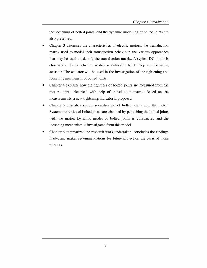
• Chapter 6 summarizes the research work undertaken, concludes the findings
made, and makes recommendations for future project on the basis of those
findings.

Chapter 2 Tightness of The Bolted Joint
8
CHAPTER 2
TIGHTNESS OF THE BOLTED JOINT
Tightness of bolted joint is the main concern in its design. The joint should be
tight enough to support the external load applied on it from the joined structures.
Improper tightness may cause the joint to loosen or put the structure under stress
and result in joint failures. However, a proper tightened bolted joint under
vibration might be loosen itself, which normally called as self-loosening.
Research in tightening and loosening of bolted joint is needed to give the designer
a better insight in designing a proper tightened bolted joint.
In this chapter, literature on the bolted joints will be reviewed. Tightness
indicators that are used in bolted joint will be introduced. Their relationship with
tightness of bolted joint is discussed and their measurement method and accuracy
are discussed. Self-loosening of bolted joint as one of common problem in bolted
joint is also explained. Theory that discussed about self-loosening is discussed to
understand cause and condition of this loosening. Lastly, dynamic model of bolted
joint is reviewed to understand dynamic behaviour of bolted joint under dynamic
condition such as vibration.
Section 2.1 discusses about common tightness indicators of bolted joint, their
measurement methods and accuracy. Section 2.2 discuss about mechanism
loosening of the bolted joint due to vibration based on several theories. Section
2.3 discusses about literature on dynamic model of a bolted joint
2.1. Tightness Indicator of the Bolted Joint
The tightness of the bolted joints is crucial in keeping the joint intact. Improper
tightness in the joint may lead to joint failure. Under-tightening may cause joint
separation while over-tightening may cause joint breakage. To properly install
bolted joints, a good tightness indicator is essential. In this section, a few

Chapter 2 Tightness of The Bolted Joint
9
commonly utilized indicators are presented, and their working functions and
measurement methods are explained.
2.1.1. Clamping force of bolted joints
The clamping force is the force generated by the bolt and nut to fasten two parts
together. A force with same magnitude is generated at the interface of the two
jointed parts. This interface force indicates that the joint is still intact. A load cell
can be installed at a bolted joint to measure the interface force. The donut load
cell, a cell with a hole in the centre (Figure 2-1), is commonly used for this
purpose. It is usually placed in between the fastened parts and the bolt is inserted
through its hole. The load cell has a high measurement accuracy (around 1%-
2%error) [11, 12]. However, this method introduces additional weight because the
load cell needs to remain at the joint.
Figure 2-1 Donut load cell
2.1.2. Preload of bolted joints
Preload is the tension force generated at the bolt due to its stretching. The
stretching occurs as a result of the compression of the jointed parts by the nut and
the pull on the bolt. In most cases, the preload is equal to the clamping force.
However, there are several cases where the two forces differ as follows:

Chapter 2 Tightness of The Bolted Joint
10
Figure 2-2 Hole interface in a bolted joint [2]
a) Bolted joint with tight hole interference
Figure 2-2 shows a bolt tightened through an undersized hole. The bolt will
have a tight fit in the hole and additional preload is generated. This additional
preload is used to overcome the frictional and embedment constraints
between the sides of bolts and the walls of the hole, but is not used to
generate clamping force at a bolted joint. Hence, the amount of preload is
higher than clamping force.
b) Bolted joint with hanged weight
Figure 2-3 shows a bolted joint with a weight hanging on its bottom part and
with a fixed top part. Due to gravity, the weight pulls down the bolt and an
additional preload is generated. This additional preload does not reflect
through the clamping force of the joint. Hence, the preload force has a higher
value than the clamping force.

Chapter 2 Tightness of The Bolted Joint
11
Top part
(Fixed)
Bottom part
Weight
Figure 2-3 A bolted joint with a hanged weight
There are 3 common methods to measure the bolt preload. They are as follows:
a) Direct measurement of preload.
The preload is measured directly using a special washer installed at the
bottom surface of bolt head or nut. The bolt preload is calculated from the
strain undergone by the washer. An example of such a washer is the direct
tension indicator washer (DTI washer) as shown in Figure 2-4. The DTI
washer is a modified washer with bumps to indicate the bolt preload. As the
nut is tightened, the bump is compressed and the gap between the nut and
surface is reduced. The preload is determined based from the amount of gap
generated. This method produces accurate measurements of the preload with
error around 10% [13]. However, each washer has its range of preload and
introduces additional weight to the joint.
Figure 2-4 Direct Tension Indicator Washer (DTI) Washer

Chapter 2 Tightness of The Bolted Joint
12
b) The elongation of a bolt/ bolt stretching
As aforementioned, the bolt preload (P) is generated from the
stretching/elongation (∆Lb) of the bolt. The relationship between the bolt
preload and the bolt stretching is written as follows:
b bP Lk= ∆
(2-1)
where, kb is bolt stiffness and is calculated as follows:
bb
b
EAk
L=
(2-2)
where E is Young Modulus of the bolt, Ab is surface area of the bolt, and Lb is
the initial bolt length.
With this relationship, the preload can be calculated from the bolt elongation.
In practice, the bolt elongation is obtained by measuring the bolt’s length
before and after the bolt is tightened. Examples of the measurement tools
used include the C-micrometer (Figure 2-5) and ultrasound measurement.
Figure 2-5 C-micrometer to measure the bolt lenght
However, there are several problems with using the bolt elongation to
measure preload. They are as follows:
a) Dimensional variation in the body part and thread part of bolts which
causes variation in stiffness for each part [14]
b) Temperature change which affects the bolt length
c) Tightening of the bolts near to the plastic region

Chapter 2 Tightness of The Bolted Joint
13
d) Bending of the bolt and non-perpendicular surfaces may lead to
dimension errors
c) Turning angle of the bolts
When a nut is turned for a full circle (360°), it will advance or retract in a
linear displacement equals to one thread pitch (p). The bolt is assumed to
stretch by the same length as the nut’s linear displacement. The amount of the
bolt’s stretch may be expressed in term of turning angle (θr) as follows:
360
rbL p
θ∆ =
° (2-3)
Thus, the bolt preload can be calculated from the turning angle as follows:
360
rb b bP k L k p
θ= ×∆ = ×
° (2-4)
The difficulty with using turning angle to calculate preload is that no or little
preload is produced for the first few turns as the bolt has not been stretched
yet. In addition, the relationship between the turning angle and the bolt
preload is not linear at the beginning of the stretch as shown at Figure 2-6.
These will lead to inaccuracies in the calculated value of the preload.
Figure 2-6 The preload vs Angle of turn graph [2]
Turn (deg)
Pre
loa
d (N
)

Chapter 2 Tightness of The Bolted Joint
14
2.1.3. Torque applied to a bolted joint
Figure 2-7 Relationship between applied torque and achieved preload [2]
Torque is the commonly used as a tightness indicator for a bolted joint due its
ease of measurement. Torque is applied to the bolted joint and causes the bolt to
turn relative to the nut. Initially, torque is used to overcome friction. When the
bolt starts to stretch (generating preload), additional torque is needed. This
additional torque is needed to turn the bolt further and to produce a higher preload.
According to Bickford[2], the additional torque and the bolt preload are linearly
related. The slope between them is constant (Figure 2-7).At higher values, the
slope is not constant because the bolt is tightened near to its plastic region.
In deriving this relationship, there are two equations which can be used as
follows:
a) Torque vs. preload: the short form equation
The short-form equation relates the slope of the graph with the diameter of
the bolt (D) multiplied by the nut factor (K) as follows:
inT K D P= × × (2-5)

Chapter 2 Tightness of The Bolted Joint
15
The nut factor (K) in this equation is determined experimentally. The
advantage of this equation lies in the use of a single constant to summarize
the relationship of the preload with torque. However, the constant has to be
determined for each new application.
Figure 2-8 Histogram of K values reported for steel bolts from a large number of
sources [2]
Equation (2-5) assumes that bolts with the same material, surface friction and
thread angle share a similar value of nut factor (K). In fact, the value of the
nut factor (K) can vary for bolt of the same material. Figure 2-8 shows the
histogram of K values for steel bolts from various sources that are gathered
by Bickford [4]. From the graph shown, the K value for a steel bolts varies
from 0.15 to a maximum value of 0.25. This variation value of K causes same
value of tightening torque for bolts of the same material generate the variation
of preload. Figure 2-9 shows that the bolt preload generated can be scattered
for ±50% for a single value of tightening torque. Thus, we can conclude that
there are inaccuracies from using torque to indicate the bolt preload.

Chapter 2 Tightness of The Bolted Joint
16
Figure 2-9 Histogram of the preload achieved from a single value of torque [6]
b) Torque vs. preload: the long-form equation
The long-form equation is proposed by Motosh [3]. According to Motosh, the
input torque applied to tighten a bolt is resisted by three reaction torques as
follows:
a. Torque from the stretching of the bolt
b. Torque from the surface friction at the threads of the bolt and nut
c. Torque from the surface friction between the face of a bolt or nut and the
washer or the joined part.
Mathematically the equation for the input torque is written as follows [3, 15-
17]:
2 cos
t tin n n
rpT P r
α
µµ
π
= + +
(2-6)
where:
a. 2
pP
πis the torque from the stretching of the bolt and p is thread pitch.
b. cos
t trPµ
αis the torque from the surface friction at the threads of the bolt
and nut, µ t is coefficient friction at the threads of the bolt and nut, rt is
the effective contact radius of the thread, and α is the thread angle.

Chapter 2 Tightness of The Bolted Joint
17
c. n nP rµ is the torque from the surface friction between the face of a bolt or
nut and the washer or the joined part, µn is coefficient friction between
the face of the nut and the joint, and rn is the effective contact radius
between the nut and joint surface.
By assuming the value of the coefficient of friction and the bolt size and
substituting them into the equation, the distribution of each reaction torque
relative to the input torque can be found as shown in Figure 2-10. Figure 2-10
shows that most of the input torque is used to overcome the friction at bolt
head and bolt thread, and only small portion (10%) of the input torque is used
to stretch the bolt.
Bolt stretch
Figure 2-10 Relative magnitude of the three reaction torques oppose the input
torque [2]
Equations (2-5) and (2-6) suggest that the torque and preload at a bolted joint is
linearly related. However this relationship is highly affected by friction of a bolted
joint. This is confirmed by Nassar, S. A. et al. in their experiments [18-22], which
identified several factors affecting the relationship between input torque and
preload generate at the bolt. They are the surface finish, tightening speed,
coefficient friction of the bolt [21], and the lubricant used [22]. These factors
affect the friction condition of a bolted joint.
An example of a tool used to measure torque is a beam type torque wrench
(Figure 2-11). The wrench consists of a long lever arm between the handle and the
wrench head. The arm is made of a material which bends elastically in response to

Chapter 2 Tightness of The Bolted Joint
18
applied torque. The other example is strain gauge torque wrench. The strain gauge
measures torsional deflection of the torque wrench’s shaft. The result is converted
into electrical display at the torque wrench. Normally, torque wrenches are
designed to have accuracies range between ±2 to 10%.
Figure 2-11 The torque wrench
Beside tools for measuring torque, there are different types of bolt designs, which
indicate the applied torque. One example is the twist-off bolts. The bolts have a
neck that will break apart when the desired torque is reached (Figure 2-12). The
disadvantages of this bolt are that the torque value is required beforehand and a
special tool is needed to tighten the bolt and break the neck.
Figure 2-12 A twist-off bolt
2.1.4. Electrical impedance measurement
Along with advancements in the development of smart materials, a piezoelectric
material was developed to measure the tightness of a bolted joint. The concept
originates from Park et al, who used piezo transducer patches to assess the
damage of a bolted joint in his experiments [23-25]. His method is known as the
impedance-based monitoring technique. The principle behind his method is the
measurement of the dynamic properties of a bolted joint that is reflected in
electrical impedance of PZT.

Chapter 2 Tightness of The Bolted Joint
19
Figure 2-13 Location of PZT patched at a bolted joint [23]
In his experiment, a piezo transducer (PZT) is patched near to the bolted joint at a
pipeline to assess the damage (Figure 2-13). When the joint is damaged
(loosening, corrosion, thermal cycling), its impedance changes. This change will
be manifested in the PZT’s electrical impedance. The relationship between the
electrical impedance, which is the ratio of the input voltage to current, is related
and the impedance of a bolted joint is as follows[26]:
( )( )
( ) ( )2
33 3ˆsT E
x xx
s a
YZI
Y i a dE Z Z
ωω ω
ω ωε
= = − + (2-7)
where:
− E is the input voltage to the PZT actuator,
− I is the output current from the PZT,
− a is the geometry constant,
− 2
3xd is the piezoelectric coupling constant,
− ˆ E
xxY is the Young’s modulus,
− 33
Tε is the complex dielectric constant of the PZT at zero stress,
− Zs(ω) is the Impedance of a bolted joint, and
− Za(ω) is the Impedance of the PZT
As most of the variables in the equation are determined by the properties of the
PZT, the change in the electrical impedance of a PZT is only affected by the
change of the impedance of the bolted joint. The results of his experiments show
that it is possible to distinguish between the loosening and tightening of bolts
from impedance.

Chapter 2 Tightness of The Bolted Joint
20
Following this concept, Mascarenas used a PZT enhanced washer to measure the
bolt preload as shown in Figure 2-14 [27].The washer was attached to each bolt to
measure the bolt’s impedance. A ½-13 bolt was used and tightened to different
torque levels. The impedance’s magnitude at the resonant frequency is measured.
The results are plotted in Figure 2-15 where the impedance of the PZT varies
under different torque levels. The change in impedance is inversely proportional
to the torque level However, for higher levels of torque, the change in impedance
is less significant.
Figure 2-14 A nut and washer equipped with PZT wafer [27]
Figure 2-15 Impedance value from PZT washer [27]
Ritdumrongkul also used the PZT to identify the damage at a bolted joint
[28].However, instead of measuring the impedance’s amplitude, he observed a
shift of resonance frequency at the PZT. His observation was concluded from a set
of experiments with different torque levels. The shifting of the resonance
frequency and the reduction of the impedance’s peak height were observed in his

Chapter 2 Tightness of The Bolted Joint
21
experiments. However, similarly to Mascarenas, the change was quite small to
observe at a higher torque level. We can conclude that impedance measurement
with PZT is only applicable at small tightening torque value.
2.2. Self- loosening of bolted joints
The common cause of bolted joints loosening by themselves is vibration. Under
severe vibration, the jointed parts may experience slip and rotation which may
lead to self-loosening of the joint. In this section, published works on the self-
loosening of bolted joint under vibration, mechanism of self-loosening and factors
to resist the self-loosening are summarized.
2.2.1. Vibration on a bolted joint
Bickford believes that when a bolt is tightened, energy is stored inside it as
potential energy [29]. After the tightening is completed, the energy is held by
friction constraints in both the bolt threads and in between the contact surfaces of
the nut and the joint. If there is an external disturbance, such as vibration, to
overcome these frictions, the potential energy will be released. The bolt is rotated
back and the joint is loosened.
Several researchers have investigated the cause of bolts loosening under vibration
[4, 30, 31]. They all agree that loosening occurs if the frictional force is overcome.
They investigated two types of vibration applied to a bolted joint based on its
direction, as follows:
1. Axial vibration
Normally, a bolted joint has a high resistance to axial load as it is designed to
sustain load in that direction. Based on Hess, the vibration in the axial
direction affects the preload of a bolted joint but does not loosen the joint
completely [32-34]. He proves this hypothesis with an experimental study of
bolted joint under axial loading. From the experiment, he found that a bolt can
be tightened or loosened in the presence of axial vibration. He also observed

Chapter 2 Tightness of The Bolted Joint
22
that the loosening occurred at the vibration frequencies of 730-1130 Hz, while
tightening occurred at the frequencies of 370-690 Hz. Based on the different
axial vibration levels and initial preloads, he found that the clamping force
would remain steady, decrease, or increase depending on the preload and
vibration levels as shown in Tables 2-1 and 2-2. Based on these results, he
concluded that a bolted joint can be tightened or loosened under axial
vibration and the maximum loosening is only 52.9% of the original tightness.
There is no complete loosening during the experiment.
Table 2-1 Change in clamping force for different preload with constant vibration
level [35]
Table 2-2 Change in clamping force for different vibration levels with constant
preload [35]
2. Transverse vibration
Transverse vibration is vibration of a bolted joint perpendicular to the axis of
the bolt. In a bolted joint, the transverse force due to vibration is resisted by
friction. Usually, the resistance of a bolted joint in the transverse loading is

Chapter 2 Tightness of The Bolted Joint
23
lower than that in the axial loading because the frictional force is product of
preload and coefficient of friction. The value of coefficient of friction is
normally less than one. Hence, the frictional force is smaller than the preload.
In 1960, Junker confirmed that a common cause of the total loosening of a
bolted joint is transverse vibration [4]. His conclusion was verified with his
“Junker Machine” (Figure 2-16). The machine consisted of an eccentric cam,
a bolted joint and a load cell to measure the bolt’s preload. In the interface
between the plates, rollers are attached to allow the plates to slide relative to
each other. The eccentric cam is driven by an electric motor and causes the
bolted joint to vibrate with a small displacement. After a few thousand cycles
of vibration, total loosening occurs if tightness is insufficient. The nut is
loosened and the load cell shows a zero preload reading.
Figure 2-16 Junker Machine [2]
Other transverse vibration experiments have also been carried out by several
other researchers [30, 36-39], who applied continuous transverse force to a
bolted joint. Their results show a total loosening of the bolted joint as well.
From these experiments, we can conclude that transverse vibration can lead to
a total loosening of a bolted joint.

Chapter 2 Tightness of The Bolted Joint
24
2.2.2. Mechanism of self loosening of a bolted joint
As mentioned previously, transverse vibration may cause self-loosening of a
bolted joint. The mechanisms of transverse vibration in loosening a bolted joint
are as follows:
a) Due to the previous cycle of vibration, the bolted joint is in the position as
shown in Figure 2-17a.The top plate is moving to the left as the transverse
vibration applies force to the left of the plate.
b) As the transverse force changes its direction, the top plate slides to the
opposite direction (right). This causes the bolt to bend towards the right
because the bolt head is fixed with the bottom plate (Figure 2-17b).
c) When the bending force overcomes the friction force at the thread and nut
surfaces, the nut moves to the left and rotates slightly. The bolt is
straightened and the top plate continues to slide to the right (Figure 2-17c).
d) When the top plate continues to slide further, the hole at the plate touches
the bolt shank and the bolt is stuck. At this point, there is no further
preload loss and the whole process is reversed where the force is applied
back to the left (Figure 2-17d).
Figure 2-17 Mechanism of loosening of bolted joint due to transerse force [2]

Chapter 2 Tightness of The Bolted Joint
25
Based on the explanation above, the loosening happens due to the relative motion
at bolt thread. According to the Bolt Science website, the common causes of this
motion are as follows [40]:
1. Bolt bending results in the induction of forces at the friction surface. If slip
occurs, the head and threads of the bolts will slip, which may lead to
loosening.
2. Differential thermal effects caused by differences in temperature or
differences in the bolted joint’s materials.
3. Applied forces on the joint that lead to the sliding of the joint parts and the
eventual loosening of the bolt.
In order to verify the mechanism of self loosening of bolted joint, Yokoyama
make a FEM analysis of bolted joint under transverse loading [12]. They analysis
the load-displacement behaviour of bolt before slip happens at bolt head. Based
on their analysis, they formulated reaction moment on the bolt head and thread
due to applied transverse force. They found out that the reaction moment is
depends on stiffness of bolt joint and the stiffness is affected by slip happen at
bolted joint.
2.2.3. The factors influencing self loosening of a bolted joint
There are several factors which influence the self-loosening of bolted joints from
vibration, such the thread pitch of the bolt, the initial tightness of the joint [7], the
coefficient of friction of the bolt surface[5, 6], the hole clearance and the fitting
between the threads [38]. A detailed discussion on each factor is as follows:
a) Thread pitch of the bolted joints
The threads of the bolt are a helical structure used to convert a given
rotational movement into linear movement. The linear distance travelled
by a bolt for one rotation is called the thread pitch. According to the
Unified Thread Standard (UTS), there are 3 types of threads: “coarse”,

Chapter 2 Tightness of The Bolted Joint
26
“fine”, and “extra fine”. A coarse thread has the largest pitch whereas an
extra fine thread has the smallest pitch. The effect of difference in pitch
sizes on the self-loosening of a bolted joint is shown in Figure 2-18. Figure
2-18 shows that the finer the bolt thread, the more cycles that are needed
to loosen a bolt. This is because a finer thread has a small lead angle due
to its small pitch. The small lead angle reduces the loosening force.
Figure 2-18 Effect of thread pitch on the self loosening [7]
b) Initial tightening of a bolted joint
c) Normally, a bolted joint is tightened to a certain value of preload. The
value of the preload is decided by considering the load applied to the joint.
This preload helps to resisting vibration as shown in Figure 2-19. The
results show that the higher the preload, the greater the number of cycles
that are needed to loosen a bolted joint. However, there is a point where
loosening will not occur. If the bolted joint is tightened above this point,
the vibration applied will not reduce the bolt preload. This point is defined
based on applied vibration’s amplitude. Figure 2-20 shows that for lower
levels of vibrational amplitudes (0.03 inch excitation), a bolted joint needs

Chapter 2 Tightness of The Bolted Joint
27
to be tightened to above 4,000 lb. to prevent loosening. For higher levels
of vibration amplitude (0.05 inch excitation), a bolted joint needs to be
tightened to above 9,000 lb.
Effect of preload on the self loosening
Bo
lt T
en
sio
n (
lb)
Number of cycles
No Loosening
Figure 2-19 Effect of initial bolt tension on the self loosening [7]
0.03 inch Excitation
0.05 inch Excitation
Figure 2-20 Effect of excitation amplitude on the self loosening [8]

Chapter 2 Tightness of The Bolted Joint
28
d) Coefficient of friction of the bolt surface
Effect of thread friction coefficient on the
self loosening
Lo
osen
ing
rate
(N
/cycle
)
Thread friction coefficient
Figure 2-21 Effect of thread friction coefficient on self loosening [6]
Effect of bearing friction coefficient on
the self loosening
Lo
ose
nin
g r
ate
(N
/cyc
le)
Bearing friction coefficient
Figure 2-22 Effect of bearing friction coeeficient on self loosening [6]
The coefficient of friction is a scalar value that describes the ratio of frictional
force between the two bodies and the normal force acting on them. Its value

Chapter 2 Tightness of The Bolted Joint
29
depends on surface condition of the bodies and their material. The rougher
the surface, the higher is the value of the coefficient of friction. There are two
friction coefficients at the bolted joint, the thread friction coefficient and
bearing friction coefficient. The thread friction coefficient describes the
friction between thread of the bolt and nut. The bearing friction coefficient
describes the friction between surface of bolt head and joined part. Both
frictions help to prevent bolt loosening as shown in Figures 2-21 and 2-22.
Less preload is lost for one cycle of vibration due to a higher coefficient of
friction.
e) Hole clearance
Figure 2-23 Effect of hole clearance on self loosening [8]
Before tightening a bolted joint, a bolt is inserted through a hole in two joined
parts. To prevent the bolt from being jammed and to generate additional preload,
the hole should be bigger than the bolt diameter (the hole clearance).The
clearance affects the contact area between the joint and the bolt head. A larger
clearance leads to smaller contact area. Hence, the resistance of bolted joint
against the vibration is lower (Figure 2-23). This has been experimentally proven
by Basil Housari [8]. His results show that with a larger hole clearance, less cycles

Chapter 2 Tightness of The Bolted Joint
30
are required to loosen a bolted joint. This is because the larger hole clearance
allows the bolt to be loosened more before it is stuck.
f) The fitting/ matching between the threads
Figure 2-24 Difference between class of fit at bolted joint
Figure 2-25 Effect of fitting on self loosening [38]
Based on the UTS, there are three classes of fit by which the external and internal
threads of a bolted joint mates together. They are classes 1, 2, and 3, in ascending
order of tightness. A (external) and B (internal) are used to indicate the types of

Chapter 2 Tightness of The Bolted Joint
31
thread. The difference between each class is the tolerance for the pitch diameter
as shown in Figure 2-24. Class 3 has a smaller tolerance compared to Class 1.
This tolerance affects the resistance of a bolted joint to loosening (Figure 2-25). A
smaller tolerance leads to a slower rate of loosening.
2.3. Dynamic modeling of a bolted joint
In the previous section, the loosening mechanism of bolted joints due to vibration
was examined by a review of the experimental studies. Vibration is an external
excitation given to the bolted joint. Under this excitation, the joint gives out a
response in form small displacement and dissipate some of the energy. Several
researchers try to model this dynamic behaviour of bolted joint by model this
dynamic behaviour. This section reviews existing dynamic models of bolted joints.
2.3.1. Bolted joint based on a spring and a damper
In his modelling of the bolted joint, Tsai used the receptance method proposed by
Bishop[41, 42]. He assumed that two structures, structure I (region a) and
structure II (region c), were assembled on an interface b (a bolted joint) as shown
in Figure 2-26. When a transverse force is applied to the structures, a small
displacement occurs at the interface. This displacement is explained with the
following matrix formula:
(2) (1) (1)
b b j bU U H f− = (2-8)
where Ub(n)
is transverse displacement of structure n, Hj is the receptance matrix
and fb is transverse force applied to the system.
This receptance matrix (Hj) is related with the system properties of the interface.
Based on the model, Tsai assumed that the matrix relates with the stiffness (K)
and damping coefficients (C) of the interface with negligible mass.
Mathematically, it is written as follows:

Chapter 2 Tightness of The Bolted Joint
32
( )1
jH K j Cω−
= + (2-9)
Structure I (a)
Structure II (c)
b (Hj)
Figure 2-26 Model for a bolted joint according to Tsai [41]
Another example of a bolted joint model with spring and damper is Hanss’ model
(Figure 2-27). Hanss assumed that damping (d) and stiffness (k) of bolted joints
are related with the geometry and material properties of two joined rods. The
damping and stiffness are calculated as shown below [43-48].E, ρ, l are Young
modulus, density and length of rod 1 and 2.
( ) ( )
( )1 2
1 2 2 1
Re Recoth coth
sk d s
s s
β β
β α β α
= − − +
(2-10)
( ) ( ) ( )
1 2
1 2 2 1
1Im
Im coth coth
sd
s s s
β β
β α β α
= − +
(2-11)
Where:
11 1
1
,lE
ρα = 2
2 2
2
,lE
ρα = 1 1 1 1 ,A Eβ ρ= 2 2 2 2A Eβ ρ=
The results were obtained with a fuzzy arithmetic method and shows a variation in
the damping and stiffness obtained (Figure 2-28). This variation is caused by the
variability of the material’s properties and geometries, frequency of excitation,
and other uncertain parameters in the bolted joint.

Chapter 2 Tightness of The Bolted Joint
33
Figure 2-27 Two rod connected by a bolted joint (Hanss' model) [43]
Figure 2-28 Uncertain stiffness parameter and damping parameter of model joint
[43]
2.3.2. Bolted joint modelling based on Jenkins element
Figure 2-29 Jenkins element model [49]
Another example of a bolted joint’s model is the Jenkins element model. Oldfield
used Jenkins element to model friction at the bolted joint[49, 50]. In Jenkins’

Chapter 2 Tightness of The Bolted Joint
34
element model, the friction is modelled as an ideal coulomb element with a
threshold value (h),and connected in series with a spring element (ci)[51, 52]. The
spring element is used to show the deformation phenomenon that occurs prior to
the interfacial slip and before the static force is fully overcome.
Figure 2-30 Hysteresis loop of bolted joint under different number of Jenkins
elements [49]
Under harmonic excitation, the Jenkins element produces an ideal
elastic/perfectly-plastic hysteresis curve. With a single element, the bolted joint
has two states, the sticking and slipping states. However, a single element of
Jenkins element is not sufficient to model the micro slip happening in a bolted
joint. The micro slip is a state in the joint where some regions are sticking while
others have exceeded the threshold of friction force and are slipping. N-numbers
of Jenkins-Elements are needed to model this micro slip. Those n-numbers of
Jenkins-Elements are arranged in parallel (Figure 2-29).The equation below
describes the relationship of the elements with the contact force (F) [51] :
( )( ) ( )
0
1
,sgn
mi i i
i i
r t r t hF u u c u
h u=
<= +
∑&
& (2-12)

Chapter 2 Tightness of The Bolted Joint
35
where:
k lu u u= − , (2-13)
( ) sgni i ir c u u h u+ += − − & (2-14)
By increasing the number of elements, the hysteresis curve becomes smoother
(Figure 2-30). However, the challenge lies in determining the spring elements and
threshold value.
2.3.3. Bolted joint modeling based on Bouc-Wen model
The Bouc-Wen model combines a hysteresis function with a non-hysteretic
function to describe the restoring force of a system that has yielded to some
degree[53, 54]. Mathematically, it is written as follows:
( ) ( ) ( ), , , ,Q x x g x x z x x t= +& & & (2-15)
where g is a non-hysteretic component and z is the hysteretic function dependent
on displacement history of the model.
The z function is defined by a nonlinear first order differential equation as
follows:
1m m
z x z z x z Axα β−
= − − +& & && (2-16)

Chapter 2 Tightness of The Bolted Joint
36
Figure 2-31 Hysteres loops using Bouc-Wen model [49]
The versatility of this model arises from the ability to tune the parameters, α, β, A,
and integer m. α and β define the shape of the hysteresis loop, while A defines the
initial stiffness, and m is used to manipulate the smoothness of the loop. When m
= 1, the response deviates from a pure elasticity. m = ∞ describes a bilinear
restoring force. The graph produced by Bouc-Wen model is a smooth graph
(Figure 2-31). However, the parameters α and β do not have any obvious physical
meaning. Thus it is difficult to associate them with the stick-slip behaviour at the
joint’s interface.
Those mentioned models are based on Finite Element Method, with no
experimental to confirm their results. Thus, an experimental method to measure
system properties of bolted joints and verify the model is needed. With the model,
dynamic cases of bolted joint, such as bolted joint under loosening, can be
simulate. The phenomenon or the response of bolted joint can be investigated
from the simulation.

Chapter 3 The DC Motor as a Tightness Measurement Tool for Bolted Joints
37
CHAPTER 3
DC MOTOR AS A TIGHTNESS MEASUREMENT
TOOL FOR BOLTED JOINTS
Bolted joints are normally tightened with a torque wrench equipped with a dial
indicator. The dial indicator shows the resistance torque exerted by the bolted
joint on the wrench. It allows the operator to see when the desired torque is
achieved so that he can stop tightening. However, the bolt’s conditions may cause
the torque to be misread by the indicator. For instance, damage to the bolt’s
coating or threads may cause the torque’s reading to increase. This may lead the
operator to stop tightening when further tightening is in fact necessary to achieve
his desired tightness. To avoid such a problem, a real time tightness measurement
system, which is able to monitor the tightening process from start to end in real
time, is required. Any change in tightness during the tightening process can then
be perceived by the operator right away.
In this project, a brushed DC motor is developed into a real time sensing and
actuating device to monitor the tightening process of bolted joints. The motor
applies mechanical output (torque and rotational speed) to the bolted joints
transduced from the motor’s electrical input (voltage and current) to tighten the
bolt joint. The transduction relationship between the mechanical outputs and
electrical inputs can be described by a 2x2 matrix called the transduction matrix.
Each element in the transduction matrix represents a transfer function between a
variable of the mechanical output and a variable of the electrical input under
certain boundary conditions in frequency domain. The transduction matrix allows
the motor’s mechanical output variables to be calculated from the motor’s
electrical input variables. This allows the motor to be developed into a
simultaneous sensing and actuating device for real time monitoring of the
tightening process of bolted joints. This chapter presents the theory behind and
method of this development.

Chapter 3 The DC Motor as a Tightness Measurement Tool for Bolted Joints
38
Section 3.1 introduces the theoretical background of the transduction matrix in the
modelling transduction process of brushed DC motors and outlines the
assumptions involved. Section 3.2 introduces the methods to identify the
transduction matrix. Section 3.3 presents the measurement results of a calibrated
brushed DC motor to assess the accuracy of the transduction matrix. Section 3.4
summarizes of the chapter.
3.1. Mechanism and Characteristic of Brushed DC Motors
In this thesis, a brushed DC motor is chosen as the tightness measurement tool for
bolted joints due to its portability, and the linear relationship between torque and
rotation speed. The motor transduces the supplied electrical power into
mechanical power. This transduction process can be modelled with the
transduction matrix, which enables the mechanical output of motor to be
calculated from its electrical input. This obviates the need to install bulky force
and motion sensors to measure the mechanical output of the motor. The DC
motor’s transduction mechanism, linear characteristic and how the transduction
mechanism is modelled by the transduction matrix will be explained in this
section.
3.1.1. Mechanism of brushed DC motors
A brushed DC motor is an internally commutated electric motor powered by a DC
power source (Figure 3-1). The voltage applied to the motor energizes the motor
and generates a current. The voltage and current is transformed into mechanical
power by the rotation of the shaft. The transduction process is based on the
electromagnetic interaction between two main components of the motor, the stator
and rotor.
a) The Stator is a stationary part of motor located under the motor housing.
In brushed DC motors, the stator acts as the field magnet and provides
magnetic flux to interact with the armature. The stator is usually made of a
permanent magnet to generate the magnetic flux.

Chapter 3 The DC Motor as a Tightness Measurement Tool for Bolted Joints
39
b) The Rotor is a rotating part of motor. It is located at the centre of the
motor and connected to the motor shaft. In brushed DC motors, the rotor
acts as the armature that carries the current and interacts with the magnetic
flux generated from the field magnet. The rotor is usually made of a
conductor or conductive winding.
Rotor
Shaft
Power Supply
Figure 3-1 Schematic diagram of brushed DC motor [55]
For simplicity, it is assumed here that the two components have two magnetic
poles (see Figure 3-2). The stator is made up of a permanent magnet and the rotor
is made up of coil windings. When voltage is applied by the power supply, current
flows to the rotor windings which generate electromagnetic flux. The
commutators connect the power supply to the rotor windings and control its
polarity. The rotor that is connected to the positive terminal of the power supply
becomes the north pole and thus has the same polarity as the stator. The repulsion
between the rotor and stator causes the motor shaft rotates for half a circle. After
this rotation, the current is reversed to change the polarity of rotor. The rotor
connected with the positive port of power supply becomes the north pole. The
repulsion between the rotor and stator causes the motor shaft rotates for a further

Chapter 3 The DC Motor as a Tightness Measurement Tool for Bolted Joints
40
half circle. This process repeats continuously as long as there is electrical power
supplied to the motor.
Rotor
Winding
Stator
Commutator
Figure 3-2 Operating process of a brushed DC motor
Due to the rotation of the shaft, the rotor experiences a time varying magnetic
field. Following Faraday’s law, the time varying magnetic field induces a back-
electromotive force (back-EMF) voltage inside the motor. The magnitude of this
voltage (Eemf) is proportional to the motor speed (Ωm) and its polarity is the
reverse of the applied voltage. The motor constant (kE) defines the relationship
between the back-EMF voltage and the motor speed. Mathematically, the
relationship is written as follows:
emf E mE k= Ω (3-1)
The kE is a function of the motor’s parameters such as the dimension of the
magnet, the generated magnetic field and the number of rotor windings. Usually,
the kE value is specified by the motor’s manufacturers.
Besides kE, there is also another motor constant (kT), which governs the
relationship between the motor’s torque (Tm) and the applied current (i).

Chapter 3 The DC Motor as a Tightness Measurement Tool for Bolted Joints
41
According to Lorentz force law, a current-carrying conductor placed within an
external magnetic field will experience a force or torque. This relationship can be
simplified with kT, which is also a function of the motor’s parameters such as the
dimension of the magnet, the generated magnetic field and the number of rotor
windings. The relationship is written as follows:
m TT k i= (3-2)
The next section shows how the relationship between the electrical power and
mechanical power of the motor can be defined with kE and kT,
3.1.2. Linear characteristic of brushed DC motors
E
+
Permanent magnet
Stator
Rotor
i
Figure 3-3 Schematic diagram of permanent magnet DC motor
Figure 3-3 is a schematic diagram of the permanent magnet of a DC motor. As the
stator is made of a permanent magnet, the voltage is only supplied to the rotor
through the commutator to energize the coil winding. The torque and rotational
speed of the permanent magnet DC motor are linearly related with the voltage and
current supplied. Thus, the permanent magnet DC motor has a more linear torque-
speed characteristic than other motors which has a stator made of coil winding. In
a motor with a stator made of coil winding, the stator and rotor share the same
electrical supply. The current supplied to the motor flows to both the rotor and the

Chapter 3 The DC Motor as a Tightness Measurement Tool for Bolted Joints
42
stator. Any change in load or disturbance at either the rotor or stator will affect the
current supply to the other. Thus, the torque and speed characteristics of such
motors are non-linear. This motor will not be discussed further as the main
concern in this thesis is with motors containing stators made of permanent
magnets.
The coil windings at the rotor of brushed DC motors with a permanent magnet
stator can be modelled with an equivalent circuit consisting of a resistance (R), an
inductance (L) and a voltage source (Eemf) connected in series (as shown in Figure
3-4). Based on the Kirchhoff’s Law, the voltage (E) of the equivalent circuit is
derived as follows:
emf
diE iR L E
dt= + + (3-3)
With this voltage, current flows through the rotor winding and induces an
electromagnetic force to produce torque (Tm) at the motor shaft. The purpose of
the torque (Tm) is to overcome the motor inertia ( mmotor
dJ
dt
Ω), the friction (Tf),
and the motor’s load (TL). The equation is derived as follows:
mm motor f L
dT J T T
dt
Ω= + + (3-4)
E
Eemf +
- -
+
i
Ωm
Figure 3-4 Equivalent circuit of coil winding at brushed DC motor

Chapter 3 The DC Motor as a Tightness Measurement Tool for Bolted Joints
43
Normally, the motor loading (TL) and the friction (Tf) are functions of its speed
(TL(Ωm) and Tf(Ωm)). Thus, Equation (3-4) can be simplified as follows:
( ) ( )mm motor f m L m
dT J T T
dt
Ω= + Ω + Ω (3-5)
Under steady state condition, the motor will rotate at a constant speed ( 0md
dt
Ω= )
and no current change will occur ( 0di
dt= ). Thus, Equation (3-3) and Equation (3-
5) can be simplified as follows:
emfE iR E= + (3-6)
and
( ) ( ) ( )m f m L m e mT T T T= Ω + Ω = Ω (3-7)
Equation (3-6) is the electrical equation of the motor and shows that there is a
linear relationship between the voltage, current and back-emf. Equation (3-7) is
the mechanical equation at the motor and simplifies the torque equation of the
motor as a function of rotational speed (Ωm). The electrical (Equation (3-6)) and
mechanical equation (Equation (3-7)) can be combined together with the motor
constants in Equations (3-1) and (3-2) to form the torque equation as follows:
( ) ( )Te m E m
kT E k
RΩ = − Ω (3-8)
It can be seen from Equation (3-8) that the linear relationship between torque and
rotation speed is governed by the voltage supply to the motor (E) since the other
parameters (kE, kT, and R) are constants. Figure 3-5 shows the torque–speed
curves of the motor under different applied voltages. It can be seen that the
gradient of the lines between torque and speed are the same. By applying different
voltages, the line is shifted up or down based on the applied voltage (Va). For a

Chapter 3 The DC Motor as a Tightness Measurement Tool for Bolted Joints
44
DC motor to achieve a higher torque and rotational output, the applied voltage
needs to be increased. On the other hand, the gradient is governed by the motor
constant which is based on the magnetic field on the motor. Figure 3-6 shows the
torque-speed curves of the motor as the motor constant is varied from high to low
(kTA to kTC). It can be seen that a higher motor constant causes torque to increase
and rotation speed to decrease (the line is shifted to the right).
Ωm
Figure 3-5 Torque-speed curves of a permanent magnet DC motor (rated armatue
voltage 440V, rated power 110 kW, rated speed 560 rpm)

Chapter 3 The DC Motor as a Tightness Measurement Tool for Bolted Joints
45
Ωm
kEA, kTA
kEB, kTB
kEC, kTC
Figure 3-6 Torque-speed curve of a permanent DC motor under different motor
constant
It can be seen from Equation (3-8) that under a steady state condition, the voltage
of the motor is linearly related its torque and rotation speed. It can be seen from
Equation (3-2) that the motor’s current is linearly related with its torque. It can be
seen from both equations that the electrical input of the motor (voltage and
current) is linearly related its mechanical output (torque and rotation speed). Thus,
we can conclude that such a motor is as a linear system. The next section explains
how the motor can be modelled by using a transduction matrix.
3.1.3. Transduction matrix of brushed DC motors
In dynamic system modelling, the characteristic of the single input-single output
linear time invariant system can be represented by a weighting function (h(τ)) and
frequency response function H(f) (FRF). When the system is subjected to a well-
defined single input ( ( )x t ), the output of the system ( ( )y t ) can be obtained from
the convolution integral between the weighting function (h(τ)) and the input ( ( )x t ).
The equation is expressed as follows:

Chapter 3 The DC Motor as a Tightness Measurement Tool for Bolted Joints
46
( ) ( ) ( )0
y t h x t dτ τ τ∞
= −∫ (3-9)
Applying the Fourier Transform to Equation (3-9), the linear relation between the
input and output of the system can be formed as follows:
( ) ( ) ( )Y H Xω ω ω= (3-10)
where
( ) ( )0
jH h e d
ωτω τ τ∞
−= ∫ (3-11)
( ) ( )0
jY y e d
ωτω τ τ∞
−= ∫ (3-12)
( ) ( )0
jX x e d
ωτω τ τ∞
−= ∫ (3-13)
H(ω), Y(ω), and X(ω) are the Fourier Transform of x(t), y(t) and h(t) respectively.
By rearranging Equation (3-10), H(ω) can be obtained from a known output over
a known input of the system in the frequency domain and formulated as follows:
( )( )( )
YFRF H
X
ωω
ω= = (3-14)
Thus, the output of the system can be directly predicted with this H(ω) from any
input given to the system. The output (Y(ω)) of a system with a known H(ω) can
be obtained by substituting H(ω) and the input (X(ω)) into Equation (3-10).
In linear systems with multiple inputs and outputs, the dynamic behaviour of the
system can be described as a combination of the subsystems’ FRF which can be
formed into a matrix. Each subsystem is treated as a “black box” that has a single

Chapter 3 The DC Motor as a Tightness Measurement Tool for Bolted Joints
47
input (Xn(ω)) and a single output (Ym(ω)). The element of the matrix is FRF of
each subsystem. Mathematically, the equation can be written as follows:
( )( )
( )
( ) ( ) ( )( ) ( ) ( )
( ) ( ) ( )
( )( )
( )
1 11 12 1 1
2 21 22 2 2
1 2
n
n
m m m mn n
Y H H H X
Y H H H X
Y H H H X
ω ω ω ω ω
ω ω ω ω ω
ω ω ω ω ω
=
L
L
M M M M M
L
(3-15)
where Xn(ω) is the Fourier Transform of the input-n (xn(t)), Ym(ω) is the Fourier
Transform of the output-m (ym(t)) and Hmn(ω) is the FRF of subsystems between
Fourier Transform of Xn(ω) and Ym(ω).
_ _
+ +
2-ports device
Output Input
flow (fout)
effort (ein)
flow (fin)
effort (eout)
Figure 3-7 Schematic diagram of 2-ports, 4-poles system
An example of a multiple input-multiple output linear system is a 2-ports, 4-poles
system (Figure 3-7). The two ports consist of an input port and an output port.
Each port in the system has two poles. One pole represents the effort variable (e)
and the other pole represents the flow variable (f). The system can be separated
into 4 subsystems with 4 FRFs (Figure 3-8). Each FRF relates an input port’s pole
with an output port’s pole. In theory, this relationship can be described by a 2x2
matrix as follows:

Chapter 3 The DC Motor as a Tightness Measurement Tool for Bolted Joints
48
( )( )
[ ]( )( )
in out
in out
e et
f f
ω ω
ω ω
=
(3-16)
( )( )
( ) ( )( ) ( )
( )( )
11 12
21 22
in out
in out
e a a e
f a a f
ω ω ω ω
ω ω ω ω
=
(3-17)
The four elements of matrix are as follows:
( )( )( )
( )
11
0out
in
out f
ea
eω
ωω
ω=
= (3-18)
( )( )( )
( )
12
0out
in
out e
ea
fω
ωω
ω=
= (3-19)
( )( )( )
( )
21
0out
in
out f
fa
eω
ωω
ω=
= (3-20)
( )( )( )
( )
22
0out
in
out e
fa
fω
ωω
ω=
= (3-21)

Chapter 3 The DC Motor as a Tightness Measurement Tool for Bolted Joints
49
11
12
21
22
t
Σ
Σ
Figure 3-8 Structured FRF for 2-ports, 4-poles system
Each element of the matrix relates an input pole with an output pole and the rest
of the output poles are assumed to be zero. Thus, the elements of the matrix in
Equations (3-18) to (3-21) can be categorized into two conditions as follows:
a) a11 and a21 are obtained when the output flow variable is equal to zero
(fout=0).
b) a12 and a22 are obtained when the output effort variable is equal to zero
(eout=0).
In this researach, A brushed DC motor is assumed as a linear system with multiple
inputs and outputs. The motor has two (2) electrical inputs, the voltage (E) and
current (i). From this inputs, the motor produces two (2) mechanical output in the
form of torque (Tm) and rotation speed (Ωm). Equations (3-2) and (3-8) show that
electrical input and mechanical output of the motor are linearly related. Thus, a
brushed DC motor can be represented with a 2-ports and 4-pole system. The two
poles of the input port are voltage (effort variable) and current (flow variable).
The two poles of the output port are torque (effort variable) and rotation speed
(flow variable) (Figure 3-9).

Chapter 3 The DC Motor as a Tightness Measurement Tool for Bolted Joints
50
Figure 3-9 A 2-ports 4-poles model of electric motor
The relationship between the input variables and output variables of the motor can
be described by the transduction matrix ([t]) in Equation (3-16). As the system
represents a brushed DC motor which is operated under constant value (0 Hz), the
elements of matrix (FRF) can be simplified into complex numbers at a frequency
of 0 Hz. Therefore, the matrix is expressed as follows:
( )( )
( )( )( )
0 00
0 0
m
m
E Tt
i
= Ω
(3-22)
( )( )
( ) ( )( ) ( )
( )( )
11 12
21 22
0 0 0 0
0 0 0 0
m
m
E t t T
i t t
=
Ω (3-23)
The four elements of the matrix are as follows:
( )( )( )11
0
00
0m
m
Et
TΩ =
= (3-24)
( )( )( )12
0
00
0m
m T
Et
=
=Ω
(3-25)
( )( )( )21
0
00
0m
m
it
TΩ =
= (3-26)
E (Voltage)
i
(Current)
Tm (Torque)
Ωm (Rotation
speed)
Electric motor

Chapter 3 The DC Motor as a Tightness Measurement Tool for Bolted Joints
51
( )( )
( )22
0
00
0m
m T
it
=
=Ω
(3-27)
where the elements of matrix are obtained under two boundary conditions. t11 and
t21 are obtained by restricting the motor motion ( 0mΩ = ). t21 and t22 are obtained
by allowing the motor to run freely ( 0mT = ).
Each element of the matrix represents a transfer function of one electrical port and
one mechanical port, where
• t11 represent the transfer function between the voltage and torque when the
motor motion is restricted (clamp condition).
• t12 represent the transfer function between the voltage and rotational speed
when motor motion is free running (free condition).
• t21 represent the transfer function between current and torque when motor
motion is restricted (clamp condition).
• t22 represent the transfer function between current and rotational speed
when motor motion is free running (free condition).
Since the matrix characterizes the transduction behaviour between the electrical
input and mechanical output of electrical motor, it is termed as the “transduction
matrix”. [10, 56]
3.2. Identification of Transduction Matrix
In the previous section, the linearity of the brushed DC motor and how the linear
relationship can be modelled by the transduction matrix were explained. The
transduction matrix can be obtained theoretically or experimentally. Theoretically,
the transduction matrix is obtained from the equivalent circuit of the brushed DC
motor and its motor constants. The elements of the matrix are computed based on
two aforementioned boundary conditions. Experimentally, the transduction matrix

Chapter 3 The DC Motor as a Tightness Measurement Tool for Bolted Joints
52
is obtained based on the least square approximation of the measurement results.
Both methods will be explained and compared.
3.2.1. Theoretical derivation of transduction matrix
E
RLs +
1 kT i
Js
1
kE Eemf
TL + Tf
Ωm Tm
_
_
Figure 3-10 Block diagram of brushed DC motor
As mentioned in section 3.1.2, a brushed DC motor can be modelled as an
equivalent circuit with a relationship as stated in Equation (3-3). To relate
Equation (3-3) with the mechanical equation of the electric motor in Equation (3-
5), Laplace Transform are applied to both equation and the motor constants in
Equation (3-1) and (3-2) are used. The equations are arranged in a block diagram
in Figure 3-10. With the block diagram, the transduction matrix can be evaluated
under the two aforementioned boundary conditions stated previously:
1. The rotational speed is equal to zero ( 0mΩ = )
a. No back-EMF voltage is induced induced ( 0=emfE ) as the relationship
between rotational speed and back-EMF voltage is direct as seen in
Equation (3-1).
b. There is no torque to overcome the motor’s inertia ( 0mmotor
dJ
dt
Ω= ).
Note that Tm is not equal to zero as the friction (Tf) and motor loading
(TL) have to be overcome as well.

Chapter 3 The DC Motor as a Tightness Measurement Tool for Bolted Joints
53
Figure 3-11 Simplified block diagram based on zero rotational speed
Based on these two conditions stated above, the block diagram can be
simplified as shown in Figure 3-11. The relationships between mechanical
and electrical ports of the motor in Figure 3-11 are as follows:
Tm
kT E
Ls R=
+ and m TT k i= (3-28)
The elements for first column of transduction matrix are as follow
11
m T
E Ls Rt
T k
+= = (3-29)
21
1
m T
it
T k= = (3-30)
2. The torque produced by the motor is assumed to be zero ( 0mT = )
a. The motor is assumed to be running at a no-load speed ( m no load−Ω = Ω )
and no extra torque is needed to accelerate the motor ( 0mmotor
dJ
dt
Ω= ).
b. The current is equal to zero ( 0i = ) due to relationship between motor
torque and current as shown in Equation (3-2).
Figure 3-12 Simplified block diagram of DC motor based on zero torque
E
RLs +
1 kT i = 0
kE Eemf Ωm
Tm =0
_
E
RLs +
1 kT i Tm

Chapter 3 The DC Motor as a Tightness Measurement Tool for Bolted Joints
54
Based on the two conditions, the block diagram can be simplified as shown
in Figure 3-12. The relationships between mechanical and electrical port of
the motor based on the figure are as follows
0emfE E− = and emf E mE E k= = Ω (3-31)
Based on these relationships, the elements for second column of
transduction matrix are as follows:
12 E
m
Et k= =
Ω (3-32)
22 0
m
it = =
Ω (3-33)
By rearranging the elements of the matrix (Equations (3-29), (3-30), (3-32), and
(3-33)) and replacing s with jω, the transduction matrix is formed as follows:
[ ] 11 12
21 22 10
E
T
T
j L Rk
kt tt
t t
k
ω + = =
(3-34)
Equation (3-34) shows that the matrix is a combination of the motor’s inductance
(L), resistance (R), and motor constants (kE and kT). These properties are usually
provided by the motor’s manufacturer.
3.2.2. Experimental identification of transduction matrix
Experimentally, the condition of null rotational motion of motor ( 0mΩ = ) can be
restricted by placing a very high load on the motor ( mT = ∞ ). However, this is not
advisable as the motor will draw a high current and may become damaged from
overheating. To overcome this difficulty, another approach is used to identify the
transduction matrix experimentally. As can be seen from the transduction matrix

Chapter 3 The DC Motor as a Tightness Measurement Tool for Bolted Joints
55
in Equation (3-22), electrical input (E and i) and mechanical output (Tm and Ωm)
of the brushed DC motor are linearly related. When there is n-number of E, i, Tm,
and Ωm, the transduction matrix ([t]) will still be a single solution 2x2 matrix
which can relate them. This relationship is written as follows:
( ) ( ) ( )( ) ( ) ( )
[ ]( ) ( ) ( )( ) ( ) ( )
ΩΩΩ=
000
000
000
000
21
21
21
21
mnmm
mnmm
n
n TTTt
iii
EEE
L
L
L
L (3-35)
Or
[ ] [ ][ ]elec mechInput t Output= (3-36)
where Inputelec represents the set of electrical data of the motor (E1(0) to En(0) and
i1(0) to in(0))
[ ]( ) ( ) ( )( ) ( ) ( )
=
000
000
21
21
n
n
eleciii
EEEInput
L
L (3-37)
and where Outputmech represents the set of mechanical data of the motor (Tm1(0) to
Tmn(0) and Ωm1(0) to Ωmn(0)).
[ ]( ) ( ) ( )( ) ( ) ( )
ΩΩΩ=
000
000
21
21
mnmm
mnmm
mech
TTTOutput
L
L (3-38)
It is not possible to obtain by experiments a single value of [t], satisfying Equation
(3-36), due to the presence of experimental errors. Thus, the least squares method
is employed to calculate an approximate solution to [t] as follows:
[ ] [ ] [ ]( ) [ ] [ ]1
t t
mech mech mech elect Output Output Output Input−
= (3-39)
where [t] in Equation (3-39) is an approximate solution. By increasing the number
of data (n), the accuracy of the obtained transduction matrix can be improved.

Chapter 3 The DC Motor as a Tightness Measurement Tool for Bolted Joints
56
3.2.3. Verification of the transduction matrix with the Matlab Simulink
A Simulink model is constructed to prove that the transduction matrix is able to
relate the electrical input and mechanical output of a brushed DC motor. The
model is constructed according to the block diagram shown in Figure 3-13. The
voltage value (E) of model is set to 24 V and the other values of the electric motor
component (L, R, kT and kE) are applied based on Appendix A. Mathematically,
the transduction matrix of motor is obtained by substituting the L, R, kT, kE and ω
= 0 (DC power) into Equation (3-34) as follows:
[ ]0.0446 10.634
0.138 0t
=
(3-41)
The friction torque is assumed to be zero ( 0fT = ) and TL increases proportionally
with the rotational angle of the motor ( 50L load m mT K θ θ= = ). The torque,
rotational speed, current and voltage of the motor are recorded for 400 data point
and stored in the Matlab workspace. Figures 3-14 to 3-17 show the recorded
torque, rotational speed, voltage and current.
E
RLs +
1 kT i
Js
1
kE Eemf
Ωm Tm
_
_
1
s θm
Kload
Tload
Figure 3-13 Block diagram model for simulink

Chapter 3 The DC Motor as a Tightness Measurement Tool for Bolted Joints
57
Voltage
0
5
10
15
20
25
30
0 100 200 300 400 500
data point
Vo
lta
ge
(V
olt
)
Figure 3-14 Voltage obtained from Simulink model of electric motor
Current
0
1
2
3
4
5
6
7
0 100 200 300 400 500data point
Cu
rre
nt
(Am
pe
re)
Figure 3-15 Current obtained from Simulink model of electric motor

Chapter 3 The DC Motor as a Tightness Measurement Tool for Bolted Joints
58
Output Torque
0
10
20
30
40
50
0 100 200 300 400 500
data point
To
rqu
e (
Nm
)
Figure 3-16 Output torque obtained from Simulink model of electric motor
Rotation Speed
2.05
2.1
2.15
2.2
2.25
2.3
0 100 200 300 400 500data point
Ro
tati
on
Sp
ee
d (
rad
/s)
Figure 3-17 Rotation speed obtained from simulink model of electric motor
By substituting the recorded torque, rotational speed, voltage and current into
Equation (3-39), the transduction matrix is calculated as follows:
[ ]0.0446 10.634
0.138 0t
=
(3-41)
It can be seen that the transduction matrix obtained from the Simulink model
(Equation (3-41)) matches the transduction matrix obtained from the equivalent
circuit of the motor (Equation 3-40). Thus, the transduction matrix’s ability to

Chapter 3 The DC Motor as a Tightness Measurement Tool for Bolted Joints
59
relate the electrical input and mechanical output of the motor is proved. By
substituting the electrical input of the motor model into the transduction matrix in
Equation (3-40), the mechanical output can be predicted. In the next section,
transduction matrix of a brushed DC motor will be identified experimentally. The
motor parameters are shown in Appendix A and Equation (3-39) is used to
calculate the transduction matrix.
3.3. Experimental Calibration of Transduction Matrix
3.3.1. Experimental setup
Tachometer
Dynamic
Signal
Analyzer
Torque
Detector
Power
Sink
Brushed DC
motor with
gearhead
Power
Supply
Voltage
Probe
Current
Probe
E, i
E
i
Tm, Ωm
Ωm
Tm
1
2
3
4
Figure 3-18 Schematic diagram for experimental setup
The experimental setup used to obtain the transduction matrix of a chosen brushed
DC motor is shown in Figure 3-18. The setup consists of a power supply, a DC
motor with a gearhead, a voltage probe, a current probe, a torque detector, a
tachometer, a power sink and a dynamic signal analyzer. The specifications of the
equipment used for the experiment can be found in Appendix A. The motor is
powered by a 24 V power supply (E =24 V) and its current is limited at 12 A (imax
=12 A) for overcurrent protection. At the applied voltage, the motor runs at a
constant speed (Ωm = constant) and generates a torque (Tm). The power sink is

Chapter 3 The DC Motor as a Tightness Measurement Tool for Bolted Joints
60
installed at the motor’s output to generate resistance torque on the motor. The
voltage and current probes are used to measure the E and i. The torque detector
and tachometer are used to measure the Tm and Ωm. All the four parameters (Tm,
Ωm, E and i) are sampled and recorded with the dynamic signal analyzer.
Figure 3-19 Current and voltage probe
The setup of the voltage and current probes is shown in Figure 3-19. The motor is
connected with a power supply and on/off switch thru two power cable (red cable
and red/black cable). The red cable is connected to positive terminal of the motor
and the black cable is connected to negative terminal. The voltage probe is clipped
to the terminal of the motor. The voltage probe consists of a pair of clips (red and
black colour clips). The red clip is connected to the positive terminal of the motor
and the black clip is connected to the negative terminal. The current probe is
clamped around in either one the power cable. There is an arrow direction located
at the current probe. The arrow direction must be positioned in the direction of
current flow to obtain the correct sign for the current signal. The outputs of
voltage and current probes are connected to dynamic signal analyzer.
Voltage
probe
Current
probe
Power
Supply
On/Off
Switch
A Brushed
DC motor

Chapter 3 The DC Motor as a Tightness Measurement Tool for Bolted Joints
61
A brushed
DC motor
Tachometer Torque
detector
Power
Sink Gearhead
Figure 3-20 Equipment setup for torque detector and tachometer
Sliding plate with
nut attached
Coupling to the
DC motor
Spring
Power
Screw
Figure 3-21 Load Torque
The setup for the torque detector and tachometer are shown in Figure 3-20. The
selected brushed DC motor with a gearhead is coupled with the torque detector
with uses of a coupling. The tachometer is attached at the side of torque detector.
The torque detector is coupled with a custom-made power sink to provide load to
the motor. The power sink uses a power screw to transform the rotary motion into
linear motion (Figure 3-21). As the motor turns the power screw, the nut is moved
in a linear direction. Since the sliding plate is attached to the nut, it will move
together with the nut to compress the springs. Due to the compression, the springs
provide a resistance load on the shaft of the motor. This resistance load is an

Chapter 3 The DC Motor as a Tightness Measurement Tool for Bolted Joints
62
incremental torque that can be calculated using the power screw formula as
shown:
2
p screw screw p
p screw screw
FD L f DT
D f L
π
π
+= −
(3-42)
where Dp is the pitch diameter of power screw, Lscrew is lead length of the screw
and fscrew is friction coefficient.
As the force (F) is exerted by compressed springs with stiffness kspring,
springF k x= (3-43)
Hence, the load torque can be calculated as follows:
2
spring p screw screw p
p screw screw
k D L f DT x
D f L
π
π
+= −
(3-44)
All the quantities in Equation (3-44) (Dp, L, f, and k) are known value (constant)
except for the displacement of the springs, (x). Hence, this power sink supplies the
load torque to the motor that is proportional to the displacement of springs. The
equation shows that as the power screw turns, the plate travels further to compress
the springs and the motor generates a higher torque.
3.3.2. Experimental procedure
The experiment is started by supplying a 24 V DC current to the motor. With this
voltage, the motor runs at 19.631 RPM (Ωm = 2.0547 rad/s) to move the sliding
plate. The sliding plate compresses the spring and torque is supplied by the motor
shaft. The measurement stops when the springs are fully compressed. The voltage
is cut off from the motor immediately to avoid overloading. The four parameters
are sampled and recorded with a sampling frequency of 2000 Hz. The chosen
sampling frequency has to be high enough to avoid aliasing. The data points of

Chapter 3 The DC Motor as a Tightness Measurement Tool for Bolted Joints
63
each recorded signal are 16,000 points/sample which is sufficient to capture the
entire process. A low pass digital filter with cut-off frequency at 10 Hz is
employed to remove any high frequency noise from the recorded signal.
3.3.3. Experimental results
Voltage
(V)
Current
(A)
Torque
(Nm)
Rotational speed
(rad/s)
22.93 1.5872 9.5329 2.1338
23.456 1.7755 10.508 2.2084
23.267 1.9758 11.751 2.1943
23.432 2.0602 12.666 2.2043
22.906 2.2745 14.587 2.0685
23.398 2.3133 14.453 2.2075
23.303 2.4838 15.676 2.1293
22.907 2.5745 16.847 2.0763
22.886 2.7907 18.365 2.0726
23.226 2.9567 18.789 2.1288
23.339 3.1554 20.577 2.1362
23.49 3.3855 22.656 2.157
23.354 3.5379 23.048 2.1386
22.796 3.6786 24.213 2.0356
23.123 3.8606 24.998 2.0672
22.794 3.884 25.579 2.0115
23.502 4.1023 27.343 2.0932
22.791 4.2125 28.074 2.0059
23.298 4.4539 29.73 2.0743
23.489 4.5985 30.691 2.101
23.492 5.4391 35.768 2.0367
Table 3-1 Measurement results in experimental calibration of transduction matrix

Chapter 3 The DC Motor as a Tightness Measurement Tool for Bolted Joints
64
Table 3-1 shows 20 samples from the measurement results. The measurement
results are plotted in Figures 3-22 to 3-25. It can be seen that the torque increases
from 10 Nm when the motor starts to 40 Nm when the spring is fully compressed.
During this process, an increase in current from 1.7 to 6 A can be observed. The
values of the voltage and rotational speed remain almost constant. The torque,
rotational speed, voltage and current are measured with 16,000 data points. These
data points are substituted into Equation (3-39) to obtain the transduction matrix
as follows:
[ ]0.0566 10.4075
0.1419 0.1109t
=
(3-45)
Figure 3-22 Voltage based on measurement

Chapter 3 The DC Motor as a Tightness Measurement Tool for Bolted Joints
65
Figure 3-23 Current based on measurement
Figure 3-24 Torque based on measurement

Chapter 3 The DC Motor as a Tightness Measurement Tool for Bolted Joints
66
Figure 3-25 Rotational speed based on measurement
This transduction matrix in Equation (3-45) differs from the one in Equation (3-
41), especially for the value of t22. The t22 from the Equation (3-45) is 0.1109
instead of zero in Equation (3-41). This difference may be explained by the
assumption made in the derivation of the transduction matrix in Equation (3-41)
that there is zero friction in the motor (Tf =0) . In reality, friction arises, for
instance, from the viscosity of the air gap and electromagnetic field. Hence, the
value of t22 is actually not zero.
The second row of the transduction matrix in Equation (3-34) shows that the
current of the motor is equal to the motor’s torque (Tm) multiplied by the motor
constant (kT) and zero rotational speed. Mathematically, this is written as follows:
[ ]1
0m
mT
Ti
k
= Ω
(3-46)
It can be seen from Equation (3-7) that Tm consists of both Tf and TL. Equation (3-
7) is substituted into Equation (3-46) as follows:
( )
( )0f L
m
T
T Ti
k
+= + Ω (3-47)

Chapter 3 The DC Motor as a Tightness Measurement Tool for Bolted Joints
67
If Tf is not zero and a function of rotational speed, it can be formulated as follows:
( )f m mT BΩ = Ω (3-48)
where B is the friction coefficient.
By substituting Equation (3-48) into Equation (3-47), the transduction matrix in
Equation (3-34) is as follows:
[ ] 11 12
21 22 1
E
T
T T
j L Rk
kt tt
t t B
k k
ω + = =
(3-49)
It can thus be seen that t22 is not zero.
A comparison of the results is done to prove that the transduction matrix in
Equation (3-45) is more accurate than Equation (3-41). The voltage and current
from Table 3-1 are substituted into Equations (3-45) and (3-41) to obtain the
torque and rotational speed for each equation. The torque and rotational speed so
obtained are compared with the torque and rotational speed in Table 3-1, as shown
in Figures 3-26 and 3-27. It can be seen from Figures 3-26 and 3-27 that the
torque calculated from Equation (3-41) has a higher value compare to the others.
The torque calculated from Equation (3-45) shows a similar result with the
measured torque. The results of the comparison for rotational speed are similar.

Chapter 3 The DC Motor as a Tightness Measurement Tool for Bolted Joints
68
Measured
Equation (3-45)
Equation (3-41)
Figure 3-26 Comparison of torque
Equation (3-45)
Equation (3-41)
Measured
Figure 3-27 Comparison of rotation speed

Chapter 3 The DC Motor as a Tightness Measurement Tool for Bolted Joints
69
Equation (3-41)
Equation (3-45)
Figure 3-28 Normalized RMS error at torque
Equation (3-41)
Equation (3-45)
Figure 3-29 Normalized RMS error at rotational speed
To calculate the error of the transduction matrix for Equations (3-45) and (3-41),
the normalized root mean square (RMS) error for both are calculated and the
plotted in Figures 3-28 and 3-29. Taking the average of the normalised error, it
can be seen that the RMS error of the torque calculated from Equation (3-45) is
1.32% and Equation (3-41) is 12.18%. The RMS error of the rotational speed
calculated from Equation (3-45) is 1.06% and Equation (3-41) is 1.51%.

Chapter 3 The DC Motor as a Tightness Measurement Tool for Bolted Joints
70
Therefore, it is concluded that the transduction matrix obtained in Equation (3-45)
can be used in this thesis to calculate the torque and rotational speed of motor.
The errors of the torque calculated from Equation (3-41) arise mostly from the
torque’s offset value, which is the friction torque (Tf). It can be seen from
Equation (3-7) that Tm consists of both Tf and TL. In the experimental condition,
the torque measured by the torque meter is TL, while Tf is immeasurable. Thus, the
torque calculated from Equation (3-41) is bigger than the experimental torque
because the torque calculated from Equation (3-41) is Tm whereas the
experimental torque is Tf.
3.4. Summary
A brushed DC motor transduces the supplied electrical power into mechanical
power. Voltage and current supplied to the motor are transformed into the form of
torque and shaft rotation. As the motor uses a permanent magnet in the stator and
the electrical power is directly supplied to the rotor, the relationship between
electrical power and mechanical power is linear which can be shown by Equation
(3-1) and Equation (3-2). Thus, transduction behaviour of brushed DC motor can
be described with a transduction matrix.
The transduction matrix is a 2x2 transfer matrix with each of its four elements is a
FRF that linearly relate an input pole with an output pole in frequency domain.
The matrix can be obtained by the theoretical or experimental method. For a
brushed DC motor, its transduction matrix is obtained theoretically from an
equivalent electric circuit of the motors and motor constant by applying two
boundary conditions to the motor. The matrix is obtained experimentally by
calculations from the experimental measurements of the electrical input and
mechanical output of the motor based on Equation (3-39). A brushed DC motor
with known transduction matrix can be used as a self-sensing actuator.
Mechanical output of the motor (torque and rotational speed) can be calculated
from its electrical input (voltage and current) with help of Transduction matrix in

Chapter 3 The DC Motor as a Tightness Measurement Tool for Bolted Joints
71
real time. Thus, the matrix helps in reduction the usage of mechanical sensor that
is bulky and space constraint and enabling real time measurement of torque and
rotational speed.
In this project, a brushed DC motor (motor specifications is listed in Appendix A)
has been calibrated to obtain its transduction matrix. The transduction matrix is
obtained theoretically and experimentally. A comparison both matrixes show that
there is less error in the calculation of the mechanical output of the DC motor in
the matrix in Equation (3-45) (mean error of 1.32%) than the matrix in Equation
(3-40). Thus, transduction matrix in Equation (3-45) is employed for an in-process
measurement of the tightness of bolted joints with the motor. The motor’s torque
and rotational speed applied to the bolted joints can be calculated from the
motor’s input electrical during the tightening process with the help of the
transduction matrix from Equation (3-45).

Chapter 4 Tightness Assessment of Bolted Joints
72
CHAPTER 4
TIGHTNESS ASSESSMENT OF BOLTED JOINTS
The tightness of a bolted joint is an important parameter in its design. The
tightness, which depends on the clamping force, quantifies the resistance of the
bolted joint under loading. The clamping force should be higher than the load to
withstand it but should not be too high such as to cause the breakage at the joint.
Thus, it is necessary to measure the clamping force needed to tighten the bolted
joint accurately.
In the previous chapter, the transduction matrix, which relates the electrical input
with the mechanical output of a brushed DC motor, was introduced. The
transduction matrix plays a major role in the development of a novel method to
measure the torque and rotational speed outputted by a motor-driven mechanical
system indirectly without the use of conventional force and motion sensors. This
chapter reports on the use of such a method to measure the tightness of bolted
joints tightened with a DC motor. The transduction matrix facilitates the
measurement of the torque and rotation speed during tightening.
Section 4.1 explains the tightening method used in industries and their advantages
and disadvantages. Section 4.2 presents the setup and procedure used to develop
the brushed DC motor into a real time tightness measurement tool for in-process
tightening of the bolted joints. Section 4.3 discusses the measurement results
acquired based on this novel method. Section 4.4 introduces and discusses a new
tightening indicator observed from the measurement results. Section 4.5
summarizes this chapter.
4.1. Tightening method
Bolted joints are fastener elements that can withstand high working loads and are
re-usable. They are tightened by turning the nut relative to the bolt to clamp the

Chapter 4 Tightness Assessment of Bolted Joints
73
jointed members. This process places the bolt under tension and generates a
clamping force at the jointed members. The clamping force is normally equal in
value to the preload (tension force) on the structures to be fastened, indicating that
the jointed members are intact. Thus, the objective in the tightening process is to
generate sufficient preload at the bolt to clamp the jointed members through
several tightening methods. This section discusses the different tightening
methods based on their indicator.
4.1.1. Tightening method based on torque
Torque is the least expensive and easiest way to control tightness at the bolted
joints because it is considered an input to the bolted joints. When the bolted joints
are tightened, torque is applied to turn the bolt and generate preload. The
tightening process stops when torque reaches a certain value, because it is
assumed that the bolt has attained the desired tightness (preload). The torque’s
value is derived from the linear relationship between the torque (T) and the
preload (P), which is expressed as follows:
T P C= × (4-1)
Experimental and theoretical analyses have defined the constant (C) in two known
equations, which are:
inT K D P= × × (2-5)
and
2 cos
t tin n n
rpT P r
α
µµ
π
= + +
(2-6)
In both equations, C is derived into several parameters based on the bolt geometry
and coefficient of friction.

Chapter 4 Tightness Assessment of Bolted Joints
74
Equation (2-5), known as the short-form equation, shows that the relationship
between torque and preload is governed by the bolt diameter (D) and nut factor
(K). This equation is used for practical application as the nut factor, a single
constant, represents all the factors that affect the torque and preload relationship.
The nut factor is determined experimentally and its value varies for each
application. In fact, many investigators have found that the nut factor obtained
from a sample or prototype joint differs significantly from that obtained from the
actual joint. This discrepancy may be caused by the conditions of the threads, the
lubricant used, operator skill, bolting procedure and the coefficient of friction.
Equation (2-6), known as the long-form equation, shows that the torque given to
the bolted joint is resisted by three reaction torques. They are the bolt stretching
torque, the frictional torque between the nut threads and bolt threads, and the
frictional torque between the nut surfaces with joint surfaces. The combination of
Equations (2-5) and (2-6) shows the relationship between the nut factor (K), the
bolt geometry (rt, rn, p, and D) and the coefficient of friction (µn and µt). The
combined equation is written as follows:
2
t t n nr rp
D cos DK
D
µ µ
π α+ += (4-2)
Where the bolt is of the same size, D, rn, rt and p are constant, the coefficient of
friction is the only factor which affects the value of the nut factor. Thus, for bolts
of the same size, the relationship between the torque and the preload is also
affected by the coefficients of friction.
Several laboratory tests have shown that coefficient of friction of a single material
varies significantly. The coefficient of friction between heavily loaded metal
surfaces coated with molydisulfide lubricants ranges from 0.026 to 0.273 based on
measurements by the Brookhaven National Laboratories [57]. This variation in
the coefficient of friction affects the accuracy of the predicted preload when
torque is used as an indicator.

Chapter 4 Tightness Assessment of Bolted Joints
75
Besides the coefficient of friction, there are other factors such as bolt geometry,
strain energy loss, hole interference, frequency of tightening and retightening
which affect the relationship between torque and preload. These factors also affect
the accuracy of the preload produced by torque. This means, even though the
input torque to the bolted joint can be measured accurately, the preload at the joint
may still vary due to the aforementioned factors. Several strategies, in the
tightening of the bolted joints with torque, are used to compensate for those
factors:
a) The value of the tightening torque is considered based on minimum-
maximum range of the nut factor and desired preload. Normally, the
supplier of the fastener material and coating will provide the minimum,
mean, and maximum values of the nut factor of the material. The torque
value is calculated from the mean value of the nut factor and the desired
preload. The minimum and maximum values of the nut factor are used to
calculate the minimum and maximum preload achieved under the
calculated torque. The sufficiency of the maximum and minimum preload
values to avoid joint failure is then considered.
b) Lubricant is applied to reduce the preload scatter. Before tightening, it is
suggested that lubricant should be applied to the surface at the bolt and nut
to reduce their friction. A lubricated surface reduces uncertainties at bolted
joint and scatter in the preload generated.
4.1.2. Tightening method based on turning angle
The turning angle is the other input to bolted joints beside torque. When torque is
applied to the nut, the nut is simultaneously turned relative to the bolt. This
turning causes the nut to advance linearly with a linear displacement equal to
exactly one pitch of the threads in one rotation. When the bolt is stretched, we can
assume that the linear stretch of bolt behaves similarly. Thus, the stretch amount
of the bolt can be predicted from the turning angle. The angle can be used as the
control parameter for bolted joints to indicate when the tightening process should

Chapter 4 Tightness Assessment of Bolted Joints
76
be stopped. Equation (2-3) can be used to calculate the preload generated at the
bolted joint from the turning angle. However, it is noted that the initial turns of the
nut will not stretch the bolts. Thus, the relationship of the preload and turning
angle is not linear at the beginning of the stretch (Figure 2-6). To overcome this
problem, the nut is first tightened to a certain degree of torque before it is further
tightened by the desired turning angle.
Figure 2-6 The preload vs Angle of turn graph [2]
Usually, the relationship between the turn and preload is one that is depicted by a
S-shaped curve as shown in Figure 2-6. However, the shape of curve may be
different due to several factors:
a) Sheet metal joint
When the joint members are very thin, they become very stiff. This causes
a sudden vertical rise in the turning angle-preload relationship, shown in
Figure 4-1. The sudden rise causes a problem when tightening the joint at
high speed. The preload value can increase suddenly and cause the joint to
break.

Chapter 4 Tightness Assessment of Bolted Joints
77
Figure 4-1 Turn-preload curve for tightened a sheet metal [2]
b) Gasketed joint
The tightening process of a gasketed joint normally is divided into several
stages to permit the gasket to relax and prevent damage. Due to the
relaxation of the gasket, the preload drops after some time. Thus, the curve
showing the relationship of turn and preload resembles the teeth of a saw
(Figure 4-2), and is thus an additional weakness of using turning angle to
predict preload.
Figure 4-2 Turn-preload curve for gasketed joint [2]
c) Reference of measurement
The reference of measurement of the turning angle affects the turning
angle-preload curve. Equation (2-3) assumes that the measured angle is the

Chapter 4 Tightness Assessment of Bolted Joints
78
relative angle between the nut and bolt. In practice, however, the measured
angle is usually the relative turn between the nut and the machine or some
other fixed reference. Due to the slippage between the bolt and the fixed
frame (machine), the turning angle-preload curves may vary for each
tightening process (Figure 4-3).
Figure 4-3 Turn-preload curve due to fixed reference [2]
4.1.3. Tightening method based on preload
The main purpose of tightening is to generate clamping force to secure the joint.
The clamping force is generated as a reaction of the joint members from the bolt
stretching (preload). To predict the preload, the input torque and turn are
measured during stretching. However, there is a big variation between the preload
generated from the torque and the aforementioned turn measurement most of the
time. Thus, several techniques have been developed to control the preload directly.
They are as follows:
a) Measurement of the bolt stretch
This technique is based on the assumption that the bolt is a heavy spring.
When a tension force is applied to a bolt, it will stretch for a certain
distance. The relationship between the stretch and the force applied was
shown in Equation (2-1). Equation (2-1) shows that the tension force
generated at the bolt (preload) is equal to its stretch distance multiplied by
its stiffness. The stretch is calculated from the difference in the length of

Chapter 4 Tightness Assessment of Bolted Joints
79
bolt before and after tightening. This technique is more suitable for
inspection rather than for controlling the amount of preload during
tightening since the preload value is calculated after, not during, the
process.
b) Strain measurement technique
This measurement method uses a washer with an attached strain gauge to
measure preload. The washer is installed in series with the bolt and joint
members to measure the preload directly. When the bolt is tightened and
stretched, it generates a tension force on the washer and joint members.
Thus, preload can be monitored during the tightening process. However,
this method introduces additional weight and material to the bolted joints.
c) Bolt tensioner
Figure 4-4 Bolt Tensioner [2]
A bolt tensioner is a tool that directly applies preload to a bolt by pulling
instead of turning it. Normally, hydraulic power is utilized for this
tightening process. Figure 4-4 shows a cutaway view of the hydraulic
tensioner. Figure 4-5 shows the sequence of operation of the bolt tensioner.
Firstly, the thread insert of tensioner is run down a bolt stud (Figure 4-5a).
Secondly, the hydraulic fluid is pumped into the tensioner to stretch the
bolt (Figure 4-5b). Thirdly, after the desired value of preload is achieved, a

Chapter 4 Tightness Assessment of Bolted Joints
80
nut is run down the bolt threads to secure the joint (Figure 4-5c). Finally,
the tensioner is removed from the bolted joint to allow the tension force of
bolt to apply directly to the joint members (Figure 4-5d). With this
technique, an accurate measurement of the value of the preload at the bolt
can be achieved. However, this technique can only work for big bolts and
nuts due to the use of the hydraulic power and mechanism.
(a) (b) (c) (d)
Figure 4-5 Sequences of operation of bolt tensioner [2]
4.1.4. Tightening method based on torque and turning angle
In the discussion thus far, the torque or turning angle is controlled in the
tightening process to achieve the desired preload. The accuracy of the preload is
affected by parameters such as the coefficient of friction, fastener geometry and
the joint elasticity. In practice, there are other problems that affect the accuracy,
such as blind holes, holes that are not tapped deeply enough, wrongly size holes,
dirt in the holes, crossed threads, partially stripped threads, soft parts, gross
misalignment of parts, chips under the head or in the hole, tool malfunctions,
warped mating parts and burrs. These may cause a sudden change in the torque or
turning angle leading the operator to conclude mistakenly that the desired preload
has been achieved. These problems have led to the development of simultaneously
using torque and turning angle to control the tightening process. Higher accuracy
can be achieved by using torque and turn together as opposed to using torque or
turn separately. Some of the measurement strategies that use torque and turn as
control parameters are as follows:

Chapter 4 Tightness Assessment of Bolted Joints
81
1. Turn–of-nut method
This is the oldest tightening technique using both torque and turn in
controlling the tightness of the bolted joints. A nut is first tightened with
torque to stretch a bolt a little. After that, the nut is turned to its desired
turning angle. The torque is used at the start of the tightening process to
compensate for the non-linear relationship between turning angle and preload.
Turning angle is then used to control tightness of bolted joints. Note that the
turning angle is linearly related with the preload after a certain region of
tightness.
2. Torque-angle window to monitor tightness of bolted joint
Figure 4-6 Torque-angle window to monitor blind hole [2]
The torque and turning angle can be measured with a torque sensor and
encoder. Based on both measurements, the torque-angle window can be
constructed as shown in Figure 4-6. This window can be used to evaluate the
torque and turning angle when the tightening process is stopped. If the
measured torque and turning angle falls within an acceptable “window” of
suggested values, the tightened bolted joint is fine. In the case of a blind hole
or that of the threads galled in a bolted joint, more torque is needed to turn the
bolt. Based on an observation of torque alone, one may conclude that the

Chapter 4 Tightness Assessment of Bolted Joints
82
desired tightness has been achieved. However, an observation of both torque
and turning angle shows that the final value of torque and turn does not fall
within the acceptable “window”. This indicates to the operator that there is
something wrong with the bolted joint.
3. Torque-time window
Another approach besides using a torque-turn window is to monitor the
amount of time required to build up the torque to a desired level. This method
is easier and cheaper than torque-time window as only torque and time are
measured. However, unlike torque-turn window, the torque-time window
does provide an improved control over the preload because turning angle is
not considered.
4. Yield control
Yield control is a technique to tighten a fastener to its yield point. This
technique can be achieved by monitoring the torque along the time and is
similar to the turn-of-nut method. At the start, the nut is in free run-down
(Figure 4-7 point 1). When the nut is engaged with the joint members, the
initial torque starts to build up. After this point, the torque increases linearly
over time (Figure 4-7 point 2). The tightening process is paused when the bolt
starts to yield. The bolt yield can be observed from radiant change in the
torque-time window (Figure 4-7 point 3). After that, torque pulsations are
applied to the bolt to permit short relaxation of the bolt. The bolted joint is
tightened to its yield point because the preload scatter less at this point. At the
yield point, the torque-preload curve is flat and any additional torque does not
produce much preload. However, this method is not recommended because
stretching the bolt up to the yield point imposes additional load on the joint
and may cause additional plastic deformation.

Chapter 4 Tightness Assessment of Bolted Joints
83
Figure 4-7 Tighten to the yield point [2]
4.2. DC motor as tightness measurement tool of bolted joints
The previous section has shown that for current bolted joint tightening techniques,
the torque and turn, as inputs to a bolted joint, are controlled to achieve the
desired preload. However, there is always a scatter of preload due to uncertainties
in their relationship (friction, uneven bolt geometry). Controlling preload is the
best choice to achieve greater accuracy in the measurement of preload but the
equipment needed to control preload are bulky and expensive. A load cell needs to
be installed into each joint whereas bolt tensioners cannot access certain joint
connection and only works on big bolts (with diameter bigger than 18 mm).
The advantages of tightening based on the torque and turning angle are the ability
to monitor the tightening process, and observe problems that may arise and the
behaviour of the bolt and nut. In this section, a method to monitor tightness with a
brushed DC motor is introduced. The torque and turn produced by the motor can
be calculated from the electrical input with the help of a transduction matrix. The
calculated data can be monitored and analyzed in real-time with a Dynamic Signal
Analyzer. This method thus provides a solution for real-time monitoring of the
tightening process.

Chapter 4 Tightness Assessment of Bolted Joints
84
4.2.1. Transduction matrix to enable simultaneous torque and turn
measurement
In the previous chapter, it was shown that the transduction matrix relates the
voltage and current of a brushed DC motor with the torque and rotation speed.
This characteristic of the transduction matrix aids us in the development of a
tightening and monitoring tool for bolted joints. As the bolted joint is tightened by
the motor, the torque and rotation speed that is applied to the joint can be
calculated from the measured voltage and current. By inversing the matrix from
Equation (3-23), the relationship between the torque and rotational speed of the
motor with its voltage and current can be written as follows:
( )( ) ( ) ( ) ( ) ( )
( ) ( )( ) ( )
( )( )
22 12
21 1111 22 12 21
0 0 0 01
0 0 0 00 0 0 0
m
m
T t t E
t t it t t t
−=
Ω −− (4-3)
In chapter 3, the transduction matrix for a specific brushed DC motor was
obtained. This specific motor will be used in this chapter as a tightening tool. The
transduction matrix of the motor based on Equation 3-45 is as follows:
[ ]0.0566 10.4075
0.1419 0.1109t
=
By substituting the matrix element into Equation (4-3), the torque and rotational
speed during the tightening process can be calculated as follows:
0.0754 7.0773
0.0965 0.0385
m
m
T E
i
− = Ω −
(4-4)
Thus, the turning angle of bolt can be calculated by integrating the rotation speed
over time:
bolt mdtθ = Ω∫ (4-5)

Chapter 4 Tightness Assessment of Bolted Joints
85
The equation can be digitized by applying the Trapezoidal rule, which is
represented by the following equation:
( )1
0
( ) ( )
2
nm i m i
bolt
i
tθ +
=
Ω + Ω= ∆∑ (4-6)
where n is the number of sample and ∆t is the sampling time.
Based on Equations (4-4) and (4-6), the torque, rotation speed and turning angle
of the bolt can be calculated from voltage and current of the motor. By connecting
the voltage and current probe to the dynamic signal analyzer, the measured
voltage and current can be calculated in real time and stored for further reference.
The in-process measurement of bolted joint tightening in this thesis is developed
from this concept.
4.2.2. Experimental setup for tightness measurement of bolted joints
The experiment setup for measuring the tightness of the bolted joints is shown in
Figure 4-8. The experiment consists of a brushed DC motor with a known
transduction matrix, a bolted joint, a load cell, a voltage probe, a current probe
and a dynamic signal analyzer. The specifications of equipments are mentioned in
Appendix A and the transduction matrix of the motor can be found in Equation (3-
45). The motor is used to tighten a bolted joint and the load cell is used to measure
preload. The voltage and current probes are used to measure the voltage and
current of the motor. The installation of the voltage and current probe is similar to
that in the experiment to calibrate of transduction matrix explained earlier in
Chapter 3.

Chapter 4 Tightness Assessment of Bolted Joints
86
A brushed
DC Motor
E
i
Tm
Ωm
Voltage
Probe
Current
Probe
Dynamic
Signal
Analyzer
A bolted
joint
Load Cell
P
Figure 4-8 Experimental setup
Figure 4-9 A bolted joint with a load cell

Chapter 4 Tightness Assessment of Bolted Joints
87
Load Cell
amplifier Bolted joint
Figure 4-10 A bolted joint with load cell and amplifier
Figures 4-9 and 4-10 show a bolted joint designed for this experiment. The bolted
joint consists of a M8 bolt, a M8 nut, two steel plates, a load cell and a load cell
cover. The plates serve as the parts to be fastened. The bottom plate is fixed to a
table to prevent movement during tightening process. The top plate has a circular
shape to allow for load cell placement. The load cell is located behind the plate to
prevent damage to the load. The load cell cover is designed in a ring shape to
distribute the force evenly from the M8 nut to the load cell. A circular coupling
(Figure 4-11) is designed to connect the motor and a bolted joint. Figure 4-12
shows how the motor and the bolted joint are connected with the coupling.
Coupled to the M8 bolt/nut
Coupled to the motor
Figure 4-11 A coupling

Chapter 4 Tightness Assessment of Bolted Joints
88
Brushed DC motor
with gearhead
A bolted joint
Coupling
Table
Figure 4-12 A bolted joint couple with a brushed DC motor
4.2.3. Experimental procedure
As the coefficient of friction is the main factor affecting tightness of the bolted
joint, the experiment was conducted by tightening normal and lubricated bolts.
The lubricant used is WD-40, which is a common lubricant find in hardware store.
The lubricant was applied at the surface of bolt thread and nut thread. Three set of
experiments were performed for each type of bolt. The voltage was set to 24 V
based on the motor’s operating condition and the current was limited to 2 A to
prevent over-tightening of bolt. When the current was at 2 A, the power supply
maintained this current value due to its configuration. The voltage and current of
the motor, and the bolt preload were measured during the tightening process. The
torque, rotational speed, and turning angle were then calculated from the
measured voltage and current with the transduction matrix in Equation (4-4). The
measurement was started when voltage was supplied to the motor and was
stopped after 5 seconds. The data was then sampled and recorded with a sampling
frequency of 2,000Hz. A low pass digital filter with cut-off frequency at 10 HZ
was applied to the data to smooth the graph. For signal processing purposes, data
was extracted from the time when the current starts to increase to the time when
the motor stops. The bolt preload, voltage and current were measured during the

Chapter 4 Tightness Assessment of Bolted Joints
89
tightening process. The torque and rotational speed applied on the bolted joint
were then calculated by substituting the voltage and current into Equation (4-4).
4.3. Experimental results
The results obtained are presented and discussed as follows:
4.3.1. Observation of tightening process
Samples of the measurement results for lubricated bolts and non-lubricated bolts
(“normal bolts”) are shown in Figures 4-13 to 4-18. It can be observed from
Figures 4-13 to 4-18 that the tightening process of lubricated and normal bolts
follow the same pattern but differs in their execution time. Thus, an explanation of
the tightening process of a normal bolted joint applies to both lubricated and
normal bolted joints. The explanation is broken into different sequences as
follows:
a) Point A
This is the point where the nut starts to touch the plate surface. Further
turning of the nut will stretch the bolt. An increase in the motor torque and
bolt preload are observed after this point.
b) Point A-B
The bolt is stretched at an almost constant speed in this region. Due to the
stretching, the motor torque increases and additional current is drawn. The
stretching creates an incremental preload in the bolt. A small decrease in
rotational speed is observed during the stretching.
c) Point B-C
The current reaches the limit value of 2 A and therefore the voltage and
rotational speed decreases significantly. At this point, it is observed that
the torque increases at a slower rate while the preload increases at normal
rate.

Chapter 4 Tightness Assessment of Bolted Joints
90
d) Point C
The motor stops as maximum torque is reached.
A
B
C
Figure 4-13 Voltage of the motor during tightening
A
B
C
Figure 4-14 Current of the motor during tightening

Chapter 4 Tightness Assessment of Bolted Joints
91
A
B
C
Figure 4-15 Torque of the motor during tightening
A
B C
Figure 4-16 Rotational speed of the motor during tightening

Chapter 4 Tightness Assessment of Bolted Joints
92
A B
C
Figure 4-17 Preload of the bolt during tightening
A
B
C
Figure 4-18 Turning angle of the bolt

Chapter 4 Tightness Assessment of Bolted Joints
93
4.3.2. Tightening torque
Figure 4-19 Tightening torque of the bolted joint over time
Figure 4-20 Tightening torque vs Turning angle
Torque values between both types of bolts are compared because it is the common
indicator of tightness of bolted joints. Based on the comparisons, the maximum
torque applied to both lubricated and normal bolts is 14 Nm. Figure 4-19 shows
that torque increases at a higher rate for normal bolts as compared to lubricated
bolts, which produces greater friction. Additionally, the normal bolts reach
maximum torque faster than the lubricated ones and turn less due greater friction

Chapter 4 Tightness Assessment of Bolted Joints
94
(Figure 4-20). Hence, the preload generated at normal bolt is smaller as shown in
Figure 4-21. This observation can be consistent with the short form equation
mentioned earlier in Chapter 2 ( inT K D P= × × ). The torque applied to a bolted
joint is equal to the preload (P) generated at the bolt multiplied by the diameter of
the bolt (D) and the nut factor (K). K is a constant that includes the friction
coefficient and the dimensional information of bolt (pitch, lead angle, etc.). In the
present case, the equation can be simplified to K P× = constant, because the input
torque and the bolt diameter are the same for the lubricated and normal bolts (Tin
and D are constant). This simplified equation shows that K is inversely
proportional with preload (P). Hence, a higher K (higher friction) will produce a
smaller preload (P). Therefore, it can be concluded that the same magnitude of
tightening torque may produce different preload at the bolted joints due to
variation in friction. Therefore, torque is not a good indicator of tightness since
friction varies easily from variations in different conditions of the tightening
process such as the lubrication applied, the tightening speed, and the material used.
Figure 4-21 Tightening torque of bolt versus preload
Figure 4-21 shows that two regions of distinct patterns in the relationship between
torque and preload during tightening process. In the first region, the relationship is
represented by a straight line, which is governed by the short form equation

Chapter 4 Tightness Assessment of Bolted Joints
95
(inT K D P= × × ). In the second region, the relationship is non-linear. This is
because the motor’s current has reached its pre-set limit. At this region, the torque
increases at a slower rate and the preload increases at a normal rate.
4.4. Total Energy input as a tightness indicator
The bolted joint can be viewed as an energy storage device. When a bolted joint is
tightened, energy is applied to the bolt in the form of torque and turn. The bolt
stores the energy in the form of bolt stretches (potential energy). This energy is
used to help the bolt resist external disturbance. This section will introduce
tightening energy as tightness indicator. Comparisons between the tightening
energy with two other tightness indicators are done to show the accuracy of the
energy as tightness indicator.
4.4.1. Total energy input to a bolted joint versus time
Since torque and rotational speed can be obtained simultaneously by the proposed
method, the total energy input to a bolted joint during the tightening process can
be calculated as follows:
bolt m mE T dt= Ω∫ (4-7)
The equation can be digitized by applying trapezoidal rule, which is written as
follows:
( )1
1
( )( ) ( )
2
nm i
bolt m i m i
i
E T T t−=
Ω= +∑ (4-8)
Based on this formula, we try to observe total energy input given to the bolted
joint and propose it as the tightness indicator
Figure 4-22 shows measurements of the total energy input to the bolts. Both
normal and lubricated bolts have the same value at the starting point. As the bolt

Chapter 4 Tightness Assessment of Bolted Joints
96
is tightened, the normal bolts need more energy due to its rougher surface (higher
friction). However, at the end of tightening process, the total energy of the
lubricated bolt is greater than that of the normal bolt. This shows that the lubricant
aids in the tightening process. It reduces surface friction and permits more energy
to be transferred to the bolt. As a result, a higher tightness is achieved. However,
it will be suggested in the next chapter that the lubricant should be removed after
tightening, as greater friction is needed to prevent the bolted joint from self-
loosening.
Figure 4-22 Total energy input vs time

Chapter 4 Tightness Assessment of Bolted Joints
97
4.4.2. Comparison between total energy input and preload
Figure 4-23 Total energy input vs preload
The total energy input and preload have a linear relationship as shown in Figure 4-
23. The relationship is represented by a straight line with different gradients for
normal and lubricated bolts. Normal bolt 1 and lubricated bolt 2 are used to
represent their respective group. Using the curve fitting functionality provided in
Microsoft Excel, equations to determine the relationship are obtained as follows:
a) Lubricated bolt:
l 1.022 0.484E P= − (4-9)
b) Normal bolt:
1.132 0.018nE P= − (4-10)
The values of the correlation coefficients (R2) for both equations are close to 0.99,
which shows a good correlation. Thus, it can be concluded that preload can be
also indirectly measured from the total energy input by obtaining the gradient of
the graph. However, the gradient needs to be obtained experimentally. In addition,
it is observed that the normal bolt has a higher gradient than lubricated bolt. This

Chapter 4 Tightness Assessment of Bolted Joints
98
shows that friction also affects the relationship between total energy and preload.
However, the effect of friction is smaller compared to the relationship between the
torque and preload.
4.4.3. Comparison between tightening torque and total energy input
Table 4-1 Comparison value of the tightness indicator
Torque
(Nm)
Preload
(kg)
Total Energy
(joule)
Lubricated bolt 1 14.082 1569.036 15.647
Lubricated bolt 2 14.065 1676.163 16.466
Lubricated bolt 3 14.076 1870.967 15.270
Normal bolt 1 14.107 1140.936 12.687
Normal bolt 2 14.144 922.762 12.248
Normal bolt 3 14.082 929.767 10.795
The relationship between the total energy input and preload is linear throughout
the entire tightening process. On the other hand, the relationship between torque
and preload can be divided into two regions. This shows that total energy input
can be used to calculate the preload accurately during the tightening process
compare to torque. Table 4-1 compares values of the torque, preload and total
energy input at the end of tightening process. It can be seen that the preload
generated to tighten the lubricated bolt is higher, but the same result does not
show in the torque value. On the other hand, a higher preload is clearly indicated
by using the total energy input. This is because most of the total energy input to
the bolt is caused by the stretching of the bolt, which is influenced by preload but
not friction. Hence, it is concluded that the total energy input is a better indicator
of the tightness of a bolted joint compare to torque because it can predict preload
accurately.

Chapter 4 Tightness Assessment of Bolted Joints
99
4.5. Summary
The tightness of bolted joints can be measured using a brushed DC motor with a
known transduction matrix. The torque and rotational speed are calculated from
the motor’s input electrical with the help of the transduction matrix. Two types of
bolt specimens — bolts with lubricant applied (lubricated bolt) and bolts without
lubricant (normal bolt) — were prepared to study effect of friction in bolted joints.
As shown in Figure 4-12, the tightening torque is affected by the bolted joint’s
friction conditions. The greater the friction is, the greater the increment rate of
torque will be and the smaller that of the preload will be. This is consistent with
the torque equation of the bolt, which shows that torque applied to the bolt
depends on a combination of preload, friction and bolt diameter. Towards the end
of tightening process, a non-linear relationship between torque and preload is
observed. Hence, it is concluded that the tightening torque is not a good tightness
indicator for use during the tightening process.
The energy input to the bolted joint can be calculated from the torque and
rotational speed using Equation (4-6). Based on the measurement results, it can be
concluded that the energy input is a better tightness indicator than the tightening
torque. Figure 4-15 shows that the energy input has a linear relationship with the
bolt preload throughout the entire tightening process. The preload can be
predicted from the energy input by experimentally obtaining gradient of the linear
relationship. Besides that, an indicator based on the energy input can also
distinguish different preloads for the two different cases of lubricated and normal
bolted joint, which have the same value of tightening torque. Due to the lower
surface friction, the lubricated bolt has a higher preload compare to the normal
bolt. This is indicated by the higher total energy input to the lubricated bolt.
Based on the aforementioned results and findings, it is recommended that the total
energy input should be used as the tightness indicator of bolted joints. As shown
in Table 4-1, different preloads are generated from the same torque under
different surface conditions. This is because the relationship between torque and

Chapter 4 Tightness Assessment of Bolted Joints
100
preload is affected by friction as reflected in the torque equation as well. On the
other hand, the influence of friction on the total energy input is little and it is more
influenced by the preload. Hence, the total energy input is a better tightness
indicator than the tightening torque.
Lastly, we observe that lubricant aids the tightening process in allowing a bolt to
be tightened more. Figure 4-17 and Figure 4-18 show that lubricated bolts are
tighter than normal bolts. Turning angle and preload generated under the same
value of tightening torque at lubricated bolts are higher than normal ones. This is
because lubricant reduces surface friction of material and input torque can be
utilized to stretch the bolts more rather than overcome surface friction. However,
higher surface friction is needed to keep the bolted joint intact because it aids in
preventing loosening of bolted joints. Thus, a quick drying lubricant is helpful in
aiding the tightening process. During the tightening process, the lubricant reduces
surface friction to permits more tightening. After tightening process, the lubricant
will dry out and increase the surface friction back to normal for loosening
prevention.

Chapter 5 Loosening of Bolted Joints
101
CHAPTER 5
LOOSENING OF BOLTED JOINTS
Bolted joints tend to lose their tightness under vibration. The vibration excites the
joints and causes it to loosen, thereby reducing the bolted joint’s capability to
support loads. Furthermore, the looseness allows the bolt to rotate freely and
separate from the joint. As reviewed in Chapter 2, the behaviour and response of
bolted joints under vibration has historically been described and studied using
dynamic models. In particular, the model’s system properties are helpful in
studying the mechanism by which the joints are loosened.
This chapter presents a method to identify the dynamic model of bolted joints. A
brushed DC motor and a calibrated transduction matrix are used to identify the
model. The motor is used to excite bolted joints of a fixed tightness at a single
excitation frequency. Both the excitation and response of the bolted joints are
calculated from the motor’s electrical input with the help of a transduction matrix.
A dynamic model of the bolted joints is then constructed from the measurements.
Based on the identified model, loosening bolted joints under vibration is
simulated in order to validate the identified model and investigate the mechanism
of loosening
Section 5.1 reviews the concept of system identification for time invariant and
time variant systems. Section 5.2 presents an experimental method to identify the
system properties of bolted joints and construct dynamic model of bolted joints
with the motor. Section 5.3 simulates the response of the bolted joint based on
identified model to simulate loosening. Section 5.4 summarizes the results and
findings.
5.1. Introduction of System Identification
A linear system under a certain excitation will give out a certain response. The
relationship between the excitation and the response can be described by

Chapter 5 Loosening of Bolted Joints
102
Frequency Response Function (FRF). FRF is formed by dividing the excitation
signal by the response signal in the frequency domain. After obtaining FRF of the
system, the system properties can be derived from its FRF. In this section, the
mathematical methods to obtain FRF of time invariant and variant system are
described. Following which, a mathematical derivation to link between system
properties and FRF will be presented.
5.1.1. Impedance of time invariant system
FRF is a transfer function that explains the system’s dynamic behaviour over a
frequency range. It is formed by dividing the excitation signal by the response
signal or vice versa in the frequency domain. Normally, the excitation and
response signals are transformed from the time domain to the frequency domain
by the Fourier Transform. There are 6 forms of FRF based on response parameters
and function arrangements. These are shown in Table 5-1 [58]. Each form of FRF
serves as a system signature based on its function arrangement.
Response
Parameter (R)
Response/Force
excitation
Force excitation
/Response
Displacement Receptance Dynamic Stiffness
Velocity Mobility Mechanical Impedance
Acceleration Inertance Apparent Mass
Table 5-1 Definitions of Frequency Response Functions
This thesis focuses on mechanical impedance. Mechanical impedance is a
function of force divided by velocity in the frequency domain. It measures the
dynamic system’s resistance of motion when subjected to a given force.
Mathematically, mechanical impedance is expressed by the following formula:
( )( )( )m
FZ
v
ωω
ω= (5-1)

Chapter 5 Loosening of Bolted Joints
103
F
v
m
k
c
Figure 5-1 Simple mechanical system
For a simple time invariant mechanical system consisting of constant mass (m),
constant damping (c) and constant spring (k) (Figure 5-1), the excitation (F(t)) and
response (v(t)) of the system can be described with the equation as follows:
( )( )
( ) ( )dv t
F t m cv t k v t dtdt
= + + ∫ (5-2)
By transforming the F(t)and v(t) into the frequency domain with Fourier
Transform, F(t)and v(t) become F(ω)and v(ω) respectively. The linear relationship
between F(ω)and v(ω) can be described by the equation as follows:
( ) ( )k
F jm c vj
ω ω ωω
= + +
(5-3)
The mechanical impedance of the system can be expressed as follows:
( )( )( )
2
m
F m kZ c j
v
ω ωω
ω ω
−= = +
(5-4)
As shown in Equation (5-4), the mechanical impedance is only presented in the
frequency domain, and the system properties (m, c, and k) are assumed to be
constants. If the system properties vary with time, a different approach is used.
This is explained in the next section.
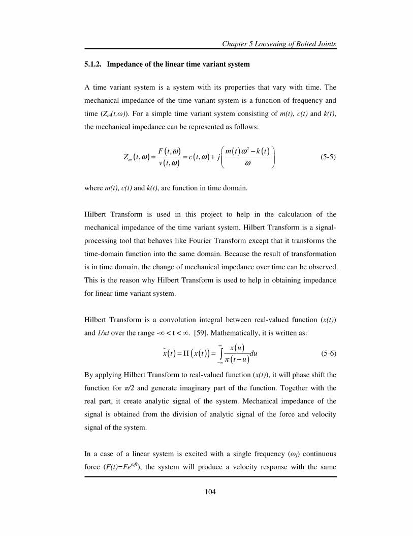
Chapter 5 Loosening of Bolted Joints
104
5.1.2. Impedance of the linear time variant system
A time variant system is a system with its properties that vary with time. The
mechanical impedance of the time variant system is a function of frequency and
time (Zm(t,ω)). For a simple time variant system consisting of m(t), c(t) and k(t),
the mechanical impedance can be represented as follows:
( )( )( )
( )( ) ( )2,
, ,,
m
F t m t k tZ t c t j
v t
ω ωω ω
ω ω
−= = +
(5-5)
where m(t), c(t) and k(t), are function in time domain.
Hilbert Transform is used in this project to help in the calculation of the
mechanical impedance of the time variant system. Hilbert Transform is a signal-
processing tool that behaves like Fourier Transform except that it transforms the
time-domain function into the same domain. Because the result of transformation
is in time domain, the change of mechanical impedance over time can be observed.
This is the reason why Hilbert Transform is used to help in obtaining impedance
for linear time variant system.
Hilbert Transform is a convolution integral between real-valued function (x(t))
and 1/πt over the range -∞ < t < ∞. [59]. Mathematically, it is written as:
% ( ) ( )( )( )
( )x u
t dx ut u
x tπ
∞
−∞
=−
= ∫H (5-6)
By applying Hilbert Transform to real-valued function (x(t)), it will phase shift the
function for π/2 and generate imaginary part of the function. Together with the
real part, it create analytic signal of the system. Mechanical impedance of the
signal is obtained from the division of analytic signal of the force and velocity
signal of the system.
In a case of a linear system is excited with a single frequency (ωf) continuous
force (F(t)=Feωft
), the system will produce a velocity response with the same
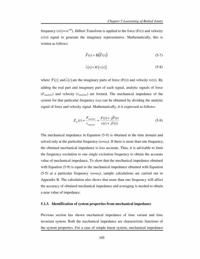
Chapter 5 Loosening of Bolted Joints
105
frequency (v(t)=veωft
). Hilbert Transform is applied to the force (F(t)) and velocity
(v(t)) signal to generate the imaginary representative. Mathematically, this is
written as follows:
( ))(~
)(~
tFtF Η=
(5-7)
( ) ( )( )v vt t=% H
(5-8)
where ( )F t and ( )v t% are the imaginary parts of force (F(t)) and velocity (v(t)). By
adding the real part and imaginary part of each signal, analytic signals of force
(Fanalytic) and velocity (vanalytic) are formed. The mechanical impedance of the
system for that particular frequency (ωf) can be obtained by dividing the analytic
signal of force and velocity signal. Mathematically, it is expressed as follows:
)(~)(
)(~
)()(
tvjtv
tFjtF
v
FtZ
analytic
analytic
m+
+== (5-9)
The mechanical impedance in Equation (5-9) is obtained in the time domain and
solved only at the particular frequency (ω=ωf). If there is more than one frequency,
the obtained mechanical impedance is less accurate. Thus, it is advisable to limit
the frequency excitation to one single excitation frequency to obtain the accurate
value of mechanical impedance. To show that the mechanical impedance obtained
with Equation (5-9) is equal to the mechanical impedance obtained with Equation
(5-5) at a particular frequency (ω=ωf), sample calculations are carried out in
Appendix B. The calculation also shows that more than one frequency will affect
the accuracy of obtained mechanical impedance and averaging is needed to obtain
a near value of impedance.
5.1.3. Identification of system properties from mechanical impedance
Previous section has shown mechanical impedance of time variant and time
invariant system. Both the mechanical impedance are characteristic functions of
the system properties. For a case of simple linear system, mechanical impedance
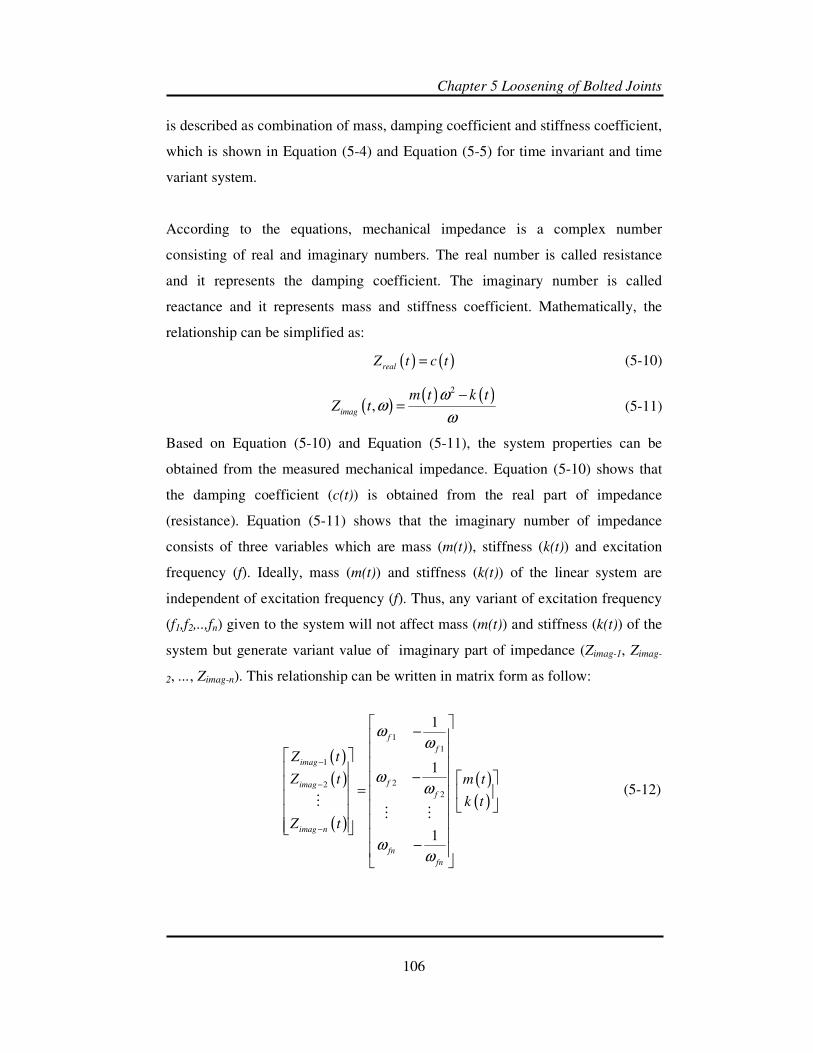
Chapter 5 Loosening of Bolted Joints
106
is described as combination of mass, damping coefficient and stiffness coefficient,
which is shown in Equation (5-4) and Equation (5-5) for time invariant and time
variant system.
According to the equations, mechanical impedance is a complex number
consisting of real and imaginary numbers. The real number is called resistance
and it represents the damping coefficient. The imaginary number is called
reactance and it represents mass and stiffness coefficient. Mathematically, the
relationship can be simplified as:
( ) ( )realZ t c t= (5-10)
( )( ) ( )2
,imag
m t k tZ t
ωω
ω
−= (5-11)
Based on Equation (5-10) and Equation (5-11), the system properties can be
obtained from the measured mechanical impedance. Equation (5-10) shows that
the damping coefficient (c(t)) is obtained from the real part of impedance
(resistance). Equation (5-11) shows that the imaginary number of impedance
consists of three variables which are mass (m(t)), stiffness (k(t)) and excitation
frequency (f). Ideally, mass (m(t)) and stiffness (k(t)) of the linear system are
independent of excitation frequency (f). Thus, any variant of excitation frequency
(f1,f2,..,fn) given to the system will not affect mass (m(t)) and stiffness (k(t)) of the
system but generate variant value of imaginary part of impedance (Zimag-1, Zimag-
2, ..., Zimag-n). This relationship can be written in matrix form as follow:
( )( )
( )
( )( )
1
1
1
22
2
1
1
1
f
f
imag
fimag
f
imag n
fn
fn
Z t
Z t m t
k t
Z t
ωω
ωω
ωω
−
−
−
−
− =
−
MM M
(5-12)

Chapter 5 Loosening of Bolted Joints
107
Based on Equation (5-12), m(t) and (k(t)) can be solved with two excitation
frequency and taking inverse matrix. In experiment, it is advisable to use more
than two (n>2) excitation frequency to reduce the experimental error. However,
this will create an overdetermined equation and the least square method is needed
to solve m(t)and k(t). Mathematically, the solution is expressed as follows:
( )( )
( )( )
1
1 1 1
1 1 1
1
2 2 2 2
2 2 2
1 1 1
1 1 1
1 1 1
T T
f f f
f f f
imag
f f f imag
f f f
im
fn fn fn
fn fn fn
Z t
Z tm t
k t
Z
ω ω ωω ω ω
ω ω ωω ω ω
ω ω ωω ω ω
−
−
−
− − −
− − − =
− − −
MM M M
( )ag n t−
(5-13)
With Equation (5-13), m(t) and (k(t)) can be obtained experimentally. Both
Equations (5-10) and (5-13) can be used to obtain the system properties of linear
system from the mechanical impedance. By applying single excitation frequency
to the system, mechanical impedance of the system is obtained. The next section
will explain this system identification method applied at the bolted joints using a
Brushed DC motor as the sensing and actuating device.
5.2. System identification of bolted joints
A bolted joint under excitation is considered as a dynamic system. The joint gives
out response in a small displacement and dissipates excitation energy to protect
the jointed structure. In order to understand this dynamic response and dissipative
behaviour of bolted joint, system properties of the joint are needed. In this project,
a brushed DC motor with a known transduction matrix is used to obtain the
mechanical impedance of the bolted joints. The motor applies a single frequency
sinusoidal excitation of small amplitude to the bolted joints and the response of
joints is reflected at the rotational speed of the motor. Both the torque and
rotational speed are calculated from the input electrical of the motor with the help
of the transduction matrix. The mechanical impedance of bolted joints is
calculated based on the Equation (5-14). Following which, the system properties

Chapter 5 Loosening of Bolted Joints
108
will be derived from the measured mechanical impedance using Equations (5-10)
and (5-13). This section introduces the aforementioned experimental method and
the derivation to obtain the system properties. The experimental setup and
procedure will also be described.
5.2.1. Dynamic model of bolted joint
A bolted joint under small range of frequency excitation can be modelled as a
simple mechanical system. The system consists of mass, spring and damping.
Each component of the system represents the dynamic behaviour of the system.
The mass component represents the inertia of the joint, the spring component
represents the stiffness of the joint and the damping represents the dissipative
behaviour of the joint. Stiffness describes the elasticity behaviour of the joint. It
describes displacement of the joint under given excitation. Damping describes the
dissipative behaviour of bolted joint. It describes how energy is dissipated from
the joint.
Figure 5-2 Hysteresis curve [49]

Chapter 5 Loosening of Bolted Joints
109
Tightness of bolted joint affects the value of those components. Figure 5-2 shows
hysteresis graph of bolted joints with different preload under excitation of single
value of torque. This graph is obtained from FEM model of bolted joint generated
by Oldfield [49]. In the figure, the displacement of each bolted joint is observed to
be varied. This implies that the components of a bolted joint is a function of its
tightness (preload)
In order to obtain value of each component, mechanical impedance of bolted joint
is measured. The mechanical impedance of bolted joint are formed from
combination of coefficient of mass, spring, and damping. By assumed a simple
mechanical model (mass, spring and damping), relationship of mechanical
impedance with coefficient of mass, spring and damping can be shown from
Equation (5-10) and Equation (5-11). The mechanical impedance of bolted joint
can be obtained by dividing the analytic signal of the excitation torque over the
rotational speed. This is mathematically expressed as follows:
)(
~)(
)(~
)()(
tjt
tTjtTTtZ
analytic
analytic
mΩ+Ω
+=
Ω= (5-14)
Based on this measured mechanical impedance of bolted joint, the coefficients of
system can be measured by using Equation (5-10) and Equation (5-13). In order to
obtain relationship between components of bolted joint, experimental is conducted
with a calibrated electric motor to apply a sinusoidal excitation to a bolted joint
with different preload. Based on this experimental measurement, the relationship
between each component of bolted joint with its tightness can be described.
5.2.2. Experimental setup
To measure the mechanical impedance of bolted joints, the experiment shown in
Figure 5-3 was set up. The experiment setup is similar with the experimental setup
in Chapter 4 with an additional motion control card to control the motor
movement. The experiment consisted of an electric motor, a motion control card,

Chapter 5 Loosening of Bolted Joints
110
a voltage probe, a current probe, a dynamic signal analyzer, and a tightened bolted
joint with a load cell. The detail and model of the equipments can be found in
Appendix A.
Figure 5-3 Experimental Setup to obtain Mechanical Impedance
Figure 5-4 Advanced Motion Control (Motion Control Card)
The electric motor used in this experiment is a brushed DC motor. The
transduction matrix for the motor has already been identified in Chapter 3. The
motion control card is attached to the motor to control the motor’s motion and
Electric
Motor
E
i
T
Ω
Voltage
Probe
Current
Probe
Signal Conditioner
Dynamic
Signal
Analyzer
Computer
Bolted
joint
Motion
control
card
Load Cell
P

Chapter 5 Loosening of Bolted Joints
111
supply power. Figure 5-4 shows the motion control card. The motion control card
amplifies any signal input to it to generate enough power to run the motor. In this
experiment, the input signal is a sinusoidal signal with frequency is varied from
0.7 Hz to 1.2 Hz. The signal amplitude after amplification is 24 Volt. This signal
from motion control card causes the motor to rotate in sinusoidal to excite the
tightened bolted joint. The tightened bolted joint is attached at the motor with
similar configuration in Chapter 4 (Figure 4-12).
Voltage and current probes are attached to the cable between the motor and
motion control card. The setups for the voltage and current probe are similar to
the setup mentioned in Chapter 3. The output ports of the probes are connected to
the dynamic signal analyzer for sampling and storing the collected data. The
bolted joint is attached to the motor shaft. The design of bolted joints and their
setup are mentioned in Chapter 4. The load cell is also connected to the dynamic
signal analyzer for storing purpose.
5.2.3. Experimental procedure
The experiment was conducted by applying sinusoidal excitation to the bolted
joints. The samples of bolted joints were prepared in five different preloads
( 2,000 N, 4,000 N, 6,000 N, 8,000N and 10,000 N) and two different friction
conditions (lubricated and non-lubricated) were applied for each preload. Six
different excitation frequencies (0.7 Hz, 0.8 Hz, 0.9 Hz, 1.0 Hz, 1.1 Hz, and 1.2
Hz) are used to excite the bolted joint. Thus, there are 60 cases of bolted joint for
each different preload, surface condition and excitation frequency. Four sets of
bolted joints were prepared for each of the cases mentioned. During the excitation,
the voltage and current of the motor were measured with the probes. The preload
was measured from the load cell and the voltage, current and the preload were
sampled and recorded with a digital signal analyzer for 3 seconds. The data were
sampled at 2000 Hz frequency. A digital low pass filter with a cut off frequency
of 10 Hz was applied to smooth the data. The applied torque and rotation speed
were calculated from the measured voltage and current with the help of the

Chapter 5 Loosening of Bolted Joints
112
transduction matrix. The formula used to calculate torque and rotation speed is
shown in Equation (4-2). The calculated torque and rotation speed were used to
calculate mechanical impedance of bolted joints by substituting them into
Equation (5-15).
5.2.4. Experimental result
A sample of measurement results is shown in Figures 5-5 to 5-8. The sample is
taken from a bolted joint with preload of 10kN, rough surface condition and under
1.0 Hz excitation frequency. The figure shows that the torque and rotation speed
oscillates with a frequency of 1 Hz. The preload decreases whereas the real and
imaginary parts of the mechanical impedance are oscillating. Thus, the mean
values of the mechanical impedance for each cycle are calculated to get the close
value of mechanical impedance as suggested from Appendix C. The calculation
result is plotted in Figure 5-9. Figure 5-9 shows that the real part of mechanical
impedance decreases while the imaginary part of mechanical impedance increases.
These results show that mechanical impedance is related to the preload.
Figure 5-5 Excitation torque of the bolted joint

Chapter 5 Loosening of Bolted Joints
113
Figure 5-6 Rotation speed response of the bolted joint
Figure 5-7 Preload of the bolted joint during the excitation

Chapter 5 Loosening of Bolted Joints
114
Zreal
Zimag
Figure 5-8 Impedance of the bolted joint
Zreal (mean)
Zimag (mean)
Figure 5-9 Mean value of mechanical impedance
Figures 5-10 to 5-15 show how the mechanical impedance of the bolted joints
changes under different friction conditions, excitation frequencies, and preloads.
The real part increases with an increase of the bolt preload whereas the imaginary
part decreases. Apart from the preload, the surface friction (no lubricant) and the
excitation frequency also affect the mechanical impedance. An increase in surface
friction causes the real part to increase and imaginary part to decrease. On the

Chapter 5 Loosening of Bolted Joints
115
other hand, an increase in excitation frequency causes both the real and imaginary
part to decrease.
Figure 5-10 Real and Imaginary part of Impedance for frequency 0.7 Hz
Figure 5-11 Real and Imaginary part of Impedance for frequency 0.8 Hz

Chapter 5 Loosening of Bolted Joints
116
Figure 5-12 Real and Imaginary part of Impedance for frequency 0.9 Hz
Figure 5-13 Real and Imaginary part of Impedance for frequency 1.0 Hz

Chapter 5 Loosening of Bolted Joints
117
Figure 5-14 Real and Imaginary part of Impedance for frequency 1.1 Hz
Figure 5-15 Real and Imaginary part of Impedance for frequency 1.2 Hz
Equation (5-10) is used to calculate the damping of the bolted joints. The results
show that the damping is affected by the excitation frequency. This indicates that
there is a hysteretic damping in the bolted joint. The hysteretic damping is the
internal damping of the material and is related with excitation frequency.

Chapter 5 Loosening of Bolted Joints
118
However, this thesis does not explore further regarding this hysteretic damping
due to its less importance in affecting loosening.
Beside excitation frequency, the preload and the surface friction also affect the
damping coefficient. The relationship between the damping value and the
excitation frequency, preload and friction conditions of bolted joint are divided
into several parts first before it is determined. Table 5-2 shows the linear
relationship between the damping value and the preload for each excitation
frequency and surface friction.
The plots in Figures 5-16 and 5-17 show the relationship between the damping
value and the excitation frequency, preload and friction conditions of bolted joint.
Relationship Frequency
(Hz) Normal Condition Lubricated
0.7 0.252
1.5571000
bolt
PC = +
0.2041.257
1000bolt
PC = +
0.8 0.139
1.6311000
bolt
PC = +
0.0801.374
1000bolt
PC = +
0.9 0.113
1.1671000
bolt
PC = +
0.0551.052
1000bolt
PC = +
1.0 0.067
0.9481000
bolt
PC = +
0.0430.802
1000bolt
PC = +
1.1 0.031
0.8531000
bolt
PC = +
0.0460.795
1000bolt
PC = +
1.2 0.016
0.9971000
bolt
PC = +
0.0381.005
1000bolt
PC = +
Table 5-2 Linear relationship between damping and preload

Chapter 5 Loosening of Bolted Joints
119
Figure 5-16 Damping of bolted joints under normal friction condition
Figure 5-17 Damping of bolted joints under lubricated condition
Equation (5-13) is used to calculate the mass and stiffness of bolted joints. The
imaginary parts of the mechanical impedance from different excitation
frequencies are substituted into the equation. It is observed that the surface
friction and preload of the bolt affect the imaginary part as well. Hence, the
imaginary parts to be substituted into the equation have to be obtained under the

Chapter 5 Loosening of Bolted Joints
120
same bolt preload and surface condition. The calculated mass and stiffness values
were obtained from different preload and surface friction conditions and the
results are plotted in Figures 5-18 and 5-19. The results show that the effective
mass and stiffness increase as the bolt preload increases. The mass in both normal
and lubricated conditions is around 2.65 to 3 kgm2whereas the stiffness of bolted
joints varies from 2.00 to 35.00 Nm/rad. As the mass is always constant, the
average value from the measurement can be calculated and the mass of bolted
joint is as follows:
2.87boltI = kgm2/rad (5-15)
The relationship between stiffness and preload of the bolt is assumed to be linear.
Hence:
a) In a normal condition:
3.21376.725
1000bolt
PK = +
(5-16)
b) In a lubricated condition:
3.0369
3.13491000
bolt
PK = + (5-17)
Figure 5-18 Effective mass and stiffness of bolted joints under normal friction
condition

Chapter 5 Loosening of Bolted Joints
121
Figure 5-19 Effective mass and stiffness of bolted joints under lubricated condition
5.2.5. Hysteresis graph of the mass, spring, and damping model of bolted
joints
To verify the mass, spring and damping model of bolted joints, hysteresis graphs
between the torque and angle displacement of the model were formed and
compared. The angle displacements are calculated by substituting the measured
rotation speed into Equation (4-5). The torque of bolted joint model is then
calculated from the measured rotation speed, mass, damping and rotation speed
values based on the following formula:
exc bolt resp bolt resp bolt resp
T I C K dt= Ω + Ω + Ω∫& (5-18)
Both the hysteresis graph of measured and system models for different excitation
frequencies are plotted in Figures 5-20 to 5-25

Chapter 5 Loosening of Bolted Joints
122
Measured
Equation 5-12
Figure 5-20 Hyteresis graph based for excitation frequency 0.7 Hz
Measured
Equation 5-12
Figure 5-21 Hyteresis graph for excitation frequency 0.8 Hz

Chapter 5 Loosening of Bolted Joints
123
Measured
Equation 5-12
Figure 5-22 Hyteresis graph for excitation frequency 0.9 Hz
Measured
Equation 5-12
Figure 5-23 Hyteresis graph for excitation frequency 1.0 Hz

Chapter 5 Loosening of Bolted Joints
124
Measured
Equation 5-12
Figure 5-24 Hyteresis graph for excitation frequency 1.1 Hz
Measured
Equation 5-12
Figure 5-25 Hyteresis graph for excitation frequency 1.2 Hz
From the results, it can be seen that the hysteresis shape of the system model
matches almost perfectly with the shape of experimental measured model for
excitation frequencies from 1.0 to 1.2 Hz. For excitation frequencies from 0.7 to
0.9 Hz, the shape does not match perfectly. Towards the end when the angle
changes direction, a drop in torque can be observed. This is caused by the change
in dry friction at the bolt. Thus, a simple m, c, and k system is not suitable for
modelling bolted joints excited with frequencies from 0.7 to 0.9 Hz.

Chapter 5 Loosening of Bolted Joints
125
5.3. Angular response of bolted joint to transverse vibration
After obtaining the dynamic model of the bolted joints, the response of the bolted
joint can be simulated with a defined excitation. As mentioned in the literature,
transverse vibration is a common cause of the self-loosening of bolted joints. Due
to the configuration and geometry of the bolt, a torque at the bolted joint is
generated by the transverse vibrations. The generated torque excites the joint and
causes the loosening. The loosening torque is derived in Appendix C. The
derivation shows that sinusoidal transverse force (|F sinωft|) on the bolted joint is
transformed into a continuous shock spectrum (|T sinωft|). To evaluate the
response of bolted joints under the loosening torque the calculations steps, shown
below in this section, are taken.
5.3.1. Response of simple mass, spring and damping system in discrete time
As explained previously, the bolted joints are modelled as a simple mass (Ibolt),
spring (Kbolt) and damping (Cbolt) system. When an impulse excitation is applied to
the system, the response of the system is calculated as follows:
1sin 0
( )
0 0
nt
d
bolt d
e t for tIg t
for t
ςω ωω
−>
= <
(5-19)
where ωn, ωd, and ζ are the natural frequency, damped natural frequency, and
damping ratio of the system. They are each calculated as follows:
boltn
bolt
K
Iω = (5-20)
2
bolt
bolt bolt
C
K Iς = (5-21)
21d nω ω ς= −
(5-22)
When the system is excited under a arbitrary torque (Texc), its response can be
obtained using the superposition method. The arbitrary torque is assumed to be a

Chapter 5 Loosening of Bolted Joints
126
superposition of impulses with varying magnitude applies at different times. The
response is then calculated by summing the responses of each impulse as follows:
( ) ( ) ( )( )0
t
bolt exct T g t dθ τ τ τ= −∫ (5-23)
As the torque and system properties are stored in the discrete time, the equation
should accordingly be changed into discrete time to calculate the response of
bolted joints. To change the equation into discrete time, a sample time, T seconds,
is chosen to divide the normal time (t) into n number of samples. The relationship
between them can be expressed as follows:
t nT= (5-24)
For each sample, there is an impulse excitation (g(n)) given to the system for T
second. The impulse response is formulated as follows:
( ) ( )g n Tg t= (5-25)
By substituting Equations (5-24) and (5-25) into Equation (5-19), the impulse
response in discrete mode can be expressed as follows:
( ) sinnnT
d
bolt d
Tg n e nT
I
ςω ωω
−= (5-26)
The response of the system in discrete mode can then be calculated by
transforming Equation (5-23) as follows:
( ) ( ) ( )0
n
bolt exc
k
n T k g n kθ=
= −∑ (5-27)
Using Equation (5-27), the response of bolted joint under an excitation torque can
be calculated. The next part shows sample calculations of bolted joint under
excitation torques.

Chapter 5 Loosening of Bolted Joints
127
5.3.2. Samples calculation of response of bolted joint under excitation torque
due to transverse vibration
Figure 5-26 Excitation torque to bolted joint
A bolted joint without a lubricant is tightened with a preload value of 8,000 N. A
transverse vibration is then applied to the joint with an excitation frequency of 1
Hz. The vibration generates a continuous loosening torque, shown in Figure 5-26,
at the bolted joint. The derivation and values of the loosening torque are shown in
Appendix C. Based on the preload and excitation frequencies, the system
properties of the bolted joint are as follows:
• 2.87boltI = kgm2/radian (5-28)
• 0.067
0.9481000
bolt
PC = + Nms/radian = 1.484 Nms/radian (5-29)
• 3.2137
6.7251000
bolt
PK = + Nm/radian = 32.4354 Nm/radian (5-30)
The impulse response of the joint is plotted in Figure 5-27.

Chapter 5 Loosening of Bolted Joints
128
Figure 5-27 Impulse response of the system
Figure 5-28 Response of bolted joint under given excitation for a constant stiffness
The loosening torque and impulse response are digitized with a sampling time of
0.002 s (T) and 8,000 data points. The sampling time, system properties, response
of the bolted joint, and excitation torque are substituted into Equation (5-27) and
the moving average for every 500 points is applied to the result. Figure 5-28
shows the result and the moving average of the result. Based on the moving
average, it is observed that the response of the bolted joint have the same sign as
the torque. This implies that the bolt is rotating in the same direction as the torque
(loosening direction). After a certain point, there is no further increment in the

Chapter 5 Loosening of Bolted Joints
129
response angle and bolt oscillates around this point. The oscillation is caused by
the stiffness of the bolted joint and existence of the torque.
As mentioned in the literature, the preload and response angle have a linear
relationship. When a bolt is turned to a certain degree, a certain value of preload is
acquired or lost depending on the turning direction. This preload also affects the
stiffness and damping of the bolted joint as mentioned earlier. Thus, the bolted
joints’ damping and stiffness changes when the bolt turns.
The relationship between the preload and response angle of the bolted joint is
normally obtained experimentally. Figure 5-29 shows an example of the
relationship for the normal bolt used in the experiment. Based on the figure, the
relationship is written as follows:
6413.3 boltP θ∆ = ∆ (5-31)
Figure 5-29 Relationship between Preload and angle of turn
Thus, the damping and stiffness of bolted joint for a 8,000 N preload in terms of
response angle can be written by substituting Equation (5-31) into Equations (5-
29) and (5-30), where
1.484 0.4297bolt boltC θ= − (5-32)
32.4354 20.61047bolt boltK θ= − (5-33)

Chapter 5 Loosening of Bolted Joints
130
Using Equations (5-32) and (5-33), response of bolted joint is solved by changing
the value Cbolt and Kbolt for each response angle. Thus, to find the new value of
Cbolt and Kbolt, the response angle needs to be solved for every data point. Based
on their values, the next response angle can be calculated. For this purpose, the
Matlab code shown in Appendix D is used. The code is used to obtain the
response of bolted joint under an arbitrary torque. By substituting the torque
response in Figure 5-26, the response of bolted joints is obtained and plotted in
Figure 5-30. The result shows that the amplitude response of the system is higher
than previous result in Figure 5-28. To smooth the line, the moving average for
500 data points is applied to the response. The trend shows that the response of
bolted joint gradually increases in the loosening direction. Thus, it is concluded
that a change of system properties affects loosening.
Figure 5-30 Response of bolted joint due to stiffnes reduction
5.3.3. Factors affecting the response of the bolted joint
Based on the sample calculation shown earlier, it can be seen that the response of
the bolted joint to excitation is affected by the system properties and amplitude of
the excitation. The effects of these factors are as follows:
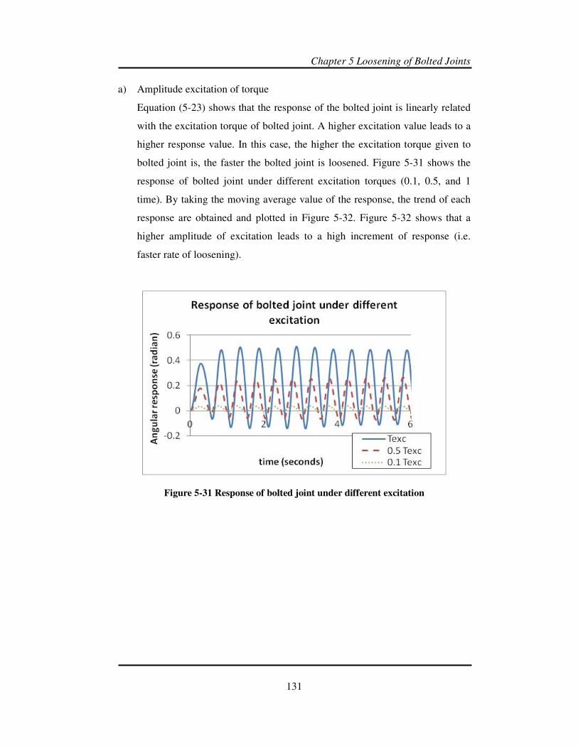
Chapter 5 Loosening of Bolted Joints
131
a) Amplitude excitation of torque
Equation (5-23) shows that the response of the bolted joint is linearly related
with the excitation torque of bolted joint. A higher excitation value leads to a
higher response value. In this case, the higher the excitation torque given to
bolted joint is, the faster the bolted joint is loosened. Figure 5-31 shows the
response of bolted joint under different excitation torques (0.1, 0.5, and 1
time). By taking the moving average value of the response, the trend of each
response are obtained and plotted in Figure 5-32. Figure 5-32 shows that a
higher amplitude of excitation leads to a high increment of response (i.e.
faster rate of loosening).
Figure 5-31 Response of bolted joint under different excitation

Chapter 5 Loosening of Bolted Joints
132
Figure 5-32 Moving average of the response of bolted joint under different
excitation
b) Damping of bolted joint
Damping is a system property that dissipates energy. In the previous section,
it was mentioned that the damping of bolted joint varies with the excitation
frequency. A higher excitation frequency leads to a lower value of damping.
Figure 5-33 shows response of bolted joint under different damping
conditions. It also shows that a higher damping value will lead to a reduction
of amplitude of response. However, the damping does not affect the rate of
loosening. Figure 5-34 is plotted by taking the moving average of the results,
and shows that the loosening rates of response are similar.

Chapter 5 Loosening of Bolted Joints
133
Figure 5-33 Response of bolted joint under different damping
Figure 5-34 Average value of response of bolted joint under different damping
c) Stiffness of bolted joint
Stiffness is a system property that measure flexibility of the system. A higher
stiffness value leads to less flexibility in the system. As discussed earlier, the
stiffness of bolted joint is linearly related with preload of bolted joint. A
higher preload value implies a higher stiffness. The effect of a higher value of
stiffness on the response of the bolted joint is shown in Figure 5-35 below. A
higher stiffness value leads to lower amplitude of response of the bolted joint.

Chapter 5 Loosening of Bolted Joints
134
Figure 5-36 shows that a bolted joint which is less stiff loosens faster. Hence,
it is advisable to have a bolted joint with higher stiffness to reduce loosening
due to vibration.
Figure 5-35 Response of bolted join under different stiffness
Figure 5-36 Average value of bolted joint under different stiffness

Chapter 5 Loosening of Bolted Joints
135
5.4. Summary
A method to obtain the mechanical impedance of time variant system with Hilbert
Transform as the processing tool was explained in this chapter. The Hilbert
Transform, as one of signal processing tool, transforms a signal in the same
domain (time domain) and generates the imaginary part of the signal. An analytic
signal can be created with a combination of the real imaginary part of the signal.
The mechanical impedance is obtained by dividing the analytic signal of force
with the analytic signal of velocity as shown in Equation (5-9). The mechanical
impedance which is obtained is in the time domain and not the frequency domain.
The frequency domain has disappeared as the mechanical impedance is solved at a
particular frequency (ωf). Since the results of the mechanical impedance taken
from the sample calculation are oscillating, it is necessary to take the average
value of the results. Furthermore, the mechanical impedance is used to derive the
system properties of the bolted joints. For a simple mass, spring and damping
system, the real part of mechanical impedance represents the damping of the
system while the imaginary part represents the mass and stiffness of the system.
The relationships were shown in Equations (5-10) and (5-11).
The behaviour of bolted joints under vibration can be modelled on this simple
mass, spring and damping system. The system properties of the bolted joints can
be identified from measuring the mechanical impedance of bolted joints and
substituting it into Equations (5-10) and (5-13). A DC motor with a calibrated
transduction matrix is employed to perform this task. The motor applies a single
frequency sinusoidal excitation to the bolted joint and the response is reflected in
the motor shaft. For the purposes of measuring the mechanical impedance, the
excitation is the torque and the response is the rotational speed. The torque and
rotation speed are obtained from the measured electrical input of motor with the
help of the transduction matrix. Hilbert Transform is applied to the torque and
rotation speed signal to obtain the mechanical impedance and the system
properties are derived from the mechanical impedance. In this experiment, bolted
joints with different tightness, surface condition, and excitation frequency are

Chapter 5 Loosening of Bolted Joints
136
measured. The results show that the damping and stiffness of bolted joint are
affected by the preload of the bolted joint and surface condition. The hysteresis
curve shows that the simple mass, spring and damping system only fit perfectly
for excitation at frequencies above 1.0 Hz. Another system model is needed for
bolted joint excited at frequencies below 1.0 Hz as the system is affected by dry
friction.
After obtaining the system properties of bolted joint, the loosening mechanism of
the bolted joint under transverse vibration can be studied. The response of the
bolted joint is calculated by substituting the system properties and the excitation
frequency into Equation (5-27). Based on the response, the cause of loosening at
bolted joints can be investigated. The results show that the change in the system
properties of the bolted joint can be attributed to the rotation of the bolt. Due to
this change, especially in the stiffness, the oscillation of the bolted joint increases
and cause the amplitude of oscillation to be higher until the total loosening occurs.
This phenomenon explains why loosening occurs at a low rate at the outset and
gradually increases in rate.

Chapter 6 Conclusions and Future Recommendations
137
CHAPTER 6
CONCLUSIONS AND RECCOMENDATIONS
This chapter summarizes the completed works, major findings from the research
and relevant suggestions.
6.1. Conclusions
6.1.1. Transduction matrix of DC motor
In this thesis, the transduction matrix of a DC motor and its applications were
investigated. A transduction matrix is a two by two matrix consisting of four
frequency response functions between the electrical inputs (voltage and current)
and mechanical outputs (torque and rotational speed) of an electric motor. Each
element of the matrix relates one input with one of output in the frequency domain
that is independent from the other elements. The value of each element reflects the
system properties of the electric motor. As a DC motor is supplied with electrical
power at DC power (constant values), the transduction matrix of a DC motor is
simplified as a matrix consisting of four (4) constant values (0 Hz frequency).
The values of the transduction matrix of a DC motor can be obtained by
theoretical and experimental methods. The theoretical method is based on an
equivalent electric circuit model of a DC motor. The values of the matrix are
obtained by applying two boundary conditions to the circuit model. On the other
hand, for the experimental method, the values of the matrix are obtained from a
pair of electrical input and mechanical output of a DC motor under different load
conditions based on Equation (3-39). It is assumed that the transduction matrix
obtained relates the electrical input to the DC motor with its mechanical output
linearly within its operating range. Since the relationship is linear, the mechanical
output of the DC motor can be calculated from its electrical input. A comparison
of the theoretical (Equation 3-41) and experimental matrixes (Equation 3-45)
shows that the experimental matrix has less mean error. Thus, with the

Chapter 6 Conclusions and Future Recommendations
138
experimentally obtained transduction matrix, the DC motor can be used as a
device to actuate and measure a mechanical system, such as a bolted joint, by
measuring and controlling the electrical input supplied to it.
6.1.2. Tightness indicator of bolted joint
Bolts and nuts are used to clamp two components (e.g. plates and mechanical
parts) together. To clamp the two components, the bolt or the nut is turned to
stretch the bolt and generate a clamping force in the components. The existence of
the clamping force ensures that the joint is kept intact. The magnitude of the
clamping force also indicates the tightness of bolted joint.
Besides clamping force, there are several other tightness indicators that are
mentioned in the literature. These indicators are used as they have a linear
relationship with the clamping force. Amongst these indicators, torque is the most
commonly used as it is relatively easy to measure. However, the relationship
between torque and clamping force is affected by the friction condition of the bolt.
That the relationship is so affected is confirmed by the results of an experiment
where the value of the clamping force between a set of normal bolt and a set of
lubricated bolt are compared. With the same value of tightening torque, the
clamping force generated by the lubricated bolt is higher than the clamping force
generated from the normal bolt.
This thesis proposed a new tightness indicator based on the total energy input
during the tightening process. The total energy input is calculated by integrating,
with respect to time, the torque applied to the bolted joint multiplied by the
rotational speed during tightening (Eqn. 3-20). This calculation is made possible
with the use of the transduction matrix, which allows the torque and rotational
speed during the tightening of the bolted joint to be concurrently obtained from
the electrical input of the DC motor, and hence for the total energy input during
the tightening process to be measured. It was found that the total energy input is a
better indicator of clamping force than torque. It is able to distinguish different

Chapter 6 Conclusions and Future Recommendations
139
preloads in the two different cases of the lubricated and normal bolts which have
the same value of tightening torque. This is because the total energy input, which
consists of the potential energy stored in the bolt and which is linearly related to
the clamping force, is independent of coefficient of friction.
6.1.3. Time variant mechanical impedance measurement with Hilbert
Transform as the signal processing tool
Mechanical impedance is a form of frequency response function. It is obtained by
dividing the excitation over response of the system in the frequency domain. The
excitation is the torque applied while the response is the rotational speed. It
describes the resistance of the system to a motion applied to it, which is a property
of the system. In the case of a tightened bolted joint, the mechanical impedance
describes the resistance of a tightened bolted joint to an external disturbance.
The Hilbert Transform is a signal processing tool that transforms a signal in the
same domain (time domain) and generates the imaginary part of the signal. An
analytic signal can be created by combining the real and imaginary part of the
signal. The mechanical impedance of the time variant system can be obtained with
the help of the Hilbert Transform as shown in Equation (5-9). The mechanical
impedance is obtained in the time domain and not in frequency domain. The
frequency of obtained mechanical impedance is limited to a particular frequency,
which is the excitation frequency (ωf). Following this concept, the mechanical
impedance of a tightened bolted joint can be measured with a calibrated DC motor
with a known transduction matrix. To obtain the mechanical impedance at a
particular frequency, the tightened bolted joint is excited with a torque at a fixed
constant frequency using the DC motor. Due to the excitation, the tightened bolted
joint gives out a response in form of rotational speed. The magnitudes of the
torque applied to the tightened bolted joint and the rotational speed response from
the torque can be obtained from electrical input of the DC motor with the help of
its transduction matrix. The torque and rotation speed that is obtained are assumed
to be mechanical signals of the tightened bolted joint. The Hilbert Transform is

Chapter 6 Conclusions and Future Recommendations
140
applied to the mechanical signals to obtain their real part and imaginary parts in
the time domain. The mechanical impedance is calculated by dividing the real and
imaginary parts of the torque signal over the rotational speed signal. Since the
mechanical impedance is obtained in time domain, it can be monitored over a
period of time. However, the mechanical impedance is restricted to a particular
frequency only which is the applied constant frequency.
The measured mechanical impedance of the tightened bolted joint shows that its
real part and imaginary parts are affected by the clamping force of the joint
(preload), the surface condition of the bolt and the excitation frequency (Figures
5-10 to 5-15). The real part increases with an increase in preload at the tightened
bolted joint, an increase in surface friction (no lubricant) and a decrease in
excitation frequency. An increase in the real part implies an increase in the
resistance of the bolted joint to motion applied to it, as the real part and damping
are associated. The imaginary part increases with a decrease in preload, a decrease
in surface friction (applying lubricant to the surface) and an increase in the
excitation frequency. The imaginary part is related to the mass and stiffness of the
system. Hence, to better understand the changes of imaginary part, system
modelling is carried out for the tightened bolted joint. This model is explained in
the next section.
6.1.4. System modelling and identification of a tightened bolted joint
A bolted joint under excitation can be modelled as a simple linear time-variant
mechanical system consisting of mass, spring and damping. Mass, spring and
damping are properties of a mechanical system which describe the dynamic
behaviour of the system. The relationship between mechanical impedance and the
system’s properties is described in Equations (5-10) and (5-11). The real part of
the impedance (resistance) is associated with the damping of the system while the
imaginary part of the impedance (reactance) is associated with the mass and
spring of the system. The result of system properties of the tightened bolted joint
are plotted in Figures 5-16 to 5-19.

Chapter 6 Conclusions and Future Recommendations
141
Based on the figures, the effective mass is assumed to be constant due to the small
change in its value. It can also be seen that the change in effective stiffness
depends on the preload and surface friction (Figures 5-18 and 5-19). The stiffness
increases with an increase in the preload and surface friction. The increase in
preload and friction leads to an increase in system rigidity, thus allowing smaller
oscillations to occur in it. Similarly, the damping increases with an increase in
surface friction and preload. The surface friction and preload increases the
resistance of the tightened bolted joint. Hence it dissipates more energy to prevent
loosening. The damping decreases with an increase in excitation frequency. This
decrease in damping may be explained by the effect of structural damping where
the damping is inversely proportional to the excitation frequency.
The simple mass, spring and damping model is only applicable for bolted joint
under an excitation frequency above 1.0 Hz as shown in the Hysteresis curve
(Figures 5-23 to 5-25). The hysteresis curve constructed from the model almost
match with the hysteresis curved constructed from the measured data. However,
another system model is needed for bolted joints excited at frequencies below 1.0
Hz as the hysteresis curve does not match.
6.1.5. Transverse vibration leading to self loosening of the bolted joint
Transverse vibrations of a bolted joint can lead to self-loosening of the joint. The
transverse force applied to the bolted joint causes its top plate to slide relatively to
its bottom plate and bends the bolt. The bolt’s bending generates a bending
moment at the bolted joint and affects its axial force. Due to the linear relationship
between friction force and axial force, a change in the axial force affects the
frictional force. Thus, a certain region of the bolted joint has a smaller frictional
force and permits a sliding motion. The sliding motion, especially at threaded part
of the bolt, rotates the bolt in the loosening direction with a certain value of torque.
The transformation of the transverse force applied on the bolted joint to a
loosening torque is mathematically derived in Appendix B. From the derivation, it

Chapter 6 Conclusions and Future Recommendations
142
can be seen that a sinusoidal transverse force applied on a bolted joint is
transformed to a loosening torque in the form of absolute value of sinusoidal
( sinθ ). The factors that affect the amplitude of the loosening torque are the
preload, the transverse force, the coefficient of friction, the grip length and the
thread type of the bolted joint. The preload and coefficient of friction reduce the
amplitude of the loosening torque. The transverse force and grip increase the
amplitude of the loosening torque. A fine thread has a smaller thread angle than a
coarse thread and thus reduces the amplitude of the loosening torque.
A bolted joint, as a mechanical system, responds to excitation in the form of
motion based on the system’s properties. The response of a bolted joint to the
loosening torque due to the transverse force is calculated from the convolution
integral of its impulse response. The impulse response of the system can be
calculated by substituting the system properties obtained and the excitation
frequency into Equation (5-26). It can be concluded from the calculated result
that a change in the system properties of the bolted joint can be attributed to the
rotation of the bolt. Due to a change in stiffness, the oscillation of the bolted joint
oscillates more and the amplitude of oscillations increases until total loosening
occurs. This phenomenon explains why loosening occurs at a low rate at the
outset and gradually increases in rate.
The factors which affect the response of a bolted joint to excitation are the
excitation amplitude, the damping and stiffness of the bolted joint. A higher
excitation amplitude leads to a greater response and the bolted joint loosens more
quickly. On the other hand, greater damping leads to a lower response. However,
the degree of damping does not affect speed of loosening of a bolted joint as
shown in Figure 5-37. The stiffness affects both the response and speed of
loosening the bolted joint. A stiffer bolted joint has a lower response and loosens
more slowly. Both the stiffness and damping of the bolted joint, as explained in
chapter 5, are affected by the preload of the bolted joint, its friction condition and
the excitation frequency applied to it. Thus, the designer of the bolted joint should

Chapter 6 Conclusions and Future Recommendations
143
take into consideration the amplitude and frequency of the excitations common to
the applications that the bolt designed for, to decide the preload and friction
condition of the bolt. The purpose of considering is to allow the designer to
provide adequate stiffness and damping in his design to minimize the self-
loosening effect of the bolted joint.
6.2. Future research direction and recommendation
6.2.1. Solution to change surface friction condition of a bolt
The surface friction of the bolt affects the relationship between the torque
experienced by the bolt and the clamping force that the bolt exerts. The rougher
the surface, the greater the torque that is needed to achieve the same magnitude of
clamping force. On the other hand, surface friction helps the bolted joint resist
external disturbances. Therefore, surface friction needs to be kept as low as
possible during the tightening process but as high as possible after the tightening
process. Hence, a solution whereby the friction condition of a bolt surface can be
changed is necessary. This solution must be able to reduce the surface friction of a
bolt during tightening and increase its surface friction after tightening.
6.2.2. System modelling of a bolted joint
By knowing the system properties of the bolted joint, its dynamic behaviours can
be predicted. The response of a tightened bolted joint to an external disturbance
can be calculated based on its system properties. This system modelling helps to
ensure the proper installation of a tightened bolted joint. The selection of the
bolt’s material and the requisite tightness can be made from its required system
properties.
In this thesis, the bolted joint was modelled as a simple mass, damping and spring
system. The value of the mass, damping and stiffness are identified from the
measured mechanical impedance of the bolted joint. However, it is found out that

Chapter 6 Conclusions and Future Recommendations
144
the simple mass, damping and spring is not sufficient to model bolted joint with
excitation frequency below 1 Hz. Thus, a new model need to be developed.
6.2.3. Sensorless control of electrical motor
In this thesis, it was shown that a transduction matrix is capable of relating the
electrical input of an electrical motor to its mechanical output. The availability of
the transduction matrix reduces the need for mechanical sensors (such as encoders,
torque meters and tachometers) to measure the mechanical output of the motor.
This application help in minimizing Brushless DC motor where the encoder is still
needed to measure the shaft position to control the motor rotation. With the help
of transduction matrix, the shaft position and the output torque of the motor can
be predicted from its electrical input. The controller will able to know the shaft
position without the usage of encoder. Thus, it will lead to development for
sensorless control of Brushless DC motor. With this sensorless control, it helps in
extending the lifetime and miniaturizing of the motor as the mechanical sensor
(encoder) is subjected to wear and tear.

References
145
REFERENCES
1. Dille, J.C. How A Bolt Works. [cited 2012 5 May 2012]; Available from:
http://home.jtan.com/~joe/KIAT/kiat_1.htm.
2. Bickford, J.H., Introduction to the design and behavior of bolted joints, in
Mechanical engineering. 2008, CRC Press: Boca Raton.
3. Motosh, N., Development of design charts for bolts preloaded up to the
plastic range. TRANS. ASME, SER. B. J. ENGNG. IND., 1976. 98(3 ,
Aug. 1976): p. 849-851.
4. Junker, G.H., New criteria for self-loosening of fasteners under vibration.
SAE Transactions, 1969. 78: p. 314-335.
5. Housari, B.A. and S.A. Nassar. Effect of coating and lubrication on the
vibration-induced loosening of threaded fasteners. 2006. Chicago, IL.
6. Housari, B.A. and S.A. Nassar, Effect of thread and bearing friction
coefficients on the vibration-induced loosening of threaded fasteners.
Journal of Vibration and Acoustics, Transactions of the ASME, 2007.
129(4): p. 484-494.
7. Nassar, S.A. and B.A. Housari, Effect of thread pitch and initial tension on
the self-loosening of threaded fasteners. Journal of Pressure Vessel
Technology, Transactions of the ASME, 2006. 128(4): p. 590-598.
8. Nassar, S.A. and B.A. Housari, Study of the effect of hole clearance and
thread fit on the self-loosening of threaded fasteners. Journal of
Mechanical Design, Transactions of the ASME, 2007. 129(6): p. 586-594.
9. Ibrahim, R.A. and C.L. Pettit, Uncertainties and dynamic problems of
bolted joints and other fasteners. Journal of Sound and Vibration, 2005.
279(3-5): p. 857-936.
10. Ling, S.-F. and Y. Xie, Mechanical impedance detection utilizing sensing
capability of piezoceramic inertial actuator. Proceedings of the
International Modal Analysis Conference - IMAC, 2000. 2: p. 1901-1905.
11. Donald, E., Fatigue-indicating fasteners("bleeding bolts"): a new
dimension in qualtiy control. Fastener Technology.
12. Yokoyama T., I.S.a.S.S., Analytical Modelling of the Mechanical Behavior
of Bolted Joint Subjected to Transverse Loading. Journal of Solid
Mechanics and Materials Engineering, 2010. 4.
13. Fisher, J.H.A.S.a.J.W., Bolt tension control with a direct tension indicator.
AISC Engineering Journal, 1973. 10: p. 1-5.
14. Cornford, A.S., Bolt preload- how can you be sure it's right. Machine
Design, March 6, 1979. 47(5): p. 78-82.
15. Nassar, S.A., G.C. Barber, and D. Zuo, Bearing friction torque in bolted
joints. Tribology Transactions, 2005. 48(1): p. 69-75.
16. Nassar, S.A., et al., An experimental study of bearing and thread friction
in fasteners. Journal of Tribology, 2005. 127(2): p. 263-272.
17. Shigley, J.E. and C.R. Mischke, Mechanical Engineering Design, 1989.
18. Nassar, S.A., et al., Effect of tightening speed on the torque-tension and
wear pattern in bolted connections. Journal of Pressure Vessel Technology,
Transactions of the ASME, 2007. 129(3): p. 426-440.

References
146
19. Nassar, S.A. and T.S. Sun, Surface roughness effect on the torque-tension
relationship in threaded fasteners. Proceedings of the Institution of
Mechanical Engineers, Part J: Journal of Engineering Tribology, 2007.
221(2): p. 95-103.
20. Nassar, S.A. and T.S. Sun. Effect of surface roughness and joint material
on the torque-tension relationship in threaded fasteners. 2005. Long
Beach, CA.
21. Nassar, S.A. and Y. Xianjie, Novel formulation of the tightening and
breakaway torque components in threaded fasteners. Journal of Pressure
Vessel Technology, Transactions of the ASME, 2007. 129(4): p. 653-663.
22. Zou, Q., et al., Effect of lubrication on friction and torque-tension
relationship in threaded fasteners. Tribology Transactions, 2007. 50(1): p.
127-136.
23. Park, G., H.H. Cudney, and D.J. Inman, Feasibility of using impedance-
based damage assessment for pipeline structures. Earthquake Engineering
and Structural Dynamics, 2001. 30(10): p. 1463-1474.
24. Park, G., D.E. Muntges, and D.J. Inman, Self-repairing joints employing
shape-memory alloy actuators. JOM, 2003. 55(12): p. 33-37.
25. Park, G., et al., Overview of piezoelectric impedance-based health
monitoring and path forward. Shock and Vibration Digest, 2003. 35(6): p.
451-463.
26. Sun, F.P., et al., Truss structure integrity identification using PZT sensor-
actuator. Journal of Intelligent Material Systems and Structures, 1995.
6(1): p. 134-139.
27. Mascarenas, D.D.L., G. Park, and C.R. Farrar. Monitoring of bolt preload
using piezoelectric active devices. 2005. San Diego, CA.
28. Ritdumrongkul, S., et al., Quantitative health monitoring of bolted joints
using a piezoceramic actuator-sensor. Smart Materials and Structures,
2004. 13(1): p. 20-29.
29. Bickford, J.H., Introduction to the design and behavior of bolted joints, in
Mechanical engineering. 2008, CRC Press: Boca Raton. p. Chapter 7:
Torque Control of Preload pp. 11.
30. Sakai, T., Investigations of Bolt Loosening Mechanisms - 1. On the Bolts
of Transversely Loaded Joints. Bull JSME, 1978. 21(159): p. 1385-1390.
31. Hess, D.P., Vibration- and shock-induced loosening. Handbook of Bolts
and Bolted Joints, 1998: p. 757-824.
32. Hess, D.P. and S.V. Sudhirkashyap, Dynamic analysis of threaded
fasteners subjected to axial vibration. Journal of Sound and Vibration,
1996. 193(5): p. 1079-1090.
33. Hess, D.P. and K. Davis, Threaded components under axial harmonic
vibration, Part 1: Experiments. Journal of Vibration and Acoustics,
Transactions of the ASME, 1996. 118(3): p. 417-422.
34. Hess, D.P., Threaded components under axial harmonic vibration, Part 2:
Kinematic analysis. Journal of Vibration and Acoustics, Transactions of
the ASME, 1996. 118(3): p. 423-429.
35. Basava, S. and D.P. Hess, Bolted joint clamping force variation due to
axial vibration. Journal of Sound and Vibration, 1998. 210(2): p. 255-265.

References
147
36. Zadoks, R.I. and X. Yu, An investigation of the self-loosening behavior of
bolts under transverse vibration. Journal of Sound and Vibration, 1997.
208(2): p. 189-209.
37. Yamamoto, A. and S. Kasei, Solution for Self-Loosening Mechanism of
Threaded Fasteners under Transverse Vibration. Bulletin of the Japan
Society of Precision Engineering, 1984. 18(3): p. 261-266.
38. Nassar, S.A. and B.A. Housari. Self-loosening of threaded fasteners due to
cyclic transverse loads. 2005. Denver, CO.
39. Jiang, Y., et al., An experimental study of self-loosening of bolted joints.
Journal of Mechanical Design, Transactions of the ASME, 2004. 126(5): p.
925-931.
40. Vibration Loosening of Bolts and Threaded Fasteners, 1999.
41. Bishop, R.E.D., The analysis and synthesis of vibrating systems. Journal of
the Royal Aeronautical Society, 1954. 58: p. 703-719.
42. Tsai, J.S. and Y.F. Chou, The identification of dynamic characteristics of a
single bolt joint. Journal of Sound and Vibration, 1988. 125(3): p. 487-502.
43. Hanss, M., S. Oexl, and L. Gaul, Identification of a bolted-joint model
with fuzzy parameters loaded normal to the contact interface. Mechanics
Research Communications, 2002. 29(2-3): p. 177-187.
44. Hanss, M., The transformation method for the simulation and analysis of
systems with uncertain parameters. Fuzzy Sets and Systems, 2002. 130(3):
p. 277-289.
45. Hanss, M., S. Oexl, and L. Gaul, Simulation and analysis of structural
joint models with uncertainties. Proc. of the International Conference on
Structural Dynamics Modeling - Test, Analysis, Correlation and
Validation, 2002: p. 165-174.
46. Hanss, M. and K. Willner, Fuzzy arithmetical approach to the solution of
finite element problems with uncertain parameters. Mechanics Research
Communications, 2000. 27(3): p. 257-272.
47. Hanss, M. and K. Willner, On using fuzzy arithmetic to solve problems
with uncertain model parameters. Proc. of the Euromech 405 Colloquium,
1999: p. 85-92.
48. Hanss, M., K. Willner, and S. Guidati, On applying fuzzy arithmetic to
finite element problems. Proc. 17th Internat. Conf. of the North Amer.
Fuzzy Informat. Process. Soc. - NAFIPS '98, 1998: p. 365-369.
49. Oldfield, M., H. Ouyang, and J.E. Mottershead, Simplified models of
bolted joints under harmonic loading. Computers and Structures, 2005.
84(1-2): p. 25-33.
50. Oldfield, M., H. Ouyang, and J.E. Mottershead, Experimental study and
analytical modelling of a bolted joint subjected to harmonic excitation.
Proceedings of the 29th International Conference on Noise and Vibration
Engineering, 2004.
51. Gaul, L. and R. Nitsche, The role of friction in mechanical joints. Applied
Mechanics Reviews, 2001. 54(2): p. 93-105.
52. Vakakis, A.F. and D.J. Ewins, Effects of weak nonlinearities on modal
analysis. Proc. 10 Int. Modal Analysis Conf.<sup>th</sup>, 1992: p. 72-
78.

References
148
53. Bouc, R., Forced vibration of mechanical systems with hysteresis.
Proceedings of the 4th Conference on Non-Linear Oscillation, 1967: p.
315-315.
54. Wen, Y.-K., METHOD FOR RANDOM VIBRATION OF HYSTERETIC
SYSTEMS. ASCE J Eng Mech Div, 1976. 102(2): p. 249-263.
55. Laboratory, T.C.U.V.E. Automotive Electronics. 3 March 2012];
Available from: http://www.cvel.clemson.edu/auto/actuators/motors-dc-
brushed.html.
56. Ling, S.F., X. Hou, and Y. Xie, Decoupling loading effect in simultaneous
sensing and actuating for dynamic measurement. Sensors and Actuators,
A: Physical, 2005. 120(1): p. 257-265.
57. Czajkowsky, C.J., Investigations of corrosion and stress corrosion
cracking in bolting materials on light water reactors. International Journal
of Pressure Vessels and Piping, 1986. 26: p. 87-96.
58. Ewins, D.J., Modal Testing: Theory and Practice. 1984. 27.
59. Piersol, J.S.B.a.A.G., Random Data. 2000.

Appendix A
A-1
APPENDIX A
EQUIPMENT LISTS
i. Maxon DC Brushed motor RE 40: Figure A-1
Model : Maxon
Power : 150 Watt
Nominal Voltage : 24 Volt
No load speed : 7580 rpm
No load cuurent : 137 mA
Nominal speed (continuous running) : 6930 rpm
Nominal torque (max Continous torque) : 94.9 mNm
Nominal current : 5.77 A
Stall torque : 2280 mNm
Starting current : 75.7 A
Efficiency : 91%
Terminal Resistance (R) : 0.317 Ω
Terminal Inductance (L) : 0.0823 mH
Torque constant (kT) : 30.2 mNm/A
Speed constant (kE) : 317 rpm/V
ii. Planetary Gearhead GP52C 40: Figure A-1
Reduction : 353 :1
Reduction absolute : 29561/81
Number of stage : 4
Max efficiency : 68%
Based on the electric motor and gear combination, the torque constant and speed
constant of the motor are:
• ( )( )( ) ANmkT /2488.768.0353102.30 3 =×= −
• radVkE /634.102
60353
317
1=××=
π

Appendix A
A-2
iii. High Voltage Differential Probe (Tektronix P5205) & TEKPROBE Power Supply
(Tektronix 1103): Figure A-2
Maximum Operating Voltage : ±1.3 kV (DC + peak AC)
Attenuation Range : 50X, 500X
Rise Time : 3.5 ns
Bandwidth Limit : 5 MHz
AC Noise : 50 Hz
Propagation Delay : 17 ns
iv. Current Probe (Tektronix A6303) & Current Probe Amplifier (Tektronix AM 503B):
Figure A-3
Maximum Operating Current : 20 Amperes
Bandwidth : DC to 50 MHz, -3 dB
Rise Time : ≤7 ns
Gain Accuracy : ≤3%
Signal Delay : Approximately 30 ns
v. Torque Detector (Ono Sokki SS 100) & Torque Converter (Ono Sokki TS-2600):
Figure A-4
Torque Range : 50 Nm / 5 kgf·m
Maximum Speed : 8000 rpm
Time Constant : 63 ms
vi. Dynamic Signal Analyzer (Dynamic Signal Acquisition Module NI 4462): Figure A-5
Analog Input : 4
Sampling Rate per Channel : 204.8 kS/s
Dynamic Range : 118 dB
Maximum Signal Bandwidth : 92 kHz
Input Range : ±316 mV to 42.4 V
vii. Donut Load Cell (LEPS CLC_DT 4060901) and Amplifier: Figure A-6
Capacity : 35000 Newton/3.5 Tonne
Output current range : 4-20 mA
Force/Ampere conversion : 2.125 kN/mA

Appendix A
A-3
Figure A-1: Maxon Brushed DC motor and
gearhead
Figure A-3: Current Probe & Current
Probe Amplifier
Figure A-5: Dynamic Signal Analyzer
Figure A-2: High Voltage Differential
Probe & Power Supply
Figure A-4: Torque Detector & Torque
Converter
Figure A-6: Donut Load Cell and
Amplifier

Appendix B
B-1
APPENDIX B
MECHANICAL IMPEDANCE CALCULATION
A single degree of freedom time variant dynamic mechanical system is modelled
as a spring mass and damping system with the following:
• Mass (m) = 1.3 kg
• Damping (c(t)) = 1.8243100
t− Ns/m
• Stiffness (k(t)) = 255
t− N/m
• Natural frequency of the system (ωn), which is calculated with the formula
( )
( )n
k tt
mω =
• Damping coefficient (ζ), which is calculated with the formula:
( )
( )2 ( )
c tt
k t mζ =
The system is excited with a single frequency continuous force (Freal):
( ) ( )3cos
real fF t t Nω=
Where 0.2fω π= and the response of the system is calculated with the following
equation
( )
( )( )
( )( )
( )( )22 2
3sin
21
f
f
f f
n n
realt t
t
v
kt
t
tt
ωω ϕ
ω ξ ω
ω ω
−−
− +
=
where

Appendix B
B-2
( )
( )( )
( )
1
2
2
tan
1
f
n
f
n
t
tt
t
ς ω
ωϕ
ω
ω
−
=
−
The Hilbert Transform is applied to both Freal and vreal to form Fimag and vimag.
Both the real and imaginary part of the excitation and response of the system are
plotted in Figures B-1 and B-2.
Fimag
Freal
Figure B-1 The force excitation given to the system
vimag
vreal
Figure B-2 The velocity response of system due to force excitation

Appendix B
B-3
Zreal (Equation 5-10) Zreal (Equation 5-5)
Zimag (Equation 5-5)
Zimag (Equation 5-10)
Zreal (mean)
Zimag (mean)
Figure B-3 Mechanical impedance of time variant system
The Mechanical impedance of the system is calculated using Equations (5-5) and
(5-11) and the results are plotted in Figure B-3. Figure B-3 shows that the
mechanical impedance obtained by Equation (5-10) is oscillating. By calculating
the mean value of the mechanical impedance (Equation (5-10)) for every cycle of
oscillation, it can be seen that an almost similar pattern with mechanical
impedance is obtained using Equation (5-5). Thus, Equation (5-10) can be used to
obtain the mechanical impedance of the time variant system. However, the mean
value needs to be implemented for every cycle to obtain the mechanical
impedance.

Appendix C
C-1
APPENDIX C
LOOSENING TORQUE DUE TO TRANSVERSE
VIBRATION
This appendix derives a mathematical formula of how an excitation torque is
generated from transverse vibration. When transverse vibration is applied to
bolted joint, the joined part will slide with relative to each other due to friction
force between the two joined parts is overcome. This slide joint makes the bolt
head or the nut to slide and generate a bending moment (Mb) at the bolt. Due to
the bending moment, an uneven distribution of axial force at the bolt is generated.
This uneven distribution of force affects friction at the bolted joint and permits
motion at threaded part. The motion normally moves the bolt to loosening
direction.
To model the bolted joint under transverse vibration, a model of a typical bolted
joint is shown in Fig. B-1. The bolted joint consists of two plates joined by bolt
and nut. The upper plate is tightened to a fixed plate with a certain value of
preload (P). A transverse force (Fs sin (ωf t)) is applied at the upper plate and
slides the plate at x-direction due to zero friction force between the plates.
Because of the upper plate and bolt head are in contact, the transverse force
applied at the upper plate is transmitted to bottom surface of the bolt head. The
transmitted force bends the bolt and generates a bending moment (MB).

Appendix C
C-2
Preload (P)
Friction force
at interface
(friction =0)
Transverse
Force
Gri
p L
ength
(L)
z
x
y
Bending Moment (MB)
Figure C-1 Model bolted joint
In Figure C-2 free body diagram of the bolt is shown. The bolt is divided into 2
segments which are bolt head and bolt thread. At the bolt head, forces and
moment act on it are preload forces (P) in negative z-axis, transverse force (Fs) at
bottom surface of the bolt head in x-axis and bending moment (MB) about y-axis.
These forces and moment act at bolt thread as well. Due to the forces and moment,
torque is generated at bolt head and bolt thread which the formulas are derived
below.
Grip Length (Lbolt)
FS
FS
Ben
din
g
Mo
men
t (M
B)
Preload (P)
FS
P
MB
z
x y
Figure C-2 Free body diagram of bolt

Appendix C
C-3
C-1 Torque generated at bolt head of bolted joint
θbh
x
y
rbh
rbho
rbh
rhol
Figure C-3 Bottom surface of bolt head
Bolt head is in a shape of a ring divided into small area by angle dθbh (Figure C-3).
Outer radius of ring is equal to radius of bolt head (rbho) and inner radius of ring is
equal to radius of hole at the plate (rhole). Force and moment act on bolt head are
differentiated into differential force act on the small area. Those differential forces
are as follow:

Appendix C
C-4
Gri
p L
ength
(L)
FS
FS
Bending Moment (MB)
Preload
(P)
Figure C-4 Free body diagram of bolt head
a) Differential force due to preload
Preload (P) is a force result from bolt elongation. At the bolt head preload
acts on negative z-direction. The preload force is distributed evenly over the
area of the ring. For a small area of ring with small angle dθbh, differential
force due to preload is calculated as:
ˆ2
bh PdF zP
π− = − (C-1)
Preload (P)
z
x
y
Figure C-5 Preload at bolted joint

Appendix C
C-5
b) Differential force due to transverse force given to upper plate
Transverse force (Fs sin (ωf t)) given to upper plate is directly transmitted to
bottom surface of bolt head that is in contact with upper plate. The force is
assumed to be evenly distributed over the area of the ring. The differential
force is calculated as:
sin
2ˆs f
bh s
F tdF x
ω
π− = (C-2)
y
x
z
FS rhole
Figure C-6 Transverse force at bolted joint
c) Differential force due to bending moment
Preload (P)
Bending Moment (MB)
Gri
p L
ength
x
y
z
Figure C-7 Bending Moment generated due to transverse force

Appendix C
C-6
As bottom part of the bolt is restricted to move, the transverse force
transmitted at the bolt head bends the bolt and generated a bending moment.
The bending moment is formulated as:
ˆb s boltM F L y= (C-3)
Due to the moment, an uneven pressure distribution is generated at bolt head
(Figure C-7). This pressure distribution is calculated using equation of
bending moment which is:
ˆring
axial
bh
Fz
Mx
IA= − (C-4)
With area moment of inertia for a ring shape object is:
( )4 4
4
bho hole
ring
r rI
π −= (C-5)
In obtaining the differential force due to bending moment, Eqn. C-3 is
derived to become:
ring
axial bhF z AMx
I
=
− $
2 2
0 0
ˆbho
bhiring
r
bh Mb bh bh
r
dF d xdxdI
zMx
π π
θ θ−
=
−
∫ ∫ ∫
2
ˆbho
bhirin
r
bh M
r g
b
Mxx
Id zF d−
=
−∫
( ) ( ) ( )
( )
33 3
4 4
sin4 cosˆ
3
s bolt bhof
bh Mb
bhi bh
bho bhi
F LtF
rz
r rd
r θ
π
ω−
−
−= − (C-6)
d) Differential force due to friction force at bottom surface of bolt head
Friction force is generated at bottom surface of the bolt head to oppose the
movement of bolt head. The friction force is calculated as product of
coefficient friction and normal force. The normal force is force that act in

Appendix C
C-7
normal direction of the surface (x-y surface). The force is summation of the
differential force due to preload and bending moment. Mathematically,
differential force due to friction is calculated as:
( )( )
sinˆ
sin
f
bh fric bh bh
s
s
Mb bh P
f
tdF dF dF
t
F
Fx
ωµ
ω− − −= + (C-7)
Where the direction of force is opposed the direction of motion.
Based on forces and moment above, the summation of differential force that act
on surface of bolt head is calculated as:
( )
( )
ˆ
ˆ0
ˆ
bh Fs bh fric
bh
bh P bh Mb
dF dF x
dF y
dF dF z
− −
− −
−
= +
(C-8)
This differential force generates a differential torque at z-axis and it is calculated
as:
ˆ ˆsin2
bhbh bhm bhdT r dF x z
θ = •
(C-9)
θbh
x
y
ℎ
ℎ cosℎ
2
rhole
rbho
rbhm
ℎ sinℎ
2 ℎ
Figure C-8 Force act on bottom surface of bolt head

Appendix C
C-8
The total torque at bolt head is calculated as integral of the differential torque over
1 revolution (2π) of bolt head which is:
$2 2
0 0
ˆ ˆsin2
bhbh bh bh bhm bh bhT dT d z r dF x d z
π π θθ θ
= = •
∫ ∫ (C-10)
With torque at positive z-direction turn the bolt at loosening direction (counter
clockwise).
C-2 Torque generated at bolt thread of bolted joint
FS Preload (P)
Bending Moment (MB)
Figure C-9 Free body diagram of bolt thread
Bending moment, preload and transverse force acting at the bolt head act at the
bolt thread as well (Figure C-9).Those force and moment generate a motion at bolt
thread. This motion is being opposed by friction force at surface of the bolt thread.
In calculating the friction force, transformation matrix is needed to transform the
direction of force and moment from global coordinate into local coordinate at
thread surface. The transformation is done by three transformations where the
global coordinate x-y-z is rotate by angle θbt, lead angle (β) and thread profile
angle (2α) to become local coordinate u2-v2-w2. The transformation matrix is
explained as follow:

Appendix C
C-9
(2α)
Lea
d (
p)
lead angle (β)
Figure C-10 Thread profile and lead angle of bolt
a) Transformation due to angle θbt
θbt
x
y
z, w
u
v
θbt
Figure C-11 Bolt thread divided into small section
Bolt thread is divided into small section based on angle dθbt. The local
coordinate u-v-w is attached to the section. The relationship between u-v-w
coordinate with x-y-z coordinate is define by transduction matrix:
(C-11)
πdt

Appendix C
C-10
b) Transformation due to thread angle (α)
β α
u1
w1
v,v1
w
u
α
Figure C-12 Thread angle of threaded part
Thread angle is the angle between the thread. Due to this angle, the local
coordinate u-v-w at section of bolt thread is rotated for α degree at v-axis and
form u1-v1-w1-coordinate. The transformation matrix is:
(C-12)
c) Transformation due to lead angle (β)
Lead angle is increment angle at thread of bolt for 1 rotation. Due to this lead
angle, the u1-v1-w1-coordinate is rotate upwards with u1 as axis of rotation for
β angle and form u2-v2-w2 coordinate. The matrix for this axis transformation
is written:

Appendix C
C-11
(C-13)
β α
v1
w1
v2
w2
u1, u2
β
Figure C-13 Lead angle of threaded part
By combining transformation matrix at equation (C-11), (C-12) and (C-13) the
transformation of x-y-z coordinate into u2-v2-w2 coordinate is obtained as:
(C-14)
where:
a) u2 is the axis point to the radial direction of bolt
b) v2 is the axis along bolt thread
c) w2 is the axis that normal to thread surface
With the transformation matrix at equation (C-14), differential friction force act
on each section of thread surface can be obtained. The normal force from thread
surface is differential force acting at in w2 directions. It is obtained by
transforming directions of differential forces act on the bolt thread from global
coordinate x-y-z into local coordinate u2-v2-w2. Those differential forces are:

Appendix C
C-12
a) Differential force due to preload at bolt thread
At bolt thread, preload acts on z-axis. The differential force due to the preload
is calculated as:
2
bt P
PdF z
π− = − $
with transformation matrix in Eqn. C-14 the force act at u2-v2-w2 coordinate
is:
2
2
2
ˆsin
ˆsin cos2
ˆcos cos
bt P
uP
dF v
w
α
β απ
α β−
− = −
(C-15)
b) Differential force due to transverse force at bolt thread
The transverse force transmitted to bolt thread is acted on x-axis. The
differential force acting on small section of bolt thread is calculated as:
$sin
2
s f
bt Fs
F tdF x
ω
π− =
The differential force acting on the u2-v2-w2 coordinate is calculated as:
2
2
2
ˆcos cossin
ˆsin sin cos cos sin2
ˆsin cos cos sin sin
bt
s f
bt Fs bt bt
bt bt
uF t
dF v
w
α θω
α β θ β θπ
α β θ β θ−
= − +
(C-16)

Appendix C
C-13
c) Differential force due to bending moment
Figure C-14 Pressure distribution due to bending moment at bolt thread
The bending moment acting at bolt thread generates a differential force at z-
axis (Figure C-13). This differential force is calculated based on Eqn. (C-6)
where:
( )
( )( )
3 3
3
4 4
4 sincos
3
bto
bti
bt Mb
rs f bolt bto bti
r ri b ing to bt
F tL rMxd
rxdxz z
r rF
I
ωϕ
π−
−==
−− −∫ $ $
( )
( )( )
3 3 23
24 4
2
ˆsin4 sin
ˆcos sin cos3
ˆcos cos
s f bolt bto bti
bto bt
M
i
bt b
uF tL r r
vr r
w
dF
αω
ϕ β απ
α β−
− − − −
=
(C-17)
θbt
rbto
x
rbti
x
y
Figure C-15 Cut section of bolt thread

Appendix C
C-14
By summation of three differential forces above, normal force acting on thread
surface can be obtained. The summation of the three differential forces above is
calculated as:
bt P b bt bFs MtdP F dF Fd d− − −= + +
( )( )
( )3 32 2
3
2 24 4
2 2
2
2
ˆ ˆsin4 sin
ˆ ˆcos sin cos23
ˆ ˆcos cos
ˆcos cossin
ˆsin sin cos cos sin2
sin cos cos sin sin
s f bolt bto bti
bt
bto bti
bt
s f
bt bt
bt bt
u uF tL r r P
dP v vr r
w w
uF t
v
αω
θ β αππ
α β
α θω
α β θ β θπ
α β θ β θ
− − • = − + • −
+ • −
− 2w
(C-18)
From the force above, normal force acting on thread surface is obtained as force
acting at w2 direction. By obtaining normal force at thread surface, differential
friction force at each section of bolt thread is calculated as:
( )
( ) ( )
( )
( ) ( )
2
22 2
2 2
2
2 22 2
2 2
2
ˆˆ
ˆ ˆ
ˆˆ ˆ
ˆ ˆ
ˆ0
bt friction bt
dP uu
dP u dP v
dP vdP w v
dP u dP v
w
dF µ−
•
• + •
• = •
• + •
(C-19)
And differential force acts at each section of bolt thread can be calculated as
summation of the differential force due to preload, transverse force and bending
moment, minus off differential friction force which is:
( )2 2
2 2
2 2
ˆ ˆ
ˆ ˆ
ˆ ˆ
bt bt Mb bt frictionbt P bt FsdF d
u u
v dF dF v
w
F dF
w
− −− −
+ + −
•
• =
(C-20)
The force above is transformed back from u2-v2-w2 coordinate into u-v-w
coordinate to calculate torque generated at bolt thread. The transformation is done
with inverse matrix of equation (C-14) which are:
1 1 2
21 1
, , 2
2
ˆ ˆ
ˆ ˆ
ˆ ˆ
u u ubt tu b
u u
v T T v
w
dF dF
w
− − =
•
•

Appendix C
C-15
2
2
2
ˆ ˆcos sin sin sin cos
ˆ ˆ0 cos sin
ˆ ˆsin sin cos cos cos
bt btdF d
u
v
w
F
u
v
w
α α β α β
β β
α β α α β
= − −
•
•
(C-21)
And differential torque generated at bolt thread in z-axis is calculated as:
( )ˆ ˆbt btm btdT r dF v z= • (C-22)
Where for 1 revolution of thread, the torque is calculated as:
2
0
ˆbt bt btT dT d z
π
θ
= ∫ (C-23)
and for n-thread engagement, the torque is equal to:
2
0
ˆbtn bt btT n dT d z
π
θ
= ∫ (C-24)
Based on Eqn. (C-10) and Eqn. (C-24), torque generated at bolted joint is obtained
as summation of both the equation where:
$( )2 2
0 0
ˆsinbolt bh bht bh bh bt bt
T r dF x d d n dT d z
π π
θ θ θ
= + ∫ ∫ (C-25)
with the torque rotate at positive z-axis (counter clockwise) is turning the bolt to
loosening direction.
C-3 Numerical analysis of total torque at the bolted joint
In previous section, a torque formulation has been derived from transverse force
given to the bolted joint. To calculate the value of the torque, the formula obtained
from previous section is discretized. The bolt head and bolt thread are assumed to
be a shape of ring divided into a large number of sections (N). The small angle
forms at each section are formulated as:
2
bhdN
πθ = (C-26)

Appendix C
C-16
2btd
N
πθ = (C-27)
By substituting the angle in Eqn. (C-26) and Eqn. (C-27) into the differential force
formula derived from previous section, the differential force formula in discrete
mode is as follow:
a) Differential force and torque at bolt head
By substituting small angle of bolt head in equation (C-26) into differential
force at equation (C-1), (C-2) and (C-6), the differential force at bolt head
become:
( ) ( )
( )
3
3 3
4 4
4 c2
os
ˆ2
i
3
s n f bs bho bhi
bh
bho bhi
oltF L r r nP
dF zr r
tN
π
π
π
ω
− • = −
−
+ (C-28)
sin si
ˆn
ˆ2 sin
s f s f
bbh h
s
h b
f
F t F tdF dF z
F tx
ω ω
πµ
ω−=• • (C-29)
And differential torque generated at each section is calculated as:
ˆ sinbh bhm bhdT r dF x nN
π = × •
(C-30)
with torque at bolt head is:
$
0
2sin
N
bh bh bh
n
T r dF x nN N
π π
=
= •
∑ (C-31)
Where n= 0 to N
b) Differential force and torque at bolt thread
Force at bolt thread in discrete mode is obtained by substituting angle at
equation (C-27) into differential force formula at equation (C-18) and (C-19)
where:

Appendix C
C-17
( )( )
3 32 23
2 24 4
2 2
ˆ ˆsin4 sin 2
ˆ ˆcos sin cos23
ˆ ˆcos cos
2cos cos
sin 2 2sin sin cos cos sin
2
2sin cos cos sin s
s f bolt bto bti
bto bti
s f
u uF tL r r P
dP v n vNr r
w w
nN
F tn n
N N
nN
αω π
β αππ
α β
πα
ω π πα β β
ππ
α β β
− − • = − + • −
+ • −
−
2
2
2
ˆ
ˆ
ˆ2
in
u
v
w
nN
π
(C-32)
( )
( ) ( )
( )
( ) ( )
2
22 2
2 2
2
2 22 2
2 2
2
ˆˆ
ˆ ˆ
ˆˆ ˆ
ˆ ˆ
ˆ0
bt friction bt
dP uu
dP u dP v
dP vdP w v
dP u dP v
w
dF µ−
•
• + •
• = •
• + •
(C-33)
and total differential force generated at bolt thread is obtained as:
( )2
2
2
ˆ ˆcos sin sin sin cos
ˆ ˆ0 cos sin
ˆ ˆsin sin cos cos cos
bt bt friction
u u
v dP v
w w
dF dF
α α β α β
β β
α β α α β−
= − −
• • −
(C-34)
With torque generated at bolt thread is obtained as:
( )0
2N
bt t btm bt
n
T n r dF vN
π
=
= •∑ $ (C-35)
From equation (C-31) and (C-35), total excitation torque at the bolted joint is
calculated as:
$ ( )0 0
2 2sin
N N
bolt bh bh t btm bt
n n
T r dF x n n r dF vN N N
π π π
= =
= • + •
∑ ∑ $ (C-36)
In calculating torque at bolted joint due to transverse vibration, a bolted joint is
assumed to be tightened at preload of 8,000 Newton. Transverse force given to the
bolted joint is a sinusoidal force with value of 6,000 Newton (6,000 sin 2πt N).

Appendix C
C-18
The joint use a M8 bolt with the length of 70 mm. Major dimension at the bolt are
as follow:
Symbol Remarks Value rbh Mean radius of bolt head 5.25 mm rbho Outer radius of bolt head 6.5 mm rbhi Inner radius of bolt head 4 mm α Thread angle of bolt 30° β Lead angle of bolt 2.8473° rbto Outer radius of thread 3.97 mm rbti Inner radius of thread 3.29 mm rbtm Mean radius of bolt thread 3.63 mm Lbolt Grip length 55 mm
Table C-1 Dimension at bolt
Coefficient friction at bolt is chosen to be 0.27 (coefficient friction of Steel- Steel
with thick oxide film). Number of thread at nut that engaged with the bolt are 3
thread (nt=3). Both bolt head and bolt thread of the bolt is divided into 36,000
section (N=36,000). By substituting the value to equation (C-31) and equation (C-
35), torque at bolt head and bolt thread are obtained and plotted in Figure C-15
and Figure C-16.
Figure C-16 Excitation torque at bolt head

Appendix C
C-19
Figure C-17 Excitation torque at bolt thread
From figure above, it shows torque at bolt head due transverse force given is zero.
Transverse force given to bolt head only slide the bolt head however it does not
generate torque to loosen bolt. At the bolt thread, the torque is generated at
positive value. The torque is in the form of a continuous shock spectrum (|A sin
ωft|). Hence, it can be conclude that cause of self-loosening of bolt is happened
only at thread part of the bolted joint.

Appendix C
C-20
C-4. Flow chart of loosening progress
Figure C-18 Flow chart loosening mechanism of bolted joint
The loosening mechanism of bolted joint due to transverse force given to the
bolted joint is shown at flow chart in Figure C-17. The transverse force given to
the top plate of bolted joint overcomes friction force between the top and bottom
plate. This permits sliding movement of the top plate with relative to the bottom
plate. As the top plate is sliding, it bends the bolt and generates a bending moment.
The bending moment affect distribution of axial force at the bolt and indirectly
affect distribution of friction force at the surface of the bolt. At some region of the
Bending moment generated at bolted joint
Transverse force given to top plate of bolted joint
Uneven axial force distribution at bolt head and
bolt thread
Friction force between the top plate and bottom
plate is overcome
Top plate slide with relatively to bottom plate
Uneven friction force distribution at bolt head and
bolt thread
Bolt is turn with certain value of torque (loosening
occurred)
Friction force is overcome at certain region of the

Appendix C
C-21
bolt, the friction force is overcome and it permits the movement of the bolt. The
movement turn the bolt to loosening direction. The torque generated to loosen the
bolt is calculated with the equation which its derivation is shown in Figure C-18
and Figure C-19.
Figure C-19 Flow chart of torque generated at bolt head
Force acting at
bolt head
Preload
(Eqn. C-1)
Force at x-axis Force at z-axis
Transverse force
(Eqn. C-2)
Bending Moment
(Eqn. C-6)
Friction force
(Eqn. C-7)
+
-
Normal force
Coefficient of
friction x
Torque at bolt head
(Eqn. C-9)
Force acting at surface
of bolt head (Eqn. C-8)

Appendix C
C-22
Figure C-20 Flow chart of torque generated at bolt thread
Force acting at
bolt thread
Transformation matrix from x-y-z coordinates into u2-v2-w2
coordinates (Eqn. C-14)
Preload
+
Normal force
Transverse
Force
Bending
Moment
Force at u2
direction
(Eqn. C-18)
Force at v2
direction
(Eqn. C-18)
Force at w2
direction
(Eqn. C-18)
Friction force
(Eqn. C-7)
Coefficient of
friction x
-
Transformation matrix from u2-v2-w2 coordinates into u-v-w
coordinates (Eqn. C-21)
Torque at bolt thread
(Eqn. C-22)

Appendix C
C-23
C-5 Factor affect amplitude of the excitation torque
From the mathematical formula shows that excitation torque is affected by
preload of bolted joint, coefficient friction of bolt surface, transverse force applied
to it, grip length of the bolt and type of thread. The effects of those factors are as
follow:
a) Preload of the bolted joint
Preload is the indicator for the existence of joint force between the jointed parts.
The higher value of preload indicates the more tighten of the joint. Figure
below shows the effect of preload to the excitation torque. By increasing the
value of preload at bolt joint, it decreases the value in excitation torque. It
implies that higher value of preload is needed in order to prevent the loosening
due to vibration.
Figure C-21 Variation of excitation torque under different preload
b) Coefficient of friction of bolt surface
Based on derivation of the formula of excitation torque, the torque is generated
at thread surface. Variation of coefficient of friction at thread surface affects
the value of excitation torque. The effect is shown at figure below. The higher
value of the coefficient friction of thread surface shows the lower amplitude of
excitation torque. It shows that higher coefficient of friction is better in

Appendix C
C-24
preventing loosening of the bolted joint. However higher coefficient of friction
of the bolt need a higher tightening torque to tighten the bolt.
Figure C-22 Variation of excitation torque under different coefficient of friction
c) Transverse force given to bolted joint
Transverse vibration generates a torque at thread part of bolted joint. Due to
this torque, the bolt is loosened. The amplitude of the transverse vibration
affects the amplitude of the torque. Figure below shows that the higher
transverse force applies to the bolted joint, the higher the torque generated to
loosen the bolt. It is advisable for the bolted joint to avoid high amplitude of
vibration.
Figure C-23 Variation of excitation torque under different transverse force

Appendix C
C-25
d) Grip length (Lbolt)
Grip length is the height of the jointed part that is supposed to hold/grip by the
bolt. Based on Eqn. B-3, the grip length affect the value of bending moment
generate at bolt joint. The bending moment affect the distribution of axial load
at the bolt and it indirectly affects value of excitation torque.
Figure below show effects of grip length to the excitation torque. The higher
the grip length of bolted joint, it generates higher value of excitation torque. It
shows that in tightening a bolted joint, it is advisable to have a grip length as
small as possible to avoid loosening.
Figure C-24 Variation of excitation torque under different grip length
e) Thread type
Normally there are two type of thread which is coarse thread and fine thread.
The difference between these two types of threads is the dimension of the pitch
of the bolt. Coarse thread has a larger pitch compare to the fine thread. The
effect of this larger pitch is increment in lead angle of the bolt and the thread
become steeper. The steeper thread makes bolt have a higher tendency to
loosen. This is shown with a higher torque that is generated at coarse thread
compare to the fine thread (Figure C-24).

Appendix C
C-26
Figure C-25 Variation of excitation under different type of thread

Appendix D
D-1
APPENDIX D
MATLAB CODE TO CALCULATE BOLTED JOINT
RESPONSE
%% clear clear all
%% Initialize the coefficient m= 1.3; %mass k= 25; %stiffness c=4; %damping wn=sqrt(k/m); %natural frequency phi=c/(2*sqrt(k*m)); %damping ratio wd=wn*sqrt(1-phi^2); %damped natural frequency Fa=10; %excitation force wf=2*pi/5; %excitation frequency
%% Response calculation
A=Fa/k(1)/sqrt((1-(wf/wn)^2)^2+(2*phi*wf/wn)^2); %amplitude
response z=atan((2*phi*wf/wn)/(1-(wf/wn)^2)); %phase angle % Initalize calculation t=1*0.001; F1(1)=Fa*cos(wf*t); x1(1)=A*cos(wf*t-z); v1(1)=-wf*A*sin(wf*t-z); a1(1)=-wf^2*A*cos(wf*t-z); A=-(D*cos(wf*ta)+E*sin(wf*ta)); B=(-wf*E*cos(wf*ta)+wf*D*sin(wf*ta)+A*phi*wn)/wd; % Loop calculation up to n=20000 point for i=2:1:20000 t=i*0.001; F1(i)=Fa*cos(wf*t); c=4+x1(i-1)/0.4257; %update damping value k=25-x1(i-1)/0.4257*5; %update stiffness value wn=sqrt(k(i)/m); phi=c/(2*sqrt(k(i)*m)); A=Fa/k(i)/sqrt((1-(wf/wn)^2)^2+(2*phi*wf/wn)^2); x1(i)=A*cos(wf*t-z); v1(i)=-wf*A*sin(wf*t-z); a1(i)=-wf^2*A*cos(wf*t-z);
end
Copyright © 2022 FDOKUMEN