Thesis Title - Department of Electrical Engineering

CITY UNIVERSITY OF HONG KONG

妆䉬㢢喽㦌

Maximum Sum Rate of Aloha Networks

磾胟Aloha䙝䖲䀛斁㦌䏚嚄䧇䀛惯䛄

Submitted to

Department of Electronic Engineering

秵敦䋳㢧奘

in Partial Fulfillment of the Requirements

for the Degree of Doctor of Philosophy

揳㟆喬墠

by

LI Yitong

䡯炍埕

June 2016

䄓䤢憘䤸兣䤸挛

Abstract

Aloha, one of the most representative random-access protocols, has

elicited much attention over the past four decades. Aloha is applied

extensively in satellite communications, cellular systems, wireless ad-

hoc networks, and machine-to-machine (M2M) networks because of its

simplicity and distributed nature.

Numerous studies have analyzed the performance of Aloha network-

s. Most of them focused on network throughput performance, which

measures the time-average of the number of successfully decoded pack-

ets. However, in reality, data rate performance should be given more

concern than network throughput performance. Although efforts have

been exerted to explore the information-theoretic limit of Aloha, how

to characterize the maximum sum rate and properly tune the system

parameters to achieve such a limit remains largely unknown.

This thesis is devoted to the characterization of the maximum sum

rate of Aloha networks under various assumptions on receiver struc-

tures. The study begins with the capture model, with which each pack-

et is decoded independently by regarding others as background noise.

A packet can be successfully decoded as long as its received signal-to-

interference-plus-noise ratio (SINR) is above a certain threshold. By

assuming that the nodes are unaware of the instantaneous realization of

channel gains and thus have a uniform information encoding rate, the

network steady-state point in saturated conditions is derived as a func-

tion of the SINR threshold, which determines a fundamental tradeoff

between the information encoding rate and the network throughput.

The maximum sum rate is further obtained as an explicit function of

the mean received signal-to-noise ratio (SNR), which is found to be

much smaller than the ergodic sum capacity of multiple access fading

channels at the high-SNR region.

iii

The capture model is essentially a single-user detector. The anal-

ysis is further extended to incorporate the capacity-achieving receiver

structure, successive interference cancellation (SIC), to identify if the

rate loss is caused by the random access nature or sub-optimality of the

receiver. Two representative SIC receivers are considered. These two

are ordered SIC in which packets are decoded in a descending order of

their received power and unordered SIC in which packets are decoded

in a random order. The analysis shows that compared with the cap-

ture model, the rate gains are significant only with the ordered SIC at

moderate values of the mean received SNR. The rate gap diminishes

at the high-SNR region, and they all have the same high-SNR slope of

e−1, which is below that of the ergodic sum capacity of fading channels.

This condition indicates that the rate loss is significant because of the

uncoordinated random transmissions of nodes. The effects of key fac-

tors, including backoff, power control, multipacket reception (MPR),

and channel fading, on the sum rate performance of Aloha networks

are also discussed to shed light on practical network design.

Acknowledgements

I would like to express my sincere gratitude to all those who

helped me during good and bad moments. My deepest gratitude goes to

my supervisor, Prof. Lin Dai, for guiding me in the area of random-

access networks. She was supportive and dedicated whenever I encoun-

tered difficulties in my research. She inspired me with her rigorous

attitude toward research, her creative ways to solve difficult problems,

and her correct outlook on life. Under her tutelage, I realized that peo-

ple should not resign themselves to fate whenever they experience bad

luck. Misfortune may be a blessing. The important thing is to continue

moving on. It is a great honor to be her student. I will strive to be a

good teacher and pass her knowledge and outlook to my future students.

I also thank my qualifying panel members, Prof. Ping Li and Prof.

Moshe Zukerman, for their valuable comments on my annual reports

and presentation skills. I thank Prof. Moshe Zukerman, Prof. Guan-

rong Chen, and Prof. Man Cho So for their outstanding teaching. I

thank my groupmates Xinghua Sun, Zhiyang Liu, Yayu Gao, Junyuan

Wang, Yue Zhang, and Wen Zhan for their encouragement and gen-

erous help. I also thank Jingjin Wu, Xueqing Gong, Jing Fu, Minrui

Cheng, Wu Yu, Chang Liu, Yi Jiang, Hongbo Yan, Jingwei Zhang, and

Weiping Wu, who helped me stay sane through these difficult years.

Lastly, I thank my parents, brothers, and old friends for supporting

me spiritually in the past eight years.

Contents

Contents i

List of Figures v

Abbreviations vii

Notations ix

1 Introduction 1

1.1 Random Access: Aloha and CSMA . . . . . . . . . . . . . . . . . . 2

1.2 Performance Analysis of Slotted Aloha . . . . . . . . . . . . . . . . 4

1.2.1 Network Throughput . . . . . . . . . . . . . . . . . . . . . . 4

1.2.2 Sum Rate . . . . . . . . . . . . . . . . . . . . . . . . . . . . 6

1.3 Thesis Contributions and Outline . . . . . . . . . . . . . . . . . . . 7

2 System Model 11

2.1 Channel Model . . . . . . . . . . . . . . . . . . . . . . . . . . . . . 12

2.2 Transmitter Model . . . . . . . . . . . . . . . . . . . . . . . . . . . 13

2.3 Receiver Model . . . . . . . . . . . . . . . . . . . . . . . . . . . . . 14

2.4 Network Throughput and Sum Rate . . . . . . . . . . . . . . . . . . 15

3 Maximum Sum Rate with Capture Model 17

3.1 Previous Work . . . . . . . . . . . . . . . . . . . . . . . . . . . . . 18

3.2 Maximum Network Throughput . . . . . . . . . . . . . . . . . . . . 19

3.2.1 Steady-state Point in Saturated Conditions . . . . . . . . . . 20

3.2.2 Maximum Network Throughput for Given µ and ρ . . . . . 22

3.2.3 Simulation Results . . . . . . . . . . . . . . . . . . . . . . . 23

3.3 Maximum Sum Rate . . . . . . . . . . . . . . . . . . . . . . . . . . 25

3.3.1 Optimal SINR Threshold µ∗ . . . . . . . . . . . . . . . . . . 26

3.3.2 Maximum Sum Rate C at High SNR Region . . . . . . . . . 28

3.3.3 Maximum Sum Rate C at Low SNR Region . . . . . . . . . 29


3.4 Discussions . . . . . . . . . . . . . . . . . . . . . . . . . . . . . . . 30

3.4.1 Effect of Adaptive Backoff . . . . . . . . . . . . . . . . . . . 31

3.4.2 Effect of Power Control . . . . . . . . . . . . . . . . . . . . . 32

3.4.3 Effect of Fading . . . . . . . . . . . . . . . . . . . . . . . . . 36

i

ii Contents

3.5 Summary . . . . . . . . . . . . . . . . . . . . . . . . . . . . . . . . 39

4 Maximum Sum Rate with Successive Interference Cancellation(SIC) 41

4.1 Previous Work . . . . . . . . . . . . . . . . . . . . . . . . . . . . . 42

4.2 Steady-State Point in Saturated Conditions . . . . . . . . . . . . . 43

4.2.1 Conditional Probability of Successful Transmission ri . . . . 44

4.2.1.1 Ordered SIC . . . . . . . . . . . . . . . . . . . . . 45

4.2.1.2 Unordered SIC . . . . . . . . . . . . . . . . . . . . 47

4.2.1.3 Comparison . . . . . . . . . . . . . . . . . . . . . . 48

4.2.2 Steady-State Point in Saturated Conditions . . . . . . . . . 49


4.3 Maximum Sum Rate . . . . . . . . . . . . . . . . . . . . . . . . . . 51

4.3.1 Maximum Network Throughput . . . . . . . . . . . . . . . . 52

4.3.2 Maximum Sum Rate . . . . . . . . . . . . . . . . . . . . . . 53


4.4 Discussions . . . . . . . . . . . . . . . . . . . . . . . . . . . . . . . 57

4.4.1 Effect of MPR . . . . . . . . . . . . . . . . . . . . . . . . . . 57

4.4.2 Rate Loss Due to Random Access . . . . . . . . . . . . . . . 60

4.5 Summary . . . . . . . . . . . . . . . . . . . . . . . . . . . . . . . . 61

5 Conclusion and Future Work 63

5.1 Conclusion . . . . . . . . . . . . . . . . . . . . . . . . . . . . . . . . 63

5.2 Future Work . . . . . . . . . . . . . . . . . . . . . . . . . . . . . . . 65

A Proof of Theorem 3.1 67

B Proof of Theorem 3.2 69

C Proof of Theorem 3.3 73

D Proof of Corollary 3.4 77

E Proof of Corollary 3.5 79

F Derivation of (3.38-3.40) 81

G Derivation of (4.7)-(4.8) 83

H Derivation of (4.13) 87

I Derivation of (4.14) 89

J Derivation of (4.20)-(4.23) 91

K Derivation of (4.27)-(4.28) 93

Contents iii

L Derivation of (4.29)-(4.30) 95

Bibliography 97

List of Figures

1.1 Graphic illustration of successful transmission and collision in slot-ted Aloha networks. . . . . . . . . . . . . . . . . . . . . . . . . . . . 2

1.2 Graphic illustration of successful transmission and collision in CS-MA networks. . . . . . . . . . . . . . . . . . . . . . . . . . . . . . . 3

2.1 Graphic illustration of an n-node slotted Aloha network. . . . . . . 12

2.2 State transition diagram of an individual HOL packet in slottedAloha networks. . . . . . . . . . . . . . . . . . . . . . . . . . . . . . 13

3.1 Maximum network throughput of slotted Aloha networks with cap-ture model λmax versus (a) SINR threshold µ and (b) mean receivedSNR ρ. n = 50. . . . . . . . . . . . . . . . . . . . . . . . . . . . . . 23

3.2 Steady-state point of slotted Aloha networks with capture modelpA versus initial transmission probability q0. (a) n = 50. µ = 1 andρ = 10dB. (b) K = 0. µ = 0.01 and ρ = 0dB. . . . . . . . . . . . . . 24

3.3 Network throughput of slotted Aloha networks with capture modelλout versus initial transmission probability q0. (a) n = 50. µ = 1and ρ = 10dB. (b) K = 0. µ = 0.01 and ρ = 0dB. . . . . . . . . . . 25

3.4 (a) Optimal SINR threshold µ∗ and (b) maximum network through-put λµ=µ

∗max of slotted Aloha networks with capture model versus

mean received SNR ρ. . . . . . . . . . . . . . . . . . . . . . . . . . 27

3.5 Maximum sum rate performance of slotted Aloha networks withcapture model. (a) Maximum sum rate C at the high SNR region.(b) Maximum sum rate C at the low SNR region. . . . . . . . . . . 28

3.6 Sum rate of slotted Aloha networks with capture model Rs versusSINR threshold µ under different values of mean received SNR ρ.n = 50. K = 0 and q0 = q∗0. . . . . . . . . . . . . . . . . . . . . . . 30

3.7 Maximum sum rate of slotted Aloha networks with capture modelversus ρ1/ρ2 for a two-group slotted Aloha network. n1 = n2 = 25.K = 0. . . . . . . . . . . . . . . . . . . . . . . . . . . . . . . . . . . 35

3.8 Network performance of slotted Aloha with the capture model overAWGN and fading channels. n = 50. (a) Maximum networkthroughput versus mean received SNR. (b) Maximum sum rate ver-sus mean received SNR. . . . . . . . . . . . . . . . . . . . . . . . . 38

v

vi List of Figures

4.1 Conditional probability of successful transmission rn−1 given thatthere are n−1 concurrent packet transmissions versus SINR thresh-old µ in slotted Aloha networks with SIC receivers. n = 20 andρ = 20dB. . . . . . . . . . . . . . . . . . . . . . . . . . . . . . . . . 48

4.2 Steady-state point of slotted Aloha networks with SIC receivers pAversus SINR threshold µ. n = 20. q0 = 0.5 and ρ = 20dB. . . . . . . 50

4.3 Conditional probability of successful transmission ri in slotted Alo-ha networks with SIC receivers versus number of concurrent packettransmissions i. µ = 1. (a) ρ = 0dB. (b) ρ = 20dB. . . . . . . . . . 51

4.4 Steady-state point of slotted Aloha networks with SIC receivers pAversus transmission probability q0. n = 20 and µ = 1. (a) ρ = 0dB.(b) ρ = 20dB. . . . . . . . . . . . . . . . . . . . . . . . . . . . . . . 51

4.5 Maximum network throughput of slotted Aloha networks with cap-ture model and SIC receivers λmax versus SINR threshold µ. n = 20and ρ = 20dB. . . . . . . . . . . . . . . . . . . . . . . . . . . . . . . 53

4.6 Maximum sum rate of slotted Aloha networks with capture modeland SIC receivers C versus mean received SNR ρ. n = 20. . . . . . 55

4.7 (a) Optimal SINR threshold µ∗ and (b) optimal transmission prob-ability q∗,µ=µ

∗

0 of slotted Aloha networks with capture model andSIC receivers. n = 20. . . . . . . . . . . . . . . . . . . . . . . . . . 55

4.8 Network throughput of slotted Aloha networks with SIC receiversλout versus transmission probability q0. n = 20 and ρ = 20dB. (a)µ = 0.05. (b) µ = 1. . . . . . . . . . . . . . . . . . . . . . . . . . . 57

4.9 Sum rate of slotted Aloha networks with SIC receivers Rs versusSINR threshold µ. n = 20 and q0 = q∗0. (a) ρ = 0dB. (b) ρ = 20dB.(c) ρ = 40dB. . . . . . . . . . . . . . . . . . . . . . . . . . . . . . . 58

4.10 Network performance of slotted Aloha with collision model, capturemodel and SIC receivers. n = 20. (a) Maximum network through-put λµ=µ

∗max and (b) maximum sum rate C versus mean received SNR

ρ. . . . . . . . . . . . . . . . . . . . . . . . . . . . . . . . . . . . . . 59

F.1 Sum rate of slotted Aloha networks with capture model over AWGNchannels versus SINR threshold. n = 50. K = 0 and q0 = q∗0. (a)ρ = 5dB. (b) ρ = 15dB. . . . . . . . . . . . . . . . . . . . . . . . . . 82

J.1dλoutdq0

versus transmission probability q0. n = 20 and ρ = 20dB. (a)

Ordered SIC. (b) Unordered SIC. . . . . . . . . . . . . . . . . . . . 92

K.1 (a) µh and µl versus mean received SNR ρ. (b) C1 and C2 versusmean received SNR ρ. n = 20. . . . . . . . . . . . . . . . . . . . . . 93

Abbreviations

1G first-generation

2G second-generation

3G third-generation

4G fourth-generation

AP Access Point

AWGN Additive White Gaussian Noise

BEB Binary Exponential Backoff

BS Base Station

CDMA Code Division Multiple Access

CSI Channel State Information

CSIT Channel State Information at the Transmitter side

CSMA Carrier Sense Multiple Access

FDMA Frequency Division Multiple Access

HOL Head-of-Line

i.i.d. Independent and identically distributed

LTE Long Term Evolution

M2M Machine-to-Machine

vii

viii Abbreviations

MAC Multiple Access Channel

MMSE Minimum Mean Square Error

MPR Multipacket Reception

OFDMA Orthogonal Frequency Division Multiple Access

PRACH Physical Random Access Channel

SNR Signal-to-Noise Ratio

SIC Successive Interference Cancellation

SIR Signal-to-Interference Ratio

SINR Signal-to-Interference-plus-Noise Ratio

TDMA Time Division Multiple Access

WLAN Wireless Local Area Network

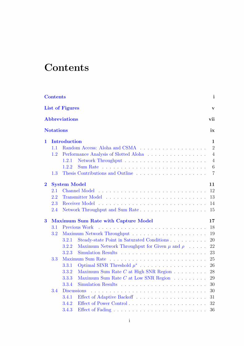
Notations

hk Small-scale fading coefficient of node k

γk Large-scale fading coefficient of node k

gk Channel gain from node k to the receiver

Pk Transmission power of node k

P0 Mean received power

Nt The number of successfully decoded packets in time slot t

n Number of nodes

K Cutoff phase of HOL packets

ρ Mean received SNR

µ SINR threshold

µ∗ Optimal SINR threshold

πT Service rate of each node’s queue

R Information encoding rate of each packet

Rs Sum Rate

p Steady-state probability of successful transmission of HOL packets

pA Network steady-state point in saturated conditions

{qi}i=0,...,K Transmission probabilities of nodes

ix

x Notations

{q∗i }i=0,...,K Optimal transmission probabilities of nodes

rCi Conditional probability of one packet being successfully decoded given that it

has i concurrent packet transmissions for the capture model over fading

channels

rAWGNi Conditional probability of one packet being successfully decoded given that it

has i concurrent packet transmissions for the capture model over AWGN

channels

rNSi Conditional probability of one packet being successfully decoded given that it

has i concurrent packet transmissions for the unordered SIC over fading

channels

rOSi Conditional probability of one packet being successfully decoded given that it

has i concurrent packet transmissions for the ordered SIC over fading

channels

λ Aggregate input rate

λout Network throughput

λCmax Maximum network throughput with the capture model over fading channels

λAWGNmax Maximum network throughput with the capture model over AWGN channels

λNSmax Maximum network throughput with the unordered SIC over fading channels

λOSmax Maximum network throughput with the ordered SIC over fading channels

C Maximum sum rate

CAWGN Maximum sum rate with the capture model over AWGN channels

Ccollision Maximum sum rate with the collision model

Chapter 1

Introduction

Wireless communications have become an inseparable part of our daily life

since Heinrich Hertz demonstrated the existence of electromagnetic waves in 1888.

Driven by the soaring demand of applications, wireless communication systems

have experienced explosive growth over the past century. Diverse wireless systems

including wireless cellular networks, Wi-Fi networks based on the family of IEEE

802.11 standards, wireless sensor networks, and wireless ad-hoc networks have

been developed, offering a wide range of services to enrich peoples lives.

Due to the broadcast nature of wireless channels and spectrum limitation,

a fundamental problem in wireless communication systems is how to provide an

efficient means for multiple nodes to share a single channel. To address this issue,

various multiple access strategies have been developed for different types of wireless

networks, which can be broadly classified into two categories: centralized and

distributed.

The centralized scenario involves the use of a central controller that collects

all information and performs resource optimization for multiple users to satisfy

their performance requirements. For instance, a base station (BS) in cellular sys-

tems serves as the central controller and allocates resources to users located in its

cell. Typical examples of centralized multiple access technologies include Frequen-

cy Division Multiple Access (FDMA) in the first-generation (1G) system, Time

Division Multiple Access (TDMA) in the second-generation (2G) system, Code

Division Multiple Access (CDMA) in the third-generation (3G) system, and Or-

thogonal Frequency Division Multiple Access (OFDMA) in the fourth-generation

(4G) Long Term Evolution (LTE) system.

1

2 Chapter 1

Despite their high efficiency, centralized multiple access strategies entail high

implementation cost and system complexity. Therefore, distributed multiple ac-

cess strategies, which are also known as random access, are more appealing for

low-cost data networks than centralized multiple access strategies. Random-access

networks have no central controller to perform resource allocation among multiple

users. Instead, each user competes for the channel resource. Random access is

widely applied in many wireless networks, such as IEEE 802.11 networks, wire-

less ad-hoc networks, and machine-to-machine (M2M) networks [1–4], because of

minimum coordination and distributed control. The following section provides an

overview of the history and evolution of random access.

1.1 Random Access: Aloha and CSMA

The first random-access network, Aloha, was developed in 1968 to connect

multiple users with a central time-sharing computer in the University of Hawaii

under the leadership of Abramson [5]. The first commercial application of Aloha

was launched in 1976 by Comsat General in the Marisat maritime satellite com-

munications system [6]. Thereafter, Aloha has been widely adopted in cellular

systems for signaling and control purposes.

A graphic illustration of the slotted Aloha scheme is shown in Fig. 1.1. The

principle of slotted Aloha is that when a node has a packet to send, it transmits

the packet at the beginning of a time slot with a certain probability. When more

than one node transmit their packets simultaneously, a collision occurs and none of

them can be successfully decoded.1 Packets involved in collisions are retransmitted

after a random time delay according to the backoff strategy.

Node A

Node B

Node C

Collsion Success Collsion Success TimeIdle Idle

Figure 1.1: Graphic illustration of successful transmission and collision inslotted Aloha networks.

1This assumption on the receiver model is referred to as “classical collision model” and hasbeen widely adopted in early studies on random access.

Chapter 1 3

Note that the channel utilization of slotted Aloha is quit poor as each node

attempts to access the channel regardless of other nodes’ behavior. The maximum

channel utilization of slotted Aloha is shown to be e−1 [7], which indicates that

over 60% of the time is wasted when the network is either in collision or idle states.

If nodes can sense the channel first before transmission, then they may reschedule

the packet transmissions to avoid collisions when they sense that the channel busy

(i.e., the channel is dominated by other nodes’ transmissions). As a result, the

channel utilization can be significantly improved. Such an observation has led to

the development of Carrier Sense Multiple Access (CSMA) [8].

A graphic illustration of the CSMA scheme is shown in Fig. 1.2. With CSMA,

time is divided into multiple mini time slots with length a, where the value of a is

determined by the ratio of channel propagation delay and the packet transmission

time. It was shown in [8] that the maximum channel utilization approaches 1 as a

goes to zero, which is much higher than that of slotted Aloha. As a result, CSMA

has been widely adopted in commercial LANs, such as IEEE 802.11 WLANs.

Node A

Node B

Node C

CollsionSuccess Success Time

a

Idle Idle Success

Figure 1.2: Graphic illustration of successful transmission and collision inCSMA networks.

Despite the huge success in practical systems, it has been long observed that a

random-access network may suffer from significant performance degradation if the

parameters are not properly set. Yet due to the distributed nature, performance

analysis and optimization of random-access networks are much more difficult than

that in the centralized case, in which a central controller performs resource opti-

mization for the entire network. This thesis focuses on the performance optimiza-

tion of slotted Aloha, which is the simplest and one of the most representative

random-access schemes. A brief literature review on the performance analysis of

slotted Aloha networks is presented in the following section.

4 Chapter 1

1.2 Performance Analysis of Slotted Aloha

1.2.1 Network Throughput

The two basic features shared by most random-access schemes are summarized

as follows.

1. Independent Encoding and Uncoordinated Transmissions : Each node inde-

pendently encodes its information, and decides when to transmit. As the

subset of active nodes is random and time-varying, it is normally assumed

to be unknown at the transmitter side.

2. Time-Slotted and Packet-Based : Though it may not seem to be essential or

necessary for random access, a time-slotted and packet-based network has

been assumed in the literature since Abramson’s Aloha was proposed [7].

Due to the uncoordinated transmissions of nodes, not all the transmitted

packets can be successfully decoded in each time slot.

With the above features of random access, the number of successfully decoded

packets would be varying from time to time. As a result, most studies have focused

on the average number of successfully decoded packets per time slot, which is

referred to as the network throughput. Network throughput performance depends

on a series of key factors including the receiver model and protocol design. Early

studies on random access have focused on the classical collision model, which

assumes that collision occurs and none of the packets can be successfully decoded

when more than one node transmit their packets simultaneously. As at most one

packet can be successfully decoded at each time slot with the collision model, the

network throughput, which is also the fraction of time that an effective output

is produced in this case, cannot exceed 1. The maximum network throughput of

slotted Aloha is shown to be only e−1 with the collision model [7].

Despite extensive studies, how to maximize the network throughput has been

an open question for a long time. In Abramson’s landmark paper [7], by modeling

the aggregate traffic as a Poisson random variable with parameter G, the network

throughput of slotted Aloha with the collision model can be easily obtained as

Ge−G, which is maximized at e−1 when G = 1. To enable the network to operate

at the optimum point for maximum network throughput, nevertheless, it requires

Chapter 1 5

the connection between the mean traffic rate G and key system parameters such

as transmission probabilities of nodes, which turns out to be a challenging issue.

Various retransmission strategies have been developed to adjust the transmission

probability of each node according to the number of backlogged nodes to stabilize2

the network [9–12]. Yet most of them were based on the realtime feedback infor-

mation on the backlog size, which may not be available in a distributed network.

Decentralized retransmission control was further studied in [10, 13–15], where al-

gorithms were proposed to either estimate and feed back the backlog size [13, 15],

or update the transmission probability of each node recursively according to the

channel output [10, 14].

The difficulty originates from the modeling of random-access networks. As

demonstrated in [22], the modeling approaches in the literature can be roughly di-

vided into two categories: channel-centric [7–15] and node-centric [16–20, 23, 24].

Channel-centric approaches capture the essence of contention among nodes by

focusing on the state transition process of the aggregate traffic but ignores the

behavior of each nodes queue; thus, the effect of backoff parameters on the perfor-

mance of each single node is not sufficiently examined. In node-centric approaches,

modeling complexity becomes prohibitively high when the interactions among n-

odes queues are considered. To simplify the analysis, a key approximation is to

regard each node’s queue as an independent queuing system with identically dis-

tributed service time. This key approximation has been widely adopted and shown

to be accurate for the performance evaluation of large multi-queue systems [25].

Service time distribution is still crucially determined by the aggregate activities

of head-of-line (HOL) packets of all the nodes, which require proper modeling of

HOL packets behavior.

A unified analytical framework for two representative random-access proto-

cols, Aloha and CSMA, was recently established by L. Dai in [21, 22], where the

network steady-state points were characterized based on the fixed-point equations

of the limiting probability of successful transmission of HOL packets by assum-

ing the classical collision model. Both steady-state points were derived as explicit

functions of key system parameters including the aggregate input rate, the number

of nodes and the transmission probabilities of nodes, which enable the characteri-

zation of stable regions and performance optimization. In this thesis, the proposed

2Note that various definitions of stability have been developed in the literature. A widelyadopted one is that a network is stable if the network throughput is equal to the aggregate inputrate.

6 Chapter 1

analytical framework is further extended to incorporate some more advanced re-

ceiver structures, based on which explicit expressions of the maximum network

throughput and the corresponding optimal transmission probabilities of nodes are

derived.

1.2.2 Sum Rate

The network throughput evaluates how efficient the time is used for successful

transmission. However, it does not reflect how much information can be trans-

mitted in terms of bits per second per Hz. The data rate performance is usually

of more concern than the network throughput in real-life applications. Therefore,

many studies have focused on the sum rate analysis of random-access networks.

Specifically, from the information-theoretic perspective, random access can

be regarded as a multiple access channel (MAC) with a random number of ac-

tive transmitters. It is well known that the sum capacity of an n-user Additive-

White-Gaussian-Noise (AWGN) MAC is determined by the received SNRs, i.e.,

Csum = log2(1+∑n

i=1 SNRi). However, with random access, the number of active

transmitters is a random variable whose distribution is determined by the protocol

and parameter setting. Moreover, to achieve the sum capacity, joint decoding of all

transmitted codewords should be performed at the receiver side, which might be

unaffordable for random-access networks. Therefore, the sum rate performance of

random access is largely dependent on assumptions on access protocol and receiver

design.

A significant amount of effort has been exerted to explore the information-

theoretic limit of random-access networks. For instance, the concept of rate s-

plitting [26] was first introduced to slotted Aloha networks in [27], where a joint

coding scheme was developed for the two-node case. If each node independently

encodes its information, [28] showed that the sum rate performance of slotted Alo-

ha networks can be improved by adaptively adjusting the encoding rate according

to the number of nodes and the transmission probability of each node. [28] and

[27] are based on the assumption of joint decoding of multiple nodes packets at

the receiver side. In [29], each node was assumed to have its own channel state

information (CSI), and the classical collision model was adopted at the receiver

side. The scaling behavior of the sum rate of slotted Aloha as the number of nodes

Chapter 1 7

n goes to infinity was characterized, and shown to be identical to that of the sum

capacity of MAC.

1.3 Thesis Contributions and Outline

Most previous studies on the performance analysis of slotted Aloha focused on

the collision model, which assumes that when more than one node transmit their

packets simultaneously, a collision occurs and none of the packets can be suc-

cessfully decoded. Although it captures the essence of contention among multiple

nodes, the collision model could be overly pessimistic for wireless systems where

a large difference in the received power of nodes may exist as a result of distinct

channel conditions. In this case, a packet can be successfully decoded as long as its

received signal-to-interference-plus-noise ratio (SINR) is above a certain thresh-

old. Such a receiver is referred to as the capture model [38–51]. Efficiency can be

further improved but at the cost of increased receiver complexity if multiple pack-

ets can be jointly decoded by using multiuser detectors, such as Minimum Mean

Square Error (MMSE) and Successive Interference Cancelation (SIC) [27, 28, 52–

56]. Studies have been conducted on the performance analysis of slotted Aloha

with highly advanced receiver structures [27, 28, 38–56]. Although various ana-

lytical models were developed in these studies, many of them rely on numerical

methods to calculate the sum rate under specific settings. How to maximize the

sum rate by optimizing the system parameters remains largely unknown.

This thesis is devoted to the maximum sum rate characterization of slotted

Aloha under various receiver structures. The effects of backoff, power control,

multipacket reception and channel fading on the sum rate performance of slotted

Aloha networks are also discussed. The contributions of this thesis are summarized

as follows.

The analysis begins with the maximum sum rate characterization of slotted

Aloha with the capture model, which is presented in Chapter 3. By assuming that

the nodes are unaware of the instantaneous realization of channel gains and thus

have a uniform information encoding rate, the conditional probability of one pack-

et being successfully decoded given that it has i concurrent packet transmissions,

ri, is derived first. Based on it, the network steady-state point in saturated con-

ditions is further obtained as a function of the SINR threshold, which determines

8 Chapter 1

a fundamental tradeoff between the information encoding rate and the network

throughput. Explicit expressions of the maximum sum rate and the optimal set-

ting are obtained, which show that similar to the ergodic sum capacity of the

multiple access fading channel, the maximum sum rate of slotted Aloha also log-

arithmically increases with the mean received SNR, however, the high-SNR slope

is only e−1.

In Chapter 4, the analysis is further extended to incorporate the capacity-

achieving receiver structure, SIC. The reason why we consider SIC is two-fold.

First of all, as shown in Chapter 3, the high-SNR slope of the maximum sum rate

of slotted Aloha with the capture model is only e−1, which is far below that of the

ergodic sum capacity of multiple access fading channels. Nevertheless, whether the

gap is caused by the random access nature or suboptimality of the receiver (i.e.,

the capture model) is difficult to determine. By adopting the capacity-achieving

receiver structure, we can pinpoint the rate loss due to random access. Moreover,

SIC and the capture model both have the multipacket reception (MPR) capability.

The effect of MPR on the maximum sum rate performance of slotted Aloha can be

further evaluated by comparing the MPR receivers, including SIC and the capture

model, with the classical collision model.

Specifically, two representative SIC receivers, ordered SIC and unordered SIC

are considered. The maximum sum rates for both ordered SIC and unordered

SIC are characterized to address the first issue. Compared to the capture model,

the analysis shows that the rate gains are significant only with the ordered SIC

at moderate values of the mean received SNR. Meanwhile, the rate gap at the

high-SNR region sharply diminishes, and all of them have the same high-SNR

slope e−1, which is much lower than that of the ergodic sum capacity of fading

channels. This indicates that the rate loss is significant due to uncoordinated

random transmissions of nodes. For the second issue, by comparing both the SIC

receivers and the capture model to the classical collision model, it is demonstrated

that in contrast to the significant network throughput improvement brought by

MPR receiver structures at the low SNR region, the rate gain is marginal, and

becomes negligible at the high SNR region.

The effects of key factors, including backoff, power control and channel fad-

ing, on the sum rate performance of Aloha networks are also discussed, which shed

important light on the practical network design. For instance, by considering the

heterogeneous case, where nodes in the same group have identical mean received

Chapter 1 9

SNRs but the SNRs differ from group to group, it is shown that a large SNR

difference among nodes may be beneficial to the sum rate performance, though

serious unfairness is introduced. Moreover, the maximum sum rate with the cap-

ture model over the AWGN channel is characterized to demonstrate the effect of

channel fading. The comparison with that over fading channels shows that fading

always exerts negative effects if CSI is unavailable at the transmitter side.

The remainder of this thesis is organized as follows. Chapter 2 introduces

the system model and basic assumptions of this thesis. Chapter 3 presents the

maximum sum rate analysis of slotted Aloha networks with the capture model.

The analysis is further extended to SIC receivers in Chapter 4. Chapter 5 provides

the conclusions and suggestions for future work.

Chapter 2

System Model

This chapter presents the system model and basic assumptions which will be

used throughout the analysis in the following chapters. It is organized as follows.

Section 2.1 describes the assumptions on the channel model. The transmitter mod-

el and receiver model are introduced in Section 2.2 and Section 2.3, respectively.

The network throughput and sum rate are further defined in Section 2.4.

11

12 Chapter 2

HOL packet

Receiver

Node 1

Node 2

Node 3

Node n

Figure 2.1: Graphic illustration of an n-node slotted Aloha network.

Consider a slotted Aloha network where n nodes transmit to a single receiver,

as Fig. 2.1 illustrates.1 All the nodes are synchronized and can start a transmis-

sion only at the beginning of a time slot. We assume perfect and instant feedback

from the receiver and ignore the subtleties of the physical layer such as the switch-

ing time from receiving mode to transmitting mode and the delay required for

information exchange.

2.1 Channel Model

Let gk denote the channel gain from node k to the receiver, which can be

further written as gk = γk · hk, where hk is the small-scale fading coefficient of

node k which varies from time slot to time slot and is modeled as a complex

Gaussian random variable with zero mean and unit variance. The large-scale

fading coefficient γk characterizes the long-term channel effect such as path loss

and shadowing. Due to the slow-varying nature, the large-scale fading coefficients

are usually available at the transmitter side through channel measurement. Let us

first assume that power control is performed to overcome the effect of large-scale

fading.2 Specifically, denote the transmission power of node k as Pk. Then we

1Note that the MAC scenario considered in this thesis should be distinguished from the ad-hoc scenario which has been extensively studied in recent years [30–36]. In contrast to theMAC where multiple nodes transmit to a common receiver, multiple transmitter-receiver pairsexist in the ad-hoc case. Representative applications of the former one include cellular systemsand IEEE 802.11 networks, where in each cell/basic-service-set, multiple users transmit to thebase-station/access-point. The latter is usually considered in a wireless ad-hoc network, such aswireless sensor networks.

2In practical systems such as cellular systems, the base-station sends a pilot signal periodicallyfor all the users in its cell to measure their large-scale fading gains and adjust their transmissionpower accordingly to maintain constant mean received power. This process is usually referredto as open-loop power control.

Chapter 2 13

T 1 2 K0

01 q

0 tq p0 tq p

0 (1 )tq p 1(1 )tq p

11 q 21 q 1 K tq p

1 tq p 2 tq p

01 q

K tq p

0 (1 )tq p

...2 (1 )tq p 1(1 )K tq p

Figure 2.2: State transition diagram of an individual HOL packet in slottedAloha networks.

have

Pk · |γk|2 = P0. (2.1)

In this case, each node has the same mean received SNR ρ = P0/σ2. To demon-

strate the effect of power control, this assumption will be relaxed in Section 3.3,

where the analysis is extended to incorporate distinct mean received SNRs.

2.2 Transmitter Model

An n-node buffered slotted Aloha network is essentially an n-queue-single-

server system whose performance is determined by the aggregate activities of HOL

packets. The behavior of each HOL packet can be modeled as a discrete-time

Markov process shown in Fig. 2.2. Specifically, a fresh HOL packet is initially in

State T, and moves to State 0 if it is not transmitted. Define the phase of a HOL

packet as the number of unsuccessful transmissions it experiences. A phase-i HOL

packet stays in State i if it is not transmitted. Otherwise, it moves to State T if its

transmission is successful, or State min(K, i+1) if the transmission fails, where K

denotes the cutoff phase. Note that the cutoff phase K can be any non-negative

integer. When K = 0, States 0 and K in Fig. 2.2 would be merged into one state,

i.e., State 0.

In Fig. 2.2, pt denotes the probability of successful transmission of HOL

packets at time slot t. The steady-state probability distribution of the Markov

chain in Fig. 2.2 can be further obtained as

πT = 1∑K−1i=0

(1−p)iqi

+(1−p)KpqK

, (2.2)

14 Chapter 2

andπ0 = 1−pq0pq0

πT . K = 0

π0 = 1−q0q0πT , πi = (1−p)i

qiπT , i = 1, . . . , K − 1, πK = (1−p)K

pqKπT . K ≥ 1,

(2.3)

where p = limt→∞

pt. Note that πT is the service rate of each node’s queue as the

queue has a successful output if and only if the HOL packet is in State T.

Throughout the thesis, we assume that the transmitters are unaware of the

instantaneous realizations of the small-scale fading coefficients. As a result, each

node independently encodes its information at a constant rate R bit/s/Hz. Assume

that each codeword lasts for one time slot, i.e., no coding over successive packets.

Moreover, we consider the saturated conditions where each node always has packets

in its buffer.

2.3 Receiver Model

At the receiver side, let

µ = 2R − 1 (2.4)

denote the signal-to-interference-plus-noise ratio (SINR) threshold. A packet can

be successfully decoded if its received SINR is above the threshold µ.3 In Chapter

3 and 4, we will consider the following two receiver structures respectively:

1) Capture model: With the capture model, each packet is decoded inde-

pendently by treating others as background noise. A packet can be successfully

decoded as long as its received signal-to-interference-plus-noise ratio (SINR) is

above a certain threshold.

2) SIC: With the SIC receivers, once a packet is successfully decoded, it

is subtracted from the aggregate received signal before decoding other packets.

There are many variants of the SIC receiver. Specifically, two representative SIC

receivers are considered:

3More specifically, denote the received SINR of node k as ηk. If log2(1 + ηk) > R, then byrandom coding the error probability of node k’s packet is exponentially reduced to zero as theblock length goes to infinity. Here we assume that the block length is sufficiently large such thatnode k’s packet can be successfully decoded as long as ηk ≥ µ. Note that this is an ideal case. Inpractice, the threshold not only depends on the information encoding rate R, but also the errorprobability that is determined by the coding and decoding schemes.

Chapter 2 15

• Ordered SIC: The most widely used SIC assumes that packets are decoded

in descending order of the received power. In each iteration, the packet with

the highest received power is decoded, and is subtracted from the aggregate

received signal if it is successfully decoded. Otherwise, the decoding process

terminates4.

• Unordered SIC: As a comparison benchmark, we also consider the case that

packets are decoded in a random order. In each iteration, a packet is decod-

ed and is subtracted from the aggregate received signal if it is successfully

decoded. Otherwise, move to the next packet and repeat the process until

all the packets are decoded.

2.4 Network Throughput and Sum Rate

In this thesis, we focus on the long-term system behavior and define the sum

rate as the time-average of the received information rate:

Rs = limT→∞

1

T

T∑t=1

R ·Nt, (2.5)

where Nt denotes the number of successfully decoded packets in time slot t, which

is a time-varying variable. Define the network throughput as the average number

of successfully decoded packets per time slot, which can be written as

λout = limT→∞

1

T

T∑t=1

Nt. (2.6)

According to (2.5-2.6), we then have

Rs = R · λout. (2.7)

Note that the sum rate is closely dependent on the transmission probabilities

{qi}i=0,...,K and the SINR threshold µ. In this thesis, we aim at maximizing the

sum rate by optimally choosing the transmission probabilities {qi}i=0,...,K and the

SINR threshold µ: C = maxµ,{qi}Rs. By combining (2.4) and (2.7), the maximum

4If the packet with the highest received power cannot be successfully decoded, then otherpackets cannot be successfully decoded either.

16 Chapter 2

sum rate can be further written as

C = maxµ

λmax log2(1 + µ), (2.8)

where λmax = max{qi} λout denotes the maximum network throughput.

Both the information encoding rate R and the network throughput λout de-

pend on the SINR threshold µ. Intuitively, by reducing µ, more packets can be

successfully decoded at each time slot, yet the information encoding rate becomes

smaller. Therefore, the SINR threshold µ should be carefully chosen to maximize

the sum rate. Note that the network throughput λout is also crucially determined

by the protocol design and backoff parameters. In the following chapters, we will

consider the capture model and SIC separately, and characterize the maximum

sum rate of slotted Aloha networks in each case.

Chapter 3

Maximum Sum Rate with

Capture Model

This chapter characterizes the maximum sum rate of Aloha networks with

the capture model. This chapter is organized as follows. Section 3.1 presents

a literature review of previous related work. The steady-state point in saturat-

ed conditions is derived in Section 3.2, based on which the maximum network

throughput is further characterized. Maximum sum rate is characterized in Sec-

tion 3.3. The effects of backoff, power control and channel fading on the sum rate

performance of slotted Aloha networks are discussed in Section 3.4. Section 3.5

summarizes this chapter.

17

18 Chapter 3

3.1 Previous Work

It has been mentioned in Chapter 1 that early studies on random-access have

focused on the classical collision model, which assumed that a packet transmission

is successful only if there are no concurrent transmissions. Though an elegant and

useful simplification of the receiver, the classical collision model could be overly

pessimistic if there exists a large difference of received power. It was first point-

ed out by Roberts in [37] that even with multiple concurrent transmissions, the

strongest signal can be successfully detected as long as the signal-to-interference

ratio (SIR) is sufficiently high. This condition is referred to as the “capture ef-

fect”, which has been extensively studied in [38–51]. With the capture model,

each node’s packet is decoded independently by regarding the packets of others

as background noise. A packet can be successfully decoded as long as its received

signal-to-interference-plus-noise ratio (SINR) is above a certain threshold. In con-

trast to the classical collision model where at most one packet can be successfully

decoded, with the capture model, it is clear that multiple packets can be decoded

simultaneously if the SINR threshold is sufficiently low, which is referred to as

multipacket reception (MPR) capability [47, 51–63].

Many studies have been conducted on performance analysis of slotted Aloha

with the capture model. By assuming Poisson distributed aggregate traffic, for

instance, the network throughput was derived as a function of mean traffic rate

G and SIR in [38–40] under distinct assumptions on channel conditions. Similar

to that in the case of collision model, the maximum network throughput can be

obtained by optimizing G, yet how to properly tune the system parameters to

achieve the maximum network throughput remains unknown. The retransmission

control strategies developed in [9], [13] and [14] were further extended to the cap-

ture model in [43], [45] and [44], respectively. To evaluate the network throughput

performance for given transmission probabilities of nodes, various Markov chains

were also established in [41, 42, 48, 51] to model the state transition of each indi-

vidual user. The computational complexity, nevertheless, sharply increases when

sophisticated backoff strategies are further involved, which renders it extremely

difficult, if not impossible, to search for the optimal configuration to maximize the

network throughput.

In contrast to the network throughput, only few studies focused on the sum

Chapter 3 19

rate performance of slotted Aloha with the capture model [46, 49, 50]. Specifi-

cally, the effects of power allocation and modulation on the sum rate of slotted

Aloha in AWGN channels were analyzed in [46] and [49], respectively. Queueing

stability and channel fading were further considered in [50], where the sum rates

with various cross-layer approaches were derived. Most of them focused on eval-

uating the sum rate under specific settings, where how to maximize the sum rate

remains largely unexplored. As we will demonstrate in this chapter, the sum rate

optimization of slotted Aloha networks can be decomposed into two parts: 1) For

given information encoding rate R, or equivalently, SINR threshold µ, the network

throughput can be maximized by properly choosing backoff parameters (i.e., the

transmission probabilities of nodes). 2) As the information encoding rate and the

maximum network throughput are both functions of the SINR threshold µ, the

sum rate can be further optimized by tuning µ.

Specifically, in this chapter, by extending the unified analytical framework

[21, 22] from the classical collision model to the capture model, the maximum

network throughput is obtained as a function of the SINR threshold µ, based on

which the maximum sum rate is derived by further optimizing the SINR threshold

µ. The effects of backoff, power control and channel fading on the sum rate

performance of slotted Aloha networks are also discussed.

3.2 Maximum Network Throughput

As Fig. 2.1 illustrates, an n-node buffered slotted Aloha network is essen-

tially an n-queue-single-server system whose performance is determined by the

aggregate activities of HOL packets. In this section, we will first derive the net-

work steady-state point in saturated conditions as the single non-zero root of the

fixed-point equation of the steady-state probability of successful transmission of

HOL packets. Then the maximum network throughput will be obtained by opti-

mizing the transmission probabilities of nodes. Finally, simulation results will be

presented to verify the preceding analysis.

20 Chapter 3

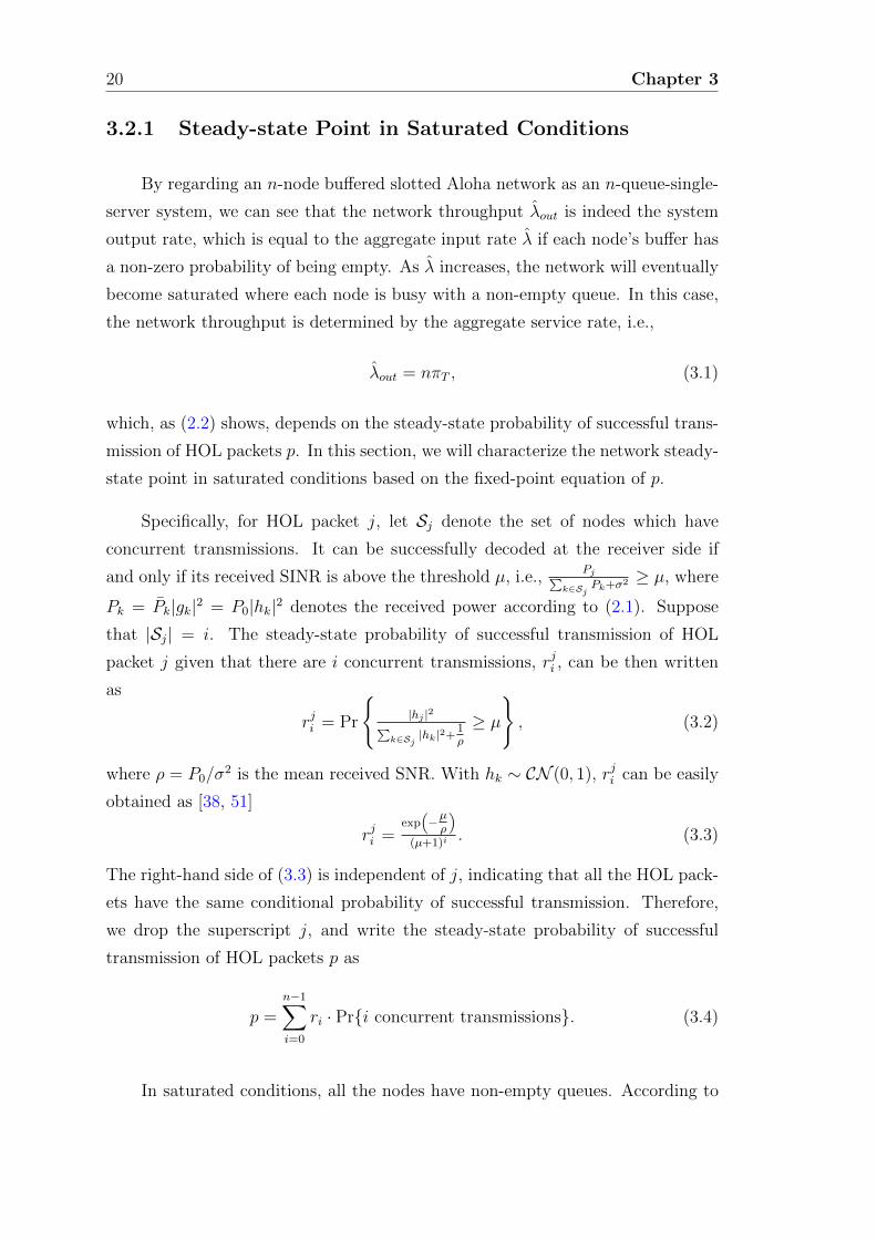
3.2.1 Steady-state Point in Saturated Conditions

By regarding an n-node buffered slotted Aloha network as an n-queue-single-

server system, we can see that the network throughput λout is indeed the system

output rate, which is equal to the aggregate input rate λ if each node’s buffer has

a non-zero probability of being empty. As λ increases, the network will eventually

become saturated where each node is busy with a non-empty queue. In this case,

the network throughput is determined by the aggregate service rate, i.e.,

λout = nπT , (3.1)

which, as (2.2) shows, depends on the steady-state probability of successful trans-

mission of HOL packets p. In this section, we will characterize the network steady-

state point in saturated conditions based on the fixed-point equation of p.

Specifically, for HOL packet j, let Sj denote the set of nodes which have

concurrent transmissions. It can be successfully decoded at the receiver side if

and only if its received SINR is above the threshold µ, i.e.,Pj∑

k∈SjPk+σ2 ≥ µ, where

Pk = Pk|gk|2 = P0|hk|2 denotes the received power according to (2.1). Suppose

that |Sj| = i. The steady-state probability of successful transmission of HOL

packet j given that there are i concurrent transmissions, rji , can be then written

as

rji = Pr

{|hj |2∑

k∈Sj|hk|2+

1ρ

≥ µ

}, (3.2)

where ρ = P0/σ2 is the mean received SNR. With hk ∼ CN (0, 1), rji can be easily

obtained as [38, 51]

rji =exp(−µρ

)(µ+1)i

. (3.3)

The right-hand side of (3.3) is independent of j, indicating that all the HOL pack-

ets have the same conditional probability of successful transmission. Therefore,

we drop the superscript j, and write the steady-state probability of successful

transmission of HOL packets p as

p =n−1∑i=0

ri · Pr{i concurrent transmissions}. (3.4)

In saturated conditions, all the nodes have non-empty queues. According to

Chapter 3 21

the Markov chain shown in Fig. 2.2, the probability that the HOL packet is re-

questing transmission is given by πT q0+∑K

i=0 πiqi, which is equal to πT/p according

to (2.3). Therefore, the probability that there are i concurrent transmissions can

be obtained as

Pr{i concurrent transmissions} =

(n− 1

i

)(1− πT

p

)n−1−i (πTp

)i. (3.5)

By substituting (3.3) and (3.5) into (3.4), the steady-state probability of successful

transmission of HOL packets p can be obtained as

p = exp(−µρ

)·(

1− µµ+1· πTp

)n−1 for large n≈ exp

{−µρ− nµ

µ+1· πTp

}, (3.6)

where the approximation is obtained by applying (1 − x)n ≈ exp (−nx) for 0 <

x < 1.1 Finally, by substituting (2.2) into (3.6), we have

p ≈ exp

(−µρ− nµ

µ+1· 1∑K−1

i=0

p(1−p)iqi

+(1−p)KqK

). (3.7)

The following theorem states the existence and uniqueness of the root of the

fixed-point equation (3.7).

Theorem 3.1. The fixed-point equation (3.7) has one single non-zero root pA if

{qi}i=0,...,K is a monotonic non-increasing sequence.

Proof. See Appendix A.

As we can see from (3.7), the non-zero root pA is closely dependent on backoff

parameters {qi}i=0,...,K . Without loss of generality, let qi = q0 · Qi where q0 is the

initial transmission probability and Qi is an arbitrary monotonic non-increasing

function of i with Q0 = 1 and Qi ≤ Qi−1, i = 1, . . . , K. With the cutoff phase

K = 0, or the backoff function Qi = 1, i = 0, . . . , K, for instance, pA can be

explicitly written as

pA = exp(−µρ− nµ

µ+1q0

). (3.8)

1Note that with a small network size, i.e., n ≤ 5 for instance, the approximation error maybecome noticeable. It, nevertheless, rapidly declines as the number of nodes n increases.

22 Chapter 3

3.2.2 Maximum Network Throughput for Given µ and ρ

It has been shown in Section 3.2.1 that the network operates at the steady-

state point pA in saturated conditions. By combining (3.1) and (3.6), the network

throughput at pA can be written as

λout = (µ+ 1) ·(−pA ln pA

µ− pA

ρ

), (3.9)

where pA is an implicit function of the transmission probabilities qi, i = 0, . . . , K,

which is given in (3.7). It can be seen from (3.9) and (3.7) that the network

throughput is crucially determined by the backoff parameters {qi}. In this section,

we focus on the maximum network throughput λmax = max{qi}λout. The following

theorem presents the maximum network throughput λmax and the corresponding

optimal backoff parameters {q∗i }.

Theorem 3.2. For given SINR threshold µ ∈ (0,∞) and mean received SNR

ρ ∈ (0,∞), the maximum network throughput is given by

λmax =

µ+1µ

exp(−1− µ

ρ

)if µ ≥ 1

n−1

n exp(− nµµ+1− µ

ρ

)otherwise,

(3.10)

which is achieved at

q∗i =

q0Qi if µ ≥ 1n−1

1 otherwise,(3.11)

i = 0, . . . , K, where q0 is given by

q0 = µ+1nµ·

{K−1∑i=0

exp(−1−µ

ρ

)[1− exp

(−1−µ

ρ

)]iQi +

[1− exp

(−1−µ

ρ

)]KQK

}. (3.12)

Proof. See Appendix B.

Eq. (3.10) shows that for given SINR threshold µ, the maximum network

throughput λmax is a monotonic increasing function of the mean received SNR ρ.

As ρ→∞, we have

limρ→∞

λmax =

µ+1µe−1 if µ ≥ 1

n−1

n exp(− nµµ+1

)otherwise,

(3.13)

Chapter 3 23

10-4

10-3

10-2

10-1

100

101

102

10-4

10-3

10-2

10-1

100

101

102

1

1n

= 0 dB

= 20 dB

= 10 dB

max

(a)

m = 0.01

m = 1

m = 0.5

m = 5

(dB) r

max

λˆ

(b)

Figure 3.1: Maximum network throughput of slotted Aloha networks withcapture model λmax versus (a) SINR threshold µ and (b) mean received SNR

ρ. n = 50.

which approaches e−1 when µ� 1.

On the other hand, for given mean received SNR ρ, λmax monotonically de-

creases as the SINR threshold µ increases, as Fig. 3.1a illustrates. With a lower

µ, the receiver can decode more packets among multiple concurrent transmissions,

and thus better throughput performance can be achieved. It can be easily shown

that multipacket reception is possible when the SINR threshold µ is sufficiently

small. Specifically, for µ ≥ 1n−1 , λmax > 1 if and only if 1

n−1 ≤ µ < 1e−1 and

ρ > µ

lnµ+1µ−1

. Otherwise, λmax > 1 if and only if ρ > µ

lnn− nµµ+1

. As Fig. 3.1b

illustrates, with n = 50, if the SINR threshold µ = 0.01 < 1n−1 , λmax > 1 when

the mean received SNR ρ > −25.3dB. On the other hand, if µ = 0.5, we have1

n−1 < µ < 1e−1 ≈ 0.582. In this case, λmax > 1 when the mean received SNR

ρ > 7dB.

3.2.3 Simulation Results

In this section, simulation results are presented to verify the preceding anal-

ysis. In particular, we consider a saturated slotted Aloha network with Binary

Exponential Backoff (BEB) [66–69], i.e., qi = q0 · 12i

, i = 0, . . . , K. Section 3.2.1

24 Chapter 3

0.01 0.1 0.2 0.3 0.4 0.5 0.6 0.7 0.8 0.90

0.1

0.2

0.3

0.4

0.5

0.6

0.7

0.8

1q0

Ap

Simulation

Analysis

Simulation

Analysis

Simulation

Analysis

K = 0 K = 1

K = 3

(a)

0.01 0.1 0.2 0.3 0.4 0.5 0.6 0.7 0.8 0.9 1

0.4

0.5

0.6

0.7

0.8

0.9

1

0.3

q0

Ap

Simulation

Analysis

Simulation

Analysis

Simulation

Analysis

n = 30

n = 50 n = 100

(b)

Figure 3.2: Steady-state point of slotted Aloha networks with capture modelpA versus initial transmission probability q0. (a) n = 50. µ = 1 and ρ = 10dB.

(b) K = 0. µ = 0.01 and ρ = 0dB.

has shown that it operates at the steady-state point pA, which is closely deter-

mined by the number of nodes n and the backoff parameters {qi}. The expression

of pA is given in (3.7) and verified by simulation results presented in Fig. 3.2.2

Fig. 3.3 illustrates the corresponding network throughput performance. The

network throughput λout has been derived as a function of pA in (3.9) in Section

3.2.2, which varies with the backoff parameters. As we can see from Fig. 3.3, the

network throughput performance is sensitive to the setting of the initial transmis-

sion probability q0. According to Theorem 3.2, when the SINR threshold µ ≥ 1n−1 ,

the maximum network throughput λmax is achieved when q0 is set to be q0. Oth-

erwise, λmax is achieved with qi=1, i = 0, . . . , K. The expressions of λmax and

the corresponding optimal backoff parameters q∗i are given in (3.10) and (3.11),

respectively, and verified by the simulation results presented in Fig. 3.3.

Note that in spite of the improvement on the maximum network throughput

by reducing the SINR threshold µ, the information encoding rate that can be

supported for reliable communications, i.e., R = log2(1 + µ), is quite low when µ

is small. It is clear that the SINR threshold µ determines a tradeoff between the

network throughput and the information encoding rate. In the next section, we

will further study how to maximize the sum rate by properly choosing the SINR

threshold µ.

2In simulations, the steady-state probability of successful transmission of HOL packets pA isobtained by calculating the ratio of the number of successful transmissions to the total numberof attempts of HOL packets over a long time period, i.e., 108 time slots.

Chapter 3 25

00.2 0.3 0.4 0.5 0.6 0.7 0.8 0.9

0.1

0.2

0.3

0.4

0.5

0.6

0.7

maxλ =0.67ˆ

0.040.07 0.15

denotes 0q

q0

out

λˆ

1

Simulation

Analysis

0K =

Simulation

Analysis

1K =

Simulation

Analysis

3K =

(a)

0.01 0.1 0.2 0.3 0.4 0.5 0.6 0.7 0.8 0.9 10

5

10

15

20

25

=30

35

40

Simulation

Analysis

Simulation

Analysis

30

max

n=22

50

max

n

100

max

n=37

q0

ou

t

n = 30

n = 50 n = 100

Simulation

Analysis

(b)

Figure 3.3: Network throughput of slotted Aloha networks with capture modelλout versus initial transmission probability q0. (a) n = 50. µ = 1 and ρ = 10dB.

(b) K = 0. µ = 0.01 and ρ = 0dB.

3.3 Maximum Sum Rate

In this section, we will derive the maximum sum rate and the corresponding

optimal SINR threshold as functions of the mean received SNR ρ, and discuss

their characteristics at the high SNR and lower SNR regions, respectively.

Specifically, it has been demonstrated in Section 2.4 that the sum rate of

slotted Aloha networks is determined by the information encoding rate R and the

network throughput λout. Section 3.2.2 further shows that if backoff parameters

{qi} are properly selected, the network throughput is maximized at λmax, which

is a function of the SINR threshold µ. By combining (2.8) and Theorem 3.2,

the maximum sum rate can be further written as C = maxµ>0 f(µ), where the

objective function f(µ) is given by

f(µ) =

µ+1µ

exp(−1− µ

ρ

)log2(1 + µ) if µ ≥ 1

n−1


ρ

)log2(1 + µ) otherwise.

(3.14)

The following theorem presents the maximum sum rate C and the optimal SINR

threshold µ∗.

26 Chapter 3

Theorem 3.3. For given mean received SNR ρ ∈ (0,∞), the maximum sum rate

is

C =

µ∗h+1

µ∗hexp

(−1− µ∗h

ρ

)log2(1 + µ∗h) if ρ ≥ ρ0

n exp(− nµ∗lµ∗l+1

− µ∗lρ

)log2(1 + µ∗l ) otherwise,

(3.15)


µ∗ =

µ∗h if ρ ≥ ρ0

µ∗l otherwise,(3.16)

where µ∗h and µ∗l are the roots of the following equations:

(µ+ 1)µ+1ρ

+1µ = e, (3.17)

and

(µ+ 1)µ+1ρ

+nµ+1 = e, (3.18)

respectively, and

ρ0 =nn−1 ln

nn−1

1−(n−1) ln nn−1

. (3.19)

Proof. See Appendix C.

Note that ρ0 is a monotonic decreasing function of n ∈ [2,∞), and limn→∞ ρ0 =

2. When the number of nodes n is large, ρ0 is close to 3dB.

3.3.1 Optimal SINR Threshold µ∗

Theorem 3.3 shows that to achieve the maximum sum rate, the SINR thresh-

old µ should be carefully selected. Fig. 3.4a illustrates how the optimal SINR

threshold µ∗ varies with the mean received SNR ρ. At the low SNR region, i.e.,

ρ < ρ0, for instance, we can obtain from (3.16) and (3.18) that µ∗ρ<ρ0 = µ∗l ≈

e−W0

(− 1n

)− 1 for large n, where W0(z) is the principal branch of the Lambert W

function [64]. In this case, the effect of the mean received SNR ρ becomes negligi-

ble, and µ∗ρ<ρ0 reduces to a monotonic decreasing function of the number of nodes

n. With a large n, µ∗ρ<ρ0 � 1, implying that multiple packets can be successfully

decoded.

Chapter 3 27

3

(dB)r

*μ

denotes 0r

30n =

50n =

100n =

(a)

3

*

max

μ=μ

λ

30n =

50n =

100n =

(dB)r

denotes 0r

(b)

Figure 3.4: (a) Optimal SINR threshold µ∗ and (b) maximum network

throughput λµ=µ∗

max of slotted Aloha networks with capture model versus meanreceived SNR ρ.

At the high SNR region, we can obtain from (3.16-3.17) that µ∗ρ≥ρ0 = µ∗h ≈eW0(ρ) for large ρ. As we can see from Fig. 3.4a, with ρ � 1, the optimal SINR

threshold µ∗ρ≥ρ0 monotonically increases with the mean received SNR ρ.

By combining (3.16) with Theorem 3.2, we can also obtain the maximum

network throughput with µ = µ∗ as

λµ=µ∗

max =

µ∗h+1

µ∗hexp

(−1− µ∗h

ρ

)if ρ ≥ ρ0

n exp(− nµ∗lµ∗l+1

− µ∗lρ

)otherwise.

(3.20)

Fig. 3.4b illustrates how the maximum network throughput λµ=µ∗

max varies with the

mean received SNR ρ. As we can see from Fig. 3.4b, at the low SNR region, i.e.,

ρ < ρ0, the effect of ρ is negligible, and λµ=µ∗

max,ρ<ρ0 becomes a monotonic increasing

function of the number of nodes n. In this case, the optimal SINR threshold

µ∗ρ<ρ0 = µ∗l is decreased as n grows, and thus more packets can be successfully

decoded, though each at a smaller information encoding rate. For large n, we

have λµ=µ∗

max,ρ<ρ0 ≈ ne−1 according to (3.20).

At the high SNR region, Fig. 3.4a has shown that the optimal SINR threshold

µ∗ρ≥ρ0 = µ∗h is much larger than 1, with which at most one packet can be successfully

decoded at each time slot. Therefore, the maximum network throughput λµ=µ∗

max,ρ≥ρ0

quickly drops below 1, and eventually approaches e−1 as ρ→∞.

28 Chapter 3

5 10 15 20 25 300

0.5

1

1.5

2

2.5

3

High-SNR

approximation

(22)

(28)

(dB)

C(bit/s/Hz)

(a)

-20 -15 -10 -5 00

0.1

0.2

0.3

0.4

0.5

30n

100n

(22)

(29)

3

12loge e

(dB)

C(bit/s/Hz)

Large-n approximation

(b)

Figure 3.5: Maximum sum rate performance of slotted Aloha networks withcapture model. (a) Maximum sum rate C at the high SNR region. (b) Maximum

sum rate C at the low SNR region.

3.3.2 Maximum Sum Rate C at High SNR Region

Similar to Section 3.3.1, let us take a closer look at the maximum sum rate

C at different SNR regions.

With ρ ≥ ρ0, it has been shown in Section 3.3.1 that the optimal SINR

threshold µ∗ρ≥ρ0 = µ∗h ≈ eW0(ρ) for large ρ. The maximum sum rate in this case

can be then approximated by

Cρ≥ρ0 ≈(1 + e−W0(ρ)

)exp

(−1− eW0(ρ)

ρ

)log2(1 + eW0(ρ)), (3.21)

for ρ � 1. As Fig. 3.5a shows, the approximation (3.21) works well when the

mean received SNR ρ is large, i.e., ρ ≥ 15dB. Moreover, a logarithmic increase of

the maximum sum rate C can be observed at the high SNR region. The following

corollary presents the high-SNR slope of C.

Corollary 3.4. limρ→∞C

log2 ρ= e−1.

Proof. See Appendix D.

Recall that the high-SNR slope of the ergodic sum capacity of MAC is 1 when

single-antenna is employed at both the transmitters and the receiver. To achieve

the ergodic sum capacity, however, a joint decoding of all received signals is re-

quired and the codewords should span multiple fading states. With the capture

Chapter 3 29

model, in contrast, each node’s packet is decoded independently by treating oth-

ers’ as background noise at each time slot. When the mean received SNR is high,

at most one packet can be successfully decoded each time due to a large SINR

threshold µ∗ � 1. Corollary 3.4 shows that with the simplified receiver, the high-

SNR slope of the maximum sum rate of slotted Aloha networks is significantly

lower than that of the sum capacity.

3.3.3 Maximum Sum Rate C at Low SNR Region

For ρ < ρ0, it has been shown in Section 3.3.1 that the optimal SINR threshold

µ∗ρ<ρ0 = µ∗l ≈ e−W0

(− 1n

)− 1 for large n. The corresponding maximum sum rate

can be then approximated by

Cρ<ρ0 ≈ −nW0

(− 1n

)· exp

−n(1−eW0

(− 1n

))− e−W0

(−1n

)−1

ρ

log2 e, (3.22)

for n � 1. As we can see from Fig. 3.5b, the approximation (3.22) works well

when the number of nodes n is large. The following corollary further presents the

limiting maximum sum rate as n→∞ at the low SNR region.

Corollary 3.5. limn→∞Cρ<ρ0 = e−1log2 e.

Proof. See Appendix E.

Note that it has been shown in Section 3.3.1 that with ρ < ρ0, the maximum

network throughput λµ=µ∗

max ≈ ne−1, which grows with the number of nodes n

unboundedly. Although more packets can be successfully decoded, the information

carried by each packet decreases as n increases due to a diminishing information

encoding rate, i.e., R = log2(1 + µ∗ρ<ρ0) ≈1n

log2 e for large n. Therefore, as

the number of nodes n → ∞, the maximum sum rate reaches a limit that is

independent of the mean received SNR, as Corollary 3.5 indicates. It is in sharp

contrast to the ergodic sum capacity of MAC which linearly increases with n and

ρ at the low SNR region.

30 Chapter 3

0.02 2 4 6 8 10 12 14 16 18 200

0.2

0.4

0.6

0.8

1

2.9 9.2

0 dBC =0.53

10 dBC =0.73

=1.0215 dBC

Simulation

Analysis

0 dB

Simulation

Analysis

10 dB

Simulation

Analysis

15 dB

sR (bit/s/Hz)

denotes *

Figure 3.6: Sum rate of slotted Aloha networks with capture model Rs versusSINR threshold µ under different values of mean received SNR ρ. n = 50.

K = 0 and q0 = q∗0.



ysis. Again we consider a saturated slotted Aloha network with the cutoff phase

K = 0. It has been demonstrated in Section 3.3 that as both the maximum net-

work throughput and the information encoding rate depend on the SINR threshold

µ, the sum rate can be maximized by optimally choosing µ. We can clearly observe

from Fig. 3.6 that the sum rate performance is sensitive to the SINR threshold

µ especially when the mean received SNR ρ is small. To achieve the maximum

sum rate, µ should be properly set according to ρ. The expressions of the optimal

SINR threshold µ∗ and the maximum sum rate C are given in Theorem 3.3, and

verified by the simulation results presented in Fig. 3.6.

3.4 Discussions

So far we have shown that to optimize the sum rate performance of slotted

Aloha networks, the SINR threshold µ and backoff parameters {qi} should be

properly set according to the mean received SNR ρ, and the maximum sum rate

logarithmically increases with ρ with the high-SNR slope of e−1. In this section,

Chapter 3 31

we will further discuss how the performance is affected by key factors such as

backoff, power control and channel fading.

3.4.1 Effect of Adaptive Backoff

Backoff is a key component of random-access networks. It has been shown

in Sections 3.2 and 3.3 that to achieve the maximum sum rate, backoff parame-

ters, i.e., the transmission probabilities {qi} of nodes, should be adaptively tuned

according to the number of nodes n and the mean received SNR ρ.3 In many stud-

ies, however, nodes are supposed to transmit their packets with a fixed probability

[39, 41, 42, 48, 51]. To see how the rate performance of slotted Aloha deterio-

rates without adaptive backoff, let us assume that each node transmits its packet

with a constant probability q at each time slot, i.e., qi = q, i = 0, . . . , K. In this

case, the network steady-state point in saturated conditions can be obtained from

(3.7) as pqi=qA = exp(−µρ− nqµ

µ+1

), and the corresponding network throughput is

λqi=qout = nq exp(−µρ− nqµ

µ+1

), according to (3.9). The sum rate can be then written

as Rqi=qs = nq exp

(−µρ− nqµ

µ+1

)· log2(1 + µ), which is an increasing function of the

mean received SNR ρ.

As ρ→∞, it can be easily obtained that Rqi=qs = limρ→∞R

qi=qs = nq exp

(− nqµµ+1

)·

log2(1 + µ), with the maximum

maxµ

Rqi=qs = nq exp

(−nq

(1−eW0

(− 1nq

)))· log2 e

−W0

(− 1nq

), (3.23)


µ∗,qi=q = e−W0

(− 1nq

)− 1. (3.24)

Eq. (3.24) shows that the optimal SINR threshold µ∗,qi=q monotonically decreases

as the number of nodes n grows. For large n � 1, it can be obtained from

3Note that for practical random-access networks, the backoff parameters can be updatedthrough the feedback from the common receiver. In IEEE 802.11 networks, for instance, as eachnode associates with the access-point (AP) upon joining the network, the AP can count thenumber of nodes through the MAC header of the frame sent by each node, calculate the optimalbackoff parameters, and broadcast them in the beacon frame periodically. Each node can thenupdate its backoff parameters according to the received beacon frame. Such a feedback-basedupdate process can also be implemented in cellular systems where the base-station serves as thecommon receiver in each cell.

32 Chapter 3

(3.23-3.24) that µ∗,qi=q ≈ 1nq

, and

maxµ

Rqi=qs

n�1≈ e−1log2 e. (3.25)

Recall that it has been shown in Section 3.3.2 that the maximum sum rate increases

with the mean received SNR ρ unboundedly. Here (3.25) indicates that with a

constant transmission probability, the sum rate converges to a limit that is much

lower than 1 as ρ→∞. It corroborates that adaptive backoff is indispensable for

random-access networks.

It is interesting to note that when q = 1, all the nodes persistently transmit

their packets, and the slotted Aloha network reduces to a typical MAC. It is well

known that for an n-user AWGN MAC, if the capture model is adopted at the

receiver side and all the users have equal received power, the sum rate approaches

log2 e as n→∞ [65]. Here we can see from (3.25) that an additional factor of e−1

is introduced, which is mainly attributed to the effect of channel fading.4

3.4.2 Effect of Power Control

So far we have focused on a homogeneous slotted Aloha network where all

the nodes have the same mean received SNR ρ. In this section, the analysis will

be extended to the heterogeneous case, where nodes in the same group have an

identical mean received SNR but SNRs differ from group to group.

Specifically, assume that n nodes are divided into M groups. Group m has nm

nodes, and each node in Group m has the mean received SNR ρm, m = 1, . . . ,M .

For HOL packet j, let Sj denote the set of nodes that have concurrent transmis-

sions. It can be successfully decoded at the receiver if and only if its received

SINR is above the SINR threshold µ, i.e.,Pj∑

k∈SjPk+σ2 ≥ µ, where Pk denotes the

received power of node k’s packet. Suppose that Sj =⋃m=1,...,M Smj , where Smj

denotes the set of nodes which have concurrent transmissions in Group m, and

|Smj | = im, m = 1, . . . ,M . The steady-state probability of successful transmission

of HOL packet j given that there are {im}m=1,...,M concurrent transmissions, rj{im},

can be then written as rj{im} = Pr

{|hj |2∑M

m=1

∑k∈Sm

j|hk|2·

ρmρj

+1ρj

≥ µ

}. It can be easily

4Note that in this thesis, each codeword is assumed to last for one channel coherence timeperiod. Without coding over different fading states, the channel fluctuations cannot be averagedout.

Chapter 3 33

shown that with hk ∼ CN (0, 1), rj{im} is given by

rj{im} =exp

(− µρj

)∏Mm=1

(1+

ρmρjµ

)im . (3.26)

It can be seen from (3.26) that rj{im} is determined by the mean received SNR ρj

of HOL packet j. Suppose that HOL packet j belongs to Group l ∈ {1, · · · ,M}.As nodes in the same group have an identical mean received SNR, the superscript

j can be replaced by its group index l. The steady-state probability of successful

transmission of HOL packet j in Group l ∈ {1, · · · ,M} can then be written as

p(l) =

n1∑i1=0

· · ·nl−1∑il=0

· · ·nM∑iM=0

rl{im}

·M∏m=1

Pr{im concurrent transmissions in Group m}. (3.27)

For each node in Group m, the probability that it is busy with the HOL packet

requesting transmission in saturated conditions is given by π(m)T q0 +

∑Ki=0 π

(m)i qi,

which is equal to π(m)T /p(m) according to (2.3). Therefore, we have

Pr{im concurrent transmissions in Group m}

=

(nmim

) (1−π(m)

T /p(m))nm−im

·(π(m)T /p(m)

)imm6=l(

nl−1il

) (1−π(l)

T /p(l))nl−1−il

·(π(l)T /p

(l))il

m=l.(3.28)

By combining (3.26-3.28), the steady-state probability of successful transmis-

sion of HOL packet j in Group l ∈ {1, · · · ,M} can be obtained as

p(l)= exp(− µρl

)·(

1− µµ+1· π

(l)T

p(l)

)nl−1·

M∏m=1,m6=l

(1− µ

µ+ρl/ρm·π

(m)T

p(m)

)nmfor large n1,...,nM≈ exp

(− µρl−

M∑m=1

nmµµ+ρl/ρm

· π(m)T

p(m)

). (3.29)

Finally, by substituting (2.2) into (3.29), we have

p(l)= exp

− µρl−

M∑m=1

nmµµ+ρl/ρm

· 1∑K−1i=0

p(m)(1−p(m))i

qi+

(1−p(m))K

qK

, (3.30)

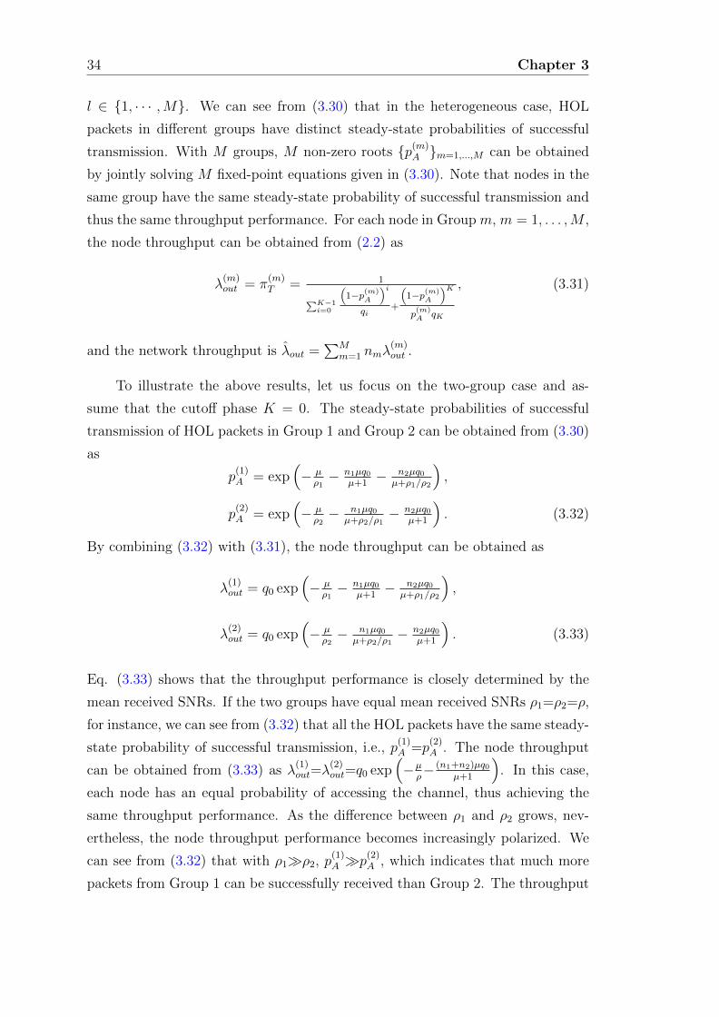
34 Chapter 3

l ∈ {1, · · · ,M}. We can see from (3.30) that in the heterogeneous case, HOL

packets in different groups have distinct steady-state probabilities of successful

transmission. With M groups, M non-zero roots {p(m)A }m=1,...,M can be obtained

by jointly solving M fixed-point equations given in (3.30). Note that nodes in the

same group have the same steady-state probability of successful transmission and

thus the same throughput performance. For each node in Group m, m = 1, . . . ,M ,

the node throughput can be obtained from (2.2) as

λ(m)out = π

(m)T = 1

∑K−1i=0

(1−p(m)

A

)iqi

+

(1−p(m)

A

)Kp(m)A qK

, (3.31)

and the network throughput is λout =∑M

m=1 nmλ(m)out .

To illustrate the above results, let us focus on the two-group case and as-

sume that the cutoff phase K = 0. The steady-state probabilities of successful

transmission of HOL packets in Group 1 and Group 2 can be obtained from (3.30)

as

p(1)A = exp

(− µρ1− n1µq0

µ+1− n2µq0

µ+ρ1/ρ2

),

p(2)A = exp

(− µρ2− n1µq0

µ+ρ2/ρ1− n2µq0

µ+1

). (3.32)

By combining (3.32) with (3.31), the node throughput can be obtained as

λ(1)out = q0 exp

(− µρ1− n1µq0

µ+1− n2µq0

µ+ρ1/ρ2

),

λ(2)out = q0 exp

(− µρ2− n1µq0

µ+ρ2/ρ1− n2µq0

µ+1

). (3.33)

Eq. (3.33) shows that the throughput performance is closely determined by the

mean received SNRs. If the two groups have equal mean received SNRs ρ1=ρ2=ρ,

for instance, we can see from (3.32) that all the HOL packets have the same steady-

state probability of successful transmission, i.e., p(1)A =p

(2)A . The node throughput

can be obtained from (3.33) as λ(1)out=λ

(2)out=q0 exp

(−µρ− (n1+n2)µq0

µ+1

). In this case,

each node has an equal probability of accessing the channel, thus achieving the

same throughput performance. As the difference between ρ1 and ρ2 grows, nev-

ertheless, the node throughput performance becomes increasingly polarized. We

can see from (3.32) that with ρ1�ρ2, p(1)A �p(2)A , which indicates that much more

packets from Group 1 can be successfully received than Group 2. The throughput

Chapter 3 35

1 100 200 300 400 500 600 700 800 900 10000.4

0.6

0.8

1

1.2

1.4

1.6

0 dB

10 dB

15dB

20 dB

1 2

C(b

it/s

/Hz)

Figure 3.7: Maximum sum rate of slotted Aloha networks with capture modelversus ρ1/ρ2 for a two-group slotted Aloha network. n1 = n2 = 25. K = 0.

performance of nodes in Group 1 is then much better than that in Group 2, i.e.,

λ(1)out�λ

(2)out according to (3.33), implying serious unfairness among nodes.

As the maximum network throughput λmax = maxq0 λout does not have an

explicit expression in general, we can only numerically calculate the maximum

sum rate C = maxµ λmax · log2(1 + µ). Fig. 3.7 illustrates how the maximum

sum rate C varies with the ratio of ρ1 and ρ2 by fixing the mean SNR of nodes

ρ =∑2m=1 nmρm∑2m=1 nm

to 0dB, 10dB, 15dB and 20dB. It is interesting to note from Fig.

3.7 that with a large SNR ratio ρ1/ρ2 � 1, the maximum sum rate is higher than

that with ρ1/ρ2 = 1, which suggests that despite serious unfairness, the sum rate

performance may be improved by introducing a large SNR difference among nodes.

Intuitively, the channel efficiency is maximized by allocating all the resources to

the strongest node(s). Here we can see that even without a central controller for

resource allocation, the fundamental tradeoff between efficiency and fairness still

holds true for random-access networks.

The tradeoff nevertheless becomes less significant when the network operates

at the low SNR region. It can be observed from Fig. 3.7 that with ρ = 0dB, the

maximum sum rate is insensitive to the SNR ratio. It indicates that power control

is desirable in this case, with which the fairness performance can be improved

without sacrificing the sum rate.

36 Chapter 3

3.4.3 Effect of Fading

Section 3.2 has shown that with the capture model, the network throughput

of slotted Aloha over fading channels can be much higher than e−1, the maximum

network throughput with the collision model in ideal channel conditions. In the

literature, it is sometimes mistaken as an improvement brought by fading channels:

the variation of the received power of nodes is enlarged due to fading, and thus the

chance that one of them can be captured, i.e., with much higher received power

than others, is increased. As we will demonstrate in this section, the gain comes

from the receiver rather than the channel fading. With the capture model, both

the maximum network throughput and the maximum sum rate of slotted Aloha

over AWGN channels are always higher than that over fading channels.

Let us first assume that the capture model is adopted. Specifically, by setting

the small-scale fading coefficients |hk| = 1, k = 1, . . . , n, the steady-state proba-

bility of successful transmission of a HOL packet given that there are i concurrent

transmissions over AWGN channels can be easily obtained from (3.2) as

rAWGNi = Pr

{1

i+ 1/ρ≥ µ

}=

1 i ≤ b 1µ− 1

ρc

0 i > b 1µ− 1

ρc.

(3.34)

By substituting (3.34) and (3.5) into (3.4), the steady-state probability of success-

ful transmission of HOL packets can be written as

p =

0 b 1

µ−1ρc<0

1 b 1µ−1ρc≥n−1

I1−πT

p

(n−1−

⌊1µ−1ρ

⌋,⌊1µ−1ρ

⌋+1)

otherwise,

(3.35)

where Ix(a, b) is the regularized incomplete beta function. The root of the fixed-

point equation (3.35) is closely determined by the backoff parameters {qi}i=0,...,K .

For the sake of illustration, let us focus on K = 0. In this case, the transmission

probability of each HOL packet is q0 regardless of how many collisions it has

Chapter 3 37

experienced. The root of (3.35) can be then written as

pA =

0 b 1

µ−1ρc<0

1 b 1µ−1ρc≥n−1

I1−q0

(n−1−

⌊1µ−1ρ

⌋,⌊1µ−1ρ

⌋+1)

otherwise.

(3.36)

and the corresponding network throughput can be obtained from (3.1) as

λout = npAq0

=

0 b 1

µ−1ρc<0

nq0 b 1µ−1ρc≥n−1

nq0I1−q0

(n−1−

⌊1µ−1ρ

⌋,⌊1µ−1ρ

⌋+1)

otherwise.

(3.37)

Appendix F shows that in this case, the maximum sum rate is given by

CAWGN =

e−1 log2(1 + ρ) ρ ≥ ρ0

n log2

(1 + 1

n−1+ 1ρ

)otherwise,

(3.38)

which is achieved when the SINR threshold is set to be

µ∗,AWGN =

ρ ρ ≥ ρ0

1n−1+ 1

ρ

otherwise,(3.39)

and the corresponding maximum network throughput is given by

λµ=µ∗,AWGN

max =

e−1 ρ ≥ ρ0

n otherwise,(3.40)

where ρ0 is the root of the following equation:

n log2

(1 +

1

n− 1 + 1ρ

)= e−1 log2(1 + ρ). (3.41)

For large number of nodes n, ρ0 ≈ ee − 1.

Fig. 3.8 illustrates how the maximum network throughput λµ=µ∗,AWGN

max and

the maximum sum rate CAWGN vary with the received SNR ρ. We can see from

(3.38) and Fig. 3.8 that at the low SNR region, i.e., ρ < ρ0, by setting the

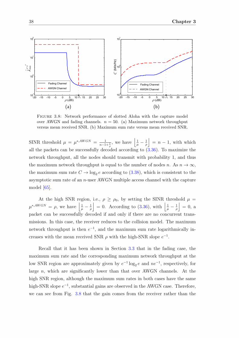
38 Chapter 3

10-1

100

101

102

AWGN Channel

Fading Channel

(dB)r

*

max

μ=μ

λˆ

-20 -15 -10 -5 0 5 10 15 20 25 300r

(a)

10-1

100

101

C(b

it/s

/Hz)

(dB)r-20 -15 -10 -5 0 5 10 15 20 25 30

AWGN Channel

Fading Channel

0r

(b)

Figure 3.8: Network performance of slotted Aloha with the capture modelover AWGN and fading channels. n = 50. (a) Maximum network throughputversus mean received SNR. (b) Maximum sum rate versus mean received SNR.

SINR threshold µ = µ∗,AWGN = 1n−1+ 1

ρ

, we have⌊1µ− 1

ρ

⌋= n − 1, with which

all the packets can be successfully decoded according to (3.36). To maximize the

network throughput, all the nodes should transmit with probability 1, and thus

the maximum network throughput is equal to the number of nodes n. As n→∞,

the maximum sum rate C → log2 e according to (3.38), which is consistent to the

asymptotic sum rate of an n-user AWGN multiple access channel with the capture

model [65].

At the high SNR region, i.e., ρ ≥ ρ0, by setting the SINR threshold µ =

µ∗,AWGN = ρ, we have⌊1µ− 1

ρ

⌋= 0. According to (3.36), with

⌊1µ− 1

ρ

⌋= 0, a

packet can be successfully decoded if and only if there are no concurrent trans-

missions. In this case, the receiver reduces to the collision model. The maximum

network throughput is then e−1, and the maximum sum rate logarithmically in-

creases with the mean received SNR ρ with the high-SNR slope e−1.

Recall that it has been shown in Section 3.3 that in the fading case, the

maximum sum rate and the corresponding maximum network throughput at the

low SNR region are approximately given by e−1 log2 e and ne−1, respectively, for

large n, which are significantly lower than that over AWGN channels. At the

high SNR region, although the maximum sum rates in both cases have the same

high-SNR slope e−1, substantial gains are observed in the AWGN case. Therefore,

we can see from Fig. 3.8 that the gain comes from the receiver rather than the

Chapter 3 39

channel fading. It corroborates that the effect of channel fading is detrimental to

the network performance if CSI is not available at the transmitter side.

3.5 Summary

In this chapter, the maximum sum rate of Aloha with the capture model is

characterized. Specifically, explicit expressions of the maximum network through-

put and the corresponding optimal backoff parameters are obtained, based on

which the maximum sum rate is derived by optimizing the SINR threshold µ. The

analysis shows that with a low SNR, the maximum sum rate linearly increases with

the number of nodes n, and approaches e−1 log2 e as n → ∞. At the high SNR

region, a logarithmic growth of the maximum sum rate is observed as ρ increases,

with the high-SNR slope of e−1.

The analysis sheds important light on the practical network design. For in-

stance, it is demonstrated that to achieve the maximum sum rate, the transmission

probabilities of nodes should be adaptively tuned according to the network size

and the mean received SNR ρ. With a fixed transmission probability, the sum

rate may significantly deteriorate, and converges to a limit that is much lower

than 1 as ρ→∞. Moreover, the throughput performance of each node is found to

be closely dependent on its mean received SNR. Although a large SNR difference

among nodes may be beneficial to the sum rate performance, it introduces serious

unfairness. A uniform mean received SNR is shown to be crucial for achieving a

good balance between fairness and sum rate when the network operates at the low

SNR region.

Note that the capture model is essentially a single-user detector. It has been

shown in this chapter that the maximum sum rate of slotted Aloha with the capture

model is much smaller than the ergodic sum capacity of multiple access fading

channels. It is nevertheless difficult to identify whether the rate loss is caused by

the random access nature or suboptimality of the receiver. The following chapter

extends the analysis to incorporate the capacity-achieving receiver structure, SIC,

to pinpoint the rate loss caused by random access.

.

Chapter 4

Maximum Sum Rate with

Successive Interference

Cancellation (SIC)

In this chapter, the analysis will be further extended to incorporate SIC. This

chapter is organized as follows. Section 4.1 presents a literature review on previous

related work. Section 4.2 derives the network steady-state point in saturated

conditions, and Section 4.3 characterizes the maximum sum rate. The effect of

MPR on the sum rate performance of slotted Aloha and the rate loss due to

random access are discussed in Section 4.4. Section 4.5 provides a summary of

this chapter.

41

42 Chapter 4

4.1 Previous Work

As a representative type of multiuser detectors, it has been shown that suc-

cessive interference cancellation (SIC) can achieve the Shannon capacity region

boundaries for multiple access channels [26, 65, 70]. The key idea of SIC is that

once a packet is successfully decoded, it should be subtracted from the aggregate

received signal so that the next packet will experience less interference, which

greatly improves the performance of wireless networks [71–74].

By adopting SIC receivers in random-access networks, the network through-

put can be significantly enhanced compared with that in the classical collision

model thanks to the MPR capability [47, 51–63]. To study the effect of MPR, a

general model was proposed in [57], where the MPR capability was described by a

reception matrix whose entry in the k-th row and l-th column εkl is the conditional

probability that l packets are successfully decoded given that there are totally k

packet transmissions. Given the reception matrix, the stability regions and net-

work throughput performance of slotted Aloha networks were further studied in

[54, 57].

As the reception matrix depends on the receiver design, various MPR receiver

models have been considered in the literature. For instance, it was assumed in

[59–62] that the receiver can successfully decode up to M packets in each time

slot, that is, εkl = 1 if l ≤ M ≤ k and εkl = 0 otherwise. Here M represents

the MPR capability of the receiver, and its effects on the network throughput

performance were analyzed in [59–62]. For many receiver structures, however,

its MPR capability may not be simplified as a fixed number. With the widely-

adopted capture model [37, 38, 44, 47, 48, 51], for instance, if each node’s packet is

decoded independently by treating others’ as background noise and a packet can

be successfully decoded as long as its received SINR is above a certain threshold,

the reception probability εkl becomes a function of the SINR threshold [44]. In

general, the reception matrix {εkl} is determined by the specific receiver structure

and the minimum required SINR for successfully decoding a packet, which could be

difficult to obtain in some cases. It was shown in [56] that with a multi-stage SIC1,

the calculation of the reception probability εkl involves multiple nested integrals.

1Specifically, it was assumed in [56] that in each stage, the packets with power higher thanan SINR threshold are decoded, and subtracted from the total received signal. The processis repeated sequentially until no packets can be successfully decoded or the number of stagesreaches the maximum.

Chapter 4 43

To reduce the computational complexity, approximations were further proposed,

based on which a simple recursive algorithm was designed to estimate the network

throughput.

Note that despite a general description for MPR capability, the reception

matrix may not be necessary for throughput analysis of random-access networks.

Instead of deriving εkl, which could become intractable when sophisticated receiver

structures are adopted, the analysis can be established based on the conditional

probability of one packet being successfully decoded given that it has i concurrent

packet transmissions, ri. As we will show in this chapter, for an n-node saturated

slotted Aloha network with SIC, both the network throughput and the sum rate

can be obtained as explicit functions of {ri}i=0,...,n−1.

Specifically, in this chapter, two representative SIC receivers are considered,

i.e., ordered SIC and unordered SIC, which are described in Chapter 2.3. The max-

imum network throughput and the corresponding optimal transmission probability

of nodes in both cases are derived as functions of {ri}i=0,...,n−1, which depend on

SINR threshold µ and mean received SNR ρ. The maximum sum rate is further

characterized by optimizing the SINR threshold µ. To demonstrate the effect of

MPR on the sum rate performance, the maximum sum rates with SIC receivers

and the capture model are further compared to that with the classical collision

model.

It is worth mentioning that the SIC structure is also assumed in the line of

research on “coded random access” [75–79]. It is, however, used to recover the

coded successive packets of each node, and the classical collision model is assumed

for packets from different nodes. It should be distinguished from this thesis where

no coding/decoding is assumed over successive packets of each node, and the SIC

receivers are adopted for packets from multiple nodes.

4.2 Steady-State Point in Saturated Conditions

In this section, we will characterize the network steady-state point in satu-

rated conditions based on the fixed-point equation of p. We will start from the

derivation of the conditional probability of successful transmission of each HOL

packet given that it has i concurrent packet transmissions, ri.

44 Chapter 4

4.2.1 Conditional Probability of Successful Transmission

ri

For HOL packet j, denote rji as its steady-state probability of successful trans-

mission given that there are i concurrent packet transmissions. It is clear that rji

depends on the receiver design. In Chapter 3, it has been shown that with the

capture model, all the packets have the same conditional probability of successful

transmission of

rCi =exp

(−µρ

)(1 + µ)i

, (4.1)

where µ is the SINR threshold and ρ is the mean received SNR.

With SIC, in contrast, rji depends on the decoding order of packet j, and the

number of packets that have been successfully decoded before packet j. Specifi-

cally, it can be written as

rji =i+1∑m=1

Pr{packet j is decoded at the mth iteration}·m−1∑k=0

Pr{There are k

successfully decoded packets before packet j and packet j is

successfully decoded}. (4.2)

Note that all the packets have independent and identically distributed (i.i.d.) re-

ceived SNRs, and thus equal probability to be decoded at a given iteration. The

first item on the right-hand side of (4.2) is then given by

Pr{packet j is decoded at the mth iteration} =1

i+ 1. (4.3)

The second item on the right-hand side of (4.2) depends on whether the packets

are ordered. In the following, let us consider the ordered SIC and unordered SIC

cases separately.

Chapter 4 45

4.2.1.1 Ordered SIC

The second item on the right-hand side of (4.2) can be written as

Pr{There are k successfully decoded packets before packet j and packet j is

successfully decoded}

=Pr{There are k successfully decoded packets before packet j | packet j

is successfully decoded} · Pr{Packet j is successfully decoded}. (4.4)

With ordered SIC, packets are decoded in descending order of their received power.

If packet j is successfully decoded at the mth iteration, then all the m− 1 packets

before packet j must be successfully decoded. Therefore, we have

Pr{There are k successfully decoded packets before packet j | packet j is


=

1 if k = m− 1,

0 otherwise.(4.5)

Moreover, denote y(l)i as the probability that the packet at the lth iteration can be

successfully decoded given that there are i concurrent packet transmissions, i.e.,

totally i + 1 packets to be decoded. The probability that packet j is successfully

decoded is equal to the probability that all the packets before it, i.e., at iteration

1 to m, are successfully decoded, which can be written as

Pr{Packet j is successfully decoded} = Πml=1y

(l)i . (4.6)

46 Chapter 4

Appendix G further shows that

y(l)i =

(i+1)!

(i+1−l)!(l−1)!

d1/µe−1∑k=0

(i+1−lk

)(−1)k

l+kexp

− l+k

ρ(

1µ−k)( 1

µ−kl+ 1

µ

)i+1−l

l ≤ i+1− 1

µ

(i+1)!

(i+1−l)!(l−1)!

i+1−l∑k=0

(i+1−lk

)(−1)k

exp

(− k+lρ( 1µ−k)

)k+l

−i−l∑s=0

((i+1−l−k)s

(i+1)s+1·

Q

(1+s,

i+1

ρ( 1µ−i−1+l)

)+ exp

(− k+lρ( 1µ−k)

)( 1µ−k)s

( 1µ+l)s+1

·

(1−

Q

(1+s,− 1

ρ(i+1−l− 1µ)·(i+1−l−k)( 1

µ+l)

1µ−k

))) l > i+1− 1

µ,

(4.7)

for l = 1, ..., i+ 1, in which Q(s, t) = 1(s−1)!

∫∞te−xxs−1dx is the regularized upper

incomplete gamma function. With µ ≥ 1, (4.7) reduces to

y(l),µ≥1i =

(i+1

l

)exp

(− lµρ

)·(

1

lµ+ 1

)i+1−l

, (4.8)

for l = 1, ..., i + 1. By substituting (4.3-4.6) into (4.2), the steady-state probabil-

ity of successful transmission of HOL packet j given that there are i concurrent

transmissions for ordered SIC can be obtained as

rj,OSi =1

i+ 1

i+1∑m=1

Πml=1y

(l)i . (4.9)

The right-hand side of (4.9) is independent of j, indicating that all the HOL pack-

ets have the same conditional probability of successful transmission. Therefore,

we drop the superscript j in the following discussion.

Chapter 4 47

4.2.1.2 Unordered SIC

The second item on the right-hand side of (4.2) can be written as

Pr{There are k successfully decoded packets before packet j and packet j is


=Pr{Packet j is successfully decoded | there are k successfully decoded packets

before packet j} · Pr{There are k successfully decoded packets before packet j}.(4.10)

With unordered SIC, packets are decoded in a random order. Therefore, given

that there are k successfully decoded packets before packet j, the probability

that packet j can be successfully decoded is equal to rCi−k, i.e., the probability of

successful transmission given that there are i− k concurrent packet transmissions

for the capture model. According to (4.1), we have

Pr{Packet j is successfully decoded | there are k successfully decoded packets

before packet j }

=exp

(−µρ

)(1 + µ)i−k

= (1 + µ)k · rCi . (4.11)

It is difficult to obtain an explicit expression of Pr{There are k successfully de-

coded packets before packet j} due to the dependency of packets decoding, i.e.,

the decoding of each packet depends on how many packets at the preceding itera-

tions are successfully decoded. Let us consider the worst case that each packet is

subject to interference from i concurrent packet transmissions during its decoding

process. In this case, the probability that there are k successfully decoded pack-

ets before packet j at the mth iteration is given by(m−1k

) (1− rCi

)m−1−k (rCi)k

.

By combining (4.2-4.3) and (4.10-4.11), we can then obtain a lower-bound of the

steady-state probability of successful transmission of HOL packet j given that

there are i concurrent packet transmissions for unordered SIC as

rj,NSi ≥ rj,NS li = 1

i+1

i+1∑m=1

m−1∑k=0

(m−1

k

)(1+µ)k

(1− rCi

)m−1−k (rCi)k+1

=(1+µrCi )i+1−1

(i+1)µ.

(4.12)

Again, we drop the superscript j in the following discussion because the right-hand

side of (4.12) is independent of j.

48 Chapter 4

m

1nr-

Figure 4.1: Conditional probability of successful transmission rn−1 given thatthere are n − 1 concurrent packet transmissions versus SINR threshold µ in

slotted Aloha networks with SIC receivers. n = 20 and ρ = 20dB.

4.2.1.3 Comparison

We can see from (4.9) and (4.12) that both rOSi and rNS li depend on the SINR

threshold µ. Fig. 4.1 illustrates how they vary with µ. For the sake of comparison,

the result of the capture model obtained in Chapter 3 is also presented.

It can be clearly observed from Fig. 4.1 that both the ordered SIC and un-

ordered SIC have a much larger conditional probability of successful transmission

than the capture model when µ is small. It can be easily obtained from (4.1) that

with the capture model, rCn−1|µ= 1n

for large n≈ e−1. Appendix H further shows that for

large ρ and n,

rOSn−1|µ= 1n≈1, rNS l

n−1 |µ= 1n≈ee−1 − 1, (4.13)

both of which are significantly higher than e−1.

The gap, nevertheless, diminishes as the SINR threshold µ increases. As µ→∞, Appendix I shows that the conditional probability of successful transmission

in both the ordered SIC and unordered SIC cases converges to that of the capture

model.

limµ→∞

rOSirCi

= limµ→∞

rNS li

rCi= 1. (4.14)

Chapter 4 49

4.2.2 Steady-State Point in Saturated Conditions

The steady-state probability of successful transmission of HOL packets p can

be written as

p =n−1∑i=0

ri · Pr{i concurrent packet transmissions}. (4.15)

In saturated conditions, all the nodes have non-empty queues. According to the

Markov chain shown in Fig. 2.2, the probability that the HOL packet is requesting

transmission is given by πT q0+∑K

i=0 πiqi, which is equal to πT/p according to (2.2)-

(2.3). Therefore, the probability that there are i concurrent packet transmissions

can be obtained as

Pr{i concurrent packet transmissions}=(n−1

i

)(1−πT/p)n−1−i (πT/p)i . (4.16)

By substituting (4.16) into (4.15), we have

p =n−1∑i=0

ri ·(n−1

i

)(1−πT/p)n−1−i (πT/p)i . (4.17)

The service rate πT depends on the transmission probabilities of nodes {qi}i=0,...,K .

In this chapter, for the sake of simplicity, we assume that qi = q0 for i = 0, . . . , K.

In this case, the fixed-point equation (4.17) has a single non-zero root pA, which

is given by

pA =n−1∑i=0

(n− 1

i

)ri (1− q0)n−1−i · qi0. (4.18)

Specifically, with ordered SIC, pOSA can be obtained by combining (4.18) and (4.9).

With unordered SIC, pNSA can be approximated by combining (4.18) and the lower-

bound rNS li developed in (4.12).2 Fig. 4.2 illustrates how the steady-state point

pA varies with the SINR threshold µ for the ordered SIC and unordered SIC cases.

The result of the capture model is also presented for the sake of comparison.

Similar to the conditional probability of successful transmission illustrated in Fig.

4.1, we can see from Fig. 4.2 that the gains achieved by SIC receivers over the

capture model are significant only when µ is small.

2Unless otherwise specified, in the following analysis, rNSi is always approximated by its

lower-bound rNS li in the unordered SIC case.

50 Chapter 4

m

Ap

Figure 4.2: Steady-state point of slotted Aloha networks with SIC receiverspA versus SINR threshold µ. n = 20. q0 = 0.5 and ρ = 20dB.


In this section, simulation results are presented to verify the preceding analy-

sis. In particular, we consider a saturated slotted Aloha network where each node

has the transmission probability q0. The simulation setting is the same as the

system model and thus we omit the details here.

In Section 4.2.1, the conditional probability of successful transmission ri for

ordered SIC has been derived in (4.9) and verified by simulation results presented

in Fig. 4.3. For the unordered SIC case, Fig. 4.3 shows that the lower-bound of

ri developed in (4.12) is quit close.

In Section 4.2.2, the steady-state point pA is further derived in (4.18) as

the non-zero root of the fixed-point equation of the steady-state probability of

successful transmission of HOL packets p, which is verified by simulation results

presented in Fig. 4.4. It can be clearly observed from Fig. 4.4 that the steady-

state point pA closely depends on the transmission probability of nodes q0. In

the next section, we will demonstrate how to optimally choose the transmission

probability of nodes q0 to maximize the network throughput and the sum rate.

Chapter 4 51

i

ir

(a)

i

ir

(b)

Figure 4.3: Conditional probability of successful transmission ri in slottedAloha networks with SIC receivers versus number of concurrent packet trans-

missions i. µ = 1. (a) ρ = 0dB. (b) ρ = 20dB.

0q

Ap

(a)

0q

Ap

(b)

Figure 4.4: Steady-state point of slotted Aloha networks with SIC receiverspA versus transmission probability q0. n = 20 and µ = 1. (a) ρ = 0dB. (b)

ρ = 20dB.

4.3 Maximum Sum Rate

In this section, let us first derive the maximum network throughput λmax by

optimizing the transmission probability of nodes q0.

52 Chapter 4

4.3.1 Maximum Network Throughput

In saturated conditions, the network throughput λout = nπT . By combining

(2.2) and (4.18), with qi = q0 for i = 0, . . . , K, the network throughput λout in

saturated conditions can be obtained as

λout = nq0pA = nn−1∑i=0

(n− 1

i

)ri (1− q0)n−1−i qi+1

0 , (4.19)

which closely depends on the transmission probability of nodes q0. For the maxi-

mum network throughput λmax = max0<q0≤1 λout, Appendix J shows that in both

the ordered SIC and unordered SIC cases, we have

λmax =

n∑n−1

i=0

(n−1i

)ri (1− q0)n−1−i qi+1

0 if µ ≥ µ0

nrn−1 otherwise,(4.20)


q∗0 =

q0 if µ ≥ µ0

1 otherwise,(4.21)

where q0 is the root of

nn−1∑i=0

(n− 1

i

)ri (1− q0)n−2−i qi0(1 + i− nq0) = 0, (4.22)

and µ0 is the root ofrn−2rn−1

=n

n− 1. (4.23)

We can see from (4.20) that both λOSmax and λNSmax depend on the SINR thresh-

old µ. Fig. 4.5 illustrates how they vary with µ. Similar to the conditional

probability of successful transmission rn−1 and the steady-state point in saturated

conditions pA shown in Fig. 4.1 and Fig. 4.2, significant gains in maximum net-

work throughput can be achieved by SIC receivers over the capture model when

µ is small. Recall that with the capture model, we have λCmax|µ= 1n

for large n≈ ne−1.

It can be further obtained from (4.20) and (4.13) that

λOSmax|µ= 1n

for large n≈ n, λNSmax|µ= 1

n

for large n≈ n

(ee−1 − 1

), (4.24)

Chapter 4 53

m

max

l

Figure 4.5: Maximum network throughput of slotted Aloha networks withcapture model and SIC receivers λmax versus SINR threshold µ. n = 20 and

ρ = 20dB.

both of which are much higher than ne−1. With a large µ, nevertheless, the

maximum network throughput in both the ordered SIC and unordered SIC cases

converges to that of the capture model. As µ→∞, it can be obtained from (4.20)

and (4.14) that limµ→∞λOSmax

λCmax= limµ→∞

λNSmax

λCmax= 1.

It can be clearly seen from Fig. 4.5 that similar to the capture model, with

SIC receivers, the maximum network throughput λmax also increases as the SINR

threshold µ decreases. Such an improvement on maximum network throughput is,

nevertheless, achieved at the cost of a smaller information encoding rate that can

be supported for reliable communications, i.e., R = log2(1 + µ). In the next sub-

section, we will further study how to maximize the sum rate by properly choosing

the SINR threshold µ.

4.3.2 Maximum Sum Rate

By combining (2.8) and (4.20), the maximum sum rate can be further written

as C = max (C1, C2), where C1 = maxµ≥µ0 f1(µ) and C2 = maxµ<µ0 f2(µ), in which

f1(µ) = λµ≥µ0max log2(1+µ) = nn−1∑i=0

(n− 1

i

)ri (1− q0)n−1−i qi+1

0 · log2(1+µ) (4.25)

54 Chapter 4

for µ ∈ [µ0,∞) and

f2(µ) = λµ<µ0max log2(1 + µ) = nrn−1 · log2(1 + µ) (4.26)

for µ ∈ (0, µ0). Denote µh = arg max f1(µ) and µl = arg max f2(µ). Note that

µh and µl can be numerically obtained given the expressions of f1(µ) and f2(µ).

Appendix K shows that for both the ordered SIC and unordered SIC cases, the

maximum sum rate is given by

C =

f1(µh) if ρ ≥ ρ0

f2(µl) otherwise,(4.27)

which is achieved when the SINR threshold µ is set as

µ∗ =

µh if ρ ≥ ρ0

µl otherwise,(4.28)

where ρ0 is the root of f1(µh) = f2(µl).

The maximum sum rate C for both the ordered SIC and unordered SIC cases is

illustrated in Fig. 4.6. For the sake of comparison, the result of the capture model

is also presented. In contrast to Fig. 4.5 where the maximum network throughput

of the unordered SIC is shown to be significantly higher than that of the capture

model, we can see from Fig. 4.6 that only marginal gains in the maximum sum

rate can be achieved by the unordered SIC over the capture model. For the ordered

SIC case, substantial gains can still be observed at moderate values of the mean

received SNR ρ, i.e., −10dB< ρ < 35dB. The gap, nevertheless, diminishes at the

high SNR region, i.e., ρ ≥ ρOS0 , where the maximum sum rates of all the three

receivers have the high-SNR slope of e−1 as ρ→∞.

It is also interesting to note from Fig. 4.6 that ordering is crucial for the

rate performance of slotted Aloha networks with SIC receivers. Without proper

ordering of packets, the maximum sum rate could be drastically degraded and

becomes comparable to that of the capture model. To achieve the maximum sum

rate, the SINR threshold µ needs to be carefully tuned according to the mean

received SNR ρ based on (4.28). Fig. 4.7a illustrates the optimal SINR threshold

µ∗ for the ordered SIC, unordered SIC and the capture model cases. It can be

clearly seen from Fig. 4.7a that in all three cases, the SINR threshold µ, or

Chapter 4 55

=3.3=4.3 =36.1

C(bit/s/Hz)

(dB) r

0

Cr

0

NSr 0

OSr

Figure 4.6: Maximum sum rate of slotted Aloha networks with capture modeland SIC receivers C versus mean received SNR ρ. n = 20.

=3.3 =4.3 =36.1

*m

(dB) r

0

Cr

0

NSr 0

OSr

(a)

=3.3 =4.3 =36.1

(dB) r

**,

0q

mm

=

10.05

n=

0

Cr

0

NSr 0

OSr

(b)

Figure 4.7: (a) Optimal SINR threshold µ∗ and (b) optimal transmission prob-

ability q∗,µ=µ∗

0 of slotted Aloha networks with capture model and SIC receivers.n = 20.

56 Chapter 4

equivalently, the information encoding rate R, should be properly enlarged as the

mean received SNR ρ increases. Moreover, by combining (4.21) and (4.28), we

can further obtain the optimal transmission probability q∗,µ=µ∗

0 for maximizing

the sum rate as a function of the mean received SNR ρ. As Fig. 4.7b illustrates,

at the low SNR region, the optimal transmission probability is 1, indicating that

all the nodes should persistently transmit their packets. As the mean received

SNR ρ increases, nevertheless, the transmission probability of each node should

be reduced accordingly, and converges to 1n

as ρ→∞.



ysis. Fig. 4.8 illustrates the network throughput performance. The network

throughput λout has been derived as a function of the transmission probability of

nodes q0 in (4.19). According to (4.20), if the SINR threshold µ ≥ µ0, the max-

imum network throughput λmax is achieved when q0 is set to be q0. Otherwise,

λmax is achieved when q0 = 1. With n = 20 and ρ = 20dB, we have µOS0 = 0.1205

and µNS0 = 0.0532 by substituting (4.9) and (4.12) into (4.23), respectively, for

the ordered SIC and unordered SIC cases. As we can see from Fig. 4.8a, with

µ = 0.05 < µ0, the network throughput in both cases monotonically increases

with q0, and is maximized at q0 = 1. With µ = 1 > µ0, on the other hand, the

network throughput is maximized at q0 = q0 which is given in (4.22), as Fig. 4.8b

illustrates. Simulation results presented in Fig. 4.8 verify that the analysis serves

as a good lower-bound in the unordered SIC case, and is accurate with ordered

SIC.

It is further shown in Section 4.3.2 that as both the information encoding rate

R and the maximum network throughput λmax depend on the SINR threshold µ,

the sum rate can be maximized by optimizing the SINR threshold µ. As Fig.

4.9 illustrates, the sum rate performance is sensitive to the setting of µ in both

ordered SIC and unordered SIC cases. To achieve the maximum sum rate, the

SINR threshold µ should be properly set according to the mean received SNR ρ.

The expressions of the maximum sum rate C and the corresponding optimal SINR

threshold µ∗ are given in (4.27)-(4.28), and verified by simulation results presented

in Fig. 4.9.

Chapter 4 57

0q

max

ˆNSl

max

ˆOSl

ˆ out

l

(a)

denotes 0q

0q

max

ˆNSl

max

ˆOSl

ˆ out

l

(b)

Figure 4.8: Network throughput of slotted Aloha networks with SIC receiversλout versus transmission probability q0. n = 20 and ρ = 20dB. (a) µ = 0.05.

(b) µ = 1.

4.4 Discussions

So far we have derived the maximum sum rates of slotted Aloha networks with

SIC receivers, and the corresponding optimal setting including the optimal SINR

threshold and the optimal transmission probability of nodes. In this section, we

will further demonstrate the effect of MPR on the sum rate performance of slotted

Aloha networks, and compare it to the ergodic sum capacity of multiple access

fading channels.

4.4.1 Effect of MPR

Note that both the SIC receivers and the capture model have the so-called

MPR capability: If the SINR threshold µ is small enough, then multiple packets

can be successfully decoded at each time slot. As a result, the network throughput

performance is expected to be substantially enhanced compared to the classical

collision model where at most one packet can be successfully decoded at each time

slot.

To further see the effect of MPR on the sum rate performance, let us consider

the classical collision model where a packet transmission is successful only if there

are no concurrent transmissions. Appendix L shows that in this case, the maximum

58 Chapter 4

*,NSm=0.05

*,OSm=0.10

=2.34OSC

=0.64NS

C

m

sR(bit/s/Hz)

(a)

*,NSm=24

*,OSm=0.12

=3

=1.46

OSC

NSC

m

sR(bit/s/Hz)

(b)

=

31.37 10´

*,NSm

*,OSm = =

m

sR

=3.43OSC

NSC

(bit/s/Hz)

(c)

Figure 4.9: Sum rate of slotted Aloha networks with SIC receivers Rs versusSINR threshold µ. n = 20 and q0 = q∗0. (a) ρ = 0dB. (b) ρ = 20dB. (c)

ρ = 40dB.

sum rate is given by

Ccollision = exp(−1− eW0(ρ)−1

ρ

)· log2(e

W0(ρ)), (4.29)

which is achieved when the SNR threshold is set to be µ∗,collision = eW0(ρ)− 1. The

corresponding maximum network throughput is given by

λµ=µ∗,collision

max = exp(−1− eW0(ρ)−1

ρ

). (4.30)

Fig. 4.10 illustrates the maximum sum rate and the corresponding maximum

network throughput with the collision model. For the sake of comparison, the

results of the capture model and SIC receivers are also presented. As we can see

Chapter 4 59

*

maxˆm

ml

=

(dB) r

(a)

(bit/s/Hz)

C

(dB) r

(b)

Figure 4.10: Network performance of slotted Aloha with collision model, cap-ture model and SIC receivers. n = 20. (a) Maximum network throughput λµ=µ

∗max

and (b) maximum sum rate C versus mean received SNR ρ.

from Fig. 4.10a, at the low SNR region, the maximum network throughput of the

collision model is significantly lower than that of SIC receivers and the capture

model, which can be much higher than 1 thanks to MPR. The gap, nevertheless,

diminishes as the mean received SNR ρ increases. All of them approach e−1 as

ρ→∞.

Similarly, Fig. 4.10b shows that the maximum sum rates of all four receivers

have the same high-SNR slope of e−1, and the rate difference becomes negligible

when the mean received SNR ρ is large. At the low SNR region, however, in

contrast to the significant throughput improvement, only marginal gains in the

maximum sum rate can be achieved by the SIC receivers and the capture model.

The rate difference between the collision model and the capture model is below

0.5 bit/Hz/s for the whole SNR region, which suggests that despite an overly pes-

simistic estimation on the network throughput, the collision model serves as a good

approximation for the capture model when analyzing the sum rate performance of

slotted Aloha networks.

Recall that it has been shown in Fig. 4.7a that at the low SNR region, the

optimal SINR thresholds with the SIC receivers and the capture model are small,

indicating that each packet has a small encoding rate. Therefore, although much

more packets can be successfully decoded compared to the collision model, the

gain in the maximum sum rate is limited. At the high SNR region, on the other

hand, both the SIC receivers and the capture model reduce to the collision model

60 Chapter 4

as the optimal SINR thresholds are much higher than 1. We can conclude from

Fig. 4.10 that although the network throughput performance at the low SNR

region can always be significantly improved thanks to MPR, the rate gain could

be marginal, and becomes negligible when the mean received SNR is large.

4.4.2 Rate Loss Due to Random Access

For an n-user multiple access fading channel, it has been well known that

the ergodic sum capacity without the channel state information at the transmitter

side (CSIT) is given by Csum = E [log2 (1 +∑n

k=1 |hk|2ρ)], where the expectation is

taken over all fading states of users. To achieve the ergodic sum capacity, an SIC

receiver should be adopted, and each node’s encoding rate is determined by its

decoding order, with codewords long enough to cover multiple fading states [65].

With slotted Aloha, in contrast, as each node transmits with a certain probability,

the subset of active nodes is time-varying, and supposed to be unknown at the

transmitter side. Therefore, rate allocation among nodes cannot be performed,

and a uniform information encoding rate is assumed for each packet with the

packet-based encoding, i.e., each packet contains one codeword lasting for one

time slot.

Fig. 4.10b illustrates the ergodic sum capacity in comparison to the maximum

sum rates of slotted Aloha under various receivers. It can be clearly seen from

Fig. 4.10b that even with the capacity-achieving receiver structure, the ordered

SIC, the maximum sum rate of slotted Aloha is still significantly lower than the

ergodic sum capacity. Specifically, different high-SNR slopes are observed, i.e., 1

for the ergodic sum capacity and e−1 for the maximum sum rates of slotted Aloha.

With the packet-based encoding/decoding and a uniform encoding rate of each

packet, even if the ordered SIC is adopted, the sum rate performance of slotted

Aloha is still bottlenecked by the first decoded packet, which can be improved by

increasing the mean received SNR ρ at the high SNR region only when there are

no concurrent packet transmissions. It has been shown in Fig. 4.7b that as ρ

increases, the optimal transmission probability of each node converges to 1/n. As

a result, the high-SNR slope of the maximum sum rates of slotted Aloha, which

is determined by the probability that there is a single packet transmission in each

time slot at the high SNR region, is only e−1. Here we can see that the huge

Chapter 4 61

rate loss of slotted Aloha at the high SNR region has its root in the contention of

packets caused by uncoordinated random transmissions of nodes.

4.5 Summary

In this chapter, the maximum sum rates of slotted Aloha with two repre-

sentative SIC receivers, ordered SIC and unordered SIC, are characterized. The

analysis shows that maximum sum rate with ordered SIC is significantly higher

than that with unordered SIC within a wide range of ρ. This result suggests that

ordering is crucial for the rate performance of slotted Aloha with SIC receivers.

Without proper ordering of packets, the maximum sum rate could be drastically

degraded and become comparable with that of the capture model. The comparison

with the classical collision model further reveals that although substantial gains

in network throughput can be achieved by SIC receivers and the capture model at

the low SNR region thanks to MPR, the rate difference could be limited, and they

all reduce to the collision model with the high-SNR slope of e−1 when the mean

received SNR ρ is large. Without proper rate allocation, even with the capacity-

achieving receiver structure, the maximum sum rate of slotted Aloha could remain

far below the ergodic sum capacity of fading channels, indicating that the rate loss

is significant due to uncoordinated random transmissions of nodes.

Chapter 5

Conclusion and Future Work

5.1 Conclusion

As a basic type of multiple access, random access has been widely applied to

a plethora of networks including cellular networks, IEEE 802.11 networks, wireless

ad-hoc networks and machine-to-machine (M2M) networks. In sharp contrast to

its simplicity in concept and success in applications, little was known about its

fundamental performance limits. Aiming to explore the information-theoretic limit

of slotted Aloha networks, this thesis presents a comprehensive analysis on the sum

rate of slotted Aloha by extending the unified analytical framework [21, 22] from

the classical collision model to the capture model and SIC receivers.

Specifically, the first part of this thesis focuses on maximum sum rate char-

acterization with the capture model. The maximum sum rate and corresponding

maximum network throughput are derived by assuming that the received SNRs

of each node’s packets are exponentially distributed with the same mean received

SNR ρ and saturated conditions. The optimal setting, including the optimal trans-

mission probability and the optimal SINR threshold, are also obtained. The anal-

ysis shows that at the low SNR region, the maximum sum rate linearly increases

with the number of nodes n, and approaches e−1 log2 e as n → ∞. At the high

SNR region, the maximum sum rate logarithmically increases with the mean re-

ceived SNR ρ, and the high-SNR slope is e−1, which is much lower than that of

the ergodic sum capacity of multiple access fading channels.

As the capture model is essentially a single-user detector, it is difficult to

determine whether the gap between the ergodic sum capacity of multiple access

63

64 Chapter 5

and the maximum sum rate of slotted Aloha with the capture model is caused by

the random-access nature or suboptimality of the receiver. Therefore, in the second

part of this thesis, the analysis is further extended to incorporate the capacity-

achieving receiver structure, SIC. Specifically, two representative SIC receivers,

ordered SIC and unordered SIC, are considered. The maximum sum rate in both

cases is obtained by optimizing the SINR threshold µ. The comparison to the

capture model shows that ordering is crucial for the rate performance of slotted

Aloha with SIC receivers: Without proper ordering of packets, the maximum

sum rate could be drastically degraded and becomes comparable to that with

the capture model. To further demonstrate the effect of MPR on the sum rate

performance, the maximum sum rates with SIC receivers and the capture model

are further compared to that with the classical collision model. It is found that

in contrast to the significant throughput improvement at the low SNR region,

only marginal gains in the maximum sum rate can be achieved by SIC receivers

and the capture model. The rate difference becomes negligible when the mean

received SNR ρ is large, and the maximum sum rates with all the receivers have

the same high-SNR slope of e−1, which is remarkably lower than that of the ergodic

sum capacity of multiple access fading channels. Evidently, the huge rate loss is

mainly due to the random access nature (i.e., uncoordinated random transmissions

of nodes).

To conclude, the main contributions of this thesis are summarized as follows:

1. The unified analytical framework in [21, 22] is extended from the classical

collision model to the capture model, where the network steady-state point in

saturated conditions is derived as a function of the SINR threshold. Explicit

expressions of the maximum network throughput, maximum sum rate and

optimal setting are obtained. The analysis shows that the maximum sum

rate of slotted Aloha with the capture model is much lower than the ergodic

sum capacity of multiple access fading channels.

2. The analysis is further extended to incorporate the capacity-achieving re-

ceiver structure, SIC, to determine whether the rate loss originates from the

random access nature or suboptimality of the receiver (i.e., the capture mod-

el). The maximum sum rate and corresponding optimal parameter setting,

which includes the transmission probability and SINR threshold for both

ordered and unordered SIC, are obtained. The comparison to the ergodic

Chapter 5 65

sum capacity of multiple access fading channels indicates that the rate loss

is due to the uncoordinated random transmissions of nodes, which make rate

allocation among nodes unfeasible.

3. The effects of adaptive backoff, power control, channel fading and multi-

packet reception on the sum rate performance of slotted Aloha networks are

further discussed. The main findings are summarized as follows:

• To achieve the maximum sum rate, the transmission probabilities of

nodes should be properly selected according to the network size and

the mean received SNR. With a fixed transmission probability, the sum

rate performance significantly deteriorates.

• Although a large SNR difference among nodes may potentially improve

the sum rate performance, serious unfairness is introduced. At the low

SNR region, power control is essential in order to achieve a good balance

between fairness and sum rate performance.

• With the capture model, both the maximum network throughput and

the maximum sum rate of slotted Aloha over AWGN channels are al-

ways higher than that over fading channels, which corroborates that

the effect of channel fading is detrimental to the network performance

if CSI is not available at the transmitter side.

• By comparing the maximum sum rates with SIC receivers and the cap-

ture model to that with the classical collision model, it is found that

substantial gains in network throughput can be achieved by MPR re-

ceivers at the low SNR region. However, the rate gain from MPR is

only marginal.

5.2 Future Work

The work in this thesis only provides a starting point. In the future, the

analysis should be extended to consider more practical assumptions. For instance,

this thesis focuses on the saturated conditions where the network throughput is

pushed to the limit, yet the mean queueing delay is infinite and the network could

be unstable. It is of great practical significance to further consider the unsaturated

scenario and study the maximum sum rate of slotted Aloha under certain system

constraints such as stability or delay requirements.

66 Chapter 5

Moreover, a key assumption throughout this thesis is that the nodes are un-

aware of the instantaneous realizations of small-scale fading, and they encode their

packets independently at the same rate. If CSI is available at the transmitter side,

each node can then adjust the information coding rate and the transmission prob-

ability according to its instantaneous channel conditions. How to characterize the

maximum sum rate with CSI at the transmitter side is another interesting and

challenging issue that deserves much attention in the future study.

From the practical perspective, the analysis can be further applied to real-

world networks, such as M2M networks. M2M communication has been regarded

as an emerging technology that can facilitate new business opportunities for both

consumers and enterprises. In M2M networks, a massive number of heterogeneous

devices such as smart meters, monitoring devices and intelligent transportation

devices operate in an automated manner, and generate small and infrequent pay-

loads. Therefore, random access is much more suitable than centralized multiple

access for M2M networks [82, 83]. Increasing attention has been provided to the

modeling and performance analysis of the current multiple access protocol for

M2M networks, namely, the Physical Random Access Channel (PRACH) of LTE

and LTE-A [3, 4, 84–91], which is a variant of slotted Aloha. Many studies have

pointed out that significant challenges for M2M networks include how to properly

tune the system parameters to optimize the network throughput performance un-

der certain delay requirement for time-restricted applications [3, 88–90] or how to

minimize the energy consumption of devices [4, 91, 92]. It would be of paramount

practical importance to further extend the proposed analytical framework in this

thesis to address the above challenging issues in M2M networks in the future.

Appendix A

Proof of Theorem 3.1

Proof. The right-hand side of (3.7) can be written as h(p) = exp(−µρ− nµ

µ+1· 1g(p)

),

where g(p) =∑K−1

i=0p(1−p)i

qi+ (1−p)K

qK. Define qi = 1/qi, for 0 ≤ i ≤ K − 1, and

qi = 1/qK for i ≥ K. g(p) can be then written as g(p) =∑∞

i=0 p(1−p)iqi = EX [qX ],

where X is a geometric random variable with parameter p.

Suppose that 0 < p1 < p2 ≤ 1. Let X1 and X2 denote geometric random

variables with parameters p1 and p2, respectively. Then we have X1 ≥st X2 [80].1

As {qi} is a monotonic non-increasing sequence, we have qX1 ≥st qX2 . We can

then conclude that g(p1) ≥ g(p2). Therefore, g(p) is a monotonic non-increasing

function with respect to p, which indicates that h(p) is a monotonic non-increasing

function. Moreover, as limp→0 h(p) = exp(−µρ− nµ

µ+1· qK

)> 0 and limp→1 h(p) =

exp(−µρ− nµ

µ+1· q0)< 1, we can then conclude that (3.7) has a single non-zero

root if {qi}i=0,...,K is a monotonic non-increasing sequence.

1X1 ≥st X2 denotes that a random variable X1 is larger than a random variable X2 in theusual stochastic order, i.e., Pr(X1 > x) ≥ Pr(X2 > x) for all x ∈ (−∞,∞).

67

Appendix B


Proof. It is shown in (3.9) that the network throughput can be obtained as an

explicit function of pA. The following lemma first presents λpmax = maxpA∈(0,1]λout

and the corresponding optimal steady-state point p∗A.

Lemma B.1. For given SINR threshold µ ∈ (0,∞) and mean received SNR ρ ∈(0,∞), λpmax is given by

λpmax = µ+1µ

exp(−1− µ

ρ

), (B.1)


p∗A = exp(−1− µ

ρ

). (B.2)

Proof. According to (3.9), the second-order derivative of λout with respect to pA

is given by −µ+1µpA

< 0, for pA ∈ (0,∞). Therefore, we can conclude that λout is a

strictly concave function of pA ∈ (0,∞) with one global maximum at p∗A, where

p∗A is the root of dλoutdpA

= 0, i.e., (µ + 1) ·(− ln pA−1

µ− 1

ρ

)= 0, which is given by

(B.2). Eq. (B.1) can be obtained by substituting (B.2) into (3.9).

We can see from Lemma B.1 and (3.7) that to achieve λpmax, the backoff

parameters {qi}i=0,...,K should be carefully selected such that pA = p∗A. For given

backoff function Qi, the optimal initial transmission probability for achieving λpmax

can be easily obtained by combining (3.7) and (B.2) as (3.12).

69

70 Appendix B

Note that the initial transmission probability q0 should not exceed 1. Lemma

B.2 shows that λpmax is achievable for qi ∈ (0, 1], i = 0, . . . , K, if and only if the

SINR threshold µ ≥ 1n−1 .

Lemma B.2. λpmax is achievable if and only if µ ≥ 1n−1 .

Proof. Define Qi = 1/Qi, for 0 ≤ i ≤ K − 1, and Qi = 1/QK for i ≥ K. Let

Y denote a geometric random variable with parameter exp(−1− µ

ρ

). Eq. (3.12)

can be then written as q0 = µ+1nµ· EY [QY ]. As Qi ≤ 1 for i = 0, 1, . . . , K, we have

EY [QY ] ≥ 1.

1) if : if µ ≥ 1n−1 , with Qi = 1 for i = 0, 1, . . . , K, we have EY [QY ] = 1 and

q0 = µ+1nµ≤ 1. In this case, λpmax can be achieved by setting q0 = q0.

2) only if : if µ < 1n−1 , we have q0 ≥ µ+1

nµ> 1, which indicates that λpmax is not

achievable.

For µ < 1n−1 , λpmax is not achievable for qi ∈ (0, 1], i = 0, . . . , K. The following

lemma shows that in this case, the maximum network throughput λmax is always

smaller than λpmax, which is achieved by setting qi = 1, i = 0, . . . , K.

Lemma B.3. For given SINR threshold µ < 1n−1 , the maximum network through-

put λmax is given by

λµ<

1n−1

max = n exp(− nµµ+1− µ

ρ

), (B.3)

which is achieved at q∗i = 1, i = 0, . . . , K.

Proof. According to (3.7), the initial transmission probability q0 can be written as

q0 = µ+1nµ

(− ln pA − µ

ρ

)· z(pA). (B.4)

where z (pA) =∑K−1

i=0pA(1−pA)iQi + (1−pA)K

QK. Similar to g(p) in Appendix A, it can

be proved that z (pA) is a monotonic non-increasing function of pA ∈ (0, 1]. Note

that − ln pA is also a monotonic non-increasing function of pA ∈ (0, 1]. Therefore,

we can conclude from (B.4) that pA is a monotonic non-increasing function of q0.

With 0 < q0 ≤ 1, we can obtain from (3.7) that

pA ≥ exp

(−µρ− nµ

µ+1· 1∑K−1

i=0

pA(1−pA)iQi +

(1−pA)KQK

), (B.5)

Appendix B 71

where “=” holds when q0 = 1. Note that the backoff functionQi ≤ 1, i = 0, . . . , K.

We can further obtain from (B.5) that

pA ≥ exp(−µρ− nµ

µ+1

), (B.6)

where “=” holds when q0 = 1 and Qi = 1, i = 0, . . . , K.

When µ < 1n−1 , we can see from (B.6) that pA > exp

(−µρ− 1)

= p∗A. Ac-

cording to the proof of Lemma B.1, the network throughput λout is a monotonic

decreasing function of pA when pA > p∗A. Therefore, in this case, λout is max-

imized when pA is minimized, i.e., pA = exp(−µρ− nµ

µ+1

)according to (B.6),

which is achieved at q∗i = 1. Eq. (B.3) can be then obtained by substituting

pA = exp(−µρ− nµ

µ+1

)into (3.9).

Finally, Eqs. (3.10) and (3.11) can be obtained by combining Lemma B.1,

Lemma B.2 and Lemma B.3.

Appendix C


Proof. According to (3.14), we can rewrite the maximum sum rate as C = max (C1, C2),

where

C1 = maxµ≥ 1

n−1

µ+1µ

exp(−1− µ

ρ

)· log2(1 + µ), (C.1)

and

C2 = max0<µ≤ 1

n−1


ρ

)· log2(1 + µ). (C.2)

Let us first focus on C1.

1) Denote the objective function of (C.1) as f1(µ) and let us first prove the fol-

lowing lemma.

Lemma C.1. f1(µ) is a monotonic decreasing function of µ ∈[

1n−1 ,∞

)if ρ < ρ0.

Otherwise, it has one global maximum at µ∗h, where µ∗h is the root of (3.17).

Proof. f1(µ) is a continuously differentiable function of µ ∈[

1n−1 ,∞

). The first-

order derivative of f1(µ) can be written as

f ′1(µ) = exp(−1− µ

ρ

)log2 e ·G1(µ), (C.3)

where

G1(µ) = 1µ− 1

µ2ln(1 + µ)− 1

ρ· 1+µ

µln(1 + µ). (C.4)

It can be easily obtained from (C.4) that

limµ→ 1

n−1

G1(µ) = (n− 1)− (n− 1)2 ln nn−1 −

nρ

ln nn−1 , (C.5)

73

74 Appendix C

and

limµ→∞

G1(µ) = −∞. (C.6)

Moreover, the first-order derivative of G1(µ) can be obtained from (C.4) as

G′1(µ) = − 1µ2

(2+µ1+µ− 2

µln(1 + µ)

)− 1

ρ

(1µ− ln(1+µ)

µ2

)< 0, (C.7)

for µ ∈[

1n−1 ,∞

), which indicates that G1(µ) is a monotonic decreasing function

of µ ∈[

1n−1 ,∞

).

i) If ρ ≥ ρ0, we can obtain from (C.5-C.6) that limµ→ 1

n−1G1(µ) ≥ 0 and limµ→∞G1(µ) <

0. As G1(µ) is a monotonic decreasing function of µ ∈[

1n−1 ,∞

), there must ex-

ist µ∗h ∈[

1n−1 ,∞

), such that G1(µ) > 0 for µ ∈

[1

n−1 , µ∗h

)and G1(µ) < 0 for

µ ∈ (µ∗h,∞), where µ∗h is the root of G1(µ) = 0, which is given in (3.17). We

can then obtain from (C.3) that f ′1(µ) > 0 for µ ∈[

1n−1 , µ

∗h

)and f ′1(µ) < 0 for

µ ∈ (µ∗h,∞), which indicates that f1(µ) has one global maximum at µ∗h.

ii) If ρ < ρ0, we can obtain from (C.5) that limµ→ 1

n−1G1(µ) < 0. As G1(µ)

is a monotonic decreasing function of µ ∈[

1n−1 ,∞

), we have G1(µ) < 0 for

µ ∈[

1n−1 ,∞

). According to (C.3), we can conclude that in this case f1(µ) is a

monotonic decreasing function as f ′1(µ) < 0 for µ ∈[

1n−1 ,∞

).

According to Lemma C.1, we can conclude that the optimal SINR threshold

for C1 is

µ∗1 =

µ∗h if ρ ≥ ρ0

1n−1 otherwise.

(C.8)

2) For C2, denote the objective function of (C.2) as f2(µ) and let us first prove

the following lemma.

Lemma C.2. f2(µ) is a monotonic non-decreasing function of µ ∈(0, 1

n−1

]if

ρ ≥ ρ0. Otherwise, it has one global maximum at µ∗l , where µ∗l is the root of

(3.18).

Proof. f2(µ) is a continuously differentiable function of µ ∈(0, 1

n−1

]. The first-

order derivative of f2(µ) can be written as

f ′2(µ) = n(1+µ)2

exp(− nµµ+1− µ

ρ

)log2 e ·G2(µ), (C.9)

Appendix C 75

where

G2(µ) = (1 + µ)−(

(1+µ)2

ρ+ n)

ln(1 + µ). (C.10)

It can be easily obtained from (C.10) that

limµ→0

G2(µ) = 1, (C.11)

and

limµ→ 1

n−1

G2(µ) = nn−1 − n ln n

n−1 −1ρ·(

nn−1

)2ln n

n−1 . (C.12)

Moreover, the first-order derivative of G2(µ) can be obtained from (C.10) as

G′2(µ) = 1− n1+µ− 1+µ

ρ(1 + 2 ln(1 + µ)) < 0, (C.13)

for µ ∈(0, 1

n−1

], which indicates that G2(µ) is a monotonic decreasing function of

µ ∈(0, 1

n−1

].

i) If ρ ≥ ρ0, we can obtain from (C.12) that limµ→ 1

n−1G2(µ) ≥ 0. As G2(µ) is a

monotonic decreasing function of µ ∈ (0, 1n−1 ], we have G2(µ) ≥ 0 for µ ∈

(0, 1

n−1

].

According to (C.9), we can conclude that in this case f2(µ) is a monotonic non-

decreasing function as f ′2(µ) ≥ 0 for µ ∈(0, 1

n−1

].

ii) If ρ < ρ0, we can obtain from (C.11-C.12) that limµ→0

G2(µ) > 0 and limµ→ 1

n−1

G2(µ) <

0. As G2(µ) is a monotonic decreasing function of µ ∈(0, 1

n−1

], there must exist

µ∗l ∈(0, 1

n−1

], such that G2(µ) > 0 for µ ∈ (0, µ∗l ) and G2(µ) < 0 for µ ∈

(µ∗l ,

1n−1

],

where µ∗l is the root of G2(µ) = 0, which is given in (3.18). We can then obtain

from (C.9) that f ′2(µ) > 0 for µ ∈ (0, µ∗l ) and f ′2(µ) < 0 for µ ∈(µ∗l ,

1n−1

], which

indicates that f2(µ) has one global maximum at µ∗l .

According to Lemma C.2, we can conclude that the optimal SINR threshold

for C2 is

µ∗2 =

1n−1 if ρ ≥ ρ0

µ∗l otherwise.(C.14)

3) By combining (C.8) and (C.14), we can see that if ρ ≥ ρ0, C1 = f1(µ∗h) and

C2 = f2(

1n−1

). As f2

(1

n−1

)= f1

(1

n−1

)and f1

(1

n−1

)≤ C1, we have C1 ≥ C2.

Therefore, we can conclude that in this case the maximum sum rate C = C1 and

the optimal SINR threshold µ∗ = µ∗h.

76 Appendix C

On the other hand, if ρ < ρ0, C1 = f1(

1n−1

)and C2 = f2(µ

∗l ). As f1

(1

n−1

)=

f2(

1n−1

)and f2

(1

n−1

)≤ f2(µ

∗l ), we have C2 ≥ C1. Therefore, we can conclude

that in this case the maximum sum rate C = C2 and the optimal SINR threshold

µ∗ = µ∗l .

Appendix D

Proof of Corollary 3.4

Proof. When ρ ≥ ρ0, the optimal SINR threshold µ∗ = µ∗h according to (3.16).

We can easily obtain from (3.17) that limρ→∞ µ∗h =∞, and

limρ→∞

µ∗hρ

lnµ∗h = limρ→∞

(1µ∗h

+1+µ∗hρ

)ln(1 + µ∗h) = 1. (D.1)

According to (D.1), we further have

limρ→∞

µ∗hρ

= limρ→∞

1lnµ∗h

= 0. (D.2)

Moreover, by applying L’Hopital’s rule on the left-hand side of (D.1), we can

obtain that

limρ→∞

dµ∗hdρ

(1 + lnµ∗h) = 1. (D.3)

Finally, by combining (3.15) with (D.1-D.3), we have

limρ→∞C

log2 ρ= e−1 · limρ→∞

log2 µ∗h

log2 ρ= e−1 · limρ→∞

ρµ∗h(1+lnµ∗h)

= e−1.

77

Appendix E

Proof of Corollary 3.5

Proof. When ρ < ρ0, the optimal SINR threshold µ∗ = µ∗l according to (3.16). We

can easily obtain from (3.18) that limn→∞ µ∗l = 0, and

limn→∞

n log2(1 + µ∗l ) = limn→∞

log2 e

1µ∗l+1

+µ∗l+1

nρ

= log2 e, (E.1)

limn→∞

nµ∗lµ∗l+1

= limn→∞

µ∗lln(1+µ∗l )

− µ∗l (µ∗l+1)

ρ= 1. (E.2)

Finally, by combining (3.15) with (E.1-E.2), we have

limn→∞Cρ<ρ0 = limn→∞ n exp(− nµ∗lµ∗l+1

− µ∗lρ

)· log2(1 + µ∗l ) = e−1 log2 e.

79

Appendix F

Derivation of (3.38-3.40)

We can see from (3.37) that the network throughput performance crucially

depends on⌊1µ− 1

ρ

⌋. Let us specifically consider the following cases:

1.⌊1µ− 1

ρ

⌋< 0: it can be easily obtained from (3.35) that pA = 0. In this case,

no packet can pass through due to an excessively high SINR threshold. Both

the network throughput and the sum rate are 0.

2.⌊1µ− 1

ρ

⌋≥ n− 1: it can be easily obtained from (3.35) that pA = 1. In this

case, all the packets can be successfully decoded, and the network through-

put is λout = nq0 according to (3.37). To maximize the network through-

put, all the nodes should transmit with probability q0 = 1, and the maxi-

mum network throughput is λµ≤ 1

n−1+ 1ρ

max = n. The corresponding sum rate is

n log2(1+µ), which is a monotonic increasing function of the SINR threshold

µ, and is maximized when µ = 1n−1+ 1

ρ

.

3. 0 ≤⌊1µ− 1

ρ

⌋< n − 1: in this case, the network throughput given by (3.37)

has one global maximum at q∗0, where q∗0 is the root of the following equation:∫ 1−q0

0

tn−2−b1µ− 1ρc(1− t)b

1µ− 1ρcdt = (1− q0)n−2−b

1µ− 1ρcqb

1µ− 1ρc+1

0 . (F.1)

The corresponding sum rate is then given by

Rs = nq∗0I1−q∗0

(n− 1−

⌊1

µ− 1

ρ

⌋,

⌊1

µ− 1

ρ

⌋+ 1

)log2(1 + µ). (F.2)

81

82 Appendix F

10-4

10-3

10-2

10-1

100

101

0

0.5

1

1.5

denotes

denotes

3.2

5 dBAWGN

C =1.45

0.02

sR (bit/s/Hz)

1

1

1n

(a)

10-4

10-3

10-2

10-1

100

101

102

0

0.5

1

1.5

2

15 dBAWGN

C =1.85

sR (bit/s/Hz)

0.02 31.6

denotes

denotes

1

1

1n

(b)

Figure F.1: Sum rate of slotted Aloha networks with capture model overAWGN channels versus SINR threshold. n = 50. K = 0 and q0 = q∗0. (a)

ρ = 5dB. (b) ρ = 15dB.

Note that when⌊1µ− 1

ρ

⌋= 0, i.e., µ = ρ, the optimal transmission probabili-

ty can be obtained from (F.1) as q∗0 = 1n. The maximum network throughput

with µ = ρ can be then obtained from (3.37) as λµ=ρmax = (1− 1n)n−1 ≈ e−1 for

large number of nodes n, and the corresponding sum rate is e−1 log2(1 + ρ).

Fig. F.1 illustrates how the sum rate varies with the SINR threshold µ. It can

be clearly observed from Fig. F.1 that there are two local maximum points at

µ = 1n−1+ 1

ρ

and µ = ρ, respectively. Which one is the global maximum point is

determined by the mean received SNR ρ. Let ρ0 denote the root of (3.41). If

ρ < ρ0, we have n log2

(1 + 1

n−1+ 1ρ

)> e−1 log2(1 + ρ). In this case, the maximum

sum rate C = n log2

(1 + 1

n−1+ 1ρ

), achieved when the SINR threshold µ = 1

n−1+ 1ρ

.

Otherwise, µ = ρ is the global maximum point, and the maximum sum rate is

given by C = e−1 log2(1 + ρ).

Appendix G

Derivation of (4.7)-(4.8)

The conditional probability that the packet at the lth iteration can be suc-

cessfully decoded given that there are i concurrent packet transmissions, y(l)i , can

be written as

y(l)i = Pr

{|hl:i+1|2∑i+1

s=l+1 |hs:i+1|2 + 1/ρ≥ µ

}, (G.1)

where |h1:i+1|2 ≥ |h2:i+1|2 ≥ · · · ≥ |hi+1:i+1|2 denotes {|hk|2}k=1,2,...,i+1 in descend-

ing order1. (G.1) can be further written as

y(l)i = Pr

{Z ≤ X

µ− 1

ρ

}=

∫ ∞0

∫ xµ− 1ρ

0

pX,Z(x, z)dzdx, (G.2)

where X = |hl:i+1|2 and Z =∑i+1

s=l+1 |hs:i+1|2, and the joint PDF pX,Z(x, z) is given

by [81]

pX,Z(x, z) =

S · exp (−lx− z)

∑i+1−lk=0

(i+1−lk

)(−1)k·

(z − kx)i−lU(z − kx) for x > 0, 0 < z < (i+ 1− l)x

0 otherwise,

(G.3)

with S = (i+1)!(i+1−l)!(l−1)!(i−l)! , and

U(a) =

1 a ≥ 0

0 otherwise.(G.4)

1Note that the order of received power of packets is solely determined by their small-scalefading gains because the effect of large-scale fading is removed according to (2.1).

83

84 Appendix G

For l = 1, ..., i+ 1, we consider the following two cases:

1) If l ≤ i + 1 − 1µ, we have (i + 1 − l)x > x

µ− 1

ρ. By combining (G.3) and

(G.2), y(l)i can be written as

y(l)i = S ·

∫ ∞µρ

∫ xµ− 1ρ

0

i+1−l∑k=0

(i+ 1− l

k

)(−1)k exp (−lx− z) (z − kx)i−lU(z − kx)dzdx

=(i+1)!

(i+1−l)!(l−1)!

d1/µe−1∑k=0

(i+1−lk

)(−1)k

l+kexp

− l+k

ρ(

1µ−k)( 1

µ−kl+ 1

µ

)i+1−l

.

(G.5)

2) If l > i + 1 − 1µ, we have (i + 1 − l)x > x

µ− 1

ρwhen x < 1

ρ(1µ−i−1+l

) and

(i+ 1− l)x < xµ− 1

ρwhen x > 1

ρ(1µ−i−1+l

) . By combining (G.3) and (G.2), y(l)i can

be written as

y(l)i = S·

∫ 1ρ(1/µ−i−1+l)

µρ

∫ xµ− 1ρ

0

i+1−l∑k=0

(i+1−lk

)(−1)k exp (−lx−z) (z−kx)i−lU(z−kx)dzdx

+ S·∫ ∞

1ρ(1/µ−i−1+l)

∫ (i+1−l)x

0

i+1−l∑k=0

(i+1−lk

)(−1)k exp (−lx−z) (z−kx)i−lU(z−kx)dzdx

=(i+1)!

(i+1−l)!(l−1)!

i+1−l∑k=0

(i+1−lk

)(−1)k

exp

(− k+lρ( 1µ−k)

)k+l

−i−l∑s=0

((i+1−l−k)s

(i+1)s+1·

Q

(1+s,

i+1

ρ( 1µ−i−1+l)

)+ exp

(− k+l

ρ( 1µ−k)

)( 1µ−k)s

( 1µ+l)s+1

·

(1−

Q

(1+s,− 1

ρ(i+1−l− 1µ)·(i+1−l−k)( 1

µ+l)

1µ−k

))) (G.6)

where Q(s, t) = 1(s−1)!

∫∞te−xxs−1dx is the regularized upper incomplete gamma

function. By combining (G.5) and (G.6), we can obtain (4.7).

With µ ≥ 1, for l = 1, ..., i, we have l ≤ i+1− 1µ. By substituting d1/µe−1 = 0

into (G.5), we have

y(l)i =

(i+1

l

)exp

(− lµ

ρ

)·(

1lµ+1

)i+1−l. (G.7)

Appendix G 85

For l = i+ 1, we have l > i+ 1− 1µ. By substituting i+ 1− l = 0 into (G.6), we

have

y(i+1)i = exp

(− (i+1)µ

ρ

). (G.8)

(4.8) can be obtained by combining (G.7) and (G.8).

Appendix H

Derivation of (4.13)

1) For ordered SIC, according to (4.9), we have

rOSn−1 = 1n

n∑m=1

Πml=1y

(l)n−1. (H.1)

With µ = 1n, i + 1 − 1

µ≤ 0 for i = 0, ..., n − 1. Therefore, according to (4.7), we

have

y(l)n−1|µ= 1

n= n!

(n−l)!(l−1)!

n−l∑k=0

(n−lk

)(−1)k

(exp

(− k+lρ(n−k)

)k+l

−n−l−1∑s=0

((n−l−k)sns+1 Q

(1+s, n

ρl

)+ exp

(− k+lρ(n−k)

)(n−k)s(n+l)s+1 ·

(1−Q

(1+s, 1

ρl· (n−l−k)(n+l)

n−k

)))), (H.2)

for l = 1, ..., n. Note that for large ρ, exp(− k+lρ(n−k)

)≈ 1, and the item

n−l−1∑s=0

((n−l−k)sns+1 Q

(1+s, n

ρl

)+ exp

(− k+lρ(n−k)

)(n−k)s(n+l)s+1 ·

(1−Q

(1+s, 1

ρl· (n−l−k)(n+l)

n−k

)))

can be approximated to∑n−l−1

s=0(n−l−k)sns+1 =

(1−

(n−l−kn

)n−l)/(k + l) because

Q(a, b) approaches 1 as b approaches 0. Therefore, y(l)n−1|µ= 1

nfor l = 1, ..., n can be

approximated to

y(l)n−1|µ= 1

n

for large ρ≈ n!

(n−l)!(l−1)!

n−l∑k=0

(n−lk

)(−1)kk+l

(n−l−kn

)n−l= 1. (H.3)

By combining (H.1) and (H.3), we can obtain that rOSn−1|µ= 1n≈ 1 for large ρ.

87

88 Appendix H

2) For unordered SIC, by combining (4.1) and (4.12), we have

rNS ln−1 |µ= 1

n=

(1 +

exp(− 1nρ

)n(1+

1n

)n−1

)n

− 1. (H.4)

For large n and ρ, we have exp(− 1nρ

)≈ 1 and

(1 + 1

n

)n−1 ≈ e. (H.4) can then be

approximated to rNS ln−1 |µ= 1

n

for large n, ρ≈

(1 + e−1

n

)n− 1

for large n≈ ee

−1 − 1.

Appendix I

Derivation of (4.14)

1) For ordered SIC, rOSi can be written as

rOSi = 1i+1

(y(1)i + y

(1)i y

(2)i + y

(1)i y

(2)i y

(3)i + · · ·+ y

(1)i · · · y

(i+1)i

), (I.1)

according to (4.9). For µ > 1, we havey(1)i

i+1= rCi by combining (4.8) and (4.1).

Therefore, we have

limµ→∞

rOSirCi

= limµ→∞

1 + y(2)i + y

(2)i y

(3)i + · · ·+ y

(2)i · · · y

(i+1)i . (I.2)

As µ → ∞, it can be easily obtained from (4.8) that limµ→∞ y(l)i = 0. We can

then obtain from (I.2) that limµ→∞rOSirCi

= 1.

2) For unordered SIC, we have

limµ→∞

rNS li

rCi= lim

µ→∞(1+µrCi )i+1−1

(i+1)µrCi, (I.3)

according to (4.12). Further note from (4.1) that

limµ→∞

µrCi = limµ→∞

ρ

exp(µρ

)(1+µ)i+1(1+µ+iρ)

= 0. (I.4)

We then have limµ→∞rNS li

rCi= 1 by combining (I.4) and (I.3).

89

Appendix J


According to (4.19), the first-order derivative of λout with respect to q0 can

be written as

dλoutdq0

= nn−1∑i=0

(n− 1

i

)ri (1− q0)n−2−i qi0(1 + i− nq0). (J.1)

It can be easily obtained from (J.1) that

dλoutdq0|q0=0= (n− 1)r0 > 0, (J.2)

anddλoutdq0|q0=1= nrn−1 − (n− 1)rn−2. (J.3)

Let µ0 denote the root of nrn−1 − (n − 1)rn−2 = 0. By substituting (4.9) and

(4.12) into (J.1), we can obtain dλoutdq0

in the ordered SIC and unordered SIC cases,

respectively, and Fig. J.1 illustrates how dλoutdq0

varies with the transmission prob-

ability q0. We can see from Fig. J.1 that with µ < µ0,dλoutdq0

> 0 for q0 ∈ (0, 1).

Therefore, the maximum network throughput λmax is achieved at q∗0 = 1, and

we have λmax = nrn−1 according to (4.19). On the other hand, with µ ≥ µ0,

we have dλoutdq0|q0=1≤ 0. It can be clearly seen from Fig. J.1 that dλout

dq0> 0 for

q0 ∈ (0, q0) and dλoutdq0≤ 0 for q0 ∈ [q0, 1], where q0 is the root of dλout

dq0= 0. In this

case, the maximum network throughput λmax is achieved at q∗0 = q0, and we have

λmax = n∑n−1

i=0

(n−1i

)ri (1− q0)n−1−i qi+1

0 according to (4.19).

91

92 Appendix J

0

OSm m<

0

OSm m>

0qdenotes

m = 0.05

m = 0.1

m = 0.5

m = 1

0

ˆ out

d dql

0q

(a)

m = 0.05

m = 0.1

m = 0.5

m = 1

0

ˆ out

d dql

0q

0

NSm m<

0

NSm m>

0qdenotes

(b)

Figure J.1:dλoutdq0

versus transmission probability q0. n = 20 and ρ = 20dB.

(a) Ordered SIC. (b) Unordered SIC.

Appendix K


By substituting (4.9) and (4.12) into (4.25) and (4.26), respectively, we can

numerically calculate µh and µl for both the ordered SIC and unordered SIC cases

as shown in Fig. K.1a, and further obtain C1 = f1(µh) and C2 = f2(µl) as shown

in Fig. K.1b. We can see from Fig. K.1b that in both cases, f1(µh) and f2(µl)

are monotonically increasing functions with respect to the mean received SNR ρ,

and there exists a unique point ρ0 such that when ρ < ρ0, f1(µh) < f2(µl) and

f1(µh) > f2(µl) when ρ > ρ0, where ρ0 is the root of f1(µh) = f2(µl). We can

then conclude that the maximum sum rate C = C1 = f1(µh) if ρ ≥ ρ0, which is

achieved when µ∗ = µh. Otherwise, the maximum sum rate C = C2 = f2(µl),

which is achieved when µ∗ = µl.

(dB) r0NS

r 0OS

r

lm

hm

and

hl

mm

(a)

(dB) r0NS

r 0OS

r

2 2( )lC f m=

1 1( )hC f m=

12

and

CC

(b)

Figure K.1: (a) µh and µl versus mean received SNR ρ. (b) C1 and C2 versusmean received SNR ρ. n = 20.

93

Appendix L


Based on the collision model, a packet transmission is successful if and only if

there are no concurrent transmissions and its received SNR is above the threshold

µ. The steady-state probability of successful transmission of HOL packets, p, can

be then written as

p = Pr{no concurrent packet transmissions}·Pr{received SNR is above the threshold µ}.(L.1)

According to (3.5), the probability that there are no concurrent transmissions is

given by

Pr{no concurrent packet transmissions} =(

1− πTp

)n−1. (L.2)

Since the received SNR is exponentially distributed with mean ρ, the probability

that the received SNR is above the threshold µ is given by

Pr{received SNR is above the threshold µ} = exp(−µρ

). (L.3)

By substituting (L.2) and (L.3) into (L.1), we have

p =(

1− πTp

)n−1· exp

(−µρ

)for large n≈ exp

(−µρ− nπT

p

), (L.4)

which can be further written as

p = exp

(−µρ− n∑K−1

i=0

p(1−p)iqi

+(1−p)KqK

), (L.5)

95

96 Appendix L

according to (2.2). With qi = q0, i = 0, ..., K, the fixed-point equation (L.5) has

a single non-zero root pcA, which is given by pcA = exp(−µρ− nq0

). The network

throughput in saturated conditions can be then obtained as λcollisionout = nq0pcA =

nq0 exp(−µρ− nq0

), which is maximized at

λcollisionmax = exp(−1− µ

ρ

), (L.6)

when the transmission probability q0 is set to be q∗,collision0 = 1n. By combining

(2.8) and (L.6), the maximum sum rate can be written as

Ccollision = maxµ>0

exp(−1− µ

ρ

)· log2(1 + µ). (L.7)

Let f(µ) denote the objective function of (L.7). It can be easily shown that

f ′(µ) ≥ 0 for µ ∈ (0, µ∗,collision] and f ′(µ) < 0 for µ ∈ (µ∗,collision,∞), indicating

that f(µ) has one global maximum at µ∗,collision, where µ∗,collision is the root of

(µ+ 1)(µ+1)/ρ = e, which is given by

µ∗,collision = eW0(ρ) − 1. (L.8)

(4.29) and (4.30) can be then obtained by substituting (L.8) into (L.7) and (L.6),

respectively.

Bibliography

[1] C. S. R. Murthy and B. S. Manoj, Ad Hoc Wireless Networks: Architectures

and Protocols, Prentice Hall, 2004.

[2] J. F. Kurose and K. W. Ross, Computer Networking: A Top-Down Approach

(5th Edition), Addison Wesley, 2009.

[3] F. Ghavimi and H.H Chen, “M2M Communications in 3GPP LTE/LTE-A

Networks: Architectures, Service Requirements, Challenges, and Applications,”

IEEE Commun. Surveys Tuts., vol. 17, no. 2, pp. 525–549, 2015.

[4] A. Laya, L. Alonso and J. Alonso-Zarate, “Is the Random Access Channel of

LTE and LTE-A Suitable for M2M Communications? A Survey of Alternatives,”

IEEE Commun. Surveys Tuts., vol. 16, no. 1, pp. 4–16, 2014.

[5] N. Abramson, “The Aloha system: another alternative for computer commu-

nications,” in Proc. Fall joint Compet. Conf., vol. 44, pp. 281–285, Nov. 1970.

[6] D. W. Lipke, D. W. Swearingen, J. F. Parker, E. E. Steinbrecher, T. O. Calvit,

H. Dodel, “MARISAT - a Maritime Satellite Communications System,” COM-

SAT Technical Review, vol. 7, pp. 351–391, Nov. 1977.

[7] N. Abramson, “Packet switching with satellites,” in Proc. Nat. joint Comput.

Conf., vol. 42, pp. 695–702, 1973.

[8] L. Kleinrock and F. Tobagi, “Packet switching in radio channels: Part I–carrier

sense multiple-access modes and their throughput-delay characteristics,” IEEE

Trans. Commun., vol. 23, no. 12, pp. 1400–1416, 1975.

[9] A. Carleial and M. Hellman, “Bistable behavior of Aloha-type systems,” IEEE

Trans. Commun., vol. 23, no. 4, pp. 401–410, Apr. 1975.

97

98 Bibliography

[10] S. Lam and L. Kleinrock, “Packet switching in a multiaccess broadcast chan-

nel: Dynamic control procedures,” IEEE Trans. Commun., vol. 23, no. 9, pp.

891–904, Sept. 1975.

[11] M. J. Feguson, “On the control, stability, and waiting time in a slotted ALO-

HA random-access system,” IEEE Trans. Commun., vol. 23, no. 11, pp. 1306–

1311, Nov. 1975.

[12] G. Fayolle, E. Gelenbe, and J. Labetoulle, “Stability and optimal control of

the packet switching broadcast channel,” J. Assoc. Comput. Machinery, vol. 24,

no. 3, pp. 375–386, Jul. 1977.

[13] V. A. Mikhailov, Method of Random Multiple Access, Candidate Engineering

Thesis, Moscow Institute of Phy. and Tech., 1979.

[14] B. Hajek and T. Van Loon, “Decentralized dynamic control of a multiaccess

broadcast channel,” IEEE Trans. Automat. Contr., vol. 27, no. 3, pp. 559–569,

Jun. 1982.

[15] R. Rivest, “Network control by Bayesian broadcast,” IEEE Trans. Inf. The-

ory, vol. 33, no. 3, pp. 323–328, May 1987.

[16] B. Tsybakov and W. Mikhailov, “Ergodicity of slotted Aloha system,” Probl.

Inf. Transmission, vol. 15, no. 4, pp. 73–87, 1979.

[17] R. Rao and A. Ephremides, “On the stability of interacting queues in a

multiple-access system,” IEEE Trans. Inf. Theory, vol. 34, no. 5, pp. 918–930,

Sep. 1988.

[18] V. Anantharam, “The stability region of the finite-user slotted Aloha proto-

col,” IEEE Trans. Inf. Theory, vol. 37, no. 3, pp. 535–540, May 1991.

[19] W. Luo and A. Ephremides, “Stability of n interacting queues in random

access systems,” IEEE Trans. Inf. Theory, vol. 45, no. 5, pp. 1579–1587, July

1999.

[20] W. Szpankowski, “Stability conditions for some multiqueue distributed sys-

tems: buffered random access systems,” Adv. Appl. Prob., vol. 26, no. 2, pp.

498–515, June 1994.

[21] L. Dai, “Stability and delay analysis of buffered Aloha networks,” IEEE Tran-

s. Wireless Commun., vol. 11, no. 8, pp. 2707–2719, Aug. 2012.

Bibliography 99

[22] L. Dai, “Toward a coherent theory of CSMA and Aloha,” IEEE Trans. Wire-

less Commun., vol. 12, no. 7, pp. 3428–3444, Jul. 2013.

[23] T. Wan and A. Sheikh, “Performance and stability analysis of buffered slotted

Aloha protocols using tagged user approach,” IEEE Trans. Veh. Technol., vol.

49, no. 2, pp. 582–593, Mar. 2000.

[24] G. Bianchi, “Performance analysis of the IEEE 802.11 distributed coordina-

tion function,” IEEE J. Sel. Areas Commun., vol. 18, no. 3, pp. 535–547, Mar.

2000.

[25] J. Y. Hui, Switching and Traffic Theory for Integrated Broadband Networks,

Kluwer Academic Publishers, 1990.

[26] B. Rimoldi and R. Urbanke, “A rate-splitting approach to the Gaussian

multiple-access channel,” IEEE Trans. Inf. Theory, vol. 42, no. 2, pp. 364–375,

Mar. 1996.

[27] M. Medard, J. Huang, A. Goldsmith, S. Meyn, and T. Coleman, “Capacity

of time-slotted Aloha packetized multiple-access systems over the AWGN chan-

nel,” IEEE Trans. Wireless Commun., vol. 3, no. 2, pp. 486–499, 2004.

[28] P. Minero, M. Franceschetti, and D. Tse, “Random access: An information-

theoretic perspective,” IEEE Trans. Inf. Theory, vol. 58, no. 2, pp. 909–930,

2012.

[29] X. Qin and R. Berry, “Distributed approaches for exploiting multiuser diver-

sity in wireless networks,” IEEE Trans. Inf. Theory, vol. 52, no. 2, pp. 392–413,

Feb. 2006.

[30] F. Baccelli, B. Blaszczyszyn, and P. Mhlethaler, “An Aloha protocol for mul-

tihop mobile wireless networks,” IEEE Trans. Inf. Theory, vol. 52, no. 2, pp.

421–436, Feb. 2006.

[31] R. Ganti and M. Haenggi, “Spatial and temporal correlation of the interfer-

ence in ALOHA ad hoc networks,” IEEE Commun. Lett., vol. 13, no. 9, pp.

631–633, Sep. 2009.

[32] S. Weber, J. G. Andrews, and N. Jindal, “An overview of the transmission

capacity of wireless networks,” IEEE Trans. Commun., vol. 58, no. 12, pp.

3593–3604, Dec. 2010.

100 Bibliography

[33] P. H. J. Nardelli, M. Kaynia, P. Cardieri, and M. Latva-aho, “Optimal trans-

mission capacity of ad hoc networks with packet retransmissions,” IEEE Trans.

Wireless Commun., vol. 11, no. 8, pp. 2760–2766, Aug. 2012.

[34] F. Baccelli and C. K. Singh, “Adaptive spatial Aloha, fairness and stochas-

tic geometry,” in Proc. of Workshop on Spatial Stochastic Models for Wireless

Netw., pp. 7–14, May 2013.

[35] Y. Zhong, W. Zhang, and M. Haenggi, “Managing interference correlation

through random medium access,” IEEE Trans. Wireless Commun., vol. 13, no.

2, pp. 928–941, Feb. 2014.

[36] Y. George, I. Bergel and E. Zehavi, “Upper bound on the ergodic rate density

of ALOHA wireless ad-hoc networks,” IEEE Trans. Wireless Commun., vol. 14,

no. 6, pp. 3004–3014, Jun. 2015.

[37] L. G. Roberts, “Aloha packet system with and without slots and capture,”

ARPANET Satellite System Note 8, NIC Document No. 11290, Stanford Re-

search Institute, 1972.

[38] J. Arnbak and W. van Blitterswijk, “Capacity of slotted Aloha in Rayleigh-

fading channels,” IEEE J. Sel. Areas Commun., vol. 5, pp. 261–269, Feb. 1987.

[39] D. Goodman and A. Saleh, “The near/far effect in local Aloha radio commu-

nications,” IEEE Trans. Veh. Technol., vol. 36, no. 1, pp. 19–27, Feb. 1987.

[40] A. Sheikh, Y. D. Yao, and X. Wu, “The Aloha systems in shadowed mobile

radio channels with slow or fast fading,” IEEE Trans. Veh. Technol., vol. 39,

no. 4, pp. 289–298, Nov. 1990.

[41] C. Namislo, “Analysis of mobile radio slotted Aloha networks,” IEEE J. Sel.

Areas Commun., vol. 2, no. 4, pp. 583–588, Jul. 1984.

[42] I. Habbab, M. Kavehrad, and C. E. Sundberg, “Aloha with capture over slow

and fast fading radio channels with coding and diversity,” IEEE J. Sel. Areas

Commun., vol. 7, no. 1, pp. 79–88, Jan. 1989.

[43] C. V. der Plas and J. P. M. G. Linnartz, “Stability of mobile slotted Aloha

network with Rayleigh fading, shadowing, and near-far effect,” IEEE Trans.

Veh. Technol., vol. 39, no. 4, pp. 359–366, Nov. 1990.

Bibliography 101

[44] M. Zorzi and R. Rao, “Capture and retransmission control in mobile radio,”

IEEE J. Sel. Areas Commun., vol. 12, no. 8, pp. 1289–1298, Oct. 1994.

[45] M. Peh, S. Hanly, and P. Whiting, “Random-access over fading channels,” in

Proc. IEEE Globecom, San Francisco, CA, pp. 888–892, Dec. 2003.

[46] G. del Angel and T. Fine, “Information capacity and power control for slotted

Aloha random-access systems,” IEEE Trans. Inf. Theory, vol. 51, no. 12, pp.

4074–4090, 2005.

[47] J. Luo and A. Ephremides, “Power levels and packet lengths in random multi-

ple access with multiple-packet reception capability,” IEEE Trans. Inf. Theory,

vol. 52, pp. 414–420, Feb. 2006.

[48] S. Rasool and A. U. H. Sheikh, “An approximate analysis of buffered S-Aloha

in fading channels using tagged user analysis,” IEEE Trans. Wireless Commun.,

vol. 6, no. 4, pp. 1320–1326, 2007.

[49] J. Wieselthier, G. D. Nguyen, and A. Ephremides, “Throughput (bits/sec/hz)

of capture-based random-access systems with SINR channel models,” in Proc.

IEEE Int. Symp. Inf. Theory (ISIT), 2007, pp. 2401–2405.

[50] V. Naware and L. Tong, “Cross layer design for multiaccess communication

over Rayleigh fading channels,” IEEE Trans. Wireless Commun., vol. 7, no. 3,

pp. 1095–1103, 2008.

[51] A. Dua, “Random access with multi-packet reception,” IEEE Trans. Wireless

Commun., vol. 7, no. 6, pp. 2280–2288, Jun. 2008.

[52] T. Shinomiya and H. Suzuki, “Slotted Aloha mobile packet communication

systems with multiuser detection in a base station,” IEEE Trans. Veh. Technol.,

vol. 49, no. 3, pp. 948–955, 2000.

[53] S. Adireddy and L. Tong, “Exploiting decentralized channel state information

for random access,” IEEE Trans. Inf. Theory, vol. 51, no. 2, pp. 537–561, Feb.

2005.

[54] V. Naware, G. Mergen, and L. Tong, “Stability and delay of finite-user slotted

Aloha with multipacket reception,” IEEE Trans. Inf. Theory, vol. 51, no. 7, pp.

2636–2656, Jul. 2005.

102 Bibliography

[55] R. Yim, N. Mehta, A. Molisch, and J. Zhang, “Dual power multiple access

with multipacket reception using local CSI,” IEEE Trans. Wireless Commun.,

vol. 8, no. 8, pp. 4078–4088, 2009.

[56] A. Zanella and M. Zorzi, “Theoretical analysis of the capture probability in

wireless systems with multiple packet reception capabilities,” IEEE Trans. Com-

mun., vol. 60, no. 4, pp. 1058–1071, 2012.

[57] S. Ghez, S. Verdu, and S. Schwartz, “Stability properties of slotted Aloha with

multipacket reception capability,” IEEE Trans. Autom. Control, vol. 33, no. 7,

pp. 640–649, 1988.

[58] S. Ghez, S. Verdu, and S. Schwartz, “Optimal decentralized control in the

random access multipacket channel,” IEEE Trans. Autom. Control, vol. 34, no.

11, pp. 1153–1163, 1989.

[59] Y. J. Zhang, P. X. Zheng, and S. C. Liew, “How Does Multiple–Packet Re-

ception Capability Scale the Performance of Wireless Local Area Networks?”

IEEE Trans. Mobile Comput., vol. 8, no. 7, pp. 923–935, Jul. 2009.

[60] Y. J. Zhang, S. C. Liew, and D. R. Chen, “Sustainable Throughput of Wireless

LANs with Multipacket Reception Capability under Bounded Delay-Moment

Requirements,” IEEE Trans. Mobile Comput., vol. 9, no. 9, pp. 1226–1241,

Sept. 2010.

[61] D. S. Chan, T. Berger, and L. Tong, “Carrier sense multiple access commu-

nications on multipacket reception channels: Theory and applications to IEEE

802.11 wireless networks,” IEEE Trans. Commun., vol. 61, no. 1, pp. 266–278,

Jan. 2013.

[62] Y. H. Bae, B. D. Choi, and S. Alfa, “Achieving Maximum Throughput in

Random Access Protocols with Multipacket Reception” IEEE Trans. Mobile

Comput., vol. 13, no. 3, pp. 497–511, Mar. 2014.

[63] C. Xu, L. Ping, P. Wang, S. Chan, and X. Lin, “Decentralized power control

for random access with successive interference cancellation,” IEEE J. Select.

Areas Commun., vol. 31, no. 8, pp. 1–10, Nov. 2013.

[64] R. M. Corless, G. H. Gonnet, D. E. G. Hare, D. J. Jeffrey, and D. E. Knuth,

“On the Lambert W function,” Adv. Comput. Math., vol. 5, pp. 329–359, 1996.

Bibliography 103

[65] D. Tse and P. Viswanath, Fundamentals of Wireless Communication, Cam-

bridge University Press, 2005.

[66] R. Metcalfe and D. Boggs, “Ethernet: distributed packet switching for local

computer networks,” Commun. ACM, vol. 19, no. 7, pp. 395–404, July 1976.

[67] J. Goodman, A. G. Greenberg, N. Madras, and P. March, “Stability of binary

exponential backoff,” J. ACM, vol. 35, no. 3, pp. 579–602, July 1988.

[68] L.A. Goldberg, H. Al-Ammal and P.D. MacKenzie, “An improved stability

bound for binary exponential backoff,” Theory Comput. Syst., pp. 229–244, Jan.

2001.

[69] Byung-Jae Kwak, Nah-Oak Song, and L. E. Miller, “Performance Analysis

of Exponential Backoff,” IEEE/ACM Trans. Networking, vol. 13, no. 2, pp.

343–355, Apr. 2005.

[70] T. Cover, “Broadcast channels,” IEEE Trans. Inf. Theory, vol. IT-18, no. 1,

pp. 2–14, Jan. 1972.

[71] A. J. Viterbi, “Very Low Rate Convolutional Codes for Maximum Theoretical

Performance of Spreadspectrum Multiple-Access Channels,” IEEE J. Select.

Areas Commun., vol. 8, pp. 641–649, May 1990.

[72] P. Patel and J. Holtzman, “Analysis of a Simple Successive Interference Can-

cellation Scheme in a DS/CDMA System,” IEEE J. Select. Areas Commun.,

vol. 12, no. 5, pp. 796–807, June 1994.

[73] J. G. Andrews, “Interference cancellation for cellular systems: A contempo-

rary overview,” IEEE Wireless Commun., vol. 12, no. 2, pp. 19–29, Apr. 2005.

[74] M. Wildemeersch, T. Q. S. Quek, M. Kountouris, A. Rabbachin, and C.

Slump, “Successive interference cancellation in heterogeneous networks,” IEEE

Trans. Commun., vol. 62, no. 12, pp. 4440–4453, Dec. 2014.

[75] E. Casini, R. De Gaudenzi, and O. del Rio Herrero, “Contention resolution

diversity slotted ALOHA (CRDSA): an enhanced random access scheme for

satellite access packet networks,” IEEE Trans. Wireless Commun., vol. 6, no.

4, pp. 1408–1419, Apr. 2007.

104 Bibliography

[76] G. Liva, “Graph-based analysis and optimization of contention resolution

diversity slotted ALOHA,” IEEE Trans. Commun., vol. 59, no. 2, pp. 477–487,

Feb. 2011.

[77] C. Stefanovic and P. Popovski, “ALOHA random access that operates as a

rateless code,” IEEE Trans. Commun., vol. 61, no. 11, pp. 4653–4662, Nov.

2013.

[78] J. Goseling, M. Gastpar, and J. H. Weber, “Random access with physical-

layer network coding,” IEEE Trans. Inf. Theory, vol. 61, no. 7, pp. 3670–3681,

Jul. 2015.

[79] E. Paolini, C. Stefanovic, G. Liva and P. Popovski, “Coded random access:

applying codes on graphs to design random access protocols,” IEEE Commun.

Mag., vol. 53, no. 6, pp. 1408–1419, Jun. 2015.

[80] M. Shaked and J. G. Shanthikumar, Stochastic Orders, Springer Series in

Statistics, 2007.

[81] H. C. Yang and M. S. Alouini, Order Statistics in Wireless Communications:

Diversity, Adaptation, and Scheduling in MIMO and OFDM Systems, Cam-

bridge University Press, 2011.

[82] J. Kim, J. Lee, J. Kim and J. Yun, “M2M Service Platforms: Survey, Issues,

and Enabling Technologies,” IEEE Commun. Surveys Tuts., vol. 16, no. 1, pp.

61–76, 2014.

[83] A. Lo, Y. W. Law and M. Jacobsson, “A cellular-centric service architecture

for machine-to-machine (M2M) communications,” IEEE Wireless Commun.,

vol. 20, no. 5, pp. 143–151, Oct. 2013.

[84] 3GPP TR 23.888 V1.0.0, “System Improvement for Machine-Type Commu-

nications,” Sept. 2010.

[85] 3GPP TS 22.368 V11.0.0, “Service Requirements for Machine-Type Commu-

nications,” Dec. 2010.

[86] 3GPP TR 37.868 V11.0.0,“Study on RAN Improvements for Machine-Type

Communications,” Sep. 2011.

Bibliography 105

[87] S. Y. Lien, K. C. Chen, and Y. Lin, “Toward ubiquitous massive accesses

in 3GPP machine-to-machine communications,” IEEE Commun. Mag., vol. 49,

no. 4, pp. 66–74, April 2011.

[88] M. Y. Cheng, G. Y. Lin, H. Y. Wei, and A. C. Hsu, “Overload control

for Machine-Type-Communications in LTE-Advanced system,” IEEE Commun.

Mag., vol. 50, no. 6, pp. 38–45, June 2012.

[89] C. Y. Oh, D. Hwang and T. J. Lee, “Joint Access Control and Resource

Allocation for Concurrent and Massive Access of M2M Devices,” IEEE Wireless

Commun., vol. 14, no. 8, pp. 4182–4192, Aug. 2015.

[90] M. Koseoglu, “Lower Bounds on the LTE-A Average Random Access Delay

Under Massive M2M Arrivals,” IEEE Trans. Commun., vol. 64, no. 5, pp. 2104–

2115, May 2016.

[91] A. Aijaz, M. Tshangini, M. R. Nakhai, X. Chu and A. H. Aghvami, “Energy-

Efficient Uplink Resource Allocation in LTE Networks With M2M/H2H Co-

Existence Under Statistical QoS Guarantees,” IEEE Trans. Commun., vol. 62,

no. 7, pp. 2353–2365, July 2014.

[92] H. S. Dhillon, H. C. Huang, H. Viswanathan and R. A. Valenzuela, “Power-

Efficient System Design for Cellular-Based Machine-to-Machine Communica-

tions,” IEEE Wireless Commun., vol. 12, no. 11, pp. 5740–5753, Nov. 2013.

Thesis Title - Department of Electrical Engineering

Documents

Transcript of Thesis Title - Department of Electrical Engineering