University of Bath

PHD

Advances in Cylindrical Algebraic Decomposition

Wilson, David

Award date:2014

Awarding institution:University of Bath

Link to publication

Alternative formatsIf you require this document in an alternative format, please contact:openaccess@bath.ac.uk

Copyright of this thesis rests with the author. Access is subject to the above licence, if given. If no licence is specified above,original content in this thesis is licensed under the terms of the Creative Commons Attribution-NonCommercial 4.0International (CC BY-NC-ND 4.0) Licence (https://creativecommons.org/licenses/by-nc-nd/4.0/). Any third-party copyrightmaterial present remains the property of its respective owner(s) and is licensed under its existing terms.

Take down policyIf you consider content within Bath's Research Portal to be in breach of UK law, please contact: openaccess@bath.ac.uk with the details.Your claim will be investigated and, where appropriate, the item will be removed from public view as soon as possible.

Download date: 11. Feb. 2022

Advances in Cylindrical Algebraic

Decomposition

David John Wilson

A thesis submitted for the degree of Doctor of Philosophy

University of Bath

Department of Computer Science

July 2014

COPYRIGHT

Attention is drawn to the fact that copyright of this thesis rests with the author. A copy of the thesis

has been supplied on condition that anyone who consults it is understood to recognise that its copyright

rests with the author and that they must not copy it or use material from it except as permitted by law

or with the consent of the author.

This thesis may be made available for consultation within the University Library and may be pho-

tocopied or lent to other libraries for the purposes of consultation with effect from . . . . . . . . . . . . . . . . . . . .

Signed on behalf of the Faculty of Science. . . . . . . . . . . . . . . . . . . . . . . . . . . . . . . . . . . . . . . . . . . . . . . . . . . . . . . . . . . . .

2

Summary

Since their conception by Collins in 1975, Cylindrical Algebraic Decompositions

(CADs) have been used to analyse the real algebraic geometry of systems of polynomi-

als. Applications for CAD technology range from quantifier elimination to robot motion

planning. Although of great use in practice, the CAD algorithm was shown to have

doubly exponential complexity with respect to the number of variables for the problem,

which limits its use for large examples.

Due to the high complexity of CAD, much work has been done to improve its perfor-

mance. In this thesis new advances will be discussed that improve the practical efficiency

of CAD for a variety of problems, with a new complexity result for one set of algorithms.

A new invariance condition, truth table invariance (TTICAD), and two algorithms to

construct TTICADs are given and shown to be highly efficient. The idea of restricting the

output of CADs, allowing for greater efficiency, is formalised as sub-decompositions and

two particular ideas are investigated in depth. Efficient selection of various formulation

choices for a CAD problem are discussed, with a collection of heuristics investigated and

machine learning applied to assist in choosing an optimal heuristic. The mathematical

expression of a problem is shown to be of great importance, with preconditioning and

reformulation investigated.

Finally, these advances are collected together in a general framework for applying

CAD in an efficient manner to a given problem. It is shown that their combination is not

cumulative and care must be taken. To this end, a prototype software CADassistant

is described to help users take advantage of the advances without knowledge of the

underlying theory.

The effects of the various advances are demonstrated through a guiding example

originally considered by Solotareff, which describes the approximation of a cubic poly-

nomial by a linear function. Naıvely applying CAD to the problem takes 916.1 seconds

of construction (from which a solution can easily be derived), which is reduced to 20.1

seconds by combining various advances from this thesis.

3

Acknowledgements

I have been fortunate to have been surrounded and supported by some brilliant

people whilst completing my doctoral research. Without those listed below, this thesis

would not have been possible.

First, I would like to thank my supervisors, Prof. James H. Davenport and Dr Russell

J. Bradford. I am forever grateful for their guidance and support during my studies and

the opportunities they have given me. I consider myself very fortunate to have been

their student and have gained much more than just academic knowledge under their

supervision.

I would also like to thank Dr Matthew England and other collaborators (particularly

Prof. McCallum, Prof. Moreno Maza, Prof. Chen, Miss Huang). Not only have I been

able to complete interesting research with them, but also had an enjoyable time doing

so.

Whilst studying for my Masters, I was inspired by Dr Doron Zeilberger to stop

thinking of mathematics and computer science as separate subjects and instead look more

deeply at their connection. Further, I am thankful to Dr Z. for the initial suggestion of

applying Bath to work on computer algebra. I also wish to thank my tutors at Wadham

College (Prof. Woodhouse, Dr Marshall, Dr Hodge) and teachers at Coquet High School

(particularly Mr. Singh and Mrs. Adams) for nurturing my mathematical interest and

encouraging me to pursue further study.

I have been lucky to have been surrounded by supportive and special friends. They

have helped me through tough times and celebrated with me through happy times.

Thanks to them, I’ve come through the last three years with a smile on my face.

Finally, I would not be where I am today without the endless support of my family:

Mum, Dad, and James. They are a constant inspiration and I love them dearly. Thank

you for everything over the last twenty-seven years, I owe it all to you.

D. J. W.

4

Table of Contents

Summary . . . . . . . . . . . . . . . . . . . . . . . . . . . . . . . . . . . . . . . 3

Acknowledgements . . . . . . . . . . . . . . . . . . . . . . . . . . . . . . . . . . 4

Table of Contents . . . . . . . . . . . . . . . . . . . . . . . . . . . . . . . . . . . 5

List of Algorithms . . . . . . . . . . . . . . . . . . . . . . . . . . . . . . . . . . 9

List of Figures . . . . . . . . . . . . . . . . . . . . . . . . . . . . . . . . . . . . 11

List of Tables . . . . . . . . . . . . . . . . . . . . . . . . . . . . . . . . . . . . . 13

1 Introduction 15

1.1 Motivation . . . . . . . . . . . . . . . . . . . . . . . . . . . . . . . . . . . 15

1.2 Contribution of this Thesis . . . . . . . . . . . . . . . . . . . . . . . . . . 16

1.3 Guiding Example: Solotareff . . . . . . . . . . . . . . . . . . . . . . . . . . 18

1.4 Experimentation . . . . . . . . . . . . . . . . . . . . . . . . . . . . . . . . 18

1.5 Collaborators . . . . . . . . . . . . . . . . . . . . . . . . . . . . . . . . . . 19

2 Background Material 21

2.1 Notation and Background Computer Algebra . . . . . . . . . . . . . . . . 21

2.2 Cylindrical Algebraic Decomposition . . . . . . . . . . . . . . . . . . . . . 24

2.3 Projection and Lifting CAD . . . . . . . . . . . . . . . . . . . . . . . . . . 30

2.4 Extensions to Collins’ algorithm . . . . . . . . . . . . . . . . . . . . . . . 34

2.5 Regular Chains CAD . . . . . . . . . . . . . . . . . . . . . . . . . . . . . . 43

2.6 Complexity of CAD . . . . . . . . . . . . . . . . . . . . . . . . . . . . . . 47

2.7 Adjacency in CAD . . . . . . . . . . . . . . . . . . . . . . . . . . . . . . . 51

2.8 Applications of CAD . . . . . . . . . . . . . . . . . . . . . . . . . . . . . . 51

2.9 Alternatives to CAD . . . . . . . . . . . . . . . . . . . . . . . . . . . . . . 55

2.10 Formalisation of CAD . . . . . . . . . . . . . . . . . . . . . . . . . . . . . 58

2.11 Implementations of CAD . . . . . . . . . . . . . . . . . . . . . . . . . . . 58

2.12 Solotareff-3 . . . . . . . . . . . . . . . . . . . . . . . . . . . . . . . . . . . 59

2.13 Conclusion . . . . . . . . . . . . . . . . . . . . . . . . . . . . . . . . . . . 64

5

3 Truth Table Invariant CAD 65

3.1 Motivation and Definition . . . . . . . . . . . . . . . . . . . . . . . . . . . 66

3.2 Projection and Lifting Algorithm . . . . . . . . . . . . . . . . . . . . . . . 71

3.3 Implementation and Experimentation . . . . . . . . . . . . . . . . . . . . 84

3.4 Further Ideas and Extensions: Projection and Lifting TTICAD . . . . . . 90

3.5 Regular Chains Algorithm . . . . . . . . . . . . . . . . . . . . . . . . . . . 94

3.6 Implementation and Experimentation . . . . . . . . . . . . . . . . . . . . 98

3.7 Comparison of Projection and Lifting and Regular Chains TTICAD . . . 100

3.8 Idea for Extension: Partial TTICAD . . . . . . . . . . . . . . . . . . . . . 103

3.9 Application: Branch Cut Analysis . . . . . . . . . . . . . . . . . . . . . . 104

3.10 Solotareff-3 . . . . . . . . . . . . . . . . . . . . . . . . . . . . . . . . . . . 107

3.11 Conclusion . . . . . . . . . . . . . . . . . . . . . . . . . . . . . . . . . . . 108

4 Cylindrical Algebraic sub-Decompositions 111

4.1 Definition and Motivation . . . . . . . . . . . . . . . . . . . . . . . . . . . 112

4.2 Variety sub-CADs . . . . . . . . . . . . . . . . . . . . . . . . . . . . . . . 114

4.3 Layered sub-CADs . . . . . . . . . . . . . . . . . . . . . . . . . . . . . . . 119

4.4 Combining sub-CAD Ideas . . . . . . . . . . . . . . . . . . . . . . . . . . . 128

4.5 Complexity of Variety sub-CADs . . . . . . . . . . . . . . . . . . . . . . . 133

4.6 Examples and Experimentation . . . . . . . . . . . . . . . . . . . . . . . . 141

4.7 Extensions to the Theory . . . . . . . . . . . . . . . . . . . . . . . . . . . 147

4.8 Solotareff-3 . . . . . . . . . . . . . . . . . . . . . . . . . . . . . . . . . . . 152

4.9 Conclusion . . . . . . . . . . . . . . . . . . . . . . . . . . . . . . . . . . . 154

5 Formulating Problems for CAD 155

5.1 Issues when Formulating a Problem for CAD . . . . . . . . . . . . . . . . 156

5.2 Heuristics for Formulation . . . . . . . . . . . . . . . . . . . . . . . . . . . 156

5.3 Applying Machine Learning to CAD . . . . . . . . . . . . . . . . . . . . . 164

5.4 CAD Dimensional Distribution . . . . . . . . . . . . . . . . . . . . . . . . 176

5.5 Solotareff-3 . . . . . . . . . . . . . . . . . . . . . . . . . . . . . . . . . . . 189

5.6 Conclusion . . . . . . . . . . . . . . . . . . . . . . . . . . . . . . . . . . . 192

6 Mathematical Description of Problems for CAD 195

6.1 Motivation for Mathematical Reformulation . . . . . . . . . . . . . . . . . 196

6.2 Preconditioning by Grobner Bases . . . . . . . . . . . . . . . . . . . . . . 199

6.3 Case Study: The Piano Mover’s Problem . . . . . . . . . . . . . . . . . . 225

6.4 General Strategies for Describing a Problem for CAD . . . . . . . . . . . 242

6

6.5 Solotareff-3 . . . . . . . . . . . . . . . . . . . . . . . . . . . . . . . . . . . 244

6.6 Conclusion . . . . . . . . . . . . . . . . . . . . . . . . . . . . . . . . . . . 247

7 A General Framework for CAD 249

7.1 Interaction of Concepts . . . . . . . . . . . . . . . . . . . . . . . . . . . . 249

7.2 General Approach for Tackling a Problem with CAD . . . . . . . . . . . . 261

7.3 Proof-of-Concept User Software — CADassistant . . . . . . . . . . . . . 266

7.4 Solotareff-3 . . . . . . . . . . . . . . . . . . . . . . . . . . . . . . . . . . . 271

7.5 Conclusion . . . . . . . . . . . . . . . . . . . . . . . . . . . . . . . . . . . 273

8 Future Work and Conclusions 275

8.1 Future Work . . . . . . . . . . . . . . . . . . . . . . . . . . . . . . . . . . 275

8.2 Solotareff-3 . . . . . . . . . . . . . . . . . . . . . . . . . . . . . . . . . . . 278

8.3 Key Contributions . . . . . . . . . . . . . . . . . . . . . . . . . . . . . . . 282

8.4 Concluding Remarks . . . . . . . . . . . . . . . . . . . . . . . . . . . . . . 285

Appendices 287

A Adjacency in CAD 289

A.1 Adjacency Background . . . . . . . . . . . . . . . . . . . . . . . . . . . . . 289

A.2 Properties Related to Adjacency . . . . . . . . . . . . . . . . . . . . . . . 291

A.3 Decidability of Adjacency in CAD . . . . . . . . . . . . . . . . . . . . . . 291

A.4 Adjacency Algorithms . . . . . . . . . . . . . . . . . . . . . . . . . . . . . 292

A.5 Future Work: Adjacency in sub-CADs . . . . . . . . . . . . . . . . . . . . 297

B A Repository of CAD Problems 303

B.1 Motivation and Practical Considerations . . . . . . . . . . . . . . . . . . . 303

B.2 Theoretical Questions . . . . . . . . . . . . . . . . . . . . . . . . . . . . . 304

C Implementations 307

C.1 The ProjectionCAD Module . . . . . . . . . . . . . . . . . . . . . . . . . . 307

C.2 Algorithms for sub-CADs in the ProjectionCAD Module (in Maple) . . . 308

C.3 Machine Learning Test Scripts . . . . . . . . . . . . . . . . . . . . . . . . 313

C.4 The CADassistant Program (in Python) . . . . . . . . . . . . . . . . . 314

D CAD Dictionary 319

D.1 A Dictionary of CAD Acronyms . . . . . . . . . . . . . . . . . . . . . . . 319

7

E Publications 323

E.1 Peer-Reviewed Articles . . . . . . . . . . . . . . . . . . . . . . . . . . . . . 323

E.2 Non-Peer-Reviewed Articles . . . . . . . . . . . . . . . . . . . . . . . . . . 326

Bibliography 327

Index 344

8

List of Algorithms

2.1 SplitR(F): 1-dimensional space decomposition algorithm. . . . . . . . . . . 32

2.2 GenerateStack(F, xk, D): Stack generation (lifting) algorithm. . . . . . . . 33

2.3 CAD(F, vars): Projection and Lifting-based CAD algorithm. . . . . . . . . . 33

2.4 CADW(F, vars): Projection and Lifting-based CAD algorithm (using McCal-

lum’s projection operator). . . . . . . . . . . . . . . . . . . . . . . . . . . . 36

2.5 Verify: Complex identity verification (with CAD) algorithm. . . . . . . . 53

3.1 TTICAD(ϕiti=1, vars): Standard truth table invariant CAD algorithm. . . 80

3.2 TTICAD(ϕiti=1, vars): Extended truth table invariant CAD algorithm. . . 83

3.3 TTICCD(L): Truth table invariant complex cylindrical decomposition algo-

rithm. . . . . . . . . . . . . . . . . . . . . . . . . . . . . . . . . . . . . . . . 96

3.4 RC− TTICAD(L): Truth table invariant (reglar chains) CAD algorithm. . . . 97

4.1 VarietySubCAD(ϕ, f,x): Variety sub-CAD algorithm. . . . . . . . . . . . . 115

4.2 VarietySubCAD(ϕ, f,x): Variety sub-CAD (with respect to a variety of

lower dimension) algorithm. . . . . . . . . . . . . . . . . . . . . . . . . . . . 120

4.3 LayeredSubCAD(ϕ, `,x): `-layered sub-CAD algorithm. . . . . . . . . . . . 122

4.4 LayeredSubCADRecursive(ϕ,x, C,LD): Recursive layered sub-CAD algo-

rithm (to produce sub-CADs with increasing numbers of layers). . . . . . 125

4.5 LayeredVarietySubCAD(ϕ, f, `,x): `-layered variety sub-CAD algorithm. . 130

4.6 BasicSimpleInequalitysubCAD(F, vars): Basic simple inequalities sub-

CAD algorithm. . . . . . . . . . . . . . . . . . . . . . . . . . . . . . . . . . 148

5.1 LayeredHeuristic(F, vars): Basic layered heuristic algorithm. . . . . . . . 185

5.2 ParallelLayeredHeuristic(F, vars): Parallel layered heuristic algorithm

(basic). . . . . . . . . . . . . . . . . . . . . . . . . . . . . . . . . . . . . . . 186

5.3 ParallelLayeredHeuristic(F, vars): Extended parallel layered heuristic

algorithm. . . . . . . . . . . . . . . . . . . . . . . . . . . . . . . . . . . . . 187

9

10

List of Figures

2.1 Stack over an interval . . . . . . . . . . . . . . . . . . . . . . . . . . . . . 25

2.2 Branch Cut geometry for identities involving square roots. . . . . . . . . . 52

2.3 The Solotareff-3 problem for x3 − x2. . . . . . . . . . . . . . . . . . . . . . 61

3.1 CADs produced by Qepcad for the motivating TTICAD example. . . . . 68

3.2 CADs produced by Maple for the motivating TTICAD example. . . . . . 69

3.3 Graphical representation of Theorem 3.2. . . . . . . . . . . . . . . . . . . 73

3.4 TTICADs produced by Maple for the motivating TTICAD example. . . 84

3.5 The polynomials in F3 for Φ3 and Ψ3 in Example 3.2 . . . . . . . . . . . . 88

3.6 Cell counts for Φj and Ψj with various technologies. . . . . . . . . . . . . 89

3.7 Case distinction for L = [cs1, cs2]. . . . . . . . . . . . . . . . . . . . . . . . 97

3.8 Case distinction in TTICADs for ϕ := [f = 0 ∧ g > 0]. . . . . . . . . . . . 101

4.1 A plot of n against the double logarithm of the complexities of sub-CAD

algorithms. . . . . . . . . . . . . . . . . . . . . . . . . . . . . . . . . . . . 140

4.2 Intersection of the three surfaces from Section 4.6.1. The red surface is

the equational constraint. . . . . . . . . . . . . . . . . . . . . . . . . . . . 143

4.3 Intersection of the surfaces from ϕ1 and Φ∗. . . . . . . . . . . . . . . . . . 146

4.4 The inequality sub-CAD for Example 4.8 in Maple’s piecewise output

format. . . . . . . . . . . . . . . . . . . . . . . . . . . . . . . . . . . . . . . 150

5.1 Box plot for the percentage saving in cell counts for each heuristic. . . . . 175

5.2 Dimensional distributions for a selection of examples. . . . . . . . . . . . . 177

5.3 Binomial and dimensional distributions. . . . . . . . . . . . . . . . . . . . 178

5.4 Dimensional distributions for combinatorially random CADs and examples.179

5.5 Box plots illustrating the savings of using the 1-layered sub-CAD heuristic.188

6.1 Graph illustrating the correlation of the ratios of time and cell count. . . 212

11

6.2 Graphs illustrating the correlation of the logarithm of the ratio of metrics

with cell count. . . . . . . . . . . . . . . . . . . . . . . . . . . . . . . . . . 213

6.3 The piano mover’s problem. . . . . . . . . . . . . . . . . . . . . . . . . . . 226

6.4 Important configurations of a ladder in a right-angled corridor. . . . . . . 228

6.5 Four canonical invalid positions of the ladder. For positions A–C only one

end needs to be outside the corridor. . . . . . . . . . . . . . . . . . . . . . 231

6.6 A two-dimensional CAD of the (x, y) configuration space for the piano

mover’s problem. . . . . . . . . . . . . . . . . . . . . . . . . . . . . . . . . 235

6.7 Angled corridors for the Piano Mover’s Problem. . . . . . . . . . . . . . . 239

7.1 Plot of the polynomials in Example 7.1. . . . . . . . . . . . . . . . . . . . 252

7.2 Decision hierarchy for a CAD problem. . . . . . . . . . . . . . . . . . . . . 265

8.1 Solution to the Solotareff problem in three variables when r = −1. . . . . 279

A.1 An example of two CAD cells that are (A1)-adjacent, but not (A2)-

adjacent. . . . . . . . . . . . . . . . . . . . . . . . . . . . . . . . . . . . . . 290

A.2 Figures demonstrating results relating to adjacency in the plane. . . . . . 293

A.3 The graph representation of the CAD of F := x2 + y2 + z2 − 1 and the

sign-invariance relation for F . . . . . . . . . . . . . . . . . . . . . . . . . . 296

A.4 Two quadrants of the plane that are path connected through the origin. . 300

C.1 The result of the |x|:=piecewise(x<0,-x,x>=0,x) command in Maple. 311

C.2 The piecewise output for a sub-CAD and complete CAD produced with

ProjectionCAD. . . . . . . . . . . . . . . . . . . . . . . . . . . . . . . . . 312

C.3 The Qepcad inputs for the quantified and unquantified version of a simple

problem. . . . . . . . . . . . . . . . . . . . . . . . . . . . . . . . . . . . . . 314

D.1 A visual representation of the hierarchy of CAD acronyms. . . . . . . . . 322

12

List of Tables

2.1 Theoretical complexities of decision algorithms. . . . . . . . . . . . . . . . 56

2.2 The Solotareff-3 problem with current technology. . . . . . . . . . . . . . 62

2.3 The Solotareff-3 problem with current technology. . . . . . . . . . . . . . 63

3.1 Comparing TTICAD (by Projection and Lifting) to other CAD algorithms. 86

3.2 Cell counts for various CADs constructed for Example 3.2. . . . . . . . . 88

3.3 Comparing the RC-TTICAD algorithm with other forms of CAD and

implementations. . . . . . . . . . . . . . . . . . . . . . . . . . . . . . . . . 99

3.4 Solotareff † and ‡ examples with TTICAD. . . . . . . . . . . . . . . . . . 108

3.5 Solotareff † and ‡ examples with TTICAD. . . . . . . . . . . . . . . . . . 108

4.1 Constructing sub-CADs and CADs for Φ with various algorithms. . . . . 143

4.2 The Solotareff-3 problem with sub-CAD techniques. . . . . . . . . . . . . 153

4.3 The Solotareff-3 problem with sub-CAD techniques. . . . . . . . . . . . . 154

5.1 The feature vector computed for all examples. . . . . . . . . . . . . . . . . 168

5.2 A full categorisation of the results for the test set. . . . . . . . . . . . . . 170

5.3 Proportion of succesful choices of an optimal heuristic by machine learning.171

5.4 Total number of problems for which machine learning and each heuristic

is optimal. . . . . . . . . . . . . . . . . . . . . . . . . . . . . . . . . . . . . 171

5.5 Total number of problems for which each heuristic is optimal. . . . . . . . 174

5.6 Savings for each heuristic compared to the average cell count over all six

variable orderings. . . . . . . . . . . . . . . . . . . . . . . . . . . . . . . . 174

5.7 Total number of problems for which each heuristic avoids a time out. . . . 175

5.8 Average fraction of full-dimensional cells for examples. . . . . . . . . . . . 182

5.9 Use of 1-layered sub-CADs as a heuristic. . . . . . . . . . . . . . . . . . . 184

5.10 Tables demonstrating the use of the layered (recursive) heuristic on 75

random examples. . . . . . . . . . . . . . . . . . . . . . . . . . . . . . . . 188

13

5.11 The Solotareff-3 problem with formulation concepts. . . . . . . . . . . . . 189

5.12 The Solotareff-3 problem with formulation concepts. . . . . . . . . . . . . 190

6.1 The original experiments rerun with other methods of constructing CADs

in Maple. . . . . . . . . . . . . . . . . . . . . . . . . . . . . . . . . . . . . 203

6.2 Examples of Grobner preconditioning sourced. . . . . . . . . . . . . . . . 204

6.3 Examples of preconditioning investigated over the complex numbers. . . . 205

6.4 Results of Grobner preconditioning on spheres and cylinder examples. . . 206

6.5 Experiments showing td*, td, sotd* and sotd alongside CAD complexity. 208

6.6 Experiments showing TNoI and TNoIF alongside CAD complexity. . . . . . 210

6.7 Correlation coefficients for heuristics with respect to preconditioning. . . . 214

6.8 Results of combining Grobner preconditioning with equational constraints. 221

6.9 The original experiments rerun with RC-Inc-CAD. . . . . . . . . . . . . . 223

6.10 Heuristic values for various descriptions of the Piano Mover’s Problem. . . 237

6.11 CADs of (6.12) modified by varying ladder length. . . . . . . . . . . . . . 238

6.12 The Solotareff-3 problem with Grobner preconditioning. . . . . . . . . . . 245

6.13 The Solotareff-3 problem with Grobner preconditioning. . . . . . . . . . . 246

7.1 Various options of applying Grobner preconditioning to Φ from Example

7.1 for use with TTICAD. . . . . . . . . . . . . . . . . . . . . . . . . . . . 253

7.2 Solotareff-B with a range of different CAD technologies . . . . . . . . . . 255

7.3 Constructing a Grobner preconditioned variety sub-TTICAD from Exam-

ple 7.1. . . . . . . . . . . . . . . . . . . . . . . . . . . . . . . . . . . . . . . 256

7.4 Constructing a Grobner preconditioned variety sub-TTICAD from Exam-

ple 7.4. . . . . . . . . . . . . . . . . . . . . . . . . . . . . . . . . . . . . . . 258

7.5 Constructing a Grobner preconditioned variety sub-TTICAD from Exam-

ple 7.5. . . . . . . . . . . . . . . . . . . . . . . . . . . . . . . . . . . . . . . 259

7.6 Variable orderings before and after Grobner preconditioning. . . . . . . . 261

7.7 The Solotareff-3 problem with the general framework of CAD. . . . . . . . 272

7.8 The Solotareff-3 problem with the general framework of CAD. . . . . . . . 273

8.1 The Solotareff-3 problem — variable order a ≺ b ≺ v ≺ u. . . . . . . . . . 280

8.2 The Solotareff-3 problem — variable order b ≺ a ≺ v ≺ u. . . . . . . . . . 281

D.1 CAD Acronyms in conceptual and alphabetical order. . . . . . . . . . . . 321

14

Chapter 1

Introduction

We introduce the subject of this thesis, cylindrical algebraic decomposition (CAD). We

illustrate the need for improvements in CAD and discuss how this thesis aims to meet

those aims. After summarising the contributions of this thesis, we also identify a guiding

example that will be considered throughout this thesis.

1.1 Motivation

Cylindrical Algebraic Decompositions (CADs) are mathematical structures that were in-

troduced by Collins [Col75] as an algorithmic way to analyse the real algebraic geometry

of a system of polynomials. A CAD decomposes real space into cells such that the input

polynomials are invariant with respect to their sign on each cell. The standard method

of constructing a CAD of Rn involves projecting the polynomials down to Rn−1, . . . ,R1,

before lifting, a variable at a time, back up to Rn.

CAD construction can be used as a sub-procedure for a variety of applications,

including Quantifier Elimination (QE) and verification of algebraic identities. Specialised

algorithms exist for particular types of problems, but CAD remains one of the most useful

general algorithms in this area.

The main issue with CAD is its inherent complexity. A CAD constructed with

respect to a set of polynomials can end up containing a large number of cells: doubly

exponential in the number of variables involved. Whilst this complexity limits the use

of CAD for problems involving many variables, there is much room within the double

exponential for improvements in efficiency.

The aim of this body work is to improve the efficiency of CAD within all areas of the

algorithm: preconditioning and expression of the input, simplification of the projection,

15

restriction of the output during lifting, and the interaction between these advances.

1.2 Contribution of this Thesis

This thesis aims to present a variety of results that enable the construction of cylindri-

cal algebraic decompositions (CADs) as efficiently as possible. This includes producing

smaller and simpler CADs for existing problems as well as constructing CADs for prob-

lems that were previously infeasible.

A thorough survey of the literature around CAD will be given in Chapter 2 before

the various advances in the theory of cylindrical algebraic decomposition are discussed.

The work will be grouped in topics and presented in an approximately chronological

order. The ideas will then be gathered in Chapter 7 to discuss their place within the

overall framework and interactions.

We summarise the main topics and results:

• In Chapter 3 a new invariance condition for CAD is given. Mathematically verified

algorithms are given to construct such CADs with two methods of CAD construc-

tion available, and thorough experimentation of all implementations is carried out.

• In Chapter 4 the idea of restricting the output of a CAD algorithm whilst retaining

all important cells is formalised and discussed. Two key ideas, and their composi-

tion, are introduced and complexity results and experimental data are given.

• In Chapter 5 various decisions that are required to construct a CAD are investi-

gated, with associated heuristics. The application of machine learning to one of

these choices is investigated and the work in Chapter 4 is used in a new heuristic.

• In Chapter 6 the importance of finding an optimal mathematical description of a

problem for CAD is shown. Preconditioning input by Grobner bases is investigated

and a classic CAD problem that was previously infeasible is reformulated to become

possible. A general strategy for describing a problem mathematically is given.

• In Chapter 7 the interaction of all this work is discussed. A collection of examples

proves that this can be non-trivial (with advances interfering with each other). A

hierarchy of the advances is given along with a proof-of-concept tool, CADassis-

tant, to assist in the decision-making process.

• In Chapter 8 various ideas for extending the work of this thesis are described,

before a short recapitulation of the key results.

16

1.2.1 Stages of Solving a Problem With CAD

We put this work in context by briefly describing the general approach to solving a

problem with CAD.

There are multiple stages to solving a problem with CAD, and decisions at all points

can impact the feasibility of a problem. Informally, the decisions to be made are:

1. Describing the problem mathematically (discussed in Chapter 6);

2. Formulating the problem for CAD, including:

(a) Selecting a CAD algorithm/Selecting an invariance condition (a new

algorithm and invariance condition are discussed in Chapter 3);

(b) Choosing a variable ordering (discussed in Chapter 5);

(c) Preconditioning input (discussed in Chapter 6);

(d) Selecting various parameters (discussed in Chapter 5);

3. Restricting the output appropriately (discussed in Chapter 4);

4. Postprocessing the output CAD (briefly discussed in Appendix A).

This process is not necessarily sequential (for example, preconditioning input depends

on variable ordering) and this interaction is discussed in Chapter 7, which also presents

a planning assistant to help navigate this complexity.

1.2.2 Author’s Contribution

Much of the theoretical work in this thesis is collaborative, and through the publication

process1 nearly all topics have been developed collaboratively. Before each chapter and

major section of work, the contribution of the author has been described. To summarise

this contribution, most of the work in Chapter 4 (including its extension to the work of

Section 5.4) and Chapter 6 was almost solely conducted by the author (with supervision

from Prof. Davenport and Dr Bradford). The author contributed to the theoretical

discussion and experimentation of the work in Chapter 3 and Chapter 5 at varying

degrees in different sections of the work. The work in Chapter 7 is mainly unpublished

and by the author.

1A full list of publications of the work in this thesis is given in Appendix E.

17

1.3 Guiding Example: Solotareff

Throughout this thesis, we will consider a guiding CAD example to demonstrate the key

concepts. Solotareff first posed a question regarding polynomial approximations in 1933

and it was heavily discussed in [Ach56]. The general Solotareff problem is stated as the

following.

Problem 1.1 (The Solotareff Problem).

Find the best approximation, with respect to the uniform norm2 on [−1, 1], of a poly-

nomial of degree n by a polynomial of degree n− 2 or less.

The Solotareff problem is clearly equivalent to approximating the binomial xn +

rxn−1.

We will pay particular interest to the case where n = 3 and r = −1: finding the best

approximation to the cubic polynomial x3 − x2 by a linear function ax+ b.

This case was discussed in [BH91] and we will consider various ways the problem

can be tackled by CAD throughout the thesis. Naıvely constructing a CAD by Collins’

algorithm to solve this problem may result in up to 161, 317 cells in over 15 minutes, but

this can be reduced to 1, 603 cells in 20 seconds using a new variant on that algorithm

(based on various advances from this thesis), or as low as 42 and 29 cells using alternative

CAD algorithms combined with advances from this thesis. These results are summarised

and contrasted in Section 8.2.

1.4 Experimentation

Experiments in this thesis, unless stated otherwise, were completed on a Linux desktop

(3.1GHz Intel processor, 8.0Gb total memory) with Maple 16 (command line interface),

development Maple (command line interface), Mathematica 9 (graphical interface)

and Qepcad-B 1.69. All graphs and figures were generated using either Maple 16-18

(graphical interface) or Qepcad-B 1.69.

The work in this thesis is necessarily heavily experimental. Clearly, the results of a

finite set of examples cannot compare to a mathematical proof of the benefit (which is

given wherever possible). However, for each piece of work all attempts have been made

to give a diverse collection of examples to show the behaviour of a particular algorithm

or technique. When possible, examples are sourced from the literature or applications of

CAD, but this is not always feasible due to the work in this thesis expanding the scope

2The uniform norm on a set S, ‖f‖∞,S , is defined to be sup|f(x)| | x ∈ S.

18

of CAD. Finally, for any work that is not universally beneficial, examples highlighting

the potential detrimental effect have been given to show the limitations of the theory.

1.5 Collaborators

As described earlier, the majority of the work in this thesis was completed in collabora-

tion with other researchers. Every effort has been made to clarify which contributions

were entirely from the author, and the author’s role in each piece of research is hopefully

clear.

The main collaborators are the University of Bath “Real Geometry and Connected-

ness via Triangular Description” research group, which consists of Prof. James H. Dav-

enport, Dr Russell J. Bradford, Dr Matthew England, and the author. A seminar hosted

by the research group (where many of the ideas in this thesis were discussed) included

contributions from Prof. Gregory Sankaran, Acyr Locatelli, and Prof. Nicolai Vorobjov.

External collaborators include Prof. Scott McCallum (Macquarie University, Australia),

Prof. Marc Moreno Maza (Western University, Canada), Dr Changbo Chen (CIGIT,

Chinese Academy of Sciences, China) and the automated theorem proving team at Cam-

bridge University (Prof. Lawrence C. Paulson, Zongyan Huang and Dr James Bridge).

1.5.1 EPSRC Funding

This PhD was funded thanks to EPSRC grant: EP/J003247/1, which funds the “Real

Geometry and Connectedness via Triangular Description” research group.

19

20

Chapter 2

Background Material

Cylindrical Algebraic Decomposition (CAD) was introduced in 1975 by Collins [Col75]

and has seen much research since. It has developed into a key tool to study real algebraic

geometry and there now exists many variants of the original algorithm.

This chapter begins by recalling key concepts in computer algebra, which also serves

to fix notation for use throughout this thesis. The original algorithm is described along

with an analysis of its complexity. This is accompanied by a discussion of key improve-

ments to CAD theory and applications of CAD. Finally, a small survey of alternatives

to CAD is given, with their merits and demerits, along with a discussion of how CAD

interacts with formalisation of mathematics.

2.1 Notation and Background Computer Algebra

We will standardise notation used throughout this thesis, along with providing some

important background in computer algebra. Further background can be found in any

good computer algebra textbook, such as [VZGG13].

2.1.1 Fields and Multivariate Polynomials

Let N denote the set of natural numbers (including 0), Z the ring of integers, Q the field

of natural numbers, A the field of real algebraic numbers, R the field of real numbers,

and C the field of complex numbers.

When discussing the background theory, we will try to keep results as generic as

possible, so will let k denote a general field of characteristic zero and K an algebraic

closure of k (in general k will represent the integers or rationals, and K the algebraic,

real or complex numbers).

21

We will consider n ∈ N ordered variables, x = x1 ≺ x2 ≺ · · · ≺ xn. We use k[x]

to denote the ring of polynomials in x1, . . . , xn with coefficients in k. We also use the

notation

Pi := k[x1, . . . , xi]

for i = 1, . . . , n, with P0 := k. When working over C we will use zj to denote the

variables, splitting them into zj = xj + yj i.

Remark 2.1.

Unfortunately, there is no standard way of notating variable order in CAD research.

Indeed, the three main systems for computing CADs we will discuss (Maple, Mathe-

matica and Qepcad) are not identical in their inputs. As such, it can be confusing to

compare variable orderings.

To try and defend against this confusion, whenever the theory of CAD is discussed,

the variables (in italicised form) will be given in ascending order: x1 ≺ x2 ≺ · · · ≺ xn.

However, when discussing a CAD implementation the variables (in monospace form)

may be given in the appropriate ordering for the algorithm discussed. So for variables

a ≺ b ≺ c the orderings would be:

• Maple [RegularChains]: [c,b,a];

• Maple [ProjectionCAD]: [c,b,a];

• Qepcad: (a,b,c);

• Mathematica: a,b,c.

These implementations of cylindrical algebraic decomposition will be discussed in Section

2.11.

We make some standard definitions that exist in the literature.

Definition 2.1.

For a polynomial f ∈ k[x], the main variable, denoted mvar(f), is the greatest, with

respect to the ordering ≺, variable v ∈ x1, . . . , xn such that deg (f, v) > 0.

The level of f , denoted level(f), is the integer k such that mvar(f) = xk.

For a polynomial f of level k and a point α ∈ Kk−1 we write f(α, xk, . . . , xn) to

denote the specialisation of f at α, producing a polynomial in K[xk, . . . , xn].

Definition 2.2.

We can consider a polynomial f ∈ k[x] as a univariate polynomial in mvar(f). We define

the following properties.

22

The main degree of f , denoted mdeg(f), is deg(f,mvar(f)).

The initial of f , denoted init(f), is the leading coefficient of f .

The trail of f , denoted trail(f), is the trailing coefficient of f .

The leading monomial (or rank) of f is denoted lm(f) (or rank(f)).

The leading term (or head) of f is denoted lt(f) (or head(f)).

The tail of f , denoted tail(f), is f without its leading term (that is, f − lt(f)).

Finally, the separant of f , denoted sep(f), is the partial derivative of f with respect

to mvar(f).

Definition 2.3.

Let f be a polynomial in Z[x1, . . . , xn]. The squarefree decomposition of f is an

expression

f =m∏i=1

f ii , (2.1)

where the fi are relatively prime and have no repeated factors. We say that f is square-

free if m = 1 in (2.1).

Definition 2.4.

A set A of polynomials in Z[x1, . . . , xn] is a squarefree basis if the elements of A have

positive degree and are primitive, squarefree, and pairwise relatively prime.

2.1.2 Polynomial Ideals

Definition 2.5.

Let F be a finite set of polynomials f1, . . . , fm ⊂ k[x]. We use 〈F 〉 to denote the

polynomial ideal generated by F :

〈F 〉 :=

h ∈ k[x]

∣∣∣∣∣ ∃gi ∈ k[x] s.t. h =m∑i=1

gifi

.

Definition 2.6.

The zero set or algebraic variety of F , denoted V(F ), is defined to be all points in

Kn such that all fi ∈ F vanish. If F is a singleton, say F = f, then we omit the set

brackets, writing simply V(F ). Note that clearly V(F ) is equal to V(〈F 〉).

23

2.2 Cylindrical Algebraic Decomposition

The concept of a cylindrical algebraic decomposition was created by Collins in 1973 and

introduced in [Col75] as a concept to tackle quantifier elimination over real closed fields.

2.2.1 Definition of Cylindrical Algebraic Decomposition

To deconstruct Collins’ definition we will introduce some terminology and notation to

make it more transparent (emulating [CMA82]). These definitions will be stated over Qand R but will extend to general k and K quite easily.

Definition 2.7.

We call a non-empty subset R of Rn a region of Rn. Over such an R we define the

cylinder over R, denoted Z(R), to be R×R. We call a region of Rn an i-cell, 0 ≤ i ≤ n,

if it is homeomorphic to Ri.For any subset X ⊆ Rn, a decomposition of X is a finite partition of X into

(disjoint) regions.

Definition 2.8.

Let f be a continuous, real-valued function on R ⊆ Rn. The f-section of Z(R) is the

set of points: (α, b) ∈ Rn+1

∣∣ α ∈ R, f(α) = b

and we call any set of this form a section.

Let f1 and f2 be continuous, real-valued functions on R such that f1 < f2 (allowing

the constant functions f1 = −∞ and f2 = +∞ if necessary). The (f1, f2)-sector of

Z(R) is the set of points:

(α, b) ∈ Rn+1

∣∣ α ∈ R, f1(α) < b < f2(α).

and we call any set of this form a sector.

Note that if the region R is an i-cell, then any section of Z(R) will also be an i-cell

and any sector of Z(R) will be an (i+ 1)-cell.

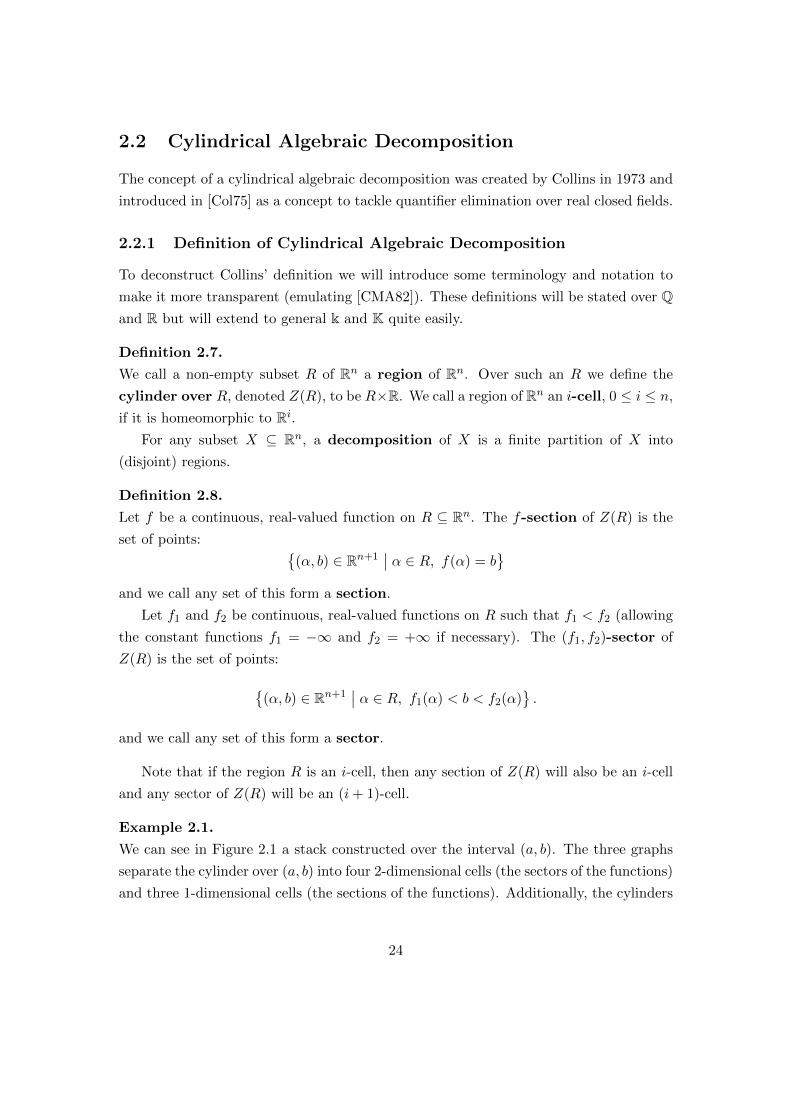
Example 2.1.

We can see in Figure 2.1 a stack constructed over the interval (a, b). The three graphs

separate the cylinder over (a, b) into four 2-dimensional cells (the sectors of the functions)

and three 1-dimensional cells (the sections of the functions). Additionally, the cylinders

24

Figure 2.1: Stack over an interval

over the points a and b have each been decomposed into four 1-dimensional cells and

three 0-dimensional cells.

Definition 2.9.

For a collection of continuous, real-valued functions f1 < f2 < · · · < fk (k ≥ 0) defined

on a region R there is a natural decomposition of Z(R) into the following:

• The fi-sections of Z(R) for 1 ≤ i ≤ k;

• The (fi, fi+1)-sectors of Z(R) for 0 ≤ i ≤ k, where f0 = −∞ and fk+1 = +∞.

Such a decomposition is called a stack over R, or an (f1, f2, . . . , fk)-stack over R.

Related to the concept of a stack is that of a delineable polynomial.

Definition 2.10.

For f ∈ Q[x] and R ⊂ Rn−1 we say that f is delineable on R if V (f) ∩ Z(R) consists

of k disjoint sections of Z(R), for some k ≥ 0.

A delineable polynomial therefore gives rise to a natural stack over R, determined

by the continuous functions whose graphs make up V (f) ∩ Z(R). We denote this stack

S(f,R) and talk of it consisting of the f-sections of Z(R).

We now define the key concept of cylindricity in two ways. The first was the orig-

inal definition given in [Col75] whilst the second has been used in more recent papers

[CMXY09] and offers an alternative perspective. When discussing algebraic decomposi-

tions (Definition 2.13) the definitions are, in fact, equivalent.

25

Definition 2.11.

A decomposition D of Rn is said to be cylindrical if:

• n = 1 and D is a stack over the singleton set (R0); or

• n > 1 and there is a cylindrical decomposition D′ of Rn−1 such that for each region

R′ of D′, some subset of D is a stack over R′.

Such a D′ is unique for a given D and is called the induced (cylindrical) decompo-

sition. We, conversely, say that D is an extension of D′.

Definition 2.12.

A decomposition D of Rn is said to be cylindrical if, for any pair of cells Di, Dj ∈ Dand any 1 ≤ k ≤ n, the canonical projections to Rk, πk(Di) and πk(Dj), are identical or

disjoint.

Definition 2.13.

A semi-algebraic set is one that can be written as a finite combination of unions,

intersections, and complements of sets of the form:

x ∈ Rn | f(x) = 0 ∧ g(x) > 0

for polynomials f, g ∈ Q[x].

A decomposition of Rn is called algebraic if each of its regions is a semi-algebraic

set.

Remark 2.2.

Definitions 2.11 and 2.12 assume an underlying fixed variable ordering for the decom-

position to be cylindrical with respect to. It may be possible to consider the idea of

semi-monotone sets [BGV13] (which are convex with respect to all coordinate directions)

and generalise to produce cells that are cylindrical with respect to multiple variables at

once.

The following result follows from the existence of a quantifier elimination method for

real closed fields, as first discovered in [Tar51].

Theorem 2.1 ([Tar51]).

A subset of Rn is semi-algebraic if and only if it is definable; that is, it equals the

solution set of some standard formula Φ.

There is a strong link between delineability and semi-algebraicity, as shown in the

following theorem.

26

Theorem 2.2 ([Col75, CMA82]).

Let n ≥ 2 and f ∈ k[x] a delineable polynomial on a semi-algebraic region R ⊂ Kn−1.

Then the stack S(f,R) is algebraic.

With the concepts described above, the definition of a cylindrical algebraic decom-

position is straightforward.

Definition 2.14 ([CMA82]).

A cylindrical algebraic decomposition (CAD) of Rn is a decomposition of Rn

that is both cylindrical and algebraic.

For the cells of a CAD we define an index.

Definition 2.15.

Let D be a cylindrical algebraic decomposition of Rn. We define the index of a cell S

of D to be a list of integers Ji1, . . . , inK defined recursively as follows.

• If n = 1 then D consists of intervals and points. List the cells in increasing order

so that the smallest is the 1-cell with −∞ as its left-endpoint, the next cell is the

0-cell immediately to its right on the real line, and so forth. With this ordering,

the smallest cell has index J1K, the next cell has index J2K, and so forth.

• If n > 1 then let D′ be the induced cylindrical decomposition (Definition 2.11)

of Kn−1. Then a cell D ∈ D is an element of a stack over a cell D′ ∈ D′. Let

Ji1, . . . , in−1K be the index of D′. Number the cells of the stack over D′ from bottom

to top (that is, the bottommost cell is the n-cell with −∞ as the left-endpoint for

xn). Then if D is the jth cell of the stack its index is defined to be Ji1, . . . , in−1, jK.

It is worth noting that the dimension of cell is then equal to the sum of the parities

of its indices; for a cell D with index Ji1, . . . , inK we have

dim(D) =n∑j=1

( ij mod 2).

It is also clear that a CAD will always have an odd number of cells (this is true for all

its induced CADs too).

We now to define the concept of invariance over a cell.

Definition 2.16.

Let f ∈ Q[x] and R a region of Rn. We say that f is (sign)-invariant on R and R is

f-invariant if either:

27

• f(α) > 0 for all α ∈ R;

• f(α) = 0 for all α ∈ R; or

• f(α) < 0 for all α ∈ R.

Let F ⊂ Q[x]. Then R is F -invariant if every polynomial in F is invariant on R.

A decomposition of Rn is F -invariant if every cell is F -invariant.

The following is the key result concerning invariance over stacks generated by a

delineable polynomial which underpins many proofs regarding projection-based CAD.

Theorem 2.3 ([Col75, CMA82]).

Let n ≥ 2, F ⊂ k[x], and R a region of Kn−1. Suppose each f ∈ F is delineable on R

and that h =∏f∈F f is delineable on R. Then S(h,R) is F -invariant.

2.2.2 Motivating Application: Quantifier Elimination

Quantifier Elimination was the original motivation of CAD, and is a well-established

problem from mathematical logic. We recall some definitions relating to the decision

theory of real closed fields.

Definition 2.17.

A standard atomic formula is a formula of one of the following six types:

f(x) = 0, f(x) > 0, f(x) < 0, f(x) 6= 0, f(x) ≥ 0, f(x) ≤ 0,

for some polynomial f ∈ k[x].

A standard formula is any formula which can be constructed from standard atomic

formulae using propositional connectives (¬, ∧, ∨, →, ↔) and quantifiers on variables

(∃ xi, ∀ xi).

Definition 2.18.

A quantifier free formula (or QFF) is a standard formula that does not involve any

quantifiers on variables.

A standard prenex formula, or Tarski formula, is a standard formula which has

the form

Φ := (Qkxk)(Qk+1xk+1) · · · (Qnxn)ϕ(x1, . . . , xn)

where ϕ(x1, . . . , xn) is a quantifier-free standard formula of x, the value of k is between

0 and n, and each Qi is a universal or existential quantifier. We say that x1, . . . , xk−1

28

are free variables with respect to Φ, and xk, . . . , xn are bound variables with respect

to Φ.

Problem 2.1 (Quantifier Elimination).

Let Φ be a standard prenex formula over k of the form:

Φ := (Qkxk)(Qk+1xk+1) · · · (Qnxn)ϕ(x1, . . . , xn).

The Quantifier Elimination Problem is to find a quantifier free formula in the free

variables, Ψ(x1, . . . , xk−1), which is equivalent to Φ:

(∀x1)(∀x2) · · · (∀xk−1)[Φ = Ψ

].

In [Tar51], it was shown that the theory of real closed fields allows an algorithmic

solution to Problem 2.1. In doing so, Tarski showed that the theory of real closed

fields is complete and decidable. This proves the important result that definability and

semi-algebraicity are equivalent properties (see Theorem 2.1).

Although Tarski proved that Problem 2.1 has an algorithmic solution, his method

has non-elementary complexity in the number of variables. This means that there is no

finite tower of exponentials, such as:

22. ..2n

sufficient to describe the complexity of the algorithm.

Cylindrical algebraic decomposition [Col75] gave a more efficient method to eliminate

quantifiers1, although (as discussed in Section 2.6) it is still limited by doubly-exponential

complexity [DH88, BD07]. By constructing a sign-invariant CAD of the polynomials for

a quantifier elimination problem, the evaluation of Φ on the induced CAD of Rk−1 can

identify all cells on which Φ holds. Taking the conjunction of the descriptions of these

valid cells gives a quantifier free formula logically equivalent to Φ.

1At the same time as Collins published his work on CAD, a quantifier elimination procedure wasgiven in [Wut74].

29

2.3 Projection and Lifting Cylindrical Algebraic Decom-

position

We now discuss the original algorithm provided by Collins in [Col75] (and also detailed

in [CMA82]), along with the many extensions to its theory and implementation.

2.3.1 Collins’ Algorithm

Informally, the algorithm has two main stages: projection and lifting. The projection

phase produces a sequence of sets of polynomials in Pn−1, Pn−2 and so forth. Once the

projection phase produces polynomials in P1 (univariate in x1) a decomposition of R1 is

produced from these. The lifting phase then takes a decomposition of R1 and produces,

using the projection polynomials, a decomposition of R2. Repeating this we eventually

produce an F -invariant cylindrical algebraic decomposition of Rn.

Definition 2.19.

We refer to any cylindrical algebraic decomposition algorithm that utilises a projection

and lifting approach to construction as a projection and lifting CAD algorithm.

We also refer to the output of such an algorithm as a PL-CAD2.

Projection

We need two more definitions before defining Collins’ projection operator.

Definition 2.20.

For f ∈ k[x] and R ⊂ Kn−1 we say f is identically zero on R if f(α, xn) is equal to

zero for all α ∈ R.

For a set of polynomials F ⊂ k[x] and a set R ⊂ Kn−1 we define the non-zero

product of F on R, FR, to be the product of all f ∈ F that are not identically zero

on R. If all elements of F are identically zero on R then FR := 1 ∈ k[x].

Definition 2.21.

For f ∈ k[x] the reductum of f , written red(f), is simply tail(f). Furthermore, for

k ≥ 0, we define the kth-reductum recursively:

red0(f) := f ;

redk+1(f) := tail(redk(f)).

2A list of CAD acronyms is given in Appendix D for easy reference.

30

The reducia set of f , denoted RED(f) is the set of non-zero reducia of f :

RED(f) := redk(f) | 0 ≤ k ≤ deg(f), redk(f) 6= 0.

We now describe the original projection operator, CP, which computes the principal

subresultant coefficient set, PSC, for various reducia. The PSC defines the interaction

of two polynomials in great detail, and culminates in the resultant of the polynomials.

Definition 2.22 ([Col75]).

Let F = f1, . . . , fm ⊂ Q[x1, . . . , xn]. For each fi ∈ F let Ri := RED(fi). We define

the two sub-projection sets:

CP1(F ) :=m⋃i=1

⋃gi∈Ri

(init(gi) ∪ PSC(gi, sep(gi))

);

CP2(F ) :=⋃

1≤i<j≤m

⋃gi∈Rigj∈Rj

PSC(gi, gj).

We then define the (Collins) projection set, CP(F ), as:

CP(F ) := CP1(F ) ∪ CP2(F ).

We now state the key theorems necessary for the use of CP.

Theorem 2.4 ([Col75, CMA82]).

Let n ≥ 2 and F ⊂ k[x1, . . . , xn]. Let R be a CP(F )-invariant region in Kn−1. Then:

• Every f ∈ F is either delineable or identically zero on R;

• The nonzero-product of F on R, FR, is delineable on R.

Therefore, there exists an algebraic, F -invariant stack over R, namely S(FR, R).

Theorem 2.5 ([Col75, CMA82]).

The projection operator CP is a valid projection operator, that is, it can be used to

produce an F -invariant CAD.

Base Case and Lifting

Let F ∗ equal CP(n−1)(F ). Construct the set of relatively prime, distinct, irreducible

factors of F ∗. The real roots of these factors will be the 0-cells of D∗ and the open

31

Algorithm 2.1: SplitR(F): 1-dimensional space decomposition algorithm.

Input : A set of univariate polynomials, F ∗.Output: A decomposition, D, of R with each cell represented as a list consisting

of a cell index and a sample point.

1 D∗ ← [ ];2 f∗ →∏

f∈F ∗ f ;

3 r ← roots(f∗); n← |r| ; // Compute roots of f∗

4 if n = 0 then5 D∗.append([J1K, 0]) ; // no roots; construct trivial stack

6 return D∗;7 D∗.append([J1K, SamplePoint((−∞, r[1]))]); // Initial interval

8 D∗.append([J2K, r[1]]);9 for i = 2, . . . , n do

10 D∗.append([J2i− 1K, SamplePoint((r[i− 1], r[i]))]);11 D∗.append([J2iK, r[i]]);

12 D∗.append([J2n+ 1K, SamplePoint((r[n],∞))]); // Final interval

13 return D∗;

intervals defined by these roots will be the 1-cells of D∗. This is described in Algorithm

2.1, where SamplePoint is a sub-algorithm that takes a (possibly infinite) interval and

provides a rational sample point from that interval.

For lifting we need to construct cells over a given cylindrical algebraic decomposition

according to the solutions of these CP sets. This is done by creating stacks over each cell

using the CP polynomials and assigning cell indices and sample points appropriately.

For implementation this requires careful treatment of algebraic numbers but this is not

the focus of our research so is not detailed here. The algorithm GenerateStack executes

this lifting stage and is described in Algorithm 2.2.

Complete Projection and Lifting Algorithm

We can combine the ideas of this section to produce Algorithm 2.3, which is the algorithm

described in [Col75] and [CMA82]. The procedure Proj refers to an implementation of

Collins’ projection operator, SplitR is defined in Algorithm 2.1, and GenerateStack is

defined in Algorithm 2.2.

32

Algorithm 2.2: GenerateStack(F, xk, D): Stack generation (lifting) algorithm.

Input : A set of k-variate polynomials, F ; a variable to lift with respect to, xk;a cell to lift over, D.

Output: A stack, S, of cells in Rk over D, with each cell represented as a listconsisting of a cell index and a sample point.

1 S ← [ ];2 I ← D.index; α← D.samplepoint;3 f∗(xk)→

∏f∈F f(α, xk); // Specialise product at α

4 r ← roots(f∗); n← |r|;5 if n = 0 then6 S.append([JI, 1K, (α, 0)]); // No roots; construct trivial stack

7 return S;

8 S.append([JI, 1K, (α, SamplePoint((−∞, r[1])))]); // Initial interval

9 S.append([JI, 2K, (α, r[1])]);10 for i = 2, . . . , n do11 S.append([JI, 2i− 1K, (α, SamplePoint((r[i− 1], r[i])))]);12 S.append([JI, 2iK, (α, r[i])]);

13 S.append([JI, 2n+ 1K, (α, SamplePoint((r[n],∞)))]); // Final interval

14 return S;

Algorithm 2.3: CAD(F, vars): Projection and Lifting-based CAD algorithm.

Input : A set of polynomials, F ; an ordered list of variables, vars = [x1, . . . , xn].Output: A CAD, D, that is sign-invariant with respect to F .

1 D ← [ ];2 P ← [ ];3 P[1]← F ;4 for i = 2, . . . , n do5 P[i] = Proj(P[i− 1], xn−(i−2)); // Projection phase

6 D[1]← SplitR(P[n]); // Base case

7 for i = 2, . . . , n do8 for D ∈ D[i− 1] do9 D[i].append(GenerateStack(P[n− i+ 1], xi, D)); // Lifting phase

10 return D[n];

33

2.4 Extensions to Collins’ algorithm

Collins’ method often provides a CAD that is much more complicated than necessary.

There have been extensions to his algorithm which will be described briefly.

2.4.1 Alternative Projection Operators

One of the key areas of improvement has been in the projection operator CP. We

present three well-documented projection operators: the Collins–Hong operator [Hon90],

McCallum’s operator [McC85, McC88] and the Brown–McCallum operator [Bro01]. We

will also discuss a projection operator proposed by Lazard [Laz94] for which the original

proof is flawed and so, as yet, is unverified.

For all of the following operators let F = f1, . . . , fm be integral polynomials defined

on variables x1, . . . , xn. We use the standard assumptions that the elements of F are

primitive, squarefree and pairwise relatively prime (which must be ensured to hold when

implementing CAD algorithms).

Hong’s Projection ([Hon90])

Definition 2.23.

The Collins–Hong projection set, which we shall denote CHP(F ), is defined as:

CHP(F ) := CP1(F ) ∪ CHP2(F ).

where the second component is defined as:

CHP2(F ) :=⋃

1≤i<j≤m

⋃gi∈Ri

PSC(gi, fj).

The Collins–Hong projection operator is a subset of the Collins operator (CP2(F )

also ranges over the reductum of fj), and requires no additional conditions on the input.

It should therefore always be used in place of Collins’ operator.

McCallum’s Projection ([McC85, McC98])

Definition 2.24.

The McCallum projection set, which we shall denote MP(F ), is defined as follows:

MP(F ) := MP1(F ) ∪MP2(F ) ∪MP3(F )

34

with the sub-projections defined as follows:

MP1(F ) :=m⋃i=1

non-zero coefficients of fi ∈ R[xn]

MP2(F ) := discxn(fi) | discxn(fi) 6= 0, i = 1, . . . ,mMP3(F ) := resxn(fi, fj) | resxn(fi, fj) 6= 0, i, j = 1, . . . ,m, i 6= j

The McCallum projection is a subset of the Collins operator, removing redundant

polynomials and is simple to implement. However, McCallum proved that lifting over

a sign-invariant cylindrical algebraic decomposition with this projection set is not suffi-

cient to guarantee sign-invariance. The stronger idea of an order-invariant cylindrical

algebraic decomposition is introduced.

Definition 2.25 ([McC85, McC98]).

Let f ∈ Q[x] and R a region of Rn. We say that f is order-invariant on R and R is

f-order-invariant if either:

1. f(α) 6= 0 for all α ∈ R; or

2. f(α) = 0 and vanishes to the same order for all α ∈ R: the order of f at α is the

least k ∈ N such that some partial derivative of f of order k does not vanish at α.

Let F ⊂ Q[x]. Then R is F -order-invariant if every polynomial in F is order-

invariant on R. A decomposition of Rn is F -order-invariant if every cell is F -order-

invariant.

Remark 2.3.

For n ≤ 2, sign-invariance implies order-invariance [McC88].

For McCallum’s operator to be valid we must ensure that the polynomials involved

do not vanish identically on cells of positive dimension.

Definition 2.26 ([McC85, McC98]).

A set, F , of polynomials is said to be well-oriented if no element of a basis for F

vanishes identically on any cell of positive dimension, and the same condition holds

recursively for MP(F ).

Theorem 2.6 ([McC85, McC98]).

Let F be a finite, square-free basis of n-variate integral polynomials. Let S be a connected

35

Algorithm 2.4: CADW(F, vars): Projection and Lifting-based CAD algorithm usingMcCallum’s projection operator as specified in [McC98].

Input : A set of polynomials, F ; an ordered list of variables, vars = [x1, . . . , xn].Output: A CAD, D, that is order-invariant with respect to F , or FAIL if F is

not well-oriented.

1 D ← [ ];2 P ← [ ];3 P[1]← F ;4 for i = 2, . . . , n do5 P[i] = MProj(P[i− 1], xn−(i−2)); // Projection phase

6 D[1]← SplitR(P[n]); // Base case

7 for i = 2, . . . , n do8 for D ∈ D[i− 1] do9 i← D.index; α← D.samplepoint;

10 if dim(D) > 0 and ∃ h ∈ P[n− i+ 1] s.t. h(α, xi) ≡ 0 then11 return FAIL; // Input not well-oriented

12 if dim(D) = 0 then13 Dpolys← Delineating Set;

14 D[i].append(GenerateStack(P[n− i+ 1] ∪DPolys, xi, D)); // Lifting

phase

15 return D[n];

submanifold of Rn−1. Suppose each element of F is not identically zero on S and each

element of MP(F ) is order-invariant on S.

Then each element of F is analytically delineable on S [McC98, §3], the sections of

F over S are pairwise disjoint, and each element of F is order-invariant in every section

of A over S.

Therefore MP can be used for a set of well-oriented polynomials. Note that sets of

polynomials are generally well-oriented: in [McC85] a discussion is given to show that

well-orientedness is likely. However, as shown by various examples, it can still prevent

CAD construction.

The full construction of a CAD by McCallum’s projection operator is given in Algo-

rithm 2.4, as discussed in [McC98]. Well-orientedness prevents nullification on positive

dimensional cells; nullification on a zero-dimensional cell is dealt with through delineat-

ing polynomials on line 13 (described in [McC98]).

36

Brown-McCallum’s Projection ([Bro01])

Definition 2.27.

The Brown–McCallum projection set, which we shall denote BMP(F ) is defined

as follows:

BMP(F ) := BMP1(F ) ∪MP2(F ) ∪MP3(F )

with the first component defined as:

BMP(F ) := init(fi) | i = 1, . . . ,m.

As with MP, we need the polynomials to be well-oriented for BMP to be a valid

projection operator. However, there is the added condition that any points where a

polynomial vanishes must also be manually included into the cylindrical algebraic de-

composition. This process of identifying these points takes significant time, but Brown

argues that using BMP is still cheaper than MP, demonstrated by its implementation

in Qepcad-B.

Lazard’s Postulated Projection ([Laz94])

Definition 2.28.

The Lazard projection set, which we shall denote LP(F ) is defined as follows:

LP(F ) := BMP(F ) ∪ LP4(F )

with the additional projection set defined as:

LP4(F ) := trail(fi) | i = 1, . . . ,m.

Note that the Lazard projection operator is a subset of McCallum’s projection opera-

tor and a superset of the Brown-McCallum projection operator. The use of this operator

would still require well-oriented polynomials but would not need vanishing points to be

added. Therefore it could replace the MP operator, and depending on the number of

vanishing points could prove more efficient than BMP.

Whilst Lazard initially presented a proof of the validity of LP it was later found to

be flawed. Recent progress on this work by McCallum and Hong has been submitted for

publication [McC14].

37

Other Work

There has recently been progress in improving the projection operator [HJX12, HDX14,

Str14]. In [HJX12] a projection operator is given to help find when, with respect to a

single parameter, a given polynomial is uniformly positive. This operator is a subset

(often strict) of the Brown’s projection operator. In [HDX14] Brown’s projection oper-

ator is computed with respect to multiple variable orders and intersects them through

gcd computation to simplify the projection. This approach guarantees a sample point in

each open connected component. In [Str14] the projection operator is adapted to each

particular cell (producing a local projection set). This not only simplifies the num-

ber of cells produced, by using the Boolean structure and signature of the problem on

each indiviual cell, but can also avoid irrelevant failure due to a lack of well-orientedness

(Definition 2.26).

2.4.2 Partial CAD

In [CH91] the idea of a partial CAD was introduced. For a given Quantifier Elimination

problem, instead of lifting a whole CAD, partial CAD constructs stacks over cells in

order and, wherever possible, the lifting is truncated using two main ideas.

Quantifiers: Consider the sentence (∃ x)(∃ y)ϕ(x, y). Then when lifting from R to R2

the algorithm would stop as soon as it found a cell satisfying (∃ y)ϕ(x, y), returning

TRUE. Alternatively, if the sentence was (∀ x)(∃ y)ϕ(x, y), the algorithm would

stop as soon as any cell is found in which ¬(∃ y)ϕ(x, y) and return FALSE.

Boolean connectives: Consider the sentence (∃ x)(∃ y)ϕ(x, y) where ϕ(x, y) = ϕ1(x)∧ϕ2(x, y), where ϕi are quantifier-free formulae. Then we can evaluate ϕ1(x) on a

cell, D′ of the R1 CAD, D′. If false, then ϕ(x, y) must be false for all y and so there

is no need to construct a stack over D′. Alternatively, if ϕ(x, y) = ϕ1(x)∨ϕ2(x, y)

and ϕ1(x) is true on D′ then there is no need to construct a stack over D′.

Whilst using partial CAD there is also the consideration of which order to choose

the cells to lift over, which can clearly affect the time taken: constructing a lone cell

that satisfies the formula first could prevent the construction of doubly-exponential cells

that do not satisfy the formula. The authors of [CH91] suggest a variety of choices

dependent on the type of problem (robot motion planning, systems of strict inequalities,

termination proofs), providing experimental justification.

There has also been work on adapting the projection operator within partial CAD

[SS03]. The authors of [SS03] introduce a generic projection operator, which is placed

38

between Collins’ and Brown’s operators and considers solutions only within a region

defined by assumptions on the parameters. This approach is particularly well-suited for

formulae with many parameters and polynomials of high degree.

2.4.3 Truth-Invariant CAD

In [Bro98], Brown introduced the idea of truth-invariance for a CAD. He gave the fol-

lowing definitions:

Definition 2.29 ([Bro98]).

Let A and B be two CADs. We say B is simpler than A if A is a refinement of B, i.e.

each cell in B is the union of some cells of A, and A and B are not equal.

Given a formula ϕ from the elementary theory of real closed fields, we say a CAD is

truth-invariant with respect to the input formula if in each cell of the decomposition

the formula is either identically true or identically false.

Brown starts by looking at cells on the top level of a CAD of free variable space.

Let x1, . . . , xk be the free variables of a quantified formula Φ, with quantifier free part

ϕ(x1, . . . , xn). Then if none of the sections of a polynomial of level k form the boundary

between a true and false region of Rk then it can be ignored when constructing a truth-

invariant CAD. As only level k polynomials are potentially being discarded, no inter-

stack boundaries will be removed, so only intra-stack adjacencies need to be considered.

When considering simplifying a CAD at lower levels the following definition is im-

portant.

Definition 2.30 ([Bro98]).

Let C ∈ D be an i-level section cell of a ϕ-truth-invariant cylindrical algebraic de-

composition, and let B and D correspond to the neighbouring cells within the stack

containing C. Suppose all polynomials of level i and greater are delineable over the

union B ∪ C ∪ D. We say that C is a truth-boundary cell (or more specifically an

i-level truth-boundary cell) if there exists a triple of cells (B′, C ′, D′) such that:

• B′, C ′, and D′ lie in the stacks over B, C, and D, respectively;

• B′ ∪ C ′ ∪D′ is a cell in the stack over B ∪ C ∪D; and

• B′, C ′, and D′ do not all have the same truth value for ϕ.

Consider a quantified formula Φ, with quantifier free part ϕ(x1, . . . , xn). Brown pro-

vides an algorithm to create a truth-invariant CAD with respect to ϕ (called SIMPLECAD).

39

This takes as input the projection factors, P , and a CAD, D, which is sign-invariant

with respect to P (and therefore truth invariant with respect to ϕ). The output is a

subset P ⊆ P (closed under projection), and a P -sign-invariant CAD D that is still

truth invariant with respect to ϕ.

Initialising P := ∅ and D := D, Brown produces his truth-invariant CAD iteratively.

Starting at the highest level and working down, at loop i:

1. add the projection of its elements to P ;

2. construct the set of all i-level truth boundary cells in D that are not sections of P ;

3. for each cell in this set, take all i-level polynomials in P which are zero on that

cell.

4. construct a minimal hitting set for these polynomials and add to P ;

5. simplify D according to the new definition of P .

The combination of the initial removal of level k polynomials that do not form bound-

aries between true and false cells, and then using SIMPLECAD, is implemented within

Qepcad-B. Brown shows that it can construct substantially simpler CADs (which also

results in a simpler quantifier-free formulae).

2.4.4 Equational Constraints

In [Col98] the idea of equational constraints was first introduced. The idea was later

expanded upon [McC99, McC01, BM05].

Definition 2.31.

For a given quantifier elimination problem Φ, a constraint is an atomic formula which

is logically implied by the quantifier free part, ϕ, of Φ. If such a constraint is an equation

we call it an equational constraint.

If ϕ := (f = 0) ∧ ϕ then f is an equational constraint, and we say that f is an

explicit equational constraint of ϕ. Alternatively, if ϕ := (f1 = 0) ∨ (f2 = 0) then

the equation f1f2 = 0 is an equational constraint, and we say that f1f2 = 0 is an

implicit equational constraint of ϕ.

The idea behind using equational constraints to simplify the projection operator

is that we only need to be concerned with the behaviour of polynomials whilst the

equational constraint is satisfied. Therefore, if f = 0 is an equational constraint and g

40

is any other polynomial in ϕ, then the behaviour of g when f is non-zero does not affect

the behaviour of ϕ. Hence, instead of including the coefficients and discriminant of g or

its resultant with any polynomial that is not f in the first projection set, we just need

to include resxn(f, g). This is given formally in Definition 2.32.

Let f be an equational constraint polynomial for Φ. Let A be the set of irreducible

factors of all polynomials in Φ with positive degree in xn. Let E be the subset of A

containing irreducible factors of f .

Definition 2.32 ([McC99]).

The restricted projection (or equational constraint projection) of A relative to

E, MPE(A) is defined to be:

MPE(A) := MP(E) ∪ resxn(f, g) | f ∈ E, g ∈ A, g /∈ E.

The following key theorem from [McC99] shows that if MPE(A) is used for the first

projection and E is used for the final lifting the produced CAD is sufficient to solve Φ.

Theorem 2.7 ([McC99]).

Let A be a set of pairwise relatively prime and irreducible integral polynomials of positive

degree in xn (n ≥ 2). Let E be a subset of A. Let S be a connected submanifold of Rn−1.

Suppose that each element of MPE(A) is order-invariant in S. Then each element of

E either vanishes identically on S or is analytic delineable on S, the sections over S

of the elements of E which do not vanish identically on S are pairwise disjoint, each

element of E is order-invariant in every such section, and each element of A not in E

is sign-invariant in every such section.

Note that the fact the elements of A are sign-invariant (and not order-invariant)

means that MPE(A) cannot be used repeatedly, unless n ≤ 3 (recall Remark 2.3).

In [McC01] the author defines the semi-restricted projection MP∗E(A) of A rela-

tive to E to be

MP∗E(A) := PE(A) ∪ discxn(g) | g ∈ A, g /∈ E.

This set guarantees order-invariance of g ∈ A in sections of f over cells and so could be

used repeatedly throughout the whole algorithm.

The author also notes how multiple equational constraints provide constraints for

lower levels: if f1 and f2 are both equational constraints, then so is their resultant. In

[BM05] the authors take this further and describe an algorithm that computes a CAD

reliant on the variety V (f, g) rather than the separate polynomials. The authors point

41

out that this is the first step towards a theory of CAD which is defined on systems of

equations rather than individual polynomials.

The theory of equational constraints and truth-invariant CADs will be generalised

in Chapter 3 into the idea of truth table invariant CADs, which allow for the logical

structure of formulae to be exploited even further.

Remark 2.4.

Theorem 2.7 allows for a simplified lifting operator at the final lifting stage. As the

non-equational constraints, A, are guaranteed to be sign-invariant on the sections of the

equational constraint, the final lift need only be conducted with respect to E. This

extension was introduced in [Eng13a, BDE+14] and will be discussed in Chapter 3.

2.4.5 Solving Strict Inequalities

Given a problem involving only strict polynomial inequalities, any cells that satisfy the

inequalities must necessarily be full dimensional. In [McC93] and later in [Str00] algo-

rithms are given that only lift over full-dimensional cells at each stage of the algorithm.

This idea will be revisited in Chapter 4.

A full-dimensional cell in a CAD is a product of open intervals, and so the sample

points are from Qn. Not requiring the use of algebraic number computation increases the

efficiency of the algorithm both in experimentation and theoretical complexity (discussed

in Section 2.6).

2.4.6 Preconditioning for CAD

It is possible to precondition the input for a CAD algorithm to try to improve the

efficiency.

In [BH91] the authors considered the use of Grobner bases as a preconditioning

technique for quantifier elimination by CAD. They show that it is often, but not al-

ways, beneficial to replace a conjunction of equalities by their Grobner basis. This is

investigated further in Chapter 6.

In [BG06] the author pre-processes the input formula for quantifier elimination. They

substitute linear equational constraints to build a space of equivalent statements. They

then use a grading function (which notes properties relating to the Boolean and quantifier

structure) and search for a minimal formula.

In [BS10] the authors provide two methods for fast simplification of quantifier elimi-

nation problems, which are integrated into algorithms for quantifier elimination by both

virtual substitution and cylindrical algebraic decomposition. Black box simplification

42

is conducted by considering the Boolean structure of the formula with respect to sign

conditions3. White box simplification uses the polynomials themselves to deduce sign

conditions (such as given 1− x+ y2 using 2x− 1 < 0 to deduce 1− x+ y2 > 0).

2.5 Regular Chains Cylindrical Algebraic Decomposition

Until recent years, the only method of calculating a cylindrical algebraic decomposi-

tion was that given in [Col75]. In [CMXY09] a new method was described reliant

on the theory of triangular decompositions and regular chains. This was later ex-

tended in [CM12] to provide an incremental (by polynomial) approach to building a

cylindrical algebraic decomposition. These algorithms have been implemented in the

RegularChains package for Maple; the former algorithm has been available, as Semi-

AlgebraicTools[CylindricalAlgebraicDecompose], since Maple 16, and the latter

will be freely available from the RegularChains research group website4.

2.5.1 Triangular Decomposition

We begin by covering some of the key concepts in the theory of regular chains and tri-

angular decompositions. This is a very deep subject and for a comprehensive discussion

see [Maz05].

Definition 2.33.

For a set of polynomials F ⊂ k[x] we define hF to be the product of the initials of all

polynomials in F . The quasi-component of F , denoted W(F ), is defined to be

W(F ) := V(F ) \V(hF ).

For any h ∈ k[x] we define Z(F, h) to be W(F ) \V(h).

Definition 2.34.

Let F ⊂ k[x] be a set of non-constant polynomials. We say F is a triangular set if the

polynomials in F have pairwise disjoint main variables.

Let mvar(F ) be the set of the main variables of the polynomials in F . A variable x

is algebraic with respect to F if x ∈ mvar(F ), and is otherwise free.

3This has been implemented, by Brown, into the Slfq extension for Qepcad-B: http://www.usna.edu/CS/~qepcad/SLFQ/Home.html

4www.regularchains.org

43

The sets F<x and F>x are defined to be all polynomials f ∈ F such that mvar(f) ≺ xand mvar(f) x, respectively. If x ∈ mvar(F ) we let Fx denote the unique polynomial

in F such that mvar(Fx) = x.

Definition 2.35.

Let h ∈ k[x] and F ⊂ k[x] be a triangular set. The iterated resultant of h with respect

to F , ires(h, F ), is defined as follows:

1. If h ∈ k or all variables in h are free with respect to F then ires(h, F ) := h.

2. Otherwise, if x is the largest variable of h which is in mvar(F ) then

ires(h, F ) := ires(r, F<x), where r := resx(h, Fx).

Definition 2.36.

Let F ⊂ k[x] be a triangular set of polynomials. The saturated ideal of F , sat(F ) is

defined to be 〈0〉 if F = ∅, otherwise:

sat(F ) := 〈F 〉 : h∞F = f ∈ k[x] | ∃k ∈ N s.t. hkF f ∈ 〈F 〉.

Definition 2.37.

A triangular set F ⊂ k[x] is a regular chain if either F = ∅ or ires(hF , F ) 6= 0. This

is equivalent to saying that hF is regular modulo sat(F ) (meaning that hF is neither

zero modulo sat(F ), nor a zero divisor modulo sat(F )).

A regular system is a pair [F, h] such that F is a regular chain and ires(h, F ) 6= 0.

The zero set of [F, h] is Z(F, h) (recall this equals W(F ) \V(h) and W(F ) = V(F ) \V(hF )).

A triangular decomposition of a zero-dimensional variety produces a sequence

of regular systems such that their zero sets decompose the zero system of the original

system.

Triangular decompositions have many desirable properties due to that fact the initials

of the polynomials in a regular chain behave nicely. For example, the variety of a regular

chain is equiprojectable: all fibers of the projection map on the variety have the same

cardinality [DMS+04].

2.5.2 Recursive Regular Chains CAD (RC-Rec-CAD)

The new algorithm for CAD introduced in [CMXY09] makes use of triangular decom-

positions to tackle CAD. Whereas the original algorithm was rooted purely in Rn, the

44

new algorithm first decomposes Cn. The idea of a cylindrical decomposition of Kn (for

which we will think of Cn) is needed, analogous to Definitions 2.11 and 2.12.

Definition 2.38 ([CMXY09]).

A cylindrical decomposition, D, of Kn is defined recursively:

• If n = 1 then D = D1, . . . , Dm+1 where either:

– m = 0 and D1 = K; or

– m > 0 and there exists m non-constant, squarefree, co-prime f1, . . . , fm ∈ k[x]

such that for 1 ≤ j ≤ m:

Dj = z1 ∈ K | f1(z1) = 0 and Dm+1 = z1 ∈ K |m∏j=1

fj(z1) 6= 0.

• If n > 1, let D′ = D1, . . . , Ds be a cylindrical decomposition of Kn−1. For each

Di let fi,1, . . . , fi,mi ⊆ k[x] be a set of polynomials that separates above Di

(for all α ∈ Di, (init(fi,j))α 6= 0 and (fi,j)αmij=1 are co-prime).

– If mi = 0 then Di,1 = Di ×K.

– If mi > 0 then for 1 ≤ j ≤ mi:

Di,j = (α, zn) ∈ Kn | α ∈ Di, fi,j(α, zn) = 0 and

Di,mi+1 = (α, zn) ∈ Kn | α ∈ Di,

mi∏j=1

fi,j(α, zn) 6= 0.

The collection D = Di,j | 1 ≤ i ≤ r, 1 ≤ j ≤ ri is then a cylindrical decomposi-

tion of Kn.

The concept of sign-invariance (Definition 2.16) is generalised to Cn:

Definition 2.39 ([CMXY09]).

Let f ∈ Q[x] and R a region of Cn. We say that f is invariant on R if either:

1. f(α) = 0 for all α ∈ R; or

2. f(α) 6= 0 for all α ∈ R.

Let F ⊂ Q[x]. Then R is F -invariant if every polynomial in F is invariant on R. A

decomposition of Cn is F -invariant if every cell is F -invariant.

45

The algorithm for a set of polynomials F ⊂ Q[x] then consists of three main steps:

1. InitialPartition: Decomposes Cn into constructible sets (a finite combina-

tion of algebraic varieties by set union and difference) that are F -invariant using

triangular decomposition techniques.

2. MakeCylindrical: Transforms the constructible sets into an F -invariant cylindri-

cal decomposition of Cn.

3. MakeSemiAlgebraic: Transforms the cylindrical decomposition of Cn into an F -

invariant cylindrical algebraic decomposition of Rn.

Whilst the initial implementation means that this algorithm is often less time-efficient

than implementations of Collins’ algorithm, it can often produce CADs with much fewer

cells. Due to many of the algorithms being recursive in nature, we refer to this algorithm

as the recursive regular chains algorithm, or RC-Rec-CAD.

2.5.3 Incremental Regular Chains CAD (RC-Inc-CAD)

Recently [CM12], a new algorithm has been published improving on the one described in

Section 2.5. Their approach is still to create an F -invariant cylindrical decomposition of

Cn and apply MakeSemiAlgebraic to produce an F -invariant CAD of Rn. Their method

of creating the cylindrical decomposition of Cn differs significantly however, utilising an

incremental approach.

Rather than thinking in terms of a decomposition, they construct a complex cylin-

drical tree.

Definition 2.40 ([CM12]).

We define the complex cylindrical tree (CCT) for a cylindrical decomposition of Cn

by induction on n. For n = 1, let D = D1, . . . , Dr+1 be a cylindrical decomposition.

The tree associated with D is a rooted tree whose nodes, other than the root, are

D1, . . . , Dr+1, which all are leaves and children of the root.

Now let n > 1, D = Di,j | 1 ≤ i ≤ s, 1 ≤ j ≤ ri+1 be the cylindrical decomposition

of Cn, over the induced cylindrical decomposition D′ = D′1, . . . , D′s of Cn−1 (where

Di,j | 1 ≤ j ≤ ri are the cells in the cylinder over D′i). If T ′ is the tree associated with

D′ then the tree T associated with D is defined as follows. For each 1 ≤ i ≤ s the set D′iis a leaf in T ′ which has all Di,j ’s for children in T ; thus the Di,j ’s are the leaves of T .

The complex tree can be thought as a mathematical realisation of the piecewise

output of CAD in Maple [CDM+09]. Starting with the trivial cylindrical tree (the tree

46

of depth n where each condition is simply “∀xj”) they ‘refine’ along each path from the

root with each of the polynomials in F . This refinement consists of taking the greatest

common divisors of the irreducible factors of the current polynomial with the conditions.

With this new method, the algorithm can make use of equational constraints and

certain partial CAD techniques (using the quantifier structure of the problem), which

were incompatible with the recursive method described in Section 2.5. With these addi-

tions the new algorithm seems to outstrip all other algorithms on most examples [CM12].

Further, this method can be used for quantifier elimination, which has been implemented

and investigated for future publication [CMM14].

As this algorithm incrementally refines the complex cylindrical tree before construct-

ing the CAD, we refer to this algorithm as the incremental regular chains algorithm,

or RC-Inc-CAD.

2.6 Complexity of Cylindrical Algebraic Decomposition

Cylindrical algebraic decomposition improved on the complexity of Tarski’s original de-

cision method [Tar51], which had non-elementary complexity. However, constructing a

cylindrical algebraic decomposition is still a difficult procedure, as shown by the com-

plexity results detailed in this section.

2.6.1 Formal Complexity of CAD and QE

In [DH88] the authors prove that quantifier elimination and CAD are both inherently

doubly exponential in the number of variables, n.

This is done by converting the complex equation:

x22j+1

1 = x2

into a quantified real formula φj in variables x1R, x1I , x2R, x2I where xj = xjR + ixjI .

Then setting x2 = 1 gives the 22j+1roots of unity.

Considering the decomposition of R6j+2 induced by φj , it must contain at least 22j+1

0-dimensional cells. Therefore, in terms of the number of variables, n, we obtain a lower

bound in complexity of

22(n−2)/6. (2.2)

This can be improved slightly by perturbing φj to get

22(n−2)/5. (2.3)

47

The best upper bounds of the time had an exponent of n + log n + 5 leaving a large

working range.

In [BD07] the authors improve on this result in a variety of ways. Their bound is

tighter, requires only linear polynomials and does not assume a dense representation of

polynomials. They also prove results about variable ordering which will be discussed in

Section 2.6.3.

Their construction starts with the piecewise function:

f0(x) =

2x for x ≤ 1

2

2− 2x for x > 12

;

and f(k)0 is the k-fold composition of f0. It is easy to define a quantified formula

Φn(xn, 1/2) which defines the midpoints of the segments of the graph of f(k)0 on [0, 1].

The bound the authors achieve is

22(n−1)/3. (2.4)

2.6.2 Complexity of CAD Algorithms

The complexity results in [DH88] and [BD07] are lower bounds for the complexity of

certain CADs. This does not inform us about the complexity of specific algorithms. We

summarise the known results here.

Collins’ Algorithm

In [Col75], after introducing the original CAD algorithm Collins gives a detailed com-

plexity analysis of its execution. For an input of m polynomials with degree d in n

variables with maximum norm length of coefficients l the complexity is:

O(

(2d)22n+8m2n+6

l3). (2.5)

Collins notes that the exponents in (2.5) can likely be reduced by using more efficient

subalgorithms (stating the exponent of l reduces from 3 to 2 + ε for any ε > 0) and by a

tighter analysis of the CAD algorithm (stating that the initial exponent of 2n+ 8 could

reduce to 2n+ 4). The analysis will be given in more detail in Section 4.5 in the context

of analysing a new algorithm.

48

McCallum’s CADMD Algorithm

In [McC93] the author introduces an algorithm to construct only the full dimensional

cells of a CAD (discussed in Section 2.4.5). The production of fewer cells and avoidance

of computations with algebraic numbers (all sample points are in Qn) offers large savings

and McCallum gives a complexity analysis producing:

O(

(2d)3n+4m2n+4

l3). (2.6)

The exponents in (2.6) are smaller than (2.5) (as 3n+4 < 22n+8 = 4n+4). This

analysis will be revisited in detail in Section 4.5 when analysing a new algorithm.

Remark 2.5.

Whilst the lower bounds of (2.2), (2.3), (2.4) and the upper bounds of (2.5), (2.6) are all

doubly exponential in n, they do not imply that CAD is 22Θ(n). There is a large range of

permissible complexities and a small difference in the double exponent (such as between

(2.5) and (2.6)) can offer huge savings in an implementation.

Also note that for a fixed n the complexities are polynomial in d, m and l. As the

exponents of d and m depend exponentially on n, any reduction in the value of the linear

terms in n will have a significant effect.

2.6.3 Variable Ordering for CAD

For a given set of polynomials the choice of variable ordering can make a significant

difference to the complexity of the CAD produced. This was demonstrated in [BD07]

where a single polynomial was given in 3n + 3 variables that produced 3 cells for a

particular ordering, but 22n cells with a different projection ordering. Note that there is

not always a “good” variable ordering; the same paper produced a set of 3n2 polynomials

in 3n+ 1 variables that produces a CAD with at least 22n cells with any of the (3n+ 1)!

projection orders.

Identifying a computationally easy way to identify an optimal variable ordering for

a given problem is of great importance. For quantifier elimination problems the choice

of variable ordering is restricted to admissible orderings.

Definition 2.41.

Let Φ be a quantifier elimination problem. Let the quantifiers in Φ be

(Qkxk)(Qk+1xk+1) · · · (Qnxn).

49

We can group together adjacent quantifiers of the same type (as ∀x∀y ↔ ∀y∀x and

∃x∃y ↔ ∃y∃x) to give the block representation of Φ as:

(Q1B1) · · · (QrBr)ϕ

where Qi 6= Qi+1 for i = 1, . . . , r−1 and the Bi are a partition of xk, . . . , xn respecting

their order. An admissible ordering for Φ is any which projects the variables of Br

first, followed by Br−1, and so forth until B1, followed by any ordering of x1, . . . , xk−1.

In [DSS04], the authors systematically tested a collection of metrics to find the one

which best correlates with CAD complexity. The most appropriate metric was found to

be the sum of total degrees, sotd.

Definition 2.42 ([DSS04]).

For a set of polynomials F ⊂ Q[x] and variable ordering x, the sum of total degrees,

sotd(F, x), is defined to be:

sotd(F, x) =n∑i=1

∑f∈Fi

σ(f)

where F1, . . . , Fn are the projection sets of F with respect to x and σ(f) sums the total

degrees of each monomial in f .

In [Bro04] a simple heuristic for deciding variable ordering was given.

Definition 2.43 ([Bro04]).

The Brown heuristic assigns the order of variables to be eliminated according to the

following conditions (breaking ties with successive conditions):

1. Descending order by degree of variable;

2. Descending order by highest total-degree term in which the variable appears;

3. Descending order by the number of terms containing the variable.

This is computationally simple, and performs remarkably well. However, Phisanbut

noticed ([Phi11]) that this heuristic does not distinguish between coupled variables (real

variables arising from the same complex variable) in Branch Cut Analysis (Section 2.8.1).

These heuristics will be revisited with respect to variable ordering in Chapter 5, as

well as in Chapters 3, 6, and 7.

50

2.7 Adjacency in Cylindrical Algebraic Decomposition

Given a CAD, it is often important to know the adjacency of cells. Although it will not

be a focus of the research in this thesis, we give the appropriate definitions, as it has

important implications on CAD algorithms and properties of CADs that enable easier

adjacency computations. Further details are given in Appendix A.

We have two alternative definitions for adjacency in a CAD, which we will refer to

as (A1) and (A2).

Definition 2.44.

Given two disjoint cells D1, D2 of Rn we say they are adjacent if either:

(A1) their union, D1 ∪D2, is connected.

(A2) the cell of smaller dimension is entirely contained in the closure of the larger-

dimensional cell.

If D1, D2 are adjacent regions, we call the set D1, D2 an adjacency. If unclear,

we can specify an (A1)-adjacency or (A2)-adjacency.

If D1, D2 is an (A2)-adjacency and D2 is the cell of smaller dimension, we say D2

is a face of D1.

Whilst (A2) implies (A1), the converse is not true and so (A1) and (A2) are not

equivalent definitions. Details on algorithms to compute adjacencies of a CAD and to

use such adjacencies to improve construction are described in Appendix A.

2.8 Applications of Cylindrical Algebraic Decomposition

The use of CAD for quantifier elimination opens up many applications. Quantifier

elimination is important for many areas of mathematics, science and engineering.

There are a variety of applications for cylindrical algebraic decompositions, along

with quantifier elimination. Five applications we briefly discuss are the analysis of branch

cuts in complex identities, robot motion planning, automated theorem proving, formal

verification of dynamical systems, and an automated examination question answering

system.

51

1

1

-1

-1

(a) Identity (2.7).

1

1

-1

-1

(b) Identity (2.8).

Figure 2.2: Branch Cut geometry for identities involving square roots.

2.8.1 Branch Cut Analysis

Consider the problem of deciding the validity of the two following identities over C:

√1− z

√1 + z

?=√

1− z2; (2.7)√z − 1

√z + 1

?=√z2 − 1. (2.8)

In [PBD11] (and further discussed in [Phi11]) the authors stress how the geometry

of the branch cuts involved in an identity are key to discovering its validity. If we look

at Figure 2.2 we can see:

• The branch cuts of (2.7) do not divide the complex plane and the identity is true

over the whole plane.

• The branch cuts of (2.8) divide the complex plane into three regions and the

identity is false on two of these regions.

Note that this is typical but not universal behaviour: examples exist where the

complex plane is split but an identity holds everywhere, or where the plane is not split

but the identity fails on the branch cuts themselves.

An automatic procedure for deciding validity of such problem can be created using

CAD. For a given complex identity the steps of Algorithm 2.5 are carried out [BPB05,

Phi11].

Branch cut verification will be revisited in Chapter 3 as an application particularly

suited to the advances described in that chapter.

52

Algorithm 2.5: Verify: Complex identity verification (with CAD) algorithm.

1 Find a possible simplification;2 Check ‘algebraically’ it is correct (e.g. using simplify(..,symbolic) in Maple);3 Check correctness for branch cuts:

i. Determine all branch cuts;

ii. Represent them as semi-algebraic equations in <(z) and =(z);

iii. Generate a CAD of Cn = R2n according to the branch cuts;

iv. Evaluate at the sample point of each cell: the simplification is either identicallytrue or generically false on cell;

2.8.2 Robot Motion Planning

Problem 2.2 (Piano Mover’s Problem).

Given an object in a space filled with other objects, is there a path from one specified

point to another without any objects colliding?

In [SS83b], the authors described a way to solve Problem 2.2 using CAD. The authors

describe a method of rewriting objects as semi-algebraic sets and translating these into

conditions to ensure safe passage of the robot. Inputting into a CAD algorithm would

then provide cells where the robot can safely traverse to. However, in [Dav86] a simple

example is considered (a 3m ladder in a right-angled corridor of 1m width) and shown

to be too complex for CAD technology. Even with current algorithms and computing

power, this example still proves too complex without geometric reasoning.

More recently, [Lee11], CAD has also been used as a subprocedure of a spatial-

awareness algorithm for robots using artificial intelligence techniques.

The Piano Mover’s Problem will be revisited in Chapter 6, where a reformulation of

the problem allows for a cylindrical algebraic decomposition to be created in a reasonable

amount of time.

2.8.3 Automated Theorem Proving

Decision methods for the first order theory of the reals have been used in automatic

theorem proving in a variety of ways. In [DSW98] the authors translate geometrical

theorems into quantifier elimination problems. A simple example is the theorem that

53

two lines intersect at one and only one point, which translates to:

∃x∀y(mx+ b = 0 ∧ (y = x ∨my + b 6= 0)). (2.9)

Although they state, quite correctly, that Qepcad is insufficient for most non-trivial

examples on its own, they do use it as an intermediary tool. This is often to prove that

their reformulation is equivalent to the problem being queried.

Qepcad is also used within the automatic theorem tool MetiTarksi which proves

results regarding elementary functions by restating them in terms of polynomial bounds.

This was first introduced in [AP08] and later extended in:[AP09, PPdM12]. There has

been much work done on optimising this code and it is often the state-of-the-art.

2.8.4 Formal Verification of Dynamical Systems

The work in [ST11] (building on work such as [Jir97, Ioa97]) describes formally verifying

and synthesising (continuous and switched) dynamical systems. By reducing a dynamical

system’s behaviour to a first-order formula over the reals, quantifier elimination can be

used to investigate its behaviour. Four case studies are given: avoiding crashes with

adaptive cruise control in cars; applying force to a robot to maintain a certain position;

ensuring stability with adaptive flight control; and maintaining an inverted pendulum

in its unstable equilibrium.

Reducing behaviour of a system to a quantified formula the authors then follow a

three step process: eliminating all variables that are allowed (due to the degree bounds)

by virtual substitution (described in Section 2.9.2); using Slfq to apply black-box pre-

conditioning (described in Section 2.4.6) to the resulting formula; constructing a CAD

for the (possibly still quantified) preconditioned formula and to provide an equivalent de-

scription of the behaviour of the system. They also note that the quantifier-free formulae

generated from CAD-based QE algorithms are very understandable: “it is well-known

that elimination results of CAD, in contrast to most other QE methods, are very concise,

nonredundant, and intuitively interpretable” ([ST11]).

2.8.5 Automated Examination Question Answering System

The Todai Robot Project5 aims to create an automated system to pass the Tokyo Uni-

versity entrance exam by 2021 [AMIA14, MIAA14]. The exam consists of seven subject

areas, including mathematics, and the automated system must interpret each exam ques-

5http://21robot.org/

54

tion, discover a solution (using methods depending on the subject area), and construct

an answer.

Approximately 47% of the mathematics questions on the entrance exams can be

expressed in the theory of real closed fields [MIAA14, Table 1], and can be solved by

quantifier elimination. A hybrid system is used, applying virtual substitution and Sturm-

Habicht sequences, where appropriate, before appealing to CAD to solve these questions.

As the automated translation from the exam script to a quantified formula often produces

overly-complicated input with many variables, preconditioning of the input is essential

(including techniques discussed in [WBD12] and Chapter 6).

2.9 Alternatives to Cylindrical Algebraic Decomposition

CAD is not the only alternative to Tarski’s original decision algorithm for the first order

theory of the reals, nor the only algorithm for analysing semi-algebraic sets. Although

CAD vastly improves on the theoretical complexity of Tarski’s algorithm, it is possible

to improve it further. This section is not intended to be an in-depth discussion of these

algorithms but an overview to offer a frame of reference to CAD. Nor is this section

intended to particularly justify the study and use of CAD or alternative algorithms:

there are situations where particular algorithms are more well-suited, and the study of

CAD in this thesis is intended purely to improve CAD’s efficiency.

2.9.1 Singly-exponential Algorithms

The first decision algorithm for the existential theory of the reals that had singly ex-

ponential complexity was presented by Grigor’ev and Vorobjov in [Gri88, GV88]. This

was improved upon in a series of papers by a range of authors, culminating in a trio

of papers by Renegar [Ren92a, Ren92b, Ren92c]. We will try to outline the basic ideas

behind these results as discussed and aggregated in [BPR06].

A problem is translated into an alternative question: for a set of polynomials,

F ⊂ R[x], find the corresponding set of all realisable sign conditions, Sign(F ) ⊆−1, 0, 1F . This is sufficient to decide existence of a solution to a Tarski formula.

The polynomials are then translated into strong l-general position with respect

to a polynomial q ∈ R[x]. First the set F needs to be partitioned into subsets Fisi=1

such that, for each i, no two elements of Fi have a common zero in Rn. Further, no

l + 1 polynomials belonging to different Fi can have a zero in common with q in Rn.

Moreover, any l polynomials belonging to different Fi can have at most a finite number

55

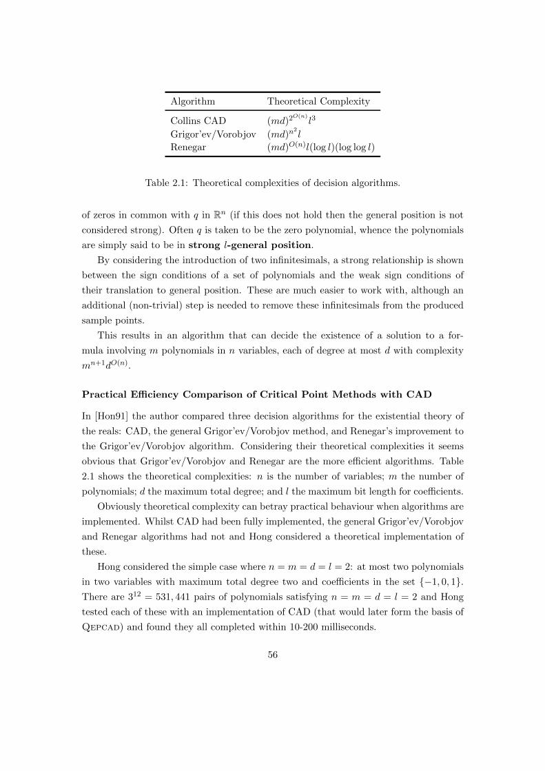
Algorithm Theoretical Complexity

Collins CAD (md)2O(n)l3

Grigor’ev/Vorobjov (md)n2l

Renegar (md)O(n)l(log l)(log log l)

Table 2.1: Theoretical complexities of decision algorithms.

of zeros in common with q in Rn (if this does not hold then the general position is not

considered strong). Often q is taken to be the zero polynomial, whence the polynomials

are simply said to be in strong l-general position.

By considering the introduction of two infinitesimals, a strong relationship is shown

between the sign conditions of a set of polynomials and the weak sign conditions of

their translation to general position. These are much easier to work with, although an

additional (non-trivial) step is needed to remove these infinitesimals from the produced

sample points.

This results in an algorithm that can decide the existence of a solution to a for-

mula involving m polynomials in n variables, each of degree at most d with complexity

mn+1dO(n).

Practical Efficiency Comparison of Critical Point Methods with CAD

In [Hon91] the author compared three decision algorithms for the existential theory of

the reals: CAD, the general Grigor’ev/Vorobjov method, and Renegar’s improvement to

the Grigor’ev/Vorobjov algorithm. Considering their theoretical complexities it seems

obvious that Grigor’ev/Vorobjov and Renegar are the more efficient algorithms. Table

2.1 shows the theoretical complexities: n is the number of variables; m the number of

polynomials; d the maximum total degree; and l the maximum bit length for coefficients.

Obviously theoretical complexity can betray practical behaviour when algorithms are

implemented. Whilst CAD had been fully implemented, the general Grigor’ev/Vorobjov

and Renegar algorithms had not and Hong considered a theoretical implementation of

these.

Hong considered the simple case where n = m = d = l = 2: at most two polynomials

in two variables with maximum total degree two and coefficients in the set −1, 0, 1.There are 312 = 531, 441 pairs of polynomials satisfying n = m = d = l = 2 and Hong

tested each of these with an implementation of CAD (that would later form the basis of

Qepcad) and found they all completed within 10-200 milliseconds.

56

Hong then worked with the equation:

(∃x1)(∃x2)[x21 + x2

2 < 1 ∧ x1x2 > 1], (2.10)

solving (2.10) with each of the three algorithms.

As expected by the practical results above, it is rather simple to work through (2.10)

with the CAD algorithm and this can be easily done by hand. However, Hong estimates

that solving (2.10) with the Grigor’ev/Vorobjov algorithm or Renegar’s algorithm would

take well over a million years.

From these results it would seem clear that if the aim is for practical quantifier

elimination, CAD is the optimal algorithm. However, there has been substantial progress

in both CAD and critical point algorithms since then and, in particular, there are special

cases of the critical point algorithm that can be highly efficient. These are discussed in

the following section.

Special Cases of Critical Point Algorithms

In [HRS93] the authors also restrict themselves to the existential theory of the reals and

respond to the discussion in [Hon91] by proposing the idea: “ It is possible to imple-

ment efficiently slight variants of single exponential methods well adapted to important

particular cases of the decision problem” ([HRS93]).

They explain that the key idea of the critical points algorithms is to work directly on

the geometrical object. Deciding a problem in the existential theory of the reals equates

to deciding if a given semi-algebraic set in Rn is non-empty, and the authors pointed

out this does not require much of the information encoded in the projection set for

CAD. They describe how to deal with a smooth bounded regular hypersurface, where

the critical points algorithms reduce to a straightforward Grobner basis computation

(and so is very efficient). They then list a sample of other special cases and point out

that it is possible to start the computations assuming the geometric situation is good

and only appeal to the more sophisticated algorithms if necessary.

There have been many advances since the discussions in [Hon91, HRS93] and [Vor03,

BPR06] give detailed discussions, including complexity analysis of the algorithms. Cer-

tain critical point algorithms have been implemented in the RAGLib package6 for

Maple.

6http://www-salsa.lip6.fr/~safey/RAGLib/

57

2.9.2 Virtual Substitution

Amongst the alternative quantifier elimination methods that are not based on critical

points, the virtual substitution method first introduced in [Wei97] is of particular

note. Through a sequence of smart substitutions (such as for the solution to a quadratic

or perturbing a variable by an infinitesimal) variables can be tested for various cases and

eliminated by combining these cases. This process is very efficient but it is restricted

by the degree in the candidate variable, which must be linear or quadratic, and this

restriction can be affected by successive eliminations (increasing the degrees of other

variables). Further, it often produces a very large output formula, although there have

since been improvements (such as [Bro05a] which also provides a survey of the subject).

The virtual substitution method of quantifier elimination is implemented in the Red-

log package7 within the Reduce computer algebra system. Virtual substitution is also

one of the techniques employed in SyNRAC8.

2.10 Formalisation of Cylindrical Algebraic Decomposition

There has been work [Mah07, MC12] to formalise the CAD algorithm in the proof

assistant Coq. Using the SSReflect library [GM10], Mahboubi has implemented

the CAD algorithm within Coq but has not yet proven it is correct. A quantifier

elimination procedure has been implemented and verified within Coq [CM10, MC12],

which combines ideas from Tarski’s algorithm and CAD. If CAD could be formalised

within Coq then it may lead to a greater understanding of the algorithm and properties.

A comprehensive description of the current progress is given in [Coh13].

2.11 Implementations of Cylindrical Algebraic Decompo-

sition

There are a range of implementations of CAD. One of the most well-used is Qepcad

(specifically Qepcad-B 1.69 [Bro03]) which is written in C using the Saclib library and

implements Collins’ algorithm (Section 2.3) with suitable extensions (Section 2.4).

Within commercial computer algebra software there are implementations in the

RegularChains library of Maple 16+ (which is based on the alternative algorithm

described in Section 2.5) and Mathematica (which is based on Collins’ algorithm of Sec-

7www.redlog.eu/8http://jp.fujitsu.com/group/labs/techinfo/freeware/synrac/

58

tion 2.3 but with further extensions by Strzebonski as described in [Str06, Str11, Str12]).

The incremental algorithm for Cylindrical Decomposition described in Section 2.5.3 is

implemented over the RegularChains library and will be freely available9.

Mathematica uses heuristics and meta-algorithms to precondition input and often

uses techniques such as Grobner Bases when more appropriate than CAD. The CADs are

often not cylindrical in the Collins’ sense: they are cylindrical with respect to themselves,

not necessarily the overall decomposition. To this extent it is often hard to compare

Mathematica with other implementations of CAD.

There are a small handful of other implementations, including Redlog10 (within Re-

duce, using virtual substitution [Wei97] and generic partial CAD [SS03]), the Maple

package SyNRAC11 (using validated numerics to combine a symbolic and numeric ap-

proach, as well as some virtual substitution techniques), and the CadPub package in

Axiom12 (using ideas related to the real closure of fields [Rio92]).

To assist in investigation of features of CAD we require a fully transparent im-

plementation of the algorithms involved. To this end, an implementation of CAD by

projection was created by the University of Bath computer algebra group and is docu-

mented in [Eng13a, Eng13b]. This package, ProjectionCAD, features both Collins’

and McCallum’s projection methods along with many algorithms related to CAD, us-

ing sub-procedures from the RegularChains package [EWBD14]. The ProjectionCAD

package also includes much of the work featured in this thesis, notably implementations

of key algorithms from Chapters 3 and 4 (the latter by the author of this thesis). The

implementation of ProjectionCAD is discussed further in Appendix C.

2.12 Solotareff-3

“Solotareff-3” is an often-quoted problem within CAD experimentation, but is stated

in various ways. An interesting example of an application of CAD, we introduce it as

a motivating example in Section 1.3 and will revisit this problem in Sections 3.10, 4.8,

5.5, 6.5 and 7.4 to discuss how the various advances in CAD theory can be used to

improve the efficiency solving this problem. Whilst CAD is not the only way to solve

the Solotareff problems, it proves a useful example to consider for each topic discussed

in this thesis.

9www.regularchains.org10www.redlog.eu/11http://jp.fujitsu.com/group/labs/techinfo/freeware/synrac/12http://rioboo.free.fr/CadPub/

59

Problem 2.3 (The Solotareff Problem).

Find the closest approximation, with respect to the uniform norm 13 on [−1, 1], of a

polynomial of degree n by a polynomial of degree n− 2 or less.

Solotareff first posed this question in 1933 and it is clearly equivalent to approximat-

ing the binomial xn + rxn−1 by a polynomial of degree n− 2.

2.12.1 Description of Solotareff-3

We will consider the case when n = 3. Let S and P be the following polynomials:

S := x3 + rx2, P := ax+ b. (2.11)

Solotareff-3 involves finding algebraic expressions, in terms of r, for a and b such that P

most closely approximates S on [−1, 1].

We can use the definition of uniform norm to formulate the problem as follows:

(∀ d)(∀ e)(∀ x)(∃ y)[[−1 ≤ x ≤ 1]⇒ [−1 ≤ y ≤ 1]∧

[((x4 + rx3)− (ax+ b))2 ≤ ((y4 + ry3 − dy + e))2]]. (2.12)

Processing this with a CAD algorithm, and performing quantifier elimination would

produce a decomposition of R3 with expressions of a, b for all values of r. However, this

is too complex a problem for CAD to be of use.

We use an reformulation of Achieser [Ach56] restricted to the case r = −1:

(∃ u)(∃v)[[3v2 − 2v − a = 0] ∧ [v3 − v2 − av − 2b+ a− 2 = 0]

∧ [3u2 − 2u− a = 0] ∧ [u3 − u2 − au− a+ 2 = 0] ∧ [1 ≤ 4a] ∧ [4a ≤ 7]

∧ [−3 ≤ 4b] ∧ [4b ≤ 3] ∧ [−1 ≤ v] ∧ [v ≤ 0] ∧ [0 ≤ u] ∧ [u ≤ 1]], (2.13)

which is quoted as an example in [BH91]. The problem is shown in Figure 2.3a: we are

finding the line within the shaded region that closest approximates the given cubic.

We will concentrate on (2.13) throughout this thesis, considering how we can con-

struct a CAD for this formula more efficiently.

CAD has also been used to solve the Solotareff-4 problem [Col97]. By considering

the Zariski closure (and using an alternative to CAD to analyse the semi-algebraic set)

Solotareff-n has been algorithmically solved up to n = 12 [Laz06].

13The uniform norm on a set S, ‖f‖∞,S , is defined to be sup|f(x)| | x ∈ S.

60

(a) Solotareff-3 problem. (b) Solution to Solotareff-3.

Figure 2.3: Solotareff-3 from [BH91]: identify the line within the given region that bestapproximates the cubic with respect to the uniform norm on [−1, 1].

2.12.2 Experimental Results for Solotareff-3 with Current Technology

We construct a CAD for the Solotareff-3 problem described in (2.13) with the current

technology. We are partly restricted in variable ordering due to the quantifier structure,

and so consider the two orderings a ≺ b ≺ v ≺ u and b ≺ a ≺ v ≺ u. The results are

summarised in Tables 2.2 and 2.3.

Projection and Lifting CAD in ProjectionCAD

We can use the implementations of projection and lifting CAD in ProjectionCAD to

construct a CAD with respect to Collins’ projection operator (Definition 2.22) or Mc-

Callum’s projection operator (Definition 2.24). With the first variable ordering, both

Collins’ and McCallum’s operators give 54, 047 cells in around four minutes. The second

variable ordering proves more difficult, producing 161, 317 cells with Collins’ operator

and 154, 527 cell with McCallum’s operator, taking around fifteen minutes.

We can utilise two of the equational constraints (f3 and f4) from (2.13): those

equational constraints containing the main variable u. Doing so produces about a third

of the cells: 20, 539 and 22, 109 cells for the first variable ordering (taking between one

and two minutes); 48, 475 and 63, 583 for the second variable ordering (taking between

three and six minutes).

61

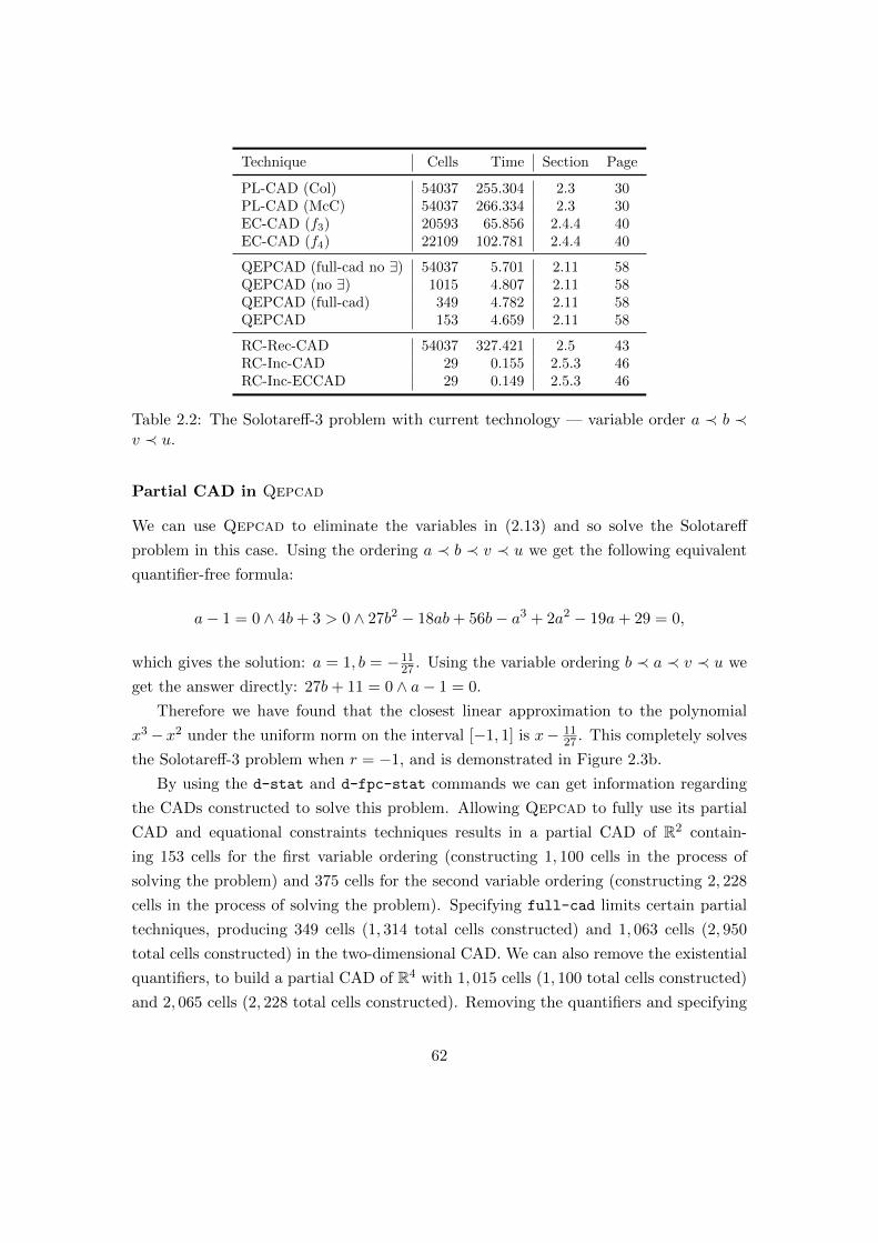
Technique Cells Time Section Page

PL-CAD (Col) 54037 255.304 2.3 30PL-CAD (McC) 54037 266.334 2.3 30EC-CAD (f3) 20593 65.856 2.4.4 40EC-CAD (f4) 22109 102.781 2.4.4 40

QEPCAD (full-cad no ∃) 54037 5.701 2.11 58QEPCAD (no ∃) 1015 4.807 2.11 58QEPCAD (full-cad) 349 4.782 2.11 58QEPCAD 153 4.659 2.11 58

RC-Rec-CAD 54037 327.421 2.5 43RC-Inc-CAD 29 0.155 2.5.3 46RC-Inc-ECCAD 29 0.149 2.5.3 46

Table 2.2: The Solotareff-3 problem with current technology — variable order a ≺ b ≺v ≺ u.

Partial CAD in Qepcad

We can use Qepcad to eliminate the variables in (2.13) and so solve the Solotareff

problem in this case. Using the ordering a ≺ b ≺ v ≺ u we get the following equivalent

quantifier-free formula:

a− 1 = 0 ∧ 4b+ 3 > 0 ∧ 27b2 − 18ab+ 56b− a3 + 2a2 − 19a+ 29 = 0,

which gives the solution: a = 1, b = −1127 . Using the variable ordering b ≺ a ≺ v ≺ u we

get the answer directly: 27b+ 11 = 0 ∧ a− 1 = 0.

Therefore we have found that the closest linear approximation to the polynomial

x3− x2 under the uniform norm on the interval [−1, 1] is x− 1127 . This completely solves

the Solotareff-3 problem when r = −1, and is demonstrated in Figure 2.3b.

By using the d-stat and d-fpc-stat commands we can get information regarding

the CADs constructed to solve this problem. Allowing Qepcad to fully use its partial

CAD and equational constraints techniques results in a partial CAD of R2 contain-

ing 153 cells for the first variable ordering (constructing 1, 100 cells in the process of

solving the problem) and 375 cells for the second variable ordering (constructing 2, 228

cells in the process of solving the problem). Specifying full-cad limits certain partial

techniques, producing 349 cells (1, 314 total cells constructed) and 1, 063 cells (2, 950

total cells constructed) in the two-dimensional CAD. We can also remove the existential

quantifiers, to build a partial CAD of R4 with 1, 015 cells (1, 100 total cells constructed)

and 2, 065 cells (2, 228 total cells constructed). Removing the quantifiers and specifying

62

Technique Cells Time Section Page

PL-CAD (Col) 161317 916.105 2.3 30PL-CAD (McC) 154527 857.357 2.3 30EC-CAD (f3) 48475 175.139 2.4.4 40EC-CAD (f4) 63583 324.663 2.4.4 40

QEPCAD (full-cad no ∃) 154527 8.249 2.11 58QEPCAD (no ∃) 2065 4.785 2.11 58QEPCAD (full-cad) 1063 4.832 2.11 58QEPCAD 375 4.687 2.11 58

RC-Rec-CAD 154527 1154.146 2.5 43RC-Inc-CAD 33 0.202 2.5.3 46RC-Inc-ECCAD 33 0.202 2.5.3 46

Table 2.3: The Solotareff-3 problem with current technology — variable order b ≺ a ≺v ≺ u.

full-cad will construct a sign-invariant CAD of R4, as shown by the same cell counts

as projection and lifting CAD with McCallum’s projection operator: 54, 037 cells and

154, 527 cells. All of the options utilising a subset of Qepcad’s optimisations take just

under five seconds (with around two seconds initialisation time), and constructing a full

four-dimensional CAD takes six or eight seconds.

This proves the strength of the equational constraint and partial CAD techniques

that Qepcad can use, along with the practical time efficiency of its implementation.

Regular Chains CAD

Constructing a sign-invariant with the original regular chains algorithm (Section 2.5.2)

produces the same number of cells as the McCallum projection and lifting algorithm and

the unquantified full-cad CAD from Qepcad: 54, 037 and 154, 527 cells (in both cases

a single cell is found to be true, corresponding to the solution found by Qepcad). The

fact that these CADs are identical suggests that it may be the minimal sign-invariant

CAD that can be algorithmically constructed.It takes around four to eight minutes to

construct such a CAD, although it takes a substantial amount of additional time (one

to twelve minutes) to construct representations of these cells to then count them (this

is an implementational issue that the developers of RegularChains hope to eliminate).

Using the incremental regular chains algorithm (Section 2.5.3) will utilise all four

equational constraints. This reduces the CAD down to 29 cells in 0.1-0.3 seconds, proving

remarkably efficient.

63

Summary

The results in Tables 2.2 and 2.3 demonstrate the power of the various advances in CAD

technology: projection operators, single equational constraints, partial CAD, regular

chains algorithms, and utilising multiple equational constraints.

This example will be revisited in later chapters and compared to the results in Ta-

bles 2.2 and 2.3 to demonstrate how new advances in CAD theory can make existing

technology more efficient. The results are summarised in Section 8.2.1 where Tables 8.1

and 8.2 demonstrate the power of the new theory given in this thesis.

2.13 Conclusion

In this chapter a thorough background of cylindrical algebraic decomposition was given.

After the necessary background, the original algorithm from [Col75] was described along

with many extensions. An alternative construction method by regular chains theory was

also described in both a recursive and incremental form.

A discussion of the known complexity results for CAD showed that any algorithm

will necessarily be doubly exponential in the number of variables. Alternatives to CAD

were discussed with lower theoretical complexity (but not necessarily better practical

performance) and some applications of CAD discussed. Finally, the Solotareff-3 example

was discussed as a guiding example for the rest of the thesis.

64

Chapter 3

Truth Table Invariant CAD

Since their inception in 1975, the primary focus while constructing CADs has been the

sign (or order) behaviour of the individual polynomials. This is generally more detail

than needed, and nearly always results in a CAD that is more complex than necessary.

This chapter introduces a new invariance property for CAD, considering the truth

values of quantifier-free formulae. A CAD satisfying this property is called truth-table

invariant (a TTICAD) and is sufficient for applications of CAD.

When constructing a CAD by the original algorithm (and extensions) these ideas can

be incorporated into the projection operator by a generalisation of equational constraints,

although care has to be taken during the lifting phase. It is also possible to adapt the

incremental regular chains CAD algorithm to incorporate TTICAD and it can be shown

to be even more beneficial than TTICAD by projection and lifting.

Author’s Contribution and Publication

The author contributed to various phases of the work in this chapter. Initial discussions

between the author and Davenport instigated the idea of a TTICAD, which was then

developed for a projection and lifting algorithm with the rest of the research group and

McCallum. McCallum provided the proof of Theorem 3.3 and England provided the

implementation of Algorithm 3.1, which the author then conducted the experimentation

on. The remaining discussion and analysis was conducted by the entire research group.

The author was involved in the discussions of applying truth table invariance to

regular chains with the rest of the research group, Chen, and Moreno Maza. The im-

plementation was conducted by Chen and the proof of correctness by other members of

the research group. The author conducted the experimentation and was involved in the

discussion and investigation.

65

The discussion on extending to partial TTICAD is by the author. The work on

branch cut analysis was mainly conducted by England (in collaboration with Cheb-

Terrab of Maplesoft) and is presented as an application of TTICAD rather than original

research.

The work in Sections 3.2 to 3.4 was published in [BDE+13] and submitted for pub-

lication in [BDE+14]. The work in Sections 3.5 to 3.7 was published in [BCD+14]. The

work in Section 3.9 was published in [EBDW13] and [ECTB+14].

3.1 Motivation and Definition

When we consider a problem with cylindrical algebraic decomposition, we generally

consider the sign-invariance of the polynomials. That is, on each cell in the CAD all

polynomials are sign-invariant. This proves important for the construction of the CAD

too, ensuring delineability in Collins’ projection operator. Later McCallum [McC85]

considered order-invariance to help the construction of CADs with his reduced projection

operator. Order-invariance requires each polynomial to be sign-invariant on each cell and

if the polynomial vanishes, then it does so to a constant order of vanishing.

Often what we are really concerned about is not the behaviour of polynomials, but

rather the behaviour of formulae involving them. We first recall work by Brown [Bro98],

which looked at truth invariance in CAD. We will discuss a motivating example that

highlights the redundancies of standard CAD techniques and inspires the definition of a

Truth Table Invariant CAD (TTICAD) that will be introduced in Section 3.1.3.

3.1.1 Truth-Invariant Cylindrical Algebraic Decompositions

Recall from Section 2.4.3 the definitions from [Bro98]:

Definition 3.1 ([Bro98]).

Let A and B be two CADs. We say B is simpler than A if A is a refinement of B, i.e.

each cell in B is the union of some cells of A, and A and B are not equal.

Given a formula ϕ from the elementary theory of real closed fields, we say a CAD is

truth-invariant with respect to the input formula if in each cell of the decomposition

the formula is either identically true or identically false.

We will generalise the idea of truth-invariance to consider the invariance of a truth

table for a collection of quantifier-free formulae.

66

3.1.2 Motivating Example

Let us consider an example to highlight some redundancies of sign-invariant projection

and lifting CAD.

Example 3.1.

Consider finding the solutions to the following quantifier elimination problem:

Ω : (∃y)

[x2 + y2 − 1 = 0 ∧ xy > 1

4

]∨[x2

8+ y2 =

1

2∧ x > y

]. (3.1)

We can pass this as input to Qepcad and get the output:

x− 2 ≤ 0 ∧[2x+ 1 > 0 ∨ 16x4 − 16x2 + 1 < 0

]. (3.2)

We can simplify (3.2) further to get the solution set as a simple half-open interval:

x ∈(−√

6−√

2

4, 2

].

Figures 3.1a and 3.1b show the full and partial CADs constructed by Qepcad to solve

this problem. It is clear that the CADs produced are more complicated than necessary

to solve this problem: the two-dimensional CAD produced by the unquantified version

of (3.1) constructs 465 cells.

Let us denote:

f1 := x2 + y2 − 1; g1 := xy − 1

4; f2 :=

x2

8+ y2 − 1

2; g2 := x− y;

so that Ω becomes simply (∃y) [f1 = 0 ∧ g1 > 0]∨[f2 = 0 ∧ g2 > 0]. Further let us denote:

ω1 := [f1 = 0 ∧ g1 > 0]; ω2 := [f2 = 0 ∧ g2 > 0]; ω := ω1 ∨ ω2;

so that (3.1) becomes (∃y) ω(x, y).

If attempting to solve Ω using CAD (utilising McCallum’s projection operator) we

would compute the following set of polynomials:coeffsy(f), discy(f), resy(f, f) | f, f ∈ f1, g1, f2, g2, f 6= f

; (3.3)

for which there are 12 non-trivial polynomials describing 21 distinct solutions. This

would therefore produce a CAD of R1 with 43 cells.

67

(a) 2D CAD produced by Qepcad. (b) 1D CAD produced by Qepcad.

Figure 3.1: CADs produced by Qepcad for the motivating TTICAD example using thep-2d-cad command. Figure 3.1a was produced with the unquantified version of (3.1)to decompose the (x, y)-plane; Figure 3.1b was produced with the quantified version of(3.1) to decompose the (x)-plane (trivially expanded to two dimensions).

When determining the truth value of ω1 (and similarly ω2) we clearly only need to

consider the behaviour of g1 when f1 = 0 is satisfied. This is exactly the observation that

lead McCallum to formalise the idea of equational constraints in [McC99]. Therefore we

need not include the full projection of g1 in our set; we simply need to include resy(f1, g1)

along with the projection of f1 to determine the behaviour of ω1.

Further, we do not need to worry about the interaction of g1 with f2 (similarly g2

and f1) as the only time when this interaction is important is when g1 intersects f2

and f1 = 0 which is already covered by the inclusion of resy(f1, g1) and resy(f1, f2).

Therefore we can use the following reduced projection set:

coeffsy(f1), coeffsy(f2), discy(f1), discy(f2),

resy(f1, g1), resy(f2, g2), resy(f1, f2). (3.4)

There are only 12 distinct solutions to (3.4), producing a one-dimensional CAD with 25

cells. The omitted polynomials from (3.3) are:

coeffsy(g1), coeffsy(g2),discy(g1), discy(g2),

resy(f1, g2), resy(f2, g1), resy(g1, g2). (3.5)

68

(a) Graph showing ω. (b) Induced TTICAD.

(c) Induced implicit ECCAD (f1f2 = 0). (d) Induced sign-invariant CAD.

Figure 3.2: CADs produced by Maple for the motivating TTICAD example, Ω. Azoomed region ((x, y) ∈ [1

3 , 1]2) of each CAD is also given.

The solutions to (3.5) account for the remaining 9 solutions of (3.3).

Although ω does not contain an explicit equational constraint, it is clear that f1 ·f2 =

0 is an implied equational constraint and must be satisfied when ω is true. It can therefore

be used with McCallum’s equational constraint projection operator. This will produce

the polynomials given in (3.4), however it will also include resy(f1, g2) and resy(f2, g1)

as factors of resy(f1 · f2, gi).

Figure 3.2 shows the effect of using the various projection sets to construct a CAD.

Figure 3.2a shows the polynomials involved in ω: the two ωi are indicated in different

colours, the fi are indicated with solid lines, and the gi are indicated with dashed lines.

Figure 3.2b shows the effect of using the reduced projection set (3.4), which produces

177 cells in the final two-dimensional CAD. Figure 3.2c indicates projection with respect

to the implied equational constraint f1f2 = 0 and contains 269 cells. Finally, Figure

3.2d is created using the full McCallum projection set (3.3) which results in 465 cells

(over 2.5 times the number of cells created by the reduced projection).

Note that Figure 3.2b is no longer a sign-invariant CAD for the polynomials in ω, nor

is it invariant for the implied equational constraint f1f2 = 0. However, the truth values

of ω1 and ω2 are constant on every cell of the CAD, and so we call it a ω1, ω2-truth

69

table invariant CAD. We could now construct a truth table for ω1 and ω2 and divide

the cells into each row from which we could describe any Boolean formula involving ω1

and ω2 (including, obviously, ω). This definition will be formalised in Section 3.1.3.

We now look more closely at a region of each of the CADs in Figure 3.2 to clarify

the behaviour of the reduced projection set (3.4). The second graph in each subfigure

of Figure 3.2 examines the CAD for the range (x, y) ∈ [13 , 1]2.

Figure 3.2a shows the polynomials for this region and it is clear there are multiple

intersections, only some of which affect the behaviour of ω. Identifying only the x-

values determined from the reduced projection set (3.4) in Figure 3.2b locates only two

intersections: x = 23 (where f2 and g2 intersect) and x = 2√

7(where f1 and f2 intersect).

If we were to use the implied equational constraint f1f2 = 0 we see in Figure 3.2c that

we also identify x =

√8−2√

142 (where f2 and g1 intersect) and x = 1√

2(where f1 and

g2 intersect). Finally, using the full projection set (3.3) in Figure 3.2d identifies x = 12

(where g1 and g2) intersect.

The inclusion of each unnecessary solution creates a spurious point in the one-

dimensional CAD, creating two additional cells and forces the inclusion of two stacks

of cells in the CAD of R2. Therefore this simplification can have a huge effect on the

number of cells produced in a final CAD. The TTICAD illustrated in Figure 3.2b can be

used for any Boolean combination of ω1 and ω2, so it is still non-optimal for ω. Ideally,

we would produce a CAD that is only truth-invariant for ω.

This example has demonstrated the power of reducing our projection set to obtain

invariance for formulae rather than polynomials.

3.1.3 Definition

We now formalise this motivation into a definition of a new kind of invariance for CAD,

related to truth-invariance, which will be the topic of this chapter.

Definition 3.2.

Let Φ := ϕiti=1 be a list of quantifier-free (Tarski) formulae. We say a cylindrical

algebraic decomposition D is truth table invariant (a TTICAD), or more specifically

Φ-truth table invariant, if the Boolean value of each ϕi is constant on each cell in D.

Truth table invariance is a weaker condition than sign-invariance (which is itself

weaker than order-invariance): if a CAD is sign-invariant with respect to all the poly-

nomials in the ϕi then it will also be a TTICAD for Φ. However, if the ϕi are combined

70

into a, possibly quantified, formula ϕ then Φ-truth table invariance is a stronger condi-

tion than truth-invariance for ϕ. An algorithm will be given to produce TTICADs that

are smaller than sign-invariant CADs for input lists of formulae. This will be achieved

by generalising the theory of equational constraints suggested by Collins [Col98] and

developed by McCallum [McC99].

In Sections 3.2 and 3.5, algorithms will be given to produce a TTICAD for a list

of input formulae some of which contain an equational constraint. This will reduce the

number of cells produced compared to a sign-invariant CAD.

As demonstrated in our motivating example, a TTICAD can be used for quantifier

elimination. Given a quantified formula where the quantifier free part, ϕ, is decomposed

into sub-formulae Φ := ϕi, then a Φ-TTICAD can be constructed to facilitate quan-

tifier elimination. Such a TTICAD would have fewer cells than a sign-invariant CAD

and so the set of valid cells would likely be smaller. This will manifest itself in a simpler

quantifier-free formula being output from the quantifier elimination algorithm (much

like how a truth-invariant CAD produces a simpler formula [Bro98]).

A TTICAD can have other uses, and certain problems require truth-table invariance

(where truth-invariance is insufficient). In Section 3.9 we will discuss the problem of

decomposing complex space according to the branch cuts of a given formula. This can

be used to validate algebraic simplification of elementary functions [BPB05, BBDP07,

Phi11]. Representing each branch cut as a semi-algebraic set, a TTICAD can be pro-

duced to define the regions on which the simplification needs to be tested.

3.2 Projection and Lifting Algorithm

We present the reduced projection operator for TTICAD, followed by the algorithm to

produce a TTICAD with this projection set.

3.2.1 Reduced Projection Operator

Previous work on Equational Constraints

Recall from Sections 2.4.1 and 2.32, McCallum’s reduced projection set [McC85, McC98],

and the theory of equational constraints [McC99], which we will generalise for the TTI-

CAD operator.

The McCallum projection operator, MP, is:

MP(A) := coeffs(f),discxn(f), resxn(f, g) | f, g ∈ A, f 6= g .

71

We also assume that the standard trivial simplifications of removing constants and iden-

tical entries (up to a constant multiple). Most implementations also only include coeffi-

cients until the first constant coefficient.

The proof that MP is a valid projection operator relies on a key result. Recall that an

order-invariant CAD requires polynomials to have constant order of vanishing on cells,

as well as sign-invariance. Also we say that a set A ⊂ Z[x] is an irreducible basis if

the elements of A are of positive degree (in the main variable), irreducible, and pairwise

relatively prime. The main result of [McC85, McC98] is Theorem 3.1:

Theorem 3.1 ([McC98, Theorem 1]).

Let A be an irreducible basis in Z[x] and let S be a connected submanifold of Rn−1.

Suppose each element of MP(A) is order-invariant in S.

Then each element of A either vanishes identically on S or is analytic delineable on

S [McC98, §3]. Further, the sections of A not identically vanishing are pairwise disjoint,

and each element of A not identically vanishing is order-invariant in such sections.

Theorem 3.1 states that an order invariant CAD can be constructed from the pro-

jection polynomials in MP(A), as long as none of them vanish identically on a lower-

dimensional cell. This motivates the following definition:

Definition 3.3.

A set A of n-variate integral polynomials, where n ≥ 1, is said to be well-oriented if

whenever n > 1 the following two conditions hold:

1). for every f ∈ prim(A), f(α, xn) = 0 for at most a finite number of points α ∈ Rn−1;

2). MP(A) is well-oriented.

It is therefore possible to construct a CAD using McCallum’s projection only if the

input polynomials are well-oriented.

As mentioned in Sections 2.4.4 and 3.1, if an equational constraint is present in a

formula then it can be used to simplify the projection set. If we have f = 0 as an

equational constraint, then we need only worry about the behaviour of a non-equational

constraint polynomial g when f vanishes. This behaviour is encoded in the resultant of

f and g and Theorem 3.2 proves that replacing g with resxn(f, g) is sufficient.

Theorem 3.2 ([McC99]).

Let f(x), g(x) be integral polynomials with positive degree in xn, let r(x1, . . . , xn−1) be

their resultant, and suppose r 6= 0. Let S be a connected subset of Rn−1 such that f is

delineable on S and r is order-invariant on S.

72

S

x

y

z

f=0

f=0

f=0

g

g

?

r=0

Figure 3.3: Graphical representation of Theorem 3.2. If f is delineable on S and r isorder-invariant then g must either avoid or completely align with each section of f .

Then g is sign-invariant in every section f over S.

Figure 3.3 gives a graphical representation of Theorem 3.2 when working in three-

dimensions. We assume that f(x, y, z) and g(x, y, z) have positive degree in z, and

non-zero resultant, r(x, y). We have S being any connected subset of R2 and assume

that r is order-invariant on S. Assuming f is delineable over S we have three cases to

consider, shown in Figure 3.3: f and g may not intersect; f and g may intersect but be

distinct; or, f and g are identical over S.

Theorem 3.2 assures us that either f and g are disjoint over S (as in the top section

of f in Figure 3.3), or they are completely aligned over S (as in the bottom section of

f). Therefore, the situation in the middle section of f , where f and g intersect but are

not identical over S, cannot happen.

Theorem 3.2 can be used to simplify the projection operator MP. The equational

constraint projection operator was first discussed in [Col98] and developed by McCallum

in [McC99]. We consider a set of polynomials A, which contains a subset E ⊆ A: here,

A represents all polynomials for a given problem, and E the equational constraints. We

define the equational constraint projection set, MPE(A), to be:

MPE(A) := MP(E) ∪ resxn(f, g) | f ∈ E, g ∈ A, g /∈ E .

This operator applies the full McCallum projection operator on the equational con-

straints polynomials, but does not do so for non-equational constraint polynomials. For

any g that does not belong to E, it computes all cross-resultants with E but nothing

73

else. Theorem 3.2 allows us to use MPE(A) for the first step of projection (followed

by MP) to construct a CAD invariant with respect to the equational constraint. As

MPE(A) ⊆ MP(A) this should result in fewer cells being constructed.

Remark 3.1.

Theorem 3.2 is used to simplify the projection set, and thus the CAD of Rn−1. It is

worth noting that we can also use Theorem 3.2 to simplify the lifting operation from

Rn−1 to Rn: we no longer need to lift with respect to g. This simplification in lifting

is implemented within the ProjectionCAD package [Eng13b] and will be used in our

TTICAD algorithm.

A TTICAD Projection Operator

We now consider how we can generalise the use of MPE(A) into the TTICAD projection

operator.

We saw in Example 3.1 that given a list of formulae each of which has an individual

equational constraint, we can apply MPE(A) to each formula. We still need to be con-

cerned with the interaction of the constraints, but can ignore behaviour of non-equational

constraint polynomials away from the projections of their respective constraints. We for-

malise this idea.

As with [McC99], we first define our operator in the case of irreducible bases, which

can then be generalised by considering contents and irreducible factors of the input sets

of polynomials.

Let1 A := Aiti=1 be a list of irreducible bases Ai and let E := Eiti=1 be a list of

subsets Ei ⊆ Ai. Let A :=⋃ti=1Ai and E :=

⋃ti=1Ei.

Definition 3.4.

We define the reduced projection of A with respect to E , denoted TTIPE(A), as:

TTIPE(A) :=t⋃i=1

MPEi(Ai) ∪ RES×(E);

where RES×(E) is the cross-resultant set:

RES×(E) :=

resxn(f, f) | ∃ i, j s.t. f ∈ Ei, f ∈ Ej , i < j, f 6= f.

1To help keep track of various forms of input, we use the convention that uppercase Roman lettersdenote sets of polynomials and calligraphic letters denote lists of these sets.

74

Given a list of formulae Φ := ϕiti=1, we write TTIP(Φ) to denote TTIPE(A) where

each Ai is the irreducible basis for the polynomials in ϕi, and the sets Ei are those

members of Ai corresponding to any equational constraints for ϕi.

To allow for easier comparison with the McCallum projection operator we formally

define the set of polynomials we omit for each formula ϕi.

Definition 3.5.

We define the excluded projection polynomials of (Ai, Ei) to be:

ExclTTIPEi(Ai) := MP(Ai) \MPEi(Ai)

= coeffsxn(g), discxn(g), resxn(g, g) | g, g ∈ Ai \ Ei, g 6= g .

Further, we can define the total set of excluded polynomials for (A, E):

ExclTTIPE(A) := MP(A) \ TTIPE(A)

=t⋃i=1

ExclTTIPEi(Ai) ∪

resxn(f, g) | ∃ i, j s.t. f ∈ Ei, g ∈ Aj , g /∈ E, i 6= j ∪resxn(g, g) | ∃ i, j s.t. g ∈ Ai, g ∈ Aj , g, g /∈ E, i 6= j .

We now provide the key theorem that proves that TTIP is a valid projection operator

and will later be used to show that Algorithm 3.1 provides a truth-table invariant CAD.

Theorem 3.3 ([BDE+13]).

Let S be a connected submanifold of Rn−1. Suppose each element of TTIPE(A) is order

invariant in S.

Then the following hold:

• each f ∈ E either vanishes identically on S or is analytically delineable on S;

• the sections over S of the f ∈ E which do not vanish identically are pairwise

disjoint;

• each element f ∈ E which does not vanish identically is order-invariant in such

sections.

Moreover, for each 1 ≤ i ≤ t, every g ∈ Ai \Ei is sign-invariant in each section over

S of every f ∈ Ei which does not vanish identically.

75

Proof.

The crucial step for proving this result is observing that MP(E) ⊆ TTIPE(A). This is

clear if we write:

MP(E) =t⋃i=1

MP(Ei) ∪ RES×(E).

It is therefore a straightforward application of Theorem 3.1 to obtain the first three

statements in this theorem.

The final statement requires the use of Theorem 3.2. Let i be in the range 1 ≤ i ≤ t,g ∈ Ai \Ei and let f ∈ Ei. Suppose further that f does not vanish identically on S. As

resxn(f, g) is contained in our projection set TTIPE(A), it must be order-invariant in S

(by hypothesis). We have from the first statement in the theorem that f is delineable,

and therefore by Theorem 3.2, g must be sign-invariant in each section of f over S.

This is a remarkably powerful theorem and it will be used to prove the correctness of

our given algorithm. We will be able to apply it as long as no f ∈ E vanishes identically

on the lower-dimensional S. This will require a generalisation of Definition 3.3 relating

to TTICAD.

Comparison of TTIPE(A) with other projection operators

It is clear that TTIPE(A) ⊆ MP(A), with strict inclusion in all but the simplest case.

If all formulae ϕiti=1 contain individual equational constraints, and are combined

to form a larger parent formula ϕ, then the equational constraint projection operator can

be used with an implied equational constraint consisting of∏f∈E f = 0. Using MPE(A)

with this equational constraint would avoid using the surplus coefficients, discriminants

and cross-resultants involving just non-equational constraints. However, there would

still be excess polynomials in the projection set: MPE(A) contains all resultants

resxn(fi, gi) | f ∈ Ei, g ∈ Aj \ Ej , i 6= j, g /∈ E .

These extra resultants describe the interaction of equational constraints with non-equational

constraints from other formulae and therefore are unnecessary for truth table invariance

with respect to ϕiti=1.

76

Worked Example

We consider the projection sets for Example 3.1 to see clearly the differences in the

various operators. We set Ai := fi, gi and Ei := fi for i = 1, 2.

First, we use the TTICAD projection operator. We compute the reduced projection

sets (with the necessary trivial simplifications) for each ωi:

MPE1(A1) =

x2 − 1, x4 − x2 +

1

16

;

MPE2(A2) =x2 − 4, 9x2 − 4

;

and the single cross-resultant of the two equational constraints:

RES×(E) =

(−7

8x2 +

1

2

)2.

The TTICAD projection set for this problem, TTIPE(A), is therefore the union of these

three sets, which has 12 distinct solutions (Figure 3.2b).

As the two formulae are part of the larger ω = ω1 ∨ ω2, we can identify the implicit

equational constraint, f1f2 = 0. We can use McCallum’s equational constraint projection

operator, which would produce all the polynomials in TTIPE(A), along with the following

two resultants:

resxn(f1, g2) = 2x2 − 1. resxn(f2, g1) =1

8x4 − 1

2x2 +

1

16.

These polynomials produce an extra 6 distinct solutions to total 18 points (Figure 3.2c).

Finally, if we take the full McCallum projection set MP(A), we will have all the

polynomials above but also gain the coefficients of g1 and g2 and their resultant. In this

example, the only non-trivial coefficient is simply x, and the resultant is:

resxn(g1, g2) = x2 − 1

4.

These additional polynomials provide 3 extra distinct solutions, totalling 21 points in

the 1-dimensional CAD (Figure 3.2d).

This gives us a concrete demonstration of the difference in projection operators. As

always, a simpler projection operator will produce a simpler CAD, but in the following

section we will also discuss how simplified lifting can be used for ECCAD and TTICAD

which will result in further savings.

77

3.2.2 A Projection and Lifting TTICAD Algorithm

We will now discuss, in detail, how the TTICAD projection operator can be used to

construct a TTICAD. This algorithm was first given in [BDE+13] and later in [BDE+14].

Given an input of a list of quantifier-free formulae ϕiti=1 in variables x1 ≺ · · · ≺xn (where each ϕi has at least one equational constraint), Algorithm 3.1 produces a

TTICAD of Rn (or FAIL if the input is not suited to the algorithm). We first discuss

various details of the algorithm, before giving a proof of its correctness.

Algorithm 3.1 calls three subalgorithms which we briefly specify:

sqfreebasis: This computes a squarefree basis (Definition 2.4) of a set of polynomials to

ensure they are primitive, squarefree, pairwise relatively co-prime. This procedure

is implemented in most computer algebra systems.

SplitR: This is given in Algorithm 2.1, and decomposes one-dimensional real space

according the roots of a set of polynomials. We assume that the output is given

as a pair (I, S) of lists of cell indices and sample points.

CADW: This is an implementation of projection and lifting CAD as specified in [McC98]

and given in Algorithm 2.4. We assume the output gives three outputs (as de-

scribed in [McC98]), the first of which is a Boolean value w describing if the

algorithm has been successful or not. If w is true, then the other two outputs are

I and S: lists of cell indices and sample points.

We use the projection operator from Definition 3.4 in Algorithm 3.1, although care

needs to be taken to ensure we obtain a valid output.

For an input list of formulae Φ = ϕiti=1 we first set Ai to be the set of all poly-

nomials in ϕi, and put Ei to be the designated equational constraint polynomial fi.We cannot simply apply the TTICAD projection operator (Definition 3.4) as we have

no guarantee that the elements of each Ai are suitable.

We therefore extend Definition 3.4 by preprocessing our input (analogous to [McC99,

§5]). We first remove the set of contents of all the elements of A, which we denote C.

We take the finest squarefree bases of the primitive parts of the elements of the Ai and

Ei, denoting them Bi and Fi, respectively. Then B = Biti=1 and F = Fiti=1 satisfy

the requirements for Definition 3.4, and so we create the set:

P := C ∪ TTIPF (B).

78

Informally, for a general input Φ = ϕiti=1 when we write TTIP(Φ) or TTIPE(A)

we mean this conditioned set P.

We will show that for appropriate input, Algorithm 3.1 will return a TTICAD for

Φ. The condition that we use is a generalisation of well-orientedness (Definitions 2.26

and 3.3), which was given in [McC98] as a condition to ensure that CADW (implementing

CAD using McCallum’s improved projection operator, MP) provided valid input. The

original definition requires the primitives of all polynomials to be nullified by at most a

finite set of points, and for this condition to hold recursively for MP.

Definition 3.6.

We say that A is (TTI)-well-oriented with respect to E (and that Φ is (TTI-)well-

oriented) if:

• for n > 1, every constraint polynomial fi is nullified by at most a finite number of

points in Rn−1;

• TTIPE(A) (hence also P in Algorithm 3.1) is well-oriented in the sense of Defini-

tions 2.26 and 3.3 (as discussed in [McC85, McC98]).

We can now prove that Algorithm 3.1 behaves as specified.

Theorem 3.4 ([BDE+13]).

The output of Algorithm 3.1 is either a TTICAD of Rn for Φ (described by lists I and

S of cell indices and sample points) or FAIL (if Φ is not well oriented as specified in

Definition 3.6).

The proof is given in full in [BDE+13]. The proof consists of checking that FAIL

will be returned for input that is not TTI-well-oriented, and otherwise that the output

is truth table invariant. In the latter case we can apply Theorem 3.3 to B, F and the

cells of the (n − 1)-dimensional CAD to get delineability of F and sign-invariance of

B as required. The final step is to confirm that each formula is truth-invariant for the

constructed CAD of Rn.

With Theorem 3.4 we can now create TTICADs for lists of quantifier-free formulae,

with each formula containing an equational constraint. We will discuss some extensions

to Algorithm 3.1: the improved lifting it offers; avoiding FAIL when an equational

constraint is nullified but the polynomials in ExclTTIPEi(Ai) are constant; and dealing

with when there are quantifier-free formulae without an equational constraint. The latter

in particular will allow TTICADs to be constructed for a much wider class of problems.

79

Algorithm 3.1: TTICAD(ϕiti=1, vars): Standard truth table invariant CAD al-gorithm.

Input : A list of quantifier-free formulae ϕiti=1; a list of ordered variablesvars = x1 ≺ · · · ≺ xn. Each formula ϕi should have a designatedequational constraint fi = 0.

Output: Either: a CAD D of Rn (described by lists I and S of cell indices andsample points) which is truth table invariant with respect to ϕiti=1;or FAIL if the input is not well-oriented (Definition 3.6).

1 for i = 1, . . . , t do2 Ei ← fi;3 Fi ← sqfreebasis(prim(Ei)); // Preprocess equational constraints

4 F ← ⋃ti=1 Fi;

5 if n = 1 then6 (I, S)← SplitR(F);7 return (I, S) to represent D; // Base case

8 else9 for i = 1, . . . , t do

10 Ai ← polys(ϕi);11 Ci ← cont(Ai);12 Bi ← sqfreebasis(prim(Ai)); // Preprocess polynomials

13 C ← ⋃ti=1Ci; B ← Biti=1; F ← Fiti=1;

14 P← C ∪ TTIPF (B); // Projection set

15 (w′, I ′, S′)← CADW(n− 1,P); // (n− 1)-dimensional CAD

16 if w′ = false then17 return FAIL; // P is not well oriented

18 I ← ∅; S ← ∅;19 for c′ ∈ D′ do20 Lc ← ∅;21 for i = 1, . . . , t do22 if ∃f ∈ Ei which is nullified on c then23 if dim (c) > 0 then24 return FAIL; // ϕiti=1 is not well oriented

25 else26 Lc ← Lc ∪Bi;27 else28 Lc ← Lc ∪ Fi;

29 (Ic, Sc)← GenerateStack(Lc, xn, c); // Lifting phase

30 I ← I ∪ Ic; S ← S ∪ Sc;31 return (I, S) to represent D;

80

Improved Lifting

We mentioned when discussing Theorem 3.2, that it allows for simpler lifting as well

as a simpler projection set. Theorem 3.2 states that the non-equational constraints are

sign-invariant on the sections of the equational constraint, which are the only cells on

which the formula can be satisfied. Therefore there is no need to lift with respect to the

non-constraint polynomials, and so we generally2 lift only with respect to the equational

constraints.

Note that we are able to do this as we only need sign-invariance to deduce the truth

value of the ϕi. If we were at a lower level in the CAD (and so needed order-invariance

to apply Theorems 3.1 or 3.2) or required global order-invariance then this step would

be invalid.

If we use Algorithm 3.1 with a single formula Φ = ϕ1 then we emulate McCal-

lum’s equational constraint theory [McC99]. However, this improved lifting has been

unexploited until now, meaning that we will often get a simpler CAD than using current

implementations of equational constraint CAD such as Qepcad.

Avoiding FAIL when ExclTTIP is constant

In [Bro05b] it was pointed out that there are cases when input to a CAD algorithm

utilising McCallum’s projection operator (without equational constraints) is not well-

oriented but an order-invariant CAD can still be produced.

When constructing a TTICAD using Algorithm 3.1 there are also cases when non-

well oriented input can still be used to create a TTICAD. The following result allows

Algorithm 3.1 to sometimes avoid failure when an equational constraint vanishes iden-

tically on a positive-dimensional cell.

Lemma 3.5 ([BDE+14]).

Let fi be an equational constraint which vanishes identically on a cell c′ ∈ D′ constructed

in Algorithm 3.1 (line 15). If all the polynomials in ExclTTIPEi(Ai) are constant on

c′, then any g ∈ Ai \ Ei will be delineable over c′.

This result allows for an implementation of Algorithm 3.1 to avoid returning FAIL in

more cases. This could be extended to include cases where the elements of ExclTTIPEi(Ai)

do not have any real roots in the cell c′ (and so are viewed as constant on that cell)

but this check could be rather substantial and it may be quicker to use a different CAD

theory.

2The only exception is if fi is nullified on a zero-dimensional cell at which point we simply lift withrespect to all non-equational constraints.

81

3.2.3 Dealing with Clauses Without an Equational Constraint

It is obviously limiting that Algorithm 3.1 requires all the quantifier-free formulae to have

an (explicit) equational constraint, and this prevents its application to many problems.

It is possible to adapt Algorithm 3.1 to deal with the case that some of the quantifier-free

formulae do not have an equational constraint: in short, all polynomials in that formula

are given the prominence that an equational constraint polynomial is given in Algorithm

3.1.

This extension is shown in Algorithm 3.2. It is clear that Algorithm 3.2 terminates,

and all that remains is to show that it is correct.

Theorem 3.6 ([BDE+14]).

The output of Algorithm 3.2 is either a TTICAD of Rn for Φ (described by lists I and

S of cell indices and sample points) or FAIL (if Φ is not well oriented as specified in

Definition 3.6).

The proof is given in full in [BDE+14] and consists of checking the addition of the

if-statement resulting in the assignment of Ei on lines 3 and 5 ensures truth-invariance

for formulae without equational constraints.

3.2.4 Worked Example

Let us consider Example 3.1 to demonstrate the power of Algorithms 3.1 and 3.2.

We begin by constructing a TTICAD for Ω using Algorithm 3.1. Our input is the

set of formulae:

Ω = ω1, ω2 = [f1 = 0 ∧ g1 > 0], [f2 = 0 ∧ g2 > 0].

Computing a TTICAD for this example (using Algorithm 3.1 or 3.2) was shown

to construct 177 cells, whilst a CAD with respect to the implicit equational constraint

(f1f2 = 0) produces 269 cells, and the full sign-invariant CAD contains 465 cells.

We now consider constructing the TTICAD for Ω† (for which Algorithm 3.1 is not

applicable):

Ω† = ω†1, ω†2 = [f1 = 0 ∧ g1 > 0], [f2 > 0 ∧ g2 > 0].

Applying Algorithm 3.2 to Ω† produces extra polynomials: discy(g2) and resy(f1, g2).

The first is trivial, whilst the latter is 2x2 − 1 so identifies two extra points in the one-

dimensional CAD. Further, the set of polynomials that is used for lifting consists of

f1, f2, g2 rather than just f1, f2. This results in 263 cells. In this case there is no

82

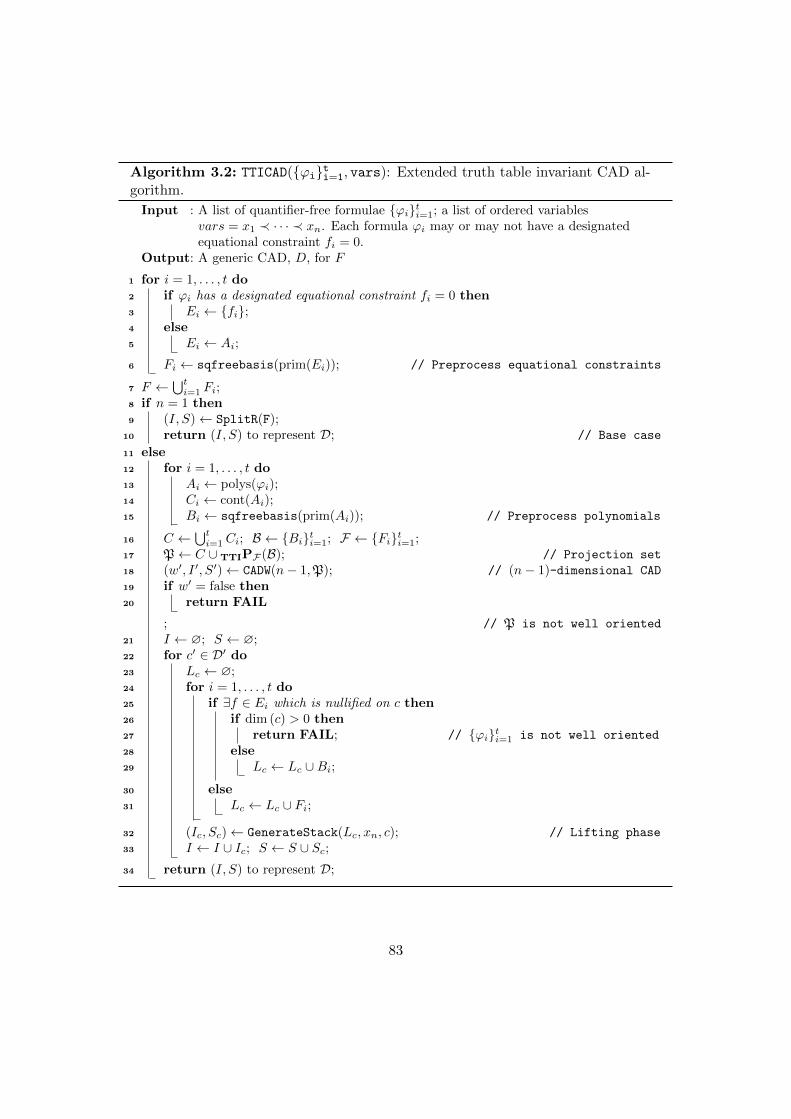
Algorithm 3.2: TTICAD(ϕiti=1, vars): Extended truth table invariant CAD al-gorithm.

Input : A list of quantifier-free formulae ϕiti=1; a list of ordered variablesvars = x1 ≺ · · · ≺ xn. Each formula ϕi may or may not have a designatedequational constraint fi = 0.

Output: A generic CAD, D, for F

1 for i = 1, . . . , t do2 if ϕi has a designated equational constraint fi = 0 then3 Ei ← fi;4 else5 Ei ← Ai;

6 Fi ← sqfreebasis(prim(Ei)); // Preprocess equational constraints

7 F ← ⋃ti=1 Fi;

8 if n = 1 then9 (I, S)← SplitR(F);

10 return (I, S) to represent D; // Base case

11 else12 for i = 1, . . . , t do13 Ai ← polys(ϕi);14 Ci ← cont(Ai);15 Bi ← sqfreebasis(prim(Ai)); // Preprocess polynomials

16 C ← ⋃ti=1 Ci; B ← Biti=1; F ← Fiti=1;

17 P← C ∪ TTIPF (B); // Projection set

18 (w′, I ′, S′)← CADW(n− 1,P); // (n− 1)-dimensional CAD

19 if w′ = false then20 return FAIL

; // P is not well oriented

21 I ← ∅; S ← ∅;22 for c′ ∈ D′ do23 Lc ← ∅;24 for i = 1, . . . , t do25 if ∃f ∈ Ei which is nullified on c then26 if dim (c) > 0 then27 return FAIL; // ϕiti=1 is not well oriented

28 else29 Lc ← Lc ∪Bi;

30 else31 Lc ← Lc ∪ Fi;

32 (Ic, Sc)← GenerateStack(Lc, xn, c); // Lifting phase

33 I ← I ∪ Ic; S ← S ∪ Sc;

34 return (I, S) to represent D;

83

(a) Induced TTICAD for Ω (b) Induced TTICAD for Ω†

Figure 3.4: TTICADs produced by Maple for Ω and Ω† in the motivating TTICADexample. A zoomed region ((x, y) ∈ [1

3 , 1]2) of the TTICADs produced is also shown.

implicit equational constraint and so the only other sufficient CAD is the sign-invariant

CAD (with 465 cells).

3.3 Implementation and Experimentation: Projection and

Lifting TTICAD

We discuss the implementation of Algorithms 3.1 and 3.2 and experimental results dis-

playing their efficacy.

3.3.1 Implementation of TTICAD by Projection and Lifting

To correctly implement an instance of Algorithms 3.1 and 3.2 a CAD needs to be pro-

duced that is order-invariant with respect to its input (to ensure the CAD produced on

line 15 is suitable). We use the implementation of CADW in ProjectionCAD (the CADFull

procedure with method=McCallum). Advances in the RegularChains package since this

work was submitted for publication, such as shifting computation of resultants into ker-

nel commands, has shown a substantial speed up in all the ProjectionCAD code. For

this reason, the tests from [BDE+13] and [BDE+14] have been updated with new results

(although the conclusions are identical).

The implementation of TTICAD is non-optimised and its purpose is not to illus-

trate the speed of TTICAD (although this proves competitive in many cases), but to

demonstrate the power of the theory. The number of cells in the TTICAD produced is

of more interest, and is directly correlated to the construction time. The hope is that in

the future a more optimised implementation of TTICAD can be created (perhaps within

another optimised system, like Qepcad) and TTICADs can be constructed even faster.

84

3.3.2 Experimental Results for TTICAD by Projection and Lifting

To demonstrate the power of the TTICAD theory we compute TTICADs for a collection

of examples, providing both cell counts and timings. To provide a context for these

results we also compute CADs using a variety of techniques. The PL-CAD column is

computed using the projection and lifting algorithm described in [McC85, McC98] using

McCallum’s projection operator. The Qepcad column refers to constructing a CAD

using Qepcad-B using the options +N500000000 and +L200000 and with initialisation

included in the timings. To allow Qepcad to perform to its full strength, we declare any

explicit equational constraints (so it can use the theory outlined in [McC99]) if present, or

declare the implicit equational constraint (the product of the equational constraints for

the individual quantifier-free formulae) if all formulae contain an equational constraint.

The Mathematica column refers to using the CylindricalDecomposition command

which does not produce a CAD, but rather a cylindrical algebraic formula (CAF) which is

constructed from one [Str12]. The author of Mathematica’s command kindly provided

cell counts for the problems, although it should be noted that the use of meta-algorithms

in Mathematica means that there is not a guarantee that a CAD was ever constructed

(for example, with a conjunction of equations Mathematica will automatically just

compute a Grobner basis).

The examples we consider are from a range of sources and we use a suffix of A/B to

illustrate different variable orderings for a single problem. We use examples from [BH91],

adapted to be suited for TTICAD by changing certain conjunctions into disjunctions, and

denote such new problems with †. We then provide two examples (Kahan and Arcsin)

sourced from the application of branch cut analysis for simplification (see Section 3.9 for

further details). We consider some worked examples from [BDE+13] and [BDE+14] and

also a small collection of randomly generated examples: disjunctions of two quantifier

free formulae, only one of which has an equational constraint, using random polynomials

in three variables of degree at most two. All examples are given in the CAD repository

described in [WBD13] and Appendix B.

The experimental results are given in Table 3.1. For each problem, along with the

name (as used in [WBD13]) and experimental results, we give the number of variables

n, the maximum degree of polynomials involved d, and the number of quantifier free

formula used for TTICAD t.

First we compare TTICAD with a sign-invariant CAD produced using the Projection-

CAD module with McCallum’s projection operator. As the TTICAD and CADFull com-

mands are both implemented in the same architecture this gives us a direct comparison

85

Problem PL-CAD TTICAD Qepcad Maple MathematicaName n d t Time Cells Time Cells Time Cells Time Cells Time Cells

IntersectionA 3 2 1 360.1 3707 1.7 269 4.5 825 — Err 0.0 3IntersectionB 3 2 1 332.2 2985 1.5 303 4.5 803 50.2 2795 0.0 3RandomA 3 3 1 268.5 2093 4.5 435 4.6 1667 23.0 1267 0.1 657RandomB 3 3 1 442.7 4097 8.1 711 5.4 2857 48.1 1517 0.0 191Intersection†A 3 2 2 360.1 3707 68.7 575 4.8 3723 — Err 0.1 601Intersection†B 3 2 2 332.2 2985 70.0 601 4.7 3001 50.2 2795 0.1 549Random†A 3 3 2 268.5 2093 223.4 663 4.6 2101 23.0 1267 0.2 808Random†B 3 3 2 442.7 4097 268.4 1075 142.4 4105 48.1 1517 0.2 1156Ellipse†A 5 4 2 — F — F 291.6 500609 1940.1 81193 11.2 80111Ellipse†B 5 4 2 T/O — T/O — T/O — T/O — 2911.2 16603131Solotareff†A 4 3 2 677.6 54037 46.1 F 4.9 20307 1014.2 54037 0.1 260Solotareff†B 4 3 2 2009.2 154527 123.8 F 6.3 87469 2951.6 154527 0.1 762Collision†A 4 4 2 264.6 8387 267.7 8387 5.0 7813 376.4 7895 3.6 7171Collision†B 4 4 2 — Err — Err T/O — T/O — 591.5 1234601KahanA 2 4 7 10.7 409 0.3 55 4.8 261 15.2 409 0.0 72KahanB 2 4 7 87.9 1143 0.3 39 4.8 1143 154.9 1143 0.1 278ArcsinA 2 4 4 2.5 225 0.3 57 4.6 225 3.3 225 0.0 175ArcsinB 2 4 4 6.5 393 0.2 25 4.5 393 7.8 393 0.0 792DEx(Φ)A 2 2 2 5.7 317 1.2 105 4.7 249 6.3 317 0.0 242DEx(Φ)B 2 2 2 6.1 377 1.5 153 4.5 329 7.2 377 0.0 1752DEx(Ψ)A 2 2 2 5.7 317 1.6 183 4.9 317 6.3 317 0.1 3722DEx(Ψ)B 2 2 2 6.1 377 1.9 233 4.8 377 7.2 377 0.1 5963DExA 3 3 2 3795.8 5453 5.0 109 5.3 739 — Err 0.1 443DExB 3 3 2 3404.7 6413 5.8 153 5.7 1009 — Err 0.1 135Random1 3 2 2 16.4 1533 76.8 1533 4.9 1535 25.7 1535 0.2 579Random2 3 2 2 837.9 7991 132.4 2911 5.2 8023 173.0 8023 0.8 2551Random3 3 2 2 258.6 8889 98.1 4005 5.3 8913 77.9 5061 0.7 3815Random4 3 2 2 1442.3 11979 167.1 4035 5.4 12031 258.3 12031 1.3 4339Random5 3 2 2 310.3 11869 110.7 4905 5.5 11893 104.3 6241 0.9 5041

Table 3.1: Comparing TTICAD (by Projection and Lifting) to the full CAD built withthe same architecture and other CAD algorithms (taken from [BDE+13, BDE+14]).

and clearly shows the benefit of the TTICAD theory.

We can see clearly that in all cases where both TTICAD and CADFull run successfully

the cell count for TTICAD is less than or equal to that of a sign-invariant CAD. This

confirms the fact that each cell of a TTICAD is a superset of cells from the sign-invariant

CAD produced by CADFull. In fact, the only examples where the cell counts are equal are

Collision†A and Random 1, in which the non-equational constraints are simple enough

that the projection polynomials remain unchanged.

This comparison also illustrates the drawback of the TTICAD theory - for Solotareff

† A/B the problem is not TTI-well-oriented so the TTICAD algorithm returns FAIL,

but the problem is well-oriented in the McCallum CAD sense (Definitions 2.26 and 3.3)

and so CADFull returns a valid CAD.

We can see that a truly impressive reduction in cell count can occur: in the 3D worked

example from [BDE+14] a 50-fold reduction in cell count (and a 759-fold reduction in

time) occurs.

We can perform some basic statistical analysis on these results to illustrate the power

of TTICAD. Of all the cases where both TTICAD and CADFull run successfully we can

compute the reduction in cell counts. On average for our data set, a TTICAD offers a

68.6% reduction the size of a sign-invariant CAD, and on average reduces the time to

86

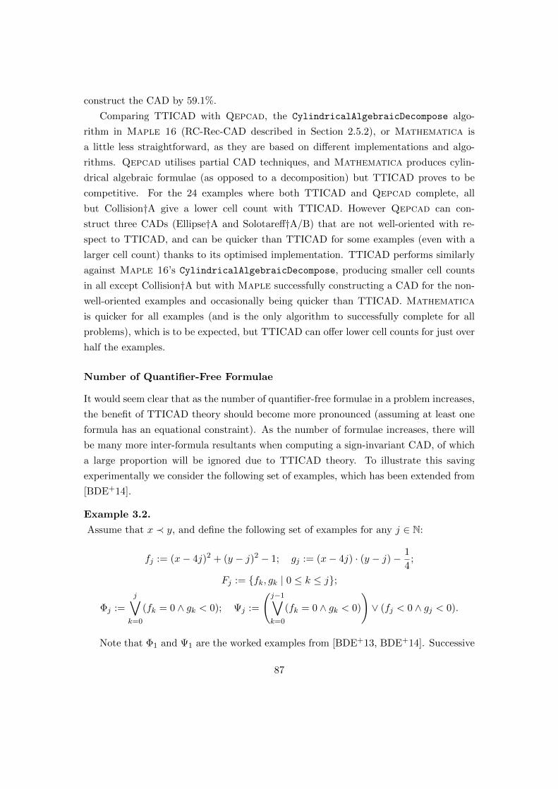
construct the CAD by 59.1%.

Comparing TTICAD with Qepcad, the CylindricalAlgebraicDecompose algo-

rithm in Maple 16 (RC-Rec-CAD described in Section 2.5.2), or Mathematica is

a little less straightforward, as they are based on different implementations and algo-

rithms. Qepcad utilises partial CAD techniques, and Mathematica produces cylin-

drical algebraic formulae (as opposed to a decomposition) but TTICAD proves to be

competitive. For the 24 examples where both TTICAD and Qepcad complete, all

but Collision†A give a lower cell count with TTICAD. However Qepcad can con-

struct three CADs (Ellipse†A and Solotareff†A/B) that are not well-oriented with re-

spect to TTICAD, and can be quicker than TTICAD for some examples (even with a

larger cell count) thanks to its optimised implementation. TTICAD performs similarly

against Maple 16’s CylindricalAlgebraicDecompose, producing smaller cell counts

in all except Collision†A but with Maple successfully constructing a CAD for the non-

well-oriented examples and occasionally being quicker than TTICAD. Mathematica

is quicker for all examples (and is the only algorithm to successfully complete for all

problems), which is to be expected, but TTICAD can offer lower cell counts for just over

half the examples.

Number of Quantifier-Free Formulae

It would seem clear that as the number of quantifier-free formulae in a problem increases,

the benefit of TTICAD theory should become more pronounced (assuming at least one

formula has an equational constraint). As the number of formulae increases, there will

be many more inter-formula resultants when computing a sign-invariant CAD, of which

a large proportion will be ignored due to TTICAD theory. To illustrate this saving

experimentally we consider the following set of examples, which has been extended from

[BDE+14].

Example 3.2.

Assume that x ≺ y, and define the following set of examples for any j ∈ N:

fj := (x− 4j)2 + (y − j)2 − 1; gj := (x− 4j) · (y − j)− 1

4;

Fj := fk, gk | 0 ≤ k ≤ j;

Φj :=

j∨k=0

(fk = 0 ∧ gk < 0); Ψj :=

(j−1∨k=0

(fk = 0 ∧ gk < 0)

)∨ (fj < 0 ∧ gj < 0).

Note that Φ1 and Ψ1 are the worked examples from [BDE+13, BDE+14]. Successive

87

Figure 3.5: The polynomials in F3 for Φ3 and Ψ3 in Example 3.2

Fj Φj Ψj

j CADFull ECCAD TTICAD Qepcad TTICAD Qepcad

1 317 145 105 249 183 3172 695 237 157 509 259 6953 1241 329 209 849 335 12414 1979 421 261 1269 411 19795 2933 513 313 1769 487 29336 4127 605 365 2349 563 41277 5585 697 417 3009 639 55858 7331 789 469 3749 715 73319 9389 881 521 4569 791 938910 11783 973 573 5469 867 11783

Table 3.2: Cell counts for various CADs constructed for Example 3.2.

Φj and Ψj are generalisations: Φj is a disjunction of j + 1 formulae each containing

an equational constraint; Ψj is a disjunction of j formulae each containing an equa-

tional constraint, and one formula without an equational constraint (therefore requiring

Algorithm 3.2). The polynomials in F3 for Φ3 and Ψ3 are shown in Figure 3.5.

Table 3.2 shows the cell counts of CADs for Fj , Φj and Ψj with a variety of methods.

The CADFull column constructs a sign-invariant CAD with ProjectionCAD with Mc-

Callum’s projection operator; the ECCAD column constructs a CAD with ProjectionCAD

according to the implicit equational constraint of Φj ; the TTICAD column constructs

a TTICAD with ProjectionCAD for Φj and Ψj according to Algorithms 3.1 and 3.2,

respectively; the Qepcad column constructs a CAD with Qepcad-B, declaring the

implicit equational constraint for Φj .

Figure 3.6 shows the difference in CAD growth for the various problems. In Figure

3.6a the cell counts for Φj are plotted for, from top to bottom: CADFull, Qepcad,

ECCAD, and TTICAD. In Figure 3.6b the cell counts for Ψj are plotted for, from top to

bottom: CADFull/Qepcad, and TTICAD. It is clear that the size of the sign-invariant

88

(a) Cell counts for Φj (b) Cell counts for Ψj

Figure 3.6: Cell counts for Φj and Ψj with TTICAD, ECCAD (implicit equational con-straint), Qepcad (implicit equational constraint), and CADFull (McCallum’s projectionoperator.

CAD constructed with CADFull or Qepcad is growing at a much faster rate than TTICAD

or ECCAD with an increase in the number of formulae.

We can explicitly describe this growth behaviour, which we list in increasing order

of growth:

• TTICAD Φj : Linear growth described by 52j + 53;

• TTICAD Ψj : Linear growth described by 76j + 107;

• ECCAD Φj : Linear growth described by 92j + 53;

• Qepcad Φj : Quadratic growth described by 40j2 + 140j + 69;

• CADFull Fj : Cubic growth described by 4j3 + 60j2 + 170j + 83 (this is the same

behaviour as Qepcad on Ψj).

These results are perhaps unsurprising if we consider the problem at hand. The in-

clusion of another formula to Φj when using TTICAD simply decomposes the rightmost

cylinder according to the circle and the points intersecting the hyperbola. Adding an-

other formula to Ψj requires the entire hyperbola to be considered, but it only intersects

one other equational constraint (the circle to its immediate left) so again there is only a

linear effect.

Considering the set of polynomials Fj , we are increasing the number of polynomials,

but keeping the degree, norm length, and number of variables fixed. The complexity

results discussed in Section 2.6 show that with a fixed number of variables the complexity

89

bounds are polynomial in the number of polynomials, degree, and norm length, which

correlates with this behaviour. We can also see in Figure 3.5 that adding an extra

formula will intersect all previous hyperbolas, as well as the last and penultimate circles,

which explains the non-linear polynomial behaviour.

3.4 Further Ideas and Extensions: Projection and Lifting

TTICAD

3.4.1 ResCAD

We introduce an intuitive way to think of TTICAD construction, which aligns with the

output of Algorithm 3.1 under specific conditions.

Definition 3.7.

Let Φ = ϕiti=1 be a collection of quantifier free formulae. Let Ai be the set of

polynomials in ϕi and let Ei be a non-empty subset of Ai. Define the ResCAD set of

Φ, denoted R(Φ), to be:

R(Φ) := E ∪t⋃i=1

resxn(f, g) | f ∈ Ei, g ∈ Ai \ Ei .

We can see the relation between the ResCAD set and the TTICAD projection oper-

ator in the following theorem.

Theorem 3.7.

Let Φ = ϕiti=1 be a collection of quantifier free formulae. Let A = Aiti=1 be a

collection of irreducible bases for the polynomials in each ϕi, and let E = Eiti=1 be a

collection of non-empty subsets Ei ⊆ Ai.Then the following relation holds:

MP (R(Φ)) = TTIPE(A).

Proof.

For each pair of sets (Ai, Ei) we define:

Rxn(Ei, Ai) = resxn(f, g) | f ∈ Ei, g ∈ Ai \ Ei,

90

so that we can write the ResCAD set as

R(Φ) = E ∪t⋃i=1

Rxn(Ei, Ai).

Consider MP(R(Φ)). We first note that for every i, the set Rxn(Ei, Ai) consists only

of resultants taken with respect to xn. As such, no polynomial in Rxn(Ei, Ai) can have

positive degree in xn. So, according to the CADW algorithm, they are simply passed down

to the next level of projection. Therefore we can write

MP(R(Φ)) = MP(E) ∪t⋃i=1

Rxn(Ei, Ai).

We now rewrite MPE(A) using the definition of MPE(A):

MPE(A) =t⋃i=1

MPEi(Ai) ∪ RES×(E)

=t⋃i=1

[MP(Ei) ∪Rxn(Ei, Ai)] ∪ RES×(E)

=

[t⋃i=1

MP(Ei) ∪ RES×(E)

]∪

t⋃i=1

Rxn(Ei, Ai).

Therefore it is sufficient to prove that

MP(E) =t⋃i=1

MP(Ei) ∪ RES×(E).

Recall for a set F of polynomials

MP(F ) = coeffs(f), discxn(f) | f ∈ F ∪ resxn(f, f ′) | f, f ′ ∈ F, f 6= f ′.

Now we can rewrite MP(E) as follows:

MP(E) = MP

(t⋃i=1

Ei

)

=

t⋃i=1

coeffs(f), discxn(f) | f ∈ Ei ∪ resxn(f, f ′) | f, f ′ ∈ E, f 6= f ′. (3.6)

91

We can split the final component of (3.6) dependent on whether f and f ′ belong to the

same Ei:

resxn(f, f ′) | f, f ′ ∈ E, f 6= f ′

=t⋃i=1

resxn(f, f ′) | f, f ′ ∈ Ei, f 6= f ′

∪ resxn(f, f ′) | f ∈ Ei, f ′ ∈ Ej , i 6= j, f 6= f ′

=t⋃i=1

resxn(f, f ′) | f, f ′ ∈ Ei, f 6= f ′ ∪ RES×(E).

Hence gathering under the union we obtain:

MP(E) =

t⋃i=1

[ ⋃f∈Ei

ai | f =

kf∑i=0

aixi, ai 6= 0

∪ discxn(f) | f ∈ Ei

∪ resxn(f, f ′) | f, f ′ ∈ Ei, f 6= f ′]

∪ RES×(E)

=t⋃i=1

MP(Ei) ∪ RES×(E).

Hence we see that

MP(R(Φ)) = TTIPE(A)

as we required.

We can use Theorem 3.7 to easily compute a TTICAD with existing technology, but

only in the case that each quantifier-free formula ϕi contains an equational constraint

and no equational constraints are nullified (otherwise the lifting stage of Algorithm 3.1

is altered).

Corollary 3.8.

If each ϕi contains an equational constraint and no fi is nullified by a point in Rn−1

then inputting R(Φ) into an implementation of CADW (which produces a sign-invariant

CAD using McCallum’s projection operator), will result in the TTICAD for Φ produced

by Algorithm 3.1.

92

This allows us to produce TTICADs in technologies such as Qepcad that are simpler

than a sign-invariant CAD. However the conditions on Corollary 3.8 are restrictive and

Algorithms 3.1 and 3.2 can be applied to many more examples (and also include advances

such as improved lifting). It would be of great use to be able to identify whether a

problem is suitable for ResCAD before any construction took place, however as Corollary

3.8 depends on nullification in the lifting stage this is unlikely.

3.4.2 Semi-restricted Projection and Bi-equational Constraints

In Section 2.4.4 the equational constraint projection operator [McC99] was introduced,

which was generalised to the truth-table invariant projection operator (Definition 3.4).

McCallum [McC01] extended the idea of equational constraints to a semi-restricted pro-

jection operator

MP∗E(A) := MPE(A) ∪ discxn(g) | g ∈ A, g /∈ E.

Whilst MP∗E(A) is a superset of the equational constraint, it guarantees order-invariance

of the g ∈ A in sections of f over cells. Therefore MP∗E(A) can be used repeatedly

throughout the whole algorithm, unlike MPE(A) which can only be applied at the highest

level.

A logical extension of the projection and lifting TTICAD algorithm would be to

expand the semi-restricted projection to deal with TTICAD. Including the discriminants

of the non-equational constraints with TTIP would be an interesting first investigation,

although from [McC01] we would only gain order invariance of each g in sections of

the equational constraint of the same sub-formula as g. Whilst this seems sufficient for

one projection/lifting phase whilst constructing a TTICAD, it may prove problematic

when used repeatedly, and should be investigated further. Care needs to also be taken if

A \ E 6= ⋃mi=1Ai \ Ei, although the problematic polynomials are equational constraints

and so order invariance is already guaranteed.

In [BM05] the authors investigate extending the theory of equational constraints to

two polynomials. This results in a CAD invariant with respect to the variety V (f1, f2)

rather than a single equation. This is an extension of the fact that if f1 and f2 are

both equational constraints, then so is their resultant. It should be profitable to look

at applying this theory to TTICAD: taking advantage of sub-formulae with multiple

equational constraints.

93

3.5 Regular Chains Algorithm

Constructing a cylindrical algebraic decomposition by regular chains technology is pos-

sible in two ways. In [CMXY09] (described in Section 2.5.2) this method of constructing

CADs was introduced and proceeds by producing a complex cylindrical decomposition

according to the triangular decomposition of regular chains and translating into real

space by real root isolation (this process is somewhat recursive, and so we denote it

RC-Rec-CAD). This can only generate a sign-invariant CAD, but RC-Rec-CAD proves

competitive, and sometimes more efficient, than projection and lifting CAD implemen-

tations.

In [CM12] (described in Section 2.5.3) an alternative algorithm was presented to

construct CADs through complex space and regular chains. This algorithm works by

constructing the complex cylindrical decomposition incrementally by polynomial: re-

fining an existing complex cylindrical tree whilst maintaining cylindricity. Once all

polynomials have been processed the tree is converted into a CAD (and we denote this

entire approach RC-Inc-CAD) This new approach is much more efficient, partly as it

allows for the recycling of subresultant calculations.

One major benefit of the incremental approach over the original recursive algorithm

is that all equational constraints can be utilised. When refining the complex cylindrical

tree with respect to an equational constraint then any branch for which the constraint

is not satisfied can be truncated. As this process can be done in any refinement step

with respect to an equational constraint it allows all possible constraints to be used.

This offers a distinct advantage to projection and lifting with equational constraints

which usually can only utilise a single equational constraint (or, at most, two equational

constraints [BM05]).

We now describe work that combines the application of equational constraints to RC-

Inc-CAD with truth table invariance to build RC-Inc-TTICADs. The adaption of the

RC-Inc-CAD is not trivial and requires new algorithms and implementation. The work

will be published in [BCD+14] and resulted from collaboration between the University

of Bath research group with Marc Moreno Maza (University of Western Ontario) and

Changbo Chen (CIGIT, Chinese Academy of Sciences). As the author of this thesis

was involved in the discussions and experimentation of this topic, but the theory and

implementation was mainly completed by other researchers on the paper, we will not

go into detail of the algorithm but concentrate on its features. The full details of the

theory and implementation can be found in [BCD+14].

94

3.5.1 RC-TTICAD Algorithm

Recall that a complex cylindrical decomposition (Definition 2.38) is a partition of Cn

such that for any pair of cells C1, C2 their canonical projections to Ck, for 1 ≤ k < n,

are equal or disjoint. Further, recall from Definition 2.40 that a complex cylindrical

tree (CCT) is a rooted tree describing a cylindrical decomposition.

Assume that T is a rooted tree, with nodes at depth i of the form: “any xi”, “p = 0”,

or “p 6= 0” (for some p ∈ Q[x1, . . . , xi]). Let Ti indicate the induced subtree of depth i,

and for a path Γ let the zero set, ZC(Γ) be the intersection of the zero sets of its notes.

Let the zero set of T , denoted ZC(T ), be the union of the zero sets of its paths.

A complete complex cylindrical tree (complete CCT) is a tree where each node

either has one child (“any xi”) or has s+1 children defined by “p1 = 0”,. . .,“ps = 0” and

“∏i pi 6= 0” (where the pi(α, xn), specialised to any α ∈ ZC(Γ) for any path Γ ending at

the node, are squarefree, co-prime, and have non-vanishing leading coefficient).

Definition 3.8.

For a complete complex cylindrical tree T , we define the complex cylindrical decom-

position of Cn associated with T to be the set:

ZC(Γ) | Γ is a path of T .

Definition 3.9.

Let T be a complex cylindrical tree of Cn and let Γ be a path of T . A polynomial

p ∈ Q[x1, . . . , xn] is (path) sign invariant on Γ if either ZC(Γ) ∩ ZC(p) = ∅ or

ZC(Γ) ⊆ ZC(p). A constraint p = 0 or p 6= 0 is (path) truth invariant on Γ if p is

sign invariant on Γ. A complex system cs is truth invariant on Γ if the conjunction of

the constraints in cs is truth-invariant on Γ, and each polynomial in cs is sign-invariant

on Γ.

Constructing a Complex Cylindrical Tree

We now give a description of Algorithm 3.3 which takes a list of complex systems of

Q[x1, . . . , xn] and produces a truth-invariant complex cylindrical tree. It does so by

continually refining an initial tree.

After constructing a trivial CCT (consisting of a single path through nodes “any

xi”), the IntersectLCS algorithm repeatedly refines T according to the input systems

L.

It does this by first selecting a complex system, say cs, containing an equational

95

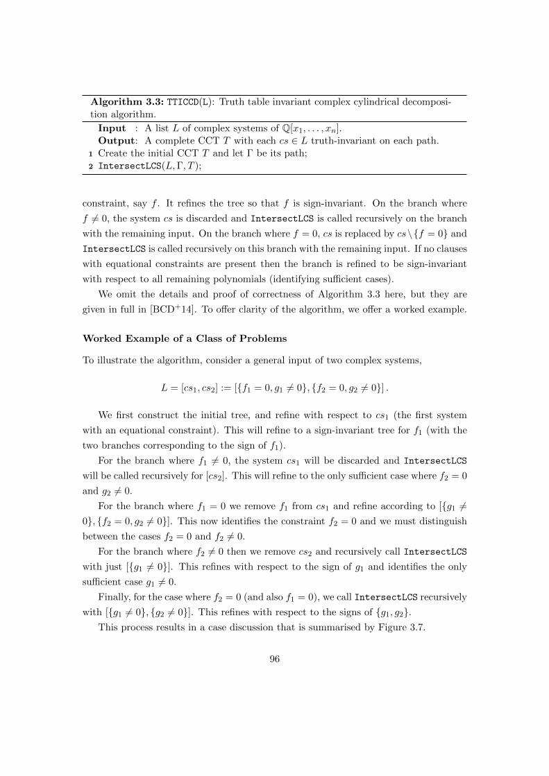
Algorithm 3.3: TTICCD(L): Truth table invariant complex cylindrical decomposi-tion algorithm.

Input : A list L of complex systems of Q[x1, . . . , xn].Output: A complete CCT T with each cs ∈ L truth-invariant on each path.

1 Create the initial CCT T and let Γ be its path;2 IntersectLCS(L,Γ, T );

constraint, say f . It refines the tree so that f is sign-invariant. On the branch where

f 6= 0, the system cs is discarded and IntersectLCS is called recursively on the branch

with the remaining input. On the branch where f = 0, cs is replaced by cs\f = 0 and

IntersectLCS is called recursively on this branch with the remaining input. If no clauses

with equational constraints are present then the branch is refined to be sign-invariant

with respect to all remaining polynomials (identifying sufficient cases).

We omit the details and proof of correctness of Algorithm 3.3 here, but they are

given in full in [BCD+14]. To offer clarity of the algorithm, we offer a worked example.

Worked Example of a Class of Problems

To illustrate the algorithm, consider a general input of two complex systems,

L = [cs1, cs2] := [f1 = 0, g1 6= 0, f2 = 0, g2 6= 0] .

We first construct the initial tree, and refine with respect to cs1 (the first system

with an equational constraint). This will refine to a sign-invariant tree for f1 (with the

two branches corresponding to the sign of f1).

For the branch where f1 6= 0, the system cs1 will be discarded and IntersectLCS

will be called recursively for [cs2]. This will refine to the only sufficient case where f2 = 0

and g2 6= 0.

For the branch where f1 = 0 we remove f1 from cs1 and refine according to [g1 6=0, f2 = 0, g2 6= 0]. This now identifies the constraint f2 = 0 and we must distinguish

between the cases f2 = 0 and f2 6= 0.

For the branch where f2 6= 0 then we remove cs2 and recursively call IntersectLCS

with just [g1 6= 0]. This refines with respect to the sign of g1 and identifies the only

sufficient case g1 6= 0.

Finally, for the case where f2 = 0 (and also f1 = 0), we call IntersectLCS recursively

with [g1 6= 0, g2 6= 0]. This refines with respect to the signs of g1, g2.This process results in a case discussion that is summarised by Figure 3.7.

96

root

f1 = 0

f2 = 0

g1, g2

f2 6= 0

g1 6= 0

f1 6= 0

f2 = 0

g2 6= 0

Figure 3.7: Case distinction for L = [cs1, cs2].

Algorithm 3.4: RC− TTICAD(L): Truth table invariant (reglar chains) CAD algo-rithm.

Input : A list L of semi-algebraic systems of Q[x1, . . . , xn].Output: A CAD such that each sas ∈ L is truth-invariant on each cell.

1 Set L′ to be the list of corresponding complex systems ;2 D := TTICCD(L′) ;3 MakeSemiAlgebraic(D, n)

Producing a TTICAD from a TTICCD

The final step is shown in Algorithm 3.4, which gives an algorithm to construct a

TTICAD with regular chains technology. It makes use of MakeSemiAlgebraic from

[CMXY09], which takes a complex cylindrical decomposition C and returns a CAD D of

Rn such that for each cell C ∈ C the set C ∩ Rn is a union of cells in D. Therefore D is

still truth-invariant for each complex system and so is a TTICAD for the original input.

The proof of correctness for Algorithm 3.4 is given in [BCD+14].

Complexity Comparison

Within [BCD+14] a comparison was given between building a sign-invariant CAD in-

crementally with regular chains and building a TTICAD with the same technology.

This was completed by one of the other authors and we summarise their results, which

demonstrate the power of the new algorithms.

We consider combination diagrams such as in Figure 3.7.

Theorem 3.9 ([BCD+14]).

Let L be a list of r complex systems. Assume each complex system of L has s equational

constraints and t constraints of other types.

Then the number of constraints in a sign-invariant computational diagram is

2r(s+t)+1 − 1.

97

The number of constraints appearing in a truth table invariant computational diagram is

2(s+ 2t)r − 2.

3.6 Implementation and Experimentation: Regular Chains

TTICAD

The implementation of Algorithm 3.4 and relevant sub-algorithms was conducted by

collaborators within the development RegularChains library. This was then loaded

into the development version of Maple using the latest procedures (such as improved

polynomial representation and real root isolation).

3.6.1 Experimental Results for TTICAD by Regular Chains

Experiments were conducted to consider the effectiveness of regular chains TTICAD

compared to: other regular chains CAD algorithms; projection and lifting TTICADs

and sign-invariant CADs; other state-of-the-art CAD algorithms.

A set of CAD examples were sourced from CAD papers [BH91, BDE+13], system

solving papers [CGL+07, CM12], and generated by branch cuts of algebraic relations

(detailed in Sections 2.8.1 and 3.9). For problems in the first two sets, alternative logical

formulations were formed by producing disjunctions where every subformula contains

an equational constraint (denoted by †) or where only some subformulae contain an

equational constraint (denoted by ††).A representative subset of the problems are given in Table 3.3. Each problem was

accompanied by a variable ordering, and the number of variables is shown in the col-

umn below n. For each result the cell count and time taken (in seconds) to construct

the CAD is recorded, with T/O indicating a time out (set at 30 minutes). FAIL in-

dicates an algorithm returning a theoretical failure (for example the input not being

well-oriented) whilst Err indicates an unexpected error (that appears to be a result of

the implementation rather than theoretical).

We first compare RC-TTICAD with RC-Inc-CAD and RC-Rec-CAD, and PL-TTICAD

and PL-CAD.

We can clearly see that RC-TTICAD never gives a higher cell count than any of

the regular chains or projection and lifting algorithms. Compared to the sign-invariant

CADs we see that RC-TTICAD offers a saving of at least an order of magnitude. This

coincides with an, often significant, general saving in time from using RC-TTICAD. We

98

RC

-TT

ICA

DR

C-I

nc-C

AD

RC

-Rec-C

AD

PL

-TT

ICA

DP

L-C

AD

Mathematica

Qepcad

SyNRAC

Redlog

Pro

ble

mn

Cells

Tim

eC

ells

Tim

eC

ells

Tim

eC

ells

Tim

eC

ells

Tim

eT

ime

Cells

Tim

eC

ells

Tim

eC

ells

Tim

e

Inte

rsecti

on†

3541

1.0

3723

12.0

3723

19.0

579

3.5

3723

29.5

0.1

3723

4.9

3723

12.8

Err

—E

llip

se†

571231

317.1

81183

544.9

81193

786.8

FA

IL—

FA

IL—

11.2

500609

275.3

Err

—E

rr—

Solo

tare

ff†

42849

8.8

54037

209.1

54037

539.0

FA

IL—

54037

407.6

0.1

16603

5.2

Err

—3353

8.6

Solo

tare

ff††

48329

21.4

54037

226.9

54037

573.4

FA

IL—

54037

414.3

0.1

16603

5.3

Err

—8367

13.6

2D

Ex†

297

0.2

317

1.0

317

2.6

105

0.6

317

1.8

0.0

249

4.8

317

1.1

305

0.9

2D

Ex††

2183

0.4

317

1.1

317

2.6

183

1.1

317

1.8

0.0

317

4.6

317

1.2

293

0.9

3D

Ex†

3109

3.5

3497

63.1

3525

1165.7

109

2.9

5493

142.8

0.1

739

5.4

—T

/O

Err

—M

onte

sS10

73643

19.1

3643

28.3

3643

26.6

—T

/O

—T

/O

T/O

—T

/O

—T

/O

Err

—W

ang

93

5507

44.4

507

49.1

507

46.9

—T

/O

T/O

—897.1

FA

IL—

Err

—E

rr—

Rose†

33069

200.9

7075

498.8

7075

477.1

—T

/O

—T

/O

T/O

FA

IL—

—T

/O

Err

—genL

inSyst

-3-2†

11

222821

3087.5

—T

/O

—T

/O

FA

IL—

FA

IL—

T/O

FA

IL—

Err

—E

rr—

BC

-Kahan

255

0.2

409

2.4

409

4.9

55

0.2

409

2.4

0.1

261

4.8

409

1.5

Err

—B

C-A

rcsi

n2

57

0.1

225

0.9

225

1.9

57

0.2

225

0.9

0.0

225

4.8

225

0.7

161

2.4

BC

-Sqrt

497

0.2

113

0.5

113

1.3

FA

IL—

113

0.6

0.0

105

4.7

105

0.4

73

0.0

BC

-Arc

tan

4211

3.5

—T

/O

—T

/O

FA

IL—

—T

/O

T/O

—T

/O

Err

——

T/O

BC

-Arc

tanh

4211

3.5

—T

/O

—T

/O

FA

IL—

—T

/O

T/O

—T

/O

Err

——

T/O

BC

-Phis

anbut-

14

325

0.8

389

1.8

389

5.8

FA

IL—

389

3.6

0.1

377

4.8

389

2.0

217

0.2

BC

-Phis

anbut-

44

543

1.6

2007

13.6

2065

21.5

FA

IL—

51763

932.5

11.9

51763

8.6

Err

—E

rr—

Tab

le3.3

:C

om

pari

ng

the

RC

-TT

ICA

Dal

gori

thm

wit

hot

her

form

sof

CA

Dan

dim

ple

men

tati

ons.

99

can also see explicitly that the TTICAD algorithms can take advantage of the logical

structure of the formula by the difference in cell counts for † and †† problems (which is

not the case for sign-invariance).

We see that sometimes constructing a TTICAD by regular chains is more efficient

than by projection and lifting (although never the reverse). Further, the regular chains

algorithm never returns FAIL, whilst the projection and lifting algorithm fails for pre-

cisely half the examples. We discuss in more detail in Section 3.7 the differences in the

algorithms that account for this behaviour.

The implementations of Qepcad, Redlog and SyNRAC all are projection and

lifting based. As was shown in Section 3.2.1 and Table 3.1, TTICAD theory can offer

greater savings than implicit equational constraints and partial CAD techniques (as

implemented in Qepcad) when all clauses have equational constraints. This is confirmed

in Table 3.3.

Both SyNRAC and Redlog fail for a large number of examples: the former returning

an error message and the latter suspending during construction producing no output or

error messages. When they complete computation they are often competitive as they

are optimised (for example Redlog offers partial lifting techniques). Whilst we use the

most current public version of SyNRAC there is a superior development version which

we do not have access too (that would presumably fail on fewer examples). Redlog is

intended for quantifier elimination by virtual substitution rather than CAD but can be

forced to construct CADs.

We note that Mathematica is often the quickest algorithm, and often by a sig-

nificant amount. As mentioned elsewhere in this thesis, the output of Mathematica

is not a CAD and so a comparison is perhaps not fair, although it is worth noting

that Mathematica times out on 5 examples (whilst RC-TTICAD is successful for all

problems).

It is clear that the results in Table 3.3 demonstrate that the RC-TTICAD is a

competitive and state-of-the-art CAD algorithm.

3.7 Comparison of Projection and Lifting and Regular Chains

TTICAD

We now compare the two algorithms for computing a TTICAD. It was shown in Table 3.3

that constructing a TTICAD by regular chains is often more efficient than by projection

and lifting and that it avoids theoretical failure. These differences are, at least partly,

100

f

f

g

R1c

(a) Projection and Lifting TTICAD.

f

f

g

R1c

(b) Regular Chains TTICAD.

Figure 3.8: Case distinction in TTICADs for ϕ := [f = 0 ∧ g > 0].

due to the following properties of the two algorithms.

3.7.1 Case Distinction

We first note that constructing a TTICAD by regular chains allows for a finer case

distinction than by projection and lifting. We demonstrate with a simple example how

it can avoid constructing certain cells if the truth value of a formula is already known.

Consider a clause of the form ϕ := [f = 0 ∧ g > 0] in two variables and let c be a

cell in the induced CAD of R1 corresponding to an intersection of f and g, as shown in

Figure 3.8. Even though f and g intersect within the stack over c, the truth value of ϕ

does not change at this intersection: g is a strict inequality so ϕ cannot be satisfied on

a 0-cell, and the cells directly above and below the intersection correspond to f 6= 0 so

ϕ is also false.

Using the projection and lifting algorithm will identify all cells where f = 0 and so

identifies the extraneous cell in the lifting phase, as shown in Figure 3.8a. The regular

chains algorithm will not identify this intersection as a cell: during construction of the

complex cylindrical tree it will discard the branch corresponding to this cell. It therefore

only considers cells over c where f = 0 and g 6= 0, as shown in Figure 3.8b.

Whilst this only reduces the cell count by 2 cells in this case, it can obviously have

a greater effect with more intersections or formulae.

3.7.2 Multiple Equational Constraints

With the introduction of the sign-invariant incremental algorithm for CAD in [CM12],

every equational constraint of a problem can be utilised due to the case analysis when

refining the complex cylindrical tree. This is unlike construction with the older regular

chains algorithm from [CMXY09] (where no equational constraints can be used) or by

101

projection and lifting (where, at most, two equational constraints can be considered).

Similarly, when constructing a TTICAD incrementally using regular chains we can

consider all equational constraints for each formula. This produces further savings over

the projection and lifting algorithm. Whilst this initially seems to remove the problem of

choosing an equational constraint to designate for use (discussed in Section 5.2.2), there

is still a choice of which order to consider the equational constraints in each formula.

This turns out to be an important choice and is investigated further in [EBC+14] (and

discussed in Section 5.2.4).

3.7.3 Well-orientedness

One of the issues of constructing an equational constraint or truth table invariant CAD

by projection and lifting is theoretical failure due to a lack of well-orientedness. If a

polynomial is nullified on a cell of positive dimension, then this can lead to theorems

validating the order/sign-invariance not being applicable.

When constructing a TTICAD through regular chains there is no well-orientedness

condition, and any problem will complete construction of a TTICAD (given sufficient

time and memory). This means we will never have theoretical failure, which makes the

regular chains algorithm much more widely applicable than projection and lifting.

Comparison of the two algorithms could lead to results concerning whether well-

orientedness is a necessary condition for the construction of the projection and lifting

CAD in question, or if it is merely a theoretical necessity for the current theorems.

Ideally, a stronger condition would be created that reduces the rate of failure for pro-

jection and lifting, or an improved projection and lifting algorithm that never results in

theoretical failure.

3.7.4 Disjunctive Normal Form

There is a drawback to the implementation of Algorithm 3.4 in that the input must be

given as a disjunction of systems. If a problem is not in a disjunctive form then it must

first be put in a disjunctive normal form3. This can be expensive, with the minimal

disjunctive normal form of [A1∨B1]∧· · ·∧ [Am∨Bm] requiring 2m conjunctive formulae.

In Theorem 3.9 it was shown that in constructing the complex cylindrical tree for a

problem the number of constraints considered is exponential in the number of formulae.

3This can be done algorithmically: Maple offers the Logic[Canonicalize] function which can begiven the option form=DNF. Note that this does not give a minimal normal form: [A1 ∨ B1] ∧ [A2 ∨ B2]gets converted into a disjunction of 9 formulae, each of size 4, whilst the minimal normal form is[A1 ∧A2] ∨ [A1 ∧B2] ∨ [B1 ∧A2] ∨ [B1 ∧B2].

102

Specifically, for r complex systems, each with s equational constraints and t constraints

of other types, the truth table invariant computational diagram contains

2(s+ 2t)r − 2

constraints. Therefore an increase in the number of these systems can prove very expen-

sive computationally4.

3.8 Idea for Extension: Partial TTICAD

The construction of a partial CAD (Section 2.4.2) involves using deductions on the truth

value of a formula to simplify the lifting phase of constructing the CAD. We now consider

how this might apply to TTICADs.

Consider a formula:

Φ := [ϕ1 ∨ · · · ∨ ϕt] ,

and assume that each ϕ has a designated equational constraint fi = 0.

It may be possible to adapt the partial CAD techniques to work on each individual

formula. When preparing to lift over a cell, c ∈ D′, from Rn−1 to Rn then we can

consider the truth value of each ϕi.

It may be possible to decide the truth of ϕi on c before lifting. For example if

ϕi = [fi(x1, . . . , xn) = 0 ∧ g(x1, . . . , xn−1) > 0 ∧ ϕi(x1, . . . , xn)] and g is negative on c

then the value of ϕi will be false in every cell above c. In this case then we cannot simply

construct the trivial cylinder over c as other ϕj may change truth value. However, we

can remove fi from the lifting set over c.

Remark 3.2.

Removing certain fi when lifting over a cell c of Rn−1 will clearly produce fewer cells and

thus improve the efficiency of the projection and lifting TTICAD algorithm. Further, if

the fi being excluded was nullified on c, violating the well-orientedness condition for the

TTICAD algorithm (Definition 3.6), then this partial technique could avoid theoretical

failure and expand the application of Algorithms 3.1 and 3.2.

Further, imagine that Φ is preceded by a sequence of quantifiers:

Ψ := (Qk+1 xk+1) · · · (Qn xn) [ϕ1 ∨ · · · ∨ ϕt] ,

4Further, if the disjunctive normal form is computed algorithmically in Maple then r will generallybe larger than for the optimal normal form, and the values of s and t will likely be increased as well.

103

where each Qi is a universal or existential quantifier.

If Qn is an existential quantifier we can distribute over the disjunction:

Ψ ≡ (Qk+1 xk+1) · · · (Qn−1 xn−1) [[(∃ xn)ϕ1] ∨ · · · ∨ [(∃ xn)ϕt]] .

Again, we may be able to decide the truth of certain (∃ xn)ϕi before finishing the lifting

process: as soon as a point is found over c satisfying ϕi we can stop lifting with respect to

fi and denote ϕi as TRUE in the entire cylinder over c. We may also avoid theoretical

failure, as mentioned in Remark 3.2.

We could extend these ideas by keeping track of when sections are produced due

to a single formula. Consider lifting over c to the cells d1, d2, d3 where d2 is a section

produced just from polynomials in ϕi (from PEi(Ai)). Then for all ϕj where j 6= i

then the polynomials in PEj (Aj) will be delineable over d1 ∪ d2 ∪ d3, therefore only a

single lifting need be conducted. This is not the case for polynomials in PEi(Ai) or the

cross-resultants which should be lifted over d1, d2, and d3 separately. This is analogous

to the cluster based CAD algorithm in [Arn88] (described in Section A.4.7).

How to utilise this case distinction is not an obvious choice. The single lifting for

those formulae not requiring this particular section could be merged back into the CAD,

or the CAD could “branch” into multiple truth-invariant CADs for each formula, with

a known relation between all the cells. The latter option seems unduly expensive, but

the branching could occur only over certain cells, offering a CAD that is “exploded” at

certain points, which would reduce the cost and could prove efficient (especially if by

not lifting over certain sections it avoids computing with expensive algebraic numbers).

3.9 Application: Branch Cut Analysis

We discuss in greater detail an application of CAD that is particularly suited for TTI-

CAD: verification of identities in the presence of branch cuts. This was initially dis-

cussed in Section 2.8.1 and the original work in this section was published in [DBEW12],

[EBDW13], and [ECTB+14]. The author was involved in many of the discussions for

the work discussed but the majority of the work was conducted by other members of

the research group.

3.9.1 Verification in the Presence of Branch Cuts

As discussed in Section 2.8.1, and covered in great detail in [Phi11], CAD can be used

to decide the validity of identities over the complex plane. When considering an identity

104

involving elementary functions such as log,√·, or inverse trigonometric functions then

the geometry of the branch cuts needs to be considered to determine the regions where

the identity is valid.

Verifying a complex identity can be approached with CAD, as described in Algorithm

2.5, by: determining the branch cuts; representing them as semi-algebraic equations in

<(z) and =(z); generating a CAD of R2n ≡ Cn according to these branch cuts; evaluating

the identity at each sample point (proving identical truth or generic falsity on each cell).

This is unfortunately necessary as many complex identities that seem obvious are not

valid for the whole plane, for example:

√z − 1

√z + 1

?=√z2 − 1. (3.7)

Whilst (3.7) appears valid, it is only correct for complex z ∈ C such that <(z) ≥ 0 or

=(z) = 0 ∧ <(z) ≥ −1.

In [DBEW12], this and other approaches to proving identities were discussed and

some of their shortcomings were identified. Three key examples were discussed: the

Kahan arccosh example from [Kah87]; the Joukowski conformal map; and, the arctan

addition rule.

The Kahan problem involves the simplification of a conformal map from fluid dynam-

ics involving arccosh. Whilst the branch cut for arccosh is simply the real axis between

(−∞, 1) (as defined in [AS72]), this simplification transforms the cuts so that it holds

over the entire complex plane, except for a small teardrop region:z = x+ iy

∣∣∣∣∣ |y| ≤√−(x+ 3)2(2x+ 9)

2x+ 5, −9

2≤ x ≤ −3

.

This is isolated by 7 transformed branch cuts, each described by a single equality and

inequality. The arctan addition formula for two real variables, (x, y), is true when

|1 − xy| < 1 due to a “branch cut at infinity” and is an example of real variables still

being affected by branch cuts.

The discussion of the Joukowski’s map:

f : z 7→ 1

2

(z +

1

z

),

consists of trying to prove bijectivity from D := z | |z| > 1 to C‡ := C \ [−1, 1]. The

quantified formula constructed to describe this bijectivity proved too difficult to naıvely

solve, which led to communications with Brown [Bro12], who maintains Qepcad-B. In

105

manipulating the problem to be better suited for Qepcad, he inspired work on how to

best express problems for CAD that is discussed in Chapter 6.

3.9.2 Understanding Branch Cuts

In [EBDW13] methods of determining and describing branch cuts were given. There are

two main methods of determining branch cuts: by decomposing into real variables or

using a complex parametric representation. Whilst the latter can be useful for visual-

isation, it is noted in [EBDW13, Section 4] that the former can provide semi-algebraic

output for use with CAD.

These algorithms were implemented in Maple 17+ within the FunctionAdvisor

command. Given an expression in one complex variable, FunctionAdvisor can provide

a description of the relevant branch cuts, either in two real variables or a parametrised

complex variable, as well as visualisations of the branch cuts. FunctionAdvisor also

applies simplification, removing spurious branch cuts, where possible The details of this

implementation are given in [ECTB+14] and the functionality is available in versions of

Maple from 17 onwards.

The semi-algebraic sets output from this algorithm all describe branch cuts and

consist of equalities and inequalities. For example, the first set for the Kahan example

is:

[8y3x+ 8yx3 + 20y3 + 84yx2 + 288yx+ 324y = 0,

− 225x2 − 324x+ 63y2 − 4x4 − 52x3 + 12y2x+ 4y4 < 0].

We wish to describe the space as decomposed by these semi-algebraic sets and previously

a sign-invariant CAD would need to be constructed with respect to all polynomials:

producing 409 (x ≺ y) or 1, 143 (y ≺ x) cells for the Kahan example. It is clear that

a TTICAD for the sets will suffice for deciding the validity of the simplification with

respect to these branch cuts and this offers a huge saving in cells: 55 (x ≺ y) and 39

(y ≺ x) cells for PL-TTICAD and RC-TTICAD. These cell counts are more efficient

than both Qepcad (261 and 1143 cells) and Mathematica (72 and 278 cells).

In general when analysing a simplification with respect to branch cuts a TTICAD

is the optimal choice of CAD. We are only concerned at interaction of polynomials in

separate sets when the branch cuts intersect, which occurs when the equalities defining

them are simultaneously zero (and the inequalities are also satisfied). Therefore TTICAD

is more appropriate than a sign-invariant CAD (or an equational constraint CAD with

106

respect to the implicit equational constraint). Further, a truth-invariant CAD is not

appropriate as the polynomials are not part of a larger formula.

3.10 Solotareff-3

The Solotareff-3 problem introduced in Section 2.12 is not particularly interesting for

TTICAD application. The formulation given in (2.13) consists of a conjunction of four

equalities and eight inequalities and so does not have the disjunctive structure that

showcases the strength of truth table invariance: a TTICAD for this problem would

simply be an equational constraint CAD.

We therefore give two problems derived from the Solotareff-3 problem, which we refer

to as Solotareff-3† and Solotareff-3‡ in the CAD repository and experimentation in this

thesis.

† :[[

[3v2 − 2v − a = 0] ∧ [v3 − v2 − av − 2b+ a− 2 > 0] ∧ [1 ≤ 4a]

∧ [4a ≤ 7] ∧ [−1 ≤ v] ∧ [v ≤ 0]]∨[[3u2 − 2u− a = 0] ∧

[u3 − u2 − au− a+ 2 > 0] ∧ [−3 ≤ 4b] ∧ [4b ≤ 3] ∧ [0 ≤ u] ∧ [u ≤ 1]]]. (3.8)

‡ :[[

[3v2 − 2v − a = 0] ∧ [v3 − v2 − av − 2b+ a− 2 > 0] ∧ [1 ≤ 4a]

∧ [4a ≤ 7] ∧ [−1 ≤ v] ∧ [v ≤ 0]]∨[[3u2 − 2u− a < 0] ∧

[u3 − u2 − au− a+ 2 > 0] ∧ [−3 ≤ 4b] ∧ [4b ≤ 3] ∧ [0 ≤ u] ∧ [u ≤ 1]]]. (3.9)

By changing the Boolean structure of the problem, we have not affected the sign-

invariant algorithms but have removed the presence of an explicit equational constraint.

In † there is still an implicit equational constraint, but this is not present in ‡.We can see some interesting results in Tables 3.4 and 3.5 from various CAD techniques

from the chapter. The Boolean structure changing does not affect the size of the CADs

for the sign-invariant CADs, although the number of valid cells increases in ‡.For all the experiments, the TTICAD projection operator fails due to the well-

oriented condition: this is due to 3v2 − 2va being nullified on a positive dimensional

cell in all cases (this is also why it cannot be used in an equational constraint CAD).

However, the regular chains TTICAD algorithm is not limited by this condition and

successfully constructs a CAD.

Appealing to truth table invariance results in a substantial cell saving in both variable

107

Technique Solotareff-3 A† Solotareff-3 A‡Cells (Valid) Time Cells (Valid) Time

RC-Inc-TTICAD 2849 (157) 8.454 8329 (343) 21.440RC-Inc-CAD 54037 (1914) 208.968 54037 (4510) 226.916

PL-TTICAD FAIL — FAIL —PL-CAD (McC) 54037 407.561 54037 414.272

Qepcad 16603 5.238 16603 5.320

Table 3.4: Solotareff † and ‡ examples with TTICAD — variable order a ≺ b ≺ v ≺ u.

Technique Solotareff-3 B† Solotareff-3 B‡Cells (Valid) Time Cells (Valid) Time

RC-Inc-TTICAD 7891 (479) 24.937 27855 (1131) 81.194RC-Inc-CAD 154527 (5180) 1149.671 154527 (11322) 1184.574

PL-TTICAD FAIL — FAIL —PL-CAD (McC) 154527 1285.656 154527 1292.400

Qepcad 49461 6.257 49461 6.430

Table 3.5: Solotareff † and ‡ examples with TTICAD — variable order b ≺ a ≺ v ≺ u.

orders for Solotareff-3†: 94.7% and 94.9% in the number of total cells, respectively, with a

saving of 91.8% and 90.8% in the number of valid cells. The savings are also substantial

for Solotareff-3‡: 84.6% and 82.0% in the number of total cells, respectively, with a

saving of 92.4% and 90.0% in the number of valid cells. In all these cases, the truth

table invariance proves more powerful than the Qepcad technology.

3.11 Conclusion

In this chapter the new concept of truth table invariance of a CAD was introduced. Given

a list of quantifier-free formulae a new projection operator was given, that identifies all

intra-formula intersections and only the necessary inter-formula intersections. This can

be incorporated into a new algorithm to produce a TTICAD where each formula has

constant truth value on each cell. The validity of the projection operator and correctness

of the algorithm was proven, but only for inputs satisfying a well-orientedness condition.

The TTICAD projection operator is a subset of the McCallum projection operator,

and also of the equational constraint operator with respect to the implicit equational

108

constraint (if present). This relation is demonstrated by experimentation with a full

implementation of the TTICAD algorithm that clearly shows an increase in efficiency.

An equivalent construction under certain conditions, the ResCAD set, was given along

with ideas to improve the TTICAD projection operator.

The idea of truth table invariance can be combined with the incremental regular

chains CAD algorithm described in Section 2.5.3. The complex cylindrical tree is refined

incrementally according to the list of complex systems (derived from the formulae).

This offers some notable benefits over construction by projection lifting (a more refined

case distinction, ability to utilise multiple equational constraints in each formula) and

perhaps most importantly does not require any well-orientedness condition. At the

moment this algorithm assumes a disjunction of the formulae but future work could

extend its use. Experimentation with an implementation of this method of constructing

TTICADs proved that it is highly competitive with current CAD implementations.

A possible extension of TTICAD theory by incorporating partial CAD techniques

with respect to the individual formulae was suggested. An application of CAD that is

particularly suited for TTICAD use was given: branch cut analysis to determine the

validity of an expression (generally over the complex numbers) involving elementary

functions.

109

110

Chapter 4

Cylindrical Algebraic

sub-Decompositions

Often an entire CAD is unnecessary to solve a problem. This issue was slightly relieved

by the introduction of partial CAD [CH91] which constructs cylinders over cells but

only splits them when necessary. This is therefore still a decomposition of Rn, albeit a

simplified one.

A cylindrical algebraic sub-decomposition (sub-CAD) is introduced as a subset of

cells of a CAD, and can be constructed for several purposes. Different types of sub-

CADs are introduced including those containing cells of specific dimensions (layered

sub-CADs) and those cells that are sections of a specific set of polynomials (variety sub-

CADs). These are investigated along with their mutual interactions and applications to

other CAD technologies (offering the construction of structures such as layered variety

sub-TTICADs).

Author’s Contribution and Publication

The work in this chapter is by the author. The theory, implementation (initially in the

LayeredCAD package and later integrated into ProjectionCAD), and experimentation

were all done by the author. The work was then discussed with the research group for

publication (incorporating feedback from reviewers).

The majority of the work in this chapter was first presented in the Technical Report

[WE13]. It was then published in [WBDE14].

111

4.1 Definition and Motivation

Often the application of a cylindrical algebraic decomposition does not require all the

cells produced. Often it is only those cells on which a given formula is satisfied or cells

of certain dimensions that are needed to obtain a solution to the question at hand. This

can produce thousands of superfluous cells which are not part of the solution. This

excess of output is even more pertinent if the CAD is then to be used in an application

(such as adjacency) which requires computations on each cell.

This chapter focuses on the identification of subsets of cells, from an overlying CAD,

that are sufficient for a given problem. Often these sets can be identified in the con-

struction phase, which saves construction time as well as reducing the size of the output

CAD.

We present the following general definition:

Definition 4.1.

Let D be a cylindrical algebraic decomposition of Rn, represented as a set of cells. Then

any subset E ⊆ D is a cylindrical algebraic sub-decomposition (sub-CAD).

Let F ⊂ Q[x1, . . . , xn] be a set of polynomials and let D be a sign-invariant CAD

of F . We say that any sub-CAD E of D is a sign-invariant sub-CAD, and similarly

define sub-CADs with other invariance conditions.

Let ϕ(x1, . . . , xn) be a Tarski formula for which D is a truth-invariant CAD (ϕ has

constant Boolean value for each cell). Then any sub-CAD E of D which contains all

those cells of D where ϕ is true is called a ϕ-sufficient sub-CAD.

Assume each cell in D and E has a cell index. Then if for every cell in E , its index is

the same in both E and D, then we say E is an index consistent sub-CAD of D.

Given a quantified formula Φ we may wish to derive an equivalent quantifier-free

formula, ϕ. For a formula over the reals this is achieved by constructing a sign-invariant

CAD for the polynomials in Φ and testing the truth of Φ at a sample point of each cell.

This is sufficient to draw a conclusion for the whole cell due to sign-invariance and thus

an equivalent quantifier free formula can be created from the algebraic description of the

cells on which Φ is true. Such an application makes no use of the cells on which Φ is

false and so a Φ-sufficient sub-CAD can be used.

Of course, for a given problem we would like the smallest possible ϕ-sufficient sub-

CAD. It is not usually possible to pre-identify this, but we have developed techniques

which restrict the output of the CAD algorithm to provide sub-CADs sufficient for certain

general classes of problems. These will offer savings on any subsequent computations

112

on the cells (such as evaluating polynomials or formulae) and in some cases also offer

substantial savings in the CAD construction itself.

The sub-CADs we construct in this chapter will be index consistent and we focus on

projection and lifting constructions.

4.1.1 Cylindrical Algebraic sub-Decompositions in Literature

Before discussing new algorithms we briefly offer a survey of previous work that can

be described as, or easily adapted to produce a sub-CAD. Other previous work will be

discussed later in this chapter relating to new concepts.

• In [McC97], whilst trying to solve a motion planning problem in the plane described

by a formula ϕ, the author identifies a subset of cells in the decomposition of R1

for which any valid cell for ϕ must lie over. Lifting over only these cells only gives a

ϕ-sufficient sub-CAD (and can be done in parallel). Similar ideas are in [IYAY09].

• In [Bro13] an algorithm is presented which, given polynomials F and a point α,

returns a single open cell (necessarily full-dimensional) containing α on which F

is sign-invariant. The cell belongs to a CAD (although not necessarily one that

could be produced by any known algorithm) and hence this is an extreme example

of a sub-CAD.

• Partial CAD [CH91] (discussed in Section 2.4.2) works by avoiding the splitting of

cylinders into stacks when lifting over cells where the truth value is already known.

If cells over which the truth value is false were discarded (rather than constructing

the trivial cylinder) then a sub-CAD sufficient to analyse the input formula would

be produced.

• In [SS03] an algorithm is described which takes polynomials F and returns a CAD

D and theory Θ (a theory is a set of negated equations). The CAD is sign-invariant

for F for all points which satisfy Θ. Rather than a sub-CAD of Rn this is actually

a CAD of RnΘ: all those points in Rn except the set of measure zero which do not

satisfy Θ.

• In [Str12], an algorithm is given for solving systems over cylindrical cells described

by cylindrical algebraic formulae. This allows cells produced from a CAD to be

used easily in further computation, which may implicitly be used to produce either

sub-CADs or CADs of a sub-space.

113

It seems beneficial to unify these ideas under the heading sub-CAD, which allows us

to notice similarities in their approaches. We will append the ideas of Variety sub-

CADs and Layered sub-CADs to this list.

4.2 Variety sub-CADs

In this section we describe a way to utilise an equational constraint to restrict the output

of a CAD algorithm to generate a sub-CAD. Recall the definition of an equational

constraint (Section 2.4.4):

Definition 4.2.

Let ϕ be a Tarski formula. An equational constraint is an equation, f = 0, logically

implied by ϕ.

We have seen that equational constraints may be given explicitly or implicitly, and

the presence of an equational constraint can be utilised both in the first projection stage

by refining the projection operator (Section 2.32 based on [McC99]) and also in the

final lifting stage by reducing the amount of polynomials used to construct the stacks

(Remark 3.1 and implemented in [Eng13b]). If more than one equational constraint

is present then further savings may be possible through the theory of bi-equational

constraints [McC01, BM05]. We restrict ourselves to a single equational constraint, and

if multiple equational constraints are present we assume that one has been designated.

We now present the key definition for this section, that of a variety sub-CAD.

Definition 4.3.

Let ϕ be a Tarski formula with equational constraint f = 0. A truth-invariant sub-CAD

for ϕ consisting only of cells lying in the variety defined by f = 0 is a variety sub-CAD

(V-sub-CAD).

The inspiration for variety sub-CADs is to combine equational constraints with the

key idea in partial CAD (Section 2.4.2, [CH91]) of using the logical structure of the

input formula to truncate lifting in CAD. Algorithm 4.1 combines these ideas to build

variety sub-CADs in the case where all factors of the equational constraint have the

main variable of the system.

Algorithm 4.1 uses various sub-algorithms. The use of ProjOp refers to an algorithm

implementing a suitable CAD projection operator. The CADAlgo and GenerateStack

respectively implement compatible algorithms for CAD construction, and stack genera-

tion over a cell with respect to the sign of given polynomials (for example Algorithms

114

Algorithm 4.1: VarietySubCAD(ϕ, f,x): Variety sub-CAD algorithm.

Input : A formula ϕ, a declared equational constraint f = 0 from ϕ andvariables x = x1, . . . , xn. ϕ is in x and all factors of f have mainvariable xn.

Output: A (truth-invariant) variety sub-CAD of Rn for (ϕ, f), or FAIL.

1 A← sqfreebasis(polys(ϕ));2 E ← sqfreebasis(f);3 P← output from applying ProjOp to (A,E) once ; // First projection stage

4 D′ ← CADAlgo(P, [x1, . . . , xn−1]) ; // Computation of a CAD of Rn−1

5 if D′ = FAIL then6 return FAIL ; // P is not well oriented

7 D ← [];8 for c ∈ D′ do9 S ← GenerateStack(E, c); // Final lifting stage

10 if S = FAIL then11 return FAIL ; // Input is not well oriented

12 if |S| > 1 then13 for i = 1 . . . (|S| − 1)/2 do14 D.append(S[2i]) ; // Cells with even index included

15 return D;

2.4 and 2.2). By compatible we mean using the same projection operator and checking

for any necessary conditions of its use. This is required as some CAD algorithms may

return FAIL if the input does not satisfy certain conditions, in which case Algorithm

4.1 must also return FAIL.

Algorithm 4.1 has been implemented in ProjectionCAD, with further details in Sec-

tion C.2.

We prove that Algorithm 4.1 satisfies its specifications when the sub-algorithms used

are those for equational constraints.

Theorem 4.1.

When the sub-algorithms are chosen to implement McCallum’s algorithm to produce

CADs with respect to an equational constraint [McC99], then Algorithm 4.1 satisfies its

specification, with the produced sub-CAD consisting of cells on which the input formula

has constant truth value.

Proof.

Projecting with respect to an equational constraint applies the projection operator

115

MPE(A) at the top level, then MP to construct the rest of the projection set. The

algorithm then incrementally constructs CADs of increasing real dimension, checking

for well-orientedness when building each stack. In [McC99] the author proved that the

CAD returned was truth-invariant for the equational constraint and sign-invariant for

any other polynomials involved on cells where the equational constraint was satisfied.

The first difference in Algorithm 4.1 is in step 9 where the final lift is performed with

respect to E rather than A. This improvement follows directly from Theorem 3.2 (given

in [McC99]), although it was not realised until [BDE+13, BDE+14] and was discussed

in Remark 3.1. This reduces the size of the output, but not its invariance structure or

correctness.

In the final loop, only some of the cells generated in the final lift are included in the

output. The cells in question are a subset of what would have been produced otherwise

and thus certainly a sub-CAD with the same invariance property as the complete CAD.

It remains to prove that they are a variety sub-CAD (in which case we can conclude ϕ

has constant truth value on each cell).

The only cells retained for the output are those with even index (the sections). If the

polynomial f is not identically zero over a cell in D then these must together define its

variety. If any of the polynomials in E were nullified then part of the variety may be in

the sectors, but in this case the input would have failed the well-orientedness condition

in [McC99] (Definition 2.26) and thus Algorithm 4.1 would return FAIL.

Remark 4.1.

As the operator, MP, from [McC99] can return FAIL in situations where others do

not, we consider how Algorithm 4.1 may be adapted to use alternative CAD projection

operators.

First, if a polynomial in E is nullified on a cell of D then [McC99] returns FAIL

while McCallum’s operator to produce sign-invariant CADs in [McC98] is still applicable

(because then the nullification is in the final lift where only sign-invariance and not

order invariance is required). However, we cannot simply apply Algorithm 4.1 with

the alternative projection operator as it will now be the case that some of the variety

is contained in the sectors over the cell in question. In this case we would need the

GenerateStack algorithm to check for nullification of E, and then if it occurs have

Algorithm 4.1 include all cells from that stack in the output.

Second, if some other polynomial is nullified causing failure then CP and CHP are

still applicable. As with the previous case we must still check for nullification over a cell

116

in the final lift, including the whole stack when nullification occurs.

In these cases there would still be output savings from building a variety sub-CAD

since the inclusion of the full stack only needs to happen over those cells where nullifi-

cation occurs.

We can see the strength of using a variety sub-CAD through a simple example.

Example 4.1.

Consider the simple task of describing the unit sphere: x2 + y2 + z2 = 1 in R3 (with

the ordering x ≺ y ≺ z). We can use a standard CAD algorithm, such as projection

and lifting with respect to McCallum’s projection operator, and obtain 25 cells which

decomposes the whole of R3. However, if we only need the cells on the sphere, then we

can construct a variety sub-CAD that contains the following six cells:

[x = −1, y = 0, z = 0],

[−1 < x < 1, y = −√−x2 + 1, z = 0],

[−1 < x < 1,−√−x2 + 1 < y <

√−x2 + 1, z = −

√−y2 − x2 + 1],

[−1 < x < 1,−√−x2 + 1 < y <

√−x2 + 1, z =

√−y2 − x2 + 1],

[−1 < x < 1, y =√−x2 + 1, z = 0],

[x = 1, y = 0, z = 0]

Now consider the slightly more involved question of finding regions where the follow-

ing expression holds:

x2 + y2 + z2 = 1 ∧ x+ y + z − 1 > 0.

We can, as above, construct a CAD of the entirety of R3, which produces 211 cells.

Alternatively, we can project with respect to the equational constraint projection oper-

ator to get the following two polynomials in x, y: [y2 + x2 − 1, y2 + yx+ x2 − y − x].

Constructing a two-dimensional CAD with respect to these polynomials generates 45

cells.

If we were to proceed by the regular theory of equational constraints we would lift

over all 45 cells with respect to the equational constraint defining the sphere. This

produces 137 cells, but lifting onto a variety sub-CAD by Algorithm 4.1 reduces this

number to 46.

We will revisit variations of this example to demonstrate other sub-CADs.

117

We will see later in Section 4.6.2 that for complicated examples the savings offered

by using a variety sub-CAD can be substantial. Using Algorithm 4.1 clearly reduces

the output size of CAD but it will save little CAD computation time since most of the

work required to define the discarded cells (such as root isolation) had to be performed.

There will however, be a large saving in applications which require computation on the

cells of the sub-CAD.

In Algorithm 4.1 we require that the equational constraint defining the variety has

factors which each have main variable xn. This is to ensure that the lift to the variety

is done at the final stage. If a formula has an equational constraint with factors not in

xn (that is, parts of the corresponding variety have lower dimension) then building a V-

sub-CAD would mean even more potential cell savings, but there would also be savings

in computation time since some stacks, lying off the variety, would never be built at all.

Suppose each factor of the equational constraint has main variable xk where k < n.

To adapt Algorithm 4.1 we must perform the restriction when lifting to a CAD of Rk,instead of Rn. Thus we would first build a CAD of Rk−1, then perform the restricted

lifting to a sub-CAD of Rk, and continue lifting to a sub-CAD of Rn. However, verifying

this approach is a little more subtle. We cannot follow Theorem 4.1 and use McCallum’s

reduced projection at the first step (as the set E is considered empty according to

[McC99]). If we were to use McCallum’s equational constraint theory to build a variety

sub-CAD of Rk then we would need to take care in how we lift over it (ensuring the

projection polynomials above are delineable).

There are two ways to tackle these subtleties:

(a) Use the tools of McCallum’s sign-invariant algorithm from [McC98] (without utilising

the equational constraint) throughout. In particular, we must perform the restricted

lifting with respect to the full set of projection polynomials of main variable xk rather

than just those defining the equational constraint. This is because to continue lifting

with respect to projection polynomials provided by McCallum’s operators we need

to conclude that the sub-CAD of Rk is order invariant on the cells, not just sign-

invariant. Thus the output sub-CAD is not a variety sub-CAD but a superset of

cells containing one. Algorithm 4.2 demonstrates this approach.

(b) Use Collins-Hong projection for the first (n− k) projection stages. Then apply Al-

gorithm 4.1 with McCallum’s reduced projection operator for equational constraints

to build a variety sub-CAD of Rk (as verified by Theorem 4.1) before continuing

lifting to a variety sub-CAD of Rn.

118

The latter approach is still a variety sub-CAD and allows for a smaller CAD of Rk

but these benefits may be overshadowed in the final sub-CAD of Rn due to lifting with

respect to a larger set of polynomial in the later stages. Of course both cases may return

FAIL in which case having all sub-algorithms implement the less efficient Collins-Hong

projection operator (which never returns FAIL) would be a potential solution. It is

worth noting that when the equational constraint is not in the main variable we may

actually avoid unnecessary failure: if the input is not well-oriented but the problematic

nullification only occurs on cells that are not on the variety then the outputted sub-CAD

will still be valid. It is interesting to note that this sub-CAD is now a subset of a CAD

we do not know how to produce algorithmically.

To allow factors of the equational constraint with different main variables would

require a further extension to perform multiple stages of restricted lifting (lines 9−22 of

Algorithm 4.2) when lifting to Ri where xi is a main variable of a factor, and full lifting

(lines 23− 29) otherwise.

Finally, note that we have only discussed using a single (designated) equational

constraint. In the case of two or more (as in f1 = 0 ∧ f2 = 0 ∧ ϕ) we could use the

theory of bi-equational constraints [McC01, BM05]. Its interaction with variety sub-

CADs has not be investigated yet and would be worthwhile future work. In Section 4.4

there will also be discussion of the interaction of TTICAD (from Chapter 3) with variety

sub-CADs.

4.3 Layered sub-CADs

In this section we discuss a generalisation of work from [McC93, Str00, Bro13]. The idea

of returning CAD cells of full dimension (also called open cells) was first discussed in

[McC93] and revisited in [Str00, Bro13]. All these papers discuss methods of returning

only CAD cells of full-dimension, noting that this is sufficient to solve problems involving

only strict polynomial inequalities. In particular, we will directly extend the Cadmd

algorithm from [McC93] to return cells with dimensions greater than a specified value.

We give the key definition for this section, that of a layered sub-CAD.

Definition 4.4.

Define the set of cells in a CAD of a given dimension as a layer. Let ` be an integer

with 1 ≤ ` ≤ n + 1. Then an `-layered sub-CAD (`-L-sub-CAD) is the subset of a

CAD of dimension n consisting of all cells of dimension n− i for 0 ≤ i < `. We refer to

a CAD consisting of all cells of all dimensions as a complete CAD.

119

Algorithm 4.2: VarietySubCAD(ϕ, f,x): Algorithm to produce sub-CADs withrespect to a variety of lower dimension. This uses McCallum’s projection operator(without equational constraints) throughout, and does not return a variety sub-CAD as defined in Definition 4.3, but rather a superset of one.

Input : A formula ϕ, a declared equational constraint f = 0 from ϕ andvariables x = x1, . . . , xn. ϕ is in x and all factors of f have the samemain variable.

Output: A sub-CAD D on which ϕ is truth invariant and which is the supersetof a variety sub-CAD for (ϕ, f), or FAIL.

1 A← sqfreebasis(polys(ϕ));2 k ← rank(f) ; // Index of mvar(f)3 Perform the first n− k projection stages using ProjOp and starting with A;4 Set P1 to be the projection polynomials with main variable xi;5 if k 6= 1 then6 Dk−1 ← CADAlgo(Pk−1, [x1, . . . , xk−1]) ; // Computation of a CAD of Rk−1

7 if Dk−1 = FAIL then8 return FAIL ; // Pk−1 is not well oriented

9 Dk ← [];10 if k = 1 then11 Set S to be the CAD formed by decomposing R according to the roots of P1.;12 if |S| > 1 then13 for i = 1 . . . (|S| − 1)/2 do14 Dk.append(S[2i]) ; // Cells with even index included

15 else16 for c ∈ Dk−1 do17 S ← GenerateStack(Pk, c); // kth lifting stage

18 if S = FAIL then19 return FAIL ; // Pk is not well oriented

20 if |S| > 1 then21 for i = 1 . . . (|S| − 1)/2 do22 Dk.append(S[2i]) ; // Cells with even index included

23 for i = k + 1, . . . n do24 Di ← [];25 for c ∈ Di−1 do26 S ← GenerateStack(Pi, c); // ith lifting stage

27 if S = FAIL then28 return FAIL ; // Pi is not well oriented

29 Di.append(S) ; // All cells included

30 return Dn;

120

Remark 4.2.

An `-layered sub-CAD consists of the top ` layers of cells of a CAD. The dimensions of

these cells will depend on the dimension of the space the CAD decomposes. There is an

alternative description defining layered sub-CADs with respect to the minimal dimension

of a cell in the sub-CAD. The convention of Definition 4.4 was chosen to make combining

layered sub-CADs with other concepts, such as variety sub-CADs (Definition 4.3) more

intuitive. This will be discussed in Section 4.4.

Remark 4.3.

In the literature the set of cells of full-dimensional has been referred to as an open

CAD, a full CAD and a generic CAD. We prefer layered CAD as it is less open to

misinterpretation and allows us to generalise the idea beyond the top dimension. The

set of cells of full dimension is then a 1-layered sub-CAD and a complete CAD of Rn is

an (n+ 1)-layered sub-CAD.

Remark 4.4.

When building a 1-layered sub-CAD it was pointed out in [Str00] that a simplified

projection operator could be used. Instead of taking the full set of coefficients for a

polynomial only the leading coefficient is required (since the others are there to ensure

delineability if the first vanishes, but this could only happen on a cell of less than full

dimension). We focus on improvements to the lifting phase, but if only a 1-layered CAD

is required then this further saving in the projection phase is available. It would be

interesting to investigate if this simplification can be extended further to offer a smaller

projection operator for any `-layered sub-CAD.

4.3.1 Direct Layered sub-CADs

In Algorithm 4.3 we describe a method to construct an `-layered sub-CAD. The key step

is during the lifting process, where a cell’s dimension is checked during stack construction.

A cell cannot increase in dimension greater than the number of lifting steps remaining

and so cell’s with too low a dimension can be identified and discarded. Algorithm

4.1 can be used with any valid projection operator and accompanying stack generation

procedure. In particular, using Collins’ projection operator with ` = 1 produces the

Cadmd algorithm from [McC93].

Algorithm 4.3 has been implemented in ProjectionCAD, with further details in Sec-

tion C.2. We prove that Algorithm 4.3 is valid.

121

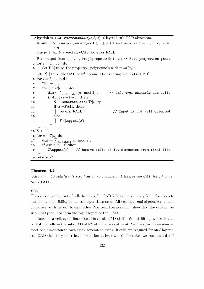
Algorithm 4.3: LayeredSubCAD(ϕ, `,x): `-layered sub-CAD algorithm.

Input : A formula ϕ, an integer 1 ≤ ` ≤ n+ 1 and variables x = x1, . . . xn. ϕ isin x.

Output: An `-layered sub-CAD for ϕ, or FAIL.

1 P← output from applying ProjOp repeatedly to ϕ ; // Full projection phase

2 for i = 1, . . . , n do3 Set P[i] to be the projection polynomials with mvar(xi);

4 Set D[1] to be the CAD of R1 obtained by isolating the roots of P[1];5 for i = 2, . . . , n do6 D[i]← [ ];7 for c ∈ D[i− 1] do8 dim←∑

α∈c.index (α mod 2) ; // Lift over suitable dim cells

9 if dim > i− `− 1 then10 S ← GenerateStack(P[i], c);11 if S =FAIL then12 return FAIL ; // Input is not well oriented

13 else14 D[i].append(S)

15 D ← [ ];16 for c ∈ D[n] do17 dim←∑

α∈c.index (α mod 2);18 if dim > n− ` then19 D.append(c); // Remove cells of low dimension from final lift

20 return D;

Theorem 4.2.

Algorithm 4.3 satisfies its specification (producing an `-layered sub-CAD for ϕ) or re-

turns FAIL.

Proof.

The output being a set of cells from a valid CAD follows immediately from the correct-

ness and compatibility of the sub-algorithms used. All cells are semi-algebraic sets and

cylindrical with respect to each other. We need therefore only show that the cells in the

sub-CAD produced form the top ` layers of the CAD.

Consider a cell, c, of dimension d in a sub-CAD of Ri. Whilst lifting over c, it can

contribute cells in the sub-CAD of Rn of dimension at most d+ n− i (as it can gain at

most one dimension in each stack generation step). If cells are required for an `-layered

sub-CAD then they must have dimension at least n − `. Therefore we can discard c if

122

d ≤ i− `− 1 (line 9).

When performing the final lift we must only build stacks over cells of dimension

n−`−1 or greater, but the sections in those stacks will not have dimension n−`. Hence

we check for this at the end (line 18) only keeping those of the required dimension.

Example 4.2.

Consider again the unit sphere from Example 4.1. A complete CAD contains 25 cells,

and it is simple to compute: a 1-layered sub-CAD with 7 cells; a 2-layered sub-CAD

with 17 cells; and a 3-layered sub-CAD with 23 cells (missing the two 0-cells (0, 0,−1)

and (0, 0, 1)) .

If we also include the plane x + y + z − 1 we can construct a complete CAD with

211 cells. Using Algorithm 4.3 we can construct: a 1-layered sub-CAD with 44 cells; a

2-layered sub-CAD with 135 cells; and a 3-layered sub-CAD with 197 cells.

When a problem consists of only strict inequalities, the cells describing the solutions

must have full-dimension [McC93, Str00]. More generally there are classes of problems

with known solution dimension. In these cases a layered sub-CAD technology will be

beneficial. To give an example, consider the cyclic polynomials:

Example 4.3.

Define the cyclic-n polynomials to be the set of n polynomials in n variables:

x1 + x2 + · · ·+ xn = 0,

x1x2 + x2x3 + · · ·+ xn−1xn + xnx1 = 0,

...

x1x2 · · ·xn−1 + x2x3 · · ·xn + · · ·+ xnx1 · · ·xn−2 = 0,

x1x2 · · ·xn − 1 = 0.

The cyclic-4 polynomials will also be used as a motivating example for the work of

Chapter 6 in Example 6.1.

In [Bac89] it is shown that if there exists an integer m > 0 such that m2|n, then there

are an infinite number of solutions to the cyclic-n polynomials. Further, the solutions

have dimension at least m−1. Therefore a layered sub-CAD containing cells of dimension

(m− 1) and higher would be sufficient to find the largest families of solutions.

Layered sub-CADs will also be useful when, although a sub-CAD may not be ϕ-

sufficient, the application for the sub-CAD only requires general families of solutions.

123

For example, if we apply CAD to robot motion planning (discussed in detail in Chapter

6) we need only identify paths through cells of full-dimension, and so it seems a 1-layered

sub-CAD may be enough. In the example considered in Chapter 6 there is an equational

constraint present and so we need the full-dimensional cells on its variety, which are part

of the 2-layered sub-CAD. Even further, to analyse the adjacency of such paths we may

need the cells of dimension one lower and thus the cells on the variety in a 3-layered

CAD will be the appropriate choice. Such a sub-CAD can be constructed by combining

the ideas of variety and layered sub-CADs, which will be discussed in Section 4.4.

This example highlights that it is not necessarily obvious how many layers are needed

for a sub-CAD when first considering a problem. This prompts an adaptation of Algo-

rithm 4.3 to a recursive procedure.

4.3.2 Recursive Layered sub-CADs

When we construct a layered sub-CAD with Algorithm 4.3 we stop lifting over a cell if

it cannot lead to cells of sufficient dimension in Rn. This only happens when the cell in

question is produced as a section (constructing a sector increases the dimension of a cell

in a stack, unlike a section). Let us refer to such a cell as a terminating section. To

construct a layered sub-CAD recursively (with respect to the number of layers, rather

than the number of variables) we will store these terminating sections in a separate

output variable, rather than discarding them. This will allow them to be used later if

another layer is required.

Consider constructing a 1-layered sub-CAD, D, and let c be a terminating section.

If c is being constructed in Ri then the dimension of c must be i − 1 (that is, c has

co-dimension 1 within Ri). Suppose we now wish to extend this 1-layered sub-CAD into

a 2-layered sub-CAD by use of the terminating sections, which we denote C.If a terminating section c ∈ C is part of Rn then it will have dimension n− 1 and so

can be included in the 2-layered sub-CAD. Otherwise, c has co-dimension 1 in Ri and

we can construct successive stacks over it retaining all sectors and storing sections into a

new set of terminating sections. The sectors produced will be n−1 dimensional cells and

these can be combined with the 1-layered sub-CAD to produce a 2-layered sub-CAD.

The new terminating sections can then be used to produce a 3-layered sub-CAD, and

we can proceed recursively in this manner. This is particularly useful if the number

of layers needed is not known in advance of computation. This method is described in

Algorithm 4.4.

Algorithm 4.4 has been implemented in ProjectionCAD, with further details in Sec-

124

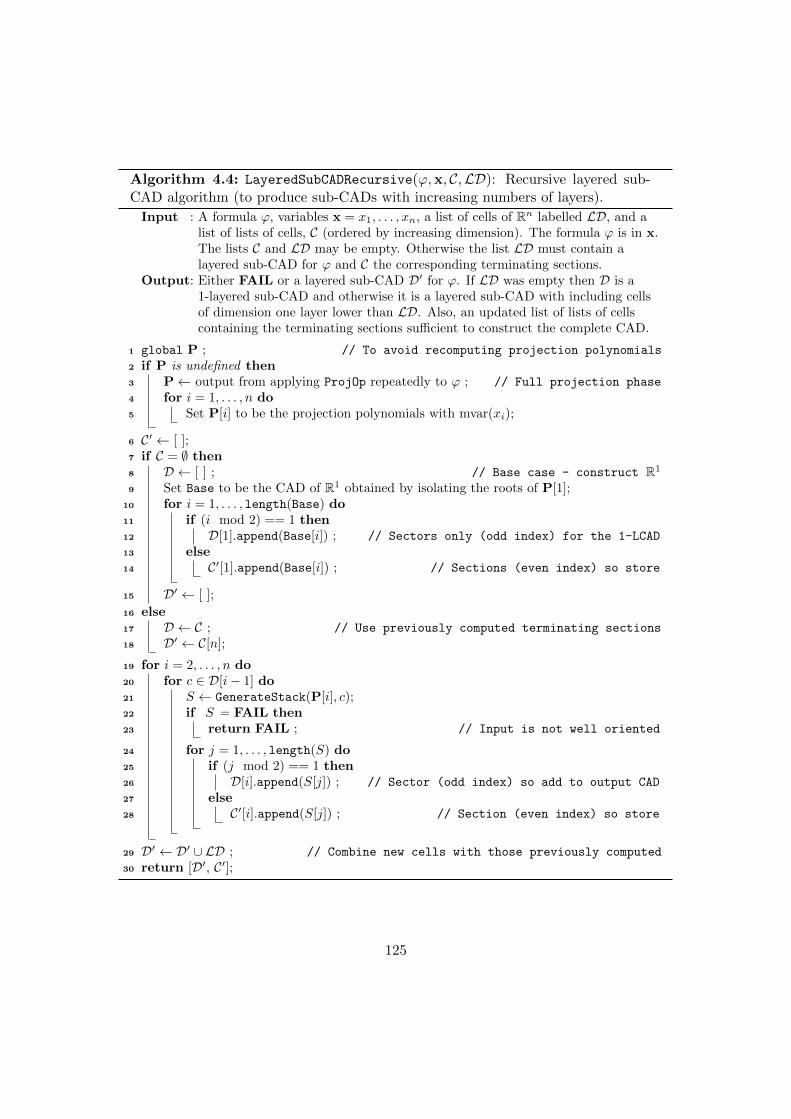
Algorithm 4.4: LayeredSubCADRecursive(ϕ,x, C,LD): Recursive layered sub-CAD algorithm (to produce sub-CADs with increasing numbers of layers).

Input : A formula ϕ, variables x = x1, . . . , xn, a list of cells of Rn labelled LD, and alist of lists of cells, C (ordered by increasing dimension). The formula ϕ is in x.The lists C and LD may be empty. Otherwise the list LD must contain alayered sub-CAD for ϕ and C the corresponding terminating sections.

Output: Either FAIL or a layered sub-CAD D′ for ϕ. If LD was empty then D is a1-layered sub-CAD and otherwise it is a layered sub-CAD with including cellsof dimension one layer lower than LD. Also, an updated list of lists of cellscontaining the terminating sections sufficient to construct the complete CAD.

1 global P ; // To avoid recomputing projection polynomials

2 if P is undefined then3 P← output from applying ProjOp repeatedly to ϕ ; // Full projection phase

4 for i = 1, . . . , n do5 Set P[i] to be the projection polynomials with mvar(xi);

6 C′ ← [ ];7 if C = ∅ then8 D ← [ ] ; // Base case - construct R1

9 Set Base to be the CAD of R1 obtained by isolating the roots of P[1];10 for i = 1, . . . , length(Base) do11 if (i mod 2) == 1 then12 D[1].append(Base[i]) ; // Sectors only (odd index) for the 1-LCAD

13 else14 C′[1].append(Base[i]) ; // Sections (even index) so store

15 D′ ← [ ];

16 else17 D ← C ; // Use previously computed terminating sections

18 D′ ← C[n];

19 for i = 2, . . . , n do20 for c ∈ D[i− 1] do21 S ← GenerateStack(P[i], c);22 if S = FAIL then23 return FAIL ; // Input is not well oriented

24 for j = 1, . . . , length(S) do25 if (j mod 2) == 1 then26 D[i].append(S[j]) ; // Sector (odd index) so add to output CAD

27 else28 C′[i].append(S[j]) ; // Section (even index) so store

29 D′ ← D′ ∪ LD ; // Combine new cells with those previously computed

30 return [D′, C′];

125

tion C.2.

We prove that Algorithm 4.4 is valid.

Theorem 4.3.

Algorithm 4.4 satisfies its specification and produces a layered sub-CAD and list of

terminating sections, or alternatively FAIL.

Proof.

As with Theorem 4.2 the proof of the correctness of Algorithm 4.4 mainly follows from

the specification of the sub-algorithms used. It remains to show that the correct layers

are produced.

If no terminating sections are provided, then a CAD of the real line is produced and

the sectors are separated to be lifted over and Algorithm 4.4 emulates Algorithm 4.3.

Otherwise, the terminating sections are used to lift over. At each stage of lifting, the

sectors are retained and any sections produced are placed in C′. All sectors produced

will have co-dimension one greater than in the previous layered CAD and these sectors,

together with the previous layered sub-CAD LD, form a layered sub-CAD, D′, with one

extra layer. The new terminating sections are returned in C′ and all have co-dimension

one greater than the newly added cells of D′.

Implementing Algorithm 4.4 in ProjectionCAD is not quite as simple as Algorithm

4.3. A global variable is used to avoid recalculation of projection polynomials (which can

be costly if many resultants and discriminants are computed). Rather than outputting

the terminating sections directly, as indicated in Algorithm 4.4, the implementation gives

the output in two parts: the first part is the layered sub-CAD as produced, the second

part is an unevaluated recursive call. This recursive call is rendered inert with Maple’s

unevaluated function call syntax (prefixing the command with %) which allows it to be

assigned to a variable and later evaluated with the value command to produce a layered

sub-CAD with one further layer (along with another inert recursive call). More details

are given in Section C.2.

4.3.3 Order Invariance of Layered sub-CADs

We discuss an interesting property of layered sub-CADs with respect to order-invariance.

We require the following lemma.

Lemma 4.4.

Let f ∈ R[x1, . . . , xn] vanish identically on a cell, D, of dimension n. Then f is

126

identically zero on the whole of Rn.

Proof.

We proceed by induction.

Let n = 1, and D ⊂ R1 an interval. As f vanishes on the whole of D, there exists at

least deg(f) + 1 points αi such that f(αi) = 0 (there are infinitely many such points).

Then by the Fundamental Theorem of Algebra, f must be the zero polynomial.

Now let n > 1. We view f as a univariate polynomial in xn with coefficients in

R[x1, . . . , xn−1]. As D is an n-dimensional cell, it must be in the cylinder of an n − 1-

dimensional cell D′ in Rn−1. Using the Fundamental Theorem of Algebra we can see

that for every point α′ ∈ D′ every coefficient in f vanishes. But by induction, these

coefficients must be zero on the whole of Rn−1 and so f ≡ 0 on all of Rn.

We can use Lemma 4.4 to show that 1-layered and 2-layered sub-CADs are order

invariant.

Theorem 4.5.

Let F ⊂ Z[x1, . . . , xn] and D be a 1-layered or 2-layered sub-CAD of Rn sign-invariant

for F . Then D is order-invariant with respect to F , meaning each polynomial has con-

stant order of vanishing on each cell.

Proof.

Let us first show that a 1-layered sign-invariant sub-CAD is order-invariant. This is

straightforward for if a non-zero polynomial f ∈ F is to have a non-zero order on a cell

it must vanish in that cell and, as D is sign invariant with respect to F , it must vanish

identically on that cell. For a cell D ∈ D this means that f vanishes identically on a cell

of dimension n and so, by Lemma 4.4, f is the zero polynomial.

Applying this result in the 2-layered case we see immediately that each f ∈ F is

order-invariant on all n-dimensional cells in D. Now let D′ be an (n − 1)-dimensional

cell, let xi be the dimension for which it is deficient and assume f ≡ 0 on the whole

of D′, but not identically zero on Rn. We will show that f cannot be identically zero,

and therefore its order is trivially zero. View f as univariate in xi and factor into its

content and primitive part: contxi(f) · primxi(f). Then if f ≡ 0 on D′ then contxi(f)

must be identically zero on D′ (as primxi(f) can only be zero at a finite set of points).

But contxi(f) is a polynomial in n− 1 variables that vanishes on an (n− 1)-dimensional

cell and so, by Lemma 4.4, it must be identically zero on R(n−1). Therefore f ≡ 0 on Rn

127

and we have the desired contradiction.

Order-invariance is a stronger property than sign-invariance, but the extra knowledge

it gives allows for the validated use of smaller projection operators (such as McCallum’s

projection operator in Definition 2.24). Hence this property allows for the avoidance of

well-orientedness checks during stack generation when building 1 or 2-layered sub-CADs.

This means not just a saving in computation time but the avoidance of unnecessary

failure declarations that can sometimes follow from such checks.

4.4 Combining sub-CAD Ideas

We have discussed two types of sub-CAD in this chapter: variety and layered sub-CADs.

They both can offer significant savings in cell count and time, but can also be combined to

create layered variety sub-CADs, which are discussed in Section 4.4.1. It is also possible

to use the idea of sub-CADs with truth table invariance (as introduced in Chapter 3) to

create a wider range of sub-CADs. These are discussed in Section 4.4.2.

4.4.1 Layered Variety sub-CADs

When constructing a sub-CAD of any type, we are filtering out those cells that are

relevant to the problem at hand. Constructing a variety sub-CAD does this in a single

step of the lifting phase (according to an equational constraint), whilst a layered sub-

CAD stratifies the cells throughout the whole lifting process (according to the dimensions

of the cells). These are quite different procedures.

There is no conceptual or theoretical reason why these ideas cannot be combined

to offer the benefit of both types of sub-CAD. We restrict our discussion to the case of

problems with an equational constraint such that all factors of this constraint have main

variable xn and are not nullified on a lower-dimensional cell, and construct the following

definition (analogous to the well-orientedness conditions of Definition 2.26 and 3.6).

Definition 4.5.

Let A be a set of n-variate integral polynomials, where n ≥ 1, and let E ⊆ A be the set

of factors of an equational constraint f , which all have main variable xn. Let D′ be a

CAD or sub-CAD of Rn−1. We say that (A,E) (or the formula ϕ they are constructed

from) are (LV)-well-oriented with respect to D′ if no element of E is nullified on a

cell of D′.

128

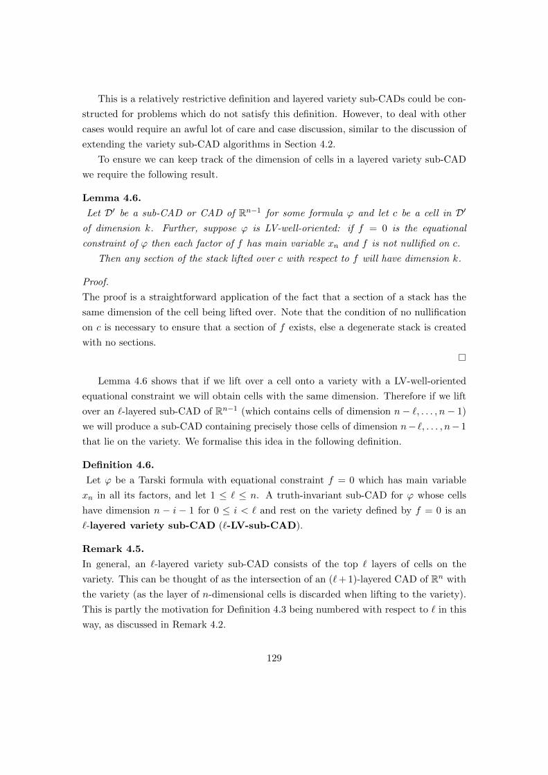
This is a relatively restrictive definition and layered variety sub-CADs could be con-

structed for problems which do not satisfy this definition. However, to deal with other

cases would require an awful lot of care and case discussion, similar to the discussion of

extending the variety sub-CAD algorithms in Section 4.2.

To ensure we can keep track of the dimension of cells in a layered variety sub-CAD

we require the following result.

Lemma 4.6.

Let D′ be a sub-CAD or CAD of Rn−1 for some formula ϕ and let c be a cell in D′of dimension k. Further, suppose ϕ is LV-well-oriented: if f = 0 is the equational

constraint of ϕ then each factor of f has main variable xn and f is not nullified on c.

Then any section of the stack lifted over c with respect to f will have dimension k.

Proof.

The proof is a straightforward application of the fact that a section of a stack has the

same dimension of the cell being lifted over. Note that the condition of no nullification

on c is necessary to ensure that a section of f exists, else a degenerate stack is created

with no sections.

Lemma 4.6 shows that if we lift over a cell onto a variety with a LV-well-oriented

equational constraint we will obtain cells with the same dimension. Therefore if we lift

over an `-layered sub-CAD of Rn−1 (which contains cells of dimension n− `, . . . , n− 1)

we will produce a sub-CAD containing precisely those cells of dimension n− `, . . . , n− 1

that lie on the variety. We formalise this idea in the following definition.

Definition 4.6.

Let ϕ be a Tarski formula with equational constraint f = 0 which has main variable

xn in all its factors, and let 1 ≤ ` ≤ n. A truth-invariant sub-CAD for ϕ whose cells

have dimension n − i − 1 for 0 ≤ i < ` and rest on the variety defined by f = 0 is an

`-layered variety sub-CAD (`-LV-sub-CAD).

Remark 4.5.

In general, an `-layered variety sub-CAD consists of the top ` layers of cells on the

variety. This can be thought of as the intersection of an (`+ 1)-layered CAD of Rn with

the variety (as the layer of n-dimensional cells is discarded when lifting to the variety).

This is partly the motivation for Definition 4.3 being numbered with respect to ` in this

way, as discussed in Remark 4.2.

129

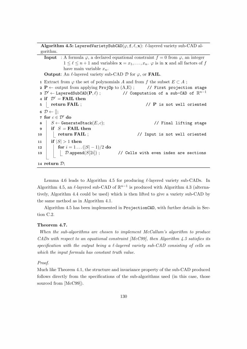
Algorithm 4.5: LayeredVarietySubCAD(ϕ, f, `,x): `-layered variety sub-CAD al-gorithm.

Input : A formula ϕ, a declared equational constraint f = 0 from ϕ, an integer1 ≤ ` ≤ n+ 1 and variables x = x1, . . . , xn. ϕ is in x and all factors of fhave main variable xn.

Output: An `-layered variety sub-CAD D for ϕ, or FAIL.

1 Extract from ϕ the set of polynomials A and from f the subset E ⊂ A ;2 P← output from applying ProjOp to (A,E) ; // First projection stage

3 D′ ← LayeredSubCAD(P, `) ; // Computation of a sub-CAD of Rn−1

4 if D′ = FAIL then5 return FAIL ; // P is not well oriented

6 D ← [];7 for c ∈ D′ do8 S ← GenerateStack(E, c); // Final lifting stage

9 if S = FAIL then10 return FAIL ; // Input is not well oriented

11 if |S| > 1 then12 for i = 1 . . . (|S| − 1)/2 do13 D.append(S[2i]) ; // Cells with even index are sections

14 return D;

Lemma 4.6 leads to Algorithm 4.5 for producing `-layered variety sub-CADs. In

Algorithm 4.5, an `-layered sub-CAD of Rn−1 is produced with Algorithm 4.3 (alterna-

tively, Algorithm 4.4 could be used) which is then lifted to give a variety sub-CAD by

the same method as in Algorithm 4.1.

Algorithm 4.5 has been implemented in ProjectionCAD, with further details in Sec-

tion C.2.

Theorem 4.7.

When the sub-algorithms are chosen to implement McCallum’s algorithm to produce

CADs with respect to an equational constraint [McC99], then Algorithm 4.5 satisfies its

specification with the output being a `-layered variety sub-CAD consisting of cells on

which the input formula has constant truth value.

Proof.

Much like Theorem 4.1, the structure and invariance property of the sub-CAD produced

follows directly from the specifications of the sub-algorithms used (in this case, those

sourced from [McC99]).

130

Theorem 4.2 verifies that D is an `-layered sub-CAD of Rn−1 and Lemma 4.6 con-

cludes that the lifting in the final loop results in an `-layered variety sub-CAD of Rn. If

the conditions of Lemma 4.6 do not hold, then the input is not well-oriented and thus

FAIL is returned in line 10.

Example 4.4.

Consider again the unit sphere from Example 4.1. A complete CAD contains 25 cells,

and we have seen that a variety sub-CAD contains 6 cells and layered sub-CADs contain

7, 17 and 23 cells for one to three layers. Constructing layered variety sub-CADs reduces

these numbers further, with a 1-layered variety sub-CAD containing 2 cells (the open

hemispheres) and the 2-layered variety sub-CAD containing 4 cells.

The effect is amplified if we also include the plane x + y + z − 1. Constructing a

complete CAD creates 211 cells and an equational constraint CAD produces 137 cells.

We have seen that a variety sub-CAD produces 46 cells, and layered sub-CADs produce

44, 135 and 197 cells for one to three layers. Constructing a 1-layered variety sub-CAD

produces 14 two-dimensional cells, and a 2-layered variety sub-CAD produces a total of

36 cells.

4.4.2 Truth Table Invariant sub-CADs

We can combine the idea of a sub-CAD with other CAD techniques. In this section

we shall discuss the interaction of layered and variety sub-CADs with projection and

lifting truth table invariant CADs, which were discussed in Chapter 3 and introduced in

[BDE+13, BDE+14].

Recall the definition of a TTICAD, given in Definition 3.2:

Definition 4.7.

Let Φ := ϕiti=1 be a list of quantifier-free (Tarski) formulae. We say a cylindrical

algebraic decomposition D is truth table invariant (a TTICAD), or more specifically

Φ-truth table invariant, if the Boolean value of each ϕi is constant (either true or

false) on each cell in D.

Sections 4.2 and 4.3 were generally concerned with sign-invariance (and order-invar-

iance where needed for theoretical justification of the McCallum projection operator).

However, the theory transfers easily to truth table invariance, and we can create truth

table invariant cylindrical algebraic sub-decompositions (sub-TTICADs).

131

Assume we have an application concerning Φ = ϕiti=1, where all the ϕi have their

own equational constraint. Then there exists a variety on which the solutions rest,

defined by the product of the individual equational constraints (the implicit equational

constraint for the problem). As with Section 4.2, for simplicity, we assume that each

equational constraint has factors which all have main variable xn. We can then define a

variety sub-TTICAD.

Definition 4.8.

Let Φ := ϕiti=1 be a list of quantifier free formulae with each ϕi having equational

constraint fi whose factors all have main variable xn. A sub-CAD of a TTICAD for

Φ containing all cells resting on the variety defined by∏ti=1 fi = 0 is called a variety

sub-TTICAD (V-sub-TTICAD).

Algorithm 4.1 can then be used for Φ with the implicit equational constraint (the

product of the individual equational constraints) being used for f . In this case ProjOp

should be the TTICAD projection operator defined in Definition 3.4 which is applied to

Φ. The GenerateStack procedure called on line 9 of Algorithm 4.1 should also check

for the TTICAD well-orientedness condition given in Definition 3.6.

It is straightforward to give a proof analogous to that of Theorem 4.1, which shows

that such an algorithm would provide a variety sub-TTICAD. Note that although the

variety considered is the same as if we had constructed a sub-CAD using just the implicit

equational constraint, the TTICAD theory allows for a simpler (n−1)-dimensional CAD,

which offers further savings when lifted to the variety.

We can also create an `-layered sub-TTICAD

Definition 4.9.

Let Φ := ϕiti=1 be a list of quantifier free formulae and let 1 ≤ ` ≤ n+ 1. A sub-CAD

of a TTICAD for Φ containing all cells of dimension n − i for 0 ≤ i < ` is called an

`-layered sub-TTICAD (`-L-sub-TTICAD).

To construct such a sub-CAD we can use either Algorithm 4.3 or Algorithm 4.4 by

using the TTICAD projection operator and a GenerateStack algorithm which checks

for the TTICAD well-orientedness condition of Definition 3.6 (as with constructing a

variety sub-TTICAD). Again, the validity follows an analogous proof to the sub-CAD

algorithm, in this case Theorems 4.2 and 4.3.

Finally, we can combine TTICAD theory with the idea in Section 4.4.1 to produce

a layered variety sub-TTICAD, as specified in the following definition.

132

Definition 4.10.

Let Φ := ϕiti=1 be a list of quantifier free formulae with each ϕi having equational

constraint fi whose factors all have main variable xn. Let 1 ≤ ` ≤ n. A sub-CAD

of a TTICAD for Φ containing all cells of dimension n − 1 − i for 0 ≤ i < ` resting

on the variety defined by∏ti=1 fi = 0 is called a `-layered variety sub-TTICAD

(`-LV-sub-TTICAD).

Remark 4.6.

As with `-layered variety sub-CADs (Definition 4.6), an `-layered variety sub-TTICAD

consists of the top ` layers of cells on the variety (in this case defined by∏ti=1 fi = 0).

This can be thought of as the intersection of an (`+ 1)-layered sub-CAD of Rn with the

variety (with the n-dimensional cells being discarded when lifting to the variety).

Constructing a layered variety sub-TTICAD can be done using Algorithm 4.5 with

the sub-algorithms (for projection and stack generation) being those needed for TTICAD

theory. The correctness follows, again, analogously to that of layered variety sub-CADs

which was given in Theorem 4.7 (relying on the sub-TTICAD versions of Theorems 4.1,

4.2 and 4.3). The exceptional case when part of the variety is nullified on a cell will be

identified by the TTICAD algorithms and will therefore produce FAIL.

All three algorithms described in this section (to produce variety sub-TTICADs,

layered sub-TTICADs, and layered variety sub-TTICADs) have been implemented in

the ProjectionCAD package, which is discussed further in Section C.2.

4.5 Complexity of Variety sub-CADs

In this section we extend the work of Collins ([Col75]) and McCallum ([McC93]) regard-

ing complexity of CAD algorithms. We give a complexity analysis of the algorithms

to compute sign-invariant variety sub-CADs (Algorithm 4.1) and 1-layered variety sub-

CADs (Algorithm 4.5) in the specific case where the equational constraint has all factors

with main variable xn.

We need to consider three parts of the complexity for the sub-CADs:

Projection The complexity of the equational constraint projection set needs to be

analysed. In particular the number of polynomials, the maximum degree and size

of their coefficients.

Calculation of (n− 1) dimension CAD/sub-CAD These values then can be used

to estimate the complexity of the (n− 1)–dimensional CAD or sub-CAD.

133

Lifting Finally the complexity of the lifting stage can be combined with the previous

step to describe the complexity of the variety sub-CADs.

We first standardise some notation for a CAD with respect to a set of polynomials A

(with equational constraint set E ⊆ A): let n be the number of variables, m the number

of polynomials in A, d the maximum degree in any variable of the polynomials in A, and

l the maximum norm length of the polynomials in A (where the norm length, |f |1, is

the sum of the absolute values of the integer coefficients of a polynomial).

Let A1 := A and let Ai+1 := Proj(Ai). In general the projection operator used

will be clear: most of the following is with respect to Collins’ projection operator CP

(Definition 2.22) and, therefore, is a ‘worst case scenario’ compared to the improved

operators of McCallum MP (Definition 2.24) and Brown BMP (Definition 2.27), which

are both subsets of the Collins operator. Let mk be the number of polynomials in Ak,

dk the maximum degree of Ak, and lk the maximum norm length.

4.5.1 Collins’ algorithm

In [Col75], Collins works through his original CAD algorithm in great detail to analyse

the complexity, and this methodology is followed in [McC93] when discussing the 1-

layered CAD algorithm. We recall some key results, noting they could all be uniformly

improved with ideas from papers such as [Bur13, Dav85] but the aim of this section

is not to achieve tighter complexity bounds for existing algorithms, but rather to give

complexity bounds for sub-CADs in the context of existing results.

In the projection stage the properties of the projection sets can be bound as follows:

mk ≤ (2d)3km2k−1; dk ≤

1

2(2d)2k−1

; lk ≤ (2d)2k l.

By combining these bounds Collins shows the projection phase is dominated by

(2d)3n+1m2n l2.

The base case and lifting algorithm requires the isolation of real roots of univariate

polynomials. Collins bounds this procedure as follows. Let A be a set of univariate

polynomials with degree bounded by d and norm length bounded by l. Then for a given

f ∈ A with d := deg(f) and l := |f |1 a lower bound on the distance between two roots

is given by1

2

(√ed

32 l)−d

. (4.1)

134

Collins uses his analysis of Heindel’s algorithm for real root isolation to show that iso-

lating the roots is dominated by

d8 + d7 l3. (4.2)

Therefore the number of operations needed to isolate all roots in A, with m := |A|, is

dominated by:

md8 +md7l3. (4.3)

For a given h, refining a root interval to 2−h is dominated by d2h3 + d2l2h. Collins

multiplies all polynomials in A and uses (4.1) to show that all roots are separated by:

δ :=1

2

(√e(md)

32 lm)−md

.

If we take h to be log(δ) we can refine all intervals of the polynomials in

md(d2(m2dl +md log(md))3 +md3l3) = O(m7d7l3 +m2d4l3).

Combining this with (4.3) tells us that the necessary refinement of intervals for all the

polynomials is dominated by

md8 +m7d7l3. (4.4)

Remark 4.7.

Whilst discussing this work for publication in [BDE+14] the authors noted that the

analysis to obtain (4.4) can be improved using recent advances in root isolation.

In [Dav85] it was noted that it is unnecessary to consider the product of all polyno-

mials when computing δ, two polynomials will suffice. Therefore δ becomes:

δ :=1

2

(√e(2d)

32 l2)−2d

.

As we take h to be log(δ) this now becomes 2d(2l+ log d) (which is O(dl)). Substituting

into the interval separation bound gives md6l3 + md4l3. We see this is dominated by

(4.3) and so (4.3) dominates the overall complexity:

md8 +md7l3. (4.5)

In [Bur13] the author states that (4.2) can be improved to O(d4l2). We therefore

have (4.3) bounded by O(md4l2) and we can combine this with the reasoning in [Dav85]

135

to obtain an overall bound of:

md4l2 +md(d5l3 + d3l3) = O(md6l3). (4.6)

We can also apply [Bur13] to the product of all polynomials in A to immediately

isolate all roots. This gives a better estimate for (4.4):

(md)4(mdl)2 = m6d6l2. (4.7)

Using any of (4.5), (4.6), and (4.7) in Collins’ analysis will filter through to the

overall complexity, reducing the exponents produced. This would not provide any great

new insight into the algorithms and so we do not go into details here. The subsequent

work continues to follow Collins’ original reasoning.

Combining (4.4) with the size of the full projection set concludes the base phase is

dominated by

(2d)3n+3m2n+2

l3.

We now need to consider the polynomials involved in the lifting stage. This involves

looking at the univariate polynomials created after substituting sample points, along

with the polynomials required to define the algebraic extensions of Q that those sample

points are contained in.

We follow the work in [Col75, McC93] by using primitive elements to calculate the

costs of operations, even though these are unlikely to be used by implementations. For

each sample point β = (β1, . . . , βk) ∈ Rk there is a real algebraic number α ∈ R such that

Q(β1, . . . , βk) = Q(α). Let fα be the polynomial in Q[x] that, along with an isolating

interval Iα, defines α (so f(α) = 0). Let d∗k be the maximum degree of these fα, and

l∗k the maximum norm length. Each coordinate βi is represented in Q(α) by another

polynomial. Let l′k be the maximum norm length of these polynomials. Then

d∗k ≤ (2d)22n−1, and l∗k, l

′k ≤ (2d2)22n+3

m2n+1l.

Let uk be the number of univariate polynomials (after substitution) and ck the number

of cells at level k. Then

uk, ck ≤ 22nn∏i=1

midi, and uk, ck ≤ (2d)3n+1m2n . (4.8)

136

Collins combines all these results to give a complexity bound for the full algorithm of

(2d)4n+4m2n+6

l3. (4.9)

4.5.2 McCallum’s Cadmd algorithm

In [McC93], McCallum introduces his Cadmd algorithm which constructs a 1-layered

sub-CAD (which he refers to as a CAD of maximal dimension) in the same manner as

Algorithm 4.3 with ` = 1. Using the same methodology as [Col75], he gives a complexity

bound for the Cadmd algorithm. As constructing a 1-layered CAD avoids using algebraic

numbers (all cells are direct products of intervals so sample points can be produced

directly in Q) the exponents in the complexity are lower than in (4.9). The complexity

is dominated by:

(2d)3n+4m2n+4

l3. (4.10)

4.5.3 Analysis of MPE(A) and (n− 1)-dimensional CADs

We need to consider properties of the projection set to consider the complexity of the

sub-CADs produced: the size, maximum degree and maximum norm length. Let E ⊆ Abe the subset of A containing the factors of the designated equational constraint (for

which the variety sub-CAD will be construct with respect to). Define the following

parameters:

mA := |A|, mE := |E|, mA\E := |A \ E|.

Let dA, dE , dA\E be the maximum degrees of the relevant sets, and let lA, lE , lA\E be

the maximum norm length of each set.

We are constructing a sub-CAD with respect to an equational constraint so we use

the projection operator MPE(A) defined by McCallum (Definition 2.32 and originally

given in [McC99]). Recall that the definition of MPE(A) is:

MPE(A) := MP(E) ∪ resxn(f, g) | f ∈ E, g ∈ A \ E

where MP(E) is the McCallum projection operator defined in [McC85, McC98] (Defini-

tion 2.24) which gives the coefficients, discriminants and cross resultants of E. We will

denote the resultant set, MPE(A) \MP(E), by ResSetE(A).

We can bound the size of MP(E) by the sum of the sizes of its components: the

number of coefficients (bounded by mEdE), the number of discriminants (bounded by

mE), and the number of resultants (bounded by(mE

2

)= mE(mE−1)

2 ). Note that in

137

practice a fraction of these elements will be trivial with respect to constructing a CAD

(either 0 or a constant) hence we can only use these numbers as bounds. Combining

these bounds gives:

|MPE(A)| ≤ mEdE +mE +mE(mE − 1)

2+mEmA\E

=mE

2

(2dE + 2mA\E +mE − 1

)=mE

2

(2dE +mA\E +mA − 1

). (4.11)

The maximum degree of MPE(A) is the greater of the maximum degrees of MP(E)

and the resultant set. We also have the following standard bound [VZGG13, Thm 6.22]

on the degree of a resultant with respect to x (where f, g ∈ K[x, y]):

deg(resx(f, g)) ≤ (degx f + degx g) · (max(degy f,degy g)).

Using our overall degree bounds gives

max deg(ResSetE(A)) ≤ (dE + dA\E) ·max(dE , dA\E)

= max(d2E + dEdA\E , d

2A\E + dEdA\E)

≤ max(2d2E , 2d

2A\E). (4.12)

We also have

max deg(MP(E)) ≤ max(dE , 2d2E , 2d

2E) = 2d2

E . (4.13)

Combining (4.12) and (4.13) gives a degree bound for MPE(A):

max deg(MPE(A)) ≤ max(2d2E , 2d

2A\E) ≤ d2

A. (4.14)

Finally, if we denote the maximum norm length of MPE(A) by l, then we know l ≤ l2

(since MPE(A) ⊆ MP(A) ⊆ CP(A)) and so

l ≤ l2 ≤ (2dA)22lA = 16d4

AlA. (4.15)

Substituting these bounds ((4.11), (4.14) and (4.15)) into (4.9) gives an estimate on

the complexity of a complete (n − 1)-dimensional MPE(A)-invariant Collins CAD. We

138

see the complexity is dominated by

≤(2 · 2d2

A

)22(n−1)+8(mE(2dE +mA +mA\E − 1)

2

)2n−1+6 (16d4

AlA)3

≤ 163(4d2

A

)22n+6(mE(2dE + 2mA − 1)

2

)2n+5

l3Ad12A . (4.16)

Similarly, the complexity of a 1-layered (n− 1)-dimensional MPE(A)-invariant sub-

CAD can be considered by substituting into (4.10). We see that the complexity of such

a sub-CAD is dominated by

≤(2 · 2d2

A

)3n−1+4(mE(2dE +mA +mA\E − 1)

2

)2n−1+4 (16d4

AlA)3

≤ 163(4d2

A

)3n+3(mE(2dE + 2mA − 1)

2

)2n+3

l3Ad12A . (4.17)

4.5.4 Overall complexities for variety sub-CADs

We have so far computed bounds for the complexities of the (n− 1)-dimensional CADs

and sub-CADs produced in Algorithm 4.1 (line 4) and Algorithm 4.5 (line 3).

We now need to consider the final step of lifting over these cells with respect to the

factors of the equational constraint. We can use (4.8) to bound the number of univariate

polynomials so know from (4.4) that the isolations will be dominated by:

(2dE)3n+1

m2n

E d8E +

((2dE)3n+1

m2n

E

)7d7El

3E . (4.18)

Remark 4.8.

We could also use the improvements of (4.5), (4.6), and (4.7) in this final lifting stage

but for the sake of consistency use (4.4).

We now have the components needed to describe the overall complexities of con-

structing a variety sub-CAD and 1-layered variety sub-CAD. We can combine (4.18)

with (4.16) and (4.17) to obtain a single bound for each. Note that (4.18) will be a large

overestimation for the 1-layered case.

Theorem 4.8.

The complexity for computing a variety sub-CAD with Algorithm 4.1 using MPE(A) and

139

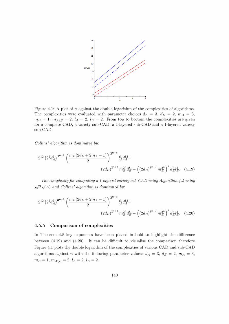
Figure 4.1: A plot of n against the double logarithm of the complexities of algorithms.The complexities were evaluated with parameter choices dA = 3, dE = 2, mA = 3,mE = 1, mA\E = 2, lA = 2, lE = 2. From top to bottom the complexities are givenfor a complete CAD, a variety sub-CAD, a 1-layered sub-CAD and a 1-layered varietysub-CAD.

Collins’ algorithm is dominated by:

212(22d2

A

)4n+3(mE(2dE + 2mA − 1)

2

)2n+5

l3Ad12A +

(2dE)3n+1

m2n

E d8E +

((2dE)3n+1

m2n

E

)7d7El

3E . (4.19)

The complexity for computing a 1-layered variety sub-CAD using Algorithm 4.5 using

MPE(A) and Collins’ algorithm is dominated by:

212(22d2

A

)3n+3(mE(2dE + 2mA − 1)

2

)2n+3

l3Ad12A +

(2dE)3n+1

m2n

E d8E +

((2dE)3n+1

m2n

E

)7d7El

3E . (4.20)

4.5.5 Comparison of complexities

In Theorem 4.8 key exponents have been placed in bold to highlight the difference

between (4.19) and (4.20). It can be difficult to visualise the comparison therefore

Figure 4.1 plots the double logarithm of the complexities of various CAD and sub-CAD

algorithms against n with the following parameter values: dA = 3, dE = 2, mA = 3,

mE = 1, mA\E = 2, lA = 2, lE = 2.

140

Figure 4.1 shows, from top to bottom:

• Collins’ complexity for a complete CAD (4.9);

• McCallum’s complexity for a 1-layered CAD (4.10);

• Theorem 4.8 complexity for a variety sub-CAD (4.19);

• Theorem 4.8 complexity for a 1-layered variety sub-CAD (4.20).

Figure 4.1 shows clearly the drop in the constant in the exponents of (4.19) and (4.20),

whilst the scaling factor of the exponent remains the same between variety and non-

variety versions of each algorithm.

4.6 Examples and Experimentation

We now discuss some experimental results that demonstrate the benefit of the new

sub-CAD algorithms. Algorithms 4.1, 4.2, 4.3, 4.5, and the respective algorithms for

sub-TTICADs have all been implemented in the ProjectionCAD package for Maple

(further details are given in Section C.2 and [Eng13a, Eng13b, WE13]).

We compare these with competing CAD implementations. We use the two CAD

procedures implemented in the RegularChains library for Maple: computing CADs

directly ([CMXY09] and described in Section 2.5.2) and incrementally ([CM12] and

described in Section 2.5.3) using regular chains technology. We use Qepcad both with

its default settings (which implements McCallum’s algorithm from [McC85, McC98] and

described in Algorithm 2.4) and also using equational constraint technology whenever

appropriate (using the theory from [McC99] described in Section 2.32). Finally, we use

the algorithms available in Mathematica, which produce cylindrical algebraic formulae

rather than CADs.

It is worth noting that Qepcad offers an option measure-zero-error which will

produce a CAD for which only the full-dimensional cells of the free variable space are

guaranteed to satisfy the specified invariance condition (normally truth invariance of

the input formula). The output of Qepcad is always a CAD, but this option clearly

has parallels with sub-CAD theory, namely 1-layered sub-CADs. More specifically, if

we only retain those cells for which the invariance condition is guaranteed to be correct

then we would have a 1-layered sub-CAD, and therefore all solutions up to an error set

of measure zero, in the free-variable space.

For the experiments below this command cannot be used: we consider unquanti-

fied formulae (so the free variable space is n-dimensional) and each has an equational

141

constraint. Therefore the specified formulae can only be satisfied on cells with dimen-

sion strictly less than n. If we use the measure-zero-error option with Qepcad then

the only cells guaranteed to be correct have dimension n and are therefore not of in-

terest. When we construct a 1-layered variety sub-CAD (using the implementation of

ProjectionCAD) we do obtain solutions: here the layer is with respect to the variety,

and not free variable space. Therefore a 1-layered variety sub-CAD provides solutions

correct up to an error set of measure zero in the solution space.

The following experiments were run on the same configuration as the rest of this

thesis: a Linux desktop (3.1GHz Intel processor, 8.0Gb total memory). The Mathe-

matica used was Version 9 and Qepcad-B 1.69 was used with the options +N500000000

and +L200000 (initialisation times are included in all results and are generally around 2

seconds). The development version of Maple is used in command line interface, using

the development version of the RegularChains Library.

4.6.1 Example: Making use of a 1-layered variety sub-CAD

We work through an example to show the benefit of a 1-layered variety sub-CAD.

Example 4.5.

Assume variable ordering x y z and consider the following formula which was

created using 3 random polynomials of degree 2 (generated using Maple’s randpoly

function) which are plotted in Figure 4.2:

Φ := −50xy + 56yz + 41z2 + 67x− 55y − 21 = 0

∧ 36xy + 76xz − 58yz + 69z2 + 75y + 27 > 0

∧ −55x2 + 10xy − 88x+ 80y + z − 39 > 0.

For a given problem we may wish to describe the regions of R3 in which Φ is satis-

fied. Figure 4.2 shows there are multiple intersections between the two non-equational

constraints away from the variety defined by the equational constraint (shown in red).

This suggests that a variety sub-CAD would be beneficial over a complete CAD. We can

obtain further savings if only generic solutions are required by constructing a 1-layered

variety sub-CAD.

We attempt to solve the given problem with a variety of theories to show the relative

benefits of each. We compute:

• a complete sign-invariant CAD for the three polynomials in Φ using McCallum’s

projection operator (CADFull: Algorithm 2.4);

142

Figure 4.2: Intersection of the three surfaces from Section 4.6.1. The red surface is theequational constraint.

Technique Cells Time

CADFull 17047 178.277ECCAD 1315 11.520V-sub-CAD 422 10.7232-LV-sub-CAD 348 7.1491-LV-sub-CAD 138 0.475

RC-Rec-CAD 9841 112.460RC-Inc-CAD 559 1.999Qepcad 17047 385.679EC-Qepcad 5271 26.614Mathematica — 0.533

Table 4.1: Constructing sub-CADs and CADs for Φ with various algorithms.

• an equational constraint CAD (ECCAD: McCallum’s theory of equational constraints

[McC99]);

• a variety sub-CAD (V-sub-CAD: Algorithm 4.1 using sub-procedures following

McCallum’s theory of equational constraints in [McC99]);

• layered variety sub-CADs (LV-sub-CAD: Algorithm 4.5 using sub-procedures fol-

lowing McCallum’s theory of equational constraints in [McC99]).

The cell counts and timings to compute such CADs and sub-CADs with Projection-

CAD are given in the first half of Table 4.1.

It is clear that utilising the equational constraint dramatically reduces computation

143

time and the number of cells produced. Restricting to a variety sub-CAD increases

this cell saving further, which will lead to even more significant time savings on any

subsequent work using the cells of the sub-CAD. The variety sub-CAD describes all

solutions to Φ, but we can also use the 1-layered variety sub-CAD to describe the generic

solutions in a much quicker time (any valid cells not in this sub-CAD will have measure

zero in the solution space). Therefore in this case, an output of 17,047 cells can be

replaced with only 138 cells. If we need to describe the other solutions then a 2-layered

variety sub-CAD or complete variety sub-CAD will only produce 348 and 422 cells

respectively.

We compare these computation times and cell counts with the current state-of-the-art

implementations of CAD algorithms, which are given in the second half of Table 4.1. As

with the algorithms from ProjectionCAD, we see that taking advantage of equational

constraints (in the incremental CAD of RegularChains, RC-Inc-CAD, and Qepcad,

EC-Qepcad) offers a large cell saving and significant reduction in speed. Comparatively,

Qepcad performs worse here than the other implementations both in terms of time

and, when using equational constraints, cell count. This is perhaps due to the fact

Qepcad does not implement the improved lifting offered by equational constraint theory

(described in Remark 3.1 and implemented in ProjectionCAD).

In both of the CADs produced by Qepcad, Φ is valid only a small fraction of the cells

produced. For the sign-invariant CAD only 290 cells from the 17,047 cells produced are

valid (1.7%) and for the equational constraint CAD 106 cells are valid from the 5271 cells

produced (2.0%). Such a large volume of false cells that are unnecessarily constructed

(and on which the polynomials in Φ are evaluated) explains the larger computation

times.

To offer a comparison, we can very quickly evaluate Φ on the cells of the 1-layered

variety sub-CAD. Of the 138 cells produced, we see that 36 of them describe solutions

to Φ (26.1%). Without a full implementation of evaluating polynomials at algebraic

sample points described by nested RootOf constructs we cannot accurately determine

the fraction of valid cells for the remaining sub-CADs.

As noted in all our experimentation, Mathematica produces cylindrical formulae

rather than CAD cells and so a direct comparison is difficult. Obviously the speed at

which Mathematica computes a cylindrical formula for Φ is impressive, but we cannot

infer any general behaviour from it.

Remark 4.9.

Qepcad allows for the measure-zero-error option to be used for Φ along with declaring

144

the equational constraint. Enabling both options allows Qepcad to produce a CAD in

under 5 seconds with 822 cells. However, as the solution space of Φ is at most (n− 1)-

dimensional, none of the full dimensional cells satisfy Φ and so Qepcad returns an

equivalent quantifier free formula of False.

In general we could consider a problem of the form f = 0 ∧ Ψ(gi) where f = 0

defines a variety of real co-dimension 1 and Ψ is a quantifier-free formula involving only

f = 0 and strict inequalities in the gi. Then a 1-layered variety sub-CAD will, in most

cases, be sufficient to describe the generic solutions for the given problem. There will

need to be checks for nullification, and there may be no solutions of full dimension on

the variety, in which case the recursive approach for layered sub-CADs can be used

to incrementally build successive layers until a solution is found (or the entire variety

sub-CAD is constructed and no solutions are possible).

4.6.2 Example: Making use of 1-layered variety sub-TTICAD

We now demonstrate the strength of sub-TTICADs with another example.

Example 4.6.

Consider the following quantifier free formulae:

ϕ1 := x2 + y2 + z2 = 1 ∧ xy + yz + zx < 1 ∧ x3 − y3 − z3 < 0;

ϕ2 := (x− 1)2 + (y − 1)2 + (z − 1)2 = 1 ∧ (x− 1)(y − 1) + (y − 1)(z − 1)

+ (z − 1)(x− 1) < 1 ∧ (x− 1)3 − (y − 1)3 − (z − 1)3 < 0.

The surfaces of ϕ1 are shown in Figure 4.3a, with the equational constraint indicated in

red (the surfaces of ϕ2 are the same but translated by the vector (1, 1, 1)).

We assume the variable ordering x y z and construct the following formula, Φ,

defining regions of R3:

Φ := ϕ1 ∨ ϕ2.

This problem is deceptively difficult to tackle directly with a sign-invariant CAD for

Φ: running the default CAD algorithm in Maple 16 (recursive regular chains CAD

as described in [CMXY09]) overnight fails to produce any output, and Qepcad hits a

memory constraint (“prime list exhausted”) after two hours of computation.

We can make some use of the equational constraints of ϕ1 and ϕ2. In Qepcad we can

declare the implicit equational constraint (the product of the two spheres) which takes

35, 304 seconds (about 10 hours) to produce a CAD with 6, 165 cells. Mathematica can

145

(a) Intersection of the surfaces from ϕ1. (b) Intersection of the surfaces from Φ∗.

Figure 4.3: Intersection of the surfaces from ϕ1 and Φ∗ in Example 4.6. The spheresdefined by the equational constraints are shown in red.

produce a relevant cylindrical formula in 1.805 seconds but it is not possible to inspect

the number of cells constructed.

Clearly Φ is well-suited for TTICAD and so we can use the implementation in

ProjectionCAD. Doing so produces 4, 861 cells in 170.515 seconds: a lower cell count

than Qepcad is obtained due to the improved TTICAD projection operator and im-

proved lifting (discussed in Section 3.2.1 and Remark 3.1).

We now consider how to obtain a more efficient output using the sub-TTICAD theory

discussed in Section 4.4.2. Both ϕ1 and ϕ2 contain an equational constraint and so any

region where Φ is valid must lie on the variety defined by the product of the equational

constraints. If we only require generic solutions then we can construct a 1-layered variety

sub-TTICAD for this variety.

To start, we project ϕ1 and ϕ2 with respect to the TTICAD projection operator

(Definition 3.4) and use these projection polynomials to construct a 1-layered sub-CAD

of R2: 249 cells are produced in 0.947 seconds. We then lift using both equational

constraints retaining only those cells on the variety, taking a further 1.191 seconds and

producing 528 2-dimensional cells on the 2-dimensional variety in R3. The 1-layered

variety sub-TTICAD therefore reduced the number of cells by 88% and construction

time by 99% compared to a full TTICAD, producing those generic solutions of two

dimensions (as ϕ1 and ϕ2 contain strict inequalities alongside the equational constraints

it is likely that there will be relatively few solution regions of smaller dimension). If

we require solutions of lower dimension then we can construct a 2-layered variety sub-

TTICAD with 1, 514 cells in 47.629 seconds.

146

If we require all solutions then we can construct a variety sub-TTICAD which will

produce 1, 976 cells in 178.196 seconds. A variety sub-TTICAD therefore takes approx-

imately the same time to compute as a full TTICAD but gives a substantial cell saving

of 59% fewer cells (indicating that over half the cells in the complete TTICAD do not

lie on either of the varieties defined by the equational constraints).

We can include a third formula (another shift of ϕ1 but with respect to (−1,−1,−1)):

ϕ3 := (x+ 1)2 + (y + 1)2 + (z + 1)2 = 1 ∧ (x+ 1)(y + 1) + (y + 1)(z + 1)

+ (z + 1)(x+ 1) < 1 ∧ (x+ 1)3 − (y + 1)3 − (z + 1)3 < 0,

and combine it with Φ to produce a new formula:

Φ∗ := ϕ1 ∨ ϕ2 ∨ ϕ3.

The nine surfaces of Φ∗ are shown in Figure 4.3b, with the spheres, which are the

equational constraints, shown in red.

It is impractical to attempt to build a CAD for Φ∗ without using equational con-

straints (as the CAD will be strictly finer than a sign-invariant CAD for Φ, which was

shown to be infeasible). Although the problem is significantly more complicated, con-

structing a 1-layered variety sub-TTICAD takes only 5.003 seconds and produces 1, 104

cells. A 2-layered variety sub-TTICAD produces 3, 166 cells in 145.898 seconds; a va-

riety sub-TTICAD produces 4, 130 cells in 429.083 seconds. By comparison a complete

TTICAD takes about the same time as a variety sub-TTICAD (432.210 seconds) but

produces over double the cells (10, 063 cells).

4.7 Extensions to the Theory

Variety and layered sub-CADs are not the only possible ways to construct a sub-CAD,

and in Section 4.1.1 a variety of related work in the literature was discussed. We now

discuss a variety of ways the theory of sub-CADs could be extended.

4.7.1 Restricted Lifting Over Simple Inequalities

Often a CAD problem sourced from a real world example will contain many simple

inequalities. This is primarily as we rarely want a variable to range over the entirety of

the reals, but rather an interval.

147

Algorithm 4.6: BasicSimpleInequalitysubCAD(F, vars): Basic simple inequali-ties sub-CAD algorithm.

Input : A formula Φ, a set of variables vars = x1, . . . , xn.Output: A sub-CAD with respect to the inequalities in the variable of R1.

1 E← EqConst(Φ); I← IneqConst(Φ); // Separate inequalities

2 P← ProjOp(Φ, vars);3 D1 ← SplitR(P[n]);4 I ← ;5 for f ∈ E ∪ I do6 I.append(InferIneq(f, x1)); // Obtain inequalities in x1

7 I ′ ← combine(I); // Combine and simplify inequalities

8 D′1 ← refine(D1, I); // Restrict according to inequalities

9 D ← lift(P, vars,D1); // Continue lifting phase

10 return D;

There are multiple extensions to CAD theory (such as equational constraints or

TTICAD) that concentrate on utilising the power of equational constraints, and the

idea behind variety sub-CADs is also centred around this, but relatively little research

into using these simple inequalities directly. They will certainly be used within partial

CAD [CH91] and the authors of SyNRAC have commented on their use within formula

simplification [YA04]. We now describe an idea to extend how inequalities are used in

partial CAD to produce sub-CADs.

In [McC97] (which will be discussed further in Section 6.3) the author considers

a problem that is infeasible when tackled directly with CAD. To make the problem

feasible, the author derives a simple inequality for the variable, r, which decomposes

R1. As the formula involves the equational constraint r2 + s2 = −1 the author notes

that −1 ≤ r ≤ 1 must hold. Manually selecting those cells that satisfy this inequality,

the author lifts only over that region, producing a sub-CAD of R4 (which is a complete

CAD of [0, 1]× R3).

This can easily be incorporated into a general algorithm, as shown in Algorithm 4.6.

Example 4.7.

We consider a simple example to show the power of utilising simple inequalities in the

lifting stage. Consider the following formula:

[[x2 + y2 + z2 ∗ 1] ∧ [x > 0] ∧ [y > 0] ∧ [z > 0]

], ∗ ∈ =, 6=, <,>,≤,≥.

This will define a property of the positive octant of the unit sphere. Were we to construct

148

a full CAD using McCallum’s projection operator for x2 +y2 +z2−1, x, y, z, we would

construct 135 cells.

Using the basic inequality sub-CAD algorithm described in Algorithm 4.6 constructs

51 cells. At the base-CAD level the only cells retained are 0 < x < 1, x = 1, x > 1. The

following liftings have the savings:

• 1-D sub-CAD: 7 cells are reduced to 3 cells;

• 2-D sub-CAD: 33 cells are reduced to 13 cells;

• 3-D sub-CAD: 135 cells are reduced to 51 cells.

Constructing a partial CAD would have the 51 cells of the basic inequality sub-

CAD, along with four trivial cells: [x = 0]×R2, [−1 < x < 0]×R2, [x = −1]×R2, and

[x < −1] × R2. These may get simplified with post-processing [Bro98] although there

will always be at least 1 extra cell (as a partial CAD is still a complete decomposition

of Rn).

Ideally, we would want to incorporate simple inequalities into every level of cells:

when lifting from Rk−1 to Rk, only retain cells which satisfy the simple inequalities that

can be inferred from the input formula. Often every variable will be considered on a

restricted domain, and so the savings could be substantial.

If the only inequalities considered are truly trivial (of the form xk < α or xk ≤ α for

α ∈ R, or preferably α ∈ Q) then this should be possible at all levels. The endpoints

will be explicitly identified (for an inequality xk < α, the polynomial xk −α will appear

in the projection set) and therefore when lifting over a cell from Rk−1 there will be a

cell with xk = α (both in the cell representation and sample point). The stack can

then be restricted appropriately in relation to this cell. This process should be relatively

inexpensive and could offer large savings. Care needs to be taken when there are nested

algebraic numbers, as demonstrated in the issues of implementing quantifier elimination

via CAD.

We demonstrate how such an algorithm could offer large savings over both a general

CAD algorithm, and a partial CAD implementation.

Example 4.8.

Consider again the formula:

[[x2 + y2 + z2 ∗ 1] ∧ [x > 0] ∧ [y > 0] ∧ [z > 0]

], ∗ ∈ =, 6=, <,>,≤,≥.

149

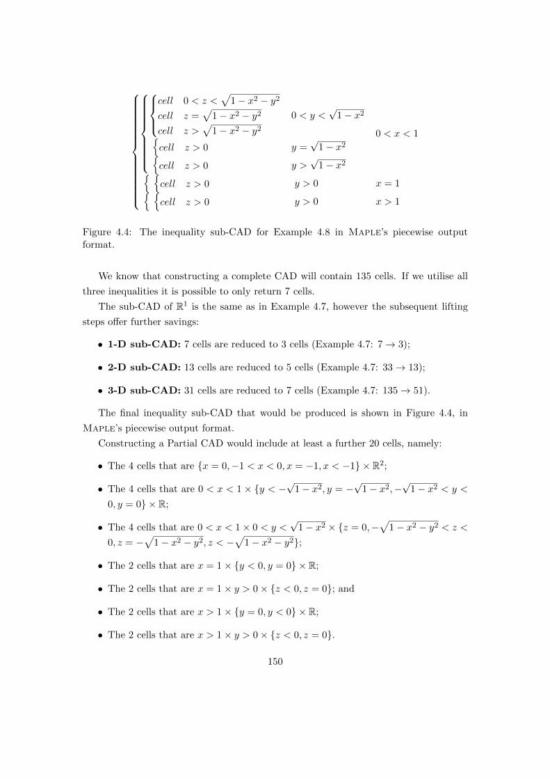
cell 0 < z <

√1− x2 − y2

cell z =√

1− x2 − y2

cell z >√

1− x2 − y2

0 < y <√

1− x2

cell z > 0 y =

√1− x2

cell z > 0 y >√

1− x2

0 < x < 1

cell z > 0 y > 0 x = 1 cell z > 0 y > 0 x > 1

Figure 4.4: The inequality sub-CAD for Example 4.8 in Maple’s piecewise outputformat.

We know that constructing a complete CAD will contain 135 cells. If we utilise all

three inequalities it is possible to only return 7 cells.

The sub-CAD of R1 is the same as in Example 4.7, however the subsequent lifting

steps offer further savings:

• 1-D sub-CAD: 7 cells are reduced to 3 cells (Example 4.7: 7→ 3);

• 2-D sub-CAD: 13 cells are reduced to 5 cells (Example 4.7: 33→ 13);

• 3-D sub-CAD: 31 cells are reduced to 7 cells (Example 4.7: 135→ 51).

The final inequality sub-CAD that would be produced is shown in Figure 4.4, in

Maple’s piecewise output format.

Constructing a Partial CAD would include at least a further 20 cells, namely:

• The 4 cells that are x = 0,−1 < x < 0, x = −1, x < −1 × R2;

• The 4 cells that are 0 < x < 1× y < −√

1− x2, y = −√

1− x2,−√

1− x2 < y <

0, y = 0 × R;

• The 4 cells that are 0 < x < 1× 0 < y <√

1− x2 × z = 0,−√

1− x2 − y2 < z <

0, z = −√

1− x2 − y2, z < −√

1− x2 − y2;

• The 2 cells that are x = 1× y < 0, y = 0 × R;

• The 2 cells that are x = 1× y > 0× z < 0, z = 0; and

• The 2 cells that are x > 1× y = 0, y < 0 × R;

• The 2 cells that are x > 1× y > 0× z < 0, z = 0.

150

To this end, an inequality sub-CAD offers direct savings over a partial CAD.

There is a chance that identification of algebraic numbers involved in non-trivial

inequalities (for example nested algebraic numbers) could prove costly to identify the

valid regions defined by inequalities. However we can construct a 1-layered inequality

sub-CAD with little effort as all sample points involved can be chosen in Q.

Along with 1-layered sub-CADs, we could combine inequality sub-CADs with various

other ideas from sub-CADs in obvious ways. For example, if the sphere in Example

4.8 was an equational constraint, then producing a variety inequality sub-CAD would

restrict the output shown in Figure 4.4 to the single cell defining the surface of the

strictly positive octant of the sphere.

Ideally we would wish to incorporate these simple inequalities into the projection

stage as well as the lifting stage. Work on generic projection in partial CAD [SS03]

appeals to assumptions in the parameters of the input to simplify projection and could

hopefully be combined with this lifting process. There is also scope for simpler well-

orientedness conditions: a projection operator may fail a well-orientedness condition

outside of the domain and so the output is still correct.

Without a full implementation we cannot run any significant experimentation, but

it seems clear that inequality sub-CADs could provide substantial savings in cells and

timing.

4.7.2 Further Extensions

There are a many other possible ways to extend the sub-CAD work and we list a few

possibilities.

When detailing algorithms for layered and variety sub-CADs, certain restrictions on

permissible inputs are imposed. It would obviously be advantageous to extend the ap-

plication of these algorithms to treat equational constraints of low level or that define

varieties with co-dimension greater than 1. The restriction of layered variety sub-CADs

to LV-well-oriented (Definition 4.5) input is to avoid cases, such as the Whitney Um-

brella, where lifting to the variety increases dimension (and so Lemma 4.6 does not hold).

Taking care of this degeneracy would increase the power of this algorithm.

Along with a selection of sub-CADs, examples have also been given of where they

may be applicable. Identifying general classes of problems where a given sub-CAD is

sufficient will extend the benefit of the theory and offer more practical uses for sub-CAD.

Section 4.1.1 gave a collection of existing CAD techniques (such as partial CAD)

that can be adapted to construct sub-CADs, and these should be investigated.

151

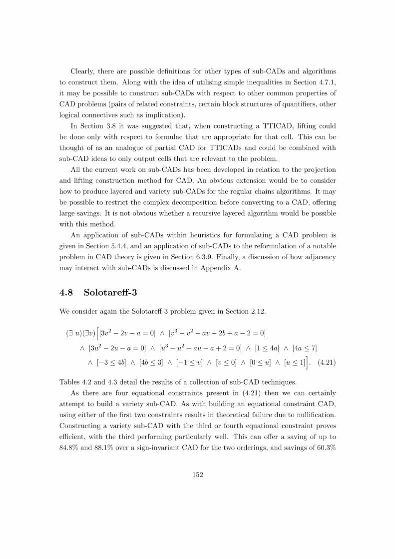
Clearly, there are possible definitions for other types of sub-CADs and algorithms

to construct them. Along with the idea of utilising simple inequalities in Section 4.7.1,

it may be possible to construct sub-CADs with respect to other common properties of

CAD problems (pairs of related constraints, certain block structures of quantifiers, other

logical connectives such as implication).

In Section 3.8 it was suggested that, when constructing a TTICAD, lifting could

be done only with respect to formulae that are appropriate for that cell. This can be

thought of as an analogue of partial CAD for TTICADs and could be combined with

sub-CAD ideas to only output cells that are relevant to the problem.

All the current work on sub-CADs has been developed in relation to the projection

and lifting construction method for CAD. An obvious extension would be to consider

how to produce layered and variety sub-CADs for the regular chains algorithms. It may

be possible to restrict the complex decomposition before converting to a CAD, offering

large savings. It is not obvious whether a recursive layered algorithm would be possible

with this method.

An application of sub-CADs within heuristics for formulating a CAD problem is

given in Section 5.4.4, and an application of sub-CADs to the reformulation of a notable

problem in CAD theory is given in Section 6.3.9. Finally, a discussion of how adjacency

may interact with sub-CADs is discussed in Appendix A.

4.8 Solotareff-3

We consider again the Solotareff-3 problem given in Section 2.12.

(∃ u)(∃v)[[3v2 − 2v − a = 0] ∧ [v3 − v2 − av − 2b+ a− 2 = 0]

∧ [3u2 − 2u− a = 0] ∧ [u3 − u2 − au− a+ 2 = 0] ∧ [1 ≤ 4a] ∧ [4a ≤ 7]

∧ [−3 ≤ 4b] ∧ [4b ≤ 3] ∧ [−1 ≤ v] ∧ [v ≤ 0] ∧ [0 ≤ u] ∧ [u ≤ 1]]. (4.21)

Tables 4.2 and 4.3 detail the results of a collection of sub-CAD techniques.

As there are four equational constraints present in (4.21) then we can certainly

attempt to build a variety sub-CAD. As with building an equational constraint CAD,

using either of the first two constraints results in theoretical failure due to nullification.

Constructing a variety sub-CAD with the third or fourth equational constraint proves

efficient, with the third performing particularly well. This can offer a saving of up to

84.8% and 88.1% over a sign-invariant CAD for the two orderings, and savings of 60.3%

152

Technique Cells Time Section Page

PL-CAD (Col) 54037 255.304 2.3 30PL-CAD (McC) 54037 266.334 2.3 30EC-CAD (f3) 20593 65.856 2.4.4 40EC-CAD (f4) 22109 102.781 2.4.4 40

V-CAD (f3) 8195 63.387 4.2 114V-CAD (f4) 8953 95.233 4.2 114

1-L-CAD 5012 5.944 4.3 1192-L-CAD 21426 133.245 4.3 1193-L-CAD 41333 318.657 4.3 1194-L-CAD 51947 354.313 4.3 1195-L-CAD 54037 428.707 4.3 119

1-LV-CAD (f3) 1372 3.222 4.4 1282-LV-CAD (f3) 4754 43.265 4.4 1283-LV-CAD (f3) 7480 92.708 4.4 1284-LV-CAD (f3) 8195 113.340 4.4 1281-LV-CAD (f4) 1522 4.347 4.4 1282-LV-CAD (f4) 5229 72.075 4.4 1283-LV-CAD (f4) 8185 136.119 4.4 1284-LV-CAD (f4) 8953 157.836 4.4 128

Table 4.2: The Solotareff-3 problem with sub-CAD techniques — variable order a ≺ b ≺v ≺ u.

and 60.5% over an equational constraint CAD. Any of the variety sub-CADs are sufficient

to solve the problem.

As there is only a a single solution to the problem, a layered sub-CAD is not ap-

propriate to solve the problem. At most, a 4-layered sub-CAD could be used to show

that there is a finite number of possible solutions. However, to demonstrate the power

of the sub-CAD theory we compute all possible layered sub-CADs. We can see that

computing a 1-layered sub-CAD is very efficient, due to the lack of algebraic numbers,

and produces a proportionally small amount of cells. It is interesting to note that the

size of the 1-layered sub-CADs suggest that a ≺ b ≺ v ≺ u is the optimal order (which

is indeed the case) and this will be investigated as a general heuristic in Section 5.4.

We can also construct layered variety sub-CADs which offer further substantial sav-

ings. We can only construct four layers, as the variety is of co-dimension 1, and each

level produces a cell saving over the layered sub-CAD. A 1-layered variety sub-CAD of-

fers the largest cell savings, 97.5% and 98.1% for the two variable orderings, along with

savings of 98.8% and 99.3% in construction time compared to the complete CADs.

Finally, we note that in the presence of simple inequalities for every variable, the

work discussed in Section 4.7.1 should be applicable, at least in the base variable when

153

Technique Cells Time Section Page

PL-CAD (Col) 161317 916.105 2.3 30PL-CAD (McC) 154527 857.357 2.3 30EC-CAD (f3) 48475 175.139 2.4.4 40EC-CAD (f4) 63583 324.663 2.4.4 40

V-CAD (f3) 19127 173.083 4.2 114V-CAD (f4) 25563 295.556 4.2 114

1-L-CAD 13716 17.868 4.3 1192-L-CAD 59598 516.734 4.3 1193-L-CAD 116924 1689.886 4.3 1194-L-CAD 148205 2925.458 4.3 1195-L-CAD 154527 4876.479 4.3 119

1-LV-CAD (f3) 3040 6.153 4.4 1282-LV-CAD (f3) 10808 76.251 4.4 1283-LV-CAD (f3) 17332 155.035 4.4 1284-LV-CAD (f3) 19127 178.588 4.4 1281-LV-CAD (f4) 4132 9.043 4.4 1282-LV-CAD (f4) 14560 139.543 4.4 1283-LV-CAD (f4) 23211 282.426 4.4 1284-LV-CAD (f4) 25563 322.241 4.4 128

Table 4.3: The Solotareff-3 problem with sub-CAD techniques — variable order b ≺ a ≺v ≺ u.

decomposing R1.

4.9 Conclusion

In this chapter we introduced and formalised the idea of a cylindrical algebraic sub-

decomposition (sub-CAD), which is a subset of a CAD. Highlighting related ideas in

the literature, it is clear that a sub-CAD is of great use in many applications of CAD

technology to a given problem. Two new sub-CADs were introduced: variety sub-

CADs and layered sub-CADs. Algorithms were given for both types of sub-CAD, and

a recursive algorithm for layered sub-CADs was also provided. All algorithms were

proven correct and examples given to demonstrate their effectiveness. It was discussed

how these can be combined to form layered variety sub-CADs, and how these concepts

interact with the TTICAD theory of Chapter 3 to form sub-TTICADs.

Complexity analysis of variety sub-CADs and 1-layered variety sub-CADs showed

the formal benefit of the new theory, and this was supported by experimental results

indicating where sub-CADs offer startling improvements in efficiency. Finally, extensions

of the sub-CAD theory were proposed.

154

Chapter 5

Formulating Problems for CAD

Before constructing a CAD, many decisions have to be made to formulate a problem

into a suitable form. One of these factors that has been studied is the effect of vari-

able ordering in the complexity of CAD [BD07, DSS04] but other factors include the

separation of sub-formulae and choice of equational constraints.

It is possible to use various heuristics to make informed choices for these factors in

formulation. We evaluate the use of existing heuristics and introduce new metrics and

heuristics. We present promising results for using machine learning to decide the best

variable ordering for a problem, and planned research will extend this to other decisions.

We also use ideas from Chapter 4 to inspire a new heuristic.

Author’s Contribution and Publication

The work in Section 5.2 was collaborative work with the rest of the Bath research group:

the author was involved in all discussions and experimentation, but the new heuristic

(ndrr) was invented by another researcher. The work in Section 5.3 was collaborative

with a research group at the University of Cambridge: the author began the collaboration

with Huang and, together, designed the experiments and feature list. The author helped

prepare the experiment, which was conducted by Huang, and discussed the results. The

work in Section 5.4 is the author’s.

The work from Section 5.2 has been published in [BDEW13, EBC+14, EBDW14].

The work in Section 5.3 will be published in [HEW+14b, HEW+14a]. The work in

Section 5.4 was initially discussed in the technical report [WE13] and has been submitted

to [WEBD14].

155

5.1 Issues when Formulating a Problem for CAD

Given a problem for which we wish to construct a CAD there are a number of choices

that are necessary to make before a CAD algorithm can be used. When provided with

either a Boolean formula (which may or may not be quantified) or a set of polynomials

(which may or may not be given with equational conditions), we refer to the process of

creating a complete input for a CAD algorithm as the formulation of the problem.

When formulating a problem the choices that need to be made vary depending on

which algorithm is to be used. These choices may include:

• variable ordering: for any CAD algorithm a variable ordering must be chosen

(that is compatible with any quantification);

• equational constraint designation: for any CAD algorithm involving equa-

tional constraints, there may be a choice of which to designate;

• formulae decomposition: for TTICAD algorithms there may be a choice of

ways to decompose the formula into sub-formulae;

• input ordering: for incremental algorithms, there may be a choice of the order

of input.

Previous work [DSS04, Bro04, BD07] has looked at the effect of variable ordering on

the complexity of the CAD constructed, and suggested various heuristics (discussed in

Section 2.6.3). Little has been discussed in literature regarding the other decisions needed

to formulate a problem for CAD (although presumably CAD users have developed their

own intuition for these choices) and this chapter discusses methods for deciding these.

5.2 Heuristics for Formulation

We now discuss each of the points raised in Section 5.1, identifying metrics and heuristics

that can be used to help make a near-optimal choice.

Due to the nature of the work, this section will be necessarily experimental and

speculative. All the following work was presented and published in [BDEW13, EBC+14,

EBDW14]. The author was involved in the discussions and experimentation for the

paper; however the new heuristics were created by another member of the research

group. Therefore we give only a survey of the results.

156

5.2.1 Variable Ordering

Section 2.6.3 discussed the work of [DSS04] and [Bro04] in developing heuristics for

selecting a variable ordering for a given CAD problem. In particular, they suggest the

following two heuristics:

• Sum of Total Degree [DSS04] For each variable ordering compute the full

projection set, then select the ordering that produces the production set with

smallest sotd (the sum of total degrees of all monomials in the set). The

variable order can also be selected greedily by projecting once and minimising

sotd, then repeating for all projection steps.

• Brown Heuristic [Bro04] decides variable ordering with following criteria (break-

ing ties with successive criteria):

1. Project the variable with the lowest overall degree in the input;

2. Project the variable with the lowest maximum total degree of all monomials

in which it occurs;

3. Project the variable with the smallest number of monomials in the input

which contain the variable.

If there is still a tie after utilising all three criteria then a decision is made lexico-

graphically1.

Both Brown’s heuristic and sotd can be deceived by problems with intricate complex

geometry that does not translate into Rn [BDEW13]. To try and encapsulate the real

geometry of the problem (which is what influences the CAD) we define a new metric:

ndrr.

Definition 5.1 ([BDEW13]).

Let F be a set of polynomials. For a given variable ordering x we compute the full

projection set (with respect to a given ordering) and define the number of distinct

real roots metric, denoted ndrr, to be the number of distinct real roots of univariate

projection polynomials.

This metric is designed to capture the complexity of the one-dimensional CAD, which

has a bearing on the complexity of the complete CAD. The associated heuristic is to

choose the variable ordering with the minimal ndrr value.

1The lexicographic choice is made with respect to the system being used: Maple and Qepcad willbehave differently due to their respective variable ordering conventions.

157

It was demonstrated in [BDEW13], that ndrr can cope with problems that trick

the alternative heuristics, but can also be deceived itself (such as deciding the positive

semidefiniteness of the general quartic).

There are some very clear detriments to using ndrr as a heuristic. The cost of

computing ndrr can be great and is equivalent to constructing the base CAD of R1.

In his complexity analysis of CAD ([Col75], discussed in Section 4.5), Collins states

that using Heindel’s algorithm real root isolation can be of the order d8 + d7l3 for a

single polynomial with degree d and norm length l. Considering the potential increase

in degree and number of polynomials through the projection operator, the complexity of

constructing a one-dimensional CAD using Collins’ operator for a set of m polynomials

in n variables with degree d and max norm length l is given in [Col75] as:

(2d)3n+3m2n+2

l3.

Although the use of improved projection operators will simplify this slightly, the base

case will always remain doubly exponential (as demonstrated in [Dav86]).

In [DSS04] the authors avoided computing sotd for all n! variable orderings by

considering a greedy algorithm, where the next projection variable was chosen by doing

a single projection with respect to all valid variables and computing sotd of the partial

projection set. This reduces the number of individual projection computations from

(n−1) ·n! to n(n+1)/2. There is no obvious way to adapt ndrr into a greedy algorithm

and so all variable orderings need to be projected fully to make a comparison of the

orderings.

As ndrr has both strong benefits and shortcomings, [BDEW13] suggests its use

alongside sotd (or another heuristic) by either using one heuristic to break ties or by

taking a weighted combination of the two metrics. Due to the relative costliness of

ndrr and the historical precedent of sotd, it seems prudent to use sotd as the primary

heuristic, breaking ties with ndrr. Using this combination of sotd and ndrr would

correctly identify the optimal variable ordering for the deceptive examples mentioned

above.

Coupled Variables

In [Phi11] it was noted that sotd and Brown can struggle to distinguish between variables

that are the real and imaginary parts of a complex variable, which we call coupled

variables. When analysing complex formulae with CAD, it is necessary to describe the

branch cuts of the formula in real space and, by construction, coupled variables become

158

hard to distinguish from degree alone. However, the ordering of couple variables can be

important, and ndrr can be used to distinguish these as shown in the following example.

5.2.2 Equational Constraint Designation

Assuming that a variable ordering has been chosen, to formulate a problem for CAD

utilising equational constraints by projection and lifting requires the identification of

a single equational constraint to project with respect to. We call such an equational

constraint, the designated equational constraint for the problem.

The choice of which equational constraint to designate can have a substantial effect on

the complexity of the resulting CAD. We are restricting our projection to when polyno-

mials interact with the variety defined by the equational constraint, so we would ideally

like to select the equational constraint that interacts least with the other polynomials.

The metrics sotd and ndrr were used to try and measure this interaction. The

metrics S and N were defined to be the sotd and ndrr, respectively, of the appropri-

ate full projection set: the equational constraint projection set, MPE(A), followed by

applications of the McCallum projection operator, MP.

Remark 5.1.

It is not possible to apply Brown’s heuristic directly to equational constraint designa-

tion. It would be interesting to do further investigation on whether the heuristic can

be adapted to this problem: the underlying ideas of minimising degrees of polynomials,

degrees of monomials, and number of monomials could be transferred onto different sets

of polynomials derived from the equational constraint.

The results from [BDEW13] demonstrated S and N are useful, but that it is not

simple to select an optimal equational constraint designation. In all examples but one

the optimal designation with respect to cell count and time is a designation with the

lowest value of S and N. However, there are examples where S or N struggle individually.

The results demonstrated that selecting an optimal equational constraint to designate

is important. In particular, they illustrated that the choice can not only provide cell

savings but also affect the validity of the equational constraint projection operator. The

S and N heuristics do a fair job of predicting good designation, although both can be

tricked (see [BDEW13, Example 5]). This is an area where further research could provide

new heuristics.

Remark 5.2.

The issue of equational constraint designation is not present when using the Regular

159

Chains incremental CAD. It is possible to utilise all equational constraints when con-

structing a CAD (see, for example, Table 6.9 in Section 6.2.8) and so designation is not

necessary.

5.2.3 Formulation for TTICAD

When using the projection and lifting TTICAD algorithms from Chapter 3, the input

needs to be a list of quantifier-free formulae.

As in Section 5.2.2, if any of these formulae have more than one equational constraint

then one needs to be designated for use with the projection operator. This decision can

be assisted with the use of the metrics sotd and ndrr by constructing the full projection

sets with each possible combinations of designated equational constraints and selecting

the designations that minimise the metrics.

It is also possible, in certain cases, to decompose Φ into sub-formulae in different

ways. For example, a formula can be separated into subformulae, or formulae with

the same equational constraint can be combined. This can also have an effect on the

complexity of the CAD [BDEW13].

Unfortunately sotd and ndrr are not completely accurate in predicting an optimal

decomposition [BDEW13]. This is unsurprising as the splitting of formulae can be very

subtle. It is not clear whether sotd or ndrr is the most appropriate so a hybrid approach

is sensible.

Splitting or joining of formulae consisting of pure conjunctions is straightforward. If

two formulae are connected by a disjunction then it is possible to join them if they share

an equational constraint (which would become the designated equational constraint in

the new formula). For example [f = 0 ∧ g > 0] ∨ [f = 0 ∧ h > 0] can be joined to

become [f = 0 ∧ [g > 0 ∨ h > 0]]. It is clear from the TTICAD projection operator that

such a joining would not affect the TTICAD construction and so is not an issue within

formulation.

The number of potential ways to decompose a formula Φ and designate equational

constraints soon becomes combinatorially huge. Therefore it was proposed in [BDEW13]

to formulate a problem Φ in the following manner, treating each subformulae in turn:

1. Put the formula into disjunctive normal form:∨i ϕi so that each ϕi is a conjunction

of atomic formulae.

2. For each ϕi let mi be the number of equational constraints:

160

• If mi = 0: then there is no choice for designation (and Algorithm 3.2 will

need to be used to accommodate this).

• If mi = 1: then the sole equational constraint should be designated.

• If mi > 1: then we consider all possible partitions of the formula ϕi into sub-

formulae with at least one equational constraint in each, and all the different

equational constraint designations within those subformulae with more than

one. Choose the partition which minimises a chosen metric (sotd or ndrr).

3. Let Φ be the list of the new formulae and use this for input to the TTICAD

algorithm.

This will not always provide the optimal formulationand will depend on the choice

of metric used. However, it provides a practical and implementable way to formulate a

problem for TTICAD.

5.2.4 Incremental Algorithms

The formulation ideas for projection and lifting CAD algorithms do not automatically

apply to regular chains algorithm, and the incremental algorithms have their own choices.

In [EBC+14] it is first noted that it is sensible to process equational constraints first,

and all equational constraints within a single formula together. This is both logical

and practical: the constraints offer greater benefit by being considered before any non-

equational constraints, and by considering all the equational constraints in a formula

before considering the next formula we can avoid unnecessary identification of shared

roots.

It was then shown that whilst the incremental regular chains TTICAD algorithm

can make use of all equational constraints in each formula, the order the equational

constraints are considered can make a difference to the efficiency. Further, the order the

formulae are considered is also important.

The reason for this difference is due to the incremental construction of the complex

cylindrical tree (whilst maintaining the regular chain structure). It is important to

understand this behaviour and develop a heuristic to make an optimal choices. To do

this the following proposition and definition were given with respect to the RC-TTICAD

algorithm.

Proposition 5.1 ([EBC+14]).

The output of RC-TTICAD is always sign-invariant with respect to the discriminant of the

first equational constraint in each formula.

161

The output of RC-TTICAD is always sign-invariant with respect to the cross-resultants

of the first equational constraints in each formula.

Definition 5.2 ([EBC+14]).

For a given constraint ordering 0, let P be the set of equational constraints which are or-

dered first in each formula. Define the constraint ordering set, C0 as the discriminants

and cross resultants in the main variable of the ordering.

C0 :=

⋃p∈Pdiscxn(p)

∪ ⋃p,q∈Pp 6=q

resxn(p, q)

.

Comparing the sotd of the constraint ordering sets proves ineffective, whilst their

total degree proves to be more effective at distinguishing an optimal ordering. This is

unsurprising considering that the latter concerns the complex geometry of the problem

(which is featured in the complex cylindrical tree of an regular chains TTICAD) whilst

the former encodes the sparseness of the polynomials (which is more important when

using a projection operator). This prompts the following heuristic.

Definition 5.3 ([EBC+14]).

Define the EC ordering heuristic as selecting the first equational constraint to be

processed in each formula such the corresponding constraint ordering set has lowest sum

of degrees of the polynomials within (all taken in the second variable of the ordering).

Utilising the EC ordering heuristic (breaking ties with either sotd or ndrr) proves

effective at ordering equational constraints within each formula, but cannot help decide

the order to consider each formula.

It is best to place a formula with only a single equational constraint first (or indeed

a formula with no equational constraints). After which we use the following heuristic.

Definition 5.4 ([EBC+14]).

Define the CCD size heuristic as selecting a constraint ordering by constructing the

complex cylindrical decomposition for each, extracting the set of polynomials used in

each tree, and choosing the one to refine to a CAD whose set has the lowest sum of

degree of the polynomial within (each taken in the main variable of that polynomial).

This combines with the EC ordering heuristic to form a hybrid heuristic.

Definition 5.5 ([EBC+14]).

Define the constraint ordering heuristic as using the EC ordering heuristic to suggest

162

the best subset of constraint orderings and then having the CCD size heuristic to pick

from these, splitting any further ties by picking lexicographically.

Through systematic testing of the three heuristics (on 100 randomly constructed

examples) it is shown that the CCD size heuristic generally performs better than the

EC ordering heuristic at picking the smallest TTICAD, but does so at a much greater

cost. This is to be expected, but the degree of correlation of the CCD size heuristic

proves that the complex and real decompositions are very closely linked.

The hybrid constraint ordering heuristic offers significantly more savings than the EC

ordering heuristics and takes significantly less time than the CCD size heuristic. This

therefore seems to be a good multi-purpose approach: using the EC ordering heuristic

if the speed of the heuristic is a priority or the CCD size heuristic if a low cell count is

of a priority.

It is also noted in [EBC+14] that two formulation issues with projection and lifting

TTICAD do not apply to regular chains. It is not necessary to designate a single

equational constraint (although selecting an order for the equational constraints is a

similar choice) as the incremental algorithm can utilise all constraints in the formulae.

The sophistication of the incremental regular chains TTICAD also renders the option

to decompose formulae further, as detailed in Section 5.2.3, obsolete: decomposing a

formula into extraneous sub-formulae will always give a higher cell count with regular

chains TTICAD.

In [EBDW14] the issue of selecting a variable ordering was considered with respect

to the regular chains TTICAD algorithm. Along with Brown’s heuristic, sotd, and

ndrr, the heuristic used in the RegularChains heuristic command SuggestVariable-

Order (which is used for all their decomposition commands, including Cylindrical-

AlgebraicDecompose).

Definition 5.6 (RegularChains[SuggestVariableOrder]).

The triangular heuristic uses the following list of criteria to decide the variable order,

breaking ties with successive criteria:

1. Let v[1] = max(deg(f, v) | f ∈ P) and let x ≺ y if x[1] > y[1].

2. Let v[2] = max(tdeg(init(f, v)) | f ∈ P (containing v)) and let x ≺ y if x[2] >

y[2].

3. Let v[3] =∑

f∈P deg(f, v) and let x ≺ y if x[3] > y[3].

163

Note that the first step is identical to the Brown heuristic and the second step

is similar (the Brown heuristic considers the maximal total degree of any monomial

containing v, not just the leading coefficients).

To evaluate the performance of the heuristics, six categories of random examples

were considered with varying numbers of equational constraints. Of the four original

heuristics, sotd offers the greatest cell savings but the cost of this heuristic means that

the Brown heuristic is the most time efficient. Hybrid heuristics combining sotd and

ndrr are more effective, but Brown is still more efficient with respect to overall time.

Applying sotd and ndrr to the TTICAD projection set offers larger savings in both cell

count and overall time, even though RC-TTICAD does not involve projection.

Finally, a new heuristic is given, based on the constraint ordering set (Definition 5.2).

This offers near-maximal cell savings along with the greatest net time savings.

5.3 Applying Machine Learning to CAD

Whilst both relatively modern advances in computer science, there has been little inter-

action between symbolic computation and machine learning. This is, perhaps, due to it

being difficult to find an appropriate question for machine learning to consider, and the

additional restriction that this question has to be accompanied by a large enough data

bank of feasible problems for it to work on. Working in collaboration with researchers

at the University of Cambridge this appears to be the first published work on an appli-

cation of machine learning to problem formulation for computer algebra (although there

have been recent applications to automated theorem proving [HP13]).

The work in this section follows [HEW+14b]. The initial collaboration was between

the author and Zongyan Huang of the University of Cambridge, and once a potential ap-

plication of machine learning within CAD was identified the two research groups started

a formal collaboration. The experiments were designed by the author, Huang, and Eng-

land; the experiments were conducted by Huang, with assistance from the author and

England in providing scripts to format the examples, compute the features in Maple,

and construct the CADs in Qepcad; the results were analysed and discussed by both

research groups.

We will apply machine learning to the problem of choosing variable ordering for a

CAD problem. It is not appropriate to choose a variable ordering directly with machine

learning, for reasons discussed later in this section, and so we instead choose a heuristic

with machine learning (which then selects a variable ordering).

164

5.3.1 Background on Machine Learning

We first give a brief description of machine learning and the particular technique used:

support vector machines. This is given in further detail in [HEW+14b].

Machine learning encompasses programs that can take a collection of data and infer

rules that can then be used to classify or optimise the treatment of further data. There

are many machine learning techniques and algorithms available, and we will consider

a recent invention: the support vector machine (SVM) [STV04]. This a machine

learning technique well-suited to efficiently deal with high-dimensional data and can

cope with diverse sources of data.

To use an SVM a vector of features must be created for each piece of data. The idea

is to then use the vectors of the training data to compute a hyperplane that can be used

to predict the classification of new data based on their feature vector. An SVM can use

a kernel function to map data into a kernel-defined feature space and computes inner

products between all pairs of data vectors. This avoids the computation of coordinates

of data and is generally cheaper than explicit computation.

Once a SVM has been initialised there are two stages: learning and classifying. In

the learning phase the model parameters are set based on the training data, parameter

choices, and the kernel function. The classification stage then constructs a hyperplane

of co-dimension 1 in the feature space according to the model, which divides the space

into two distinct classes. A new feature vector can then be classified with respect to

this hyperplane with the distance to the hyperplane representing the confidence in the

prediction.

Previous Work

Recently [HP13] the research group at Cambridge have looked at applying machine

learning techniques to decision procedures for the theory of real closed fields. Using the

SVMs they consider choosing the most efficient real closed fields decision procedure for

the MetiTarski software [AP08] choosing between Z3, Mathematica and Qepcad.

With a data set of 825 problems, 418 were used as a learning set. A further 213

problems were used to validate and decide kernel options. This left 194 problems to

test the effectiveness of the machine learning technique. The efficiency was measured

by considering the number of problems proven by MetiTarski with a given decision

procedure. The results are:

• Z3: 160 problems proven;

165

• Mathematica: 153 problems proven;

• Qepcad: 158 problems proven;

• Machine Learning: 163 problems proven.

It can be seen that using the Machine Learning techniques is beneficial. As a benchmark,

choosing the best decision procedure would prove 172 out of the 194 test problems, giving

SVM as a 94.7% optimal choice.

Although a small data set, this proves that machine learning can be useful in the

theory of real closed fields and motivates our investigation into its application to CAD.

5.3.2 Design of Experiment

We have seen that variable ordering is a key choice in formulating a CAD problem

and can prove the difference between a doubly exponential or constant number of cells

[BD07]. Unfortunately we cannot apply machine learning to directly select an optimal

variable ordering for a problem. In essence, a SVM cannot distinguish between variable

ordering choices: it considers all variable orderings to be essentially the same (simply a

choice) and so cannot consider relationships between the orderings or associate a feature

relating to a variable with the variable’s position within an order. It therefore loses the

meaning behind the orderings. Instead, we use machine learning to select a heuristic (to

then select a variable ordering) which allows the heuristics to encode the relationships

of the variables and orderings.

Heuristic Choices

In Section 5.2 we discussed three heuristics that can be used to choose a variable ordering:

sotd, ndrr, and Brown’s heuristic (in the case that any heuristic identifies more than

one variable ordering as a suitable choice, the first of the choices lexicographically2 is

selected). Machine learning was used to select between these three heuristics.

All the heuristics were computed within Maple using commands from the Projection-

CAD package. Qepcad was used to compute the CADs for two reasons: it is a heavily

optimised and freely-available implementation of projection based CAD; and it allows

us to compare problems for CAD that are both quantified and unquantified.

2This lexicographic choice changes for Qepcad and Maple due to their variable ordering conventions.We select with respect to Maple, but this choice is arbitrary and the important point is that it isconsistent and reproducible.

166

Data Set

Any application of machine learning requires a substantial problem set to allow for

enough data to split into sizeable training and evaluation sets. Therefore, the nlsat

database3 [New12] was used and adapted for use with CAD.

The problems from the nlsat database with three variables, totalling 7001 examples,

were used. This variable restriction avoided the possibility of errors relating to well-

orientedness of the McCallum projection. The nlsat database is a collection of quantifier

elimination problems and we considered each example in two manners: quantified and

unquantified.

• Quantified: The problems are fully existentially quantified. We give this quan-

tified version to Qepcad and use the d-stat command following construction to

obtain the number of cells constructed in the partial CAD.

• Unquantified: Removing the existential quantifiers, each problem gives a formula

to construct a CAD of R3 with respect to. Then d-fpc-stat is used to compute

the number of cells produced in the CAD of R3.

Sample Qepcad input for quantified and unquantified examples is given in Section C.3.

Remark 5.3.

CAD is generally not the optimal method for solving a SAT problem (see for example

[JdM12]). The use of the existential problems is due to the data set rather than it being

a requirement of the technology. An advantage to this choice is that a fully existential or

fully universal quantification allows for all six possible variable orderings. Further work

will include expanding the experiments to consider other forms of quantification.

The examples from the nlsat database were randomly split into three sets: 3545

problems in the training set, 1735 problems in the validation set, and 1721 problems in

the test set4.

Feature Set

When using a SVM a vector of features needs to be provided for all problems. These

features are not pre-determined and should be chosen to highlight, numerically, any

3Available online at: http://cs.nyu.edu/~dejan/nonlinear/.4All data used for the experiment is available for download at http://www.cl.cam.ac.uk/~zh242/

data.

167

Feature Description

1 Number of polynomials.2 Maximum total degree of polynomials.3-5 Maximum degree of x0, x1, x2 among all polynomials.6-9 Proportion of x0, x1, x2 occurring in polynomials.9-11 Proportion of x0, x1, x2 occurring in monomials.

Table 5.1: The feature vector computed for all examples. The proportion of a vari-able occurring in polynomials/monomials is the number of polynomials/monomials thatvariable occurs in divided by the total number of polynomials/monomials.

properties of the input that may be relevant to the heuristic choice and the CAD pro-

duced. Eleven features were identified for the examples, with respect the variable labels

(x0, x1, x2), and they are given in Table 5.1.

All the features used are trivial to compute and are properties of simply the input

(not requiring any computation or projection). The number of features is smaller than

in many machine learning experiments: other features were considered (such as the size

of coefficients and proportion of constraints that are equations) but were found to not

provide any benefit. Identifying other useful features to improve the performance of

machine learning is a potential area for future investigation.

The feature vector was computed within Maple using simple commands such as

degree and nops (the number of operands of an expression, which gives the size of a

set). The conversion from Nlsat to Maple for this computation is described in Section

C.3.

Once the feature vectors had been calculated for the 3545 elements of the training

data, each feature was normalised to have zero mean and unit variance. This normali-

sation was then applied to the validation and test sets.

Evaluation of Heuristic Choices

For each problem there are six permissible variable orderings and Qepcad was used

to build a CAD for all of these orderings. The number of cells was measured, in the

appropriate manner, in every case. Cell counts and timing are usually closely positively

correlated (this will also be shown in Figure 6.1) so the experimentation can also be used

for selecting an ordering for near-optimal construction time.

All three heuristics (Brown, sotd, ndrr) were computed within Maple (using com-

mands from the ProjectionCAD module and the scripts discussed in Section C.3) and

for each example the ordering suggested by each heuristic was recorded, along with the

168

cell count from Qepcad for that ordering. We will use the following definitions related

to variable orderings and heuristics.

Definition 5.7.

For a given example the best variable ordering is defined to be the variable ordering

resulting in the smallest cell count. If multiple orderings produce the minimal number

of cells then they are all considered best variable orderings.

For a given example the optimal variable ordering with respect to the three

heuristics (Brown, sotd, ndrr) is defined to be the variable ordering with the lowest cell

count out of those orderings selected by the heuristics. If multiple orderings selected by

the heuristics produce the minimal number of cells (of those chosen by the heuristics)

then they are all considered optimal variable orderings. We say that a heuristic is an

optimal heuristic if it selects an optimal variable ordering.

Machine learning was used to predict an optimal heuristic, and therefore produce

an optimal variable ordering. It is of course possible that the optimal and best variable

orderings can be different.

Each feature vector in the training set has an associated label for each heuristic:

+1 for positive examples where the heuristic in question selected an optimal variable

ordering; −1 for negative examples where the heuristic in question did not select an

optimal variable ordering. These labels are then used by the SVM to decompose the

feature vector space and enable it to predict heuristic choice. The parameter choices for

the SVM were chosen methodically, as detailed in [HEW+14b].

5.3.3 Results of experimentation

For each heuristic, the number of problems for which an optimal variable ordering was

chosen is used as a measure of its efficacy. For machine learning, we use the number of

problems of which it selected an optimal heuristic as a measure of its efficacy.

Table 5.2 details the results. There are 13 possible5, mutually exclusive, cases de-

pending on whether each heuristic selected an optimal variable ordering and whether

machine learning selected an optimal heuristic. For each heuristic a Y indicates that

heuristic selected an optimal variable ordering, and a N indicates it did not. For the

machine learning column a Y indicates it selected an optimal heuristic, and a N indicates

it did not.

5Of the 16 possible cases, at least one heuristic must be optimal (removing two cases) and if allheuristics are optimal then machine learning is always successful (removing one case).

169

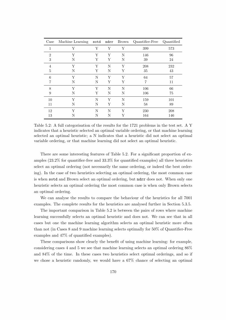
Case Machine Learning sotd ndrr Brown Quantifier-Free Quantified

1 Y Y Y Y 399 573

2 Y Y Y N 146 963 N Y Y N 39 24

4 Y Y N Y 208 2325 N Y N Y 35 43

6 Y N Y Y 64 577 N N Y Y 7 11

8 Y Y N N 106 669 N Y N N 106 75

10 Y N Y N 159 10111 N N Y N 58 89

12 Y N N Y 230 20813 N N N Y 164 146

Table 5.2: A full categorisation of the results for the 1721 problems in the test set. A Yindicates that a heuristic selected an optimal variable ordering, or that machine learningselected an optimal heuristic; a N indicates that a heuristic did not select an optimalvariable ordering, or that machine learning did not select an optimal heuristic.

There are some interesting features of Table 5.2. For a significant proportion of ex-

amples (23.2% for quantifier-free and 33.3% for quantified examples) all three heuristics

select an optimal ordering (not necessarily the same ordering, or indeed the best order-

ing). In the case of two heuristics selecting an optimal ordering, the most common case

is when sotd and Brown select an optimal ordering, but ndrr does not. When only one

heuristic selects an optimal ordering the most common case is when only Brown selects

an optimal ordering.

We can analyse the results to compare the behaviour of the heuristics for all 7001

examples. The complete results for the heuristics are analysed further in Section 5.3.5.

The important comparison in Table 5.2 is between the pairs of rows where machine

learning successfully selects an optimal heuristic and does not. We can see that in all

cases but one the machine learning algorithm selects an optimal heuristic more often

than not (in Cases 8 and 9 machine learning selects optimally for 50% of Quantifier-Free

examples and 47% of quantified examples).

These comparisons show clearly the benefit of using machine learning: for example,

considering cases 4 and 5 we see that machine learning selects an optimal ordering 86%

and 84% of the time. In these cases two heuristics select optimal orderings, and so if

we chose a heuristic randomly, we would have a 67% chance of selecting an optimal

170

sotd ndrr Brown Quantifier-Free Quantified Random Choice

Y Y N 79% 80% 67%Y N Y 86% 84% 67%N Y Y 90% 84% 67%

Y N N 50% 47% 33%N Y N 73% 53% 33%N N Y 58% 59% 33%

Table 5.3: Proportion of successful choices of an optimal heuristic by machine learning,in comparison to the chance of a random choice selecting an optimal heuristic.

Machine Learning sotd ndrr Brown

Quantifier-Free 1312 76.2% 1039 60.4% 872 50.7% 1107 64.3%Quantified 1333 77.5% 1109 64.4% 951 55.3% 1270 73.8%

Table 5.4: Total number of problems for which machine learning and each heuristic isoptimal.

heuristic. For all cases where either one or two heuristics are optimal, we can compare

the use of machine learning with a random choice: as shown in Table 5.3. We can see

that machine learning does significantly better than random choice in all cases, often by

a startling degree.

Obviously, given a new problem there is no way of immediately knowing which of the

heuristics will be optimal (otherwise we would simply select the optimal heuristic) and

so whilst Tables 5.2 and 5.3 are useful for analysing the performance of machine learning

on the test examples, they are not helpful in predicting performance on a new problem.

Table 5.4 gives the total number of problems (out of 1721) for which each heuristic and

machine learning is optimal.

Considering the heuristics alone it seems that Brown is the heuristic that is most

often optimal (with sotd competitive), whilst ndrr performs relatively poorly. This

will be discussed further in Section 5.3.5 where the data for all 7001 examples will be

considered.

It is clear from Table 5.4 that using machine learning is better than using a single

heuristic. To compare the overall behaviour of machine learning and selecting a heuristic

at random we need to summarise the data in Table 5.2 according to the number of

heuristics that are optimal in each case. For quantifier-free problems there are 399 where

all heuristics are optimal (Case 1), 499 where two are optimal (Cases 2-7), and 823 where

only one is optimal (Cases 8-13). Therefore the expected proportion of optimal heuristics

171

if chosen at random is 58.5%. In the quantified case there are 573 where all heuristics

are optimal (Case 1), 463 where two are optimal (Cases 2-7), and 685 where only one is

optimal (Cases 8-13). Therefore the expected proportion of optimal heuristics if chosen

at random is 64.5%.

We can therefore say that machine learning performs significantly better than any

individual heuristic or using a random heuristic. It offers an increase in performance

compared to random choice and the best performing heuristic (Brown):

• Quantifier-free:

– Random Choice: 58.5%;

– Brown’s Heuristic: 64.3%;

– Machine Learning: 76.2%.

• Quantified:

– Random Choice: 64.5%;

– Brown’s Heuristic: 73.8%;

– Machine Learning: 77.5%.

It should be noted that all the results given here were specifically for problems in

three variables and fully existentially quantified. There is therefore no guarantee that

this SVM would be appropriate for any other class of examples. It would be interesting

to conduct a thorough investigation to see how appropriate this application of machine

learning is for other classes of CAD problems. Machine learning is therefore superior to

the known methods of selecting a variable ordering.

5.3.4 Future work on Machine Learning

There are many ways in which this work could be extended to futher explore the benefit

machine learning can offer in the formulation of problems for CAD, and there are plans

to tackle a range of these in further collaboration between the two research groups.

Extending current investigation

Whilst a large corpus of data was used in this investigation, the data set was rather

uniform (three variables, existential quantifiers, same source). An obvious extension to

the work in this section is to apply machine learning to a wider set of examples to verify

its efficacy (along with the superiority of Brown’s heuristic). This could be investigated

first by altering the quantifiers of the current set of examples (although if not uniformly

existential or universal this would limit the permissible variable orderings), or considering

examples from the nlsat database with different numbers of variables.

There is also the option to use an expanded set of heuristics in the experimentation.

There are variants on sotd and ndrr (applied greedily or on different input sets) as well

172

as hybrid heuristics. Adding more heuristics may, however, decrease the accuracy of the

SVM.

We have also singularly used Qepcad for all CAD construction. Other implemen-

tations could be considered, and an attempt made for machine learning to select an

optimal choice.

There are also many questions relating to the machine learning choices for this ex-

periment that could be explored. The use of SVM as the machine learning method is

not the only choice and other machine learning techniques could be investigated with

the same data set to compare performance. Further, the choice of feature vector for the

SVM is not predetermined and can be investigated further.

Applying Machine Learning to Grobner Preconditioning

In Chapter 6, Grobner preconditioning is investigated. This generally proves benefi-

cial and reduces the cell count of the resulting CAD, but this effect is not universal.

To help identify when preconditioning is useful, a metric TNoI is introduced (Defini-

tion 6.7), which proves highly effective (but not universally so) at predicting when the

preconditioning should be applied.

In Section 6.2.9 it is suggested that machine learning could be useful to help predict

the benefit (or detriment) of preconditioning. This is obviously an important question

for computer algebra, but such an investigation could also offer an insight to the machine

learning. Machine learning could be applied in the two following ways:

• Indirectly: Use machine learning to pick the most appropriate heuristic for de-

ciding whether to precondition.

• Directly: Use machine learning directly to decide whether preconditioning should

be used for a given problem.

It would be insightful to compare the performance of both these approaches.

5.3.5 Further Analysis of the Heuristic Data

In the process of applying machine learning to pick a heuristic for selecting a variable

ordering, a large amount of data was generated. For each of the 7001 three-variable

examples in the nlsat database a CAD was constructed for all six variable orderings,

and all three heuristics were used to predict a variable ordering. Previous work on

CAD heuristics has involved small data sets ([DSS04] used 48 examples to obtain their

conclusions), so such a large data set allows for fresh insight. This was considered

173

sotd ndrr Brown

Quantifier-Free 4221 60.3% 3620 51.7% 4523 64.6%Quantified 4603 65.8% 4000 57.1% 5166 73.8%

Table 5.5: Total number of problems for which each heuristic is optimal from the 7, 001three-variable problems in nlsat database.

Mean Mediansotd ndrr Brown sotd ndrr Brown

Quantifier-Free 27.3% −0.2% 25.3% 29.5% 0.0% 32.3%Quantified 19.5% 4.2% 21.0% 14.7% 0.0% 16.7%

Table 5.6: Savings for each heuristic compared to the average cell count over all sixvariable orderings. The results were computed with the 5, 262 quantifier-free and 5, 332quantified problems for which no variable ordering timed out.

by members of the research groups at Bath and Cambridge and published as a poster

abstract [HEW+14a]. The author was involved in discussions of the results but did not

conduct the analysis.

For each of the 7001 examples (in both quantifier-free and fully existentially quanti-

fied formats) we can record whether each heuristic selects an optimal variable ordering.

Table 5.5 shows these values for each heuristic. We can see that, for both quantifier-free

and quantified problems, the Brown heuristic selects an optimal variable ordering most

often. This highlights the strength of the heuristic, especially when coupled with the

fact that it is computationally cheap and simple to implement.

We can also see from Table 5.5 that sotd is a competitive heuristic, but ndrr performs

worse than the other choices. This is perhaps indicative of the fact that ndrr was initially

created to handle cases that sotd fails to identify, and designed as a heuristic to break

ties.

Whilst selecting an optimal variable ordering is important, it is also relevant to

consider the actual savings in cell counts. When a heuristic selects a non-optimal variable

ordering it may differ from the optimal choice by as little as 2 cells or as many as

thousands of cells. Table 5.6 summarises this behaviour by computing the average cell

count for each problem over the six variable orderings, then computing the percentage

saving (with a negative percentage indicating an increase in cell count) for the variable

ordering each heuristic selects. The mean and median of the savings of each heuristic

are given in Table 5.6.

The data used to construct Table 5.6 is also summarised in Figure 5.1. This figure

174

Figure 5.1: Box plot for the percentage saving in cell counts for each heuristic. Therange of the data is indicated (discounting outlier values), interquartile range, mean,and median.

sotd ndrr Brown

Quantifier-Free 559 32.1% 537 30.9% 594 34.2%Quantified 512 30.7% 530 31.8% 478 28.6%

Table 5.7: Total number of problems for which each heuristic avoids a time out. Theresults are with respect to the 1, 739 quantifier-free and 1, 669 quantified problems forwhich at least one variable timed out.

displays the means and median of each data, along with the interquartile range of the

data and overall range. It discounts any outliers, which are points further than 32 times

the interquartile range away from the upper and lower quartiles.

In most cases the performance of the heuristics is similar, and resembles their opti-

mality: Brown offers the greatest savings, with sotd offering a slightly smaller saving,

and ndrr performing relatively poorly (and in one case proving worse than average). For

quantifier-free examples sotd offers a slightly better mean saving, although has a lower

median than Brown.

The saving in cell count is not necessarily the most important metric, and there

are cases where it may be more important to simply ensure that the CAD construction

finishes. Of the 7001 examples, 1739 quantifier-free and 1669 quantified problems timed

out for at least one variable ordering. Table 5.7 gives the number of these examples

where each heuristic avoids a time out. Table 5.7 shows that for quantifier-free problems

the Brown heuristic is also the best at guaranteeing completion. However, for quantified

problems it performs poorly, with ndrr being the most effective at selecting a feasible

ordering.

175

To summarise the work on existing heuristics it is evident that Brown is clearly the

best choice in general. Not only is it the cheapest to compute (requiring no projection or

further computation) but it picks an optimal ordering more often than sotd and ndrr.

It offers good savings over the average cell count (along with sotd) and is the most

effective at choosing feasible orderings for quantifier-free problems (although it performs

the worst out of the heuristics for quantified problems).

The data used for these conclusions, as with the machine learning experiment, is of

a particular format: three variables with all quantifiers being existential. It is therefore

important to consider these results within that context, and there is no guarantee that

similar results will be achieved on a different or more varied data set (and this would be

interesting future work). However, it is compelling evidence and the largest investigation

into CAD heuristics that the author knows of.

5.3.6 Machine Learning Conclusions

It is clear from the work throughout this section that machine learning can be used to

great effect within computer algebra. Applying machine learning (using support vector

machines) to the task of selecting a variable ordering for CAD it is necessary to approach

the problem indirectly, by selecting a heuristic to then choose a variable ordering.

Machine learning selected an optimal heuristic for 76.2% of quantifier-free problems

and 77.5% of quantified problems. This is better than the best-performing heuristic of

Brown (by 11.9% and 3.7%, respectively) and also better than selecting a heuristic at

random (by 6.0% and 1.3%, respectively). Machine learning also proves to be beneficial

in nearly all individual cases relating to which heuristics are optimal.

Using the results of all 7, 001 examples from the nlsat database that were used

for the experimentation, it was also shown that Brown’s heuristic outperforms sotd and

ndrr. Combined with the very small computation cost, it is clear that if machine learning

is not available then Brown’s heuristic is a great alternative, with sotd performing only

slightly worse. It also highlighted that ndrr as an individual heuristic performs rather

poorly (and is very costly), and so it is best suited to be used within a hybrid heuristic

to break ties.

5.4 CAD Dimensional Distribution

In Section 4.3 the idea of a layered sub-CAD was introduced, consisting of all cells with

a specified dimension or greater. This motivates the investigation of the distribution of

176

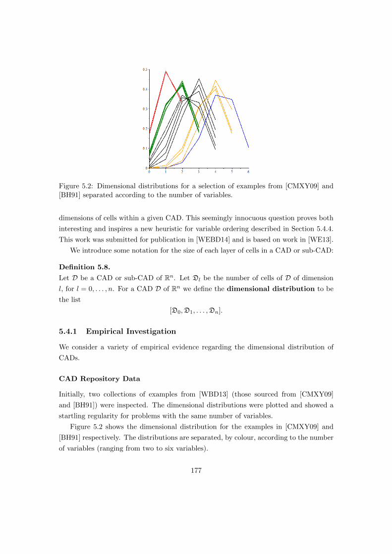
Figure 5.2: Dimensional distributions for a selection of examples from [CMXY09] and[BH91] separated according to the number of variables.

dimensions of cells within a given CAD. This seemingly innocuous question proves both

interesting and inspires a new heuristic for variable ordering described in Section 5.4.4.

This work was submitted for publication in [WEBD14] and is based on work in [WE13].

We introduce some notation for the size of each layer of cells in a CAD or sub-CAD:

Definition 5.8.

Let D be a CAD or sub-CAD of Rn. Let Dl be the number of cells of D of dimension

l, for l = 0, . . . , n. For a CAD D of Rn we define the dimensional distribution to be

the list

[D0,D1, . . . ,Dn].

5.4.1 Empirical Investigation

We consider a variety of empirical evidence regarding the dimensional distribution of

CADs.

CAD Repository Data

Initially, two collections of examples from [WBD13] (those sourced from [CMXY09]

and [BH91]) were inspected. The dimensional distributions were plotted and showed a

startling regularity for problems with the same number of variables.

Figure 5.2 shows the dimensional distribution for the examples in [CMXY09] and

[BH91] respectively. The distributions are separated, by colour, according to the number

of variables (ranging from two to six variables).

177

(a) Binomial distributions (n, p) =[(2, 0.6), (3, 0.6), (4, 0.65), (5, 0.7), (6, 0.7)].

(b) Dimensional distributions for[CMXY09, BH91].

Figure 5.3: Binomial distributions and dimensional distributions of examples from[CMXY09] and [BH91].

Binomial Distributions

All the graphs in Figure 5.2 exhibit a clear shape similar to a normal distribution that

is biased towards cells with large dimension. An emulation of this can be created with

the binomial distribution.

Recall that the binomial distribution for n trials with probability p of success is

given by:

P(X = x) :=

(nx

)px(1− p)n−x 0 ≤ x ≤ n

0 otherwise.

We can consider a binomial distribution with a value of p greater than 0.5 to give a bias

similar to what was exhibited in the dimensional distributions of Figure 5.2. In Figure

5.3a a binomial distribution is shown for n ranging from 2 to 6. with p values selected

by eye, increasing from 0.6 to 0.7. These distributions are shown alongside Figure 5.3b

which shows the corresponding dimensional distributions from [CMXY09] and [BH91].

It would seem that as n increases, then the appropriate value of p also increases, which

suggests a greater shift towards higher dimensional cells, however there is also less data

to compare for large n so this may not be a general trend.

178

(a) Combinatorially random CADs. (b) The [CMXY09] and [BH91] exam-ples.

Figure 5.4: The dimensional distributions of 45 combinatorially random CADs (withvariables 2 ≤ n ≤ 6 and number of sections 1 ≤ s ≤ 7) with the dimensional distributionsfrom examples in [CMXY09] and [BH91]

Combinatorially Random CADs

It would seem from the regularity of Figure 5.2 that the distribution of cells is relatively

unaffected by the specific polynomials used to generate the CAD. To test this idea,

we consider combinatorially random CADs: these are constructed by selecting a

random number of variables, and splitting each cylinder over a cell into a random number

of cells. The construction is done in Maple using its rand command to construct lists

of cell indices representing the theoretical cells. This is much quicker than constructing

CADs for random polynomials and is obviously unrelated to a choice of polynomials and

intentionally independent of any underlying real algebraic geometry.

Figure 5.4a shows the dimensional distribution of 45 random combinatorially random

CADs. Each CAD had a random number of variables chosen from 2, . . . , 6 and each

cylinder was split according to a random number of sections chosen from 1, . . . , 7(therefore having 3 to 15 cells). This is given alongside the examples from [CMXY09]

and [BH91] in Figure 5.4b and it is clear that they have a similar distribution, although

there are obviously some differences.

It is worth noting that for both examples and random constructions the top two

layers often form a large proportion of the cells. This is unfortunate, as 2-layered sub-

CADs can be useful for applications such as adjacency (discussed further in Appendix

A).

179

5.4.2 Combinatorial Investigation

As Figures 5.3 and 5.4 suggest the dimension distribution is independent of the real

algebraic geometry, we now consider the underlying combinatorial structure of a CAD.

To do this we strip away the reliance on input polynomials and consider the combinatorial

construction of a CAD in the following manner.

Lemma 5.2.

Let D be a partition of Rn constructed by the following:

1. Decompose R1 using k1 0-cells.

2. When lifting from the Rm to Rm+1 decompose the cylinder over a cell of dimension

m′ using km (m′)-cells.

Decomposing Rn this way gives:

Dl =∑L⊆[n]|L|=l

∏i∈L

(ki + 1)∏

j∈[n]\L

kj

,

where [n] is the combinatorial notation for 1, . . . , n.In particular we have:

D0 =

n∏i=1

ki, Dn =

n∏i=1

(ki + 1).

Proof.

The dimension of a cell in D is equal to the sum of the parity of its cell indices. For a

cell to have dimension l, it must therefore have l odd indices and n− l even indices.

We can characterise an l-dimensional cell by the position of its odd indices. Call the

set of these positions L. For a fixed L there are many cells associated to it. For level

1, there are a total k1 + 1 choices of 1-cells if 1 ∈ L and k1 choices of 0-cells if 1 /∈ L.

Continuing to build the CAD, at level i there are ki + 1 cell choices if i ∈ L and ki

choices if i /∈ L.

Therefore, for a fixed L, the number of cells that have an appropriate cell index is

given by: ∏i∈L

(ki + 1)∏

i∈[n]\L

ki.

180

All that remains is to sum over all possible subsets L of [n] with cardinality l.

This is a major simplification of the problem at hand, however it does well to model

standard CAD behaviour empirically.

It is very easy to see that if ki = k for all i then the sequence Dl is simply the

sequence of binomial coefficients of (k + (k + 1)x)n. This is proven in the following

lemma.

Lemma 5.3.

Let D be as given in Lemma 5.2. Then the generating function for Dl is given by:

Γ(x) :=n∏i=1

(ki + (ki + 1)x).

That is, Dl is the coefficient of xl in the expansion of Γ(x).

Proof.

Expanding out Γ(x), xl is obtained precisely by choosing x from l different linear factors.

This amounts to selecting l integers from the set [n]. For a given L, each i ∈ L contributes

ki + 1 to the coefficient of the generated monomial, and each i /∈ L contributes ki. This

means the coefficient of the generated xl is:∏i∈L

(ki + 1)∏

i∈[n]\L

ki.

The coefficient of xl in Γ(x) is precisely the summation of all such coefficients:

∑L⊆[n]|L|=l

∏i∈L

(ki + 1)∏

j∈[n]\L

kj

,

which was shown in Lemma 5.2 to be Dl.

Lemma 5.3 certainly lends some credibility to the idea that the dimension of cells in

a CAD roughly obeys a binomial statistical distribution.

It may seem at first like this construction has somehow avoided the doubly-exponential

complexity of CAD. This is not the case: taking a resultant at each level in projection

results in an increase of each degree by a factor of 2n.

181

Variables 2 3 4 5

Fraction 0.334 0.192 0.161 0.181

Table 5.8: Average fraction of full-dimensional cells for examples sourced from [WBD13].

5.4.3 Estimation of CAD size

This consistency in dimensional distribution can be of great use. As a one-layered CAD

is generally easy to compute we can use it to predict the size of a complete CAD.

The obvious way to do this is to compute the dimensional distribution for a collection

of examples with the same number of variables and take the average of the fraction of

full cells in each. Multiplying the number of cells for the 1-layered CAD in question by

the reciprocal of this average should give a reasonable estimate for a complete CAD.

Computing values for examples sourced from [WBD13] we can also calculate average

fractions of full cells in distributions for a given number of variables. These results are

shown in Table 5.8.

Remark 5.4.

We can also create random distribution fractions by using the formulae obtained in

Lemma 5.2 so that:

Dl∑ni=1 Di

=

∑L⊆[n]|L|=l

(∏i∈L(ki + 1)

∏j∈[n]\L kj

)∏ni=1(2ki + 1)

and in particular the fraction the top layer constitutes is given by the simple formula:

Dn∑ni=1 Di

=

∏ni=1(ki + 1)∏ni=1(2ki + 1)

.

This simplifies even further when all the ki are equal, simply giving:

Dn∑ni=1 Di

=

(k + 1

2k + 1

)n.

Obviously using an averaged value to predict the size of a complete CAD will not

work universally but initial results are promising, as shown in the following example.

182

Example 5.1.

Two random polynomials in x, y, z were created, each with total degree 2:

g := 81zy − 3zx− 88yx+ 99x2 − 12y − 48; (5.1)

h := 80z2 + 40zy − 41y2 + 44yx− 28z + 11. (5.2)

These were input into the CAD algorithms under the two variable orderings: x ≺ y ≺ zand x y z.

With variable ordering x ≺ y ≺ z a 1-layered CAD was produced with 372 cells, which

gives a predicted complete CAD of 1941 cells. In reality, a complete CAD produced by

McCallum’s projection contains 2057 cells, which is a difference of 116 (around 5%).

With variable ordering x y z a 1-layered CAD was produced with 454 cells, which

gives a predicted complete CAD of 2368 cells. In reality, a complete CAD produced by

McCallum’s projection contains 2373 cells, which is a difference of only 5 cells (around

0.2%).

From experimentation, it would seem that larger CADs have more accurate predic-

tions, which is to be expected. For example when dealing with only a single polynomial

with a CAD of at most 200 cells the results can be inaccurate but with more polynomials

and CADs over 1000 cells the predictions seem to mostly be within 5%. Arguably, the

larger examples are those for which an accurate prediction is most important.

Indeed, it seems the most appropriate use of this approximation is estimating fea-

sibility of problems and predicting good variable orderings. This will be discussed in

Section 5.4.4.

5.4.4 Cell Dimension Heuristic

We can use the ideas behind the dimension distribution of cells in a CAD as a method

of selecting a variable ordering.

We consider a motivating example before describing the general heuristics.

Example 5.2.

We consider the set of random polynomials in three variables:

F :=x2 + y − z3 − 1, x2 − 5y + 1, z3 − xy, z3 − 5

.

We wish to know which of the six possible variable orderings gives the smallest CAD.

We proceed by computing the six possible 1-layered sub-CADs.

183

Cells TimeOrder 1-LCAD Prediction Complete CAD 1-LCAD Complete CAD

z ≺ y ≺ x 544 2833 2949 1.112 11.734y ≺ z ≺ x 710 3698 3995 1.025 13.870z ≺ x ≺ y 264 1375 1299 0.758 5.033x ≺ z ≺ y 312 1625 1545 0.527 5.784y ≺ x ≺ z 592 3083 3207 0.971 12.955x ≺ y ≺ z 448 2333 2347 0.711 9.006

Table 5.9: Use of 1-layered sub-CADs as a heuristic for F . Cell counts and timingsare given for 1-layered sub-CADs and complete CADs. The predicted cell count is alsogiven: obtained by multiplying the 1-layered sub-CAD cell count by 1/0.192.

The results for F are given in Table 5.9. We see that the 1-layered sub-CAD cell

counts predict that z ≺ x ≺ y gives the smallest complete CAD, which is indeed correct

(the ranking of the variable orderings is equal for the 1-layered and complete CADs). It

is worth noting that the timings are less clear, with z ≺ x ≺ y being the third quickest to

produce a 1-layered CAD, but the quickest to produce a full CAD. This highlights how

cell count is a more useful and consistent measure for CAD complexity. The total time

to compute all 1-layered sub-CADs for F is 5.104 seconds which means that it takes,

in total, 10.137 seconds to predict and construct the complete CAD for z ≺ x ≺ y.

Constructing the complete CAD for y ≺ z ≺ x directly takes 13.870 seconds and so this

heuristic offers a practical saving of 3.733 seconds from the worst case (and a saving of

2696 cells). With respect to the average of all six variables the 1-layered heuristic incurs

a slight cost of 0.410 seconds (but saves 1258 cells).

We formally define the layered heuristic.

Definition 5.9.

Given a set of input polynomials and set of permitted variable orderings, the layered

heuristic computes the 1-layered sub-CAD with respect to each of the given variable

orderings and selects the one producing the smallest sub-CAD.

The layered heuristic (for a complete set of variable orderings) is described in Al-

gorithm 5.1. The one layered sub-CADs for each variable ordering can be constructed

using either the direct or recursive sub-CAD algorithms (described in Algorithms 4.3

and 4.4), with the latter offering the benefit of not repeating computations.

Obviously this may not necessarily be a practical heuristic. For small examples (as

shown for F in Example 5.2) the time computing n! 1-layered sub-CADs may be more

costly than the average time saved by picking the near-optimal variable ordering for the

184

Algorithm 5.1: LayeredHeuristic(F, vars): Basic layered heuristic algorithm.

Input : A set of polynomials F , a set of variables vars.Output: The predicted optimal variable ordering optvars, and a CAD, D, for F

with respect to optvars.

1 V ← combinat[permute](vars); // All variable orderings

2 mincells←∞;3 for v ∈ V do4 Lv ← LCAD(F, 1, v); // 1-layered sub-CAD

5 if |Lv| < mincells then6 optvars← v; // If smallest, set to optvars

7 D ← FullCAD(F, optvars, [Loptvars]); // Construct complete CAD

8 return [optvars,D];

complete CAD. For large examples (especially in many variables) the computation time

for the n! 1-layered sub-CADs may simply be too large. This is investigated in Section

5.4.5.

Computing a collection of 1-layered CADs is certainly feasible as a tie-breaking

heuristic. We know that all the heuristics mentioned in this chapter can have trouble

distinguishing between variable orderings (i.e. coupled variables with Brown’s heuristic)

and so the size of the 1-layered CADs for the set of potential variable orders can be used

as a tie-breaker. It may also be the case that, due to restrictions on variable ordering

due to quantifiers, there are only a small number of possible variable orderings to check.

Parallel Implementation

We can improve the efficiency of the layered heuristic by computing the 1-layered sub-

CADs in parallel. We describe two potential algorithms, neither of which has yet been

implemented. With the Maple Threads package, these could be interfaced with the

ProjectionCAD module.

Algorithm 5.2 describes a basic parallel algorithm for the layered heuristic across a set

of cores. Each 1-layered sub-CAD algorithm is computed in parallel across the threads.

As soon as one sub-CAD finishes computation all other computations are terminated

(this may not be the optimal ordering choice but it will be near-optimal). The remaining

lifting calls are then computed in parallel.

Algorithm 5.3 is slightly more sophisticated and also guarantees that the variable

ordering with the smallest 1-layered sub-CAD is selected. The sub-CAD algorithms are

again launched in parallel, but now any time a sub-CAD finishes construction its size is

185

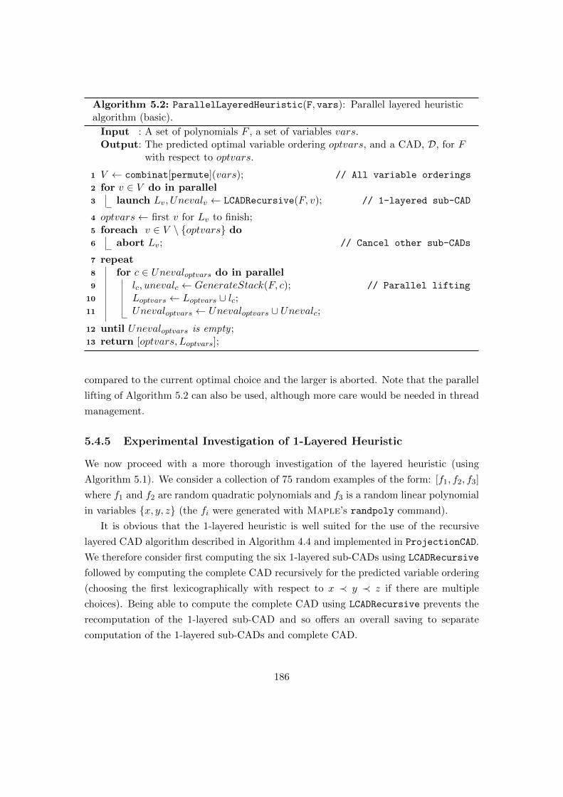
Algorithm 5.2: ParallelLayeredHeuristic(F, vars): Parallel layered heuristicalgorithm (basic).

Input : A set of polynomials F , a set of variables vars.Output: The predicted optimal variable ordering optvars, and a CAD, D, for F

with respect to optvars.

1 V ← combinat[permute](vars); // All variable orderings

2 for v ∈ V do in parallel3 launch Lv, Unevalv ← LCADRecursive(F, v); // 1-layered sub-CAD

4 optvars← first v for Lv to finish;5 foreach v ∈ V \ optvars do6 abort Lv; // Cancel other sub-CADs

7 repeat8 for c ∈ Unevaloptvars do in parallel9 lc, unevalc ← GenerateStack(F, c); // Parallel lifting

10 Loptvars ← Loptvars ∪ lc;11 Unevaloptvars ← Unevaloptvars ∪ Unevalc;12 until Unevaloptvars is empty ;13 return [optvars, Loptvars];

compared to the current optimal choice and the larger is aborted. Note that the parallel

lifting of Algorithm 5.2 can also be used, although more care would be needed in thread

management.

5.4.5 Experimental Investigation of 1-Layered Heuristic

We now proceed with a more thorough investigation of the layered heuristic (using

Algorithm 5.1). We consider a collection of 75 random examples of the form: [f1, f2, f3]

where f1 and f2 are random quadratic polynomials and f3 is a random linear polynomial

in variables x, y, z (the fi were generated with Maple’s randpoly command).

It is obvious that the 1-layered heuristic is well suited for the use of the recursive

layered CAD algorithm described in Algorithm 4.4 and implemented in ProjectionCAD.

We therefore consider first computing the six 1-layered sub-CADs using LCADRecursive

followed by computing the complete CAD recursively for the predicted variable ordering

(choosing the first lexicographically with respect to x ≺ y ≺ z if there are multiple

choices). Being able to compute the complete CAD using LCADRecursive prevents the

recomputation of the 1-layered sub-CAD and so offers an overall saving to separate

computation of the 1-layered sub-CADs and complete CAD.

186

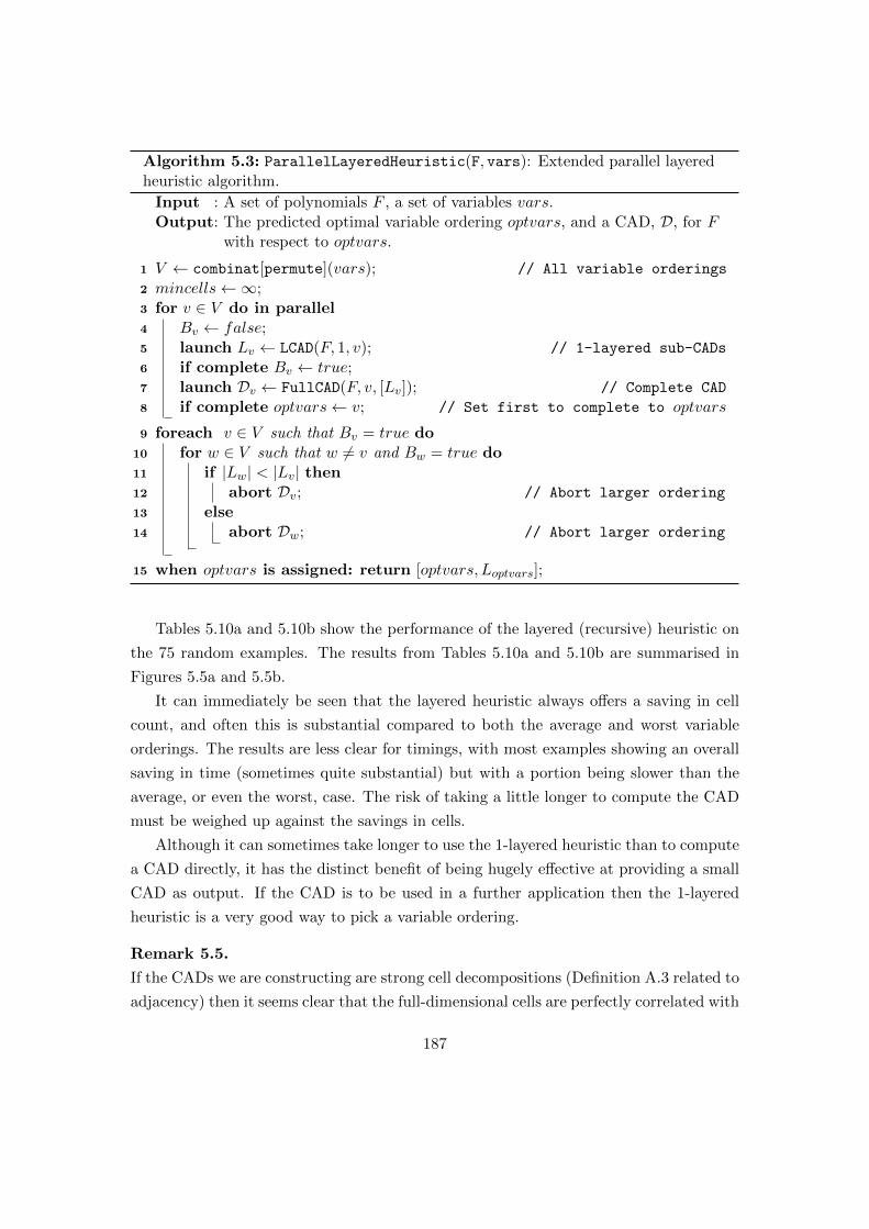
Algorithm 5.3: ParallelLayeredHeuristic(F, vars): Extended parallel layeredheuristic algorithm.

Input : A set of polynomials F , a set of variables vars.Output: The predicted optimal variable ordering optvars, and a CAD, D, for F

with respect to optvars.

1 V ← combinat[permute](vars); // All variable orderings

2 mincells←∞;3 for v ∈ V do in parallel4 Bv ← false;5 launch Lv ← LCAD(F, 1, v); // 1-layered sub-CADs

6 if complete Bv ← true;7 launch Dv ← FullCAD(F, v, [Lv]); // Complete CAD

8 if complete optvars← v; // Set first to complete to optvars

9 foreach v ∈ V such that Bv = true do10 for w ∈ V such that w 6= v and Bw = true do11 if |Lw| < |Lv| then12 abort Dv; // Abort larger ordering

13 else14 abort Dw; // Abort larger ordering

15 when optvars is assigned: return [optvars, Loptvars];

Tables 5.10a and 5.10b show the performance of the layered (recursive) heuristic on

the 75 random examples. The results from Tables 5.10a and 5.10b are summarised in

Figures 5.5a and 5.5b.

It can immediately be seen that the layered heuristic always offers a saving in cell

count, and often this is substantial compared to both the average and worst variable

orderings. The results are less clear for timings, with most examples showing an overall

saving in time (sometimes quite substantial) but with a portion being slower than the

average, or even the worst, case. The risk of taking a little longer to compute the CAD

must be weighed up against the savings in cells.

Although it can sometimes take longer to use the 1-layered heuristic than to compute

a CAD directly, it has the distinct benefit of being hugely effective at providing a small

CAD as output. If the CAD is to be used in a further application then the 1-layered

heuristic is a very good way to pick a variable ordering.

Remark 5.5.

If the CADs we are constructing are strong cell decompositions (Definition A.3 related to

adjacency) then it seems clear that the full-dimensional cells are perfectly correlated with

187

Cells vs Maximum vs Average

Mean 4719 222055.0% 38.7%

Best 12816 520493.6% 84.6%

Worst 762 29713.9% 6.49%

(a) Comparison of cell counts.

Time vs Maximum vs Average

Mean 64.3 10.038.7% 12.9%

Best 631.9 143.384.6% 70.1%

Worst −44.1 −66.1−27.9% −49.3%

(b) Comparison of timings (in seconds).

Table 5.10: Tables demonstrating the use of the layered (recursive) heuristic on 75random examples in three variables. All examples are of the form [f1, f2, f3] where f1

and f2 are random quadratic polynomials, and f3 is a random linear polynomial (allgenerated using randpoly in Maple).

(a) Percentage savings in cell count. (b) Percentage savings in time.

Figure 5.5: Box plots illustrating the savings of using the 1-layered sub-CAD heuristic.The blue (left) plot indicates the percentage saving compared to the worst variableordering, and the red (right) plot indicates the percentage saving compared to the averageover all six variable orderings.

188

Technique Cells Time sotd td ndrr 1-Lay Section Page

PL-CAD (Col) 54037 255.304 67 39 14 5012 2.3 30PL-CAD (McC) 54037 266.334 67 39 14 5012 2.3 30

EC-CAD (f3) 20593 65.856 67 39 14 1372 2.4.4 40EC-CAD (f4) 22109 102.781 67 39 14 1522 2.4.4 40

Table 5.11: The Solotareff-3 problem with formulation concepts — variable order a ≺b ≺ v ≺ u.

the size of the complete CAD. The full dimensional cells in a strong cell decomposition

implicitly define the (n − 1)-dimensional cells, which inductively define the (n − 2)-

dimensional cells and so forth. Therefore for strong cell decompositions the layered

heuristic is completely accurate. This accuracy is not guaranteed if we do not have a

strong cell decomposition, although it should be closely correlated, and this should be

investigated.

The layered heuristic need not be limited to just variable ordering. It can clearly can

be used for other formulation choices such as equational constraints. It can also be made

more efficient by constructing a 1-layered variety sub-CAD for the heuristic: this will

be an accurate heuristic for variety sub-CADs but not necessarily a complete CAD. The

layered heuristic can also be used to help decide the optimal mathematical expression

of a CAD, an issue that will be discussed in Chapter 6.

5.5 Solotareff-3

We consider again the Solotareff-3 problem given in 2.12.

(∃ u)(∃v)[[3v2 − 2v − a = 0] ∧ [v3 − v2 − av − 2b+ a− 2 = 0]

∧ [3u2 − 2u− a = 0] ∧ [u3 − u2 − au− a+ 2 = 0] ∧ [1 ≤ 4a] ∧ [4a ≤ 7]

∧ [−3 ≤ 4b] ∧ [4b ≤ 3] ∧ [−1 ≤ v] ∧ [v ≤ 0] ∧ [0 ≤ u] ∧ [u ≤ 1]]. (5.3)

We consider the formulation issues of choosing between the two variable orderings6,

a ≺ b ≺ v ≺ u and b ≺ a ≺ v ≺ u, and designating an equational constraint. The

relevant data is shown in Tables 5.11 and 5.12

6There are two further permissible orderings by swapping u and v, due to the quantifier blockstructure, but we do not consider them here to prevent excessive calculations.

189

Technique Cells Time sotd td ndrr 1-Lay Section Page

PL-CAD (Col) 161317 916.105 76 52 26 14268 2.3 30PL-CAD (McC) 154527 857.357 75 51 25 13716 2.3 30

EC-CAD (f3) 48475 175.139 71 48 23 3040 2.4.4 40EC-CAD (f4) 63583 324.663 75 51 25 4132 2.4.4 40

Table 5.12: The Solotareff-3 problem with formulation concepts — variable order b ≺a ≺ v ≺ u.

We will consider the following heuristics and metrics: Brown’s heuristic from [Bro04];

sotd and td from [DSS04]; ndrr from [BDEW13]; and the 1-layered sub-CAD heuristic

introduced in Section 5.4.

Variable Order

We consider the choice of variable order, and examine the appropriate heuristics for

a ≺ b ≺ v ≺ u and b ≺ a ≺ v ≺ u:

Brown: Both a and b appear with degree 1, but a appears in two quadratic terms, so

b should be eliminated before a.

Selection: a ≺ b ≺ v ≺ u.

sotd Heuristic: The projection set of the first variable ordering gives 67, whilst the

second gives 76 or 75 (depending on projection operator).

Selection: a ≺ b ≺ v ≺ u.

td Heuristic: The projection set of the first variable ordering gives 39, whilst the second

gives 52 or 51 (depending on projection operator).

Selection: a ≺ b ≺ v ≺ u.

ndrr Heuristic: The projection set of the first variable ordering gives 14, whilst the

second gives 26 or 25 (depending on projection operator).

Selection: a ≺ b ≺ v ≺ u.

1-Layered Heuristic: The 1-layered sub-CAD of the first variable ordering gives 5012

cells, whilst the second gives 14268 or 13716 (depending on projection operator).

Selection: a ≺ b ≺ v ≺ u.

We see that all heuristics correctly select the optimal variable ordering. The first four

heuristics all complete in a near-instant time, whilst the 1-layered heuristic takes 24

190

seconds to construct. Whilst this is much longer than the other heuristics, it is small

compared to the time to construct the complete CADs: 266 seconds and 857 seconds,

respectively.

Machine learning is not suitable for this problem: all experimentation in Section

5.3 was with respect to three variable examples that were either unquantified or fully

existentially quantified, and the feature vector cannot be computed for problems with

more variables. Future work on the machine learning application will expand its use to

allow it to apply to the Solotareff problem.

Equational Constraint Designation

We now consider the selection of an equational constraint for each variable ordering. We

use the equational constraint projection operator for the sotd, td, and ndrr metrics,

and construct a 1-layered variety sub-CAD for the final heuristic:

• Variable ordering a ≺ b ≺ v ≺ u.:

sotd Heuristic: All four equational constraints give 67.

Selection: No choice.

td Heuristic: All four equational constraints give 39.

Selection: No choice.

ndrr Heuristic: All four equational constraints give 14.

Selection: No choice.

1-Layered Variety Heuristic: f1 and f2 return FAIL, f3 gives 1372, f4 gives

1522.

Selection: f3.

• Variable ordering b ≺ a ≺ v ≺ u.:

sotd Heuristic: f1 and f2 give 68, f3 gives 71, f4 gives 75.

Selection: f1 and f2.

td Heuristic: f1 and f2 give 45, f3 gives 48, f4 gives 51.

Selection: f1 and f2.

ndrr Heuristic: f1 and f2 give 21, f3 gives 23, f4 gives 25.

Selection: f1 and f2.

1-Layered Variety Heuristic: f1 and f2 return FAIL, f3 gives 3040, f4 gives

4132.

Selection: f3.

191

We see some interesting results. For a ≺ b ≺ v ≺ u, none of the projection operator

heuristics are able to distinguish between the four equational constraints. However, the

1-layered heuristic not only identifies f3 as the optimal designation, but also indicates

that f1 and f2 are unsuitable for designation. As we are constructing a layered variety

sub-CAD, and with the equational constraint projection operator, this is quicker than

when selecting a variable ordering, taking 8 seconds (compared to 66 and 103 seconds

to construct the complete CADs).

For b ≺ a ≺ v ≺ u, the projection operator heuristics can separate between the

designations, but identifies f1 and f2 which are not suitable for designation. Again, the

layered variety sub-CAD correctly identifies f3 and returns FAIL for f1 and f2. This

takes 15 seconds, compared to 175 and 325 seconds to construct the complete CADs.

5.6 Conclusion

In this chapter we considered various formulation choices that need to be made before

using a CAD algorithm: the variable ordering to use; which equational constraint to

designate; how to decompose a formula for TTICAD; and the order of polynomials to

consider for incremental algorithms. All of these can have a large effect on the complexity

of the constructed CAD. Two existing heuristics, Brown’s heuristic and sotd, were

investigated and a new metric, ndrr, introduced. All heuristics are to a certain degree

effective, but can also be fooled by constructed examples. Separate heuristics need to be

considered for the recent advances in incremental regular chains algorithms for CADs

and TTICADs, and these were briefly discussed.

The application of machine learning to select a heuristic for variable ordering was

given, and is thought to be the first application of machine learning to computer alge-

bra formulation. Using a support vector machine to select between Brown, sotd, ndrrproves highly effective: selecting an optimal heuristic for 76.2% of quantifier-free prob-

lems and 77.5% quantified problems (compared with 58.5% and 64.5% for a random

choice). Further analysis of the data used for the machine learning gave new insight

into the heuristics and indicated that Brown is the best performing heuristic. There is

much scope for applying machine learning to other questions within CAD and future

experiments to decide the application of Grobner preconditioning from Chapter 6 were

detailed.

Through empirical and combinatorial investigation, it was demonstrated that CADs

generally have the same distribution of cell dimensions (approximately a binomial dis-

tribution for a value of p > 0.5). It was described how this can be combined with the

192

1-layered sub-CAD algorithms of Chapter 4 to predict the size of a complete CAD from

its full-dimensional cells. This can be extended to a heuristic for selecting a variable or-

dering. Although this requires the construction of n! 1-layered sub-CADs it was shown

to be an effective heuristic for a collection of random examples in 3 variables: saving on

average 38.7% in cell count and 12.9% in total time over the average of all six variable

orderings.

All of the formulation choices can interact and influence each other. Therefore the

heuristics detailed in this chapter should not be considered independently of each other

and this is discussed in Chapter 7.

193

194

Chapter 6

Mathematical Description of

Problems for CAD

Given a specific problem for which CAD is to be used, there may be many ways to state

the problem before applying CAD. This is somewhat different to choosing parameters

such as variable ordering or equational constraints, as was discussed in Chapter 5. There

is a great amount of freedom in how to express a problem mathematically and there

can be much debate as to when reformulation becomes simply solving the problem by

alternative methods.

Grobner basis technology can be applied to a system of polynomial equalities and

inequalities to precondition a problem before applying a CAD algorithm. We analyse

this preconditioning and show that it can often result in a sharp drop in CAD complexity

and construction time. This benefit is not universal and a new metric is identified that

can be used to predict the behaviour of the preconditioning.

We also investigate the “Piano Mover’s Problem” of navigating a ladder through a

right-angled corridor. Previously considered infeasible [Dav86] it has been tackled in the

literature [Mar89, Wan96, McC97, YZ06] by making geometric deductions about the

problem. We provide a feasible formulation that does not rely on geometric reasoning.

Further work is needed to consider the adjacency configuration of the produced CAD and

thus construct valid paths when possible. We discuss a collection of general strategies

inspired by this problem.

195

Author’s Contribution and Publication

The motivating examples in Section 6.1 resulted from discussion with Bradford and

Davenport and communications with Brown [Bro12] for [DBEW12]. All other work in

this chapter is the author’s.

The work in Section 6.2 was published in [WBD12]. The work in Section 6.3 was

first given in the Technical Report [WBDE13] and later published in [WDEB13].

6.1 Motivation for Mathematical Reformulation

6.1.1 Motivation for Grobner Preconditioning

We consider the cyclic-4 system of polynomials.

Example 6.1.

Let a b c d and consider the system of equations:

a+ b+ c+ d = 0

ab+ bc+ cd+ da = 0

abc+ bcd+ cda+ dab = 0

abcd− 1 = 0.

This proves to be difficult to tackle directly for most CAD technology. Using a

projection and lifting based approach or the recursive Regular Chains algorithm both

time out after a day’s computation. Using the incremental Regular Chains approach

completes after around 25 minutes, but produces 187,225 cells.

A Grobner basis is a structured way to represent an algebraic variety, and we can

compute such a basis with respect to the pure lexicographic ordering to get:

1− d4 − d2c2 + c2d6 = 0

−c− d+ c2d3 + d2c3 = 0

d4b+ d5 − b− d = 0

c2d4 + bc− bd+ cd− 2d2 = 0

b2 + 2bd+ d2 = 0

a+ b+ c+ d = 0

This will have the exact same solution set as the original problem (they describe

196

the same polynomial ideal), so any CAD of the second systems of polynomials will be

sufficient to analyse the solutions to the first system of polynomials.

This proves much more efficient input for all three CAD algorithms. Projection

and lifting CAD now produces 1569 cells in 8.3 seconds, recursive regular chains CAD

produces 621 cells in 6.1 seconds, and incremental regular chains CAD produces 621

cells in just 1.0 seconds.

A key question is to consider whether such a saving is always gained from taking a

Grobner basis, which motivates further investigation into the interaction between various

CAD techniques and Grobner bases. This will be discussed in Section 6.2.

6.1.2 Motivation for Mathematical Reformulation

Whilst investigating verification [DBEW12] a particular example proved too difficult

for computation. In private correspondence with Brown [Bro12] (the maintainer of

Qepcad) he illustrated how expressing a problem correctly for Qepcad, and hence

CAD, can make a big difference in feasibility.

Joukowsky’s Transformation

The Joukowsky transformation is a conformal map on the complex plane defined as:

f : C→ Cz 7→ 1

2

(z + 1

z

) .The work in [DBEW12] aimed to show that f is a bijection from D = z | |z| > 1to C‡ = C \ [−1, 1] automatically. This amounts to showing the following quantified

formula is equivalent to TRUE:

(∀ a)(∀ b)(∀ c)(∀ d)[[

[a(c2 + d2)(a2 + b2 + 1)− c(a2 + b2)(c2 + d2 + 1) = 0]∧

[b(c2 + d2)(a2 + b2 − 1)− d(a2 + b2)(c2 + d2 − 1) = 0] ∧ [bd > 0] ∧ [c2 + d2 − 1 > 0]]

=⇒[[a = c] ∧ [b = d]

]]. (6.1)

Trying to use this as direct input for Qepcad proves too difficult with default ini-

tialisation settings. Brown points out that using Qepcad as a “black box” for either

quantifier elimination or CAD construction is unwise and suggests the following steps to

manually recast the problem.

197

Initially, Brown takes the negation of (6.1). This converts the universal quantifiers

into existential quantifiers and allows the final conclusion (consisting of a conjunction of

equalities) to split the problem into a disjunction of two formulae:

(∃ a)(∃ b)(∃ c)(∃ d)[b2cd2 + a2cd2 − ab2d2 − a3d2 − ad2 + b2c3 + a2c3 − ab2c2−

a3c2 − ac2 + b2c+ a2c = 0 ∧ b2d3 + a2d3 − b3d2 − a2bd2 + bd2 + b2c2d+

a2c2d− b2d− a2d− b3c2 − a2bc2 + bc2 = 0 ∧ db > 0 ∧ d2 + c2 − 1 > 0 ∧ c− a 6= 0]

∨

(∃ a)(∃ b)(∃ c)(∃ d)[b2cd2 + a2cd2 − ab2d2 − a3d2 − ad2 + b2c3 + a2c3 − ab2c2−

a3c2 − ac2 + b2c+ a2c = 0 ∧ b2d3 + a2d3 − b3d2 − a2bd2 + bd2 + b2c2d+

a2c2d− b2d− a2d− b3c2 − a2bc2 + bc2 = 0 ∧ db > 0 ∧ d2 + c2 − 1 > 0 ∧ d− b 6= 0]

(6.2)

There are multiple points that are notable about this formulation. The first is the

ability to split the new formulation into two smaller problems: this only reduces the

problem by one polynomial for each half, but recall that the complexity is polynomial

in the number of polynomials with an exponent that is exponential in n. Each half of

equation (6.2) is preceded by existential quantifiers which is beneficial as it can allow

for a simpler calculation: only one sample point needs to be found to determine the

statement (in this case, no such points exist and so all cells need to be checked). Finally,

both halves of (6.2) are conjunctions involving equations, and so are amenable to the

theory of equational constraints (in fact the theory of Grobner preconditioning from

Section 6.2 can also be used).

After splitting this disjunction we can attempt to solve both halves of (6.2). Here

Brown uses a slightly counter-intuitive step (due to the implementation of Qepcad

rather than a theoretical issue) of leaving c and d free which allows Qepcad to utilise

the inequality d2 + c2 > 1.

Following all of these manipulations, Qepcad can solve each half of (6.2) in around

5–6 seconds. Both halves are shown to be equivalent to FALSE, and therefore their

disjunction is also FALSE. As (6.2) is the negation of (6.1), we obtain that the original

statement is proven equivalent to TRUE.

We investigate how a change in the mathematical description (such as used here)

can be beneficial for CAD in Section 6.3.

198

6.2 Preconditioning by Grobner Bases

We now describe an extension to the work of [BH91], investigating the effect of Grobner

preconditioning on CAD construction.

6.2.1 Grobner Bases

We will provide a brief summary of the basic theory of Grobner bases, first introduced

in [Buc65]. Further details can be found in most computer algebra textbooks (such as

[VZGG13]).

Definition 6.1.

A partial order < on a set is a transitive and non-reflexive relation. A partial order is

a total order if for any pair (α, β) of elements of the set either α = β, α < β, or β < α

holds. A total order is a well-order if any non-empty subset has a least element.

Definition 6.2.

For a given monomial m ∈ k[x] we identify with m the vector of exponents α =

(α1, α2, . . . , αn) ∈ Nn. We also use the notation:

m = xα = xα11 · xα2

2 · · ·xαnn .

A monomial order in k[x] is a relation ≺ on the exponent vectors such that:

1. ≺ is a total order;

2. α ≺ β implies α + γ ≺ β + γ for all α, β, γ ∈ Nn (corresponding to multiplication

of monomials);

3. ≺ is a well-order.

We give two monomial orderings that we will use (although many others exists and

are used in applications).

Definition 6.3.

Define the lexicographic order ≺lex using the following relation:

α ≺lex β ⇔ the leftmost non-zero entry in α− β is negative.

Define the inverted lexicographic order ≺ilex to be lexicographic order with the

variable order inverted (this is not a standard definition but will be useful). That is:

α ≺ilex β ⇔ the rightmost non-zero entry in α− β is negative.

199

Note that the inverted lexicographic order is not the same as the reverse lexico-

graphic order, which places α before β if the rightmost non-zero entry in α − β is

positive.

Definition 6.4.

Given a polynomial f ∈ k[x] and a monomial order ≺, we write lt≺(f), for the leading

term of f with respect to ≺, and lm≺(f), for the leading monomial of f with respect

to ≺.

The leading term ideal, 〈lt(F )〉, of a set of polynomials F ⊂ k[x] with respect

to a monomial order ≺ is the monomial ideal generated by the leading terms of all

polynomials in F :

〈lt(F )〉 := 〈lt≺(f) | f ∈ F 〉.

Definition 6.5.

Let ≺ be a monomial order and I a polynomial ideal in k[x]. A finite set G ⊆ I is a

Grobner basis for I with respect to ≺ if and only if:

〈lt(G)〉 = 〈lt(I)〉.

We give an equivalent definition of a Grobner basis. G is a basis of the ideal I that

satisfies the following condition:

1. For all f ∈ I, there exists a g ∈ G such that lm≺(g) | lm≺(f).

A reduced Grobner basis also satisfies the additional condition:

2. For all g, g′ ∈ G with g 6= g, we have lm≺(g) - lm≺(g′)

The original algorithm to compute a Grobner basis was given by Buchberger in his

PhD thesis [Buc65]. It consists of computing S-polynomials:

S(f, g) = lcm(lm(f), lm(g)) ·(

f

lt(f)− g

lt(g)

).

It can be shown that a criterion for deciding if a basis is a Grobner basis is to check that

all the S-polynomials (for all pairs of polynomials in the basis) reduce to 0 with respect

to the basis. Buchberger’s algorithm consists of repeatedly taking reduced S-polynomials

and adding any non-zero S-polynomials until all reduce to zero.

200

6.2.2 Key idea

Consider a (possibly quantified) formula in the first order of the reals, Φ, with quantifier-

free part ϕ(x1, . . . , xn). Assume the variable ordering is fixed.

Let us assume that ϕ (or a subformula of ϕ) has the form:

ϕ :s∧i=1

(fi = 0) ∧t∧

j=1

(gj ∗j 0), ∗j ∈ <,≤, >,≥,=, 6=. (6.3)

Let f1, . . . , fs be a Grobner basis of the fi, with respect to some given monomial

ordering. Then let ϕ be defined as follows:

ϕ :

s∧i=1

(fi = 0) ∧t∧

j=1

(gj ∗j 0). (6.4)

It is clear from the definition of Grobner bases that the solutions for ϕ are exactly the

same as the solutions for ϕ. Therefore we have an equivalent formula to Φ by replacing

ϕ with ϕ. For convenience, we will denote this preconditioning by =G.

Once we have computed the fi we can further use Grobner reduction on the gi with

respect to the fi, to produce g1, . . . , gt which have the same sign behaviour as the gi

when the fi vanish. Therefore we define ϕ as follows:

ϕ :s∧i=1

(fi = 0) ∧t∧

j=1

(gj ∗j 0). (6.5)

This will have the same solutions as ϕ, and so we have an equivalent formula to Φ and

Φ by replacing ϕ with ϕ. We will refer to this further reduction by →∗G.

6.2.3 Experimentation and analysis

The idea of combining Grobner bases and CAD was previously investigated in the Tech-

nical Report [BH91]. The authors considered problems of the form (6.3) and use a purely

lexicographical Grobner basis (=G) to produce (6.4). Their motivation were the ideas

that a pure lexicographic Grobner basis is “triangularized”, the number of projection

polynomials may be reduced if the basis has fewer polynomials, and any polynomials in

simply the main variable can be used as constraints.

The authors considered five examples (each with two variable orderings), including

the special case of the Solotareff-3 example introduced in Sections 1.3 and 2.12. They

201

showed that, in general, preconditioning a problem by computing a (purely lexicographic)

Grobner basis can be beneficial, often showing a very substantial speed-up in the total

computation time.

Improvements to algorithms (and their implementations) has done much to speed

up CAD construction and Grobner basis computation since [BH91]. However, when re-

computing the examples from [BH91] with modern technology the results remain largely

the same [WBD12]: preconditioning by computing a lexicographical Grobner basis gen-

erally makes the construction of a CAD for quantifier elimination more efficient. The

main difference between the results is that the computation time for the Grobner bases

is largely insignificant in the modern results, whereas there were examples in [BH91]

where the cost of computing a basis cancelled out an improvement in CAD construction.

All Grobner bases in this chapter were computed in under 0.03 seconds and therefore

only the total computation times (for Grobner basis and CAD) are given.

The authors of [BH91] note the substantial improvement offered in most cases, but

acknowledge that it can be detrimental. They state their plan to research further into

the area to try and give an explanation of why the preconditioning works. They finish by

stating an aim to “specialise the Grobner bases algorithm for the use as a preprocessor

to quantifier elimination algorithm.” Unfortunately, no further research was published

by the authors on this topic.

[BH91] with Current Technology

In [BH91] the authors considered using Grobner preconditioning with an early version of

Qepcad. It seems obvious to investigate their preconditioning tests with other methods

of constructing CADs. The same set of examples are considered in Table 6.1.

Table 6.1 compares CADFull from ProjectionCAD (using McCallum’s projection op-

erator) with the recursive approach to building CAD through RegularChains. These

both produce CADs of real space and there are multiple interesting results to note.

Using PL-CAD behaves much the same as Qepcad, which is to be expected as

both are based on projection and lifting construction of CAD. For six of the ten experi-

ments preconditioning was beneficial, for three the experiment timed out both with and

without preconditioning, and for Collision A a previously feasible problem was rendered

infeasible by preconditioning. Using the recursive version of CAD via Regular Chains

(Section 2.5.2) we get similar results to the other methods discussed so far (seven ex-

amples are improved by preconditioning, and three remain infeasible with or without

preconditioning).

202

Problem PL-CAD =G-PL-CAD RC-Rec-CAD =G-RC-Rec-CADCells Time Cells Time Cells Time Cells Time

Int A 3723 18.885 273 0.897 3723 11.248 273 1.400Int B 3001 15.272 189 0.528 2795 8.896 189 1.034Ran A 2101 11.376 165 0.530 1267 5.790 165 0.580Ran B 7119 73.856 141 0.540 7119 62.182 141 0.531Ell A FAIL T/O FAIL T/O 81193 516.385 37789 212.289Ell B — T/O — T/O — T/O — T/OSol A 54037 263.054 28501 126.930 54037 329.205 28501 220.144Sol B 154527 851.669 10633 44.437 154527 1136.397 10633 113.368Col A 8387 79.006 — T/O — T/O — T/OCol B — T/O — T/O — T/O — T/O

Table 6.1: The experiments from [BH91] as rerun with other methods of constructingCADs in Maple. Times are in seconds and “T/O” means a time-out (limit 30mins).

New Data Set

We investigate a new collection of examples using two algorithms: CADFull from Project-

ionCAD (using McCallum’s projection operator where possible); and the recursive Cylind-

ricalAlgebraicDecompose algorithm from RegularChains (as released in Maple 16).

These represent the projection and lifting approach (Section 2.3), and the original regu-

lar chains approach to computing CAD (Section 2.5.2). These algorithms offer the added

benefits of providing us with the number of cells computed (a more accurate measure-

ment of CAD complexity than timing) and can all be run (along with the preconditioning

stage) within the same Maple environment.

Whilst preconditioning is not changing the underlying theoretically minimal CAD,

it is changing the way such a CAD can be formed. This is not reliant on the method of

construction, so the behaviour should be broadly similar across both algorithms.

Remark 6.1.

Any results given in this thesis for RC-Rec-CAD may differ slightly from those in

[WBD12] owing to the use of new implementations of this algorithm1. There also may be

differences in Maple’s implementation of the Grobner algorithms. We have noted when

results have been sourced from [WBD12]; otherwise the results are new and current.

203

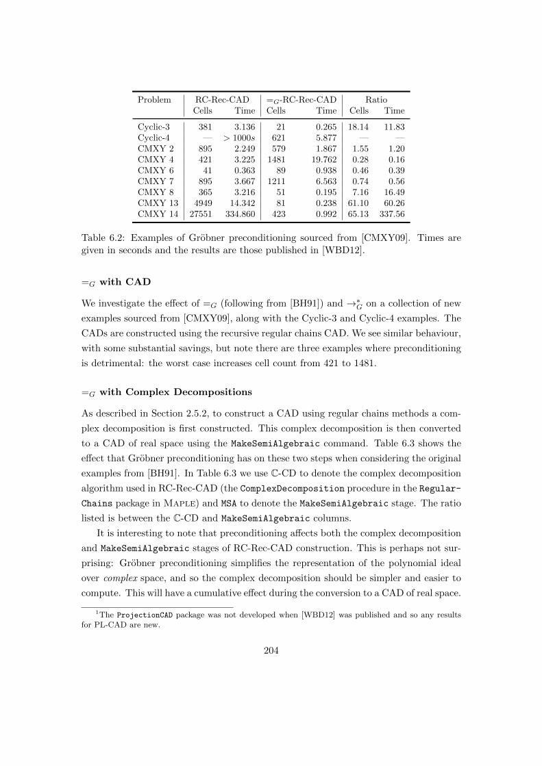
Problem RC-Rec-CAD =G-RC-Rec-CAD RatioCells Time Cells Time Cells Time

Cyclic-3 381 3.136 21 0.265 18.14 11.83Cyclic-4 — > 1000s 621 5.877 — —CMXY 2 895 2.249 579 1.867 1.55 1.20CMXY 4 421 3.225 1481 19.762 0.28 0.16CMXY 6 41 0.363 89 0.938 0.46 0.39CMXY 7 895 3.667 1211 6.563 0.74 0.56CMXY 8 365 3.216 51 0.195 7.16 16.49CMXY 13 4949 14.342 81 0.238 61.10 60.26CMXY 14 27551 334.860 423 0.992 65.13 337.56

Table 6.2: Examples of Grobner preconditioning sourced from [CMXY09]. Times aregiven in seconds and the results are those published in [WBD12].

=G with CAD

We investigate the effect of =G (following from [BH91]) and →∗G on a collection of new

examples sourced from [CMXY09], along with the Cyclic-3 and Cyclic-4 examples. The

CADs are constructed using the recursive regular chains CAD. We see similar behaviour,

with some substantial savings, but note there are three examples where preconditioning

is detrimental: the worst case increases cell count from 421 to 1481.

=G with Complex Decompositions

As described in Section 2.5.2, to construct a CAD using regular chains methods a com-

plex decomposition is first constructed. This complex decomposition is then converted

to a CAD of real space using the MakeSemiAlgebraic command. Table 6.3 shows the

effect that Grobner preconditioning has on these two steps when considering the original

examples from [BH91]. In Table 6.3 we use C-CD to denote the complex decomposition

algorithm used in RC-Rec-CAD (the ComplexDecomposition procedure in the Regular-

Chains package in Maple) and MSA to denote the MakeSemiAlgebraic stage. The ratio

listed is between the C-CD and MakeSemiAlgebraic columns.

It is interesting to note that preconditioning affects both the complex decomposition

and MakeSemiAlgebraic stages of RC-Rec-CAD construction. This is perhaps not sur-

prising: Grobner preconditioning simplifies the representation of the polynomial ideal

over complex space, and so the complex decomposition should be simpler and easier to

compute. This will have a cumulative effect during the conversion to a CAD of real space.

1The ProjectionCAD package was not developed when [WBD12] was published and so any resultsfor PL-CAD are new.

204

Problem C-CD MSA RC-CAD =G-C-CD MSA =G-RC-CADTime Time Time Ratio Time Time Time Ratio

Int A 5.691 23.735 29.426 4.17 1.168 1.302 2.470 1.11Int B 5.584 30.678 36.262 5.49 0.886 0.595 1.481 0.67Ran A 4.614 12.741 17.355 2.76 0.310 0.260 0.570 0.84Ran B 67.343 289.327 356.670 4.30 0.318 0.152 0.470 0.47Ell A* 85.425 177.198 262.623 2.07 27.916 34.580 62.496 1.24Ell B* 441.245 — > 1000s — — — > 1000s —Sol A* 6.666 9.348 16.014 1.40 1.760 0.265 2.025 0.15Sol B* 9.536 33.903 43.439 3.56 1.404 0.243 1.647 0.17Col A* 41.085 174.943 216.028 4.26 — — > 1000s —Col B* — — > 1000s — — — > 1000s —

Table 6.3: Examples from [BH91] investigated over the complex numbers with the re-cursive regular chains algorithms (an asterisk indicates that any inequalities have beenomitted to ease CAD construction). Times are given in seconds and the results are thosepublished in [WBD12].

This is supported by the fact that without preconditioning the MakeSemiAlgebraic stage

is often costly, but this cost is heavily reduced after =G preconditioning.

Another note of interest is the shift in the division of time between the C-Rec-CD and

MakeSemiAlgebraic algorithms following preconditioning. Without preconditioning the

majority of time is always spent in the MakeSemiAlgebraic phase and this is often a

significant portion (nearly 5.5 times the time taken for the complex decomposition in

Intersection B). Following preconditioning this is no longer true, with only two out of

seven examples taking longer to convert the complex decomposition into a CAD (with

the worse case being only a ratio of 1.24). This is often quite a shift (Intersection B

changes ratio from 5.49 to 0.67) and it would be of interest to investigate this behaviour

further.

→∗G with CAD

We wish to investigate the effect of →∗G. Consider the following four spheres in R3:

S1 : (x− 1)2 + y2 + z2 − 3; S2 : (x+ 1)2 + y2 + z2 − 3;

S3 : (x− 1)2 + (y − 1

2)2 + z2 − 3; S4 : (x+ 1)2 + (y +

2

3)2 + (z +

3

4)2 − 3.

Define the infinite cylinder centred on the z-axis with radius 1 to be C, so that the

equation defining C is:

C : x2 + y2 − 1.

205

PL-CAD A PL-CAD B =G-CAD A =G-CAD B →∗G-CAD A →∗

G-CAD BSpheres Cells Time Cells Time Cells Time Cells Time Cells Time Cells Time

13 0.053 13 0.030 — — — —

1 617 2.190 123 0.506 617 2.176 123 0.512 71 0.257 123 0.5172 617 2.104 123 0.438 617 2.110 123 0.494 71 0.220 123 0.4783 1109 4.306 173 0.833 1109 4.430 173 0.846 351 1.555 173 0.8634 1401 5.481 173 0.997 1401 5.543 173 0.891 351 1.535 173 0.991

1, 2 1073 4.156 631 2.513 267 0.795 171 0.353 99 0.230 99 0.2061, 3 9859 53.507 897 4.820 783 2.274 195 0.533 141 0.476 75 0.2061, 4 10817 62.232 2999 17.407 1439 4.976 315 1.244 213 0.853 249 1.0302, 3 12097 67.623 1317 7.001 1299 3.888 227 0.802 213 0.638 99 0.2532, 4 9051 51.918 1679 9.821 919 3.026 219 0.854 141 0.542 141 0.4713, 4 11957 75.832 3089 18.264 1359 4.781 315 1.259 213 0.841 249 1.010

1, 2, 3 23691 138.355 4673 27.607 165 0.398 305 0.468 45 0.096 45 0.0541, 2, 4 21999 138.096 11359 68.513 237 0.844 249 0.666 63 0.160 63 0.1321, 3, 4 62847 479.794 16601 110.485 787 2.298 225 0.748 63 0.250 63 0.1462, 3, 4 64343 544.725 14845 111.714 939 3.012 225 0.780 63 0.173 63 0.165

1, 2, 3, 4 140309 1226.077 53509 438.107 13 0.027 13 0.030 1 0.007 1 0.002

Table 6.4: Results of experimentation with Grobner preconditioning (both =G and→∗G) on examples involving spheres and a cylinder using PL-CAD (CADFull fromProjectionCAD with the McCallum projection operator).

We consider the intersection of spheres in relation to the cylinder and consider all

possible combinations, with some ‘simpler’ (with regards to the projection structure

needed for CAD) than others. We use two variable orders: z ≺ y ≺ x and x ≺ y ≺ z,

which we denote by A and B respectively. The latter variable ordering is arguably the

more suitable for these examples: the cylinder C gets projected down to a unit circle in

(x, y)-space.

We will assume that the spheres will always be required to equal 0, but make no

assumptions on the condition for the cylinder. All problems will therefore be of the

form: ∧i∈I

Si = 0 ∧ C ∗ 0 I ⊆ P(1, 2, 3, 4), ∗ ∈ =, 6=, <,>,≤,≥.

and we denote such a problem as Spheres I. These problems are therefore naturally

suited to both =G and →∗G forms of Grobner preconditioning.

Table 6.4 shows the results of preconditioning for these examples when using PL-

CAD with the McCallum projection operator.

These results show a wide variety of features of Grobner preconditioning. Consider-

ing just =G, we see that preconditioning is always beneficial when taking a non-trivial

basis (two or more polynomials). Moreover, the effect of the preconditioning is usually

greater with more polynomials: the size ratio of the preconditioned CAD compared to

the original CAD is more pronounced. This is as the Grobner basis is describing the

intersection of the polynomials, which can only reduce in size with the inclusion of more

polynomials (although the description of this intersection may be more complicated).

206

The results from the preconditioning by →∗G are also uniformly beneficial. In most

cases it reduces the number of cells significantly, and it never increases the complexity

of the CAD. Remarkably, it reduces every CAD to under 400 cells and with Spheres

1, 2, 3, 4 it reduces 140309 cells to just a single cell.

When considering all four spheres, computing a Grobner basis identifies that there

are no common solutions and so =G-PL-CAD produces a CAD with only 13 cells corre-

sponding to the cylinder, identical to the CAD of Spheres (note that as the cylinder

does not contain z, this is actually a CAD of (x, y)-space uniformly extended in the

z-direction). When also using →∗G the cylinder is reduced with respect to the trivial

ideal, 〈1〉, and so vanishes: the result CAD is the trivial one consisting of a single cell

that encompasses all of R3.

Monomial Ordering

Note that we have chosen to do our preconditioning with respect to the compatible

monomial ordering, ≺lex: if the Grobner basis contains univariate polynomials then

they will be in the variable corresponding to the one-dimensional induced CAD. This

property indicates that either this ordering or its reverse (≺ilex) would be the most

structured for preconditioning.

In [WBD12] it is shown comprehensively that the compatible ordering, ≺lex, is a

better choice compared to the reverse ordering, (≺ilex). The reverse ordering is never

more beneficial than the compatible ordering, and for all examples from [BH91] it renders

the examples infeasible.

6.2.4 Heuristics for Grobner preconditioning

For a given problem involving a conjunction of equations, we have seen there is a choice

of whether to apply Grobner preconditioning (=G or →∗G) and in the previous section it

was shown that this is a significant choice. To make this decision, we wish to identify a

metric or heuristic that closely correlates with the effect of preconditioning.

Previous Metrics: td*/td and sotd*/sotd

We have seen in this thesis that sotd (Definition 2.42) from [DSS04] can be effective at

selecting a variable ordering for CAD. In [DSS04] the authors also considered the total

degree metric, td, defined to be∑

f∈PROJ(F ) deg(f).

In [DSS04] the authors discarded td as a metric by observing its correlation with

sotd and noting that sotd favours sparse polynomials. It is natural to investigate td

207

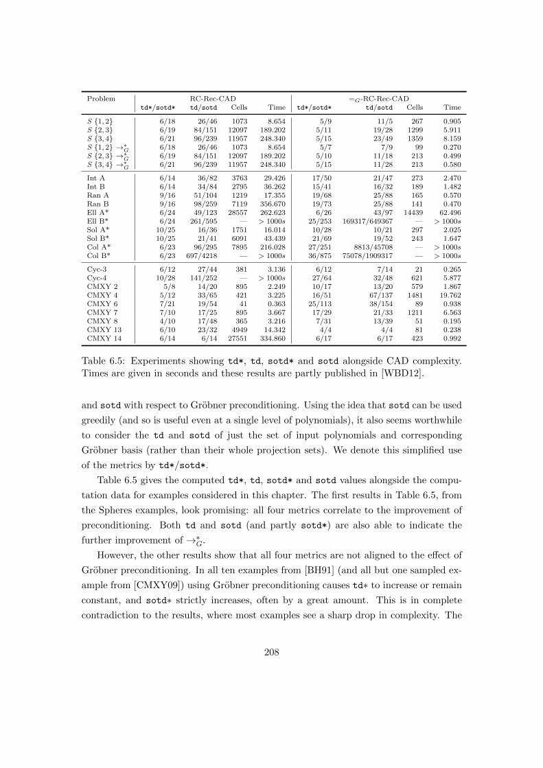
Problem RC-Rec-CAD =G-RC-Rec-CADtd*/sotd* td/sotd Cells Time td*/sotd* td/sotd Cells Time

S 1, 2 6/18 26/46 1073 8.654 5/9 11/5 267 0.905S 2, 3 6/19 84/151 12097 189.202 5/11 19/28 1299 5.911S 3, 4 6/21 96/239 11957 248.340 5/15 23/49 1359 8.159S 1, 2 →∗G 6/18 26/46 1073 8.654 5/7 7/9 99 0.270S 2, 3 →∗G 6/19 84/151 12097 189.202 5/10 11/18 213 0.499S 3, 4 →∗G 6/21 96/239 11957 248.340 5/15 11/28 213 0.580

Int A 6/14 36/82 3763 29.426 17/50 21/47 273 2.470Int B 6/14 34/84 2795 36.262 15/41 16/32 189 1.482Ran A 9/16 51/104 1219 17.355 19/68 25/88 165 0.570Ran B 9/16 98/259 7119 356.670 19/73 25/88 141 0.470Ell A* 6/24 49/123 28557 262.623 6/26 43/97 14439 62.496Ell B* 6/24 261/595 — > 1000s 25/253 169317/649367 — > 1000sSol A* 10/25 16/36 1751 16.014 10/28 10/21 297 2.025Sol B* 10/25 21/41 6091 43.439 21/69 19/52 243 1.647Col A* 6/23 96/295 7895 216.028 27/251 8813/45708 — > 1000sCol B* 6/23 697/4218 — > 1000s 36/875 75078/1909317 — > 1000s

Cyc-3 6/12 27/44 381 3.136 6/12 7/14 21 0.265Cyc-4 10/28 141/252 — > 1000s 27/64 32/48 621 5.877CMXY 2 5/8 14/20 895 2.249 10/17 13/20 579 1.867CMXY 4 5/12 33/65 421 3.225 16/51 67/137 1481 19.762CMXY 6 7/21 19/54 41 0.363 25/113 38/154 89 0.938CMXY 7 7/10 17/25 895 3.667 17/29 21/33 1211 6.563CMXY 8 4/10 17/48 365 3.216 7/31 13/39 51 0.195CMXY 13 6/10 23/32 4949 14.342 4/4 4/4 81 0.238CMXY 14 6/14 6/14 27551 334.860 6/17 6/17 423 0.992

Table 6.5: Experiments showing td*, td, sotd* and sotd alongside CAD complexity.Times are given in seconds and these results are partly published in [WBD12].

and sotd with respect to Grobner preconditioning. Using the idea that sotd can be used

greedily (and so is useful even at a single level of polynomials), it also seems worthwhile

to consider the td and sotd of just the set of input polynomials and corresponding

Grobner basis (rather than their whole projection sets). We denote this simplified use

of the metrics by td*/sotd*.

Table 6.5 gives the computed td*, td, sotd* and sotd values alongside the compu-

tation data for examples considered in this chapter. The first results in Table 6.5, from

the Spheres examples, look promising: all four metrics correlate to the improvement of

preconditioning. Both td and sotd (and partly sotd*) are also able to indicate the

further improvement of →∗G.

However, the other results show that all four metrics are not aligned to the effect of

Grobner preconditioning. In all ten examples from [BH91] (and all but one sampled ex-

ample from [CMXY09]) using Grobner preconditioning causes td∗ to increase or remain

constant, and sotd∗ strictly increases, often by a great amount. This is in complete

contradiction to the results, where most examples see a sharp drop in complexity. The

208

two more complex metrics, td and sotd, perform better but still have flaws: they are

tricked by examples such as Solotareff B and CMXY 14.

These results will be more closely investigated in Section 6.2.6.

6.2.5 Total Number of Indeterminates: TNoI and TNoIF

When we apply Grobner basis preconditioning to a problem, we are in some sense trying

to simplify the set of equations. There is a process similar to variable elimination hap-

pening, with equations in few variables being preferable to those with many. With this is

mind, it seems sensible to consider the number of variables present in each polynomials

of a given problem, which inspires the following definition.

Definition 6.6.

Let F be a set of polynomials and for a polynomial f ∈ F let NoI(f) be the number of

indeterminates present in the polynomial (e.g. NoI(z−x2y) = 3). Then define the total

number of indeterminates of F , TNoI(F ), to be:

TNoI(F ) =∑f∈F

NoI(f).

The TNoI of the problems considered in this chapter is given in Table 6.6, showing

a promising correlation to the benefit of Grobner preconditioning. In particular the

following three points are of note regarding =G:

1. In the 15 cases where applying =G reduces TNoI there is a significant benefit to

preconditioning.

2. In the remaining 7 cases where TNoI increases from =G preconditioning it is gen-

erally detrimental to precondition (with one false positive).

3. TNoI is not a measure of abstract difficulty of CAD construction.

It is clear from point 3 above that calculating TNoI alone is not of huge use, and

that something related to the difference or ratio of TNoI would be more appropriate.

The difference or ratio alone does not predict the improvement to expect, but taking

the logarithm of the ratio (equivalently the difference of the logarithms) of TNoI is more

interesting. This investigated in Section 6.2.6.

Inspired by [DSS04] we also consider the following metric:

Definition 6.7.

For a set of polynomials, F , define the full total number of indeterminates of F ,

209

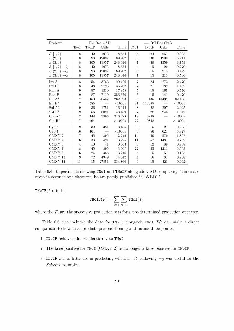
Problem RC-Rec-CAD =G-RC-Rec-CADTNoI TNoIF Cells Time TNoI TNoIF Cells Time

S 1, 2 8 42 1073 8.654 5 24 267 0.905S 2, 3 8 93 12097 189.202 6 30 1299 5.911S 3, 4 8 105 11957 248.340 7 39 1359 8.159S 1, 2 →∗G 8 42 1073 8.654 4 15 99 0.270S 2, 3 →∗G 8 93 12097 189.202 6 15 213 0.499S 3, 4 →∗G 8 105 11957 248.340 7 15 213 0.580

Int A 8 54 3763 29.426 7 24 273 2.470Int B 8 48 2795 36.262 7 21 189 1.482Ran A 9 57 1219 17.355 5 15 165 0.570Ran B 9 87 7119 356.670 5 15 141 0.470Ell A* 7 150 28557 262.623 6 135 14439 62.496Ell B* 7 585 — > 1000s 21 112685 — > 1000sSol A* 9 36 1751 16.014 8 28 297 2.025Sol B* 9 56 6091 43.439 7 28 243 1.647Col A* 7 148 7895 216.028 18 6248 — > 1000sCol B* 7 464 — > 1000s 22 10848 — > 1000s

Cyc-3 9 39 381 3.136 6 15 21 0.265Cyc-4 16 164 — > 1000s 6 56 621 5.877CMXY 2 7 45 895 2.249 14 40 579 1.867CMXY 4 6 33 421 3.225 11 57 1481 19.762CMXY 6 4 10 41 0.363 5 12 89 0.938CMXY 7 8 45 895 3.667 22 55 1211 6.563CMXY 8 6 24 365 3.216 5 15 51 0.195CMXY 13 9 72 4949 14.342 4 16 81 0.238CMXY 14 11 15 27551 334.860 9 15 423 0.992

Table 6.6: Experiments showing TNoI and TNoIF alongside CAD complexity. Times aregiven in seconds and these results are partly published in [WBD12].

TNoIF(F ), to be:

TNoIF(F ) =

n∑i=1

∑f∈Fi

TNoI(f),

where the Fi are the successive projection sets for a pre-determined projection operator.

Table 6.6 also includes the data for TNoIF alongside TNoI. We can make a direct

comparison to how TNoI predicts preconditioning and notice three points:

1. TNoIF behaves almost identically to TNoI.

2. The false positive for TNoI (CMXY 2) is no longer a false positive for TNoIF.

3. TNoIF was of little use in predicting whether →∗G following =G was useful for the

Spheres examples.

210

Overall TNoIF seems a better metric than TNoI, although the fact that it did not iden-

tify the substantial benefit of preconditioning for CMXY 14 is disconcerting. Whether

the added benefit of TNoIF outweighs the additional cost of computing the full projec-

tion set (which can be costly in complicated examples such as Ellipse or Collision) is

debatable and is discussed further in Section 6.2.6.

6.2.6 Statistical Analysis of Heuristics

We now give a statistical analysis of the behaviour of the six metrics: td*, td, sotd*,

sotd, TNoI, TNoIF. We give graphical evidence of the degree of their correlation followed

by analysis of their sample correlation coefficients. All of these are given with respect to

the logarithm of the ratios of the data, as suggested by point 3 of the analysis of TNoI.

Recall that the sample correlation coefficient between two sets of data X and Y

is defined to be:

rX,Y =

∑ni=1

(Xi −X

)·(Yi − Y

)√∑ni=1

(Xi −X

)2 ·√∑ni=1

(Yi − Y

)2 .The correlation coefficient is a number between −1 and 1 and indicates the degree of

correlation between X and Y : a coefficient of 1 indicates perfect positive correlation; a

coefficient of -1 indicates perfect negative correlation; and a coefficient of 0 indicates no

correlation between the data sets.

We begin by considering cell counts and time. Figure 6.1 illustrates the standard

assumption that the number of cells in a CAD is closely (positively) correlated with

the time taken to construct the CAD. This corroborates the findings in [DSS04] and

vindicates our decision to often concentrate solely on cell counts (which is unaffected

by the hardware used for experimentation). If we perform a linear regression on the

logarithmic data we obtain the line 1.27x+0.03 which suggests a near-linear correlation.

We now consider the metrics derived from [DSS04] and the new metric TNoI in all

forms: td*, td, sotd*, sotd, TNoI, and TNoIF. In Figure 6.2, the red circles represent

the metric on the input only (td*, sotd*, TNoI) and the blue boxes represent the metric

on the full projection set (td, sotd, TNoIF) using the McCallum projection operator.

Figure 6.2a shows the lack of correlation between td∗ or td with cell count for the

examples considered. Figure 6.2b gives the same for sotd∗ and sotd. Figure 6.2c shows

that TNoI and TNoIF both seem comparatively well-correlated with cell count.

We have a limited data set (the 18 examples that completed construction both with

and without preconditioning) but the correlation coefficients shown in Table 6.7 give a

211

(a) Time against cell count. (b) Log time against log cellcount.

Figure 6.1: Graph illustrating the correlation of the ratios of time and cell count.

quantitative indication of the results.

As expected, the cell counts and construction time are very strongly positively cor-

related. Both td* and sotd* perform poorly, with neither indicating much correlation

to the complexity measures. The two more complex measures, td and sotd, perform

better than their simpler counterparts.

It is a little surprising that td* and td perform better than their respective sotd*

and sotd: total degree is a coarser metric that was dismissed by [DSS04] due to its

apparent correlation to sotd. It seems this is not the case for Grobner preconditioning:

Grobner bases can take sparse polynomials and produce quite dense polynomials, which

would increase sotd* and sotd without necessarily increasing td* or td. For an example

of this, computing a Grobner basis of yn− 1, xy+x+ 1 with respect to either variable

ordering produces a fully-dense univariate polynomial of degree n− 1 with n terms (e.g.

(yn − 1)/(y + 1)). This difference between td*/td and sotd*/sotd is worthy of further

investigation.

Most importantly, the results show that there is a decent correlation between TNoI

and TNoIF against cell count and construction time. Whilst the correlation is not as

strong as the correlation between cell counts and construction time (which is to be

expected), it is still significant in all cases. Although working with a relatively small

data set, a coefficient greater than 0.75 indicates decent correlation.

What is intriguing is that, unlike td and sotd, the correlation is slightly worse when

the TNoI is measured over the whole projection set, as TNoIF, rather than just the input.

The difference is slight, but contrasts the other metrics where the accuracy doubled

212

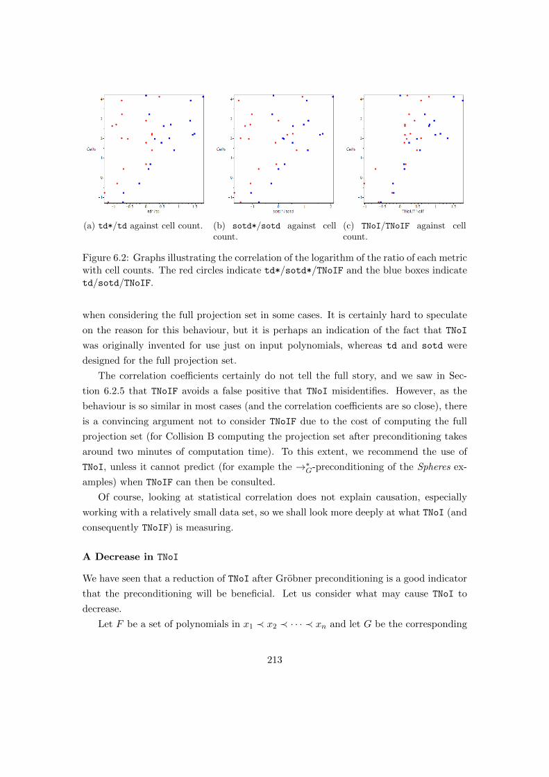
(a) td*/td against cell count. (b) sotd*/sotd against cellcount.

(c) TNoI/TNoIF against cellcount.

Figure 6.2: Graphs illustrating the correlation of the logarithm of the ratio of each metricwith cell counts. The red circles indicate td*/sotd*/TNoIF and the blue boxes indicatetd/sotd/TNoIF.

when considering the full projection set in some cases. It is certainly hard to speculate

on the reason for this behaviour, but it is perhaps an indication of the fact that TNoI

was originally invented for use just on input polynomials, whereas td and sotd were

designed for the full projection set.

The correlation coefficients certainly do not tell the full story, and we saw in Sec-

tion 6.2.5 that TNoIF avoids a false positive that TNoI misidentifies. However, as the

behaviour is so similar in most cases (and the correlation coefficients are so close), there

is a convincing argument not to consider TNoIF due to the cost of computing the full

projection set (for Collision B computing the projection set after preconditioning takes

around two minutes of computation time). To this extent, we recommend the use of

TNoI, unless it cannot predict (for example the →∗G-preconditioning of the Spheres ex-

amples) when TNoIF can then be consulted.

Of course, looking at statistical correlation does not explain causation, especially

working with a relatively small data set, so we shall look more deeply at what TNoI (and

consequently TNoIF) is measuring.

A Decrease in TNoI

We have seen that a reduction of TNoI after Grobner preconditioning is a good indicator

that the preconditioning will be beneficial. Let us consider what may cause TNoI to

decrease.

Let F be a set of polynomials in x1 ≺ x2 ≺ · · · ≺ xn and let G be the corresponding

213

Correlation Coefficient

rCells,T ime = 0.939

rtd∗,Cells = 0.456rtd,Cells = 0.692rtd∗,T ime = 0.446rtd,T ime = 0.677

rsotd∗,Cells = 0.330rsotd,Cells = 0.609rsotd∗,T ime = 0.272rsotd,T ime = 0.579

rTNoI,Cells = 0.770rTNoIF,Cells = 0.743rTNoI,T ime = 0.778rTNoIF,T ime = 0.754

Table 6.7: Correlation coefficients for the logarithm of ratios of cell counts, time, andvarious heuristics (td*, sotd*, td, sotd, TNoI, TNoIF).

(purely lexicographic) Grobner basis. The following three reasons are ways that TNoI

may be less for G than F :

1. The number of polynomials in a particular set of variables, xi1 , . . . , xi`, is de-

creased. If xk is the most important variable in this set, then having fewer polyno-

mials can simplify the decomposition of (x1, . . . , xk)-space. If constructing CAD

by projection and lifting, then this will also reduce the size of all projection sets at

or below level k. These effects will then manifest themselves in the overall CAD

by simplifying lifting stages, reducing both the number of cells and the time taken

to construct the remaining levels.

2. At least one variable is eliminated from a polynomial in F when computing G. If

the variable xk is eliminated from f (that is, when f is reduced during construction

of G, xk is eliminated), then this will have an effect on the CAD constructed. In

particular for projection and lifting, p will not be involved in the kth lift: from

(x1, . . . , xk−1)-space to (x1, . . . , xk−1, xk)-space. If k < n then this simplification

will also simplify further lifting stages. This simplification will reduce the cells

produced and the time taken to construct the CAD.

3. A polynomial, f , in a large number of variables, say k, is replaced by polynomials

g1, . . . , gj (j > 1) each with ki variables such that∑j

i=1 ki < k. If we consider

CAD construction (by projection and lifting or by regular chains) then increasing

214

the number of polynomials will generally increase the number of resultants and

discriminants computed. However, these polynomials, as they are in fewer vari-

ables, will be involved in fewer levels and so will have a smaller effect on the CAD

than the larger polynomial with many variables.

Let us consider this case a little more precisely: through discriminants, coefficients

and resultants, f will be involved in k levels of projection and lifting (all variables

will be used). Similarly, the gi will each feature in ki levels of projection and lifting.

Obviously the sets of variables each gi involves may intersect one another, but at

most there will be∑j

i=1 ki distinct variables. Therefore at worst the gi will feature

in∑j

i=1 ki levels of projection and lifting. This is strictly less than the levels that

would be involved with f and so, as long as the degrees of the gi are not excessive,

this should be similar to the effect of point 2 and CAD construction will see a

benefit.

Of course, in general, there is not simply one reason for the decrease in TNoI: there

may be many factors at work at once. There may also be increases in TNoI that are

getting counteracted, which presumably explains the occasional ‘false positive’ such as

CMXY 2 which shows an increase in TNoI but an improvement in CAD efficiency.

Also, it is interesting to note TNoI does not take into account the degree of the

polynomials produced by Grobner preconditioning. The degree of a Grobner basis was

shown [Yap91] to be, in the worst case, at least:

d2cn , with c ∼ 0.5.

This makes it more surprising that TNoI does so well to predict the effect of precon-

ditioning and suggests, with respect to Grobner preconditioning at least, variables are

more significant than degree (which, of course, agrees with the complexity estimates of

CAD discussed in Section 2.6).

These arguments should transfer to justify the use of TNoIF, where many of the

points discussed (projection set size, elimination of variables throughout projection sets)

should directly manifest themselves.

Using metrics with →∗GIt is interesting to consider how the metrics align with preconditioning by →∗G. The re-

sults in Tables 6.5 and 6.6 suggest that all three of the top-level metrics (td*, sotd* and

TNoI) behave similarly: there is a reduction from no preconditioning to→∗G precondition-

215

ing, and only sometimes a reduction from =G preconditioning to →∗G preconditioning.

This aligns loosely with the benefits shown from the preconditioning but is obviously

based on a minimal set of examples. The results are clearer with the metrics on the

full projection sets (td, sotd, TNoIF) where generally the metric predicts the benefits of

→∗G, however sotd misidentifies Spheres 1, 2 (sotd increases from 5 to 9, whereas the

cell counts decreases from 267 to 99).

6.2.7 Mathematical Justification

Grobner basis preconditioning (=G)

Informally, taking a Grobner basis of a set of polynomials constructs a ‘simple’ way of

representing the ideal they generate — they exhibit a clear structure and are as reduced

(with respect to each other) as possible. However, as exhibited by examples where

preconditioning is detrimental, matters are not so simple.

A Grobner basis will generally remove any redundancies from a set of polynomials.

This may involve reducing polynomials with respect to each other, or identifying common

factors. Doing so should benefit the construction of a CAD: when using projection-based

CAD we would otherwise still be identifying these factors and having simpler polynomials

to start with will produce simpler projection sets. This structural simplification will also

be produced when creating CADs through complex decompositions (as in [CMXY09] or

[CM12]) where resultants and greatest common divisors are computed, although the

simplification is not in such an obvious way.

Remark 6.2.

In Maple’s implementation of the Grobner basis algorithm there is no guarantee that

the polynomials are reduced with respect to the basis. They are also generally not

computed using Buchberger’s Algorithm from [Buc65, Buc06] but instead more modern

algorithms such as the F4 algorithm or FGLM algorithm [FGLM93] which converts a

basis to one of a different monomial order.

We can be a little more precise than the comment in [BH91] that Grobner bases

produce “triangularized” formulae. Let G be a purely-lexicographical (with x1 ≺ x2 ≺· · · ≺ xn) Grobner basis of a zero-dimensional ideal. Then G has the form:

216

G1 : p1(x1)

G2 : p2,1(x1, x2), . . . , p2,k2(x1, x2)

· · · · · ·Gn : pn,1(x1, . . . , xn), . . . , pn,kn(x1, . . . , xn)

where degxi(pi,j) ≤ degxi(pi,j+1) and pi,ki is monic in xi [Dav14, §3.3.7]. It seems clear

that a set of polynomials in this form would be ideal for CAD construction by projection

and lifting.

Denote the set of polynomials in G of level k by Gk. Then in the first round of

projection (eliminating xn) only the polynomials in Gn are used to compute coefficients,

discriminants and resultants. In general, when eliminating xk the polynomials from Gk

along with those generated by earlier projections of Gk+1, . . . , Gn are used (and the

polynomials in G1, . . . , Gk−1 are disregarded). If we are dealing with a set of polyno-

mials that have not been preconditioned then the set is unlikely to have this structure.

Therefore more polynomials are likely to have variables at a high level and so influence

the entire projection process.

This discussion is only for zero-dimensional ideals, but it explains why a purely

lexicographical monomial order is of use. When an ideal has positive dimension then it

may have part of this structure, with stratification across levels of polynomials, but in

not quite as strict a way (see Example 6.1).

An interesting question is why Grobner basis preconditioning is not universally bene-

ficial. When trying to find the ‘simplest’ way to represent a polynomial ideal, a Grobner

basis might produce extra polynomials of possibly high degree. In [MR10] the authors

show that an upper bound on the total degree of a Grobner basis of a set of polynomials

with maximum total degree d defining an r-dimensional ideal in n variables is:

≤ 2

(1

2dn−r + d

)2r

.

Further, we know from [Yap91], there exists a set of polynomials of degree bounded by

d for which a Grobner basis will include a polynomial of degree at least:

d2cn , with c ∼ 0.5.

Therefore a Grobner basis can increase the number and degree of polynomials sub-

217

stantially (up to a doubly exponential factor), which will increase the complexity and

cost of constructing a CAD due to a large increase in the number and degree of resultants

and discriminants computed (and the extra cells that they would subsequently define).

It is worth noting that when a Grobner basis is computed, it is done so with respect

to the complex ideal for the polynomials. It does not distinguish between the real and

complex solutions. This means that the ‘simplified structure’ will be as viewed over

the complexes which may have ramifications over the reals. Obviously a perfect pre-

conditioning method would work over the reals instead, which would eliminate solutions

over the complexes. Even though CADs are constructed over the real numbers, complex

behaviour can be significant: if we consider the two non-intersecting circles x2 + y2 − 9

and x2 + (y − 1)2 − 1 then constructing a CAD (with PL-CAD, RC-Rec-CAD or RC-

Inc-CAD and y ≺ x) identifies a spurious point y = 92 which corresponds to a complex

intersection of the circles with x = ±3i√

52 [Dav11]. Ideally a real-solution inclined pre-

conditioning method would identify that, whilst the y-component of this solution is real,

the x-component is complex and so this ‘shadow’ of a solution would not appear in the

CAD.

The issue with preconditioning over the real numbers is that doing so would come

much closer to simply solving the problem and so is likely to be much more costly. It

would be a worthy research topic to investigate the interaction of triangular decomposi-

tions over the reals (for example [CDM+10, Che11]) with CAD. Triangular decomposi-

tion may prove useful preconditioning for CADs constructed by regular chains [CMXY09]

as they are based on the same technology.

Grobner reduction preconditioning (→∗G)

Now let us consider the further preconditioning of →∗G where inequalities are reduced

with respect to the Grobner basis. It is worth noting that this is not restricted to

simply Grobner bases: any equational constraint, f = 0, can be used to reduce other

polynomials in a CAD problem as the only solutions that we care about are when f

vanishes, and so multiples of f can be added or subtracted to the other polynomials

without changing the set of solutions.

Remark 6.3.

Although we do not require a Grobner basis to apply reduction, it is necessary to ensure

a canonical and well-defined complete reduction. For example [Dav14], if f1 := x − 1,

f2 := x2 and g := x2 − 1 then reducing g with respect to f1, f2 gives both 0 and

−1 depending on which polynomial we chose to use for reduction. However, taking a

218

Grobner basis of f1, f2 gives the trivial ideal 〈1〉 and so g uniquely reduces to 0.

Consider a set of m polynomials, A, with max degree d, and maximum norm length

l. Collins [Col75] showed that the construction of a CAD for A is dominated by:

(2d)4n+4m2n+6

l3. (6.6)

Now let E be the set of equational constraints (f = 0 | f ∈ E) for the problem (with

each f ∈ A) and let g ∈ A be any non-equational constraint. We assume that E is a

Grobner basis simply to prevent the need to worry about non-unique reductions. Let g∗

be the complete reduction of g with respect to E. Then three cases may occur:

g∗ = 0 If g reduces to 0 then m is reduced by 1, d is possibly reduced (or at worst stays

constant), and l is possibly reduced (or at worst stays constant). Therefore the

CAD will be dominated by a lower bound.

g∗ 6∈ 0, g In this case then g has been reduced but not fully. Therefore m remains

constant and d is possibly reduced (or at worst stays constant). The norm length

of g may have increased, and therefore l may have increased. However if there is

any change in d then this will greatly outweigh any increase in l (due to the double

exponential in d).

g∗ = g If g does not reduce at all then m, d and l remain unchanged and therefore so

does the complexity bound.

Obviously this discussion is related to an upper bound on the complexity, so the CAD

itself may not be simplified. However, any decrease in degree or number of polynomials

will simplify the CAD if there is a reduction in the real roots present in the polynomial,

its discriminant, or its resultants. If an increase in norm length occurs, this should not

affect the constructional complexity of the CAD significantly.

The TNoI Metric

We have already discussed in Section 6.2.6 why the TNoI (and TNoIF) metric may be

reduced, and why it is useful for predicting the benefit of Grobner preconditioning. This

aligns with the mathematical justification given in Section 6.2.7 for =G.

In Section 6.2.6, it was discussed briefly how the metrics are loosely aligned with

→∗G-preconditioning on a small set of examples (with the metrics on the full projection

sets being preferable). We now think about the effect this preconditioning would have

on the metrics.

219

When we take the Grobner normal form of a polynomial we are successively taking

the remainder of the polynomial with respect to the Grobner basis. In doing so, we

will potentially reduce the total degree of the polynomial, or the number of indetermi-

nates. However it will potentially increase the number of monomials in a polynomial

(by reducing a term in a polynomial by a dense polynomial in the Grobner basis).

Therefore it is possible that td*, td, TNoI and TNoIF will remain constant or reduce

with →∗G-preconditioning, but sotd* and sotd will increase. We have seen that →∗G-

preconditioning should be generally beneficial which suggests that td*, td, TNoI and

TNoIF are better metrics to use than sotd* and sotd. This is supported by the fact that

sotd wrongly predicts the effect of →∗G-preconditioning on some of the Spheres 1, 2examples.

6.2.8 Grobner preconditioning with EC-CAD and RC-Inc-CAD

Grobner preconditioning can be combined with other CAD techniques. We will now

briefly investigate the effect it has on building CADs with equational constraints and

with new CAD algorithms. Later (Section 7.1.2), we will look at preconditioning in

relation to TTICADs and other ideas.

Grobner preconditioning with equational constraints

For =G preconditioning to be possible, a problem needs to contain a conjunction of

at least two equalities in a sub-formula. If these conjuncted equalities occur in the

main formula, then all the fi are also equational constraints. Therefore the equational

constraint projection operator and lifting procedure [McC99] can be used to reduce the

size of the CAD. We will only consider utilising one equational constraint primarily as

the ProjectionCAD package does not implement the theory of bi-equational constraints.

Once =G-preconditioning has been applied, then replacing the fi with the new

Grobner basis means all the fi are equational constraints and eligible for use with equa-

tional constraint technology. It seems of interest to investigate if equational constraints

are still of use following Grobner preconditioning and whether they have the same effect.

Table 6.8 shows the effect of =G-preconditioning combined with equational constraint

technology. For each example the following are constructed: a standard PL-CAD (us-

ing McCallum’s projection operator); a =G-preconditioned PL-CAD; an equational con-

straint PL-CAD with respect to each of the original equational constraints (where ‘FAIL’

indicates the equational constraint is nullified); an equational constraint PL-CAD with

respect to each of the =G-preconditioned equational constraints.

220

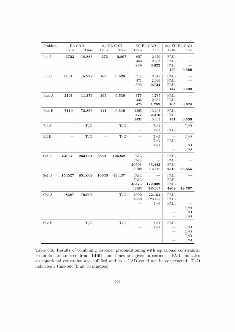
Problem PL-CAD =G-PL-CAD EC-PL-CAD =G-EC-PL-CADCells Time Cells Time Cells Time Cells Time

Int A 3723 18.885 273 0.897 657 2.670 FAIL —463 2.633 FAIL —269 0.822 FAIL —

195 0.566

Int B 3001 15.272 189 0.528 711 2.617 FAIL —471 2.936 FAIL —303 0.724 FAIL —

147 0.408

Ran A 2101 11.376 165 0.530 375 1.785 FAIL —435 2.367 FAIL —425 1.759 165 0.624

Ran B 7119 73.856 141 0.540 1295 13.293 FAIL —477 2.416 FAIL —1437 15.433 141 0.530

Ell A — T/O — T/O — T/O — T/O— T/O FAIL —

Ell B — T/O — T/O — T/O — T/O— T/O FAIL —— T/O — T/O

— T/O

Sol A 54037 263.054 28501 126.930 FAIL — FAIL —FAIL — FAIL —

20593 65.443 FAIL —22109 116.412 12513 53.655

Sol B 154527 851.669 10633 44.437 FAIL — FAIL —FAIL — FAIL —

48475 172.039 FAIL —63583 345.607 4809 19.767

Col A 8387 79.006 — T/O 2999 22.152 FAIL —2999 23.198 FAIL —

— T/O FAIL —— T/O— T/O— T/O

Col B — T/O — T/O — T/O FAIL —— T/O — T/O

— T/O— T/O— T/O

Table 6.8: Results of combining Grobner preconditioning with equational constraints.Examples are sourced from [BH91] and times are given in seconds. FAIL indicatesan equational constraint was nullified and so a CAD could not be constructed. T/Oindicates a time-out (limit 30 minutes).

221

There are some interesting things to note from Table 6.8. Comparing the =G-PL-

CAD and EC-PL-CAD columns we see that Grobner preconditioning usually has a

stronger effect than equational constraints. However, equational constraints has the

added benefit of never being detrimental to CAD construction (the equational constraint

projection set is simply a subset of the McCallum projection operator).

When combined, Grobner preconditioning and equational constraints prove even

more powerful. The final column shows that startlingly low cell counts can be obtained

for these reasonably difficult problems. As utilising an equational constraint can only

be beneficial, this is unsurprising.

What is also unsurprising is that lifting with respect to equational constraints from

the Grobner basis often fails due to nullification on a cell of positive dimension. This

is due to the loosely triangular structure that lexicographical Grobner bases exhibit (as

discussed in Section 6.2.7) which results in equational constraints in few variables. As a

compatible variable ordering is used, these polynomials with few variables are at a low

level (including often, a univariate polynomial in the lowest variable) and so are nullified

on positive dimensional cells simply by construction of a sign-invariant CAD.

Grobner preconditioning with incremental CAD

We now consider constructing CADs incrementally by regular chains [CM12] (Section

2.5.3). One particular advantage of this approach is the ability to easily use all possible

equational constraints. In constructing the complex tree for a given problem, refine-

ment with respect to equational constraints allows for all constraints to be used, unlike

projection-based techniques.

This has an interesting effect on Grobner preconditioning. Table 6.9 shows the

effect of Grobner preconditioning on RC-Inc-CAD. Preconditioning seems to alter the

constructed CAD to a smaller degree than PL-CAD or RC-Rec-CAD, in part due to the

fact multiple equational constraints are being considered.

Consider the first example, Intersection A.

x2 − 1

2y2 − 1

2z2 = 0 ∧ xz + zy − 2x = 0 ∧ z2 − y = 0.

Utilising all the equational constraints will consist of identifying all the points were

all three equations are satisfied. The solution set consists of 3 real solutions and the

incremental algorithm will identify these three points and build a CAD that identifies

just these points. This CAD consists of three planes (parallel to the plane defined by

the axes of the two largest variables) intersecting the solution points. Each plane is

222

Problem RC-Inc-CAD =G-RC-Inc-CADCells Time Cells Time

Int A 19 0.105 19 0.101Int B 19 0.102 19 0.092Ran A 31 0.131 31 0.124Ran B 31 0.140 31 0.130Ell A 10395 28.966 10395 31.113Ell B 67113 399.152 9345 46.292Sol A 29 0.158 29 0.147Sol B 33 0.202 33 0.160Col A 595 3.041 271 1.664Col B 2803 318.570 — T/O

Table 6.9: The experiments from [BH91] as rerun with RC-Inc-CAD in Maple. Timesare in seconds and T/O means a time-out (limit 30mins).

divided by a line through its solution point (parallel to the axis of the main variable),

and the solution point divides this line. This results in four three-dimensional cells,

six two-dimensional cells, six one-dimensional cells, and the three zero-dimensional cells

at the solution points. This gives the smallest possible CAD that is identified by the

incremental algorithm.

Applying Grobner basis preconditioning to the polynomials in the above example

does not change the solution set as the Grobner basis is, by definition, a basis of the

ideal defined by the polynomials. Therefore exactly the same CAD is produced by the

incremental CAD. This is true of the first four examples.

The latter examples show that Grobner preconditioning can still be of use when

there are non-equational constraints present, although the Solotareff examples show

that the presence of non-equational constraints does not guarantee a change when using

preconditioning.

Note also that as the behaviour of preconditioning is notably different to that of PL-

CAD or RC-Inc-CAD it is likely that TNoI or TNoIF will not be as effective as heuristics.

They should still be of more use than td*, td, sotd*, or sotd though, and could still be

used to help decide whether to precondition (although this requires further research).

6.2.9 Extensions to the theory

We briefly discuss some interesting extensions to Grobner preconditioning and potential

future research topics.

223

Phisanbut [Phi11] investigated the application of CAD to branch cuts in the complex

plane (discussed in Section 2.8.1). These problems generally contain “half-line” formulae:

f = 0 ∧ g > 0. These can be pseudo-reduced to f = 0 ∧ prem(g, f) > 0, where prem

indicates the pseudo-remainder. To ensure the sign of this pseudo-remainder is the same

as g, we must multiply g by an even power of the leading coefficient of f . Phisanbut

found that often, but not always, this pseudo-reduction resulted in a significant decrease

in the number of cells. It would be interesting to investigate the combination of this

preconditioning following the application of =G, and compare to the effect of →∗G.

We know that variable ordering is of importance for both CAD construction and

Grobner basis computation. Throughout this chapter we have assumed that the variable

ordering has been fixed before considering whether to precondition or not. Obviously a

variable ordering may not be fixed (although the choice may be restricted in quantifier

elimination problems) and the choice of ordering and preconditioning will likely be de-

pendent on each other. Initial exploratory experiments suggest that the choices are not

straightforward: preconditioning may be beneficial with one variable ordering and not

with another; the best variable ordering without preconditioning can be different from

the best variable ordering with preconditioning. Ideally, one could identify a heuristic

that could be used to pick the best choice of variable ordering and preconditioning, but

this would not be a small task: a large amount of data would need to be collected (for

each problem in n variables, 2(n!) experiments would need to be conducted). This is

revisited in Chapter 7.

In Table 6.3 the proportion of time spent between creating the complex decompo-

sition and converting it to a RC-Rec-CAD of real space was investigated. There was

an interesting shift, with the complex decomposition dominating most examples after

preconditioning. It would be interesting to investigate whether this shift still occurs

when using RC-Inc-CAD, along with how variable ordering affects these timings.

One of the most promising ideas for heuristics is that of machine learning and in

Section 5.3 we discussed the application of machine learning techniques to choose a

heuristic for the choice of variable ordering. It seems like Grobner preconditioning is

also well-suited for the application of machine learning. It would be interesting to use

machine learning in two ways with Grobner preconditioning: indirectly making it select

a heuristic to use for a given problem (from those heuristics discussed in Section 6.2.4);

or directly answering if preconditioning should be applied or not.

224

6.2.10 Conclusions on Grobner Preconditioning

In this section we conclusively showed that Grobner preconditioning for CAD construc-

tion is a worthwhile area of study. Taking a Grobner basis of a conjunction of equalities

was shown to be generally beneficial, although there are cases where it can be detri-

mental to the complexity of the subsequent CAD. Experimental data was backed up by

mathematical justification why this may be the case. A metric, TNoI (and its generali-

sation TNoIF), was given and it was shown to be well correlated to when preconditioning

is beneficial, with mathematical reasons given for this behaviour.

Further preconditioning was given by reducing inequalities with respect to the com-

puted Grobner basis. Experimentation suggests this is always beneficial (when it is

possible) and complexity bounds on CAD support this.

The effect of combining Grobner preconditioning with other advances in CAD theory

was investigated and shown to be beneficial when combined with equational constraints

or incremental CAD. Finally, suggestions of how to extend this preconditioning and more

accurately predict its effect were briefly discussed.

6.3 Case Study: The Piano Mover’s Problem

We demonstrate the benefit of choosing the correct expression of a problem for CAD

by considering the Piano Mover’s Problem2 of moving an infinitesimally thin piano

through a right angled corridor. An expression of this problem was shown in [Dav86] to

be infeasible when tackled with CAD and that is still the case 25 years later.

We do not present this section as an argument for using CAD for robotic motion

planning. Indeed, the intention of using the Piano Mover’s problem is precisely to have

a problem that is very difficult for CAD to tackle, and to therefore have a case study

of how the mathematical description of a problem can affect the feasibility of using

CAD. Further, any motion planning application would not require the solution of a

single setting (such as given in this chapter), but repeated computations for different

environments with multiple objects. These would need to be solved in essentially real

time, which is beyond the scope of CAD.

Various amounts of geometric analysis can offer alternative expressions and we survey

the literature demonstrating their effectiveness. These simpler formulations allow CAD

2There seems little consistency in the literature with regards to the punctuation of Piano Mover’s,with instances of Piano Mover’s, Piano Movers’, and Piano Movers. All options are valid possibilities,and we use the convention of Piano Mover’s, corresponding to a singular protagonist (as our piano isinfinitely thin, therefore weightless, and so easily carried by one piano mover).

225

1

2

Figure 6.3: The piano mover’s problem considered in [Dav86].

to easily address the question of the existence of a path. We do not rely on subtle geo-

metric analysis but produce a new expression for which both a CAD can be constructed

and from which an actual path could be determined (if one exists). A comparison of the

CADs produced by all methods is given.

The ideas in this section will lead to general ideas about the expression of a problem

for CAD which will be discussed in Section 6.4.

All the work in this section is adapted from [WDEB13] which first appeared in the

Technical Report [WBDE13].

6.3.1 Introduction to the Piano Mover’s Problem

In [SS83b] the authors define the general Piano Mover’s Problem as: “given a body B

and a region bounded by a collection of walls, either find a continuous motion connecting

two given positions and orientations of B during which B avoids collisions with the walls,

or else establish that no such motion exists.” Such a problem can commonly arise in

robotics.

A simple example of such a problem was given in [Dav86], where the author consid-

ered moving a ladder of length 3 through a right-angled corridor of unit width. This is

shown in Figure 6.3 where we wish to move the ladder from position 1 to position 2. A

simple geometric analysis shows that with a ladder of length 3 there is no solution to this

particular problem: it is only possible to traverse the corridor if the ladder has length

less than√

8. The work in [SS83a, SS83b, Dav86, etc] and continued in [WDEB13]

investigates how this and similar piano mover’s problems may be decided automatically

through CAD, providing a path when a solution exists.

In [SS83b] the authors proposed a generic approach to piano mover’s problems in

which the problem is described using polynomial algebra and then solved using a CAD

algorithm. However, for even very simple examples this approach can be computationally

226

infeasible. In [Dav86] the author applied this approach to the problem shown in Figure

6.3 and demonstrated that the scale of computations required rendered this approach

completely infeasible. Despite 25 years of improvements in CAD theory and computer

hardware, creating a CAD with respect to this algebraic formulation is still infeasible.

6.3.2 Original formulation of the problem from [Dav86]

In [Dav86] the author considered building a CAD to solve the problem of moving a ladder

of length 3 through a right-angled corridor of width 1 (as in Figure 6.3). Denoting the

endpoints of the ladder as (x, y) and (w, z) and assuming the outer corner of the corridor

as the origin, the formulation provided was:

[[(x− w)2 + (y − z)2 − 9 = 0

]∧[

[yz ≥ 0] ∨ [x(y − z)2 + y(w − x)(y − z) ≥ 0]]∧[

[(y − 1)(z − 1) ≥ 0] ∨ [(x+ 1)(y − z)2 + (y − 1)(w − x)(y − z) ≥ 0]]∧[

[xw ≥ 0] ∨ [y(x− w)2 + x(z − y)(x− w) ≥ 0]]∧[

[(x+ 1)(w + 1) ≥ 0] ∨ [(y − 1)(x− w)2 + (x+ 1)(z − y)(x− w) ≥ 0]] ]. (6.7)

The first equation in (6.7) describes the length of the ladder, and the remaining

inequalities describe the valid positions, ensuring the ladder does not intersect any of

the four walls. In [Dav86] the author completed the projection phase of Collin’s CAD

algorithm, finding over 250 distinct univariate projection factors with total degree as

high as 26. The technology available for the paper did not allow for the simultaneous

root isolation of these. With current hardware and software (Qepcad-B 1.69 and the

recursive regular chains CAD algorithm) it still remains outside the realm of computation

to complete the construction of the CAD.

6.3.3 Other Approaches in the Literature

We freely acknowledge that in a practical robotic application, the piano mover’s problem

would typically be tackled using numerical or hybrid methods. This allows for an effi-

cient solution and can even provide exact solutions. We are instead concerned with the

symbolic approach to the problem through CAD. We now discuss previous approaches

to this problem with CAD in the literature.

The first substantial work on approaching the piano mover’s problem symbolically

with CAD was [SS83b]. In [SS83a] the same authors had proposed a separate approach

227

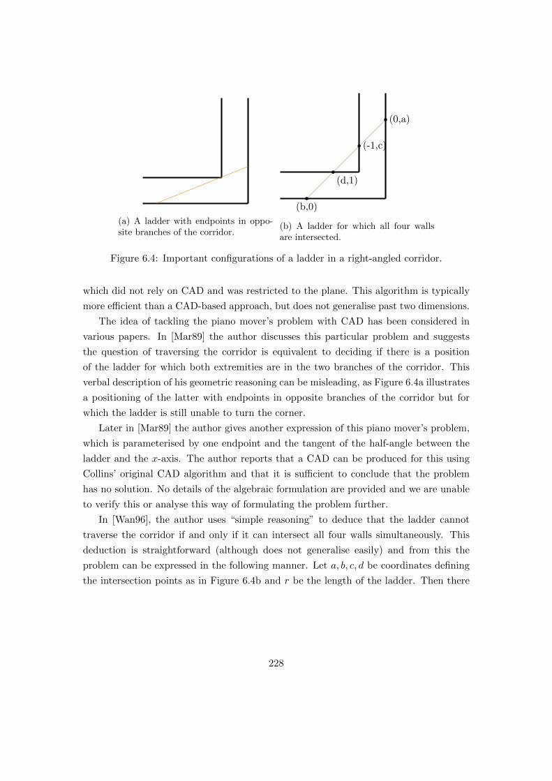
(a) A ladder with endpoints in oppo-site branches of the corridor.

(b,0)

(0,a)

(d,1)

(-1,c)

(b) A ladder for which all four wallsare intersected.

Figure 6.4: Important configurations of a ladder in a right-angled corridor.

which did not rely on CAD and was restricted to the plane. This algorithm is typically

more efficient than a CAD-based approach, but does not generalise past two dimensions.

The idea of tackling the piano mover’s problem with CAD has been considered in

various papers. In [Mar89] the author discusses this particular problem and suggests

the question of traversing the corridor is equivalent to deciding if there is a position

of the ladder for which both extremities are in the two branches of the corridor. This

verbal description of his geometric reasoning can be misleading, as Figure 6.4a illustrates

a positioning of the latter with endpoints in opposite branches of the corridor but for

which the ladder is still unable to turn the corner.

Later in [Mar89] the author gives another expression of this piano mover’s problem,

which is parameterised by one endpoint and the tangent of the half-angle between the

ladder and the x-axis. The author reports that a CAD can be produced for this using

Collins’ original CAD algorithm and that it is sufficient to conclude that the problem

has no solution. No details of the algebraic formulation are provided and we are unable

to verify this or analyse this way of formulating the problem further.

In [Wan96], the author uses “simple reasoning” to deduce that the ladder cannot

traverse the corridor if and only if it can intersect all four walls simultaneously. This

deduction is straightforward (although does not generalise easily) and from this the

problem can be expressed in the following manner. Let a, b, c, d be coordinates defining

the intersection points as in Figure 6.4b and r be the length of the ladder. Then there

228

is no solution if and only if:

(∃a)(∃b)(∃c)(∃d)[ [a2 + b2 = r2

]∧ [r > 0] ∧ [a ≥ 0] ∧ [b < 0] ∧ [c ≥ 1] ∧ [d < −1]

∧ [c− (1 + b)(c− a) = 0] ∧ [d− (1− a)(d− b) = 0]]. (6.8)

As there is only a single free variable, the length r, and the relative simplicity of the

formulation Qepcad can solve the given problem almost instantly, using a partial CAD

of 19 cells to state that the maximal length of the ladder is√

8 (a fact that can be

verified with a purely geometric argument). Note also that this problem contains three

equational constraints, of which Qepcad can use the theory of [McC99] to utilise one

of these.

In [Wan96], the authors notes that if the ladder intersected both outer walls and one

of the inner walls then it must also intersect the other inner wall. Therefore (6.8) can be

simplified further by removing the two formulae [d < −1] and [d − (1 − a)(d − b) = 0].

This can be considered further topological reasoning, but does not make a difference in

the timing or cell counts from Qepcad (although such reasoning could be powerful for

other problems).

In [McC97] the author approaches path-finding by considering transformations of

objects by a translation vector (x, y) and a rotation angle θ (instead of their absolute

position in Cartesian space). This produces 21 formulae in a relatively complicated

Boolean formula which describes the techniques. McCallum then appeals the theory of

equational constraints, partial CAD techniques, parallelisation and a form of sub-CAD

(described in Section 4.1.1) to construct a four-dimensional sub-CAD consisting of 16138

cells in 429 seconds.

In [YZ06] the authors looked at a two-dimensional rectangular piano, instead of the

one-dimensional ladder. They use geometric analysis to produce a simple condition for

the problem to have a solution. They describe the problem according to the position of a

particular corner of the rectangle and the angle the rectangle makes with the horizontal

axis. They allow for the corridors to have non-unit (and non-equal) widths (denoted a

and b) and include the length and width of the rectangle (denoted L and r) as two other

parameters. They then provide, through some highly non-trivial analysis, a positive

definiteness condition on a degree 8 polynomial involving these four parameters and a

single variable x: if this condition holds, then a valid route exists. Reducing the problem

to the ladder in Figure 6.3 with the ladder having length L, their reasoning states that

229

the existence of a valid route is equivalent to the truth of the following Tarski formula:

(∀x)[4x8 − 4(L− 3)x6 − 2(3L− 6)x4 − 2(L− 3)x2 + 1 > 0

].

As this is a single polynomial in two variables (one of which is quantified) it takes

Qepcad just 1.936 seconds (mostly initialisation time), and a partial CAD containing

only 5 cells, to return the equivalent formula[ [L2 − 8 < 0

]∨ [L < 0]

].

Although the approaches of [Wan96, YZ06] are highly efficient, they are also limited.

They require (especially in the case of [YZ06]) significant geometric deductions before

they use any CAD technology. Further, they can only answer whether the ladder can

traverse the corridor successfully, without information about what a successful path

could be. This approach could therefore be used as an initial way of deciding whether

a path is possible, thereafter a necessarily more-complicated CAD could be constructed

which would be sufficient for constructing a path.

The geometric approaches give descriptions in the real space describing the geometry

of the plan in which the ladder exists. In contrast, the approaches in [SS83b, Dav86] and

the new formulation we will give in 6.3.4 describe the geometry in a four-dimensional

configuration space: the coordinates of the two endpoints of the ladder within the plane.

This is an important distinction: working in a configuration space allows the constructed

CAD to be used to construct an explicit path, whereas a CAD of the real space can only

analyse if a ladder can move through the corridor or not.

The configuration space also allows us to consider further properties such as the ori-

entation of the ladder. The descriptions given in [Wan96] and [YZ06] cannot distinguish

whether the ladder is able to rotate within the corridor and exit in the reverse orientation

to its entry. This is an important point for generalisations of this problem, including

those discussed in Section 6.3.8.

The description of the problem in [McC97] is also within a configuration space,

although a different non-trivial one where positions are encoded through transformations.

6.3.4 New Formulation of the Problem

We now consider the problem from a different perspective within the same configuration

space as in [Dav86]. We describe all the possible invalid regions and then take their nega-

tion to describe the valid regions. As in (6.7) we denote the positions of the endpoints

230

AB

C

D

Figure 6.5: Four canonical invalid positions of the ladder. For positions A–C only oneend needs to be outside the corridor.

of the ladder by (x, y) and (w, z).

We break down this process to give the most clarity to the method.

Describing the invalid regions

There are four canonical invalid configurations of the ladder, and an example of each is

shown in Figure 6.5. Each invalid positioning can be described by an equivalent formula:

A: x < −1 ∧ y > 1 or w < −1 ∧ z > 1 — this describes any collision with the ‘inside’

walls along with the ladder being entirely on the inside of these (like ladder A is

positioned in Figure 6.5).

B: x > 0 or w > 0 — this describes any collision with the rightmost wall along with

the ladder being entirely to the right of this wall (like ladder B is positioned in

Figure 6.5).

C: y < 0 or z < 0 — this describes any collision with the bottommost wall along with

the ladder being entirely below this wall (like ladder C is positioned in Figure 6.5).

D: (∃t)[0 < t ∧ t < 1 ∧ x+ t(w − x) < −1 ∧ y + t(z − y) > 1] — this ensures no inner

point of the ladder lies in the invalid top-left region (like ladder D is positioned in

Figure 6.5).

We can hence characterise the invalid regions as:

(∃t)[

[x < −1 ∧ y > 1] ∨ [w < −1 ∧ z > 1] ∨ [x > 0] ∨ [w > 0] ∨ [y < 0]

∨ [z < 0] ∨ [0 < t ∧ t < 1 ∧ x+ t(w − x) < −1 ∧ y + t(z − y) > 1]]. (6.9)

231

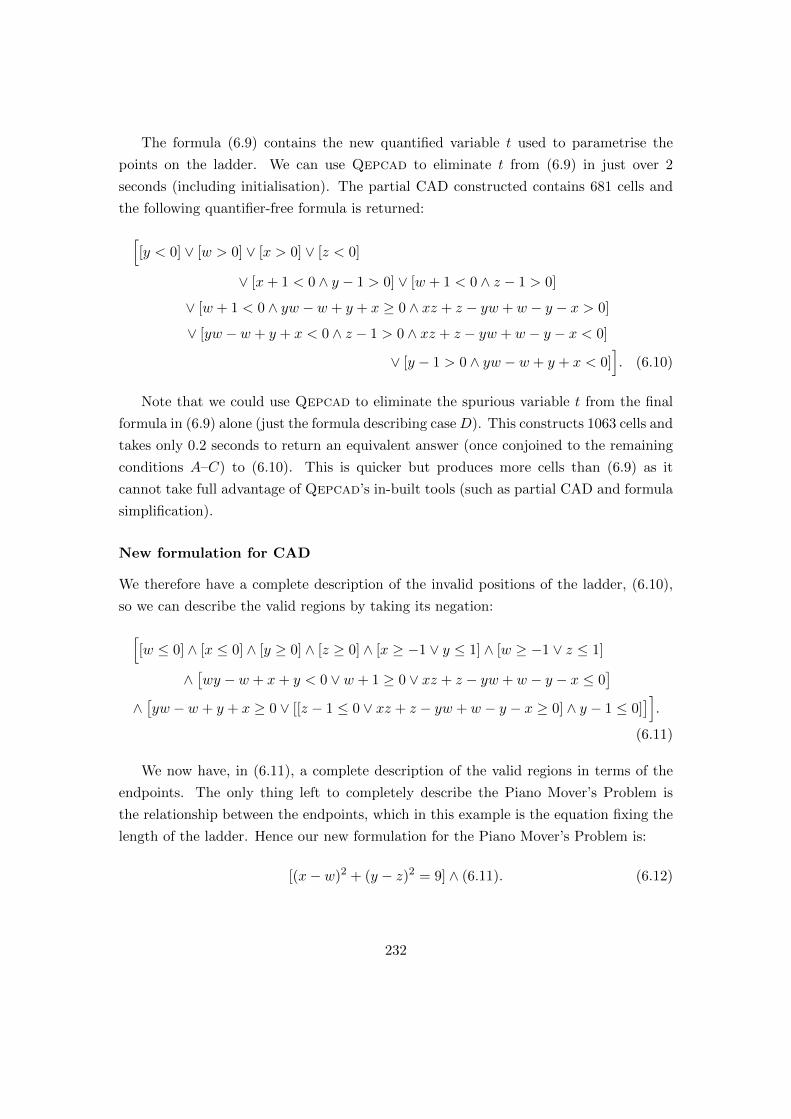
The formula (6.9) contains the new quantified variable t used to parametrise the

points on the ladder. We can use Qepcad to eliminate t from (6.9) in just over 2

seconds (including initialisation). The partial CAD constructed contains 681 cells and

the following quantifier-free formula is returned:

[[y < 0] ∨ [w > 0] ∨ [x > 0] ∨ [z < 0]

∨ [x+ 1 < 0 ∧ y − 1 > 0] ∨ [w + 1 < 0 ∧ z − 1 > 0]

∨ [w + 1 < 0 ∧ yw − w + y + x ≥ 0 ∧ xz + z − yw + w − y − x > 0]

∨ [yw − w + y + x < 0 ∧ z − 1 > 0 ∧ xz + z − yw + w − y − x < 0]

∨ [y − 1 > 0 ∧ yw − w + y + x < 0]]. (6.10)

Note that we could use Qepcad to eliminate the spurious variable t from the final

formula in (6.9) alone (just the formula describing caseD). This constructs 1063 cells and

takes only 0.2 seconds to return an equivalent answer (once conjoined to the remaining

conditions A–C) to (6.10). This is quicker but produces more cells than (6.9) as it

cannot take full advantage of Qepcad’s in-built tools (such as partial CAD and formula

simplification).

New formulation for CAD

We therefore have a complete description of the invalid positions of the ladder, (6.10),

so we can describe the valid regions by taking its negation:

[[w ≤ 0] ∧ [x ≤ 0] ∧ [y ≥ 0] ∧ [z ≥ 0] ∧ [x ≥ −1 ∨ y ≤ 1] ∧ [w ≥ −1 ∨ z ≤ 1]

∧[wy − w + x+ y < 0 ∨ w + 1 ≥ 0 ∨ xz + z − yw + w − y − x ≤ 0

]∧[yw − w + y + x ≥ 0 ∨ [[z − 1 ≤ 0 ∨ xz + z − yw + w − y − x ≥ 0] ∧ y − 1 ≤ 0]

]].

(6.11)

We now have, in (6.11), a complete description of the valid regions in terms of the

endpoints. The only thing left to completely describe the Piano Mover’s Problem is

the relationship between the endpoints, which in this example is the equation fixing the

length of the ladder. Hence our new formulation for the Piano Mover’s Problem is:

[(x− w)2 + (y − z)2 = 9] ∧ (6.11). (6.12)

232

6.3.5 Applying CAD to the New Formulation

We can input (6.12) to Qepcad with the standard initialisation parameters (+N500000000

+L200000) and variable ordering x ≺ y ≺ w ≺ z. After a little under 5 hours (16933.701

seconds) of computation time a CAD of R4 was constructed with 285419 cells. The

following was the output, which is an equivalent formula to (6.12):

x ≤ 0 ∧ y ≥ 0 ∧ w ≤ 0 ∧ z ≥ 0 ∧ (y − z)2 + (x− w)2 = 9∧[[x+ 1 ≥ 0 ∧ w + 1 ≥ 0] ∨

[y − 1 ≤ 0 ∧ w + 1 ≥ 0 ∧ y2w2 − 2yw2 + x2w2+

2xw2 + 2w2 − 2xy2w + 4xyw − 2x3w − 4x2w − 4xw + x2y2 − 2x2y + x4+

2x3 − 7x2 − 18x− 9 ≥ 0]∨[x+ 1 ≥ 0 ∧ yw − w + y + x ≥ 0∧

w2 − 2xw + y2 − 2y + x2 − 8 > 0 ∧ z − 1 ≤ 0]∨[x+ 1 ≥ 0 ∧ yw − w + y + x ≥ 0∧

y2w2 − 2yw2 + x2w2 + 2xw2 + 2w2 − 2xy2w + 4xyw − 2x3w − 4x2w − 4xw+

x2y2 − 2x2y + x4 + 2x3 − 7x2 − 18x− 9 ≤ 0 ∧ z − 1 ≤ 0]∨ [y − 1 ≤ 0 ∧ z − 1 ≤ 0]

].

(6.13)

The output formula is not of great interest to solving the problem; the CAD con-

structed for (6.12) is needed for any substantial analysis. However, it is interesting to

try and deconstruct (6.13). The first five terms state that the ladder should have both

endpoints in the second quadrant of the plane, and that the ladder should have length 3.

The remainder of (6.13) is a large disjunction of clauses describing the valid positions.

The first clause of this disjunction describes the ladder being entirely within the vertical

corridor, and the final clause describes the ladder being entirely in the horizontal cor-

ridor. The remaining three clauses characterise the intermediate positions. Analysis of

the decompositions these equations describe requires knowledge of the adjacency of the

CAD of R4: this is far from trivial and will be discussed in Section 6.3.6.

When constructing a CAD, and producing an equivalent formula, Qepcad uses a

host of techniques, including partial CAD techniques (Section 2.4.2) and equational

constraints (Section 2.4.4) to simplify its calculations. We can suppress many of these

by using the full-cad command, which greatly increases the difficulty of constructing

a CAD. Constructing a full-cad of (6.12) takes just over a full day of computation

(88238.442 seconds) and produces 1691473 cells. The formula Qepcad produces in this

case is almost identical to (6.13), although a couple of cases are split differently.

A useful technique to attempt to speed up the construction is to introduce quantifiers.

In this case we can existentially quantify an endpoint of the ladder, which leads to a CAD

233

defining the valid positions of the opposite endpoint. Prefixing (6.12) with (∃ w)(∃ z) will

characterise the position of the (x, y) endpoint and takes Qepcad just over 50 minutes

(3052.753 seconds) to construct a CAD with 5453 cells. This sharp reduction will be

due to the reduced dimension of the CAD produced (R2 rather than R4) and the use

of partial CAD techniques, which can use these quantifiers to simplify the lifting stage.

The quantifier-free formula that Qepcad produces is

x ≤ 0 ∧ y ≥ 0 ∧ [x+ 1 ≥ 0 ∨ y − 1 ≤ 0], (6.14)

which is clearly stating that the point is within the original corridor. This is to be

expected as the quantified version of (6.12) is asking for those points where it is possible

to place an end of the ladder and find a valid position to place the other endpoint. There

is clearly a large redundancy in creating such a CAD however as the minimal CAD to

describe the corridor contains only 17 cells.

This existential partial CAD is not enough to solve the path finding problem, and

(6.14) contains little information. However, this is a useful experiment to test the feasi-

bility and complexity of a CAD problem: the original formulation from [Dav86], given in

(6.7), remains infeasible under the quantification (∃ w)(∃ z). Note also, that if a quan-

tified problem does not return the entire corridor then it can identify invalid regions

where no placing of the ladder can occur. If these invalid regions separate the start and

end positions into two distinct connected components, then it can be deduced that no

valid path exists.

We can use the p-2d-cad command in Qepcad to produce a visualisation of the

two-dimensional CAD (the induced CAD of R2 if the CAD has dimension 3 or greater).

Figure 6.6 shows the representation for the two-dimensional CAD for the existentially

quantified version of 6.12 (without quantifiers a similar diagram is produced, but with

the valid region simplified to omit all internal cell boundaries within the corridor). The

horizontal axis shows x in the range [−7, 2], and the vertical axis shows y in the range

[−2, 7]. There is a step size of 0.0025, which means that if two stacks are within 0.0025,

with respect to x, or two intra-stack cells are within 0.0025, with respect to y, then they

will be indistinguishable on the diagram.

It is clear from Figure 6.6 how complicated this seemingly simple problem is. It is

easy to identify important cell boundaries in the CAD that demonstrate edge cases of

the Piano Mover’s Problem: for example, when the ladder is stuck abutting the corner.

However, there are clearly many boundaries with little or no significance to answering the

question at hand. It would obviously be of great use to develop further CAD technology

234

Figure 6.6: A two-dimensional CAD of the (x, y)-configuration space constructed for thepiano mover’s problem from (6.12).

235

that removes these spurious boundaries.

Remark 6.4.

Mathematica can produce a cylindrical formula in 558.721 seconds, but for this appli-

cation such a formula is not sufficient to deduce paths (since that will require knowledge

of cell adjacencies and boundary cells, which cannot be inferred from the formula).

6.3.6 Adjacency for the Piano Mover’s Problem

One reason for working in four-dimensional configuration space (as opposed to the real

space that [Wan96, YZ06] consider) is that the constructed CAD can be used to construct

a valid path, as well as determine the existence of such a path. To construct a path

the adjacency and connectedness of the cells needs to be decided. Previous work on

adjacency in CAD is discussed in Appendix A. The original approach of [ACM84b]

for two dimensions was extended to three dimensions in [ACM88] but is not easily

generalised further and often requires well-behaved input. Four-dimensional adjacency is

currently not implemented within existing technology, and would be a hugely expensive

and complicated computation. Possible improvements to adjacency algorithms which

may be appropriate for the piano mover’s problem will be discussed in Appendix A.

In [SS83b] the authors considered adjacencies between cells in the top two layers

(of dimension n and n − 1). For our expression of the problem we have an equational

constraint so actually need the adjacencies between cells of dimension (n−1) and (n−2)

so this theory does not apply.

6.3.7 Choosing a Formulation

Comparing (6.12) to (6.7) there are some indicators that our new formulation is more

appropriate for CAD. In particular, the new formulation involves polynomials of lesser

degree: quadratic polynomials instead of cubics.

We can use the sotd metric from Definition 2.42 (from [DSS04]) to measure this.

Calculating the sotd of the input polynomials, which we denote sotd*, of the original

formulation gives 100 whereas the new formulation has an sotd* of only 33.

As originally defined in [DSS04], the sotd should be computed for the entire projec-

tion set. Doing so still indicates the new formulation is better, but the total sotd drops

only from 2006 to 1693. The size of these total sotd values emphasises the size of the

projection sets produced, with over 100 univariate polynomials alone being produced in

both formulations. It is therefore impractical to compute the ndrr from Definition 5.1

236

Formulation Cell Count sotd* sotd ndrr sowtd

Davenport — 100 2006 367 148Davenport (∃) — 100 2006 367 92New Formulation 285419 33 1693 301 72New Formulation (∃) 5453 33 1693 301 46

McCallum 16138 68 32 5 70Wang 19 19 98 17 27Yang-Zeng 5 35 39 2 23

Table 6.10: Heuristic values for various descriptions of the Piano Mover’s Problem.

(from [BDEW13]) for the formulations directly. We can compute the ndrr for each uni-

variate polynomial separately (which risks over counting by considering roots multiple

times), which gives 367 for the original formulation and 301 for the new formulation.

We can consider the sotd (at the top level and full projection set) and ndrr for the

alternative formulations of the piano mover’s problem, which are summarised in Table

6.10. Note that the sotd for the McCallum formulation is actually lower for the full

projection set than only at the top level due to repeated factors in the input.

None of the current heuristics incorporate quantifiers: their primary use is variable

ordering where quantifiers are involved passively by restricting possible orderings. Quan-

tifiers clearly have a huge effect on the feasibility of a formulation. We try to incorporate

the effect of quantifiers along with variable ordering into the following heuristic, sowtd.

Definition 6.8.

Let a CAD problem be defined with respect to the ordered variables x1 ≺ x2 ≺ · · · ≺ xn.

For each variable xi we assign a weight, w(xi): if xi is unquantified then w(xi) = i, and

if xi is quantified then w(xi) = i/2. We define the sum of weighted total degrees,

denoted sowtd, of a problem Φ (with polynomial set F ) to be

sowtd(Φ) =∑f∈F

∑m∈f

n∑i=1

w(xi) · degxi(m);

where m ranges over the monomials in f .

Table 6.10 also lists the sowtd values for each description of the Piano Mover’s

Problem. The sowtd values align with the cell counts for the formulations and seem a

fair indication of the magnitude of each one. It would be of interest to investigate the

behaviour of sowtd further: in particular to see if it be used to predict variable ordering

237

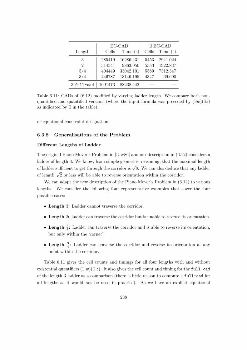
EC-CAD ∃ EC-CADLength Cells Time (s) Cells Time (s)

3 285419 16286.431 5453 2941.0242 314541 9863.950 5353 1922.837

5/4 404449 33042.101 5589 7312.3473/4 446787 13146.195 4347 69.690

3 full-cad 1691473 88238.442 — —

Table 6.11: CADs of (6.12) modified by varying ladder length. We compare both non-quantified and quantified versions (where the input formula was preceded by (∃w)(∃z)as indicated by ∃ in the table).

or equational constraint designation.

6.3.8 Generalisations of the Problem

Different Lengths of Ladder

The original Piano Mover’s Problem in [Dav86] and our description in (6.12) considers a

ladder of length 3. We know, from simple geometric reasoning, that the maximal length

of ladder sufficient to get through the corridor is√

8. We can also deduce that any ladder

of length√

2 or less will be able to reverse orientation within the corridor.

We can adapt the new description of the Piano Mover’s Problem in (6.12) to various

lengths. We consider the following four representative examples that cover the four

possible cases:

• Length 3: Ladder cannot traverse the corridor.

• Length 2: Ladder can traverse the corridor but is unable to reverse its orientation.

• Length 54 : Ladder can traverse the corridor and is able to reverse its orientation,

but only within the ‘corner’.

• Length 34 : Ladder can traverse the corridor and reverse its orientation at any

point within the corridor.

Table 6.11 gives the cell counts and timings for all four lengths with and without

existential quantifiers (∃ w)(∃ z). It also gives the cell count and timing for the full-cad

of the length 3 ladder as a comparison (there is little reason to compute a full-cad for

all lengths as it would not be used in practice). As we have an explicit equational

238

θ

θ

(a) Generic obtuse angled corridor.

ψ

ψ

(b) Generic acute angled corridor.

Figure 6.7: Angled corridors for the Piano Mover’s Problem.

constraint (the equation defining the length of the ladder) Qepcad can automatically

apply the theory of equational constraints.

The results of Table 6.11 are not necessarily intuitive. In the un-quantified formula-

tion the length 3 ladder produces the least cells, but the length 2 ladder is significantly

quicker than all other lengths. When quantified, the lengths all produce similar numbers

of cells, with length 3/4 producing the least cells and being substantially quicker than

the other lengths (with length 5/4 substantially longer than the other lengths).

Angled Corridors

We can generalise the Piano Mover’s Problem considered in [Dav86] to a non-right angled

corridor. We can easily consider the two cases of an obtuse angled corridor (Figure 6.7a)

and an acute angled corridor (Figure 6.7b).

We can easily convert the equations of the walls in Figures 6.7a and 6.7b into a

formula describing the new set of invalid positions (given in detail in [WDEB13]). We

proceed in the same manner as for the right-angled corridor (Section 6.3.4) by eliminating

the parameter t, taking the negation of the output, and then conjuncting with the length

of the ladder. This stage is straightforward, although produces around 170, 000 cells

when θ is π/4, and 100, 000 cells when ψ is π/4.

We can then use this formula to attempt to construct a CAD of the configura-

tion space. The two cases mentioned above (when θ or ψ is π/4) aborted after Qep-

cad had computed 50000000 cells (the limit imposed by the initialisation parameter

+N50000000). This increase in cells compared to (6.12) is due to the fact the corridor

is no longer aligned with the coordinate axes.

Generalising the methods of [Wan96] and [YZ06] is not straightforward. Whilst

Wang’s idea can be applied to the obtuse case (giving a maximal length of approximately

6.68), it does not suffice for the acute case (giving the wrong answer of 1.84). With an

239

acute corridor of angle π/4, a ladder of length√

5 can pass through, but has to reverse

orientation in the corner in the process. This orientation would be accounted for in

our formulation of configuration space, but is not encoded in the geometrical reasoning

of real space. Using the approach of [McC97] for angled corridors should be possible,

although care may need to be taken to ensure that certain trigonometric identities hold.

6.3.9 Constructing sub-CADs for the Piano Mover’s Problem

In Chapter 4 the idea of a cylindrical algebraic sub-decomposition (sub-CAD) was in-

troduced. Two particular types of sub-CAD were introduced: layered and variety sub-

CADs. We consider their applications to the Piano Mover’s Problem.

Lifting to a Layered Variety sub-CAD

All the cells that are valid in configuration space must lie on the three-dimensional variety

described by (x − w)2 + (y − z)2 = `2 (where ` is the length of the ladder). Therefore

we can construct a variety sub-CAD with respect to this equational constraint to help

tackle the Piano Mover’s Problem.

On this manifold, the cells of greatest importance are those that are full-dimensional

(with respect to the variety). We can therefore construct a 1-layered variety sub-CAD

which will contain the 3-dimensional cells satisfying the length constraint. To tackle the

problem we also require knowledge of the adjacency of these cells. We therefore need

the cells on the variety of one less dimension (two-dimensional cells for this example):

adjacencies of three-dimensional cells through one-dimensional or zero-dimensional cor-

respond to infeasible situations in the real space (such as a robot having to “tightrope

walk” an infinitesimally thin cell) and so are unnecessary. Therefore a 2-layered variety

sub-CAD should be sufficient to answer the Piano Mover’s Problem and provide a path.

We use the implementation of sub-CAD procedures in ProjectionCAD (discussed

in Appendix C). We begin by constructing a 1-layered variety sub-CAD. Constructing

the equational constraint projection set produces 11 polynomials (in R[y, w, z]) and

constructing a 1-layered sub-CAD of R3 takes 124.22 seconds in Maple to produce 64764

cells. Lifting over this sub-CAD to the variety takes a further 196.672 seconds, producing

101924 cells. This obviously offers substantial savings over computing a complete CAD

with Qepcad in both cells and time.

It is not yet feasible to construct the 2-layered variety sub-CAD (or complete variety

sub-CAD) within Maple. With the inclusion of partial CAD techniques or utilising

the simple inequalities as discussed in Section 4.7.1 this should be feasible. Adjacency

240

computations are still an issue and are discussed further in Appendix A.

6.3.10 Conclusions on the Piano Mover’s Problem

Although a generic symbolic solution to robot motion planning was provided in theory

by [SS83b], it still remains infeasible to tackle even simple examples, such as the one

considered in this section.

The simple example of moving a ladder through a right-angled corridor was shown in

[Dav86] to be infeasible when tackled directly by the approach [SS83b]. This approach

remains infeasible with current technology but by considering a different description of

the proof it is possible to construct a CAD of the four-dimensional configuration space

with Qepcad. By considering the negation of the invalid positions a formulation was

given with lower degree polynomials that was more suited for CAD.

It is possible to create a 1-layered variety sub-CAD with ProjectionCAD of the new

description, although a 2-layered variety sub-CAD is still infeasible. The CAD alone

does not provide a solution to the Piano Mover’s Problem, and the adjacencies of the

cells needs to be considered. This is beyond current technology, and it is an important

question whether adjacency techniques could be adapted to consider cells on a variety.

An alternative approach is to use geometric reasoning to rephrase the problem, such

as in [Wan96] and [YZ06]. This can be immensely powerful, reducing the problem to

a relatively simple quantifier elimination problem. However, such an approach cannot

provide a valid path, only reveal if such a path exists. Further, care needs to be taken

when generalising their approaches, as demonstrated with angled corridors. It is also

possible to adapt the configuration space, such as in [McC97] where the ladder was

parametrised trignometrically.

This example demonstrates the importance of how a problem is described for CAD,

and suggests that any major progress in tackling the robot motion planning problem

symbolically may be just as likely from more appropriate formulations than from ad-

vances in technology or hardware. The new description of the Piano Mover’s Problem

also suggests some general strategies for expressing a problem. These are discussed in

Section 6.4.

241

6.4 General Strategies for Describing a Problem for Cylin-

drical Algebraic Decomposition

The work of Brown in expressing the Joukowsky and Collision examples in Section

6.1 and the progress in the Piano Mover’s Problem discussed in Section 6.3 indicate

the benefit of an optimal expression of a problem for CAD. Further, the methods of

generating and manipulating the descriptions of the problems were all straightforward

and mathematically simple. Once an expression is given, then it may also be possible to

precondition using Grobner bases, as described in Section 6.2.

These examples suggest some general strategies for finding an optimal expression of

a problem:

Consider Negation In both the Joukowsky example and the Piano Mover’s Problem

the negation of the problem was considered and proved more effective. In the

Joukowsky example this was a logical negation of the formula whilst the Piano

Mover’s Problem was negated before constructing the formula (considering invalid

positions).

Split into Sub-Problems In the example that Brown reformulated, he separates it

into sub-problems that he can solve separately and combine the answers. The

Joukowsky problem is fully quantified so each sub-problem returns a Boolean value

which can be combined together easily. Even with one free variable (the Collision

problem [Bro12]) combining the quantifier-free formulae is straightforward. If there

is more than a single free variable then combining the output of sub-problems into

a meaningful formula may prove difficult (and could involve another application of

CAD).

Eliminate Parameters In the Piano Mover’s Problem a sub-problem was generated

by the presence of an extra parameter, t. An extreme version of the splitting into

sub-problems mentioned above, we completely eliminate the parameter t before

attempting to construct the CAD for the four free variables.

Maximising Chains of Conjunctions In general, it is a good idea to have chains of

conjunctions which allow equational constraints (either of the whole formula or

through TTICAD) to be utilised. This can influence other choices: input of the

form f 6= 0→ ϕ should be negated to form f = 0 ∧ ¬ϕ.

Minimising Degree and Density One difference between the new expression of the

Piano Mover’s Problem and the one given in [Dav86] is the degree of the poly-

242

nomials involved. The new formulation involves quadratic polynomials that are

relatively sparse in terms of degree 2 monomials (aside from the length formula,

each polynomial has at most two quadratic monomials of the ten possible quadratic

monomials). On the other hand, the original formulation contained four cubic poly-

nomials, where almost every monomial has degree three. As the maximum degree

of the polynomials in the problem features explicitly in the complexity estimates

for CAD (Section 2.6) this is obviously an important consideration.

Grobner Preconditioning As shown in Section 6.2, preconditioning may be benefi-

cial if the problem involves a conjunction of equations (after which reduction of

conjuncted inequalities and inequations can be used). To predict its effect the

heuristic TNoI can be used.

Unfortunately there is no guaranteed algorithm for finding the best expression of

a CAD problem. It is a necessarily bespoke process that requires a trial and error

approach.

In [BG06] the manipulation of a mathematical expression for quantifier elimination

is approached as an artificial intelligence problem. The authors develop a space of al-

ternative formulations of an existentially quantified disjunctive normal form Boolean

formula by substitution according to any linear equational constraints and grade each

expression according to a set of criteria (that notes properties such as number of equali-

ties/inequalities, number of conjunctions/disjunctions and number of existential/universal

quantifiers). Mimicking search strategies such as A*-search, they find the formula with

the smallest grade. This is an interesting systematic approach, which proves useful for

the examples given. Pruning strategies are used to avoid an impractical search space,

and care is taken to avoid explosion in formula size.

The heuristics investigated in Chapter 5, TNoI (Definition 6.7), and sowtd (Definition

6.8) can be used to help decide on particular choices. Incorporating these heuristics into

a grading function that can then be used within the algorithm of [BG06] would seem an

interesting and fruitful area of research.

243

6.5 Solotareff-3

6.5.1 Grobner Preconditioning

We consider how Grobner preconditioning can be used for the Solotareff-3 example

discussed in Section 2.12:

(∃ u)(∃v)[[3v2 − 2v − a = 0] ∧ [v3 − v2 − av − 2b+ a− 2 = 0]

∧ [3u2 − 2u− a = 0] ∧ [u3 − u2 − au− a+ 2 = 0] ∧ [1 ≤ 4a] ∧ [4a ≤ 7]

∧ [−3 ≤ 4b] ∧ [4b ≤ 3] ∧ [−1 ≤ v] ∧ [v ≤ 0] ∧ [0 ≤ u] ∧ [u ≤ 1]]. (6.15)

Note that this has already been discussed within this chapter as it is sourced from the

problems in [BH91].

We can see in (6.15) that the first four components are conjoined equational con-

straints, and so Grobner preconditioning can be applied. As the inequalities are linear

and univariate, there is little point investigating the effect of →∗G.

We need to compute separate bases for the two variable orderings. Both basis com-

putations take around 0.025 seconds to compute, which is insignificant compared to the

CAD construction time. The Grobner bases for both a ≺ b ≺ v ≺ u and b ≺ a ≺ v ≺ u

produce four polynomials, one of which is univariate (in a or b). We can therefore re-

place the four equational constraints with the appropriate basis and construct a CAD.

The TNoI of the original four equational constraints is 9, and this is reduced to 8 and

7 for the two orderings, respectively. Therefore, TNoI predicts that for both orderings

preconditioning should prove beneficial.

Tables 6.12 and 6.13 show the effect this preconditioning has. We can see that

for a ≺ b ≺ v ≺ u preconditioning reduces the cell count by 48.3% for projection

and lifting (with either Collins’ or McCallum’s projection operator) and the recursive

regular chains algorithm. For b ≺ a ≺ v ≺ u we see a reduction in cell count of 93.4% for

Collins’ projection operator, and 93.1% for both McCallum’s projection operator and the

recursive regular chains algorithm. This aligns with the predictions by TNoI (and also

that the second ordering showed a greater decrease in TNoI). It is also worth noting that

following preconditioning all three CADs for the second order are now identical, which

was not the case before preconditioning, and this fact should be investigated further.

Preconditioning is beneficial for Qepcad in all four constructions and, interestingly,

has a greater effect on the four-dimensional CAD (without ∃) than the full-cad, result-

ing in them changing ranking of efficiency. When using the incremental regular chains

244

Technique Cells Time Section Page

PL-CAD (Col) 54037 255.304 2.3 30PL-CAD (McC) 54037 266.334 2.3 30GB-CAD (Col) 28501 128.270 6.2.2 201GB-CAD (McC) 28501 128.533 6.2.2 201

QEPCAD (full-cad no ∃) 54037 5.701 2.11 58QEPCAD (no ∃) 1015 4.807 2.11 58QEPCAD (full-cad) 349 4.782 2.11 58QEPCAD 153 4.659 2.11 58GB-QEPCAD (full-cad no ∃) 28501 5.198 6.2.2 201GB-QEPCAD (no ∃) 73 4.669 6.2.2 201GB-QEPCAD (full-cad) 625 4.628 6.2.2 201GB-QEPCAD 63 4.801 6.2.2 201

RC-Rec-CAD 54037 327.421 2.5 43RC-Inc-CAD 29 0.155 2.5.3 46GB-RC-Rec-CAD 28501 219.280 6.2.2 201GB-RC-Inc-CAD 29 0.148 6.2.8 220

Table 6.12: The Solotareff-3 problem with Grobner preconditioning — variable ordera ≺ b ≺ v ≺ u.

algorithms there is no change after preconditioning. As discussed in Section 6.2.8 this is

to be expected, as all equational constraints are utilised so there is no difference in the

CAD whether using the original equations or a Grobner basis.

6.5.2 Mathematical Reformulation

Whilst we have considered a particular formulation of the Solotareff-3 problem through-

out this thesis, it is worth noting that there was a reformulation of the problem before

any CADs were constructed.

In Section 2.12.1, the Solotareff-3 problem was stated, and a formulation derived

from the definition of the uniform norm:

(∀ d)(∀ e)(∀ x)(∃ y)[[−1 ≤ x ≤ 1]→ [−1 ≤ y ≤ 1]∧

[((x4 + rx3)− (ax+ b))2 ≤ ((y4 + ry3)− (dy + e))2]]. (6.16)

We note a few key features of this formulation: it is in seven variables, with three

free variables; it contains six monomials with degree 8, and the key polynomial does

not contain any monomials with degree less than quadratic; it contains no equational

constraints; it contains a logical implication. These features suggest that this would be

245

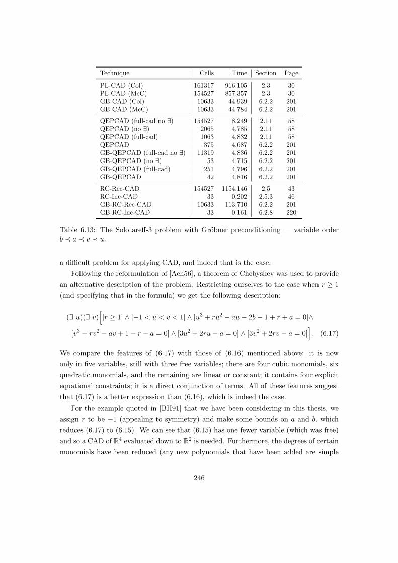
Technique Cells Time Section Page

PL-CAD (Col) 161317 916.105 2.3 30PL-CAD (McC) 154527 857.357 2.3 30GB-CAD (Col) 10633 44.939 6.2.2 201GB-CAD (McC) 10633 44.784 6.2.2 201

QEPCAD (full-cad no ∃) 154527 8.249 2.11 58QEPCAD (no ∃) 2065 4.785 2.11 58QEPCAD (full-cad) 1063 4.832 2.11 58QEPCAD 375 4.687 6.2.2 201GB-QEPCAD (full-cad no ∃) 11319 4.836 6.2.2 201GB-QEPCAD (no ∃) 53 4.715 6.2.2 201GB-QEPCAD (full-cad) 251 4.796 6.2.2 201GB-QEPCAD 42 4.816 6.2.2 201

RC-Rec-CAD 154527 1154.146 2.5 43RC-Inc-CAD 33 0.202 2.5.3 46GB-RC-Rec-CAD 10633 113.710 6.2.2 201GB-RC-Inc-CAD 33 0.161 6.2.8 220

Table 6.13: The Solotareff-3 problem with Grobner preconditioning — variable orderb ≺ a ≺ v ≺ u.

a difficult problem for applying CAD, and indeed that is the case.

Following the reformulation of [Ach56], a theorem of Chebyshev was used to provide

an alternative description of the problem. Restricting ourselves to the case when r ≥ 1

(and specifying that in the formula) we get the following description:

(∃ u)(∃ v)[[r ≥ 1] ∧ [−1 < u < v < 1] ∧ [u3 + ru2 − au− 2b− 1 + r + a = 0]∧

[v3 + rv2 − av + 1− r − a = 0] ∧ [3u2 + 2ru− a = 0] ∧ [3v2 + 2rv − a = 0]]. (6.17)

We compare the features of (6.17) with those of (6.16) mentioned above: it is now

only in five variables, still with three free variables; there are four cubic monomials, six

quadratic monomials, and the remaining are linear or constant; it contains four explicit

equational constraints; it is a direct conjunction of terms. All of these features suggest

that (6.17) is a better expression than (6.16), which is indeed the case.

For the example quoted in [BH91] that we have been considering in this thesis, we

assign r to be −1 (appealing to symmetry) and make some bounds on a and b, which

reduces (6.17) to (6.15). We can see that (6.15) has one fewer variable (which was free)

and so a CAD of R4 evaluated down to R2 is needed. Furthermore, the degrees of certain

monomials have been reduced (any new polynomials that have been added are simple

246

inequalities, so could potentially be used for sub-CADs, as described in Section 4.7.1)

and the logical structure has been retained. As to be expected from the discussions in

this chapter, this proves to be the most efficient expression and completes in a reasonable

time.

6.6 Conclusion

In this chapter the issue of expressing a problem for CAD was investigated. Motivation

was given in the form of two problems that were infeasible in their original format but

proved relatively straightforward after some mathematical manipulation.

We conclusively showed that Grobner preconditioning for CAD construction is a

worthwhile area of study. Taking a Grobner basis of a conjunction of equalities was shown

to be generally beneficial, although there are cases where it can be detrimental to the

complexity of the subsequent CAD. Experimental data was backed up by mathematical

justification why this may be the case. A metric, TNoI (and its generalisation TNoIF),

was given and it was shown to be well correlated to when preconditioning is beneficial,

with mathematical reasons given for this behaviour. Further preconditioning was given

by reducing inequalities with respect to the computed Grobner basis. Experimentation

suggests this is always beneficial (when it is possible) and complexity bounds on CAD

support this.

An investigation into the “Piano Mover’s Problem” of moving a ladder through a

right angled corridor was also discussed. Whilst a simple problem for numerical tech-

niques it was shown to be infeasible for CAD in [Dav86]. Whilst technology and CAD

algorithms have both advanced significantly since then, this particular expression re-

mains infeasible. A collection of successful work was described, but all required either

non-trivial geometric reasoning or a trigonometric description of the problem (the for-

mer not allowing for the construction of valid paths, and the latter requiring non-trivial

transformations). A new expression was given that was shown to be feasible, although

still difficult. Generalisations for various ladder lengths and angled corridors were con-

sidered as well as the application of the sub-CAD theory from Chapter 4. All this work

requires adjacency analysis, which is not possible with current algorithms.

These investigations led to some general strategies for expressing a problem for CAD.

Unfortunately this is a rather bespoke process and nothing further than guidelines can

be given, although the use of heuristics from Chapter 5 can prove useful.

247

248

Chapter 7

A General Framework for CAD

A range of new ideas and theory relating to CAD have been given in this thesis. These all

interact with each other in a non-trivial manner. We now investigate their compositions

and a general hierarchy of choices given as a guideline for how to tackle a problem.

CAD has applications outside of computer algebra, and so it is important to al-

low users to utilise advances in theory without a deep understanding of the underly-

ing mathematics. We introduce the proof-of-concept software CADassistant, which

demonstrates how tools can be used to let users appeal to a combination of heuristics and

requirements for a problem to identify an appropriate statement for input into various

CAD algorithms.

Author’s Contribution and Publication

The work in this chapter is the author’s. The experimentation and analysis are by the

author, as is the implementation of CADassistant.

The discussion of TTICAD and Grobner preconditioning in Section 7.1.2 was pub-

lished in [BDEW13].

7.1 Interaction of Concepts

In this section we will discuss a variety of ways in which CAD concepts can interact.

The work in this section is by the author, and has been partly published [BDEW13].

This survey is intended to indicate the complexity of using multiple CAD advances, and

highlight that decisions are not independent. We will primarily be concerned with the

projection and lifting based algorithms, as they offer the most formulation choices and

applicable theories. As the work in this thesis has extended CAD technology, there are

249

few examples in the literature large enough to allow for investigating the interaction of

these advances. Therefore the examples in this chapter have been created specifically

for this thesis.

7.1.1 Interactions Previously Discussed

We briefly mention interactions that have already been discussed in this thesis, and

summarise the findings.

Grobner Preconditioning and Equational Constraints

In Section 6.2.8 the interaction between Grobner bases and the theory of equational

constraints was investigated. Preconditioning can be applied to any conjunction of

equations in the formula. If the equations being consider for preconditioning are also

equational constraints for the whole formula, then the equations in the basis produced

can also be used to construct a CAD using equational constraint theory.

Experimentation in Section 6.2.8 confirmed that combining Grobner precondition-

ing and equational constraints can very powerful: for the Solotareff-3 problem a sign-

invariant CAD produces 154527 cells; with equational constraints alone it reduces to

48475; with preconditioning alone it reduces to 10633; and with both preconditioning

and equational constraints it produces only 4809 cells (3.1% of the sign-invariant CAD).

There is an added complication when combining these techniques: building an equa-

tional constraint CAD with respect to most of the polynomials produced by the precon-

ditioning fails (due to nullification on a cell of positive dimension). This is unsurprising

as a purely lexicographical Grobner basis provides a triangular structure, with polyno-

mials in few variables of low levels. These polynomials will be automatically nullified

due to the construction of the CAD. Therefore it seems prudent to always attempt to

construct a preconditioned equational constraint CAD with a polynomial of the highest

level first.

TTICAD and Layered/Variety sub-CADs

In Section 4.4.2 the construction of truth table invariant sub-CADs was discussed. The

theory of layered sub-CADs, variety sub-CADs and their amalgamation transfer over to

TTICADs. All three forms of sub-TTICAD have been implemented in the Projection-

CAD package as described in Section C.2. The layered sub-TTICAD algorithm computes

the sub-decomposition directly rather than recursively. As the TTICAD algorithm be-

250

haves differently at the highest level, in both projection and lifting, it is not clear whether

a recursive algorithm would be possible.

There is a slight limiting factor to the construction of variety sub-TTICADs. In

the final lifting stage we must lift to the variety defined by the implicit equational

constraint obtained by multiplying all the designated equational constraints from the

subformulae. This is somewhat wasteful as we would really want to consider the variety

for each separate formula and consider their union (for disjunctions) or intersection (for

conjunctions). There is no immediate way to incorporate this into the lifting stage: there

has been work [Str12] investigating the intersection and union of CAF cells so this is a

possibility for future integration.

7.1.2 Grobner Preconditioning for TTICAD

In Chapter 6 the preconditioning of an input to CAD by taking a Grobner basis was

investigated. In Chapter 3 the idea of a truth table invariant CAD was introduced and

algorithms given for their construction by either projection and lifting or regular chains

technology. This section will investigate the interaction of these concepts and discuss

work by the author from [BDEW13].

We consider the application of Grobner preconditioning to each subformula in a TTI-

CAD problem. We know that preconditioning can be hugely beneficial, but occasionally

detrimental, and it is of interest to see whether this effect amplifies when applied to each

subformulae. This work extends the investigation of the interaction between Grobner

preconditioning and constructing a CAD with respect to an equational constraint.

For a TTICAD problem to be suitably complicated for Grobner preconditioning

requires subformulae to have multiple equational constraints. This complexity means

there are few examples in the literature that are suitable and feasible for experimentation.

We therefore do not give a full survey of results, but consider one example in detail.

Example 7.1.

Consider the following polynomials:

f1,1 := x2 + y2 − 1; f2,1 := (x− 4)2 + (y − 1)2 − 1;

f1,2 := x3 + y3 − 1; f2,2 := (x− 4)3 + (y − 1)3 − 1;

g1 := xy − 1

4; g2 := (x− 4)(y − 1)− 1

4.

251

Figure 7.1: Plot of the polynomials in Example 7.1. The polynomials f1,1, f1,2, g1 areshown in red (solid) and f2,1, f2,2, g2 are shown in blue (dashed).

These are shown in Figure 7.1. We combine the polynomials into the formula Φ:

Φ :=[

[f1,1 = 0 ∧ f1,2 = 0 ∧ g1 > 0] ∨ [f2,1 = 0 ∧ f2,2 = 0 ∧ g2 > 0]].

We can construct a sign-invariant CAD of the polynomials in Φ with respect to the

two variable orderings: y ≺ x and x ≺ y. This gives CADs with 725 and 657 cells, as

shown in Table 7.1.

To use TTICAD directly for Φ allows four possible formulations depending on equa-

tional constraint designation (as discussed in Section 5.2). Table 7.1 shows that all

formulations of TTICAD offer a substantial saving in time and cell count. The values

of sotd and ndrr on the entire projection set are also given and we can see that ndrr

selects the optimal formulation (whilst sotd selects the worst ordering).

We can apply Grobner preconditioning to both formulae in Φ separately, computing a

Grobner basis for fi,1, fi,2 with respect to a compatible purely lexicographical ordering.

In both cases this computation is trivial and produces three polynomials in the basis. We

denote the polynomials fi,1, fi,2, fi,3 listed in decreasing order of the leading monomials

with respect to the order for the basis (although note that the polynomials will differ

depending on the variable ordering).

We can see in Table 7.1 that applying Grobner preconditioning can have a substantial

effect on the complexity. The cell count can drop as low as 27 and 29 cells, taking under

0.1 seconds in both cases. As was demonstrated in Chapter 6, it is not always beneficial

to precondition and there are multiple cases where a preconditioned formulation is less

efficient than the worst TTICAD formulation (1 case for y ≺ x and 3 cases for x ≺ y). It

is testament to the power of TTICAD theory that even when preconditioning is harmful,

it still performs much better than a sign-invariant CAD.

252

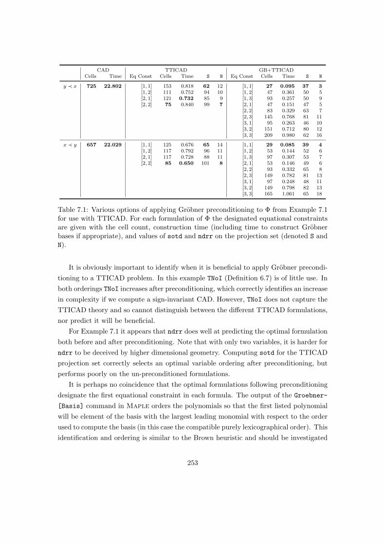
CAD TTICAD GB+TTICADCells Time Eq Const Cells Time S N Eq Const Cells Time S N

y ≺ x 725 22.802 [1, 1] 153 0.818 62 12 [1, 1] 27 0.095 37 3[1, 2] 111 0.752 94 10 [1, 2] 47 0.361 50 5[2, 1] 121 0.732 85 9 [1, 3] 93 0.257 50 9[2, 2] 75 0.840 99 7 [2, 1] 47 0.151 47 5

[2, 2] 83 0.329 63 7[2, 3] 145 0.768 81 11[3, 1] 95 0.263 46 10[3, 2] 151 0.712 80 12[3, 3] 209 0.980 62 16

x ≺ y 657 22.029 [1, 1] 125 0.676 65 14 [1, 1] 29 0.085 39 4[1, 2] 117 0.792 96 11 [1, 2] 53 0.144 52 6[2, 1] 117 0.728 88 11 [1, 3] 97 0.307 53 7[2, 2] 85 0.650 101 8 [2, 1] 53 0.146 49 6

[2, 2] 93 0.332 65 8[2, 3] 149 0.782 81 13[3, 1] 97 0.248 48 11[3, 2] 149 0.798 82 13[3, 3] 165 1.061 65 18

Table 7.1: Various options of applying Grobner preconditioning to Φ from Example 7.1for use with TTICAD. For each formulation of Φ the designated equational constraintsare given with the cell count, construction time (including time to construct Grobnerbases if appropriate), and values of sotd and ndrr on the projection set (denoted S andN).

It is obviously important to identify when it is beneficial to apply Grobner precondi-

tioning to a TTICAD problem. In this example TNoI (Definition 6.7) is of little use. In

both orderings TNoI increases after preconditioning, which correctly identifies an increase

in complexity if we compute a sign-invariant CAD. However, TNoI does not capture the

TTICAD theory and so cannot distinguish between the different TTICAD formulations,

nor predict it will be beneficial.

For Example 7.1 it appears that ndrr does well at predicting the optimal formulation

both before and after preconditioning. Note that with only two variables, it is harder for

ndrr to be deceived by higher dimensional geometry. Computing sotd for the TTICAD

projection set correctly selects an optimal variable ordering after preconditioning, but

performs poorly on the un-preconditioned formulations.

It is perhaps no coincidence that the optimal formulations following preconditioning

designate the first equational constraint in each formula. The output of the Groebner-

[Basis] command in Maple orders the polynomials so that the first listed polynomial

will be element of the basis with the largest leading monomial with respect to the order

used to compute the basis (in this case the compatible purely lexicographical order). This

identification and ordering is similar to the Brown heuristic and should be investigated

253

to see if it is a viable heuristic for preconditioning with TTICAD. Further, this heuristic

could be applied to the general issue of equational constraint designation as discussed

in Section 5.2.2.

Example 7.2.

In Section 6.2.8 it was shown that Grobner preconditioning can also benefit the regular

chains incremental algorithm for sign-invariant CAD but that often it has little effect

as all equational constraints are utilised by the CAD algorithm. Following the work

in Section 5.4 the improvement could also be due to a new input order of equational

constraint as well as the preconditioning.

We can use the incremental TTICAD algorithm for Example 7.1. Before precondi-

tioning it already produces a small number of cells: 29 cells when y ≺ x and 33 cells

when x ≺ y (compared to an optimal 75 and 85 cells when using the projection and

lifting algorithm). Preconditioning proves beneficial once again, reducing these down to

15 cells and 17 cells for the two variable orderings. This compares to an optimal 27 and

29 cells when using the projection and lifting algorithm with the preconditioned input.

Note that in the incremental algorithm there is no need for equational constraint

designation and no chance for theoretical failure, unlike when projecting and lifting.

This avoids the possibility of choosing a bad designation, such as f1,3, f2,3 in Table 7.1,

which can increase the cell count and cancel out the benefit of preconditioning. The

more sophisticated case analysis discussed in Section 3.5 allows for an even lower cell

count than when using the projection-based TTICAD.

7.1.3 Grobner Preconditioning and Layered/Variety sub-CADs

As with the interaction of Grobner preconditioning with equational constraints, there

should be little issue of incorporating preconditioning with the sub-CAD algorithms of

Chapter 4. Constructing a preconditioned layered sub-CAD will be straightforward,

with the two processes working independently. Constructing a preconditioned variety

sub-CAD (or a preconditioned layered variety sub-CAD) will be possible, but likely only

with respect to a few polynomials in the Grobner basis. The triangular shape of a

purely-lexicographic Grobner basis ensures that only a small number of polynomials will

contain the main variable xn, and variety sub-CADs can currently only be constructed

with respect to polynomials with main variable xn (although it was described in Chapter

4 how the work could be extended).

Consider the Solotareff-B example again. A sign-invariant CAD using McCallum’s

operator produces 154527 cells, and we have seen that equational constraints and pre-

254

Technique Cells

PL-CAD 154527 —EC-CAD 48475 31.4%GB-CAD 10633 6.9%GB-EC-CAD 4809 3.1%

GB-4-L-sub-CAD 10300 6.7%GB-3-L-sub-CAD 8440 5.5%GB-2-L-sub-CAD 4608 3.0%GB-1-L-sub-CAD 1152 0.75%

GB-V-sub-CAD 1603 1.04%

GB-3-LV-sub-CAD 1385 0.90%GB-2-LV-sub-CAD 904 0.59%GB-1-LV-sub-CAD 272 0.18%

Table 7.2: Solotareff-B with a range of different CAD technologies.

conditioning can be applied separately or collaboratively to offer savings. Table 7.2

reproduces these results and considers constructing preconditioned sub-CADs. If we

require a description of all regions satisfying the input formula, then we can use the

preconditioned variety sub-CAD (the variety is with respect to the only element of the

Grobner basis that contains the main variable). This produces only 1603 cells, which is

around 1% of the cell count for the sign-invariant CAD. We can also construct precondi-

tioned layered variety sub-CADs that can reduce the cell count even further to 272 cells

in the 1-layered case.

7.1.4 Grobner Preconditioning, TTICAD, and sub-CADs

We can combine the concepts of Chapters 3, 4 and 6 to build preconditioned truth table

invariant cylindrical algebraic sub-decompositions. We begin by looking at precondi-

tioned variety sub-TTICADs and reconsider Example 7.1.

Example 7.3.

Recall Example 7.1, which involved constructing a TTICAD for:

Φ :=[

[f1,1 = 0 ∧ f1,2 = 0 ∧ g1 > 0] ∨ [f2,1 = 0 ∨ f2,2 = 0 ∧ g2 > 0]].

It was shown that preconditioning can be highly beneficial (although also detrimental)

compared to computing a normal TTICAD.

We investigate the benefit of computing a preconditioned variety sub-TTICAD. Ta-

ble 7.3 gives the result of computing a TTICAD, variety sub-TTICAD, preconditioned

255

CAD TTICAD V-TTICAD GB-TTICAD GB-V-TTICADCells Eq Const Cells Cells Eq Const Cells Cells

y ≺ x 725 [1, 1] 153 64 [1, 1] 27 —[1, 2] 111 45 [1, 2] 47 —[2, 1] 121 51 [1, 3] 93 —[2, 2] 75 30 [2, 1] 47 —

[2, 2] 83 26[2, 3] 145 56[3, 1] 95 —[3, 2] 151 60[3, 3] 209 88

x ≺ y 657 [1, 1] 125 48 [1, 1] 29 —[1, 2] 117 47 [1, 2] 53 —[2, 1] 117 47 [1, 3] 97 —[2, 2] 85 34 [2, 1] 53 —

[2, 2] 93 46[2, 3] 149 62[3, 1] 97 —[3, 2] 149 62[3, 3] 165 64

Table 7.3: Constructing a Grobner preconditioned variety sub-TTICAD from Example7.1.. For each formulation of Φ the designated equational constraints are given with thecell count, construction time (including time to construct Grobner bases if appropriate),and values of sotd and ndrr on the projection set (denoted S and N).

TTICAD, and preconditioned variety sub-TTICAD.

We can note some interesting properties of Table 7.3. As it is simply a subset of

cells, the variety TTICADs all have lower cell counts than the complete TTICADs. As

discussed in Example 7.1, preconditioning for TTICAD is beneficial overall, but can

be more costly depending on the designation of equational constraints. We note that

the preconditioning is marginally more effective than lifting to the variety, although the

difference is minimal and this is a relatively small example.

When constructing a preconditioned variety TTICAD we see that five of the nine

possible designations result in an error. This is due to f1,1 and f2,1 not containing

the relevant main variable for variety lifting. By necessity, the optimal designation

for a preconditioned variety sub-TTICAD is therefore different from a preconditioned

TTICAD. However, if we only designations without f1,1 or f2,1, the optimal orderings

agree.

For variable ordering y ≺ x combining all three theories proves the most efficient,

reducing 725 cells in a full sign-invariant CAD to 26 cells (3.6%). However, for x ≺ y

combining all three theories is not the most efficient. A full sign-invariant CAD produces

657 cells and the optimal preconditioned variety sub-TTICAD produces 46 cells (7.0%).

The optimal variety sub-TTICAD produces fewer cells (34 cells, 5.2%) and the optimal

256

preconditioned full TTICAD produces the minimal 29 cells (4.4%).

We now demonstrate that the addition of more subformulae or more variables can

further complicate the interaction of these three concepts.

Example 7.4.

Consider the three clause version of Example 7.3 where we include a third formula in

Φ:

[f3,1 = 0 ∧ f3,2 = 0 ∧ g3 > 0] ,

where

f3,1 := (x+ 4)2 + (y + 1)2 − 1; f3,2 := (x+ 4)3 + (y + 1)3 − 1;

g3 := (x+ 4)(y + 1)− 1

4.

Table 7.4 displays the results of combining preconditioning, TTICAD, and sub-CAD

techniques.

We see that once again, each theory proves useful individually, with a preconditioned

TTICAD again more powerful than a variety sub-TTICAD. However, we see that for

both variable orderings the optimal preconditioned variety sub-TTICAD has more cells

than the preconditioned TTICAD.

Example 7.5.

We now consider a three variable version of Example 7.3, and see the effect is also

amplified. Consider the following polynomials:

f1,1 := x2 + y2 + z2 − 1; f2,1 := (x− 4)2 + (y − 1)2 + (z + 2)2 − 1;

f1,2 := x3 + y3 + z3 − 1; f2,2 := (x− 4)3 + (y − 1)3 + (z + 2)3 − 1;

g1 := xyz − 14 ; g2 := (x− 4)(y − 1)(z + 2)− 1

4 .

We can combine them to form Φ in the same manner as Example 7.3 and attempt to

construct various forms of CAD (with respect to the variable ordering: z ≺ y ≺ x).

There are 2 equational constraints for each formula, giving 4 designations for TTI-

CAD. Preconditioning produces Grobner bases with 5 polynomials for each formula, re-

sulting in 25 possible formulations for preconditioned TTICAD and variety sub-TTICAD.

Therefore there are 55 possible formulations for the single variable ordering (making 330

formulations if the variable ordering is not fixed).

We consider every possible formulation for TTICAD, variety sub-TTICAD, precon-

ditioned TTICAD, and preconditioned variety sub-TTICAD. The formulations shown

257

Variables CAD EC TTI V+TTI GB+EC GB+TTI GB+V+TTI

y ≺ x 1789 [1, 1, 1] 243 104 [1, 1, 1] 39 —[1, 1, 2] 231 101 [1, 1, 2] 63 —[1, 2, 1] 221 95 [1, 1, 3] 107 —[1, 2, 2] 189 82 [1, 2, 1] 63 —[2, 1, 1] 205 87 [1, 2, 2] 103 —[2, 1, 2] 189 82 [1, 2, 3] 159 —[2, 2, 1] 183 78 [1, 3, 1] 105 —[2, 2, 2] 147 63 [1, 3, 2] 153 —

[1, 3, 3] 173 —[2, 1, 1] 63 —[2, 1, 2] 103 —[2, 1, 3] 167 —[2, 2, 1] 103 —[2, 2, 2] 159 54[2, 2, 3] 235 94[2, 3, 1] 161 —[2, 3, 2] 225 87[2, 3, 3] 265 108[3, 1, 1] 105 —[3, 1, 2] 161 —[3, 1, 3] 221 —[3, 2, 1] 161 —[3, 2, 2] 233 92[3, 2, 3] 305 130[3, 3, 1] 219 —[3, 3, 2] 299 125[3, 3, 3] 335 144

x ≺ y 1653 [1, 1, 1] 187 72 [1, 1, 1] 43 —[1, 1, 2] 207 85 [1, 1, 2] 75 —[1, 2, 1] 207 85 [1, 1, 3] 111 —[1, 2, 2] 203 86 [1, 2, 1] 75 —[2, 1, 1] 207 85 [1, 2, 2] 123 —[2, 1, 2] 203 86 [1, 2, 3] 171 —[2, 2, 1] 203 86 [1, 3, 1] 111 —[2, 2, 2] 175 75 [1, 3, 2] 171 —

[1, 3, 3] 179 —[2, 1, 1] 75 —[2, 1, 2] 123 —[2, 1, 3] 171 —[2, 2, 1] 123 —[2, 2, 2] 187 66[2, 2, 3] 247 98[2, 3, 1] 171 —[2, 3, 2] 247 98[2, 3, 3] 267 108[3, 1, 1] 111 —[3, 1, 2] 171 —[3, 1, 3] 179 —[3, 2, 1] 171 —[3, 2, 2] 247 98[3, 2, 3] 267 108[3, 3, 1] 179 —[3, 3, 2] 267 108[3, 3, 3] 247 96

Table 7.4: Constructing a Grobner preconditioned variety sub-TTICAD from Example7.4. For each formulation of Φ the designated equational constraints are given with thecell count.

258

TTICAD V+TTICAD GB+TTICAD GB+V+TTICADDesignation Cells Designation Cells Designation Cells Designation Cells

[1, 1] 359 [1, 1] 108 [1, 1] 37 [4, 5] 2125[1, 4] 2543 [5, 5] 908[1, 5] 1097[2, 1] 1217[4, 1] 887[4, 5] 5473[5, 1] 1093[5, 5] 2463

Table 7.5: Constructing a Grobner preconditioned variety sub-TTICAD from Example7.5. For each formulation of Φ the designated equational constraints are given with thecell count.

in Table 7.5 are the only ones not to time out or produce an error.

All formulations of preconditioned variety sub-TTICADs involving the first equa-

tional constraint in either clause resulted in theoretical failure (these equational con-

straints did not contain the main variable) and all other formulations timed out after 10

minutes.

We are in the unenviable position where using a pair of theories (either variety sub-

TTICAD or preconditioned TTICAD) gives an efficient CAD, but using all three gives

relatively poor results (indeed, worse than just computing a complete TTICAD) . This

is because the optimal options for designation in preconditioned TTICAD involve the

first polynomial in either basis, which do not contain the main variable (in this case, x).

Note also that whilst preconditioning gives the optimal formulation across all options

([1, 1] with 37 cells), it also gives the worst formulation that does not time out ([4, 5]

with 5473 cells).

This example was conducted with respect to a single variable ordering, and there is

no guarantee that any of the above reasoning applies to the other 5 variable orderings.

However, the symmetry in x, y and z suggests similar issues would occur.

Remark 7.1.

It might be that we can avoid certain failures due to sub-CAD techniques if the cell

on which nullification occurs is omitted from the sub-CAD. Further, the regular chains

TTICAD algorithm would prevent failure when constructing a preconditioned TTICAD

(resulting in 21 and 25 cells for Example 7.4 and 43 cells for Example 7.5), but does not

allow for the use of sub-CAD techniques.

In general, if each theory is beneficial then the combination is not necessarily more

259

efficient. Care must be taken particularly with Grobner preconditioning which can have

a negative influence (and the effect can vary in scale and between positive and negative

depending on the other theories) whilst TTICAD and sub-CAD techniques are always

beneficial individually.

In particular, the behaviour of the theories depend on the formulation of the problem,

which will be discussed in the following section.

7.1.5 Interaction with Variable Ordering and Formulation

There is a further complication in that optimal choices for formulation can change de-

pending on which variable order is used. We have seen this phenomenon at various

points through this thesis and summarise in this section.

Variable Ordering and Grobner Preconditioning

In Section 6.2 we assumed each problem for preconditioning had a fixed variable ordering.

It is necessary to fix a variable ordering before preconditioning, as a Grobner basis

must be taken with respect to the compatible purely lexicographic monomial ordering.

However, there are examples where the optimal ordering can change before and after

preconditioning, as demonstrated in Example 7.6.

Example 7.6.

Consider the randomly generated polynomials:

f := −4x2 + yz − z2 − 5x− 2; g := 3y − 4z + 5;

h := x2 − 3xz + y + 5z + 1.

Consider the formula Φ:

[f = 0 ∧ g = 0] ∧ h > 0.

We can apply Grobner preconditioning in its simplest form by taking a Grobner basis of

f and g and taking its conjunction with h > 0. Table 7.6 gives the result of constructing

a sign-invariant CAD before and after preconditioning for all 6 variable orders.

We can see that the optimal variable ordering for cell count changes from z ≺ x ≺ yto x ≺ z ≺ y. Note that computing the sotd, ndrr or TNoI of the projection set after

preconditioning all predict the optimal variable choice (but requires all six Grobner bases

to be computed along with their projections).

In this example all variable orderings benefit from preconditioning, as predicted by

the fact that in all cases the TNoI of the input reduces from 8 to 7. However there

260

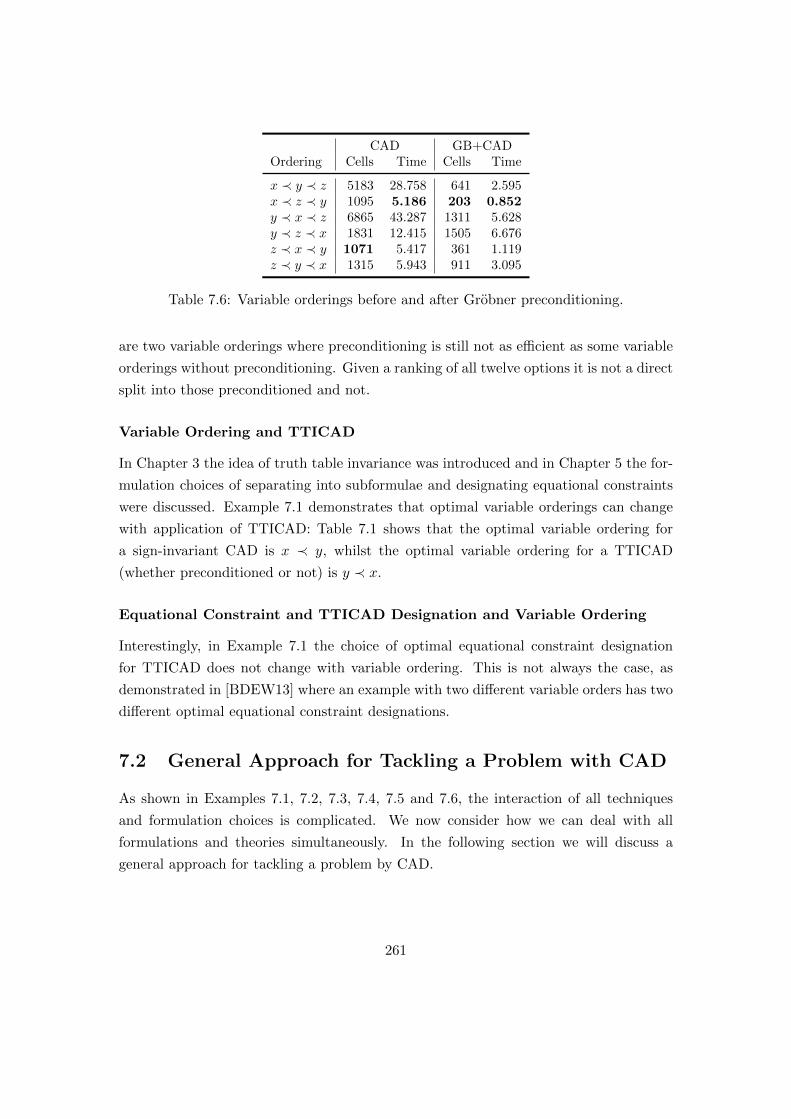
CAD GB+CADOrdering Cells Time Cells Time

x ≺ y ≺ z 5183 28.758 641 2.595x ≺ z ≺ y 1095 5.186 203 0.852y ≺ x ≺ z 6865 43.287 1311 5.628y ≺ z ≺ x 1831 12.415 1505 6.676z ≺ x ≺ y 1071 5.417 361 1.119z ≺ y ≺ x 1315 5.943 911 3.095

Table 7.6: Variable orderings before and after Grobner preconditioning.

are two variable orderings where preconditioning is still not as efficient as some variable

orderings without preconditioning. Given a ranking of all twelve options it is not a direct

split into those preconditioned and not.

Variable Ordering and TTICAD

In Chapter 3 the idea of truth table invariance was introduced and in Chapter 5 the for-

mulation choices of separating into subformulae and designating equational constraints

were discussed. Example 7.1 demonstrates that optimal variable orderings can change

with application of TTICAD: Table 7.1 shows that the optimal variable ordering for

a sign-invariant CAD is x ≺ y, whilst the optimal variable ordering for a TTICAD

(whether preconditioned or not) is y ≺ x.

Equational Constraint and TTICAD Designation and Variable Ordering

Interestingly, in Example 7.1 the choice of optimal equational constraint designation

for TTICAD does not change with variable ordering. This is not always the case, as

demonstrated in [BDEW13] where an example with two different variable orders has two

different optimal equational constraint designations.

7.2 General Approach for Tackling a Problem with CAD

As shown in Examples 7.1, 7.2, 7.3, 7.4, 7.5 and 7.6, the interaction of all techniques

and formulation choices is complicated. We now consider how we can deal with all

formulations and theories simultaneously. In the following section we will discuss a

general approach for tackling a problem by CAD.

261

7.2.1 Dealing with All Formulations and Theories

Before we can begin to formulate a problem for CAD we need to first express it in a

manner that allows for CAD construction. This was discussed in Chapter 6 where the

following general strategies were outlined:

• consider negating the formula;

• split into sub-problems if possible;

• eliminate parameters before constructing the final CAD;

• maximise chains of conjunctions;

• minimise degree and density.

As with the formulation choices from Chapter 5, it is possible to use heuristics to assist

with these manipulations, but it is a much more bespoke process and cannot necessarily

be conducted algorithmically (although hopefully the work of [BG06] could be adapted

for this purpose).

We deal with producing this mathematical expression independently of the algo-

rithm and formulation choices, to avoid adding further combinatorial complexity to the

decision-making process. These two steps may not strictly be independent: it is possi-

ble, for example, that different expressions are optimal for different variable orderings,

or that when considering different algorithms with well-orientedness conditions, various

expressions are better suited. However, the expression of a problem can change the

underlying (theoretically minimal) CAD and the formulation choices are more centred

around the algorithmic construction, so it seems fair to separate the two.

Once we have a mathematical expression of a problem as a Tarski formula we may

need to: select a variable ordering; choose a projection operator; designate equational

constraints; decompose into subformulae; decide whether to apply preconditioning; de-

cide which sub-CAD techniques to apply; and more. Considering all possible formula-

tions and choices quickly becomes combinatorially overwhelming: a problem for TTI-

CAD with three variables and two sub-formulae, each with two equational constraints,

allows 990 formulations of [TTI]CADs and sub-[TTI]CADs (ignoring possible splitting

of sub-formulae). Computing even basic heuristics for all of these formulations can easily

negate any benefit of selecting an optimal formulation.

There is no predefined order in which these should be decided and the previous

sections show that they are dependent on each other. We now try to describe a hierarchy

of which to approach these decisions.

262

7.2.2 Hierarchy

The following is a suggested order for the choices:

1 Mathematical Description: Before we can start making any algorithm or formu-

lation choices we need to have the mathematical expression of the problem. We can

appeal to the suggestions from Chapter 6 along with heuristics to help with this

decision, but there is not a general approach.

2 Algorithm: We know that constructing a CAD by projection and lifting or by regular

chains behaves slightly differently. Although the underlying (theoretically minimal)

CAD does not change, different algorithms can produce different sized CADs and

formulation choices can be dependent on the algorithm used so it is important to

select it immediately. In general it appears best to select the regular chains algorithm,

if possible, but this has not been thoroughly investigated, and if sub-CADs or partial

CADs are needed then projection and lifting is the only choice.

3 Projection Operator (if applicable): If constructing a CAD through projection

and lifting, the choice of projection operator is straightforward. The projection opera-

tors of Collins, Collins–Hong, McCallum and Brown–McCallum are successive subsets:

CP(A) ⊃ CHP(A) ⊃ MP(A) ⊃ BMP(A).

Further, if an equational constraint exists, or the problem can be split into subformulae

then the equational constraint operator, MPE(A), or TTICAD operator, TTIPE(A),

should be used. Depending on the formulation, certain projection operators may not

be valid (due to well-orientedness conditions), but this will not be discovered until the

lifting stage of construction. If this is the case, then the next best projection operator

should be used.

4 Variable Ordering: We have repeatedly seen that variable ordering is key to the

complexity of a problem. It is arguably the most important choice and further deci-

sions will be dependent on variable ordering. It should therefore be selected before

the other choices, and can be decided with heuristics (Brown, sotd, ndrr, layered)

which can be selected with machine learning (Section 5.3).

5 Formula Decomposition (if applicable): If constructing a TTICAD then there

may be a choice of formula decomposition. Although it is generally advantageous

to separate into as few formulae as possible (maximising the effect of the equational

263

constraints), this is not always the case for projection and lifting TTICAD, and the

decision method described in Section 5.2.3 can be used to make this decision.

6 Grobner Preconditioning (if applicable): We need to have decided a variable or-

dering and separated into subformulae before potentially applying Grobner precondi-

tioning (as described in Chapter 6), and any preconditioning should be applied before

designating any equational constraints or using a sub-CAD technique. Therefore, the

decision regarding preconditioning should be made next, using TNoI (Definition 6.7)

or some other measure.

7 Constraint Designation (if applicable): Next, the choice of equational constraint

designation should be made if using a projection and lifting algorithm. If an incremen-

tal regular chains algorithm is being used then the order of input should be decided.

These decisions can be made with a variety of heuristics as was discussed in Chapter

5.

8 Sub-CAD Techniques (if applicable): As constructing a sub-CAD (Chapter 4)

will always produce a subset of the cells in a complete CAD, the decision can be

made independently and after all other choices. If equational constraints are present

(explicit or implicit) then a variety sub-CAD may be appropriate, and if only generic

solutions or those of a certain dimension are needed then a layered sub-CAD may be

appropriate.

This hierarchy is shown diagrammatically in Figure 7.2. Most of these decisions have

the opportunity to influence each other so it may be necessary to work non-sequentially,

returning to previous steps to alter them with respect to later decisions.

7.2.3 Identifying General Classes of CAD Problems

In [McC93] and [Str00] it was noted that if a CAD problem consists purely of strict in-

equalities then any cells that satisfy all conditions must necessarily be full-dimensional.

Therefore a 1-layered sub-CAD is sufficient, and highly efficient, for this class of prob-

lems.

Similarly, if a problem consists purely of a conjunction of equalities, then Section 6.2.8

demonstrated that the incremental regular chains algorithm is the sensible choice. As it

can utilise all equational constraints, it will effectively solve the problem and construct

the minimal CAD around the solutions.

Extending the idea of [McC93, Str00] we could try to identify classes of problems for

which a 1-layered variety sub-CAD will suffice. Given a problem of the form f = 0∧g > 0

264

Figure 7.2: Decision hierarchy for a CAD problem.

265

where f defines a variety of co-dimension 1 then the full-dimensional cells on the variety

will describe at least some of the solutions. In certain cases these cells will describe all

the valid regions, and a condition to determine when this is the case would be highly

valuable.

Ideally, we could identify a collection of classes to dictate when certain algorithms

are well-suited or sufficient. This could be incorporated directly into CAD algorithms or

into a separate piece of software, such as CADassistant described in Section 7.3. This

is viewed as important future work, which would extend the applicability of the work in

this thesis significantly.

7.3 Proof-of-Concept User Software — CADassistant

CADassistant is a proof-of-concept tool for enabling a user to take advantage of ad-

vances in CAD theory (including the ones described in this thesis) without knowledge of

the underlying mathematics. It has only basic functionality and is intended to demon-

strate the potential of such a tool.

The code is freely available1 and is implemented in Python (further details of the

implementation are given in Section C.4).

The user runs the tool from the command line and CADassistant can be run in

interactive (the default) or manual modes:

> python CADassistant.py interactive

> python CADassistant.py manual

The user then gives details of the problem either directly (in manual mode) or through

answering a sequence of questions regarding the needs of the application (in interactive

mode).

The decisions made in interactive mode centre around trying to find if there is an

optimal way to solve the given problem. It can help identify if a layered sub-CAD or

variety sub-CAD may be appropriate, if Grobner preconditioning is possible, whether

quantifier elimination is needed, and so forth.

The output is then given for the appropriate platform. Currently support is only

given for Maple and Qepcad but other technologies (such as Mathematica, SyNRAC

and Redlog) could be integrated in the future.

The implementation of CADassistant in Python is described in Section C.4. The

problems are stored in an object from a hierarchy of classes: CadProblem for a ba-

1The code can be downloaded from http://www.github.com/DavidJohnWilson/CADassistant.

266

sic problem, CadProblemMethod if the method is also specified, and CadTTICAD if it is

separated into separate formulae for TTICAD.

7.3.1 Sample CADassistant Session

We describe a sample CADassistant session to demonstrate its usage. On running the

program in either interactive or manual mode the following is displayed, requiring input

from the user. We will assume the following input for this session:

############################################################

# CADassistant #

# by David Wilson (D.J.Wilson@bath.ac.uk) #

# #

# A tool for computing CADs with various technologies #

# and techniques. #

# #

############################################################

Please enter a name for the CAD problem (or ’help’):

Sample CADassistant Problem

Please enter the polynomials for your problem,

within square brackets and separated by commas:

[3*x^2+4*y-3, x^2-y^3,x^3-y^2,y-x]

Please enter the variables for your problem,

within square brackets and separated by commas:

[x,y]

Manual Mode

Manual mode is intended for use by users who already have some knowledge of CAD or

an implementation of CAD. It asks the following three questions to ascertain the kind

of CAD required:

Please specify a construction method (default:

projection&lifting):

projection

Please specify an invariance to build the CAD with respect to

(default: sign-invariance):

truth table

Please specify any subCAD techniques to use (default: none):

variety

267

If the invariance condition is given as truth table invariance, then the decomposition

into sub-formulae and equational constraint designation needs to be specified. This is

done with respect to the order the polynomials were entered and the formulae are defined

by a list of lists.

Polynomials are:

Poly 0: 3*x^2+4*y-3

Poly 1: x^2-y^3

Poly 2: x^3-y^2

Poly 3: y-x

Please enter in the clauses of the TTICAD (as a list of lists

identifying the correct polynomials), or if dealing with

equational constraints leave empty:

[[0,3],[1,2]]

For every subformula specified, the designated equational constraint needs to be

specified. If no equational constraint is present in a particular clause then an empty

answer can also be given.

Clause 0:

Poly 0: 3*x^2+4*y-3

Poly 3: y-x

Select the equational constraint for this clause:

3

Clause 1:

Poly 1: x^2-y^3

Poly 2: x^3-y^2

Select the equational constraint for this clause:

1

A summary of the problem is given, including the kind of CAD (using the acronyms

in Appendix D) and TTICAD details (if appropriate).

Summary of TTICAD Problem:

Name : Sample CADassistant Problem

Polys: 3*x^2+4*y-3, x^2-y^3, x^3-y^2, y-x

Vars : x,y

CAD : V-PL-TTICAD

Clauses: [0,3] [1,2]

EqCons : [3] [1]

The user is then asked if they wish to have the Maple code to construct the defined

CAD:

268

Would you like the input for Maple?

yes

Cad := VTTICAD([[y-x,[3*x^2+4*y-3]],[x^2-y^3,[x^3-y^2]]],[x, y]);

The user can then use this command within Maple using the ProjectionCAD package

to produce a sub-CAD with 18 cells.

Interactive Mode

In interactive mode less understanding of CAD is assumed of the user. As shown

in the general hierarchy in Section 7.1, it is generally a good idea to select a variable

ordering of the problem straight away.

The user is first asked if they wish to use a heuristic to select the variable ordering,

or enter a predetermined order. On selecting to use a heuristic they have the option to

select one manually or automatically from: Brown’s heuristic [B], sotd [S], ndrr [N],

or the layered heuristic [LAY].

If the user asks to select the heuristic automatically, they are given the choice to

select a quick heuristic (where Brown’s heuristic is used) or the most accurate (where

the layered heuristic is used). Finally, the user is given code to run the heuristic in

Maple with ProjectionCAD to then set the variable ordering.

Do you wish to use a heuristic to choose a variable ordering? [Y/n] :

Y

Please load Projection CAD to use any of the following heuristics.

Do you wish to pick the heuristic manually [M], or

automatically [A]? [m/A] :

A

Do you want a quick heuristic that may be less accurate [Q], or a

slower heuristic that is more accurate [S]? [Q/s] :

Q

Please copy the following code into your Maple window:

S:=VariableOrderingHeuristic([x, y], [3*x^2+4*y-3, x^2-y^3,

x^3-y^2, y-x],heuristic=’BrownBasic’,SeeAll=false);

Please paste the output from the above command:

[x,y]

Variable ordering has been successfully changed.

The user is then asked if the problem contains just strict inequalities, in which case

they are able to select whether to use the LCAD command in ProjectionCAD or the

269

measure-zero-error option in Qepcad. The appropriate code is then given to the

user for their chosen technology.

Does your problem involve only strict inequalities? [y/N] :

Y

You should use a 1-layered CAD.

Would you like to use ProjectionCAD [P] or Qepcad [Q]? [P/q] :

P

Please load Projection CAD and use the following input:

C:=LCAD( [3*x^2+4*y-3, x^2-y^3, x^3-y^2, y-x], 1,

[x, y],method=’McCallum’):

There is also basic functionality for Grobner basis preconditioning. At the moment

it is restricted to preconditioning the entire input (assuming a conjunction of equalities).

If preconditioning is possible the user can use TNoI to predict if preconditioning will be

beneficial, and is given code to compute the basis (and replace the polynomials for the

given problem).

Does your problem involve just a conjunction of equalities that

you can use Grobner preconditioning for? [y/N] :

Y

Do you wish to use TNoI to predict whether preconditioning

will be useful? [Y/n] :

Y

Please run the following two lines of code:

TNoI:=proc(F): add(nops(indets(f)),f in F): end proc:

TNoIdiff := TNoI([3*x^2+4*y-3, x^2-y^3, x^3-y^2, y-x]) -

TNoI(Groebner[Basis]([3*x^2+4*y-3, x^2-y^3, x^3-y^2, y-x],

plex(op([x, y]))));

Is the value positive? [y/n] :

Y

Please copy the following code into Maple to compute the Grobner basis:

Groebner[Basis]([3*x^2+4*y-3, x^2-y^3, x^3-y^2, y-x], plex(op([x, y])));

Please copy the output:

[1]

In this case there are no solutions to the system of equations and so the basis is

trivial, and the difference in TNoI is 8 (and therefore positive).

The user can then select different CAD algorithms in a similar way to the manual

method.

270

7.3.2 Extending CADassistant

As discussed above, CADassistant is currently a proof-of-concept tool and the previous

section only demonstrates basic functionality. There are obvious ways for the features

of CADassistant to be extended. In particular: a wider range of CAD methods could

be introduced; more subtle options for Grobner preconditioning and the like; integration

with the machine learning techniques used in Section 5.3; direct interface with Maple

and Qepcad (avoiding the need for the user to copy and paste input and output).

7.4 Solotareff-3

We consider again the Solotareff-3 problem from [BH91]:

(∃ u)(∃v)[[3v2 − 2v − a = 0] ∧ [v3 − v2 − av − 2b+ a− 2 = 0]

∧ [3u2 − 2u− a = 0] ∧ [u3 − u2 − au− a+ 2 = 0] ∧ [1 ≤ 4a] ∧ [4a ≤ 7]

∧ [−3 ≤ 4b] ∧ [4b ≤ 3] ∧ [−1 ≤ v] ∧ [v ≤ 0] ∧ [0 ≤ u] ∧ [u ≤ 1]]. (7.1)

We consider how this problem fits within the general framework of CAD, and how the

various choices affect its solution. Tables 7.7 and 7.8 show the results, for the two

variable orderings, for all CADs and sub-CADs that are sufficient to solve the problem.

We can see that when using projection and lifting algorithms, all the relevant tech-

nologies complement each other to increase efficiency. For a ≺ b ≺ v ≺ u utilising equa-

tional constraints, through an equational constraint CAD or variety sub-CAD, proves

more efficient than Grobner preconditioning, whilst for b ≺ a ≺ v ≺ u the precondition-

ing is more powerful (even than a variety sub-CAD). Indeed, a preconditioned variety

sub-CAD with the second ordering is the smallest projection and lifting CAD that can

be constructed using the theory presented in this thesis.

When combining preconditioning with the equational constraint CAD or variety sub-

CAD we see that the optimal variable order changes, with b ≺ a ≺ v ≺ u becoming 61.6%

more efficient compared to the other variable ordering, whilst it was 66.6% less efficient

for a sign-invariant CAD.

With Qepcad we have little control over the interactions and can only externally af-

fect it through Grobner preconditioning. It is interesting to note that the preconditioning

has a greater effect when we omit quantifiers (constructing a CAD of R4 rather than R2)

than specifying a full-cad (preventing the use of certain partial-CAD techniques and

equational constraints). Without knowledge of the implementation of Qepcad it would

271

Technique Cells Time Section Page

PL-CAD (Col) 54037 255.304 2.3 30PL-CAD (McC) 54037 266.334 2.3 30EC-CAD (f3) 20593 65.856 2.4.4 40EC-CAD (f4) 22109 102.781 2.4.4 40V-CAD (f3) 8195 63.387 4.2 114V-CAD (f4) 8953 95.233 4.2 114GB-CAD (Col) 28501 128.270 6.2.2 201GB-CAD (McC) 28501 128.533 6.2.2 201GB-EC-CAD (g4) 12513 55.749 7.1 249GB-V-CAD (g4) 4171 53.251 7.1 249

QEPCAD (full-cad no ∃) 54037 5.701 2.11 58QEPCAD (no ∃) 1015 4.807 2.11 58QEPCAD (full-cad) 349 4.782 2.11 58QEPCAD 153 4.659 2.11 58GB-QEPCAD (full-cad no ∃) 28501 5.198 6.2.2 201GB-QEPCAD (no ∃) 73 4.669 6.2.2 201GB-QEPCAD (full-cad) 625 4.628 6.2.2 201GB-QEPCAD 63 4.801 6.2.2 201

RC-Rec-CAD 54037 327.421 2.5 43RC-Inc-CAD 29 0.155 2.5.3 46GB-RC-Rec-CAD 28501 219.280 6.2.2 201GB-RC-Inc-CAD 29 0.148 6.2.8 220

Table 7.7: The Solotareff-3 problem with the general framework of CAD — variableorder a ≺ b ≺ v ≺ u.

be remiss to speculate why this may be the case, but it warrants further investigation.

When considering the regular chains algorithms, we have even fewer options for in-

teraction: the recursive algorithm can only construct sign-invariant CADs and neither

it nor the incremental algorithm have been adapted to admit sub-CADs. The recursive

algorithm can only utilise preconditioning, which proves beneficial in both variable or-

derings (as it did for the projection and lifting algorithms). The incremental algorithm

automatically utilises all four equational constraints in (7.1) and so explicitly requiring

an equational constraint CAD has no effect. Similarly, preconditioning has no effect (as

discussed in Section 6.2.8) and does not change the optimal variable ordering like when

using projection and lifting algorithms.

272

Technique Cells Time Section Page

PL-CAD (Col) 161317 916.105 2.3 30PL-CAD (McC) 154527 857.357 2.3 30EC-CAD (f3) 48475 175.139 2.4.4 40EC-CAD (f4) 63583 324.663 2.4.4 40V-CAD (f3) 19127 173.083 4.2 114V-CAD (f4) 25563 295.556 4.2 114GB-CAD (Col) 10633 44.939 6.2.2 201GB-CAD (McC) 10633 44.784 6.2.2 201GB-EC-CAD (g4) 4809 20.420 7.1 249GB-V-CAD (g4) 1603 20.053 7.1 249

QEPCAD (full-cad no ∃) 154527 8.249 2.11 58QEPCAD (no ∃) 2065 4.785 2.11 58QEPCAD (full-cad) 1063 4.832 2.11 58QEPCAD 375 4.687 6.2.2 201GB-QEPCAD (full-cad no ∃) 11319 4.836 6.2.2 201GB-QEPCAD (no ∃) 53 4.715 6.2.2 201GB-QEPCAD (full-cad) 251 4.796 6.2.2 201GB-QEPCAD 42 4.816 6.2.2 201

RC-Rec-CAD 154527 1154.146 2.5 43RC-Inc-CAD 33 0.202 2.5.3 46GB-RC-Rec-CAD 10633 113.710 6.2.2 201GB-RC-Inc-CAD 33 0.161 6.2.8 220

Table 7.8: The Solotareff-3 problem with the general framework of CAD — variableorder b ≺ a ≺ v ≺ u.

7.5 Conclusion

Whilst each advance described in this thesis is beneficial individually, we have shown

that combining them is not straightforward. Certain combinations naturally work well

together but when certain conditions are needed, such as well-orientedness, the only pos-

sible formulations may prove to be less efficient than using only a selection of advances.

This was demonstrated through a collection of examples.

Unfortunately there is not a general algorithm to select an optimal combination of

formulations and theories, but a hierarchy was given as a guideline for these choices.

As the process is non-sequential, with later choices affecting earlier ones, care must be

taken.

CADassistant, a proof-of-concept tool designed to help a user use CAD to solve

a given problem was described. CADassistant is meant to demonstrate that whilst

the interaction of the ideas in this thesis is complex, a computer can be used to assist

273

someone wishing to take advantage of them.

274

Chapter 8

Future Work and Conclusions

Whilst constructing a CAD can seem excessive for many applications, the use of various

advances in CAD theory can tailor the output to the desired purpose and needs of a

problem. It is important not only to devise new methods of constructing CADs, but

also to understand the interaction of various improvements with each other.

We discuss how the work in this thesis can be extended in multiple directions and

summarise the effect of the advances on the guiding example, Solotareff-3. Finally, the

contributions of this thesis are summarised.

8.1 Future Work

Throughout this thesis we have noted possible extensions of the work and ideas for future

investigation. We summarise these suggestions here:

• Chapter 3: Truth Table Invariant CAD.

1. Identify conditions for when lifting with respect to the ResCAD set (Definition

3.7) will produce a TTICAD. This will allow for easy use in other projection

and lifting CAD implementations.

2. Extend the semi-restricted equational constraint projection operator to TTI-

CAD. By using TTIPE(A)∪ discxn(g) | g ∈ ⋃mi=1Ai \Ei it may be possible

to extend the TTICAD projection past the first projection level.

3. Extend the TTICAD projection operator to include the work on bi-equational

constraints when sub-formulae have multiple equational constraints.

4. Compare the output of the projection and lifting TTICAD algorithm (which

requires well-oriented input) and the regular chains TTICAD algorithm. This

275

can be used to help decide if the restriction of well-orientedness can be

avoided.

5. Combine TTICAD with partial CAD techniques. This will likely require

keeping track of sources of cells to simplify lifting with respect to each sub-

formula.

• Chapter 4: Cylindrical Algebraic sub-Decompositions.

1. Identify classes of problems that different sub-CADs are well-suited for, to

extend their application.

2. Implement and extend the idea of utilising simple inequalities in both the

projection and lifting stages.

3. Consider how the regular chains algorithms could be adapted to incorporate

the idea of various sub-CADs. It should be possible to restrict the complex

cylindrical tree and decomposition, at least partially, according to dimension

or a variety (but possibly only with respect to complex space).

• Chapter 5: Formulation of Problems.

1. Adapt Brown’s heuristic, which is very effective for variable ordering, to other

formulation issues such as equational constraint designation.

2. Investigate selecting a variable ordering with machine learning for different

classes of problems (with more variables and different quantifier structures).

3. Investigate the application of alternative machine learning techniques to the

problem of selecting a variable ordering.

4. Apply machine learning to other formulations issues.

5. Improve the efficiency of the layered heuristic by implementing a parallel

version and incorporating other sub-CAD techniques.

• Chapter 6: Mathematical Description.

1. Investigate whether pseudo-remainder reduction with respect to Grobner bases

can offer greater savings.

2. Investigate how preconditioning affects the proportion of time spent in various

parts of CAD algorithms: the projection against the lifting phase, or the

complex decomposition against the MakeSemiAlgebraic phase.

276

3. Use machine learning to predict whether Grobner preconditioning will be

beneficial or not. This can be done either by selecting a heuristic or using the

heuristics as features to decide directly.

4. Extend the work on the piano mover’s problem to consider more difficult

problems and to incorporate adjacency.

5. Investigate sowtd, which proved useful for the piano mover’s problem, as a

general heuristic.

6. Incorporate various heuristics into a grading function for use with the artificial

intelligence algorithm of [BG06] to identify optimal mathematical expressions.

• Chapter 7: General Framework.

1. Investigate further the multiple interactions that exist between the different

extensions to CAD.

2. Look at whether it is possible to extend variety sub-TTICADs by taking

intersections of the variety sub-CADs for each sub-formula, rather than lifting

with respect to the implicit equational constraint.

3. Investigate designating an equational constraint after Grobner precondition-

ing and whether the lexicographic ordering the polynomials are presented in

can be utilised.

4. Develop CADassistant to offer more options and more sophisticated deci-

sion techniques.

• Other Extensions and Ideas:

1. Investigate adjacency within CAD, as discussed in Appendix A. In particular:

(a) Adapt and develop algorithms to consider adjacency in TTICADs and

sub-CADs.

(b) Develop the new idea of `-dimensional path connectedness (Definition

A.9), linking the topology and geometry of the problem with layered

sub-CADs.

(c) Investigate the new idea of an algorithmically minimal CAD (Definition

A.6) to improve current algorithms.

2. Semi-monotonicity of sets [BGV13] generalises the idea of convexity to only

require convexity aligned with axes (the direction of projection for CAD).

Investigate whether such an idea could be used to construct a stronger CAD

277

where cells are cylindrical in multiple projection directions at once. Such

a CAD would be more complex but could offer theoretical benefits: semi-

monotone sets are topologically regular cells [BGV13].

3. Investigate he idea of order invariance, which is used in the proofs of the

validity of certain projection operators. It is not clear if the regular chains

algorithms generate order-invariant CADs, what the complexity cost of order-

invariance is, and whether order-invariance guarantees CADs with particu-

larly nice properties.

4. Extend previous work on parallelism in CAD [McC97, MD11] both by separat-

ing the problem (such as described in Section 6.1) and through the algorithm

itself. A parallel implementation of the main CAD algorithm in Projection-

CAD (using the Threads package of Maple) would allow for greater investiga-

tion. There has also been recent work on utilising GPUs for real root isolation

[TM12] which may prove useful to CAD construction.

5. Whilst most of the work on CAD has been done to minimise the number of

cells produced, it may be worth investigating if this is always the desired out-

put. An example given in [BD07] produces 3 cells with one variable ordering

and doubly-exponential cells for all other orderings. The three cell descrip-

tion hides much of the behaviour of the function that may be necessary for

applications and identifying such restrictions on variable orderings (outside

of quantifier elimination) could prove important.

Most importantly, all the work in this thesis should be considered in relation to other

CAD technology, such as Qepcad or Mathematica. This may be done directly, or by

identifying alternative methods of constructing concepts introduced in this thesis.

8.2 Solotareff-3

We have been considering the Solotareff example as given in [BH91]:

(∃ u)(∃v)[[3v2 − 2v − a = 0] ∧ [v3 − v2 − av − 2b+ a− 2 = 0]

∧ [3u2 − 2u− a = 0] ∧ [u3 − u2 − au− a+ 2 = 0] ∧ [1 ≤ 4a] ∧ [4a ≤ 7]

∧ [−3 ≤ 4b] ∧ [4b ≤ 3] ∧ [−1 ≤ v] ∧ [v ≤ 0] ∧ [0 ≤ u] ∧ [u ≤ 1]]. (8.1)

We have seen that Qepcad can be used to eliminate the variables in (8.1) and so

278

(a) Solotareff-3 problem. (b) Solution to Solotareff-3.

Figure 8.1: Solution to the Solotareff problem in three variables when r = −1.

solve the Solotareff problem in this case. Using the ordering a ≺ b ≺ v ≺ u we get the

following equivalent quantifier-free formula:

a− 1 = 0 ∧ 4b+ 3 > 0 ∧ 27b2 − 18ab+ 56b− a3 + 2a2 − 19a+ 29 = 0,

which gives the solution: a = 1, b = −1127 . Using the variable ordering b ≺ a ≺ v ≺ u we

get the answer directly: 27b+ 11 = 0 ∧ a− 1 = 0.

Therefore we have found that the closest linear approximation to the polynomial

x3 − x2 under the uniform norm on the interval [−1, 1] is x− 1127 . This is demonstrated

in Figure 8.1.

8.2.1 Results

We have considered (8.1) with respect to two permissible variable orderings and now

collect the results from this thesis: a ≺ b ≺ v ≺ u is given in Table 8.1 and b ≺ a ≺v ≺ u is given in Table 8.2. These describe the possible CADs that are sufficient to

solve (8.1), separated according to whether they are constructed using ProjectionCAD,

Qepcad, or RegularChains. Omitted CADs (that are not sufficient in this case to

tackle (8.1)) include: TTICADs (which would be equivalent to an equational constraint

CAD); layered sub-CADs (as the solution is 0-dimensional); layered variety sub-CADs;

and the preconditioned versions of these theories.

It is clear from Tables 8.1 and 8.2 that the correct use of various advances in CAD

can have a substantial effect on the complexity of the problem, particularly for projection

and lifting algorithms.

279

Technique Cells Time Section Page

PL-CAD (Col) 54037 255.304 2.3 30PL-CAD (McC) 54037 266.334 2.3 30EC-CAD (f3) 20593 65.856 2.4.4 40EC-CAD (f4) 22109 102.781 2.4.4 40V-CAD (f3) 8195 63.387 4.2 114V-CAD (f4) 8953 95.233 4.2 114GB-CAD (Col) 28501 128.270 6.2.2 201GB-CAD (McC) 28501 128.533 6.2.2 201GB-EC-CAD (g4) 12513 55.749 7.1 249GB-V-CAD (g4) 4171 53.251 7.1 249

QEPCAD (full-cad no ∃) 54037 5.701 2.11 58QEPCAD (no ∃) 1015 4.807 2.11 58QEPCAD (full-cad) 349 4.782 2.11 58QEPCAD 153 4.659 2.11 58GB-QEPCAD (full-cad no ∃) 28501 5.198 6.2.2 201GB-QEPCAD (no ∃) 73 4.669 6.2.2 201GB-QEPCAD (full-cad) 625 4.628 6.2.2 201GB-QEPCAD 63 4.801 6.2.2 201

RC-Rec-CAD 54037 327.421 2.5 43RC-Inc-CAD 29 0.155 2.5.3 46GB-RC-Rec-CAD 28501 219.280 6.2.2 201GB-RC-Inc-CAD 29 0.148 6.2.8 220

Table 8.1: The Solotareff-3 problem — variable order a ≺ b ≺ v ≺ u. The results areseparated according to whether they are constructed using ProjectionCAD, Qepcad,or RegularChains.

For the first variable ordering using ProjectionCAD, 54037 cells are reduced by 92.3%

to 4171 cells in the sub-CAD of the appropriate variety generated from a Grobner basis

of the equational constraint polynomials. Similarly, for the second variable ordering with

ProjectionCAD, 161317 cells are reduced by 99.0% to 1603 cells in the preconditioned

variety sub-CAD.

There are some things to note on the results that have been mentioned in earlier

sections. Out of the four equational constraints in the problem, only two are valid for

use with either EC-CAD or V-CAD. Once a Grobner basis has been computed, this

reduces down to only one valid equation for use with GB-EC-CAD or GB-V-CAD. This

is due to only a single polynomial involving the main variable: computing a Grobner

basis will never eliminate the main variable completely so we are always guaranteed

at least one valid equation, but generally the main variable will be present in as few

equations as possible.

280

Technique Cells Time Section Page

PL-CAD (Col) 161317 916.105 2.3 30PL-CAD (McC) 154527 857.357 2.3 30EC-CAD (f3) 48475 175.139 2.4.4 40EC-CAD (f4) 63583 324.663 2.4.4 40V-CAD (f3) 19127 173.083 4.2 114V-CAD (f4) 25563 295.556 4.2 114GB-CAD (Col) 10633 44.939 6.2.2 201GB-CAD (McC) 10633 44.784 6.2.2 201GB-EC-CAD (g4) 4809 20.420 7.1 249GB-V-CAD (g4) 1603 20.053 7.1 249

QEPCAD (full-cad no ∃) 154527 8.249 2.11 58QEPCAD (no ∃) 2065 4.785 2.11 58QEPCAD (full-cad) 1063 4.832 2.11 58QEPCAD 375 4.687 6.2.2 201GB-QEPCAD (full-cad no ∃) 11319 4.836 6.2.2 201GB-QEPCAD (no ∃) 53 4.715 6.2.2 201GB-QEPCAD (full-cad) 251 4.796 6.2.2 201GB-QEPCAD 42 4.816 6.2.2 201

RC-Rec-CAD 154527 1154.146 2.5 43RC-Inc-CAD 33 0.202 2.5.3 46GB-RC-Rec-CAD 10633 113.710 6.2.2 201GB-RC-Inc-CAD 33 0.161 6.2.8 220

Table 8.2: The Solotareff-3 problem — variable order b ≺ a ≺ v ≺ u. The results areseparated according to whether they are constructed using ProjectionCAD, Qepcad,or RegularChains.

When using Qepcad, preconditioning proves useful for all variants of its algorithm1.

Whilst the percentage savings from preconditioning are more modest than the savings

for projection and lifting, it improves an already highly efficient algorithm and imple-

mentation.

The recursive RegularChains algorithm performs in an identical manner to pro-

jection and lifting by McCallum’s operator, and is improved by preconditioning. The

incremental algorithm provides quite startling results due to its ability to utilise all

four equational constraints at once, which is not improved by preconditioning (as the

Grobner basis describes the same finite set of results). This is the optimal choice for all

algorithms, even when compared against the two-dimensional partial CADs of Qepcad.

The prominence of the incremental regular chains algorithm suggests that the most

fruitful area of research in projection and lifting based CAD algorithms would be to try

1All Qepcad timings include initialisation time, consisting of around two seconds per problem.

281

to utilise all equational constraints (extending the work on bi-equational constraints in

[BM05]). This would allow for interaction with sub-CAD (within ProjectionCAD) or

partial CAD (within Qepcad) which could reduce this number even further.

8.3 Key Contributions

We now summarise the key contributions described in this thesis, followed by a summary

of the author’s individual contribution.

Chapter 3: Truth Table Invariant CAD

The new idea of truth table invariance was introduced, which considers a CAD

with respect to a list of formulae rather than a set of polynomials. An algorithm

was given that utilises equational constraints from each individual formula to sim-

plify the projection and lifting stages of construction. This new algorithm was

mathematically verified and shown experimentally to be hugely beneficial. This

work was extended to interface with the incremental regular chains CAD algorithm

from [CM12], which allows for the use of multiple equational constraints within

each formula and more subtle case distinction to further improve the algorithm’s

efficiency. An application of CAD to branch cut analysis of complex identities was

shown to be particularly suited for TTICAD.

The work in Chapter 3 was published in [BDE+13], [BCD+14], [EBDW13] and

[ECTB+14], and has been submitted in [BDE+14].

Chapter 4: Cylindrical Algebraic sub-Decompositions

The idea of restricting the output of a CAD for a particular problem was formalised

into the idea of a cylindrical algebraic sub-decomposition (sub-CAD). Further util-

ising the theory of equational constraints, the variety sub-CAD was defined to

consist of all cells lying on a variety and an algorithm was given for its construc-

tion. Generalising the work in [McC93], an `-layered sub-CAD consists of all cells

of dimension n − ` + 1 to n. Layered sub-CADs can be constructed directly or

recursively, where the latter returns an unevaluated command to produce a further

layer (which can be repeated until a full CAD is constructed). These ideas were

combined with each other, and with TTICAD theory from Chapter 3, to further

improve efficiency and reduce the size of the output CAD. A formal complexity

analysis of variety sub-CADs and 1-layered variety sub-CADs showed that both

offer a drop in the linear term in the double exponential for the computational

282

complexity. This theoretical saving was shown to equate to a practical increase in

efficiency through a full implementation of the algorithms.

The work in Chapter 4 was first given in [WE13] and published in [WBDE14].

Chapter 5: Formulation of Problems

Variable ordering has been known to be of key importance to the complexity of

CAD [BD07]. A new heuristic, ndrr, was introduced is particularly useful as

a tie-breaker in conjunction with sotd from [DSS04]. Existing heuristics were

investigated and shown to be useful for application to other formulation issues:

equational constraint designation, formula decomposition, and incremental input

ordering. Machine learning was used to select the optimal heuristic (from Brown’s

heuristic, sotd, and ndrr) for a large collection of examples, proving highly effec-

tive, and the experimental data was further used to indicate that Brown’s heuristic

performs the best of the three heuristics considered. The work in Chapter 4 in-

spired a new layered heuristic, which computes multiple 1-layered sub-CADs to

predict the complexity of complete CADs. This was shown to be highly accurate,

although at times costly.

The work in Chapter 5 was published in [BDEW13], [HEW+14b], [HEW+14a] and

[EBDW14], and the work appearing in [WE13] has been submitted in [WEBD14].

Chapter 6: Mathematical Description

It was shown that the mathematical description of a problem, and how it is then

processed for a CAD algorithm, can be a key factor that determines the feasibil-

ity of CAD construction. The idea of Grobner preconditioning from [BH91] was

investigated in depth, including a new effective heuristic for predicting its benefit,

TNoI. A mathematical explanation for the behaviour of preconditioning was also

given. The classic Piano Mover’s Problem was investigated; whilst the original

description of the problem is infeasible, a new expression was given that proves

more suited for CAD. Although producing many cells, the new formulation was

shown to have certain advantages over other approaches to this problem by CAD:

working within the configuration space retains orientation information, and the

formulation requires little geometric reasoning. A general approach to optimally

expressing a problem mathematically for CAD was discussed.

The work in Chapter 6 has been published in [WBD12], [DBEW12] and [WDEB13].

283

Chapter 7: General Framework

It was demonstrated that whilst many of the concepts in this thesis can be com-

bined together, this is not always the optimal choice. Due to restrictions in the

applicability of certain algorithms, a sub-optimal formulation may need to be cho-

sen when combining technologies. At worst, this sub-optimal formulation may

prove less efficient than applying any of the technologies alone. This inspired a

general approach to tackling a problem with CAD through a hierarchy of decisions

(that may need to be traversed non-sequentially). A proof-of-concept piece of soft-

ware was demonstrated, with the aim of helping a user utilise the recent advances

in CAD theory.

Chapter 8: Future Work

Finally, a comprehensive list of directions in which this work could be extended

was given. Each topic presented in this thesis has great potential for future work

to build on the results discussed.

Author’s Contribution

Work in this thesis has come from collaborations with researchers from the University

of Bath and other universities. We briefly summarise the author’s contribution:

Chapter 3: Truth Table Invariant CAD The author mainly contributed to discus-

sions, experimentation, and analysis (in collaboration with the research group,

McCallum, Chen, and Moreno Maza).

Chapter 4: Cylindrical Algebraic sub-Decompositions The work in this chapter

was primarily the author’s.

Chapter 5: Formulation of Problems The author contributed to discussions, ex-

perimentation, and analysis of the first section of work (in collaboration with the

research group). The author contributed to designing and analysing the following

section (in collaboration with Huang, Paulson and Bridge). The final section was

primarily the author’s work.

Chapter 6: Mathematical Description The work in this chapter was primarily the

author’s.

Chapter 7: General Framework The work in this chapter was primarily the au-

thor’s.

284

8.4 Concluding Remarks

The aim of this thesis is to present a collection of advances within the theory of cylindrical

algebraic decompositions and their applications. This has been achieved through five key

topics: truth table invariant CAD; cylindrical algebraic sub-decompositions; formulation

for CAD algorithms; mathematical description of problems; and how these concepts fit

into a general framework. The topics have each been accompanied, where appropriate,

with new definitions, formal algorithms, mathematical justification, implementations,

experimental data, and scope for future research. The efficacy of these advances has

been conclusively demonstrated (e.g. the Solotareff-3 example had 916.1 seconds of con-

struction time reduced to 20.1 seconds) and disseminated through peer-reviewed articles

in conference proceedings and journals.

This thesis has contributed to the field of CAD theory by providing a collection of

advances that can significantly improve the efficiency of CAD algorithms in two ways.

This is done both by improving the way a question is asked (Chapters 5 and 6) and

tailoring the solution methodology to the precise formulation of the question (Chapters

3 and 4). Building on previous work in the field, these theories have allowed for a new

implementation to compete with state-of-the-art software. With incorporation of the

ideas of this thesis into optimised software even greater efficiency should be achievable.

Although the work in this thesis can be considered alone, it is hoped that it will also

be viewed as a platform for further improvements to the efficient construction of CADs

tailored to particular problems in the future.

285

286

Appendices

287

288

Appendix A

Adjacency in CAD

We offer a survey of work concerning adjacency in cylindrical algebraic decompositions,

as well as indicating implications on CAD algorithms and research. Whilst the subject

of adjacency has not featured heavily in this thesis, it is of key interest and important to

consider whilst developing CAD techniques. The current work into CAD adjacency will

be described briefly, before suggestions of adaptations to the work of this thesis. This

includes a new topological concept considered by the author in relation to sub-CADs.

A.1 Adjacency Background

Recall the two definitions of adjacency:

Definition A.1.

Given two disjoint cells D1, D2 of Rn we say they are adjacent if either:

(A1) their union, D1 ∪D2, is connected.

(A2) the cell of smaller dimension, (without loss of generality assumed to be D2), is

entirely contained in the closure of the larger-dimensional cell: D2 ⊆ D1.

If D1, D2 are adjacent regions, we call the set D1, D2 an adjacency. If unclear,

we can specify an (A1)-adjacency or (A2)-adjacency.

If D1, D2 is an (A2)-adjacency and D2 is the cell of smaller dimension, we say D2

is a face of D1.

The following example demonstrates that whilst (A2) implies (A1), the converse is

not true.

289

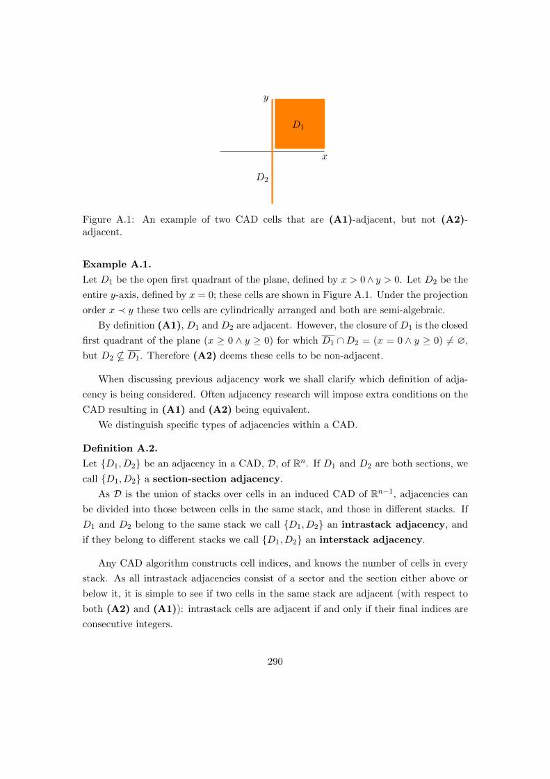
D2

D1

x

y

Figure A.1: An example of two CAD cells that are (A1)-adjacent, but not (A2)-adjacent.

Example A.1.

Let D1 be the open first quadrant of the plane, defined by x > 0∧ y > 0. Let D2 be the

entire y-axis, defined by x = 0; these cells are shown in Figure A.1. Under the projection

order x ≺ y these two cells are cylindrically arranged and both are semi-algebraic.

By definition (A1), D1 and D2 are adjacent. However, the closure of D1 is the closed

first quadrant of the plane (x ≥ 0 ∧ y ≥ 0) for which D1 ∩D2 = (x = 0 ∧ y ≥ 0) 6= ∅,

but D2 * D1. Therefore (A2) deems these cells to be non-adjacent.

When discussing previous adjacency work we shall clarify which definition of adja-

cency is being considered. Often adjacency research will impose extra conditions on the

CAD resulting in (A1) and (A2) being equivalent.

We distinguish specific types of adjacencies within a CAD.

Definition A.2.

Let D1, D2 be an adjacency in a CAD, D, of Rn. If D1 and D2 are both sections, we

call D1, D2 a section-section adjacency.

As D is the union of stacks over cells in an induced CAD of Rn−1, adjacencies can

be divided into those between cells in the same stack, and those in different stacks. If

D1 and D2 belong to the same stack we call D1, D2 an intrastack adjacency, and

if they belong to different stacks we call D1, D2 an interstack adjacency.

Any CAD algorithm constructs cell indices, and knows the number of cells in every

stack. As all intrastack adjacencies consist of a sector and the section either above or

below it, it is simple to see if two cells in the same stack are adjacent (with respect to

both (A2) and (A1)): intrastack cells are adjacent if and only if their final indices are

consecutive integers.

290

Therefore the difficulty lies in interstack adjacencies, and in particular interstack

section-section adjacencies (from which the entire interstack adjacencies can be calcu-

lated).

A.2 Properties Related to Adjacency

There are certain properties of CAD cells that are related to adjacency. These are

not restricted just to cells of CADs and can be used for other decompositions or cell

complexes.

Definition A.3.

Let D be a CAD of Rn, and let D be a cell of D with dimension k. Recall that the

boundary of D, ∂D, is equal to the difference of D and its closure: D \D.

We say that D is boundary coherent if its boundary is the union of cells of di-

mension less than or equal to d− 1.

We say that D is well-bordered if its boundary is the closure of finitely many cells

of dimension d− 1.

We say that D is boundary smooth if for all points p ∈ ∂D, there exists an ε > 0

such that the ball of radius ε centred at p is connected.

If every cell of D is boundary coherent, well-bordered, and boundary smooth then

we say that D is a strong cell decomposition.

A strong cell decomposition is a very well-behaved CAD with respect to adjacency,

and has appealing topological properties. It has not been shown which CAD algorithms

produce a strong cell decomposition and it is being investigated by other researchers at

the University of Bath.

A.3 Decidability of Adjacency in CAD [Arn79]

In [Arn79] the (A2) definition of adjacency is considered (and referred to as incidence).

Arnon proves the following result which gives the decidability of adjacency:

Theorem A.1 ([Arn79]).

If the defining formulae and dimensions are known for each cell in a CAD then we can

determine the incidences among cells.

Proof.

Let Di be an i-cell and Dj be a j-cell, with i < j. We produce a sentence in the

291

elementary theory of real closed fields representing the statement “Di is incident on

Dj”.

Let ϕi and ϕj be the defining formulae for Di and Dj . Recall a limit point, x, of

a set, S, is a point such that for every open ball of radius ε > 0 centred at x contains a

point y ∈ S with y 6= x. Then the definition of (A2)–adjacency is equivalent to every

point of Di being a limit point of Dj (by the definition of closure).

The statement “every point of Di is a limit point of Dj” can be expressed as the

following sentence in the elementary theory of real closed fields:

∀x∀ε [[ϕi(x) ∧ ε > 0]→ ∃y [ϕj(y) ∧ 0 < d(x, y) < ε]] .

This is a statement in the elementary theory of real closed fields and therefore can

be decided (for example by CAD-based quantifier elimination).

A.4 Adjacency Algorithms

We give a brief description of some of the work that has been done on algorithms for

adjacency.

A.4.1 The Piano Mover’s Problem [SS83b]

The authors of [SS83b] introduce a well-based condition that is similar to the stronger

well-oriented condition required for Brown’s projection operator. They prove that for

well-based CADs (A1) and (A2) are equivalent.

The authors show that the compact cells within a well-based CAD form a regular

cell complex (a well-studied topological structure). They use this along with the fact

that every regular cell complex admits an incidence function to show the construction

of an incidence function for a well-based CAD. They show explicitly how to compute

incidence between cells of dimension n and n−1, which is all that is theoretically needed

for the Piano Mover’s Problem, using the number of roots over cells (computed by Sturm

sequences). They describe a method to extend to cells of a lower dimension, although

it requires fractional Laurent series and Newton approximation (with exponential com-

plexity).

292

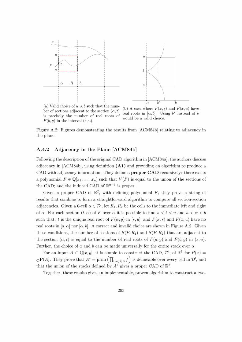
α

t

F

R

F

u

s

b

(a) Valid choice of u, s, b such that the num-ber of sections adjacent to the section (α, t)is precisely the number of real roots ofF (b, y) in the interval (s, u).

α b

s

t

u

b∗

(b) A case where F (x, s) and F (x, u) havereal roots in [α, b]. Using b∗ instead of bwould be a valid choice.

Figure A.2: Figures demonstrating the results from [ACM84b] relating to adjacency inthe plane.

A.4.2 Adjacency in the Plane [ACM84b]

Following the description of the original CAD algorithm in [ACM84a], the authors discuss

adjacency in [ACM84b], using definition (A1) and providing an algorithm to produce a

CAD with adjacency information. They define a proper CAD recursively: there exists

a polynomial F ∈ Q[x1, . . . , xn] such that V (F ) is equal to the union of the sections of

the CAD; and the induced CAD of Rn−1 is proper.

Given a proper CAD of R2, with defining polynomial F , they prove a string of

results that combine to form a straightforward algorithm to compute all section-section

adjacencies. Given a 0-cell α ∈ D′, let R1, R2 be the cells to the immediate left and right

of α. For each section (t, α) of F over α it is possible to find s < t < u and a < α < b

such that: t is the unique real root of F (α, y) in [s, u]; and F (x, s) and F (x, u) have no

real roots in [a, α] nor [α, b]. A correct and invalid choice are shown in Figure A.2. Given

these conditions, the number of sections of S(F,R1) and S(F,R2) that are adjacent to

the section (α, t) is equal to the number of real roots of F (a, y) and F (b, y) in (s, u).

Further, the choice of a and b can be made universally for the entire stack over α.

For an input A ⊂ Q[x, y], it is simple to construct the CAD, D′, of R1 for P (x) =

CP(A). They prove that A∗ = prim(∏

0 6=f∈A f)

is delineable over every cell in D′, and

that the union of the stacks defined by A∗ gives a proper CAD of R2.

Together, these results gives an implementable, proven algorithm to construct a two-

293

dimensional CAD with adjacency information for all cells.

A.4.3 Algebraic Cell Decomposition [KY85]

This paper mainly deals with augmenting the algorithm of Ben-Or, Kozen and Reif

(BKR) to provide a decomposition that, like CAD, distinguishes between connected

components determined by the signs of a set of polynomials. This is done in approxi-

mately the same complexity of BKR: singly-exponential.

They work with cell complexes, so the closure of a cell is a union of cells and there-

fore (A1) and (A2) are equivalent. They construct a graph for the cell complex such

that each node is a maximal connected component and the edges provide adjacency

information.

A.4.4 Approximation and Incidence [Pri86]

Prill openly distinguishes between (A1) (which he names adjacency) and (A2) (which

he names incidence). He uses a linear change of coordinates to guarantee the bounded

cells form a cell complex and so has restricted application. With these transformed

coordinates he builds an approximate decomposition and uses incidence points to

identify incident cells.

A.4.5 Adjacency in Three Dimensions [ACM88]

The authors extend their work from [ACM84b] and consider (A1). They define the

boundary coherent property (which they call the boundary property), and show that

for a CAD with this property (A1) and (A2) are equivalent. Further, a proper CAD

will always have this property (but the converse is not necessarily true).

Considering three-dimensional CADs over proper CADs of R2, each boundary point

of a cell must either be in the same stack as the cell or in some adjacent low-dimensional

stack. Determining these interstack adjacencies separates into three cases depending

on the possible dimension pairs: 1, 2, 0, 1, and 0, 2 (with the latter two needing

special consideration in the case of nullification). Nullification is a possibility (unlike in

two dimensions) and can be avoided with a coordinate change, but this is undesirable.

The authors give a method to ensure nullification can only occur on 0-cells, which allows

an adaptation of the lifting stage to construct a CAD of R3 with boundary coherence.

With additional concepts such as basis-determined CADs and section boundary prop-

erties they provide an algorithm, CADA3, which constructs a CAD of R3 with boundary

coherence along with a list of all adjacencies (finite and infinite) of the CAD.

294

A.4.6 Non-nullifying 0, 1-Adjacency and Local Box Adjacency [CM95,

MC02]

These papers extend the work of [ACM88] looking at particular cases of the box algo-

rithm.

In [CM95] the case of a non-nullifying 0, 1-adjacency is considered. It provides a

theorem that allows a more efficient way to deal with these adjacencies. Further, it can

be extended to four dimensions in certain cases.

The case of 0, 1-adjacencies is investigated further in [MC02], where the authors

give a local algorithm for these adjacencies, building on the work of [CM95]. Efficient

algorithms are given for cells in R2, R3, and R4 and a general algorithm is given for Rn

that is unlikely to fail (and if so, can be rectified by an change of isolating interval).

This work is, to the best of the author’s knowledge, the most current research in CAD

adjacency.

A.4.7 Using Adjacency Whilst Constructing CADs [Arn88]

In [Arn88] the author uses adjacency information to streamline the lifting stage of CAD

by clustering cells together according to their signature with respect to the input poly-

nomials (so that certain computations can be done only once for the whole cluster). The

(A1) definition of adjacency is used, but as the output CADs from [ACM84b, ACM88]

are being considered, this will be equivalent to (A2). The idea of a graph representation

and clustering is given and used throughout.

Given a set of polynomials F = f1, . . . , fm ⊆ Q[x1, . . . , xn] we represent a cell of a

CAD D by a triple (I, σ, S) where I is the cell index, σ = (σ1, . . . , σm) ∈ −1, 0,+1mis the signature (sign of each polynomial in F on the cell), and S a sample point.

Definition A.4.

Let F = f1, . . . , fm ⊆ Q[x1, . . . , xn] and D an F -invariant CAD of Rn. The graph

representation of D is defined to be G = (F,B, V,E,G′) where:

F is the polynomials used to define D.

B is a basis for prim(F ) such that D is a basis-determined CAD for B.

V is the set of vertices of the graph — all triples representing the cells in D.

E is the set of edges of the graph. If (D1, D2) is an element of E, then D1 and D2 are

adjacent in D. If all adjacencies are represented by such an edge, G is called a full

graph, else G is a partial graph.

295

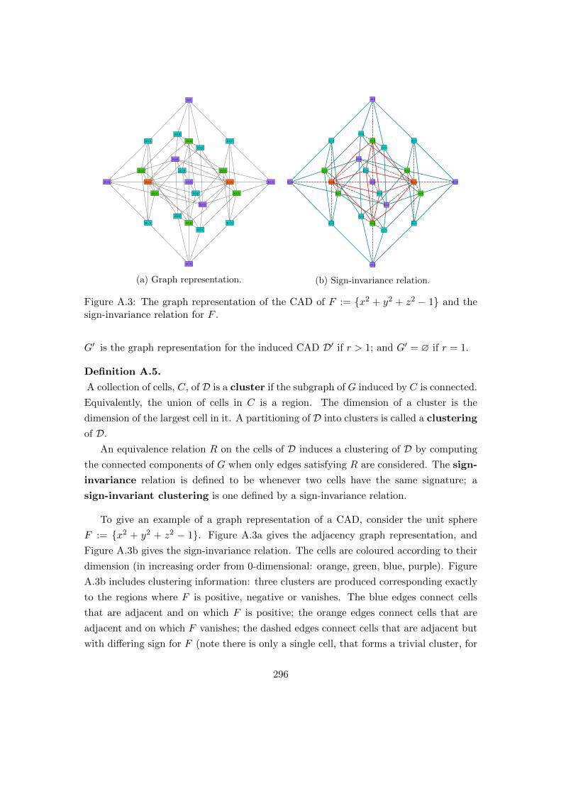
(a) Graph representation. (b) Sign-invariance relation.

Figure A.3: The graph representation of the CAD of F := x2 + y2 + z2 − 1 and thesign-invariance relation for F .

G′ is the graph representation for the induced CAD D′ if r > 1; and G′ = ∅ if r = 1.

Definition A.5.

A collection of cells, C, of D is a cluster if the subgraph of G induced by C is connected.

Equivalently, the union of cells in C is a region. The dimension of a cluster is the

dimension of the largest cell in it. A partitioning of D into clusters is called a clustering

of D.

An equivalence relation R on the cells of D induces a clustering of D by computing

the connected components of G when only edges satisfying R are considered. The sign-

invariance relation is defined to be whenever two cells have the same signature; a

sign-invariant clustering is one defined by a sign-invariance relation.

To give an example of a graph representation of a CAD, consider the unit sphere

F := x2 + y2 + z2 − 1. Figure A.3a gives the adjacency graph representation, and

Figure A.3b gives the sign-invariance relation. The cells are coloured according to their

dimension (in increasing order from 0-dimensional: orange, green, blue, purple). Figure

A.3b includes clustering information: three clusters are produced corresponding exactly

to the regions where F is positive, negative or vanishes. The blue edges connect cells

that are adjacent and on which F is positive; the orange edges connect cells that are

adjacent and on which F vanishes; the dashed edges connect cells that are adjacent but

with differing sign for F (note there is only a single cell, that forms a trivial cluster, for

296

which F is negative).

The idea of using the sign-invariant adjacency information is as follows. Given an ar-

bitrary PROJ(F )-invariant decomposition (not necessarily cylindrical) D of Rn−1 then

we can extend it to a decomposition D∗ of Rn by exactly the steps used in CAD for

extension over a single cell. D∗ may not be cylindrical, but if D is algebraic then so is

D∗. Given a graph for a PROJ(F )-invariant CAD of Rn−1 we can form a decomposi-

tion by taking the PROJ(F )-invariant clusters and lift as above to form an F -invariant

decomposition of Rn. This is summarised as follows:

1. If n > 1 call the algorithm recursively to build a graph for the induced CAD of

Rn−1.

2. (a) If n > 1 extend, over the maximal sign-invariant clusters of the induced CAD,

to a graph for the CAD of Rn.

(b) If n = 1 build a graph directly

3. Construct additional adjacencies in Rn. Cluster as appropriate.

This suggests a new definition for minimal CADs that could be useful.

Definition A.6.

We say an F -invariant decomposition D∗ of Rn is a (algorithmically) minimal de-

composition if during its construction no further clustering can be conducted.

We say an F -invariant CAD D of Rn is a (algorithmically) minimal CAD if the

only clustering steps not used during its construction invalidate cylindricity.

Identifying algorithmically minimal CADs could be a fruitful research topic and

comparing to algorithmically minimal decompositions could give further insight into

what the cost of ensuring cylindricity is.

A.5 Future Work: Adjacency in sub-CADs

We discuss how the work in this thesis could apply to the adjacency theory described in

the previous sections.

A.5.1 Adjacency in New CAD Algorithms

All the current CAD adjacency algorithms discussed in Section A.4 are designed for

use with a projection and lifting CAD algorithm. There are no algorithms designed for

297

use with any of the regular chains algorithms, or for either a TTICAD or equational

constraint CAD.

As deciding adjacency is a difficult process, but clearly useful, it would seem prudent

to look at whether any properties of these new CAD algorithms and the CADs they

produce are amenable to deciding adjacency. It may be that a particular algorithm

can be shown to always produce a strong cell decomposition (Definition A.3), which

automatically permits certain adjacency computations. Indeed, a tailored adjacency

algorithm may be possible for certain new CADs.

A.5.2 Clustering in Adjacency Graphs and Minimality of CADs

In [Arn88] the definition of the graph representation of a CAD and sign-invariant clus-

tering was given (reproduced in Definitions A.4 and A.5) where adjacent cells with iden-

tical sign signatures are clustered together. The algorithm described in [Arn88] then

uses these clusters to simplify the CAD during the lifting phase.

This inspired the new Definition A.6 of algorithmically minimal decompositions.

It would seem worthwhile to investigate this property to first identify algorithmically

minimal CADs and then use this to motivate new advances. It is tempting to define

minimality of a CAD related to the theoretically minimal CAD, but such a CAD may

not be constructible by any algorithm. Definition A.6 is tied to an algorithm and so the

algorithmically minimal CAD must be constructible.

A collection of algorithmically minimal CADs for a given algorithm would provide

a ground truth to compare other algorithms to, along with allowing further insight

into concepts like variable orders. This would avoid any artefacts of the algorithms’

implementations having an impact on the results.

A.5.3 Adapting Adjacency in sub-CADs

Previous work on adjacency in CAD has had limited impact due to both the complexity

of the algorithms (for D cells, O(D2) adjacencies will need to be considered, of which

some will be non-trivial) and necessary conditions such as boundary coherence or well-

borderedness (which need to not just hold, but be explicitly shown to hold).

There is hope that the sub-CAD techniques introduced in Chapter 4 might help. A

sub-CAD is a subset of the cells in a CAD and so the issue of complexity of an adjacency

algorithm is immediately reduced, although still present. The issue of boundary coher-

ence or well-borderedness is also still present but reduced. Given a TTICAD that fails

the well-orientedness condition there is a chance that a sub-TTICAD avoids the trou-

298

blesome cells and so constructs without theoretical failure. The same possibility exists

with sub-CADs and the adjacency conditions from Section A.2: if the cells that violate

one of those conditions are not contained in the sub-CAD then an existing adjacency

algorithm can be applied.

There is an additional benefit to constructing a layered sub-CAD. In [SS83b] the au-

thors give an explicit algorithm for computing adjacencies of n and (n− 1) dimensional

cells, pointing out that comparing cells of lesser dimension introduces further complica-

tion. Therefore a 2-layered sub-CAD (but not a 2-layered variety sub-CAD) would allow

application of the simpler form of this algorithm. It also suggests that the n, n − 1adjacencies are somehow “simpler” than other adjacencies. This should be investigated

further to see if adjacencies behave differently depending on the layers being considered,

and if the restriction to a variety sub-CAD affects this relation.

A.5.4 Topology: `-dimensionally Path Connected

We attempt to relate the concepts arising within layered sub-CADs to topological prop-

erties. Recall the definition of an `-dimensional ball:

Definition A.7.

The `-dimensional ball centred at the point α ∈ R` of radius ε > 0, denoted by B(`)ε (α),

is defined to be:

B(`)ε (α) :=

x ∈ R` | |x− α| < ε

(A.1)

The idea of spaces being connected by paths is well-defined and studied within Topol-

ogy, with the following definition being the basis of path-connectedness.

Definition A.8. [Wil04]

A space X is pathwise connected if and only if for any two points x and y in X, there

is a continuous function f : [0, 1]→ X such that f(0) = x, f(1) = y.

However, path-connectedness can be perhaps deceptive as the following example

shows.

Example A.2.

Consider the plane, R2, and the four open quadrants labelled clockwise from the positive

quadrant. Let X be the first quadrant and Y the third quadrant, as shown in Figure

A.4.

The closures, X and Y , are path connected. In particular, X ∩ Y = (0, 0) so any

path between points in separate quadrants must pass through the origin.

299

X

Y

(0, 0)

Figure A.4: Two quadrants of the plane that are path connected through the origin.

For practical applications of CAD we often want a stronger condition. Unaware of a

formal definition in Topology, we create such a definition here:

Definition A.9.

A space X is said to be `-dimensionally pathwise connected if for any two points

x and y in X, there is ε > 0 and a continuous function f : B(`)ε (0)× [0, 1]→ X such that

f(0, 0) = x and f(0, 1) = y.

Clearly 0-dimensionally pathwise connected is equivalent to the definition of pathwise

connected given in Definition A.8. Informally, 1-dimensionally and 2-dimensionally path-

connected spaces are those in which we can connect any two points by a deformation of

a non-trivial ribbon or cylinder, respectively.

Consider Example A.2. We see that whilst the quadrants are 0-dimensionally path-

connected, they are not 1-dimensionally path connected (unlike the closure of two adja-

cent quadrants).

With Definition A.9 we can consider connectivity of an `-layered sub-CAD.

Theorem A.2.

Let D be an `-layered CAD. Then each path-connected component of D is, at least,

(n− `+ 1)-dimensionally path connected.

Proof.

Let x and y be in the same path-connected component of D, say X, and let f : [0, 1]→ X

be a path connecting x and y.

As D is `-layered, X is comprised of a union of a finite number of cells, each with

dimension in the range n−`+1 ≤ d ≤ n. For each cell Di, let εi be the smallest distance

from a point on the image of f to the boundary of the closure of Di. As each cell is

open, this value is non-zero and an (n− `+1)-dimensional ball of radius εi can surround

every point of f([0, 1]) in Di without intersecting the boundary of Di.

300

Choosing ε > 0 such that ε < min(ε1, . . . , εm) therefore proves that X is (n− `+ 1)-

dimensionally path-connected.

The idea of `-dimensional path connectedness can also transfer to layered variety sub-

CADs, although care needs to be taken with dimensions to account for the co-dimension

of the variety.

It would seem that this new definition of path connectedness is well-suited for robot

motion planning: a solid three-dimensional object cannot move between two three-

dimensional regions by passing through just a 0-dimensional or 1-dimensional cell, and

so 2-dimensional path connectedness is required. Dimensional path connectedness does

not guarantee the presence of a valid path however, only the topological possibility (e.g.

something of 10m width can topologically fit through a 1cm hole but cannot geometri-

cally).

The work on the Piano Mover’s Problem in Section 6.3 showed that it is now feasible

to construct CADs for motion planning problems, albeit only for the most simple cases.

Combined with sub-CAD techniques, as described in Section 6.3.9, the construction

is simplified and the main issue is that of adjacency. An algorithm that constructs a

graph representation of a layered variety sub-CAD with respect to the `-dimensional

path connectedness relation would be sufficient to solve this problem.

301

302

Appendix B

A Repository of CAD Problems

In the process of investigating various properties of CADs, it seemed important to have a

large collection of examples to consider. This prompted the creation of a CAD repository

which was opened for public use in [WBD13] and is available online at [Wil12].

B.1 Motivation and Practical Considerations

Due to the high complexity of CAD (Section 2.6) it can be difficult to find feasible

problems to test.

As a CAD is a representation of the underlying structure of a system of polynomials,

random examples behave quite differently to those sourced from applications or pre-

defined problems.

Because of these two facts, the majority of problems were sourced from various key

papers in the CAD literature. These currently include: [CMXY09], [Laz88], [McC88],

[CMA82], [DSS04], [CH91], [Hon90], [Ach56], [Dav86], [BH91], [AM88], [Dav11], [BG06],

[BDE+13].

Whilst this approach avoids the creation of random examples, it is not without

its own drawbacks. The examples in the literature are generally those well-suited to

particular existing techniques. With advances in CAD technology like those mentioned

in this thesis, problems that were previously considered ‘hard’ may become simple to

tackle. Also, if a new technique is suited for problems of a certain form (for example

TTICAD in Chapter 3) then there may not be examples in the literature appropriate to

test it with. This is compensated by the creation of new examples and their inclusion

into the example bank.

For each example sourced, the following are provided:

303

• The full statement of the problem (with quantifiers if appropriate);

• A list of free and quantified variables, along with a suggested variable ordering if

one is given in the original statement;

• The best achieved number of cells (see Section B.2);

• Notes on the problem and the original source;

• Input for both Maple and Qepcad.

Since its creation and public launch in [WBD13], the repository has grown to contain

a variety of examples, although it is still small compared to other example banks such as

nlsat. Hopefully it will continue to expand and become a useful resource for researchers

of CAD theory.

B.2 Theoretical Questions

Although a rather simple database of examples, certain questions arose during its cre-

ation that have proven interesting and significant.

On a broad level, the main question to be considered is what constitutes a new

CAD problem. It seems fairly clear that reordering the variables in a problem does not

fundamentally change the problem (unless the ordering is dictated by a quantifier elimi-

nation problem). However, for example, preconditioning input can produce a drastically

different CAD.

This highlights a hierarchy of specificity for CAD problems, that was discussed in

Chapter 7. Consider the Piano Mover’s Problem discussed in Section 6.3. At the highest

level we have a completely abstract problem: “can a ladder fit through a corridor”. This

translates (in a variety of ways, as discussed) into a “logical” problem, which leads to a

semi-algebraic variety. The semi-algebraic variety in question can be formulated into an

expression of polynomials (again, possibly in multiple ways). This equation can then be

“oriented” through the choice of a variable order before, finally, a CAD can be produced

(after deciding invariance conditions, sub-CAD techniques and so forth).

There is a choice of which part of this hierarchy we describe in our repository, and

it seems that the translation of the logical problem into an expression of polynomials is

a sensible thing to consider. All formulations derived from such an expression will be

related, in that (after possible re-orientation) cells from CADs of different formulations

will be subsets or supersets of each other. However, a different logical formulation (such

as Section 6.3.4 compared to [Dav86]) will produce a completely different CAD.

304

Including a field that showed the minimal number of cells for a given problem is

desirable - it gives an indication of the difficulty of the CAD problem. However, it is

not obvious what “minimal” should stand for. There are theoretically minimal CADs

for problems that cannot be constructed by any known algorithm. Therefore, the field

was changed to be “best achievable number of cells” (with information on how to obtain

this number where appropriate).

The idea of minimality of CADs is a hugely complex area without even a well-defined

question. Work in [Bro98] discusses the idea of simplifying a CAD post-production

according to truth value to minimise its complexity. Certain lifting techniques can be

thought of as methods of minimising complexity during the construction phase, and

restriction of output (for example sub-CADs and partial CADs) can be thought an

extreme case. Many of these ideas are being considered by other members of the research

group.

305

306

Appendix C

Implementations

The implementation of the work in this thesis is discussed. Certain issues that occurred

during the implementation of various algorithms, but which were not related to the

theory, are given along with descriptions of their solutions.

Implementation of the projection and lifting CAD algorithms in the ProjectionCAD

module for Maple was not conducted by the author, but by Dr. England of the research

group. Details are given in [Eng13a, Eng13b, EWBD14] and the work is summarised

here due to its relevance to the theory and experimentation of this thesis.

Details of the author’s implementation of sub-CAD algorithms in ProjectionCAD

were originally described in [WE13] (describing the original LayeredCAD extension).

All Maple packages described in this appendix are available freely for download

from the author’s website1. The CADassistant tool is available freely for download

from the author’s GitHub repository2.

C.1 The ProjectionCAD Module

Many of the algorithms discussed in this thesis are from the ProjectionCAD module

in Maple. This was created by another member of the research team at Bath to

provide a projection and lifting CAD algorithm that is customisable and for which we

can post-process the output within Maple. The implementation is discussed in detail

in [Eng13a, Eng13b, EWBD14], and we briefly discuss it here.

The ProjectionCAD algorithms are all projection and lifting based and follow the

CAD algorithms of [Col75, McC85, McC99, Bro01], which cover construction by the

1http://www.cs.bath.ac.uk/~djw422http://www.github.com/DavidJohnWilson/CADassistant

307

various projection operators (using the CADFull command along with the method pa-

rameter) along with utilising equational constraints (using the ECCAD command). These

are extended using the theory of Chapter 3 to include the TTICAD algorithm. There are

also algorithms to use the various heuristics detailed in Chapter 5.

Whilst the CAD algorithms are projection and lifting based, ProjectionCAD is built

over the RegularChains module (and the SemiAlgebraicSetTools sub-module), as

described in [EWBD14]. Cells are represented by regular chains, and lifting is done

using the RegularChains stack generation procedure.

One particular property of the ProjectionCAD module compared to other projection

and lifting implementations is that it includes the improved equational constraint lifting

that follows from [McC99] but was not explicitly noted until [BDE+13]: the final lifting

stage needs to only be with respect to the equational constraint as opposed to the

entire input set. This means that the ECCAD can sometimes perform better than other

equational constraint implementations (such as Qepcad). However ProjectionCAD does

not implement the theory of partial CAD or contain a quantifier elimination procedure.

C.2 Algorithms for sub-CADs in the ProjectionCAD Mod-

ule (in Maple)

In developing the theory of cylindrical algebraic sub-decompositions (described in Chap-

ter 4) it was important to have an implementation of the algorithms described to allow

for comprehensive experimentation. Algorithms to construct variety, layered (direct and

recursive), and layered variety sub-CADs were implemented by the author in Maple

as an extension of the ProjectionCAD package. The corresponding algorithms for sub-

TTICADs (Section 4.4.2) are also given. This explanation was first given in the technical

report [WE13].

Originally provided as a separate package, LayeredCAD, the following user-level com-

mands are available:

• VCAD([f,G],vars);

• VCADLiftOverLowCAD(lowCAD, equCon, vars);

• VTTICAD(Phi,vars);

• LCAD(F,L,vars);

• LCADRecursive(F,vars,C,LD);

308

• LTTICAD(Phi,L,vars);

• LCADDisplay(LCAD);

• LVCAD([f,G],L,vars);

• LVTTICAD(Phi,L,vars);

The functions also allow further options through additional input parameters: for ex-

ample those constructing sub-CADs allow for an output parameter of list, listwithrep,

or piecewise (which is discussed in Section C.2.4).

We discuss briefly the implementations of these procedures, highlighting points of

interest.

C.2.1 Variety sub-CAD Procedures

The variety sub-CAD procedures were straightforward to implement over the Projection-

CAD package, and VCAD follows Algorithm 4.1.

Upon calling VCAD, the input polynomials are projected and an (n− 1)-dimensional

CAD is created using the standard CAD algorithms in ProjectionCAD. The important

step is then a call to VCADLiftOverLowCAD which lifts from an (n−1)-dimensional CAD

to the variety. This is simple (assuming the input satisfies the requirements of Algorithm

4.1): for each cell of the lower-dimensional CAD a stack is generated with respect to the

equational constraint (defining the variety) and if this contains more than one cell, the

even indexed cells are retained.

C.2.2 Layered sub-CAD Procedures

Constructing a layered sub-CAD requires a little more care to ensure that the correct

dimension cells are returned. Underlying all algorithms is a check whether a cell is of suf-

ficient dimension to produce cells for the specified layered sub-CAD. This is determined

using the following formula:

dim(D) =∑

i∈D.index(i mod 2) .

A valid cell for an `-layered sub-CAD of Rn must have dimension greater than or equal

to n+1−`. Similarly, when considering a cell in Rk, then it can only contribute a cell to

an `-layered sub-CAD of Rn if the cell has dimension greater than or equal to k+ 1− `.

309

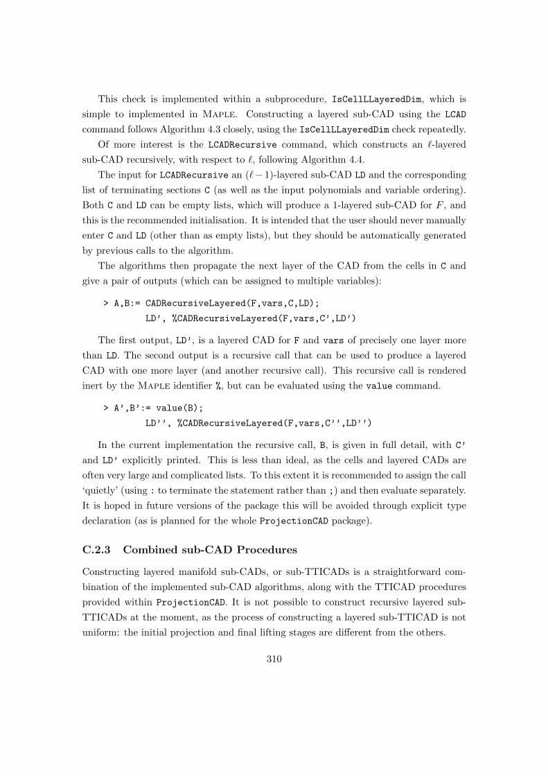
This check is implemented within a subprocedure, IsCellLLayeredDim, which is

simple to implemented in Maple. Constructing a layered sub-CAD using the LCAD

command follows Algorithm 4.3 closely, using the IsCellLLayeredDim check repeatedly.

Of more interest is the LCADRecursive command, which constructs an `-layered

sub-CAD recursively, with respect to `, following Algorithm 4.4.

The input for LCADRecursive an (`− 1)-layered sub-CAD LD and the corresponding

list of terminating sections C (as well as the input polynomials and variable ordering).

Both C and LD can be empty lists, which will produce a 1-layered sub-CAD for F , and

this is the recommended initialisation. It is intended that the user should never manually

enter C and LD (other than as empty lists), but they should be automatically generated

by previous calls to the algorithm.

The algorithms then propagate the next layer of the CAD from the cells in C and

give a pair of outputs (which can be assigned to multiple variables):

> A,B:= CADRecursiveLayered(F,vars,C,LD);

LD’, %CADRecursiveLayered(F,vars,C’,LD’)

The first output, LD’, is a layered CAD for F and vars of precisely one layer more

than LD. The second output is a recursive call that can be used to produce a layered

CAD with one more layer (and another recursive call). This recursive call is rendered

inert by the Maple identifier %, but can be evaluated using the value command.

> A’,B’:= value(B);

LD’’, %CADRecursiveLayered(F,vars,C’’,LD’’)

In the current implementation the recursive call, B, is given in full detail, with C’

and LD’ explicitly printed. This is less than ideal, as the cells and layered CADs are

often very large and complicated lists. To this extent it is recommended to assign the call

‘quietly’ (using : to terminate the statement rather than ;) and then evaluate separately.

It is hoped in future versions of the package this will be avoided through explicit type

declaration (as is planned for the whole ProjectionCAD package).

C.2.3 Combined sub-CAD Procedures

Constructing layered manifold sub-CADs, or sub-TTICADs is a straightforward com-

bination of the implemented sub-CAD algorithms, along with the TTICAD procedures

provided within ProjectionCAD. It is not possible to construct recursive layered sub-

TTICADs at the moment, as the process of constructing a layered sub-TTICAD is not

uniform: the initial projection and final lifting stages are different from the others.

310

|x| :=x x ≥ 0−x x < 0

(a) Maple GUI Output.

x 0 <= x

|x| :=

-x x < 0

(b) Maple Command-line Output.

Figure C.1: The result of the |x|:=piecewise(x<0,-x,x>=0,x) command in Maple.

C.2.4 LCADDisplay and piecewise Output

It is notably difficult [CDM+09] to display a CAD in a clear and concise way, and

communicating a sub-CAD presents extra challenges. It is important to communicate

to the user of a sub-CAD algorithm the following items:

• The cells within the sub-CAD (represented by a sample point and index), prefer-

ably with a clear representation of the semi-algebraic set they define;

• The structure and relations of these cells, highlighting their cylindrical nature;

• An indication of where cells have been discarded in the creation of the sub-CAD.

The piecewise construct in Maple is used to display piecewise functions, such

as the absolute value function, in a typographic style. Figure C.1 shows the result of

defining the absolute value function (with |x|:=piecewise(x<0,-x,x>=0,x)) with this

construct: Figure C.1a shows the formatted output available in the Maple graphical

user interface; Figure C.1b shows the output available in the Maple command-line

interface.

In [CDM+09] the authors demonstrated how the piecewise command could be used

to display geometrical decompositions in a meaningful manner. They provide usage of

this construct for comprehensive triangular decompositions, cylindrical algebraic decom-

positions, and real triangular decompositions. Furthermore, they demonstrate usage of

inert computations (designation in Maple with the prefix of % and evaluation with the

value command) when discussing lazy real triangular decompositions [CDM+10].

If a layered CAD has been constructed using the listwithrep formulation then it

can be displayed in an informative tree-like structure using LCADDisplay. This outputs

a Maple piecewise structure that gives an intuitive description of the layered CAD.

Whenever a branch has been terminated a placeholder is given.

A simple example is given in Figure C.2a. This can be compared to Figure C.2b which

shows the equivalent complete CAD in piecewise format. We see that the layered CAD

displayed omits all information regarding the cylinder above y = 0 as this is unnecessary

311

> LD,RLD:=LCADRecursive(x+y-1,y,[x,y],[],[],output=listwithrep):

> LCADDisplay(LD);

[regular_chain, [[-1, -1],[1, 1]]] x < -y + 1

["*********"] branch = truncated y < 0

[regular_chain, [[-1, -1],[3, 3]]] -y + 1 < x

["*********"] branch = truncated

[regular_chain, [[1, 1],[-1, -1]]] x < -y + 1

["*********"] branch = truncated 0 < y

[regular_chain, [[1, 1],[1, 1]]] -y + 1 < x

(a) Usage of LCADDisplay for a piecewise layered CAD

> CADFull(x y-1,y,[x,y],method=McCallum,output=piecewise);

[regular_chain, [[-1, -1],[1, 1]]] x < -y + 1

[regular_chain, [[-1, -1],[2, 2]]] x = -y + 1 y < 0

[regular_chain, [[-1, -1],[3, 3]]] -y + 1 < x

[regular_chain, [[0, 0],[0, 0]]] x < 1

[regular_chain, [[0, 0],[1, 1]]] x = 1 y = 0

[regular_chain, [[0, 0],[2, 2]]] 1 < x

[regular_chain, [[1, 1],[-1, -1]]] x < -y + 1

[regular_chain, [[1, 1],[0, 0]]] x = -y + 1 0 < y

[regular_chain, [[1, 1],[1, 1]]] -y + 1 < x

(b) Full piecewise CAD

Figure C.2: The piecewise output for a sub-CAD and complete CAD produced withProjectionCAD.

312

for a 1-layered CAD, along with the sections x = 1− y when y > 0 or y < 0. However,

and importantly, it still indicates that cells are present in these branches, although no

further details (such as the number of missing cells) are given as these are not computed.

Obviously this is a near-minimal example, and the added clarity of representing a sub-

CAD in this manner becomes even more pronounced and useful for larger sub-CADs.

C.3 Machine Learning Test Scripts

The problems chosen for the experiments in Section 5.3 [HEW+14b, HEW+14a] were

all chosen from the nlsat database, which provides descriptions of existential problems

in the Qepcad format. Construction of the CADs (and partial CADs) would be done

within Qepcad and thus require no adaptation of the input. The computation of the

feature vector or heuristics could not be completed within Qepcad as it is not a computer

algebra system, so Maple and ProjectionCAD were used for these purposes.

The author had already written a Python script to convert polynomials in the

Qepcad format to the Maple convention3 (and vice versa) and this was expanded as

necessary.

The resulting script, CADqepcadtomaple.py, takes an input file and output destina-

tion and performs the following:

1. Extracts the polynomials from the Qepcad input formula and converts them into

Maple polynomials.

2. Extracts the variable ordering from the Qepcad input and converts it into a

Maple ordering4.

3. Constructs Maple code to compute the feature vector for the problem, which

requires only basic Maple functions such as degree, coeffs and nops.

4. Constructs Maple code to compute the variable ordering choice for Brown’s

heuristic, sotd and ndrr using the VariableOrderingHeuristic procedure from

ProjectionCAD (also reversing the ordering choices to align with Qepcad’s con-

vention).

3The main difference in notation is that Qepcad indicates multiplication by whitespace, whilst inMaple an asterisk is used. Therefore 2 x3 y2 would be converted to 2 ∗ (x3) ∗ (y2).

4The ordering conventions are reversed, so that z ≺ y ≺ x is represented as (z, y, x) in Qepcad andas [x, y, z] in Maple.

313

(x0,x1,x2)

0

(E x0)(E x1)(E x2)[[((x0 x0) +

((x1 x1) + (x2 x2)))=1]].

go

go

go

d-stat

go

finish

(a) Quantified input.

(x0,x1,x2)

3

[[((x0 x0) + ((x1 x1) + (x2 x2)))=1]].

go

go

d-proj-factors

d-proj-polynomials

go

d-fpc-stat

go

finish

(b) Unquantified input.

Figure C.3: The Qepcad inputs for the quantified and unquantified version of a simpleproblem.

5. Writing the above commands to the output destination, which can then be read

into any instance of Maple (in this case, command-line interface) to output the

feature vector and three heuristic choices.

Following application of this script, the feature vector and heuristic choices for each

example could then be easily computed. Ideas from this script were subsequently used

in CADassistant.

The input into Qepcad also had to be prepared appropriately for the quantified and

unquantified cases. Sample input files are shown in Figure C.3.

C.4 The CADassistant Program (in Python)

We describe the implementation of CADassistant, which is discussed in Section 7.3.

The prototype of CADassistant is implemented in Python and can be run from

the command line with either interactive or manual mode specified:

$ python CADassistant.py interactive

$ python CADassistant.py manual

The interactive and manual modes are simply different approaches to deciding formu-

lation choices such as those discussed in Chapter 5.

In manual mode a list of questions are asked requiring the user to specify the con-

struction method, invariance condition, sub-CAD techniques (if applicable), formula de-

composition (if applicable), and equational constraints (if applicable). The interactive

314

method instead asks the user a sequence of questions to assist or automatically make

these choices. This may require the user to paste commands into Maple (such as heuris-

tic computations) and copy the output back into CADassistant. These decisions are

then encoded into an instance of a CAD object based on one of the CAD classes detailed

in the following section.

C.4.1 CAD Classes

A basic CadProblem class is used to create an object for each problem to store important

information. It contains instance variables to store the name, polynomials, and variables

of the problem, and methods to output strings containing information related to the

CAD.

1. CadProblem(name, polys, variables):

• Variables:

– name: string;

– polys: list of strings;

– variables: list of strings.

• Methods:

– printCAD(): returns a string describing the CAD (including name, polyno-

mials, and variables);

– listOfPolys(): returns a comma-separated list of the polynomials (delim-

ited by [ and ]);

– listOfVariables(): returns a comma-separated list of the variables (de-

limited by [ and ]);

Inheriting from the CadProblem class is the CadProblemMethod class which specifies

which algorithm should be used for the given problem. This information is stored in extra

variables, and an additional method creates a string with the CAD acronym (using the

acronyms listed in the CAD Dictionary in Appendix D).

2. CadProblemMethod(name, polys, variables, constr, inva, subCAD) (inherited from Cad-

Problem):

• Variables:

– constr: string (construction method; pl or rc);

– inva: string (invariance; si, oi, ec, or tti);

315

– subCAD: string (subCAD type; m, l, or lm).

• Methods:

– printCADproblem(): returns a string describing the CAD (including name,

polynomials, variables, and CAD acronym);

– CADacronym(): returns a string describing the CAD using an acronym (as

described in Appendix D).

If the CAD to be constructed is a truth table invariant CAD, the CadTTICAD class can

be used. This is inherited from CadProblemMethod and contains variables to describe

the formulae and designated equational constraints. All numbering is done with respect

to the order of the polynomials in the poly variable, and methods are used to check that

the designation and formula decomposition is valid.

3. CadTTICAD(name, polys, variables, constr, inva, subCAD, clauses, eqcons) (inherited

from CadProblemMethod):

• Variables:

– clauses: list of lists of integers (identifying clauses from the order of the

polynomials in polys);

– eqcons: list of lists of integers (identifying the equational constraint, if any,

in each clause).

• Methods:

– printTTICAD(): returns a string describing the CAD (including name, poly-

nomials, variables, CAD acronym, clause decomposition, and equational

constraint designation);

– printTTICADClauses(): returns a string describing the clauses and desig-

nated equational constraints (corresponding to the order of the polynomials

in polys);

– setClauses(clauses): sets the clauses according to a list of lists of integers

(calls checkClausesInp(clauses) to check the clauses given are valid, and

then calls setClauses(clauses));

– setEqCons(eqcons): sets the equational constraint designations according

to a list of lists of integers (calls checkEqConsInp(clauses) to check the

equational constraints given are valid, and then calls setEqCons(clauses)).

316

C.4.2 Output Formats

The output format of CADassistant depends on which algorithm is required. Currently

output can be given for Maple and Qepcad. The conversion is done using sections of

the scripts described in Section C.3 and the output can be copied into the appropriate

system to construct the requested CAD.

317

318

Appendix D

CAD Dictionary

A reference list of the various CAD acronyms that are used throughout this thesis. In

particular, the various composed forms of CAD are given in their acronym and full

descriptive form.

D.1 A Dictionary of CAD Acronyms

We provide a reference list of abbreviations and definitions for various forms of CAD.

CAD: Cylindrical Algebraic Decomposition as defined in Definition 2.14.

SICAD: Sign-Invariant CAD as defined in Definition 2.16.

OICAD: Order-Invariant CAD as defined in Definition 2.25.

PL-CAD: Projection and Lifting based CAD using one of the following projection

operators:

Collins: [Col75] as defined in Definition 2.22;

Collins–Hong: [Hon90] as defined in Definition 2.23;

McCallum: [McC85] as defined in Definition 2.24;

Brown–McCallum: [Bro01] as defined in Definition 2.27.

EC-CAD: Equational Constraint CAD [McC99] described in Section 2.32.

P-CAD: Partial CAD [CH91] described in Section 2.4.2.

RC-CAD: Regular Chains CAD using either:

319

RC-Rec-CAD: Recursive algorithm [CMXY09] described in Section 2.5.2;

RC-Inc-CAD: Incremental algorithm [CM12] and described in Section 2.5.3.

TTICAD: Truth Table Invariant CAD [BDE+13, BDE+14, BCD+14], defined in Def-

inition 3.2, and described in Chapter 3.

L-CAD: Layered sub-CAD [WBDE14], defined in Definition 4.4, and described in

Section 4.3.

V-CAD: Variety sub-CAD [WBDE14], defined in Definition 4.3, and described in

Section 4.2.

LV-CAD: Layered Variety sub-CAD [WBDE14], defined in Definition 4.6, and de-

scribed in Section 4.4.

L-TTICAD: Layered Truth Table Invariant sub-CAD [WBDE14] and described in

Section 4.4.2.

V-TTICAD: Layered Truth Table Invariant sub-CAD [WBDE14] and described in

Section 4.4.2.

LV-TTICAD: Layered Variety Truth Table Invariant sub-CAD [WBDE14] and de-

scribed in Section 4.4.2.

Table D.1 gives a quick-reference list of the CAD acronyms used in this thesis, listed

in an approximately conceptual order and in alphabetical order. Figure D.1 gives a

hierarchical representation of the various acronyms.

320

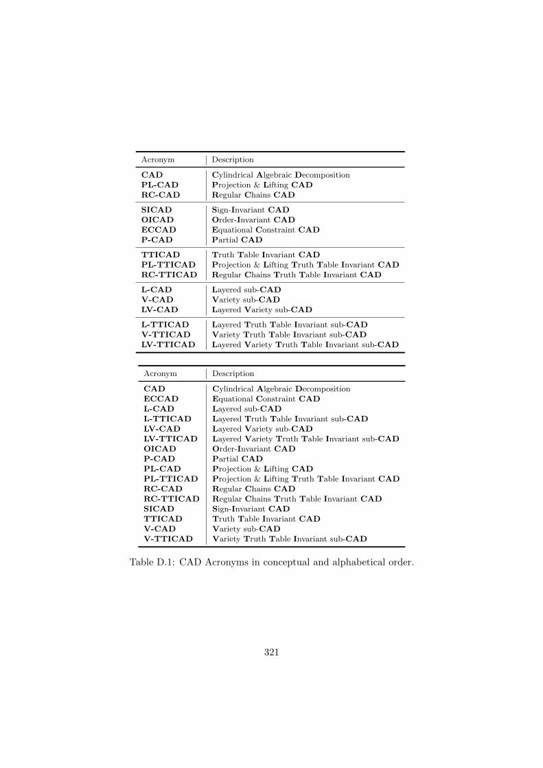
Acronym Description

CAD Cylindrical Algebraic DecompositionPL-CAD Projection & Lifting CADRC-CAD Regular Chains CAD

SICAD Sign-Invariant CADOICAD Order-Invariant CADECCAD Equational Constraint CADP-CAD Partial CAD

TTICAD Truth Table Invariant CADPL-TTICAD Projection & Lifting Truth Table Invariant CADRC-TTICAD Regular Chains Truth Table Invariant CAD

L-CAD Layered sub-CADV-CAD Variety sub-CADLV-CAD Layered Variety sub-CAD

L-TTICAD Layered Truth Table Invariant sub-CADV-TTICAD Variety Truth Table Invariant sub-CADLV-TTICAD Layered Variety Truth Table Invariant sub-CAD

Acronym Description

CAD Cylindrical Algebraic DecompositionECCAD Equational Constraint CADL-CAD Layered sub-CADL-TTICAD Layered Truth Table Invariant sub-CADLV-CAD Layered Variety sub-CADLV-TTICAD Layered Variety Truth Table Invariant sub-CADOICAD Order-Invariant CADP-CAD Partial CADPL-CAD Projection & Lifting CADPL-TTICAD Projection & Lifting Truth Table Invariant CADRC-CAD Regular Chains CADRC-TTICAD Regular Chains Truth Table Invariant CADSICAD Sign-Invariant CADTTICAD Truth Table Invariant CADV-CAD Variety sub-CADV-TTICAD Variety Truth Table Invariant sub-CAD

Table D.1: CAD Acronyms in conceptual and alphabetical order.

321

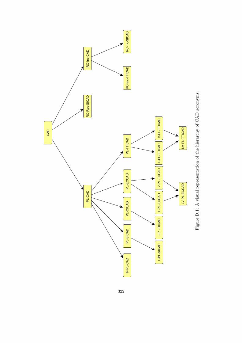
Fig

ure

D.1

:A

vis

ual

rep

rese

nta

tion

ofth

eh

iera

rchy

ofC

AD

acro

nym

s.

322

Appendix E

Publications

A list of references to publications describing work contained in this thesis. All papers

are available in their final draft form on the University of Bath Opus directory1, in

accordance to the Research Councils UK policy on open access.

E.1 Peer-Reviewed Articles

E.1.1 Published Articles

• David J. Wilson, Russell J. Bradford, and James H. Davenport. Speeding Up

Cylindrical Algebraic Decomposition by Grobner Bases. In Johan Jeuring, John A.

Campbell, Jacques Carette, Gabriel Dos Reis, Petr Sojka, Makarius Wenzel, and

Volker Sorge, editors, Intelligent Computer Mathematics, volume 7362 of Lec-

ture Notes in Computer Science, pages 280–294. Springer Berlin Heidelberg, 2012

(Refers to work in Chapter 6, Section 6.2).

• James H. Davenport, Russell J. Bradford, Matthew England, and David J. Wilson.

Program Verification in the Presence of Complex Numbers, Functions with Branch

Cuts etc. In Proceedings of the 2012 14th International Symposium on Symbolic

and Numeric Algorithms for Scientific Computing, SYNASC ’12, pages 83–88, 2012

(Refers to work in Chapter 6, Section 6.1).

• David J. Wilson, Russell J. Bradford, and James H. Davenport. A Repository

for CAD Examples. ACM Communications in Computer Algebra, 46(3/4):67–69,

January 2013 (Refers to work in Appendix B).

1The author’s Opus directory page: http://opus.bath.ac.uk/view/person_id/6172.html

323

• Russell J. Bradford, James H. Davenport, Matthew England, Scott McCallum, and

David J. Wilson. Cylindrical Algebraic Decompositions for Boolean Combinations.

In Proceedings of the 38th International Symposium on Symbolic and Algebraic

Computation, ISSAC ’13, pages 125–132, New York, NY, USA, 2013. ACM (Refers

to work in Chapter 3).

• David J. Wilson, James H. Davenport, Matthew England, and Russell J. Bradford.

A “Piano Movers” Problem Reformulated. In Proceedings of the 15th Interna-

tional Symposium on Symbolic and Numeric Algorithms for Scientific Computing,

SYNASC ’13, pages 53–60, Sept 2013 (Refers to work in Chapter 6, Section

6.3).

• Russell J. Bradford, James H. Davenport, Matthew England, and David J. Wil-

son. Optimising Problem Formulation for Cylindrical Algebraic Decomposition.

In Jacques Carette, David Aspinall, Christoph Lange, Petr Sojka, and Wolfgang

Windsteiger, editors, Intelligent Computer Mathematics, volume 7961 of Lecture

Notes in Computer Science, pages 19–34. Springer Berlin Heidelberg, 2013 (Refers

to work in Chapters 3 and 5).

• Matthew England, Russell J. Bradford, James H. Davenport, and David J. Wilson.

Understanding Branch Cuts of Expressions. In Jacques Carette, David Aspinall,

Christoph Lange, Petr Sojka, and Wolfgang Windsteiger, editors, Intelligent Com-

puter Mathematics, volume 7961 of Lecture Notes in Computer Science, pages 136–

151. Springer Berlin Heidelberg, 2013 (Refers to work in Chapter 3, Section

3.9).

• Matthew England, Edgardo Cheb-Terrab, Russell J. Bradford, James H. Daven-

port, and David J. Wilson. Branch Cuts in Maple 17. ACM Communications in

Computer Algebra, 48(1/2):24–27, March 2014 (Refers to work in Chapter 3,

Section 3.9).

• David J. Wilson, Russell J. Bradford, James H. Davenport, and Matthew England.

Cylindrical Algebraic Sub-Decompositions. Mathematics in Computer Science,

8(2):263–288, 2014 (Refers to work in Chapter 4).

• Matthew England, Russell J. Bradford, Changbo Chen, James H. Davenport, Mar-

cMoreno Maza, and David J. Wilson. Problem Formulation for Truth-Table In-

variant Cylindrical Algebraic Decomposition by Incremental Triangular Decompo-

sition. In Stephen M. Watt, James H. Davenport, Alan P. Sexton, Petr Sojka, and

324

Josef Urban, editors, Intelligent Computer Mathematics, volume 8543 of Lecture

Notes in Computer Science, pages 45–60. Springer International Publishing, 2014

(Refers to work in Chapters 3 and 5).

• Zongyan Huang, Matthew England, David J. Wilson, James H. Davenport, Lawrence C.

Paulson, and James Bridge. Applying Machine Learning to the Problem of Choos-

ing a Heuristic to Select the Variable Ordering for Cylindrical Algebraic Decompo-

sition. In Stephen M. Watt, James H. Davenport, Alan P. Sexton, Petr Sojka, and

Josef Urban, editors, Intelligent Computer Mathematics, volume 8543 of Lecture

Notes in Computer Science, pages 92–107. Springer International Publishing, 2014

(Refers to work in Chapter 5, Section 5.3).

E.1.2 Accepted for publication/presentation

• Zongyan Huang, Matthew England, David J. Wilson, James H. Davenport, and

Lawrence C. Paulson. A comparison of three heuristics to choose the variable order-

ing for cylindrical algebraic decomposition. ACM Communications in Computer

Algebra, 2014 (Accepted to ISSAC 2014 poster session to be published

in Communications in Computer Algebra; refers to work in Chapter 5,

Section 5.3.5).

• Matthew England, David J. Wilson, Russell J. Bradford, and James H. Davenport.

Using the Regular Chains Library to build cylindrical algebraic decompositions

by projecting and lifting. In Proceedings of the 2014 International Congress on

Mathematical Software, 2014 (Accepted to ICMS 2014; refers to work in

Appendix C).

• Matthew England, Russell J. Bradford, James H. Davenport, and David J. Wilson.

Choosing a variable ordering for truth-table invariant cylindrical algebraic decom-

position by incremental triangular decomposition. In Proceedings of the 2014 Inter-

national Congress on Mathematical Software, 2014 (Accepted to ICMS 2014;

refers to work in Chapters 3 and 5).

• Russell J. Bradford, Changbo Chen, James H. Davenport, Matthew England, Marc

Moreno Maza, and David J. Wilson. Truth Table Invariant Cylindrical Algebraic

Decomposition by Regular Chains. CoRR, abs/1401.6310, 2014 (Accepted to

CASC 2014; refers to work in Chapter 3).

325

• David J. Wilson, Matthew England, Russell J. Bradford, and James H. Davenport.

Using the distribution of cells by dimension in a cylindrical algebraic decomposi-

tion. SYNASC 2014, 2014 (Accepted to SYNASC 2014; refers to work in

Section 5.4).

E.1.3 Submitted for consideration

• Russell J. Bradford, James H. Davenport, Matthew England, Scott McCallum,

and David J. Wilson. Truth Table Invariant Cylindrical Algebraic Decomposition.

CoRR, abs/1401.0645, 2014 (Submitted to Journal of Symbolic Computa-

tion; refers to work in Chapter 3).

E.2 Non-Peer-Reviewed Articles

E.2.1 University of Bath Technical Reports

• David J. Wilson. Real Geometry and Connectedness via Triangular Description:

CAD Example Bank. Opus: University of Bath Online Publication Store, 2012

(Refers to work in Appendix B).

• David J. Wilson and Matthew England. Layered Cylindrical Algebraic Decom-

position. Technical report, Bath, August 2013 (Refers to work in Chapter

4).

• David J. Wilson, Russell J. Bradford, James H. Davenport, and Matthew England.

The Piano Mover’s Problem Reformulated. Technical report, Bath, June 2013

(Refers to work in Chapter 6).

326

Bibliography

[Ach56] N. I. Achieser. Solotareff’s Problems and Related Problems. In Theory of

Approximation, pages 280–289. Frederick Ungar Publishing Co., New York,

1956.

[ACM84a] Dennis S. Arnon, George E. Collins, and Scott McCallum. Cylindrical alge-

braic decomposition I: The basic algorithm. SIAM Journal on Computing,

13(4):865–877, 1984.

[ACM84b] Dennis S. Arnon, George E. Collins, and Scott McCallum. Cylindrical

Algebraic Decomposition II: An Adjacency Algorithm for the Plane. SIAM

Journal on Computing, 13(4):878, 1984.

[ACM88] Dennis S. Arnon, George E. Collins, and Scott McCallum. An adjacency al-

gorithm for cylindrical algebraic decompositions of three-dimensional space.

Journal of Symbolic Computation, 5(1-2):163–187, February 1988.

[AM88] Dennis S. Arnon and Maurice Mignotte. On mechanical quantifier elimi-

nation for elementary algebra and geometry. Journal of Symbolic Compu-

tation, pages 237–259, 1988.

[AMIA14] Noriko H Arai, Takuya Matsuzaki, Hidenao Iwane, and Hirokazu Anai.

Mathematics by machine. In Proceedings of the 39th International Sym-

posium on Symbolic and Algebraic Computation, ISSAC 2014, pages 1–8.

ACM, 2014.

[AP08] Behzad Akbarpour and Lawrence C. Paulson. MetiTarski: An Automatic

Prover for the Elementary Functions. In Serge Autexier, John Campbell,

Julio Rubio, Volker Sorge, Masakazu Suzuki, and Freek Wiedijk, editors,

Intelligent Computer Mathematics, volume 5144 of Lecture Notes in Com-

puter Science, pages 217–231. Springer Berlin Heidelberg, 2008.

327

[AP09] Behzad Akbarpour and Lawrence C. Paulson. MetiTarski: An Automatic

Theorem Prover for Real-Valued Special Functions. Journal of Automated

Reasoning, 44(3):175–205, August 2009.

[Arn79] Dennis S. Arnon. A cellular decomposition algorithm for semialgebraic

sets. In Edward W. Ng, editor, Symbolic and Algebraic Computation, vol-

ume 72 of Lecture Notes in Computer Science, pages 301–315. Springer

Berlin Heidelberg, 1979.

[Arn88] Dennis S. Arnon. A cluster-based cylindrical algebraic decomposition al-

gorithm. Journal of Symbolic Computation, 5(1):189–212, 1988.

[AS72] Milton Abramowitz and Irene A. Stegun. Handbook of Mathematical Func-

tions with Formulas, Graphs, and Mathematical Tables. National Bureau

of Standards Applied Mathematics Series 55. Tenth Printing. 1972.

[Bac89] J. Backelin. Square multiples n give infinitely many cyclic n-roots. Matem-

atiska Institutionen reports series, Stockholms Universitet, 1989.

[BBDP07] James C. Beaumont, Russell J. Bradford, James H. Davenport, and Nalina

Phisanbut. Testing elementary function identities using CAD. Applicable

Algebra in Engineering, Communication and Computing, 18(6):513–543,

2007.

[BCD+14] Russell J. Bradford, Changbo Chen, James H. Davenport, Matthew Eng-

land, Marc Moreno Maza, and David J. Wilson. Truth Table Invari-

ant Cylindrical Algebraic Decomposition by Regular Chains. CoRR,

abs/1401.6310, 2014.

[BD07] Christopher W. Brown and James H. Davenport. The Complexity of Quan-

tifier Elimination and Cylindrical Algebraic Decomposition. In Proceedings

of the 32nd International Symposium on Symbolic and Algebraic Computa-

tion, ISSAC ’07, pages 54–60, New York, NY, USA, 2007. ACM.

[BDE+13] Russell J. Bradford, James H. Davenport, Matthew England, Scott Mc-

Callum, and David J. Wilson. Cylindrical Algebraic Decompositions for

Boolean Combinations. In Proceedings of the 38th International Sympo-

sium on Symbolic and Algebraic Computation, ISSAC ’13, pages 125–132,

New York, NY, USA, 2013. ACM.

328

[BDE+14] Russell J. Bradford, James H. Davenport, Matthew England, Scott Mc-

Callum, and David J. Wilson. Truth Table Invariant Cylindrical Algebraic

Decomposition. CoRR, abs/1401.0645, 2014.

[BDEW13] Russell J. Bradford, James H. Davenport, Matthew England, and David J.

Wilson. Optimising Problem Formulation for Cylindrical Algebraic De-

composition. In Jacques Carette, David Aspinall, Christoph Lange, Petr

Sojka, and Wolfgang Windsteiger, editors, Intelligent Computer Mathe-

matics, volume 7961 of Lecture Notes in Computer Science, pages 19–34.

Springer Berlin Heidelberg, 2013.

[BG06] Christopher W. Brown and Christian Gross. Efficient Preprocessing Meth-

ods for Quantifier Elimination. In Victor G. Ganzha, Ernst W. Mayr, and

Evgenii V. Vorozhtsov, editors, Computer Algebra in Scientific Computing,

volume 4194 of Lecture Notes in Computer Science, pages 89–100. Springer

Berlin Heidelberg, 2006.

[BGV13] Saugata Basu, Andrei Gabrielov, and Nicolai Vorobjov. Semi-monotone

sets. Journal of the European Mathematical Society, 15(2):635–657, 2013.

[BH91] Bruno Buchberger and Hoon Hong. Speeding-up Quantifier Elimination by

Grobner Bases. RISC Report Series, pages 1–21, February 1991.

[BM05] Christopher W. Brown and Scott McCallum. On Using Bi-equational Con-

straints in CAD Construction. In Proceedings of the 30th International

Symposium on Symbolic and Algebraic Computation, ISSAC ’05, pages 76–

83, New York, NY, USA, 2005. ACM.

[BPB05] James C. Beaumont, Nalina Phisanbut, and Russell J. Bradford. Practical

Simplification of Elementary Functions Using CAD. pages 35–39, 2005.

[BPR06] Saugata Basu, Richard Pollock, and Marie-Francoise Roy. Algorithms in

Real Algebraic Geometry, Algorithms and Computation in Mathematics,

vol. 10. 2006.

[Bro98] Christopher W. Brown. Simplification of Truth-invariant Cylindrical Alge-

braic Decompositions. In Proceedings of the 23rd International Symposium

on Symbolic and Algebraic Computation, ISSAC ’98, pages 295–301, New

York, NY, USA, 1998. ACM.

329

[Bro01] Christopher W. Brown. Improved Projection for Cylindrical Algebraic De-

composition. Journal of Symbolic Computation, 32(5):447 – 465, 2001.

[Bro03] Christopher W. Brown. QEPCAD B: a program for computing with semi-

algebraic sets using CADs. SIGSAM Bulletin, 37(4), December 2003.

[Bro04] Christopher W. Brown. Companion to the Tutorial Cylindrical Algebraic

Decomposition Presented at ISSAC 2004. United States Naval Academy,

June 2004.

[Bro05a] Christopher W. Brown. On Quantifer Elimination by Virtual Term Sub-

stitution. Technical report, DTIC Document, 2005.

[Bro05b] Christopher W. Brown. The McCallum projection, lifting, and order-

invariance. Technical report, DTIC Document, 2005.

[Bro12] Christopher W. Brown. Re: Query about QEPCAD. Private Communica-

tion, 2012.

[Bro13] Christopher W. Brown. Constructing a single open cell in a cylindrical al-

gebraic decomposition. In Proceedings of the 38th International Symposium

on Symbolic and Algebraic Computation, ISSAC ’13, pages 133–140, New

York, NY, USA, 2013. ACM.

[BS10] Christopher W. Brown and Adam Strzebonski. Black-box/white-box sim-

plification and applications to quantifier elimination. In Proceedings of the

35th International Symposium on Symbolic and Algebraic Computation, IS-

SAC ’10, pages 69–76, New York, NY, USA, July 2010. ACM.

[Buc65] Bruno Buchberger. Ein Algorithmus zum Auffinden der Basiselmente des

Restklassenringes nach einem nulldimensionalen Polynomideal (translated

in [Buc06]). PhD thesis, Universitat Innsbruck, 1965.

[Buc06] Bruno Buchberger. Bruno Buchberger’s PhD thesis 1965: An algorithm for

finding the basis elements of the residue class ring of a zero dimensional

polynomial ideal. Journal of Symbolic Computation, 41(34), 2006.

[Bur13] M. A. Burr. Applications of Continuous Amortization to Bisection-based

Root Isolation. CoRR, abs/1309.5991, 2013.

330

[CDM+09] Changbo Chen, James H. Davenport, John P. May, Marc Moreno Maza,

Bican Xia, Rong Xiao, and Yuzhen Xie. User Interface Design for Geomet-

rical Decomposition Algorithms in Maple, June 2009.

[CDM+10] Changbo Chen, James H. Davenport, John P. May, Marc Moreno Maza,

Bican Xia, and Rong Xiao. Triangular Decomposition of Semi-algebraic

Systems. In Proceedings of the 35th International Symposium on Symbolic

and Algebraic Computation, ISSAC ’10, pages 187–194, New York, NY,

USA, 2010. ACM.

[CGL+07] Changbo Chen, Oleg Golubitsky, Francois Lemaire, Marc Moreno Maza,

and Wei Pan. Comprehensive Triangular Decomposition. In Victor G

Ganzha, Ernst W Mayr, and Evgenii V Vorozhtsov, editors, Lecture Notes

in Computer Science, pages 73–101. Springer Berlin Heidelberg, Berlin,

Heidelberg, 2007.

[CH91] George E. Collins and Hoon Hong. Partial Cylindrical Algebraic De-

composition for quantifier elimination. Journal of Symbolic Computation,

12(3):299–328, September 1991.

[Che11] Changbo Chen. Solving Polynomial Systems via Triangular Decomposition.

PhD thesis, University of Western Ontario, 2011.

[CM95] George E. Collins and Scott Mccallum. Adjacency Algorithms for Cylin-

drical Algebraic Decompositions of Three and Higher Dimensional Space

I: Adjacencies Over a Non-nullifying 0, 1 Adjacency. Technical report,

Citeseer, 1995.

[CM10] Cyril Cohen and Assia Mahboubi. A formal quantifier elimination for alge-

braically closed fields. In AISC’10/MKM’10/Calculemus’10: Proceedings

of the 10th ASIC and 9th MKM international conference, and 17th Cal-

culemus conference on Intelligent computer mathematics. Springer-Verlag,

July 2010.

[CM12] Changbo Chen and Marc Moreno Maza. An Incremental Algorithm for

Computing Cylindrical Algebraic Decompositions. arXiv.org, cs.SC, Octo-

ber 2012.

331

[CMA82] George E. Collins, Scott McCallum, and Dennis S. Arnon. Cylindrical Alge-

braic Decomposition I: The Basic Algorithm. Computer Science Technical

Reports, 1982.

[CMM14] Changbo Chen and Marc Moreno Maza. Quantifier Elimination by Cylin-

drical Algebraic Decomposition Based on Regular Chains. In Proceedings of

the 29th International Symposium on Symbolic and Algebraic Computation,

ISSAC ’14, 2014.

[CMXY09] Changbo Chen, Marc Moreno Maza, Bican Xia, and Lu Yang. Comput-

ing Cylindrical Algebraic Decomposition via Triangular Decomposition. In

ISSAC ’09, pages 95–102, Seoul, Republic of Korea, 2009. ORCCA, Uni-

versity of Western Ontario.

[Coh13] C Cohen. Formalized algebraic numbers: construction and first-order the-

ory. PhD thesis, Ecole Polytechnique, Ecole Polytechnique, 2013.

[Col75] George E. Collins. Quantifier elimination for real closed fields by cylindrical

algebraic decompostion. 33:134–183, 1975.

[Col97] George E. Collins. Application of Quantifier Elimination to Solotareff’s

Approximation Problem. Technical report, Research Institute for Symbolic

Computation, Johannes Kepler University, 1997.

[Col98] George E. Collins. Quantifier Elimination by Cylindrical Algebraic Decom-

position - Twenty Years of Progress. In Bob F. Caviness and Jeremy R.

Johnson, editors, Quantifier Elimination and Cylindrical Algebraic Decom-

position, pages 8–23. SpringerWienNewYork, New York, 1998.

[Dav85] James H. Davenport. Computer Algebra for Cylindrical Algebraic De-

composition. Technical Report TRITA-NA-8511, NADA KTH Stockholm.

Reissued as Bath Computer Science Technical report 88-10. Available at

http://staff.bath.ac.uk/masjhd/TRITA.pdf, 1985.

[Dav86] James H. Davenport. A “Piano Movers” Problem. ACM SIGSAM Bulletin,

1986.

[Dav11] James H. Davenport. Exploring Cylindrical Algebraic Decomposition.

pages 1–3, November 2011.

[Dav14] James H. Davenport. Computer Algebra. Pre-publication, 2014.

332

[DBEW12] James H. Davenport, Russell J. Bradford, Matthew England, and David J.

Wilson. Program Verification in the Presence of Complex Numbers, Func-

tions with Branch Cuts etc. In Proceedings of the 2012 14th International

Symposium on Symbolic and Numeric Algorithms for Scientific Computing,

SYNASC ’12, pages 83–88, 2012.

[DH88] James H. Davenport and Joos Heintz. Real Quantifier Elimination is Dou-

bly Exponential. Journal of Symbolic Computation, 5(12):29 – 35, 1988.

[DMS+04] Xavier Dahan, Marc Moreno Maza, Eric Schost, Wenyuan Wu, and Yuzhen

Xie. Equiprojectable decompositions of zero-dimensional varieties. Proc

ICPSS, 2004.

[DSS04] Andreas Dolzmann, Andreas Seidl, and Thomas Sturm. Efficient Projection

Orders for CAD. In Proceedings of the 29th International Symposium on

Symbolic and Algebraic Computation, ISSAC ’04, pages 111–118, New York,

NY, USA, 2004. ACM.

[DSW98] Andreas Dolzmann, Thomas Sturm, and Volker Weispfenning. A New

Approach for Automatic Theorem Proving in Real Geometry - Springer.

Journal of Automated Reasoning, 21(3):357–380, 1998.

[EBC+14] Matthew England, Russell J. Bradford, Changbo Chen, James H. Daven-

port, MarcMoreno Maza, and David J. Wilson. Problem Formulation for

Truth-Table Invariant Cylindrical Algebraic Decomposition by Incremen-

tal Triangular Decomposition. In Stephen M. Watt, James H. Davenport,

Alan P. Sexton, Petr Sojka, and Josef Urban, editors, Intelligent Computer

Mathematics, volume 8543 of Lecture Notes in Computer Science, pages

45–60. Springer International Publishing, 2014.

[EBDW13] Matthew England, Russell J. Bradford, James H. Davenport, and David J.

Wilson. Understanding Branch Cuts of Expressions. In Jacques Carette,

David Aspinall, Christoph Lange, Petr Sojka, and Wolfgang Windsteiger,

editors, Intelligent Computer Mathematics, volume 7961 of Lecture Notes

in Computer Science, pages 136–151. Springer Berlin Heidelberg, 2013.

[EBDW14] Matthew England, Russell J. Bradford, James H. Davenport, and David J.

Wilson. Choosing a variable ordering for truth-table invariant cylindri-

cal algebraic decomposition by incremental triangular decomposition. In

333

Proceedings of the 2014 International Congress on Mathematical Software,

2014.

[ECTB+14] Matthew England, Edgardo Cheb-Terrab, Russell J. Bradford, James H.

Davenport, and David J. Wilson. Branch Cuts in Maple 17. ACM Com-

munications in Computer Algebra, 48(1/2):24–27, March 2014.

[Eng13a] Matthew England. An Implementation of CAD in Maple Utilising McCal-

lum Projection. Technical report, Bath, January 2013.

[Eng13b] Matthew England. An Implementation of CAD in Maple Utilising Problem

Formulation, Equational Constraints and Truth-Table Invariance. Techni-

cal report, Bath, May 2013.

[EWBD14] Matthew England, David J. Wilson, Russell J. Bradford, and James H.

Davenport. Using the Regular Chains Library to build cylindrical alge-

braic decompositions by projecting and lifting. In Proceedings of the 2014

International Congress on Mathematical Software, 2014.

[FGLM93] Jean-Charles Faugere, Patrizia Gianni, Daniel Lazard, and Teo Mora. Effi-

cient computation of zero-dimensional Grobner bases by change of ordering.

Journal of Symbolic Computation, 16(4):329–344, 1993.

[GM10] Georges Gonthier and Assia Mahboubi. An introduction to small scale

reflection in Coq. Journal of Formalized Reasoning, 3(2):95–152, 2010.

[Gri88] Dima Yu Grigor’ev. Complexity of deciding Tarski algebra. Journal of

Symbolic Computation, 5(1-2):65–108, February 1988.

[GV88] Dima Yu Grigor’ev and Nicolai Vorobjov. Solving systems of polynomial

inequalities in subexponential time. Journal of Symbolic Computation, 5(1-

2):37–64, February 1988.

[HDX14] Jingjun Han, Liyun Dai, and Bican Xia. Constructing Fewer Open Cells

by GCD Computation in CAD Projection. CoRR, abs/1401.4953, 2014.

[HEW+14a] Zongyan Huang, Matthew England, David J. Wilson, James H. Davenport,

and Lawrence C. Paulson. A comparison of three heuristics to choose the

variable ordering for cylindrical algebraic decomposition. ACM Communi-

cations in Computer Algebra, 2014.

334

[HEW+14b] Zongyan Huang, Matthew England, David J. Wilson, James H. Davenport,

Lawrence C. Paulson, and James Bridge. Applying Machine Learning to the

Problem of Choosing a Heuristic to Select the Variable Ordering for Cylin-

drical Algebraic Decomposition. In Stephen M. Watt, James H. Davenport,

Alan P. Sexton, Petr Sojka, and Josef Urban, editors, Intelligent Computer

Mathematics, volume 8543 of Lecture Notes in Computer Science, pages

92–107. Springer International Publishing, 2014.

[HJX12] Jingjun Han, Zhi Jin, and Bican Xia. Proving inequalities and solv-

ing global optimization problems via simplified CAD projection. CoRR,

abs/1205.1223, 2012.

[Hon90] Hoon Hong. An Improvement of the Projection Operator in Cylindrical

Algebraic Decomposition. In Proceedings of the 15th International Sympo-

sium on Symbolic and Algebraic Computation, ISSAC ’90, pages 261–264,

New York, NY, USA, 1990. ACM.

[Hon91] Hoon Hong. Comparison of Several Decision Algorithms for the Existential

Theory of the Reals. Technical report, September 1991.

[HP13] Zongyan Huang and Lawrence C Paulson. An application of machine learn-

ing to RCF decision procedures. In Proceedings of the 20th Automated

Reasoning Workshop, 2013.

[HRS93] J. Heintz, M.-F. Roy, and P. Solern. On the Theoretical and Practical

Complexity of the Existential Theory of Reals. The Computer Journal,

36(5):427–431, 1993.

[Ioa97] Nikolaos I. Ioakimidis. Quantifier elimination in applied mechanics prob-

lems with cylindrical algebraic decomposition. International journal of

solids and structures, 34(30):4037–4070, 1997.

[IYAY09] H. Iwane, H. Yanami, H. Anai, and K. Yokoyama. An effective imple-

mentation of a symbolic-numeric cylindrical algebraic decomposition for

quantifier elimination. In Proceedings of the 2009 conference on Symbolic

Numeric Computation, SNC ’09, pages 55–64, 2009.

[JdM12] D. Jovanovic and L. de Moura. Solving Non-linear Arithmetic. In B. Gram-

lich, D. Miller, and U. Sattler, editors, Automated Reasoning: 6th Interna-

335

tional Joint Conference (IJCAR), volume 7364 of Lecture Notes in Com-

puter Science, pages 339–354. Springer, 2012.

[Jir97] Mats Jirstrand. Nonlinear Control System Design by Quantifier Elimina-

tion. Journal of Symbolic Computation, 24(2):137–152, 1997.

[Kah87] W. Kahan. Branch cuts for complex elementary functions. The State of

the Art m Numerical Analyszs, MJD Powell and A Iserles, Eds., Oxford

University Press, NY, 1987.

[KY85] Dexter Kozen and Chee-Keng Yap. Algebraic Cell Decomposition in NC.

In FOCS, pages 515–521, 1985.

[Laz88] Daniel Lazard. Quantifier elimination: Optimal solution for two classical

examples. Journal of Symbolic Computation, 5(12):261 – 266, 1988.

[Laz94] Daniel Lazard. An Improved Projection for Cylindrical Algebraic Decompo-

sition. Algebraic geometry and its applications : Conference, pages 467–476,

1994.

[Laz06] Daniel Lazard. Solving Kaltofen’s challenge on Zolotarev’s approximation

problem. In Proceedings of the 31st International Symposium on Symbolic

and Algebraic Computation, ISSAC ’06’, pages 196–203, 2006.

[Lee11] Jae Hee Lee. Cylindrical algebraic decomposition for reasoning about qual-

itative spatial knowledge. ACM Communications in Computer Algebra,

44(3/4):123–124, January 2011.

[Mah07] Assia Mahboubi. Implementing the cylindrical algebraic decomposition

within the Coq system. Mathematical Structures in Computer Science,

17(01):99, March 2007.

[Mar89] Joel Marchand. The algorithm by schwartz, sharir and collins on the piano

mover’s problem. In J.-D. Boissonnat and J.-P. Laumond, editors, Geome-

try and Robotics, volume 391 of Lecture Notes in Computer Science, pages

49–66. Springer Berlin Heidelberg, 1989.

[Maz05] Marc Moreno Maza. On Triangular Decompositions of Algebraic Varieties.

In MEGA-2000 Conference, pages 1–38, Bath, UK, November 2005.

336

[MC02] Scott McCallum and George E. Collins. Local box adjacency algorithms

for cylindrical algebraic decompositions. Journal of Symbolic Computation,

33(3):321–342, 2002.

[MC12] Assia Mahboubi and Cyril Cohen. Formal proofs in real algebraic geometry:

from ordered fields to quantifier elimination. CoRR, abs/1201.3731, 2012.

[McC85] Scott McCallum. An Improved Projection Operation for Cylindrical Al-

gebraic Decomposition. In Proceedings of the European Computer Algebra

Conference, EUROCAL ’85, 1985.

[McC88] Scott McCallum. An Improved Projection Operation for Cylindrical Al-

gebraic Decomposition of Three-dimensional Space. Journal of Symbolic

Computation, pages 141–161, 1988.

[McC93] Scott McCallum. Solving Polynomial Strict Inequalities Using Cylindri-

cal Algebraic Decomposition. The Computer Journal, 36(5):432–438, May

1993.

[McC97] Scott McCallum. A Computer Algebra Approach to Path Finding in the

Plane. In Proceedings of CATS’97, 1997.

[McC98] Scott McCallum. An Improved Projection Operation for Cylindrical Alge-

braic Decomposition. In Bob F Caviness and Jeremy R Johnson, editors,

Quantifier Elimination and Cylindrical Algebraic Decomposition, pages

242–268. SpringerWienNewYork, New York, 1998.

[McC99] Scott McCallum. On Projection in CAD-Based Quantifier Elimination with

Equational Constraint. In Proceedings of the 24th International Symposium

on Symbolic and Algebraic Computation, ISSAC ’99, pages 145–149. ACM,

1999.

[McC01] Scott McCallum. On Propagation of Equational Constraints in CAD-Based

Quantifier Elimination. In the 2001 international symposium, pages 223–

231, New York, New York, USA, 2001. ACM.

[McC14] Scott McCallum. Re: Your Submission. Private Communication, 2014.

[MD11] Hari Krishna Malladi and Ambedkar Dukkipati. A Parallel Cylindrical

Algebraic Decomposition Algorithm for Quantifier Elimination on Real

Closed Fields. CoRR, abs/1112.5352, 2011.

337

[MIAA14] Takuya Matsuzaki, Hidenao Iwane, Hirokazu Anai, and Noriko H Arai.

The most uncreative examinee: a first step toward wide coverage natu-

ral language math problem solving. In Proceedings of 28th Conference on

Artificial Intellegence (AAAI 2014), to appear, pages 1098–1104, 2014.

[MR10] Ernst W. Mayr and Stephan Ritscher. Degree Bounds for Grobner Bases

of Low-dimensional Polynomial Ideals. In Proceedings of the 35th Inter-

national Symposium on Symbolic and Algebraic Computation, ISSAC ’10,

pages 21–27, New York, NY, USA, 2010. ACM.

[New12] New York University. The benchmarks used in solving Nonlinear Arith-

metic. Online at http://cs.nyu.edu/~dejan/nonlinear/, 2012.

[PBD11] Nalina Phisanbut, Russell J. Bradford, and James H. Davenport. Geometry

of branch cuts. ACM Communications in Computer Algebra, 44(3/4):132–

135, January 2011.

[Phi11] Nalina Phisanbut. Practical Simplification of Elementary Functions using

Cylindrical Algebraic Decomposition. PhD thesis, University of Bath, 2011.

[PPdM12] Grant Olney Passmore, Lawrence C. Paulson, and Leonardo de Moura.

Real Algebraic Strategies for MetiTarski Proofs. In Proceedings of the 11th

International Conference on Intelligent Computer Mathematics, CICM’12,

pages 358–370, Berlin, Heidelberg, 2012. Springer-Verlag.

[Pri86] David Prill. On Approximations and Incidence in Cylindrical Algebraic

Decompositions. SIAM Journal on Computing, 15(4):972–993, November

1986.

[Ren92a] James Renegar. On the computational complexity and geometry of the first-

order theory of the reals. Part I: Introduction. Preliminaries. The geometry

of semi-algebraic sets. The decision problem for the existential theory of

the reals. Journal of Symbolic Computation, 13(3):255–299, March 1992.

[Ren92b] James Renegar. On the computational complexity and geometry of the

first-order theory of the reals. Part II: The general decision problem. Pre-

liminaries for quantifier elimination. Journal of Symbolic Computation,

13(3):301–327, March 1992.

338

[Ren92c] James Renegar. On the computational complexity and geometry of the

first-order theory of the reals. Part III: Quantifier elimination. Journal of

Symbolic Computation, 13(3):329–352, March 1992.

[Rio92] Renaud Rioboo. Real Algebraic Closure of an Ordered Field: Implemen-

tation in Axiom. In Proceedings of the 17th International Symposium on

Symbolic and Algebraic Computation, ISSAC ’92, pages 206–215, New York,

NY, USA, 1992. ACM.

[SS83a] Jacob T. Schwartz and Micha Sharir. On the piano movers’ problem: I. The

case of a two-dimensional rigid polygonal body moving amidst polygonal

barriers. Communications on Pure and Applied Mathematics, 36(3):345–

398, 1983.

[SS83b] Jacob T. Schwartz and Micha Sharir. On the piano movers’ problem: II.

General techniques for computing topological properties of real algebraic

manifolds. Advances in applied Mathematics, 4(3):298–351, 1983.

[SS03] Andreas Seidl and Thomas Sturm. A generic projection operator for par-

tial cylindrical algebraic decomposition. In Proceedings of the 28th Inter-

national Symposium on Symbolic and Algebraic Computation, ISSAC ’03,

pages 240–247, New York, NY, USA, 2003. ACM.

[ST11] Thomas Sturm and Ashish Tiwari. Verification and synthesis using real

quantifier elimination. In Proceedings of the 36th International Symposium

on Symbolic and Algebraic Computation, ISSAC ’11, pages 329–336, New

York, NY, USA, 2011. ACM.

[Str00] Adam Strzebonski. Solving systems of strict polynomial inequalities. Jour-

nal of Symbolic Computation, 29(3), March 2000.

[Str06] Adam Strzebonski. Cylindrical Algebraic Decomposition using validated

numerics. Journal of Symbolic Computation, 41(9):1021–1038, September

2006.

[Str11] Adam Strzebonski. Cylindrical decomposition for systems transcendental

in the first variable. Journal of Symbolic Computation, 46(11):1284–1290,

November 2011.

[Str12] Adam Strzebonski. Solving Polynomial Systems over Semialgebraic Sets

Represented by Cylindrical Algebraic Formulas. In Proceedings of the 37th

339

International Symposium on Symbolic and Algebraic Computation, ISSAC

’12, pages 1–8, June 2012.

[Str14] Adam Strzebonski. Cylindrical Algebraic Decomposition Using Local Pro-

jections. CoRR, abs/1405.4925, 2014.

[STV04] Bernhard Scholkopf, Koji Tsuda, and Jean-Philippe Vert. Kernel methods

in computational biology. MIT press, 2004.

[Tar51] Alfred Tarski. A Decision Method for Elementary Algebra and Geometry.

1951.

[TM12] Alexandre Temperville and Marc Moreno Maza. Real root isolation for uni-

variate polynomials on GPUs and multicores. Technical report, University

of Lille 1 and University of Western Ontario, August 2012.

[Vor03] Nicolai Vorobjov. Effective Quantifier Elimination over Real Closed Fields.

In Matthias Baaz and Johann A. Makowsky, editors, Computer Science

Logic, volume 2803 of Lecture Notes in Computer Science, pages 545–545.

Springer Berlin Heidelberg, 2003.

[VZGG13] Joachim Von Zur Gathen and Jurgen Gerhard. Modern computer algebra.

Cambridge University Press, 2013.

[Wan96] Dongming Wang. Geometry machines: From AI to SMC. In Jacques Cal-

met, JohnA. Campbell, and Jochen Pfalzgraf, editors, Artificial Intelligence

and Symbolic Mathematical Computation, volume 1138 of Lecture Notes in

Computer Science, pages 213–239. Springer Berlin Heidelberg, 1996.

[WBD12] David J. Wilson, Russell J. Bradford, and James H. Davenport. Speed-

ing Up Cylindrical Algebraic Decomposition by Grobner Bases. In Johan

Jeuring, John A. Campbell, Jacques Carette, Gabriel Dos Reis, Petr Sojka,

Makarius Wenzel, and Volker Sorge, editors, Intelligent Computer Mathe-

matics, volume 7362 of Lecture Notes in Computer Science, pages 280–294.

Springer Berlin Heidelberg, 2012.

[WBD13] David J. Wilson, Russell J. Bradford, and James H. Davenport. A Repos-

itory for CAD Examples. ACM Communications in Computer Algebra,

46(3/4):67–69, January 2013.

340

[WBDE13] David J. Wilson, Russell J. Bradford, James H. Davenport, and Matthew

England. The Piano Mover’s Problem Reformulated. Technical report,

Bath, June 2013.

[WBDE14] David J. Wilson, Russell J. Bradford, James H. Davenport, and Matthew

England. Cylindrical Algebraic Sub-Decompositions. Mathematics in Com-

puter Science, 8(2):263–288, 2014.

[WDEB13] David J. Wilson, James H. Davenport, Matthew England, and Russell J.

Bradford. A “Piano Movers” Problem Reformulated. In Proceedings of the

15th International Symposium on Symbolic and Numeric Algorithms for

Scientific Computing, SYNASC ’13, pages 53–60, Sept 2013.

[WE13] David J. Wilson and Matthew England. Layered Cylindrical Algebraic

Decomposition. Technical report, Bath, August 2013.

[WEBD14] David J. Wilson, Matthew England, Russell J. Bradford, and James H.

Davenport. Using the distribution of cells by dimension in a cylindrical

algebraic decomposition. SYNASC 2014, 2014.

[Wei97] Volker Weispfenning. Quantifier Elimination for Real Algebra - the

Quadratic Case and Beyond. Applicable Algebra in Engineering, Com-

munication and Computing, 8(2):85–101, 1997.

[Wil04] Stephen Willard. General Topology. Dover Publications, 1st edition, 2004.

[Wil12] David J. Wilson. Real Geometry and Connectedness via Triangular De-

scription: CAD Example Bank. Opus: University of Bath Online Publica-

tion Store, 2012.

[Wut74] H. R. Wuthrich. Ein Entscheidungsverfahren fur die Theorie der

reellabgeschlossenen Korper. Komplexitat von Entscheidungsproblemen –

Ein Seminar, 43:138–162, 1974.

[YA04] Hitoshi Yanami and Hirokazu Anai. Development of SyNRACFormula De-

scription and New Functions. In Marian Bubak, GeertDick van Albada, Pe-

terM.A. Sloot, and Jack Dongarra, editors, Computational Science - ICCS

2004, volume 3039 of Lecture Notes in Computer Science, pages 286–294.

Springer Berlin Heidelberg, 2004.

341

[Yap91] C. K. Yap. A new lower bound construction for commutative Thue systems,

with applications. Journal of Symbolic Computation, 12:1–28, 1991.

[YZ06] Lu Yang and Zhenbing Zeng. Symbolic Solution of a Piano Movers’ Prob-

lem with Four Parameters. In Hoon Hong and Dongming Wang, editors,

Automated Deduction in Geometry, volume 3763 of Lecture Notes in Com-

puter Science, pages 59–69. Springer Berlin Heidelberg, 2006.

342

343

Index

=G, 201

B(`)ε (α), 299

S(f,R), 25

ExclTTIP, 75

〈F 〉, 23

〈lt(F )〉, 200

C0, 162

R(Φ), 90

≺ilex, 199

≺lex, 199

→∗G, 201

f(α, xk, . . . , xn), 22

hF , 43

V(F ), 23

W(F ), 43

Z(F, h), 43

TTIP(Φ), 75

RES×(E), 74

head(f), 23

init(f), 23

level(f), 22

lm(f), 23

lm≺(f), 200

lt(f), 23

lt≺(f), 200

mdeg(f), 23

mvar(f), 22

rank(f), 23

sep(f), 23

tail(f), 23

trail(f), 23

PSC, 31

TNoIF(F ), 210

TNoI(F ), 209

N, 159

S, 159

TTIPE(A), 74

ndrr, 157

sotd, 50, 157

sowtd, 237

adjacency, 51, 289

interstack, 290

intrastack, 290

section-section, 290

adjacent, 51, 289

admissible ordering, 50

algebraic, 26

algebraic variety, 23

ball

`-dimensional, 299

basis

squarefree, 23

binomial distribution, 178

block representation, 50

bound variables, 29

boundary, 291

boundary coherent, 291

344

boundary property, 294

boundary smooth, 291

Brown heuristic, 50, 157

CAD, 27

cell

i-cell, 24

index, 27

open, 119

truth-boundary, 39

combinatorially random CAD, 179

complete CAD, 119

complex cylindrical decomposition

associated, 95

complex cylindrical tree, 46, 95

complete, 95

path sign invariant, 95

path truth invariant, 95

complex system

truth invariant, 95

constraint, 40

constraint ordering set, 162

constructible set, 46

coupled variables, 158

cyclic-n, 123

cyclic-4, 196

cylindrical, 26, 45

cylindrical algebraic decomposition, 27

complete, 119

projection and lifting, 30

proper, 293

simpler, 39, 66

truth table invariant, 70, 131

truth-invariant, 39, 66

cylindrical algebraic sub-decomposition, 112

index consistent, 112

layered, 119

layered variety, 129

sign-invariant, 112

sufficient, 112

variety, 114

decomposition, 24

algebraic, 26

cylindrical, 26, 45

definable, 26

delineable, 25

designated equational constraint, 159

dimensional distribution, 177

equational constraint, 40, 114

designated, 159

explicit, 40

implicit, 40

projection, 41

equational constraint projection, 41

equiprojectable, 44

excluded projection polynomials, 75

extension, 26

formula

equivalent, 29

formulation, 156

free variables, 29

Grobner basis, 200

reduced, 200

head, 23

heuristic

Brown, 50, 157

CCD size, 162

constraint ordering, 162

EC ordering, 162

345

layered, 184

ndrr, 157

number of distinct real roots, 157

optimal, 169

sotd, 50, 157

sowtd, 237

sum of total degrees, 50, 157

triangular, 163

identically zero, 30

incremental regular chains algorithm, 47

index, 27

index consistent sub-CAD, 112

induced decomposition, 26

initial, 23

invariant, 27, 45

inverted lexicographic order, 199

irreducible basis, 72

iterated resultant, 44

L-sub-CAD, 119

L-sub-TTICAD, 132

layered heuristic, 184

layered sub-CAD, 119

layered sub-TTICAD, 132

layered variety sub-CAD, 129

layered variety sub-TTICAD, 133

leading monomial, 23, 200

leading term, 23, 200

leading term ideal, 200

level, 22

lexicographic order, 199

inverted, 199

reverse, 200

limit point, 292

local projection set, 38

LV-sub-CAD, 129

LV-sub-TTICAD, 133

main degree, 23

main variable, 22

monomial order, 199

non-zero product, 30

norm length, 134

number of distinct real roots, 157

open cell, 119

order, 35

order-invariant, 35

partial order, 199

pathwise connected, 299

`-dimensionally, 300

Piano Mover’s Problem, 225, 226

PL-CAD, 30

polynomial ideal, 23

principal subresultant coefficient set, 31

projection operator

reduced, 74

projection set, 31

Brown–McCallum, 37

Collins, 31

Collins–Hong, 34

Lazard, 37

local, 38

McCallum, 34

restricted, 41

semi-restricted, 41

QFF, 28

Quantifier Elimination Problem, 29

quantifier free formula, 28

quasi-component, 43

rank, 23

346

RC-CAD

RC-Inc-CAD, 47

RC-Rec-CAD, 46

RC-Inc-CAD, 47

RC-Rec-CAD, 46

realisable sign condition, 55

recursive regular chains algorithm, 46

reduced Grobner basis, 200

reduced projection operator, 74

reducia set, 31

reductum, 30

kth-reductum, 30

reducia set, 31

region, 24

cylinder, 24

regular, 44

regular chain, 44

regular chains algorithm

incremental, 47

recursive, 46

regular system, 44

zero set, 44

ResCAD set, 90

restricted projection, 41

reverse lexicographic order, 200

S-polynomial, 200

sample correlation coefficient, 211

saturated ideal, 44

section, 24

f -section, 24

sector, 24

(f1, f2)-sector, 24

semi-restricted projection, 41

separant, 23

separates, 45

sign invariant, 27

Solotareff-3, 59

squarefree, 23

basis, 23

decomposition, 23

squarefree basis, 23

stack, 25

standard atomic formula, 28

standard formula, 28

standard prenex formula, 28

strong l-general position, 55

strong cell decomposition, 291

sub-CAD, 112

index consistent, 112

layered, 119

layered variety, 129

sign-invariant, 112

sub-TTICAD, 131

sufficient, 112

variety, 114

sub-TTICAD, 131

layered, 132

layered variety, 133

variety, 132

sufficient sub-CAD, 112

sum of total degrees, 50, 157

sum of weighted total degrees, 237

support vector machine, 165

tail, 23

Tarski formula, 28

terminating section, 124

total number of indeterminates, 209

full, 209

total order, 199

trail, 23

347

triangular decomposition, 44

triangular heuristic, 163

triangular set, 43

truth table invariant, 70, 131

truth-boundary cell, 39

truth-invariant, 39, 66

TTICAD, 70, 131

layered, 132

layered variety, 133

sub-TTICAD, 131

variety, 132

uniform norm, 18, 60

V-sub-TTICAD, 132

variable

algebraic, 43

free, 43

variable ordering

best, 169

optimal, 169

variety sub-CAD, 114

variety sub-TTICAD, 132

virtual substitution, 58

well-based, 292

well-bordered, 291

well-order, 199

well-oriented, 35, 72, 79, 128

layered variety, 128

TTICAD, 79

zero set, 23

348