S_Marchetti_thesis.pdf - the University of Bath's research portal

University of Bath

PHD

Wedge diffraction in planar microwave circuits

Marchetti, S.

Award date:1992

Awarding institution:University of Bath

Link to publication

Alternative formatsIf you require this document in an alternative format, please contact:[email protected]

Copyright of this thesis rests with the author. Access is subject to the above licence, if given. If no licence is specified above,original content in this thesis is licensed under the terms of the Creative Commons Attribution-NonCommercial 4.0International (CC BY-NC-ND 4.0) Licence (https://creativecommons.org/licenses/by-nc-nd/4.0/). Any third-party copyrightmaterial present remains the property of its respective owner(s) and is licensed under its existing terms.

Take down policyIf you consider content within Bath's Research Portal to be in breach of UK law, please contact: [email protected] with the details.Your claim will be investigated and, where appropriate, the item will be removed from public view as soon as possible.

Download date: 31. Mar. 2022

https://researchportal.bath.ac.uk/en/studentthesis/wedge-diffraction-in-planar-microwave-circuits(520e7a62-b94b-4123-8e6f-0a0f36777680).html

WEDGE DIFFRACTION

IN PLANAR MICROWAVE CIRCUITS

W E D G E D IF F R A C T IO N

IN P L A N A R M IC RO W A V E C IR C U IT S

Submitted by S. M a rc h e tti

for the degree of P h D

of the U n iversity of B a th

1992

C O P Y R IG H T

Attention is drawn to the fact that copyright of this thesis rests with its

author . This copy of the thesis has been supplied on condition that anyone who

consults it is understood to recognise that its copyright rests with its author and

that no quotation from the thesis and no information derived from it may be

published without the prior written consent of the author .

This thesis may be made available for consultation within the University

Library and may be photocopied or lent to other libraries for the purposes of

consultation . ,/

0 . ' ' ■ *

UMI Number: U036252

All rights reserved

INFORMATION TO ALL USERS The quality of this reproduction is dependent upon the quality of the copy submitted.

In the unlikely event that the author did not send a complete manuscript and there are missing pages, these will be noted. Also, if material had to be removed,

a note will indicate the deletion.

Dissertation Publishing

UMI U036252Published by ProQuest LLC 2013. Copyright in the Dissertation held by the Author.

Microform Edition © ProQuest LLC.All rights reserved. This work is protected against

unauthorized copying under Title 17, United States Code.

ProQuest LLC 789 East Eisenhower Parkway

P.O. Box 1346 Ann Arbor, Ml 48106-1346

To m y Parents

and their grand-daughter V irginia

PREFACE

This work is concerned with the field analysis of Microwave and Millimeter

wave Circuits Components and Antennas where wide use is required of conducting

plane sectors, cones and bidimensional wedges . A complete rigorous solution for

the EM fields diffracted on these wedges is presented together with the simplified

formulation of their main behaviour by the conductors, where singularities occur

that are distribuited along the edges and localised on the tips .

There is a wide gap to cover between the more recent developments in Ap

plied Mathematics on the solutions of Maxwell’s equations in coordinate system

like the Ellipsoidal, Conical and Spherical ones, and the more recent algorithms

developed by the Microwave Community to analyse and/or synthesize circuitry

in Printed Conductor Tecnology . The connection point of these two disciplines

is represented by the ’’elementary brick” in printed circuits, that is a finite plane

conductor, often shaped as a wedge or double-wedge, where an incident EM wave

diffracts in a predictable way by knowing the three-dimensional vector solutions

of Maxwell’s equations for the ideal infinite sector or double- sector. In fact the

two geometries fit each other by the tip, permitting, in particular, rigorous and

easily formulated descriptions of the singularities along the conductor boundary,

as required in circuit analysis.

Chapter 1 is dedicated to a unified formulation for the above geometries

where we investigate the general physically meaningful solutions of the scalar

wave Helmholtz equation, using Jacobian or Trigonometric forms according to

their usefulness at the various stages of the development .

In Chapter 2 physical boundary conditions are introduced such as those

pertaining to the plane sector, double-sector and related geometries, recovering

the complete spectra of eigenvalues and eigenfunctions that are straightforwardly

related to the static E-field . From the latter, a ” singularity vector” is deduced

which describes just the singular or the main behaviour of the dynamic E-field

so as required in circuit analysis.

In Chapter 3 we solve the complete vector Maxwell’s equations for the EM

fields diffracted by the same geometries where, among other things, Babinet’s

principle and the Image principle are implied. A ” singularity vector ” for the

H-field, with the features above indicated for the E-field, is then formulated.

In Chapter 4 we recover classical, but sometimes more accurate results

for the cone and bi-dimensional wedges using a quite novel specialization of the

theoretical apparatus developed for conical geometry to the case of a spherical co

ordinate system . These wedges are met in the most widespread applications and

their behaviour permits to point out differences between the scalar and vectorial

nature respectively of the density of charge and of current on the tips.

In Chapter 5 the results obtained are applied in a new ” Generalized Trans

verse Resonance Approach ” as an attem pt to quantify the reflection due to a

corner in a waveguide taper and has resulted into a new analysis alghorithm for

the design of an ” Optimum Smooth Taper ” in waveguide .

In Chapter 6 applications of the singularity vector on the plane of the con

ductor, normal to it and on the conductor itself are indicated in the implemen

tation of classical algorithms like the ” Transverse Resonance Approach ” , the

” Matching Mode Method ” and the ” Moment Method ” respectively .

A K N O W LED G EM EN TS

The author would like to thank Prof. T. Rozzi for his expert supervision

and reviewing of the work .

Many thanks are also directed to Prof. D.S. Jones, Prof. F.M. Arscott and

Prof. R. Lupini for their suggestions in m atters of Applied Mathematics .

The author would also like to thank Ir. F.C. De Ronde, Dr. S. Pennock

and all the others from the Electrical Engineering of B ath’s University who con

tributed, directly or indirectly, to discussions about experimental, computational

and theoretical aspects of MIC circuit applications .

Thanks are also due to the EEC ( Grant no. ST 200349 ) and to the

Electrical Engineering Departement for their financial support .

Finally, thanks are due to the, ” Dipartimento di Elettronica della Univer-

sita’ di Ancona ” and to the ” INS A de l ’Universite’ de Rennes ” for their kind

technical support in preparing the typesetting of this thesis .

LIST OF PU BLICA TIO N S

S. Marchetti and T. Rozzi, ” Electric Field Behavior Near Metallic Wedges”,

IEEE Trans, on A&P , vol. 38, no. 9, September 1990 .

S.Marchetti and T. Rozzi, ” Electric Field Singularities at Sharp Edges of

Planar Conductors ” , IEEE Trans, on A&P, vol. 39, pp. 1312-1320, Sept. 1991.

S. Marchetti and T. Rozzi, ” AT-field and J-current Singularities at Sharp

Edges in Printed Circuits ” , IEEE Trans, on A&P, vol. 39, pp. 1321-1331,

Sept. 1991 .

LIST OF CO NFER EN C ES

S. Marchetti and T. Rozzi, ” Edges Singularities of Discontinuities in Mi

crowave Integrated Circuits (MIC) ” , 7th National Meeting of Applied Electro

magnetism., pp. 189-192, September 1988, Rome .

S. Marchetti and T. Rozzi, ” Electric Field Singularities in Microwave Inte

grated Circuits (MIC) ” , Proc. 20th European Microwave Conference,

pp. 823-828, September 1990, Budapest .

S. Marchetti and T. Rozzi, ” EM Field Singularities in Microwave Integrated

Circuits (MIC) ” , Proc. International IEEE AP-S, pp. 882-885, June 1991,

London, Ontario .

S. Marchetti and T. Rozzi, ” Generalized Transverse Resonance Method for

Nonuniform Lines in Microwave integrated Circuits (MIC) ” , Proc. 21s* European

Microwave Conference, pp. 878-883, September 1991, Stuttgart .

O R IG IN A L A N D NOVEL C O N T R IB U TIO N S

The eigenvalues relative to the problem of the plane sector are determined

with higher accuracy with respect to previous works because of the novel analytic

approach to the problem .

In particular the evaluations of the first eigenvalue, which establishes the

Electro-Magnetic singularities at the tip, has been obtained with an accuracy of

say 7 decimal figures .

The complete spectrum of diffracted modes for the problem of the double

sector has been originally obtained with the accuracy used for the sector .

The complete spectra of diffracted modes for other five 3D-wedges conductor

geometries of secondary applicativity in Microwave, have been recovered as sub-

spectra of those relative to the sector and double-sector .

Original formulation of some ’’singularity vectors” for the Electro-Magnetic

fields relative to the named 3D-wedges has permitted to express the singular

behaviour of the fields in an easy-to-handle way for Microwave and Millimeter

wave applications .

The theory of the 2D-wedge and Cone-wedge has been reduced to a partic

ular case of that of the 3D-wedge permitting general conclusions and comparison

for the Electric and Magnetic singularities relative to tips conductor of arbitrary

cross section .

Original method of analysis for smooth taper in unilateral Fin-line has been

ideated which has permitted evaluation of the complex distribuited impedance .

An original method of numerical synthesis has followed which also has per

m itted the synthesis of an approximate novel analytic expression for the taper

profile .

Indication of the way in which the singularity vectors enter the usual algo

rithm s for the analysis of Passive Circuit Components for Microwave has been

finally reported .

L ist of A bbrev ia tions

b.c. boundary conditions

c.s. coordinate system

EM Electro- Magnetic

i.e. id est, that is to say

e.g. that is to say

List of sym bols and functions in o rd er of ap p aritio n

( N .B .: a very few symbols are used 2 times with different meanings )

x , y , z right tern of rectangular coordinates for the rectangular c.s.

X , Y , Z right tern of rectangular coordinates for the main rectangular c.s.

r,0,(t> right tern of trigonometric coordinates for the spherical c.s.

r,e,4> right tern of trigonometric coordinates for the conical c.s.

r',Oy(j> right tern of trigonometric coordinates for the ellipsoidal c.s.

r,P, cl right tern of Jacobian coordinates for the conical c.s.

l , P , a right tern of Jacobian coordinates for the conical c.s.

sn, cn, dn Jacobian functions of complex variable

e semi angular aperture of the sector

k parameter of the conical and ellipsoidal c.s.

K complete elliptic integral of parameter fc

k’ related parameter of the conical and ellipsoidal c.s.

K' complete elliptic integral of parameter k'

I second parameter of the ellipsoidal c.s.

w{z) Lame’s function versus complex variable z

y(v) Lame’s function versus real variable v

useful real variables for Lame’s functions

A (a ),-(*>),*(« Lame’s functions versus the 3rd coord, of the conical c.s.

B(P),U (u), T W ,e (0 ) Lame’s functions versus the 2nd coord, of the conical c.s.

C(r),£(r;u;),.R(r) Bessel’s functions versus the Is* coord, of the conical c.s.

i/, h order and degree of the Lame’s functions

li,h! useful variables function of v, h

V useful variables function of v, h or /i, h'

X{, At, Bi series expansion coeff. for periodic Lame’s functions

K wave number

U) angular frequency

f frequency

ALMo magnetic permeability of generic medium and of vacuo

6,C0,*r dielectric constant of generic medium, vacuo, relative

a angular aperture of the sector conductor

forms of the scalar Helmholtz potential

V scalar electric potential

V vector operator

E ,L ,N ,M forms of the vector electric field

H ,H n , Hm forms of the vector magnetic field

X

&E electric field singularity vector

Sex , SEy > SEZ scalar components of se

SH magnetic field singularity vector

SHx,SHy,SHz scalar components of sh

T EM degree of singularity or zero at the tip

Te electric degree of singularity or zero at the tip

Th magnetic degree of singularity or zero at the tip

ju spherical Bessel function of l 3t kind

spherical Bessel function of 2st kind

'"v Henkel function of 2st kind

V characteristic impedance of the medium

Ps surface density of charge

J vector density of current

T ,P ,S useful functions of $, of (f> and of 9, <f>

§9} ^Ofj 5 useful functions of r, 9, (f)

Sjt,S<pN, S^M useful functions of r, 0 , (j>

A , A i , A 2 useful functions of x, y, 2 or X, Y, Z

ne, fl(, vector electric and magnetic Hertzian potentials

/(*) correction function

*«,#* functional components of n e, lU

Xen J X/m functional components of

<^en j <^/m functional components of ^h.

U '„ ,U h„ series expansion coefficients for

iJP propagation constant along z

h/v7nn propagation constant along y

xi

Yij kernel of integral equation

Vijn series expansion coefficients for Y{j

Y . .=IJ block of the matrix impedance

(Xij )mn component of the matrix impedance

Q mn) Pmn series expansion coefficients for (Yi j)mn

<*1.2,3, Pi,2,3» 71,2,3 coefficients used in the recursive relations for QmmPmn

w(z) fin-line aperture

e(x) ,o(x) ,e1(x),e2(x) forms of mapping of x or X into 0

F{z) useful functional for the mapping

fine lengths

T transition length

A , Ao wavelength in the guide and in the vacuo

Z , Z i fine impedances

V electric tension

p power

r reflection coefficient

£ scattering matrix

S a scattering matrix coefficients

£ impedance matrix

Zij impedance matrix coefficients

a , G A,Gv dyadic,vector and scalar Green’s functions

A vector potential

s , i i electric and magnetic trial fields

hn electric and magnetic modal fields

F m Hn electric and magnetic waveguide modal fields

Contents

1 SO LUTIO N OF TH E SCALAR WAVE EQ UATIO N 1

1.1 In troduction ............................................................................................... 1

1.2 Characterization of the coordinate sy s tem s ........................................ 4

1.2.1 Spherical coordinate s y s te m .................................................... 5

1.2.2 Conical coordinate s y s te m ........................................................ 5

1.2.3 Ellipsoidal coordinate s y s t e m .................................................. 8

1.3 Characterization of the S o lu tio n s ........................................................ 14

1.3.1 The geometrical properties of the conical coordinate system 15

1.3.2 The smoothness properties of the so lu tions ........................... 17

1.3.3 The mathematical properties of Helmholtz’ equation . . . 18

1.3.4 The physical boundary conditions........................................... 21

1.4 The S o lu tio n s ............................................................................................ 23

1.4.1 The analytical forms of the Lame’s e q u a tio n ........................ 24

1.4.2 The analytical form of the so lu tions........................................ 26

1.4.3 The analytical expression of the solutions.............................. 28

1.4.4 The degenerate cases k2 — 0, k2 = 1 ........................................ 29

xiii

2 TH E E-FIELD SIN G U LA R ITY V E C T O R 32

2.1 Introduction . .................................................................................... 32

2.2 Solution of the scalar Helmholtz’s eq u a tio n ................................ 35

2.3 Static E-field spectrum for the sector and double-sector......... 39

2.3.1 Static E-field spectra for composite s e c to rs ............................ 52

2.3.2 Comparison of the approaches and results . ..................... 53

2.4 The main behaviour and singularity vector of the E-field in trigono

metric variables ..................................................................................... 56

2.4.1 The main behaviour of the density of c h a rg e ........................ 60

2.5 E-field singularity vectors for the main sectors relatively to the

main a x e s .......................................................................................... 63

2.6 E-field singularity vectors for sectors of any angular aperture . . . 73

3 TH E H -FIE LD SIN G U LA R ITY V E C TO R 75

3.1 The dynamic E - f ie ld ....................................................................... 75

3.1.1 Solutions of the scalar wave equation for ^ 0) 5 ^2 . . . . 77

3.1.2 Physical considerations on N and M ...................................... 81

3.2 The H-field and J-density of cu rren t..................................................... 83

3.3 The H-field fundamental mode and its main behaviour by the tip 85

3.4 The EM fields in trigonometric coordinates........................................ 90

3.5 The H-field singularity vector for the main s e c to rs ........................... 93

3.6 EM singularity vectors for arbitrary wedges ..................................... 102

3.7 Uniqueness of the fundamental so lu tion .........................................106

3.8 General r e m a rk s .........................................................................................108

xiv

4 W E D G E S IN SPH ER IC A L G EO M ETRY 111

4.1 In tro d u c tio n .................................................................................................. I l l

4.2 Characterization of the solutions.............................................................. 114

4.3 The physical boundary conditions and the spectra of eigenvalues

and eigenfunctions ..................................................................................... 118

4.3.1 2D-w e d g e s ..................................................................................... 119

4.3.2 Cone wedges..................................................................................... 124

4.4 EM fields in spherical coordinate sy s tem .............................................. 128

4.4.1 Fundamental mode and singularity vectors for 2D-wedges . 129

4.4.2 Fundamental mode and singularity vectors for Cone-wedges 134

4.4.3 The terminating wire and the wire crossing a plane conductorl41

4.5 General features of the charge and current s in g u la rities ....................144

5 TA PER S ANALYSIS A N D SY N TH ESIS OF A N O PTIM U M

SM O O TH PROFILE 149

5.1 In tro d u c tio n .................................................................................................. 149

5.2 The coexistence of metallic and dielectric wedges ..............................152

5.3 Non-uniform unilateral f in - l in e .............................................................. 155

5.4 Theoretical developm ent........................................................................... 157

5.4.1 The map x — 0 ...............................................................................166

5.5 Computational and theoretical re su lts .....................................................172

5.5.1 The determination of /3(z) and fields for the fundamental

m o d e .................................................................................................. 172

5.5.2 The determination of the correction fu n c tio n ............................173

5.5.3 The solution of the equivalent transmission l i n e ..................... 174

xv

5.6 Experimental results ...............................................................................179

5.7 Physical considerations and optimization of a smooth profile . . . 182

5.7.1 Compensation of the reactance of the two t ip s ................183

5.7.2 Design of more general taper p ro f i le s .........................................184

5.8 A new approach to syn thesis .............................................................186

5.9 C onclusions.......................................................................................... 190

6 A PPLIC A TIO N TO TH E ANALYSIS OF P L A N A R CIRCUIT

C O M PO N EN TS 191

6.1 In troduction .......................................................................................... 191

6.2 Application of the quarter and three-quarter plane singularity vec

tors on the plane normal to the c o n d u c to r 194

6.3 Application of the quarter and three-quarter plane singularity vec

tors on the plane of the conductor 201

6.4 Application of the current and charge singularity v e c to r s ........ 207

6.5 C onclusions.......................................................................................... 209

SUM M ARY............................................................................................................210

APPENDICES

A Boundary conditions and periodicity conditions 213

B Fourier series espression of the solution 218

C Evaluation of the eigenvalues 224

D The E-field expressed in a rectangular coordinate system 231

E The EM fields in rectangular coordinates 236

xvi

F T he double cone wedge and related geom etries 239

F .l In troduction .................................................................................................239

F.2 The spectra of the double cone structures ......................................... 240

F.3 The main field behaviour for double cone s tru c tu re s .........................243

G Changing sets of basis functions 246

G .l Recursivity relation for the coefficients Pm n ......................................... 246

G.2 Recursivity relation for the coefficients Qmn ...................................... 248

xvii

Chapter 1

SOLUTION OF THE

SCALAR WAVE EQUATION

1.1 Introduction

From a general point of view, the diffraction by a conductor body, in particular

with edges, can be completely quantified once the solution of the Maxwell’s wave

equations satisfying the boundary conditions ( b.c. ) pertaining to the conductor

itself axe known.

Actually, this problem can be solved in an analytical or quasi-analytical

way only if there exists a geometry, that is to say a coordinate system ( c.s. ),

where the solutions of the vectorial wave Maxwell’s equations are obtainable from

those of the scalar wave Helmholtz’s equation and are expressible in separable

form, allowing an easy implementation of the b.c. . In a more general sense, this

problem could be solved in a complete numerical way in the space domain but the

numerical algorithm involved requires in any case an approximate starting point

1

in order to converge fast and accurately, especially in the presence of singularities.

Often, in fact, just the formulation of the main characteristics of the unknown

EM fields, as, for instance, its singularities distributed along the edges or on tips

as well as the zero distributions on regular surfaces, will suffice to increase speed

and accuracy of the solution .

In this context we place the ” coordinate matching procedure ” (see [1] ),

according to which, locally fitting one or more equicoordinate surfaces of one of

the 11 c.s. in which the scalar Helmholtz equation separates with just a part of

the whole conducting structure, is sufficient to determine the main characteristics

of the EM fields there .

When, in particular, these surfaces are plane degenerate ones, the solutions

are among the easiest to be represented and to be computed in the given c.s. .

Naturally, the considerable simplification involved is due to the Applied Math

ematics work gone on mainly during these last 50 years, roughly speaking from

Ince to Arscott ( see [1, 2, 3, 5, 6, 7]) and some important questions in this m atter

are still waiting for an answer. Examples are the lack of a unique characteristic

equation for Lame’s functions double-periodic with periods 4K xS K ' (i.e. 27rx47r)

met in the study of the plane sector, or the computation of the more general

ellipsoidal waves (see [2] ) .

Today’s reduced interest in functional analysis is perhaps due to the fact

that finding an analytical solution to a differential equation is considered by

many workers a waste of time . Numerical solutions, however, give no real idea

of its properties and their relations with the physical reality. This is why we

decided to develop a simple procedure, closely connected to the physical meaning

of the solution, which allows to operate successive selections in the whole space

2

of solutions for the Maxwell’s equations in the given c.s. .

Once the final set of solutions for our problem has been singled out , there

arises the problem of formulating it in such a way as to be put to use in further

theoretical developments or to be physically interpreted or numerically computed,

which purposes might require the use of different variable domains . In fact, we

can state that the Jacobian form is by far the easier one to handle in the process of

identification of the solution . On the other side, computation and application is

far easier when the trigonometric form is used . Consequently, also remembering

that various authors prefer to use just the first or second form according to

whether their interests are purely theoretical or also applicative ( see [8, 9, 10] ),

we make use of both forms according to the context .

Specifically, we will start with an overview on the equicoordinate surfaces

for the spherical, conical and ellipsoidal c.s. with particular attention to the

degenerate plane ones, among which axe those involved in our ” local fitting pro

cedure ” . Also noted is the specialization of geometrical parameters, permitting

to derive from the ellipsoidal c.s. the conical c.s. and from the latter the spherical

c.s. [1]. The solutions in separable form of the scalar wave equation in conical

c.s. axe then investigated, giving priority to those of the Lame’s differential equa

tion in the complex plane . The Lame’s solutions of our interest are obtained

by selecting firstly those physically acceptable, then satisfying the Hill’s group

properties and finally satisfying the physical b.c. . Thanks to the fact that the

latter fit degenerate equicoordinate surfaces, the solutions can only be periodic

Lame’s functions, whose evaluation can be reduced to solving a system of two

continued fractions, to any prescribed accuracy .

3

1.2 Characterization o f the coordinate system s

It is essential here to recall in brief the mathematical formulation of the three

geometries involved in the work .

The transformation relations between the usual rectangular coordinates

x ,y ,z , the spherical coordinates r ,0, the conical coordinates r,/? ,a and the

ellipsoidal coordinates 7 , /?, a are explicitely reported for the Spherical, Conical

and Ellipsoidal coordinate systems .

An analytic procedure is also pointed out which permits to consider the

conical geometry as a generalization of the spherical one and the ellipsoidal one

as a generalization of the conical one . On this degeneracy procedure is based

the possibility of a unified theory for the solution of the scalar wave equation in

the three geometries .

Particular emphasis is given to the equation of the degenerate plane surfaces,

always lying on the three cartesian planes, because the physical b.c. of our interest

always will pertain one or more of them .

4

1.2.1 Spherical coordinate system

For this classic geometry the transformation relations and intervals for the vari

ables are simply expressible like ( see [11] pg. 24 ) :

x = rsinOcoscj) r € [0, oo)

y = rsinOsin<f> 0 E [0, 7r]

z = rcosO <j> 6 [0,27r)

The equation of the equicoordinate surfaces shown in Fig. 1.1 are :

i) (? )2 + ( r )2 + (f )2 = 1 : spheres of radius r

“ ) = 0 : cones with angular aperture 9

***) ^ — lint = ® planes forming an angle ^ with the a;—axis .

The degenerate surfaces in this geometry are shown in Figs. 1.2,3,4 and are :

i) on x = 0 , the two half planes y < 0, y > 0

ii) on y = 0, the two half lines x = 0 : z > 0 , z < 0

iii) on z = 0, the plane z — 0 without the origin and the origin r = 0

1.2.2 Conical coordinate system

In this geometry we will make use of either the transformation relations in terms

of the Jacobian variables r , ^ , a or those in terms of the spherical ones r, 0, <j>.

As announced in the introduction, the first formalism will result by far more

useful in handling the theoretical procedure aiming to identify the properties of

the solution we will look for . On the other hand, the trigonometric formalism

will simplify the physical interpretation and handling of the solutions.

(1.1)

(1.2)

(1.3)

5

The Jacobian form make use of the elliptic functions sn(t; k), cn(t; k), dn(t; k)

where the complex variable t can be either a o t (3 while k £ [0,1] is the parameter.

On the complex plane these functions are double periodic respectively with

periods AKxj2K', AKxjAK', 2KxjAKf ; K = K(k) is known as the complete

elliptical integral of the first kind while K' — K'(k') is the same function of

k' = y /l — k2 as K is of k ( see for instance [1] ) .

When k = 0, sn and cn degenerate into the common circular functions sin

and cos while dn = 1 . On the other end when k = 1, sn becomes the tanh while

cn and dn becomes -Xr .ttn n

Using these symbols the transformation relations may be written like :

x = krsnasnj3 = rcos(f>y/1 — (k'cosO)2 (1*4)

y = jjprcnacnP — rsin<j>sin9 (1-5)

z — jprdnadnf} = rcosOy/1 — (kcos<j>)2 (1-6)

As far the relations between Jacobian and Trigonometric variables, as well

as of their intervals of existence, is concerned, it is :

r = r r € [0, oo) (1.7)

/3 £ [K, K + 2jK'] jj?cn(3 — sinO 0 £ [0, tt] (1.8)

a £ [K , —3K ) cna = sin<f> <j> £ [0, 2tt) (1.9)

For the given classic intervals for 0, <j), those for (3 and a defined through

6

out the previous relations are not univocally determinable because of the named

periodicity properties of the elliptic functions . The choice of the intervals for a

and /? is made in such a way to let them concide at the extremity a = /? = K

but otherwise the first is always real and the second always complex . These

properties will result of great importance in determining the double periodicity

of the solutions in respect of these two variables .

The equations of the equicoordinate surfaces shown in Fig. 1.5 are :

i) ( f )2 + ( r )2 + ( r )2 = 1 : spheres of radius r

“ ) - (tofe)2 “ ( jf e )2 = 0 : elliptic cones with angular aperture 6

***) — ( * ^ ) 2 — (dfe)2 = ^ * elliptic half cones with angular apert. </)

Besides, the degenerate surfaces are now obtainable as :


ii) on y = 0, the sectors delimited by the straight lines ( | ) 2 — (jp)2 — 0

iii) on z = 0, the plane z = 0 without the origin and the origin r = 0

These are shown in Figs. 1.6,7,8 respectively together with the Jacobian and

Trigonometric variable values to them associated . Of great importance for our

work is the relation between the geometric parameters k , k ' and the semi-angular

aperture e of the sector 0 = 0 in Fig. 1.7:

k = sine k' = cose k2 = 1 — k'2 6 [0, 1] (1-10)

Finally, we have to point out that the conical c.s. so characterized degener

ates back into the spherical one previously considered when k —*■ 0, and naturally

the same properties are verifiable for the degenerate surfaces .

7

1.2.3 E llipsoidal coordinate system

For this geometry too we can formalize the transformation relations either in

Jacobian 7 ,/?, a or in some trigonometric r\0,<j> coordinates .

Nevertheless, to r ', 0, <f> we can no longer associate the familiar geometrical

meanings because a new parameter I E [0, 00) is introduced which generalizes the

equicoordinate surfaces in the way shown here after .

In any case the transformation relations are :

x = k2lsnasn{3sn,y = r'cos(j)yJ\ — (k'cosO)2 (1*H)

I kly = (jk )2-pcriacn/3cn~f = r'sincfrsinOd 1 — (—)2 (1-12)

z = j-jpdnadnj3dni = r'cosQyJ 1 — (kcos<j))2\J 1 — (-^J2 (1*13)

The relations between the two sets of three variables and relative intervals of

definitions are chosen consistently with the previous ones, i.e. :

7 E [if + jK ' , jK ') klsn7 = r ' r' E [/, 00) (1-14)

P E [if, i f + 2j K f] jy c n f i = sinO 6 E [0, 7r] (1.15)

a G [if, — 3if) cna = sin<j> <^e[0,27t) (1-16)

The equicoordinate surfaces equations can be now expressed together as :

(■ )2 - ( y )2 - (— - ) 2 = 1 (1.17)klsnto klcnto Idnto

where tQ = ao,Po, or 7o and then, respectively, the surfaces are ( see Fig. 1.9 ):

8

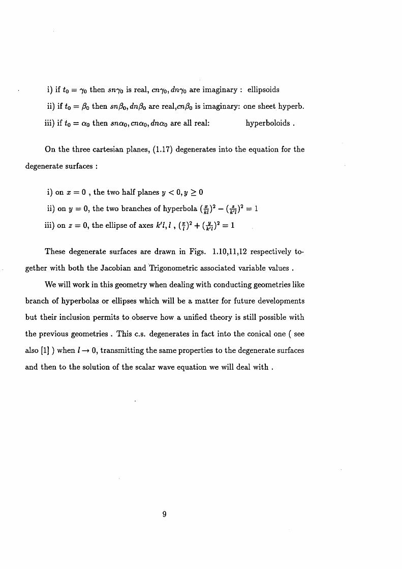
i) if to = 70 then 57170 is real, 07170, dn^o are imaginary : ellipsoids

ii) if to = Po then s7i/?0, dnf30 are real,c72/?0 is imaginary: one sheet hyperb.

iii) if to = ao then snao ,cnao ,dnao are all real: hyperboloids .

On the three cartesian planes, (1.17) degenerates into the equation for the

degenerate surfaces :


ii) on y = 0, the two branches of hyperbola ( p )2 — (p j)2 = 1

iii) on z = 0, the ellipse of axes k 'l, / , (j )2 + (^ f )2 = 1

These degenerate surfaces are drawn in Figs. 1.10,11,12 respectively to

gether with both the Jacobian and Trigonometric associated variable values .

We will work in this geometry when dealing with conducting geometries like

branch of hyperbolas or ellipses which will be a m atter for future developments

but their inclusion permits to observe how a unified theory is still possible with

the previous geometries . This c.s. degenerates in fact into the conical one ( see

also [1] ) when / —* 0, transmitting the same properties to the degenerate surfaces

and then to the solution of the scalar wave equation we will deal with .

9

$ = constFig. 1.1 : spherical coordinate system

Fig. 1.5 : conical coordinate system

♦ = const

con si

Fig. 1.9 : ellipsoidal coordinate system

Fig. 1.2 : spherical degenerate surfaces on the plane x = 0

•0 = 0

.=. K:

0 = K \

Fig. 1.3 : spherical degenerate surfaces on the plane y = 0

Fig. 1.4 : spherical degenerate surfaces on the plane z = 0

Fig. 1.6 : conical degenerate surfaces on the plane x= 0

0 = K+2iK’| |

Fig. 1.7 : conical degenerate surfaces on the plane y= 0

Fig. 1.8 : conical degenerate surfaces on the plane z= 0

12

Fig. 1.10 : ellipsoidal degenerate surfaces on the plane x = 0

iTiTri1

Fig. 1. 11: ellipsoidal degenerate surfaces on the plane y = 0

Fig. 1.12 : ellipsoidal degenerate surfaces on the plane z = 0

13

1.3 Characterization o f the Solutions

The theory of ” the solution ” is developed in conical geometry as it permits an

easy extension to the ellipsoidal c.s. and an easy particularization to the spherical

c.s. . In this geometry, the three-dimensional EM fields solutions can be deduced

from those of the scalar wave equation, which, in their turn, are separable along

r as Bessel’s, and along a, /? as Lame’s differential equations (see [11, 12] ) .

Hence, from now on we denote by F(r, /?, a) the solutions of the scalar Helmholtz

equation.

The complete characterization of the Lame’s solutions is still in progress

and they might present quite difficult forms to be classified and computed [7].

Nevertheless, a sequence of successive requirements to be satisfied by ” the so

lution ” make it at least periodic along a , /3 and consequently well classifiable,

representable and easily computable .

The path of progressive specialization in the space of the totality of solutions

passes through the following steps :

i) the geometrical properties of the coordinate system

ii) the smoothness properties of the solutions

iii) the mathematical properties of the Helmholtz equation

iiii) the physical boundary conditions

At this stage, the Jacobian formalism is simpler to use, even though we

report sometimes the trigonometric one because of its familiarity to the reader .

14

1.3.1 T he geom etrical properties o f th e

conical coordinate system

The choice of the intervals for the variables r, (3, a made in 1.2.2 is such that they

are as short as possible, compatibly with the necessity to associate to any point

of the space at least one tern ro, flo, c*o .

Nevertheless, with that choice, the one-to-one correspondence fails some

where and in particular on the sectors shown in Fig. 1.7 where two sets of three

variables are associated to the same point .

It is obvious to ask ourself if this fact implies that F assumes the same value

on them and if this occurrence may be turned into a periodicity condition on F

itself. In order to analytically demonstrate this possibility, we consider the sphere

of radius r0 of Fig. 1.13 which intersects the degenerate sectors /? = K , K -\-j2K*

( i.e. 0 = 0, 7r ) of Fig. 1.7 in the two arcs C+,C“ . On these two arcs, the values

a, 2K — a ( i.e. 0 , ?r — <j>) give the same point.

Any other value f30 £ (K, K + jK ' ) ( i.e. 0O £ (0,^) ) gives a closed path

surrounding C+ and a value (to £ (K + j K \ K + j2 K ' ) ( i.e . $o £ ( | ,*■) ) gives an

analogous path surrounding C~ while a varies over [.K , —3K), i.e. <f> varies over

[0, 2* ) .

On the contrary, for a fixed a 0 £ [K, —3K) the point (r0, (3, a 0) moves

following to an arc from a point on C+ to one on C~ while /? varies through its

domain [K, K + j2K'] .

Summing up, a variation of a in [K1 —3K ) brings the point (ro, /fa, a) back

to its starting point ( for this we exclude a = —3K in the interval ) while a

variation of f3 in [ K ,K + j2K'] moves the point (ro, /?, «o) along an half circuit

15

only .

Consequently, any physically meaningful solution F(r,/3,a) must be peri

odic in a with period 4K or, equivalently, in <f> with period 2ir but not necessarily

in P , i.e. :

F(r ,P ,a) = F ( r ,0 ,a + 4ff) (1.18)

a=-K a=K

p=K+2jK'

Fig. 1.13 : sphere of radius r<> and degenerate arcs C C+

16

1.3.2 T he sm oothness properties o f th e solutions

Similar arguments arise when we further require smoothness of any physically

acceptable solution in conical c.s., i.e. it has to be continuous with continuous

gradient in any homogeneous region .

Actually, new restrictions on F arise from the imposition of smoothness

on the singular arcs C+,C“ , at the singular origin point and on the sphere with

infinite radius whenever no other physical b.c. are present .

Without loss of generality, we can limit attention to separable solutions of

the general form :

F(r,p ,a) = C(r)B(/3)A(a) (1.19)

The smoothness condition in F imposes some properties on the functions

A yB , C which we can summarize, refering again to Fig. 1.13 and [1], as :

i) on the upper half of a sphere we must have :

lim A(a) = A ( K ), lim A(a) = A(K) i.e. :or—►—3a a —►—3a

either A(o;) is even about K and, B (K ) = 0 (1.20)

or A(a) is odd about K and, B (K ) = 0 (1-21)

ii) on the bottom half of a sphere we must have :

! » » / ( “ ) = ¥ ) > l i m i ( a ) = A(K) i .e . :cr—►—J A Of—►—O A

either A(a) is even about K and, B ( K + j2K') = 0 (1.22)

or A(q) is odd about K and, B ( K + j 2 K >) = 0 (1.23)

17

iii) at the origin r = 0 must be :

MmC(r)B(p)A(a) independent on a and /? (1-24)r —»0

iiii) at infinity r —► oo :

lim C(r)B((3)A(a) must satisfy radiation conditions such as Sommerfield’sr —► oo

(1.25)

The dot ‘ indicates the first total derivative with respect to the argument .

1.3.3 T he m athem atical properties o f th e

H elm holtz equation

In third instance ” the solution ” has to satisfy the scalar wave equation :

V 2F + k2F = 0 (1.26)

which in conical c.s. separates into the following ordinary differential equations:

w(z) — [a + b(ksnz)2 + q(ksnz)4]w(z) = 0 Lame’s equation (1*27)

“ 2 * n dC(r) H— C(r) + ( « ---- r)^ (r) = 0 Bessel’s spherical equation (1.28)r r2

The solutions of Bessel’s equation are well known for a long time (see [7] )

and we remember here only the fact that one of its solutions of the 1st kind satisfies

the smoothness in the origin since l imr^oC(r) = 0, while one of its solutions of

the 3rd kind satisfies the radiation conditions since /imr«*0oC,(r') oc e 3*r .

Equation (1.27) is satisfied by both A(a),B(P) on the two different but

18

contiguous intervals a 6 [K, — 3K) and /? £ [K, K + j 2 K f] .

In a complete general way it features the following properties :

i) it does not contain the term w(z) and the coefficient of w is even so

that there is one solution which is even and one which is odd with respect to any

ordinary point zq [2], in particular the points zo = m K , Zo = K + jn K ' with m, n

integers. Among them is the point Zq = K where the intervals for a and (3 m eet.

ii) When z equals a , (1.27) is a Hill type equation with even coefficients and

period 2K , while when z equals /?, it is a Hill type equation with even coefficients

and period 2K'\ no singularities are present on or near the path in question .

Thus the well known theory of Hill’s equation [2] is suitable for our purposes .

According to the latter theory, conditions like (1.20,21) are turned into the

properties that A(a ) is either even or odd about a = 0 , K and 2K is either a

period or an anti-period, that is to say, it may only be one of 8 different forms .

Furthermore, for the property i), the condition (1.20) means B(/3) is even

with respect to K , while (1.21) means B(j3) is odd with respect to K .

Thus, incidentally, A(a) and B(f3) are of the same parity with respect to

z0 = K where, being zq a regular point, the Lame’s equation admits a unique

even or odd solution .

Likewise, we can state the remarkable conclusion that the smoothness con

dition on the upper half of a sphere implies A(a), B(/3) to be the same solution,

i.e. :

F(r,/?,a) = C(r)w((3)w(a) (1.29)

Similar arguments arise when we apply i) in (1.22,23) so that B(/3) is either

even or odd about K + j2K* as well as about K . Hill’s equation shows then that

19

B(P) must be periodic with j2 K ' either a period or an anti-period .

The 8 types of solutions so identified are the Lame’s polynomials and in

Applied Mathematics they are often characterized by the combination of the

three properties of (i) being odd or even in 2, (ii) having real period 2K or 4K

and (iii) having imaginary period j2K* or j4 K ' . They can be expressed in a

truncated Fourier-Jacobi series ( see [6] ) whose computation is easier and more

accurate than any other Lame’s solution .

Nevertheless, the solutions we are searching for cannot be among these

because the physical b.c., that axe established by the conductor, will relax at

least one of the set of hypotheses (1.20,23) .

However, the knowledge of the link and of the properties of the solutions

along a and /? will permit us to choice the position of the conductor, i.e. where

smoothness is no longer required, in such a way to maintain the maximum sim

plicity for the solutions .

This way, it will be possible to maintain uniqueness and double-periodicity

of the solution for the plane sector along a and (3 but with no longer fundamental

periodicity along /? which is now of 8K \ whereas the second solution is completely

aperiodic .

In the problem of the double-sector, both the two distinct solutions are

involved but the first presents only real fundamental periodicity of 2K or 4K

along a and the second only imaginary fundamental periodicity of 2K* or 4 K '

along /?.

These are the Transcendental Lame’s functions .

In both cases the Fourier-Jacobi series representations of the solution do not

terminate in general but, in spite of that, their computation is quite practicable.

20

1.3.4 T he physical boundary conditions

At last, the conditions still to be satisfied by ” the solution ” are those estab

lished by the plane sector conductors fitting one or more degenerate surfaces

a = —K , + K y P = K, K + j2 K ' showed in Fig. 1.7 .

We will show later that they are belong the Sturm-Liouville class and pre

cisely of just the forms :

w(zQ) = 0 w(zo) = 0 (1.30)

When it; is A then z0 = dzK while when w is B then zq = K, K + j 2 K ' .

In order to reduce the number of different forms (1.30) for the b.c. we may

change the variable ft into u along a real interval according to :

P e [ K ,K + j2K'] P = K + j K ’ - j u « € [ - # ' , i n (1.31)

This way, it will only prove necessary to consider the following three groups

of b.c. in our applications :

« ; ( - # ) = 0, w(K) = 0 (1.32)

w(—K ) = 0, w(K) = 0 or w(—K ) = 0, w(K) = 0 (1.33)

w(—K ) = 0, w(K) = 0 (1-34)

and the analogous with K ' in the place of K .

It is now obvious to ask ourself whether these conditions, as well as the

previous ones, can be reduced to conditions of parity and periodicity for w(z) .

21

A rigorous demonstration based on the general properties of the Hill’s equa

tion is given in Appendix A whose conclusions can be summarized as in the

following .

The b.c. w(—K ) = 0,w (K ) = 0 im ply :

either w(z) even with period 4K

or w(z) odd with period 2K

The b.c. w (—K ) = 0,w (K ) = 0 im ply :

w(z) = wi(z) -f Wi{z) with period SK

T he b.c. w(—K ) — 0 ,w(K) = 0 im ply :

w(z) — w\(z) — W2(z) with period 8K

T he b .c. w (—K ) = 0 ,w(K) = 0 im ply :

either w(z) even with period 2K

or w(z) odd with period 4K

This is a very remarkable result because in the following

we will be allowed to translate straightforwardly the physical b.c. into the previous

simple parity and periodicity conditions for ” the solution ” .

(1.35)

(1.36)

(1.37)

(1.38)

(1.39)

(1.40)

22

1.4 T he Solutions

Once the possible solutions have been identified as those with the properties just

discussed, we have to express them in a form easy to compute and to handle

theoretically .

Unfortunately, the up to date literature on this matter, see [1,5 , 6,19,10,9],

makes use of the more disparate forms either because of different symbolism and

conventions or because the characteristics of the solutions ( i.e. parity, peri

odicity, finiteness or fast convergence series representation, etc ... ) are more

understandable in one than in another form .

23

1.4.1 T he analytic form s o f th e L am e’s equation

In the attempt to achieve goals like simplicity, rigour and accordance with the

main literature, we shall present three main forms of the Lame’s equation . This

way, we can start making the form (1.27) explicit as it will appear later in Jacobian

form versus a .

A + [h — v(v -f l)(fcsria)2]A = 0 a € [if, — 3 if) (1-41)

whose trigonometric form ( see [5] ) and associated change of variable are given

by :

[1 — (ksinp)2]E — k 2 sirupcospE + [h — + l)(fcdin^)3]E = 0 (1-42)

a € [if, - 3 i f ) (p = am(a) tp € [ f , — 3 f ) (1-43)

where am is the amplitude function (see also [1] ) whose property

am(nK) = permits a straightforward translation of the periodicities in Ja

cobian variables to those in trigonometric variables making use of the correspon

dence i f —►

As function of trigonometric variables in the conical c.s., (1.41) becomes :

[1 — (kcos<t>)2]^ + k2sin</>cos(t)i + [p2 + + l)(ksin<t>)2]$ = 0 (1-44)

sin<j> = cna that is <)>=£— ip <j> £ [0,27r) (1*45)

24

The Lame’s equation versus /? assumes the same form (1.41) :

B + [ h — v(v + 1 ){ksnPf]B = 0 fi <E [K, K + j 2 K f] (1.46)

but since (3 belongs to a complex interval is preferable to turn it into a real

variable according to :

U + [h1 — v(v + l)(k'snu)2]U = 0 (1-47)

0 = K + j K ’ - j u u e [ K \ - K rl (1.48)

Thus, following previous lines, we recover the trigonometric form and related

change of variable :

[1 — (fc'smi?)2]T — k^sinflcosfl'T + [h* — v(v + l)(A/s*ntf)2]T = 0 (1.49)

u e l K ’t - K l t? = am(u) [= ,_£ ) (1.50)

and using the trigonometric variables in the conical c.s. (1.46) becomes :

[1 — (h'cosO)2]0 + knsinOcosQQ + [—/z2 + v(v + l)(fc'sin0)2]0 = 0 (1.51)

sinO = cnu that is 0 = — d that is sinO = j-pcnfl 0 £ [0, 7t](1.52)

The symbols h,v will be obtained as separation constants while h!, fi are related

to them by the :

h’ = - h + i/ ( i/ + 1) (1.53)

fi2 = h — v(v + l )k2 (1*54)

25

1.4.2 T he analytical form of the solutions

The representation problem of the Lame’s solutions with given parity and peri

odicity was successfully treated by Ince in 1940 [5, 6] .

His conclusion was that all the solutions we are interested in can be ex

pressed as series whose coefficients are given by a three-terms recursive formulae.

Moreover when the series are not finite, their convergence can be greatly

enhanced when trigonometric form is used and, especially as k2 —> 1 .

Precisely, if we indicate by Xi the i th coefficient of the Jacobi or Fourier

series, we have, respectively :

lim = k2 lim | - ^ - | = (^-r— f < k2 e (0,1) (1.55)I-+OO X { - 1 *-*■ 00 X i - 1 K

The Fourier form presents two more advantages consisting in the orthogonal

properties, of great utility in the applications, and in the easier computability of

the circular functions in respect of the Jacobian ones ( see Appendix in [1] ) . In

addition, during the study of the singularities we need only the first fundamental

term of the series, which is easy to turn into Jacobian form, if necessary .

Furthermore, when an accurate complete solution is needed, we can express

it straightforwardly in terms of the conical trigonometric coordinates 6 and <f> by

simply shifting by those relative to and <p as indicated in (1.44,51) .

T he continued fraction properties

The Fourier series representation, and then the function it represents, is uniquely

identified by the succession of its coefficients {Xt} .

They obey a three-terms recursive formula associable to a continued fraction

26

whose main properties we now recall ( see [7] pg.60 ) .

In the case of unilateral coefficients, that are those different from 0 only for

i > 0, the recursivity relations can be expressed using the elements a,-, 6,, c, as :

6o*o "I" C\X\ — 0 t = 0 (1.56)

+ hiXi + c;+iXi+i = 0 t > 1 (1*57)

whose associated iih approximants are :

* = - t • a - 58)* bi+1 ~ u'+_2 2'

The convergence of the continued fraction are characterized by the two

solutions <i,<2 of the equation :

a + bt + ct2 = 0 (1.59)

where : a = lim^oo a, b = limt_f0o b{ c = lim^oo c.

If | i | < |*21 to ensure convergence, it must be :

X-bo = qici lim ^ * = t\ (1.60)

*-*•00 A , _ i

The first equation represents the vanishing conditions for the coefficients

with negative index and the second their asymptotic behaviour; together they

ensure the uniqueness of the succession {X, } and then of the solution .

We will also meet more general solutions with bilateral coefficients in which

to the first condition is substituted an asymptotic behaviour at —00 .

27

1.4.3 T he analytical expression o f th e solutions

We can now proceed by writing down the Fourier forms of the 6 kinds of solution

we need consider and which we can characterize by the combinations of the two

properties (i) of being even or odd and (ii) having periods 7r,2x ,47r .

For simplicity, we indicate by y(v) the generic solution along (p or i? .

Moreover, for each kind there exists ( see [6] ) a numerable infinity of so

lutions for each v-value and given k 2 . Hence each individual solution should be

labeled like ( see [7, 6] ) :

»— .(») = EZ(v, k2) h = <(fc2) (1.61)

y M » ) = EZ(v, i 2) h = (1.62)

where m is any integer, for example, with the meaning of :

pm = number of zeros in v € [0,p7r) (1.63)

and px is the periodicity of the solution .

For each one of the 6 kinds of solutions we report in Appendix B the three-

terms recursive formula and associated continued fraction where we always have:

t12 = (^^-)2 • Besides, we show in the same Appendix B the tail-to-head com

putational implementation of the characteristic equation which permits to satisfy

the conditions of convergence and uniqueness (1.60), so as to compute at once

the eigenvalues i/(A:2), h ( k 2 ) and associated succession {X ,} .

28

1.4.4 T he degenerate cases k2 = 0, k2 = 1

There is still something important to say about the characteristic equations which

can be seen as a transcendental equation in the unknowns v(k2), h(k2), and pre

cisely how they degenerate into a simple algebraic equation when k2 reaches the

limit values of its interval of definition.

Geometrically speaking, the conical c.s. degenerates into spherical c.s. and

the Lame’s equations degenerate one into a harmonic equation and the other into

a Legendre’s equation ( see [1] ) .

This way, relatively for example to the Lame’s equation along a we get :

A + hA = 0 when k2 = 0 (1-64)

In this situation h becomes independent of v and the solution degenerates into a

circular function as :

per 2K or 7r even and odd :

h = (2m0)2, Ec™° = cos(2m0)a

per 4K or 2x even and odd :

h = (2mo + l ) 2, i?2™0+1 = cos(2mo -f l )a

per 8K or Air even and odd :

h = (m0 + i ) 2, E™° = cos(m0 + \ ) a

where mo = 0, 1, 2,...

The odd solutions are obtainable from these by simply changing cos with

sin .

29

(1.65)

(1.66)

(1.67)

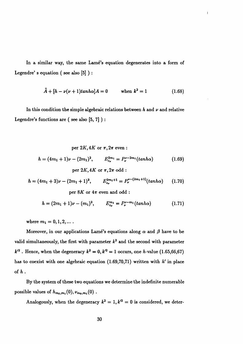
In a similar way, the same Lame’s equation degenerates into a form of

Legendre’ s equation ( see also [5] ) :

A + [h — 1/(1/ + l)tanha]A = 0 when k2 = 1 (1.68)

In this condition the simple algebraic relations between h and v and relative

Legendre’s functions are ( see also [5, 7] ) :

per 2K, AK or 7r, 2n even :

h = (Ami + I)*7 — (2m i)2, E 2™1 = Pjf~2mi (tanha) (1.69)

per 2if, AK or x, 2n odd :

h = (Ami + 3)i/ — (2mi -f l ) 2, E 2™1+1 = P ^ 2mi+1\ t a n h a ) (1.70)

per SK or An even and odd :

h = (2mi + 1)^ — (mx)2) E ™1 = P ”~mi (tanha) (1*71)

where mi — 0 ,1 ,2 ,... .

Moreover, in our applications Lame’s equations along a and /? have to be

valid simultaneously, the first with parameter k2 and the second with parameter

k '2 . Hence, when the degeneracy k2 = 0, k '2 — 1 occurs, one lv a lu e (1.65,66,67)

has to coexist with one algebraic equation (1.69,70,71) written with h! in place

of h .

By the system of these two equations we determine the indefinite numerable

possible values of /imo.m^O), */mo>mi(0) .

Analogously, when the degeneracy k2 = 1, k '2 = 0 is considered, we deter-

30

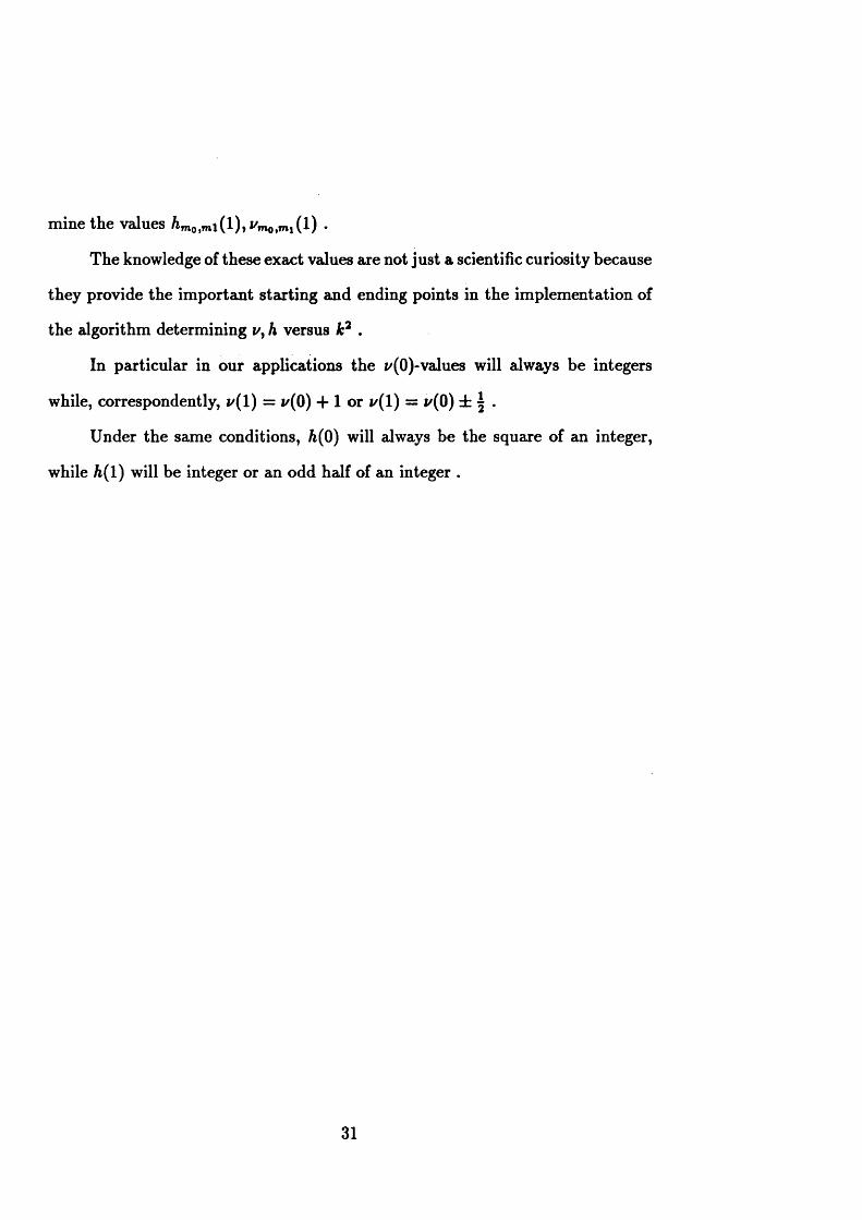
mine the values /imo,mi(l), •

The knowledge of these exact values are not just a scientific curiosity because

they provide the im portant starting and ending points in the implementation of

the algorithm determining */, h versus k2 .

In particular in our applications the i/(0)-values will always be integers

while, correspondently, i/(l) = i/(0) -f 1 or i/(l) = 1/(0) ± \ .

Under the same conditions, h(0) will always be the square of an integer,

while h(l) will be integer or an odd half of an integer .

31

Chapter 2

THE E-FIELD

SINGULARITY VECTOR

2.1 Introduction

This Chapter begins by dealing with the exact solutions of the scalar wave

Helmholtz’s equation satisfying the b.c. pertaining to the sector and double

sector perfect plane conductor.

The problem is a three dimensional scalar one which, in the more appro

priate geometry of a conical c.s., is reduced, in fact, to finding the solutions of

a Bessel’s equation and two Lame’s equations . As the first are well known,

the problem is led again to determining for every sector aperture <r E [0,27r] or

double-sector aperture a E [0,7r] the eigenvalues spectrum {v, h] and eigenfunc

tion spectrum {B({3),A(a)} for a two-dimensional Sturm-Liouville problem.

The theory just developed in Chapter 1 permits the determination of these

spectra with an accuracy which has never been reached before for the plane sector

32

( see [10, 9,17,14] ) and, as far as we know, for the first time for the double-sector.

Furthermore, from these spectra are recovered those relative to other five

novel derived wedges geometries by, say, simple identification of sub-spectra. This

is possible because the conductor relative to these wedges fit, beside the sectors,

some others degenerate surfaces, that are planes of symmetry, so as to realize

those geometries that are met especially in boxed waveguide discontinuities or

antennas .

In microwave (3 — 30 GHz) and millimeter waves (30 — 300 GHz) integrated

circuits, only the tip wedges of these ideal structures are involved and only the

knowledge of the main EM characteristics might suffice there when the frequencies

are not too high and dimensions sufficiently small .

For this purpose, the Chapter will end by presenting the more accurate

static E-field solutions subjected to successive approximations till a final E-field

singularity vector is recovered that maintains just the correct satisfaction of the

regular and singular b.c. .

The whole topic finds its location in the general context of diffraction by

objects with edges, corners, tips etc... that has occupied the attention of several

authors ( see [23, 13, 12] and literature quoted there ) since Sommerfeld solved

the classic case of a half plane .

Analytically speaking, the plane sector and double-sector are ” double dis

continuities ” , for the straight edges represent a discontinuity in the scattering

surface since a normal cannot be defined univocally there . On the tip, however,

also the tangent to the edge is undetermined .

Several authors like Kraus [21], Radlow [22], Jones [24] have made con

jectures, centred particularly on the unicity of the singular solution, based on

33

approximations and physical reasoning .

Moreover, if we consider the aims of this work, the present approach seems

to be redundantly rigorous, but a few theoretical and applicative motivations

indicate the contrary . For instance the Green’s function for the sector can be

determined from the spectrum as indicated in [10] and it should be possible to

identify a ” scattering coefficient ” for the tip using the procedure given in [23] .

Closer to our applications is the problem of representing an unknown

diffracted field by means of an orthogonal, complete set of functions satisfying

the b.c. . As a whole, these conditions cannot be satisfied by the EM field spec

tra. Hence in common microwave and millimeter waves applications it would be

helpful to be able to express the unknown field on a finite plane surface accord

ing to a simple set of orthogonal and complete functions times a simple function

satisfying exactly the b.c. pertaining to one or more wedges linked together .

Specifically to this b.c.-satisfying function, which we name singularity func

tions, is entrusted the task of describing exactly the distribution of zeros and

singularities over all the conductor surfaces, edges and vertices of the compo

nents of the EM fields .

From this point of view, the work of this Chapter can be summarized as a

procedure starting with the determination of the complete spectrum of solutions

for the static E-field with the purpose of formulating the easiest possible E-

field singularity vector still satisfying exactly the b.c. on the conductor and

featuring its main behaviour on its vicinity . The singularity vector so defined is

independent of frequency ( see [13] ), in accordance with a classic result which

states that approaching a conducting surface by a quantity much smaller than

the wavelength, the dynamic solution converges to the static one .

34

2.2 Solution o f th e scalar H elm holtz’s equation

It has been proved ( see for instance [12] pp.1762 —1767 ) that in the geometry of

a conical c.s. the solutions of the general vector wave equation for the EM fields,

as well as those of the Laplace’s equation for the static E-field, axe obtainable by

simply applying vector operators to the solutions of the scalar wave Helmholtz’s

equation for a potential function :

V 2 cl’,w) 4- K2ty(r,/3,a-,uj) = 0 (2.1)

A sinusoidal excitation will be always considered so that the time depen

dence is included in the wave number k = Uy/jH, where u = 2 irf is the angular

frequency , / is the frequency and, finally, fi and e are respectively the magnetic

permeability and dielectric constants of the medium which, in first approxima

tion, we regard as homogeneous.A ^ AIn the conical c.s. described in 1.2.2 and shown in Fig. 1.5, r,/?, a

A A A( or r , 0, <f>) constitute a proper set of three unit vectors and the metric coefficients

( see also [11] pp. 1 — 3 ) are given by :

<7n = 1 £22 = (kr)2(sn2a — sn2(3) <733 = (kr)2{sn2p — sn2a) (2.2)

9 = (911922933)^ = j{kr)2 (sn2a - sn 2/3) (2.3)

Hence the scalar operator V 2 in (2-1) can be written explicitely as :

d (<72 dijA d ( g i d ( g i 2 1 , .

35

W ithout invalidating the generality of the solution, we can limit the atten

tion to just the separable forms :

w) = R(r\u)B(P)A(a) (2.5)

where the space and frequency dependence are separated by ; .

W ith this position, (2.1) separates into the three following ordinary differ

ential equations :

R 4— R + [ft2 — + l )- ^r L r£B -\-\h — v(v + 1 )(ksnf3)

A 4- [/i — v(v + 1 )(ksna)

R = 0

B = 0

A = 0

(2 .6)

(2.7)

(2 .8)

where v and h are two generic separation constants .

The general solution of the spherical Bessel’s equation (2.6) is chosen for a

reason which will appear in Chapter 3, in the form :

R(r]u) = C $ \ n r ) + D h^(K r) = C\ — Jv+i(Kr) + D\ -*-Hv+i (nr) (2.9)/cr 2

where the first solution is the spherical Bessel function of 1st kind, the second

solution hj,2) is an Hankel function of 2nd kind while v is their oder and C, D are

the linear combination constants .

Incidentally, R is the only part of W that is dependent on u through the

factor «r, so that frequency, medium and radius act on it in the same way, that

is, as a change of scale .

The differential equations (2.7,8), together with the b.c. along a,/? of the

36

kinds considered in 1.3.4, constitute a two-dimensional Sturm-Liouville problem

with general solution :

B(P) = E£*(/?) + FJ*{0) (2.10)

A(a) = G # ( a ) + H J? (a ) (2.11)

where are the l*1 and 2n', solutions of 1“ kind of order v and degree h of

the Lame’s equations, while E,F,G,H are the linear combination constants .

Some preliminary properties of these solutions can be obtained also consid

ering the associated 2-dimensional Sturm-Liouville operator defined as in [10].

First of all, the b.c. require the solutions or their derivatives to vanish, but

not simultaneously, thus for the linear independence of £, T the solutions B , A

are reduced to just £*br T , but not to any of their linear combinations .

The operator associable to the system (2.7,8) and specified in [10] is self-

adjoint and positive definite and it can be easily proved looking at (2.6,7,8) that

for any possible v > — - there is one v < — | which gives the same solution .

Furthermore no solution occurs in v € (0, —|] , for, without loss of generality, we

can choose :

v > 0 (2.12)

and for every v there exist at most a finite number of h-values > 0 (see (1.4.4))

and hence of eigenfunctions .

As a whole, for any couple of b.c. along a and ft and for any geometry, i.e.

given &, a spectrum of eigenvalues {v,h} and eigenfunctions {£?(/?),A(a)} are

identified .

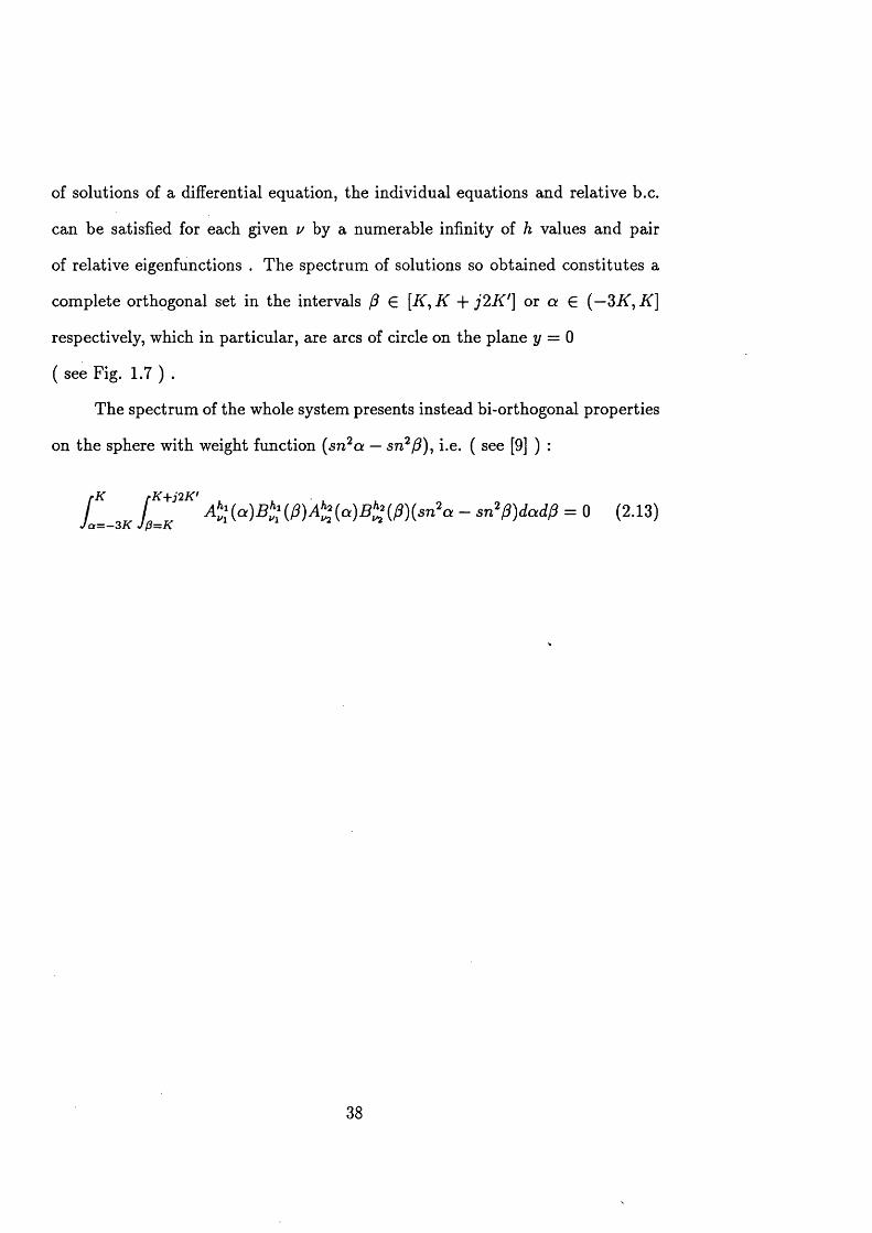
From another point of view, because of the usual properties of the spectrum

37

of solutions of a differential equation, the individual equations and relative b.c.

can be satisfied for each given v by a numerable infinity of h values and pair

of relative eigenfunctions . The spectrum of solutions so obtained constitutes a

complete orthogonal set in the intervals /? € [K, K + j2K '] or a £ (—3K ,K ]

respectively, which in particular, are arcs of circle on the plane y = 0

( see Fig. 1.7 ) .

The spectrum of the whole system presents instead bi-orthogonal properties

on the sphere with weight function (sn2a — sn2/?), i.e. ( see [9] ) :

fK rK +j 2K ' t t/ _ L - r A *l(a )B »l(P)A »l(a )B SAP)(sn a ~ sn /3)dadfl = 0 (2.13)

• / Of — — 3 j \ v p — A

38

2.3 Static E-field spectrum

for the sector and double-sector

In order to obtain maximum simplicity of the solutions in the sense specified in

1.3.3, the sector and double-sector are disposed in a conical c.s. as in Figs. 2.1,2.

There we highlight the degenerate coordinate surfaces on the plane y = 0 and

associated values of the variables a , p and of the real variable u defined in (1.48).

For any given e, and hence k = sine, we obtain the acute sector and double

sector of angular aperture <r = 2e of Fig. 2.1a,b as well as the obtuse sector of

angular aperture a = 2(tt — c) of Fig. 2.1b .

The static E-field generated by a static charge induced on these conductors,

can be derived from a potential V :

V (r ,P ,a ) = lim ( r , /?,<*; u;) = $ (r ,/? ,a ;0 ) = R(r; 0)B(P)A(a) (2.14)u>—*0

according to the gradient expression in conical c.s. :

R B A P + ------. RP A---- --- $ + ------ , R^ A---- --- akry/sn2a — sn2P kry /sn2P — sn2a

(2.15)E = - \ j - V = -

The Bessel’s R solution degenerates now into the exponential one :

R(r) = C rv + (2.16)

The solutions for A and B instead can be recovered by applying the b.c. .

These are relative to the sector surfaces P = K ,K + j2 K ' and a = —K , K and

can be obtained by means of physical considerations and using (2.14,15) .

39

a) b)

Fig. 2.1: plane acute a) and obtuse b) sector

Fig. 2.2 : plane double sector

40

This way, we note that the conductor is an equipotential surface where,

without loss of generality, we may set V = 0 . From (2.14) it follows that if the

conductor lies on a surface a = K or —K then A(a) — 0 there and analogously

for B (p ), when the conductor fits the sectors /? = K or K + J2A7 .

In second instance, since the static charge lies completely on the plane y — 0,

the field component Ey must vanish on the portion of this plane that is adjacent

to the conductor . Introducing this symmetry property in (2.15), we get the

further conditions A = 0 for a surface a = constant, whereas B — 0 on a surface

/? = constant .

Consequently, considering U(u) in the place of B((3) ( see (1.47) ), the full

conditions to be satisfied in the three situations of Figs. 2.1a-b,2 are :

acute sector

obtuse sector

double-sector period 2K ' odd, *4K ' even

A (K ) = j4(—K ) = 0 —> period *2K even, AK odd

(2.17)

(2.18)

(2.19)

In the above, the use of real variable u permits to recover the sole forms

of b.c. studied in 1.3.4; also indicated there by a —* are their straightforward

reductions to parity and periodicity conditions according to the discussion of

1.3.4 .

It appears now evident that the choice of the position of the acute and

obtuse sectors is such that A (a ) and B(/3) assume the same value at the meeting

41

point z — K of the intervals for the variables . Hence, they are effectively part of

the same double-periodic solution whose imaginary period 8K ' is no longer the

fundamental one, as announced in 1.3.3 .

Analogous properties cannot be obtained for the double-sector for which,

however, the position of the conductor on the surfaces /3 = K , K + j2 K ' ensure

that both A(a) and B(/3) are periodic of fundamental period, one being the first

and the other the second solution of the Lame’s equation, as anticipated in 1.3.3.

W ith these premises, the solution can be finally computed in Fourier series

form in the manner discussed in 1.4.3 and indicated in Appendix B .

For example, relatively to the acute sector and because of the (2.17),

(B.20,21) hold with the indicated change of sign; (B.28) holds with k and h

changed into k ' and b! respectively according to (1.47,48) .

By implementing the two correspondent continued fractions (B.23,24,25)

and (B.29,30,31,32,33) in the more stable tail-to-head sequence and simultane

ously solving them, we compute the eigenvalues i/,h versus k2 € (0,1) with an

accuracy that is only dependent on the maximum truncation index I and on the

zero-finding procedure used.

For instance, in order to maintain an accuracy of, say, 6 decimal figures, I

has to increase from a few tens when k2 —> 0 up to a few hundreds when A:2 —► 1

according to (1.55), as the speed of convergence of the fraction slows down .

The i/, /i-values assumed in the limit situations k2 = 0,1 can instead be de

termined analytically, as indicated in 1.4.4, thus providing, at the same time, the

essential start and end points for determining the complete curves v(k2), h(k2),

as just described .

Explicitly, for the same acute sector, when k2 = 0, k!2 = 1 , using the

42

(1.65,66,71) it must be :

b! — (2mi + 1)*/ — raj h = (2mo)2 or (2m0 + l ) 2 (2.20)

that is to say :

i/(0) = mi + xZMO) = n period SK ' (2.21)

h(0) = (2m0)2 = m period 2K (2.22)

h(0) = (2mo + l ) 2 = m period 4K (2.23)

where mo, m \ = 0 ,1 ,2 ,..., and m, n are the two integer values of i/(0), /i(0) .

It can be easily proved that the same values hold for the obtuse sector but

with the exclusion of mi = 0 .

For the double sector, we get instead in a similar way :

i/(0) = 2mi + 1 + \A (0 ) = n period 2K ' (2.24)

*/(0) = 2mi H- y fh (0) = n period 4K f (2.25)

h(0) = (2m0)2 = m period 2K (2.26)

h(0) = (2mo + l )2 = m period 4K (2.27)

So that for the single couple of curves */(fc2), h(k2) we choose the 1/, ^-values

corresponding to the given periodicities .

43

On the other hand, when k2 = 1, kn = 0 we get for the sector :

„ 2/(1) = 2mi + m0 + l = n + i periods 2 K ,4 K (even) , 8K f (2.28)

/i(l) = 4mi(mi + m0 + 1) + m0 -f \

, 2/(1) = 2mi + m0 + i = n + !periods 2AT,4A' (odd) , 8K ' { 2 2 (2.29)

h(l) = 4m1(m1 + m0 + 2) + 3m0 + |

And, finally, for the double-sector we obtain :

z/(l) = 2mi + ^ ' ( 1 ) = n period 2K (2.30)

i/(l) = 2m\ + 1 + ^ ' ( 1 ) = n period 4i f (2.31)

/^(l) = (2mo)2 = m period 2K f (2.32)

/fc'( 1) = (2m0 + l ) 2 = m period 4K* (2.33)

These simple formulae can be interpreted by saying that for the acute sector

the upvalues start from any integer n for the terminating wire (see also Fig.4-7),

corresponding to k2 = 0, and increase monotonically up to n -f ^ fo r the half

plane, corresponding to k2 = 1, continuing to increase for obtuse sectors up to

n *f 1 fo r the plane conductor associated again with k2 = 0 ( see also Fig. 2.3 ) .

The h-curves follow similar rules starting from the square of any integer

number and ending at the square o f the successive, however, in general, they no

longer increase monotonically ( see also Fig. 2.3 ) .

The i/(k2), h(k2)-curves for the double-sector are easier, as i/ starts from any

integer for the wire (k2 = 0) and increases monotonically up to the successive

44

integer for the plane conductor (A;2 = 1), whereas the ^-curves start from any

square of an integer for the indefinite wire (k2 = 0) and increase monotonically

up to the integer recoverable from (2.32,33) for the plane conductor (k2 = 1) as

also indicated in Fig. 2.4 .

These repetitive properties of the spectrum {v>h} permit to limit the a t

tention, for instance, to just the first 15 of their numerable double infinity . As

a way of example, relatively to the acute sector, we report in Appendix C the

numerical evaluations of v(k2), h(k2) for steps of 0.02 of k2 and with an accuracy

of 6 decimal figures .

More visually, the above reported properties of the curves v(k2)y h(k2) can

be singled out from the plot in Fig. 2.3 for the sector and in Fig. 2.4 for the

double sector .

When the zero-searching-procedure ends successfully, just by looking at the• • • • • X ' • • •ratio of the successive series expansion coefficients -^ tl in the continued fraction,

we recover without any further operation the succession {A,} within an arbitrary

multiplicative constant, and, then, the solution itself .

In Figs. 2.5-6 we draw the first 5 eigenfunctions normalized with respect

to the maximum value relative to the particular 90°, 270° sectors corresponding

to k2 = \ . They show explicitly all the different variables previously introduced

for various reasons in the symmetric intervals 0, (j> € [—27r, 27t], where all their

periodicity and parity properties are identified . Similar graphs are reported in

Fig. 2.7 for the right double-sector with k2 = 1 .

In order to make these eigenvalue and eigenfunctions spectra readable, we

present now a enumeration that is slightly different from that presented in 1.4.3,

but closer to those used in waveguide theory . In fact, we label the single eigen

45

value with two integer (t’1, 12) defined so that i/(0) = *1 + *2 while h(0) — i\.

Relatively to the eigenfunctions instead, for the same reason of better readabil

ity, we produce artificially a cusp in the point correspondent to the conductor

simply by changing the sign of the functions after it . In these drawings i\ in

dicates the number of zeros in 0 £ (0 ,7r) while *2 indicates the number of zeros

in <f> € (0 ,7r), that is to say, the zeros other than those possibly present on the

conductor along $ and halve of those along <j> . This permits to retrieve the

waveguide convention ( see [25] ) where the single modes were labeled by (*1, 2*2)

and the fundamental one by (0,0) .

46

0.9"

0 . 8 "

100.7"

0 . 6 "

0.4 ■ •

0.3"0 1

0 . 2 - ■

0.1-■

Eigenvalue v

0.9-

0 . 8 "

0.7- ■

0 . 6 "

0.5"

0.4-

0.3-

0 . 2 -

0.1

Eigenvalue h

Fig. 2.3 : first 15 eigenvalues {v(k ,fr(k^} for the sector

47

0.9

0.8 T

0 .7 1

0.6 f

0.5 f

0.4 +

0 .3 1

0.2 t

o.i 4-o/o

Eigenvalue v

0 .9 +l

0 .8 *

0.7 t|

0 .6-1

0.5 +

0.4 +

0.3

0.2 +0.1 -K

Eigenvalue h

Fig. 2.4 : first 15 eigenvalues {v(k ,/7(k^} for the double sector

48

Lame's functions A(a)

TTO

103

2K -K 0 K 2K- n -k /2 0 71/2 tc q>

3/27t 7i tc/2 0 - tc/2 <!>

Lame's functions B(p)

f j f /lo /

K+]3K’-2K’

K+j2K'-K’

K+jK'

0 K'- k - k /2 0 k / 2 k d

3 /2tc k k / 2 0 - tc /2 0

Fig. 2.5 : first 5 eigenvalues (B(P),A(a)} for the acute sector49


2K K 0 K 2K- r e - r e / 2 0 tc/ 2 tc cp

3 /2 tc 7c 71/2 0 - tc/2 $

Lame's functions B(P)

K+j2K'-K’

K+jK'

0K-jK' p

2K’ uK'- re - tc /2 0 tc/2 k V3 /2 jc re tc/2 0 - ji/2 0

Fig. 2.6 : first 5 eigenvalues {B(P),A(a)} for the obtuse sector50

-2K -K 0 K 2K- k - k /2 0 k / 2 K3/2 tc K k /2 0 - k /2

Lame's functions B(p)

a<P9

Pu00

Fig. 2.7 : first 5 eigenvalues {B(p),A(oc)} for the double sector51

2.3.1 S tatic E-field spectra for com posite sectors

There axe five more conductor wedges geometries that we can easily analyze

making use of the results just obtained for the sector and double sector . These

wedges are mostly enclosed in metallic waveguides, or antennas making use of

the image principle in order to reduce the burden .

They can be named the half acute and obtuse sector, the half double-sector

the sector on a plane and the half sector on a plane, and can be drawn respectively

as in Figs. 2.8a-b,9,10,ll .

Geometrically speaking, they can be obtained by inserting some plane con

ductors on the symmetry planes of the conductor for Figs. 2.8a-b and of the

double-sector for Figs. 2.10,11,12 . These planes fit the other degenerate surfaces

of the conical c.s., i.e. a = 0 ,2K and /? = K + j K \ that is u = 0

(see Figs. 1.6,8).

Analytically speaking, all these new b.c. can be reduced to periodicity

conditions ( see [7] p.64 ) with a procedure completely similar to that reported in

1.3.4. Incidentally, the latter indicate that the spectra for these new structures

are a selection of the spectra relative to the fundamental sector and double-

sector . To be precise, the condition V = 0 on the inserted plane select among

the conditions (2.17,18,19) the following ones :

half acute sectorU (K ') = U (-K ') = 0 - p. *8K ', (0,1)

A (K ) = A(0) = A(2K ) = 0 - t p . *4K(o.), (0,1)

52

half obtuse sector

half double-sector <

sector on a plane <

half sector on a plane

U (K') = U (-K ') = 0 -4 p. *8K \ (0,1)

A (K ) = >1(0) = A(2K ) = 0 -> p. *2K{o.), (0,1)

U(K') = t f ( - t f ') = 0 -* p. *2ff,(o.),4lir/(e.), (0,1)

A (K ) = >1(0) = A{2K) = 0 -> p. *4K (o .)y (0,1)

U (K ’) = U(0) = 0 -> p. *2K ’(o.), (1,0)

A (K ) = A ( - K ) = 0 -+ p. 2 K (e .)* 4 K (o .), (1,0)

U (K') = If(0) = 0 -> p. *4K \e .) , (1,1)

A (K ) = >1(0) = A(2K ) = 0 p. *4K(o.), (1,1)

(2.35)

(2.36)

(2.37)

(2.38)

Where ”p.” stands for "period”, (e.),(o.) stand for even, odd respectively

and the two integers between ( ) are the labels characterizing the fundamental

mode for these geometries. The periodicities related to them are those indicated

with *, as recoverable by remembering the meaning of the two integers and looking

at Figs. 2.5,6,7; from the latter, it also appears that v is always > 1 .

2.3.2 Com parison o f th e approaches and results

It is perhaps appropriate to spend a few words about the various approaches used

and degrees of accuracy reached over the years in determining the spectrum of

eigenvalues and, in particular, the fundamental one that is responsible for the

main EM fields behaviour by the conductor .

53

One of the most complete works was that already mentioned by Satterwhite

[10], who used the present approach, but focused the attention on the quarter

plane, for which he determined the first 192 eigenvalues and eigenfunctions so as

to produce a very complete Green’s function for it . He reached an accuracy of 4

decimals aided by a graphic method in order to identify the intersections in the

locus of possible v and /i-values, for a given k2, with a view to determining the

approximate starting solutions.

Our approach, instead, starts from the exact v, h limit values for k2 = 0,1

and uses them as first approximations to the values relative to a small variation

of k2. By successive steps, the whole curves u(k2) ,h (k 2) are recovered with an

accuracy up to 6 decimals and more .

Authors like De Smedt [14] see the sector as a particular cone with arbitrary

cross-section and solve numerically the eigenvalue problem by an application of

the variational principle reaching, with some difficulty, the accuracy of 5 decimals.

One of the more recent works by Boersma [17] analyses the general problem

of a cone with elliptic section whose b.c. provide a periodic and an aperiodic

Lame’s function. No continued fraction exists for the aperiodic solution and

consequently the accuracy of 5 decimals is reached somewhat laboriously .

Several other works have dealt with this problem, but the ones quoted are suf

ficient to let us conclude that the present approach, even at the price of an higher

theoretical effort, produces the most accurate results available today and indicates

that the ultimate goal in this direction would possibly be a further simplification

due to the property of double periodicity o f the solution .

In fact, we have to consider that this property simplifies considerably the

problem when fundamental periodicity occurs, as in the Lame’s polynomials .

54

acute a) and obtuse b) sector

Fig. 2.9 : half double sector ^

Fig. 2.10 : sector on a plane conductor Fig.'2.11: half sector on a plane conductor

55

2.4 T he m ain behaviour and singularity vector

o f th e E-field in trigonom etric variables

There is still a couple of physical conditions to be satisfied by (2.14,15), as stated

in 1.3.2, and, precisely, that of smoothness at the origin and another condition

at infinity .

Smoothness at the origin requires V^O,/?, a ) to be independent on (3 and a ,

but, as V vanishes identically on the conductor, it must also vanish at the origin,

that is to say :

R(r) = rv (2.39)

On the other side, a physical condition at infinity can be the finiteness of the

energy (oc f \E\2dv) stored in the space around the conductor, so that necessarily,

lim ^oo E = 0, which can be satisfied by an i?-solution of the form :

R(r) = r - (‘,+1) (2.40)

In practical applications, we are asked to analyze wedges making part of

a printed circuit, so that whenever we are interested in the El-field behaviour

in a limited region containing the tip, we use (2.39), while, if the region is the

indefinite space we use (2.40) and, finally, if the region is limited and does not

contain the tip, we can use the complete (2.16) .

Naturally, we limit our attention to the region around the tip, where, to

gether with (2.39), we express A (a ),B (fl) preferably in trigonometric variables

like $(<^), 0(0) respectively .

56

For this purpose, the metric coefficients become :

, (k2sin2<l> + k'2sin20) 2(k2sin2</> + k'2sin2Q) , x* ‘ = 1 g” = r 1 - J b W g g33 = r i - * w * (2-41)

Hence, the static E-field can be explicited as :

E = -_ A I 1 — k ' 2COS20 • A / 1 — k 2c o s 2 <j> • *

r k 2s i n 24, + k ‘2s i n 2$ + V * 2 s « ' n 2 0 + k ' 2s i n 2 6 *r1'" 1

(2.42)

The above shows clearly the presence of the tip singularity whenever i/ < 1.

This is matched to a — | degree singularity of Ee, Ej, along the conductor edges,

where two among the values 0 = 0, x and <l> = 0 ,7r occur simultaneously in the

t e r m y jk * s in 2<f>+k'*sin29 *

In conclusion, the E-field fundamental modes for the sector and double

sector assume primary theoretical importance because their singularities on the

tip represent there the main behaviour of any diffracted E-field while the dis

tributed singularities along the edges, are common to all the modes .

Nevertheless, applicatively speaking, the rigorous expression of the funda

mental mode in the form (2.42) is not particularly helpful, if we except the special

case in which the E-field is conveniently expressible in terms of the spectrum itself.

More often, only its main behaviour is sufficient. Hence, we have to formu

late it as a simple function which still satisfies exactly the b.c. inclusive of edge

and vertex conditions .

Ideally, this could be used as a ” weight function ” for a complete and or

thogonal set of functions used to represent the E-field on some convenient surfaces

along the circuit and ensuring exact satisfaction of the b.c., locally pertaining to

57

one of the 8 ideal structures in question .

The main behaviour is due to the fundamental mode, which is identifiable

by means of its periodicity and parity as indicated by * in (2.17,18,19) for the

fundamental sectors and by (2.34,35,36,37,38) for the composite wedges .

As a way of example, we determine explicitly the functions R(r), 0(0),

for the particular, more useful situation, of k2 = 0.5 . The v-value and the series

coefficients {A,} characterizing these functions are reported in Table 2.1 .

The coefficients show a clear dominance of the term with fundamental period

so as to justify the pseudo-harmonic form of 0(0), 4>(< ) shown in the Figs. 2.5-6-

7. The number of oscillations and parity are of fact maintained for any k2 value,

including the case k2 = 0, when only the first coefficient is present, and k2 — 1

when the function degenerates into one of Legendre’s .

In view of simplifications, we can note that in proximity of a zero of 0 , $

on a conductor surface, the terms of their series representations, for instance that

in (B.2), go singularly to 0 because the conductor surface always fits some of the

particular coordinate values 0 = 0, 7r or ^ = 0, 7r, 3^ .

W hat is more, the asymptotic behaviour of these terms on these zeros differ

from each other by a multiplicative constant, so that the asymptotic behaviour

of 0(0) and $ (} ) is correctly represented by the whole series as well as by its

fundamental term . The latter, depending on the parity and periodicity, can be

written as: t1 period ir sin28

cosS period 2ir sinS / °dd (2.43)even

cos\ period Air s in |2 ^ 2

where 6 stands for 0 or ^ according to the context .

58

Then, if we consider, for instance, the acute sector, a simplified trigonomet

ric expression of the E-field (2.42) which still satisfies exactly the b.c.

is :0 a 1 I 1 — k'2cos2Q . 6 a

= ^-vco s- r + \

This equation describes in quite an easy analytical way the map of singu

larities and zeros on the conductor as a product o f the singularity on the tip,

formulated by the term rv~x, with that along the edges, formulated by the term

y /fc2sin2<f>+k,' sin20 ’ an^ w z e r o s 071 ^ ie conductor surface, formulated by the

eigenfunctions c o s |,s m | .

Remarkably, these simplified forms are valid for every sector or double-sector

aperture only changing the j/-values . For this purpose, we collect in Table 2.2 the

values of rc = i/(<t) — 1, namely, the degree of electric singularity, for cr-steps of 5°

or 10° accurate up to 7 decimal figures for all the 8 geometries; values relative to

apertures not reported in the Table can be obtained by means of interpolation .

This is why we name the expression (2.44) E-field singularity vector in

trigonometric form, which, together with its easier expression in rectangular co

ordinates, constitutes one of the main goals of the work .

(2.44)

59

2.4.1 T he m ain behaviour o f th e density o f charge

A dual way of implementing field analysis algorithms makes use of the density of

charge on the conductor which presents the advantage of being a bi-dimensional

function .

The surface density of charge is related to the diffracted fields as :

p , = eE- n= ±eE„ (2.45)

where n is the outward pointing unit vector normal to the conducting surface, c

is the dielectric constant of the media in contact with it, while the ± signs refer

to En going into or out of the conductor surface respectively . According to this

definition, p9 assumes the forms :

\p.\ = f\E*\ = A in 0 = 0,jt (2.46)

\ p , \ = t\Ee\ = in ^ = 0, jt (2.47)

The validity of the above equations could be queried at the two edges and

at the tip, where the normal to the conductor can no longer be univocally defined

and the expressions become singular . However, we can anticipate a result proved

for the general dynamic situation which asserts that there can not exist an isolated

charge on the conductor, that is to say, the density of charge changes continuously

on it and assumes the limit value (2.46,47) when 0,<j> —* 0, x .

60

CHARACTERISTIC COEFFICIENTS OF THE FUNCTIONS R(r),0(0),$(<()) Fundamental mode - k2=o.s

Fig. 2.1a v = 0 .2 9 6 5 8 4 Fig. 2.8a v = 1 .1 3 1 2 4 8i 0 - p e r 4-7T e v e n 0 - p e r it e v e n 0 - p e r 4 tt e v e n 0 - p e r 277 e v e n-5 0 .0 0 0 0 0 1 - 0 .0 0 0 0 0 3-4 0 .0 0 0 0 0 9 - 0 .0 0 0 0 2 5-3 0 .0 0 0 0 7 5 - 0 .0 0 0 2 2 9-2 0 .0 0 0 7 5 2 - 0 .0 0 2 5 2 4-1 0 .0 1 0 4 6 8 - 0 .0 4 6 6 8 40 1.000000 1.000000 1.000000 1.0000001 - 0 .0 5 4 6 4 4 - 0 .0 3 3 0 8 4 - 0 .2 1 8 4 6 8 -0 .0 0 9 2 7 12 - 0 .0 0 2 6 3 2 - 0 .0 0 1 5 9 4 - 0 .0 0 4 1 4 3 -0 .0 0 0 6 4 63 - 0 .0 0 0 2 3 1 -0 .0 0 0 1 8 6 - 0 .0 0 0 3 1 5 -0 .0 0 0 0 6 44 -0 .0 0 0 0 2 5 -0 .0 0 0 0 2 1 - 0 .0 0 0 0 3 2 -0 .0 0 0 0 0 75 -0 .0 0 0 0 0 3 -0 .0 0 0 0 0 3 - 0 .0 0 0 0 0 3 -0 .0 0 0 0 0 1

Fig. 2.1b i/= 0 .8 1 4 6 5 5 Fig. 2.8b v = 1 .9 5 5 3 2 6i 0 - p e r 47t e v e n 0 - p e r 27t o d d 0 - p e r 477 e v e n 0 - p e r 77 o d d-5 -0 .0 0 0 0 0 2 - 0 .0 0 0 0 0 3-4 - 0 .0 0 0 0 1 4 - 0 .0 0 0 0 2 5-3 - 0 .0 0 0 1 2 2 - 0 .0 0 0 2 4 9-2 - 0 .0 0 1 2 8 9 - 0 .0 0 3 2 6 4-1 -0 .0 2 0 7 0 8 - 0 .1 3 1 9 1 90 1.000000 1.000000 1.0000001 -0 .1 4 6 1 7 1 0 .0 1 0 8 3 5 - 0 .4 1 7 2 6 1 1.0000002 -0 .0 0 4 7 3 3 0 .0 0 0 8 0 6 0 .0 1 1 5 4 7 0 .0 0 3 1 5 43 -0 .0 0 0 3 8 6 0 .0 0 0 0 8 2 0 .0 0 0 6 4 5 0 .0 0 0 2 4 04 - 0 .0 0 0 0 4 0 0 .0 0 0 0 1 0 0 .0 0 0 0 5 9 -0 .0 0 0 0 2 55 -0 .0 0 0 0 0 5 0 .0 0 0 0 0 1 0 .0 0 0 0 0 6 0 .0 0 0 0 0 3

Fig. 2.2 v = 0 .7 0 4 3 2 1 Fig. 2.9 v = 1 3 1 1 8 6 3i 0 - p e r 2 v o d d 0 - p e r 7r e v e n 0 - p e r 27t o d d 0 - p e r 277 e v e n0 1.000000 1.000000 1.000000 1.0000001 0 .0 1 6 7 1 4 -0 .1 0 2 7 6 2 -0 .0 2 3 5 8 8 -0 .0 2 3 5 8 82 0 .0 0 1 2 7 9 -0 .0 0 5 2 8 4 - 0 .0 0 1 5 4 3 - 0 .0 0 1 5 4 33 0 .0 0 0 1 3 1 -0 .0 0 0 4 7 3 -0 .0 0 0 1 5 0 - 0 .0 0 0 1 5 04 0 .0 0 0 0 1 5 -0 .0 0 0 0 5 2 -0 .0 0 0 0 1 7 -0 .0 0 0 0 1 75 0 .0 0 0 0 0 2 -0 .0 0 0 0 0 6 -0 .0 0 0 0 0 2 - 0 .0 0 0 0 0 2

Fig. 2.10 v = 1 .9 1 8 0 2 3 Fig. 2.11 v = 2 .6 8 8 0 0 0i 0 - p e r it o d d 0 - p e r 7t e v e n 0 - p e r 77 o d d 0 - p e r 277 e v e n0 1.000000 1.0000001 1.000000 - 0 .4 3 8 1 2 6 1.000000 -0 .2 0 0 6 6 02 0 .0 0 5 7 4 7 -0 .0 0 1 8 4 1 - 0 .0 5 3 4 9 2 -0 .0 0 3 3 5 03 0 .0 0 0 4 4 3 - 0 .0 0 0 1 2 5 -0 .0 0 2 9 1 2 -0 .0 0 0 2 4 84 0 .0 0 0 0 4 6 -0 .0 0 0 0 1 2 -0 .0 0 0 2 6 7 -0 .0 0 0 0 2 55 0 .0 0 0 0 0 5 -0 .0 0 0 0 0 1 - 0 .0 0 0 0 3 0 -0 .0 0 0 0 0 3

Table 2.1: characterization of the eigenfunctions i?(r), 0(0), $(<f>) for the acute sector, half acute sector, obtuse sector, half obtuse sector, double sector, half double sector, sector on a plane and half sector on a plane respectively indicated by their Fig. number .

61

3D-WEDGES

Degree of electric singularity Te

Fig.2.1a,b|Fig.2.8a,b| K -O ° 2

Fig. 2.10 Fig. 2.11 Fig. 2.2 Fig. 2.9

0.00 0.0000000 1.0000000 0.00 0.0000000 1.0000000 -1.0000000 0.00000005.00 -0.0019269 0.9999945 2.50 0.2789616 1.0028342 -0.7719023 0.0009497

10.00 -0.0079077 0.9999121 5.00 03434077 1.0111690 -0.7278994 0.003782415.00 -0.0183830 0.9995488 7.50 0.3960998 1.0246795 -0.6931375 0.008468120.00 -0.0338525 0.9985454 10.00 0.4435835 1.0430298 -0.6624549 0.014979925.00 -0.0546955 0.9963541 12.50 0.4881265 1.0659169 -0.6340G66 0.023300430.00 -0.0809612 0.9921894 15.00 0330753^ 1.0930816 -0.6068899 0.033424235.00 -0.1121971 0.9849673 17.50 03719618 1.1243052 -0 3 805848 0.045359140.00 -0.1474300 0.9732592 20.00 0.6119693 1.1594002 -03547600 0.059126845.00 -0.1853447 0.9553263 22.50 0.6508186 1.1981970 -03291900 0.074763050.00 -0.2245699 0.9293612 25.00 0.6884303 1.2405277 -03037155 0.092317555.00 -0.2639208 0.8940430 27.50 0.7246354 1.2862073 -0.4782217 0.111853660.00 -0.3025154 0.8492627 30.00 0.7592010 13350107 -0.4526276 0.133447765.00 -0.3397789 0.7964791 32.50 0.7918567 13866444 -0.4268797 0.1571889"0.00 -0.3753875 0.7382866 35.00 0.8223226 1.4407145 -0.4009492 0.183177875.00 -0.4092000 0.6775165 37.50 0.8503404 1.4966899 -0.3748310 0.211523980.00 -0.4411957 0.6165389 40.00 0.8757026 13538665 -0.3485447 0.242343285.00 -0.4714297 0.5570221 42.50 0.8982774 1.6113393 -0.3221360 0.275752790.00 -0.5000000 0.5000000 45.00 0.9180227 1.6680001 -0.2956786 0.311863195.00 -0.5270279 0.4460391 47.50 0.9349886 1.7225767 -0.2692759 0.3507670100.00 -0.5526446 0.3953982 50.00 0.9493082 1.7737333 -0.2430628 0.3925218105.00 -0.5769839 0.3481468 52.50 0.9611799 1.8202266 -0.2172050 0.4371258110.00 0.6001782 0.3042465 55.00 0.9708463 1.8610865 -0.1918973 0.4844843115.00 -0.6223566 0.2636024 57.50 0.9785726 1.8957597 -0.1673581 0.5343655120.00 -0.6436452 0.2260961 60.00 0.9846294 1.9241631 -0.1438215 0.5863474125.00 -0.6641679 0.1916060 62.50 0.9892784 1.9466328 -0.1215263 0.6397625130.00 -0.6840488 0.1600209 65.00 0.9927634 1.9638027 -0.1007028 0.6936545135.00 -0.7034156 0.1312484 67.50 0.9953053 1.9764651 -0.0815593 0.7467763140.00 -0.7224051 0.1052212 70.00 0.9970996 1.9854520 -0.0642704 0.7976561145.00 -0.7411714 0.0819025 72.50 0.9983159 1.9915554 -0.0489683 0.8447508150.00 -0.7598998 0.0612908 75.00 0.9990985 1.9954829 -0.0357391 0.8866607155.00 -0.7788320 0.0434251 77.50 0.9995683 1.9978387 -0.0246241 0.9223365160.00 -0.7983164 0.0283903 80.00 0.9998242 1.9991204 -0.0156253 0.9511953165.00 -0.8189236 0.0163220 82.50 0.9999446 1.9997231 -0.0087142 0.9731090170.00 -0.8417794 0.0074089 85.00 0.9999891 1.9999455 -0.0038427 0.9882884175.00 -0.8699635 0.0018859 87.50 0.9999993 1.9999966 -0.0009547 0.9971206180.00 -1.0000000 0.0000000 90.00 1.0000000 2.0000000 0.0000000 1.0000000

Table 2.2: degree of electric singularity or zero versus the angular aperture cr for the sector, half sector, sector on a plane, half sector on a plane, double sector and half double sector respectively indicated by their Fig. number .

62

2.5 E-field singularity vectors for th e

m ain sectors relatively to th e m ain axes

Commonly, in EM fields analysis one make use of the more usual rectangular

space domain ( see Chapters 5,6 ) .

A complete formulation for the change of variables is given in Appendix

D together with the analogous formulation in respect of a main rectangular c.s.

X,Y,Z. This is obtained rotating clockwise by 7r — e the axes x — z so as to fit

the positive semi z-axes with a conductor edge; x will fit the other edge in the

particular cases of 90°, 270° sector and 90° double sector, which, for this reason,

we indicate as main sectors .

Any E-field component along the main axes can be obtained from (D.7,8,9)

using the unit vector relations recoverable from (D. 16,17,18) and the functions

P, T, So, S<j> defined in the same Appendix D .

E x = v(kPcos0 + k,Tcos<f>)rv~1Q<& + T \ k zcos0cos<j> — kT P \ $ 0 0 $ +

P [k3cos0cos(l> - k'PT] 5 * 0 $ (2.48)

E y = vsin6sin<t>Q$ + T 2cos0S<(>Q$ + P 2cos<t>S$®$ (2.49)

E z = viJc'PcosO — kTcos<f)rv~l ®$ — T \kk'2cos0cos<(> — kT P \ 5 ^ 0 $ +

P [k2k'cos0cos<j> - kPT] S+Q& (2.50)

As far the esplicit formulation of the singularity vector is concerned, we

limit the attention instead to the main sectors both because of their applicative

importance and their simpler analytic formulation, proposing a generalization in

the next section .

63

T he quarter plane

Starting with the quarter plane of Fig. 2.12 and the half quarter plane, from

(2.17-34) and Table 2.1 we recover respectively the approximate eigenfunctions :

0 ~ cos\ $ ~ 1 (2.51)

0 ~ cos| 4> ~ cos<f> (2.52)

By substituting these into (2.48,49,50) and simplifying so as to maintain

unaltered the distribution of zeros and singularities all over the conductor surface

and boundary, we obtain the singularity vector in rectangular components :

sex = r |/-1cos | -f (1 — cos9cos<f>)sin^Sg (2.53)

sey = sm f $(<£),S (2.54)

sez = r l/~1cos| + (1 4- cos9cos</>)sin^Sg (2.55)

These forms in the system r, 0, <j> are transformed in that X , K, Z by using

(D.21,22) but, in view of application requirements, we will explicit them only on

the three m ain cartesian planes . On these planes, the following simple relations

between 9, <j> occur :

X = 0^<t> = 7c±9 (2.56)

Y = Q—><f> = 0 ,7r;0 = O, 7r (2.57)

Z = 0 ->4> = 9 (2.58)

After inserting the latter into (2.53,54,55), we obtain a first substantial

64

simplification that also deals with the indeterminate forms ® in the space r, 0, <j>.

Leaving aside in the formulae so reduced multiplicative constants and/or

additive functions vanishing on the conductor to higher degrees, we can isolate

the simpler functions which still exactly satisfy the b.c, on the conductor.

Expressing the latter by means of the variables X, Y, Z we recover just the

six simple expressions reported in Table 2.3 :

0 r*-1 J \X Z \r u~2 —r — -C-2- (2.59)v ^J\xz\ v W \

In Table 2.3 th e ; stands for intersection while in the last section are reported

between brackets the forms on the plane Z = 0 whenever they are distinct from

the correspondent ones on the plane X = 0 .

Incidentally, the forms relative to the half quarter sector are exactly those

in Table 2.3 and for the sole half space x < 0 or x > 0 and with the

v = 1.131248 > 1 reported in Table 2.1 which indicates the presence of a zero

rather than a singularity on the tip .

In particular, by consulting this Table we recover all the classic results

regarding the half plane, i.e. the presence of a zero of degree | for the tangential

components and a singularity of the same degree for the normal components .

On the conducting surfaces only the normal components is different from 0

and proportional to the density of charge according to what said in 2.4.1 .

On the tip, instead, all the components behave like ~ x z or simply like

r*'-1 , which denotes an asymptotic behaviour dependent on the direction but

whose limit value on the tip is always a singularity or a zero of degree never

greater than v — 1 .

65

These behaviours can be easily recognized as the traces on the cartesian

planes of the three-dimensional matching between the cylindrical and polar sin

gularities that appear exactly like those noted in Se, S+ while studying (D.23,24).

In order to show the physical continuity of the field of different nature and

degree of singularity along the conducting boundary we draw in Fig. 2.15 the

magnitude of E t in the plane of the conductor . Moreover, the En component is

the continuation of this function on the sector where it is also proportional to the

density of charge .

For the same purpose in Fig. 2.14 is drawn the magnitude of E on the plane

Z = 0, which again shows the continuous passage between a singularity of degree

—| along the edge to one of degree i / - l ^ —0.703116 on the tip .

The three-quarter plane

Following the same lines, the three-quarter plane drawn in Fig. 2.15 and the

half-three-quarter plane are characterized by, respectively, the eigenfunctions and

singularity functions :

0(0) ~ s«n | $(<t>) — sin<j> (2.60)

0(0) ~ s m | $ (^ ) ~ sin2(j> (2.61)

sex = (1 — cosdcos<f>)sin S<j> (2.62)

se y = cos|$(<^)5^ + sin^cos(j>SB (2.63)

se z = (1 + cosQcosfysin^Sij, (2.64)

66

Using the formalism and reasons argued for the quarter plane, the projec

tions of these forms on the main planes are those collected in Table 2.4 .

The ones corresponding to Figs. 2.13,14 are now drawn in Figs. 2.16,17

which clearly show a singularity of degree v — 1 a —0.185345 on the tip that is

weaker than that of degree —| along the two edges .

T he double quarter plane

The discussion relative to the double-quarter plane drawn in Fig. 2.18 is sub

stantially similar . Hence, we may start collecting, in the order, its simplified

eigenfunctions, those of its half, of a quarter plane on a plane and of a half-

quarter plane on a plane.

0(0) ~ sinO — 1 (2.65)

0(0) ~ sinO — sin<j> (2.66)

0(0) ~ s tn f $(<£) ~ 1 (2.67)

0(0) ~ s m | $(<!>) — c°s<l> (2.68)

In spite of 4 distinct geometries the singularity vectors can be brought back

to just the forms :

sex = (1 — cosQcos<j>)Se (2.69)

sey — cos6^{<j>)S^ (2.70)

sez = (1 + cos0cos<!>)Se (2-71)

67

The projections of these formulae relatively to the double-quarter plane

on the main planes are collected in Table 2.5, while the graphic evidence of

the distributed singularities are shown in Figs. 2.19,20 . In this case also, the

singularity on the tip of degree v — 1 ~ —0.295679 is weaker than —1, which

corresponds instead to an angular aperture of ~ 26°, as can be deduced from

Appendix C .

The forms relative to the other three wedges are those reported in

Table 2.5, relative to just the parts of the three main planes belonging to the

wedges themselves as illustrated in Figs. 2.9,10,11 . Obviously, also according to

the v-values reported in Table 2.1 a zero is always present on the tip .

68

E-field singularity vector components for a quarter planesex sEy(and p, ) 3EZ Sector

on the plane Y = 0r"

J \ X Z0 \J \X Z \rv~2 2: < 0; <t> = 0

r»-i 0 r" -1 ^ > 0; <f> = 0 ,7r, 6 = 0y / \ x z y ~ 2 0 r"

J \X Z \z < 0; <f> = t

0 ... r^~V f x z J 0 z < 0; 0 = 7r

on the plane X = 0 (or Z = 0)

T F i ( ' ^ • Orv~h

v l F f r - * Z > 0 ( or X > 0 )

r""1 r - 1 r ^ 1 Z < 0 ( or X < 0)

Table 2.3: E-field singularity vector projections on the main planes relative to the conductor and geometry indicated in Fig. 2.12; v ~ 0.296884 for the quarter plane and v ~ 1.131248 for the half-quarter plane .

0 = 0

Fig. 2.12 : quarter plane

69

E-field singularity vector components for a three-quarter planesEx S£y(and p t ) sez Sector

on the plane Y = 00 r

^ x z0 z < 0; <f> = 0

0 r »-1 0 z > 0; <f> = O,7r,0 = 00

s / \ X Z \0 z < 0; <f> = x

rv 0 V IA -Z Ir-2 x > 0; 0 = 7T

y /\X Z \r“~1 07 \ x z \

x < 0; 0 = 7r

on the plane X = 0 (or Z = 0)rv~5

vW "-* ( 5 f t ) Z > 0 ( o r J ^ > 0 )

\Y \ru~2 rv~l | y | r - 2 Z < 0 ( or X < 0)

Table 2.4: E-field singularity vector projection on the main planes relative to the conductor and geometry indicated in Fig. 2.15; v ~ 0.814655 for the three-quarter plane and v ~ 1.955326 for the half three-quarter plane .

Fig. 2.15 : three-quarter plane

70

E-field singularity vector components for a double-quarter planes Ex SEy(and pB) SEZ Sector

on the olane Y = 0r 1'

J\xz 0 y /\X Z \rv~2 z < 0; <f> = 0

y /IX Z Ir1'- 2 0 r l>J \ x

z > 0; <l> = 0

0 rv7 \ x T \

0 0 = 0

r"7 \ x z j

0 y j \ x z \ r ^ z > 0;<f> = tt

y / \ X Z y - 2 0 rvv m

z < 0; <!> = 7r

0 rv 0 0 = 7T

on the plane X = 0 (or Z = 0)

7 M ( ^ - * ) 7 Wany Z ( or X )

Table 2.5: E-field singularity vector projections on the main planes relative to the conductor and geometry indicated in Fig. 2.18; v ~ 0.704321 for the double- quarter plane, v ~ 1.311863 for the half double-quarter plane, u ~ 1.918027 for the quarter plane on a plane and u ~ 2.68800 for the half quarter plane on a plane .

Fig. 2.18: double-quarter plane

71

Magnitude of the e l e c t r i c f i e l d on the p l a n e s Y = 0 I Z = 0

mm.

Fig. 2 .2 0Fig. 2 . 19

72

2.6 E-field singularity vectors

for sectors o f any angular aperture

Although the singularity function forms reported in the Tables 2.3,4,5 would be

those of most common application, it is also true that because of the evolution

of fabrication techniques for planar circuits it becomes increasingly im portant to

avail the analogous forms for sectors of arbitrary aperture a ( see the taper in

Chapter 5 ) .

Fortunately, from an inspection of the general formulas (2.48,49,50) and of

the singularity vectors components for the special cases of k2 = 0.5, we deduce

the singularity vectors for a sector of any aperture, i.e. k2 € (0,1) .

In fact, just by using the (D.12,13) for S$, S $ and using the terms between

[ ] of (2.48,50) for (1 ±.cos9cos(j>) in the expressions relative to the quarter, three-

quarter and double-quarter sectors, we obtain the singularity functions relative

to arbitrary acute, obtuse and double-sectors respectively .

Also, their projection on the main axes can be extended directly considering

that while the first edge still fits the Z axis, the other edge is no longer coincident

with the X axis ( see also Figs. D .la ,lb ,2 ) but rather with the line k 'x -f kz = 0,

i.e. (k2 - k'2)X -I- 2kk!Z = 0 .

A simple inspection of the zeros and singularities in Tables 2.3,4,5 permits

then to generalize those forms simply by operating the following substitutions:

Z -► (k2 - k ^ X + 2kk'Z (2.72)

Some care has to be taken when dealing with composite sectors and in the

73

7r ’'7

limit cases k2 = 0,1 because some new zeros are introduced which do not appear

in the Tables . For example, in the case of the 90° sector, the median plane

conductor imposes E x + E z = E t = 0 on its surface even though E x , E z do not

vanish there, as shown in Table 2.3, except in the limit cases .

For this reason, we postpone the treatm ent of composit sectors to Chapter

4 when dealing with wedges in spherical c.s. .

74

Chapter 3

THE H-FIELD

SINGULARITY VECTOR

3.1 T he dynam ic E-field

Following the introductory notes and in the context of the results presented in

Chapter 2, we are now aware of all the physical, theoretical, computational and

graphical means necessary to approach the general dynamic problem of diffraction

by a sector or double-sector with the main purpose of determining the singularity

vector for the H-field .

We may start by recalling that in the linear, isotropic and homogeneous

medium surrounding the conductor, the diffracted E-field is a solution of the

Helmholtz wave equation :

V x v x F - k2E = 0 (3.1)

75

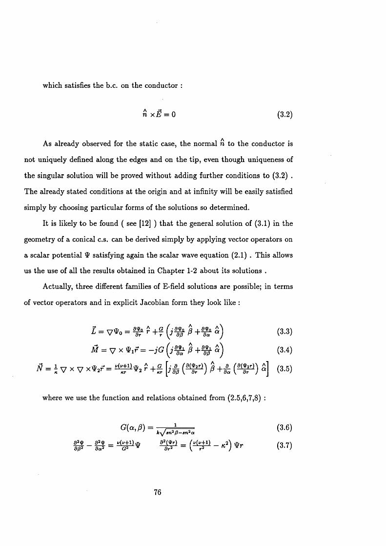
which satisfies the b.c. on the conductor :

n x E = 0 (3.2)

As already observed for the static case, the normal n to the conductor is

not uniquely defined along the edges and on the tip, even though uniqueness of

the singular solution will be proved without adding further conditions to (3.2) .

The already stated conditions at the origin and at infinity will be easily satisfied

simply by choosing particular forms of the solutions so determined.

It is likely to be found ( see [12] ) that the general solution of (3.1) in the

geometry of a conical c.s. can be derived simply by applying vector operators on

a scalar potential satisfying again the scalar wave equation (2.1) . This allows

us the use of all the results obtained in Chapter 1-2 about its solutions .

Actually, three different families of E-field solutions are possible; in terms

of vector operators and in explicit Jacobian form they look like :

L = V *o = a- t r + ? ( j f y fi « ) (3.3)

M = V x = - j G ( j ^ L p a ) (3.4)

AT = I v x V x V = P + £ [ j f0 (% £ * ) P + £ ( * T ) S] (3.5)

where we use the function and relations obtained from (2.5,6,7,8) :

76

3.1.1 Solutions o f th e scalar wave equation for ^ro?^ri ?^ r2

We can immediately see that the source of the diffracted field is virtually localized

on the conductor . Thus, in the space around it, it must be V E = V * V^o = 0,

that is to say = 0 .

Thus, limiting the attention to the vectors M , iV, we can proceed by trans

lating the vectorial b.c. (3.2) into simple scalar conditions on ^ 1, ^ 2? or better

on their individual factors A(a),B({3) .

In order to do this, we can note that whenever the conductor fits a surface

ft = constant or a = constant, (3.2) imposes there the conditions

M p( r , /?, a ) = iV/j(r,/?, a) = 0 or Ma(r,/?,d:) = iVa(r,/?, a) = 0 respectively. In

accordance to (3.4,5) and (2.5), these conditions become on A(ct),B(f3) respec

tively :

= R {r)B {p)A (a) = 0 /? = /?,V r,a B(fl) = 0 (3.8)

e_ ( a g d ) = * k W l B {p )A(a) = o /j = /5jVr, a =* £ (£ ) = 0 (3.9)

or

= i?(r)^(y0)y4(a) = 0 a = a,V r,/? => i4(a) = 0 (3.10)

& W ) = = 0 a = a,V r,/? =» A(a) = 0 (3.11)

Further im portant conditions on A(a),B(/3) can be identified by considering

symmetry conditions pertaining to the ” adjacent sectors ” in respect to the

conducting ones above ( see Fig. 1.7 ) . In fact, because of the coplanarity of

the latter with the source, that is to say the charge on the conductor, the normal

77

normal component of the E-field must vanish there . Using again (3.4,5), these

conditions pertaining to ” adjacent sectors ” = constant or a = constant

can be explicited respectively as :

^ = R(r)B(0)A(a) P = P,Vr,a => B(p) = 0 (3.12)

^ = W l B ( p ) A ( a ) P = P,Vr,a => B(p) = 0 (3.13)

or

^ = R(r)B(j3)A(a) = 0 a = a,V r,/? => A(a) = 0 (3.14)

£ P § ^ ) = ^ B ( / ) ) A ( a ) = 0 a = a , Vr, ft =» A (a) = 0 (3.15)

Summing up we can write :

on the sector conductor on the sector adjacent to the conductor

for M : A and/or B — 0 Neumann b.c. A and/or B = 0 (3.16)

for N : A and/or B = 0 Dirichlet b.c. A and/or B — 0 (3-17)

The latter are sufficient, according to the modalities exposed in 1.3.4, to sin

gle out periodicity and parity of the solution from which the spectra of eigenvalues

{i/j h] and eigenfunctions { v 4 (o ) , are recovered .

For this purpose, it is important to note that Dirichlet b.c. are the same

as in electrostatics, so that ^2 and its relative spectra are identical to and its

spectra respectively as determined in Chapter 2 .

Equally important is the fact that Neumann b.c. are the same as in the

static case but with a conductor complementary to the given one . This is ex

pressed analytically by saying that the -spectra relative to an acute sector are

78

those in electrostatics for the complementary obtuse sector and vice-versa .

This simple and remarkable result permits to obtain all the M and N solu

tions with no further computational effort nor further consideration about spectral

properties with respect to the static .

The same property naturally occurs for the double-sector in the sense that

^2 is the static determined in Chapter 2 while \Pi is determined like but

relatively to the complementary double-sector so that it is recoverable from VE

itself by operating the substitutions :

k - + k ', h{k2) -* h '( lfc'2), v(k2) -* v{k'2) (3.18)

Taking into account these last relations, in fact, also the plots of the first 15

eigenvalues {v(k2), h(k2)} and first 5 eigenfunctions {B (P ),A (a )} relative to the

Neumann problem are directly recoverable from Figs. 2.4,7 respectively, relative

to the static or ^2 •

For what concerns composite wedges, instead, the ^ -sp e c tra are selected

from those relative to the sector or double-sector of origin exactly as indicated in

the static case .

The -spectra are selected instead in the complementary sector or double-

sector spectra with the criterion that A (a), B((3) also present vanishing derivative

( see (3.16) ) in correspondence of the plane conductors .

79

Finally, we ought to state that for all the wedges considered the T?-solution

is given by (2.9), where the explicit expression of the spherical Bessel function of

the \ at kind is :

As v > 0 ( see (2.12) ), this is the only solution which satisfies the cpnditions

of smoothness at the origin (1.24) as it vanishes there: the limit value v = 0 will

be considered in Chapter 4 .

On the other hand, the Hankel function is the linear combination of the \ st

and 2nd kind of spherical Bessel functions so defined :

W = ju + j K (3.20)

Its behaviour at infinity is of the type :

p —JKT

lim hW(Kr) = / /+1)------ (3.21)

That is to say, the fields TV, M present an out-going wave nature satisfying

the Sommerfeld radiation conditions ( see also [13] ) .

This said, we limit our attention to the solution (3.19) valid on the tip and

its neighbourhood .

80

3.1.2 Physical considerations on N and M

The above observations on the ^ -sp ec tra permit now to draw some important

physical considerations about the fields M , N related to them trough (3.4,5) .

Firstly, we note that the ” tie-up” between the above spectra finds its more

rigourous justification in the classic Babinet’s principle ( see also [13, 23] ) which

allows replacement of the acute sector problem with the equivalent complemen

tary obtuse sector problem .

Nevertheless, only very recently it has been explicitely formulated for the

plane sector and its complementary ( [18] ) in term of fields iV, M and related

magnetic field Hn , H m we define in the next section .

No analogous explicit formulation is available as yet for the double sector

even though an extension of the previous ones would be quite staightforward .

Secondly, we ought to express analytically the fact N is the dynamic gen

eralization of the static E-field . This can be proved by noting that as r —> 0, we

have :

^ = (* + 1 ) U kt) - ~ („ + l)(« r)*- (3.22)ar nr

so that the expression for N by the tip can be approximated as :

N ~ (u + 1) uA B r -\— . A^ H— ; ^ B ak y s n 2a —sn?l3 k y /» n 2 (3—sn?a

(3.23)

which, apart from the multiplicative factor (i/ + l ) k' i/ *1, is the static form (2.15).

Furthermore, the dependence of N only on the product nr yields the min

imum distance from the tip where the dynamic and static solutions are pro

portional to each other and where the singular behaviour of the static case ap-

81

proaches, in fact, the true field. Quantitatively speaking, we can say that for any

media and frequency, i.e. k = there exists a maximum radius rmax defined

by :

2jt 1Krmax = — rmox = — < 1 with N 6 [10 -*■ 100] (3.24)

so that for any r < rmax the Bessel function in (3.22) approaches a linear be-

haviour in «r, and the JV-field becomes proportional to the static field according

to (3.23) .

We can also state again the fact that, physically speaking, N is originated

by the distribution of charge on the conductor, whilst the appearance of M is

necessarily related to the dynamic effect of moving charges, that is the current,

on the conductor .

82

3.2 The H-field and J-density o f current

From the characterization of the E-field spectra just completed we can deduce

the spectra relative to the H-field simply remembering Maxwell’s equation which

link them in the free space surrounding the conductor, i.e :

H = — r— v x £ (3.25)JUft

Using (3.4,5) for the E-field, we obtain for H :

S m = i r + £ [ ,•£ ( * £ i ) % + fa ( s j u i ) a ] } (3.26)

^ = (3-27)

where 77 = y / j is the impedance of the medium . ^The above show immediately that the //m* spectrum is that of M and con-

sequently of \Pi, while the Hjq-spectra is that of N and of ^2 •

Naturally the ^-solutions so identified satisfy the b.c. for the magnetic

field, which are explicitly :

n - S = 0 i.e. Hn = 0 (3.28)

where n is the usual normal unit vector to the conducting surface . The tangential

component instead generates on the conductor the density of current :

J =n xH i.e. |J | = \H,\ (3.29)

83

Because of the (3.28-29) we will speak indifferently of density of current or mag

netic field on the conductor surface .

Finally, looking at (3.4,5,26,27) we point out that the fields N ,H n con

stitute an E-mode while M, H\f constitute an H-mode in respect to the radial

direction .

All these properties allow us to complete the similitude between propagation

around a sector and in a closed waveguide introduced in 2.3 .

We can also attem pt to draw an equivalent rectangular waveguide in the

space r, /?, a or more suitably in the space r, 0, <f> as shown in Fig. 3.1 where

some walls are effective conductors while others may be thought of as electric or

magnetic walls, in accordance to which components of E or H vanish there .

The so called E and H modes are completely similar to the TM{Xii2 and

TE{lti2 respectively in any transverse section where they present i*i, i2 zeros apart

from those possibly present on the conductors along the two dimensions 0, </> .

The situation differs in the longitudinal direction and by the termination

r = 0 of the guide where the r-dependence is that of j„ or . The usual pure

propagation term, however, is recovered far away from the origin .

2 k -

K-

Fig. 3.1 : equivalent rectangular guide in the r,e,<|> domain

84

3.3 T he H-field fundam ental m ode

and its m ain behaviour by th e tip

A simple inspection of (3.26,27), taking also in account (3.22), indicates that

by the tip H m goes like (/cr)1'-1 whilst H s goes like (kr)17, thus the singular

behaviour is due to just H m generated by the satisfying Neumann b.c. with

minimum v G [0,1] .

The eigenfunctions /?(/?), A(a), ( or 0(0), 4>(^)), pertaining to the funda

mental mode are then characterized by the followings parities and periodicities:

acute sector <

obtuse sector <

double-sector period 2w (odd)

P period 8K \ 0 period 4tt (even)

a period 2K (even) , <j> period 7r (even)

P period 2K ' (even), 0 period rr (even)

a period 4K (even) , <j> period 2tt (odd)

(3.30)

(3.31)

(3.32)

The function R(r) is characterized instead by the curve i/(<t) or better by

the degree of magnetic singularity r/^cr) = i/(a) — 1 .

Because of the discussed ’tie-up’ between the spectra relative to the Dirichlet

and Neumann problems, that is to say as a consequence of the Babinet’s principle

[18], we can state the simple and very remarkable relation between the electric

and magnetic degrees of singularity for plane sectors and double-sectors :

85

Th(<r) = Te(2ir — a) for the sector (3.33)

Th(a) = re(7r — (7) for the double-sector (3.34)

For its practical importance we draw the curves relative to the sector in

Fig. 3.2 and we report an approximate expression around the particular points

<7 = 0 ,7r, 2tt respectively associated with the semi-indefinite wire, the half-plane

and the plane conductor . Only at these points, in fact, v can be computed in an

exact way as 0,^,1 respectively, whereas techniques are available which permit

the determination of approximate analytical expression around these points .

We have :

= - i ^ ) 2 + + 1 ) (2 ^ )4 +

^ [(^ T 2")6 around a = 2ir (3.35)

- $cos( l ) + £ c o s2( f ) - (4r + -h) cos3( f ) -f

O (cos4( |) ) around <r = n (3.36)

t c (<7) = - 1 + — 3- around = 0 (3.37)

(3.35) had been first determined using perturbation techniques but, in the

attem pt to extend indefinitely the number of terms in the series, Brown

( see [20] ) expressed v and h asymptotically about k = 1 that is a = 2x; the first

four terms axe just those reported and analogous relation were recovered for h .

(3.36) had been approached instead firstly by Legendre who gives three

86

terms . Brown succesfully extended to 4 in the above work [20], also providing

analogous expression for h .

The accuracy of these two espressions versus the angular distance from the

points <r = 7r,27r respectively is indicated in [20] .

Relation (3.37) has been, among the others Authors, deduced by De Smedt

[16] as the limit case of a sharp corner of arbitrary section . He implemented a

static analysis in spherical c.s. turning the problem of applying the b.c. into one

of solving integrals of some normal derivatives of the potential along an arbitrary

irregular boundary . (3.37) results the particular case of a sector in the more

general formula describing the degree of electric singularity for a solid conducting

tip .

The complementarity of behaviour for the electric and magnetic singularities

can be graphically explained if we think in terms of E-field lines on the plane

facing the conductor and, for what said in 3.2, of the density of current lines on

the conductor itself as shown in Fig. 3.3 . Precisely, the more reentrant is the

sector, the more the E-field lines thicken on the tip while the current bends before

it . Conversely, the more protruding is the sector, the more the lines of current

thicken on the very tip while the E-field lines rarefy there .

The situation is different for all the other five composite wedges because the

above defined fundamental H \f-n lode does not belong to the excitable spectrum.

This can be proved in an alternative, more physical way by requiring that

the EM fields around the conducting sectors and the charge and currents on

them must satisfy the image principle with respect to the conductor plane(s) of

symmetry .

For this purpose, Fig. 3.4a shows the typical behaviour of an H-mode

87

0

-0.185343

-0.5

-0.703416

10 90 180 270 360

Fig. 3.2 : EM fields degrees of singularity for the plane sector

a) b)

Fig. 3.3 : lines of E andTfor an acute a) and obtuse b) sector

88

current while Fig. 3.4b shows the typical behaviour of an E-mode current.

Only the latter would satisfy the image principle with respect to the median

plane, like for the structure in Fig. 2.8, and presents necessarily a zero on the

tip.

Similar arguments are valid for all the other four composite wedges .

Thus, for all them, the fundamental H-mode is just the Hn associated to

the fundamental N-field so that the minimum degree of magnetic zeros in the

origin is related to the degree of electric singularity re by means of :

Th(<r) = t c{(j ) + 1

We can summarize all these considerations simply by saying that:

fo r the sector and double-sector the main H and E behaviours are those of the

fundamental H-mode and E-mode respectively, while fo r any other case, the main

behaviour is that o f the fundamental E-mode .

a) b)

Fig. 3.4 : J-current lines relative to a) an H-mode and b) an E-mode

89

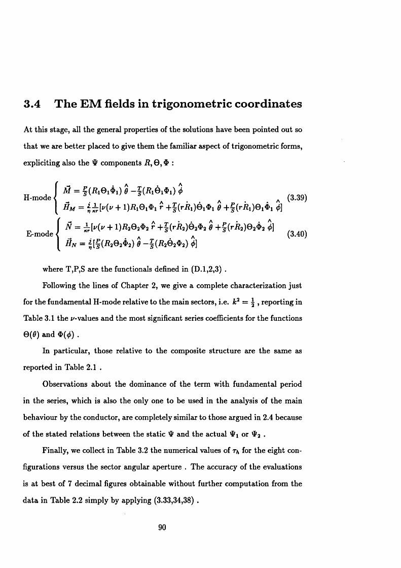
3.4 T he EM fields in trigonom etric coordinates

At this stage, all the general properties of the solutions have been pointed out so

that we are better placed to give them the familiar aspect of trigonometric forms,

expliciting also the W components R, 0 , $ :

H-mode <

E-mode <

m = f (*,e,*,) e -f (Jiidi*,) $Hm = r 6 + f 2]

N = + l)i2202$2 r + |(ri?2)02$2 0 + ^ (r-^2)02$2a a (3.40)

8 N = *[§ (i?202*2) 9 - f ( JR2©2^2)

where T,P,S axe the functionals defined in (D.1,2,3) .

Following the lines of Chapter 2, we give a complete characterization just

for the fundamental H-mode relative to the main sectors, i.e. k2 = | , reporting in

Table 3.1 the v-values and the most significant series coefficients for the functions

0(0) and Sty) .

In particular, those relative to the composite structure are the same as

reported in Table 2.1 .

Observations about the dominance of the term with fundamental period

in the series, which is also the only one to be used in the analysis of the main

behaviour by the conductor, are completely similar to those argued in 2.4 because

of the stated relations between the static W and the actual or ^ •

Finally, we collect in Table 3.2 the numerical values of for the eight con

figurations versus the sector angular aperture . The accuracy of the evaluations

is at best of 7 decimal figures obtainable without further computation from the

data in Table 2.2 simply by applying (3.33,34,38) .

90

CHARACTERISTIC COEFFICIENTS OF THE FUNCTIONS R(r),e(0),<D(0)

Fundamental m ode - k2 = 0.5

Fig. 2.1a v=0.814655 Fig. 2.8a v =1.131248i 0-per 4tc odd 0-per 2k odd 0-per 47c even 0-per 2k even-5 -0.000002 -0.000003-4 -0.000014 -0.000025-3 -0.000122 -0.000229-2 -0.001289 -0.002524- 1 -0.020708 -0.046684

0 1.000000 1 . 0 0 0 0 0 0 1 . 0 0 0 0 0 0 1.0000001 -0.146171 0.010835 -0.218468 -0.0092712 -0.004733 0.000806 -0.004143 -0.0006463 -0.000386 0.000082 -0.000315 -0.0C00644 -0.000040 0.000010 -0.000032 -0.0000075 -0.000005 0.000001 -0.000003 -0.000001

Fig. 2.1b v=0.296584 Fig. 2.8b v=1.955326i 0-per 7i even 0-per 4k even 0-per 7c odd 0-per 4k odd-5 0.000001 -0.000003-4 0.000009 -0.000025-3 0.000075 -0.000249-2 0.000752 -0.003264- 1 0.010468 -0.1319190 1 . 0 0 0 0 0 0 1 . 0 0 0 0 0 0 1 . 0 0 0 0 0 01 -0.033084 -0.054644 1.000000 -0.4172612 -0.001994 -0.002632 0.003154 0.0115473 -0.000186 -0.000231 0.000240 0.0006454 -0.000021 -0.000025 -0.000025 0.0000595 -0.000003 -0.000003 0.000003 0.000006

Fig. 2.2 v =0.704321 Fig. 2.9 v =1311863i 0-per 7C even 0-per 2tc odd 0-per 2tc odd 0-per 2k even0 1 . 0 0 0 0 0 0 1 . 0 0 0 0 0 0 1 . 0 0 0 0 0 0 1 . 0 0 0 0 0 01 -0.102762 0.016714 -0.023588 -0.0235882 -0.005284 0.001279 -0.001543 -0.0015433 -0.000473 0.000131 -0.000150 -0.0001504 -0.000052 0.000015 -0.000017 -0.0000175 -0.000006 0.000002 -0.000002 -0.000002

Fig. 2.10 v = 1.918023 Fig. 2.11 v = 2.688000i 0-per 71 odd 0-per 7t even 0-per K odd 0-per 271 even0 1 . 0 0 0 0 0 0 1 . 0 0 0 0 0 01 1 . 0 0 0 0 0 0 -0.438126 1.000000 -0.2006602 0.005747 -0.001841 -0.053492 -0.0033503 0.000443 -0.000125 -0.002912 -0.0002484 0.000046 -0.000012 -0.000267 -0.0000255 0.000005 -0.000001 ________ -0-000030 - - - - - - - - - - - - -O .O Q C O O j

Table 3.1: characterization of the eigenfunctions R(r), 0(0), $(</>) for the acute sector, half acute sector, obtuse sector, half obtuse sector, double sector, half double sector, sector on a plane and half sector on a plane respectively indicated by their Fig. number .

91

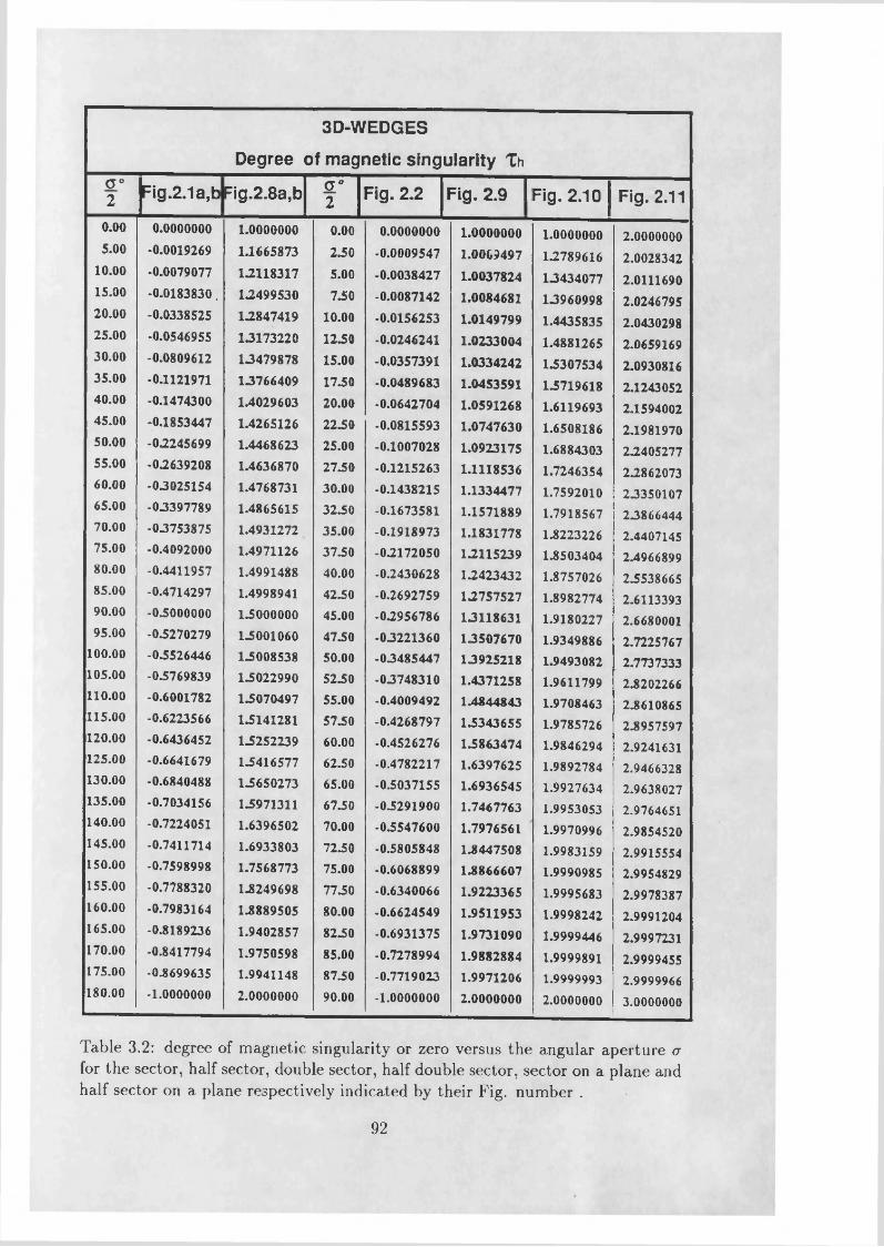
3D-V

Degree of mag

VEDGES

netic singularity Thc°2 fig .2 .ia ,b Fig.2.8a,b| C °

2 Fig. 2.2 Fig. 2.9 1Fig. 2.10 | Fig. 2.110.00 0.0000000 1.0000000 0.00 0.0000000 1.0000000 1.0000000 2.00000005.00 -0.0019269 1.1665873 230 -0.0009547 1.0009497 13789616 2.0028342

10.00 -0.0079077 13118317 5.00 -0.0038427 1.0037824 13434077 2.011169015.00 -0.0183830. 13499530 730 -0.0087142 1.0084681 13960998 2.024679520.00 -0.0338525 13847419 10.00 -0.0156253 1.0149799 1.4435835 2.043029825.00 -0.0546955 13173220 1230 -0.0246241 1.0233004 1.4881265 2.065916930.00 -0.0809612 13479878 15.00 -0.0357391 1.0334242 13307534 2.093081635.00 -0.1121971 13766409 1730 -0.0489683 1.0453591 13719618 2.124305240.00 -0.1474300 1.4029603 20.00 -0.0642704 1.0591268 1.6119693 2.159400245.00 -0.1853447 1.4265126 2230 -0.0815593 1.0747630 1.6508186 2.198197050.00 •0.2245699 1.4468623 25.00 -0.1007028 1.0923175 1.6884303 2.240527755.00 •0.2639208 1.4636870 2730 -0.1215263 1.1118536 1.7246354 2.286207360.00 -03025154 1.4768731 30.00 -0.1438215 1.1334477 1.7592010 2335010765.00 -03397789 1.4865615 3230 -0.1673581 1.1571889 1.7918567 2386644470.00 -03753875 1.4931272 35.00 -0.1918973 1.1831778 13223226 2.440714575.00 -0.4092000 1.4971126 37.50 -0.2172050 13115239 13503404 2.496689980.00 -0.4411957 1.4991488 40.00 -0.2430628 13423432 1.8757026 2353866585.00 -0.4714297 1.4998941 4230 -0.2692759 13757527 1.8982774 2.611339390.00 •03000000 13000000 45.00 -0.2956786 13118631 1.9180227 2.668000195.00 -03270279 13001060 4730 -03221360 13507670 1.9349886 2.7225767

100.00 -03526446 13008538 50.00 -03485447 13925218 13493082 2.7737333105.00 -03769839 13022990 5230 -03748310 1.4371258 1.9611799 23202266110.00 -0.6001782 13070497 55.00 •0.4009492 1.4844843 1.9708463 23610865115.00 -0.6223566 13141281 5730 -0.4268797 13343655 1.9785726 23957597120.00 -0.6436452 13252239 60.00 -0.4526276 13863474 1.9846294 2.9241631125.00 -0.6641679 13416577 6230 -0.4782217 1.6397625 1.9892784 2.9466328130.00 •0.6840488 13650273 65.00 -0.5037155 1.6936545 1.9927634 2.9638027135.00 -0.7034156 13971311 6730 -03291900 1.7467763 1.9953053 2.9764651140.00 -0.7224051 1.6396502 70.00 -03547600 1.7976561 1.9970996 2.9854520145.00 -0.7411714 1.6933803 7230 -0.5805848 13447508 1.9983159 2.9915554150.00 -0.7598998 1.7568773 75.00 -0.6068899 13866607 1.9990985 2.9954829155.00 -0.7788320 13249698 7730 -0.6340066 1.9223365 1.9995683 2.9978387160.00 -0.7983164 13889505 80.00 •0.6624549 1.9511953 1.9998242 2.9991204165.00 -03189236 1.9402857 8230 -0.6931375 13731090 1.9999446 2.9997231170.00 -0.8417794 1.9750598 85.00 -0.7278994 1.9882884 1.9999891 2.9999455175.00 -03699635 1.9941148 8730 -0.7719023 1.9971206 1.9999993 2.9999966180.00 •1.0000000 2.0000000 90.00 •1.0000000 2.0000000 2.0000000 3.0000000

Table 3.2: degree of magnetic singularity or zero versus the angular aperture a for the sector, half sector, double sector, half double sector, sector on a plane and half sector on a plane respectively indicated by their Fig. number .

92

3.5 The H-field singularity vector

for the m ain sectors

Considering the main behaviour by the tip of the wedge proper to the fundamental

H-mode, we achieve a first general simplification for R if we note that by the tip,

i.e. «r —► 0, ( see also (3.22) and E.6 ) we have :

lim R U r) = U rY lira ff(«r) = (v + l)(Kr)(‘/- 1> (3.41)« r—*• 0 « r—► 0

consequently, the S functions defined in Appendix D,E become related to

each other as :

S*s = (v + 1 ) ^ - = (* + (3.42)/cr

So* = (y + l ) ^ 1 = {y + (3.43)KT

so that their explicit forms in x , y , z and X ,Y ,Z can be obtained directly from

the (D.23,24) respectively .

Furthermore, for what will follow, we may neglect the multiplicative depen

dence on v and /c, possibly reintroducing it at right time .

We can now apply again the simplifying procedure presented in Chapter 2

so as to recover the singularity functions for the H-field in a complete three-

dimensional trigonometric space and its projections on the main rectangular

planes .

93

The quarter plane

Starting then with the quarter plane in the geometry indicated in Fig. 3.5 and

the derived structures of the half quarter plane, from (3.30) and (2.43) we can

use the approximate eigenfunctions :

0 2(0) stnf ^2{4) — sin<j> (3-44)

0i(0 ) ~ cos| ^i(^) — cos<f> (3.45)

Consequently, the H-field singularity vector components can be written as :

sjjx — (1 “ cos0cos<t>)S<f>Nsin^ (3.46)

shy = sin^SgN + cos|S ^ . (3*47)

shz — (1 4- cosOcos(f))S<t>NsinTi (3.48)

These assume forms helplessly complicated if rectangular coordinates are

explicited, however, following the motivations given for the E-field, we will report

explicitly in Table 3.3 only their projections on the main planes .

The resulting forms are obviously just of the six kinds (2.59) already met

for se , even though differently distributed in space .

In order to give more physical interpretation to the contents of the Table, we

draw in Fig. 3.6 the magnitude \H\ on the conductor, where it is also proportional

to | J |, according to (3.28,29), while Fig. 3.7 shows \H\ on the plane normal to

the conductor and tangential to its edge .

The eminent features of this behaviour is the transition between the singu

larity of degree — along the edges to that of degree —0.186345 on the tip . Very

94

remarkably, we note another advantage of the original choice of orientation for

the acute and obtuse sectors of Fig. 2.1 . It consists in the fact that

Table 3.3 results identical to Table 2.4, relative to the E-field singularity vector

for the three-quarter plane .

Some care has to be taken while dealing with sjj for the sector cut by

its median plane as its eigenfunctions are relative to the Dirichlet b.c. so that

(3.46,47,48) have to be corrected according to the substitutions:

Se„ -> S6u, I / - 1 - H / (3.49)

Nevertheless, the projection of the singularity functions on the main planes

assumes the same forms as in Table 3.3 with just v — 1 replaced by v .

T he three-quarter plane

When we deal instead with the three-quarter plane of Fig. 3.8 and the half three-

quarter plane we can approximate the eigenfunctions and the components of s j j

in trigonometric form respectively as :

0 2(0) ^ cos| — cos2<j> (3.50)

01 (0) ~ s m | $ i(0 ) — sin2(j) (3.51)

sh x = r I/_1cos| -f (1 — cos9cos<f>)SeNsin% (3.52)

shy = <SW5zn§ (3.53)

shz = r l,_1cos | + (1 + cosOcos<j>)SeNsin^ (3.54)

95

Their explicit forms on the main planes are those reported in Table 3.4

whilst the magnitude \H\, \J\ on the conductor plane and the \H\ on the plane

orthogonal to it by its edge are shown in Figs. 3.9,10 respectively , The latter

highlight the sharper singularity of degree ~ —0.703416 on the tip as compared

to that of degree — - along the confluent edges . Obviously, as observed for the

quarter plane, Table 3.4 is identical to Table 2.3 relative to the E-field singularity

vector for the quarter plane .

The formulae relative to the half-three-quarter plane can be recovered from

(3.52,53,54) by operating the substitutions :

SeN -*SoM, S+s -*S+ U9 rv~l —* S^M (3.55)

hence, their projection on the main planes are still those reported in Table 3.4

with just v — 1 replaced by v ~ 1.955326, that is a very strong zero on the tip .

The double-quarter plane

Even simpler are the forms relative to the double-quarter plane and derived ge

ometries of Figs. 2.9,10,11 for which the approximate eigenfunctions are, in the

order, recovered from Table 2.2 as :

e 2(0) * i M<t>)Oi(0) cz sinO ^ i(^ )

0 i(0 ) ~ sin20 ^ i(^ )

0 i(0 ) ~ sin20 ^ i(^ )

~ sin<j> (3.56)

~ cos<f> (3.57)

~ 1 (3.58)

~ cos<j> (3.59)

96

which using (E.3) provide the sjj components for the double-quarter plane:

sjjx = (1 — cosOcos(j>)S^N (3.60)

shy = Sbn (3.61)

shz = (1 + cosOcosfySfa (3.62)

In particular the 2nd equation reveals the physical meaning of Sg ( or ) as

being the shy singularity vector component for the double-sector with conductor

on $ = 0 ,7T ( or <l> = 0, ir ) .

By projecting these formulas on the main planes, we get in explicit rectan

gular coordinates the forms of which in Table 3.5 and their interpretation is shown

graphically in Figs. 3.12,13, representing respectively the plane of the conductor

and the plane orthogonal to the conductor passing through its edge. The order of

the Sectors in the Table has been changed in such a way as to put in evidence the

fact that Table 3.5 is identical to Table 2.5 relative to the Complementary double

sector once x, 0 are interchanged with z, <j> respectively .

Analogously to the previous cases, the singular vector components for the

derived wedges are obtainable from (3.60,61,62) by operating the substitutions:

S<t,N —► 5 ^ 0 6 , Sbn —► 5 ^ 0 $ , v — 1 —► v (3.63)

where 0 , $ are as in (3.57,58,59) . The forms on the main planes are again those

reported in Table 3.5 with just v — 1 replaced into v whose value, case for case,

is recoverable from Table 3.2 .

97

H-field singularity vector components fo r a quarter planesh x ( and J z ) sh y sh z ( and — Jx ) Sector

on the plane Y = 00 r“

y /\X Z \0 z < 0; <f> = 0

0 r—1 0 z > 0; 4> = o, 7r,0 = o0

y /\X Z \0 z < 0; <f> = 7r

J \ X Z0 VI x z y - 2 x > 0; 0 = 7r

v/l x z y 0 rvT J x z J

x < 0; 9 = 7r

on the pi ane X = 0 (or Z = 0)

f a ( V I F k - l )V i n

Z > 0 ( o r X > 0 )

l » " ' r*7-1 -* 1 <o Z < 0 ( or X < 0)

Table 3.3: H-field singularity vector projections on the main planes relative to the conductor and geometry indicated in Fig. 3.5; v ~ 0.814655 for the quarter plane and u ~ 1.131248 for the half quarter plane .

0 = 0

10 = id

Fig. 3.5 : quarter plane

98

H-field singularity vector components for a three-quarter planesHx ( and Jz ) SHy 8fjz ( and —J x ) | Sector

on the plane Y = 0rv

V\xz\ 0 yj\xzy~2 z < 0; <t> = 0

I-1'*1 0 r"-1 z > 0; (f> = 0, X, 0 = 00 rv z < 0; <f> = 7r

0 r r v H

d\xz\ 0 2 < 0; 0 = 7T

on the pi ane X = 0 (or Z = 0)

5 f t t v H T r - t )rv~h7 \ y \

( - * ) Z > 0 ( or X > 0 )

r""1 r*-t rv~l Z < 0 ( or X < 0)

Table 3.4: H-field singularity vector projections on the main planes relative to the conductor and geometry indicated in Fig. 3.8; v ~ 0.296584 for the three-quarter plane and v ~ 1.955326 for the half three-quarter plane .

Fig. 3.8 : three-quarter plane

99

H-field singularity vector components for a double-quarter planesHx ( and Jz ) SHy SHZ( and — Sector

on the plane Y = 0r

7ixz\ 0 ^ x z y - ' 1 x < 0; 0 = 0

07 \ x T \

x > 0; 0 = 7r

0V \ x z \

0

oII

V \X Z \0 v /IX Z I r -2 a: > 0; 0 = 7r

yJ\XZI r - 3 0 rvs / \ m

x < 0; 9 = 7r

0 r"J \X Z \

0 <f> = T

o\i the plane X = 0 (or Z = 0)

f a ( V U V - I )rv~h7 m

y iF K - S ( - , any Z ( or X )

Table 3.5: H-field singularity vector projections on the main planes relative to the conductor and geometry indicated in Fig. 3.11; u ~ 0.704321 for the double- quarter plane, v ~ 1.311863 for the half double-quarter plane, v ~ 1.918023 for the quarter plane on a plane and v ~ 2.68800 for its half .

Fig. 3.11: double quarter plane

100

Magnitude of the ma gn et i c f i e l d on the p l an es

F1q. 3.9

101

3.6 EM singularity vectors for arbitrary w edges

From equations (3.39,40) it follows a similitude between the espressions of N and^ ^

Hm ( or M and Hn ) •

This similitude becomes a true identity, apart for the multiplicative factor

if we consider the W-spectrum associated to an acute sector ( Fig. 2.1 ) and

the H -spectrum associated to its complementar obtuse sector ( Fig. 2.1b ) .

In fact the functions f?i,0i,4>j of the first geometry and f?2,02>$2 of the

second geometry are identical because they satisfy Dirichlet and Neumann b.c.

pertaining to complementar sectors, that is to say exactly the same b.c. . The

same properties are demonstrable in a similar way for M and H n and can be

extended to the case of the double sector .

In particular, the fundamental 7V-mode of an acute sector and the funda

mental HM~mode of its complementary are proportional so tha t the associated

singularity vectors are identical as observed, in particular, by comparing

Tables 2.3,4,5 with Tables 3.3,4,5 .

Also remembering that the E-fiels singularity vector can be recovered from

a simple static analysis we can summarize by postulating that :

In a full dynamical analysis, the EM-field spectra pertaining to any plane

sector are recoverable from those pertaining to the sole acute sectors .

Likewise, the EM-Jields spectra pertaining to any plane sector are recoverable

from those o f the sole E-field spectra or H-field spectra pertaining to any plane

sector .

In particular, the H-field singularity vectors pertaining to any sector are

102

recoverable from the E-field singularity vectors pertaining to the complementary

sector and then from the static analysis only .

The first postulate is a consequence of the Babinet’s principle while the

second is a consequence of the first and of the fact the static and dynamical

E-fields present the same main behaviour by the conductor .

The two postulates are important also for their possible extension to arbi

trarily shaped complementary plane conductors such as, for instance, the degen

erate surfaces of the ellipsoidal c.s. for which a static analysis is already available

in separable form while the dynamical one is not .

The limit cases Jb2 = 0 ,l are again postponed to Chapter 4 .

W hat instead now matters more to us is to attem pt the determination of

■ s j f o r a plane conductor with arbitrary boundary C whose tangent varies

continuously everywhere except at a cusp-point 0 .

Fixing in 0 the origin of a conical c.s. with the plane conductor lying on

the plane Y = 0, we can depict the situation as in Fig. 3.14 .

In this situation, the right and left branches of C with respect to 0 can be

expressed by the continuous functions with continuous derivatives z = f i (x ) ,

z = f 2(x) . The right and left tangents to C at O are related to the angular

coefficients of the curves there as tg(T\ = /i(0 ), tgcr2 = f 2(0) .

The values <7i, cr2 permit the unique orientation of the main system X , Y, Z

making the Z -axis fit the right tangent of C in 0 .

Naturally, is always possible to single out a small neighbourhood of the tip

where the wedge is well enough approximated by the sector of angular aperture

103

i1iiI

a = tt — (<7i + 02) and for which se and sjj are computed as seen previously .

Obviously, we cannot extend these singularity vectors to the whole of the

conductor but the generalization used to pass from the main sectors to arbitrary

sectors on the main planes, suggests possible forms, at least, on particular sur

faces. For instance, the formulae collected in Tables 3.3,4,5 of Chapter 2,3 on the

plane Y = 0 can be generalized by substituting :

X - M X , Z) Z - f 22(X, Z) (3.64)

where f n and f 22 are the implicit forms of the right and left branches of C, in

similitude to the implicit straight line equations (2.72) of the sector edge .

The forms relative to the plane X = 0, Z = 0 instead now hold respectively

on the planes :

f n ( X , Z ) = 0 f 22( X , Z ) = 0 (3.65)

whose traces on the plane Y = 0 are exactly the right and left branches of C .

The u-value used in each case is that relative to a sector of angular aperture a .

The complete three-dimensional singularity vectors can be eventually fully

determined for just the special cases in which they fit one or more degenerate

surfaces of the more general Ellipsoidal c.s. reported in Figs. 1.3,4 .

The investigation of these geometries constitutes one of the main future

aims of the work, also motivated by future applications to microwave techniques.

104

Az

z = f2(x) f22(X,Z) = 0

Fig. 3.14 : sector of generic boundary shape C but with a cusp in O

105

3.7 U niqueness o f th e fundam ental solution

We observed while imposing the b.c. (3.2,28) that, because of the non uniqueness

of the definition of the normal n to the conductor on the edges and on the tip,

the fundamental solution might not be unique .

This problem was posed first by Rayleigh at the beginning of the century

and approached by several authors in different ways . Their conclusions have been

satisfactorily summarized by Jones ( see [24] and bibliography quoted there ) .

Of all this analytical effort, we will only report the outstanding physical results .

If we suppose to illuminate with an incident field Eo, Ho a wedge conductor

of arbitrary shape as that of Fig. 3.14, a current J , a surface charge ps and,

possibly, a line of charge pi on C are induced, which generate the diffracted fields

E \,H \ . Finiteness and continuity of J and pa might only fail on C while those

of pi only at 0 .

Nevertheless, J ,p s and pi must always be integrable on the conductor sur

face S and on C respectively because the complete charge and current on the

conductor must remain finite . Under these hypotheses, the application of the

regular b.c. on S implies pi = 0 , i.e. neither a line of charge is present on C

nor an isolated charge is present at 0 . Consequently, the EM fields components

tangential to C vanish there .

Under these conditions, it is possible to satisfy the physical principle that

no energy is radiated by the edge, from which the uniqueness of the solution is

derived.

A consequence of this result is that there is one only solution, for which

J and pa are singular at C with degree > —1 and the same happens of the

106

perpendicular components of E i and H i to C but external to the conductor .

Similar observations apply to the neighborhood of 0 where the components

Ei and Hi radial to 0 are singular of degree > —1, but become finite on the

conductor and on the two straight lines tangent to C at O and arbitrarily close

to it .

From the Tables 3,4,5 of Chapters 2,3 it appears immediately how the den-

sity of current J and charge pt as well as the EM fields relative to the fundamental

mode satisfy all these properties .

We can thus conclude by saying that :

just the sole regular b.c. (3.2,28) pertaining to the conductor surface S are suffi

cient to ensure uniqueness o f the fundamental solution . In spite o f a singularity

of J , pa, E i, Hi along C this ensure Jiniteness o f charge and current on the con

ductor and o f the diffracted EM energy .

The latter singular b.c. will be denoted as ” singular edge and vertex con

ditions on C ” as complementary to the ” regular boundary conditions on S ”.

107

3.8 General remarks

Before closing this Chapter we would like to make some other applicative and

general remarks :

i) From the point of view of the applications, it is im portant to establish

how large is the region around the tip where the effect of the spherical singularity

may be considered dominant with respect to that along the edges . Analytically

speaking, the effect of the tip singularity is originated by and can be con

sidered terminated where the Bessel function j v assumes the first maximum ;

dependently on i/, this is located where k t ~ 1 ( see [11] pg 187 ) .

Physically speaking, and in order to determine a distance independent of

the sector aperture, i.e. of i/, we consider the effect limited to «r <C 1, likewise

quantified as in 3.24 .

In the spherical region centered at 0 and within the above radius, we assume

the tip singularity as significant .

ii) The singularity vectors forms reported in Tables 3,4,5 of the last two

Chapters can be further simplified .

For instance, when dealing with shx for the quarter sector we may consider

the single form :

This no longer represents the actual way in which zeros and singularities

along the edges match those on the tip, as obtainable from the exact solution,

108

but still shows the right degrees of zeros and singularities along the conductor

contour.

This might suffice in an application where a single form for the whole surface

of integration is of help .

While this simplification is obviously applicable to all the other components

and for all the other wedge geometries on the plane Y = 0, other forms better

suited to the particular problem in question may also be produced .

iii) As a third point, we note the possibility that in particular and quite

unusual situations of excitation, the above fundamental modes might not be

excited, thus leaving the main behaviour on the tip to be described by a higher

mode .

It could be shown in a way similar to that used by Satterwhite [10], that

the fundamental mode is not excited when an elementary dipole source of current

is placed and oriented respectively as ( see also Figs. 3.5,8,11 ) :

r

on the median plane z = 0, orthogonally to it

< on the sector plane y — 0 out of the conductor, orthogonally to it

on the sector conductor, in radial directionr

on the median plane z — 0, parallel to it

on the sector plane y = 0 out of the conductor, orthogonally to it<

on the sector conductor, for every direction

everywhere for a radial direction

It is also possible to show that the next mode to be excited is of the Dirichlet

for E-field

for H-field

type for both the EM fields .

iv) The more rigorous analyst can also observe that the scalar wave equation

admits for v — h = 0 the separate solutions :

R — cq 4* — B = do *1" di/3 A. — co -4* eio: (3.67)r

However, the corresponding fields are the trivial null solution .

v) Last, we would like to note that the structure of Fig. 2.11 can be virtually

substituted by the double-sector but with asymmetric excitation as it has satisfied

the image principle in respect to the plane conductor itself . As observed, this

excitation that may be met in applications never produces a singularity at the

tip .

110

Chapter 4

WEDGES

IN SPHERICAL GEOMETRY

4.1 Introduction

This Chapter shows how classical results dealing with the bidimensional and cone-

wedges are analyzable in the framework of a unified theory of the plane sectors

and draws some general conclusions about the EM fields singularities on perfectly

conducting wedges .

The Chapter can therefore be missed by those who are strictly interested in

Microwave applications which are instead presented in the next Chapters .

Proceeding in accordance with the "coordinate matching procedure” pre

sented in Chapter 1, we now analyse those perfectly conducting geometries which

are fitting one or more equi-coordinate surfaces of the spherical c.s. .

Studies relative to bidimensional and conical wedges can by now be con

sidered classic ones even though some do resort to approximate or numerical

111

algorithms ( see [25] p. 18,[14, 17] ) .

Other composite geometries originated by the similitude with the composite

plane wedges studied in the Chapters 2,3 are now introduced for the first time

with the main purpose to help us state general properties of the singularity of

charge and current at tips of arbitrary shape .

Finally, some limit geometries directly obtained by the degeneracy

k = sine —► 0 of the planar sectors are analytically better characterized in spher

ical coordinates as already observed in the Chapters 2,3 .

Actually, there is much more to be obtained from an appropriate use of

the named degeneracy process, as not only the spherical geometry, but also the

differential equations, the general properties of the solutions and the solutions

themselves can be obtained in this way from those pertaining to the conical

geometry .

This permits a rigorous, simple and unified analysis of all the above men

tioned wedges as well as of those considered in conical geometry and even more.

At this stage, the most important difference is constituted by the degener

ation of the two Lame’s equations along a and /? into Harmonic and Legendre

equations respectively . Consequently a ”tie up” between the solutions along 0

and (f> is no longer possible .

Nevertheless, these solutions can be obtained from those formulated in

Chapter 1 by submitting them to a degeneracy procedure, even though some

of them may behave badly by ” blowing up” at 0 = 0 ,7r where the Legendre’s

equation presents its two singular points .

In this context, the most important example is represented by the two

112

Lame’s solutions, odd and even, of period 4ir along 0 relative to the acute sector.

When k2 —► 0 the series solutions for both cases lose convergence so that the odd

one, which in 0 = 0, it is 0, now assumes the finite values ±1 pertaining to the

Legendre associated functions P ^ (± l) , while the even one, which in 0 = 0, tt is

finite, now diverges to the 2 kind of Legendre associated functions Q” (±1) .

It is just this ”bad degeneracy” which prevents satisfaction of the physical

b.c. for the EM fields associated with limit structures like the semi-infinite wire

fitting the degenerate surface 0 = 0 for which a proper degenerate eigenfunction

is Pq = 1 . This problem leads us to make a distinction between this ”physically

unrealizable wire” and the wire with finite cross section usually met in appli

cations and for which a possible eigenfunction may be s m |, presenting a 0 on

the conductor . This, incidentally, is just the main term in the original Lame’s

solution already used for acute sectors of any aperture .

This example, and a few others, justify the study of all the named wedges

according to a rigorous and unified dynamic theory so as to single out explicitly

or implicitly the whole spectrum of solutions from which we separate, as required,

the fundamental mode or a simplified singularity vector .

The procedure aiming to the progressive characterization of the solution

will follow the lines of the case of conical geometry, while the static analysis will

be left for the sake of brevity .

Finally, from an application point of view, we can remember that the clas

sical bidimensional and conical wedges are more usually met in boxed waveguide

and antennas respectively, but, they also occur in the more widespread applica

tions of low frequency and high power engineering .

113

4.2 Characterization o f th e solutions

We follow the path of progressive specialization of ” the solution ” already taken

for the conical c.s. . The analytical formulation for this geometry is illustrated

in 1.2.1, where the sole trigonometric formalism is used which, since a long time,

has been recognized to be by far the most useful one in stating theoretical, com

putational and applicative results .

Thus, we retrace, one by one, the steps of 1.3 .

The geom etrical properties o f th e spherical coordinate system

We can make again reference to Fig. 1.13 but the two arcs C+,C” on the sphere

of radius ro now degenerate into the two points V +, V~ of intersection of this

sphere with the positive and negative z semi-axes, namely the degenerate cones

0 = 0, w respectively ( see Fig. 1.3 ) .

Any regular cone 0 = 0 intersects the sphere on a circle surrounding V + if

0 < % or V~ if 0 > \ while <t> varies from 0 to 27T .

Conversely, the half planes <j> = ^ intersect the sphere on a half circle joining

V + with V ~, while 0 varies from 0 to tt .

Consequently, any physically meaningful solution F in this geometry has to

be 2x-periodic in </>, i.e. :

F(r,0,<j>) = F(r,0,<!>-f 2 x ) (4.1)

114

The sm oothness properties o f th e solution

Further conditions must be verified on the singular points 'P+,'P~, at the origin

and on the sphere of infinite radius whenever they are part of the homogeneous

space .

Precisely, in order to ensure smoothness in the way indicated in 1.3.2, at

V + and V~ we must have :

lim i?(r)0(0)$(<^) independent on </> (4.2)8—+ 0,7T

while in r = 0, oo the same conditions (1.24,25) have to be satisfied .

The m athem atical properties o f th e H elm holtz equation

In third instance, the solution must also satisfy the scalar wave equation (1.26)

for the scalar potential which, in spherical c.s., separates into the ordinary

differential equations directly obtainable from (2.6,1.51,1.44) by setting k2 = 0,

i.e. :

R + 1 R + ( , < ? - 4 $ £ ) r = 0 (4.3)

© + ^ 0 + ( ^ + 1) - ^ ) 0 = O (4-4)

$ -f fi2$ = 0 (4.5)

(4.3) is the Bessel’s equation analysed in conical c.s., (4.5) is the common Har

monic equation while (4.6) is the Legendre’s equation, more commonly known,

115

as a function of the variable t = cosO :

(1 - t2)0 - 2*0 + ^ 1/(1/ -f 1) - 0 = 0 (4.6)

where the derivatives are now with respect to cosO .

In summary, the general solutions along the three dimensions can be written

as :

R(nr) = Cjl^(Kr) + V h ^ \n r ) (4.7)

0(0) = SP?(cosO) + FQ^cosO) (4.8)

$(4) = Qcos(fi(j>) + 'Hsin{y.<j>) (4.9)

where P* and are the Legendre functions of 1** and 2nd kind whose gen

eral properties are by now well known and to be found for instance in [11, 7];

Ci /DyS,^F,Q,'H are the linear combination constants .

The smoothness conditions at r = 0,oo are satisfied by (4.7) as already

shown in 3.1.1 while those at 0 = 0, tt can be satisfied if

0 (± 1 ) = EP»{± 1) + T Q l(± 1) = 0 there.

Actually, at these points Pjf, Q% present, in general, a singularity so that the

previous equation is written using their asymptotic expression there, as available

for instance in [7] .

116

This way, the conditions can be reduced to the simpler relations :

S = — f Z c t g ( n x ) in 0 = 0 (4-10)

S = — T \d g [ y ,K) in 0 = tt (4.11)

In the more important situation where /i = 0 ,1 ,2 ,..., in order to ensure

finiteness of 0 , from (4.10) follows T = 0 and from (4.8) follows 0(0) = P™(cos0)

which, in particular, for m = 0 assumes the finite value 1 at 0 = 0 but, then, it

is also $(<!>) = 1 so to satisfy in any case the condition (4.2) .

It is interesting to note that just applying the periodicity condition (4.1)

the general solution 4.9 implies :

H = m = 0 ,1 ,2 ,... (4-12)

117

4.3 T he physical boundary conditions and the

spectra o f eigenvalues and eigenfunctions

In the present geometry the EM fields can be derived from two potential functions

\Pi, ^2 satisfying the scalar wave equation, according to the same formulation as

for the conical case ( see [12] ) .

Furthemore, since we are going to analyse conductor geometries only fitting

one or more equi-coordinate surfaces 9 — const, ^ = const, the b.c. they establish

on the EM fields can be straightforwardly reduced to either the Dirichlet or the

Neumann type on the eigenfunctions 0(0), $(<£) in which Wi, ^2 are separated .

Omitting the explicit treatment of the static case, we identify from now on

by the suffixes D,N the two kinds of b.c. respectively .

Moreover, we group the b.c. in two main categories : those pertaining to

one or more half planes <f> = <f> and those pertaining to one or more cones 0 = 6 .

We start with the bidimensional wedges ( 2D-wedges ) delimited by planes

^ = const .

In particular, we will study the half plane and the plane by considering

them as limit cases of the acute and obtuse sector respectively .

This is why these two geometries represent the main meeting point between

2D and 3D-wedge analysis .

118

4.3.1 2D -w edges

These wedges are the easiest to be analysed because the spectrum of eigenvalues

i/y fi is determinable in a complete analytical way and the 0-eigenfunctions are

the same for the Dirichlet and Neumann problems .

The half plane

If we consider the half plane conductor fitting, without loss of generality, the

surface ^ = 0, the spectrum of eigenvalues established there by the Dirichlet

$(0) = 0 b.c. can be obtained, apart from an unessential rotation of axes, from

the limit cases k2 —► 1 of the acute sector . In this way, from the same Fig. 2.3

we can recover the eigenvalues spectrum like :

/i = m — I with m — 1 , 2 , 3...

v — fi,fi + 1,/z + 2,... = ^ with n = 1,2,3... (4.13)

For this special case, the Neumann b.c. establish in fact exactly the same

spectrum since the complementary conductor is the half plane itself . Conse

quently, for both situations on the conductor wedges 0 = 0 ,7r (4.10,11) imply

5 = 0, i.e. :

®zvv(0) = Q f{cos9) (4.14)

It is perhaps appropriate to note how the above are the only Legendre

functions of 2nd kind to be everywhere finite .

The eigenfunctions along <j> satisfying the two kinds of b.c. are instead

119

respectively :

$z?(<£) = sin(^<j>) $ n () = cos(^(j> ) (4.15)

The plane

The situation of a complete plane conductor, without loss of generality fitting

the surfaces <j> = 0, tt, can be seen as the limit case k2 —► 0 of the double sector .

From the same Fig. 2.4 the eigenvalue spectrum can be recovered as :

fi = m with m = 1 ,2 ,3 ,...

v = + 1,/* + 2,... = n with m = 1 ,2 ,3 ,... (4.16)

Consequently, with the same considerations as for the half plane, the eigen

functions spectrum is given by :

0 d ,jv(0 ) = P™(cosQ) (4.17)

$ d () = sin(m<f>) = cos(m</>) (4.18)

We remark that this is the only case where the Legendre functions of 1st

kind are polynomials finite everywhere .

120

T he 2D -sector ( Fig. 4.1 )

The generalization of the two previous cases is represented by a conductor delim

ited by an arbitrary plane <f> = <f> =6 (0, 2t t ) and, without loss of generality <f> = 0

( see Fig. 4.1 ) . Satisfaction there of the Newmann and Dirichlet b.c. imply

from (4.9,10,11) :

u = —-— with m = 1,2,3... r 2 x -< £V = fi.fi + 1,/x -I- 2,... (4.19)

For these eigenvalues, the eigenfunction spectrum (4.8,9) reduces to :

0£>,at(0) = P?(cos0) - ltg(fiTr)QZ(cos0) (4.20)

$ d {) — sin(n(2ir — <l>)) $ n () = cos(fi( 2k — <j>)) (4-21)

where the values of the constants £, T in (4.20) are such that (4.10,11) are satified

keeping ®d,n (9) everywhere finite .

121

T he 2D -sector on a plane conductor ( Fig. 4.2 )

This is a useful conductor configuration, especially in its particular cases of infinite

and semiinfinite plane conductors as met in boxed waveguides .

The cutting plane is likely to fit just the equi-coordinate 6 = f , where

P u iQ i and their first derivatives assume an easy expression ( see [7] p. 145 ) so

that the new conditions 0 (^ ) = O or 0 ( f ) = 0 mean respectively :

£ = ((i/ + p + l ) f ) (4-22)

£ = - T \ c t g ((i/ + /*)!) (4.23)

Naturally, the /i-spectrum is given by (4.19) itself, since no further b.c. are

introduced on ^-surfaces while the i/-spectrum is a selection of (4.19) so as to

satisfy also (4.10), i.e. :

vd — P + 2n + 1 (4.24)

= /* + 2n with n = 0 ,1 ,2 ,... (4.25)

As a consequence, the eigenfunctions 0 , $ are selections of (4.20,21) accord

ing to the i/-values (4.24,25) .

122

Fig. 4.1 : bidimensional sector

Fig. 4.2 : half bidimensional sector

4.3.2 Cone w edges

When no conductor is present on a plane <j) = the periodic condition (4.1)

implies the fi and ^-spectra to be given respectively by :

[i = m = 0 ,1 ,2 ,... 4>(< ) = Qcos(rri(j>) + ?{sin(m<j>) (4.26)

The spectra for v and 0 are now completely independent of the latter and,

case for case, can be determined as follows .

124

T he cone ( Fig. 4.3 )

The cone 9 = 9 divides the whole space into region 1 containing the positive semi

axis ( that is the degenerate cone 9 = 0 ) and region 2 containing the negative

semi-axis ( that is the degenerate cone 9 = w ) as indicated in Fig. 4.3 .

Thus, if the free space is region 1 , taking into account ( 4 .1 0 ) and the / i - values

( 4 .2 6 ) , the Dirichlet b.c. 0(0) = 0 implies that the v-spectrum is represented by

the zeros of just the 1** kind of the Legendre’s functions . We express this by

writing :

vjy : P^(cos0) = 0 for m = 0 , 1 , 2,... (4-27)

so that the related eigenfunctions are :

®{0) = P?D(cos0) (4.28)

Instead, in region 2 from (4.11) and the fi-values (4.26), the same Dirichlet

b.c. are satisfied when ( see (14) p. 144 [7] ) :

0 (0) = PZ(cosB) - hg(vx)Q Z(cos§) = = 0 (4.29)7r cos[u + m)ir

So that, as physically obvious, in region 2 the u and 0-spectra , within a

multiplicative constant are, given by :

vd ■ P£,(.cos(ir - 0 ) ) = 0

0(*) = j » H t - « ) )

for m = 0,1,2,... (4.30)

(4.31)

125

For what concerns the Neumann problem in the two regions, the eigenfunc

tions 0 assumes the same form since the conditions (4.10,11) are still valid while

the i/-spectra are now generated by :

in region 1 i/jy : P ^(cos0) = 0 for m = 0,1,2... (4.32)

in region 2 vn ' ~~ &)) = 0 f°r m = 0,1,2... (4.33)

If a plane conductor is placed at 0 = 0, x ( see Fig. 4.4 ) the equations for

the v and 0-spectra remain valid, but the value fi = 0 must be excluded, obtainig

finally the spectra :

/i = m = 1 ,2 ,3 ,... (4*34)

$£>(</>) = sin(m<j>) — cos(m<j>) (4.35)

Analogous considerations can be done for the double cone and related ge

ometries as reported in Appendix F .

126

Fig. 4.3 : cone

v v y s\AAAAA.

^VVWw^yyyvy?yv"

Fig. 4.4 : half cone

127

4.4 EM fields in spherical coordinate system

Moving along the lines of the procedure presented for the conical geometry, the

complete modal spectra for the EM fields relative to a given conductor can be now

derived from the spectra of the two scalar potentials \Pi, \p2 obtainable from the

eigenvalues z/,/z and eigenfunctions 0 £ ,$ £ just presented in the previous section.

The explicit EM field expressions can be obtained directly from (3.39,40)

passing to the limit k2 —► 0 in the functions P,T,S :

E-mode <N = dj; I/(v + 1 )RD®D$Dr + (rjf?jr>)0£)$£)$ + -^ { r R D ^ D ^ D ^ ]

^ R d Q d $ d Q — R d & d $ d $ \Hn = lV

H-mode <

(4.36)

M = - ^ R n ^ n ^ n O — R n ®n $ n 4>

H m = ^ \ y ( v + l ) R N & N $ N r + (rf?7v)0^^N^ + ^ ? ( r^iv)0fv^iv^](4.37)

These forms present naturally the same behaviour for r —► 0,00 and the

same distinction in E and H-modes with respect to the radial direction as in the

conical geometry ( see 3.4 ) .

We now have at hand all the formulation necessary to identify the fun

damental mode as well as the main and the, sometimes, singular behaviour of

the EM fields by the tip . Its simplified expression, e.g. a singularity vector

representation, will be expressed in the more convenient rectangular coordinates

according to the application of the conductor geometry .

128

4.4.1 Fundam ental m ode and singularity vectors for

2D -w edges

Considering firstly 2D-wedges as shown in Fig. 4.1 the minimum eigenvalues are:

" = " = 2 ^ (438)

which are < 1 only for ^ € [0,7r] . The correspondent 0-eigenfunction can be

written, using the 3.4(17),3.6.1(15) in [7], as :

2 2 - * T ( 2 i/ -4-11!®d,n (0) = PZ(cos0) tg{v*)Q vv(cosO) = - — ■- (sinO y (4.39)

7T i yU -f- 1)

so that, leaving aside an unessential multiplicative constant, the fundamental

eigenfunctions satisfying Neumann and Dirichlet b.c. are respectively :

® d ,n ( 0 ) = (sin0)v (4.40)

$£,(<£) = 5in( i/(2x — <f>)) $ n () = cos(i/(2x — </>)) (4-41)

The main behaviour by the conductor tip can then be recovered by passing

to the limit /cr —* 0 and simplifying in consequence the 72-function, as done in

(3.22) .

129

The simplified expression for the fields is then :

N oc (nrsinOy 1

• [i/sin$sin(v(2ft — <f>))r + cosQsin(v(2k — <j>))0 + i/ cos(v(2tt — <j>))<£] (4.42)

H m o c ( k rsin9)v 1

• [i/szn0cos(i/(27r — <j>))r + cos0cos(v(2n — <j>))0 — vsin(v(2n — <f>))4>] (4.43)

These expressions can be considered, as the singularity vectors s~e , sh for 2D-

wedges .

Remarkably, the possible singularity is controlled by just the term :

which expresses the fact that :

the cylindrical singularity, i f u — 1 < 0, or zero, i f u — 1 > 0, is uniformly

We note now that, conversely to what happens for 3D-wedges and for the great

part of wedges, r is the same for both the E and H fields .

The complete expression of (4.42,43) in rectangular coordinates is simply

obtained by using the inversion formulae :

(rsin0)v 1 = (x 2 + y2) ^ (4.44)

distribuited along the conducting edge which fits the z axis .

The degree of singularity is nowaday generally indicated by :

(4.45)

130

sin9 = — sin<t> = j i n | = —7=\l1 — -r- (4.46)r r A 2 v/2V Ar a; = — cos—= ± —=4/1 + — (4*47)A A 2 V2Y A

where we use the signs ± according to y < 0 respectively while A = \y jx2 -{■ y2\ .

For their applicative importance, we limit the attention to the half plane

(y = /i = 1) and the plane (i/ = /* = 1) conductor, whose minimum eigenfunctions

are respectively given by :

®d,n (0) = VsinO $ d () = s in (^ ) = cos(^) (4.48)

©d,jv(^) = sinO $ d () = sin{<j>) = cos(<j>) (4.49)

The plane conductor introduces the well known zero of degree 1 in the

tangential E-field and in the normal H-field . The half plane instead introduce a

singularity of degree — | in the E and H components normal to the edge and a

zero of the same degree on those tangential to it, as known since Sommerfeld’s

studies .

Quite interesting is also the 2D-wedge cut by the plane conductor

0 = ^ of Fig. 4.2 because of its occurence in boxed resonators, short circuits

or discontinuities in waveguides . Nevertheless, the literature does not treat this

case probably because the fields are never singular on the tip .

If, in fact, we look at the (4.24,25), we see that in the origin the fields

131

present a zero of degree :

T = 2 ^ = , / " 1 = / ‘ (4'50)

so that the minimum eigenfunction is ( see 3.4(17) in [7] ) :

O b W = K '(cosB) - ^ tg{{v - l)x)Q " '(cos6) = 2c o s { ( l - v ) x ) P" ^ cos^

(4.51)

while those along $ remain of the forms (4.41) .

Surprisingly, (4.43) already satisfies the b.c. H$(%) = 0, so this is also a

solution for the actual geometry .

This shows that :

the degree o f singularity for H remains as in (j^.^5), that is negative for <j> E [0, tt],

the only difference being a physical one and consisting in the flow o f current from

the top half wedge to the plane conductor instead of the lower half one .

W ith a view to application, we give an explicit formulation of the main

E-field only for the half plane cut by a plane conductor, for which the minimum

eigenvalues are p = vq — 1 = \ while the associated eigenfunctions and field

expressions are :

= cosOy/ sinO (4.52)

N oc (^jp)* 3sin0cos0sin(^<f>)r -f (1 — 3sin20)sin(^<f>)0 + 3cos0co,s(|<^)^j (4.53)

This last singularity vector, together with (4.43) relative to the H-field, can

132

be explicited, using the (D.16,17,18) for k2 = 0, in terms of the main rectangular

coordinates X , Y, Z oriented as in Fig. 4.5 . The projections on the three main

planes assume the simpler forms reported in Table 4.1 and they are proportional

to the charge and current on the conductor according to the conventions used in

2.4.1,3.2 respectively .

EM fields singularity vectors for a half plane cut by a planeSEx SHX 8Ey shy SEZ SHZ Sector

on the plane Y — 0

0 x y / mr 2

XW \

0 0 1v W l

oII

V\z\ 0 0 17121

A7 ! z \

0 <f> = 7T

on the plane X = 0+ Z 0 0 i

7 ?0 1

v7II

on the plane Z — 0X y /\Y \

r2X

W \i

W \A

7 ^ w \ -e- II toN

Table 4.1: EM fields singularity vectors projections on the main planes for the conductor and geometry of Fig. 4.5 .

z = X

Fig. 4.5 : half plane on a plane conductor

133

4.4.2 Fundam ental m ode and singularity vectors for

Cone-w edges

From the point of view of determining the spectra of eigenvalues and eigenfunc

tions, Cone-wedges are located between 2D and 3D-wedges . In fact, while for the

former the eigenvalues are determined analytically and for the latter both numer

ically, for the Cone-wedge, // is already determined analytically but v d ,n has to

be computed as one of the zeros or zero derivatives of the Legendre’s functions.

The accuracy with which the spectrum can be determined is then controlled

by the accuracy of this zero-finding procedure so that, from the experience in

using conical c.s., we use Hypergeometric series espressions for Q£, P£

( see [7] p. 144) :

Q*(cos0) = [ t g ( ( v + h ) \ ) T £ ( c o s 20 ) — c t g ( ( v + / » ) § ) 2 co30U‘;(cos20)]

P?(cos0) = V “(6) [T»(cos*0) - 2cos0Ui(cos‘20)] (4.54)

where while :

r « ^ ) . 2 = S g E ^ , 2 = p s S t e p ,,.55)

are related to the hypergeometric function F and expressible in power series of

cos20 ( see [7] p. 144 ) whose coefficients obey a two-terms recursive relation .

The dependence on cos20 ensures rapid convergence which is of vital importance

when we require high accuracy in the evaluation of the i/-value for a given fi .

134

By the way of example, when we require an accuracy of, say, 7 decimal figures,

the maximum index of the series goes from a few tens when 0 ~ ^ to almost one

thousand when 0 ~ 0, t ,

Among other things, the literature reports various approximate analytical

expressions for the zeros of our interest around the integer values of i/,/x since

then the series degenerates into terminating polynomials . This permits the use

of perturbative techniques for determining approximate series expansions .

Instead, if we look for an easy-to-apply expression for the Legendre func

tions, we need the Fourier representation :

ooPtt — 0,(0; I/, n)sin((y + // + 2i -f 1)0) (4.56)

»=ooo

Qv = i; y ' 0,(0; I/, n)cos((v + /z + 2i + 1)0) (4.57)»=o

where :

r \ t i a \ 2 / o • + + ^ + SA KQ\

°' {0' = ^ ( ) “ r(7+ |j------ Sm I); (4-58)

The latter also produces a two-terms recursive relation for the coefficients in the

series .

The last remark deals with the determination of a simple function which

represents just the correct b.c. on the conductor, so as required in a singularity

vector for the fields .

This time, things go differently than for the 2D case where the Legendre

135

functions involved degenerated advantageously into powers of Trigonometric func

tions, and than for the 3D case where all the terms of the Fourier series for the

Lame’ periodic functions present the same behaviour on the conductor, so that

the first term is representative of the whole function there . Now, the zeros of

P, Q and of their derivatives occur for arbitrary values of 0 so that, in general,

just the term of fundamental period does not represent correctly the zero on the

conductor . For the sake of simplicity, we leave indicated the exact eigenfunction

0(0) leaving to the user interested in a simplified expression of the EM field the

choice of its most appropriate approximations in the specific context .

Thus, let us discuss the main EM field behaviour for Cone-wedges .

T h e cone ( F ig . 4.3 )

Thanks to (4.29), only the space region 1 in Fig. 4.3 need to be considered .

From (4.26,29) it follows that the fundamental eigenvalue and eigenfunction for

the Dirichlet problem are respectively :

/x = 0 vd(P) ' PvD{cosd) = 0 for 6 E [0, x] (4.59)

Qd = PVD (cos0) = 1 (4.60)

In fact, from the properties of Pv follows that vd is its smallest zero and

the one which tends to 0 as 0 —> x, that is the case of the half wire, which tends

to 1 as 0 —► that is the case of the plane, and which goes to oo as 0 —> 0, that

is the space filled by a conductor .

The numerical values of re accurate up to 7 decimal figures versus 0 in steps

136

of 5°, are collected in Table 4.2 .

A useful asymptotic formula is available around the limit 6 —► 7r, = 0

which, if 0 is expressed in radiants, yields ( see [16] ) :

re ~ ■ ■ 2 ■■ — 1 around 6 = 7: (4.61)

This formula can be interestingly compared with (3.37), relative to the

sector wedge approaching the same wire .

Moreover, the analogous quantities for the Neumann problem are

( see 3.8(19) in [7] ) :

fi = l vN(0) : PlN{cos0) = (4.62)

= -^q[cos6PIn {cos6) + vN(yN + lJstnfflJP^cosfl)] = 0 for 0 E [0,7r] (4.63)

®n(B) = PlN{cos0) = cos(j> (4.64)

W ithout loss of generality and for simplicity, from now on we consider the ori

entation of the axes such that the ^-eigenfunction with p = m = 1 ( see (4.9) )

equals sin<j> for the Dirichlet and cos<j> for the Neumann case . The vn in question

is the smallest positive zero of P j and precisely the one which approaches unity

as 0 —► 7r, that is the case of the semi-indefinite wire, to decrease down to ~ 0.85

when 0 ~ 130°, which again approaches unity as 0 —► that is, the case of

the plane conductor, and which diverges as 0 —*• 0, that is the space filled by a

conductor .

The evident loss of monotony of the curve v n {6) can be physically so ex-

137

complete oscillation along any circumference of revolution on the cone surface,

that is to say the current flows down from one half cone surface, converging on

the acute tip, where it becomes singular, returning on the opposite half surface

of the cone ( see also Fig. 4.14 ) . Nevertheless, when the cone degenerates into a

wire, the infinitely thin conductor does not permit fluxes in opposite directions at

the same points . On the other hand, for the plane conductor there is no longer

a tip for the current to converge into, corresponding again to unit value of the

vj>j-curve .

The explicit accurate computation of this behaviour is left as further work .

However, it has been determined in [14,17] by mens of a different, more numerical

oriented approach .

Finally, the main behaviour of the EM fields by the cone tip can be approx

imated as :

N oc (Kr)VD 1[i/DPVD(cos9)r + PiD(cos^W] (4.65)

Hm (kt)"*-1 [vnPIn (cos$)cos(j)r + PlN(cos0)cos(f)0 — P*N(cosO)sin<j><j>] (4.66)

138

T h e h a lf cone ( F ig. 4.4 )

By the arguments relative to the previous case and using the spectra determined

in the previous paragraph, it is possible to state that the fundamental eigenvalues

and eigenfunctions for the Dirichlet and Neumann problem are now :

fi = 1 i/£>(0) : PlD(cos$) = 0 for 9 G [0,?r] (4*67)

®d (0) = PlD(cos0) ^ d (4>) = sin(f> (4.68)

ft = 1 vn (0) : PlN(cosO) = 0 for 9 £ [0, w] (4.69)

Q n ( 0 ) = PlN(cosO) $ n (4>) = cos<f> (4.70)

so that the main behaviour of the fields by the tip is :

N oc (Kr)VD 1 VDPlD(cos9)sin<j>r 4- PlD(cosO)sin<j>Q\ + - ^ P l D{cosO)cos(j>>j (4.71)

H m oc ^(«r)*'*_1 VNPlN{cosO)cos(j>r + PlN{cos0)cos<j>0 — PlN(cos9)sin<j><j (4.72)

Since rc > 0 ( see Table 4.2 ), the E-field is never singular, while r* is exactly

that of the cone because the current distribution on the cone surface is unaltered,

the only difference being a back-flux on the plane conductor on the location of

the missing half cone surface .

The electric singularity relative to the double cone and related geometries

are treated in Appendix F and the values obtained axe collected in Table 4.2 .

In the same Appendix we outline the procedure to identify the magnetic

singularity . As a whole, these result are summarized in [43] .

139

CONE-WEDGES

Degree of electric singularity Te

0! Fig. 4.3 Fig. 4.4 0 ‘ Fig. F.3 Fig. F.4 Fig. F.1 Fig. F.2

40.0045.0050.0055.0060.0065.0070.0075.0080.0085.0090.0095.00

100.00105.00110.00115.00120.00125.00130.00135.00140.00145.00150.00155.00160.00165.00170.00175.00180.00

1.93227601.54789921.24003700.98780770.77728830.59883740.44556620.31242030.19560630.09222010.00000000.0828438

-0.1577473-0.2258785-0.2881988-0.3455104-0.3984907-0.4477207-0.4937070-0.5369014-0.5777187-0.6165558-0.6538161-0.6899452-0.7254978-0.7612835-0.7987796-0.8418562- 1.0000000

4.0120050 3.4053292 2.9207043 23248790 2.1956912 1.9178032 1.6802657 1.4750556 1.2961622 1.1389971 1.0000000 0.8763697 0.7658762 0.6667270 03774703 0.4969239 0.4241233 03582830 0.2987687 0.2450771 0.1968230 0.1537332 0.1156457 0.0825 161 0.0544315 0.0316313 0.0145328 0.0037440 0.0000000

0.002 3 05.007 3 0

10.00123015.00 173020.00 223025.00 273030.00 323035.00 37 3 040.00 42 3 045.00 473050.00 5 2 3 055.00 5 7 3 060.00 623065.00 6 7 3 070.00

0.0000000034352460.4444840033402530.62062420.70755210.7966360038915810.98617671.08867231.1976296131409301.4392119137428581.7208126138054642.05556872.24838042.46202262.70023852.96769643.27029923.61562774.01358794.47738045.02499935.68163056.48364767.4856050

1.0000000 1.0056380 1.0220296 1.0482850 1.0836456 1.1275821 1.1797961 1.2401994 13088946 13861618 1.4724542 13684030 1.6748298 1.7927696 1.9235041 2.0686081 2.2300135 2.4100946 2.6117846 2.8387344 3.0955318 33880097 3.7236879 4.1124176 43673511 5.1064393 5.7548288 63488576 73430475

-1.0000000-0.2781341-0.2378589-0.2071357-0.1810110-0.1576552-0.1361582-0.1159804-0.0967612-0.0782365-0.0601974-0.0424675-0.0248880-0.00730780.01042400.02846640.04699340.06620420.08633480.10767610.13059970.15559990.18336490.21490970.25184920.29706610.35684680.4537021

0.000000003035213031365930329482203499078037387560.60042490.62872090.65805780.68785400.71764820.74709430.77595570.80406620.83146830.8581004038408390.90956310.93472760.95981120.98509521.01092001.03770741.06599921.09652501.13032631.16900261.21527171.2745362

Table 4.2: degree of electric singularity versus the angular aperture 6 for the cone, half cone, double cone, half double cone, cone on a plane conductor and half cone on a plane conductor respectively indicated by their Fig. number .

140

4.4.3 T he term inating wire

and th e wire crossing a plane conductor

In microwave techniques one occasionally meets a conductor represented by a

segment of wire, sometimes crossing a plane conductor, used as reflecting ( fence

guide ) or radiating ( wire antenna ) element ( see Fig. 4.6 ) .

One may suppose that the analysis of the main behaviour of the EM fields

diffracted by these geometries may possibly be approached by studing the limit

case of a cone with 0 —► 0, for the region by the tip of the wire, and of a cone

with 0 —► 0 on the plane conductor 0 = ^ .

It is straighforward to show, however, that we cannot accept the solution

relative to these two limit cases because it physically represents absence of wire

conductor. In fact the limit Dirichlet solution are respectively :

©£>(0) = Pq(cqs0) = I 0d(0) = Pi(cos0) = cos0 (4-73)

which satisfy the b.c. pertaining to the free space and the plane conductor

0 = j respectively .

Thus, for a ” physical wire conductor ” that is a wire conductor with non

vanishing cross section of radius negligible with respect to the wavelength, we

have to determine an approximate solution, for instance, by extracting the limit

k2 —► 0 of the singularity vector relative to the acute sector and sector on a plane

conductor respectively . This way, we establish the eigenvalues, eigenfunctions

and singularity vectors :

141

i) for the terminating wire ( Fig. 4.7 ) :

i ' d — 0 / i D = 0 0 d ( 0 ) = c o s f = 1

uN = 1 /iAT = 1 0n(0) = ^d(^) = co5<

N oc (*r) x[cos\r — \sin \B )

H m oc (/cr)°[sm|co5<^r -f ^ cos|cos< ^ —

ii) for the wire crossing a plane conductor ( Fig. 4.8 ) :

ud — 0 \iD — 1 0d(0) = cos(20) * D(<f>) =

i/jv = 0 hn = 0 0^v(^) = cos(20) = cos<—4 A A

JV oc (/er)o[6tn204tn^r — co

H m oc(icr)°[cos2 Ocos<j>r — 2

Fig. 4.6 : segm ent of wire crossing a plane conductor

142

(4.74)

(4.75)

(4.76)

(4.77)

(4.78)

(4.79)

(4.80)

(4.81)

The presence of a variation along (f> ensure H+ / 0 and is necessary in order

to allow the flow of longitudinal current along the wire .

Furthemore, for all those applications in which just an easy formulation in

rectangular coordinate is sufficient, we report in Table 4.3 the projections of the

(4.76,77,80,81) on the main planes .

EM fields singularity vectors for the terminated wiresEx S H X s e y s h y &Ez S H Z

W i - » v / i + f W 1 - * V 1 + F T \ / 1 + T v A - f

EM fields singularity vectors for the wire crossing a plane conductorz y /x 2 + y2 z y /x 2 - F y2 y j x 2 + y2 zr r r..._ ...... r ____ r __ r

Table 4.3: EM field singularity vectors for the conductors and geometry shown in Figs. 4.7,8 .

0 7CT

IFig. 4.7 : terminating wire Fig. 4.8: wire crossing a plane conductor

4.5 General features o f th e

charge and current singularities

Having developed the mathematical aspect of the EM singularities involved in

the 2D,3D and Cone-wedges, we are now in a position to draw some physical

conclusions about the singularities of charge and current with the main aim to

find out some features suitable for generalization to any wedge geometry .

The electric singularity is easier to treat than the magnetic one essentially

thanks to the fact it is physically originated by the scalar static distribution of

charge on the tip .

To state this, we can compare re for the six Cones and 3D-wedges drawn in

Fig. 4.9 . We note a monotonic behaviour everywhere, starting from the same

point when the conical and plane sector degenerate into the same conductor and

departing from each other as the solid angle of the cone increases given the same

angular aperture as the sector, i.e. 0 = a .

Moreover, any cone with elliptic section but with maximum aperture angle

0m = $ = a presents a re-curve located between the two above, named as stated

for instance in [14, 17] .

This feature, also approximative^ formulated by De Smedt in [16], let us

postulate that:

every wedge with conducting surface always contained between an inscribing

3D-wedge and a circumscribing Cone-wedge, but otherwise arbitrarily irregular,

presents a value o f re between those relative to the latter two ideal limit structures.

144

------------Cone-wedges of angular aperture 0------------ 3D-wedges of angular aperture a

Fig. 4 .9 : d eg ree of electric singularity relative to the conductor g eo m etr ies individuated by the Fig . num ber indicated

145

The situation is quite different for the magnetic singularity because it is

physically originated by the density of current which, being a vector, is dependent

not only on the conducting solid angle, but also on its shape as potential path

for the current flux .

In this contex, in Figs. 4.10,11,12,14,15 are drawn the main lines of current

associated to the fundamental H-mode and El-mode diffracted by the 2D, 3D and

Cone-wedges considered . Also indicated is the analytical formulation of the main

terms using the radial distance r from the tip, the 2?r-periodic Lame’s functions

C and trigonometric functions $ .

Comparison of the H-singularities for 2D and 3D-wedges is illuminating in

showing the importance of the path . For a 2D-wedge the singularity of the

current is always located along the straight wedge and its order increases with

decreasing conductor angles . The charge behaves exactly in the same way and

the minimum degree of singularity is — for both .

For a 3D-wedge the singular current bends around the tip along smaller and

smaller circles as the conductor angle increases, reaching the absolute minimum

of degree —1 . This is a complementary behaviour with respect to that of the

charge.

For a Cone-wedge, as the path of the current is completely three-dimensional,

it is allowed to flow around and on the tip, so that the minimum degree of sin

gularity is just ~ —0.15 .

In this situation, it appears difficult to gauge the degree of magnetic singu

larity for more irregular structures, conversely to the electrical case .

If, in fact, we look at the results for the elliptic cone treated in the above

mentioned works [14, 17], we note the existence of two magnetic singularities .

146

If we look at the cone along the minor axis of its elliptic section, i.e. at

its flatter surface, we see the current related to the first singularity flowing down

onto the tip to return on the opposite half-cone surface .

In a similar way, the current related to the second singularity flows onto the

tip from the half-cone surface one sees looking at the cone along the major axis

of its elliptic section, i.e. at its rounder surface .

As intuitive, the named works show that the 2nd singularity is dominant on

the first one, the two being identical only for the circular cone .

On the other hand, when the minor axis of the elliptic section vanishes,

i.e. 3D-wedges occur, the first singularity vanishes because the flux of current

to it related presents opposit signs at the same point of the conductor .The 2nd

singularity becomes instead that of the 3D-wedge studied in Chapter 3 .

Another important fact to note is that th for the generic elliptic cone is

no longer monotonic with the maximum angular aperture of the conductor, even

though the deeper degree of singularity is always comprised between those relative

to the Cone-wedge and 3D-wedge with the same maximum angular aperture

( see [14] ) .

In this context, in similitude to what said for the electric singularity, we

postulate that :

every wedge with conducting surface always contained between an inscribing 3D-

wedge and a circumscribing Cone-wedge, but otherwise arbitrarily irregular, presents

a value of Th between those relative to the limit ideal structures . However, no

monotonicity holds in general with respect to the maximum angular aperture of

the solid angle o f the conductor and other weaker singularities may appears as

the irregularity o f the conductor shape increases .

147

CURRENT LINES BEHAVIOR ON THE WEDGES

H-modes E-modes

2D-WEDGES

Fig. 4 .10 : like (r s in e )v*1 Fig. 4.11 : like rv(sin 0) v-1

3D-WEDGES

Fig. 4 .12 : like rv-1L(<J>) Fig. 4 .13 : like rv L(<J>)

CONE-WEDGES

\i = 0

Fig. 4 .14 : like rv_1 <l>(<|)) Fig. 4 .15 : like rv <!>(<!>)

148

Chapter 5

TAPERS ANALYSIS

AND SYNTHESIS

OF AN OPTIMUM

SMOOTH PROFILE

5.1 Introduction

To the complete mathematical characterization of wedge singularities we have

to add a circuital one . In other words, workers in microwave and millimetric

integrated circuits ( MIC ) need to know how much the presence of a 3D-wedge

influences the parameters characterizing the circuit of which the wedge is part .

Unfortunately, from this point of view, is not possible to characterize in

absolute the wedge behaviour because its effects are strongly dependent on the

geometry of the Printed Conductor in its vicinity and from the EM phenomenon

149

in consideration .

This means that application for application, component for component,

the same 3D-wedge produces effects that are qualitatively and quantitatively

different.

Printed Conductors involved in planar circuits are often shaped as polygo-

nals, that are a chain of straight edges forming 3D-wedges of arbitrary aperture.

Producing sectors of more arbitrary shape as, for instance, curves of 2nd

degree, increases degrees of freedom thus allowing satisfaction of further specifi

cations .

For example, the optimization of the shape of the transition between fin-line

and rectangular waveguide has been the object of many studies as we are going

to discuss .

In all these situations, it is still possible to apply the singularity vectors

forms at least on the plane of the conductor or on the surface normal to it

as specified in 3.6 . For a conductor shaped as of segment of hyperbola or

parabola, singularity vector forms valid all over space could be determined by

solving Laplace’s equation in Ellipsoidal or Paraboloidal c.s. ( see [1] ) .

Moreover, we note that the knowledge of the singularities permits to eval

uate the risks of electric breakdowns .

This Chapter starts by remarking that the ” elementary brick ” of a pas

sive microwave integrated circuits is a thin conductor printed or imbedded in a

dielectric support . Hence, it is important to be able to tell whether the latter

influences the singularities or not .

150

Then, we will proceed to analyse extensively a specific application of wedges

with arbitrary aperture, like those used in the transition between fin-line and

waveguide . We will make an attem pt to evaluate the reflection produced by

sharp corners and, consequently, suggest a new algorithm to determine the

” optimum smooth profile ” with respect to the reflection coefficient itself .

The process of optimization of a smooth profile gone on during these last

40 years ( see [26, 39, 38, 36, 35] and many others ) will be reconsidered pointing

out the role of the distribuited singularities . This will permit us to make another

step in this direction by ascertaining that the best smooth profile is a product

between an exponential and a cosinusoidal function .

151

5.2 The coexistence of

m etallic and dielectric wedges

To the hypothesis already formulated in Chapters 2,3 about the independence

of the solution of frequency near the conductor, its convergence to that relative

to a wedge by the tip and its satisfaction of the edge and vertex conditions, we

have to add a new one about the influence of the dielectric usually supporting

the printed conductor ( see Fig. 5.1 ) .

Moreover, dielectric wedges may well exist on their own .

The m atter has been treated by De Smedt in [15] and others quoted there.

The b.c. involved are now more general than the simple Dirichlet or Neumann

ones and the determination of the degree of singularity is obtained numerically,

so that simple analytic singularity vector forms axe not available .

For what concerns our purposes, we have already noted that the normal E

and tangential H-components of the singular mode diffracted by the plane con

ductor vanish, for symmetry, on the portion of plane adjacent and complementary

to the conductor itself, that is, the interface air-dielectric in Fig. 5.1,2 .

Moreover the b.c. pertaining to this interface axe :

t< > E n a ir ^ d E n<i i eU c tr ic ^ t a i r ^ t d i e l e c t r i c

but these are automatically satisfied by the fields of the fundamental mode

diffracted by the printed conductor because all their components involved in (5.1)

vanish .

152

In other words, the singularity vectors remain unaltered in presence of the

supporting dielectric .

From the classic point of view of waveguide discontinuities [28], we can say

that the geometry of the substrate does not destroy the radial symmetry of the

metallization, at least at the air-dielectric interface, so that the radially-directed

E an H-modes fitting the conductor can be determined in each medium as if all

the space were plenty of it .

The situation is different for the 2D-wedge ( see [15] ) because the air-

dielectric interface is equiplanar to one conductor surface but not to the other,

so that the above symmetry is destroyed and v decreases with consequent higher

singularity at the edge .

In some circumstances, the dielectric is cut at the edge of the conductor, so

that the two types of edges coexist .

In other cases, the dielectric is cut to a shape of its own, as for the quarter

wavelength transformer reported in [31] p.283 .

All these situations have been analysed sufficiently in [15] which reports at

least an approximate value of v .

153

a/2

w/2

-(h+s)

printedcircuit

dielectric box conductor

Fig. 5.1 : unilateral fin-line cross section

dielectric

Fig. 5.2 : longitudinal linear taper

LC 0

Fig. 5.3 : schematic nonuniform equivalent line

154

5.3 Non-uniform unilateral fin-line

Given recent improvements in the manufacturing of planar circuits, it would

be possible, in principle, to increase design freedom by making use of printed

conductors with gradually changing profiles, instead of the abrupt ones that we

will consider in Chapter 6 .

For instance, the step impedance in unilateral fin-line shown in Fig. 6.1

could be replaced by a taper of moderate physical length with minimum reflection

over a broad band .

Several authors have been working at this problem for the last 40 years,

looking for a compromise between specifications and optimum synthesis .

To this effort, we now contribute the exact knowledge of the distributed

singularity, which permits us to formulate a new algorithm of analysis with the

double purpose of quantifying diffraction by a sharp corner while helping towards

a novel synthesis approach .

For this purpose, we start by demonstrating the method for the linear taper

profile drawn in Fig. 5.2, that acts as an impedance transformer between two

uniform lines of different impedances .

The discontinuity diffracts propagating modes from a uniform section to a

non-uniform section, were higher order modes must be excited in order to satisfy

the nonuniform b.c., and in particular those at the tips A and B .

Apart from several approximate methods of analysis which involve

( see [31] ), in fact, optimization by empirical means, up to date, two main

complete methods of analysis have been developed .

The first one is the ” Equivalent Line Approach”, which associates an equiv

155

alent line to each guide mode appreciably involved in the phenomenon ( see [35]),

so that at least a few lines and their mutual couplings need to be involved .

Alternatively, complete multi-mode models require the generation of the

complete modal spectrum and the determinations of the coupling between at

least the first few modes, which is increasingly difficult as frequency increases .

In fact, only the fundamental has been employed in [36] .

These works let us realize that the main analytic difficulty is due to the

coupling between several lines or modes along the taper where, singularly, they

do not satisfy the b.c. .

In the attem pt to avoid this difficulty, we present a ” Transverse Resonance

Diffraction Method ” for non-uniform lines, able to generates modes coincident

with those of the uniform guide in regions 1 and 2 of Fig. 5.2 ( see also [33] ),

varying continuously along the non-uniform section in such a way as to satisfy

exactly the b.c. the printed conductor actually imposes there .

This way, all the equivalent line modes will be decoupled and, in particular,

the progressive and regressive waves of the same mode also result decoupled. An

incident mode non propagating in the following uniform section vanishes along

the taper, i.e. its energy remains stored along the taper and/or is reflected back.

The only approximation consists in the fact that Maxwell’s equations are

not exactly satisfied far from the boundaries . The accuracy, however, improves

as the taper length increases, that is to say, when the impedance profile of the

line we associate to each mode does not change too fast per wavelength along z.

Nevertheless, this is exactly the validity hypothesis for the application of

the line theory we are going to use and the optimum taper length will be shown

to be at least so that the approximation is not restrictive .

156

5.4 T heoretical developm ent

The analysis developed in order to identify the modes just defined has been

thought of as a generalization of the "Transverse Resonance Diffraction Method”,

applied since 1986 ( see [33] ) to the unilateral fin-line with the purpose of deter

mining its complete modal spectrum .

For this reason and that of brevity, we will use the terminology of [33], with

the motivations reported there and in the literature quoted there, while pointing

out the main steps involved in the generalization .

We start analysing any distinct z — z — const section . There we can

note that the field can be described completely as a superposition of the LSE

and LSM-to-i modes which can be derived from two ^/-directed Hertzian vector

potentials as follows :

e = —jujfi'Vxiih + k2 n e + vv • n c (5-2)H = «2fl^ -1- VV • Uh + ;u;eV xne (5-3)

Diffraction on the printed conductor is responsible for coupling between

LSE and LSM modes, even though the dominant are LSE and become pure when

the fin width reduces to zero .

In the three homogeneous regions of the guide these potentials satisfy the

usual scalar wave equation (2.1), but, in order to satisfy the non uniform b.c.

along the taper, a more general z-dependence has to be assumed, i.e. :

157

n e ,fc (z ,S f ,z ) = 'St 'h( x ,y , z ) f ( z )e ^ z)zy (5.4)

In order for (5.4) to satisfy the wave equation, the correction function / can

be shown to satisfy the ordinary differential equation :

/ “ 2 /(72 + 7 ) - f [ l z + 272 - (7 + 7)2 + 72] = 0 (5.5)

under the only hypotesis of negligible derivatives of with respect to z.

In order to ensure decoupling between different modes and between pro

gressive and regressive waves of the same mode it can be shown that (5.5) must

be supplied with the b.c. :

= 0 on the uniform section (5.6)dz

The analogous regressive wave quantities are recoverable from (5.4,5) by

replacing 7 by —7 .

In order to satisfy the b.c. on the metallic walls x = we can further

decompose as :

<Se( z ,3/;z) = ^ 2 Ue,(z )xen{y\z)<j>en(x) (5.7)n—2,4,...

^ k { x ,y ,* )= Y 2 u h»(z )xh»(y<z )<l>h»{x ) (5-8)n = 0,2,...

with :

158

/ / \ /2 . / TITT<f>en \X ) = \ I - s m ( X) 71 = 2 ,4,...

V a a4hn(x) =

17* n = 0

\ f i coa(rirx) " = 2 ,4 ,...

(5.9)

where the wavenumber in the x direction is related to that 7 along z, to fcmn

along y and to the wavenumber in the medium k according to the relation :

7 7 7T

T i W + **(») = ( - 7 )* + * L (» ,» ) (s-io)a

where m is the index of the mode along z .

(5.10) shows the dependence of kmn on z which, together with the z-

dependence of the coefficients U in (5.7,8), constitutes the dependence on

z . In other words, the accuracy of the (5.5) increases, in particular, as

decreases . Naturally, this happens as the profile changes more gradually .

Finally, the b.c. on the surfaces y = const are systematically introduced

in the spectral domain so it remains to impose the b.c. pertaining to the fins

directly on the fields, whose explicit espressions can be recovered from (5.2,3,4)

as :

& = [ ( S " 4 + + w ) * ~ + *]

r, r( W h , . „ \ . , ( . ( . a * . d v k \ .1H = [ \ d i d - y + ) X + { K * h + ^ - ) y ~ [ 3UJe^ ~ I ' t ' - d i ) Z\

(5.12)

159

where :

7 .//(* ) = ^ [7 ( z ) z - ln( f ( z ) ) ] (5.13)

& „(* ) = P{z) - (5.14)z

In particular, leaving aside the common terms \f\e~ ^ e z, the fields on the

plane of the fins y = 0 can be synthetically written as :

E x ( x , b , z ) = ^ 2 E * n ( * ) < l > h n ( x ) > H x ( x , 0 , z ) = ^ 2 # T n ( * ) & » ( * ) ( 5 *1 5 )n=0,2,... n=2,4...

E z(x,Q,z) = ^ 2 Ezn{z)(j>en{x), Hz( x ,0 , z ) = ^ 2 HZn(x)<f>hn(x) (5.16)n=2,4,... n=2,4...

There are linked by some integral relations expressible in terms of the

Green’s admittances on the right and left side of the fins as in [33] . The kernels

of these integral equations are expressible in useful series form which, however,

are all properly convergent after appropriate integration by parts . Differently

to what happens in a uniform section, both Ex and Ez present a singularity of

degree — along the taper which becomes deeper in the corner A and weaker in

B .

Consequently, the derivatives of the E-field components are no longer inte-

grable and the only remaining possibility is the use of integrals of the H-field .

Then, if we leave aside the z dependence, we can write for instance :

160

Y u (x ,x ') Y g (x ,x ') E?(x ')

( i ) 2 r r ' H?(x")dx"dx' _ Y2i (x , x ') Y g (x ,x ') E?(x ')(5.17)

where R indicates that the equation is valid in the right sheet of the surface y = 0.

The b.c. imposed by the fins can be thought as those of continuity of the H-field

on the air-dielectric interface since no current flows there .

Writing the analogous of (5.17) on the left of the fins and substracting term

by term we can eliminate H :

Yn (x ,x ') Y i 2(x , x ') Ex(x')

Y2i (x , x ') Y22(x , x ') Ez(x')= 0 r a a

x e t _ 2 ’ 2 (5.18)

This formula holds all over the guide width a as E Xi E z vanish on the fins .

Explicitly, the convergent series kernels are :

Fu (x ,x ') = Yn=0,2,..

y12(x ,x ')= Y y n J ’S x ) ^ { x ')n=0,2,..

y 21(x , x’) = Yn = 2,4,..

* » (* ,* ') = Y

(5.19)

(5.20)

(5.21)

(5.22)

161

where :

S'n„(z) =2fti„(z) n = 0

^ n = 2,4, ...

<KSX) = "

y’u S z ) = '0 n = 0

" = 2 ,4 ,

^ (fx ) n = 0

&„(x) n = 2,4, ...(5.23)

and t/iin,y i2„» J/22„ are those defined in [42, 33] where the z dependence is

due to the propagation constants and to the strip width w(z) .

In order to solve the integral equation (5.18), we have to reduce it to a

matrix equation for a discrete and sufficiently large number of z- values along

the taper length . In first instance, and by the way of example, thanks to the

fact that Ex,E y = 0 on the fins and the integrands are always even for symmetry

with respect to x, we can reduce the 1'* integral equation to :

n r-** ./ ... = I ... = 2 I \Yn(x ,x ')E x(x') + Yi2(x ,x ')E z(x')]dx' = 0 (5.24)

J-% J - ^ l J0

In second instance, we operate an useful change of variable which avoids

explicit integration of the singularities and permits to complete the discretization

of the integral :

.

/■? . dx' f i . dx'I {Yu ( x , X'(e l ))}Ex ( x ' ( e l ) ) — d91 + J [Y21( x , x \ e 2)) ] E ,( x '(6 2) ) — dB2 = 0

(5.25)

162

where the functions $i( s ') ,02(x') have to be chosen in such a way that

compensate exactly the singularities present in EX1 Ez respectively so that the

functions :

d r ' « _Sx(0t) = Et (x'(6i))w = Y , (5-26)

1 m=0,2,...

d r ' *Sz(02) = E z{x '{02))— = V Zm<pm(02) (5.27)

d02 m=lX..

are everywhere finite functions in 0i ,#2 € [0,^] while x' € [y,0] . For this

purpose, are expressed in terms of complete and orthogonal functions ipm with

coefficients X m, Zm . A suitable set of functions for this purpose is as follows :

V t ( * ) = \ 77 ° 0€[O,7t] (5.28)^ cos(m0) m = 1, 2 , . . .

This is a complete set in the space of the even functions in respect of 0 = 0, and

then can represent Sx(0\),Sz{02) because they can always be extended even in

respect of this point .

Furthemore £x is also even while £z is also odd with respect to 0 = | so

that only the terms with m even represent completely £x and those with m odd

represent completely £x .

These two sub-sets are also orthogonal in 0 E [0, ~] because the product of

any two of them is even in respect of 0 = ir and | allowing us to write:

163

r< t 'm(0 )vW )d0 = 2 r <p*m(0)<pl(0)d6 = Smn (5.29)Jo Jo

where m, n are both even or odd . In conclusion, a set of functions orthonormal

over the half aperture is given by :

1y/2 ir m — 0

^ cos(mO) m = 1, 2,(5.30)

Following the same argument, the two sets of functions <j>en(x), <j>hn{x) are

expressible on the aperture as :

(f>en(X) ~ Ylm=l,3t...Qmn,pm{^2)

^hn{x ) = $Zm=o,2,...n = 0 ,2,4, ... (5.31)

The iterative procedure by which the matrix Q and P are determined for any

z section is vital in reducing computing time and will be presented in Appendix

G .

Integral equation (5.18) now can be reduced to the matrix equation :

Z n (z) Z 12(z) K ( z )

m= 0 (5.32)

164

where :

( F l l ) m i — X3n=o,2,... VllnQinPmn

( ^ 2 l ) m t = S n = 2 ,4 t... ? LQ i n ^ m n

(^12)mi = En=0,2,... V l i n Q i n Q m n

(^22)mi = Y ln = 2,4,... ^ f ~ Q i n Q m n

In particular, E z being odd implies E ^ = Zq = 0 .

The condition for non-trivial solutions of the system (5.32) is expressible

as :

def[7 (f, w(z)), geometric parameters, EM parameters] = 0 (5.35)

As a way of example, we analyse the following fin-line geometry :

geometric par.: I = 11.43mm, h = 11.186mm, s = 0.254mm, a = 10.16mm

EM parameters : fio = 47T • 10“7^p , Co — 8.854 • 10-12^ , er = 2.20

u> : 2ir f at the central X band f = 10GHz .

For any 2, u> the roots of (5.35) identify the propagation constants 7m(2,o>)

and the EM fields in the same section . The working frequency is such that only

the fundamental mode is in propagation for every possible fin aperture w .

The determination of the whole curve 7 (2,0;) in the frequency band and of

the complete mode spectra is left to further applications .

m = 0 ,2 ,..., i = 1,3 ,... (5.33)

m = l ,3 , . . . , i = 1 ,3,... (5.34)

165

5.4.1 T he m ap x — 0

The mapping of the variable x into 0, with a view to translate our analysis to a

orthonormed space of functions finite everywhere, has been devised by Schwinger

[28] for the study of irises in waveguides .

We will now deal with an extension to singularities of arbitrary degree .

At the intersection of a line z = z with the edge conductor we fix the origin for

a new c.s. X , Y , Z as indicated in Fig. 5.1, i.e. related to the waveguide ones

according to :

X = ^ — x Y = y Z = z - z (5.36)

The particular situation is shown in Fig. 5.4, where the variable 0 is also

indicated . The required map can be taken in the general form :

02 = F (z )X (5.37)

Since the electric field is transformed by this map like :

d6 dO 1 / F(z)w h e re : d x = - d i = 2 ] j ^ n ^ (5 -38)

(5.38) must be chosen in such a way that ^ satisfies the right edges condi

tions at x = 0 = 0 which, for any z , can be determined from those obtained

166

yy

1L

in Chapter 2 .

Precisely, relatively to Ex and around A, for z = 0+ , we can write :

0ex — z ^ A ^ V X cgsct i.e. Fex = z 2va ^cosa (5.39)

where a is the angular aperture and v& — 1 is the electric singularity pertaining to

the wedge in A . W ith this choice, (5.38) shows exactly the degree of singularity

—| along the edge X = 0 and of degree va — 1 on the tip, where also z —> 0 .

The factor cosa takes into account also the limit cases a = .

Ez shows exactly the same singularities with the sole exeption of the above

limit cases which can be accounted simply by changing cosa with sincr, i.e. :

0 E X = z ^ A~ ^ V X s in a i.e. Fez = z^2va~^ sincr (5.40)

If we indicate with T the taper length ( see Fig. 5.2 ) the expressions around B

are the same but with the substitutions va —+ vb , z —> z — T .

In order to be useful in determining some recursive relations shown in Ap

pendix G, the previous mapping has to be put in the following form :

dsin40 -f bsin20 = F(z)cos(—x) -f c (5-41)a

where 5, c, d are constants to be determined so as to satisfy the following mapping

conditions :

167

i) when 6 = 0, we must have x = y , i.e.

(5.42)

(5.43)

iii) in the open interval 6 6 (0, the curve 0(X) must be monotonic in

order to ensure a one-to-one correspondence between 0 and x values .

0 ( ^ ) (5.44)4 a

where Fmin is the absolute minimum that F assumes in the 2-interval under

consideration ( see Fig. 5.5 ) .

W ith these coefficients, we can make the map explicit in the form :

7Tcos—x = a\ + ct2cos20 + c*3cos40 (5.45)

a

where a\ — cti + as = 1 and, moreover, we have :

- r5 Fmin,S i 0 . pi Fmin^Si , .“ 1 = 1 —[3 + — J y oc2 = - S i « 3 = [ - - - p ] y (5.46)

where Si = sin2( ^ ) .

Remarkably, are the same for Ex and E x ( see Fig. 5.6 ), so that the

form (5.45) also presents the advantage of defining a single map :

c = i r [2sm 2(-j—) - 1] 4a

ii) when 0 = y, we must have X = 0, i.e. :

d = 2i W ( ^ ) - b 4 a

168

0i(aO = 02(x) = 0(x) (5.47)

It is interesting to note as in A is (2i/a — 1) < 0 while in B is (2i/b — 1) > 0,

so that F(z) diverges in A and vanishes in B as shown in Fig. 5.5 . For what

concerns the zone of influence of the 3D-wedges, in accordance to what said for

(3.24), we can consider it to extend to a distance from the tips of the order of :

rmar € [0.5 -5- 5]mm when / = 10G H z (5.48)

Consequently, the whole taper can be divided into 3 intervals where different

mapping of the forms (5.45) are used . The F profile for the three intervals are

indicated in Fig. 5.6: by A, FminA can be given the F value at z — rmax while in

the interval around B, is chosen as the value at a point arbitrarily near to

z = T and in the intermediate intervals Fmin is chosen \ F .

This results in the behaviour of shown in Fig. 5.6 where, in particular,

the value ^ far from the tips ensures az = 0 so that there (5.45) reduces to a two

term relation as for the classic Schwinger map along the uniform sections .

Because of the necessity to decompose <j>en(x) also, we need the following

form of the map :

s in —x = PicosO + facosSO + facosbO (5.49)a

where /?i,/?2»/?3 are constants determined in such a way that the curves 0(x)

(5.45,49) are as similar as possible . This goal is achieved, for instance, by making

the two curves to coincide at the end points 0 = | , 0, ( i.e. x = 0, j ) a t a point

169

0i = 0(x\) very close to the conductor wedge 0 = 0, so as to assume the same

derivatives there, and at an intermediate point 02 — 0 {x2) such as to minimize

the mean distance between the two curves at all other points .

From the explicit relations (5.45,49), it is possible to recover the physical

meaning of the map by drawing a typical ^ behaviour in the three regions as

shown in Fig. 5.7 .

One could observe that analogous maps would be required at the tips on

the uniform section of the fin-line, however, it will be shown that the value of the

propagation constant 7 (z) closer point to the tip, as computed by the previous

map, is quantitatively very close to that obtainable in the uniform section by

using the Schwinger map .

In fact, the analytical effort of generating a new map is avoided simply by

connecting the curve 7 (z) in the oblique side and in the uniform section .

170

*■— hX A

2f e "

4—I5!!®

i t

0

W (Z 0 - w(z) -A22 2

Fig. 5.4 : position of the coordinates x,X,0 with respect of the conductor

FminA

FminB

Fig. 5.5

T-rmaxTmax

Fig 5.6

degree of singul. o1/2 (by A

>-1/2 (by B) |

W (z)0 X2

Fig. 5.7

171

5.5 C om putational and theoretical results

For a better physical undestanding, the whole procedure starting with the de

termination of the propagation constant (3(z) and ending with the determination

of the reflection coefficient at the input of the line, can be usefully divided into

three well defined steps :

5.5.1 T he determ ination o f (3(z) and fields

for th e fundam ental m ode

The first program is centered on the implementation of the m atrix equation (5.32)

and related characteristic equation (5.35) . In order to put in evidence the effect of

the 3D-wedges on the curve /?(z), the dimensions of m atrix (5.32) were increased

up to 20x20 . We have noted that in X-band the propagation constant is in

the range j3 £ [100 — 200] rad/m and the right singularities at the tips have an

influence on the (3-value within 1% if compared with the case of — | singularity .

Nevertheless, their inclusion is essential for obtaining a monotonic (3{z),

according to the monotonicity of the conductor profile . Also, it ensures continuity

of the derivative of (3 so as required for any physically meaningful quantity . The

latter are essential conditions in order to evaluate correctly f3{z) and j3(z) at the

tips, whose importance is shown in the next paragraph .

It has also been noted a small difference between the values of f3(z) on

the uniform side and those at a point just beyond the tip A . This requires

interpolating the curve (3{z) between a point on the uniform side of A and enough

distant from it to be considered to be beyond the 3D-wedge effect, and the above

point beyond A so as to also satisfy continuity of the first and second derivatives.

172

The length of the uniform line segment still influenced by the 3D-wedges at

A and B, may be taken as r m ax evaluated in (5.48), so that the electrical length

of the taper may be assumed as L ~ T + 2rmax as indicated in Fig. 5.2 .

The evaluation of the set of transverse modal amplitudes EXn(z), E Zn(z) in

(5.15,16) is more critical because, increasing the matrix dimension in (5.32), their

values decrease so rapidly that error propagation creeps in . In order to keep the

error moderate, two alternative driving equations, expressing the b.c. on the fins

in alternative ways, have been substituted in the system ( see (5.51,52) below ).

This is why, the optimum matrix size n goes from 8 for very narrow aperture w

down to just 1 when w —► a, that is when only EXq is different from 0 . In any

case, E Zn is about 2 orders of magnitude smaller than EXn . This confirms for the

nonuniform section the same property observed for the uniform ones : LSE and

LSM modes are weakly coupled .

5.5.2 T he determ ination o f th e correction function

The second program deals with the solution of the ordinary complex second order

differential equation (5.5) subject to the b.c. (5.6) .

An exact solution obviously does not exist, but an expansion of f ( z ) by

means of a series of Chebyschev polynomials Tn seems quite suitable because

both its real and imaginary parts have resulted almost linear, i.e. T\ dominant.

The critical point is now constituted by the correct reproduction of the first

derivative and, even more, of the second derivative of /3(z) at the two tips where

they take on their absolute maxima . As a consequence both 7e/ / and /?e/ / in

(5.11,12) present a step particularly evident in correspondence of the acute tip A

( see Fig. 5.8 ) . However, no cusps are present there . Furthemore, because of

173

the real part of / , 7C/ / presents a real part which is almost an order of magnitude

smaller than its imaginary part, as shown in the same Fig. 5.8 .

5.5.3 T he solution o f th e equivalent transm ission line

To a third program is entrusted the determination of the characteristic

impedance Z(z) with consequent translation of the problem into non-uniform line

theory. A common definition for the fin-line impedance is :

Z(*) = V'(z) (5.50)

where V is the voltage difference between the fins expressed within a multiplicative

constant as, either :

v (z ) = f Ex(x,0,z)dx = -^=EX0(z) + w J ^ J3 E*«(z )— n ^V a V a „ " n2 n=2,4,..

or Ex(x ,0 ,z)dx = y/aEX0(z)

ww( z )2a

20 ' (5.51)

(5.52)

Hence, we obtain one of the driving equations mentioned above as :

s in(n%—)SnEXn = 0 with : £ „ = (

n=0,2,... U 2 a

tv—a „ r»—r~ n = UV “ (5.53)

w \ h n = 2 ,4 ,...

the other being the analogous one for Ez .

The arbitrary multiplicative constant may be fixed in such a way that

EXo = 1 or V = 1 so as to simplify (5.50) .

The average power flowing across an arbitrary guide cross-section S is :

174

P*u = \ j j { E xH'y - EyHt)dxdy (5.54)

where * indicates the complex conjugate . This expression can also be reduced to

simple summations since the fields components are expressible in easily integrable

Circular and Hyperbolic functions along x and y respectively ( see (5.7,8,9),[42]).

According to these definitions, for the transition from a very narrow fin-line

with w ~ 0.08a, Z ~ 50H to a rectangular waveguide with w — a, Z ~ 450fl, we

have obtained the Z profile given in Fig. 5.9 .

It shows an almost linear behaviour for the real part of Z except near the

tips and an imaginary part about one order of magnitude lower than the real one.

The imaginary part is positive by the acute tip and negative by the obtuse one, so

that there always exists an intermediate point where the taper mode impedance

is almost real: it is used sometimes to introduce matching elements .

To this profile of impedance we can associate the non-uniform line shown

earlier in Fig. 5.3 . In accordance with lines convention, we introduce the coor

dinate I with origin on the load corresponding to the 2nd uniform fin-line.

The reflection coefficient T relative to an incident wave proceeding from

section 1 satisfies along the line the well known Riccati’s equation :

f + 27r + i ( i - r ’) M = o (5.55)

with the only b.c. T(0) = 0 pertaining to a matched termination .

The problem has been solved numerically according to the procedure in

dicated in [37] that expresses all the functions involved in Chebyschev series so

as to reduce all integrations to finite sums . The difficulty is presented by the

175

interpolation of Z(£) or rather of -| = because of the large values of the

derivatives of both the imaginary and real parts near the tips ( see Fig. 5.9 ) .

|T| is reported in Fig. 5.9 where the usual oscillating behaviour with in

creasing maxima is recovered . The novelty is represented by the fact the minima

are no longer 0 due to the presence of the imaginary part of Z.

In order to obtain the taper length that realizes the minimum input reflec

tion coefficient, we compute the scattering parameter S n = T for discrete values

of the physical length T of the taper as reported in Fig. 5.10 .

In accordance to previous works ( see [31] for an overview ), the length

which realises minimum reflection is T ~ 18mm, that is ~ 0.57Aq ~ ^ . In fact,

the wavelength in guide A is not too different from that in vacuo Ao, which at

the midband frequency considered is 30mm . The successive minima in the curve

of [31] are located at about multiples of half a wavelength due to the analytical

properties of the Riccati’s equation itself and to the given impedance profile, as

rigourously shown in [26] .

For comparison, analogous curves are obtained for a smaller impedance step

of ratio 3:1 . Here we pass from a fin-line width w ~ 0.16a with Z ~ 100ft to

w — 0.66a, Z ~ 300ft . The situation is reported in Fig. 5.11, that shows how the

first minimum of reflection is below 0.1 as generally required in applications . By

comparison, a similar attenuation in the previous case of ratio 9:1 is reached at

the second or third minimum, that is to say, with a taper length at least double.

Finally we observe that the two Fig. 5.10,11 are not reliable for very short

tapers . Roughly speaking, they are those with aperture at A <j < 100°

( see Fig. 5.2 ) but, as said before, these values are enough removed from the

first minimum which is the shortest length of practical interest .

176

220

200

180

160

140

120

100

80

60

40

20

0 -2 0

longitudinal guide dimension z in mm

Fig. 5. 8 : perr and y«t compared with p

450

400N

350Q)OC 300o

■ g 250C L £ 200 • MBX 1 5 0

0Q_ 100

o 50 o

0

- 5 0

equivalent-line length l in mm

Fig. 5. 9 Z and |H p ro f i l es along the line

: - i a 7 — 3te Z

//t

i✓»\\\

ri

i' 7 ^

\1% /// NV_

\1\/;/

/r 1Vr*------ ti10 15 20 25 L

1.0

0.9

0.8

0.7

0.6

0.5

0.4

0.3

0.2

0.1

0.0

to

ZJ"OoE

■*->c0

’o4—4—0oocoo_0

4 -0

fle 7«w

0 5 10 15 20 25 L

177

1.0

0.9

0.8

0.7

0.6

0.4

0.3

0.2

0.1

0.0

Fig. 5.10 : |Snl at an impedance ratio 9:1

1.0

0.9

0.8

0.7

0.6

T - 0.5tn_0.4

0.3

0.2

0.1

0.0

Fig. 5.1 I ISnl at an impedance ra t io 3:1

So /* -f(x )d x1 2 3 4 5 6 7

without sharp comers with sharp comers

S11S11

10 15 20 25 30 355transit ion length T in m m

f o L /**#(x)dx2 3 41 7

without sharp comers with sharp comers

S11S11

5 10 15 20 25 30 35

transit ion length T in m m

178

5.6 Experim ental results

Differences among authors arise not only about the best analysis technique but

also about measurement techniques .

Generically speaking, there are two main ways to proceed .

i) The measurement equipment is calibrated in the medium of the device

and then the standards ( open, short, offset, match ) have to be constructed, and

which task presents difficulties when, as in our case, dealing with non standard

transmission m ed ia .

ii) The measurement equipment is calibrated in the standard X-band rect

angular waveguide and the transition to the fin-line medium is characterized in

such a way as to perform de-embedding calculations .

Because of the less than perfect fin-line structure that can be manufactured

in our laboratory, we follow the 2nd way and carry out the measurement with the

help of a HP8510 Network Analyser .

Recently, this m atter has been treated in [41], where it is suggested to

characterize the device under test by making use of two sets of back-to-back

transitions separated by different, known, electrical lengths .

The printed conductor involved in the measurements in question is drawn

in Fig. 5.12 where the two identical back-to-back transitions between narrow

fin-line and rectangular waveguide are separated by a uniform line of length I .

The ” serrated choke ” configuration shown in Fig. 5.12 realizes a virtual

open circuit exactly at the plane where the box-wall is located : this avoids losses

due to a parasitic TEM-mode propagating between the printed conductor and

the casing itself because of the imperfect contact .

179

The analysis of the double transition may be made easier by making use

of their transmission matrices and, the transitions being identical, the scattering

m atrix of the transition itself can be uniquely de-embedded by two measurements

of the global S-matrix with different line lengths .

The dimensions of the two circuits and relative measurements of 5 n , Si2 for

the complete circuit are reported in the Fig. 5.13,14 .

The two line lengths have been chosen so that the lines resonate at a fre

quency enough removed from 10GHz so as not to affect appreciately the global

S-matrix parameters there .

To be precise, the electrical line lengths are about A at the resonant fre

quency for S n and their difference is about ^ at the frequency of 10GHz of our

interest . This ( see [41] ) permits to minimize errors due to inaccurate electrical

length datas, since in the formulae we need just their difference expressible in

terms of the resonant frequencies .

If, in fact, we were considering the line length to be equal to £, we would

be wrong both because of measurement errors and because the uniform line is

effectively shorter than the uniform segment due to 3D-wedge effects around the

tips A, as observed in 5.5 .

The S n values of the global S-matrix at 10GHz are then all we need in

order to completely recover S n = T of the transition .

This procedure has been repeated for the three different taper lengths

T = 16 mm, 18 mm, 21 mm so as to characterize well enough the more interesting

region around the first minimum . The values obtained, indicated in Fig. 5.10

with an asterix, are in good agreement with the theoretical data .

180

mm

Fig. 5.12: printed conductor for a linear transition between fin-line and rectangular waveguide

*21REF - 2 0 . 3 •>0

lag MAO■ -20 .0 dB

9 .0 dB/ ■41.049 dB 0. ' . 7 1 4 dB

G H z

START 8.000000000 GH*STOP 12.400000000 GH*

Fig. 5.13: printed conductor dimensions t - 25 mm, T - 21

S n lag MAOREF -20.0 dB 1 3.0 dB/V -32.89 dB

S2i lag MAflPF.F -20 .0 dB ,\ 5 .0 dB/1 -0.5408 dB

1 . 2 34. GHz

eoeeoeeoo gh«START

Fig. 5.14 : printed conductor dimensions t * 32 rrwi, T =• 21 mm

181

5.7 Physical considerations and

optim ization o f a sm ooth profile

The analysis just concluded permits to look back at the effort gone on during these

last 40 years on the synthesis of the n optimum smooth profile ” giving a further

physical explanation of the reflection in terms of concentrated and d istributed

singularities .

This will allow us to devise new means in order to improve performance,

i.e. decresing |S n | over a wider band and with a shorter taper length, that is to

say, to approach the ” optimum taper ” .

It is noted that several workers in the field prefer to use shapes with abrupt

steps, for instance the quarter wavelength taper, where the reduction of |5 l l | in

the broadband is obtained by introducing matching elements whose position and

shape are determined in a quasi-empirical way .

In this work, we only consider a continuous changing profile on the basis of

the results obtained from the analysis of the linear taper .

Commenting firstly on Fig. 5.8, we note a faster propagation of the taper

mode with respect to the fundamental fin-line mode since /?e/ / > /? . This implies

a slight decrease of the physical length T necessary to obtain a given electric

length indicated by f$ejj{x)dx in Fig. 5.10,11 .

More significant is the presence of a real part of 7c/ / , representing the

reactive attenuation associated to the higher order modes excited and decaying

in any section of the non uniform guide so as required for the EM fields in order

to satisfy the b.c. there . This effect is responsible for the imaginary part of

the equivalent impedance shown in Fig. 5.9 : it shows a dominant capacitive

182

behaviour at the acute tip and around it and an inductive behaviour at the

obtuse tip and around i t . From the point of view of the fields, and, in particular,

of their distributed singularities, this can be understood noting that there is an

increment of charge density in A and of current density in B, as stated in Chapters

2,3 .

Commenting instead Fig. 5.10, we may argue that the steepness of the

curve of |S n | around the first minimum indicates that reflection changes fast

with frequency, so that the linear taper is only suitable for a narrow band .

Using this information in the context of the general problem of optimization

of the profile, we consider two main ways to improve taper performance .

5.7.1 C om pensation o f th e reactance o f th e two tips

A first attem pt to estimate the reflection due to the tips consists in imposing a

vanishing derivative in the algorithm interpolating the curve Z(z) at the tips .

This yelds the 2nd curves in Fig. 5.10,11, showing appreciably lower minima of

l^n | and of taper length than the accurate values .

All profiles without cusps in A and B present vanishing derivatives of the

curve Z(z) there but the exact |5 ii| for the whole taper is dependent on the

specific shape of the conductor replacing the tips . For this reason, we do not

synthesize any particular conductor profile and we assume that a quantitative

approximation of the reflection due to the 3D-wedges A and B is given by the

difference between the two minima in Fig. 5.10,11 .

A first practical form of compensation consists in inserting an inductive

step in correspondence of the acute corner and a capacitive one at the obtuse

one . Unfortunately, their forms and positions have to be optimized empirically

183

because of the just observed problem of quantifying and localizing the reflection

due to the tips .

To this method is perhaps preferable just to cut the sharp edges off by

replacing each of them with two corners of angular aperture closer to 180°, which,

as seen in Chapters 2,3, present the same electric and magnetic singularities and

intrinsic self-compensating properties .

5.7.2 D esign o f m ore general taper profiles

Perhaps the more serious limitation to compensation techniques is due to band

width . For this reason Klopfestein in [39] presented an extension of the theory

by Collin [27] dealing with optimum cascaded step transformers . He noted that,

by allowing the number of sections to increase indefinitely for a fixed over-all

length, Collin’s result can be extended to the case of a continuous transmission

line taper, possibly maintaining small abrupt steps at each end .

This way, the Dolph-Chebyschev profile, with possibly a small impedance

step at the ends, produces the minimum reflection coefficient magnitude in the

pass band for a specific length of the taper, and likewise, for a given maximum

reflection in the pass band, it has minimum length .

The small impedance steps at the ends consist of small steps in the con

ductor profile, each containing a pair of corners of about 90° and 270°, so that

the two complementary effects are localised in a small region producing in fact

self-compensation .

Unfortunately, when we actually synthesize these steps, performance decays

because higher order mode are excited there which do not allow realization of a

pure real impedance step .

184

In order to avoid this problem, Hecken [38] suggested to substitute the two

small steps by two small arcs of exponential lines . This change produces a small

but definite increase in the taper length for a given bandwidth and does not

completely solve the problem of synthesis .

For all these reasons, in more recent years, workers directed their efforts

towards the analysis and synthesis of continuously changing profiles like the ex

ponential, cosine square, circular and others . Renouncing to the optimum per

formance stated by Klopfestein, they find, more or less empirically, that the best

profile is the one that follows a law similar to that of the impedance ( see [31]

p. 279 ) .

The exponential line presents the best performance ( see [31] p. 274 ) even

though it is somewhat reduced by too abrupt an end at the final section, so that

other devices such as quarter wave transformer using notches or protusions in

the dielectric need to be employed ( see [31] pp. 283 ) . Other solutions are

the double exponential and the double circular taper where two arcs of the same

curve but with opposite concavities are connected in order to avoid altogether a

discontinuity of the tangent of the curve .

In this search for the best profile, our analysis aims to give analytic justifi

cation of the profiles above discussed suggesting, at the same time, an additional

shape .

185

5.8 A new approach to synthesis

Recent developments in CAD programmes allow us the freedom to design any

required profile given either analytically or by interpolation between points of a

given set .

From the foregoing analysis, we may argue that the profile with minimum

reflection is the one with the smoothest / and the smoothest and minima real

part of 7c// and imaginary part of Z .

Similarly to what happens along uniform sections, i.e. where 7 is constant,

this condition can be expressed by saying that 7e/ / ought to assume a constant

complex value :

C = a + jb (5.56)

Unfortunately, this is too strong a requirement because under the hypothesis

of validity of (5.5) and because of the (5.5) itself, (5.56) can be shown to imply

7 = C, which is against the hypothesis of nonuniform line .

For the same reasons, but under weaker conditions, we may require in (5.13):

ln( f (z )) = J = C (5-57)

On the other hand, (5.5) can be reduced to a non-linear differential equation

in just ^ as :

+ (J )2 “ 2( j ) ( 7* + 7 ) - [7* + 27 + 7j - (7 * + 7 )j] = 0 (5-58)

186

which, using (5.57), can be turned into a 2nd degree ordinary differential equation

in 7 and relative b.c. :

7 + (7 z f + 27(72 + C z - 1 ) + 27C = C 2 (5.59)

7 = 7! when z < 0 7 = 72 when z > T (5.60)

An approximate numerical solution to this problem is always possible and

it provides a function of z with parameters T,C :

l = l{z ' ,T ,C ) (5.61)

Nevertheless, the dispersion characteristics :

7 = j[w( z)\ (5.62)

can be found independently from (5.35), so that from the system (5.61,62) we

can synthesize, at least numerically, the profile :

w(z] T, C) (5.63)

The length T and the constant C are determined so as to satisfy the given

attenuation requirement in the band with minimum T .

Remarkably, the family of curves (5.63) is determinable without using Ric-

cati’s equation, having been deduced from just the waveguide properties .

An approximate analytical form of (5.63) is possible in the reasonable hy

pothesis, already observed for the linear profile, that the imaginary part of /

187

presents a behaviour almost equal to that of the conductor profile .

In fact, in this hypothesis, noting that the solution of (5.57) is of the form :

/ cxe°‘ ' (5.64)

we set :

w(z') = T>eaz'cos(bz') + or (T eaz>sin{bz') + (5.65)

where z = z + z0 and £, T , Q, zo> a, b are constant design parameters .

The length T is chosen in such a way that the curve has vanishing derivative

at A and B so that no cusps are present in the taper .

The points of vanishing derivative are found to be :

z = ^arctg(^) (5.66)

Thus they are a numerable infinity because of the indetermination of mr of

the axctg .

At these extremants, the 2nd derivative of w (z ) is shown to be given by :

— (a2 + b2)cos(bz) (5.67)

and we may limit attention to the pair contained in each period of the cos function,

since at the smaller point of the two the concavity is positive whereas at the other

is negative, so as required when we pass from an aperture W\ to one W2 > W\ .

For instance, if we indicate by zQ the smallest negative solution of (5.66),

the two solutions in question are given by :

188

/ X / X * c l ^ 7r ^ _ _ v*0 = -arctg(—), z1 = -a rc tg ( - ) + - (5.68)

Hence the length T is given by :

T = z '1 - z 0' = t (5.69)0

This shows that the constants T and b are in fact unique .

The constants X>, S are determined by forcing the curve to fit the points

w(z — zo) = w(O) = wi and w(T) = w2 that is to say :

„ ^ 1 v = W l - £ (5_7Q)

W\ e^7r(X — e**) 2eazocos(bzo')

Hence, just the two parameters T and a remain available for optimization

in respect to reflection and bandwidth .

Relaxing the condition (5.69), b also remains free, but then at least at one

end there is a cusp with all that is implied by diffraction produced there .

In conclusion, we have derived a novel conductor profile for a ” quasi op

timum smooth taper ” introducing the shape (5.65), that is to say the product

of an exponential times a cosinusoidal function which has never been considered

in previous works, restricted to the simpler double-exponential or double-circular

profiles . This includes the properties of the exponential taper by the tip A and

those of the circular one by B while avoiding the presence of cusps along all its

length .

The m atter has been discussed in [45] . The rigorous implementation of the

system (5.61,62) to synthesize pointwise the profile (5.63) is left for further work.

X89

5.9 Conclusions

In this Chapter, we found that the dielectric support of the planar circuit does

not influence the singularity vectors .

The exact fitting of the boundary conditions pertaining to non uniform lines

has perm itted a novel general modal analysis .

We have analysed theoretically and experimentally a linear taper in fin-line

and found that the 3D-wedge influences only within 1% the value of (3 but much

more those of /? and .

Furthermore, the classical problem of the synthesis of the ” optimum smooth

profile ” has been reconsidered in the light of a novel algorithm and a new smooth

profile of higher degree has been suggested .

190

Chapter 6

APPLICATION TO THE

ANALYSIS OF PLANAR

CIRCUIT COMPONENTS

6.1 Introduction

This Chapter shows how the EM fields singularity vectors enters the algorithms

more usually implemented in the analysis of Microwave Integrated Circuits (MIC).

Algorithms like the ” Mode Matching Technique ” and the ” Moment

Method ” require an unknown "trial field" at particular surfaces like that normal

to the printed conductor or that of the conductor itself.

Until now the "trial field” has been formulated by series of simple func

tions which, however, suffer from convergence problems when they are asked to

represent the singularities at tips or wedges . However, the exact formulation of

the latter given in Chapters 2,3, now allow us to know "a priori” the singular

191

behaviour of the unknown field .

Consequently, we suggest a more physical way to formulate ” trial fields”^ ^ » * # / • •

S and 7i , e.g. by multiplying dyadically ( i.e. vector component times vector

component ) the se,s*h singularity vectors pertaining to the printed conductor

times the E , H fields pertaining to the structure without it .

E and H are often determinable rigorously and easily because they satisfy

the b.c. pertaining to an easy geometry of the EM environment ( see loaded

rectangular waveguide, etc ... ) while s*c,Sh confer to the resulting £, 7i also

exact satisfaction of the b.c. on the printed conductor, thus providing a ”trial

field” as similar as possible to the true unknown one .

Specifically, following the general purposes of Chapter 5, we consider the use

of the above formulated "trial field” in the analysis of some fundamental planar

circuit configurations . We will start by considering an abrupt step in strip-line

or fin-line by means of the ” Variational Approach ” , and proceed to study a

situation where more than two 90°, 270° sectors are involved . This requires the

introduction of the concept of global singularity function in a case of application

of ” Transverse Resonance Approach ” . The Chapter ends with some remarks

on the problem of a rectangular patch antenna where the ” Moment Method ” is

involved .

Particularly important are the main 90°, 270° sectors and their singularity

vector projections on the main planes, including the conductor itself where the

nonvanishing fields components become proportionals to the density of charge

and current as announced in Chapters 2,3 .

192

printedconductor

substrate

Fig . 6.1 : abrupt step in strip-line

printedconductor

box conductorsubstrate

Fig. 6 .2 : abrupt step in unilateral fin-line

Aa 0 Dort 1 port 2 X b

a c c e s s . a c c e s s .rnrvHac n DOrt 3 _ ....._ p s r4 4_o m o d e s

•••

Q•••

1 1 IvUvw

* . 1

r— Ilocalised m odes1 W V t H W W I 1 1 1 W l w w

with m atched----------- ]term ination | "' l

l t| termination

•••

•••

Fig. 6 .3 : equivalent network model

193

6.2 A pplication o f the quarter and three-quarter

plane singularity vectors

on the plane normal to the conductor

Currently used Microwave Integrated Circuit configurations, such as strip-line

and fin-line, make use of abrupt discontinuities as schematically shown in

Fig. 6.1,2 where a 90°-wedge A and a 270°-wedge B are linked together .

Several passive circuit components such as stepped impedance transformers,

filters, mixers, patch antennas etc ..., are manufactured by connections of these

two elementary wedges in the form of cascaded transmission lines .

Development and manufacturing costs of these circuit components could

be greately reduced if simple and accurate equivalent circuits or network were

available for them, as shown for instance in Fig. 6.3 .

Analysis methods such as the simple quasi-static CAD techniques are lim

ited in validity as frequency increases . On the other hand, the numerical effi

ciency of rigorous, more expensive analyses approaches such as the ” Variational

Method ” ( see [32, 33] ) may be enhanced by knowing ”a priori” the E-field

behaviour around the conductor wedges and, in particular, that of its singularity

d istributed along the contour .

From a physical point of view, we can think in terms of incident fields

constituted by ”a” propagating modes in region 1 to the left of the discontinuous

cross section S and ”6” propagating modes in region 2 to its right . These modes

diffract at the discontinuity exciting higher order modes in such a way to satisfy

the b.c., in particular, producing on the tips A and B the EM fields singularities

194

discussed in Chapter 2,3 .

The discontinuity can be represented with the equivalent network model of

Fig. 6.3 characterized by its equivalent scattering m atrix S .

If we use for the inner product the formalism :

< E , H > = J j E x H z d S (6.1)

the scattering matrix elements Sik can be computed as in [32] .

Rik = — — (6.2)c u i 1) v . ^ c i r l i ) v 7

< E , g , E >

< £, H$l) >< >

where G is a dyadic Green operator for scattering depending exclusively on the

complete spectrum in the regions 1 and 2, Hi, Hk are the magnetic fields associ

ated to the ith, kth mode in either regions 1 or 2 and E is the unknown electric

field at the cross-section S .

Rik is then related to the scattering matrix elements simply by :

Rik = <-g—x- i < a

i > a

where : Sik — <

(6.3)

A previously used expression for the unknown E is given by

E = ^ cntn(x ’ V) (6*4)n

where en is the electric field of the nth mode in one of the two uniform sections

195

or in a virtual uniform section with strip or fin conductor width intermediate

between those in the regions 1 and 2 .

In any case, modes of the input and output guides present a singularity of

degree —| or of a finite value in A and B respectively so that, at least theoretically,

we need an infinity of them in order to realize the correct degrees of singularity

at the tips .

Thanks to the fact that (6.4) enters the scattering m atrix only under the

integral sign, in practice, only a few cn coefficients need to be computed when

using variational techniques ( see [32] ) .

However, the knowledge of the singularity vector se permits now to express

the field on S in a different way, namely :

ooS = (sfsxx + s °y y ) • ^ CnEn(x , y) (6.5)

n = l

where the E n are the modes of just the slab-loaded waveguide, easier computable

than en as they do not include the printed conductor . is the global singularity

vector on the cross-section S, that can be obtained from those relative to the single

wedges A and B by a matching procedure .

We can identify essentially 3 ways of matching the singularity forms relative

to the 4 tips involved :

i) the forms relative to A and B determined in Chapter 2 are valid around

the tips up to an arbitrary abscissa | as reported in Fig. 6.4,5 and Tables 6.1,2

for the strip-line and fin-line respectively .

196

ii) W ith somewhat better physical motivation, the forms in Tables 6.1,2 axe

valid up to a distance rmax from the tips, dependent on the minimum A involved,

as indicated in the general remarks of Chapter 3 . The same forms are then set

to a convenient constant value on the remainig part of the surface S .

iii) The two forms are matched along the locus where they assume the same

values which, however, is determinable only numerically .

Thus, the global s f is everywhere continuous only in the case (iii) while for

the other two it is piecewise continuous, the only discontinuity being present in

the matching line x = | .

In specific applications, for instance like in the integration (6.2), we choose

between the above matching procedures the one that produces an overall

which contributes to the value of the integral almost exclusively because of its

behaviour by the conductor and, in particular, that of its singularities .

Thus, in particular, if the position of the matching section x = | or the

value of the discontinuity that s® presents there in cases (i) and (ii) is important,

we must use the more expensive matching procedure (iii) .

Coming back to (6.5), we note that it satisfies exactly all the regular and sin

gular b.c. on the cross section S . Further developments will be directed towards

exploring how well s'f only represents the E-field in S .

A practical difficulty consists now in the integration of forms like :

a,- = < s f , Hi > = / Js (s°H iy - s °H ix)dS (6.6)

197

In the case of the 90°-tip, in particular, each integrand shows a singularity

of degree :

- 0.703416 - 0.5 = -1.203416 < - 1 (6.7)

that is the sum of the electric and magnetic singularities associated to s ° and

H respectively . Nevertheless, the difference of the two integrands is indeed

integrable as can be shown by remembering that a; assumes the physical meaning

of excitation coefficient for the modal field component H{ by the source 5-field

on S ( see also [47] ) .

Once the integrability is so ensured, it remains to solve the problem of

expressing s j ,H i in the more appropriate c.s. by the tips in order to investigate

the possibility of an analytical solution .

198

Electric singularity vectors on the plane of an abrupt step in strip-line

&ex range\ y V T ‘ r ? - ‘ 0 < x < |

\ Z W a ~1 r r - < X < - 2 — 2\f\if\

v W f rB ± < T < - 2 — 2vVlB rsB - < X < - 2 — 2

Table 6.1: Referred to the abrupt strip-line of Fig. 6.4

W ith :

vA = 0.296884, i>b = 0.814655, r\ 4 = y/{x - f )2 + y2, rB = y j(x - f )2 + y2

Fig. 6 .4 : geom etry of th e abrupt s te p in strip-line

199

Electric singularity vectors on the plane of an abrupt step in fin-line

*ex ■% ranger r * 0 < x < f

v W 1 i < * < i7 m> / w r %

z r i! < * < fV\y

\ y V T ‘ t' b f < * < f

Table 6.2: Referred to the abrupt fin-line of Fig. 6.5

With :

vA =0.296884, vB =0.814655, rA = yj(x - )2 + y2, = F + F

Z

Fig. 6 .5 : geom etry of the abrupt s te p in fin-line

200

6.3 A pplication o f the quarter and three-quarter

plane singularity vectors

on the plane o f the conductor

Moving along the outline of the previous paragraph, we can now consider a situa

tion where the matching surface for the modes incident from the uniform regions

is located on the plane of the printed conductor itself .

In order to fix the ideas, we make reference to an inductive notch in bi

lateral fin-line which cross and longitudinal sections are drawn in Fig. 6.6,7 .

Nevertheless, the following can be easily extended to arbitrary conductor shapes

as indicated in [34] .

The fin-line is short-circuited at given distances l \ , £2 away from the abrupt

discontinuities so as to realise a resonator of length £ .

Looking transversally, the EM fields can be thought as the superposition of

the usual TE and TM modes in a loaded rectangular waveguide of inner dimen

sions £ x a , i.e. satisfying the regular b.c. pertaining to the box conductor and

the two air-dielectric interfaces .

We suppose that the dominat modes only are propagating along y, or better

resonating, but when the printed conductor is introduced transversally to the

propagating direction, they diffract on it exciting higher order modes so as to

satisfy the new b.c. and, in particular, the singular ones at the 90°, 270° tips like

A and B respectively .

Circuitally speaking, the discontinuity can be characterized by a two ports

of impedance matrix Z_ closed on two short-circuited lines with the known char-

201

acteristic impedance of the two uniform fin-lines to the left and to the right of

the discontinuity as depicted in Fig. 6.8 .

For a given resonant frequency u>r and positioning the short-circuits at the

distances away from the discontinuity, the resonance condition of the equiv

alent network is expressible as :

(Z\\ -f Z \)(Z n + Z2) — Z \2 = 0 (6-8)

where, from line theory, it is simply :

Zi = j Z oitg(f3i£i) for i = 1,2 (6.9)

and pi is the modal propagation constant .

The condition for nontrivial solutions for (6.8) can be expressed as :

/(W r,/l,/2 ) = 0 (6.10)

The latter permits to determine by means of three successive experiments three

pairs of lengths ^1,^2 which substituted in (6.8,9), yield the three independent

parameters ^11,^12,^22 •

Condition (6.8) is obtained from the application of the b.c. pertaining to

the conductor, which in [34] have been chosen of the forms :

€tl = £h = £ t0 = Y , V'S' n ‘> = n ‘* = H ‘o = S (6-11)i k

202

on the aperture surface So'. €t0i 1>7 are the tangential components of the electric

field on the interface air-dielectric, on its right and on its left respectively and

analogously for 7t , while e and h are defined in the following .

This approach makes use of classical stepped waveguide modes e,-, h* or

thogonal over So . Their expressions are not easy to handle even for relatively

simple geometries of So .

Furthemore, the vectors e,-, hk so determined do not satisfy the 3D-wedges

singularities on tips like A and B . Consequently, we need to consider quite a few

coefficients Vi, Ik in (6.11) and in the non trivial solution (6.10) . Modal couplings

are expressed as integrals of the type :

[ Etjm ■ &idS [ Htjm-h kdS (6.12)JSo JSo

where E tjm, Ht]m are the components tangential at So of the modal fields of

the rectangular waveguide £xa .

In this context, we suggest instead to express the b.c. equivalent to (6.11)

in the form :

£tt = £h = + * ? ," ) • Y h Vik^i,k

uni = nn2 = K o = • Y (6-13)i,k

where Etik, Hnik are the tangential electric and normal magnetic components of

the waveguide modes respectively .

The first advantage of (6.13) consists in the fact that we can avoid the

203

determination of the espressions for e,-, hk whereas the waveguide modes are easier

to handle .

The singularity vector components for the whole conductor are obtainable

from the matching procedure indicated in the previous paragraph and the forms

for just s® are reported piecewise in Fig. 6.9 for the chain of 90°,270°

corners ( see also [48] ) .

Because of the exact satisfaction of the regular and singular b.c. by these

functions, further work will aim to exploit the possibility that they alone, possibly

multiplied by the fundamental waveguide mode when the aperture is large in

respect to the wavelength, need to be considered so as to reduce the non trivial

condition (6.10) to finding the roots of just a single equation .

A practical difficulty, also in this case, will be caused by the integration

of the forms (6.12) and further effort will be directed in obtaining maximum

analyticity of the solution .

204

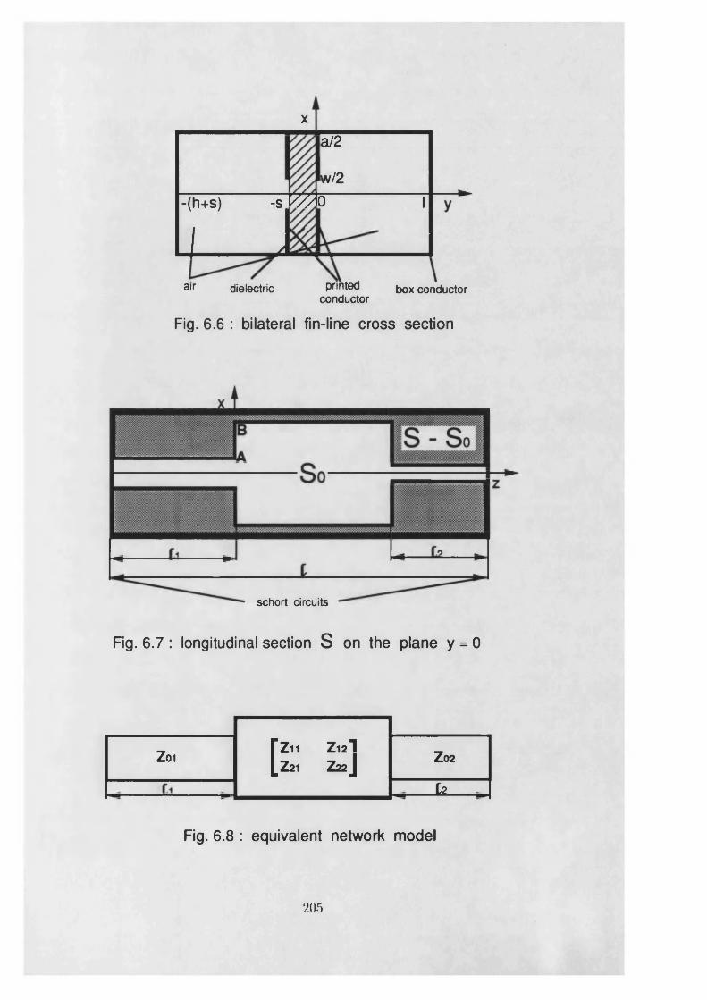
X

p 2 ~

w /2

-(h+s) -s

L Jv /A 3 I

air dielectric printed box conductorconductor

Fig. 6.6 : bilateral fin-line cross section

schort circuits

Fig. 6 .7 : longitudinal section S on the plane y = 0

Z01 [Z11 Z12IZ21 Z22J Z02

I I

Fig. 6.8 : equivalent network m odel

205

x

Fig. 6.9 : singularity vectors components on the plane of the conductor

The three expressions indicated in each sector of Fig. 6.9 represent the

values of , s z, s® respectively and the symbols used there stand for :

rex = i/e(90°) - 1 = -0.703416 = t Hb

reB = i/e(270°) — 1 =-0.185343 = t Ha

XA = X - \ A A = JlXB = X - f

206

6.4 A pplication o f the

current and charge singularity vectors

A typical antenna problem requires the radiation pattern due to diffraction of a

printed conductor which, also depending on the required polarization of the EM

fields, may assume the shape of a rectangular patch or of an arbitrary polygonal.

A standard analysis method determines the fields from a scalar V and a

vectorial A potentials which, in their turn, are expressible in terms of integrals of

the corresponding Green’s functions G, weighted by the unknown distributions

of surface density of electric charge and current ( see for instance [40] ) as :

A(r) = f G A ( r / r ) - J s ( r ) d S ' (6.14)Js0

V(r) = f G v ( r / r ) p s { r ) d S ' (6.15)J Sq

These integrals are currently solved by applying the Moments Method .

This effects a subdivision of the conductor surface So according to a grate, often

rectangular, each cell of which is identified by the vector r .

The unknown current J s ( r ) and charge ps ( r ) pertaining to each cell are

represented by a set of simple and everywhere continuous functions which satisfy

some consistency conditions on the boundaries of contiguous cells .

Even though the number of representing functions is of fact reducible to

1 or 2 for cells belonging to regular conductor areas, things go differently for

those belonging to the edges and tips since the singularities there cause serious

problems of convergence .

207

The situation is remedied by decreasing the step size of the cells in proximity

of the singular points . We suggest instead to change the representing functions

or better to weight them with the projections of the singularity vectors on the

conductor where they become proportional to the charge and current as indicated

in 2.4.1 and 3.2 respectively .

In particular, the forms pertaining to the fundamental sectors can be recov

ered directly from Tables 2.3,4,5 and 3.3,4,5 for the charge and current respec

tively .

No problem of matching between singularity functions of contiguous wedges

rise for the rectangular patch antenna, since the wedges are all of 90° aperture .

Moreover, generalization to any angular aperture follows the lines of 2.6 and 3.6.

This way, the step size of the singular cells can again be equal to that of

the regular cells, but the problem of convergence is turned into the integration of

(6.14,15) where it appears a multiplicative weight function for Js and ps which

is a known, singular but integrable function .

208

6.5 Conclusions

In this Chapter we have made some comments about the application to three

commonly used algorithms in the analysis of planar circuits, of the exact knowl

edge of the EM fields singularities distributed along the edges or concentrated on

the tip of the Printed Conductor .

Actually, a preliminary operation of matching of the singularity vectors rela

tive to contiguous wedges is necessary in order to determine the global singularity

vector for the whole Printed Conductor .

A global singularity function pertaining to the whole Printed Conductor

permits the choice of a different and more physical formulation of the ” trial field”

on the aperture or "trial current and charge” on the conductor .

In this approach, the problem of the determination of the coefficients of a

series representation, as for instance when using variational techniques, and of

their convergence in correspondence of the tips is turned into the integration of

the integrable singularity functions times a function finite everywhere .

Further work will be directed towards an analytic solution of this problem .

209

SUM M ARY

The results obtained in this work are of utility in the analysis of circuitry

involving Printed Conductors .

Conceptually speaking, we have ideally devided the EM environment of the

circuit into the supporting structure and the Printed Conductor .

The EM fields pertaining to the supporting structure are completely and

rigorously determinable by classic methods, like those of the Hertzian potentials,

for instance .

From the point of view of the analysis, the Printed Conductor introduces,

instead, new and somewhere singular vector boundary conditions for the fields in

the existing environment .

The first three Chapters have dealt with the reduction of the named bound

ary conditions pertaining to sectors or double-sectors into singularity vectors of

easy analytical form, by studying the solutions of the scalar and vector wave

equations in the geometry of a conical coordinate system .

Several analytical simplifications due to the separability of the above equa

tions in the conical geometry and to the special coordinate surfaces the boundary

conditions pertain to, has permitted to single out very accurately the complete

modal spectra of the wedges .

In particular we formulate exactly the singularity of the fundamental wedge

mode distributed along the edge and concentrated at the tip conductor .

The singularity vector we require is just its simplified form .

210

As a confirmation of the Babinet’s Principle we have found, by an indipen-

dent approach, that the EM-fields spectra pertaining to any plane sector are re

coverable from those of just the E-field spectrum or H-field spectrum pertaining

to any plane sector .

As a consequence of this, the H-field singularity vector pertaining to any

sector is equal to the E-field singularity vector pertaining to the complementary

sector, which in turn is just that of the static analysis .

Similar properties are established for the double sector .

The investigation of the EM singularities has been extended in Chapter 4

to 2D and Cone-wedges .

Even though these are analyzable in a spherical coordinate system, a uni

fication of the theory of Chapters 1 to 4 has been possible, which also suggests

some general conclusions about the charge and current singularities at the tips of

a conductor of arbitrary shape .

A clear relation of inverse proportionality between degree of electric singu

larity and the maximum angle of aperture of the tip has appeared that affords

insight into more irregular tip geometries .

Conversely, the vector density of current is related to the shape of the

conductor at the tip rather than to the maximum angular aperture . As a conse

quence, more than one singularity may occur and a monotonic relation between

degree of current singularity and maximum angle of aperture of the conductor is,

in general, no longer possible .

211

Chapter 5 has dealt with the classic problem of tapers .

A more general method of analysis has been suggested by the exact knowl

edge of the distribuited singularities along the conductor edge and has perm itted

an estimation of the reflection due to the sharp corners .

A new ” optimum” smooth taper profile has been suggested .

Finally, in Chapter 6 we have indicated how to match the singularity vectors

pertaining to individual wedges to each other so as to determine a singularity

vector for the whole Printed Conductor .

Their introduction in three typical algorithms for circuit component analysis

is suggested .

212

Appendix A

Boundary conditions and

periodicity conditions

In 1.3.4 we are asked to investigate the possibility that the boundary conditions

(1.32,33,34) for the Lame’s equation (1.27) are reducible to parity and periodicity

conditions for the solution w(z) . For this purpose, we need to recall the following

properties of Hill’s equation relatively to an odd and an even solution with respect

to the origin :

i) w\ (z) is even , W2 (z) is odd (A .l)

it) u>i(0) = 1 2(0 ) = 1, thi(O) = w2(0) = 0 (A.2)

in) w i ( z ± 2 K ) = w i ( 2 K ) w i ( z ) ± w i ( 2 K ) w 2 ( z ) (A.3 )

iv) w2(z ± 2K) = w 2 ( 2 K ) w i ( z ) ± w2(2K)w2 (z) ( A . 4 )

v) wi(z)w2(z) — w2(z)wi(z) = 1 (A.5)

vi ) 1 1(27^) =w2 (2K) (A.6)

213

and analogous relations are valid changing 2K with ± m 2 K , m integer.

For reasons of syntheticity, through the demonstrations we will use the

symbolism :

: (), , . . . which stands for from ( ) and, ,and .. . it follows th a t”

and which means that: ” from ( ) and , , and . . . it is = to ”

The general solution and derivative of (1.27) are expressed as :

w(z) = awi(z) + bw2(z) (A.7)

w(z) = aibi(z) -f bw2(z) (A.8)

where a,b are two constants to be determined together with the periodicity prop

erties from the b.c. as in what follows .

T h e b .c . w(—K ) = 0, w(K) = 0

Under this condition the properties of w can be recovered considering that :

: (A.7) written in z = 0 —> tu(0) = aitfi(O) + &u>2(0) : («) a = u>(0)

: (A 8) written in z = 0 —* u>(0) = au>i(0) 4- 61 2(0) : (**) 6 = ii;(0)

which together with (A.7) imply :

w(z) = u;(0)iyi(2r) + w($)w2(z) (A.9)

214

but (A.9) can be reduced to :

in z = K w(K) = u;(O)i0i(liQ + iy(0)u>2(if) 0

in z = —K w(—K ) = w(0)wi(—K) + w(0 )w2(—K)

= iu(0)u;i(iiQ — w ( 0 ) w 2 ( K ) 0

i.e. either u;(0)u;i(liQ = w(0 )w2(K)

or w(0)wi(K) = — w(Q)w2(K)

This system admits 4 solutions :

u;(0) = 0, u>(0) = 0 : (A.9) w(z) = 0

u>(0) = 0 ,W2(K) = 0 : (A.9) w(z) = w(0 )w2( z ) ,w2(K) = 0 (A.10)

ioi(0) = 0,ti;(0) = 0 : (A.9) w(z) = w(0 )wi (z ) ,w2(K) = 0 (A.11)

W\(K) = ^^w2{K) = 0 : (^) with z = K is impossible

Nevertheless only (A.10,11) are consistent and express the fact that the

solution can be only pure even or pure odd . Let us see if periodicity also occurs:

: (m ), z = K w\(K) = w ^ K ^ K ) - w ^ K ^ K ) : (A.10) Wl(2K) = 1

: {iv),z = K w2(K) = w2(2K)w1(K) - w2(2K)w2 (K) : (A. 10) w2 (2K) = 0

which together with :

: (v),2 = 2K w\(2K)w2(2K) — W2(2 K)tbi(2 K) — 1

imply : w2(2K) = 1 : (iv) 1 2(2 ± 2K ) = —w2(z)

215

so that : w2(z) and hence w(z) is odd with period 2K

analogously :

: (m ),2 = K W\(K) = wi(2K)wi(K) — tbi(2K)w2(K) : [A. 11) w\(2K) = 0

: (iv), z = K w2(K) = w2(2K)w1(K) - w2(2K)w2(K) : ( A l l ) w2(2 K ) = - 1

which together with :

: ( y ) , z = 2 if u;i(2^ ) 162(2/^) — w2{2 K)w\ (2K) = 1

imply : 1 1(2/^) = — 1 : ( i t ; ) W \ ( z ± 2K) = — u > i ( z )

hence : 1 1(2:) has anti-period 2K

so that w in question is even and periodic with period 4K .

Summing up, the initial b.c. are translated into :

either w(z) even with period 4K (A.12)

or w(z) odd with period 2K (A. 13)

T h e b .c. w(—K ) = 0, w(K) = 0 o r w(—K ) = 0, w( K) = 0

An analogous but more tedious proof can be developed for the above b.c. which

yields the periodicity condition :

w(z) has period 8 K (A. 14)

However, this time w is neither even nor odd but a linear combination of w\

and w2 . From the complete proof it is possible to show that the b.c. can only

216

determine the ratio :

= wA2K) w( 0) v '

Furthermore, it will be proved that between the even W\ and odd w2 solutions

there exists the relation w2(z) — 2K), which derived and written at z = 0

yields ii>2(0) = wi(2K) == 1 .

This way, tu(0) = iu(0) = 1 and the general form (A.9) becomes simply :

w(z) — wi(z) + w2(z) (A.15)

The b.c. w(—K ) = w(K) = 0 give obviously origin to the specular solution

w8(z) = w(—z) i.e. :

wa(z) = ttfi(z) — w2(z) (A.16)

Finally we can show using the properties of wi and w2 that w(z) and wa(z)

are odd or even with respect to the points where the b.c. they satisfy vanish or

have vanishing derivative respectively .

T h e b .c . w(—K ) = 0, w(K) = 0

These b.c. can be proved to yield a condition of fundamental periodicity in a way

similar to that of the first case, in fact they imply :

either w(z) even with period 2K (A. 17)

or w(z) odd with period 4K (A. 18)

217

Appendix B

Fourier series espression

of the solution

In this Appendix we explicitly collect the three-term recursive formulae and asso

ciated continued fractions relative to the coefficients of the Fourier series represen

tation of the 6 periodic Lame’s functions presented in 1.4.3 . Precisely, we report

the more useful characteristic equation obtained from the continued fraction by

making explicit the variable :

rj = 2h — u(u + 1 )k2 (B.l)

Also explicitly indicated are the forms that are more suitable for the nu

merical implementation of the characteristic equation itself . For the 6 cases in

question the solutions can be written in the order as follows .

218

Even solution w ith period ir ( i.e. 2 K or 2K f )

The Fourier series form for this solution is :

oo3 t » = £> 2 ,« « > (2 n 0 (B.2)

»=0

The recursivity of the coefficients can be shown to be expressible as ( see [6] ) :

i(z/ - l ) ( u + 2)k2A 2 + t A q = 0 i = 0 (B.3)

i(z/ — 3) (u + 4)fc2j44 + [tj — 4(2 — k2)]A2 + + l)&2i40 = 0 i = 1 (B.4)

i ( i / - 2i - l )(v + 2i + 2 )k2A 2i+2 + [n ~ 4z2(2 - k2)\A2i+

v + 2i — l)(i/ — 2i + 2)^2i42»_2 = 0 i > 2 (B.5)z

The latter generate a continued fraction ( see, for instance, [7] ) which we

report, for reason of space, writing the successive fractions on the same line :

( „ * - ! )„ ( „ + 2 )£ ( ^ _ 9)(„ _ 2)(„ + 4 ) £ ( * * - 2 5 ) ( . / - 4 ) ( v + 6 )& * 2 — k2 — 2 _ 2 - t * - £ _ 2 - k 2 - %

(B.6)

This espression can also be seen as a transcendental function in i/, h with

parameter k2 and can be usefully implemented using the following espressions :

A2I+2 ^ / l - f c ' \ 2 A2I — V k ) / > 1 (B.7)

_ - ± ( v + 2 i - l ) ( v - 2 i + 2 ) k 2 2 < i < I (B.8)»7-4*2(2-jk2)+i(i/-2i-l)(i/+2*+2)*:2^ t 2 .

A2 _ -i/(i/+1)&2 Aq ^_4(2_fc2)+ I ( J/_ 3)(|/+4)A2 d l

II• N (B.9)

oII (B.10)

219

The first and last equations correspond to the (1.60) ; in particular the truncation

maximum index I depends on the accuracy required for the solution {X,} and

decreases with increasing rate of convergence, i.e. with k2, for :

Odd solution w ith period tt ( i.e . 2K or 2K ' )


*=iO ) = £ B 2isin{2iv) (B.12)

The recursivity relations axe now :

(rj — 8 + 4fc2)#2 + \ ( y — 3)(^ + 4)fc2i?4 = 0 i = 0 (B.13)

i ( i / — 2 i)(v + 2 i + l )k 2B 2i + [ij — (2t + 2)2(2 — k2 )]B2i+2+

i ( i / - 2i - 3)(i/ + 2i + 4)k2B 2i+i = 0 i > 1 (B.14)

which generates the characteristic equation :

o _ 1,2 n 9 — 1-2___ aL K 16 - 36

and which is computationally implemented as :

~ ~ ( * ^ ) 2 / > 1 (B.16)

= ------------- -frfc-MH.+M+l)*8 1 ? = 4 (2 - fc 2) - i ( i / - 3 ) ( i / + 4)Jfe2| j i = 0 (B.18)

220

Even solution w ith period 2k ( i.e. 4K or 4K* )

In this case the Fourier series form is :

E l : » ( v ) = Y M m cos(2 i + 1)„ (B.19)i= 0

The three-term recursivity relations among the coefficients are :

— 3)(u + 3 )Jc2A 3 + [v ~ (2 — k2) +W \v (y + \ ) k 2]A\ = 0 ? = 0 (B.20)

^(z/ — 2i — 2)(i/ + 2i + 3)k2A2i+3 + [tf ~~ (2z + 1)2(2 — k2)]A2i+i +

\{ v - 2 i + 1 )(i/ + 2i)k2A 2i- i = 0 i > 1 (B.21)

which generates the characteristic equation :

(B.22)

and which is computationally implemented as :

g m ~ _ ( ! £ ) * / » 1 (B.23)

A 2j+i _ _________ -^(t/-2t+l)(i/+2t)fc2______

i, = ( 2 - k i ) - M \ v { v + l )k2 - \ { v - 2 ) ( u + Z)k2%- t = 0 (B.25)

_________ - T(i—2i+i)(i/+2.)t______ 1 li

Odd solution w ith period 2 k ( i.e . 4K or 4K' )


< m+1 («) = Y B v + iM * + 1)® (B.26)t ' = l

221

The relation are completely analogous to those of the even case but with an

opposition of the signs indicated with in the (B.20,22,25) .

E ven so lu tio n w ith p e rio d 47r ( i.e. 8K o r 8K* )


EZ(v) - £ A<cos(2i + 5)” (B-27)x= —0 0

Now the series is bilateral so that a unique relation expresses the three-term

recursivity where the index i assumes all the positive and negative integers :

i ( 2 v + 4i + 3)(2v — 4i — l)k 2Ai+i + [4rj - (4* - 1)2(2 - k2)\Ai +

i ( 2 i /+ 4i — 3)(2i/— 4 i-f 5)A;2i4i-i = 0 — 0 0 < i < 0 0 (B.28)Li

Consequently, in general, we can write a continued fraction for i departing from

+ 0 0 and another for i departing from — 0 0 to be made consistent at a common

finite i value .

No useful form for the characteristic equation does exist if we except the

case in which u = is any odd integer, when it becomes an algebraic equation

of degree v + | .

In our applications this will not happen so we report only the relations used

in the computational implementation :

~ - ( ! = £ ? h > 1 (B.29)

T p - = --------------------------------------------- ! < < < / , (B.30)

222

( ^ ) + = consistency condition (B.31)

* L - = ---------------j(2,+4.'+3)(2,/-4.-l)*»----------- 0 > 1 > I 2 (B.32)Ai+i 4»j-(4t-l)2(2-A:2)+|(2t/+4t-3)(2i/-4i+5)Jk2-J= i — V J

d M l ~ _(1= f y h « _1 (B.33)

The consistency condition equates the value (^£)+ obtained when i = 1 in

(B.30) with ( ^ ) ~ obtained when i = 0 in (B.32) .

The l 5t equation (1.60) is now substituted by the asymptotic behaviour at

—oo as reported in (B.33) .

Odd solution w ith period 47r ( i.e. 8K or 8K1 )

Finally the Fourier form for this solution is :

£ . » = E Bicos(2i - ^ (B-34)t=—oo

It is immediate to prove that a 7r shift introduced in the even solution (B.27)

provides an odd form of this kind, in fact :

OO - OO 1

EZ (V + 7r) = X I A iCOS(2i + 2 ^ V + *) = C°5( \ ) X ] AiC0S(2i + 2 ^ +t = —oo i = —oo

OO J OO J

s i n ( E Aisin(2 i + - ) v = Aisin(2i + - ) v (B.35)2

i = —oo

Furthermore, the above is still solution of Lame’s equation because it presents

periodic coefficients with period 7r, s o that we can use in (B.34) the same coeffi

cients {A,} used for the even solution (B.27) .

223

Appendix C

Evaluation of the eigenvalues

In this Appendix we report as a way of example the numerical evaluation of the

first 15 components of the {1/, h} spectrum of eigenvalues relative to the acute

sector .

The individual eigenvalues are identified by the mode label defined in 2.3 .

We compute values with fc2-steps of 0.02 for a total of 50 evaluations in the

complete interval k2 € [0,1], inclusive of the limit values k2 = 0,1 where v and h

are determinable analytically as indicated in 2.3 .

The accuracy is up to 6 decimal places and the evaluations relative to k2 not

present in the Table may be recovered by interpolation; in this case, the accuracy

increases where the higher order derivatives decrease .

224

M p p p p p p p p p p p o p p p p p p p p o p p p p p p p p p p p p p p p p p p p p p p p p p p p p o

O 0 0 C ' i k ( O O 0 C C ' ^ S J O 0 C O ' ^ W O « i a ^ K ) O 0 0 0 ' ^ M O 0 0 0 ' ^ U O 0 0 C 7 ' ^ k ) O W C ' ^ t J O » 3 0 ' ^ K ) O 0 0 ^ ^ W O

o©

OOMOvO O O mn1-4C

pK>

u u u w u w w u w u u u w u u u u u w<g> sq vO vO vO v,0 vO '•OO O ' 5 ' 0 > 0 v 0 v 0 v 0 \ 0 v 0 v D v 0 ^ O ' 0 v 0 ' 0 > 0 0 0 ^ j « ) v j \ i w ' u \ ' j i * » N H \ u s i v i N ' 4 j u ' H x i > - * k N ) i A J s i u i i -O O v o ^ ' O v o ^ \ O v o v o » o f l ' g a y i ^ K ) 0 « o i M v j s ) ^ o o o o o o w - s ) v i y i o o s a M \ a o ^ o o M W \ o o o s jOOvOvOÔO-g^^M-J(oÔOxlÔOOOWWt»i.WMÔ(OOOÛvOWC\slC'0' 'JOOÛMO'UOOvO'4^lXvOÛ'JvOvOikMO'^MOL«000'«OWOO'400sl^v4UWvOWîkOCO^Ûl^WW

U> u> u> u> w w oj u> L> w to o 00 0“\ & o O ' O Ui C/1 O vO .u o m to 00 Ui O' oM M ^ O £5 OO W W OO to o

pU)

t/» l/» In l/i I* in Ino o o o o o oo o o o o o oo o o o o o oo o o o o o oo o o o o o o

pu

ACUTE SEC

TOR

Eigenvalue

v

ACUTE SECTOR Eigenvalue h

* z (0 ,0 ) (0 ,1 ) (0 ,2 ) (0 ,3 ) (0 ,4 )

0 .0 0 0 .0 0 0 0 0 0 0 .0 0 0 0 0 0 0 .0 0 0 0 0 0 0 .0 0 0 0 0 0 0 .0 0 0 0 0 00 .0 2 0 .0 0 1 7 1 1 0 .0 2 6 2 4 8 0 .0 7 1 7 1 1 0 .1 3 7 1 3 4 0 .2 2 1 3 1 70 .0 4 0 .0 0 3 8 7 8 0 .0 5 4 3 4 6 0 .1 4 6 4 0 5 0 .2 7 6 3 5 2 0 .4 3 9 3 7 50 .0 6 0 .0 0 6 3 1 4 0 .0 8 3 4 8 7 0 .2 2 2 2 1 3 0 .4 1 4 1 4 5 0 .6 4 8 4 8 20 .0 8 0 .0 0 8 9 6 8 0 .1 1 3 4 2 5 0 .2 9 8 4 6 8 0 .5 4 9 1 3 8 0 .8 4 6 6 1 90 .1 0 0 .0 1 1 8 1 4 0 .1 4 4 0 2 0 0 .3 7 4 7 4 5 0 .6 8 0 4 7 4 1 .0 3 2 9 3 80 .1 2 0 .0 1 4 8 3 7 0 .1 7 5 1 7 7 0 .4 5 0 7 2 7 0 .8 0 7 5 7 9 1 .2 0 7 3 0 60 .1 4 0 .0 1 8 0 2 6 0 .2 0 6 8 2 5 0 .5 2 6 1 5 8 0 .9 3 0 0 7 5 1 .3 7 0 0 7 20 .1 6 0 .0 2 1 3 7 6 0 .2 3 8 9 0 5 0 .6 0 0 8 2 3 1 .0 4 7 7 3 7 1 .5 2 1 8 9 10 .1 8 0 .0 2 4 8 8 1 0 .2 7 1 3 6 8 0 .6 7 4 5 3 9 1 .1 6 0 4 6 5 1 .6 6 3 5 9 20 .2 0 0 .0 2 8 5 4 1 0 .3 0 4 1 7 0 0 .7 4 7 1 4 4 1 .2 6 8 2 6 0 1 .7 9 6 0 8 30 .2 2 0 .0 3 2 3 5 3 0 .3 3 7 2 7 2 0 .8 1 8 5 0 3 1 .3 7 1 2 0 4 1 .9 2 0 2 7 10 .2 4 0 .0 3 6 3 1 7 0 .3 7 0 6 3 5 0 .8 8 8 4 9 8 1 .4 6 9 4 4 3 2 .0 3 7 0 2 90 .2 6 0 .0 4 0 4 3 4 0 .4 0 4 2 2 6 0 .9 5 7 0 2 9 1 .5 6 3 1 6 6 2 .1 4 7 1 6 10 .2 8 0 .0 4 4 7 0 4 0 .4 3 8 0 0 9 1 .0 2 4 0 1 6 1 .6 5 2 5 9 4 2 .2 5 1 3 9 70 .3 0 0 .0 4 9 1 3 1 0 .4 7 1 9 5 2 1 .0 8 9 3 9 3 1 .7 3 7 9 6 8 2 .3 5 0 3 8 60 .3 2 0 .0 5 3 7 1 5 0 .5 0 6 0 2 3 1 .1 5 3 1 1 2 1 .8 1 9 5 3 6 2 .4 4 4 7 0 10 .3 4 0 .0 5 8 4 6 1 0 .5 4 0 1 8 9 1 .2 1 5 1 3 6 1 .8 9 7 5 5 0 2 .5 3 4 8 4 40 .3 6 0 .0 6 3 3 7 2 0 .5 7 4 4 1 8 1 .2 7 5 4 4 7 1 .9 7 2 2 5 5 2 .6 2 1 2 5 50 .3 8 0 .0 6 8 4 5 2 0 .6 0 8 6 7 8 1 .3 3 4 0 3 4 2 .0 4 3 8 8 9 2 .7 0 4 3 1 40 .4 0 0 .0 7 3 7 0 7 0 .6 4 2 9 3 8 1 .3 9 0 9 0 2 2 .1 1 2 6 7 7 2 .7 8 4 3 5 50 .4 2 0 .0 7 9 1 4 2 0 .6 7 7 1 6 4 1 .4 4 6 0 6 2 2 .1 7 8 8 3 1 2 .8 6 1 6 6 60 .4 4 0 .0 8 4 7 6 2 0 .7 1 1 3 2 4 1 .4 9 9 5 3 7 2 .2 4 2 5 5 2 2 .9 3 6 5 0 00 .4 6 0 .0 9 0 5 7 7 0 .7 4 5 3 8 5 1 .5 5 1 3 5 6 2 .3 0 4 0 2 2 3 .0 0 9 0 7 90 .4 8 0 .0 9 6 5 9 2 0 .7 7 9 3 1 5 1 .6 0 1 5 5 5 2 .3 6 3 4 1 3 3 .0 7 9 5 9 30 .5 0 0 .1 0 2 8 1 7 0 .8 1 3 0 7 8 1 .6 5 0 1 7 5 2 .4 2 0 8 8 0 3 .1 4 8 2 1 50 .5 2 0 .1 0 9 2 6 3 0 .8 4 6 6 4 2 1 .6 9 7 2 6 2 2 .4 7 6 5 6 9 3 .2 1 5 0 9 10 .5 4 0 .1 1 5 9 3 9 0 .8 7 9 9 7 3 1 .7 4 2 8 6 5 2 .5 3 0 6 1 0 3 .2 8 0 3 5 40 .5 6 0 .1 2 2 8 5 9 0 .9 1 3 0 3 7 1 .7 8 7 0 3 4 2 .5 8 3 1 2 4 3 .3 4 4 1 2 00 .5 8 0 .1 3 0 0 3 7 0 .9 4 5 7 9 9 1 .8 2 9 8 2 4 2 .6 3 4 2 2 0 3 .4 0 6 4 9 30 .6 0 0 .1 3 7 4 8 7 0 .9 7 8 2 2 4 1 .8 7 1 2 8 8 2 .6 8 3 9 9 9 3 .4 6 7 5 6 40 .6 2 0 .1 4 5 2 2 9 1 .0 1 0 2 7 9 1 .9 1 1 4 8 1 2 .7 3 2 5 5 2 3 .5 2 7 4 1 60 .6 4 0 .1 5 3 2 8 2 1 .0 4 1 9 2 8 1 .9 5 0 4 5 8 2 .7 7 9 9 6 3 3 .5 8 6 1 2 20 .6 6 0 .1 6 1 6 6 9 1 .0 7 3 1 3 8 1 .9 8 8 2 7 1 2 .8 2 6 3 0 7 3 .6 4 3 7 4 90 .6 8 0 .1 7 0 4 1 8 1 .1 0 3 8 7 3 2 .0 2 4 9 7 6 2 .8 7 1 6 5 4 3 .7 0 0 3 5 60 .7 0 0 .H 9 5 6 0 1 .1 3 4 1 0 0 2 .0 6 0 6 2 4 2 .9 1 6 0 6 8 3 .7 5 5 9 9 8

; 0 .7 2 0 .1 8 9 1 3 1 1 .1 6 3 7 8 4 2 .0 9 5 2 6 6 2 .9 5 9 6 0 6 3 .8 1 0 7 2 20 .7 4 0 .1 9 9 1 7 4 1 .1 9 2 8 9 1 2 .1 2 8 9 5 2 3 .0 0 2 3 2 0 3 .8 6 4 5 7 40 .7 6 0 .2 0 9 7 4 1 1 .2 2 1 3 8 7 2 .1 6 1 7 3 1 3 .0 4 4 2 6 0 3 .9 1 7 5 9 50 .7 8 0 .2 2 0 8 9 5 1 .2 4 9 2 3 7 2 .1 9 3 6 4 9 3 .0 8 5 4 7 0 3 .9 6 9 8 2 10 .8 0 0 .2 3 2 7 1 3 1 .2 7 6 4 0 6 2 .2 2 4 7 5 2 3 .1 2 5 9 8 9 4 .0 2 1 2 8 70 .8 2 0 .2 4 5 2 9 2 1 .3 0 2 8 5 8 2 .2 5 5 0 8 4 3 .1 6 5 8 5 5 4 .0 7 2 0 2 30 .8 4 0 .2 5 8 7 5 8 1 .3 2 8 5 5 7 2 .2 8 4 6 8 6 3 .2 0 5 1 0 2 4 .1 2 2 0 6 00 .8 6 0 .2 7 3 2 7 5 1 .3 5 3 4 6 3 2 .3 1 3 6 0 0 3 .2 4 3 7 6 0 4 .1 7 1 4 2 30 .8 8 0 .2 8 9 0 7 2 1 .3 7 7 5 3 1 2 .3 4 1 8 6 6 3 .2 8 1 8 5 9 4 .2 2 0 1 3 70 .9 0 0 .3 0 6 4 7 3 1 .4 0 0 7 1 4 2 .3 6 9 5 2 3 3 .3 1 9 4 2 3 4 .2 6 8 2 2 60 .9 2 0 .3 2 5 9 7 9 1 .4 2 2 9 5 2 2 .3 9 6 6 0 8 3 .3 5 6 4 7 8 4 .3 1 5 7 1 20 .9 4 0 .3 4 8 4 2 9 1 .4 4 4 1 7 0 2 .4 2 3 1 5 9 3 .3 9 3 0 4 4 4 .3 6 2 6 1 30 .9 6 0 .3 7 5 4 5 7 1 .4 6 4 2 6 0 2 .4 4 9 2 1 5 3 .4 2 9 1 4 2 4 .4 0 8 9 5 00 .9 8 0 .4 1 1 2 7 2 1 .4 8 3 0 4 1 2 .4 7 4 8 1 3 3 .4 6 4 7 8 8 4 .4 5 4 7 4 01 .0 0 0 .5 0 0 0 0 0 1 .5 0 0 0 0 0 2 -5 0 0 0 0 0 3 .5 0 0 0 0 0 4 .5 0 0 0 0 0

226

N - p p p p p p p p p p p p p p p p p p p p o o p o p p p p p p p p p p p p p p p p p p p p p p p p p o©oo*ooobobobobobo*-o^^^^b'^b'C'C' l />lnU>lnU»k^k^ôjUiWWU>tototototoi-‘ !-*i-!-*!-‘0 © 0 © ©o o o o ' ^ M O » o ' ^ w o » c ' ^ N J O * i o ' ^ M O o c c ' ^ i o o » o ' ^ M O o o a ' ^ N J O o o o ' ^ f J o » c ' ^ k ) O o o o ' ^ t o o

UÛUUUUtOKJS) OM»UUMO00-s ja OUOlÔislMNHkK) COUC'MÔOeOO-4 Ci*-^CrtW»tOWvO O m WUWM v|00 0\O

o o o o o o o o o oÛWKIKJm m OOO U 9 9 U O ^ O ^ O U O -4 OC vO h (O ti O' 'J vO O C'UlvlklOOO'WvOUlO vO^- l MO'OavO W O

t ot o- o

w W U> U) w ut M o b b o bMVO- JOI WO l/lUikMvJO 0 0 C/1 t o OS tO O UOlikOtvOO 00 .u U\ U O ' o

to

^ «U**►-»>-* o o og m i 4i CM- to to O U) o o VO oo VO U) oU v I O U i m O M w O M OO o

U)

. — .— .— .— .— .— .— ' MMWO^KJIXiCflUlMOOoaUl^MMOOvOOOvlsjÔlUl^^WWUiK) OMOJODvOViC/iaOl«MOOOOOOO\OM^N| ■OOOWO'JOOm * ^ n|U)0-4UOOJ3vIOO Ov|(4l\OCAUlW^vOKJOUOtOOOUlMOO OWm WOÔOOOOUi m O(4I\Ov) iO ^ O ^

t o

ACUTE SEC

TOR

Eigenvalue

v


k 2 (1 ,0 ) (1 ,1 ) (1 ,2 ) ( 1 ,3 ) (2 ,0 )

0 .0 0 1 .0 0 0 0 0 0 1 .0 0 0 0 0 0 1 .0 0 0 0 0 0 1 .0 0 0 0 0 0 4 .0 0 0 0 0 00 .0 2 1 .0 2 0 2 2 3 1 .0 8 1 0 7 2 1 .1 7 2 6 7 6 1 .2 9 5 0 3 0 4 .0 2 0 3 0 50 .0 4 1 .0 4 0 8 8 6 1 .1 6 4 1 6 9 1 3 5 0 0 7 3 1 3 9 8 1 6 8 4 .0 4 1 2 4 00 .0 6 1 .0 6 1 9 9 1 1 .2 4 9 1 7 8 1 3 3 1 5 9 5 1 .9 0 7 6 2 7 4 .0 6 2 8 3 80 .0 8 1 .0 8 3 5 3 8 1 .3 3 6 0 3 0 1 .7 1 6 8 4 2 2 .2 2 2 1 7 1 4 .0 8 5 1 3 1

; o . i o 1 .1 0 5 5 3 2 1 .4 2 4 6 7 4 1 .9 0 5 4 9 5 2 3 4 0 7 7 3 4 .1 0 8 1 5 60 .1 2 1 .1 2 7 9 8 1 1 .5 1 5 0 7 5 2 .0 9 7 2 8 1 2 .8 6 2 5 0 0 4 .1 3 1 9 5 10 .1 4 1 .1 5 0 8 9 1 1 .6 0 7 2 0 3 2 .2 9 1 9 5 0 3 .1 8 6 4 5 8 4 .1 5 6 5 5 6

; 0 .1 6 1 .1 7 4 2 7 1 1 .7 0 1 0 3 6 2 .4 8 9 2 6 2 3 3 1 1 7 6 1 4 .1 8 2 0 1 3; 0 .1 8 1 .1 9 8 1 3 0 1 .7 9 6 5 5 7 2 .6 8 8 9 8 3 3 .8 3 7 5 2 0 4 .2 0 8 3 6 8; 0 .2 0 1 .2 2 2 4 8 1 1 .8 9 3 7 5 1 2 .8 9 0 8 7 7 4 .1 6 2 8 3 4 4 .2 3 5 6 6 8

0 .2 2 1 .2 4 7 3 3 5 1 .9 9 2 6 0 7 3 .0 9 4 6 9 9 4 .4 8 6 7 8 7 4 .2 6 3 9 6 40 .2 4 1 .2 7 2 7 0 6 2 .0 9 3 1 1 3 3 .3 0 0 1 9 6 4 .8 0 8 4 5 8 4 .2 9 3 3 1 10 .2 6 1 .2 9 8 6 0 8 2 .1 9 5 2 5 9 3 3 0 7 1 0 2 5 .1 2 6 9 2 8 4 .3 2 3 7 6 4

i 0 .2 8 1 .3 2 5 0 5 7 2 .2 9 9 0 3 6 3 .7 1 5 1 3 5 5 .4 4 1 2 9 4 4 .3 5 5 3 8 60 .3 0 1 .3 5 2 0 7 0 2 .4 0 4 4 3 5 3 .9 2 3 9 9 7 5 .7 5 0 6 8 7 4 .3 8 8 2 4 00 .3 2 1 .3 7 9 6 6 6 2 .5 1 1 4 4 5 4 .1 3 3 3 7 3 6 .0 5 4 2 9 3 4 .4 2 2 3 9 40 .3 4 1 .4 0 7 8 6 5 2 .6 2 0 0 5 4 4 .3 4 2 9 2 9 6 .3 5 1 3 7 4 4 .4 5 7 9 2 20 .3 6 1 .4 3 6 6 9 0 2 .7 3 0 2 4 9 4 3 5 2 3 1 2 6 .6 4 1 2 8 5 4 .4 9 4 9 0 2

; 0 .3 8 1 .4 6 6 1 6 4 2 .8 4 2 0 1 3 4 .7 6 1 1 5 3 6 .9 2 3 4 9 0 4 3 3 3 4 1 6! 0 .4 0 1 .4 9 6 3 1 3 2 .9 5 5 3 2 7 4 .9 6 9 0 6 8 7 .1 9 7 5 7 7 4 3 7 3 5 5 3

0 .4 2 1 .5 2 7 1 6 5 3 .0 7 0 1 6 8 5 .1 7 5 6 6 0 7 .4 6 3 2 6 0 4 .6 1 5 4 0 70 .4 4 1 .5 5 8 7 5 2 3 .1 8 6 5 0 7 5 .3 8 0 5 2 6 7 .7 2 0 3 8 3 4 .6 5 9 0 7 90 .4 6 1 .5 9 1 1 0 7 3 .3 0 4 3 1 2 5 3 8 3 2 5 6 7 .9 6 8 9 0 9 4 .7 0 4 6 7 8

! 0 .4 8 1 .6 2 4 2 6 7 3 .4 2 3 5 4 3 5 .7 8 3 4 4 5 8 .2 0 8 9 1 5 4 .7 5 2 3 2 10 .5 0 1 .6 5 8 2 7 3 3 .5 4 4 1 5 0 5 .9 8 0 6 9 5 8 .4 4 0 5 7 1 4 .8 0 2 1 3 40 .5 2 1 .6 9 3 1 7 0 3 .6 6 6 0 7 9 6 .1 7 4 6 2 5 8 .6 6 4 1 3 0 4 .8 5 4 2 5 20 .5 4 1 .7 2 9 0 0 6 3 .7 8 9 2 6 1 6 .3 6 4 8 7 8 8 .8 7 9 9 0 5 4 .9 0 8 8 2 40 .5 6 1 .7 6 5 8 3 8 3 .9 1 3 6 1 8 6 3 5 1 1 2 4 9 .0 8 8 2 5 4 4 .9 6 6 0 0 90 .5 8 1 .8 0 3 7 2 5 4 .0 3 9 0 5 7 6 .7 3 3 0 7 4 9 .2 8 9 5 6 5 5 .0 2 5 9 8 50 .6 0 1 .8 4 2 7 3 7 4 .1 6 5 4 7 0 6 .9 1 0 4 7 7 9 .4 8 4 2 4 4 5 .0 8 8 9 4 30 .6 2 1 .8 8 2 9 5 1 4 .2 9 2 7 3 2 7 .0 8 3 1 3 1 9 .6 7 2 6 9 9 5 .1 5 5 0 9 70 .6 4 1 .9 2 4 4 5 4 4 .4 2 0 6 9 7 7 .2 5 0 8 8 3 9 .8 5 5 3 3 6 5 .2 2 4 6 8 50 .6 6 1 .9 6 7 3 4 6 4 .5 4 9 2 0 0 7 .4 1 3 6 3 0 1 0 .0 3 2 5 4 9 5 .2 9 7 9 7 10 .6 8 2 .0 1 1 7 4 0 4 .6 7 8 0 4 8 7 3 7 1 3 1 9 1 0 .2 0 4 7 1 7 5 .3 7 5 2 5 60 .7 0 2 .0 5 7 7 6 9 4 .8 0 7 0 2 4 7 .7 2 3 9 4 5 1 0 .3 7 2 1 9 7 5 .4 5 6 8 8 00 .7 2 2 .1 0 5 5 8 6 4 .9 3 5 8 8 1 7 .8 7 1 5 4 8 1 0 3 3 5 3 2 9 5 .5 4 3 2 3 60 .7 4 2 .1 5 5 3 7 3 5 .0 6 4 3 4 3 8 .0 1 4 2 0 8 1 0 .6 9 4 4 2 6 5 .6 3 4 7 7 90 .7 6 2 .2 0 7 3 4 7 5 .1 9 2 0 9 7 8 .1 5 2 0 3 9 1 0 .8 4 9 7 8 0 5 .7 3 2 0 4 70 .7 8 2 .2 6 1 7 6 9 5 .3 1 8 7 9 9 8 .2 8 5 1 8 9 1 1 .0 0 1 6 6 1 5 .8 3 5 6 8 20 .8 0 2 .3 1 8 9 6 1 5 .4 4 4 0 6 8 8 .4 1 3 8 2 9 1 1 .1 5 0 3 1 5 5 .9 4 6 4 6 70 .8 2 2 .3 7 9 3 2 6 5 .5 6 7 4 8 6 8 3 3 8 1 5 0 1 1 .2 9 5 9 6 8 6 .0 6 5 3 7 20 .8 4 2 .4 4 3 3 8 3 5 .6 8 8 5 9 8 8 .6 5 8 3 5 9 1 1 .4 3 8 8 2 7 6 .1 9 3 6 3 00 .8 6 2 .5 1 1 8 1 2 5 .8 0 6 9 1 1 8 .7 7 4 6 7 6 1 1 3 7 9 0 7 8 6 .3 3 2 8 5 80 .8 8 2 .5 8 5 5 4 6 5 .9 2 1 8 9 2 8 .8 8 7 3 2 9 1 1 .7 1 6 8 8 9 6 .4 8 5 2 5 10 .9 0 2 .6 6 5 9 2 3 6 .0 3 2 9 6 0 8 .9 9 6 5 5 4 1 1 .8 5 2 4 1 3 6 .6 5 3 9 3 60 .9 2 2 .7 5 4 9 8 4 6 .1 3 9 4 7 6 9 .1 0 2 5 9 1 1 1 .9 8 5 7 8 6 6 .8 4 3 6 6 10 .9 4 2 .8 5 6 1 4 8 6 .2 4 0 7 0 7 9 .2 0 5 6 8 7 1 2 .1 1 7 1 3 0 7 .0 6 2 3 3 10 .9 6 2 .9 7 6 0 4 0 6 .3 3 5 7 4 6 9 .3 0 6 0 9 8 1 2 .2 4 6 5 5 4 7 .3 2 5 1 8 50 .9 8 3 .1 3 1 6 5 7 6 .4 2 3 2 6 5 9 .4 0 4 0 9 6 1 2 .3 7 4 1 5 1 7 .6 7 1 0 5 91 .0 0 3 .5 0 0 0 0 0 6 .5 0 0 0 0 0 9 3 0 0 0 0 0 1 2 3 0 0 0 0 0 8 3 0 0 0 0 0

228

ACUTE SECTOR Eigenvalue v

k 2 (2 ,1 ) (2 ,2 ) (3 ,0 ) (3 ,1 ) (4 ,0 )

0 .0 0 3 .0 0 0 0 0 0 4 .0 0 0 0 0 0 3 .0 0 0 0 0 0 4 .0 0 0 0 0 0 4 .0 0 0 0 0 00 .0 2 3 .0 0 0 1 9 1 4 .0 0 0 5 7 2 3 .0 0 0 0 0 0 4 .0 0 0 0 0 2 4 .0 0 0 0 0 00 .0 4 3 .0 0 0 7 7 8 4 .0 0 2 3 1 9 3 .0 0 0 0 0 2 4 .0 0 0 0 1 4 4 .0 0 0 0 0 00 .0 6 3 .0 0 1 7 8 0 4 .0 0 5 2 6 6 3 .0 0 0 0 0 7 4 .0 0 0 0 4 9 4 .0 0 0 0 0 00 .0 8 3 .0 0 3 2 1 4 4 .0 0 9 4 2 0 3 .0 0 0 0 1 7 4 .0 0 0 1 1 9 4 .0 0 0 0 0 00 .1 0 3 .0 0 5 0 9 6 4 .0 1 4 7 6 9 3 .0 0 0 0 3 4 4 .0 0 0 2 3 9 4 .0 0 0 0 0 10 .1 2 3 .0 0 7 4 3 9 4 .0 2 1 2 8 4 3 .0 0 0 0 6 1 4 .0 0 0 4 2 6 4 .0 0 0 0 0 20 .1 4 3 .0 1 0 2 5 6 4 .0 2 8 9 2 4 3 .0 0 0 1 0 0 4 .0 0 0 6 9 7 4 .0 0 0 0 0 40 .1 6 3 .0 1 3 5 5 7 4 .0 3 7 6 3 4 3 .0 0 0 1 5 5 4 .0 0 1 0 7 4 4 .0 0 0 0 0 80 .1 8 3 .0 1 7 3 5 1 4 .0 4 7 3 5 5 3 .0 0 0 2 2 8 4 .0 0 1 5 7 7 4 .0 0 0 0 1 30 .2 0 3 .0 2 1 6 4 5 4 .0 5 8 0 1 9 3 .0 0 0 3 2 3 4 .0 0 2 2 3 1 4 .0 0 0 0 2 10 .2 2 3 .0 2 6 4 4 5 4 .0 6 9 5 5 5 3 .0 0 0 4 4 5 4 .0 0 3 0 6 3 4 .0 0 0 0 3 20 .2 4 3 .0 3 1 7 5 3 4 .0 8 1 8 9 1 3 .0 0 0 5 9 9 4 .0 0 4 1 0 2 4 .0 0 0 0 4 80 .2 6 3 .0 3 7 5 7 2 4 .0 9 4 9 5 4 3 .0 0 0 7 9 0 4 .0 0 5 3 7 8 4 .0 0 0 0 6 90 .2 8 3 .0 4 3 9 0 3 4 .1 0 8 6 7 2 3 .0 0 1 0 2 3 4 .0 0 6 9 2 6 4 .0 0 0 0 9 80 .3 0 3 .0 5 0 7 4 4 4 .1 2 2 9 7 7 3 .0 0 1 3 0 5 4 .0 0 8 7 8 2 4 .0 0 0 1 3 60 .3 2 3 .0 5 8 0 9 5 4 .1 3 7 8 0 1 3 .0 0 1 6 4 4 4 .0 1 0 9 8 5 4 .0 0 0 1 8 50 .3 4 3 .0 6 5 9 5 1 4 .1 5 3 0 7 8 3 .0 0 2 0 4 9 4 .0 1 3 5 7 5 4 .0 0 0 2 4 90 .3 6 3 .0 7 4 3 0 9 4 .1 6 8 7 4 6 3 .0 0 2 5 2 9 4 .0 1 6 5 9 6 4 .0 0 0 3 3 00 .3 8 3 .0 8 3 1 6 4 4 .1 8 4 7 4 2 3 .0 0 3 0 9 3 4 .0 2 0 0 9 3 4 .0 0 0 4 3 30 .4 0 3 .0 9 2 5 1 1 4 .2 0 1 0 0 7 3 .0 0 3 7 5 6 4 .0 2 4 1 1 5 4 .0 0 0 5 6 2

! 0 .4 2 3 .1 0 2 3 4 4 4 .2 1 7 4 7 9 3 .0 0 4 5 2 9 4 .0 2 8 7 0 8 4 .0 0 0 7 2 2! 0 .4 4 3 .1 1 2 6 5 6 4 .2 3 4 0 9 8 3 .0 0 5 4 2 8 4 .0 3 3 9 2 4 4 .0 0 0 9 2 2

0 .4 6 3 .1 2 3 4 4 1 4 .2 5 0 8 0 2 3 .0 0 6 4 7 0 4 .0 3 9 8 1 2 4 .0 0 1 1 6 9I 0 .4 8 3 .1 3 4 6 9 2 4 .2 6 7 5 2 7 3 .0 0 7 6 7 4 4 .0 4 6 4 2 3 4 .0 0 1 4 7 3

0 .5 0 3 .1 4 6 4 0 3 4 .2 8 4 2 0 5 3 .0 0 9 0 6 2 4 .0 5 3 8 0 6 4 .0 0 1 8 4 60 .5 2 3 .1 5 8 5 6 5 4 .3 0 0 7 6 7 3 .0 1 0 6 6 0 4 .0 6 2 0 0 9 4 .0 0 2 3 0 10 .5 4 3 .1 7 1 1 7 3 4 .3 1 7 1 3 7 3 .0 1 2 4 9 4 4 .0 7 1 0 7 9 4 .0 0 2 8 5 60 .5 6 3 .1 8 4 2 1 6 4 .3 3 3 2 3 7 3 .0 1 4 5 9 7 4 .0 8 1 0 5 9 4 .0 0 3 5 3 20 .5 8 3 .1 9 7 6 8 8 4 .3 4 8 9 8 5 3 .0 1 7 0 0 5 4 .0 9 1 9 9 1 4 .0 0 4 3 5 4

; 0 .6 0 3 .2 1 1 5 7 8 4 .3 6 4 2 9 4 3 .0 1 9 7 5 9 4 .1 0 3 9 1 2 4 .0 0 5 3 5 00 .6 2 3 .2 2 5 8 7 6 4 .3 7 9 0 7 7 3 .0 2 2 9 0 7 4 .1 1 6 8 5 6 4 .0 0 6 5 5 90 .6 4 3 .2 4 0 5 6 8 4 .3 9 3 2 4 5 3 .0 2 6 5 0 2 4 .1 3 0 8 5 1 4 .0 0 8 0 2 40 .6 6 3 .2 5 5 6 3 9 4 .4 0 6 7 1 1 3 .0 3 0 6 0 7 4 .1 4 5 9 2 2 4 .0 0 9 7 9 90 .6 8 3 .2 7 1 0 6 8 4 .4 1 9 3 9 0 3 .0 3 5 2 9 3 4 .1 6 2 0 8 9 4 .0 1 1 9 5 20 .7 0 3 .2 8 6 8 3 3 4 .4 3 1 2 0 9 3 .0 4 0 6 4 4 4 .1 7 9 3 6 5 4 .0 1 4 5 6 40 .7 2 3 .3 0 2 9 0 3 4 .4 4 2 1 0 4 3 .0 4 6 7 5 6 4 .1 9 7 7 5 7 4 .0 1 7 7 3 70 .7 4 3 .3 1 9 2 3 8 4 .4 5 2 0 2 2 3 .0 5 3 7 4 1 4 .2 1 7 2 6 2 4 .0 2 1 5 9 70 .7 6 3 .3 3 5 7 9 0 4 .4 6 0 9 3 2 3 .0 6 1 7 3 5 4 .2 3 7 8 6 8 4 .0 2 6 3 0 20 .7 8 3 .3 5 2 4 9 5 4 .4 6 8 8 1 8 3 .0 7 0 8 9 6 4 .2 5 9 5 4 6 4 .0 3 2 0 5 10 .8 0 3 .3 6 9 2 7 2 4 .4 7 5 6 8 3 3 .0 8 1 4 1 6 4 .2 8 2 2 4 6 4 .0 3 9 0 9 60 .8 2 3 .3 8 6 0 2 2 4 .4 8 1 5 5 0 3 .0 9 3 5 3 1 4 .3 0 5 8 8 4 4 .0 4 7 7 6 00 .8 4 3 .4 0 2 6 1 6 4 .4 8 6 4 5 8 3 .1 0 7 5 3 9 4 .3 3 0 3 3 5 4 .0 5 8 4 6 00 .8 6 3 .4 1 8 8 9 6 4 .4 9 0 4 6 3 3 .1 2 3 8 1 9 4 .3 5 5 4 0 5 4 .0 7 1 7 4 90 .8 8 3 .4 3 4 6 6 7 4 .4 9 3 6 3 2 3 .1 4 2 8 8 4 4 .3 8 0 8 1 1 4 .0 8 8 3 6 80 .9 0 3 .4 4 9 6 9 2 4 .4 9 6 0 4 3 3 .1 6 5 4 4 9 4 .4 0 6 1 3 8 4 .1 0 9 3 5 00 .9 2 3 .4 6 3 6 8 3 4 .4 9 7 7 8 3 3 .1 9 2 5 9 0 4 .4 3 0 7 9 7 4 .1 3 6 2 2 00 .9 4 3 .4 7 6 2 9 2 4 .4 9 8 9 4 4 3 .2 2 6 0 8 0 4 .4 5 3 9 7 2 4 .1 7 1 4 1 80 .9 6 3 .4 8 7 0 8 6 4 .4 9 9 6 2 6 3 .2 6 9 3 2 2 4 .4 7 4 5 4 6 4 .2 1 9 4 8 00 .9 8 3 .4 9 5 4 5 3 4 .4 9 9 9 3 5 3 .3 3 0 9 6 6 4 .4 9 0 9 4 5 4 .2 9 1 6 1 61 .0 0 3 .5 0 0 0 0 0 4 .5 0 0 0 0 0 3 .5 0 0 0 0 0 4 .5 0 0 0 0 0 4 .5 0 0 0 0 0

229


k 2 (2 ,1 ) (2 ,2 ) (3 ,0 ) (3 ,1 ) (4 ,0 )

0.00 4 .0 0 0 0 0 0 4 .0 0 0 0 0 0 9 .0 0 0 0 0 0 9 .0 0 0 0 0 0 1 6 .0 0 0 0 0 00.02 4 .0 8 1 5 2 8 4 .1 6 4 3 5 8 9 .0 3 0 1 9 1 9 .1 1 0 8 0 6 1 6 .0 4 0 2 3 60 .0 4 4 .1 6 6 2 2 8 4 .3 3 7 7 8 6 9 .0 6 0 7 7 7 9 .2 2 3 3 0 0 1 6 .0 8 0 9 5 30 .0 6 4 .2 5 4 2 7 2 4 .5 2 0 7 7 1 9 .0 9 1 7 8 2 9 .3 3 7 6 0 6 1 6 .1 2 2 1 6 70 .0 8 4 .3 4 5 8 3 7 4 .7 1 3 7 2 9 9 .1 2 3 2 2 9 9 .4 5 3 8 6 4 1 6 .1 6 3 8 9 40.10 4 .4 4 1 0 9 9 4 .9 1 6 9 9 6 9 .1 5 5 1 4 6 9 .5 7 2 2 2 7 1 6 .2 0 6 1 5 30.12 4 .5 4 0 2 3 2 5 .1 3 0 8 1 5 9 .1 8 7 5 6 1 9 .6 9 2 8 6 5 1 6 .2 4 8 9 6 50 .1 4 4 .6 4 3 4 1 0 5 .3 5 5 3 3 5 9 .2 2 0 5 0 6 9 .8 1 5 9 6 7 1 6 .2 9 2 3 4 90 .1 6 4 .7 5 0 8 0 1 5 .5 9 0 6 0 9 9 .2 5 4 0 1 7 9 .9 4 1 7 4 0 1 6 .3 3 6 3 2 90 .1 8 4 .8 6 2 5 6 8 5 .8 3 6 6 0 2 9 .2 8 8 1 3 2 1 0 .0 7 0 4 1 6 1 6 .3 8 0 9 3 20.20 4 .9 7 8 8 7 0 6 .0 9 3 1 9 7 9 .3 2 2 8 9 3 1 0 .2 0 2 2 4 8 1 6 .4 2 6 1 8 50.22 5 .0 9 9 8 5 6 6 .3 6 0 2 1 0 9 .3 5 8 3 4 7 1 0 .3 3 7 5 1 4 1 6 .4 7 2 1 1 90 .2 4 5 .2 2 5 6 6 8 6 .6 3 7 3 9 4 9 .3 9 4 5 4 5 1 0 .4 7 6 5 2 2 1 6 .5 1 8 7 6 90 .2 6 5 .3 5 6 4 3 9 6 .9 2 4 4 5 7 9 .4 3 1 5 4 5 1 0 .6 1 9 6 0 6 1 6 .5 6 6 1 7 20 .2 8 5 .4 9 2 2 9 3 7 .2 2 1 0 6 2 9 .4 6 9 4 0 8 1 0 .7 6 7 1 3 1 1 6 .6 1 4 3 7 10 .3 0 5 .6 3 3 3 4 4 7 .5 2 6 8 4 3 9 .5 0 8 2 0 3 1 0 .9 1 9 4 9 6 1 6 .6 6 3 4 1 30 .3 2 5 .7 7 9 6 9 7 7 .8 4 1 4 0 3 9 .5 4 8 0 0 9 1 1 .0 7 7 1 3 0 1 6 .7 1 3 3 5 00 .3 4 5 .9 3 1 4 4 8 8 .1 6 4 3 1 7 9 .5 8 8 9 1 0 1 1 .2 4 0 4 9 7 1 6 .7 6 4 2 4 30 .3 6 6 .0 8 8 6 8 5 8 .4 9 5 1 3 6 9 .6 3 1 0 0 1 1 1 .4 1 0 0 9 4 1 6 .8 1 6 1 5 80 .3 8 6 .2 5 1 4 8 7 8 .8 3 3 3 8 0 9 .6 7 4 3 8 8 1 1 .5 8 6 4 5 1 1 6 .8 6 9 1 7 20 .4 0 6 .4 1 9 9 2 5 9 .1 7 8 5 3 6 9 .7 1 9 1 8 9 1 1 .7 7 0 1 2 9 1 6 .9 2 3 3 7 00 .4 2 6 .5 9 4 0 6 6 9 .5 3 0 0 5 1 9 .7 6 5 5 3 5 1 1 .9 6 1 7 1 7 1 6 .9 7 8 8 5 10 .4 4 6 .7 7 3 9 6 6 9 .8 8 7 3 2 7 9 .8 1 3 5 7 4 1 2 .1 6 1 8 3 1 1 7 .0 3 5 7 2 90 .4 6 6 .9 5 9 6 7 9 1 0 .2 4 9 7 1 0 9 .8 6 3 4 7 2 1 2 .3 7 1 1 0 7 1 7 .0 9 4 1 3 30 .4 8 7 .1 5 1 2 5 0 1 0 .6 1 6 4 8 5 9 .9 1 5 4 1 3 1 2 .5 9 0 1 9 9 1 7 .1 5 4 2 1 20 .5 0 7 .3 4 8 7 2 1 1 0 .9 8 6 8 6 4 9 .9 6 9 6 0 6 1 2 .8 1 9 7 6 7 1 7 .2 1 6 1 4 20 .5 2 7 .5 5 2 1 2 5 1 1 .3 5 9 9 7 7 1 0 .0 2 6 2 8 7 1 3 .0 6 0 4 7 8 1 7 .2 8 0 1 2 40 .5 4 7 .7 6 1 4 8 8 1 1 .7 3 4 8 7 1 1 0 .0 8 5 7 2 2 1 3 .3 1 2 9 9 4 1 7 .3 4 6 3 9 40 .5 6 7 .9 7 6 8 2 8 1 2 .1 1 0 4 9 9 1 0 .1 4 8 2 0 9 1 3 .5 7 7 9 6 4 1 7 .4 1 5 2 3 20 .5 8 8 .1 9 8 1 4 8 1 2 .4 8 5 7 2 6 1 0 .2 1 4 0 9 1 1 3 .8 5 6 0 2 0 1 7 .4 8 6 9 6 30 .6 0 8 .4 2 5 4 4 1 1 2 .8 5 9 3 3 1 1 0 .2 8 3 7 5 4 1 4 .1 4 7 7 6 9 1 7 .5 6 1 9 7 80 .6 2 8 .6 5 8 6 7 4 1 3 .2 3 0 0 2 0 1 0 .3 5 7 6 3 8 1 4 .4 5 3 7 8 6 1 7 .6 4 0 7 3 70 .6 4 8 .8 9 7 7 9 4 1 3 .5 9 6 4 4 7 1 0 .4 3 6 2 4 6 1 4 .7 7 4 6 0 7 1 7 .7 2 3 7 9 50.66 9 .1 4 2 7 0 9 1 3 .9 5 7 2 4 4 1 0 .5 2 0 1 5 5 1 5 .1 1 0 7 2 2 1 7 .8 1 1 8 1 70.68 9 .3 9 3 2 8 6 1 4 .3 1 1 0 5 3 1 0 .6 1 0 0 2 7 1 5 .4 6 2 5 6 7 1 7 .9 0 5 6 0 60 .7 0 9 .6 4 9 3 3 3 1 4 .6 5 6 5 7 7 1 0 .7 0 6 6 2 4 1 5 .8 3 0 5 1 3 1 8 .0 0 6 1 4 20 .7 2 9 .9 1 0 5 8 4 1 4 .9 9 2 6 1 9 1 0 .8 1 0 8 3 2 1 6 .2 1 4 8 4 7 1 8 .1 1 4 6 1 90 .7 4 1 0 .1 7 6 6 7 8 1 5 .3 1 8 1 3 5 1 0 .9 2 3 6 8 2 1 6 .6 1 5 7 4 7 1 8 .2 3 2 5 1 10 .7 6 1 0 .4 4 7 1 3 0 1 5 .6 3 2 2 7 0 1 1 .0 4 6 3 8 7 1 7 .0 3 3 2 4 8 1 8 .3 6 1 6 3 80 .7 8 1 0 .7 2 1 3 0 6 1 5 .9 3 4 3 8 8 1 1 .1 8 0 3 8 3 1 7 .4 6 7 1 7 7 1 8 .5 0 4 2 7 30 .8 0 1 0 .9 9 8 3 7 6 1 6 .2 2 4 0 9 4 1 1 .3 2 7 3 9 3 1 7 .9 1 7 0 7 4 1 8 .6 6 3 2 7 50 .8 2 1 1 .2 7 7 2 7 7 1 6 .5 0 1 2 3 3 1 1 .4 8 9 5 1 6 1 8 .3 8 2 0 6 2 1 8 .8 4 2 2 6 90 .8 4 1 1 .5 5 6 6 5 8 1 6 .7 6 5 8 8 1 1 1 .6 6 9 3 6 3 1 8 .8 6 0 6 6 5 1 9 .0 4 5 9 1 60.86 1 1 .8 3 4 8 3 0 1 7 .0 1 8 3 2 6 1 1 .8 7 0 2 7 0 1 9 .3 5 0 5 5 4 1 9 .2 8 0 2 9 10.88 1 2 .1 0 9 7 0 9 1 7 .2 5 9 0 3 6 1 2 .0 9 6 6 5 1 1 9 .8 4 8 1 9 0 1 9 .5 5 3 5 0 40 .9 0 1 2 .3 7 8 7 6 9 1 7 .4 8 8 6 3 8 1 2 .3 5 4 6 3 8 2 0 .3 4 8 3 6 9 1 9 .8 7 6 7 3 70 .9 2 1 2 .6 3 8 9 8 5 1 7 .7 0 7 8 7 9 1 2 .6 5 3 3 2 6 2 0 .8 4 3 6 7 0 2 0 .2 6 6 2 4 80 .9 4 1 2 .8 8 6 7 6 7 1 7 .9 1 7 6 1 6 1 3 .0 0 7 5 5 2 2 1 .3 2 3 8 4 4 2 0 .7 4 7 7 6 70 .9 6 1 3 .1 1 7 7 6 9 1 8 .1 1 8 8 0 1 1 3 .4 4 5 4 4 1 2 1 .7 7 5 1 2 4 2 1 .3 6 8 4 2 90 .9 8 1 3 .3 2 6 2 0 9 1 8 .3 1 2 4 9 8 1 4 .0 3 7 6 8 1 2 2 .1 7 8 7 9 2 2 2 .2 4 3 0 8 31.00 1 3 .5 0 0 0 0 0 1 8 .5 0 0 0 0 0 1 5 .5 0 0 0 0 0 2 2 .5 0 0 0 0 0 2 4 .5 0 0 0 0 0

230

Appendix D

The E-field expressed in a

rectangular coordinate system

In 2.5 we are asked to express the E-field in rectangular coordinates for

ease of application .

In this Appendix we effect this change of variables and also define a main

c.s. which permits easier formulation of the singularity vector .

A first step toward the ”rectangularization” of forms like (2.42) implies

tedious geometrical transformations that we simplify by making use of the ab

breviations :

T(0; P ) = VI - k '^co sH P ) = V l - P o o s '14, (D .l)

5(0, (/>; P ) = ^ P s i n 2<t> + k^sirP O (D.2)

St(r, 0 , P ) = 5*(r, 0, P ) = (D.3)

The rectangular E components can be recovered by decomposing the unit vectors

231

r, 0, <l> along £, J/, z according to their direction cosines as ( see also [12] pg 25 )

r = Tcos(/> x +sin$sin<f> V +Pcos0 z (D»4)

$= j;[k'2sinOcosOcos(j> x +Tcos0sin<f> y —PTsinO z] (D.5)

(j>= j;[—PTsin<l> x +Psin0cos<j> y —k2cos0sin(j)cos(j> z\ (D.6)

and then from (2.42) we get :

Ex = -T[vcos<t>rv- l m + k'2cos0co8<t>SBQ $ - P 2^ 0 6 ] (D.7)

E y = — [i/sin0sin<j>r,/~1O $ -f T 2cosOS®$ + P 2cos(j>So®$\ (D.8)

Eg = — P[vcos0r,/~ 1 — T 2S$Q$ + k 2cos0cos<f>S<f>Q$] (D.9)

where (D.1,2,3) can be expressed in rectangular coordinates by making use of the

useful transformation formulae :

■ w + » . + *- (D..0)

from which the expression for sin 0 , cos0 , sin</>, cos<j> can be straightforwardly ob

tained by adopting the following signs for the square root :

> 0 for y > 0

sin<j> any value 6 [—1, +1] for y = 0 cos<j> gets the sign of x

< 0 for y < 0

sin0 > 0 cos0 gets the sign of z (D .ll)

232

In this way, 5#, 5^ becomes :

S e(x ,y ,z ; k 2) = - ^ ^ 1 + ^ with the sign of sin 6 (D.12)

S+(x, y, z; k2) = with the siSn of sin<t> (D-13)

The new symbols a ^ a^ , A 2 stand for :

ag(x, y, 2; A;2) = [(k'x — kz)(k 'x + kz) + (A;'2 — A;2)y2] = — *ty(x, y, 2; A;2) (D.14)

A 2 = [(k'x — k z ) 2 + y2][(k*x + kz ) 2 + y2] > 0 (D.15)

the latter present the property to vanish on the two degenerate lines k'x = ±A:z

where the sector edges lie . For this reason, it would be very advantageous to

rotate the axes x, z of 7r — e clockwise so that the positive z-axis always fits a

conductor edge as shown in Fig. D.la-b,2 . Obviously, the other edge also fits

the positive x axis in the special but important case of sector apertures

cr = 90°, 270° . For this reason, we name by main sector and main rectangular

c.s. the conductor with k2 = 0.5 and the c.s. X, Y, Z fitting exactly its edges .

The direct and reverse relations between x ,y ,z and X, Y, Z can be expressed

as :

X — —(k'x + kz) x = - k 'X + k Z (D.16)

Y = y y = Y (D.17)

Z = kx — k'z z = - ( k X + kfZ) (D.18)

233

In the main system a # ,^ , A 2 become simply :

a* = p 2 - k'2) (X 2 + Y 2) + 2kk'XZ] = - a e (D.19)

A2 = {[(k2 - k '2)X + 2k k 'Z }2 + Y 2}[X 2 + y 2] (D.20)

But their simplest form is obtained when the main sectors are considered,

i.e. k2 = k ' 2 = 0.5 :

a4 — X Z = —ae (D.21)

A2 = (X Z ) 2 + (Y r ) 2 (D.22)

which substituted in (D.10) not only provides the easiest expressions for

r 2 ,s in 20 ,s in 2<f> but also sets in evidence an important interpretation of :

Y 7 r v-iS0 = J l > - - - . = = T Y (D.23)

W W ( x z y + (Kr)2| IyJ(XZf + (y r )> |i

I Y Z r v ~ xS+ = , / l + — , . = r (D.24)

V W( X Z V + (*>)2I W ( X Z f + (Kr)2|i

The functions Sq, 5^ are continuous everywhere except on the two axes

X and Z along which they present a cylindrical singularity like {Y 2 + Z2) and

(X2 + F 2) respectively that matches the spherical singularities r"-1 on the tip .

The terms under the main root represent just the zeros of S$ in 6 = 0 ,7r

and of Stf, in <j> = 0 ,7r .

The physical importance of these functions consists in the fact that the

matching of the zeros and of the singularities they describe are those of some

E-field components, as we prove in 2.5 .

234

Fig. D.1 : main rectangular system for acute a) and obtuse b) sector

Fig. D.2 : main rectangular system for double sector

235

Appendix E

The EM fields

in rectangular coordinates

In this Appendix, following the lines of Appendix D, we express the dynamic EM^ ^ ^ ^ _

fields Hm , M , Hjv, N in rectangular coordinates x , y, z or in those X , Y t Z of the

main rectangular c.s. defined by means of the (D.16,17,18) .

To start with, it is well to have a look at the (3.39,40) and note that if we

indicate by R, 0 ,$ , without distinction, the components of ^ 1,^2 we can write

the formal identifications :

Hu = (E .l)

Hn = - M (E.2)

So that, leaving the distinction to emerge at the due time, we can limit our• • ^ # A ^ A

attention to the expressions for N and M . Their forms in terms of z can be

236

obtained from (3.39,40) using the (D.4,5,6) :

N = T

+

+ P

Rv(y + 1 )cos(f>— 0 $ + k'2cos0cos<f>S$N®<S> — P 2S<j>NQ$

KrR

v(v + 1 )sin0sin<l>— 0 $ + T 2c o s 0 S ^ 0 $ + P 2cos<j>S$NQ$ Kr

Rv(i/ + 1 )cos0— 0 $ — T 2S$n ®$ + k2 cos0cos<f>S<j>NQ&

k t (E.3)

where, using the functions S in (D.2), is :

(E.4)

(E.5)

(E.6)

while :

S 6N(Kr,0,(t>) = ^ r e i K r )

S*s(Kr,0,<l>) = ^ g ( r e r )

g(Kr) == \ / nr dr kt “(**")

M = P [ifc'2co s0 co ^ & M0 i + r 2S #M0 $ ] £

+ P T fco«0S^M0<& — 0$1 y

- T [p 2Ss„ 0 $ + t f c o s e c o s tS ^ e * ] z (E.7)

237

where :

(E.8)

S * J * r ,« , t ) = & X ( * r ) (E.9)

A further decomposition along the main axes X, Y, Z can be recovered using

the (D.16,17,18) so as to obtain straightforwardly N y = N y,M y = M y and,

respectively :

N x = —v(y + 1) [k'Tcos(j> + kPcosO] — 0 $ + T Jfc.PT — fc3co.s0cos< j SgNQ$

+ P [k'PT - k3cosOcos<f>] S+Ne& (E.10)

N z = v{y + 1) [kTcos<l> — k'Pcos$] — 0 $KT

+ [PT + kk'cos$cos(j>] k'TSt,NQ $ - k P S ^ Q Q i (E .ll)

M x = P kT P - k'3cos0 cos<t>} SjM0 $ - T [k'TP - k3cos6 cos<£\ S*M03(E.12)

M z = [PT + k k 'c o s e c o s ^ lk 'P S ^ e i + k T S ^ Q ^ (E.13)

238

Appendix F

The double cone wedge and

related geometries

F .l Introduction

In this Appendix we deal with the determination of the complete spectra of

eigenvalues, eigenfunctions and associated fields pertaining to the double cone of

Fig. F .l, the half double cone of Fig. F.2, the cone on a plane of Fig. F.3 and

the half cone on a plane of Fig. F.4 .

The main behaviour of the fields by the tip is also formulated and, in par

ticular, the electric degree of singularity or of zero is computed with an accuracy

of 7 decimal figures while that of the magnetic field is estimated .

239

F.2 T he spectra o f the double cone structures

If we consider the region between the surfaces 0 = 0, tt — 0 in Fig. F .l, satisfaction

of the Dirichlet b.c. imply ( see (4.8) ) :

SP?(cos0) + FQT(cos0) = 0 (F .l)

£P?(cos(w - 0)) + FQ?(cos(ir - 0)) = 0 (F.2)

which, for the properties (14,15) p.144 of [7], ensure non trivial solutions for £

and T if and only if :

£ = -T ^ c tg { (y + m )^ ) (F.3)

Thus the v and 0-spectra are respectively given by :

ud • P£>(cos0) - %tg((vD + m)Z)Q™D(cos0) = 0 for m = 0 ,1 ,2 ,... (F.4)

&d (0) = P™(cos0) - ltg ((v D + m )f )Q™ (cos0) (F.5)

Furthermore, because of the same relations in [7], (F .l,2) also hold for the

derivatives of P™,Q™ . Consequently, the v and 0-spectra pertaining to the

Neumann b.c. are given respectively by :

vn : P™(cos0) - h g ( (v N + m )f )Q™ (cos0) = 0 for m = 0 ,1, 2,... (F.6)

240

Qn(0) = P™(cos9) - |< ff((i/jv + m)l)Q™N{cos6 ) (F.7)

On this structure we can imagine three different cuts effected by plane

conductors fitting the cartesian planes similar to those analysed for the 3D double

sector in Chapters 2 .

They can still be analysed in an easy way because the associate spectra can

be determined, in the order, as :

i) The half-double cone ( see Fig. F.2 )

Simple physical considerations about this geometry let us realize that the

i/, 0-spectra are those in (F.4,5,6,7) whilst the /i, 4>-ones are selections from (4.26)

according to the (4.34,35) ( i.e. excluding the value m = 0 ) .

ii) The cone on a plane conductor ( Fig. F.3 )

The relations between the constants introduced by the plane conductor

0 = ^ are as in (4.22,23) hence, for the Dirichlet and Neumann cases we have :

VD • P?D{cos9) - §<j((vD + m + 1)§)Q™D(cos§) = 0 for ro = 0 ,1 ,... (F.8)

& d ( 0 ) = P?D(cos0) - ltg {(vD + m + l ) f ) < 3 " {cos9) (F.9)

VN ■ P?h (cos9) - ^tg((vN + m)l)Q™N(cosO) = 0 for m = 0 ,1 ,... (F.10)

&N(0) = P™(cos9) - H g((vN + m)z)Q™N(cosO) ( F . l l )

while the / i , $ spectra are the general ones (4.26) .

iii) The half-cone on a plane conductor ( Fig. F.4 )

The new b.c. pertaining the plane ^ = 0 ,7r in respect to the previous case

leave (F.8,9,10,11) unaltered, whereas the / / ,$ spectra are those in (4.34,35).

241

r

Fig. F.1 : double cone Fig. F.2 : half double cone

Fig. F.3 : cone on a plane conductor Fig. F.4 : half cone on a plane conductor

242

F.3 The m ain field behaviour

for double cone structures

The physical considerations about the current flux made for the cone in 4.4.2 still

hold for the present geometry permitting a straightforward indentification of the

fundamental modes .

Starting with the double cone, the fundamental quantities for the Dirichlet

problem are :

fi = 0 vD(0) : P„D{cosO) - ltg{vD^)QuD{cos9) = 0 for 0 € [0, f] (F.12)

©£>(0) = PVD(cosO) - %tg(i/D%)QVD(cos9) = 0 $ d (4>) = 1 (F.13)

In this case too, the determination of the electric degree of singularity does

not present difficulty since re grows monotonically from — 1 as 0 = 0, that is the

case of the wire, to 0 when 0 ~ 33° up to oo as 0 = ^ which is the space filled by

a conductor . Its values are reported in Table 4.2 with the usual accuracy .

For what concerns instead the Neumann problem, the main quantities are :

fi = 1 uN(0) : P}N(cos0) - %tg(vNz)Q lN(cos0) = 0 for 0 € [0, f ] (F.14)

Qn (9) = PlN(cos0) - %tg(vN%)QlN(cos0) = 0 = cos<t> (F *!5)

The 7Vcurve is again nonmonotonic and its evaluation is left to further

developments; for our purposes, we restrict attention to the limit solution for

243

0 —> 0, that is the case of the wire, that can be obtained as a limit case of the

double sector :

1/ = 1 // = 1 0jv(0) = ^ n ( 4>) = cos(/> (F.16)

In any case, the main behaviour of the fields is of the type :

N oc (Acr)t/r,-1[i/£)0£)(cos^)r + 0£>(cos0)0] (F.17)

H m ° c i(K r)UN~1[i'NON(cos0)co8<f>r + Q n ( c o s 0 ) c o s <1>0 — 0 N(cos0)sin<j>4>\ (F.18)

G eom etries related to the double-cone

For these three last geometries, the value /i = 0 is excluded for the Neumann

problem so that the main H-field behaviour is as for the original double-cone .

Instead, for what concerns the main eigenvalues, eigenfunctions and

E-field behaviour related to the Dirichlet problem we can write in the order :

i) for the half double cone ( Fig. F.2 ) :

li = l vD(B) ■ PlD(cosd) - l tg (vDi ) Q lD(cos6) = 0 for 0 € [0, f ] (F.19)

&d {6) = PlD{cos0) - ^tg(vD\ )Q lD{coa9) $d(<£) = sin<j> (F.20)

N oc («r)1/I?“1[i/£)0£)(cos^)sm<^r + QD(cos0)sin<j>0 + Qd (cos0)cos</>4>] (F.21)

244

ii) for the cone on a plane conductor ( Fig. F.3 ) :

H = 0 v D ( 0 ) : P VD( c o s O ) - % t g ( ( v D + l ) f ) Q Vd ( c o s 0 ) = 0 for B G [0, f ] (F.22)

®d(0) = P vd ( c o s B) - l t g { { v D + 1)§ ) Q v d ( c o s Q) = 0 $d{4) = 1 (F.23)

N oc («r)*/iJ”1[0 £)(co5^)f + 0£>(co.s0)0] (F.24)

iii) for the half cone on a plane ( Fig. F.2 ) :

fi = 1 vD{0) : PVD(cos0) — %tg{vD%)QvD(cosO) = 0 for 0 £ [0,f] (F.25)

©£>(#) = PVD{cos0) - ^tg(vD ^)Q VD(cos9) = 0 (F.26)

JV oc (Kr)l'D~1[QE>(cos0)sin<j>r + O£>(cos0)sin<j>0 + Qd (cos9)cos</>}\ (F.27)

The values of rc for these last three geometries are collected together with

those relative to the others Cone-wedges in Table 4.2 versus 0 at 2.5° intervals .

245

Appendix G

Changing sets of basis functions

G .l R ecursivity relation for th e coefficients P m n

In 5.4 we axe asked to determine the coefficients Pmn relative to the mapping

between the sets of functions <f>hn, <pm ’•

71 = 0 ,2 ,... <t>hnix) = ^>2 Pmn<Pm(0) ™ = 0 ,2 ,... (G.l)

according to the map 0(x) in the form (5.45) .

For this purpose we can start decomposing the generic term of the first base

malting use of the Chebyschev polinomials of the 1st kind :

4 nTtTT 7T *2/ ^

cos(— x) = Tn(cos— ) = Tn(a\ + a 2cos20 + a3cosi0) = Pmncos(m0)m =0,2,..

n = 0, 2, ... (G.2)

Since n is even and the (5.45) contains only even multiple of 0 up to 4, m can be

246

only even with a maximum An .

Furthemore the recursive relation for the Chebyschev polynomials :

__ * 7T X v _ / 7T X __ > 7T «T v _ > X v ~ A vTn(cos— ) = 2cos(— )Tn-i(cos— ) — Tn_2(cos— ) (G.3)

a a a a

yields analogous properties for the expansion coefficients pmn .

In fact substituting the last equation into the previous we obtain :

4 nT , PmnCOs(m0) =m=0

4(n—1) 4(n—2)= 2[«i + a 2cos20 + a cosAO] pmn-\cos(mQ) — pmn_2cos(m0) (G.4)

m=0 m —0

and taking in account the following properties of the cos function :

cos(—i0) = cos(i0 ) cos(i0)cos(j0) = \\cos(i -f j)0 + cos(i — j ) 0 ] (G.5)

we can establish a recursivity relation among the coefficients :

P m n = & lP m n—1 "I" 2Pm+4n—1 ' \ m& zPm +2n—1 ~\~&4Pm—2n—1 “I" 5 P m —4n—1 "I" &6Pmn—2 (G.6)

where:

r

2a i + a 3 m = 2S2 = «3 Vm £3 = a 2 Vm (G.7)

2ai m ^ 2

247

0 m + 0 0 m = 0,2

64 = < 2a 2 m = 2 <£5 — i 2 a 3 m = 4 S6 = - 1 Vm (G.8)

a 2 m > 4k a3 m > 6

with the initial values :

Poo = 1 P01 = otx P21 = «2 P 4 i = <*3 (G.9)

2 m . n = 0&n 2 nPmn — \ l r \l Pmn where I Gn, Om — <

1 m ,n f 0

If w g further take into account the orthonormalization constants in the two

sets of functions <j>hn ( x ) , ( p m ( 9 ) we obtain the coefficients :

(G.10)

We need just to consider even n and m values of this matrix so that the

resulting matrix is always triangular and with a number of non vanishing terms

larger than in the uniform sections, especially around the tips where also ctz ^ 0.

The rapidity of convergence to 0 with m of the single column (n = c o n s t )

depends on w and increases els w —► a .

m nG.2 R ecursivity relation for the coefficients Q

Together with the previous transformation, we have to consider the following one:

n = 0 ,2 ,... <t>en{x) = YsQmn<Pm(0) T U = 1,3,... (G .ll)

248

Along the previous lines we can make use of the 2nd kind of Chebyschev

polynomials and their properties so as to write :

4(n—1)TITT 7T 7T . 772 = 0 ,2 ,... sin(— x) = sin(—x)Un-\(cos—x) = V ' qmncos(m0) (G.12)

a a a m =0,2,..

Since the recursivity relation for U is identical to that for T, the qmn presents

exactly the same recursivity relation (G.3), however since T\(x) = x and

Ui(x) = 2x the initial values are :

Poo = 1 Poi = 2c*i P21 = 2a2 P41 = 2a3 (G.13)

Because of the (5.49), the (G .ll) may be written for m odd as :

„ _ 4n+l. 727Tsm-

a\— X = 2 ^ Q m n C0S( m 0) =m=l,3,..

4(n-l)= [PiCosQ + focosSQ + /?3co,s50] ^ <7mn_i cos (7720) (G.14)

m=0,2,..

which, for the same (G.5), leads to the relations valid for n = 1, 2,... :

Qln = (2<Z0n-l + q2n - l) ^ - + (<?2n-l + <?4n-l)^ + (?4n-l + <76n-l)^ m = 1

C?3n = (<?2n-l + <Z4n-l)^ + (2<?0n-l + ? 6 n - l)^ + (<?2n-l + <?8n-l)^ 771 = 3

Q5n = (?4n-l + <Z6n-l)^~ + (<?2n-l + <?8n-l)^ + (2#0n-l + #10n-l)^ 772 = 5

Q m n — (<7m—In—1 + Qm+ln-l)^ + (<7m-3n-l + 9 m + 3 n -l)^ *

249

where /?i,/?2,/?3 are coefficients computed as indicated in 5.4.1 .

Finally, taking in account the orthonormalization constants we obtain

On /2xQmn = \ h - \ — Qmn where: 6n,6m = <

2 m ,n = 0

1 m ,n ^ 0(G.16)

At last, we need to map the function :

7r(—)a; = 71 cosO + ^oosZO + ^cos^O a

(G.17)

where the constants 71, 72,73 can be obtained directly for comparison of (5.49)

with (G.17), that is to say, they assume the same expressions for /?i,/?2,/?3 re

spectively but with the substitutions :

s in - X t -» - X i s i n - X 2 -> - X 2 s i n - X 3 -» - X 3 (G.18)a a a a a a

Hence, in order to obtain the expansion coefficients of the function

we set :

<3l0 = —7=7l QsO = “ 7=72 Q50 = “ 7=73y /C L y / d y / a

(G.19)

In conclusion, apart from the first row, the U_ matrix presents the same

triangular properties as P_.

250

Bibliography

[1] F.M. Arscott and A. Darai, ” Curvilinear Co-ordinate Systems in which the

Helmholtz Equation Separates ”,

IMA Journal o f Applied Mathematics, vol. 27, pp. 33-70, 1981 .

[2] F.M. Arscott, ” Periodic Differential Equations ” ,

London, Pergamon Press, 1964.

[3] F.M. Arscott, ” The land beyond Bessel: a survey of Higher special func

tions” ,

Proc. o f Ordinary and Partial Diff. Equations, Dundee, pp. 26-45, 1980.

[4] W. Magnus and S. Winkler, ” HilVs Equation ” ,

New York, Wiley, 1966 .

[5] E.L. Ince, ” The Periodic Lame’ Functions ” ,

Proc. Royal Society, Edinburg, vol. 60, pp. 47-63, 1940 .

[6] E.L.Ince, ” Further Investigations into the Periodic Lame’ Functions ” ,

Proc. Royal Society, Edinburg, vol. 60, pp. 83-99, 1940 .

251

[7] A. Erdelyi, W. Magnus, F. Oberhettinger, F.G. Tricomi, ( Bateman

Manuscript Project ), ” Higher Transcendental Functions ” ,

New York, McGraw Hill, 1955 .

[8] J.K.M. Jansen, ” Simple-Periodic and non-Periodic Lam e1 Functions ” ,

Amsterdam, Mathematical Centre Tracs, no. 72 .

[9] L. Kraus and L.M. Levine, ” Diffraction by An Elliptic Cone ” ,

Research Report, New York University, no. EM-156, March 1960 .

[10] R.S. Satterwhite, ” Diffraction by a plane angular sector ” ,

PhD Dissertation, The Ohio State University, 1969 .

[11] P. Moon and D.E. Spencer, ” Field Theory Handbook ”,

Berlin, Springer-Verlag, 1971 .

[12] P.M. Morse and H. Feshbach, ” Method o f Theoretical Physics ”,

New York, McGraw-Hill, 1953 .

[13] J. Van Bladel, ” Electromagnetic Fields ” ,

New York, McGraw-Hill, 1964, pp. 201-202 .

[14] R. De Smedt and J.G. Van Bladel, ” Field Singularities at the Tip of a

Metallic Cone of Arbitrary Cross Section ”,

IEEE Trans, on A&P, vol. AP-34, no. 7, pp. 865-870, July 1986 .

[15] R. De Smedt, ” Singular field behaviour near the tip of a dielectric-metallic

corner ”,

Radio Science, vol. 22, no. 7, pp. 1190-1196, December 1987 .

252

[16] R. De Smedt, ” Electric Singularity Near the tip of a Sharp Cone ” ,

IEEE Trans, on A&P, vol. 36, no. 1, pp. 152-155, January 1988 .

[17] J. Boersma and J.K.M. Jansen, ” Electromagnetic fields singularities at the

tip o f an elliptic cone ” ,

Res. Report, Eindoven Univ. of Tecnology The Netherlands, December 1990.

[18] J. Boersma, ” Singularity exponents for complementary sectors ” ,

Electronic Letters, vol. 27, no. 16, pp. 1484-1485, August 1991 .

[19] J.N. Sahalos, ” Investigation into Nonperiodic Lame’ Functions and Appli

cations to Electromagnetic Problems ”,

Journal o f Franklin Institute, vol. 315, no. 3, pp. 195-210, March 1983 .

[20] S.N. Brown and K. Stewartson, ”Flow near the Apex of a Plane Delta Wing”,

JIMA Journal, pp. 206-216, 1969 .

[21] L. Kraus, ” Diffraction by a Plane Angular Sector ” ,

New York University, Thesis, 1955 .

[22] J. Radlow, ” Diffraction by a Quarter Plane ”,

Archive for Mechanics and Analysis, vol. 8, pp. 139-158, 1961 .

[23] D.S. Jones, ” The Theory of electromagnetism ”,

New York, Pergamon Press, 1964 .

[24] D.S. Jones, ” Diffraction by an Edge and by a Corner ” ,

Quart. Joum. Mech. and Applied Math., vol. 5, pt. 3, pp. 363-378, 1952 .

[25] R.E. Collin, ” Field Theory o f Guided Waves ” ,

New York, McGraw Hill, 1960 .

[26] R.E. Collin, ” Fundation for microwave engineering ” ,

McGraw-Hill, Physical and Quantum Electronics Serie, 1966 .

[27] R.E. Collin, ” Theory and design of wide-band multisection quarter-wave

transformers ”,

Proc. IRE , vol. 43, pp. 179-185, February 1955 .

[28] J. Schwinger and D.S. Saxon, ”Discontinuities in waveguides ” ,

Doc. on Modern Physics, New York, Gordon and Br. Sc. Publ. inc., 1968.

[29] B.A. Hargrave and B.D. Sleeman, ” The Numerical Solution of Two-

parameter Eigenvalue Problems in Ordinary Differential Equations with an

Application to the Problem of Diffraction by a Plane Angular Sector ” ,

Journal Inst. Maths Applies, no. 14, pp. 23-30, 1974 .

[30] I.S. Gradshtein and I.M. Ryshik, ” Tables o f integral series and products ” ,

New York-London, Accademic Press, 1980 .

[31] B. Bhat and S.K. Koul, ” Analysis, Design and Applications of fin line ” ,

Norwood, MA, Artech House, 1987 .

[32] C.J. Railton and T. Rozzi, ” The Rigorous Analysis of Cascaded Step Dis

continuities in Microstrip ”,

IEEE Trans, on M T T , vol. 36, no. 7, pp. 1177-1185, July 1988 .

[33] C. A. Olley and T. Rozzi, ” An Approximate Variational Solution to the Step

Discontinuity in Finline ”,

IEEE Trans, on M T T , vol. 37, no. 6, pp. 977-983, June 1989 .

254

[34] R. Sorrentino and T. Itoh, ” Transverse Resonance Analysis of Finline Dis

continuities ” ,

IEEE Trans, on M TT , vol. MTT-32, no. 12, pp. 1633-1638, December 1984.

[35] A. Beyer and I. Wolff, ” Calculation of the Transmission Properties of Inho-

mogeneous Finline ” ,

Proc. 10</l European Microwave Conference, pp. 322-326, 1980 .

[36] D. Mirshekar-Syahkal and J.B. Davies, ” Accurate Analysis of Tapered Pla

nar Transmission Lines for Microwave Integrated Circuits ”,

IEEE Trans, on M T T , pp. 123-128, February 1981 .

[37] A. Bergquist, ” Wave Propagation on Nonuniform Transmission Lines ” ,

IEEE Trans, on M T T , pp. 557-558, August 1978 .

[38] R.P. Hecken, ” A Near-Optimum Matching Section W ithout Discontinuities” ,

IEEE Trans, on M T T , vol. MTT-20, no. 11, pp. 734-739, November 1972 .

[39] R.W. Klopfstein, ” A transmission line taper of improved design ” ,

Proc. IRE , vol. 44, pp. 31-35, January 1956 .

[40] J.R. Mosig and F.E. Gardiol, ” General integral equation formulation for

microstrip antennas and scatterers ” ,

IEE Proceedings vol. 132, pt. H, no. 7, pp. 424-432, December 1985 .

[41] S.R. Pennock, C.M.D. Rycroft, P.R. Shepherd and T. Rozzi, ” Transition

characterization for de-embedding purposes ”,

Proc. 17th European Microwave C o n f pp. 355-360, Rome, September 1987.

255

[42] S. Marchetti, ” Modal Characterization o f Finline Structures for Millimeter

Waves ” , Degree Thesis, Ancona University, 1986 .

[43] S. Marchetti and T. Rozzi, ”Electric Field Behavior Near Metallic Wedges” ,

IEEE Trans, on A&P, vol. 38, no. 9, September 1990 .

[44] S.Marchetti and T. Rozzi, ” Electric Field Singularities at Sharp Edges of

Planar Conductors ” ,

IEEE Trans, on A&P, vol. 39, pp. 1312-1320, September 1991 .

[45] S. Marchetti and T. Rozzi, ” H -field and J-current Singularities at Sharp

Edges in Printed Circuits ” ,

IEEE Trans, on A&P, vol. 39, pp. 1321-1331, September 1991 .

[46] S. Marchetti and T. Rozzi, ” Edges Singularities of Discontinuities in Mi

crowave Integrated Circuits (MIC) ” ,

7th National Meeting of Applied Electromag., pp. 189-192, Sept. 1988, Rome.

[47] S. Marchetti and T. Rozzi, ” Electric Field Singularities in Microwave Inte

grated Circuits (MIC) ”,

Proc. 20</l European Microwave Conf., pp. 823-828, Sept. 1990, Budapest.

[48] S. Marchetti and T. Rozzi, ” EM Field Singularities in Microwave Integrated

Circuits (MIC) ” ,

Proc. International IEEE AP-5, pp. 882-885, June 1991, London, Ontario .

[49] S. Marchetti and T. Rozzi, ” Generalized Transverse Resonance Method for

Nonuniform Lines in Microwave integrated Circuits (MIC) ” ,

Proc. 21st European Microwave Conf., pp. 878-883, September 1991,

S tuttgart .

256

S_Marchetti_thesis.pdf - the University of Bath's research portal

Documents

Transcript of S_Marchetti_thesis.pdf - the University of Bath's research portal