Thesi Construction of Superimposed Codes Using Graphs and Galois Fields

Konstruktion av överlagrade koder med grafer och Galoiskroppar

David Johansson

Faculty of Health, Science and Technology

Mathematics, Bachelor Degree Project

15.0 ECTS Credits

Supervisor: Igor Gachkov

Examiner: Niclas Bernhoff

July 2017

Abstract

In this thesis some constructions of superimposed codes are presented. Many of theknown nontrivial constructions arise from t−designs, and the constructions discussedin this thesis is also based on a block design idea. Superimposed codes are rather com-binatorial in nature, so the connection to t−designs is not too surprising. What maybe a little surprise, however, is the connection between superimposed codes and linearcodes and Galois �elds. Linear codes are quite intuitive and have nice properties, asis the case for Galois �elds; combinatorial structures are quite often the contrary, notintuitive and quite di�cult to understand. Because of this, it is interesting that a com-binatorial structure like superimposed codes can be constructed from structures likelinear codes and Galois �elds.The main goal of this thesis is to present two possibly new approaches to construct su-perimposed codes. The constructions are described, but not proved to be correct. The�rst construction presented is using graphs. In practice, this is not a good way to con-struct codes, since it requires the construction of a graph and �nding certain cycles inthe graph. It is still an interesting construction, however, since it provides a connec-tion between constant weight codes and superimposed codes. Another construction ispresented, one that seems much more useful when constructing codes. In [7] one par-ticular superimposed code is constructed from a Galois �eld. In this thesis we will seethat this construction using Galois �elds can be generalized.

Sammanfattning

I denna uppsats presenteras några konstruktioner av överlagrade koder. Många av deredan kända konstruktionerna har sitt ursprung i t-designer, och även konstruktionernasom behandlas i denna uppsats är baserade på en blockdesignsidé. Överlagrade koderär tämligen kombinatoriska till sin natur, så kopplingen mellan överlagrade koder ocht-designer är inte speciellt överraskande. Däremot kan kopplingen mellan överlagradekoder, linjära koder och Galoiskroppar vara överraskande. Linjära koder är ganska in-tuitiva och har trevliga egenskaper, likaså Galoiskroppar; kombinatoriska strukturerär ofta tvärt om, inte intuitiva och svåra att förstå. På grund av detta är det intres-sant att kombinatoriska strukturer som överlagrade koder kan konstrueras med hjälpav strukturer som linjära koder och Galoiskroppar.Det primära målet med denna uppsats är att presentera två möjligen nya konstruk-tioner av överlagrade koder. Konstruktionerna beskrivs men deras korrekthet bevisasinte. Den första konstruktionen som presenteras är baserad på grafer. I praktiken ärdenna konstruktionen inte bra för att skapa koder, eftersom den kräver konstruktionav en graf och sedan att hitta vissa cykler i grafen. Det är dock fortfarande en intres-sant konstruktion, eftersom den bidrar till en intressant koppling mellan konstantviktkoder och överlagrade koder. En annan konstruktion presenteras, och den är mycketmer praktiskt användbar. I [7] skapas en speci�k överlagrad kod med hjälp av en Galo-iskropp. I denna uppsats ser vi hur denna konstruktion med Galoiskroppar kan genera-liseras.

Contents

1 Introduction 1

2 Finite Fields 3

2.1 Introduction to Ring and Field Theory . . . . . . . . . . . . . . . . . . . . 32.2 Polynomial Rings . . . . . . . . . . . . . . . . . . . . . . . . . . . . . . . . 62.3 Field Extensions . . . . . . . . . . . . . . . . . . . . . . . . . . . . . . . . 8

3 An Introduction to Codes 10

3.1 General Concepts . . . . . . . . . . . . . . . . . . . . . . . . . . . . . . . . 103.2 Linear Codes . . . . . . . . . . . . . . . . . . . . . . . . . . . . . . . . . . 113.3 Nonlinear Codes . . . . . . . . . . . . . . . . . . . . . . . . . . . . . . . . 15

4 Constant Weight Codes 18

5 Superimposed Codes 20

6 Main Results 22

6.1 Construction Using Graphs . . . . . . . . . . . . . . . . . . . . . . . . . . 226.2 Construction Using Galois Fields . . . . . . . . . . . . . . . . . . . . . . . 27

6.2.1 Concluding Remarks . . . . . . . . . . . . . . . . . . . . . . . . . . 33

A Code Veri�cation Program 35

i

Chapter 1

Introduction

Many of the known constructions of superimposed codes are based on combinatorialdesigns. Not too much research seems to be done directly on the subject of superim-posed codes, but quite a bit of work is done indirectly via combinatorial designs. Sev-eral constructions of superimposed codes is presented in [9], one of which uses super-simple t-designs. Because of this connection between t-designs and superimposed codes,some research on t-designs is also very useful for the study of superimposed codes.Some researchers uses this connection as additional motivation for their study of super-simple t-designs and related combinatorial designs. For example, all of [6],[2],[3],[4] and[1] are research articles on super-simple t-designs, but the main results in those articlescan also be used to create superimposed codes. As demonstrated in [7] and [8], how-ever, super-simple t-designs were studied before the results in [9] were known.The main goal of this thesis is to propose some new constructions of superimposedcodes. Initially, the goal was to �nd geometrical constructions, but after some not verysuccessful attempts, the focus was shifted to a more algebraic approach. The best con-structions that was found are based on Galois �elds, but also a construction based oncycles in graphs is proposed. The graph construction is not very good for constructingsuperimposed codes, but it provides an interesting connection between constant weightcodes and superimposed codes. None of the constructions are proved to be correct, butseveral examples are provided for both constructions. However, the codes constructedfrom graphs was already known before this thesis, thus no new codes was found thatway. The construction using Galois �elds is much more practical and is demonstratedin a few constructions of not previously known nontrivial examples. The constructionusing Galois �elds may in fact be a construction of some combinatorial design thatsometimes also happens to be a superimposed code. This is discussed further in Chap-ter 6.Since the construction of superimposed codes using Galois �elds seems to be the bestone found in this thesis, we start the thesis o� by a review of �eld theory and construc-tion of Galois �elds in Chapter 2.In Chapter 3 a brief review of the theory of linear codes and t−designs is given. Su-perimposed codes seems not to be directly connected to linear codes. But one particu-

1

lar very good superimposed code can be constructed from the extended [8, 4, 4] Ham-ming code and thus we review the theory of linear codes up to and including Hammingcodes. Many of the previously known constructions of superimposed codes are directlyconstructed from the incidence matrices of t−designs. Therefore, these concepts arealso discussed in Chapter 3.While constant weight codes are not directly used for the construction of superimposedcodes, every construction of superimposed codes presented in this thesis also turns outto be a constant weight code. For this reason, a very brief introduction to the theory ofconstant weight codes is given in Chapter 4. Also, in this chapter, a slight motivationis given for why the idea of geometrical constructions was studied.In Chapter 5 the concept of superimposed code is de�ned and some well known anduseful theorems are presented. Here the topics of linear codes, t-designs and superim-posed codes are tied together with theorems and an example.In Chapter 6 the constructions found during the project are presented. This chapteralso contains a short discussion of possible future research topics directly related to theconstructions presented.In Appendix A is the program code that was used to verify the (2, 2) superimposedcodes.The source of all the theory presented in Chapter 2 is [11].In Chapter 3, the source of Theorem 3.5, Theorem 3.12 and their proofs is [11]. Thesource of the rest of the theory in Chapter 3 is [10].In Chapter 4, the source of Theorem 4.1, Theorem 4.2 and the proof of Theorem 4.1 is[10]. The source of Theorem 4.3 and its proof is [5].In Chapter 5, the source of Theorem 5.2 and Theorem 5.3 and the proof of Theorem5.3 is [9]. Example 5.4 can be found as Lemma 5.3 in [7].

2

Chapter 2

Finite Fields

The theory in this chapter mainly deals with the construction of �elds. The goal ofthis chapter is to describe some constructions of �elds, as well as to brie�y describe thestructure of Galois �elds.

2.1 Introduction to Ring and Field Theory

In coding theory, Galois �elds are a powerful tool for constructing codes and for prov-ing properties of codes. Because of this, we here give a brief review of the �eld theoryneeded in this thesis.

De�nition 2.1. A ring (R,+, ∗) is a set R with two operations + and ∗, called addi-tion and multiplication, such that for any a, b, c ∈ R

a+ b = b+ a,

a+ (b+ c) = (a+ b) + c, a ∗ (b ∗ c) = (a ∗ b) ∗ c,a ∗ (b+ c) = (a ∗ b) + (a ∗ c) ,

and there exists an element 0 ∈ R and for every a ∈ R there exists −a ∈ R such that

a+ 0 = 0 + a = a, and

a+ (−a) = 0.

Even though the proper notation for a ring is of the form (R,+, ∗) , we will for conve-nience often use the shorter notation of R unless this may cause confusion. A commu-tative ring R is a ring in which multiplication is commutative, that is, when a, b ∈ R,we have a ∗ b = b ∗ a. A ring R with unity is a ring in which there exists an element1 such that for any a ∈ R, we have a ∗ 1 = 1 ∗ a = a. A commutative ring F withunity is called a �eld if for any nonzero element a ∈ F there exists a−1 ∈ F such thata ∗ a−1 = 1. A �nite �eld will be referred to as a Galois �eld. For convenience, and tomake expressions easier to read, we will generally write ab instead of a ∗ b. The orderof a ring R is the size of the ring. If R is a ring with unity, the characteristic of R is

3

de�ned to be the least positive integer c such that 1 added to itself c times equals 0. Ifno such c exists, the characteristic is said to be −∞.A simple example of a �eld is the real numbers R with addition and multiplication.The real numbers have in�nitely many elements, but for our purposes we generallyneed Galois �elds. An example of a Galois �eld is the set {0, 1} with addition and mul-tiplication done modulo 2.

De�nition 2.2. Let F and G be �elds. A bijective function φ : F → G is called anisomorphism if

φ(a+ b) = φ(a) + φ(b)

φ(a ∗ b) = φ(a) ∗ φ(b)

is true for any a, b ∈ F. If an isomorphism exists, F and G are said to be isomorphicand we denote this by F ∼= G.

Galois �elds have many nice properties but we will not provide proofs for them. Forexample, the number of elements in a Galois �elds must be pn where p is a prime num-ber and n a natural number. Furthermore, there exists only one Galois �eld of orderpn in the sense that if we have two seemingly di�erent �elds of order pn then they areisomorphic. Thus we can say the Galois �eld of order pn. This �eld is denoted GF (pn).It can be proved that for GF (pn), the characteristic is p.

De�nition 2.3. Let (R,+, ∗) be a ring and let S ⊆ R. (S,+, ∗) is a subring of (R,+, ∗) ,denoted (S,+, ∗) ≤ (R,+, ∗) or S ≤ R, if (S,+, ∗) is a ring with the operations addi-tion and multiplication of (R,+, ∗) restricted to the set S. If S is a proper subset ofR we may use the notation (S,+, ∗) < (R,+, ∗) . Similarily, let (F,+, ∗) be a �eldand G ⊆ F. If (G,+, ∗) is a �eld with the operations addition and multiplication of(F,+, ∗) restricted to the set G, we say that (G,+, ∗) is a sub�eld of (F,+, ∗) , also de-noted (G,+, ∗) ≤ (F,+, ∗) . Also, if G is a proper subset of F we may again use thenotation (G,+, ∗) < (F,+, ∗) .

De�nition 2.4. Let R be a ring. A subring I of R is said to be an ideal if and only ifar, ra ∈ I for all a ∈ I and all r ∈ R.

Example 2.5. The integers Z with addition and multiplication de�ned the usual wayforms a ring. All subrings, and thus all ideals, of Z are of the form nZ = {nz : z ∈ Z}where n is an integer. Furthermore, if a ∈ nZ and r ∈ Z then ar = nzr ∈ nZ for somez ∈ Z and thus nZ is an ideal.

To describe the following construction of rings properly, we need the notion of cosetfrom group theory. If G is a group, H is a subgroup of G, and g ∈ G, then the setgH = {gh : h ∈ H} is called the left coset of H with respect to g and Hg = {hg : h ∈ H}is called the right coset of H with respect to g. If g1H and g2H contain the same ele-ments, that is if g1H = g2H, then we consider g1H and g2H to be the same coset.Given a coset g1H, then for any g2 ∈ g1H the coset g2H is the same as g1H. For all

4

groups dealt with in this thesis, the left coset gH is the same as the right coset Hg.When gH = Hg the subgroup H is said to be a normal subgroup and then we neednot specify whether a coset is a left coset or right coset. Of course, if G is an abeliangroup then gH = Hg, and thus all subgroups of G are normal. It can be proved thatall cosets of a given normal subgroup H are pairwise disjoint and that their union isequal to the group G. In the remainder of this thesis we will only deal with normalsubgroups, thus we will say coset instead of left or right coset. Let G /H denote theset of all cosets of H. If we de�ne the operation ∗ in G /H by (aH) ∗ (bH) = (ab)H,we get the quotient group of G modulo H. In a quotient group, the elements are thecosets of some other group. To make notation simpler, we may choose an element ineach coset that represents that coset. If a, b and ab are representatives of the cosetsaH, bH and abH, respectively, we may write a ∗ b = ab (mod H) instead of writing(aH) ∗ (bH) = (ab)H. Since rings are groups under addition, the notion of coset carriesover to rings in a natural way. If F is a �eld, we may refer to (F,+) as the additivegroup of F and (F \ {0} , ∗) as the multiplicative group of F. The multiplicative groupof F is denoted by F ∗.

Example 2.6. Let Z be the ring of integers and 5Z an ideal in Z. 5Z is a subgroup ofthe additive group of Z and Z /5Z = {0 + 5Z, 1 + 5Z, 2 + 5Z, 3 + 5Z, 4 + 5Z} is thequotient group. Here, we have chosen 0, 1, 2, 3 and 4 to be representatives of the cosets,but we could have chosen many others. For the coset 1 + 5Z = {1 + z : z ∈ 5Z} ={1 + 5n : n ∈ Z} we can choose any element 1 + 5n with n ∈ Z to be a representative.But with the choice of representatives being 0, 1, 2, 3 and 4 we see that this looks a lotlike the group of integers with addition done modulo 5, which we denote Z5. In fact,Z /5Z and Z5 are isomorphic. Just like the group Z5 can be provided an extra opera-tion, the operation multiplication, to become a ring, the group Z /5Z can similarly bemade into a ring with addition and multiplication of cosets.

The following theorem, along with its proof, can be found in [11].

Theorem 2.7. Let R be a ring and I an ideal in R then R /I is a ring under additionand multiplication modulo I, that is, addition and multiplication of cosets of I.

De�nition 2.8. Let R be a ring. An ideal M 6= R in R is said to be a maximal idealif there exists no ideal I such that M ⊂ I ⊂ R.

Example 2.9. Both 6Z and 3Z are ideals in Z. Since 6Z ⊂ 3Z, 6Z is not a maximalideal. However, there exists no ideal nZ 6= Z such that 3Z ⊂ nZ, so 3Z is a maximalideal in Z.

The following theorem will be important for further constructions of �elds. A proof ofthe theorem can be found in [11].

Theorem 2.10. Let R be a commutative ring with unity and M an ideal in R. M is amaximal ideal if and only if the quotient ring R /M is a �eld.

Since 3Z is a maximal ideal in Z, the quotient ring Z /3Z is in fact a �eld.

5

2.2 Polynomial Rings

Consider the �eld Z2 and denote by Z2[x] all polynomials with coe�cients in Z2. Z2[x]is a ring, not a �eld. In the previous section we saw how a �eld can be constructedfrom a ring using a maximal ideal. In this section we will see how such ideals can befound in polynomial rings. To do this we begin with the following result, which statesthat all ideals in a polynomial ring are in some sense similar to each other. The sourceof this theorem and its proof is [11].

Theorem 2.11. Let F be a �eld. Then all ideals in F [x] is of the form 〈g(x)〉 ={g(x)h(x) : h(x) ∈ F [x]} for some g(x) ∈ F [x].

Proof. Let I be an ideal in F [x]. If I = {0} is the trivial ideal, then I = 〈0〉 . So in theremainder of the proof, we assume that I contain at least one nonzero polynomial.Let g(x) 6= 0 be a polynomial with minimal degree in I. We want to show that allpolynomials in I is a multiple of g(x). Let f(x) ∈ I be arbitrary. The division algo-rithm gives f(x) = g(x)q(x) + r(x) for some q(x), r(x) ∈ F [x], where r(x) = 0 ordeg r(x) < deg g(x). Since f(x) and g(x) belongs to I, and I is an ideal, then r(x) =f(x) − g(x)q(x) must also belong to I. Since g(x) has minimal degree in I, we cannotalso have deg r(x) < deg g(x). Thus, r(x) = 0 and we have f(x) = g(x)q(x). Q.E.D.

If I = 〈g(x)〉 is an ideal, it is not unreasonable to think that the properties of the poly-nomial g(x) may carry over into properties of the ideal. One property that a polyno-mial might have that decides some properties for the corresponding ideal, is whetheror not the polynomial can be factorized. Polynomials that cannot be factorized plays asimilar role for polynomial rings as prime numbers does in Z. This will be very impor-tant for the construction of Galois �elds, as the following example suggests.

Example 2.12. The quotient ring Z2[x]/〈x3 + x+ 1〉 is a �eld. The multiplicative iden-tity is the constant polynomial 1 and below is the elements with their multiplicativeinverses.

p(x) p−1(x)

0 unde�ned1 1x x2 + 1

x+ 1 x2 + xx2 x2 + x+ 1

x2 + 1 xx2 + x x+ 1

x2 + x+ 1 x2

Obviously multiplication in Z2[x]/〈x3 + x+ 1〉 is commutative. Thus Z2[x]/〈x3 + x+ 1〉 is a�eld of order 23 = 8.

6

In the above example, the polynomial x3+x+1 was chosen carefully. If x3+1 was used,the resulting quotient ring would not be a �eld. The important property that x3+x+1has but x3 + 1 has not, is that x3 + x + 1 cannot be factorized as the product of twopolynomials in Z2[x] of lower degree than 3. Unlike x3 + x+ 1, x3 + 1 can be factorizedas the product of two lower degree polynomials, namely x3 + 1 = (x+ 1)

(x2 + x+ 1

).

The polynomials x + 1 and x2 + x + 1 cannot, however, be written as the productof two lower degree polynomials in Z2[x]. This is the property that we need to create�elds from polynomial rings. These polynomials are what is called irreducible, which isde�ned as follows.

De�nition 2.13. Let F be a �eld and F [x] a polynomial ring over F. A polynomialf(x) ∈ F [x] of degree greater than 1 is said to be irreducible over F if there exists nopolynomials g(x), h(x) ∈ F [x], both with lower degree than f(x), such that f(x) =g(x)h(x).

The following theorem is important for our construction of �elds, and its proof can befound in [11].

Theorem 2.14. Let F be a �eld and f(x) polynomial in F [x]. Then the quotient ringF [x]/〈f(x)〉 is a �eld if and only if f(x) is irreducible over F.

The following theorem states an important property of Galois �elds, and the source oftheorem and its proof is [11].

Theorem 2.15. The multiplicative group GF ∗(pn) of a Galois �eld GF (pn) is a cyclicgroup.

Proof. It is obvious that GF ∗(pn) is a �nite abelian group under multiplication. Ac-cording to the structure theorem for �nite abelian groups, every �nite abelian group isisomorphic with the direct product of some primary cyclic groups. So we know that

GF ∗(pn) ∼= Zd1 ×Zd2 × · · · ×Zdr (2.1)

where di = pini and pi is a prime number and ni ∈ N. What we want to show is that

the direct product on the right-hand side of 2.1 is a cyclic group. We will do this byshowing that all di are pairwise relatively prime.Let m = LCM(d1, d2, . . . , dr). Then m ≤ d1d2 · · · dr = |GF ∗(pn)| . If ai ∈ Zdi thenadii = 1. Since di divides m we also have ami = 1. Consequently we have

(a1, a2, . . . , ar)m = (am1 , a

m2 , . . . , a

mr ) = (1, 1, . . . , 1)

for all (a1, a2, . . . , ar) ∈ Zd1 ×Zd2 ×· · ·×Zdr . Thus all elements in GF ∗(pn) is a root ofthe polynomial xm − 1 ∈ GF (pn)[x]. The polynomial xm − 1 can have at most m rootsin GF (pn). Since all elements in GF ∗(pn) are roots of xm − 1, we have

m ≥ |GF ∗(pn)| = d1d2 · · · dr.

7

Thus, we have

m = d1d2 · · · dr.

But now we have d1d2 · · · dr = LCM(d1, d2, . . . , dr) which implies that all di are pair-wise relatively prime. Since all di are pairwise relatively prime, we have Zd1 × Zd2 ×· · · ×Zdr ∼= Zd1d2···dr , which is a cyclic group. Q.E.D.

An element α in a Galois �eld GF (pn) is said to be a primitive element of GF (pn) if〈α〉 = GF ∗(pn). A primitive element is guaranteed to exist, since every �nite cyclicgroup have at least one generator α. Every nonzero element in GF (pn) can thus bewritten as αk for some integer k. When powers of α is a useful notation of the elementsin the �eld and we need to use 0, we use the notation α−∞ for the zero element.

2.3 Field Extensions

In the previous section we saw how polynomial rings can be made into �elds by usingmodular arithmetic. In some sense, what we did in the previous section was to shrinka ring into a structure that meets the requirements of a �eld. By �guring out a wayin which certain elements in the ring can be considered equivalent, we could in somesense remove a lot of elements in the ring until the structure became a �eld. The wayin which elements were considered equivalent is that the elements belong to the sameresidue class modulo some �xed polynomial. What we do in this section is in a waythe opposite. In this section we describe a way in which we can extend an existing �eldinto a bigger �eld by adjoining an element that was not previously in the initial �eld.

De�nition 2.16. If F and G are �elds such that F ≤ G, then G is said to be a �eldextension of F. If G = {a+ bα : a, b ∈ F} for some α 6= F, then G is said to be con-structed from F by adjoining the element α and this is denoted by F (α) = G.

Example 2.17. The �eld of complex numbers C is a �eld extension of the �eld of realnumbers R. The complex numbers is obtained by adjoining the element i to R, that is,C = R(i).

It is well known that the imaginary unit i can be de�ned as a root to the irreduciblepolynomial x2 + 1 ∈ R[x]. At �rst it may not be obvious how the element to be ad-joined to a �eld is obtained. Any element that satis�es the axioms of a �eld but is notalready in the �eld, will do the job. A way to guarantee that this is the case is to de-�ne the element as a root of a polynomial which is irreducible over the �eld, becauseirreducible polynomials have no roots in the �eld. This enables us to create �elds in asimilar way to how it was done in the previous section; in essence, all we need to do is�nding an irreducible polynomial.

Example 2.18. Consider the �eld Q of rational numbers and the polynomial ringQ[x]. The polynomial x2 − 3 is irreducible over Q. We can de�ne

√3 as a root of x2 − 3

and extend Q to Q(√

3). The polynomial x2 − 3 is not irreducible over Q

(√3), since

x2 − 3 =(x+√3) (x−√3).

8

In Chapter 5 and Chapter 6, Galois �elds will be used to construct superimposed codes.So, let us see an extension of a Galois �eld.

Example 2.19. For a prime number p a Galois �eld GF (p) can be constructed. Asimple example of such a �eld is Zp with arithmetic done modulo p. To create GF (pn)we will adjoin a root of an irreducible polynomial of order n. For simplicity, let p = 2and n = 3. To extend GF (2) to GF

(23)we can use the polynomial x3 + x+ 1 which is

irreducible over GF (2). So let α be a root of x3 + x + 1. Now GF (2) can be extendedto GF

(23)={g0 + g1α+ g2α

2 + g3α3 + · · · : g0, g1, g2, g3, . . . ∈ GF (2)

}. But since α

is a root of x3 + x + 1, α3 = α + 1. Thus αk, k ∈ Z, can always be written as a sumof powers of α where all powers are strictly less than 3. For example, α4 = α (α+ 1) .Finally, we have GF

(23)={g0 + g1α+ g2α

2 : g0, g1, g2 ∈ GF (2)}.

The Galois �eld constructed in the above example looks very similar to the polynomial�eld constructed in Example 2.12. Indeed these two �elds are isomorphic, but one isconstructed as a quotient ring and the other is constructed as a �eld extension.

9

Chapter 3

An Introduction to Codes

3.1 General Concepts

In this section we introduce the notion of codes. Codes are interesting for several rea-sons. A common application of codes is error correction in communication systems.While error correcting codes are not the focus of this thesis, the codes discussed canstill be used to perform error correction. The codes that are of main interest in thisthesis are interesting for their combinatoric properties, rather than their error correct-ing capabilities.

De�nition 3.1. Let B be a set of symbols and n a natural number. A code C is anonempty subset of Bn. The elements of Bn are called words and the elements of C arecalled codewords.

If x is a word in Bn we write x = x1x2 . . . xn, where each xi represents one symbol. Inthis thesis we will deal with binary codes, that is, the case B = {0, 1} .

Example 3.2. Let B4 be the set of all binary words with four symbols. The code C ofall words with even number of ones is C = {0000, 0011, 0101, 0110, 1100, 1010, 1001, 1111} .

De�nition 3.3. Let x,y ∈ Bn. The Hamming distance, or just distance, dist (x,y)between x and y is de�ned to be the number of positions where xi 6= yi. Similarly,de�ne the Hamming weight, or just weight, to be wt (x) = dist (x,0) , where 0 is theword with 0 in all positions.

Note that the notion of Hamming distance and Hamming weight is de�ned in the setof all words, not only in a given code. Therefore the Hamming distance and Hammingweight functions can be used on words regardless of which code the words belong to.

Example 3.4. Let the set of all words be B4. For the words 0000, 0110, 1001, and1111 we have wt (0110) = dist (0110, 0000) = 2,wt (1111) = 4, and dist (0110, 1001) =4.

The next theorem provides a poverful tool for proving theorems and solving problemsin coding theory. The presented proof of the theorem can also be found in [10].

10

Theorem 3.5. For all x,y, z ∈ Bn the following is true

1. dist (x,y) ≥ 0 with equality if and only if x = y

2. dist (x,y) = dist (y,x)

3. dist (x,y) ≤ dist (x, z) + dist (y, z)

Proof. Statements 1 and 2 are trivial, so we will only prove statement 3. Let x =x1x2 . . . xn,y = y1y2 . . . yn, and z = z1z2 . . . zn.First, suppose xi 6= zi for some i, then position i will contribute 1 to dist (x, z) . Noweither xi = 0 and zi = 1, or xi = 1 and zi = 0. Since yi is either 0 or 1, yi has toequal one of xi and zi, but di�er from the other. Thus position i will contribute 1 toeither dist (x,y) or dist (z,y) , but not both. That is, position i will contribute 1 toboth sides of statement 3, or position i will contribute 0 to the left-hand side and 2 tothe right-hand side.Now suppose xi = zi for some i, then position i will contribute 0 to dist (x, z) . If,further, xi = yi = zi, then position i will also contribute 0 to both dist (x,y) anddist (z,y) . If, on the other hand, xi = zi 6= yi, then position i will contribute 1 to bothdist (x, y) and dist (z, y) . That is, position i will always contribute the same amount toboth sides of statement 3.Thus, any position i will contribute the same amount to both sides of statement 3, ormore to the right-hand side than to the left-hand side. Q.E.D.

De�nition 3.6. The minimum distance d of a code C is de�ned to be

d = min {dist (x,y) : x,y ∈ C,x 6= y}

It may not be immediately obvious why the notion of minimum distance is important,but it is possibly the most important property for deciding the error correcting capa-bilities of a code. As stated before, this thesis is not about error correction, so the de-tails of the role minimum distance plays in error correction will not be discussed. Theconcept of minimum distance is still important, though, but will be used mainly forproving theorems.

3.2 Linear Codes

Thus far, we have not assigned any properties to the individual symbols or words thatwe are dealing with. To develop the theory further, however, we need to do that. Ifthe size of the set of symbols we are dealing with is a prime power, we can in a naturalway consider the set to be a �nite �eld. In our case, with B = {0, 1} , we can considerB to be a �nite �eld with addition and multiplication done in the usual way mudulo 2.This enables us to consider Bn as an n−dimensional vector space over the �nite �eldB. In the remaining part of the thesis, the terms vector and word will be used inter-changeably to describe elements in Bn. Addition of vectors in Bn is done componentby component, x+y = (x1, x2, · · · , xn)+(y1, y2, · · · , yn) = (x1 + y1, x2 + y2, · · · , xn + yn)and multiplication by scalar is done as follows, rx = (rx1, rx2, · · · , rxn).

11

De�nition 3.7. A code C is said to be linear if C is a subspace of Bn.

Since any linear code C is a subspace of the n−dimensional vector space Bn, the di-mension of C is at most n. If the dimension of C is k, we say that C is an [n, k] code. IfC has minimum distance d, we may emphasize this by saying that C is an [n, k, d] code.Codewords in a linear [n, k] code can be said to have k symbols of information, whilethe remaining n − k symbols are used for other purposes, often to detect or correcterrors.If C is an [n, k] code, there exists a basis for C of k linearly independent vectors. If Gis a k × n matrix whose rows are all the vectors of a given basis for C, then we canconveniently describe C as C =

{xG : x ∈ Bk

}. The matrix G may be used as a conve-

nient way to construct the code. If G has the form G = [Ik|A], where Ik is the k × kidentity matrix and A is some �xed k × (n− k) matrix, then the encoded codewordswill have the property that the �rst k symbols of a codeword is identical to the wordthat is encoded.

De�nition 3.8. Let C be an [n, k] code. A k × n matrix G whose rows are all thevectors of a given basis for C is called a generator matrix for C. If G = [Ik|A] for somek × (n− k) matrix A, then we call G a standardized generator matrix.

Example 3.9. Consider the code C de�ned by the standardized generator matrix

G =

1 0 0 10 1 0 10 0 1 1

.After some calculations, we get C = {0000, 0011, 0101, 0110, 1001, 1010, 1100, 1111} . Cis the code of all even weight words of length 4.

Next, we will de�ne another useful matrix.

De�nition 3.10. Let C be a linear [n, k] code. An (n− k) × n matrix H with theproperty that Hxtr = 0 for all x ∈ C is called a parity check matrix. If H = [A|In−k]for some (n− k)× k matrix A, then we call H a standardized parity check matrix.

Both a parity check matrix and a generator matrix can be used to de�ne a linear codeand they are both useful in applications. When using a linear code for error correction,it is natural to use a generator matrix for encoding. Before decoding an encoded word,we want to know if the word is corrupted or not. We know that the linear code con-tains all codewords that equals zero when multiplying by the parity check matrix. Soto check if the word to be decoded is corrupt or not, we can multiply the word by theparity check matrix. If the product is zero we assume the codeword was not corrupted,and if the product is nonzero we know that the codeword was corrupted. It is also pos-sible to use the parity check matrix to correct errors, but that is not important for ourwork so we will not discuss that here. However, a parity check matrix will be used fora very convenient de�nition of a code that is important for this thesis, so the conceptof parity check matrix is still important.

12

Example 3.11. In Example 3.9 we de�ned the even weight code of length 4 using thestandardized generator matrix

G =

1 0 0 10 1 0 10 0 1 1

.A corresponding parity check matrix is the standardized parity check matrix H =[1 1 1 1

]. We can now easily check whether a word is a codeword or not. For ex-

ample, 0110 is a codeword but 1110 is not, since

[1 1 1 1

] 0110

= 0,[1 1 1 1

] 1110

= 1.

The following theorem states a correspondence between standardized generator andparity check matrices. The proof provided for the theorem can be found in [11].

Theorem 3.12. Let C be a linear [n, k] code de�ned by the standardized generator ma-trix G =

[Ik| −Atr

]. Then the matrix H = [A|In−k] is a standardized parity check

matrix for C.

Proof. Let K ={x ∈ Bn : Hxtr = 0

}. We are going to prove that K ⊆ C and C ⊆ K.

To this end, suppose u ∈ C, that is, u = vG for some v ∈ Bk. Now we have

Hutr = H(vG)tr = H(Gtrvtr

)=(HGtr

)v.

Written in blockform, the product HGtr is

HGtr = [A|In−k][

Iktr

−(Atr)tr] = [A|In−k]

[Ik−A

]= AIk + In−k (−A) = A−A = 0

So if u is a codeword, then Hutr = 0; thus C ⊆ K. To show that K ⊆ C, let y ∈ K.It will be useful to write y in the form y = [x|z] where x ∈ Bk and z ∈ Bn−k. Sincey ∈ K, we have

0 = Hytr = [A|In−k][xtr

ztr

]= Axtr + In−kz

tr = Axtr + ztr

which yields ztr = −Axtr. Now we have

y = [x|z] =[x|(−Axtr

)tr]=[x| − xAtr

]= x

[Ik|−Atr

]= xG.

Since y is an arbitrary element in K, this implies K ⊆ C. We conclude that C = K.Q.E.D.

13

An important class of linear codes are the Hamming codes.

De�nition 3.13. A linear [n = 2r − 1, 2r − 1− r, d = 3] code is called a Hamming codeand has a parity check matrix whose columns are all possible nonzero binary vectors oflength r. Denote this code by Hr.

We have not yet come to the main topic of this thesis, which is superimposed codes.As we will later see, superimposed codes are di�cult to construct. But by clever useof Hamming codes, we can construct some very good superimposed codes. We havealready seen some Hamming codes in earlier examples, but here is another example.

Example 3.14. For r = 3 we have the [7, 4, 3] Hamming code. The columns of a par-ity check matrix of the [7, 4, 3] Hamming code are all possible nonzero binary vectors oflength 3. The following matrix H3 is a standardized parity check matrix for the [7, 4, 3]

H3 =

1 1 1 0 1 0 01 1 0 1 0 1 01 0 1 1 0 0 1

.The corresponding standardized generator matrix G3 is

G3 =

1 0 0 0 1 1 10 1 0 0 1 1 00 0 1 0 1 0 10 0 0 1 0 1 1

.The codewords in the Hamming code H3 de�ned by these two matrices are

0000000, 10001110001011, 10011000010101, 10100100011110, 10110010100110, 11000010101101, 11010100110011, 11101000111000, 1111111.

There are multiple common techniques for constructing new codes from old codes. Onesuch technique that will be important for our work is to add an over all parity bit toa code. Let C be an [n, k, d] code that contains words of both odd and even weight.We can create a new extended code C by adding a 1 at the end of every codeword ofodd weight in C and a 0 at the end of every codeword of even weight in C. The newcode C contains only codewords of even weight. The distance between any two evenweight codewords has to be even. Thus, if C has odd minimum distance d, C will haveminimum distance d+ 1.One important code that will turn up again later is the code constructed by extendingthe [7, 4, 3] Hamming code. This code is shown in the next example.

14

Example 3.15. Let H3 be the parity check matrix for the [7, 4, 3] Hamming codefrom the previous example. The [8, 4, 4] extended Hamming code H3 has the the fol-lowing parity check matrix H

H =

1 · · · 1

0

H3...0

=

1 1 1 1 1 1 1 11 1 1 0 1 0 0 01 1 0 1 0 1 0 01 0 1 1 0 0 1 0

.The codewords in the [8, 4, 4] extended Hamming code de�ned by this parity check ma-trix are

00000000, 1000111000010111, 1001100100101011, 1010010100111100, 1011001001001101, 1100001101011010, 1101010001100110, 1110100001110001, 11111111.

3.3 Nonlinear Codes

Linear codes have many advantages over nonlinear codes. Since linear codes are vectorspaces they have many nice properties, and they are easy to encode and decode. Insome respects, however, there exist better codes. If it is important to have as manycodewords as possible in some application, then linear codes are not always the bestchoice. Hence, the development of the theory of nonlinear codes.

De�nition 3.16. A code C of M codewords of length n with minimum distance d isdenoted by (n,M, d) .

As for linear codes, we can consider the codewords of a nonlinear code to be vectors ina vector space. The nonlinear code itself is not a vector space, but it is a subset in thevector space Bn. This allows us to use the notion of Hamming distance and Hammingweight in nonlinear codes as well.Since we are not studying nonlinear codes for the sake of studying nonlinear codes, wewill restrict our focus to just the set of nonlinear codes that will be useful to us. Basi-cally, this means that we will restrict our focus to t−designs and incidence matrices.

De�nition 3.17. Let X be a set with |X| = v. The elements of X are called points.A t − (v, k, λ) design is a pair (X,B) where B is a set whose elements are k−subsets(sets of size k) of X called blocks, such that any t−subset of X is a subset of exactly λblocks.

15

De�nition 3.18. Given a t − (v, k, λ) design with the points P1, P2, . . . , Pv and blocksB1, B2, . . . , Bb. The incidence matrix of this t−design is a v × b matrix A = (aij)de�ned by

aij =

{1 if Pj ∈ Bi,0 if Pj 6∈ Bi.

The incidence matrix of a given t − (v, k, λ) design serves as a good tool to make thefairly abstract concept of a t−design into something more concrete. The incidence ma-trix obviously has v columns. Each row in the incidence matrix has exactly k ones. Forany t columns of the incidence matrix there are exactly λ rows where all t columns hasa one.

Example 3.19. An example of a 2−(7, 3, 1) design is the set of points X = {1, 2, . . . , 7}together with set of blocks B = {124, 235, 346, 457, 561, 672, 713} , where 124 denotesthe set {1, 2, 4} just to keep it somewhat readable. The following matrix is the inci-dence matrix of this t−design.

1 1 0 1 0 0 00 1 1 0 1 0 00 0 1 1 0 1 00 0 0 1 1 0 11 0 0 0 1 1 00 1 0 0 0 1 11 0 1 0 0 0 1

De�nition 3.20. A codeword u is said to cover a codeword v if u has ones in at leastall positions where v has ones.

The following theorem is important since it will allow us to construct a superimposedcode from the extended [8, 4, 4] Hamming code. The source of this theorem and itsproof is [10].

Theorem 3.21. The codewords of weight 4 in the extended [n = 2m, k = 2m −m− 1, d = 3]Hamming code Hm forms a 3− (2m, 4, 1) design.

Proof. The codewords of weight 4 in Hm will be blocks in the t−design. That is, eachcodeword of weight 4 in Hm will be a row in the corresponding incidence matrix andeach position in the codewords correspond to one column in the incidence matrix. Whatwe want to show is that for any 3 columns in the incidence matrix, there is exactly onerow that has ones in those 3 columns. In the terminology of Hamming codes, what wewant to show is that given any word u of length n and weight 3, there is exactly onecodeword in Hm that covers u. Denote the positions in the codewords by P1, P2, . . . , Pn.Assume u has ones in position Ph, Pi and Pj with h < i < j. There cannot be twocodewords of weight 4 in Hm that covers u, because then they would have 3 of their

16

4 ones in common, which requires them to be at distance less than 3; a contradiction.We will look at two cases, j < n and j = n.Assume j < n. Then, since Hm is a perfect single-error-correcting code, there is aunique codeword c ∈ Hm at distance at most 1 from u. If c = u then the extendedcodeword c = [c |1] ∈ Hm has weight 4 and covers u. If c 6= u then c has weight 4 andhas 3 ones in common with u. Now c = [c |0] belongs to Hm, has weight 4 and coversu.Now assume j = n. Let u′ have ones in position Ph and Pi. There exists a unique code-word c ∈ Hm with weight 3 that is distance 1 away from u′ and thus covers u′. Theextended codeword c = [c |1] ∈ Hm covers u. Q.E.D.

17

Chapter 4

Constant Weight Codes

Constant weight codes are of interest to us mainly because all constructions of super-imposed codes that later will be presented also turns out to be constructions of con-stant weight codes. The connection between constant weight codes and superimposedcodes will be discussed more in the next chapter.The main question of interest when studying constant weight codes is how many code-words there exist of a given length n, weight w and minimum distance d. Let A(n, d, w)be a function that to each triple (n, d, w) assigns a value; the value is the maximumnumber of codewords possible for a code with length n, weight w and minimum dis-tance d. It is not always easy to directly calculate the exact value of A(n, d, w), so weoften only have bounds on A(n, d, w).As described in [5], some constant weight codes can be constructed with geometricalmethods. A previous student of my supervisor1 found a way to use graphs to obtainbounds on A(n, d, w), and sometimes even the exact value. This method is in someways reminiscent of a construction of superimposed codes that will be presented inChapter 6.Below is a theorem that states some basic results on A(n, d, w), and the source of thetheorem is [10].

Theorem 4.1. 1. A(n, 2d− 1, w) = A(n, 2d,w)

2. A(n, 2d,w) = A(n, 2d, n− w)

3. A(n, 2d,w) = 1 if w < d

4. A(n, 2d,w) =⌊nd

⌋Generally we do not have a formula for A(n, d, w), but if we put some restrictions onthe parameters, then some formulas are known, as the next theorem shows. The sourceof this theorem is also [10].

1I am having trouble �nding this particular thesis again

18

Theorem 4.2.

A(n, 4, 4) =

n(n−1)(n−2)

4·3·2 if n ≡ 2 or 4 (mod 6)n(n−1)(n−3)

4·3·2 if n ≡ 1 or 3 (mod 6)n(n2−3n−6)

4·3·2 if n ≡ 0 (mod 6)

According to [10] it is unknown what happens for n ≡ 5 (mod 6) in the above theorem.There are several similar formulas presented in [10] and all of them requires the mini-mum distance d and weight w to be some �xed values. If we want d and w also to bevariable, we can for example look at the results in [5]. By using geometrical construc-tions, exact formulas for A(n, d, w) was found, where n, d and w all depend on someother variable v. In the constructions described in [5], each codeword is represented bya line in a 2-dimensional plane and the components in codewords are represented bypoints in said plane. If a codeword v has a one in position i then the line that repre-sents v contains the point that represents position i. Using some clever constructionsbased on this idea, the following two formulas were found in [5].

Theorem 4.3. For v ≥ 3,

A

(v (9v − 7)

2, 6 (v − 1) , 3v − 2

)= 3v and

A(v (8v − 7) , 8 (v − 1) , 4v − 3) = 4v.

The above theorem was actually found as a special case for another formula found in[5], which provided a lower bound on A(n, d, w).We have already seen a few examples of constant weight codes. In Example 3.19 boththe rows and columns of the incidence matrix make up codewords in constant weightcodes. In Example 3.15 we constructed the [8, 4, 4] extended Hamming code H3. If wechoose the codewords of weight 4 in H3 we of course get a constant weight code. Also,if we let the codewords of weight 4 in H3 be rows in a matrix, then the columns of thesame matrix also make up codewords in a constant weight code.We will not delve any deeper into the �eld of constant weight codes. Mainly what wewant to see is that geometrical constructions can sometimes be useful when solvingcertain problems in coding theory and thus we have some motivating examples behindthe use of graph constructions that is presented in Chapter 6.

19

Chapter 5

Superimposed Codes

De�nition 5.1. An N × T matrix C = (cij) is called an (N,T,w, r) superimposedcode if for every pair of subsets W,R ⊂ {1, 2, . . . , T} with |W | = w and |R| = r andW ∩ R = ∅, there exists an i ∈ {1, 2, . . . , N} such that cij = 1 for j ∈ W and cij = 0for j ∈ R.

A simple example of a superimposed code is a matrix C with T columns whose rowsare all possible binary vectors of weight w. This code has N =

(Tw

)and r can be any

positive integer less than T − w. This code will be referred to as the trivial (N,T,w, r)superimposed code.The main goal when studying superimposed codes is to �nd the minimal N, givenT,w and r or to �nd the maximal T, given N,w and r. A code with said minimal Nor maximal T is said to be optimal. Superimposed codes are di�cult to construct di-rectly, so we will try to �nd theoretical constructions. Some theoretical constructionsare already known, as for example the following theorem, the source of which is [9].

Theorem 5.2. A (t+ 1)− (v, k, 1) design is an (N, v, t, r) superimposed code with

N =

(vt+1

)(kt+1

) =(v − t)

(vt

)(k − t)

(kt

) and r <v − tk − t

.

It was proved in Theorem 3.21 that the codewords of weight 4 in the extended Ham-ming [8, 4, 4] code is a 3−(8, 4, 1) design. Using this design, we can construct a (14, 8, 2, 2)superimposed code. In [9] it is also proved that this superimposed code is optimal. An-other construction presented in [9] uses the notion of super-simple t−design. A super-simple t−design is a t−design in which the intersection of any two blocks has at most telements. The following theorem is proved in [9].

Theorem 5.3. A super-simple t − (v, k, λ) design is an (N, v, t, λ− 1) superimposed

code with N =λ(vt)(kt)

.

In [7] it was proved that a 2−(v, 4, 3) design exists if and only if v ≡ 0 or 1 (mod 4), v ≥8. When v = 9 Theorem 5.3 says that we have an (18, 9, 2, 2) superimposed code.

20

A construction of such a 2 − (9, 4, 3) design is presented in the next example. It isan interesting construction since it is based on Galois �elds. Later, we will generalizethis construction of superimposed codes using Galois �elds to parameters representingt−designs of block size di�erent from 4 and λ di�erent from 3.

Example 5.4. Let X = GF(32), f(x) = x2 + x + 2 and α a root of f. Note that f is

irreducible over GF (3). Further let B ={(α0, α2, α4, α6

),(α1, α3, α5, α7

)}and de�ne

devB =⋃b∈B

{b+ g : g ∈ GF

(32)}, where b + g means addition of g to every compo-

nent of b, just like it is done when constructing cosets. Now X is the set of points of asuper-simple 2− (9, 4, 3) design and devB is the set of blocks. The incidence matrix ofthis super-simple 2 − (9, 4, 3) is a superimposed code. The blocks, that is the elementsof devB, are listed in the following table⟨

α2⟩

α⟨α2⟩(

α0, α2, α4, α6) (

α1, α3, α5, α7)(

α4, α3, α−∞, α1) (

α7, α5, α2, α6)(

α−∞, α5, α0, α7) (

α6, α2, α3, α1)(

α7, α0, α6, α3) (

α5, α4, α−∞, α2)(

α2, α7, α3, α4) (

α−∞, α6, α1, α0)(

α6, α4, α1, α5) (

α2, α−∞, α0, α3)(

α3, α6, α5, α−∞) (

α0, α1, α7, α4)(

α1, α−∞, α7, α2) (

α3, α0, α4, α5)(

α5, α1, α2, α0) (

α4, α7, α6, α−∞)

and the incidence matrix is the following

0 1 0 1 0 1 0 1 01 0 1 0 1 1 0 0 01 1 0 0 0 0 1 0 10 1 0 0 1 0 0 1 10 0 0 1 1 1 0 0 10 0 1 0 0 1 1 1 01 0 0 0 1 0 1 1 01 0 1 1 0 0 0 0 10 1 1 1 0 0 1 0 00 0 1 0 1 0 1 0 10 0 0 1 0 0 1 1 10 0 1 1 1 0 0 1 01 0 0 1 0 1 1 0 01 1 1 0 0 0 0 1 01 1 0 1 1 0 0 0 00 1 1 0 0 1 0 0 10 1 0 0 1 1 1 0 01 0 0 0 0 1 0 1 1

.

21

Chapter 6

Main Results

6.1 Construction Using Graphs

In this section we will take a closer look at the (14, 8, 2, 2) superimposed code obtainedfrom the [8, 4, 4] extended Hamming code and see that it can be described as a graphwith a very speci�c structure. This construction will not use any di�cult graph theory,so there is little need to review more graph theory than the following de�nitions.

De�nition 6.1. Let V be a nonempty �nite set of vertices and E ⊆ V × V be a set ofunordered pairs called edges. The pair G = (V,E) is called an undirected graph.

Since we only deal with undirected graphs in this thesis, we will simply say graph in-stead of undirected graph.

De�nition 6.2. Let G = (V,E) be a graph, a, b, a0, a1, · · · , an ∈ V be vertices ande1, e2, · · · , en ∈ E be edges. An a-b walk is a �nite alternating sequence

a = a0, e1, a1, e2 . . . , en−1, an−1, en, an = b

of vertices and edges. The length of the walk is the number n of edges in the walk.

De�nition 6.3. An a-b walk with a = b is called a closed walk. A closed walk is calleda cycle if the only repeated vertex is the starting and ending vertex a = b.

The discussion in this section about construction of superimposed codes using graphs

22

is based on the following (14, 8, 2, 2) superimposed code

0 0 0 1 0 1 1 10 0 1 0 1 0 1 10 0 1 1 1 1 0 00 1 0 0 1 1 0 10 1 0 1 1 0 1 00 1 1 0 0 1 1 00 1 1 1 0 0 0 11 0 0 0 1 1 1 01 0 0 1 1 0 0 11 0 1 0 0 1 0 11 0 1 1 0 0 1 01 1 0 0 0 0 1 11 1 0 1 0 1 0 01 1 1 0 1 0 0 0

.

Let the rows in the (14, 8, 2, 2) superimposed code be represented by vertices in a graph.In the graphs discussed in this section, row i of a superimposed code is represented byvertex pi. Each codeword is represented by a cycle containing the vertices correspond-ing to the positions in which the codeword has ones. There are several ways to drawthe edges that make up the cycles. In Figure 6.1 the edges that are required for eachcolumn are created as needed when reading the column from top to bottom. In Fig-ure 6.2 the vertices corresponding to the ones in each column was �rst marked andthen the edges was drawn so that the graph looked as subjectively pleasing as possible.There is a remarkable di�erence in the looks of the graphs in Figure 6.1 and Figure6.2, yet they represent the same superimposed code.

23

Figure 6.1: A graph represention of a (14, 8, 2, 2) superimposedcode.

Figure 6.2: A subjectively nicer looking graph represention of a(14, 8, 2, 2) superimposed code.

There are 14 vertices in each graph representing the (14, 8, 2, 2) superimposed code. Inthese graphs there are 8 cycles such that if any two cycles a, b and any other two cy-cles c,d are chosen, then there is at least one vertex that both a and b contain, butneither c nor d contain. We will use the term cover-free cycles for cycles with thisproperty.If graphs are to be used for constructing superimposed codes the number of edges needs

24

to be kept low, otherwise the search for cover-free cycles will be too di�cult. Howwould one go about constructing a graph that contains cover-free cycles and has asfew edges as possible? The goal is of course not to construct the graph as the superim-posed code is already known. The goal is to use a graph to construct the superimposedcode, not the other way around. So while it was rather easy to construct the graphsrepresenting the (14, 8, 2, 2) superimposed code, it is quite di�cult to construct such agraph when the code is not yet known.If we want to construct a graph that represents some other code than the (14, 8, 2, 2)superimposed code, then how would we construct the graph? We see that the graphsrepresenting the (14, 8, 2, 2) superimposed code have 24 − 2 = 14 vertices, so maybethis number can be used to generalize the number of vertices needed. Before proposingsome of the properties of the general construction, let us look at some more propertiesof the (14, 8, 2, 2) superimposed code.One property that the graphs representing the (14, 8, 2, 2) superimposed code have thatseems to be important is that any two cover-free cycles have exactly 3 vertices in com-mon. What this means for the (14, 8, 2, 2) superimposed code is that any two columnshave exactly 3 ones in common. This is of course easy to verify for the (14, 8, 2, 2) su-perimposed code since we have its matrix. If something similar is true for a generalgraph construction as well, we would have enough information to derive the minimumdistance of the code.Also, since the (14, 8, 2, 2) superimposed code was constructed by speci�cally choos-ing the codewords of weight 4 in the extended [8, 4, 4] Hamming code, then each ver-tex in the graph representations of the (14, 8, 2, 2) superimposed code is contained inexactly 4 cover-free cycles. Since this is such a deliberate restriction of the choice ofcodewords, maybe this is also something that will be important for a general graphconstruction. This makes the rows of the superimposed code a constant weight code aswell. However, we do not have a derivation of the minimum distance of the constantweight code whose codewords are the rows of the superimposed code.So let us propose some properties of the graph construction, that might be true.

Conjecture 6.4. Let n ≥ 2 be a natural number and let the graph have 2n+1 − 2 ver-tices. Then it is possible to add edges to the graph in such a way that 2n cover-free cy-cles of length 2n−1 appear, all with the property that any given pair of cover-free cycleshave exactly 2n−1 − 1 vertices in common. Furthermore, each vertex is contained in ex-actly 2n−1 cover-free cycles. The cover-free cycles in this graph represent codewords ina(2n+1 − 2, 2n, 2, 2

)superimposed code.

This is of course true for n = 3, since that is the (14, 8, 2, 2) superimposed code.If Conjecture 6.4 is true, then the resulting code is of course not only a superimposedcode, but also a constant weight code. The code has length 2n+1− 2, weight 2n− 1 andbelow we will derive its minimum distance.

Theorem 6.5. The(2n+1 − 2, 2n, 2, 2

)superimposed code conjectured to exist in Con-

jecture 6.4 has minimum distance 2n.

25

Proof. Consider any two codewords a and b of the(2n+1 − 2, 2n, 2, 2

)superimposed

code. a and b have exactly 2n−1 − 1 ones in common. Since the weight of the code iss = 2n − 1 we have that a has ones in s −

(2n−1 − 1

)= 2n−1 positions where b has

zeros. Now b has s −(2n−1 − 1

)= 2n−1 positions with ones left, but in all those 2n−1

positions, a has zeros because otherwise a and b would have more than 2n−1 − 1 onesin common. Remember that the length of the code is N = 2n+1 − 2. On the remainingN − s − 2n−1 = 2n+1 − 2 − (2n − 1) − 2n−1 = 2n−1 − 1 positions, both a and b havezeros. That is, a has ones in 2n−1 positions where b has zeros and b has ones in 2n−1

positions where a has zeros. Thus, we have the distance dist (a, b) = 2n. Since a and bwere chosen arbitrarily, the distance is the same between any pair of codewords. Thus,the minimum distance is d = 2n. Q.E.D.

We do not know how the edges should be added to the graph in order for this to bea valid construction of a superimposed code. But if there is a way to construct sucha graph in general, then we have a construction of a

(2n+1 − 2, 2n, 2, 2

)superimposed

code that is also a constant weight code with length 2n+1 − 2, weight 2n − 1 and mini-mum distance 2n.Let us conclude this section with an example, showing that the Conjecture 6.4 is truefor the parameter n = 2. Conjecture 6.4 was purely designed from the superimposedcode constructed from the extended [8, 4, 4] Hamming code, so it could strengthen ourcase a little if we could �nd another example where the conjecture is true.

Example 6.6. For n = 2 we should have a (6, 4, 2, 2) superimposed code with constantweight 3, where any two codewords have exactly 1 one in common. Also, the rows ofthe matrix should be a constant weight code of weight 2. This sounds a lot like thetrivial (6, 4, 2, 2) superimposed code. Indeed, the trivial (6, 4, 2, 2) superimposed codemeets all those requirements. Below are two (6, 4, 2, 2) superimposed codes. The codeH corresponds to the graph in Figure 6.3 and G corresponds to the graph in Figure6.4. G is only presented to show that also this time it is possible to manipulate thecode a little to get a subjectively nicer looking graph.

H =

1 1 0 01 0 1 01 0 0 10 1 1 00 1 0 10 0 1 1

,G =

1 1 0 01 0 1 01 0 0 10 0 1 10 1 0 10 1 1 0

26

Figure 6.3: A graph represention of a (6, 4, 2, 2) superimposedcode.

Figure 6.4: A subjectively nicer looking graph representation ofa (6, 4, 2, 2) superimposed code.

6.2 Construction Using Galois Fields

As we saw in Example 5.4, one superimposed code can be constructed from a Galois�eld. The construction in Example 5.4 was �rst presented in [7], however, no argumentwas given for why the construction gives rise to the super-simple t−design. It turnsout that the construction in Example 5.4 can be used to construct other superimposedcodes as well.Recall from Example 5.4 the set B =

{(α0, α2, α4, α6

),(α1, α3, α5, α7

)}. Note that

the elements in(α0, α2, α4, α6

)are the elements of the subgroup

⟨α2⟩< GF ∗

(32)and

the elements in(α1, α3, α5, α7

)are the elemnts of the coset α

⟨α2⟩. As we will soon

see, this method for constructing superimposed codes is not restricted to the case withGF(32). We will give a few more examples of codes that are constructed in this way,

but using other �elds than GF(32), but still using the cosets of the subgroup

⟨α2⟩.

Let us summarize what the proposed construction is.

27

Conjecture 6.7. Let GF (pn) be a Galois �eld and α a primitive element. If the sub-group

⟨α2⟩< GF ∗(pn) contains half the elements of GF ∗(pn), then let B =

{⟨α2⟩, α⟨α2⟩}

and devB =⋃b∈B{b+ g : g ∈ GF (pn)} . Now if X = GF (pn) is considered a set of

points, then the pair (X,devB) is a block design with 2 |GF (pn)| blocks and block size∣∣⟨α2⟩∣∣ . Sometimes the incidence matrix of (X,devB) is a (2pn, pn, 2, 2) superimposed

code.

In the following example we use GF (5) to construct the trivial (10, 5, 2, 2) superim-posed code.

Example 6.8. Let X = GF (5), f(x) = x + 2 and α be a root of f. Further, letB =

{⟨α2⟩, α⟨α2⟩}

={(α0, α2

),(α1, α3

)}and devB =

⋃b∈B{b+ g : g ∈ GF (5)} . In

this case we get a 2− (5, 2, 1) design with the following blocks⟨α2⟩

α⟨α2⟩(

α0, α2) (

α1, α3)(

α3, α−∞) (

α2, α1)(

α1, α0) (

α−∞, α2)(

α2, α3) (

α0, α−∞)(

α−∞, α1) (

α3, α0)

and the incidence matrix

0 1 0 1 01 0 0 0 10 1 1 0 00 0 0 1 11 0 1 0 00 0 1 0 10 0 1 1 01 0 0 1 01 1 0 0 00 1 0 0 1

.

This matrix is so small that it is rather easy to verify by hand that this indeed is thetrivial (10, 5, 2, 2) superimposed code.

In the next two examples we will see that this construction does not work with GF (7)and GF (11). After those two examples, we will give another two examples that indeeddo result in superimposed codes, and hopefully we will see a pattern emerging.

Example 6.9. Let X = GF (7), f(x) = x + 2 and α be a root of f. Further, let B ={⟨α2⟩, α⟨α2⟩}

={(α0, α2, α4

),(α1, α3, α5

)}and devB =

⋃b∈B{b+ g : g ∈ GF (7)} .

The blocks are presented in the table below

28

⟨α2⟩

α⟨α2⟩(

α0, α2, α4) (

α1, α3, α5)(

α4, α1, α5) (

α3, α−∞, α2)(

α5, α3, α2) (

α−∞, α0, α1)(

α2, α−∞, α1) (

α0, α4, α3)(

α1, α0, α3) (

α4, α5, α−∞)(

α3, α4, α−∞) (

α5, α2, α0)(

α−∞, α5, α0) (

α2, α1, α4)

and the incidence matrix is the following

C =

0 1 0 1 0 1 00 0 1 0 0 1 10 0 0 1 1 0 11 0 1 1 0 0 00 1 1 0 1 0 01 0 0 0 1 1 01 1 0 0 0 0 10 0 1 0 1 0 11 0 0 1 1 0 01 1 1 0 0 0 00 1 0 0 1 1 01 0 0 0 0 1 10 1 0 1 0 0 10 0 1 1 0 1 0

.

If we let W = {1, 2} and R = {3, 7} we have W ∩ R = ∅, but there is no i ∈{1, 2, . . . , 14} such that ci,1 = 1, ci,2 = 1, ci,3 = 0 and ci,7 = 0. Thus, this is not a(2, 2) superimposed code.

Example 6.10. Let X = GF (11), f(x) = x + 4 and α be a root of f. Further,let B =

{⟨α2⟩, α⟨α2⟩}

={(α0, α2, α4, α6, α8

),(α1, α3, α5, α7, α9

)}and devB =⋃

b∈B{b+ g : g ∈ GF (11)} . The blocks are presented in the table below

29

⟨α2⟩

α⟨α2⟩(

α0, α2, α4, α6, α8) (

α1, α3, α5, α7, α9)(

α3, α7, α6, α2, α5) (

α9, α4, α−∞, α1, α8)(

α4, α1, α2, α7, α−∞) (

α8, α6, α0, α9, α5)(

α6, α9, α7, α1, α0) (

α5, α2, α3, α8, α−∞)(

α2, α8, α1, α9, α3) (

α−∞, α7, α4, α5, α0)(

α7, α5, α9, α8, α4) (

α0, α1, α6, α−∞, α3)(

α1, α−∞, α8, α5, α6) (

α3, α9, α2, α0, α4)(

α9, α0, α5, α−∞, α2) (

α4, α8, α7, α3, α6)(

α8, α3, α−∞, α0, α7) (

α6, α5, α1, α4, α2)(

α5, α4, α0, α3, α1) (

α2, α−∞, α9, α6, α7)(

α−∞, α6, α3, α4, α9) (

α7, α0, α8, α2, α1)

and the incidence matrix is the following

C =

0 1 0 1 0 1 0 1 0 1 00 0 0 1 1 0 1 1 1 0 01 0 1 1 0 1 0 0 1 0 00 1 1 0 0 0 0 1 1 0 10 0 1 1 1 0 0 0 0 1 10 0 0 0 0 1 1 0 1 1 11 0 1 0 0 0 1 1 0 1 01 1 0 1 0 0 1 0 0 0 11 1 0 0 1 0 0 0 1 1 00 1 1 0 1 1 1 0 0 0 01 0 0 0 1 1 0 1 0 0 10 0 1 0 1 0 1 0 1 0 11 0 1 0 0 1 0 0 0 1 10 1 0 0 0 0 1 1 0 1 11 0 0 1 1 0 1 0 0 1 01 1 0 0 0 1 1 0 1 0 01 1 1 0 1 0 0 1 0 0 00 1 0 1 1 1 0 0 0 0 10 0 0 0 1 1 0 1 1 1 00 0 1 1 0 1 1 1 0 0 01 0 0 1 0 0 0 1 1 0 10 1 1 1 0 0 0 0 1 1 0

.

If we let W = {1, 3} and R = {6, 8} we have W ∩ R = ∅, but there is no i ∈{1, 2, . . . , 22} such that ci,1 = 1, ci,3 = 1, ci,6 = 0 and ci,8 = 0. Thus, this is not a(2, 2) superimposed code.

Unlike the above two examples, the next two examples will actually be valid construc-tions of superimposed codes. In the next example, we construct a (26, 13, 2, 2) superim-posed code.

30

Example 6.11. Let X = GF (13), f(x) = x + 6 and α be a root of f. Further, letB =

{⟨α2⟩, α⟨α2⟩}

={(α0, α2, α4, α6, α8, α10

),(α1, α3, α5, α7, α9, α11

)}and devB =⋃

b∈B{b+ g : g ∈ GF (13)} . Below is the incidence matrix of this design, along with a

table of the blocks

0 1 0 1 0 1 0 1 0 1 0 1 01 0 0 1 1 0 1 0 0 0 0 1 10 1 0 0 1 0 1 1 1 1 0 0 01 0 1 0 0 0 0 1 1 0 0 1 11 1 1 0 1 0 0 0 0 1 1 0 00 1 0 0 0 1 0 0 1 0 1 1 10 0 1 1 1 1 0 0 0 1 0 0 10 0 0 1 0 0 1 0 1 1 1 1 00 0 1 0 1 1 1 1 0 0 0 1 01 0 0 1 1 0 0 1 1 0 1 0 01 1 1 0 0 1 1 0 1 0 0 0 00 1 1 1 0 0 0 1 0 0 1 0 11 0 0 0 0 1 1 0 0 1 1 0 10 0 1 0 1 0 1 0 1 0 1 0 10 0 1 0 0 1 0 1 1 1 1 0 01 0 1 1 0 1 0 0 0 0 1 1 00 1 0 1 1 1 1 0 0 0 1 0 00 0 0 1 0 1 1 1 1 0 0 0 11 0 1 1 0 0 1 1 0 1 0 0 01 1 0 0 0 0 1 1 0 0 1 1 01 1 0 0 1 1 0 1 0 0 0 0 11 1 0 1 0 0 0 0 1 1 0 0 10 1 1 0 0 0 1 0 0 1 0 1 10 0 0 0 1 0 0 1 0 1 1 1 11 0 0 0 1 1 0 0 1 1 0 1 00 1 1 1 1 0 0 0 1 0 0 1 0

,

31

⟨α2⟩

α⟨α2⟩(

α0, α2, α4, α6, α8, α10) (

α1, α3, α5, α7, α9, α11)(

α11, α5, α2, α−∞, α10, α3) (

α9, α7, α6, α1, α4, α8)(

α8, α6, α5, α0, α3, α7) (

α4, α1, α−∞, α9, α2, α10)(

α10, α−∞, α6, α11, α7, α1) (

α2, α9, α0, α4, α5, α3)(

α3, α0, α−∞, α8, α1, α9) (

α5, α4, α11, α2, α6, α7)(

α7, α11, α0, α10, α9, α4) (

α6, α2, α8, α5, α−∞, α1)(

α1, α8, α11, α3, α4, α2) (

α−∞, α5, α10, α6, α0, α9)(

α9, α10, α8, α7, α2, α5) (

α0, α6, α3, α−∞, α11, α4)(

α4, α3, α10, α1, α5, α6) (

α11, α−∞, α7, α0, α8, α2)(

α2, α7, α3, α9, α6, α−∞) (

α8, α0, α1, α11, α10, α5)(

α5, α1, α7, α4, α−∞, α0) (

α10, α11, α9, α8, α3, α6)(

α6, α9, α1, α2, α0, α11) (

α3, α8, α4, α10, α7, α−∞)(

α−∞, α4, α9, α5, α11, α8) (

α7, α10, α2, α3, α1, α0)

.

It is not easy to verify by hand that this indeed is a (26, 13, 2, 2) superimposed code.But if the above matrix is plugged into the program in Appendix A, it turns out thatthis indeed is a (26, 13, 2, 2) superimposed code.

Example 6.12. Let X = GF (17), f(x) = x+14 and α be a root of f. Further, let B ={⟨α2⟩, α⟨α2⟩}

={(α0, α2, α4, α6, α8, α10, α12, α14

),(α1, α3, α5, α7, α9, α11, α13, α15

)}and devB =

⋃b∈B{b+ g : g ∈ GF (17)} . A table of the blocks of this design and its

incidence matrix is printed below:⟨α2⟩

α⟨α2⟩(

α0, α2, α4, α6, α8, α10, α12, α14) (

α1, α3, α5, α7, α9, α11, α13, α15)(

α14, α3, α9, α8, α−∞, α2, α5, α1) (

α12, α7, α15, α13, α6, α10, α4, α11)(

α1, α7, α6, α−∞, α0, α3, α15, α12) (

α5, α13, α11, α4, α8, α2, α9, α10)(

α12, α13, α8, α0, α14, α7, α11, α5) (

α15, α4, α10, α9, α−∞, α3, α6, α2)(

α5, α4, α−∞, α14, α1, α13, α10, α15) (

α11, α9, α2, α6, α0, α7, α8, α3)(

α15, α9, α0, α1, α12, α4, α2, α11) (

α10, α6, α3, α8, α14, α13, α−∞, α7)(

α11, α6, α14, α12, α5, α9, α3, α10) (

α2, α8, α7, α−∞, α1, α4, α0, α13)(

α10, α8, α1, α5, α15, α6, α7, α2) (

α3, α−∞, α13, α0, α12, α9, α14, α4)(

α2, α−∞, α12, α15, α11, α8, α13, α3) (

α7, α0, α4, α14, α5, α6, α1, α9)(

α3, α0, α5, α11, α10, α−∞, α4, α7) (

α13, α14, α9, α1, α15, α8, α12, α6)(

α7, α14, α15, α10, α2, α0, α9, α13) (

α4, α1, α6, α12, α11, α−∞, α5, α8)(

α13, α1, α11, α2, α3, α14, α6, α4) (

α9, α12, α8, α5, α10, α0, α15, α−∞)(

α4, α12, α10, α3, α7, α1, α8, α9) (

α6, α5, α−∞, α15, α2, α14, α11, α0)(

α9, α5, α2, α7, α13, α12, α−∞, α6) (

α8, α15, α0, α11, α3, α1, α10, α14)(

α6, α15, α3, α13, α4, α5, α0, α8) (

α−∞, α11, α14, α10, α7, α12, α2, α1)(

α8, α11, α7, α4, α9, α15, α14, α−∞) (

α0, α10, α1, α2, α13, α5, α3, α12)(

α−∞, α10, α13, α9, α6, α11, α1, α0) (

α14, α2, α12, α3, α4, α15, α7, α5)

,

32

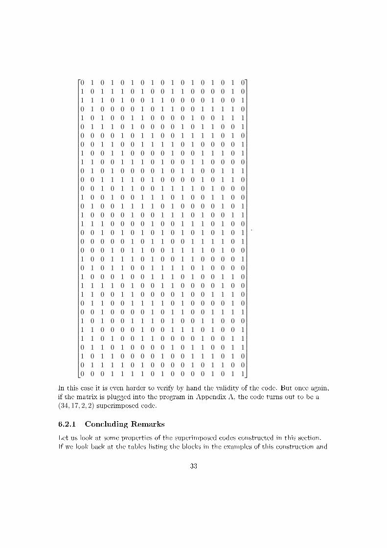
0 1 0 1 0 1 0 1 0 1 0 1 0 1 0 1 01 0 1 1 1 0 1 0 0 1 1 0 0 0 0 1 01 1 1 0 1 0 0 1 1 0 0 0 0 1 0 0 10 1 0 0 0 0 1 0 1 1 0 0 1 1 1 1 01 0 1 0 0 1 1 0 0 0 0 1 0 0 1 1 10 1 1 1 0 1 0 0 0 0 1 0 1 1 0 0 10 0 0 0 1 0 1 1 0 0 1 1 1 1 0 1 00 0 1 1 0 0 1 1 1 1 0 1 0 0 0 0 11 0 0 1 1 0 0 0 0 1 0 0 1 1 1 0 11 1 0 0 1 1 1 0 1 0 0 1 1 0 0 0 00 1 0 1 0 0 0 0 1 0 1 1 0 0 1 1 10 0 1 1 1 1 0 1 0 0 0 0 1 0 1 1 00 0 1 0 1 1 0 0 1 1 1 1 0 1 0 0 01 0 0 1 0 0 1 1 1 0 1 0 0 1 1 0 00 1 0 0 1 1 1 1 0 1 0 0 0 0 1 0 11 0 0 0 0 1 0 0 1 1 1 0 1 0 0 1 11 1 1 0 0 0 0 1 0 0 1 1 1 0 1 0 00 0 1 0 1 0 1 0 1 0 1 0 1 0 1 0 10 0 0 0 0 1 0 1 1 0 0 1 1 1 1 0 10 0 0 1 0 1 1 0 0 1 1 1 1 0 1 0 01 0 0 1 1 1 0 1 0 0 1 1 0 0 0 0 10 1 0 1 1 0 0 1 1 1 1 0 1 0 0 0 01 0 0 0 1 0 0 1 1 1 0 1 0 0 1 1 01 1 1 1 0 1 0 0 1 1 0 0 0 0 1 0 01 1 0 0 1 1 0 0 0 0 1 0 0 1 1 1 00 1 1 0 0 1 1 1 1 0 1 0 0 0 0 1 00 0 1 0 0 0 0 1 0 1 1 0 0 1 1 1 11 0 1 0 0 1 1 1 0 1 0 0 1 1 0 0 01 1 0 0 0 0 1 0 0 1 1 1 0 1 0 0 11 1 0 1 0 0 1 1 0 0 0 0 1 0 0 1 10 1 1 0 1 0 0 0 0 1 0 1 1 0 0 1 11 0 1 1 0 0 0 0 1 0 0 1 1 1 0 1 00 1 1 1 1 0 1 0 0 0 0 1 0 1 1 0 00 0 0 1 1 1 1 0 1 0 0 0 0 1 0 1 1

.

In this case it is even harder to verify by hand the validity of the code. But once again,if the matrix is plugged into the program in Appendix A, the code turns out to be a(34, 17, 2, 2) superimposed code.

6.2.1 Concluding Remarks

Let us look at some properties of the superimposed codes constructed in this section.If we look back at the tables listing the blocks in the examples of this construction and

33

focus on the �rst position in the blocks derived from the subgroup⟨α2⟩. Then we see

that as we look through all the blocks corresponding to⟨α2⟩and look in the �rst posi-

tion, every element of the corresponding Galois �eld is found exactly once. This is truefor any position in the blocks for both cosets of the subgroup

⟨α2⟩. This is true since

if αk is the element in position i of either coset, in the corresponding blocks will be onposition i elements of the form g + αk where g belongs to the corresponding Galois�eld. If the same element is found on position i in two di�erent blocks, then we haveg1 + αk = g2 + αk, from which we get that g1 = g2 and thus we cannot have the sameelement on the same position in di�erent blocks. Since the block size is

∣∣⟨α2⟩∣∣ then if

we count over all blocks corresponding to both cosets of the subgroup, we see that ev-ery element in the Galois �eld is found exactly 2

∣∣⟨α2⟩∣∣ times. Thus, the superimposed

codes constructed in this way is a constant weight code of weight 2∣∣⟨α2

⟩∣∣ . It is, how-ever, uncertain what the minimum distance would be.Now one question to think about is whether or not this construction works in general.We saw examples where the construction does not work, so clearly the constructiondoes not work for any arbitrary subgroup of the multiplicative group of any Galois�eld. But what is the property that the Galois �eld must have in order for this con-struction to work? Unfortunately, this question will not be answered in this thesis. Assaid earlier, however, we can see a pattern emerging in the examples above. In everycase where the construction failed, the subgroup

⟨α2⟩< GF ∗(pn) has odd size and in

every case where the construction worked the subgroup⟨α2⟩has even size. However,

the sample size is rather small so it is hard to say too much about this connection, andfor that reason it might be something worth studying further.But what if this construction goes further than superimposed codes? Clearly, the pair(X,devB) as described in Conjecture 6.7 is some form of block design. But what arethe properties of this block design? If (X,devB) is a t-design, then what are the validvalues of t and λ? Of course v = pn, since the points are the elements of the Galois�eld, and in the examples we have seen, k = pn−1

2 . The 2 in the denominator of kcomes from the fact that |B| = 2, which in turn comes from the fact that

⟨α2⟩con-

tains half the elements of the multiplicative group GF ∗(pn). This suggests that Con-jecture 6.7 could possibly be modi�ed to work for other subgroups than

⟨α2⟩, with B

being the set of cosets to this subgroup. If this modi�cation of Conjecture 6.7 is pos-sible, then the block size k would still be the size of the subgroup, which can also beexpressed k = pn−1

|B| . So we know which values we expect to possibly work for v andk, but still, what about t and λ? Valid values for t and λ will not be provided in thisthesis, but maybe this could be the topic for further research.Another way to continue working on this construction is to �nd su�cient conditionsfor this construction to also be a superimposed code. By the examples in this thesis itlooks like the size of the subgroup

⟨α2⟩could be important. Also, all the superimposed

codes presented in this thesis have the parameters w = r = 2. But can this construc-tion maybe be used to construct superimposed codes with the parameters w and r notboth equal to 2, and if so, what exactly does w and r depend on? This could also bethe topic for further research.

34

Appendix A

Code Veri�cation Program

/* Compiled wi th gcc 5 . 4 . 0 *//* Compiler f l a g s used −s t d=c11 −Wall −Wextra −pedant i c *//* This program cu r r en t l y on ly works f o r w = 2 and r = 2 */#include <s td i o . h>#include <s t d l i b . h>#include <ctype . h>

void pr int_array ( long * , long ) ;long f a c t o r i a l ( long ) ;long n_choose_k ( long , long ) ;

void pr int_array ( long *x , long s i z e ){for ( int i = 0 ; i < s i z e ; i++){ i

p r i n t f ( "%2ld " , x [ i ] ) ;i f ( i < s i z e − 1) p r i n t f ( " , " ) ;

}}

long f a c t o r i a l ( long x ){long i = 1 ;while ( x > 1) i *= x−−;return i ;

}

long n_choose_k ( long n , long k ){return f a c t o r i a l (n) / ( f a c t o r i a l (n − k ) * f a c t o r i a l ( k ) ) ;

}

int main ( int argc , char ** argv ){i f ( argc != 5){

35

p r i n t f ( "USE: . / SIC_check N T w r\ nQuitt ing \n" ) ;return 1 ;

}

FILE * fp = fopen ( "Code" , " r " ) ;const long N = ato i ( argv [ 1 ] ) ;const long T = ato i ( argv [ 2 ] ) ;const long w = ato i ( argv [ 3 ] ) ;const long r = a t o i ( argv [ 4 ] ) ;long Code [N ] [T ] ;long num_of_subsets = n_choose_k (T, 2 ) ;long subse t s [ num_of_subsets ] [w ] ;long is_ok , i , j , k ;char c ;

p r i n t f ( "\n__________________________________________________" ) ;p r i n t f ( "\n Ver i f y i ng (N, T, w, r ) = (%ld , %ld , %ld , %ld ) SIC" , N, T, w, r ) ;p r i n t f ( "\n__________________________________________________" ) ;p r i n t f ( "\n The W, R s e t s " ) ;p r i n t f ( "\n__________________________________________________" ) ;

/* I n i t i a l i z e s the f i r s t e lement in the s u b s e t s */for ( i = 2 , j = 1 , k = 0 ; k < num_of_subsets ; k++){

subse t s [ k ] [ 1 ] = ( j < T ? ++j : ( j = ++i ) ) ;}

/* I n i t i a l i z e s the second element in the s u b s e t s */for ( j = 1 , k = 0 ; k < num_of_subsets ; k++){

subse t s [ k ] [ 0 ] = ( subse t s [ k ] [ 1 ] == T ? j++: j ) ;}p r i n t f ( "\n" ) ;for ( i = j = 0 ; i < num_of_subsets ; i++, j++){i f ( j == 5){

j = 0 ;p r i n t f ( "\n" ) ;

}p r i n t f ( " {" ) ; pr int_array ( ( long *) subse t s [ i ] , 2 ) ; p r i n t f ( "}" ) ;

}

/* Reads the code in t o b u f f e r */i f ( ! fp ){

p r i n t f ( "\ nF i l e po in t e r e r r o r " ) ;return 1 ;

36

}for ( i = 0 ; i < N; i++){for ( j = 0 ; j < T; j++){while ( i s s p a c e ( c = f g e t c ( fp ) ) ) ;Code [ i ] [ j ] = c − ' 0 ' ;

}}f c l o s e ( fp ) ;

p r i n t f ( "\n__________________________________________________" ) ;p r i n t f ( "\n The code to be t e s t ed " ) ;p r i n t f ( "\n__________________________________________________" ) ;for ( i = 0 ; i < N; i++){

p r i n t f ( "\n" ) ;for ( j = 0 ; j < T; j++){

p r i n t f ( "%ld " , Code [ i ] [ j ] ) ;}

}

p r i n t f ( "\n__________________________________________________" ) ;p r i n t f ( "\n The pa i r s o f W, R that f a i l ( i f any ) " ) ;p r i n t f ( "\n__________________________________________________" ) ;

/* Loops through a l l p a i r s o f s e t s W, R */for ( i = 0 ; i < num_of_subsets ; i++){for ( j = 0 ; j < num_of_subsets ; j++){

is_ok = 0 ;

/* The f o l l ow i n g cond i t i on checks i f *//* the curren t s e t s W, R are d i s j o i n t */i f ( ( subse t s [ i ] [ 0 ] != subse t s [ j ] [ 0 ] ) &&

( subse t s [ i ] [ 0 ] != subse t s [ j ] [ 1 ] ) &&( subse t s [ i ] [ 1 ] != subse t s [ j ] [ 0 ] ) &&( subse t s [ i ] [ 1 ] != subse t s [ j ] [ 1 ] ) ) {for ( k = 0 ; k < N; k++){

/* The f o l l ow i n g cond i t i on checks i f *//* row k has 1 in columns in W and 0 *//* in columns in R */i f ( ( Code [ k ] [ subs e t s [ i ] [ 0 ] − 1 ] == 1) &&

(Code [ k ] [ subse t s [ i ] [ 1 ] − 1 ] == 1) &&(Code [ k ] [ subse t s [ j ] [ 0 ] − 1 ] == 0) &&(Code [ k ] [ subse t s [ j ] [ 1 ] − 1 ] == 0)){

37

is_ok = 1 ;}

}i f ( ! is_ok ){

p r i n t f ( "\n W = {%ld , %ld } , R = {%ld , %ld }" , subse t s [ i ] [ 0 ], subse t s [ i ] [ 1 ], subse t s [ j ] [ 0 ], subse t s [ j ] [ 1 ] ) ;

}}

}}

p r i n t f ( "\n" ) ;return 0 ;

}

38

Bibliography

[1] Haitao Cao, Kejun Chen, and Ruizhong Wei. �Super-simple balanced incompleteblock designs with block size 4 and index 5�. In: Discrete Mathematics 309.9(2009), pp. 2808�2814.

[2] Kejun Chen, Zhenfu Cao, and Ruizhong Wei. �Super-simple balanced incompleteblock designs with block size 4 and index 6�. In: Journal of statistical planningand inference 133.2 (2005), pp. 537�554.

[3] Kejun Chen and Ruizhong Wei. �Super-simple (v, 5, 5) Designs�. In: Designs,Codes and Cryptography 39.2 (2006), pp. 173�187.

[4] Kejun Chen and Ruizhong Wei. �Super-simple (v,5,4) designs�. In: Discrete Ap-plied Mathematics 155.8 (2007), pp. 904�913.

[5] Igor Gashkov, J AO Ekberg, and D Taub. �A geometric approach to �nding newlower bounds of A (n, d, w)�. In: Designs, Codes and Cryptography 43.2 (2007),pp. 85�91.

[6] Hans-Dietrich O.F. Gronau, Donald L. Kreher, and Alan C.H. Ling. �Super-simple (v,5,2)-designs�. In: Discrete Applied Mathematics 138.1 (2004), pp. 65�77.

[7] Chen Kejun. �On the existence of super-simple (v, 4, 3)-BIBDs�. In: Journal ofCombinatorial Mathematics and Combinatorial Computing 17 (1995), pp. 149�159.

[8] Chen Kejun. �On the existence of super-simple (v,4,4)-BIBDs�. In: Journal ofStatistical Planning and Inference 51.3 (1996), pp. 339�350.

[9] Hyun Kwang Kim and Vladimir Lebedev. �On Optimal Superimposed Codes�.In: Journal of Combinatorial Designs 12.2 (2004), pp. 79�91.

[10] Florence Jessie MacWilliams and Neil James Alexander Sloane. The Theory ofError-Correcting Codes. Elsevier, 1977.

[11] Per-Anders Svensson. Abstrakt algebra. Studentlitteratur, 2007.

39