Thermionic Current Densities from First Principles

Johannes Voss,1, 2, a) Aleksandra Vojvodic,1, 2 Sharon H. Chou,3 Roger T. Howe,3 Igor

Bargatin,4 and Frank Abild-Pedersen2, b)

1)Department of Chemical Engineering, Stanford University, Stanford, CA,

USA

2)SUNCAT Center for Interface Science and Catalysis,

SLAC National Accelerator Laboratory, Menlo Park, CA,

USA.

3)Department of Electrical Engineering, Stanford University, Stanford, CA,

USA.

4)Department of Mechanical Engineering and Applied Mechanics,

University of Pennsylvania, Philadelphia, PA, USA.

(Dated: 25 June 2013)

Post-print of the article

J. Chem. Phys. 138, 204701 (2013),

Copyright (2013) American Institute of Physics. For personal use only. Any other use

requires prior permission of the author and the American Institute of Physics.

http://link.aip.org/link/?JCP/138/204701

We present a density functional theory-based method for calculating thermionic

emission currents from a cathode into vacuum using a non-equilibrium Green’s func-

tion approach. It does not require semi-classical approximations or crude simplifica-

tions of the electronic structure used in previous methods and thus provides quanti-

tative predictions of thermionic emission for adsorbate-coated surfaces. The obtained

results match well with experimental measurements of temperature-dependent cur-

rent densities. Our approach can thus enable computational design of composite

electrode materials.

PACS numbers: 79.40.+z, 68.47.De, 73.30.+y

a)Electronic mail: vossj@stanford.edub)Electronic mail: abild@slac.stanford.edu

1

I. INTRODUCTION

The efficiency of hot cathodes can be increased by developing new materials with suffi-

cient thermionic emission of electrons operating at lower temperatures. These cathodes are

important for a growing range of applications, including electron guns (used e.g. in electron

microscopes), thermionic energy converters and the recently demonstrated photon-enhanced

thermionic energy converters.1 Computational prediction of thermionic current densities will

greatly aid the design of new electrodes. However, first-principles modeling of tunneling am-

plitudes governing thermionic emission has proven elusive. This Article presents a method

for calculating these tunneling rates from first principles, which is able to treat structurally

complex surfaces. Hence we can predict thermionic emission from composite or multi-layer

electrodes, which can often yield higher current densities than relatively simple elemental

surfaces.

The work function of a metal surface, i.e. the energy required to remove an electron at the

Fermi level from the metal, can easily be extracted from potential energies obtained within

density functional theory (DFT). The prediction of electronic emission currents, however,

also requires knowledge about the scattering properties of the surface. Existing approaches to

calculating thermionic or field emission are based on crude approximations in terms of semi-

classical statistics and averaging the surface electronic structure to one dimension, which

restricts the applicability to simple surfaces.2–5 In the case of field emission, previous first-

principles calculations have considered a jellium model to describe the reservoir of electrons

and have also used an average 1D potential.6 Huang et al.7 employed matching of wave

functions in 3D to calculate field emission, but the analytical approximation of the wave

functions decaying into vacuum yields non-zero currents only for finite fields and thermionic

currents cannot be calculated. Musho et al.8 accounted for quantum statistics in thermionic

emission via Green’s functions, but relied on simple wave functions with an effective electron

mass and the work function as free parameters.

The method presented here does not involve semi-classical approximations nor simplifi-

cation of the electronic structure, and is thus able to predict thermionic current densities

purely from first principles even for complex surface structures with adsorbates. The method

uses a non-equilibrium Green’s function (NEGF) approach based on DFT calculations,9,10

where both the semi-infinite systems of the metallic lead and vacuum are accounted for via

2

self-energies, thus overcoming the limitations of existing approaches outlined above.

II. THEORY

The NEGF approach (see Refs. 9 and 10 for an introduction) allows for a description of

systems that are not in thermodynamic equilibrium, e.g. due to the presence of reservoirs

held at different chemical potentials or temperatures, which we use here to model steady cur-

rents due to temperature differences. We consider the non-interacting Kohn-Sham states11

obtained from DFT calculations as eigenstates of the separate subsystems (reservoirs and

scattering region) in equilibrium. We also neglect other interactions such as electron-phonon

scattering, only considering coherent transport. Of central importance is the retarded single-

particle Green’s function of the system

GR(E) = (E + iη −H)−1, (1)

where the infinitesimally small parameter η = 0+ assures that GR describes the response to

perturbations in the past, and H is the Hamiltonian of the system. In the following we will

drop the superscript R from all Green’s functions and self-energies, and we will also omit

the term iη.

In NEGF transport calculations, the leads are typically modeled as semi-infinite systems,9,10

serving as reservoirs for electrons and holes which are in thermodynamic equilibrium. To de-

scribe electronic emission through a surface into vacuum, we consider a semi-infinite metallic

lead as a source and a semi-infinite vacuum region as a drain for electrons. The supercells

employed to calculate the DFT bandstructures entering the Green’s function calculations

are depicted in Fig. 1 for bulk lead (a) and surface slab (b).

Approaches to treating the coupling of the scattering region to the semi-infinite reservoirs

include matching of Kohn-Sham potentials with open boundary conditions on the scatter-

ing region12 or extracting the coupling matrix elements by expansion of a DFT super cell

Hamiltonian in a localized basis set.13 We follow the latter approach, performing separate

calculations for the scattering region (a surface slab) and for the periodically continued left

and right hand sides of the system. The periodically continued systems are subdivided into

principal layers along the transport direction.14 These layers are chosen to be thick enough

such that interactions beyond neighboring layers are negligible. Green’s functions for princi-

pal layers of the isolated, semi-infinite systems are then calculated iteratively using a highly

3

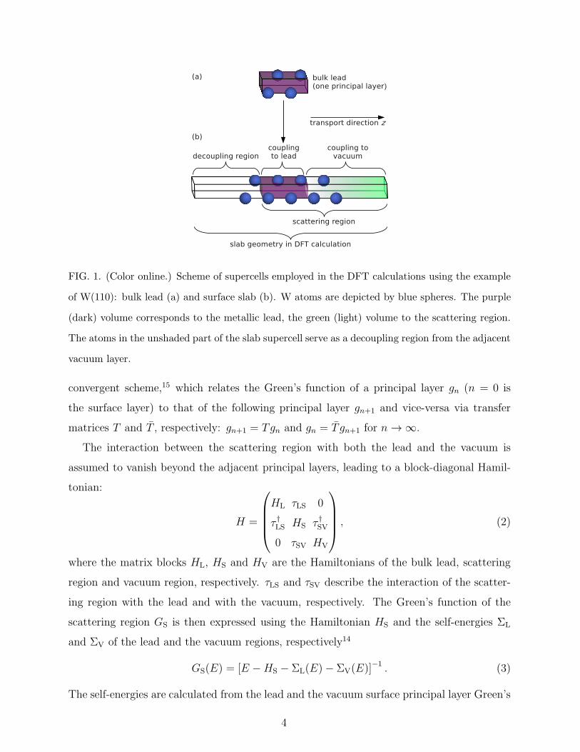
FIG. 1. (Color online.) Scheme of supercells employed in the DFT calculations using the example

of W(110): bulk lead (a) and surface slab (b). W atoms are depicted by blue spheres. The purple

(dark) volume corresponds to the metallic lead, the green (light) volume to the scattering region.

The atoms in the unshaded part of the slab supercell serve as a decoupling region from the adjacent

vacuum layer.

convergent scheme,15 which relates the Green’s function of a principal layer gn (n = 0 is

the surface layer) to that of the following principal layer gn+1 and vice-versa via transfer

matrices T and T , respectively: gn+1 = Tgn and gn = T gn+1 for n → ∞.

The interaction between the scattering region with both the lead and the vacuum is

assumed to vanish beyond the adjacent principal layers, leading to a block-diagonal Hamil-

tonian:

H =

HL τLS 0

τ†LS HS τ

†SV

0 τSV HV

, (2)

where the matrix blocks HL, HS and HV are the Hamiltonians of the bulk lead, scattering

region and vacuum region, respectively. τLS and τSV describe the interaction of the scatter-

ing region with the lead and with the vacuum, respectively. The Green’s function of the

scattering region GS is then expressed using the Hamiltonian HS and the self-energies ΣL

and ΣV of the lead and the vacuum regions, respectively14

GS(E) = [E −HS − ΣL(E)− ΣV(E)]−1. (3)

The self-energies are calculated from the lead and the vacuum surface principal layer Green’s

4

functions gL and gV, respectively:

ΣL(E) = τ†LS gL(E) τLS

ΣV(E) = (τSV − E SV)† gV(E) (τSV − E SV), (4)

where SV accounts for the overlap of the basis functions used for the slab and the vacuum

region. This will be explained in detail below.

For the metallic lead, the calculation of the surface principal layer Green’s function15

gL(E) =[

E − h00L −

(

h01L

)†TL(E)

]−1

(5)

is based on the on-layer and layer-to-layer hopping matrices h00L = HL and h01

L , respectively,

represented here in a maximally-localized Wannier function (MLWF) basis16,17 obtained

from DFT calculations. TL is the lead transfer matrix. For all calculations presented here,

we have chosen a principal layer thickness of four atomic layers for the metallic leads.

Since the momenta qx, qy perpendicular to the transport direction z are conserved, we

only perform a Wannier transformation of the Bloch states |εq〉 in the z-direction:

|wqx,qy,Rz〉 =c

2π

∫

dqz∑

εq

Uq

wεe−iqzRz |εq〉. (6)

w enumerates the Wannier functions, U is a unitary matrix, c is the supercell lattice con-

stant in the transport direction and Rz is a lattice vector component. For the periodically

continued vacuum system, the eigenstates are plane waves. We express the conserved in-

plane components of the kinetic energy operator in momentum space, whereas the normal

direction is described as a finite difference in real space (we use atomic units unless otherwise

noted):

HV =1

2

(

q2x + q2y)

+1

2h2(2δz,z′ − δz,z′+1 − δz,z′−1) |z〉〈z

′|+ Φ, (7)

where z, z′ denote principal vacuum layers along the transport direction. The addition of

the work function Φ obtained from the surface slab calculation is required to align the

subsystem Hamiltonians in (2). For numerical convenience when evaluating τSV and SV,

the grid spacing h is chosen to match that of the Fourier grid used in the plane wave DFT

calculation of the surface slab, i.e. the principal vacuum layer thickness h is of the order

of 0.1 A. The vacuum region in the slab is thus spanned by the order of 100 principal

5

layers. This is a good approximation, since states with energies too high to be sufficiently

well represented in the basis determined by the chosen plane wave cut-off have a vanishing

contribution to thermionic emission for the temperatures considered here. Considering the

off-diagonal elements with z 6= z′ of (7) as coupling between neighboring principal vacuum

layers of width h, the vacuum surface layer Green’s function is calculated analogously to the

above case of the metallic lead as

gV(E) =[

E − h00V − h01

V TV(E)]−1

. (8)

h00V , h01

V and TV are the on-layer, layer-to-layer hopping and transfer matrices for the vacuum

system, respectively.

The interaction τSV between the scattering region and vacuum is calculated by projection

of the scattering region Hamiltonian in its Wannier function representation onto the vacuum

principal layer basis functions |qx, qy, z〉:

〈qx, qy, z|τSV|wqx,qy,Rz=0〉 =

⟨

qx, qy, z

∣

∣

∣

∣

∣

c

2π

∑

εq

εqUq

wε

∣

∣

∣

∣

∣

εq

⟩

. (9)

Since the surface slab is aperiodic along z, there are no q-point sampling sub-divisions along

z: q = (qx, qy, 0) and thus also Rz = 0. The Wannier functions extend into vacuum, and

there is overlap with the vacuum basis functions |qx, qy, z〉:

〈qx, qy, z|SV|wqx,qy,Rz=0〉 = 〈qx, qy, z|w

qx,qy,Rz=0〉 6= 0. (10)

The range of z considered in Eqs. (9) and (10) is restricted to be greater than some

constant z0, typically at a few A above the surface. Note that the overlap matrix SV

partially compensates the effect of including small values of z into the calculation of τSV,

such that the results for (3) are relatively insensitive to the exact choice of z0.

Since z0 lies relatively deep in the vacuum layer of the slab system, no ionic pseudo core

spheres are included in the integration intervals. Therefore, all-electron and pseudo valence

Bloch states coincide in the regions considered for integration, and no corrections due to

ultrasoft pseudopotential or projector-augmented wave implementations in the DFT code

appear.

We now consider the Landauer-Buttiker formalism,18,19 in which the thermionic current

density is given as

J(T ) =1

πA

∫

dE f [E − µ(T ), T ] T (E), (11)

6

where A is the surface area of the considered supercell geometry, f [E − µ(T ), T ] is the

Fermi-Dirac distribution, and

T (E) = Tr[

ΓL(E)G†S(E) ΓV(E)GS(E)

]

(12)

is the transmission function.9,10 ΓL/V(E) = i [ΣL/V(E)−Σ†

L/V(E)] are broadening functions.

Since qx and qy are good quantum numbers, T (E) can be calculated for fixed values of the

in-plane momenta, where the total transmission is then given as a two-dimensional Brillouin

zone integral.

We will compare first principles results obtained from (11) to experimental results, often

available as fits against the Richardson-Dushman equation

J(T ) = AT 2 exp

(

−Φ

kBT

)

. (13)

This equation is based on a semi-classical treatment of an electron gas at a potential step.3

A is the Richardson-Dushman constant, Φ the work function and kB Boltzmann’s constant.

Fitted constants of A and Φ effectively include first-order temperature dependencies of

the work function and are therefore also referred to as the apparent Richardson-Dushman

constant and work function, respectively.3

III. DETAILS OF CALCULATION

DFT calculations were performed with the dacapo20 ultrasoft pseudopotential21 code.

Kohn-Sham states were expanded in plane wave basis sets with a cutoff of 350 eV. Brillouin

zones were sampled with k-point spacings of at most ∼0.1 A−1. Fermi surface smearing was

performed using Fermi-Dirac statistics with temperatures kBT ≥ 0.1 eV (kBT = 0.1 eV was

used for all structural relaxations, while higher temperatures were used to self-consistently

calculate the temperature dependence of the work function; this temperature dependence can

be more efficiently approximated by recalculating the Fermi level at different temperatures

for fixed electronic energy levels). Transformation of Bloch states to Wannier functions was

performed using the ase software suite.22

7

10-10

10-8

10-6

10-4

5 5.5 6 6.5 7 7.5 8 8.5 9

J/T

2 [A/c

m2 /K

2 ]

1/T [10-4/K]

LaB6(100)

Experimenta

Experimentb

DFT - PBEDFT - RPBE

DFT - LDA

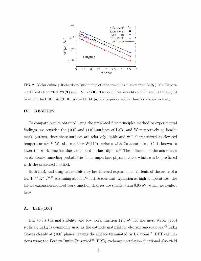
FIG. 2. (Color online.) Richardson-Dushman plot of thermionic emission from LaB6(100). Experi-

mental data from aRef. 28 (H) and bRef. 23 (�). The solid lines show fits of DFT results to Eq. (13)

based on the PBE (⋄), RPBE (N) and LDA (•) exchange-correlation functionals, respectively.

IV. RESULTS

To compare results obtained using the presented first principles method to experimental

findings, we consider the (100) and (110) surfaces of LaB6 and W respectively as bench-

mark systems, since these surfaces are relatively stable and well-characterized at elevated

temperatures.23,24 We also consider W(110) surfaces with Cs adsorbates. Cs is known to

lower the work function due to induced surface dipoles.25 The influence of the adsorbates

on electronic tunneling probabilities is an important physical effect which can be predicted

with the presented method.

Both LaB6 and tungsten exhibit very low thermal expansion coefficients of the order of a

few 10−6 K−1.26,27 Assuming about 1% lattice constant expansion at high temperatures, the

lattice expansion-induced work function changes are smaller than 0.05 eV, which we neglect

here.

A. LaB6(100)

Due to its thermal stability and low work function (2.3 eV for the most stable (100)

surface), LaB6 is commonly used as the cathode material for electron microscopes.29 LaB6

cleaves cleanly at (100) planes, leaving the surface terminated by La atoms.23 DFT calcula-

tions using the Perdew-Burke-Ernzerhof30 (PBE) exchange-correlation functional also yield

8

2.3 eV for the work function of the (100) surface,31 while for the revised PBE20 (RPBE)

functional it is underestimated by 0.1 eV and for the local density approximation11 (LDA)

it is overestimated by 0.3 eV. Relaxing the surface structure according to the LDA func-

tional increases the work function further by only 0.05 eV. We neglect the effect of different

relaxed surface structures due to different functionals and focus on the dominant differences

in the electronic structure only; all transport properties have been calculated for surfaces

relaxed according to the PBE functional. Despite the fact that the LaB6 work function is

described best by the PBE functional, we also performed transport calculations using the

LDA and RPBE functionals to benchmark the sensitivity of the emission current densities

to the exchange-correlation functional employed.

Using the PBE approximation for the exchange and correlation functional also yields very

good agreement with experiments23,28 for thermionic current densities (Fig. 2), in particular

for the current density reported in Ref. 23, where perfect stoichiometry and absence of

reconstruction of the LaB6(100) surface was confirmed by Auger electron spectroscopy and

low energy electron diffraction, respectively. In agreement with the trends in work functions

described above, RPBE and LDA calculations over- and underestimate thermionic current

densities of LaB6(100), respectively. Note that the apparent work functions obtained from

fitting the DFT current density data to Eq. (13) differ less than the work functions listed

above, which were obtained from the electrostatic potential for a fixed temperature (kBT =

0.1 eV ≈ 1160 K·kB). The apparent work functions for both PBE and LDA are about

2.3 eV, with 2.2 eV for RPBE.

B. W(110) and Cs/W(110)

For the tungsten surfaces, we employ the RPBE functional since it performs well for the

description of covalent bonds to transition metal surfaces.20 The bulk lattice constants of

tungsten relaxed according to the PBE and RPBE functionals are very similar with values of

3.18 A and 3.20 A, respectively, in good agreement with the experimental result of 3.16 A.32

The fixed-temperature work function predicted using the RPBE functional is 4.61 eV for the

W(110) surface (close to the experimental value of 4.65 eV),24 while the PBE prediction is

0.14 eV higher. For an optimal description of the work function, we have chosen the RPBE

functional also for the clean tungsten surface.

9

10-17

10-14

10-11

10-8

4 4.5 5 5.5 6 6.5 7 7.5J/

T2 [A

/cm

2 /K2 ]

1/T [10-4/K]

W(110)

Experimenta

DFT

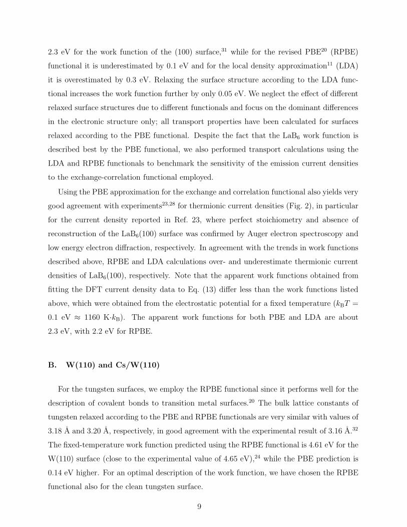
FIG. 3. (Color online.) Richardson-Dushman plot of thermionic emission from a close-packed

tungsten surface with experimental data (•) from aRef. 24 and DFT results (�) based on the

RPBE functional.

Current densities predicted from the presented method compare very well to experimental

data24 for the most stable W(110) surface (Fig. 3). The RPBE calculations yield a value of

4.62 eV and 4.61 eV for the apparent and fixed-temperature work functions at kBT = 0.1 eV,

respectively, comparing well to the experimental result for the apparent work function of

4.65 eV.24

Adsorbate-induced surface dipoles lower the work functions of the bare substrates. Here,

we study cesiated tungsten as an example. We consider two coverage ratios of cesium atoms:

one monolayer (ML), corresponding to about one Cs per 2x2 W(110) supercell, where the

surface area per Cs is about the same as in Cs(110), and ∼0.69 ML, (one Cs per 3x2 W(110)

supercell), where the adsorbate-induced work function reduction is the largest.33

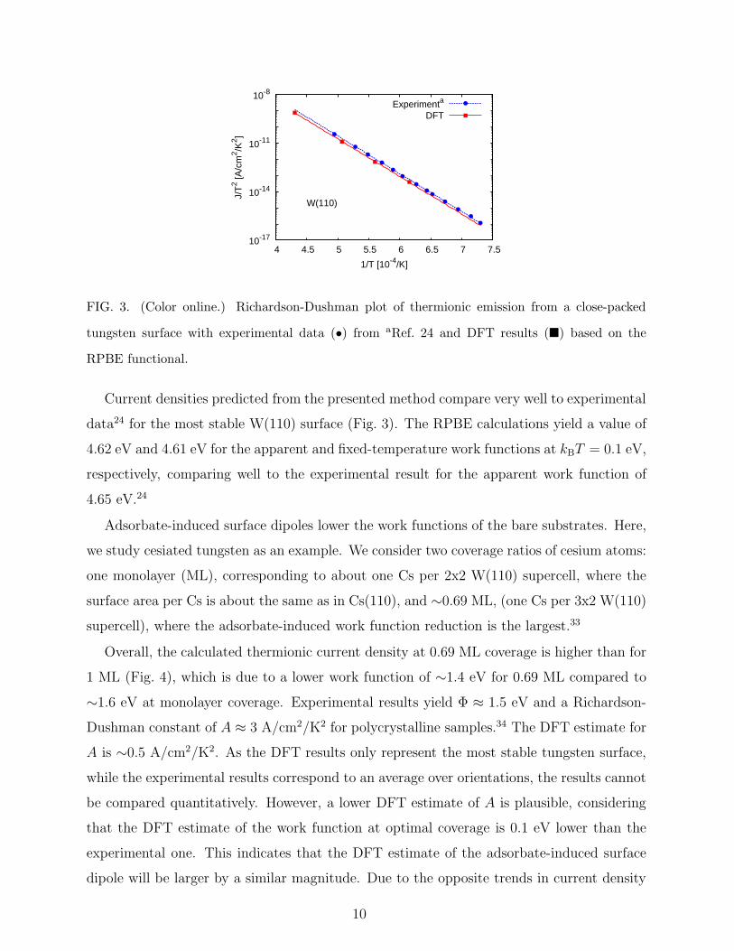
Overall, the calculated thermionic current density at 0.69 ML coverage is higher than for

1 ML (Fig. 4), which is due to a lower work function of ∼1.4 eV for 0.69 ML compared to

∼1.6 eV at monolayer coverage. Experimental results yield Φ ≈ 1.5 eV and a Richardson-

Dushman constant of A ≈ 3 A/cm2/K2 for polycrystalline samples.34 The DFT estimate for

A is ∼0.5 A/cm2/K2. As the DFT results only represent the most stable tungsten surface,

while the experimental results correspond to an average over orientations, the results cannot

be compared quantitatively. However, a lower DFT estimate of A is plausible, considering

that the DFT estimate of the work function at optimal coverage is 0.1 eV lower than the

experimental one. This indicates that the DFT estimate of the adsorbate-induced surface

dipole will be larger by a similar magnitude. Due to the opposite trends in current density

10

10-7

10-6

10-5

10-4

10-3

5 5.5 6 6.5 7

J/T

2 [A/c

m2 /K

2 ]

1/T [10-4/K]

1ML Cs/W(110)0.69ML Cs/W(110)

FIG. 4. (Color online.) Calculated thermionic current densities for cesiated W(110) based on the

RPBE functional. The red (solid) line shows a fit of the DFT data to the Richardson-Dushman

equation for monolayer Cs-coverage, the blue (dashed) line for (near optimal) 0.69 monolayer

coverage.

with increasing magnitudes of Φ and A, the current densities estimated e.g. at 1000 K from

the experimental parameters and calculated within DFT only differ by a factor of about

two.

The contribution of electrons with non-zero tranverse momenta, q, to the thermionic

current densities for clean and cesiated W(110) (Fig. 5) shows that considering only the

q = 0 component of the current density is insufficient to describe thermionic emission

from surfaces with adsorbates. For bare tungsten, an integral over the current density

contributions at kBT = 0.17 eV over ∼1% of the Brillouin zone around Γ accounts for ∼80%

of the total current density. On the other hand, an integral over an equivalent area of the

Brillouin zone of the cesiated system only yields ∼30% of the total current density. This

shows that the description of thermionic emission of composite electrode surfaces involving

e.g. adsorbates requires a three dimensional description of the scattering problem.

V. CONCLUSION

We have developed a first-principles technique for calculating thermionic current den-

sities which yields very good agreement with experiments. The method is based on non-

equilibrium Green’s functions. Unlike previous approaches, which involved semi-classical

approximations or crude simplifications of the electronic structure, there are no limititations

11

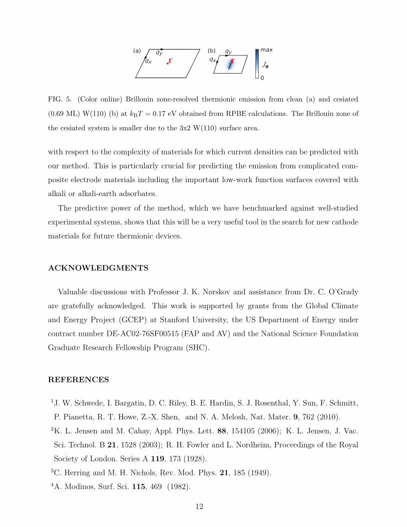
FIG. 5. (Color online) Brillouin zone-resolved thermionic emission from clean (a) and cesiated

(0.69 ML) W(110) (b) at kBT = 0.17 eV obtained from RPBE calculations. The Brillouin zone of

the cesiated system is smaller due to the 3x2 W(110) surface area.

with respect to the complexity of materials for which current densities can be predicted with

our method. This is particularly crucial for predicting the emission from complicated com-

posite electrode materials including the important low-work function surfaces covered with

alkali or alkali-earth adsorbates.

The predictive power of the method, which we have benchmarked against well-studied

experimental systems, shows that this will be a very useful tool in the search for new cathode

materials for future thermionic devices.

ACKNOWLEDGMENTS

Valuable discussions with Professor J. K. Nørskov and assistance from Dr. C. O’Grady

are gratefully acknowledged. This work is supported by grants from the Global Climate

and Energy Project (GCEP) at Stanford University, the US Department of Energy under

contract number DE-AC02-76SF00515 (FAP and AV) and the National Science Foundation

Graduate Research Fellowship Program (SHC).

REFERENCES

1J. W. Schwede, I. Bargatin, D. C. Riley, B. E. Hardin, S. J. Rosenthal, Y. Sun, F. Schmitt,

P. Pianetta, R. T. Howe, Z.-X. Shen, and N. A. Melosh, Nat. Mater. 9, 762 (2010).

2K. L. Jensen and M. Cahay, Appl. Phys. Lett. 88, 154105 (2006); K. L. Jensen, J. Vac.

Sci. Technol. B 21, 1528 (2003); R. H. Fowler and L. Nordheim, Proceedings of the Royal

Society of London. Series A 119, 173 (1928).

3C. Herring and M. H. Nichols, Rev. Mod. Phys. 21, 185 (1949).

4A. Modinos, Surf. Sci. 115, 469 (1982).

12

5R. Ramprasad, L. R. C. Fonseca, and P. von Allmen, Phys. Rev. B 62, 5216 (2000).

6Y. Gohda, Y. Nakamura, K. Watanabe, and S. Watanabe, Phys. Rev. Lett. 85, 1750

(2000).

7S. Huang, T. Leung, and C. Chan, Solid State Commun. 137, 498 (2006).

8T. D. Musho, W. F. Paxton, J. L. Davidson, and D. G. Walker, J. Vac. Sci. Technol. B

31, 021401 (2013).

9H. Haug and A.-P. Jauho, Quantum Kinetics in Transport and Optics of Semiconductors,

2nd ed. (Springer, Berlin, 2008).

10S. Datta, Electronic Transport in Mesoscopic Systems (Cambridge University Press, Cam-

bridge, 1995).

11W. Kohn and L. J. Sham, Phys. Rev. 140, A1133 (1965).

12J. Taylor, H. Guo, and J. Wang, Phys. Rev. B 63, 245407 (2001).

13M. Brandbyge, J.-L. Mozos, P. Ordejon, J. Taylor, and K. Stokbro, Phys. Rev. B 65,

165401 (2002).

14M. B. Nardelli, Phys. Rev. B 60, 7828 (1999).

15M. P. Lopez Sancho, J. M. Lopez Sancho, and J. Rubio, J. Phys. F: Met. Phys. 14, 1205

(1984); 15, 851 (1985).

16N. Marzari and D. Vanderbilt, Phys. Rev. B 56, 12847 (1997).

17K. S. Thygesen, L. B. Hansen, and K. W. Jacobsen, Phys. Rev. Lett. 94, 026405 (2005).

18R. Landauer, IBM Journal of Research and Development 1, 223 (1957); Philos. Mag. 21,

863 (1970).

19M. Buttiker, Phys. Rev. B 33, 3020 (1986).

20B. Hammer, L. B. Hansen, and J. K. Nørskov, Phys. Rev. B 59, 7413 (1999).

21D. Vanderbilt, Phys. Rev. B 41, 7892 (1990).

22S. R. Bahn and K. W. Jacobsen, Comput. Sci. Eng. 4, 56 (2002); https://wiki.fysik.dtu.dk.

23L. Swanson and D. McNeely, Surf. Sci. 83, 11 (1979).

24M. H. Nichols, Phys. Rev. 57, 297 (1940).

25V. Vlahos, J. H. Booske, and D. Morgan, Phys. Rev. B 81, 054207 (2010).

26V. Craciun and D. Craciun, Appl. Surf. Sci. 247, 384 (2005).

27F. C. Nix and D. MacNair, Phys. Rev. 61, 74 (1942).

28M. Futamoto, M. Nakazawa, K. Usami, S. Hosoki, and U. Kawabe, J. Appl. Phys. 51,

3869 (1980).

13

29R. Nishitani, M. Aono, T. Tanaka, C. Oshima, S. Kawai, H. Iwasaki, and S. Nakamura,

Surf. Sci. 93, 535 (1980).

30J. P. Perdew, K. Burke, and M. Ernzerhof, Phys. Rev. Lett. 77, 3865 (1996).

31R. Monnier and B. Delley, Phys. Rev. B 70, 193403 (2004).

32W. P. Davey, Phys. Rev. 26, 736 (1925).

33S. H. Chou, J. Voss, I. Bargatin, A. Vojvodic, R. T. Howe, and F. Abild-Pedersen, J.

Phys.: Condens. Matter 24, 445007 (2012).

34D. Wright, Proc. IEE—Part III: Radio and Communication Engineering 100, 125 (1953).

14