Thermal and seismic analysis of piping systems using ...

AN ABSTRACT OF THE THESIS OF

Arun L. Nisargand for the degree of Master of Science in Mechanical

Engineering Presented on January 9, 1981.

Title: Thermal and Seismic Analysis of Piping Systems Using Classical

Methods

Abstract approved:

Redacted for PrivacyDr. WillianyC. Kinsel

"Piping Design and Engineering" first published in 1963 by

Grinnell, Co. is widely used by engineers to perform approximate

thermal stress analysis of high-temperature piping systems. The

text consists of numerical to calculate end reactions and

maximum bending stresses in a variety of piping configurations from

known properties of pipes such as outside diameter and moment of

inertia, material properties such as Modulus of Elasticity and

Coefficient of Linear Expansion and specific properties of the

configurations such as aspect ratio (length/height) and temperature

differential. The results obtained by using formulae from the text

are close to the ones obtained by the use of finite element computer

programs. However, the text has some limitations. It lacks

theoretical bases from which the numerical constants were derived.

Thus, the text cannot be used to analyze piping configurations with

aspect ratios outside the range listed in the text. The text also

limits itself to piping configurations without intermediate restraints.

The following thesis investigates three most common configura-

tions, viz., L, U, and Z, and determines theoretical basis and general

equations which yield numerical constants identical to the ones

given in the above text. It also describes how similar methods

can be used to analyze piping systems with intermediate restraints.

A numerical check of data thus derived along with the methods and

the data to analyze deadweight and seismic stresses in the piping

configurations is also included.

Thermal and Seismic Analysisof Piping Systems Using Classical Methods

by

Arun L. Nisargand

A THESIS

submitted to

Oregon State University

in partial fulfillment ofthe requirements for the

degree of

Master of Science

Completed January 9, 1981

Commencement June 1981

APPROVED:,

Redacted for PrivacyDr. William C. Kinsel,/Lecturer of Mechanical Engineering in charge of major

Redacted for Privacy

Dr. JameiR. WetlY.Head of/Dppartment of Mechanit#1 Engineering

i/

Redacted for Privacy

Dean of raduate School

Date thesis is presented: January 9, 1981

Typed by Mrs. Richard Hoyt for Arun L. Nisargand

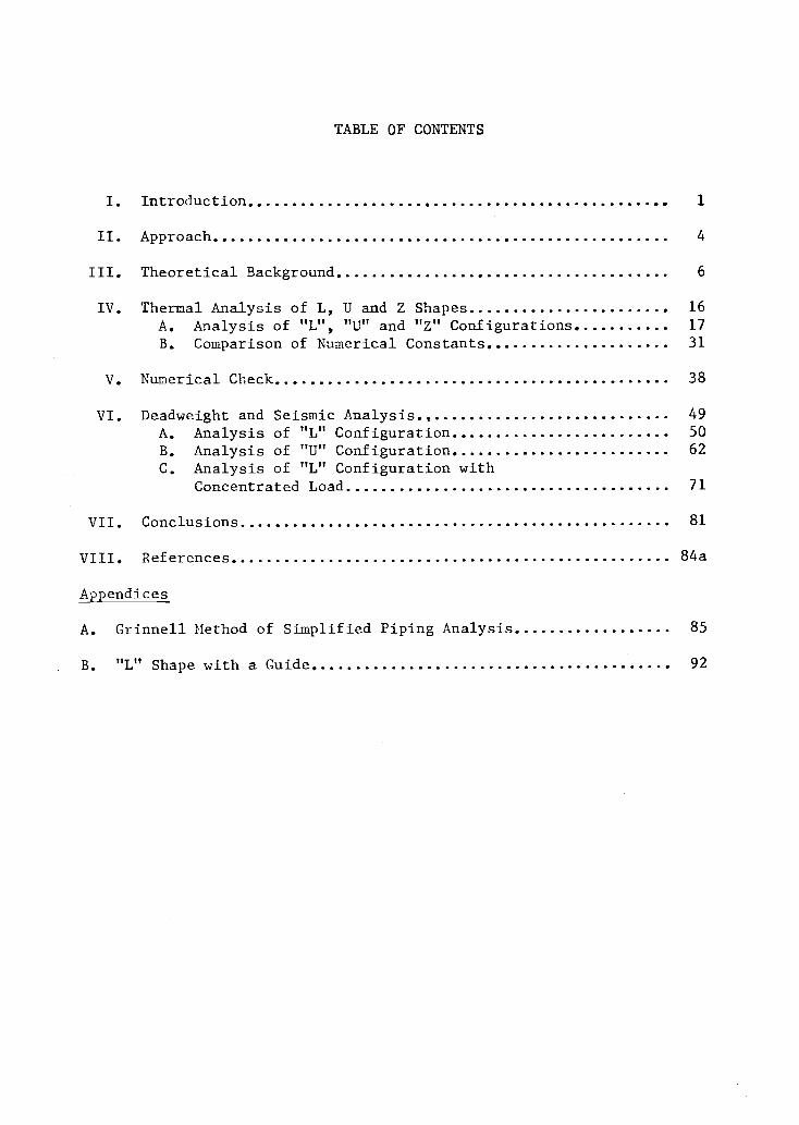
TABLE OF CONTENTS

I. Introduction 1

II. Approach 4

III. Theoretical Background 6

IV. Thermal Analysis of L, U and Z Shapes 16

A. Analysis of "L", "U" and "Z" Configurations. 17

B. Comparison of Numerical Constants 31

V. Numerical Check 38

VI. Deadweight and Seismic Analysis., 49

A. Analysis of "L" Configuration 50

B. Analysis of "U" Configuration 62

C. Analysis of "L" Configuration withConcentrated Load 71

VII. Conclusions 81

VIII. References 84a

Appendices

A. Grinnell Method of Simplified Piping Analysis 85

B. "L" Shape with a Guide 92

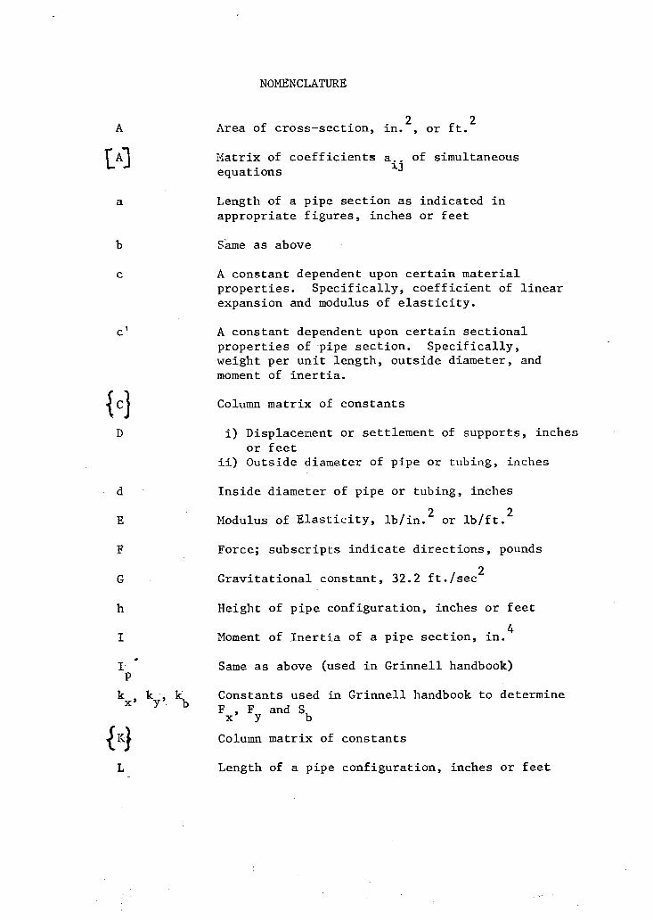
NOMENCLATURE

A Area of cross-section, in.2

, or ft.2

LA] Matrixofcoefficientsa_of simultaneousequations

3.3

a Length of a pipe section as indicated inappropriate figures, inches or feet

b Same as above

c A constant dependent upon certain materialproperties. Specifically, coefficient of linearexpansion and modulus of elasticity.

c' A constant dependent upon certain sectionalproperties of pipe section. Specifically,weight per unit length, outside diameter, andmoment of inertia.

lc}D

E

F

G

h

I

Column matrix of constants

i) Displacement or settlement of supports, inchesor feet

ii) Outside diameter of pipe or tubing, inches

Inside diameter of pipe or tubing, inches

Modulus of Elasticity, lb/in.2 or lb/ft.2

Force; subscripts indicate directions, pounds

Gravitational constant, 32.2 ft./sec2

Height of pipe configuration, inches or feet

Moment of Inertia of a pipe section, in.4

Same as above (used in Grinnell handbook)p

kx, ky,_ kb Constants used in Grinnell handbook to determineFx, F

yand S

b

K)Column matrix of constants

L Length of a pipe configuration, inches or feet

[L3 Lower triangular matrix used in Cholesky's method

M Bending moment; subscripts indicate location,in.-lb or ft.-lb

My Bending moment due to force F; normally used inslope-deflection method, in.-lb or ft.-lb

m Ratio of L/h or h/L as explained in the text

N A constant as indicated in the text

n Load factor due to seismic or other conditions

P Applied force or concentrated weight, lb

Sb

Bending stress, lb/in.2

[T] Upper triangular matrix as used in Cholesky'smethod

AT Temperature differential, °F

U Total strain energy, lb-in.

w Weight per unit length, lb/ft.

x Distance of section under consideration alongx axis, inches or feet

{xi Column matrix of variables

y Distance of section under consideration alongy axis, inches or feet

YB 2 YC

a

Vertical deflections of points B and C

i) Coefficient of linear thermal expansion,in./in.

oF

ii) Ratio a/L where indicated

Ratio b/L

Strain, subscript indicates direction

Stress (usually bending stress), lb/in.2

Angle of rotation, radians

THERMAL AND SEISMIC ANALYSISOF PIPING SYSTEMS USING CLASSICAL METHODS

I. INTRODUCTION

Piping in a processing or a power plant represents a substantial

portion of the cost of the plant. Design of the piping system in a

typical nuclear power_plant requires several thousand man-hours

representing 30 to 35% of the total design effort and is usually on

the critical path. Increasing regulatory requirements for commercial

nuclear power plants has forced the construction contractors to

perform thorough stress analysis of the piping systems to assure its

safety during a variety of seismic and thermal conditions.

Piping systems in a nuclear power plant are classified in two

groups. Piping consisting of pipes of 2 1/2 inches in diameter and

above are called "large bore" piping. Piping less than 2 1/2 inches

nominal diameter are called "small bore".

Large bore piping usually carries process fluids such as steam

at process temperature and pressure. Small bore piping normally

consists of piping for fluid samples, instrument air and sensing lines

subjected to less severe conditions than the process piping. Instru-

ment tubing which is usually 1/2 inches outside diameter and smaller

is classified as small bore piping. Design criteria are the same for

both types of piping and usually involve a "code" check to assure

compliance to ASME Boiler and Pressure Vessel Code Section III

class 1, 2 and 3 (1).

The design process consists mainly of preliminary design and

layout, field check before installation, installation, "as built"

drawings and stress analysis to verify code compliance. If the

analysis indicates that the piping does not meet the specified code

criteria, the piping is rerouted to increase thermal flexibility or

2

additional supports are added to reduce seismic stresses. Yet another

option is changing pipe size.

The cost of such rework can be prohibitive depending upon the

complexity, available space, type of material and type of N.D.E.

(Non-Destructive Examination) required. Hence, the preliminary

design is made conservative to reduce the possibility of failure

when rigorous analysis is performed.

Most architect-engineering firms and piping contractors have

some form of "cookbook" or approximate criteria for pipe spans and

thermal flexibility which serve as an aide for preliminary design.

All these cookbooks are based on two well-known texts, namely,

"Design of Piping Systems" by M. W. Kellogg Co. (2) and "Piping

Design-and Engineering" by Grinnell Co. (3). The latter is a

practical version of the former and is in wide use among piping

designers and engineers.

The Grinnell handbook (as it is normally referred to), though

a very good reference, does not describe the theoretical basis for

the data delineated in the text. The basis of the relations in the

text, first published 20 years ago, is apparently unknown to the

personnel currently working for the company. Apparently, the

theoretical basis was never documented; the originators are unknown.

Specifically, the effort was undertaken to answer the following

questions.

1. It is a common misconception among practicing engineers

that the Grinnell method of approximate analysis

applies only to pipes and not to the thin wall tubing

(which is specified by the outside diameter as against

the pipes which are specified by nominal diameters).

3

This is despite the fact that there is nothing in the

text to suggest this. The question then is: Can the

Grinnell handbook be used to determine the flexibility

of instrument tubing or is it limited to only pipe

sizes?

2. The handbook has its limitations. It does not list the

values of the constants for all "L/h" (length to height)

ratios. As an approximation, the values can be

interpolated between the ones given in the book.

However, there are no guidelines in the handbook to

determine the constants outside the range given in the

tables for various shapes. An effort to use curve

fitting techniques yields a relation of the form

a = bxn where b and n both are fractions. The question

then is: What is the theoretical basis or governing

equation from which the data in the handbook were

created?

3. Do the above governing equations, if any, yield same or

similar constants as the ones given in the Grinnell

handbook?

4. Does an independent numerical check confirm the accuracy

of the constants?

, 5. Can similar data be developed for pipe stresses due to

say deadweight or seismic loads?

The purpose of this thesis is to answer these questions.

4

II. APPROACH

Grinnell handbook contains data for numerous piping configura-

tions. However, most commonly used configurations are the "L" shape

(page 89), "U" shape (page 91) and the "Z" shape (page 90). These

are chosen for derivation. Most piping configurations can be

idealized as assemblages of these simple shapes.

A cursory look at the "L" shape with fixed ends reveals that the

problem of stresses due to the restrained expansion can be solved by

using Castigliano's second theorem used for statically indeterminate

structures. Thus, the scope of work for this project has been

organized as follows:

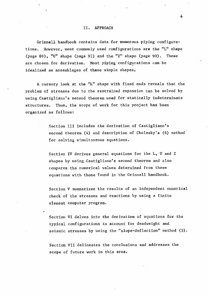
Section III includes the derivation of Castigliano's

second theorem (4) and description of Cholesky's (6) method

for solving simultaneous equations.

Section IV derives general equations for the L, U and Z

shapes by using Castigliano's second theorem and also

compares the numerical values determined from these

equations with those found in the Grinnell handbook.

Section V summarizes the results of an independent numerical

check of the stresses and reactions by using a finite

element computer program.

Section VI delves into the derivation of equations for the

typical configurations to account for deadweight and

seismic stresses by using the "slope-deflection" method (5).

Section VII delineates the conclusions and addresses the

scope of future work in this area.

5

Section VIII contains a list of important references used

for this thesis.

Appendix A contains catalogue cuts from the Grinnell hand-

book with a solution to a sample problem. It is recommended

that a reader not familiar with piping analysis review

Appendix A before the rest of the text.

Appendix B lists the data created for "L" shape with an

intermediate restraint.

6

III. THEORETICAL BACKGROUND

3.1 Energy Method of Castigliano (4)

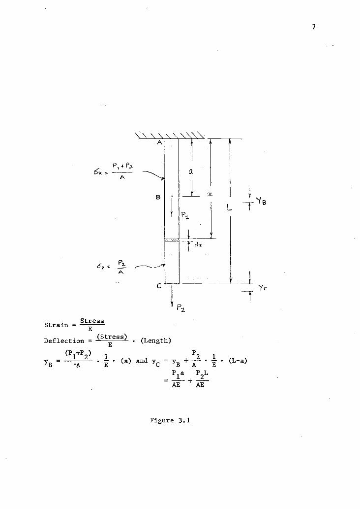
Consider a relatively long vertical weightless bar of length

L and cross-sectional area A supported at the top and axially loaded

as shown in Figure 3.1.

The strain energy UAL. for Section AB is

1(P1 +13 2

P1+P

2) (P

1+P

2)

2

UAB

=(:4 xe x)2 2 A AE

AB 2A2E

and for Section BC

P22

xcxl. 1 P2) P2 "2

UBC =((2 2(:A (AE)C 2A

2E

Hence, the total strain energy stored in the bar is

a

U = UAB

A dx + UBC

A dx

0 a

2 L 2

'2E -"

a,=

a

(Pli-P)2AE

2dx +

2A

0 a

(P1+P

2)2a P

2

2(L-a)

2AE 2AE

Castigliano's second theorem can now be stated as follows:

The partial derivative of the expression for the total

strain energy stored in a body with respect to a load

acting on the body gives the expression for the displacement

1'4P2z.)c -

A

(5i

A

Strain =Stress

Deflection

yB

E(Stress)

E(P

1+P

2)

1

(Length)

E(a) and yc = yB

2

Pla P2L

AE AE

Figure 3.1

(L-a)

7

8

at the point of load application in the direction of the

load. In the event that the load is a moment, or a torque,

the displacement at the point of application will take the

form of an angle of rotation.

The theorem can be proved by taking the partial derivatives of

U with respect to forces P1 and P2

. We obtain

and

aU(P

1+P

2)a

aP1

= yB

aU.(P

1+P

2)a P

2(L-a) P

1a P2L

=P2 AE AE AE AE YC

where yB and can be readily recognized as the expressions for the

displacements at B and C, respectively.

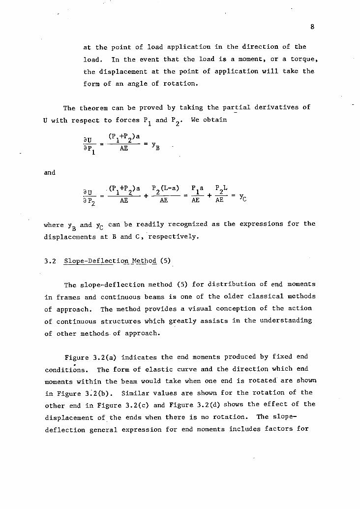
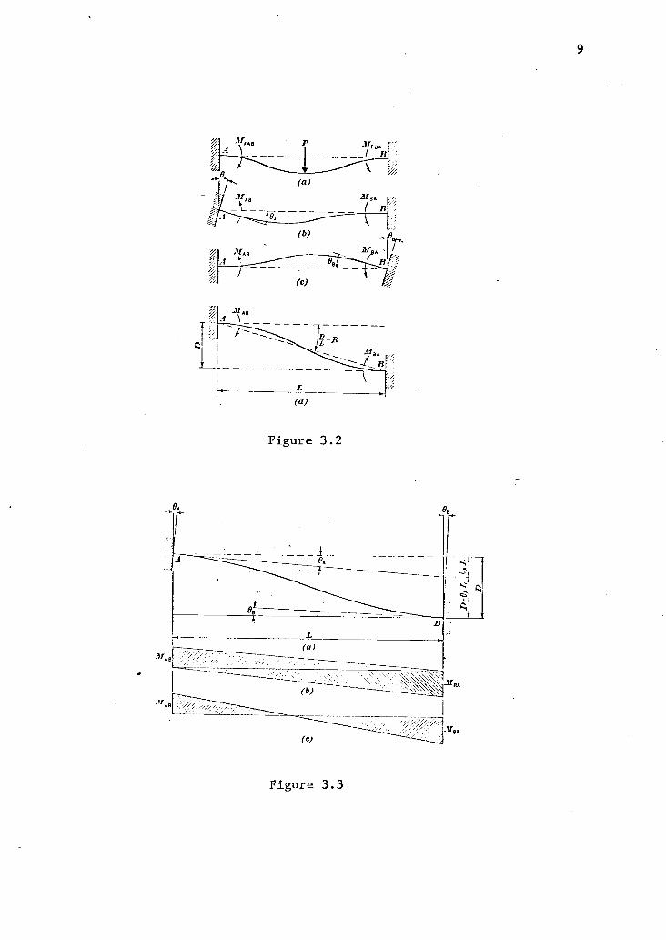
3.2 Slope-Deflection Method (5)

The slope-deflection method (5) for distribution of end moments

in frames and continuous beams is one of the older classical methods

of approach. The method provides a visual conception of the action

of continuous structures which greatly assists in the understanding

of other methods of approach.

Figure 3.2(a) indicates the end moments produced by fixed end

conditions. The form of elastic curve and the direction which end

moments within the beam would take when one end is rotated are shown

in Figure 3.2(b). Similar values are shown for the rotation of the

other end in Figure 3.2(c) and Figure 3.2(d) shows the effect of the

displacement of the ends when there is no rotation. The slope-

deflection general expression for end moments includes factors for

9

Figure 3.2

ArA8

(a)

Figure 3.3

10

each of these conditions which, when properly evaluated, will give

the amount of the end moment for any existing condition.

Figure 3.3(a) indicates a condition in which clockwise rotation

of the end supports has been assumed. Let OA represent the angular

rotation of end A, 0B

the angular rotation of end B, and D the

displacement. Displacement is measured with respect to a line

connecting the positions of the ends when the beam is in its

unstressed condition. The end moment at end A of the beam AB will

be called MAB and that at the opposite end, MBA. These end moments

may be represented by triangular moment diagrams as shown in

Figure 3.3(b). The elastic deflection of point B from the tangent at

point A is seen to be D-0AL. The moment of M/EI areas between A and

B about point B must equal D-OAL. The change in slope to the end

tangents from A to B will be 0B-0A, or the area of the M/EI diagram

from A to B must be equal to 0B-0

A.The two equations which are

obtained when the areas and arms are expressed in terms of the end

moments and spans are:

MABL2L

MDA

LL

2E1 x 3 + 2E1 x -3- D °AL

AB L MBAx + xL =NO e

EI 2 EI 2 B A

A value for MAB

may be found from these equations by eliminating

MBA as follows:

Eq. 3.2.1

Eq. 3.2.2

6EIOA

2NAB 1- NBA

GEID

L2

NAB + MBA

2EIOA 2EIOB

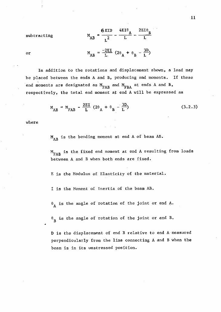
subtracting

or

6EID 4EIeA

2EI6B

MAB

L2

AB

LEI(26

A+ 0

B L-32

)

11

In addition to the rotations and displacement shown, a load may

be placed between the ends A and B, producing end moments. If these

end moments are designated as MFAB and NBA at ends A and B,

respectively, the total end moment at end A will be expressed as

where

m= 2

1E.,

3D

AB ic

(20A

+ 0B

- )

MAB

is the bending moment at end A of beam AB.

(3.2.3)

NAB is the fixed end moment at end A resulting from loads

between A and B when both ends are fixed.

E is the Modulus of Elasticity of the material.

I is the Moment of Inertia of the beam AB.

6A is the angle of rotation of the joint or end A.

Bis the angle of rotation of the joint or end B.

D is the displacement of end B relative to end A measured

perpendicularly from the line connecting A and B when the

beam is in its unstressed position.

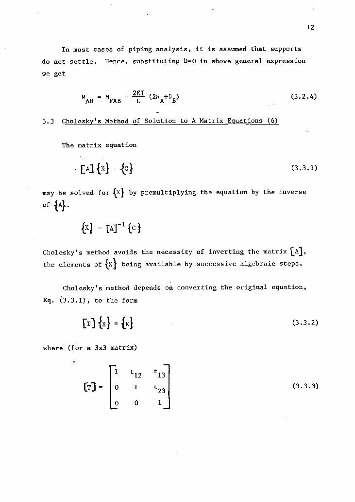
In most cases of piping analysis, it is assumed that supports

do not settle. Hence, substituting D=0 in above general expression

we get

2E1M= M,AB MFAB L

(28A B

)

3.3 Cholesky's Method of Solution to A Matrix Equations (6)

The matrix equation

EA] {,X3 =

12

(3.2.4)

(3.3.1)

may be solved for 0 by premultiplying the equation by the inverse

of {A }.

LX= rie {c}

Cholesky's method avoids the necessity of inverting the matrix tA3,

the elements of W being available by successive algebraic steps.

Cholesky's method depends on converting the original equation,

Eq. (3.3.1), to the form

[T3 {x) {K1

where (for. a 3x3 matrix)

t12

t13

[i] = 0 1 t23

0 0 1

(3.3.2)

(3.3.3)

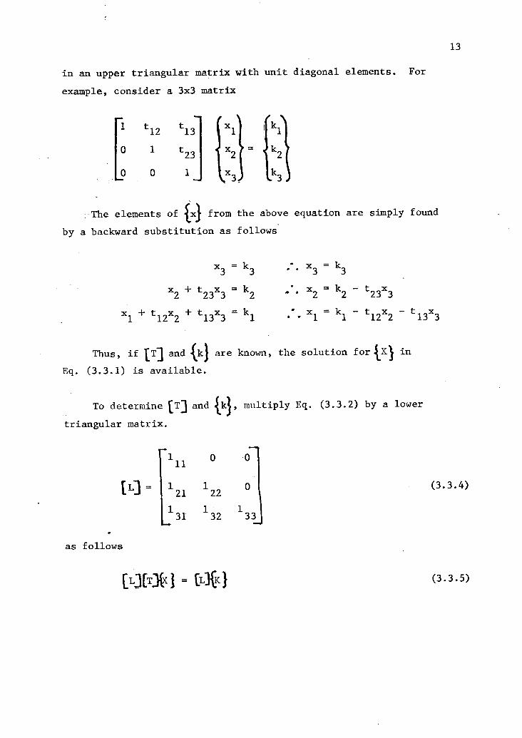
in an upper triangular matrix with unit diagonal elements. For

example, consider a 3x3 matrix

0 0 1

1

x2

=1 t23

x3 k3

0

{i

1 t12

t

The elements of {x) from the above equation are simply found

by a backward substitution as follows

x3 = k3

x2 t23x3 k2

xl t12x2 t13x3 kl

x3 = k3

x2 = k2 - t23x3

xl kl t12x2 - t13x3

Thus, if IT] and {lc} are known, the solution forILK1 in

Eq. (3.3.1) is available.

To determine [T] and tki, multiply Eq. (3.3.2) by a lower

triangular matrix.

[L]

as follows

ylll0 0

121 122

1 1 131 32 33

[LIT)(x) = (13(K}

13

(3.3.4)

(3.3.5)

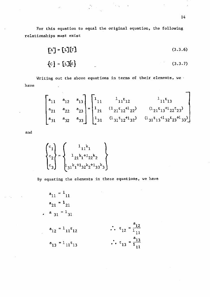
14

For this equation to equal the original equation, the following

relationships must exist

[A] = (131T)

.(c =

Writing out the above equations in terms of their elements, we-

have

NNW

alla12

a13

111 111112 111113

a21

a22 a23 21

(121

t12+1

22)

(121t 13+122t23)

a31 a32 a33 131 (1

31t12+1

32) (1

31t13

+132

t23

+13

and

cl

C21

c3

I11k

1

121

k1+1

22k2

3k1+1

32k2+1

33k3

By equating the elements in these equations, we have

all= 1

11

a21

= 121

a = 131 31

a = 1 t12 11 12

a131

13 11113

15

a22

= (121

t12+1

22)

(121t13+122t23)

.6- 122

= a -1 t22 21 12

a23t23 t

22

(a23 21

t13

)

a32. 1

32= a

32-1

31t12

a33

= (131

t13+1

32t23+1

33) .. 133 a33-L31t13-132123

c1= 1

11k1

c2

= 121

k1+1

32k2

c3= 1

31k

1+1

32k2+1

33k3

k =1

k2

k3 =

c1

111

1 (

r, -2

(c3-1

k21 1

)

k32k2)

1

33

Thus, the elements of the matrices [13, (T) and tKi are now available

in terms of the known elements of CA] and {C) and Eq. (3.3.1) may be

solved without inverting the matrix [A].

Reference (6) describes a generalized form of the above method

for nxn matrix. A method for 3x3 matrix will suffice for the

following analysis.

16

IV. THERMAL ANALYSIS OF L, U AND Z SHAPES

This section deals with developing general relations for the

three most common piping configurations (viz L, U and Z) subjected

to a temperature differential.

Castigliano's second theorem is used to derive these relations

because movements of the released ends can be easily determined

by using known linear expansions (aATL) which then can be equated to

the partial derivative of the total strain energy with respect to

unknown reactions, 3U/3F; thus, a general expression for unknown

reactions can be determined. The expressions for these are then

compared with the ones given in the Grinnell handbook for corre-

sponding shapes.

Substitution of numerical values for L/h into these expressions

yields values for kx , ky

and kb. The values thus determined are close

to the ones given in the Grinnell handbook. The maximum variation

is approximately 3% although most common variation is 2%. The values

are calculated by using a programmable calculator which rounds off

only the final answer and not the intermediate results. This may

explain the difference in numerical values from the Grinnell handbook.

17

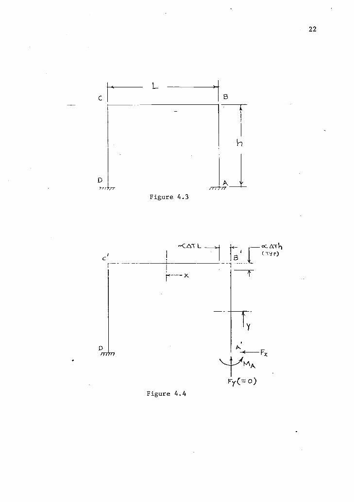
IV.A. Analysis of "L", "U" and "Z" Configurations

Figures 4.1, 4.3 and 4.5 show "L", "U" and "Z" configurations. All

the configurations are clamped at two ends preventing the translation

and rotation of the ends. They are all subjected to a temperature dif-

ferential due to the high-temperature fluid inside the pipe giving rise

to a temperature differential AT °F.

To determine the end reactions and moments of this statically inde-

terminate problem, we can release end A in each case. Due to the ther-

mal expansion, point A will move to a new location A'.

Figures 4.2, 4.4 and 4.6, respectively, show the "L", "U"'and "Z"

configurations in the above situation.

The derivation of the general equations is based on the fact that

forces Fx

and F and a moment MA

is applied to the end A to bring it

back to its original position before the thermal expansion.

Analysis of "L" Configuration:

To bring A' back to A, we apply forces Fx

and F and a moment MA

as shown in Figure 4.2.

Thus, the moment on leg BA is MBA = (Fx)y + MA.

Similarly, the moment on leg CB is MCB = (Fx)h - (F )x + MA.

Therefore, the total strain energy is

h 2 2

U =(MBA) dy +

(NCB)dx

2E1 2E10 0

ht(Fx)y + MA)2 jr:L L(Fx)h - (Fy)x + MA]2

2E1 2IE1dxdy +

0

Figure 4.1

2C

A

--1

MA

Figure 4.2

A

B

-17

Fy

cc LYN" L

18

According to Castigliano's second theorem, partial derivatives of

U with respect to Fes, Fy

and MA should yield the movements along

Fx

and F and rotation at A.y

3U DU 3U- Lx, = Ay and = e

aFx

aFy 3MA

where Ax = LaAT, Ay = haAT and 0 = 0

Then

Similarly,

19

h2CF y+M:3 L 21.(F)h-(Fy)x+MO

DF

DU

(2E1

) A(Y)dY +f 2E1

(h)dx = aATL

x0

-3- +h L)Fx

L2F + (h2

+hL)M = aATLEI1 3 2

y 2(4.1)

h rau f 2[(Fx)y +MA

(0)dy

]L21.(Fx)h(Fy)x+mt)

aF 2E1 2E1( x)dx

Y 0 0

= aLTh

2hL

2Fx +

1L3Fy - 1 L2M = aAThEI

and finally;

h21(F):

)

au211(Fx)h(F )x-Fm

(1)dy +y 18:

1(1)dx =

Aam 2E1 2E1

0 0

(4.2)

2

1h2+hL F

x1L2Fy+ (h+L)M

A= 0

2

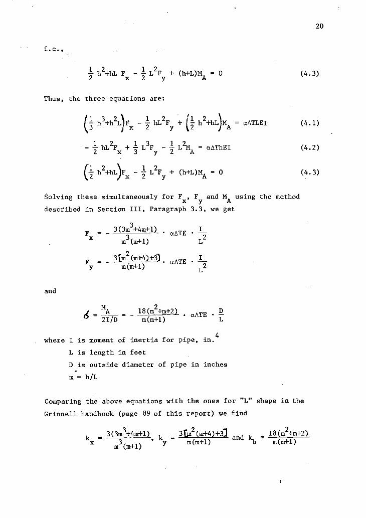
Thus, the three equations are:

(1 h3+h2L)Fx 2

- hL2Fy 2+ (1 h2+hL)M

A= aATLEI

3

- 1 hL2Fx+ 1 L3F

y2 1-L M = aAThEI

A

20

(4.3)

(4.1)

(4.2)

h2+hL)Fx - L2Fy + (h+L)MA = 0 (4.3)

Solving these simultaneously for Fx, F

yand M

Ausing the method

described in Section III, Paragraph 3.3, we get

and

3(3m3+4m+1)

Fxx - aATEm3(m+1) L`

F =3lm

2(m+4)+1

aATEI

Y m(m+1)L2

6MA 18(m

2+m+2)

aATE D2I/D m(m+1)

where I is moment of inertia for pipe, in.4

L is length in feet

D is outside diameter of pipe in inches

m = h/L

Comparing the above equations with the ones for "L" shape in the

Grinnell handbook (page 89 of this report) we find

3(3m3+4m+1)

k -3br

2(m+4)+33 18(m

2+m+2)

kx = , and kbm3

(m+1)m(m+1) m(m+1)

21

Table 4.1 shows a comparison of the values of kx y, k and kb, as shown

in the Grinnell handbook (page 89 of this report), and the ones calcu-

lated using above relationships.

As seen from the table, the values are similar with only minor

differences probably due to rounding errors.

Analysis of a "U" Configuration:

The legs DC and BA are assumed to be of equal length. Thus, to

bring A' back to A, we apply force Fx and moment MA as shown in

Figure 4.4.

The moment on leg BA is

MBA (Fx)Y MA

The moment on leg CB is

mcB (Ex)hMA

and the moment on leg DC is

MDC (Fx)Y MA


h(MBA) (MCB)

2 h 2 h(MDC)2

2E1

' SU = dy +

52E1

dy +2E1

dy

0 0 0

h

SUFx

2E1

)y - MA]2 1,

[(Fx

2E1

)h -Mi2

= dy + dx

0 0

[(Fx)y MA]2

2E1

0

/7/7/1

Figure 4.3

mu/

.o.0 AT L

I

Figure 4.4

A.

MA

Fy(= 0)

oC AT hCry?)

22

According to Castigliano's second theorem, partial derivatives of U

with respect to Fx and MA should yield the movement along Fx and

rotation at A.

3U= Ax and aU

a= 0

3Fx

mA

where Ax = aATL and 0 = 0.

Thus,

hau

q(Fx)y M] 2[(Fx)h m;)= 2

AJ " h dx3Fx

2E1 2E1

0 0

= aATL

h

2(2h + L)Fx - h(h+L)M

A= aATLEI

3

Similarly,

DU= 2

2[(Fx)y MA](-1)dy +

2[(Fx)h MA]

3MA 2E1 2E1( 1)dx

= 0

0 0

23

(4.4)

h(h+L)Fx - (2h+L)MA = 0 (4.5)

therefore, the equations are

and

h2(2h+3L)F - 3h(h+L)M

A= 3aATLEI (4.4)

h(h+L)Fx - (2h+L)MA = 0 (4.5)

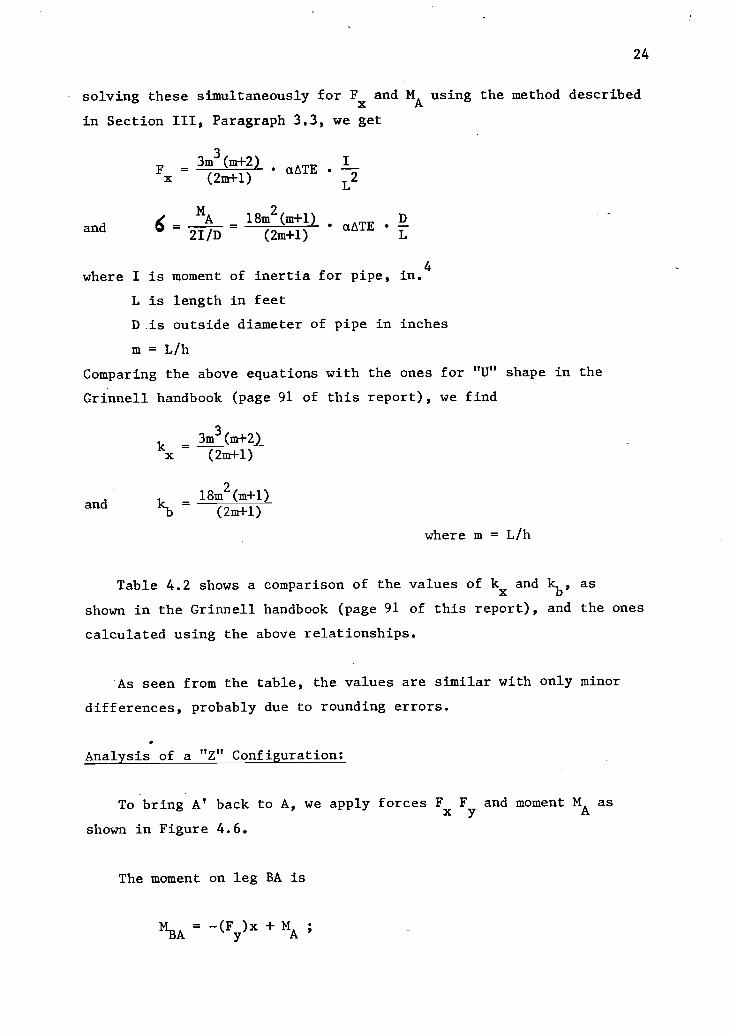
24

solving these simultaneously for Fx and MA using the method described

in Section III, Paragraph 3,3, we get

and

3m3F (m+2) GATEx (2m+1)

6 MA 18m2(m+1)

DGATE2I/D (2m+1)


L is length in feet


m = L/h

Comparing the above equations with the ones for "U" shape in the

Grinnell handbook (page 91 of this report), we find

and

k3m

3(m+2)

x (2m+1)

18m2(m+1)

kb(2m+1)

where m = L/h

Table 4.2 shows a comparison of the values of kxand kb, as

shown in the Grinnell handbook (page 91 of this report), and the ones

calculated using the above relationships.


differences, probably due to rounding errors.

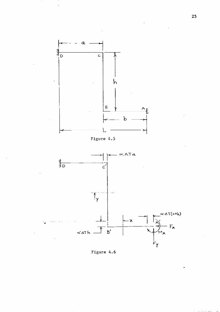
Analysis of a "Z" Configuration:

To bring A' back to A, we apply forces Fx

Fyand moment M

Aas

shown in Figure 4.6.

The moment on leg BA is

MBA = -(Fy)x + MA ;

Q

D

r

L

b

Figure 4.5

h

cK L\T

Figure 4.6

czAT(a+b)

I Ai

FY

A

Fx

25

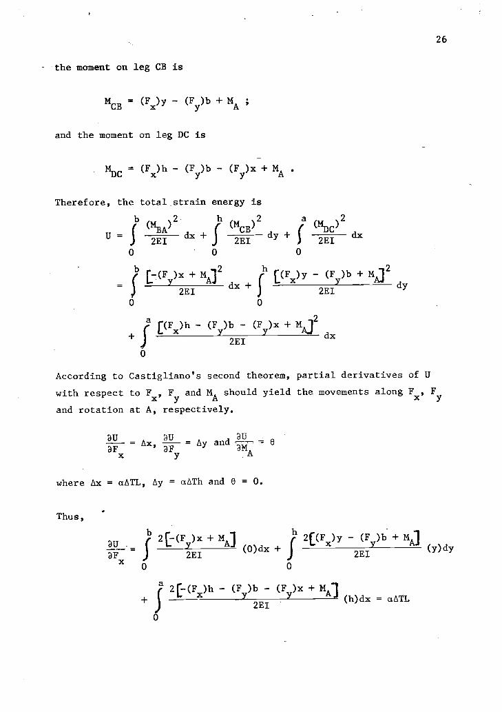
26

the moment on leg CB is

MCB(Fx)y - (F )b + MA ;

and the moment on leg DC is

MDC = (Fx)h - (F )b - (F )x + MA .


b 2 2 a 2

S (MBA)dx +

jdy +

r1 (MCB) (MDC)U = dx

2E1 2E1 2E1

0 0 0

b h(Fy)x + NO

2

dx +[(Fx)y - (Fy

d

)b + Mj2

= y2E1 2E1

0 0

a[(Fx)h - (F )b - (F )x + 1

2

+y y

"""' dx2E1

0

According to Castigliano's second theorem, partial derivatives of U

with respect to F , F and MA should yield the movements along F , Fx y x y

and rotation at A, respectively.

311 DU

Ax,= Ay and

DU0

8F Fx

aFy A

where Ax = aATL, Ay = aATh and 6 = 0.

Thus,

3U .

2E1

2 F )x + MA]

(0)dx +21(Fx)y - (F )b + MLA]

aF 2E1(Y)dY

x0 0

0

a2(E(Fx)h - (F )b - (F )x + MA]

2E1(h)dx = aATL

27

3h3 +h2Fx--2-

) hh2 1-2--

) (1ha

2Fy 2+ h

2+ ha)M

A

= EIaATL (4.7)

Similarly,

DU 2[-(F )x MA]2[(Fx)y (Fy)b + M

3F 2E1

A]( x)dx + (-b)dy

y0 0-

a2I(Fx)h - (F )b - (F )x + MAI

2E1(-b-x)dx = aATh

0

(1 2 1 2) 1 3 2 2 2 1 3)- .y. bh + bha + -2- ha + -j- b +bh+b a + ba +3 a F

y

- -i1 2 1 )b + bh + ba +

-2-

aMA

= MaATh(

(4.8)

and finally,

DUJ-13 2[7(F )x + MAJ rh 2L(Fx)y - (F )b + MA)

(1)dx + (1)dyDMA 2E1 2E1

0 0

JP 2 1..(Fx)h(F )b - (F )x + MA]

(1)dx = 02E1

0

h2+ ha F

x1

- b2+ bh + ba + 1 a

9Fy+ (b + b + a)M

Az 2

= 0 (4.9)

28

Therefore, the equations are

3

(1 (1 1 1h3+ h2 a)Fx -2- bh

21-+ bha + hat Fy + 2 h2 + ha MA

= EIaAT (a + b) (4.7)

-(1 2 1 2) (1 3 2 2 2 1 3)+ bha ha Fx + V3* +bh+ba+ ba +bh

-2

(, 2 1 2)b + bh + ba + a MA = AIaLTh (4.8)

(1 2 ) (1 2 1 2)h + ha Fx f b + bh + ba + T a F + (b + h + a)MA

Y

= 0 (4.9)

Solving these equations simultaneously to get a long hand or

general solution is difficult. But the task can be greatly simplified

for specific numerical values for the ratio of a/b.

Thus, substituting a/b=1 (or a=b=L/2) we get simplified equations

as follows

2h2(3b+h)F

x- 3bh(3b+h)F + 3h(3b+h)M

A= 12EIaATb

-3bh(3b+h)Fx

+ 2b2(8b+3h)F 6b(2b+h)M

A= 6EIaATh

hF 2bF + 2MA

= 0. x

Solving Equations 4.10, 4.11 and 4.12 simultaneously for Fx

, Fy

and

MA

using the method described in Section III, Paragraph 3.3, we get

Fx

=24m(2m2+3)

Ea1T(3m+4) L2

F =24(3m

3+6m+2)

EaATy m(3m+4)

L2

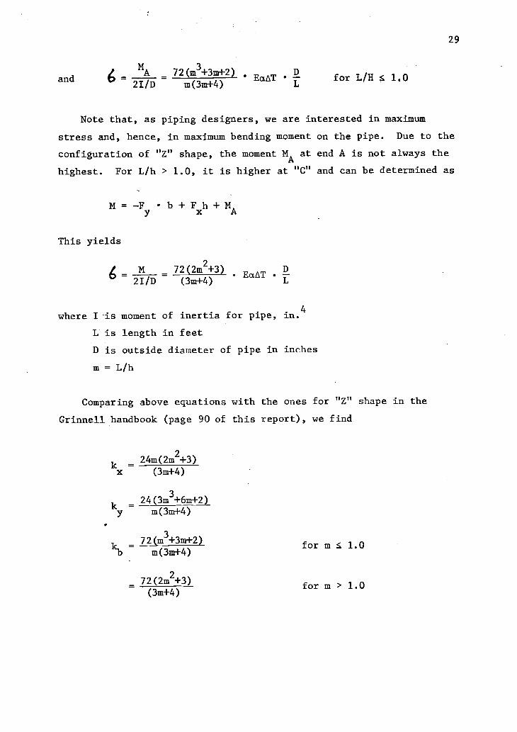
29

and 6 =MA 72(m

3+3m+2)

EaATD

for L/H 5 1.02I/D m(3m+4)

Note that, as piping designers, we are interested in maximum

stress and, hence, in maximum bending moment on the pipe. Due to the

configuration of "Z" shape, the moment MA at end A is not always the

highest. For L/h > 1.0, it is higher at "C" and can be determined as

M = -Fy b + Fxh + MA

This yields

2

6 = 2I/D 7T17-44)-3)EaAT -12-


L is length in feet


m = L/h

Comparing above equations with the ones for "Z" shape in the

Grinnell handbook (page 90 of this report), we find

24m(2m2+3)

kx (3m+4)

k =24(3m

3+6m+2)

y m(3m+4)

=72(m

3+3m+2)

kbm(3m+4)

72(2m2+3)

(3m+4)

for m 5 1.0

for m > 1.0

30

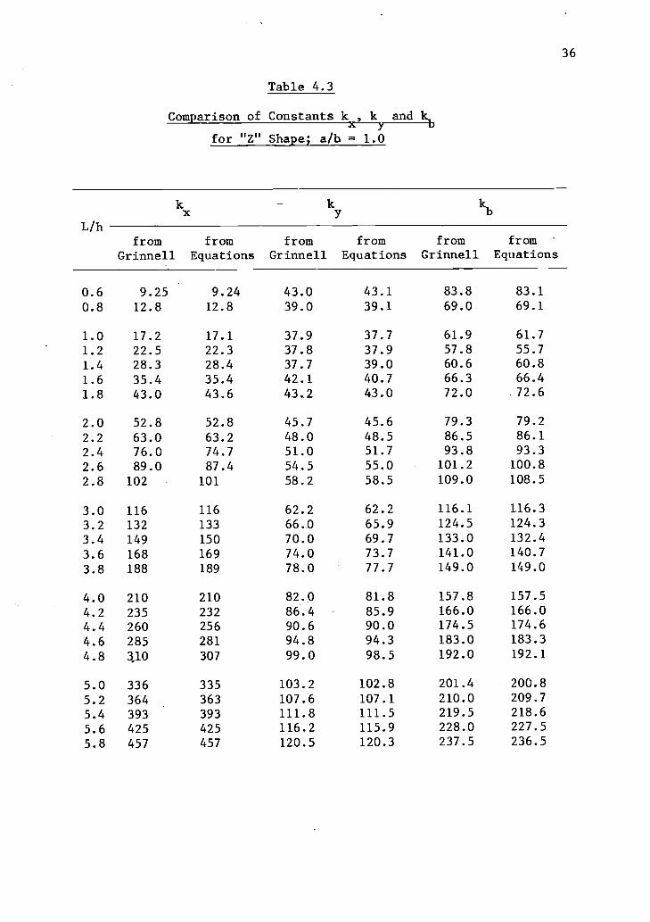
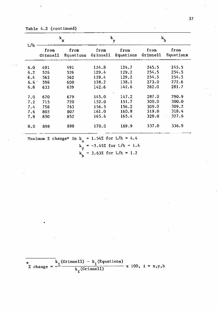
Table 4.3 shows a comparison of the values of k , kyand kb as shown

xin the Grinnell handbook (page 90 of this report) and the ones cal-

culated using above relationships.


differences, probably due to rounding errors.

31

IV.B. Comparison of Numerical Constants

Table 4.1, 4.2 and 4.3 on the following pages show a comparison

of numerical constants computed from the general equations for "L",

"U" and "Z" configurations.

The constants were computed using HP-67 programmable calculator.

Rounding of the decimals was limited to the final answer. This may

explain the small differences between the constants as shown in the

Grinnell handbook and the ones calculated using generalized equations.

The tables prove the similarity of theoretical basis used by the

Grinnell handbook and the one developed in the previous section.

32

Table 4.1

Com arison of Constants k , k and for "L" Sha e

L/h

k kkb

fromGrinnell

fromEquations

fromGrinnell

fromEquations

fromGrinnell

fromEquations

1.0 12.0 12.0 12.0 12.0 36 36

1.2 17.2 17.2 12.5 12.5 46 46

1.4 23.0 23.8 13.4 13.2 58 57

1.6 32.0 32.0 14.4 14.2 71 71

1.8 42.0 42.0 15.4 15.3 85 86

2.0 54.0 54.0 16.6 16.5 102 102

2.2 68.3 68.1 17.8 17.8 120 120

2.4 84.4 84.4 19.2 19.1 140 139

2.6 103 103 20.6 20.6 161 160

2.8 125 124 22.0 22.0 184 183

3.0 150 149 23.5 23.5 209 207

3.2 175 175 25.0 25.0 234 232

3.4 207 205 26.5 26.6 259 259

3.6 237 238 28.0 28.1 287 288

3.8 274 275 29.5 29.7 318 318

4.0 315 314 31.5 31.4 349 349

4.2 356 358 33.0 33.0 381 382

4.4 406 405 34.6 34.6 414 416

4.6 456 456 36.2 36.3 450 452

4.8 510 511 37.8 37.9 487 489

5.0 570 570 39.5 39.6 528 528

5.2 630 633 41.2 41.3 569 568

5.4 700 701 43.0 43.0 610 610

5.6 775 774 44.7 44.7 652 653

5.8 855 851 46.2 46.4 696 697

6.0 938 933 48.2 48.1 743 743

6.2 1,020 1,021 49.8 49.8 790 791

6.4 1,110 1,113 51.6 51.5 840 839

6.6 1,212 1,211 53.4 53.2 892 890

6.8 1,313 1,314 55.0 54.9 944 941

33

Table 4.1 (continued)

L/h

kx kykb

fromGrinnell

fromEquations

fromGrinnell

fromEquations

fromGrinnell

fromEquations

7.0 1,426 1,423 56.8 56.7 997. 994

7.2 1,517 1,537 58.6 58.4 1,050 1,049

7.4 1,655 1,658 60.2 60.1 1,104 1,105

7.6 7,785 1,784 61.8 61.9 1,159 1,163

7.8 1,917 1,917 63.6 63.6 1,219 1,222

8.0 2,059 2,056 65.4 65.4 1,284 1,282

Maximum % change* in kx = -3.48% for L/h = 1.4

k = 1.49% for L/h = 1.4

kb = 1.72% for L/h = 1.4

k.1 (Grinnell) - ki(Equations)

% change = x 100, i = x,y,bki(Grinnell)

34

Table 4.2

Comparison of Constants kx and kb for "U" Shape

L/h

kx kb

fromGrinnell

fromEquations

fromGrinnell

fromEquations

0.2 0.0377 0.0377 0.617 0.617

0.3 0.1165 0.1164 1.308 1.316

0.4 0.256 0.256 2.232 2.240

0.5 0.469 0.469 3.370 3.375

0.6 0.765 0.766 4.580 4.713

0.7 1.191 1.158 6.430 6.248

0.8 1.68 1.65 8.110 7.975

0.9 2.38 2.27 10.39 9.894

1.0 3.00 3.00 12.00 12.00

1.2 4.88 4.88 16.74 16.77

1.4 7.37 7.37 22.26 22.28

1.6 10.55 10.53 28.56 28.53

1.8 14.48 14.45 35.52 35.50

2.0 19.2 19.2 43.20 43.20

2.2 24.6 24.8 52.32 52.63

2.4 31.4 31.5 60.72 60.78

2.6 39.2 39.1 70.56 70.65

2.8 48.0 47.9 81.24 81.25

3.0 57.8 57.9 92.64 92.57

3.2 69.1 69.1 104.5 104.6

3.4 82.2 81.6 118.2 117.4

3.6 95.6 95.6 130.8 130.9

3.8 111.0 111.0 138.4 145.1

4.0 128.1 128.0 160.0 160.0

4.2 147.0 146.6 176.1 175.6

4.4 166.6 166.9 192.0 192.0

4.6 189.0 188.9 208.8 209.1

4.8 213.0 212.8 227.4 226.9

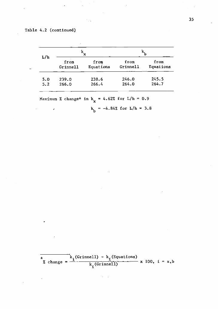
35


L/hkx kb

from from from fromGrinnell Equations Grinnell Equations

5.0 239.0 238.6 246.0 245.5

5.2 266.0 266.4 264.0 264.7

Maximum % change* in kx = 4.62% for L/h = 0.9

kb = -4.84% for L/h = 3.8

k.1 (Grinnell) k.(Equations)% change =

k (Grinnell)x 100, i = x,b

36

Table 4.3

Comparison of Constants kx2

k--y

and kb

for "Z" Shape; a/b = 1.0

L/h

kx

fromGrinnell

fromEquations

fromGrinnell

fromEquations

fromGrinnell

fromEquations

0.6 9.25 9.24 43.0 43.1 83.8 83.1

0.8 12.8 12.8 39.0 39.1 69.0 69.1

1.0 17.2 17.1 37.9 37.7 61.9 61.7

1.2 22.5 22.3 37.8 37.9 57.8 55.7

1.4 28.3 28.4 37.7 39.0 60.6 60.8

1.6 35.4 35.4 42.1 40.7 66.3 66.4

1.8 43.0 43.6 43..2 43.0 72.0 72.6

2.0 52.8 52.8 45.7 45.6 79.3 79.2

2.2 63.0 63.2 48.0 48.5 86.5 86.1

2.4 76.0 74.7 51.0 51.7 93.8 93.3

2.6 89.0 87.4 54.5 55.0 101.2 100.8

2.8 102 101 58.2 58.5 109.0 108.5

3.0 116 116 62.2 62.2 116.1 116.3

3.2 132 133 66.0 65.9 124.5 124.3

3.4 149 150 70.0 69.7 133.0 132.4

3.6 168 169 74.0 73.7 141.0 140.7

3.8 188 189 78.0 77.7 149.0 149.0

4.0 210 210 82.0 81.8 157.8 157.5

4.2 235 232 86.4 85.9 166.0 166.0

4.4 260 256 90.6 90.0 174.5 174.6

4.6 285 281 94.8 94.3 183.0 183.3

4.8 110 307 99.0 98.5 192.0 192.1

5.0 336 335 103.2 102.8 201.4 200.8

5.2 364 363 107.6 107.1 210.0 209.7

5.4 393 393 111.8 111.5 219.5 218.6

5.6 425 425 116.2 115.9 228.0 227.5

5.8 457 457 120.5 120.3 237.5 236.5

37


L/h

k kx kb

fromGrinnell

fromEquations

fromGrinnell

fromEquations

fromGrinnell

fromEquations

6.0 491 491 124.8 124.7 245.5 245.5

6.2 526 526 129.4 129.2 254.5 254.5

6.4 562 562 129.4 129.2 254.5 254.5

6.6- 598 600 138.2 138.1 273.0 272.6

6.8 633 639 142.6 142.6 282.0 281.7

7.0 670 679 145.0 147.2 287.0 290.9

7.2 715 720 152.0 151.7 300.0 300.0

7.4 758 763 156.5 156.2 309.0 309.2

7.6 803 807 161.0 160.8 319.0 318.4

7.8 850 852 165.6 165.4 328.0 327.6

8.0 898 898 170.0 169.9 337.0 336.9

Maximum % change* in kx = 1.54% for L/h = 4.4

k = -3.45% for L/h = 1.4ykb = 3.63% for L/h = 1.2

k.(Grinnell) - ki(Equations)% change =

k.(Grinnell)x 100, i = x,y,b

38

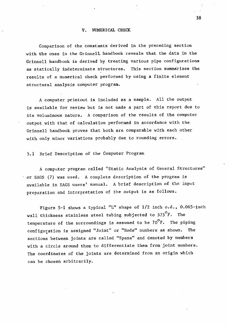
V. NUMERICAL CHECK

Comparison of the constants derived in the preceding section

with the ones in the Grinnell handbook reveals that the data in the

Grinnell handbook is derived by treating various pipe configurations

as statically indeterminate structures. This section summarizes the

results of a numerical check performed by using a finite element

structural analysis computer program.

A computer printout is included as a sample. All the output

is available for review but is not made a part of this report due to

its voluminous nature. A comparison of the results of the computer

output with that of calculation performed in accordance with the

Grinnell handbook proves that both are comparable with each other

with only minor variations probably due to rounding errors.

5.1 Brief Description of the Computer Program

A computer program called "Static Analysis of General Structures"

or SAGS (7) was used. A complete description of the program is

available in SAGS users' manual. A brief description of the input

preparation and interpretation of the output is as follows.

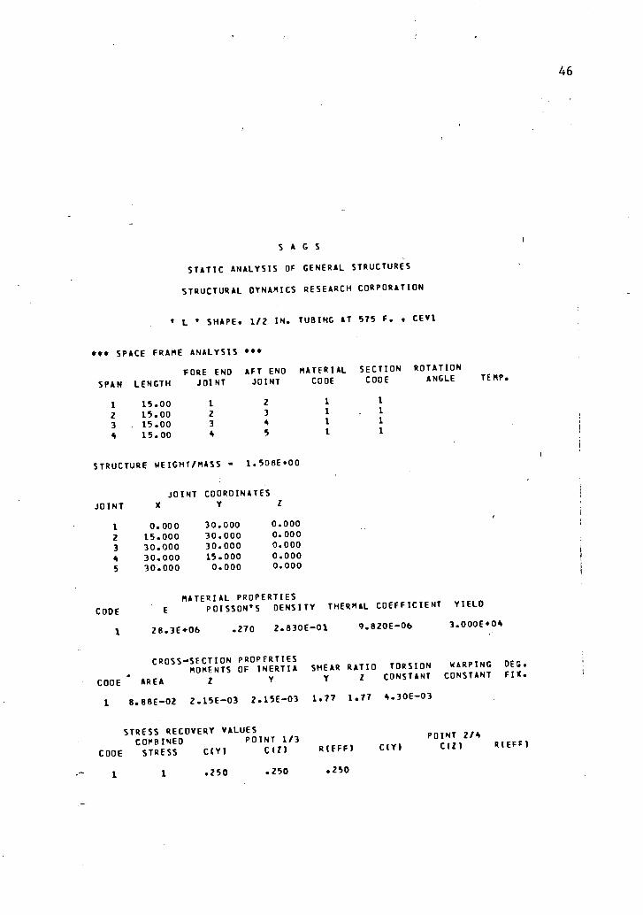
Figure 5-1 shows a typical "L" shape of 1/2 inch o.d., 0.065-inch

wall thickness stainless steel tubing subjected to 575°F. The

temperature of the surroundings is assumed to be 70°F. The piping

configuration is assigned "Joint" or "Node" numbers as shown. The

sections between joints are called "Spans" and denoted by numbers

with a circle around them to differentiate them from joint numbers.

The coordinates of the joints are determined from an origin which

can be chosen arbitrarily.

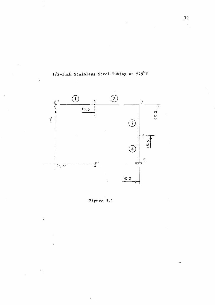
1/2-Inch Stainless Steel Tubing at 575°F

Figure 5.1

30.0

39

40

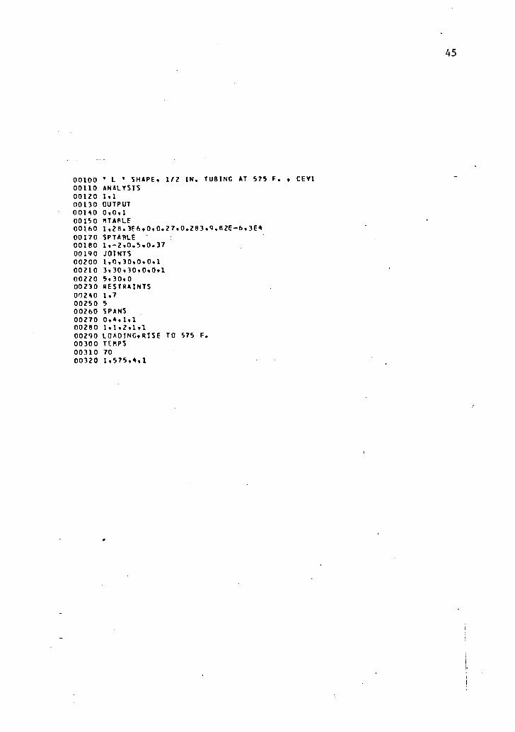
An input "file" was then prepared as follows: A title of maximum

72 characters forms a title "card" or line. The next four lines

denote the stress calculation and output printout options. Material

properties, such as Modulus of Elasticity, Poisson's Ratio, Density

and Coefficient of Linear Expansion, along with section properties,

such as outside the inside diameters, are then entered. The piping

geometry is entered by defining coordinates of all joints followed

by type and location of restraints and spans or connectivity of

joints. The final card is a loading card which specifies base tem-

perature (70°F) and design temperature (575°F). Page 45 shows a

copy of the file for L/h = 1.0 with L = 30 inches and h = 30 feet.

After processing this data, the computer prints out input data

(pages 46 and 47) and output results, such as joint displacements,

joint reactions and various stress components and combined stresses

(page 48). Note that the computer program takes into account

both bending and axial stresses while the Grinnell handbook method

can calculate only the bending stresses. Thus, it is expected

that joint reactions in the printout will be slightly different from

the ones calculated by using the Grinnell handbook. A more exact

computer program, such as ANSYS, can be used for a similar check, but

accuracy of "SAGS" results is sufficient for our work.

A file, such as the one shown on page 45 was prepared for each

of the three configurations as follows:

Temperature L/h Combinations

"L" Shape 575 °F 36

500°F 36

400°F 36

"U" Shape 575 °F 31

400°F 31

"Z" Shape 575 °F 38

400°F 38

Total 246

41

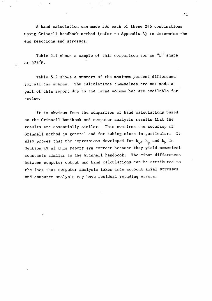
A hand calculation was made for each of these 246 combinations

using Grinnell handbook method (refer to Appendix A) to determine the

end reactions and stresses.

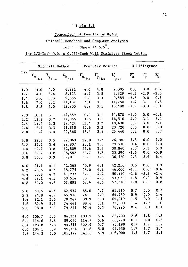
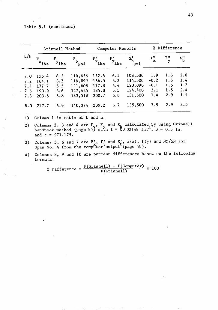
Table 5.1 shows a sample of this comparison for an "L" shape

at 575 °F.

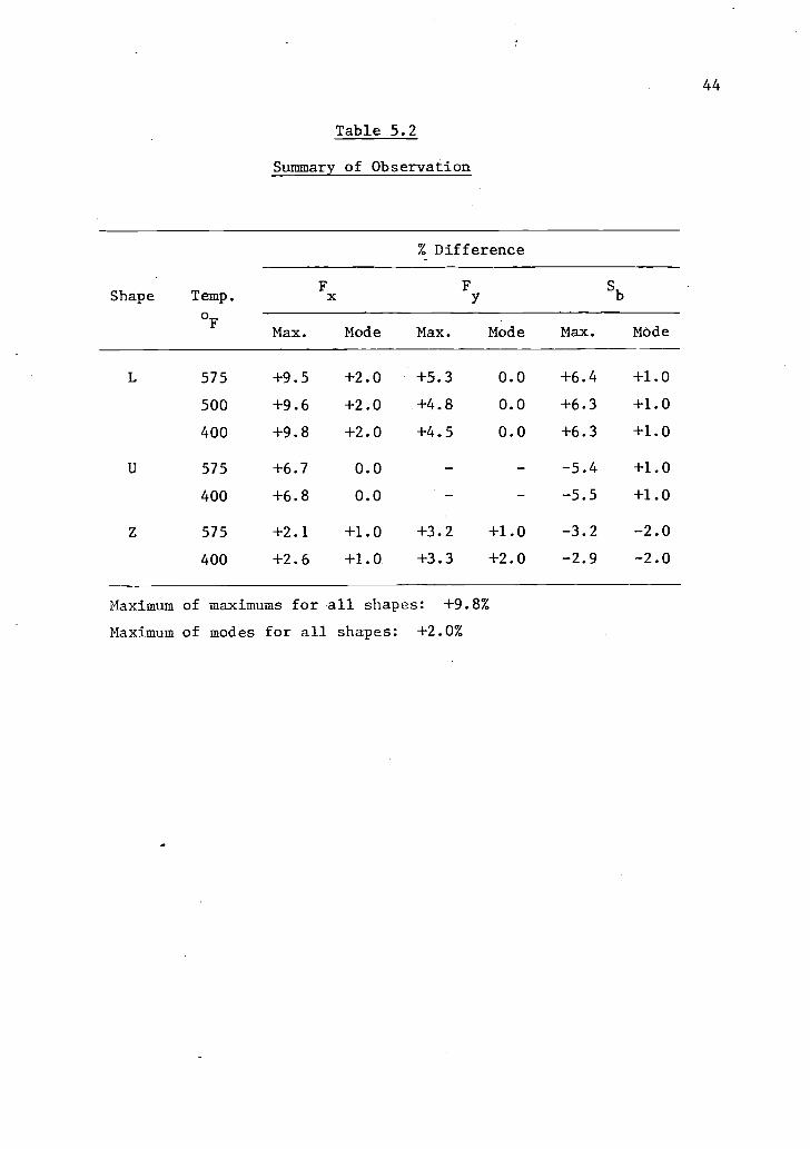
Table 5.2 shows a summary of the maximum percent difference

for all the shapes. The calculations themselves are not made a

part of this report due to the large volume but are available for

review.

It is obvious from the comparison of hand calculations based

on the Grinnell handbook and computer analysis results that the

results are essentially similar. This confirms the accuracy of

Grinnell method in general and for tubing sizes in particular. It

also proves that the expressions developed for kx, k and kb in

YSection IV of this report are correct because they yield numerical

constants similar to the Grinnell handbook. The minor differences

between computer output and hand calculations can be attributed to

the fact that computer analysis takes into account axial stresses

and computer analysis may have residual rounding errors.

42

Table 5.1

Comparison of Results by Using

Grinnell Handbook and Computer Analysis

for "L" Shape at 575°,

for 1/2-Inch 0.D. x 0.065-Inch Wall Stainless Steel Tubing

L/h

Grinnell Method Computer Results % Difference

F _ Fxlbs Ylbs

Sbpsi

F'

xlbsF'

YlbsS'bPsi

F"x

F"y

S"

1.0 4.0 4.0 6,992 4.0 4.0 7,005 0.0 0.0 -0.2

1.2 4.0 3.4 8,123 4.9 3.5 8,329 -4.3 -2.9 -2.5

1.4 5.6 3.3 9,656 5.8 3.3 9,585 -3.6 0.0 0.7

1.6 7.0 3.2 11,182 7.1 3.1 11,250 -1.4 3.1 -0.6

1.8 8.3 3.0 12,700 8.9 3.1 13,480 -7.2 -3.3 -6.1

2.0 10.1 3.1 14,859 10.2 3.1 14,870 -1.0 0.0 -0.1

2.2 12.2 3.2 17,055 11.6 3.1 16,510 4.9 3.1 3.2

2.4 14.4 3.3 19,424 13.4 3.2 18,430 6.9 3.0 5.1

2.6 16.7 3.3 21,818 15.6 3.3 20,720 6.6 0.0 5.0

2.8 19.4 3.4 24,368 18.4 3.4 23,460 5.2 0.0 3.7

3.0 22.3 3.5 27,063 22.0 3.5 26,780 1.3 0.0 1.0

3.2 25.2 3.6 29,837 25.1 3.6 29,530 0.4 0.0 1.0

3.4 29.4 3.8 32,809 26.6 3.6 30,840 9.5 5.3 6.0

3.6 32.2 3.8 35,582 32.7 3.8 35,890 -1.6 0.0 -0.9

3.8 36.5 3.9 39,011 33.1 3.8 36,520 9.3 2.6 6.4

4.0 41.1 4.1 42,368 40.9 4.1 42,250 0.5 0.0 0.3

4.2 45.5 4.2 45,775 46.0 4.2 46,060 -1.1 0.0 -0.6

4.4 50.8 4.3 49,233 52.1 4.4 50,410 -2.6 -2.3 -2.4

4.6 57.1 4.5 53,514 56.1 4.5 53,030 1.8 0.0 0.9

4.8 62.0 4.6 57,098 62.6 4.6 57,570 -1.0 0.0 -0.8

5.0 68.5 4.7 62,534 68.0 4.7 61,110 0.7 0.0 0.7

5.2 74.8 4.9 65,916 74.1 4.9 64,980 0.9 0.0 1.4

5.4 82.1 5.0 70,247 80.9 5.0 69,210 1.5 0.0 1.5

5.6 89.9 5.2 74,641 88.6 5.1 73,800 1.4 1.9 1.0

5.8 98.0 5.3 79,211 97.4 5.3 78,990 0.6 0.0 0.3

6.0 106.7 5.5 84,231 103.9 5.4 82,700 2.6 1.8 1.8

6.2 114.6 5.6 89,040 114.7 5.6 88,770 -0.1 0.0 0.3

6.4 123.8 5.8 94,311 122.9 5.7 93,190 0.7 1.7 1.2

6.6 134.1 5.9 99,764 131.8 5.8 97,930 1.7 1.7 2.4

6.8 144.2 6.0 105,177 141.6 5.9 103,000 1.8 1.7 2.1

43


L/h

Grinnell Method Computer Results % Difference

F F Sb x

F' F' 5' F" F" S"xlbs Ylbs psi lbs Ylbs bpsi

7.0 155.4 6.2 110,658 152.5 6.1 108,500 1.9 1.6 2.0

7.2 164.1 6.3 116,099 164.5 6.2 114,500 -0.2 1.6 1.4

7.4 177.7 6.5 121,608 177.8 6.4 120,090 -0.1 1.5 1.2

7.6 190.9 6.6 127,425 185.0 6.5 124,400 3.1 1.5 2.4

7.8 203.5 6.8 133,518 200.7 6.6 131,600 1.4 2.9 1.4

8.0 217.7 6.9 140,374 209.2 6.7 135,500 3.9 2.9 3.5

1) Column 1 is ratio of L and h.

2) Columns 2, 3 and 4 are F , F, and Sh calculated by using Grinnellhandbook method (page 855 with I = 6.002148 in.4, D = 0.5 in.

and c = 971.175.

3) Columns 5, 6 and 7 are F', F' and Si), F(x), F(y) and MZ/SM for

Span No. 4 from the computerYoutput (page 48).

4) Columns 8, 9 and 10 are percent differences based on the following

formula:

DifferenceF(Grinnell) - F(Computer)

x 100% F(Grinnell)

44

Table 5.2

Summary of Observation

Shape Temp.

of

% Difference

Fx Fy

Sb

Max. Mode Max. Mode Max. MOde

L 575 +9.5 +2.0 +5.3 0.0 +6.4 +1.0

500 +9.6 +2.0 +4.8 0.0 +6.3 +1.0

400 +9.8 +2.0 +4.5 0.0 +6.3 +1.0

U 575 +6.7 0.0 -5.4 +1.0

400 +6.8 0.0 -5.5 +1.0

Z 575 +2.1 +1.0 +3.2 +1.0 -3.2 -2.0

400 +2.6 +1.0 +3.3 +2.0 -2.9 -2.0

Maximum of maximums for all shapes: +9.8%

Maximum of modes for all shapes: +2.0%

45

00100 ' L SHAPE. 112 IN. TUBING AT 575 F. CEV100110 ANALYSIS00120 1,100130 OUTPUT00140 0,0.100150 MTAPLE00160 1,28.3E6.0.0.27.0.283,9.82E-6,3E400170 SPTARLE00180 1.-20.5.0.3700190 JOINTS00200 1.0.30.0.0.100210 3,30,30,010.100220 5,30,000230 RESTRAINTS00240 1,700250 5

00260 SPANS00270 0,4,1,100280 1,1,2,1,100290 LOADING,RISE TO 575 F.00300 TEMPS00310 7000320 1,575,4,1

46

SAGSSTATIC ANALYSIS OF GENERAL STRUCTURES

STRUCTURAL DYNAMICS RESEARCH CORPORATION

L SHAPE. 1/2 IN. TUBING AT 575 F. , CEV1

*to, SPACE FRAME ANALYSIS e'

FORE END AFT END MATERIAL SECTION ROTATION

SPAN LENGTH JOINT JOINT CODE CODE ANGLE TEMP.

1 15.00 1 2 1 1

2 15.00 2 3 1 1

3 15.00 3 4 1 1

4 15.00 4 5 1 1

STRUCTURE WEIGHT/MASS 4 1.508E400

JOINT COORDINATESJOINT

1 0.000 30.000 0.000

2 15.000 30.000 0.000

3 30.000 30.000 0.000

4 30.000 15.000 0.000

5 30.000 0.000 0.000

MATERIAL PROPERTIES

CODE E POISSON'S DENSITY THERMAL COEFFICIENT YIELD

28.3E406 .270 2.830E-01 9.820E-06 3.000E404

CROSS- .SECTION PROPERTIESMOMENTS OF INERTIA SHEAR RATIO TORSION WARPING DEG.

CODE AREA 1 Y Y 2 CONSTANT CONSTANT FIX.

1 8.88E-02 2.15E-03 2.15E-03 1.77 1.77 4.30E-03

STRESS RECOVERY VALUESCOMBINED POINT 1/3 POINT 2/4

CODE STRESS CIY) CII) RIEFF) CIY) CIII RIEFF)

1 1 .250 .250 .250

47

SFLEA00 01/19/81 17.09.18.

STATIC ANALYSIS OF GENERAL STRUCTURESL SHAPE, 1/2 IN. TUBING AT 575 F. CEY1

SPECIFIED RESTRAINTSJOINT DIRECTION VALUE

1 1234565 123156

LOADING NO. 1: RISE TO 575 F.

TEMPERATURE LOADING

REFERENCE TEMPERATURE 70.

SPAN TEMPERATURE FINAL SPAN INCREMENT

1 575. 1

TOTAL APPLIED FORCES:F(X) O. F(Y) - O.

48



L ' SHAPE. 112 IN. TUBING AT 575 F. CEV1

*** LOADING NO. 1 RISE TO 575 F.

JOINT DISPLACEMENTSJOINT X r 1 THETAIXI THETAIYI .THETAIII

1 O. O. O. O. O. O.

2 7.436E-02 7.436E-02 O. O. O. 7.425E-03

3 1.487E-.01 1.487E-01 O. O. O. -2.776E-174 7.436E -02 7.436E-02 O. O. O. -7.425E-03

5 O. O. O. O. O. O.

JOINTJOINT REACTIONSFIX) F(Y) FII/ MIX) MIYI MII)

1 4.012E+00 -4.012E+00 O. O. O. -6.018E+01

5 -4.012E+00 4.012E+00 O. O. O. 6.018E+01

TOTAL 2.206E-11 -1.526E-10 O.

STRESS CALCULATIONS

0. 0. -9.095E-13

YIELD

SPAN END MIFSM MY/SM P/A SHEAR COMBINED RAIIO

1 FORE -7.005E+03 O.

2 AFT 7.005E+03 O.

3 FORE 7.005E+03 O.4 AFT -7.005E+03 O.

-4.517E+01 O. 7.050F+03 .23- 4.517E+01 O. 7.050E+03 .23- 4.517E+01 O. 7.050E+03 .23- 4.517E+01 O. 7.050E+03 .23

MAXIMUM STRESS * 7.050E+03 ON SPAN 1

49

VI. DEADWEIGHT AND SEISMIC ANALYSIS

A piping system has to conform to more than one stress criteria.

Section V dealt with thermal stresses. In addition to thermal stress,

a piping system will be subjected to stresses due to deadweights of

piping and its contents, e.g., fluids and insulation, and additional

stresses due to seismic forces.

The Grinnell handbook does not detail methods for such analyses

except for stresses due to deadweight on straight pipe runs. It is

common practice to reduce the span lengths used for straight runs

around a pipe bend. This is done to account for out-of-plane bending.

This section develops a relationship to determine deadweight and

seismic stresses for "L" and "U" configurations and a relationship

to determine similar stresses for "L" configurations with a concen-

trated load (e.g., a valve) on the pipe. Note that in most high-

temperature piping, thermal stresses are more critical than dead-

weight or seismic stresses. However, for so-called "cold" piping,

seismic stresses may be higher and control the design. Thus, the

methods described in this section may not find a wide application

but will may be helpful in isolated cases for quick "cookbook" type

checks.

The slope-deflection method described in Section III is used

to develop the equations. These equations are checked for accuracy

by comparing them to literature in text, such as "Rigid Frame

Formulas" (8), and numerical checks by using computer analysis.

50

VI.A. Deadweight and Seismic Stresses on a "L" Shape

6.1 Review of Slope-Deflection Method

Before we proceed to develop a relationship for a "L" configura-

tion, it is worth recapitulating a summary of slope-deflection method

and especially Eq. (3.3.4).

Figure 6.1 shows a beam AB fixed at both ends A and B.

Assuming that there is no settlement at A and B, the end moments

MAB and MBA can be determined by using Eq. (3.2.4), i.e.,

2EI(28 +

MAB MFAB L A °B)

if settlements at A or B exist and are known, Eq. (3.2.3) instead

of (3.2.4) can be used.

6.2 General Method of Solution

1. Assume each leg or member of the configuration to be fixed

at both ends.

2. Determine intermediate external moment (MFAB or NBA) by

using simple beam formulae.A reference, such as "Formulas

for Stress and Strain" by R. Roark (9) is useful.

3. Using Eq. (3.2.4), determine end moments for each leg or

beam.

4. For unrestrained ends of the configurations, the ends are

free to rotate and the sum of moments at those ends

eeA

Figure 6.1

A.

51

52

is zero. This will give the rotation angle (0) for that

end.

5. Substitute this value in the relation for moments at fixed

ends to get those moments in terms of known parameters.

6.3 Derivation for "L" Configurations

Figure 6.2 shows an "L" shape with leg AB vertical and leg BC

horizontal.

Let the weight of the pipe and its contents be w lbs/unit length

and n be the load factor or acceleration due to seismic forces. For

only deadweight analysis n=1.0.

Consider leg AB.

MFAB °= 0, OB = 0B and L = h

using the slope-deflection method Eq. (3.2.4),

and

m 2E1AB

{2(0)+(-0B

2E10B

(

2(-

4EBMBA

02E1

t(3B)+14IO

Consider leg BC.

nwL2

MFAB MFBC 12 '

nwL2

2E1m --BC 12 L ( 2e

B)

nwL2

4E10+ B

12 L

ec = 0

(6.1)

(6.2)

(6.3)

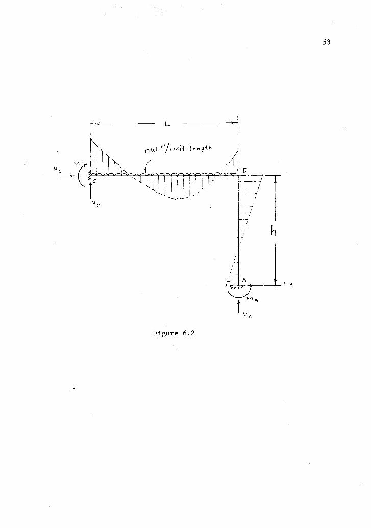
Figure 6.2

4-t A

53

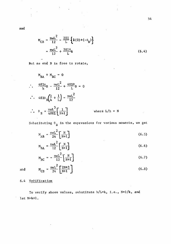
54

and

and

MCB

n=

2EI2(0)+( -.0

B)1

wL12

2

nwL2

2E10

12+

But as end B is free to rotate,

MBA MBC

4E1BB

nwL2

4E1.9B = 0

12

1 1) nwL24E1B

B he +

L 12

nwL3 r

B 48E1 L N-F-1where L/h = N

(6.4)

Substituting BB in the expressions for various moments, we get

nwL2

N-1(6.5)

MAB 24 N+lj

nwL2 r N 1

MBA 12 LN+ij(6.6)

nwL2 i N

MBC 12 I.N+1]

(6.7)

nwL2

j. (6.8)MCB 24 N+1

6.4 Verification

To verify above values, substitute h/L=k, i.e., N=1/k, and

let M=k+1.

nwL2

MB MBA 12M

nwL2 M

BM = M = =A AB 24M 2

nwL2(3k+2)M = M

C CB 24M

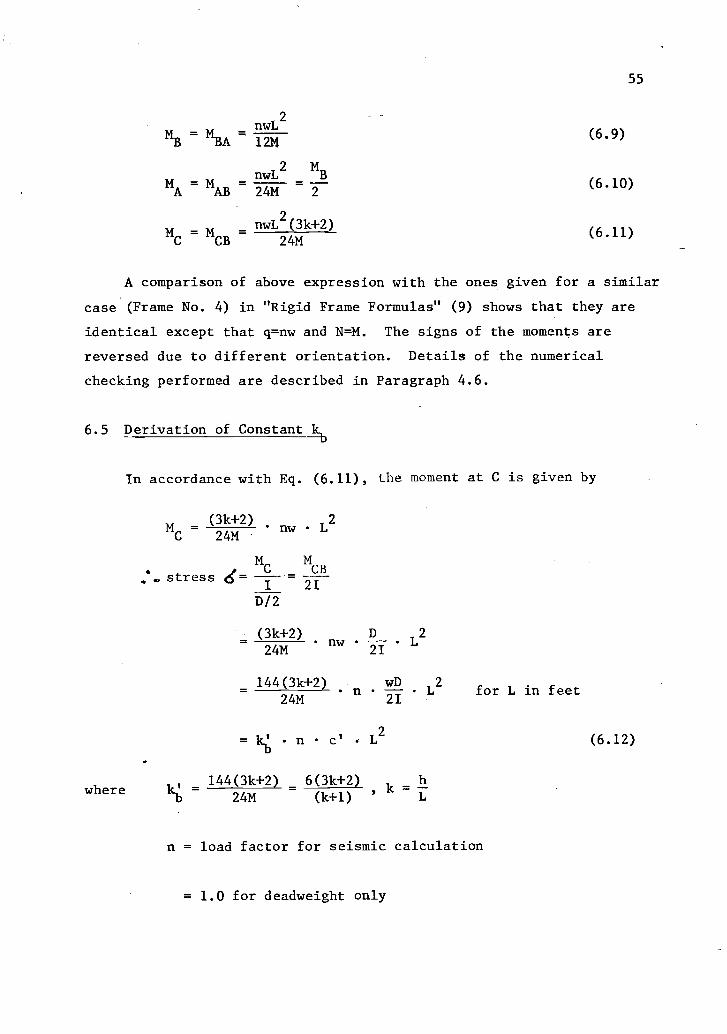
55

A comparison of above expression with the ones given for a similar

case (Frame No. 4) in "Rigid Frame Formulas" (9) shows that they are

identical except that q=nw and N=M. The signs of the moments are

reversed due to different orientation. Details of the numerical

checking performed are described in Paragraph 4.6.

6.5 Derivation of Constant kb

where

In accordance with Eq. (6.11), the moment at C is given by

(3k+2)M = nw L

2

C 24M

Mc CB

stress (=I 21

D/2

(3k+2)nw

ifL2

24M

144(3k+2)n

EDL

24M 21

= ki') n c' L2

144(3k+2) 6(3k+2)ki10

24M (k+1) '

k = E

for L in feet

n = load factor for seismic calculation

= 1.0 for deadweight only

(6.12)

56

, wc =-

D= constant based on sectional properties of

pipe/tubing

L = length in feet

Numerical values for kit) are shown in Table 6.1.

Table 6.1

L/h 1.0 2.0 3.0 4.0 5.0 6.0 7.0 8.0

kb 15.000 14.000 13.500 13.200 13.000 12.857 12.750 12.667

6.6 Numerical Check

An "L" configuration similar to Figure 6.1 with L+h = 60 inches

and L/h = 1.0 through 8.0 was checked for 10G (n=10) loading on a

SAGS (7) computer program.

Comparison of hand calculation using Eq. (6.12) and computer

program is shown in Table 6.2.

6.7 Constants for Reactions at the Fixed Ends

An expression for end reactions can be derived for end reactions

based on the formulae given in Reference (8). However, those are

not derived for the following reasons:

1. Reactions due to dead weight or seismic loading are

negligible as compared to the reactions due to thermal

conditions, e.g., a 10-foot run of 1/2-inch diameter

tubing weighs only 3 pounds, thus, giving rise to a

reaction of about 1.5 pounds on each support.

57

2. For the above reason, the utility of constants for

deadweight is marginal.

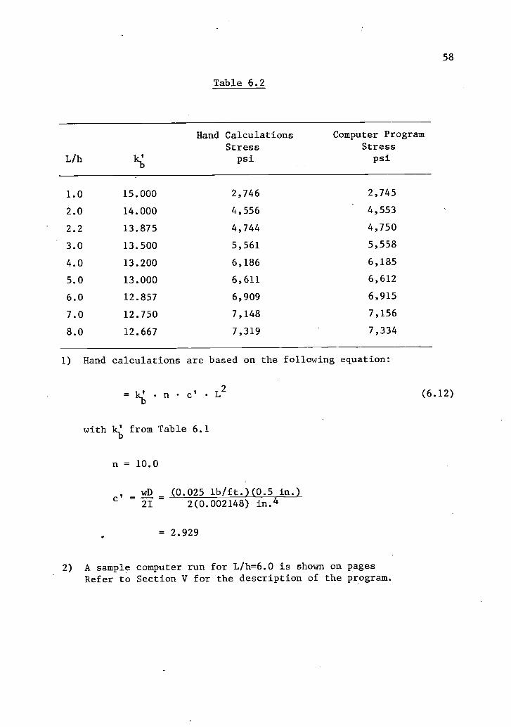
Table 6.2

L/h 1c13:

Hand CalculationsStress

psi

Computer ProgramStresspsi

1.0 15.000 2,746 2,745

2.0 14.000 4,556 4,553

2.2 13.875 4,744 4,750

3.0 13.500 5,561 5,558

4.0 13.200 6,186 6,185

5.0 13.000 6,611 6,612

6.0 12.857 6,909 6,915

7.0 12.750 7,148 7,156

8.0 12.667 7,319 7,334

1) Hand calculations are based on the following equation:

= kit) n c' L

with 1(1'3 from Table 6.1

n = 10.0

2

, wD (0.025 lb/ft.)(0.5 in.)c 21 2(0.002148) in.4

= 2.929

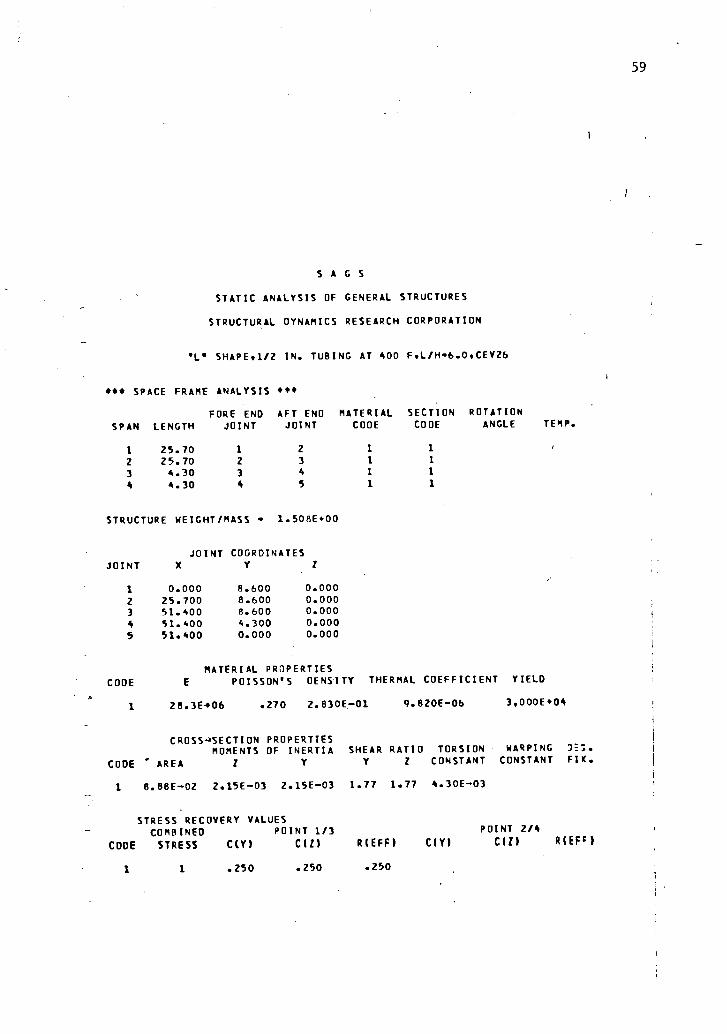
A sample computer run for L/h=6.0 is shown on pagesRefer to Section V for the description of the program.

58

(6.12)

A



SHAPE.1/2 IN. TUBING AT 400 F.L/H6.0.CEV26

SPACE FRAME ANALYSIS

FORE END AFT END MATERIAL SECTION ROTATION

SPAN LENGTH JOINT JOINT CODE CODE ANGLE TEMP.

1 25.70 1 2 1 1

2 25.70 2 3 1 1

3 4.30 3 4 1 1

4 4.30 4 5 1 1

STRUCTURE WEIGHT/MASS 1.508E+00

JOINT COORDINATESJOINT X

1 0.000 8.600 0.0002 25.700 8.600 0.0003 51.400 8.600 0.0004 51.400 4.300 0.0005 51.400 0.000 0.000

MATERIAL PROPERTIESCODE E POISSON'S DENSITY THERMAL COEFFICIENT YIELD

1 28.3E406 .270 2.830E-01 9.820E-06 3.000E+04

CROSS - 'SECTION PROPERTIESMOMENTS OF INERTIA SHEAR RATIO TORSION WARPING

CODE ' AREA I Y Y Z CONSTANT CONSTANT FIX.

1 8.88E-02 2.15E-03 2.15E-03 1.77 1.77 4.30E-03


CODE STRESS C(Y1 Cu) RIEFFI C(Y) RUM

1 1 .250 .250 .250

1

59

60

SFLIAOA 01/19/81 17.05.39.

STATIC ANALYSIS OF GENERAL STRUCTURES'L. SHAPE91/2 IN. TUBING AT 400 F9L/H=6.09CEV26


1 1234565 123456

LOADING NO. t 10 G LOAD IN Y DIRN.

ACCELERATION LOADINGA(X) O. A:Y1 - 1.000E.01 4(Z) - O.

TOTAL APPLIED FORCES:FIX/ O. F(Y1 - 1.508E+01 FtI) O.

61



61. SHAPE,1/2 IN. TUBING AT 400 F9L/H6.0.CE1/26

LOADING NO. 1 10 G LOAD IN Y

JOINT DISPLACEMENTSJOINT X Y

1 O. O. O.

2 8.332E-05 8.639E-02 O.

3 1.666E-04 2.499E-05 O.

4 -1.766E-03 1.342E-05 O.

5 0. 0. 0.

DIRN.

2 THETA(X) THETA(Y) THUMP

O. O. O.O. O. 4.302E-04O. O. -1.721E-03O. O. 3.792E-040. 0. 0.

.JOINT REACTIONSJOINT F(X) F(Y) m(XI MIYI MUT

1 -8.150E400 -6.698E+00 0. 0. O. -5.942E.Ca5 8.150E+00 -8.385E+00 O. O. O. -2.288E401

TOTAL -3.411E-13 -1.508E+01 O. 0. 0. -8.230E41

STRESS CALCULATIONSYIELD

SPAN END MZ/SM MY/SM P/A SHEAR COMBINED RATIO

1 FORE -6.915E+03 O. 9.175E+01 O. 7.007E+03 .23

2 AFT -5.494E403 O. 9.175E+01 O. 5.586E+03 .19

3 FORE -5.494E+03 O. 7.006E+01 O. 5.564E+03 .19

4 AFT 2.663E+03 O. 9.439E+01 O. 2.758E+03 .09


62

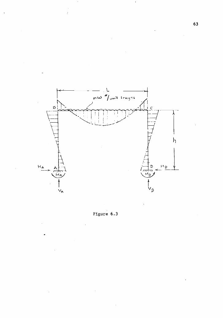
VI.B. Deadweight and Seismic Analysis for "U" Shape

6.8 Derivation for "U" Shape

Consider a "U" configuration of piping or tubing as shown in

Figure 6.3 with legs AB and CD vertical and leg BC horizontal.

Assume that leg BC is acted upon by a uniform force of magnitude

nw #/unit length where n represents a load factor during seismic

conditions. For consideration of deadweight only n=1.0. Slope-

deflection method will be used to derive the relationship similar to

the one used in Paragraph 6.3.

The general slope-deflection equation is:

2E1

MAB MFAB L(28

A+6

B)

Consider leg AB,

and

MFAB MFBA = 0

2EIeBMme=

4E16B

MBA

Consider leg BC,

and

MFBC MFCB

nwLM=BC 12

MCB

2

nwL2

12

2E1(20B-6c)

L = h

nwL2

2E1_L (-26C+811)12

(6.13)

(6.14)

HA

44/i-cv.11-tA

.....1111111... 1.41M.....m. Alb

I

h

Figure 6.3

fv9

63

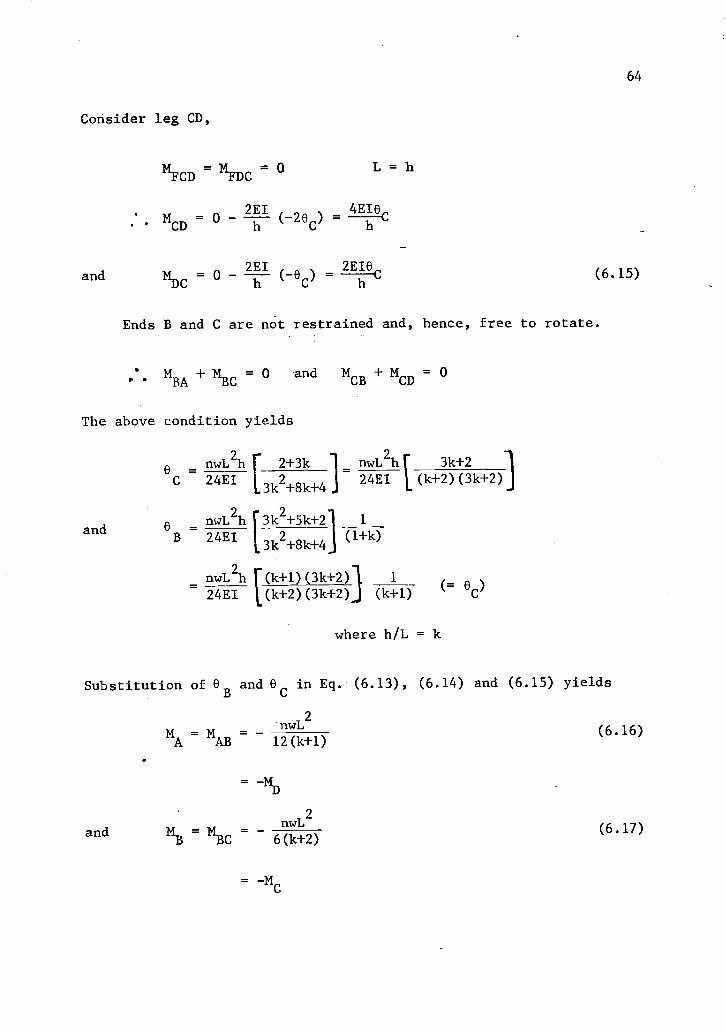
Consider leg CD,

and

HFCD MFDC 0L = h

MCD

2E1= 0 - ( 2e C)

4E16----c

.

2 2E16

HDC °

E1( e ) ----c

64

(6.15)

Ends B and C are not restrained and, hence, free to rotate.

.s. MBA + MBc = 0 and MCB MCD 0

The above condition yields

and

nwL2h 2+3k 1_ nwL

2h[ 3k+2

24E1 (k+2)(3k+2)C 24E13k

2+8k+4

6 nwL2h [3k2+5k+2 1

B 24E13k

2+8k+4

(1 +k)

nwL2h [(k+1)(3k+2)1 1

24E1 (k+2)(3k+2) -(+1) (= OC)

where h/L = k

Substitution of eB

and ecin Eq. (6.13), (6.14) and (6.15) yields

and

nwL2

MA NAB 12(k+1)

nwLMB

HBC 6(k+2)

=-HC

(6.16)

(6.17)

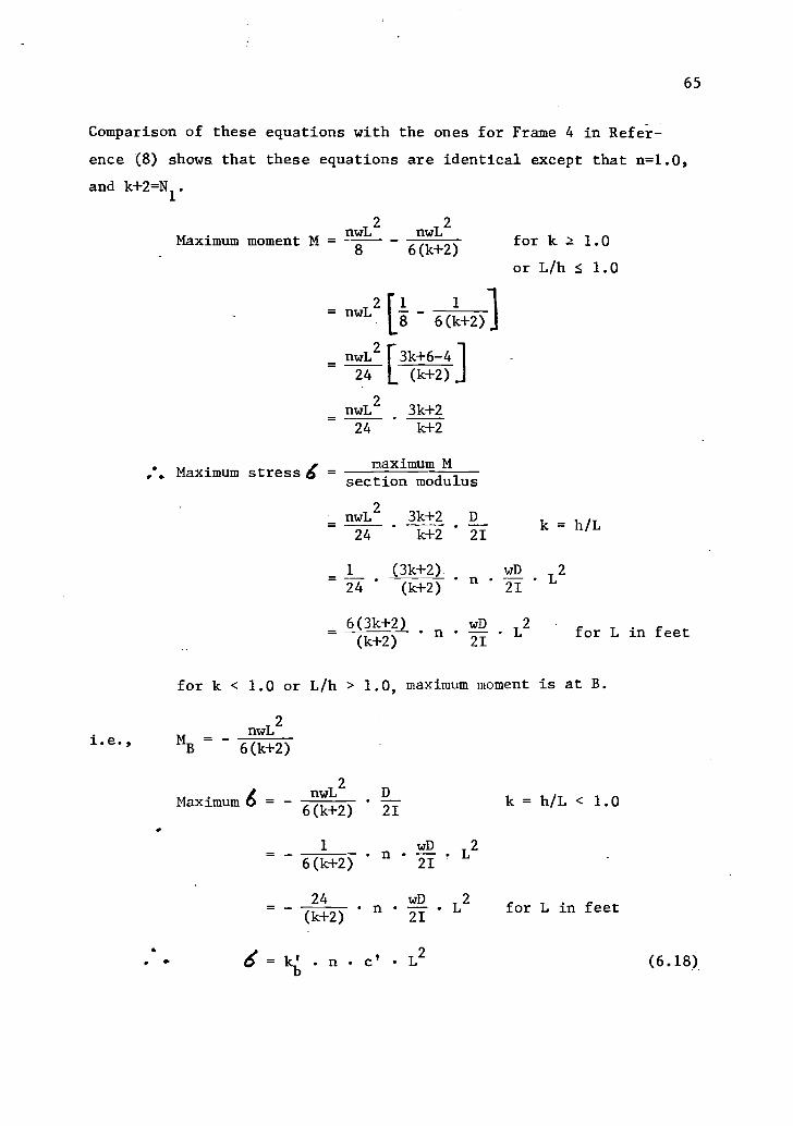
65

Comparison of these equations with the ones for Frame 4 in Refer-

ence (8) shows that these equations are identical except that n=1.0,

and k+2=N1.

Maximum moment M =8 6(k+2)

nwL2

nwL2

= nwL2 [1

8 6(k1+2)1

nwL2[3k+6-4]

24 (k+2)

nwL2 3k+224 k+2

Maximum stress 4Cmaximum M

section modulus

nwL2

3k+2 D

24 k+2 21

for k z 1.0

or L/h s 1.0

k = h/L

1 (3k+2) wD 2---24 (k+2)

n TE L

6(3k+2) wD ,2

(k+2) 21for L in feet

for k < 1.0 or L/h > 1.0, maximum moment is at B.

nwL2

MB 6(k+2)

nwL2Maximum 6 =

nwL6(k+2) 21

1 wD= - n6(k+2) 21

k = h/L < 1.0

24

(k+2) 21

wD= n L2 for L in feet

. n c' L2

(6.18)

66

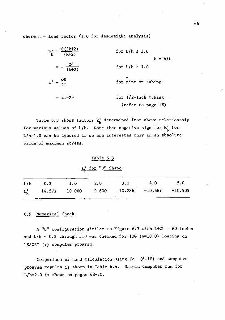
where n = load factor (1.0 for deadweight analysis)

6(3k+2)

(k+2)

_ 24

(k+2)

wDc -

21

for L /h .S 1.0

k = h/L

for L/h > 1.0

for pipe or tubing

= 2.929 for 1/2-inch tubing

(refer to page 58)

Table 6.3 shows factors kb determined from above relationship

for various values of L/h. Note that negative sign for kb for

L/h>1.0 can be ignored if we are interested only in an absolute

value of maximum stress.

Table 6.3

for "U" Shape

L/h 0.2 1.0 2.0 3.0 4.0 5.0

il14.571 10.000 -9.600 -10.286 -10.667 -10.909

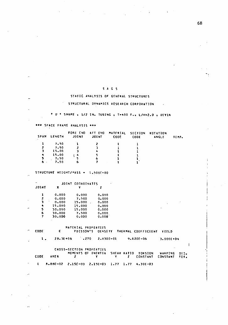
6.9 Numerical Check

A "U" configuration similar to Figure 6.3 with L+2h = 60 inches

and L/h = 0.2 through 5.0 was checked for 10G (n=10.0) loading on

"SAGS" (7) computer program.

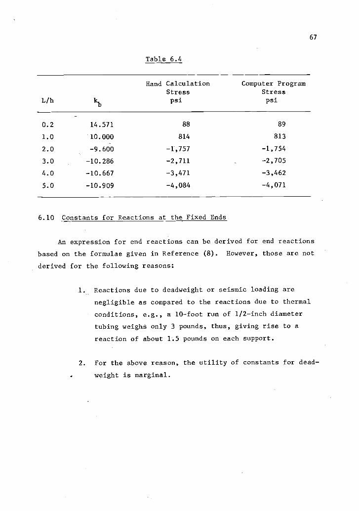
Comparison of hand calculation using Eq. (6.18) and computer

program results is shown in Table 6.4. Sample computer run for

L/h=2.0 is shown on pages 68-70.

67

Table 6.4

L/h

Hand CalculationStresspsi

kb

Computer ProgramStresspsi

0.2 14.571 88 89

1.0 10.000 814 813

2.0 -9.600 -1,757 -1,754

3.0 -10.286 -2,711 -2,705

4.0 -10.667 -3,471 -3,462

5.0 -10.909 -4,084 -4,071

6.10 Constants for Reactions at the Fixed Ends

An expression for end reactions can be derived for end reactions

based on the formulae given in Reference (8). However, those are not

derived for the following reasons:

1. Reactions due to deadweight or seismic loading are

negligible as compared to the reactions due to thermal

conditions, e.g., a 10-foot run of 1/2-inch diameter

tubing weighs only 3 pounds, thus, giving rise to a

reaction of about 1.5 pounds on each support.

2. For the above reason, the utility of constants for dead-

weight is marginal.

68



U SHAPE 1/2 IN. TUBING 11 T -400 F.. L /H -2.0 9 UEV14

. SPACE FRAME ANALYSIS

FORE END AFT END MATERIAL SECTION ROTATIONSPAN LENGTH JOINT JOINT CODE CODE ANGLE TEMP.

1 7.50 1 2 i. 1

2 7.50 2 3 1 13 15.00 3 4 1 14 15.00 t 4 5 1 15 7.50 5 6 1 1

6 7.50 6 7 1 1'



1 0.000 0.000 0.0002 0.000 7.500 0.0003 0.000 15.000 . 0.0004 15.000 15.000 0.0005 30.000 15.000 0.0006 30.000 7.500 0.0007 30.000 0.000 0.000

CODEMATERIAL PROPERTIES

E POISSON'S DENSITY THERMAL COEFFICIENT YIELD

1. 28.3E+06 .270 2.830E-01 9.820E-06 3.000E+04

CROSS-SECTION PROPERTIESMOMENTS OF INERTIA SHEAR RATIO TORSION WARPING DES.

CODE AREA 1 Y Y 2 CONSTANT CONSTANT FIX.

1 8.88E-02 2.15E-03 2.15E-03 1.77 1.77 4.30E-03

SFFBAOK 01/20/e1 13.23.05.

STATIC ANALYSIS OF GENERAL STRUCTURESU SHAPE 1/2 IN. TUBING T.400 F.. 1/11.2.0 UEV14


CODE STRESS CIY1 CI21 R(EFF) CIYI CU) RIEF:1_

1 1 .250 .250 .250


1 1234567 123456

LOADING NO. 1: 10 G. LOADING IN Y DIRN.

ACCELERATION LOADINGAIX) O. A(Y) - 1.000E+01

TOTAL APPLIED FORCES:FIX) O. F(Y) 1.50BE.01 FIZ1 O.

O.

69

70



U SHAPE 1/2 IN. TUBING . T.400 F.. L/H.2.0 UEV14

*1* LOADING NO. 1 10 G. LOADING IN Y DIRN.

JOINTJOINT DISPLACEMENTSX Y 1 THETAM THETAtYI TMETAI/1

1 O. O. O. O. O. O.2 1.748E-,03 1.969E-05 O. O. O. -2.287E-043 -8.975E-06 3.375E-05 O. O. O. 9.344E-044 -1.891E-16 1.582E-02 O. O. O. -8.334E-185 8.975E-06 3.375E-05 O. O. O. -9.344E-046 -1.748E-03 1.969E-05 O. O. O. 2.287E-047 0. O. O. O. O. O.

JOINT REACTIONSJOINT FIX) Fri') FIl) MIX) MC() MU)

1 -1.504E+00 -7.542E+00 O. O. O. 7.494E007 1.504E+00 -7.542E+00 O. O. O. -7.494E+00

TOTAL 5.684E-14 -1.508E+01 O. O. O. -3.979E-13

SPAN

STRESS CALCULATIONS

END MZ/SM MY /SM P/A SHEAR COMBINEDYIELDRATIO

I FORE 8.722E+02 O. 8.490E+01 O. 9.571E+02 .032 AFT -1.754E+03 O. 4.245E+01 O. 1.796E+03 .063 FORE -1.754E+03 O. 1.693E+01 O. 1.771E+03, .064 AFT -1.754E+03 O. 1.693E+01 O. 1.771E+03 .065 FORE -1.754E+03 O. 4.245E+01 O. 1.796E+03 .066. AFT 0.722E+02 O. B.490E+01 O. 9.571E+02 .03


71

VI.C. Analysis of "L" Shape with a

Concentrated Weight On

6.11 Concentrated Weights on Piping Configurations

Concentrated weights often occur on pipe/tubing runs. Common

instances are line mounted instruments or valves. These tend to

overstress the piping which otherwise would meet "cookbook" criteria.

6.12 Derivation of Expression for "L" Shape with a Concentrated

Weight or Force On

Figure 6.4 shows an "L" configuration with a valve weighing

P pounds at a distance "a" from the free end.

The moments and reactions in the configuration can be determined

by using "slope-deflection" method, as described in Section III and

used in Section VI.A and VI.B. Total stresses due to the concentrated

weights and self-weight of the piping which is uniformly distributed

can be calculated using the principle of superposition.

and

Consider leg AB:

MFAB MFBA = 0

2E1 2E10B' M = 0 (0+0B) =" AB

MBA = 0 -2Eh I 4E10

B(20B+0) = -

Consider leg BC:

Pab2

Pa2b

MFBCand 14,_

teCBL2

L2

(6.19)

13

Figure 6.4

C

He

72

and

at B,

Pab2

2E1. -Bc 2

(20 +0)

Pab2

4EI0

L2

Pa2b 2E1

NCB_ (0+0B)

L2

Pa2b 2E10

B_

L2

NBA + NBC0

4E1a+

Pab.2

4E18B

hL2

= 0

Pab2

1 (h )eB '4E1 L L+h

Pab S()14

where a= b/L, k= h/L and N= k+1

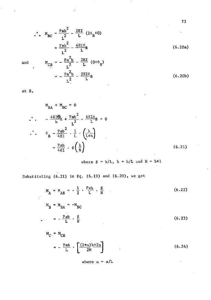
Substituting (6.21) in Eq. (6.19) and (6.20), we get

1 Pab a

14A NAB 2 L N

NB MBA NBC

PabL N

M = MC. CB

=Pab [(1+a)k+2]L 2N

where a = a/L

73

(6.20a)

(6.20b)

(6.21)

(6.22)

(6.23)

(6.24)

74

Comparison of the above with the results for Frame 4 in Refer-

ence (8) shows that they are identical. A numerical check using

SAGS computer program and above equations yield same results proving

the accuracy of above equations.

Moment under the load is given by

Mp PabL + a% 4- dMc

Substituting the values of a, MB and Mc and substituting

P=nw where w is weight of the value and n the load factor, we get

MP.= nwla(1-a)(1 (1-a)21 at(l+a

2N

)k+2a/11

and bending stress

tr= L'c(i_a),(11 (1_002 1 al(l+a)k+2a/11 wD_ n L2N 21

where

= k; n w c'L (6.25)

1 at(l+a)k+20kkb = 12 all -a) (1-a)

2

2N

, Dc =

21for pipe or tubing

= 116.387 for 1/2-inch o.d. tubing

w = concentrated weight in pounds

n = load factor, 1.0 for deadweight analysis

75

The location of the maximum moment and stress varies depending

on L/h and a/L ratios. The value of kl; is as. follows;

4(1+a)k+2a1-.1= 12ta(1 a)

2N

1(1'3= 12r")2-.1

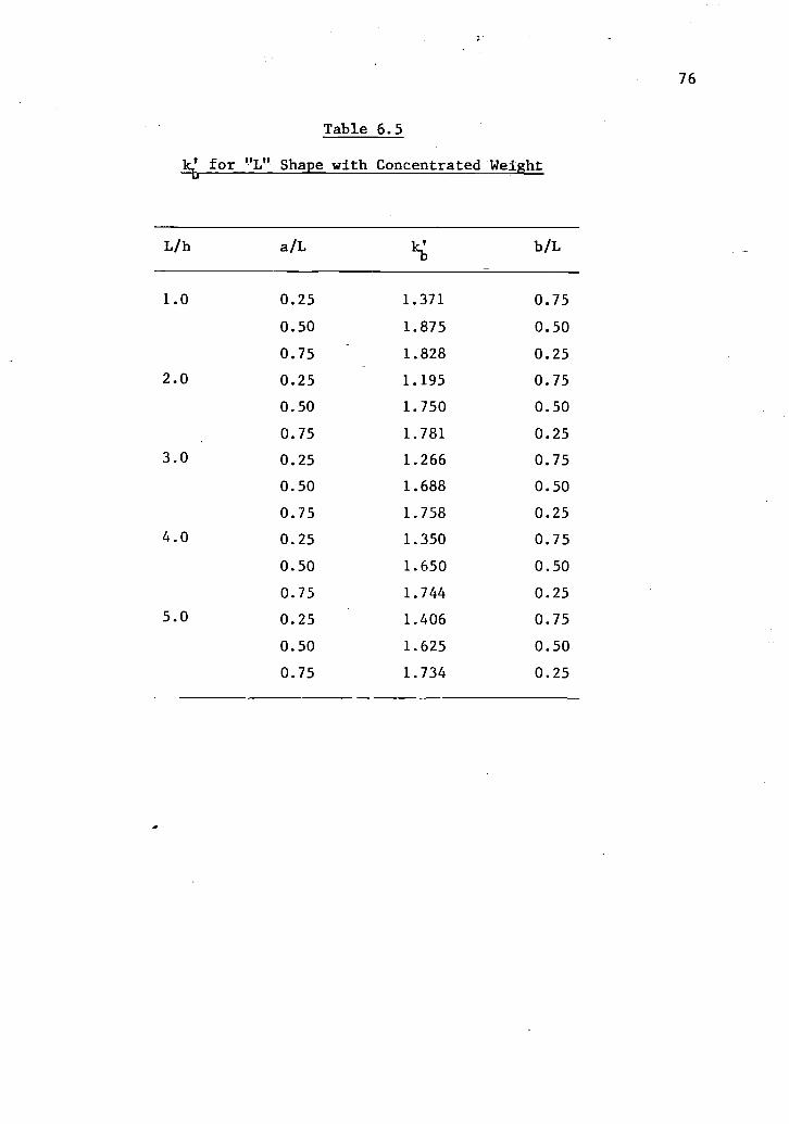
Table 6.5 shows factor

a/L for "L" shape.

6.13 Numerical Check

for a/L 2. 0.5

for L/h 2 2.0

for a/L < 0.5

for various combinations of L/h and

A "L" configuration similar to the one shown in Figure 6.4

with L+h = 60 inches and L/h = 1.0 through 5.0 and a/L = 0.25, 0.5 and

0.75 was checked for a concentrated weight of 10 pounds on "SAGS" (7)

computer program.

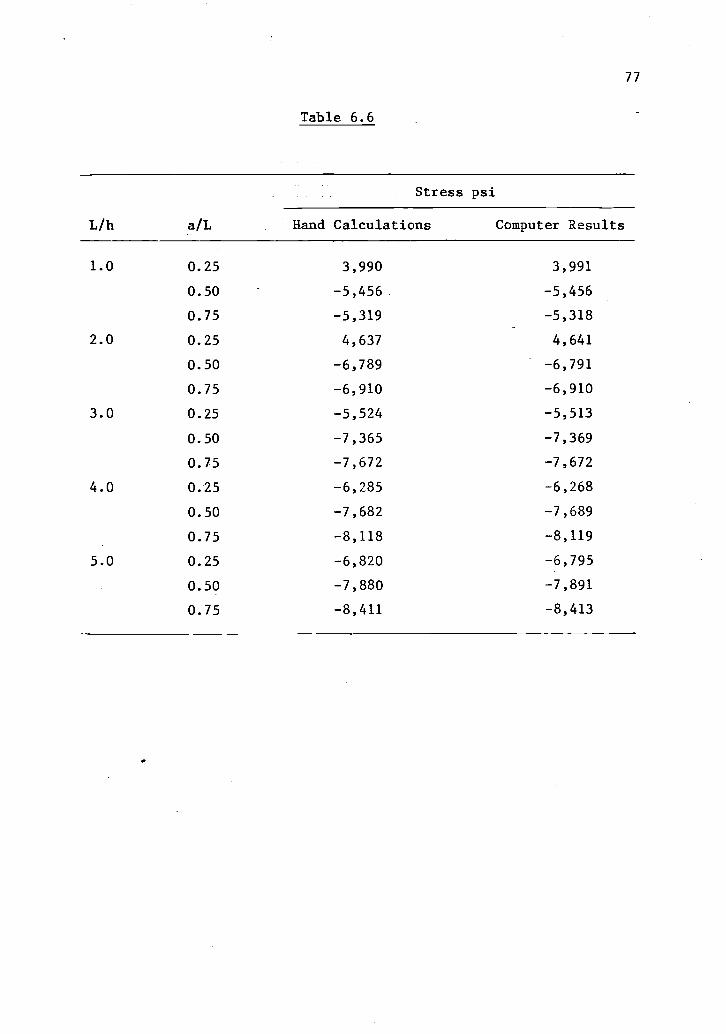
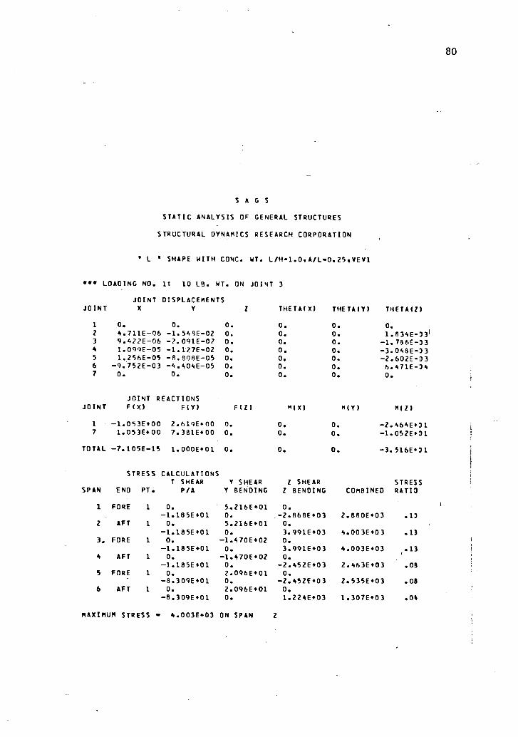
Comparison of hand calculations using Eq. (6.25) and computer

program results is shown in Table 6.6. A sample computer run for

L/h=1.0 and a/L=0.25 is shown on pages 78 through 80.

76

Table 6.5

for "L" Shape with Concentrated Weight

L/h a/L kb b/L

1.0 0.25 1.371 0.75

0.50 1.875 0.50

0.75 1.828 0.25

2.0 0.25 1.195 0.75

0.50 1.750 0.50

0.75 1.781 0.25

3.0 0.25 1.266 0.75

0.50 1.688 0.50

0.75 1.758 0.25

4.0 0.25 1.350 0.75

0.50 1.650 0.50

0.75 1.744 0.25

5.0 0.25 1.406 0.75

0.50 1.625 0.50

0.75 1.734 0.25

77

Table 6.6

L/h a/L

Stress psi

Hand Calculations Computer Results

1.0 0.25 3,990 3,991

0.50 -5,456 -5,456

0.75 -5,319 -5,318

2.0 0.25 4,637 4,641

0.50 -6,789 -6,791

0.75 -6,910 -6,910

3.0 0.25 -5,524 -5,513

0.50 -7,365 -7,369

0.75 -7,672 -7,672

4.0 0.25 -6,285 -6,268

0.50 -7,682 -7,689

0.75 -8,118 -8,119

5.0 0.25 -6,820 -6,795

0.50 -7,880 -7,891

0.75 -8,411 -8,413



L SHAPE WITH CONC. WT. L/H.1.0.11/10.25YEY1

* SPACE FRAME ANALYSIS

FORE END AFT END MATERIAL SECTION ROTATIONSPAN LENGTH JOINT JOINT CODE CODE ANGLE TEMP.

1 11.25 1 2 1 1

2 11.25 2 3 1 1

3 3.75 3 4 1 1

4 3.75 4 5 1 1

5 15.00 5 6 1 1

6 15.00 6 7 1 1


JOINT COORDINATESJOINT X

1 0.000 30.000 0.0002 -11.250 30.000 0.0003 -22.500 30.000 0.0004 -26.250 30.000 0.0005 -30.000 30.000 0.0006 -30.000 15.000 0.0007 -30.000 0.000 0.000


1 28.3E+06 .270 2.830E-01 9.820E-06 3.000E+04

CROSS- SECTION PROPERTIESMOMENTS OF INERTIA SHEAR RATIO TORSION WARPING 05G.

CODE AREA I Y Y I CONSTANT CONSTANT FIX.

1 8.88E-02 2.15E-03 2.15E-03 1.77 1.77 4.30E-03

1

78

79

MONDAY JAN 19, 1981 19.07.55.

STATIC ANALYSIS OF GENERAL STRUCTURESL SHAPE WITH CONC. WT. L/H1.0.A/L.0.25.VEV1

STRESS RECOVERY VALUESCOMBINED POINT 1/3 POINT 2/

CODE STRESS CIY) C(II RIEFF) C(Y) C(21 R(EFF) 1

1 1 .250 .250 .250


1 1234567 123456

LOADING NO. 12 10 LB. WT. ON JOINT 3

APPLIED FORCES FINALJOINT DIR TYPE VALUE

3 Y FORCE -1.000E+01

JOINT INC.

TOTAL APPLIED FORCESFIX) 0. F(Y) -1.000E+01 F221 O.

80



' L SHAPE WITH CONC. WT. L/H-1.0.A/L-0.25.YEY1

LOADING NO. 1: 10 LB. WT. ON JOINT 3

JOINT DISPLACEMENTSJOINT X Y Z THETA(X) THETA(Y) THETA(2)

1 O. O. O. O. O. O.Z 4.711E-06 -1.548E-02 O. O. O. 1.834E-3313 9.427E-06 -2.091E-02 O. O. O. -1.796E-334 1.099E-05 -1.127E-02 O. O. O. -3.048E-D35 1.256E-05 -8.808E-05 O. O. O. -2.602E-036 -9.752E-03 -4.404E-05 O. O. O. 6.471E -)47 O. O. O. O. O. O.

JOINT REACTIONSJOINT F(X) FLY) F(2) M(X) M(Y) m(2)

1 -1.053E+00 2.619E+00 O. O. O. -2.464E+317 1.053E+00 7.381E+00 O. O. O. -1.052E+31

TOTAL -7.105E-15 1.000E+01 O. O. O. -3.516E+31

SPAN

STRESS

END PT.

CALCULATIONST SHEAR

P/AY SHEARY BENDING

Z SHEARZ BENDING COMBINED

STRESSRATIO

1 FORE 1 O. 5.216E+01 O.-1.185E+01 O. -2.868E+03 2.880E+03 .13

2 AFT 1 O. 5.216E+01 O.-1.185E+01 O. 3.991E+03 4.003E+03 .13

3, FORE 1 O. -1.470E+02 O.-1.185E+01 O. 3.991E+03 4.003E+03 .13

4 AFT 1 O. -1.470E+02 O.-1.185E+01 O. -2.452E+03 2.463E+03 .08

5 FORE 1 O. 2.096E901 O.-8.309E+01 O. -2.452E+03 2.535E+03 .08

6 AFT 1 O. 2.096E+01 O.-8.309E+01 O. 1.224E+03 1.307E903 .08

MAXIMUM STRESS 4.003E+03 ON SPAN 2

VII. CONCLUSIONS

7.1 Section II of this report stated the reasons for undertaking

the present investigation. It also lists five specific questions

which we were trying to answer. Based on the discussion in Sec-

tions IV, V and VI, we now can answer the questions as follows:

81

1. The data given in Grinnell handbook can be used

for both tubing and piping sizes. The equations

developed in Section IV prove that the factors k , kx Y

and kb used in the Grinnell handbook are independent

of member geometry. Equations used in the Grinnell

handbook to determine reactions Fx, F

yand stresses

Sb

can be used for any size of pipe or tubing as

long as appropriate values of outside diameter D

and moment of inertia I are used.p

2. Section IV gives the general expressions from which

values of k , k and kb can be determined for anyx y

value of L/h ratio for the three configurations,

i.e., "L", "U" and "Z". They are derived in Sec-

tion IV and summarized here as follows:

a) for "L" shape:

kX m

3(m+1)

3(3m3+4m+1)

k =

23Lmr

(m+4)+3]m(m+1)

18(m2+m+2)

and kbm(m+1)

with m = h/L.

b) for "U" shape;

k3M

3(jr1-2)

x (2m+1)

18m2(m+1)

and kb(2m+1)

where m = L/h.

c) for "Z" shape with a/b = 1.0

24m(2m2+3)

kx

=(3m+4)

k =24(3m

3+6m+2)

y m(3m+4)

72(m3+3m+2)

and kb =m(3m+4)

72(2m2+3)

(3m+4)

where m = L/h.

form_ 1.0

for m > 1.0

82

3. Use of above relationships yield numerical values

of k , k and kb which are similar to the onesx y

listed in the Grinnell handbook. This is established

in Tables 4.1, 4.2 and 4.3. Thus, data shown in

Grinnell handbook is accurate for all practical

purposes.

4. A numerical check by using a finite element analysis

program "SAGS" (7), as explained in Section V,

confirms the accuracy of the data given in the

Grinnell handbook. This also proves the correctness

83

of the formulae derived in Section IV and VI of this

report.

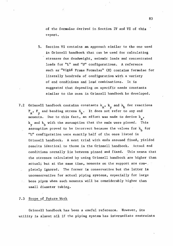
5. Section VI contains an approach similar to the one used

in Grinnell handbook that can be used for calculating

stresses due deadweight, seismic loads and concentrated

loads for "L" and "U" configurations. A reference

such as-"Rigid Frame Formulas" (8) contains formulae for

literally hundreds of configuration with a variety

of end conditions and load combinations. It is

suggested that depending on specific needs constants

similar to the ones in Grinnell handbook be developed.

7.2 Grinnell handbook contains constants kx, k

yand kb for reactions

Fx, F and bending stress Sb. It does not refer to any end

Ymoments. Due to this fact, an effort was made to derive k

x,

k and kb with the assumption that the ends were pinned. This

assumption proved to be incorrect because the values for kb for

"L" configuration were exactly half of the ones listed in

Grinnell handbook. A next trial with ends assumed fixed, yielded

results identical to those in the Grinnell handbook. Actual end

conditions normally lie between pinned and fixed. This means that

the stresses calculated by using Grinnell handbook are higher than

actual; but at the same time, moments on the support are com-

pletely ignored. The former is conservative but the latter is

unconservative for actual piping systems, especially for large

bore pipes when such moments will be considerably higher than

small diameter tubing.

7.3 Scope of Future Work

Grinnell handbook has been a useful reference. However, its

utility is almost nil if the piping system has intermediate restraints

84

which all actual systems have. Appendix B details an attempt to devise

a relation for an "L" configuration with one intermediate restraint.

The solution involves four simultaneous equations and quickly gets

out of hand. A programmable calculator, HP-67, was programmed to

numerically solve these equations. A new generation of programmable

calculators, such as HP-41C will be able to solve up to eight

simultaneous equations thus enabling to solve a configuration with

up to three intermediate restraints. This will solve the need at

a preliminary design level. Larger computers and finite element

programs can be used for final analysis of complete pipe runs with up

to 200 restraints and load combinations. A computer program, such as

"HANGIT" (10), have been developed recently to work backward on a

piping system (i.e., determine the location and types of supports

from allowable loads and stresses) which greatly simplify routing

and supporting a piping system. However, computer facilities are

not always available for preliminary design level.

The author intends to pursue analysis of smaller systems, develop-

ment of data and programs for handheld calculators as a future

assignment.

SECTION VIII

REFERENCES

1. ASME Boiler and Pressure Vessel Code Section III Division 1,1974 edition, by the American Society of Mechanical Engineers,New York.

2. Design of Piping Systems, The M. W. Kellogg Company, second

edition, 1956. John Wiley & Sons, Inc., New York.

3. Piping Design and Engineering, ITT Grinnell Industrial Piping,Inc., fifth edition, 1976.

4. Frank A. D'isa, Mechanics of Metals, Addison-Wesley PublishingCompany, 1968.

5. Clifford D. Williams, Analysis ofStructures, fourth edition, 1960,

6. Beautait, Rowan, Hoadley, Hackett,Analysis, Prentice-Hall Inc., 1965

84a.

Statically IndeterminateInternational Textbook Company.

Computer Methods of Structural

7. Static Analysis of General Structures, SAGS, by StructuralDynamics Research Corporation, manual 1176073600C published byControl Data Corporation, P. O. Box 0, HQCO2C, Minneapolis,

Minnesota 55440.

8. A Kleinlogel, Rigid Frame Formulas, Frederick Ungar PublishingCompany, New York, 1930.

9. Raymond J. Roark, Warren C. Young, Formulas for Stress andStrain, fifth edition, 1975, McGraw-Hill Book Company.

10. Analysis and Design Optimization for Piping Systems, HANGIT,by Ernst, Armand and Botti Associates, Inc., 60 Hickory Drive,

Waltham, Massachusetts 02154.

APPEND ICES

85

APPENDIX A

GRINNELL METHOD OF SIMPLIFIED PIPING ANALYSIS

"Piping Design and Engineering" was first published in 1963

by Grinnell Corporation. It was the first attempt to compile

comprehensive data for piping design and_includes a variety of topics

such as expansion and stresses, velocity and pressure drop, heat

transfer, pipe fabrication, nuclear piping, pipe hangers and supports,

and other piping data. It is widely used and is extremely valuable

at preliminary design levels.

The handbook is used mainly to calculate stresses in piping due

to thermal expansion and reactions at the supports. This section

describes the method of calculation for three most common piping

configurations, "L", "U" and "Z". Appropriate cuts from the text

are at the end of this section.

Sample Problem

Determine the stresses in the tubing and end reactions for the

configuration shown in Figure A-1.

Fy

Fx

L -0

Figure A-1

k -._ 2 - 0

Design Temperature: 550°F

Size: 1/2-inch o.d. x .

0.065-inch wall

Material: austeniticstainless steel

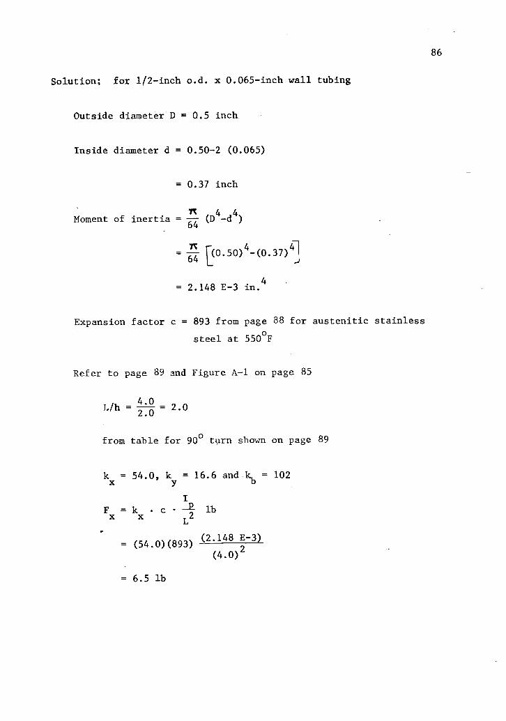
86

Solution; for 1/2 inch o.d. x 0.065-inch wall tubing

Outside diameter D = 0.5 inch.

Inside diameter d = 0.50-2 (0.065)

= 0.37 inch

7r

-I)

4Moment of inertia = (

64 -d4\

= ['(0.50) 4 -(0.37)4]64

= 2.148 E-3 in.4

Expansion factor c = 893 from page 88 for austenitic stainless

steel at 550°F

Refer to page 89 and Figure A-1 on page 85

4.0L/h

2.0= 2.0

from table for 90° turn shown on page 89

kx

= 54.0, k = 16.6 and kb = 102y

I

Fx= k

x 2c lb2

= (54.0)(893)(2.148 E-3)

(4.0)2

= 6.5 lb

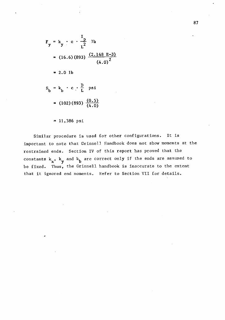
87

I

y =ky c lb

L2

= (16.6)(893)(2.148 E-,3)

= 2.0 lb

(4.0)2

DSb = kb -E psi

= (102)(893)(0.5)

= 11,386 psi

Similar procedure is used for other configurations. It is

important to note that Grinnell Handbook does not show moments at the

restrained ends. Section IV of this report has proved that the

constants k , k and kb are correct only if the ends are assumed tox y

be fixed. Thus, the Grinnell handbook is inaccurate to the extent

that it ignored end moments. Refer to Section VII for details.

88

EXPANSION AND STRESSES

EXPANSION FACTOR, c

Temp.T.F

CarbonSteel

C s .30%

CarbonSteelC > .30%

C-Moly& Low

Cr.-MolyCr < 3%

Cr.-MolvN517.0 << 9C7.r.

AusteniticStainless

Steels

Cr. StainlessStreit,

12 Cr. 17Cr.& 2 Cr.

25 Cr.- -20 Ni

WroughtIron

70 0 0 0 0 0 0 0 0100 37 40 40 35 54 34 47 44

150 98 106 106 92 143 90 125 120

200 160 171 171 149 232 145 204 105

250 228 244 244 212 323 204 287 273300 294 315 315 271 414 264 368 352

3.50 365 391 391 335 509 326 455 434

400 436 467 467 396 603 389 541 814

430 510 547 547 465 699 455 529 598

500 584 625 626 531 7P4 520 718 681

550 664 711 711 603 893 500 809 768

600 743 796 796 672 589 559 901 855

650 827 886 81913 714 1089 730 995 945

7110 909 974 974 815 1189 799 1088 1035

750 996 1068 1068 891 1292 874 1186 1125

775 1038 1113 1113 929 1344 P09 1235 1171

800 1159 967 1395 946 1284 1216

825 1208 1005 1448 983 1335

830 1256 1043 1000 1022 1381

875 1303 1081 1552 1061 1435

900 1351 1121 1605 1097 1484

92.5 1398 1161 1659 1134 1533

950 1445 1200 1713 1174 1585

975 1492 1240 1766 1212 1634

1000 1538 1278 1820 12.50 1681

1030 1639 1357 1928 1328 1781

1100 1737 1435 2036 1404 1870

1150 1511 2144 1480 1980

Expansion Factor cExpansion in inches per 100 f . X Ec

1728 X 100

For Straight and Curved Pipe

Da = Nominal Pipe Size

D = Outside Diameter

Wall Thickness

d = Inside Diameter

D 2l

PROPERTIES OF PIPE

IreAlInside Area

Metal Area Aa, = wi(D

Moment of Inertia I y = 0.019I(D4 d4)

- 0.0625z1,(D2 d2)

1Section Modulus -

2

11

89

ITT GRINNELL l'IPING DEsIGN AND ENGINEERING

90* TURN

h

FT

1pReacting Force

2

Ib

/pReacting Force F k . c Li lb

1)Maximum Bonding Stress sB 14. C. )7 psi

L in feet D in inches/p in inches'

r.

A k. k, 84

1.0 12.0 12.0 361.2 17.2 12.5 461.4 23.0 13.4 581.6 32.0 14.4 71

1.8 42.0 15.4 85

2.0 54.0 16.6 1022.2 08.3 17.8 1202.4 84.4 10.2 1402.6 103 20.0 101

2.8 126 22.0 184

3.0 150 23.5 2093.2 175 25.0 234

3.4 207 26.5 2393.6 237 20.0 2873.8 274 26.5 318

4.0 315 31.5 3494.2 336 33.0 301

4.4 406 34.6 414

4.6 456 30.2 430

4.8 510 37.8 487

5.0 570 39.5 5205.2 630 41.2 5095.4 700 43.0 010

5.6 775 44.7 652

5.8 855 40.2 096

6.0 938 48.2 7436.2 1020 49.8 790

6.4 1110 51.6 8106.6 1212 53.4 8926.8 1313 65.0 044

7.0 1426 56.8 0977.2 1.517 50.0 1050

7.4 1055 60.2 1104

7.0 1785 61.8 1159

7.8 1017 G1.6 1219

8.0 2069 65.4 1284

20

HOOKED Z SHAPE

_

Pestling Force F. = k, e lb

Ifending Force k, c. 4

L2

MaNitnum Bending Stress aB kb e

/p in inches' L in

k,

feet I) in invites

k4

1

A

0.60.8

1.01.21.41.01.8

2.02.22 42 6

1.182.7

4.37.8

)1.215.219.7

24.330.037.045.0

1.312.2

3.34.70.27.70.2

10.913.015.1

17.2

5.09.4

13.117.322.020.731.4

30.441.5460bl 7

. 2.8 54.0 16.3 58.0

3.0 64.8 21.6 64 g3.2 76.0 24.0 72 03.4 68 0 20.5 79 5

3.6 )00 0 20.0 87.0

3.8 113.6 31.0 05.0

4.0 128.7 34.5 103

4.2 144 37.4 112

4.4 160 40.4 121

4.6 178 43.4 130

4.8 198 40.4 )39

50 219 49.4 148

6.2 241 52.6 157

64 263 65.6 167

56 206 68.7 170

5.8 310 61.8 185

0.0 334 05.0 195

0.2 3(3) 68.4 205

6.4 308 71.8 215

0.6 416 76-2 2260 446 78.0 230

70 479 82.0 240

7.2 508 85 5 257

7.4 540 80 1 208

7.6 679 92 7 278

7.8 615 96 3 289

8.0 653 100.0 300

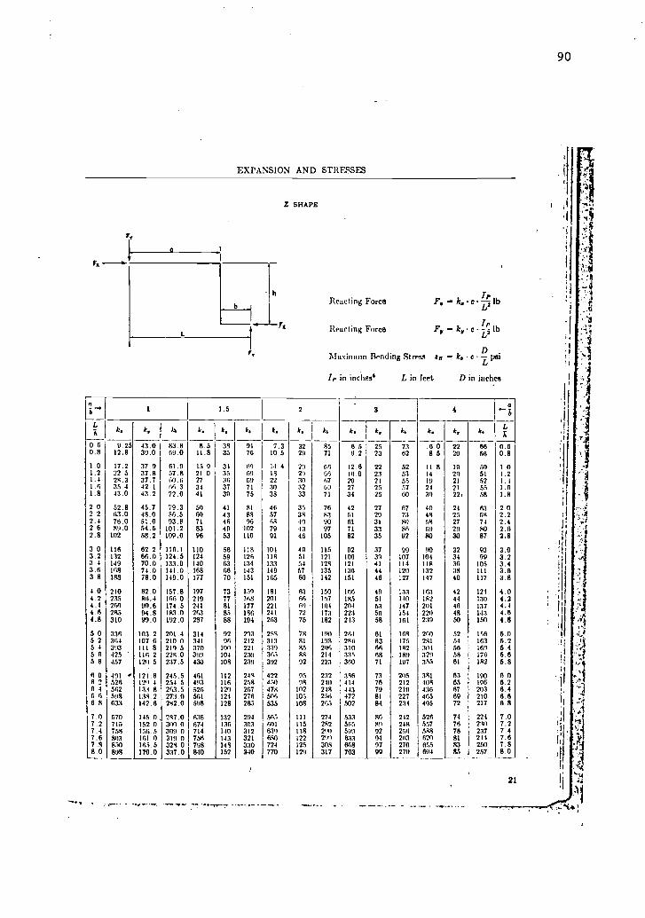
EXPANSION AND STRESSES

Z SHAPE

ry

rA

Reacting Force

Reacting Force

:Maximum Bending Stress

1p in inches4 L in feet

k, cL-

lb2

F9 k, c -L-2 lb

BB psi

D in inches

-4"

L.

h

ri,

1 1.5 2.

3 4a

.- b

L LI k k, 84 k. k, 44 8. k, k, k. k, 4 8. k, 8, K

0.6 9.25 43.0 83.8 8.5 38 91 7.3 32 85 6.5 25 73 .6.0 22 88 0.80.8 12.8 39.0 69.0 11.8 35 76 10.5 29 71 9.2 23 62 8.5 20 58 0.8

1.0 17.2 37.9 61.9 15.9 31 60 14.4 29 66 12.6 22 52 11.8 19 50 1.01.2 22 3 37.8 57.8 21.0 35 69 18 29 66 16.0 23 53 14 20 51 1.21.4 24.3 37.7 60.6 27 36 69 22 30 67 20 24 55 19 21 52 1.41.6 35.4 42 L 66.3 34 37 71 30 32 69 27 25 57 24 21 55 1.81.8 43.0 43.2 72.0 41 39 75 38 33 71 34 28 60 30 22, 58 1.8

2 0 52.8 45.7 79.3 50 41 81 46 35 76 42 27 67 40 24 63 2.02 2 63.0 48.0 86.5 60 43 88 57 38 143 51 29 73 48 25 64 2.22.4 76.0 51.0 93.8 71 46 96 68 40 90 61 31 KO 58 27 74 2.42.6 89.0 54.5 101.2 83 49 102 79 43 97 71 33 86 69 29 80 2.62.8 102 58.2 109.0 96 53 110 91 46 105 82 35 92 80 30 87 2.8

3.0 118 82.2 116.1 110 58 118 104 49 115 02 37 99 00 32 03 3.03.2 132 66.0 124.5 124 59 126 118 51 121 106 39 107 104 34 99 3.23 4 149 70.0 133.0 140 63 134 133 54 128 121 41 114 11R 36 105 3.43.6 168 74.0 141.0 168 66 143 149 57 135 138 44 120 132 38 III 3.83.8 188 78.0 149.0 177 70 151 165 60 142 151 46 127 147 40 117 3.8

4.0 210 82.0 157.8 197 73 159 181 6.3 150 166 49 133 163 42 121 4.04.2 235 86.4 166.0 219 77 168 201 66 157 185 51 140 182 44 130 4.24.4 260 90.6 174.5 241 81 177 221 69 164 204 83 147 201 46 137 4.44.0 288 94.8 IR3.0 263 85 186 241 72 173 223 50 154 221) 48 143 4.04.8 310 99.0 192.0 287 88 194 263 75 182 2)3 58 161 239 50 150 4.8

5 0 336 103.2 201.4 314 92 2n3 288 78 190 264 01 168 260 52 15n 5.05 2 364 107.6 210.0 341 96 212 313 81 19R 2146 63 175 281 54 163 5.25 4 393 III .8 219 5 370 100 221 339 R5 206 310 66 182 301 56 169 6.45 0 425 116.2 228.0 399 104 230 361 1114 214 335 68 189 329 58 176 6.85 8 457 120 5 237.5 430 108 239 392 92 223 360 71 197 355 61 182 5.8

0 0 491 121.8 245.5 461 112 244 422 95 232 386 73 205 3141 63 190 6.06 2 526 129 4 254 5 493 116 258 450 98 210 414 76 212 408 6.5 196 6.26 4 562 13:1 8 263.5 526 120 267 474 102 248 443 79 211) 436 67 203 8.4G 6 598 138.2 273 0 561 121 276 506 105 256 472 81 227 465 60 210 6.66 8 633 142.8 242.0 598 128 281 535 108 265 502 84 231 495 72 217 0.8

7.0 670 145.0 287.0 636 132 294 561 III 274 533 86 212 526 74 224 7.07.2 718 152 0 300 0 674 136 303 601 115 282 565 89 248 557 76 230 7.27.4 758 156.5 309.0 714 140 312 639 118 210 599 92 256 588 78 237 7.47.6 803 161.0 319.0 756 143 321 600 122 219 633 94 263 629 81 211 7.07.8 8700 165.5 329.0 798 148 330 724 125 308 668 97

I

270 655 R3 250 7.8

8.0 898 170.0 337.0 840 152 340 770 129 317 703 99 279 694 83 257 8.0

21

90

rrr (VRINNELL PIPING I)EsIGN AND ENGINEEHING

II SHAPE- -EQUAL LEGS

LK

k, k,

0.2 0.0377 0.6170.3 0.1165 -1.3090.4 0.256 2.2320.5 0.469 3.3700.6 0.765 4.5800.7 1.191 0.4300.8 1.68 8.1100.9 2.38 10.39

1.0 3.00 12 001.2 4.88 16.741.4 7.37 22.261.6 10.55 28.561.8 14.48 35.52

2.0 19.2 43.202.2 24.6 52 322.4 31.4 60.722.6 39.2 70.562.8 48.0 81.24

3.0 57.8 02.643.2 69.1 104.53.4 82.2 118.23.6 95.6 130.83.8 111.0 138.4

4.0 128.1 160.04.2 147.0 176.1

4.4 166.6 192.04.6 180.0 208.84.8 213.0 227.4

5.0 239.0 240.05.2 266.0 254.0

I.

Fx

Reacting Force k,e- --/p I

L2

Maximum Bending tress 1 DB . kb C --L psi

I,, in inches' L in feet Din inches

II SHAPE- MODIFIED

Reacting Force

Reacting Force

F. leg e1p--

k, c Ip-Maximum Rending &rem 83 ". kb C

r in inches' L in feet D in inches

h

Fx

..1,-4

a4/3 1.6 2 8 Dirlso-

lion

Zi

afro

I 6. 6, 64 k, k, 144 k. kw ka 6. 4, h Force

1 2.62 0.51 10.45 2.63 0.75 10.50 2.82 1.41 11.2 3.30 2.28 12.8

1.2 3.32 0.69 14.1 3.38 1.01 14.45 3.69 1.85 16.5 4,37 2.79 17.8 I

13.5 4.12 0.86 13.3 4.5 0.42 14.5

__-_-

1.6 4.17 1.26 13.8 4.12 1.15

2 5.46 2.66 17.3 5.50 2.60 17.2 5 30 2.44 16.1 5.6 2.14 17.3

9 7.20 4.70 22.2 7.10 4.70 21.5 7.08 4.65 21.3 7.8 4.50 22.01

6 9.30 7.80 28.7 9.33 7.76 28.2 9.40 7.87 28.2 9.4 7.68 28.2

28

/- eq77.4

91

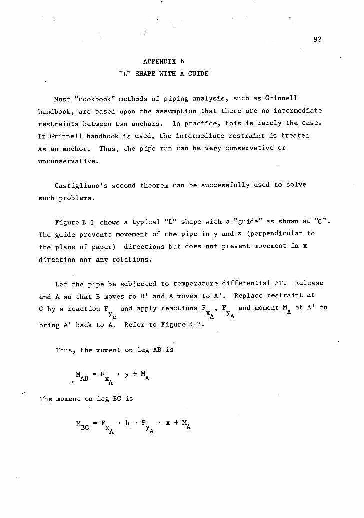
92

APPENDIX B

"L" SHAPE WITH A GUIDE

Most "cookbook" methods of piping analysis, such as Grinnell

handbook, are based upon the assumption that there are no intermediate

restraints between two anchors. In practice, this is rarely the case.

If Grinnell handbook is used, the intermediate restraint is treated

as an anchor. Thus, the pipe run can be very conservative or

unconservative.

Castigliano's second theorem can be successfully used to solve

such problems.

Figure B -1 shows a typical "L" shape with a "guide" as shown at "C".

The guide prevents movement of the pipe in y and z (perpendicular to

the plane of paper) directions but does not prevent movement in x

direction nor any rotations.

Let the pipe be subjected to temperature differential AT. Release

end A so that B moves to B' and A moves to A'. Replace restraint at

C by a reaction F and apply reactions FxA

, FYA

and moment MA

at A' to

37c

bring A' back to A. Refer to Figure B-2.

Thus, the moment on leg AB is

MAB Fxy

MAA

The moment on leg BC is

MBC Fx 11 F 3 -I- MAA YA

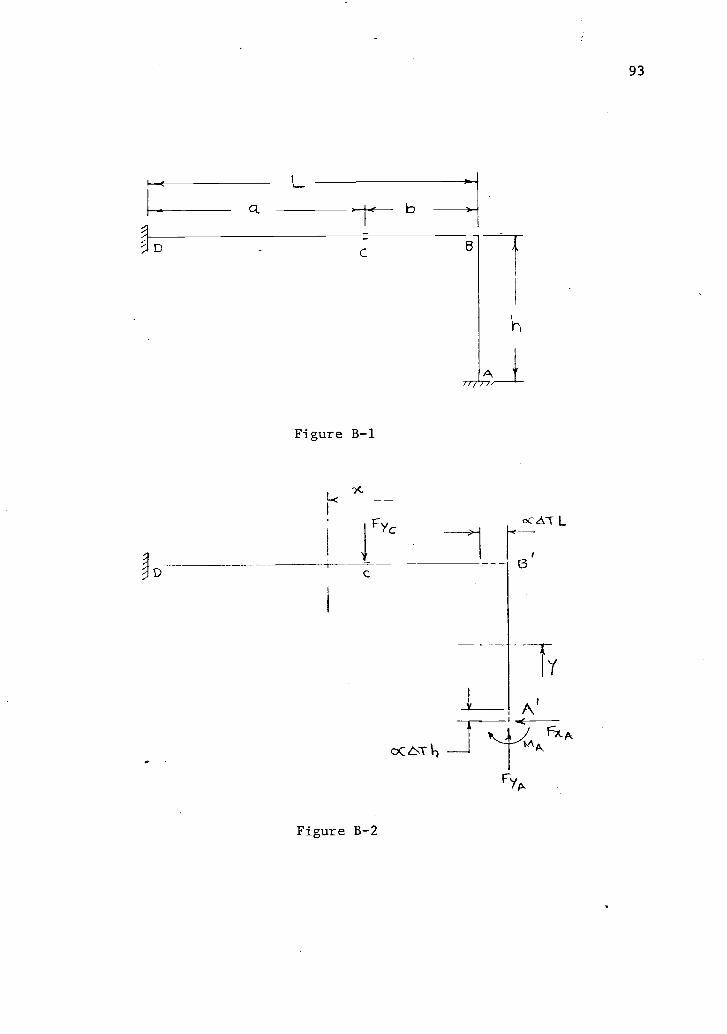
ct

Lb

D

D

C

Figure B-1

IFYc

Figure B-2

oC &T

A

oc dT L

93

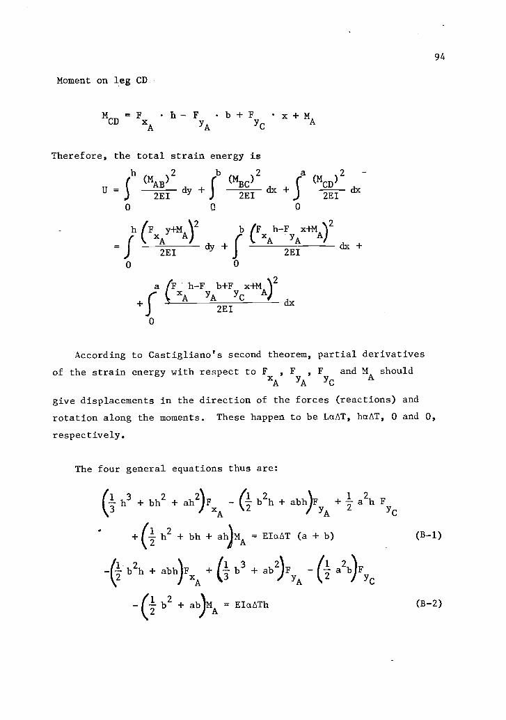
Moment on leg CD

MCD

=FxAh-F

YAb+F

YCx+ M

A


h 2 2 2

U =S dy +

(MAB) NC)dx

(mcD)dx

2E1 2E1 2E1

0 0 0

h (F y+M )2 b tFx h-F_ x+MA)xA A

2E1dy +

jr k A JA2E1

dx +

0 0

a (F.h-F b+F x+M )2

+xA yA

yCA

dx2E1

2

0

According to Castigliano's second theorem, partial derivatives

of the strain energy with respect to F , F , F and M shouldxA yA yc A

give displacements in the direction of the forces (reactions) and

rotation along the moments. These happen to be LaAT, haLT, 0 and 0,

respectively.

The four general equations thus are:

h3 + bh2 + ah2,)F - b2h + abh)F + 2h F-ixA

21 a

/A YC

1+(2- h

2+ bh + ah)MA = EIaAT (a + b)

- lb2h + abh)Fx

+ (1 b3 + ab2,)F (1-a2b Fz

(7-- A3

YA2 YC

b2+ aby1

A= EIaATh

94

(B-1)

(B-2)

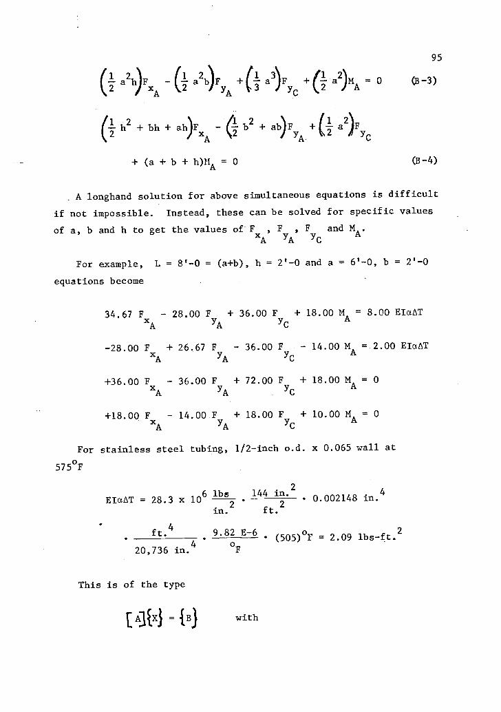
( 1 2a h)Fx - (y a 2 ) 1b F + -3- a3) Fy1 + a2)14A = 0

A YA

(1 2h + bh + ah)F b2 + ab F + 1 a2)FxA 2 YA- YC

95

(B -3)

+ (a + b + h)MA = 0 (B-4)

_ A longhand solution for above simultaneous equations is difficult

if not impossible. Instead, these can be solved for specific values

of a, b and h to get the values of-F , F , F and MA.

xA YA YC

For example, L = 8'-0 = (a+b), h = 2'-0 and a = 6'-0, b = 2'-0

equations become

34.67 F 28.00 F + 36.00 F + 18.00 MA

= 8.00 EIaAT

xA YA YC

-28.00 F + 26.67 FYA

36.00 F 14.00 MA= 2.00 EIaAT

xAYC

+36.00 F 36.00 F + 72.00 F + 18.00 MA= 0

xA YA YC

+18.00 F - 14.00 F + 18.00 F + 10.00 MA= 0

A YA YC

For stainless steel tubing, 1/2-inch o.d. x 0.065 wall at

575°F

EIaAT = 28.3 x 106 lbs

2

144 in.20.002148 in.

4

in. ft.2

ft.4

9.82 E-6(505)°F = 2.09 lbs-

20,736 in.4

°F

This is of the type

AAci IB) with

96

34.67 -28.00 +36.00

-28.00 +26.67 -36.00

+36.00 -36.00 +72.00

+18.00 -14.00 +18.00

and

+18.00

-14.00

+18.00

+10.00

16.72

4.18

The solution of four simultaneous equations

[Ajfx} = {B}

=IA]

tB}

can be found by Gaussion Elimination as follows: First, by

eliminating F , the equations are transformed to three following

equationsYC

44.01 F 36.00 FYA

+ 24.00 MA

= 54.34xA

-112.20 FxA

+ 240.48 F 56.10 MA

= 11.16YA

48.00 FxA

36.00 F + 30.00 MA

= 4.18YA

Above equations are solved using 3x3 matrix program available

on Hewlett-Packard HP-67 calculator. The answers are

F = 11.07 lbsxA

97

F = 1.54 lbs.

YA

MA

= -15.72 ft.-lbs or = - 188.64 in.-lbs

Comparison of above values with the ones for joint 7 on page 100

of the computer output shows they are very close. Numerous such

output and checks are available for review.

Conclusion

Above example of "L" shape with one restraint proves that similar

problems can be solved by using Castigliano's second theorem. This

ability is limited only by the capability of solving simultaneous

equations. An upcoming version of programmable calculator "HP-41C"

has more storage capacity ("bytes") and should be able to solve

6x6 matrix or six simultaneous equations. It is the intent of the

author to prepare such a program when the calculator becomes available.

Widespread use of such calculators will enable accurate calculations

of simple piping configurations with intermediate restraints without

resorting to use of large digital computers.

98



L ' SHAPE WITH A GUIDE H1 /H -3.0 T.575 F. LEVI

ts0 SPACE FRAME ANALYSIS *

FORE END AFT END MATERIAL SECTION ROTATIONSPAN LENGTH JOINT JOINT CODE CODE ANGLE TEMP.1 12.00 1 2 1 12 12.00 2 3 1 13 36.00 3 4 1 14 36.00 4 5 1 15 17.00 5 6 1 16 12.00 6 7 1 1

STRUCTURE WEIGHT/MASS 4 3.017E00


1 0.000 24.000 0.0002 12.000 24.000 0.0003 24.000 24.000 0.0004 60.000 24.000 0.0005 96.000 24.000 0.0006 96.000 12.000 0.0007 96.000 0.000 0.000


1 28.3E406 .270 2.830E-01 9.820E-06 3.000E404

CROSSSECTION PROPERTIESMOMENTS OF INERTIA SHEAR RATIO TORSION WARPING MS.CODE AREA 2 Y Y 2 CONSTANT CONSTANT FIX.

1 8.88E-02 2.15E-03 2.15E-03 1.77 1.77 4.30E-03

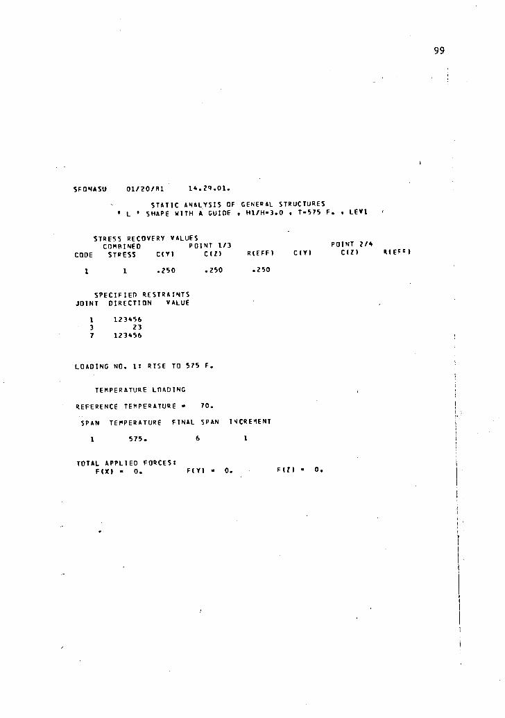
SFONASU 01/20/R1 14.29.01.

STATIC ANALYSIS OF GENERAL STRUCTURESL ' SHAPE WITH A GUIDE H1 /H -3.0 T=575 F. LEVI


CODE STRESS C(Y) Cu) I R(EFF) C(Y) C(I) R(EFg)

1 1 .250 .250 .250


1 1234563 237 123456

LOADING NO. RISE TO 575 F.

TEMPERATURE LOADING

REFERENCE TEMPERATURE - 70.

SPAN TEMPERATURE FINAL SPAN INCREMENT

1 575. 6 1

TOTAL APPLIED FORCES:F(X) O. F(Y) O.

99

100



L SHAPE WITH A GUIDE HI/H3.0 1 -575 F. LEVI

LOADING NO. 1 RISE TO 575

JOINT DISPLACEMENTSJOINT X Y

F.

1 THETAIXI THETAIYI THETA(1)

1 O. O. 0. O. O. O.

2 5.946E-02 -1.015E-02 O. O. O. -8.400E-043 1.189E-01 O. O. O. O. 3.333E-034 2.973E-01 2.886E-01 O. O. O. 7.149E-035 4.756E-,01 1.190E-01 O. O. O. -2.208E-026 1.716E-01 5.950E-02 0. O. O. -2.418E-027 O. O. O. O. O. O.

JOINT REACTIONSJOINT F(X) F(.() FIII M(X) M(Y) MIZI

I 1.109E+01 2.137E+00 O. O. O. 1.708E+013 O. -3.685E+00 O. O. O. O.

7 -1.109E+01 1.547E+00 O. O. O. 1.890E+02

TOTAL -1.196E-10 -1.847E-13 O.

STRESS CALCULATIONS

0. 0. .2.061E+32

YIELD

SPAN END mI/SN MY/SM P/A SHEAR COMBINED RATIO

I FORE 1.988E+03 O. -1.249E+02 O. 2.113E+03 .07

2 AFT -3.982E+03 O. -1.249E+02 O. 4.107E+03 .14

3 FORE -3.982E+03 O. -1.249E+02 O. 4.107E+03 .14

4 AFT 8.986E+03 O. -1.249E+02 O. 9.111E+03 .30

5 FORE 8.986E+03 O. -1.742E+01 O. 9.003E+03 .30

6. AFT -2.200E+04 O. -1.742E+01 O. 2.202E+04 .7

MAXIMUM STRESS 2.202E+04 ON SPAN 6

Thermal and seismic analysis of piping systems using ...

Documents

Transcript of Thermal and seismic analysis of piping systems using ...