Piping and Instrumentation

CHAPTER 5

Piping and Instrumentation

5.1. INTRODUCTION

The process flow-sheet shows the arrangement of the major pieces of equipment and theirinterconnection. It is a description of the nature of the process.The Piping and Instrument diagram (P and I diagram or PID) shows the engineering

details of the equipment, instruments, piping, valves and fittings; and their arrangement.It is often called the Engineering Flow-sheet or Engineering Line Diagram.This chapter covers the preparation of the preliminary P and I diagrams at the process

design stage of the project.The design of piping systems, and the specification of the process instrumentation and

control systems, is usually done by specialist design groups, and a detailed discussionof piping design and control systems is beyond the scope of this book. Only generalguide rules are given. The piping handbook edited by Nayyar et al. (2000) is particularlyrecommended for the guidance on the detailed design of piping systems and processinstrumentation and control. The references cited in the text and listed at the end of thechapter should also be consulted.

5.2. THE P AND I DIAGRAM

The P and I diagram shows the arrangement of the process equipment, piping, pumps,instruments, valves and other fittings. It should include:

1. All process equipment identified by an equipment number. The equipment shouldbe drawn roughly in proportion, and the location of nozzles shown.

2. All pipes, identified by a line number. The pipe size and material of constructionshould be shown. The material may be included as part of the line identificationnumber.

3. All valves, control and block valves, with an identification number. The type andsize should be shown. The type may be shown by the symbol used for the valve orincluded in the code used for the valve number.

4. Ancillary fittings that are part of the piping system, such as inline sight-glasses,strainers and steam traps; with an identification number.

5. Pumps, identified by a suitable code number.6. All control loops and instruments, with an identification number.

For simple processes, the utility (service) lines can be shown on the P and I diagram.For complex processes, separate diagrams should be used to show the service lines, so

194

PIPING AND INSTRUMENTATION 195

the information can be shown clearly, without cluttering up the diagram. The serviceconnections to each unit should, however, be shown on the P and I diagram.The P and I diagram will resemble the process flow-sheet, but the process

information is not shown. The same equipment identification numbers should be usedon both diagrams.

5.2.1. Symbols and layout

The symbols used to show the equipment, valves, instruments and control loops willdepend on the practice of the particular design office. The equipment symbols are usuallymore detailed than those used for the process flow-sheet. A typical example of a P and Idiagram is shown in Figure 5.25.Standard symbols for instruments, controllers and valves are given in the British

Standard BS 1646.Austin (1979) gives a comprehensive summary of the British Standard symbols, and

also shows the American standard symbols (ANSI) and examples of those used by someprocess plant contracting companies.The German standard symbols are covered by DIN 28004, DIN (1988).When laying out the diagram, it is only necessary to show the relative elevation of

the process connections to the equipment where these affect the process operation; forexample, the net positive suction head (NPSH) of pumps, barometric legs, syphons andthe operation of thermosyphon reboilers.Computer aided drafting programs are available for the preparation of P and I diagrams,

see the reference to the PROCEDE package in Chapter 4.

5.2.2. Basic symbols

The symbols illustrated below are those given in BS 1646.

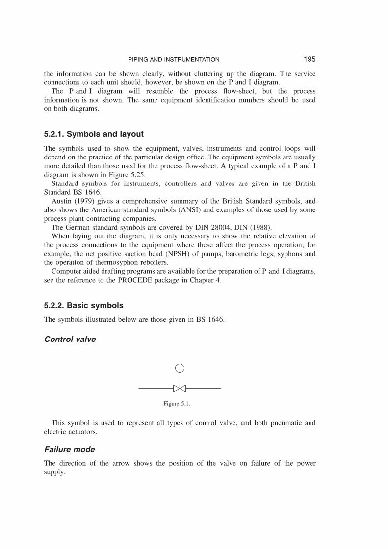
Control valve

Figure 5.1.

This symbol is used to represent all types of control valve, and both pneumatic andelectric actuators.

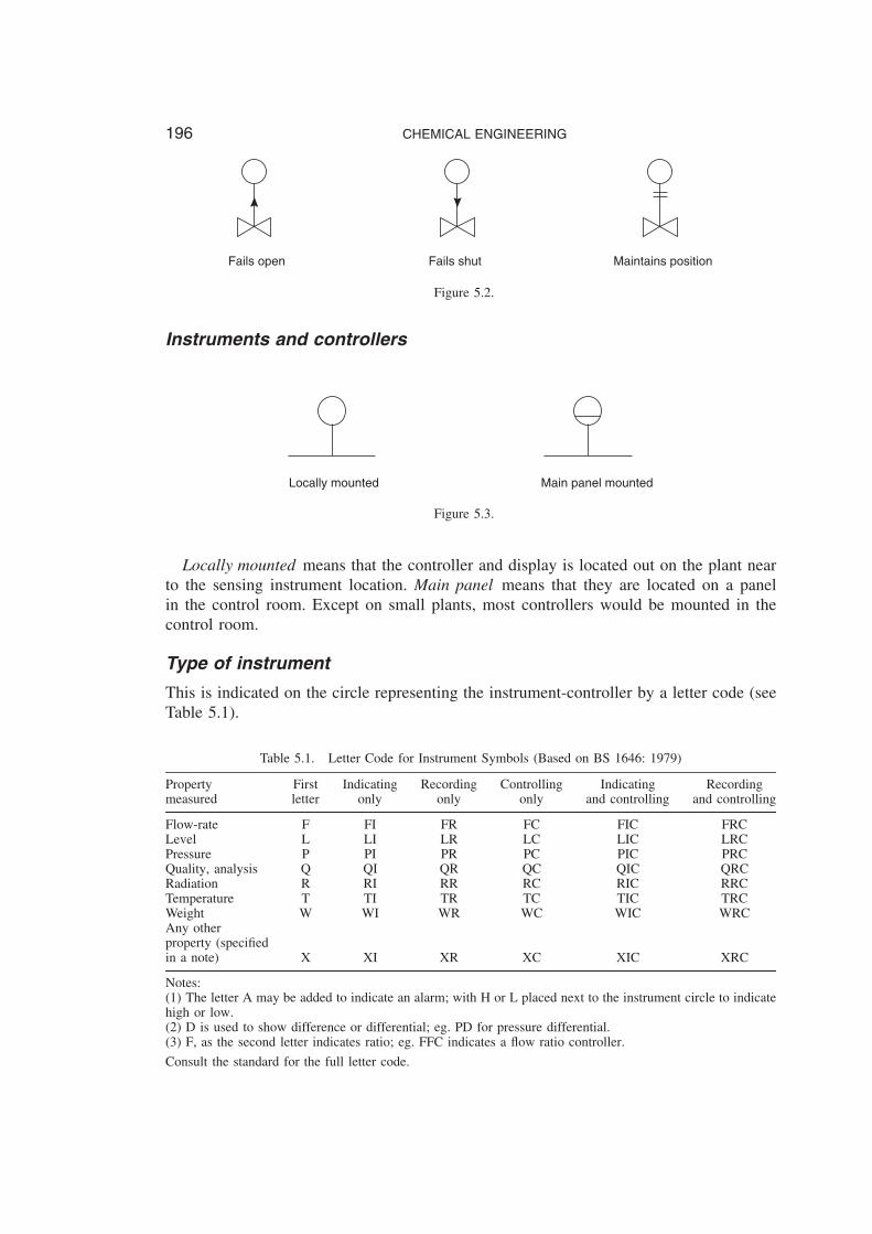
Failure mode

The direction of the arrow shows the position of the valve on failure of the powersupply.

196 CHEMICAL ENGINEERING

Fails open Fails shut Maintains position

Figure 5.2.

Instruments and controllers

Locally mounted Main panel mounted

Figure 5.3.

Locally mounted means that the controller and display is located out on the plant nearto the sensing instrument location. Main panel means that they are located on a panelin the control room. Except on small plants, most controllers would be mounted in thecontrol room.

Type of instrument

This is indicated on the circle representing the instrument-controller by a letter code (seeTable 5.1).

Table 5.1. Letter Code for Instrument Symbols (Based on BS 1646: 1979)

Property First Indicating Recording Controlling Indicating Recordingmeasured letter only only only and controlling and controlling

Flow-rate F FI FR FC FIC FRCLevel L LI LR LC LIC LRCPressure P PI PR PC PIC PRCQuality, analysis Q QI QR QC QIC QRCRadiation R RI RR RC RIC RRCTemperature T TI TR TC TIC TRCWeight W WI WR WC WIC WRCAny otherproperty (specifiedin a note) X XI XR XC XIC XRC

Notes:(1) The letter A may be added to indicate an alarm; with H or L placed next to the instrument circle to indicatehigh or low.(2) D is used to show difference or differential; eg. PD for pressure differential.(3) F, as the second letter indicates ratio; eg. FFC indicates a flow ratio controller.

Consult the standard for the full letter code.


The first letter indicates the property measured; for example, F D flow. Subsequentletters indicate the function; for example,

I D indicating

RC D recorder controller

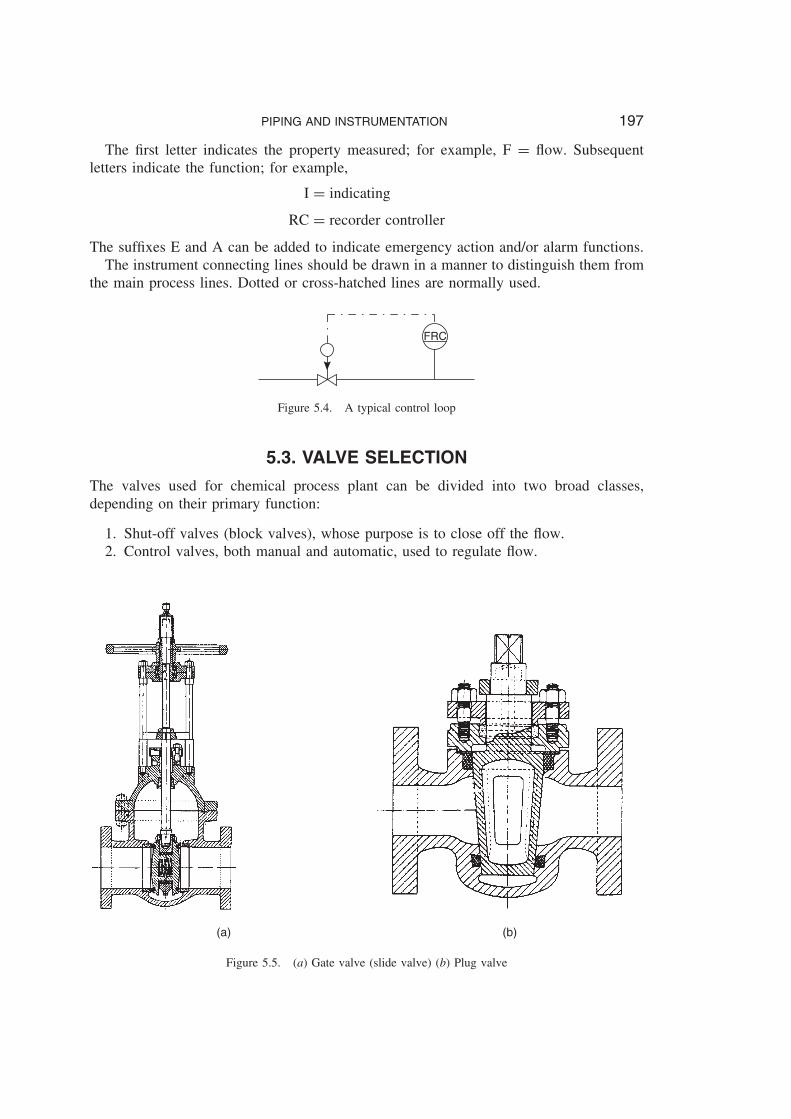
The suffixes E and A can be added to indicate emergency action and/or alarm functions.The instrument connecting lines should be drawn in a manner to distinguish them from

the main process lines. Dotted or cross-hatched lines are normally used.

FRC

Figure 5.4. A typical control loop

5.3. VALVE SELECTION

The valves used for chemical process plant can be divided into two broad classes,depending on their primary function:

1. Shut-off valves (block valves), whose purpose is to close off the flow.2. Control valves, both manual and automatic, used to regulate flow.

(a) (b)

Figure 5.5. (a) Gate valve (slide valve) (b) Plug valve


(c)

(d) (e)

Figure 5.5. (c) Ball valve (d) Globe valve (e) Diaphragm valve

The main types of valves used are:

Gate Figure 5.5aPlug Figure 5.5bBall Figure 5.5cGlobe Figure 5.5dDiaphragm Figure 5.5eButterfly Figure 5.5f

A valve selected for shut-off purposes should give a positive seal in the closed position andminimum resistance to flow when open. Gate, plug and ball valves are most frequentlyused for this purpose. The selection of values is discussed by Merrick (1986) (1990),Smith and Vivian (1995) and Smith and Zappe (2003).If flow control is required, the valve should be capable of giving smooth control over the

full range of flow, from fully open to closed. Globe valves are normally used, though the


(f) (g)

Figure 5.5. (f) Butterfly valve (g) Non-return valve, check valve, hinged disc type

other types can be used. Butterfly valves are often used for the control of gas and vapourflows. Automatic control valves are basically globe valves with special trim designs (seeVolume 3, Chapter 7).The careful selection and design of control valves is important; good flow control must

be achieved, whilst keeping the pressure drop as low as possible. The valve must also besized to avoid the flashing of hot liquids and the super-critical flow of gases and vapours.Control valve sizing is discussed by Chaflin (1974).Non-return valves are used to prevent back-flow of fluid in a process line. They do

not normally give an absolute shut-off of the reverse flow. A typical design is shown inFigure 5.5g.Details of valve types and standards can be found in the technical data manual of the

British Valve and Actuators Manufacturers Association, BVAMA (1991). Valve design iscovered by Pearson (1978).

5.4. PUMPS5.4.1. Pump selection

The pumping of liquids is covered by Volume 1, Chapter 8. Reference should be madeto that chapter for a discussion of the principles of pump design and illustrations of themore commonly used pumps.Pumps can be classified into two general types:

1. Dynamic pumps, such as centrifugal pumps.2. Positive displacement pumps, such as reciprocating and diaphragm pumps.

The single-stage, horizontal, overhung, centrifugal pump is by far the most commonlyused type in the chemical process industry. Other types are used where a high head orother special process considerations are specified.


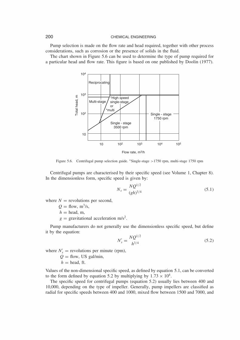
Pump selection is made on the flow rate and head required, together with other processconsiderations, such as corrosion or the presence of solids in the fluid.The chart shown in Figure 5.6 can be used to determine the type of pump required for

a particular head and flow rate. This figure is based on one published by Doolin (1977).

Reciprocating

Multi-stage*High speedsingle-stageor

*multi

Single - stage3500 rpm

Single - stage1750 rpm

Tot

al h

ead,

m104

103

102

10

10 102 103 104 105

Flow rate, m3/h

Figure 5.6. Centrifugal pump selection guide. ŁSingle-stage >1750 rpm, multi-stage 1750 rpm

Centrifugal pumps are characterised by their specific speed (see Volume 1, Chapter 8).In the dimensionless form, specific speed is given by:

Ns D NQ1/2

�gh�3/4�5.1�

where N D revolutions per second,Q D flow, m3/s,h D head, m,g D gravitational acceleration m/s2.

Pump manufacturers do not generally use the dimensionless specific speed, but defineit by the equation:

N0s D

NQ1/2

h3/4�5.2�

where N0s D revolutions per minute (rpm),Q D flow, US gal/min,h D head, ft.

Values of the non-dimensional specific speed, as defined by equation 5.1, can be convertedto the form defined by equation 5.2 by multiplying by 1.73ð 104.The specific speed for centrifugal pumps (equation 5.2) usually lies between 400 and

10,000, depending on the type of impeller. Generally, pump impellers are classified asradial for specific speeds between 400 and 1000, mixed flow between 1500 and 7000, and


axial above 7000. Doolin (1977) states that below a specific speed of 1000 the efficiencyof single-stage centrifugal pumps is low and multi-stage pumps should be considered.For a detailed discussion of the factors governing the selection of the best centrifugal

pump for a given duty the reader should refer to the articles by De Santis (1976), Neerkin(1974), Jacobs (1965) or Walas (1983).Positive displacement, reciprocating, pumps are normally used where a high head is

required at a low flow-rate. Holland and Chapman (1966) review the various types ofpositive displacement pumps available and discuss their applications.A general guide to the selection, installation and operation of pumps for the processes

industries is given by Davidson and von Bertele (1999) and Jandiel (2000).The selection of the pump cannot be separated from the design of the complete piping

system. The total head required will be the sum of the dynamic head due to frictionlosses in the piping, fittings, valves and process equipment, and any static head due todifferences in elevation.The pressure drop required across a control valve will be a function of the valve

design. Sufficient pressure drop must be allowed for when sizing the pump to ensure thatthe control valve operates satisfactorily over the full range of flow required. If possible,the control valve and pump should be sized together, as a unit, to ensure that the optimumsize is selected for both. As a rough guide, if the characteristics are not specified, thecontrol valve pressure drop should be taken as at least 30 per cent of the total dynamicpressure drop through the system, with a minimum value of 50 kPa (7 psi). The valveshould be sized for a maximum flow rate 30 per cent above the normal stream flow-rate.Some of the pressure drop across the valve will be recovered downstream, the amountdepending on the type of valve used.Methods for the calculation of pressure drop through pipes and fittings are given in

Section 5.4.2 and Volume 1, Chapter 3. It is important that a proper analysis is made ofthe system and the use of a calculation form (work sheet) to standardize pump-head calcu-lations is recommended. A standard calculation form ensures that a systematic methodof calculation is used, and provides a check list to ensure that all the usual factors havebeen considered. It is also a permanent record of the calculation. Example 5.8 has beenset out to illustrate the use of a typical calculation form. The calculation should includea check on the net positive suction head (NPSH) available; see section 5.4.3.Kern (1975) discusses the practical design of pump suction piping, in a series of

articles on the practical aspects of piping system design published in the journal ChemicalEngineering from December 1973 through to November 1975. A detailed presentationof pipe-sizing techniques is also given by Simpson (1968), who covers liquid, gas andtwo-phase systems. Line sizing and pump selection is also covered in a comprehensivearticle by Ludwig (1960).

5.4.2. Pressure drop in pipelines

The pressure drop in a pipe, due to friction, is a function of the fluid flow-rate, fluiddensity and viscosity, pipe diameter, pipe surface roughness and the length of the pipe.It can be calculated using the following equation:

1Pf D 8f�L/di��u2

2�5.3�


where 1Pf D pressure drop, N/m2,f D friction factor,L D pipe length, m,di D pipe inside diameter, m,� D fluid density, kg/m3,u D fluid velocity, m/s.

The friction factor is a dependent on the Reynolds number and pipe roughness. Thefriction factor for use in equation 5.3 can be found from Figure 5.7.

The Renolds number is given by Re D �� ð uð di�/� �5.4�

Values for the absolute surface roughness of commonly used pipes are given in Table 5.2.The parameter to use with Figure 5.7 is the relative roughness, given by:

relative roughness, e D absolute roughness/pipe inside diameter

Note: the friction factor used in equation 5.3 is related to the shear stress at the pipe wall,R, by the equation f D �R/�u2�. Other workers use different relationships. Their chartsfor friction factor will give values that are multiples of those given by Figure 5.7. So, it isimportant to make sure that the pressure drop equation usedmatches the friction factor chart.

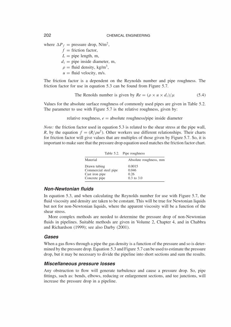
Table 5.2. Pipe roughness

Material Absolute roughness, mm

Drawn tubing 0.0015Commercial steel pipe 0.046Cast iron pipe 0.26Concrete pipe 0.3 to 3.0

Non-Newtonian fluidsIn equation 5.3, and when calculating the Reynolds number for use with Figure 5.7, thefluid viscosity and density are taken to be constant. This will be true for Newtonian liquidsbut not for non-Newtonian liquids, where the apparent viscosity will be a function of theshear stress.More complex methods are needed to determine the pressure drop of non-Newtonian

fluids in pipelines. Suitable methods are given in Volume 2, Chapter 4, and in Chabbraand Richardson (1999); see also Darby (2001).

GasesWhen a gas flows through a pipe the gas density is a function of the pressure and so is deter-mined by the pressure drop. Equation 5.3 and Figure 5.7 can be used to estimate the pressuredrop, but it may be necessary to divide the pipeline into short sections and sum the results.

Miscellaneous pressure lossesAny obstruction to flow will generate turbulence and cause a pressure drop. So, pipefittings, such as: bends, elbows, reducing or enlargement sections, and tee junctions, willincrease the pressure drop in a pipeline.

0.00

05

102

103

104

105

106

107

23

45

67

89

23

45

67

89

23

45

67

89

23

45

67

89

23

45

67

89

0.00

06

0.00

07

0.00

08

0.00

090.

001

0.00

125

0.00

15

0.00

175

0.00

20

0.00

225

0.00

250.

0027

50.

0030

0.00

35

0.00

40

0.00

450.

0050

0.00

550.

0060

0.00

650.

0070

0.00

75f

0.00

800.

0085

0.00

900.

0095

0.01

0.01

5

0.02

0.03

0.04

0.05

0.06

0.07

0.08

0.090.1

Lam

inar

flow

Sm

ooth

pip

es

Pip

e ro

ughn

ess

Criticalzone

Equ

atio

n 5.

3, ∆

p f = 8

fL d

ru

2

2

0.05

0.03

0.01

0.00

80.

006

0.00

4

0.00

2

0.00

1

0.00

06

0.00

02

0.00

01

0.00

001

0.00

0005

0.02

0.01

5

Rey

nold

s nu

mbe

r R

e =

udr

m

0.04

e/d

Figure

5.7.

Pipe

frictionversus

Reynoldsnumberandrelativeroughness


There will also be a pressure drop due to the valves used to isolate equipment andcontrol the fluid flow. The pressure drop due to these miscellaneous losses can be estimatedusing either of two methods:

1. As the number of velocity heads, K, lost at each fitting or valve.A velocity head is u2/2g, metres of the fluid, equivalent to �u2/2��, N/m2. Thetotal number of velocity heads lost due to all the fittings and valves is added to thepressure drop due to pipe friction.

2. As a length of pipe that would cause the same pressure loss as the fitting or valve.As this will be a function of the pipe diameter, it is expressed as the number ofequivalent pipe diameters. The length of pipe to add to the actual pipe length isfound by multiplying the total number of equivalent pipe diameters by the diameterof the pipe being used.

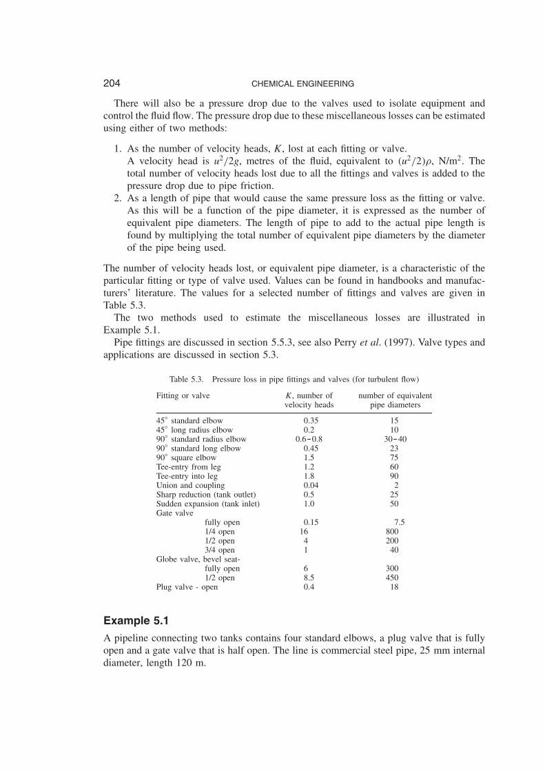
The number of velocity heads lost, or equivalent pipe diameter, is a characteristic of theparticular fitting or type of valve used. Values can be found in handbooks and manufac-turers’ literature. The values for a selected number of fittings and valves are given inTable 5.3.The two methods used to estimate the miscellaneous losses are illustrated in

Example 5.1.Pipe fittings are discussed in section 5.5.3, see also Perry et al. (1997). Valve types and

applications are discussed in section 5.3.

Table 5.3. Pressure loss in pipe fittings and valves (for turbulent flow)

Fitting or valve K, number of number of equivalentvelocity heads pipe diameters

45° standard elbow 0.35 1545° long radius elbow 0.2 1090° standard radius elbow 0.6 0.8 30 4090° standard long elbow 0.45 2390° square elbow 1.5 75Tee-entry from leg 1.2 60Tee-entry into leg 1.8 90Union and coupling 0.04 2Sharp reduction (tank outlet) 0.5 25Sudden expansion (tank inlet) 1.0 50Gate valve

fully open 0.15 7.51/4 open 16 8001/2 open 4 2003/4 open 1 40

Globe valve, bevel seat-fully open 6 3001/2 open 8.5 450

Plug valve - open 0.4 18

Example 5.1

A pipeline connecting two tanks contains four standard elbows, a plug valve that is fullyopen and a gate valve that is half open. The line is commercial steel pipe, 25 mm internaldiameter, length 120 m.


The properties of the fluid are: viscosity 0.99 mNM�2 s, density 998 kg/m3.Calculate the total pressure drop due to friction when the flow rate is 3500 kg/h.

Solution

Cross-sectional area of pipe D �

4�25ð 10�3�2 D 0.491ð 10�3m2

Fluid velocity, u D 3500

3600ð 1

0.491ð 10�3ð 1

998D 1.98 m/s

Reynolds number, Re D �998ð 1.98ð 25ð 10�3�/0.99ð 10�3

D 49,900 D 5ð 104 �5.4�

Absolute roughness commercial steel pipe, Table 5.2 D 0.046 mmRelative roughness D 0.046/�25ð 10�3� D 0.0018, round to 0.002From friction factor chart, Figure 5.7, f D 0.0032

Miscellaneous losses

fitting/valve number of velocity equivalent pipeheads, K diameters

entry 0.5 25elbows �0.8ð 4� �40ð 4�globe valve, open 6.0 300gate valve, 1/2 open 4.0 200exit 1.0 50Total 14.7 735

Method 1, velocity heads

A velocity head D u2/2g D 1.982/�2ð 9.8� D 0.20 m of liquid.

Head loss D 0.20ð 14.7 D 2.94 m

as pressure D 2.94ð 998ð 9.8 D 28,754 N/m2

Friction loss in pipe,1Pf D 8ð 0.0032�120�

�25ð 10�3�998ð 1.982

2

D 240,388 N/m2 �5.3�

Total pressure D 28,754C 240,388 D 269,142 N/m2 D 270 kN/m2

Method 2, equivalent pipe diameters

Extra length of pipe to allow for miscellaneous losses

D 735ð 25ð 10�3 D 18.4 m


So, total length for 1P calculation D 120C 18.4 D 138.4 m

1Pf D 8ð 0.0032�138.4�

�25ð 10�3�998ð 1.982

2D 277,247 N/m2

D 277 kN/m2 �5.3�

Note: the two methods will not give exactly the same result. The method using velocityheads is the more fundamentally correct approach, but the use of equivalent diameters iseasier to apply and sufficiently accurate for use in design calculations.

5.4.3. Power requirements for pumping liquids

To transport a liquid from one vessel to another through a pipeline, energy has to besupplied to:

1. overcome the friction losses in the pipes;2. overcome the miscellaneous losses in the pipe fittings (e.g. bends), valves, instru-

ments etc.;3. overcome the losses in process equipment (e.g. heat exchangers);4. overcome any difference in elevation from end to end of the pipe;5. overcome any difference in pressure between the vessels at each end of the pipeline.

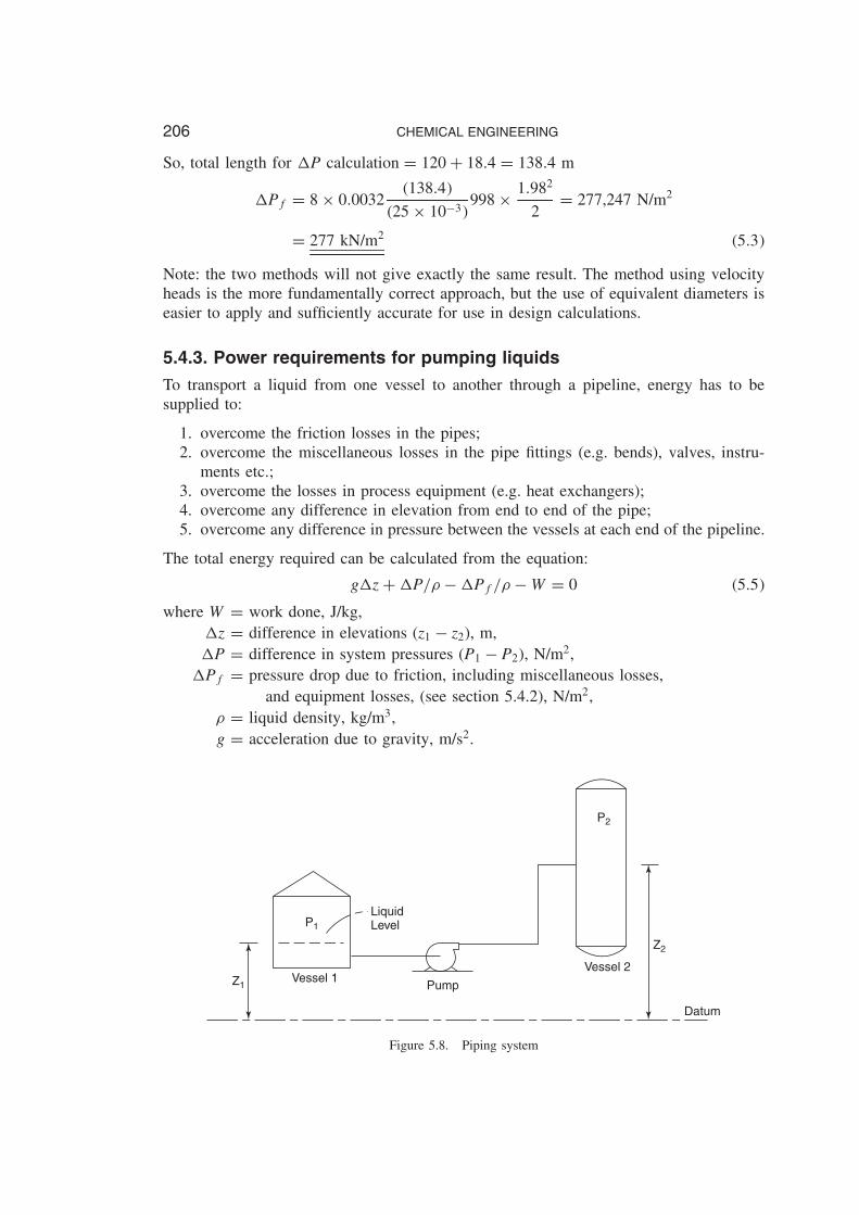
The total energy required can be calculated from the equation:

g1z C1P/� �1Pf/� �W D 0 �5.5�

where W D work done, J/kg,1z D difference in elevations (z1 � z2), m,1P D difference in system pressures (P1 � P2), N/m2,

1Pf D pressure drop due to friction, including miscellaneous losses,and equipment losses, (see section 5.4.2), N/m2,

� D liquid density, kg/m3,g D acceleration due to gravity, m/s2.

P1

P2

Z1

Z2

LiquidLevel

Vessel 1Vessel 2

Datum

Pump

Figure 5.8. Piping system


If W is negative a pump is required; if it is positive a turbine could be installed to extractenergy from the system.

The head required from the pump D 1Pf/�g�1P/�g�1z �5.5a�

The power is given by:

Power D �Wð m�/�, for a pump �5.6a�

and D �Wð m�ð �, for a turbine �5.6b�

where m D mass flow-rate, kg/s,� D efficiency = power out/power in.

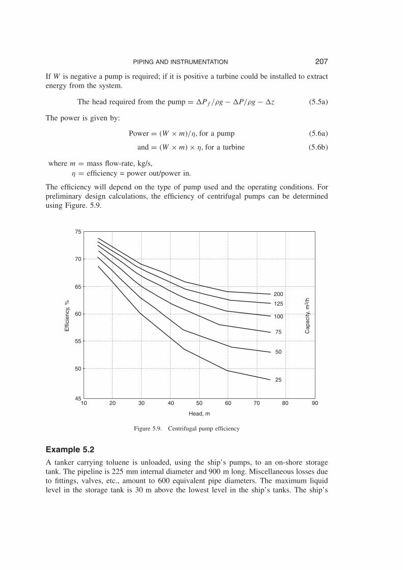
The efficiency will depend on the type of pump used and the operating conditions. Forpreliminary design calculations, the efficiency of centrifugal pumps can be determinedusing Figure. 5.9.

75

70

65

60

55

50

4510 20 30 40 50 60 70 80 90

200

125

100

75

50

25

Head, m

Effi

cien

cy, %

Cap

acity

, m3 /

h

Figure 5.9. Centrifugal pump efficiency

Example 5.2

A tanker carrying toluene is unloaded, using the ship’s pumps, to an on-shore storagetank. The pipeline is 225 mm internal diameter and 900 m long. Miscellaneous losses dueto fittings, valves, etc., amount to 600 equivalent pipe diameters. The maximum liquidlevel in the storage tank is 30 m above the lowest level in the ship’s tanks. The ship’s


tanks are nitrogen blanketed and maintained at a pressure of 1.05 bar. The storage tankhas a floating roof, which exerts a pressure of 1.1 bar on the liquid.The ship must unload 1000 tonne within 5 hours to avoid demurrage charges. Estimate

the power required by the pump. Take the pump efficiency as 70 per cent.Physical properties of toluene: density 874 kg/m3, viscosity 0.62 mNm�2 s.

Solution


4�225ð 10�3�2 D 0.0398 m2

Minimum fluid velocity D 1000ð 103

5ð 3600ð 1

0.0398ð 1

874D 1.6 m/s

Reynolds number D �874ð 1.6ð 225ð 10�3�/0.62ð 10�3

D 507,484 D 5.1ð 105 �5.4�

Absolute roughness commercial steel pipe, Table 5.2 D 0.046 mmRelative roughness D 0.046/225 D 0.0002Friction factor from Figure 5.7, f D 0.0019Total length of pipeline, including miscellaneous losses,

D 900C 600ð 225ð 10�3 D 1035 m

Friction loss in pipeline,1Pf D 8ð 0.0019ð(

1035

225ð 10�3

)ð 874ð 1.622

2

D 78,221 N/m2 �5.3�

Maximum difference in elevation, �z1 � z2� D �0� 30� D �30 m

Pressure difference, (P1 � P2� D �1.05� 1.1�105 D �5ð 103 N/m2

Energy balance

9.8��30�C ��5ð 103�/874� �78,221�/874�W D 0 �5.5�

W D �389.2 J/kg,

Power D �389.2ð 55.56�/0.7 D 30,981 W, say 31 kW . �5.6a�

5.4.4. Characteristic curves for centrifugal pumps

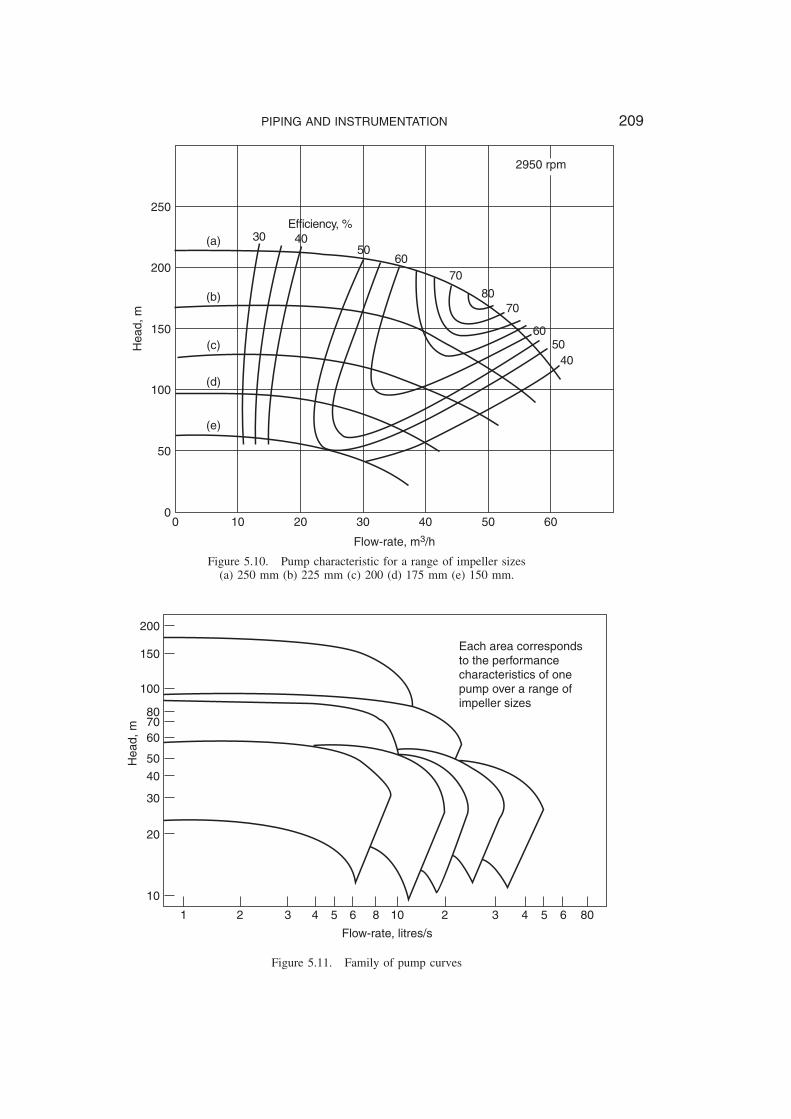
The performance of a centrifugal pump is characterised by plotting the head developedagainst the flow-rate. The pump efficiency can be shown on the same curve. A typicalplot is shown in Figure 5.10. The head developed by the pump falls as the flow-rate isincreased. The efficiency rises to a maximum and then falls.For a given type and design of pump, the performance will depend on the impeller

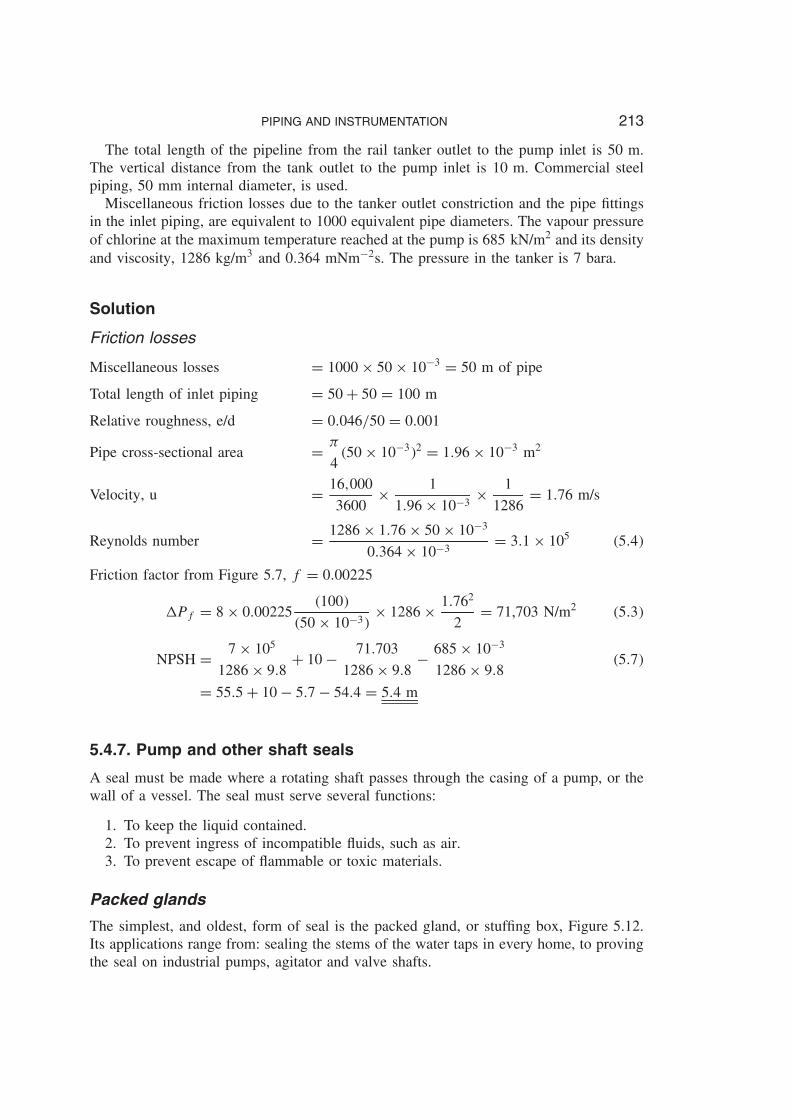
diameter, the pump speed, and the number of stages. Pump manufacturers publish familiesof operating curves for the range of pumps they sell. These can be used to select the bestpump for a given duty. A typical set of curves is shown in Figure 5.11.


00 10 20 30

Flow-rate, m3/h

40 50 60

50

100

150

Hea

d, m

200

250

(a)

(b)

(c)

(d)

(e)

2950 rpm

30 4050

6070

8070

6050

40

Efficiency, %

Figure 5.10. Pump characteristic for a range of impeller sizes(a) 250 mm (b) 225 mm (c) 200 (d) 175 mm (e) 150 mm.

200

150

100

807060

50

40

30

20

10

1 2 3 4 5 6 8 10 2 3 4 5 6 80

Flow-rate, litres/s

Hea

d, m

Each area corresponds to the performancecharacteristics of onepump over a range ofimpeller sizes

Figure 5.11. Family of pump curves


5.4.5. System curve (operating line)

There are two components to the pressure head that has to be supplied by the pump in apiping system:

1. The static pressure, to overcome the differences in head (height) and pressure.2. The dynamic loss due to friction in the pipe, the miscellaneous losses, and the

pressure loss through equipment.

The static pressure difference will be independent of the fluid flow-rate. The dynamicloss will increase as the flow-rate is increased. It will be roughly proportional to the flow-rate squared, see equation 5.3. The system curve, or operating line, is a plot of the totalpressure head versus the liquid flow-rate. The operating point of a centrifugal pump can befound by plotting the system curve on the pump’s characteristic curve, see Example 5.3.When selecting a centrifugal pump for a given duty, it is important to match the pump

characteristic with system curve. The operating point should be as close as is practical tothe point of maximum pump efficiency, allowing for the range of flow-rate over whichthe pump may be required to operate.Most centrifugal pumps are controlled by throttling the flow with a valve on the pump

discharge, see Section 5.8.3. This varies the dynamic pressure loss, and so the positionof the operating point on the pump characteristic curve.Throttling the flow results in an energy loss, which is acceptable in most applications.

However, when the flow-rates are large, the use of variable speed control on the pumpdrive should be considered to conserve energy.A more detailed discussion of the operating characteristics of centrifugal and other

types of pump is given by Walas (1990) and Karassik et al. (2001).

Example 5.3

A process liquid is pumped from a storage tank to a distillation column, using a centrifugalpump. The pipeline is 80 mm internal diameter commercial steel pipe, 100 m long.Miscellaneous losses are equivalent to 600 pipe diameters. The storage tank operates atatmospheric pressure and the column at 1.7 bara. The lowest liquid level in the tank will be1.5 m above the pump inlet, and the feed point to the column is 3 m above the pump inlet.Plot the system curve on the pump characteristic given in Figure A and determine the

operating point and pump efficiency.Properties of the fluid: density 900 kg/m3, viscosity 1.36 mN m�2s.

Solution

Static head

Difference in elevation,1z D 3.0� 1.5 D 1.5 m

Difference in pressure,1P D �1.7� 1.013�105 D 0.7ð 105 N/m2

as head of liquid D �0.7ð 105�/�900ð 9.8� D 7.9 m

Total static ead D 1.5C 7.9 D 9.4 m


Dynamic head

As an initial value, take the fluid velocity as 1 m/s, a reasonable value.


4�80ð 10�3�2 D 5.03ð 10�3 m2

Volumetric flow-rate D 1ð 5.03ð 10�3 ð 3600 D 18.1 m3/h

Reynolds number D 900ð 1ð 80ð 10�3

1.36ð 10�3D 5.3ð 104 �5.4�

Relative roughness D 0.46/80 D 0.0006

Friction factor from Figure 5.7, f D 0.0027

Length including miscellaneous loses D 100C �600ð 80ð 103� D 148 m

Pressure drop,1Pf D 8ð 0.0027�148�

�80ð 10�3�ð 900ð 12

2D 17,982 N/m2

D 17,982/�900ð 9.8� D 2.03 m liquid �5.3�

Total head D 9.4C 2.03 D 11.4 m

30.0

25.0

20.0

15.0

10.0

5.0

0.00 10 20 30 40 50 60 70 80

Flow-rate, m3/h

Liqu

id h

ead,

m

77

80

Efficiency

Pump curve

79

79

77

Systemcurve

Figure A. Example 5.3


To find the system curve the calculations were repeated for the velocities shown in thetable below:

velocity flow-rate static head dynamic head total headm/s m3/h m m m

1 18.1 9.4 2.0 11.41.5 27.2 9.4 4.3 14.02.0 36.2 9.4 6.8 16.22.5 45.3 9.4 10.7 20.13.0 54.3 9.4 15.2 24.6

Plotting these values on the pump characteristic gives the operating point as 18.5 m at40.0 m3/h and the pump efficiency as 79 per cent.

5.4.6. Net positive suction head (NPSH)

The pressure at the inlet to a pump must be high enough to prevent cavitation occurringin the pump. Cavitation occurs when bubbles of vapour, or gas, form in the pump casing.Vapour bubbles will form if the pressure falls below the vapour pressure of the liquid.The net positive suction head available �NPSH avail � is the pressure at the pump suction,

above the vapour pressure of the liquid, expressed as head of liquid.The net positive head required �NPSH reqd � is a function of the design parameters of

the pump, and will be specified by the pump manufacturer. As a general guide, the NPSHshould be above 3 m for pump capacities up to 100 m3/h, and 6 m above this capacity.Special impeller designs can be used to overcome problems of low suction head; seeDoolin (1977).The net positive head available is given by the following equation:

NPSH avail D P/� CH� Pf/� � Pv/� �5.7�

where NPSH avail D net positive suction head available at the pump suction, m,

P D the pressure above the liquid in the feed vessel, N/m2,

H D the height of liquid above the pump suction, m,

Pf D the pressure loss in the suction piping, N/m2,

Pv D the vapour pressure of the liquid at the pump suction, N/m2,

� D the density of the liquid at the pump suction temperature, kg/m3.

The inlet piping arrangement must be designed to ensure that NPSH avail exceeds NPSH reqd

under all operating conditions.The calculation of NPSH avail is illustrated in Example 5.4.

Example 5.4

Liquid chlorine is unloaded from rail tankers into a storage vessel. To provide thenecessary NPSH, the transfer pump is placed in a pit below ground level. Given thefollowing information, calculate the NPSH available at the inlet to the pump, at a maximumflow-rate of 16,000 kg/h.


The total length of the pipeline from the rail tanker outlet to the pump inlet is 50 m.The vertical distance from the tank outlet to the pump inlet is 10 m. Commercial steelpiping, 50 mm internal diameter, is used.Miscellaneous friction losses due to the tanker outlet constriction and the pipe fittings

in the inlet piping, are equivalent to 1000 equivalent pipe diameters. The vapour pressureof chlorine at the maximum temperature reached at the pump is 685 kN/m2 and its densityand viscosity, 1286 kg/m3 and 0.364 mNm�2s. The pressure in the tanker is 7 bara.

Solution

Friction losses

Miscellaneous losses D 1000ð 50ð 10�3 D 50 m of pipe

Total length of inlet piping D 50C 50 D 100 m

Relative roughness, e/d D 0.046/50 D 0.001

Pipe cross-sectional area D �

4�50ð 10�3�2 D 1.96ð 10�3 m2

Velocity, u D 16,000

3600ð 1

1.96ð 10�3ð 1

1286D 1.76 m/s

Reynolds number D 1286ð 1.76ð 50ð 10�3

0.364ð 10�3D 3.1ð 105 �5.4�

Friction factor from Figure 5.7, f D 0.00225

1Pf D 8ð 0.00225�100�

�50ð 10�3�ð 1286ð 1.762

2D 71,703 N/m2 �5.3�

NPSH D 7ð 105

1286ð 9.8C 10� 71.703

1286ð 9.8� 685ð 10�3

1286ð 9.8�5.7�

D 55.5C 10� 5.7� 54.4 D 5.4 m

5.4.7. Pump and other shaft seals

A seal must be made where a rotating shaft passes through the casing of a pump, or thewall of a vessel. The seal must serve several functions:

1. To keep the liquid contained.2. To prevent ingress of incompatible fluids, such as air.3. To prevent escape of flammable or toxic materials.

Packed glands

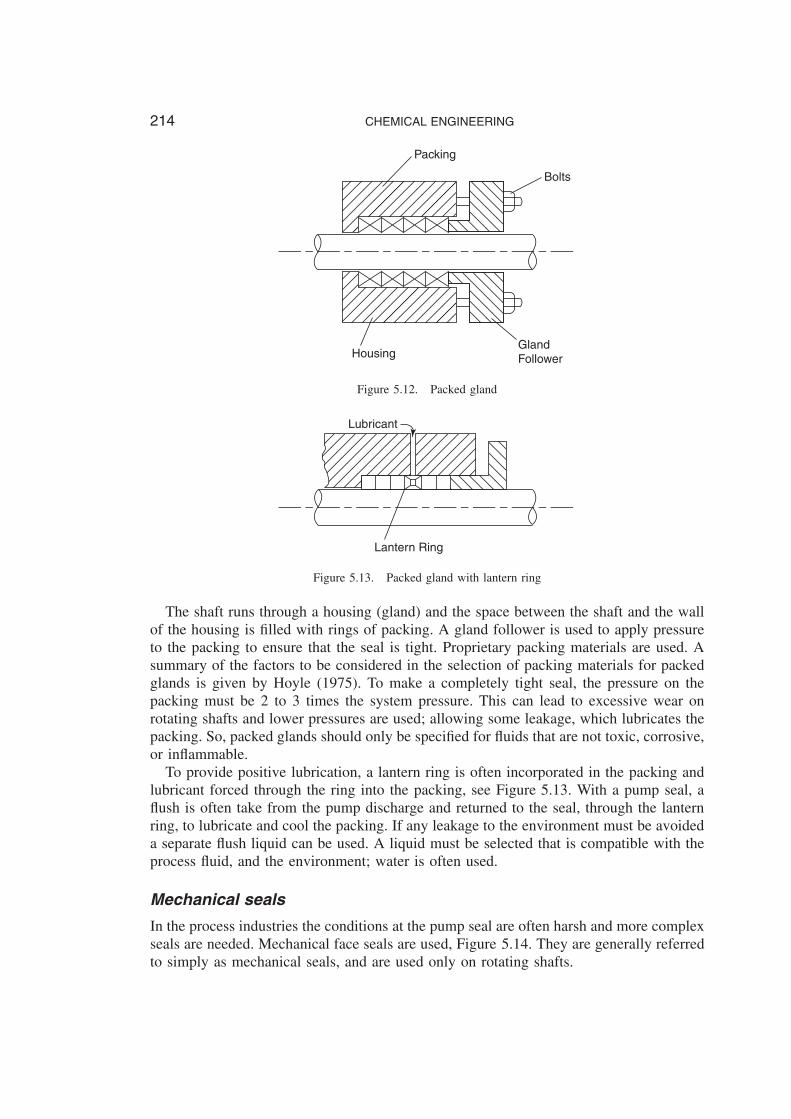
The simplest, and oldest, form of seal is the packed gland, or stuffing box, Figure 5.12.Its applications range from: sealing the stems of the water taps in every home, to provingthe seal on industrial pumps, agitator and valve shafts.


��

��

��

��

��

��

��

��

��

��

��

��

�

Packing

Bolts

GlandFollowerHousing

Figure 5.12. Packed gland

��

��

��

��

��

�

��

��

Lubricant

Lantern Ring

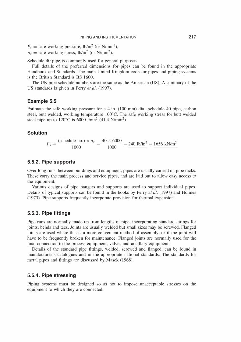
Figure 5.13. Packed gland with lantern ring

The shaft runs through a housing (gland) and the space between the shaft and the wallof the housing is filled with rings of packing. A gland follower is used to apply pressureto the packing to ensure that the seal is tight. Proprietary packing materials are used. Asummary of the factors to be considered in the selection of packing materials for packedglands is given by Hoyle (1975). To make a completely tight seal, the pressure on thepacking must be 2 to 3 times the system pressure. This can lead to excessive wear onrotating shafts and lower pressures are used; allowing some leakage, which lubricates thepacking. So, packed glands should only be specified for fluids that are not toxic, corrosive,or inflammable.To provide positive lubrication, a lantern ring is often incorporated in the packing and

lubricant forced through the ring into the packing, see Figure 5.13. With a pump seal, aflush is often take from the pump discharge and returned to the seal, through the lanternring, to lubricate and cool the packing. If any leakage to the environment must be avoideda separate flush liquid can be used. A liquid must be selected that is compatible with theprocess fluid, and the environment; water is often used.

Mechanical seals

In the process industries the conditions at the pump seal are often harsh and more complexseals are needed. Mechanical face seals are used, Figure 5.14. They are generally referredto simply as mechanical seals, and are used only on rotating shafts.


��

��

��

��

��

��

��

��

��

��

��

��

��

��

��

��

��

��

��

��

��

��

��

��

��

��

�

�

��

��

��

��

��

��

��

��

��

��

��

��

��

��

��

��

��

Retainingscrew O-rings

Sealface

Staticseal

Rotatingseal

Spring

��

��

��

��

��

��

��

��

��

��

��

��

��

��

Figure 5.14. Basic mechanical seal

The seal is formed between two flat faces, set perpendicular to the shaft. One facerotates with the shaft, the other is stationary. The seal is made, and the faces lubricatedby a very thin film of liquid, about 0.0001�m thick. A particular advantage of this typeof seal is that it can provide a very effective seal without causing any wear on the shaft.The wear is transferred to the special seal faces. Some leakage will occur but it is small,normally only a few drops per hour.Unlike a packed gland, a mechanical seal, when correctly installed and maintained, can

be considered leak-tight.A great variety of mechanical seal designs are available, and seals can be found to suit

virtually all applications. Only the basic mechanical seal is described below. Full details,and specifications, of the range of seals available and their applications can be obtainedfrom manufacturers’ catalogues.

The basic mechanical seal

The components of a mechanical seal, Figure 5.14 are:

1. A stationary sealing ring (mating ring).2. A seal for the stationary ring, O-rings or gaskets.3. A rotating seal ring (primary ring), mounted so that it can slide along the shaft to

take up wear in the seal faces.4. A secondary seal for the rotating ring mount; usually O-rings, or or chevron seals.5. A spring to maintain contact pressure between the seal faces; to push the faces

together.


6. A thrust support for the spring; either a collar keyed to the shaft or a step in theshaft.

The assembled seal is fitted into a gland housing (stuffing box) and held in place by aretaining ring (gland plate).Mechanical seals are classified as inside or outside, depending on whether, the primary

(rotating ring) is located inside the housing; running in the fluid, or, outside. Outside sealsare easier to maintain, but inside seals are more commonly used in the process industries,as it is easier to lubricate and flush this type.

Double seals

Where it is necessary to prevent any leakage of fluid to the atmosphere, a doublemechanical seal is used. The space between the two seals is flushed with a harmlessfluid, compatible with the process fluid, and provides a buffer between the two seals.

Seal-less pumps (canned pumps)

Pumps that have no seal on the shaft between the pump and the drive motor are available.They are used for severe duties, where it is essential that there is no leakage into theprocess fluid, or the environment.The drive motor and pump are enclosed in a single casing and the stator windings

and armature are protected by metal cans; they are usually referred to as canned pumps.The motor runs in the process fluid. The use of canned pumps to control environmentalpollution is discussed by Webster (1979).

5.5. MECHANICAL DESIGN OF PIPING SYSTEMS

5.5.1. Wall thickness: pipe schedule

The pipe wall thickness is selected to resist the internal pressure, with an allowancefor corrosion. Processes pipes can normally be considered as thin cylinders; only high-pressure pipes, such as high-pressure steam lines, are likely to be classified as thickcylinders and must be given special consideration (see Chapter 13).The British Standard 5500 gives the following formula for pipe thickness:

t D Pd

20�d C P�5.8�

where P D internal pressure, bar,d D pipe od, mm,�d D design stress at working temperature, N/mm2.

Pipes are often specified by a schedule number (based on the thin cylinder formula).The schedule number is defined by:

Schedule number D Ps ð 1000

�s�5.9�


Ps D safe working pressure, lb/in2 (or N/mm2),�s D safe working stress, lb/in2 (or N/mm2).

Schedule 40 pipe is commonly used for general purposes.Full details of the preferred dimensions for pipes can be found in the appropriate

Handbook and Standards. The main United Kingdom code for pipes and piping systemsis the British Standard is BS 1600.The UK pipe schedule numbers are the same as the American (US). A summary of the

US standards is given in Perry et al. (1997).

Example 5.5

Estimate the safe working pressure for a 4 in. (100 mm) dia., schedule 40 pipe, carbonsteel, butt welded, working temperature 100ŽC. The safe working stress for butt weldedsteel pipe up to 120ŽC is 6000 lb/in2 (41.4 N/mm2).

Solution

Ps D �schedule no.�ð �s

1000D 40ð 6000

1000D 240 lb/in2 D 1656 kN/m2

5.5.2. Pipe supports

Over long runs, between buildings and equipment, pipes are usually carried on pipe racks.These carry the main process and service pipes, and are laid out to allow easy access tothe equipment.Various designs of pipe hangers and supports are used to support individual pipes.

Details of typical supports can be found in the books by Perry et al. (1997) and Holmes(1973). Pipe supports frequently incorporate provision for thermal expansion.

5.5.3. Pipe fittings

Pipe runs are normally made up from lengths of pipe, incorporating standard fittings forjoints, bends and tees. Joints are usually welded but small sizes may be screwed. Flangedjoints are used where this is a more convenient method of assembly, or if the joint willhave to be frequently broken for maintenance. Flanged joints are normally used for thefinal connection to the process equipment, valves and ancillary equipment.Details of the standard pipe fittings, welded, screwed and flanged, can be found in

manufacturer’s catalogues and in the appropriate national standards. The standards formetal pipes and fittings are discussed by Masek (1968).

5.5.4. Pipe stressing

Piping systems must be designed so as not to impose unacceptable stresses on theequipment to which they are connected.


Loads will arise from:

1. Thermal expansion of the pipes and equipment.2. The weight of the pipes, their contents, insulation and any ancillary equipment.3. The reaction to the fluid pressure drop.4. Loads imposed by the operation of ancillary equipment, such as relief valves.5. Vibration.

Thermal expansion is a major factor to be considered in the design of piping systems. Thereaction load due to pressure drop will normally be negligible. The dead-weight loadscan be carried by properly designed supports.Flexibility is incorporated into piping systems to absorb the thermal expansion. A piping

system will have a certain amount of flexibility due to the bends and loops required bythe layout. If necessary, expansion loops, bellows and other special expansion devicescan be used to take up expansion.A discussion of the methods used for the calculation of piping flexibility and stress

analysis are beyond the scope of this book. Manual calculation techniques, and the appli-cation of computers in piping stress analysis, are discussed in the handbook edited byNayyar et al. (2000).

5.5.5. Layout and design

An extensive discussion of the techniques used for piping system design and specificationis beyond the scope of this book. The subject is covered thoroughly in the books bySherwood (1991), Kentish (1982a) (1982b), and Lamit (1981).

5.6. PIPE SIZE SELECTIONIf the motive power to drive the fluid through the pipe is available free, for instance whenpressure is let down from one vessel to another or if there is sufficient head for gravityflow, the smallest pipe diameter that gives the required flow-rate would normally be used.If the fluid has to be pumped through the pipe, the size should be selected to give the

least annual operating cost.Typical pipe velocities and allowable pressure drops, which can be used to estimate

pipe sizes, are given below:

Velocity m/s 1P kPa/m

Liquids, pumped (not viscous) 1 3 0.5Liquids, gravity flow 0.05Gases and vapours 15 30 0.02 per cent of

line pressureHigh-pressure steam, >8 bar 30 60

Rase (1953) gives expressions for design velocities in terms of the pipe diameter. Hisexpressions, converted to SI units, are:


Pump discharge 0.06dC 0.4 m/sPump suction 0.02dC 0.1 m/sSteam or vapour 0.2d m/s

where d is the internal diameter in mm.Simpson (1968) gives values for the optimum velocity in terms of the fluid density.

His values, converted to SI units and rounded, are:

Fluid density kg/m3 Velocity m/s

1600 2.4800 3.0160 4.916 9.40.16 18.00.016 34.0

The maximum velocity should be kept below that at which erosion is likely to occur.For gases and vapours the velocity cannot exceed the critical velocity (sonic velocity)(see Volume 1, Chapter 4) and would normally be limited to 30 per cent of the criticalvelocity.

Economic pipe diameter

The capital cost of a pipe run increases with diameter, whereas the pumping costsdecrease with increasing diameter. The most economic pipe diameter will be the onewhich gives the lowest annual operating cost. Several authors have published formulaeand nomographs for the estimation of the economic pipe diameter, Genereaux (1937),Peters and Timmerhaus (1968) (1991), Nolte (1978) and Capps (1995). Most apply toAmerican practice and costs, but the method used by Peters and Timmerhaus has beenmodified to take account of UK prices (Anon, 1971).The formulae developed in this section are presented as an illustration of a simple

optimisation problem in design, and to provide an estimate of economic pipe diameterthat is based on UK costs and in SI units. The method used is essentially that firstpublished by Genereaux (1937).The cost equations can be developed by considering a 1 metre length of pipe.The purchase cost will be roughly proportional to the diameter raised to some power.

Purchase cost D Bdn £/m

The value of the constant B and the index n depend on the pipe material and schedule.The installed cost can be calculated by using the factorial method of costing discussed

in Chapter 6.Installed cost D Bdn�1C F�

where the factor F includes the cost of valves, fittings and erection, for a typical run ofthe pipe.The capital cost can be included in the operating cost as an annual capital charge. There

will also be an annual charge for maintenance, based on the capital cost.

Cp D Bdn�1C F��a C b� �5.10�


where Cp D capital cost portion of the annual operating cost, £,a D capital charge, per cent/100,b D maintenance costs, per cent/100.

The power required for pumping is given by:

Power D volumetric flow-rateð pressure drop.

Only the friction pressure drop need be considered, as any static head is not a functionof the pipe diameter.To calculate the pressure drop the pipe friction factor needs to be known. This is a

function of Reynolds number, which is in turn a function of the pipe diameter. Severalexpressions have been proposed for relating friction factor to Reynolds number. Forsimplicity the relationship proposed by Genereaux (1937) for turbulent flow in cleancommercial steel pipes will be used.

f D 0.04Re�0.16

where f is the Fanning friction factor D 2�R/�u2�.Substituting this into the Fanning pressure drop equation gives:

1P D 4.13ð 1010G1.84�0.16��1d�4.84 �5.11�

where 1P D pressure drop, kN/m2 (kPa),G D flow rate, kg/s,� D density, kg/m3,� D viscosity, m Nm�2 sd D pipe id, mm.

The annual pumping costs will be given by:

Cf D Ap

E1P

G

�

where A D plant attainment, hours/year,p D cost of power, £/kWh,E D pump efficiency, per cent/100.

Substituting from equation 5.11

Cf D Hp

E4.13ð 1010G2.84�0.16��2d�4.84 �5.12�

The total annual operating cost Ct D CpCCf.Adding equations 5.10 and 5.12, differentiating, and equating to zero to find the pipe

diameter to give the minimum cost gives:

d, optimum D[2ð 1011 ð ApG2.84�0.16��2

EnB�1C F��a C b�

]1/�4.84Cn�

�5.13�

Equation 5.13 is a general equation and can be used to estimate the economic pipediameter for any particular situation. It can be set up on a spreadsheet and the effect ofthe various factors investigated.


The equation can be simplified by substituting typical values for the constants.

A The normal attainment for a chemical process plant will be between90 95%, so take the operating hours per year as 8000.

E Pump and compressor efficiencies will be between 50 to 70%, so take 0.6.p Use the current cost of power, 0.055 £/kWh (mid-1992).F This is the most difficult factor to estimate. Other authors have used

values ranging from 1.5 (Peters and Timmerhaus (1968)) to 6.75 (Nolte(1978)). It is best taken as a function of the pipe diameter; as has beendone to derive the simplified equations given below.

B, n Can be estimated from the current cost of piping.a Will depend on the current cost of capital, around 10% in mid-1992.b A typical figure for process plant will be 5%, see Chapter 6.

F, B, and n have been estimated from cost data published by the Institution of ChemicalEngineers, IChemE (1987), updated to mid-1992. This includes the cost of fittings, instal-lation and testing. A log-log plot of the data gives the following expressions for theinstalled cost:

Carbon steel, 15 to 350 mm 27 d0.55 £/m

Stainless steel, 15 to 350 mm 31 d0.62 £/m

Substitution in equation 5.12 gives, for carbon steel:

d, optimum D 366 G0.53�0.03��0.37

Because the exponent of the viscosity term is small, its value will change very littleover a wide range of viscosity

at� D 10�5 Nm�2s �0.01 cp�, �0.03 D 0.71

� D 10�2 Nm�2s �10 cp�, �0.03 D 0.88

Taking a mean value of 0.8, gives the following equations for the optimum diameter,for turbulent flow:

Carbon steel pipe:d, optimum D 293 G0.53��0.37 �5.14�

Stainless steel pipe:d, optimum D 260 G0.52��0.37 �5.15�

Equations 5.14 and 5.15 can be used to make an approximate estimate of the economicpipe diameter for normal pipe runs. For a more accurate estimate, or if the fluid or piperun is unusual, the method used to develop equation 5.13 can be used, taking into accountthe special features of the particular pipe run.The optimum diameter obtained from equations 5.14 and 5.15 should remain valid

with time. The cost of piping depends on the cost power and the two costs appear in theequation as a ratio raised to a small fractional exponent.Equations for the optimum pipe diameter with laminar flow can be developed by using

a suitable equation for pressure drop in the equation for pumping costs.


The approximate equations should not be used for steam, as the quality of steam dependson its pressure, and hence the pressure drop.Nolte (1978) gives detailed methods for the selection of economic pipe diameters,

taking into account all the factors involved. He gives equations for liquids, gases, steamand two-phase systems. He includes in his method an allowance for the pressure dropdue to fittings and valves, which was neglected in the development of equation 5.12, andby most other authors.The use of equations 5.14 and 5.15 are illustrated in Examples 5.6 and 5.7, and the

results compared with those obtained by other authors. Peters and Timmerhaus’s formulaegive larger values for the economic pipe diameters, which is probably due to their lowvalue for the installation cost factor, F.

Example 5.6

Estimate the optimum pipe diameter for a water flow rate of 10 kg/s, at 20ŽC. Carbonsteel pipe will be used. Density of water 1000 kg/m3.

Solution

d, optimum D 293ð �10�0.53 1000�0.37 �5.14�

D 77.1 mm

use 80-mm pipe.

Viscosity of water at 20ŽC D 1.1ð 10�3 Ns/m2,

Re D 4G

��dD 4ð 10

� ð 1.1ð 10�3 ð 80ð 10�3D 1.45ð 105

>4000, so flow is turbulent.Comparison of methods:

Economic diameter

Equation 5.14 180 mmPeters and Timmerhaus (1991) 4 in. (100 mm)Nolte (1978) 80 mm

Example 5.7

Estimate the optimum pipe diameter for a flow of HCl of 7000 kg/h at 5 bar, 15ŽC,stainless steel pipe. Molar volume 22.4 m3/kmol, at 1 bar, 0ŽC.

Solution

Molecular weight HCl D 36.5.

Density at operating conditions D 36.5

22.4ð 5

1ð 273

288D 7.72 kg/m3


Optimum diameter D 260(7000

3600

)0.52

7.72�0.37 �5.15�

D 172.4 mm

use 180-mm pipe.Viscosity of HCl 0.013 m Ns/m2

Re D 4

�ð 7000

3600ð 1

0.013ð 10�3 ð 180ð 10�3D 1.06ð 106, turbulent

Comparison of methods:

Economic diameter

Equation 5.15 180 mmPeters and Timmerhaus (1991) 9 in. (220 mm) carbon steelNolte (1978) 7 in. (180 mm) carbon steel

Example 5.8

Calculate the line size and specify the pump required for the line shown in Figure 5.15;material ortho-dichlorobenzene (ODCB), flow-rate 10,000 kg/h, temperature 20ŽC, pipematerial carbon steel.

Datum

4 m

1m

Datum

0.5

1.0

m

2.5

m

5.5

m0.

5 m

5 m

6.5

m

7.5

m20 m

2 m

Preliminary layoutnot to scale

Figure 5.15. Piping isometric drawing (Example 5.8)


Solution

ODCB density at 20ŽC D 1306 kg/m3.Viscosity: 0.9 mNs/m2 (0.9 cp).

Estimation of pipe diameter required

typical velocity for liquid 2 m/s

mass flow D 10,000

3600D 2.78 kg/s

volumetric flow D 2.78

1306D 2.13ð 10�3 m3/s

area of pipe D volumetric flow

velocityD 2.13ð 10�3

2D 1.06ð 10�3 m2

diameter of pipe D√(

1.06ð 10�3 ð 4

�

)D 0.037 m

D 37 mm

Or, use economic pipe diameter formula:

d, optimum D 293ð 2.780.53 ð 1306�0.37 �5.14�

D 35.4 mm

Take diameter as 40 mm

cross-sectional area D �

4�40ð 10�3� D 1.26ð 10�3 m2

Pressure drop calculation

fluid velocity D 2.13ð 10�3

1.26ð 10�3D 1.70 m/s

Friction loss per unit length, 1f1:

Re D 1306ð 1.70ð 40ð 10�3

0.9ð 10�3D 9.9ð 104 �5.5�

Absolute roughness commercial steel pipe, table 5.2 D 0.46 mmRelative roughness, e/d D 0.046/40 D 0.001Friction factor from Figure 5.7, f D 0.0027

1f1 D 8ð 0.0027ð �1�

�40ð 10�3�ð 1306ð 1.72

2D 1019 N/m2 �5.3�

D 1.02 kPa


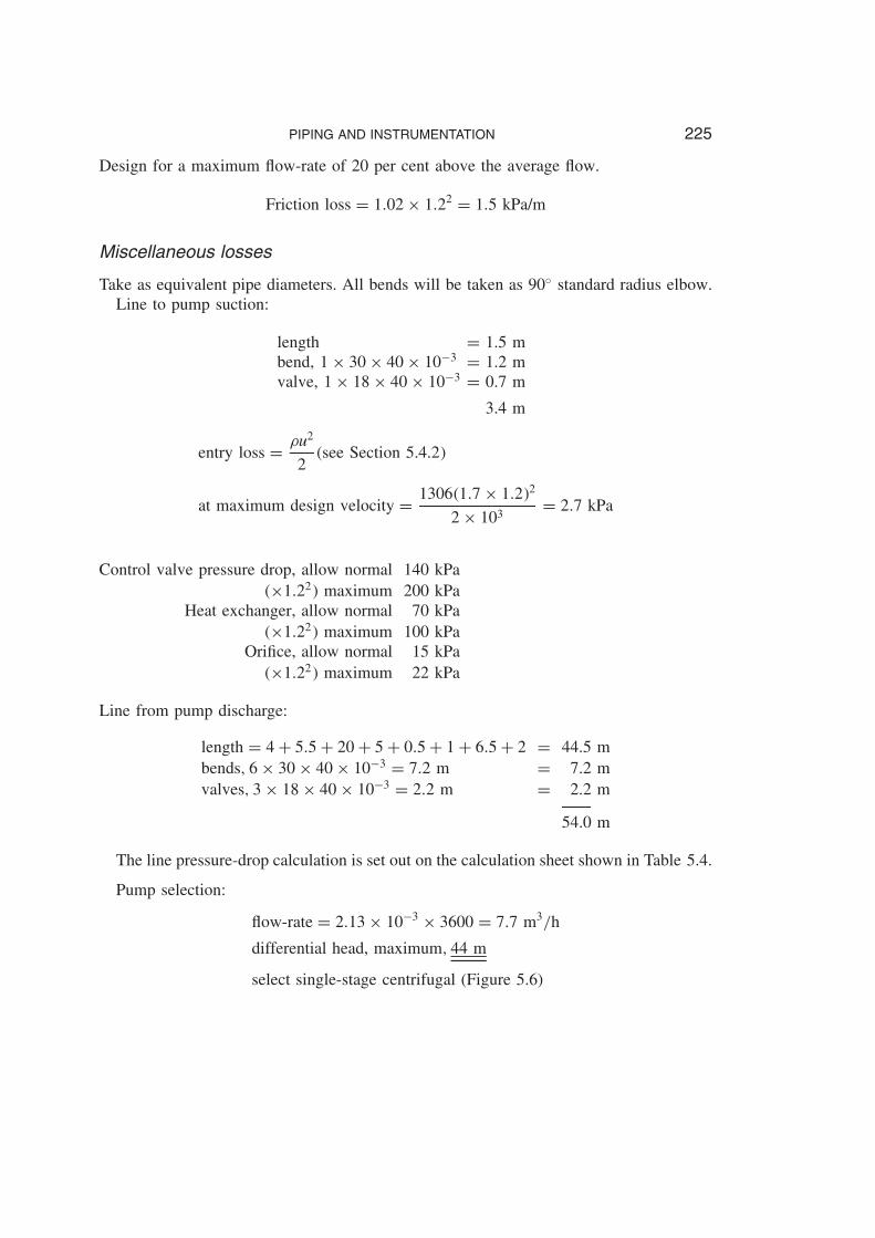
Design for a maximum flow-rate of 20 per cent above the average flow.

Friction loss D 1.02ð 1.22 D 1.5 kPa/m

Miscellaneous losses

Take as equivalent pipe diameters. All bends will be taken as 90Ž standard radius elbow.Line to pump suction:

length D 1.5 mbend, 1ð 30ð 40ð 10�3 D 1.2 mvalve, 1ð 18ð 40ð 10�3 D 0.7 m

3.4 m

entry loss D �u2

2�see Section 5.4.2�

at maximum design velocity D 1306�1.7ð 1.2�2

2ð 103D 2.7 kPa

Control valve pressure drop, allow normal 140 kPa�ð1.22� maximum 200 kPa

Heat exchanger, allow normal 70 kPa�ð1.22� maximum 100 kPa

Orifice, allow normal 15 kPa�ð1.22� maximum 22 kPa

Line from pump discharge:

length D 4C 5.5C 20C 5C 0.5C 1C 6.5C 2 D 44.5 mbends, 6ð 30ð 40ð 10�3 D 7.2 m D 7.2 mvalves, 3ð 18ð 40ð 10�3 D 2.2 m D 2.2 m

54.0 m

The line pressure-drop calculation is set out on the calculation sheet shown in Table 5.4.

Pump selection:

flow-rate D 2.13ð 10�3 ð 3600 D 7.7 m3/h

differential head, maximum, 44 m

select single-stage centrifugal (Figure 5.6)


Table 5.4. Line calculation form (Example 5.4)

Pump and line calculation sheet

Job no. Sheet no. By RKS, 7/7/79 Checked

4415A 1

Fluid ODCB DISCHARGE CALCULATION

Temperature °C 20 Line size mm 40

Density kg/m3 1306 Flow Norm. Max. Units

Viscosity mNs/m2 0.9 u2 Velocity 1.7 2.0 m/s

Normal flow kg/s 2.78 1f2 Friction loss 1.0 1.5 kPa/m

Design max. flow kg/s 3.34 L2 Line length 54 m

1f2L2 Line loss 54 kPa

SUCTION CALCULATION Orifice 15 22 kPa

Line size mm 40 30% Control valve 140 200 kPa

Flow Norm. Max. Units Equipment

u1 Velocity 1.7 2.0 m/s (a) Heat ex. 70 100 kPa

1f1 Friction loss 1.0 1.5 kPa/m (b) kPa

L1 Line length 3.4 m (c) kPa

1f1 L1 Line loss 3.4 5.1 kPa (6) Dynamic loss 279 403 kPa

�u21/2 Entrance 1.9 2.7 kPa

(40 kPa) Strainer kPa z2 Static head 6.5 m

(1) Sub-total 5.3 7.8 kPa �gz2 85 85 kPa

Equip. press (max) 200 200 kPa

z1 Static head 1.5 1.5 m Contingency None None kPa

�gz1 19.6 19.6 kPa (7) Sub-total 285 285 kPa

Equip. press 100 100 kPa (7) C (6) Discharge press. 564 685 kPa

(2) Sub-total 119.6 119.6 kPa (3) Suction press. 114.3 111.8 kPa

(8) Diff. press. 450 576 kPa(2) � (1) (3) Suction press 114.3 111.8 kPa

(8)/�g 34 44 m(4) VAP. PRESS. 0.1 0.1 kPa

(3) � (4) (5) NPSH 114.2 111.7 kPaValve/(6) Control valve

(5)/�g 8.7 8.6 m % Dyn. loss 50%

2.5

m

C 2032 bar

1.0

m

C 2011 bar

7.5

m

H 205

Z1 = 2.5 − 1 = 1.5 mZ2 = 7.5 − 1 = 6.5 m


Table 5.5. Pump Specification Sheet (Example 5.8)

Pump Specification

Type: CentrifugalNo. stages: 1Single/Double suction: SingleVertical/Horizontal mounting: HorizontalImpeller type: ClosedCasing design press.: 600 kPa

design temp.: 20°CDriver: Electric, 440 V, 50 c/s 3-phase.Seal type: Mechanical, external flushMax. flow: 7.7 m3/hDiff. press.: 600 kPa (47 m, water)

.


5.11. REFERENCESANON. (1969) Chem. Eng., NY 76 (June 2nd) 136. Process instrument elements.ANON. (1971) Brit. Chem. Eng. 16, 313. Optimum pipeline diameters by nomograph.AUSTIN, D. G. (1979) Chemical Engineering Drawing Symbols (George Godwin).BERTRAND, L. and JONES, J. B. (1961) Chem. Eng., NY 68 (Feb. 20th) 139. Controlling distillation columns.BUCKLEY, P. S., LUYBEN, W. L. and SHUNTA, J. P. (1985) Design of Distillation Column Control Systems

(Arnold).BVAMA (1991) Valves and Actuators from Britain, 5th edn (British Valve and Actuator Manufacturers’ Associ-

ation).CAPPS, R. W. (1995) Chem. Eng. NY, 102 (July) 102. Select the optimum pipe diameter.CHABBRA, R. P. and RICHARDSON, J. F. (1999) Non-Newtonian Flow in the Process Industries (Butterworth-

Heinemann).CHAFLIN, S. (1974) Chem. Eng., NY 81 (Oct. 14th) 105. Specifying control valves.COUGHANOWR, D. R. (1991) Process Systems Analysis and Control, 2nd edn. (MacGraw-Hill).DARBY, R. (2001) Chem. Eng., NY 108 (March) 66. Take the mystery out of non-Newton fluids.DAVIDSON, J. and VON BERTELE, O. (1999) Process Pump Selection A Systems Approach (I. Mech E.)DE SANTIS, G. J. (1976) Chem. Eng., NY 83 (Nov. 22nd) 163. How to select a centrifugal pump.DOOLIN, J. H. (1977) Chem. Eng., NY (Jan. 17th) 137. Select pumps to cut energy cost.ECKERT, J. S. (1964) Chem. Eng., NY 71 (Mar. 30th) 79. Controlling packed-column stills.GENEREAUX, R. P. (1937) Ind. Eng. Chem. 29, 385. Fluid-flow design methods.HOLLAND, F. A. and CHAPMAN, F. S. (1966) Chem. Eng., NY 73 (Feb. 14th) 129. Positive displacement pumps.HOYLE, R. (1978) Chem. Eng. NY, 85 (Oct 8th) 103. How to select and use mechanical packings.ICHEME (1988) A New Guide to Capital Cost Estimation 3rd edn (Institution of Chemical Engineers, London).JACOBS, J. K. (1965) Hydrocarbon Proc. 44 (June) 122. How to select and specify process pumps.JANDIEL, D. G. (2000) Chem. Eng. Prog. 96 (July) 15. Select the right compressor.KALANI, G. (1988) Microprocessor Based Distributed Control Systems (Prentice Hall).KARASSIK, I. J. et al. (2001) Pump Handbook, 3rd edn (McGraw-Hill).KENTISH, D. N. W. (1982a) Industrial Pipework (McGraw-Hill).KENTISH, D. N. W. (1982b) Pipework Design Data (McGraw-Hill).KERN, R. (1975) Chem. Eng., NY 82 (April 28th) 119. How to design piping for pump suction conditions.LAMIT, L. G. (1981) Piping Systems: Drafting and Design (Prentice Hall).LIPAK, B. G. (2003) Instrument Engineers’ Handbook, Vol 1: Process Measurement and Analysis, 4th edn (CRC

Press).LUDWG, E. E. (1960) Chem. Eng., NY 67 (June 13th) 162. Flow of fluids.MASEK, J. A. (1968) Chem. Eng., NY 75 (June 17th) 215. Metallic piping.MERRICK, R. C. (1986) Chem. Eng., NY 93 (Sept. 1st) 52. Guide to the selection of manual valves.MERRICK, R. C. (1990) Valve Selection and Specification Guide (Spon.).MURRILL, P. W. (1988) Application Concepts of Process Control (Instrument Society of America).NAYYAR, M. L. et al. (2000) Piping Handbook, 7th edn (McGraw-Hill).


NEERKIN, R. F. (1974) Chem. Eng., NY 81 (Feb. 18) 104. Pump selection for chemical engineers.NOLTE, C. B. (1978) Optimum Pipe Size Selection (Trans. Tech. Publications).PARKINS, R. (1959) Chem. Eng. Prog. 55 (July) 60. Continuous distillation plant controls.PEARSON, G. H. (1978) Valve Design (Mechanical Engineering Publications).PERRY, R. H. and CHILTON, C. H. (eds) (1973) Chemical Engineers Handbook, 5th edn (McGraw-Hill).PERRY, R. H., GREEN, D. W. and MALONEY, J. O. (eds) (1997) Perry’s Chemical Engineers’ Handbook, 7th

edn. (McGraw-Hill).PETERS, M. S. and TIMMERHAUS, K. D. (1968) Plant Design and Economics for Chemical Engineers, 2nd edn

(McGraw-Hill).PETERS, M. S. and TIMMERHAUS, K. D. (1991) Plant Design and Economics, 4th edn (McGraw-Hill).RASE, H. F. (1953) Petroleum Refiner 32 (Aug.) 14. Take another look at economic pipe sizing.RASMUSSEN, E. J. (1975) Chem. Eng., NY 82 (May 12th) 74. Alarm and shut down devices protect process

equipment.SHERWOOD, D. R. (1991) The Piping Guide, 2nd edn (Spon.).SHINSKEY, F. G. (1976) Chem. Eng. Prog. 72 (May) 73. Energy-conserving control systems for distillation units.SHINSKEY, F. G. (1984) Distillation Control, 2nd edn (McGraw-Hill).SHINSKEY, F. G. (1996) Process Control Systems, 4th edn (McGraw-Hill).SIMPSON, L. L. (1968) Chem. Eng., NY 75 (June 17th) 1923. Sizing piping for process plants.SMITH, E. and VIVIAN, B. E. (1995) Valve Selection (Mechanical Engineering Publications).SMITH, P. and ZAPPE, R. W. (2003) Valve Selection Handbook, 5th edn (Gulf Publishing).WALAS S. M. (1990) Chemical Process Equipment (Butterworth-Heinemann).WEBSTER, G. R. (1979) Chem. Engr. London No. 341 (Feb.) 91. The canned pump in the petrochemical

environment.

British Standards

BS 806: 1986 Ferrous pipes and piping for and in connection with land boilers.BS 1600: 1991 Dimension of steel pipes for the petroleum industry.BS 1646: 1984 Symbolic representation for process measurement control functions and instrumentation.Part 1: 1977 Basic requirements.Part 2: 1983 Specifications for additional requirements.Part 3: 1984 Specification for detailed symbols for instrument interconnection diagrams.Part 4: 1984 Specification for basic symbols for process computer, interface and shared display/controlfunctions.

American Standards

USAS B31.1.0: The ASME standard code for pressure piping.ASA B31.3.0: The ASME code for petroleum refinery piping.

5.12. NOMENCLATUREDimensionsin MLT£

A Plant attainment (hours operated per year)B Purchased cost factor, pipes £L�1a Capital charges factor, pipingb Maintenance cost factor, pipingCf Annual pumping cost, piping £L�1T�1Cp Capital cost, piping £L�1Ct Total annual cost, piping £L�1T�1d Pipe diameter Ldi Pipe inside diameter LE Pump efficiencye Relative roughness


F Installed cost factor, pipingf Friction factorG Mass flow rate MT�1g Gravitational acceleration LT�2H Height of liquid above the pump suction Lh Pump head LK Number of velocity headsL Pipe length Lm Mass flow-rate MT�1N Pump speed, revolutions per unit time T�1Ns Pump specific speedn Index relating pipe cost to diameterP Pressure ML�1T�2Pf Pressure loss in suction piping ML�1T�2Ps Safe working pressure ML�1T�2Pv Vapour pressure of liquid ML�1T�21P Difference in system pressures (P1 � P2) ML�1T�2

1Pf Pressure drop† ML�1T�2p Cost of power, pumpingQ Volumetric flow rate L3T�1R Shear stress on surface, pipes ML�1T�2t Pipe wall thickness Lu Fluid velocity LT�1W Work done L2T�2z Height above datum L1z Difference in elevation (z1 � z2) L� Pump efficiency� Fluid density ML�3� Viscosity of fluid ML�1T�1�d Design stress ML�1T�2�s Safe working stress ML�1T�2Re Reynolds number

NPSH avail Net positive suction head available at the pump suction LNPSH reqd Net positive suction head required at the pump suction L

†Note: In Volumes 1 and 2 this symbol is used for pressure difference, and pressure drop (negative pressuregradient) indicated by a minus sign. In this chapter, as the symbol is only used for pressure drop, the minussign is omitted for convenience.

5.13. PROBLEMS

5.1. Select suitable valve types for the following applications:

1. Isolating a heat exchanger.2. Manual control of the water flow into a tank used for making up batches of

sodium hydroxide solution.3. The valves need to isolate a pump and provide emergency manual control on

a by-pass loop.4. Isolation valves in the line from a vacuum column to the steam ejectors

producing the vacuum.5. Valves in a line where cleanliness and hygiene are an essential requirement.

State the criterion used in the selection for each application.


5.2. Crude dichlorobenzene is pumped from a storage tank to a distillation column.The tank is blanketed with nitrogen and the pressure above the liquid surface isheld constant at 0.1 bar gauge pressure. The minimum depth of liquid in the tankis 1 m.The distillation column operates at a pressure of 500 mmHg (500 mm of mercury,absolute). The feed point to the column is 12 m above the base of the tank. Thetank and column are connected by a 50 mm internal diameter commercial steelpipe, 200 m long. The pipe run from the tank to the column contains the followingvalves and fittings: 20 standard radius 90Ž elbows; two gate valves to isolate thepump (operated fully open); an orifice plate and a flow-control valve.If the maximum flow-rate required is 20,000 kg/h, calculate the pump motor rating(power) needed. Take the pump efficiency as 70 per cent and allow for a pressuredrop of 0.5 bar across the control valve and a loss of 10 velocity heads across theorifice.Density of the dichlorobenzene 1300 kg/m3, viscosity 1.4 cp.

5.3. A liquid is contained in a reactor vessel at 115 bar absolute pressure. It is trans-ferred to a storage vessel through a 50 mm internal diameter commercial steel pipe.The storage vessel is nitrogen blanketed and pressure above the liquid surface iskept constant at 1500 N/m2 gauge. The total run of pipe between the two vessels is200 m. The miscellaneous losses due to entry and exit losses, fittings, valves, etc.,amount to 800 equivalent pipe diameters. The liquid level in the storage vessel isat an elevation 20 m below the level in the reactor.A turbine is fitted in the pipeline to recover the excess energy that is available,over that required to transfer the liquid from one vessel to the other. Estimatethe power that can be taken from the turbine, when the liquid transfer rate is5000 kg/h. Take the efficiency of the turbine as 70%.The properties of the fluid are: density 895 kg/m3, viscosity 0.76 mNm�2s.

5.4. A process fluid is pumped from the bottom of one distillation column to another,using a centrifugal pump. The line is standard commercial steel pipe 75 mminternal diameter. From the column to the pump inlet the line is 25 m long andcontains six standard elbows and a fully open gate valve. From the pump outlet tothe second column the line is 250 m long and contains ten standard elbows, fourgate valves (operated fully open) and a flow-control valve. The fluid level in thefirst column is 4 m above the pump inlet. The feed point of the second column is6 m above the pump inlet. The operating pressure in the first column is 1.05 baraand that of the second column 0.3 barg.Determine the operating point on the pump characteristic curve when the flow issuch that the pressure drop across the control valve is 35 kN/m2.The physical properties of the fluid are: density 875 kg/m3, viscosity1.46 mN m�2s.Also, determine the NPSH, at this flow-rate, if the vapour pressure of the fluid atthe pump suction is 25 kN/m2.

Pump characteristicFlow-rate, m3/h 0.0 18.2 27.3 36.3 45.4 54.5 63.6Head, m of liquid 32.0 31.4 30.8 29.0 26.5 23.2 18.3


5.5. A polymer is produced by the emulsion polymerisation of acrylonitrile and methylmethacrylate in a stirred vessel. The monomers and an aqueous solution of catalystare fed to the polymerisation reactor continuously. The product is withdrawn fromthe base of the vessel as a slurry.Devise a control system for this reactor, and draw up a preliminary piping andinstrument diagram. The follow points need to be considered:

1. Close control of the reactor temperature is required.2. The reactor runs 90 per cent full.3. The water and monomers are fed to the reactor separately.4. The emulsion is a 30 per cent mixture of monomers in water.5. The flow of catalyst will be small compared with the water and monomer flows.6. Accurate control of the catalyst flow is essential.

5.6. Devise a control system for the distillation column described in Chapter 11,Example 11.2. The flow to the column comes from a storage tank. The product,acetone, is sent to storage and the waste to an effluent pond. It is essential thatthe specifications on product and waste quality are met.

Piping and Instrumentation

Documents

Transcript of Piping and Instrumentation