June 29, 2013 10:30 WSPC/S0218-1274 1330020

International Journal of Bifurcation and Chaos, Vol. 23, No. 6 (2013) 1330020 (18 pages)c© World Scientific Publishing CompanyDOI: 10.1142/S0218127413300206

THEORY AND EXPERIMENT OF A FIRST-ORDERCHAOTIC DELAY DYNAMICAL SYSTEM

TANMOY BANERJEE∗ and DEBABRATA BISWASDepartment of Physics, University of Burdwan,

Burdwan 713 104, West Bengal, India∗tanbanrs@yahoo.co.in

Received August 10, 2012; Revised October 4, 2012

We report the theory and experiment of a new time-delayed chaotic (hyperchaotic) system witha single scalar time delay and a nonlinearity described by a closed form mathematical function.Detailed stability and bifurcation analyses establish that with the suitable delay and systemparameters, the system shows a stable limit cycle through a supercritical Hopf bifurcation.Numerical simulations exemplify that the system depicts mono-scroll and double-scroll chaosand hyperchaos for a range of delay and other system parameters. Nonlinear behavior of thesystem is characterized by Lyapunov exponents and Kaplan–Yorke dimension. It is establishedthat, for some suitably chosen system parameters, the system shows hyperchaos even for a smallor moderate time delay. Finally, the system is implemented in an analogue electronic circuit usingoff-the-shelf circuit elements. It is shown that the behavior of the time delay chaotic electroniccircuit qualitatively agrees well with our analytical and numerical results.

Keywords : Delay dynamical system; chaos; hyperchaos; bifurcation; hyperchaotic electroniccircuit.

1. Introduction

In recent years, a significant amount of researchhas been devoted to explore the dynamics of thedelay dynamical systems. A plethora of naturalsystems are mathematically modeled by nonlineardelay differential equations (DDE) [Lakshmanan &Senthilkumar, 2011]; few examples are blood pro-duction in patients with leukemia (Mackey–Glassmodel) [Mackey & Glass, 1977], dynamics of anoptical bistable resonator (Ikeda system) [Ikedaet al., 1980; Ikeda & Matsumoto, 1987], populationdynamics [Kuang, 1993], tumor growth [Villasana &Radunskaya, 2003], El Nino/southern oscillation(ENSO) [Boutle et al., 2007], genetic regulatory net-works [Wu, 2009], neural networks [Murray, 1990],control systems [Namajunas et al., 1997; Liao &Chen, 2003; Pyragas, 2006], etc.

An ever increasing attention towards the delaydynamical systems can be attributed to the fol-lowing aspects of DDEs: (i) The presence of delay

in a nonlinear system makes the system infinitedimensional and may lead to instability and variouscomplex phenomena like bifurcation, chaos, hyper-chaos, multistability, amplitude death, etc., mostof which cannot be anticipated by low dimensionalsystems [Banerjee, 2012]. (ii) Infinite dimensional-ity of delayed systems offers a great opportunityto the researchers to harness the richness of hyper-chaos. As it has already been established that com-munication with a low dimensional chaos (havinga single positive Lyapunov exponent) is not fullysecure [Perez & Cerdeira, 1995], therefore, synchro-nization of hyperchaotic systems has been proposedas an alternative method for improving the securityin the communication schemes [Peng et al., 1996]. Asimple time delay system with suitable nonlinearitycan produce a hyperchaotic signal with a large num-ber of positive Lyapunov exponents, thus they havebeen identified as good candidates for secure com-munication system [Pyragas, 1998; Kye et al., 2004].

1330020-1

Int.

J. B

ifur

catio

n C

haos

201

3.23

. Dow

nloa

ded

from

ww

w.w

orld

scie

ntif

ic.c

omby

PH

YSI

CA

L R

ESE

AR

CH

LA

BO

RA

TO

RY

LIB

RA

RY

& I

NFO

RM

AT

ION

SC

IEN

CE

on

07/2

3/13

. For

per

sona

l use

onl

y.

June 29, 2013 10:30 WSPC/S0218-1274 1330020

T. Banerjee & D. Biswas

Apart from secure communication system [Yang &Chua, 2000; Vanwiggeren & Roy, 1999], chaotic andhyperchaotic circuits have important applicationsin chaos-based noise generators [Ando & Graziani,2000], improvement of sensors [Fortuna et al., 2003]and of motion capabilities in robotics [Buscarnioet al., 2007], etc.

For these reasons, efforts are on to design sim-ple and well characterized time delay systems thatcan produce chaos and hyperchaos [Ucar, 2003;Sprott, 2007; Hu & Jiang, 2008; Zhang et al.,2011]. Although a large number of systems canbe found in the literature where DDEs are usedfor mathematical modeling, but only a few practi-cal implementations of the delayed dynamical sys-tems are reported. That is why, nonlinear timedelayed systems that can be implemented with off-the-shelf electronic circuits deserve the attention ofthe research community due to their applicationpotentiality [Banerjee et al., 2012]. Many electroniccircuits and systems have been reported in the lit-erature, most of which used piecewise-linear (PWL)nonlinearity for the ease of circuit design and anal-ysis [Lu & He, 1996; Tian & Gao, 1997; Lu et al.,1998; Thangavel et al., 1998; Mykolaitis et al., 2003;Senthilkumar & Lakshmanan, 2005; Tamaseviciuset al., 2006; Wang & Yang, 2006; Tamaseviciuset al., 2007; Yalcin & Ozoguz, 2007; Srinivas et al.,2010; Kilinc et al., 2010; Buscarnio et al., 2011].Often, an exact analysis of those circuits needs adescribing function representation of the nonlin-earity [Buscarnio et al., 2011]. Thus, search for adelay dynamical system with a closed form mathe-matical function for the nonlinearity deserves extraattention.

In this paper, we propose a simple chaotic non-linear time delay system having a single constanttime delay and a closed form mathematical functionfor the nonlinearity (unlike PWL nonlinearity). Thenonlinear function is a weighted superposition of aproportionality function and a tanh function bothof which can be realized with simple electronic cir-cuits. We carry out stability analysis to identify theparameter zone for which the system shows a sta-ble equilibrium response. Through the bifurcationanalysis, we identify the parameter conditions forwhich the system shows a stable limit cycle throughsupercritical Hopf bifurcation. Next, we simulatethe system model numerically to show that with thevariation of delay and other system parameters,the system shows chaos, hyperchaos and double

scroll. Complexity of the system is characterized byLyapunov exponents and Kaplan–Yorke dimension.Finally, the system is implemented on hardwarelevel using off-the-shelf electronic circuit elements.We use an active all pass filter (APF) as the delayelement. In [Banerjee et al., 2012] we show that anAPF can be used as a suitable delay element inchaotic electronic circuits. In the literature, LCL-filters are generally used to produce a preassigneddelay [Namajunas et al., 1995; Senthilkumar & Lak-shmanan, 2005]. The main disadvantage associatedwith the LCL filter is that the output becomesstrongly attenuated to achieve a larger delay. Toovercome this problem, Buscarnio et al. [2011] useda second order Bessel low pass filter to producea delay line. Another approach to this end is toimplement a digitally implemented delay line thatis reported in [Pham et al., 2012]. In the case of anAPF, the output power level does not depend uponinput signal frequency; only the phase part changeswith input signal frequency. Thus, one gets anunattenuated power at the output even for higherfrequency zone. We show that the experimentalresults are in good agreement with the numericalresults.

The paper is organized in the following man-ner: the next section describes the proposed timedelayed system. Stability and bifurcation analy-sis are reported in Sec. 3. Numerical simulations,computations of nonlinear dynamical measures, e.g.Lyapunov exponents and Kaplan–Yorke dimensionsare reported in Sec. 4. Section 5 reports the circuitimplementation of the proposed system. Experi-mental results are described in Sec. 6. Finally, Sec. 7concludes the outcome of the whole study.

2. System Description

We consider the following first-order nonlinearretarded type delay differential equation with asingle constant scalar delay,

x(t) = −ax(t) + bf (xτ ), (1)

where a > 0 and b are system parameters. Also,xτ ≡ x(t−τ), where τ ∈ R

+ is a constant time delay.Now, we define the following closed form mathemat-ical function for the nonlinearity

f(xτ ) = −nxτ + m tanh(lxτ ), (2)

where n, m and l are all positive system param-eters and they are restricted by the following

1330020-2

Int.

J. B

ifur

catio

n C

haos

201

3.23

. Dow

nloa

ded

from

ww

w.w

orld

scie

ntif

ic.c

omby

PH

YSI

CA

L R

ESE

AR

CH

LA

BO

RA

TO

RY

LIB

RA

RY

& I

NFO

RM

AT

ION

SC

IEN

CE

on

07/2

3/13

. For

per

sona

l use

onl

y.

June 29, 2013 10:30 WSPC/S0218-1274 1330020

Theory and Experiment of a First-Order Chaotic Delay Dynamical System

-1

-0.5

0

0.5

1

-1 -0.5 0 0.5 1

f(x τ

)

xτ

N1

N2

N3

n>ml

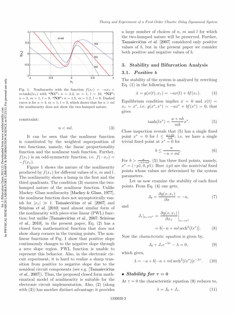
Fig. 1. Nonlinearity with the function f(xτ ) = −nxτ +m tanh(lxτ ) with “N1”: n = 2.2, m = 1, l = 10; “N2”:n = 3, m = 1, l = 8, “N3”: n = 1.5, m = 1.2, l = 8. Dashedcurve is for n = 4, m = 1, l = 3, which shows that for n > mlthe nonlinearity does not show the two-humped nature.

constraint:

n < ml. (3)

It can be seen that the nonlinear functionis constituted by the weighted superposition oftwo functions, namely, the linear proportionalityfunction and the nonlinear tanh function. Further,f(xτ ) is an odd-symmetric function, i.e. f(−xτ ) =−f(xτ ).

Figure 1 shows the nature of the nonlinearityproduced by f(xτ ) for different values of n, m and l.The nonlinearity shows a hump in the first and thethird quadrants. The condition (3) ensures the two-humped nature of the nonlinear function. UnlikeMackey–Glass nonlinearity [Mackey & Glass, 1977],the nonlinear function does not asymptotically van-ish for |xτ | 1. Tamasevicius et al. [2007] andSrinivas et al. [2010] used almost similar form ofthe nonlinearity with piece-wise linear (PWL) func-tion; but unlike [Tamasevicius et al., 2007; Srinivaset al., 2010], in the present paper, Eq. (2) has aclosed form mathematical function that does notshow sharp corners in the turning points. The non-linear functions of Fig. 1 show that positive slopecontinuously changes to the negative slope througha zero slope region. PWL function is unable torepresent this behavior. Also, in the electronic cir-cuit experiment, it is hard to realize a sharp tran-sition from positive to negative slope due to thenonideal circuit components (see e.g. [Tamaseviciuset al., 2007]). Thus, the proposed closed form math-ematical model of nonlinearity is suitable for theelectronic circuit implementation. Also, (2) (alongwith (3)) has another distinct advantage; it provides

a large number of choices of n, m and l for whichthe two-humped nature will be preserved. Further,Tamasevicius et al. [2007] considered only positivevalues of b, but in the present paper we considerboth positive and negative values of b.

3. Stability and Bifurcation Analysis

3.1. Positive b

The stability of the system is analyzed by rewritingEq. (1) in the following form

x = g(x(t), xτ ) = −ax(t) + bf (xτ ). (4)

Equilibrium condition implies x = 0 and x(t) =xτ = x∗, i.e. g(x∗, x∗) = −ax∗ + bf (x∗) = 0; thatgives

tanh(lx∗) =a + nb

mbx∗. (5)

Close inspection reveals that (5) has a single fixedpoint x∗ = 0 for l ≤ a+nb

mb ; i.e. we have a singletrivial fixed point at x∗ = 0 for

b ≤ a

−n + ml. (6)

For b > a−n+ml , (5) has three fixed points, namely,

x∗ = (−p1, 0, p1). Here ±p1 are the nontrivial fixedpoints whose values are determined by the systemparameters.

Let us now examine the stability of each fixedpoints. From Eq. (4) one gets,

J0 =∂g(x, xτ )

∂x= −a, (7)

and

Jτ |xτ=x∗ =∂g(x, xτ )

∂xτ

∣∣∣∣xτ =x∗

= b[−n + ml sech2(lx∗)]. (8)

Now the characteristic equation is given by,

J0 + Jτe−λτ − λ = 0, (9)

which gives,

λ = −a + b[−n + ml sech2(lx∗)]e−λτ . (10)

• Stability for τ = 0

At τ = 0 the characteristic equation (9) reduces to,

λ = J0 + Jτ . (11)

1330020-3

Int.

J. B

ifur

catio

n C

haos

201

3.23

. Dow

nloa

ded

from

ww

w.w

orld

scie

ntif

ic.c

omby

PH

YSI

CA

L R

ESE

AR

CH

LA

BO

RA

TO

RY

LIB

RA

RY

& I

NFO

RM

AT

ION

SC

IEN

CE

on

07/2

3/13

. For

per

sona

l use

onl

y.

June 29, 2013 10:30 WSPC/S0218-1274 1330020

T. Banerjee & D. Biswas

Taking λ = µ + iν, and comparing the real andimaginary parts, one gets

µ = −a + b[−n + ml sech2(lx∗)],

ν = 0.(12)

Asymptotic stability will occur when all the roots ofthe characteristic equation have negative real parts(i.e. negative µ); from (12) we get the condition ofstability as,

b[−n + ml sech2(lx∗)] < a. (13)

Equation (13) imposes the first condition for choos-ing the system parameters to achieve asymptoticstability of the system for τ = 0. Let us now exam-ine the case for x∗ = 0, from (13) we have thecondition for stability as b < a

−n+ml , which is inter-estingly identical with (6). Thus, one can concludethat for b < a

−n+ml , x∗ = 0 is the only stable fixedpoint for any τ ≥ 0, but beyond that, x∗ = 0becomes unstable through a supercritical pitchforkbifurcation and two nontrivial fixed points (±p1)emerge. Next, we have to examine the stability ofthe nontrivial fixed points (±p1).

• Stability for τ = 0

Hopf bifurcation will appear if at least one of theeigenvalues crosses the imaginary axis from left andenter the right half plane. Thus if µ varies from leftto right we can say that, µ < 0 represents a sta-ble state, µ > 0 is bifurcated state and µ = 0 isthe limiting case. At the emergence of Hopf bifur-cation, we assume µ = 0; thus using λ = iνwe get

J0 + Jτe−iντ − iν = 0 (14)

J0 + Jτcos(ντ) − i sin(ντ) − iν = 0. (15)

Now equating the real and imaginary parts on bothsides of above equations we get,

Jτ cos(ντ) = −J0, (16)

Jτ sin(ντ) = −ν. (17)

Equations (16) and (17) lead to ν =√

Jτ2 − J0

2.This is possible if and only if |Jτ | ≥ |J0|, i.e.

|b−n + ml sech2(lx∗)| ≥ |−a|. (18)

Again Eq. (16) gives the following sets of solutionsof τ

τk1 =

[cos−1

(−J0

Jτ

)+ 2kπ

]√

Jτ2 − J0

2, for f ′(x∗) < 0,

(19a)

τk2 =

[2π − cos−1

(−J0

Jτ

)+ 2kπ

]√

Jτ2 − J0

2,

for f ′(x∗) > 0, (19b)

here k = 0, 1, 2, . . . . Also, let us set ν0 =√Jτ

2 − J02 and let λk(τ) = µk(τ) + iνk(τ) be a

root of (1) near τ = τk satisfying µk(τ) = 0 andνk(τ) = ν0. We have

λ = J0 + Jτe−λτ ,

λ = −a + b[−n + ml sech2(lx∗)]e−λτ .(20)

Taking s = b[−n + ml sech2(lx∗)] and differen-tiating both sides with respect to τ , we get

dλ

dτ= se−λτ

(−λ − τ

dλ

dτ

),

dλ

dτ= − λse−λτ

1 + τse−λτ.

(21)

Again from Eq. (20) we have se−λτ = λ + a, we usethis in (21) and get

dλ

dτ=

−λ(λ + a)1 + τ(λ + a)

.

Now at τ = τk; λ = iν0, as µk(τ0) = 0, therefore,

dλ

dτ

∣∣∣∣τ=τk

=ν0

2 − iν0a

(1 + τa) + iτν0. (22)

Equating the real parts on both sides we get,

µ′(τk) =ν0

2

(1 + τa)2 + τ2ν02. (23)

Thus, µ′(τk) > 0 for any k = 0, 1, 2, . . . .Now, let us investigate the stability of the sys-

tem for the following parameter set: a = 1, n = 2.2,m = 1 and l = 10 (as we have used in “N1” ofFig. 1). Figure 2 shows the first six stability curvesτki (i = 1, 2) [using (19)] in the τ–b parameterspace. In the figure, τk1 and τk2 are representedby solid lines and dotted lines, respectively. Since

1330020-4

Int.

J. B

ifur

catio

n C

haos

201

3.23

. Dow

nloa

ded

from

ww

w.w

orld

scie

ntif

ic.c

omby

PH

YSI

CA

L R

ESE

AR

CH

LA

BO

RA

TO

RY

LIB

RA

RY

& I

NFO

RM

AT

ION

SC

IEN

CE

on

07/2

3/13

. For

per

sona

l use

onl

y.

June 29, 2013 10:30 WSPC/S0218-1274 1330020

Theory and Experiment of a First-Order Chaotic Delay Dynamical System

Fig. 2. Stability zone in the τ–b (b > 0) parameter spacewith parameters a = 1, n = 2.2, m = 1 and l = 10. Shadedregion indicates the zone of stable fixed point.

µ′(τk) > 0 for any k = 0, 1, 2, . . . thus, stabilityzone cannot be situated between two consecutive τki

curves [Lakshmanan & Senthilkumar, 2011]. So, weconclude that the stable island lies between τ = 0and τ01 curves. The shaded region in the figure rep-resents the stable zone, and τ01 curve represents theHopf bifurcation curve.

Let us now summarize the stability scenario ofthe system for b ≥ 0:

(i) x∗ = 0: for this fixed point, the condition of sta-bility reads b < 1

−n+ml for any τ ≥ 0. Beyondthis value of b, for any τ ≥ 0, the trivial fixedpoint x∗ = 0 becomes unstable through a pitch-fork bifurcation and ±p1 fixed points emerge.

(ii) x∗ = ±p1: These two nontrivial fixed pointscome into play for b ≥ 1

−n+ml . Since at thesefixed points |Jτ | > |−a|, thus the systemdepicts a stable fixed point for the delay τ ,0 ≥ τ < τ01. Beyond τ = τ01, Hopf bifurca-tion occurs and a stable limit cycle appears.

Next, we study the direction of Hopf bifurca-tion and the stability of the bifurcating solutionsfor x∗ = ±p1 at τ = τ01. Using the techniquesdescribed by Wei [2007] let us define

D =1

1 + τ01a − iτ01ν0. (24)

We can obtain the following coefficients:

g20 = Dbτ01f′′(x∗)e−2iτ01ν0

= −2Dbτ01ml2 sech2(lx∗) tanh(lx∗)e−2iτ01ν0 ,

g11 = Dbτ01f′′(x∗)

= −2Dbτ01ml2 sech2(lx∗) tanh(lx∗),

g02 = Dbτ01f′′(x∗)e2iτ01ν0

= −2Dbτ01ml2 sech2(lx∗) tanh(lx∗)e2iτ01ν0 ,

g21 = Dbτ01[f ′′(x∗)e−iτ01ν0W11(−1)

+ eiτ01ν0W20(−1) + f ′′′(x∗)e−iτ01ν0],

= −2ml2Dbτ01 sech2(lx∗)[e−iτ01ν0W11(−1)

+ eiτ01ν0W20(−1) tanh(lx∗)

− l2 − 3 sech2(lx∗)e−iτ01ν0]

(25)

where

W20(−1) = − g20

iτ01ν0e−iτ01ν0 − g02

3iτ01ν0eiτ01ν0

+ E1e−2iτ01ν0 ,

W11(−1) =g11

iτ01ν0e−iτ01ν0 − g11

iτ01ν0eiτ01ν0 + E2,

E1 =bf ′′(x∗)e−2iτ01ν0

2iν0 + a − bf ′(x∗)e−2iτ01ν0

=−b2ml2 sech2(lx∗) tanh(lx∗)e−2iτ01ν0

2iν0 + a − b[−n + ml sech2(lx∗)]e−2iτ01ν0

and

E2 =bf ′′(x∗)

a − bf ′(x∗)

=−2bml2 sech2(lx∗) tanh(lx∗)a − b[−n + ml sech2(lx∗)]

.

Because each gij in equation set (25) isexpressed by the parameters and delay, we cancompute the following quantities:

c1(0) =i

2τ01ν0

(g11g20 − 2|g11|2 − |g02|2

3

)+

g21

2,

µ2 = − Re(c1(0))Re(λ′(τ01))

,

β2 = 2Re(c1(0)),

T2 = − Im(c1(0)) + µ2Im(λ′(τ01))ν0

.

(26)

1330020-5

Int.

J. B

ifur

catio

n C

haos

201

3.23

. Dow

nloa

ded

from

ww

w.w

orld

scie

ntif

ic.c

omby

PH

YSI

CA

L R

ESE

AR

CH

LA

BO

RA

TO

RY

LIB

RA

RY

& I

NFO

RM

AT

ION

SC

IEN

CE

on

07/2

3/13

. For

per

sona

l use

onl

y.

June 29, 2013 10:30 WSPC/S0218-1274 1330020

T. Banerjee & D. Biswas

The parameter µ2 determines the direction ofthe Hopf bifurcation: if µ2 > 0 (µ2 < 0), then theHopf bifurcation is supercritical (subcritical) andthe bifurcating periodic solutions exist for τ > τ01

(τ < τ01). β2 determines the stability of bifurcat-ing periodic solutions: the bifurcating periodic solu-tions are orbitally asymptotically stable (unstable)if β2 < 0 (β2 > 0). Finally, T2 determines theperiod of bifurcating periodic solutions: the periodincreases (decreases) if T2 > 0 (T2 < 0).

To test the validity of our analysis let us usethe following parameter values: a = 1, n = 2.2,m = 1 and l = 10. For b = 1 we have: p1 = 0.31,J0 = −a = −1 and Jτ = b[−n + ml sech2(±lp1)] =−2.121. Thus we see that |Jτ | > |J0| [satisfy-ing (18)]. Also, at these parameter values we haveτ01 = 1.102 [from (19)]. Thus we expect that atb = 1, and τ01 = τH = 1.102, the fixed point losesits stability through Hopf bifurcation. Further, atthese parameter values, we have g11 = −0.421 +0.413i, g20 = 0.582 + 0.095i, g02 = −0.11 − 0.58i,g21 = −11.622 − 3.812i, E1 = −0.217 − 0.082i,E2 = −0.525, W20 = 0.519− 0.302i, W11 = −0.354,and c1(0) = −5.86 − 2.172i. Using these set of val-ues in (26) we have, µ2 = 14.524 > 0; that meansthe resulting bifurcation is a supercritical Hopfbifurcation. Also, since β2 = −11.72 < 0; thus thebifurcating periodic solutions are orbitally asymp-totically stable. Finally, T2 = 11.142 > 0 indicatesthat the period of the limit cycle increases withincreasing τ .

3.2. Negative b

Let us define b = −b1, where b1 > 0. For negativeb, we have

ax∗ = −b1f(x∗). (27)

That gives the following equation

tanh(lx∗) = −a − nb1

mb1x∗. (28)

Again a close observation reveals that for b1 ≤ an ,

one has only one trivial fixed point, which is x∗ = 0;beyond this value of b there exists three equilibriumpoints, namely x∗ = q1, 0, and −q1. Using the sim-ilar arguments of the previous subsection, we canshow that the nontrivial fixed points (i.e. ±q1) areunstable for any τ ≥ 0. For the trivial fixed point(i.e. x∗ = 0), we can derive the following equations

J0 = −a, Jτ = −b1[−n + ml]. (29)

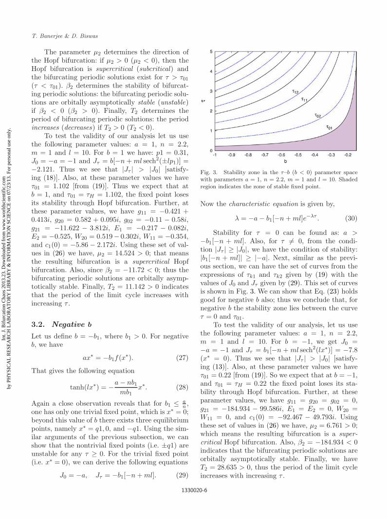
Fig. 3. Stability zone in the τ–b (b < 0) parameter spacewith parameters a = 1, n = 2.2, m = 1 and l = 10. Shadedregion indicates the zone of stable fixed point.

Now the characteristic equation is given by,

λ = −a − b1[−n + ml]e−λτ . (30)

Stability for τ = 0 can be found as: a >−b1[−n + ml]. Also, for τ = 0, from the condi-tion |Jτ | ≥ |J0|, we have the condition of stability:|b1[−n + ml]| ≥ |−a|. Next, similar as the previ-ous section, we can have the set of curves from theexpressions of τk1 and τk2 given by (19) with thevalues of J0 and Jτ given by (29). This set of curvesis shown in Fig. 3. We can show that Eq. (23) holdsgood for negative b also; thus we conclude that, fornegative b the stability zone lies between the curveτ = 0 and τ01.

To test the validity of our analysis, let us usethe following parameter values: a = 1, n = 2.2,m = 1 and l = 10. For b = −1, we get J0 =−a = −1 and Jτ = b1[−n + ml sech2(lx∗)] = −7.8(x∗ = 0). Thus we see that |Jτ | > |J0| [satisfy-ing (13)]. Also, at these parameter values we haveτ01 = 0.22 [from (19)]. So we expect that at b = −1,and τ01 = τH = 0.22 the fixed point loses its sta-bility through Hopf bifurcation. Further, at theseparameter values, we have g11 = g20 = g02 = 0,g21 = −184.934 − 99.586i, E1 = E2 = 0, W20 =W11 = 0, and c1(0) = −92.467 − 49.793i. Usingthese set of values in (26) we have, µ2 = 6.761 > 0;which means the resulting bifurcation is a super-critical Hopf bifurcation. Also, β2 = −184.934 < 0indicates that the bifurcating periodic solutions areorbitally asymptotically stable. Finally, we haveT2 = 28.635 > 0, thus the period of the limit cycleincreases with increasing τ .

1330020-6

Int.

J. B

ifur

catio

n C

haos

201

3.23

. Dow

nloa

ded

from

ww

w.w

orld

scie

ntif

ic.c

omby

PH

YSI

CA

L R

ESE

AR

CH

LA

BO

RA

TO

RY

LIB

RA

RY

& I

NFO

RM

AT

ION

SC

IEN

CE

on

07/2

3/13

. For

per

sona

l use

onl

y.

June 29, 2013 10:30 WSPC/S0218-1274 1330020

Theory and Experiment of a First-Order Chaotic Delay Dynamical System

4. Numerical Studies: Phase PlanePlots, Bifurcation Diagrams andLyapunov Exponents

System equation (1) is solved numerically usingfourth order Runge–Kutta algorithm with step sizeh = 0.005. A constant initial function φ(t) = 0.8for t ∈ [−τ, 0] is used. A large delay and small stepsize generally increase the transient time of the sys-tem, thus we exclude a large number of iterationsin the transient region to allow the system to settleto the steady state.

4.1. Varying τ with constant b

At first, we vary the time delay τ with constant b.For all the numerical simulations, we consider thefollowing system parameters a = 1, n = 2.2, m = 1and l = 10.

(i) b = 1: For τ ≥ 1.102, the fixed point losesits stability through Hopf bifurcation, which is inaccordance with the analysis of the previous section.At τ = 1.65, limit cycle of period-1 becomes unsta-ble and a period-2 (P2) cycle appears. Further,

period doubling occurs at τ = 1.79 (P2 to P4).Through a period doubling sequence, the systementers into the chaotic regime at τ = 1.84. With fur-ther increase of τ , at τ = 2.60, the system shows theemergence of hyperchaos. The system shows a dou-ble scroll at τ ≈ 3.24. Phase plane representation inthe representative x–x(t− τ) plane for different τ isshown in Fig. 4, which shows the following charac-teristics: period-1 (τ = 1.40), period-2 (τ = 1.72),chaos (τ = 1.94), and double scroll hyperchaos(τ = 3.52).

(ii) b = −1: The fixed point loses its stabilitythrough Hopf bifurcation at τ = 0.22 which againagrees with the analysis. Pitchfork bifurcation ofthe limit cycle occurs at τ = 1.3. Period-2 andperiod-4 occurs at τ = 1.84 and 1.99, respectively.Chaos appears at τ ≈ 2.05. Double scroll occursat τ ≈ 2.38. Finally, hyperchaos occurs at τ ≈ 3.39.All the behaviors in phase space are shown in Fig. 5.

These observations are summarized throughbifurcation diagram with τ as the control param-eter. Bifurcation diagrams are obtained by plotting

(a) (b)

(c) (d)

Fig. 4. Phase plane plot in x–x(t − τ ) space for different τ (b = 1): (a) τ = 1.40 (period-1), (b) τ = 1.72 (period-2),(c) τ = 1.94 (chaos), (d) τ = 3.52 (double scroll hyperchaos) (other parameters are: a = 1, n = 2.2, m = 1, l = 10).

1330020-7

Int.

J. B

ifur

catio

n C

haos

201

3.23

. Dow

nloa

ded

from

ww

w.w

orld

scie

ntif

ic.c

omby

PH

YSI

CA

L R

ESE

AR

CH

LA

BO

RA

TO

RY

LIB

RA

RY

& I

NFO

RM

AT

ION

SC

IEN

CE

on

07/2

3/13

. For

per

sona

l use

onl

y.

June 29, 2013 10:30 WSPC/S0218-1274 1330020

T. Banerjee & D. Biswas

(a) (b)

(c) (d)

Fig. 5. Phase plane plot in x–x(t − τ ) space for different τ (b = −1): (a) τ = 0.52 (period-1), (b) τ = 1.876 (period-2),(c) τ = 2.17 (chaos), (d) τ = 3.5 (double scroll hyperchaos) (other parameters are: a = 1, n = 2.2, m = 1, l = 10).

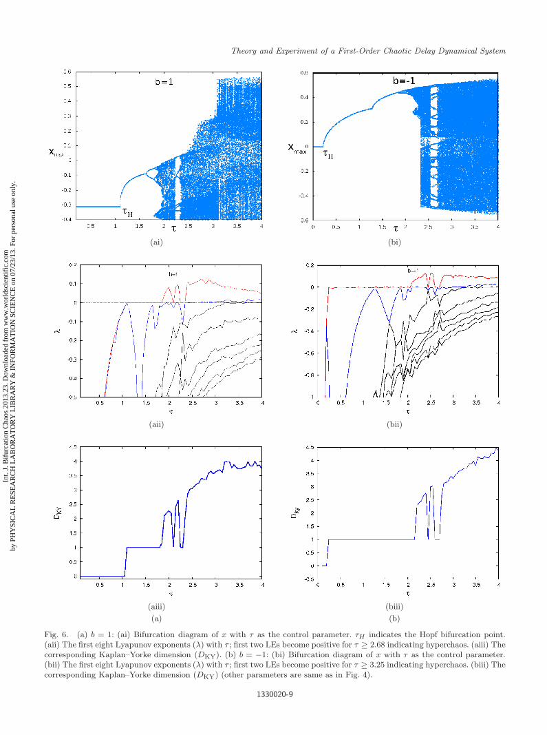
the local maxima of x, excluding a large numberof transients (∼ 106). Figures 6(ai) and 6(bi) showthe bifurcation diagram of x with τ for b = 1 andb = −1, respectively. Clearly, they show a perioddoubling route to chaos. For quantitative mea-sure of the system dynamics, we compute the firsteight Lyapunov exponents using the algorithm pro-posed in [Farmer, 1982]. Figures 6(aii) and 6(bii)show the spectrum of Lyapunov exponents (LEs)in the τ parameter space. They agree well withthe bifurcation diagrams. Figures 6(aiii) and 6(biii)show the corresponding Kaplan–Yorke dimensions(DKY) with different τ . Presence of a strange attrac-tor, multiple LEs and higher values of DKY (> 3)ensures [Leonov & Kuznetsov, 2007] that hyper-chaos occurs for τ ≈ 2.68 (b = 1) and τ ≈ 3.25(b = −1).

4.2. Varying b with constant τ

Next, we keep the delay fixed at τ = 4 and vary bto explore the system dynamics.

(i) b > 0: Starting from b = 0, if we increase b,at b = 0.128, the trivial fixed point x = 0 loses

stability through pitchfork bifurcation and the non-trivial fixed points arise. Nontrivial fixed points losestability through Hopf bifurcation and limit cycleappears at b = 0.62 = bH+. At b = 0.750, limitcycle of period-1 becomes unstable and a period-2(P2) cycle appears. Further period doubling occursat b = 0.777 (P2 to P4). Through a period doublingcascade, the system enters into the chaotic regime atb ≈ 0.786. With further increase of b, at b ≈ 0.9, thesystem shows the emergence of hyperchaos. Doublescroll appears at b ≈ 0.985. Finally, the system-equation shows diverging behavior beyond b > 1,indicating boundary crises.

(ii) b < 0: For b ≤ −0.156 the trivial fixed pointloses stability through Hopf bifurcation and givesbirth to a limit cycle. Pitchfork bifurcation of limitcycle is observed at b = −0.62. Period-2 limitcycle appears at b = −0.77, and period-4 oscil-lation occurs at b = −0.795. At b ≈ −0.807, weobserve chaotic behavior; double scroll hyperchaosis observed at b ≈ −0.98.

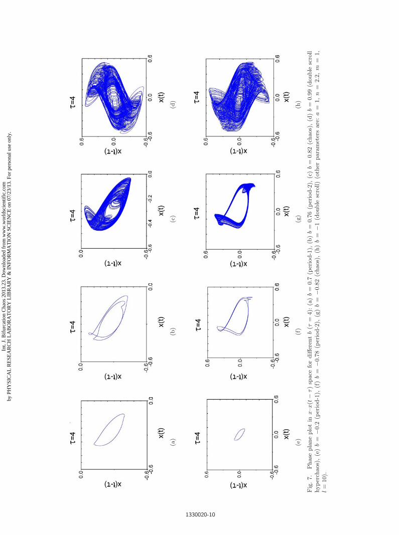
Phase plane representation in the represen-tative x–x(t − τ) plane for different b is shown

1330020-8

Int.

J. B

ifur

catio

n C

haos

201

3.23

. Dow

nloa

ded

from

ww

w.w

orld

scie

ntif

ic.c

omby

PH

YSI

CA

L R

ESE

AR

CH

LA

BO

RA

TO

RY

LIB

RA

RY

& I

NFO

RM

AT

ION

SC

IEN

CE

on

07/2

3/13

. For

per

sona

l use

onl

y.

June 29, 2013 10:30 WSPC/S0218-1274 1330020

Theory and Experiment of a First-Order Chaotic Delay Dynamical System

(ai) (bi)

(aii) (bii)

(aiii) (biii)

(a) (b)

Fig. 6. (a) b = 1: (ai) Bifurcation diagram of x with τ as the control parameter. τH indicates the Hopf bifurcation point.(aii) The first eight Lyapunov exponents (λ) with τ ; first two LEs become positive for τ ≥ 2.68 indicating hyperchaos. (aiii) Thecorresponding Kaplan–Yorke dimension (DKY). (b) b = −1: (bi) Bifurcation diagram of x with τ as the control parameter.(bii) The first eight Lyapunov exponents (λ) with τ ; first two LEs become positive for τ ≥ 3.25 indicating hyperchaos. (biii) Thecorresponding Kaplan–Yorke dimension (DKY) (other parameters are same as in Fig. 4).

1330020-9

Int.

J. B

ifur

catio

n C

haos

201

3.23

. Dow

nloa

ded

from

ww

w.w

orld

scie

ntif

ic.c

omby

PH

YSI

CA

L R

ESE

AR

CH

LA

BO

RA

TO

RY

LIB

RA

RY

& I

NFO

RM

AT

ION

SC

IEN

CE

on

07/2

3/13

. For

per

sona

l use

onl

y.

June 29, 2013 10:30 WSPC/S0218-1274 1330020

(a)

(b)

(c)

(d)

(e)

(f)

(g)

(h)

Fig

.7.

Phase

pla

ne

plo

tin

x–x(t

−τ)

space

for

diff

eren

tb

(τ=

4):

(a)

b=

0.7

(per

iod-1

),(b

)b

=0.7

6(p

erio

d-2

),(c

)b

=0.8

2(c

haos)

,(d

)b

=0.9

9(d

ouble

scro

llhyper

chaos)

,(e

)b

=−0

.2(p

erio

d-1

),(f

)b

=−0

.78

(per

iod-2

),(g

)b

=−0

.82

(chaos)

,(h

)b

=−1

(double

scro

ll)

(oth

erpara

met

ers

are

:a

=1,

n=

2.2

,m

=1,

l=

10).

1330020-10

Int.

J. B

ifur

catio

n C

haos

201

3.23

. Dow

nloa

ded

from

ww

w.w

orld

scie

ntif

ic.c

omby

PH

YSI

CA

L R

ESE

AR

CH

LA

BO

RA

TO

RY

LIB

RA

RY

& I

NFO

RM

AT

ION

SC

IEN

CE

on

07/2

3/13

. For

per

sona

l use

onl

y.

June 29, 2013 10:30 WSPC/S0218-1274 1330020

Theory and Experiment of a First-Order Chaotic Delay Dynamical System

(a) (b)

0

0.5

1

1.5

2

2.5

3

3.5

4

4.5

-1 -0.5 0 0.5 1

DK

Y

b

(c)

Fig. 8. (a) Bifurcation diagram of x (upper trace) with b as the control parameter. (b) The first eight Lyapunov exponents (λ)with b; first two LEs become positive for b ≥ 0.9 and b ≤ −0.92 indicating hyperchaos. (c) The corresponding Kaplan–Yorkedimension (DKY). Parameter values are same as in Fig. 7.

in Fig. 7, which shows the following characteristics:period-1 (b = 0.70), period-2 (b = 0.76), chaos (b =0.82), and double scroll (b = 0.99); period-1 (b =−0.2), period-2 (b = −0.78), chaos (b = −0.82),double scroll hyperchaos (b = −1).

As before, these observations are summarizedthrough a bifurcation diagram with b as the con-trol parameter. Figure 8(a) shows the bifurca-tion diagram of x with b. At bH+ = 0.62, andbH− = −0.156 limit cycles emerge through Hopfbifurcation. Figure 8(b) shows the first eight LEs; itcan be seen that for b > 0.9 and b < −0.93 we havetwo positive LEs indicating the occurrence of hyper-chaos. This fact is supported by Fig. 8(c), which

plots DKY with b. It is noteworthy that to obtainhyperchaos we do not need to make τ large; suitablechoice of b with a moderate value of τ is sufficientto observe hyperchaos.

5. Electronic Circuit Realization

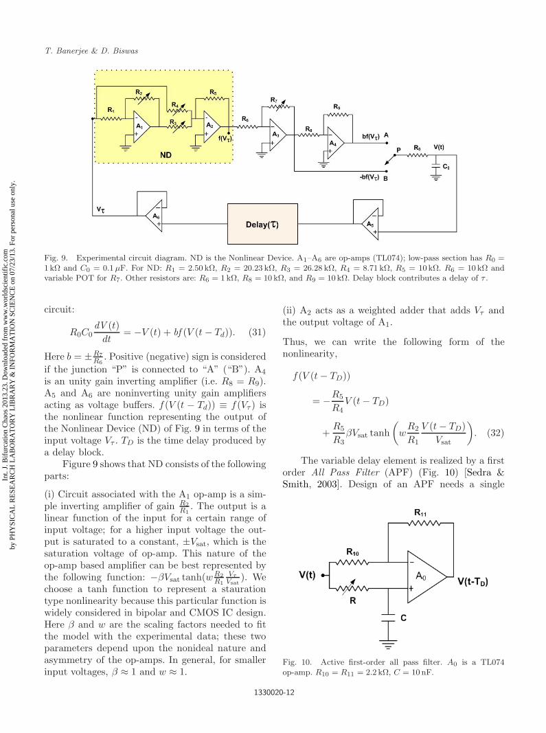
The proposed system is implemented in an analogelectronic circuit. Figure 9 shows the circuit dia-gram of the experimental arrangement. Here V (t)represents the voltage drop across the capacitor C0

of the low-pass filter section R0 −C0. Thus the fol-lowing equation governs the time evolution of the

1330020-11

Int.

J. B

ifur

catio

n C

haos

201

3.23

. Dow

nloa

ded

from

ww

w.w

orld

scie

ntif

ic.c

omby

PH

YSI

CA

L R

ESE

AR

CH

LA

BO

RA

TO

RY

LIB

RA

RY

& I

NFO

RM

AT

ION

SC

IEN

CE

on

07/2

3/13

. For

per

sona

l use

onl

y.

June 29, 2013 10:30 WSPC/S0218-1274 1330020

T. Banerjee & D. Biswas

Fig. 9. Experimental circuit diagram. ND is the Nonlinear Device. A1–A6 are op-amps (TL074); low-pass section has R0 =1kΩ and C0 = 0.1 µF. For ND: R1 = 2.50 kΩ, R2 = 20.23 kΩ, R3 = 26.28 kΩ, R4 = 8.71 kΩ, R5 = 10kΩ. R6 = 10 kΩ andvariable POT for R7. Other resistors are: R6 = 1 kΩ, R8 = 10 kΩ, and R9 = 10kΩ. Delay block contributes a delay of τ .

circuit:

R0C0dV (t)

dt= −V (t) + bf (V (t − Td)). (31)

Here b = ±R7R6

. Positive (negative) sign is consideredif the junction “P” is connected to “A” (“B”). A4

is an unity gain inverting amplifier (i.e. R8 = R9).A5 and A6 are noninverting unity gain amplifiersacting as voltage buffers. f(V (t − Td)) ≡ f(Vτ ) isthe nonlinear function representing the output ofthe Nonlinear Device (ND) of Fig. 9 in terms of theinput voltage Vτ . TD is the time delay produced bya delay block.

Figure 9 shows that ND consists of the followingparts:

(i) Circuit associated with the A1 op-amp is a sim-ple inverting amplifier of gain R2

R1. The output is a

linear function of the input for a certain range ofinput voltage; for a higher input voltage the out-put is saturated to a constant, ±Vsat, which is thesaturation voltage of op-amp. This nature of theop-amp based amplifier can be best represented bythe following function: −βVsat tanh(wR2

R1

VτVsat

). Wechoose a tanh function to represent a staurationtype nonlinearity because this particular function iswidely considered in bipolar and CMOS IC design.Here β and w are the scaling factors needed to fitthe model with the experimental data; these twoparameters depend upon the nonideal nature andasymmetry of the op-amps. In general, for smallerinput voltages, β ≈ 1 and w ≈ 1.

(ii) A2 acts as a weighted adder that adds Vτ andthe output voltage of A1.

Thus, we can write the following form of thenonlinearity,

f(V (t − TD))

= −R5

R4V (t − TD)

+R5

R3βVsat tanh

(w

R2

R1

V (t − TD)Vsat

). (32)

The variable delay element is realized by a firstorder All Pass Filter (APF) (Fig. 10) [Sedra &Smith, 2003]. Design of an APF needs a single

Fig. 10. Active first-order all pass filter. A0 is a TL074op-amp. R10 = R11 = 2.2 kΩ, C = 10nF.

1330020-12

Int.

J. B

ifur

catio

n C

haos

201

3.23

. Dow

nloa

ded

from

ww

w.w

orld

scie

ntif

ic.c

omby

PH

YSI

CA

L R

ESE

AR

CH

LA

BO

RA

TO

RY

LIB

RA

RY

& I

NFO

RM

AT

ION

SC

IEN

CE

on

07/2

3/13

. For

per

sona

l use

onl

y.

June 29, 2013 10:30 WSPC/S0218-1274 1330020

Theory and Experiment of a First-Order Chaotic Delay Dynamical System

op-amp (A0), an R − C combination which deter-mines the phase shift between the input and outputsignals; two resistors R10 and R11 determine thegain of the APF. Thus, the APF has the followingtransfer function:

T (s) = −a1s − ω0

s + ω0, (33)

with a flat gain a1 = R11R10

, and ω0 = 1/CR is thefrequency at which the phase shift is π/2. In thepresent work, we take R11 = R10 thus, a1 = 1. Sinceit has a maximally linear phase response aroundthe frequency ω0, one can thus approximate thatan APF imposes a delay of TD ≈ RC aroundω0 [Banerjee et al., 2012]. Thus i blocks producea delay of TD ≈ iRC (i = 1, 2, . . .). By simplychanging the resistance R, one can vary the amountof delay; and hence one can control the resolution ofthe delay line. Further, we have another advantageof using an APF as a delay element, that is, in anAPF the output power level does not attenuate evenfor a higher frequency range, only the phase shift isa function of input signal frequency. Thus, unlikean LCL-filter based delay line, we do not have touse a compensator circuit for an APF.

Let us define the following dimensionless vari-ables and parameters: t = t

R0C0, τ = Td

R0C0, x =

V (t−TD)Vsat

, R5R4

= n1, β R5R3

= m1, wR2R1

= l1. Now,the system equation (32) can be reduced to thefollowing dimensionless first-order, nonlinear delaydifferential equation

dx

dt= −x(t) + bf (x(t − τ)), (34)

where

f(x(t − τ)) ≡ f(xτ )

= −n1xτ + m1 tanh(l1xτ ). (35)

It can be seen that Eq. (34) [along with (35)] isequivalent to Eq. (1) [along with (2)] with a = 1,and appropriate choices of n1, m1 and l1.

6. Experimental Results

The proposed circuit is designed in hardware on abreadboard using IC TL074 (quad JFET op-amp)with ±12 volt power supply. Capacitors and resis-tors have 5% tolerance. For the low pass sec-tion, we choose R0 = 1kΩ and C0 = 0.1µF. Forthe nonlinear device (ND), the following resistorvalues are used: R1 = 2.50 kΩ, R2 = 20.23 kΩ,

Fig. 11. Experimentally obtained nonlinearity produced bynonlinear device in Fig. 9. x-axis: 0.2 v/div and y-axis:0.5 v/div.

R3 =26.28 kΩ, R4 = 8.71 kΩ, R5 = 10 kΩ. Figure 11shows the experimentally obtained nonlinearityproduced by the ND. Qualitatively, it is equivalentto the nonlinear function “N1” of Fig. 1. The gainof the noninverting amplifier (A3) that follows theND is designed with R6 = 1kΩ and variable R7;R7 is varied through a potentiometer to change theparameter b. Other resistors are: R8 = 10 kΩ andR9 = 10 kΩ.

For the delay section, the all pass filter (APF) isdesigned with the following parameters: R = 10 kΩ(POT), C = 10 nF, R8 = 2.2 kΩ, R9 = 2.2 kΩ. EachAPF contributes a delay of TD = RC = 0.1 ms;thus the dimensionless parameter τ = RC

R0C0= 1,

i.e. one needs i blocks to produce a delay τ = i. Inthe experiment, we vary R to get variable delays.Note that, one can also change R0 to get a variabledelay, but in that case the power spectral propertyof the circuit will also be changed [Namajunas et al.,1995].

6.1. Variable τ, fixed b

(i) Positive b: The nodes “A” and “P” of Fig. 9 areconnected. We fix the value of b with R7 = 1.57 kΩ(POT). Now, we vary the delay by varying R. Atfirst to get a small delay, we use only one APFstage. For R ≥ 9.56 kΩ (approx.) a stable limit cycleappears with frequency 3846 Hz. Next, we use twoblocks of APF; R = 10 kΩ is taken for the first block(contributing ≈ 0.1 ms delay) and vary R of the sec-ond block; at R = 0.35 kΩ the limit cycle of period-1loses its stability and a period-2 oscillation emerges.At R = 6.43 kΩ, chaotic oscillation occurs in the cir-cuit. Next, we use three blocks of APF; R = 10 kΩ istaken for the first two blocks (contributing ≈ 0.2 ms

1330020-13

Int.

J. B

ifur

catio

n C

haos

201

3.23

. Dow

nloa

ded

from

ww

w.w

orld

scie

ntif

ic.c

omby

PH

YSI

CA

L R

ESE

AR

CH

LA

BO

RA

TO

RY

LIB

RA

RY

& I

NFO

RM

AT

ION

SC

IEN

CE

on

07/2

3/13

. For

per

sona

l use

onl

y.

June 29, 2013 10:30 WSPC/S0218-1274 1330020

T. Banerjee & D. Biswas

(a) (b)

(c) (d)

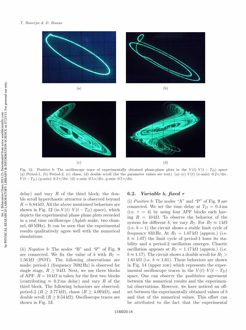
Fig. 12. Positive b: The oscilloscope trace of experimentally obtained phase-plane plots in the V (t)–V (t − TD) space(a) Period-1, (b) Period-2, (c) chaos, (d) double scroll (for the parameter values see text). (a)–(c) V (t) (x-axis): 0.2 v/div,V (t − TD) (y-axis): 0.2 v/div. (d) x-axis: 0.5 v/div, y-axis: 0.5 v/div.

delay) and vary R of the third block; the dou-ble scroll hyperchaotic attractor is observed beyondR = 6.84 kΩ. All the above mentioned behaviors areshown in Fig. 12 (in V (t)–V (t − TD) space), whichdepicts the experimental phase plane plots recordedin a real time oscilloscope (Aplab make, two chan-nel, 60 MHz). It can be seen that the experimentalresults qualitatively agree well with the numericalsimulations.

(ii) Negative b: The nodes “B” and “P” of Fig. 9are connected. We fix the value of b with R7 =1.56 kΩ (POT). The following observations aremade: period-1 (frequency 7692 Hz) is observed forsingle stage, R ≥ 9 kΩ. Next, we use three blocksof APF: R = 10 kΩ is taken for the first two blocks(contributing ≈ 0.2 ms delay) and vary R of thethird block. The following behaviors are observed:period-2 (R ≥ 2.77 kΩ), chaos (R ≥ 4.09 kΩ), anddouble scroll (R ≥ 9.54 kΩ). Oscilloscope traces areshown in Fig. 13.

6.2. Variable b, fixed τ

(i) Positive b: The nodes “A” and “P” of Fig. 9 areconnected. We set the time delay at TD = 0.4 ms(i.e. τ = 4) by using four APF blocks each hav-ing R = 10 kΩ. To observe the behavior of thesystem for different b, we vary R7. For R7 ≈ 1 kΩ(i.e. b = 1) the circuit shows a stable limit cycle offrequency 833 Hz. At R7 = 1.07 kΩ (approx.) (i.e.b ≈ 1.07) the limit cycle of period-1 loses its sta-bility and a period-2 oscillation emerges. Chaoticoscillation appears at R7 = 1.17 kΩ (approx.) (i.e.b ≈ 1.17). The circuit shows a double scroll for R7 >1.61 kΩ (i.e. b ≈ 1.61). These behaviors are shownin Fig. 14 (upper row) which represents the exper-imental oscilloscope traces in the V (t)–V (t − TD)space. One can observe the qualitative agreementbetween the numerical results and the experimen-tal observations. However, we have noticed an off-set between the experimentally obtained values of band that of the numerical values. This offset canbe attributed to the fact that the experimental

1330020-14

Int.

J. B

ifur

catio

n C

haos

201

3.23

. Dow

nloa

ded

from

ww

w.w

orld

scie

ntif

ic.c

omby

PH

YSI

CA

L R

ESE

AR

CH

LA

BO

RA

TO

RY

LIB

RA

RY

& I

NFO

RM

AT

ION

SC

IEN

CE

on

07/2

3/13

. For

per

sona

l use

onl

y.

June 29, 2013 10:30 WSPC/S0218-1274 1330020

Theory and Experiment of a First-Order Chaotic Delay Dynamical System

(a) (b)

(c) (d)

Fig. 13. Negative b: The oscilloscope trace of experimentally obtained phase-plane plots in the V (t)–V (t − TD) space (a)Period-1, (b) Period-2, (c) chaos, (d) double scroll (for the parameters see text). (a)–(d) x-axis: 0.5 v/div, y-axis: 0.5 v/div.

(a) (b) (c) (d)

(e) (f) (g) (h)

Fig. 14. The oscilloscope trace of experimentally obtained phase-plane plots in the V (t)–V (t − TD) space: “A”–“P” (ofFig. 9) are connected (positive b): (a) Period-1 at R7 = 1.01 kΩ, (b) Period-2 at R7 = 1.12 kΩ, (c) chaos at R7 = 1.3 kΩ,(d) double scroll at R7 = 1.7 kΩ. “B”–“P” (of Fig. 9) are connected (negative b): (e) Period-1 at R7 = 0.75 kΩ, (f) Period-2at R7 = 1.12 kΩ, (g) chaos at R7 = 1.30 kΩ, (h) double scroll at R7 = 1.45 kΩ (for other parameters see text).(a)–(c) x-axis:0.1 v/div, y-axis: 0.2 v/div. (d) x-axis: 0.5 v/div, y-axis: 0.5 v/div, and (e)–(g) x-axis: 0.1 v/div, y-axis: 0.2 v/div, (h) x-axis:0.5 v/div, y-axis: 0.5 v/div.

1330020-15

Int.

J. B

ifur

catio

n C

haos

201

3.23

. Dow

nloa

ded

from

ww

w.w

orld

scie

ntif

ic.c

omby

PH

YSI

CA

L R

ESE

AR

CH

LA

BO

RA

TO

RY

LIB

RA

RY

& I

NFO

RM

AT

ION

SC

IEN

CE

on

07/2

3/13

. For

per

sona

l use

onl

y.

June 29, 2013 10:30 WSPC/S0218-1274 1330020

T. Banerjee & D. Biswas

nonlinear function [given by (32)] is not exactlyidentical to the theoretical nonlinearity given by (2);their difference arises mainly because of the twoparameters, namely, β and w, which are dependentupon the nonideal nature of the op-amps used andthe asymmetry in their two power supply terminals.Thus, experimental values of m1, and l1 [see (35)]slightly differ from numerically used m, and l; this,in turn, makes a difference between the experimen-tal and numerical values of b. However, it is note-worthy that the bifurcation scenario in both thenumerical and experimental cases remain the same,i.e. the system shows a period doubling route tochaos for an increasing b.

(ii) Negative b: The nodes “B” and “P” of Fig. 9are connected. We set the time delay at TD = 0.4ms (i.e. τ = 4). Following observations are made:period-1 (R7 ≥ 0.67 kΩ, b = 0.67), period-2 (R7 ≥1.08 kΩ, b = 1.08), chaos (R7 ≥ 1.09 kΩ, b = 1.09),and Double scroll (R7 ≥ 1.43 kΩ, b = 1.43). Allthe above mentioned behaviors are shown in Fig. 14(lower row) (in V (t)–V (t−TD) space) depicting thereal time oscilloscope traces. Thus we see that theexperimental results qualitatively agree well withthe numerical results.

7. Conclusion

In this paper, we have reported the theory andexperiment of a simple first-order time-delayedchaotic system having a single constant delay and anonlinearity with a closed form mathematical func-tion. Stability analysis followed by bifurcation anal-ysis have established that the system shows a stablelimit cycle through a supercritical Hopf bifurcation.Detailed numerical simulation proved that with thevariation of time delay the system shows a perioddoubling route to chaos, hyperchaos, and doublescroll. Also, if we vary a system parameter keepingthe delay constant, the system shows chaotic andhyperchaotic behaviors. The occurrence of chaoticand hyperchaotic behaviors have been establishedthrough the computation of Lyapunov exponents(LEs) and Kaplan–Yorke dimension (DKY). Thepresence of strange attractor, multiple positive LEs,and high value of DKY (> 3) ensure the occurrenceof hyperchaos in the system. The proposed systemhas been implemented in an analog electronic cir-cuit using off-the-shelf electronic circuit elements.

Finally, it has been shown that the experimentalresults qualitatively agree well with the numericalobservations.

The following salient features of the proposedsystem can be identified for its application poten-tiality: (i) The proper choice of system parametersmake the system hyperchaotic even for a small ormoderate value of time delay indicating its poten-tial for hyperchaos generator for electronic commu-nication applications, chaos-based noise generatorsystem [Ando & Graziani, 2000], etc. (ii) As thenonlinearity is represented by a closed form math-ematical function, and also the chaotic dynamics iswell characterized, studies on synchronization prob-lem of this circuit will be revealing and deservefurther investigation.

Acknowledgments

Authors are grateful to Prof. B. C. Sarkar, Dept.of Physics, University of Burdwan for the usefuldiscussions and suggestions. One of the authors(D. Biswas) gratefully acknowledges the financialsupport provided by the University of Burdwan,Burdwan, in the form of state funded researchfellowship.

References

Ando, B. & Graziani, S. [2000] Stochastic Resonance:Theory and Applications (Kluwer, Norwell).

Banerjee, T. [2012] “Single amplifier biquad basedinductor-free Chua’s circuit,” Nonlin. Dyn. 68, 565–573.

Banerjee, T., Biswas, D. & Sarkar, B. C. [2012] “Designand analysis of a first order time-delayed chaoticsystem,” Nonlin. Dyn. 70, 721–734.

Boutle, I., Taylor, R. H. S. & Romer, R. A. [2007] “Elnino and the delayed action oscillator,” AmericanJ. Phys. 53, 15–24.

Buscarnio, A., Fortuna, L., Frasca, M. & Muscato, G.[2007] “Chaos does help motion control,” Int. J.Bifurcation and Chaos 17, 3577–3581.

Buscarnio, A., Fortuna, L., Frasca, M. & Sciuto, G.[2011] “Design of time-delayed chaotic electroniccircuits,” IEEE Trans. Circuits Syst.-I 58, 1888–1896.

Farmer, J. D. [1982] “Chaotic attractor of infinite dimen-sional dynamical system,” Physica D 4, 366–393.

Fortuna, L., Frasca, M. & Rizzo, A. [2003] “Chaotic pulseposition modulation to improve the efficiency of sonarsensors,” IEEE Trans. Instr. Meas. 52, 1809–1814.

1330020-16

Int.

J. B

ifur

catio

n C

haos

201

3.23

. Dow

nloa

ded

from

ww

w.w

orld

scie

ntif

ic.c

omby

PH

YSI

CA

L R

ESE

AR

CH

LA

BO

RA

TO

RY

LIB

RA

RY

& I

NFO

RM

AT

ION

SC

IEN

CE

on

07/2

3/13

. For

per

sona

l use

onl

y.

June 29, 2013 10:30 WSPC/S0218-1274 1330020

Theory and Experiment of a First-Order Chaotic Delay Dynamical System

Hu, G. & Jiang, S. [2008] “Generating hyperchaoticattractors via approximate time delayed state feed-back,” Int. J. Bifurcation and Chaos 18, 3485–3494.

Ikeda, K., Daido, H. & Akimoto, O. [1980] “Optical tur-bulence: Chaotic behaviour of transmitted light froma ring cavity,” Phys. Rev. Lett. 45, 709–712.

Ikeda, K. & Matsumoto, K. [1987] “High dimensionalchaotic behavior in systems with time-delayed feed-back,” Physica D 29, 223–235.

Kilinc, S., Yalcin, M. E. & Ozoguz, S. [2010] “Multiscrollchaotic attractors from a hysteresis based time-delaydifferential equation,” Int. J. Bifurcation and Chaos20, 3275–3282.

Kuang, Y. [1993] Delay Differential Equations withApplications in Population Dynamics (AcademicPress, San Diego).

Kye, W. H., Chio, M., Kurdoglion, M. S., Kim, C. M. &Park, J. Y. [2004] “Synchronization of chaotic oscil-lators due to common delay time modulation,” Phys.Rev. E 70, 046211.

Lakshmanan, M. & Senthilkumar, D. V. [2011] Dynam-ics of Nonlinear Time-Delay Systems, 1st edition(Springer).

Leonov, G. A. & Kuznetsov, N. V. [2007] “Time-varyinglinearization and the Perron effects,” Int. J. Bifurca-tion and Chaos 17, 1079–1107.

Liao, J. & Chen, G. [2003] “Chaos synchronizationof general Lur’e systems via time-delay feedbackcontrol,” Int. J. Bifurcation and Chaos 13, 207–214.

Lu, H. & He, Z. [1996] “Chaotic behaviour in first orderautonomous continuous-time systems with delay,”IEEE Trans. Circuits Syst.-I : Fund. Th. Appl. 43,700–702.

Lu, H., He, Y. & He, Z. [1998] “A chaos-generator:Analysis of complex dynamics of a cell equationin delayed cellular neural networks,” IEEE Trans.Circuits Syst.-I: Fund. Th. Appl. 45, 178–181.

Mackey, M. C. & Glass, L. [1977] “Oscillation and chaosin physiological system,” Science 197, 287–289.

Murray, J. D. [1990] Mathematical Biology (Springer,NY).

Mykolaitis, G., Tamasevicius, A., Cenys, A., Bumeliene,S., Anagnostopoulos, A. N. & Kalkan, N. [2003] “Veryhigh and ultrahigh frequency hyperchaotic oscillatorswith delay line,” Chaos Solit. Fract. 17, 343.

Namajunas, A., Pyragas, K. & Tamasevicius, A. [1995]“An electronic analog of the Mackey–Glass system,”Phys. Lett. A 201, 42–46.

Namajunas, A., Pyragas, K. & Tamasevicius, A. [1997]“Analog techniques for modeling and controlling theMackey–Glass system,” Int. J. Bifurcation and Chaos7, 957–962.

Peng, J. H., Ding, E. J., Ding, M. & Yang, W. [1996]“Synchronizing hyperchaos with a scalar transmittedsignal,” Phys. Rev. Lett. 76, 904.

Perez, G. & Cerdeira, H. [1995] “Extracting messagesmasked by chaos,” Phys. Rev. Lett. 74, 1970.

Pham, V. T., Fortuna, L. & Frasca, M. [2012] “Imple-mentation of chaotic circuits with a digital time-delayblock,” Nonlin. Dyn. 67, 345–355.

Pyragas, K. [1998] “Transmission of signals via synchro-nization of chaotic time-delay systems,” Int. J. Bifur-cation and Chaos 8, 1839–1842.

Pyragas, K. [2006] “Delayed feedback control of chaos,”Phil. Trans. R. Soc. A 364, 2309–2334.

Sedra, A. S. & Smith, K. C. [2003] MicroelectronicCircuits (Oxford Univ. Press, Oxford, UK).

Senthilkumar, D. V. & Lakshmanan, M. [2005] “Bifur-cations and chaos in time delayed piecewise lineardynamical systems,” Int. J. Bifurcation and Chaos15, 2895–2912.

Sprott, J. C. [2007] “A simple chaotic delay differentialequation,” Phys. Lett. A 366, 397–402.

Srinivas, K., Mohamed, I. R., Murali, K., Lakshmanan,M. & Sinha, S. [2010] “Design of time delayed chaoticcircuit with threshold controller,” Int. J. Bifurcationand Chaos 20, 2185–2191.

Tamasevicius, A., Mykolaitis, G. & Bumeliene, S.[2006] “Delayed feedback chaotic oscillator withimproved spectral characteristics,” Electron. Lett. 42,736–737.

Tamasevicius, A., Pyragine, T. & Meskauskas, M.[2007] “Two scroll attractor in a delay dynamicalsystem,” Int. J. Bifurcation and Chaos 17, 3455–3460.

Thangavel, P., Murali, K. & Lakshmanan, M. [1998]“Bifurcation and controlling of chaotic delayed cel-lular neural networks,” Int. J. Bifurcation and Chaos17, 2481–2492.

Tian, Y. C. & Gao, F. [1997] “Adaptive control of chaoticcontinuous-time systems with delay,” Physica D 108,113.

Ucar, A. [2003] “On the chaotic behaviour of a prototypedelayed dynamical system,” Chaos Solit. Fract. 16,187–194.

Vanwiggeren, G. D. & Roy, R. [1999] “Chaotic commu-nication using time-delayed optical systems,” Int. J.Bifurcation and Chaos 9, 2129–2156.

Villasana, M. & Radunskaya, A. [2003] “A delay differ-ential equation model for tumor growth,” J. Math.Biol. 47, 270.

Wang, L. & Yang, X. [2006] “Generation of multi-scrolldelayed chaotic oscillator,” Electron. Lett. 42, 1439–1441.

Wei, J. [2007] “Bifurcation analysis in a scalar delay dif-ferential equation,” Nonlinearity 20, 2483–2498.

1330020-17

Int.

J. B

ifur

catio

n C

haos

201

3.23

. Dow

nloa

ded

from

ww

w.w

orld

scie

ntif

ic.c

omby

PH

YSI

CA

L R

ESE

AR

CH

LA

BO

RA

TO

RY

LIB

RA

RY

& I

NFO

RM

AT

ION

SC

IEN

CE

on

07/2

3/13

. For

per

sona

l use

onl

y.

June 29, 2013 10:30 WSPC/S0218-1274 1330020

T. Banerjee & D. Biswas

Wu, F. X. [2009] “Delay-independent stability of geneticregulatory networks with time delays,” Int. J. Bifur-cation and Chaos 12, 3–19.

Yalcin, M. E. & Ozoguz, S. [2007] “n-scroll chaoticattractors from a first-order time-delay differentialequation,” Chaos 17, 033112.

Yang, T. & Chua, L. O. [2000] “Chaotic impulse radio:A novel chaotic secure communication system,” Int.J. Bifurcation and Chaos 10, 345–357.

Zhang, X., Chen, J. & Peng, J. [2011] “A new familyof first-order time-delayed chaotic systems,” Int. J.Bifurcation and Chaos 21, 2547–2558.

1330020-18

Int.

J. B

ifur

catio

n C

haos

201

3.23

. Dow

nloa

ded

from

ww

w.w

orld

scie

ntif

ic.c

omby

PH

YSI

CA

L R

ESE

AR

CH

LA

BO

RA

TO

RY

LIB

RA

RY

& I

NFO

RM

AT

ION

SC

IEN

CE

on

07/2

3/13

. For

per

sona

l use

onl

y.