ARTICLE IN PRESS

Journal of Crystal Growth 311 (2009) 1640–1645

Contents lists available at ScienceDirect

Journal of Crystal Growth

0022-02

doi:10.1

�Corr

Sherbro

Tel.: +1

E-m

journal homepage: www.elsevier.com/locate/jcrysgro

Theoretical and experimental molecular beam angular distribution studiesfor gas injection in ultra-high vacuum

L. Isnard �, R. Ares

Laboratoire d’Epitaxie Avancee, Centre de Recherche en Nanofabrication et Nanocaracterisation, Universite de Sherbrooke, 2500, Boul. de l’Universite, Sherbrooke,

Quebec, Canada J1K 2R1

a r t i c l e i n f o

Available online 3 December 2008

PACS:

81.15.Hi

83.10.Rs

Keywords:

A1. Rarefied gas dynamics

A1. Gas injection

A1. Computer simulation

A1. Angular distribution modeling

48/$ - see front matter & 2008 Elsevier B.V. A

016/j.jcrysgro.2008.11.088

esponding author at: Departement de geni

oke, 2500, Boul. de l’Universite, Sherbrooke,

819 8218000x61390; fax: +1819 8217163.

ail address: laurent.isnard@usherbrooke.ca (L

a b s t r a c t

A dedicated set-up was designed and constructed for the purpose of accurately measuring flux

distributions out of gas injectors of various shapes into ultra-high vacuum (UHV). Angular flux profiles

of nitrogen exiting through various axially symmetric injectors over a range of flow rates are measured.

The intent of these experiments is to validate a self-consistent simulation model based on the cosine

law of molecular scattering on the walls. The experimental results give a clear confirmation of the

proposed model within the limits of the molecular flow regime. Beyond this limit, the experimental

profiles become flow rate dependent and gradually deviate from the model predictions.

& 2008 Elsevier B.V. All rights reserved.

1. Introduction

In order to maximize fabrication yield, device manufacturersrequire thin films with extremely uniform thickness, compositionand doping level on large substrates (X100 mm diameter).Currently, most deposition systems take advantage of theaveraging effects of substrate rotation, combined with diffuseinjection of the source species in order to achieve the highuniformity (better than 1%) necessary to comply with theserequirements. These performances are obtained at the expense ofsource-use efficiency (usually below 10%) resulting in most of theinjected species missing the growth surface and being eitherpumped out or collected by the cryopanels. Considering the highcost per gram of the chemical sources involved, more efficient gasinjectors would generate significant savings. However, such animprovement must be achieved without sacrificing the currentuniformity levels. Gas injectors optimized for both flux uniformityand efficiency could also eliminate the necessity for substraterotation which requires the use of mechanically complex andexpensive rotating substrate manipulators and can be detrimentalto in-situ real-time analysis techniques or even to the growthquality [1,2]. Surprisingly, very little research has been done tosystematically optimize the injection of source chemicals in UHVepitaxy systems, especially for gas sources. In order to be ableto design optimized injectors for stationary substrates, a fast

ll rights reserved.

e mecanique, Universite de

Quebec, Canada J1K 2R1.

. Isnard).

numerical model simulating accurately the flux distribution of gasemitted from injectors with arbitrary geometry into UHV isneeded. Besides, on a more fundamental point of view, such amodel would be very useful in understanding transport andinjection of highly rarefied gases. Before being used as a tool forinjector design, the model needs to be validated by comparing itsresults with carefully controlled experimental data.

Similar studies have been carried out by other groups either forelemental sources molecular beam epitaxy (ESMBE) [3–6] or forother deposition techniques [7]. Typically, model validation wasachieved by fitting simulation data to measured thickness profileson grown layers using several adjustable parameters. In this work,gaseous sources were used and validation was obtained using aset-up specially designed for flux distribution measurements anda variety of conical and cylindrical injectors.

The aim of this work was to explore the domain of validity of asimple and general model based on the cosine law of molecularscattering on the walls for calculating gas flux distribution. Thiswas done using a dedicated test bench designed to directlymeasure gas flux distributions. In order to insure the generality ofthe model, the number of adjustable parameters was reduced to aminimum. Once its domain of validity is established, the modelwill be used to simulate complex injectors and optimize theirgeometry.

2. Model description

The mathematical background behind the model used in thiswork was originally proposed by Wu [8] as a discrete solution to a

ARTICLE IN PRESS

L. Isnard, R. Ares / Journal of Crystal Growth 311 (2009) 1640–1645 1641

collisionless Boltzmann equation. Models based on the samecalculation technique have been previously used by other researchgroups [3,4]. The one described in the paper is based on thefollowing physical hypotheses:

dS2

D

θ2

(1)

dF

1

muc

diffu

emission from the injector’s inlet (source) is uniform andassumes a cosine distribution,

12

(2)

θ1

molecules are diffusively scattered on the walls with negli-gible sorption, backscattering, specular reflection or surfacediffusion1 implying that all the molecules impinging on anarea are instantaneously re-emitted from the same location ina cosine angular distribution,

(3)

I1, dS1

Fig. 1. Flux exchanged between two infinitesimal surfaces assuming cosine

emission and line of sight flux.

molecules travel in straight line between two wall collisionsimplying no long range interactions (billiard-ball type ofmotion) and a mean free path much longer than thecharacteristic geometrical dimensions (both inside the in-jector and the chamber),

(4)

contributions from the molecules that are scattered from thechamber back into the injector are negligible (very highvacuum maintained inside the chamber),

(5)

the gas temperature is determined by the wall temperatureand is assumed to be isothermal,

(6)

steady-state flow prevails (no parameter is time-dependent).

If needed, some of these assumptions may be relaxed at theexpense of code simplicity and speed of processing.

The model is based on the flux exchange equation between twodifferential area assuming cosine emission and the line of sightflux [9]. The flux dF12 exchanged between area elements dS1

(source) and dS2 (target) is given by

dF12 ¼ ðI1dS1 cos y1dO12Þ=p, (1)

where dO12 is the solid angle subtended by dS2 from dS1 given by

dO12 ¼ ðdS2 cos y2Þ=D2, (2)

I1 is the total flux density emitted by dS1, y1 and y2 are the anglesbetween the line, of length D, joining the centers of the twoelements, dS1 and dS2 and their respective normal vectors (Fig. 1).

Simulations are carried out using a three-steps processdescribed below:

(1)

2D-meshing of all the surfaces involved (injector and target), (2) calculations of the flux exchanged inside the injector, (3) calculations of the flux received by the target from the

injector.

The assumption that a negligible quantity of molecules arescattered back inside the injector, from the surrounding vacuum,allows the calculations of the last two steps to be carried outseparately, effectively neglecting any contribution from theexterior of the injector.

In step 1, all the walls inside the injector as well as those of thetarget are divided in small area elements each of them beingassociated with its center point.

During step 2, iterative calculations of the flux exchangedbetween all the elements of the injector are carried out self-consistently using Eq. (1). This results in the steady-state fluxdensities impinging on each area element. These calculations arebased on the fact that molecules impinging on one element areoriginating from all the other parts of the injector and may bedivided into those coming directly from the source and those

It is sufficient that the adsorbed molecules residence time at the surface be

h smaller than the duration of a single measurement, and that the surface

sion length be much smaller than the element length.

having previously undergone a certain number of collisions on thewalls. Thus, the total flux impinging on one element is given bythe summation of the contributions from all the other elementsfor molecules having undergone zero to an infinite number ofcollisions. Considering the fact that some of molecules exit theinjector after each new collision, the magnitude of the summationterms will quickly decrease with the number of collisions,insuring the convergence of the summation and facilitating itscomputation. The higher summation terms are, therefore, verysmall and the summation can be stopped when the remainderbecomes negligible compared to the ongoing sum total.

Step 3 consists in calculating the flux going from each elementof the injector to each discrete area element on the target. Thetarget geometry and position may be chosen arbitrarily.For instance, for gas impinging on a wafer, it is set as a disk.Again, Eq. (1) is used, but this time, an extra test must be added toexclude exchanges between surface elements that have no directline of sight, the so-called ‘‘shadowing effects’’. For divergingconical nozzles (including cylinders) studied here, this test simplyconsists in calculating the coordinates of the points where thestraight line between two elements intersects an infinite cone andthen testing if it lies on the real nozzle. For more complexgeometries, a more general procedure is needed.

For the purpose of validating the physical model, thepreliminary version of the code was limited to basic axiallysymmetric injectors (divergent cones, cylinders and thin orifices)containing no baffles. However, the model is completely generaland by no means limited to any specific geometry. Complexinjector geometries require a more extensive code, which isslower to run, more demanding on computer memory and muchmore difficult to validate. In the cases involving baffles or non-convex shapes, shadowing effects inside the injector need to betaken into account in step 2.

All the calculations are carried out using matrices in aMATLABTM environment which results in short computationtimes (typically 2–30 s for a complete flux map depending onthe geometry, accuracy and spatial resolution needed). Speed ofcalculation is a strong point of this model which comparesadvantageously to the commonly used Monte Carlo method. Itsother advantages include self-consistency, simplicity, generality(it is not limited to a specific geometry) and its possible extensionbeyond its basic assumptions. Accuracy of the results can beimproved using a more aggressive mesh (smaller element areas)at the expense of calculation time and computer memory. Themodel being linear, extending its application to multi-nozzleinjectors only requires the superposition of each nozzle’s fluxprofile according to its spatial position.

ARTICLE IN PRESS

ϕ

Pressure cell

OrificeInjector

RUN lineVENT line

MFM

N2

P

Z

X

L. Isnard, R. Ares / Journal of Crystal Growth 311 (2009) 1640–16451642

As a first-order validation, results from the model can becompared with acknowledged data from the literature. Thetransmission probability of a vacuum component, also referredas its Clausing factor (CF) [10] is defined as the probability, for amolecule entering it according to the cosine law, of exitingthrough the opposite end. Variational methods have been used byCole [11] to calculate the upper and lower bounds to thetransmission probability for tubes whose ratio of length to radius(L/R) ranged from 0.1 to 1000. His results are often cited as themost precise and reliable data and they correlate very well withthose of Nawyn and Meyer [12]. Using the model previouslydescribed, there are two methods for calculating the CF of aninjector. The first one (Method1) uses only step 2 intermediateresults to get the normalized flow exiting the injector. The otherone (Method2) consists in summing the fluxes impinging on ahalf-sphere centered on the injector inlet, thus using both steps 2and 3. Table 1 compares CF values given by Cole for tubes ofvarious L/R with results obtained using the methods previouslydescribed. The relative error is of the order or below 1% for all L/Rexcept the largest one. All the calculations have been done usingthe same number of discrete elements for the injector walls. Asmentioned earlier, the number of elements can be increased inorder to improve the results’ accuracy. The very good agreementwith Cole’s data is a proof of the validity of the code written forsteps 2 and 3 (at least for tubes).

Strictly speaking, Eqs. (1) and (2) are only valid for elements ofinfinitely small area. The approximate results they give are fairlygood as long as dS1 and dS2 are small compared to D2. In principle,as the element areas become smaller, the results should becomemore accurate [8]. However, this is not true for elements betweenthe very edge of the inlet disc and the closest edge of the conicalsurface. At these corners, D2 scales as fast as dS resulting in asystematic error in Eq. (1) which propagates to the entirecalculations. One way out of this problem is to use an integralversion of Eq. (1) over one or both surfaces. Due to the similaritybetween the propagation laws of radiations and of free molecules,similar integrals have already been evaluated by researchers inradiative heat transfer. They are listed in a catalog [13] as radiationconfiguration factors or ‘‘view factors’’ (VF) which are given by thefollowing general formula:

ðVFÞ12 ¼1

S1

ZS1

ZS2

ðcos y1 cos y2dS1dS2Þ

pD2. (3)

The flux between two finite areas S1 and S2 is then given byI1S1(VF)12 if the flux density emitted by S1 is assumed to beuniform across the emission area. Because this hypothesis is theonly approximation used, the Clausing factors derived using VFare much more accurate than the previous ones using Eq. (1). Thesuperiority of this method is clearly shown in Table 1 as itscalculated CF values are essentially identical to Cole’s results.

Table 1Comparison between Clausing factors for tubes calculated by Cole and with the

present model (using either view factors or discrete area elements).

L/R Cole’s data View factors Discrete area elements

Method1 Error (%) Method2 Error (%)

0.1 0.952399 0.952399 0.9528 0.04 0.9540 0.2

0.5 0.801271 0.801271 0.8009 �0.04 0.8019 0.1

1 0.671984 0.671984 0.6714 �0.1 0.6726 0.1

2 0.514231 0.514231 0.5106 �0.7 0.5151 0.2

3 0.420055 0.420056 0.4146 �1.3 0.4211 0.2

4 0.356572 0.356573 0.3514 �1.5 0.3576 0.3

7 0.247735 0.247734 0.2450 �1.1 0.2473 �0.2

10 0.19094 0.19094 0.1890 �1.0 0.1904 �0.3

20 0.10930 0.10926 0.0944 �14 0.1167 6.7

Besides, calculations using VF are also much faster since muchfewer area elements are needed. However, because of therequirement of uniform flux density from the emitter, the use ofVF is restricted to purely axially symmetric geometries.

3. Experimental

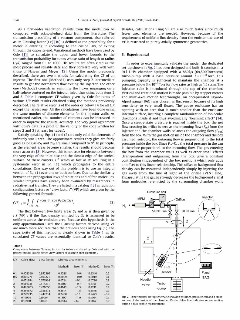
In order to experimentally validate the model, the dedicatedset-up shown in Fig. 2 has been designed and built. It consists in a91 l UHV chamber equipped with a 880 l/s (69,500 Torr sccm)turbo-pump with a base pressure around 7�10�8 Torr. Thispumping capacity is sufficient to maintain the chamber at apressure below 3�10�5 Torr for flow rates as high as 1.5 sccm. Theinjection tube is introduced through the top of the chamber.Vertical and rotational motion is made possible by stepper motorsand multi-axes motion feedthroughs. An encapsulated Bayard–Alpert gauge (BAG) was chosen as flux sensor because of its highsensitivity to very small fluxes. The gauge enclosure has anopening with an area that is much smaller than the enclosureinternal surface, insuring a complete randomization of moleculardirections inside it and thus avoiding any ‘‘beaming effect’’ [14].Once a steady-state pressure is reached inside the box, the netflow crossing its orifice is zero as the incoming flow (Fin) from theinjector and the chamber walls balances the outgoing flow (Fout)from the box. With the gas motion inside the chamber and the boxassumed isotropic, the outgoing flow is proportional to the totalpressure inside the box. Since Fin=Fout the total pressure in the canis therefore proportional to the incoming flow. The gas enteringthe box from the chamber walls as well as other small effects(transpiration and outgassing from the box) give a constantcontribution (independent of the box position) which only addsan offset to this linear relationship. This offset or background fluxdensity can be measured independently simply by injecting thegas away from the line of sight of the orifice (VENT line).Encapsulating the gauge strongly decreases the background signalfrom molecules re-emitted by the surrounding chamber walls

θ

FixedBAG

Turbo-pump

Fluxsensor

Needlevalve

Fig. 2. Experimental set-up schematic showing gas lines, pressure cell and a cross-

section of the inside of the chamber. Dashed blue line indicates sensor motion

during a flux profile measurement.

ARTICLE IN PRESS

0

1

2

3

4

0

Flow

rate

(scc

m)

BAG pressure (x10-5 Torr)

Encapsulated gauge

Fixed gauge

2 4 6 8 10

Fig. 3. Experimental relations between Bayard–Alpert gauges pressure and mass

flow rate as measured by the thermal mass-flow meter. Straight lines are linear fits

of the data.

6.8

7.3

7.8

8.3

50-50Angle (degree)

Gau

ge p

ress

ure

(x10

-5 T

orr)

ExperimentSimulation

0

Fig. 4. Angular flux distribution exiting from a thin orifice demonstrating the

cosine law at injector inlet. Insert shows the randomizer and orifice arrangement.

L. Isnard, R. Ares / Journal of Crystal Growth 311 (2009) 1640–1645 1643

since they can only enter the box through a very small hole.Similar flux sensors have previously been used by other groupsand have shown excellent sensitivity [14,15]. The encapsulatedBAG is attached to a rocking pendulum assembly that keeps thesensor aligned with the center of the injector inlet at all times. Theangle of the pendulum is varied using a stepper motor drivenactuator that is attached to the pendulum arm. It can becontrolled with an accuracy better than 0.11 via a LabViewTM

software. A second BAG is located on the side of the chamber. Thependulum motion of the flux-sensing gauge allows for thegeneration of angular gas flow profiles.

Several injectors were machined from stainless steel with‘mirror polished’ finish (macroscopically smooth at the micronlevel). A quick mounting system allows for easy injector change.Right before the injector inlet, a randomizer, consisting of severalsheets of thin paper, is inserted in order to comply with themodel’s assumption of uniform and diffuse emission at the source.Since molecules have to permeate through it, its effect is to insurethat the inlet flux distribution does not vary with the upstreamconditions. The flow rate through the injector is preciselycontrolled via a pressure cell consisting in a volume bounded byan adjustable valve at the entrance and a small orifice at the exit.The valve opening is controlled to maintain a constant pressurewithin the cell, as measured by a capacitance manometer. Thistechnique is widely used in gas source UHV epitaxy tools andexhibits unmatched flux reproducibility and stability. The flowrate passing through the injector can be read on a thermal massflow meter (MFM) situated upstream of the pressure cell. Asecond gas line allows for redirection of the gas flow away fromthe injection tube, towards a second port through the side of thechamber (VENT line). It is fitted with a manual needle valve that isadjusted to match the conductance of the line going throughinjector (RUN line). A double valve cell is used to switch the floweither to the RUN or to the VENT line. As will be discussed later,the purpose of the VENT line is to provide an independentmeasurement of the background level inside the sensor. For all theresults presented here, the test gas is pre-purified nitrogen, theinjectors have an inlet diameter of 1.970.1 mm and a maximumlength of 20.1 mm, the distance between the nozzle’s and thesensor’s inlets is 5170.5 mm and the box orifice has a diameter of2.170.1 mm.

Before each individual injector characterization, the pressuresignals from both BAGs were measured against the flow rate asgiven by the MFM. This systematically resulted in very linearcurves at least up to pressures around 1�10�4 Torr as shown inFig. 3 and in agreement with the results of Adamson [14]. Thisallows the fixed gauge to be used as flow rate measurementdevice even at very low flows where the MFM readings becomeunreliable. For the mobile gauge, it is a basic linearity check thatcannot be used any further since the slope of the line depends onthe gauge position. During profile measurements, at each polarangle, the encapsulated gauge signal is given sufficient time tostabilize, allowing the pressure inside the enclosure to reach asteady state. The electronic noise in the gauge signal is filtered outby time averaging. The pressure readings of both the mobile andfixed gauges are collected, the latter data being used only to insurethat the chamber is kept in the molecular flow regime and tomonitor the effect of the mobile gauge position on the chamberpressure.

The characterization of an injector consists in acquiring fluxdata along an arc (arc-scan) at various flow rates. Once the desiredflow rate is stabilized, an arc-scan of typically 64 points in bothdirections is acquired using the RUN line (signal+background). Theflow is then switched to the VENT line and after its conductance isadjusted to match the RUN line (same pressure reading on thefixed BAG), a short scan is acquired in order to get the average

background pressure inside the box. This data is used later duringthe curve fitting. For each injector, scans are acquired for a rangeof flow rates starting at the lowest controllable flow andincreasing it by a factor of about two each time.

4. Results and discussion

The fitting process consists in generating a flux simulation onthe arc corresponding to the measurements, adjusting its peakangle position, adding the measured background level and finallyadjusting its height using a scaling factor in order to obtain thebest fit of the experimental data. Thus, the only adjustableparameters are the scaling factor and the centerline position(origin of the angles).

In the case of a thin orifice, the model fits the experimentaldata very closely and can be superimposed to a cosine function(Fig. 4), as predicted by theory. This proves the validity of thecosine law at the injector inlet and thus the adequate performance

ARTICLE IN PRESS

L. Isnard, R. Ares / Journal of Crystal Growth 311 (2009) 1640–16451644

of the randomizer as an effusion source. As a more generic form ofinjectors, a frustum of a cone was tested using low (0.07 sccm) andhigh (1.2 sccm) flow rates. The data and simulation are given inFig. 5. The quality of the fit between data and simulation isexcellent for the low flow rate, but a significant deterioration isobserved as the flow rate is increased, because of the effects ofintermolecular collisions within the injector. In these conditions,the model breaks down since one of the hypotheses on which itrelies is not fulfilled any more. However, in the low flow regime,the excellent agreement between the simulated and experimentaldata is proof of the validity of the model. Another way to verify themodel’s performance is through simple geometry. Assuming thatthe flux density emitted by the inlet disk (source) is much largerthan that of the injector walls, one can identify three zones in theangular flux profile of a given injector. Zone 1 includes all angleswhere the inlet disk is not shadowed by the injector walls. It ischaracterized by a modified cosine angular dependence. In zone 2,the flux intensity drops abruptly, as the inlet disk is progressivelyshadowed by the injector walls. Finally, in zone 3, moleculesreaching the target are emitted solely by the injector walls andproduce a slowly decreasing tail. The limits of the different zonescan be calculated from the injector geometry and are identified onFig. 5. The good agreement between the model, the data and thelimits of zone 1 is especially easy to verify. The flat top and thesloped flanks of cylindrical injectors are also well fitted at lowflow rates. Being able to fit both the experimental peak height andwidth using simulation data and only one adjustable parameter isvery unlikely unless the simulated curve has the right height towidth ratio. Thus the nearly perfect fits obtained for 101 and 151half-angle cones at low flow rates provides the most convincingproof of the model validity.

As mentioned in Section 3, these measurements are based onthe box pressure varying linearly with the injector flux densitythrough the orifice with the flux density from the chamber wallsadding a constant offset pressure:

PBAGðyÞ ¼ a½F injðyÞ þ Fwalls�, (4)

where PBAG represents the gauge pressure and Finj, Fwalls, the fluxdensity coming, respectively, from the injector and the walls whilea is a constant that relates the BAG pressure with the flux densityout of it. If the mobile pressure gauge was perfectly calibrated and

0.3

0.5

0.7

0.9

1.1

1.3

-50Angle (degree)

Flux

den

sity

(a. u

.)

Kn = 5Kn = 0.3Fit - Kn = 5

13

2

3

0 50

2 1

Fig. 5. Angular flux distributions exiting from a conical injector (half-angle 101) for

low (Kn=5) and high (Kn=0.3) flow rates. Left insert shows injector’s details. Right

insert shows the injector’s three geometric zones.

its temperature known, a could be calculated, but this is notnecessary if one is only interested in reproducing the shape of theflux profile.

Now the model, being purely geometric and dimensionless,predicts a linear scaling of the flux density (or box pressure)profile with the flow rate. To perform a fit, a simulated profile isgenerated using an arbitrary flow rate of 1, then the measuredbackground pressure is subtracted from the experimental dataand finally the peak height is adjusted using a scaling factor.Therefore, within the domain of validity of the model, one expectsthe experimental profiles to keep the same shape and the scalingfactor to vary linearly with flow rate. This is indeed observed atlow flow rates where the model’s assumptions are still valid. Asshown in Fig. 6, the fitted scaling factor (as well as the measuredbackground level) for a single injector vary linearly with flow rateup to high values, indicating that once this factor is set for a givenflow rate, its value can be calculated for any flow rates inside themolecular flow regime. Fig. 6 also shows that this factor is nearlyindependent of the injector geometry at low flow rates, limitingthe dependency of the fitting parameter solely to flow rate.

For high flow rates, fit quality is degraded and significantwidening of the experimental distributions is observed. This canbe explained by a change in the flow conditions inside the injectortowards the so-called ‘‘transition flow regime’’. A method toestimate the flow regime using the injector geometry and the flowrate was devised.

The injector transmission probability K being known, itsconductance C can be deduced using

C ¼ KvsA=4, (5)

where vs and A are, respectively, the gas mean molecular velocityand the injector inlet area. Assuming negligible pressure in thechamber just outside the injector, the inlet pressure Ps can beobtained from C and the molar flow rate. The mean free path atthe source (ls) is then given by

ls ¼ C=ðffiffiffi2p

pd20NAFmÞ, (6)

where d0, NA and Fm are, respectively, the molecular diameter,Avogadro’s number and the molar flow rate. The ratio of ls to theinjector’s inlet diameter gives the Knudsen number at the source(Kn) which can be used to characterize the flow regime inside the

0

2

4

6

8

0Flow rate (sccm)

Sca

ling

fact

or (a

. u.)

0

4

8

12

Bac

kgro

und

(a.u

.)

Cone1 Tube Cone2

1 2

Fig. 6. Measured background and fitted scaling factor variations with flow rate for

three different injectors showing linear scaling nearly independent of the injector’s

geometry. Dashed lines are linear fits of the data.

ARTICLE IN PRESS

L. Isnard, R. Ares / Journal of Crystal Growth 311 (2009) 1640–1645 1645

injector. The molecular flow regime is usually defined as theregion where KnX1 while the transition flow regime as the onewhere 1XKnX0.01. As shown in Fig. 5, the fit quality for a conicalinjector is significantly degraded for a value of Kn of 0.3. As theflow rate through the injector is increased, a gradual widening ofthe angular flux distribution is observed for Kn values below E1.This is attributed to the increasing number of intermolecularcollisions inside the injector. These collisions reduce the directflux out of the injector which decreases the peak height whilepromoting higher angle exit which increases its width. Thiswidening of flux distributions as Kn decreases towards thetransition regime has previously been observed by Stickneyet al. [16]. Below KnE1, the proposed model, which assumes alinear dependency of the exchanged fluxes with flow rate, starts tobreak down as the flux distribution becomes flow rate dependent.Modifications of the model in order to include the effects ofintermolecular collisions are then needed to accurately simulatethe data.

5. Conclusions

A dedicated set-up was used to evaluate a simple and generalmodel for the simulation of gas flux distributions exiting axiallysymmetric injectors into UHV. Using nitrogen as a test gas, themodel predictions show excellent agreement with the experi-mental data within the limits of its physical assumptions(molecular flow). As the molecules’ mean free path decreasesbelow the injector’s inlet diameter, intermolecular collisionsgradually widen the experimental distributions and this simplemodel breaks down. Improving the model in order to fit these datawould require an upgrade that would take into account molecularinteractions within the volume of the injector. The present workhas shown that gas flux distributions out of a gas injector are flowrate independent only within the molecular flow regime. If astationary substrate is to be used for thin film deposition usingmolecular beams, it will be necessary to carefully choose theinjector’s dimensions in order to insure molecular flow over therange of useful flow rates. For example, the growth of GaAs by CBEat 1mm/hr on a 100 mm diameter wafer, assuming a sourceefficiency of 10%, requires a flow rate of E1.1 sccm of trimethyl-gallium (TMG). In order to reach a Kn value of 5, assuming amolecular diameter of 6 A for TMG and a short injector (CF of 0.8),a 6 cm inlet diameter is required. This is quite unrealistic and the

model applicability seems to be compromised for the design ofsingle injectors for CBE. However, the model being linear, ifmolecular flow prevails inside the chamber, the superpositionprinciple can be used to simulate multi-nozzle injection devices.In that case, with each nozzle injecting only a fraction of the totalflow rate, the restrictions on their dimensions are much lessstringent. Then the predicting capabilities of the present modelcan be used to design optimized CBE injectors capable of insuringhigh levels of both flux uniformity and source use efficiency forrotating or stationary substrates.

Acknowledgements

Financial support from the Natural Sciences and EngineeringResearch Council of Canada, le Fonds Quebecois de la Recherchesur la Nature et les Technologies and Canada Foundation forInnovation is gratefully acknowledged. The authors are grateful toEric Breton, Roger Dumoulin and Jean-Pierre Ares for technicalassistance and to Etienne Shaffer and Charles Vidal for contribut-ing to the computer programs.

References

[1] C.W. Farley, G.E. Crook, V.P. Kesan, T.R. Block, H.A. Stevens, T.J. Mattord, D.P.Neikirk, B.G. Streetman, J. Vac. Sci. Technol. B 5 (1987) 1374.

[2] S.N.G. Chu, N. Chand, D.L. Sivco, A.T. Macrander, J. Appl. Phys. 65 (1989) 3838.[3] J.A. Curless, J. Vac. Sci. Technol. B 3 (1985) 531.[4] Z.R. Wasilewski, G.C. Aers, A.J. SpringThorpe, C.J. Miner, J. Vac. Sci. Technol. B 9

(1991) 120.[5] J.-L. Vassent, A. Marty, B. Gilles, C. Chatillon, Vacuum 64 (2002) 65.[6] R. Venkat, B.R. Pemmireddy, R. Vijayagopal, H. Cheng, R. Bresnahan, J. Vac. Sci.

Technol. B 22 (2004) 1549.[7] G. Benvenuti, E. Halary-Wagner, A. Brioude, P. Hoffmann, Thin Solid Films 427

(2003) 411.[8] Y. Wu, J. Maths. Phys. 45 (1966) 169.[9] D.J. Santeler, M.D. Boeckmann, J. Vac. Sci. Technol. A 5 (1987) 2493.

[10] P. Clausing, Ann. Phys. 12 (1932) 961 (English translation in J. Vac. Sci.Technol. 8 (1971) 636).

[11] R.J. Cole, Rarefied Gas Dynamics, American Institute of Aeronautics andAstronautics, New York, 1977 p. 261.

[12] Unpublished results cited in D. van Essen, W. Chr. Heerens, J. Vac. Sci. Technol.13 (1976) 1183.

[13] http://www.me.utexas.edu/~howell/.[14] S. Adamson, J.F. McGilp, Vacuum 36 (1986) 227.[15] L. Holland, C. Priestland, Vacuum 16 (1966) 601.[16] R.E. Stickney, R.F. Keating, S. Yamamoto, W.J. Hastings, J. Vac. Sci. Technol. 4

(1967) 10.