The well-designed logical robot: Learning and experience from observations to the Situation Calculus
38
Artificial Intelligence 175 (2011) 378–415 Contents lists available at ScienceDirect Artificial Intelligence www.elsevier.com/locate/artint The well-designed logical robot: Learning and experience from observations to the Situation Calculus Fiora Pirri DIS, Sapienza, University of Rome, Italy article info abstract Article history: Received 21 January 2007 Received in revised form 11 March 2010 Accepted 14 March 2010 Available online 3 April 2010 Keywords: Visual perception Action space Action recognition Parametric probability model Learning knowledge Inference from visual perception to knowledge representation Theory of action Learning theory of action from visual perception The well-designed logical robot paradigmatically represents, in the words of McCarthy, the abilities that a robot-child should have to reveal the structure of reality within a “language of thought”. In this paper we partially support McCarthy’s hypothesis by showing that early perception can trigger an inference process leading to the “language of thought”. We show this by defining a systematic transformation of structures of different formal languages sharing the same signature kernel for actions and states. Starting from early vision, visual features are encoded by descriptors mapping the space of features into the space of actions. The densities estimated in this space form the observation layer of a hidden states model labelling the identified actions as observations and the states as action preconditions and effects. The learned parameters are used to specify the probability space of a first-order probability model. Finally we show how to transform the probability model into a model of the Situation Calculus in which the learning phase has been reified into axioms for preconditions and effects of actions and, of course, these axioms are expressed in the language of thought. This shows, albeit partially, that there is an underlying structure of perception that can be brought into a logical language. © 2010 Elsevier B.V. All rights reserved. To John and his surprising innate abilities 1. Introduction 1.1. Foreword In this paper I discuss McCarthy’s exploration of the relation between appearance and reality in the “well-designed child” [77,79]. McCarthy’s arguments, in my opinion, are twofold. The first addresses the need to axiomatise the appearance– reality relation within a language of thought, while the second, addressing the archetype of inner abilities, contests the ability of current learning methods to explain the appearance–reality relation. My thesis here is to show that early learning, via perception, is necessary to tune knowledge formation. I argue that the perception of reality, although local and particular, can be shaped by learning the parameters of the appearance of events, and that these parameters provide a structure for a symbolic representation supporting the inference from appearance to reality. Other than the cited papers and many works that are on McCarthy’s web site, some of his arguments about learning are taken from my personal conversations with him during these last 18 years of friendship. E-mail address: fi[email protected]. 0004-3702/$ – see front matter © 2010 Elsevier B.V. All rights reserved. doi:10.1016/j.artint.2010.04.016
Transcript of The well-designed logical robot: Learning and experience from observations to the Situation Calculus
Artificial Intelligence 175 (2011) 378–415
Contents lists available at ScienceDirect
Artificial Intelligence
www.elsevier.com/locate/artint
The well-designed logical robot: Learning and experience fromobservations to the Situation Calculus
Fiora Pirri
DIS, Sapienza, University of Rome, Italy
a r t i c l e i n f o a b s t r a c t
Article history:Received 21 January 2007Received in revised form 11 March 2010Accepted 14 March 2010Available online 3 April 2010
Keywords:Visual perceptionAction spaceAction recognitionParametric probability modelLearning knowledgeInference from visual perception toknowledge representationTheory of actionLearning theory of action from visualperception
The well-designed logical robot paradigmatically represents, in the words of McCarthy, theabilities that a robot-child should have to reveal the structure of reality within a “languageof thought”. In this paper we partially support McCarthy’s hypothesis by showing that earlyperception can trigger an inference process leading to the “language of thought”. We showthis by defining a systematic transformation of structures of different formal languagessharing the same signature kernel for actions and states. Starting from early vision, visualfeatures are encoded by descriptors mapping the space of features into the space of actions.The densities estimated in this space form the observation layer of a hidden states modellabelling the identified actions as observations and the states as action preconditions andeffects. The learned parameters are used to specify the probability space of a first-orderprobability model. Finally we show how to transform the probability model into a modelof the Situation Calculus in which the learning phase has been reified into axioms forpreconditions and effects of actions and, of course, these axioms are expressed in thelanguage of thought. This shows, albeit partially, that there is an underlying structure ofperception that can be brought into a logical language.
© 2010 Elsevier B.V. All rights reserved.
To John and his surprising innate abilities
1. Introduction
1.1. Foreword
In this paper I discuss McCarthy’s exploration of the relation between appearance and reality in the “well-designed child”[77,79]. McCarthy’s arguments, in my opinion, are twofold. The first addresses the need to axiomatise the appearance–reality relation within a language of thought, while the second, addressing the archetype of inner abilities, contests the abilityof current learning methods to explain the appearance–reality relation. My thesis here is to show that early learning, viaperception, is necessary to tune knowledge formation. I argue that the perception of reality, although local and particular,can be shaped by learning the parameters of the appearance of events, and that these parameters provide a structure for asymbolic representation supporting the inference from appearance to reality.
Other than the cited papers and many works that are on McCarthy’s web site, some of his arguments about learning aretaken from my personal conversations with him during these last 18 years of friendship.
E-mail address: [email protected].
0004-3702/$ – see front matter © 2010 Elsevier B.V. All rights reserved.doi:10.1016/j.artint.2010.04.016

F. Pirri / Artificial Intelligence 175 (2011) 378–415 379
1.2. The well-designed child
In his notes on The well-designed child [77,79], John McCarthy argues that the Lockean view that knowledge is built fromsensations is not adequate for what he calls the designer stance, a theme taken from Dennett [31], who paradigmaticallyused it to understand and predict the structure and behaviour of biological and artificial systems.
“In so far as we have an idea what innate knowledge of the world would be useful, AI can work on putting it intorobots, and cognitive science and philosophy can look for evidence of how much of it evolved in humans. This is thedesigner stance.”
Evidence of evolution efficiency [77,79] supersedes the point of view, shared by behaviourism in psychology and pos-itivist philosophy, that knowledge proceeds from sensations. Evolution had gradually shaped optimal predispositions inhumans, in so determining a correspondence between an innate mental structure and facts about the world. The criticismof the Lockean child, nevertheless, is not addressed as a mind/body problem; instead, stepping aside it, McCarthy offers thebold view of the robot-child experiment: an AI (or possibly a psychological) system replicating the intelligent behaviourof a child. So what is innate and what can be learned? McCarthy recognises learning as central to the experiment design,but grounded in meanings independent of sensations and facts, “what a child learns about the world is based on its innatemental structure” [77,79]. Specifically, the innate mental structure is based on three interdependent aspects:
1. “world characteristics”, such as appearance and reality, continuity of motion, gravity, and relations,2. “mental characteristics” such as central decision making, incompleteness of appearance, senses,3. “innate abilities” such as introspection, noise rejection, principle of mediocrity.
These innate mental structures evolved for survival and control purposes, thus are necessitated by adaptation “A baby in-nately equipped to deal with them will outperform a Lockean baby”. They have been investigated also in neurophysiologicalstudies; for example, it is known that the vestibular system has specialised sensors, such as canals and otoliths, to detectgravity direction and disambiguate spatial orientation and localisation. Likewise there is a specialised motion sensitive areain the temporal cortex for both control of locomotion and perception of spatial relations. Most important, in connectionwith what McCarthy calls the principle of mediocrity, both imitation and the innate ability to put oneself in the place of othershave been explained by the mirror neurons discovered by Rizzolatti and colleagues [103,63,39].
Psychological, neurological and neurophysiological findings on the function and structure of the brain justify the above-mentioned innate abilities. Innate structures take a step beyond the view (see e.g. Russell in [105]) that sensations alonedetermine knowledge. The question, from the designer stance, is whether it is possible, with a language of thought, inMcCarthy words, to represent the innate child’s brain structure by means of logical sentences?
1.3. Appearance and Reality: the language of thought
McCarthy discusses the implementation of four innate structures, namely the relation of appearance and reality, persistentobjects, the spatial and temporal continuity of perception and the language of thought. In his notes on Appearance and Reality:a challenge to machine learning [78], that complements those on Appearance and Reality included in the Well-designed child,McCarthy says that classifying “experience is inadequate as a model of human learning and also inadequate for roboticapplications”. He argues that mere classification does not “dis-cover” (in the sense of “un-cover” and “reveal”) the hiddenreality behind appearance. To unlock reality behind appearance McCarthy suggests “brute force logical attitude toward makingtheir relations (appearance–reality) explicit”, and proposes to axiomatise their relation in a formal language, such as theSituation Calculus, as follows:
holds(appears(appearance,object), s
)(1)
So, for each single object one would have an accurate description through the term appearance. Instances of the termappearance would need some recursive definition or some intended interpretation. These descriptions of the term “appear-ance” are not qualia,1 in the sense of attributes of pure perceptual experience [70,44], but designate quantifiable attributesof physical objects, e.g., as projected on the retina, however not necessarily evoking the sensory experience.
A well-known argument about the relation between innate knowledge (abilities) and learned knowledge is that of Mary’sRoom [56,57,32] and it is interesting to compare it with McCarthy’s arguments. We recall that Jackson’s knowledge argumentwas the following. Mary is a perfect scientist who cannot see colours but knows all the cause-effect laws that regulate thehuman perception of colours and the utterance of colour nouns of any object whatsoever [56,57]. When she eventuallyis made capable to see colours would she learn anything? Would she have an experience inducing knowledge differentfrom her current knowledge which, by hypothesis is complete? Daniel Dennett in [32] rejects the argument that Maryderives incremental knowledge when she is allowed to see colours, based on the fact that her knowledge is complete.Furthermore, having reformulated the argument to make Mary a perfect logician [33,55] he argues that when Mary finallycan see the colours and she is offered a blue banana, then she is able to discover that she has been deceived as she knows
1 Note that also in [76] McCarthy proposes a basic consciousness made of propositions and images of scenes and objects.
380 F. Pirri / Artificial Intelligence 175 (2011) 378–415
what bananas look like (see also [32]). Dennett’s statement [33,55] is to clarify the abstract precondition of the knowledgeargument, describing the best circumstances under which Mary’s (RoboMary’s) knowledge is to be complete, so that shecan infer everything, just applying useful lemmas (actually her knowledge should be equivalent to its deductive closure).“What matters is whether Mary (or RoboMary) can deduce what it’s like to see red from her complete physical knowledge,not whether one could use one’s physical knowledge in some way or other to acquire knowledge of what it’s like to seein colour” [33]. Obviously if RoboMary has complete knowledge [33] her perceptual experience (or any form of knowledgeacquisition whatsoever) is unnecessary and irrelevant. In fact, by definition, nothing can be added to a complete theory,without making it inconsistent.
However, as far as visual perception is concerned, it should be pointed out, that there is no complete axiomatisationeven for the partial structure concerning colour perception, as it would at least include arithmetic, so there would be trueappearances that could not be derived.
Clearly McCarthy is not proposing a complete axiomatisation of the appearance–reality relation. Nevertheless a concretequestion about the “brute force logical attitude” is whether any such term designating the appearance of a physical objectcan make the relation “appear” a logical truth, accounting for the innate brain structure, such as colour-selective perceptivefields, chromatic adaptation, and the Purkinje effect, and with correlated phenomena, such as light change or backgroundchanges.
1.4. From the language of thought to learning
An immediate and concrete problem is how the robot-child uses its sensors. A robot-child is endowed with sound andvisual sensors, and proprioperception sensors for moving. The term designating “appearance”, as posed in (1), cannot matchthe continuous stimuli obtained from the sensor instruments. It might be possible that the appearance term is either notaccurate enough or too accurate, or that there is a variability in the object phenomenology or a variability in the instrumentsthat has not been taken care of by the amanuensis instructor who “if any, should have to know the subject matter and verylittle about how the program or hardware works” [77]. So a typical situation would be a mismatch between the termdesignating appearance and the measurements, since for the robot-child there is no way (in the language of thought) tosample data from its instrument and obtain an adequate model of the current stimulus. Even if the innate abilities couldbe hardwired in the sensors, the pathway from sensors to reasoning must be explained. Perceptual stimuli, driven fromappearance, though informing the robot-child’s reasoning, undergo a complex and hardly predictable processing that cannotbe described by logical sentences. In our view the variability of the appearance induces a stimulus gradient which, throughthe learning experience, solicits the “innate abilities” to determine (possibly new) correlations between events and objects.An innate ability is, for example, finding hidden parameters for any partially perceivable phenomenon, and eliciting fromthese a prediction of future appearance.
A single statement in which “both appearances of objects and physical objects will be represented as logical objects,i.e. as the values of variables and terms” [77,79] seems to reduce the power of scientific findings to the Kantian synthetictruth [60]. Whereas, as Sloman would note [111,112], there is a tradeoff between deterministic and probabilistic causation(Humean versus Kantian view).
Furthermore, appearance categorisation in the language of thought requires the language to name all the phenomenadenoted in the ontology. An enumeration of objects and phenomena would be against a parsimony principle that entia nonsunt multiplicanda praeter necessitatem. The parsimony principle, instead, is applied when learning from experience. Whenwe look at a scene, we can distinguish more entities than we can designate, yet the detailed acknowledgement of several“un-named” phenomena allows us to abstract concepts, find correlations, indicate causal power, and infer the deep andessential structure of the scene.
Designation of appearance, in the language, is the result of some episodic inference producing knowledge of causationthrough perceptual evidence of correlation.
It still remains open how to determine what could be an appropriate explanation of the appearance–reality relation.Recall that we started with “the design of a robot-child that has some chance of learning from experience and education”. Intheir developmental studies, Gopnik, Meltzoff and colleagues argue that children’s theories converge to accurate descriptions,by learning mechanisms that are analogous to “scientific-theory formation” [47], see also [46,45,93,80]. On this basis wecan view the problem of modelling the relation appearance reality as the relation between science and experimental data.In this way the appearance–reality problem is transformed into a problem of causation and prediction. Sloman, in [111,112], discussing the Gopnik and colleagues’ view of a child as a tiny scientist, proposes a cleavage between Humean andKantian attitude towards causation. The first involving the direct experience of co-occurrence and correlations that can becompared to what Gopnik and Shulz [47] consider the children’s learning mechanisms. That is, the Humean view specifiescorrelations among physical objects in terms of probabilities and causation. On the other hand, the Kantian view concernsthe inner structure of causation that affects universal and deterministic laws. He argues that a child starts with a Humeanapproach to correlation and ends up with a Kantian causal structure of the environment. Sloman foresees a progressionfrom one attitude towards the other “Typically in science causation starts off being Humean until we acquire a deep (oftenmathematical) theory of what is going on: then we use a Kantian concept of causation”.
These issues are close to the reification steps explained by Quine in [97], initiated with observation sentences and accom-plished with the whole sketch of epistemological settings. Observation sentences, also occasion sentences, vehicle perceptual

F. Pirri / Artificial Intelligence 175 (2011) 378–415 381
stimuli to the formation of a scientific theory. The empirical significance of the observation sentences is in the relationbetween a scientific theory and its sensory evidence [95]. For Quine it is folly to separate the synthetic sentences “whichhold contingently on experience” and the analytic ones “which hold come what may”. He speaks of a varying distance froma sensory periphery, where statements are closer to experience, stimuli and measurements, to the centre which is heldby “highly theoretical statements of physics or logic or ontology” [94]. Highly theoretical statements constitute the backlogof the scientific theory. To cope with prediction Quine introduces observation categorical whose doctrine is to explain “thebearing of sensory stimulation” (see [96,97]).
Although our discussion is quite limited, it seems that different notions of causation are involved in learning mechanismsthat take place, initially, with perception, experience and observations.
1.5. Commonsense and learning from experience
At this point we can say that modelling the appearance–reality relation can be reduced to the problem of the scientifictheory formation through its natural steps: from the perceptual stimulus to the elicitation of the hypotheses and theirconfirmation. These steps lead to a description of the appearance and its underlying correlation with objects, possiblycounting also refutation.
As it is, at least in its generality, the problem has been addressed since the early approaches to commonsense reasoning,from the foundational Programs with commonsense [75] to the recent reviews of Davies and Morgenstern in [35]. In fact, withthe well-designed robot-child McCarthy intends explicitly an AI experiment in the commonsense world.
However, in the huge literature on commonsense AI, few approaches have effectively faced the appearance–realityrelation. Here we distinguish between attempts to formalise perception and learning. Approaches seeking to formalise per-ception from the stimulus, here with the specific meaning of the observation and its variability, have been at earliest takenby Levesque in [67] and by Bacchus, Halpern and Levesque in [8] (see also [9]). These are the most thorough attemptsto epistemologically formalise sensory data. In particular, [8] has been the very first meaningful attempt to explicate theappearance–reality relation in a simulated system. Similarly the works of [68] and [87,102].
While there is a prodigious literature on learning from perception in the computer vision and statistical learning commu-nities, this is not the case for the knowledge representation and commonsense communities. Often, learning from perceptionis confused with learning from the representation of perception. If the representation of perception is already provided(through specific terms or predicates or any symbolic structure not dealing with measure, scale, dimension, and otherquantities) nothing is left to learning, nothing is left to understanding the real problem: what is learned from appearanceand how, what is mapped from appearance to reality, and how.
Nevertheless we have to bear in mind that McCarthy starting point, for the robot-child experiment, is the innate mentalstructures of the child, which is paramount to both the designer stance and the notion of the child as a “tiny scientist”.
McCarthy’s designer stance could be implemented taking care of a crucial passage. That is, providing a plausible repre-sentation for those patterns of sensory stimuli, first classified by computational models of pattern recognition.
An empirical method of learning from experience should formally take care of the inductive attitude (in the sense men-tioned by Polya in [89]) towards abstraction, and the determination of “the spatio-temporal world behind appearance” canbe obtained by shifting these forms of empirical reasoning into the “language of thought”. This coincides with Quine’s argu-ment [94] of shifting from the sensory periphery towards the centre of the system, using the categorical observations [97].
1.6. The designer stance
Dennett’s design stance is concerned with predicting both purpose and function of an entity from its design whileMcCarthy’s designer stance is concerned with what features have to be put in an intelligent system to implement a be-haviour. Thus the designer stance predicts a behaviour by defining the rules governing a robot-child’s function.
The design of a database of actions begins by specifying a signature, spelling out the words to denote actions, objects,properties and fluents, to formalise a set of tasks. This is the representation context. In so doing the designer has alreadyin mind an abstraction layer which is a schematisation of an agent activity, whose execution laws are formalised by a setof axioms. The designer, jumping beyond the learning steps, separates distinctly what is essential from what is inessential,according to her judgement, expressed in form of axioms. These judgements form the instructions of a robot-system tasksexecution. This schema is induced not from data but from what she, the designer, theorises is an execution process. Thestructure of data is not even considered.
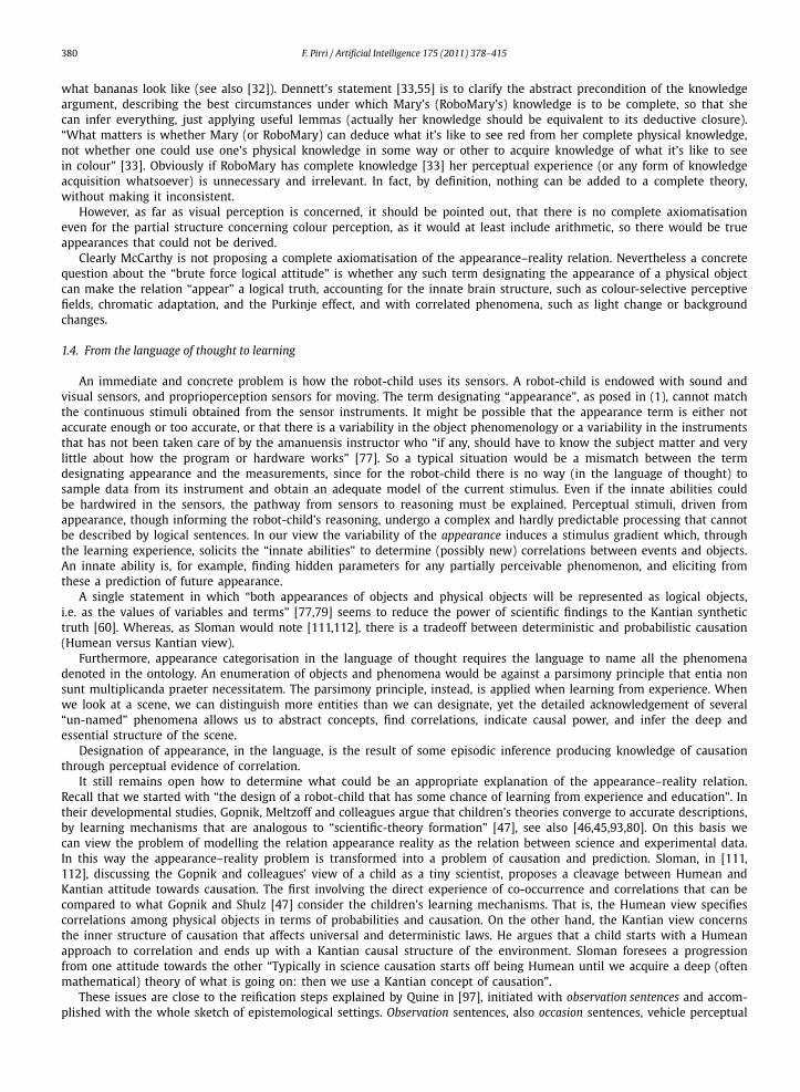
On the other hand, here we try to go upstream and conjecture a more general setting for the designer stance. The designof a learning process that starts with perception and ends with an ontology of actions is exemplified in Fig. 1. Here it issupposed that the designer shows a task, such as, for example, opening a door, to someone that does not speak the languageand has never seen the task. So she would begin by designating the action names such as unlock or push the door. But thelanguage would not be self-explaining if at the same time she did not point out the uttered action names while the learnerwas looking at the sequence. On the other hand, this pointing would not be effective if, at the same time, the learner wouldnot be able to infer, from an enormous amount of data gathered from its stimuli, that these and those events are from asingle specific action, the very one indicated by the designer while uttering the action name. So we have added two further
382 F. Pirri / Artificial Intelligence 175 (2011) 378–415
Fig. 1. Structure of the learning model, from observations to axioms, for the task open the door.
inference processes: inferring actions from movements and inferring a correlation among actions and between terms andactions.
Showing and pointing is often successful, and not only with children; even dogs and cats learn how to open a door justby looking at adult humans doing so. A dog understands two essential concepts: an aperture needs to be created, somehow,to quickly pass through. The actions are that the door needs to be unlocked by turning or lowering the handle and thatit has to be pushed in some direction. How does the dog infer these two concepts, not having hands, and often using themouth, not even knowing the name of actions and the name of the afforded objects, like the handle or the door?
To implement our interpretation of the designer stance, as hinted above, we formalise a continuous learning processfrom the perceptual stimulus to the language of thought. Indeed, we show how a simple task such as opening a door islearned in three steps of the pathway from perceptual stimulus to categorisation.
The first step is concerned with early visual perception, eliciting a number of actions from a sequence of movements.This step leads to learning to categorise an action from a large number of simpler movements and to correlate actions onthe basis of speed of movements, positions in space, distances, centres of mass and their brightness. The second step isconcerned with understanding the local causal relations among the actions. This step, which we identify with the inductionhypothesis, extends the basic terms to a signature and to a language for the quantities learned in the first step, mappingthe specific parameters into a probability space. The third step, the inductive generalisation, is concerned with establishingthe rules of what has been learned, for example, that at the end of the task the door is open.
Starting from a number of videos of different people opening a door (actually the same door), we show that a sequenceof events, such as the sequence of frames illustrating a hand opening a door, can be used to assess the basic laws of causeand effect that specify the task.
Although this is a simple example it gives a substantial insight into a crucial issue, that is, which are the critical stepsof the process that from observations leads to the formation of abstract concepts like the cause and effect laws involved ina simple task. The most important aspect of the transformation is to move from quantitative information (the observations)to qualitative judgements (the laws). The information collected from observations lies in a high-dimensional space (colours,intensity, velocity, positions, etc.) and the simplest way to reduce the dimension and move towards a qualitative assessmentof the underpinning properties of the observed events, is to use probability functions. Stochastic variables, in a true Bayesianconception, are by far the only entities that can convey the beliefs about observations, expressed as measures in terms ofpriors and posterior probabilities, into epistemic states that can further be named by words or specified by properties. Forexample, the probability of a certain motion direction, given the parameters of a class, becomes the belief that a certainaction can be executed after another one has produced its effects.
Our idea, that we illustrate below with the aid of the opening the door task, is that the data underlying the observationscan be explained with stochastic variables denoting values of actions and states. These values initially describe the proba-bility of events, for example, a sequence of movements is specified by descriptors assessed via visual perception. Further,the induced densities generate the action space by gathering the movements into main actions that can be named. For
F. Pirri / Artificial Intelligence 175 (2011) 378–415 383
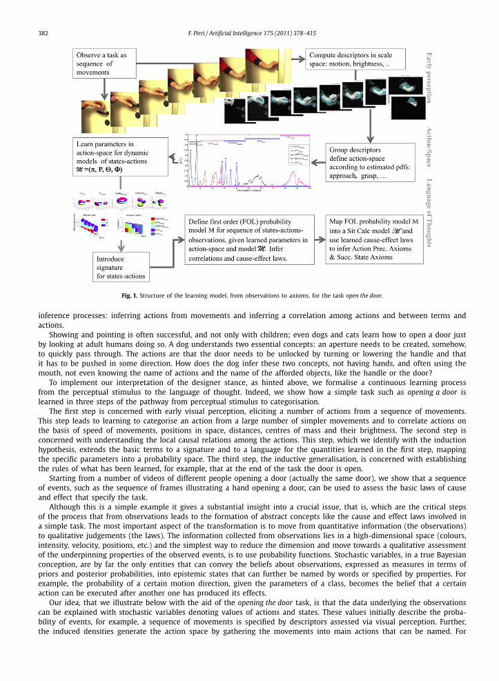
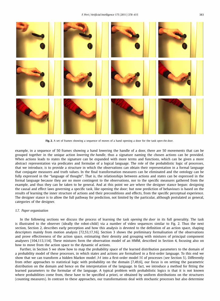
Fig. 2. A set of frames showing a sequence of moves of a hand opening a door for the task open the door.
example, in a sequence of 50 frames showing a hand lowering the handle of a door, there are 50 movements that can begrouped together in the unique action lowering the handle, thus a signature naming the chosen actions can be provided.When actions leads to states the signature can be expanded with more terms and functions, which can be given a moreabstract representation via predicates and formulae of a logical language. The role of the probabilistic logic of processes,that we introduce, is to provide a structure in which the observations can obtain their representation in a formal languagethat conjugate measures and truth values. In the final transformation measures can be eliminated and the ontology can befully expressed in the “language of thought”. That is, the relationships between actions and states can be expressed in theformal language because they are no more contingent to the observations, nor to the specific measures gathered from theexample, and thus they can be taken to be general. And at this point we are where the designer stance begun: designingthe causal and effect laws governing a specific task, like opening the door; but now prediction of behaviours is based on theresults of learning the inner structure of actions and their preconditions and effects, from the specific perceptual experience.The designer stance is to allow the full pathway for prediction, not limited by the particular, although postulated as general,categories of the designer.
1.7. Paper organisation
In the following sections we discuss the process of learning the task opening the door in its full generality. The taskis illustrated to the observer (ideally the robot-child) via a number of video sequences similar to Fig. 2. Thus the nextsection, Section 2, describes early perception and how this analysis is devoted to the definition of an action space, shapingdescriptors mainly from motion analysis [72,53,17,16]. Section 3 shows the preliminary formalisation of the observationsand prove effectiveness of the action space, estimating their density and grouping with mixtures of principal componentanalysers [104,113,114]. These mixtures form the observation model of an HMM, described in Section 4, focusing also onhow to move from the action space to the dynamic of actions.
Further, in Section 5 we show how to map the probability space of the learned distribution parameters to the domain ofa probability model of these processes, in which states and actions are formalised in a first-order language. To this end weshow that we can transform a hidden Markov model M into a first-order model M of processes (see Section 5). Differentlyfrom other approaches to statistical logic with probability on the domain [7,49,6], our focus is on setting the parametricdistribution on the domain and hence on the interpretation of the language. In fact, we introduce a method for fitting thelearned parameters to the formulae of the language. A typical problem with probabilistic logics is that it is not knownwhere probabilities come from, these have to be specified a priori, or obtained by uniform distributions on the structures(counting measures). In contrast to these approaches, our transformations deal with stochastic processes but also determine
384 F. Pirri / Artificial Intelligence 175 (2011) 378–415
the learned distribution, indeed learned from the observations, and map it to the domain of the first-order interpretation.Our approach is also rather different from the work of, for example, [24,25,83,99] and [107] because we can directly mapthe computational learning model to the first-order domain. In this sense our formalisation of a first-order probabilitymodel is closer to the concept of BLOG [81], inasmuch as the domain inherits a distribution just by suitably fixing theinterpretation of the atoms, according to a transformation of the terms of the statistical model. This can be clearly extendedto other graphical models and sampling methods. Finally (see Section 6) we show how the probability first-order model M
can be transformed into a model M of a basic theory of actions in the language of the Situation Calculus. Here, at last, thegeneralisation is accomplished and thus, for learning purposes, the probabilities can be discarded.
2. Features descriptors and action space
The study of human actions via motion analysis has received a good deal of attention in recent years. We refer thereader to the recent reviews of [54,82,92,65], to get an idea of the progress made on the application of motion analysisto the understanding of human actions and behaviour. Beside being focused on a specific example, the contribution ofour approach, with respect to this early phase of the designer stance, is mainly in the specification of a mapping from afeature space to an eigen action space. The eigen action space is obtained by grouping the motion features into actions, byboth combining the smoothed functions of the velocity, and estimating the features descriptors density, with mixtures ofprobabilistic principal component analysers.
The first step of the design is to obtain a set of descriptors of the motion of a hand opening a door. A video sequence ofthe task open the door is composed of 200 to 280 frames at 35–40 fps, where each image has size 640× 420 as in Fig. 2.Thus, a sequence is a volume or 3D matrix 640×420× T of frames I(t), t = 1, . . . , T . For each sampled video sequence threenew volumes are generated. The first one is the result of early segmentation obtained by combining attention-based motiondetection (see [13]) with an intensity-based mean-shift tracking (see [21,22]). The result of segmentation is a sequence ofimages in which the non-interesting pixels, with respect to both motion and saliency, are blurred and uniformly set to null.This segmented volume is denoted G
T , and its binarisation, used for further analysis, is defined as:
δG (x, y, t)={
1 if G(x, y, t) > 0, ∀x, y, and t = 1, . . . , T
0 otherwise(2)
That is δTG is like G
T but the pixel values different from null are set to 1.
Two more volumes are generated from GT , for the optical flow vector components. The optical flow problem amounts to
computing the displacement field between two images, from the image intensity variation. Here it is assumed that the 2Dvelocity is the projection, on the image plane, of the space–time path of a 3D point. The optical flow vector w = (u, v,1)
is computed between two successive images of an image sequence using a natural constraint based on the principle ofbrightness constancy.
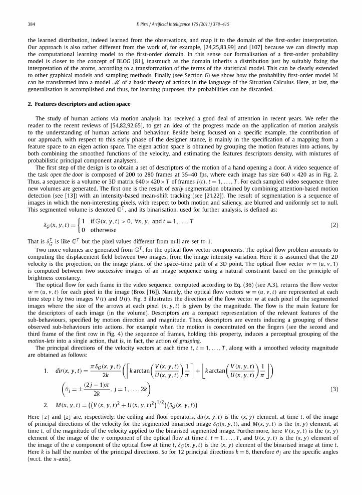
The optical flow for each frame in the video sequence, computed according to Eq. (36) (see A.3), returns the flow vectorw = (u, v, t) for each pixel in the image (Brox [16]). Namely, the optical flow vectors w = (u, v, t) are represented at eachtime step t by two images V (t) and U (t). Fig. 3 illustrates the direction of the flow vector w at each pixel of the segmentedimages where the size of the arrows at each pixel (x, y, t) is given by the magnitude. The flow is the main feature forthe descriptors of each image (in the volume). Descriptors are a compact representation of the relevant features of thesub-behaviours, specified by motion direction and magnitude. Thus, descriptors are events inducing a grouping of theseobserved sub-behaviours into actions. For example when the motion is concentrated on the fingers (see the second andthird frame of the first row in Fig. 4) the sequence of frames, holding this property, induces a perceptual grouping of themotion-lets into a single action, that is, in fact, the action of grasping.
The principal directions of the velocity vectors at each time t , t = 1, . . . , T , along with a smoothed velocity magnitudeare obtained as follows:
1. dir(x, y, t)= πδG (x, y, t)
2k
(⌈k arctan
(V (x, y, t)
U (x, y, t)
)1
π
⌉+
⌊k arctan
(V (x, y, t)
U (x, y, t)
)1
π
⌋)(
θ j =± (2 j − 1)π
2k, j = 1, . . . ,2k
)(3)
2. M(x, y, t)= ((V (x, y, t)2 + U (x, y, t)2)1/2)(
δG (x, y, t))
Here �z� and �z� are, respectively, the ceiling and floor operators, dir(x, y, t) is the (x, y) element, at time t , of the imageof principal directions of the velocity for the segmented binarised image δG (x, y, t), and M(x, y, t) is the (x, y) element, attime t , of the magnitude of the velocity applied to the binarised segmented image. Furthermore, here V (x, y, t) is the (x, y)
element of the image of the v component of the optical flow at time t , t = 1, . . . , T , and U (x, y, t) is the (x, y) element ofthe image of the u component of the optical flow at time t , δG (x, y, t) is the (x, y) element of the binarised image at time t .Here k is half the number of the principal directions. So for 12 principal directions k = 6, therefore θ j are the specific angles(w.r.t. the x-axis).
F. Pirri / Artificial Intelligence 175 (2011) 378–415 385
Fig. 3. Frames, corresponding to those shown in Fig. 2, illustrating part of the observations descriptors, see Section 2. Here the optical flow is shown,highlighted by the arrows indicating motion direction.
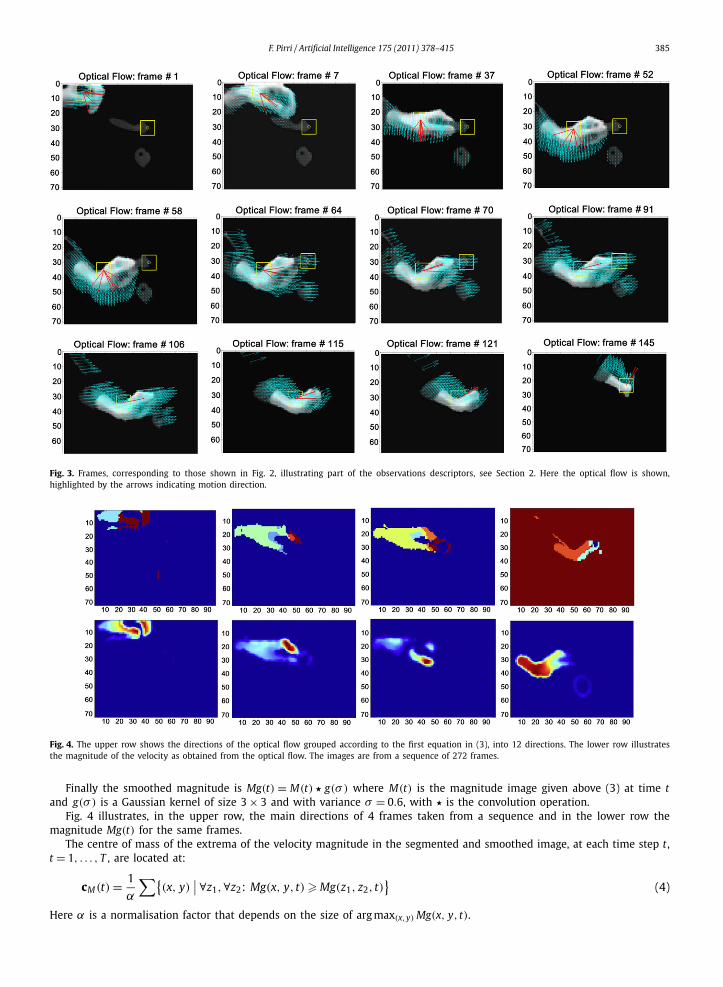
Fig. 4. The upper row shows the directions of the optical flow grouped according to the first equation in (3), into 12 directions. The lower row illustratesthe magnitude of the velocity as obtained from the optical flow. The images are from a sequence of 272 frames.
Finally the smoothed magnitude is Mg(t) = M(t) � g(σ ) where M(t) is the magnitude image given above (3) at time tand g(σ ) is a Gaussian kernel of size 3× 3 and with variance σ = 0.6, with � is the convolution operation.
Fig. 4 illustrates, in the upper row, the main directions of 4 frames taken from a sequence and in the lower row themagnitude Mg(t) for the same frames.
The centre of mass of the extrema of the velocity magnitude in the segmented and smoothed image, at each time step t ,t = 1, . . . , T , are located at:
cM(t)= 1
α
∑{(x, y)
∣∣ ∀z1,∀z2: Mg(x, y, t) � Mg(z1, z2, t)}
(4)
Here α is a normalisation factor that depends on the size of arg max(x,y) Mg(x, y, t).
386 F. Pirri / Artificial Intelligence 175 (2011) 378–415
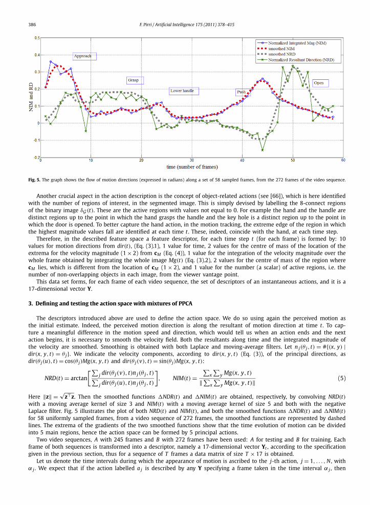
Fig. 5. The graph shows the flow of motion directions (expressed in radians) along a set of 58 sampled frames, from the 272 frames of the video sequence.
Another crucial aspect in the action description is the concept of object-related actions (see [66]), which is here identifiedwith the number of regions of interest, in the segmented image. This is simply devised by labelling the 8-connect regionsof the binary image δG (t). These are the active regions with values not equal to 0. For example the hand and the handle aredistinct regions up to the point in which the hand grasps the handle and the key hole is a distinct region up to the point inwhich the door is opened. To better capture the hand action, in the motion tracking, the extreme edge of the region in whichthe highest magnitude values fall are identified at each time t . These, indeed, coincide with the hand, at each time step.
Therefore, in the described feature space a feature descriptor, for each time step t (for each frame) is formed by: 10values for motion directions from dir(t), (Eq. (3).1), 1 value for time, 2 values for the centre of mass of the location of theextrema for the velocity magnitude (1× 2) from cM (Eq. (4)), 1 value for the integration of the velocity magnitude over thewhole frame obtained by integrating the whole image Mg(t) (Eq. (3).2), 2 values for the centre of mass of the region wherecM lies, which is different from the location of cM (1× 2), and 1 value for the number (a scalar) of active regions, i.e. thenumber of non-overlapping objects in each image, from the viewer vantage point.
This data set forms, for each frame of each video sequence, the set of descriptors of an instantaneous actions, and it is a17-dimensional vector Y.
3. Defining and testing the action space with mixtures of PPCA
The descriptors introduced above are used to define the action space. We do so using again the perceived motion asthe initial estimate. Indeed, the perceived motion direction is along the resultant of motion direction at time t . To cap-ture a meaningful difference in the motion speed and direction, which would tell us when an action ends and the nextaction begins, it is necessary to smooth the velocity field. Both the resultants along time and the integrated magnitude ofthe velocity are smoothed. Smoothing is obtained with both Laplace and moving-average filters. Let n j(θ j, t) = #{(x, y) |dir(x, y, t) = θ j}. We indicate the velocity components, according to dir(x, y, t) (Eq. (3)), of the principal directions, asdir(θ j(u), t)= cos(θ j)Mg(x, y, t) and dir(θ j(v), t)= sin(θ j)Mg(x, y, t):
NRD(t)= arctan
[∑j dir(θ j(v), t)n j(θ j, t)∑j dir(θ j(u), t)n j(θ j, t)
], NIM(t)=
∑x
∑y Mg(x, y, t)
‖∑x
∑y Mg(x, y, t)‖ (5)
Here ‖z‖ = √zz. Then the smoothed functions �NDR(t) and �NIM(t) are obtained, respectively, by convolving NRD(t)
with a moving average kernel of size 3 and NIM(t) with a moving average kernel of size 5 and both with the negativeLaplace filter. Fig. 5 illustrates the plot of both NRD(t) and NIM(t), and both the smoothed functions �NDR(t) and �NIM(t)for 58 uniformly sampled frames, from a video sequence of 272 frames, the smoothed functions are represented by dashedlines. The extrema of the gradients of the two smoothed functions show that the time evolution of motion can be dividedinto 5 main regions, hence the action space can be formed by 5 principal actions.
Two video sequences, A with 245 frames and B with 272 frames have been used: A for testing and B for training. Eachframe of both sequences is transformed into a descriptor, namely a 17-dimensional vector Yt , according to the specificationgiven in the previous section, thus for a sequence of T frames a data matrix of size T × 17 is obtained.
Let us denote the time intervals during which the appearance of motion is ascribed to the j-th action, j = 1, . . . , N , withα j . We expect that if the action labelled a j is described by any Y specifying a frame taken in the time interval α j , then
F. Pirri / Artificial Intelligence 175 (2011) 378–415 387
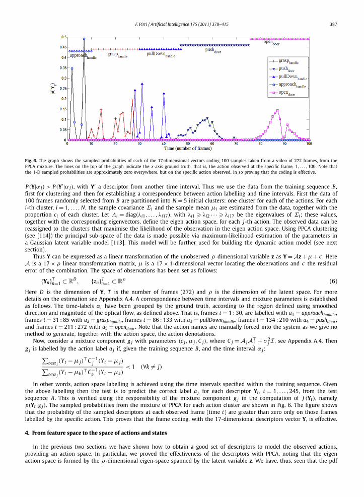
Fig. 6. The graph shows the sampled probabilities of each of the 17-dimensional vectors coding 100 samples taken from a video of 272 frames, from thePPCA mixture. The lines on the top of the graph indicate the x-axis ground truth, that is, the action observed at the specific frame, 1, . . . ,100. Note thatthe 1-D sampled probabilities are approximately zero everywhere, but on the specific action observed, in so proving that the coding is effective.
P (Y|α j) > P (Y′|α j), with Y′ a descriptor from another time interval. Thus we use the data from the training sequence B ,first for clustering and then for establishing a correspondence between action labelling and time intervals. First the data of100 frames randomly selected from B are partitioned into N = 5 initial clusters: one cluster for each of the actions. For eachi-th cluster, i = 1, . . . , N , the sample covariance Σi and the sample mean μi are estimated from the data, together with theproportion ci of each cluster. Let Λi = diag(λi1, . . . , λi17), with λi1 � λi2 · · · � λi17 be the eigenvalues of Σi ; these values,together with the corresponding eigenvectors, define the eigen action space, for each j-th action. The observed data can bereassigned to the clusters that maximise the likelihood of the observation in the eigen action space. Using PPCA clustering(see [114]) the principal sub-space of the data is made possible via maximum-likelihood estimation of the parameters ina Gaussian latent variable model [113]. This model will be further used for building the dynamic action model (see nextsection).
Thus Y can be expressed as a linear transformation of the unobserved ρ-dimensional variable z as Y= Az+μ+ ε . HereA is a 17× ρ linear transformation matrix, μ is a 17× 1-dimensional vector locating the observations and ε the residualerror of the combination. The space of observations has been set as follows:
{Yn}Tn=1 ⊂R
D , {zn}Tn=1 ⊂R
ρ (6)
Here D is the dimension of Y, T is the number of frames (272) and ρ is the dimension of the latent space. For moredetails on the estimation see Appendix A.4. A correspondence between time intervals and mixture parameters is establishedas follows. The time-labels αi have been grouped by the ground truth, according to the region defined using smootheddirection and magnitude of the optical flow, as defined above. That is, frames t = 1 : 30, are labelled with a1 = approachhandle ,frames t = 31 : 85 with a2 = grasphandle , frames t = 86 : 133 with a3 = pullDownhandle , frames t = 134 : 210 with a4 = pushdoor ,and frames t = 211 : 272 with a5 = opendoor . Note that the action names are manually forced into the system as we give nomethod to generate, together with the action space, the action denotations.
Now, consider a mixture component g j with parameters (c j,μ j, C j), where C j = A j Aj + σ 2
j I , see Appendix A.4. Theng j is labelled by the action label a j if, given the training sequence B , and the time interval α j :∑
t∈α j(Yt −μ j)
C−1j (Yt −μ j)∑
t∈α j(Yt −μk)
C−1k (Yt −μk)
< 1 (∀k = j)
In other words, action space labelling is achieved using the time intervals specified within the training sequence. Giventhe above labelling then the test is to predict the correct label a j for each descriptor Yt , t = 1, . . . ,245, from the testsequence A. This is verified using the responsibility of the mixture component g j in the computation of f (Yt), namelyp(Yt |g j). The sampled probabilities from the mixture of PPCA for each action cluster are shown in Fig. 6. The figure showsthat the probability of the sampled descriptors at each observed frame (time t) are greater than zero only on those frameslabelled by the specific action. This proves that the frame coding, with the 17-dimensional descriptors vector Y, is effective.
4. From feature space to the space of actions and states
In the previous two sections we have shown how to obtain a good set of descriptors to model the observed actions,providing an action space. In particular, we proved the effectiveness of the descriptors with PPCA, noting that the eigenaction space is formed by the ρ-dimensional eigen-space spanned by the latent variable z. We have, thus, seen that the pdf
388 F. Pirri / Artificial Intelligence 175 (2011) 378–415
of each descriptor is a Gaussian with variance maximised in the eigen-space, and that its likelihood is thus maximal whenthe descriptor comes from the space of the action it represents.
However, the PPCA does not capture the dynamic of actions or their time–space relation. Given an observation sequenceY1, . . . ,YT , where now the observation is the description of the visual process, we want to find out if each observation Yt canbe explained by a condition and effect on the action it predicts. These conditions and effects are the unobservable states.We made the hypothesis that the appearance of an action starting and ending depends on scale, motion evolution, lightchange and space location of afforded objects (the definition of Yt ). Since the descriptors do not capture the interactionbetween an action ending and another action beginning, these are in fact unobserved, in terms of the visual features ofeach frame. Thus a state is unobserved and records the executability of an action in the following sense: the transition froma state to another state specifies under what conditions an action starts and what conditions are rated at the end of theaction. Thus, according to the results of the previous section, there are 5 states and 5 actions.
A continuous observation HMM is a suitable dynamic model for actions and states, requiring estimation of a transitionmatrix P between states, a distribution π on the initial states, and the mixture parameters Ψ modelling the local evolutionof actions (that is, with respect to the observed sequences) and their interactions. HMM are useful when a chain cannot beobserved directly but only through another process; that is, of the two processes {Xi, Yi}i�0, only {Yi}i�0 is observed. Moreprecisely:
Definition 1. Consider the bivariate discrete time process, with continuous observations, {Yi, Xi}i�0, where {Xi}i�0, is a chainand {Yi}i�0, is a set of continuous random variables. Let {Xi}i�0 satisfy the independence properties of a Markov chain (seeAppendix A.4) and let Yi be conditionally independent of all other Y j , i = j, and any other Xk , k = j, given a specifiedassignment to the variable Xk , it depends on. The model M for the bivariate process is identified by the parameters vector(π,P,Ψ,γ ) where:
1. (π,P) is a Markov chain.2. Ψ is the family of parameters of the mixtures of normal densities, specifying the state emissions. Given M mixture
components, N states, the probability of the observation Y at state j is, according to a mixture PPCA-HMM:
b j(Y)=M∑
k=1
c jk N(Y|μ jk, A jk A
jk + σ 2jk I
), j = 1, . . . , N (7)
Here c jk is the probability of the k-th mixture at state j, μ jk is the mean of the k-th normal density of the mixture atstate j, and A jk , σ 2
jk are the variances of observed and hidden parameters of the k-th normal density at state j, theseare specified for the mixture of PPCA in Eqs. (44), (45) and (46) in Appendix A.4.1.
3. γ is the family of parameters of the mixtures of PPCA densities, used to determine and test the action space (seeSection 3).
The re-estimation procedure of the model parameters (π,Ψ,P) for HMMs with Gaussian observation densities is de-scribed in [98,71,59], based on Expectation Maximisation (EM), this does not concern the action space. The adaptation ofthe re-estimation procedure for mixture of PPCA to the HMM-PPCA is described in Appendix A.4.
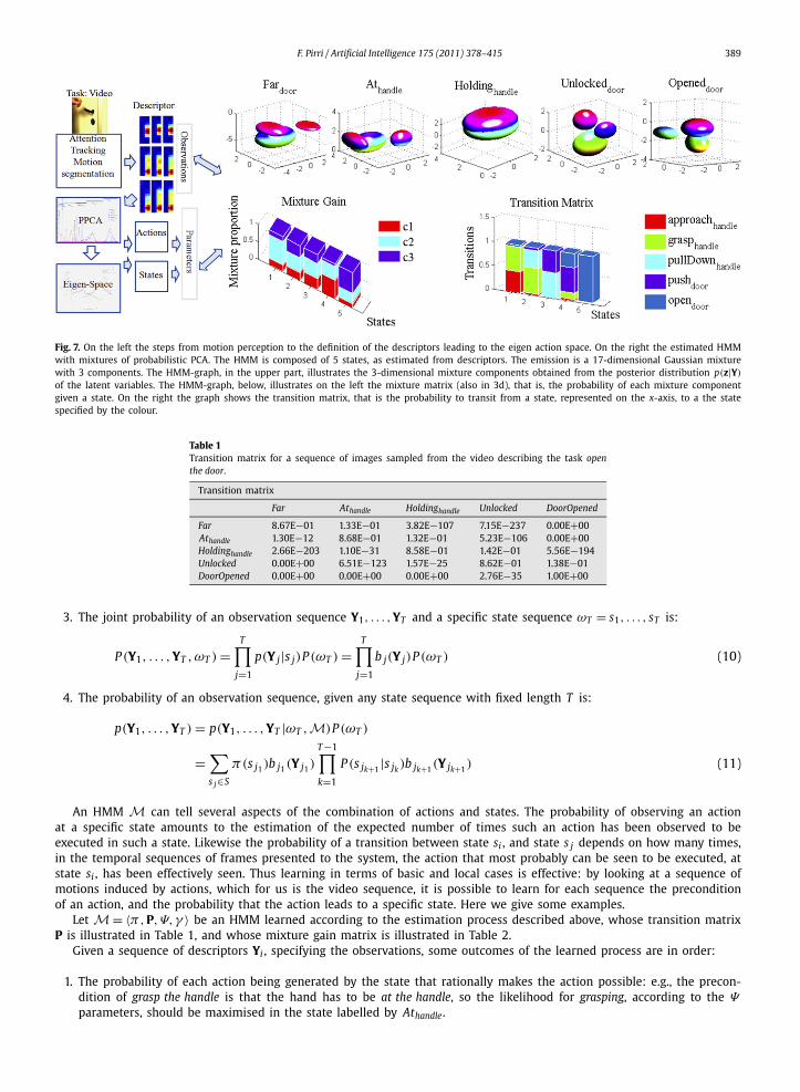
An example of the HMM for the open-the-door problem described in the paper, with the 17-dimensional observations,with 5 states, and with 5 mixtures of PPCA, each formed by three components, is illustrated in Fig. 7: above, the mixturesrepresented as 3D ellipsoids and, below, the figures illustrate the mixture matrix on the left, which in this case is ofdimension 5 × 3, each element of which is the mixture gain c jk , indicating the probability that in state j the mixturecomponent k is chosen, and on the right the transition matrix P. The states of the HMM are labelled with terms specifyingthe preconditions/effect of each action.
We recall useful facts about estimation of sequences for HMMs with continuous observation densities, given a model M,with states S:
1. The probability of a state sequence ωT = s j1 , . . . , s jT is:
P (ωT )=∑s j∈S
π(s j1)
T−1∏k=1
P (s jk+1 |s jk ) (8)
2. The probability of an observation sequence Y1, . . . ,YT , given a specific state sequence ωT = s1, . . . , sT is, given indepen-dence of observations:
p(Y1, . . . ,YT |ωT )=T∏
j=1
p(Y j|s j)=T∏
j=1
b j(Y j) (9)
F. Pirri / Artificial Intelligence 175 (2011) 378–415 389
Fig. 7. On the left the steps from motion perception to the definition of the descriptors leading to the eigen action space. On the right the estimated HMMwith mixtures of probabilistic PCA. The HMM is composed of 5 states, as estimated from descriptors. The emission is a 17-dimensional Gaussian mixturewith 3 components. The HMM-graph, in the upper part, illustrates the 3-dimensional mixture components obtained from the posterior distribution p(z|Y)
of the latent variables. The HMM-graph, below, illustrates on the left the mixture matrix (also in 3d), that is, the probability of each mixture componentgiven a state. On the right the graph shows the transition matrix, that is the probability to transit from a state, represented on the x-axis, to a the statespecified by the colour.
Table 1Transition matrix for a sequence of images sampled from the video describing the task openthe door.
Transition matrix
Far Athandle Holdinghandle Unlocked DoorOpened
Far 8.67E−01 1.33E−01 3.82E−107 7.15E−237 0.00E+00Athandle 1.30E−12 8.68E−01 1.32E−01 5.23E−106 0.00E+00Holdinghandle 2.66E−203 1.10E−31 8.58E−01 1.42E−01 5.56E−194Unlocked 0.00E+00 6.51E−123 1.57E−25 8.62E−01 1.38E−01DoorOpened 0.00E+00 0.00E+00 0.00E+00 2.76E−35 1.00E+00
3. The joint probability of an observation sequence Y1, . . . ,YT and a specific state sequence ωT = s1, . . . , sT is:
P (Y1, . . . ,YT ,ωT )=T∏
j=1
p(Y j|s j)P (ωT )=T∏
j=1
b j(Y j)P (ωT ) (10)
4. The probability of an observation sequence, given any state sequence with fixed length T is:
p(Y1, . . . ,YT )= p(Y1, . . . ,YT |ωT , M)P (ωT )
=∑s j∈S
π(s j1)b j1(Y j1)
T−1∏k=1
P (s jk+1 |s jk )b jk+1(Y jk+1) (11)
An HMM M can tell several aspects of the combination of actions and states. The probability of observing an actionat a specific state amounts to the estimation of the expected number of times such an action has been observed to beexecuted in such a state. Likewise the probability of a transition between state si , and state s j depends on how many times,in the temporal sequences of frames presented to the system, the action that most probably can be seen to be executed, atstate si , has been effectively seen. Thus learning in terms of basic and local cases is effective: by looking at a sequence ofmotions induced by actions, which for us is the video sequence, it is possible to learn for each sequence the preconditionof an action, and the probability that the action leads to a specific state. Here we give some examples.
Let M = 〈π,P,Ψ,γ 〉 be an HMM learned according to the estimation process described above, whose transition matrixP is illustrated in Table 1, and whose mixture gain matrix is illustrated in Table 2.
Given a sequence of descriptors Yi , specifying the observations, some outcomes of the learned process are in order:
1. The probability of each action being generated by the state that rationally makes the action possible: e.g., the precon-dition of grasp the handle is that the hand has to be at the handle, so the likelihood for grasping, according to the Ψ
parameters, should be maximised in the state labelled by Athandle .
390 F. Pirri / Artificial Intelligence 175 (2011) 378–415
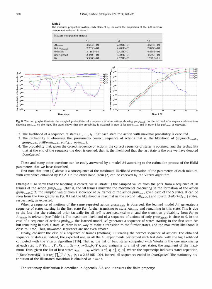
Table 2The mixtures proportion matrix, each element ci j indicates the proportion of the j-th mixturecomponent activated in state i.
Mixture components matrix
c1i c2i c3i
Athandle 3.653E−01 2.693E−01 3.654E−01Holdinghandle 2.763E−01 4.408E−01 2.829E−01Unlocked 3.118E−01 2.425E−01 4.458E−01DoorOpened 2.440E−01 3.005E−01 4.555E−01Far 5.536E−01 2.677E−01 1.787E−01
Fig. 8. The two graphs illustrate the sampled probabilities of a sequence of observations showing grasphandle on the left and of a sequence observationsshowing pushdoor on the right. The graph shows that the probability is maximal in state 2 for grasphandle and in state 4 for pushdoor , as expected.
2. The likelihood of a sequence of states s1, . . . , sT , if at each state the action with maximal probability is executed.3. The probability of observing the, presumably correct, sequence of actions that is, the likelihood of (approachhandle,
grasphandle,pullDownhandle,pushdoor,opendoor).4. The probability that, given the correct sequence of actions, the correct sequence of states is obtained, and the probability
that at the end of the sequence the door is opened, that is, the likelihood that the last state is the one we have denotedDoorOpened.
These and many other questions can be easily answered by a model M according to the estimation process of the HMMparameters that we have described.
First note that item (1) above is a consequence of the maximum-likelihood estimation of the parameters of each mixture,with covariance obtained by PPCA. On the other hand, item (2) can be checked by the Viterbi algorithm.
Example 1. To show that the labelling is correct, we illustrate 1) the sampled values from the pdfs, from a sequence of 58frames of the action grasphandle (that is, the 58 frames illustrate the movements concurring in the formation of the actiongrasphandle); 2) the sampled values from a sequence of 32 frames of the action pushdoor , given each of the 5 states. It can beseen from the two graphs in Fig. 8 that the likelihood is maximal in the second (Athandle) and fourth (Unlockeddoor) states,respectively, as expected.
When a sequence of motions of the same repeated action grasphandle is observed, the learned model M generates asequence of states starting in the first state Far, further transiting to state Athandle and remaining in this state. This is dueto the fact that the estimated prior (actually for all M) is arg maxx π(x) = s1 and the transition probability from Far toAthandle is relevant (see Table 1). The maximum likelihood of a sequence of actions of only grasphandle is close to 0. In thecase of a sequence of actions pushdoor , the learned model M generates a sequence of states starting in the first state Farbut remaining in such a state, as there is no way to make a transition to the further states, and the maximum likelihood isclose to 0 too. Thus, unwanted sequences are not even created.
Finally, consider the case of a sequence of frames (motions) illustrating the correct sequence of actions. The obtainedsequence of states is, indeed, the expected one, in all the 10 experiments performed with test data, with the log likelihoodcomputed with the Viterbi algorithm [116]. That is, the list of best states computed with Viterbi is the one maximisingat each step t , P (Y1, . . . ,Yt , X1, . . . , Xt = x j |M)pijb j(Yt), and assigning to a list of best states, the argument of the maxi-mum. Thus, given the list of best states x15, . . . , x0 which is s2
1, s22, s4
3, s34, s4
5, where the superscript indicates states repetition,
P (DoorOpened|X) is π(x0)∏T−1
t=1 P (xt+1|xt)= 2.6516E−004. Indeed, all sequences ended in DoorOpened. The stationary dis-tribution of the illustrated transition is obtained at T = 87.
The stationary distribution is described in Appendix A.2, and it ensures the finite property:

F. Pirri / Artificial Intelligence 175 (2011) 378–415 391
Definition 2. Let M be an HMM such that P is either irreducible or it satisfies the conditions of Lemma 5 (see Ap-pendix A.3), then we say that M has the finite property.
At last, given our example of learning the task opening the door, we have seen that a specific HMM model M is obtainedfrom each sequence and each starting parameters set. Each model, as long as it is trained according to the correct observedsequence, starting with the hand approaching the handle, and ending with the door opened, will lead to the expected re-sults, with slight variations. Thus we have a whole class of models that are tuned to the task, i.e. to the specific observationssequence. For the parameters estimation see Appendices A.3 and A.4.
5. First-order parametric models
In this section we start to take care of the induction step. We have settled the basic step by learning the parametersof the probability space of actions and the hidden values, specifying the states. Hidden state transitions have been learned,likewise the likelihood of observations given the states. These amount to a set of parameters (π,P,Ψ,γ ) for each initialdata set, that is, for each finite set of sequences, via their induced transformations and their initial parameters, used totrain the model, as described in previous sections. There is, thus, an infinite number of possible models, one for each setof initial parameters, though learning a task requires few observations. Continuing with the open the door example we lookfor a generalisation step transforming the parameter space, learned from a small number of sequences, into general rulesof behaviours. In the next subsections we show that the learned parameters can be used to extend the simple signature ofaction terms to a new signature encoding predicates, functions and terms. We show that a language can be obtained, sothat there is a correspondence between both formulae and field terms, in a first-order probability structure, and the randomvariables in the HMM.
5.1. Probability structures
Usually we assume that real world events are described by random variables behaving according to some unknowndistribution that has to be estimated from the observed cases and, possibly, some prior belief about the distribution. Inother words we see the random variable in practice and we want to determine its distribution. In most of the studies onprobabilistic logic this problem is not faced, and the axiomatisation is pushed forward to assess properties of probabilisticinference. For example, Keisler in [61] shows that in the first-order probabilistic logic with quantifiers it is possible to assertthat two random variables X1 and X2 are independent. Indeed McCarthy in [74] argues that “The information necessaryto assign numerical probabilities is not ordinarily available. Therefore a formalism that required numerical probabilitieswould be epistemologically inadequate”,2 exactly because of the lack of methods on how to feed parameter learning intoformalisms for reasoning.
Since the early studies on first-order probability by Gaifman [40], Krauss and Scott [110], Keisler [62,61] and Hoover [52],a wealth of research has been dedicated to the integration of logic and probability. Nowadays the seminal contributions forcomputational purposes have been the works of Abadi, Bacchus, Fagin and Halpern in [36,7,6,1,49,38,48], introducing a first-order probabilistic logic with both first-order quantifiers and real valued formulae. More recently several streams of researchon logic and probability integration have appeared concerning probabilistic logic programs, Poole [90], likewise [24,99,83]connected learning with stochastic logic programs. Koller and colleagues [64] and [42] introduced probability relationalmodels, while Domingo and colleagues introduced Markov logics [4] (see also a general overview in [34]). Milch and Russell[81] introduced first-order models with unknown objects. These are examples of a wealth of approaches that we cannotenumerate here. The clear direction has become that of adapting first-order probability languages to the statistical needs ofcomputational learning or, the other way round, to lift statistical learning to first-order logic. Here our aim is different. Herewe aim at embedding the distribution learned into a first-order probability model. More precisely, we are not interestedto learn within the probability logic (as, for example, in PRISM [106]), but to use the parameters to feed the logic as aninductive step towards the language of thought. The task is to build a first-order probability model that accepts formulaeenunciating all the events an HMM describes with random variables, such as the probability of an observed action, given asequence of states, or the probability of a state, given a sequence of actions, or comparing probabilities between events. Thisseems to be a natural approach that, on one side preserves the declarative-relational structure of logic and, on the otherside, prepares the ground for embedding learning, viewed as an early computational process, into reasoning.
For our example we are thus concerned only with the model construction and not with the proof theory and axioma-tisation. For this aspects we mainly refer to the seminal works of Gaifman, Halpern and Bacchus [41,7,48]. In fact, themain results of Bacchus and Halpern work is the specification of a proof theory, which is complete only under alternativerestrictive conditions. That is, the logic is complete if either
(a) The domain is assumed to be countable and the measure functions are field-valued (non-Archimedean) and the gener-ated algebra of events is finitely additive [7,6].
2 Bacchus in [6] also refers to this sentence.
392 F. Pirri / Artificial Intelligence 175 (2011) 378–415
(b) The collection of axioms includes the proper axiomatisation for reals, the language excludes random variables and thedomain is bounded in size [49].
(c) The language includes the random variables, the domain is bounded in size, but the Archimedean property is given up[7,6].
In fact, while Halpern chooses to axiomatise the reals, using the theory of the real closed field, Bacchus admits measurefunctions ranging over non-Archimedean ordered fields, in the sense that his logic admits infinitesimals.3,4
Let us consider the first-order language Lp with probabilities on the domain as presented in [7,6]. The language Lpis formed by all formulae and sentences of first-order logic plus the field terms [α(�x)]�x , where α(�x) is a first-orderformula with free variables �x and [·] is the probability term constructor. A statistical probability structure for Lp isM = 〈A,F, (Πn,μn)n<ω〉, where A = (D, I) is a classical first-order structure, F is the totally ordered field of numbersand, for each n, Πn is a field of subsets of Dn , and μn is a probability function on Πn whose range is F. The languageL1(Φ) presented in [49] is like Lp, but the field terms range over the reals, hence F is the real closed field, having thesame first-order properties as the field of real numbers, and field terms are denoted by w�x(α). A structure for L1(Φ) isM= (D,π, X ,μ) where D is the domain, π is an interpretation, X is a σ -algebra over D and μ is a probability functionon X , which is essentially a counting measure. In this section we substantially refer to the work of [7,49].
Let us start with the learned HMM M = 〈S, H, (π,P,Ψ,γ )〉 with S the finite set of states, H the set of observations,of fixed dimension, with respect to the model. For example for the task open the door the observations are 17-dimensionalvectors and the parameters Ψ have been tuned for this 17-dimensional space, as shown in Section 4. However here weassume that variables are 1-dimensional to simplify the notation. Finally, the whole set of parameters is formed by atransition matrix P, the mixture parameters Ψ , the initial distribution parameter π , selecting an initial state from S , andthe action space parameters γ . We define the canonical (i.e. parametric, because the parameters π,P and Ψ are given)probability structure M for M, as follows.
5.1.1. The signatureThe signature �M of the language includes terms of sort state to denote the set S of states, terms of sort observations to
denote the set H of observations. Note that states and observations induce random variables (see Appendix A.1), and whilethe domain of states is finite and of dimension n, the domain of observations is R. To these sorts we add the terms ofsort sequence of states w : SN → W , endowed with the constructor ◦ and W the domain of countable sequences of states.Finally, the signature includes terms of sort natural numbers, for indexing.
Notation. Indices are denoted by natural numbers n, m or t . When we refer to states as elements of the domain we denotethem by s, when they are referred to by variables are denoted by x, possibly indexed. Sequences of states are denoted byw , we use w both to denote a variable of sort sequence of states and the term (xn ◦ · · · ◦ x0). When we refer to observationsin the domain we denote them by h, when they are referred to by variables of sort observations are denoted by y.
The language includes monadic predicate symbols Ri , one for each state si ∈ S , taking as argument a sequence in W ,binary predicates A j , one for each observation (of an action), taking as argument an observation h ∈ H and a state si ∈ S ,and binary predicate symbols O ji , that can be defined as the conjunction of Ri and A j and take as arguments an observationand a sequence of states. Finally the language includes the relation �, abbreviating <∨=, between sequences.
To the above sorts we add the real line R, which we assume represented as in Matlab, and the Borel σ -field on the realline B(R). Sorts taking values in the reals include, beside observations, field terms, the mixture gain matrix c : S × [0,1]→[0,1], the normal distribution N (μik, Aik A
ik + σ 2ik I), with μik , Aik and σik , elements of Ψ , similarly for γ , and random
variables Xi, Yi , i = 1,2, . . . . Sorts mapping to the reals include the initial distribution π on states, with π : S → [0,1], thetransition matrix P : S × S →[0,1].
5.1.2. Formulae of the languageFirst-order formulae are defined as usual. Field terms and formulae including field terms are defined as follows, where
classical laws for connectives and quantifiers are implicitly assumed.
Definition 3. A field-base α, for a field term, is defined inductively as follows:
1. If y, x and w are, respectively, terms of sort observation, of sort state and sequence of states, then A j(y, x), Ri(w) andO i(y, w) are all field-bases.
2. If w, w ′ are terms of sort W then w = w , w < w ′ and w > w ′ are field-bases.3. If α1 and α2 are field-bases, then ¬αi , α1 ∧ α2 are field-bases.
3 The Archimedean property says that any set of reals have a positive upper bound, that is, if x ∈R and x > 0 there is an n ∈N such that xn > 1.4 See Hammond [50] for a discussion on the advantages of non-Archimedean ordered field in game theory.
F. Pirri / Artificial Intelligence 175 (2011) 378–415 393
4. If α(x) is a field-base, with x a free variable (possibly among others) varying on sort state, observation and sequence,then ∀x.α(x) is a field-base.
Definition 4. A field term constructor is [·] : α �→ [0,1] where α is a field-base formula. A field term is defined as follows:
1. If xi, x j are terms of sort states, P(xi, x j) is a field term, likewise π(xi); μi j, σi j, i = 1, . . . , n, j = 1, . . . ,k, are field terms.Also Xi(x), i = 1,2, . . . , T , are field terms. If y is a term of sort observation then N (y|μi j, σi j), Y j(y), i, j � 1, are fieldterms. In particular these are the atomic field terms.
2. If α1 and α2 are field-bases with free variables var(αi) = V , i = 1,2, then: if V is of sort state or sequence of statesthen [αi(V )] is a discrete probability term, if V ranges over observations then [αi(V )] is a continuous probability term,both are defined field terms.
3. [α1(V )] · [α2(V ′)], [α1(V )] + [α2(V ′)], [α1(V )]/[α2(V ′)], 1− [αi(V )] are field terms.4. [αi(V )|α j(V ′)] is a field term.
Definition 5. If f (z) is a field term, with z a variable of sort either state, observation, or sequence of states, and p ∈ [0,1]then formulae can be formed using field terms as follows:
1. f (z)= p, f (z) < p and f (z) > p are formulae, we shall abbreviate <∨= with � and >∨= with �.2. If f (z) and g(z′) are field terms, f (z) � g(z′) and f (z) � g(z′) are formulae.3. If φ(z) and ψ(z′) are formulae including field terms, then φ(z)∧ψ(z′) and ¬φ(z) are formulae.4. If ϕ(z) is a formula, in which z is a variable occurring free (possibly among others) and such that z can be of sort either
state or observation ∃z.ϕ(z) is a formula.
To these terms the measure terms ηX , with X an index to be specified, and their products are added, as detailed in thenext section.
5.1.3. Domain and probability spaceThe domain D is partitioned into the following sets: a finite space S of states, the space H of observations taking value
in R, and the space W = S × S × · · · = S T of sequences of states denoted by ω, T � N. Let �0 be the σ -field formed by allsubsets of S and �=�0×�0×· · · =�T
0 . Given the distribution π , the initial distribution on S , and the transition matrix P,as specified by the HMM parameters, we consider discrete random variables X1, X2, . . . , with Markov property, all definedon the same probability space, mapping S T into S , such that Xt(ω)= s jt . A probability measure ηs :� �→ R, satisfying theMarkov property, is
ηs({
X1(ω)= s j1 , . . . , Xt(ω)= s jt
}j=1,...,|S|
)= ∑s j1 ,...,s jt
π(s j1)
t−1∏i=1
P(s ji+1 |s ji ) (12)
ηs is a countably additive measure (see [15]). Since the sum of the initial density π is 1 and P is a stochastic matrix, then(W ,�,ηs) is a probability space.
H is the set of observations with domain R. Let Θ be the smallest σ -field generated by the Borel sets on R. The elementsof Θ are Borel sets denoted B . Let (H,Θ) be a measure space with measure η. On the space (H,Θ,η) we consider togetherwith the elements of H random variables Y j , as identities. The probability measure on this measure space induced by therandom variables is defined as
η(B)=∫B
f (y)dy (B ∈Θ)
f (y)=M∑
k=1
ck N(
y|μk, Ak Ak + σ 2
k I) (
μk, Ak,σ2k ∈ γ
)(13)
Here f (y) is the density specified by the mixture of PPCA, as defined in Section 3, see also Appendix A.4, Eq. (40), andN is the normal density. When the random events are specified with respect to a fixed state s ∈ S then η is extended to ηIon the product space H × W with σ -field Θ ×� formed by the measurable rectangles B × Q , B ∈Θ and Q ∈�. That is,if E ∈Θ ×� then Q = {ω | (h,ω) ∈ E} lies in � and B = {h | (h,ω) ∈ E} lies in Θ . On the measure space (H × W ,Θ ×�)
the density of the random variables is bi , taking two arguments y and, implicitly, a state si .
ηI (B)=∫B
bi(y)dy (B ∈Θ)
bi(y)=M∑
cik N(
y|μik, Aik Aik,σ
2ik I
) (μik, Aik,σ
2ik ∈ Ψ, i = 1, . . . , N
)(14)
k=1
394 F. Pirri / Artificial Intelligence 175 (2011) 378–415
Here N is the number of states, M the number of mixture components. When B is R then the bi integrates to 1 and whenB = ∅ then ηI (∅)= 0. Indeed, (H ×W ,Θ ×�,ηI ) is a probability space. We can thus introduce the structure M as follows:
Definition 6. A probability structure of first-order with parameters fixed by an HMM model M = (S, H, (π,P,Ψ,γ ))
is M = (D,Ψ,Φ,I ). Here D is the domain, D = (S, W , H), Ψ is the set of parameters defined by the HMM M =(S, H, (π,P,Ψ,γ )), Φ is the probability space defined as
Φ = ((W,�,ηs), (H,Θ), (H × S,Θ ×�,ηI )
). (15)
Here �,Θ ×� are the sigma-fields defined above and ηs, ηI are the associated probability measures.Finally I is the interpretation for the signature, defined as follows.
1. Interpretation of predicates Ri, A j, O ji , with i, j = 1, . . . , N , N the number of states and the number of observationactions:Let Xi : S T �→ S be a discrete random variable
Ri(·)I =⋃
t
{ω
∣∣ X1(ω)= arg maxs
π(s), Xt(ω)= si, t � i}
(i = 1, . . . , N) (16)
Let N be both the number of observation actions (hence the mixture components for observations independently ofstates) and the number of states, and M the number of mixture components for the observations at each state:Let z ∈R
A�j(·)I =
{h
∣∣∣∣ (h−μ j)2
σ 2j
� z
} (j = 1, . . . , N, μ j,σ j as in (13)
)(17)
Let z ∈R
A j(·, si)I =
{h
∣∣∣∣ (h−μik)2
σ 2ik
� z,h ∈ A�j(·)I ,k = 1, . . . , M
} (i, j = 1, . . . , N, μ jk,σ jk as in (14)
)O ji(·,·)I = {〈h, sit ◦ wt−1〉
∣∣ h ∈ A j(·, sit )I ∧ sit ◦ wt−1 ∈ Ri(·)I
}(i, j = 1, . . . , N) (18)
2. Interpretation of field terms. Let v be any assignment to the free variables:[Ri(wt)
](I ,v) = ηs({
v(
wt/(
X1(ω), . . . , Xt(ω))) ∣∣ ω ∈ RI , t � i
})=
∑v(wt/(X1(ω),...,Xt (ω)))
π(
X1(ω)= s j1
) t−1∏k=1
P(
Xk+1(ω)= s jk+1
∣∣ Xk(ω)= s jk
)(s jt = si) (19)
Let Y j : H �→ H , be the identity:[A j(y, si)
](I ,v) = ηI({
h∣∣ v
(y/Y j(h)
) ∈ A j(·, si)I , i = 1, . . . , N
})=
∫B
bi(h)dh (B ∈Θ) (20)
Finally:[O ji(·,·)
](I ,v) = [A j(·,·), Ri(·)
](I ,v)(21)
3. The field terms π,P and N are interpreted as themselves.
In particular I ensures that the distribution on the domain agree with the model M. This is established in the follow-ing:
Lemma 1. Given an HMM M = (S, H, (P,π,Ψ,γ )), with finite property (see Definition 2) there exists a probability structure M=(D,Ψ,Φ,I ), with domain D = (S, H, W ,R), probability space Φ generated from D, such that the atoms and terms are interpretedaccording to the M-parameters P,π and Ψ . Furthermore, according to the given interpretation I , for each field-based atom ϕ thereis a corresponding measurable set such that the field term for ϕ has the intended distribution.
Proof. See Appendix A.5, proof of Lemma 1. �We have, thus, shown that the interpretation of atoms fully determines the distribution of field terms and the structure
M for the HMM M. Before showing how to extend this to formulae we illustrate how the above lemma is implemented,with an example.
F. Pirri / Artificial Intelligence 175 (2011) 378–415 395
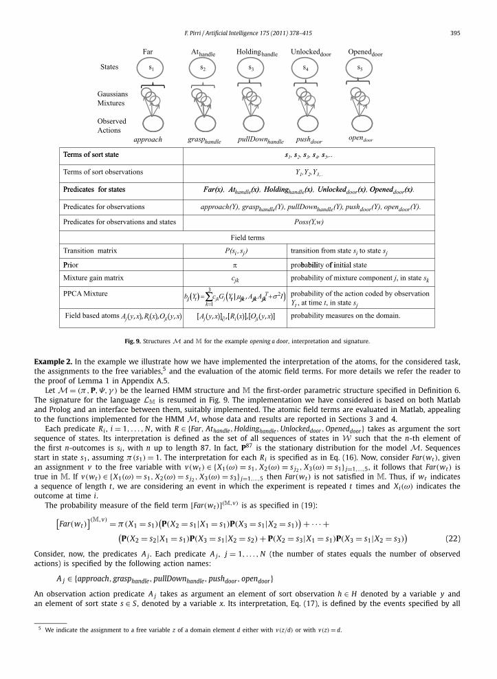
Fig. 9. Structures M and M for the example opening a door, interpretation and signature.
Example 2. In the example we illustrate how we have implemented the interpretation of the atoms, for the considered task,the assignments to the free variables,5 and the evaluation of the atomic field terms. For more details we refer the reader tothe proof of Lemma 1 in Appendix A.5.
Let M = (π,P,Ψ,γ ) be the learned HMM structure and M the first-order parametric structure specified in Definition 6.The signature for the language LM is resumed in Fig. 9. The implementation we have considered is based on both Matlaband Prolog and an interface between them, suitably implemented. The atomic field terms are evaluated in Matlab, appealingto the functions implemented for the HMM M, whose data and results are reported in Sections 3 and 4.
Each predicate Ri , i = 1, . . . , N , with R ∈ {Far, Athandle,Holdinghandle,Unlockeddoor,Openeddoor} takes as argument the sortsequence of states. Its interpretation is defined as the set of all sequences of states in W such that the n-th element ofthe first n-outcomes is si , with n up to length 87. In fact, P87 is the stationary distribution for the model M. Sequencesstart in state s1, assuming π(s1)= 1. The interpretation for each Ri is specified as in Eq. (16). Now, consider Far(wt), givenan assignment v to the free variable with v(wt) ∈ {X1(ω) = s1, X2(ω) = s j2 , X3(ω) = s1} j=1,...,5, it follows that Far(wt) istrue in M. If v(wt) ∈ {X1(ω)= s1, X2(ω)= s j2 , X3(ω)= s3} j=1,...,5 then Far(wt) is not satisfied in M. Thus, if wt indicatesa sequence of length t , we are considering an event in which the experiment is repeated t times and Xi(ω) indicates theoutcome at time i.
The probability measure of the field term [Far(wt)](M,v) is as specified in (19):[Far(wt)
](M,v) = π(X1 = s1)(P(X2 = s1|X1 = s1)P(X3 = s1|X2 = s1)
)+ · · · +(P(X2 = s2|X1 = s1)P(X3 = s1|X2 = s2)+ P(X2 = s3|X1 = s1)P(X3 = s1|X2 = s3)
)(22)
Consider, now, the predicates A j . Each predicate A j , j = 1, . . . , N (the number of states equals the number of observedactions) is specified by the following action names:
A j ∈ {approach,grasphandle,pullDownhandle,pushdoor,opendoor}An observation action predicate A j takes as argument an element of sort observation h ∈ H denoted by a variable y andan element of sort state s ∈ S , denoted by a variable x. Its interpretation, Eq. (17), is defined by the events specified by all
5 We indicate the assignment to a free variable z of a domain element d either with v(z/d) or with v(z)= d.
396 F. Pirri / Artificial Intelligence 175 (2011) 378–415
those descriptors, real valued variables, having Mahalanobis distance from the mean, with covariance σ 2, less than z, see(17) in Definition 6. The domain of each A j is generated as follows. Let U ∈ R be a set of values generated from normaldistributions with parameters fixed by the HMM M. Take from U the interval Bz delimited by those values y ∈ U havingMahalanobis distance, according to the parameters μiu, σiu ∈ Ψ , u = 1, . . . , M , less than a specified value z and assign it toAI
j , for each state si . To ensure that the values are centred on the mixture generated by AIj we first check the Mahalanobis
distance for the mixture specified in Eq. (13). In general we assume that z is decided according to the distances betweenmeans of different mixtures. For example, if μ ju and μku are the means of the component u of two mixtures at states sk
and s j , we require that (μ ju − μku)2 > σ 2juσ
2ku z. This would ensure that the interpretation of two observations does not
overlap at the modes. The probability measure ηI of the field term is the distribution function of the random variable Y j
over the domain of A j(·, si). Given an assignment v(y/h) ∈ AIj , the field term for A j(h, si) is evaluated by the density
bi(h), specified in ((14), see also (1)), that is, the derivative of the distribution function.Finally the denotation of the predicate O ji is intended as Poss ji(action, state), where the j indicates the observation
action and the i the state. The action is meant as the observation of the action via the descriptor. The interpretation of O jiis the conjunction of A j and Ri as defined in (18). Its field term is as defined in (21).
We can, now, extend the interpretation to formulae, as stated in the following theorem.
Theorem 1. Let M be a probability structure of first-order, with probability space Φ . Let Φ be extended to the probability space Φ�
with product measures ηns , ηn
I , (ηs × ηI )n, n � 1, and their space product. For each field-base formula ϕ there exists a measurable set,
whose distribution agree with the HMM.
Proof. See Appendix A.5, proof of Theorem 1. �We can now extend the relation |� to field terms and formulae mentioning field terms as follows, let P ∈ {ηs, ηI , ηs×ηI }
and let Γϕ be the measurable set of ϕ:
1. M, v |� [ϕ(�x)] � p iff P (Γϕ) � p
2. M, v |� ∀y.[ϕ(�x)] � p iff M, v(y/d) |� [
ϕ(�x)] � p for all d ∈ D of the right sort
4. M, v |� [ψ(�y)|ϕ(�x)] � p iff M, v |� [
ψ(�y)∧ ϕ(�x)] � p · [ϕ(x)]
(23)
Proposition 1. Let v and v ′ agree on all the assignments to the free variables then M, v |� ϕ iff M, v ′ |� ϕ .
Proof. See Appendix A.5, proof of Lemma 1. �Theorem 2. Let M = (S, H, (π,P,Ψ,γ )) then there exists a probability model M which is a structure for M, that is M and M agreeon the distribution on the domain.
Proof. See Appendix A.5, proof of Theorem 2. �Example 3. Let us continue with Example 2 as illustrated in Fig. 9. Let us assume that the interpretation for each atom hasbeen specified, as described in Example 2, according to Lemma 1. Let the binary predicate O ji be Poss ji , indicating thataction A j is observable (hence executable) at the final state sni of a n-length sequence. Let y and y′ be variables of sortobservation. Consider two sequences, one ending at the state labelled by Unlockeddoor and the other at Athandle . We wantto verify the likelihood of observing Pushdoor at the state Unlockeddoor and the likelihood of observing Pushdoor at the stateAthandle . We would express this fact as follows. Let wn−1 and wm−1 be two variables of sort sequence of states, referring tosequences of length m− 1 and n− 1, m= 3 and n= 4:[
Poss jk(y, xn ◦ wn−1)∧ Pushdoor(y, xn)∧ Unlockeddoor(xn ◦ wn−1)]
>[Poss jk
(y′, xm ◦ wm−1
)∧ Pushdoor(
y′, xm)∧ Athandle(xm ◦ wm−1)
](24)
Let us assume that the assignment to the free variables of sort sequence of states is as follows v(w3) ∈ {X1(ω) = s1,
X2(ω) = s2, X3(ω) = s3}, v(w2) ∈ {X1(ω′) = s1, X2(ω
′) = s2}, the terms of sort state are {v(x3/s3), v(x4/s4)}. Furthermoreassume that π(s1)= 1 and s1 is the first state, labelled by Far. Let h ∈ H with Y j(h) < z so that M |� Pushdoor(v(y/h), s2)
and M |� Pushdoor(v(y′/h), s4). We recall from the previous example that Pushdoor is a predicate verified in the parametricmodel M according to a Mahalanobis distance, and its atomic field term is evaluated by Eq. (7).
The pdfs b4(h) = bUnlockeddoor(h) and b2(h) = bAthandle(h) return the likelihood of the field terms [Pushdoor(h, s2)]δ and
[Pushdoor(h, s4)]δ .

F. Pirri / Artificial Intelligence 175 (2011) 378–415 397
In our implemented model, an observation is a 17-dimensional vector projected in 3D space (in this section we have,actually, further reduced the space to 1D stochastic variables). For this example we consider a real 17-D observation h =[0.05,0.48,0.47,0.47,0.55, . . .] . Hence, h is a 17-dimensional descriptor. The results for the projected h′ are:[
Pushdoor(h′, s4
)]M = [A4
(h′, s4
)]M = b4(h′)∼ 0.274
b1(h′)= b2
(h′)= b3
(h′)∼ 0.001,b5
(h′)∼ 0.002
[Unlockeddoor(x4 ◦ w3)
](M,v) = π(s1)
3∏i=1
P(si, si+1)∼ 0.006
[Athandle(x3 ◦ w2)
](M,v) = π(s1)
2∏i=1
P(si, si+1)∼ 0.192
[Poss44(y, x4 ◦ w3)
]M = b4(h′)π(s1)
3∏i=1
P(si, si+1)∼ 0.006 · 0.274= 0.0016 (25)
On the other hand, according to the assignment v:
[Poss42(y, x3 ◦ w2)
]M = b4(h)π(s1)
2∏i=1
P(si, si+1)∼ 0.001 · 0.192= 0.0002 (26)
Now, using the definition of O ji , the product rule and Bayes rule, we obtain that the right-hand side of (24) reduces to (26),hence to 0.0002.
Hence we gather that it is more likely that the action Pushdoor is executed at state Unlockeddoor , hence this is the mostlikely precondition for the observed action.
We can finally note that in the absence of a proof theory we can use Bayes’ rule only at the semantic level. Indeed,being our models parametric, hence canonical, a proof theory should be defined modulo parameters. In fact, given a classA of HMM models M1, M2, . . . of some observed event, there exist a class B of parametric probability models M1,M2,corresponding to A, according to Theorem 2. Now, given that both classes of structures model the same group of events,there must be formulae which are true of all these structures, independently of the variation of the parameters in eachstructure. Thus there might be a proof theory by lifting from the individual parametric models to a class of models. Theanalysis of this issue might be a next step of research.
6. The final induction step, concluding with the Situation Calculus
At this step our purpose is to complete the induction obtaining a simple theory of action. This last step is attained bymapping formulae true of the parametric probability model into formulae of the Situation Calculus. Learning has concludeda cycle and reasoning is the next step.
Recently several research efforts have been directed towards the problem of formalising learning steps in a theory ofactions, also for planning purposes.
For example, Amir and Chang in [3] have introduced a dynamic model of actions for solving the problem of simulta-neous learning and filtering from partial observations. The model constructs a system aware of its real states, with respectto the expected ones. The model, though has aims similar to the one we investigate here with the induction of structures,does not rely on a logic of first-order nor on probabilistic logic. On the other hand Pasula and colleagues, in [86] proposea framework for learning how to suitably represent new concepts and, thus, new rules for handling action effects in plan-ning domains. So, in particular, the objective of [86] is to learn a transition model. This is done in a language with Skolemconstants, in which first-order rules for actions are combined with probabilistic rules. As in our approach, a determinis-tic model of action is learned. However because in [86] learning does not construct from perception most of the effort isdone at the representation level, by adding noise. Therefore it is not clear how the combination of rules would allows forreasoning on the learned structure. The differences with our approach are both with respect to the methodology and theformalism. For example, we do not use operators and we model learning as an induction process based on different phases.On the other hand [86] assess the process via a set of rules that are embedded in a specific logical formalisms. Furthermore,in our approach learning is precisely from experience, the action model can be actually constructed online, as shown inthe examples, while in [86] approach online learning cannot really be addressed. In fact, learning rules are initialised bythe designer and not completely learned as in our method. Under a view similar to [86], indeed, logical learning has beenstudied in connection with logic in several works. For example in connection with logic programming in the language SLP(Stochastic Logic Programs) by Muggleton [118,83] and Cussens [24] and in PRISM (Programming in statistical logic) bySato and Kameya [107]. On the other hand BLOG [81] offers a representation paradigm, in which also HMM can be com-puted, but it cannot really embed parameters into first-order formulae although it offers interesting methods for samplinginterpretations. Learning the axioms of an action ontology should be regarded also as a discovery problem.
398 F. Pirri / Artificial Intelligence 175 (2011) 378–415
The Situation Calculus (SC) [74,100,101] is optimal for the purpose illustrated in the example, because it provides alanguage for a dynamic theory of action. Despite being deterministic, the SC models the first-order Markov property (actuallyit can model also the n-th order Markov property), it models time-homogeneity, and sequences of situations as histories ofactions on an infinite tree of choices [101].
We recall that the Situation Calculus, has been earlier formalised by McCarthy and Hayes in [74] and further extendedby Reiter, in order to give a simple solution to the frame problem, exploiting the definitional strength of first-order logicwithout appealing to the meta-language. The version of the Situation Calculus provided initially by Reiter in [100], thatMcCarthy calls the Toronto Situation Calculus, is a multi-sorted language powered by a second order induction axiom. Inparticular, the language is sorted on three distinguished disjoint domains (Act,Obj, Sit), i.e. Actions, Objects and Situationsand it comes with an axiomatisation for situations denoted by Σ , inducing the above mentioned tree, rooted in a specialsituation called S0. Situations are bounded to be countable by the second order axiom, specified in Σ , forcing the structuresof the language to be the intended ones.
Reiter, as a solution to the frame problem, has also introduced axiom schemata that are classified into three sets: Duna ,axioms specifying unique names for actions, Dap , axioms specifying preconditions for actions and Dss which are the succes-sor state axioms. These sort of axiom schemata can be suitably elaborated to obtain a full dynamic theory of actions whichis made meaningful by specifying the initial conditions of the state of affairs, that is, those axioms telling what is true inS0: the state of the world at the very instant in which actions clock in.
This initial description is called Ds0 . In [88], it is shown that if this initial theory, called, D S0 is consistent then theadditions of all the others axioms turns out to be a conservative extensions of D S0 ∪ Duna , given by induction.
A structure for LSC is defined as follows.
Definition 7. A structure M for the language LSC is defined by (D,ISC), where D is the domain partitioned in three sets,object X , actions A and situations S and ISC is the interpretation. The signature for the language LSC is formed by acountable set of variables for each sort, the constant S0 of sort situation, the function do : A ×S �→S , a countable set ofdistinguished predicates called fluents, taking as last argument a term of sort situation, and a special fluent symbol Poss. Tothis set any other predicate and function symbol can be added. The language LSC is formed by terms and formulae over thesignature, with usual connectives and quantifiers and it is extended to include first-order predicate variables of sort fluent.
The discovery problem here is to generate a very simple theory of actions for the task open the door, from the parametricmodel M. To this end we will build a structure M , of the specified language, in which D S0 , and the set of axioms Dss andDuna , are obtained from sentences with maximal probability values in M.
Let us specify the signature for LSC on the basis of the signature of LM as follows:
Definition 8 (Signature of LSC). The signature of LSC is defined via the signature of LM as follows:
1. Variables of sort object, action and situation are freely introduced.2. A new constant symbol S0 of sort situation is introduced.3. Constants of sort object are freely introduced as names for each element devised in the image sequence.6
4. For each predicate symbol A j in LM a zero-ary or unary function symbol of sort action is introduced; and for eachpredicate symbol Ri in LM an analogous unary or binary fluent symbol is introduced.
5. For the predicate symbols O ji in LM , with j = 1, . . . ,m, m the number of actions and i = 1, . . . , N , N the number ofstates, the binary predicate symbol Poss is introduced.
Given a structure M for LSC , by a suitable construction (see [88]) it is possible to ensure that M satisfies the founda-tional axioms Σ (see Appendix A.6, Definition 66). Let M be any structure for LSC satisfying the foundational axioms Σ ,for each introduced symbol A j , Ri and O ij , with v and v ′ assignments to the free variables, we define:
M , v |� A j(z) = Ai(z) (∀i j, i = j)
M , v |� Ri(z, S0) iff M, v ′ |� Ri(x) and v ′(x)= arg maxs∈S
π(s)
M , v |� Poss(
Ai(z), S0)
iff M, v ′ |� Ai(y, x) and v ′(y/h) ∈ arg maxh∈B
[Ai(y, x)
](M,v ′)δ
and v ′(x)= arg maxs∈S
π(s) (27)
Here v ′(y) and v ′(x) are, respectively, elements of the domain observation and states in M, π assigns a probability to each
initial state in both the structures HMM and M and [Ai(y, x)](M,v ′)δ , with the subscript δ, indicates the density bs(y) if
6 In this paper, these constants denoting objects would not be derived from learning since we have only identified the number of interesting elementsin each image, which are recorded in the descriptors, but not an interpretation for each of them. To adequately develop this issue it is either necessary toextend the visual step with tagging or to add a suitable sound analysis, also with tagging.
F. Pirri / Artificial Intelligence 175 (2011) 378–415 399
v(x/s), see Appendix A, proof of Lemma 1. We have thus defined both Duna and D S0 , and ensured that M is a model ofΣ, Duna and D S0 .
Now given a structure M for Σ ∪Duna ∪D S0 in LSC we can extend it using the first-order probability model M. We cando that because if we obtain, from M, a set of successor state axioms (ssa) and a set of action precondition axioms (apa),then these axioms can be added consistently to the above defined initial axiomatisation, as a consequence of the relativeconsistency theorem of [88]. The relative consistency theorem, in fact, says that starting with a structure which is a modelfor the set Σ ∪ Duna ∪ D S0 , this structure will also model the set Dap ∪ Dss defined in the language (see [88]).
Generating these axioms from M cannot be done just considering the first-order part of M. In fact, it is clear that relyingjust on the first-order information recorded in the structure M would be insufficient because the information in a structureis complete. On the other hand the probabilistic information is more conspicuous. The learned likelihood of the observed(executed) actions of a sequence and the likelihood of states, can tell us how to connect actions, transitions and states. Itturns out that only preconditions can be clearly established and the effect of actions can be reasoned about only by referringor projecting to the next state. This is what is presented below.
Going back to Eq. (27), arg maxv ′(y)∈B [Ai(y, sk)](M,v ′)δ indicates the value in B , a Borel set on R, at which the density of
Ai is maximal, according to the state sk and the assignment v ′ . More precisely:
Definition 9. [A j(y, sk)](M,v)δ is maximal in M, precisely at sk iff for v(y/h) ∈ B:
1. [A j(y, sk)](M,v)δ > [A j(y′, sk)](M,v)
δ , for all v(y′/h′) /∈ B
2. [A j(y, sk)](M,v)δ � [A j(y, su)](M,v)
δ , for any su , su = sk
[Ri(x ◦ wt)] is maximal (most likely) in M, at v(x/si) if:
3. [Ri(si ◦ wt)]� [R j(s j ◦ wt)], si = s j .
The observation values for which [A j(y, sk)](M,v)δ is maximal in M, under the assignment v , are defined by v(y/h) ∈
arg maxh∈B([A j(y, sk)]δ).
The above definition can be extended also to terms including Pi j .According to the learned structure M, at each state si ∈ S there exists an action field term which is maximal, indepen-
dently from the process or sequence that leads to si , see also the example in Fig. 6. This is made precise in the followinglemma:
Lemma 2. For each t, there exists a most likely state Ri(x ◦ wt), with M, v |� Ri(x ◦ wt), and there exists an A j such that
[A j(y, x)](M,v)δ is maximal. Furthermore [A j(y, x)](M,v)
δ is maximal precisely at v(x/s), for some s, in the interpretation of Ri , butindependently of any assignment v to wt .
Proof. See Appendix A.6, proof of Lemma 2. �In a similar way we can show maximality for field terms concerning state predicates and transitions.
Lemma 3. For each most likely state Ru(x ◦ wt), with M, v |� Ru(x ◦ wt), there exists an observation action A j(y, x) and a transitionP(Xt+2 = x′|Xt+1 = x) that extends Ru(x ◦ wt) to Ri(x′ ◦ x ◦ wt), maximally, for some i.
That is, [A j(y, x)](M,v)δ P(Xt+2 = x′|Xt+1 = x) is maximal at v(x/su).
Proof. See Appendix A.6, proof of Lemma 3. �An immediate corollary of the above property is:
Corollary 1. For each state predicate Ri(x ◦ x′ ◦ wt), with M, v |� Ri(x ◦ x′ ◦ wt), there exist two observation actions Am and A jand a unique transition P(Xt+2 = x|Xt+1 = x′) that extends Ru(x′ ◦ wt) to Ri(x ◦ x′ ◦ wt), maximally. That is, (P(Xt+2 = x|Xt+1 =x′)[A j(y′, x′)]δ[Am(y, x)]δ)(M,v) is maximal at v(x/si).
Proof. See Appendix A.6, proof of Corollary 1. �We can now make the following remarks concerning observations. Given a state Ru(x ◦ wt), with wt any sequence,
t = 1, . . . , T , three cases might occur for any observed action A j(y, x′) relatively to this state:
400 F. Pirri / Artificial Intelligence 175 (2011) 378–415
1. Remaining. [A j(y, x′)](M,v)δ is maximal at x, with v(x)= v(x′) and P(Xt+2 = x|Xt+1 = x) is maximal, hence the process
remains in the same state.2. Entering. [A j(y, x′)](M,v)
δ is maximal at x′ and P(Xt+2 = x|Xt+1 = x′) is maximal, v(x′) = v(x). In this case the processenters in state x′ incoming from another state.
3. Exiting. [A j(y, x)](M,v)δ is maximal at x, and P(Xt+2 = x′|Xt+1 = x) is maximal with v(x′) = v(x). Hence the process
abandons x to go to another state, via the execution of A j .
Note the importance of [A j(y, x)]δ being maximal at x, because this is the action observed, according to the parametersestimation and the distributions in the learned models. Thus the observed action is the one executed at the state, whichspecifies the action preconditions. However the effects can be only specified (as with Lemma 3) by the joint of the observedaction and the transition.
Since the successor state axiom captures the persistence of properties, we need to use the above properties to ensure asomewhat analogous persistence property as follows:
Definition 10 (Persistence). Let wt be a fixed sequence, with v(wt) ∈ {X1(ω) = s j1 , . . . , Xt(ω) = s jt } and [R jt+2 (x ◦ x′ ◦wt)](M,v) = [R jt+1 (x′ ◦ wt)]P(Xt+2 = x|Xt+1 = x′). A state predicate (property) R j is said to happen at wt , at t , ifM, v |� R j(wt) and, for any state predicate at wt , at t − k, [Rit−k (x ◦ wt−k)]P(Xt−k+1 = x′|Xt−k = x) · · ·P(Xt = x∗|Xt−1 =x′)= [R j(wt)]. When [R jt (x ◦ x′ ◦ wt−k)] happens at t and it does not happen at t − 1 then it is said to enter wt ; and whenit happens at t and it does not happen at t + 1 then it is said to exit from wt (see also the definition above).
A predicate R j that happens for a fixed sequence wt at t + k, k � 0, is persistent if M, v |� R j(x ◦ wt), [Ri(x ◦ wt)](M,v) ismaximal at t and:
1. When it enters wt , at t + 2, in the form Ri(x ◦ x′ ◦ wt), there exist two actions A j(y′, x′) and Am(y, x), with M, v |�A j(y′, x′) ∧ Am(y, x). Moreover the terms [A j(y′, x′)]δ, [Am(y, x)]δ are maximal at x′ and x, with v(x/su), for some u,such that the predicate of state Ru(x′ ◦ wt) happens at wt , at t + 1, and it is persistent.
2. When it exits from wt (maybe for future reappearance) there exist two actions Aq(y′, x′) and Ak(y, x), with termsmaximal at x′ and x, respectively. Furthermore:
M, v |� Aq(
y′, x′)∧ Ak(y, x)∧ Ri
(x′ ◦ wt
)∧¬Ri(x ◦ x′ ◦ wt
)That is, v(x′/si), v(x/su) for some u = i. However, it is always possible to delay the exit at wt , from t to t + k, that is(for k = 1):
M, v |� ¬Ak(
y, x′)∧ Ri
(x′ ◦ wt
)∧ Ri(x′ ◦ x′ ◦ wt
)These conditions can be expressed by the maximality of the term[
Ri(x ◦ x′ ◦ wt
)|A j(y, x)]+ [
Ri(x ◦ x ◦ wt)|¬Ak(
y′, x)]
(28)
in M, for some v .
The persistence of a predicate of state is stated below:
Theorem 3. Given M and an assignment v, with v(wt)= wt , wt ∈ {X1(ω)= s j1 , . . . , Xt(ω)= s jt }, t � 0, and for all Ri there existsa sequence (x ◦ x′ ◦ wt) such that Ri(x ◦ x′ ◦ wt)
(M,v) is persistent.
Proof. See Appendix A.6, proof of Theorem 3. �Given the above results we can finally specify how to obtain the action precondition axioms and the successor state
axioms for the learned theory, note that the variables z, z′ and z′′ are free variables denoting the domain object of M , notspecified in M:
1. M , v ′ |� ∀s.Poss(
A j(z), s)≡ Ri
(z′, s
)iff
M, v |� ∃x.A j(y, x)∧ Ri(x ◦ wt), and [A j(y, si)]M,vδ is maximal precisely at the si , chosen for x
2. M , v ′ |� ∀a s.Ri(z,do(a, s)
)≡ A j(z′)= a∨ ∀z′′Am
(z′′) = a∧ Ri(z, s)
iff
M, v |� [Ri(x ◦ x′ ◦ wt
)|A j(
y, x′)]+ [
Ri(x ◦ x ◦ wt |¬Am
(y′, x
))]> 0
and Ri(x ◦ x′ ◦ wt) is persistent for some v(wt) ∈ {X1(ω)= s j , . . . , Xt(ω)= s jt }, t � TP (29)
1
F. Pirri / Artificial Intelligence 175 (2011) 378–415 401
So it is interesting to note that the universal quantifiers for the sort situation in LSC are introduced both by actionmaximality and by persistence, in the domain W of the structure M. On the other hand the quantifiers on the actions arefixed by the equality in the successor state axioms, and this fact is justified by the choice of the argument v(y) with respectto maximality.
Note that the variables of sort objects are freely (and arbitrarily) added, according to the comment in item (3) above,concerning the signature of LSC .
We have thus obtained a basic theory of actions on the basis of what has been learned from the initial perception.
Example 4 (A basic theory of actions for the task open the door). According to the above definitions, the action theory turns outto be the following, here we have added (arbitrarily) variables and constants of sort object. The signature is the one specifiedin Example 2 and illustrated in Fig. 9, with subscripts removed. All the actions and situation variables are universallyquantified as gathered above.
Initial database D S0 :
Far(z, S0)∧ z = door
this coincide with the first state in the models M and M, indeed arg maxx π = s1 whose label is R1, whose denotation isFar.
Action Precondition axioms:
∀s.Poss(approach(z), s
)≡ Far(z, s)
∀s.Poss(grasp(z), s
)≡ At(z, s)
∀s.Poss(pullDown(z), s
)≡ Holding(z, s)
∀s.Poss(push(z), s
)≡ Unlocked(z, s) (30)
Successor state axiom:
∀a s.Far(z,do(a, s)
)≡ a = approach(z)∧ Far(z, s)
∀a s.At(z,do(a, s)
)≡ a= approach(z)∨ At(z, s)
∀a s.Holding(z,do(a, s)
)≡ a= grasp(z)∨ Holding(z, s)
∀a s.Unlocked(z,do(a, s)
)≡ a= push(z)∨ Unlocked(z, s)
∀a s.Opened(z,do(a, s)
)≡ a= open(z)∨ Opened(z, s) (31)
It remains to prove that the conditions on M in Eqs. (29) are well defined. That is, we need to ensure that the successorstate axioms can be obtained uniquely from a parametric probability model of first-order. In other words, there must be noambiguities in the choice of the action precondition axioms and in the successor state axioms.
This is stated in the following theorem.
Theorem 4. Let M be a first-order parametric probability structure, as defined in Definition 6 and v any assignment to the freevariables. Let v(wt) ∈ {X1(ω)= s j1 , . . . , Xt(ω)= s jt } and let Ri(x ◦ wt) be any predicate of state, with M, v |� Ri(x ◦ wt):
1. There is at least an action A j(y, x) that is maximal at v(x/s), for s in the interpretation of Ri , i = 1, . . . , N. Hence the actionprecondition for each A j is uniquely determined by Ri .
2. There exists at least one action A j , and possibly Am, ensuring both persistence and satisfiability of Ri , i = 1, . . . , N. Hencethe successor state axiom for Ri is uniquely determined by the maximal values of [Ri(x ◦ x′ ◦ wt)|(A j(y, x)] + [Ri(x ◦ x ◦wt)|¬Am(y′, x))](M,v) .
Proof. See Appendix A.6, proof of Theorem 4. �The method provided ensures that, given a first-order probability structure M it is possible to construct uniquely a
theory of actions and to derive the initial database, the action precondition axioms and the successor state axioms. It is alsointeresting to note that in the probability model M it is always possible to establish several properties of states that arestronger than in a classical HMM because states and observations are specified by first-order properties. This has allowedus to obtain the axioms for a basic theory of actions in the Situation Calculus. We do not need, in fact, in M to deal withobservations as single variables.
There are several limits though. First of all the example is still quite poor. The main reason is the fact that we have notbeen able to learn the signature, and we have just used the labels of the HMM. Furthermore no method has been establishedto assign elements of sort object to the domain, it could even be possible that there is only one element in the domain of
402 F. Pirri / Artificial Intelligence 175 (2011) 378–415
sort object. The limited example and the limited vocabulary make also impossible to define axioms for unobserved fluents.For example as closing the door was not observed, we do not have axioms mentioning the action close:
Openeddoor ≡ a= Opendoor ∨ a = Closedoor ∧ Openeddoor(s)
Thus the axioms are quite naive.Another important limitation is that, in order to construct the theory, maximality on the densities associated with field
terms for observation actions is required. These requirements so far are restricted to very simple cases, because of the lackof a clear condition on effect of actions. Indeed what is observed is only the precondition of an action, thus effects arestated only under some maximality requirement. However determining maximality can be a difficult and expensive task.
7. Comparisons and conclusions
We have proposed a completely new method that from perception discovers a genuine theory of actions in the SituationCalculus. We wanted to show that the design of a logical robot-child requires different steps of modelling, starting froma pure visual path. The transformation requires building the concept of observation as action. Then, on top of this theinduction process can build a computational model of observations actions and states and finally an action theory forreasoning.
The transformations we have shown start from trials, concerning observed events (phenomena), and move to the HMMmodel M of the observed events. Then, from this, to the parametric probability model M, and finally from the probabilitymodel to the first-order model M . These are the inductive steps underlying the process of learning reality behind appear-ance [78]. At the very beginning, the robot-child can observe a sequence of phenomena, from which it learns measures ofthe real-world features, forming its perception of actions. It learns to observe, constructing from motion a space of actions,this is modelled by a computational structure such as, for example, the HMM model M. The terms in the computationalstructure are, however, volatile so they have no strength to explain the events and the observed phenomena. Thus the nextstep is to state properties and relations among these terms, according to the given signature. These can be done within astructure embedding the parameters into relations and assessing connections between relations, which is the probabilitymodel M. These properties enable the robot-child hypotheses to be formed about what it has seen. At this point it shouldbe able to induce regularities regarding the hidden reality behind appearance.
The robot-child has observed events affected by uncertainty, events that are subject to randomness, and the canonicalmodel proves only a specific sample of observations (independently of how many trials have been performed). Therefore itis quite hazardous to induce general laws, from these hypotheses. This, in fact, is achieved in the last step of the inductionobtaining a theory of actions. Still the crucial problem of effectively inducing general laws remains open, we have notprovided a proof theory for the parametric probability model.
Actually the induction process needs a vocabulary too, i.e. the signature, denoting the observations, and how to obtainthis it is not faced here. It would be interesting to find out how to combine visual and audio learning to connote eachobservation with a word and then, following a suitable transformation, obtain a theory of actions in which also the signatureis learned. Another limitation is that no object is learned.
Nevertheless we have not even completely explicated in details all the steps and passages on how to generate a fulltheory of actions from visual observations. We have just hinted some crucial passage that have to be further developed.However we have shown, with respect to McCarthy argument, that learning reality behind appearance is possible, directlyvia perception.
The novelty of our approach resides in several aspects. First of all the whole transformation methodology has never beenfaced, mainly because the communities of vision and knowledge representation and learning are not yet well integrated.Further, although the interpretation and recognition of gestures is an active research area, our approach based on building amultidimensional descriptor and then training a continuous observations PPCA-HMM, to build the action space, is quite new.Finally the construction of a probability first-order model for visual processes, embedding parameters, is, to our knowledge,new.
Despite the novelty, this is not the first research attempt to generate knowledge by learning from observations, howeverit is certainly the first that directly from perception builds a formal theory of actions.
The concept of observation is vague enough to be used in several contexts. In many approaches an observation is not evenconnected with perception and it is a structured representation of code, as for example in [43,117] or similar approaches,where learning is not burden by the problem of building the data.
On the other hand, robot learning, by sensing and vision, is a wide research area, in which robot actions are learnedfor both assessing and improving robot performances. A particular prolific research area connected with robot learning islearning by imitation, an example are the works of [73,29,58,27,18,19,12]. Other approaches have otherwise favoured thediscovery and planning aspects to inform actions, without stressing a biological inspiration. These are, for example, theapproaches of Cohen and colleagues [20,108,109]. Although these approaches introduce a clear connection among discovery,learning and the effect of actions, there is no attempt to generate a theory that would allow a robot to reason on what hasbeen learned, which is, instead the purpose of our approach. A survey on robot learning facing the current state of the arthas been recently provided by [5].

F. Pirri / Artificial Intelligence 175 (2011) 378–415 403
A quick comparison with other research approaches to action learning from perception has been done in Section 2, whilethe methodology behind the approach has been discussed in Appendix A. Apart from the works on probabilistic logic citedin Section 5 several works have studied stochastic processes and the problem of verifying whether a sentence about theprocess is satisfied in some logical language. These approaches were mainly based on temporal propositional logic, but alsowith some monadic first-order logic, beginning with the works of Vardi [115]. From [115] a huge literature germinatedon probabilistic model checking and automatic verification of processes, starting with CTL and then logics such as DTMC,MDPs, PCTL etc. Model checking algorithms have been developed for both discrete time Markov chains, such as in thework of Alur [2] and Hansson and Jonsson [51] and for Markov decision processes, as in the works of [14,23,28]. Theseare only few examples of a vast literature on probabilistic model checking essentially based on propositional logic. FurtherBeauquier, Rabinovich and Slissenko have studied model checking for a specific class of first-order formulae representingliveness properties of Markov chains [11], their work is indeed inspired by the work of Halpern on probabilistic logic [36,49,37], and the possible worlds approach.
Hidden Markov models have been studied in connection with logic programming for example in the language SLP(Stochastic Logic Programs) by Muggleton [118,83] and Cussens [24] and in PRISM (Programming in statistical logic) ofSato and Kameya [107]. These approaches, however seem to be more attracted by the statistical learning computation,of which the HMM are a particular case, than by the representation problem concerned with probabilistic logic. On theother hand BLOG [81] offers a representation paradigm, in which also HMM can be computed, but it cannot really embedparameters into first-order formulae, although it offers interesting methods for sampling interpretations.
Indeed, as Poole notes in [91] “probability specifies a semantic construction and not a representation of knowledge”.Poole briefly discusses a possible representation for HMM in the language ICL, the Independent Choice Logic [90], as aspecial case of Dynamic Belief Networks. A discussion on the close relationship existing between the above three frameworkscombining probabilities and logic is presented in Cussens in [26].
On the other hand a number of formalisms have been devised for combining probabilistic reasoning, logical represen-tation and machine learning. This integration is nowadays a strong research area, in [99] De Raedt and Kersting show aVenn diagram intersecting probability, learning and logic whose kernel is probabilistic logic learning, they also providean overview of the different formalisms developed in recent years. The analysis is mostly concerned with stochastic logicprograms.
Our approach differs in many respects with the above cited ones. First of all because, even though we have shown thatall the computations valid in a specific HMM M are equivalent to those obtained in the probability model M, we firmlybelieve that all the computational steps (for the parameters) have to be carried in the computational model (see Example 2).Our view is not to supersede with the logic what can be quite easily achieved with the computational learning models, butto build an induction process.
A limitation of our approach is that we have considered only the construction of a canonical model for the HMM.Furthermore we assume the finite property for the HMM models. More understanding is needed to prove several propertiesconcerning parameters embedding and lifting to first-order logic.
The system has been implemented up to the transformation into the theory of actions. The whole visual process has beenimplemented using an original script for segmentation, motion detection and optical flow, all has been realised in Matlab.This part of the implementation creates a matrix of 17-dimensional vectors each one standing for the processed frame. Theimplementation of PPCA-HMM is also done in Matlab, and extends other well-known implementations to the mixture ofprobabilistic PCA, where the re-estimation parameters of the PPCA-HMM are those discussed in Appendix A.4. To this endwe have widely used, as basic work, the implementation provided by Kevin Murphy [84] and the primitives for mixtures ofGaussian provided by Netlab [85]. The probability model of first-order has been implemented using an embedding of Prologinto Matlab, as explained in Example 2. To conclude, the mechanisation of the process of learning reality behind appearance,still lack an automatic introduction of the signature, this will require the integration with either voice or image tagging.
Acknowledgements
I would like to express gratitude to and recall a number of people. First, I would like to thank the organisers, Leora, Sheila,and Vladimir, for their support of the contributors to this issue. Vladimir was actually the first person to introduce me tothe Situation Calculus 20 years ago. I would also like to thank my PhD student Mario Gianni, who helped me implementthe interface Prolog-Matlab. Finally, I would like to recall Ray Reiter, his ongoing influence in the formal AI community andin the Situation Calculus, and his love for John. This special issue seems incomplete without his contribution.
Appendix A
In Appendix A.1 we introduce some preliminaries on the probability space and measure space. In Appendix A.2 weintroduce the basic concepts of Markov chains. Further, in Appendix A.3 we introduce some details concerning the opticalflow problem which is used in Section 2 for the features descriptors. In Appendix A.4 we introduce the mixture of principalcomponent analysers [113,114] used to model the action space via the descriptors, and the extension of the re-estimationprocedure for mixtures PPCA to Hidden Markov Models with continuous observation densities. In Appendix A.5 and inAppendix A.6 we report the proofs of Sections 5 and 6.
404 F. Pirri / Artificial Intelligence 175 (2011) 378–415
A.1. Probability space
A measurable space is a pair (Ω,F ) with Ω a set and F a σ -field of subsets of Ω . The collection F of subsets of Ω
is a σ -field, if the empty set is in F , if A1, A2, . . . are elements of F then also their union is in F (F is closed underthe operation of taking countable unions), and if A ∈F also the complement A of A is in F .
A probability space is a triple (Ω,F , P ) s.t. Ω is the sample space, and an event is any field set of F , with Ω thecertain event. If P is a measure, the domain of P is the σ -field of all sets G ∈F for which P (G) is defined. Hence P is aprobability measure on (Ω,F ) if P :F �→ [0,1] and it satisfies the conditions: P (∅)= 0, P (Ω)= 1 and
P
( ∞⋃i=1
Ai
)=
∞∑i=1
P (Ai)
whenever for all i = j, Ai ∩ A j = ∅.Given a probability space (Ω,F , P ) and a measurable space (Θ, B) a random variable X on (Ω,F ) is a measurable F
function X :Ω →Θ , such that:
if F ∈ B, then X−1(F )= {ω ∈Ω
∣∣ X(ω) ∈ F} ∈F
That is, the inverse image of X-measured events are events in the original σ -algebra.The probability measure induced by X is:
P X({
ω∣∣ X(ω) ∈ B
}), B ∈Θ
the distribution function F X is:
F X (z)= {x∣∣ X(x) � z
}A.2. Markov chains
We recall that a chain (discrete time stochastic process), is defined by a family of random variables {Xt}t�0 indexed withdiscrete time, with T the discrete time-index set. That is, a chain is a function taking as arguments the time t ∈ T and thestates in a sample space S . X( j) or X j indicates the random variable varying on both states and time and the values of X jare states, e.g. (X j = si) indicates that the random variable at time j takes as value the state si ∈ S .
Given a probability space a process {Xi}i�0 is a discrete time Markov chain if:
P (Xk+1 = s|X0 = s j0 , . . . , Xk = s jk )= P (Xk+1 = s|Xk = s jk ) (32)
Property (32) is the Markov property. A Markov chain is homogeneous if the transition does not depend on the time step.That is,
P (Xi+1 = sm|Xi = sk)= P (X1 = sm|X0 = sk) (33)
We shall only consider discrete time homogeneous Markov chains.A model M for a Markov chain {Xi}i�0 is identified by two parameters: (π,P).
1. π is a stochastic vector (i.e. it sums to 1, and each entry is nonnegative) defining the initial distribution of the states;2. P, the state transition matrix, is a stochastic matrix (i.e. each row is a stochastic vector) defining the probability to move
from states to states.
All the entries of P will be of the kind P (Xk = s j |Xk−1 = si), si, s j ∈ S , abbreviated by pij . Since we assume that the setof states is finite then P will have a dimension n× n if |S| = n. At time 1 the probability of each state is determined by theinitial distribution π . The matrix Pn is the n-step transition matrix. The distribution of the Markov chain (π,P), at time nis given by the stochastic vector
pn = pn−1P= πPn
For our purpose, we shall deal with transition matrices which are either irreducible (i.e. all states communicate) or parti-tioned into the set of absorbing states, which are persistent (i.e. P (Xn = si |X0 = si)= 1), and the set of non-persistent states(i.e. state q is non-persistent or transient if starting from q the probability of returning to it is less than 1), but such thatthere is a path from each non-persistent state to a persistent one. A vector p is called a stationary distribution of the chain ifp is a stochastic vector and pP= p. The distribution is said to be stationary because pPn = pPn−1 = p. When P is irreducibleand all states are non-null persistent then the stationary distribution exists and it is unique. Let P be not irreducible, Tr bethe transient states and As the absorbing states.
Lemma 4. Let P be finite, and such that some of the states in As are accessible from all the non-absorbing states, then absorption inone or another of these states is certain.
F. Pirri / Artificial Intelligence 175 (2011) 378–415 405
Lemma 5. Let P be a finite transition matrix, partitioned in transient states Tr and absorbing states As, such that all absorbing statesare accessible and for each transient state there exists a path to an absorbing state. Then there exists an n such that Pn = Pn+k,∀k > 0.
Proof. Let Pm be the m-step matrix such that absorption in all absorbing states holds, by the previous lemma. Then Pm canbe expressed as Q = [ I O
R O
]. Here I is the identity matrix of all the absorbing states, s.t. qii = 1, the elements of R are the
one step probabilities from non-absorbing to absorbing states, and O is a matrix of zeroes. On the other hands P can beexpressed as P= [ I O
R Q
], where the elements of Q are the one step probabilities between non-absorbing states. It is easy to
see that QP= Q. �Lemma 6. Let P be a stochastic matrix, m ×m, and let Pn+k = Pn, k = 0,1, . . . , each row ri of Pn+k is a stochastic vector and it is astationary distribution for Pn, hence for P.
Proof. Let Pn = Q , clearly Q Q = Q because Pn+n = Pn , let ri be the i-th row of Q 2,
ri = [qi1, . . . ,qim] =[
m∑k=1
qikqk1, . . . ,
m∑k=1
qikqkm
]= ri Q
Since Q is stochastic, ri is stochastic and it is a stationary distribution of Pn , since ri = riPn+k = pn+kP, ∀k, then ri is also astationary distribution of the chain. �A.3. Optical flow
The optical flow problem amounts to compute the displacement field between two images, from the image intensityvariation. Here is assumed that the 2D velocity is the projection, on the image plane, of the space–time path of a 3D point.The optical flow vector w = (u, v,1) is computed between two successive images of an image sequence using a naturalconstraint based on the principle of brightness constancy. That is, a point (pixel) on a moving object does not changeintensity between two frames:
I(x, y, t)= I(x+ u, y + v, t + 1) ⇒ optical flow constraint: Ixu + I y v + It = 0 (34)
Here Iz is the image partial derivative with respect to z. We thus have a single constraint for the two unknown (u, v) of theflow vector w . Usually local methods (e.g. [72]) introduce a least square estimation on a small window of nearby pixels, toovercome the problem. However when many brightness patterns move independently (such as the motion of a deformableobject, like a hand), it is quite hard to recover the velocities. Global methods combine the optical flow constraint with aglobal smoothness term. These methods are based on the minimisation of an energy functional E(u, v) (see [53]):
E(u, v)=∫R
((Ixu + I y v + It)
2 + α(|∇u|2 + |∇v|2))dx dy with smoothness term: α
(|∇u|2 + |∇v|2) (35)
α a regularisation parameter. This functional can be minimised solving the corresponding Euler–Lagrange (PDE) equationswith reflecting boundary conditions, 0=�u − (1/α)(I2
x u + Ix I y v + Ix It) and 0=�v − (1/α)(I2yu + Ix I y v + I y It) (see [17]).
Recently Brox [16]7 has extended the above mentioned global approach applying a multi-resolution strategy to the imagesequence obtaining a better approximation of the optimum of the energy functional E(u, v)= Edata + Esmooth , where
EData(u, v)=∫R
Ψ(∣∣I(x+w)− I(x)
∣∣2 + γ∣∣∇ I(x+w)−∇ I(x)
∣∣2)dx (36)
Here x = (x, y,1) and w = (u, v,1) , Ψ is a concave function and γ a weight, and Esmooth(u, v) is derived. Esmooth(u, v)
integrates over the sum of a function taking care of outliers, and the spatio-temporal image gradient. E(u, v) is then min-imised with using numerical approximation.
A.4. Probabilistic PCA for the action space and the HMM
Probabilistic PCA [113,114] is here used to build the mixtures of principal component analysers both for clustering thedescriptors Yt in the action space, and to account for the mixtures of observations at each state in the HMM. PPCA definesa probability model relating two sets of variables: a D-dimensional vector of observations and a ρ-dimensional vector ofunobserved variables.
7 See also http://perception.inrialpes.fr/~chari/myweb/Software/flow_documentation.pdf.
406 F. Pirri / Artificial Intelligence 175 (2011) 378–415
Given a Gaussian noise model N (0, σ 2 I) for ε and a Gaussian prior model N (z|0, Iρ) for the latent variable z, themarginal distribution of Y is Gaussian. More precisely [113,104], let B = AA + σ 2 Iρ :
P (z|Y)= N(z|B−1 A(Y −μ),σ 2 B−1)
P (Y|z)= N(Y|Az+μ,σ 2 I D
)p(Y)= N
(Y|μ, AA + σ 2 I D
)(37)
Here Iρ is the identity ρ × ρ matrix. The maximum-likelihood estimation of the D × ρ matrix A relating latent variablesand observations is [113]:
AML = Uρ
(Λρ − σ 2 Iρ
)1/2 Iρ (38)
Here Uρ is the D × ρ vector formed by the eigenvectors corresponding to the greatest eigenvalue λ1, . . . , λρ , of the samplevariance Σ of the whole data, Λρ is the ρ × ρ diagonal matrix of the eigenvalues of Σ and σ is the average variance perdiscarded dimension. The ML estimation of the residual variance is [113]:
σ 2ML =
1
D − q
D∑j=q+1
λ j (39)
The mixture of PPCA is thus defined for the model (Ak, ck,μk, σ2k ), k = 1, . . . , N , and N the number of clusters, and the
distribution of the observation Yt has the form:
f (Yt)=M∑
k=1
ck N(Yt |μk, Ak A
k + σ 2k I
), t = 1, . . . , T (40)
Here ck is the mixture proportion. The parameters of the mixture of PPCA can be approximated by the re-estimationprocedure given in [104,113,114], in which the EM approach is taken to maximise the log-likelihood of the complete-dataLC =∑T
t=1∑M
k=1 wtk ln{ck p(Yt , ztk)} and the re-estimation steps are as follows, see [114]. Let Y1, . . . ,Yt be an observationsequence and zt be the latent variable z at time t (or its t-th row), let Bk = A
k Ak + σ 2k Iρ . Let N be fixed (here N = 5).
The estimation step accounts for the computation of the expectation E[LC ], using the expectation of the latent variables:
E[ztk] = B−1k A
k (Yt −μk)
E[ztkztk
]= σ 2k B−1
k +E[ztk]E[ztk] (41)
In the maximisation step E[LC ] is maximised with respect to ck , μk , Ak and σ 2k , using the posterior responsibility of the
k-th mixture to generate Yt . Here k = 1, . . . , N according to the initial clustering of the descriptors defined in Section 3:
γt(k)= p(k|Yt) (42)
This is obtained initially just by the clustering via the smoothed functions, and via the sample mean and variance of eachobtained cluster. Then Ak and σ 2
k are estimated as follows [114]:
Ak =∑T
t=1 γt(k)(Yt − μk)E[ztk]∑Tt=1 γt(k)E[ztkztk]
σ 2k =
1
D∑T
t=1 γt(k)
{T∑
t=1
γt(k)‖Yt − μk‖2 − 2T∑
t=1
γt(k)E[ztk]Ak (Yt − μk)+
T∑t=1
γt(k)tr(E[ztkztk
]A
k Ak)}
(43)
Here X is the new estimated variable, D is the space dimension. While both μk and ck can be obtained as in classical EM[10,30]. For visualization, the projection of the data Yt on the mean of the posterior distribution of the latent variables isused.
A.4.1. PPCA-HMMAn HMM with continuous observation densities is a suitable dynamic model for actions and states requiring to estimate a
transition matrix P between states, a distribution π on the initial states, and the mixture parameters Ψ modelling the localevolution of actions (that is, with respect to the observed sequences) and their interactions. In the HMM the observationsare estimated with respect to the state they are observed, therefore there are N mixtures, given N states. So we have theobservation mixtures f , as described in the previous section, and the observation mixture at each state, as we shall specifybelow. Now, for the PPCC-HMM we have (differently from above) M mixture components, and a sequence of length T of
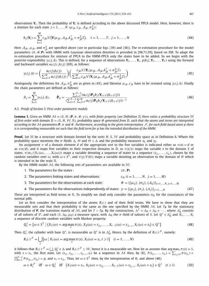
F. Pirri / Artificial Intelligence 175 (2011) 378–415 407
observations Yt . Then the probability of Yt is defined according to the above discussed PPCA model. Here, however, there isa mixture for each state j = 1, . . . , N (μ jk, c jk, A jk, σ
2jk):
b j(Yt)=M∑
k=1
c jk N(Y|μ jk, A jk A
jk + σ 2jk I
), t = 1, . . . , T ; j = 1, . . . , N (44)
Here A jk , μ jk , and σ 2jk are specified above (see in particular Eqs. (39) and (38)). The re-estimation procedure for the model
parameters (π,Ψ,P) with HMM with Gaussian observation densities is provided in [98,71,59], based on EM. To adapt there-estimation procedure for mixture of PPCA to the HMM-PPCA only the states have to be added. So we begin with theposterior responsibility γt( j,k). This is defined, for a sequence of observations Y1, . . . ,Yt , p(k| j,Y1, . . . ,YT ) using the forwardand backward variables αt( j), βt( j) [69], as follows:
γt( j,k)=(
αt( j)βt( j)∑Nj=1 αt( j)βt( j)
)( c jk N (Yt |μ jk, A jk Ajk + σ 2
jk I)∑Mk=1 c jk N (Yt |μ jk, A jk A
jk + σ 2jk I)
)(45)
Analogously, the definitions for A jk, σ2jk are as given in (43), and likewise μ jk, c jk have to be restated using γt( j,k). Finally
the chain parameters are defined as follows:
π j =M∑
k=1
γ1( j,k), Pi j =∑T−1
t=1 (αt( j)Pi jb j(Yt+1)βt+1( j))
(∑T−1
t=1∑N
j=1 αt( j)Pi jb j(Yt+1)βt+1( j))−1(46)
A.5. Proofs of Section 5: First-order parametric models
Lemma 1. Given an HMM M = (S, H, (P,π,Ψ,γ )), with finite property (see Definition 2) there exists a probability structure M
of first-order with domain D = (S, H, W ,R), probability space Φ generated from D, such that the atoms and terms are interpretedaccording to the M-parameters P,π and Ψ . Furthermore, according to the given interpretation I , for each field-based atom φ thereis a corresponding measurable set such that the field term for φ has the intended distribution of the HMM.
Proof. Let M be a structure with domain formed by the sorts H, S , W and probability space as in Definition 6. Where theprobability space mentions the σ -fields �, Θ and Θ ×� and the probability measures ηs and ηI .
An assignment v of a domain element d of the appropriate sort to the free variables is indicated either as v(x)= d oras v(x/d), and it maps free variables to their respective domains in D , so v(x/s) maps the variable x to the domain S ofstates, v(wt/(X1(ω), . . . , Xt(ω))) maps a variable denoting a sequence of states to a sequence (s j1 , . . . , s jt ), chosen by therandom variables over ω, with ω ∈ S T , and v(y/Y (h)) maps a variable denoting an observation to the domain of H whichis intended to be the reals R.
By the HMM model M, the following sets of parameters are available to M:
1. The parameters for the states : (π,P)
2. The parameters linking states and observations: cik (i = 1, . . . , N, j = 1, . . . M)
3. The parameters for the observations at each state: Ψ = {{μi j}, {σi j}, {Ai j}}i=1,...,N, j=1,...,M
4. The parameters for the observations independently of states: γ = {{μ j}, {σ j}, {A j}} j=1,...,N (47)
These are interpreted as field terms in R. To simplify we shall only consider the parameters σik for the covariances of thenormal pdfs.
Let us first consider the interpretation of the atoms Ri(·) and of their field terms. We have to show that they aremeasurable sets and that their probability is the same as the one specified by the HMM M. Let TP be the stationarydistribution of P, the transition matrix of M, and let T > TP . By the construction, �T =�0 ×�0 × · · · , where �t
0 consistsof all subsets of St , and each (S,�0,μ0) a measure space, with �0 the σ -field of subsets of S . Let Q t ∈�t
0 and X1, . . . , Xta sequence of discrete random variables with Markov property:
Q it =
{ω ∈ S T
∣∣ (X1(ω)= arg maxs
π(s), X2(ω)= s j2 , . . . , Xt−1(ω)= s jt−1 , Xt(ω)= si) ∈ Q t} (48)
Then Q it , the cylinder with base Q t , is measurable as Q t is in �t
0. Hence, by the definition of Ri(·)I , namely:
Ri(·)I =⋃
t
{ω
∣∣ X1(ω)= arg maxs
π(s), Xt(ω)= si, t � i}
(i = 1, . . . , N) (49)
it follows that Ri(·)I =⋃t Q i
t ∈� and Ri(·)I ⊂ W , hence it is a measurable set. Now let as assume that arg maxs π(s)= 1,with s = s1, the first state. Let (s j1 , s j2 , . . . , s jt−1 , si) be a sequence in M then, by (8), P (s j1 , . . . , s jt ) =
∑s j∈S π(s j1 )×∏T−1
k=1 P (s jk+1 |s jk )= p, and s1 = s j1 . Thus, let ω ∈ S T then, by the interpretation of Ri and above (48):
ω ∈ RI iff ω ∈ Q it iff
(X1(ω)= s1, X2(ω)= s j , . . . , Xt−1(ω)= s j , Xt(ω)= si
) ∈ Q t (t � i) (50)
i 2 t−1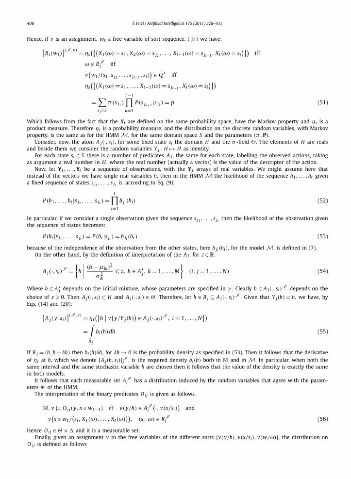
408 F. Pirri / Artificial Intelligence 175 (2011) 378–415
Hence, if v is an assignment, wt a free variable of sort sequence, t � i we have:
[Ri(wt)
](I ,v) = ηs({(
X1(ω)= s1, X2(ω)= s j2 , . . . , Xt−1(ω)= s jt−1 , Xt(ω)= si)})
iff
ω ∈ RIi iff
v(
wt/(s1, s j2 . . . , s jt−1 , si)) ∈ Q t iff
ηs({(
X1(ω)= s1, . . . , Xt−1(ω)= s jt−1 , Xt(ω)= si)})
=∑s j∈S
π(s j1)
T−1∏k=1
P (s jk+1 |s jk )= p (51)
Which follows from the fact that the Xi are defined on the same probability space, have the Markov property and ηs is aproduct measure. Therefore ηs is a probability measure, and the distribution on the discrete random variables, with Markovproperty, is the same as for the HMM M, for the same domain space S and the parameters (π,P).
Consider, now, the atom A j(·, si), for some fixed state si the domain H and the σ -field Θ . The elements of H are realsand beside them we consider the random variables Y j : H �→ H as identity.
For each state si ∈ S there is a number of predicates A j , the same for each state, labelling the observed actions, takingas argument a real number in H , where the real number (actually a vector) is the value of the descriptor of the action.
Now, let Y1, . . . ,Yt be a sequence of observations, with the Y j arrays of real variables. We might assume here thatinstead of the vectors we have single real variables h, then in the HMM M the likelihood of the sequence h1, . . . ,ht givena fixed sequence of states s j1 , . . . , s jt is, according to Eq. (9):
P (h1, . . . ,ht |s j1 , . . . , s jt )=t∏
i=1
b ji (hi) (52)
In particular, if we consider a single observation given the sequence s j1 , . . . , s jt then the likelihood of the observation giventhe sequence of states becomes:
P (ht |s j1 , . . . , s jt )= P (ht |s jt )= b ji (ht) (53)
because of the independence of the observation from the other states, here b ji (hi), for the model M, is defined in (7).On the other hand, by the definition of interpretation of the A j , for z ∈R:
A j(·, si)I =
{h
∣∣∣∣ (h−μik)2
σ 2ik
� z, h ∈ A�j, k = 1, . . . , M
}(i, j = 1, . . . , N) (54)
Where h ∈ A�j depends on the initial mixture, whose parameters are specified in γ . Clearly h ∈ A j(·, si)
I depends on the
choice of z � 0. Then A j(·, si) ⊂ H and A j(·, si) ∈ Θ . Therefore, let h ∈ B j ⊆ A j(·, si)I . Given that Y j(h) = h, we have, by
Eqs. (14) and (20):
[A j(y, si)
](I ,v) = ηI({
h∣∣ v
(y/Y j(h)
) ∈ A j(·, si)I , i = 1, . . . , N
})=
∫B j
bi(h)dh (55)
If B j = (h,h+ δh) then bi(h)δh, for δh → 0 is the probability density as specified in (53). Then it follows that the derivativeof ηI at h, which we denote [A j(h, si)]Iδ , is the required density bi(h) both in M and in M. In particular, when both thesame interval and the same stochastic variable h are chosen then it follows that the value of the density is exactly the samein both models.
It follows that each measurable set AIi has a distribution induced by the random variables that agree with the param-
eters Ψ of the HMM.The interpretation of the binary predicates O ij is given as follows.
M, v |� O ij(y, x ◦ wt−1) iff v(y/h) ∈ AIi
(·, v(x/si))
and
v(x ◦ wt/
(si, X1(ω), . . . , Xt(ω)
)), (si,ω) ∈ RI
i (56)
Hence O ij ∈Θ ×� and it is a measurable set.Finally, given an assignment v to the free variables of the different sorts {v(y/h), v(x/si), v(w/ω)}, the distribution on
O ji is defined as follows
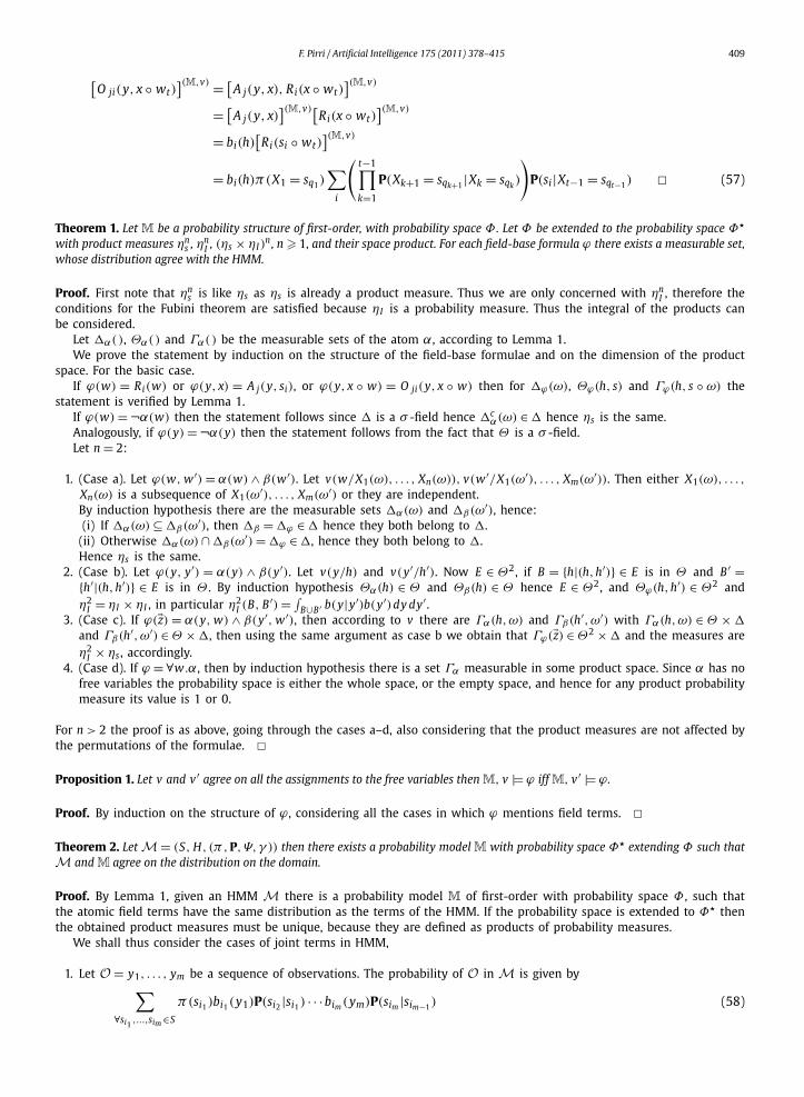
F. Pirri / Artificial Intelligence 175 (2011) 378–415 409
[O ji(y, x ◦ wt)
](M,v) = [A j(y, x), Ri(x ◦ wt)
](M,v)
= [A j(y, x)
](M,v)[Ri(x ◦ wt)
](M,v)
= bi(h)[
Ri(si ◦ wt)](M,v)
= bi(h)π(X1 = sq1)∑
i
(t−1∏k=1
P(Xk+1 = sqk+1 |Xk = sqk )
)P(si |Xt−1 = sqt−1) � (57)
Theorem 1. Let M be a probability structure of first-order, with probability space Φ . Let Φ be extended to the probability space Φ�
with product measures ηns , ηn
I , (ηs × ηI )n, n � 1, and their space product. For each field-base formula ϕ there exists a measurable set,
whose distribution agree with the HMM.
Proof. First note that ηns is like ηs as ηs is already a product measure. Thus we are only concerned with ηn
I , therefore theconditions for the Fubini theorem are satisfied because ηI is a probability measure. Thus the integral of the products canbe considered.
Let �α( ), Θα( ) and Γα( ) be the measurable sets of the atom α, according to Lemma 1.We prove the statement by induction on the structure of the field-base formulae and on the dimension of the product
space. For the basic case.If ϕ(w) = Ri(w) or ϕ(y, x) = A j(y, si), or ϕ(y, x ◦ w) = O ji(y, x ◦ w) then for �ϕ(ω), Θϕ(h, s) and Γϕ(h, s ◦ ω) the
statement is verified by Lemma 1.If ϕ(w)=¬α(w) then the statement follows since � is a σ -field hence �c
α(ω) ∈� hence ηs is the same.Analogously, if ϕ(y)=¬α(y) then the statement follows from the fact that Θ is a σ -field.Let n= 2:
1. (Case a). Let ϕ(w, w ′)= α(w)∧ β(w ′). Let v(w/X1(ω), . . . , Xn(ω)), v(w ′/X1(ω′), . . . , Xm(ω′)). Then either X1(ω), . . . ,
Xn(ω) is a subsequence of X1(ω′), . . . , Xm(ω′) or they are independent.
By induction hypothesis there are the measurable sets �α(ω) and �β(ω′), hence:(i) If �α(ω)⊆�β(ω′), then �β =�ϕ ∈� hence they both belong to �.
(ii) Otherwise �α(ω)∩�β(ω′)=�ϕ ∈�, hence they both belong to �.Hence ηs is the same.
2. (Case b). Let ϕ(y, y′) = α(y) ∧ β(y′). Let v(y/h) and v(y′/h′). Now E ∈ Θ2, if B = {h|(h,h′)} ∈ E is in Θ and B ′ ={h′|(h,h′)} ∈ E is in Θ . By induction hypothesis Θα(h) ∈ Θ and Θβ(h) ∈ Θ hence E ∈ Θ2, and Θϕ(h,h′) ∈ Θ2 andη2
I = ηI × ηI , in particular η2I (B, B ′)= ∫
B∪B ′ b(y|y′)b(y′)dy dy′ .3. (Case c). If ϕ(�z) = α(y, w) ∧ β(y′, w ′), then according to v there are Γα(h,ω) and Γβ(h′,ω′) with Γα(h,ω) ∈ Θ ×�
and Γβ(h′,ω′) ∈Θ ×�, then using the same argument as case b we obtain that Γϕ(�z) ∈Θ2 ×� and the measures areη2
I × ηs , accordingly.4. (Case d). If ϕ = ∀w.α, then by induction hypothesis there is a set Γα measurable in some product space. Since α has no
free variables the probability space is either the whole space, or the empty space, and hence for any product probabilitymeasure its value is 1 or 0.
For n > 2 the proof is as above, going through the cases a–d, also considering that the product measures are not affected bythe permutations of the formulae. �Proposition 1. Let v and v ′ agree on all the assignments to the free variables then M, v |� ϕ iff M, v ′ |� ϕ .
Proof. By induction on the structure of ϕ , considering all the cases in which ϕ mentions field terms. �Theorem 2. Let M = (S, H, (π,P,Ψ,γ )) then there exists a probability model M with probability space Φ� extending Φ such thatM and M agree on the distribution on the domain.
Proof. By Lemma 1, given an HMM M there is a probability model M of first-order with probability space Φ , such thatthe atomic field terms have the same distribution as the terms of the HMM. If the probability space is extended to Φ� thenthe obtained product measures must be unique, because they are defined as products of probability measures.
We shall thus consider the cases of joint terms in HMM,
1. Let O = y1, . . . , ym be a sequence of observations. The probability of O in M is given by∑∀si ,...,si ∈S
π(si1)bi1(y1)P(si2 |si1) · · ·bim(ym)P(sim |sim−1) (58)
1 m

410 F. Pirri / Artificial Intelligence 175 (2011) 378–415
Thus the term requires to represent all sequences of states of length m. To represent these sequences we need to definea suitable set of variables. First let Q m
i = {ωm|Xm(ω)= si}, that is, Q mi is formed by all ω whose subsequence of length
m have last state si . Let Umi = {wi
m|v(wim/(X1(ω), . . . , Xm(ω))), and (X1(ω), . . . , Xm(ω)) ∈ Q m
i }, that is Umi provides a
variable name, of sort sequence, for each element in Q mi , then
ϕ =∨
i=1,...,Nwi
m∈Umi
N∧j=1
O ji(
y j, wim
)(59)
Let θ� = {y1, . . . , ym},ω� =⋃i Q m
i
[ϕ] = (ηm
I × ηs)Γϕ
(θ�,ω�
)=
∑s j1 ,...,s jm∈ω�
π(s j1)b j1(y1)P(s j2 |s j1) · · ·b jm(ym)P(s jm |s jm−1)
2. Let p be a stationary distribution of the Markov chain in M i.e. pPt = pP = p and such that p(t) = 0. Consider, now,any variable wi
t , such that wit ∈ U t
i (as defined in the previous item), then for any sequence wit+k , denoting a sequence
(X1(ω), . . . , Xt+1(ω)) ending in state si ,[Ri(
wit
)]= [Ri(
wit+k
)]= p(t)= π(s j1)Pt (60)
By the interpretation of Ri (see (49)).3. Let P (h1, . . . ,hm, s1, . . . , sm) in M be the joint probability of a sequence of observations and a sequence of states (see
(11)). Consider a formula of the form:
ψ(y1, . . . , ym, x1, . . . , xm ◦ wm−1)∧ ϕ(w1, . . . , wm)
Since the only predicate mentioning both observations and states is O ji and O ji(y, x ◦ w)≡ Ri(x ◦ w) ∧ A j(y, x) thenthe above formula can be reduced in normal form:
m∧i=1
A j(yi, xi)∧m∧
i=1
Ri(xi ◦ wm−1)
Then the joint probability of the observations, given the states is[ψ(y1, . . . , ym, x1, . . . , xm)∧ ϕ(w1, . . . , wm)
]= (ηm
I × ηs)(Γψ∧ϕ)(Γϕ) (61)
by Theorem 1 and (23).
Furthermore:
M, v |� ¬(Ri(w)∧ R j(w)), ∀i, j, i = j
M, v |� ¬(O i(y, w)∧ O j(y, w)), ∀i, j, i = j (62)
Simply by the definition of interpretation given in Lemma 1.Hence M is the required model. �
A.6. Proofs of Section 6: Final induction step, concluding with the Situation Calculus
We recall that a basic theory of actions is formed by the set of sentences:
Σ ∪ D S0 ∪ Duna ∪ Dap ∪ Dss (63)
Where Σ is the set of foundational axioms described below. D S0 is the set of formulae which either do not mentionsituation terms or they mention only the situation term S0. Duna are the set of unique name of action axioms, that is,for each action name Ai and A j we have Ai = A j . Dap are the axioms specifying the preconditions to execute an action,such as:
Poss(pushdoor, s)≡ Unlockeddoor (64)
Finally Dss are the axioms specifying the effect of an action: what comes true after the execution of an action, such as, forexample:
Openeddoor
(do(a, s)
)≡ a= pushdoor ∨ a = closedoor ∧ Openeddoor(s) (65)
The set of foundational axioms Σ is:
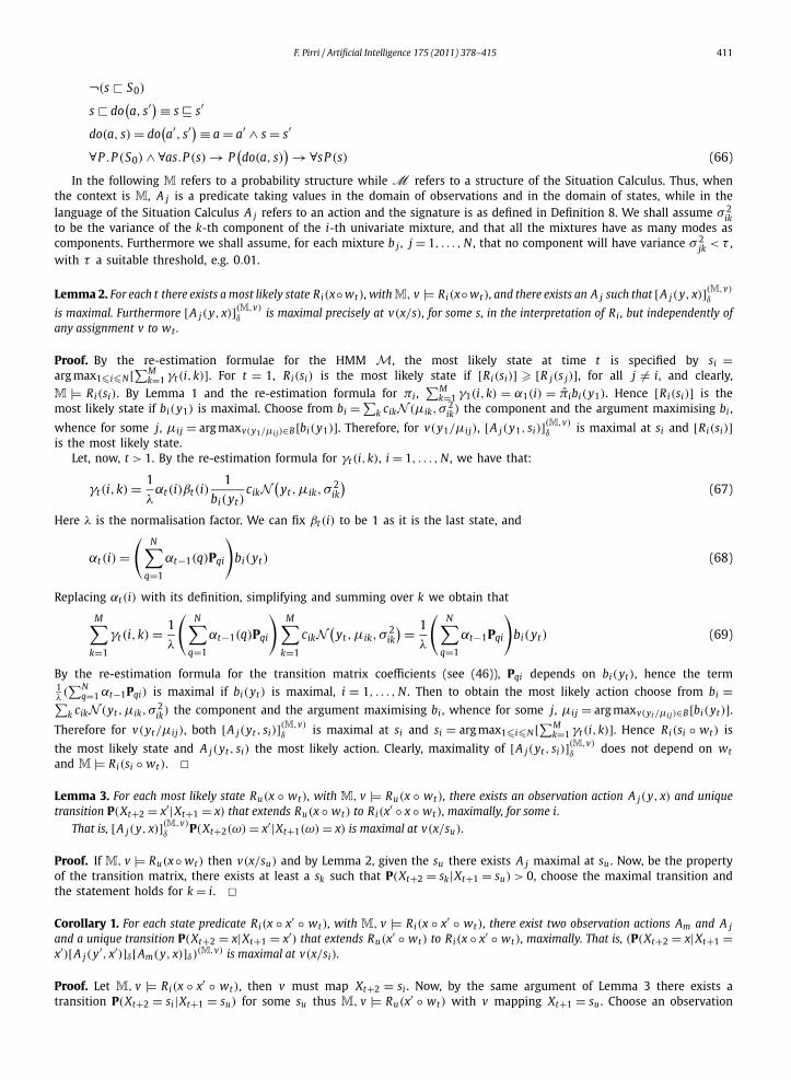
F. Pirri / Artificial Intelligence 175 (2011) 378–415 411
¬(s � S0)
s � do(a, s′
)≡ s $ s′
do(a, s)= do(a′, s′
)≡ a= a′ ∧ s = s′
∀P .P (S0)∧ ∀as.P (s)→ P(do(a, s)
)→∀sP (s) (66)
In the following M refers to a probability structure while M refers to a structure of the Situation Calculus. Thus, whenthe context is M, A j is a predicate taking values in the domain of observations and in the domain of states, while in thelanguage of the Situation Calculus A j refers to an action and the signature is as defined in Definition 8. We shall assume σ 2
ikto be the variance of the k-th component of the i-th univariate mixture, and that all the mixtures have as many modes ascomponents. Furthermore we shall assume, for each mixture b j , j = 1, . . . , N , that no component will have variance σ 2
jk < τ ,with τ a suitable threshold, e.g. 0.01.
Lemma 2. For each t there exists a most likely state Ri(x◦wt), with M, v |� Ri(x◦wt), and there exists an A j such that [A j(y, x)](M,v)δ
is maximal. Furthermore [A j(y, x)](M,v)δ is maximal precisely at v(x/s), for some s, in the interpretation of Ri , but independently of
any assignment v to wt .
Proof. By the re-estimation formulae for the HMM M, the most likely state at time t is specified by si =arg max1�i�N [∑M
k=1 γt(i,k)]. For t = 1, Ri(si) is the most likely state if [Ri(si)] � [R j(s j)], for all j = i, and clearly,M |� Ri(si). By Lemma 1 and the re-estimation formula for πi ,
∑Mk=1 γ1(i,k) = α1(i) = πibi(y1). Hence [Ri(si)] is the
most likely state if bi(y1) is maximal. Choose from bi =∑k cik N (μik, σ
2ik) the component and the argument maximising bi ,
whence for some j, μi j = arg maxv(y1/μi j)∈B [bi(y1)]. Therefore, for v(y1/μi j), [A j(y1, si)](M,v)δ is maximal at si and [Ri(si)]
is the most likely state.Let, now, t > 1. By the re-estimation formula for γt(i,k), i = 1, . . . , N , we have that:
γt(i,k)= 1
λαt(i)βt(i)
1
bi(yt)cik N
(yt,μik,σ
2ik
)(67)
Here λ is the normalisation factor. We can fix βt(i) to be 1 as it is the last state, and
αt(i)=(
N∑q=1
αt−1(q)Pqi
)bi(yt) (68)
Replacing αt(i) with its definition, simplifying and summing over k we obtain that
M∑k=1
γt(i,k)= 1
λ
(N∑
q=1
αt−1(q)Pqi
)M∑
k=1
cik N(
yt,μik,σ2ik
)= 1
λ
(N∑
q=1
αt−1Pqi
)bi(yt) (69)
By the re-estimation formula for the transition matrix coefficients (see (46)), Pqi depends on bi(yt), hence the term1λ(∑N
q=1 αt−1Pqi) is maximal if bi(yt) is maximal, i = 1, . . . , N . Then to obtain the most likely action choose from bi =∑k cik N (yt ,μik, σ
2ik) the component and the argument maximising bi , whence for some j, μi j = arg maxv(yt/μi j)∈B [bi(yt)].
Therefore for v(yt/μi j), both [A j(yt, si)](M,v)δ is maximal at si and si = arg max1�i�N [∑M
k=1 γt(i,k)]. Hence Ri(si ◦ wt) is
the most likely state and A j(yt , si) the most likely action. Clearly, maximality of [A j(yt, si)](M,v)δ does not depend on wt
and M |� Ri(si ◦ wt). �Lemma 3. For each most likely state Ru(x ◦ wt), with M, v |� Ru(x ◦ wt), there exists an observation action A j(y, x) and uniquetransition P(Xt+2 = x′|Xt+1 = x) that extends Ru(x ◦ wt) to Ri(x′ ◦ x ◦ wt), maximally, for some i.
That is, [A j(y, x)](M,v)δ P(Xt+2(ω)= x′|Xt+1(ω)= x) is maximal at v(x/su).
Proof. If M, v |� Ru(x◦wt) then v(x/su) and by Lemma 2, given the su there exists A j maximal at su . Now, be the propertyof the transition matrix, there exists at least a sk such that P(Xt+2 = sk|Xt+1 = su) > 0, choose the maximal transition andthe statement holds for k = i. �Corollary 1. For each state predicate Ri(x ◦ x′ ◦ wt), with M, v |� Ri(x ◦ x′ ◦ wt), there exist two observation actions Am and A jand a unique transition P(Xt+2 = x|Xt+1 = x′) that extends Ru(x′ ◦ wt) to Ri(x ◦ x′ ◦ wt), maximally. That is, (P(Xt+2 = x|Xt+1 =x′)[A j(y′, x′)]δ[Am(y, x)]δ)(M,v) is maximal at v(x/si).
Proof. Let M, v |� Ri(x ◦ x′ ◦ wt), then v must map Xt+2 = si . Now, by the same argument of Lemma 3 there exists atransition P(Xt+2 = si|Xt+1 = su) for some su thus M, v |� Ru(x′ ◦ wt) with v mapping Xt+1 = su . Choose an observation
412 F. Pirri / Artificial Intelligence 175 (2011) 378–415
action Am whose pdf is maximal at si , and an observation action A j whose pdf is maximal at su for some v(y/h), v(y′/h′),by Lemma 2. Hence, by Lemma 3, ([A j(y, su)]δP(Xt+1 = si |Xt+1 = su))(M,v) extends Ru(x′ ◦ wt) maximally to Ri(x ◦ x′ ◦ wt)
and since the pdf of Am is maximal at si the statement follows. �Theorem 3. Given M and an assignment v, with v(wt)= wt , wt ∈ {X1(ω)= s j1 , . . . , Xt(ω)= xs jt
}, t � 0, and for all Ri , there exists
a sequence (x ◦ x′ ◦ wt) such that Ri(x ◦ x′ ◦ wt)(M,v) is persistent.
Proof. Note that, by construction, either the transition matrix is irreducible or all transient states are connected with anabsorbing state, therefore the probability that a state happens at wt is greater than zero for all states. By Lemma 2 andDefinition 10 for each state Ri(x ◦ wt) that happens at wt at t + k, M, v |� R j(x ◦ wt) and [Ri(x ◦ wt)](M,v) is maximal atv(x/si). Furthermore, by Lemma 2 again, there is an action A j(y, x) such that [A j(y, x)]δ is maximal at v(x/si). In fact, inthe proof of Lemma 2 we have shown that, if Ri is maximal, this is due, indeed, to some action A j maximal at si ∈ RI
i , viathe re-estimation formulae.
Let us assume that [Ri(x◦x′ ◦wt)](M,v) , t � 0, is maximal and M, v |� Ri(x◦x′ ◦wt). We define the following construction:
Ut+2 = si (given the choice of Ri)
Tt+2 = arg maxv(y/h j∈AI
j )
[A j(y, si)
]δ
Mt+2 ={
Ri(si ◦ x′ ◦ wt
), A j(Tt+2, si)
}Ut+1 = arg max
1�u�N,v(x′/su){[Ru
(x′ ◦ wt
)]P(Xt+2 = si |Xt+1 = Ut+1)
Tt+1 = arg maxv(y′/hm∈AI
m )
[Am
(y′, Ut+1
))]δ
Mt+1 = Mt+2 ∪{
Ru(Ut+1 ◦ x′′ ◦ wt−1
), Am(Tt+1, Ut+1), v
(x′/Ut+1
)}...
U1 = arg max1�q�N,v(x∗/sq)∈S
([Rq
(x�)]
P(
X2 = U2|X1 = x�))
T1 = arg maxv(y∗/hk∈AI
k )
[Ak
(y∗, U1
))]δ
M1 = M2 ∪{
Rq(U1), Am(T1, U1), v(x�/U1
)}(70)
Let v be as defined in M1, then it is easy to see that by the construction and by Lemma 2, M, v |�∧M� , where M� is
the set of atoms in M1. Furthermore for each n, n = 1, . . . , t + 2, if v(yn/h j) ∈ Tn and v(xn/su) ∈ Un , then [A j(h j, su)] ismaximal for Ru(su ◦ wn−1). Now let us consider:(
A j1(h j1 , si1), . . . , A jt+2(h jt+2 , sit+2))(
Ri1(si1), . . . , Rit+2(sit+2))
By the above construction, each of the field term of the atoms in the two sequences is maximal.We show by induction on t , on the given construction, that Ri , i = 1, . . .n, is persistent according to Definition 10. We
have to show item (1) and (2) and that the term introduced in Eq. (28) is maximal.For the basic case item (1) and (2) are straightforward because Ri is entering wt at t = 1. Thus (28) reduces to the
maximality of [Ri(U1)].Let t > 1. Again (1) is obviously verified by the construction and the inductive hypothesis. Hence [Ri(Ut+2 ◦ Ut+1 ◦ wt)∧
A j(Tt+2, Ut+2)∧ Am(Tt+1, Ut+1)∧ Ru(Ut+1 ◦ wt)] is maximal and, thus, [Ri(Ut+2 ◦ Ut+1 ◦ wt)|A j(Tt+2, Ut+2)] is maximal.Consider (2). Suppose that at t + 2 there is a change. In M1 there are two actions Aq(Tt+1, Ut+1) and Ak(Tt+2, Ut+2),
with terms maximal at Ut+1 and Ut+2, respectively. Because they are in M1 they are both satisfied in M. Since by hypothesisthere is a change, then:
M, v |� Aq(Tt+1, Ut+1)∧ Ak(Tt+2, Ut+2)∧ Ri(Ut+1 ◦ wt)∧¬Ri(Ut+2 ◦ Ut+1 ◦ wt)
We need only to show that a delay is possible. If Ut+1 is an absorbing state then change cannot occur, thus, it is transientbut not null, by definition of the transition matrix of the system, that is, Pii > 0. We can suppose that a delay does not affectthe observation, hence [Aq(Tt+1, Ut+1)]δ maximal at Ri(Ut+1 ◦ wt) is still maximal at Ri(Ut+1 ◦ Ut+1 ◦ wt). From this factand the fact that [Ak(Tt+2, Ut+2)]δ is maximal at state Ut+2 = Ut+1, it follows that 1− [Ak(T1, U1)]δ > 0. We have also tonote that, by Corollary 1, [Aq(Tt+1, Ut+1)]δP(Xt+2 = Ut+1|Xt+1 = Ut+1)[Aq(Tt+1, Ut+1)]δ extends maximally [Ri(Ut+1 ◦ wt)]to [Ri(Ut+1 ◦ Ut+1 ◦ wt)], hence it is possible to delay the change with
M, v |� ¬Ak(Tt+2, Ut+2)∧ Ri(Ut+1 ◦ wt)∧ Ri(Ut+1 ◦ Ut+1 ◦ wt)

F. Pirri / Artificial Intelligence 175 (2011) 378–415 413
The delay is like having added, between t + 1 and t + k (here k = 2) Ut+1, Tt+1, Mt+1, k-times, hence both Ri(Ut+1 ◦ wt)
and Ri(Ut+1 ◦ Ut+1 ◦ wt) are in M1, thus they are both maximal. But Aq , by the right choice of y, must be the A j of item(1) hence, renaming the states, [Ri(si ◦Ut+1 ◦ wt)|A j(Tt+2, si)] = [Ri(si ◦ si ◦ wt)|Aq(Tt+2, si)] therefore, without consideringnormalisation factors:[
Ri(si ◦ si ◦ wt)|A j(Tt+2, si)]+ [
Ri(si ◦ Ut+1 ◦ wt)|¬Ak(Tt+2, si)]
must be maximal. That is, choosing ¬Ak is like having chosen any maximal action that let Ri remaining at wt . �Theorem 4. Let M be a first-order parametric probability structure, as defined in Definition 6 and v any assignment to the freevariables. Let v(wt) ∈ {X1(ω), . . . , Xt(ω)= x∗}, ω ∈ RI , and let Ri(x ◦ wt) be any predicate of state, with M, v |� Ri(x ◦ wt):
1. There is at least an action A j(y, x) that is maximal at v(x/s), for s in the interpretation of Ri . Hence the action precondition forA j is uniquely determined by Ri .
2. There exists at least one action A j , and possibly Am, ensuring both persistence and satisfiability of Ri . Hence the successor stateaxiom for Ri is uniquely determined by the maximal values of [Ri(x ◦ x′ ◦ wt)|A j(y, x)] + [Ri(x ◦ x ◦ wt)|¬Am(y′, x)].
Proof. 1) follows from Lemma 2 and Eq. (29) and 2) follows from Theorem 3 and Eq. (29). More precisely, by Theorem 3,given a fixed wt , t � Tp, each [Ri(x ◦ wt)](M,v) is a most likely state, at t + 1. Then:
1. By Lemma 2 for each t � 0 choose the most likely state Ri(x ◦wt) and the action A j(y, x) maximal at the state and addto the action precondition axioms, possibly with free variables z and z′ of sort object:
∀s.Poss(
A j(z), s)≡ Ri
(z′, s
)2. By Theorem 3 and the above item for each time t � 0, choose the most likely state and at least an action A j(y, x)
maximal at the state according to the construction specified in Theorem 3. Further, if Ri does not correspond to anabsorbing state, then there is an action Am that, according to Theorem 3, induces a change, such that Ri exits wt . Then[Ri(x ◦ x′ ◦ wt)|A j(y, x)]+ [Ri(x ◦ x ◦ wt)|¬Am(y′, x)] is maximal. Then Am is the action hence add to the successor stateaxioms, possibly with free variables z, z′ and z′′ of sort object:
∀a s.Ri(z,do(a, s)
)≡ A j(z′)= a∨ ∀z′′Am
(z′′) = a∧ Ri(z, s) �
References
[1] Martin Abadi, Joseph Y. Halpern, Decidability and expressiveness for first-order logics of probability, in: IEEE Symposium on Foundations of ComputerScience (FOCS)-89, 1989, pp. 148–153.
[2] Rajeev Alur, Costas Courcoubetis, David L. Dill, Model-checking for probabilistic real-time systems (extended abstract), in: Automata, Languages andProgramming, 18th International Colloquium, ICALP91, Proceedings, 1991, pp. 115–126.
[3] Eyal Amir, Allen Chang, Learning partially observable deterministic action models, J. Artif. Intell. Res. (JAIR) 33 (2008) 349–402.[4] Corin R. Anderson, Pedro Domingos, Daniel S. Weld, Relational Markov models and their application to adaptive web navigation, in: KDD, 2002,
pp. 143–152.[5] Brenna D. Argall, Sonia Chernova, Manuela Veloso, Brett Browning, A survey of robot learning from demonstration, Robot. Auton. Syst. 57 (5) (2009)
469–483.[6] Fahiem Bacchus, Lp: A logic for statistical information, in: M. Henrion, R.D. Shachter, L.N. Kanal, J.F. Lemmer (Eds.), Uncertainty in Artificial Intelli-
gence, vol. 5, North-Holland, Amsterdam, 1990, pp. 3–14.[7] Fahiem Bacchus, Representing and Reasoning with Probabilistic Knowledge: A Logical Approach to Probabilities, MIT Press, Cambridge, MA, USA, 1990.[8] Fahiem Bacchus, Joseph Y. Halpern, Hector J. Levesque, Reasoning about noisy sensors (and effectors) in the Situation Calculus, in: Reasoning with
Uncertainty in Robotics, 1995, pp. 218–220.[9] Fahiem Bacchus, Joseph Y. Halpern, Hector J. Levesque, Reasoning about noisy sensors and effectors in the Situation Calculus, Artificial Intelli-
gence 111 (1–2) (1999) 171–208.[10] Leonard E. Baum, Ted Petrie, George Soules, Norman Weiss, A maximization technique occurring in the statistical analysis of probabilistic functions
of Markov chains, Ann. Math. Statist. 41 (1970) 164–171.[11] Danièle Beauquier, Alexander Moshe Rabinovich, Anatol Slissenko, A logic of probability with decidable model-checking, in: CSL, 2002, pp. 306–321.[12] Anna Belardinelli, Fiora Pirri, Andrea Carbone, Bottom-up gaze shifts and fixations learning by imitation, IEEE Transactions on Systems, Man, and
Cybernetics, Part B 37 (2) (2007) 256–271.[13] Anna Belardinelli, Fiora Pirri, Andrea Carbone, Motion saliency maps from spatiotemporal filtering, in: Proc. of the 5th International Workshop on
Attention in Cognitive Systems, WAPCV 2008, 2008, pp. 7–17.[14] Andrea Bianco, Luca de Alfaro, Model checking of probabilistic and nondeterministic systems, in: FSTTCS, Foundations of Software Technology and
Theoretical Computer Science, 15th Conference, Proceedings, 1995, pp. 499–513.[15] Patrick Billingsley, Probability and Measure, Wiley, 1995.[16] T. Brox, B. Rosenhahn, D. Cremers, Contours, optic flow, and prior knowledge: Cues for capturing 3D human motion in videos, in: Human Motion –
Understanding, Modeling, Capture, and Animation, Springer, 2007.[17] Andrés Bruhn, Joachim Weickert, Christoph Schnörr, Lucas/Kanade meets Horn/Schunck: Combining local and global optic flow methods, International
Journal of Computer Vision 61 (3) (2005) 211–231.[18] Carlos A. Acosta Calderon, Husheng Hu, Robotic societies: Elements of learning by imitation, in: Proc. of 21st IASTED International Conference on
Applied Informatics, Innsbruck, Austria, 2003, pp. 315–320.[19] Antonio Chella, Haris Dindo, Ignazio Infantino, Learning high-level tasks through imitation, in: IROS, 2006, pp. 3648–3654.[20] Paul R. Cohen, Tim Oates, Carole R. Beal, Niall M. Adams, Contentful mental states for robot baby, in: AAAI/IAAI, 2002, pp. 126–131.

414 F. Pirri / Artificial Intelligence 175 (2011) 378–415
[21] Dorin Comaniciu, Peter Meer, Mean shift: A robust approach toward feature space analysis, IEEE Trans. Pattern Anal. Mach. Intell. 24 (5) (2002)603–619.
[22] Dorin Comaniciu, Visvanathan Ramesh, Peter Meer, Kernel-based object tracking, IEEE Trans. Pattern Anal. Mach. Intell. 25 (5) (2003) 564–575.[23] Costas Courcoubetis, Mihalis Yannakakis, The complexity of probabilistic verification, J. ACM 42 (4) (1995) 857–907.[24] James Cussens, Parameter estimation in stochastic logic programs, Machine Learning 44 (3) (2001) 245–271.[25] James Cussens, At the interface of inductive logic programming and statistics, in: ILP, 2004, pp. 2–3.[26] James Cussens, Integrating by separating: Combining probability and logic with ICL, PRISM and SLPs, Technical report, APRIL project report, York,
2005.[27] Cynthia Breazeal, Daphna Buchsbaum, Jesse Gray, David Gatenby, Bruce Blumberg, Learning from and about others: Towards using imitation to
bootstrap the social understanding of others by robots, Artificial Life 11 (1–2) (January 2005) 31–62.[28] Luca de Alfaro, Temporal logics for the specification of performance and reliability, in: STACS 97, 14th Annual Symposium on Theoretical Aspects of
Computer Science, Proceedings, 1997, pp. 165–176.[29] Yiannis Demiris, Gillian Hayes, Imitation as a Dual Route Process Featuring Predictive and Learning Components: A Biologically-Plausible Computa-
tional Model, MIT Press, 2002.[30] Arthur P. Dempster, Nan M. Laird, Donald B. Rubin, Maximum likelihood from incomplete data via the EM algorithm, Journal of the Royal Statistical
Society 39 (1) (1977) 1–38.[31] Daniel C. Dennett, Brainstorms: Philosophical Essays on Mind and Psychology, MIT Press, 1978.[32] Daniel C. Dennett, Consciousness Explained, Little Brown, Boston, 1991.[33] Daniel C. Dennett, What RoboMary knows, in: Torin Alter, Sven Walter (Eds.), Phenomenal Concepts and Phenomenal Knowledge: New Essays on
Consciousness and Physicalism, 2006.[34] Thomas G. Dietterich, Pedro Domingos, Lise Getoor, Stephen Muggleton, Prasad Tadepalli, Structured machine learning: The next ten years, Machine
Learning 73 (1) (2008) 3–23.[35] Davis Ernest, Leora Morgenstern, Introduction: Progress in formal commonsense reasoning, Artificial Intelligence 153 (1–2) (2004) 1–12.[36] Ronald Fagin, Joseph Y. Halpern, Reasoning about knowledge and probability, in: Proc. of the Second Conference on Theoretical Aspects of Reasoning
about Knowledge, Asilomar, CA, 1988, pp. 277–293.[37] Ronald Fagin, Joseph Y. Halpern, Reasoning about knowledge and probability, J. ACM 41 (2) (1994) 340–367.[38] Ronald Fagin, Joseph Y. Halpern, Nimrod Megiddo, A logic for reasoning about probabilities, Information and Computation 87 (1/2) (1990) 78–128.[39] L. Fogassi, P.F. Ferrari, B. Gesierich, S. Rozzi, F. Chersi, G. Rizzolatti, Parietal lobe: From action organization to intention understanding, Science 308
(2005) 662–667.[40] Haim Gaifman, Concerning measures in first order calculi, Israel Journal of Mathematics 2 (1964) 1–18.[41] Haim Gaifman, A theory of higher order probabilities, in: TARK, 1986, pp. 275–292. Already presented at NSF, Irvine, 1985.[42] Lise Getoor, Nir Friedman, Daphne Koller, Benjamin Taskar, Learning probabilistic models of relational structure, in: ICML, 2001, pp. 170–177.[43] Yolanda Gil, Learning by experimentation: Incremental refinement of incomplete planning domains, in: ICML, 1994, pp. 87–95.[44] Nelson Goodman, The Structure of Appearance, Harvard University Press, Cambridge, MA, 1951.[45] Alison Gopnik, Andrew N. Meltzoff, P.K. Kuhl, The Scientists in the Crib, Harper Collins, New York, 2000.[46] Alison Gopnik, Andrew N. Meltzoff, Words, Thoughts, and Theories, MIT Press, Cambridge, MA, 1997.[47] Alison Gopnik, Laura Schulz, Mechanisms of theory-formation in young children, Trends in Cognitive Science 8 (8) (2004) 371–377.[48] Joseph Y. Halpern, An analysis of first-order logics of probability, Artificial Intelligence 46 (3) (1990) 311–350.[49] Joseph Y. Halpern, David A. McAllester, Likelihood probability and knowledge, Comput. Intelligence 5 (3) (1990) 151–160.[50] Peter Hammond, Elementary non-Archimedean representations of probability for decision theory and games, in: Probability and Probabilistic Causal-
ity, Kluwer Academic, 1994.[51] Hans Hansson, Bengt Jonsson, A logic for reasoning about time and reliability, Formal Asp. Comput. 6 (5) (1994) 512–535.[52] Douglas N. Hoover, Probability logic, Annals of Mathematical Logic 14 (1978) 287–315.[53] Berthold K.P. Horn, Brian G. Schunck, Determining optical flow, Artificial Intelligence 17 (1–3) (1981) 185–203.[54] Weiming Hu, Tieniu Tan, Liang Wang, Steve Maybank, A survey on visual surveillance of object motion and behaviors, IEEE Transactions on Systems,
Man and Cybernetics 34 (2004) 334–352.[55] Frank Jackson, Peter Ludlow, Yujin Nagasawa, Daniel Stoljar, There’s Something about Mary: Essays on Phenomenal Consciousness and Frank Jackson’s
Knowledge Argument, MIT Press, Bradford Book, 2004.[56] Frank C. Jackson, Epiphenomenal qualia, Philosophical Quarterly 32 (127) (1982) 127–136.[57] Frank C. Jackson, What Mary didn’t know, Journal of Philosophy 83 (5) (1986) 291–295.[58] Alex Pentland, Tony Jebara, Statistical imitative learning from perceptual data, in: 2nd International Conference on Development and Learning, ICDL02,
2002.[59] Bing-Hwang Juang, Stephen E. Levinson, M. Mohan Sondhi, Maximum likelihood estimation for multivariate mixture observations of Markov chains,
IEEE Transactions on Information Theory 32 (2) (1986) 307.[60] Immanuel Kant, Critique of Pure Reason, Riga, 1781–1787.[61] H. Jerome Keisler, Probability quantifiers, in: J. Barwise, S. Feferman (Eds.), Model-Theoretic Logics, Springer, New York, 1985, pp. 509–556.[62] H. Jerome Keisler, Hyperfinite Model Theory, North-Holland, Amsterdam, 1977.[63] E. Kohler, C. Keysers, M.A. Umiltà, L. Fogassi, V. Gallese, G. Rizzolatti, Hearing sounds, understanding actions: Action representation in mirror neurons,
Science 297 (2002) 846–848.[64] Daphne Koller, Structured probabilistic models: Bayesian networks and beyond, in: AAAI/IAAI, 1998, pp. 1210–1211.[65] V. Krüger, D. Kragic, A. Ude, C. Geib, The meaning of action: A review on action recognition and mapping, Advanced Robotics 21 (13) (2007) 1473–
1501.[66] M. Land, N. Mennie, J. Rusted, The roles of vision and eye movements in the control of activities of daily living, Perception 28 (1999) 1311–1328.[67] Hector J. Levesque, Knowledge, action, and ability in the Situation Calculus, in: TARK, 1994, pp. 1–4.[68] Hector J. Levesque, What is planning in the presence of sensing?, in: AAAI/IAAI, vol. 2, 1996, pp. 1139–1146.[69] S.E. Levinson, L.R. Rabiner, M.M. Sondhi, An introduction to the application of the theory of probabilistic functions of a Markov process to automatic
speech recognition, Bell Systems Technical Journal 62 (4) (1983) 1035–1074.[70] Clarence Irving Lewis, Mind and the World Order, C. Scribner’s Sons, New York, 1929.[71] Louis A. Liporace, Maximum likelihood estimation for multivariate observations of Markov sources, IEEE Transactions on Information Theory 28 (5)
(1982) 729–734.[72] Bruce D. Lucas, Takeo Kanade, An iterative image registration technique with an application to stereo vision, in: IJCAI, 1981, pp. 674–679.[73] Maja Mataric, Sensory-Motor Primitives as a Basis for Imitation: Linking Perception to Action and Biology to Robotics, MIT Press, 2002.[74] John McCarthy, Patrick J. Hayes, Some philosophical problems from the standpoint of artificial intelligence, in: B. Meltzer, D. Michie (Eds.), Machine
Intelligence, vol. 4, Edinburgh Univ. Press, Edinburgh, Scotland, 1969, pp. 463–502.

F. Pirri / Artificial Intelligence 175 (2011) 378–415 415
[75] John McCarthy, Programs with common sense, in: Teddington Conference on the Mechanization of Thought Processes, http://www-formal.stanford.edu/jmc/mcc59.html, 1959.
[76] John McCarthy, Todd Moody’s zombies, Journal of Consciousness Studies 2 (4) (1995).[77] John McCarthy, AI papers in preparation: The well-designed child, 1999.[78] John McCarthy, Notes on AI: Appearance and reality: A challenge to machine learning, 1999.[79] John McCarthy, The well-designed child, Artificial Intelligence 172 (18) (2008) 2003–2014.[80] Andrew N. Meltzoff, W. Prinz, The Imitative Mind: Development, Evolution, and Brain Bases, Cambridge University Press, 2002.[81] Brian Milch, Bhaskara Marthi, Stuart J. Russell, David Sontag, Daniel L. Ong, Andrey Kolobov, BLOG: Probabilistic models with unknown objects, in:
IJCAI, 2005, pp. 1352–1359.[82] Thomas B. Moeslund, Adrian Hilton, Volker Kreger, A survey of advances in vision-based human motion capture and analysis, Computer Vision and
Image Understanding 104 (2–3) (2006) 90–126.[83] Stephen Muggleton, Learning stochastic logic programs, Electron. Trans. Artif. Intell. 4 (B) (2000) 141–153.[84] Kevin Murphy, Hidden Markov model (HMM) toolbox for Matlab, http://www.cs.ubc.ca/~murphyk/Software/HMM/hmm.html, 1998.[85] Ian T. Nabney, Netlab: Algorithms for Pattern Recognition, Springer, 2001.[86] Hanna M. Pasula, Luke S. Zettlemoyer, Leslie Pack Kaelbling, Learning symbolic models of stochastic domains, J. Artif. Intell. Res. (JAIR) 29 (2007)
309–352.[87] Fiora Pirri, Alberto Finzi, An approach to perception in theory of actions: Part I, Electron. Trans. Artif. Intell. 3 (C) (1999) 19–61.[88] Fiora Pirri, Ray Reiter, Some contributions to the metatheory of the Situation Calculus, J. ACM 46 (3) (1999) 325–361.[89] George Polya, Induction and Analogy in Mathematics: A Guide to the Art of Plausible Reasoning, Mathematics and Plausible Reasoning, vol. 1, Prince-
ton University Press, 1954 (eighth printing in 1973).[90] David Poole, The independent choice logic for modelling multiple agents under uncertainty, Artificial Intelligence Journal 94 (1–2) (1997) 7–56.[91] David Poole, Logic, knowledge representation and Bayesian decision theory, in: First International Conference on Computational Logic, 2000 (Invited
paper).[92] Ronald Poppe, Vision-based human motion analysis: An overview, Computer Vision and Image Understanding 108 (1–2) (2007) 4–18.[93] Daniel J. Povinelli, Folk Physics for Apes: The Chimpanzee’s Theory of How The World Works, Oxford University Press, 2000.[94] Willard Van Orman Quine, Main trends in recent philosophy: Two dogmas of empiricism, The Philosophical Review 60 (1) (1951) 20–43.[95] Willard Van Orman Quine, Theories and Things, second ed., Harvard University Press, 1981.[96] Willard Van Orman Quine, Quiddities: An Intermittently Philosophical Dictionary, Harvard University Press, 1987.[97] Willard Van Orman Quine, Pursuit of Truth, third ed., Harvard University Press, 1996.[98] Lawrence R. Rabiner, A tutorial on hidden Markov models and selected applications in speech recognition, Proceedings of the IEEE 77 (1989) 257–286.[99] Luc De Raedt, Kristian Kersting, Probabilistic logic learning, SIGKDD Explor. Newsl. 5 (1) (2003) 31–48.
[100] Raymond Reiter, Proving properties of states in the Situation Calculus, Artificial Intelligence Journal 64 (2) (1993) 337–351.[101] Raymond Reiter, Knowledge in Action: Logical Foundations for Specifying and Implementing Dynamical Systems, MIT Press, 2001.[102] Raymond Reiter, On knowledge-based programming with sensing in the Situation Calculus, ACM Trans. Comput. Log. 2 (4) (2001) 433–457.[103] G. Rizzolatti, L. Fogassi, V. Gallese, Neurophysiological mechanism underlying the understanding and imitation of action, Nature Neurosci. 2 (2001)
661–670.[104] Sam T. Roweis, EM algorithms for PCA and SPCA, in: NIPS, 1997.[105] Bertrand Russell, The Problems of Philosophy, 1912.[106] Taisuke Sato, A glimpse of symbolic-statistical modeling by prism, J. Intell. Inf. Syst. 31 (2) (2008) 161–176.[107] Taisuke Sato, Yoshitaka Kameya, Parameter learning of logic programs for symbolic-statistical modeling, J. Artif. Intell. Res. (JAIR) 15 (2001) 391–454.[108] Matthew D. Schmill, Tim Oates, Paul R. Cohen, Learning planning operators in real-world, partially observable environments, in: AIPS, 2000, pp. 246–
253.[109] Matthew D. Schmill, Michael T. Rosenstein, Paul R. Cohen, Paul E. Utgoff, Learning what is relevant to the effects of actions for a mobile robot, in:
Agents, 1998, pp. 247–253.[110] Dana Scott, Peter Krauss, Assigning probabilities to logical formulas, in: Aspects of Inductive Logic, North-Holland, 1966, pp. 219–264.[111] Aaron Sloman, What’s wrong with the priority of dynamical systems hypothesis, 2005.[112] Aaron Sloman, Two views of child as scientist: Humean and Kantian, 2006.[113] Michael E. Tipping, Christopher M. Bishop, Probabilistic principal component analysis, Journal of the Royal Statistical Society, Series B 61 (1999)
611–622.[114] Michael E. Tipping, Christopher M. Bishop, Mixtures of probabilistic principal component analysers, Neural Computation 11 (2) (1999) 443–482.[115] Moshe Y. Vardi, Automatic verification of probabilistic concurrent finite-state programs, in: FOCS, IEEE, 1985, pp. 327–338.[116] Andrew J. Viterbi, Error bounds for convolutional codes and an asymptotically optimal decoding algorithm, IEEE Trans. Inform. Theory IT-13 (1967)
260–269.[117] Wang Xuemei, Learning by observation and practice: An incremental approach for planning operator acquisition, in: ICML, 1995, pp. 549–557.[118] Hiroaki Watanabe, Stephen Muggleton, Learning stochastic logical automaton, in: JSAI Workshops, 2005, pp. 201–211.