5TH EUROPEAN CONFERENCE FOR AERONAUTICS AND SPACE SCIENCES (EUCASS)

Copyright 2013 by First Author and Second Author. Published by the EUCASS association with permission.

The Turbulent Flight Environment Close to the Ground and Its Effects on Fixed and Flapping Wings at Low Reynolds Number

Simon Watkins, Alex Fisher, Abdulghani Mohamed, Matthew Marino, Mark Thompson, Reece Clothier*, and;

Sridhar Ravi**

*RMIT University, Melbourne, Australia

**Harvard University, Boston, USA

Abstract The atmospheric boundary layer exists from the ground up to 400-1000m and is highly turbulent. This layer is the flight domain of insects, birds and Micro-Air Vehicles (MAVs). Low-speed flight through the layer results in significant turbulence intensities relative to the flying craft; these are much higher than experienced by larger manned aircraft. An approach for describing this turbulent regime is presented and wind-tunnel tests on fixed and flapping wing MAVs are described where turbulence levels were varied. Results are described to illustrate turbulence effects on time-averaged and time-varying pressures and forces.

1. Introduction and Aim

Micro Air Vehicles (MAVs) are small aircraft that typically are of less than about 600mms maximum dimension and their small size results in new challenges compared with large craft. These include operating at low relative speed, having low mass and moment of inertia (MOI), and flying at low altitude through turbulent air. The latter gives rise to stability and control issues; considerably greater than those faced by larger aircraft, since the mean and time-varying atmospheric wind speeds can be of the order of the MAV flight speed. These challenges are also faced by nature’s flyers (birds, bees, etc.) which have evolved over thousands of years to cope with this low-speed, low-altitude turbulent environment in a way that man-made counterparts are trying to emulate. Typically MAVs operate at altitudes well within the Earth’s Atmospheric Boundary Layer (ABL, or sometimes termed the planetary boundary layer), a region where the winds are influenced by the roughness of the ground. Here the mean wind speeds increase with height up to the “gradient height” (essentially the thickness of the ABL), which can vary from about 400m to 1000m. The variation of the wind with height has been studied for many years in the fields of meteorology and wind engineering, and is known to vary significantly with elevation and ground roughness. The turbulence intensity levels increase as the ground is approached and/or as the terrain becomes rougher. Thus when any appreciable wind is present the flight environment of an MAV will be relatively turbulent. MAV operating Reynolds (Re) numbers are typically 20,000 to 100,000 and due to recent increased interest in these vehicles there have been several studies on airfoil performance in this Re range, including the review paper by Lissaman [1] and more recent work e.g. [2]. Such research has demonstrated that for both 2-D and 3-D conditions, airfoil performance reduces as Reynolds number reduce even for airfoils specifically designed for this range. However the majority of work has taken place in smooth flow wind tunnels or CFD domains, whereas in reality MAV flight will generally be in high turbulence. The aims of this paper are to provide a consideration of the relative turbulence intensity experienced by MAV flight through the turbulent ABL at various angles to the mean wind direction and give examples of the effects of turbulence on fixed and flapping aerodynamics.

2. The Flight Mission and Environment

MAVs are particularly suited to surveillance operations in complex terrains, such as cities, where turbulence intensities in the atmospheric wind (i.e. relative to the ground) are high. Such a mission is typically bounded by a number of considerations: 1) highest and lowest flight speeds of the MAV; 2) endurance considerations; 3) altitude, 4) sensor range and capability, and; 5) regulatory restrictions imposed on their operation e.g., [3,4]. Missions would

Watkins, Fisher et al

2

normally have a cruise component, where the MAV would fly in a relatively uncluttered environment (perhaps suburban) from launch, to a loiter location in a more complex environment (such as a city centre) where they would be used to collect data. During a cruise phase, the MAV flight speed (relative to the air) would normally be greater than the wind speed and will depend upon the MAV type (fixed wing, rotary, flapping), propulsion capability, aircraft size etc. Flight loiter speed is often required to be zero (relative to the ground) for surveillance purposes; for this flight case the speed relative to the air is the vector opposite of the air speed. Civilian regulations (e.g., [3]) generally restrict MAV operations to a maximum altitude of 400ft also impose limitations on how close a MAV can be to a building or person not associate with the flying activity. In the United Kingdom the minimum clearance distance is 50m during non-terminal phases of flight [4]. Restrictions are also imposed on the operation of MAVs over populous or congested areas. In a meteorological context turbulence intensities are defined as the standard deviation in the wind speed, divided by the mean speed. The wind speed fluctuations are Gaussian in nature, are considered to be locally homogeneous and are not isotropic. Thus for any point in space there are different values for the along-wind, cross-wind and vertical standard deviations. The variation of intensity to the mean wind direction has been shown to vary in an ellipsoidal manner, and therefore different relative intensities are experienced by an MAV depending upon the direction it is flying relative to the wind direction.

2.1 Characterising the Flight Environment

The MAV design process typically assumes a non-turbulent operating environment. Turbulence not only poses a challenge to the flight control design also on communication performance (i.e, due to directional antennas) and the usability of on-board sensors. The robustness of the design to these effects is often not known until later stages of the design process; during wind-tunnel or prototype flight tests. Turbulence consideration early in the design requires a simple method for characterising the turbulent operating environment, which can be represented using simulation tools (e.g., MATLAB Simulink, in wind-tunnels and using CFD). For studying the effect of turbulence on any moving vehicles (such as wind-tunnel or CFD replications) the relative flow field needs to be reproduced, which includes the component of flight speed relative to the ground. When the MAV is hovering relative to the ground it experiences the same flow conditions as a building thus meteorological data can be used directly. However, a model is required to predict the relative turbulence intensities for a general case (where the flight speed and direction are not aligned with the wind).. Referring to Figure 1, initial inputs (column one) are the terrain type, elevation (i.e. flight altitude) and the mean atmospheric wind speed. From standard meteorological sources the turbulence intensities in the three orthogonal directions (relative to the ground) can easily be determined. The least turbulent environment will be at high altitude, over smooth terrain and in conditions of low winds. Conversely the highest turbulence will be experienced close to the ground in rough (city centre) terrain and under high-speed winds. For the most critical case, which will be the loiter location of an MAV, the location will be in city terrain and at low altitude. Meteorological sources cite low-altitude turbulence levels for cities of the order of 50% with slightly lower levels for the crosswind and vertical components (e.g. see the review by Roth [5] for details).

Turbulence Intensity(Relative to Ground)

Terrain Type• Open Country• Residential Suburb• City Center

Elevation

Mean Atmospheric Windspeed Flight Speed and Direction

(Relative to Ground)

Determine

Atmospheric Turbulence Replication in Windtunnels for MAVs

Relative Turbulence

Compute

Figure 1) Determination of the relative turbulence environment

3

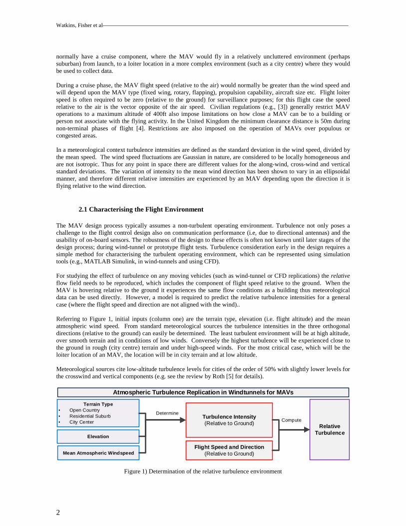
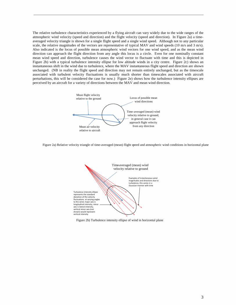
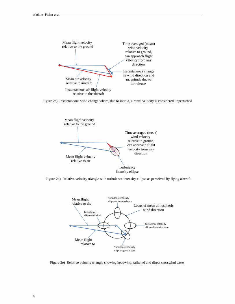
The relative turbulence characteristics experienced by a flying aircraft can vary widely due to the wide ranges of the atmospheric wind velocity (speed and direction) and the flight velocity (speed and direction). In Figure 2a) a time-averaged velocity triangle is shown for a single flight speed and a single wind speed. Although not to any particular scale, the relative magnitudes of the vectors are representative of typical MAV and wind speeds (10 m/s and 3 m/s). Also indicated is the locus of possible mean atmospheric wind vectors for one wind speed, and as the mean wind direction can approach the flight direction from any angle this locus is a circle. Even for one nominally constant mean wind speed and direction, turbulence causes the wind vector to fluctuate with time and this is depicted in Figure 2b) with a typical turbulence intensity ellipse for low altitude winds in a city centre. Figure 2c) shows an instantaneous shift in the wind due to turbulence, where the MAV instantaneous flight speed and direction are shown unchanged. (NB in reality the flight speed and direction may not remain entirely unchanged, but as the timescale associated with turbulent velocity fluctuations is usually much shorter than timescales associated with aircraft perturbations, this will be considered the case for now.) Figure 2e) shows how the turbulence intensity ellipses are perceived by an aircraft for a variety of directions between the MAV and mean wind direction.

Locus of possible meanwind directions

Mean flight velocity relative to the ground

Mean air velocity relative to aircraft

Time- averaged (mean) wind velocity relative to ground,

in general case it can approach flight velocity

from any direction

Figure 2a) Relative velocity triangle of time-averaged (mean) flight speed and atmospheric wind conditions in horizontal plane -

Time - averaged (mean) windvelocity relative to ground

Turbulence intensity ellipse

represents the standard

deviation of the velocity

fluctuations at varying angles

to the wind, major axis is

longitudinal intensity, minor

axis is lateral intensity,

vertical minor axis (not

shown) would represent

vertical intensity

Examples of instantaneous wind

magnitudes and directions due to

turbulence, this varies in a

Gaussian manner with time

Figure 2b) Turbulence intensity ellipse of wind in horizontal plane

Watkins, Fisher et al

4

Mean flight velocity relative to the ground

Mean air velocityrelative to aircraft

Time-averaged (mean)wind velocity

relative to ground,can approach flightvelocity from any

direction

Instantaneous change in wind direction and

magnitude due to turbulence

Instantaneous air flight velocityrelative to the aircraft

Figure 2c) Instantaneous wind change where, due to inertia, aircraft velocity is considered unperturbed

Mean flight velocity relative to the ground

Mean flight velocityrelative to air

Time- averaged (mean)wind velocity

relative to ground, can approach flightvelocity from any

direction

Turbulence intensity ellipse

Figure 2d) Relative velocity triangle with turbulence intensity ellipse as perceived by flying aircraft

Locus of mean atmospheric wind direction

Mean flight relative to the

Mean flight relative to

Turbulence intensity

ellipse – headwind case

Turbulence intensity

ellipse – general case

Turbulence

ellipse – tailwind

Turbulence intensity

ellipse – crosswind case

Figure 2e) Relative velocity triangle showing headwind, tailwind and direct crosswind cases

5

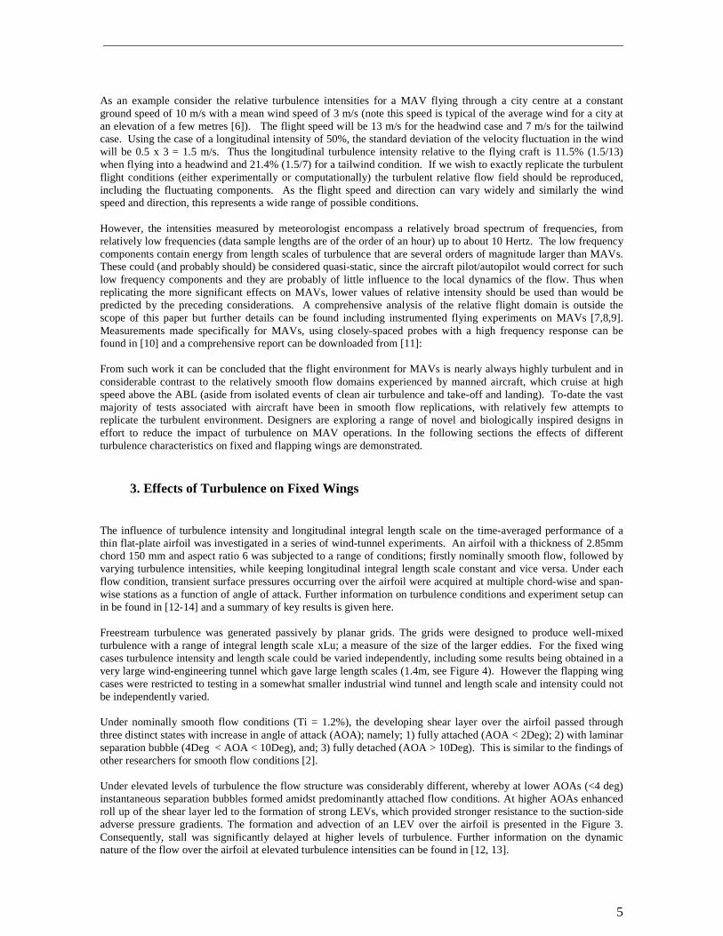
As an example consider the relative turbulence intensities for a MAV flying through a city centre at a constant ground speed of 10 m/s with a mean wind speed of 3 m/s (note this speed is typical of the average wind for a city at an elevation of a few metres [6]). The flight speed will be 13 m/s for the headwind case and 7 m/s for the tailwind case. Using the case of a longitudinal intensity of 50%, the standard deviation of the velocity fluctuation in the wind will be 0.5 x 3 = 1.5 m/s. Thus the longitudinal turbulence intensity relative to the flying craft is 11.5% (1.5/13) when flying into a headwind and 21.4% (1.5/7) for a tailwind condition. If we wish to exactly replicate the turbulent flight conditions (either experimentally or computationally) the turbulent relative flow field should be reproduced, including the fluctuating components. As the flight speed and direction can vary widely and similarly the wind speed and direction, this represents a wide range of possible conditions. However, the intensities measured by meteorologist encompass a relatively broad spectrum of frequencies, from relatively low frequencies (data sample lengths are of the order of an hour) up to about 10 Hertz. The low frequency components contain energy from length scales of turbulence that are several orders of magnitude larger than MAVs. These could (and probably should) be considered quasi-static, since the aircraft pilot/autopilot would correct for such low frequency components and they are probably of little influence to the local dynamics of the flow. Thus when replicating the more significant effects on MAVs, lower values of relative intensity should be used than would be predicted by the preceding considerations. A comprehensive analysis of the relative flight domain is outside the scope of this paper but further details can be found including instrumented flying experiments on MAVs [7,8,9]. Measurements made specifically for MAVs, using closely-spaced probes with a high frequency response can be found in [10] and a comprehensive report can be downloaded from [11]: From such work it can be concluded that the flight environment for MAVs is nearly always highly turbulent and in considerable contrast to the relatively smooth flow domains experienced by manned aircraft, which cruise at high speed above the ABL (aside from isolated events of clean air turbulence and take-off and landing). To-date the vast majority of tests associated with aircraft have been in smooth flow replications, with relatively few attempts to replicate the turbulent environment. Designers are exploring a range of novel and biologically inspired designs in effort to reduce the impact of turbulence on MAV operations. In the following sections the effects of different turbulence characteristics on fixed and flapping wings are demonstrated.

3. Effects of Turbulence on Fixed Wings

The influence of turbulence intensity and longitudinal integral length scale on the time-averaged performance of a thin flat-plate airfoil was investigated in a series of wind-tunnel experiments. An airfoil with a thickness of 2.85mm chord 150 mm and aspect ratio 6 was subjected to a range of conditions; firstly nominally smooth flow, followed by varying turbulence intensities, while keeping longitudinal integral length scale constant and vice versa. Under each flow condition, transient surface pressures occurring over the airfoil were acquired at multiple chord-wise and span-wise stations as a function of angle of attack. Further information on turbulence conditions and experiment setup can in be found in [12-14] and a summary of key results is given here. Freestream turbulence was generated passively by planar grids. The grids were designed to produce well-mixed turbulence with a range of integral length scale xLu; a measure of the size of the larger eddies. For the fixed wing cases turbulence intensity and length scale could be varied independently, including some results being obtained in a very large wind-engineering tunnel which gave large length scales (1.4m, see Figure 4). However the flapping wing cases were restricted to testing in a somewhat smaller industrial wind tunnel and length scale and intensity could not be independently varied. Under nominally smooth flow conditions (Ti = 1.2%), the developing shear layer over the airfoil passed through three distinct states with increase in angle of attack (AOA); namely; 1) fully attached (AOA < 2Deg); 2) with laminar separation bubble (4Deg < AOA < 10Deg), and; 3) fully detached (AOA > 10Deg). This is similar to the findings of other researchers for smooth flow conditions [2]. Under elevated levels of turbulence the flow structure was considerably different, whereby at lower AOAs (<4 deg) instantaneous separation bubbles formed amidst predominantly attached flow conditions. At higher AOAs enhanced roll up of the shear layer led to the formation of strong LEVs, which provided stronger resistance to the suction-side adverse pressure gradients. The formation and advection of an LEV over the airfoil is presented in the Figure 3. Consequently, stall was significantly delayed at higher levels of turbulence. Further information on the dynamic nature of the flow over the airfoil at elevated turbulence intensities can be found in [12, 13].

Watkins, Fisher et al

6

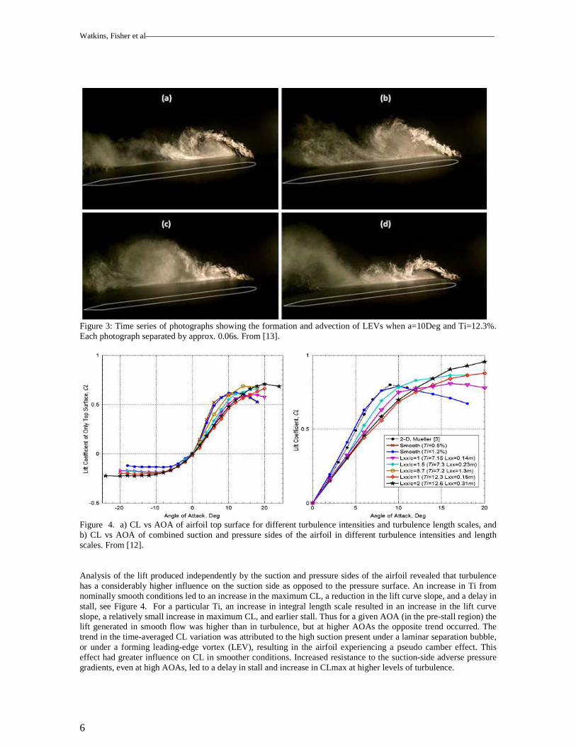
Figure 3: Time series of photographs showing the formation and advection of LEVs when a=10Deg and Ti=12.3%. Each photograph separated by approx. 0.06s. From [13].

Figure 4. a) CL vs AOA of airfoil top surface for different turbulence intensities and turbulence length scales, and b) CL vs AOA of combined suction and pressure sides of the airfoil in different turbulence intensities and length scales. From [12]. Analysis of the lift produced independently by the suction and pressure sides of the airfoil revealed that turbulence has a considerably higher influence on the suction side as opposed to the pressure surface. An increase in Ti from nominally smooth conditions led to an increase in the maximum CL, a reduction in the lift curve slope, and a delay in stall, see Figure 4. For a particular Ti, an increase in integral length scale resulted in an increase in the lift curve slope, a relatively small increase in maximum CL, and earlier stall. Thus for a given AOA (in the pre-stall region) the lift generated in smooth flow was higher than in turbulence, but at higher AOAs the opposite trend occurred. The trend in the time-averaged CL variation was attributed to the high suction present under a laminar separation bubble, or under a forming leading-edge vortex (LEV), resulting in the airfoil experiencing a pseudo camber effect. This effect had greater influence on CL in smoother conditions. Increased resistance to the suction-side adverse pressure gradients, even at high AOAs, led to a delay in stall and increase in CLmax at higher levels of turbulence.

7

Only pressure drag could be estimated from the measured surface pressures; in comparison to smooth flow a lower pressure drag was measured in turbulence at low AOAs while the pressure drag at higher AOAs was higher in elevated levels of turbulence. Turbulence intensity and length scale also had a considerable influence on the CM versus AOA variation of the airfoil [12]. An extended range of AOAs, whereby pitching moment coefficient remained close to zero, was noticed at higher levels of turbulence. At higher AOAs, however, Ti and length scale had an opposing influence on the rate of reduction of pitching moment coefficient with increased AOA.

4. Effects of Turbulence on Flapping Wings

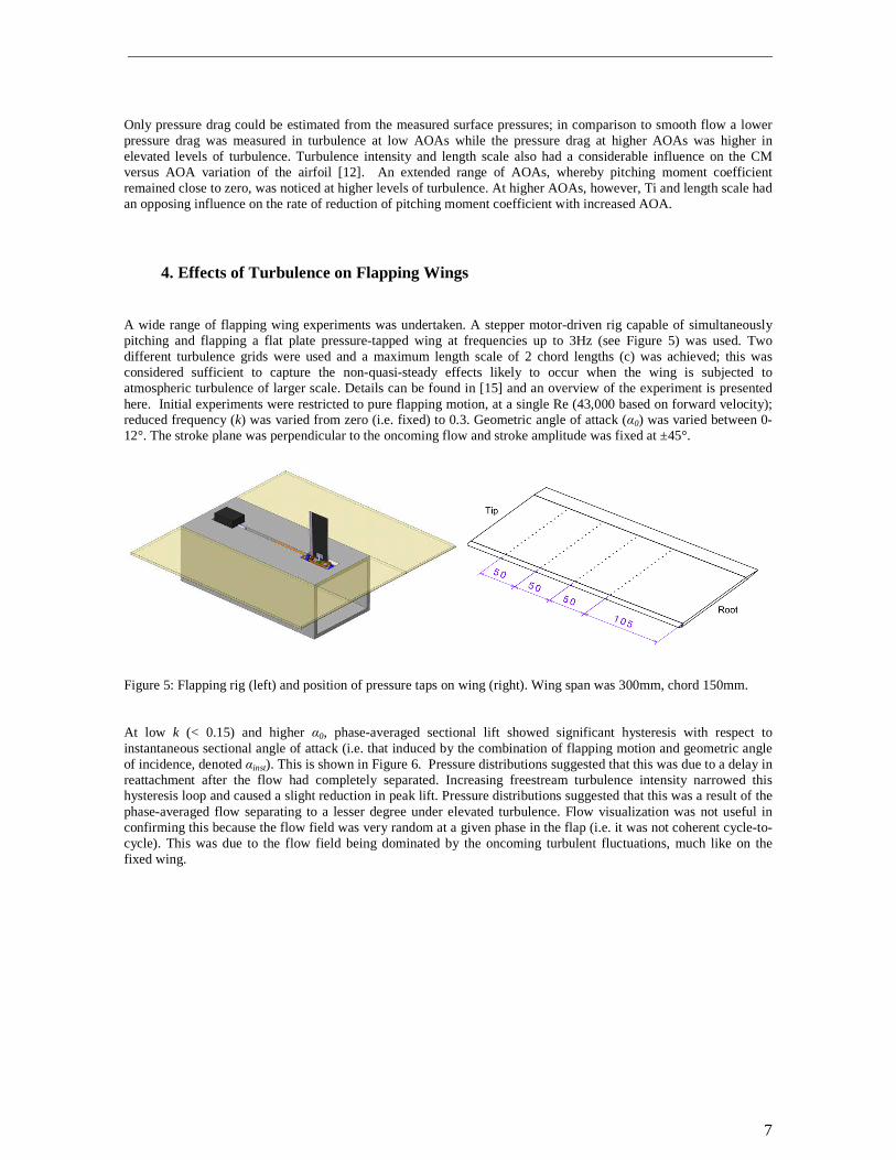
A wide range of flapping wing experiments was undertaken. A stepper motor-driven rig capable of simultaneously pitching and flapping a flat plate pressure-tapped wing at frequencies up to 3Hz (see Figure 5) was used. Two different turbulence grids were used and a maximum length scale of 2 chord lengths (c) was achieved; this was considered sufficient to capture the non-quasi-steady effects likely to occur when the wing is subjected to atmospheric turbulence of larger scale. Details can be found in [15] and an overview of the experiment is presented here. Initial experiments were restricted to pure flapping motion, at a single Re (43,000 based on forward velocity); reduced frequency (k) was varied from zero (i.e. fixed) to 0.3. Geometric angle of attack (α0) was varied between 0-12°. The stroke plane was perpendicular to the oncoming flow and stroke amplitude was fixed at ±45°.

Figure 5: Flapping rig (left) and position of pressure taps on wing (right). Wing span was 300mm, chord 150mm. At low k (< 0.15) and higher α0, phase-averaged sectional lift showed significant hysteresis with respect to instantaneous sectional angle of attack (i.e. that induced by the combination of flapping motion and geometric angle of incidence, denoted αinst). This is shown in Figure 6. Pressure distributions suggested that this was due to a delay in reattachment after the flow had completely separated. Increasing freestream turbulence intensity narrowed this hysteresis loop and caused a slight reduction in peak lift. Pressure distributions suggested that this was a result of the phase-averaged flow separating to a lesser degree under elevated turbulence. Flow visualization was not useful in confirming this because the flow field was very random at a given phase in the flap (i.e. it was not coherent cycle-to-cycle). This was due to the flow field being dominated by the oncoming turbulent fluctuations, much like on the fixed wing.

Watkins, Fisher et al

8

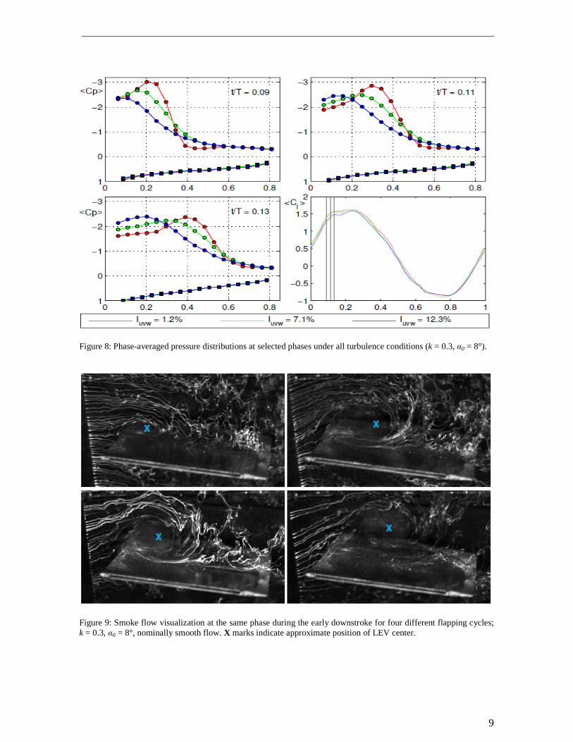
Figure 6: Phase-averaged sectional lift coefficient vs. αinst under several turbulence conditions; y/s = 0.51, α0 = 12°, k = 0.075. The relative effect of turbulence on phase-averaged sectional lift diminished as k increased, becoming negligible at most sections for k ≥ 0.225, although a very slight reduction in peak lift was still evident. Despite this negligible effect on lift, turbulence still significantly affected the phase-averaged pressure distributions. In nominally smooth flow, a leading edge vortex (LEV) was noticed for k ≥ 0.225 and the suction peak caused by it was clearly visible in the phase-averaged pressure distributions. This is illustrated in Figure 7. As freestream turbulence levels were increased, this suction peak became smoothed out and the point of peak suction moved forward. Figure 7 shows pressure distributions under all turbulence conditions at several phases in the early downstroke to illustrate this; note that phase-averaged pitching moment would be significantly more nose-up under elevated turbulence conditions.

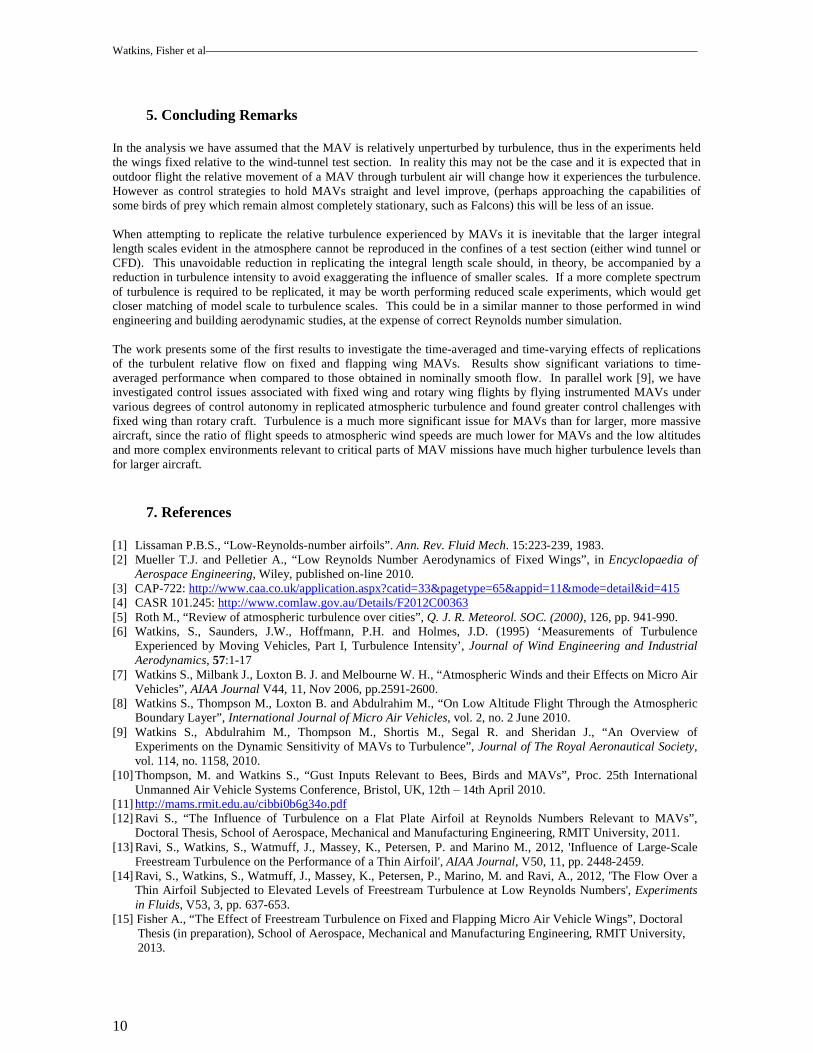
Figure 7: Smoke flow visualization showing LEV during early downstroke (left) and phase-averaged pressure distributions and lift during the early downstroke (right) (k = 0.3, α0 = 8°, nominally smooth flow). Note that t/T = 0 is defined as the start of the downstroke and colors indicate phase according to the position of the marker in the Cl vs. t/T plot. Flow visualisation showed that under turbulent conditions, as k was increased, the large-scale flow field during the early downstroke became more coherent from cycle-to-cycle at a given phase. However it was still much more random than that seen in nominally smooth flow. The smoothing of the phase-averaged LEV suction peak under elevated turbulence could be mistaken to indicate that a more diffuse LEV is being created consistently from cycle-to-cycle, this diffusion perhaps be ing enhanced by small-scale mixing from the oncoming turbulence. This was not the case; rather it was the result of the LEV timing and strength varying from cycle-to-cycle, these variations being induced by large-scale fluctuations in the oncoming turbulent flow. This cycle-to-cycle variation in LEV characteristics is illustrated in Figure 8. Note that while LEV size and position could not be linked quantitatively to oncoming fluctuations, it is clearly visible in Figure 8 that a lower oncoming flow angle (top left, indicated by the lower angle of smoke filaments coming off the wire along its length) causes a delay in LEV formation, causing it to be smaller at a given phase, and vice versa.

9

Figure 8: Phase-averaged pressure distributions at selected phases under all turbulence conditions (k = 0.3, α0 = 8°).

Figure 9: Smoke flow visualization at the same phase during the early downstroke for four different flapping cycles; k = 0.3, α0 = 8°, nominally smooth flow. X marks indicate approximate position of LEV center.

Watkins, Fisher et al

10

5. Concluding Remarks

In the analysis we have assumed that the MAV is relatively unperturbed by turbulence, thus in the experiments held the wings fixed relative to the wind-tunnel test section. In reality this may not be the case and it is expected that in outdoor flight the relative movement of a MAV through turbulent air will change how it experiences the turbulence. However as control strategies to hold MAVs straight and level improve, (perhaps approaching the capabilities of some birds of prey which remain almost completely stationary, such as Falcons) this will be less of an issue. When attempting to replicate the relative turbulence experienced by MAVs it is inevitable that the larger integral length scales evident in the atmosphere cannot be reproduced in the confines of a test section (either wind tunnel or CFD). This unavoidable reduction in replicating the integral length scale should, in theory, be accompanied by a reduction in turbulence intensity to avoid exaggerating the influence of smaller scales. If a more complete spectrum of turbulence is required to be replicated, it may be worth performing reduced scale experiments, which would get closer matching of model scale to turbulence scales. This could be in a similar manner to those performed in wind engineering and building aerodynamic studies, at the expense of correct Reynolds number simulation. The work presents some of the first results to investigate the time-averaged and time-varying effects of replications of the turbulent relative flow on fixed and flapping wing MAVs. Results show significant variations to time-averaged performance when compared to those obtained in nominally smooth flow. In parallel work [9], we have investigated control issues associated with fixed wing and rotary wing flights by flying instrumented MAVs under various degrees of control autonomy in replicated atmospheric turbulence and found greater control challenges with fixed wing than rotary craft. Turbulence is a much more significant issue for MAVs than for larger, more massive aircraft, since the ratio of flight speeds to atmospheric wind speeds are much lower for MAVs and the low altitudes and more complex environments relevant to critical parts of MAV missions have much higher turbulence levels than for larger aircraft.

7. References

[1] Lissaman P.B.S., “Low-Reynolds-number airfoils”. Ann. Rev. Fluid Mech. 15:223-239, 1983. [2] Mueller T.J. and Pelletier A., “Low Reynolds Number Aerodynamics of Fixed Wings”, in Encyclopaedia of

Aerospace Engineering, Wiley, published on-line 2010. [3] CAP-722: http://www.caa.co.uk/application.aspx?catid=33&pagetype=65&appid=11&mode=detail&id=415 [4] CASR 101.245: http://www.comlaw.gov.au/Details/F2012C00363 [5] Roth M., “Review of atmospheric turbulence over cities”, Q. J. R. Meteorol. SOC. (2000), 126, pp. 941-990. [6] Watkins, S., Saunders, J.W., Hoffmann, P.H. and Holmes, J.D. (1995) ‘Measurements of Turbulence

Experienced by Moving Vehicles, Part I, Turbulence Intensity’, Journal of Wind Engineering and Industrial Aerodynamics, 57:1-17

[7] Watkins S., Milbank J., Loxton B. J. and Melbourne W. H., “Atmospheric Winds and their Effects on Micro Air Vehicles”, AIAA Journal V44, 11, Nov 2006, pp.2591-2600.

[8] Watkins S., Thompson M., Loxton B. and Abdulrahim M., “On Low Altitude Flight Through the Atmospheric Boundary Layer”, International Journal of Micro Air Vehicles, vol. 2, no. 2 June 2010.

[9] Watkins S., Abdulrahim M., Thompson M., Shortis M., Segal R. and Sheridan J., “An Overview of Experiments on the Dynamic Sensitivity of MAVs to Turbulence”, Journal of The Royal Aeronautical Society, vol. 114, no. 1158, 2010.

[10] Thompson, M. and Watkins S., “Gust Inputs Relevant to Bees, Birds and MAVs”, Proc. 25th International Unmanned Air Vehicle Systems Conference, Bristol, UK, 12th – 14th April 2010.

[11] http://mams.rmit.edu.au/cibbi0b6g34o.pdf [12] Ravi S., “The Influence of Turbulence on a Flat Plate Airfoil at Reynolds Numbers Relevant to MAVs”,

Doctoral Thesis, School of Aerospace, Mechanical and Manufacturing Engineering, RMIT University, 2011. [13] Ravi, S., Watkins, S., Watmuff, J., Massey, K., Petersen, P. and Marino M., 2012, 'Influence of Large-Scale

Freestream Turbulence on the Performance of a Thin Airfoil', AIAA Journal, V50, 11, pp. 2448-2459. [14] Ravi, S., Watkins, S., Watmuff, J., Massey, K., Petersen, P., Marino, M. and Ravi, A., 2012, 'The Flow Over a

Thin Airfoil Subjected to Elevated Levels of Freestream Turbulence at Low Reynolds Numbers', Experiments in Fluids, V53, 3, pp. 637-653.

[15] Fisher A., “The Effect of Freestream Turbulence on Fixed and Flapping Micro Air Vehicle Wings”, Doctoral Thesis (in preparation), School of Aerospace, Mechanical and Manufacturing Engineering, RMIT University, 2013.