The Term Structure of Real Rates andExpected Inflation∗

Andrew Ang†

Columbia University and NBER

Geert Bekaert‡

Columbia University, CEPR and NBER

Min Wei§

Federal Reserve Board of Governors

This Version: 14 November 2006

∗We thank Kobi Boudoukh, Qiang Dai, Rob Engle, Martin Evans, Rene Garcia, Bob Hodrick,Refet Gurkaynak, Monika Piazzesi, Bill Schwert, Ken Singleton, Peter Vlaar, and Ken West forhelpful discussions, and seminar participants at the American Finance Association, Asian FinanceAssociation, Barclays Capital Annual Global Inflation-Linked Conference, CIREQ and CIRANO-MITACS conference on Macroeconomics and Finance, Empirical Finance Conference at the LSE,European Finance Association, FRBSF-Stanford University conference on Interest Rates and MonetaryPolicy, Washington University-St Louis Federal Reserve conference on State-Space Models, Regime-Switching and Identification, Bank of England, Bank of Norway, Campbell and Company, Universityof Amsterdam, Columbia University, Cornell University, Erasmus University, European Central Bank,Federal Reserve Board of Governors, Financial Engines, HEC Lausanne, Indiana University, IMF,London Business School, NYU, Oakhill Platinum Partners, PIMCO, Tilburg University, UCL-COREat Louvain-la-Neuve, University of Gent, University of Illinois, University of Michigan, University ofRochester, University of Washington, UCLA, UC Riverside, UC San Diego, USC, and the World Bank.Andrew Ang and Geert Bekaert both acknowledge funding from the National Science Foundation.

†Columbia Business School, 802 Uris Hall, 3022 Broadway, New York, NY 10027; ph: (212) 854-9154; fax: (212) 662-8474; email: aa610@columbia.edu; www.columbia.edu/∼aa610.

‡Columbia Business School, 802 Uris Hall, 3022 Broadway, New York, NY 10027; ph: (212) 854-9156; fax: (212) 662-8474; email: gb241@columbia.edu; www.gsb.columbia.edu/faculty/gbekaert/

§Board of Governors of the Federal Reserve System, Division of Monetary Affairs, Washington,DC 20551; ph: (202) 736-5619; email: min.wei@frb.gov; www.federalreserve.gov/research/staff/weiminx.htm

Abstract

Changes in nominal interest rates must be due to either movements in real interest rates,

expected inflation, or the inflation risk premium. We develop a term structure model with

regime switches, time-varying prices of risk, and inflation to identify these components of the

nominal yield curve. We find that the unconditional real rate curve in the U.S. is fairly flat

around 1.3%. In one real rate regime, the real term structure is steeply downward sloping.

An inflation risk premium that increases with maturity fully accounts for the generally upward

sloping nominal term structure.

1 Introduction

The real interest rate and expected inflation are two key economic variables; yet, their dynamic

behavior is essentially unobserved. A large empirical literature has yielded surprisingly few

generally accepted stylized facts. For example, whereas theoretical research often assumes

that the real interest rate is constant, empirical estimates for the real interest rate process vary

between constancy (Fama, 1975), mean-reverting behavior (Hamilton, 1985), or a unit root

process (Rose, 1988). There seems to be more consensus on the fact that real rate variation,

if it exists at all, should only affect the short end of the term structure but that the variation in

long-term interest rates is primarily affected by shocks to expected inflation (see, among others,

Mishkin, 1990; Fama, 1990), but this is disputed by Pennacchi (1991). Another phenomenon

that has received wide attention is the Mundell (1963) and Tobin (1965) effect: the correlation

between real rates and (expected) inflation appears to be negative.

In this article, we seek to establish a comprehensive set of stylized facts regarding real rates,

expected inflation and inflation risk premiums, and to determine their relative importance for

determining the U.S. nominal term structure. To infer the behavior of these variables, we use a

model with three distinguishing features. First, we specify a no-arbitrage term structure model

with both nominal bond yields and inflation data to efficiently identify the term structure of

real rates and inflation risk premia. Second, our model accommodates regime-switching (RS)

behavior, but still produces closed-form solutions for bond prices. We go beyond the extant

RS literature by attempting to identify the real and nominal sources of the regime switches.

Third, the model accommodates flexible time-varying risk premiums crucial for matching time-

varying bond premia (see, for example, Dai and Singleton, 2002). These features allow our

model to fit the dynamics of inflation and nominal interest rates.

This paper is organized as follows. Section 2 develops the model and discusses the effect of

regime switches on real yields and inflation risk premia. In Section 3, we detail the specification

tests used to select the best model, analyze factor dynamics, and report parameter estimates.

Section 4 contains the main economic results, which can be summarized as follows:

1. Unconditionally, the term structure of real rates assumes a fairly flat shape around 1.3%,

with a slight hump, peaking at a 1-year maturity. However, there are some regimes in

which the real rate curve is downward sloping.

2. Real rates are quite variable at short maturities but smooth and persistent at long

maturities. There is no significant real term spread.

3. The real short rate is negatively correlated with both expected and unexpected inflation,

1

but the statistical evidence for a Mundell-Tobin effect is weak.

4. The model matches an unconditional upward-sloping nominal yield curve by generating

an inflation risk premium that is increasing in maturity.

5. Nominal interest rates do not behave pro-cyclically across NBER business cycles but our

model-implied real rates do.

6. The decompositions of nominal yields into real yields and inflation components at various

horizons indicate that variation in inflation compensation (expected inflation and inflation

risk premia) explains about 80% of the variation in nominal rates at both short and long

maturities.

7. Inflation compensation is the main determinant of nominal interest rate spreads at long

horizons.

Finally, Section 5 concludes.

2 A Real and Nominal Term Structure Model with Regime

Switches

2.1 Decomposing Nominal Yields

The nominal yield on a zero-coupon bond of maturityn, ynt , can be decomposed into a real

yield, ynt , and inflation compensation,πe

t,n. The real yield represents the yield on a zero-coupon

bond perfectly indexed against inflation.1 Inflation compensation reflects expected inflation,

Et(πt+n,n), and an inflation risk premium,ϕt,n (ignoring Jensen’s inequality terms):

ynt = yn

t + πet,n

= ynt + Et(πt+n,n) + ϕt,n, (1)

whereEt(πt+n,n) is expected inflation fromt to t + n:

Et(πt+n,n) =1

nEt(πt+1 + · · ·+ πt+n),

1 Since real interest rates can be defined as real returns on investment, an alternative literature estimates real

interest rates by using models of capital and productivity. However, this approach produces very imprecise

estimates of real rates with substantial measurement error and often still uses interest rate data to help identification

(see Laubach and Williams, 2003).

2

andπt+1 is one-period inflation fromt to t + 1.

The goal of this article is to achieve this decomposition of nominal yields,ynt , into real and

inflation components (ynt , Et(πt+n,n), andϕt,n) for U.S. data. Unfortunately, we do not observe

real rates for most of the U.S. sample. Inflation-indexed bonds (the Treasury Income Protection

Securities or TIPS) have traded only since 1997 and the market faced considerable liquidity

problems in its early days (see Roll, 2004). Consequently, our endeavor faces an obvious

identification problem as we must estimate two unknown quantities – real rates and inflation

risk premia – from only nominal yields. We obtain identification by using a no-arbitrage term

structure model that imposes restrictions on the nominal term structure. That is, the movements

of long-term nominal yields are linked both to the dynamics of short-term nominal yields and

inflation. These pricing restrictions, together with standard parameter identification restrictions,

uniquely identify the dynamics of real rates and inflation risk premiums using data on inflation

and nominal yields. To pin down the average level of real rates, we further restrict the one-

period inflation risk premium to be zero.

The remainder of this section sets up the model to identify the various components of

nominal yields. Section 2.2 presents the technical details of the term structure model, while

at the same time discussing the economic background of the term structure factors and our

parametric assumptions. The model must be flexible, yet remain identifiable from a finite set

of nominal yields. Importantly, both the empirical literature and economic logic suggests that

the process generating inflation and real rates may undergo discrete shifts over time, which

we model using a regime switching model following Hamilton (1990). We present solutions

to bond prices in Section 2.3 and discuss how regime switches affect our decomposition in

Section 2.4. Section 2.5 briefly covers econometric and identification issues. Finally, Section

2.6 discusses how our work relates to the literature.

2.2 The Model

State Variable Dynamics

We employ a three-factor representation of yields, which is the number of factors often used to

match term structure dynamics in the finance literature (see, for example, Dai and Singleton,

2000). We incorporate an observed inflation factor, denoted byπt, which switches regimes.

The other two factors are unobservable term structure factors. One factor,ft, represents a latent

RS term structure factor. The other latent factor is denoted byqt and represents a time-varying,

but regime-invariant, price of risk factor, which directly enters into the risk prices (see below).

The factorqt plays two roles. First, it helps generate realistic and plausible time-variation in

3

expected excess returns on long-term bonds,2 as demonstrated by Dai and Singleton (2002).

Second,qt also accounts for part of the time-variation of inflation risk premia, as we show

below.

We stack the state variables in the3 × 1 vectorXt = (qt ft πt)′, which follows the RS

process:

Xt+1 = µ(st+1) + ΦXt + Σ(st+1)εt+1, (2)

wherest+1 indicates the regime prevailing at timet + 1 and

µ(st) =

µq

µf (st)

µπ(st)

, Φ =

Φqq 0 0

Φfq Φff 0

Φπq Φπf Φππ

, Σ(st) =

σq 0 0

0 σf (st) 0

0 0 σπ(st)

. (3)

The regime variable representsK different regimes,st = 1, . . . , K, and follows a Markov

chain with transition probability matrixΠ = pij = Pr(st+1 = j|st = i). These regimes are

independent of the shocksεt+1 in equation (2). We specify all the transition probabilities to be

constant.3

In equation (3), the conditional mean and volatility offt andπt switch regimes, but the

conditional mean and volatility ofqt do not. The feedback parameters for all variables in the

companion formΦ also do not switch across regimes. These restrictions are necessary to permit

closed-form solutions for bond prices.

We order the factors so that the latent factors appear first. As a consequence, expected

inflation depends on lagged inflation, other information captured by the latent variables, as well

as a non-linear drift term. The inflation forecasting literature strongly suggests that expected

inflation depends on more than just lagged inflation (see, for example, Stockton and Glassman,

1987). In addition, by placing inflation last in the system, the reduced-form process for inflation

involves moving average terms. This is important because the autocorrelogram of inflation is

empirically well approximated by a low-order ARMA process.

2 Fama and Bliss (1987), Campbell and Shiller (1991), Bekaert, Hodrick and Marshall (1997), and Cochrane

and Piazzesi (2005), among many others, document time-variation in expected excess holding period returns of

long-term bonds.3 Transition probabilities must be constant under the risk-neutral measure to obtain closed-form solutions for

bond prices. A price of RS risk can only be identified if the transition probabilities vary through time. Dai,

Singleton and Yang (2006) allow transition probabilities to vary under the real measure, and then define the price of

RS risk to perfectly offset the time-varying component of the probability to obtain a constant transition probability

under the risk-neutral measure. It is hard to motivate this assumption with an equilibrium model. In contrast, our

model can be supported by a representative agent economy with a utility function with habit, and a RS endowment

process.

4

Real Short Rate Dynamics

We specify the real short rate,rt, to be affine in the state variables:

rt = δ0 + δ′1Xt. (4)

For reference, we letδ1 = (δq δf δπ)′. The real rate process nests the special cases of a constant

real rate (δ1 = 03×1) advocated by Fama (1975) and mean-reverting real rates within a single

regime (δf = δπ = 0) following Hamilton (1985). Allowing non-zeroδf or δπ causes the real

rate to switch regimes. Ifδq 6= 0, then the time-varying price of risk can directly influence the

real rate, as it would in any equilibrium model with growth. In general, ifδπ 6= 0, then money

neutrality is rejected, and real interest rates are functions of inflation.

The model allows for arbitrary correlation between the real rate and inflation. To gain some

intuition, we compute the conditional covariance between real rates and actual or expected

inflation for an affine model without regime switches. First,δπ primarily drives the covariance

between real rates and unexpected inflation. That is, covt(rt+1, πt+1) = δπσ2π. Second, without

regimes, the covariance between expected inflation and real rates is given by:

covt(rt+1, Et+1(πt+2)) = δqΦπqσ2q + δfΦπfσ

2f + δπΦππσ2

π.

The Mundell-Tobin effect predicts this covariance to be negative, whereas an activist Taylor

(1993) rule would predict it to be positive, as the monetary authority raises real rates in response

to high expected inflation (see, for example, Clarida, Gali and Gertler, 2000). Clearly, the sign

of the covariance is parameter dependent, and a negativeδπ does not suffice to obtain a Mundell-

Tobin effect.

To compare the conditional covariance between real rates and expected inflation in our

model with regimes, we derive covt(rt+1, Et+1(πt+2)|st = i) for K = 2 regimes to be:

covt(rt+1, Et+1(πt+2)|st = i) = δqΦπqσ2q

+ δfΦπf

[2∑

j=1

pijσ2f (j) + pi1pi2(µf (1)− µf (2))2

]

+ δπΦππ

[2∑

j=1

pijσ2π(j) + pi1pi2(µπ(1)− µπ(2))2

]

+ δfδπΦπfΦππpi1pi2[(µπ(1)− µπ(2))(µf (1)− µf (2))].

Relative to the one-regime model, the contribution of the factor variances for the RS factors

now depends on the regime prevailing at timet and has two components: an average of the

5

two regime-dependent factor variances and a term measuring the volatility impact of a change

in the regime-dependent drifts. In addition, there is a new factor contributing to the covariance

coming from the covariance between these regime-dependent drifts forft andπt.

Pricing Kernel and Prices of Risk

We specify the real pricing kernel to take the form:

mt+1 = log Mt+1 = −rt − 1

2λt(st+1)

′λt(st+1)− λt(st+1)′εt+1 (5)

where the vector of time-varying and regime-switching prices of riskλt(st+1) is given by:

λt(st+1) = (γt λ(st+1)′)′,

whereλ(st+1) is a 2 × 1 vector of RS prices of riskλ(st+1) = (λf (st+1) λπ(st+1))′ and the

scalarγt takes the form:

γt = γ0 + γ1qt = γ0 + γ1e′1Xt, (6)

whereei represents a vector of zeros with a 1 in theith position. In this formulation, the prices

of risk of ft andπt change across regimes. The variableqt controls the time-variation of the

price of risk associated withγt in (6) but does not switch regimes. Allowingγt to switch across

regimes results in the loss of closed-form solutions for bond prices.

We formulate the nominal pricing kernel in the standard way asMt+1 = Mt+1Pt/Pt+1:

mt+1 = log Mt+1 = −rt − 1

2λt(st+1)

′λt(st+1)− λt(st+1)′εt+1 − e′3Xt+1. (7)

Real Factor and Inflation Regimes

We introduce two different regime variables,sft ∈ 1, 2, affecting the drift and variance of

theft process, andsπt ∈ 1, 2, affecting the drift and variance of the inflation process. Since

both theft andπt factors enter the real short rate in equation (4), the real short rate contains

bothft andπt regime components. This modeling choice accommodates the possibility thatsft

captures changes of regimes in real factors. Sinceft enters the conditional mean of inflation in

equation (2), theft regime also potentially affects expected inflation and can capture non-linear

expected inflation components not directly related to past inflation realizations.

The model withsft and sπ

t can be rewritten using an aggregate regime variablest ∈1, 2, 3, 4 to account for all possible combinations ofsf

t , sπt = (1, 1) , (1, 2) , (2, 1) , (2, 2).

Hence, our model hasK = 4 regimes. To reduce the number of parameters in the4×4 transition

probability matrix, we consider three restricted models of the correlation betweensft andsπ

t .

6

Case A represents the simplest case of independent regimes. In Cases B and C, thesft andsπ

t

regimes are correlated.

In Case B, the currentft regime depends on the contemporaneous realization of the inflation

regime and on the pastft−1 regime. Nevertheless, the future inflation regime only depends on

current inflation. Case B could represent a reduced-form description of a monetary authority

changing real rates, through the latent factorft, in response to inflation shocks. We describe this

case more fully in Appendix A. However, one shortcoming of Case B is that it cannot capture

periods where aggressive real rates, through a regime with highft, would successfully stave off

a regime of high inflation.

In Case C, the inflation regime att + 1 depends on the stance of theft+1 regime as well as

the previous inflation environment, but we restrict futureft+1 regimes to depend only on current

ft regimes. This leads to the following conditional transition probability:

Pr(sft+1 = j, sπ

t+1 = k|sft = m, sπ

t = n)

= Pr(sπt+1 = k|sf

t+1 = j, sft = m, sπ

t = n)× Pr(sft+1 = j|sf

t = m, sπt = n)

= Pr(sπt+1 = k|sf

t+1 = j, sπt = n)× Pr(sf

t+1 = j|sft = m), (8)

where we assume thatPr(sπt+1|sf

t+1, sft , s

πt ) = Pr(sπ

t+1|sft+1, s

πt ) and Pr(sf

t+1|sft , s

πt ) =

Pr(sft+1|sf

t ). We denotePr(sft+1 = 1|sf

t = 1) = pf andPr(sft+1 = 2|sf

t = 2) = qf and

parameterizePr(sπt+1 = k|sf

t = m, sπt = n) asp“j”,“m”, where:

j =

A if sπt+1 = sf

t+1 = 1

B if sπt+1 = sf

t+1 = 2.

The “j”-component captures (potentially positive) correlation between theft andπt regimes.

The “m”- component captures persistence inπt regimes:

m =

A if sπt = 1

B if sπt = 2.

This formulation can capture instances where a high real rate regime, as captured by theft

regime, contemporaneously influences the inflation regime. Using the notation introduced

above, the transition probability matrixΠ for Case C takes the form:

[st+1 = 1] [st+1 = 2] [st+1 = 3] [st+1 = 4]

[st = 1] pfpAA pf(1− pAA

) (1− pf

) (1− pBA

) (1− pf

)pBA

[st = 2] pfpAB pf(1− pAB

) (1− pf

) (1− pBB

) (1− pf

)pBB

[st = 3](1− qf

)pAA

(1− qf

) (1− pAA

)qf

(1− pBA

)qfpBA

[st = 4](1− qf

)pAB

(1− qf

) (1− pAB

)qf

(1− pBB

)qfpBB

7

This model has four additional parameters relative to the model with independent real and

inflation regimes. We can test Case C against the null of the independent regime Case A by

testing the restrictions:

H0 : pBA = 1− pAA andpBB = 1− pAB.

We find evidence to reject the case of independent regimes in favor of Case C with a p-value of

0.033. Thus, our benchmark specification uses the probability transition matrix of Case C.

2.3 Bond Prices

Our model produces closed-form solutions for bond prices, enabling both efficient estimation

and the ability to fully characterize real and nominal yields at all maturities without discretiza-

tion error.

Real Bond Prices

In our model, the real zero coupon bond price of maturityn conditional on regimest = i,

P nt (st = i), is given by:

P nt (i) = exp(An(i) + BnXt), (9)

whereAn(i) is dependent on regimest = i, Bn is a1 × N vector andN is the total number

of factors in the model, including inflation. The expressions forAn(i) and Bn are given in

Appendix C. Since the real bond prices are given by (9), it follows that the real yieldsynt (i)

conditional on regimei are affine functions ofXt:4

ynt (i) = − log(P n

t )

n= − 1

n(An(i) + BnXt). (10)

While the expressions forAn(i) andBn are complex, some intuition can be gained on how

the prices of risk affect each term. The prices of riskγ0 andλ(st) enter only the constant term in

the yieldsAn(st), but affect this term in all regimes. More negative values ofγ0 or λ(st) cause

long maturity yields to be, on average, higher than short maturity yields. In addition, since the

λ(st) terms differ across regimes,λ(st) also controls the regime-dependent level of the yield

curve away from the unconditional shape of the yield curve. Thus, the model can accommodate

the switching signs of term premiums documented by Boudoukh et al. (1999). The prices of

4 The technical innovation in deriving (9) is to recognize that theBn parameter does not switch for two reasons.

First,Φ remains constant across regimes. Second, the time-varying price of risk parameterγ1 also does not switch

across regimes. If these parameters become regime-dependent, closed-form bond solutions are no longer possible.

8

risk affect the time-variation in the yields through the parameterγ1. This term only enters the

Bn terms. A more negativeγ1 means that long-term yields respond more to shocks in the price

of risk factorqt.

The pricing implications of (10), together with the assumed dynamics ofXt in (2), imply

that the autoregressive dynamics of inflation and bond yields are constant over time, but the

drifts vary through time, and shocks to inflation and real yields are heteroskedastic. Hence,

our model is consistent with the macro models of Sims (1999, 2001) and Bernanke and

Mihov (1998), who stress changing drifts, for example induced by changes in monetary policy,

and heteroskedastic shocks. On the other hand, Cogley and Sargent (2001, 2005) advocate

models with changes in the feedback parameters, for example induced by changes in systematic

monetary policy, which we do not accommodate.

Nominal Bond Prices

Nominal bond prices take the form:

P nt (i) = exp(An(i) + BnXt) (11)

for P nt (i), the zero-coupon bond price of a nominaln-period bond conditional on regimei. The

scalarAn(i) is dependent on regimest = i andBn is an1 × N vector. It follows that the

nominaln-period yield conditional on regimei, ynt (i), is an affine function ofXt:

ynt (i) = − log(P n

t )

n= − 1

n(An(i) + BnXt). (12)

Appendix D shows that the only difference between theAn(i) andBn terms for real bond prices

and theAn(i) andBn terms for nominal bond prices are due to terms that select inflation from

Xt. Positive inflation shocks decrease nominal bond prices.

2.4 The Effect of Regime Switches

The key ingredient differentiating our model from the standard affine term structure paradigm

is the presence of regimes. In this section, we develop intuition on how regimes affect the

decomposition of nominal rates into real rate and inflation components.

Expected Inflation

In our model, one-period expected inflation,Et(πt+1), takes the form:

Et(πt+1|st = i) = e′3E[µ(st+1)|st = i] + e′3ΦXt

=

(K∑

j=1

pij µπ(j)

)+ e′3ΦXt. (13)

9

This process is only different from a simple linear process because of the non-linear drift,

which can accommodate sudden discrete changes in expected inflation. Because expected

inflation depends onft andπt, the contemporaneoussft andsπ

t regimes also both affect expected

inflation.

Inflation Compensation

With only one regime, one-period inflation compensation,πet,1 = y1

t − rt, is given by:

πet,1 =

(µπ − 1

2σ2

π − σπλπ

)+ e′3ΦXt.

With regimes, inflation compensation is more complex:

πet,1(i) = − log

[K∑

j=1

pij exp

(−µπ(j) +

1

2σ2

π(j) + σπ(j)λπ(j)

)]+ e′3ΦXt, (14)

The last term in the exponential represents the one-period inflation risk premium, which is

zero by assumption in our model. The12σ2

π(j) term is the standard Jensen’s inequality term,

which now becomes regime-dependent. The−µπ(st) term represents the non-linear, regime-

dependent part of expected inflation. The last terme′3ΦXt represents the time-varying part of

expected inflation, which does not switch across regimes, and is the only term that is the same

as in the affine model.

In comparing expected inflation in equation (13) with inflation compensation in equation

(14), we see that the constant terms forπet,1 andEt(πt+1|st) are different. The constants in

the inflation compensation expression (14) reflect both a Jensen’s inequality term12σ2

π(st) and a

non-linear term, driven by taking the log of a sum, weighted by transition probabilities. Because

exp(.) is a convex function, Veronesi and Yared (1999) call this effect a “convexity bias.” Like

the Jensen’s term, this also makesπet,1 < Et(πt+1). In our estimations, both the Jensen’s term

and the convexity bias amount to less than 1 basis point, even for longer maturities.

Real Term Spreads

The intuition for how regimes affect real term spreads can be readily gleaned from considering

a two-period real bond. We first analyze the case of the real term spread,y2t − rt, in an affine

model without regime switches:

y2t − rt =

1

2(Et(rt+1)− rt)− 1

4vart (rt+1) +

1

2covt (mt+1, rt+1) . (15)

The first term(Et(rt+1) − rt) is an Expectations Hypothesis (EH) term, the second term

vart (rt+1) is a Jensen’s inequality term and the last term, covt(mt+1, rt+1), is the risk premium.

10

In the single-regime affine setting, the last term is given by:

covt(mt+1, rt+1) = −γ0σq − λfσf − γ1σqqt. (16)

Hence, the price of risk factorqt determines the time variation in the term premium.

The RS model has a more complex expression for the two-period real term spread:

y2t (i)− rt =

1

2(Et(rt+1|st = i)− rt)− 1

2(γ0σq + γ1σqqt)

− 1

2log

(K∑

j=1

pij exp[−δ′1

(µ(j)− E [µ(st+1)|st = i]

)

+1

2δ′1Σ(j)Σ(j)′δ1 + λf (j)σf (j)

]), (17)

for K regimes. First, the term spread now switches across regimes, explicitly shown by the

dependence ofy2t (i) on regimest = i. Not surprisingly, the EH term(Et(rt+1|st = i) − rt)

now switches across regimes. The time-varying price of risk term,−12(γ0σq + γ1σqqt), is the

same as in (16) because the process forqt does not switch regimes. The remaining terms in

(17) are non-linear, as they involve the log of the sum of an exponential function of regime-

dependent terms, weighted by transition probabilities. Within the non-linear expression, the

term 12δ′1Σ(j)Σ(j)′δ1 represents a Jensen’s inequality term, which is regime-dependent, and

λf (j)σf (j) represents a RS price of risk term. Thus, the average slope of the real yield curve can

potentially change across regimes and produce a variety of regime-dependent shapes of the real

yield curve, including flat, inverse-humped, upward-sloping or downward-sloping yield curves.

A new term in (17) that does not have a counterpart in (16) is−δ′1(µ(j)− E [µ (st+1) |st = i]),

reflecting the “jump risk” of a change in the regime-dependent drift.

Inflation Risk Premia

The riskiness of nominal bonds is driven by the covariance between the real kernel and inflation:

if inflation is high (purchasing power is low) when the pricing kernel realization (marginal

utility in an equilibrium model) is high, nominal bonds are risky and the inflation risk premium

is positive. It is tempting to conclude that the sign of the inflation risk premium determines

the correlation between expected inflation and real rates. For example, a Mundell-Tobin

effect implies that when a bad shock is experienced (an increase in real rates), the holders

of nominal bonds experience a countervailing effect, namely a decrease in expected inflation,

which increases nominal bond prices. This intuition is not completely correct as we now

discuss.

Consider the two-period pricing kernel, which depends on real rates both through its

conditional mean and through real rate innovations. Interestingly, the effects of these two

11

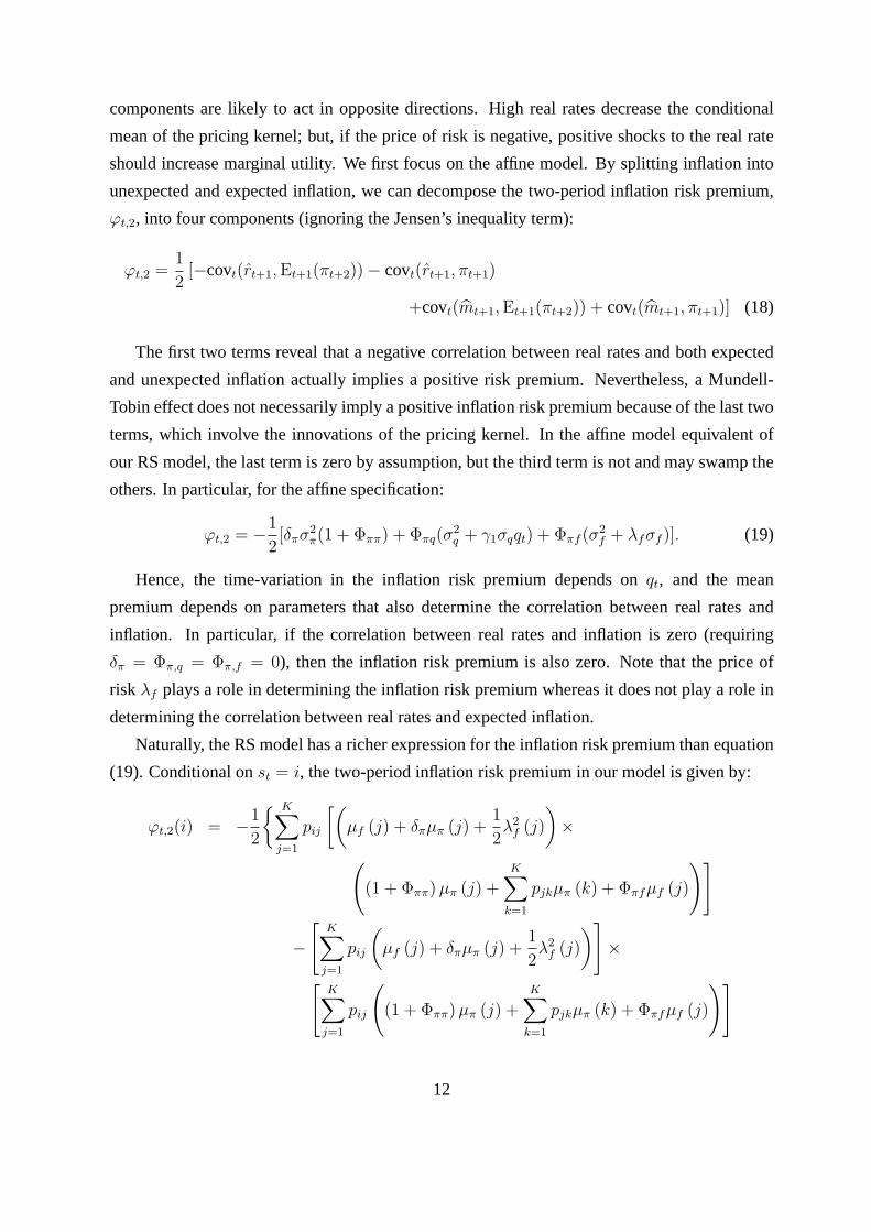
components are likely to act in opposite directions. High real rates decrease the conditional

mean of the pricing kernel; but, if the price of risk is negative, positive shocks to the real rate

should increase marginal utility. We first focus on the affine model. By splitting inflation into

unexpected and expected inflation, we can decompose the two-period inflation risk premium,

ϕt,2, into four components (ignoring the Jensen’s inequality term):

ϕt,2 =1

2[−covt(rt+1, Et+1(πt+2))− covt(rt+1, πt+1)

+covt(mt+1, Et+1(πt+2)) + covt(mt+1, πt+1)] (18)

The first two terms reveal that a negative correlation between real rates and both expected

and unexpected inflation actually implies a positive risk premium. Nevertheless, a Mundell-

Tobin effect does not necessarily imply a positive inflation risk premium because of the last two

terms, which involve the innovations of the pricing kernel. In the affine model equivalent of

our RS model, the last term is zero by assumption, but the third term is not and may swamp the

others. In particular, for the affine specification:

ϕt,2 = −1

2[δπσ2

π(1 + Φππ) + Φπq(σ2q + γ1σqqt) + Φπf (σ

2f + λfσf )]. (19)

Hence, the time-variation in the inflation risk premium depends onqt, and the mean

premium depends on parameters that also determine the correlation between real rates and

inflation. In particular, if the correlation between real rates and inflation is zero (requiring

δπ = Φπ,q = Φπ,f = 0), then the inflation risk premium is also zero. Note that the price of

risk λf plays a role in determining the inflation risk premium whereas it does not play a role in

determining the correlation between real rates and expected inflation.

Naturally, the RS model has a richer expression for the inflation risk premium than equation

(19). Conditional onst = i, the two-period inflation risk premium in our model is given by:

ϕt,2(i) = −1

2

K∑j=1

pij

[(µf (j) + δπµπ (j) +

1

2λ2

f (j)

)×

((1 + Φππ) µπ (j) +

K∑

k=1

pjkµπ (k) + Φπfµf (j)

)]

−[

K∑j=1

pij

(µf (j) + δπµπ (j) +

1

2λ2

f (j)

)]×

[K∑

j=1

pij

((1 + Φππ) µπ (j) +

K∑

k=1

pjkµπ (k) + Φπfµf (j)

)]

12

+ δπ (1 + Φππ)K∑

j=1

pijσ2π (j) + Φπq

(σ2

q + γ1σqqt

)

+ Φπf

K∑j=1

pij

(σ2

f (j) + λf (j) σf (j))

(20)

The time-varying inflation risk term involvingqt is the same as the affine model, but the other

terms become regime-dependent and non-linear. The inflation risk premium is affected by

regime switches both through the RS price of risk,λf (st+1), and also through the regime-

dependent means.5 The effects of the RS drifts impart considerable flexibility to introduce

non-linear movements in the risk premium, especially the ability to induce sudden shifts due to

changing inflation environments.

2.5 Econometrics and Identification

We derive the likelihood function of the model in Appendix B. The likelihood is not simply the

likelihood of the yields measured without error multiplied by the likelihood of the measurement

errors, which would be the case in a standard affine model estimation. Instead, the regime

variables must be integrated out of the likelihood function. Our model implies a RS-VAR for

inflation and yields with complex cross-equation restrictions imposed by the term structure

model.

Since the model has latent factors, identification restrictions must be imposed to estimate

the model. We also discuss these issues in Appendix B. An important identification assumption

is that we set the one-period inflation risk premium equal to zero,λπ(st+1) = 0. This parameter

identifies the average level of real rates and the inflation risk premium, and is very hard to

identify without using real yields in the estimation. This restriction does not undermine the

ability of the model to fit the dynamics of nominal interest rates and inflation well, as we show

below. Models with non-zeroλπ give rise to lower and more implausible real rates than our

estimates imply and have a poorer fit with the data.

Finally, we specify the dependence of the prices of risk for theft and πt factors onst.

Because we setλπ = 0, we only need to modelλf (st+1). In general, there are four possible

λf parameters across the fourst+1 regimes. This potentially allows real and nominal yield

curves to take on different unconditional shapes in different inflationary environments. When

5 In particular, in the RS model, the term covt(mt+1, πt+1) is not zero even though we assumeλπ = 0, but this

term is less than 1 basis point in our estimation.

13

estimating a model whereλ(st+1) varies over all regimes, a Wald test on the equality ofλ(st+1)

acrosssπt+1 regimes is strongly rejected with a p-value less than 0.001, while a Wald test on the

equality ofλ(st+1) acrosssft+1 regimes is not rejected at the 5% level. Hence, in our benchmark

model, we consider prices off risk to vary only across inflation regimes,sπt+1.

2.6 Related Models

To better appreciate the relative contribution of the model, we link it to three distinct literatures:

(i) the extraction of real rates and expected inflation from nominal yields and realized inflation or

inflation forecasts, (ii) the empirical regime-switching literature on interest rates and inflation,

and (iii) the theoretical term structure literature and equilibrium affine models in finance.

Time-Series Models

An earlier literature uses neither term structure data, nor a pricing kernel to obtain estimates

of real rates and expected inflation. Mishkin (1981) and Huizinga and Mishkin (1986) simply

project ex-post real rates on instrumental variables. This approach is sensitive to measurement

error and omitted variable bias. Other authors, such as Hamilton (1985), Fama and Gibbons

(1982), and Burmeister, Wall and Hamilton (1986), use low-order ARIMA models and identify

expected inflation and real rates using a Kalman filter, under the assumption of rational

expectations. The time-series processes driving real rates and expected inflation, with rational

expectations, remain critical ingredients in our approach, but we use inflation data and the

entire term structure to obtain more efficient identification. In addition, our approach identifies

the inflation risk premium, which this literature cannot do.

Empirical Regime-Switching Models

Many articles document RS behavior in interest rates (see, among many others, Hamilton, 1988;

Gray, 1996; Sola and Driffill, 1994; Bekaert, Hodrick and Marshall, 2001; Ang and Bekaert,

2002a) without analyzing the real and nominal sources of the regimes. Evans and Wachtel

(1993) and Evans and Lewis (1995) document the existence of inflation regimes, whereas Garcia

and Perron (1996) focus on real interest rate regimes. Our model simultaneously identifies

inflation and real factor sources behind the regime switches and analyzes how they contribute

to nominal interest rate variation.

Term Structure Models

Relative to the extensive term structure literature, our model appears to be the first to identify

14

real interest rates and the components of inflation compensation in a model accommodating

regime switches, while still admitting closed-form solutions. Most of the articles using a pricing

model to obtain estimates of real rates and expected inflation have so far ignored RS behavior.

This includes papers by Pennacchi (1991), Sun (1992), Boudoukh (1993) and Buraschi and

Jiltsov (2005) for U.S. data and Barr and Campbell (1997), Remolona, Wickens and Gong

(1998), and Evans (1998) for U.K. data. This is curious, because the early literature implicitly

demonstrated the importance of accounting for potential structural or regime changes. For

example, the Huizinga-Mishkin (1986) projections are unstable over the 1979-1982 period, and

the slope coefficients of regressions of future inflation onto term spreads in Mishkin (1990) are

substantially different pre- and post-1979, which is also recently confirmed by Goto and Torous

(2003).

The articles that have formulated term structure models accommodating regime switches

mostly focus only on the nominal term structure. Articles by Hamilton (1998), Bekaert, Hodrick

and Marshall (2001), Bansal and Zhou (2002), and Bansal, Tauchen and Zhou (2004) allow for

RS in mean reversion parameters which we do not, but their derived bond pricing solutions,

using discretization or linearization, are only approximate. None of these models features a

time-varying price of risk factor likeqt in our model. Naik and Lee (1994) and Landen (2000)

present models with closed-form bond prices, but these models feature constant prices of risk

and only shift the constant terms in the conditional mean.

The RS term structure model by Dai, Singleton and Yang (2006) incorporates regime-

dependent mean reversions and state-dependent probabilities under the real measure, while

still admitting closed-form bond prices. However, under the risk-neutral measure, both the

mean reversion and the transition probabilities must be constants, exactly as in our formulation.

Dai, Singleton and Yang allow for only two regimes, while we have a much richer RS

specification. Another point of departure is that in their model, the evolution of the factors

and the prices of risk depend onst rather thanst+1. In contrast, our model specifies regime

dependence usingst+1 as in Hamilton (1989), implying that the conditional variances of our

factors embed a jump term reflecting the difference in conditional means across regimes.

This conditional heteroskedasticity is absent in the Dai-Singleton-Yang parameterization. Our

results show that the conditional means of inflation significantly differ across regimes, while

the conditional variances do not, making the regime-dependent means an important source of

inflation heteroskedasticity.

There are two related articles that use a term structure model with regime switches to

investigate real and nominal yields. The first specification by Veronesi and Yared (1999) is

quite restrictive as it only accommodates switches in the drifts. The second paper by Evans

15

(2003) is most closely related to our article. He formulates a model with regime switches for

U.K. real and nominal yields and inflation, but he does not accommodate time-varying prices

of risk. Evans incorporates switches in mean-reversion parameters, but does not separate the

sources of the regime switches into real factors and inflation.6

Final Comments

While the model is quite general, it has two main caveats. First, Gray (1996) and Bekaert,

Hodrick and Marshall (2001), among others, show that mean-reversion of the short rate is

significantly different across regimes. Evans and Wachtel (1993) and Evans and Lewis (1995)

also present some evidence for state-dependent mean reversion in inflation. Second, Ang and

Bekaert (2002b) show that only time-varying transition probabilities (for example, used by

Diebold, Lee and Weinbach, 1994), can reproduce the non-linearities in the short rate drift

and volatility functions documented by Aıt-Sahalia (1996) and Stanton (1997). If we relax

either of these constraints, we can no longer derive closed-form bond prices. While these are

important concerns, the numerical difficulties in computing bond prices for these more complex

specifications are formidable and the use of term structure information is critical in identifying

both the inflation and real rate components in nominal interest rates. Moreover, our model with

a latent term structure factor and a time-varying price of risk, combined with the RS means and

variances, is very rich and cannot be identified from inflation and short rate data alone. Despite

these two caveats, we show below that our model provides a good fit with the data in terms of

matching data moments.

3 Model Estimates

3.1 Data

We use 4-, 12- and 20-quarter maturity zero-coupon yield data from CRSP and the 1-quarter

rate from the CRSP Fama risk-free rate file as our yield data. We compute inflation from the

Consumer Price Index – All Urban Consumers (CPI-U, seasonally adjusted, 1982:Q4=100),

6 Evans (2003) claims to derive an exact, closed-form bond pricing formula that switches in the mean-reversion

term, but his claim is erroneous. On p378 of his article, Evans definesΦjk,t to be a vector that does not depend on

the regimest, but this should be a matrixΦjk,t(s, s), representing values for all transitions betweenst andst+1.

Dai and Singleton (2003) show that whenΦ becomes state-dependent, the bond prices are given by a solution to

a series of coupled partial differential equations. This reduces to our differential equation solutions (see below)

only for the case whenΦ is not regime-dependent. WhenΦ is regime-dependent under the risk-neutral measure,

closed-form solutions can no longer be obtained.

16

from the Bureau of Labor Statistics. Our data spans the sample from 1952:Q2 to 2004:Q4.

Using monthly CPI figures creates a timing problem because prices are collected over the course

of the month and monthly inflation data is seasonal. Therefore, similar to Campbell and Viceira

(2001), we sample all data at the quarterly frequency. For the benchmark model, we specify the

1-quarter and 20-quarter yields to be measured without error to extract the unobserved factors

(see Chen and Scott, 1993). The other yields are specified to be measured with error and provide

over-identifying restrictions for the term structure model.7

3.2 Model Nomenclature

In Table 1, we describe the different term structure models we estimate. The top row represents

models with the three factors(qt ft πt)′. In the bottom row, we list alternative models that add

an unobserved factor representing expected inflation, which we denote bywt, which generalize

classic ARMA-models of expected inflation. We describe these models in Appendix E.

To gauge the contribution of regime switches, we estimate single-regime counterparts to the

benchmark and unobserved expected inflation models. The single regime modelsI andIw are

simply affine models. ModelI is the single regime counterpart of the benchmark RS modelIV ,

described in Section 2. ModelIw is similar to the model estimated by Campbell and Viceira

(2001), except that Campbell and Viceira assume that the inflation risk premium is constant,

whereas in all our models the inflation risk premium is stochastic. We specifically contrast

real rates and inflation risk premia from ModelIw with the real rates and inflation risk premia

implied by our benchmark model below.

The remaining models in Table 1 are RS models. ModelsII andIIw contain two regimes

wheresft = sπ

t . Two regime models are the main specifications used in the empirical and term

structure literature (see, for example, Bansal and Zhou, 2002). ModelIII considers a similar

model but the regime variable can take on three values. ModelIV represents the benchmark

model, which has four regimes, with the different cases describing the correlation of thesft and

thesπt regimes (Cases A, B, and C as described in Section 2.2). ModelV I contains two regimes

for sft which are independent of the three regimes forsπ

t .

3.3 Specification Tests

We report two specification tests of the models, an unconditional moment test and an in-sample

serial correlation test for first and second moments in scaled residuals. The former is particularly

7 We estimate several of our models using alternative schemes where other yields are assumed to be measured

without error and find that the results are very similar.

17

important because we want to decompose the variation of nominal yields into real and expected

inflation components. A well-specified model should imply unconditional means, variances and

autocorrelograms of inflation and yields close to the sample moments. We outline these tests in

Appendix F.

Table 2 reports the results of these specification tests. Panel A focuses on matching inflation

dynamics, while Panel B focuses on matching the dynamics of yields. Of all the models, only

Model IV C passes the inflation residual tests and fits the mean, variance, and autocorrelogram

of inflation (using autocorrelations of lags 1, 5, and 10). About half of the models fail to match

the autocorrelogram of inflation. Inflation features a relatively low first-order autocorrelation

coefficient with very slowly decaying higher-order autocorrelations. Generally, the presence of

regimes and the additional expected inflation factor help in matching this pattern. However,

most of the models with thew-factor fail to match the mean and variance of inflation. While

ModelV I passes all moment tests, both residual tests reject strongly at the 1% level, eliminating

this model. The match with inflation dynamics is extremely important as the estimated inflation

process not only identifies expected inflation but also plays a critical role in identifying the

inflation risk premium. This makes ModelIV C the prime candidate for the best model.

Panel B reports goodness-of-fit tests for two sets of yield moments: the mean and variance

of the spread and the long rate (all models fit the mean of the short rate by construction in the

estimation procedure) and the autocorrelogram of the spread. Only four models fit the moments

of yields and spreads:I, III, IV A, andIV C . Unfortunately, apart from modelIV C , these

other models fail to match the inflation moments in Panel A.

We also report the residual test for the short rate and spread equations in Panel B. With the

exception of modelsIV B andV I, most models produce reasonably well-behaved residuals.

While modelIV C nails the dynamics of inflation in Panel A and closely matches term structure

moments, the model’s residual tests for short rates and spreads are significant at the 5% level,

but not at the 1% level. Thus, there is some serial correlation and heteroskedasticity that remains

present in the residuals. Consequently, the unconditional moments of unobserved real rates and

inflation risk premia produced by modelIV C will imply nominal rates and inflation behavior

close to that in data, but the conditional dynamics of real short rates and inflation risk premia

may be slightly more persistent or heteroskedastic than our estimates suggest.

18

3.4 Model Estimates

We focus on the benchmark modelIV C , which is the model that best fits the inflation and

term structure data.8 We discuss the parameter estimates, the implied factor dynamics, and the

identification and interpretation of the regimes.

Parameter Estimates

Table 3 reports the parameter estimates. Inflation enters the real short rate equation (4) with

a highly significant, negative coefficient ofδπ = −0.49. In the companion formΦ of the

VAR, the term structure latent factorsqt andft are both persistent, with correlations of 0.97

and 0.76, respectively. Their effects on the conditional mean of inflation and thus on expected

inflation is positive with coefficients of 0.62 and 0.95, respectively. However, the coefficient on

ft is only borderline significant with a t-statistic of 1.85. Not surprisingly, lagged inflation also

significantly enters the conditional mean of inflation, with a loading of 0.54. A test of money

neutrality (δπ = Φπ,q = Φπ,f = 0) rejects with a p-value less than 0.001.

The conditional means and variances of the factors reveal that the firstsft = 1 regime

is characterized by a lowft mean and low standard deviation. Both the mean and standard

deviations are significantly different across the two regimes at the 5% level. For the inflation

process, the conditional mean of inflation is significantly different across thesπt regimes, with

sπt = 1 being a relatively high inflation environment. However, there is no significant difference

across regimes in the innovation variances. This does not mean that inflation is homoskedastic

in this model. The regime-dependent means offt induce heteroskedastic inflation across theft

factor regimes.

Table 3 also reports that the price of risk for theqt factor is negative but imprecisely

estimated. The prices of risk for theft factor are both significantly different from zero and

significantly different across the two regimes. Moreover, they have a different sign in each

regime, which may induce different term structure slopes across the regimes.

The transition probability matrix shows that thesft regimes are persistent with probabilities

Pr(sft+1 = 1|sf

t = 1) = 0.93 andPr(sft+1 = 2|sf

t = 2) = 0.77. The probabilitypAA =

Pr(sπt+1 = 1|sf

t+1 = 1, sπt = 1) is estimated to be one. Conditional on a period with a negative

ft and relatively high inflation (regime 1), we cannot transition into a period of lower expected

inflation unless theft regime also shifts to the higher mean regime. Thus, the model assigns

zero probability from transitioning fromst = 1 ≡ (sft = 1, sπ

t = 1) to st+1 = 2 ≡ (sft+1 =

1, sπt+1 = 2). Similarly, starting in regime 3,st = 3 ≡ (sf

t = 2, sπt = 1), we can transition into

8 Estimates of other models are available upon request.

19

the low inflation regime (sπt+1 = 2) only with a realization ofsf

t+1 = 2, whereft is high and

volatile. We demonstrate below that this behavior has a plausible economic interpretation.

Factor Behavior

Table 4 reports the relative contributions of the different factors driving the short rate, long

yield, term spread, and inflation dynamics in the model. The price of risk factorqt is relatively

highly correlated with both inflation and the nominal short rate, but shows little correlation with

the nominal spread. In other words,qt can be interpreted as a level factor. The RS term structure

factorft is highly correlated with the nominal spread, in absolute value, soft is a slope factor.

The factorft is also less variable and less persistent thanqt. Consequently,ft does not play a

large role in the dynamics of the real rate, only accounting for 9% of its variation. The most

variable factor is inflation and it accounts for 51% of the variation of the real rate. Inflation is

negatively correlated with the real short rate, at -34%, as a result of the negativeδπ = −0.49

coefficient, whileqt is positively correlated with the real short rate (44%). The model produces

a 69% (-44%) correlation between inflation and the nominal short rate (nominal 5-year spread),

which matches the data correlation of 68% (-37%) very closely.

Panel A also reports how the different factors contribute to the expected inflation dynamics.

The latent factor components play an important role in the dynamics of expected inflation, with

qt andft accounting for 37% of the variance of expected inflation. Inflation itself accounts for

is 62% of the variance of inflation. Expected inflation also has a non-linear RS component.

We calculate the contribution of regimes to the variance of expected inflation by computing

the variance of expected inflation assuming we never transition from regime 1, relative to the

variance of expected inflation from the full model. Unconditionally, RS accounts for 12% of the

variance of expected inflation. We also show later that regimes are critical for capturing sudden

decreases in expected inflation occurring occasionally during the sample.

The implied processes for expected inflation and actual inflation are both very persistent.

The first-order autocorrelation coefficient of one-quarter expected inflation is 0.89, which

implies a monthly autocorrelation coefficient of 0.96 under the null of an AR(1). The

autocorrelations decay slowly to 0.51 at 10 quarters. Fama and Schwert (1977) also note the

strong persistence of expected inflation using time-series techniques to extract expected inflation

estimates. For actual inflation, the first-order autocorrelation implied by the model is 0.76 and

it is 0.35 at 10 quarters, matching the data almost perfectly at 0.72 and 0.35, respectively.9 It is

this very persistent nature of inflation that many of the other models cannot match. For example,

9 The autocorrelations of inflation only modestly vary across regimes, with the first-order autocorrelation of

inflation being highest in regimest = 1 at 0.77 and lowest in regimest = 4 at 0.74.

20

in modelIw similar to Campbell and Viceira (2001), the autocorrelations of actual inflation are

0.48 and 0.20 at one and 10 lags, respectively.

Because the factors are highly correlated with inflation, the nominal short rate and the

nominal spread, these three variables should capture a substantial proportion of the variance

of expected inflation in our model. To verify this implication of our model with the data, we

project inflation onto the short rate, spread, and past inflation both in the data and in the model.

Panel B of Table 4 reports these results. When the short rate increases by 1%, the model signals

an increase in expected inflation of 39 basis points. A 1% increase in the spread predicts an 8

basis point decrease in expected inflation. These patterns are consistent with what is observed

in the data, but the response to an increase in the spread is somewhat stronger in the data. Past

inflation has a coefficient of 0.52, matching the data coefficient of 0.49 almost exactly.

The model also matches other predictive regressions of future inflation. For example,

Mishkin (1990) regresses the difference between the futuren-period inflation rate and the one-

period inflation rate onto the then-quarter term spread. In the data, this coefficient takes on

a value of 0.98 with a standard error of 0.36 for a horizon of one year. The model-implied

coefficient is 0.97. Thus, we are confident that the model matches the dynamics of expected

inflation well.

Regime Interpretation

How do we interpret the behavior of the regime variable in economic terms? In Table 5, we

describe the behavior of real short rates, one-quarter ahead inflation compensation (which

is virtually identical to one-period expected inflation except for Jensen’s inequality terms),

and nominal short rates across regimes. This information leads to the following regime

characterization:

Real Short Rates Inflation % Time

st = 1 sft = 1, sπ

t = 1 Low and Stable High and Stable 72%

st = 2 sft = 1, sπ

t = 2 High and Stable Low and Stable 4%

st = 3 sft = 2, sπ

t = 1 Low and Volatile High and Volatile 20%

st = 4 sft = 2, sπ

t = 2 High and Volatile Low and Volatile 4%

All the levels (low or high) and variability (stable or volatile) are relative statements, so caution

must be taken in the interpretation. The last column lists the proportion of time spent in each

regime in the sample based on the population stable probabilities.10 The means of both real

10 If we identify the regimes through the sample by using the ex-post smoothed regime probabilities, then

we spend less time in regimest = 1 in sample than the population frequency. Unlike traditional two-regime

estimations, like Gray (1996) and Bansal and Zhou (2002), this is not caused purely by switching out ofst = 1

21

rates and inflation are driven mostly by thesπt regime, while their volatilities are driven by the

sft regime.

The first regime is a low real rate-high inflation regime, where both real rates and inflation

are not very volatile. We spend most of our time in this regime. As we will see, it is better

to characterize the relatively high inflation regime as a “normal regime” and the low inflation

regime as a “disinflation regime.” The volatilities of real short rates, inflation compensation,

and nominal short rates are all lowest in regime 1. The regime with the second largest stable

probability is regime 3, which is also a low real rate regime. In this regime, the mean of inflation

compensation is highest. Thus, in population we spend around 90% of the time in low real rate

environments. Regimes 2 and 4 are characterized by relatively high and volatile real short rates.

The inflation compensation in these regimes is relatively low. Table 5 shows that these regimes

are also associated with downward sloping term structures of real yields. Consequently, the

transition probability estimates imply that passing through a downward sloping real yield curve

is necessary to reach the regime with relatively low inflation. Finally, regime 4 has the highest

volatility of real rates, inflation compensation, and nominal rates.

Regimes Over Time

In Figure 1, we plot the short rate, long rate, and inflation over the sample in the top panel and

the smoothed regime probabilities in the bottom panel over the sample period. From 1952 to

1978, the estimation switches betweenst = 1 andst = 3. Recall that these regimes feature

relatively low real rates and high inflation. In regime 3, inflation has its highest mean and is

quite volatile, leading to high and volatile nominal rates. These regimes precede the recessions

of 1960, 1970 and 1975.

Post-1978, the model switches between all four regimes. The period around 1979-1982 of

monetary targeting is mostly associated with regime 4, characterized by the highest volatility of

real rates and inflation and a downward sloping real yield curve. Before the economy transitions

to regimest = 2 in 1982, with high real rates and low and more stable inflation, there are a few

jumps into the higher inflation regime 3.

Post-1982, the regimes 2 and 4, with lower expected inflation, occur regularly. These

regimes are associated with rapid decreases in inflation and downward sloping real yield curves.

From a Taylor (1993) rule perspective, these regimes may reflect periods where an activist

monetary policy of raising real rates, especially through actions at the short-end of the yield

curve, achieved disinflation. There are several features of the occurrence of these regimes

during the monetary targeting period of 1979-1982. In contrast, our model produces more recurring switches into

regimesst = 2 andst = 4 also occur during the early 1990s and early 2000s, which we discuss below.

22

consistent with this interpretation. First, transitioning into regimes 2 and 4 requires high real

rates. Second, these regimes only occur after the Volcker period, which is consistent with the

economic arguments of Nelson (2004) and Meltzer (2005), who argue that only after 1979,

US monetary authorities had sufficient credibility to change inflation behavior. Third, it also

consistent with the econometric analysis of the Taylor rule in Bikbov (2005), Boivin (2006), and

Cho and Moreno (2006), among others, who document a structural break from accommodating

to activist monetary policies around 1980.

Towards the end of the 1980s we transition back to the normal regime 1, but just before the

1990-1991 recession, the economy enters into regime 4, followed by regime 2, which lasts until

1994. During the late 1990s, the normal regimest = 1 prevails with normal, stable inflation

and low real rates. During the early 2000s, quarter-on-quarter inflation was briefly negative,

and the model transitions to the disinflation regimesst = 2 andst = 4 around the time of the

2001 recession. At the end of the sample, December 2004, the model seems to be transitioning

back to the normalst = 1 regime.

In Figure 2, we sum the fourst regimes into theirsft andsπ

t sources. In the top panel, we

graph the real short and long 20-quarter real rates, together with one-period expected inflation

and long-term inflation compensation for comparison. The real short rate exhibits considerable

short-term variation, sometimes decreasing and increasing sharply. There are sharp decreases

of real rates in the 1958 and 1975 recessions and after the 2001 recession. Real rates are

highly volatile around the 1979-1982 period and increase sharply during the 1980 and 1983

recessions.11 Consistent with the older literature like Mishkin (1980), real rates are generally

low from the 1950s until 1980. The sharp increase in the early 1980s up to above 7% was

temporary, but it took until after 2001 before real rates reached the low levels common before

1980. Over 1961-1986, Garcia and Perron (1996) find three non-recurring regimes for real

rates: 1961-1973, 1973-1980, and 1980-1986. In Figure 2, these periods roughly align with

low but stable real rates, very low to negative and volatile real rates, and high and volatile real

rate periods. We generate this behavior with recurringsft andsπ

t regimes. The Garcia-Perron

model could not generate the gradual decrease in real rates observed since the 1980s. The long

real rate shows less time variation, but the same secular effects that drive the variation of the

short real rate are visible.

In the middle panel of Figure 2, we plot the smoothed regime probabilities for the regime

sft = 1, which is the low volatilityft regime associated with relatively high nominal term

spreads. The high variabilitysft = 2 regime occurs just prior to the 1960 recession, during the

11 The 95% standard error bands computed using the delta method are very tight and well within 20 basis points,

so we omit them for clarity.

23

OPEC oil shocks of the early 1970s, during the 1979-1982 period of monetary targeting, during

the 1984 Volcker disinflation, in the 1991 recession, briefly in 1995, and in 2000.

In the bottom panel of Figure 2, the smoothed regime probabilities ofsπt look very different

from the regime probabilities ofsft , indicating the potential importance of separating the real

and inflation regime variables. We transition tosπt = 2, the disinflation regime, only after

1979 with the 1979-1982 period featuring some sudden, short-lived transitions tosπt = 2. The

second inflation regime also occurs after 1985, during a sustained period in the early 1990s, and

after 2000. In this last recession, there were significant risks of deflation. Clearly, the model

accommodates rapid decreases in inflation by a transition to the second regime.12

Standard two-regime models of nominal interest rates (both empirical and term structure

models), predominantly pick up the late 1970’s and early 80’s as one regime change. These two-

regime models identify the pre-1979 period and the period after the mid-1980s as a low mean,

low volatility regime (see for example, Gray, 1996; Ang and Bekaert, 2002a; Dai, Singleton

and Yang, 2006). Our regimes for real factors and inflation have more frequent switches than

two-regime models. In fact, the famous 1979-1982 episode is a period of both high real rates

and high inflation in the late 1970s (regime 3), combined with high real rates and a transition to

the second inflation regime caused by a dramatic decrease in inflation in the early 1980s (regime

4). Hence, our regime identification does not seem to be driven by a single period, but rather

reflects a series of recurring regimes.

4 The Term Structure of Real Rates and Expected Inflation

We describe the behavior of real yields in Section 4.1. Section 4.2 discusses the behavior of

expected inflation and inflation risk premia. Combining real yields with expected inflation and

inflation risk premia produces the nominal yield curve, which we discuss in Section 4.3, before

turning to variance decompositions in Section 4.4.

4.1 The Behavior of Real Yields

The Real Term Structure

We examine the real term structure in Figure 3 and Table 6. Figure 3 graphs the regime-

dependent real term structure. Every point on the curve for regimei represents the expected

12 The inflation regime identifications of Evans and Wachtel (1993) and Evans and Lewis (1995) are not directly

comparable as their models feature a random walk component in one regime (with no drift) and an AR(1) model

in the other.

24

real zero coupon bond yield conditional on regimei, (E[ynt |st = i]).13 The unconditional real

yield curve is graphed in the circles, which shows a slightly humped real curve peaking around a

1-year maturity before converging to 1.3%. Panel A of Table 6 reports that in the normal regime

(st = 1), the long-term rate curve assumes the same shape but is shifted slightly downwards,

ranging from 1.14% at a 3-month horizon to 1.29% at a 5-year horizon.

In regimes 2 and 4, real rates start just below 2% at a 1-quarter maturity and decline to

1.59% for regime 2 and 1.52% for regime 4 at a 20-quarter maturity. Finally, regime 3, a low

real rate-high inflation and volatile regime, has a humped, non-linear, real term structure. This

real yield curve peaks at 1.54% at the 1-year maturity before declining to the same level as the

unconditional yield curve at 20 quarters. Thus, we uncover our first claim:

Claim 1 Unconditionally, the term structure of real rates assumes a fairly flat shape around

1.3%, with a slight hump, peaking at a 1-year maturity. However, there are some regimes in

which the real rate curve is downward sloping.

Panel A of Table 6 also reports that while the standard deviation of real short rates are

lowest in regime 1 at 1.40%, the standard deviations of real long rates are approximately the

same across regimes, at 0.55%. We compute unconditional moments of real yields in Panel

B, which shows that the unconditional standard deviation of the real short rate (20-quarter real

yield) is 1.46% (0.55%). These moments solidly reject the hypothesis that the real short rate is

constant, but at long horizons real yields are much more stable and persistent. This is reflected

in the autocorrelations of the real short rate and 20-quarter real rate, which are 60% and 94%,

respectively. The mean of the 20-quarter real term spread is only 7 basis points. The standard

error is only 28 basis points, so that the real term structure cannot account for the 1.00% nominal

term spread in the data. Hence:

Claim 2 Real rates are quite variable at short maturities but smooth and persistent at long

maturities. There is no significant real term spread.

The Correlation of Real Rates and Inflation

Panel C of Table 6 reports conditional and unconditional correlations of real rates and inflation.

At the 1-quarter horizon, the conditional correlation of real rates with actual inflation is negative

in all regimes and hence also unconditionally. The negative estimate forδπ mostly drives this

13 Appendix G details the computation of these conditional moments. It is also possible to compute the more

extreme caseE[ynt |st = i, ∀t], that is, assuming that the process never leaves regimei. These curves have similar

shapes to the ones shown in the figures but lie at different levels.

25

result. The correlations with expected inflation are smaller in absolute value, but still mostly

negative. However, the differences across regimes are not large in economic terms and the

correlations are overall not significantly different from zero. Consequently, we do not find

strong statistical evidence for a Mundell-Tobin effect:

Claim 3 The real short rate is negatively correlated with both expected and unexpected

inflation, but the statistical evidence for a Mundell-Tobin effect is weak.

This negative correlation between real rates and inflation is consistent with earlier studies

such as Huizinga and Mishkin (1986) and Fama and Gibbons (1982), but their analysis

implicitly assumes a zero inflation risk premium so their instrumented real rates may partially

embed inflation risk premiums. The small Mundell-Tobin effect we estimate is consistent with

Pennachi (1991), who uses a two-factor affine model of real rates and expected inflation, but

opposite in sign to Barr and Campbell (1997), who use U.K. interest rates and find that the

unconditional correlation between real rates and inflation is small but positive. As each regime

records a negative correlation between real rates and inflation, we do not find any evidence

that the sign of the correlation has changed over time, unlike what Goto and Torous (2006) find

using an empirical model that does not employ term structure information or preclude arbitrage.

The correlations between real yields and actual or expected inflation robustly turn positive

at long horizons. Some of these correlations are statistically significant, although most are again

not precisely estimated. The positive signs at long horizons result from the positive feedback

effect of theΦ coefficients dominating the negative effect of theδπ coefficient in the short rate

equation. This indicates that the Mundell-Tobin effect is only a short-horizon phenomenon.

Over long horizons, real yields and inflation are positively correlated.

A commonly-imposed restriction in structural models on the relation between inflation and

real rate is that the effect of inflation on real rates is relatively short lived. Figure 4 graphs

impulse responses of one- and 20-quarter real yields to factor shocks (q, f , andπ). The impact

of inflation shocks on both the short and the long real rate dies out quickly, while shocks to the

price of risk factor,q, and the real rate factor,f , have more persistent effects. In particular, the

effect of an inflation shock on real yields lasts less than a year.

The Effect of Regimes on Real Rates

Introducing regimes allows a further non-linear mapping between latent factors and nominal

yields not available in a traditional affine model, so that the dynamics of real long yields are

not just linear transformations of nominal yield factors. To compare the effect of incorporating

regimes, we contrast our model-implied real yields with those implied by modelIw. Figure 5

26

plots real yields from modelsIw andIV C and we characterize the differences between the real

yields from each model in Table 7.

Panel A of Table 7 reports the population moments of real yields from modelsIw andIV C .

The mean real short rate in modelIw is 1.42%, very close to the 1.39% mean of the one-quarter

real yield for a similar model estimated by Campbell and Viceira (2001). This is slightly higher,

but very similar to the mean level of short rates from our modelIV C , at 1.24%. The standard

deviations of real short rates are also similar across the two models, at 1.59% and 1.46%, for

modelsIw andIV C , respectively. However, ModelIw’s real short rates are somewhat more

persistent, at 0.72, than the autocorrelation of short rates from modelIV C , at 0.60. There are

bigger differences for population moments for real long yields between the models. The real

long-end of the yield curve for modelIw is, on average, 40bp higher than for modelIV C and

twice as variable, with standard deviations of 1.04% and 0.55%, respectively. The correlation

between short and long real rates is higher for modelIw, at 0.79, than for modelIV C , at 0.64.

Thus, the addition of regimes has important consequences for inferring long real rates.

Figure 5 plots the real short and long yields over the sample from the two models. The

top panel shows that the real short rates from modelsIw and IV C follow the same secular

trends, but the correlation between the two model implied real rates is only 0.57. The main

difference occurs during the late 1970s. ModelIV C documents that real short rates were fairly

low during this period, consistent with the early estimates of Mishkin (1981) and Garcia and

Perron (1986). In contrast, modelIw’s real rates are much higher during this period. To quantify

these differences, Panel B of Table 7 reports summary statistics on the difference betweenrt

from modelIw andrt from modelIV C . The largest difference of 6.01% occurs during the 1974

recession. In the bottom panel of Figure 5, we graph the real long yield from the two models.

While the higher variability of theIw-implied real long yield is apparent, the two models clearly

share the same trends. In fact, the real long rates from the two models have a 0.95 correlation.

In a traditional affine model, there is a direct linear mapping between the latent factors and

nominal yields, which may imply that real rates, which are linear combinations of the latent

factors, are highly correlated with nominal yields. This is the case for modelIw. The bottom

panel of Figure 5 shows that real long yields from modelIw start from below zero in 1952 and

reach close to 5% in 1981, before declining to 30bp in 2005. These long real rates are highly

correlated with long nominal rates, with a correlation coefficient of 0.98. Incorporating regimes

in modelIV C reduces the correlation between real and nominal long rates to 90%. In contrast to

modelIw, real long yields implied by modelIV C are more stable and have never been negative.

This appears a more economically reasonable characterization of real long yields.

27

4.2 The Behavior of Inflation and Inflation Risk

The Term Structure of Expected Inflation

Table 8 reports some characteristics of inflation compensation,πet,n; expected inflation,

Et(πt+n,n); and the inflation risk premium,ϕt,n. We focus first on the inflation compensation

estimates. The most striking feature in Table 8 is that the term structure of inflation

compensation slopes upwards in all regimes. Regimest = 1 is the normal regime and in this

regime, the inflation compensation spread isπet,20−πe

t,1 = 1.17%, very close to the unconditional

inflation compensation spread of 1.14%. In regimesst = 2 andst = 4, inflation compensation

starts at a lower level because these are the regimes with downward sloping real yield curves

and a disinflationary environment. However, the inflation compensation spreads are roughly

comparable to the unconditional compensation spread, at 1.34% and 1.16% for regimesst = 2

andst = 4, respectively. We report the term structure of expected inflation in the second panel

of Table 8. Expected inflation always approaches the unconditional mean of inflation as the

horizon increases in all regimes, because inflation is a stationary process.

The Inflation Risk Premium

Since the term structure of inflation compensation is upward sloping but expected inflation

converges to long-run unconditional expected inflation, the increasing term structure of inflation

compensation is due to an inflation risk premium:

Claim 4 The model matches an unconditional upward-sloping nominal yield curve by generat-

ing an inflation risk premium that is increasing in maturity.

The third panel of Table 8 reports statistics on the inflation risk premiumϕt,n. In the normal

regimest = 1 and unconditionally, the five-year inflation risk premium is around 1.15%, which

is almost the same magnitude as the 5-year term spread generated by the model of 1.21%. The

inflation risk premium is higher in regimest = 3 with higher and more variable inflation than in

regimest = 1. In the high real rate regimesst = 2 andst = 4, the inflation risk premium is less

than 55 basis points. In regimest = 4, the inflation risk premium is not statistically different

from zero. In Campbell and Viceira’s (2001) one-regime setting,ϕt,40 is approximately 0.42%,

accounting for about half of their model-implied 40-quarter nominal term spread of 0.88%.14

14 Campbell and Viceira (1996) report that the difference in expected holding period returns on ten-year nominal

bonds over nominal 3-month T-bills in excess of the expected holding period returns on ten-year real bonds

over the real 3-month short rate is approximately 1.1% and define this to be the inflation risk premium. In

our model, the corresponding number for this quantity at a 20-quarter maturity isE[ln

(P 19

t+1/P 20t

)− y1t

] −E

[ln

(P 19

t+1/P 20t

)− rt

]= 1.46%.

28

We obtain inflation risk premiums of this low magnitude only in high real rate regimes, and in

normal times assign almost all of the positive nominal yield spread to inflation risk premiums.

Figure 6 provides some intuition on which parameters have the largest effect on the

unconditional 20-quarter inflation risk premium. The risk premium is not very sensitive toδπ

or Φπq. However, increasing the persistence of the inflation process either throughΦππ or Φπf

considerably increasesϕt,n. Increasing these parameters would also turn the slightly negative

correlation between expected inflation and real rates into a positive correlation. The effect of

persistence is also stronger than the effect of the price of riskλf (sπt ). Making the price of risk

more negative naturally increases the inflation risk premium, but this would cause the model to

grossly over-estimate the nominal term spread.

The time variation of the inflation risk premium is correlated with the time variation of the

price of risk factor,qt, but the correlation of the inflation risk premium withqt is small, at 9.5%

for a 20-quarter maturity. To calculate the proportion of the variance ofϕt,20 due to regime

changes, we compare the unconditional variance ofϕt,20 varying across all four regimes with

the variance ofϕt,20 if the model never switched fromst = 1. We find that a significant fraction,

namely 40%, of the variation ofϕt,20 is due to regime changes.

Figure 7 graphs the 20-quarter inflation risk premium over time and shows that the inflation

risk premium decreased in every recession. During the 1981-83 recession, the inflation premium

is very volatile, increasing and decreasing by over 75 basis points. The general trend is that the

premium rose very gradually from the 1950s until the late 1970s before entering a very volatile

period during the monetary targeting period from 1979 to the early 1980s. It is then that the

premium reached a peak of 2.04%. While the trend since then has been downward, there have

been large swings in the premium. From a temporary low of 50 basis points in the mid-1980s

it shot above 1%, coinciding with the halting of the large dollar appreciation of the early 1980s.

The inflation premium dropped back to around 50 basis points after the 1987 stock market crash

and reached a low of 0.38% in 1993. The sharp drops in the inflation risk premium coincide

with transitions to regimes with high real short rates. During 1994, the premium shot back up

to 1.37% at the same time the Federal Reserve started to raise interest rates. During the late

1990s bull market inflation risk premiums were fairly stable and declined to 0.15% after the

2001 recession when there were fears of deflation. At the end of the sample in December 2005,

the inflation risk premium started to increase again edging close to 1%.

29

4.3 Nominal Term Structure

Figure 8 graphs the average nominal yield curve. The unconditional yield curve is upward

sloping, with the slope flattening out for longer maturities. The benchmark model produces a

nominal term spread ofy20t − y1

t = 1.21%, well inside a one standard error bound of the 1.00%

term spread in data. Strikingly, in no regime does the benchmark model generate a conditional

downward sloping nominal yield curve. In regimesst = 2 and st = 4, the real rate term

structure is downward sloping, but the upward sloping term structure of inflation risk premiums

completely counteracts this effect. Thus, regimes are important for the shape of the real, not

nominal yield curve.

The first regime (low real rate-normal inflation regime) displays a nominal yield curve that

almost matches the unconditional term structure. In the second regime, the yield curve is shifted

downwards but is more steep because rates are lower than in the first regime due to lower

expected inflation and inflation risk. In the third regime, the term structure is steeply upward

sloping at the short end but then becomes flat and slightly downward sloping for maturities

extending beyond 10 quarters. Nominal interest rates are the highest in this regime because in

this regime, expected inflation is high and the level of real rates is about the same as in regime

1. In regime 4, the real interest rate curve is downward sloping starting at a high level. Inflation

compensation, however, is low in this regime (resulting in nominal yields of an average level),

and is upward sloping, making the nominal yield curve upward sloping on average. Yet, in

both regimes 2 and 4, a slight J-curve effect is visible at short maturities with nominal rates

decreasing slightly before starting to increase.

Interest rates are often associated with the business cycle. The business cycle dates reported

by the NBER are regarded as benchmark dates by both academics and practitioners. According

to the conventional wisdom, interest rates are pro-cyclical and spreads counter-cyclical (see,

for example, Fama, 1990). Table 9 shows that this is incorrect when measuring business

cycles using NBER recessions and expansions. Interest rates are overall larger during NBER

recessions. However, when we focus on real rates, the conventional story is right:

Claim 5 Nominal interest rates do not behave pro-cyclically across NBER business cycles but

our model-implied real rates do.

This can only be the case if expected inflation is counter-cyclical. The table shows that this is

indeed the case, with inflation compensation being strongly counter-cyclically, averaging 4.73%

in recessions but only 3.57% in expansions. Veronesi and Yared (1999) also find that real rates

are pro-cyclical in a RS model. In contrast, the real rates implied by modelIw are actually

30

counter-cyclical, averaging 1.58% (1.80%) across NBER expansions (recessions). Thus, the

presence of the regimes helps to induce the pro-cyclical behavior of real rates. Finally, Table 9

also illustrates that recessions are characterized by more volatility in real rates, nominal rates,

and inflation.

4.4 Variance Decompositions

Table 10 reports the population variance decomposition of the nominal yield into real and

inflation compensation. The conditional variance decompositions are very similar across the

regimes and so are not reported. The results show that

Claim 6 The decompositions of nominal yields into real yields and inflation components at

various horizons indicate that variation in inflation compensation (expected inflation and

inflation risk premia) explains about 80% of the variation in nominal rates at both short and

long maturities.

This is at odds with the folklore wisdom that expected inflation primarily affects long-term

bonds (see, among others, Fama, 1975; Mishkin, 1981). The single-regime modelIw attributes

even less of the variance of long-term yields to inflation components: at a 20-quarter maturity

variation in real yields account for 37% of movements in nominal rates compared to 28% at a

1-quarter maturity. This may be caused by the poor match of inflation dynamics using an affine

model calibrated to inflation data. Pennachi’s (1991) affine model identifies expected inflation

from survey data and finds that expected inflation and inflation risk shows little variation across

horizons. Table 10 also reports that the inflation risk premium accounts for 10% of the variance

of a 20-quarter maturity nominal yield.

In Table 11, we decompose the variation of nominal term spreads into real rate, expected

inflation, and inflation risk premium components. Unconditionally, inflation components

account for 49% of the 4-quarter term spread and 80% of the 20-quarter term spread variance.

For term spreads, inflation shocks only dominate at the long-end of the yield curve. In the

regimes with relatively stable real rates (regimes 1 and 2), inflation components acount for over

100% of the variance of long-term spreads. In regimes 3 and 4, real rates are more volatile, and

expected inflation accounts for approximately 35% of the variation in the 4-quarter term spread,

increasing to over 70% for the 20-quarter term spread. Hence, the conventional wisdom that

inflation is more important for the long end of the yield curve holds, not for the level of yields,

but for term spreads:

31

Claim 7 Inflation compensation is the main determinant of nominal interest rate spreads at

long horizons.

The intuition behind this result is that the long and short end of nominal yields have large

exposure to common factors, including the factors driving inflation and inflation risk. It is only

after controlling for an average effect, or by computing a term spread, that we can observe

relative differences at different parts of the yield curve. Thus, only after computing the term

spread do we isolate the factors differentially affecting long yields controlling for the short

rate exposure. The finding that inflation components are the main driver of term spreads is

not dependent on having regimes in the term structure model. Mishkin (1990, 1992) finds

consistent evidence with simple regressions using inflation changes and term spreads, as do

Ang, Dong and Piazzesi (2005) in a single-regime affine model. In modelIw, the attribution of

the unconditional variance the 20-quarter term spread to the variation in inflation compensation

is also close to 100%.

5 Conclusion

In this article, we develop a term structure model that embeds regime switches in both real and

nominal factors, and incorporates time-varying prices of risk. The model that provides the best

fit with the data has correlated regimes coming from separate real factor and inflation sources.

We find that the real rate curve is fairly flat but slightly humped, with an average real

rate of around 1.3%. The real short rate has an unconditional variability of 1.46% and has

an autocorrelation of 60%. In some regimes, the real rate curve is downward sloping. In

these regimes, expected inflation is low. The term structure of inflation compensation, the

difference between nominal and real yields, is upward sloping. This is due to an upward sloping

inflation risk premium, which is unconditionally 1.14% on average. We find that expected

inflation and inflation risk account for 80% of the variation in nominal yields at both short and

long maturities. However, nominal term spreads are primarily driven by changes in expected

inflation, particularly during normal times.

It is interesting to note that our results are qualitatively consistent with Roll’s (2004) analysis

on TIPS data, over the very short sample period since TIPS began trading. Consistent with our

results, Roll also finds that the nominal yield curve is more steeply sloped than the real curve,

which is also mostly fairly flat over our over-lapping sample periods. Roll also shows direct

evidence of an inflation premium that increases with maturity.

Our work here is only the beginning of a research agenda. In future work, we could use our

32

model to link the often discussed deviations from the Expectations Hypothesis (Campbell and

Shiller, 1991, for example) to deviations from the Fisher hypothesis (Mishkin, 1992). Although

we have made one step in the direction of identifying the economic sources of regime switches

in interest rates, more could be done. In particular, a more explicit examination of the role of

business cycle variation and changes in monetary policy as sources of the regime switches is an

interesting topic for further research.

33

Appendix

A Modeling Separatef and π Regimes: Case BFor completeness, we first state the case of independent regimes forsf

t andsπt as Case A. In this case,

Pr(sft+1 = j, sπ

t+1 = k|sft = m, sπ

t = n) = Pr(sft+1 = j|sf

t = m)× Pr(sπt+1 = k|sπ

t = n). (A-1)

DenotingPr(sft+1 = 1|sf

t+1 = 1) = pf , Pr(sπt+1 = 1|sπ

t+1 = 1) = pπ, Pr(sft+1 = 2|sf

t+1 = 2) = qf , andPr(sπ

t+1 = 2|sπt+1 = 2) = qπ gives rise to a restricted transition probability matrixΠ:

[st+1 = 1] [st+1 = 2] [st+1 = 3] [st+1 = 4][st = 1] pfpπ pf (1− pπ)

(1− pf

)pπ

(1− pf

)(1− pπ)

[st = 2] pf (1− qπ) pfqπ(1− pf

)(1− qπ)

(1− pf

)qπ

[st = 3](1− qf

)pπ

(1− qf

)(1− pπ) qfpπ qf (1− pπ)

[st = 4](1− qf

)(1− qπ)

(1− qf

)qπ qf (1− qπ) qfqπ

(A-2)

In Case B of Section 2.2,sft andsπ

t are correlated and we decompose the joint transition probability off andπ regimes as:

Pr(sft+1 = j, sπ

t+1 = k|sft = m, sπ

t = n)

= Pr(sft+1 = j|sπ

t+1 = k, sft = m, sπ

t = n)× Pr(sπt+1 = k|sf

t = m, sπt = n)

= Pr(sft+1 = j|sπ

t+1 = k, sft = m)× Pr(sπ

t+1 = k|sπt = n) (A-3)

In the last line, we assume that the past inflation regime does not determine the contemporaneous correlation of theft and theπt regime. Mathematically, we assume thatPr(sf

t+1 = j|sπt+1 = k, sf

t = m, sπt = n) = Pr(sf

t+1 =j|sπ

t+1 = k, sft = m). We also assume thatPr(sπ

t+1 = k|sπt = n, sr

t = m) = Pr(sπt+1 = k|sπ

t = n), or that thepast real rateft factor regime does not influence future inflation regime realizations.

In equation (A-3), we parameterizePr(sft+1 = j|sπ

t+1 = k, sft = m) asp“j”,“m”, where:

j =

A if sf

t+1 = sπt+1 = 1

B if sft+1 = sπ

t+1 = 2

m =

A if sf

t = 1B if sf

t = 2.

With this notation, the transition probability matrixΠ assumes the form:

[st+1 = 1] [st+1 = 2] [st+1 = 3] [st+1 = 4][st = 1] pAApπ

(1− pBA

)(1− pπ)

(1− pAA

)pπ pBA (1− pπ)

[st = 2] pAA (1− qπ)(1− pBA

)qπ

(1− pAA

)(1− qπ) pBAqπ

[st = 3] pABpπ(1− pBB

)(1− pπ)

(1− pAB

)pπ pBB (1− pπ)

[st = 4] pAB (1− qπ)(1− pBB

)qπ

(1− pAB

)(1− qπ) pBBqπ

(A-4)

This model has four additional parameters relative to the benchmark model. We can test the null of independentreal rate and inflation regimes versus correlated regimes by:

H0 : pBA = 1− pAA andpBB = 1− pAB .

In our estimation, we reject the null of independent regimes in equation (A-1) against the alternative of Case B,but this model provides a worse fit to the data than Case C.

34

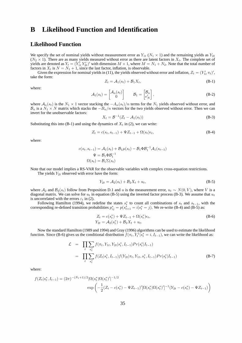
B Likelihood Function and Identification

Likelihood Function

We specify the set of nominal yields without measurement error asY1t (N1 × 1) and the remaining yields asY2t

(N2 × 1). There are as many yields measured without error as there are latent factors inXt. The complete set ofyields are denoted asYt = (Y ′

1t Y ′2t)

′ with dimensionM × 1, whereM = N1 + N2. Note that the total number offactors inXt is N = N1 + 1, since the last factor, inflation, is observable.

Given the expression for nominal yields in (11), the yields observed without error and inflation,Zt = (Y ′1t πt)′,

take the form:Zt = A1(st) + B1Xt, (B-1)

where:

A1(st) =[An(st)

0

]B1 =

[Bn

e′N

], (B-2)

whereAn(st) is theN1 × 1 vector stacking the−An(st)/n terms for theN1 yields observed without error, andBn is aN1 × N matrix which stacks the−Bn/n vectors for the two yields observed without error. Then we caninvert for the unobservable factors:

Xt = B−1(Zt −A1(st)) (B-3)

Substituting this into (B-1) and using the dynamics ofXt in (2), we can write:

Zt = c(st, st−1) + ΨZt−1 + Ω(st)εt, (B-4)

where:

c(st, st−1) = A1(st) + B1µ(st)− B1ΦB−11 A1(st−1)

Ψ = B1ΦB−11

Ω(st) = B1Σ(st)

Note that our model implies a RS-VAR for the observable variables with complex cross-equation restrictions.The yieldsY2t observed with error have the form:

Y2t = A2(st) + B2Xt + ut, (B-5)

whereA2 andB2(st) follow from Proposition D.1 andu is the measurement error,ut ∼ N(0, V ), whereV is adiagonal matrix. We can solve forut in equation (B-5) using the inverted factor process (B-3). We assume thatut

is uncorrelated with the errorsεt in (2).Following Hamilton (1994), we redefine the statess∗t to count all combinations ofst and st−1, with the

corresponding re-defined transition probabilitiesp∗ij = p(s∗t+1 = i|s∗t = j). We re-write (B-4) and (B-5) as:

Zt = c(s∗t ) + ΨZt−1 + Ω(s∗t )εt, (B-6)Y2t = A2(s∗t ) + B2Xt + ut.

Now the standard Hamilton (1989 and 1994) and Gray (1996) algorithms can be used to estimate the likelihoodfunction. Since (B-6) gives us the conditional distributionf(πt, Y

1t |s∗t = i, It−1), we can write the likelihood as:

L =∏

t

∑

s∗t

f(πt, Y1t, Y2t|s∗t , It−1)Pr(s∗t |It−1)

=∏

t

∑

s∗t

f(Zt|s∗t , It−1)f(Y2t|πt, Y1t, s∗t , It−1)Pr(s∗t |It−1) (B-7)

where:

f(Zt|s∗t , It−1) = (2π)−(N1+1)/2|Ω(s∗t )Ω(s∗t )′|−1/2

exp(−1

2(Zt − c(s∗t )−ΨZt−1)′[Ω(s∗t )Ω(s∗t )

′]−1(Y2t − c(s∗t )−ΨZt−1))

35

is the probability density function ofZt conditional ons∗t and

f(Y2t|πt, Y1t, s∗t , It−1) =

(2π)−N2/2|V |−1/2 exp(−1

2(Y2t −A2(s∗t )− B2Xt)′V −1(Y2t −A2(s∗t )− B2Xt

)

is the probability density function of the measurement errors conditional ons∗t .The ex-ante probabilityPr(s∗t = i|It−1) is given by:

Pr(s∗t = i|It−1) =∑

j

p∗jiPr(s∗t−1 = j|It−1), (B-8)

which is updated using:

Pr(s∗t = j|It) =f(Zt, s

∗t = j|It−1)

f(Zt|It−1)

=f(Zt|s∗t = j, It−1)Pr(s∗t = j|It−1)∑k f(Zt|s∗t = k, It−1)Pr(s∗t = k|It−1)

An alternative way to derive the likelihood function is to substitute (B-3) into (B-5). We then obtain a RS-VARwith complex cross-equation restrictions for all variables in the system(Z ′t Y ′

2t)′. Note that unlike a standard affine

model, the likelihood is not simply the likelihood of the yields measured without error multiplied by the likelihoodof the measurement errors. Instead, the regime variables must be integrated out of the likelihood function.

Identification

There are two identification problems. First, there are the usual identification conditions that must be imposed toestimate a model with latent variables, which have been derived for affine models by Dai and Singleton (2000).In a single-regime Gaussian model, Dai and Singleton show that identification can be accomplished by setting theconditional covariance to be a diagonal matrix and letting the correlations enter through the feedback matrix (Φ),which is parameterized to be lower triangular, which we do here.

The regime-switching model complicates identification relative to an affine model. The parameterization inequations (2)-(7) already imposes some of the Dai and Singleton (200) conditions, but some further restrictions arenecessary. Sinceqt andft are latent variables, they can be arbitrarily scaled. We setδ1 = (δq δf δπ)′ = (1 1 δπ)′in (4). Settingδq andδf to be constants allowsσq andσf (st+1) to be estimated. Becauseqt is an unobservedvariable, estimatingµq in (3) is equivalent to allowingγ0 in (6) or δ0 in (4) to be non-zero. Hence,qt must havezero mean for identification. Therefore, we setµq = 0, sinceqt does not switch regimes. Similarly, because weestimateλf (st+1), we constrainft to have zero mean.

The resulting model is theoretically identified from the data, but it is well known that some parameters thatare identified in theory can be very hard to estimate in small samples. This is especially true for price of riskparameters. Because we using four nominal yields, we should be able to identify all three prices of risk. However,Dai and Singleton (2000) note that it is typically difficult to identify more than one constant price of risk. Hence,we setγ0 = 0 in (6) and instead estimate the RS price of riskλf (st+1).

We also setΦfq = 0 in equation (3). With this restriction, there are, in addition to inflation factors,two separate and easily identifiable sources of variation in interest rates: a regime-switching factor and a time-varying price of risk factor. Identifying their relative contribution to interest rate dynamics becomes easy with thisrestriction and it is not immediately clear how a non-zero coefficient would help enrich the model.

As qt andft are zero mean, the mean level of the real short rate in (4) is determined by the mean level ofinflation multiplied byδπ and the constant termδ0. We setδ0 to match the mean of the nominal short rate in thedata, similar to Ang, Dong and Piazzesi (2006) and Dai, Singleton and Yang (2006).

Finally, we set the one-period price of inflation risk equal to zero,λπ(st+1) = 0. Theoretically, this parameteris uniquely identified, but in practice the average level of real rates and the premium is largely indeterminatewithout further restrictions. It turns out that the first-order effect ofλπ on real rates and the inflation risk premiumis similar and of opposite sign. Because of this, the parameter is not only hard to pin down, but also essentiallyprevents the identification of the average level of real rates and the average level of the inflation risk premium.Models with a positive one-period inflation risk premium will imply lower real rates and higher inflation premiumsthan the results we report.

36

C Real Bond PricesLet N1 be the number of unobserved state variables in the model (N1 = 3 for the stochastic inflation model,N1 = 2 otherwise) andN = N1 + 1 be the total number of factors including inflation. The following propositiondescribes how our model implies closed-form real bond prices.

Proposition C.1 Let Xt = (qt ft πt)′ or Xt = (qt ft wt πt)′ follow (2), with the real short rate (4) and realpricing kernel (5) with prices of risk (6). The regimesst follow a Markov chain with transition probability matrixΠ = pij. Then the real zero coupon bond price for periodn conditional on regimei, Pn

t (st = i), is given by:

Pnt (i) = exp(An(i) + BnXt). (C-1)

The scalarAn(i) is dependent on regimest = i andBn is a1×N vector that is partitioned asBn = [Bnq Bnx],whereBnq corresponds to theq variable andBnx corresponds to the other variables inXt. The coefficientsAn(i)andBn are given by:

An+1 (i) =−(δ0 + B′

nqσqγ0

)+ log

∑

j

pij exp(

An (j) + Bnµ (j)

− BnxΣx (j) λ (j) +12BnΣ(j)Σ (j)′ B′

n

)

Bn+1 =− δ′1 + BnΦ− Bnqσqγ1e′1, (C-2)

whereei denotes a vector of zero’s with a 1 in theith place andΣx(i) refers to the lowerN1 × N1 matrix of ofΣ(i) corresponding to the non-qt variables inXt. The starting values forAn(i) andBn are:

A1 (i) = −δ0

B1 = −δ′1. (C-3)

Proof:

We first derive the initial values in (C-3):

P 1t (i) =

∑

j

pijEt

[Mt+1|St+1 = j

]

=∑

j

pij exp(−rt − 1

2λt (j)′ λt (j)− λt (j)′ εt+1

)

= exp (−δ0 − δ′1Xt) (C-4)

Hence:P 1

t (i) = exp(A1(i) + B1Xt),

whereA1(i) andB1 take the form in (C-3).We prove the recursion (C-2) by induction. We assume that (C-1) holds for maturityn and examinePn+1

t (i):

Pn+1t (i) =

∑

j

pijEt exp[−rt − 1

2λt (j)′ λt (j)− λt (j)′ εt+1 + An (j) + BnXt+1

],

=∑

j

pijEt exp[−δ0 − δ′1Xt − 1

2λt (j)′ λt (j)− λt (j)′ εt+1 + An (j)

+Bn (µ (j) + ΦXt + Σ(j) εt+1)]

(C-5)

37

Evaluating the expectation, we have:

Pn+1t (i) =

∑

j

pij exp[−δ0 − δ′1Xt − 1

2λt (j)′ λt (j) + An (j) + Bnµ (j)

+BnΦXt +12

(BnΣ (j)− λt (j)′

)(BnΣ(j)− λt (j)′

)′]

=exp[−δ0 +

(BnΦ− δ′1

)Xt

]

×∑

j

pij exp[An (j) + Bnµ (j)− BnΣ(j)λt (j) +

12BnΣ(j)Σ (j) B′

n

](C-6)

But, we can write:

BnΣ (j) λt (j) = [Bnq Bnx][

σq (γ0 + γ1e′1Xt)

Σx (j) λ (j)

]

= Bnqσq (γ0 + γ1e′1Xt) + BnxΣx (j)λ (j) . (C-7)

Then, expanding and collecting terms, we can write:

Pnt (i) = exp(An(i) + BnXt),

whereAn(i) andBn take the form of (C-2).¥

D Nominal Bond PricesFollowing the notation of Appendix C, letN1 be the number of unobserved state variables in the model (N1 = 3for the stochastic inflation model,N1 = 2 otherwise) andN = N1 + 1 be the total number of factors includinginflation. The following proposition describes how our model implies closed-form nominal bond prices.

Proposition D.1 Let Xt = (qt ft πt)′ or Xt = (qt ft wt πt)′ follow (2), with the real short rate (4) and realpricing kernel (5) with prices of risk (6). The regimesst follow a Markov chain with transition probability matrixΠ = pij. Then the nominal zero coupon bond price for periodn conditional on regimei, Pn

t (st = i), is givenby:

Pnt (i) = exp(An(i) + BnXt), (D-1)

where the scalarAn(i) is dependent on regimest = i andBn is anN × 1 vector:

An+1(i) =− (δ0 + B′

nqσqγ0

)+ log

∑

j

pij exp(

An (j) + (Bn − e′N ) µ (j)

− (Bnx − e′N1

)Σx (j)λ (j) +

12

(Bn − e′N )Σ (j)Σ (j) (Bn − e′N )′)

Bn+1 =− δ′1 + (Bn − e′N )Φ−Bnqσqγ1e′1, (D-2)

whereei denotes a vector of zero’s with a 1 in theith place,A(i) is a scalar dependent on regimest = i, Bn is arow vector, which is partitioned asBn = [Bnq Bnx], whereBnq corresponds to theq variable andΣx(i) refers tothe lowerN1 × N1 matrix of ofΣ(i) corresponding to the non-qt variables inXt. The starting values forAn(i)andBn are:

A1 (i) = −δ0 + log∑

j

pij exp(−e′Nµ (j) +

12e′NΣ(j)Σ (j)′ eN + e′N1

Σx (j) λ (j))

B1 = − (δ′1 + e′NΦ) . (D-3)

38

Proof:

We first derive the initial values (D-3) by directly evaluating:

P 1t (i) =

∑

j

pijEt

[Mt+1|St+1 = j

]

=∑

j

pij exp(−rt − 1

2λt (j)′ λt (j)− λt (j)′ εt+1 − e′N (µ (j) + ΦXt + Σ(j) εt+1)

)

= exp (−δ0 − δ′1Xt − e′NΦXt)

×∑

j

pij exp(−e′Nµ (j)− e′NΣ(j) εt+1 − 1

2λt (j)′ λt (j)− λt (j)′ εt+1

)

= exp (−δ0 − δ′1Xt − e′NΦXt)

×∑

j

pij exp(−e′Nµ (j) +

12e′NΣ(j)Σ (j)′ eN + e′NΣ(j)λt (j)

). (D-4)

Note thate′NΣ(j)λt(j) = e′N1Σx(j)λ(j). Hence:

P 1t (i) = exp (A1 (i) + B1Xt)

whereA1(i) andB1 are given by (D-3).To prove the general recursion we use proof by induction:

Pn+1t (i) =

∑

j

pijEt

[exp

(−rt − 1

2λt (j)′ λt (j)− λt (j)′ εt+1 − e′NXt+1

)

exp (An (j) + BnXt+1)]

=∑

j

pijEt

[exp

(−δ0 − δ′1Xt − 1

2λt (j)′ λt (j)− λt (j)′ εt+1 + An (j)

+ (Bn − e′N ) (µ (j) + ΦXt + Σ (j) εt+1))]

=∑

j

pij exp(−δ0 − δ′1Xt − 1

2λt (j)′ λt (j) + An (j) + (Bn − e′N )µ (j)

+ (Bn − e′N )ΦXt +12

((Bn − e′N )Σ (j)− λt (j)′

) ((Bn − e′N )Σ (j)− λt (j)′

)′)

=exp (−δ0 + ((Bn − e′N )Φ− δ′1)Xt)∑

j

pij exp(

An (j) + (Bn − e′N ) µ (j)

− (Bn − e′N )Σ (j) λt (j) +12

(Bn − e′N )Σ (j)Σ (j) (Bn − e′N )′)

(D-5)

Now note that:

(Bn − e′N )Σ (j) λt (j) = (Bn − e′N )[

σq (γ0 + γ1e′1Xt)

Σx (j) λ(j)

]

=[

Bnq

Bnx − e′N1

] [σq (γ0 + γ1e

′1Xt)

Σx (j)λ(j)

]

= Bnqσq (γ0 + γ1e′1Xt) +

(Bnx − e′N1

)Σx (j) λ(j) (D-6)

whereBn = [Bnq Bnx].Hence, collecting terms and substituting (D-6) into (D-5), we have:

Pn+1t (i) = exp [An+1 (i) + Bn+1Xt] ,

where:An(i) andBn are given by (D-2).¥

39

E A Regime-Switching Model with Stochastic Expected In-flation

In a final extension, motivated by the ARMA-model literature (see Fama and Gibbons, 1982; Hamilton, 1985), weallow inflation to be composed of a stochastic expected inflation term plus a random shock:

πt+1 = wt + σπεπt+1,

wherewt = Et [πt+1] is the one-period-ahead expectation of future inflation. This can be accomplished in ourframework by expanding the state variables toXt = (qt ft wt πt)′ which follow the dynamics of equation (2),except now:

µ(st) =

µq

µf (st)µw(st)

0

, Φ =

Φqq 0 0 0Φfq Φff 0 0Φwq Φwf Φww Φwπ

0 0 1 0

, (E-7)

and Σ(st) is a diagonal matrix with(σq σf (st)σw(st)σπ(st))′ on the diagonal. Note that both the varianceof inflation and the process of expected inflation are regime-dependent. Moreover, past inflation affects currentexpected inflation throughΦwπ.

The real short rate and the regime transition probabilities are the same as in the benchmark model. The realpricing kernel also takes the same form as (5) with one difference. The regime-dependent part of the prices of riskin equation (6) is now given by:

λ(i) = (λf (i) λw(i) λπ(i))′,

but we setλw(i) = 0 for identification.

F Specification TestsMoment Tests

To enable comparison across several non-nested models of how the moments implied from various models compareto the data, we introduce the point statistic:

H = (h− h)′Σ−1h (h− h), (F-1)

whereh are sample estimates of unconditional moments,h are the unconditional moments from the estimatedmodel, andΣh is the covariance matrix of the sample estimates of the unconditional moments, estimated by GMMwith four Newey-West (1987) lags. In this comparison, the moments implied by various models are comparedto the data, with the data sampling errorΣh held constant across the models. The moments we consider arethe first and second moments of term spreads and long yields; the first and second moments of inflation; theautocorrelogram of term spreads; and the autocorrelogram of inflation.

Equation (F-1) ignores the sampling error of the moments of the model, implied by the uncertainty in theparameter estimates, making our moment test informal. However, this allows the same weighting matrix, computedfrom the data, to be used across different models. If parameter uncertainty is also taken into account, we mightfail to reject, not because the model accurately pins down the moments, but because of the large uncertainty inestimating the model parameters.

Residual Tests

We report two tests on in-sample scaled residualsεt of yields and inflation. The scaled residualsεt are not thesame as the shocksεt in (2). For a variablext, the scaled residual is given byεt = (xt−Et−1(xt))/

√vart−1(xt),

wherext are yields or inflation. The conditional moments are computed using our RS model and involve ex-anteprobabilitiesp(st = i|It−1). Following Bekaert and Harvey (1997), we use a GMM test for serial correlation inscaled residualsεt:

E[εt εt−1] = 0. (F-2)

We also test for serial correlation in the second moments of the scaled residuals:

E[((εt)2 − 1) ((εt−1)2 − 1)] = 0. (F-3)

40

G Computing Moments of the Regime-Switching ModelThe formulae given here assume that there areK regimesst = 1, . . . K. Timmermann (2000) provides explicitformulae for a similar formulation of (2), except that the conditional mean ofXt+1 depends onµ(st+1)+Φ(Xt−µ(st)) rather than onµ(st+1) + ΦXt. In Timmermann’s set-up,E(Xt|st) is trivially µ(st), whereas in our modelthe computation is more complex.

Conditional First Moments E(Xt|st)

Starting from (2), and taking expectations conditional onst+1, we have:

E(Xt+1|st+1) = E(µ(st+1)|st+1) + ΦE(Xt|st+1) (G-1)

To evaluateE(Xt|st+1) we use Bayes Rule:

E(Xt|st+1 = i) =K∑

j=1

E(Xt|st = j)Pr(st = j|st+1 = i). (G-2)

The probabilityPr(st = j|st+1 = i) is the transition probability of the ‘time-reversed’ Markov chain that movesbackward in time. These backward transition probabilities are given by:

Pr(st = j|st+1 = i) , bij = pji

(πj

πi

),

wherepji = Pr(st+1 = i|st = j) are the forward transition probabilities andπi = Pr(st = i) is the stableprobability of regimei. Denote the backward transition probability matrix asB = bij

Using the backward transition probabilities, (G-1) can be rewritten:

E(Xt+1|st+1 = i) = µ(i) + ΦK∑

j=1

E(Xt|st = j)bji. (G-3)

Assuming stationarity, that isE(Xt+1|st+1 = i) = E(Xt|st = i), and defining theK × 1 vectors:

~E(Xt|st) =

E(Xt|st = 1)...

E(Xt|st = K)

and ~µ(st) =

µ(1)...

µ(K)

,

we can write:~E(Xt|st) = ~µ(st) + Φ~E(Xt|st)B′.

Hence, we can solve for~E(Xt|st) as:

vec[~E(Xt|st)] = (I −B ⊗ Φ)−1vec[~µ(st)] (G-4)

Conditional Second MomentsE(XtX′t|st)

Starting from (2), we can write:

Xt+1X′t+1 = (µ(st+1) + ΦXt + Σ(st+1)εt+1)(µ(st+1) + ΦXt + Σ(st+1)εt+1)′, (G-5)

and taking expectations conditional onst+1, we have:

E(Xt+1X′t+1|st+1) = µ(st+1)µ(st+1)′ + Σ(st+1)Σ(st+1)′

+ µ(st+1)E(Xt|st+1)′Φ′ + ΦE(Xt|st+1)µ(st+1)′ + ΦE(XtXt|st+1)Φ′. (G-6)

41

We can evaluate the termE(Xt|st+1) from (G-2). Hence, we can define anN ×N matrixG(i):

G(i) = µ(i)µ(i)′ + Σ(i)Σ(i)′ + µ(i)E(Xt|st+1 = i)′Φ′ + ΦE(Xt|st+1 = i)µ(i)′. (G-7)

Substituting (G-7) into (G-6) and using Bayes’ Rule, we have:

E(Xt+1X′t+1|st+1 = i) = G(i) +

K∑

j=1

Φ[E(XtX′t|st = j)Pr(st = j|st+1 = i)]Φ′

= G(i) +K∑

j=1

bijΦE(XtX′t|st = j)Φ′

Taking vec’s of both sides, we obtain:

vec(E(Xt+1X′t+1|st+1 = i)) = vec(G(i)) + (Φ⊗ Φ)

K∑

j=1

vec(E(Xt+1X′t+1|st+1 = i))bij (G-8)

If we define theKN2 × 1 vectors:

~E(XtX′t|st) =

vec(E(Xt+1X′t+1|st+1 = 1))...

vec(E(Xt+1X′t+1|st+1 = K))

and ~G =

vec(G(1))...

vec(G(K))

we can write (G-8) as:~E(XtX

′t|st) = ~G + (Φ⊗ Φ)~E(XtX

′t|st)B′.

Hence, we can solve for~E(XtX′t|st) as:

vec[~E(XtX′t|st)] = (IKN2 −B ⊗ (Φ⊗ Φ))−1vec[~G]. (G-9)

Unconditional Moments

The first unconditional momentE(Xt) is solved simply by taking unconditional expectations of (2), giving

E(Xt) = (I − Φ)−1K∑

i=1

πiµ(i). (G-10)

To solve the second unconditional moment var(Xt), we use:

var(Xt) = E(XtX′t)− E(Xt)E(Xt)′

= E(E(XtX′t|st))− E(Xt)E(Xt)′

=K∑

i=1

πi

var(Xt|st = i) + E(Xt|st = i)E(Xt|st = i)′

− E(Xt)E(Xt)′ (G-11)

Moments of Yields

Bond yields are affine functions ofXt, from Propositions C.1 and D.1. Hence, they can be written asYt =A(St) + BXt for some choice ofA(St) andB. Then, regime-dependent moments ofYt are given by:

E(Yt|st) = A(St) + BE(Xt|st)var(Yt|st) = Bvar(Xt|st)B′, (G-12)

42

and the unconditional moments ofYt are:

E(Yt) =K∑

i=1

πiE(Yt|st = i)

var(Yt) = E(YtY′t )− E(Yt)E(Yt)′

= E(E(YtY′t |St))− E(Yt)E(Yt)′

=K∑

i=1

πi

var(Yt|St) + E(Yt|St)E(Yt|St)′

− E(Yt)E(Yt)′ (G-13)

43

References[1] Aıt-Sahalia, Y., 1996, “Testing Continuous-Time Models of the Spot Interest Rate,”Review of Financial

Studies, 9, 2, 385-426.

[2] Ang, A., and G. Bekaert, 2002a, “Regime Switches in Interest Rates,”Journal of Business and EconomicStatistics, 20, 163-182.

[3] Ang, A., and G. Bekaert, 2002b, “Short Rate Nonlinearities and Regime Switches,”Journal of EconomicDynamics and Control, 26, 7-8, 1243-1274

[4] Ang, A., S. Dong, and M. Piazzesi, 2005, “No-Arbitrage Taylor Rules,” working paper, Columbia BusinessSchool.

[5] Bansal, R., and H. Zhou, 2002, “Term Structure of Interest Rates with Regime Shifts,”Journal of Finance,57, 5, 1997-2043.

[6] Bansal, R., G. Tauchen, and H. Zhou, 2004, “Regime-Shifts, Risk Premiums in the Term Structure, and theBusiness Cycle,”Journal of Business and Economic Statistics, 22, 396-409.

[7] Barr, D. G., and J. Y. Campbell, 1997, “Inflation, Real Interest Rates, and the Bond Market: A Study of U.K.Nominal and Index-Linked Government Bond prices,”Journal of Monetary Economics, 39, 361-383.

[8] Bekaert, G., and C. R. Harvey, 1997, “Emerging Equity Market Volatility,”Journal of Financial Economics,43, 1, 29-77.

[9] Bekaert, G., R. Hodrick, and D. Marshall, 1997, “On Biases in Tests of the Expectations Hypothesis of theTerm Structure of Interest Rates,”Journal of Financial Economics, 44, 309-48.

[10] Bekaert, G., R. Hodrick, and D. Marshall, 2001, “Peso Problem Explanations for Term Structure Anomalies,”Journal of Monetary Economics, 48, 2, 241-270.

[11] Bernanke, B. S., and I. Mihov, 1998, “Measuring Monetary Policy,”Quarterly Journal of Economics, 113,3, 869-902.

[12] Bikbov, R., 2005, “Monetary Policy Regimes and the Term Structure of Interest Rates,” working paper,Columbia University.

[13] Boivin, J., 2006, “Has U.S. Monetary Policy Changed? Evidence from Drifting Coefficients and REal-TimeData,”Journal of Money, Credit and Banking, 38, 1149-73.

[14] Boudoukh, J., 1993, “An Equilibrium-Model of Nominal Bond Prices with Inflation-Output Correlation andStochastic Volatility,”Journal of Money Credit and Banking, 25, 3, 636-665.

[15] Boudoukh, J., M. Richardson, T. Smith and R. F. Whitelaw, 1999, “Regime Shifts and Bond Returns,”working paper, NYU.

[16] Buraschi, A. and A. Jiltsov, 2005, “Time-Varying Inflation Risk Premia and the Expectations Hypothesis: AMonetary Model of the Treasury Yield Curve,”Journal of Financial Economics, 75, 2, 429-490.

[17] Burmeister, E., K. Wall, and J. Hamilton, 1986, “Estimation of Unobserved Expected Monthly Inflation usingKalman Filtering,”Journal of Business and Economic Statistics, 4, 147-160.

[18] Campbell, J. Y., and R. J. Shiller, 1991, “Yield Spreads and Interest Rate Movements: A Bird’s Eye View,”Review of Economic Studies, 58, 495-514.

[19] Campbell, J. Y., and L. M. Viceira, 2001, “Who Should Buy Long-Term Bonds?”American EconomicReview, 91, 99-127.

[20] Chen, R. R., and L. Scott, 1993, “Maximum Likelihood Estimation for a Multi-factor Equilibrium Model ofthe Term Structure of Interest Rates,”Journal of Fixed Income, 3, 14-31.

[21] Cho, S., and A. Moreno, 2006, “A Small-Sample Study of the New-Keynesian Macro Model,” forthcomingJournal of Money, Credit and Banking.

[22] Clarida, R., J. Gali, and M. Gertler, 2000, “Monetary Policy Rules And Macroeconomic Stability: EvidenceAnd Some Theory,”Quarterly Journal of Economics, 115, 1, 147-180.

[23] Cochrane, J., and M. Piazzesi, 2005, “Bond Risk Premia,”American Economic Review, 95, 138-160.

44

[24] Cogley, T., and T. J. Sargent, 2001, “Evolving Post World War II U.S. Inflation Dynamics,”NBERMacroeconomics Annual, 16, 331-373.

[25] Cogley, T., and T. J. Sargent, 2005, “Drifts and Volatilities: Monetary Policies and Outcomes in the PostWWII U.S.,” Review of Economic Dynamics, 8, 263-302.

[26] Dai, Q., and K. J. Singleton, 2000, “Specification Analysis of Affine Term Structure Models,”Journal ofFinance, 55, 5, 1943-1978.

[27] Dai, Q., and K. J. Singleton, 2002, “Expectation Puzzles, Time-Varying Risk Premia, and Affine Models ofthe Term Structure,”Journal of Financial Economics, 63, 415-41.

[28] Dai, Q., and K. J. Singleton, 2003, “Term Structure Dynamics in Theory and Reality,”Review of FinancialStudies, 16, 631-678.

[29] Dai. Q., K. J. Singleton, and W. Yang, 2006, “Are Regime Shifts Priced in U.S. Treasury Markets?” workingpaper, Stanford University.

[30] Diebold, F., J. Lee, and G. Weinbach, 1994, “Regime Switching with Time-Varying Transition Probabilities,”in Hargreaves, C., (ed.) Nonstationary Time Series Analysis and Cointegration (Advanced Texts inEconometrics, Granger, C. W. J., and G. Mizon, eds.), 283-302, Oxford University Press.

[31] Evans, M. D. D., 1998, “Real Rates, Expected Inflation, and Inflation Risk Premia,”Journal of Finance, 53,1, 187-218.

[32] Evans, M. D. D., 2003, “Real Risk, Inflation Risk, and the Term Structure,”Economic Journal, 113, 487,345-389.

[33] Evans, M. D. D., and K. Lewis, 1995, “Do Expected Shifts in Inflation Affect Estimates of the Long-RunFisher Relation,”Journal of Finance, 50, 1, 225-253.

[34] Evans, M. D. D., and P. Wachtel, 1993, “Inflation Regime and the Sources of Inflation Uncertainty,”Journalof Money, Credit and Banking, 25, 3, 1993.

[35] Fama, E. F., 1975, “Short-term Interest Rates as Predictors of Inflation,”American Economic Review, 65, 3,269-282.

[36] Fama. E. F., 1990, “Term-structure Forecasts of Interest Rates, Inflation and Real Returns,”Journal ofMonetary Economics, 25, 59-76.

[37] Fama, E. F., and Bliss, R. R., 1987, “The Information in Long-Maturity Forward Rates,”American EconomicReview, 77, 680-92.

[38] Fama, E. F., and M. Gibbons, 1982, “Inflation, Real Returns and Capital Investment,”Journal of MonetaryEconomics, 9, 297-323.

[39] Fama, E. F., and G. W. Schwert, 1977, “Asset Returns and Inflation,”Journal of Financial Economics, 5,115-146.

[40] Garcia, R., and P. Perron, 1996, “An Analysis of the Real Interest Rate under Regime Shifts,”Review ofEconomics and Statistics, 78, 1, 111-125.

[41] Gavin, W. T., and F. E. Kydland, 2000, “The Nominal Facts and the October 1979 Policy Change,”FederalReserve Bank of St Louis Review, 82, 39-61.

[42] Goto, S., and W. Torous, 2003, “The Conquest of U.S. Inflation: Its Implications for the Fisher Hypothesisand the Term Structure of Nominal Interest Rates,” working paper, University of South Carolina.

[43] Gray, S. F., 1996, “Modeling the Conditional Distribution of Interest Rates as a Regime-Switching Process,”Journal of Financial Economics, 42, 27-62.

[44] Hamilton, J., 1985, “Uncovering Financial Market Expectations of Inflation,”Journal of Political Economy,93, 1224-1241.

[45] Hamilton, J., 1988, “Rational-Expectations Econometric Analysis of Changes in Regime: An Investigationof the Term Structure of Interest Rates,”Journal of Economic Dynamics and Control, 12, 385-423.

[46] Hamilton, J., 1989, “A New Approach to the Economic Analysis of Nonstationary Time Series and theBusiness Cycle,”Econometrica, 57, 357-384.

[47] Hamilton, J., 1994,Time Series Analysis, Princeton University Press, New Jersey.

45

[48] Hodrick, R. J., E. C. Prescott, 1997, “Postwar US Business Cycles: An Empirical Investigation,”Journal ofMoney, Credit and Banking, 29, 1-16.

[49] Huizinga, J., and F. Mishkin, 1986, “Monetary Policy Regime Shifts and the Unusual Behavior of RealInterest Rates”,Carnegie-Rochester Conference Series on Public Policy, 24, 231-74.

[50] Landen, C., 2000, “Bond Pricing in a Hidden Markov Model of the Short Rate,”Finance and Stochastics, 4,371-389.

[51] Laubach, T., and J. C. Williams, 2003, “Measuring the Natural Rate of Interest,”Review of Economics andStatistics, 85, 4, 1063-1070.

[52] Meltzer, A. H., 2005, “From Inflation to More Inflation, Disinflation and Low Inflation,” Keynote Address,Conference on Price Stability, Federal Reserve Bank of Chicago.

[53] Mishkin, F., 1981, “The Real Rate of Interest: An Empirical Investigation,”Carnegie-Rochester ConferenceSeries on Public Policy, 15, 151-200.

[54] Mishkin, F., 1990, “The Information in the Longer Maturity Term Structure about Future Inflation,”QuarterlyJournal of Economics, 105, 3, 815-828.

[55] Mishkin, F. S., 1992, “Is the Fisher Effect for Real?”Journal of Monetary Economics, 30, 195-215.

[56] Mundell, R., 1963, “Inflation and Real Interest,”Journal of Political Economy, 71, 280-283.

[57] Naik, V., and M. Lee, 1994, “The Yield Curve and Bond Option Prices with Discrete Shifts in EconomicRegimes,” working paper, University of British Columbia.

[58] Nelson, E., 2004, “The Great Inflation of the Seventies: What Really Happened?” Federal Reserve Bank ofSt Louis working paper 2004-001.

[59] Newey, W. K., and K. D. West, 1987, “A Simple Positive Semi-Definite, Heteroskedasticity andAutocorrelation Consistent Covariance Matrix,”Econometrica55, 703-8.

[60] Pennacchi, G., 1991, “Identifying the Dynamics of real Interest Rates and Inflation: Evidence using SurveyData,”Review of Financial Studies, 1, 53-86.

[61] Remolona, E. M., M. R. Wickens and F. F. Gong, 1998, “What was the Market’s View of U.K. MonetaryPolicy? Estimating Inflation Risk and Expected Inflation with Indexed Bonds,” Federal Reserve Bank of NewYork, Staff Reports 57.

[62] Roll, R., 2004, “Empirical TIPS,”Financial Analysts Journal, 60, 1, 31-53.

[63] Rose, A., 1988, “Is the Real Interest Rate Stable?”Journal of Finance, 43, 1095-1112.

[64] Sims, C. A., 1999, “Drifts and Breaks in Monetary Policy,” working paper, Yale University.

[65] Sims, C. A., 2001, “Comment on Sargent and Cogley’s ‘Evolving Post World War II U.S. InflationDynamics,’ ”NBER Macroeconomics Annual, 16, 373-379.

[66] Sola, M., and J. Driffill, 1994, “Testing the Term Structure of Interest Rates Using a Vector Autoregressionwith Regime Switching,”Journal of Economic Dynamics and Control, 18, 601-628.

[67] Stanton, R., 1997, “A Nonparametric Model of Term Structure Dynamics and the Market Price of InterestRate Risk”,Journal of Finance, 52, 5, 1973-2002.

[68] Stockton, D., and J. Glassman, 1987, “An Evaluation of the Forecast Performance of Alternative Models ofInflation,” Review of Economics and Statistics, 69, 108-117.

[69] Sun, T., 1992, “Real and Nominal Interest-Rates: A Discrete-Time Model and its Continuous-Time Limit,”Review of Financial Studies, 5, 4, 581-611.

[70] Taylor, J. B., 1993, “Discretion versus Policy Rules in Practice,”Carnegie-Rochester Conference Series onPublic Policy, 39, 195-214.

[71] Timmermann, A., 2000, “Moments of Markov Switching Models,”Journal of Econometrics, 96, 1, 75-111.

[72] Tobin, J., 1965, “Money and Economic Growth,”Econometrica, 33, 671-684.

[73] Veronesi, P., and F. Yared, 1999, ”Short and Long Horizon Term and Inflation Risk Premia in the US TermStructure: Evidence from an Integrated Model for Nominal and Real Bond Prices under Regime Shifts,”CRSP working paper 508.

46

Table 1: Nomenclature of Models

Regime-Switching Models

Affine Two Regimes Three Regimes Four Regimes Six Regimes

3-Factor Models I II III IV A,IV B , IV C V I

4-Factor Models Iw IIw – IV Aw , IV B

w , IV Cw –

This table summarizes the models estimated. The affine models are single regime models. In the two and threeregime models, the real rate factor and inflation share the same regimes, sost = sf

t = sπt , which take values

from 1, 2 or 1, 2, 3, respectively. In the four and six regime models, the regimesst reflect switches inbothsf

t andsπt . In the four-regime model,sf

t ∈ 1, 2 andsπt ∈ 1, 2, and the probability transition matrix

can be one of three cases, independent (Case A) and correlated cases B and C, which are outlined in Section2.4. In the six-regime model,sf

t ∈ 1, 2 andsπt ∈ 1, 2, 3, andsf

t andsπt are independent. The three-factor

models contain the factorsXt = (qt ft πt)′ with qt a time-varying price of risk factor,ft is a latent RS termstructure factor, andπt is inflation. The dynamics ofXt are outlined in Section 2.2. The models denoted withw subscripts also contain an additional factor representing expected inflation. These models are described inAppendix E.

47

Table 2: Specification Tests

Panel A: Matching Inflation Dynamics

Moment Tests

Mean/ Auto- ResidualModel Variance correlogram Tests

I 0.00** 0.02* 0.00**0.08

Iw 0.08 0.00** 0.02*0.09

II 0.00** 0.01* 0.100.17

IIw 0.00** 0.16 0.03*0.31

III 0.02* 0.02* 0.670.22

IV A 0.15 0.04* 0.160.12

IV B 0.09 0.03* 0.01*0.01*

IV C 0.60 0.08 0.210.10

IV Aw 0.00** 0.27 0.26

0.26

IV Bw 0.00** 0.17 0.01**

0.36

IV Cw 0.00** 0.18 0.22

0.27

V I 0.50 0.13 0.00**0.00**

48

Table 2 Continued

Panel B: Matching Yield Dynamics

Moment Tests Residual Tests

Mean/Var Spread ShortModel Long Rate/Spread Autocorrelogram Rate Spread

I 0.78 0.14 0.19 0.140.27 0.22

Iw 0.00** 0.26 0.47 0.340.15 0.29

II 0.61 0.01** 0.05 0.650.02* 0.15

IIw 0.00** 0.01* 0.52 0.480.01** 0.34

III 0.12 0.09 0.05 0.050.04* 0.05

IV A 0.37 0.33 0.02* 0.960.04* 0.08

IV B 0.00** 0.00** 0.01** 0.00**0.00** 0.00**

IV C 0.63 0.39 0.02* 0.340.04* 0.03*

IV Aw 0.00** 0.06 0.31 0.11

0.08 0.35

IV Bw 0.00** 0.10 0.81 0.56

0.16 0.12

IV Cw 0.00** 0.24 0.33 0.07

0.12 0.30

V I 0.04* 0.00** 0.01** 0.01*0.01** 0.00**

This table reports moment and residual tests of inflation (Panel A) and of yields (Panel B), which are outlinedin Appendix F. In the columns titled “Moment Tests,” we report the p-values of goodness-of-fitχ2 tests forvarious moments implied by the different models. In Panel A, the first moment test matches the mean andvariance of inflation, whereas in Panel B, the first moment test matches the mean and variance of the longrate and the spread jointly. The long rate refers to the 20-quarter nominal ratey20

t and the spread refers toy20

t −y1t , for y1

t the 3-month short rate. The second autocorrelogram moment test matches autocorrelations atlags 1, 5, and 10. The columns titled “Residual Tests” report p-values of scaled residual tests for the differentmodels. The first entry reports the p-value of a test ofE(εtεt−1) = 0 and the second row reports the p-valueof a GMM-based test ofE[(ε2t − 1)(ε2t−1 − 1)] = 0, whereεt is a scaled residual. P-values less than 0.05(0.01) are denoted by * (**). Table 1 contains a nomenclature of the various models.

49

Table 3: Benchmark ModelIV C Parameter Estimates

Short Rate Equationrt = δ0 + δ′1Xt

δ1

δ0 q f π

0.008 1.000 1.000 -0.488(0.001) – – (0.056)

Companion FormΦ

q f π

q 0.975 0.000 0.000(0.014) – –

f 0.000 0.762 0.000– (0.012) –

π 0.618 0.954 0.538(0.164) (0.516) (0.064)

Conditional Means and Volatilities

P-valueRegime 1 Regime 2 Test of Equality

µf (sft )× 100 -0.010 0.034 0.037

(0.005) (0.016)µπ(sπ

t )× 100 0.473 0.248 0.002(0.082) (0.110)

σq × 100 0.094 –(0.011)

σf (sft )× 100 0.078 0.175 0.000

(0.019) (0.047)σπ(sπ

t )× 100 0.498 0.573 0.249(0.028) (0.063)

Prices of Riskλ(sπt ) = (γ1qt λf (sπ

t ) 0)′

λf (sπt )

P-valueγ1 Regime 1 Regime 2 Test of Equality

-17.1 -0.613 0.504 0.000(15.7) (0.097) (0.151)

50

Table 3 Continued

Transition ProbabilitiesΠ

st+1 = 1 st+1 = 2 st+1 = 3 st+1 = 4

st = 1 0.930 0.000 0.065 0.005(0.025) (0.008) (0.020) (0.002)

st = 2 0.125 0.804 0.019 0.052(0.030) (0.029) (0.007) (0.016)

st = 3 0.228 0.000 0.716 0.056(0.047) (0.002) (0.045) (0.024)

st = 4 0.031 0.197 0.205 0.567(0.010) (0.041) (0.039) (0.064)

pf 0.930 qf 0.772(0.021) (0.047)

pAA 1.000 pAB 0.135(0.009) (0.031)

pAB 0.865 pBB 0.735(0.031) (0.055)

Std Dev×100 of Measurement Errors

y4t y12

t

0.050 0.024(0.003) (0.001)

The table reports estimates of the benchmark RS modelIV C with correlatedsft andsπ

t regimes accordingto Case C. The model is outlined in Section 2. The stable probabilities of regime 1 to 4 are 0.725, 0.039,0.197, and 0.038, with standard errors of 0.081, 0.029, 0.052, and 0.018, respectively. We reject the null ofindependent regimes (Case A) with a p-value of 0.033 using a likelihood ratio test.

51

Table 4: Factor Behavior

Panel A: Moments of Factors

Correlation with

ContributionContribution to Expected Nominal Realto Real Rate Inflation Short Nominal Short Real

Stdev Auto Variance Variance Inflation Rate Spread Rate Spread

q 1.70 0.98 0.51 0.28 0.61 0.90 -0.20 0.44 -0.09(0.55) (0.01) (0.35) (0.08) (0.11) (0.05) (0.07) (0.21) (0.02)

f 0.68 0.74 0.09 0.09 0.24 0.43 -0.99 0.19 -0.24(0.20) (0.02) (0.10) (0.05) (0.07) (0.11) (0.02) (0.17) (0.17)

π 3.50 0.76 0.40 0.62 1.00 0.69 -0.44 -0.34 0.59(0.42) (0.05) (0.36) (0.08) – (0.08) (0.06) (0.29) (0.12)

Dataπ 3.16 0.72 0.68 -0.37

Panel B: Projection of Inflation on Lagged Instruments

NominalShort Nominal

Inflation Rate Spread

Model 0.52 0.39 -0.08(0.06) (0.07) (0.17)

Data 0.49 0.29 -0.39(0.06) (0.07) (0.15)

The table reports various unconditional moments of the three factors: the time-varying price of risk factorqt, the regime-switching factorft and inflationπt, from the benchmark model with independent real andinflation regimes (Model IV). The short rate refers to the 1-quarter nominal yield and the spread refers to the20-quarter nominal term spread. The row labelled ‘Dataπ’ refers to actual inflation data. The numbersbetween parentheses are standard errors reflecting parameter uncertainty from the estimation, computedusing the delta method. The variance decomposition of the real rate is computed as cov(rt, zt)/var(rt),with zt respectivelyqt, ft and δππt. The variance decomposition of expected inflation is computedas cov(Et[πt+1], zt)/var(Et[πt+1]), with zt respectivelyΦπq qt, Φπf ft, and Φππ πt. Panel B reportsmultivariate projection coefficients of inflation on the lagged short rate, spread and inflation implied by themodel and in the data. Standard errors in parenthesis are computed using the delta method for the model-implied coefficients and are computed using GMM for the data coefficients.

52

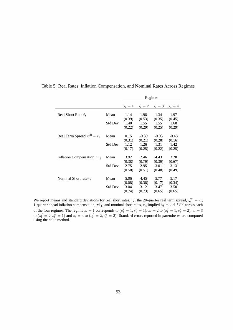
Table 5: Real Rates, Inflation Compensation, and Nominal Rates Across Regimes

Regime

st = 1 st = 2 st = 3 st = 4

Real Short Ratert Mean 1.14 1.98 1.34 1.97(0.39) (0.53) (0.35) (0.45)

Std Dev 1.40 1.55 1.55 1.68(0.22) (0.29) (0.25) (0.29)

Real Term Spready20t − rt Mean 0.15 -0.39 -0.03 -0.45

(0.31) (0.21) (0.28) (0.16)Std Dev 1.12 1.26 1.31 1.42

(0.17) (0.25) (0.22) (0.25)

Inflation Compensationπet,1 Mean 3.92 2.46 4.43 3.20

(0.38) (0.79) (0.39) (0.67)Std Dev 2.75 2.95 3.01 3.13

(0.50) (0.51) (0.48) (0.49)

Nominal Short ratert Mean 5.06 4.45 5.77 5.17(0.08) (0.38) (0.17) (0.34)

Std Dev 3.04 3.12 3.47 3.50(0.74) (0.73) (0.65) (0.65)

We report means and standard deviations for real short rates,rt; the 20-quarter real term spread,y20t − rt,

1-quarter ahead inflation compensation,πet,1; and nominal short rates,rt, implied by modelIV C across each

of the four regimes. The regimest = 1 corresponds to(sft = 1, sπ

t = 1), st = 2 to (sft = 1, sπ

t = 2), st = 3to (sf

t = 2, sπt = 1) andst = 4 to (sf

t = 2, sπt = 2). Standard errors reported in parentheses are computed

using the delta method.

53

Tabl

e6:

Cha

ract

eris

tics

ofR

ealR

ates

Pan

elA

:Con

ditio

nalM

omen

ts

Reg

imes

t=

1R

egim

est=

2R

egim

est=

3R

egim

est=

4M

atur

ityQ

trs

Mea

nS

tdev

Mea

nS

tdev

Mea

nS

tdev

Mea

nS

tdev

11.

141.

401.

981.

551.

341.

551.

971.

68(0

.39)

(0.2

2)(0

.53)

(0.2

9)(0

.35)

(0.2

5)(0

.45)

(0.2

9)4

1.33

0.86

1.85

0.93

1.54

0.89

1.83

0.94

(0.3

8)(0

.25)

(0.5

4)(0

.25)

(0.4

0)(0

.25)

(0.4

8)(0

.25)

201.

290.

551.

590.

561.

310.

551.

520.

56(0

.39)

(0.3

2)(0

.42)

(0.3

2)(0

.44)

(0.3

2)(0

.41)

(0.4

9)

Pan

elB

:Unc

ondi

tiona

lMom

ents

Mat

urity

Qtr

sM

ean

Std

evA

uto

11.

241.

460.

60(0

.38)

(0.2

3)(0

.08)

41.

410.

880.

73(0

.38)

(0.2

5)(0

.13)

201.

320.

550.

94(0

.40)

(0.3

2)(0

.05)

Spr

ead

20-1

0.07

1.19

0.52

(0.2

8)(0

.18)

(0.0

6)

Pan

elC

:Cor

rela

tions

with

Act

uala

ndE

xpec

ted

Infla

tion

Reg

imes

t=

1R

egim

est=

2R

egim

est=

3R

egim

est=

4U

ncon

ditio

nal

Mat

urity

Qtr

sA

ctua

lE

xpec

ted

Act

ual

Exp

ecte

dA

ctua

lE

xpec

ted

Act

ual

Exp

ecte

dA

ctua

lE

xpec

ted

1-0

.34

-0.0

2-0

.47

-0.1

2-0

.40

0.03

-0.4

9-0

.06

-0.3

4-0

.03

(0.3

1)(0

.24)

(0.3

1)(0

.25)

(0.3

7)(0

.28)

(0.3

5)(0

.29)

(0.2

9)(0

.31)

4-0

.11

0.14

-0.2

60.

02-0

.17

0.16

-0.2

90.

06-0

.13

0.16

(0.4

3)(0

.32)

(0.4

5)(0

.36)

(0.5

6)(0

.44)

(0.5

5)(0

.46)

(0.4

3)(0

.44)

200.

410.

460.

300.

380.

460.

540.

340.

450.

370.

57(0

.26)

(0.2

0)(0

.33)

(0.2

6)(0

.36)

(0.2

9)(0

.41)

(0.3

5)(0

.29)

(0.2

8)

54

Note to Table 6The table reports various moments of the real rate, implied from modelIV C . Panel A reports the conditionalmean and standard deviation of real rates of various maturities in quarters across regimes. Panel B reports theunconditional mean, standard deviation and autocorrelation of real yields. Panel C reports the correlationof real yields with actual and unexpected inflation implied from the model. We report the conditionalcorrelation of real yields with actual inflation corr(yn

t+1, πt+1|st), and the conditional correlation of realyields with expected inflation corr(yn

t+1, Et+1(πt+1+n,n)|st). Standard errors reported in parentheses arecomputed using the delta method.

55

Table 7: Effect of Regimes on Real Rates

Panel A: Real Yield Characteristics

Model Iw Model IV C

Real Short Ratert Mean 1.42 1.24(0.31) (0.38)

St Dev 1.59 1.46(0.29) (0.23)

Auto 0.72 0.60(0.09) (0.08)

Real Long Ratey20t Mean 1.69 1.32

(0.30) (0.40)St Dev 1.04 0.55

(0.34) (0.32)Auto 0.96 0.94

(0.02) (0.05)

Correlationrt, y20t 0.79 0.64

(0.08) (0.06)

Panel B: Comparisons ofIw and IV C over the Sample

Real Short Ratert Differences Std Dev 1.40Min -2.61Max 6.01

Real Long Ratey20t Differences Std Dev 0.54

Min -1.06Max 1.85

The table reports various characteristics of real yields from modelIw, an affine model similar to Campbelland Viceira (2001), and our modelIV C . In Panel A, we report population means, standard deviations, andautocorrelations of real one-quarter short rates and real 20-quarter long yields, together with their correlation.Standard errors reported in parentheses are computed using the delta method. In Panel B, we report statisticson the differences between the real yields implied by modelIw and modelIV C over the sample.

56

Table 8: Inflation Compensation, Expected Inflation, and Inflation Risk Premiums

Uncondi-Qtrs st = 1 st = 2 st = 3 st = 4 tional

Inflation Compensationπet,n

1 3.92 2.46 4.43 3.20 3.94(0.38) (0.78) (0.39) (0.67) (0.38)

4 4.20 2.49 4.95 3.34 4.25(0.34) (0.70) (0.39) (0.59) (0.35)

20 5.09 3.80 5.45 4.36 5.08(0.41) (0.45) (0.43) (0.42) (0.38)

Expected InflationEt(πt+n,n)

1 3.93 2.47 4.44 3.21 3.94(0.38) (0.79) (0.39) (0.67) (0.38)

4 3.89 2.63 4.48 3.47 3.94(0.38) (0.73) (0.41) (0.65) (0.38)

20 3.91 3.39 4.20 3.82 3.94(0.38) (0.49) (0.39) (0.46) (0.38)

Inflation Risk Premiumϕt,n

4 0.31 -0.14 0.47 -0.13 0.31(0.09) (0.06) (0.15) (0.09) (0.10)

20 1.18 0.42 1.25 0.55 1.14(0.36) (0.23) (0.42) (0.31) (0.36)

The table reports means of inflation compensation, the difference between nominal and real yields; expectedinflation; and the inflation risk premium implied from the benchmark modelIV C . Standard errors reportedin parentheses are computed using the delta method.

57

Table 9: Conditional Moments Across NBER Business Cycles

Mean Std Dev

MaturityQtrs Expansion Recession Expansion Recession

Real Ratesynt 1 1.45 1.23 1.30 2.06

(0.20) (0.20) (0.04) (0.08)20 1.33 1.43 0.65 0.87

(0.38) (0.38) (0.18) (0.25)

Nominal Ratesynt 1 5.03 5.95 2.59 4.07

(0.09) (0.14) (0.27) (0.41)20 6.05 6.85 2.46 3.71

(0.20) (0.22) (0.26) (0.38)

Inflation Compensationπet,n 1 3.57 4.73 2.23 3.62

(0.19) (0.17) (0.18) (0.28)20 4.72 5.42 1.89 2.93

(0.37) (0.39) (0.38) (0.57)

Actual Inflation 3.47 5.00 2.74 4.44

The table reports various sample moments of real rates, nominal rates and inflation compensation from thebenchmark modelIV C , conditional on expansions and recessions as defined by the NBER. Standard errorsreported in parentheses are computed using the delta method on sample moments.

Table 10: Unconditional Variance Decomposition of Nominal Yields

Maturity Real Expected InflationQtrs Rates Inflation Risk

1 0.20 0.80 0.00(0.09) (0.09) (0.00)

20 0.20 0.71 0.10(0.09) (0.09) (0.08)

The table reports unconditional variance decompositions of nominal yields,ynt , into real rate, expected

inflation, and inflation risk premium components, denoted byynt , Et(πt,n), andϕt,n, respectively. This

is done using the equation:

1 =var(yn

t , ynt )

var(ynt )

=cov(yn

t , ynt ) + cov(Et(πt,n), yn

t ) + cov(ϕt,n, ynt )

var(ynt )

.

Standard errors reported in parentheses are computed using the delta method on population moments.

58

Table 11: Unconditional Variance Decomposition of Nominal Yield Spreads

Panel A: Unconditional

Maturity Real Expected InflationQtrs Rates Inflation Risk

4 0.38 0.49 -0.01(0.14) (0.14) (0.00)

20 0.20 0.88 -0.05(0.19) (0.19) (0.02)

Panel B: Conditional on Regime

Maturity Real Expected Inflation Real Expected InflationQtrs Rates Inflation Risk Rates Inflation Risk

Regimest = 1 Regimest = 2

4 0.14 0.87 -0.01 0.08 0.93 -0.01(0.19) (0.19) (0.00) (0.22) (0.22) (0.00)

20 0.04 1.03 -0.08 -0.02 1.07 -0.05(0.20) (0.20) (0.03) (0.22) (0.22) (0.03)

Regimest = 3 Regimest = 4

4 0.69 0.32 -0.00 0.64 0.36 -0.00(0.12) (0.12) (0.00) (0.13) (0.13) (0.00)

20 0.31 0.71 -0.02 0.29 0.73 -0.02(0.16) (0.16) (0.01) (0.17) (0.17) (0.01)

The table reports unconditional variance decompositions of nominal yield spreads,ynt − y1

t , into real rate,expected inflation, and inflation risk premium components, denoted byyn

t − rt, Et(πt,n) − Et(πt+1), andϕt,n, respectively. This is done using the equation:

1 =var(yn

t − y1t , yn

t − y1t )

var(ynt − y1

t )

=cov(yn

t − rt, ynt − y1

t ) + cov(Et(πt,n)− Et(πt+1), ynt − y1

t ) + cov(ϕt,n, ynt − y1

t )var(yn

t − y1t )

.

Standard errors reported in parentheses are computed using the delta method on population moments.

59

Figure 1: Smoothed Regime Probabilities: All Regimes

Data

1955 1960 1965 1970 1975 1980 1985 1990 1995 2000 2005

−2

0

2

4

6

8

10

12

14

16

Short RateLong RateInflation

Regimes

1955 1960 1965 1970 1975 1980 1985 1990 1995 2000 20050

0.5

1

Pr(st=1)

1955 1960 1965 1970 1975 1980 1985 1990 1995 2000 20050

0.5

1

Pr(st=2)

1955 1960 1965 1970 1975 1980 1985 1990 1995 2000 20050

0.5

1

Pr(st=3)

1955 1960 1965 1970 1975 1980 1985 1990 1995 2000 20050

0.5

1

Pr(st=4)

The top graph plots the nominal short rate (1-quarter yield) and nominal long rate (20-quarter yield) togetherwith quarter-on-quarter inflation. The top panel’sy-axis units are annualized and are in percentages. In thebottom graph, we plot the smoothed probabilities of each of the four regimes,Pr(st = i|IT ), conditioningon data over the entire sample, from the benchmark modelIV C . NBER recessions are indicated by shadedbars.

60

Figure 2: Smoothed Regime Probabilities

1955 1960 1965 1970 1975 1980 1985 1990 1995 2000 2005

−2

0

2

4

6

8

10

12

Real Short RateReal Long RateExpected InflationInflation Compensation

1955 1960 1965 1970 1975 1980 1985 1990 1995 2000 20050

0.2

0.4

0.6

0.8

1

Pr(sft = 1)

1955 1960 1965 1970 1975 1980 1985 1990 1995 2000 20050

0.2

0.4

0.6

0.8

1

Pr(sπt = 1)

The top panel graphs the real short rate,rt; real long rate,y20t ; one-quarter expected inflation,Et(πt+1); and

long-term inflation compensation,πet,20. The top panel’sy-axis units are annualized and are in percentages.

The middle and bottom panels plot smoothed regime probabilities using information from the whole sample.The middle panel shows the smoothed probabilitiesPr(sf

t = 1|IT ) of thef factor regimes,sft . The bottom

panel graphs the smoothed probabilitiesPr(sπt = 1|IT ) of the inflation factor regime,sπ

t . NBER recessionsare indicated by shaded bars.

61

Figure 3: Real Term Structure

0 2 4 6 8 10 12 14 16 18 201.1

1.2

1.3

1.4

1.5

1.6

1.7

1.8

1.9

2Regime 1Regime 2Regime 3Regime 4Unconditional

We graph the real yield curve, conditional on each regime and the unconditional real yield curve. Thex-axisdisplays maturities in quarters of a year. They-axis units are annualized and are in percentages.

62

Figure 4: Impulse Responses of Real Yields

0 10 20−0.02

0

0.02

0.04

0.06

0.08

0.1

0.12

Quarters

Perc

enta

ge

1q real yield to q shocks

0 10 20−0.1

−0.05

0

0.05

0.1

0.15

Quarters

Perc

enta

ge1q real yield to f shocks

0 10 20−0.4

−0.3

−0.2

−0.1

0

0.1

Quarters

Perc

enta

ge

1q real yield to π shocks

0 10 20−0.02

0

0.02

0.04

0.06

0.08

Quarters

Perc

enta

ge

20q real yield to q shocks

0 10 20−0.03

−0.02

−0.01

0

0.01

0.02

Quarters

Perc

enta

ge

20q real yield to f shocks

0 10 20−0.05

−0.04

−0.03

−0.02

−0.01

0

0.01

Quarters

Perc

enta

ge20q real yield to π shocks

The figure plots impulse responses (IRs) of 1- and 20-quarter real yields (solid lines), together with twostandard errors bands (dashed lines), as implied by modelIV C . All IRs are computed using a one standarddeviation shock. The units on they-axis are in annualized percent.

63

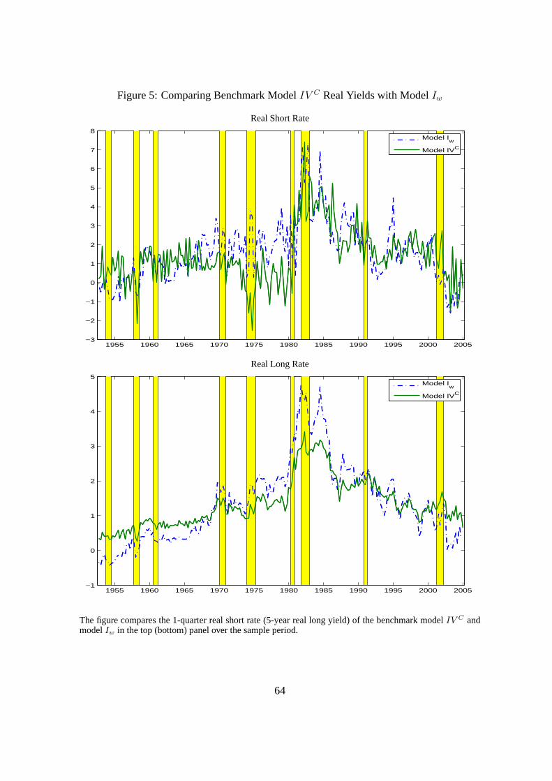
Figure 5: Comparing Benchmark ModelIV C Real Yields with ModelIw

Real Short Rate

1955 1960 1965 1970 1975 1980 1985 1990 1995 2000 2005−3

−2

−1

0

1

2

3

4

5

6

7

8

Model I

w

Model IVC

Real Long Rate

1955 1960 1965 1970 1975 1980 1985 1990 1995 2000 2005−1

0

1

2

3

4

5

Model I

w

Model IVC

The figure compares the 1-quarter real short rate (5-year real long yield) of the benchmark modelIV C andmodelIw in the top (bottom) panel over the sample period.

64

Figure 6: Comparative Statics of the Long-Term Inflation Risk Premium

−4 −2 0 2 4−1

0

1

2

3

4

5

6

Φπ q

−4 −2 0 2 4−1

0

1

2

3

4

5

6

Φπ f

−4 −2 0 2 4−1

0

1

2

3

4

5

6

Φπ π

−4 −2 0 2 4−1

0

1

2

3

4

5

6

δπ

−4 −2 0 2 4−1

0

1

2

3

4

5

6

λf(s

tπ=1)

−4 −2 0 2 4−1

0

1

2

3

4

5

6

λf(s

tπ=2)

In each plot, we show the unconditional 20-quarter inflation risk premium,ϕt,20, as a function of variousparameters of the benchmark modelIV C . The units on they-axis are annualized and are in percentageterms, and we alter the value of each parameter on thex-axis by up to±4 standard errors of the estimates ofeach parameter. The circle represents the baseline case at the estimated parameter value, of 1.14%.

65

Figure 7: Inflation Risk Premiums

1955 1960 1965 1970 1975 1980 1985 1990 1995 2000 2005−1

−0.5

0

0.5

1

1.5

2

2.5

3

3.5

4

The figure graphs the time-series of the 20-quarter inflation risk premium,ϕt,20, with two standard errorbounds. NBER recessions are indicated by shaded bars.

66

Figure 8: Nominal Term Structure

0 2 4 6 8 10 12 14 16 18 204

4.5

5

5.5

6

6.5

7

Regime 1Regime 2Regime 3Regime 4Unconditional

The figure graphs the nominal yield curve, conditional on each regime and the unconditional nominal yieldcurve from the benchmark modelIV C . Thex-axis displays maturities in quarters of a year. They-axis unitsare annualized and are in percentages. Average yields from data are represented by ’x’, with 95% confidenceintervals represented by vertical bars.

67