The Statistics of a Practical Seizure Warning System

David E. Snyder1, Javier Echauz2, David B. Grimes1, and Brian Litt31NeuroVista Corporation, 100 4th Avenue North, Suite 600, Seattle, WA 981092JE Research, Inc., 170 Wentworth Terrace, Alpharetta, GA 300223University of Pennsylvania, Department of Neurology, 3400 Spruce St., Philadelphia, PA 19104

AbstractStatistical methods for evaluating seizure prediction algorithms are controversial and a primarybarrier to realizing clinical applications. Experts agree that these algorithms must, at a minimum,perform better than chance, but the proper method for comparing to chance is in debate. We derivea statistical framework for this comparison, the expected performance of a chance predictor accordingto a predefined scoring rule, which is in turn used as the control in a hypothesis test. We verify theexpected performance of chance prediction using Monte Carlo simulations that generate random,simulated seizure warnings of variable duration. We propose a new test metric, the difference betweenalgorithm and chance sensitivities given a constraint on proportion of time spent in warning, and usea simple spectral power-based measure to demonstrate the utility of the metric in four patientsundergoing intracranial EEG monitoring during evaluation for epilepsy surgery. The methods arebroadly applicable to other scoring rules. We present them as an advance in the statistical evaluationof a practical seizure advisory system.

Keywordsseizure prediction; EEG; epilepsy; intracranial; statistics; brain

1. IntroductionMethods for evaluating seizure prediction algorithms represent a statistical challenge and havegenerated a great deal of controversy (Litt and Lehnertz 2002, Lehnertz and Litt 2005). WhenViglione's group formally assessed the first seizure warning system over 35 years ago, theybuilt a pocket-sized scalp-EEG audiovisual warning device using spectral features, and atrainable analog decision structure (Viglione et al 1970a, 1970b, 1973a, 1973b, 1975a). Their15-month study concluded that the device was “reasonably efficient” (Viglione 1975b).Although the resulting system exhibited a high true prediction rate, it also produced a high rateof false positive warnings (Gevins 2001). The same malady—sensitive but nonspecificprediction—may afflict many of the seizure advisory systems proposed to date, though formalvalidation is lacking (see reviews Litt and Echauz 2002, Iasemidis 2003, Mormann et al2007). Wide recognition of this problem and some consensus on data and statistical methodsrequired to evaluate the performance of seizure prediction algorithms began to emerge at themost recent International Seizure Prediction Workshop (Schulze-Bonhage et al 2007). Arecurring theme is that algorithms must, at a minimum, perform better than chance.Investigators address this challenge through a variety of approaches: benchmarks against

dsnyder@neurovista.com .Disclosure: Drs. Echauz and Litt are paid consultants to NeuroVista.

NIH Public AccessAuthor ManuscriptJ Neural Eng. Author manuscript; available in PMC 2010 June 20.

Published in final edited form as:J Neural Eng. 2008 December ; 5(4): 392–401. doi:10.1088/1741-2560/5/4/004.

NIH

-PA Author Manuscript

NIH

-PA Author Manuscript

NIH

-PA Author Manuscript

chance predictors, scientific debates on what electrophysiological events constitute a seizure,and an international collaborative effort to create an archive of continuous, prolonged, gold-standard data sets (Schulze-Bonhage et al 2007). Some of these formulations consider seizuregeneration as an intrinsically probabilistic process, where pro-seizure “permissive” statesmight come and go, not always leading to ictal events (Wong et al 2007). This conclusion issupported by clinical observation (Litt et al 2001, Haut 2006, Haut et al 2007) but remainsdifficult to confirm. Other formulations in the category of benchmarks against chancepredictors include surrogate data sets, periodic predictors, and random or pseudo-randomprocesses (Andrzejak et al 2003, Chaovalitwongse et al 2005).

Despite these efforts, investigators in the field of seizure prediction do not yet agree on: (1)how to account for the imprecise and enormously variable temporal relationship between initialalgorithm warnings and seizure onset, and (2) a mathematical framework for chance predictionthat enables them to translate statistical evaluation of research into clinical utility for epilepsypatients. In our experience, experimental seizure warning signals may vary from brief andsporadic to lengthy or repeated events lasting many hours. One proposal for resolving thisdilemma is to trigger a persistent warning light in response to a seizure warning. The durationof the light is designed to accommodate the temporal uncertainty of the prediction. The lightstays on for a predetermined period of time, so that it does not flash off and on as the next datawindow is processed, which might confuse the patient. A persistent warning scheme has beendescribed by Winterhalder et al (2003), who also propose a methodology for evaluatingalgorithm performance.

In this paper, we introduce a statistical approach for evaluating practical seizure advisorysystems, specifically, systems in which interactions with patients are carefully considered. Firstwe propose to allow the illumination period of a seizure warning light to be extended inresponse to additional positive predictions by an algorithm. A detailed Poisson-process-basedmodel for a corresponding persistence chance predictor is developed, with appropriateperformance metrics and methods for hypothesis testing. The theory is corroborated via MonteCarlo simulation (detailed in the Appendix), and then applied to the seizure predictionperformance of a simple illustrative algorithm reproducible from published literature, observedover long-term intracranial EEG recordings from four patients. We further demonstrate viaMonte Carlo simulation that the derived expressions for this statistical validation method areuseful even in non-Poisson stochastic settings, in particular ones that produce clusteredwarnings with gamma distributed inter-warning intervals. Finally, the candidate and chancepredictors are constrained to have a matched percentage of time spent in warning. Thisstipulation indirectly controls for specificity, without explicitly pitting sensitivity againstspecificity, as is classically done, which forces data segments to be scored into a priori mutuallyexclusive preictal vs. non-preictal classes.

2. Methods2.1 Phenomenology of the Seizure Advisory Algorithm

Consider a seizure advisory algorithm that analyzes real-time EEG and produces a uniformlysampled time series of binary data classifications: 1 if preictal, 0 if interictal. These binaryclassifications are translated into a suitable user interface by interpreting preictal classificationsas seizure warnings, and illuminating a persistent warning light according to the followingrules: whenever a preictal classification is observed, it triggers a timer of duration τw; whenanother preictal classification occurs, an additional and independent timer is triggered. Thewarning light is illuminated for as long as any timer is activated, i.e., the logical disjunction(OR) of the timer outputs. In the parlance of electrical engineering, this process is referred toas a retriggerable monostable multivibrator. The basic warning duration τw is referred to as

Snyder et al. Page 2

J Neural Eng. Author manuscript; available in PMC 2010 June 20.

NIH

-PA Author Manuscript

NIH

-PA Author Manuscript

NIH

-PA Author Manuscript

persistence parameter here. Uninterrupted illumination of the warning light is considered asingle warning, regardless of its duration.

2.2 SensitivityAlgorithm sensitivity Sn, typically defined as the probability of correctly anticipating a seizurewithin a time horizon, is vital for judging the performance of seizure prediction algorithms asit directly affects patients. In a microtemporal sense, the predictor output at each time pointcan be compared against preseizure-class labels, with each seizure contributing multiple pointsto count. In a macrotemporal sense, each seizure is taken as one single, missed or predicted,event to count. We adopt this latter framework, and further define sensitivity as the probabilityof illuminating a warning light at a time at least τw0 prior to the electrographic onset of a seizure,with the light remaining illuminated at least until the seizure begins. The period τw0 is providedto accommodate uncertainty regarding the precise moment of seizure onset, and to distinguishseizure detection from seizure prediction. This parameter, τw0, is referred to in this paper asthe detection interval. Alternatively, it can be used to represent a minimum desired predictioninterval, e.g., to accommodate a particular intervention strategy. While these definitions differin detail and perspective from the scoring intervals defined by Winterhalder et al (2003) andSchelter et al (2006), they are nonetheless mathematically equivalent: the detection intervalτw0 corresponds to the seizure prediction horizon (SPH), while τw corresponds to the sum ofSPH and the seizure occurrence period of the earlier work.

It is important to note that the definition of seizure, particularly in the setting of assessingalgorithm performance in a clinical setting, is not straightforward. One working definition forclinical use might focus on seizures that have clinical impact. In this way, subclinicalelectrographic events or events that might have minimal quality-of-life impact, such as mildsensory “auras,” might not be counted. Thus, an algorithm meant to predict both clinicalseizures and subclinical bursts on the intracranial EEG might have a very different seizuredefinition than a system meant to prevent patient injury from significant clinical events. Theexamples given in this paper are scored against electrographic seizures, regardless of clinicalmanifestation, but the method is applicable to any a priori definition of “seizure.”

2.3 Specificity-Related MetricsA classic definition of specificity in the seizure prediction context is the probability of correctlyindicating a nonpreseizure state at any given time. In our experience, the temporal relationshipbetween predictor outputs and seizure onset is highly variable, likely as a function of currentlyhidden properties of the system, in contrast to the classic treatment where preictal periods arefixed a priori. Additionally, any warning (true or false) represents an interruption to the patientthat must be dealt with. Thus we propose the proportion of time spent in warning ρw, and thewarning rate rw, as specificity-related metrics. These metrics are compelling from a patientperspective, since they provide information on the frequency and duration of inconveniencescaused by warnings. Some combination of proportion of time in warning and warning rateappears to provide a good balance of universality and unambiguous information whiledisallowing degenerate solutions. In particular, a chance predictor can be constructed so as toprovide the same proportion of time under warning as the algorithm under evaluation. Thecorresponding sensitivity and warning rate may be calculated for the chance predictor andcompared against observed performance of the algorithm under evaluation. A successfulalgorithm will provide higher sensitivity with the same or fewer warning light illuminationsper seizure. Alternatively, the chance predictor can be constructed to match the warning rate,and the proportion of time under warning calculated for comparison with the algorithm undertest.

Snyder et al. Page 3

J Neural Eng. Author manuscript; available in PMC 2010 June 20.

NIH

-PA Author Manuscript

NIH

-PA Author Manuscript

NIH

-PA Author Manuscript

2.4 The Chance PredictorTo test whether an algorithm is different from chance, it is necessary to define and characterizea sensorless chance predictor, i.e., without knowledge of EEG signal. One sensible choice isto use a Poisson process, whereby the probability of generating a preictal classification isuniformly distributed. More precisely, the probability of raising a preictal flag in a short intervalof duration Δt is approximately equal to λwΔt, independent of t, where λw is referred to as thePoisson rate parameter. For any time interval [0, t], the count of trigger events follows aPoisson probability distribution given in the Appendix (along with all derivations of ourmethod). The continuous-time idealization in this Poisson framework leads to formulas thatare significantly more compact than those using a purely discrete-time and binomialframework.

2.4.1 Sensitivity of the Chance Predictor—To determine the sensitivity of the chancepredictor, Snc, we must first identify the conditions that result in a correct seizure warning.Examples of both successful and unsuccessful warnings are shown in figure 1. Six observationsfollow: (a) All successful warnings require one or more trigger events to occur in period TBand/or TC, otherwise the warning light is extinguished prematurely. (b) One or more triggerevents occurring in period TB is sufficient for a correct warning. (c) One or more trigger eventsoccurring in period TC is not sufficient for a correct warning, since the light may not have beenilluminated early enough. (d) Trigger events occurring in period TC can only contribute to acorrect warning if they serve to retrigger an already illuminated warning light. (e) Correctwarnings can occur without a trigger event in period TB, but only if there are one or moretrigger events in period TA that are successfully retriggered in TC. (f) The only trigger eventsfor which a retrigger event in period TC is necessary, are those that occur in period TA.

With these observations in mind, an expression for Snc is shown to be

(1)

2.4.2 Specificity-Related Metrics of the Chance Predictor—In order to comparealgorithm performance versus chance, it is also necessary to characterize our proposedspecificity-related metrics—proportion of time spent in warning and warning rate—for acorresponding chance predictor. To accomplish this, one constructs a mathematical model forthe process of warning light illuminations as originally described, i.e., the logical OR of acollection of independently triggered warning light timers. The proportion of time that thechance predictor spends in warning is shown to be

(2)

Comparison of (2) to (1) reveals that for λwτw0 << 1 (as will be the case for any clinically usefulseizure advisory algorithm), the sensitivity of the chance predictor is approximately equal tothe proportion of time spent in warning—an intuitive result. The corresponding warning rateis shown to be

(3)

2.5 Performance Metric for Hypothesis TestingComparing the performance of different algorithms presents an interesting dilemma, since bothsensitivity and the proportion of time in warning will typically differ for alternative algorithms

Snyder et al. Page 4

J Neural Eng. Author manuscript; available in PMC 2010 June 20.

NIH

-PA Author Manuscript

NIH

-PA Author Manuscript

NIH

-PA Author Manuscript

applied to the same patient. If one algorithm offers better sensitivity, but a greater percentageof time in warning, should it be considered superior or inferior? A solution is suggested by theearlier observation that the sensitivity of a chance predictor is approximately equal to ρw, theproportion of time in warning. Therefore, the difference between observed and chancesensitivity, subject to matched ρw, is a powerful metric of predictive ability. It also offersappropriate behavior for limiting cases, being equal to zero if the warning light is eitherpermanently illuminated or extinguished. For an algorithm with observed sensitivity Sn andproportion of time in warning ρw, it follows from (1) and (2) that the sensitivity improvement-over-chance metric is calculated as:

(4)

where

(5)

2.5.1 P-Value of the Performance Test Result—To assess the significance of animprovement over chance, suppose a candidate algorithm identifies n of N seizures (i.e.,observed sensitivity Sn = n/N) for an individual patient. The two-sided p-value is the probabilityof observing a difference |n/N –Snc| or greater if the algorithm under evaluation is not differentfrom chance. This is shown to be, in terms of the binomial cumulative distribution function,equal to

(6)

where kf = ⌊2NSnc – n⌋ and kc = ⌈2NSnc – n⌉. The square bracketed terms of (6) comprise theone-sided p-value for superiority of the algorithm compared to chance. Of particular note isthe observation that the remaining terms in (6) will contribute to the p-value only when expectedsensitivity of the chance predictor is at least half that of the algorithm under test.

When algorithms are designed and applied prospectively to a population of patients, the valuesof ρw will vary from patient to patient. In this case, the overall significance involves the statisticsof, e.g., the median sensitivity improvement, with corresponding hypotheses

Similarly, when comparing two different algorithms that have been applied to the samepopulation, a paired test is indicated. In general, exact permutation tests may be applied to theStudentized and/or rank-ordered observations involved in the sensitivity improvement metriccalculation to account for unknown distributions and multiple-comparison testing in a patientpopulation.

2.6 Monte Carlo Corroboration of the Algorithm-vs.-Chance Prediction TheoryThe essential formulas of the retriggerable Poisson chance predictor presented thus far, (1)-(3)and (6), were corroborated using discrete-time Monte Carlo simulations. Additionally, gammadistributed interarrival times were evaluated to examine whether chance prediction might be

Snyder et al. Page 5

J Neural Eng. Author manuscript; available in PMC 2010 June 20.

NIH

-PA Author Manuscript

NIH

-PA Author Manuscript

NIH

-PA Author Manuscript

improved by clustering the seizures and/or the generated warnings. The purpose of thesesimulations was not only to corroborate the analytical formulas, but to confirm our suspicionthat using a temporal distribution of seizures and/or chance predictions which can modeltemporal clustering does not change the result. The latter could only be done by simulationbecause no closed-form analytical expressions could be derived from gamma distributions.Results of these Poisson and gamma simulations are shown in Appendix D, and lend supportto the Poisson-based formulas and their applicability in a wide sense of algorithm-vs.-chanceprediction.

2.7 Application to Intracranial EEG RecordingsThe method of comparing candidate seizure predictors to chance was applied to continuousEEG obtained from four patients undergoing evaluation for epilepsy surgery with intracranialelectrodes. These data sets were chosen such that half of them display significant predictionperformance and half of them do not, in order to illustrate application of the statistical methodsdetailed in this paper to real clinical data.

2.7.1 Patient and Data Characteristics—Multichannel digital intracranial EEGrecordings were obtained from Epilepsy Monitoring Units (EMUs) in Europe and the UnitedStates, with approval of the Institutional Review Boards of universities contributing data toNeuroVista Corporation under appropriate material transfer agreements, using approved (NBs/CE Mark in Europe, FDA in the US) clinical EMU equipment. Recordings were meticulouslychecked for misplugged or mislabeled electrodes, accurate seizure annotations, and electrodeplacement (validated by MRI). Only complete, continuous recordings were used for the presentapplication, covering each patient's entire EMU stay. Data were normalized to have a common16-bit dynamic range rescaled to microvolts, and sampling rate of 400 Hz. Table 1 showsredacted characteristics of the four patients whose records were used to demonstrate thestatistical methods.

2.7.2 Algorithm—A simple candidate seizure predictor involving spectral power featureextraction and patient-specific classification was employed for all patients. The algorithmanalyzed all available channels of cortical potentials including electrodes placed on andsurrounding the seizure focus, as well as a reference electrode well-separated from the focus.Multichannel referential EEG was first digitally remontaged to average reference. Eachchannel was pre-whitened by taking the first forward difference, bandpass filtered to beta band(implemented as 16-32 Hz corner frequencies in a Kaiser window FIR filter design), thensubjected to feature extraction in a 5-second sliding window scheme displaced in 1-secondincrements. For each channel, the output feature every 1 second was the beta power

(7)

where xβ[m] is the beta-filtered signal at time index m. A feature vector at each time was formedby collecting the beta powers of all channels.

The feature vectors collected over decimated time samples covering both preictal and interictalperiods formed training inputs with which kNN classifiers (k=15 neighbors) were induced. Thetraining outputs stored by the kNNs were integers {1,2} representing “interictal” vs. “90-minute preictal” classes. This latter label was used for immediate training, keeping in mindthat final “preictal” labels are revealed only during actual scoring/testing in our framework(e.g., a warning could end up being 5 hours long thus scored as “preictal,” with specificity-related metrics controlling for this asymmetry). When confronted with a new feature vector,

Snyder et al. Page 6

J Neural Eng. Author manuscript; available in PMC 2010 June 20.

NIH

-PA Author Manuscript

NIH

-PA Author Manuscript

NIH

-PA Author Manuscript

kNN looks up the nearest neighbor in its training table, however, the simple estimate of preictalposterior probability (fraction of nearest neighbors belonging to preictal class) was employedinstead. No adjustment was used for prior probabilities of the classes. When run as time-serialprobability estimator, the kNN output was 60-point-Chebyshev filtered in preparation forsmooth predictions. A prediction alert was issued whenever the smooth probability output met/exceeded a threshold. The threshold was algorithmically set such that, in-sample, percentageof time in warning tracked to 25%, however, the relation to actual measured ρw over a test setis inexact. This internal threshold can be fixed arbitrarily (recall our comparison to chancerequires only some “final” Sn and ρw). The output of all predictors were subjected to persistenceprocessing with parameters τw = 90 minutes and τw0 = 1 minute.

If seizures clustered within a 4-hour period, only the leading (first) seizure in that cluster wasenforced for prediction scoring purposes, for reasons similar to those of earthquake prediction—the goal is prediction of main events rather than detection of aftershocks. The scoring offollow-up clustered seizures was treated as deleted or never-seen data. For example, if originaldata had seizure onsets indicated as [0 0 0 0 1 0 0 0 0 1 0 1 1 0 0 0 0 1], the removal of clusteredseizures looked like [0 0 0 0 1 0 0 0 0 1 0 0 0 0 1]. Once these labels were fixed, the treatmentof candidate predictors and the theoretical chance predictor against which we compare remainsequitable and consistent with the theory. Without loss of generality, the estimation of expectedSn, ρw, and rw for each patient was based on N-fold cross validation, where N is the number ofleading seizures, with data assigned to folds in approximately 3-hour epochs.

2.7.3 Resetting the Warning System After Seizures—It is important to note that theoccurrence of seizures has been reported to “reset” the process of seizure generation, and thatperformance of a seizure warning system, particularly its specificity, may be enhanced byincluding this feature. We have chosen not to expand our analysis to take this into account forthe following reasons: First, when a clinical seizure warning system is deployed, patient-systeminteractions will inevitably form a closed loop. For example, patients may take fast-actingmedications when receiving indication of a high probability of seizure onset, which will likelyprevent, delay or otherwise alter the process of seizure generation. At present these isinsufficient data on such interactions to generate models to incorporate into the aboveparadigm. In such a system, even without intervention, a patient may learn to alter their seizureswhen informed of oncoming events. Second, we wanted to keep the chance predictor“sensorless,” without mixing it with EEG information.

With regard to seizure localization during epilepsy monitoring, clustered seizures within 4hours or less which we delete for scoring in our example are often treated as a single event,because of their tendency to arise from the same location (Wieser et al 1979). The formulas inour model applied to the cluster-removed data are still the same. Formulas would change withwarning cancellation after seizure detection, but as explained above this falls outside the desiredscope of comparing against pure chance.

3. ResultsFigure 2 shows one week's worth of the candidate warning outputs for each of the patients inrelation to their leading seizures (patients A and C had data exceeding 1 week, not fitting inthe plots but represented in the statistical results).

Table 2 lists the observed prediction metrics and significance levels for the four exemplarypatients. We now use Patient C in order to clarify the calculation of p-value in the frameworkpresented thus far. The seizure advisory algorithm with persistence of warning lights wasapplied to intracranial EEG over the entire 187.4 hour observation period. We have:

Snyder et al. Page 7

J Neural Eng. Author manuscript; available in PMC 2010 June 20.

NIH

-PA Author Manuscript

NIH

-PA Author Manuscript

NIH

-PA Author Manuscript

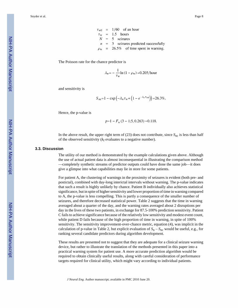
The Poisson rate for the chance predictor is

and sensitivity is

Hence, the p-value is

In the above result, the upper right term of (23) does not contribute, since Snc is less than halfof the observed sensitivity (kf evaluates to a negative number).

3.3. DiscussionThe utility of our method is demonstrated by the example calculations given above. Althoughthe use of actual patient data is almost inconsequential in illustrating the comparison method—completely synthetic streams of predictor outputs could have done the same job—it doesgive a glimpse into what capabilities may lie in store for some patients.

For patient A, the clustering of warnings in the proximity of seizures is evident (both pre- andpostictal), combined with day-long interictal intervals without warning. The p-value indicatesthat such a result is highly unlikely by chance. Patient B individually also achieves statisticalsignificance, but in spite of higher sensitivity and lower proportion of time in warning comparedto A, the p-value is less compelling. This is partly a consequence of the smaller number ofseizures, and therefore decreased statistical power. Table 2 suggests that the time in warningaveraged about a quarter of the day, and the warning rates averaged about 2 disruptions perday in the lives of these two patients, in exchange for 87.5-100% prediction sensitivity. PatientC fails to achieve significance because of the relatively low sensitivity and modest event count,while patient D fails because of the high proportion of time in warning, in spite of 100%sensitivity. The sensitivity improvement-over-chance metric, equation (4), was implicit in thecalculation of p-value in Table 2, but explicit evaluation of Sn – Snc would be useful, e.g., forranking several candidate predictors during algorithm development.

These results are presented not to suggest that they are adequate for a clinical seizure warningdevice, but rather to illustrate the translation of the methods presented in this paper into apractical warning system for patient use. A more accurate prediction algorithm would berequired to obtain clinically useful results, along with careful consideration of performancetargets required for clinical utility, which might vary according to individual patients.

Snyder et al. Page 8

J Neural Eng. Author manuscript; available in PMC 2010 June 20.

NIH

-PA Author Manuscript

NIH

-PA Author Manuscript

NIH

-PA Author Manuscript

4. ConclusionsWe present a framework for comparing the performance of EEG-based candidate seizurepredictors to sensorless chance predictors in a way that facilitates development of a clinicallyuseful system. A key departure of this method from previous approaches is allowing the brainto inform the algorithm, dynamically, how far in advance of seizures the epileptic networkbecomes “proictal” (i.e., enters a state with a high probability of seizure onset), as opposed tothe algorithm evaluator predefining rigid preictal vs. non-preictal time windows. This variable-length warning requirement is modestly accomplished through our proposed: (1) retriggerablepersistence indicator light, and (2) new performance metric: difference between algorithm andchance sensitivities, given a constraint on proportion of time spent in warning, which indirectlycontrols for specificity. For evaluating the statistical significance of candidate predictors, wepresent an explicit p-value formula. Both the theory and the Monte Carlo simulations suggestthat our chance prediction formulation holds independent of seizure clustering and for a wideclass of sensorless predictors.

A practical example of the method is offered in the analysis of four patient records selected sothat half of them show predictive value and half of them do not. A simple algorithm is used toshow how the evaluation scheme works to identify, accept, and reject predictive results, andhow a candidate predictor can show statistically honest superiority over chance withoutnecessarily involving extreme complexity. We do not present this algorithm or its performanceas sufficient for a clinically useful device. For those patients whose prediction performanceshows statistical significance, the sensitivity, proportion of time in warning, and warning ratesof the advisory systems may be within the range of clinical useful values, though they havenot been controlled for possible confounding effects (e.g., states of awareness). Based uponthe above methods and results, however, we believe that an appropriately powered, controlledstudy showing prospective prediction from EMU data is warranted to guide the developmentof a clinically useful, patient-oriented, seizure advisory system.

AcknowledgmentsThe authors would like to gratefully acknowledge the collaboration of Gregory Worrell, M.D., Ph.D., in providingclinical data and insight into this research. Dr. Litt's research is funded by the National Institutes of Health(RO1NS048598, 1NS041811-02, 2RO1CA084438-05A2), the Klingenstein Foundation, the Dana Foundation, TheEpilepsy Research Foundation, the Pennsylvania Tobacco Fund, and the Whitaker Foundation.

Appendix A. Derivation of Chance Predictor SensitivityTo count the trigger events, the counting random process {Nt, 0 ≤ t < ∞} is introduced, whichhas the Poisson probability distribution

(A.1)

From the six figure 1 observations,

(A.2)

Snyder et al. Page 9

J Neural Eng. Author manuscript; available in PMC 2010 June 20.

NIH

-PA Author Manuscript

NIH

-PA Author Manuscript

NIH

-PA Author Manuscript

As already observed, P[successful seizure advisory | one or more trigger events in B] is equalto unity, so (A.2) reduces to

(A.3)

P[one or more trigger events in B] is easily calculated using (A.1), and represents the sensitivitydue to preictal classifications that do not require retriggering. The result is in agreement withthe formula of Winterhalder et al (2003):

(A.4)

The conditional term in (A.3) is more subtle. To have a successful warning without a triggerevent in period TB requires that a trigger event first occur in period TA and be successfullyretriggered in period TC. The rate of these rarer events is found by multiplying the underlyingtrigger event rate, λw, by the probability of being retriggered successfully in TC:

(A.5)

To illustrate, the example of figure 1c is reproduced in figure A.1 with the time origin shiftedfor notational convenience. A trigger event occurring at time t in period TA is successfullyretriggered in TC if another trigger event occurs within the period τw to t+τw. As a consequence,the probability of a successful retrigger in TC is simply the probability of one or more triggerevents occurring in an interval of duration t (the period from τw to t+τw) which according to(A.1) is

(A.6)

Substitution of (A.6) into (A.5) yields

(A.7)

An important observation is that the rate of successful trigger events in A is not constant, buta function of t, so that the distribution of successful trigger events in period TA is characterizedby a non-homogeneous Poisson process. Accordingly, we define the counting random variable{Mt, 0 ≤ t < τw0} for the non-homogeneous Poisson process characterized by the rate parameterλA. The probability distribution of the non-homogeneous Poisson process is given by

(A.8)

Hence,

Snyder et al. Page 10

J Neural Eng. Author manuscript; available in PMC 2010 June 20.

NIH

-PA Author Manuscript

NIH

-PA Author Manuscript

NIH

-PA Author Manuscript

(A.9)

Substitution of (A.4) and (A.9) into (A.3) yields the sensitivity of the chance predictor

(A.10)

Appendix B. Derivation of Chance Predictor Specificity-Related MetricsConsider a set of warning trigger events occurring at times {Tj, j = 1, 2, 3,..., Nt} where Nt isthe previously defined Poisson counting variable and the Tj are referred to as arrival times.Define a new random process It to count the number of active timers:

(B.1)

where

(B.2)

The function h(t) represents a warning light timer of duration τw. Since the warning light isextinguished only when It is identically zero, the proportion of time in alert is equal to 1 – P[It = 0].

Equation (B.1) represents a filtered (or compound) Poisson process. Since It is comprised of asum of functions of random variables, evaluation of P[It = k] is most easily performed viaFourier transform to obtain the characteristic function of the filtered Poisson process(Davenport 1970).

(B.3)

Substitution of (B.2) into (B.3) leads to

(B.4)

Fourier inversion of (B.4) provides

Snyder et al. Page 11

J Neural Eng. Author manuscript; available in PMC 2010 June 20.

NIH

-PA Author Manuscript

NIH

-PA Author Manuscript

NIH

-PA Author Manuscript

(B.5)

and the proportion of time in warning is

(B.6)

To calculate the rate of warnings, rw, we observe that a new warning will occur whenever theinterval between successive preictal trigger events exceeds τw. To examine the properties ofsuch intervals, we define a corresponding random process:

(B.7)

For Tk determined by a Poisson process, such “interarrival times” are themselves exponentiallydistributed, independent random variables (Davenport 1970).

(B.8)

With this information, the rate of warnings can be computed by multiplying the rate of preictalclassifications by the proportion of interarrival times greater than τw:

(B.9)

Appendix C. Derivation of P-Value for the Performance Test ResultGiven a candidate algorithm's observed sensitivity Sn = n/N, the two-sided p-value is theprobability of the chance predictor also displaying a difference |n/N –Snc| or greater:

(C.1)

where n' is the random variable corresponding to the number of predicted seizures under thenull hypothesis. Each of the N seizures can be considered a Bernoulli trial with the probabilityof advisory equal to the expected sensitivity of the chance predictor. Accordingly, (C.1) canbe rewritten in terms of the binomial cumulative distribution function

(C.2)

where

Snyder et al. Page 12

J Neural Eng. Author manuscript; available in PMC 2010 June 20.

NIH

-PA Author Manuscript

NIH

-PA Author Manuscript

NIH

-PA Author Manuscript

(C.3)

(C.4)

and

(C.5)

Appendix D. Monte Carlo Corroboration of the TheoryThe performance of a hypothetical EEG-based predictor was used as a reference for definingchance prediction experiments to corroborate formulas (1)-(3) and (6). The reference predictorhad sensitivity Sn = 80% (e.g., predicts 4 out of 5 seizures), with a proportion of time in warningρw = 27.5%, persistence τw = 90 minutes, and detection interval τw0 = 1 minute. To test thechance predictor, two types of seizure sequences were generated: the first with uniformlydistributed seizures (5 seizures over a 140-hour period), and the second based on gammadistributions to simulate the seizure clustering phenomena often seen in epilepsy (Haut2006).

To generate chance predictions, the time axis was discretized into 1-second increments. Triggerevents for the Poisson-based discrete-time chance predictor were obtained as a sequence ofBernoulli trials with probability pB equal to the rate parameter given by formula (5): λw =5.955×10–5 chance assertions/second (pB ≈ λw Δt, with Δt = 1 s). The trigger events were usedto generate persistent warning indicators with persistence sample count = 5400 (90 minutes).Ten thousand Monte Carlo simulation trials were conducted for each type of seizure sequence(uniform and clustered). The following quantities were tallied: (a) number of true positives,(b) cumulatively revised sensitivity, proportion of time spent in warning and rate of warnings(number of rising edges per hour), and (c) fraction of trials where sensitivity of the chancepredictor was equal to or better than the 80% sensitivity of the reference predictor (for p-valuecorroboration). At the end of a simulation, each Monte Carlo estimate is an average across alltrials. Results of these trials are summarized in the first two rows of Table D.1.

An experiment was additionally performed to explore whether formulas (1)-(3) and (6) mightgeneralize to non-Poisson chance predictors. A gamma-based chance predictor that issuedclustered warnings was constructed and scored against clustered seizure sequences. This wasaccomplished by sampling inter-trigger intervals from a gamma distribution

(D.1)

with shape parameter α = 0.2, and scale parameter β set to obtain the desired ρw = 27.5%, andthen applying the persistent warning indicator rules. The results of this experiment are shownin the final row of Table D.1. For three combinations of seizure distribution and type of chancepredictor {(uniform, Poisson), (gamma, Poisson), and (gamma, gamma)}, Table D.1 shows

Snyder et al. Page 13

J Neural Eng. Author manuscript; available in PMC 2010 June 20.

NIH

-PA Author Manuscript

NIH

-PA Author Manuscript

NIH

-PA Author Manuscript

the agreement found between expected values of the variables according to the Poissonformulas and the corresponding Monte Carlo estimates.

ReferencesAndrzejak RG, Mormann F, Kreuz T, Rieke C, Kraskov A, Elger CE, Lehnertz K. Testing the null

hypothesis of the nonexistence of a preseizure state. Phys. Rev. E Stat. Nonlin. Soft Matter Phys2003;67:010901. [PubMed: 12636484]

Chaovalitwongse W, Iasemidis LD, Pardalos PM, Carney PR, Shiau DS, Sackellares JC. Performanceof a seizure warning algorithm based on the dynamics of intracranial EEG. Epilepsy Res 2005;64:93–113. [PubMed: 15961284]

Davenport, WB. Probability and Random Processes. McGraw-Hill Book Company; New York: 1970.Gevins, A. Pers. comm. 2001.Haut SR. Seizure clustering. Epilepsy Behav 2006;8:50–5. [PubMed: 16246629]Haut SR, Hall CB, Masur J, Lipton RB. Seizure occurrence: precipitants and prediction. Neurology

2007;69:1905–10. [PubMed: 17998482]Iasemidis LD. Epileptic seizure prediction and control. IEEE Trans. Biomed. Eng 2003;50:549–58.

[PubMed: 12769431]Lehnertz K, Litt B. The First International Collaborative Workshop on Seizure Prediction: summary and

data description. Clin. Neurophysiol 2005;116:493–505. [PubMed: 15721063]Litt B, Echauz J. Prediction of epileptic seizures. The Lancet Neurol 2002;1:22–30.Litt B, Esteller R, Echauz J, D'Alessandro M, Shor R, Henry T, Pennell P, Epstein C, Bakay R, Dichter

M, et al. Epileptic seizures may begin hours in advance of clinical onset: a report of five patients.Neuron 2001;30:51–64. [PubMed: 11343644]

Litt B, Lehnertz K. Seizure prediction and the preseizure period. Curr. Opin. Neurol 2002;15:173–7.[PubMed: 11923631]

Marsaglia G, Tsang W. A simple method for generating gamma variables. ACM Trans. Math. Software2000;26:363–72.

Mormann F, Andrzejak RG, Elger CE, Lehnertz K. Seizure prediction: the long and winding road. Brain2007;130:314–33. [PubMed: 17008335]

Schelter B, Winterhalder M, Maiwald T, Brandt A, Schad A, Schulze-Bonhage A, Timmer J. Testingstatistical significance of multivariate time series analysis techniques for epileptic seizure prediction.Chaos 2006;16:013108. [PubMed: 16599739]

Schulze-Bonhage, A.; Timmer, J.; Schelter, B. 3rd International Workshop on Epileptic SeizurePrediction; Freiburg, Germany. 2007.

Viglione, S. Applications of pattern recognition technology. In: Mendel, J.; Fu, K., editors. Adaptive,Learning, and Pattern Recognition Systems: Theory and Applications. Academic Press; New York:1970. p. 115-61.

Viglione, S.; Ordon, V.; Martin, W.; Kesler, C. Epileptic seizure warning system (U.S.). 1973. Patent3,863,625

Viglione, S.; Ordon, V.; Risch, F. Proc. 21st Western Institute on Epilepsy. McDonnell DouglasAstronautics Co.; West Huntington Beach, CA: 1970. A methodology for detecting ongoing changesin the EEG prior to clinical seizures. p WD1399(A)

Viglione, SS. Detection and prediction of epileptic seizures validation program--Proposal for testing andevaluation of epileptic seizures alerting systems. McDonnell Douglas Astronautics Co.; WestHuntington Beach, CA: 1973.

Viglione, SS. Validation of epilepsy seizure warning system. McDonnell Douglas Astronautics Co.; WestHuntington Beach, CA: 1974. APA 74133

Viglione, SS. Validation of the epilepsy seizure warning system (special report). Social and RehabilitationService; Washington, D.C.: 1974. Grant SRS-23-57680

Viglione, SS. Validation of the epilepsy seizure warning system (final report). Social and RehabilitationService; Washington, D.C.: 1975. Grant SRS-23-57680

Snyder et al. Page 14

J Neural Eng. Author manuscript; available in PMC 2010 June 20.

NIH

-PA Author Manuscript

NIH

-PA Author Manuscript

NIH

-PA Author Manuscript

Viglione SS, Walsh GO. Proceedings: Epileptic seizure prediction. Electroencephalogr. Clin.Neurophysiol 1975;39:435–6. [PubMed: 51767]

Wieser HG, Bancaud J, Talairach J, Bonis A, Szikla G. Comparative value of spontaneous and chemicallyand electrically induced seizures in establishing the lateralization of temporal lobe seizures. Epilepsia1979;20:47–59. [PubMed: 421676]

Winterhalder M, Maiwald T, Voss HU, Aschenbrenner-Scheibe R, Timmer J, Schulze-Bonhage A. Theseizure prediction characteristic: a general framework to assess and compare seizure predictionmethods. Epilepsy Behav 2003;4:318–25. [PubMed: 12791335]

Wong S, Gardner AB, Krieger AM, Litt B. A stochastic framework for evaluating seizure predictionalgorithms using hidden Markov models. J. Neurophysiol 2007;97:2525–32. [PubMed: 17021032]

Snyder et al. Page 15

J Neural Eng. Author manuscript; available in PMC 2010 June 20.

NIH

-PA Author Manuscript

NIH

-PA Author Manuscript

NIH

-PA Author Manuscript

Figure 1.Examples of successful and unsuccessful warnings in relation to a seizure onset at time ts: (a)Definition of TA, TB, TC time periods. (b) A successful seizure warning. (c) A failed seizurewarning. (d) A seizure warning made successful by retriggering.

Snyder et al. Page 16

J Neural Eng. Author manuscript; available in PMC 2010 June 20.

NIH

-PA Author Manuscript

NIH

-PA Author Manuscript

NIH

-PA Author Manuscript

Figure 2.Actual candidate predictor outputs after persistence over a week-long recording of four patientsin relation to their leading seizures (‘x’ indicates false negative, and ‘+’ indicates true positive).

Snyder et al. Page 17

J Neural Eng. Author manuscript; available in PMC 2010 June 20.

NIH

-PA Author Manuscript

NIH

-PA Author Manuscript

NIH

-PA Author Manuscript

Figure A.1.Successfully retriggered warning light with time origin shifted.

Snyder et al. Page 18

J Neural Eng. Author manuscript; available in PMC 2010 June 20.

NIH

-PA Author Manuscript

NIH

-PA Author Manuscript

NIH

-PA Author Manuscript

NIH

-PA Author Manuscript

NIH

-PA Author Manuscript

NIH

-PA Author Manuscript

Snyder et al. Page 19

Tabl

e 1

Patie

nt a

nd d

ata

char

acte

ristic

s. C

P=co

mpl

ex p

artia

l; G

TC=g

ener

aliz

ed to

nic-

clon

ic.

Patie

ntG

ende

rSe

izur

e T

ype(

s)Ic

tal O

nset

Zon

e(s)

Side

of R

esec

tion

Rec

ordi

ng D

urat

ion

(hou

rs)

AF

CP,

GTC

Infe

rior t

empo

ral g

yrus

of t

he le

ft te

mpo

ral l

obe

Left

422.

7

BF

CP

Tem

pora

l, pa

rieta

l and

fron

tal l

obes

Left

131.

1

CM

CP

Mul

tifoc

al, m

ore

freq

uent

ly le

ft m

esia

l tem

pora

lN

one

(inde

term

inat

e)18

7.4

DM

CP,

GTC

Rig

ht fr

onta

lR

ight

90.0

J Neural Eng. Author manuscript; available in PMC 2010 June 20.

NIH

-PA Author Manuscript

NIH

-PA Author Manuscript

NIH

-PA Author Manuscript

Snyder et al. Page 20

Tabl

e 2

Obs

erve

d pr

edic

tion

met

rics a

nd si

gnifi

canc

e le

vels

for t

he fo

ur e

xem

plar

y pa

tient

s.

Patie

ntT

otal

# o

f Sei

zure

sSe

nsiti

vity

Sn

War

ning

Pro

port

ion

War

ning

Rat

e (p

er h

our)

P-V

alue

A8

87.5

%29

.0%

0.09

90.

001

B2

100.

0%19

.1%

0.07

60.

036

C5

60.0

%26

.5%

0.09

10.

118

D2

100.

0%53

.3%

0.11

10.

502

J Neural Eng. Author manuscript; available in PMC 2010 June 20.

NIH

-PA Author Manuscript

NIH

-PA Author Manuscript

NIH

-PA Author Manuscript

Snyder et al. Page 21

Table D.1

Monte Carlo estimates of chance prediction metrics. P-value is the probability of chance explaining the Sn=80%of a matched reference algorithm. The expected values according to the Poisson formulas are E[Snc] = 0.27241,E[ρw] = 0.275, E[rw] = 0.155/hr, and p = 0.02153.

Seizures vs. Chance Predictor Distributions Quantity of Interest Monte Carlo Simulation

Uniform, Poisson

E[Snc] 0.27053

E[ρw] 0.275

E[rw] 0.156/hr

p-value 0.02008

Gamma, Poisson

E[Snc] 0.27390

E[ρw] 0.275

E[rw] 0.155/hr

p-value 0.02480

Gamma, Gamma

E[Snc] 0.27558

E[ρw] 0.275

E[rw] 0.131/hr

p-value 0.03100

J Neural Eng. Author manuscript; available in PMC 2010 June 20.