ISCORMA-3, Cleveland, Ohio, 19-23 September 2005

1

THE STABILITY OF AUTOMATIC BALL BALANCERS

Kirk Green, Michael I. Friswell, Alan R. Champneys and Nicholas A. J. Lieven BRISTOL LABORATORY FOR ADVANCED DYNAMICS ENGINEERING University of Bristol, Queen’s Building, University Walk, Bristol BS8 1TR, UK

Kirk.Green, M.I.Friswell, A.R.Champneys, Nick.Lieven@bristol.ac.uk ABSTRACT

One realisation of an automatic balancer uses two or more balls that are free to travel in a race, filled with a viscous fluid, at a fixed distance from the shaft centre. The objective is for the balls to position themselves so that they counteract any residual unbalance. The fact that no external force is required to achieve balance, that is the system is passively controlled, means that the balancer is potentially able to cope with a time-varying unbalance. Typical applications include optical disc drives and machine tools. However, the usefulness of this device depends on the balanced steady state solution being achievable and stable. This paper describes a dynamic model of a Jeffcott rotor with an automatic balancer and provides a non-linear analysis of its dynamics to determine steady states and their bifurcations as parameters are varied. The pseudospectra of the linearization of the system about a balanced steady state solution are computed. This approach allows the eigenvalues that are most sensitive to perturbation to be quantified. Furthermore, how the sensitivity of the eigenvalues influences the transient response may be determined. These tools will help to design reliable and robust automatic balancers.

Keywords: ball balancer, bifurcation analysis, pseudospectra, Jeffcott rotor

NOMENCLATURE ,X Yc c Damping coefficients of disk support

iD Viscous damping for i th ball D Viscous damping coefficient for all balls

,X Yk k Stiffness coefficients of disk support m Equal mass of balls

im Mass of i th ball M mass of disk Mε Residual unbalance R Radius of ball race x, y Position of disk in rotating coordinates X, Y Position of disk in fixed coordinates

X , Y Non-dimensional position of disk β Non-dimensional ball damping δ Non-dimensional shaft eccentricity

iφ Angular position of i th ball µ Ratio of ball to disk masses ψ Angular position of shaft ω Shaft speed

nω Machine natural frequency Ω Non-dimensional shaft speed ζ Non-dimensional machine damping

INTRODUCTION Unbalance is a major cause of vibration in rotating machinery. In most cases standard methods of

balancing are able to reduce the vibration to satisfactory levels. Sometimes, however, the unbalance varies with time, for example due to the fouling of blades. Here some sort of active or semi-active system of balancing is required. This motivates the use of self-compensating, automatic dynamic balancers (ADB), that require no external forces to achieve balance. ADBs have been applied to optical disc drives to obtain higher operating speeds without any reduction in the tracking performance [2, 8, 9], and to balance machine tools, such as, lathes, angle grinders and cutting tools [11]. Lee and van Moorhem [10] reviewed the early history of ADBs. The ADB of interest here consists of two or more

ISCORMA-3, Cleveland, Ohio, 19-23 September 2005

2

masses that are free to travel around a race, filled with a viscous fluid, at a fixed distance from the centre of rotation of the rotor. Chung and Ro [3] and Adolfsson [1] derived the equations of motion and performed a linear stability analysis using perturbation methods to identify stability regions of the full nonlinear problem. However, due to the highly nonlinear nature of the problem, the ADB mechanism can make the vibration response much worse for some parameter values. This has limited the successful commercial application of the devices [12]. A linear stability analysis, used alone, is an inadequate tool for understanding such nonlinear behavior.

In this paper, we provide a detailed nonlinear bifurcation analysis of the dynamics of the ADB by using numerical continuation tools [4]. The equations of motion are solved in the rotating frame, since the problem is then a time-independent (autonomous) system that is very amenable to a full nonlinear bifurcation analysis. The approach finds, and then follows, steady states and periodic solutions, irrespective of their stability, and is able to detect their local bifurcations. These bifurcations mark the stability boundaries of the steady state equilibrium in the full nonlinear system [5]. We also consider the transient response of a machine fitted with an ADB mechanism. The transient behavior in linear dynamical systems can be very different to that predicted by a linear stability analysis, where the eigenvalues determine the asymptotic behavior. Often, in stable non-normal systems, transients may exhibit an undesired dynamic response, such as, a large transient growth (or apparent instability) preceding a long, highly oscillatory, exponential decay or, alternatively, a rapid collapse before eventual asymptotic decay to the stable equilibrium [6]. This behavior is of particular concern when considering a linearization about an equilibrium of a system with strong nonlinearities. In this case, a large transient growth may result in a trajectory of the full nonlinear system coming close to regions of state space where the linearization breaks down. Thus the eigenvalues of the linearization do not always correctly predict the behavior of the full nonlinear system, particularly in a finite time interval [7]. Thus an analysis and understanding of the sensitivity to perturbation and the ensuing transient response is necessary for the robust design of a practical device.

1. EQUATIONS OF MOTION Figure 1 shows a schematic of an ADB with two balancing masses. Movement is confined to in

plane motions of the disk, whose position is given by X and Y. The shaft stiffness and damping is modeled by springs ( Xk , Yk ) and dashpots ( Xc , Yc ) in the X and Y directions. The disk has mass M. The balls are free to move in a race of radius R, and the angular position of the i th ball is denoted by iφ . The fluid exerts a force on the balls that is modeled as a viscous drag with coefficient iD . The unbalance on the disk is modeled as a mass eccentricity ε, giving an unbalance magnitude of Mε. The angular position of the shaft is denoted by ψ.

The equations of motion describing this system are derived using Lagrange’s equation [5]. With two balls there are four degrees of freedom, namely the position of the disk (X and Y ) and the angular position of the two balls ( 1φ and 2φ ). The equations describing the displacement in the X and Y directions are given by

( ) ( ) ( ) ( ) 2

22

1

cos sin

sin cos 0,

X X

i i i i i

i

MX c X k X M M

m X R R=

+ + − εψ ψ − εψ ψ

+ − ψ + φ ψ + φ − ψ + φ ψ + φ =∑ (1)

ISCORMA-3, Cleveland, Ohio, 19-23 September 2005

3

( ) ( ) ( ) ( ) 2

2 22

1 1

sin cos

cos sin 0.

Y Y

i i i i i i

i i

MY c Y k Y M M Mg

m Y R R m g= =

+ + − εψ ψ + εψ ψ +

+ + ψ + φ ψ +φ − ψ + φ ψ + φ + =∑ ∑ (2)

Y

X0

CR

CM

ε

φ1

φ2

ωt

cY

kY

cXkX

D RM

m

Fig. 1. Automatic dynamic balancer.

In Eqs. (1) and (2) the standard terms relating to the disk, shaft and unbalance are readily identified. The inertia terms and gravity force relating to the balls are given by the summations. Finally, the equation of motion of the i th ball is given by ( ) ( ) ( ) ( )2 sin cos cos 0.i i i i i i i i im R D m R X Y m gR⎡ ⎤ψ + φ + φ − ψ +φ − ψ +φ + ψ +φ =⎣ ⎦ (3)

These equations can be simplified by assuming equal masses of the balancing balls ( )1 2m m m= = ,

an equal viscous drag coefficient for each ball ( )1 2D D D= = , a constant angular velocity of the rotor ω (where tψ = ω ) and isotropic suspension of the rotor ( X Yc c c= = and X Yk k k= = ). Finally, we neglect the effect of gravity on the motion of the balls, that is we set g=0.

We can write the equations in dimensionless form by introducing the following non-dimensional degrees of freedom and non-dimensional time

, , ,nX YX Y t tR R

= = = ω (4)

and the dimensionless parameters

ISCORMA-3, Cleveland, Ohio, 19-23 September 2005

4

2, , , , ,2n n

m c DM R kM mR

ω εΩ = µ = δ = ς = β =

ω ω (5)

where Mkn /=ω is the natural frequency of the rotor.

Finally, we obtain a time independent set of equations by transforming to a rotating frame of reference,

( ) ( )( ) ( )tytxY

tytxXΩ+Ω=Ω−Ω=

cossinsincos

(6)

This results in the following second-order dimensionless system describing the ADB in a rotating frame:

( )( )

( )( )

( ) ( )

22

21

2 2

2 2 11 0 22 1 20 1 2

cos,

sin0

2 sin 2 cos .

ni i i

ii i i

i i i i

nn x x K xnn y y K y

x x y y y x

=

ς − Ω + µ⎛ ⎞+ µ − Ως⎛ ⎞⎛ ⎞ ⎛ ⎞ ⎛ ⎞⎛ ⎞+ +⎜ ⎟⎜ ⎟⎜ ⎟ ⎜ ⎟ ⎜ ⎟⎜ ⎟Ω + µ ς+ µ Ως⎝ ⎠⎝ ⎠ ⎝ ⎠ ⎝ ⎠⎝ ⎠⎝ ⎠

⎛ ⎞Ω + φ φ⎛ ⎞ φ⎛ ⎞δΩ ⎜ ⎟= +µ⎜ ⎟ ⎜ ⎟⎜ ⎟⎜ ⎟ φ⎝ ⎠⎝ ⎠ ⎜ ⎟−φ Ω+ φ⎝ ⎠

φ +βφ = −Ω − Ω φ − −Ω + Ω φ

∑ (7)

In this paper, we only consider two balancing masses. Therefore, our system describing the ADB has

four degrees of freedom, and when written in state space form is eight-dimensional. This system has three steady state solutions. Namely, a balanced steady state where the radial vibration is reduced to zero; a ‘coincident’ steady state where the balls occupy the same position in the race, resulting in a non-zero radial vibration; and an ‘in-line’ steady state where the two balls lie on opposite sides of the race in a line with the centre of mass of the rotor [5]. Here, we concentrate on the balanced steady state solution given by,

0== yx , ⎟⎟⎠

⎞⎜⎜⎝

⎛ −= −

µδφ

2cos 1

1 , 12 φφ −= . (8)

A conclusion we can immediately make for the balanced steady state to exist is that, δµ 2> . In

words, the balancing balls must have sufficient mass in order to overcome the residual unbalance.

2. BIFURCATION ANALYSIS Bifurcation analysis is used to ‘map’ out how the stability of a system depends on changes in its

parameters. We use the numerical continuation package AUTO [4] to investigate the stability of the steady states detailed above as the dimensionless parameters for the mass µ , eccentricity δ , external damping ς , and internal damping β are varied. Figure 2 shows the stability regions in ( )µ,Ω -space (a), ( )δ,Ω -space (b), ( )ς,Ω -space (c), and ( )β,Ω -space (d). In each case, when fixed, the other parameters are µ = 0.05, β = δ = ζ = 0.01. Dark shaded regions in Fig. 2 correspond to parameter values where the balanced state is stable. Lighter regions correspond to parameter values where the coincident

ISCORMA-3, Cleveland, Ohio, 19-23 September 2005

5

equilibrium is stable. No shading corresponds to regions of instability. Dashed curves indicate lines of Hopf bifurcations, marked by a H. In other words, crossing one of these curves, due to the variation in the parameters, will result in an oscillatory instability. In particular, the Hopf curves bordering the regions with dark shading result in an oscillatory instability of the stable balanced state and a subsequent stable periodic solution. The solid curves indicated in Fig. 2, labeled SN, indicate lines of saddle-node bifurcations. As a line of saddle-node bifurcations is crossed a coincident equilibrium is born (when crossing into the light shaded region) or destroyed (when crossing into a region of instability). Finally, the curve in Fig. 2(a) marked PF indicates a line of pitch-fork bifurcations in which an additional steady state is born or destroyed. For example, as µ is increased from zero, the balanced state is born at the curve PF. This balanced state, born at PF, is unstable for 3.1<Ω but stable otherwise, that is, crossing from the light shaded region to the dark shaded region for large values ofΩ .

0.5 1 1.5 2 2.50

0.02

0.04

0.06

0.08

µ

Ω

SN2±

H1

PF1,2−

SN2±

H2+ H1

PF1,2+

0 1 2 30

0.05

0.1

δ

Ω

SN2± SN2±

H1

H1H1

0 1 2 30

0.25

0.5

ζ

Ω

SN2± SN2±

H1

H1

0 1 2 30

0.25

0.5

β

Ω

SN2± SN2±

H1

H1

(a) (b)

(c) (d)

Fig. 2. Two-parameter bifurcation diagrams showing regions of stability in parameter space of the balanced steady state (dark shading), and the coincident steady state (light shading); see text for full details.

A main conclusion to be drawn from Fig. 2 is that for rotation speeds of approximately 5.2>Ω the

balanced state is always achievable. Furthermore, Fig. 2(a) shows a ‘wedge’ of stability of the balanced state for 1=Ω , the rotation speed corresponding to the first resonant frequency, nω . This is the rotation speed at which one observes greatest radial vibration in a standard eccentric (Jeffcott) rotor. The fact that

ISCORMA-3, Cleveland, Ohio, 19-23 September 2005

6

balance may be achievable for rotation speeds at and close to the resonant frequency is of great physical interest.

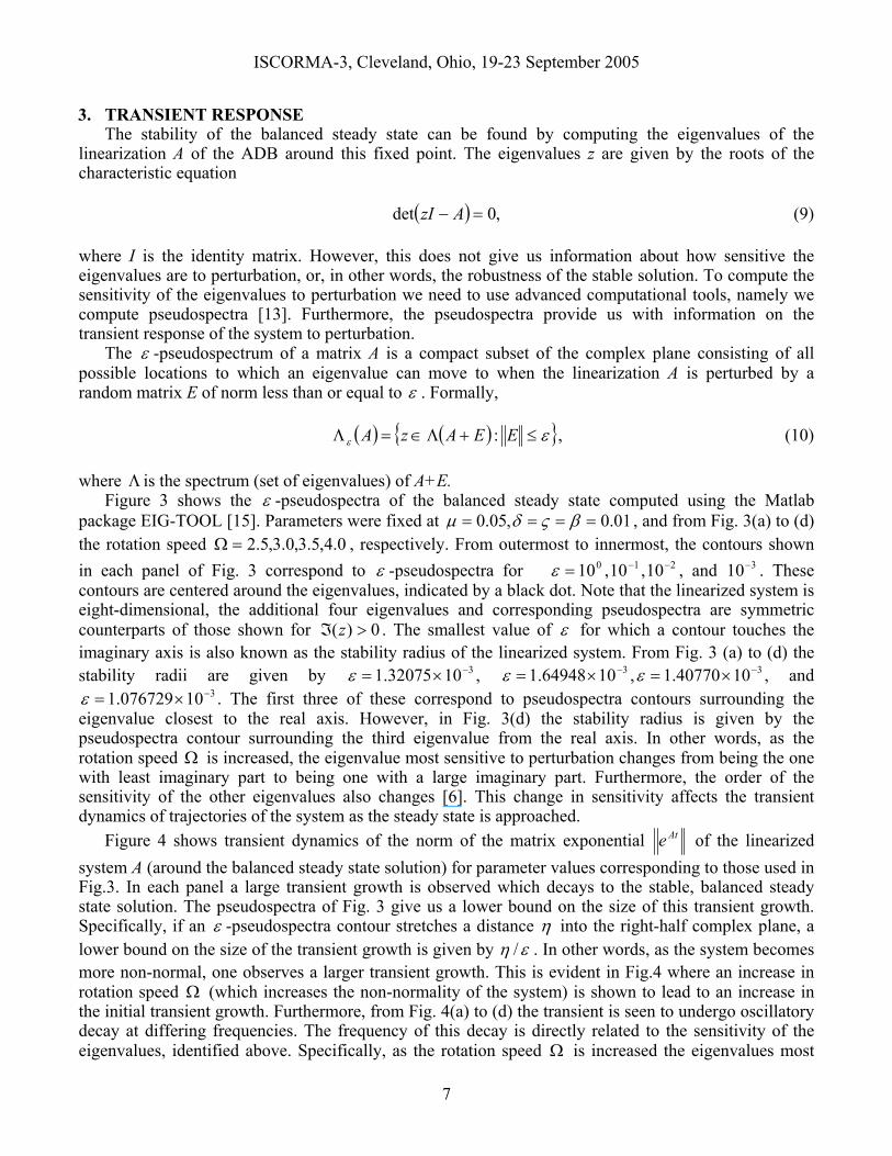
However, we must note that the ADB is highly nonlinear. This has the consequence that while a balanced steady state may be achievable, it may not be a unique solution; see Ref. [5] for a detailed analysis of coexisting periodic solutions. Furthermore, a linearization of the equations describing the ADB leads to a highly non-normal system. In such systems with high non-normality, the eigenvalues providing the stability information are known to be very sensitive to perturbation. Moreover, non-normal systems can show a large growth in the amplitude of the transient dynamics after the system is perturbed from a stable equilibrium. We now investigate these phenomena.

−1 0 1

−6

−4

−2

0

−1 0 1

−6

−4

−2

0

−1 0 1

−6

−4

−2

0

−1 0 1

−6

−4

−2

0

(z) (z)

(z) (z)

(z) (z)

(z) (z)

(a) (b)

(c) (d)

Fig. 3. Pseudospectra of the balanced steady state of the linearized system describing the ADB; see text for full details.

ISCORMA-3, Cleveland, Ohio, 19-23 September 2005

7

3. TRANSIENT RESPONSE The stability of the balanced steady state can be found by computing the eigenvalues of the

linearization A of the ADB around this fixed point. The eigenvalues z are given by the roots of the characteristic equation

( ) ,0det =− AzI (9) where I is the identity matrix. However, this does not give us information about how sensitive the eigenvalues are to perturbation, or, in other words, the robustness of the stable solution. To compute the sensitivity of the eigenvalues to perturbation we need to use advanced computational tools, namely we compute pseudospectra [13]. Furthermore, the pseudospectra provide us with information on the transient response of the system to perturbation.

The ε -pseudospectrum of a matrix A is a compact subset of the complex plane consisting of all possible locations to which an eigenvalue can move to when the linearization A is perturbed by a random matrix E of norm less than or equal to ε . Formally,

( ) ( ) εε ≤+Λ∈=Λ EEAzA : , (10)

where Λ is the spectrum (set of eigenvalues) of A+E.

Figure 3 shows the ε -pseudospectra of the balanced steady state computed using the Matlab package EIG-TOOL [15]. Parameters were fixed at 01.0,05.0 ==== βςδµ , and from Fig. 3(a) to (d) the rotation speed 0.4,5.3,0.3,5.2=Ω , respectively. From outermost to innermost, the contours shown in each panel of Fig. 3 correspond to ε -pseudospectra for 010=ε , 110− , 210− , and 310− . These contours are centered around the eigenvalues, indicated by a black dot. Note that the linearized system is eight-dimensional, the additional four eigenvalues and corresponding pseudospectra are symmetric counterparts of those shown for 0)( >ℑ z . The smallest value of ε for which a contour touches the imaginary axis is also known as the stability radius of the linearized system. From Fig. 3 (a) to (d) the stability radii are given by 31032075.1 −×=ε , 31064948.1 −×=ε , 31040770.1 −×=ε , and

310076729.1 −×=ε . The first three of these correspond to pseudospectra contours surrounding the eigenvalue closest to the real axis. However, in Fig. 3(d) the stability radius is given by the pseudospectra contour surrounding the third eigenvalue from the real axis. In other words, as the rotation speed Ω is increased, the eigenvalue most sensitive to perturbation changes from being the one with least imaginary part to being one with a large imaginary part. Furthermore, the order of the sensitivity of the other eigenvalues also changes [6]. This change in sensitivity affects the transient dynamics of trajectories of the system as the steady state is approached.

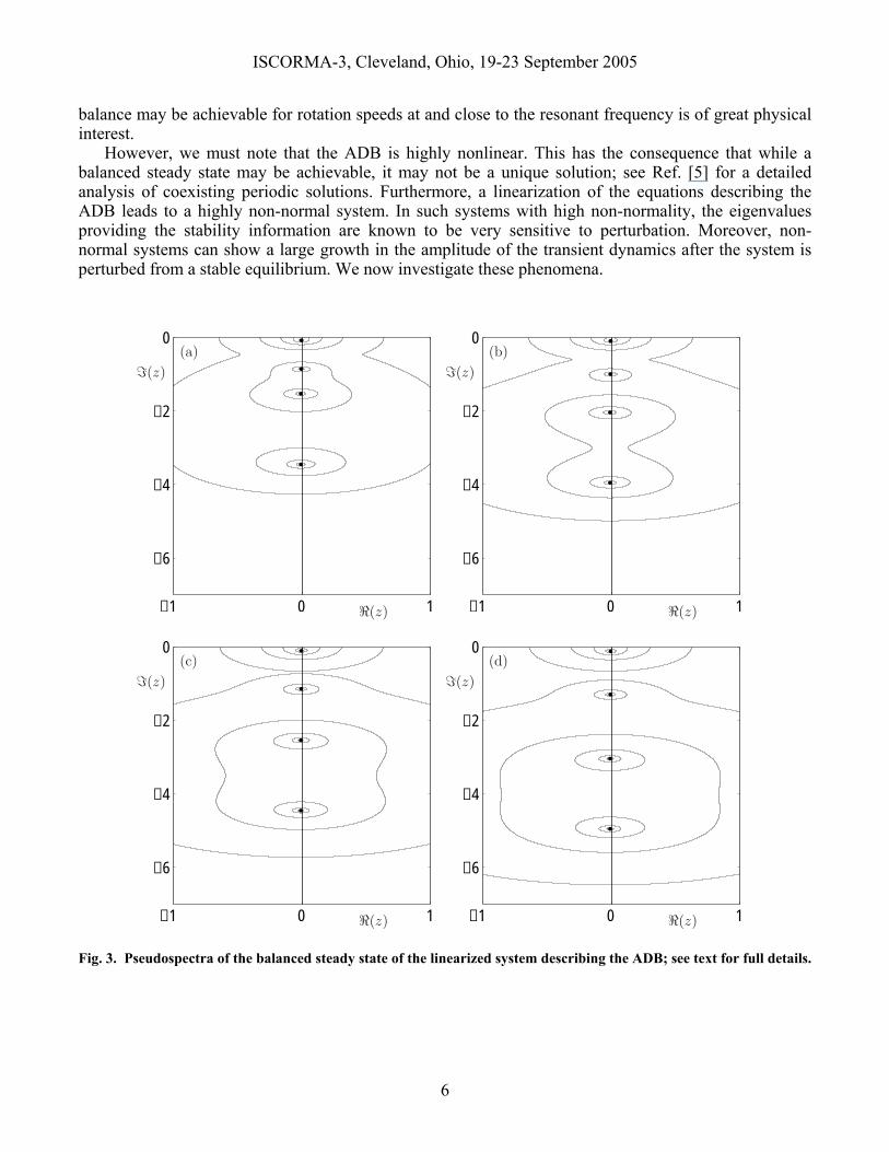
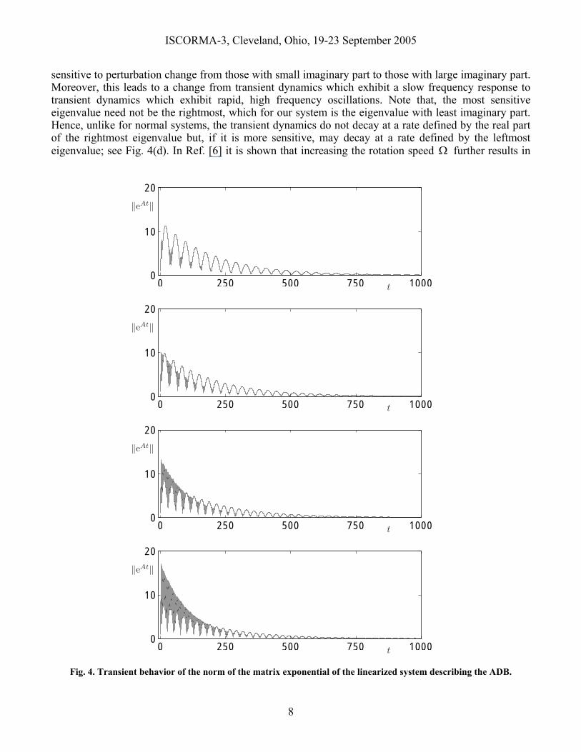
Figure 4 shows transient dynamics of the norm of the matrix exponential Ate of the linearized system A (around the balanced steady state solution) for parameter values corresponding to those used in Fig.3. In each panel a large transient growth is observed which decays to the stable, balanced steady state solution. The pseudospectra of Fig. 3 give us a lower bound on the size of this transient growth. Specifically, if an ε -pseudospectra contour stretches a distance η into the right-half complex plane, a lower bound on the size of the transient growth is given by εη / . In other words, as the system becomes more non-normal, one observes a larger transient growth. This is evident in Fig.4 where an increase in rotation speed Ω (which increases the non-normality of the system) is shown to lead to an increase in the initial transient growth. Furthermore, from Fig. 4(a) to (d) the transient is seen to undergo oscillatory decay at differing frequencies. The frequency of this decay is directly related to the sensitivity of the eigenvalues, identified above. Specifically, as the rotation speed Ω is increased the eigenvalues most

ISCORMA-3, Cleveland, Ohio, 19-23 September 2005

8

sensitive to perturbation change from those with small imaginary part to those with large imaginary part. Moreover, this leads to a change from transient dynamics which exhibit a slow frequency response to transient dynamics which exhibit rapid, high frequency oscillations. Note that, the most sensitive eigenvalue need not be the rightmost, which for our system is the eigenvalue with least imaginary part. Hence, unlike for normal systems, the transient dynamics do not decay at a rate defined by the real part of the rightmost eigenvalue but, if it is more sensitive, may decay at a rate defined by the leftmost eigenvalue; see Fig. 4(d). In Ref. [6] it is shown that increasing the rotation speed Ω further results in

0 250 500 750 10000

10

20

0 250 500 750 10000

10

20

0 250 500 750 10000

10

20

0 250 500 750 10000

10

20

‖eAt‖

‖eAt‖

‖eAt‖

‖eAt‖

t

t

t

t

Fig. 4. Transient behavior of the norm of the matrix exponential of the linearized system describing the ADB.

ISCORMA-3, Cleveland, Ohio, 19-23 September 2005

9

larger transient growths and higher frequency oscillations to the balanced state. Furthermore, in Ref. [6] we show how this transient growth and decay is directly related to the dynamics of the full nonlinear system. In particular, we show how increased initial transient growth may cause the trajectory to escape the basin of attraction of the steady state, resulting in possible attraction to more complex, periodic dynamics.

CONCLUSIONS

This paper has demonstrated the nonlinear bifurcation analysis of an automatic dynamic balancing mechanism for a simple Jeffcott rotor model. Bifurcation diagrams show that dynamic balance can be achieved provided the mass of the balancing balls is sufficiently high. However it is also clear that any automatic balancing system must be carefully designed, since there are large regions of parameter space where there are no stable solutions. Of particular interest is the region where the shaft speed is close to a critical speed, since the response to any residual unbalance will be high at these speeds. In this case obtaining a stable solution requires a very careful choice of system parameters, and work is continuing to increase the size of these stable regions. Transient dynamics also play a crucial role in a complete understanding of this highly nonlinear mechanism. In many applications it is important to know which frequencies may be excited by a perturbation. In particular, the degree and nature of the transient response to perturbation can be highly unpredictable. The transient response and sensitivity to perturbation of a rotor fitted with an ADB has been investigated by computing the pseudospectra of the first-order linearization. The results have shown that the system exhibits a large transient growth phenomena and that this may be predicted using the pseudospectrum. Much more work is required, utilizing the methods presented in this paper, in order to optimize the design for a particular physical application. Experimental work is also in progress to validate the nonlinear models of the rotor and ADB.

ACKNOWLEDGEMENTS

The authors acknowledge the support of the Engineering and Physical Sciences Research Council through grant GR/S35684/01, ‘Pseudospectra, Uncertainty, Vulnerability and Bifurcation in Structural Mechanics’. Friswell acknowledges the support of a Royal Society-Wolfson Research Merit Award.

REFERENCES 1. Adolfsson, J., Passive Control of Mechanical Systems: Bipedal Walking and Autobalancing, PhD

thesis, Royal Institute of Technology, Stockholm (2001). 2. Chao, P. C. P., Huang, Y.-D, Sung, C.-K., Non-Planar Dynamic Modeling for the Optical Disk

Drive Spindles Equipped with an Automatic Balancer, Mechanism and Machine Theory, Vol. 38 (2003) 1289-1305.

3. Chung, J., Ro, D. S., Dynamic Analysis of an Automatic Dynamic Balancer for Rotating Mechanisms, Journal of Sound and Vibration, Vol. 228 (1999) 1035-1056.

4. Doedel, E., Champneys, A. R., Fairgrieve, T., Kuznetsov, Yu., Sandstede, B., Wang, X., AUTO 97: Continuation and Bifurcation Software for Ordinary Differential Equations, http://indy.cs.concordia.ca/auto/ (1997).

5. Green, K., Champneys, A. R., Lieven, N. A. J., Bifurcation Analysis of an Automatic Dynamic Balancing Mechanism for Eccentric Rotors, Technical report. University of Bristol. http://www.enm.bris.ac.uk/anm/preprints/2004r19.html (2004).

6. Green, K., Champneys, A. R., Friswell, M. I., Analysis of the Transient Response of an Automatic Dynamic Balancer for Eccentric Rotors, Technical report. University of Bristol. http://www.enm.bris.ac.uk/anm/preprints/2004r26.html (2004).

7. Higham, D. J., Trefethen, L. N., Stiffness of ODEs, BIT, Vol. 33 (1992) 285-303.

ISCORMA-3, Cleveland, Ohio, 19-23 September 2005

10

8. Huang, W.-Y., Chao, C.-P., Kang, J.-R., Sung, C.-K., The Application of Ball-Type Balancers for Radial Vibration Reduction of High-Speed Optic Drives, Journal of Sound and Vibration, Vol. 250 (2002) 415-430.

9. Kim, W., Chung, J., Performance of Automatic Ball Balancers on Optical Disc Drives, Proc. IMechE Part C: Journal of Mechanical Engineering Science, Vol. 216 (2002) 1071-1080.

10. Lee, J., van Moorhem, W. K., Analytical and Experimental Analysis of a Self-Compensating Dynamic Balancer in a Rotating Mechanism, Trans. ASME, Journal of Dynamic Systems Measurement and Control, Vol. 118 (1996) 468-475.

11. Rajalingham, R., Rakheja, S., Whirl Suppression in Hand-Held Power Tool Rotors using Guided Rolling Balancers, Journal of Sound and Vibration, Vol. 217 (1998) 453-466.

12. SKF Autobalance Systems, Dynaspin, http://dynaspin.skf.com 13. Trefethen, L. N., Computation of Pseudospectra, Acta Numerica (1999) 1-46. 14. van de Wouw, N., van den Heuvel, M. N., van Rooij, J. A., Nijmeijer, H., Performance of an

Automatic Ball Balancer with Dry Friction, Eindhoven University of Technology, The Netherlands (2004).

15. Wright, T. G., EIG-TOOL: a Graphical Tool for Nonsymmetric Eigenproblems, Oxford University. http://www.comlab.ox.ac.uk/pseudospectra/eigtool (2002).