arX

iv:1

108.

1000

v1 [

mat

h.G

T]

4 A

ug 2

011

THE SPACE OF FRAMED FUNCTIONS IS

CONTRACTIBLE

To Stephen Smale on his 80th birthday

Y. M. Eliashberg ∗

Stanford University,Stanford, CA 94305 USA

eliash@math.stanford.edu

N. M. Mishachev

Lipetsk Technical University,Lipetsk, 398055 Russia

mishachev@lipetsk.ru

Abstract

According to K. Igusa ([Ig84]) a generalized Morse function on M isa smooth function M → R with only Morse and birth-death singu-larities and a framed function on M is a generalized Morse functionwith an additional structure: a framing of the negative eigenspaceat each critical point of f . In ([Ig87]) Igusa proved that the space offramed generalized Morse functions is (dimM−1)-connected. J. Luriegave in [Lu09] an algebraic topological proof that the space of framedfunctions is contractible. In this paper we give a geometric proof ofIgusa-Lurie’s theorem using methods of our paper [EM00].

Contents

1 Framed Igusa functions 21.1 Main theorem . . . . . . . . . . . . . . . . . . . . . . . . . . . 21.2 Framed Igusa functions . . . . . . . . . . . . . . . . . . . . . . 31.3 Framed formal leafwise Igusa functions . . . . . . . . . . . . . 51.4 Outline of the proof and plan of the paper . . . . . . . . . . . 8

∗Partially supported by the NSF grant DMS-0707103

1

2 Tangency of a submanifold to a distribution 92.1 Submanifolds folded with respect to a distribution . . . . . . . 102.2 Pleating . . . . . . . . . . . . . . . . . . . . . . . . . . . . . . 11

3 Geometry of FLIFs 143.1 Homomorphisms ΓΦ and ΠΦ . . . . . . . . . . . . . . . . . . . 143.2 Twisted normal bundle and the isomorphism ∆Φ . . . . . . . . 163.3 The holonomic case . . . . . . . . . . . . . . . . . . . . . . . . 183.4 Balanced and well balanced FLIFs . . . . . . . . . . . . . . . 213.5 Pleating a FLIF . . . . . . . . . . . . . . . . . . . . . . . . . . 233.6 Stabilization . . . . . . . . . . . . . . . . . . . . . . . . . . . . 283.7 From balanced to well balanced FLIFs . . . . . . . . . . . . . 313.8 Formal extension . . . . . . . . . . . . . . . . . . . . . . . . . 313.9 Integration near V . . . . . . . . . . . . . . . . . . . . . . . . 33

4 Proof of Extension Theorem 1.1.1 35

1 Framed Igusa functions

1.1 Main theorem

This paper is written at a request of D. Kazhdan and V. Hinich who askedus whether we could adjust our proof in [EM00] of K. Igusa’s h-principlefor generalized Morse functions from [Ig84] to the case of framed generalizedMorse functions considered by K. Igusa in his paper [Ig87] and more recentlyby J. Lurie in [Lu09]. We are very happy to devote this paper to StephenSmale whose geometric construction in [Sm58] plays the central role in ourproof (as well as in the proofs of many other h-principle type results.)

Given an n-dimensional manifold W , a generalized Morse function, or aswe call it in this paper Igusa function, is a function with only Morse (A1)and birth-death (A2) type singularities. A framing ξ of an Igusa functionϕ : W → R is a trivialization of the negative eigenspace of the Hessianquadratic form at A1-points which satisfy certain extra conditions at A2-points, see a precise definition below.

If the manifold W is endowed with a foliation F then we call ϕ : (W,F) → R

a leafwise Igusa function if restricted to leaves it has only Morse or birth-

2

death type singularities. A framing ξ of a leafwise Igusa function ϕ : (W,F) →R is a leafwise framing; see precise definitions below.

The following theorem is the main result of the paper. We use Gromov’snotation Op A for an unspecified open neighborhood of a closed subset A ⊂W .

1.1.1. (Extension theorem) Let W be an (n + k)-dimensional manifoldwith an n-dimensional foliation F . Let A ⊂ W be a closed (possibly empty)subset and (ϕA, ξA) a framed leafwise Igusa function defined on Op A ⊃ A.Then there exists a framed leafwise Igusa function (ϕ, ξ) on the whole Wwhich coincides with (ϕA, ξA) on Op A.

Theorem 1.1.1 is equivalent to the fact that the space of framed Igusa func-tions is contractible, which is a content of J. Lurie’s extension (see Theorem3.4.7 in [Lu09]) of K. Igusa’s result from [Ig87]. The current form of thetheorem allows us to avoid discussion of the topology on this space, comp.[Ig87].

Acknowledgements. We are grateful to D. Kazhdan and V. Hinich for theirencouragement to write this paper and to S. Galatius for enlightening dis-cussions.

1.2 Framed Igusa functions

Objects associated with a leafwise Igusa function. Let TF denote the n-dimensional subbundle of TW tangent to the leaves of the foliation F . Letus fix a Riemannian metric on W . Given a leafwise Igusa function (LIF) ϕwe associate with it the following objects:

• V = V (ϕ) is the set of all its leafwise critical points, i.e. the set ofzeros of the leafwise differential dFϕ : W → T ∗F .

• Σ = Σ(ϕ) is the set of A2-points. Generically, V is a k-dimensionalsubmanifold of W which is transversal to F at the set V \ Σ of A1-points and has the fold type tangency to F along a (k−1)-dimensionalsubmanifold Σ ⊂ V of leafwise A2-critical points of ϕ.

• Vert is the restriction bundle TF|V .

3

• d2Fϕ is the leafwise quadratic differential of ϕ. It is invariantly definedat each point v ∈ V . d2Fϕ can be viewed as a homomorphism Vert →Vert∗. Using our choice of a Riemannian metric we identify the bundlesVert and Vert∗ and view d2Fϕ as a self-adjoint operator Vert → Vert.This operator is non-degenerate at the points of V \ Σ , and has a 1-dimensional kernel λ ⊂ Vert|Σ. Note that λ is tangent to V , and thuswe have λ = Vert ∩ TV |Σ.

• d3Fϕ is the invariantly defined third leafwise differential, which is acubic form on λ. For a leafwise Igusa function ϕ this cubic form isnon-vanishing, and hence the bundle λ is trivial and can be canonicallyoriented by choosing the direction in which the cubic function d3Fϕincreases. We denote by λ+ the unit vector in λ which defines itsorientation.

Decomposition of V (ϕ) and splitting of Vert. The index of the leafwisequadratic differential d2Fϕ (v), v ∈ V , may takes values 0, 1, . . . , n for v ∈V \ Σ and 0, 1, . . . , n− 1 for v ∈ Σ. Let

V \ Σ = V 0 ∪ · · · ∪ V n and Σ = Σ1 ∪ · · · ∪ Σn−1

be the decompositions of V \ Σ and Σ according to the index. Note that Σi

is the intersection of the closures of V i and V i+1. Then for v ∈ V i we havethe splitting

TvF = Vert(v) = Verti+(v)⊕ Verti−(v)

where Verti+(v) and Verti−(v) are the positive and the negative eigenspacesof d2Fϕ(v), and for any σ ∈ Σi we have the splitting

TσF = Vert(σ) = Ver(σ)⊕ λ(σ) = Veri+(σ)⊕Veri−(σ)⊕ λ(σ)

(Ver 6= Vert !), where Veri+(v) and Veri−(v) are the positive and the negativeeigenspaces of d2Fϕ (σ). For σ ∈ Σi and v ∈ V i we have

limv→σ

Verti+(v) = Veri+(σ)⊕ λ(σ) and limv→σ

Verti−(v) = Veri−(σ) .

For σ ∈ Σi and v ∈ V i+1 we have

limv→σ

Verti+1− (v) = Veri−(σ)⊕ λ(σ) and lim

v→σVerti+1

+ (v) = Veri+(σ) .

Framing of a leafwise Igusa function. A framing of a leafwise Igusa functionϕ is an ordered set ξ = (ξ1, . . . , ξn) of unit vector fields in Vert(V ) such that:

4

• ξi is defined (only) over the union Σi−1 ∪ V i ∪ · · · ∪ Σn−1 ∪ V n;

• ξi|Σi−1 = λ+|Σi−1 ;

• (ξ1, . . . , ξi)|V i is an orthonormal framing for Verti−.

In particular, ξn is defined only on Σn−1∪V n and ξ1 is defined only on V \V 0.The pair (ϕ, ξ) is called a framed leafwise Igusa function (see Fig.1).

The motivation for adding a framing is discussed in [Ig87].

0

0V

1VΣ

Figure 1: Framed leafwise Igusa function

1.3 Framed formal leafwise Igusa functions

A formal leafwise Igusa function (FLIF) is a quadruple Φ = (Φ0,Φ1,Φ2, λ+)where:

• Φ0 : W → R is any function;

• Φ1 : W → TF is a vector field tangent to F , vanishing on a subsetV = V (Φ) ⊂ W ;

• Φ2 is a self-adjoint operator Vert → Vert, which has rank n− 1 over asubset Σ = Σ(Φ) ⊂ V and rank n over V \ Σ;

• λ+ is a unit vector field in the line bundle where λ := Ker (Φ2|TV |Σ).

5

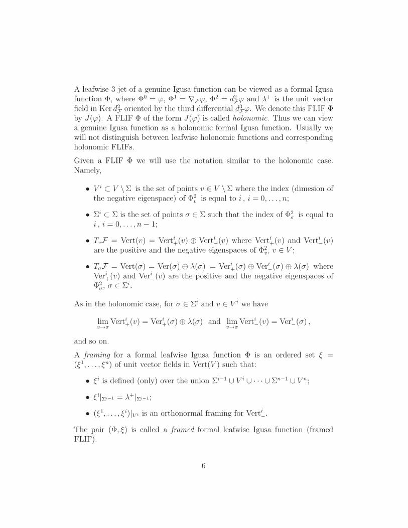
A leafwise 3-jet of a genuine Igusa function can be viewed as a formal Igusafunction Φ, where Φ0 = ϕ, Φ1 = ∇Fϕ, Φ

2 = d2Fϕ and λ+ is the unit vectorfield in Ker d2F oriented by the third differential d3Fϕ. We denote this FLIF Φby J(ϕ). A FLIF Φ of the form J(ϕ) is called holonomic. Thus we can viewa genuine Igusa function as a holonomic formal Igusa function. Usually wewill not distinguish between leafwise holonomic functions and correspondingholonomic FLIFs.

Given a FLIF Φ we will use the notation similar to the holonomic case.Namely,

• V i ⊂ V \Σ is the set of points v ∈ V \Σ where the index (dimesion ofthe negative eigenspace) of Φ2

v is equal to i , i = 0, . . . , n;

• Σi ⊂ Σ is the set of points σ ∈ Σ such that the index of Φ2σ is equal to

i , i = 0, . . . , n− 1;

• TvF = Vert(v) = Verti+(v) ⊕ Verti−(v) where Verti+(v) and Verti−(v)are the positive and the negative eigenspaces of Φ2

v, v ∈ V ;

• TσF = Vert(σ) = Ver(σ) ⊕ λ(σ) = Veri+(σ) ⊕ Veri−(σ) ⊕ λ(σ) whereVeri+(v) and Veri−(v) are the positive and the negative eigenspaces ofΦ2

σ, σ ∈ Σi.

As in the holonomic case, for σ ∈ Σi and v ∈ V i we have

limv→σ

Verti+(v) = Veri+(σ)⊕ λ(σ) and limv→σ

Verti−(v) = Veri−(σ) ,

and so on.

A framing for a formal leafwise Igusa function Φ is an ordered set ξ =(ξ1, . . . , ξn) of unit vector fields in Vert(V ) such that:

• ξi is defined (only) over the union Σi−1 ∪ V i ∪ · · · ∪ Σn−1 ∪ V n;

• ξi|Σi−1 = λ+|Σi−1 ;

• (ξ1, . . . , ξi)|V i is an orthonormal framing for Verti−.

The pair (Φ, ξ) is called a framed formal leafwise Igusa function (framedFLIF).

6

Σ0

0V

V0

V1

Σ0

Σ 0V

1

Σ 0

Figure 2: Framed FLIF

As in the holonomic case, for a generic FLIF Φ the set V is a k-dimensionalmanifold and Σ its codimension 1 submanifold. However, Σ has nothing todo with tangency of V to F , and moreover there is no control of the type ofthe tangency singularities between V and F (see Fig.2).

In what follows we will need to consider FLIFs for different foliations on W .We will say that Φ is an F -FLIF when we need to emphasize the correspond-ing foliation F . Moreover, the notion of a FLIF can be generalized withoutany changes to an arbitrary, not necessarily integrable n-dimensional distri-bution ζ ⊂ TW . We will call such an object a ζ-FLIF. In the case when adistribution ζ is integrable and integrates into a foliation F we will use assynonyms both terms: ζ-FLIF and F -FLIF.

Push-forward operation for FLIFs. Let ζ, ζ be two n-dimensional distribu-tions in TW . Let f : W → W be a diffeomorphism covered by an isomor-phism F : ζ → ζ . Let Φ be a ζ-FLIF. Then we define the push-forward ζ-FLIF Φ = (f, F )∗Φ = (Φ0, Φ1, Φ2, λ+) as

- Φ0(f(x)) := Φ0(x), x ∈ W ;

- Φ1f(x)(F (Z)) = Φ1

x(Z), x ∈ W, Z ∈ ζx;

- Φ2f(x)(F (Z)) = F (Φ2

x(Z)), x ∈ V, Z ∈ Vertx = ζx ;

7

- λ+(f(x)) = F (λ+(x)), x ∈ Σ.

If Φ is framed then the push-forward operator (f, F )∗ transforms its framing

ξ to a framing ξ of Φ in a natural way:

- ξi(f(x)) = F (ξi(x)), x ∈ V .

Note that if ζ and ζ are both integrable, i.e. tangent to foliations F andF , F = df and Φ is holonomic i.e. Φ = J(ϕ) then Φ is also holonomic,

Φ = J(ϕ), where ϕ = ϕ f−1.

1.4 Outline of the proof and plan of the paper

Any framed leafwise Igusa function can be extended from Op A to W for-mally, i.e. as a framed FLIF (Φ, ξ), see Lemma 3.8.1. This is, essentially, anoriginal Igusa’s observation from [Ig87]. We then gradually improve (Φ, ξ)to make it holonomic. Note that unlike the holonomic case, the homotopicaldata associated with Φ1 and Φ2 are essentially unrelated. We formulate thenecessary so-called balancing homotopical condition for a FLIF to be holo-nomic, see Section 3.4, and show that one can always make a FLIF (Φ, ξ)balanced via a modification, called stabilization, see Section 3.6.Our next task is to arrange that V (ϕ) has fold type tangency with respectto the foliation F , as it is supposed to be in the holonomic case. FLIFssatisfying this property, together with certain additional coorientation con-ditions over the fold, are called prepared, see Section 3.1. We observe that fora prepared FLIF one can define a stronger necessary homotopical conditionfor holonomicity. We call prepared FLIFs satisfying this stronger conditionwell balanced, see Section 3.4.Given any FLIF Φ one can associate with it a twisted normal bundle (alsocalled virtual vertical bundle) ΦVert over V = V (Φ) which is a subbundle ofTW |V obtained by twisting the normal bundle of V in W near Σ = Σ(Φ),see Section 3.2. In the holonomic case we have ΦVert = Vert, see 3.3.1. Acrucial observation is that the manifold V has fold type tangency to anyextension ζ of the bundle ΦVert to a neighborhood of V , see 3.2.1. Moreover,if Φ is balanced then there exist a global extension ζ of ΦVert and a bundleisomorphism F : Vert → ΦVert homotopic to the identity Vert → Vertthrough injective bundle homomorphisms into TW |V such that the push-

forward framed ζ-FLIF (Φ, ξ) = (Id, F )∗(Φ, ξ) is well balanced, see 3.4.4.

8

If Φ is holonomic on Op A then the bundle ζ and the framed FLIF (Φ, ξ)coincide with TF and (Φ, ξ) over Op A.The homotopy of the homomorphism F generates a homotopy of distribu-tions ζs connecting ζ and TF . If it were possible to construct a fixed onOp A isotopy Vs of V in W keeping Vs folded with respect to ζs then onecould cover this homotopy by a fixed on Op A homotopy of framed well bal-anced ζs- FLIFs (Φs, ξs) beginning with (Φ0, ξ0) = (Φ, ξ). Though this is, ingeneral, impossible, the wrinkling embedding theorem from [EM09] allowsus to do that after a certain additional modification of V , called pleating, seeTheorem 2.2.1. We then show that the pleating construction can be extendedto the class of framed well balanced FLIFs, see Section 3.5. Thus we get aframed well balanced FLIF (Φ, ξ) extending the local framed leafwise Igusafunction (ϕA, ξA).The proof now is concluded in two steps. First, we show, see Lemma 3.9.1,that a framed well balanced FLIF can be made holonomic near V , and thenuse the wrinkling theorem from [EM97] to construct a holonomic extensionto the whole manifold W , see Step 5 in Section 4.

The paper has the following organization. In Section 2.1 we discuss thenotion of fold tangency of a submanifold with respect to a not necessarilyintegrable distribution, define the pleating construction for submanifolds andformulate the main technical result, Theorem 2.2.1, which is an analog forfolded maps of Gromov’s directed embedding theorem, see [Gr86]. This is acorollary of the results of [EM09]. Section 3 is the main part of the paper.We define and study there the notions and properties of balanced, preparedand well balanced FLIFs, and gradually realize the described above programof making a framed FLIF well balanced, see Proposition 3. We also provehere Igusa’s result about existence of a formal extension for framed FLIFs,see 3.8.1, and local integrability of well balanced FLIFs, see 3.9.1. Finally,in Section 4 we just recap the main steps of the proof.

2 Tangency of a submanifold to a distribu-

tion

In this section we always denote by V an n-dimensional submanifold of an(n + k)-dimensional manifold W , by Σ a codimension 1 submanifold of Vand by Norm = Norm(V ) the normal bundle of V .

9

2.1 Submanifolds folded with respect to a distribution

Let ζ be an n-dimensional distribution, i.e. a subbundle ζ ⊂ TW . Thenon-transversality condition of V to ζ defines a variety Σζ of the 1-jet spaceJ1(V,W ). We say that V has at a point p ∈ V a tangency to ζ of fold typeif

• Corank π ζ |TpV = 1;

• J1(j) : V → J1(V,W ), where j : V → W is the inclusion, is transverseto Σζ ; we denote Σ := (J1(j))−1(Σζ);

• π ζ |TpΣ : TpΣ → TWp/ζ is injective.

If ζ is integrable, and hence locally is tangent to an affine foliation definedby the projection π : R

n+k → Rk, these conditions are equivalent to the

requirement that the restriction π|V has fold type singularity, and in thiscase one has a normal form for the fold tangency.

If V has fold type tangency to ζ along Σ then we say that V is folded withrespect to V along Σ. The fold locus Σ ⊂ V is a codimension one subman-ifold, and at each point σ ∈ Σ the 1-dimensional line field λ = Kerπζ |TV =ζ |V ∩ TV is transverse to Σ.

The hyperplane field TΣ⊕ζ |Σ can be canonically cooriented. In the case whenζ is integrable this coorientation can be defined as follows. The leaves of thefoliation trough points of Σ form a hypersurface which divides a sufficientlysmall tubular neighborhood Ω of Σ in W into two parts, Ω = Ω+∪Ω−, whereΩ− is the part which contains V ∩ Ω. Then the characteristic coorientationof the fold Σ is the coorientation of the hyperplane TΣ⊕ ζ |Σ determined bythe outward normal vector field to Ω− along Σ, see Fig.3. For a general ζ

Figure 3: Characteristic coorientation of the fold

take a point σ0 ∈ Σ, a neighborhood U of σ0 in V , an arbitrary unit vector

10

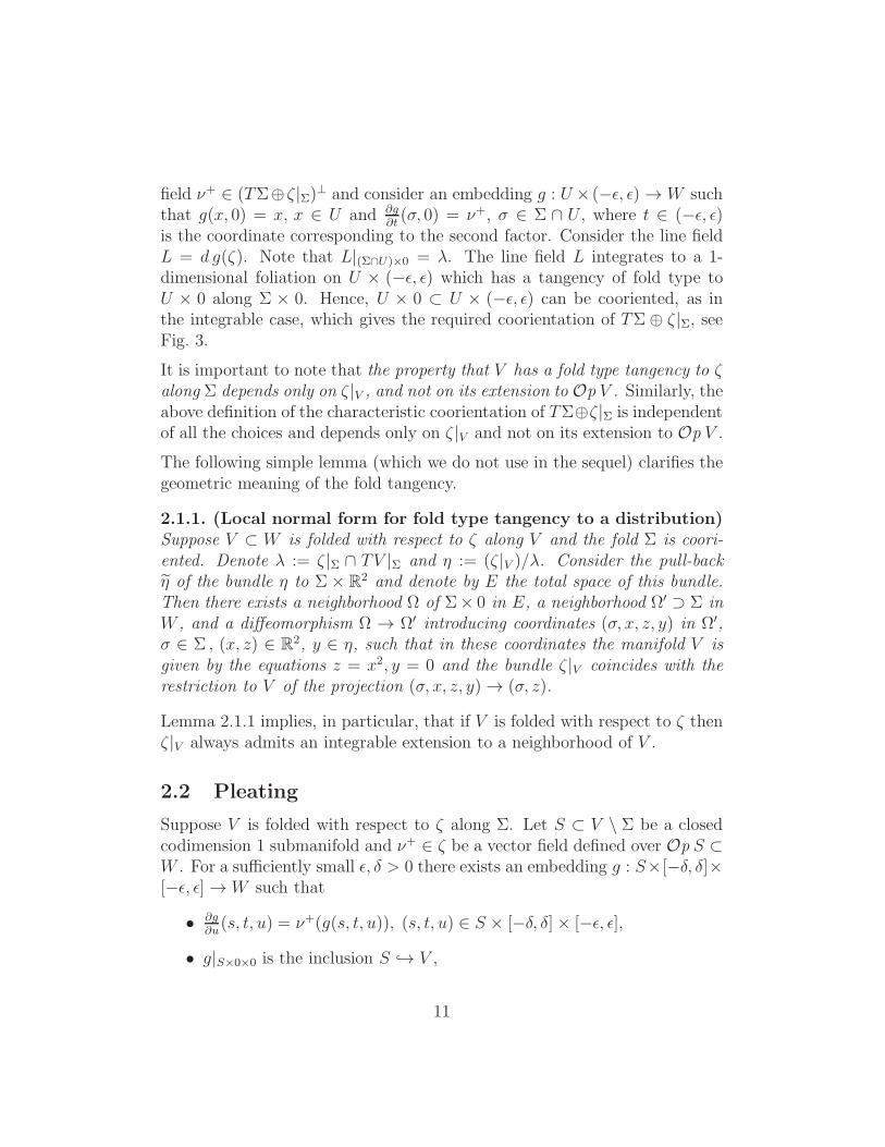
field ν+ ∈ (TΣ⊕ ζ |Σ)⊥ and consider an embedding g : U × (−ǫ, ǫ) → W such

that g(x, 0) = x, x ∈ U and ∂g

∂t(σ, 0) = ν+, σ ∈ Σ ∩ U , where t ∈ (−ǫ, ǫ)

is the coordinate corresponding to the second factor. Consider the line fieldL = d g(ζ). Note that L|(Σ∩U)×0 = λ. The line field L integrates to a 1-dimensional foliation on U × (−ǫ, ǫ) which has a tangency of fold type toU × 0 along Σ × 0. Hence, U × 0 ⊂ U × (−ǫ, ǫ) can be cooriented, as inthe integrable case, which gives the required coorientation of TΣ ⊕ ζ |Σ, seeFig. 3.

It is important to note that the property that V has a fold type tangency to ζalong Σ depends only on ζ |V , and not on its extension to Op V . Similarly, theabove definition of the characteristic coorientation of TΣ⊕ζ |Σ is independentof all the choices and depends only on ζ |V and not on its extension to Op V .

The following simple lemma (which we do not use in the sequel) clarifies thegeometric meaning of the fold tangency.

2.1.1. (Local normal form for fold type tangency to a distribution)Suppose V ⊂ W is folded with respect to ζ along V and the fold Σ is coori-ented. Denote λ := ζ |Σ ∩ TV |Σ and η := (ζ |V )/λ. Consider the pull-backη of the bundle η to Σ × R

2 and denote by E the total space of this bundle.Then there exists a neighborhood Ω of Σ× 0 in E, a neighborhood Ω′ ⊃ Σ inW , and a diffeomorphism Ω → Ω′ introducing coordinates (σ, x, z, y) in Ω′,σ ∈ Σ , (x, z) ∈ R

2, y ∈ η, such that in these coordinates the manifold V isgiven by the equations z = x2, y = 0 and the bundle ζ |V coincides with therestriction to V of the projection (σ, x, z, y) → (σ, z).

Lemma 2.1.1 implies, in particular, that if V is folded with respect to ζ thenζ |V always admits an integrable extension to a neighborhood of V .

2.2 Pleating

Suppose V is folded with respect to ζ along Σ. Let S ⊂ V \ Σ be a closedcodimension 1 submanifold and ν+ ∈ ζ be a vector field defined over Op S ⊂W . For a sufficiently small ǫ, δ > 0 there exists an embedding g : S×[−δ, δ]×[−ǫ, ǫ] → W such that

• ∂g

∂u(s, t, u) = ν+(g(s, t, u)), (s, t, u) ∈ S × [−δ, δ]× [−ǫ, ǫ],

• g|S×0×0 is the inclusion S → V ,

11

• g|S×[−δ,δ]×0 is a diffeomorphism onto the tubular δ-neighborhood U ⊃ Sin V , which sends intervals s× [−δ, δ] × 0, s ∈ S, to geodesics normalto S.

Let Γ ⊂ P := [−1, 1]× [−1, 1] be an embedded connected curve which near∂P coincides with the line u = 0. Here we denote by t, u the coordinatescorresponding to the two factors. We assume that Γ is folded with respectto the foliation defined by the projection (t, u) 7→ t (this is a generic condi-tion). We denote by Γδ, ǫ the image of Γ under the scaling (t, u) 7→ (δt, ǫu).

Consider a manifold V obtained from V by replacing the neighborhood Uby a deformed neighborhood UΓ = g(Sn−1 × Γδ, ǫ). We say V is the result ofΓ-pleating of V over S in the direction of the vector field ν+, see Fig. 4.

ΓΓ−pleating

Figure 4: Γ-pleating

The Γ+0 -pleating with the curve Γ+

0 shown on Fig. 5 will be referred simplyas pleating.

Γ0−Γ0

+

Figure 5: Curves Γ±0

2.2.1. (Pleated isotopy) Suppose V ⊂ (W, ζ) is folded with respect to ζalong Σ ⊂ V . Let ζs, s ∈ [0, 1], be a family of n-dimensional distributionsover a neighborhood Ω ⊃ V . Then there exist

- a manifold V ⊂ Ω obtained from V by a sequence of pleatings over bound-aries of small embedded balls in the direction of vector fields whichextend to these balls, and

12

- a C0-small isotopy hs : V → Ω,

such that for each s ∈ [0, 1] the manifold hs(V ) has only fold type tangency to

ζs. If Σ = Σ∪Σ ′ is the fold of V with respect to ζ0 then hs(Σ) is the fold of

hs(V ) with respect to ζs. If the homotopy ζs is fixed over a neighborhood OpA

of a closed subset A ⊂ V then one can arrange that V ∩ Op A = V ∩ Op Aand the isotopy hs is fixed over Op A.

Theorem 2.2.1 is a version of the wrinkled embedding theorem from [EM09],see Theorem 3.2 in [EM09] and the discussion in Sections 3.2 and 3.3 inthat paper on how to replace the wrinkles by spherical double folds and howto generalize Theorem 3.2 to the case of not necessarily integrable distribu-tions. Another cosmetic difference between the formulations in [EM09] andTheorem 2.2.1 is that the former one allows not only double folds, but alsotheir embryos, i.e. the moments of death-birth of double folds. This can beremedied by preserving the double folds till the end in the near-embryo state,rather than killing them, and similarly by creating the necessary number offolds by pleating at the necessary places before the deformation begins.

2.2.2. (Remark) If V satisfies the conclusion of Theorem 2.2.1 then any

manifold˜V obtained from V by an additional Γ-pleating with any Γ will also

have this property. For our purposes we will need to pleat with three specialcurves Γ1 and Γ±

2 shown on Figure 6. As it clear from this picture, a pleating

Γ1

Γ +2 Γ2

−

Figure 6: Curves Γ1 and Γ±2

with any of these curves can be viewed as a result of a Γ+0 -pleating followed

by a second Γ−0 -pleating. Hence, in the formulation of Theorem 2.2.1 one can

pleat with any of the curves Γ1 and Γ±2 instead of Γ+

0 .

13

3 Geometry of FLIFs

3.1 Homomorphisms ΓΦ and ΠΦ

Given a ζ-FLIF Φ we will associate with it several objects and constructions.

Isomorphism ΓΦ : Norm → Vert. This isomorphism is determined by Φ1.The tangent bundle T (ζ |V ) to the the total space of the bundle ζ |V canoni-cally splits as Vert ⊕ TW |V , and hence the bundle of tangent planes to thesection Φ1 along its 0-set V can be viewed as a graph of a homomorphismΓΦ : TW |V → Vert vanishing on TV . The restriction of this homomorphismto Norm will be denoted by ΓΦ. The transversality of the section Φ1 to the0-section ensures that Ker ΓΦ = TV and hence ΓΦ is an isomorphism.

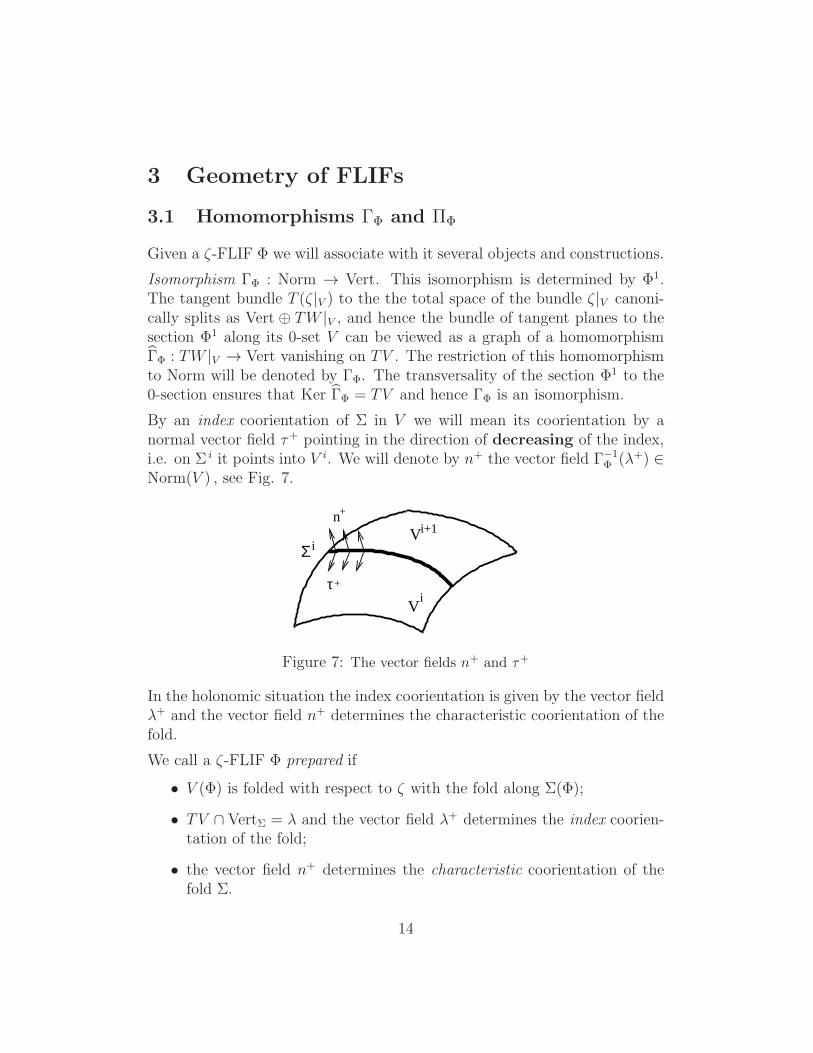
By an index coorientation of Σ in V we will mean its coorientation by anormal vector field τ+ pointing in the direction of decreasing of the index,i.e. on Σ i it points into V i. We will denote by n+ the vector field Γ−1

Φ (λ+) ∈Norm(V ) , see Fig. 7.

Vi+1

Vi

n+

Σi

τ+

Figure 7: The vector fields n+ and τ+

In the holonomic situation the index coorientation is given by the vector fieldλ+ and the vector field n+ determines the characteristic coorientation of thefold.

We call a ζ-FLIF Φ prepared if

• V (Φ) is folded with respect to ζ with the fold along Σ(Φ);

• TV ∩ VertΣ = λ and the vector field λ+ determines the index coorien-tation of the fold;

• the vector field n+ determines the characteristic coorientation of thefold Σ.

14

Thus, any holonomic FLIF (when, in particular, ζ is integrable) is prepared.

Isomorphism ΠΦ : Norm → Vert. Given a prepared ζ-FLIF Φ, let us denoteby K the restriction of the orthogonal projection TW |V → Norm to thesubbundle Vert = ζ |V ⊂ TW |V . The homomorphism K is non-degenerateover V \ Σ and has a 1-dimensional kernel λ over Σ.

3.1.1. (Definition of ΠΦ) The composition Φ2K−1 : Norm|V \Σ → Vert|V \Σ

continuously extends to a non-degenerate homomorphism ΠΦ : Norm → Vert.

Proof. Let us prove the extendability of the inverse operator K (Φ2)−1.

There exists a canonical extension of the vector field λ+ as a unit Φ2-eigenvector field λ+ on Op Σ ⊂ V . Then

Φ2(λ+(v)) = c(v)λ+(v) , v ∈ Op Σ ,

where the eigenvalue function c : Op Σ → R has Σ as its regular 0-level.Denote Ver = λ⊥(v) the orthogonal eigenspace of Φ2(v). Denote Nor :=

K(Ver). The operator K (Φ2)−1

is well defined on Ver = Ver|Σ ⊂ Vert|Σand maps it isomorphically onto Nor = Nor|Σ. It remains to prove existenceof a non-zero limit

limv→v0∈Σ

K((

Φ2)−1

(λ+))= lim

v→v0∈Σ

1

c(v)K(λ+(v)) .

The vector-valued function K(λ+(v)) vanishes on Σ while the function c(v)has no critical points on Σ. Hence, the above limit exists. On the otherhand, the transversality condition for the fold implies that ||K(λ+(v))|| ≥a dist(v,Σ), while |c(v)| ≤ b dist(v,Σ) for some positive constants a, b > 0,

and therefore limv→v0∈Σ

1c(v)

K(λ+(v)) 6= 0.

3.1.2. If Φ is holonomic then ΠΦ = ΓΦ.

Proof. Indeed, recall that ΓΦ = ΓΦ|Norm, where ΓΦ : TW |V → Vert is thehomomorphism defined by the section Φ1 linearized along its zero-set V . Inthe holonomic situation one has over V \ Σ the equality

ΓΦ|Vert = d2ϕ = Φ2 ,

where ϕ = Φ0. But ΓΦ|Vert and ΓΦ|Norm are related by a projection along

the kernel of ΓΦ which is equal to TV . Hence, ΓΦ = Φ2 K−1 = ΠΦ. Bycontinuity, the equality ΠΦ = ΓΦ holds everywhere.

15

3.2 Twisted normal bundle and the isomorphism ∆Φ

Given any ζ-FLIF Φ we define here a twisted normal bundle, or as we alsocall it virtual vertical bundle ΦVert ⊂ TWV over V . As we will see later (see3.3.1), in the holonomic case ΦVert coincides with Vert.

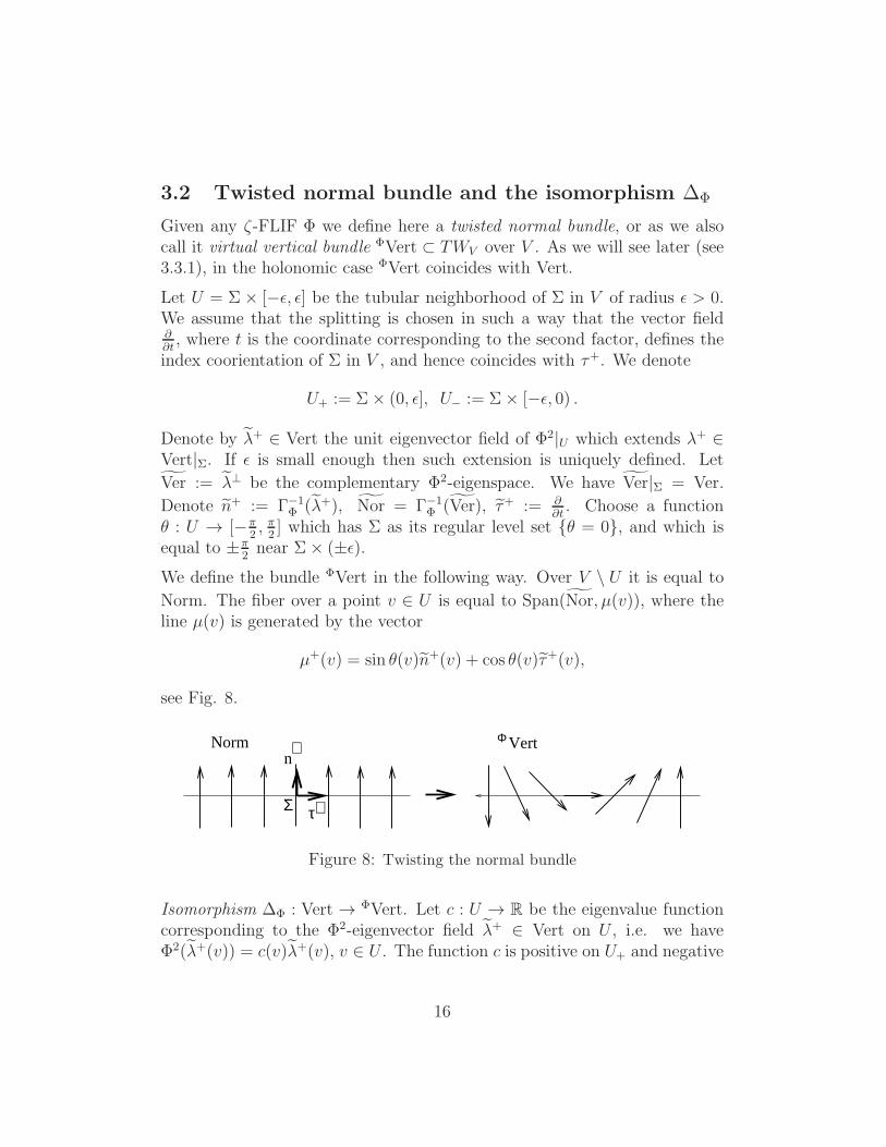
Let U = Σ × [−ǫ, ǫ] be the tubular neighborhood of Σ in V of radius ǫ > 0.We assume that the splitting is chosen in such a way that the vector field∂∂t, where t is the coordinate corresponding to the second factor, defines the

index coorientation of Σ in V , and hence coincides with τ+. We denote

U+ := Σ× (0, ǫ], U− := Σ× [−ǫ, 0) .

Denote by λ+ ∈ Vert the unit eigenvector field of Φ2|U which extends λ+ ∈Vert|Σ. If ǫ is small enough then such extension is uniquely defined. Let

Ver := λ⊥ be the complementary Φ2-eigenspace. We have Ver|Σ = Ver.

Denote n+ := Γ−1Φ (λ+), Nor = Γ−1

Φ (Ver), τ+ := ∂∂t. Choose a function

θ : U → [−π2, π2] which has Σ as its regular level set θ = 0, and which is

equal to ±π2near Σ× (±ǫ).

We define the bundle ΦVert in the following way. Over V \ U it is equal to

Norm. The fiber over a point v ∈ U is equal to Span(Nor, µ(v)), where theline µ(v) is generated by the vector

µ+(v) = sin θ(v)n+(v) + cos θ(v)τ+(v),

see Fig. 8.

Σ

n+

τ+

Norm VertΦ

Figure 8: Twisting the normal bundle

Isomorphism ∆Φ : Vert → ΦVert. Let c : U → R be the eigenvalue functioncorresponding to the Φ2-eigenvector field λ+ ∈ Vert on U , i.e. we haveΦ2(λ+(v)) = c(v)λ+(v), v ∈ U . The function c is positive on U+ and negative

16

on U−. Let c : U → R be any positive function which is equal to c on∂U+ = Σ× ǫ and equal to −c on ∂U− = Σ× (−ǫ).We then define the operator

∆Φ : Vert → ΦVert

by the formula

∆Φ(Z) =

Γ−1Φ (Φ2(Z)), over V \ U, Z ∈ Vert ;

Γ−1Φ (Φ2(Z)), over U, Z ∈ Ver ;

c(v) (sin θ(v)n+ + cos θ(v)τ+) , Z = λ+(v), v ∈ U .

(1)

It will be convenient for us to keep some ambiguity in the definition of ΦVertand ∆Φ. However, we note that the space of choices we made in the definitionis contractible, and hence the objects are defined in a homotopically canonicalway.

Let us extend ΦVert and ∆Φ to a neighborhood Op V ⊂ W . We will keepthe same notation for the extended objects.

3.2.1. For any ζ-FLIF Φ the ΦVert-FLIF

ΦNorm = (Id,∆Φ)∗Φ

on Op V is prepared.

∼

Figure 9: V is folded with respect to ΦVert.

Proof. Denote Φ := ΦNorm. We have V (Φ) = V (Φ) = V . First of all weobserve (see Fig. 9) that V is folded with respect to ΦVert along Σ and thevector field n+ = n+(Φ) defines the characteristic coorientation of the fold.

On the other hand, λ+(Φ) = ∆Φ(λ+(Φ)) = τ+(Φ) = τ+(Φ) and

n+(Φ) = Γ−1

Φ(λ+(Φ)) = Γ−1

Φ(τ+) = Γ−1

Φ (∆−1Φ (τ+)) = Γ−1

Φ (λ+) = n+(Φ),

17

and hence n+(Φ) defines the characteristic coorientation of the fold Σ. Thus

Φ is prepared.

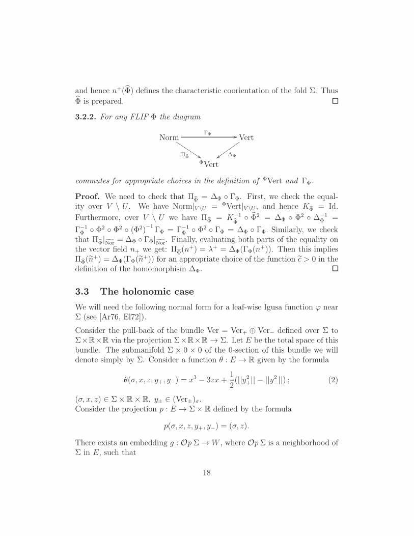
3.2.2. For any FLIF Φ the diagram

Norm

ΠΦ $$JJJJJJJJJ

ΓΦ// Vert

∆Φzzvvvv

vvvv

v

ΦVert

commutes for appropriate choices in the definition of ΦVert and ΓΦ.

Proof. We need to check that ΠΦ = ∆Φ ΓΦ. First, we check the equal-ity over V \ U . We have Norm|V \U = ΦVert|V \U , and hence KΦ = Id.

Furthermore, over V \ U we have ΠΦ = K−1

Φ Φ2 = ∆Φ Φ2 ∆−1

Φ =

Γ−1Φ Φ2 Φ2 (Φ2)

−1ΓΦ = Γ−1

Φ Φ2 ΓΦ = ∆Φ ΓΦ. Similarly, we checkthat ΠΦ|Nor = ∆Φ ΓΦ|Nor. Finally, evaluating both parts of the equality onthe vector field n+ we get: ΠΦ(n

+) = λ+ = ∆Φ(ΓΦ(n+)). Then this implies

ΠΦ(n+) = ∆Φ(ΓΦ(n

+)) for an appropriate choice of the function c > 0 in thedefinition of the homomorphism ∆Φ.

3.3 The holonomic case

We will need the following normal form for a leaf-wise Igusa function ϕ nearΣ (see [Ar76, El72]).

Consider the pull-back of the bundle Ver = Ver+ ⊕ Ver− defined over Σ toΣ×R×R via the projection Σ×R×R → Σ. Let E be the total space of thisbundle. The submanifold Σ × 0 × 0 of the 0-section of this bundle we willdenote simply by Σ. Consider a function θ : E → R given by the formula

θ(σ, x, z, y+, y−) = x3 − 3zx+1

2(||y2+|| − ||y2−||) ; (2)

(σ, x, z) ∈ Σ× R× R, y± ∈ (Ver±)σ.Consider the projection p : E → Σ× R defined by the formula

p(σ, x, z, y+, y−) = (σ, z).

There exists an embedding g : Op Σ → W , where Op Σ is a neighborhood ofΣ in E, such that

18

• g(σ) = σ, σ ∈ Σ;

• g maps the fibers of the projection p to the leaves of the foliation F .

• ϕ g = θ.

Via the parameterization map g we will view (σ, x, z, y+, y−) as coordinatesin Op Σ ⊂ W . In these coordinates the function ϕ has the form (2), themanifold V is given by the equations z = x2, y± = 0, the foliation F is givenby the fibers of the projection p, the vector field − ∂

∂zdefines the characteristic

coorientation of the fold Σ, and the vector field ∂∂x

∈ TV |Σ defines the indexcoorientation.

The normal form (2) can be extended to a neighborhood of V using theparametric Morse lemma. However, we will not need it for our purposes.

3.3.1. If Φ is holonomic then for appropriate auxilliary choices the virtualvertical bundle ΦVert coincides with Vert and the isomorphism

∆Φ : Vert → ΦVert = Vert

is the identity.

Figure 10: Holonomic case: the bundle ΦVert coincides with Vert

Proof. Let Φ be holonomic and Φ0 = ϕ. The bundle Vert is transverseto V over V \ U , and over U it splits as Ver ⊕ λ. We have Nor ∩ TV =

0, the bundle λ is tangent to V along Σ and λ = λ|Σ is transverse toΣ . Let us choose a metric such that the transversality condition for thebundles Vert|V \U , Ver|U , λ|U are replaced by the orthogonality one. Thenthe operator Γ−1

Φ , and hence ∆Φ leaves invariant the bundles Vert|V \U and

19

Ver|U . Moreover, on both these bundles the operators Φ2 = d2ϕ and ΓΦ

coincide, and hence ∆Φ = Id.It remains to analyze ∆Φ|λ+ . By definition,

∆Φ(λ+(v)) = c(v)

(cos θ(v)τ+(v) + sin θ(v)n+(v)

), v ∈ U,

where n+ = Γ−1Φ (λ+). It is sufficient to ensure that the line ∆Φ|λ coincides

with λ+ because then the similar equality for vectors could be achieved justby choosing an appropriate amplitude function c in the definition of theoperator ∆Φ. Note that we have ∆Φ(λ(v)) = λ(v) for v ∈ ∂U or v ∈ Σ. Toensure this equality on the rest of U we need to further specify our choices.As it was explained above in Section 3.3 we can assume that the function ϕin a neighborhood Ω ⊃ U in W is given by the normal form (2). ChoosingΩ = |x|, |z| ≤ ǫ we have

U := V ∩ Ω = z = x2, y± = 0, |x| ≤ ǫ ,

and bundles Vert, Ver and λ are given, respectively, by restriction to V ofthe projections (σ, x, z, y+, y−) 7→ (σ, z) , (σ, x, z, y+, y−) 7→ (σ, x, z) and(σ, x, z, y+, y−) 7→ (σ, z, y−, y+) . Let us choose the tangent to V vector field∂∂x

+2z ∂∂z

as τ+ and recall that we have chosen a metric for which the vectors

τ+(v) and λ+(v) for v ∈ ∂U are orthogonal. Let us choose any vector fieldν ∈ P := Span( ∂

∂x, ∂∂z) such that

• ν+|∂U+ = λ+|∂U+;

• ν+|∂U−= −λ+|∂U−

;

• ν+|Σ = − ∂∂z

defines the characteristic coorientation;

• the vector field λ+|IntU+ belongs to the positive cone generated by τ+

and ν+;

• the vector field λ+|IntU− belongs to the positive cone generated by τ+

and −ν+.

Let us pick a metric on P for which the vector fields τ+ and ν+ are orthogonaland the vector fields τ+ and λ+ have length 1. By rescaling, if necessary, thevector field ν+ we can arrange that it has length 1 as well. Let us denote byθ(v) the angle between the vectors τ+ and λ+ in this metric. If we construct

20

the virtual vertical bundle ΦVert with this choice of the metric and the anglefunction θ, then the condition ∆Φ(λ) = λ will be satisfied.

In all our results below concerning an extension of a holonomic FLIF from aneighborhood of a closed set A we will always assume that over Op A all thenecessary special choices are made to ensure the conclusion of Lemma 3.3.1:the virtual vertical bundle ΦVert coincides with Vert and the isomorphism∆Φ : Vert → ΦVert = Vert is the identity, and hence, according to Lemma3.2.2, we have ΓΦ = ΠΦ, where Φ = ΦNorm.

3.4 Balanced and well balanced FLIFs

We call a FLIF Φ balanced if the compositions

NormΓΦ−→Vert → TW |V and Norm

ΠΦ−→ ΦVert → TW |V

are homotopic in the space of injective homomorphisms Vert → TW |V . Here

we denote by Φ the FLIF ΦNorm. If Φ is holonomic over Op A ⊂ W then wesay that Φ is balanced relative A if the homotopy can be made fixed over A.

Lemma 3.2.2 shows that the balancing condition is equivalent to the re-

quirement that the composition Vert∆Φ−→ ΦVert → TW |V is homotopic

to the inclusion Vert → TW |V in the space of injective homomorphismsVert → TW |V .

Lemma 3.1.2 shows that a holonomic Φ is balanced. Moreover, it is balancedrelative to any closed subset A ⊂ W .

We say that a FLIF Φ is well balanced if it is prepared and the isomorphismsΠΦ,ΓΦ : Norm → Vert are homotopic as isomorphisms. Similarly we definethe notion of a FLIF well balanced relative to a closed subset A.It is not immediately clear from the definition that a well balanced FLIF isbalanced. The next lemma shows that this is still the case.

3.4.1. A well balanced FLIF is balanced.

Proof. We need to check that over V \ Σ we have ΠΦ = Φ2 K−1 and

ΠΦ = Φ2 K−1, where K is the projection Norm → Vert and K is the pro-

jection Norm → ΦVert. We have K = T K, where T : Vert → ΦVert is the

21

projection along TV . Hence, we have ΠΦ = ΠΦ T which implies, in partic-ular, that the projection T is non-degenerate over the whole V . Hence, the

composition of the projection operator T with the inclusion ΦVerti→ TW |V

is homotopic to the inclusion Vertj→ TW |V as injective homomorphisms, and

so do the compositions i ΠΦ and j ΠΦ.

Note that for the codimension 1 case, i.e. when n = 1 the well balancedcondition for a prepared FLIF is very simple:

3.4.2. (Well-balancing criterion in codimension 1) Suppose dim ζ = 1.Then any prepared ζ-FLIF Φ is well balanced if and only if at one pointv ∈ V \ Σ of every connected component of V the map

(ΠΦ)v (ΓΦ)−1v : Vertv → Vertv

is a multiplication by a positive number. The same statement holds also inthe relative case.

3.4.3. (Well balanced FLIFs and folded isotopy) Let Φ be a well bal-anced FLIF. Let hs : W → W be a diffeotopy, ζs a family of n-dimensionaldistributions on W , and Θs : ζ0 → ζs a family of bundle isomorphismscovering hs, s ∈ [0, 1], such that h0 = Id and for each s ∈ [0, 1]

• submanifold Vs := hs(V ) ⊂ W is folded with respect to ζs along Σs :=hs(Σ);

• dhs(ζ0 ∩ TV )) = dhs(ζs) ∩ TVs;

• dhs|ζ0∩TV = Θs|ζ0∩TV .

Then the push-forward ζs-FLIF Φs := (hs,Θs)∗Φ , s ∈ [0, 1], is well balanced.

Proof. By assumption V (Φs) is folded with respect to ζs. Next, we ob-serve that all co-orientations cannot change in the process of a continuousdeformation, and similarly, the isomorphisms ΠΦs

and ΓΦsvary continuously,

and hence remain homotopic as bundle isomorphisms Norm(Φs) → Vert(Φs).Thus the well balancing condition is preserved.

Note that if Φ is balanced then the homomorphism ∆Φ : ζ |V → ΦVert com-posed with the inclusion ΦVert → TW extends to an injective homomor-phism F : ζ → TW . Then (Id, F )∗Φ is a ν-FLIF extending the local ν-FLIF

Φ. Here we denoted by ν := F (ζ).

22

3.4.4. The ν-FLIF Φ = ΦNorm on Op V is well balanced.

Proof. We already proved in 3.2.1 that Φ is prepared. Let us show thatΠΦ = ΓΦ. According to the definition of the push-forward operator we haveΓΦ = ∆Φ ΓΦ. But according to Lemma 3.2.2 we have ∆Φ ΓΦ = ΠΦ.

Consider a ζ-FLIF Φ. Suppose there exists a (k+1)-dimensional submanifoldY ⊂ W , Y ⊃ V , such that

• Y is transverse to ζ ;

• the line field µ|V ⊂ Vert is an eigenspace field for Φ2, where we denotedµ := ζ ∩ TY ;

• Φ2|N :=µ⊥|V is non-degenerate, where µ⊥ is the orthogonal complementto µ in ζ |Y .

Consider the restriction µ-FLIF Φ = Φ|Y defined as follows: Φ0 = Φ0|Y , Φ1

is the projection of Φ1 along µ⊥, Φ2 = Φ2|µ , λ = λ. Note that we have

V (Φ) = V and Σ(Φ) = Σ.

We will assume that the bundle N is orthogonal to TY . Under this assump-tion we have ΓΦ(N) = N . The next criterion for a FLIF to be well-balancedis immediate from the definition.

3.4.5. If Φ is prepared then so is Φ. If Φ is well balanced and Φ2|N = ΓΦ|Nthen Φ is well balanced as well.

3.5 Pleating a FLIF

We adjust in this section the pleating construction defined in Section 2.2 forsubmanifolds to make it applicable for framed well balanced FLIFs. et Φ bea well balanced ζ-FLIF. We will use here the following notation from Section2.2:

- S ⊂ Vi ⊂ V \ Σ, i = 0, . . . , n, is a closed cooriented codimension 1submanifold;

- U = S × [−δ, δ] ⊃ S = S × 0 is a tubular δ-neighborhood of S in Vi;

- ν+ ∈ ζ is a unit vector field defined over a neighborhood Ω of U in W ;

23

- g : S× [−δ, δ]× [−ǫ, ǫ] → Ω → W is an embedding such that ∂g

∂u(s, t, u) =

ν+(g(s, t, u)), (s, t, u) ∈ S× [−δ, δ]× [−ǫ, ǫ], which maps S×0×0 ontoS and S × [−δ, δ]× 0 onto U ;

- Γ ⊂ P := [−1, 1] × [−1, 1] is an embedded connected curve which near∂P coincides with the line u = 0;

- V ⊂ W is the result of Γ-pleating of V over S in the direction of thevector field ν+.

We will make the following additional assumptions:

∗ the splitting Vert|S = Vert+|S ⊕ Vert−|S is extended to a splitting ζ =ζ+ ⊕ ζ− over the neighborhood Ω ⊂ W ;

∗ the vector field ν+ is a section of either ζ−|Ω or ζ+|Ω;

∗ the vector field ν+|U is an eigenvector field for Φ2;

∗ Norm(Φ)|U = Vert(Φ)|U and ∆Φ|Vert|U = Id.

There exists a diffeotopy hs : W → W supported in Ω connecting Id with adiffeomorphism h such that h(V ) = V . We denote U = UΓ := h1(Γ). LetΨs : ζ → ζ , s ∈ [0, 1], be a family of isomorphisms covering hs which preserveVert± and ν+.

The manifold U is folded with respect to ζ with the fold S =2N⋃1

Sj where

Sj = h1(Sj), where Sj = S × tj , −δ < t1 < . . . t2N < δ. Over S we have

τ = ν = T V ∩ ζ .

Consider the push-forward FLIF Φ := (h1,Ψ1)∗Φ. Though the manifold

V (Φ) = V is folded with respect to ζ , it is not prepared. We will modify Φ

to a prepared FLIF Φ = PleatS,ν+,Γ(Φ) as follows.

Let c : U → R be a function which on ∂U = ∂U coincides with the eigenvaluefunction of the operator Φ2 for the eigenvector field ν+, and have the fold

S :=2N⋃1

Sj as its regular 0-level. We call component of U \ S positive or

negative depending on the sign of the function c on this component. We thendefine

24

+

−

+

−

+

−

+S~ S

~S~

2

6

S~

4 S~

3 1S~

5

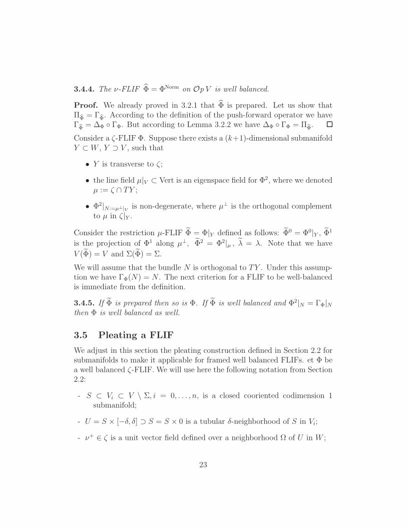
Figure 11: Γ-pleating of a well balanced FLIF

• Φ1 = Φ1;

• Φ2|ν⊥ = Φ2|ν⊥;

• Φ2(ν+) = c ν+;

• λ+(Φ2) = ±ν+, where the sign is chosen in such way that the vector

field λ+(Φ2) define an inward coorientation of positive components of

U \ S, see Fig. 11.

We say that Φ = PleatS,ν+,Γ(Φ) is obtained from Φ by Γ-pleating over S inthe direction of the vector field ν+ see Fig. 11.

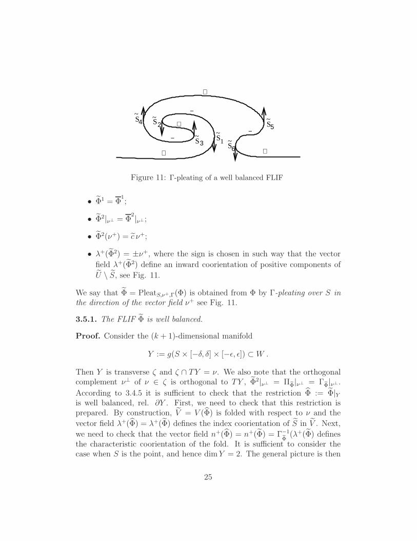
3.5.1. The FLIF Φ is well balanced.

Proof. Consider the (k + 1)-dimensional manifold

Y := g(S × [−δ, δ]× [−ǫ, ǫ]) ⊂ W .

Then Y is transverse ζ and ζ ∩ TY = ν. We also note that the orthogonalcomplement ν⊥ of ν ∈ ζ is orthogonal to TY , Φ2|ν⊥ = ΠΦ|ν⊥ = ΓΦ|ν⊥.

According to 3.4.5 it is sufficient to check that the restriction Φ := Φ|Yis well balanced, rel. ∂Y . First, we need to check that this restriction isprepared. By construction, V = V (Φ) is folded with respect to ν and the

vector field λ+(Φ) = λ+(Φ) defines the index coorientation of S in V . Next,

we need to check that the vector field n+(Φ) = n+(Φ) = Γ−1

Φ(λ+(Φ) defines

the characteristic coorientation of the fold. It is sufficient to consider thecase when S is the point, and hence dimY = 2. The general picture is then

25

λ+(Φ∼

)

n+(Φ∼

) = ΦΓ∼ ( +)λ

ν+

ΦΓ∼ (ν+)

+

−

Figure 12: Vector n+(Φ) determines the characteristic coorientation of the fold

obtained by taking a direct product with S. Note that the characteristic co-orientation of the fold Sj is given by the vector field ∂

∂tif j is odd, and by − ∂

∂t

if j is even. Consider first the case when j is odd, see Fig. 12. Then if thelower branch of the parabola is positive then the vector field ΓΦ(ν

+) definesthe same coorientation as the vector field − ∂

∂t. But in this case λ+ = −ν+,

and hence ΓΦ(λ+) defines the characteristic coorientation of the fold. The

other cases can be considered in a similar way. Finally, we use Lemma 3.4.2to conclude that Φ is well balanced relative the boundary ∂Y .

In order to extend the Γ-pleating operation to framed well-balanced FLIFswe need to impose additional constraints on the choice of the vector fieldν+ and the curve Γ, see Fig. 13. For each j = 1, . . . 2N denote by σj theproportionality coefficient in λ+|Sj

= σjν+|Sj

, σj = ±1. Then we requirethat

(α) if Sj and Sj+1, j = 1, . . . , 2N − 1 bound a negative component of U \ Sthen σj = σj+1;

(β) if the component bounded by S1 and S2 is positive then σ1 = σ2N = ±1for ν+ = ±ξi.

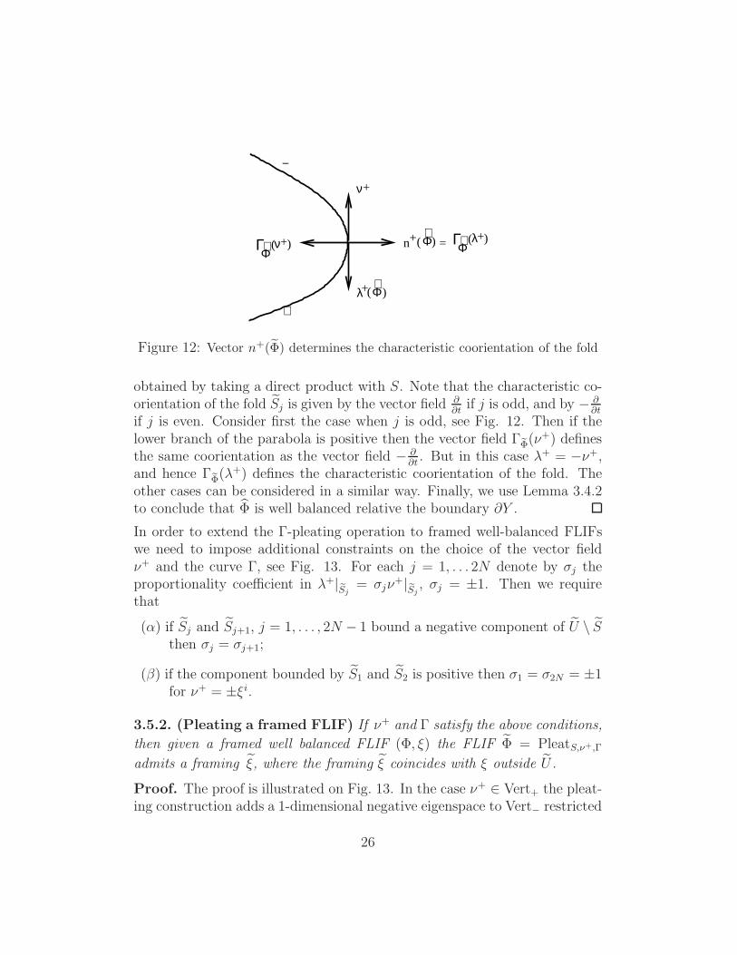
3.5.2. (Pleating a framed FLIF) If ν+ and Γ satisfy the above conditions,

then given a framed well balanced FLIF (Φ, ξ) the FLIF Φ = PleatS,ν+,Γ

admits a framing ξ, where the framing ξ coincides with ξ outside U .

Proof. The proof is illustrated on Fig. 13. In the case ν+ ∈ Vert+ the pleat-ing construction adds a 1-dimensional negative eigenspace to Vert− restricted

26

ν+

+

+

− −

+ +

+ +

−

−

−

Γ

Γ2+

Γ2_

+ν

ν+

i

i

−

+

−

ξ

1

ξ

−

Figure 13: Framing of a Γ-pleated FLIF

to negative components U \ S. Condition (α) then allows us to frame this1-dimensional space either with ξi+1 := σjν

+. Similarly, if ν+ ∈ Vert− (or,

equivalently when the component bounded by S1 and S2 is positive) thenthe pleating construction removes the negative eigenspace generated by ν+

on positive components. The remaining negative components bounded S2j

and S2j+1, j = 1, . . . , N − 1, can be framed with ξ := (ξ1, . . . , σ2jξi). Condi-tion (β) ensures that the existing framing in the complement of U satisfies

the necessary boundary conditions on S1 and S2N .

3.5.3. Given any framed well balanced FLIF (Φ, ξ), one of the curves Γ1,Γ±2

shown on Fig. 6 can always be used as the curve Γ to produce a framed wellbalanced FLIF (Φ, ξ) by a Γ-pleating.

Proof. Indeed, as it follows from Criterion 3.5.2, the curve Γ1 can always beused if ν+|S ∈ Vert+, while if ν+|S ∈ Vert− then the curve Γ±

2 can be usedin the case ν+ = ±ξi, see Fig. 13.

27

The next proposition is a corollary of Theorem 2.2.1 and the results discussedin the current section.

3.5.4. (Pleated isotopy of framed well balanced FLIFs) Let ζs, s ∈[0, 1], be a family of n-dimensional distributions on W , and (Φ, ξ) a framedwell-balanced ζ0-FLIF with V (Φ) = V ⊂ W . Then there exist

• a framed well balanced ζ0-FLIF Φ obtained from Φ by a sequence ofpleatings, and

• a C0-small isotopy hs : V → W , s ∈ [0, 1] such that h0 is the inclusion

V → W and Vs := hs(V (Φ)) is folded with respect to ζs along Σs :=

hs(Σ(Φ)).

If Φ is holonomic over Op A then one can arrange that Φ = Φ on Op A andthat the homotopy hs is fixed over Op A.

Proof. According to Theorem 2.2.1 there exists a manifold V for which theisotopy with the required properties does exist. This manifold can be con-structed beginning from V by a sequence of Γ+

0 -pleatings along the bound-aries of balls embedded into V \ Σ, in the direction of vector fields whichextend to these balls. The latter property allows us to deform these vectorfields into vector fields contained in Vert+ or Vert− (we need to use Vert−only if dimVert+ = 0). Moreover, when using ν+ ∈ Vert−|Vi

and wheni = dimVert−|Vi

> 1 we can deform it further into the last vector ξi of theframing. In the case i = 1 we can deform ν+ into ±ξi, but we cannot, ingeneral, control the sign. Note that we need to use this case only if n = 1.As it was explained in Remark 2.2.2, we can replace at our choice each Γ+

0 -pleating in the statement of Theorem 2.2.1 by any of the Γ-pleatings withΓ = Γ1,Γ

±2 . But according to Lemma 3.5.3 one can always use one of these

curves to pleat in the class of framed well balanced FLIFs. It remains toobserve that if Φ is holonomic over Op A then all the constructions which weused in the proof can be made relative to Op A.

3.6 Stabilization

Let Φ be a ζ-FLIF. Suppose that we are given a connected domain U ⊂ V \Σwith smooth boundary such that the bundles Vert±|U are trivial. Let C bean exterior collar of ∂U ⊂ V \ Σ. We set U ′ := U ∪ C.

28

Let us assume that U is contained in V i. If i < n we choose a section θ+ ofthe bundle Vert+ over U ′ and we define a negative stabilization of Φ over Uas a FLIF Φ = Stab−

U,θ+(Φ) such that

• Φ1 = Φ1;

• Φ2 = Φ2 over V \ U ′;

• Σ(Φ) = Σ(Φ) ∪ ∂U ; IntU ⊂ V i+1(Ψ);

• Vert−(Φ)|IntU = Span(Vert−(Φ)|IntU , θ+);

• λ+(Φ)|∂U = θ+.

We will omit a reference to θ in the notation and write simply Stab−U(Φ)

when this choice will be irrelevant.

Note that in order to construct Φ2 on U ′ which ensures these property we needto adjust the background metric on ζ to make θ+ an eigenvector field for Φ2

corresponding the eigenvalue +1. The vector field θ+ remains the eigenvectorfield for Φ2 but the eigenvalue function is changed to c : U ′ → [−1, 1], wherec is negative on U , equal to 1 near ∂U ′ and has ∂U as its regular 0-level.

If the FLIF Φ is framed by ξ = (ξ1, . . . , ξi) then Φ can be canonically

framed by ξ such that ξ = ξ over V \ U and Vert−(Φ)|IntU is framed by

ξ := (ξ1. . . . , ξi, θ+) and we define

Stab−U(Φ, ξ) := (Stab−

U, ξi(Φ), ξ),

In the case when U ⊂ Vi and i > 0 we can similarly define a positive stabi-lization of Φ over U as a FLIF Φ = Stab+

U, θ(Φ), where θ is a section of Vert−over U ′ such that

• Φ1 = Φ1;

• Φ2 = Φ2 over V \ U ′;

• Σ(Φ) = Σ(Φ) ∪ ∂U ; IntU ⊂ V i−1(Ψ);

• Vert+(Φ)|IntU = Span(Vert+(Φ)|Int U, θ+);

• λ+(Φ)|∂U = θ+.

29

If Φ is framed by a framing ξ = (ξ1, . . . , ξi) then we will always chooseθ+ = ξi|U and define a positive stabilization by the formula

Stab+U(Φ, ξ) := (Stab+

U, ξi(Φ), ξ),

where ξ|IntU = (ξ1, . . . , ξi−1).

3.6.1. (Balancing via stabilization) Any FLIF can be stabilized to a bal-anced one. If Φ is balanced and χ(U) = 0 then Stab±

U (Φ) is balanced as well.The statement holds also in the relative form.

Proof. The obstruction for existence of a fixed over A ⊂ V homotopybetween two monomorphisms Ψ1,Ψ2 : Norm → TW |V is an n-dimensionalcohomology class δ(Ψ1,Ψ2;V,A) ∈ Hk(V,A; πk(Vn(R

n+k))), or more preciselya cohomology class with coefficients in the local system πk(Vn(TvW )), v ∈ V .Note that πk(Vn(R

n+k)) = Z if k is even or n = 1 and Z/2 otherwise. It isstraightforward to see that

δ(∆(Φ),∆(Stab±U(Φ);U, ∂U) =

χ(U)Θ, k is even;

±χ(U)Θ, k is odd,

for an appropriate choice of a generator Θ ofHk(U, ∂U ; πk(Vn(Rn+k))). Hence,

stabilization over a domain with vanishing Euler characteristic does notchange the obstruction class δ(Γ(Φ),∆(Φ)) and with the exception of thecase k = n = 1 this obstruction class can be changed in an arbitrary way byan appropriate choice of U . Indeed, if k > 1 then one can take as U eitherthe union of l copies of n-balls or a regular neighborhood of an embeddedbouquet of l circles (comp. a similar argument in [EGM11]). If k = 1 andn > 1 then the sign issue is irrelevant because the obstruction is Z/2-valued.If k = n = 1 then one may need two successive stabilizations in order to bal-ance a FLIF. Indeed, the domain U in this case is a union of some number lof intervals, and hence χ(U) = l. Thus the positive stabilization increases theobstruction class by l, while the negative one decreases it by l. Suppose, fordeterminacy, we want to stabilize over a domain in V0. If we need to changethe obstruction class by −l then we just negatively stabilize over the unionof l intervals. If we need to change it by +l we first negatively stabilize overone interval I and then positively stabilize over the union of l + 1 disjointintervals in I.

30

3.7 From balanced to well balanced FLIFs

3.7.1. (From balanced to well balanced) Let (Φ, ξ) be a balanced framedζ-FLIF which is holonomic over a neighborhood of a closed subset A ⊂ W .Then there exists a framed well-balanced FLIF (Φ′, ξ′) which coincides withΦ over Op A. In addition, V (Φ′) is obtained from V (Φ) via a C0- small,fixed on Op A isotopy.

Proof. There exists a family of monomorphisms Ψs : Vert → TW , s ∈

[0, 1], connecting Vert∆Φ−→ ΦVert → τ and the inclusion j : Vert → τ . The

homotopy can be chosen fixed over Op A. The family Ψs can be extendedto a family of monomorphisms ζ → TW . We will keep the notation Ψs

for this extension. Denote ζs := Ψs(ζ), s ∈ [0, 1]. Thus ζ1 = ζ and ζ0is an extension to W of the bundle NormΦ. Lemma 3.4.4 then guaranteesthat the push-forward ζ0-FLIF (Id,Ψ0)∗(Φ, ξ) is well balanced. According

to Theorem 3.5.4 there exists a well balanced framed ζ0-FLIF (Φ, ξ) where

V = V (Φ) is obtained from V by a C0-small isotopy which i8s fixed outside aneighborhood of V and over a neighborhood of A, and a C0- small supportedin (Op V )\A isotopy gs starting with g0 = Id such that for each s ∈ [0, 1] the

manifold Vs := gs(V ) is folded with respect to ζs along Σs = gs(Σ). Thereexists a family of bundle isomorphisms Θs : ζ0 → ζs covering the diffeotopyhs and such that Θ0 = Id and Θs = dgs over the line bundle TV |Σ ∩ ζ0. Thehomotopy Θs can be chosen fixed over Op A. Then, according to Lemma3.4.3, the push-forward ζ-FLIF (g1,Θ1)∗(Φ, ξ) is well balanced relative A.

3.8 Formal extension

3.8.1. (Formal extension theorem) Any framed ζ-FLIF (Φ, ξ) on Op A ⊂

W extends to a framed ζ-FLIF (Φ, ξ) on the whole manifold W .

The proof is essentially Igusa’s argument in [Ig87] (see pp.438-442).

We begin with the following lemma which will be used as an induction stepin the proof.

3.8.2. (Decreasing the negative index) Let j = 1, . . . , n. Suppose W isa cobordism between ∂−W and ∂+W , and for a framed FLIF (Φ, ξ) on W

one has V i = ∅ for i > j. Then there exists a framed FLIF (Φ, ξ) such that

31

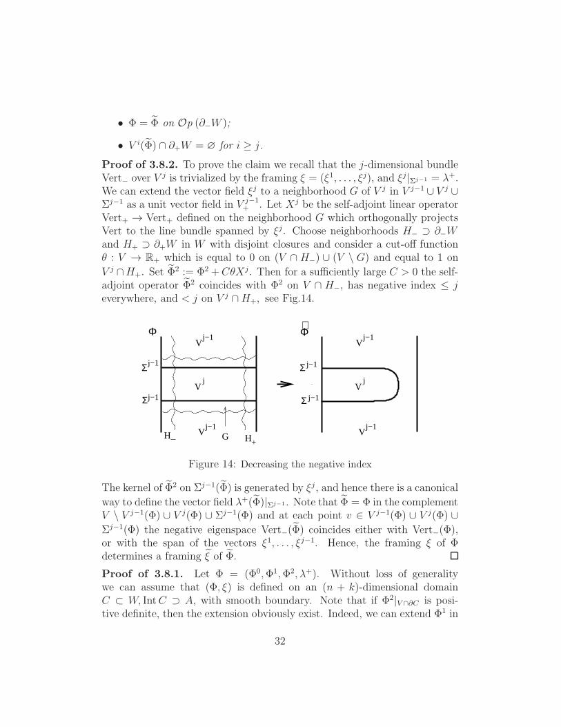
• Φ = Φ on Op (∂−W );

• V i(Φ) ∩ ∂+W = ∅ for i ≥ j.

Proof of 3.8.2. To prove the claim we recall that the j-dimensional bundleVert− over V j is trivialized by the framing ξ = (ξ1, . . . , ξj), and ξj|Σj−1 = λ+.We can extend the vector field ξj to a neighborhood G of V j in V j−1 ∪ V j ∪Σj−1 as a unit vector field in V j−1

+ . Let Xj be the self-adjoint linear operatorVert+ → Vert+ defined on the neighborhood G which orthogonally projectsVert to the line bundle spanned by ξj. Choose neighborhoods H− ⊃ ∂−Wand H+ ⊃ ∂+W in W with disjoint closures and consider a cut-off functionθ : V → R+ which is equal to 0 on (V ∩ H−) ∪ (V \ G) and equal to 1 on

V j ∩H+. Set Φ2 := Φ2 +CθXj. Then for a sufficiently large C > 0 the self-

adjoint operator Φ2 coincides with Φ2 on V ∩ H−, has negative index ≤ jeverywhere, and < j on V j ∩H+, see Fig.14.

V

V

Vj

j−1

j−1

H_ H+G V

V

Vj

j−1

j−1Φ Φ∼

Σ

Σj−1

j−1 Σ j−1

Σ j−1

Figure 14: Decreasing the negative index

The kernel of Φ2 on Σj−1(Φ) is generated by ξj, and hence there is a canonical

way to define the vector field λ+(Φ)|Σj−1 . Note that Φ = Φ in the complementV \ V j−1(Φ) ∪ V j(Φ) ∪ Σj−1(Φ) and at each point v ∈ V j−1(Φ) ∪ V j(Φ) ∪

Σj−1(Φ) the negative eigenspace Vert−(Φ) coincides either with Vert−(Φ),or with the span of the vectors ξ1, . . . , ξj−1. Hence, the framing ξ of Φdetermines a framing ξ of Φ.

Proof of 3.8.1. Let Φ = (Φ0,Φ1,Φ2, λ+). Without loss of generalitywe can assume that (Φ, ξ) is defined on an (n + k)-dimensional domainC ⊂ W, IntC ⊃ A, with smooth boundary. Note that if Φ2|V ∩∂C is posi-tive definite, then the extension obviously exist. Indeed, we can extend Φ1 in

32

any generic way to W , and then extend Φ2 as a positive definite operator onVert. We will inductively reduce the situation to this case. Let C ′ ⊂ IntC bea smaller domain such that A ⊂ IntC ′. Let us apply 3.8.2 to the cobordismW(0) = C \IntC ′ between ∂−W(0) = ∂C ′ and ∂+W(0) = ∂C and to the restric-tion (Φ, ξ)|W(0)

in order to modify (Φ, ξ)|W(0)into a framed FLIF (Φ(0), ξ(0))

which coincides with (Φ, ξ) near ∂−W(0) and such that V n(Φ(0))∩ (∂+W(0)) =∅. Then for a sufficiently small tubular neighborhood W(1) of ∂+W(0) inW(0) we have W(1) ∩ A = ∅ and W(1) ∩ V n(Φ(0)) = ∅. We view W(1) as acobordism between ∂−W(1) = ∂W(1) \ ∂+W(0) and ∂+W(1) = ∂+W(0). Now weagain apply 3.8.2 to the cobordism W(1) and Φ(0)|W(1)

and construct a framedFLIF (Φ(1), ξ(1)) on W(1) which coincides with (Φ(0), ξ(0)) near ∂−W(1) andsuch that V i(Φ(1)) ∩ ∂+W(1) = ∅) for i ≥ n− 1. Continuing this process weconstruct a sequence of nested cobordisms C ⊃ W(0) ⊃ W(1) ⊃ · · · ⊃ W(n−1)

and a sequence of framed FLIFs (Φ(j), ξ(j)) on W(j), j = 0, . . . , n − 1, suchthat for all j = 0, . . . , n− 1

• ∂+W(j) = ∂C;

• (Φ(j+1), ξ(j+1)) coincides with (Φ(j), ξ(j)) on Op (∂−W(j+1));

• V i(Φ(j)) ∩ ∂+W(j) = ∅ for i ≥ n− j.

Let us also set W(n) = ∅. Hence we can define a framed formal Igusa function

(Φ, ξ) over C by setting (Φ, ξ) = (Φ, ξ) on C ′ and (Φ, ξ) = (Φ(j), ξ(j)) on

W(j) \ W(j+1) for j = 0, . . . , n − 1. Note that the quadratic part Φ2 of Φ is

positive definite on ∂C, and hence the framed formal Igusa function Φ canbe extended to the whole W .

3.9 Integration near V

3.9.1. (Local integration of a well balanced FLIF) Any well balancedF-FLIF Φ can be made holonomic near V after a small perturbation nearV . Namely, there exists a homotopy of well balanced FLIFs Φs, s ∈ [0, 1],s ∈ [0, 1], beginning with Φ0 = Φ with the following properties:

- V (Φs) = V (Φ),Σ(Φs) = Σ(Φ) for all s ∈ [0, 1];

- (Φ2s, λ

+s ) is C

0-close to (Φ2, λ+) for all s ∈ [0, 1];

- Φ1 is holonomic on Op V .

33

If for a closed subset A ⊂ W the FLIF Φ is already holonomic over Op A ⊂W then the homotopy can be chosen fixed over Op A.

Proof. According to Lemma 2.1.1 there exist local coordinates (σ, t, z, y) ina neighborhood of Σ in W , where σ ∈ Σ, x, z ∈ R and y ∈ Ver|Σ such thatthe manifold V is given by the equations z = x2, y = 0 and the foliationF is given by the fibers of the projection (σ, x, z, y) → (σ, z). The vectorfield ∂

∂xgenerates the line bundle λ = TV |Σ ∩ Vert and we can additionally

arrange that ∂∂x|Σ = λ+. By a small C0-small perturbation of the operator Φ2

(without changing it along Σ) we can arrange the the vector field ∂∂x

serves anan eigenvector field for Φ2 in a neighborhood of Σ. We will keep the notationλ for the extended line field ∂

∂x. Then the operator Φ2 : Vert = Ver ⊕ λ →

Ver ⊕ λ can be written as A ⊕ c, where A is a non-degenerate self-adjointoperator and c is an operator acting on the line bundle λ by multiplicationby a function c = c(σ, x) on Op Σ ⊂ V such that for all σ ∈ Σ we havec(σ, 0) = 0, d(σ) := ∂c

∂x(σ, 0) > 0.

Define a function ϕ on Op Σ ⊃ W given by the formula

ϕ(σ, x, z, y) =d(σ)

6(x3 − 3zx) +

1

2〈Ay, y〉. (3)

Then V (ϕ) = V ∩ Op Σ and the operator d2Fϕ : Ver⊕ λ → Ver⊕ λ is equalto A ⊕ c, where the operator c acts on λ by multiplication by the functiond(σ)x. Hence the operator functions d2ϕ and Φ2 coincides with the firstjet along Σ, and therefore, one can adjust Φ2 by a C0- small homotopy tomake Φ2 equal to d2ϕ over Op Σ ⊂ W . To extend ϕ to a neighborhoodOp V ⊂ W we observe that the neighborhood of V in W is diffeomorphicto the neighborhood of the zero section in the total space of the bundleVert|V \U . In the corresponding coordinates we define ϕ(v, y) := 1

2〈Φ2(v)y, y〉,

v ∈ V, y ∈ Vertv. On the boundary of the neighborhood of Σ where wealready constructed another function, the two functions differ in terms oforder o(||y||2). Hence they can be glued together without affecting d2Fϕ, andthus we get a leafwise Igusa function ϕ with d2Fϕ = Φ2. It remains to extend∇Fϕ as a non-zero section of the bundle TF to the whole W . Accordingto Lemmas 3.1.2 and 3.3.1 we have Γϕ = Πϕ = d2ϕ = Φ2. Then the wellbalancing condition for Φ implies that Γϕ is homotopic (rel. Op A) to ΓΦ

as isomorphisms Norm → Vert. But this implies that there is a homotopy(rel. Op A) of sections Φ1

s : W → Vert, s ∈ [0, 1], connecting Φ10 = Φ1 and

Φ11 = ∇Fϕ and such that the zero set remains regular and unchanged.

34

4 Proof of Extension Theorem 1.1.1

Step 1. Formal extension. We begin with a leafwise framed Igusafunction (ϕA, ξA). Using 3.8.1 we extend it to a FLIF (Φ, ξ) on W .All consequent steps are done without changing anything on Op A.

Step 2. Stabilization. Using 3.6.1 we make (Φ, ξ) balanced.

Step 3. From balanced to well balanced. Using 3.7.1 we furtherimprove (Φ, ξ) making it well balanced.

Step 4. Local integration near V . Using 3.9.1 we deform (Φ, ξ)without changing V (Φ) to make it holonomic near V .

Step 5. Holonomic extension to W . Now onW \Op V we are in a posi-tion to apply Wrinkling Theorem 1.6B from [EM97] (see also [EM98], p.335)to extend the constructed ϕA∪V as a leafwise wrinkled map ϕ : (W,F) → R.The wrinkles of ϕ of any index have the canonical framing and thus thiscompletes the proof of Theorem 1.1.1.

References

[Ar76] V.I. Arnold, Wave front evolution and equivariant Morse lemma,Comm. Pure Appl. Math., 29(1976), 557–582.

[El72] Y. Eliashberg, Surgery of singularities of smooth maps, Izv. Akad.Nauk SSSR Ser. Mat., 36(1972), 1321–1347.

[EM97] Y. Eliashberg and N. Mishachev, Wrinkling of smooth mappings andits applications - I, Invent. Math., 130(1997), 345–369.

[EM98] Y. Eliashberg and N. Mishachev, Wrinkling of smooth mappings -III. Foliation of codimension greater than one, Topol. Methods inNonlinear Analysis, 11(1998), 321-350.

[EM00] Y. Eliashberg and N. Mishachev, Wrinkling of smooth mappings - II.Wrinkling of embeddings and K.Igusa’s theorem, Topology, 39(2000),711-732.

[EM02] Y. Eliashberg and N. Mishachev, Introduction to the h-principle,AMS, Graduate Studies in Mathematics, v.48, 2002.

35

[EM09] Y. Eliashberg and N. Mishachev, Wrinkled Embeddings, Contempo-rary Mathematics, 498(2009), 207-232.

[EGM11] Y. Eliashberg, S. Galatius and N. Mishachev, Madsen-Weiss forgeometrically minded topologists, , Geom. and Topol., 15(2011), 411-472.

[Gr86] M. Gromov, Partial differential relations, Springer-Verlag, 1986.

[Ig84] K. Igusa, Higher singularities are unnecessary, Annals of Math.,119(1984), 1–58.

[Ig87] K. Igusa, The space of framed functions, Trans. of Amer. Math. Soc.,301(1987), no 2, 431–477.

[Lu09] J. Lurie, On the Classification of Topological Field Theories,arXiv:0905.0465.

[Sm58] S. Smale, The classification of immersions of spheres in Euclideanspaces, Ann. of Math.(2) 69(1959), 327–344.

36