The Search for Dark

Matter:

Detection Rates of Axion-like Particles

as a Function of Mass in Ge and NaI

Detectors

Eric Gutman

Master’s Thesis Advisor: Dr. Juan Collar

The Kavli Institute for Cosmological Physics

The University of Chicago

Submitted: November 21, 2008

Revised: December 2, 2008

Accepted: December 12, 2008

Abstract

Theoretical derivations of the pseudoscalar and scalar dark matter (DM) particle counting

rates by detectors with Ge and NaI targets have been put forth by the DAMA research

team and other such groups, with those of the DAMA team being recently disputed. This

paper impartially performs a computation of counting rate versus DM particle mass using

each of these theories, presents the final quantitative results, and analyzes their

significance and mutual compatibility. A background of the physical context behind the

derivations is given first, and a discussion of their potential impacts, should they be found

correct, on the theoretical and experimental exploration of dark matter concludes.

I. Introduction

In the search for dark matter (DM) and its mysterious properties, several hypothetical

particles are currently under research as candidates for its composition. In 1977, the

Peccei-Quinn axion was proposed to solve the strong CP problem of quantum

chromodynamics, and was later realized to possess properties necessary to make it a

viable DM particle candidate. Various theoretical models of axions exist, each describing

its characteristics differently, especially its mass and coupling properties. Many models

of “axion-like” particles, which are similar to but not the same as axions, exist as well.

While axions themselves are defined to have pseudoscalar coupling, axion-like particle

candidates are theorized to include light bosonic particles of both pseudoscalar and scalar

varieties, which will be notated in relevant expressions as a and h.

Experimentally, detectors with targets comprised of sodium iodide, germanium, as well

as other elements and compounds, have been constructed to detect such particles, though

none are known to have been detected to date. However, even the negative results

obtained represent significant accomplishments, providing increasingly restrictive limits

on relevant physical parameters, such as the mass, coupling strength, etc. of these axion-

like particles. As the windows of possible values for such parameters shrink, we learn

more and more about these mysterious, theoretical particles.

The research presented in this paper is neither the beginning nor the end of the story of

the search for non-baryonic dark matter. It is but a link in the long chain of collaboration

between the theoretical and experimental facets of this undertaking, and has been

performed to both corroborate previous theoretical predictions, and to provide initial

predictions for current and future experiments. Specifically, the rate of particle-target

interaction versus particle mass has been theoretically derived [1, 2] and computationally

calculated for NaI and pure Ge detectors by the University of Chicago’s COGENT

research group and others for the case of pseudoscalar axion-like particles, and the

DAMA research team [3] predicted the same using its own, completely different method,

one which has recently come under dispute [2]. While remaining neutral in this

disagreement, this research corroborates and analyzes the quantitative results of both

theoretical derivations. Non-trivially, the assigned values of relevant physical parameters

remain the same in both, and are in line with those assigned by previous computations.

Additionally, this research computes analogous event rate curves for scalar axion-like

particles using a similarly disputed [2] DAMA team theory, which has not previously

been done.

2

II. Physical Background

The flux across the Earth of DM particles which comprise the galactic halo of the Milky

Way contains two components, one that is constant, and one that modulates in a

sinusoidal pattern throughout the solar year. This is caused by the sum of the two

velocity vectors which describe the Earth’s motion in the galaxy. The larger of the

velocity vectors is that of the Sun, which moves (and takes the solar system along with it)

with respect to the approximately isotropic halo of dark matter at a constant speed, which

in turn is the source of the constant part of the flux. The much smaller velocity vector,

that of the Earth’s revolution around the Sun, causes a modulation on the order of a few

percent of the constant flux. In June, the Earth is moving in the same direction as the

Sun, causing a greater number of DM particles to cross the Earth, than in December,

when its motion is directly opposite that of the Sun (the maximum and minimum fluxes

usually take place around the 2nd

of these months, respectively). An annual modulation

signature of the DM particle flux emanating from the galactic halo is the result [4,5],

which is added to the constant part (i.e., that which does not change throughout the solar

year). It is this specific modulation signature that DM detectors are looking for (for a list

of the six necessary characteristics of this signature, see [3]), as evidence that it is, in fact,

DM that is being observed, and not some other background particle. Attention within the

research community is therefore focused primarily on the modulation of potential DM

flux; predictions relevant to the detection of physical phenomena which contribute

specifically to this modulation, and how the rate of which varies with axion-like particle

mass, are the focus of this paper.

The physical phenomena that would theoretically take place within detector targets as a

result of a pseudoscalar or scalar DM interaction, shown in Fig. 1, are a Compton-like

effect (note the suffix “like,” since the incident particles in question are not photons, as

would be the case in the actual Compton effect), what is known as the “axioelectric

effect” (a photoelectric-like effect), and the Primakoff effect (traditionally, the suffix

“like” is not added here). The Compton-like effect involves an axion-like particle of

mass ma (or in the scalar case, mh) coupling to a charged fermion, either an electron or a

quark, being absorbed (as it would be in the regular Compton effect), and emitted as a

photon with energy ma. It is essentially the same process as the Compton effect of

ordinary matter, only the incident particle is a pseudoscalar or scalar particle rather than a

photon. Similarly, the replacement of a photon with an axion-like particle is the basic

difference between the photoelectric effect of ordinary matter, and the axioelectric (or

photoelectric-like) effect. In the latter case, the additional axion-like particle energy ma

(as opposed to photon energy ω in the former) to the system transforms into the kinetic

energy of the absorbing electron, as well as the radiation the electron emits as it

accelerates. Finally, the story is similar with the Primakoff effect. Rather than involving

a photon interacting with a nucleus, as is ordinarily the case, an axion-like particle

incident on a nucleus couples to two photons, one of which is virtual (not having its own

energy, but related to the electric field of the atom), and the other having energy ma.

3

Fig. 1. From Bernabei et al. [3]

The source of the disputes concerning the DAMA team’s approximations in both

pseudoscalar and scalar particle detection lies in the Hamiltonian of the photoelectric-like

effect. Maxim Pospelov et al. assert [2] that the DAMA team misidentified the leading

term, which would make this effect much larger in both the pseudoscalar and scalar

cases. As will be described in the next two paragraphs, this would result in the DAMA

team’s pseudoscalar count rate being a few orders of magnitude too small, and perhaps

even more monumentally, its theoretical approximation of the scalar counting rate being

completely invalid.

In targets set up to detect pseudoscalar axion-like DM particles, all three physical

phenomena discussed contribute to the constant part of the flux, with the axioelectric and

Primakoff effects contributing to the flux modulation as well. However, there is a

general consensus that the axioelectric effect is especially dominant with respect to

pseudoscalar particle-nucleus interactions, and dominant to a lesser extent even in the

case of pseudoscalar particle-electron events [3]. Therefore, to predict the detection rate

of pseudoscalar DM particles which comprise the modulation, one need consider only the

axioelectric effect to obtain a good approximation. However, due to the dispute over

whether or not to include an additional leading term in its Hamiltonian, there is

disagreement within the research community over just how large the counting rate of this

effect should be. This paper will present and examine quantitative count rates using

DAMA’s theory, without the additional Hamiltonian term.

In the scalar case, according to the DAMA research team, the photoelectric-like effect

dominates in the constant part of the flux, but does not contribute to its modulation,

leaving the Compton-like and Primakoff effects as the two contributors to the latter.

However, to account for such scalar particles having lifetimes comparable to that of the

universe, the Primakoff effect’s contribution must be negligible [3]. Therefore, only the

Compton-like effect need be considered to obtain a good approximation, in predicting the

detection rate of particles comprising flux modulation of scalar DM, according to

DAMA. However, the above dispute over the photoelectric-like effect’s Hamiltonian

affects this approximation as well. If Pospelov and his collaborators were correct, the

photoelectric-like effect would be much larger than the DAMA team is presently holding

it to be, and would be dominant over the Compton-like effect in the modulation of the

scalar particle flux as well. The DAMA team would therefore have used the wrong

physical effect in its approximation. To perhaps shed light on the matter, and contribute

to a resolution of this dispute, this paper computes and analyzes the quantitative results of

this approximation.

4

III. Research Objective

The specific objective of all three parts of this research was to compute the counting rates

of pseudoscalar and scalar axion-like particles incident on Ge and NaI targets as

functions of axion-like particle mass, given theoretical approximations of the physical

phenomena which contribute to the annual modulation signature of such DM. For the

COGENT group’s pseudoscalar method, which will be referred to as “pseudoscalar

method I,” no specific time of year was chosen; rather, the calculations were designed to

yield the mean counting rate over the course of the year. For the DAMA team’s

pseudoscalar (referred to as “pseudoscalar method II,”) and scalar methods, the time of

year was arbitrarily chosen to be June 2nd

, when the modulation is at its maximum. In all

cases, the axion-like particle mass range considered was from .1 to 10 keV.

IV. Pseudoscalar Method I

As discussed earlier, for a pseudoscalar DM particle flux modulation, it is agreed that the

axioelectric effect is dominant, and so a good approximate prediction for a detector’s

counting rate can be given by it alone.

Beginning with the non-relativistic electron Hamiltonian, and substituting the

pseudoscalar particle mass ma for the photon energy ω as explained above, the ratio of

the cross section for pseudoscalar particle absorption to that of the photoelectric-like

effect can be derived [2]:

24

3

)(

2

a

a

ape

abs

f

m

cm

v

where v is the pseudoscalar particle velocity, α is the fine structure constant, and

eeagf

1 , where eeag is the coupling strength. Rearranging terms and simplifying, the

mean detector counting rate for the year can be expressed as

-1-12119 day kg 102.1 peaeea mgAR

where A is the mass number of the target atom (or molecule), ma is in terms of keV, σpe is

in terms of barns/atom, and eeag is dimensionless.

Methodology:

The curve was initially graphed using Excel, and for the purposes of this paper, the data

were imported into and plotted in KaleidaGraph (as were all curves included in this

research). As in the COGENT group’s computation [1], the coupling strength eeag was

5

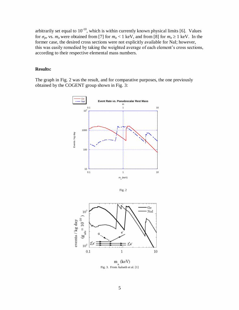
arbitrarily set equal to 10-10

, which is within currently known physical limits [6]. Values

for σpe vs. ma were obtained from [7] for ma < 1 keV, and from [8] for ma 1 keV. In the

former case, the desired cross sections were not explicitly available for NaI; however,

this was easily remedied by taking the weighted average of each element’s cross sections,

according to their respective elemental mass numbers.

Results:

The graph in Fig. 2 was the result, and for comparative purposes, the one previously

obtained by the COGENT group shown in Fig. 3:

10

100

1000

104

0.1 1 10

0.1 1 10

Event Rate vs. Pseudoscalar Rest MassGeNaI

Eve

nts

/ k

g d

ay

ma (keV)

m

Fig. 2

Fig. 3. From Aalseth et al. [1]

6

The jumps are caused by sudden increases in the number of electron subshells with

binding energies less than ma. As ma becomes greater than the binding energies of

electrons in those subshells, the electrons suddenly become able to be displaced by

pseudoscalar particle interactions, which results in jumps in count rate.

It is clear that the results agree well. If the theory behind this approximation is correct,

this data can now be used to help construct flux modulation curves of pseudoscalar axion-

like particles, by predicting the average amplitudes over the course of the solar year for

various pseudoscalar particle masses.

V. Pseudoscalar Method II

The DAMA team’s approach was to use a hydrogenic wave approximation to estimate

the axioelectric effect in the pseudoscalar case. Absorption of such a particle by an

electron in an atomic subshell with quantum numbers nlm has the differential cross

section (see [3])

23)(

3

2,

22

xdem

gd

dnlm

i

e

eea

nlmeA

xkp

pk

where k is the momentum of the incident pseudoscalar particle, p is the electron’s final

momentum resulting from the collision, and me is the electron mass. The magnitude of p

is given by

p = [(2me(ma- Enl)]1/2

The last term, containing the wave functions in the hydrogenic case, ψnlm, satisfies

e-iqx

ψnlm d3x = (2)

3/2Fnl(q) Ylm(Ω)

where Ylm(Ω) are the spherical harmonics, q is the initial momentum of the target

electron prior to collision, and the form factor of the nucleus [9], Fnl(q), is

Fnl(q) =

2/3

0

22

221

1222

222

2/1

1

1

)1(!2

)!(

)!1(2

a

Z

Qn

QnC

Qn

Qnln

ln

ln l

lnl

lll

where Z

qaQ 0 , a0 being the Bohr radius and Z the atomic number. 1

1

l

lnC is a

Gegenbauer polynomial, defined by

221)( sxssxC . Every electron in

every subshell of the target atoms must be taken into account when summing the overall

detection rate:

7

)()(2

2

,

22

nlanl

INa nl

nl

e

eeaaTeA EmpqFNv

m

gNR

NT is the number of atoms (or molecules) per kg of target, a is the local density of

pseudoscalar particles in the galactic halo, me is the electron mass, v is the pseudoscalar

particle velocity (see below), Nnl is the number of electrons in subshell nl, and Enl is the

binding energy of each one. Note the Heaviside step function , which indicates that if

ma is less than Enl, no electron from that subshell or any subshell of equal or greater

binding energy is unbound by the incident pseudoscalar particle, and so electrons from

those subshells will make no contribution to the overall detector count.

For purposes of detection rate, the pseudoscalar particle velocity we are primarily

interested in is the axion-like particle velocity with respect to the Earth in the reference

frame of the galaxy, which is equal to

v = vg + v

where vg is the particle’s velocity, and v is the velocity of the Earth, both in the galactic

reference frame. Summing the magnitudes of the vectors, we have

22

gvv + v2

The Earth’s velocity in the galactic reference frame is equal to the sum of the Sun’s

velocity and the Earth’s periodic orbital velocity around the Sun, in that reference frame.

That is,

v = v + vorb

Again summing vectors, we have

v2 = v

2 + 2

orbv

which yields

22

gvv + v2 =

2

gv + v2 + 2 v ∙ vorb + v

2orb

Since the v2

orb term is small, we can neglect it [3, 10], and we get

22

gvv v2 + v vorb 0cos tt

As discussed previously, this calculation is for annual maximum counting rates, those

that occur around June 2nd

, and so t = June 2 t0, and the cosine term equals 1. The

Sun’s velocity v 120 v km s-1

where v0 is the local velocity, and from [11, 12], v0 =

220 50 km s-1

at a 90% confidence level. Using the maximum likelihood estimate, v0 =

8

220. The particle’s velocity in the galactic frame, vg, using an isothermal halo model

approximation, satisfies 2

0

2

2

3vvg , and so we have

2

32 v (220 km s-1)2 + (220 km s-1 + 12 km s-1)2 + (220 km s-1 + 12 km s-1)(30 km s-1) 130,000 km2 s-2

v 360 km s-1

Methodology:

As derived above, v was given the value 360 km s-1

, and as in pseudoscalar method I, the

value of eeag was set to 10-10

. In Mathematica, first calculated were the initial and final

momenta (which were approximately equal) for a given electron from each atomic

subshell. With the exception of the Heaviside step function in the final expression for the

count rate, this contained the only explicit dependence on pseudoscalar particle mass.

However, this dependence on particle mass was carried through, since R =

R(F(Q(q(ma)))). As this functional form suggests, the form factor for each subshell was

derived from the initial electron momentum, and calculating the overall detector count

rate R involved summing over all subshells.

Since electrons with binding energies greater than ma do not contribute to the rate count,

and ma is the variable on which R depends, some coding was necessary to ensure this

taken into account for each subshell, and for every value of ma. The final input into

Mathematica computed the count rate for 6600 values of ma, ranging from .1 to 10 keV,

at intervals of .0015 keV.

The data were then imported into Excel in which the count rates for sodium and iodine

were summed together (since a molecule of NaI contains one atom of each), and graphed

along with the germanium count rate, both as functions of pseudoscalar particle mass.

Finally, the data were imported in KaleidaGraph, and plotted again.

For more details of the computation for pseudoscalar method II, including the

Mathematica inputs, see Appendix A.

Results:

The results are displayed on the left below (Fig. 4), next to those previously obtained by

the COGENT research group, which had computed quantitative results using the DAMA

team’s pseudoscalar theory, on the right (Fig.5):

9

0.01

0.1

1

10

100

0.1 1 10

Event Rate vs. Pseudoscalar Axion Mass

(6600 Data Points)

NaIGe

Eve

nts

/ k

g d

ay

ma (keV)

Fig. 4 Fig. 5. From personal communication, COGENT collaboration.

Though not identical, the results are quite similar. The curves’ respective trends are the

same, though those on the left are slightly higher. However, the difference represents not

even one order of magnitude, indicating very slight systematic difference in the way they

were calculated. These results also agree with the order of magnitude of the

computations published by the DAMA team itself [13], using this, its own theoretical

groundwork. If the DAMA team’s theoretical foundation for this approximation is

correct, this agreement in order of magnitude of the quantitative results it generates will

be helpful when it comes to definitively restricting physical parameters by negative

detection results, such as pseudoscalar particle mass or coupling strength. Additionally,

in an analogous fashion to the results of pseudoscalar method I, this data can be used to

help construct flux modulation curves of pseudoscalar axion-like particles, by predicting

the maximum amplitudes for various pseudoscalar particle masses in the solar year.

A potential difficulty with these results is that they do not match those of pseudoscalar

method I, which has a different theoretical basis, and is supported by multiple research

groups [1,2,14,15]. In fact, they are approximately three orders of magnitude smaller, a

gap which coincidentally would be bridged if Pospelov’s leading Hamiltonian term were

used [2]. Also, the fact that the smaller results of method II (which used DAMA’s

theoretical approximation) are for the maximum annual flux, and the larger results of

method I (other groups’ theoretical approximation) are for the mean flux, does not help

either. Even the other way around, agreement between the results of the two methods

would still be out of reach, since DM particle flux modulation is on the order of a few

percent, far less than the three orders of magnitude difference.

VI. Scalar Dark Matter

According to the DAMA team, for scalar DM flux modulation, the Compton-like effect is

dominant, and was therefore used to approximate the prediction of count rate vs. scalar

axion-like particle mass. Though the photoelectric-like effect is the primary source of

detecting scalar particle-electron interactions, the DAMA team claims it does not

contribute to the modulation, and the effects of such interactions via the Compton-like

10

effect are small. Therefore, the effect on flux modulation of scalar particle-electron

interactions is negligible, and so only interactions involving the target nuclei are

important [3], and therefore included in the approximation.

The differential cross section of the Compton-like effect [3] is given by

22

2

2

4

222

sin218

vv h

f

f

hffhflC

m

m

m

mgQ

d

d

where Qf is the charge of the fermion loop (the one involved in a potential interaction),

ffhg is the scalar particle coupling strength, mh is its mass, and mf is the fermion mass.

Integrating, we obtain for the total count rate of nuclear interaction

)(3

41

2

2

,

2

2

2

4

22

,

, qFvm

m

m

mgZNR nucA

h

A

A A

hAAheffAa

TnuclC

Note that mA is synonymous with the atomic mass A, but is written as it is here to

demonstrate that it is summed over all the atoms in the target molecule. Since we are

dealing with nuclear interactions, the effects of inner electron screening must be taken

into account, and so the effective nuclear charge, ZA,eff, is used. Greatly simplifying

matters, the nuclei are point-like on the keV energy scale [3], and so the form factor FA,nuc

can be set equal to 1.

Methodology:

The first step was to calculate the effective nuclear charges, ZA,eff, using Slater’s Rules.

Taking into account the screening of inner subshell electrons, this gave values of 9, 35,

and 22 for sodium, iodine, and germanium respectively.

The same axion-like particle mass range and coupling strength as in the pseudoscalar

methods were used, and the velocity (and its derivation) was identical to that of

pseudoscalar method II. Additionally, separate calculations using a coupling strength of

10-5

were performed, after the initial value of 10-10

yielded results of very small orders of

magnitude.

With no electron interactions or form factor complications (and the momentum

computations that go with them) to deal with, as there had been in the pseudoscalar case,

the input into Mathematica was much simpler for scalar axion-like particles. After

defining terms, three lines of input for each element were all that it took. The count rate

was computed for 100 values of ma, ranging from .1 to 10 keV, at intervals of .1 keV.

For the code that was used, see Appendix B.

Similarly to the pseudoscalar case, the count rates of sodium and iodine were summed

together in Excel, and plotted along with the germanium count rate as functions of scalar

11

particle mass. The data were later imported into KaleidaGraph, where they were re-

plotted.

As mentioned earlier, upon producing these plots using a scalar coupling strength of

10-10

, the count rate results were quite small, and so the entire procedure was repeated

using a coupling strength of 10-5

.

Results:

See Figs. 6 and 7. The former uses a coupling strength of 10-10

, and the latter that of 10-5

.

It is no surprise that the respective count rates differ by a factor of 1010

, since R 2

AAhg ,

and the two coupling strengths differ by a factor of 105. However, there is no reason why

the slopes of the curves would differ, and so both are linear on a logarithmic scale,

indicative of a power-law relationship between count rate and mass. Additionally,

whereas the pseudoscalar case had jumps in the curves caused by electron binding energy

being eclipsed by axion-like particle mass, here we are concerned only with nuclear

interactions, resulting in the omission of such jumps.

10-12

10-11

10-10

10-9

0.1 1 10

Event Rate vs. Scalar Axion Mass

(100 Data Points, ghAA

= 10-10

)

NaI

Ge

Eve

nts

/ k

g d

ay

ma (keV)

Fig. 6.

12

0.01

0.1

1

10

0.1 1 10

Event Rate vs. Scalar Axion Mass

(100 Data Points, ghAA

= 10-5

)

NaiGe

Eve

nts

/ k

g d

ay

ma (keV)

Fig. 7.

Comparing these results to those of pseudoscalar method II yields an important

consequence of the DAMA team’s theoretical approximations for scalars and

pseudoscalars, neither of which contain the Pospelov group’s leading term in the

Hamiltonian. The scalar count rate is on the order of 10-11

times the size of the

pseudoscalar count rate, using the same coupling strength (10-10

). Since a scalar coupling

strength 105 times greater than its pseudoscalar counterpart (theoretically, it would be

105.5

, due to the R 2

AAhg relationship, but in this computation, 10

5 was used) produces a

count rate of the same order of magnitude, it follows that the physical upper limit of the

pseudoscalar coupling strength would be considerably more restrictive than that of the

scalar coupling strength, should two detectors yield negative results for both over an

equal period of time. Not surprisingly, Pospelov’s group, which disagrees with the

theoretical approximation upon which this computation is based, explicitly states the

reverse, that the upper physical limit of the coupling strength is more restrictive in the

scalar case [2].

Using Pospelov’s additional Hamiltonian term, the pseudoscalar count rate increases by 3

orders of magnitude (see pseudoscalar method I), and if his assertion that the scalar

coupling strength limit is more restricted than that of the pseudoscalar were correct, the

scalar count rate would have to increase by at least 14 orders of magnitude. Pospelov

does not discuss the quantitative consequences of adding the extra Hamiltonian term in

the scalar case; however, such an enormous increase in count rate merits explanation, and

could potentially pose a legitimate question to either this extra term, or the claim that the

scalar coupling constant is more restricted. A possible answer is that according to

Pospelov’s group, DAMA’s entire scalar approximation is invalid, since the extra

Hamiltonian term implies that the photoelectric-like effect, not the Compton-like effect,

should be used. This would change the entire theoretical groundwork from that used by

the DAMA team, which agrees that the photoelectric-like effect dominates the constant

part of a scalar particle flux. The additional Hamiltonian term in the photoelectric-like

effect would spread its dominance over the Compton-like effect to the modulation as

13

well, as Pospelov’s group maintains is the case, and perhaps a count rate increase of 14

orders of magnitude can be attained. Also, the point can be made that the R 2

AAhg

relationship would imply a decrease in scalar coupling strength of only 7 orders of

magnitude, as opposed to 14. However, it is important to note that this is all conjecture,

and not meant to represent definitive answers. This paper leaves an explanation of such

an enormous count rate increase to the source of the additional Hamiltonian term,

Pospelov’s group itself.

VII. Conclusion

Perhaps the most significant finding is the one that came at the end—that if the DAMA

team’s theoretical approximations are correct, the upper limit of pseudoscalar axion-like

particle coupling strength is more restrictive than that of the scalar variety. This would

have special importance in the theory behind dark matter particles, and applications in the

experimental search for them as well. This paper’s computational results, of the mean

and maximum amplitudes of the annual modulation of count rate for both pseudoscalar

and scalar axion-like particles, pose questions to both the DAMA team’s theoretical

models upon which they are based, and the Pospelov group’s additional Hamiltonian

term in the photoelectric-like effect. However, they also corroborate previous

computations, including those of the COGENT and other research groups (using their

own and DAMA derivations), and if their theoretical foundations are correct, would be

most helpful in constructing DM particle flux modulation curves, “signatures” which can

then be compared against detector data in the hopes of finding matches, evidence that

dark matter exists. How often such particles are detected, and through what physical

phenomena, can then give us insight into the nature of this mysterious matter which

comprises nearly all of our galaxy.

14

Appendix A—Pseudoscalar Method II

Computation

Programming in Mathematica, the first input was for the initial and final momenta, which

were approximately the same, for a given electron from each atomic subshell. For

example, for the momentum of electrons in the n,m = 1,0 subshell of germanium, the

input was

qGe10 pGe10 2 me ma 11.103 ^.5

The next step was to input for Q:

QGe10 qGe10 a0 ZGe 1.9733 10^ 8

Note that 1.9733 x 10-8

is the unit conversion factor. Q was then used to calculate the

form factor for each subshell:

FGe10 2 n l 1 n l ^.5 n^2 2^ 2 l 2 l n^l QGe10^l GegenbauerC n l 1,

l 1, n^2 QGe10^2 1 n^2 QGe10^2 1 ZGe a0 ^ 3 2 n^2 QGe10^2 1 ^ l 2

In accordance with the theoretical derivation, calculating the overall detector count rate

involved summing over all subshells:

RGe NGe a gaee^2 v^2 2 me NGe10 FGe10^2 pGe10 NGe20 FGe20^2 pGe20 NGe21 1 2

FGe21 1 2 ^2 pGe21 1 2 NGe21 3 2 FGe21 3 2 ^2 pGe21 3 2 NGe30 FGe30^2 pGe30 NGe31 1 2

FGe31 1 2 ^2 pGe31 1 2 NGe31 3 2 FGe31 3 2 ^2 pGe31 3 2 NGe40 FGe40^2 pGe40 NGe32 3 2

FGe32 3 2 ^2 pGe32 3 2 NGe32 5 2 FGe32 5 2 ^2 pGe32 5 2 NGe41 1 2 FGe41 1 2 ^2 pGe41 1 2

NGe41 3 2 FGe41 3 2 ^2 pGe41 3 2 1.9733 10^ 19 ^ 2 6.5822 10^ 25 3600 24

where 1.9733 10^ 19 ^ 2 6.5822 10^ 25 3600 24 were the unit conversion

factors. This yielded a somewhat complicated output (see next page), but one that clearly

shows R as a function of ma. The dependence on pseudoscalar particle mass was carried

through, since R = R(F(Q(q(ma))):

15

3.380836291655545`*^251.4725803865001923`*^-27 11.103` ma

0.5` NGe10

1 0.07177397011357067` 11.103` ma 1.` 4

4.7122572368006147`*^-26 1.` 0.2870958804542827` 1.414` ma1.` 2

1.414` ma0.5` NGe20

1 0.2870958804542827` 1.414` ma 1.` 4 1.` 0.2870958804542827` 1.414` ma 1.` 2

1.8038261871017838`*^-26 1.248` ma1.5` N Ge21

2

1 0.2870958804542827` 1.248` ma 1.` 6

1.8038261871017838`*^-26 1.217` ma1.5` N 3Ge21

2

1 0.2870958804542827` 1.217` ma 1.` 6

3.975967043550519`*^-26 1.`4.` 1.` 0.6459657310221361` 0.18` ma

1.` 2

1.` 0.6459657310221361` 0.18` ma1.` 2

2

0.18` ma0.5` NGe30

1 0.6459657310221361` 0.18` ma 1.` 4

8.218683064982502`*^-25 1.` 0.6459657310221361` 0.128` ma1.` 2

0.128` ma1.5` N Ge31

2

1 0.6459657310221361` 0.128` ma 1.` 6 1.` 0.6459657310221361` 0.128` ma 1.` 2

8.218683064982502`*^-25 1.` 0.6459657310221361` 0.121` ma1.` 2

0.121` ma1.5` N 3 Ge31

2

1 0.6459657310221361` 0.121` ma 1.` 6 1.` 0.6459657310221361` 0.121` ma 1.` 2

4.247190091288538`*^-25 0.029` ma2.5` N 3Ge32

2

1 0.6459657310221361` 0.029` ma 1.` 8

4.247190091288538`*^-25 0.029` ma2.5` N 5Ge32

2

1 0.6459657310221361` 0.029` ma 1.` 8

9.42451447360123`*^-268.` 1.` 1.1483835218171308` 0.005` ma

1.` 3

1.` 1.1483835218171308` 0.005` ma1.` 3

4.` 1.` 1.1483835218171308` 0.005` ma1.`

1.` 1.1483835218171308` 0.005` ma1.`

2

0.005` ma0.5` NGe40

1 1.1483835218171308` 0.005` ma 1.` 4

1.1544487597451416`*^-25 2.`12.` 1.` 1.1483835218171308` 0.002` ma

1.` 2

1.` 1.1483835218171308` 0.002` ma1.` 2

2

0.002` ma1.5` N Ge41

2

1 1.1483835218171308` 0.002` ma 1.` 6

1.1544487597451416`*^-25 2.`12.` 1.` 1.1483835218171308` 0.002` ma

1.` 2

1.` 1.1483835218171308` 0.002` ma1.` 2

2

0.002` ma1.5` N 3Ge41

2

1 1.1483835218171308` 0.002` ma 1.` 6

To ensure that electrons with binding energies greater than ma did not contribute to the

rate count, an “IF loop” was necessary for each subshell, using that subshell’s threshold

ma. Rather than risk an error that may go undetected in a code that elegantly expresses

this physical situation, “brute force” was used, and was quite feasible, given limited

number of subshells. The final input into Mathematica to compute the count rate for

6600 values of ma, ranging from .1 to 10 keV, at intervals of .0015 keV, was

16

For ma .1, If ma 11.103, NGe10 2, NGe10 0 If ma 1.414, NGe20 2, NGe20 0

If ma 1.248, NGe21 1 2 3, NGe21 1 2 0 If ma 1.217, NGe21 3 2 3, NGe21 3 2 0

If ma 0.180, NGe30 2, NGe30 0 If ma 0.128, NGe31 1 2 3, NGe31 1 2 0

If ma 0.121, NGe31 3 2 3, NGe31 3 2 0 If ma 0.005, NGe40 2, NGe40 0

If ma 0.029, NGe32 3 2 5, NGe32 3 2 0 If ma 0.029, NGe32 5 2 5, NGe32 5 2 0

If ma 0.002, NGe41 1 2 1, NGe41 1 2 0 If ma 0.002, NGe41 3 2 1, NGe41 3 2 0 ;

ma 10, ma .1, Print RGe

The code for subshells and elements not shown above is similar.

The data were then imported into Excel where the count rates for sodium and iodine were

summed together, and those for NaI and Ge were simultaneously graphed as functions of

pseudoscalar particle mass. Finally, the data were imported in KaleidaGraph, and plotted

again.

Appendix B—Scalar Dark Matter Computation

After defining terms, for iodine, the input was

FIn 1

1

RIn NI a 1 137 ZI,eff^2 ghee^2 mh 1 4 3 mI^2 mh^2 3.146614 10^65 v^2

FIn^2 2 mI^4 1.7827 10^ 27 ^4 1.9733 10^ 14 10^4 6.5822 10^ 25 3600 24

3.09768 1033

12.48489 10

21

mh2

mh

where 1.7827 10^ 27 ^4 1.9733 10^ 14 10^4 6.5822 10^ 25 3600 24 were the

unit conversion factors.

The count rate was for 100 values of ma, ranging from .1 to 10 keV, at intervals of .1

keV:

For mh .1, mh 10, mh .1, Print RIn

The code for the other elements, Na and Ge, is similar.

The count rates of sodium and iodine were summed together in Excel and plotted along

with the germanium count rate as functions of scalar particle mass. The data were later

imported into KaleidaGraph, where they were re-plotted.

The entire procedure was repeated using a coupling strength of 10-5

.

17

References

1. C. Aalseth et al., arXiv: 0807.0879v4.

2. M. Pospelov et al., arXiv: 0807.3279v3 [hep-ph] (2008).

3. R. Bernabei et al., International Journal of Modern Physics A 21, 7, 1445-

1469 (2006).

4. P. Belli et al., Physical Review D 66, 043503 (2002).

5. R. Bernabei et al., arXiv: 0804.2741 (2008).

6. P. Gondolo & G. Raffelt, arXiv: 0807.2926v1 [astro-ph] (2008).

7. Atomic Data Tables 5, 51-111 (1973).

8. National Inst. of Standards and Tech.,

http://physics.nist.gov/PhysRefData/Xcom/Text/XCOM.html.

9. B. Brandsen & C. Joachain, Physics of Atoms and Molecules (Longman, London,

1983).

10. R. Bernabei et al., arXiv: 0802.4336v2 (2008).

11. R. Bernabei et al., Physical Review D 61, 023512 (2000).

12. C. Kochanek, Astrophysical Journal 457, 228 (1996).

13. DAMA Collaboration, R. Bernabei et al., Physical Letters B 480, 23-31 (2000).

14. J. Lewin & P. Smith, Astroparticle Physics 6, 87-112 (1996).

15. F. Avignone et al., Physical Review D 35, 9, 2752-2757 (1987).