
16-Channel TCSPC / FLIM Detectors - Becker & Hickl GmbH
63
Becker & Hickl GmbH 16-Channel TCSPC / FLIM Detectors 2016 PML-16C and PML-16 GaAsP PML-SPEC and MW FLIM Multi-Wavelength Detectors
-
Upload
khangminh22 -
Category
Documents
-
view
0 -
download
0
Transcript of 16-Channel TCSPC / FLIM Detectors - Becker & Hickl GmbH

Becker & Hickl GmbH
16-Channel
TCSPC / FLIM Detectors
2016
PML-16C and PML-16 GaAsP
PML-SPEC and MW FLIM
Multi-Wavelength Detectors


16 Channel TCSPC / FLIM Detectors PML-16-C
PML-16 GaAsP
PML-SPEC, PML-SPEC GaAsP
MW-FLIM, MW-FLIM GaAsP
User Handbook
January 2016

Becker & Hickl GmbH Nahmitzer Damm 30 12277 Berlin Germany Tel. +49 / 30 / 787 56 32 FAX +49 / 30 / 787 57 34 http://www.becker-hickl.com email: [email protected]
January 2016
This handbook is subject to copyright. However, reproduction of small portions of the material in scientific papers or other non-commercial publications is considered fair use under the copyright law. It is requested that a complete citation be included in the publication. If you require confirmation please feel free to contact Becker & Hickl.

1
Contents
General Information...............................................................................................................3 Recording Principle ...............................................................................................................5
Multi-Dimensional TCSPC................................................................................................5 Simultaneous Recording in Several Detection Channels...................................................5 Multi-Wavelength TCSPC.................................................................................................6 Multi-wavelength TCSPC FLIM .......................................................................................7
TCSPC Parameter Setup ........................................................................................................8 Routing Parameters ............................................................................................................8 CFD Parameters .................................................................................................................9 Detector Gain ...................................................................................................................10 Channel Delay Correction................................................................................................11 System Parameter Setup for Typical Operation Modes...................................................12
Single Mode and Oscilloscope Mode ..........................................................................12 SPCM Main Panel Configuration ............................................................................12 System Parameters ...................................................................................................13
F(xyt) Mode .................................................................................................................13 SPCM Main Panel Configuration ............................................................................13 System Parameters ...................................................................................................14
Multi-Wavelength FLIM - FIFO Imaging Mode.........................................................15 SPCM Main Panel Configuration ............................................................................15 System parameters ...................................................................................................16 Window Parameters and 3D Trace Parameters........................................................17 Display Parameters ..................................................................................................17
Multi-Wavelength FLIM - Mosaic FLIM Function ....................................................18 SPCM Main Panel....................................................................................................18 System Parameters ...................................................................................................18 Channel Delay Correction........................................................................................19
Application Options .........................................................................................................19 Predefined Setups.............................................................................................................20
Switching between different instrument configurations ..........................................20 Creating Predefined Setups......................................................................................20
Detector Parameters .............................................................................................................22 Cathode Quantum Efficiency...........................................................................................22
Spectral Quantum Efficiency ...................................................................................22 Comparison of PML-16C and PML-16 GaAsP.......................................................22 Channel Uniformity .................................................................................................23
Instrument Response Function (IRF)...............................................................................24 IRF Shape.................................................................................................................24 IRF Uniformity of Channels ....................................................................................25
Background Count Rate ...................................................................................................25 Dark Count Rate ......................................................................................................25 Effect of the Dark Counts on TCSPC Results .........................................................26 Afterpulsing .............................................................................................................27
Status LEDs......................................................................................................................28 Detector Safety.................................................................................................................28
Implementation in TCSPC Experiments..............................................................................29 Cable Connections ...........................................................................................................29 Detector Front Face..........................................................................................................30 PML-SPEC Assembly......................................................................................................30

2 16-Channel TCSPC / FLIM Detectors
Optical Principle ......................................................................................................30 Gratings....................................................................................................................31 Slit and filter holder .................................................................................................31 Free-Beam Coupling into the Polychromator ..........................................................31 Fibre Coupling .........................................................................................................32
MW-FLIM Detector.........................................................................................................33 Principle ...................................................................................................................33 Fibre bundle .............................................................................................................33
Applications .........................................................................................................................35 Multi-Spectral Fluorescence Lifetime Measurement.......................................................35 Multi-Wavelength Tissue Lifetime Spectrometers ..........................................................35 Tissue Spectroscopy with Implantable Fibre Probe.........................................................37 Multi-Wavelength Micro Spectrometers .........................................................................38 Applications in Diffuse Optical Tomography..................................................................39 Chlorophyll Transients.....................................................................................................40 Confocal FLIM Microscopy ............................................................................................42 FLIM with Stage Scanning Systems................................................................................44 Multiphoton FLIM Microscopy.......................................................................................45 Applications of Multi-Spectral FLIM..............................................................................48
Assistance through bh ..........................................................................................................50 Specification ........................................................................................................................51
Electrical ..........................................................................................................................51 Mechanical Outline ..........................................................................................................52
References............................................................................................................................53 Index ....................................................................................................................................57

16-Channel TCSPC / FLIM Detectors 3
General Information The PML-16-C and PML-16-GaAsP devices are 16-channel detectors for use with the bh TCSPC devices [25]. Signal recording is based on bh’s multi-dimensional TCSPC technique [21, 25, 12, 26]. For every photon, the detector delivers a photon timing pulse and the number of the channel that detected the photon. From this information, the TCSPC module builds up a photon distribution over the time of the photons in the signal period and the channel number. The results is a set of individual optical signal waveforms for the 16 channels of the detector. The detectors are shown in Fig. 1, left and second left.
The PML-SPEC, PML-SPEC-GaAsP, MW-FLIM and MW-FLIM-GaAsP devices are combinations of the PML-16-C and PML-16-GaAsP detectors with a polychromator. The polychromator splits the optical signal into its spectral components. These are detected by the 16 channels of the detector. The results is a set of optical waveforms for 16 wavelength channels. The PML-SPEC has a free-beam or an optical-fibre input, the MW-FLIM has a fibre-bundle input, see Fig. 1, second right and right.
Fig. 1: Left to right: PML-16-C, PML-16 GaAsP, PML-SPEC, and MW-FLIM detectors
The detectors come in different cathode types. The PML-16C, PML-SPEC, and MW-FLIM detectors come with conventional bialkali or multialkali cathodes. The PML-16 GaAsP, PML-SPEC-GaAsP, and MW FLIM-GaAsP have high-efficiency GaAsP cathodes.
All detectors connect directly to the bh SPC-150, SPC-150N, SPC-160, SPC-630, SPC-730, and SPC-830 TCSPC/FLIM devices. The high-voltage power supply for the PMT, the routing electronics, and the preamplifiers are integrated in the detector modules. The devices are controlled by a DCC-100 detector controller card, which provides for power supply, gain control, and overload shutdown. The devices also connect directly to the bh Simple-Tau TCSPC systems, see Fig. 2.
Fig. 2: MW-FLIM detector connected to a Simple Tau-150 TCSPC/FLIM system

4 16-Channel TCSPC / FLIM Detectors
Compared to sequential recording of 16 signals with a single detector the 16-channel detectors yields a dramatically increased detection efficiency. Moreover, the data in all channels are recorded simultaneously. Therefore, transient phenomena in a sample can be recorded without time shifts between the recordings in the individual channels. Typical applications are fluorescence lifetime spectroscopy, fluorescence lifetime imaging (FLIM) microscopy, recording of transient fluorescence phenomena, stopped flow experiments, and diffuse optical tomography. Two examples are shown in Fig. 3. More can be found in the application chapter of this handbook.
Fig. 3: Multichannel TCSPC. Left: Multi-wavelength fluorescence decay recording. Right: multi-wavelength FLIM.
This handbook covers the general function of the PML-16-C, PML-16 GaAsP, PML-SPEC, and MW-FLIM devices, their general spectral and temporal parameters, the interaction with the SPC module, the setting of the TCSPC system parameters, and the special technical issues of photon detection with multichannel PMTs. For detailed description of the bh SPC modules, the associated SPCM software, and applications of the bh TCSPC technique please refer to the bh TCSPC Handbook [25]. The handbook is available on www.becker-hickl.com, printed copies are available from Becker & Hickl and their international sales representatives.

16-Channel TCSPC / FLIM Detectors 5
Recording Principle
Multi-Dimensional TCSPC
The operation of the PML-16-C, PML-16-GaAsP, PML-SPEC, PML-SPEC-GaAsP, MW-FLIM and MW-FLIM-GaAsP detectors is based on a multi-dimensional TCSPC process introduced by Becker & Hickl in 1993. Different than classic TCSPC [80], which build up a photon distribution only over the photon times in the signal period, multi-dimensional TCSPC builds up a distribution over additional parameters, such as the wavelength of the photons, the location of a detection event on the detector, the location of a laser beam in a scan area, or the time from the start of a periodic stimulation of the sample [21, 25, 26].
Classic TCSPC is shown in Fig. 4, left. The technique is based on the detection of single photons of a periodic light signal, the measurement of the detection times, and the reconstruction of the waveform from the individual time measurements [80]. The earliest publications data back to the 60s and 70s of the past century [33, 48, 67, 68, 88, 95]. TCSPC makes use of the fact that for low-level, high-repetition rate signals the light intensity is usually low enough that the probability to detect more than one photon in one signal period is negligible. The buildup of the result is then a straightforward task: Measure the detection times of the photons and build up a histogram (or a photon distribution) over the photon times.
Optical Waveform
n
Photon distribution
Measurement
photon times
time in signal period, t time in signal period, t
ofPhotons
Photon distribution
time in signal period, t
Measurement oft and P
time in signal period, t
Parameter, P:over t and P
P
Wavelength
Location inan image area
Exp. Time
Photons
Fig. 4: Left: Classic TCSPC. Single photons of a periodic light signal are detected, and the distribution of the photons over the detection times of the photons in the signal period is built up. Right: Multi-dimensional TCSPC. Several
parameters are determined for the individual photons, and a multi-dimensional photon distribution is built up.
The disadvantage of the classic TCSPC technique is that it is intrinsically one-dimensional. If the shape of the curve has to be observed in dependence of a additional parameter the experiment has to be repeated for different values of that parameter. This is time-consuming, and, if the parameter cannot be actively controlled, inefficient. In 1993 bh therefore introduced a technique that builds up photon distributions not only over the detection times but, simultaneously, over additional parameters of the photons, such as wavelength, time after a stimulation of the sample, spatial coordinates within the sample, or other parameters that characterise the state of the measurement object in the moment of the photon detection. The principle is shown in Fig. 4, right. For every photon the technique not only determines the time after an excitation pulse, but also other parameters such as the wavelength, or the spatial position within an image area from which the photon was detected. The photon distribution then becomes multi-dimensional. It can be considered a set of waveforms for different values of the additional parameters, or for different combinations of these parameters.
Simultaneous Recording in Several Detection Channels
The bh 16-channel detectors make use of the multi-dimensional recording technique illustrated in Fig. 4, right. The principle of multi-channel detector TCSPC is shown in Fig. 5.

6 16-Channel TCSPC / FLIM Detectors
Start
Stop
CFD
CFD
from laserReference
TCSPC Module
Channel
RoutingPMT
+
Multianode
ChannelEn-
coder
Channel register
latch
Time, tmeasure-Time
ment
Photon Distribution
t
Channel
Multichannel Detector
Fig. 5: TCSPC multichannel detector operation. The TCSPC module builds up the photon distribution over the time in the pulse period and the PMT channel number. Separate waveforms are recorded for the 16 PMT channels.
The multi-anode PMT detects photons in 16 spatially distinct detection channels. Within the detector module, the single-photon pulses of all channel are combined into a common timing pulse line. This is possible because the photon rate is much lower than the pulse period of the light signal. The photon pulses delivered by the detectors are therefore unlikely to overlap, or even to be detected within the same signal period. The combined photon pulses can therefore be processed in a single TCSPC channel [21, 25, 14].
Moreover, an encoder in the detector module generates a digital (4-bit) signal that indicates in which PMT channel a particular photon has been detected. This signal is transferred into the TCSPC module together with the timing pulse. The TCSPC module builds up a photon distribution over the times of the photons after the excitation pulses and the detector-channel number. The result is a set of 16 waveform recordings for the individual channels of the multi-anode PMT. The technique is also called ‘routing’, because the ‘channel’ data word routes the photons into different waveform blocks of the TCSPC memory.
Multi-Wavelength TCSPC
The principle described above can easily be adapted to create a multi-wavelength TCSPC device. An optical signal is split into its spectral components by a prism or grating. The spectrum is projected on the input face of a 1 x 16 multi-anode PMT, and the signals are recorded as described above. The result is a photon distribution over the detection times and the wavelengths of the photons, as indicated in Fig. 6. In other words, optical waveforms for 16 different wavelengths are recorded.
Start
Stop
CFD
CFD
from laserReference
TCSPC Module
Wavelength,
Routing
+
Multianode
ChannelEn-
coder
Channel register
latch
Time, tmeasure-Time
ment
Photon Distribution
t
Dispersive
Element
Multi-Channel Detector
PMT
Fig. 6: Multi-wavelength TCSPC
Please note that the recording process does not reject any photons by temporal gating or spectral scanning. Instead, the photons are recorded into memory locations according to their wavelength

16-Channel TCSPC / FLIM Detectors 7
and their detection times after the excitation. All photons seen by the detector contribute to the result, so that the techniques works at near-ideal photon efficiency.
Multi-wavelength TCSPC FLIM
Multi-wavelength FLIM uses a combination of the multi-wavelength detection principle shown in Fig. 6 with laser scanning [21, 25, 16, 27]. The principle is shown in Fig. 7. The sample is periodically scanned by a focused laser beam. The fluorescence light is separated from the excitation light, and a spectrum of the fluorescence light is spread over the detector channels. The TCSPC module determines the times of the photons after the excitation pulses, the detector channel number (i.e. the wavelengths) of the photons, and the position of the laser beam in the scan area in the moment of the photon detection.
These pieces of information are used to build up a photon distribution over the time of the photons in the fluorescence decay, the wavelength, and the position of the scan coordinates [1, 22, 24, 26]. The result is an image that contains 16 decay curves for different wavelength in each pixel, see Fig. 7, right.
Measurement
Frame Sync
Line Sync
Pixel Clock
Start
Stop
Scanning
CFD
TAC ADC
CFD
Microscope
from Laser
Time
Counter Y
Counter X
Position in
fromy
Wavelength
Detectors
Channel register
Interface
TCSPC Module
En-
coder
Scanner /
+
Time in decay curve
x
n (x, y, t, )
X
Y
t
pixels
pixels
Photon Distribution
built up in TCSPC device
or in computer memory
scan area
channel
16-Channel DetectorLaser ScanningMicroscope
SpectralDispersion
Scan HeadLaser
Scanmirrors
Fig. 7: Multi-wavelength FLIM. The recording process builds up a photon distribution over x,y,t, and λ in the device memory. The result is an array of pixels, each containing a number of fluorescence decay curves for different wavelength.
Multi-wavelength FLIM requires a large amount of memory. Each pixel contains 16 decay curves, each with 256 time channels or more. Already for images of 128 x 128 pixels, 256 time channels, and 16 wavelength channels a memory space of 134 MB is required. Multi-wavelength FLIM can therefore performed at reasonable pixel numbers only by building up the photon distribution in the computer memory, i.e. in the FIFO Imaging mode of the bh TCSPC modules. Significant progress has been made with the introduction of 64 bit SPCM data acquisition software [5, 91]. In the 64-bit environment, data with 16 wavelength channels can be resolved into images of 512 x 512 pixels, and 256 time channels [5, 25, 5, 91]. Please see application chapter of this handbook.

8 16-Channel TCSPC / FLIM Detectors
TCSPC Parameter Setup All bh TCSPC modules come with the ‘Multi SPC Software’, SPCM, a comfortable software package that allows the user to operate up to four SPC-600/630, SPC-700/730, SPC-830, SPC-130, SPC-130EM, SPC-150 or SPC-160 modules. The software includes measurement parameter setting, measurement control, detector and laser control, scanner control, loading and saving of measurement and setup data, and data display and evaluation in 2-dimensional and 3-dimensional modes. A comprehensive description of the SPCM software can be found in the bh TCSPC Handbook [25]. This section describes the parameters and functions essential to the operation of the 16-channel detectors.
Routing Parameters
For recording data with the 16-channel detectors the SPCM software has to know the number of detector channels, and the TCSPC device has to know the exact time when the detector channel signal is valid after the detection of a photon. These parameters are defined in the ‘Page Control’ section of the SPCM system parameters. ‘Delay’ is the time after a photon when the TCSPC module reads the routing signals, ‘Routing Channels X’ is the number of detector channels. The Page Control panel for typical operation modes is shown in Fig. 8.
Fig. 8: Page Control panel. Left to right: Single, Oscilloscope and f (xyt) mode, Scan Sync In mode, FIFO mode, FIFO Imaging mode. ‘Routing Channels X’ defines the number of detector channels (16 for the PML-16 detectors), ‘Delay’ defines the time after the photon detection when the detector channel signal is read.
‘Page Control’ defines the data structure of the measurement data pages, i.e. the memory data blocks in which the photon distributions are built up. It therefore contains also a few other parameters which depend on the operation mode. Some modes have several ‘measurement pages’ into which data can be recorded; imaging modes have a definition for the number of pixels of the images. The FIFO and FIFO imaging mode have an option for correcting the transit time differences in the individual PML-16 channels. The FIFO Imaging mode can record a mosaic of FLIM images. All these parameters have an influence on the organisation in the TCSPC module memory or the data memory in the computer, and are therefore defined in Page Control panel. Please see sections below or bh TCSPC Handbook [25].
Setting the correct ‘Delay’ for the 16 channel detector is essential to the function of the device. After the detection of each photon, the ‘channel’ data word generated by the detector is valid for a period of about 30 ns. A delay must be chosen that places the read-in of the ‘channel’ information within this period. That means that length differences between the detector signal cable and the routing cable have an influence on the ‘Delay’ value (20 cm of cable delays the signal by about 1 ns). The correct Delay is therefore not exactly predictable. The easiest way to find it is to run a measurement in the oscilloscope or a repeated measurement in the f (xyt) mode, click through the possibly ‘Delay’ values, and find the range where all detector channels deliver the expected signals.
The parameters described above apply for the bh SPC-130EM, SPC-150, SPC-150N, SPC-160, SPC-630, SPC-730, and SPC-830 TCSPC modules but not for the SPC-130. The SPC-130 module

16-Channel TCSPC / FLIM Detectors 9
has no ‘Delay’ parameter. It is therefore not recommended for operation with the PML-16 detectors. If an SPC-130 has to be used with a PML-160 detector for whatever reasons correct operation can be established by inserting about 7 m of 50 cable in the CFD pulse line. This places the read-in of the channel signal approximately in the middle of the period where the routing signal is valid. Some adjustment of the cable length may nevertheless be required.
CFD Parameters
The single-photon pulses delivered by a PMT vary randomly in amplitude. Single-photon pulses of a PML-16C detector are shown in Fig. 9, left. The pulses have an amplitude spread of about 1:5, rise time of about 600 ps, and a width of about 2 ns. At the input of the SPC module, these pulses are processed by a ‘constant fraction discriminator’, or CFD. The CFD has to accomplish two tasks. The first one is to suppress amplifier noise and PMT pulses which are too small to deliver an accurate photon timing. The second one is to convert the PMT pulses into accurate timing pulses the time of which is not influenced by the pulse amplitude variation. The principle of the CFD is shown in Fig. 9, right. The CFD has two discriminators, D1 and D2. D1 selects pulses the amplitude of which exceeds a certain ‘CFD Threshold’. D2 measures the difference of the PMT pulses with their delayed counterparts. The zero-cross point of the difference voltage does not depend on the pulse amplitude. The CFD thus delivers an output when the difference voltage crosses the ‘CFD Zero Cross’ level and the input amplitude has exceeded the ‘CFD Threshold’.
zero cross
DEL1
+-
Input differencevoltage of D1:
DEL2
+-
CFD Threshold
Input D2
D1
Zero Cross
Enable
Input pulse
Difference
CFD
zero cross level
Delayedpulse
Threshold
CFD
CFD
Fig. 9: Single-photon pulses delivered by the PML-16C. Gain = 95%, recorded with 500 MHz oscilloscope. Horizontal 2 ns / div, vertical 20 mV / div.
Both the CFD Threshold and the CFD Zero Cross level are adjustable. The parameters are accessible either via the ‘System Parameters’ or directly in the main panel of the SPCM software, see Fig. 10.
Fig. 10: CFD Parameters. The parameters are accessible via the ‘System Parameters’ (left) or directly in the main window of the SPCM software. (Parameters shown for SPC-x30 modules)
For the PML-16 detectors and the corresponding PML-SPEC and MW FLIM assemblies we recommend a CFD Threshold (or ‘Limit Low’) of -80 to -120 mV. Smaller values than -80 mV can result in noise pickup from the routing electronics of the PML-16, values higher (more negative) than -120 mV may impair the counting efficiency and the channel uniformity, please see Fig. 33,

10 16-Channel TCSPC / FLIM Detectors
page 24. The CFD Zero Cross has an influence on the instrument response function (IRF) of the system. It should be adjusted for best IRF shape, see Fig. 36, page 25.
Detector Gain
The PML-16 detectors are controlled by the bh DCC-100 detector controller. Since 2015 the detector control via the DCC-100 is part of the SPCM TCSPC software. The detector control parameters are thus saved in the same file as the TCSPC data. The DCC-100 software panel is shown in Fig. 11. The DCC-100 panel can be placed anywhere in the screen area. To keep the panel visible at any time we recommend to switch on the ‘always on top’ function in the ‘Parameters’ of the DCC-100.
Fig. 11: DCC-100 control panel. Left: After starting the DCC software. Middle: After enabling the outputs. Right: After an overload shutdown.
After starting the DCC-100 software the panel comes up with ‘Outputs disabled’, see Fig. 11, left. This is a safety feature to avoid unintentionally switching on a detector or a high voltage power supply unit that may be connected to the DCC. (The DCC-100 can be configured to start with the outputs enabled, but this configuration should not be used for controlling PMTs or any other detectors that use external or internal high voltage.)
The DCC-100 is able to control two detectors, several shutters or actuators, and the thermoelectric coolers of one or two detector modules. Connector 1 and connector 3 are for the detectors, connector 2 is for the shutters. The PML-16 detectors can be operated both at connector 1 and at connector 3. For both connectors the control panel contains a ‘Gain’ slider and three buttons for activating the supply voltages. The settings shown in Fig. 11 are for operation of a PML-16 detector at connector 1.
To operate the PML-16 the supply voltages, +12 V, +5 V, and -5 V, at the used connector must be activated (click on the corresponding buttons). There is no special switch-on sequence. You can turn the supply voltages on and off at any time.
When a new detector is installed we recommend to pull down the gain sliders before clicking the ‘Enable Outputs’ button. This avoids running into a possible overload condition at full detector gain. After enabling the DCC outputs, slowly pull up the ‘Gain’ slider. When the gain approaches 80 to 85% you may see the first photons being detected by the SPC module. Check the CFD count rate of the SPC module while further increasing the gain. If the count rate exceeds 5106 s-1 decrease the light intensity at the detector. Full operation of the PML-16C is obtained at a gain of 90% to 100%. Please note that the ‘Gain’ slider controls the operating voltage of the PMT. The actual gain of a PMT increases with approximately the 4th power of the operating voltage.

16-Channel TCSPC / FLIM Detectors 11
Please note:
Photon counting records the pulses the detector delivers for the individual photons of the light signal. The detector gain influences the amplitude of these pulses, not their frequency. The detector gain can therefore not be used to control the magnitude of the recorded photon distributions. Any attempt to decrease the sensitivity by reducing the detector gain results in decreased signal-to-noise ratio and poor channel uniformity (see Fig. 33, page 24).
If the light intensity at the PML detector is too high the DCC-100 shuts down the gain and the +12 V supply voltage. In extreme cases this may happen at a gain far below the single-photon detection level, i.e. before the SPC module displays a CFD count rate. The DCC-100 panel after an overload shutdown is shown in Fig. 11, right. If an overload shutdown has occurred, remove the source of the overload. Then click on the ‘Reset’ button. After the reset the PML-16 resumes normal operation.
Channel Delay Correction
The individual channels of a multi-anode PMTs have slightly different transit times. The transit time variations are no problem for conventional multi-wavelength fluorescence decay and FLIM measurements. The bh SPCImage data analysis software calculates a synthetic IRF for each channel. The result is thus independent of the delay variation. Problems can, however, occur when global analysis is applied to multi-wavelength data, or when multi-wavelength FLIM by the Mosaic function of the SPCM software is used. SPCM versions later than August 2015 therefore have a channel delay correction implemented. The feature is available in the FIFO and FIFO Imaging mode. It is reached via the ‘Channel Correction’ button in the page control section of the system parameters, see Fig. 12, left. The detector correction panel itself is shown in Fig. 12, right. For each channel, a correction value (in picoseconds) can be typed in. For multi-modules systems with several PML detectors the number of the SPC module (M1, M2, M3, M4) can be selected. The correction data can be saved into a text file.
Fig. 12: Correction of the delay variation of the PML-160 channels. Left: Page control section of the SPCM system parameters, the delay correction is reached via the ‘Channel Correction’ button. Right: Detector correction panel. The
delay correction values for channel 1 to 16 are entered in picoseconds.

12 16-Channel TCSPC / FLIM Detectors
System Parameter Setup for Typical Operation Modes
The PML-16 detectors and the PML-SPEC and MW FLIM multi-wavelength assemblies can be used in almost all operation modes of the bh TCSPC devices. A set of 16 curves can be recorded by the ‘Single’, ‘oscilloscope, and f(xyt) modes. Several such data sets can be recorded in subsequent ‘Memory Pages’ of the TCSPC module. The measurement can be combined with time-series recording via the ‘Cycle’ function of the SPCM software or by the f(t,T) mode. The PML detectors and the multi-wavelength assemblies can also be used for TCSPC imaging. Multi-channel operation for all these modes is enabled by defining the number of routing channels in the Page control section in the SPC System Parameters, see Fig. 8, page 8. Of course, different operation modes deliver data of different structure, and require different user interface configurations. The display of such multi-dimensional data is controlled by the Window Intervals, the 2D and 3D Trace Parameters, and the Display Parameters of the SPCM software. The general function of these parameters is described in detail in the bh TCSPC Handbook [25]. Parameters settings for typical measurement modes and system configurations are described in the sections below.
Single Mode and Oscilloscope Mode
SPCM Main Panel Configuration
The ‘Single’ mode and the ‘Oscilloscope’ mode can be configured to record data with the 16-channel detectors and to display data from 8 of the 16 channels. The recommended main panel of the SPCM software for this kind of operation is shown in Fig. 13. The data are from a MW FLIM GaAsP multi-wavelength detector. Channels 1 to 8 are displayed. The DCC-100 detector control panel is open on the upper right. The 2D trace parameter panel is open on the lower right.
Fig. 13: Main panel for 16-channel detection in the ‘Single’ mode. PML channels 1 to 8 are displayed.
The 2D trace parameters define which of the 16 PML channels are displayed. In the example given in the figure these are the channels 1 to 8. The curves can be assigned different colours. In the example the colours have been chosen according to the wavelength of the channels. The memory of the TCSPC device contains several memory ‘pages’. Each page holds a complete data set of a

16-Channel TCSPC / FLIM Detectors 13
multichannel detector measurement. In the example given in Fig. 13 the data of memory page 2 are displayed.
The style of the curves in the display window, the vertical scale, the colours, etc. are defined in the Display Parameters. The corresponding panel is open middle right. The vertical scale is linear, the maximum is set by the autoscale function of the display routine.
System Parameters
The TCSPC system parameters are shown in Fig. 14. Operation mode is ‘Single’. The measurement runs until an overflow occurs (Stop on Overflow is set), or until it is stopped by the operator (Stop on T is not set). Intermediate data are displayed every 2 seconds (Display time is 2s).
Fig. 14: SPCM system parameters for 16-channel detection in the ‘Single’ mode
Alternatively, the measurement can be stopped after a defined Collection Time (Stop on T must be set). Moreover, several ‘Steps’ or ‘Cycles’ of the measurement can be defined. ‘Steps’ record data into subsequent pages of the device memory, ‘Cycles’ in combination with ‘Autosave’ record data into subsequent data files. Please see section below for details.
The settings for the oscilloscope mode are essentially the same, except for the fact that Mode is ‘Oscilloscope’, and that STOP T must be set.
F(xyt) Mode
SPCM Main Panel Configuration
The f(xyt) mode displays the curves of the 16 channels of the detector in a quasi-three-dimensional graph. The recommended main panel configuration is shown in Fig. 15. The results are displayed in the upper left part of the main panel. The DCC-100 detector control panel, the display parameter panel, and the predefined setup panel are open on the right.

14 16-Channel TCSPC / FLIM Detectors
Fig. 15: SPCM Main panel for the f(xyt) mode
The style of the data display is defined by the display parameters. A linear or logarithmic scale can be used, the upper and lower display limit are defined by Max Count, Baseline, and Log Baseline. Maxcount can be determined automatically by the Autoscale function. Offset X and Y determine the offset of the curves of the subsequent channels in the display.
System Parameters
The TCSPC system parameters for the f(xyt) mode are shown in Fig. 16. With the setting shown, the SPC module performs a single measurement for the 16 channels of the PML-16 detector. Data are collected until an overflow occurs or the measurement is stopped by the operator. Intermediate data are displayed in intervals of ‘Display Time’.
Fig. 16: system parameters for f(xyt) mode. A single measurement is performed, data are collected until an overflow occurs or the measurement is stopped by the operator. Intermediate data are displayed in intervals of ‘Display Time’.

16-Channel TCSPC / FLIM Detectors 15
The measurement can be combined with the ‘Repeat’, the ‘Step’, or the ‘Cycle’ and ‘Autosave functions of the SPCM software. The corresponding Measurement Control sections of the system parameters are shown in Fig. 17.
Fig. 17: Measurement control section of the system parameters for repeated measurement (left), recording of several measurements into subsequent memory pages (middle), and recording into subsequent data files (right).
The setup shown in Fig. 17, left repeats the measurement in intervals of 0.5 seconds. The setup is useful for adjusting experiment parameters, such as laser power, or wavelength range of a PML-SPEC or MW FLIM device.
The setup in Fig. 17, middle, runs a series of 20 measurements in intervals of 5 seconds. The results are stored into subsequent memory pages of the SPC device. In Fig. 17, right, the ‘Cycle’ function in combination with ‘Autosave’ is used. 20 measurements of 20 seconds collection time are performed, and the results of the measurements are saved into subsequent data files. Both the Step and Cycle functions can be used with external triggering.
Multi-Wavelength FLIM - FIFO Imaging Mode
SPCM Main Panel Configuration
The SPCM main panel recommended for multi-wavelength FLIM is shown in Fig. 18. Eight images are displayed, each for two subsequent channels of the MW FLIM detector. The data shown in Fig. 18 were recorded by a bh DCS-120 confocal scanning system. Therefore, the DCS-120 scanner control panel is open on the lower right. The predefined setup panel and the detector control panel are open on the upper and middle right.

16 16-Channel TCSPC / FLIM Detectors
Fig. 18: SPCM main panel for multi-wavelength FLIM. Eight images are displayed, each containing the combined data of two wavelength channels
System parameters
The TCSPC system parameters of a FLIM measurement with the MW-FLIM detectors are shown in Fig. 19. The measurement mode is FIFO Imaging. The measurement runs until it is stopped by the operator. Intermediate results are displayed every 5 seconds.
The image size and the number of wavelength channels are specified under ‘Page Control‘. Until recently, the image format was limited by the amount of memory provided by Windows 32 bit. Typical data formats were 256x256 pixels and 64 time channels, or 125x128 pixels and 256 time channels. With the introduction of SPCM 64 bit the memory limitation does no longer exist [5, 25, 91]. With the system parameters shown in Fig. 19 the DCS-120 system delivers images of 512x512 pixels and 256 time channels for all 16 wavelength channels.
Fig. 19: System parameters for a multi-wavelength FLIM measurement, FFO Imaging Mode, 16 detector channels, 512 x 512 pixels, 256 time channels

16-Channel TCSPC / FLIM Detectors 17
Window Parameters and 3D Trace Parameters
The Window Parameters and 3D Trace Parameters define how many images are displayed in the SPCM main panel, and which data they contain. The Window Parameters for multi-wavelength FLIM differ from those for single-detector FIFO imaging in that several routing windows are defined. The routing windows define wavelength intervals in which images are to be displayed. The window parameters shown in Fig. 20 define eight routing windows, each containing two subsequent wavelength channels.
Fig. 20: Window parameters for multi-wavelength FLIM
The 3D Trace parameters shown in Fig. 21 define independent display windows for the eight routing windows. With the settings shown eight images for subsequent wavelength intervals are displayed. Each image contains the data of two wavelength channels.
Fig. 21: 3D Trace parameters for multi-wavelength FLIM
The setups shown in Fig. 20 and Fig. 21 assume that there is only one MW detector, and that it is connected to SPC module 1. In principle, it is possible to use a second MW detector at the second output of the DCS-120 scanner, and connect it to SPC module 2. (This is a possible configuration for multi-wavelength anisotropy experiments!). The number of routing windows then should be reduced to four, and four images be defined for each detector.
Please note that the combination of the detector channels by the window intervals act only on the way the data are displayed. The .sdt files produced by the SPCM software contain the data of all individual wavelength channels, for all detectors, and for all SPC modules used.
Display Parameters
The display parameters define the intensity scale and the colour of the images. Display mode is ‘Colour-Intensity’, and F(x,y). Every window defined in the 3D trace parameters has its own set of display parameters. The display parameter panel is shown in Fig. 22.

18 16-Channel TCSPC / FLIM Detectors
Fig. 22: Display parameters for FIFO Imaging mode. Every display window defined in the 3D parameters has independent display parameters. The figure shows the parameters for Window 1 and Window 2.
Multi-Wavelength FLIM - Mosaic FLIM Function
SPCM Main Panel
The FIFO Imaging with the parameters shown above records multi-wavelength FLIM data that are structured as a set of 16 individual images for different wavelength. With the Mosaic FLIM function multi-wavelength data can be recorded into a single image that is considered a mosaic of the images of the individual wavelength channels. The SPCM main panel configuration is shown in Fig. 23. The image on the left is a mosaic of the images recorded in the 16 wavelength channels of the PML-16 detector. 512x512 pixels and 256 time channels are recorded for each of the 16 detector channels. The entire mosaic therefore has 2048 x 2048 pixels, each with 256 time channels.
Fig. 23: Main panel for multi-wavelength FLIM by the mosaic function
System Parameters
The system parameters for multi-wavelength mosaic FLIM are essentially the same as for normal multi-wavelength FIFO imaging, see Fig. 24, left. With the parameters shown data with 512x512 pixels and 256 time channels are recorded for each of the 16 detector channels.

16-Channel TCSPC / FLIM Detectors 19
A click on the ‘Mosaic Imaging’ button opens the mosaic imaging configuration panel shown on the right. The mosaic type is ‘Routing Channels’, the layout of the mosaic is 4x4. This yields a mosaic of 16 elements, each containing a 512x512 pixel image for one detector channel.
Fig. 24: System parameters for FIFO imaging with the mosaic function. Mosaic configuration panel shown on the right.
Channel Delay Correction
Mosaic data are analysed as a single, large image. Consequently, the data analysis uses the same instrument response function for the analysis of all wavelength channels. Systematic variation of the channel delay in the detector (see Fig. 36, page 25) then induces a systematic variation in the fluorescence decay times calculated for individual wavelength channels. The variation in the decay time is the same as the delay variation, which is on the order of 100 to 200 ps. Mosaic multi-wavelength FLIM should therefore be used with channel delay correction, see page 11.
Application Options
Additional configuration data are defined in the Application Options panel, see Fig. 25. The application options control which panels are automatically opened when the SPCM software is started, which parameters remain unchanged when files are loaded or a new setup is started from the predefined setup panel. There are also different options for loading and saving data files, and options for operation of the DCS-120 confocal scanner. Please see [8] for details. Fig. 25 shows the recommended application options for a system without (left) and with (right) a DCS-120 confocal scanner.
Fig. 25: Application options. Left without, right with DCS-120 scanner

20 16-Channel TCSPC / FLIM Detectors
Important: The application options are stored in the registry of Windows, not in the SPCM setup or data files. They remain therefore unchanged when a file from a different TCSPC system is loaded.
Predefined Setups
Switching between different instrument configurations
The entire set of system parameter, including the user interface configuration, is restored when the corresponding measurement or setup data are loaded. To simplify switching between different configurations the SPCM software has a ‘predefined setup’ panel, see Fig. 26. Setups of frequently used system configurations are stored in this panel, and then recalled by a single mouse click, see Fig. 27.
Fig. 26: Predefined-Setup panel. You can change between different instrument configurations by a single mouse click, see figure below.
Fig. 27: Switching the instrument configuration via the ‘Predefined Setup’ panel
Creating Predefined Setups
To use the predefined setup function, click on ‘Main’, ‘Load Predefined Setups’. This opens the panel shown in Fig. 28, left. To manage the predefined setups list, click into one of the name fields with the right mouse key. This opens the panel shown in Fig. 28, middle.
To add a setup to the list, click on the disc symbol right of the ‘File Name’ field and select a ‘.set’ file or a ‘.sdt’ file. Select the files you want add to the list, and click on the ‘Add’ button. In principle, you can select any .sdt or .set file in any directory of the computer. We do, however, discourage using files in such locations for the simple reason that they can be overwritten. To avoid unintentional overwriting the SPCM software has a directory ‘Default Setups’, see Fig. 28, right. Files in this directory cannot be overwritten by the SPCM software. Files that are used as predefined setups should be saved or copied into this directory. If a file in the Default Setups

16-Channel TCSPC / FLIM Detectors 21
directors has to be replaced, either copy it from another directory by using the Windows Explorer or delete the old file before you save the new one by the SPCM software.
Every setup has a user-defined ‘nickname’. The default nickname is the file name of the file. To change the nickname, click into the nickname filed and edit the name. Then click on ‘Replace’.
Fig. 28: Editing the list of predefined setups
You can add both ‘.set’‘ files and .sdt’ files to the setup list. A .set file contains only setup parameters, a .sdt file contains both setup parameters and measurement data. You can define whether a .sdt file is loaded with or without the data by the ‘load with data’ button.

22 16-Channel TCSPC / FLIM Detectors
Detector Parameters
Cathode Quantum Efficiency
Spectral Quantum Efficiency
Spectral quantum efficiency curves for the different PML-16 detectors are shown in Fig. 29. The conventional cathodes - bi-alkali and multi-alkali - have a maximum quantum efficiency of about 18%. The GaAsP cathode reaches an efficiency of almost 50% in the wavelength range between 500 and 600 nm.
1.0
0.1
0.01
200 300 400 500 600 700
Wavelength
QuantumEfficiency
800 900 nm
Cathode GaAsP
Multialkali
Bialkali
Fig. 29: Typical spectral sensitivity of the bialkali and the multialkali photocathode, after [65].
The quantum efficiency curves should be used for orientation only. The formation of the photocathode of a PMT is a complicated and sometimes empirical process. Even with modern manufacturing techniques results are not entirely predictable. Thus, the quantum efficiency curves for different PMTs of similar cathode type may differ slightly in the peak value and in the spectral shape. Moreover, the effective detection efficiency of a PMT is lower than the cathode quantum efficiency. The reason is that not every photoelectron arrives at the first dynode of the multiplication system, and not every photoelectron that arrives at the first dynode generates secondary electrons. The corresponding loss is not included in the quantum efficiency specifications.
The cathode quantum efficiency should not be confused with the ‘cathode spectral sensitivity’. The quantum efficiency is the average number of photoelectrons per photon arriving at the cathode. The spectral sensitivity of a PMTs the photocurrent per Watt incident power. The relation between quantum efficiency, QE, and spectral sensitivity, S, is
A
Wm1024.1 6
S
e
hcSQE
with S = Spectral Sensitivity, h = Planck constant, e = elementary charge, = Wavelength, c = velocity of light.
Comparison of PML-16C and PML-16 GaAsP
Despite all these uncertainties, it can be concluded that the sensitivity of the PML-16 GaAsP in the visible region is about 5 to 6 times higher than for the PML-16C-0 (bialkali) and PLM-16-1 (multialkali). Test experiments even deliver a slightly higher sensitivity ratio. Fig. 30 shows multi-wavelength fluorescence decay data, Fig. 31 multi-wavelength FLIM data measured with a PML-16-1 (multialkali) and a PML-16 GaAsP under identical conditions. The ratio in the number of recorded photons is about 6 at 550 nm, and increases to 7.5 at 650 nm.

16-Channel TCSPC / FLIM Detectors 23
Fig. 30: Multi-wavelength fluorescence decay measurement with PML-16-1 (multi-alkali, left) and PML-16 GaAsP (right). Same intensity scale, 500 to 700 nm, long wavelength is at the front.
Fig. 31: Multi-wavelength FLIM measurement with PML-16-1 (multi-alkali, left) and PML-16 GaAsP (right). Same intensity scale. Channels 9 to 16 of the entire 16-channel data set.
Channel Uniformity
The effective gain in the individual channels of a multianode PMT is not exactly the same. Although all PMT channels use the same dynode system and the same operating voltage the pulse amplitude distribution for the individual channels differ noticeably, see Fig. 32, left. As a result, the function of the detection efficiency versus the CFD threshold or DCC ‘Gain’ is different for the individual channels, see Fig. 32, right. A CFD Threshold / DCC Gain combination that is perfect for a channel of high electron multiplication factor (blue in Fig. 32, left) may not be optimal for a channel of low multiplication factor (green in Fig. 32, left). For the PML-16 detectors it is therefore important to set the DCC gain high enough (or the CFD threshold low enough) to obtain a near-ideal counting efficiency for the PMT channel of the lowest gain.
CFD Threshold
Channel A
Channel B
DCC 'Gain'
Low efficiencyin channel B, C
High efficiencyin channel AHigh efficiency
in all channels
Detection
Efficiency
ChC
Fig. 32: Left: Pulse amplitude distribution for three selected channels of a PML-16. Right: Dependence of count rate on the CFD threshold and DCC gain. The counting efficiency of two channels is different for high CFD threshold or low
gain but almost similar for low CFD threshold or high DCC gain.

24 16-Channel TCSPC / FLIM Detectors
A practical example is shown in Fig. 33. The channels of a PML-16C were evenly illuminated with continuous light. The DCC gain was set to 100%, corresponding to a PMT operating voltage of 1000 V. From left to right, the CFD threshold was increased from -80 mV to -240 mV. It can clearly be seen that with increasing CFD threshold there is not only a decrease in efficiency but also a degradation in the channel uniformity.
Fig. 33: Uniformity of the efficiency of the PML-16C channels. DCC gain setting 95%. Left to right: CFD threshold -80 mV, -120 mV, -160 mV, -200 mV, -240 mV
Instrument Response Function (IRF)
IRF Shape The instrument response function (IRF) is the temporal response of the TCSPC system to an infinitely short light pulse. The IRF is essentially given by the transit-time spread (TTS) of the photoelectrons on their path through the detector. The largest part of the TTS is caused by different start velocities and trajectories between the photocathode and the first dynode. A (usually smaller) contribution comes from the amplitude-induced timing jitter in the CFD of the SPC module. For the conventional bialkali and multialkali cathodes there is virtually no TTS contribution from the photocathode. The photoelectron emission from these cathodes occurs almost instantaneously. In the GaAsP cathode, however, there is a noticeable TTS contribution from the electron diffusion inside the photocathode. Tubes with GaAsP cathodes therefore have a broader IRF than tubes with bialkali or multialkali cathodes. Typical IRFs of the bialkali and multialkali tubes and the GaAsP tubes are shown in Fig. 34. The IRF width is 150 ps FWHM for the tubes with the conventional cathodes, and 203 ps for the tube with the GaAsP cathode.
Fig. 34: IRF of PML detectors, single channel. Top: PML-16C, linear and logarithmic scale. FWHM is 150 ps. Bottom: PML-16 GaAsP, linear and logarithmic scale. FWHM is 203 ps.

16-Channel TCSPC / FLIM Detectors 25
The IRF contains a small contribution from the amplitude-induced timing jitter in the discriminator of the SPC module. This part can be minimised by adjusting the CFD zero cross level, see page 9. The dependence of the IRF on the CFD zero cross for a PML-16C-1 (bialkali) detector is shown in Fig. 35.
Fig. 35: Dependence of the IRF of a single PML-16C channel on the CFD Zero-Cross Level. Black +30 mV, green +10 mV, red -10 mV, magenta -30 mV. The FWHM of the IRF is shown in the inserts. Left: Linear scale, 200 ps / division, 1.22 ps / point. Right: Logarithmic scale, 500 ps / division, 1.22 ps / point. Light pulses from BHL-600 (650 nm) ps diode laser, pulse width 30 ps, repetition rate 50 MHz.
IRF Uniformity of Channels
The R5900 and R12309U multianode PMTs used in the PML detectors - as all metal channel type PMTs - have a noticeable dependence of the transit time on the location on the photocathode [25]. Fig. 36 shows that there is a systematic wobble in the transit time of the channels. In applications where the SPCImage data analysis software determines a synthetic IRF for every channel individually [25] this is no problem. For applications where the uniformity of the channel delay is critical the SPCM software has an option to compensate for different delay in the channels, please see page 19.
Fig. 36: Instrument response functions of the PML-16 C channels. Response to 50 ps diode laser pulses at 650 nm. Left: curve plot. Right colour-intensity plot, the vertical axis is the channel number.
Background Count Rate
Dark Count Rate
The dark count rate of a PMT is dominated by thermal electron emission from the photocathode. Consequently, the amplitude distribution of the output pulses is essentially the same as for the photoelectrons. Only at very low amplitudes there is a contribution of thermal emission from the

26 16-Channel TCSPC / FLIM Detectors
dynodes. With a correctly adjusted CFD threshold these pulses are rejected anyway. Attempts to reduce the dark count rate by further increasing the CFD threshold are therefore useless. The only effect would be a decrease in counting efficiency, i.e. the dark count rate would decrease by the same ratio as the photon count rate. Moreover, the channel uniformity would be impaired, for reasons described above.
The only way to keep the dark count rate low is to reduce the temperature of the detector. A decrease in temperature by 10 °C results in a decrease in the dark count rate by a factor of about 5. Even a small decrease in temperature can therefore have a large effect. At an ambient temperature of 22°C typical total dark count rates for the PML-16C are 20 to 200 for -0 (bialkali), 400 to 2000 for the -1 (multialkali) versions, and 2000 to 10,000 for the GaAsP version.
Exposure of the cathode to daylight increases the dark count rate temporarily, even if no operating voltage is applied to the PMT. The increase can be as large as a factor of 100. The dark count rate resumes its normal value after some time. Full recovery can take several hours.
Exposure to strong light with the PMT operating voltage being switched on (i.e. with a DCC gain setting >0) can increase the dark count rate permanently. The overload shutdown function of the PML-16C - DCC-100 combination makes this kind of damage unlikely. Nevertheless, extreme overload should be avoided.
Effect of the Dark Counts on TCSPC Results
The effect of the dark counts on the TCSPC results is usually smaller than expected. Assume an experiment with a given acquisition time, Tacq and a detector with a given dark count rate, Rdark. The total number of dark counts within the acquisition time is, obviously, Ndark = Tacq Rdark. However, within the laser pulse period, Tper, the TCSPC module records photons only for the recording period, Tr, which is smaller than laser pulse period. Within the recording period the dark counts are distributed over a large number of time channels, each of which have a width of Tchannel, see Fig. 37.
Tper
Tr
Time channels Tchannel
Fig. 37: Effect of dark counts on the TCSPC result. The TCSPC device records dark counts within a period, Tr, shorter than the laser pulse period, Tper, and puts the events in a large number of time channels that have a width of Tchannel
The number of counts, Cdark, per time channel is then
Cdark = Tacq Rdark Tchannel / Tper
For a multichannel detector the counts are further distributed into several detection channels of the detector, Nch . The number of counts per time channel of one detector channel is then
Cdark = Tacq Rdark Tchannel / Tper / Nch
Assume a detector with 16 channels, a total dark count rate of 20,000, a number of time channels of 1024, a time channel width of 10 ps, and a laser pulse period of 50 ns, and an acquisition time of 100 seconds. The number of dark counts under these circumstances is about 25 per time channel.

16-Channel TCSPC / FLIM Detectors 27
Afterpulsing
The dark count rate is often considered the only source of signal background. This is not correct. A substantial part of the signal background is caused by detector afterpulsing. Almost all photon-counting detectors (also single-photon avalanche photodiodes) have an increased probability of producing additional background pulses within a few microseconds following the detection of a photon. These afterpulses are detectable in any conventional PMT. It is believed that they are caused by ion feedback, or, by a smaller amount, by luminescence of the dynode material and the glass of the tube.
Afterpulsing becomes noticeable especially in high-repetition-rate TCSPC applications. At high repetition rate, the afterpulses from many signal periods pile up and can cause a considerable signal-dependent background. The total afterpulsing rate can easily exceed the dark count rate of the detector by a factor of 100 [21, 25].
The R5900-L16 and R12309U tubes used in the PML-16C have a relatively low afterpulsing probability and thus deliver an excellent dynamic range in high-repetition rate applications. Fig. 38, upper row, shows a recording of a fluorescence signal, taken with a PML-16C-0 in a PML-SPEC multi-spectral detection assembly.
-
Fig. 38: Background from afterpulsing. Upper row: Fluorescence signal. All 16 channels (left) and channel with highest intensity. Lower row: Dark counts. The comparison shows that most of the background counts are afterpulses, not dark
counts. Laser pulse repetition rate 20 MHz, acquisition time 100 seconds.
The complete multi-spectral decay data are shown left, the channel of highest intensity right. The useful dynamic range (peak to background) is more than 4 orders of magnitude, about as good as for an MCP PMT [25].

28 16-Channel TCSPC / FLIM Detectors
A dark recording taken with the same acquisition time and pulse repetition rate as the fluorescence recording is shown in the lower row of Fig. 38. It can easily be seen that the dark count level is lower than the background of the fluorescence recording. The average background levels are 1.8 photons per channel and 0.015 photons per channel, respectively. Thus, the dynamic range at high pulse repetition rate is limited by afterpulsing, not by the dark count rate.
Status LEDs
The PML-16C has three LEDs at its rear panel, see Fig. 39. The ‘Count’ LED indicates that photons (or at least dark counts) are detected. The ‘Count Disable’ LED indicates the fraction of photons suppressed by the ‘count disable’ signal. Please note that there are always some photons that cannot be unambiguously assigned to a particular channel, e.g. photons with extremely small pulse amplitudes at the PMT output. The ‘overload’ LED turns on if the count rate is high so that an increasing number of photons are either rejected or misrouted. It does not mean that the PMT is overloaded. Unless you need maximum routing efficiency you can therefore ignore the overload LED.
Fig. 39: Rear panel of the PML-16C
Detector Safety
The multi-anode PMTs of the PML-16 detectors are operated at cathode voltage of up to 1200 V. The cathode voltage is generated by a DC-DC converter inside the PML-16C. Therefore do not open the housing of the PML-16C when the 15 pin cables from the DCC-100 and the SPC module are connected. Moreover, please operate the PML-16 only with the correct routing and power supply cables. Make sure that the cables are connected to the correct connectors of the DCC-100 and the SPC module. Using wrong cables or connecting the cables to a wrong connector (e.g. a monitor output from a display card) can seriously damage the PML-16, the DCC-100, the SPC module or the display card.

16-Channel TCSPC / FLIM Detectors 29
Implementation in TCSPC Experiments
Cable Connections
The system components and cable connections for a PML-16 / SPC system are shown in Fig. 40. The 15 pin sub-D connector of the PML-16C or PML-16 GaAsP is connected both to the TCSPC module [25] and the DCC-100 detector controller [2]. The TCSPC module can be any of the bh SPC-630, 730, 830, 150, 150N or SPC-160 modules.
'SYNC'
'CFD'
SPC module
DCC-100
Routing
Power supply
PML-16C
fromLaser
C1
C2
C3
see (1)
(1) cable length:<1.5m for SPC-630, 730, 830, 1407m for SPC-130
Photonpulses
PML-16 GaAsP
Fig. 40: Cable connections between the PML-16C, the DCC-100 and the TCSPC module.
The routing signals (the ‘channel’ bits) are connected to the routing input connector of the SPC module. For modules with two connectors (such as the SPC-830) the routing connector is the lower one, i.e. the one closer to the motherboard of the computer. The photon pulses of the PML detector are connected to the ‘CFD’ input of the SPC modules. A 50- SMA cable is used for this connection. The photon pulse cable should have about the same length as the routing cable to maintain the correct temporal position of the routing bits to the photon pulses.
The bh SPC-130 modules (or the SPC-132 and SPC-134 two and four module packages) cannot directly be used with the PML-16 detectors. The routing inputs of these modules were designed for multiplexing, not for multi-detector operation. Therefore the SPC-130 cards do not have an adjustable latch delay to read the routing signals from a multichannel detector head. Nevertheless, SPC-130 modules manufactured later than January 2004 can be used with the PML-16C. To provide for the correct latch delay the photon pulses from the PML must be delayed by about 35 ns. This can be achieved by using a 7 m cable in the photon pulse line from the PML to the SPC-130, see Fig. 40.
The PML-16C and PML-16 GaAsP detectors do not require any external high-voltage power supply. The high voltage for the PMT tube is generated internally. The voltage, i.e. the PMT gain, is controlled via a DCC-100 detector controller card. The DCC-100 also delivers the +5V, -5V, and +12V power supply to the PML-16. The PML-16C can be connected both to ‘Connector 1’ and to ‘Connector 3’ of the DCC-100.

30 16-Channel TCSPC / FLIM Detectors
Detector Front Face
The PML-16C and the PML-16 GaAsP detectors use different PMTs. The front faces of both detectors is shown in Fig. 41. The channel pitch is 1 mm for both detectors, the total width is 16 mm. The height of the channels is 16 mm for the PML-16C and 6 mm for the PML-16 GaAsP.
Fig. 41: Front face of the PML16C detectors (left) and of the PML-15 GaAsP detector (right)
The detector photocathode is located 7.5 mm behind the front plate of the detector module, please see mechanical specifications, page 52.
PML-SPEC Assembly
Optical Principle
The PML-SPEC multi-wavelength detection assembly is a combination of the PML-16C and a grating polychromator (spectrograph). A photo of the PML-SPEC is shown in Fig. 42 left, the optical principle in Fig. 42 right.
Slit
Mirror
Mirror
Detector
Input
Grating
M1
M2
Output Plane
Fig. 42: PML-SPEC multi-wavelength detection assembly. Left: Photo. Right: Optical Principle
The light passing the entrance slit is collimated by a concave mirror, M1. The collimated beam is projected on the diffraction grating. Light diffracted at the grating is collected by a second mirror, M2, and focused into the output plane of the polychromator. Because light of different wavelength leaves the grating at different angles a spectrum of the light is formed in the output plane. The photocathode of the multichannel detector is placed in this plane. The channels of the detector are thus detecting light of different wavelength.

16-Channel TCSPC / FLIM Detectors 31
The setup requires a few precautions to work without artefacts and loss in resolution. The first one is that light reflected from the photocathode of the detector must be directed out of the beam path. Otherwise it is reflected back to the grating by M2, bounces off the grating via the zero diffraction order, and travels back via M2 to detector. The result would be an afterpulse in the detected waveforms. To avoid such afterpulses the detector is slightly tilted to the optical axis.
Even at a wavelength close to the blaze wavelength a grating disperses some light into higher diffraction orders. The light of the unused orders can cause straylight problems. In fluorescence applications the PML-SPEC should therefore be used with a filter that blocks the excitation wavelength.
Gratings
The PML-SPEC is available with three different gratings, see table below. The grating determines the dispersion and thus the wavelength interval recorded via the 16 channels of the PML detectors. The start wavelength of the interval is selectable by a micrometer screw at the polychromator.
Grating Primary wavelength region Width of recorded wavelength Blaze Wavelength Part No. adjustable by set screw interval, channel 1 to 16 77417 340-820 nm 300 nm 500 nm 77414 (standard) 340-820 nm 200 nm 400 nm 77411 340-820 nm 100 nm 350 nm The blaze wavelength is the wavelength at which the grating works at its highest efficiency. The amount of light diffracted into the first diffraction order is at maximum at this wavelength.
Slit and filter holder
The PML-SPEC polychromator has a slot for a filter slider or for a slider with an entrance slit. The location on the polychromator is shown in Fig. 43, left. The sliders are shown middle and right. The width of the slit is one millimeter, which corresponds to the channel pitch of the detectors. Sliders with smaller slits are available on request. Please note that an input slit is only needed for free-beam coupling of light into the PML-SPEC. For fibre coupling the slit is not needed. However, the slot at the side of the polychromator must be closed to keep the daylight out. We recommend to insert the filter holder in this case, no matter whether it contains a filter not.
Fig. 43: Sliders for entrance slit or filter in PML-SPEC polychromator
Free-Beam Coupling into the Polychromator
The polychromator accepts light within a focal ratio (or ‘f number’) of about 1:3.5. To project a maximum amount of light into the polychromator, the f number of the input light cone must match the f number of the monochromator. Moreover, the image of the light source in the input plane must not be larger than the input slit. Building an appropriate relay lens system is no problem if the light comes from a point source. For larger sources the throughput is limited by the slit size and the f number of the monochromator, see Fig. 44.

32 16-Channel TCSPC / FLIM Detectors
Sourceof
Emission
Lens Polychromator, f / n
f / n
Sourceof
Emission
Lens Polychromator, f / n
f / n
Image on slit
Image on slit
Sourceof
Emission
Lens
Polychromator, f / n
f / n
> f / n
a) f number of lens matchesf number of polychromator
b) f number too highslit fully illuminated, but c)
unused
used
matches slit size
Image on slitmatches slit size f number of lens matches
f number of polychromator too large
but image on slit too large
Fig. 44: Limitations of the light throughput of a polychromator. Once the slit is fully illuminated and the f numbers are equal, neither (a) a larger lens nor (b) a lens with a higher NA at the source side will increase the throughput.
Once the f number of input light cone matches the f number of the polychromator and the size of image of the light source matches the slit size (a), neither a larger lens (b) nor a lens with a higher NA at the source side (c) will increase the amount of transmitted light. Case (b) leads to an input cone of a larger f number than accepted by the polychromator. Case (c) results in an image larger than the polychromator slit. In both cases the additional light collected by the lens is not transmitted by the polychromator.
Please note that relatively wide input slits can be used for the PML-SPEC. The centre distance of the PML channels is 1 mm. A slit diameter up to 1 mm can therefore be used without noticeable loss in resolution.
The only way to increase the throughput is to reduce the size of the excited spot in the sample or to match the shape of the source spot to the monochromator slit. In cuvette fluorescence systems with a horizontal excitation beam a large improvement can be obtained from rotating the polychromator 90°, so that the slit is horizontal and matches the orientation of the excited sample volume.
Fibre Coupling
Another way to couple light into the PML-SPEC is via an optical fibre. For fibre-coupled systems the input slit of the polychromator is replaced with a fibre adapter, with the end of the fibre is placed in the slit plane, see Fig. 45. The maximum numerical aperture of a multi-mode fibre is almost the same as the maximum numerical aperture of the polychromator. The coupling efficiency from the fibre into the polychromator is therefore very good. However, coupling the light into the fibre faces the same basic optical problems as coupling the light directly into the polychromator slit. Coupling into the fibre is simplified by large fibre diameter. Fibre diameters up to 1 mm can be used without noticeable decrease in wavelength resolution.
Transmission of fast optical signals through multi-mode fibres causes temporal dispersion. The dispersion increases with the length of the fibre and with the numerical aperture at which the light is coupled into it. If the fibre is used at its maximum NA the dispersion is about 100 ps per meter [21]. Unnecessarily long fibres and unnecessarily high NA should therefore be avoided. Please note that the dispersion does not depend on the fibre diameter [76]. It is therefore better to use a large diameter fibre at low NA than a small-diameter fibre at high NA.

16-Channel TCSPC / FLIM Detectors 33
Mirror
Mirror
Detector
Grating
M1
M2
Output Plane
Optical Fibre
Fig. 45: Fibre coupling into the polychromator
MW-FLIM Detector
Principle
The MW FLIM system uses a fibre bundle at the input of the polychromator. The fibre bundle has a circular cross section it the input and a rectangular cross section at the output. The fibre bundle output acts as an entrance slit of the polychromator. Although the shape transformation by the bundle does not change the area of the light beam it considerable increases the efficiency: Light that is out of the slit horizontally is re-distributed to the parts of the slit that extend beyond the original spot vertically. A photo and the principle are shown in Fig. 46, left and right.
Detector
PML
Fibre Bundle
Polychromator
Fig. 46: MW FLIM assembly. Photo (left) and principle (right)
The MW FLIM system was originally developed for multi-wavelength FLIM in multiphoton laser scanning microscopes with non-descanned detection [30, 31] (see section Multiphoton FLIM Microscopy, page 45) but is used also for other application that requires large-area light collection.
Fibre bundle
The fibre bundle of the MW-FLIM assembly is shown in Fig. 47. When you insert the fibre bundle into its adapter at the polychromator input please make sure that the orientation of the bundle output is vertical. The fibre output face must be in the input focal plane of the polychromator. The longitudinal position is not critical. We recommend to put one the sliders (Fig. 43) into the polychromator, push the bundle into its adapter until its front face touches the slider, and then fix it

34 16-Channel TCSPC / FLIM Detectors
by the set screw. The face is then in the correct focal plane. To keep daylight out of the beam path we recommend to insert the filter slider, even if no filter is used.
Fig. 47: Fibre bundle of MW-FLIM assembly output left, input right.

16-Channel TCSPC / FLIM Detectors 35
Applications
Multi-Spectral Fluorescence Lifetime Measurement
The principle of a multi-spectral fluorescence lifetime spectrometer is shown in Fig. 48. The sample is excited the usual way by a high-repetition rate pulsed laser. The fluorescence light from the sample is transferred by a lens to the input slit of a PML-SPEC device.
Lens
Laser
Sample
PML-SPEC
Grating PML-16C
TCSPC Module
Simple-TauTCSPC Systemor
DCC-100
orPML-16 GaAsP
Polychromator
Fig. 48: Multi-wavelength fluorescence experiment
Fig. 49 shows decay curves of a mixture of Rhodamine 6G and fluorescein, both at a concentration of 5.10-4 mol/l, recorded by a bh PML-SPEC system.
Fig. 49: Fluorescence of a mixture of Rhodamin 6G and fluorescein, simultaneously recorded over time and wavelength
A multi-wavelength system based on a polychromator is by far more efficient than a system that scans the spectrum by a monochromator. Another advantage of multi-wavelength TCSPC is that transient changes in the fluorescence lifetime or other signal parameters within the acquisition time do not induce artefacts in the fluorescence decay curves or spectra detected, please see section Chlorophyll Transients, page 40.
Multi-Wavelength Tissue Lifetime Spectrometers
An optical setup for multi-wavelength single-point measurements of tissue autofluorescence is shown in Fig. 50, left. It consists of a 375 nm, 405 nm, or 473 nm BDL-SMC picosecond diode laser, a fibre probe, the PML-SPEC detector, and an SPC-150, SPC-160, SPC-630 or SPC-830 TCSPC module [19].

36 16-Channel TCSPC / FLIM Detectors
Polychromator
Laser
SingleFibre
Fibre bundle
Crosssection
of
Sample
(405nm)BDL-405
PML-16C
bundle
Grating
Filter 420nm LPTCSPC Module
orBDL-375(375nm)
Powercontrol
PML-SPEC
Simple-TauTCSPC Systemor
DCC-100
Fig. 50: Multi-wavelength tissue spectrometer
Multi-spectral fluorescence decay data of human skin obtained this way are shown in Fig. 51. The count rate was about 2106 s-1, at an excitation power of about 60 µW. The sensitivity of the instrument is very good. It not only records the photons in all spectral channels simultaneously, it also collects the photons efficiently from the tissue: The effective numerical aperture of the detection fibres in on the order of 0.3. This is more than in a cuvette spectrometer with a lens that transfers the light into a monochromator.
Fig. 51: Autofluorescence of human skin, 1024 time channels, logarithmic scale from 500 to 30,000 counts per channel, excitation wavelength 405 nm.
A pitfall of the optical design shown in Fig. 50 can be fluorescence from the polymer in the fibre probe. The problem can be hard to identify. As long as the probe is not in contact with the sample the polymer is not exposed to the excitation light, and light emitted in the polymer is not transferred into the detection fibres. This is different when the probe is in contact with a sample that scatters light: Excitation light is scattered into the polymer, and polymer fluorescence is scattered back into the detection fibres. To make things entirely confusing, the fluorescence decay functions from the polymers are usually multi-exponential with lifetime components from 0.5 to about 5 ns. The decay functions can be virtually undistinguishable from those of biological tissue. Tests with non-fluorescent scattering targets are therefore recommended.
A portable instrument of the principle shown in Fig. 50 has been described by De Beule et al. [52]. It uses two multiplexed ps lasers of 355 nm and 440 nm wavelength. The laser-multiplexing signal was connected to routing bit R4 of the SPC module. Thus, the detector routes photons of different detection wavelength into 16 separate channels, which, in turn, are routed into separate data blocks by the laser multiplexing. The result is a set of 32 channels with different combination of excitation and detection wavelength. The instrument has later been extended by a super-continuum laser and a prism on a translation stage for wavelength selection [55].

16-Channel TCSPC / FLIM Detectors 37
The spectrometer was used as a lifetime-probe for skin cancer diagnosis [52, 55]. The authors found a decreased average lifetime both for basal cell carcinoma (BCC) and squamous cell carcinoma (SCC). BCC and SCC could be discriminated by their fluorescence spectra. Melanoma could be separated from naevi by a decrease in the lifetime, and a red-shift in the spectrum. The application to excised colon samples was described by Coda et al. [47]. They obtained statistically significant changes in the mean fluorescence lifetimes between normal and neoplastic tissue. The instrument was also used by Thompson et al. [92] who compared tumor discrimination by multispectral fluorescence lifetime and by CW fluorescence and diffuse reflection measurement.
A similar instrument based on excitation by a super-continuum laser was described in [78]. The instrument can be used both for measurements of cell suspensions in cuvettes and of tissue samples. The cuvette is placed directly in the beam path, for tissue measurements a fibre probe is used. Time-resolved emission spectra are obtained via the PML-SPEC multi-wavelength detector assembly, excitation spectra by scanning a slit over the spectrum of the super-continuum radiation. Fluorescence anisotropy data from cuvettes are obtained by rotating a polarizer in the detection beam path.
Tissue Spectroscopy with Implantable Fibre Probe
The instrument consists of the fibre probe, the exchangeable tip, the excitation laser, the detector, and the TCSPC system. A photo of the system components is shown in Fig. 52.
Fig. 52: Tissue spectrometer with fibre system and implantable fibre tip. Simple-Tau TCSPC system, fibre system, BDL-SMN laser, PML-SPEC detector
The excitation light is delivered by a BDL-SMN or BDS-SM picosecond diode laser. It is injected into the input fibre of the fibre probe. The fluorescence light returned from the measurement object is transferred to a PML-SPEC detector by the output fibre of the probe. The input fibre is single-mode to minimise motion artefacts. The output fibre is multi-mode to obtain a high collection efficiency. The fluorescence decay curves are recorded by a bh Simple-Tau 150 TCSPC system.
The principle of the fibre probe [6] is shown in Fig. 53. The probe consists of the input fibre (single mode) with a Qioptiq compatible fibre connector, the output fibre (multi-mode) with an FC connector, a miniature fibre connector, and the exchangeable tip. The tip contains of a short piece of multi-mode fibre. The tip is the only part of the system that is common for the excitation and the detection beam. Background signals from fluorescence and Raman light generation in the glass of the probe are therefore kept at an extremely low level. Photos of the tip and the miniature fibre connector are shown in Fig. 54.

38 16-Channel TCSPC / FLIM Detectors
FC Connector
to Detector
from Laser
QIOPTIQ compatibleFibre Connector
Tip
Single-ModeFibre
Multi-ModeFibre
Laser
Fluorescence
MiniatureFibre
Connector
Multi-ModeFibre
Diameter0.3 mm
Fig. 53: Principle of the fibre probe
Fig. 54: Left: Exchangeable tip. Right: Connection of the tip to the fibre system by miniature fibre connector
The sensitivity of the system is demonstrated in Fig. 55. Multi-wavelength data recorded from a fluorescein solution of 10-7 mol/l are shown on the left, autofluorescence data of human skin on the right. Both measurements were performed at only 20 µW excitation power, and with an acquisition time of only 0.5 seconds.
Fig. 55: Multi-wavelength decay data recorded with the MW FLIM GaAsP detector. Left: Fluorescein-Na, 10-7 mol/l, acquisition time 0.5 seconds. Right: Autofluorescence of mammalian skin, acquisition time 0.5 seconds. Excitation
473 nm, 20 µW.
An instrument of this type has been used to record Ca++ signals from the brain of living mice. Concurrent activation of SPNs from both pathways in one hemisphere preceded the initiation of contraversive movements and predicted the occurrence of specific movements within 500 ms [49, 50].
Multi-Wavelength Micro Spectrometers
Chorvat & Chorvatova used a PML-SPEC-based micro-spectrometer to record time- and wavelength resolved fluorescence from NAD(P)H in live cardio-myocytes. The optical and electrical setup is shown in Fig. 56, details are described in [36] and [46].

16-Channel TCSPC / FLIM Detectors 39
16channelPMT
Routing
electronics
Polychromator
SYNC from Laser
SPC Module
Sync
Routing
CFD
Timingpulse
Wavelength
to TCSPC
PML-16C
BDL-375nmps DiodeMicroscope
lens Dichroicmirror
Tubelens
Microscope
Filter
SYNC
or PML-16 GaAsP
PML-SPEC
laser
Fig. 56: Micro-spectrometry setup for time- and wavelength resolved fluorescence spectroscopy of cardio-myocytes
The authors recorded changes in the metabolic oxidative state of the cells via analysis of the fluorescence decay components of bound and unbound NAD(P)H. They were able to detect changes induced by metabolic modulation, by the application of drugs, by various pathological and non-pathological processes, and changes during the rejection of transplanted hearts [38, 40, 41, 42, 43]. Please see [44, 46] for an overview. A similar micro-spectrometry setup was used by Wu et al. [93]. Also this instrument was used for sensing cell metabolism via the fluorescence of NAD(P)H and FAD.
Candelario, Chachisvilis, and Zhang used a micro-spectrometry setup with a Ti:Sapphire laser, a frequency doubler, a microscope, a PML-16 detector, a polychromator, and an SPC-630 TCSPC module. They used the instrument to investigate the effect of shear forces in cells on the protein conformation [34, 35, 96]. The proteins were labelled with CFP and YFP, and FRET was used as an indicator of protein conformation. The same setup was used to record changes of the FRET intensity with oxygen partial pressure [97].
Applications in Diffuse Optical Tomography
Applications of multi-wavelength detection in optical tomography (or near-infrared spectroscopy, NIRS) concentrate on the recording of absorption and scattering coefficients of tissue over a range of wavelengths, and on measuring effects of inhomogeneous binding, re-absorption, and possible aggregation of exogenous fluorophores.
To obtain absorption and scattering coefficients over a wide spectral range the sample is irradiated with supercontinuum laser radiation. The waveforms (or ‘distributions of times of flight, DTOFs) of the diffusely transmitted light are detected by multi-wavelength TCSPC [1, 51, 59]. A fibre switch switches between different source positions so that data are obtained for several source-detector distances. The principle is shown in Fig. 57.
Fibre
switch
Sample
Multi-channel
detectorSpectral
dispersionTi:Sa with photonic
SYNC
CFD
DTOFs
TCSPC Module
RoutingSupercontinuum
laser
or
crystal fibre
Fig. 57: Principle of a tissue spectrometer with wideband illumination and spectrally resolved detection

40 16-Channel TCSPC / FLIM Detectors
Gerega et al. have demonstrated multi-wavelength fluorescence detection of ICG boli in the human brain [57]. The authors used a MW-FLIM 16-channel detector connected to an SPC-830 TCSPC module. The light from the tissue was collected by the MW-FLIM fibre bundle and transferred into the input slit of the polychromator, see Fig. 58, left. A time-series over the time after the injection of the bolus was recorded in the Scan Sync Out mode of the SPC-830 module. A result is shown in Fig. 58, right. The authors discuss the effects of absorption, re-absorption, ICG concentration, and depth in the tissue on the recorded data. A general discussion of the spectral and temporal fluorescence behaviour of ICG in a physiological environment has been given by the same authors [56]. For an overview on TCSPC measurement of dynamic effects in the brain please see [77].
DCC-100 Board
CFD
SYNC
SPC 830
Output
Power Supply& Control
Con 1
Con 3
RoutingFibre Bundle
PML-16-1 C Routing
From SYNC Photodiode
Ti:SaLaser
Mai Tai760 nm
Human Head
Poly-
Fibre
Detector
Detector
MW FLIM Assembly
chromator
TCSPC Board
Fig. 58: Setup for time- and wavelength-resolved bolus detection used by Gerega et al. [57]
Chlorophyll Transients
Multi-wavelength detection becomes almost mandatory if transient fluorescence effects are to be investigated. In these cases scanning the wavelength - as in a conventional fluorescence-lifetime spectrometer - would not only result in unacceptably long acquisition times but also interfere with the transient effects to be observed.
A typical examples of transient fluorescence effects are the ‘fluorescence transients’ of chlorophyll in living plants [79]. When a dark-adapted leaf is exposed to light the intensity of the chlorophyll fluorescence starts to increase. After a steep rise the intensity falls again and finally reaches a steady-state level. The rise time is of the order of a few milliseconds to a second, the fall time can be from several seconds to minutes. The initial rise of the fluorescence intensity is attributed to the progressive closing of reaction centres in the photosynthesis pathway. Therefore the quenching rate of the fluorescence by the photosynthesis decreases with the time of illumination, with a corresponding increase of the fluorescence intensity. The fluorescence quenching by the photosynthesis pathway is termed ‘photochemical quenching’. The slow decrease of the fluorescence intensity at later times is termed ‘non-photochemical quenching’.
Results of a non-photochemical quenching measurement are shown in Fig. 59. The fluorescence in a leaf was excited by a bh BDL-405 (405 nm) picosecond diode laser. Simultaneously with the switch-on of the laser a recording sequence was started in the TCSPC module. 30 recordings were taken in intervals of 2 seconds; Fig. 59 shows four selected steps of this sequence. The decrease in the fluorescence lifetime with the time of exposure is clearly visible.

16-Channel TCSPC / FLIM Detectors 41
Fig. 59: Non-photochemical quenching of chlorophyll in a leaf, excited at 405 nm. Recorded wavelength range from 620 to 820 nm, time axis 0 to 8 ns, logarithmic display, normalised on peak intensity. Left to right: 0 s, 20 s, 40 s, and 60 s after start of exposure.
Fig. 60 shows fluorescence decay curves at selected wavelengths versus the time of exposure, extracted from the same measurement data set as Fig. 59. The sequence starts at the back and extends over 60 seconds. Also here, the decrease of the fluorescence lifetime with the time of exposure is clearly visible.
Fig. 60: Non-photochemical quenching of chlorophyll in a leaf, excited at 405 nm. Fluorescence decay curves in different wavelength channels versus time of exposure. 2 s per curve, sequence starts from the back. Extracted from same measurement data as Fig. 59.
The non-photochemical transients shown above occur on a time scale of several 10 seconds. Good results are therefore obtained by recording a single sequence of decay curves at an acquisition time of a few seconds per curve.
The photochemical quenching transients are much faster. Recording these transients requires a resolution of 100 µs per step of the sequence. Of course, the number of photons detected in a time interval this short is too small to build up a reasonable decay curve. Photochemical quenching transients must therefore be recorded by triggered accumulation [21, 25]. The principle is shown in Fig. 61. The excitation laser is periodically switched on an off. Each ‘on’ phase initiates a photochemical quenching transient in the leaf; each ‘off’ phase lets the leaf recover. Within each ‘on’ phase a fast sequence of decay curves is recorded in the TCSPC module. The measurement is continued for a large number of such on-off cycles, and the results are accumulated.
Laseron
off
on
Experiment trigger
to SPC module
Recording Recording
Leaf recovers
sequence sequence
2.5ms 90ms 2.5ms
Fig. 61: Triggered sequential recording of photochemical quenching transients. The laser is cycled on and off. Each ‘on’ phase starts a photochemical quenching transient in the leaf. A sequence of waveform recordings is taken within each ‘on’ phase. A large number of such on/off cycles is accumulated to obtain enough photons with the individual steps of the accumulated sequence.

42 16-Channel TCSPC / FLIM Detectors
A typical result is shown in Fig. 62. The ‘on’ time was 2.5 ms. Within this time a sequence of 50 decay curves of 50 µs collection time each was recorded. The ‘off’ time was 90 ms. 20,000 of such on-off cycles were accumulated.
Fig. 62: Photochemical quenching of chlorophyll in a leaf. Fluorescence decay curves in different wavelength channels versus time. Triggered sequential recording, 50 µs per curve, 20,000 measurement cycles accumulated.
Confocal FLIM Microscopy
The general setup of a confocal multi-wavelength FLIM system is shown in Fig. 63. A picosecond diode laser [3] delivers picosecond pulses into one of the laser input fibres of the scanning microscope. The power of the laser is controlled via the DCC-100 card. The fluorescence light from the scanned spot of the sample is fed into a PML-SPEC via a multi-mode fibre output from the scan head. The setup is straightforward for microscopes which have a fibre inputs and outputs for the laser and the detector. Examples are the Olympus FV 1000 and the Nikon C1 and A1 systems.
TCSPC Module
Microscope
Scanhead
Grating
Input fibre
single mode
Output fibremulti mode PML Detector
DCC-100Power control
BDL-SMN or BDL-SMCPicosecond diode laser
PML-SPEC
or bh Simple TauTCSPC System
Fig. 63: Multi-wavelength FLIM system, one-photon excitation by picosecond diode laser, confocal detection
Other microscopes, such as the Zeiss LSM 710, 780 and 880 microscopes or the bh DCS-120 system have a free-beam output to an external detector [8, 9]. The beam diameter is on the order of 2 to 3 mm. The easiest way to couple the light into a multi-wavelength detector is to use the MW FLIM assembly. Adapters to the Zeiss BIG port and to the DCS-120 ports are available from bh.
An example of a multi-spectral FLIM data obtained by 64 bit SPCM software and the new PML-16 GaAsP detector is shown in Fig. 64. The data were recorded by a bh DCS-120 confocal scanning system with a bh MW-FLIM GaAsP 16-channel detector. The photons were collected in 16 wavelength channels at a resolution of 512 x 512 pixels and 256 time channels per pixel. The wavelength channel width was 12.5 nm, the centre wavelengths of the channels range from 490 nm to 690 nm.

16-Channel TCSPC / FLIM Detectors 43
Fig. 64: Multi-wavelength FLIM with a bh MW-FLIM GaAsP 16-channel detector. 16 images with 512 x 512 pixels and 256 time channels were recorded simultaneously. Wavelength from upper left to lower right, 490 nm to 690 nm, 12.5 nm per image. DCS-120 confocal scanner, Zeiss Axio Observer microscope, x20 NA=0.5 air lens.
Fig. 65 demonstrates the true spatial resolution of the data. Images from two wavelength channels, 502 nm and 565 nm, of the data shown Fig. 64 are displayed at larger scale and with individually adjusted lifetime ranges. The spatial resolution is comparable with what previously could be reached for FLIM at a single wavelength. Nevertheless, the decay data are recorded at a temporal resolution of 256 time channels. Decay curves for an arbitrary selected pixel of the images are shown in Fig. 66.

44 16-Channel TCSPC / FLIM Detectors
Fig. 65: Two images from the array shown in Fig. 64, displayed in larger scale and with individually adjusted lifetime range. Wavelength channels 502 nm (left) and 565 nm (right). The images have 512 x 512 pixels and 256 time channels.
Fig. 66: Decay curves at selected pixel position in the images shown above. Blue dots: Photon numbers in the time channels. Red curve: Fit with a double-exponential model.
FLIM with Stage Scanning Systems
A stage scanning system is a cost-efficient alternative to a confocal microscope with galvanometer scanning. The principle of the PZ-FLIM-101 stage scanning system of bh [10, 11] is shown in Fig. 67, left. A ps diode laser (bh BDL or BDS series ) is coupled into the system via a single-mode fibre. The beam is collimated and reflected down into the microscope by a dichroic mirror. L1 focuses the laser into the upper image plane of the microscope. The laser thus forms a focused spot in the sample. Scanning is performed by shifting the sample via a piezo stage. The fluorescence light from the sample is collected back through the microscope lens, collimated by L1, and separated from the laser beam by the dichroic mirror. A second lens, L2, focuses the light directly into the core of an optical fibre. The fibre transfers the light to the detector. Please see [10] for more technical details. Because of the fibre output the system can easily be coupled to a PML-SPEC assembly, see Fig. 67. A multi-wavelength FLIM result recorded with the PZ-FLIM system is shown in Fig. 67, right.

16-Channel TCSPC / FLIM Detectors 45
QioptiqKineflex
Single-Mode Fibre
Upper Image Plane
Tube lensAdjustable
Adapter
of Microscope
Fibre manipulator
Microscope Lens
SampleScan Stage
L1L2
Dichroic
Mirror
Microscope
Fibre
LeftSidePort
BDL orBDS seriesps diode laser
FibrePML-SPEC
Multi-Mode
to TCSPC System
PML16
Fig. 67: Left: Optical principle of the PZ-FLIM piezo stage scanning system. Right: Multi-wavelength FLIM image recorded with the system. 256 x 256 pixels, 1024 time channels per pixel, 16 wavelength channels. Colour indicates
amplitude-weighted lifetime of double-exponential decay.
Multiphoton FLIM Microscopy
Multiphoton microscopes excite fluorescence in the sample by a multiphoton (usually two-photon) process [53, 58, 62]. The high peak power required for multiphoton excitation is achieved by a femtosecond pulsed laser, usually of the titanium-sapphire type. Due to the nonlinearity of the multiphoton process fluorescence is excited only in the focal plane of the microscope lens. It is therefore not necessary to de-scan the fluorescence light beam and project it into a confocal pinhole. Instead, the fluorescence light is separated from the excitation beam directly behind the microscope lens, and transferred to a large-area detector [27, 81]. Because the fluorescence is not sent back through the scanner the principle is called ‘non-descanned detection’, or NDD. NDD not only simplifies the scanner design, it has also another advantage: Fluorescence photons from deep sample layers are scattered on the way out of the sample. They cannot be detected through a descanned (confocal) beam path. A correctly designed NDD beam path, however, transfers scattered photons to the detector. Multiphoton excitation with NDD is therefore the method of choice for imaging deep layers of biological tissue. It is even used in clinical applications [63, 64, 87].
The principle on non-descanned detection is shown in Fig. 68. A transfer lens (or a similar lens system) collects the fluorescence light emerging from the back aperture of the microscope lens. The light is projected into in the plane P where it forms a de-magnified image of the back aperture of the microscope lens. Early multi-wavelength NDD systems used a single fibre of large diameter to transfer the light onto the polychromator [29]. However, the diameter of the spot in the plane P is a few millimeters - too large to fit into a single optical fibre or into the entrance slit of a PML-SPEC system. Further de-magnification (by using a transfer lens of shorter focal length, or by adding a second lens) would result in a smaller spot but the focal ratio would exceed the f number of the fibre or the polychromator. It is exactly the problem shown in Fig. 44, page 32, b and c.

46 16-Channel TCSPC / FLIM Detectors
MicroscopeLens
TransferLens
Dichroic Mirror
Laser
Fluorescence
SampleDetector
PML
Fibre Bundle
Polychromator
Laserblockingfilter
P
NDD Beam PathMW FLIM System
Fig. 68: MW FLIM system for NDD detection in multiphoton microscopes
The MW FLIM system solves the problem by the shape transformation in a fibre bundle, see Fig. 68. The circular input of the bundle area is large enough to accept the fluorescence light the plane P, and the output is narrow enough to work as an entrance slit of the polychromator [21, 22]. The bh MW FLIM assembly was the world’s first multi-wavelength TCSPC NDD FLIM detector, and has led to an impressive number of publications. Please see section Applications of Multi-Spectral FLIM, page 48, for references.
Optical components of the MW FLIM system are shown in Fig. 69. The polychromator with the fibre bundle adapter is shown on the left, the fibre bundle in the middle. The system is available with a shutter that prevents excessive illumination of the PML photocathode when the microscope lamp is used. The shutter assembly also contains the transfer lens that projects the back aperture of the microscope lens on the input of the fibre bundle.
Fig. 69: NDD MW-FLIM system. Left: Input side of polychromator with adapter for fibre bundle. Middle: Fibre bundle. Right: Shutter assembly with integrated transfer lens and fibre bundle adapter.
Fig. 70 shows multiphoton multi-wavelength NDD FLIM data of a plant sample. The data were recorded by a bh Simple-Tau 510 with bh multi-wavelength FLIM assembly connected to the non-descanned output of a Zeiss LSM 710 NLO [4, 9].

16-Channel TCSPC / FLIM Detectors 47
Fig. 70: Multiphoton Multispectral NDD FLIM. LSM 710 NLO, bh MW FLIM detector. FLIM images for wavelength channels from 500 nm to 725 nm. Fluorescence decay curves shown for selected spatial positions in the 620 nm
665 nm, and 710 nm channel.
Autofluorescence multi-wavelength FLIM data of mouse kidney tissue are shown in Fig. 71. The data were recorded by a bh SPC-830 with a MW-FLIM assembly attached to the NDD switch box of a Zeiss LSM 510 NLO [9]. Two-photon excitation at 750 nm was used. The acquisition time was 100 seconds.
Fig. 71: Multi-spectral NDD FLIM of unstained mouse kidney tissue. Zeiss LSM 510 NLO, bh MW FLIM assembly, bh SPC 830. Two-photon excitation at 750 nm.
The signal-to-noise ratio of the data obtained in this time is sufficient to analyse the decay functions by double-exponential analysis, please see bh TCSPC Handbook [25], Chapter SPCImage Data Analysis. The upper row shows single-exponential lifetime images in wavelength intervals of 350 to 380 nm, 380 to 430 nm, 430 to 480 nm, and 480 to 530 nm. The second row, left, shows the fluorescence decay curve at the cursor position of the 430 to 480 nm image. Even at first glance it can be seen that the decay is not single-exponential. A good fit can be obtained by a double-exponential fit. The lifetime images in the second row show the fast decay component, the slow decay component, and the amplitude ratio of both. The fluorescence in the 430 to 480 nm interval is dominated by NADH. The lifetime of NADH is known to depend on the binding to proteins [66]. The images can therefore expected to represent the different binding states of NADH.

48 16-Channel TCSPC / FLIM Detectors
Fig. 72: Upper row: Single-exponential lifetime images in selected wavelength intervals. Lower row, left to right: Fluorescence decay curve at cursor position of 430 to 480 nm image with double exponential fit (red), lifetime image of the fast decay component, lifetime image of the slow decay component, image of the amplitudes of the lifetime components.
Applications of Multi-Spectral FLIM
Multi-wavelength FLIM was first demonstrated in 2002 by Becker et al. for recording decay data in the complete donor-acceptor wavelength range of a FRET experiment [15]. Further FRET measurements by multi-wavelength FLIM are described in [30, 31] and [32]. Bird et al. demonstrated the technique for lifetime imaging of stained kidney tissue samples [29]. Rück et al. used multi-wavelength FLIM for monitoring the conversion of photosensitisers for PDT and the generation of photoproducts [83, 84, 85].
The majority of multi-wavelength FLIM applications are in autofluorescence imaging, especially imaging of the coenzymes NADH and FAD [39, 69, 86, 94]. Chorvatova and Chorvat worked out spectral unmixing techniques based on multi-wavelength FLIM data and used them to determine metabolic parameters in cardio-myocytes to and investigate their response to drugs and stress conditions [36, 37, 39 40, 41, 42, 43, 44, 45, 46].
Li et al. used multi-wavelength FLIM for NADH imaging. They found different bound/unbound ratios (represented by the a1/a2 ratio of the amplitudes of the lifetime components) in the cytosol and in the mitochondria, and changes induced by variable concentration of deoxyglucose [69]. They also found changes in the bound/unbound ratio when cells were exposed to sub-lethal concentrations of cadmium [70, 94].
A multi-wavelength FLIM study of extramacular drusen in the fundus of the eye has been published by Schweitzer et al. [89]. Based on the FLIM data, the authors were able to clearly discriminate the RPE from Bruch’s membrane, drusen, and choroidal connective tissue. Images can be found in the autofluorescence chapter of the bh TCSPC Handbook [25].
Using two-photon excitation and multi-wavelength FLIM Li et al. were able to detect and characterise two-photon excited fluorescence from haemoglobin [98]. Multi-wavelength FLIM was used to discriminate the haemoglobin fluorescence from fluorescence of other endogenous

16-Channel TCSPC / FLIM Detectors 49
fluorophores. This way, haemoglobin fluorescence was used for label-free imaging of microvasculature in live tissue [74, 75].
A multiphoton multi-colour excitation system with a Titanium Sapphire laser, super-continuum-generation in a photonic crystal fibre and a Becker & Hickl PML-16 / SPC-150 multi-wavelength FLIM system has been developed by Li et al. [71]. The system excites tryptophane and NADH simultaneously and separates the fluorescence of both compounds spectrally. The authors found that the ratio of NADH and Tryptophane fluorescence is a sensitive indicator of cell metabolism. The same instrument was used to record Tryptophane and NADH lifetime images in combination with SHG images in different depth of epithelial tissue [72] and for investigation of squamous intraepithelial neoplasia [61]. Simultaneous recording of tryptophane, SHG, NADH intensity images by the system has been described in [90]. Other applications are autofluorescence lifetime imaging of leukocytes [99], multi-modal label-free imaging of zebra fish [73], and skeletal muscle tissue [90].
Multi-wavelength FLIM in combination with multiphoton tomography of human skin [63, 64, 82] was used by Dimitrow et al. [54]. The authors found changes in the fluorescence spectra and shorter fluorescence lifetime in malignant melanoma compared to normal skin.

50 16-Channel TCSPC / FLIM Detectors
Assistance through bh Becker & Hickl offer a setup and training service for their TCSPC and FLIM systems. The service normally covers two days. It includes system setup, optimisation of the system parameters, configuration of the main panels according to the preferences of the user, definition of setups for special experiments planned by the users, definition of the predefined setups, etc. An important point is user training and discussion of the experiments the FLIM system is intended for. Unless you are perfectly familiar with the bh TCSPC systems we strictly recommend to take advantage of the setup service.
Software updates, new handbook versions and application notes are available from the bh web site, www.becker-hickl.de. Furthermore, we are pleased to support you in all problems concerning the measurement of fast electrical or optical signals. This includes discussions of new applications, the installation of the SPC modules, their application to your measurement problem, the technical environment and physical problems related to time-resolved spectroscopy. Simply call us or send us an email.
Should there be a problem with your PML or SPC module, please contact us. To fix the problem we ask you to send us a data file (.sdt) of the questionable measurement or, if a measurement is not possible, a setup file (.set) with your system settings. Furthermore, please add as much as possible of the following information:
Description of the Problem SPC and PML Module, Type and Serial Number Software Version Detector type, PMT Cathode type DCC-100 settings Laser System: Type, Repetition Rate, Wavelength, Power SYNC Signal Generation: Photodiode, Amplitude, Rise Time Optical System: Basic Setup, Sample, Monochromator System Connections: Cable Lengths, Ground Connections. Add a drawing if necessary. Environment: Possible Noise Sources Your personal data: E-mail, Telephone Number, Postal Address The fastest way is to send us an email with the data file(s) attached. We will check your system settings and – if necessary – reproduce your problem in our lab. We will send you an answer within one or two days.
Becker & Hickl GmbH Nahmitzer Damm 30 12277 Berlin Tel. +49 / 30 / 787 56 32 FAX +49 / 30 / 787 57 34 http://www.becker-hickl.de email: [email protected]

16-Channel TCSPC / FLIM Detectors 51
Specification
Electrical Number of Channels 16 Arrangement linear (1 by 16) Active Area (PML-16C) 16 16 mm Active Area (PML-16GaAsP) 16 x 6 mm Channel Pitch 1 mm Spectral response 300 to 650 nm (bialkali) 185 to 650 nm (bialkali, UV window) 300 to 820 nm (multialkali) 330 to 700 (GAsP) Dark count rate (total, 22°C, typical values) Bialkali 100 counts per second Multialkali 2000 counts per second GaAsP 4000 counts per second Single Photon Pulse, Output Polarity negative Average Photon Pulse Amplitude > 100 mV at DCC Gain 100% Time Resolution (FWHM of IRF) PML-16 C 150 ps (typical value, for individual channels) Time Resolution (FWHM of IRF) PML-16 GaAsP 220 ps (typical value, for individual channels) Time Skew between Channels < 100 ps for PML-16C, <200 ps for PML-16 GaAsP Timing Output Connector SMA, 50 Misrouted Photons (100 kHz Count Rate) < 0.1 % Suppressed Photons (100 kHz Count Rate) < 1 % Routing Signal 4 ‘Channel’ bits + ‘Disable Count’ bit, TTL/CMOS Optimum 'Latch Delay' in SPC module 0 ns (SPC-630, 730, 830) 20 ns (SPC-140, 150, 160) Connector for routing and power supply 15 pin Sub-D / HD (3 rows of pins) Power Supply +5V, -5V, +12V, from DCC-100 card Gain control signal 0 to 1V, from DCC-100 card Overload shutdown at >2µA channel current, via DCC-100 card Dimensions 50 mm 50 mm 160 mm 15 Pin Sub-D HD connector Pin assignment
1 +5 V 2 Routing, /R0 (TTL) 3 Routing, /R1 (TTL) 4 Routing, /R2 (TTL) 5 GND 6 -5 V 7 Routing, /R3 (TTL) 8 do not connect 9 do not connect 10 +12 V 11 do not connect 12 /Overload (TTL, open collector) 13 Gain Control, 0 to 1 V 14 /Disable Count (TTL) 15 GND
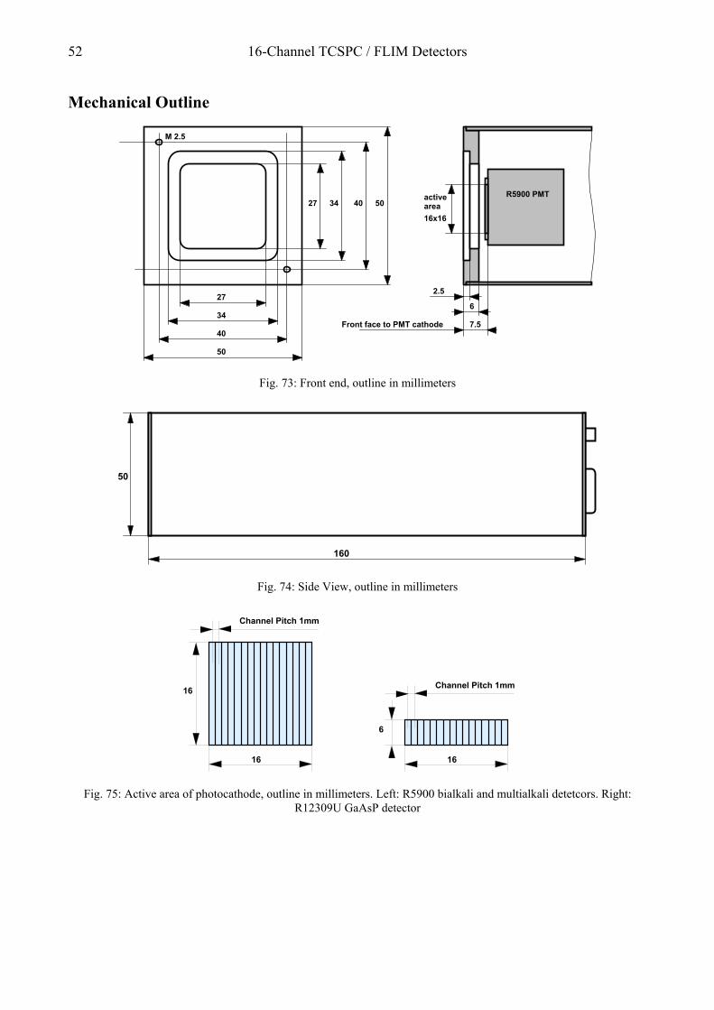
52 16-Channel TCSPC / FLIM Detectors
Mechanical Outline
R5900 PMT
27
34
40
27 34 40 50
50
M 2.5
7.5
6
2.5
Front face to PMT cathode
16x16
activearea
Fig. 73: Front end, outline in millimeters
50
160
Fig. 74: Side View, outline in millimeters
16
16
Channel Pitch 1mm
16
Channel Pitch 1mm
6
Fig. 75: Active area of photocathode, outline in millimeters. Left: R5900 bialkali and multialkali detetcors. Right: R12309U GaAsP detector

16-Channel TCSPC / FLIM Detectors 53
References 1. A. Bassi, J. Swartling, C. D’Andrea, A. Pifferi, A. Torricelli, R. Cubeddu, Time-resolved spectrophotometer for
turbid media based on supercontinuum generation in a photonic crystal fibre, Opt. Lett. 29, 2405-2407 (2004) 2. Becker & Hickl GmbH, DCC-100 detector control module, manual, www.becker-hickl.com 3. Becker & Hickl GmbH, BDL-375, BDL-405, BDL-475 Ultraviolet and Blue Picosecond Diode Laser Modules,
www.becker-hickl.com 4. Becker & Hickl GmbH, Multiphoton Multiwavelength NDD FLIM with Zeiss LSM 710 NLO. Application note,
available on www.becker-hickl.com 5. Becker & Hickl GmbH, Megapixel FLIM with bh TCSPC Modules. The New SPCM 64-bit Software. Application
note, available on www.becker-hickl.com (2014) 6. Becker & Hickl GmbH, IFP-201 Implantable Fibre Probe for in vivo Fluorescence Decay Measurements. Data
sheet, www.becker-hickl.com (2015) 7. Becker & Hickl GmbH, TCSPC Fibre-Probe System with an Exchangeable Tip. Application note (2015), available
on www.becker-hickl.com 8. Becker & Hickl GmbH, DCS-120 Confocal Scanning FLIM Systems. User handbook, 6th edition (2015).
Available on www.becker-hickl.com 9. Becker & Hickl GmbH, Modular FLIM systems for Zeiss LSM 710 / 780 / 800 family laser scanning microscopes.
User handbook, 6th edition (2015). Available on www.becker-hickl.com 10. Becker & Hickl GmbH, The PZ-FLIM-110 Piezo-Scanning FLIM System. Application note (2015), available on
www.becker-hickl.com 11. Becker & Hickl GmbH, PZ-FLIM-110 Piezo-Scanning FLIM System. Data sheet (2015), available on
www.becker-hickl.com 12. W. Becker, Verfahren und Vorrichtung zur Messung von Lichtsignalen mit zeitlicher und räumlicher Auflösung,
Patent DE 43 39 787 (1993) 13. W. Becker, A. Bergmann, Detector assemblies for picosecond microscopy, Becker & Hickl GmbH, www.becker-
hickl.com 14. W. Becker, A. Bergmann, H. Wabnitz, D. Grosenick, A. Liebert, High count rate multichannel TCSPC for optical
tomography, Proc. SPIE 4431, 249-245 (2001) 15. W. Becker, A. Bergmann, C. Biskup, T. Zimmer, N. Klöcker, K. Benndorf, Multi-wavelength TCSPC lifetime
imaging, Proc. SPIE 4620 79-84 (2002) 16. W. Becker, A. Bergmann, M.A. Hink, K. König, K. Benndorf, C. Biskup, Fluorescence lifetime imaging by time-
correlated single photon counting, Micr. Res. Techn. 63, 58-66 (2004) 17. W. Becker, A. Bergmann, G. Biscotti, K. Koenig, I. Riemann, L. Kelbauskas, C. Biskup, High-speed FLIM data
acquisition by time-correlated single photon counting, Proc. SPIE 5323, 27-35 (2004) 18. W. Becker, A. Bergmann, Timing Stability of TCSPC Experiments, Becker & Hickl GmbH (2004), available on
www.becker-hickl.com 19. W. Becker, A. Bergmann, G. Biscotti, A. Rück, Advanced time-correlated single photon counting technique for
spectroscopy and imaging in biomedical systems, Proc. SPIE 5340, 104-112 (2004) 20. W. Becker, A. Bergmann, C. Biskup, D. Schweitzer, M. Hammer, Time- and Wavelength-Resolved
Autofluorescence Detection by Multi-Dimensional TCSPC, Proc. SPIE 5862, 174-181 (2005) 21. W. Becker, Advanced time-correlated single-photon counting techniques. Springer, Berlin, Heidelberg, New York,
2005 22. W. Becker, A. Bergmann, C. Biskup, Multi-Spectral Fluorescence Lifetime Imaging by TCSPC. Micr. Res. Tech.
70, 403-409 (2007) 23. W. Becker, Fluorescence Lifetime Imaging - Techniques and Applications. J. Microsc. 247 (2) (2012) 24. W. Becker, Fluorescence Lifetime Imaging Techniques: Time-correlated single-photon counting. In: L. Marcu.
P.M.W. French, D.S. Elson, (eds.), Fluorecence lifetime spectroscopy and imaging. Principles and applications in biomedical diagnostics. CRC Press, Taylor & Francis Group, Boca Raton, London, New York (2015)
25. W. Becker, The bh TCSPC Handbook, Becker & Hickl GmbH, 6th edition, (2015), available on www.becker-hickl.com
26. W. Becker, Introduction to Multi-Dimensional TCSPC. In W. Becker (ed.) Advanced time-correlated single photon counting applications. Springer, Berlin, Heidelberg, New York (2015)
27. W. Becker, V. Shcheslavskiy, H. Studier, TCSPC FLIM with Different Optical Scanning Techniques, in W. Becker (ed.) Advanced time-correlated single photon counting applications. Springer, Berlin, Heidelberg, New York (2015)
28. A. Bergmann, SPCImage Data Analysis Software for Fluorescence Lifetime Imaging Microscopy, Becker & Hickl GmbH, available on www.becker-hickl.com
29. D.K. Bird, K.W. Eliceiri, C-H. Fan, J.G. White, Simultaneous two-photon spectral and lifetime fluorescence microscopy, Appl. Opt. 43, 5173-5182 (2004)

54 16-Channel TCSPC / FLIM Detectors
30. C. Biskup, L. Kelbauskas, Th. Zimmer, S. Dietrich, K. Benndorf, W. Becker, A. Bergmann, N. Klöcker, Spectrally resolved fluorescence lifetime and FRET measurements, Proc. SPIE 5700, 188-196 (2005)
31. C. Biskup, T. Zimmer, L. Kelbauskas, B. Hoffmann, N. Klöcker, W. Becker, A. Bergmann, K. Benndorf, Multi-Dimensional Fluorescence Lifetime and FRET Measurements. Micr. Res. Tech. 70, 403-409 (2007)
32. C. Biskup, B. Hoffmann, K. Benndorf, A. Rueck, Spectrally resolved lifetime imaging microscopy. In: A. Periasamy, R.M. Clegg, eds., FLIM Microscopy in Biology and Medicine. CRC Press 2009
33. L. M. Bollinger, G. E. Thomas, Measurement of the time tependence of scintillation intensity by a delayed coincidence method. Rev. .Sci. Instrum. 32, 1044-1050 (1961)
34. J. Candelario, M.S Chachisvilis, Mechanical stress stimulates conformational changes in 5-hydroxytryptamine receptor 1B in bone cells. Cellular and Molecular Bioengineering (2012)
35. M. Chachisvilis, Y.-L. Zhang, J. A. Frangos, G protein-coupled receptors sense fluid shear stress in endothelial cells. PNAS 103, 15463-15468 (2006)
36. D. Chorvat, A. Chorvatova, Spectrally resolved time-correlated single photon counting: a novel approach for characterization of endogenous fluorescence in isolated cardiac myocytes. Eur. Biophys. J. 36:73-83 (2006)
37. D. Chorvat, A. Mateasik, J. Kirchnerova, A. Chorvatova, Application of spectral unmixing in multi-wavelength time-resolved spectroscopy. Proc. SPIE 6771, 677105-1 to -12 (2007)
38. D. Chorvat Jr., S. Abdulla, F. Elzwei, A. Mateasik, A. Chrovatova, Screening of cardiomyocyte fluorescence during cell contraction by multi-dimensional TCSPC. Proc. SPIE 6860, 686029-1 to -12 (2008)
39. D. Chorvat, A. Chorvatova, Multi-wavelength fluorescence lifetime spectroscopy: a new approach to the study of endogenous fluorescence in living cells and tissues. Laser Phys. Lett. 6 175-193 (2009)
40. D. Chorvat Jr., A. Mateasik, Y.G Cheng, N.Y Poirier, J. Miro, N.S. Dahdah, A. Chorvatova, Rejection of transplanted hearts in patients evaluated by the component analysis of multi-wavelength NAD(P)H fluorescence lifetime spectroscopy. J. Biophotonics 3 646-652 (2010)
41. A. Chorvatova, F. Elzwiei, A. Mateasik, D. Chorvat, Effect of ouabain on metabolic oxidative state in living cardiomyocytes eavaluated by time-resolved spectroscopy of endogenous NAAD(P)H fluorescence. J. Biomed. Opt. 17(10) 101505-1 to -7 (2012)
42. A. Chorvatova, S. Aneba, A. Mateasik, D. Chorvat Jr., B. Comte, Time-resolved fluorescence spectroscopy investigation of the effect of 4-hydroxynonenal on endogenous NAD(P)H in living cardiac myocytes. J. Biomed. Opt. 18(6), 067009-1 to -11 (2013)
43. A. Chorvatova, A. Mateasik, D. Chorvat Jr, Spectral decomposition of NAD(P)H fluorescence components recorded by multi-wavelength fluorescence lifetime spectroscopy in living cardiac cells. Laser Phys. Lett. 10 125703-1 to -10 (2013)
44. A. Chorvatova, Autofluorescence-assisted examination of cardiovascular system physiology and pathology. In: A. A. Heikal and V. Ghukasyan, eds., Natural Biomarkers for Cellular Metabolism: Biology, Techniques and Applications. CRC Press, Taylor & Francis Group, Boca Raton, London, New York (2015)
45. A. Chorvatova, D. Chorvat, Tissue fluorophores and their spectroscopic characteristics. In: L. Marcu. P.M.W. French, D.S. Elson, (eds.), Fluorecence lifetime spectroscopy and imaging. Principles and applications in biomedical diagnostics. CRC Press, Taylor & Francis Group, Boca Raton, London, New York (2015)
46. A. Marcek Chorvatova, Time-Resolved Spectroscopy of NAD(P)H in Live Cardiac Myocytes. In: W. Becker (ed.) Advanced time-correlated single photon counting applications. Springer, Berlin, Heidelberg, New York (2015)
47. S. Coda, A. J. Thompson, G. T. Kennedy, K. L. Roche, L. Ayaru, D. S. Bansi, G. W. Stamp, A. V. Thillainayagam, P. M. W. French, C. Dunsby, Fluorescence lifetime spectroscopy of tissue autofluorescence in normal and diseased colon measured ex vivo using a fiber-optic probe. Biomed. Opt. Expr. 5, 515-538 (2014)
48. S. Cova, M. Bertolaccini, C. Bussolati, The measurement of luminescence waveforms by single-photon techniques, Phys. Stat. Sol. 18, 11-61 (1973)
49. G. Cui, S.B. Jun, X. Jin, M.D. Pham, S.S. Vogel, D.M. Lovinger, R.M. Costa, Concurrent activation of strial direct and indirect pathways during action initiation. Nature 494, 238-242 (2013)
50. G. Cui, S.B.Jun, X. Jin, G. Luo, M.D. Pham, D.M. Lovinger, S.S. Vogel, R.M. Costa, Deep brain optical measurement of cell type-specific neural activity in behaving mice. Nature Protocols, 9(6) 1213-1228 (2014)
51. C. D’Andrea, L. Spinelli, A. Bassi, A. Giusto, D. Contini, J. Swartling, A. Torricelli, R. Cubeddu, Time-resolved spectrally constrained method for the quantification of chromophore concentrations and scattering parameters in diffusing media. Opt. Expr. 14, 1888-1898 (2006)
52. P. A. A. De Beule, C. Dunsby, N. P. Galletly, G. W. Stamp, A. C. Chu, U. Anand, P. Anand, C. D. Benham A. Naylor, P. M. W. French, A hyperspectral fluorescence lifetime probe for skin cancer diagnosis. Rev. Sci. Instrum. 78, 123101 (2007)
53. W. Denk, J.H. Strickler, W.W.W. Webb, Two-photon laser scanning fluorescence microscopy, Science 248, 73-76 (1990)
54. E. Dimitrow, I. Riemann, A. Ehlers, M. J. Koehler, J. Norgauer, P. Elsner, K. König, M. Kaatz, Spectral fluorescence lifetime detection and selective melanin imaging by multiphoton laser tomography for melanoma diagnosis. Experimental Dermatology 18, 509-515 (2009)

16-Channel TCSPC / FLIM Detectors 55
55. C. Dunsby, P.M.W. French, Single-point probes for lifetime spectroscopy: Time-correlated single-photon counting technique. In: L. Marcu. P.M.W. French, D.S. Elson, (eds.), Fluorecence lifetime spectroscopy and imaging. Principles and applications in biomedical diagnostics. CRC Press, Taylor & Francis Group, Boca Raton, London, New York (2015)
56. A. Gerega, N. Zolek, T. Soltysinski, D. Milej, P. Sawosz, B. Toczylowska, A. Liebert, Wavelength-resolved measurements of fluorescence lifetime of indocyanine green. J. Biomed. Opt. 16(6) 067010-1 to -9 (2011)
57. A. Gerega, D. Milej, W. Weigl, M. Botwicz, N. Zolek, M. Kacprzak, W. Wierzejski, B. Toczylowska, E. Mayzner-Zawadzka, R. Maniewski, A. Liebert, Multiwavelength time-resolved detection of fluorescence during the inflow of indocyanine green into the adult’s brain. J. Biomed. Opt. 17(8), 087001-1 to -9 (2012)
58. M. Göppert-Mayer, Über Elementarakte mit zwei Quantensprüngen, Ann. Phys. 9, 273-294 (1931) 59. A. Giusto, C. D’Andrea, L. Spinelli, D. Contini, A. Torricelli, F. Martelli, G. Zaccanti, R. Cubeddu, Monitoring
Absorption Changes in a Layered Diffusive Medium by White-Light Time-Resolved Reflectance Spectroscopy. IEEE Trans. Instrum. Measur. (2009)
60. Hamamatsu Photonics K.K., R5900U-16 series Multianode photomultiplier tube (2001) 61. S. Khoon Teh, W. Zheng, S. Li, D. Li, Y. Zeng, Y. Yang, J. Y. Qu, Multimodal nonlinear optical microscopy
improves the accuracy of early diagnosis of squamous intraepithelial neoplasia. J. Biomed. Opt. 18(3) 036001-1 to -11 (2013)
62. K. König, Multiphoton microscopy in life sciences, J. Microsc. 200, 83-104 (2000) 63. K. König, Clinical multiphoton tomography. J. Biophoton. 1, 13–23 (2008) 64. K. König, A. Uchugonova, Multiphoton Fluorescence Lifetime Imaging at the Dawn of Clinical Application. In: A.
Periasamy, R.M. Clegg, eds., FLIM Microscopy in Biology and Medicine. CRC Press 2009 65. H. Kume (ed.), Photomultiplier Tube, Hamamatsu Photonics K.K. (1994) 66. J.R. Lakowicz, Principles of Fluorescence Spectroscopy, 2nd edn., Plenum Press, New York (1999) 67. B. Leskovar, C.C. Lo, Photon counting system for subnanosecond fluorescence lifetime measurements, Rev. Sci.
Instrum. 47, 1113-1121 (1976) 68. C. Lewis, W.R. Ware, The Measurement of Short-Lived Fluorescence Decay Using the Single Photon Counting
Method, Rev. Sci. Instrum. 44, 107-114 (1973) 69. D. Li, W. Zheng, J. Y. Qu, Time-resolved spectroscopic imaging reveals the fundamentals of cellular NADH
fluorescence. Opt. Lett. 33, 2365-2367 (2008) 70. D. Li, M.S. Yang, W. Zheng, J.Y. Qu, Study of cadmium-induced cytotoxicity using two-photon excitation
endogenous fluorescence microscopy. J. Biomed. Opt. 14(5), 054028-1 to -8 (2009) 71. D. Li, W. Zheng, J.Y. Qu, Two-photon autofluorescence microscopy of multicolor excitation. Opt. Lett. 34, 202-
204 (2009) 72. D. Li, W. Zheng, J.Y. Qu, Imaging of epithelial tissue in vivo based on excitation of multiple endogenous
nonlinear optical signals. Lett. 34, 2853-2855 (2009) 73. D. Li, W. Zheng, Y. Zeng, and J.Y. Qu, In vivo and simultaneous multimodal imaging: Integrated multiplex
coherent anti-Stokes Raman scattering and two-photon microscopy. Appl. Phys. Lett 97, 223702-1 to -3 (2010) 74. D. Li, W. Zheng, Y. Zeng, Y. Luo, J.Y. Qu, Two-photon excited hemoglobin fluorescence provides contrast
mechanism for label-free imaging of microvasculature in vivo. Opt. Lett. 36, 834-836 (2011) 75. D. Li, W. Zheng, W. Zhang, S. Khoon Teh, Y. Zeng, Y. Luo, J.Y. Qu, Time-resolved detection enables standard
two-photon fluorescence microscopy for in vivo label-free imaging of microvasculature in tissue. Opt. Lett. 36, 2638-2640 (2011)
76. A. Liebert, H. Wabnitz, D. Grosenick, R. Macdonald, Fiber dispersion in time domain measurements compromising the accuracy of determination of optical properties of strongly scattering media, J. Biomed. Opt. 8, 512-516 (2003)
77. A. Liebert, M. Kacprzak, D. Milej, W. Becker, A. Gerega, P. Sawosz, R. Maniewski, Dynamic Mapping of the Human Brain by Time-Resolved NIRS Techniques. In: W. Becker (ed.) Advanced time-correlated single photon counting applications. Springer, Berlin, Heidelberg, New York (2015)
78. H.B. Manning, G.T. Kennedy, D.M. Owen, D.M. Grant, A.I. Magee, M.A.A. Neil, Y. Itoh, C. Dunsby, P.M.W. French, A compact, multidimensional spectrofluorometer exploiting supercontinuum generation. J. Biophoton 1, 494-505 (2008)
79. K. Maxwell, G.N. Johnson, Chlorophyll fluorescence - a practical guide, Journal of Experimental Botany 51, 659-668 (2000)
80. D.V. O’Connor, D. Phillips, Time-correlated single photon counting, Academic Press, London (1984) 81. J. Pawley (ed.), Handbook of biological confocal microscopy, 2nd edn., Plenum Press, New York (1995) 82. Roberts, M. S., Dancik, Y., Prow, T.W., Thorling, C.A., Li, L., Grice, J.E., Robertson, T.A., König, K., Becker,W.
Non-invasive imaging of skin physiology and percutaneous penetration using fluorescence spectral and lifetime imaging with multiphoton and confocal microscopy. European Journal of Pharmaceutics and Biopharmaceutics 77, 469-488 (2011)
83. A. Rück, F. Dolp, C. Hülshoff, C. Hauser, C. Scalfi-Happ, FLIM and SLIM for molecular imaging in PDT, Proc. SPIE 5700, 182-187 (2005)

56 16-Channel TCSPC / FLIM Detectors
84. A. Rück, F. Dolp, C. Hülshoff, C. Hauser, C. Scalfi-Happ, Fluorescence lifetime imaging in PDT. An overview. Medical Laser Application 20, 125-129 (2005)
85. A. Rück, Ch. Hülshoff, I. Kinzler, W. Becker, R. Steiner, SLIM: A New Method for Molecular Imaging. Micr. Res. Tech. 70, 403-409 (2007)
86. A. Rück, C. Hauser, S. Mosch, S. Kalinina, Spectrally resolved fluorescence lifetime imaging to investigate cell metabolism in malignant and nonmalignant oral mucosa cells. J. Biomed. Opt. 19(9), 096005-1 to -9 (2014)
87. W. Y. Sanchez, M. Pastore, I. Haridass, K. König, W. Becker, M. S. Roberts, Fluorescence Lifetime Imaging of the Skin. In: W. Becker (ed.) Advanced time-correlated single photon counting applications. Springer, Berlin, Heidelberg, New York (2015)
88. R. Schuyler, I. Isenberg, A Monophoton Fluorometer with Energy Discrimination, Rev. Sci. Instrum. 42 813-817 (1971)
89. D. Schweitzer, E.R. Gaillard, J. Dillon, R.F. Mullins, S. Russell, B. Hoffmann, S. Peters, M. Hammer, C. Biskup, Time-Resolved Autofluorescence Imaging of Human Donor Retina Tissue from Donors with Significant Extramacular Drusen. IOVS, 53, 3376-3386 (2012)
90. Q. Sun, Y. Li, S. He, C. Situ, Z. Wu, J. Y. Qu, Label-free multimodal nonlinear optical microscopy reveals fundamental insights of skeletal muscle development. Biomed. Opt. Expr. 5, 158-166 (2013)
91. H. Studier, W. Becker, Megapixel FLIM. Proc. SPIE 8948 (2014) 92. A.J. Thompson, S. Coda, M. Brydegaard Sorensen, G. Kennedy, R. Patalay, U.A Waitong-Brämming, P.A.A. De
Beule, M.A.A. Neil, S. Andersson-Engels, N. Bendsoe, P.M.W. French, K. Svanberg, C. Dunsby, In vivo measurements of diffuse reflectance and time-resolved autofluorescence emission spectra of basal cell carcinomas. J. Biophotonics 5, No. 3, 240–254 (2012)
93. Y. Wu, W. Zheng, Y. Qu, Sensing cell metabolism by time-resolved autofluorescence. Opt. Lett. 31 3122-3124 (2006)
94. M.S. Yang, D. Li, T. Lin, J.J. Zheng, W. Zheng, J.Y. Qu, Increase in intracellular free/bound NAD[P]H as a cause of Cd-induced oxidative stress in the HepG2 cells. Toxicology247, 6-10 (2008)
95. J. Yguerabide, Nanosecond fluorescence spectroscopy of macromolecules, Meth. Enzymol. 26, 498-578 (1972) 96. Y.-L. Zhang, J. A. Frangos, M.S Chachisvilis, Mechanical stimulus alters conformation of type 1 parathyroid
hormone receptor in bone cells. Cellular and Molecular Bioengineering Am. J. Physiol. Cell Physiol. 296, C1391-C1399 (2009)
97. Y.-L. Zhang, H. Tavakoli, M. Chachisvilis, Apparent PKA activity responds to intermittent hypoxia in bone cells: A redox pathway? Am. J. Physiol. Heart Circ. Physiol. 299, H225–H235 (2010)
98. W. Zheng, D. Li, Y. Zeng, Y. Luo, J.Y. Qu, Two-photon excited hemoglobin fluorescence. Biomed. Opt. Expr. 2, 71-79 (2011)
99. Y. Zeng, B. Yan, Q. Sun, S. Khoon Teh, W. Zhang, Z. Wen, Jianan Y. Qu, Label-free in vivo imaging of human leukocytes using two-photon excited endogenous fluorescence. J. Biomed. Opt. 18(4), 040103-1 to -3 (2013)

16-Channel TCSPC / FLIM Detectors 57
Index 2D trace parameters 12 3D trace parameters 17 Afterpulsing 27 Applications
cardio-myocytes 38 chlorophyll transients 40 confocal microscopy 42 FAD 48 FRET 39, 48 fundus of the eye 48 haemoglobin 48 ICG boli 40 ICG time-reolved spectra 40 lifetime spectrometers 35 Melanoma 49 Micro-spectrometer 38 multiphoton microscopy 45 Multiphoton tomography of human skin 49 Multi-spectral FLIM 48 NADH 38, 48, 49 NIRS 39 optical tomography 39 protein conformation 39 SHG 49 Supercontinuum laser 49 tryptophane 49
Assistance through bh 50 handbooks 50 setup service 50 software updates 50 troubleshooting 50
Background count rate 25 Afterpulsing 27 dark count rate 25 effect on TCSPC results 26
Bialkali photocathode 22 Blaze wavelength 31 Cable connections 29 CFD
parameters 9 principle 9 threshold 9 zero cross 9
Change Modes 20 Channel delay correction 11 Channel Uniformity
Efficiency 23 IRF 25
Chlorophyll transients 40 Classic TCSPC 5 Connector
of DCC-100 29 of PML-16C 51
Dark count rate 25 different photocathodes 26 effect on TCSPC results 26
DCC-100 10, 29 Enable outputs 10 Overload shutdown 11
shutter control 10 software panel 10 Supply voltages for detectors 10
DCS-120 15, 17, 42 application options 19 scan control panel 15, 19
Detector dark count rate 25 gain 10 photocathode 22 quantum efficiency 22 spectral sensitivity 22
Detector control, see DCC-100 10 Display parameters
f(xyt) mode 14 FIFO imaging mode 17 oscilloscope mode 13 single mode 13
f(xyt) mode 13 FAD 48 FIFO imaging mode 15 FLIM 33
applications 48 confocal 42 image size 7 multiphoton 45 multi-wavelength 7 principle 7
f-number 31 FRET 39, 48 Front face of PML-16 detectors 30 GaAsP photocathode 22 Gain control, for detector 29 Grating 31 Haemoglobin 48 High voltage 28, 29 Image size, for multi-wavelength FLIM 7 IRF
channel uniformity 25 effect of discriminator 25 effect of photocathode 24 PML-C 24 PML-GaAsP 24
Laser scanning microscope Confocal detection 42 multiphoton 45
Lifetime spectrometers cuvettes 35 micro spectrometers, multi-wavelength 38 tissue, multi-wavelength 35
Melanoma 49 Multialkali photocathode 22 Multi-dimensional TCSPC 5 Multiphoton microscope 45 Multiphoton tomography of human skin 49 Multi-wavelength FLIM
3D trace parameters 17 mosaic FLIM function 18 system parameters 16

58 16-Channel TCSPC / FLIM Detectors
window parameters 17 MW-FLIM
fibre bundle 46 multiphoton microscope 45
MW-FLIM detector 33 fibre bundle 33 optical tomography systems 40 principle 33
NADH 38, 47, 48, 49 Non-descanned detection 45 Oscilloscope mode 12 Outline of PML-16 detectors 52 Overload shutdown 11 Photocathode
bialkali 22 channel uniformity, efficiency 23 channel uniformity, IRF 25 dark counts 25 GaAsP 22 GaAsP versus multialkali 22 multialkali 22 of PML-16, outline 52 quantum efficiency 22 spectral sensitivity 22
Pin assignment, PML-16C 51 PML-16 detectors
afterpulsing 27 applications 35 cable connections 29 channel uniformity of efficiency 23 channel uniformity of IRF 25 dark count rate 25 front face 30 implementation in TCSPC systems 29 IRF 24 mechanical outline 52 pin assignment 51 PML-SPEC assembly 30 quantum efficiency 22 safety 28 specification 51 status LEDs 28
PML-SPEC 30 Blaze wavelength 31 chlorophyll transients 40 confocal microscope 42 Fibre coupling 32 f-number 31 free-beam coupling 31 Gratings 31 implantable fibre probe 37 lifetime spectrometer 35 micro spectrometer 38 NIRS 39 optical principle 30 optical tomography systems 39 polychromator 30 pulse dispersion in fibres 32 slit width 32 tissue lifetime spectrometer 35
Polychromator 30
Predefined setups creating predefined setups 20 switching between instrument configurations 20
Quantum efficiency of photocathode 22 Routing 6, 8 Routing parameters 8 Routing signals 29 Safety 28 Setup service 50 SHG 49 Simple-Tau 3 Single mode of SPC system 12 Software updates 50 SPC modules 3, 8, 29 SPC-130, use with PML detectors 29 SPCM main panel configuration
f(xyt) mode 13 FIFO imaging mode 15 mosaic FLIM function 18 oscilloscope mode 12 single mode 12
SPCM software 8 3D trace parameters 17 application options 19 main panel configuration 12, 13, 15, 18 predefined setups 20 window parameters 17
Specification of PML-16 detectors 51 Spectral sensitivity of photocathode 22 Status LEDs of PML-16 detectors 28 Switch modes command 20 TCSPC
classic 5 multi-channel 5 multi-dimensional 5 multi-wavelength 6, 35 multi-wavelength FLIM 7 photon distribution 5
TCSPC system parameters 8 application options 19 autosave function 15 CFD 9 channel delay correction 11, 19 cycle function 15 detector gain 10 display parameters 13, 14, 17 f(xyt) mode 13, 14 FIFO imaging mode 15, 16 latch delay 8 measurement pages 8 mosaic FLIM function 18 operation mode 12 oscilloscope mode 12, 13 page control 8 predefined setups 20 repeat function 15 routing channels 8 single mode 12, 13 trace parameters 2D 12
Tryptophane 49 Window parameters 17

16-Channel TCSPC / FLIM Detectors 59
Zeiss LSM 510 47 Zeiss LSM 710 42, 46
Zeiss LSM 880 42