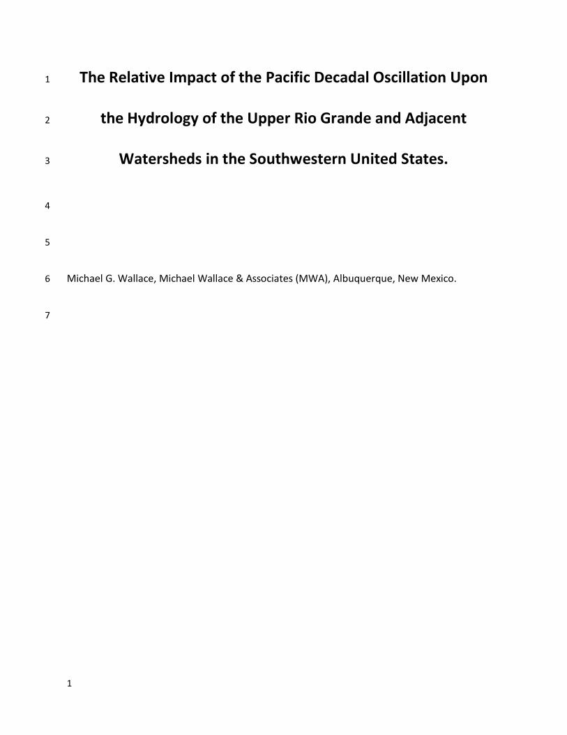
1

The Relative Impact of the Pacific Decadal Oscillation Upon 1

the Hydrology of the Upper Rio Grande and Adjacent 2

Watersheds in the Southwestern United States. 3

4

5

Michael G. Wallace, Michael Wallace & Associates (MWA), Albuquerque, New Mexico. 6

7

2

8

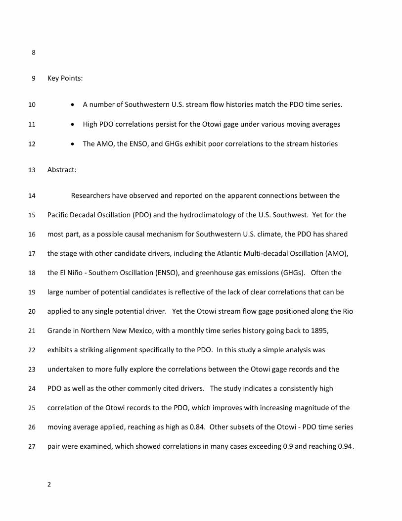
Key Points: 9

A number of Southwestern U.S. stream flow histories match the PDO time series. 10

High PDO correlations persist for the Otowi gage under various moving averages 11

The AMO, the ENSO, and GHGs exhibit poor correlations to the stream histories 12

Abstract: 13

Researchers have observed and reported on the apparent connections between the 14

Pacific Decadal Oscillation (PDO) and the hydroclimatology of the U.S. Southwest. Yet for the 15

most part, as a possible causal mechanism for Southwestern U.S. climate, the PDO has shared 16

the stage with other candidate drivers, including the Atlantic Multi-decadal Oscillation (AMO), 17

the El Niño - Southern Oscillation (ENSO), and greenhouse gas emissions (GHGs). Often the 18

large number of potential candidates is reflective of the lack of clear correlations that can be 19

applied to any single potential driver. Yet the Otowi stream flow gage positioned along the Rio 20

Grande in Northern New Mexico, with a monthly time series history going back to 1895, 21

exhibits a striking alignment specifically to the PDO. In this study a simple analysis was 22

undertaken to more fully explore the correlations between the Otowi gage records and the 23

PDO as well as the other commonly cited drivers. The study indicates a consistently high 24

correlation of the Otowi records to the PDO, which improves with increasing magnitude of the 25

moving average applied, reaching as high as 0.84. Other subsets of the Otowi - PDO time series 26

pair were examined, which showed correlations in many cases exceeding 0.9 and reaching 0.94. 27

3

The study also confirmed the consistent lack of correlation between the Otowi gage and the 28

other candidate drivers. 29

Introduction 30

Whether simulation or stochastic methodologies are used in climate forecasting, a 31

comprehensive evaluation of the actual time series data is a critical component to both. This 32

evaluation is challenged by the unbounded nature of the climatic data, necessitating at some 33

point, somewhat arbitrary designations and/or cut offs in both temporal and spatial data. For 34

example, the use of a 30 year climatology, also known as a 30 year climate normal, has been 35

recognized as an arbitrary designation, ever since it was first adopted by nation members of the 36

International Meteorological Organization (IMO) for the initial period of 1901 - 1930. Moreover 37

the value of a climate normal for causal identification and predictive purposes is acknowledged 38

to be low, if only due to perceived non-stationary behavior (Arguez and Vose, 2011). In 39

extending the scope of desired prediction from climatologic to hydroclimatologic causality, the 40

challenges are compounded. In that scale-dependent context, causality must account for both 41

stationary and non-stationary factors, and some of those can often clearly be attributed to 42

human influences, including reservoirs, irrigation activities, levee developments, urban 43

pavement expansion, and numerous other factors. 44

Hydroclimatologists recognize as well as other climatologists that secular trends in a 45

time series may either indicate non-stationarity, or the trend may be a component of a larger 46

scale cycle that is longer than the time series being evaluated. Accordingly, the concept of 47

cyclostationarity can often be employed successfully for time-series evaluations (if not 48

4

predictive purposes) via spectral analysis, when and where such cycles can be appropriately 49

identified (Wei, 2006, also Weedon, 2003). 50

Outside of obvious diurnal and seasonal oscillations, such cycles have long been sought 51

in modern climatic patterns. The most notable candidates are associated with oceanic 52

influences and include the El Niño - Southern Oscillation (ENSO), the Atlantic Multi-decadal 53

Oscillation (AMO) and the Pacific Decadal Oscillation (PDO). Of these oscillations, the PDO not 54

only has an interesting correspondence to the 30 year climate normal, but it also exhibits at the 55

very least, a recognized partial causality with regard to Southwestern U.S. climate as well as 56

other parts of the world, including roughly half of the northern hemisphere as well as locations 57

along every continent in the Southern Hemisphere (Mantua, 2002, also Okumura, 2012). 58

Naturally any improvements to current techniques in climate prediction would be of 59

extreme value at any region of the populated globe. Moreover, the Southwestern U.S., by 60

virtue of its typically arid regime in conjunction with a growing population, is a region that has 61

an acute need for improved climate prediction techniques. Yet any such climate predictive 62

product would require extensive validation prior to its use. Validation exercises of interest 63

include one of the simplest stochastic tools of all, namely correlation coefficients (ρ), and 64

associated lag correlations. 65

This investigation constitutes such an initial first order validation study applied to 66

several candidate oceanic and other drivers as they might relate to a key region within the 67

Southwestern United States, namely the Upper Rio Grande Watershed (URGW). 68

The Upper Rio Grande Watershed 69

5

The headwaters of the Upper Rio Grande Watershed (URGW) (Figure 1) originate at an 70

approximate elevation of 4300 masl (14107 ft) along the Continental Divide within the San Juan 71

Mountains of southwestern Colorado (U.S.). The 'pour point' of this watershed is defined at an 72

elevation of approximately 1670 masl (5479 ft) at the Otowi gage along the main stem of the 73

Rio Grande in north central New Mexico . The sparsely populated watershed covers 74

approximately 37040 km2 (14301 mi2). Approximately half of the watershed is steep 75

mountainous terrain, and roughly half of the remaining lowlands, over 86,000 hectares (212500 76

acres), are devoted to irrigation-based agriculture. Significant portions of the watershed have 77

been under cultivation for over a century (Scurlock, 1998). 78

Following a pattern typical of the surrounding Southern Rocky Mountains and the 79

adjacent Basin and Range environments, the upper elevations are dominated by conifer forests 80

while the lower terrain consists of mixed grasslands, sagebrush and riparian vegetative covers, 81

in addition to the cultivated portions. Significant portions of the watershed are composed of 82

exposed bare rock and sediments, in association with the steep terrain and primary geologic 83

features. That geologic framework covers a diverse range of components; from an extension 84

of the Rio Grande Rift Zone trending from south to north, to the Rocky Mountain orogenic 85

network on either side of the rift zone. Precambrian rocks form the basement of the 86

groundwater regime. Those are overlain in large sections by sequences of Mesozoic and 87

Cenozoic sediments and those are intermingled with Tertiary igneous intrusions including dikes, 88

sills, and ash layers from volcanic activities. This portion of the rift zone is structurally 89

characterized by horst and graben features and accordingly contains numerous long and deep 90

faults trending south to north. (Falk et al., 2013 also Bexfield and Anderholm, 2010) 91

6

The large sediment filled structural depression roughly covering the northern half of the 92

watershed includes a topographically closed basin with an evaporite sump feature near the 93

Great Sand Dunes National Park. That area has been termed the Closed Basin, and the closure 94

only extends to local drainage at the surface. Underlying groundwater resources are significant 95

within that region and it is believed that for the most part, the boundaries of the groundwater 96

basin correspond laterally to the boundaries of the watershed. Regardless of the surface 97

drainage closure at the Closed Basin, there are no physical obstructions to groundwater flow 98

motion from the upper portions of the watershed to the lower southern portions. (Bexfield and 99

Anderholm, 2010, and Simonds, 1994). Within New Mexico, the Rio Grande Rift structure 100

continues as well as the mountainous boundaries defining the western and eastern sides, but 101

the alluvial sediment filled basin is significantly narrowed and in many places disrupted by fault 102

related plateaus. 103

Numerous stream flow gages are located throughout the Upper Rio Grande, its 104

tributaries and adjacent watersheds, including the Otowi gage in north central New Mexico 105

(USGS 2014a). Other gages outside of this watershed have been examined in association with 106

this study, including the Navajo River at Banded Peak Ranch, gage in Southern Colorado (simply 107

termed 'Navajo gage' in the remainder of this text) 144 km (89.5 mi) to the northwest of Otowi 108

(Falk et al., 2013), and the Gila river gage, 381 km (236.7 mi) to the southwest (USGS 2014b), of 109

the Otowi gage as depicted in Figure 1. 110

The Otowi gage has been monitored since 1895 by the U.S. Geological Survey, making 111

this point one of the oldest continuous sources of stream flow data in North America (USGS 112

7

2014a) . Moreover this site is closely monitored with regard to an interstate and international 113

water rights compact involving the states of Colorado, New Mexico, and Texas, as well as the 114

Republic of Mexico (Rio Grande Compact, 1939). Figure 2 is a representation of the recorded 115

stream flows at that gage using three different (centered) moving averages; a 12 month, a 10 116

year, and a 20 year average respectively. 117

The Otowi gage measures both natural flows and captures the impacts of several 118

reservoir operations upstream in addition to a river augmentation project known as the Closed 119

Basin Project (Simonds, 1994) and a trans basin diversion program known as the San Juan 120

Chama Project (U.S. Bureau of Reclamation, 2014), both administered by the U.S. Bureau of 121

Reclamation. The average stream flow rate past the gage is approximately 42.5 cubic meters 122

per second (cms) (1,500 cubic feet per second, cfs) , such that the total volume of water 123

transmitted per year is roughly 1.23 km3 (1 million acre feet). Stream flows have a seasonal 124

component, overlain by related water use for irrigation, with a major peak typically occurring in 125

late Spring and a major low typically occurring in Winter. In this investigation, seasonal and 126

diurnal components have been filtered out through the use of moving averages. 127

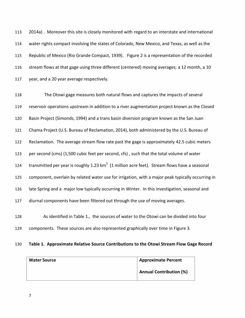
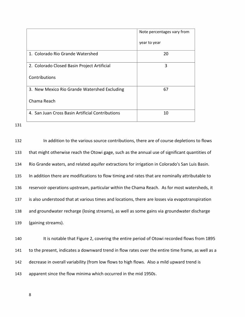
As identified in Table 1., the sources of water to the Otowi can be divided into four 128

components. These sources are also represented graphically over time in Figure 3. 129

Table 1. Approximate Relative Source Contributions to the Otowi Stream Flow Gage Record 130

Water Source Approximate Percent

Annual Contribution (%)

8

Note percentages vary from

year to year

1. Colorado Rio Grande Watershed 20

2. Colorado Closed Basin Project Artificial

Contributions

3

3. New Mexico Rio Grande Watershed Excluding

Chama Reach

67

4. San Juan Cross Basin Artificial Contributions 10

131

In addition to the various source contributions, there are of course depletions to flows 132

that might otherwise reach the Otowi gage, such as the annual use of significant quantities of 133

Rio Grande waters, and related aquifer extractions for irrigation in Colorado's San Luis Basin. 134

In addition there are modifications to flow timing and rates that are nominally attributable to 135

reservoir operations upstream, particular within the Chama Reach. As for most watersheds, it 136

is also understood that at various times and locations, there are losses via evapotranspiration 137

and groundwater recharge (losing streams), as well as some gains via groundwater discharge 138

(gaining streams). 139

It is notable that Figure 2, covering the entire period of Otowi recorded flows from 1895 140

to the present, indicates a downward trend in flow rates over the entire time frame, as well as a 141

decrease in overall variability (from low flows to high flows. Also a mild upward trend is 142

apparent since the flow minima which occurred in the mid 1950s. 143

9

Apart from natural variability and/or the fact that several years of data are missing from 144

the early half of the series, the long term downward trend at Otowi might be explained by the 145

history of continual growth in irrigated acreage of the San Luis Valley in the upstream Colorado 146

segment of the watershed study area over the first half of the time series. Irrigation was 147

already widespread via purely surface water diversions in the valley at the beginning of gage 148

recording just prior to 1900. Yet by the time of the Rio Grande Interstate Compact agreement 149

in 1940, irrigation consumption of water via both surface water diversion and groundwater 150

pumping in the San Luis Valley rose to three quarters of a cubic kilometer (600,000 acre ft) per 151

year. Irrigation has held constant in that area since that time, in line with requirements 152

associated with the Compact. The decrease in stream flow variability (as compared to stream 153

flow rate) over the total time frame may be partially explained by a history of upstream 154

reservoir developments along with the other features cited. 155

Although anthropogenic explanations can be proposed for features of an early trend 156

and a contraction in variability, they do not explain the overall major pattern of peak - trough - 157

peak most strongly represented in the 10 and 20 year moving average curves in Figure 2. 158

Moreover, notable secondary patterns are also apparent in other regionally proximal 159

stream gages which are not impacted by irrigation or reservoirs, as represented in Figure 4. 160

That figure includes the Otowi gage as well as the Gila River gage and the Navajo gage time 161

series. Both additional gages are in separate basins and are closer to their respective 162

headwaters. 163

10

For this initial study, given this first order confirmation, and its regional importance to 164

water planning within and interstate compact framework, the Otowi gage is utilized in this 165

paper as the signature time series for evaluation of the candidate climate drivers featured in 166

this report. 167

Candidate Climate Drivers for Stream Flows of the URGW 168

As defined initially by Zhang et al (1997), and extended and summarized by Mantua 169

(2002), the PDO index has been derived through principal component (PC) analyses using 170

empirical orthogonal functions (EOFs) of sea surface temperature patterns associated with the 171

Pacific Ocean north of 20o latitude. Mantua's (2002) summary provides several examples of 172

positive PDO correlations with regional climates at locations ranging from Africa to North 173

America. 174

According to Mantua, a high PDO index is expressed by a persistent cold phase in the 175

north central Pacific Ocean surface and a related warm phase along the margins of the eastern 176

Pacific in the northern hemisphere. This is accompanied by a persistent low sea level pressure 177

at the north central Pacific Ocean. The oscillation between a high PDO index and a low PDO 178

index appears to roughly correspond to a 25 to 30 year periodicity (Lewis and Hathaway, 2001). 179

Given that transition period, a total cyclic period of the PDO is considered to range from 50 to 180

60 years, at least for the few periods measured over the past 100+ years. 181

Mantua summarized the wide ranging correlations of the PDO time series with 182

hydroclimatologic teleconnections that reach around the world. These include precipitation 183

anomalies within the coastal Gulf of Alaska, and the Southwestern United States (SWUS). 184

11

Mantua also cited supporting dendrochronology research by numerous authors, which to a 185

greater or lesser degree, correlate to the PDO over the modern period for which the PDO can 186

be directly estimated (approximately since 1900). By this correlation, researchers such as 187

Biondi (2001) have produced proxy based PDO histories which extend back in time to the 17th 188

Century. 189

Subsequent researchers (Lewis and Hathaway, 2001, 2002) have pointed to such work 190

to propose (but not quantify) a correlation between the PDO (in conjunction with ENSO and 191

GHG patterns) and drought patterns in northern New Mexico, including the stream flows at 192

Otowi gage and other points within and west of the URGW. 193

In spite of the widely observed relations of the PDO to distal climates, researchers have 194

typically been careful to frame PDO influences within a broader background of uncertainty and 195

variability. They have done so in part because the PDO phenomenology remains largely 196

unexplained. Yet as Mantua relates "Even in the absence of a theoretical understanding, PDO 197

climate information improves season-to-season and year-to-year climate forecasts for North 198

America because of its strong tendency for multi-season and multi-year persistence" 199

As already suggested, the PDO typically shares significant attention from researchers 200

with at least three other candidates in relation to causality of SWUS climate; the Atlantic Multi-201

decadal Oscillation (AMO), the El Niño - Southern Oscillation (ENSO), and global changes in 202

atmospheric greenhouse gas concentrations (GHGs). Recent work by Chylek et al. represents 203

an example of that approach (Chylek et al., 2013, 2014). Those papers document the 204

application of multiple linear regression analysis to those factors, as well as to solar forcing and 205

12

dust effects, in order to develop empirical relations which might be useful to forecast future 206

climate over the next several decades. The papers posit the AMO in particular, and also GHGs 207

as important co-drivers of global climate at least with regard to mean near-surface air 208

temperature. Notably the 2013 devotes attention to the climate of the US Southwest and 209

places a somewhat higher focus upon the PDO. 210

The AMO is an index based on sea surface temperature (SST) anomalies across the 211

northern hemisphere portion of the Atlantic Ocean. It has an apparent periodicity of 65 to 80 212

years (Schlesinger and Ramankutty, 1994). Its impact on North American climate has been 213

investigated by numerous researchers, since the pattern was first identified in the 1990s 214

(Schlesinger and Ramkutty, 1994, McCabe et al., 2004), and formally defined in 2000 (Kerr). The 215

work of Enfield et al. (2001) includes a consideration of the correlations between the AMO and 216

stream flow histories associated with the Mississippi and Okeechobee rivers in the US. That 217

analysis indicated in some cases a correlation that slightly exceeded 0.5. The AMO is believed 218

by some researchers to be the primary driver of drought in the conterminous US. Those 219

authors also contend that the PDO sign merely modulates that primary AMO impact feature 220

(McCabe, 2004). 221

The ENSO and its potential impacts on SWUS climate have also been investigated in 222

great detail, including the research by Hidalgo and Dracup (2003), and as already described, 223

Lewis and Hathaway (2001, 2002). The Lewis and Hathaway team asserted that "ENSO drives 224

weather patterns for nearly three quarters of the globe and is one of the most powerful 225

influences on world climate, second only to the changes in weather brought by the seasons". 226

However those authors did not develop correlations of the ENSO to the climate of the SWUS. 227

13

Correlations of the ENSO to SWUS climate were explored in some detail by Hidalgo and Dracup, 228

who compiled selected seasonal precipitation and stream flow data from a relatively large 229

number of stations within the Upper Colorado River Basin (UCRB). From that data set, they 230

developed synoptic correlation maps to the various types of El Niño series identified in the 231

literature. They determined that the correlations were for the most part, greatest for summer 232

and fall and weakest for winter and spring periods. 233

These investigators also explored possible relationships between the robustness of the 234

ENSO - UCRB correlations and the timing of PDO peaks, based on past work by Gershunov and 235

Barnett (1998). It is notable that these studies cover an area immediately adjacent to the 236

Upper Rio Grande Basin, including the southern Rocky Mountain chain which contains some of 237

the headwaters for both the Rio Grande and the Colorado river. Yet, although the authors 238

explored a relationship between the PDO and the ENSO series, and also a relationship between 239

the ENSO series and the UCRB, they did not explore a correlation relationship between the PDO 240

and the UCRB series. 241

The potential impact of GHGs upon climate of the SWUS has also been investigated over 242

many decades. In an early example (Revelle and Waggoner, 1983), researchers employed an 243

empirical relationship (Langbein 1949) between runoff, temperature, and precipitation for arid 244

climates, to suggest that rising global levels of GHGs (presumably leading to increased 245

temperatures) would lead to increased drought in the SWUS. It should be noted that although 246

this paper asserted a strong correlation, no actual correlation statistics were provided. Also that 247

paper had been authored before the enhanced identification of the ocean patterns of PDO, 248

ENSO, and AMO. Subsequently the Lewis and Hathaway studies suggested an opposite relation 249

14

in which a warming SWUS climate, in conjunction with the PDO and the ENSO would lead to 250

more moist conditions. 251

More recent reports have fallen back upon conclusions similar to the assertions made 252

by Revelle and Waggoner. For example the Upper Rio Grande Impact Assessment (Llewellyn et 253

al., 2013) nominally describes ocean drivers, but does not evaluate their potential impacts to 254

the study area. Moreover the report largely disregards approximately 60 years of Otowi gage 255

and related records and concludes that rising GHGs are the primary driver of contemporary 256

amplified drought in the upper Rio Grande watershed. Many additional examples of a narrative 257

in which GHGs first raise temperatures and those temperature increases lead directly to 258

amplifications of drought occurrence and severity in the Southwestern U.S. can be found in the 259

peer reviewed literature including Nohara et al.( 2006), Cook et al. (2010), and Willliams et al. 260

(2014, in press). These conclusions are also featured in UN IPCC publications (Stocker et al., 261

2013), and in popular news media (Chuck, 2014). 262

Although nominal diurnal and seasonal cycles can be seen, it is clear from the 263

instrumental record of the Mauna Loa series that lower frequency oscillatory behavior of CO2 264

emissions over time frames of years is not evident. Rather, the average global atmospheric 265

concentration of CO2 rises essentially monotonically. This puts the CO2 causality question in a 266

somewhat different frame than the other candidate drivers, which all express clear oscillatory 267

behavior over multi-year time scales. 268

As this section documents, a variety of drivers for climate in the URGW have been 269

proposed within peer reviewed publications. Most if not all research to date attributes URGW 270

15

climate to a combination of several drivers. Most relevant reports assign a primary causality of 271

contemporary SWUS and/or URGW drought patterns to GHG-induced global warming. Those 272

sources in some cases indicate that the patterns are modulated to some extent by various 273

candidate ocean oscillations. However, in most cases, correlation metrics are notably lacking. 274

Comparisons between Otowi Flows and Candidate Climatic Drivers 275

In this investigation, the Otowi gage represents the signature hydroclimatologic index 276

for the URGW. Accordingly, the candidate causality components are each independently 277

compared to the time series of the Otowi gage under a low pass filter prior to the development 278

of correlation coefficient evaluations. For each comparison, it was desired to capture the 279

longest available continuous records reaching to the current time. Naturally the correlation 280

development is focused on comparisons of two independently derived time series which at a 281

zero lag, cover the same time spans in those series. 282

For ease of visual comparison, the various time series have been broken out into several 283

individual charts. Figure 5 is a time series comparison of the Otowi gage and the PDO under a 284

four year trailing average. Figure 6 provides a comparison for the Otowi gage versus the AMO, 285

and Figure 7 covers a pattern for the Otowi gage versus ENSO. Although each ocean oscillatory 286

pattern has been characterized in the original literature according to a favored lowest 287

frequency, the actual time series data for each, as well as for the Otowi gage, are available in 288

raw form as monthly values. Figure 8 closes the candidate set by comparing the Otowi gage 289

series and the PDO index to the measured atmospheric CO2 values recorded at Mauna Loa 290

Station in Hawaii. 291

16

Visual examination of each figure is suggestive that the PDO pattern most consistently 292

aligns with the Otowi stream gage history by any reasonable measure. Moreover the PDO 293

pattern typically anticipates or is synchronous with the Otowi gage pattern. It appears that the 294

same case could be made for the PDO versus the Gila and the Navajo gages as well, and that is 295

suggestive of a broad PDO influence beyond the neighborhood of the Otowi gage. 296

However, these two observations of alignment and precedence cannot be asserted for 297

any of the other causal candidates. For example, in Figure 6, the late 1940s downward trend of 298

the Otowi gage anticipates a downward trend in the AMO by approximately 2 decades, yet the 299

beginning of an upward trend in the AMO anticipates the Otowi upward trend by several years. 300

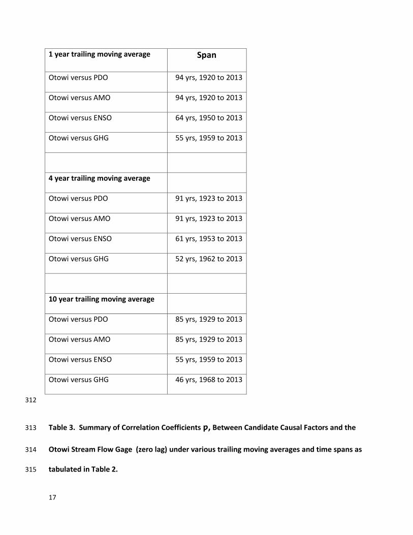
In order to develop a more systematic and quantitative assessment, correlation metrics 301

were obtained from these time series sets and are summarized in Tables 2 and 3, as well as 302

Figure 9. To facilitate development of these correlation metrics in a consistent fashion, the 303

longest time series in each specific comparison case was truncated to match the shortest time 304

series. Moreover, because of a series of missing years in the Otowi gage record prior to 1919, 305

the 1919 date was the earliest Otowi year selected as the starting point. Also the Mauna Loa 306

series and the ENSO series have later starting dates than the other parameters, as detailed in 307

the tables. Moreover the actual starting dates in the correlations vary further, because of the 308

use of trailing averages. Accordingly, for example, because of the employment of a 4 year 309

moving average, the starting date for a CO2 related comparison is 1962. 310

Table 2. Summary of Settings for the Otowi Correlation Coefficient Analyses 311

17

1 year trailing moving average Span

Otowi versus PDO 94 yrs, 1920 to 2013

Otowi versus AMO 94 yrs, 1920 to 2013

Otowi versus ENSO 64 yrs, 1950 to 2013

Otowi versus GHG 55 yrs, 1959 to 2013

4 year trailing moving average

Otowi versus PDO 91 yrs, 1923 to 2013

Otowi versus AMO 91 yrs, 1923 to 2013

Otowi versus ENSO 61 yrs, 1953 to 2013

Otowi versus GHG 52 yrs, 1962 to 2013

10 year trailing moving average

Otowi versus PDO 85 yrs, 1929 to 2013

Otowi versus AMO 85 yrs, 1929 to 2013

Otowi versus ENSO 55 yrs, 1959 to 2013

Otowi versus GHG 46 yrs, 1968 to 2013

312

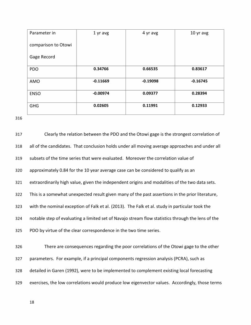
Table 3. Summary of Correlation Coefficients ƿ, Between Candidate Causal Factors and the 313

Otowi Stream Flow Gage (zero lag) under various trailing moving averages and time spans as 314

tabulated in Table 2. 315

18

Parameter in

comparison to Otowi

Gage Record

1 yr avg 4 yr avg 10 yr avg

PDO 0.34766 0.66535 0.83617

AMO -0.11669 -0.19098 -0.16745

ENSO -0.00974 0.09377 0.28394

GHG 0.02605 0.11991 0.12933

316

Clearly the relation between the PDO and the Otowi gage is the strongest correlation of 317

all of the candidates. That conclusion holds under all moving average approaches and under all 318

subsets of the time series that were evaluated. Moreover the correlation value of 319

approximately 0.84 for the 10 year average case can be considered to qualify as an 320

extraordinarily high value, given the independent origins and modalities of the two data sets. 321

This is a somewhat unexpected result given many of the past assertions in the prior literature, 322

with the nominal exception of Falk et al. (2013). The Falk et al. study in particular took the 323

notable step of evaluating a limited set of Navajo stream flow statistics through the lens of the 324

PDO by virtue of the clear correspondence in the two time series. 325

There are consequences regarding the poor correlations of the Otowi gage to the other 326

parameters. For example, if a principal components regression analysis (PCRA), such as 327

detailed in Garen (1992), were to be implemented to complement existing local forecasting 328

exercises, the low correlations would produce low eigenvector values. Accordingly, those terms 329

19

would logically drop out of such a regression based forecasting equation. However, this paper 330

is primarily focused on understanding the relative degree of correlations between the 331

candidates, and therefore follow up work to develop such a forecasting tool is outside of the 332

scope of this paper. 333

Within the scope of this study, the correlation between the PDO and the Otowi gage 334

invites additional attention with regard to a possible lag correlation. To produce lag outputs, 335

one series must be shifted with respect to the other. In the case of the 10 year moving average 336

series for PDO versus Otowi gage, this lag series was approached in a simple step wise process. 337

First, the Otowi time series was anchored to the late terminus at year 2013, while the PDO 338

series was allowed to shift temporally backward in one - year increments until a maximum 339

correlation was identified. This necessitated reducing the total time span of each series by 4 340

years (from 85 years length to 81 years length) to fit within the total span utilized for this 341

moving average value. Figure 10 is a representation of the time series which encompasses the 342

possible cases. Second, correlation coefficients are calculated for lag cases from zero to three 343

years. Figure 11 is a chart of those results which shows not only a new high correlation for the 344

zero lag case but also indicates the highest correlation so far in this analysis, exceeding 0.88, at 345

a lag of one year. 346

A lag of one year nominally offers the potential for improved predictive value. However, 347

such a lag may be simply due to storage effects within the watershed, both natural (snow 348

accumulation, and plant and soil storage effects) and artificial (reservoir effects). For example, 349

depleted reservoirs along the Chama tributary can contain more than enough capacity in their 350

20

own right to receive over 1 million acre feet, which is roughly the annual flow volume past the 351

Otowi gage over the course of one year. On the other hand, when reservoirs are full, then the 352

artificial storage capacity has a relatively insignificant impact on the flow response. Overall, in 353

this context, a lag of one year to zero years would be consistent with the time series 354

observations but does not add significant predictive value without more detailed evaluations of 355

reservoir and other time series histories. 356

As stated, the truncation of the 10 year trailing average time series case at a zero lag led 357

to a further improved correlation coefficient for the Otowi gage versus the PDO, from 0.84 to 358

0.88. This invites additional exploration of potentially even larger correlations under selected 359

subsets of the time series. A limited manual approach was undertaken to simply see if any such 360

subsets might exist. It was found quickly that many such subsets likely can be found. Figure 12 361

shows an example in which (for a zero lag condition), spans centered around the year 1971 362

(roughly the midpoint of the time series shown in Figure 10) were successively narrowed until 363

an optimal correlation of 0.94 was reached at a total span of 53 years. Notably, the cycle 364

length already estimated in the literature for the PDO and discussed earlier in this report is 365

approximately equivalent to that value. 366

More systematic approaches might lead to the discovery of even higher correlations. 367

However, the further removed in time such span-based correlations are found, the less 368

potentially relevant they are to the current time frame of greatest concern. In any event 369

correlations greater than 0.5 are customarily considered to merit attention, while those less 370

than 0.5 are typically considered to be diagnostic of an uncorrelated pattern. 371

21

Summary and Discussion 372

A literature review, along with simple time series analyses and correlation techniques 373

were applied to evaluate causality of ocean oscillatory and GHG influences upon climate in the 374

Upper Rio Grande Watershed of the Southwestern United States. The analysis adopted the 375

Otowi gage time series record as the performance metric. Through a set of correlation 376

evaluations based on a 1 year, 4 year, and a 10 year moving average, the PDO expressed 377

exceptionally high correlation coefficients, reaching as high as 0.94, while the correlations for 378

the remaining candidates were for all cases significantly below 0.5. 379

ACKNOWLEDGEMENTS 380

All reviewers will be acknowledged in the final product. 381

I also wish to acknowledge my advisor at University of New Mexico, Dr. Harjit Ahluwalia for 382

perspective and guidance on this project. 383

Also in accordance with AGU specifications, the data and calculations are also included in this 384

initial submission as a zip file, MGW_WRR_datafiles.zip. 385

REFERENCES 386

Arguez, A. and R. S. Vose, 2011, The Definition of the Standard WMO Climate Normal - The key 387

to Deriving Alternate Climate Normals American Meteorological Society. June 2011. pp. 699-388

703 DOI: 10.1175/2010BAMS2955.1 389

22

Bexfield, L.M. and S.K. Anderholm. 2010, Section 10.—Conceptual Understanding and 390

Groundwater Quality of the Basin-Fill Aquifer in the San Luis Valley, Colorado and New Mexico, 391

in Conceptual Understanding and Groundwater Quality of Selected Basin-Fill Aquifers in the 392

Southwestern United States, National Water-Quality Assessment Program. Professional Paper 393

1781, U.S. Department of the Interior, Geological Survey 394

395

Biondi, F., A. Gershunov, and D.R. Cayan, 2001, North Pacific Decadal Climate Variability Since 396

AD 1661 Journal of Climate, Volume 14, Number 1, pp. 5-10, January 2001. 397

Cayan, D. R., A. A. Kammerdiener, M. D. Dettinger, J. M.Caprio and D. H. Peterson 2001: 398

Changes in the onset of spring in the western United States. Bull. Amer. Meteor. Soc., 82, 399–399

415. 400

Chuck, E. 2014 OUR YEAR OF EXTREMES: DID CLIMATE CHANGE JUST HIT HOME? NBC news 401

online http://www.nbcnews.com/news/us-news/our-year-extremes-did-climate-change-just-402

hit-home-n70976 403

Chylek, P., J.D. Klett, G. Lesins, M. K. Dubey, and N. Hengartner 2014, The Atlantic Multidecadal 404

Oscillation as a dominant factor of oceanic influence on climate, Geophys. Res. Lett., 41, 405

doi:10.1002/2014GL059274. 406

Chylek, P., M. K. Dubey, G. Lesins, J. Li, and N. Hengartner August, 2013 Imprint of the Atlantic 407

multi-decadal oscillation and Pacific decadal oscillation on southwestern US climate: past, 408

present, and future Clim Dyn DOI 10.1007/s 00382-013-1933-3 409

23

Colorado Dept. of Water Resources, 2014 NAVAJO R AT BANDED PEAK RANCH, NEAR CHROMO, CO, 410

accessed online at http://www.dwr.state.co.us/Streamflow/Monthly_XTab.aspx 411

Cook, E R; Seager, R; Heim, R R; Vose, R S; Herweijer, C; Woodhouse, C W , 2010 Megadroughts 412

in North America: Placing IPCC projections of hydroclimatic change in a long-term paleoclimate 413

context Journal of Quaternary Science, Volume 25, Issue 1, p.48-61, 2010 414

Enfield, D.B., A.M. Mestas-Nuñez, and P.J. Trimble, 2001, The Atlantic multidecadal oscillation 415

and its relation to rainfall and river flows in the continental U.S. GEOPHYSICAL RESEARCH 416

LETTERS, VOL. 28, NO. 10, PAGES 2077-2080, MAY 15, 2001 417

Falk, S.A., S.K. Anderholm, and K.A. Hafich, 2013, Water Quality, Streamflow Conditions, and 418

Annual Flow-Duration Curves for Streams of the San Juan–Chama Project, Southern Colorado 419

and Northern New Mexico, 1935–2010. Scientific Investigations Report 2013–5005. U.S. 420

Department of the Interior, U.S. Geological Survey 421

Garen, D.C. 1992, Improved Techniques in regression-Based Streamflow Volume Forecasting. 422

Journal of Water Resources Planning and Management 118(6), 654-670 423

Gershunov and Barnett 1998 Interdecadal modulation of ENSO teleconnections. Bull. Amer. 424

Meteor. Soc., 79, 2715–2725. 425

GeoBrain system http://geobrain.laits.gmu.edu http://ws.csiss.gmu.edu/DEMExplorer/ 426

HIDALGO, H.G. and J. A. DRACUP, 2003, ENSO and PDO Effects on Hydroclimatic Variations of 427

the Upper Colorado River Basin, Civil Journal of Hydrometeorolgy February 2003, pp 5-23 428

24

Kerr, R.A., 2000, A North Atlantic Climate Pacemaker for the Centuries. Science 16 June 2000: 429

Vol. 288 no. 5473 pp. 1984-1985 DOI: 10.1126/science.288.5473.1984 430

Lewis, K. and D. Hathaway, SSP&A, 2001, Analysis of paleo-climate and climate-forcing 431

information for New Mexico and implications for modeling in the Middle Rio Grande Water 432

Supply Study Memorandum to U.S. Army Corps of Engineers and to New Mexico Interstate 433

Stream Commission November 8, 2001. 434

Lewis, K.J. and D. Hathaway – S. S. Papadopulos & Associates, Inc., 2002, Using Paleo-Climate 435

Records to Assess the Current Hydrology of the New Mexico Middle Rio Grande. Southwest 436

Hydrology July/August 2002, pp. 20-21. 437

http://www.swhydro.arizona.edu/archive/V1_N2/feature5.pdf 438

Llewellyn, D., S. Vaddey, J. Roach, and A. Pinson, 2013, West-Wide Climate Risk Assessment: 439

Upper Rio Grande Impact Assessment. U.S. Department of the Interior Bureau of Reclamation 440

Upper Colorado Region Albuquerque Area Office 441

Mantua, N.J. and S.R. Hare, 2002, The Pacific Decadal Oscillation. Journal of Oceanography, 442

Vol. 58, pp. 35-44 2002 443

Mantua, N.J. and S.R. Hare, Y. Zhang, J.M. Wallace, and R.C. Francis,1997: A Pacific interdecadal 444

climate oscillation with impacts on salmon production. Bulletin of the American Meteorological 445

Society, 78, pp. 1069-1079 446

Mantua N.J., 2014, PDO Index, http://jisao.washington.edu/pdo/PDO.latest 447

25

McCabe, G. J., M. A. Palecki, and J. L. Betancourt, 2004, Pacific and Atlantic Ocean influences on 448

multidecadal drought frequency in the United States PNAS, vol. 101, no. 12 449

National Weather Service. Climate Prediction Center. 2014 Changes to the Oceanic Niño Index 450

(ONI), 451

http://www.cpc.ncep.noaa.gov/products/analysis_monitoring/ensostuff/ensoyears.shtml 452

NOAA-ESRL Mauna Loa CO2 Data. 2014, http://co2now.org/Current-CO2/CO2-Now/noaa-453

mauna-loa-co2-data.html 454

NOAA/ESRL/PSD1 2014, http://www.esrl.noaa.gov/psd/data/correlation/amon.us.long.data 455

456

Nohara, D., A. Kitoh, M. Hosaka, and T. Oki, Impact of Climate Change on River Discharge 457

Projected by Multimodel Ensemble. Journal of Hydrometeorology . Oct 2006, Vol. 7 Issue 5, 458

p1076-1089. 14p. 459

Okumura, Y.M., Schneider, D., Deser, C., and Wilson, R., 2012, Decadal-Interdecadal Climate 460

Variability over Antarctica and Linkages to the Tropics: Analysis of Ice Core, Instrumental, and 461

Tropical Proxy Data. Journal of Climate . Nov 2012, Vol. 25 Issue 21, p7421-7441 462

Revelle, R.R. and P. E. Waggoner, 1983, Effects of a Carbon Dioxide-Induced Climatic Change on 463

Water Supplies in the Western United States, in Changing Climate, pp. 419-432, Nat. Acad., 464

Washington, D. D., 1983 465

Rio Grande Compact. Archived at http://wrri.nmsu.edu/wrdis/compacts/Rio-Grande-Compact.pdf, 466

including original 1939 Articles and subsequent regulatory notes. 467

26

Schlesinger, M. E., and N. Ramankutty, 1994, An oscillation in the global climate system of 468

period 65-70 years, Nature, 367, 723-726, 1994. 469

Scurlock, D., 1998, Chapter 2 MODERN AND HISTORICAL CLIMATE, in FROM THE RIO TO THE 470

SIERRA: AN ENVIRONMENTAL HISTORY OF THE MIDDLE RIO GRANDE BASIN. US Dept of 471

Agriculture, Forest Service, Rocky Mountain Research Station RMRS–GTR–5. 1998 472

Simonds, W.J. 1994, San Luis Valley Project. U.S. Bureau of Reclamation. 473

Stocker, T.F, et al., 2013, UN IPCC AR 5 Physical Science Basis, Technical Summary Report. TFE.1. 474

Figure 3. in: http://www.climatechange2013.org/images/report/WG1AR5_TS_FINAL.pdf 475

U.S. Bureau of Reclamation, 2014, San Juan-Chama Project 476

http://www.usbr.gov/projects/Project.jsp?proj_Name=San+Juan-Chama+Project 477

USGS 2014a 08313000 Rio Grande At Otowi Bridge, NM accessed online at 478

http://www.usgs.gov/water/ 479

USGS 2014b 09430500 Gila River near Gila, NM accessed online at http://www.usgs.gov/water/ 480

USGS 2014c 8251500 Rio Grande At Lobatos, Colorado accessed online at 481

http://www.usgs.gov/water/ 482

Weedon, G.P., 2003, TIME-SERIES ANALYSIS AND CYCLOSTRATIGRAPHY, EXAMINING 483

STRATIGRAPHIC RECORDS OF ENVIRONMENTAL CYCLES, Press Syndicate of the University of 484

Cambridge publishers. 485

27

Wei, W.W.S., 2006, TIME SERIES ANALYSIS, UNIVARIATE AND MULTIVARIATE METHODS. 2nd 486

Ed. Pearson / Addison Wesley publishers. 487

Williams, A.P., C.D. Allen, A.K. Macalady, D.Griffen, C.A. Woodhouse, D.M. Meko, T.W. 488

Swetnam, S.A. Rauscher, R. Seager, H.D. Grissino-Mayer, J.S. Dean, E.R. Cook, C. 489

Gangodagamage, M. Cai, and N.G. McDowell, 2014, Temperature as a Potent Driver of Regional 490

Forest Drought Stress and Tree Mortality, Nature Climate Change, XX. Month.XXXX DOI: 491

10.1038/NCLIMATE1693 (in press) 492

Zhang, Y., J.M. Wallace, D.S. Battisti, 1997: ENSO-like interdecadal variability: 1900-93. J. 493

Climate, 10, 1004-1020 494

495

496

497

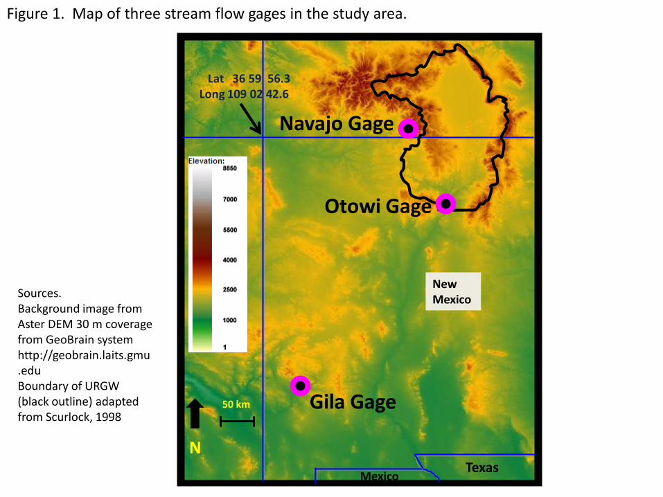
Sources. Background image from Aster DEM 30 m coverage from GeoBrain system http://geobrain.laits.gmu.edu Boundary of URGW (black outline) adapted from Scurlock, 1998

Navajo Gage

Otowi Gage

Gila Gage

New Mexico

50 km

N

Lat 36 59 56.3 Long 109 02 42.6

Texas Mexico

Figure 1. Map of three stream flow gages in the study area.

Figure 2. Otowi gage time series as represented by three moving averages.

Derived from source USGS 2014a

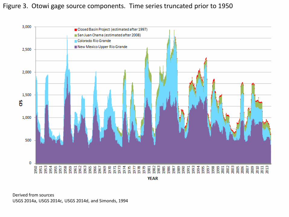
Figure 3. Otowi gage source components. Time series truncated prior to 1950

Derived from sources USGS 2014a, USGS 2014c, USGS 2014d, and Simonds, 1994

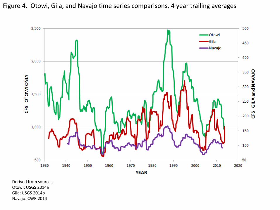
Figure 4. Otowi, Gila, and Navajo time series comparisons, 4 year trailing averages

Derived from sources Otowi: USGS 2014a Gila: USGS 2014b Navajo: CWR 2014

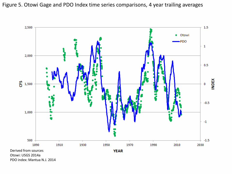
Figure 5. Otowi Gage and PDO Index time series comparisons, 4 year trailing averages

Derived from sources Otowi: USGS 2014a PDO index: Mantua N.J. 2014

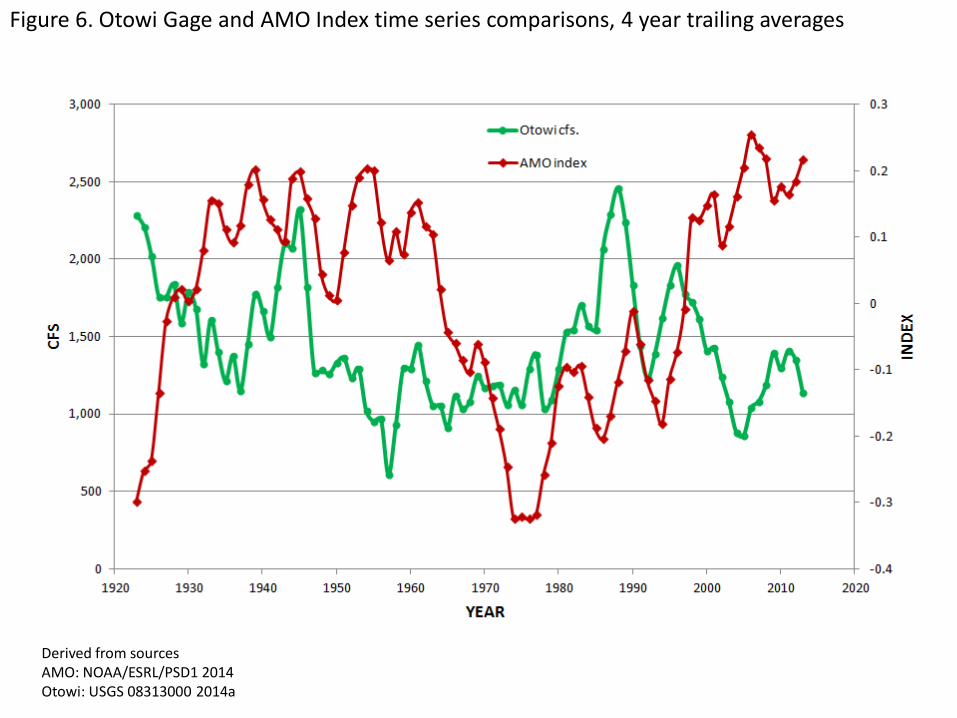
Figure 6. Otowi Gage and AMO Index time series comparisons, 4 year trailing averages

Derived from sources AMO: NOAA/ESRL/PSD1 2014 Otowi: USGS 08313000 2014a

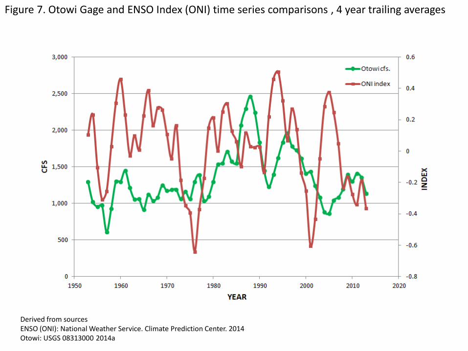
Figure 7. Otowi Gage and ENSO Index (ONI) time series comparisons , 4 year trailing averages

Derived from sources ENSO (ONI): National Weather Service. Climate Prediction Center. 2014 Otowi: USGS 08313000 2014a

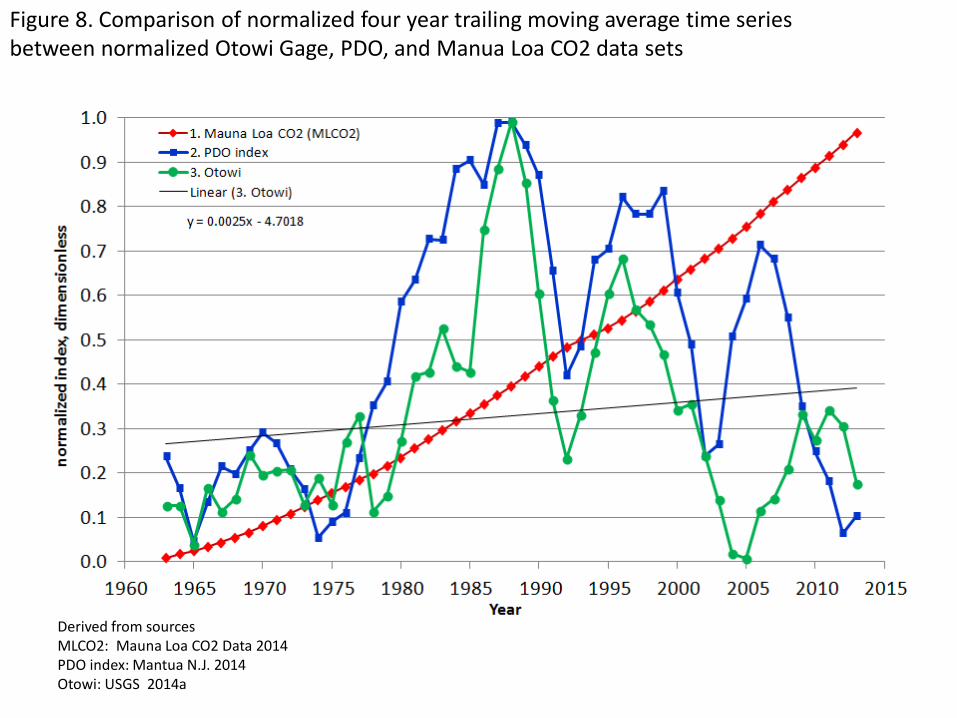
Figure 8. Comparison of normalized four year trailing moving average time series between normalized Otowi Gage, PDO, and Manua Loa CO2 data sets

Derived from sources MLCO2: Mauna Loa CO2 Data 2014 PDO index: Mantua N.J. 2014 Otowi: USGS 2014a

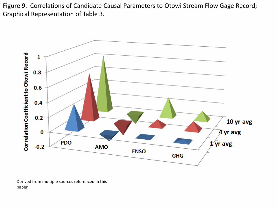
Figure 9. Correlations of Candidate Causal Parameters to Otowi Stream Flow Gage Record; Graphical Representation of Table 3.

Derived from multiple sources referenced in this paper

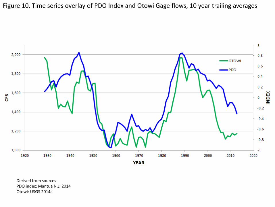
Figure 10. Time series overlay of PDO Index and Otowi Gage flows, 10 year trailing averages

Derived from sources PDO index: Mantua N.J. 2014 Otowi: USGS 2014a

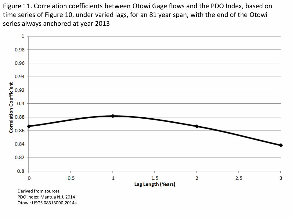
Figure 11. Correlation coefficients between Otowi Gage flows and the PDO Index, based on time series of Figure 10, under varied lags, for an 81 year span, with the end of the Otowi series always anchored at year 2013

Derived from sources PDO index: Mantua N.J. 2014 Otowi: USGS 08313000 2014a

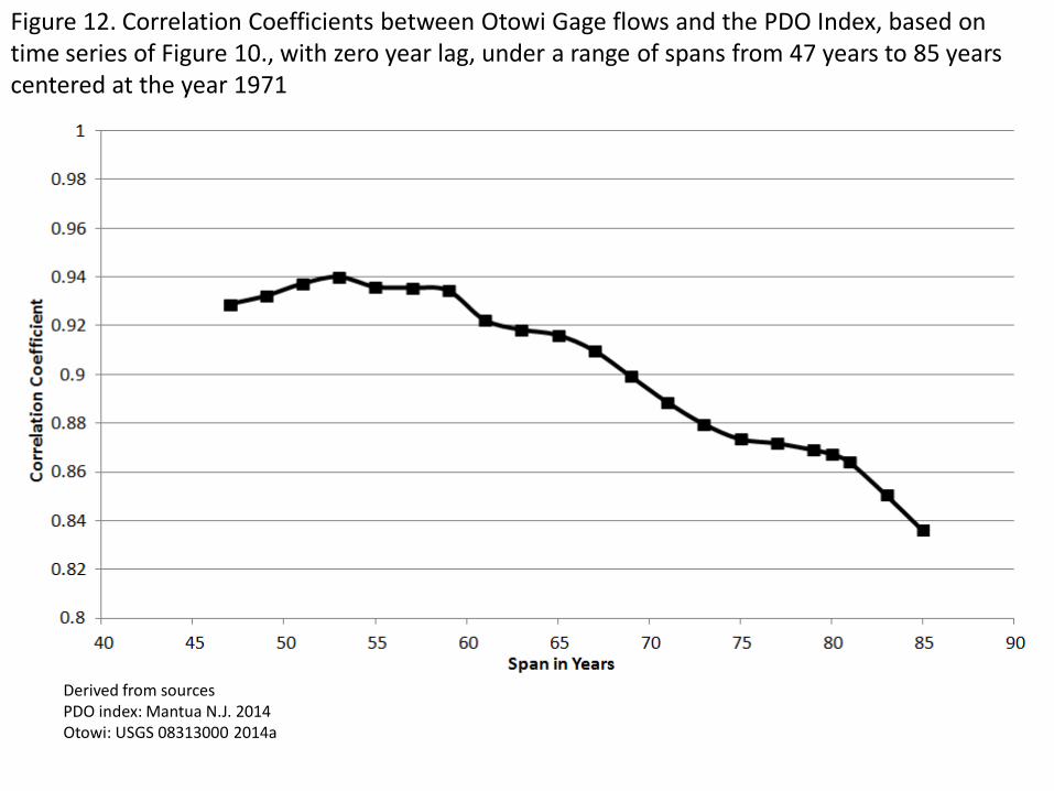
Figure 12. Correlation Coefficients between Otowi Gage flows and the PDO Index, based on time series of Figure 10., with zero year lag, under a range of spans from 47 years to 85 years centered at the year 1971

Derived from sources PDO index: Mantua N.J. 2014 Otowi: USGS 08313000 2014a