arX

iv:0

711.

0746

v4 [

astr

o-ph

] 2

Apr

200

8

Mon. Not. R. Astron. Soc. 000, 000–000 (0000) Printed 2 April 2008 (MN LATEX style file v2.2)

The redshift dependence of the structure of massive

ΛCDM halos

Liang Gao1, Julio F. Navarro2,3⋆, Shaun Cole1, Carlos S. Frenk1, Simon D.M.

White4, Volker Springel4, Adrian Jenkins1, Angelo F. Neto5

1Institute of Computational Cosmology, Department of Physics, University of Durham,

Science Laboratories, South Road, Durham DH1 3LE, UK2Astronomy Department, University of Massachusetts, LGRT-B 619E, Amherst, MA 01003, USA3Department of Physics and Astronomy, University of Victoria, PO Box 3055 STN CSC, Victoria, BC, V8W 3P6 Canada4Max-Planck Institute for Astrophysics, Karl-Schwarzschild Str. 1, D-85748, Garching, Germany5Instituto de Fısica, Universidade Federal do Rio Grande do Sul, Porto Alegre RS, Brazil

2 April 2008

ABSTRACT

We use two very large cosmological simulations to study how the density profiles ofrelaxed ΛCDM dark halos depend on redshift and on halo mass. We confirm thatthese profiles deviate slightly but systematically from the NFW form and are betterapproximated by the empirical formula, d log ρ/d log r ∝ rα, first used by Einasto to fitstar counts in the Milky Way. The best-fit value of the additional shape parameter, α,increases gradually with mass, from α ∼ 0.16 for present-day galaxy halos to α ∼ 0.3for the rarest and most massive clusters. Halo concentrations depend only weaklyon mass at z = 0, and this dependence weakens further at earlier times. At z ∼ 3the average concentration of relaxed halos does not vary appreciably over the massrange accessible to our simulations (M ∼> 3×1011 h−1M⊙). Furthermore, in our biggestsimulation, the average concentration of the most massive, relaxed halos is constant at〈c200〉 ∼ 3.5 to 4 for 0 ≤ z ≤ 3. These results agree well with those of Zhao et al (2003b)and support the idea that halo densities reflect the density of the universe at the timethey formed, as proposed by Navarro, Frenk & White (1997). With their originalparameters, the NFW prescription overpredicts halo concentrations at high redshift.This shortcoming can be reduced by modifying the definition of halo formation time,although the evolution of the concentrations of Milky Way mass halos is still notreproduced well. In contrast, the much-used revisions of the NFW prescription byBullock et al. (2001) and Eke, Navarro & Steinmetz (2001) predict a steeper dropin concentration at the highest masses and stronger evolution with redshift than arecompatible with our numerical data. Modifying the parameters of these models canreduce the discrepancy at high masses, but the overly rapid redshift evolution remains.These results have important implications for currently planned surveys of distantclusters.

Key words: methods: N-body simulations – methods: numerical –dark matter –galaxies: haloes – galaxies:structure

1 INTRODUCTION

Over the past decade, cosmological N-body simulations haveshown consistently that equilibrium dark matter halos havespherically-averaged mass density profiles which are approx-imately “universal” in form; i.e., their shape is independentof mass, of the values of the cosmological parameters, and of

⋆ Fellow of the Canadian Institute for Advanced Research

the linear power spectrum from which nonlinear structureshave grown. As a result, it is useful to parametrize halo pro-files by simple empirical formulae, such as that proposed byNavarro, Frenk & White (1995, 1996, 1997, hereafter NFW):

ρ(r)

ρcrit

=δc

(r/rs)(1 + r/rs)2, (1)

2 Gao et al.

where ρcrit = 3H2/8πG is the critical density for closure1, δc

is a characteristic density contrast, and rs is a scale radius.Note that this formula contains two scale parameters but noadjustable shape parameter.

As discussed in some detail by NFW and confirmed bysubsequent numerical work, the two parameters of the NFWprofile do not take arbitrary values, but are instead corre-lated in a way that reflects the mass-dependence of haloassembly times (e.g., Kravtsov, Klypin & Khokhlov 1997;Avila-Reese et al. 1999; Jing 2000; Ghigna et al. 2000; Bul-lock et al. 2001; Eke, Navarro & Steinmetz 2001; Klypin etal. 2001). The basic idea behind this interpretation is thatthe characteristic density of a halo tracks the mean densityof the universe at the time of its formation. Thus, the latera halo is assembled, the lower its characteristic density, δc,or, equivalently, its “concentration” (see Section 2.2 for adefinition).

Although the general validity of these trends is wellestablished, a definitive account of the redshift and massdependence of halo concentration is still lacking, even forthe current concordance cosmology. This is especially trueat high masses, where enormous simulation volumes are re-quired in order to collect statistically significant samples ofthese rare systems. Simulating large cosmological volumeswith good mass resolution is a major computational chal-lenge, and until recently our understanding of the mass pro-file of massive halos has been rather limited, derived largelyfrom small numbers of individual realizations or from ex-trapolation of models calibrated on different mass scales(NFW; Moore et al. 1998; Ghigna et al. 2000; Klypin et al.2001; Navarro et al. 2004; Tasitsiomi et al. 2004; Diemandet al. 2004; Reed et al. 2005).

Individual halo simulations may result in biased con-centration estimates, depending on the specific selection cri-teria used to set them up. In addition, they are unlikelyto capture the full scatter resulting from the rich varietyof possible halo formation histories. Extrapolation based onpoorly tested models can also produce substantial errors, asrecently demonstrated by Neto et al. (2007). These authorsanalyzed the mass-concentration relation for halos identi-fied at z = 0 in the Millennium Simulation of Springel et al.(2005, hereafter MS) and confirmed the earlier conclusion ofZhao et al. (2003b) that the models of Bullock et al. (2001,hereafter B01) and Eke et al. (2001, hereafter ENS) (whichwere calibrated to match galaxy-sized halos) severely un-derestimate the average concentration of massive clusters,by up to a factor of ∼ 3.

Estimates of concentrations can also be biased by theinclusion of unrelaxed halos. These often have irregular den-sity profiles caused by major substructures. Smooth densityprofiles are often poor fits to such halos, and the resultingconcentration estimates are ill-defined because they dependon the radial range of the fit and choice of weighting. Theycan also lead to spurious correlations (see for example fig-ure 9 of Neto et al. 2007). Consequently, in this paper wefollow Neto et al. and select only relaxed halos for analy-sis. This is not without its own problems. Such selectionbiases against recently formed halos, which may preferen-

1 We express Hubble’s constant as H(z) and its present-day valueas H(z = 0) = H0 = 100 h km s−1 Mpc−1.

tially have lower concentrations. However we believe this ispreferable to polluting the sample with meaningless concen-tration estimates of the kind that arise when smooth spheri-cal models are force-fit to lumpy, multi-modal mass distribu-tions. Hayashi & White (2008) stacked all halos, regardlessof dynamical state, in the MS and studied the resulting meanprofiles as a function of halo mass. The relatively small dif-ferences between their results and those found below showsthat the inclusion of unrelaxed halos has rather little effectin the mean.

A further preoccupation concerns indications that haloprofiles deviate slightly but systematically from the NFWmodel (Moore et al. 1998, Jing & Suto 2000, Fukushige &Makino 2001, Navarro et al. 2004, Prada et al. 2006, Merrittet al. 2006), raising the possibility that estimating concen-trations by force-fitting simple formulae to numerical datamay result in subtle biases that could mask the real trends.This is especially important because of hints that such de-viations depend systematically on halo mass (Navarro et al.2004, Merritt et al. 2005). Evaluating and correcting for suchdeviations is important in order to establish conclusively themass and redshift dependence of halo concentration.

These uncertainties are unfortunate since observations,especially at high redshift, often focus on exceptional sys-tems. For example, massive galaxy clusters are readily iden-tified in large-scale surveys of the distant universe, and un-derstanding their internal structure will be critical for thecorrect interpretation of cluster surveys intending to con-strain the nature of dark energy. These will make precisemeasurements of the evolution of cluster abundance in sam-ples detected by gravitational lensing, by their optical or X-ray emission, or through the Sunyaev-Zel’dovich effect (see,e.g., Carlstrom et al. 2002, Hu 2003, Majumdar & Mohr2003, Holder 2006, and references therein).

There is at present no ab initio theory that can reliablypredict the internal structure of CDM halos. The models ofZhao et al (2003a), Wechsler et al (2002) (see also Lu etal. 2006) are interesting, but as shown in Neto et al (2007)they account for only a small fraction in the measured dis-persion in concentration at a fixed mass. There is currentlyno substitute for direct numerical simulation when detailedpredictions are needed for comparison with observation.

We address these issues here by combining results fromthe MS with results from an additional simulation which fol-lowed a substantially smaller volume but with better massresolution. This allows us to extend the range of halo massesfor which we can measure concentrations and to assess howthese measures are affected by numerical resolution. Ouranalysis procedure follows closely that of Neto et al. (2007).In particular, we concentrate in this paper on the propertiesof halos which are relaxed according to the criteria definedby these authors; mean density profiles for all MS halos ofgiven mass, regardless of dynamical state, are presented byHayashi & White (2008). We begin in Section 2 by describ-ing briefly the numerical simulations and the halo catalogueon which this study is based. In Section 3 we present ourmain results for the dependence of profile shape and con-centration on halo mass and redshift. We conclude with abrief discussion and summary in Section 4.

Evolution of Halo Mass Profiles 3

Figure 1. Left panels: The stacked density profile of 464 halos of virial mass ∼ 2 × 1014h−1M⊙, identified at z = 0 in the MS. Thecurves in the upper left panel show different NFW fits obtained by varying the radial range fitted: [0.02, 1]rvir (solid red), [0.05, 1]rvir

(dashed green) and [0.1, 1]rvir (dot-dashed blue). Note the small disagreement between the actual profile shape and the NFW model(upper panels). This leads to concentration estimates which depend slightly on the innermost radius of the fit. Fits using eq. (4) aremore robust to such variations in fitting range, as shown in the lower left panel. Panels on the right show the residuals corresponding tothe fits shown on the left.

2 THE NUMERICAL SIMULATIONS

The analysis presented here is based primarily on halos iden-tified in the Millennium Simulation (MS) of Springel et al.(2005). The halo identification and cataloguing procedurefollows closely that described in detail by Neto et al. (2007).For completeness, we here recapitulate the main aspects ofthe procedure, referring the interested reader to the earlierpapers for details.

2.1 Simulations

The MS is a large N-body simulation of the concordanceΛCDM cosmogony. It follows N = 21603 particles in a peri-odic box of side Lbox = 500 h−1Mpc. The chosen cosmolog-ical parameters were Ωm = Ωdm + Ωb = 0.25, Ωb = 0.045,h = 0.73, ΩΛ = 0.75, n = 1, and σ8 = 0.9. Here Ω de-notes the present-day contribution of each component to thematter-energy density of the Universe, expressed in units ofthe critical density for closure, ρcrit; n is the spectral in-dex of the primordial density fluctuations, and σ8 is the rms

linear mass fluctuation in a sphere of radius 8 h−1 Mpc atz = 0. The particle mass in the MS is 8.6 × 108 h−1M⊙.Particle interactions are softened on scales smaller than the(Plummer-equivalent) softening length, ǫ = 5 h−1kpc.

We also use a second simulation of a smaller volume(1003 h−3 Mpc3) within the same cosmological model. Thissimulation followed N = 9003 particles of mass 9.5 ×107 h−1M⊙ and softened interactions on scales smaller thanǫ = 2.4 h−1kpc. It thus has approximately 9 times bettermass resolution than the MS. Hereafter we refer to it as thehMS.

2.2 Halo Catalogues

Our halo cataloguing procedure starts from a standardb = 0.2 friends-of-friends list of particle groups (Davis etal. 1985) and refines it with the help of SUBFIND, the sub-

halo finder algorithm described by Springel et al. (2001).Each halo is centred at the location of the minimum of thegravitational potential of its main SUBFIND subhalo, and

4 Gao et al.

Figure 2. Left panel: The best-fit shape parameter, α (eq. (4)), as a function of halo mass and redshift, after binning and stacking halosby mass. Solid and dashed lines correspond to the MS and hMS simulations, respectively. Only results corresponding to halos with morethan ∼ 500 particles and to stacks with more than 10 halos are shown. Note the good general agreement between the two simulations.Differences are substantial only where the number of particles is less than 3000. Right panel: Values of α for halos with more than3000 particles plotted as a function of the dimensionless “peak height” parameter ν(M, z), defined as the ratio between the criticaloverdensity δcrit(z) for collapse at redshift z and the linear rms fluctuation at z within spheres containing mass M . The larger the valueof ν the rarer and more massive the corresponding halo. Note that this scaling accounts satisfactorily for the redshift dependence of themass-concentration relation shown in the left-hand panel.

this centre is used to compute the virial radius and mass ofeach halo.

We define the virial radius, r∆, as that of a sphere ofmean density ∆× ρcrit. Note that this defines implicitly the“virial mass” of the halo, M∆, as that enclosed within r∆.The choice of ∆ varies in the literature. The most popularchoices are: (i) a fixed value, as in NFW’s original work,where ∆ = 200 was adopted; or (ii) a value motivated bythe spherical top-hat collapse model, where ∆ ∼ 178 Ω0.45

m

for a flat universe (Eke et al. 1996). The latter choice gives∆ = 95.4 at z = 0 for the cosmological parameters adoptedfor the MS. We keep track of both definitions in our halocatalogue, and will specify our choice by a subscript. Thus,M200 and r200 are the mass and radius of a halo adopting∆ = 200, whereas Mvir and rvir are the values correspondingto ∆ = 95.4 at z = 0. Quantities specified without subscriptassume ∆ = 200, so that, e.g., M = M200. The halo con-centration is defined as the ratio between the virial radiusand the scale radius: c = c200 = r200/rs. In this case, thecharacteristic density is related to the concentration by

δc = (200/3) c3/[ln(1 + c) − c/(1 + c)]. (2)

Since halos are dynamically evolving structures, we usea combination of diagnostics in order to flag non-equilibriumsystems. Following Neto et al. (2007), we assess the equilib-rium state of each halo by measuring: (i) the substruc-

ture mass fraction; i.e., the total mass fraction in re-solved substructures whose centres lie within r200, fsub =∑Nsub

i6=0Msub,i/M200; (ii) the centre of mass displace-

ment, s = |rc − rcm|/r200, defined as the normalized offsetbetween the location of the minimum of the potential andthe barycentre of the mass within r200; and (iii) the virial

ratio, 2T/|U |, where T is the total kinetic energy of the haloparticles within rvir and U their gravitational self-potentialenergy.

Using these criteria, we shall consider halos to be re-

laxed if they satisfy all the following conditions: fsub < 0.1,s < 0.07, and 2T/|U | < 1.35. (See Neto et al. 2007 for fulldetails.) We shall also impose a minimum number of parti-cles in order to be able to say something meaningful aboutinternal halo structure. We initially set this limit at 500 par-ticles, but following the analysis of profile shapes presentedin Section 3.2 we subsequently adopt a stricter criterion of3000 particles. We consider only relaxed halos in this study,since only for such systems can the mass profiles of indi-vidual objects be represented accurately by a simple fittingformula with a small number of parameters. Such formulaeare also useful for characterizing the average profiles of largeensembles of halos, since the fluctuations in the individualsystems then average out. Hayashi & White (2007) presentsuch mean profiles as a function of mass for all MS halos re-gardless of their dynamical state. We compare their resultswith our own below.

With these restrictions, including the 3000 particlelimit, our final MS catalogue contains 128233, 77190, 30603,and 9392 relaxed halos at z = 0, 1, 2, and 3, respectively.(The corresponding numbers for the hMS catalogue are 8131,6652, 4112 and 2194.) The overall fractions of these halosthat are relaxed in the MS are 78%, 60%, 50%, and 48%at these redshifts, respectively. We note that these frac-tions also depend on halo mass: at z = 0 about ∼ 85%of ∼ 1012 h−1M⊙ halos are relaxed by our criteria, but only∼ 60% of ∼ 1015 h−1M⊙ halos. In order to obtain usefullylarge statistical samples, we restrict our analysis to the red-shift range 0 ≤ z ≤ 3 in the following.

3 HALO DENSITY PROFILES

For each halo in the samples described in Section 2 we havecomputed a spherically-averaged density profile by measur-

Evolution of Halo Mass Profiles 5

ing the halo mass in 32 equal intervals of log10

(r) over therange 0 ≥ log10(r/rvir) ≥ −2.5.

Profiles may also be stacked in order to obtain an aver-

age profile for halos of similar mass. This procedure has theadvantage of erasing individual deviations from a smoothprofile which are typically due to the presence of substruc-ture. Such deviations increase the (already considerable)scatter in the parameters fitted to individual profiles andmay mask underlying trends in the data. The left panels inFig. 1 show the profile that results from stacking 464 ha-los of mass ∼ 2 × 1014h−1M⊙ identified at z = 0 in theMS. We choose to show r2ρ vs r rather than ρ vs r in orderto remove the main radial trend and enhance the dynamicrange of the plot. Similar stacked profiles for all halos in theMS (regardless of dynamical state) are shown by Hayashi &White (2008).

3.1 Deviations from NFW and concentration

estimates

The concentration of a halo is defined using the scale radiusof the profile, rs. This identifies the location of the maxi-mum of the r2ρ profile. However, as shown in Fig. 1, thepeak is rather broad, leading to some uncertainty in its ex-act location when noise is present. Typically this problemis addressed by fitting the numerical data to some specifiedfunctional form over an extended radial range. The curvesin the top-left panel of Fig. 1 show the result of fitting thestacked halo profile with the NFW formula (eq. (1)), butvarying the radial range of the fit as shown by the labels.This results in slightly different estimates for rs, and conse-quently for the concentration, cvir = rvir/rs. Increasing theinnermost radius of the fit from 0.02 to 0.1 rvir results in aconcentration estimate that decreases from ∼ 7.5 to ∼ 6.7.

This variation is a result of the slight (but significant)mismatch between the shape of the NFW profile and that ofthe stacked halo, as shown by the residuals in the top-rightpanel of Fig. 1. The “S” shape of the residuals implies thatthe stacked profile steepens more gradually with radius ina log-log plot than does the NFW profile, a result that hasbeen discussed in detail by Navarro et al. (2004), Prada etal. (2006) and Merritt et al. (2006).

These results suggest that force-fitting NFW profilesmay induce spurious correlations between mass and concen-tration. In particular, when halos are identified in a sin-gle cosmological simulation, the numerical resolution variessystematically with halo mass (less massive halos are morepoorly resolved) so that the radial range available for fittingis a strong function of halo mass.

One way to address this issue is to adopt a fitting for-mula that better matches the mean profile of simulated ha-los. As discussed by Navarro et al. (2004), Prada et al. (2006)and Merritt et al. (2006), improved fits are obtained adopt-ing a radial density law where the logarithmic slope is apower-law of radius,

d log ρ

d log r= −2

(

r

r−2

)α

, (3)

which implies a density law of the form

ln(ρ/ρ−2) = −(2/α)[(r/r−2)α − 1]. (4)

Here ρ−2 is the density at r = r−2. This density law was

Figure 3. Three stacked halo density profiles with different valuesof ν, and at different redshifts, as labelled. The profiles are chosento illustrate the variation in halo structure as a function of ν

indicated in Fig. 2. The larger the halo mass, the larger the valueof α and the sharper the curvature in the density profile as afunction of radius.

first introduced by Einasto (1965) who used it to describethe distribution of old stars within the Milky Way. For con-venience, we will thus refer to it as the Einasto profile. Notethat according to our definition, r−2 corresponds to the ra-dius where the logarithmic slope of the density profile hasthe “isothermal” value, −2. In this sense, r−2 is equivalentto the NFW scale-length, rs, and again marks the locationof the maximum in the r2ρ profile shown in Fig. 1.

The bottom-left panel of Fig. 1 shows that, at the costof introducing an extra shape parameter, the fits improveto the point that the sensitivity of concentration estimatesto the fitted radial range is effectively eliminated. Thus,concentrations obtained by fitting eq. (4) to the stackedhalo profiles are robust against variations in fitting details.Hayashi & White (2007) show that the same is true for fitsto stacks of all halos of a given mass, rather than just therelaxed halos used to make Fig. 1, and indeed, the α and cvalues they find are very similar to the values we obtain here,showing that our restriction to relaxed halos has relativelylittle effect in the mean.

We conclude that accounting for the subtle differencebetween halo profile shape and the NFW fitting formula isworthwhile in order to avoid possible fitting-induced biasesin concentration estimates. In the remainder of this paperwe quote concentrations, c∆ = r∆/r−2, which are estimatedby fitting density profiles by eq. (4). We discuss in the nextsection how α is chosen for these fits.

3.2 The mass and redshift dependence of profile

shape

The above discussion suggests that the shape parameter,α, should be used to improve the description of the typicaldensity profiles of simulated halos and to eliminate possiblebiases in estimates of their concentration. To do this, it isnecessary to understand whether (and how) α varies withredshift and/or halo mass.

6 Gao et al.

Figure 4. Distributions of concentration parameters estimatedusing eq. (4) for the 464 individual halo profiles stacked in Fig. 1.The solid (black) histogram corresponds to fits where α was ad-justed separately for each individual halo, the dashed (red) his-togram to fits where α was set to the value implied by the α(ν)relation of Fig. 2 (eq. (5)). The numbers in the legend give themedian and scatter of the distributions. The excellent agreementbetween the two distributions indicates that unbiased and accu-rate concentration estimates for relaxed halos may be obtainedby fixing α to the value determined by eq. (5).

We explore this in Fig. 2. The left panel shows howthe best-fit value of α depends on halo mass for the averageprofiles of relaxed halos stacked according to their mass. Weconsider only halos with at least 500 particles within thevirial radius, and stacks containing at least 10 halos. Thesolid and dashed curves in this plot correspond to the MS

and hMS simulations, respectively.This figure illustrates several interesting points. In the

first place, we note that there is good agreement between thetwo simulations for halos which are represented by at least3000 particles, but that systematic differences are visiblewhen the MS halos contain fewer particles than this. In therest of this paper we will thus only present results for haloscontaining at least 3000 particles within the virial radius.

A second interesting point is that there are well-definedtrends for α to increase with mass at each redshift, andwith redshift at each mass. The (weak) trend with mass wasalready visible in Navarro et al. (2004) and Merritt et al.(2005), although the small number of halos in these studiesmade their results rather inconclusive in the face of the largehalo-to-halo scatter. The use of stacked profiles in Fig. 2,together with the much larger number of halos in the simu-lations used here, leads to a far more convincing demonstra-tion of the trends than was previously possible.

The trend with redshift at given mass may seem sur-prising, but its interpretation is made clear by the rightpanel of Fig. 2. Here we show α as a function of a di-mensionless “peak-height” parameter, defined as ν(M, z) ≡δcrit(z)/σ(M, z); i.e., as the ratio of the linear density thresh-old for collapse at z to the rms linear density fluctuationat z within spheres of mean enclosed mass M . The pa-rameter ν(M, z) is related to the abundance of objects ofmass M at redshift z. ν(M∗, z) = 1 defines the charac-teristic mass, M∗(z), of the halo mass distribution at red-

shift z. ν(M, z) ≫ 1 then corresponds to rare objects withM ≫ M∗, while ν(M,z) ≪ 1 corresponds to objects in thelow-mass tail of the distribution. The parameter ν plays akey role in the Press-Schechter model for the growth of non-linear structure (see, for example, Lacey & Cole 1993).

The right panel of Fig. 2 shows that all curves coincidewhen expressed in terms of ν(M, z) (and when consideringhalos with N > 3000 particles). Thus, the redshift depen-dence in the left panel merely reflects the fact that objectsof given virial mass correspond to very different values of νat different redshifts. It is interesting that the dependenceof α on ν is very weak for ν < 1 (it is nearly constant atα ∼ 0.16), but it increases rapidly for rarer, more massiveobjects, reaching α ∼ 0.3 for ν ∼ 3.5. A simple formula,

α = 0.155 + 0.0095 ν2 (5)

describes the numerical results quite accurately.Taylor & Navarro (2001), Austin et al (2005) and

Dehnen & McLaughlin (2005) investigated a halo modelbased on the assumption that the phase space density, ρ/σ3,was a simple powerlaw of radius. Interestingly, the densityprofile they found is almost identical to an Einasto profilewith 0.14 < α < 0.18 and so the sharp upturn we find in αat ν > 1 could be taken as indication that such a model isnot valid for rare and massive halos.

The dependence of profile shape on ν is illustrated inFig. 3, where we plot r2ρ profiles for halo stacks correspond-ing to three different values of ν: 1.0, 2.0, and 3.2. The largerν, the larger α, and the more sharply the profile peaks. Itis unclear what causes these systematic trends, but the factthat they depend on ν (rather than, say, on mass alone) isan important clue for models that attempt to explain thenear-universality of dark halo density profiles. While our re-sults here are based purely on relaxed halos, very similarresults were found by Hayashi & White (2007) for the aver-age profiles of stacks of all MS halos, regardless of dynamicalstate.

3.3 Concentration estimates

As we discussed above, a fitting formula other than NFW isneeded to obtain concentration estimates that are insensitiveto the radial range fitted. Einasto’s profile, eq. (4), accom-plishes this at the cost of introducing an additional shape pa-rameter, α. Adjusting α to fit the detailed structure of indi-vidual halos would negate the spirit of the NFW programmewhich attempts to predict the structure of dark halos in anyhierarchical cosmology from its initial power spectrum andthe global cosmological parameters. Three-parameter fits toindividual halos are also susceptible to strongly correlatedparameter errors. We have therefore explored whether fixingα as a function of halo mass and redshift according to theα(ν) relation of eq. (5) results in significantly different con-centration distributions than adjusting it freely to fit eachhalo.

We show the result in Fig. 4, which shows concentra-tion distributions for the 464 individual halos which werestacked to make Fig. 1. We compare the distribution ob-tained from full three-parameter Einasto fits to that ob-tained when α is set to the value predicted for each halofrom its mass. We find that for most halos the fits give es-sentially the same concentration, and the distributions of

Evolution of Halo Mass Profiles 7

Figure 5. The mass dependence of concentration as a function of redshift. Concentration estimates are derived from Einasto fits to thedensity profile of “relaxed” halos over the radial range [0.05, 1]rvir. Points, boxes and whiskers show the median and the 5, 25, 75, and95 percentiles of the concentration distribution within each mass bin. Black symbols correspond to the MS, red symbols to the smaller,but higher resolution hMS. Only results for halos with more than 3000 particles are shown for each simulation. The solid-dotted, dashed,dot-dashed and solid lines show the models of NFW, ENS, B01 and the modified NFW, respectively, for comparison with our results.The lower dotted line in the upper left panel indicates the relation obtained by Neto et al. (2007) from NFW fits to relaxed halos atz = 0. The remaining dotted lines show the powerlaw fits given in Table 1.

concentration are almost indistinguishable. The medians ofthe fixed-α and floating-α distributions are 6.85 and 6.90, re-spectively. The scatters also coincide, as noted in the labelsof Fig. 4. Interestingly, the scatter around the best-fit profileis typically only slightly smaller for the Einasto model thanfor the NFW model, showing that the difference between thetwo models is much smaller than the deviation of the profileof typical individual halos from either model. In this sense,the 3-parameter Einasto profile has little advantage over the2-parameter NFW profile when estimating dark matter haloconcentrations.

This is easily understood. Estimating the concentrationof a halo is equivalent to locating the “peak” of the r2ρprofile. Provided that the shape of the fitted profile is, onaverage, a good approximation to the simulated ones, no sys-tematic offset is expected between concentrations estimatedusing the two procedures. We conclude that concentrationsmay be estimated robustly by fitting Einasto profiles to indi-vidual halos with α fixed to the value obtained from eq. (5).All values reported below were obtained using this proce-dure.

3.4 The mass and redshift dependence of halo

concentration

The concentration-mass relation is shown in Fig. 5 forz = 0, 1, 2 and 3. The upper-left panel is equivalent to Fig. 6of Neto et al. (2007), except that our concentrations are es-timated from fits covering the range [0.05, 1]rvir using anEinasto rather than an NFW profile, and we only show re-sults for halos with more than 3000 particles. The differencesare small, as may be judged from the power-law fit proposedby Neto et al., c200 = 5.26 (M200/10

14h−1M⊙)−0.10, shownas a dotted line in the upper-left panel of Fig. 5. This powerlaw fit is very similar (after correction for differing concen-tration and mass definitions) to that which Maccio et al.(2007) obtained from NFW fits to halos in an independentset of (smaller) simulations, despite the fact that these au-thors included halos with as few as 250 particles, which wewould consider to be significantly under-resolved on the ba-sis of our own tests.

Both the concentration values and the trends with massand redshift are very similar to those presented in figure 2of Zhao et al (2003b) who analysed a set of ΛCDM simula-

8 Gao et al.

tions of varying resolution. The small offsets between theirmean concentrations and our results are consistent with theslight differences we have noted when switching from NFWto Einasto models for determining concentrations. In ad-dition to confirming these earlier results, the much largervolume of our simulations results in a better determinationof the intrinsic scatter about the mean relation.

Red and black symbols in Fig. 5 correspond to the MS

and hMS simulations, respectively, with dots plotted at themedian concentration for each mass bin. Boxes represent thelower and upper quartiles of the concentration distributions,while the whiskers show their 5% and 95% tails. We alsoshow the concentrations predicted by three previously pro-posed analytic models: NFW (solid-dotted magenta), B01(dot-dashed black), ENS (dashed green). As discussed byNeto et al. (2007), none of these models reproduces the sim-ulation results over the full mass range accessible at z = 0:the NFW and ENS models underestimate the concentrationof galaxy-sized halos, whereas the B01 model fails dramati-cally at the high-mass end, where it predicts a sharp declinewhich is not seen in the simulations. 2

There is a hint in the z = 0 panel that the relationis flattening at the high-mass end, where the NFW predic-tions at z = 0 appear slightly better than those of ENS. Thisis because a constant concentration for very rare and mas-sive objects is implicit in the NFW model, which assumesthat the characteristic density of a halo reflects that of theuniverse at the time it collapsed. Very massive systems as-sembled very recently, and therefore share the same collapsetime (i.e., they are being assembled today).

The near-constant concentration of the most massivehalos is considerably more obvious at higher redshift, pre-sumably because well-resolved halos (i.e., those with N >3000 in the MS or hMS) become rarer and rarer with increas-ing lookback time. Indeed, whereas at z = 0 our MS halocatalogue spans the range 0.75 < ν < 3, at z = 3 all thehalos retained have ν ∼> 3. As a result, the average concen-tration at z = 3 is almost independent of mass over theaccessible mass range, i.e., M ∼> 3 × 1011h−1M⊙. It is inter-esting that the average concentration of the most massivehalos (i.e. ν ≥ 3) is similar at all redshifts, c ∼ 3.5 to 4.This evokes the proposals of Zhao et al. (2003a,b), Tasit-siomi et al. (2004) and Lu et al. (2006), all of whom arguethat halos undergoing rapid growth should all have similarconcentration.

The evolution of the mass-concentration relation seenin our numerical simulations is not predicted by any of thepublished prescriptions. The original NFW model shows a

2 We note that NFW, ENS and B01 parametrize the initialpower spectrum in slightly different ways, and that the pre-dicted concentrations are sensitive to the exact choice of pa-rameters. For example, NFW and ENS use the parameter Γ tocharacterize the shape of the linear power spectrum. We useΓ = 0.15 here since that provides the best fit to the actual

power spectrum used in the MS. For B01 we have used the de-fault values advocated in the latest version of their software(K = 2.8 and F = 0.001 in their notation), which is availablefrom http://www.physics.uci.edu/∼bullock/CVIR/ . The differ-ences between the predictions shown here and in Fig. 4 of Hayashi& White (2008), or in Neto et al (2007), for example, are due toslight differences in the values chosen for these parameters.

Table 1. Values of the constants A and B for the best straight-line fit (6) to the data shown in Fig. 5.

Redshift A B

0 -0.138 2.6460.5 -0.125 2.3721 -0.092 1.8912 -0.031 0.9853 -0.004 0.577

flattening of the concentration-mass relation with increas-ing redshift, similar to that observed in the simulations, butit predicts insufficient evolution in concentration at givenmass. As a result, this model overestimates the concen-trations by an increasing amount with increasing redshift,about 40% at z = 3. The ENS and B01 models fail toreproduce the features of the mass-concentration-redshiftrelations at high mass, predicting a stronger mass depen-dence and much more evolution than is seen. In these twomodels, the concentration of halos of given mass scales in-versely as the expansion factor, so that shape of the mass-concentration relation remains fixed. While the high-massdiscrepancy between the B01 model and our measurementscan be reduced by changing the parameters to K = 2.8and F = 0.001 (see Wechsler et al 2006), neither for thismodel nor for the ENS model can parameter changes pro-duce agreement with the weak redshift evolution seen athigh mass both here and by Zhao et al. (2003b). On theother hand, the ENS and B01 models predict the concen-tration evolution of galaxy mass halos substantially betterthan the NFW model. Note that our simulation data donot disagree significantly from those analysed by ENS andB01. The discrepancies result from extrapolation of theirproposed relations beyond the range where they were reli-ably tested.

In the NFW model, the definition of formation time in-volves two physical parameters, F and f , and a proportion-ality constant, C, that relates the value of the characteristichalo density to the mean density of the universe at the timeof collapse. The formation redshift of a halo is taken to bethe redshift at which a fraction, F , of its mass was first con-tained in progenitors each individually containing at leasta fraction f of its mass. In the original NFW prescription,F = 0.5, f = 0.01 and C = 3000. We find that the ob-served trend in the slope of the mass-concentration relationwith redshift can be approximately reproduced by simplychanging F to F = 0.1, keeping f = 0.01 as before; the nor-malization of the relation is then approximately reproducedby taking C = 600. The resulting curves are shown as solidblue lines in Fig. 5. This modified NFW model succeeds wellin matching the redshift evolution, but its mass dependenceis still too shallow at z = 0 and too steep at z = 3, leavingroom for improvement, especially at low masses where theB01 and ENS prescriptions give better predictions of theevolution rate. We have checked that the same model alsogives an acceptable fit for other cosmologies, in particular fora simulation of a ΛCDM model similar to hMS but with thevalues of the cosmological parameters inferred from the 3-year WMAP satellite data (Spergel et al. 2007) (Ω = 0.236,ΩΛ = 0.764, n = 0.97 and σ8 = 0.74). We have also checkedthat this modified NFW model gives a good description of

Evolution of Halo Mass Profiles 9

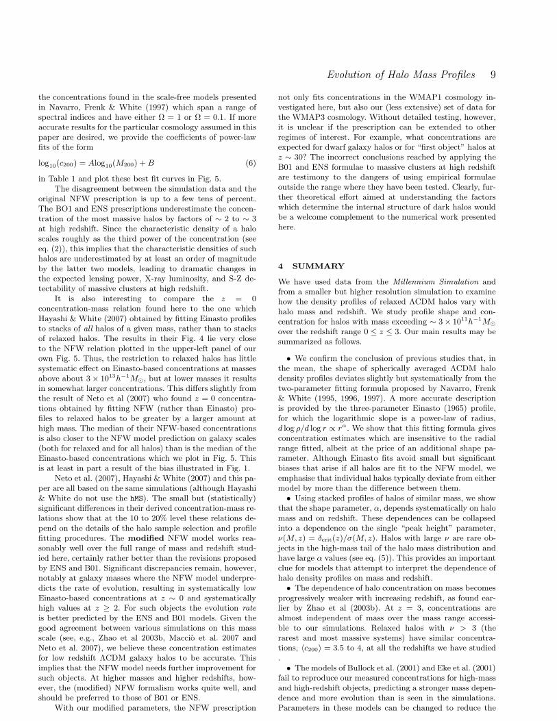
the concentrations found in the scale-free models presentedin Navarro, Frenk & White (1997) which span a range ofspectral indices and have either Ω = 1 or Ω = 0.1. If moreaccurate results for the particular cosmology assumed in thispaper are desired, we provide the coefficients of power-lawfits of the form

log10

(c200) = Alog10

(M200) + B (6)

in Table 1 and plot these best fit curves in Fig. 5.The disagreement between the simulation data and the

original NFW prescription is up to a few tens of percent.The BO1 and ENS prescriptions underestimate the concen-tration of the most massive halos by factors of ∼ 2 to ∼ 3at high redshift. Since the characteristic density of a haloscales roughly as the third power of the concentration (seeeq. (2)), this implies that the characteristic densities of suchhalos are underestimated by at least an order of magnitudeby the latter two models, leading to dramatic changes inthe expected lensing power, X-ray luminosity, and S-Z de-tectability of massive clusters at high redshift.

It is also interesting to compare the z = 0concentration-mass relation found here to the one whichHayashi & White (2007) obtained by fitting Einasto profilesto stacks of all halos of a given mass, rather than to stacksof relaxed halos. The results in their Fig. 4 lie very closeto the NFW relation plotted in the upper-left panel of ourown Fig. 5. Thus, the restriction to relaxed halos has littlesystematic effect on Einasto-based concentrations at massesabove about 3 × 1013h−1M⊙, but at lower masses it resultsin somewhat larger concentrations. This differs slightly fromthe result of Neto et al (2007) who found z = 0 concentra-tions obtained by fitting NFW (rather than Einasto) pro-files to relaxed halos to be greater by a larger amount athigh mass. The median of their NFW-based concentrationsis also closer to the NFW model prediction on galaxy scales(both for relaxed and for all halos) than is the median of theEinasto-based concentrations which we plot in Fig. 5. Thisis at least in part a result of the bias illustrated in Fig. 1.

Neto et al. (2007), Hayashi & White (2007) and this pa-per are all based on the same simulations (although Hayashi& White do not use the hMS). The small but (statistically)significant differences in their derived concentration-mass re-lations show that at the 10 to 20% level these relations de-pend on the details of the halo sample selection and profilefitting procedures. The modified NFW model works rea-sonably well over the full range of mass and redshift stud-ied here, certainly rather better than the revisions proposedby ENS and B01. Significant discrepancies remain, however,notably at galaxy masses where the NFW model underpre-dicts the rate of evolution, resulting in systematically lowEinasto-based concentrations at z ∼ 0 and systematicallyhigh values at z ≥ 2. For such objects the evolution rate

is better predicted by the ENS and B01 models. Given thegood agreement between various simulations on this massscale (see, e.g., Zhao et al 2003b, Maccio et al. 2007 andNeto et al. 2007), we believe these concentration estimatesfor low redshift ΛCDM galaxy halos to be accurate. Thisimplies that the NFW model needs further improvement forsuch objects. At higher masses and higher redshifts, how-ever, the (modified) NFW formalism works quite well, andshould be preferred to those of B01 or ENS.

With our modified parameters, the NFW prescription

not only fits concentrations in the WMAP1 cosmology in-vestigated here, but also our (less extensive) set of data forthe WMAP3 cosmology. Without detailed testing, however,it is unclear if the prescription can be extended to otherregimes of interest. For example, what concentrations areexpected for dwarf galaxy halos or for “first object” halos atz ∼ 30? The incorrect conclusions reached by applying theB01 and ENS formulae to massive clusters at high redshiftare testimony to the dangers of using empirical formulaeoutside the range where they have been tested. Clearly, fur-ther theoretical effort aimed at understanding the factorswhich determine the internal structure of dark halos wouldbe a welcome complement to the numerical work presentedhere.

4 SUMMARY

We have used data from the Millennium Simulation andfrom a smaller but higher resolution simulation to examinehow the density profiles of relaxed ΛCDM halos vary withhalo mass and redshift. We study profile shape and con-centration for halos with mass exceeding ∼ 3× 1011h−1M⊙

over the redshift range 0 ≤ z ≤ 3. Our main results may besummarized as follows.

• We confirm the conclusion of previous studies that, inthe mean, the shape of spherically averaged ΛCDM halodensity profiles deviates slightly but systematically from thetwo-parameter fitting formula proposed by Navarro, Frenk& White (1995, 1996, 1997). A more accurate descriptionis provided by the three-parameter Einasto (1965) profile,for which the logarithmic slope is a power-law of radius,d log ρ/d log r ∝ rα. We show that this fitting formula givesconcentration estimates which are insensitive to the radialrange fitted, albeit at the price of an additional shape pa-rameter. Although Einasto fits avoid small but significantbiases that arise if all halos are fit to the NFW model, weemphasise that individual halos typically deviate from eithermodel by more than the difference between them.

• Using stacked profiles of halos of similar mass, we showthat the shape parameter, α, depends systematically on halomass and on redshift. These dependences can be collapsedinto a dependence on the single “peak height” parameter,ν(M,z) = δcrit(z)/σ(M,z). Halos with large ν are rare ob-jects in the high-mass tail of the halo mass distribution andhave large α values (see eq. (5)). This provides an importantclue for models that attempt to interpret the dependence ofhalo density profiles on mass and redshift.

• The dependence of halo concentration on mass becomesprogressively weaker with increasing redshift, as found ear-lier by Zhao et al (2003b). At z = 3, concentrations arealmost independent of mass over the mass range accessi-ble to our simulations. Relaxed halos with ν > 3 (therarest and most massive systems) have similar concentra-tions, 〈c200〉 = 3.5 to 4, at all the redshifts we have studied.

• The models of Bullock et al. (2001) and Eke et al. (2001)fail to reproduce our measured concentrations for high-massand high-redshift objects, predicting a stronger mass depen-dence and more evolution than is seen in the simulations.Parameters in these models can be changed to reduce the

10 Gao et al.

strength of their mass dependence, but the predicted red-shift evolution, while fitting galaxy mass halos well up toredshift z = 1, remains substantially too strong at high massand at higher redshifts. As a result, the predictions of thesemodels for high-redshift galaxy clusters can be in error bylarge factors. The original model of Navarro et al. (1997)overpredicts the concentrations of such objects at redshiftsbeyond 1 (by up to ∼ 40% at z = 3) but a modified NFWmodel with a different definition of formation redshift re-produces the simulation results substantially better over theredshift and mass ranges we have examined. Both the orig-inal and the modified NFW models underestimate the con-centration evolution of relaxed 1012h−1M⊙ halos, leading to30% discrepancies at z = 0 and z = 3.

We hope that our simulation results will stimulate the-oretical work aimed at a deeper understanding of the factorswhich determine the internal structure of ΛCDM halos. Suchwork may eventually result in simple recipes like those ofNFW, ENS and B01. Substantial errors are found, however,when these published prescriptions are extrapolated beyondthe regime where their authors tested them, in particular,to the regime relevant to high-redshift galaxy clusters. Thisdemonstrates that careful numerical work is mandatory be-fore any recipe can be applied in a new regime. When makingforecasts for surveys of distant massive clusters, our simula-tions show our modified NFW recipe to give reliable resultsat least out to z = 3.

ACKNOWLEDGMENTS

The Millennium Simulation was carried out as part of theprogramme of the Virgo Consortium on the Regatta super-computer of the Computing Centre of the Max-Planck So-ciety in Garching. The hMS simulation was carried out usingthe Cosmology Machine at Durham. We thank Adam Mantzfor pointing out an error in the NFW97 curve plotted inthe original preprint version of Figure 5. JFN acknowledgessupport from the Alexander von Humboldt Foundation andfrom the Leverhulme Trust, as well as the hospitality of theMax-Planck Institute for Astrophysics in Garching, Ger-many, and the Institute for Computational Cosmology inDurham, UK. CSF ackowledges a Royal Society WolfsonResearch Merit Award. This work was supported in partby the PPARC Rolling Grant for Extragalactic Astronomyand Cosmology at Durham.

REFERENCES

Austin, C. G., Williams, L. L. R., Barnes, E. I., Babul, A.,& Dalcanton, J. J. 2005, ApJ, 634, 756

Avila-Reese V., Firmani C., Klypin A., Kravtsov A. V.,1999, MNRAS, 310, 527

Bullock J. S., Kolatt T. S., Sigard Y., Sommervile R. S.,Kravtsov A. V., Klypin A. A, Primack J. R., Dekel A.,2001, 321, 559

Carlstrom J. E., Holder G. P., Reese E. D., 2002, ARA&A,40, 643

Davis M., Efstathiou G., Frenk C. S., White S. D. M., 1985,ApJ, 292, 371

Dehnen, W., & McLaughlin, D. E. 2005, MNRAS, 363,1057

Diemand J., Moore B., Stadel J., 2004, MNRAS, 353, 624Einasto J., Trudy Inst. Astrofiz. Alma-Ata, 1965, 51, 87Eke V. R., Cole S., & Frenk C. S., 1996, MNRAS, 282, 263Eke V. R., Navarro J. F., Steinmetz M. 2001, ApJ, 554,114

Fukushige T., Makino J., 2001, ApJ, 557, 533Ghigna S., Moore B., Governato F., Lake G., Quinn T.,Stadel J., 2000, ApJ, 544, 616

Hayashi E., White S. D. M., 2007, ArXiv e-prints, 709,arXiv:0709.3933

Holder G., 2006, ArXiv Astrophysics e-prints,arXiv:astro-ph/0602251

Hu W., 2003, Phys. Rev. D, 67, 081304Jing Y. P., 2000, ApJ, 535, 30Jing Y. P., Suto Y., 2002, ApJ, 574, 538Kravtsov A. V., Klypin A. A., Khokhlov A. M., 1997, ApJS,111, 73

Klypin A., Kravtsov A. V., Bullock J. S., Primack J. R.,2001, ApJ, 554, 903

Lahav O., Lilje P. B., Primack J. R., Rees M. J., 1991,MNRAS, 251, 128

Lu Y., Mo H. J., Katz N., Weinberg M. D., 2006, MNRAS,368, 1931

Majumdar S., Mohr J. J., 2003, ApJ, 585, 603Maccio A. V., Dutton A. A., van den Bosch F. C., MooreB., Potter D., Stadel J., 2007, MNRAS, 378, 55

Merritt D., Navarro J. F., Ludlow A., Jenkins A., 2005,ApJL, 624, L85

Merritt D., Graham A. W., Moore B., Diemand J., TerzicB., 2006, AJ, 132, 2685

Moore B., Governato F., Quinn T., Stade l, J., Lake G.,1998, ApJL, 499, L5

Navarro J. F., Frenk C. S., White S. D. M. 1995, MNRAS,275, 56

Navarro J. F., Frenk C. S., White S. D. M., 1996, ApJ, 462,563

Navarro J. F., Frenk C. S., White S. D. M., 1997, ApJ, 490,493

Navarro, J. F., et al., 2004, MNRAS, 349, 1039Neto A. F., et al. 2007, MNRAS, 381, 1450Reed D., Governato F., Verde L., Gardner J., Quinn T.,Stadel J., Merritt D., Lake G., 2005, MNRAS, 357, 82

Prada F., Klypin A. A., Simonneau E., Betancort-Rijo J.,Patiri S., Gottlober S., Sanchez-Conde M. A., 2006, ApJ,645, 1001

Spergel D. N., et al., 2007, ApJS, 170, 377Springel V., White S. D. M., Tormen G., Kauffmann G.,2001, MNRAS, 328, 726

Springel V., 2005, MNRAS, 364, 1105Taylor, J. E., & Navarro, J. F. 2001, ApJ, 563, 483Tasitsiomi A., Kravtsov A. V., Gottlober S., Klypin A. A.,2004, ApJ, 607, 125

Wechsler R. H., Bullock J. S., Primack J. R., KravtsovA. V., Dekel A., 2002, ApJ, 586, 52

Wechsler, R. H., Zentner, A. R., Bullock, J. S., Kravtsov,A. V., & Allgood, B. 2006, ApJ, 652, 71

Zhao D. H., Mo H. J., Jing Y. P., Boerner G., 2003a, MN-RAS, 339, 127

Zhao D. H., Jing Y. P., Mo H. J., Boerner G., 2003b, ApJL,597, L9