1

The Normative Structure of Mathematization in Systematic Biology

Sterner, Beckett W, and Scott Lidgard. 2014. “The Normative Structure of Mathematization in Systematic Biology.” Studies in the History and Philosophy of Biological and Biomedical Sciences 46 (April): 44–54. doi:10.1016/j.shpsc.2014.03.001.

This version does not reflect final copy-editing. Please refer to the published article for citation purposes.

Abstract: We argue that the mathematization of science should be understood as a normative activity of advocating for a particular methodology with its own criteria for evaluating good research. As a case study, we examine the mathematization of taxonomic classification in systematic biology. We show how mathematization is a normative activity by contrasting its distinctive features in numerical taxonomy in the 1960’s with an earlier reform advocated by Ernst Mayr starting in the 1940’s. Both Mayr and the numerical taxonomists sought to formalize the work of classification, but Mayr introduced a qualitative formalism based on human judgment for determining the taxonomic rank of populations, while the numerical taxonomists introduced a quantitative formalism based on automated procedures for computing classifications. The key contrast between Mayr and the numerical taxonomists is how they conceptualized the temporal structure of the workflow of classification, specifically where they allowed meta-level discourse about difficulties in producing the classification. Keywords: numerical taxonomy; classification; species; new systematics; methodology; logical positivism

2

1. Introduction

Is mathematizing practice the best way to achieve the aims of science? Answering this is

crucial to evaluating how computer technology is changing science. More frequently, though,

philosophers and scientists have sought to answer the question, “Why is mathematics so useful

for science?” The physicist Eugene Wigner famously attempted to account for the

“unreasonable effectiveness of mathematics” in terms of metaphysical correspondences between

nature and reason (Wigner 1960). Philosophers of science have also examined the

“indispensability” of mathematics for science and the implications this may have for the

existence of mathematical objects (Colyvan 2014).

Although superficially similar, the two questions we posed differ profoundly in the

assumptions they bring to understanding the place of mathematics in science. The second

question views mathematics as a body of knowledge and practice more or less autonomous from

science. Penelope Maddy, for example, has argued that we should treat the standards for research

in mathematics as distinct from science (Maddy 1997). Applying math to science then typically

depends on mapping an abstract mathematical structure onto a concrete empirical scenario.

Baker (2012), for instance, presupposes this sort of mapping relationship in evaluating what it

means for mathematics to be indispensable for a scientific explanation. Given this starting point,

explaining the usefulness of mathematics becomes a problem of explaining why and how this

mapping holds between pre-existing mathematical and scientific objects.

Yet this view of math as autonomous from science is in fact a fairly recent historical

development, and represents only a partial account of the overall relationship between math and

science. Our present image of mathematics as a pure, abstract, and autonomous activity

originated out of particular epistemic problems facing mathematicians a hundred years ago, such

3

as confusions over the nature of physical space in conjunction with geometric reasoning (Corry

2006; also see Wilson 2006). Similarly, historian Jeremy Gray has argued that math underwent a

modernist transformation in the early twentieth century analogous to modern art or music (Gray

2008). It would be a mistake to take this image of math as eternal, or to emphasize the successes

that motivate it without paying attention to the failures that continue to drive math to change and

grow.

By contrast, the first question we posed foregrounds how mathematization is an

inherently normative, dynamic, and institutional activity that alters the proper conduct of science.

The question focuses on how the work of mathematization changes the doing of science and does

not presuppose facts about the general success or failure of mathematization. Rather, it highlights

how mathematization transforms the way scientists themselves judge success and failure.

Influence can also flow in the other direction, as mathematics changes from its interaction with

science — consider, for example, the importance of genetics (and eugenics) and Brownian

motion for the development of statistics (for the case of genetics see Stigler 2010).

From this practical perspective, mathematization is a project of institution-building or

reform carried out by certain scientists within a community with regards to certain aspects of

their work, often in opposition to other scientists within the community. It requires making the

case that things should be done this way, i.e. mathematically, and not as they were done in the

past. In this manner, mathematization is an historical process that incorporates cognitive work by

scientists to interpret, articulate, and argue for mathematical methods in a concrete organizational

context. Studying scientists’ practices of mathematization therefore offers a way to investigate its

pros and cons: how do its advocates and opponents make their cases, what resources do they

draw upon, and how are their efforts are judged over time by other scientists? We believe this

4

represents a rigorous way of investigating the ongoing relationship between math and science,

including where they are indistinguishable or overlap.

The normative structure of mathematization is thus organized around ideal and

realization. Scientists draw on outside conceptual resources, such as a positivist theory of reason,

to specify a normative ideal for their practices. In the case we will consider from systematic

biology, the ideal describes what should hold true of classifications as a result of how they are

made. Given this, there remains the task of realizing it in practice. Ensuring this happens is the

charge of methodology. We can separate this into at least two parts: 1) stipulating how the ideal

should be realized and 2) providing means to validate that it has. The way that methodology

represents practice reflects both of these subtasks, in that the actions that are most important to

stipulate are also the most important to validate (not that they are always possible or easy to

track). These new tests reflect scientists’ growing knowledge about sources of failure in the

stipulated method that have to be recognized and corrected.1 In this way, we can track the

process of mathematization by studying how scientists revise their methodology to account for

important sources of error that obstruct their ability to realize the ideal. We draw here on recent

work by James Griesemer, viewing theories as tracking devices (Griesemer 2006; Griesemer

2007; Griesemer 2012).

In fact, the normative relationship between methodology and practice is quite general; we

use this way of thinking to investigate what changes are introduced into the relationship by

mathematization. We characterize the distinctive features of mathematization here using a

comparison between two efforts to reform the practice of biological taxonomy between

1 It is a general requirement for any robust methodology that it have techniques for addressing cases where following the method does not lead to the realization of one’s aims. The best methodologies use failures as sources of knowledge in their own right, which William Wimsatt has discussed under the slogan “metabolism of error” (2007).

5

approximately 1940 and 1965. Our focal contrast is the numerical taxonomy movement in the

1960’s with Ernst Mayr’s contribution to the New Systematics in the 1940’s. Both Mayr and the

numerical taxonomists sought to formalize the work of classification, but Mayr introduced a

qualitative formalism based on human judgment for determining the taxonomic rank of

populations, while the numerical taxonomists introduced a quantitative formalism based on

automated procedures for computing classifications. Regarding mathematization, we will argue

that the defining contrast is how each movement conceptualized the temporal structure of the

workflow of classification: more specifically, where and whether they allowed meta-level

discourse about problems that occur in the process of producing the classification. We suggest

that numerical taxonomy used a widespread strategy for coping with failure, “complete first-

order linearization,” that attempts to exile meta-level discourse from the classification process,

relegating it to before and after the.work of the process itself.

We begin by introducing the historical and conceptual background to biological

classification in the early twentieth century. We also introduce Griesemer’s notion of tracking

devices and show how it helps us analyze mathematization in a comparative framework. We then

discuss Mayr’s efforts to reform classification using a theory of evolution in his 1942 book,

Systematics and the Origin of Species. Afterward, we move to consider Sokal and Sneath’s

parallel effort to reform classification in their 1963 book, The Principles of Numerical

Taxonomy.

2. Rules of the game

“The methods and techniques of a field of science are often like the rules of a game. It

was Linnæus’s principal service to biology that he established a set of rules by which to play the

taxonomic game” (Mayr 1942, 108). This comment from Ernst Mayr sets our scene, in which

6

Mayr and later systematists raised the stakes on the taxonomic game so high that the field shook

with debates reaching from the metaphysics of species to the organization of the life sciences

(Hull 1990).2 Although these arguments often reached unprecedented levels of mathematical and

theoretical abstraction for systematics, their character was different from more familiar stories of

mathematical modeling in biology (e.g. Abraham 2004). The point of all this theorizing was not

to model or simulate processes of evolution per se, although the nature of evolution was an

important factor. Instead, the effort was primarily methodological: to specify how scientists

should classify organisms into groups. Hence ours is a story of the difference that introducing

mathematics into “the rules of the game” made for systematists’ practice of classification.

Mayr’s choice to talk about the rules of “the taxonomic game” takes on particular

significance against the fractured institutional history of systematics and its predecessor, natural

history. Emerging from the 19th century, taxonomy was fragmented geographically and across

groups of organisms. There were no methodological standards across the whole of taxonomy in

the sense of agreed-upon, explicit rules for how to select and analyze specimens in order to

produce a classification. Indeed, instituting international rules about nomenclature — how to

name a species and designate specimens as material representatives — led to protracted

arguments over many years in subfields such as zoology (Johnson 2012, 216-218). Practical

training predominantly focused on what worked in a particular group of organisms rather than on

a uniform approach across the kingdoms of life. As Mayr wrote in 1942, “the best textbook in

most systematic groups is some particularly good monograph in that group which, by its

thoroughness and lucid treatment, sets an example of method” (Mayr 1942, 11).

2 To be precise, the issue shifted strongly away from classification toward phylogenetics over the 1970’s and 80’s while larger debates continued to rage.

7

The project of standardizing classification is fundamentally an institutional one: getting

every scientist in the field to reliably classify their organisms in the same way (Gerson 2008). A

number of systematists, including Mayr and the numerical taxonomists, would go on to attempt

to rationalize the process of classification during the middle and late decades of the twentieth

century. Their projects required considerable conceptual innovation: reformers like Mayr had to

synthesize new arguments to convince other scientists why they should change and how. This

section will lay out some of the basic structural elements common to the cases that Mayr and

numerical taxonomists made for reform.

Despite their disagreements on many issues, Mayr and the numerical taxonomists shared

some points in common. Their different methodologies for classification agreed on elementary

requirements for a classification: a classification would describe a set of variable traits found in

collected specimens and group them into a hierarchical tree according to rank (species, genus,

family, order, etc). This constituted a static presentation of formal relations between the

specimens and implied nothing per se about how the taxonomist arrived at these relations in the

classification process. One could thus recognize a classification across systematics independently

of how it was produced. In addition, both approaches relied on morphological traits as evidence

for classifications.3

Nonetheless, how a taxonomist made the classification was crucial to evaluating its

quality. The central activity of methodology, therefore, was to specify the structure and proper

regulation of classification as a work process. While certain tasks are intrinsic to any method of

3 The morphology of an organism generally refers to its outward appearance and anatomy (external, internal, or both), such as the colors of a bird’s plumage, the kind of mouth parts on an insect, or the segments in a fossilized trilobite. It could also include subtle features, such as those revealed by chemical stains. These are aspects of an organism's phenotype, as opposed to its genotype, which would later come into prominence as nucleotide sequencing assumed a much greater role in taxonomy and phylogenetic systematics.

8

producing a classification (see Table 1), methodology has to go further: it must specify how and

why certain performances of classification have more or less epistemic value than others. One

challenge for methodology is therefore to specify tests for the correctness of the classification

process. These might occur at the end, for instance comparing the final product to the inputs, or

along the way, such as testing whether certain procedures had been followed. Another challenge

is defending these tests as appropriate and adequate to guarantee the value (or robustness) of a

classification for future use.

Where existing practices of classification were largely embodied and implicit,

methodology had to render them explicit in order to succeed. That is, whether scientists had

acted in certain ways while producing the classification had to be objective empirically. In some

cases, this meant defining new terms to describe successive elements of the workflow so that

they could be talked and thought about in new ways. In other cases, this would mean re-

conceptualizing existing practices as significant and observable in new ways. This dimension of

methodology marks out and alters the activity of classification in order to make it “visible” for

inspection.

Tests for the correctness of classification also have to cohere as a unit. A major reason

systematists would develop theories of methodology, then, was to articulate general evaluative

standards for the quality of classifications and to justify why certain practices were necessary to

achieve proper results. Theories of method in effect offered a normative view of what

classification should be by specifying what had to be done and why. In the next section we say

more about how these theories served as “tracking devices” for regulating scientific practice.

Articulating a method is not the same as mathematization. At its core, articulating a

method is a way of talking and thinking explicitly about what often happens implicitly in

9

embodied practice. Bringing actions into “the space of reasons,” to borrow a phrase from Wilfrid

Sellars, is already to change how things are done (Sellars 1997). By contrast, articulating a

theory of method means being able to give coherent and interlocking reasons for one’s ideal of

good practice. Part of what distinguished Mayr and the numerical taxonomists from their

predecessors is how they gave general, theoretically motivated justifications for their methods,

which in turn specified universal steps and procedures for anyone producing a classification.

Mathematization, however, goes a step further. Methodological theory can still be

qualitative in nature: it can specify formalized rules and templates for classification without

incorporating something like an externalized, deductive system. For instance, we will see how

Mayr used visual patterns of geographic speciation as a guide for distinguishing species from

subspecies. These geographical patterns are a qualitative formalism because their consequences

can only be drawn by a human interpreter. By contrast, Robert Sokal and Peter Sneath — co-

founders of numerical taxonomy — pursued quantitative formalization. In their view,

classification was a sequence of symbolic manipulations using mathematical rules that could be

verified as correct over a domain of mathematical variables. In mathematizating classification,

they articulated a set of externalized, syntactic manipulations — in practice, computer programs

— that operated within a semantic domain of abstract numbers, i.e. the input matrix of specimen

traits.

Sokal and Sneath’s articulation of a quantitative formalism for the game of classification

transformed both the visibility of the practice and its accessibility to normative tracking. In this

context, mathematization meant specifying the process of classification as a calculation that

could be precisely repeated by anyone, regardless of their expertise in biological taxonomy of a

particular group of organisms. Carrying out this ideal enabled numerical taxonomy to take

10

immediate advantage of computing technology, which helped make the tedious calculations

involved feasible (Vernon 1988). As a result, each step of the classification process was

represented explicitly in the structure (code) of the algorithm, and differences in input and

procedure could be traced comprehensively by their consequences for downstream calculations.

3. Theories as tracking devices This section sets out a framework for comparative study of mathematization as a

normative project, a determinant of changing scientific practice. We will treat the concept of

mathematization as open-ended and contextual: it is a process we believe has happened many

times in the history of science, yet we take the full meaning of mathematization to be situation-

specific. As a consequence, studying this complexity while maintaining general relevance

requires an interpretive framework that facilitates the comparison and analysis of multiple,

varying factors. Such a framework needs to orient us toward the things that might matter in a

case and then allow us flexibility in deciding what did matter.

To begin, we can characterize mathematization as making mathematics indispensable.

Superficially, this is common sense — how could something be mathematized if it didn’t require

math? However, if the meaning of these concepts is open-ended and contextual, then the slogan

itself says nothing yet. Rather, it serves as an interpretive guide to those features of an historical

sequence we need to identify and specify in order to understand it as mathematization. We must

figure out, for example, what it could mean for the scientists involved for “mathematics” to be

“indispensable." This turns on its head the normal manner in which philosophers of science have

sought to analyze the indispensability of math, which presuppose the existence of universal

meanings.

11

However, this characterization does not tell us on its own how to go about localizing the

meaning of its concepts to a concrete historical situation. As a guide, we can add the idea that

what is indispensable is what is tracked and normalized. This might seem counterintuitive if we

think that the indispensable is what happens without any effort or care on our part. That is hardly

an accurate description of scientific work. The tasks of research are better understood as fragile,

demanding achievements. Indispensable things are thus exactly those that have to be put into

place by someone in order for the work to succeed. For this very reason, scientists spend an

immense amount of time and effort tracking whether these things are present and performed in

the right way.

If we understand indispensability in this practical way, it also becomes clear why

mathematization is an intrinsically normative activity. The project of mathematization is to

change what is indispensable, and hence to alter what must be done to carry out research.

Moreover, mathematization is intrinsically caught up in revising what needs to be tracked and

evaluated in the research process. This suggests that we can unpack the meaning of mathematics

in a case by looking at changes in how the scientists involved tracked and evaluated their work

practices.

This approach extends recent work by James Griesemer on how scientific theories

function as tracking devices (Griesemer 2006; Griesemer 2007; Griesemer 2012). His work thus

far has emphasized how scientists track living processes, while we focus on how they track their

own practices. Griesemer starts with the observation that “scientists frequently follow a process

in order to understand both its causal character and where it may lead” (Griesemer 2007, 375).

He then argues that we can analyze scientists’ theories about the process in terms of how they

serve as tools for tracking what happens in the process. A necessary, general feature of causal

12

processes in this regard is that they can be “marked.” For instance, “radioactive tracers,

fluorescent stains, genetic markers, and embryonic transplants all facilitate tracking processes

and determining how physiological, molecular, and genetic outcomes result from known inputs”

(Griesemer 2007, 375).

Marking a process can happen through experimental intervention but also by natural

processes. Griesemer argues that scientists rely on mental marking through the application of

attention to a pre-existing feature of the process: “noticing a morphological feature (a structure, a

pigment pattern, a cell in a particular location) of an embryonic region is an important type of

mental marking in embryology. Noted morphological features can be tracked to where they end

up several or many cell divisions or developmental stages later” (Griesemer 2007, 379).

Most importantly, many causal processes of interest can be tracked and represented in

multiple, distinct but overlapping ways. Griesemer develops an extended case study about how

Gregor Mendel necessarily incorporated the tracking of developmental processes in his research

(Griesemer 2007). The discipline of genetics sought historically to isolate inheritance and

development as distinct processes, yet for Mendel the two in practice were closely intertwined.

The distinction between inheritance and development should therefore not be taken for granted

historiographically (or within biology itself). Griesemer argues that the different histories of

genetics and developmental biology in the twentieth century can be understood in terms of how

“foregrounding and backgrounding of different aspects of the same biological process lead to

different research styles” (Griesemer 2007, 380).

We will unpack this variation in style via one of the defining tasks of methodology: to

manage failures that occur during research. We argue that the shift between Mayr and numerical

taxonomy is fundamentally a re-organization of where and how their methodological theories

13

localize and cope with errors. Mayr believed that taxonomy was irrevocably both objective and

subjective: the human element of expert judgment could never be removed. His theory of method

imposed objective constraints on the process without specifying a complete, linear procedure. In

this way, Mayr’s methodological strategy functioned using “checkpoints” at certain key stages in

classification. By contrast, Sokal and Sneath believed that the quality of classification depended

on taxonomists following an externalized, repeatable procedure that rendered each step visible in

an unbroken chain. By transforming the process into a complete, first-order and strictly linear

process, they displaced failure management from within the process proper, moving it instead to

the start and finish.

4. Mayr’s biological species concept as a normative resource

This section begins our examination of Mayr’s methodological contributions, starting

with evolutionary theory as the source of Mayr’s normative reasons for revising practice. We

often think of “is” and “ought” as independent, yet the two are entangled for the purposes of

classification: knowledge about what species are informs how we ought to study them. In two

subsequent sections, we describe how Mayr used his theory of evolution to identify a particular

stage in the process of classification as methodologically crucial, and how he drew on empirical

and theoretical knowledge of evolution to develop tools for managing the difficulties of this

stage. Our later discussion of numerical taxonomy will follow a parallel structure.

As an émigré to the United States in 1931 from Germany, Mayr found himself standing

between two movements within biology. Taxonomists in Europe had been developing an

approach to classification that distinguished between species and subspecies based on gaps in the

geographic variation among populations. This approach was much rarer in the Anglo-Saxon

world (for an exception that proves the rule see Johnson 2012). On the other hand, biologists in

14

America and England were leaders in the development of genetics and its importance to

evolutionary theory (Mayr and Provine 1980). They were largely ignorant of developments in

Continental systematics and saw little use for it in studying evolution. Mayr’s 1942 book,

Systematics and the Origin of Species, simultaneously addressed Anglo-Saxon geneticists and

taxonomists in order to demonstrate the mutual relevance of genetics and a geographic approach

to evolution. His book used the genetic theory of species as reproductively isolated populations

to articulate and revise the methods and aims of systematics. It also established the relevance of

geographic variation for studying speciation.

The pivotal issue in Systematics and the Origin of Species is the nature of species and

speciation. Mayr’s definition of species has become famous as the “biological species concept,”

although the version he offered in 1942 was in fact a mild revision of a longer tradition involving

reproductive continuity and inclusiveness (Wilkins 2009). What matters for us here is not the

uniqueness of Mayr’s version, but how he used the concept to articulate a methodology for

classification.

In a section titled “Species Criteria and Species Definitions,” Mayr draws a contrast

between three major approaches to defining species: the practical, morphological, and biological

species concepts.4 For the practical species concept, Mayr quotes Darwin from the Origin of

Species: “In determining whether a form should be ranked as a species or a variety, the opinion

of naturalists having sound judgment and wide experience seems the only guide to follow”

(quote taken from Mayr 1942, 115). As Mayr saw it, this definition would be endorsed by “a

good proportion” of systematists at the time. He respected the practicality of the definition for

“taxonomic routine work,” perhaps meaning the placement of specimens in genera with well-

4 In fact, he also mentions two other minor definitions based on genetic identity and sterility of offspring, which we omit for the sake of brevity.

15

established diagnostic characters. His objections, however, were that the practical definition

“cuts the Gordian knot and is therefore quite unsuitable in a more theoretical discussion of the

origin of species. Furthermore, it suggests that the species is an entirely subjective unit, which is

not true, as we shall shortly see” (Mayr 1942, 115).

The morphological species concept holds that “a species is a group of individuals or

populations with the same or similar morphological characters” (Mayr 1942, 115). In practice, a

taxonomist might decide that a specimen fits within no pre-established groupings and should be

established as a reference standard for a new species. See (Farber 1976) for a broader discussion

of the roles that specimens played for taxonomy in this regard. Under the morphological concept,

new specimens would be added to that species insofar as their bodily features were similar to the

key characters used in describing the original specimen. At a more technical level, Mayr asserted

that a “great many systematists” would say that “a species is what can be separated on the basis

of clear-cut, qualitative key-characters, [while] a subspecies is characterized by quantitative

differences and can be identified only by the actual comparison of material of the two studied

forms” (Mayr 1942, 116).

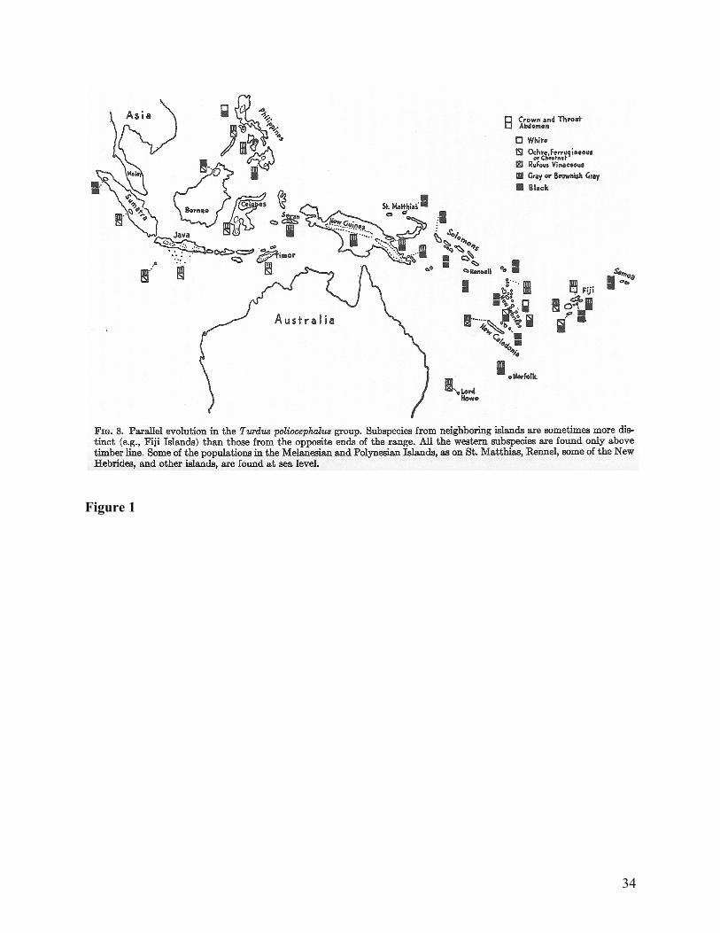
The key difficulty with the morphological concept is that “fertility and crossability vary

to some extent independently of morphological characters” (Mayr 1942, 116). This is a practical

problem in several ways. Variation within a geographically connected population sometimes

exceeds variation across isolated populations. See Figure 1 for an example of the geographic

variation Mayr had in mind. The morphological concept has no resources for helping the

systematist manage widespread geographic variation within populations. Another issue is that

organisms that are nearly identical morphologically and live in the same area may nonetheless

16

fail to interbreed — Mayr called these “sibling species.” It would be misleading to place these

two populations within the same species when their evolutionary fates are separate.

The biological species concept, then, tried to rectify these difficulties by defining species

as “groups of actually or potentially interbreeding natural populations, which are reproductively

isolated from other such groups” (Mayr 1942, 120). However, it is often difficult or impossible

to determine whether two populations can “actually or potentially” interbreed. Direct observation

only demonstrates actual interbreeding. Even laboratory experiments simply demonstrate the

possibility of interbreeding in an artificial setting, while what matters is whether species would

interbreed in the wild, given the opportunity.

In order to assist the practical application of the biological species concept, Mayr re-

appropriated morphological similarity as an indicator of propensity for interbreeding. “If we

examine the ‘good’ species of a certain locality we find that the reproductive gap is associated

with a certain degree of morphological difference. If we find a new group of individuals at a

different locality, we use the scale of differences between the species of the familiar area to help

us in determining whether the new form is a different species or not” (Mayr 1942, 121). In

addition, the judgment of the taxonomist would still play a role in some cases: when two

populations are similar but geographically isolated, “it is necessary … to leave it to the judgment

of the individual systematist, whether or not he considers two particular forms as ‘potentially

capable’ of interbreeding” (Mayr 1942, 120)

The biological species concept therefore set a new standard — reproductive isolation —

within which previous standards became re-interpreted and constrained. Simple morphological

similarity was no longer adequate evidence for grouping specimens together as species, since

sometimes highly similar species still do not interbreed. In the same way, dissimilarity alone was

17

no longer sufficient for placing specimens in different species. One also had to demonstrate the

absence of geographic continuity linking the populations and judge whether the dissimilarity

between isolated populations would prevent interbreeding. Difficult cases where good evidence

was lacking or the relationship between populations themselves was in flux would require expert

judgment (Mayr 1942, 114).

5. Articulating structure in the process of classification

In the introductory part of Systematics, Mayr briefly summarized the “procedure of the

systematist” (Mayr 1942, 11). As he wrote, “before our knowledge of a species reaches the point

where it can be included in a monograph, it has to be subjected to a definite process of study, of

which I will now give a short outline” (Mayr 1942, 12). One begins with collecting specimens,

and proceeds to identify them using previously published diagnostic criteria. “Very frequently,

however, particularly in less well-known groups of animals, some of the investigated specimens

do not agree with any described species. Here is where the difficulties of the conscientious

systematist begin. Before he can proceed to describe his specimens as a new species, he must

eliminate a number of other possibilities” (Mayr 1942, 13). Mayr goes on to describe several

issues that must be resolved: “There is considerable individual variation in most animals.

Perhaps his specimens are just extreme variants? Or there may be an undescribed sex or age

class, or an unknown ecotype” (Mayr 1942, 13). If the specimens cannot be resolved back into

known species, the systematist must then proceed to give a description, define which specimens

will stand as “types” for future reference, and follow the rules of nomenclature to name the new

species.5

5 For a broader discussion of how systematists presented the process of classification, see (Sterner 2013)

18

The “difficulties of the conscientious systematist” pick out exactly the point at which

Mayr sought to articulate new structure in the process of classification using his biological

species concept. When one finds that some specimens cannot be fit into an existing taxonomy,

certain questions must be answered in order to correctly judge their status as new species,

subspecies, developmental stages, different sexes, or extreme individual variants. Answering

these questions would require examining many other specimens labeled with their geographic

origin, local ecology, and so on.

Mayr’s intervention on the stage of identifying new species therefore had repercussions

throughout the whole process. For instance, one would need to collect many specimens from

populations across a geographic range and carefully record where they came from. Historically,

systematists and natural historians had often named new species based on a single specimen with

no geographic data (Johnson 2012), but this was hardly adequate from Mayr’s perspective, even

if sometimes unavoidable. However, this repercussion involved a shift in the content of the steps

— what must be done to move forward — instead of the order of steps6

6. Instituting methodological checkpoints

Mayr’s intervention in the practice of classification was intended to reform systematics,

alter the direction of the community as a whole. He sought to articulate both how cutting edge

biology should be done in systematics and how researchers in the field should judge each other’s

work. One major methodological innovation he developed was akin to a checklist of questions

one should answer in deciding the taxonomic rank of some group, i.e. species, subspecies, or

population. The checklist is effectively a tool for collecting existing knowledge about sources of

6 Classifying species using geographic variation also depended on a major shift in practice to using multiple type specimens to describe a species rather than a single type.

19

error and facilitating correct reasoning. However, it supplemented rather than replaced the expert

systematists’ judgment about how to deal with difficult cases. Next, we describe how Mayr

arrived at such methodological tools and what their limits were.

What could be articulated about the process of classification given Mayr’s theory of

species? In his view, the process of evolution exhibited an almost topological level of continuity:

in even attempting to define the nature of species, “we are confronted by the paradoxical

incongruity of trying to establish a fixed stage in the evolutionary stream. If there is evolution in

the true sense of the word, as against catastrophism or creation, we should find all kinds of

species—incipient species, mature species, and incipient genera, as well as all intermediate

conditions. To define the middle stage of this series perfectly… is just as impossible as to define

the middle stage in the life of man, mature man, so well that every single human male can be

identified as boy, mature man, or old man” (Mayr 1942, 114). What can be said within this

uniform stream of evolution? For Mayr, one could still draw distinctions between populations

based on observed discontinuities in a given slice of time.

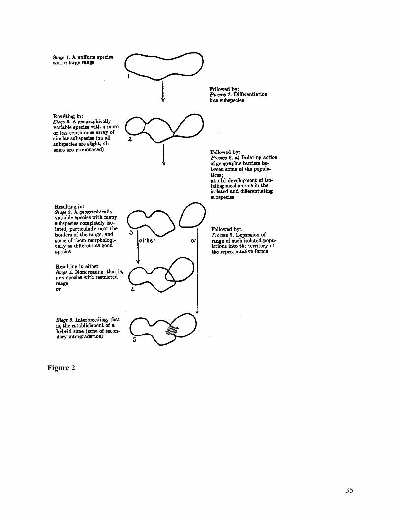
Figure 2 gives Mayr’s best shot at breaking the evolutionary process into stages. The

figure also serves as a practical guide for differentiating species and subspecies. Stage 2 of the

figure illustrates what it looks like for a species to be appropriately separable into subspecies.

Stages 3–5 illustrate the complex reasoning process that is involved with determining when

subspecies have become species. Once a group of populations that constitute a species has been

isolated geographically (Stage 3), it is able evolve independently. If a systematist observes two

populations that are similar but distinct and have overlapping ranges but no interbreeding, then

that is a good reason to declare them distinct but closely related species (Stage 4). However, if

the populations are taxonomically distinct but interbreed when their ranges overlap, they have

20

probably been isolated in the past but did not evolve to become different species (Stage 5).

Hence Figure 2 offers standardized criteria for recognizing species and subspecies, and it walks

the reader through what the evidence says about populations’ history and Mayr's inferred

evolutionary causes.

When the conscientious systematist faced specimens that he could not readily identify, he

was then supposed to consult his knowledge of their geographic distribution and variation. This

marked a distinctive stage in the overall process of classification that nonetheless potentially

concealed a great deal of further work as the systematist sought to classify his data under the

different stages. Mayr left it up to the systematist, for instance, how to judge what degree and

kinds of morphological variation would count as a barrier to reproduction. He also left it entirely

implicit how to account for limitations in the sampling of specimens in judging whether two

populations were geographically isolated.

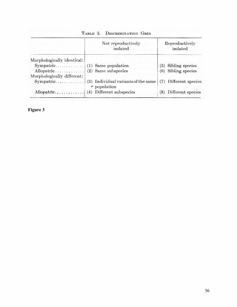
Mayr later codified the comparisons involved in using Figure 2 as a table in a textbook he

co-authored with E. Gorton Linsley and Robert L. Usinger (Mayr, Linsley, and Usinger 1953).

The table is called the discrimination grid (see Figure 3), and it differentiates classificatory

outcomes based on distinctions between three common sources of data: morphological similarity,

reproductive isolation, and geographic distribution.7 It offers a practical aid for the systematist

once he had gathered together the available evidence and compared the two samples using the

three distinctions. However, the authors note that evidence on reproductive isolation is often

7 The book suggests moving through the process by considering in order whether two samples are from the same population, the same species, or the same subspecies (Mayr, Linsley, and Usinger 1953, 79). However, the discussion of the discrimination grid that follows indicates that this sequence is imperfect. For example, the authors’ discussion of the grid indicates that one must sometimes decide whether two samples are from the same population or are sibling species.

21

missing, and they provide extensive further discussion of how to use indirect evidence to

distinguish between columns in the grid.

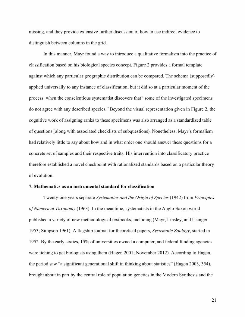
In this manner, Mayr found a way to introduce a qualitative formalism into the practice of

classification based on his biological species concept. Figure 2 provides a formal template

against which any particular geographic distribution can be compared. The schema (supposedly)

applied universally to any instance of classification, but it did so at a particular moment of the

process: when the conscientious systematist discovers that “some of the investigated specimens

do not agree with any described species.” Beyond the visual representation given in Figure 2, the

cognitive work of assigning ranks to these specimens was also arranged as a standardized table

of questions (along with associated checklists of subquestions). Nonetheless, Mayr’s formalism

had relatively little to say about how and in what order one should answer these questions for a

concrete set of samples and their respective traits. His intervention into classificatory practice

therefore established a novel checkpoint with rationalized standards based on a particular theory

of evolution.

7. Mathematics as an instrumental standard for classification

Twenty-one years separate Systematics and the Origin of Species (1942) from Principles

of Numerical Taxonomy (1963). In the meantime, systematists in the Anglo-Saxon world

published a variety of new methodological textbooks, including (Mayr, Linsley, and Usinger

1953; Simpson 1961). A flagship journal for theoretical papers, Systematic Zoology, started in

1952. By the early sixties, 15% of universities owned a computer, and federal funding agencies

were itching to get biologists using them (Hagen 2001; November 2012). According to Hagen,

the period saw “a significant generational shift in thinking about statistics” (Hagen 2003, 354),

brought about in part by the central role of population genetics in the Modern Synthesis and the

22

rise of computer technology.

While method was an ongoing subject of discussion in systematics, it took Sokal and

Sneath to fan the spark of methodology into a raging debate. Although they did not target Mayr

as a primary opponent in their book, they did argue against all systematists who used

evolutionary theory as a guide for selecting characters and naming species. Instead, Sokal and

Sneath grounded their methodology in a logical positivist theory of human reason. They also

updated and revised classical morphological traditions in taxonomy by introducing statistics,

computer technology, and information theory. In this section, we describe the positivist

background to numerical taxonomy and show how Sokal and Sneath appropriated it as a tool for

criticizing any reliance on evolutionary theory in classification.

The numerical taxonomy movement grew out of remarkably similar criticisms of existing

practices that originated independently in the U.S. and England in the late 1950’s, driven in each

case by the desire of an outsider for greater methodological clarity (Vernon 1988; Vernon 2001).

Eventually, Robert Sokal in Kansas connected with Peter Sneath in London, and they

collaborated to produce Principles of Numerical Taxonomy.

Sneath in particular was inspired by the botanist John Scott Lennox Gilmour, who wrote

an influential paper linking taxonomy and logical positivism (Gilmour 1940). Gilmour’s ideas

are readily apparent in Principles as theoretical backing for Sokal and Sneath’s methodology.

However, Principles contributed a practical interpretation to Gilmour’s work by aligning his

view of human reason with the use of statistics and computational procedures. Before getting to

the practical implementation, though, we need to describe the theoretical role played by logical

positivism in Gilmour’s view of classification.

23

Gilmour’s article, which ironically appeared in Julian Huxley’s volume on the New

Systematics (1940), begins by describing an ongoing debate among systematists. Gilmour

identifies himself with a group, in contrast to Mayr and others, that “feels doubtful whether a

‘logical’ classification (based on correlation or coherence of characters) is always and

necessarily a phylogenetic one” (Gilmour 1940, 461). Rather than engage in a further analysis of

evolutionary theory, Gilmour advances the view “that no satisfactory solution to these problems

is possible without first examining the fundamental principles which underlie the process of

classification, and, further, that these principles cannot be adequately formulated without basing

them on some epistemological theory of how scientists obtain their knowledge of the external

world” (Gilmour 1940, 462). In other words, Gilmour was advancing an alternative normative

basis for the debate over classification: systematists needed a better understanding of the

acquisition of scientific knowledge in general rather than of evolution, which was only one

natural process among many.

Gilmour went on to endorse a picture of human thought where the conscious mind

receives units of sense data that it actively packs together to form concepts. “For example, the

object which we call a chair consists partly of a number of experienced sense-data such as

colours, shapes, and other qualities, and partly of the concept chair which reason has constructed

to ‘clip’ these data together” (Gilmour 1940, 464; emphasis original). Since the classification of

a set of specimens under a common name is equivalent to subsuming them under a concept,

Gilmour reasoned that this theory of human knowledge has direct bearing on how to do

taxonomy:

“In any consideration of scientific method it is essential to distinguish between these ‘clips’ and the sense-data which they hold together. The latter are given, once and for all, and cannot be altered, whereas the former can be created and abolished at will so as the better to give a coherent picture of the every-increasing range of sense-data experienced.

24

For example, the phenomena of specific differentiation in Linnaeus’s day were clipped together by the concept of special creation, which was later replaced by the concept of gradual evolutionary differentiation” (Gilmour 1940, 464).

Epistemology therefore presents a methodological imperative for the taxonomist: keep

the category of “sense-data,” i.e. taxonomic characters of specimens, separate from the category

of concepts, which may change over time. Sokal and Sneath interpreted this imperative to mean

keeping evolutionary theory out of any role in guiding what data is relevant to classification and

weighting its importance. They believed that evolutionary theory was too theoretical in the

pejorative, speculative sense, and that involving systematists’ pet theories in the building of

classifications would breed instability, bias, and logical regress. Far from being a universal

standard for classification, Mayr’s application of the biological species concept would count as

radically limiting the value of any classification built under its guidance.

A general-purpose classification, by contrast, would be one that maximizes the number of

inductive generalizations that can be made about the specimens’ properties. These

generalizations of course represent a shorthand that “clips” together the properties for ease of

use. Gilmour calls this inductively optimal classification “natural,” whereas other classifications

are by comparison “artificial.” He writes, “What is the essential difference between [natural and

artificial]? Apart from any possible phylogenetic significance, … surely the fundamental

difference is that natural groups class together individuals which have a large number of

attributes in common, whereas in artificial groups the individuals concerned possess a much

smaller number of common attributes” (Gilmour 1940, 466).

While Gilmour’s argument is presented in purely qualitative terms, Sokal and Sneath

developed a computational procedure that realized it quantitatively. They used statistical

measures to evaluate the correlations between character data and applied clustering algorithms to

group the specimens according to their degree of similarity. The crucial challenge, then, became

25

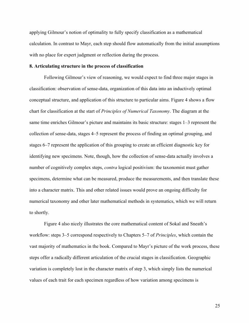
applying Gilmour’s notion of optimality to fully specify classification as a mathematical

calculation. In contrast to Mayr, each step should flow automatically from the initial assumptions

with no place for expert judgment or reflection during the process.

8. Articulating structure in the process of classification

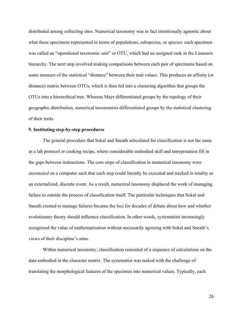
Following Gilmour’s view of reasoning, we would expect to find three major stages in

classification: observation of sense-data, organization of this data into an inductively optimal

conceptual structure, and application of this structure to particular aims. Figure 4 shows a flow

chart for classification at the start of Principles of Numerical Taxonomy. The diagram at the

same time enriches Gilmour’s picture and maintains its basic structure: stages 1–3 represent the

collection of sense-data, stages 4–5 represent the process of finding an optimal grouping, and

stages 6–7 represent the application of this grouping to create an efficient diagnostic key for

identifying new specimens. Note, though, how the collection of sense-data actually involves a

number of cognitively complex steps, contra logical positivism: the taxonomist must gather

specimens, determine what can be measured, produce the measurements, and then translate these

into a character matrix. This and other related issues would prove an ongoing difficulty for

numerical taxonomy and other later mathematical methods in systematics, which we will return

to shortly.

Figure 4 also nicely illustrates the core mathematical content of Sokal and Sneath’s

workflow: steps 3–5 correspond respectively to Chapters 5–7 of Principles, which contain the

vast majority of mathematics in the book. Compared to Mayr’s picture of the work process, these

steps offer a radically different articulation of the crucial stages in classification. Geographic

variation is completely lost in the character matrix of step 3, which simply lists the numerical

values of each trait for each specimen regardless of how variation among specimens is

26

distributed among collecting sites. Numerical taxonomy was in fact intentionally agnostic about

what these specimens represented in terms of populations, subspecies, or species: each specimen

was called an “operational taxonomic unit” or OTU, which had no assigned rank in the Linneaen

hierarchy. The next step involved making comparisons between each pair of specimens based on

some measure of the statistical “distance” between their trait values. This produces an affinity (or

distance) matrix between OTUs, which is then fed into a clustering algorithm that groups the

OTUs into a hierarchical tree. Whereas Mayr differentiated groups by the topology of their

geographic distribution, numerical taxonomists differentiated groups by the statistical clustering

of their traits.

9. Instituting step-by-step procedures

The general procedure that Sokal and Sneath articulated for classification is not the same

as a lab protocol or cooking recipe, where considerable embodied skill and interpretation fill in

the gaps between instructions. The core steps of classification in numerical taxonomy were

automated on a computer such that each step could literally be executed and tracked in totality as

an externalized, discrete event. As a result, numerical taxonomy displaced the work of managing

failure to outside the process of classification itself. The particular techniques that Sokal and

Sneath created to manage failures became the loci for decades of debate about how and whether

evolutionary theory should influence classification. In other words, systematists increasingly

recognized the value of mathematization without necessarily agreeing with Sokal and Sneath’s

views of their discipline’s aims.

Within numerical taxonomy, classification consisted of a sequence of calculations on the

data embodied in the character matrix. The systematist was tasked with the challenge of

translating the morphological features of the specimen into numerical values. Typically, each

27

measurement of a trait would turn into a discrete variable (e.g. 0 or 1) or a continuous variable

(any value from 0 to 1). For each specimen, the taxonomist would measure or score a set number

of traits. The data for each specimen forms a column in step 3 of Figure 4. Since there are

multiple specimens, the lists of measurements for each specimen are then combined together as a

matrix. This matrix is the basic mathematical object on which all further computations depended,

and the set of all possible matrices (according to certain restrictions) forms the semantic domain

over which the classification algorithms would work.

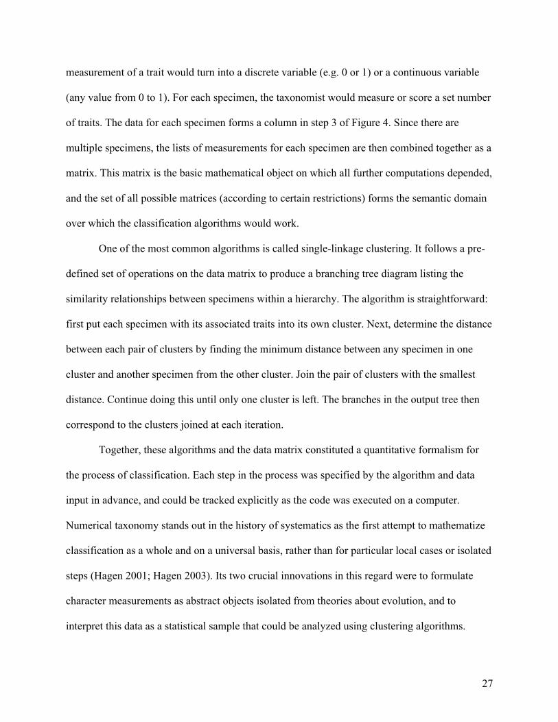
One of the most common algorithms is called single-linkage clustering. It follows a pre-

defined set of operations on the data matrix to produce a branching tree diagram listing the

similarity relationships between specimens within a hierarchy. The algorithm is straightforward:

first put each specimen with its associated traits into its own cluster. Next, determine the distance

between each pair of clusters by finding the minimum distance between any specimen in one

cluster and another specimen from the other cluster. Join the pair of clusters with the smallest

distance. Continue doing this until only one cluster is left. The branches in the output tree then

correspond to the clusters joined at each iteration.

Together, these algorithms and the data matrix constituted a quantitative formalism for

the process of classification. Each step in the process was specified by the algorithm and data

input in advance, and could be tracked explicitly as the code was executed on a computer.

Numerical taxonomy stands out in the history of systematics as the first attempt to mathematize

classification as a whole and on a universal basis, rather than for particular local cases or isolated

steps (Hagen 2001; Hagen 2003). Its two crucial innovations in this regard were to formulate

character measurements as abstract objects isolated from theories about evolution, and to

interpret this data as a statistical sample that could be analyzed using clustering algorithms.

28

While the character matrix and clustering algorithm appear to jointly determine the

classification, the methodological challenge for numerical taxonomy quickly became coping

with the need for multiple competing techniques for building matrices, measuring distances, and

clustering. In the case of clustering algorithms, single-linkage is only one of many possibilities,

each of which differs over exactly how it joins groups together. For instance, should one instead

join groups based on the maximum distance between any of their members, or between their

centers of mass? Another vexing issue was whether to count the absence of a character in a

particular specimen as providing positive information. This appeared counterintuitive in cases

where one specimen had a unique trait, such as a spiny back, that no other specimen shared.

Should all the other specimens be judged more similar because one specimen stands out?

Attempting to answer these questions led Sokal and Sneath to adopt a strategy of

contextualizing the overall process of classification. Gilmour’s notion of clipping together sense

data in an optimal way offered little guidance for these practical difficulties, but they pursued the

idea that one could manage the plurality of methodological choices by identifying kinds of

situations where one option was demonstrably better than the others (Sneath and Sokal 1973,

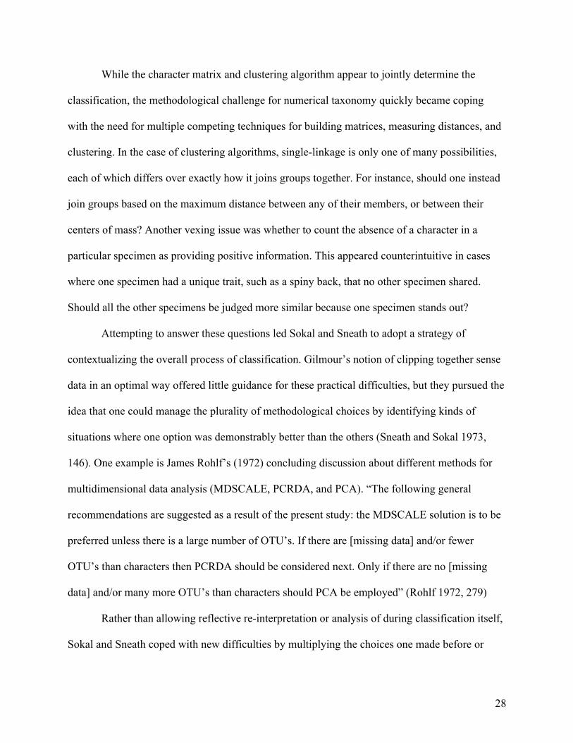
146). One example is James Rohlf’s (1972) concluding discussion about different methods for

multidimensional data analysis (MDSCALE, PCRDA, and PCA). “The following general

recommendations are suggested as a result of the present study: the MDSCALE solution is to be

preferred unless there is a large number of OTU’s. If there are [missing data] and/or fewer

OTU’s than characters then PCRDA should be considered next. Only if there are no [missing

data] and/or many more OTU’s than characters should PCA be employed” (Rohlf 1972, 279)

Rather than allowing reflective re-interpretation or analysis of during classification itself,

Sokal and Sneath coped with new difficulties by multiplying the choices one made before or

29

after the process. Once one embarks on the classification process (for instance by telling the

computer to execute the code), no further human judgment is needed — the determination of the

process by the character matrix and clustering algorithm is complete. This reflects what we call a

“complete first-order linearization” strategy for mathematization, such that meta-level judgment

or discussion about the mathematized process is only legitimate outside the process itself. While

this view of how classification should work may seem extreme, or even implausibly naïve, Sokal

in particular was genuinely motivated by the idea that human expertise was entirely replaceable

by mathematical procedures (Sokal and Rohlf 1970; Vernon 1988).

10. Conclusion

Instead of attempting to explain a static field of mathematical successes collected

according to present-day standards, we have argued for viewing mathematization as a normative

activity that transforms what counts as scientific success. This approach enabled us to establish

the distinctive features of mathematization as a program for institutional change in the case of

numerical taxonomy within systematic biology. One important remaining issue, though, is to

clarify what roles logical positivism and operationalization played in mathematizing

classification.

Looking forward from the 1960’s, new methods for classification, such as numerical

cladistics and phyletics, grew out of numerical taxonomy that did not always share its allegiance

to logical positivism (Eades 1970; Hagen 2001). In this regard, we can see that Sokal and Sneath

used positivism to formulate a particular way in which classification should be statistical. As a

sequence of mathematical procedures, however, their method could be used and modified

independently of positivism. Given the basic sequence of steps identified in Figure 4, one could

substitute different calculations that abandoned certain key tenets of numerical taxonomy, such

30

as equal weighting of character traits. The effects of mathematization on classification therefore

extended beyond the influence of positivism, although the rise of “pattern cladism” in the 1980’s

shows how they remained intimately related (Hull 1990).

By contrast, we argue that operationalization cannot be isolated in this way from the

mathematization of classification. In general, operationalizing a task by listing a sequence of

actions, for example in a recipe or protocol, does not require mathematization. In the particular

historical context of numerical taxonomy, however, mathematical reasoning had come to depend

constitutively on operationalization. In the first half of the twentieth century, multiple normative

projects within mathematics, such as Whitehead and Russell’s Principia Mathematica or

Hilbert’s program, sought to define mathematical reasoning axiomatically as a sequence of steps

justified by the application of universal rules (Gray 2008). Under this ideal, one could not

successfully mathematize a reasoning process without also operationalizing it by stating the

sequence of manipulations to be applied at each step. This shift in the standards of mathematics

also proved decisive for the invention and design of computers, which automated mathematical

reasoning as a formal process of symbolic manipulations.

While Sokal and Sneath did not engage with axiomatics directly, some of their students

did (e.g. Jardine and Sibson 1971). Sokal and Sneath also recognized the value of mathematical

methods for the objectivity and repeatability of classification and the necessity of using

computers for numerical taxonomy to be practical (Sokal and Sneath 1963, 48-49; Vernon 1988).

Similarly, a basic tenet of logical positivism was that valid human reasoning could be fully

articulated in terms of first-order logic. While one could perhaps have sought to mathematize

classification based on an alternative ideal of math, Sokal and Sneath embraced this historical

change in math rather than rejecting it. As a result, operationalizing classification was part and

31

parcel of mathematizing it for numerical taxonomy. This reality is likely here to stay because the

growing size of genomic data sets has entrenched the necessity of computers for taxonomy

(Suárez-Díaz and Anaya-Muñoz 2008).

11. Acknowledgments

[Removed for blinding.]

12. References

Abraham, Tara H. 2004. “Nicolas Rashevsky's Mathematical Biophysics.” Journal of the History of Biology 37 (2): 333–385.

Baker, A. 2012. “Science-Driven Mathematical Explanation.” Mind 121 (482): 243–267. Colyvan, Mark. 2014. “Indispensability Arguments in the Philosophy of Mathematics.” Edited

by Edward N Zalta. The Stanford Encyclopedia of Philosophy. March. http://plato.stanford.edu/archives/spr2014/entries/mathphil-indis/.

Corry, Leo. 2006. “Axiomatics, Empiricism, and Anschauung in Hilbert's Conception of Geometry: Between Arithmetic and General Relativity.” In The Architecture of Modern Mathematics: Essays in History and Philosophy, edited by J Ferreiros and Jeremy J Gray, 133–156. New York: Oxford University Press.

Eades, David C. 1970. “Theoretical and Procedural Aspects of Numerical Phyletics.” Systematic Zoology 19 (2): 142–171.

Farber, Paul Lawrence. 1976. “The Type-Concept in Zoology During the First Half of the Nineteenth Century.” Journal of the History of Biology 9 (1): 93–119.

Gerson, Elihu M. 2008. “Reach, Bracket, and the Limits of Rationalized Coordination: Some Challenges for CSCW.” In Resources, Co-Evolution and Artifacts: Theory in CSCW, edited by Mark S Ackerman, Christine A Halverson, Thomas Erickson, and Wendy A Kellogg, 193–220. London: Springer.

Gilmour, John Scott Lennox. 1940. “Taxonomy and Philosophy.” In The New Systematics, edited by Julian Huxley, 461–474. The New Systematics. Oxford: Oxford: Clarendon Press.

Gray, Jeremy. 2008. Plato's Ghost: the Modernist Transformation of Mathematics. Princeton, NJ: Princeton University Press.

Griesemer, James R. 2006. “Theoretical Integration, Cooperation, and Theories as Tracking Devices.” Biological Theory 1 (1): 4–7.

Griesemer, James R. 2007. “Tracking Organic Processes: Representations and Research Styles in Classical Embryology and Genetics.” In From Embryology to Evo-Devo: a History of Developmental Evolution, edited by Jane Maienschein and Manfred D Laubichler, 375–435. Cambridge, MA: MIT Press.

Griesemer, James R. 2012. “Formalization and the Meaning of ‘Theory’ in the Inexact Biological Sciences.” Biological Theory 7 (4): 298–310.

Hagen, Joel B. 2001. “The Introduction of Computers Into Systematic Research in the United States During the 1960s.” Studies in the History and Philosophy of Biological and Biomedical Sciences 32 (2): 291–314.

Hagen, Joel B. 2003. “The Statistical Frame of Mind in Systematic Biology From Quantitative

32

Zoology to Biometry.” Journal of the History of Biology 36 (2): 353–384. Hull, David L. 1990. Science as a Process: an Evolutionary Account of the Social and

Conceptual Development of Science. Chicago: University of Chicago Press. Huxley, Julian, ed. 1940. The New Systematics. Oxford: Oxford: Clarendon Press. Jardine, Nicholas, and Robin Sibson. 1971. Mathematical Taxonomy. New York: Wiley. Johnson, Kristin. 2012. Ordering Life: Karl Jordan and the Naturalist Tradition. Baltimore:

Johns Hopkins University Press. Maddy, Penelope. 1997. Naturalism in Mathematics. Oxford: Clarendon Press. Mayr, Ernst. 1942. Systematics and the Origin of Species From the Viewpoint of a Zoologist. 1st

ed. New York: Columbia University Press. Mayr, Ernst. 1999. Systematics and the Origin of Species From the Viewpoint of a Zoologist. 2nd

ed. Cambridge, MA: Harvard University Press. Mayr, Ernst, and William Provine. 1980. The Evolutionary Synthesis. Edited by Ernst Mayr and

William Provine. Cambridge, MA: Harvard University Press. Mayr, Ernst, EG Linsley, and R Usinger. 1953. Methods and Principles of Systematic Zoology.

New York: McGraw-Hill. November, Joseph A. 2012. Biomedical Computing: Digitizing Life in the United States.

Baltimore: Johns Hopkins University Press. Rohlf, F James. 1972. “An Empirical Comparison of Three Ordination Techniques in Numerical

Taxonomy.” Systematic Zoology 21 (3): 271–280. Sellars, Wilfrid. 1997. Empiricism and the Philosophy of Mind. Cambridge, MA: Harvard

University Press. Simpson, George Gaylord. 1961. Principles of Animal Taxonomy. New York: Columbia

University Press. Sneath, Peter HA, and Robert R Sokal. 1973. Numerical Taxonomy: the Principles and Practice

of Numerical Classification. San Francisco: WH Freeman and Company. Sokal, Robert R, and F James Rohlf. 1970. “The Intelligent Ignoramus, an Experiment in

Numerical Taxonomy.” Taxon 19 (3): 305–319. Sokal, Robert R, and Peter HA Sneath. 1963. Principles of Numerical Taxonomy. San Francisco:

W.H. Freeman and Company. Sterner, Beckett W. 2013. “Well-Structured Biology: Numerical Taxonomy and Its

Methodological Vision for Systematics.” In The Evolution of Phylogenetic Systematics, edited by Andrew Hamilton. Los Angeles: University of California Press.

Stigler, Stephen M. 2010. “Darwin, Galton and the Statistical Enlightenment.” Journal of the Royal Statistical Society A 173 (3): 469–482.

Suárez-Díaz, Edna, and Victor H Anaya-Muñoz. 2008. “History, Objectivity, and the Construction of Molecular Phylogenies.” Studies in History and Philosophy of Biolo 39 (4): 451–468.

Vernon, Keith. 1988. “The Founding of Numerical Taxonomy.” British Journal for the History of Science 21 (2): 143–159.

Vernon, Keith. 2001. “A Truly Taxonomic Revolution? Numerical Taxonomy 1957-1970.” Studies in the History and Philosophy of Biological and Biomedical Sciences 32 (2): 315–341.

Wigner, Eugene P. 1960. “The Unreasonable Effectiveness of Mathematics in the Natural Sciences.” Communications on Pure and Applied Mathematics XII: 1–14.

Wilkins, John S. 2009. Species: a History of the Idea. Berkeley, CA: University of California

33

Press. Wilson, Mark. 2006. Wandering Significance: an Essay on Conceptual Behavior. New York:

Oxford University Press. Wimsatt, William C. 2007. Re-Engineering Philosophy for Limited Beings: Piecewise

Approximations to Reality. Cambridge, MA: Harvard University Press.

34

Figure 1

35

Figure 2

36

Figure 3

37

Figure 4

38

Collecting How many specimens are needed and from where?

Identifying Does a specimen fall under any pre-existing species descriptions?

Describing Two possible objects of description: the particular specimen that one collected, and the group of which it is an instance.

Naming If a specimen doesn’t match existing categories, should it stand for a new subspecies or species (and maybe genus)?

Revising How should a classification change to reflect novel variation observed in new specimens?

Table 1

39

Figure and Table Captions Table 1: Common tasks in taxonomy. Figure 1: An example of geographic variation in two characters across a range and between subspecies within the range. From (Mayr 1999, 58) Figure 2: “The Stages of Speciation” from (Mayr 1999, 160). Figure 3: Distinguishing ranks of populations. Figure 4: The seven stages of classification according to numerical taxonomy. From (Sokal and Sneath 1963).