The Mean and Scatter of the Velocity Dispersion-Optical Richness Relation for maxBCG Galaxy Clusters
25
arXiv:0704.3614v2 [astro-ph] 19 Oct 2007 Draft version December 31, 2013 Preprint typeset using L A T E X style emulateapj v. 08/22/09 THE MEAN AND SCATTER OF THE VELOCITY-DISPERSION–OPTICAL RICHNESS RELATION FOR MAXBCG GALAXY CLUSTERS M. R. Becker 1 , T.A. McKay 1,2 , B. Koester 3 , R. H. Wechsler 4 , E. Rozo 5 , A. Evrard 1,2,6 , D. Johnston 7 , E. Sheldon 8 , J. Annis 9 , E. Lau 3 , R. Nichol 10 , and C. Miller 2 Draft version December 31, 2013 ABSTRACT The distribution of galaxies in position and velocity around the centers of galaxy clusters encodes important information about cluster mass and structure. Using the maxBCG galaxy cluster catalog identified from imaging data obtained in the Sloan Digital Sky Survey, we study the BCG–galaxy velocity correlation function. By modeling its non-Gaussianity, we measure the mean and scatter in velocity dispersion at fixed richness. The mean velocity dispersion increases from 202 ± 10 km s −1 for small groups to more than 854 ± 102 km s −1 for large clusters. We show the scatter to be at most 40.5 ± 3.5%, declining to 14.9 ± 9.4% in the richest bins. We test our methods in the C4 cluster catalog, a spectroscopic cluster catalog produced from the Sloan Digital Sky Survey DR2 spectroscopic sample, and in mock galaxy catalogs constructed from N-body simulations. Our methods are robust, measuring the scatter to well within one-sigma of the true value, and the mean to within 10%, in the mock catalogs. By convolving the scatter in velocity dispersion at fixed richness with the observed richness space density function, we measure the velocity dispersion function of the maxBCG galaxy clusters. Although velocity dispersion and richness do not form a true mass–observable relation, the relationship between velocity dispersion and mass is theoretically well characterized and has low scatter. Thus our results provide a key link between theory and observations up to the velocity bias between dark matter and galaxies. Subject headings: galaxies: clusters: general — cosmology — methods: data analysis 1. INTRODUCTION Galaxy clusters play an important role in observa- tions of the large-scale structure of the Universe. As dramatically non-linear features in the matter distri- bution, they stand out as individually identifiable ob- jects, whose abundant galaxies and hot X-ray emit- ting gas provide a rich variety of observable prop- erties. Clusters can be identified by their galaxy content (Bahcall et al. 2003; Gladders & Yee 2005; Miller et al. 2005; Gerke et al. 2005; Berlind et al. 2006; Koester et al. 2007a,b), their thermal X-ray emission (Rosati et al. 1998; B¨ohringer et al. 2000; Popesso et al. 2004), the Sunyaev-Zeldovich decrement they produce in the microwave background signal (Grego et al. 2000; Lancaster et al. 2005), or the weak lensing signature they produce in the shapes of distant background galax- ies (Wittman et al. 2006). Each of these identification methods also produces proxies for mass: e.g, the num- ber of galaxies, total stellar luminosity, galaxy velocity 1 Department of Physics, University of Michigan, Ann Arbor, MI 48109 2 Department of Astronomy, University of Michigan, Ann Arbor, MI, 48109 3 Department of Astronomy and Astrophysics, University of Chicago, Chicago, IL, 60637 4 Kavli Institute for Particle Astrophysics and Cosmology, Physics Department, and Stanford Linear Accelerator Center, Stanford University, Stanford, CA 94305 5 CCAPP, The Ohio State University, Columbus, OH 43210 6 Michigan Center for Theoretical Physics, University of Michi- gan, Ann Arbor, MI 48109 7 Jet Propulsion Laboratory, Caltech, Pasadena, CA, 91109 8 Department of Physics, New York University, 4 Washington Place, New York, NY 10003 9 Fermi National Accelerator Laboratory, Batavia, IL, 60510 10 Portsmouth University, Portsmouth England dispersion, X-ray luminosity and temperature, or SZ and weak lensing profiles. Simulations of the formation and evolution of large- scale structure through gravitational collapse provide us with rich predictions for the expected matter dis- tribution within a given cosmology (Evrard et al. 2002; Springel et al. 2005). These predictions include not only first-order features, like the halo mass function n(M,z), but higher-order correlations as well, like the precise way in which galaxy clusters are themselves clustered as a function of mass. Comparisons of these theoretical pre- dictions to the observed Universe provide an excellent op- portunity to test our understanding of cosmology and the formation of large-scale structure. The weak point in this chain is that simulations most reliably predict the dark matter distribution, while observations are most directly sensitive to luminous galaxies and gas. Connections be- tween observable properties and theoretical predictions for dark matter have often been made through simplify- ing assumptions that are hard to justify a priori. Progress toward solving this problem has been made by the construction of various mass–observable scaling rela- tions, which are based on combinations of theoretical pre- dictions and observational measurements (Levine et al. 2002; Dahle 2006; Stanek et al. 2006). However, knowl- edge of the mean mass at a fixed value of the observ- able is not sufficient to extract precise cosmological con- straints given the exponential shape of the halo mass function (Lima & Hu 2004, 2005). To perform precision cosmology, we must understand the scatter in the mass– observable relations as well. Recently, Stanek et al. (2006) measured the scatter in the temperature-luminosity relation for X-ray selected galaxy clusters and used it to infer the scatter in the
-
Upload
independent -
Category
Documents
-
view
1 -
download
0
Transcript of The Mean and Scatter of the Velocity Dispersion-Optical Richness Relation for maxBCG Galaxy Clusters

arX
iv:0
704.
3614
v2 [
astr
o-ph
] 1
9 O
ct 2
007
Draft version December 31, 2013Preprint typeset using LATEX style emulateapj v. 08/22/09
THE MEAN AND SCATTER OF THE VELOCITY-DISPERSION–OPTICAL RICHNESS RELATION FORMAXBCG GALAXY CLUSTERS
M. R. Becker1, T.A. McKay1,2, B. Koester3, R. H. Wechsler4, E. Rozo5, A. Evrard1,2,6, D. Johnston7, E.Sheldon8, J. Annis9, E. Lau3, R. Nichol10, and C. Miller2
Draft version December 31, 2013
ABSTRACT
The distribution of galaxies in position and velocity around the centers of galaxy clusters encodesimportant information about cluster mass and structure. Using the maxBCG galaxy cluster catalogidentified from imaging data obtained in the Sloan Digital Sky Survey, we study the BCG–galaxyvelocity correlation function. By modeling its non-Gaussianity, we measure the mean and scatter invelocity dispersion at fixed richness. The mean velocity dispersion increases from 202 ± 10 km s−1
for small groups to more than 854 ± 102 km s−1 for large clusters. We show the scatter to be atmost 40.5± 3.5%, declining to 14.9± 9.4% in the richest bins. We test our methods in the C4 clustercatalog, a spectroscopic cluster catalog produced from the Sloan Digital Sky Survey DR2 spectroscopicsample, and in mock galaxy catalogs constructed from N-body simulations. Our methods are robust,measuring the scatter to well within one-sigma of the true value, and the mean to within 10%, in themock catalogs. By convolving the scatter in velocity dispersion at fixed richness with the observedrichness space density function, we measure the velocity dispersion function of the maxBCG galaxyclusters. Although velocity dispersion and richness do not form a true mass–observable relation,the relationship between velocity dispersion and mass is theoretically well characterized and has lowscatter. Thus our results provide a key link between theory and observations up to the velocity biasbetween dark matter and galaxies.Subject headings: galaxies: clusters: general — cosmology — methods: data analysis
1. INTRODUCTION
Galaxy clusters play an important role in observa-tions of the large-scale structure of the Universe. Asdramatically non-linear features in the matter distri-bution, they stand out as individually identifiable ob-jects, whose abundant galaxies and hot X-ray emit-ting gas provide a rich variety of observable prop-erties. Clusters can be identified by their galaxycontent (Bahcall et al. 2003; Gladders & Yee 2005;Miller et al. 2005; Gerke et al. 2005; Berlind et al. 2006;Koester et al. 2007a,b), their thermal X-ray emission(Rosati et al. 1998; Bohringer et al. 2000; Popesso et al.2004), the Sunyaev-Zeldovich decrement they producein the microwave background signal (Grego et al. 2000;Lancaster et al. 2005), or the weak lensing signaturethey produce in the shapes of distant background galax-ies (Wittman et al. 2006). Each of these identificationmethods also produces proxies for mass: e.g, the num-ber of galaxies, total stellar luminosity, galaxy velocity
1 Department of Physics, University of Michigan, Ann Arbor,MI 48109
2 Department of Astronomy, University of Michigan, Ann Arbor,MI, 48109
3 Department of Astronomy and Astrophysics, University ofChicago, Chicago, IL, 60637
4 Kavli Institute for Particle Astrophysics and Cosmology,Physics Department, and Stanford Linear Accelerator Center,Stanford University, Stanford, CA 94305
5 CCAPP, The Ohio State University, Columbus, OH 432106 Michigan Center for Theoretical Physics, University of Michi-
gan, Ann Arbor, MI 481097 Jet Propulsion Laboratory, Caltech, Pasadena, CA, 911098 Department of Physics, New York University, 4 Washington
Place, New York, NY 100039 Fermi National Accelerator Laboratory, Batavia, IL, 6051010 Portsmouth University, Portsmouth England
dispersion, X-ray luminosity and temperature, or SZ andweak lensing profiles.
Simulations of the formation and evolution of large-scale structure through gravitational collapse provideus with rich predictions for the expected matter dis-tribution within a given cosmology (Evrard et al. 2002;Springel et al. 2005). These predictions include not onlyfirst-order features, like the halo mass function n(M,z),but higher-order correlations as well, like the precise wayin which galaxy clusters are themselves clustered as afunction of mass. Comparisons of these theoretical pre-dictions to the observed Universe provide an excellent op-portunity to test our understanding of cosmology and theformation of large-scale structure. The weak point in thischain is that simulations most reliably predict the darkmatter distribution, while observations are most directlysensitive to luminous galaxies and gas. Connections be-tween observable properties and theoretical predictionsfor dark matter have often been made through simplify-ing assumptions that are hard to justify a priori.
Progress toward solving this problem has been made bythe construction of various mass–observable scaling rela-tions, which are based on combinations of theoretical pre-dictions and observational measurements (Levine et al.2002; Dahle 2006; Stanek et al. 2006). However, knowl-edge of the mean mass at a fixed value of the observ-able is not sufficient to extract precise cosmological con-straints given the exponential shape of the halo massfunction (Lima & Hu 2004, 2005). To perform precisioncosmology, we must understand the scatter in the mass–observable relations as well.
Recently, Stanek et al. (2006) measured the scatter inthe temperature-luminosity relation for X-ray selectedgalaxy clusters and used it to infer the scatter in the
2 BECKER ET AL.
mass–luminosity relationship. Unfortunately, there arerelatively few measurements of the scatter in any mass–observable relationship in the optical. (An exception isan early observation of scatter in the velocity-dispersion–richness relationship for a small sample of massive clus-ters by Mazure et al. 1996.) For optically selected clus-ters, the scatter is usually included as a parameter in theanalysis (e.g. Gladders et al. 2007; Rozo et al. 2007a,b).
The primary goal of this work is to develop a methodto estimate both the mean and scatter in the clustervelocity-dispersion–richness relation. This comparisonbetween two observable quantities can be made withoutreference to structure formation theory. The method de-veloped is applied to the SDSS maxBCG cluster catalog-a photometrically selected catalog with extensive spec-troscopic follow-up. These methods are tested exten-sively with both the C4 catalog (Miller et al. 2005), asmaller spectroscopically-selected sample of clusters, andnew mock catalogs generated by combining N-body sim-ulations with a prescription for galaxy population (Wech-sler et al. 2007, in preparation).
Ultimately, we aim to connect richness to mass throughmeasurements of velocity dispersion. While the linkbetween dark matter velocity dispersion and mass isknown from N-body simulations to have very small scat-ter (Evrard et al. 2007), the relationship between galaxyand dark matter velocity dispersion (the velocity bias) re-mains uncertain and will require additional study. Con-straints on the normalization and scatter of the totalmass-richness relation obtained by this method are thuslimited by uncertainty in the velocity bias.
An outline of the SDSS data and simulations used inthis work is presented in §2. In §3, we provide a briefoverview of the maxBCG cluster finding algorithm andthe properties of the detected cluster sample. We willfocus in this paper on measurements of the BCG–galaxyvelocity correlation function (BGVCF), which is intro-duced along with the various fitting methods we employin §4. Section 5 presents a new method for understand-ing the scatter in the optical richness-velocity dispersionrelation and the computation of the velocity dispersionfunction for the maxBCG clusters. Section 6 presentsmeasurements of the BGVCF as a function of variouscluster properties. We connect our velocity dispersionmeasurements to mass in §7. Finally, we conclude anddiscuss future directions in §8.
2. SDSS DATA AND MOCK CATALOGS
2.1. SDSS Data
Data for this study are drawn from the SDSS(York et al. 2000; Abazajian et al. 2004, 2005;Adelman-McCarthy et al. 2006), a combined imag-ing and spectroscopic survey of ∼ 104 deg2 in the NorthGalactic Cap, and a smaller, deeper region in the South.The imaging survey is carried out in drift-scan modein the five SDSS filters (u, g, r, i, z) to a limitingmagnitude of r<22.5 (Fukugita et al. 1996; Gunn et al.1998; Smith et al. 2002). Galaxy clusters are selectedfrom ∼ 7500 sq. degrees of available SDSS imagingdata, and from the mock catalogs described below, usingthe maxBCG method (Koester et al. 2007b) which isoutlined in §3.
The spectroscopic survey targets a “main” sample of
galaxies with r<17.8 and a median redshift of z∼0.1(Strauss et al. 2002) and a “luminous red galaxy” sample(Eisenstein et al. 2001) which is roughly volume limitedout to z=0.38, but further extends to z=0.6. The “main”sample composes about 90% of the catalog, with the “lu-minous red galaxy” sample making up the rest. Velocityerrors in the redshift survey are ∼30 km s−1. We usethe SDSS DR5 spectroscopic catalog which includes over640,000 galaxies. The mask for our spectroscopic catalogwas taken from the New York University Value-AddedGalaxy Catalog (Blanton et al. 2005).
2.2. Mock Galaxy Catalogs
In order to understand the robustness of our meth-ods for measuring the mean and scatter of the relationbetween cluster velocity dispersion and richness, we per-form several tests on realistic mock galaxy catalogs. Be-cause the maxBCG method relies on measurements ofgalaxy positions, luminosities, and colors and their clus-tering, these catalogs must reproduce these aspects ofthe SDSS data in some detail.
In this work, we use mock catalogs created by theADDGALS (Adding Density-Determined Galaxies toLightcone Simulations) method (described by Wechsleret al. 2007, in preparation) which is specifically de-signed for this purpose. These catalogs populate adark matter light-cone simulation with galaxies using anobservationally-motivated biasing scheme. Galaxies areinserted in these simulations at the locations of individ-ual dark matter particles, subject to several empiricalconstraints. The relation between dark matter particlesof a given over-density (on a mass scale of ∼ 1013M⊙)is connected to the two point correlation function ofthese particles. This connection is used to assign subsetsof particles to galaxies using a probability distributionP (δ|Lr), chosen to reproduce the luminosity-dependentcorrelation function of galaxies as measured in the SDSSby Zehavi et al. (2005). The number of galaxies of agiven brightness placed within the simulations is deter-mined from the measured SDSS r-band galaxy luminos-ity function (Blanton et al. 2003). We consider galaxiesbrighter than 0.4 L∗, because it is these galaxies that arecounted in the maxBCG richness estimate. Finally, col-ors are assigned to each galaxy by measuring their localgalaxy density in redshift space, and assigning to themthe colors of a real SDSS galaxy with similar luminosityand local density (see also Tasitsiomi et al. 2004). Thelocal density measure used is the fifth nearest neighborgalaxy in a magnitude and redshift slice, and for SDSSgalaxies is taken from a volume-limited sample of theCMU-Pitt DR4 Value Added Catalog11.
This method produces mock galaxy catalogs whosegalaxies reproduce several properties of the observedSDSS galaxies. In particular, they follow the empir-ical galaxy color–density relation and its evolution, aproperty of fundamental importance for ridgeline-basedcluster detection methods. The process accounts for k-corrections between rest and observed frame colors andassigns realistic photometric errors. Each mock galaxy isassociated with a dark matter particle and adopts its 3Dmotion. This is important, as it encodes in the motionsof the mock galaxies the full dynamical richness of the
11 Available at www.sdss.org/dr4/products/value added.

THE CLUSTER VELOCITY-DISPERSION–RICHNESS RELATION 3
N-body simulation. Galaxies may occupy fully virializedregions, be descending into clusters for the first time, orbe slowly streaming along nearby filaments. This com-plete sampling of the velocity field around fully realizedN-body halos is essential, as these mock catalogs allowus to predict directly the velocity structure we ought toobserve in the data. Note that this simulation process,by design, assumes no velocity bias between the darkmatter and the luminous galaxies, except for the BCG,which is made by artificially placing the brightest galaxyassigned to a given halo at its dynamic center.
In this work, we use two mock catalogs based on dif-ferent simulations. The first is based on the Hubble Vol-ume simulation (the MS lightcone of Evrard et al. 2002),which has a particle mass of 2.25 × 10¹²M⊙ while thesecond is based on a simulation run at Los Alamos Na-tional Laboratory (LANL) using the Hashed-Oct-Treecode (Warren 1994). This simulation tracks the evolu-tion of 3843 particles with 6.67×10¹¹M⊙ in a box of sidelength 768 Mpc h−1, and is referred to as the “higherresolution” simulation in what follows. Both simula-tions have cosmological parameters Ωm = 0.3, ΩΛ = 0.7,h = 0.7 and σ8 = 0.9.
In addition to the galaxy list we have a list of dark mat-ter halos, defined using a spherical over-density clusterfinder (e.g. Evrard et al. 2002). By running the clusterfinding algorithm on the mock catalogs, we connect clus-ters detected “observationally” from their galaxy contentwith simulated dark matter halos in a direct way.
2.3. Velocity Bias
Given that there is still substantial uncertainty in theamount of velocity bias for various galaxy samples, wemust be careful to avoid velocity bias dependent conclu-sions. The mock catalogs with which we are comparingdo not explicitly include velocity bias. Fortunately, wewill only incur errors due to velocity bias when we es-timate masses or directly compare velocity dispersionsmeasured in the mock catalogs to those measured in thedata. Therefore in most of our analysis, velocity biashas no effect. Where it is relevant, we choose to leavevelocity bias as a free parameter because of its currentobservational and theoretical uncertainties.
Observational uncertainties in velocity bias arise sim-ply because it is exceedingly difficult to measure. Tomake such a measurement, one usually requires two in-dependent determinations of mass, one of them based ondynamical measurements, each subject to systematic andrandom errors (e.g. Carlberg 1994). Another techniquewas recently used by Rines et al. (2006), namely con-straining the velocity bias by measuring the virial massfunction and comparing it to other independent cosmo-logical constraints. Their analysis resulted in a bias ofbv ∼ 1.1 − 1.3. Unfortunately, this technique folds insystematic errors from the other analyses.
In the past, theoretical predictions of velocity biaswere affected by numerical over-merging and low reso-lution (e.g. Frenk et al. 1996; Ghigna et al. 2000). Mostestimates of velocity bias based on high-resolutionN-body simulations have given bv ∼ 1.0 − 1.3(Colın et al. 2000; Ghigna et al. 2000; Diemand et al.2004; Faltenbacher et al. 2005), partially depending onthe mass regime studied. Recent theoretical work has
shown that differing methods of subhalo selection in N-body simulations change the derived velocity bias. Inparticular, Faltenbacher & Diemand (2006) have shownthat when subhalos are selected by their propertiesat the time of accretion onto their hosts (a modelwhich also matches the two-point clustering better, seeConroy et al. 2006), they are consistent with being un-biased with respect to the dark matter. Still, under-standing velocity bias with confidence will require moreobservational and theoretical study. As a result, we leavevelocity bias as a free parameter where assumptions arerequired.
3. THE MAXBCG CLUSTER CATALOG
3.1. The maxBCG Cluster Detection Algorithm
The maxBCG cluster detection algorithm identifiesclusters as significant over-densities in position-colorspace (Koester et al. 2007a,b). It relies on the factthat massive clusters are dominated by bright, red,passively-evolving ellipticals, known as the red-sequence(Gladders & Yee 2000). In addition, it exploits the spa-tial clustering of red-sequence and the presence of a cD-like brightest cluster galaxy (BCG). The brightest of thered-sequence galaxies form a color–magnitude relation,the E/S0 ridgeline (Annis et al. 1999), whose color is astrong function of redshift. Thus, in addition to reliablydetecting clusters, maxBCG also returns accurate pho-tometric redshifts. The details of the algorithm can befound in Koester et al. (2007b).
The primary parameter returned by the maxBCG clus-ter detection algorithm is N200
gal , the number of E/SO
ridgeline galaxies dimmer than the BCG, within +/- 0.02in redshift (as estimated by the algorithm), and withina scale radius RN
200 (Hansen et al. 2005):
RN200 = (140 h−1kpc) × N0.55
gal (1)
where Ngal is the number of E/SO ridgeline galaxiesdimmer than the BCG, within +/- 0.02 in redshift, andwithin 1 h−1Mpc.
The value of RN200 is defined by Hansen et al. (2005)
as the radius at which the galaxy number density of thecluster is 200Ω−1
m times the mean galaxy space density.This radius may not be physically equivalent to the stan-dard R200 defined as the radius in which the total matterdensity of the cluster is 200 times the critical density.
In the work below, we also use the results of Sheldon etal. (2007, in preparation) and Johnston et al. (2007, inpreparation) who calculate R200 from weak lensing anal-ysis on stacked maxBCG clusters. Johnston et al. (2007)show that these weak lensing measurements can be non-parametrically inverted to obtain three-dimensional, av-erage mass profiles. In the context of the halo model,these mass profiles are fit with a one- and two-halo term.The best fit NFW profile (Navarro et al. 1997), whichcomprises the one-halo term, is used to measure R200.Several systematic errors are accounted for includingnon-linear shear, cluster mis-centering, and the contri-bution of the BCG light (modeled as a point mass).
It is notable that the redshift estimates for themaxBCG cluster sample are quite good. They can betested with SDSS data by comparing them to spectro-scopic redshifts for a large number of BCG galaxies ob-tained as part of the SDSS itself. The photometric red-

4 BECKER ET AL.
shift errors are a function of cluster richness, varyingfrom δz = 0.02 for systems of a few galaxies to δz ≤ 0.01for rich clusters (Koester et al. 2007a).
Koester et al. (2007a,b) estimate the completeness(fraction of real dark matter halos identified) as a func-tion of halo mass and purity (fraction of clusters iden-tified which are real dark matter halos) as a function ofN200
gal by running the detection algorithm defined above onthe ADDGALS simulations. The maxBCG cluster cat-alog is demonstrated to have a completeness of greaterthan 90% for dark matter halos above a mass of 2× 10¹⁴
M⊙, and a purity of greater than 90% for detected clus-ters with observed richness greater than N200
gal =10. Theselection function has been further characterized for usein cosmological constraints by Rozo et al. (2007a).
We finally note that clusters at lower redshift are moreeasily identified directly from the spectroscopic sample(e.g. the C4 catalog, Miller et al. 2005 or the catalog ofBerlind et al. 2006), but are limited in number due tothe high flux limit of the spectroscopic sample. Clustersat redshifts higher than 0.3 can be identified easily inSDSS photometric data, but measurement of their rich-nesses, locations, and redshifts in a uniform way becomesincreasingly difficult as their member galaxies becomefaint. Future studies similar to the one described in thispaper will be possible as the maxBCG method is pushedto higher redshift and higher redshift spectroscopy is ob-tained.
3.2. The Cluster Catalog
The published catalog (Koester et al. 2007a) includesa total of 13,823 clusters from ∼ 7500 square degreesof the SDSS, with 0.1 < z < 0.3 and richnesses greaterthan N200
gal =10. For this study, we extend the range of this
catalog to 0.05 < z < 0.31 and N200gal≥ 3. The lower red-
shift bound allows us to include more of the SDSS spec-troscopy, which peaks in density around z ∼ 0.1. Theextended catalog used in this study sacrifices the well-understood selection function of the maxBCG clustersfor the extra spectroscopic coverage and thus improvedstatistics. The lower richness cut additionally cut allowsus to probe a wider range of cluster and group masses.This larger sample has a total of 195,414 clusters andgroups.
The selection function has only been very well charac-terized (by Koester et al. 2007a,b and Rozo et al. 2007a)for the maxBCG catalog presented in Koester et al.(2007a). The broader redshift range and lower richnesslimit considered for this study are not encompassed in thepreceding studies. This is primarily because we expectthe color selection may produce less complete samples forlow richness; since the red fraction in clusters and groupsdecreases with decreasing mass, maxBCG may be biasedagainst the bluest low mass groups.
Requiring sufficient spectroscopic coverage for eachcluster, defined in §4.1 in the context of the construc-tion of the BCG–galaxy velocity correlation function,significantly restricts the sample of clusters studied heredue to the limited spectroscopic coverage of the SDSSin comparison with its photometric coverage. Most ofthe maxBCG clusters above z ≈ 0.2 contribute rela-tively little to the BGVCF. The final cluster sample in-cludes only 12,253 clusters. A total of 57,298 of the more
than 640,000 SDSS DR5 galaxy redshifts are used in thisstudy.
4. THE VELOCITY DISPERSION–RICHNESS RELATION
To compare cluster catalogs derived from data to theo-retical predictions of the cluster mass function, we mustexamine cluster observables which are related to mass.For individual clusters, the primary mass indicators wehave for this photometrically-selected catalog are basedon observations of galaxy content. Some of the observ-able parameters include Ngal, total optical luminosityLopt, and comparable parameters measured within ob-servationally scaled radii N200
gal and L200opt . To understand
the relationship between these various richness measuresand cluster mass, we can refer to several observables moredirectly connected to mass: the dynamics of galaxies, X-ray emission, and weak lensing distortions the clustersproduce in the images of background galaxies. In thiswork we concentrate on the extraction of dynamical in-formation from the maxBCG cluster catalog. Weak lens-ing measurements of this cluster catalog are described bySheldon et al. (2007, in preparation) and Johnston et al.(2007, in preparation). An analysis of the average X-rayemission by maxBCG clusters is in preparation (Rykoffet al. 2007). Preliminary cosmological constraints fromthis catalog, based only on cluster counts, have beenpresented by Rozo et al. (2007b); these will be extendedwith the additon of these various mass estimators.
4.1. Extracting Dynamical Information from Clusters:the BCG–Galaxy Velocity Correlation Function
Using the SDSS spectroscopic catalog, we can learnabout the dynamics of the maxBCG galaxy clusters. Forthis sample, drawn from a redshift range from 0.05 to0.31, the spectroscopic coverage of cluster members isgenerally too sparse to allow for direct measurement ofindividual cluster velocity dispersions. We instead focushere on the measurement of the mean motions of galax-ies as a function of cluster richness. We study these mo-tions by first constructing the BCG–galaxy velocity cor-relation function, ξ(δv, r, Pcl, Pgal), hereafter, the BCG–galaxy velocity correlation function, BGVCF.
To construct the BGVCF, we identify those clusters forwhich a BCG spectroscopic redshift has been measured.We then search for other galaxies with spectroscopic red-shifts contained within a cylinder in redshift-projectedseparation space which is ±7, 000 km s−1deep and hasa radius of one R200, which varies as a function of N200
gal ,
as measured by Johnston et al. (2007, in preparation).For each such spectroscopic neighbor we form a “pair”,recording the velocity separation of the pair, δv, theirprojected separation at the BCG redshift, r, informa-tion about the properties of each galaxy (the BCG andits neighbor) Pgal, and information about the cluster inwhich the BCG resides Pcl. This pair structure containsthe observational information relevant to the BGVCF.
The quantities Pgal and Pcl will change depending onthe context in which we are considering the BGVCF.Some examples of Pcl include Ngal, Lopt, N200
gal , L200opt , lo-
cal environmental density, and R200. Examples of Pgal
include the magnitude differences between members andthe BCG, BCG i-band luminosity, and stellar velocitydispersion. The mean of δv is consistent with zero so

THE CLUSTER VELOCITY-DISPERSION–RICHNESS RELATION 5
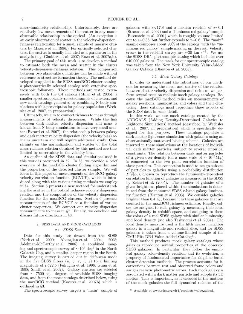
Fig. 1.— The projected separation and velocity separation forthe pairs of galaxies in clusters with N200
gal ≥ 15 (right) and N200
gal
≤ 5 (left). There is a clear change in the BGVCF with N200
gal .
that the BGVCF is independent of the parity of δv. InFigure 1 we show the BGVCF of the catalog in two binsof N200
gal , one with N200gal < 5 (left panel) and one with N200
gal
> 15 (right panel). The structure of the BGVCF clearlychanges with richness.
When we stack clusters to measure their velocity dis-persion as described below, the statistical properties ofour sampling of the BGVCF determine the errors inour measurements. Figures 2(a)-(d) show the numberof pairs in the BGVCF per cluster as a function of N200
gal
plotted for the entire BGVCF and in three redshift bins.As the redshift of the bins increases, we can see thatthe number of spectroscopic pairs becomes less reflectiveof the value of N200
gal for the cluster. Clusters at lowerredshift tend to have more pairs, as expected. Figure 2shows that if we want to measure the velocity dispersionof individual clusters, we are limited to low redshift andhigh richness because only these clusters are sufficientlywell sampled by the SDSS spectroscopic data.
4.2. Characterizing the BGVCF of Stacked Clusters
In this work, we are primarily concerned with the mag-nitude of the velocity dispersion and its scatter at fixedrichness, as well as its dependence on the properties of
Fig. 2.— The number of spectroscopic pairs in the BGVCF percluster as a function of redshift. The redshift ranges for each panelare indicated; the first panel includes the entire catalog. Clusterswith lower redshifts and higher richness are better sampled by thespectroscopic survey. The points in this diagram are displacedrandomly from their integral values (i.e. 1, 2, ...) so that the truedensity can be seen.
clusters and their galaxies. To greatly simplify our analy-sis, we now integrate the BGVCF radially to produce thepairwise velocity difference histogram (PVD histogram).Strictly speaking, we do not produce a true PVD his-togram because the only pairs we consider are those be-tween BCGs and non-BCGs around the same cluster (i.e.all other galaxies in the BGVCF around each cluster).We do not include non-BCG to non-BCG pairs.
Ideally, if every cluster had a properly selected BCGand all BCGs were at rest with respect to the center-of-mass of the cluster, our measurements of the mean veloc-ity dispersion would be unbiased with respect to the truecenter-of-mass velocity dispersion. Unfortunately, thesesimplifying assumptions are not likely to be true. Inparticular it has been found that BCGs move on averagewith ∼ 25% of the cluster’s velocity dispersion, but thatat higher mass BCG movement becomes more significant(e.g. van den Bosch et al. 2005). In §5.2.1 we show thata correction must be applied to our mean velocity dis-persions due to centering on the BCG (hereafter calledBCG bias), but that we cannot distinguish between im-properly selected BCGs and BCG movement. However,we will still focus on the BCG in the measurements of theBGVCF because it is a natural center for the cluster inthe context of the maxBCG cluster detection algorithm.
Having decided to concentrate on the PVD histogram,we now motivate the construction of a fitting algo-rithm for the PVD histogram. Previous work byMcKay et al. (2002), Prada et al. (2003), and others(Brainerd & Specian 2003; van den Bosch et al. 2004;Conroy et al. 2005, 2007) has focused on measuring thehalo mass of isolated galaxies by using dynamical mea-surements. McKay et al. (2002) found the velocity dis-persion around these galaxies by stacking them in lumi-nosity bins and fitting a Gaussian curve plus a constant,representing the constant interloper background, to thestacked PVD histogram. In this method, the standarddeviation of the fit Gaussian curve is then taken as anestimate of the mean value of the velocity dispersion ofthe stacked groups.
The algorithm presented above is insufficient for ourpurposes for the following reason. The PVD histogram ofstacked galaxy clusters is shown in Figure 3; it is clearlynon-Gaussian. Although the width of a single Gaussiancurve likely still provides some information about thetypical dispersion of the sample, it cannot adequatelycapture the information contained in the non-Gaussianshape of the PVD histogram. As we will show belowin §5, although the PVD histogram for a stack of similarvelocity dispersion clusters is expected to be nearly Gaus-sian, there are multiple sources of non-Gaussianity thatcan contribute to the non-Gaussian shape of the stackedPVD histograms. To adequately characterize this non-Gaussianity, one of the primary goals of this paper, wemust use a better fitting algorithm to characterize thePVD histograms.
In this work we will mention a variety of different meth-ods of fitting the PVD histograms. We give their namesand definitions here and follow with a full description ofthe primary method used, 2GAUSS. The various meth-ods are:
1GAUSS: This is the method used for isolated galax-ies as discussed above. We do not use it because,

6 BECKER ET AL.
Fig. 3.— PVD histograms in four N200
gal bins. The EM algorithm fits are shown along with the Poisson errors of the histograms. Notice
the change in the degree of non-Gaussianity of the lower N200
gal bins compared to the higher N200
gal bins. As richness increases, the stacked
PVD histogram becomes more Gaussian. Section 5 shows that this decrease indicates a decrease the width of the lognormal distributionof velocity dispersions in each bin. The deviations of the fits near the centers of the distributions are only at the two-sigma level and arehighly dependent on the bin size used to produce the cluster-weighted PVD histograms.
as described in §4.2.2, it systematically underesti-mates the second moment of the PVD histogramby ∼ 8%.
2GAUSS: This method is the one motivated and de-scribed in detail below. It is the primary methodused throughout the rest of the paper. Simply, itfits the PVD histogram with two Gaussians anda constant background term, but with a specialweighting by cluster and not by galaxy (see §5).
NGAUSS: This is a generalized version of the 2GAUSSmethod with N Gaussians instead of two (i.e. athree Gaussian fit will be denoted by 3GAUSS).Although it fits the PVD histogram as well as the2GAUSS method, it is more computationally ex-pensive, and adds parameter degeneracies withoutsubstantially improving the quality of the fit.
NONPAR: There are several possible methods for us-ing non-parametric fits to the PVD histogram (e.g.kernel density estimators). We do not use thembecause they do not naturally account for theconstant interloper background in the PVD his-togram. For a good review of these techniques seeWasserman et al. (2001).
BISIGMA: This method is not used for the PVD his-tograms of stacked clusters, but is used for the PVDhistograms of individual clusters. The biweight is
a robust estimator of the standard deviation thatis appropriate for use with samples of points whichcontain interlopers (Beers et al. 1990). See §4.3 fora description of its use in this paper.
BAYMIX: This method is a Bayesian or maximum like-lihood method that can be used in the context ofthe model of the scatter in velocity dispersion atfixed richness. This method will be described fullyin §5, but we do not use it in this paper becausewe have found it to be unstable.
We will refer to these methods by their names givenabove. Although we mention these other methods,for deriving the main results of the paper we use the2GAUSS method for stacked cluster samples (4.2.1) andthe BISIGMA method for individual clusters (§4.3).
4.2.1. Fitting the PVD Histogram
In order to more fully capture the shape of the PVDhistogram of stacked clusters, avoid systematic fitting er-rors, and avoid fitting degeneracies, we would ideally usethe NONPAR method to fit the PVD histogram. In thisway we would impose no particular form on the PVD his-togram, allowing us to extract its true shape with as fewassumptions as possible. However, this method does notnaturally account for the interloper background term ofthe PVD histogram which can be easily fit by a constant(Wojtak et al. 2006).

THE CLUSTER VELOCITY-DISPERSION–RICHNESS RELATION 7
In the pursuit of simplicity, we compromise by fittingthe PVD histogram of stacked clusters with two Gaus-sian curves plus a constant background term. The meansof the two Gaussians are free parameters but are fixed tobe equal. In all cases the mean is consistent with zero.The two Gaussian curves allow us to more fully capturethe shape of the PVD histogram, while still accountingfor the interloper background of the BGVCF with theconstant term. It could be that the shape of the PVDhistogram cannot be satisfactorily accounted for by twoGaussians. We show in §4.2.2 that two Gaussians are suf-ficient to describe the shape of PVD histogram. Usingthe 2GAUSS method instead of the NGAUSS methodavoids expensive computations and limits the number ofparameters in the fitting procedure to six, avoiding de-generacies in the fit parameters due to limited statistics.
In the interest of fitting stability and ease of use (butsacrificing speed), we use the expectation maximiza-tion algorithm (EM) for one dimensional Gaussian mix-tures to fit the PVD histogram (Dempster et al. 1977;Connolly et al. 2000). In Appendix A, we re-derivethe EM algorithm for one dimensional Gaussian mix-tures such that it assigns every Gaussian the same meanand weights groups of galaxies, not individual galaxies,evenly. This last step is important in the context of themodel of the distribution of velocity dispersions at fixedN200
gal discussed in §5. To account for our velocity errors,
we use the results of Connolly et al. (2000) and subtractin quadrature the 30 km s−1redshift error from the stan-dard deviation of each fit Gaussian.
We have described our measurements in the contextof the PVD histogram and not the BGVCF. However,these two view points in our case are completely equiva-lent. Wojtak et al. (2006) have shown that galaxies un-correlated with the cluster in PVD histograms (i.e. in-terlopers) form a constant background. Thus by fittinga constant term to the PVD histogram, we are in effectsubtracting out the uncorrelated pairs statistically to re-tain the BGVCF.
4.2.2. Tests of the 2GAUSS Fitting Algorithm
In order to measure the moments of the PVD his-togram as a function of richness, the data is first binnedlogarithmically in N200
gal and then the 2GAUSS method isapplied to each bin. The results of our fitting on four binsof N200
gal are shown in Figure 3. In all cases, the modelprovides a reasonable fit to the data. We defer a fulldiscussion of the fitting results to §5 where we show howto compute the mean velocity dispersion and scatter invelocity dispersion at fixed N200
gal using the results of the2GAUSS fitting algorithm, including corrections for im-properly selected BCG centers and/or BCG movement.
To ensure that the use of the 2GAUSS method doesnot bias our fits in any way, we repeated them usingthe 1GAUSS, 3GAUSS, and 4GAUSS methods. We findthat while the measured second moment for the 1GAUSSfits are consistently lower than those measured from the2GAUSS fits by approximately 8%, both the second andfourth moments measured by the 2GAUSS, 3GAUSS,and 4GAUSS fits are the same to within a few percent.Therefore we conclude that the fits have converged andthat two Gaussians plus a constant are sufficient to cap-ture the overall shape of the PVD histogram. The fitting
errors are determined using bootstrap resampling overthe clusters in each bin.
The results are not dependent on the radial or velocityscale used to construct the BGVCF and thus the PVDhistogram. We repeated the 2GAUSS fits using 0.75R200,1.0R200, 1.25R200, and 1.5R200 projected radial cuts aswell as ±10000 km s−1, ±5σ scaled, and ±10σ scaledapertures in velocity space. We found no significant dif-ferences in the fits using each of the various cuts, withthe exception of the value of the background normaliza-tion, which will change when a larger aperture allowsmore background to be included in the PVD histogram.The scaled apertures were made by first determining therelation in a fixed aperture, and then rescaling the aper-ture according to this relation. For example, in a bin ofN200
gal from 18 to 20, the velocity dispersion is ∼ 500 km
s−1as measured in a ±7000 km s−1fixed aperture. Tomake the five sigma scaled aperture measurements, weused an aperture in this N200
gal bin of ±5 × 500 = ±2500
km s−1.
4.3. Estimating Individual Cluster Velocity Dispersions
To measure the velocity dispersion of individual clus-ters in the SDSS, we select all clusters that have at leastten redshifts in its PVD histogram within three sigmameasured by the mean velocity-dispersion–N200
gal relationcalculated in §5. Of the 12,253 clusters represented in theBGVCF, only 634 meet the above requirement. We thenapply the BISIGMA method to calculate the velocity dis-persion which uses the biweight estimator (Beers et al.1990). The resulting velocity dispersions are plotted inFigure 4. The BCG bias manifests itself here in that theICVDs show a downward bias with respect to the meanrelation calculated in §5, but not corrected for BCG bias.We will correct for this bias in §5.2.1. The two relationsdo however agree to within one- to two-sigma (computedthrough jackknife resampling with the biweight). Usingthese individual cluster velocity dispersions (ICVDs), wecan directly compute the scatter in the velocity disper-sion at fixed N200
gal . We will compare this computationwith the estimate based on measuring non-Gaussianityin the stacked sample in §5.
5. MEASURING SCATTER IN THE VELOCITYDISPERSION–RICHNESS RELATION
5.1. Mass Mixing Model
The subject of non-Gaussianity of pair-wise velocitydifference histograms has been debated extensively inthe literature. Diaferio & Geller (1996) have shown thatnon-Gaussianity in the total PVD histogram for darkmatter halos arises from two sources: stacking halos ofdifferent masses according to the mass function, and in-trinsic non-Gaussianity in the PVD histogram due tosubstructure, secondary infall, and dissipation of orbitalkinetic energy into subhalo internal degrees of freedom.However for galaxy clusters, they conclude that the PVDhistogram of an individual galaxy cluster that is virial-ized is well approximated by a Gaussian.
Sheth (1996) independently reached the same conclu-sions but did not consider any intrinsic non-Gaussianity,just the effect of stacking halos of different masses ac-cording to the mass function. Sheth & Diaferio (2001)gave a more complete synthesis of non-Gaussianity in
8 BECKER ET AL.
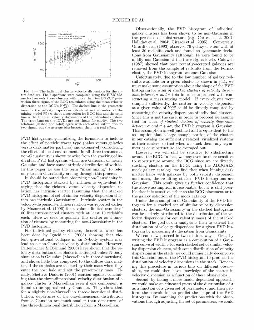
Fig. 4.— The individual cluster velocity dispersions for the en-tire data set. The dispersions were computed using the BISIGMAmethod on only those clusters with more than ten BGVCF pairswithin three-sigma of the BCG (calculated using the mean velocitydispersion at the BCG’s N200
gal ). The dashed line is the geometric
mean of the velocity dispersions calculated in the context of themixing model (§5) without a correction for BCG bias and the solidline is the fit to all velocity dispersions of the individual clusters.The error bars on the ICVDs are not shown for clarity. The tworelations (dashed and solid) agree with each other within one- totwo-sigma, but the average bias between them is a real effect.
PVD histograms, generalizing the formalism to includethe effect of particle tracer type (halos versus galaxiesversus dark matter particles) and extensively consideringthe effects of local environment. In all three treatments,non-Gaussianity is shown to arise from the stacking of in-dividual PVD histograms which are Gaussian or nearlyGaussian and have some intrinsic distribution of widths.In this paper we use the term “mass mixing” to referonly to non-Gaussianity arising through this process.
It should be noted that observing non-Gaussianity inPVD histograms stacked by richness is equivalent tosaying that the richness verses velocity dispersion re-lation has intrinsic scatter (assuming that the stackedPVD histogram of set of similar velocity dispersion clus-ters has intrinsic Gaussianity). Intrinsic scatter in thevelocity-dispersion–richness relation was reported earlierby Mazure et al. (1996) for a volume-limited sample of80 literature-selected clusters with at least 10 redshiftseach. Here we seek to quantify this scatter as a func-tion of richness by measuring the non-Gaussianity in thePVD histogram.
For individual galaxy clusters, theoretical work hasbeen done by Iguchi et al. (2005) showing that vio-lent gravitational collapse in an N-body system maylead to a non-Gaussian velocity distribution. However,Faltenbacher & Diemand (2006) have shown that the ve-locity distribution of subhalos in a dissipationless N-bodysimulation is Gaussian (Maxwellian in three dimensions)and shows little bias compared to the diffuse dark mat-ter, if the subhalos are selected by their mass when theyenter the host halo and not the present-day mass. Fi-nally, Sheth & Diaferio (2001) caution against conclud-ing that the three-dimensional velocity distribution of agalaxy cluster is Maxwellian even if one component isfound to be approximately Gaussian. They show thatfor a slightly non-Maxwellian three-dimensional distri-bution, departures of the one-dimensional distributionfrom a Gaussian are much smaller than departures ofthe three-dimensional distribution from a Maxwellian.
Observationally, the PVD histogram of individualgalaxy clusters has been shown to be non-Gaussian inthe presence of substructure (e.g. Cortese et al. 2004;Halliday et al. 2004; Girardi et al. 2005). Conversely,Girardi et al. (1993) observed 79 galaxy clusters with atleast 30 redshifts each and found no systematic devia-tions from Gaussianity (although 14 were found to bemildly non-Gaussian at the three-sigma level). Caldwell(1987) showed that once recently-accreted galaxies areremoved from the sample of redshifts from the Fornaxcluster, the PVD histogram becomes Gaussian.
Unfortunately, due to the low number of galaxy red-shifts available for a given cluster as shown in §4.1, wemust make some assumption about the shape of the PVDhistogram for a set of stacked clusters of velocity disper-sion between σ and σ + dσ in order to proceed with con-structing a mass mixing model. If every cluster weresampled sufficiently, the scatter in velocity dispersionat a given value of N200
gal could be directly computed bymeasuring the velocity dispersions of individual clusters.Since this is not the case, in order to proceed we assumethat for a set of stacked clusters of velocity dispersionbetween σ and σ + dσ, the PVD histogram is Gaussian.This assumption is well justified and is equivalent to theassumption that a large enough portion of the clustersin our catalog are sufficiently relaxed, virialized systemsat their centers, so that when we stack them, any asym-metries or substructure are averaged out.
However, we will still be sensitive to substructurearound the BCG. In fact, we may even be more sensitiveto substructure around the BCG since we are directlystacking clusters on the BCG. Using the ADDGALSmock galaxy catalogs, we find that when binning darkmatter halos with galaxies by both velocity dispersionand mass, the resulting stacked PVD histograms areGaussian. This result gives us further confidence thatthe above assumption is reasonable, but it is still possi-ble that it is sensitive either to the BCG placement or tothe galaxy selection of the mock catalogs.
Under the assumption of Gaussianity of the PVD his-togram for a stacked set of similar velocity dispersionclusters, the non-Gaussianity in the stacked histogramscan be entirely attributed to the distribution of the ve-locity dispersions (or equivalently mass) of the stackedclusters. The goal of our analysis is then to extract thedistribution of velocity dispersions for a given PVD his-togram by measuring its deviation from Gaussianity.
We can now proceed in two distinct ways. First, bywriting the PVD histogram as a convolution of a Gaus-sian curve of width σ for each stacked set of similar veloc-ity dispersion clusters, with some distribution of velocitydispersions in the stack, we could numerically deconvolvethis Gaussian out of the PVD histogram to produce thedistribution of velocity dispersions in the stack. Repeat-ing this procedure in various bins on different observ-ables, we could then have knowledge of the scatter invelocity dispersion as a function of these observables.
Second, by taking a more model dependent approach,we could make an educated guess of the distribution of σas a function of a given set of parameters, and then per-form the convolution to predict the shape of the PVDhistogram. By matching the predictions with the obser-vations through adjusting the set of parameters, we could

THE CLUSTER VELOCITY-DISPERSION–RICHNESS RELATION 9
then have a parameterized model of the entire distribu-tion.
Based on the results shown below in §6, it is appar-ent that the only parameter upon which σ varies sig-nificantly, neglecting the modest redshift dependence, isN200
gal . Thus we choose a parametric model that is a func-
tion of N200gal only. The dependence of mass mixing on any
secondary parameters (e.g. the BCG i-band luminosity)can then be explored through first binning on N200
gal andthen splitting on these secondary parameters, becausetheir effects are small (see §6).
The ADDGALS mock catalogs show the scatter aboutthe mean of the logarithm of the velocity dispersion mea-sured from the dark matter for a given value of Ngal tobe approximately Gaussian for dark matter halos. Us-ing this distribution as our educated guess, we apply thismodel to the data in logarithmic bins of N200
gal . We avoidthe deconvolution due to its inherent numerical difficulty.Using the mock catalogs, we can test our method of de-termining the parameters of this model as a function ofN200
gal by applying our analysis to clusters identified in themocks and then matching those clusters to halos in orderto determine their true velocity dispersions.
To summarize, there are two and possibly even threesources of non-Gaussianity in our PVD histograms (sim-ilar to those discussed in Sheth (1996), Diaferio & Geller(1996), and Sheth & Diaferio (2001) discussed above):(1) intrinsic non-Gaussianity in the PVD histogram foran individual galaxy cluster, (2) the range of velocitydispersions that contribute to the PVD histogram fora given value of N200
gal (mass mixing), and (3) stacking
of clusters with different values of N200gal in the same
PVD histogram. We handle the last two sources of non-Gaussianity jointly through the model below and ignorethe first, which is expected to be small, both becausemost clusters are relaxed, virialized systems and manyare stacked together here.
As a final note, by binning logarithmically in N200gal and
then measuring the mass mixing, we only approximatelyaccount for non-Gaussianity arising from clusters withdifferent richnesses in the same bin. By avoiding binningall together and finding the model parameters througha maximum likelihood approach, we could remedy thisissue. This approach is the BAYMIX method. However,we have found this process to be computationally expen-sive and slightly unstable due the integral in equation 3below. Its only true advantage is in the computation ofthe errors in the parameters and their covariances. Us-ing a maximum likelihood approach, one could calculatethe full covariance matrix of the parameters introducedbelow. As will be shown below, binning in N200
gal and thenmeasuring the mass mixing will allow us to only easilyfind the covariance matrices of the parameters in sets oftwo. Since we are not significantly concerned with theexact form of these errors or the covariances of the pa-rameters, we choose to bin for simplicity.
Future analysis of this sort with PVD histograms willhopefully take a less model-dependent approach by de-convolving a Gaussian directly from the stacked PVDhistogram. This will allow for a direct confirmation ofthe distribution of velocity dispersions at fixed richness.Also, a direct deconvolution would allow one to make
mass mixing measurements of stacks of clusters binnedon any observable. Although the lognormal form as-sumed here may in fact have wider applicability, we canonly confirm its use for clusters stacked by richness.
5.2. Results Using The Mass Mixing Model
We can write the shape of the non-background part ofthe stacked cluster-weighted PVD histogram, P (v), as
P (v) =
∫
p(v, σ)dσ =
∫
p(v|σ)p(σ)dσ (2)
where v is the velocity separation value and σ is theGaussian width of a stacked set of similar velocity dis-persion clusters. Using the assumptions from the previ-ous discussion, we let p(v|σ) be a Gaussian of width σwith mean zero, and p(σ) be a lognormal distribution.Performing the convolution, we get that P (v) is givenby
P (v) =∫ ∞
0
1
σ22πSexp
(
− v2
2σ2− (ln σ− < lnσ>)2
2S2
)
dσ (3)
where < lnσ > is the geometric mean of σ and S is thestandard deviation of lnσ. We note that the quantity100 × S is the percent scatter in σ. The second andfourth moments of this PVD distribution, µ(2) and µ(4)
are given by
µ(2) = exp (2 < lnσ> +2S2) (4)
andµ(4) = 3 exp (4 < lnσ> +8S2) . (5)
For convenience we define the normalized kurtosis to be
γ2N =
µ(4)
3µ2(2)
= exp4S2 . (6)
Note that the odd moments of this distribution are ex-pected to vanish, and in fact the data is consistent withboth the first and third moments being zero. Equation4 shows us why the velocity dispersions derived directlyfrom the second moment of the PVD histogram must becorrected. The factor of exp S2 artificially increases thevelocity dispersions. In practice this effect is at most∼ 20% at low richness and declines to ∼ 5% for the mostmassive clusters in our sample.
To complete our model, we need a term correspondingto the background of the PVD histogram. This back-ground has two parts, an uncorrelated interloper compo-nent and an infall component (i.e. galaxies which are notin virial equilibrium but are bound to the cluster in theinfall region). Wojtak et al. (2006) have shown that theuncorrelated background is a constant in the PVD his-togram, while van den Bosch et al. (2004) have shownthat the infall component is not constant and forms awider width component for PVD histograms around iso-lated galaxies. We ignore the possible infall componentsin our PVD histograms but note that they may bias thewidths of our lognormal distributions high. Investigationof this issue in the mock catalogs shows that the resultof van den Bosch et al. (2004) holds for galaxy clustersas well. Although we do not explore this here, it may bepossible to reduce the mass mixing signal from infalling

10 BECKER ET AL.
galaxies by selecting galaxies by color (i.e. red galaxiesonly or just maxBCG cluster members), which preferen-tially selects galaxies near the centers of the clusters.
Accounting for the constant interloper background, thefull model of the cluster-weighted PVD histogram, P(v),can now be written as,
P(v) =p
2L+ (1 − p)P (v) (7)
where L is the maximum allowed separation in velocitybetween the BCG and the cluster members, set to 7000km s−1, and p is a weighting factor that sets the back-ground level in the PVD histogram. Here we ignore thesmall error in the normalization due to integrating P(v)over v from −∞ to ∞ instead of −L to L. As long asL is sufficiently large, say on the order of 4 exp(< ln σ>)for a given PVD histogram, this error is small.
Now, it can be seen why the stacked PVD histogrammust be weighted by cluster instead of by galaxy. Inequation 3, equal weight is assigned to each cluster be-cause p(v|σ) is a Gaussian normalized to integrate tounity. In order to predict the pair-weighted PVD his-togram correctly, we would have to predict the totalnumber of BGVCF pairs, both cluster and background,as function of N200
gal and include this total in the integral
and the background term. (The factors of p and 1 − ptake care of the relative weighting of the background rel-ative to cluster, assuming this weighting is the same forevery cluster. This may not be true, in which case thefactors of p and 1 − p would have to be included in theintegral as well.) This is a significant problem due toits dependence on redshift, local environment, and theselection function of the survey.
By using the cluster-weighted PVD histogram fit bythe EM algorithm derived in Appendix A (i.e. the2GAUSS method), we can avoid this issue. This weight-ing could be included in the BAYMIX method as well.We choose to use the 2GAUSS method because it is morestable and less computationally expensive. In practicethe extra weighting factors do not change our resultsdrastically, indicating that most clusters already get ap-proximately equivalent weight even in the pair-weightedPVD histogram. However, for completeness we includethe weighting factor. Note that two Gaussians is the thefewest number of Gaussians a distribution could be com-posed of and have a normalized kurtosis different fromunity (the normalized kurtosis of a single Gaussian dis-tribution is unity). According to equation 6, then, if wemeasure a normalized kurtosis of unity for any of ourbins, mass mixing in that bin (i.e. S) will be zero.
The quantities < lnσ>, S2, and p are measured by bin-ning the data in N200
gal and applying the 2GAUSS methodas described earlier. This method outputs the constantbackground level p automatically. The normalized kur-tosis is calculated as
γ2mes =
p1(σ1)4 + p2(σ2)
4
(p1(σ1)2 + p2(σ2)2)2 (8)
and the second moment is calculated as
µmes(2) =
p1(σ1)2 + p2(σ2)
2
p1 + p2, (9)
where p1, p2 and σ1, σ2 are the normalizations and
TABLE 1MaxBCG mass mixing model fit parameters.
Parameter Value
mean-normalization, A 6.17 ± 0.04mean-slope, B 0.436 ± 0.015
scatter-normalization, C 0.096 ± 0.014scatter-slope, D −0.0241 ± 0.0050
background-normalization, E −0.980 ± 0.052background-slope, F −0.00154 ± 0.00018
standard deviations calculated for the two Gaussians inthe 2GAUSS PVD histogram fit. See Appendix A formore details. Although equation 8 is not properly nor-malized, we find that the bias correction computed inAppendix B is small, and thus equation 8 is a good esti-mator of the normalized kurtosis.
Using equations 4, 6, 8, and 9, we solve for the pa-rameters < lnσ > and S2. The background normaliza-tion p and the normalization and scatter in the velocity-dispersion–richness relation are all modeled as powerlaws, which provides a good description of the relationsin both the data and the simulations:
< lnσ>= A + B ln N200gal /25 (10)
S2 = C + D ln N200gal /25 . (11)
ln p = E + F exp (< lnσ>) (12)
The fit of the measured parameters < lnσ > and S2 tothe above relations for the maxBCG cluster sample areshown in Figure 5. The parameters A, B, C, D, E, and Fare given in Table 1 and the mass mixing model values foreach bin are given in Table 2. The mean relation plottedin this figure is corrected for BCG bias due to improp-erly selected BCGs and/or BCG movement as discussedin §5.2.1. The errors for our data points are derived fromthe bootstrap errors employed in the 2GAUSS method.Note that we only have knowledge of the full error dis-tributions of the parameters in sets of two, and are thusneglecting covariance between, for example, parametersA and C or B and C, etc. The BAYMIX method wouldallow for each of the three relations to be fit simultane-ously, giving full covariances between the parameters.
5.2.1. BCG Bias in the 2GAUSS Fitting Algorithm
Despite that fact that the two mean relations plottedin Figure 4 agree within one- to two-sigma, we show inthis section that the bias between the two relations hassignificance and arises from two sources. The first sourceis intrinsic statistical bias in the 2GAUSS method itself.Using Monte Carlo tests as described in Appendix B, wefind that this bias is approximately 3-5% downward andhas some slight dependence on the number of data pointsused in the 2GAUSS fitting method. The Monte Carlocomputation of the bias is shown in the middle panel ofFigure 6. We call this bias b2G.
The second source of bias is due to some combinationof BCG movement with respect to the parent halo (seevan den Bosch et al. 2005) and the incorrect selection ofBCGs by the maxBCG cluster detection algorithm (i.e.mis-centering). We can test for this effect by reconstruct-ing the BGVCF around randomly selected cluster mem-ber galaxies output from the maxBCG cluster detection
THE CLUSTER VELOCITY-DISPERSION–RICHNESS RELATION 11
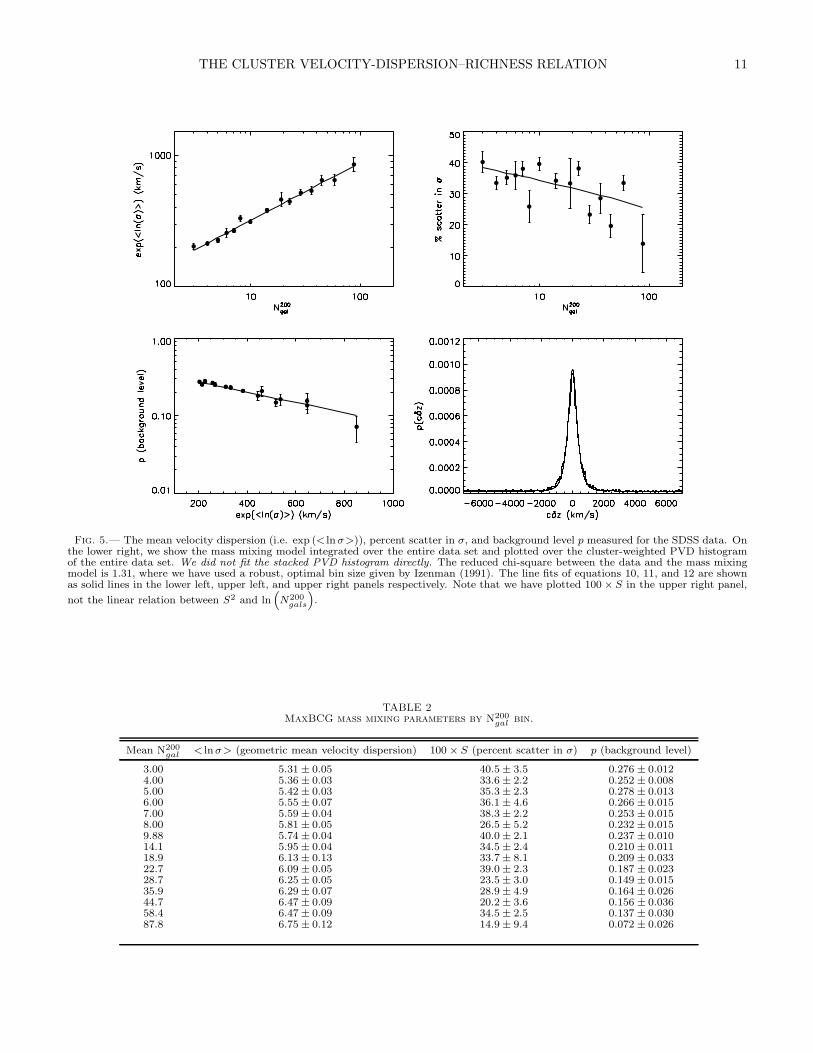
Fig. 5.— The mean velocity dispersion (i.e. exp (< lnσ>)), percent scatter in σ, and background level p measured for the SDSS data. Onthe lower right, we show the mass mixing model integrated over the entire data set and plotted over the cluster-weighted PVD histogramof the entire data set. We did not fit the stacked PVD histogram directly. The reduced chi-square between the data and the mass mixingmodel is 1.31, where we have used a robust, optimal bin size given by Izenman (1991). The line fits of equations 10, 11, and 12 are shownas solid lines in the lower left, upper left, and upper right panels respectively. Note that we have plotted 100 × S in the upper right panel,
not the linear relation between S2 and ln“
N200
gals
”
.
TABLE 2MaxBCG mass mixing parameters by N200
gal bin.
Mean N200
gal < lnσ> (geometric mean velocity dispersion) 100 × S (percent scatter in σ) p (background level)
3.00 5.31 ± 0.05 40.5 ± 3.5 0.276 ± 0.0124.00 5.36 ± 0.03 33.6 ± 2.2 0.252 ± 0.0085.00 5.42 ± 0.03 35.3 ± 2.3 0.278 ± 0.0136.00 5.55 ± 0.07 36.1 ± 4.6 0.266 ± 0.0157.00 5.59 ± 0.04 38.3 ± 2.2 0.253 ± 0.0158.00 5.81 ± 0.05 26.5 ± 5.2 0.232 ± 0.0159.88 5.74 ± 0.04 40.0 ± 2.1 0.237 ± 0.01014.1 5.95 ± 0.04 34.5 ± 2.4 0.210 ± 0.01118.9 6.13 ± 0.13 33.7 ± 8.1 0.209 ± 0.03322.7 6.09 ± 0.05 39.0 ± 2.3 0.187 ± 0.02328.7 6.25 ± 0.05 23.5 ± 3.0 0.149 ± 0.01535.9 6.29 ± 0.07 28.9 ± 4.9 0.164 ± 0.02644.7 6.47 ± 0.09 20.2 ± 3.6 0.156 ± 0.03658.4 6.47 ± 0.09 34.5 ± 2.5 0.137 ± 0.03087.8 6.75 ± 0.12 14.9 ± 9.4 0.072 ± 0.026

12 BECKER ET AL.
Fig. 6.— The bias correction to the mean velocity dispersionfor the maxBCG clusters. Left: The ratio of the random membercentered dispersions to < ln σ>, rRM . Middle: The statistical biasin the 2GAUSS method, b2G. See Appendix B for details. Right:The ratio of < lnσ > to the geometric average of the ICVDs foreach bin in N200
gal , rICV D. The circles in the right panel show the
quantity√
2b2G/rRM for each bin in N200
gal . Note that the right
panel indicates√
2b2G/rRM ≈ rICV D .
algorithm. If the BCGs are picked correctly and are atrest with respect to their parent halos, then by pickinga random member galaxy, we should observe the meanvelocity dispersion increase by
√2. This calculation as-
sumes that each stack of similar velocity dispersion clus-ters has a Gaussian PVD histogram. This test is per-formed in the data in the left panel of Figure 6. Wesee that the random member centered dispersions are in-creased above < lnσ > for each bin in N200
gal , but by less
than√
2. This result indicates that either or both ofthe situations discussed above is happening. The ratioof the random member centered dispersions to < ln σ >is denoted as rRM .
We can test the above conclusion by using the ICVDscomputed in §4.3. To do this, we calculate the ratioof < lnσ > to the geometric average of the ICVDs foreach bin in N200
gal . This ratio is plotted in the right panelof Figure 6 and is called rICV D. We can also estimatethis from the computations described in the previous twoparagraphs. We compute
√2b2G/rRM for each bin N200
gal ;this quantity is shown in the right panel of Figure 6. Thiscomputation assumes that the biases add linearly in thelogarithm of the velocity dispersion.
We find that generally√
2b2G/rRM ≈ rICV D withinthe one-sigma errors. This observation indicates thatour explanation of the bias observed in Figure 4 is self-consistent. To correct the < lnσ > values for each binin N200
gal , we use the mean of the quantity√
2b2G/rRM
because the ICVDs are limited to low redshift, bettersampled clusters, and our measurements are quite noisy.
In Figure 7, we repeat the above computations for themock catalogs. We again find that
√2b2G/rRM ≈ rICV D
and our explanation of the bias is self-consistent. Fur-thermore, since we know the true velocity dispersion val-ues we can directly test our arguments above in an ab-solute sense. This comparison is discussed in §5.3.2. Wefind that in fact, our correction will likely over correctthe mean velocity dispersion so that it is 5-10% too low.Briefly, this effect occurs because the random “member”we select is in fact not always a member of the cluster.
Fig. 7.— The bias correction to the mean velocity dispersion forthe mock catalogs. The panels are the same as those in Figure 6.According to the right panel,
√2b2G/rRM ≈ rICV D holds in the
mock catalogs as well.
Finally, the Monte Carlo tests described in Appendix Ballow us to test for bias in S2 as well. We find and correctfor bias in this parameter and note that on average wemeasure slightly lower values of S2 than we should, byabout 5-10%.
5.3. Tests of the Mass Mixing Model
We now present several checks of our method for es-timating mass mixing. These checks fall in three broadcategories. The first set are done with the data itselfand test for self-consistency along with dependence onsample selection functions and/or redshift. The secondset are done with mock catalogs. Here we run the meth-ods developed above on the mocks in the same way theyare run on the data, and ask whether we can recoverthe true velocity-dispersion–richness relation for halos.If the measurements on the mock catalogs do not matchthe true values, then we will suspect that some of theassumptions made above are not adequate to sufficientlydescribe the BGVCF (i.e. we might suspect that theinfall component of the PVD histogram contributes sig-nificantly).
The third set of tests are done with a spectroscopically-selected catalog run on lower redshift data, the C4 cata-log (Miller et al. 2005). For this sample, we can computethe distribution of velocity dispersion at fixed richness bydirectly computing velocity dispersions for each individ-ual cluster. We can then test our methods by comparingthe measurements based on the stacked PVD histogramto the true measured distributions.
5.3.1. Data Dependent Tests
As a first check of our method with the data, we lookfor self-consistency. In the lower right panel of Figure 5,we plot the mass mixing model integrated over the entiredata set using equations 3, 7, 10, 11, and 12 on top ofthe full cluster-weighted stacked PVD histogram. We didnot fit the stacked PVD histogram directly. The reducedchi-square between the data and the mass mixing modelis 1.31, where we have used a robust, optimal bin sizegiven by Izenman (1991). The above model reproducesthe first four moments of the stacked PVD histogramas a function of N200
gal and reproduces the stacked PVDhistogram to a good approximation, indicating that themodel is self-consistent.

THE CLUSTER VELOCITY-DISPERSION–RICHNESS RELATION 13
Fig. 8.— Tests of the mass mixing model with the data (upper panels) and with the high resolution mock catalogs (lower panels). UpperLeft: The ratio of the geometric mean velocity dispersion determined by the stacked PVD histogram to that determined by the IVCDs.Upper Right: The percent scatter in σ computed directly from the individual cluster velocity dispersions (diamonds) to those computedfrom the stacked PVD histogram (circles). Lower Left: The ratio of the geometric mean velocity dispersion determined by the stackedPVD histogram in the high resolution simulation to the true values found by matching clusters to halos. Lower Right: The percent scatterin σ computed using the stacked PVD histogram (circles) compared to the true values found by matching clusters to halos (diamonds).The error bars for the simulation parameters are jackknife errors computed by breaking the sample into the same bins in Ngal as usedwith measurements of the stacked PVD histograms. In the mock catalogs, note the 5-10% downward bias of the geometric mean velocitydispersion, as determined by the stacked PVD histogram, with respect to the true values.
In the upper two panels of Figure 8, we compare themodel parameters computed from the ICVDs (diamonds)computed using the BISIGMA method, with those com-puted from the stacked PVD histogram (circles). Thetwo agree to within one-sigma. We note however thatthe relation for the standard deviation of lnσ for theindividual cluster velocity dispersions looks “flatter” asfunction of N200
gal than for the relation computed from theshape of the stacked PVD histogram.
We hypothesize two possible explanations for this ob-servation. First, the “flatness” could just be a statisticalfluctuation. Notice that according to the error bars, therelations are consistent with each other in most instancesby less than one standard deviation. Second, the “flat-ness” could be caused by a sampling effect with the popu-lation of clusters used to compute the individual clustervelocity dispersions. In other words, because we com-puted the individual velocity dispersions be requiring acluster to have ten pairs in the BGVCF within three-sigma of the BCG as given by the mean velocity disper-sion relation, we selectively measure only a low redshiftsubset of the cluster population.
This issue is however more than just insufficient sam-pling. For small groups of galaxies, it may be impossibleto properly define an observationally-measurable velocitydispersion unless one is willing to stack groups of similar
mass to fully sample their velocity distributions. Thuswe hypothesize that while the two relations disagree atlow richness, the relation computed from the shape of thestacked PVD histograms may in fact be a better indica-tor of scatter in the σ−N200
gal relation for all richnesses,especially low richness clusters.
When computing the model above, we used the entiremagnitude-limited sample of the SDSS spectroscopy. Wecan investigate selection effects by examining our modelin both magnitude- and volume-limited samples. Thevolume-limited samples are constructed by extracting allgalaxies above 0.4L∗, and below the redshift at which0.4L∗ is equal to the magnitude limit of the SDSS spec-troscopy. Thus we are complete above 0.4L∗ up to fibercollisions, out to this redshift. Between the volume- andmagnitude-limited samples, the differences in the massmixing parameters is only slight and within the one-sigma errors.
We also binned the volume-limited sample in redshiftto check for evolution in the scatter. Although thereare only negligible differences in the scatter in mass be-tween between the upper and lower redshift bins, thereis a larger difference between the mean relations for eachredshift bin. This evolution will be described in detail in§6.1 for the full magnitude-limited sample.
Finally, we compare the mixing parameters measured

14 BECKER ET AL.
with cluster members (with redshifts) defined by themaxBCG algorithm only to those measured with the en-tire spectroscopic sample (i.e. the full BGVCF). We findno significant differences in this test. We might suspect,as suggested earlier, that cluster members better tracethe fully virialized regions of clusters. Either infallinggalaxies do not contribute significantly, or the radial cutused to select members of the BGVCF was small enoughthat most of the infalling galaxies could be excluded, ex-cept those directly along our line-of-sight.
5.3.2. Tests with the Mock Catalogs
After running the maxBCG cluster finder on the mockcatalogs, we measure the mass mixing of the identifiedclusters in the same way that it is measured for themaxBCG clusters identified in SDSS data. In the bot-tom two panels of Figure 8, the mass mixing parame-ters computed using the 2GAUSS method with the massmixing model for clusters measured in the higher resolu-tion simulation are compared to the true relations, foundby matching our clusters to halos and then assigning agiven cluster the dark matter velocity dispersion of itsmatched halo. We also performed the same analysis in alower resolution simulation. We find that we can success-fully predict the mass mixing in both simulations abovetheir respective mass thresholds, except for the 5-10%downward bias of the mean value.
The bias in the mean value of the velocity dispersionin the mock catalogs is due to the imperfect selectionof member galaxies by the maxBCG cluster finding al-gorithm. When we select perfectly centered clusters (i.e.cluster in which the true BCG at rest in the halo is foundas the BCG by the maxBCG cluster finding algorithm)and repeat the computation of rRM , we find that therandom member dispersions still do not increase by
√2.
Instead, they increase by less than this factor and withthis measured rRM decreasing with N200
gal . However, we
can recover the factor of√
2 if we use only halo centersand only members within R200 of the halo center. Thus,because we cannot perfectly select members, the quantity√
2/rRM is a little more than unity, so that the BCG bias
correction (in which one divides by√
2b2G/rRM ) makesthe mean too low. We cannot test for this effect in thedata directly, but the simulations indicate that it is lessthan 10%.
The matching between clusters and halos is done ac-cording to a slight modification of the method used byRozo et al. (2007b,a). The halos are first ranked in orderof richness, highest to lowest. Then the cluster with themost shared members with the halo is called the match.If two clusters share the same number of members, theone containing the halo BCG is taken as the match. Ifthese two criteria fail to produce a unique match (i.e. nocluster contains the halo’s BCG), the cluster with a thehigher richness measure is chosen as the match. Finally,if all three criteria still fail to produce a unique match,the matching cluster is chosen at random from all clus-ters that meet all three criteria. When a match is made,both the cluster and halo are then removed from consid-eration and the next highest richness halo is matched inthe same way. This procedure produces unique matches,but may not match every halo to a cluster or every clus-ter to a halo. Of the halos with matched clusters in the
high resolution mock catalogs, we find that the first cri-teria fails in only 6.23% of all cases. In these failed cases,only 5.20%, 0.68%, and 0.35% of the halos are matchedusing the second, third, and fourth criteria respectively.
In the SDSS data the use of cluster members only toconstruct the BGVCF caused no change in the amountof mass mixing. We repeat this measurement in thehigher resolution simulation using only the cluster mem-bers selected by the maxBCG algorithm to construct theBGVCF. We see no significant improvement in the pre-diction of the true mass mixing parameters using clustermembers only as compared to using all galaxies in theBGVCF.
In the mock catalogs, we did not properly replicate theselection function of the SDSS spectroscopic sample. Un-fortunately, the mock catalogs have approximately halfthe sky coverage area of SDSS sample, so that when theproper selection function of the SDSS spectroscopic sam-ple is applied, there are too few galaxies to use with ourmethods. We require high signal-to-noise measurementsof the fourth moment of the BGVCF, which is not pos-sible with only half the sky coverage area. However, wecan test for the effects of spectroscopic selection withinthe C4 sample, as described below.
5.3.3. Tests with the C4 Catalog
Using the C4 catalog (Miller et al. 2005), we can per-form an independent test of our mass mixing method.The C4 catalog is produced by running the C4 clus-ter finding algorithm on low redshift SDSS spectroscopicdata. This algorithm finds clusters using their density in4-D color space and 3-D position space. We make useof five pieces of information from the C4 catalog: a rich-ness estimate, an estimate of the velocity dispersion ofeach cluster, the BCG redshift, the mean cluster redshift,and a “Structure Contamination Flag” (SCF). This flagtakes on the values of 0, 1, or 2, depending upon thedegree of interaction of a given cluster with any of itsneighbors. Isolated clusters have SCF= 0 and clustersthat have neighbors very close by (i.e. ∆z ≈ 0.01) haveSCF= 2. Clusters with SCF =1 are in between these twoextremes. The mean cluster redshift is the biweight mean(Beers et al. 1990) redshift of all SDSS spectroscopically-sampled galaxies within 1 h−1Mpc and ±0.02 in redshiftof the centroid found in the PVD histogram of the clus-ter.
We use every cluster in the C4 catalog with SCF6= 2and in the redshift range 0.03 < z < 0.12. Centering onthe BCGs listed in the C4 catalog, we process the clustersin the same way we have processed the maxBCG clusters,i.e. we measure the BGVCF and then apply the 2GAUSSmethod with the mass mixing model to the PVD his-togram. Instead of using a projected radius cut of R200
we used a fixed radius of 1h−1Mpc. We used a fixedradius here because we have no estimate of the naturalradial scaling appropriate for the C4 richness measure.In order to have sufficient statistics for the computationof the mass mixing model, we are limited to splitting theclusters into two logarithmically-spaced bins of richness.
We then compare our inferred distribution of velocitydispersions with the distribution of velocity dispersionsfor each individual C4 cluster in the catalog for each bin.The results are shown in the upper two panels of Fig-ure 9, which compares the lognormal with our derived

THE CLUSTER VELOCITY-DISPERSION–RICHNESS RELATION 15
Fig. 9.— The distribution of velocity dispersion in two bins ofrichness for the C4 catalog. Upper panels show the measurementfor all clusters with SCF 6= 2 (those with close neighbors). Lowerpanels use all clusters with SCF = 0 (isolated clusters). The boldlines show the lognormal distributions measured by applying the2GAUSS method with the mass mixing model to the C4 clusters us-ing BCG redshifts in the same way as it is applied to the maxBCGclusters. The regular lines are lognormal fits directly to the his-tograms shown above. Notice that in the bottom panels, the highvelocity dispersion tail due to C4 clusters with close neighbors isgone.
parameters to the best fit lognormal for the individualC4 velocity dispersions. Note the slight bias in the meanbetween the lognormal curves computed from the massmixing model and the curves fit to the C4 velocity dis-persions.
In Figure 10, we repeat our measurements, but usingthe cluster redshift instead of the BCG redshift. In thiscase we see better agreement between the mass mixingmeasurements and the C4 velocity dispersions. This re-sult indicates that the slight bias in the mean was due tomovement of the BCGs. Finally, to be complete, we com-pute the average velocity dispersion of the BCGs in eachbin of C4 richness, and then use this value to correct themeasurements made using BCG centers. We find that wecan reproduce the cluster redshift measurements throughthis procedure. Our understanding of how mis-centeringand/or BCG movement effects our measurements is self-consistent in both the data and mock catalogs. If we hadtrue cluster redshifts for the maxBCG clusters (i.e. anaccurate average redshift of all of the cluster members),then according to the results of the C4 catalog, no cor-rection due to BCG bias would have to be applied to themean velocity dispersion.
We note that there seems to be high dispersiontail/shoulder in the histograms plotted in the upper pan-els of Figures 9 and Figures 10. Including clusters withSCF= 2 increases this shoulder. This result is consistentwith the finding of Miller et al. (2005) that clusters withSCF= 2 have their measured velocity dispersions artifi-cially increased by their nearby neighbors. This resultis also consistent with a finding of Evrard et al. (2007),that the velocity dispersions of interacting dark matterhalos form a high tail in the lognormal distribution ofvelocity dispersion at fixed mass. In the bottom panelsof Figures 9 and 10, we repeat our measurements usingcluster redshifts, now including only those clusters withSCF= 0, (i.e. we exclude clusters with SCF= 1 or 2).The distribution of dispersions from this set of clustersis in better agreement with the mass mixing method.
In the maxBCG catalog, interacting clusters may not
Fig. 10.— Same as Figure 9 except the bold lines were made withthe mass mixing model using the mean cluster redshift, not theBCG redshift. The geometric mean velocity dispersion as measuredby the mass mixing model now agrees with the true geometric meanof the C4 clusters because we have used cluster redshifts and notBCG redshifts. Notice again that in the bottom panels, the highvelocity dispersion tail due to C4 clusters with close neighbors isgone.
be as significant of a problem because the clusters areby definition much farther away from each other (i.e.∆z ≥ 0.02 as opposed to ∆z = 0.01 for some clusters inthe C4 catalog). In fact, many of the clusters that theC4 algorithm would flag as SCF= 2, the maxBCG al-gorithm may group together. We do not mean to implythat the maxBCG algorithm has a significant problem ofover-merging distinct objects, but only that the redshiftresolution of the cluster finder is less than the C4 algo-rithm. Thus the high velocity dispersion shoulder wouldlikely be down-weighted by algorithmic merging of ob-jects together in combination with sparse spectroscopicsampling. For example, if two C4 clusters with SCF= 2would be merged by the maxBCG algorithm, then thevelocity structure according to the maxBCG algorithmwould only be measured about a combination center, andnot two centers as in the C4 catalog. Therefore, in com-bination with the sparse spectroscopic sampling, the rel-ative weight of these two objects in a maxBCG PVDhistogram might be decreased as compared to a C4 PVDhistogram, where they would contribute twice as muchand possibly at higher velocity dispersion. While thesearguments remain untested at the moment, the high ve-locity dispersion shoulder seen in the upper panels ofFigures 9 and 10 has a clear origin and is well predictedtheoretically.
For the C4 sample, we can also investigate the effectsthe spectroscopic selection. We recomputed our measure-ments using three higher r-band magnitude limits, 17.0,16.5, and 16.0. Because the SDSS main sample r-bandmagnitude limit is 17.8, these three cuts replicate increas-ing amounts of spectroscopic incompleteness. We foundno statistically significant differences between these mea-surements, indicating that spectroscopic incompletenesshas a small effect on our measurements for the C4 cata-log.
5.3.4. Sensitivity to the Scatter Model
Here we investigate the sensitivity of our results to thechoice of using a lognormal to describe the scatter in σ atfixed N200
gal . There may be other distributions that couldpossibly describe the scatter just as well. As a test case,

16 BECKER ET AL.
we investigate how well a Gaussian distribution describesthe data in comparison with the lognormal.
We first study whether the two scatter models result indifferent conclusions. In the SDSS data, we find that athigh richness the measured scatter assuming a Gaussianor a lognormal differ by less than one standard devia-tion. However at low richness, the measured scatter inthe two models differs by almost three standard devia-tions. These results cannot tell us which model is better,but only whether one model is equivalent to the other.This seems to be the case in the SDSS, except at lowrichness. From a theoretical standpoint, we prefer thelognormal model because it always ensures that σ ≥ 0without an arbitrary cutoff value.
In the C4 data the results are more dramatic: the mea-sured scatter between the two models differs by aroundeight to ten standard deviations. This fact primarily re-flects the fact that in the C4 catalog, there is high ve-locity dispersion tail/shoulder, which a lognormal distri-bution can fit much more easily than a Gaussian. Sucha tail/shoulder may be less prevalent in the maxBCGclusters for reasons discussed previously.
In the mock catalogs, the differences between the twomodels follow the same differences as function of rich-ness as seen between the two models in the SDSS data:they are quite similar but become more different at lowrichness. Here, we can test which model provides a bet-ter match to the intrinsic dispersion in the catalog. Wefind that the scatter derived from the Gaussian modeldiffers from the true scatter at around four standard de-viations, whereas the scatter derived from the lognormalmodel agrees well with the true scatter as shown in thelower right panel of Figure 8. We have explicitly verifiedthat the distribution of velocity dispersion at fixed rich-ness is approximately lognormal for the mock catalogs.These results give us some confidence that the mock cat-alogs describe the SDSS data well and that a lognormalis a better approximation to the true distribution than aGaussian at all richness, but especially lower richnesses.
5.4. The Velocity Dispersion Number Function
Using the mass mixing model and the abundance func-tion of the maxBCG clusters, we can integrate to findthe velocity dispersion function, usually defined as thenumber density of clusters per d ln(σ). This techniquehas been used to find the velocity dispersion function ofearly-type galaxies in the SDSS (Sheth et al. 2003) andto estimate the X-ray luminosity function of REFLEXclusters (Stanek et al. 2006).
In the interest of brevity, the result presented hereis only approximate. We assume a ΛCDM cosmologyfor our volume computation. We restrict our analy-sis here to only those clusters in the redshift range0.1 < z < 0.3 (over which the catalog is approximatelyvolume-limited), but we use the mixing results measuredfrom the extended catalog. This procedure is justifiedbecause we previously observed no change in the mix-ing results using the smaller volume-limited sample. Wedo not include any corrections for the selection functionof the catalog, but note that for the maxBCG clustersthe completeness and purity are at or above the 90% leveland approximately richness independent above N200
gal = 10
(Koester et al. 2007a,b). Finally, we ignore any possible
redshift evolution of the N200gal measure.
The velocity dispersion number function (solid curve)with systematic and statistical errors (gray band) is givenin the left panel of Figure 11. Due to these approxi-mations, the systematic errors in our result could likelybe reduced in a more detailed treatment. We aim hereto demonstrate the feasibility of such an exercise andnote that much more careful considerations of the selec-tion function can be used to constrain cosmology ratherwell (Rozo et al. 2007b). The systematic errors shownhere arise from the selection function, photometric red-shift errors, and evolution in N200
gal . We estimate the total
systematic error to be approximately 30% in the veloc-ity dispersion function normalization due these effects.We also include a 10% systematic error in the geomet-ric mean velocity dispersion due to the uncertain natureof the BCG bias correction. The statistical error barsare generated using a Monte Carlo technique, assumingPoisson errors in the N200
gal number function and using thecovariance matrices of the parameters determined in thechi-square line fits given by equations 10 and 11. Thestatistical errors are too small to be shown alone. In-stead, we plot the systematic error convolved with thestatistical errors as a gray band in the left panel of Fig-ure 11.
Although a detailed treatment of the velocity disper-sion function, which is beyond the scope of this paper, re-quires more careful consideration of velocity bias and thesystematic errors, we provide a preliminary comparisonto the predictions of the velocity dispersion function forthree values of the power spectrum normalization. In or-der to make this prediction for our sample of clusters overthe redshift range of the maxBCG catalog, 0.1 < z < 0.3,we use the full statistical relation between velocity dis-persion and mass determined in dark matter simulationsby Evrard et al. (2007), combined with the Jenkins massfunction (JMF Jenkins et al. 2001) and its calibration forgalaxy cluster surveys (Evrard et al. 2002). We vary σ8
between three values, 0.80, 0.90, and 1.00, while fixingΩm = 0.30. These three curves are plotted as the dashed,dash-dotted, and dotted lines in the left panel of Figure11.
We can give a qualitative estimate of the effect ofthe selection function of the maxBCG catalog on thevelocity dispersion function. As noted previously, be-cause the fraction of red galaxies in a clusters decreaseswith cluster mass, the maxBCG catalog may be incom-plete in the lowest mass groups. This incompletenesswould cause our calculation to underestimate the num-ber density of such low mass groups, as seen in theleft panel of Figure 11 for the lowest velocity disper-sion groups. Note that the low mass deviation of thedata from the predicted velocity dispersion functions oc-curs below σ ≈ 350 km s−1. This velocity dispersionis equivalent to N200
gal≈ 10, in agreement with the de-termination of the selection function by Koester et al.(2007a,b). Rozo et al. (2007b,a) has shown that at highrichness, the purity of the maxBCG catalog decreases.This decrease in purity would cause an overestimate inthe number density of the most massive clusters, as seenin left panel of Figure 11 for the highest velocity disper-sion groups.
Also in the left panel of this figure, we compare our
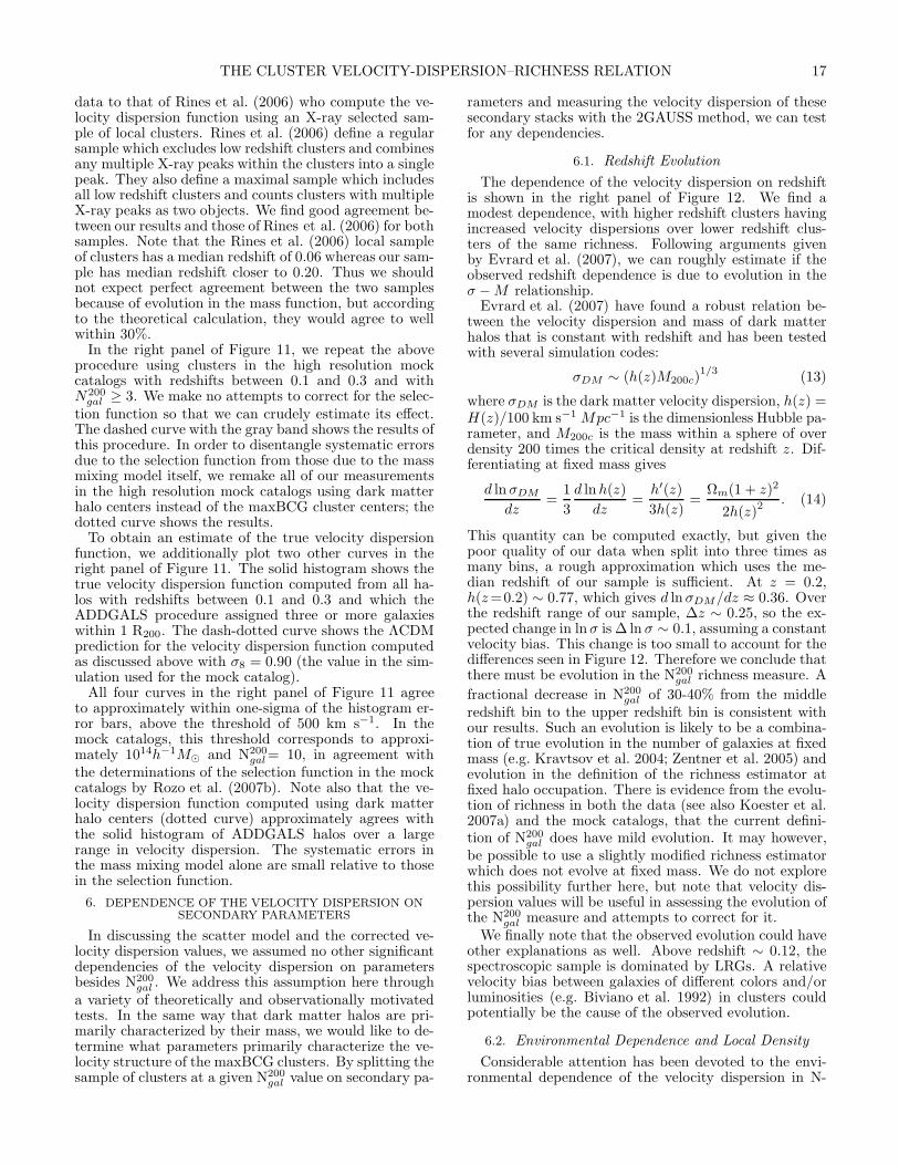
THE CLUSTER VELOCITY-DISPERSION–RICHNESS RELATION 17
data to that of Rines et al. (2006) who compute the ve-locity dispersion function using an X-ray selected sam-ple of local clusters. Rines et al. (2006) define a regularsample which excludes low redshift clusters and combinesany multiple X-ray peaks within the clusters into a singlepeak. They also define a maximal sample which includesall low redshift clusters and counts clusters with multipleX-ray peaks as two objects. We find good agreement be-tween our results and those of Rines et al. (2006) for bothsamples. Note that the Rines et al. (2006) local sampleof clusters has a median redshift of 0.06 whereas our sam-ple has median redshift closer to 0.20. Thus we shouldnot expect perfect agreement between the two samplesbecause of evolution in the mass function, but accordingto the theoretical calculation, they would agree to wellwithin 30%.
In the right panel of Figure 11, we repeat the aboveprocedure using clusters in the high resolution mockcatalogs with redshifts between 0.1 and 0.3 and withN200
gal ≥ 3. We make no attempts to correct for the selec-tion function so that we can crudely estimate its effect.The dashed curve with the gray band shows the results ofthis procedure. In order to disentangle systematic errorsdue to the selection function from those due to the massmixing model itself, we remake all of our measurementsin the high resolution mock catalogs using dark matterhalo centers instead of the maxBCG cluster centers; thedotted curve shows the results.
To obtain an estimate of the true velocity dispersionfunction, we additionally plot two other curves in theright panel of Figure 11. The solid histogram shows thetrue velocity dispersion function computed from all ha-los with redshifts between 0.1 and 0.3 and which theADDGALS procedure assigned three or more galaxieswithin 1 R200. The dash-dotted curve shows the ΛCDMprediction for the velocity dispersion function computedas discussed above with σ8 = 0.90 (the value in the sim-ulation used for the mock catalog).
All four curves in the right panel of Figure 11 agreeto approximately within one-sigma of the histogram er-ror bars, above the threshold of 500 km s−1. In themock catalogs, this threshold corresponds to approxi-mately 1014h−1M⊙ and N200
gal = 10, in agreement withthe determinations of the selection function in the mockcatalogs by Rozo et al. (2007b). Note also that the ve-locity dispersion function computed using dark matterhalo centers (dotted curve) approximately agrees withthe solid histogram of ADDGALS halos over a largerange in velocity dispersion. The systematic errors inthe mass mixing model alone are small relative to thosein the selection function.
6. DEPENDENCE OF THE VELOCITY DISPERSION ONSECONDARY PARAMETERS
In discussing the scatter model and the corrected ve-locity dispersion values, we assumed no other significantdependencies of the velocity dispersion on parametersbesides N200
gal . We address this assumption here througha variety of theoretically and observationally motivatedtests. In the same way that dark matter halos are pri-marily characterized by their mass, we would like to de-termine what parameters primarily characterize the ve-locity structure of the maxBCG clusters. By splitting thesample of clusters at a given N200
gal value on secondary pa-
rameters and measuring the velocity dispersion of thesesecondary stacks with the 2GAUSS method, we can testfor any dependencies.
6.1. Redshift Evolution
The dependence of the velocity dispersion on redshiftis shown in the right panel of Figure 12. We find amodest dependence, with higher redshift clusters havingincreased velocity dispersions over lower redshift clus-ters of the same richness. Following arguments givenby Evrard et al. (2007), we can roughly estimate if theobserved redshift dependence is due to evolution in theσ − M relationship.
Evrard et al. (2007) have found a robust relation be-tween the velocity dispersion and mass of dark matterhalos that is constant with redshift and has been testedwith several simulation codes:
σDM ∼ (h(z)M200c)1/3
(13)
where σDM is the dark matter velocity dispersion, h(z) =H(z)/100 km s−1 Mpc−1 is the dimensionless Hubble pa-rameter, and M200c is the mass within a sphere of overdensity 200 times the critical density at redshift z. Dif-ferentiating at fixed mass gives
d lnσDM
dz=
1
3
d lnh(z)
dz=
h′(z)
3h(z)=
Ωm(1 + z)2
2h(z)2 . (14)
This quantity can be computed exactly, but given thepoor quality of our data when split into three times asmany bins, a rough approximation which uses the me-dian redshift of our sample is sufficient. At z = 0.2,h(z=0.2) ∼ 0.77, which gives d lnσDM/dz ≈ 0.36. Overthe redshift range of our sample, ∆z ∼ 0.25, so the ex-pected change in lnσ is ∆ ln σ ∼ 0.1, assuming a constantvelocity bias. This change is too small to account for thedifferences seen in Figure 12. Therefore we conclude thatthere must be evolution in the N200
gal richness measure. A
fractional decrease in N200gal of 30-40% from the middle
redshift bin to the upper redshift bin is consistent withour results. Such an evolution is likely to be a combina-tion of true evolution in the number of galaxies at fixedmass (e.g. Kravtsov et al. 2004; Zentner et al. 2005) andevolution in the definition of the richness estimator atfixed halo occupation. There is evidence from the evolu-tion of richness in both the data (see also Koester et al.2007a) and the mock catalogs, that the current defini-tion of N200
gal does have mild evolution. It may however,be possible to use a slightly modified richness estimatorwhich does not evolve at fixed mass. We do not explorethis possibility further here, but note that velocity dis-persion values will be useful in assessing the evolution ofthe N200
gal measure and attempts to correct for it.We finally note that the observed evolution could have
other explanations as well. Above redshift ∼ 0.12, thespectroscopic sample is dominated by LRGs. A relativevelocity bias between galaxies of different colors and/orluminosities (e.g. Biviano et al. 1992) in clusters couldpotentially be the cause of the observed evolution.
6.2. Environmental Dependence and Local Density
Considerable attention has been devoted to the envi-ronmental dependence of the velocity dispersion in N-

18 BECKER ET AL.
Fig. 11.— The velocity dispersion number function with no corrections for the selection function of the maxBCG clusters (left) and itsreconstruction in the high resolution mock catalogs (right). Left: The theoretical prediction for the velocity dispersion number functionusing the Jenkins mass function is combined with the N-body calibrated relation between mass and velocity dispersion, using the workof Evrard et al. (2007), for three values of σ8. Each assumes that Ωm = 0.30. The circles and squares show the results of Rines et al.(2006) for their regular and maximal local X-ray selected clusters samples. The solid line is the velocity dispersion function of the maxBCGclusters. The gray band errors indicate the systematic errors, neglecting any corrections for the selection function, convolved with thestatistical errors in our measurements. Above approximately 1000 km s−1 the data is extrapolated. Right: The dashed line with grayband errors shows the velocity dispersion function computed from clusters in the high resolution mock catalogs in exactly the same wayas done with the maxBCG catalog, neglecting any corrections for the selection function. To estimate the systematic errors in the massmixing model alone, we compute the velocity dispersion function using halo centers (dotted line) instead of BCGs. The solid histogramshows the velocity dispersion function of all halos between redshifts of 0.1 and 0.3 which the ADDGALS algorithm assigned three or moregalaxies within 1 R200. This is compared with the ΛCDM prediction for the velocity dispersion function computed as in the left panel withσ8 = 0.90 (the value in the simulation used for the mock catalog).
Fig. 12.— The dependence of exp(< ln(σ) >) at fixed richnesson the BCG photometric redshift. The dependence of the velocitydispersion on redshift likely indicates evolution in the N200
gal mea-
sure. The solid lines are the best-fit power-laws to the highest andlowest redshift bins.
body simulations (e.g. Sheth & Diaferio 2001). It hasbeen found that the velocity dispersion does depend onlocal density, but only because massive halos tend to oc-cupy more dense environments (i.e. halo bias) and thevelocity dispersion is strongly correlated with halo mass.No direct dependence of the velocity dispersion on the lo-cal density has been found (e.g. Sheth & Diaferio 2001).
In order to test this prediction, we construct four in-dicators of local density: N200
gal of closest cluster, the pro-jected distance to the closest cluster, the total numberof cluster members of any cluster within 5 h−1Mpc and±0.04 in redshift, and the total number of clusters within5 h−1Mpc and ±0.04 in redshift. This redshift cut is cho-sen to match twice the redshift cut used in the maxBCGpercolation process to ensure that only clusters from oneredshift slice on either side of the cluster under consid-eration are used.
We complete the test by comparing two binning
schemes. First, we bin in N200gal and then on the lower
25%, middle 50%, and upper 25% quantiles of the localdensity parameters within each N200
gal bin. This methodshould roughly account for the mass trend with clusterrichness before comparing local environments. Second,we reverse the binning orders, using the lower 25%, mid-dle 50%, and upper 25% quantiles of the N200
gal distribu-tion in the second step. If there is in fact no dependenceof the velocity dispersion on local density, except becausemassive halos tend to occupy more dense environments,then the relations in this binning scheme should be con-stant for a given N200
gal bin. Note however that if the halooccupation itself correlates with local density at fixedmass, then our test could be significantly biased.
Using this technique, we find little significant depen-dence of the velocity dispersion on any of our measuresof local density. Figure 13 shows the results of this testfor one of the parameters, the total number of clusterswithin 5 h−1Mpc and ±0.04 in redshift. We have testedthese results for fixed bins in N200
gal and the local densityparameters, finding that they are robust. We appliedthese tests to the mock catalogs as well, producing simi-lar results.
6.3. Multiple Bright Members and BCG i-bandLuminosity
It has been shown that clusters which have undergonerecent mergers and show significant substructure are notvirialized (e.g. Iguchi et al. 2005; Diaferio & Geller 1996)and that their velocity dispersions are increased abovethe expectation for their mass (e.g. Cortese et al. 2004;Halliday et al. 2004; Girardi et al. 2005). One might ex-pect that a cluster with multiple bright members thatresemble the BCG has undergone a recent merger or hassignificant substructure. However, it has also been shownthat dark matter halos which form earlier at fixed masshave brighter, redder central subhalos (i.e. brighter, red-

THE CLUSTER VELOCITY-DISPERSION–RICHNESS RELATION 19
Fig. 13.— Dependence of the velocity dispersion on secondary parameters. Upper left: The histogram of the total number of clusterswithin 5 h−1Mpc and ±0.04 in redshift of each BCG in the BGVCF. Upper right: The velocity-dispersion–N200
gal relation in bins of the
number of clusters in a projected volume of each BCG. Lower left: The relation between velocity dispersion and the number of clusters ina projected volume of BCG in bins of N200
gal . Lower right: The dependence of the velocity dispersion–N200
gal relation on the absolute i-band
magnitude of the BCG. No secondary parameter dependence would result in constant relations in the lower left panel and completelyparallel relations with the same normalization in the upper right panel, assuming the halo occupation does not correlate with local densityat fixed mass.
der BCGs) and lower richness (e.g. Wechsler et al. 2006;Croton et al. 2007). Note that a brighter BCG at fixedmass for earlier forming halos likely corresponds to alarger magnitude difference between the BCG and themember galaxies.
We repeat the first binning scheme used above withthe i-band magnitude difference of the BCG and thenext brightest cluster member as the secondary param-eter. For each bin in N200
gal , the brightest member andBCG i-band magnitude difference distribution is split byits lower 25%, middle 50%, and upper 25% quantiles.The naive expectation that clusters with more than onebright member might have undergone a recent mergeror have significant substructure is not born out by thevelocity dispersions, which show no significant increase.However, because the computations are done at fixedrichness, it could be that late-forming halos, which havehigher richness for their mass, also have higher velocitydispersions for their mass, because they merged recently,so that the two effects conspire to roughly cancel eachother. Unfortunately, this hypothesis is difficult to testobservationally.
One can similarly test for mass dependence of the clus-ters on the luminosity of the BCG alone. In the lowerright panel of Figure 13, we plot the velocity dispersion ofthe clusters first binned in N200
gal and then in the absolute
i-band magnitude of the BCG using the lower 25%, mid-
dle 50%, and upper 25% quantiles within each N200gal bin.
We see dependence on this parameter: at fixed richness,clusters with more luminous BCGs have higher velocitydispersions. This same effect is observed in the stackedX-ray measurements of these same clusters by (Rykoffet al. 2007, in preparation); here, clusters with brighterBCGs have on average more X-ray emission. These ob-servations indicate that BCG luminosity may contain ad-ditional information about cluster mass beyond that inN200
gal alone.In the case of BCG i-band luminosity, the expectd
correlation mentioned above consistent with the obser-vations, since early-forming halos would have brighterBCGs and lower richness, so that at fixed richness, haloswith brighter BCGs tend to be more massive. However,for this explanation to be consistent with the previoushypothesis concerning the magnitude difference of theBCG and the next brightest cluster member, we mustassume that whether or not a halo has formed through amajor merger recently correlates more strongly with themagnitude difference of the BCG and the next bright-est member galaxy, than with the BCG i-band luminos-ity alone. In other words, we need to assume that theBCG i-band luminosity is not indicative of a recent majormerger (which would cause the velocity dispersion to beoverestimated at fixed mass), even though BCG i-bandluminosity correlates with formation time.

20 BECKER ET AL.
6.4. Cluster Concentration and Radial Dependence
Although we cannot measure the true mass concen-tration, we investigate the dependence of the velocity-dispersion richness relation on the galaxy concentration,measured here by the ratio of the number of cluster mem-bers (determined by the maxBCG cluster finder, not thenumber of pairs in the BGVCF) within 0.2 R200 to thenumber of members within R200. We see no dependenceof the velocity dispersions on this parameter when the de-pendence on N200
gal is accounted for first. When one binsdirectly on this ratio, the velocity dispersion decreaseswith increasing concentration.
Finally, we investigate the dependence of the velocitydispersion on cluster radius. The scaling of σ with radiusis measured in logarithmic bins of N200
gal . In general, thedispersion stays constant or decreases with radius. Thisis consistent with the results from previous studies (e.g.Rines et al. 2003; Rines & Diaferio 2006).
7. CONNECTING VELOCITY DISPERSION TO MASS
Using velocity measurements to probe clustermasses has a long history in astronomy; the virialtheorem was the earliest tool used to determinecluster masses (e.g. Zwicky 1933, 1937; Smith1936) and remains in use today (e.g. Girardi et al.1998; Struble & Rood 1999; Rines et al. 2003, 2006;Rines & Diaferio 2006). Other methods for determiningcluster masses, such as the projected mass estimator(a modified virial mass estimator) (e.g. Heisler et al.1985; Rines et al. 2003; Rines & Diaferio 2006), theJeans equation (e.g. Carlberg et al. 1997; Girardi et al.1998; van der Marel et al. 2000; Biviano & Girardi2003; Rines et al. 2003; Katgert et al. 2004), and thecaustic method (Diaferio & Geller 1997; Diaferio 1999)have also been widely applied (e.g. Biviano & Girardi2003; Rines et al. 2003, 2006; Diaferio et al. 2005;Rines & Diaferio 2006).
In order to connect the velocity-dispersion–richness re-lation to a mass–richness relation, we use the recent re-sults of Evrard et al. (2007), who found a dark mattervirial relation which appears to hold for all redshifts anda wide range of cosmologies. Evrard et al. (2007) useda suite of dissipationless simulations run with a range ofsimulation codes and resolutions to measure the velocitydispersion of dark matter particles at fixed mass. Theyfind that the dark matter virial relation can be charac-terized as a power-law,
M200c = 1015M⊙
1
h(z)
(
σDM
σ15
)1/α
(15)
where h(z) = H(z)/100 km s−1 Mpc−1 is the dimen-sionless Hubble parameter and M200c is the mass withina sphere of over density 200 times the critical density atredshift z. The values of the fit parameters for the meanrelation are found to be σ15 = 1084 ± 13 km s−1 andα = 0.3359± 0.0045.
Evrard et al. (2007) additionally found that the scatterof velocity dispersion at fixed mass is well fit by a lognor-mal with a small scatter of only 0.0402±0.024. However,the lognormal scatter in velocity dispersion at fixed massdoes not directly relate to the scatter in mass at fixed ve-locity dispersion without assuming the shape of the halo
mass function. In light of this difficulty, and the smallscatter in the relation, we take the mean power-law re-lation given by Evrard et al. (2007) to be a completelydeterministic relation.
As there is still substantial theoretical uncertainty invelocity bias, this will be a primary driver of the system-atic error in the N200
gal -mass relationship. To avoid thisuncertainty, we constrain a combination of velocity biasand mass as described below. Using the standard defi-nition of velocity bias, bv = σGAL/σDM where σGAL isthe galaxy velocity dispersion and σDM is the dark mat-ter velocity dispersions. The virial relation for galaxyvelocity dispersions then becomes
b1/αv M200c = 1015M⊙
1
h(z)
(
σGAL
σ15
)1/α
, (16)
where the quantity b1/αv M200c parameterizes our lack of
knowledge about velocity bias.To use this relation with the maxBCG clusters, we
calculate <σ1/α > using the measured lognormal distri-bution of σ in each bin. The result is
<σ1/α >=
exp
(
1
2αlnµmes
(2) − 1
4αln γ2
mes +1
8α2ln γ2
mes
)
(17)
where γ2mes and µmes
(2) are given by the 2GAUSS fits for
each N200gal bin (i.e. equations 8 and 9 respectively). This
value is then substituted for σGAL in equation 16. Toaccount for the factor of h(z), we repeat the 2GAUSSfits for each N200
gal bin, weighting each pair in the BGVCF
by 1/h(z)α. The inclusion of this factor has a negligibleeffect on the observed evolution in §6.1. We include thecorrection for BCG bias by dividing our results by theaverage BCG bias factor raised to the 1/α power.
We apply this method first to the mock catalogs, todetermine whether we recover an unbiased estimate ofthe mass–richness relation. In the left panel of Figure14, we show the results of this procedure applied to themock catalogs. The best-fit power-law is plotted as thesolid curve. For comparison, the mean mass of a clusterin each N200
gal bin, computed as the mean M200c massof the halos matched to the clusters within the bin, isshown as the diamonds. We again see the slight overcorrection of the BCG bias correction. Because the massis proportional to σ3, the masses we measure in the mockcatalogs are too low by ∼ 15 − 25%. The dashed line inthe left panel of Figure 14 shows the best-fit power-lawrelation between N200
gal and mass in the simulation, but
with the normalization increased by 25%. Note that inthe mock catalogs the velocity bias is defined to be unity,so that equation 16 should be exact with bv = 1 andσGAL = σDM .
The results for the maxBCG clusters are given in theright panel of Figure 14. The error bars include the the-oretical uncertainties in both α and σ15. The theoreticaluncertainties increase the error bars in our mass determi-nations by a fixed factor uniformly across each bin. Thebest-fit power-law for the mass-N200
gal relation is
b1/αv M200c =

THE CLUSTER VELOCITY-DISPERSION–RICHNESS RELATION 21
Fig. 14.— The dark matter virial relation applied to our stacksof clusters in the mock catalogs (left, circles), and in the dataon maxBCG clusters (right, circles). The mean M200c masses formatched halos in each bin are plotted for the mock catalogs onthe left (diamonds). The solid line shows the best-fit power-law
relationship between b1/αv M200c and N200
gal . The dashed lines show
the mass normalization shifted upward by 25% to account for theover correction of the BCG bias correction.
(
1.18+0.12−0.11 × 10¹⁴h−1M⊙
)
×[
N200gal /25
]1.15±0.12
,
and is shown as the solid line in the right panel of Figure14. The dashed line shows the approximate effect of theBCG bias over correction by shifting the mass normal-ization up by 25%.
8. CONCLUSIONS AND FUTURE PROSPECTS
In this paper we have presented new measurements ofthe BCG–galaxy velocity correlation function (BGVCF)for a sample of clusters identified from the SDSS with themaxBCG algorithm (Koester et al. 2007a,b). Throughcareful modeling of the shape of the BGVCF, we havemeasured the mean and scatter in velocity dispersion atfixed N200
gal . We find that the mean velocity dispersion at
fixed N200gal is well described by a power-law. The mean
velocity dispersion increases from 202 ± 10 km s−1 forsmall groups to more than 854 ± 102 km s−1 for largeclusters. The scatter in velocity dispersion at fixed N200
gal
is at most 40.5 ± 3.5% and falls to 14.9 ± 9.4% as N200gal
increases. We test our methods on both the C4 clustercatalog and on mock catalogs. Although there may bea slight 5-10% downward bias in the mean velocity dis-persion due to the corrections made for BCG bias, ourmethod successfully recovers the true scatter in both ofthese data sets with little bias.
The method presented here for measuring the scatterdepends on two assumptions: (1) the Gaussianity of thePVD histogram of a stacked set of clusters with simi-lar velocity dispersion, and (2) the lognormal shape ofthe distribution of velocity dispersion at fixed richness.While the first assumption is valid in cluster samplesproduced by running the cluster finder on realistic mockcatalogs, it is hard to directly test observationally. Simu-lations with galaxies based on resolved dark matter sub-halos may clarify this issue. The second assumption isdirectly supported in the mock catalogs and by inde-pendent observations with the C4 catalog (Miller et al.2005).
In addition to the measurement of the mean and scat-ter in the velocity-dispersion–richness relation, we ex-
plore the dependence of the velocity dispersion on pa-rameters secondary to richness. The velocity dispersionseems to be affected significantly by the i-band luminos-ity of the BCG. We also see velocity dispersion depen-dence on redshift and local density. While the correlationbetween N200
gal , velocity dispersion, and the BCG i-bandluminosity may be a true physical effect, we interpret thecorrelations of N200
gal and velocity dispersion with redshiftand local density as unphysical, systematic effects of themaxBCG cluster finder. Ultimately, it may be that thebest way to estimate cluster mass will be to use multipleobservables in combination. By making the comparisonsof different parameters and their dependence on veloc-ity dispersion as done in this paper, we will be able todetermine which observables correlate significantly withmass.
Our methods, in combination with weak lensing massprofiles measured for stacked maxBCG clusters (Shel-don et al. 2007, in preparation; Johnston et al. 2007,in preparation) and the radial phase-space informationcontained in the BGVCF, will allow for precise determi-nations of the velocity bias and the anisotropy of galaxyorbits in clusters. Precise measurements of these quan-tities will help to constrain current theoretical modelsof galaxy clustering and the velocity bias between darkmatter and galaxies.
This work also demonstrates the feasibility of usingour methods to measure the velocity dispersion function.The velocity dispersion function computed in this pa-per agrees with the results of Rines et al. (2006). How-ever, given the current estimated systematic errors inour computation (due the selection function, photomet-ric redshift errors, evolution in N200
gal , and the BCG bias
correction), we are unable to reach any strong conclu-sions about the magnitude of σ8. With this caveat, wedo however see from Figure 11, that our results supporta higher value of σ8 than the most recent CMB+LSSestimates (e.g. Spergel et al. 2006; Tegmark et al. 2006),as recently suggested by other analyses (e.g. Buote et al.2006; Evrard et al. 2007; Rozo et al. 2007b). This con-clusion is however degenerate with velocity bias. A ve-locity bias of approximately 1.1-1.2 could equally wellexplain our results.
The methods presented in this paper are a significantadvancement for the use of optical cluster surveys to de-termine cosmology. Our method can fully characterizethe velocity-dispersion–richness relation for any opticalcluster survey with a large spectroscopic sample. Futureredshift surveys with more galaxy redshifts will allow formore precise measurements of this scatter. Specifically,because the SDSS spectroscopy is mostly at or belowz ∼ 0.1, a higher redshift sample of spectroscopy wouldallow for further tests of any redshift dependence.
The measurement of the scatter in mass–observablerelations is key to the measurement of cosmologyfrom galaxy cluster surveys and self-calibration schemes(Lima & Hu 2004, 2005). Through adding an additionalpiece of observational information, the methods devel-oped here will undoubtedly tighten constraints on andlift degeneracies in current estimates of cosmology.
MRB would like to thank Brian Nord, Eli Rykoff,and Jiangang Hao for the useful discussions and sug-

22 BECKER ET AL.
gestions. We also thank Mike Warren for running thehigher resolution simulation described here, and KenRines for the generous use of his data. MRB acknowl-edges the support of the Michigan Space Grant Con-sortium. TAM acknowledges support from NSF grantAST 044327 and 0206277. RHW was partially sup-ported by NASA through Hubble Fellowship grant HST-HF-01168.01-A awarded by the Space Telescope ScienceInstitute, and also received support from the U.S. De-partment of Energy under contract number DE-AC02-76SF00515. AEE acknowledges support from the MillerFoundation for Basic Research in Science at Universityof California, Berkeley. The research described in thispaper was performed in part at the Jet Propulsion Lab-oratory, California Institute of Technology, under a con-tract with the National Aeronautics and Space Admin-istration. The authors acknowledge the partial support
of the Michigan Center for Theoretical Physics.The Sloan Digital Sky Survey (SDSS) is a joint project
of The University of Chicago, Fermilab, the Institutefor Advanced Study, the Japan Participation Group,The Johns Hopkins University, the Max-Planck-Institutefor Astronomy, Princeton University, the United StatesNaval Observatory, and the University of Washington.Apache Point Observatory, site of the SDSS, is operatedby the Astrophysical Research Consortium. Funding forthe project has been provided by the Alfred P. SloanFoundation, the SDSS member institutions, the NationalAeronautics and Space Administration, the National Sci-ence Foundation, the U.S. Department of Energy, andMonbusho. The SDSS Web site is http://www.sdss.org/.This work made extensive use of the NASA AstrophysicsData System and of the astro-ph preprint archive atarXiv.org.
APPENDIX
A. GROUP WEIGHTED EM-ALGORITHM FOR 1-DIMENSIONAL GAUSSIAN MIXTURES WITH EQUAL MEANS
Here we present the modification of the standard EM-algorithm (Dempster et al. 1977) for Gaussian mixturemodels that is used to fit the PVD histograms. It has the advantage of weighting clusters (or groups) of pointsevenly and fixing the the mean of each Gaussian to be equal. We also verify that the algorithm works using simplenumerical experiments. The derivation and notation given here is that of Connolly et al. (2000) with our changesnoted appropriately.
Let j index the number of Gaussians in the model, i index the data points, and Ni be the total number of datapoints in the group from which the ith data point is drawn. The statistical model for the entire set data set will be asum of Gaussians plus a single constant background component. We differ from Connolly et al. (2000) by presentingthe derivation of the algorithm with the background components included. Letting the Gaussian components be givenas
φ(x, µ, σj) =1
σj
√2π
exp
(
−(x − µ)2
2σ2j
)
(A1)
where µ is the common mean of all of the model components, σj is the standard deviation of the jth Gaussian, andthe background component, U(x), be given as
U(x) =1
2L(A2)
where 2L is the range of all of the data, X , we can write the model as
P (X |µ, σ1, . . . , σj) = p0 U(x) +∑
j=1
pj φ(x, µ, σj) (A3)
where the pj ’s are the weights for each model component and we require that p0+∑
j pj = 1. This model is exactly thatof the standard EM-algorithm for Gaussian mixtures. The difference here will be in the structure of the latent variables.
Let zij be defined such that zij = 1 if the ith data point is in the jth Gaussian and zij = 0 otherwise. Now we canwrite the complete data log-likelihood as
L =∑
i
zi0 ln (p0 U(x)) +∑
j
∑
i
zij [ln pj + lnφ(x, µ, σj)]. (A4)
Now we perform the expectation step of the algorithm given the current parameter guesses, θ, computing
Q=E(L |X, θ)
=∑
i
E(zi0 |X, θ) ln (p0 U(x)) +∑
j
∑
i
E(zij |X, θ) [ln pj + lnφ(x, µ, σj)]
=∑
i
τi0 ln (p0 U(x)) +∑
j
∑
i
τij [ln pj + lnφ(x, µ, σj)]
where τij is now weighted by cluster (or group) to give
τij =E(zij |X, θ )

THE CLUSTER VELOCITY-DISPERSION–RICHNESS RELATION 23
=P (xi is in group j |X, θ)
=1
Ni
P (xi | group j)P (group j)∑
r P (xi | group r)P (group r)
=1
Ni
pj φ(xi, µ, σj)
p0 U(x) +∑
r pr φ(xi, µ, σr)(A5)
and for the background
τi0 =E(zi0 |X, θ )
=P (xi is in background |X, θ)
=1
Ni
P (xi | background)P (background)∑
r P (xi | group r)P (group r)
=1
Ni
p0 U(x)
p0 U(x) +∑
r pr φ(xi, µ, σr). (A6)
Now we compute the maximization step by maximizing Q over the parameters. Following Connolly et al. (2000),we first rewrite Q into a more manageable form and then maximize Q. Using the definition of our model and itscomponents we have
Q =∑
i
τi0 [ln p0 − ln (2L)] +∑
j
∑
i
τij
[
ln pj −1
2ln 2π − lnσj −
(xi − µ)2
2σ2j
]
. (A7)
Letting
µ =
∑
ij τij xi∑
ij τij(A8)
and noting that∑
ij
τij
σ2j
(xi − µ)(µ − µ) = 0, we get
∑
ij
τij(xi − µ)2 =∑
ij
τij [(xi − µ) + (µ − µ)]2
=∑
ij
τij
[
(xi − µ)2 + (µ − µ)2]
=∑
j
Bj +∑
ij
τij(µ − µ)2,
whereBj =
∑
i
τij(xi − µ)2. (A9)
Now we rewrite Q as
Q =∑
i
τi0 [ln p0 − ln (2L)] +∑
j
∑
i
τij
[
ln pj −1
2ln 2π − lnσj −
Bj
2σ2j
− (µ − µ)2
1σ2j
]
. (A10)
The maximum of Q subject to p0 +∑
j pj = 1 will be given by letting µ be given by equation A8 and the rest of theparameters by
pj =
∑
i τij∑
ij τij, σ2
j =Bj
∑
ij τij. (A11)
The primary differences between the derivation given here and that given by Connolly et al. (2000) are the re-weighted expectation values of zij , equations A5 & A6, and that the means of each of the Gaussian components arefixed to one value (i.e. equation A8). The cluster-weighting is encoded in the factor of 1/Ni in equations A5 and A6.Each cluster of points contributes an equal amount to the parameters of the mixture model, making the total modelwighted by cluster, not by point.
In Figure 15, we plot the point-weighted histogram of data created from 5000 and 500 random draws from twoGaussians with dispersion 800 and 300 respectively along with the standard EM algorithm fit using 10 components.

24 BECKER ET AL.
Fig. 15.— A simple test of the cluster-weighted EM algorithm. The bold line and histogram are cluster-weighted; the thin line andhistogram are point-weighted. The point-weighted histogram can statistically “hide” non-Gaussianity because it allows one component tocontribute the majority of the points to the histogram, and thus determine its shape. The cluster-weighted histogram eliminates this issueby forcing each component to contribute equally. See text for details.
We also plot the cluster-weighted histogram of the same data fit with the EM algorithm derived above using 10components (bold line). The shapes seen in the figure are expected. In the point-weighted case, the 5000 samples ofthe 800 width Gaussian dominate the PVD histogram so it appears to be Gaussian. However, in the cluster-weightedcase, the two Gaussians of width 800 and 300 contribute equally. Thus we explicitly see the the non-Gaussianity inthe histogram. In effect, by not weighting the histogram by cluster, one can “hide” non-Gaussianity statistically.
B. STATISTICAL BIAS IN THE 2GAUSS METHOD
In this appendix, we describe the statistical bias correction we apply to the 2GAUSS method. Suppose we have ran-dom samples, D = d1, d2, . . . , dN, from a distribution, p(x), characterized by a set of parameters, z = z1, z2, . . . , zn,so that we can write p(x; z). A simple example would be a Gaussian characterized by its mean and variance. Fromthese random samples, we can construct estimators, µ, of the moments of the distribution, µ(i) =
∫∞
−∞xip(x; z)dx.
A well known example of an estimator of µ(1) is the mean, µ =∑N
k=0 dk/N . An estimator of the ith moment of a
distribution is said to be unbiased if∫∞
−∞µ(D) p(x; z)dx = µ(i). In some cases the sampling distribution of an estimator
can be computed exactly, so that bias can be computed and corrected for analytically.Because the 2GAUSS method is rather complicated, instead of attempting to compute the bias analytically, we use
a Monte Carlo method to estimate the bias. For each bin in N200gal , we construct 10,000 Monte Carlo samples of the
set of velocity separation values, v = v1, v2, . . . , vN, using the measured parameters < lnσ > and S2, the numberof clusters in the bin, and the number of samples per cluster in the bin. Then we remeasure < lnσ > and S2 foreach Monte Carlo sample. From these 10,000 reestimations of < lnσ > and S2, we estimate the bias in the 2GAUSSmethod. We then use this bias to correct our measurements.
We note here that the Monte Carlo tests indicate that the estimations of < lnσ > and S2 are correlated in a non-trivial way. The BAYMIX method would naturally account for these correlations in a transparent way. Alternatively,a different, unbiased procedure could be used to estimate < lnσ > and S2. One candidate method might be the useof Gauss-Hermite moments (van der Marel & Franx 1993). Given that we already have a well developed method toestimate < lnσ > and S2, we do not explore this possibility here. A detailed understanding of the correlations isbeyond the scope of this work, but would be necessary for the use of these results to understand cosmology precisely.
REFERENCES
Abazajian, K. et al. 2004, AJ, 128, 502 —. 2005, AJ, 129, 1755

THE CLUSTER VELOCITY-DISPERSION–RICHNESS RELATION 25
Adelman-McCarthy, J. K. et al. 2006, ApJS, 162, 38Annis, J. et al. 1999, in Bulletin of the American Astronomical
Society, 1391–+Bahcall, N. A. et al. 2003, ApJS, 148, 243Beers, T. C., Flynn, K., & Gebhardt, K. 1990, AJ, 100, 32Berlind, A. A. et al. 2006, ApJS, 167, 1Biviano, A., Girardi, M., Giuricin, G., Mardirossian, F., &
Mezzetti, M. 1992, ApJ, 396, 35Biviano, A., & Girardi, M. 2003, ApJ, 585, 205Blanton, M. R. et al. 2003, ApJ, 592, 819—. 2005, AJ, 129, 2562Bohringer, H. et al. 2000, ApJS, 129, 435Brainerd, T. G., & Specian, M. A. 2003, ApJ, 593, L7Buote, D. A., Gastaldello, F., Humphrey, P. J., Zappacosta, L.,
Bullock, J. S., Brighenti, F., & Mathews, W. G. 2006, ApJ, inpress, arXiv:astro-ph/0610135
Caldwell, N. 1987, AJ, 94, 1116Carlberg, R. G. 1994, ApJ, 434, L51Carlberg, R. G., Yee, H. K. C., & Ellingson, E. 1997, ApJ, 478,
462Colın, P., Klypin, A. A., & Kravtsov, A. V. 2000, ApJ, 539, 561Connolly, A. J., Genovese, C., Moore, A. W., Nichol, R. C.,
Schneider, J., & Wasserman, L. 2000, arXiv:astro-ph/0008187Conroy, C. et al. 2005, ApJ, 635, 982—. 2007, ApJ, 654, 153Conroy, C., Wechsler, R. H., & Kravtsov, A. V. 2006, ApJ, 647,
201Cortese, L., Gavazzi, G., Boselli, A., Iglesias-Paramo, J., &
Carrasco, L. 2004, A&A, 425, 429Croton, D. J., Gao, L., & White, S. D. M. 2007, MNRAS, 374,
1303Dahle, H. 2006, ApJ, 653, 954Dempster, A., Laird, N., & Rubin, D. 1977, J. Roy. Stat. Soc., 39,
1Diaferio, A. 1999, MNRAS, 309, 610Diaferio, A., & Geller, M. J. 1996, ApJ, 467, 19—. 1997, ApJ, 481, 633Diaferio, A., Geller, M. J., & Rines, K. J. 2005, ApJ, 628, L97Diemand, J., Moore, B., & Stadel, J. 2004, MNRAS, 352, 535Eisenstein, D. J. et al. 2001, AJ, 122, 2267Evrard, A. E. et al. 2007, ApJ, submitted—. 2002, ApJ, 573, 7Faltenbacher, A., & Diemand, J. 2006, MNRAS, 369, 1698Faltenbacher, A., Kravtsov, A. V., Nagai, D., & Gottlober, S.
2005, MNRAS, 358, 139Frenk, C. S., Evrard, A. E., White, S. D. M., & Summers, F. J.
1996, ApJ, 472, 460Fukugita, M., Ichikawa, T., Gunn, J. E., Doi, M., Shimasaku, K.,
& Schneider, D. P. 1996, AJ, 111, 1748Gerke, B. F. et al. 2005, ApJ, 625, 6Ghigna, S., Moore, B., Governato, F., Lake, G., Quinn, T., &
Stadel, J. 2000, ApJ, 544, 616Girardi, M., Biviano, A., Giuricin, G., Mardirossian, F., &
Mezzetti, M. 1993, ApJ, 404, 38Girardi, M., Demarco, R., Rosati, P., & Borgani, S. 2005, A&A,
442, 29Girardi, M., Giuricin, G., Mardirossian, F., Mezzetti, M., &
Boschin, W. 1998, ApJ, 505, 74Gladders, M. D., & Yee, H. K. C. 2000, AJ, 120, 2148—. 2005, ApJS, 157, 1Gladders, M. D., Yee, H. K. C., Majumdar, S., Barrientos, L. F.,
Hoekstra, H., Hall, P. B., & Infante, L. 2007, ApJ, 655, 128Grego, L., Carlstrom, J. E., Joy, M. K., Reese, E. D., Holder,
G. P., Patel, S., Cooray, A. R., & Holzapfel, W. L. 2000, ApJ,539, 39
Gunn, J. E. et al. 1998, AJ, 116, 3040Halliday, C. et al. 2004, A&A, 427, 397Hansen, S. M., McKay, T. A., Wechsler, R. H., Annis, J.,
Sheldon, E. S., & Kimball, A. 2005, ApJ, 633, 122Heisler, J., Tremaine, S., & Bahcall, J. N. 1985, ApJ, 298, 8Iguchi, O., Sota, Y., Tatekawa, T., Nakamichi, A., & Morikawa,
M. 2005, Phys. Rev. E, 71, 016102Izenman, A. J. 1991, Journal of the American Statistical
Association, 86, 205
Jenkins, A., Frenk, C. S., White, S. D. M., Colberg, J. M., Cole,S., Evrard, A. E., Couchman, H. M. P., & Yoshida, N. 2001,MNRAS, 321, 372
Johnston, D. E., Sheldon, E. S., Tasitsiomi, A., Frieman, J. A.,Wechsler, R. H., & McKay, T. A. 2007, ApJ, 656, 27
Katgert, P., Biviano, A., & Mazure, A. 2004, ApJ, 600, 657Koester, B. P. et al. 2007a, ApJ, in press, arXiv:astro-ph/0701265—. 2007b, ApJ, in press, arXiv:astro-ph/0701268Kravtsov, A. V., Berlind, A. A., Wechsler, R. H., Klypin, A. A.,
Gottlober, S., Allgood, B., & Primack, J. R. 2004, ApJ, 609, 35Lancaster, K. et al. 2005, MNRAS, 359, 16Levine, E. S., Schulz, A. E., & White, M. 2002, ApJ, 577, 569Lima, M., & Hu, W. 2004, Phys. Rev. D, 70, 043504—. 2005, Phys. Rev. D, 72, 043006Mazure, A. et al. 1996, A&A, 310, 31McKay, T. A. et al. 2002, ApJ, 571, L85Miller, C. J. et al. 2005, AJ, 130, 968Navarro, J. F., Frenk, C. S., & White, S. D. M. 1997, ApJ, 490,
493Popesso, P., Boehringer, H., & Voges, W. 2004,
arXiv:astro-ph/0403357Prada, F. et al. 2003, ApJ, 598, 260Rines, K., & Diaferio, A. 2006, AJ, 132, 1275Rines, K., Diaferio, A., & Natarajan, P. 2006, ApJ, in press,
arXiv:astro-ph/0606545Rines, K., Geller, M. J., Kurtz, M. J., & Diaferio, A. 2003, AJ,
126, 2152Rosati, P., della Ceca, R., Norman, C., & Giacconi, R. 1998, ApJ,
492, L21+Rozo, E., Wechsler, R. H., Koester, B. P., Evrard, A. E., &
McKay, T. A. 2007a, ApJ, submitted, astro-ph/0703574Rozo, E. et al. 2007b, ApJ, submitted, astro-ph/0703571Sheth, R. K. 1996, MNRAS, 279, 1310Sheth, R. K. et al. 2003, ApJ, 594, 225Sheth, R. K., & Diaferio, A. 2001, MNRAS, 322, 901Smith, J. A. et al. 2002, AJ, 123, 2121Smith, S. 1936, ApJ, 83, 23Spergel, D. N. et al. 2006, ApJ, in press, arXiv:astro-ph/0603449Springel, V. et al. 2005, Nature, 435, 629Stanek, R., Evrard, A. E., Bohringer, H., Schuecker, P., & Nord,
B. 2006, ApJ, 648, 956Strauss, M. A. et al. 2002, AJ, 124, 1810Struble, M. F., & Rood, H. J. 1999, ApJS, 125, 35Tasitsiomi, A., Kravtsov, A. V., Wechsler, R. H., & Primack,
J. R. 2004, ApJ, 614, 533Tegmark, M. et al. 2006, Phys. Rev. D, 74, 123507van den Bosch, F. C., Norberg, P., Mo, H. J., & Yang, X. 2004,
MNRAS, 352, 1302van den Bosch, F. C., Weinmann, S. M., Yang, X., Mo, H. J., Li,
C., & Jing, Y. P. 2005, MNRAS, 361, 1203van der Marel, R. P., & Franx, M. 1993, ApJ, 407, 525van der Marel, R. P., Magorrian, J., Carlberg, R. G., Yee,
H. K. C., & Ellingson, E. 2000, AJ, 119, 2038Warren, M. S. 1994, PhD thesis, AA(California Univ., Santa
Barbara, CA.)Wasserman, L. et al. 2001, arXiv:astro-ph/0112050Wechsler, R. H., Zentner, A. R., Bullock, J. S., Kravtsov, A. V.,
& Allgood, B. 2006, ApJ, 652, 71Wittman, D., Dell’Antonio, I. P., Hughes, J. P., Margoniner,
V. E., Tyson, J. A., Cohen, J. G., & Norman, D. 2006, ApJ,643, 128
Wojtak, R., Lokas, E. L., Mamon, G. A., Gottloeber, S., Prada,F., & Moles, M. 2006, A&A, in press, arXiv:astro-ph/0606579
York, D. G. et al. 2000, AJ, 120, 1579Zehavi, I. et al. 2005, ApJ, 630, 1Zentner, A. R., Berlind, A. A., Bullock, J. S., Kravtsov, A. V., &
Wechsler, R. H. 2005, ApJ, 624, 505Zwicky, F. 1933, Helvetica Physica Acta, 6, 110—. 1937, ApJ, 86, 217