On the maintenance of reproductive isolation in a mosaichybrid zone between the toads Bombina bombina and B.variegata.

T.H.Vines *†, S.C..Koehler †, M.Thiel †, T.R.Sands*, I.Ghira +, C.J. MacCallum, N.H. Barton* & B.D. Nürnberger †

* Institute of Cell, Animal and Population Biology, University of Edinburgh, Edinburgh EH9 3JT, Scotland

† Department Biologie II, Ludwig-Maximilians-Universität, Karlstr. 23, 80333 München, Germany

+ Babew-Bolyai University, Department of Zoology, 3400 Cluj-Napoca, Romania

1

Introduction

When ecologically differentiated taxa interbreed, the ultimate outcome of hybridisation may criti-

cally depend on the distribution of habitat in the zone of contact. While a smooth clinal transition

should form across an abrupt ecotone, a more intimate intermingling of habitat types may result in

a mosaic of distinct genotypes (Harrison and Rand 1989). The associated increase in the rate of

hybridisation should accelerate introgression at neutral traits. Taxon differences that do not confer

adaptation to one or the other habitat may collapse, and the situation may ultimately resemble a

case of early sympatric divergence due to local adaptation. Moreover, even the conditions for the

maintenance of adaptive differences become more stringent as the mosaic takes up an increasingly

large area between the two pure gene pools. Explaining such combinations of broad geographic

gradients with fine-scaled divergence may require a hybrid between existing theories, which apply

to either smooth clines or to metapopulations of discrete demes (Endler 1977, Barton and Whitlock

1997, Pannell and Charlesworth 2000).

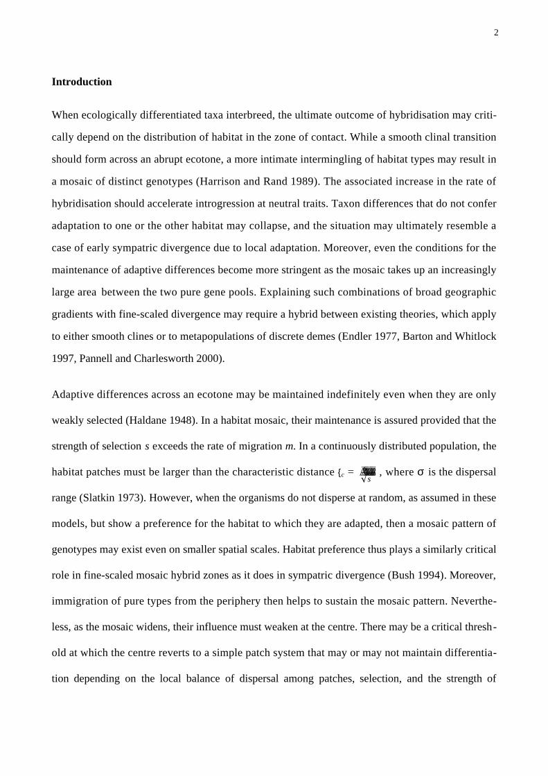
Adaptive differences across an ecotone may be maintained indefinitely even when they are only

weakly selected (Haldane 1948). In a habitat mosaic, their maintenance is assured provided that the

strength of selection s exceeds the rate of migration m. In a continuously distributed population, the

habitat patches must be larger than the characteristic distance {c = sÄÄÄÄÄÄÄÄÄè!!!s

, where σ is the dispersal

range (Slatkin 1973). However, when the organisms do not disperse at random, as assumed in these

models, but show a preference for the habitat to which they are adapted, then a mosaic pattern of

genotypes may exist even on smaller spatial scales. Habitat preference thus plays a similarly critical

role in fine-scaled mosaic hybrid zones as it does in sympatric divergence (Bush 1994). Moreover,

immigration of pure types from the periphery then helps to sustain the mosaic pattern. Neverthe-

less, as the mosaic widens, their influence must weaken at the centre. There may be a critical thresh-

old at which the centre reverts to a simple patch system that may or may not maintain differentia-

tion depending on the local balance of dispersal among patches, selection, and the strength of

2

habitat preference. Examples of mosaics apparently maintained by associations with patchily distrib-

uted habitat include Gryllus (Rand and Harrison 1989, Harrison and Bogdanowicz 1997), Sce-

loporus (Sites et al 1995) and Allonemobius (Howard 1986, Britch et al 2001), although the degree

to which these associations are due to selection or an active habitat preference is currently

unknown. In the case of Iris, individual plants are associated with different habitats over very small

scales. This is probably due to a combination of strong ecological selection and limited seed dis-

persal (Arnold and Bennett 1993).

Mosaic patterns may also arise from random drift if the number of migrants between demes (Nm)

or the neighborhood size (Wright 1943) is small. Such randomly generated divergence may be

preserved by selection against hybrids (i.e. towards different adaptive peaks, Barton and Whitlock

1997). A particularly important form of random drift is due to long range dispersal into the space

between two expanding populations (e.g. Ibrahim et al. 1996), or into unoccupied patches in the

mosaic from the parental populations (Nichols and Hewitt 1994). Examples of patchwork distribu-

tions apparently generated by dispersal and drift (as opposed to habitat associations) include Sole-

nopsis (Shoemaker et al 1996), Mus (Hauffe and Searle 1993), Limnoporus (Klingenberg et al

2000) and Palaemonetes (Garcia and Davis 1994). An interesting example where both factors may

be involved is the hybrid zone between Chorthippus brunneus and C. jacobsi, where habitat associa-

tions alone cannot satisfactorily explain the deviations in allele frequency away from a smooth

cline. The excess variation here could be explained by long distance dispersal from pure popula-

tions into the area of contact, either when the zone was initially forming or after the extinction of a

local population (Bridle et al 2001).

More generally, hybrid zones represent barriers to gene flow that delay but cannot ultimately pre-

vent introgression of neutral traits into the opposite gene pool (Barton and Bengtsson 1986). The

initial association between neutral and selected loci must break down as long as some recombina-

3

tion occurs between them. However, the time scale of this process is typically very slow, such that

original differences at marker loci are still diagnostic today in most recent (i.e. post-glacial) hybrid

zones. A higher rate of hybridisation in mosaic hybrid zones should hasten the decay of differences

in neutral allele frequencies. This rate of decay depends on the total selection strength and on the

way this selection is distributed across the genetic map. The barrier to gene flow becomes more

effective as the total selection increases and as it is distributed over an increasing number of loci

(Barton and Bengtsson 1986). While most hybrid zones may be far from equilibrium with regard to

neutral loci, the same need not be true for those loci that are under selection. Despite extensive

introgression at marker loci, the organisms may continue to be very well adapted to the specific

habitat patch in which they are found. Mosaic hybrid zones are thus promising places in which to

investigate the erosion rates of both selected and neutral traits under hybridisation, a issue which

has receiving much recent attention (Wu 2001).

In this paper, we present data from a mosaic hybrid zone between the fire-bellied toads B. bombina

and B.variegata in Romania. These two taxa have been diverging for around 3-5 million years, and

have adapted to different breeding habitats. Nevertheless, they are capable of producing fertile

hybrids (Szymura 1993). Several of its features should adapt B.variegata to reproduction in and

dispersal between ephemeral habitats: a robust skeleton, thicker skin (to reduce water loss), larger

and faster developing eggs and tadpoles. B. bombina is smaller, and produces a larger number of

slow growing and consistently more quiescent tadpoles. The latter trait is thought to reduce their

visibility to pond based predators (Nürnberger et al 1995, Kruuk & Gilchrist 1997, Vorndran et al,

in press). B. bombina is found in lowlands and flood plains throughout Eastern Europe, whereas B.

variegata is found at higher altitudes in Central and Eastern Europe (Figure1a).

Bombina hybrid zones in Poland, Croatia and the Ukraine consist of narrow clines, 5-10 km wide,

which separate extensive pure populations. In all these regions, there is strong linkage disequilib-

rium within populations of adult hybrids, even between unlinked marker loci. In Croatia and the

Ukraine, there is also an association between local habitat and genotype which is probably due to

4

linkage disequilibrium between the markers and genes that affect active habitat preference.

Although no systematic survey of habitats was made in Poland, habitat associations cannot be

strong, simply because the hybrid zones fit closely to a set of smooth clines (Szymura and Barton,

1991). These clinal patterns contrast sharply with Romania, where there is no steep cline in geno-

type frequencies (Figure 1b & c). Instead, the distribution of toads reflects the distribution of habi-

tats in the area, with B. bombina alleles being associated with pond-like habitats and B. variegata

with puddles. An important consequence of this structure is that isolated sites cannot easily main-

tain differences at marker loci in the face of immigration and hybridisation: even if selection is

strong enough to maintain adaptations to different habitats and different genetic backgrounds, we

expect divergence at neutral markers to dissipate. In the following, we make a detailed comparison

between the hybrid zones in Croatia and Romania, and use the observed habitat-genotype associa-

tions to quantify the strength of the barrier to gene exchange required for divergence to persist

indefinitely at marker loci.

5

Methods

In 1999, we sampled waterbodies extensively around Cluj county, in the NW of the Transylvanian

Plain, and collected 336 toads from 37 sites (Figure 1a & b). Adult toads were caught by hand or

with a net and immediately anaesthetised in 0.2% MS222 (3-amino benzoic acid ethyl ester,

Sigma). A toe was taken as a tissue sample and stored in 99.9% ethanol. They were subsequently

scored for 3 diagnostic marker loci: two SSCPs (Bb7.4 and Bv24.11) and one microsatellite

(Bv12.19), all of which segregate independently (Nürnberger et al, submitted). These samples

provide a wider regional context for the Apahida area (see Figure1b). They were not included in the

detailed genetic analyses (see below).

In 2000 and 2001 we focused our attention in an area 20 by 20 km centred around 46°50'N,

23°47'E, our main study area near the village of Apahida on the Transylvanian plain, Romania

(Figure 1b & c). Here, the landscape consists of rolling hills dissected by small river valleys flow-

ing to the nearby Somew river to the north west. The soil is mostly sandy loam, becoming more

clay rich in the valleys . The altitude ranges from 100 to 280m above sea level, and the vegetation is

either small arable strip fields or pasture. There are some small woodlands and few patches of

forest in the area, principally beech, oak and hornbeam. Toads were collected from 93 sites: 745

individuals from 70 sites in 2000, and a further 189 toads from 23 new sites in 2001. Only three or

four of these were large ponds, the majority being either drainage ditches or tractor wheel ruts. One

group of sites consisted of 10 circular excavated holes around 3 – 4 m deep and 3 – 5 m in diame-

ter. Several smaller, isolated watering holes were also found in other parts of the study area. As

above, adult toads were caught by hand or with a net and immediately anaesthetised in 0.2%

MS222 (3-amino benzoic acid ethyl ester, Sigma). After a photograph was taken of the toads'

individual belly pattern, a toe was taken as a tissue sample from either the right (2000) or the left

6

(2001) foot and stored in 99.9% ethanol. We also measured snout-vent and tibiofibula lengths, and

recorded the presence of nuptial pads (found only on breeding males), dorsal warts and dorsal

spots. Recaptures were simply re-photographed and released.

Habitat data were collected on the first visit for all the Apahida sites. The following were mea-

sured: width, depth, % emerged vegetation, % submerged vegetation and % bank vegetation

(subdivided into three height classes: % <15 cm, % 15-50 cm , %> 50 cm), along with the grid

reference. To enable direct comparison between the Romanian habitats and those sampled in

Croatia, we calculated a discriminant function axis on both data sets jointly. We used the approach

outlined in MacCallum et al (1998), in which a subset of sites are chosen as example 'ponds' or

'puddles', and the linear combination of habitat variables that best separated them calculated. All

variables were transformed to improve their normality (log for continuous variables, arcsine for

percentages: Sokal & Rohlf 1981) and the discriminant function was found for 152 sites (25 ponds

and 36 puddles in Romania, 23 and 68 in Croatia) using the stepwise routine in SPSS. The results

are given in Table 1. The four retained variables were width, % emerged vegetation, depth and %

submerged vegetation. With the exception of substituting % bank cover <15 cm for % submerged

vegetation, the variables are the same as those in the axis calculated by MacCallum et al (1998).

The distinction between the two habitat types was highly significant (F4,146 = 91.3, P < 10-6). The

function was then calculated for the remaining intermediate sites, and the axis rescaled to run from

0 (ponds) to 1 (puddles), using most the pond-like and the most puddle-like sites in the dataset as a

whole as endpoints. We denote this axis by H. It correlates well with the original Croatian habitat

axis (r = 0.95; MacCallum 1994) and an axis calculated for the Romanian sites alone (r = 0.97).

The 2000 and 2001 animals were scored for Bb7.4 and Bv24.11 and Bv12.19, along with an addi-

tional unlinked microsatellite locus Bv24.12. Two competing ways of scoring locus Bv12.19 were

found for 479 of the 748 animals genotyped in 2000, depending on whether faint alleles were

scored as present or not. Including the faint alleles gave only a weak heterozygote deficit FIS= 0.09

(support limits 0.8-0.30), whereas leaving them out gave FIS= 0.54 (support limits 0.43-0.64). The

7

former is similar to the remaining 2000 samples FIS= 0.08 (support limits -0.01 to 0.20) and the

toads genotyped in 2001 FIS= 0.02 (support limits -0.04 to 0.19). Since there was no reason to

believe that Bv12.19 was subject to greatly different evolutionary forces between the samples, the

faint alleles were included. In the case of Bb7.4, Bv12.19 and Bv24.11, there were two alleles

associated with B. variegata and one with B. bombina, but Bv24.12 had five characteristic of

B.variegata, one characteristic of B. bombina, and one of exactly intermediate length. Since the

latter was found on only four occasions, and then only in hybrid sites, it was left unscored. The B.

variegata alleles were combined to make all the loci biallelic, alleles are henceforth labelled either

0 (B. bombina) or 1 (B. variegata). Mis-scoring rates for these loci have been found to be around

0.5% in a parallel study (Nürnberger et al. submitted). We summarise the state of a toad's genome

by the total number of '1' alleles carried, forming a hybrid index (HI) which runs from 0 for pure B.

bombina to 8 for pure B. variegata. It is important to bear in mind that this measure is an estimate

based on four markers, and individuals with a 'pure' HI of 0 or 8 may well be introgressed at other

loci (Boecklen and Howard 1997).

We use maximum likelihood techniques to estimate heterozygote deficits and linkage disequilibria

(Edwards 1972, Hill 1974; see Szymura and Barton (1991) and MacCallum et al (1998) for

details). All calculations were performed on the Macintosh software package Analyse (by S.J.E.

Baird), available at http://helios.bto.ed.ac.uk/evolgen/Mac/Analyse/index.html. Briefly, the good-

ness-of-fit of an estimate for either heterozygote deficit (FIS) or standardised linkage disequilib-

rium (R) is given by the natural logarithm of its likelihood (LogL), a comparison between two

LogL estimates is distributed as c2 ê 2 with 1 degree of freedom in large samples provided that the

estimate is not at the boundary. Heterogeneity between sites in FIS can be assessed by comparing

log likelihoods when FIS is held constant or allowed to vary between them. The same approach can

also detect differences between loci, although linkage disequilibrium makes loci behave non-

8

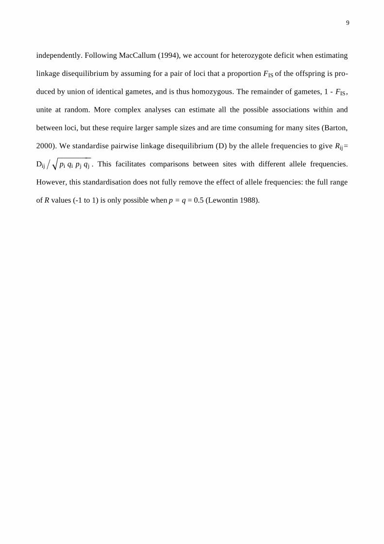
independently. Following MacCallum (1994), we account for heterozygote deficit when estimating

linkage disequilibrium by assuming for a pair of loci that a proportion FIS of the offspring is pro-

duced by union of identical gametes, and is thus homozygous. The remainder of gametes, 1 - FIS ,

unite at random. More complex analyses can estimate all the possible associations within and

between loci, but these require larger sample sizes and are time consuming for many sites (Barton,

2000). We standardise pairwise linkage disequilibrium (D) by the allele frequencies to give Rij=

Dij ë "####################pi qi pj qj . This facilitates comparisons between sites with different allele frequencies.

However, this standardisation does not fully remove the effect of allele frequencies: the full range

of R values (-1 to 1) is only possible when p = q = 0.5 (Lewontin 1988).

9

Results

The spatial pattern of hybridisation between Bombina bombina and B.variegata in the area around

Apahida, Transylvania, differs strikingly from the narrow transition zones that have been described

in Poland, Croatia and in the Ukraine (Szymura and Barton 1986, 1991, MacCallum et al 1998,

Yanchukov et al, unpublished). There, allele frequency clines were found in bands 6 – 9 km wide,

located at ecotones between forested hills and open plains and flanked on either side by extensive

areas containing only pure animals. In contrast the hybrid populations to the east of Apahida (Roma-

nia) are about 20 km from pure B. variegata populations to the NW in the foothills of the Apuweni

mountains and 100 km from the main expanse of pure B. bombina in the Hungarian plains (Figure

1b). Nevertheless, populations of the latter are found sporadically in large ponds across the entire

Transylvanian Plains, often in close proximity to the puddle-dwelling B. variegata (Stugren 1959,

Stugren & Vancea 1968).

Our collections across an area of about 40 x 40 km around the city of Cluj confirm this extended

mosaic (Figure 1b, note the relatively pure area of B. variegata to the NW). Isolated B. bombina

sites in areas dominated by B. variegata have been documented before on the Slovakian karst

plateau (Gollmann et al 1988) and in the Mátra mountains of Hungary (Gollmann 1987). Further-

more, in Kostajnica, Bosnia, large allele frequency differences were observed between pond and

puddle sites even when they were in close proximity (Szymura 1988, 1993). In the following analy-

ses, we compare the spatial and genetic structure of the Apahida (Romania) study area to the previ-

ously described hybrid zone in Pe<.enica, Croatia (MacCallum et al 1998, our Figure 1c). The

latter has a strong clinal structure across an altitudinal gradient, yet also has mosaic pattern at its

centre. Around Apahida, in contrast, there is no evidence for a cline over the same spatial scale, and

neither is there is a comparable ecological gradient (Figure 1c). It should be noted that the genetic

data for Croatia were 6 allozyme loci, whereas here 4 neutral DNA markers are used. Since the

10

allozymes Ldh-B and Mdh-1 and SSCP loci Bb7.4 and Bv24.11 are closely concordant in a Ukrai-

nian transect (Yanchukov, unpublished data), we treat them as equivalent. In any case, the hybrid

populations in Apahida and Pe<.enica are remarkably similar in their genetic structure.

Spatial distribution of allele frequencies and habitats

In the majority of sites, the population mean frequency of B. variegata alleles, pèè, among sampled

adults ranged from 0.5 to 0.8. There were hardly any pure B. variegata populations. Only four sites

had pèè < 0.4, and in these, only 13 out of 33 animals contained only B. bombina alleles (hybrid

index: HI = 0). Overall, the adult sample was dominated by hybrid individuals (Figure 2, see Appen-

dix I for a complete listing of the genetic parameters for each site). In order to determine how much

of the variation in mean allele frequency was explained a) by a clinal transition and b) by the fea-

tures of the aquatic habitat, we fitted a multiple regression model to the logit transformed allele

frequencies (i.e. z = log[pèè /(1- pèè)] ), sites with pèè = 0 or 1 were set to z = –3.5 and 3.5 respectively.

This transformation turns a sigmoidal cline into a straight line. The x, y-coordinates and the discrimi-

nant habitat score H (see Materials and Methods) for each site were entered simultaneously as

independent variables. The fitted regression was z = 0.61 – 0.07 x – 0.01 y + 1.93 H. The east-west

axis (x) was significant (F1,92= 4.7, P = 0.03), while the north-south axis (y) was not (P = 0.7). The

former result appears to be largely due to one pond with an almost pure B. bombina population at

the eastern edge of the study area (site 0293, see Appendix I): when it is removed, the x-axis is no

longer significant (P = 0.1). The habitat variable was of overwhelming importance in both cases

(original model: F1,92= 31.4, P < 10-6), as illustrated in Figure 3. When the same analysis was

applied to MacCallum’s (1994) data on the Pe<.enica transect, the best fit was z = 2.69 – 0.3 x –

0.08 y + 2.0 H. Spatial location was highly significant in this case (x: F1,92= 98.5, P < 10-10; y:

F1,92= 12.3, P < 0.003), as expected from the layout of the transect along the SW-NE axis (Figure

1d). The habitat score H was highly significant as well (F1,92= 12.3, P < 0.003).

11

We can describe the spatial distribution of habitat in a similar way, by regressing the habitat axis H

against the x and y coordinates. There is a significant relationship between east-west position and

habitat type in Croatia (F1,92= 19.7, P < 10-5), but not north-south (P > 0.1). There is no relation-

ship in Romania (P > 0.1 for both x and y). This suggests that different structures of the hybrid

zones in Croatia and Romania might be due to a different spatial distribution of habitat. A caveat

remains, in that these data only address occupied sites rather than all waterbodies. Collecting data

on the latter is hampered by the difficulty of defining a 'usable' waterbody, especially from the

perspective of a toad. We are confident the majority of occupied sites in the study area in each year

were sampled. The distributions of habitat types in Croatia and Romania are comparable, although

there are more intermediate habitats in the latter (Figure 4).

Association between habitat and allele frequency

In Romania, we can gauge the overall allele frequency difference between ponds (H = 0) and pud-

dles (H = 1) from the slope of a regression of pèè onto the habitat axis (Figure 3). This gives Dpèè =

0.39. Getting a comparable figure for Croatia is difficult: the steep cline confounds any analysis of

habitat associations over large spatial scales. We can, however, examine how the difference in pèè

corresponds to the difference in habitat score between nearby sites. Taking only those pairs that are

less than 1 km apart (an estimate of the lifetime dispersal distance derived from the Polish

transects, Szymura & Barton 1991, MacCallum et al 1998), the relationships in Croatia and Roma-

nia are similar: D pèè = 0.16 DH and D pèè = 0.24 DH respectively (Figure 5). It is difficult to test

whether there is any significant difference between these relationships, because the regressions are

based on pairs of sites rather than on independent data, and hence significance will be overesti-

mated. (This procedure does not bias the regression estimate however).

These slopes provide a second estimate of the maximum difference in allele frequency between

ponds and puddles (i.e. when DH = 1, Dpèè = 0.16 and 0.24 in Croatia and Romania respectively); we

consider them a more reliable reflection of habitat association because it is made over local scales,

of the same order as the dispersal range (see Discussion). We should note here that estimates of

habitat association were also made in two different ways in a previous analysis of the Croatian data.

12

MacCallum et al (1998) calculated the difference in allele frequency between adjacent ponds and

puddles (≤ 300m apart) as 0.25; this figure is probably less accurate, however, as it is based on only

7 pairs of sites. MacCallum (1994) fitted a model of a sigmoid cline to the whole Croatian dataset,

allowing the habitat as an additional explanatory variable. This gave D pèè = 0.15, which is close to

our simpler estimate of 0.16.

Concordance of allele frequencies

As is expected for diagnostic neutral markers in hybridising populations, the four loci are in fairly

close concordance (Figure 6). This justifies treating them as equivalent in subsequent analyses. To

quantify how the loci deviate from exact concordance, a cubic polynomial model was fitted

(Szymura and Barton 1991, Table 2):

pi= pèè + 2 pèè qèè@ai + bi Hpèè - qèèLD

In this model, pi is the frequency of variegata alleles at the i'th locus and pèè and qèè (= 1- pèè) are the

average frequencies across all loci. This formula was chosen because necessarily, pi= 0 when pèè =

0, and pi = 1 when pèè = 1. The parameter ai represents consistent deviations across the allele fre-

quency range, a positive a indicates a shift in favour of B. variegata alleles. A positive bi indicates

that there is a greater difference in pi between sites at either end of the spectrum compared to pèè. In

the context of a cline this corresponds to a steepening of the cline at that locus; here, it indicates

sharper divergence at a locus relative to the average. The largest deviation is at locus Bv24.11,

where a = -0.08, indicating a consistent excess of B. bombina alleles compared to other loci, of

~ aiÄÄÄÄÄÄ2 = 4%. Locus Bv24.11 also shows the largest difference in allele frequency between either end

of the spectrum , with b = -0.15. Neither of these deviations is larger than the largest of those found

for allozyme loci in Croatia (MacCallum et al. 1998) indicating that there is similarly close concor-

dance between regions. Random variations in discordance are quantified using the standardised

variance in allele frequency FST (cf. MacCallum et al 1998). Averaging across all sites and loci,

FST = 0.031, somewhat larger than the equivalent measure in Croatia (0.0068). Nevertheless,

random fluctuations are small in both Romania and Croatia: loci change in unison across the entire

range of sites.

13

Genotype frequencies: heterozygote deficit and linkage disequilibria

Pooling all sites, there is a significant deficit of heterozygotes at loci Bb7.4 and Bv12.19; overall,

there is a significant deficit when FIS is constrained to be the same across all loci (Table 2). There

is also marginally significant heterogeneity between loci (DL3= 7.63, P = 0.054). The higher defi-

cits at Bb7.4 and Bv12.19 are not associated with high levels of b, which might have indicated

stronger selection on those loci. We note it is possible that the higher deficit at Bv12.19 is due to

remaining scoring errors (see Materials and Methods). We divided the sites into seven groups by

their mean allele frequency and obtained FIS estimates both singly and across all loci within each

group. Considered individually, all four loci show a greater heterozygote deficit towards the B.

bombina side (data not shown). When FIS is estimated as a common value across all loci, there is a

clear peak on the B. bombina side (FIS = 0.22 at pèè = 0.21; Figure 7a). Since there are few sites in

the three left hand groups (n = 1, 2 and 3 respectively), this asymmetry does not result in a better fit

for a cubic model weighted by the support limits (F3,6= 1.34, P = 0.33) over a simple linear one

(F1,6= 52.05, P = 0.005). However, the means for each bin show a remarkably similar asymmetric

pattern to that seen in Croatia (MacCallum et al 1998, Figure7c), where the maximum FIS is 0.23

at pèè = 0.32 when a weighted regression is used (the equivalent regressions in MacCallum et al 1998

are unweighted, the cubic fit is the best with either method). We show the cubic curve in Figure 7a

for comparability with the Croatian data.

The standardised linkage disequilibria between loci, Rij = Dij ë "####################pi qi pj qj were estimated across

all sites. In these computations, the non-zero estimates of FIS were taken into account in order to

remove any undue inflation of disequilibrium through correlations of genes within loci (see Materi-

als and Methods). Table 3 gives values of R estimated across all sites for each pair of loci. Across

all sites and loci, R = 0.090 (support limits: 0.083, 0.097). This indicates that combinations of

genes found in the parental taxa are in excess, despite their constant breakup by recombination.

There is some heterogeneity between loci: the reduction in log likelihood of DL5= 13.2 when the

14

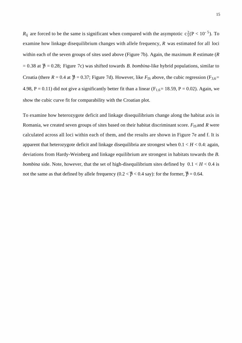
Rij are forced to be the same is significant when compared with the asymptotic c52(P < 10-5). To

examine how linkage disequilibrium changes with allele frequency, R was estimated for all loci

within each of the seven groups of sites used above (Figure 7b). Again, the maximum R estimate (R

= 0.38 at pèè = 0.28; Figure 7c) was shifted towards B. bombina-like hybrid populations, similar to

Croatia (there R = 0.4 at pèè = 0.37; Figure 7d). However, like FIS above, the cubic regression (F3,6=

4.98, P = 0.11) did not give a significantly better fit than a linear (F1,6= 18.59, P = 0.02). Again, we

show the cubic curve fit for comparability with the Croatian plot.

To examine how heterozygote deficit and linkage disequilibrium change along the habitat axis in

Romania, we created seven groups of sites based on their habitat discriminant score. FISand R were

calculated across all loci within each of them, and the results are shown in Figure 7e and f. It is

apparent that heterozygote deficit and linkage disequilibria are strongest when 0.1 < H < 0.4: again,

deviations from Hardy-Weinberg and linkage equilibrium are strongest in habitats towards the B.

bombina side. Note, however, that the set of high-disequilibrium sites defined by 0.1 < H < 0.4 is

not the same as that defined by allele frequency (0.2 < pèè < 0.4 say): for the former, pèè = 0.64.

15

Discussion

Our survey of genotype frequencies across the Bombina hybrid zone around Apahida is in striking

contrast with the narrow clines seen in Poland and Croatia. No steep gradient in allele frequencies

was apparent; instead, there was a fine-scaled mosaic with strong divergence in marker frequency

between different habitats. The frequency distribution of pure and hybrid populations was asymmet-

ric. Pure B. bombina populations were only found in sporadically occurring large ponds, whereas B.

variegata-like hybrid populations inhabited the much more abundant temporary sites in the sur-

rounding landscape. This asymmetry is even more remarkable as the nearest extensive pool of

entirely pure B. bombina lies 100 km away in the Hungarian plains: local strongholds of B. bom-

bina appear to cause the observed massive introgression of B. bombina alleles into the surrounding

B. variegata-like gene pool, in which 83% of adults were recombinant at our four marker loci.

Despite the very different spatial pattern of the hybrid zones near Apahida and near Pe<.enica,

Croatia, their local adult populations were very similar in their genetic structures (cf. MacCallum et

al 1998). When sites were pooled by their allele frequency, the maximum heterozygote deficit was

FIS= 0.23 in Croatia and 0.21 in Romania (Figure 7a & b). The analogous maxima for the standard-

ised linkage disequilibrium, R, were 0.40 and 0.38, respectively (Figure 7c & d). Moreover, both

parameters showed an asymmetric pattern in both regions, being stronger in sites with more B.

bombina-like toads. Associations between habitat and marker frequencies were of similar strength

(Dpèè = 0.16 in Croatia vs. 0.24 in Romania), and, finally, marker loci were concordant in both areas.

The Polish transects (Szymura and Barton, 1991) showed somewhat weaker linkage disequilibrium

(R = 0.22), but no heterozygote deficit, and little evidence of habitat associations. However, their

clinal pattern was similar to that in Croatia. Other Bombina hybrid zones studied in Austria (Goll-

mann 1984) and to the west of Zagreb in Croatia (Szymura 1988) appear to have lost the interven-

ing hybrid populations, and contain only slightly introgressed animals separated by an unpopulated

16

area. More interestingly, surveys in Slovakia (Gollmann 1988) and Kostajnica, Bosnia (Szymura

1988) are also consistent with a mosaic distribution created by an active habitat preference (see

Szymura 1993 for a discussion of Bombina hybrid zone structure). The mosaic pattern in Romania

raises several issues, which we address in turn: why should hybrid zones differ from place to place?

How is strong linkage disequilibrium maintained within a broadly sympatric distribution? And,

under what circumstances will either selected or neutral divergence persist despite migration and

hybridisation?

Why do hybrid zones differ from place to place?

As noted by MacCallum et al (1998) in their comparison of the Polish and Croatian contact zones,

differences between transects could arise in several ways. Firstly, the toads may differ. While B.

bombina populations show little regional differentiation across Europe, the B. variegata gene pool

is strongly subdivided: the Carpathian B. variegata is featured in our Polish and Romanian studies,

whereas the Pe<.enica transect borders on the Western form of this species. These two forms differ

considerably at 9 allozyme loci (Nei's IN = 0.85), compared to IN = 0.52 between B. bombina and

B. variegata. The maximum differentiation between B. bombina populations is IN = 0.91 (Szymura

1993, Figure 10.2). However, at the phenotypic level, the typical species differences were observed

wherever B. bombina and B. variegata were compared (e.g. egg size, tadpole development time,

relative leg length, belly coloration, mating call: Rafinska 1991, Sanderson et al 1992, Nürnberger

et al 1995, Vorndran and Nürnberger, in press). Second, the distribution of habitat may differ from

place to place, and this might lead to qualitatively different spatial patterns: for example, an inter-

mingling of distinct habitats might sustain a corresponding intermingling of more or less distinct

genotypes (cf. Introduction). Third, the zones may be of different ages. It is possible that two taxa

might remain distinct at first, because sets of genes would be in strong linkage disequilibrium, so

that selection and mate choice would act strongly against introgression. However, as the proportion

of recombined individuals increases, hybridisation might accelerate, leading to a broader hybrid

17

zone. Finally, the same argument suggests that a hybrid zone could reach alternative stable states,

depending on the vagaries of history: strong reproductive isolation might break down if the distinct

genotypes are bridged by the chance appearance of a hybrid population. Distinguishing between

these various possibilities is difficult, and they are not mutually exclusive. Regressions of habitat

score onto spatial location in the two countries where habitat data have been collected do show that

the gradient in habitat type seen in Croatia is not found in Romania, and that there is a wider range

of intermediate habitats in Romania. It is therefore likely that the spatial arrangement of habitat

contributes to the particular features of the Apahida hybrid zone.

How is strong linkage disequilibrium maintained within a broadly sympatric distribution?

As mentioned in the introduction, an active habitat preference can maintain local habitat patches

more easily than ecological selection, as effective migration will be reduced between adjacent sites

(Bush 1994). Habitat preference among hybrids was shown to affect the dynamics of the Pe<.enica

transect (MacCallum et al 1998), and could play an important role in stabilising the Apahida hybrid

zone. In the case of Pe<.enica, evidence that the typical preference of pure B. bombina and B.

variegata for ponds and puddles, respectively, was expressed even in toads of mixed ancestry

rested on three lines of evidence: a) the more pond like of 7 adjacent pond/puddle pairs always had

a higher frequency of bombina alleles; b) Toads moved extensively within and between seasons,

implying that local habitat associations in adults would quickly disappear in the absence of an

active preference; and c) more directly, in two sites, individual movements within a season were

correlated with genotype: toads leaving a puddle-like site and travelling to a more pond-like one

were significantly more B. bombina-like than the ones that remained. In Apahida, it is more diffi-

cult to demonstrate non-random dispersal because suitable sites are further apart, making the study

of dispersal by mark recapture less efficient. However, several observations indicate the existence

of a preference. The presence of pure B. bombina populations in ponds is striking in a landscape in

which B. variegata-like animals are found in practically all temporary sites. If they immigrated into

aquatic sites at random, selection against B. variegata adults in ponds would have to be very strong

18

indeed in order to eliminate them completely. In addition, the observed strong linkage disequilibria

imply substantial mixing of populations, making selection on adults an unlikely explanation for

habitat associations. Lastly, our sample included 13 adjacent man-made sites in various stages of

succession (distance between neighbouring sites ~5 m). Even on this scale, there was a significant

correlation between genotype and habitat score (r = 0.64, P = 0.006). In the following, we assume

that the local habitat associations in Romania are mainly due to active preference, as in Croatia.

Over wider scales, habitat associations are influenced by spatial structure. Specifically, the differ-

ence in allele frequency between extreme habitats is larger when estimated over larger spatial

scales: we estimated D pèè = 0.24 by comparing pairs of sites within 1 km of each other (Figure 5b),

whereas a regression of allele frequency against habitat for all sites gave D pèè = 0.39 (Figure 4). This

may be because sites are not evenly spaced, and the habitat preference is not complete: more iso-

lated sites are less likely to contain casual visitors and hence pèè will reflect H more closely. In

addition, local migration will impede the accumulation of allele frequency differences due to ecolog-

ical selection. This will further increase the discrepancy between D pèè estimates for adjacent pairs of

sites and across the study area as a whole. Data collection to determine the relative magnitude of

these effects is in progress.

Those adults that do immigrate into sites of the opposite habitat type contribute to the local linkage

disequilibrium. In general, the strong linkage disequilibria often seen in hybrid zones are most

likely to be generated by admixture of genetically distinct populations. Even if divergence is main-

tained entirely by epistatic selection, the disequilibrium generated by that selection is small relative

to that due to mixing of populations; this is so particularly for associations among neutral markers,

as opposed to selected genes (Barton and Gale 1993, Kruuk et al 1999). Thus, estimates of migra-

tion can be derived from observed linkage disequilibria.

In the Polish transects, linkage disequilibrium was assumed to be generated by dispersal across the

cline. Based on a diffusion model, it is then expected to equal D = s2

ÄÄÄÄÄÄÄÄÄÄrw2 when measured after dis-

19

persal and before selection. Here, w is the cline width, r the recombination rate (r = 0.5 for unlinked

loci) and s2the mean dispersal distance between parent and offspring. In both Polish transects, this

relationship gave estimates of s ≈ 1 km gen-1 (Szymura and Barton, 1991). In Croatia, the argu-

ment was complicated by the existence of a mosaic structure in the cline centre. Observed linkage

disequilibria are then generated both by the immigration of pure toads from the periphery (i.e. the

clinal component) and by dispersal between the two types of habitats in the centre. Migration at a

rate m between nearby habitats which differ by Dp in marker frequency will generate an additional

linkage disequilibrium D =Hm Dp2Lê r, with a coefficient that depends on detailed assumptions

about the life cycle (Appendix II). The two sources cannot be disentangled from genetic data alone.

Assuming (generously) that m = 0.5, our two estimates of Dpèè, 0.16 and 0.25 (cf. Results) give

estimates of D that can account for 27% and 66% of the observed maximum (D = 0.094 at pèè = 0.43;

MacCallum et al 1998) respectively. The key point here is that the distortion in genotype frequency

generated by admixture is proportional to the square of the difference in allele frequency, and so is

very sensitive to that parameter.

The situation in Romania is comparatively simpler, because there is no steep cline and both linkage

disequilibrium and heterozygote deficit can only be generated through mixing between nearby

populations in different habitats. Given the asymmetry of introgression from ponds with almost

pure B. bombina populations into the surrounding B. variegata gene pool, we can further simplify

the computations: a site with allele frequency pèèi receives immigrants from ponds with pèè ≈ 0, and so

Dpèèi ≈ pèè

i . For each site, we can then estimate an immigration rate from Di = Hmi D pèèi2 Lê r. For

populations with a mean allele frequency in the range 0.2 <pèè< 0.6, this yields an average immigra-

tion rate mèèè = 0.19 (s.d. = 0.19). The more detailed treatment in Appendix II shows that this expres-

sion for Di is a reasonable approximation for this range of allele frequencies and migration rates.

The mean FIS in these sites is 0.17; in the model assumed in Appendix II, FIS= mpÄÄÄÄÄÄÄÄÄÄÄÄÄÄÄÄÄqH1-mL , which gives

20

0.16 for mèèè = 0.19, pèè = 0.4. Thus, the migration rate inferred from linkage disequilibrium can also

account for the observed deficit of heterozygotes.

The contribution of pure B. bombina individuals to local linkage disequilibria can be assessed more

directly. Even in a population with pèè = 0.2, adult toads with entirely B. bombina alleles at the four

marker loci (HI = 0) are unlikely to arise by chance (Figure 8) and so can be assumed to be newly

arrived immigrants. Their average frequency, over sites with 0.2 < pèè < 0.6 is 11%, which is about

half the proportion needed to account for the observed linkage disequilibrium (mèèè = 0.19). The

difference must be due to immigration by recombinant genotypes from sites with pèè > 0. Closer

inspection shows that the hybrid sites in which adults with HI = 0 are found are not a random

subset of the habitat spectrum but are significantly more pond-like (t = 4.57, P = 0.001). This

implies that our failure to find pure B. bombina adults elsewhere is not just accidental, and that

disequilibrium in the more temporary sites must stem from recombinants. This distinction is impor-

tant, since a pure B. bombina that is found in a given site need not reproduce there, whereas linkage

disequilibrium generated by recombinant genotypes shows that introgression has actually occurred.

For example, disequilibrium in the nine sites with 0.55 < pèè < 0.6 can be accounted for by immigra-

tion of mèèè = 0.26 from sites with pèè = 0.2, although part of this is probably due to immigration from

B. variegata-like sites as well. (It is possible that the immigrants from sites with pèèè= 0.2 may effec-

tively be only first generation hybrids at selected loci and not later hybrid generations, see below).

Under what circumstances will divergence persist despite migration and hybridisation?

Our observed high rates of immigration are plausible, given our estimates of dispersal from other

areas and the observation of pure B. bombina several kilometers away from source ponds in Apa-

hida. This large influx of foreign alleles could potentially swamp the B. variegata gene pool around

Apahida and erode its adaptations to reproduction in temporary habitat. Furthermore, unless the

21

introgressing B. bombina alleles are actively countered by selection, the entire range of Bombina in

the Transylvanian plain will become a hybrid swarm.

If, for simplicity, we divide the genome into neutral and selected loci, this question about stability

has two parts: a) will differentiation be maintained with respect to those traits that mediate differen-

tial adaptation to ponds and puddles (including the habitat preference), and b) will frequency differ-

ences at neutral marker loci be maintained? The answer to the latter question is in principle ‘no’,

because as long as a tiny fraction of fertile recombinants are produced, linkage disequilibria

between selected and neutral loci must eventually disappear, even in a clinal hybrid zone. However,

this process may occur on a very long time scale so that it is imperceptible especially in younger

(e.g. post-glacial) hybrid zones and markers may still behave in a diagnostic manner. In the present

case, however, gene flow into the B. variegata population in Apahida is strong and asymmetric,

which greatly accelerates the dissociation of neutral and selected loci.

Will divergence be maintained in the traits adapting toads to ponds and puddles?

A spatial polymorphism at a single selected locus will be maintained if selection favouring the

locally adapted allele is stronger than the rate of immigration (s > m, Haldane 1932 p.211). This

argument holds even if there are other selected loci elsewhere in the genome, as long as there are

no linkage disequilibria between them. But as their number increases, selected loci cannot remain

independent: linkage disequilibria should build up among them. Both the per locus selection (s) and

the total selection across n loci (S = ns) then determine the dynamics of the hybrid zone (Barton,

1983). Moreover, the question of stability depends on precisely how selection acts. Since it is likely

that the many differences between B. bombina and B. variegata are based on many genes, we

briefly consider two models in which selection is either purely against hybrids or against alleles in

the wrong habitat.

22

We have made some numerical calculations for a symmetrical model with n = 5 to 20 unlinked loci,

following Barton and Shpak (2000). With selection against hybrids, such that the fitness of an

individual with a fraction p of variegata alleles is Exp@-4 SpH1 - pLD, the critical migration rate

above which migration swamps selection is m ~ SÄÄÄÄÄÄÄÄ4 n when selection is weak, and the population is

close to linkage equilibrium (Figure 9 left). However, as selection gets stronger, the critical migra-

tion rate becomes almost independent of the number of loci, and approaches a maximum of me=

3 - 2 è!!!

2 = 0.172. (This limit can be understood by supposing that B. bombina and B. variegata

mate at random, but produce no progeny; then, the frequency of B. variegata changes from p to

H1-mL pÄÄÄÄÄÄÄÄÄÄÄÄÄÄÄÄÄÄÄÄÄÄÄÄÄÄÄ1-2 p H1-pL over a generation). Thus, even if selection is so strong that no hybrids survive, migration

rates high enough to account for our observed linkage disequilibria would swamp local differences.

In contrast, if selection favours genotypes that are adapted to the local environment, selection is

able to counter higher rates of immigration, simply because the immigrant genotypes have low

fitness (Figure 9 right). With fitness Exp@-2 SpD, arbitrarily strong migration can be countered by

strong selection; for example, m = 0.2 can be countered by selection on 20 loci S≥1.7, which

implies a fitness of immigrant pure genotypes (p =1) of Exp[-2S] = 3.3%, and of F1's of 18%. With

more loci, the reduced selection per locus is outweighed by the strengthening of linkage disequilib-

ria, which makes selection more effective overall (Barton 1983). (Note that this model assumes

immigration from only one parental taxon. Immigration from both would reduce the swamping

effect, both because allele frequencies would be under weaker pressure, and because linkage disequi-

librium would be higher). The exact outcome depends strongly on the form of selection: if individ-

ual alleles are under strong selection (i.e. they cause large population fitness reductions even at low

frequency), relative to the selection against F1 hybrids, then introgression will be lower (Barton and

Shpak, 2000).

How quickly will frequency differences at neutral markers decay?

Strong selection on multiple genes and traits could maintain different adaptations in the different

habitats, and in particular, could maintain the different preferences of toads living in those habitats.

However, one would expect differences at neutral loci to dissipate rapidly - naively, over a times-

23

cale of ~ 1ÄÄÄÄÄm = 5 generations. It may be that the present hybrid zone is relatively recent, and that

differences at marker loci are indeed collapsing. Alternatively, if Bombina have been hybridising in

the Apahida area for more than a few tens of generations, then the rate of exchange of neutral genes

must be substantially lower. Introgression will be slowed by selection against linked alleles, but as

long as some F2 or backcross hybrids reproduce, neutral alleles will eventually introgress. For the

scenario above, selection against incoming alleles of S≥1.7 on 20 unlinked loci would counter

migration m = 0.2, but would not greatly reduce gene flow at an unlinked locus: for this model me =

0.09 m. However, the barrier to gene flow is much stronger when selection is spread over more loci,

because the neutral locus is then likely to be linked more closely to selected loci. Barton and Bengts-

son (1986, Fig.4a) calculated the reduction in gene flow for a model of weak additive selection on n

evenly spaced loci, with the neutral marker embedded at the centre. With 40 loci on one such

chromosome, and equal rates of selection and recombination, gene flow would be reduced 100 fold.

It is hard to be more definite without knowing just how selection acts, and without simulations

which take into account strong selection on large numbers of linked loci.

A more sophisticated argument takes into account the presence of populations with predominantly

variegata alleles 20 km NW of the study area (Figure 1b). If we treat our high linkage disequilibria

sites as analagous to a cline centre, there will be a shallow gradient in allele frequency between

these and the B. variegata area. If this is at equilibrium, then the flux of variegata alleles into the

hybrid zone must balance the flux of B. bombina alleles in from ponds. The former flux is propor-

tional to the gradient in allele frequency, ∂x p~ 1ÄÄÄÄÄÄÄÄÄÄÄÄÄÄ20 km : me w = s2

ÄÄÄÄÄÄÄÄ2 ∂x p. Taking s2 as 1 km2per

generation, we estimate the effective rate of influx of B. bombina alleles me ~ 1ÄÄÄÄÄÄÄÄÄ800 (a larger

me would imply faster introgression and thus a steeper gradient). As mentioned above, existing

theory suggests that very strong selection would be needed to reduce gene flow by this amount

(Barton & Bengtsson 1986).

There is some circumstantial evidence that selection against immigrant B. bombina alleles may not

be strong enough to significantly slow the decay in marker frequency differences. Firstly, F1 individ-

uals from Polish parents can produce viable offspring in the laboratory. The number of offspring in

24

backcrosses tends to be higher than in F2 families (J.M. Szymura, personal communication), but

this reduction is not of the required magnitude to reduce gene flow. Unfortunately, we have no data

on the fitness of F2 animals in the wild, and it is potentially much lower. Secondly, an analysis of

egg batches from a site containing a wide range of adults in Croatia showed that pure B. bombina

had successfully mated with B. variegata-like hybrids on several occasions (Nürnberger et al,

submitted), although we have no data on the long term viability or fertility of the offspring. Further-

more, these data were collected from other parts of the species ranges, and we cannot rule out the

existence of isolating mechanisms (e.g. incompatibility loci) that occur only in Apahida. Lastly,

detecting a habitat association in the 0.2<pèè< 0.9 sites with our neutral markers (Figure 4) implies

that there must be some linkage disequilibrium between these and the habitat preference loci. Since

linkage disequilibria are approximately halved every generation, introgression must be occurring at

an appreciable rate.

In any case, we know that the Apahida hybrid zone cannot be extremely old because the entire area

was inhospitable tundra or under ice 10,000 years ago (Hewitt 2000). Nonetheless, if the initial

contact was shortly after the end of the last ice age, the zone has now been stable for over 1000

generations. As this still requires a very low influx of B. bombina alleles (me~0.001), there is little

practical difference between the selection required for this and for much longer term persistence.

However, there is reason to believe the zone is much younger than this. Transylvania was heavily

forested until the 14th century (Pounds 1979), and since B. bombina is known to avoid wooded

areas (MacCallum 1994), it is possible they only invaded from the Hungarian Plain once extensive

deforestation had taken place. Under this scenario, hybridisation has gone on for ~100 generations,

and the selection required to preserve neutral marker differences to the present day is much lower.

Unfortunately we have no reliable estimate for the strength of selection against immigrant B. bom-

bina alleles, and hence we cannot distinguish between these two timescales. However, projects are

under way to estimate the strength of ecological selection on hybrid offspring in Apahida, and

controlled rearing experiments will measure the viability of F1 tadpoles from Romania. An analysis

25

of mating patterns using the techniques outlined in Nürnberger et al (submitted) is also near

completion.

To summarise, we have described a very broad mosaic hybrid zone between the fire-bellied toads

B. bombina and B. variegata in Apahida, on the Transylvanian Plain of Romania. This differs

remarkably in spatial structure from the clinal hybrid zones described previously (Poland: Szymura

and Barton 1991; Croatia: MacCallum et al 1998). More interestingly, the genetic structure in terms

of heterozygote deficit and linkage disequilibria in marker loci between Romania and Croatia are

broadly similar, indicating that migration, selection and habitat associations may be of the same

magnitude. Since maintaining divergence in a mosaic hybrid zone requires more stringent condi-

tions than a simple cline, we examined how strong selection must be for stability at either selected

or neutral loci given our high estimates for migration. We found that very strong selection against

B. bombina entering B. variegata habitat and against first generation hybrids is needed for neutral

marker divergence to have persisted since the last ice age, although considerably less is required for

selected loci (S≥1.7 for 20 loci). However, since it is also plausible that the zone formed in the last

500 years following extensive deforestation, the level of selection needed to preserve marker fre-

quency differences to the present day may be much lower. Finally, the analysis presented here may

also help to explain marker frequency differences (or lack thereof) in other situations involving

selection-mediated gene flow, such as sympatric speciation by host race formation, as discussed by

Bush (1994).

26

Acknowledgments

We thank Gyongyver Mara and Trabantul Galbena for enthusiastic field assistance, Alex Hofmann

and Robert Sieglsletter for access to their unpublished data, Bruni Förg-Brey and Gabi Praetzel for

help in the lab. Helpful comments on the manuscript were provided by ... This work was supported

by NERC studentships to THV and TRS and DFG grant Nu 51/2-1 to BN.

References

Arnold ML, Bennett BD (1993) Natural hybridization in Louisiana irises: genetic variation and ecologicaldeterminants. Pp. 115-139 in R. G. Harrison, ed. Hybrid zones and the evolutionary process. Oxford Univer-sity Press, Oxford.

Asmussen MA, Orive MM (2000) The effects of pollen and seed migration on nuclear-dicytoplasmic sys-tems. I. Nonrandom associations and equilibrium structure with both maternal and paternal cytoplasmicinheritance. Genetics 155: 813-831.

Barton NH (1983) Multilocus clines. Evolution 37: 454-471.

Barton NH (2000) Estimating multilocus linkage disequilibria. Heredity 84, pp 373-389.

Barton NH, Bengtsson BO (1986) The barrier to genetic exchange between hybridising populations. Hered-ity 57:357-376.

Barton NH, Gale KS (1993) Genetic analysis of hybrid zones. Pp. 13-45 in R. G. Harrison, ed. Hybrid zonesand the evolutionary process. Oxford University Press, Oxford.

Barton NH, Shpak M (2000) The effects of epistasis on the structure of hybrid zones. Genetical Research75:179-198.

Barton NH, Whitlock MC (1997) The evolution of metapopulations. In Metapopulation dynamics: ecology,genetics, and evolution (ed I. Hanski & M.E. Gilpin), pp 183-210. San Diego, CA: Academic Press.

Boecklen WJ, Howard DJ (1997) Genetic analysis of hybrid zones: number of markers and power of resolu-tion. Ecology 78, pp 2611-2616.

Bridle JR, Baird SJE, Butlin RK (2001) Spatial structure and habitat variation in a grasshopper hybrid zone.Evolution 55: 1832-1843.

Britch SC, Cain ML, Howard DJ (2001) Spatio-temporal dynamics of the Allonemobius fasciatus - A. sociushybrid zone: a 14-year perspective. Molecular Ecology 10: 627-638.

Bush GL (1994) Sympatric speciation in animals: new wine in old bottles. TREE 9: 285-289.

Edwards, A. W. F. 1972. Likelihood. Cambridge Univ. Press. Cambridge.

Endler JA (1977) Geographic variation, speciation and clines. Princeton Univ. Press. Princeton.

Garcia DK, Davis SK (1994) Evidence for a mosaic hybrid zone in the grass shrimp Palaemonetes kadiaken-sis (Palaemonidae) as revealed by multiple genetic markers. Evolution 48, pp 376-391.

27

Gollmann G (1984) Allozymic and morphological variation in the hybrid zone between Bombina bombinaand Bombina variegata (Anura, Discoglossidae) in northeastern Austria. Z. zool. Syst. Evolut.-forsch 22:51-64.

Gollmann G (1987) Bombina bombina and B. variegata in the Mátra mountains (Hungary): New data ondistribution and hybridisation (Amphibia, Anura, Discoglossidae). Amphibia Reptilia 8: 213-224.

Gollmann G (1988) Hybridisation between the fire-bellied toads Bombina bombina and Bombina variegatain the karst regions of Slovakia and Hungary. Journal of Evolutionary Biology 1: 3-14.

Haldane JBS (1932) The causes of evolution. Longmans, New York.

Haldane JBS (1948) The theory of a cline. J. Genet. 48: 277-284.

Harrison RG, Rand DM (1989) Mosiac hybrid zones and the nature of species boundaries. In Speciationand its consequences (ed. D. Otte & J Endler), pp 110-133. Sunderland, MA: Sinauer Associates.

Harrison RG, Bogdanowicz SM (1997) Patterns of variation and linkage disequilibrium in a field crickethybrid zone. Evolution 51: 493-505.

Hauffe, HC, Searle JB (1993) Extreme karyotypic variation in a Mus musculus domesticus hybrid zone: thetobacco mouse story revisited. Evolution 47: 1374-1395.

Hewitt GM (2000) The genetic legacy of the Quaternary ice ages. Nature 405: 907-913.

Hill WG (1974) Estimation of linkage disequilibrium in randomly mating populations. Heredity 33: 229-239.

Howard DJ (1986) A zone of overlap and hybridization between two ground cricket species. Evolution 40,pp 34-43.

Ibrahim KM, Nichols RA, Hewitt GM (1996) Spatial patterns of genetic variation generated by differentforms of dispersal during range expansions. Heredity 77, pp 282-291.

Klingenberg CP, Spence JR, Mirth CK (2000) Introgressive polarization between two species of waterstrid-ers (Hemiptera: Gerridae: Limnoporus): geographical structure and temporal change of a hybrid zone. J.Evol. Biol., pp 756-765.

Kruuk LEB, Gilchrist J (1997) Mechanisms maintaining species differentiation: predator mediated selectionin a Bombina hybrid zone. Proc. Roy. Soc. Lond. B 264, pp 105-110.

Kruuk LEB, Baird SJE, Gale KS, Barton NH (1999) A comparison of multilocus clines maintained byenvironmental adaptation or by selection against hybrids. Genetics 153: 1959-1971.

Lewontin RC (1988) On measures of gametic disequilibrium. Genetics 120, pp 849-852.

MacCallum CJ (1994) Adaptation and habitat preference in a hybrid zone between Bombina bombina andBombina variegata in Croatia. PhD diss., University of Edinburgh.

MacCallum CJ, Nürnberger B, Barton NH, Szymura JM (1998) Habitat preference in a Bombina hybridzone in Croatia. Evolution 52, pp 227-239.

Nichols, RA Hewitt GM (1994) The genetic consequences of long distance dispersal during colonization.Heredity 72: 312-317.

Nürnberger B, Barton NH, MacCallum CJ, Gilchrist J, Appleby M (1995) Natural selection on quantitativetraits in a Bombina hybrid zone. Evolution 49, pp 1224-1238.

28

Nürnberger B, Kruuk LEB, Barton NH, Vines TH. Mating patterns in a Bombina hybrid zone: inferencesfrom full sib genotypes when neither parental genotype is known. Submitted to Molecular Ecology.

Nürnberger B, Szymura JM, MacLean A, Förg-Brey B, Praetzel G, Abbott C, Barton NH. A linkage map forthe hybridising toads Bombina bombina and B. variegata (Anura, Discoglossidae). Submitted to MolecularEcology

Pannell JR, Charlesworth B (2000) Effects of metapopulation processes on measures of genetic diversity.Phil. Trans. R. Soc. Lond. B 355, pp 1851-1864.

Pounds NJG (1979) A historical geography of Europe 1500-1840. Cambridge University Press, Cambridge.

Rafinska A (1991) Reproductive biology of the fire-bellied toads, Bombina bombina and B. variegata(Anura: Discoglossidae): egg size, clutch size and larval period length differences. Biol. J.Linn. Soc. 43:197-210.

Rand D, Harrison RG (1989) Ecological genetics of a mosaic hybrid zone: mitochondrial, nuclear, andreproductive differentiation of crickets by soil type. Evolution 43, pp 432-449.

Sanderson N, Szymura JM, Barton NH (1992) Variation in mating call across the hybrid zone between thefire-bellied toads Bombina bombina and B. variegata. Evolution 46: 595-607.

Shoemaker DD, Ross KG, Arnold ML (1996) Genetic structure and evolution of a fire ant hybrid zone.Evolution, pp 1958-1976.

Slatkin M (1973) Gene flow and selection in a cline. Genetics 75, pp 733-756.

Sites JW, Barton NH, Reed KM (1995) The genetic structure of a hybrid zone between two chromosomeraces of the Sceloporus grammicus complex (Sauria, Phrynosomatidae) in Central Mexico. Evolution 49, pp9-36.

Sokal RR, Rohlf FJ (1981) Biometry. New York, NY: W.H. Freeman & Co.

Stugren B (1959) Eidonomische Untersuchungen an Bombina Oken (Amph., Discoglossidae) aus demGurghiu-Tale. Zool. Jb. Syst. 86 (4/5) p382-394.

Stugren B, Vancea S (1968) Geographic variation of the Yellow Bellied Toad (Bombina variegata) (L.)from the Carpathian mountains of Romania and the USSR. J. Herpetology 2: 97-105.

Szymura, J. M. 1988. Regional differentiation and hybrid zones in the fire-bellied toads Bombina bombinaand B. variegata in central Europe (in Polish). Uniwersytet Jagiellonski, Krakow.

Szymura JM (1993) Analysis of hybrid zones with Bombina. In RG Harrison (ed) Hybrid Zones and theevolutionary process, pp 261-289. OUP Oxford

Szymura JM, Barton NH (1986) Genetic analysis of a hybrid zone between the fire bellied toads Bombinabombina and B. variegata, near Cracow in Southern Poland. Evolution 40, pp 1141-1159.

Szymura JM, Barton NH (1991) The genetic structure of a hybrid zone between the fire bellied toads Bom-bina bombina and B. variegata: comparisons between loci and between transects. Evolution 45, pp 237-261.

Vorndran IC, Reichwaldt E, Nürnberger B (2002) Does differential susceptibility to predation on tadpolesstabilize the Bombina hybrid zone? Ecology, in press.

Wright S (1943) Isolation by distance. Genetics 28:114-138.

29

Wu CI (2001) The genic view of the process of speciation. J. Ev. Biol. 14: 851-865.

30

Tables

Table 1: Discriminant function coefficients (standardised) and their Wilks l, which measures the effect of that term on

the function. Variables were entered together, and are ordered by their contribution to the function. All Wilks l gave p

< 0.0001.

Overall Ponds Puddles Wilks l Correlation

Width 0.50 2.48 0.79 0.41 0.75

EmergentVeg 0.79 -7.21 -0.22 0.34 0.58

Depth 2.19 -2.24 4.93 0.29 0.57

SubmergedVeg 0.66 0.67 -1.58 0.28 0.34

Constant 0.49 -5.60 -5.11

GroupMean 2.33 -1.05

31

Table 2: Patterns at diagnostic loci. Discordance between loci are quantified by a and b (see text, Figure 5). FST gives

the standardised variance in allele frequency due to genetic drift, and FI S is an estimate of the heterozygote deficit.

Support limits are given in parentheses and significant values (where DlogL >2) are in bold.

Locus a b FST FIS

Bb7 .4 0.029 H-0.019, 0.080L 0.039 H-0.089, -0.163L -0.003 0.016 H0.097, 0.243LBv12 .19 0.004 H-0.047, 0.053L -0.020 H-0.155, 0.106L 0.048 0.085 H0.013, 0.159LBv24 .11 -0.080 H-1353, -0.033L -0.158 H-0.293, -0.028L 0.020 0.011 H-0.035, 0.081LBv24 .12 0.052 H-0.000, 0.100L 0.148 H0.020, 0.268L -0.002 -0.011 H-0.035, 0.062LOverall 0.031 0.06 H0.02, 0.101L

32

Table 3: Pairwise standardised linkage disequilibria across all sites. The maximum likelihood value for R for each pair

of loci is given in the main body of the table, and the value when R is constrained to be the same across all sites and

loci is given at the bottom of the right hand column. The remainder of this column contains the average for each locus.

All pairs of loci were significant (i.e. DlogL >2 for all).

Bb7 .4 Bv12 .19 Bv24 .11 AverageBb7 .4 0.145

Bv12 .19 0.085 0.078

Bv24 .11 0.203 0.105 0.153

Bv24 .12 0.148 0.046 0.153 0.115

0.090

33

Figures

Figure 1a: Locations of the study sites in Romania (inset B) and Croatia (inset D), the insets correspond to Figure 1b

and 1d respectively.

34

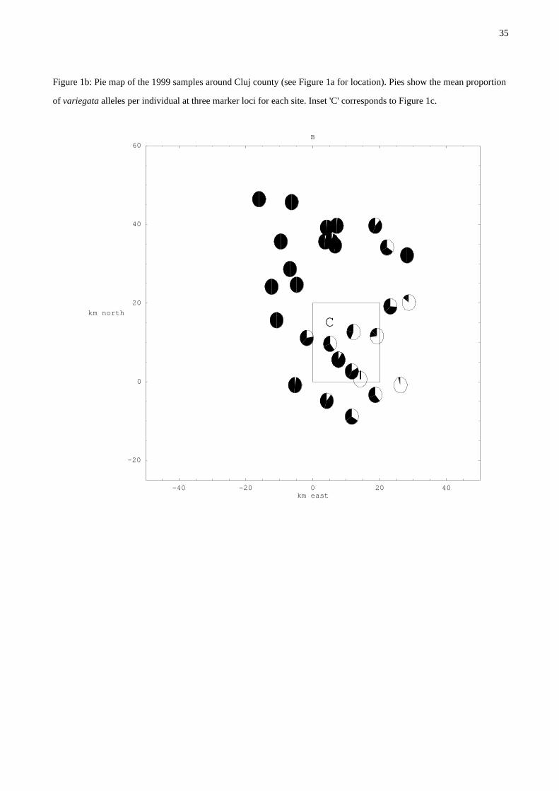
Figure 1b: Pie map of the 1999 samples around Cluj county (see Figure 1a for location). Pies show the mean proportion

of variegata alleles per individual at three marker loci for each site. Inset 'C' corresponds to Figure 1c.

-40 -20 0 20 40km east

-20

0

20

40

60

km north

B

C

35

Figure 1c: Pie map of the Apahida study area, showing only the samples collected in 2000 and 2001. Pies show the

proportion of variegata alleles per individual at four marker loci for each site.

0 2.5 5 7.5 10 12.5 15 17.5km east

0

5

10

15

km north

C

36

Figure 1d: Pie maps for the transect in Pe<.enica, Croatia (see Figure 1a for location). Pies show the proportion of

variegata alleles per individual at four allozyme loci for each site.

0 5 10 15 20km east

0

5

10

15

20

km north

D

37

Figure 2: Bar chart of HI distribution within sites binned by their mean variegata allele frequency. See Figure 2 of

MacCallum et al (1998) for the equivalent chart for the Croatian data.

mean p

2

4

6

8HI

0

20

40

mean p

2

4

6

8HI

38

Figure 3: Mean B. variegata allele frequency against the habitat axes for Romania. The regression is pèè = 0.46 + 0.38 H

(F1,92= 30.2, p < 10-6 ).

0.2 0.4 0.6 0.8 1hab

0.2

0.4

0.6

0.8

1

pmean

39

Figure 4: The distribution of habitat in Croatia (shaded bars) and Romania (white bars),

0.05 0.15 0.25 0.35 0.45 0.55 0.65 0.75 0.85 0.95

10

20

30

habitat axis

40

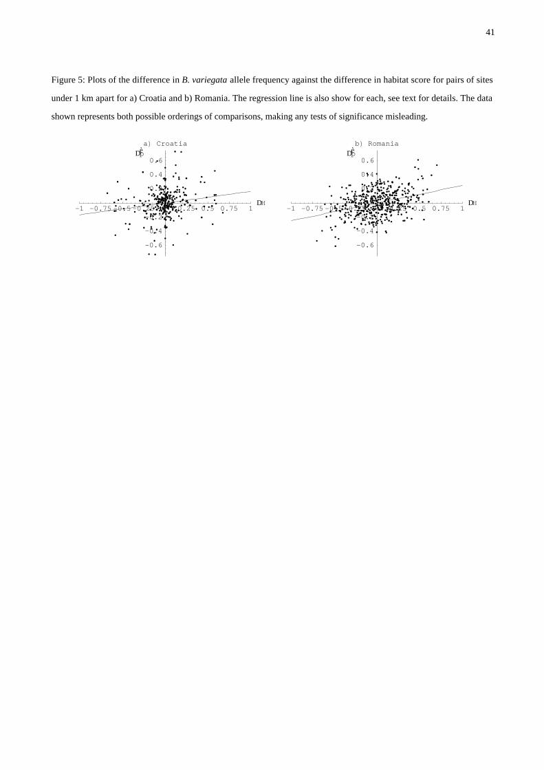
Figure 5: Plots of the difference in B. variegata allele frequency against the difference in habitat score for pairs of sites

under 1 km apart for a) Croatia and b) Romania. The regression line is also show for each, see text for details. The data

shown represents both possible orderings of comparisons, making any tests of significance misleading.

-1 -0.75 -0.5 -0.25 0.25 0.5 0.75 1DH

-0.6

-0.4

-0.2

0.2

0.4

0.6

aL Croatia

Dpè

-1 -0.75 -0.5 -0.25 0.25 0.5 0.75 1DH

-0.6

-0.4

-0.2

0.2

0.4

0.6

bL Romania

Dpè

41

Figure 6: Concordance of allele frequency across loci. Each graph shows the allele frequency for each of the four loci

plotted against the mean across those loci. The smooth curves show a cubic polynomial regression fitted by the maxi-

mum likelihood (see text, Table 1). The a, b for each regression are given in parentheses.

0.2 0.4 0.6 0.8 1pè

0.2

0.4

0.6

0.8

1

pi 24.11H-0.08,-0.158L

0.2 0.4 0.6 0.8 1pè

0.2

0.4

0.6

0.8

1

pi 24.12H0.052,0.148L

0.2 0.4 0.6 0.8 1pè

0.2

0.4

0.6

0.8

1

pi 7.4H0.029,0.039L

0.2 0.4 0.6 0.8 1pè

0.2

0.4

0.6

0.8

1

pi 12.19H0.004,-0.02L

42

Figure 7: Fis and R for binned sites estimated across all loci. For each group, the value and the 2-unit support limits

were obtained using maximum likelihood. The curves are a cubic regressions on the overall data, fitted by least squares,

see text for details. Plots 'a' and 'b' show FISand R for Apahida, binning sites by allele frequency pèè, 'c' and 'd' are the

equivalent plots for Pe<.enica (data from MacCallum et al 1998). Plots 'e' and 'f' show FISand R for Apahida, binning

sites by their habitat score H.

0.2 0.4 0.6 0.8 1habitat axis

0

0.2

0.4

0.6

0.8

1

F

e: Fis in Apahida

F=0.15+0.43H-1.97H2+1.43H3

0.2 0.4 0.6 0.8 1habitat axis

0

0.2

0.4

0.6

0.8

1

R

f: R in Apahida

R=0.15+0.78H-2.51H2+1.83H3

0.2 0.4 0.6 0.8 1mean p

0

0.2

0.4

0.6

0.8

1

F

c: Fis in Pe</enica

F=-0.09+2.20p-4.71p2+2.63p3

0.2 0.4 0.6 0.8 1mean p

0

0.2

0.4

0.6

0.8

1

R

d: R in Pe</enica

R=-0.13+3.16p-5.56p2+2.47p3

0.2 0.4 0.6 0.8 1mean p

0

0.2

0.4

0.6

0.8

1

F

a: Fis in Apahida

F=0.15+0.65p-1.9p2+1.06p3

0.2 0.4 0.6 0.8 1mean p

0

0.2

0.4

0.6

0.8

1

R

b: R in Apahida

R=-0.14+4.07p-9.72p2+6.0p3

43

Figure 8: A plot of the percentage of pure genotypically pure B. bombina animals against pèè in each site. The line is

H1 - pL8 , the expected frequency of animals of (0,0,0,0) animals under Hardy Weinburg proportions.

0.1 0.2 0.3 0.4 0.5 0.6p mean

20

40

60

80

100

% pure Bb

44

Figure 9: The critical rate of immigration, mc , which just swamps selection, S. Left: selection against hybrids,

W = Exp@-4 SpqD; Right: selection against incoming alleles, W = Exp@-2 SpD. Calculations are for n=5, 10, 20 loci

(top to bottom). In each figure, the lines to the left show the approximation assuming linkage equilibrium

(mc = SÄÄÄÄÄÄÄÄ4 n forselectionagainsthybrids; SÄÄÄÄn for selection against incoming alleles)

1 2S

0.1

0.2

m

1 2S

0.2

0.4

m

45

Appendix I: Table of all genetic parameters for all sites

site N p x y H Fis R HI

0 1 2 3 4 5 6 7 8

0293 14 0.063 16. 14. 0.045 0.14 0.044 9 3 2

1333 7 0.26 15. 18. 0.069 0.37 0.25 2 1 1 1 1 1

1085 12 0.27 4.3 5.5 0.014 0.21 0.25 2 3 3 2 1 1

0246 5 0.29 6.9 9.6 0.43 0.054 0.57 1 2 1 1

0282 9 0.33 11. 15. 0.24 0.18 0.31 3 1 4 1

0292 14 0.41 16. 14. 0.58 0.31 0.43 5 2 4 3

0251 12 0.44 5.4 5.6 0.49 0.15 0.42 2 1 2 1 1 1 3 1

0283 7 0.46 13. 16. 0.62 0.041 0. 1 2 2 2

0200.7 6 0.48 7.1 6.6 0.3 0. 0. 1 2 1 1 1

1389 7 0.5 16. 17. 0.39 0.29 0.21 2 2 2 1

0290 9 0.51 12. 15. 0.25 0.14 0.16 1 2 2 2 1 1

0307 8 0.52 13. 4.3 0.87 0.21 0.093 1 2 1 2 2

0200.8 9 0.53 7.1 6.6 0.34 0. 0. 2 1 1 1 3 1

0299 13 0.53 16. 15. 0.83 0.059 0. 2 6 3 2

1335 10 0.54 7.1 6.6 0.22 -0.19 0.27 1 1 3 3 2

0258 31 0.55 9.7 12. 0.32 0.22 0.47 5 1 1 3 4 1 6 9 1

0276 11 0.57 13. 16. 0.43 0.043 0.13 1 3 2 1 2 2

1397 8 0.57 16. 14. 0.49 0.042 0.27 1 4 1 1 1

0245 7 0.58 6.9 9.9 0.37 0.36 0.41 1 2 3 1

0253 8 0.58 4.7 6.8 0.56 0.039 0.3 2 1 1 2 1 1

1321 10 0.58 15. 16. 0.22 0.29 0. 2 3 2 2 1

0289 9 0.58 12. 15. 0.45 -0.13 0. 2 2 3 1 1

0249 8 0.59 5.5 7.3 0.45 0.13 0.44 1 3 1 1 1 1

1330 12 0.59 15. 17. 0.44 0.34 0.026 1 1 2 4 1 2 1

0302 15 0.6 14. 16. 0.68 0.084 0. 8 3 3 1

0297 13 0.61 19. 14. 0.53 0.29 0.027 1 1 3 4 1 3

0287 10 0.61 13. 16. 0.82 -0.2 0.021 2 1 4 2 1

0247 12 0.62 9.9 12. 0.68 -0.14 0.4 1 2 2 2 2 1 2

0286 18 0.63 13. 15. 0.55 0.071 0. 3 2 6 5 2

0304 10 0.63 15. 15. 0.62 -0.083 0. 1 5 3 1

1385 5 0.64 16. 17. 0.58 0.26 0. 2 1 1 1

0298 15 0.64 13. 16. 0.92 0.0016 0.15 1 5 4 1 3 1

0284 7 0.65 12. 17. 0.67 0.55 0.01 1 2 1 2 1

1334 10 0.65 7.1 6.5 0.37 0.043 0.045 1 2 1 5 1

1315 10 0.66 7.1 6.6 0.22 0.3 0.2 1 1 2 1 1 2 2

1345 7 0.66 15. 17. 0.51 -0.2 0. 1 1 4 1

0257 28 0.66 4.5 5.3 0.65 0.12 0.37 1 3 3 3 1 9 2 6

0248 10 0.67 9.5 12. 0.62 -0.014 0.41 1 2 1 2 3 1

1396 8 0.67 16. 14. 0.53 -0.12 0.46 1 2 1 2 1 1

0295 12 0.69 17. 15. 0.6 0.1 0.18 1 1 1 1 4 4

0300 15 0.69 16. 15. 0.71 0. 0.2 1 4 2 3 4 1

1379 8 0.69 16. 17. 0.41 0.023 0. 1 1 4 1 1

0296 11 0.69 18. 15. 0.55 0.048 0. 2 4 3 1 1

0305 9 0.69 8.3 7.8 0.27 -0.19 0.088 1 1 1 4 2

0291 9 0.69 14. 14. 0.75 -1500. 0. 1 4 2 2

1377 8 0.7 16. 17. 0.34 -0.059 0.33 1 1 1 2 1 2

0277 7 0.7 14. 16. 0.76 0.11 0.12 1 2 4

46

0301 15 0.71 16. 16. 0.66 -0.063 0. 3 5 1 6

0200.4 12 0.72 7.1 6.6 0.46 0. 0. 1 2 1 4 3 1

1372 10 0.73 10. 7.9 0.57 0.008 0.16 1 2 1 5 1

0259 10 0.73 9.8 12. 0.86 -0.21 0.45 1 2 1 2 2 2

0285 34 0.74 12. 16. 0.65 0.055 0.054 1 1 3 6 9 12 2

0288 9 0.74 14. 15. 0.77 0.034 0. 1 2 3 3

0250 12 0.74 5.9 6.2 0.67 -0.095 0.37 2 5 2 3

1380 6 0.74 10. 11. 0.57 -0.08 0. 1 4 1

1344 8 0.74 14. 17. 0.52 0.21 0. 1 1 3 2 1

0303 9 0.74 13. 16. 0.66 0.13 0. 2 5 2

0256 12 0.75 4.5 5.8 0.5 0.31 0.22 1 1 1 4 2 3

0244 6 0.75 5.5 7.4 0.59 -0.08 0.17 1 1 1 3

0200.5 8 0.75 7.1 6.6 0.39 0.24 0.21 1 2 1 3 1

0200.1 5 0.75 7.1 6.6 0.35 0.1 0.17 1 3 1

0260 12 0.76 9.5 12. 0.75 0.14 0.4 1 1 1 2 4 3

1342 10 0.76 15. 16. 0.28 -0.065 0.021 1 2 2 4 1

0264 12 0.77 10. 3.6 0.75 0.039 0.13 1 1 2 2 4 2

0200.9 6 0.77 7.1 6.6 0.48 0. 0. 1 3 2

1374 8 0.77 10. 7.7 0.27 0.063 0.5 2 2 4

0263 10 0.78 7. 4.6 0.73 -0.14 0. 1 2 2 4 1

1317 12 0.78 7. 6.6 0.64 0.16 0. 2 1 3 4 2

0279 5 0.78 16. 16. 0.81 -0.11 0.32 1 2 1 1

0200.3 12 0.79 7.2 6.5 0.34 0. 0. 1 1 3 5 2

0306 12 0.79 9.3 7.4 0.87 0.21 0.17 1 2 3 3 3

0252 7 0.8 5.2 5.4 0.72 0.13 0.24 1 1 4 1

1388 6 0.81 16. 17. 0.53 -0.14 0. 1 2 1 2

0200.6 7 0.81 7.1 6.6 0.33 0. 0. 3 4

1318 11 0.82 7.1 6.6 0.6 -150. 0.41 1 1 3 3 3

0262 12 0.83 2.9 5.5 0.65 0.026 0. 1 4 5 2

0270 12 0.83 9.4 12. 0.33 -0.08 0. 1 4 5 2

0281 12 0.84 10. 14. 0.87 -0.035 0.065 2 2 4 4

0268 12 0.84 2.8 5.4 0.3 0.58 0. 3 2 2 5

0280 11 0.86 4.6 9.5 0.76 0.17 0.39 1 1 4 5

0271 8 0.86 7.1 6.6 0.82 -0.065 0.062 4 1 3

1327 6 0.86 13. 16. 0.51 0.14 0. 2 2 2

0272 10 0.87 6.5 4.2 0.69 -0.11 0.18 1 2 3 4

0274 12 0.88 0.41 4. 0.75 -0.018 0.038 4 3 5

0267 12 0.89 5.6 3.5 0.78 0.063 0.12 4 2 6

0261 7 0.89 5. 3.9 0.89 0.21 0. 1 4 2

0273 6 0.92 0.61 3.9 0.72 -0.08 0. 4 2

0266 11 0.92 2.2 1.8 0.56 -0.035 0. 7 4

0275 12 0.93 3.8 0.64 0.82 -0.035 0.13 2 3 7

0265 12 0.96 2.1 1.9 0.92 -0.08 0. 4 8

47

Appendix II: Linkage disequilibrium generated by admixture

Immigration at a rate m between populations which differ in allele frequency by Dp at each of two loci generates

pairwise linkage disequilibrium proportional to m Dp2

ÄÄÄÄÄÄÄÄÄÄÄÄÄÄÄr . However, the precise relationship depends on detailed assump-

tions about the life cycle, the stage at which D is measured, and the forces acting on allele frequency. The formulae

given by Asmussen and Orive (2000) and Barton (2000) assume that there is immigration from two source demes, such

that allele frequencies remain at equilibrium. Barton and Gale (1993) consider immigration from a single deme, such

that allele frequency differences and linkage disequilibrium decay at a steady rate. Here, we suppose that strong

selection acts to impede gene flow, so that marker frequencies change slowly despite high rates of immigration. We

must therefore find the linkage disequilibrium when immigration is countered by selection at linked loci.

Assume that individuals mate at random within demes, producing zygotes in Hardy-Weinberg proportions. Juveniles

are subject to multiplicative selection, which again maintains Hardy-Weinberg proportions. Epistatic selection could

generate heterozygote deficit and linkage disequilibrium, and so our assumptions may underestimate these. Note that

we need not assume that selection acts directly on the two loci in question: the change in genotype frequencies depends

on the marginal fitnesses, which may be determined by selection at linked loci. Adults migrate between demes, and

then mate at random to begin the next generation. Migration may represent movement from place to place, or mixing

between habitats due to imperfect habitat preference. Genotype frequencies are measured in breeding adults after

migration. We assume that immigrants come from a source deme with allele frequencies p = 0 at both loci, and that

there is an equilibrium between selection and immigration;this determines the selection coefficients as a function of

immigration rate.

The heterozygote deficit in this model can readily be shown to be mpÄÄÄÄÄÄÄÄÄÄÄÄÄÄÄÄÄqH1-mL . There is no simple explicit solution for the

linkage disequilibrium as a function of immigration rate and allele frequency. However, the relation can be calculated

numerically (Figure A1). For low migration rates, D~3 mDp2 , as expected from formulae which assume a quasi-

equilibrium between immigration, and with recombination . r = 1ÄÄÄÄ2 for unlinked loci (Barton, 2000). For higher migra-

tion rates, disequilibrium remains close to this expectation when allele frequency is low, but falls below it for higher

allele frequencies. In the extreme case, D~0.5 mDp2 for m = 0.5, p = 0.5. Since we will be concentrating on migration

rates less than m ~ 0.3, and allele frequencies in the range 0.2 to 0.4, we take the relation as D~2 mDp2 .

48

Figure A1. The strength of linkage disequilibrium D scaled relative to difference in allele frequency is plotted against

immigration rate ( DÄÄÄÄÄÄÄÄÄÄDp2 vs. m). The curves are for allele frequency p = 0.05, 0.1, 0.2, 0.3, 0.4, 0.5 (top to bottom). Allele

frequency and linkage disequilibria are measured in adults, after multiplicative selection and migration.

0.2 0.4m

0.5

1

DÄÄÄÄÄÄÄÄÄÄDp2

49