
The long-run Phillips curve and non-stationary inflation
28
THE LONG-RUN PHILLIPS CURVE AND NON-STATIONARY INFLATION * Bill Russell # Anindya Banerjee † 27 April 2006 ABSTRACT Modern theories of inflation incorporate a vertical long-run Phillips curve and are usually estimated using techniques that ignore the non-stationary behaviour of inflation. Consequently, the estimates obtained are imprecise and are unable to distinguish between competing models of inflation and test the veracity of a vertical long-run Phillips curve. We estimate a Phillips curve model taking into account the non-stationary properties in inflation and identify a small but significant positive relationship between inflation and unemployment. The results provide some evidence that the trade-off between inflation and the unemployment rate in the short-run worsens as the mean rate of inflation increases. Keywords: Inflation, unemployment, long-run Phillips curve, business cycle, GMM. JEL Classification: C22, C32, C52, D40, E31, E32 * # The Department of Economic Studies, University of Dundee. Correspondence: [email protected]. † Department of Economics, European University Institute. The final version of the paper was written while the first-named author was a Visiting Fellow at the Department of Economics of the European University Institute.
-
Upload
independent -
Category
Documents
-
view
1 -
download
0
Transcript of The long-run Phillips curve and non-stationary inflation

THE LONG-RUN PHILLIPS CURVE AND
NON-STATIONARY INFLATION*
Bill Russell# Anindya Banerjee†
27 April 2006
ABSTRACT
Modern theories of inflation incorporate a vertical long-run Phillips curve and are usually estimated using techniques that ignore the non-stationary behaviour of inflation. Consequently, the estimates obtained are imprecise and are unable to distinguish between competing models of inflation and test the veracity of a vertical long-run Phillips curve. We estimate a Phillips curve model taking into account the non-stationary properties in inflation and identify a small but significant positive relationship between inflation and unemployment. The results provide some evidence that the trade-off between inflation and the unemployment rate in the short-run worsens as the mean rate of inflation increases.
Keywords: Inflation, unemployment, long-run Phillips curve, business cycle, GMM.
JEL Classification: C22, C32, C52, D40, E31, E32
* #The Department of Economic Studies, University of Dundee. Correspondence: [email protected]. †Department of Economics, European University Institute. The final version of the paper was written while the first-named author was a Visiting Fellow at the Department of Economics of the European University Institute.

2
1. INTRODUCTION
The insight of Friedman (1968) and Phelps (1967) that permanently higher inflation would
not lead to a permanent reduction in the unemployment rate and that the long-run Phillips
curve is vertical underpins the modern theoretical, empirical and policy literature on inflation.
Their insight is both simple and powerful. Simple in the sense that the concept of a vertical
long-run Phillips curve now appears to be ‘common sense’ and powerful in so far as this
concept completely dominates modern macroeconomics.
One of the implications of a vertical long-run Phillips curve is that inflation may be non-
stationary with multiple long-run rates of inflation. Indeed, the argument that the original
Phillips curve ‘broke down’ in the late 1960s and early 1970s implies that the expected rate
of inflation had changed due to a change in the long-run rate of inflation. Therefore, the
‘breakdown’ was due to a period where inflation was non-stationary. Subsequently, the issue
of how rapidly expectations of inflation adjust to changes in the long-run rate of inflation
came to be a crucial element of the debate surrounding adaptive and rational expectations.
To argue the converse, namely that inflation is stationary with a constant mean over the past
five decades, would imply that (a) there has only been one short-run Phillips curve over this
time (i.e. the curve where expected inflation matches the unique long-run rate of inflation);
and (b) the long-run Phillips curve in a practical sense is a single point corresponding to a
unique long-run rate of inflation and the long-run rate of unemployment. From this it follows
that stationary inflation data cannot identify a vertical long-run Phillips curve as the data
contain no relevant information concerning different long-run rates of inflation. Unless we
are willing to abandon all the Phillips curve literature since Friedman and Phelps that
incorporates a vertical long-run Phillips curve we must conclude that inflation is non-
stationary.1
Paradoxically, the conclusion that inflation is non-stationary sits uncomfortably with most of
the recent literature that estimates Phillips curve models of inflation. The papers by Batini,
Jackson and Nickell (2000, 2005), Galí and Gertler (1999), Galí, Gertler and López-Salido
1 The argument that inflation is non-stationary, by considering the implications of the converse, is dealt with in more detail in Russell (2006).

3
(2001, 2005), and Rudd and Whelan (2005) are particularly notable in this regard. This is
because the techniques chosen to estimate these models are appropriate only if inflation is
stationary with a constant mean. For example, Phillips curve models are frequently estimated
using generalised method of moments (GMM) so as to allow for correlation between the
forward looking variables and the error term. It is well documented (see for example Pesaran
1981, 1987, Stock, Wright, and Yogo 2002 and Mavroeidis 2004, 2005) that GMM is an
unsuitable estimation technique if the data are non-stationary and will provide biased
estimates leading to poor inference. These difficulties are exacerbated if, as we suspect, there
are breaks in the data. Consequently, these estimation techniques are inappropriate for
examining the validity of the competing standard models of inflation.2
In the following section we demonstrate the shortcomings of inflation models estimated by
GMM when the data are non-stationary. We conclude that the behavioural emphasis placed
on the estimates in terms of how expectations are formed and whether agents are forward or
backward-looking in these models is misplaced. This does not imply that agents do not
behave in the ways outlined in the standard theories, only that empirical inflation models
estimated using GMM provide such imprecise and biased estimates that they are unhelpful
when trying to distinguish between the competing models. Furthermore, we conclude that
these estimated models lack the precision necessary to identify whether or not the long-run
Phillips curve is indeed vertical.
Graph 1 shows United States quarterly CPI inflation for the period March 1952 to September
2004.3 The long period of low inflation in the 1950s and early 1960s is brought to an end by
increasing inflation towards the end of the 1960s. This is followed by the high inflation of
the 1970s and early 1980s associated with the OPEC oil price increases and then two discrete
reductions in inflation in the early 1980s and early 1990s. The first reduction is commonly
referred to as the ‘Volker deflation’ and the second coincides with a large recession. These
visual shifts in mean inflation can be shown more formally by a rolling 10-year regression of
inflation on a constant in the form:
2 The argument in this paper that GMM is an inappropriate method for estimating Phillips curve models due to the non-stationary properties of inflation data can be generalised to any estimation technique that is appropriate only for stationary data with a constant mean.
3 See the data appendix for details and sources of the data used in this paper.

4
ttp φγ +=∆ (1)
where tp∆ is United States CPI inflation and γ is a constant. The estimated constant, γ̂ ,
along with the 5 per cent critical value are plotted in Graph 2 and shows the steady increase
in the mean rate of inflation in the first half of the sample followed by a steady decline in the
second half.
The changes in mean have not been confined to inflation. Graph 3 shows the United States
unemployment rate for the period March 1952 to September 2004. We again see a general
increase in the unemployment rate up until the early 1980s followed by a general decline
thereafter. Similar to the above, we can show this more formally by a 10-year rolling
regression of the unemployment rate on a constant similar to that estimated in equation (1).
The estimated constant is shown in Graph 4.
How then can we examine Friedman and Phelps’ original insight that the long-run Phillips
curve is vertical? One way forward is to model inflation as an integrated process of order one
which allows us to examine directly if there is a long-run relationship between inflation and
the unemployment rate in the sense of Engle and Granger (1987).4 In section 3 we estimate a
two variable I(1) system containing inflation and the unemployment rate. We find that
Friedman and Phelps were possibly not pessimistic enough as we find evidence for a small
but significant positive slope to the long-run relationship between inflation and the
unemployment rate. That is, persistently high inflation leads not only to unemployment
returning to its long-run level but that the long-run unemployment rate is higher with higher
inflation. Persistently high inflation leads to higher unemployment in the long-run.
Indeed Friedman (1977), in his Nobel lecture, conjectures that the long-run Phillips curve
may have a positive slope. In that lecture he presents some graphical analysis based on 5-
year averaging of inflation and the unemployment rate to support this conjecture. We
undertake a similar analysis by plotting in Graph 5 the rolling means of inflation against
unemployment (taken from Graphs 2 and 4). This graph shows a clear positive correlation
4 We argue below that, although the ‘true’ statistical process may be stationary with a very frequently shifting mean, we can approximate this process as integrated of order 1.

5
between mean unemployment and inflation, suggesting that Friedman’s graphical analysis in
1977 near the peak in inflation continues to show in our data which includes the long general
decline in inflation since the start of the 1980s.
One might argue that the positive long-run relationship that we identify between inflation and
the rate of unemployment is simply due to supply-side influences on the long-run rate of
unemployment. The steady increase in the rate of unemployment up until the early 1980s
simply reflects a steady worsening in the supply-side influences on unemployment.
Similarly, the steady decrease thereafter reflects a steady improvement in the supply-side
influences which are independent of, and not due to, changes in the mean rate of inflation. If
this is the case then the positive correlation between the mean rate of inflation and these
supply side influences must be regarded as extremely unlikely and therefore fortuitous.
Friedman (1977) argues that the positive slope to the long-run Phillips curve that he identifies
may persist for many decades due to the greater uncertainty that is associated with higher
inflation.5 The uncertainty persists in the transition due to the time taken for new
arrangements to develop and deal with the higher uncertainty.
Our preferred explanation for the positive long-run relationship between inflation and the rate
of unemployment is based on Banerjee and Russell (2001a) and Banerjee, Cockerell and
Russell (2001). These papers identify a negative long-run relationship between inflation and
the markup of price on unit labour costs for a range of developed economies including the
United States. This relationship implies that there is a positive relationship between inflation
and the real wage relative to productivity.6 Consequently, persistently high inflation is
associated with a persistently high real wage relative to the level of productivity. If high real
wages relative to productivity leads to higher unemployment then the positive long-run
relationship between inflation and the rate of unemployment rate can be explained through
5 Friedman (1977) argues, in what he calls the ‘long-long-run’, that the Phillips curve will again be vertical. However, in the transition period that may extend for many decades, the long-run Phillips curve will have a positive slope. The slope persists due to the difficulty that economic agents have in fully adjusting to the new institutional and political arrangements that occur with changes in mean inflation.
6 The markup, mu , on unit labour costs can be written in natural logarithms as ( ) ( )lywpmu −+−= where p , w , y , and l are the price level, wage rate, output and labour
input respectively. Decreases in the markup, therefore, correspond to an increase in the real wage relative to the level of productivity.

6
the effect of inflation on the real wage. This explanation is examined in section 4 where we
estimate a 3 variable I(1) system consisting of inflation, the markup of price on unit labour
costs and the rate of unemployment. Two long-run relationships are identified in the data.
The first is the positive long-run relationship between inflation and the rate of unemployment
and the second re-establishes the negative long-run relationship between inflation and the
markup identified in our earlier work.
Our findings suggest that Friedman’s (1977) conjecture was correct. Furthermore, not
acknowledging explicitly the non-stationary nature of inflation has meant that the positive
slope may have been masked by the imprecise estimates, obtained using techniques that are
suitable only if the data are stationary with constant mean, or by the invalid imposition of a
vertical Phillips curve.
It is a moot question whether the estimated relationships between inflation and the rate of
unemployment and between inflation and the markup are truly ‘long-run’ in the sense used by
economic theorists. It may be that after a number of decades (i.e. Friedman’s ‘long-long-
run’) of a constant high rate of inflation the relationship disappears. However, from a policy
perspective the relationship appears to persist for enough time for it to be considered the
‘long-run’. Certainly the persistence in the data easily satisfies the standard tests of the long-
run in the sense of Engle and Granger (1987).
2. ESTIMATING THE HYBRID PHILLIPS CURVE
The mainstream literature that incorporates a vertical long-run Phillips curve can be
understood in terms of the hybrid Phillips curve where inflation, tp∆ , in time t depends on
expected inflation, etp 1+∆ , conditioned on information available in time t , lagged inflation,
1−∆ tp , and a ‘forcing’ variable, *uut − .7 The hybrid model can be written:
( ) ttutbetft uuppp εδδδ +−+∆+∆=∆ −+
*11 (2)
7 There are now a number of clear expositions of the New Keynesian Phillips curve and the hybrid Phillips curve. One such exposition is Henry and Pagan (2004).

7
where the error term, tε , represents the random errors of agents and inflation shocks, ∆ is the
change in the variable and lower case variables are in natural logarithms so that
1−−=∆ ttt ppp . The ‘forcing’ variable represents excess demand and is measured in a
variety of ways in the literature including the gap between real and potential output, real
marginal costs, labour’s share of income and, as shown here, the gap between the
unemployment rate, tu , and the long-run rate of unemployment, *u .
The Friedman-Phelps Phillips curve and New Keynesian Phillips curve models are special
cases of the hybrid Phillips curve. In the purely backward looking Freidman-Phelps model,
agents hold adaptive expectations and so 0=fδ and 1=bδ . In the purely forward-looking
rational expectations New Keynesian models of Clarida, Galí and Gertler (1999) and
Svensson (2000) 0=bδ and 1=fδ . Finally, hybrid models assume that there are both
forward and backward-looking price setting agents and that 1=+ bf δδ .
The hybrid Phillips curve has a number of appealing characteristics. First, the model
embodies a vertical long-run Phillips curve if 1=+ bf δδ , and 1,0 << bf δδ where inflation
is independent of the real variables in the model in the long-run. Second, the hybrid model
incorporates the observationally legitimate staggered price adjustment in contrast with
instantaneous price adjustment in the New Keynesian models. Third, the hybrid model
allows for both forward and backward looking elements that would appear consistent with
how many firms and agents operate. The model, therefore, provides a simple way to choose
between the three competing standard theories of the Phillips curve by identifying the
proportion of firms that base their pricing decisions on past inflation and expected inflation.
Finally, estimating the model allows us to empirically verify the validity of the vertical long-
run Phillips curve if we find that 1=+ bf δδ .
These ‘appealing characteristics’ are somewhat tempered by the theoretical and practical
difficulties associated with the estimation of these models. On a theoretical level, Phillips
curve models that incorporate a vertical long-run Phillips curve make very strong statements
concerning the statistical properties of the inflation data. If the model is true and 1=+ bf δδ
then inflation is non-stationary and empirical work should proceed by allowing for the

8
possibility that inflation is non-stationary.
Furthermore, the defining features of each model are the underlying behavioural assumptions
concerning expectation formation and pricing behaviour and that these behavioural
assumptions correspond to particular values of fδ , bδ and that 1=+ bf δδ . If these models
are true then such important ‘model-defining’ behavioural assumptions should be present at
all times. That is, the behaviour must be present not just over the entire sample but during
sub samples as well. In this case, the estimated values for fδ and bδ should be stable over
time and sum to 1. Unfortunately, what we find with inflation data is that there are long
periods when inflation behaves as a stationary variable. Without estimating the model, we
know that when inflation is stationary the sum of the coefficients bf δδ + must be less than
1. Therefore, the coefficients cannot be stable over time and this must question the
behavioural significance of the estimated coefficients.
On a practical level, if we estimate Phillips curve models with non-stationary inflation data
using techniques such as GMM that are suitable for stationary data then the estimates will
lack precision and are likely to be biased.8 Consequently, any estimates of fδ and bδ that
are retrieved will be unable to distinguish between the competing theories and whether or not
1=+ bf δδ . Very small deviations in these imprecise estimates will lead to very different
conclusions in terms of choosing between the models.
A number of conclusions follow from this discussion. First, unless we allow for the non-
stationary nature of inflation, there can be no behavioural significance to particular estimated
values of fδ and bδ unless we are happy to accept that the behaviour of economic agents is
very unstable. Second, to estimate the long-run Phillips curve requires non-stationary
8 Estimating Phillips curve models that incorporate expected inflation and a contemporaneous ‘forcing’ variable imply that expected inflation will be correlated with the error term in equation (2). The standard solution is to estimate the model using GMM where the instruments are usually lags of both inflation and the ‘forcing’ variable. Considerable work has focused on overcoming problems when estimating hybrid Phillips curves using GMM. Most of the focus in the empirical literature is on determining whether or not lags in inflation and the ‘forcing’ variable are suitable instruments for the variables. As inflation more closely approximates an integrated variable the instruments become better predictors of expected inflation but simultaneously more correlated with the error term.

9
inflation data so that 1=+ bf δδ . Finding 1<+ bf δδ does not invalidate theories that
incorporate a vertical long-run Phillips curve. All it implies is that the data are stationary and
that it contains no relevant information concerning different long-run rates of inflation.
Finally, estimation of the model should proceed under the assumption that the model is
correct and therefore estimation should allow for the possibility that inflation is non-
stationary.
These conclusions concerning estimating the hybrid Phillips curve can be demonstrated by
estimating the model using GMM over the full sample between March 1952 and September
2004 and comparing the results with those obtained from a rolling 10-year estimation of the
model. The results for the full sample are reported in Table 1. The last five columns provide
critical values assuming that the data are stationary, SprobCV , a random walk, RW
probCV , and
autoregressive with a coefficient on lagged inflation of 0.9, 9.0probCV . The degree of
significance of the critical value is indicated by the subscript prob.9 We find that the
coefficients on expected and lagged inflation are significantly less than 1 while the sum of the
coefficients is insignificantly different from 1. These results are similar to those found in the
literature. However, the diagnostics indicate that the residuals are stationary but highly
serially correlated and the J-test indicates that the instruments are not valid.
Leaving aside the fact that the diagnostic tests indicate that the model is poorly specified, the
results are broadly supportive of the hybrid Phillips curve hypothesis. In particular, the
behavioural underpinnings of the model are supported with expected inflation and forward
looking agents having a large and possibly dominant role in the inflation process, there is a
smaller proportion of backward looking agents and, finally, that the long-run Phillips curve is
vertical.
However, the poor model specification indicated by the diagnostic tests should not be
overlooked. Estimating the hybrid Phillips curve on a rolling 10-year basis reveals the
estimates of the model are poorly identified with the coefficients on expected and lagged
9 The critical values shown in the table as RWCV and 9.0CV were calculated using Monte Carlo simulation techniques. That is, the same model with 209 observations is re-estimated 10,000 times and the histogram of the t-statistics used to compute the 95 per cent critical value.

10
inflation highly unstable. The three panels of Graph 6 report the rolling estimates of the
coefficients on expected inflation, lagged inflation and the sum of the inflation coefficients.
Also shown on the graphs are the critical values testing for the coefficients equal to 1
assuming that the data are stationary. We see that for much of the period the coefficients on
expected and lagged inflation display large variation and that for much of the time they are
significantly less than 1 based on critical values assuming that the data are stationary. We
also see in the bottom panel that for nearly the entire sample the sum of the coefficients is
insignificantly different from 1. However the imprecision of the estimates is evident in the
graphs. We cannot reject that the sum of the coefficient is 1 even though the point estimates
of the sum range between around zero and 2 ½.
These results draw attention to two issues. First, the estimates are very poorly determined
with very large standard errors. Consequently, it is very difficult to reject hypotheses
concerning the size of the estimates. We cannot be confident from these results that the long-
run Phillips curve is vertical even though we cannot reject the hypothesis that the sum of the
coefficients equals to one. It may be that the long-run Phillips curve has a small but
economically important slope.
Second, placing a behavioural emphasis on these results in terms of the expectation formation
or proportions of agents who are forward or backward looking is misplaced as the estimates
are so inaccurate that we cannot reject most hypotheses. Furthermore, given the importance
of the behavioural hypotheses in defining their respective models the behaviour should be
stable over time. If the behavioural arguments are correct then it appears from the results in
Graph 6 that agents appear to forget quickly and learn again only to forget again.
3. THE LONG-RUN INFLATION-UNEMPLOYMENT RATE RELATIONSHIP
So far we have not addressed the issue of what type of non-stationarity is present in the
inflation data. Two forms of non-stationarity present themselves. The first is to assume the
monetary authorities respond to a series of shocks by making discrete changes in their
implicit inflation target and this leads inflation to be stationary with shifting means. The
usual way to proceed here would be to introduce as many shift dummies as necessary to
‘render’ inflation a stationary series. Typically this will not require a large number of shift
dummies. Invariably this small number of dummies will not identify all the shifts in the

11
mean rate of inflation and the unidentified shifts will continue to be problematic when
estimating inflation models. Furthermore, it is not easy to interpret the dummies in an
economic sense other than they indicate shifts in the mean rate of inflation.
The second way to proceed is to assume that inflation shocks are very frequent and that the
monetary authorities adjust the target rate of inflation at least partially in response to the
shocks. This assumption is consistent with the view that central banks did not actively offset
the increases in inflation during the 1970s by increasing nominal interest rates by more than
the increase in expected inflation (for example see McCullum 2000). This suggests central
banks accommodated the higher inflation and raised their implicit inflation target in the
1970s and may well have acted in a similar fashion when shocks served to reduce inflation at
other times like in the early 1950s and 1990s. We therefore assume that, while the ‘true’
statistical process of inflation may be stationary around a very frequently shifting mean, this
process can be approximated by an integrated process of order 1. In any case, as the number
of shifts in means increases, a stationary process with shifting means converges in the limit
on an integrated variable.
The hybrid Phillips curve model in equation (2) suggests that the inflation process can be
considered in terms of four variables, namely inflation, expected inflation, the unemployment
rate and the long-run unemployment rate. In the long-run expectations are realised and
expected inflation equals actual inflation. Similarly, actual unemployment will equal the
long-run unemployment rate. If we assume that the long-run rate of unemployment may not
be fixed then this variable can vary in the long-run. In this case, the long-run relationship
that implicitly underpins the hybrid Phillips curve when expectations are realised can be
written:
ttt up εαα ++=∆ *10 (3)
In the standard models that incorporate a vertical long-run Phillips curve, the long-run
coefficient 1α is equal to zero. Alternatively, if 01 ≠α then the long-run Phillips curve is not
vertical. The advantage of this approach over estimating the model using GMM is threefold.
First, in estimating (3) we can allow for the possibility that the variables are non-stationary
and in so doing improve the precision of the estimates. Second, in equation (3) the test of the

12
slope of the long-run relationship is whether or not 1α is significantly different from zero.
This is in contrast with equation (2) where the test is whether or not the sum of the leads and
lags in inflation is significantly different from 1.10 Third, estimating equation (3) allowing
for non-stationary data allows us to either reject or accept the vertical long-run relationship.
This is in contrast with the GMM estimates of the hybrid Phillips curve model which is
unable to reject the vertical Phillips curve when the data are non-stationary.
However, these advantages do come with a disadvantage insofar as estimating equation (3)
does not allow us to distinguish among the three competing standard theories of inflation. In
particular, the estimates cannot distinguish between the proportions of forward and backward
looking agents or how expectations are formed. Estimating equation (3) allowing for non-
stationary data simply allows us to answer the question of the slope of the long-run Phillips
curve and provide better estimates of the dynamics of inflation.
If we assume that inflation is an integrated variable of order 1, we can estimate a two variable
I(1) system containing inflation and the unemployment rate. The system is conditioned on a
predetermined business cycle variable which is measured as de-trended constant price gross
domestic product (GDP) and a series of spike dummies for periods when the residuals of each
estimated equation in the system are greater than 3 standard errors.
The results of estimating the inflation-unemployment rate I(1) system are provided in
Table 2. The trace statistics for the number of cointegrating vectors indicate that the
hypothesis of one long-run relationship between the variables is evident in the data. We find
that the long-run coefficient, 1α , is significant and negative indicating a positive long-run
relationship between inflation and the unemployment rate. The estimated long-run
coefficient is – 2.714 and this implies that a 1 percentage point increase in annual inflation is
associated with approximately a 0.37 of a percentage point increase in the rate of
10 Consider the case where 1>+ bf δδ and 0<uδ in the ‘true’ model in equation (2). If we solve for the
long-run relationship then the coefficient on unemployment will be ( ) 11
>+− bf
u
δδδ
. If bf δδ + is
only slightly larger than 1 then it will be difficult when estimating equation (2) not to accept the hypothesis that the coefficients sum to 1 even though in the true model the sum of the coefficients is greater than 1. This difficulty is due to the large standard errors associated with estimating equation (2) using GMM.

13
unemployment in the long run. This estimate can be compared with Graphs 2 and 4 where
we see that mean inflation increased by around 7 percentage points between the start of 1962
and the peak in 1982 while the unemployment rate increased by about 3 percentage points
over the same period. A ‘crude’ estimate of the long-run relationship from these figures
would suggest a long-run coefficient of around 0.4 (i.e. 3 divided by 7).
4. EXPLAINING THE LONG-RUN INFLATION-UNEMPLOYMENT RATE RELATIONSHIP
An explanation of the positively sloping long-run Phillips curve is provided in a series of
papers by us that estimate a negative long-run relationship between inflation and the markup
of price on unit costs for a number of developed economies.11 This suggests that higher
inflation leads to a lower markup of price on unit costs in the long-run or, equivalently, a
higher real wage relative to the level of productivity. If high real wages increase
unemployment then high inflation will be associated with high unemployment and a positive
sloping long-run Phillips curve.
To examine this proposition we estimate a three variable I(1) system that includes inflation,
the markup of price on unit labour costs, and the rate of unemployment. We expect that the
data will show two long-run relationships. The first is that identified in the previous section
between inflation and the rate of unemployment. The second relationship follows Banerjee,
Cockerell and Russell (2001) and is given by:12
mup 10 ββ +=∆ (4)
where mu is the markup of price on unit labour costs and 1β is the parameter that measures
the trade-off in the long-run between inflation and the markup. The markup is calculated as
ulcp − , where the price level, p , is the consumer price index and ulc is a measure of unit
11 For example, see estimates of the long-run inflation-markup relationship provided in Banerjee, Cockerell and Russell (2001), and Banerjee and Russell (2001a, 2001b, 2004, 2005).
12 The two long-run relationships of equations (3) and (4) cannot strictly be true since the markup approaches zero and the unemployment rate approaches infinity as inflation tends to infinity. This suggests the ‘true’ relationships are non-linear. However, over the small range of inflation as experienced in the United States over the last 50 years, the log-linear relationship appears to be a good approximation.

14
labour costs. The long-run model is again conditioned on a business cycle variable and a
series of spike dummies that capture the sometimes erratic behaviour of the data.
In the standard Phillips curve models, inflation has no impact on the markup in the long run
as the real wage will return to its constant long-run value on the vertical long-run Phillips
curve. Thus 01 =β in equation (4) and 01 =α in equation (3). In our more general model
estimated here we expect that 01 <β as in earlier work and 01 >α as estimated in section 3.
The results of estimating the three variable, inflation-unemployment rate-markup I(1) system
are provided in Table 3. The trace statistic indicates that we can comfortably accept the
hypothesis of 2 long-run relationships in the data and these are reported at the top of the table.
The first long-run relationship between inflation and the unemployment rate is slightly larger
but similar in magnitude to that reported above with a long-run coefficient of – 3.271. The
second long-run relationship between inflation and the markup reports a long-run coefficient
of 26.344 which is slightly larger but similar to estimates reported in earlier work.13 Both
long-run relationships are highly significantly different from zero leading us to conclude that
there is a positive slope to the long-run Phillips curve.
The long-run estimates from the three variable I(1) system suggest that an increase in general
inflation of around 5 percentage points as happened during the 1970s would be associated
with an increase in unemployment in the long-run of around 1 ½ percentage points.
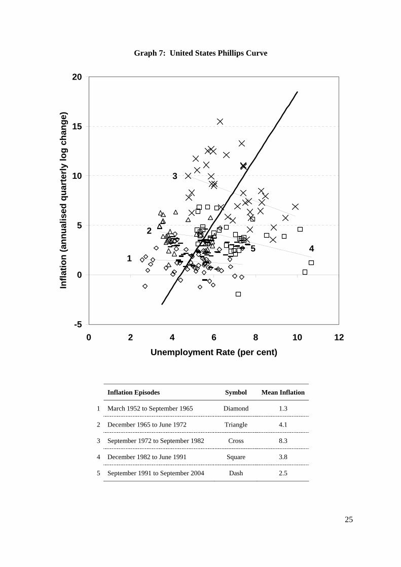
Graph 7 shows as a solid thick line the estimated long-run Phillips curve along with the actual
combinations of inflation and the unemployment rate used in the estimation. The latter are
shown by the scattering of symbols. The positive relationship is evident in the data and the
long-run relationship.
The actual data on the graph are separated into 5 inflationary ‘episodes’ that are listed below
the graph along with the identifying symbols and mean rates of inflation. We would expect
13 The long-run inflation-markup coefficient can be re-parameterised and compared with earlier work. The re-parameterised value is 3.795. Earlier estimates for the United States reported in Banerjee and Russell (2001a, 2001b) of 0.62 using annual ‘private sector’ gross domestic product data and 0.46 using aggregate gross domestic product data and 6.602 using a measure of marginal cost markups and 2.526 using unit cost markups in Banerjee and Russell (2005).

15
the actual inflation and unemployment rate data to be strung out and clustered around a series
of short-run Phillips curves associated with each inflationary episode. Unfortunately the
short-run Phillips curves can not be identified directly from this analysis. As a proxy for
these short-run Phillips curves, the trend lines for the data in each inflationary episode are
shown as thin lines and identified with numbers 1 to 5 that correspond to each inflationary
episode in the table.
If we consider the data in each episode we see that at the start of the sample we are in a
period of low inflation with low unemployment rates (diamonds). This is followed by a
period of increasing inflation and unemployment rates at the end of the 1960s and early
1970s (triangles) and then the high inflation and high unemployment of the 1970s (crosses).
The deflation of the 1980s (squares) and the 1990s (dashes) see us again return to a low
inflation and low unemployment environment on the graph. What is made clear by
separating the data into inflationary episodes is that as inflation rises the short-run Phillips
curve as proxied by the thin trend lines and the associated cluster of data not only moves
upwards but also to the right. Importantly, this process is reversed with declining inflationary
episodes and we see the short-run Phillips curve shifting not only down as expected but to the
left. It is the apparent sideway shifts, rather than purely vertical shifts, of the short-run curve
that justifies our result of a positive sloping long-run Phillips curve.
5. CONCLUSION
This paper argues that modern theoretical models of inflation suggest that inflation is non-
stationary. However, empirical work on identifying which of the competing theories ‘best’
describes the inflationary process appears to ignore resolutely the possibility that the inflation
data may be non-stationary. Consequently, inflation models are typically estimated using
techniques that are best suited for stationary data and the resulting estimates are likely to be
biased and lack precision so that inference concerning which model is the ‘best’ is poor. The
problem of poorly estimated coefficients makes it impossible to test properly whether or not
the long-run Phillips curve is vertical as small deviations in the estimated inflation
coefficients from 1 imply that the long-run curve has a slope.
To overcome this problem we explicitly acknowledge the non-stationary nature of inflation in
our estimation of the long-run Phillips curve. We estimate that there is a small but

16
significant positive slope to the long-run Phillips curve. This slope implies that a 5
percentage point increase in the general rate of inflation leads to an increase in the
unemployment rate in the long-run of around 1 ½ percentage points. Movements of this
magnitude in the unemployment rate are likely to be important in both economic and political
senses.
Finally, notice on Graph 7 that the proxies for the short-run Phillips curves become steeper
with increases in the mean rates of inflation. The trend lines for the low inflation episodes
numbered 1 and 5 are almost horizontal. As the mean rates of inflation increase the trend
lines rotate in a clockwise direction and become steeper suggesting the short-run trade-off
between inflation and unemployment diminishes. The very flat short-run Phillips curves at
low mean rates of inflation suggests that the temptation for governments to use expansionary
macroeconomic policy is great. However, the positive slope to the long-run Phillips curves
argues strongly against such myopic behaviour and lends support to the idea of independent
central banks that deliver low stable inflation.

17
6. REFERENCES
Banerjee, A., Cockerell, L. and B. Russell (2001). An I(2) An analysis of Inflation and the
Markup, Journal of Applied Econometrics, Sargan Special Issue, vol. 16, pp. 221-240.
Banerjee, A. and B. Russell (2001a). The Relationship between the Markup and Inflation in
the G7 Economies and Australia, Review of Economics and Statistics, vol. 83, No. 2, May,
pp. 377-87.
Banerjee, A. and B. Russell. (2001b). Industry Structure and the Dynamics of Price
Adjustment, Applied Economics, 33:17, pp. 1889-901.
Banerjee, A. and B. Russell, A Reinvestigation of the Markup and the Business Cycle,
Economic Modelling, vol. 21, pp. 267-84.
Banerjee, A. and B. Russell (2005). Inflation and Measures of the Markup, Journal of
Macroeconomics, vol. 27, pp. 289-306.
Batini, N., B. Jackson, and S. Nickell. (2000). Inflation Dynamics and the Labour Share in
the UK, Bank of England External MPC Unit Discussion Paper: No. 2 November.
Batini, N., B. Jackson, and S. Nickell. (2005). An Open-Economy New Keynesian Phillips
Curve for the U.K., Journal of Monetary Economics, vol. 52, pp. 1061-71.
Clarida, R., Gali, J. and Gertler, M. (1999). The Science of Monetary Policy: a New
Keynesian Perspective, Journal of Economic Literature, vol. 37, pp. 1661-1707.
Engle, R.F. and C.W.J. Granger, (1987). Co-integration and Error Correction:
Representation, Estimation, and Testing, Econometrica, vol. 55, no. 2, May, pp. 251-76.
Friedman, M. (1968). The role of monetary policy, American Economic Review, 58, 1
(March), pp. 1-17.
Friedman, M. (1977). Nobel Lecture: Inflation and Unemployment, The Journal of Political
Economy, vol. 85, no. 3, pp. 451-72.
Gali, J., and M. Gertler (1999). Inflation Dynamics: A Structural Econometric Analysis,

18
Journal of Monetary Economics, vol. 44, pp. 195-222.
Gali, J., Gertler M., and J.D. Lopez-Salido (2001). European Inflation Dynamics, European
Economic Review, vol. 45, pp. 1237-1270.
Gali, J., Gertler M., and J.D. Lopez-Salido (2005). Robustness of the Estimates of the Hybrid
New Keynesian Phillips Curve, Journal of Monetary Economics, vol. 52, pp. 1107-18.
Hansen, L.P. (1982). Large Sample Properties of Generalized Method of Moments
Estimators, Econometrica, Vol. 49, pp. 1377-98.
Henry, S.G.B. and A.R. Pagan (2004). The Econometrics of the New Keynesian Policy
Model: Introduction, Oxford Bulletin of Economics and Statistics, vol. 66, supplement, pp.
581-607.
Johansen, S. (1995). Likelihood-Based Inference in Cointegrated Vector Autoregressive
Models, Oxford: Oxford University Press.
Mavroeidis, S. (2004). Weak Identification of Forward-looking Models in Monetary
Economics, Oxford Bulletin of Economics and Statistics, vol. 66, supplement, pp. 609-35.
Mavroeidis, S. (2005). Identification Issues in Forward-looking Models Estimated by GMM,
with an Application to the Phillips Curve, Journal of Money, Credit and Banking, vol. 37, pp.
421-48.
McCullum (2000). Alternative Monetary Policy Rules: A Comparison with Historical
Settings for the United States, the United Kingdom, and Japan, Federal Reserve Bank of
Richmond Economic Quarterly, vol. 86, Winter, pp. 49-79.
Perron, P., (1997). Further Evidence on Breaking Trend Functions in Macroeconomic
Variables. Journal of Econometrics, 80 no. 2, 355-385.
Pesaran, M.H. (1981). Identification or Rational Expectations Models, Journal of
Econometrics, vol. 16, no. 3, pp. 375-98.
Pesaran, M.H. (1987). The Limits to Rational Expectations, Blackwell, Oxford.
Phelps, E.S. (1967). Phillips curves, expectations of inflation, and optimal unemployment

19
over time, Economica, 34, 3 (August), pp. 254-81.
Rudd, J. and K. Whelan (2005). New Tests of the New-Keynesian Phillips Curve, Journal of
Monetary Economics, vol. 52, pp. 1167-81.
Russell, B. (2006). Non-stationary Inflation and the Markup: an Overview of the Research
and some Implications for Policy, forthcoming in Dundee Discussion Papers, Department of
Economic Studies, University of Dundee
Stock, J., J. Wright, and M. Yogo (2002). GMM, Weak Instruments, and Weak
Identification, Journal of Business and Economic Statistics, vol. 20, pp. 518-30.
Svennson, L.E.O. (2000). Open Economy Inflation Targeting, Journal of International
Economics, vol. 50, pp. 155-83.

20
A1 DATA APPENDIX
The CPI data and unemployment rate data were downloaded from the United States of
America, Bureau of Labour Studies. The national accounts data was downloaded from the
National Income and Product Account tables from the United States of America, Bureau of
Economic Analysis. The data for March 1952 to September 2004 was downloaded on
25 November 2004. Except where indicated, the data are quarterly and seasonally adjusted.
The mnemonics are from the databases that they were downloaded from.
Table A1: Sources and details of the data manipulation
Variable Details
Consumer price inflation
The monthly CPI is the US city average, all items, 1982-84=100, ID: CUSSR0000SA0. The derived quarterly data is the average of the monthly data. CPI inflation is the change in the natural logarithm of the quarterly CPI multiplied by 400 to give the annualised rate.
Unemployment rate The unemployment rate is the number of people over 16 years as a percentage of the non-institutionalised civilian population, ID: LNS14000000. The derived quarterly data is the average of the monthly data.
Gross domestic product (GDP) at constant prices
Constant price GDP at 2000 prices, Table 1.1.6, line 1.
Gross domestic product (GDP) implicit price deflator at factor cost
Nominal GDP at factor cost is nominal GDP (Table 1.1.5, line 2) plus subsidies (Table 1.10, line 10) less taxes (Table 1.10, line 9). GDP implicit price deflator is nominal GDP at factor cost divided by constant price GDP.
Total labour compensation
Wages, salaries and supplements, Table 1.10, line 2.
Unit labour costs Calculated as total labour compensation divided by constant price GDP.
Markup Calculated as the consumer price index divided by unit labour costs.
De-trended Variables The variables are de-trended using broken linear trends. The breaks are identified using the augmented Perron (1997) unit root test which allows for the presence of an endogenous change in the level and slope of the trend function. Having identified the break (or breaks by using the technique sequentially) the data is regressed on a constant and trend as well as a ‘short’ trend, shift constant, and spike dummy for each break in trend. The short trend is zero for each period up to the break and then a linear trend thereafter. The shift dummy is zero up until the break and one thereafter. The 95 % critical value is - 3.13.
Unemployment Rate: There is a break in trend and constant in June 1978 (test statistic -4.1).
Business cycle (measured as de-trended natural logarithm of constant price GDP): The test identifies two breaks in the trend and constant. September 1963 (test statistic – 4.8). December 1979 (test statistic – 5.6).

21
Graph 1: United States CPI Inflation
March 1952 – September 2004
-5
0
5
10
15
20
Mar-52 Mar-57 Mar-62 Mar-67 Mar-72 Mar-77 Mar-82 Mar-87 Mar-92 Mar-97 Mar-02 Mar-07
Ann
ualis
ed Q
uart
erly
Log
Cha
nge
Graph 2: Estimated Constant from Rolling 10 Year CPI Inflation Regression
0
2
4
6
8
10
Mar-62 Mar-67 Mar-72 Mar-77 Mar-82 Mar-87 Mar-92 Mar-97 Mar-02 Mar-07
Estim
ated
Coe
ffici
ents
and
Crit
ical
Val
ues
Estimated Constant
Critical Value for the constant = 0

22
Graph 3: United States Unemployment Rate
March 1952 – September 2004
0
2
4
6
8
10
12
Mar-52 Mar-57 Mar-62 Mar-67 Mar-72 Mar-77 Mar-82 Mar-87 Mar-92 Mar-97 Mar-02 Mar-07
Per C
ent
Graph 4: Estimated Constant from Rolling 10 Year Unemployment Rate Regression
0
2
4
6
8
10
Mar-62 Mar-67 Mar-72 Mar-77 Mar-82 Mar-87 Mar-92 Mar-97 Mar-02 Mar-07
Estim
ated
Coe
ffici
ents
and
Crit
ical
Val
ues
Critical Value for the constant = 0
Estimated Constant

23
Graph 5: Mean Inflation and Unemployment Rates
0
2
4
6
8
10
3 4 5 6 7 8 9Unemployment Rate (per cent)
Infla
tion
(ann
ualis
ed q
uart
erly
log
chan
ge)
Notes: The mean values of inflation and the unemployment rate are the estimated constants from the 10-year
rolling regressions reported in Graphs 2 and 4.

24
Graph 6: GMM Rolling 10-Year Estimation of Phillips Curve Model
Coefficient on Leading Inflation
-2
-1
0
1
2
3
4
Mar-62 Mar-67 Mar-72 Mar-77 Mar-82 Mar-87 Mar-92 Mar-97 Mar-02
Estim
ated
Coe
ffici
ent a
nd C
ritic
al V
alue
s
Thick Line - Estimated CoefficientThin Line - Critical values for coefficient equal to 1
Coefficient on Lagged Inflation
-1
0
1
2
3
Mar-62 Mar-67 Mar-72 Mar-77 Mar-82 Mar-87 Mar-92 Mar-97 Mar-02
Estim
ated
Coe
ffici
ent a
nd C
ritic
al V
alue
s
Thick Line - Estimated CoefficientThin Line - Critical values for coefficient equal to 1
Coefficient on the Sum of Leading & Lagged Inflation
-2
-1
0
1
2
3
4
Mar-62 Mar-67 Mar-72 Mar-77 Mar-82 Mar-87 Mar-92 Mar-97 Mar-02
Estim
ated
Coe
ffici
ent a
nd C
ritic
al V
alue
s
Thick Line - Sum of Estimated CoefficientsThin Line - Critical values for sum of coefficients equal to 1
25
Graph 7: United States Phillips Curve
-5
0
5
10
15
20
0 2 4 6 8 10 12Unemployment Rate (per cent)
Infla
tion
(ann
ualis
ed q
uart
erly
log
chan
ge)
1
2
3
45
Inflation Episodes Symbol Mean Inflation
1 March 1952 to September 1965 Diamond 1.3
2 December 1965 to June 1972 Triangle 4.1
3 September 1972 to September 1982 Cross 8.3
4 December 1982 to June 1991 Square 3.8
5 September 1991 to September 2004 Dash 2.5

26
Table 1: Estimates of the United States Hybrid Phillips Curve March 1952 to September 2004
Variable EstimatedCoefficient
Standard Error
t Statistic SCV %5RWCV %5.2
RWCV %5.97 9.0%5.2CV 9.0
%5.2CV
1+∆ tp 0.7055 0.0988 7.14 1.96 - 0.36 2.78 - 0.39 2.59
1−∆ tp 0.2946 0.0822 3.59 1.96 - 0.37 2.75 - 0.32 3.09
tUE - 0.0238 0.0567 - 0.42 1.96
δ - 0.0305 0.1140 - 0.27 1.96
Testing if coefficients are insignificantly different from 1
Estimated Coefficient
Standard Error t Statistic SCV %5 RWCV %5 9.0%5CV
1−fδ - 0.2945 0.0988 - 2.98 - 1.64 - 2.23 - 2.14
1−bδ - 0.7054 0.0822 - 8.58 - 1.64 - 2.37 - 2.66
1−+ bf δδ 0.0001 0.0303 0.00 - 1.64 - 0.72 - 0.90
Diagnostic Tests
Lagrange multiplier test of serial correlation: 09.17321 =χ , p-value 0.0000; 85.2022
4 =χ , p-value 0.0000. ADF test of residuals: t statistic = - 8.17, CV1% = - 2.58. J Test (Hansen 1992) of instrument validity: 12.43, p-value 0.0060, CV1% 64.62
1 =χ and CV5% 84.321 =χ . 79.02 =R .
SEE = 1.3951.
Notes: Estimated model: ttUtbetft UEppp εδδδδ +++∆+∆=∆ −+ 11
Instruments: constant, three lags of p∆ and three lags of UE . Number of usable observations, 207. Data are quarterly and the unemployment rate is demeaned before estimation with a broken linear trend. Further details of the data are provided in the data appendix.

27
Table 2: I(1) Inflation-Unemployment Rate Model
Normalised Cointegrating Vector u p∆
Long-run Relationship - 2.714 (0.333)
1 (0.160)
Adjustment Coefficients 0.038 [8.2]
0.034 [1.3]
Standard errors reported as ( ), t-statistics reported as [ ]. The adjustment coefficients are the values with which the long-run relationship enters each equation of the system. The long-run relationship, or dynamic error correction term is therefore: ttt upECM 714.2−∆≡ .
Likelihood ratio tests on the long-run relationship (a) test of coefficient on inflation is zero is rejected, 41.312
1 =χ , p-value = 0.00, (b) test of coefficient on the unemployment rate is zero
is rejected, 65.5021 =χ , p-value = 0.00, and (c) test of the coefficient on the trend is zero is
accepted 00.021 =χ , p-value = 1.00.
Predetermined Variables: de-trended constant price GDP, spike dummies for periods where residuals are greater than 3 standard errors – March 1954, December 1958, March 1975, September 1980, December 1981, June 1986.
Testing for the Number of Cointegrating Vectors
Estimated trace statistic for the null hypothesis 0:0 =rH is 59.16 {13.31}, 1:0 =rH is 0.17 {2.71}. Numbers in { } are the relevant 90 per cent critical values from Table 15.3 of Johansen (1995). Statistics computed with 3 lags of the core variables chosen by the significance of the last dynamic terms. The sample is December 1952 to September 2004 and has 208 observations with 194 degrees of freedom.
System Diagnostics for the Mode
(a) Tests for Serial Correlation
Ljung-Box (52) 2χ (198) = 211.744, p-value = 0.24
LM(1) 2χ (4) = 9.143, p-value = 0.06
LM(4) 2χ (4) = 9.441, p-value = 0.05
(b) Test for Normality: Doornik-Hansen Test for normality: 2χ (4) = 5.941, p-value = 0.20.

28
Table 3: I(1) Inflation-Unemployment Rate-Markup Model
Normalised Cointegrating Vector u p∆ mu
Long-run Relationship 1 - 3.271 (0.376)
1 (0.158)
Adjustment Coefficients 0.030 [7.5]
- 0.005 [- 0.2]
- 0.000 (- 3.9)
Long-run Relationship 2 1 (0.176)
26.344 (5.088)
Adjustment Coefficients 0.014 [2.2]
0.026 [0.7]
0.001 [5.7]
Standard errors reported as ( ), t-statistics reported as [ ]. The adjustment coefficients are the values with which the long-run relationship enters each equation of the system. The two long-run relationship, or dynamic error correction term are therefore: ttt upECM 271.31 −∆≡
and ttt mupECM 344.262 +∆≡ .
Likelihood ratio tests (a) Long-run Relationship 1 - test of coefficient on inflation is zero is rejected, 43.262
1 =χ , p-value = 0.00, and the markup is zero is rejected, 28.1921 =χ , p-
value = 0.00 (b) Long-run Relationship 2 - test of coefficient on the inflation is zero is rejected, 06.122
1 =χ , p-value = 0.00, and (c) test of the coefficient on the trend is zero is accepted
58.121 =χ , p-value = 0.45.
Predetermined Variables: de-trended constant price GDP, and spike dummies for periods where residuals are greater than 3 standard errors – March 1954, March 1956, March 1958, March 1975, June 1978, September 1980, December 1981, March 1982, December 1982, June 1986, and March 2000.
Testing for the Number of Cointegrating Vectors
Estimated trace statistic for the null hypothesis 0:0 =rH is 102.26 {26.70}, 1:0 =rH is
35.85 {13.31}, 2:0 =rH is 2.01 {2.71}. Numbers in { } are the relevant 90 per cent critical values from Table 15.3 of Johansen (1995). Statistics computed with 4 lags of the core variables chosen by the significance of the last dynamic terms. The sample is March 1953 to September 2004 and has 207 observations with 182 degrees of freedom.
System Diagnostics for the Model
(a) Tests for Serial Correlation
Ljung-Box (51) 2χ (426) = 426.949, p-value = 0.48
LM(1) 2χ (9) = 12.295, p-value = 0.20
LM(4) 2χ (9) = 12.358, p-value = 0.19
(b) Test for Normality: Doornik-Hansen Test for normality: 2χ (6) = 7.126, p-value = 0.31.