The likely regional impacts of an agricultural emissions policy in New Zealand: Preliminary

analysis

Isabelle Sin, Emma Brunton, Joanna Hendy, Suzi Kerr

Motu Working Paper 05–08 Motu Economic and Public Policy Research

June 2005

Author contact details Suzi Kerr Motu Economic and Public Policy Research PO Box 24390 Wellington New Zealand suzi.kerr@motu.org.nz Emma Brunton Isabelle Sin Motu Economic and Public Policy Research isabelle.sin@motu.org.nz Joanna Hendy Motu Economic and Public Policy Research jo.hendy@motu.org.nz

Acknowledgements This research is part of Motu’s “Land Use, Climate Change and Kyoto” research programme, which is carried out in collaboration with Landcare Research and others. This research programme is funded by a grant from the Foundation for Research, Science and Technology. We would like to thank Jason Timmins for his assistance, and participants at the 2004 New Zealand Association of Economists conference and Motu’s “Land Use, Climate Change and Kyoto: Human dimensions research to guide New Zealand policy” policy workshop, October 2004 for their helpful comments. We would also like to thank participants of Motu’s “Land Use, Climate Change and Kyoto: Human dimensions research to guide New Zealand policy” research workshops between 2002 and 2005, for their input into the development of the fundamental project, which this report relies on. Any remaining errors or omissions are the responsibility of the authors.

Motu Economic and Public Policy Research PO Box 24390 Wellington New Zealand Email info@motu.org.nz Telephone +64-4-939-4250 Website www.motu.org.nz

© 2005 Motu Economic and Public Policy Research Trust. All rights reserved. No portion of this paper may be reproduced without permission of the authors. Motu Working Papers are research materials circulated by their authors for purposes of information and discussion. They have not necessarily undergone formal peer review or editorial treatment. ISSN 1176-2667.

Abstract Hendy and Kerr (2005b) find that an emissions charge on agricultural

methane and nitrous oxide of $25 per tonne of carbon dioxide (CO2) equivalent

would be likely to reduce New Zealand’s net land-use related emissions for

commitment period one in the order of 3%, with full accounting. The costs per

farmer and as a percentage of profit would be very high. This paper considers the

regional impacts of such a policy in New Zealand by allocating the emission

charge across space according to the location of animals. We then combine our

emissions charge information with data on the socio-economic characteristics of

the affected areas. Obviously rural areas are heavily affected. In many respects,

for example median income, ethnic mix, and percentage of working people with a

university degree, the rural areas most affected have very similar socio-economic

characteristics to other parts of rural New Zealand. Only in two ways do they

appear to differ. Our findings indicate that areas with high emission costs tend to

have high employment rates, but that they also have a disproportionately high

number of unqualified people.

JEL classification Q25, Q28, R14 Keywords climate change, land use, social impacts, methane, nitrous oxide, dairy, sheep, beef, distribution of costs, regional

Contents 1 Introduction..................................................................................................... 1

2 Tax incidence .................................................................................................. 3 2.1 Theory..................................................................................................... 3 2.2 Previous literature on the incidence of environmental taxes.................. 7

3 Data ................................................................................................................. 8 3.1 Emissions charge impact data ................................................................ 8

3.1.1 Dairy ........................................................................................ 9 3.1.2 Sheep/beef ............................................................................... 9 3.1.3 Spatial allocation ................................................................... 10

3.2 Socio-economic data ............................................................................ 10

4 The differential regional impact of an agricultural emissions policy ........... 11 4.1 Direct effects ........................................................................................ 11 4.2 Indirect effects ...................................................................................... 14

5 Socio-economic characteristics of affected LMAs ....................................... 17 5.1 Employment rates ................................................................................. 17 5.2 Median income ..................................................................................... 18 5.3 Ethnicity and occupation ...................................................................... 19 5.4 Education and formal qualifications..................................................... 20

6 Conclusions................................................................................................... 21

Appendix A : Data................................................................................................. 22 Methane and nitrous oxide emissions data ................................................... 22 Social characteristics data ............................................................................. 22

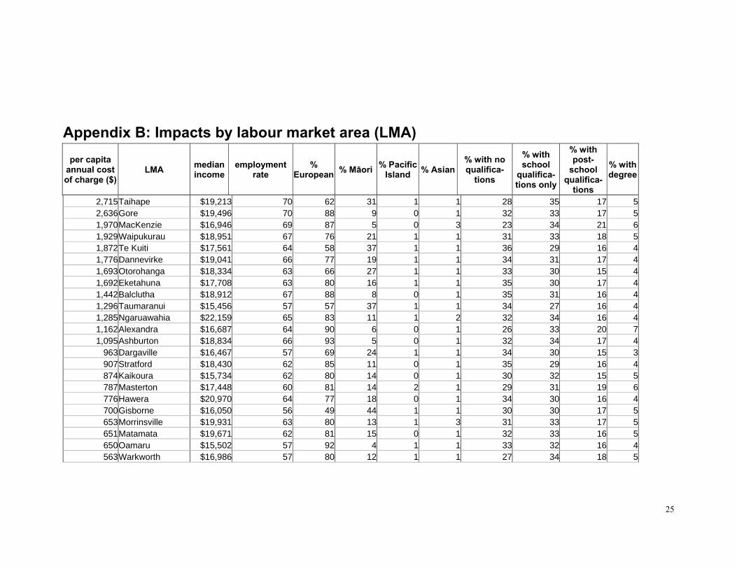
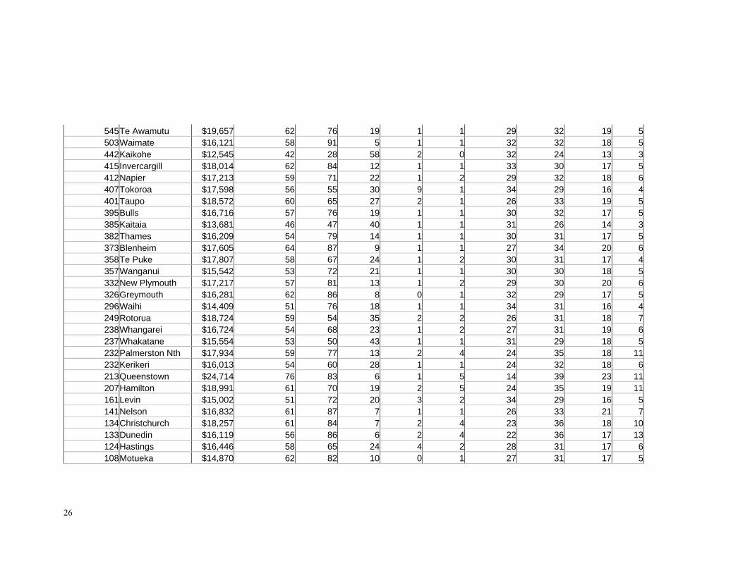
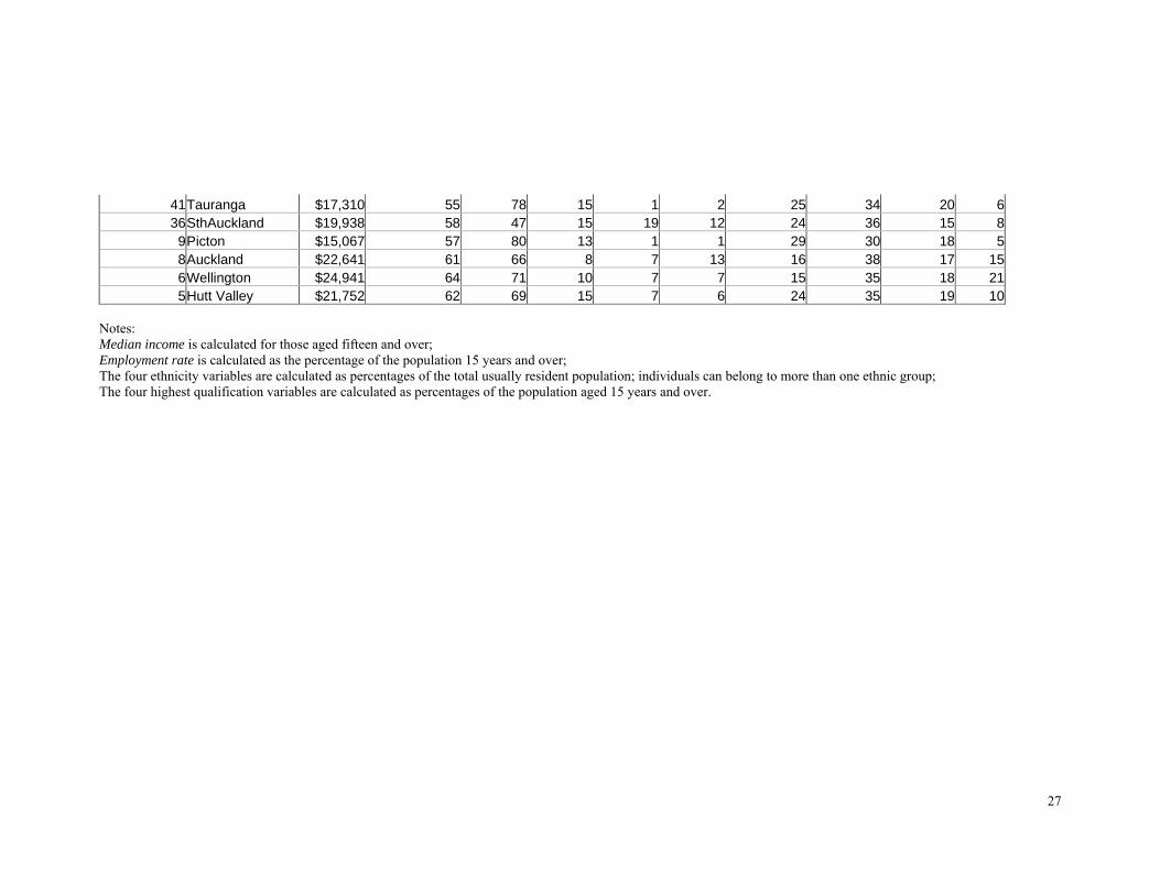
Appendix B : Impacts by labour market area (LMA) ........................................... 25

References ............................................................................................................. 28 Table of figures Figure 1: A tax shared between producers and consumers ..................................... 4

Figure 2: The distribution of land use ................................................................... 13

Figure 3: The distribution of a per capita emissions charge over LMAs .............. 16

Figure 4: The distribution of emissions charge effects over LMAs...................... 17

Figure 5: Emissions charge effects by employment rates ..................................... 18

Figure 6: Emissions charge effects by median income ......................................... 19

Figure 7: Emissions charge effects by people with no qualifications ................... 20

1

1 Introduction In most developed countries, agricultural emissions are a tiny fraction

of total greenhouse gas emissions. In New Zealand, however, they are much more

significant, constituting approximately half of the country’s overall emissions

(Brown and Plume, 2004). It therefore seems likely that New Zealand’s fight to

reduce greenhouse gas emissions will one day come to include agricultural

emissions. In fact, the regulation of agricultural emissions has already entered the

thoughts of politicians. The New Zealand Government recently proposed a

methane research levy aimed at increasing funding for research into reducing

ruminant methane emissions. However, this proposal was met by violent

opposition on the part of farmers, and became infamously known as the ‘fart tax’.1

Despite all the public debate over the proposed methane levy, we still know very

little about what the actual economic and social costs of an agricultural emissions

charge would be. This information is necessary for making informed policy

decisions.

The policy we consider in this preliminary paper is an emissions charge

of $25 per tonne of carbon dioxide (CO2) equivalent on agricultural methane and

nitrous oxide in 2002. In Hendy and Kerr (2005b) we use an integrated model,

Land Use in Rural New Zealand: Climate (LURNZv1: Climate), to suggest that

such a charge would have reduced net land-use related emissions for commitment

period one by 3%, if it had been introduced from 2003. The very small size of this

effect may be partly because currently a methane charge would be based on

animal numbers and species only, and a nitrous oxide tax would probably be

based on these and on fertiliser use only so farmers’ ability to reduce taxed

emissions is extremely limited. They can only reduce animal numbers and

fertiliser use. In our current model, the response is further limited because we

allow only the area of each land use to change, and not stocking rates or rates of

1 In mid-2003 the Government proposed that farm businesses pay an agricultural emissions research levy that would raise NZ$8.4 million to fund research into ways of reducing non-CO2 emissions from agricultural activities. This proposal was replaced in 2004 by a partnership agreement on voluntary research into agricultural greenhouse gas emissions signed by the Government and agricultural sector groups.

2

fertiliser application within each land use. Thus our estimate is likely to be low

relative to what could be achieved with a more sophisticated policy.

In this paper we consider the regional impacts of a climate change

policy that targets agricultural emissions. Agricultural emissions may be targeted

through a tax, a credit system (with credits allocated in a range of ways), or a

command and control policy. Any emissions charge levied by the Government

would probably be accompanied by a reduction in other distortionary taxes, such

as labour taxes, so that the policy would be fiscally neutral overall. It is not clear,

however, which other taxes the Government would cut. Consequently, we cannot

determine the distribution of effects of the tax cut. Thus we make the implicit

assumption that the benefits of the tax cut are spread equally across all people and

regions in the economy, and focus only on the distributional effects of the

methane and nitrous oxide charges. The distributional effects of any specific

choice of tax reduction could be analysed separately and added to the effects we

find here.

We assume that every hectare with a specific land use is equally

affected by the cost of the emissions policy in proportion to regional stocking

rates, and that the cost is not shifted out of the geographic area in which the land

lies. For example, we assume that impact on dairy land only differs between the

Far North and Gore because there are more dairy cows per hectare on a dairy farm

in the Far North than on a dairy farm in Gore. We expect that the costs of the

charge will mostly be borne by the farmers but that the charge would also have a

significant effect on the local economy, in the same way that recent high dairy

prices have led to regional economic expansion. Having estimated how the costs

of the emissions charge will fall across the country, we combine this information

with data on the socio-economic characteristics of areas by linking the Geographic

Information System (GIS) datasets of current land use with meshblock level

census data. This allows us to assess the characteristics of the areas that are likely

to be most affected by the tax.

3

2 Tax incidence

2.1 Theory Through legislation, taxes are levied on particular groups of agents,

such as employers, employees, or the producers of a specific good. These agents

face the impact of the tax, or its direct effects, in the absence of any changes to

price or economic behaviour. However, the ultimate cost of the tax may be

passed on through prices, and thus may end up distributed quite differently across

agents. The agents upon whom the tax is levied may in fact bear only a small (or

even zero) direct cost. The agents that ultimately bear the cost of tax are said to

bear the tax incidence, or indirect effects.2

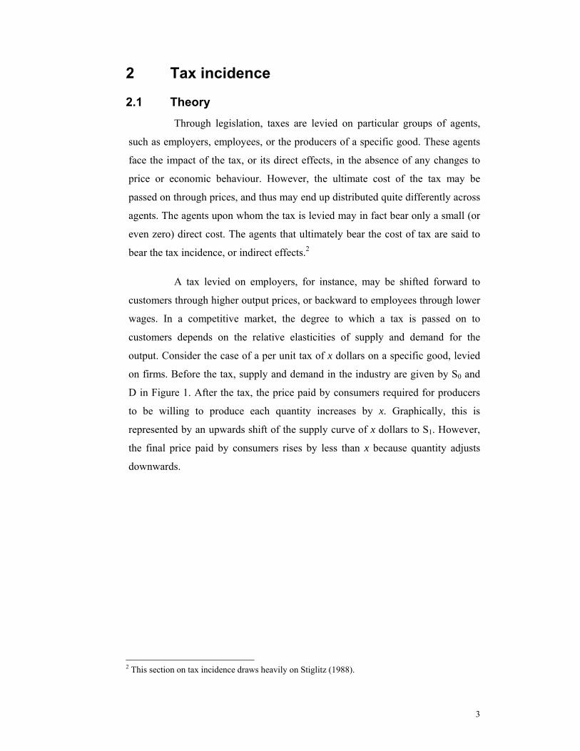
A tax levied on employers, for instance, may be shifted forward to

customers through higher output prices, or backward to employees through lower

wages. In a competitive market, the degree to which a tax is passed on to

customers depends on the relative elasticities of supply and demand for the

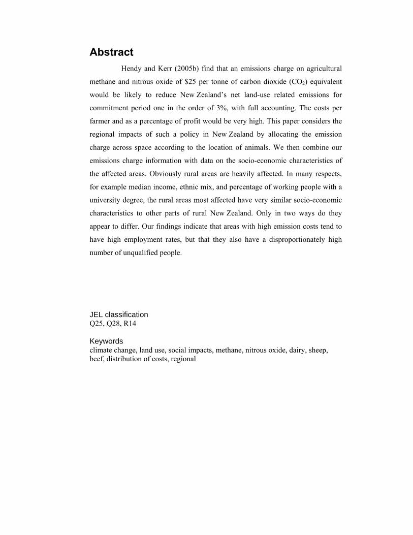
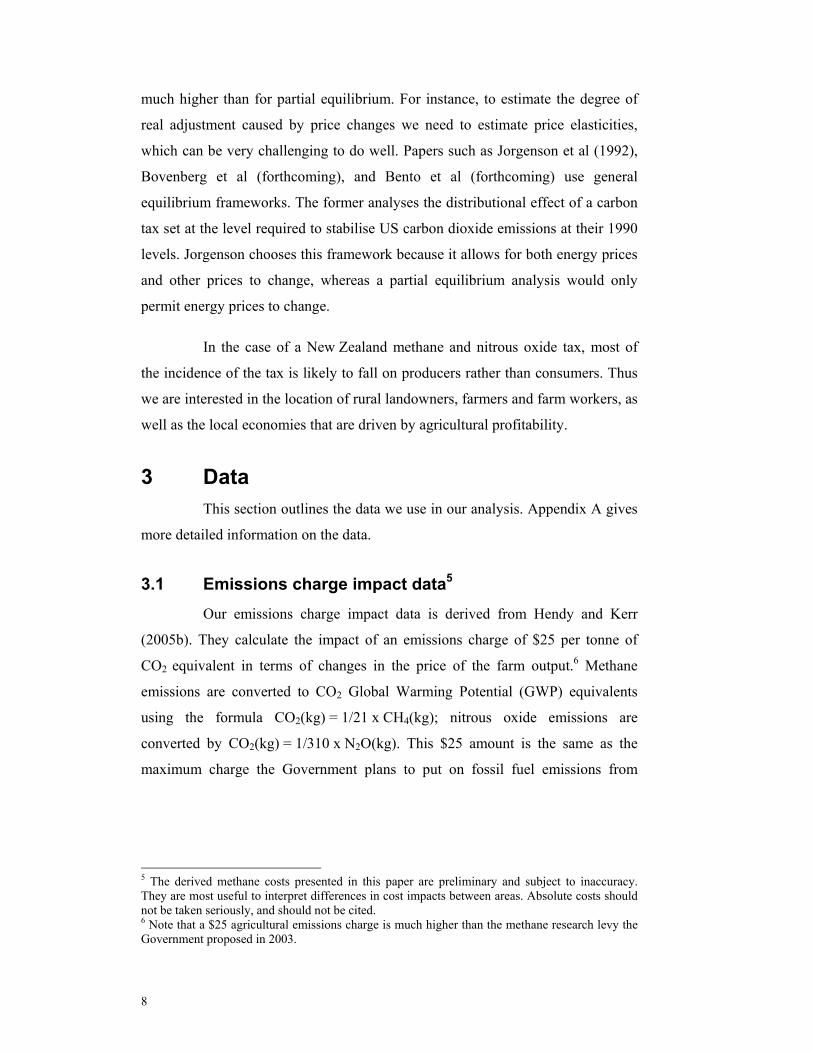
output. Consider the case of a per unit tax of x dollars on a specific good, levied

on firms. Before the tax, supply and demand in the industry are given by S0 and

D in Figure 1. After the tax, the price paid by consumers required for producers

to be willing to produce each quantity increases by x. Graphically, this is

represented by an upwards shift of the supply curve of x dollars to S1. However,

the final price paid by consumers rises by less than x because quantity adjusts

downwards.

2 This section on tax incidence draws heavily on Stiglitz (1988).

4

Figure 1: A tax shared between producers and consumers

In this illustrated case, part of the incidence falls upon producers, who

receive a lower price, and part upon consumers, who pay a higher price.

However, it may be that most or all of the incidence falls on just one type of

party. If demand is perfectly elastic (the demand curve is horizontal), or supply is

perfectly inelastic (the supply curve is vertical), it is easy to see that the price paid

by consumers does not change at all, thus producers bear the entire incidence.

Conversely, if demand is perfectly inelastic (vertical) or supply is perfectly elastic

(horizontal), then the price paid by consumers rises by x, quantity does not

change, and consumers bear the entire incidence. These cases suggest a general

result for competitive markets: the more elastic is demand or inelastic is supply,

the greater is the proportion of the incidence borne by suppliers, and vice versa.

A tax of this type could also cause demand for labour by the producing

firms to fall, and thus the wage to decline. If this occurs, the tax incidence is

partially or fully shifted backwards to employees. Similarly to the case detailed

Q1 Q0

x

quantity

price

S0

D

S1

post-tax price paid by consumers

pre-tax price

post-tax price

received by firms

5

above, the extent to which the tax incidence is shifted backwards depends on the

elasticities of supply and demand for labour. The more elastic is labour demand

in the affected industry or inelastic is labour supply, the greater is the proportion

of the tax borne by workers, the suppliers of labour.

When an additional tax is levied in an economy, however, the effects

tend to spread beyond those directly associated with the party on whom the tax is

levied. This occurs because those who bear the tax incidence may alter their other

economic behaviour because of the effects of the tax. A workers who have wages

reduced may cut back on consumption expenditure, as may a shareholder in a

firm that bears some of the tax incidence. The firm itself may reduce investment.

The economic agents affected by these secondary effects may also alter their

behaviour, and so on.

In this paper, we consider a tax levied at the level of the farmer.

New Zealand sheep/beef farmers sell their products in a large international

market. Furthermore, the outputs from sheep/beef farms are commodities, and so

are undifferentiated from sheep/beef products produced in other countries.

Consequently, New Zealand sheep/beef farmers are price takers and are unable to

pass any tax burden on to their customers. Thus the only way they are able to shift

the tax burden is backwards to their workers.

Dairy farmers, on the other hand, may have a small influence on

international dairy prices. Although international demand for New Zealand’s dairy

exports is still very elastic, dairy exports face one of the least elastic international

demands of any of New Zealand’s exports.3 That is, international demand for

New Zealand’s exports of dairy products falls more slowly as dairy output price

rises than do the demands for most of New Zealand’s other exports when their

prices rise.

The supply of New Zealand farm outputs may be reasonably elastic

because if returns to farm labour decrease, farmers may choose to work less on

their farms, reduce farm output, and increase their off-farm work. There is

3 Personal communication with Ralph Lattimore, agricultural economics consultant, 9 June 2005. Also see Finlayson et al (1988).

6

evidence to suggest that many farmers do some form of additional non-farm work,

so they may not have great difficulty increasing the quantity of this.4 They may

also choose to change their land use. However, in this paper we do not consider

how supply is likely to change in response to an agricultural emissions charge. We

assume perfectly inelastic supply.

In addition to potentially being able to pass a small proportion of the

cost of an emissions charge forwards to international consumers, dairy farmers

may pass some of the burden to farm workers. The degree to which both dairy and

sheep/beef farmers would pass the burden of an agricultural emissions charge on

to their workers depends on two major factors. The first is the degree to which

they are able to reduce their labour requirements through measures such as

substituting unpaid family labour for hired employees, reducing work on farm

maintenance, or reducing farm production. If farmers are more able to reduce their

demand for labour, they will pass more of the effects of the tax on to farm

workers. The second factor is the degree to which farm workers are willing and

able to find work in alternative industries. If farm workers have a lot of options

for work outside the agricultural industry, farm owners will have difficulty

retaining labour if they attempt to reduce the wages of their employees. In this

case, farmers will bear more of the tax incidence.

The effects of a methane tax would spread beyond farmers and farm

employees. These people, when faced with lower incomes, would most likely

curtail their spending in a range of areas, thus adversely affecting businesses that

relied on their custom.

We expect that most of the cost would stay with farmers, and perhaps

some be passed on to farm employees, who tend to be located where the farms

are. Though these people may affect their local communities, by curtailing their

spending and thus adversely affecting businesses that relied on their custom, we

expect the short run spread of the cost of the emissions charge to mostly be

limited to the geographic areas containing farms. Hall and McDermott (2004,

Abstract) find “considerable evidence of certain regional cycles being associated

4 See, for example, Parminter (1997).

7

with movements in New Zealand’s aggregate terms of trade, real prices of

milksolids, real dairy land prices and total rural land prices”.

In the long run, migration and capital movements will tend to smooth

out regional differences. The wider macroeconomic impacts of changes in

agricultural returns will be felt all over the country.

2.2 Previous literature on the incidence of environmental taxes A range of literature explores the incidence of environmental taxes. The

simplest consideration that relates to an environmental tax is the question of who

legally pays the tax bill.

At the next level of complexity, we can consider who pays the cost of

the tax in a partial equilibrium setting. In the context of this paper, this means that

we allow for farmers to pass the cost of the tax on to consumers or back to

workers, but we assume that farmers do not change the use of their land in

response to the tax, nor do other prices or behaviours in the economy change. The

majority of environmental policy incidence studies fall into this level of

complexity. For instance, Poterba (1990 and 1991) investigates the extent to

which gasoline tax is regressive by calculating expenditure on gasoline as a

proportion of total expenditure for households with different levels of overall

expenditure. It allows the cost of the gasoline tax to be passed on to consumers,

but does not consider the extent to which different households are likely to have

changed their gasoline purchasing habits in response to the tax. Kerr (2001), a

New Zealand paper, uses the same approach to analyse the distributional effects of

a tax on petrol in New Zealand. At a slightly higher level of complexity, Creedy

and Sleeman (2004), a New Zealand study, uses input–output analysis to explore

the impacts of carbon taxes on consumer prices.

The highest level of complexity is general equilibrium. For

investigating a methane tax, this would mean allowing for adjustments such as

converting some sheep/beef farms (which emit methane) to forestry (which does

not), as well as adjustments that would occur throughout other sectors of the

economy. The information requirements for general equilibrium analysis are

8

much higher than for partial equilibrium. For instance, to estimate the degree of

real adjustment caused by price changes we need to estimate price elasticities,

which can be very challenging to do well. Papers such as Jorgenson et al (1992),

Bovenberg et al (forthcoming), and Bento et al (forthcoming) use general

equilibrium frameworks. The former analyses the distributional effect of a carbon

tax set at the level required to stabilise US carbon dioxide emissions at their 1990

levels. Jorgenson chooses this framework because it allows for both energy prices

and other prices to change, whereas a partial equilibrium analysis would only

permit energy prices to change.

In the case of a New Zealand methane and nitrous oxide tax, most of

the incidence of the tax is likely to fall on producers rather than consumers. Thus

we are interested in the location of rural landowners, farmers and farm workers, as

well as the local economies that are driven by agricultural profitability.

3 Data This section outlines the data we use in our analysis. Appendix A gives

more detailed information on the data.

3.1 Emissions charge impact data5 Our emissions charge impact data is derived from Hendy and Kerr

(2005b). They calculate the impact of an emissions charge of $25 per tonne of

CO2 equivalent in terms of changes in the price of the farm output.6 Methane

emissions are converted to CO2 Global Warming Potential (GWP) equivalents

using the formula CO2(kg) = 1/21 x CH4(kg); nitrous oxide emissions are

converted by CO2(kg) = 1/310 x N2O(kg). This $25 amount is the same as the

maximum charge the Government plans to put on fossil fuel emissions from

5 The derived methane costs presented in this paper are preliminary and subject to inaccuracy. They are most useful to interpret differences in cost impacts between areas. Absolute costs should not be taken seriously, and should not be cited. 6 Note that a $25 agricultural emissions charge is much higher than the methane research levy the Government proposed in 2003.

9

2007.7 These impacts are calculated for the two main rural land uses that produce

methane and nitrous oxide emissions: sheep/beef farming (63% of total enteric

methane emissions and 70.3% of agricultural direct nitrous oxide emissions), and

dairy farming (35% of total enteric methane emissions and 27.3% of direct nitrous

oxide emissions).

Dairy cattle produce different emissions to sheep and beef cattle and

have outputs of different values. The manner in which Hendy and Kerr (2005b)

translate the $25 emissions charge into a cost per kg of output, when combined

with data on revenue per kg of output, makes the two impact values comparable.

Emissions per animal are based on the total national emissions for 2002

in Clark et al (2003) and the Statistics New Zealand Agricultural Production

Census 2002. The two sections below detail the revenue implications of a charge

on dairy and sheep/beef emissions as calculated in Hendy and Kerr (2005b).

3.1.1 Dairy

The cost of a tax of $25 per tonne of CO2 equivalent emitted is $0.30

per kg of milksolids. Revenue per kg of milksolids in 2002 was $5.31, so this tax

equates to a 7% reduction in revenue.

3.1.2 Sheep/beef

To calculate the impact of an emissions charge on sheep/beef land use,

Hendy and Kerr (2005b) derive an emissions function based on actual national

emissions 2002, with its unit defined in terms of a composite sheep/beef product.

The components of this composite product are beef, lamb, mutton, and wool. The

cost of a charge of $25 per tonne of CO2 equivalent emitted is $0.42 per kg of

composite product. Revenue per kg of composite product in 2002 was $3.94, so

this tax equates to an 11% reduction in revenue.

7 The Government will introduce an emissions charge of $15 per tonne of carbon dioxide equivalent on fossil fuels and industrial process emissions (i.e. carbon dioxide and fossil methane) from 2007 (New Zealand. Ministry for the Environment, 2005). The charge of $25 that we use approximates the international emissions price.

10

3.1.3 Spatial allocation

We use the model LURNZv1 from Hendy and Kerr (2005a) to allocate

land uses and animal numbers spatially across the country. LURNZ assigns a

single land use and a land use intensity to each 25 hectare area using information

from the Ministry for the Environment’s Landcover Database 2 (LCDB2), which

is based on a composite of satellite maps in the summer of 2001/02, territorial

authority animal numbers from Statistics New Zealand 2002 Agricultural

Production Census, and physical productivity mappings from Landcare Research.

For this paper, we aggregate the LURNZv1 results to labour market area (LMA)

level, i.e. an area defined so that most people live and work within the same area.8

Emissions costs are then allocated to LMAs in direct proportion to animal

numbers in sheep/beef farming and dairy farming.

Because most people live and work in the same LMA, they operate as

self-contained labour markets in the short run so that wage and employment

effects from emissions charges borne in these areas will be felt within these areas.

Other effects, such as through purchase of inputs and retail shopping, may also

tend to occur within the same LMA. Thus LMAs seem the natural geographic

units in which the costs of a methane tax are likely to be confined in the short run.

3.2 Socio-economic data Details of the data used are given in Appendix A. One question that is

of particular interest to us is whether emissions charges would primarily affect

people who are in a poor position to cope with the costs. The socio-economic

characteristics of the people in the most affected areas give us some indication of

this. Equity issues arise if the emissions charge disproportionately targets one

group. There is also potential for a political backlash, particularly if the charge

targets a specific ethnic group.

We use the 2001 Statistics New Zealand meshblock census database,

and compile the following variables:

8 There are 58 LMAs in New Zealand as defined in Newell and Papps (2001). The LMAs are defined so that most people who live in an LMA also work in it, and most people who work in an LMA also live in it.

11

• Median incomes (of those aged 15 and over)

• Employment rates (as percentages of the population 15 years and over)

• Ethnicity—New Zealand European, Māori, Pacific Islander, Asian

(percentages of the total usually resident population who specify these

ethnicities as either their ethnicity, or as one of their ethnicities)

• Occupation (percentages of the employed population 15 years and over

with each of these occupations: administration, professional, clerical,

sales and services, agricultural, and manual)

• Qualifications (percentages of the population aged 15 and over with

each of these highest qualification levels: no qualifications, school

qualifications, vocational qualifications, and degrees)

Employment rates tell us about the level of activity in the economy and

the strength of its labour market. Qualifications give another perspective on the

ability of people to adjust to shocks. Those with higher qualifications tend to have

more employment options, and are more able to move to other areas of the

country for work.

4 The differential regional impact of an agricultural emissions policy

The effects of an emissions charge would touch many people and

businesses. We classify the effects of an emissions charge into direct effects and

indirect effects. Direct effects are those on the people who actually have to pay the

charge. Indirect effects are all the other effects that occur as the effects of the

charge feed through the economy.

4.1 Direct effects At $25 per tonne of CO2 equivalent, the total annual revenue from the

charge would have been around $207m from dairy farms and $363m from sheep

and beef farms in 2002, assuming no behavioural response. This corresponds to

$109 per ha per year in dairy and $42 per ha per year on sheep/beef land, and will

probably have corresponding effects on the value of that land. For the average

dairy farm this corresponds to a loss of $15,000 in profit out of average farm net

trading profits of $48,739 in 2002/03 and $85,029 in 2003/04 (New Zealand.

12

Ministry of Agriculture and Forestry, 2004a). For the average sheep/beef farm it

corresponds to a loss of $13,000 out of average farm net trading profits of

$86,620in 2002/03 and $40,492 in 2003/04 (New Zealand. Ministry of

Agriculture and Forestry, 2004b).

The people directly affected by an emissions charge are dairy farmers

and sheep/beef farmers, who actually pay the emissions charge. We can get a fair

idea of where these farmers tend to live from the proportions of rural land in the

LMAs, specifically the share of sheep/beef land or dairy land. Consequently,

direct effects will be concentrated in areas with high proportions of sheep/beef or

dairy land.

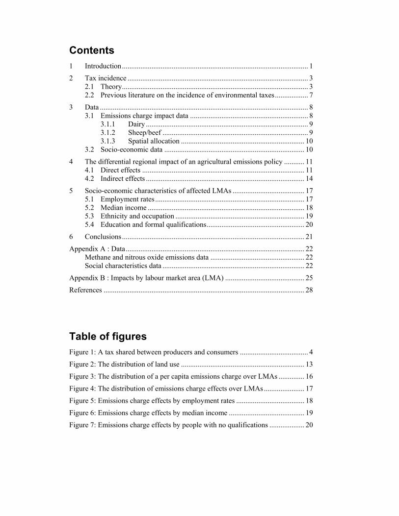
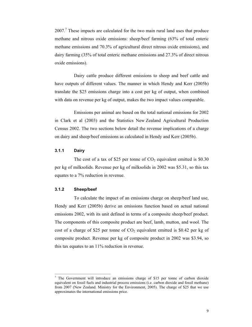
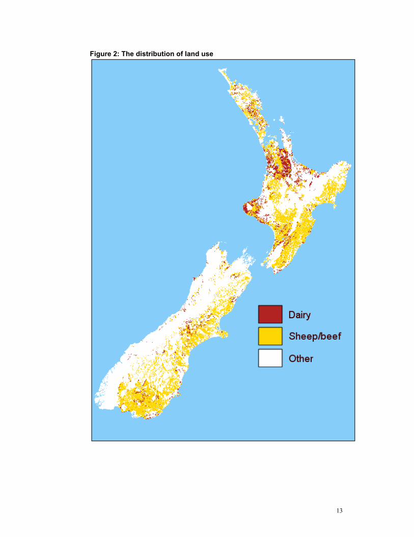
The parties directly affected by an emissions charge, the owners of

dairy and sheep/beef farms, face charges in proportion to their number of stock.

Geographically, the distribution of these people is close to the distribution of dairy

and sheep/beef farms, which we show in Figure 2. When the owners are not living

on the farms, the impact of charges on profit and land values may occur in other

regions but the employment impacts will still be co-located with the farms. The

distributions of farmland shown here are derived using the model LURNZv1.

With detailed information on the socio-economic characteristics of farm

owners, including information on the level of debt farmers bear, we would be able

to determine the ability to cope of the people directly affected by the emissions

charge. In the absence of this information, we focus for the remainder of this

paper on the characteristics of those indirectly affected.

13

Figure 2: The distribution of land use

14

4.2 Indirect effects Indirect effects spread out through the economy from those directly

affected. For example, when an emissions charge is introduced dairy farmers will

find themselves facing increased costs. They will reduce their spending. Some of

these farmers may lay off farm workers or reduce the wages they offer. These

adversely affected farm workers may reduce their own expenditure, negatively

affecting businesses in their communities. In this manner, the effects of a methane

charge would flow on through the community.

We expect indirect effects to be strongest for people geographically

close to those directly affected, and thus we make the assumption that indirect

effects strike the LMAs in which the direct effects occur. It is important to

examine these impacts spatially because the size of the impact depends on the

nature of the local economy. For instance, the impact of laying off 50 people in an

isolated area will be much greater than laying off 50 people in a dynamic urban

area with a strong labour market.

One way that we can gauge the magnitude of the indirect effect in

various LMAs is by measuring the per capita cost of an emissions charge by

LMA. Alternatives include calculating the proportion of the population of the

LMA employed directly by the dairy or sheep/beef industries, and calculating the

proportion employed either directly or indirectly by the dairy or sheep/beef

industries. Another way of estimating where impacts will be most severe is by

looking at the proportion of the total economy that consists of agricultural

farming. Where agricultural farming is a large proportion of the overall value of

the economy, impacts are likely to be severe. We calculate these alternative

measures, and find a high correlation between them and our chosen measure, the

per capita annual emissions charge. This measure controls for the population of

the area and tells us about how the charge is spread between LMAs.

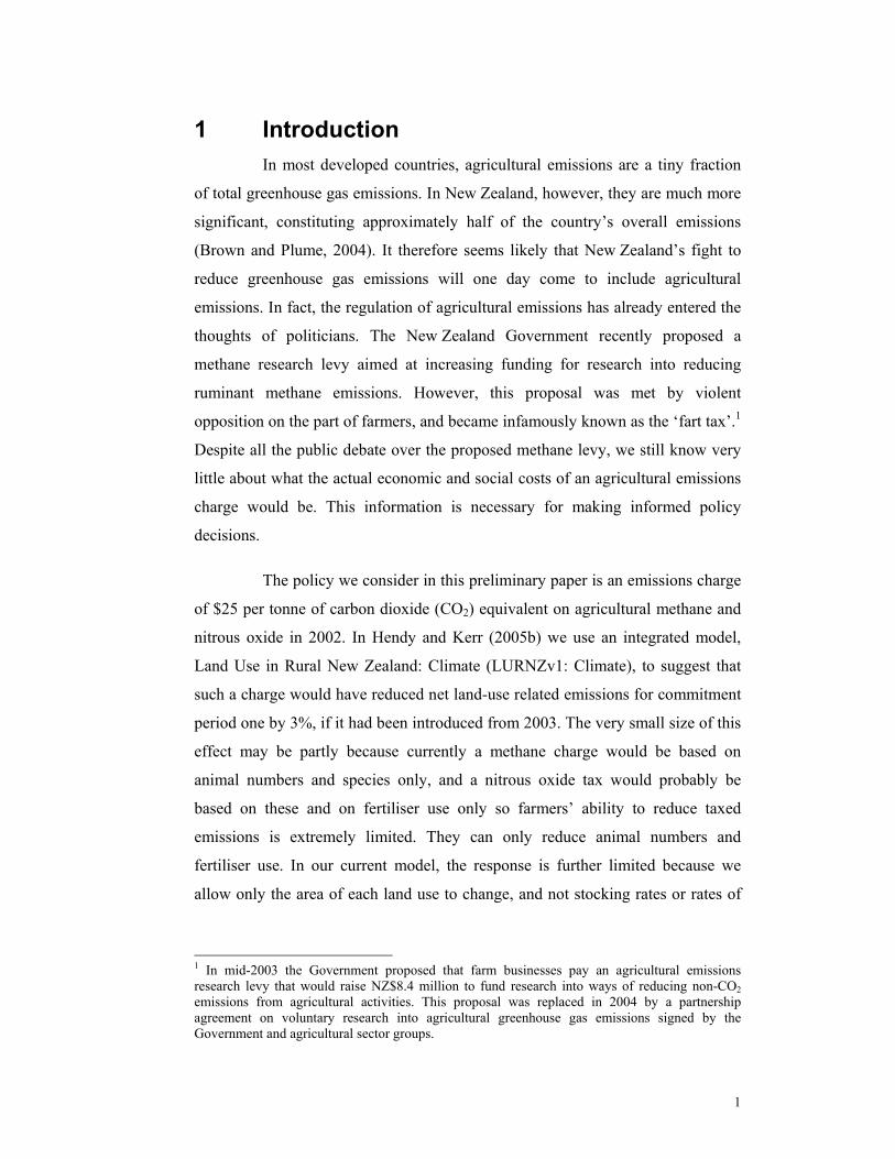
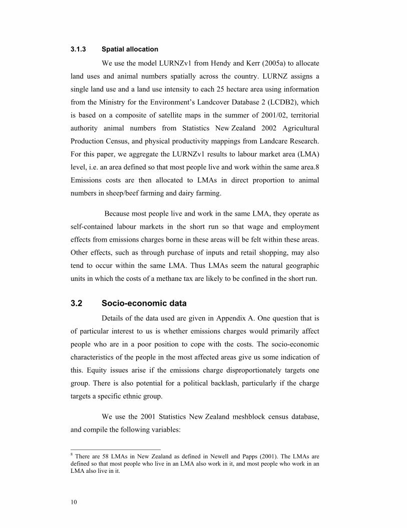
Figure 3 illustrates the locations of the areas that are most affected by

the emissions charge. The black lines are LMA boundaries. The higher is the cost

per capita of the charge, the darker is the LMA. The white areas on the map are

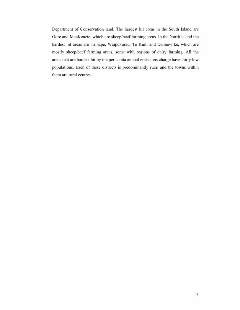
15

Department of Conservation land. The hardest hit areas in the South Island are

Gore and MacKenzie, which are sheep/beef farming areas. In the North Island the

hardest hit areas are Taihape, Waipukurau, Te Kuiti and Dannevirke, which are

mostly sheep/beef farming areas, some with regions of dairy farming. All the

areas that are hardest hit by the per capita annual emissions charge have fairly low

populations. Each of these districts is predominantly rural and the towns within

them are rural centres.

16

Figure 3: The distribution of a per capita emissions charge over LMAs

17

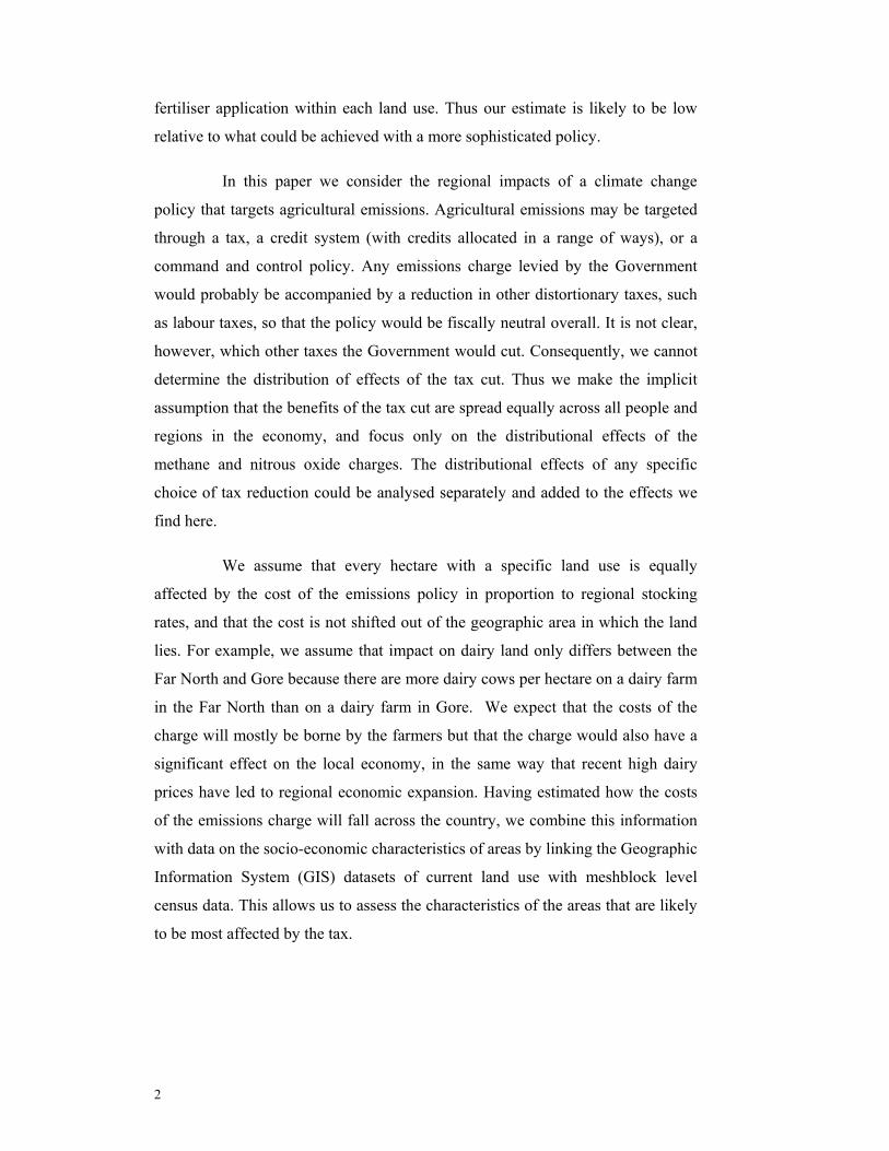
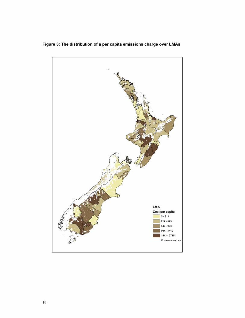
Figure 4 illustrates graphically the spread of per capita costs over

LMAs. It is immediately evident that the effects of the emissions charge are

spread very unequally across LMAs. A large number of LMAs are hardly affected

at all, while a few are very highly affected. The least affected LMAs tend to have

large urban populations, and include New Zealand’s major cities. Appendix B

includes a table of LMAs ranked as in Figure 4.

Figure 4: The distribution of emissions charge effects over LMAs

$0

$1,000

$2,000

$3,000

Annu

al e

mis

sion

s ch

arge

per

cap

ita in

the

LMA

LMAs ranked by effect

Taihape

Gore

5 Socio-economic characteristics of affected LMAs In this section of the paper we examine the relationship between the

socio-economic characteristics of LMAs and their emissions charge costs, based

on current land use. We use the measure “per capita annual emissions charge”

throughout this discussion.

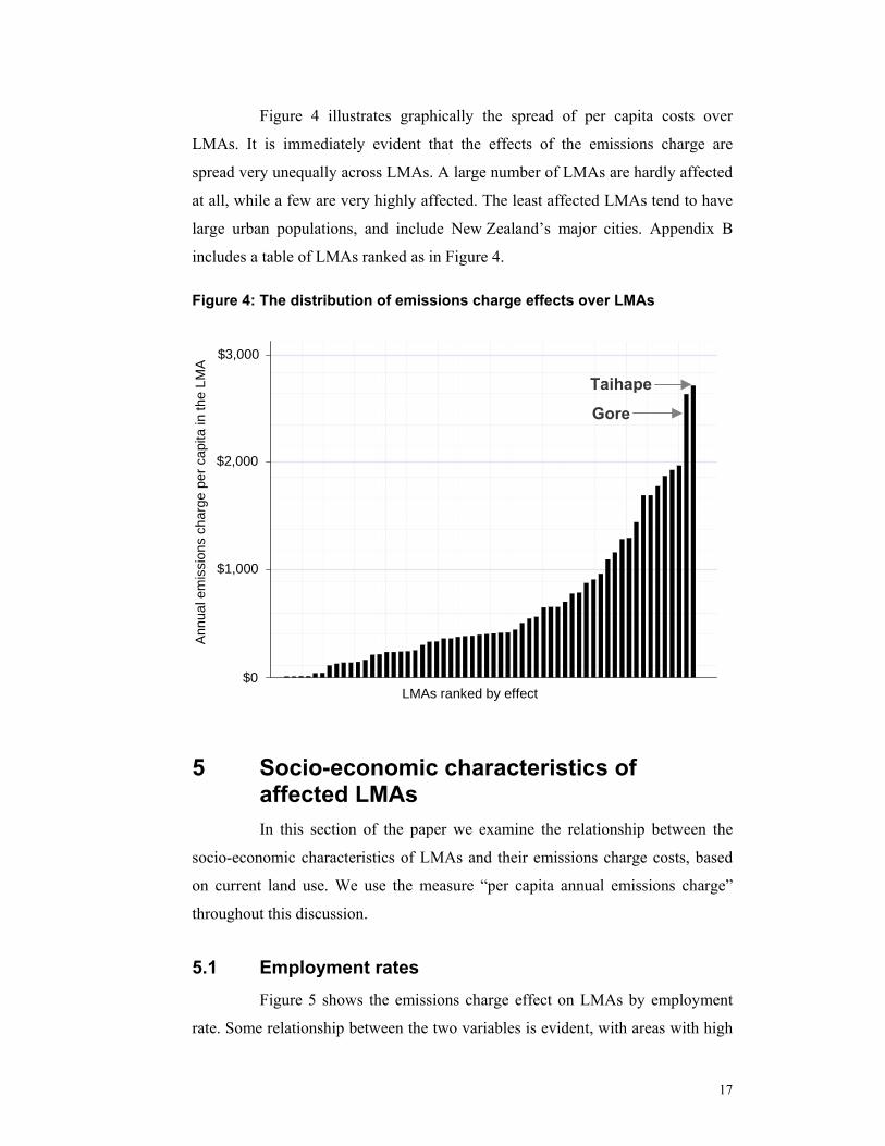
5.1 Employment rates Figure 5 shows the emissions charge effect on LMAs by employment

rate. Some relationship between the two variables is evident, with areas with high

18

emissions charge effects also tending to have fairly high employment rates. One

result of the emissions charge is likely to be job losses in the hard-hit areas. From

the graph it seems that the areas most likely to face job losses have fairly strong

labour markets. They may be well placed to absorb the displaced workers back

into the workforce. This ignores the uneven distribution of people who are not in

the labour force across LMAs. For instance, an LMA with a very large proportion

of retired people will have a deceptively low employment rate in this figure.

Figure 5: Emissions charge effects by employment rates

em

issi

ons

char

ge p

er c

apita

in L

MA

$0

$1,000

$2,000

$3,000

40% 50% 60% 70% 80% employment rate

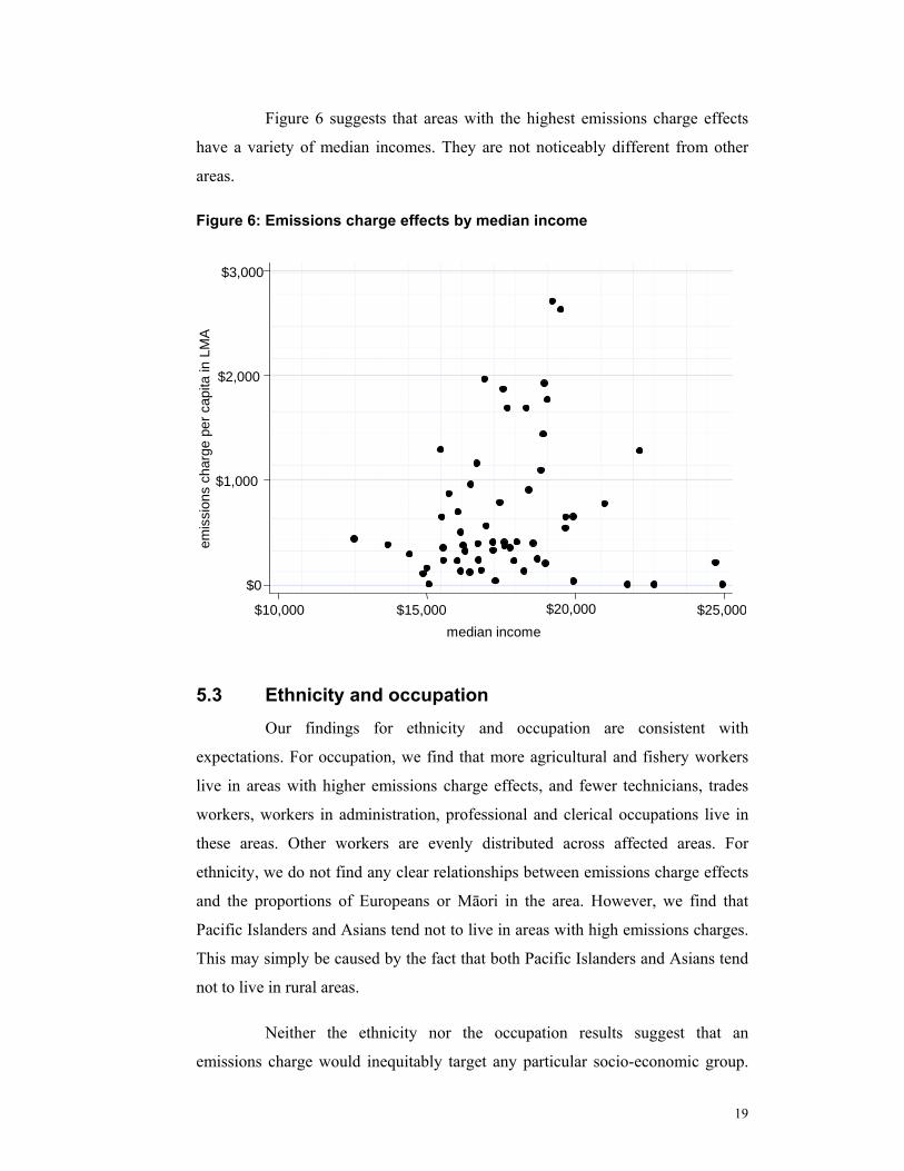
5.2 Median income An emissions charge would affect the incomes of many people,

especially in the harder-hit areas. Median income levels in these areas give one

indication of how well those affected would be able to cope with decreases in

their incomes. However, we cannot say from this data where in the income

distributions of these areas are the people who are most affected.

19

Figure 6 suggests that areas with the highest emissions charge effects

have a variety of median incomes. They are not noticeably different from other

areas.

Figure 6: Emissions charge effects by median income

em

issi

ons

char

ge p

er c

apita

in L

MA

$0

$1,000

$2,000

$3,000

$10,000 $15,000 $20,000 $25,000median income

5.3 Ethnicity and occupation Our findings for ethnicity and occupation are consistent with

expectations. For occupation, we find that more agricultural and fishery workers

live in areas with higher emissions charge effects, and fewer technicians, trades

workers, workers in administration, professional and clerical occupations live in

these areas. Other workers are evenly distributed across affected areas. For

ethnicity, we do not find any clear relationships between emissions charge effects

and the proportions of Europeans or Māori in the area. However, we find that

Pacific Islanders and Asians tend not to live in areas with high emissions charges.

This may simply be caused by the fact that both Pacific Islanders and Asians tend

not to live in rural areas.

Neither the ethnicity nor the occupation results suggest that an

emissions charge would inequitably target any particular socio-economic group.

20

However, agricultural workers would unavoidably be affected to a greater extent

than most other professions.

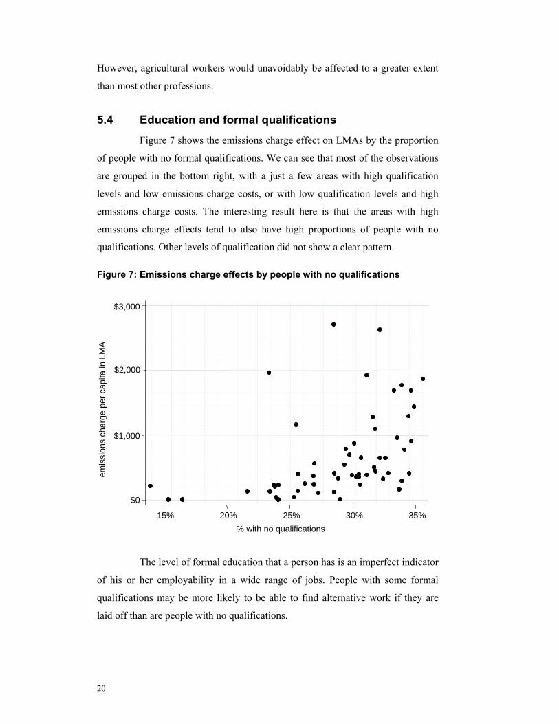
5.4 Education and formal qualifications Figure 7 shows the emissions charge effect on LMAs by the proportion

of people with no formal qualifications. We can see that most of the observations

are grouped in the bottom right, with a just a few areas with high qualification

levels and low emissions charge costs, or with low qualification levels and high

emissions charge costs. The interesting result here is that the areas with high

emissions charge effects tend to also have high proportions of people with no

qualifications. Other levels of qualification did not show a clear pattern.

Figure 7: Emissions charge effects by people with no qualifications

em

issi

ons

char

ge p

er c

apita

in L

MA

$0

$1,000

$2,000

$3,000

15% 20% 25% 30% 35% % with no qualifications

The level of formal education that a person has is an imperfect indicator

of his or her employability in a wide range of jobs. People with some formal

qualifications may be more likely to be able to find alternative work if they are

laid off than are people with no qualifications.

21

Many of the occupations that revolve around dairy and sheep/beef

farms, however, tend to involve ‘learning by doing’ rather than formal

qualifications. Thus many people working in these regions who lack formal

qualifications may in fact be highly skilled, though the skills may not all be

transferrable outside the agricultural sector. Consequently, the data on numbers of

people with no formal qualifications are likely to be a little misleading as an

indicator of employability.

6 Conclusions In this paper we have investigated the possible social impacts of an

agricultural emissions charge levied on methane and nitrous oxide of $25 per

tonne of CO2 equivalent. For dairy farmers, this equates to a 7% decrease in

revenue in the absence of price changes; for sheep/beef farmers, it equates to an

11% decrease. We assume the effects of the charge stay in the labour market areas

in which the affected farms are located, and disregard the benefits of the likely

accompanying tax decrease on the implicit assumption that they are evenly

distributed across the country. Calculated on a labour market area basis, annual

emissions charges per capita range from $5 in the Hutt Valley to $2,715 in

Taihape.

We examine the socio-economic characteristics of the labour market

areas with very high per capita emissions charges. These labour market areas

mostly have high employment rates, which suggests people who lose their jobs

because of the emissions charge are likely to have decent prospects for finding

alternative work. On the other hand, labour market areas that would face high per

capita emissions charges tend to have high proportions of people with no

qualifications. This may mean that people who are made redundant would tend to

have low levels of formal qualifications, and thus may have difficulty finding jobs

in alternative industries. On the whole the socio-economic characteristics of high

emissions rural areas are very similar to those in rural New Zealand as a whole.

22

Appendix A: Data

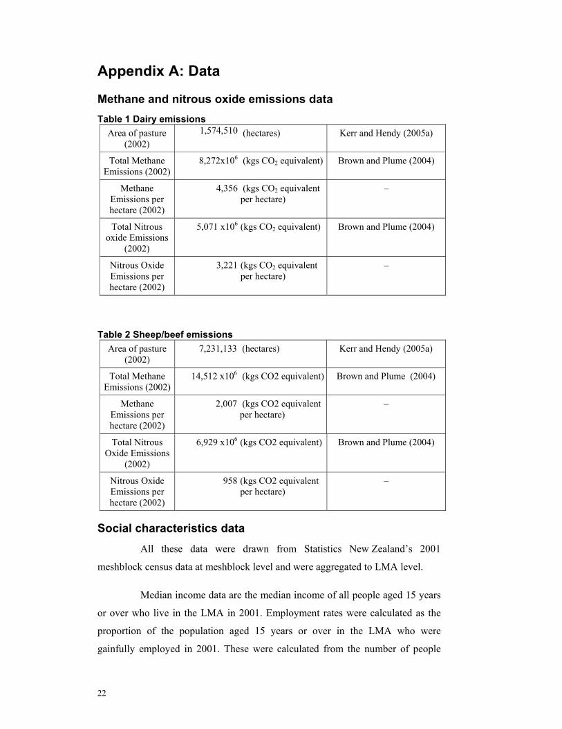
Methane and nitrous oxide emissions data Table 1 Dairy emissions

Table 2 Sheep/beef emissions Area of pasture

(2002) 7,231,133 (hectares) Kerr and Hendy (2005a)

Total Methane Emissions (2002)

14,512 x106 (kgs CO2 equivalent) Brown and Plume (2004)

Methane Emissions per hectare (2002)

2,007 (kgs CO2 equivalent per hectare)

–

Total Nitrous Oxide Emissions

(2002)

6,929 x106 (kgs CO2 equivalent) Brown and Plume (2004)

Nitrous Oxide Emissions per hectare (2002)

958 (kgs CO2 equivalent per hectare)

–

Social characteristics data

All these data were drawn from Statistics New Zealand’s 2001

meshblock census data at meshblock level and were aggregated to LMA level.

Median income data are the median income of all people aged 15 years

or over who live in the LMA in 2001. Employment rates were calculated as the

proportion of the population aged 15 years or over in the LMA who were

gainfully employed in 2001. These were calculated from the number of people

Area of pasture (2002)

1,574,510 (hectares) Kerr and Hendy (2005a)

Total Methane Emissions (2002)

8,272x106 (kgs CO2 equivalent) Brown and Plume (2004)

Methane Emissions per hectare (2002)

4,356 (kgs CO2 equivalent per hectare)

–

Total Nitrous oxide Emissions

(2002)

5,071 x106 (kgs CO2 equivalent) Brown and Plume (2004)

Nitrous Oxide Emissions per hectare (2002)

3,221 (kgs CO2 equivalent per hectare)

–

23

aged 15 or over who were gainfully employed, and the total number of people

aged 15 years or over.

Ethnicity data for 2001 are series giving the percentage of the

population claiming each of Māori, European, Pacific Island and Asian ethnicity

as either their only ethnicity or one of their ethnicities. These were calculated

from the number of people in each LMA claiming each ethnicity, and the total

population of the LMA.

Occupation data for 2001 are the percentage of the employed

population aged 15 years and over in each of a number of occupations. This is the

percentage of the gainfully employed population aged 15 and over in an LMA that

are in a particular occupation. The occupations used are:

• agriculture and fishery workers

• legislators, administrators, and managers

• professionals

• technicians and associate professionals

• clerks

• service and sales workers

• trades workers

• plant and machine operators and assemblers.

We also use ‘employment by industry’ data drawn from the 2001

census at the meshblock level.

Qualification data are the proportion of the population aged 15 years or

over in the LMA whose highest qualification fell into one of the categories: ‘no

qualifications’, ‘school qualifications’, ‘vocational qualifications’, and ‘degree’.

These categories exclude those with post-school qualifications such as university

diplomas. Except for ‘no qualifications’, each qualification category is an

aggregation of a number of finer categories.

• “School qualifications” contains School Certificate, sixth form

qualifications, higher school qualifications, unspecified school

qualifications, and overseas school qualifications.

24

• “Vocational qualifications” contains basic vocational, skilled

vocational, intermediate vocational, and advanced vocational

qualifications.

• “Degree” contains bachelor degree and higher degree.

25

Appendix B: Impacts by labour market area (LMA) per capita

annual cost of charge ($)

LMA median income

employment rate

% European % Māori % Pacific

Island % Asian % with no qualifica-

tions

% with school

qualifica-tions only

% with post-

school qualifica-

tions

% with degree

2,715 Taihape $19,213 70 62 31 1 1 28 35 17 52,636 Gore $19,496 70 88 9 0 1 32 33 17 51,970 MacKenzie $16,946 69 87 5 0 3 23 34 21 61,929 Waipukurau $18,951 67 76 21 1 1 31 33 18 51,872 Te Kuiti $17,561 64 58 37 1 1 36 29 16 41,776 Dannevirke $19,041 66 77 19 1 1 34 31 17 41,693 Otorohanga $18,334 63 66 27 1 1 33 30 15 41,692 Eketahuna $17,708 63 80 16 1 1 35 30 17 41,442 Balclutha $18,912 67 88 8 0 1 35 31 16 41,296 Taumaranui $15,456 57 57 37 1 1 34 27 16 41,285 Ngaruawahia $22,159 65 83 11 1 2 32 34 16 41,162 Alexandra $16,687 64 90 6 0 1 26 33 20 71,095 Ashburton $18,834 66 93 5 0 1 32 34 17 4

963 Dargaville $16,467 57 69 24 1 1 34 30 15 3907 Stratford $18,430 62 85 11 0 1 35 29 16 4874 Kaikoura $15,734 62 80 14 0 1 30 32 15 5787 Masterton $17,448 60 81 14 2 1 29 31 19 6776 Hawera $20,970 64 77 18 0 1 34 30 16 4700 Gisborne $16,050 56 49 44 1 1 30 30 17 5653 Morrinsville $19,931 63 80 13 1 3 31 33 17 5651 Matamata $19,671 62 81 15 0 1 32 33 16 5650 Oamaru $15,502 57 92 4 1 1 33 32 16 4563 Warkworth $16,986 57 80 12 1 1 27 34 18 5

26

545 Te Awamutu $19,657 62 76 19 1 1 29 32 19 5503 Waimate $16,121 58 91 5 1 1 32 32 18 5442 Kaikohe $12,545 42 28 58 2 0 32 24 13 3415 Invercargill $18,014 62 84 12 1 1 33 30 17 5412 Napier $17,213 59 71 22 1 2 29 32 18 6407 Tokoroa $17,598 56 55 30 9 1 34 29 16 4401 Taupo $18,572 60 65 27 2 1 26 33 19 5395 Bulls $16,716 57 76 19 1 1 30 32 17 5385 Kaitaia $13,681 46 47 40 1 1 31 26 14 3382 Thames $16,209 54 79 14 1 1 30 31 17 5373 Blenheim $17,605 64 87 9 1 1 27 34 20 6358 Te Puke $17,807 58 67 24 1 2 30 31 17 4357 Wanganui $15,542 53 72 21 1 1 30 30 18 5332 New Plymouth $17,217 57 81 13 1 2 29 30 20 6326 Greymouth $16,281 62 86 8 0 1 32 29 17 5296 Waihi $14,409 51 76 18 1 1 34 31 16 4249 Rotorua $18,724 59 54 35 2 2 26 31 18 7238 Whangarei $16,724 54 68 23 1 2 27 31 19 6237 Whakatane $15,554 53 50 43 1 1 31 29 18 5232 Palmerston Nth $17,934 59 77 13 2 4 24 35 18 11232 Kerikeri $16,013 54 60 28 1 1 24 32 18 6213 Queenstown $24,714 76 83 6 1 5 14 39 23 11207 Hamilton $18,991 61 70 19 2 5 24 35 19 11161 Levin $15,002 51 72 20 3 2 34 29 16 5141 Nelson $16,832 61 87 7 1 1 26 33 21 7134 Christchurch $18,257 61 84 7 2 4 23 36 18 10133 Dunedin $16,119 56 86 6 2 4 22 36 17 13124 Hastings $16,446 58 65 24 4 2 28 31 17 6108 Motueka $14,870 62 82 10 0 1 27 31 17 5

27

41 Tauranga $17,310 55 78 15 1 2 25 34 20 636 SthAuckland $19,938 58 47 15 19 12 24 36 15 89 Picton $15,067 57 80 13 1 1 29 30 18 58 Auckland $22,641 61 66 8 7 13 16 38 17 156 Wellington $24,941 64 71 10 7 7 15 35 18 215 Hutt Valley $21,752 62 69 15 7 6 24 35 19 10

Notes: Median income is calculated for those aged fifteen and over; Employment rate is calculated as the percentage of the population 15 years and over; The four ethnicity variables are calculated as percentages of the total usually resident population; individuals can belong to more than one ethnic group; The four highest qualification variables are calculated as percentages of the population aged 15 years and over.

28

References Bento, Antonio; Lawrence H. Goulder, Emeric Henry, Mark Jacobsen, and Roger von Haefen.

2005. “Efficiency and Distributional Impacts of Gasoline Taxes: An Econometrically Based Multi-Market Study,” American Economic Review Papers and Proceedings, forthcoming.

Bovenberg, A. Lans; Lawrence H. Goulder and Derek J. Gurney. 2005. “Efficiency Costs of Meeting Industry-Distributional Constraints under Environmental Permits and Taxes,” RAND Journal of Economics, forthcoming.

Brown, Len and Helen Plume. 2004. Climate Change National Inventory Report, New Zealand, Greenhouse Gas Inventory 1990–2002. Wellington: New Zealand Climate Change Office.

Clark, Harry; Ian Brookes and Adrian Walcroft. 2003. “Enteric Methane Emissions from New Zealand Ruminants 1990–2001 Calculated Using an IPCC Tier 2 Approach,” Unpublished report prepared for the Ministry of Agriculture and Forestry, AgResearch, Palmerston North.

Creedy, John and Catherine Sleeman. 2004. “Carbon Taxation, Prices and Household Welfare in New Zealand,” Treasury Working Paper 04/23, The Treasury, Wellington, New Zealand. Available online at www.treasury.govt.nz/workingpapers/2004/twp04-23.pdf Last accessed 30 June 2005.

Finlayson, Bob; Ralph Lattimore and Bert Ward. 1988. “New Zealand’s Price Elasticity of Export Demand Revisited,” New Zealand Economic Papers, 22, pp.25-34.

Hall, Viv B. and C. John McDermott. 2004. “Regional Business Cycles in New Zealand: Do They Exist? What Might Drive Them?” Motu Working Paper 04–10, Motu Economic and Public Policy Research, Wellington, NZ. Available online at http://www.motu.org.nz/motu_wp_series.htm.

Hendy, Joanna and Suzi Kerr. 2005a. “The Land Use in Rural New Zealand (LURNZ) Model: Version 1 Model Description,” Motu Manuscript, Motu Economic and Public Policy Research, Wellington, NZ.

Hendy, Joanna and Suzi Kerr. 2005b. “Spatial Simulations of Rural Land-Use Change in New Zealand: The Land Use in Rural New Zealand (LURNZ) Model,” Motu Manuscript, Motu Economic and Public Policy Research, Wellington, NZ.

Jorgenson, Dale W.; Daniel T. Slesnick and Peter J. Wilcoxen. 1992. “Carbon Taxes and Economic Welfare,” Brookings Papers: Microeconomics, Brookings Institution, Washington DC.

Kerr, Suzi. 2001. “Ecological Tax Reform,” Report prepared for the Ministry for the Environment, Motu Economic and Public Policy Research, Wellington, NZ.

New Zealand. Ministry for the Environment. 2005. “Climate Change Policy in Brief,” Webpage, http://www.climatechange.govt.nz/resources/info-sheets/policy-in-brief.html. Last accessed 30 June 2005.

New Zealand. Ministry of Agricultural and Forestry. 2004a. “Dairy Monitoring Report,” MAF Policy, Ministry of Agriculture and Fisheries, Wellington.

New Zealand. Ministry of Agricultural and Forestry. 2004b. “Sheep and Beef Monitoring Report,” MAF Policy, Ministry of Agriculture and Fisheries, Wellington.

29

Newell, James O. and Kerry L Papps. 2001. “Identifying Functional Labour Market Areas in New Zealand: A Reconnaissance Study Using Travel-to-Work Data,” Occasional Paper 2001/6, Department of Labour, Wellington, NZ

Parminter, Irene. 1997. “Off-Farm Income: Theory and Practice,” MAF Policy Technical Paper 97/5, Rural Policy, Ministry of Agriculture and Forestry, Wellington. Available online at www.maf.govt.nz/mafnet/rural-nz/profitability-and-economics/employment/off-farm-income-theory-and-practice/httoc.htm. Last accessed 30 June 2005.

Poterba, James. 1990. “Is the Gasoline Tax Regressive?” MIT Working Paper 586, MIT, Cambridge MA.

Poterba, James. 1991. “Tax Policy to Combat Global Warming: On Designing a Carbon Tax,” in Global Warming: Economic Policy Responses, Rudiger Dornbusch and James Poterba (Eds). Cambridge MA: MIT Press, pp. 71-97.

Stiglitz, Joseph E. 1988. Economics of the Public Sector, New York: W. W. Norton & Company.

30

Motu Working Paper Series

05–07. Stillman, Steven, “Examining Changes in the Value of Rural Land in New Zealand between 1989 and 2003”

05–06. Dixon, Sylvia and David C. Maré, “Changes in the Māori Income Distribution: Evidence from the Population Census”.

05–05. Sin, Isabelle and Steven Stillman, “The Geographical Mobility of Māori in New Zealand”.

05–04. Grimes, Arthur, “Regional and Industry Cycles in Australasia: Implications for a Common Currency”.

05–03. Grimes, Arthur, “Intra & Inter-Regional Industry Shocks: A New Metric with an Application to Australasian Currency Union”.

05–02. Grimes, Arthur, Robert Sourell and Andrew Aitken, “Regional Variation in Rental Costs for Larger Households”.

05–01. Maré, David C., “Indirect Effects of Active Labour Market Policies”.

04–12. Dixon, Sylvia and David C Maré, “Understanding Changes in Maori Incomes and Income Inequality 1997-2003”.

04–11. Grimes, Arthur, “New Zealand: A Typical Australasian Economy?”

04–10. Hall, Viv and C. John McDermott, “Regional business cycles in New Zealand: Do they exist? What might drive them?”

04–09. Grimes, Arthur, Suzi Kerr and Andrew Aitken, “Bi-Directional Impacts of Economic, Social and Environmental changes and the New Zealand Housing Market”.

04–08. Grimes, Arthur, Andrew Aitken, “What’s the Beef with House Prices? Economic Shocks and Local Housing Markets”.

04–07. McMillan, John, “Quantifying Creative Destruction: Entrepreneurship and Productivity in New Zealand”.

04–06. Maré, David C and Isabelle Sin, “Maori Incomes: Investigating Differences Between Iwi”

04–05. Kerr, Suzi, Emma Brunton and Ralph Chapman, “Policy to Encourage Carbon Sequestration in Plantation Forests”.

04–04. Maré, David C, “What do Endogenous Growth Models Contribute?”

04–03. Kerr, Suzi, Joanna Hendy, Shuguang Liu and Alexander S.P. Pfaff, “Uncertainty and Carbon Policy Integrity”.

04–02. Grimes, Arthur, Andrew Aitken and Suzi Kerr, “House Price Efficiency: Expectations, Sales, Symmetry”.

04–01. Kerr, Suzi; Andrew Aitken and Arthur Grimes, “Land Taxes and Revenue Needs as Communities Grow and Decline: Evidence from New Zealand”.

03–19. Maré, David C, “Ideas for Growth?”.

03–18. Fabling, Richard and Arthur Grimes, “Insolvency and Economic Development:Regional Variation and Adjustment”.

03–17. Kerr, Suzi; Susana Cardenas and Joanna Hendy, “Migration and the Environment in the Galapagos:An analysis of economic and policy incentives driving migration, potential impacts from migration control, and potential policies to reduce migration pressure”.

03–16. Hyslop, Dean R. and David C. Maré, “Understanding New Zealand’s Changing Income Distribution 1983–98: A Semiparametric Analysis”.

03–15. Kerr, Suzi, “Indigenous Forests and Forest Sink Policy in New Zealand”.

03–14. Hall, Viv and Angela Huang, “Would Adopting the US Dollar Have Led To Improved Inflation, Output and Trade Balances for New Zealand in the 1990s?”

31

03–13. Ballantyne, Suzie; Simon Chapple, David C. Maré and Jason Timmins, “Movement into and out of Child Poverty in New Zealand: Results from the Linked Income Supplement”.

03–12. Kerr, Suzi, “Efficient Contracts for Carbon Credits from Reforestation Projects”.

03–11. Lattimore, Ralph, “Long Run Trends in New Zealand Industry Assistance”.

03–10. Grimes, Arthur, “Economic Growth and the Size & Structure of Government: Implications for New Zealand”.

03–09. Grimes, Arthur; Suzi Kerr and Andrew Aitken, “Housing and Economic Adjustment”.

03–07. Maré, David C. and Jason Timmins, “Moving to Jobs”.

03–06. Kerr, Suzi; Shuguang Liu, Alexander S. P. Pfaff and R. Flint Hughes, “Carbon Dynamics and Land-Use Choices: Building a Regional-Scale Multidisciplinary Model”.

03–05. Kerr, Suzi, “Motu, Excellence in Economic Research and the Challenges of 'Human Dimensions' Research”.

03–04. Kerr, Suzi and Catherine Leining, “Joint Implementation in Climate Change Policy”.

03–03. Gibson, John, “Do Lower Expected Wage Benefits Explain Ethnic Gaps in Job-Related Training? Evidence from New Zealand”.

03–02. Kerr, Suzi; Richard G. Newell and James N. Sanchirico, “Evaluating the New Zealand Individual Transferable Quota Market for Fisheries Management”.

03–01. Kerr, Suzi, “Allocating Risks in a Domestic Greenhouse Gas Trading System”.

All papers are available online at http://www.motu.org.nz/motu_wp_series.htm