RESEARCH ARTICLE10.1002/2014GC005327

Soil CO2 emissions as a proxy for heat and mass flowassessment, Taup�o Volcanic Zone, New ZealandS. Bloomberg1, C. Werner2, C. Rissmann3, A. Mazot4, T. Horton1, D. Gravley1, B. Kennedy1, and C. Oze1

1Department of Geological Sciences, University of Canterbury, Christchurch, New Zealand, 2Alaska Volcano Observatory,Anchorage, Alaska, USA, 3Environment Southland, Waikiwi, New Zealand, 4GNS Science, Wairakei, New Zealand

Abstract The quantification of heat and mass flow between deep reservoirs and the surface is importantfor understanding magmatic and hydrothermal systems. Here, we use high-resolution measurement of car-bon dioxide flux (uCO2) and heat flow at the surface to characterize the mass (CO2 and steam) and heatreleased to the atmosphere from two magma-hydrothermal systems. Our soil gas and heat flow surveys atRotokawa and White Island in the Taup�o Volcanic Zone, New Zealand, include over 3000 direct measure-ments of uCO2 and soil temperature and 60 carbon isotopic values on soil gases. Carbon dioxide flux wasseparated into background and magmatic/hydrothermal populations based on the measured values andisotopic characterization. Total CO2 emission rates (RCO2) of 441 6 84 t d21 and 124 6 18 t d21 were calcu-lated for Rotokawa (2.9 km2) and for the crater floor at White Island (0.3 km2), respectively. The total CO2

emissions differ from previously published values by 1386 t d21 at Rotokawa and 125 t d21 at WhiteIsland, demonstrating that earlier research underestimated emissions by 700% (Rotokawa) and 25% (WhiteIsland). These differences suggest that soil CO2 emissions facilitate more robust estimates of the thermalenergy and mass flux in geothermal systems than traditional approaches. Combining the magmatic/hydro-thermal-sourced CO2 emission (constrained using stable isotopes) with reservoir H2O:CO2 mass ratios andthe enthalpy of evaporation, the surface expression of thermal energy release for the Rotokawa hydrother-mal system (226 MWt) is 10 times greater than the White Island crater floor (22.5 MWt).

1. Introduction

Heat and mass transfer through magmatic-hydrothermal systems in the Taup�o Volcanic Zone (TVZ) of NewZealand has been evaluated using a variety of surface geophysical, geochemical, and geological techniques[Donaldson and Grant, 1978; Lyon and Hulston, 1984; Bibby et al., 1995a; Seward and Kerrick, 1996; Rowlandand Sibson, 2004]. Surveys of magmatic-hydrothermal emissions are used to (1) better quantify the contribu-tion of such emissions to the global carbon cycle (cf. Seward and Kerrick, 1996; M€orner and Etiope, 2002;Inguaggiato et al., 2012], (2) identify temporal changes for volcano monitoring purposes [Chiodini et al.,1998, 2005, 2008; Brombach et al., 2001; Frondini et al., 2004; Werner et al., 2004a; Mazot et al., 2011], and (3)assess the potential for geothermal power. As the measurement of CO2 flux and its use as a proxy for totalheat and total mass transfer has improved, the technique now has applications in geothermal explorationand field management [Sheppard et al., 1990; Werner et al., 2004b; Bergfeld et al., 2006; Fridriksson et al. 2006;Werner and Cardellini, 2006; Werner et al., 2008b; Dereinda and Armannsson, 2010; Viveiros et al. 2010; Riss-mann et al., 2011, 2012].

Magmatic-hydrothermal systems can be divided into nonvolcanic and volcanic types [Kerrick, 2001; M€ornerand Etiope, 2002]. The CO2 emission from actively degassing volcanoes (i.e., Vulcano; Chiodini et al., 1998] isvariable over a wide range of magnitudes. Diffuse degassing of nonvolcanic systems (i.e., Reykjanes; Fridriks-son et al., 2006], when properly constrained, produces a similar range of emissions to active volcanoes or insome cases higher emissions as exemplified in New Zealand (cf. Seward and Kerrick, 1996; Werner et al.,2004a, 2004b; Werner and Cardellini, 2006; Rissmann et al., 2012]. As such, when calculating total CO2 emis-sions for convergent plate boundary volcanism (like the TVZ), inclusion of nonvolcanic systems is necessaryfor accurate estimation of regional scale carbon fluxes.

Here we compare high-spatial resolution surveys of soil CO2 flux and heat flow for Rotokawa (RK), a devel-oped high-temperature (>200�C) nonvolcanic geothermal system, and White Island (WI), an active andesitic

Key Points:� Hydrothermal areas in the Taup�o

Volcanic Zone release 100s of tons ofCO2 each day� Soil gas stable isotopic compositions

facilitate CO2 flux sourceapportionment� Heterogeneities in bedrock

permeability control diffuse fluxzonation

Supporting Information:� Readme� Supporting Information—Hedenquist

Figure 7

Correspondence to:S. Bloomberg,simonhbloomberg@gmail.com

Citation:Bloomberg, S., C. Werner, C. Rissmann,A. Mazot, T. Horton, D. Gravley,B. Kennedy, and C. Oze (2014), Soil CO2

emissions as a proxy for heat and massflow assessment, Taup�o Volcanic Zone,New Zealand, Geochem. Geophys.Geosyst., 15, doi:10.1002/2014GC005327.

Received 10 MAR 2014

Accepted 29 OCT 2014

Accepted article online 5 NOV 2014

BLOOMBERG ET AL. VC 2014. American Geophysical Union. All Rights Reserved. 1

Geochemistry, Geophysics, Geosystems

PUBLICATIONS

stratovolcano, both within theTVZ (Figure 1). Total heat flow(MWt), total mass flow (kg s21),and soil CO2 emission rates(t d21) are quantified for eachsurvey along with detailedmaps of the spatial extent andmagnitude of CO2 flux andheat flow. In addition, we usestable isotopic analysis ofd13CCO2 to determine the sour-ces of CO2 at RK and WI. Ther-mal area-normalized emissionrates are contrasted with val-ues reported for fields withinthe TVZ [Werner and Cardellini,2006] and spatial maps of sur-face flux and heat flow areused to infer structural controlson fluid flow. Finally, we com-pare the observed CO2 andderived heat flow estimatesreported therein with previ-ously published estimates[Seward and Kerrick, 1996; War-dell et al., 2001; Werner et al.,2004a].

2. Geological Setting

2.1. Rotokawa (RK)The geothermal system at RKfits within an 18–26 km2 resis-tivity boundary defined by sur-veys completed in the 1960sand 1980s [Hedenquist et al.,1988]. The principal thermalfeature is a warm (�24�C, sur-face) acid (pH �2.2) lake (LakeRotokawa) with an area of�0.62 km2. To the north of thelake lies the RK thermal areawith numerous thermal fea-tures (steaming ground, hotpools, sink holes, sulfur banks,hydrothermal eruption craters,and fumaroles; Krupp and Sew-ard, 1987]. Collar and Browne[1985] noted that the hydrother-mal explosions craters are lessthan 20,000 years old and struc-turally aligned in a NE/SW orien-tation coincident with deepfield faults [Winick et al., 2011].

Figure 1. Mapped locations of soil gas measurements at WI (A) and WI (C) withrespect to the Taup�o Volcanic Zone (B), New Zealand. Gray shading on RK representsextent of thermal area, white and yellow points are the unmodeled or background(BGR) samples, divided into white (<30 g m22 d21) and yellow (5114>30 g m22 d21).SCP 5 Scarp; RKF 5 RK Fumarole; PRK 5 Parariki; LGN 5 Lagoon; LSD 5 Lakeside;MPL 5 Mudpools.

Geochemistry, Geophysics, Geosystems 10.1002/2014GC005327

BLOOMBERG ET AL. VC 2014. American Geophysical Union. All Rights Reserved. 2

The RK thermal area has been extensively modified by historic sulfur mining and thermal features have beencreated where the land surface was excavated and/or a confining impermeable cap removed.

Two power stations generate electrical power from the geothermal reservoir (Figure 1), Rotokawa A (34MWe) and Nga Awa Purua (140 MWe). The maximum fluid temperature is �340�C at 2500 m depth,recorded within the Rotokawa andesite deep reservoir rock [Hedenquist et al., 1988; Winick et al., 2011]. Acontinuously boiling two-phase fluid flows from the deep reservoir to the surface along a deep field faultand mixes with a shallow aquifer which outflows around the lake [Winick et al., 2011]. A local confining layer(the Huka Falls Formation; a volcaniclastic lake deposit rich in clays) has been removed in the thermal areaby both hydrothermal eruptions and dissolution, which has opened pathways for a mixed neutral chlorideand acid sulfate fluid to produce hot springs and steaming ground at the surface [Krupp and Seward, 1987].

2.2. Whakaari/White Island (WI)Whakaari/White Island is an active andesitic stratovolcano located 50 km to the northeast of the town ofWhakatane, and is along strike of the eastern edge of the TVZ. The volcano is one of New Zealand’s mostactive volcanoes during historic times; recent volcanic activity has been phreatic, phreatomagmatic, andmagmatic (Houghton and Nairn, 1991; Cole et al., 2000; Wardell et al., 2001]. The gas chemistry is typical ofactive arc volcanism [Giggenbach, 1995].

The crater floor is comprised of unconsolidated volcaniclastic material from prior eruptions, a landslide unit inthe form of hummocks, and ancestral crater lake deposits (Houghton and Nairn, 1991). Fumarolic activitymonitored for the last 50 years has shown variations in chemistry and temperature coincident with volcanicactivity [Giggenbach 1975a, 1975b, 1987; Rose et al. 1986; Marty and Giggenbach, 1990; Giggenbach and Mat-suo, 1991; Werner et al., 2008a]. Thermal features (as of 2012) included steaming vents, active fumaroles (100–150�C; Werner et al., 2008a], acid streams and pools, and steaming and boiling mud pots and pools. The west-ern crater was filled with a large boiling acid lake (pH � 20.2, Werner et al., 2008a] demarking the center ofcurrent volcanic activity. Areas of high permeability create regions of diffuse degassing that are often colo-cated with landslide hummocks that have deposited on the crater floor during historic eruptions. Tracheo-phytes, or bacteria may facilitate the precipitation of minerals and CH4 and CO2 production [Castaldi andTedesco, 2005], exist within the crater floor soils and waters [Donachie et al., 2002; Giggenbach et al., 2003], butonly occur on the seaward flanks of the volcano. It is important to note that eruptive activity commencedsoon after this study finished, and it is likely that thermal features and active degassing rates have changed.

3. Methods and Materials

3.1. Soil Gas Flux and Temperature MeasurementsSoil gas flux of CO2 (uCO2) and H2S (uH2S) and soil temperatures were measured in the thermal areas at RK,n 5 2532, and at locations within the WI crater floor, n 5 691 (Figure 1). The accumulation chamber methodwas used for assessing uCO2 and uH2S [Chiodini et al., 1998; Werner et al., 2000; Lewicki et al., 2005; Rissmannet al., 2012]. uCO2 was measured using a West SystemsVR accumulation chamber and LICOR LI-820 infraredgas analyzer for CO2 (maximum concentration 20,000 ppm) following the recommendations of Welles et al.[2001]. uH2S was measured using the same chamber and a TOX05 H2S gas analyzer (maximum concentra-tion 20 ppm) with a sensor error of 625% (West Systems, 2012). The fieldwork was undertaken in dry andstable conditions in order to minimize the influence of rain, wind, soil humidity, and atmospheric pressurechanges on uCO2. Successful sampling of H2S flux was sometimes limited due to the long response time ofthe chemical sensor in which the purge time (<2 min) between consecutive measurements did not enablethe H2S sensor to recover from previous high measurements. Due to the limited uH2S measurements, ‘‘flux’’in this study refers to uCO2 unless otherwise stated.

Soil temperatures were measured using a Yokogawa TX-10 digital thermometer and a K-type thermocouple(manufacturer’s accuracy 60.5�C) between 10 and 15 cm depth within �0.1m of the accumulation chamberfootprint using a Yokogawa TX-10 digital thermometer and a K-type thermocouple (manufacturer’s accu-racy 60.5�C). Ambient air temperature and barometric pressure were recorded at the start of each day andafter each 25 consecutive measurements of flux and soil temperature.

The flux survey design at RK used a systematic sampling approach (quasi-regular grid spacing of 10–25 m)coupled with an adaptive cluster component [e.g., Thompson, 1990; Rissmann et al., 2012]. The adaptive

Geochemistry, Geophysics, Geosystems 10.1002/2014GC005327

BLOOMBERG ET AL. VC 2014. American Geophysical Union. All Rights Reserved. 3

component was initiated when measurements exceeded a predetermined value expected to be over 3times the biogenic background flux level (i.e., >90 g m22 d21), and the deviation from the systematic sam-pling pattern often correlated to visual cues of high flux such as ground alteration and H2S odor. For theseadaptive areas, the resolution of flux measurements increased to a 5 m spacing. Due to time constraints atWI, measurements were based on the systematic sampling approach only (Figure 1).

Two fumaroles were sampled at RK to find the CO2 and H2S concentration in steam. A stainless steel funnel andan insulated heating pipe were left to equilibriate for 4 h each within or covering the fumarole. The pipe washeated to>110�C prior to sampling. Vapor phase samples were drawn into evacuated rotoflow flasks with 50 mL8N NaOH solution. Results were returned from the laboratory in mmol/100 mol H2O (see supporting information).

3.2. Carbon Isotope Analysis of Soil GasThe stable isotopic composition of CO2 (d13CCO2) was determined for gas samples collected concurrentlywith soil gas flux measurements in the West Systems accumulation chamber (n 5 60 at both RK and WI). A1 mL syringe and needle was used to pierce a rubber septum on top of the chamber. A gas sample was

Figure 2. Plot of soil temperature at 10 cm (�C) versus uCO2 and d13CCO2 and coefficient of determination (R2) trend lines are shown for(a) Rotokawa and (b) White Island. Red trends are for uCO2 data with a soil temperature of larger than 50�C.

Geochemistry, Geophysics, Geosystems 10.1002/2014GC005327

BLOOMBERG ET AL. VC 2014. American Geophysical Union. All Rights Reserved. 4

drawn and emptied into a helium filled 10 mL exetainerVR vial capped with a pierceable butyl rubber sep-tum. A fresh needle and syringe was used for each sample. Samples were taken direct from the chamber toprevent mixing and contamination from other possible sources of CO2 [Chiodini et al., 2008].

Values of d13CCO2 were determined at the University of Canterbury using a Thermo ScientificVR GasBench IIconnected to a Delta V Plus gas isotope ratio mass spectrometer under continuous flow conditions within48 h of collection. Stable oxygen and carbon isotopic compositions are accurate to <0.10 & based on repli-cate analysis of CO2 produced from the reaction of NBS-19 and NBS-22 certified reference materials.

3.3. Data AnalysisRaw uCO2 and uH2S data were converted from ppm s21 to g m22 d21 to account for the ambient tempera-ture, atmospheric pressure, and the area and volume of the accumulation chamber. Soil temperatures wereconverted from �C to W (watts) m22 following the procedure discussed in the next section.

Interpolation between sampled points was conducted using the sequential Gaussian simulation (sGs) algorithmwithin the WinGsLib software toolbox [Deutsch and Journel, 1998], and following the methods of Cardellini et al.[2003]. uCO2 and soil temperature/heat flow data (Figures 2a and 2b) were first declustered to remove the sam-ple bias (Figures 3a and 3b) due to clustering, and then normal-score transformed prior to interpolation (Figures

Figure 3. Histograms and variograms for RK (a,d.1–6) and WI (b,c). Histograms show statistics and lognormal distributions. Variogram models used in sGs are in blue and should matchthe semivariograms for the data (red dots).

Geochemistry, Geophysics, Geosystems 10.1002/2014GC005327

BLOOMBERG ET AL. VC 2014. American Geophysical Union. All Rights Reserved. 5

3c and 3d). At RK, the data werebroken into six smaller areas(Figure 1b) because the spatialcorrelation (i.e., the variogramparameters, Figure 3d(1–6) var-ied across the region. Each simu-lation ran for 500 realizationsusing a 5 m cell size and the var-iogram models defined by thedata (e.g., Figures 3c and 3d).Post processing of the 500 fluxgrids included computation ofmean flux and the probability ofhigh and low fluxes at eachlocation. Emission rates (t d21)for each modeled area were cal-culated by summing the simu-lated fluxes across the grid andmultiplying by the grid areausing the back-transformeddata. Unsampled regions weretrimmed from the simulationresults before summing. Themean and standard deviationsof the emission rates were com-puted from the 500 flux realiza-tions conducted for each gridarea, and at RK, the individualmodeled areas were summed tocompute the CO2 emission forthe whole area. uCO2 and soiltemperature models weremapped as 2-D pixel plotsobtained from a point-wise lin-ear averaging of the 500 realiza-tions (E-type estimation) of eachsite. Soil temperature was alsomodeled using the same meth-ods described above for uCO2.

The Graphical StatisticalApproach (GSA) is based onlog cumulative probability

plots (here of the flux and isotope data) and was used to both separate the data into significantpopulations as well as estimate total emissions following the methods of Sinclair [1974] and Chiodiniet al. [1998]. Log cumulative probability plots were applied to d13CCO2 (Figures 4 and 5) and uCO2

(Figures 6 and 7) to resolve the contribution of soil-respired or background sources of CO2 occurringat RK and WI. Using this approach, each population was separated based on inflections in the cumu-lative probability plots, where each linear portion of data represents a separate population and theinflection is the break between populations. The emission for each population (Ei) which is calcu-lated by multiplying the mean (Mi) CO2 flux of each population (where ‘‘i’’ stands for each populationrecognized by cumulative probability plots) by Si, the corresponding surface area (i.e., Ei 5 Mi(Si)). Anevaluation of Si is obtained by multiplying the surface (S) of each study area (RK or WI) by the corre-sponding proportion (fi) of the population (i.e., Si 5 fiS). The total CO2 output from RK and WI resultsfrom the summation of each population contribution. The central 95% confidence interval of the

Figure 4. Diagrams plotting uCO2 versus d13CCO2 for RK, (a) all samples are plotted (filledcircles) and show a logarithmic trend when plotted on a linear scale. All samples are plotted(filled triangles) on a cumulative probability plot and show the inflections that were used tobreak the data into populations; (b) due to the clustering of data <1000g m22 d21, a loga-rithmic scale is used to show the variation of those fluxes. The value for well RK4 is plottedon the diagram to show the reservoir value and best estimate of the hydrothermal source[Hedenquist et al., 1988]. Gray shading indicates limit of detection for uCO2.

Geochemistry, Geophysics, Geosystems 10.1002/2014GC005327

BLOOMBERG ET AL. VC 2014. American Geophysical Union. All Rights Reserved. 6

mean is used to calculate theuncertainty of the total CO2

output estimation for eachpopulation (see the support-ing information for details).

3.4. Heat and Mass FlowFrom Soil TemperatureSoil temperature measure-ments were taken at RK(n 5 2532) and WI (n 5 691) ata depth of �10 to 15 cm. If atemperature of 97�C wasreached before 10 cm this wasnoted. Soil temperature meas-urements were converted toequivalent heat flow valuesusing empirical soil-temperature heat flow func-tions [Dawson, 1964; Fridrikssonet al., 2006; Rissmann et al.,2012]. These equations arederived from the relationshipbetween surface heat flow (Wm22) and soil temperature at15 cm depth at the Wairakeigeothermal field. Broadly simi-lar parent materials and cli-matic conditions exist at RKand WI, and therefore it wasassumed that the same empiri-cal relations apply. Due to 80%of temperature measurementsbeing recorded at the shal-lower depth of 10 cm weexpect the converted heat flowvalues to be underestimates.Hochstein and Bromley [2005]found a dry-summer diurnalvariation of between 1 and 3�Cat a depth of 10 cm at 24 sites

within the Karapiti thermal area, and due to this minimal variation no diurnal temperature correction wasapplied to the soil temperature data.

Where soil temperature was below 97�C at 15 cm, equation (1) was applied:

qs55:231026t415 (1)

where t15 is the soil temperature at 15 cm depth and qs is the soil heat flux in Wm22.

At sites where soil temperature exceeded 97�C at a depth (d87) of 10 or 15 cm, we applied:

qs510Logd9723:548

20:84

� �(2)

From the transformed soil temperature data heat flow was simulated across each field using the sGsmethod as described above for CO2. Total heat flow (MWt) for each field was then computed by summing

Figure 5. Diagrams plotting uCO2 versus d13CCO2 for WI, (a) all samples are plotted (filled circles)and show a logarithmic trend when plotted on a linear scale. All samples are plotted (filled trian-gles) on a cumulative probability plot and show the inflections that were used to break the datainto populations; (b) due to the clustering of data at low flux (<1000 g m22 d21), a logarithmicscale is used to visualize the variation. The fumarole values sampled in Giggenbach and Matsuo[1991] for WI-3(G1) is plotted on the diagram to show the reservoir value and best estimate ofthe pure hydrothermal source. Gray shading indicates limit of detection for uCO2.

Geochemistry, Geophysics, Geosystems 10.1002/2014GC005327

BLOOMBERG ET AL. VC 2014. American Geophysical Union. All Rights Reserved. 7

the simulated heat flow across the grid and multiplying by the grid area using the back-transformed data.The mean and standard deviations of the heat flow rates were computed from the 500 realizations con-ducted for each grid area.

Steam mass flow through the soil (FS;H2O in kg s21) for each study area was approximated from heat flowvalues using the equation of Fridriksson et al. [2006]:

FSðH2OÞ5Hs

hs;100�C2hw;tr

(3)

Figure 6. Cumulative probability plot of the uCO2 from RK. Empty circles are for all flux data points where d13CCO2 was taken (60). Solidlines show the populations partitioned based on flux values and the GSA method (BG 5 Background; HT 5 Hydrothermal). Filled colorcircles show the same population partitioning but by using the d13CCO2 (per mille, &) values.

Figure 7. Cumulative probability plot of the uCO2 from WI. Empty circles are for all flux data points where d13CCO2 was taken (60). Solidlines show the populations partitioned based on flux values and the GSA method (BG 5 Background; HT 5 Hydrothermal). Filled colorcircles show the same population partitioning but by using the d13CCO2 (per mil, &) values.

Geochemistry, Geophysics, Geosystems 10.1002/2014GC005327

BLOOMBERG ET AL. VC 2014. American Geophysical Union. All Rights Reserved. 8

where Hs is the calculated heat flow in Watts from equations (1) and (2), hs,100�C is the enthalpy of steam at100�C (2676 kJ/kg) and hw;tr is the enthalpy of water at the mean annual temperature for the field areas(RK 5 23�C;96kJ/kg, WI 5 10�C:41.9kJ/kg; http://www.NIWA.co.nz (accessed during 2011)) [Schmidt andGrigull, 1979].

3.5. Heat and Mass Flow and Emissions Calculations From CO2 FluxAn alternative measure of the steam mass flow (or heat release) from the high temperature reservoirs atboth fields can be made by multiplying the RCO2 by the representative mass ratio of CO2 in steam(H2O:CO2) supplying surface thermal activity [Chiodini et al., 2005; Fridriksson et al., 2006]:

FstmðCO2Þ5FCO2 �H2O½ �CO2½ � (4)

where FCO2 is the total flux of CO2 in g s21, H2O½ �CO2½ � is the mass ratio, and Fstmðco2Þ is the steam mass flow in g s21.

In this way, we can calculate the quantity of steam mass flow that is condensed within the subsurface by com-paring Fstmðco2Þ with the value from heat flow through soil, FsðH2OÞ (equation (3)) [Fridriksson et al., 2006].

An equivalent heat flow (Hs) can be calculated for the steam mass flow (Fstmðco2Þ) derived from equation (4)using:

Hs5FstmðCO2Þ � hs;100�C (5)

where Fstmðco2Þ is from equation (4), and is the steam flux in g s21, and hs,100�C is the enthalpy of steam at100�C (2676 kJ/kg) and Hs is the heat flow in Watts [Fridriksson et al., 2006].

4. Results

4.1. Rotokawa: Diffuse Soil Gas Fluxes and Emissions, Soil Temperatures, and Stable IsotopesDiffuse soil CO2 fluxes range from below detection (<3 g m22 d21) to 127,808 g m22 d21 from 2532 directmeasurements (Figure 2a). The arithmetic mean of the whole dataset was 1086 6 133 g m22 d21, wherethe error represents the standard error of the mean. Of the raw fluxes, 28% were greater than 100 g m22

d21 and 9.5% were greater than 1000 g m22 d21. The coefficient of variation (CV; i.e., the standard deviationdivided by the mean) is 8.4, consistent with a CV >1 for positively skewed nonnormally distributed data(Figure 3a). Fluxes were spatially variable across the study area and generally highest in thermal areas. Highfluxes (> 8500 g m22 d21) were observed in every area except the Rotokawa fumarole area, and the highestfluxes measured were measured in the Lagoon and Scarp regions (Figure 1 and Table 1). Isolated areas ofhigh flux were also observed across the entire thermal area. Of the 508 measurements in the ‘‘background’’(unmodeled) regions of the thermal area, 72 sites were above our initial background threshold of 90 g m22

d21, and 16 were> 1000 g m22 d21, though none of these areas extended more than 25–50 m.

Shallow soil temperatures (Figure 2a) ranged from 9�C to boiling point (98.7�C at 350 m above sea level).The arithmetic and declustered means were 30 and 23.4�C. 10% of the data had temperatures >50�C

Table 1. Results of Soil Gas Surveys at RK and WIa

Area (km2)Arithmetic MeanuCO2 (g m22 d21)

Declustered MeanuCO2 (g m22 d21) RCO2 (t d21)

RK (modeled) 0.85 1,086 6 133 270 6 51 230 6 441. Lagoon 0.05 1,940 532 27 6 52. Lakeside 0.07 1,884 437 32 6 63. Mudpools 0.17 1,144 226 39 6 84. Parariki 0.14 426 279 41 6 85. RKF 0.21 160 90 19 6 46. Scarp 0.19 1,445 369 72 6 13

RK (estimated) 2.03 104 16 211 6 40Total RK diffuse degassing 2.88 - - 441 6 84WI (modeled) 0.31 619 6 77 368 6 45 116 6 15WI (estimated) 0.3 25 - 8 6 3Total WI diffuse degassing 0.61 - - 124 6 18

aArea of modeled or estimated uCO2, mean uCO2, and modeled and estimates of total CO2 daily emission. Bold indicates total CO2

emission values for the area(s) of study.

Geochemistry, Geophysics, Geosystems 10.1002/2014GC005327

BLOOMBERG ET AL. VC 2014. American Geophysical Union. All Rights Reserved. 9

and< 2% of the data was within error of boiling point (60.5�C). The log of uCO2 and soil temperatureshowed a broad positive correlation with an R2 value of 0.29 which is only slightly improved (0.3) when cor-relating with temperatures of> 50�C (Figure 2a).

d13CCO2 values range from 216.5 to 27.3 & (n 5 60, Figure 4). The relationships between d13CCO2 and soil tem-perature (Figure 2a) and uCO2 (Figure 4) have R2 values of 0.09 and 0.3, respectively. The d13CCO2 values of theuCO2 at RK can be arbitrarily split into those areas of flux>1000 g m22 d21 with a mean of 28.5 6 0.4 & andareas of flux<1000 g m22 d21 with a mean of 210.3 6 0.5 &. The mean for the whole data set is 29.7 6 0.4 &.

Cumulative probability plots of d13CCO2 (Figure 4) and uCO2 (Figure 6) result in thresholds for backgroundat 6 and 37, and 30 g m22 d21, respectively. The total flux data set was broken into five populations thatrepresent 18% (background), 40% (background mix), 27% (mix), 11% (mix-HT), and 2% (pure hydrothermal)of the data (Figure 6). Breaking the same data set into populations using d13CCO2 is not as straightforward.There is not a robust relationship between uCO2 and d13CCO2 at RK (Figure 4), due to the multiple sourcesof uCO2 and large area of activity affecting flux rates, source contributions, and diffusive enrichment. Thetwo samples used to corroborate a background uCO2 threshold of 30 g m22 d21 qualified both as low fluxand were the lightest d13CCO2 values.

Results of the sGs simulations show that areas of elevated flux extended for hundreds of meters and manywere consistent with the location of hydrothermal eruption craters (Figure 8). The arithmetic averages ofthe individual areas ranged from 160 (RKF) to 1940 g m22 d21 (Lagoon) with the highest averages in theLagoon and Lakeside areas (Table 1). Emissions calculated from sGs for each of the areas range from19 t d21 (Rotokawa fumarole) to 72 t d21 (Scarp). The sum of the emission rate for the thermal areasis 230 6 44 t d21 which is emitted from 0.85 km2, whereas the background region was estimated at211 6 40 t d21 by multiplying the average value (104 g m22 d21 by the area of 2.03 km2). Summing thesetogether gives 441 6 84 t d21 for the whole region, whereas the GSA approach gives 3135 6 752 t d21 foran emission estimate (see supporting information for details of the calculation). In order to calculate heatflow from CO2 emission, the background contribution must be removed for accuracy (�1 t d21), resulting inan emission of 440 6 84 t d21.

Figure 8. uCO2 mapped within the thermal area’s resistivity boundary (black outline) [Hedenquist et al. 1988], selected simulation areas arelabeled. White dashes outline hydrothermal eruption craters [Krupp and Seward, 1987]. Orange dash is the Central Field Fault (CFF; Winicket al., 2011].

Geochemistry, Geophysics, Geosystems 10.1002/2014GC005327

BLOOMBERG ET AL. VC 2014. American Geophysical Union. All Rights Reserved. 10

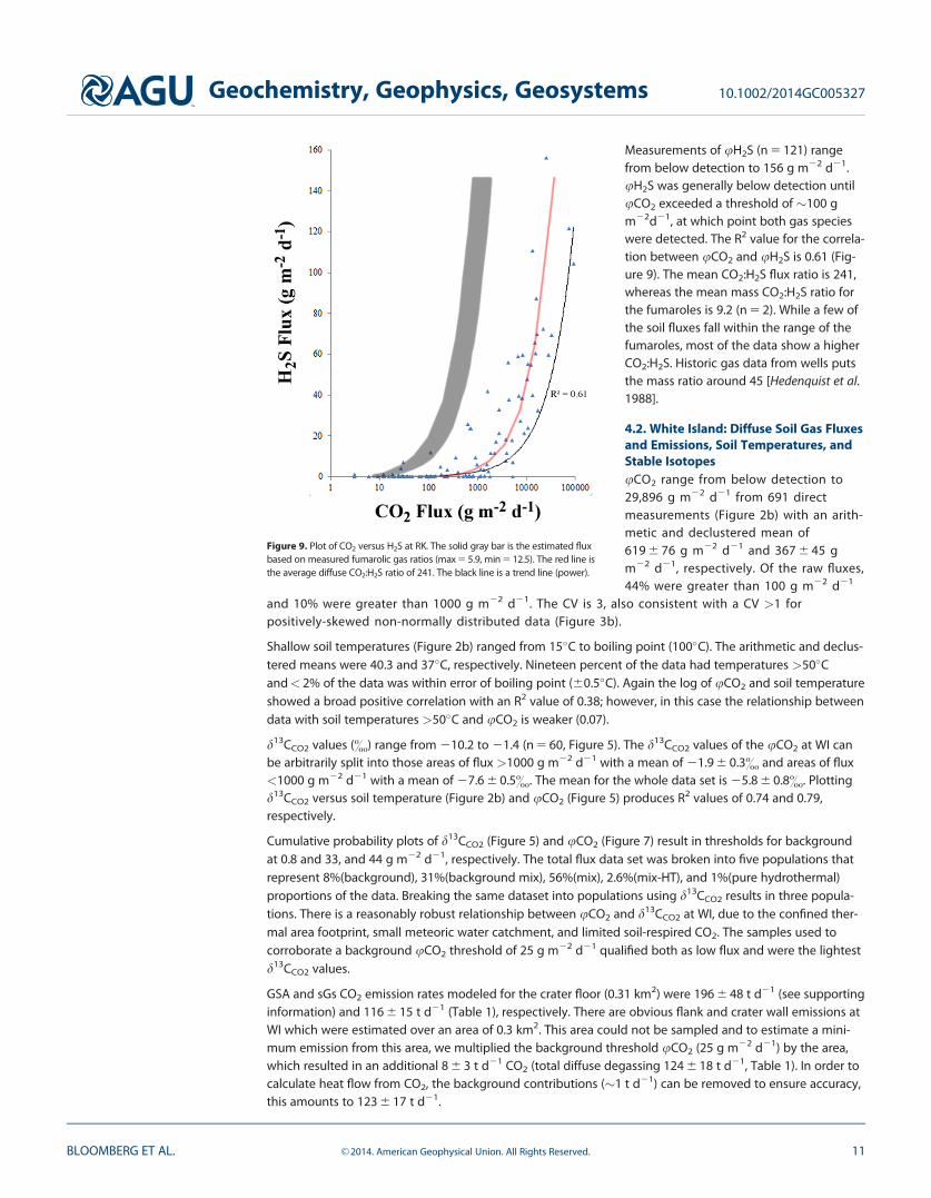
Measurements of uH2S (n 5 121) rangefrom below detection to 156 g m22 d21.uH2S was generally below detection untiluCO2 exceeded a threshold of �100 gm22d21, at which point both gas specieswere detected. The R2 value for the correla-tion between uCO2 and uH2S is 0.61 (Fig-ure 9). The mean CO2:H2S flux ratio is 241,whereas the mean mass CO2:H2S ratio forthe fumaroles is 9.2 (n 5 2). While a few ofthe soil fluxes fall within the range of thefumaroles, most of the data show a higherCO2:H2S. Historic gas data from wells putsthe mass ratio around 45 [Hedenquist et al.1988].

4.2. White Island: Diffuse Soil Gas Fluxesand Emissions, Soil Temperatures, andStable IsotopesuCO2 range from below detection to29,896 g m22 d21 from 691 directmeasurements (Figure 2b) with an arith-metic and declustered mean of619 6 76 g m22 d21 and 367 6 45 gm22 d21, respectively. Of the raw fluxes,44% were greater than 100 g m22 d21

and 10% were greater than 1000 g m22 d21. The CV is 3, also consistent with a CV >1 forpositively-skewed non-normally distributed data (Figure 3b).

Shallow soil temperatures (Figure 2b) ranged from 15�C to boiling point (100�C). The arithmetic and declus-tered means were 40.3 and 37�C, respectively. Nineteen percent of the data had temperatures >50�Cand< 2% of the data was within error of boiling point (60.5�C). Again the log of uCO2 and soil temperatureshowed a broad positive correlation with an R2 value of 0.38; however, in this case the relationship betweendata with soil temperatures >50�C and uCO2 is weaker (0.07).

d13CCO2 values (&) range from 210.2 to 21.4 (n 5 60, Figure 5). The d13CCO2 values of the uCO2 at WI canbe arbitrarily split into those areas of flux >1000 g m22 d21 with a mean of 21.9 6 0.3& and areas of flux<1000 g m22 d21 with a mean of 27.6 6 0.5&. The mean for the whole data set is 25.8 6 0.8&. Plottingd13CCO2 versus soil temperature (Figure 2b) and uCO2 (Figure 5) produces R2 values of 0.74 and 0.79,respectively.

Cumulative probability plots of d13CCO2 (Figure 5) and uCO2 (Figure 7) result in thresholds for backgroundat 0.8 and 33, and 44 g m22 d21, respectively. The total flux data set was broken into five populations thatrepresent 8%(background), 31%(background mix), 56%(mix), 2.6%(mix-HT), and 1%(pure hydrothermal)proportions of the data. Breaking the same dataset into populations using d13CCO2 results in three popula-tions. There is a reasonably robust relationship between uCO2 and d13CCO2 at WI, due to the confined ther-mal area footprint, small meteoric water catchment, and limited soil-respired CO2. The samples used tocorroborate a background uCO2 threshold of 25 g m22 d21 qualified both as low flux and were the lightestd13CCO2 values.

GSA and sGs CO2 emission rates modeled for the crater floor (0.31 km2) were 196 6 48 t d21 (see supportinginformation) and 116 6 15 t d21 (Table 1), respectively. There are obvious flank and crater wall emissions atWI which were estimated over an area of 0.3 km2. This area could not be sampled and to estimate a mini-mum emission from this area, we multiplied the background threshold uCO2 (25 g m22 d21) by the area,which resulted in an additional 8 6 3 t d21 CO2 (total diffuse degassing 124 6 18 t d21, Table 1). In order tocalculate heat flow from CO2, the background contributions (�1 t d21) can be removed to ensure accuracy,this amounts to 123 6 17 t d21.

Figure 9. Plot of CO2 versus H2S at RK. The solid gray bar is the estimated fluxbased on measured fumarolic gas ratios (max 5 5.9, min 5 12.5). The red line isthe average diffuse CO2:H2S ratio of 241. The black line is a trend line (power).

Geochemistry, Geophysics, Geosystems 10.1002/2014GC005327

BLOOMBERG ET AL. VC 2014. American Geophysical Union. All Rights Reserved. 11

4.3. Heat and Mass Flow Based on Soil Temperature Measurements for RK and WIUsing equations (1) and (2), the data were modeled with sGs then converted to heat flow in W m22 andfinally into a total megawatt (MWt) value. For RK heat flow measurements ranged between 0.03 and 5624 Wm22 with a mean of 15 W m22. At WI they ranged from 0.28 to 5624 W m22 with a mean of 62 W m22. Thetotal heat flow through soil estimates and equivalent steam mass flow (Fs (H2O)) values are 42 6 10 MWtand 1390 6 347 t d21 for RK and 20 6 5 MWt and 642 6 160 t d21 for WI.

4.4. Heat and Mass Flow Calculated From CO2 DegassingCalculating the total heat output from RK was accomplished using equations (4) and (5), where the totalmagmatic-hydrothermal uCO2 (440 6 84 t d21) was multiplied by the H2O:CO2 ratio from well discharges(16.6) [Hedenquist et al. 1988; Winick et al., 2011] and fumarolic vents (47.38, this study, 2011) to give a rangeof mass flow values (t d21), of 90 6 17 and 246 6 47, respectively, and heat flow values of 226 6 43 and645 6 123 MWt, respectively (Table 2). Mass flow values are produced by combining the H2O and CO2 dailyemissions, these compare to previously published values of 144 and 105 kg s21 for total mass flow at RK[Seward and Kerrick, 1996; Bowyer and Holt, 2010]. Calculations of the heat flow and CO2 emission weremade using the above mentioned mass flow values of 144 and 105 (Table 2). Finally, a theoretical value ofCO2 concentration in steam produced by adiabatic boiling of a parent fluid (61 g kg21 CO2) from maximumreservoir temperature (340�C) [Winick et al., 2011] to surface BP (98.7�C) was calculated (116.17 g kg21 CO2)and multiplied by the most recently published mass flow estimate (105 kg s21) [Bowyer and Holt, 2010] toassess the theoretical maximum heat release from the upflow of 248 MWt (Table 2).

At WI, the total magmatic-hydrothermal CO2 emission of 123 6 17 t d21 was multiplied by the best estimateH2O:CO2 ratio in the deep fluid (6.27) [Giggenbach and Matsuo, 1991; Werner et al., 2008a] as well as several otherpublished values (Table 3) to give a range of mass flows (4–131 kg s21) and heat flows of 6–347 MWt (Table 3).

Table 2. Range of Results for RK Heat and Mass Flow Calculations From CO2 Daily Emissions and H2O:CO2 Mass Ratios

Mass Ratio CO2 (t d21) MWt H2O (t d21) MF (kg s21)

16.6a 440 6 84b 226 6 43 7,304 6 1,394 90 6 1747.38c 440 6 84b 645 6 123 20,845 6 3,979 246 6 4716.6a 749 361 11,691 144d

227.27d 54 383 12,387 144d

16.6a 546 263 8,525 105e

47.38c 191 274 8,880 105e

8.6f 1,054 248 8,018 105e

aHedenquist et al. [1988].bMagma-hydrothermal daily CO2 emission.cAverage RK fumaroles 2011.dSeward and Kerrick [1996].eBowyer and Holt [2010].fTheoretical value from adiabatic boiling.

Table 3. Range of Results for WI Heat and Mass Flow Calculations From CO2 Daily Emissions and H2O:CO2 Mass Rations

Mass Ratio CO2 (t d21) MWt H2O (t d21) MF (kg s21)

6.26a b123 6 17 24 6 3 770 6 106 10 6 18.5a, Median b123 6 17 32 6 4 1,046 6 145 14 6 2

38.05a b123 6 17 145 6 20 4,681 6 647 56 6 810.03c b123 6 17 38 6 5 1,234 6 171 16 6 213.13d b123 6 17 50 6 7 1,615 6 223 20 6 391.17d, Max b123 6 17 347 6 48 11,214 6 1,550 131 6 18

1.48e, Min b123 6 17 6 6 1 182 6 25 4 6 17.61e b123 6 17 29 6 4 936 6 129 12 6 22.06f b123 6 17 8 6 1 253 6 35 4 6 16.26a g1,249 6 117 242 6 23 7,821 6 732 105 6 9

aGiggenbach and Matsuo [1991].bMagma-hydrothermal daily CO2 emission.cRose et al. [1996].dMarty and Giggenbach [1990].eGiggenbach and Sheppard [1989].fWerner et al. [2008a].gTotal Island degassing.

Geochemistry, Geophysics, Geosystems 10.1002/2014GC005327

BLOOMBERG ET AL. VC 2014. American Geophysical Union. All Rights Reserved. 12

We estimate a total island heat and mass flow by combining the crater and flank diffuse degassing emission(123 6 17 t d21, 0.61 km2) with the average plume emission during the study period (1126 6 100 t d21 CO2,http://www.geonet.org.nz (accessed during 2012)) to produce a total island daily CO2 emission of1249 6 117 t d21 CO2 (Table 3).

5. Discussion

5.1. Defining the Multisource Nature of CO2

In order to use RCO2 values to estimate heat and mass flow from a magmatic-hydrothermal system, it isnecessary to define the contributions from the different uCO2 sources. Any contribution from nonmagmatic-hydrothermal sources (background or soil-respired/biogenic in this case) must be removed from the calcula-tion. Two methods were employed in this study: (1) the GSA method of breaking the flux data into populationsand (2) the use of stable isotopic analysis of the uCO2 to identify source components.

When using GSA, we assume that lowest flux populations (<30 g m22 d21) represent the background val-ues. The heterogeneity in permeability at our field sites and pervasiveness of magma-hydrothermal CO2

emission means this method, on its own, may not fully constrain the source populations. This became evi-dent when stable isotope analysis was paired with flux data (Figures 6 and 7), as there were sites which hadmagma-hydrothermal d13CCO2 values (filled circles, Figures 6 and 7) within the low flux populations definedby GSA. While GSA does not fully constrain a source, it can illustrate the natural variations within the totalflux population, allowing quick estimates source contributions. However, as noted by others, the partition-ing procedure does not result into a unique solution [Chiodini et al., 2008].

When Chiodini et al. [2008] first applied this method to finding the source populations, GSA populations ofthe flux data were reduced into two partitions, a low and high flux group. This meant that when they com-pared their isotopically partitioned populations to the GSA populations, the GSA populations were found tohave overestimated the limits of the background flux populations significantly. In this study, the flux datawere fully partitioned using GSA in to five populations and then compared with the three isotopically parti-tioned flux populations (Figures 4 and 5). Overestimation of the low flux GSA populations was not pro-duced, and the two different data sets produced similar thresholds for background fluxes.

While the GSA populations are defined by inflections in the slope and therefore span defined sections ofthe total flux (Figures 6 and 7, straight lines), the stable isotope analysis provides source populations whichin some instances span the whole range of fluxes (Figures 6 and 7, filled circles). The paired use of stable iso-topes and GSA to isolate the source populations was the method used in this study, as it was in Chiodiniet al. [2008]; however, a complete analysis of the flux data using the paired assessment of sources led towell-defined thresholds for constraining the magmatic-hydrothermal CO2 emission.

Figures 6 and 7 show the cumulative probability plots of total flux at RK and WI with populations from theGSA and from the stable isotopic analysis superimposed. These methods combine to produce values for thebackground or nonmagma-hydrothermal contribution threshold. The thresholds were set at <30 for RK and<25 g m22 d21 for WI. The thresholds were derived from averaging the lightest isotopic population (Figures6 and 7) which fits within GSA populations 1 and 2 (determined to be ‘‘background’’). The value at WI wasslightly higher than the 15 g m22 d21 threshold found by Werner et al. [2004a], though their study used sta-tistical analysis to constrain the flux population.

5.2. Soil Gas Emissions at RotokawaSoil gas flux measurements at RK cover a wide range (<1 to 127,808 g m22 d21) with a significant through-put of magmatic-hydrothermal CO2 within regions of thermal ground. The highest fluxes in this study aresome of the highest reported in the literature for hydrothermal areas worldwide by an order of magnitude(e.g., 11,535 g m22 d21 reported at Rotorua hydrothermal area, Werner and Cardellini [2006]; 14,000 g m22

d21 reported at Hot Spring Basin area of Yellowstone, Werner et al., [2008b]; 27,518 g m22 d21, reported forOhaaki West, Rissmann et al. [2012]) The emission rate of 441 t d21 (Table 1), however, is comparable toother large hydrothermal systems (620 t d21 at Rotorua and 410 t d21 at Hot Spring Basin) suggesting thatthe high fluxes are spatially localized and were captured most likely due to the very small sample spacing(5 m) in the cluster component of sampling here in comparison to other studies.

Geochemistry, Geophysics, Geosystems 10.1002/2014GC005327

BLOOMBERG ET AL. VC 2014. American Geophysical Union. All Rights Reserved. 13

Our CO2 emission rates for Rotokawa depended greatly on the interpolation approach whereas at WhiteIsland the emission estimates were fairly consistent with one another. The GSA method allows definition ofa confidence interval on emission rates, but does not take into account the spatial distribution of data,which can bias the data population distribution, especially if the data are clustered in one region more thananother [Cardellini et al., 2003]. GSA will also not accurately represent any unsampled (in this case, mostlynonthermal) areas. For these reasons, we report the sGs emission rate for Rotokawa and use this value herefor further analysis (Table 1). The GSA approach was used in this study as a technique for assessing the natu-ral distribution and thresholds of CO2 and heat flow data, and can be used in conjunction with other datato assess the origins of CO2, which will be discussed in more detail below.

The CO2 emission when normalized to the thermal area (55,879 t yr21 km22, 441 t d21 at 2.88 km2) pro-duces a value that is one of the largest nonvolcanic CO2 emissions in New Zealand. The RK value is equiva-lent to 200% of the normalized emission for the Rotorua geothermal system (25,426 t yr21 km22; Wernerand Cardellini, 2006] and 40% of the normalized soil gas emissions of WI (132,247 t yr21 km22). Previousmeasurements at RK indicated a smaller CO2 emission; Seward and Kerrick [1996] calculated a RCO2 from RKto be �55 t d21 based on a total mass flow of 144 kg s21 and a CO2 concentration of kgH2O:4.4gCO2 or amass ratio of 227 (Table 2). The H2O:CO2 ratio was the key factor in their underestimation of the CO2 flux,this is likely because the value was from the low gas borefield rather than the degassing upflow near LakeRotokawa. The high spatial resolution of direct measurements in this study has produced a higher CO2 valueof 441 6 84 t d21, but when coupled with a smaller mass ratio (16.6), less upflow is required (Table 2). Con-sidering a sizeable variance in mass ratio’s presented in Table 2, multiple assesments of the daily CO2 emis-sion are produced using published mass flow values. Despite previously published estimates [Bloomberget al., 2012] which depended entirely on the Hedenquist et al. [1988] value, it appears that the the additionalinvestigation of other ratios and upflows has only encouraged the use of this value, as other ratios do notcorroborate well with the prescribed upflow [Bowyer and Holt, 2010] for RK.

A marked difference is present between the theoretical mass ratio in steam (8.6) and the measured fumar-olic ratio (47.83). It is likely that slowly upflowing (105 kg s21), deeper-sourced CO2 is dispersed throughoutthe thermal area rather than eminating through high-gas fumaroles (of which none are found at RK) as wellas the boiling of a relatively degassed shallow thermal aquifer could result in these low-gas fumarole sam-ples. By comparing the value of total daily emissions (441 t d21) with the predicted CO2 emission (546 td21) using the prescribed mass flow of 105 kg s21, it would appear that regardless of whether the CO2 isdegassed from the shallow aquifer or the deeper, continuosuly boiling upflow, it is quantitatively degassedthrough the thermal area at RK (Figure 8).

5.3. A Sulfur Budget for RotokawaAs in most hydrothermal areas, H2S is a significant component both in fumarolic and diffuse emission, SO22

4 iselevated in surface waters, and S-bearing minerals are abundant at the ground surface at RK. The general corre-lation observed between CO2 and H2S fluxes (Figure 9) is similar to that observed in other hydrothermal regions(e.g., Hot Spring Basin in Yellowstone, Werner et al., 2008b). In general uH2S occurs is below detection except inareas where uCO2 becomes large. Based on interpretations of this phenomenon in Werner et al. [2008b], it isassumed that for low CO2 flux locations, the H2S is removed through scrubbing processes (precipitated as nativeS or reacts with local groundwaters), but when CO2 flux is high, H2S gas can reach the surface.

Based on the observed relationship of CO2 and H2S, we can estimate the amount of S being deposited in thesubsurface. A total expected H2S emission from diffuse degassing of � 1 6 1 t d21 is calculated by multiplyingthe minimum total CO2 emission (230 t d21) by the molar CO2:H2S flux ratio. Two previous studies from LakeRotokawa found 84.3 and 10.4 t d21 SO22

4 [Krupp and Seward, 1987; Hedenquist et al., 1988], which equates to29.9 and 3.67 t d21 H2S (multiplying by the molar weight ratio, sulfur oxidation), respectively. Summing thesegives a minimum total surface sulfur emission for RK of �4.5 t d21 or �31 t d21 respectively, compared witha predicted emission of H2S from the reservoir of �48 t d21 (multiplying the total CO2 by the CO2:H2S fumar-ole ratio, 9.2). The inferred loss of�43 t d21 of H2S within the subsurface could be due to scrubbing by shal-low groundwater and/or precipitation (as elemental S) before reaching the surface. This can be reconciledwith the large (2.6 Mt, Hedenquist et al., 1988] sulfur lode found within meters of the surface at RK which Kruppand Seward [1987] estimated accumulated at 5 t d21 over 1420 years. If we consider the second surface sulfuremission of 30 t d21, we find the loss is reduced to 17 t d21 H2S.

Geochemistry, Geophysics, Geosystems 10.1002/2014GC005327

BLOOMBERG ET AL. VC 2014. American Geophysical Union. All Rights Reserved. 14

5.4. Rotokawa d13CCO2 AnalysisThe maximum d13CCO2 of the uCO2 (27.3&) is consistent with the findings of Hedenquist et al. [1988] forwell RK4 (gas phase CO2 in the well, 27.9&) and for the Rotokawa fumarole (vent, 27.8&), and indicatesthat the deep carbon source is indistinguishable from the soil CO2 samples taken within the thermal area.The contribution to soil CO2 from different sources can be observed in Figure 4 where the maximum iso-topic value of 27.3& is defined as the magmatic-hydrothermal end-member and the minimum value of216.5& is the background end member. A large area of the thermal area at RK is vegetated by C3 plants(e.g., prostrate Manuka) which yield a d13CCO2 of 224& [Amundson et al., 1998] during decomposition androot respiration. The other minor contributions to uCO2 are from litter and humus decomposition and infil-tration of the atmospheric CO2, both of which contribute minimally if there is active root respiration occur-ring [Amundson et al., 1998].

The average d13CCO2 value from the sampling at RK was 29.7 6 0.4& though no spatial correlations can bedrawn here due to the biased sampling design. In locations of hydrothermal-dominant CO2 (>29.9&), wealso find a good correlation with high uCO2 (mean of 8000 g m22 d21) while in areas of mixed sources(<210&) we find a mean uCO2 of 114 g m22 d21. High water tables can reduce anomalous soil tempera-tures while not affecting the flux, therefore the correlation between soil temperature and uCO2 and d13CCO2

is weak (Figure 2a).

In areas of low flux (<100 g m22 d21), many d13CCO2 signatures were >28& (Figure 4), suggesting a mag-matic as opposed to a soil-respired source. The lowest measured d13CCO2 signature was 216.5& and corre-sponded to a uCO2 of 59 g m22 d21. If the origin of the isotopically lightest soil-respired CO2 is 224&

[Amundson et al., 1998], then the 216.5& value is still significantly mixed with hydrothermally sourced CO2.A flux of 59 g m22 d21 is at least 2–4 times larger than natural soil respired background (15–30 g m22 d21)measured for unirrigated pasture in the Taup�o Volcanic Zone (Clinton Rissmann, personal communication,2012). This indicates a significant hydrothermal CO2 input even at low flux sites (<100 g m22 d21) and sug-gests the dominant control on flux is soil permeability. These types of correlations show that d13CCO2 measure-ments have important implications for the discovery of blind geothermal systems concealed by low uCO2.

5.5. Rotokawa: Structural and Permeability Controls on CO2 EmissionsSignificant flux anomalies (>500 g m22 d21) are quasi-circular in nature but become more diffuse andbroadly distributed at lower flux rates. There is a clear correlation of surface thermal features with areas ofhigh flux (Figure 8). Thermal features are concentrated either along lineations that trend NE or within thebounds of historic hydrothermal eruption craters (Figure 8). The highest flux values occur along the lakeshore and coincide with lower average soil temperatures (<50�C, Figure 2a) indicating some decoupling ofsteam flow likely due to high water tables adjacent to the lake. To the north and northwest greater couplingbetween heat flow (high soil temperatures) and CO2 flux indicates less scrubbing of the steam phase bycooler lake waters. The active thermal area has been mapped previously using resistivity boundaries andthermal anomalies [Gregg, 1958; Hochstein et al., 1990] and Figure 8 reproduces these features with minimaladditions.

The thermal area at RK coincides with a series of historic hydrothermal explosion craters, the largest ofwhich is the site of Lake Rotokawa [Collar and Browne, 1985]. Vigorous surface thermal activity surroundsthe explosion craters and includes boiling acidic SO4-Cl springs and steaming ground. Most diffuse degass-ing is coupled to these thermal features and decreases rapidly in magnitude with distance away from them.There is a major anomaly along a feature attributed to a hydrothermal eruption crater rim by Krupp andSeward [1987] which runs E-W for 300 m across the thermal area.

Lake Rotokawa, a depression caused by a hydrothermal eruption crater, has a large recharge of CO2-unsatu-rated meteoric waters to depths of >200 m. This depth is enough to dissolve any fluxing CO2 and no visiblebubbles are present mid lake. Closer to the lake shore the water column can be saturated in CO2 and a pro-portion of incoming flux will degas at the surface as bubbles [Chiodini et al., 2000]. Some of the highestmeasured uCO2 is located close to the shore line which is indicative of significant permeability related tothe rim of the large hydrothermal eruption crater [Collar and Browne, 1985; Krupp and Seward, 1987].

Faulting can cause hot spots of high permeability that allows boiling fluids to rise [Fairley and Hinds, 2004;Rowland and Sibson, 2004; Heffner and Fairley, 2006; Rissmann et al., 2011]. There is a large field fault running

Geochemistry, Geophysics, Geosystems 10.1002/2014GC005327

BLOOMBERG ET AL. VC 2014. American Geophysical Union. All Rights Reserved. 15

through the middle of the RK thermal area, the Central Field Fault (CFF) of Winick et al. [2011], which indi-rectly influences the diffuse degassing structures with historic eruptions craters that appear to focus ther-mal activity, occurring along its strike. The magnitude of the gas fluxes in the vicinity of these craters andalong the strike of the CFF suggests a deep-seated connection between surface eruption craters and theCFF, which is likely channeling fluids from depth.

5.6. White Island CO2 EmissionsThe difference between the total mean uCO2 and magmatic-hydrothermal mean uCO2 for the crater floordiffuse degassing (368 versus 723 g m22 d21) indicates a significant area has background emission as dis-played by the flux map (Figure 10a). The range of flux values at WI, though not as broad as at RK, does havea higher mean value, which is an indicator of the reduced contribution of background sources to the RCO2

through the crater floor (4% of samples at RK versus 1.3% at WI). Removing the background contribution to

Figure 10. (a) uCO2 mapped within the accessible crater floor, historic craters are outlined in white. (b) Soil temperatures at 10cm (�C) aremapped within the crater floor; surface thermal features (steaming ground, mud pots, hot springs) are mapped with black dotted lines.

Geochemistry, Geophysics, Geosystems 10.1002/2014GC005327

BLOOMBERG ET AL. VC 2014. American Geophysical Union. All Rights Reserved. 16

the RCO2 (�1 t d21) and additionally estimating the emission for the flank and crater walls gives a value of123 6 17 t d21.

The value of 123 t d21 or �10% of the RCO2 (1247 t d21) is consistent with the latest published study at WIby Werner et al. [2004a] who found an emission of 99 t d21 and 10% of the total emission from 268 points�9000 points/km2). Wardell et al. [2001] found an emission of 10 t d21 and <1% of the total emission,though their survey was less than 20 points (�100 points/km2).

5.7. White Island d13CCO2 AnalysisThe samples of soil CO2 had a maximum d13CCO2 of 21.4& which is slightly more positive than the ventsamples by Marty and Giggenbach (max 22&, 1990) but within error of Giggenbach and Matsuo (max21.5&, 1991). The d13CCO2 samples measured at high flux sites (>1000 g m22 d22) are between 21.4 and22& (mean 21.9&) which matches the historic fumarole samples (Figure 5). This indicates that themagmatic-hydrothermal source has been sampled and gives a value for the magmatic-hydrothermal end-member.

Isotopically heavy signatures paired to high flux zones (>1000 g m22 d21, Figure 5) supports a magma-hydrothermal origin for the uCO2. The highest fluxes measured in our study are located along the centralsubcrater’s eastern rim. The correlation of the highest flux with the heaviest d13CCO2 is indicative of an areawhere fluids ascend rapidly to the surface due to high permeability [Werner and Cardellini, 2006; Rissmannet al., 2012].

The minimum value of 210.2& occurs at low uCO2 of 12.5 g m22 d21. The signature in this case is signifi-cantly lighter than magmatic but heavier than any pure soil-respired signature and the associated flux isconsidered low or background. Due to the total lack of vegetation or soil development within the craterfloor, the 210.2& value must be wholly atmospheric CO2 and/or potentially related to microbial respiration(i.e., methanogenesis) of CH4.

The average value of d13CCO2 at WI is 25.8 6 0.7& and indicates saturation of the soil with a mix of magma-hydrothermal sourced CO2 and input from background sources (atmospheric and/or microbial respiration). Inlocations of magma-hydrothermal-dominant CO2 (>24&), we also find a good correlation with high uCO2

(mean of 9216 g m22 d21) while in areas of mixed sources (<24 &) we find a mean uCO2 of 86 g m22 d21.

5.8. White Island: Structural and Permeability Controls on CO2 EmissionsAt WI we show a correlation with surface thermal feature such as mounds and areas around fumaroles, his-toric crater margins, and breaks in slope (Figures 10a and 10b). The mounds host numerous small fumarolicvents that are encrusted with sulfur condensate, are of high temperature, and are comprised of highlyaltered clays, all of which makes them analogous to the diffuse degassing structures (DDS) described byChiodini et al., [2005]. The vigor, size, and number of DDS, along with steaming ground and acidic-Cl out-flows, increases with proximity to the Crater Lake and the modern day center of volcanic activity.

Most of the RCO2 is exhausted through the Crater Lake [Werner et al., 2008a] and around its rim there is ahigh flux zone. In the middle of the crater floor, there is an arcuate channel of high flux and high temperaturesthat aligns closely with an old crater rim (Figures 10a and b). Boiling mud pots and steaming ground are evi-dence of a connection at depth as has been suggested by Houghton and Nairn [1991] and Giggenbach et al.[2003]. Diffuse degassing, fumaroles, and steaming ground are present at breaks in slope (crater floor/wall,crater wall/rim, crater floor/mound) which may be structurally constrained by subsurface features.

Elsewhere on the island there are areas of capping clays and iron-rich precipitates at around 1 m depth thatlimit degassing locally. These are hypothesized to be the remnants of the old crater floor/lake [Giggenbachet al., 2003], consisting of impermeable and altered volcaniclastic material.

5.9. Heat Flow From CO2 EmissionsFor both RK and WI, measured soil temperature data was converted to equivalent heat flow (subsection 4.3)using equations (1) and (2), and heat flow based on CO2 emissions was calculated using equations (4) and(5). Both RK and WI display lower observed heat flow than that estimated from CO2 emissions (Tables 2 and3). The discrepancies in heat flow values likely reflect the condensation of between 81 to 93% (42 and 226–646 MWt, RK) and 12.5% (19.5 and 22 MWt, WI) of the steam phase within shallow groundwater that overliesthe high temperature reservoirs.

Geochemistry, Geophysics, Geosystems 10.1002/2014GC005327

BLOOMBERG ET AL. VC 2014. American Geophysical Union. All Rights Reserved. 17

Fridriksson et al. [2006] report the condensation of 87% of steam mass flow for the Reykjanes thermal areain Iceland based on the discrepancy between observed heat flow and heat flow estimated from CO2 flux,similar to the discrepancy at RK. The system at RK probably loses more heat laterally (like Reykjanes) tocooler groundwater inflows, triggering condensation of rising hydrothermal fluids, as well as having adeeper conductive heat source (4–5 km; Winick et al., 2011]. Conversely, WI probably loses less heat to thelocal groundwaters as the conductive heat source is shallower (<1–2 km depth; Cole et al., 2000; Wardellet al., 2001; Werner et al., 2008a] and there is a concentrated plume that only opens to lateral degassing atdepths of <300m [Werner et al., 2008a].

Historic heat flow studies at RK presented in Hedenquist et al. [1988] and Seward and Kerrick [1996] put thethermal energy release between 210 and 236 MWt, but also report numbers as high as 600MWt. This studyhas produced a range of values (226 6 43 to 645 6 123 MWt, Table 2) that is perhaps only representative ofthe thermal area plume and not the complete field heat flow (unmeasured conductive heat flow from deepintrusions). The value derived from fumarolic CO2 (47.83) is less robust than the deep fluid value (16.6) giventhe difference in theoretical CO2 concentration and measured, and the probable causes of those differen-ces. Therefore, this study presents the value of 226 6 43 MWt as its best estimate of heat flow at RK.

The historic heat flow values are all based on chloride measurements, which might be less conservativewhen it comes to fluid-rock interaction [Bibby et al., 1995b] and is also less mobile than CO2 (CO2 has a gaspartitioning coefficient of 1185). For groundwater having reached saturation with respect to CO2, the majorityof the gas passes through to the surface. This behavior of CO2 makes it a relatively conservative proxy ofheat release from the shallow reservoir compared to chloride flux or measurement of observable heat flow[Chiodini et al., 2005; Rissmann et al., 2011]. The main error associated with any CO2-based estimate of reser-voir heat release is the correct estimation of CO2 emission and the selection of a representative molarH2O:CO2 ratio. At RK we used a high spatial resolution to reduce the uncertainty in the CO2 emission, andpresent the published mass ratio of 16.6 as representative of the deep fluid and the degassing plume andtherefore the values of 226 6 43 MWt is considered representative. It is possible that the discrepancy in CO2

degassed at the surface (441 t d21), and the theoretical CO2 daily emission (1054 t d21, Table 2) is accountedfor by the unmeasured CO2 degassing through the numerous hot pools, fumaroles, and Lake Rotokawa itself.

White Island’s plume was assessed by Giggenbach and Sheppard [1989] as a proxy for the island’s mass andheat flow, who found that it depended on the state of volcanic activity. Quieter periods had steam plumesof 5000 t d21 and 240 MWt, and active periods had plumes of 18,000 t d21 and 810 MWt. These mass flowswere derived using SO2 flux measured aerially with COSPEC-V and H2O:CO2:SO2 mass ratios, which were higher(kgH2O/240gCO2) than the concentration of CO2 in steam used in this study (kgH2O:159.5gCO2; see subsection4.4). Rose et al. [1986] found a steam degassing rate of 8000–9000 t d21 which is similar to this study’s value(Table 3; 7821 6 732 t d21). Werner et al. [2008a] described the H2O:CO2 ratios at WI as stable since a notabledecrease in activity since 2000 and therefore the CO2 concentration of 159.5g kg21 is considered a representa-tive mean value and was used in this study to calculate a heat flow of 242 6 23 MWt (Table 3).

6. Conclusions

The Rotokawa and White Island hydrothermal systems and their respective surface thermal expressionsemit a large quantity of CO2 and thermal energy per unit area. Our findings contribute to a growing numberof geothermal field-scale surveys of soil gas emissions in the Taup�o Volcanic Zone, reinforcing the benefitsof pairing GSA and stable isotopic compositions in determinations of the nonmagmatic-hydrothermal con-tribution to geothermal field emissions. Our findings demonstrate that soil gas surveys that do not partitionthe source of the uCO2 using stable isotope analysis may inaccurately delineate magma-hydrothermal CO2

flux from depth. It is therefore appropriate to pair a survey of uCO2 with analysis of the d13CuCO2 asadopted here. At Rotokawa, the RCO2 was 441 6 84 t d21, producing a total mass flux (90 617 kg s21). AtWhite Island, the CO2 emission rate of 123 6 17 t d21 was estimated for diffuse degassing through the cra-ter floor and is consistent with previous estimates (�100 t d21) [Werner et al., 2004a] and the RCO2

(1249 6 116 t d21; plume 1 soil gas) for the island is similar to previous estimates [Rose et al., 1986; Martyand Giggenbach, 1990; Wardell et al., 2001; Werner et al., 2004a; Werner et al., 2008a]. Overall, the methodol-ogy and approach utilized here is well suited to constraining the anomalous magma-hydrothermal noncon-densable gas release for total heat and mass flow estimations in the Taup�o Volcanic Zone.

Geochemistry, Geophysics, Geosystems 10.1002/2014GC005327

BLOOMBERG ET AL. VC 2014. American Geophysical Union. All Rights Reserved. 18

ReferencesAmundson, R., L. Stern, T. Baisden, and Y. Wang (1998), The isotopic composition of soil and soil-respired CO2, Geoderma, 82(1-3), 83–114,

doi:10.1016/S0016-7061(97)00098-0.Bergfeld, D. W. C. Evans, J. F. Howle, and C. D. Farrar (2006), Carbon dioxide emissions from vegetation-kill zones around the resurgent

dome of Long Valley Caldera, eastern California, USA, J. Volcanol. Geotherm. Res., 152, 140–156, doi:10.1016/j.jvolgeores.2005.11.003.Bibby, H. M., T. G. Caldwell, F. J. Daey, and T. H. Webb (1995a), Geophysical evidence on the structure of the Taupo Volcanic Zone and its

hydro-thermal circulation, J. Volcanol. Geotherm. Res., 68, 29–58, doi:10.1016/0377-0273(95)00007-H.Bibby, H. M., R. B. Glover, and P. C. Whiteford (1995b), The Heat Output of the Waimangu, Waiotapu-Waikite and Reporoa Geothermal Sys-

tems (NZ): Do Chloride Fluxes Provide an Accurate Measure?, paper presented at Proceedings of the 17th NZ Geothermal Workshop,pp. 91–97. [Available at http://www.geothermal-energy.org/pdf/IGAstandard/NZGW/1995/Bibby.pdf.]

Bloomberg, S., C. Rissmann, A. Mazot, C. Werner, T. Horton, C. Oze, D. Gravley, and B. Kennedy (2012), Soil CO2 emissions: A proxy for heatand mass flow assessment, Rotokawa, New Zealand, paper presented at Proceedings of the 34th New Zealand Geothermal Workshop,Auckland, N. Z., 21–23 November 2012. [Available at http://www.geothermal-energy.org/pdf/IGAstandard/NZGW/2012/46654final00010.pdf.]

Bowyer, D., and R. Holt (2010), Case study: Development of a numerical model by a multi-disciplinary approach, Rotokawa GeothermalField, paper presented Proceedings of the World Geothermal Congress 2010, Bali, Indonesia, 25–29 April. [Available at http://www.geo-thermal-energy.org/pdf/IGAstandard/WGC/2010/2236.pdf.]

Brombach, T., J. C. Hunziker, G. Chiodini, C. Cardellini, and L. Marini (2001), Soil diffuse degassing and thermal energy fluxes from the south-ern Lakki Plain, Nisyros (Greece), Geophys. Res. Lett., 28(1), 69–72, doi:10.1029/2000GL008543.

Cardellini, C., G. Chiodini, and F. Frondini (2003), Application of stochastic simulation to CO2 flux from soil: Mapping and quantification ofgas release, J. Geophys. Res., 108(B9), 2425, doi:10.1029/2002JB002165.

Castaldi, S., and D. Tedesco (2005), Methane production and consumption in an active volcanic environment of Southern Italy, Chemo-sphere, 58(2), 131–139, doi:10.1016/j.chemosphere.2004.08.023.

Chiodini, G., R. Cioni, M. Guidi, B. Raco, and L. Marini (1998), Soil CO2 flux measurements in volcanic and geothermal areas, Appl. Geochem.,13, 543–552, doi:10.1016/S0883-2927(97)00076-0.

Chiodini, G., et al. (2000), Rate of diffuse carbon dioxide Earth degassing estimated from carbon balance of regional aquifers: The case ofcentral Apennine, Italy, J. Geophys. Res., 105(B4), 8423–8434, doi:10.1029/1999JB900355.

Chiodini, G., D. Granieri, R. Avino, S. Caliro, A. Costa, and C. Werner (2005), Carbon dioxide diffuse degassing and estimation of heat releasefrom volcanic and hydrothermal systems, J. Geophys. Res., 110, B08204, doi:10.1029/2004JB003542.

Chiodini, G., S. Caliro, C. Cardellini, R. Avino, D. Granieria, and A. Schmidt (2008), Carbon isotopic composition of soil CO2 efflux; a powerfulmethod to discriminate different sources feeding soil CO2 degassing in volcanic-hydrothermal areas, Earth Planet. Sci. Lett., 274, 372–379, doi:10.1016/j.epsl.2008.07.051.

Cole, J. W., T. Thordarson, and R. M. Burt (2000), Magma origin and evolution of White Island (Whakaari) volcano, Bay of Plenty, New Zea-land, J. Petrol., 41(6), 867–895,doi:10.1093/petrology/41.6.867.

Collar, R. J., and P. R. L. Browne (1985), Hydrothermal eruptions at the Rotokawa Geothermal Field, Taupo Volcanic Zone, New Zealand,paper presented at Proceedings of the 7th NZ Geothermal Workshop, pp. 1–5. [Available at http://www.geothermal-energy.org/pdf/IGAstandard/NZGW/1985/Collar.pdf.]

Dawson, G. B. (1964), The nature and assessment of heat flow from hydrothermal areas. N. Z. J. Geol. Geophys., 7, 155–171.Dereinda, F. H., and H. Armannsson (2010), CO2 emissions from the Krafla geothermal area, Iceland, paper presented at Proceedings World

Geothermal Congress 2010, Bali, Indonesia, 25–29 April 2010. [Available at http://www.geothermal-energy.org/pdf/IGAstandard/WGC/2010/0250.pdf.]

Deutsch, C. V., and A. G. Journel (1998), GSLIB: Geostatistical Software Library and User’s Guide, Oxford Univ. Press, N. Y.Donachie, S. P., B. W. Christenson, D. D. Kunkel, A. Malahoff, and M. Alam (2002), Microbial community in acidic hydrothermal waters of vol-

canically active White Island, New Zealand, Extremophiles, 6, 419–425, doi:10.1007/s00792-002-0274-7.Donaldson, I. G., and M. A. Grant (1978), An estimate of the resource potential of New Zealand geothermal fields for power generation,

Geothermics, 7(2–4), 243–252, doi:10.1016/0375-6505(78)90014-7.Fairley, J. P., and J. J. Hinds (2004), Field observation of fluid circulation patterns in a normal fault system. Geophys. Res. Lett., 31, L19502,

doi:10.1029/2004GL020812.Fridriksson, T., B. R Kristj�ansson, H. �Armannsson, E. Margr�etard�ottir, S. �Olafsd�ottir, and G. Chiodini (2006), CO2 emissions and heat flow

through soil, fumaroles, and steam-heated mud pools at the Reykjanes geothermal area, SW Iceland, Appl. Geochem., 21, 1551–1569,doi:10.1016/j.apgeochem.2006.04.006.

Frondini, F., G. Chiodini, S. Caliro, C. Cardellini, D. Granieri, and G. Ventura (2004), Diffuse CO2 degassing at Vesuvio, Italy. Bull. Volcanol.,66(7), 642–651, doi:10.1007/s00445-004-0346-x.

Giggenbach, W. F. (1975a), A Simple method for the collection and analysis of volcanic gas samples, Bull. Volcanol, 39(1), 132–145, doi:10.1007/BF02596953.

Giggenbach, W. F. (1975b), Variations in the carbon, sulfur and chlorine contents of volcanic gas discharges from White Island, New Zea-land, Bull. Volcanol, 39, 15–27.

Giggenbach, W. F. (1987), Redox processes governing the chemistry of fumarolic gas discharges from White Island, New Zealand, Appl.Geochem., 2(1), 143–161.

Giggenbach, W. F. (1995), Variations in the chemical and isotopic composition of fluids discharged from the Taupo Volcanic Zone, NewZealand, J. Volcanol. Geotherm. Res., 68(1-3), 89–116.

Giggenbach, W. F., and S. Matsuo (1991), Evaluation of results from Second and Third IAVCEI field workshops on volcanic gases, Mt. Usu,Japan and White Island, New Zealand, Appl. Geochem., 6, 125–141, doi:10.1016/0883-2927(91)90024-J.

Giggenbach, W. F., and D. S. Sheppard (1989), Variation in the temperature and chemistry of White Island fumarole discharges 1972-85, N.Z. Geol. Surv. Bull., 103, 119–126.

Giggenbach, W., H. Shinohara, M. Kusakabe, and T. Ohba (2003), Formation of acid volcanic brines through interaction of magmatic gases,seawater, and rock within the White Island volcanic-hydrothermal system, New Zealand, Spec. Publ. Soc. Econ. Geol., 10, 19–40.

Gregg, D. R. (1958), Natural heat flow from the thermal areas of Taupo Sheet District (N 94), N. Z. J. Geol Geophys., 1(1), 65–75, doi:10.1080/00288306.1958.10422795.

Hedenquist, J. W., E. K. Mroczek, and W. F. Giggenbach (1988), Geochemistry of the Rotokawa Geothermal System: Summary of Data, inInterpretation and Appraisal for Energy Development: DSIR Chemistry Division Tech. Note, 88/6, pp. 64.

AcknowledgmentsWe would like to thank GNS Scienceand GeoNet for the use of theirequipment (Karen Britten, JeremyCole-Baker), Mighty River PowerLimited, (Tom) Powell Geoscience Ltd.,University of Canterbury (Jo Pawson,Mark Letham, Heather Bickerton, JelteKeeman, Joshua Blackstock), D.O.C andTauhara North No.2 Trust for access tothe RK thermal area, pilots and crewfrom SQDRN 3 RNZAF and Peejay IVand V (White Island Tours) fortransport to (and from) White Island,The Buttle Family for access to theirprivate volcano. This study contributesto and is funded by the UC-MRPSource 2 Surface research program.Additional funding is from the Ministryof Science and Innovation’sFoundation for Research, Science, &Technology through a TechNZScholarship and the University ofCanterbury’s Mason trust. Dataavailable as supporting information.This manuscript benefitted greatlyfrom the anonymous peer reviewprocess and a candid yet helpfulreview by Mike Doukas (USGS).

Geochemistry, Geophysics, Geosystems 10.1002/2014GC005327

BLOOMBERG ET AL. VC 2014. American Geophysical Union. All Rights Reserved. 19

Heffner, J., and J. Fairley (2006), Using surface characteristics to infer the permeability structure of an active fault zone, Sediment. Geol., 184,255–265.

Hochstein, M. P., and C. J. Bromley (2005), Measurement of heat flux from steaming ground, Geothermics, 34, 133–160, doi:10.1016/j.geothermics.2004.04.002.

Hochstein, M.P., I. Mayhew and R.A. Villarosa (1990), Self-Potential Surveys of the Mokai and Rotokawa High Temperature Fields (NZ), paperpresented at Proceedings of the 12th NZ Geothermal Workshop. [Available at http://www.geothermal-energy.org/pdf/IGAstandard/NZGW/1990/Hochstein.pdf.]

Houghton, B.F., and I.A., Nairn (1991). The 1976-82 Strombolian and phreatomagmatic eruptions of White Island, New Zealand: Eruptionand depositional mechanisms at a ‘wet’ volcano, Bull. Volcanol, 54, 25–49.

Inguaggiato, S., A. Mazot, I. S. Diliberto, C. Inguaggiato, P. Madonia, D. Rouwet, and F. Vita (2012), Total CO2 output from Vulcano island(Aeolian Islands, Italy), Geochem. Geophys. Geosyst., 13, Q02012, doi:10.1029/2011GC003920.

Kerrick, D. M. (2001), Present and past non-anthropogenic CO2 degassing from the solid earth, Rev. Geophys., 39(4), 565–585, doi:10.1029/2001RG000105.

Krupp, R. E., and T. M. Seward (1987), The Rotokawa geothermal system, New Zealand: An active epithermal gold-depositing environment,Econ. Geol., 82(5), 1109–1129, doi:10.2113/gsecongeo.82.5.1109.

Lewicki, J. L., D. Bergfeld, C. Cardellini, G. Chiodini, D. Granieri, N. Varley, and C. Werner (2005), Comparative soil CO2 flux measurementsand geostatistical estimation methods on Masaya volcano, Nicaragua, Bull. Volcanol, 68(1), 76–90, doi:10.1007/s00445-005-0423-9.

Lyon, G. L. and J. R. Hulston (1984), Carbon and Hydrogen isotopic compositions of New Zealand geothermal gases, Geochem. Cosmochim.Acta, 48, 1161–1171, doi:10.1016/0016-7037(84)90052-8.

Marty, B., and W. F. Giggenbach (1990), Major and rare gases at White Island volcano, New Zealand: origin and flux of volatiles, Geophys.Res. Lett., 17(3), 247–250, doi:10.1029/GL017i003p00247.

Mazot, A., D. Rouwet, Y. Taran, S. Inguaggiato, and N. Varley (2011), CO2 and He degassing at El Chich�on volcano (Chiapas, Mexico): Gasflux, origin, and relationship with local and regional tectonics, Bull. Volcanol., 73, 423–441, doi:10.1007/s00445-010-0443-y.

M€orner, N. A., and G. Etiope (2002), Carbon degassing from the lithosphere, Global Planet. Change, 33, 185–203, doi:10.1016/S0921-8181(02)00070-X.

Rissmann, C., A. Nicol, J. Cole, B. Kennedy, J. Fairley, B. Christenson, M. Leybourne, S. Milicich, U. Ring, and D. Gravley (2011), Fluid flow asso-ciated with silicic lava domes and faults, Ohaaki hydrothermal field, New Zealand, J. Volcanol. Geotherm. Res., 204, 12–26, doi:10.1016/j.jvolgeores.2011.05.002.

Rissmann, C., B. Christenson, C. Werner, M. Leybourne, J. Cole, and D. Gravley (2012), Surface heat flow and CO2 emissions within theOhaaki hydrothermal field, Taupo Volcanic Zone, New Zealand, Appl. Geochem., 27, 223–239, doi:10.1016/j.apgeochem.2011.10.006.

Rose, W. I., R. L. Chuan, W. F. Giggenbach, P. R. Kyle, and R. B. Symonds (1986), Rates of sulfur dioxide and particle emissions from WhiteIsland Volcano, New Zealand, and an estimate of the total flux of major gaseous species, Bull. Volcanol., 48, 181–188, doi:10.1007/BF01087672.

Rowland, J. V., and R. H. Sibson (2004), Structural controls on hydrothermal flow in a segmented rift system, Taupo Volcanic Zone, NewZealand, Geofluids, 4, 259–283, doi:10.1111/j.1468-8123.2004.00091.x.

Seward, T. M., and D. M. Kerrick (1996), Hydrothermal CO2 emission from the Taupo Volcanic Zone, New Zealand, Earth Planet. Sci. Lett.,139, 105–113, doi:10.1016/0012-821X(96)00011-8.

Schmidt, E., and U. Grigull (1979), Properties of Water and Steam in SI-units: 0–800 C, 0–1000 bar, Springer, Berlin.Sheppard, D. S., R. X. Faivre-Pierret, C. J. Orange, and F. Le Guern (1990), Soil gas surveys: A cheaper alternative to geophysical surveys:

Three examples from the Taupo Volcanic Zone, paper presented at Proceedings of the 12th NZ Geothermal Workshop. [Available athttp://www.geothermal-energy.org/pdf/IGAstandard/NZGW/1990/Sheppard.pdf.]

Sinclair, A. J. (1974), Selection of thresholds in geochemical data using probability graphs, J. Geochem. Explor., 3, 129–149.Thompson, S. K. (1990), Adaptive cluster sampling, J. Am. Stat. Assoc., 85, 1050–1059. [Available at http://www.jstor:stable/2289601.]Viveiros, F., C. Cardellini, T. Ferreira, S. Caliro, G. Chiodini, and C. Silva (2010), Soil CO2 emissions at furnas volcano, S~ao Miguel Island, Azores

archipelago: Volcano monitoring perspectives, geomorphologic studies, and land use planning application, J. Geophys. Res., 115,B12208, doi:10.1029/2010JB007555.

Wardell, L. J., P. R. Kyle, N. Dunbar, and B. Christenson (2001), White Island volcano, New Zealand: carbon dioxide and sulphur dioxide emis-sion rates and melt inclusion studies, Chem. Geol., 177, 187–200, doi:10.1016/S0009-2541(00)00391-0.

Welles, J. M., T. H. Demetriades-Shah, and D. K. McDermitt (2001), Considerations for measuring ground CO2 effluxes with chambers, Chem.Geol., 177(1-2), 3–13, doi:10.1016/S0009-2541(00)00388-0.

Werner, C., and C. Cardellini (2006), Comparison of carbon dioxide emissions with fluid upflow, chemistry, and geologic structures at theRotorua geothermal system, New Zealand, Geothermics, 35, 221–238, doi:10.1016/j.geothermics.2006.02.006.

Werner, C., S. L. Brantley, and K. Boomer (2000), CO2 emissions related to the Yellowstone volcanic system: 2. Statistical sampling, totaldegassing, and transport mechanisms, J. Geophys. Res., 105(B5), 10,831–10,846, doi:10.1029/1999JB900331.

Werner, C., B. W. Christenson, B. J. Scott, K. Britten, and G. Kilgour (2004a), Monitoring CO2 emissions at White Island volcano, New Zealand:Evidence for total decreases in magmatic mass and heat output, in proceedings of the 11th Symposium on Water-Rock Interaction,Water-Rock Interact. Working Group of the Int. Assoc. of Geochem. and Cosmochem., Saratoga Springs, N. Y., 27 June to 2 July.

Werner, C., M. P. Hochstein, and C. J. Bromley (2004b), CO2-flux of steaming ground at Karapiti (Wairakei, NZ), Geol. Soc. N. Z., 117A, 115–116.Werner, C., T. Hurst, B. Scott, S. Sherburn, B.W. Christenson, K. Britten, J. Cole-Baker, and B. Mullan (2008a), Variability of passive gas emis-

sions, seismicity, and deformation during crater lake growth at White Island Volcano, New Zealand, 2002–2006, J. Geophys. Res., 113,B01204, doi:10.1029/2007JB005094.

Werner, C., S. Hurwitz, W. C. Evans, J. B. Lowenstern, D. Bergfeld, H. Heasler, C. Jaworowski, and A. Hunt (2008b), Volatile emissions and gasgeochemistry of Hot Spring Basin, Yellowstone National Park, USA, J. Volcanol. Geotherm. Res., 178(4), 751–762, doi:10.1016/j.jvolgeores.2008.09.016.

Winick, J., T. Powell, and E. Mroczek (2011). The natural-state geochemistry of the Rotokawa reservoir, paper presented at Proceedings ofthe 33rd NZ Geothermal Workshop, 16–18 November. [Available at http://www.geothermal-energy.org/pdf/IGAstandard/NZGW/2011/21.pdf.]

Geochemistry, Geophysics, Geosystems 10.1002/2014GC005327

BLOOMBERG ET AL. VC 2014. American Geophysical Union. All Rights Reserved. 20