CONCEPTS & SYNTHESISEMPHASIZING NEW IDEAS TO STIMULATE RESEARCH IN ECOLOGY

Ecology, 95(5), 2014, pp. 1141–1152� 2014 by the Ecological Society of America

The landscape of fear: the missing link to understand top-down andbottom-up controls of prey abundance?

JOHN W. LAUNDRE,1,2,3,8 LUCINA HERNANDEZ,1,2,3,9 PERLA LOPEZ MEDINA,4 ANDREA CAMPANELLA,5

JORGE LOPEZ-PORTILLO,1 ALBERTO GONZALEZ-ROMERO,1 KARINA M. GRAJALES-TAM,1 ANNA M. BURKE,6

PEG GRONEMEYER,2 AND DAWN M. BROWNING7

1Instituto de Ecologıa, A.C., Xalapa, Veracruz 91070 Mexico2New Mexico State University, Las Cruces, New Mexico 88003 USA

3State University of New York, Oswego, New York 13126 USA4Universidad Autonoma de Queretaro, Queretaro, Qro 76010 Mexico

5Jornada Basin LTER/USDA-ARS, New Mexico State University, Las Cruces, New Mexico 88003 USA65505 Jackson Avenue, Louisville, Kentucky 40202 USA

7USDA-ARS Jornada Experimental Range, 2995 Knox Street, Wooton Hall, Las Cruces, New Mexico 88003 USA

Abstract. Identifying factors that may be responsible for regulating the size of animalpopulations is a cornerstone in understanding population ecology. The main factors that arethought to influence population size are either resources (bottom-up), or predation (top-down), or interspecific competition (parallel). However, there are highly variable and oftencontradictory results regarding their relative strengths and influence. These varied results areoften interpreted as indicating ‘‘shifting control’’ among the three main factors, or a complex,nonlinear relationship among environmental variables, resource availability, predation, andcompetition. We argue here that there is a ‘‘missing link’’ in our understanding of predator–prey dynamics. We explore whether the landscape-of-fear model can help us clarify theinconsistencies and increase our understanding of the roles, extent, and possible interactions oftop-down, bottom-up, and parallel factors on prey population abundance. We propose twomain predictions derived from the landscape-of-fear model: (1) for a single species, we suggestthat as the makeup of the landscape of fear changes from relatively safe to relatively risky,bottom-up impacts switch from strong to weak as top-down impacts go from weak to strong;(2) for two or more species, interspecific competitive interactions produce variouscombinations of bottom-up, top-down, and parallel impacts depending on the dominantcompeting species and whether the landscapes of fear are shared or distinctive amongcompeting species. We contend that these predictions could successfully explain many of thecomplex and contradictory results of current research. We test some of these predictions basedon long-term data for small mammals from the Chihuahuan Desert in the United States. andMexico. We conclude that the landscape-of-fear model does provide reasonable explanationsfor many of the reported studies and should be tested further to better understand the effectsof bottom-up, top-down, and parallel factors on population dynamics.

Key words: bottom-up control; Chihuahuan Desert, United States and Mexico; fox abundance; JornadaExperimental Range, New Mexico, USA; landscape of fear; Mapimı Biosphere Reserve, Durango, Mexico;Merriami kangaroo rat, Dipodomys merriami; parallel control effects; population density; predation risk;species conservation and management; top-down control.

INTRODUCTION

The main influences on population size are thought to

be either resources, e.g., bottom-up, predation, e.g., top-

down, or interspecific competition, what we call here

parallel, factors (Brown and Heske 1990, Meserve et al.

1993, Brown and Ernest 2002, Ernest et al. 2008). The

extent to which any one of these factors influences

Manuscript received 10 June 2013; revised 29 October 2013;accepted 15 November 2013. Corresponding Editor: B. P.Kotler.

8 E-mail: launjohn@hotmail.com9 Deceased.

1141

primarily herbivore populations has been extensively

studied (Ernest et al. 2000, Denno et al. 2003, Meserve et

al. 2003, Vucetich and Peterson 2004, Hernandez et al.

2005, 2011a, Ale and Whelan 2008, just to list a few)

Regarding impacts of bottom-up factors, it is assumed

that climate (primarily precipitation and evapotranspi-

ration) directly affects food supplies (plant productivi-

ty), which in turn, have direct effects on the population

size of primary consumers. There is ample support for

the climate–productivity–population density relation-

ship (Brown and Heske 1990, Dickman et al. 1999,

Meserve et al. 1999, Ernest et al. 2000, Hernandez et al.

2005, 2011a, Previtali et al. 2009). However, this

relationship varies in strength across and even within

studies and species, and some studies have failed to find

support for bottom-up impacts on density of some areas

(Ernest et al. 2000).

For top-down predation control of prey populations

the assumption is that lethal removal of individuals by

the predator, or consumptive effects, directly affect

population abundance of the prey (Sih et al. 1985, Estes

1996). However, the impact of consumptive effects on

the population is still unclear (Kittlein 1997, Denno et

al. 2003, Vucetich and Peterson 2004, Bishop et al. 2005,

Laundre et al. 2006). Reviews of vertebrate predator–

prey systems (Connolly1978, Jaksic et al. 1997, Kittlein

1997, Ballard et al. 2001, Meserve et al. 2003, Previtali et

al. 2009) failed to demonstrate conclusive top-down CE

control by predators on their prey. However, others

have noted strong top-down effects (Erlinge et al. 1983,

Hanski et al. 2001, Terborgh et al. 2001) or show

evidence that top-down effects varied among species and

even within the same species over time (Meserve et al.

2003, Previtali et al. 2009).

With regard to interspecific competition or parallel

effects, the assumption involves relative competitive

advantages (Pimm et al. 1985, Sih et al. 1985), with the

better competitor keeping the poorer competitor(s) at

lower population levels than would otherwise be

predicted. Though this competitive mechanism seems

realistic, again, field evidence of competitive interactions

affecting population densities is mixed (Sih et al. 1985,

Brown and Heske 1990, Meserve et al. 2003).

The general interpretation of all these studies is that

the results are too varied and often contradictory to

make definite conclusions regarding the relative influ-

ence of bottom-up, top-down, and parallel factors.

These varied results are interpreted as indicating

‘‘shifting control’’ between the various forces (Meserve

et al. 2003) or the existence of a complex, nonlinear

relationship among climate, resource availability, pre-

dation, and competition (Ernest et al. 2000, Brown and

Ernest 2002).

It can be argued that if there is shifting control, some

factor or factors should cause that shift to occur.

Likewise, if the relationship is complex and nonlinear,

could there be a factor or factors that might transform it

into a simpler, more direct, predictable relationship? In

both cases an argument can be made for an unconsid-

ered factor, a ‘‘missing link,’’ that will help us betterunderstand the relationships among bottom-up, top-

down, and parallel effects and how they impactpopulation abundance. To that end, we explore whether

the relatively recent ecological model of the landscape offear (Laundre et al. 2001, 2010) can help clarify theinconsistencies found and to explain the roles, extent,

and possible interactions among top-down, bottom-up,and parallel impacts on prey population abundance.

Under the landscape-of-fear model, the area used by aprey consists of high- to low-risk microhabitat patches

as determined by the lethality and ubiquity of thepredator within those patches (Shrader et al. 2008, van

der Merwe and Brown 2008). These microhabitatpatches are imbedded within landscapes sufficiently

large to contain local populations of a species (Olssonand Molokwu 2007). The sizes, shapes, and juxtaposi-

tion of these patches in an area define the structuralmakeup of the landscape of fear. Another important

property of these landscapes is the proportion of riskyvs. safe microhabitat patches making up that landscape,

as it can affect the overall risk to individuals living there,e.g., landscapes with higher proportions of risky patches

will have higher overall risk.Others have shown that changes in predation risk can

impact absolute population density and even communitystructure of prey species (Kotler 1984, Eggers et al. 2006,

Creel et al. 2007, Zanette et al. 2011). Consequently,with regard to population density, we propose that theproportion of risky to safe microhabitat patches of an

area (the makeup of the landscape of fear) can affect theabsolute population density of a species living there. We

further propose the hypothesis that the relative contri-butions of bottom-up, top-down, and parallel factors to

changes in that absolute density over time will alsodepend on the makeup of the landscape of fear that a

species lives in.Based on our proposed hypothesis, we develop

various predictions regarding the impacts of differingproportions of risky and safe microhabitat patches on

absolute population density and bottom-up, top-down,and parallel effects on that density. We then test some of

these predictions with long-term data from small-mammal populations in the Chihuahuan Desert. We

discuss whether it is worth pursuing further tests of thelandscape-of-fear model in other predator–prey systems

regarding its possible role in the relative impact ofbottom-up, top-down, and parallel influences on popu-lation dynamics.

PREDICTIONS

Impacts of the landscape of fear on population abundance

Under our hypothesis, differences in absolute preypopulation abundances are dependent on the makeup of

the landscape of fear. For the initial example, weconsider two hypothetical areas large enough to contain

enough safe and risky patches (Olsson and Molokwu

JOHN W. LAUNDRE ET AL.1142 Ecology, Vol. 95, No. 5

CONCEPTS&SYNTHESIS

2007) to maintain local populations of a given species. It

is understood that local densities of the safe and risky

patches will differ but that the sum of these patch

densities produce the absolute abundance of the area. In

fact, we propose that this is the mechanism by which the

landscape of fear impacts the absolute population

abundance of an area. By altering the amount of safe

vs. risky patches within that area we change their

relative contributions to the absolute abundance of prey

in the area.

We first consider an area consisting of 75% safe

patches for a particular species. Assuming an area of

75% safe patches may appear to be an extreme case. The

proportion of risky and safe patches in an area can

range reciprocally from total risky to total safe patches,

assuming, in this case, no ‘‘neutral’’ risk patches.

However, it is probably rare that the amounts of safe

and risky patches will be exactly equal (50:50), either one

or the other patch type will be dominant on the

landscape and occur between 51% to 100%. Conse-

quently, 75% occurrence of the dominant type, in this

case safe patches, actually represents a medium value

between 50% and 100%.

With this amount of safe patches, regardless of patch

size, configuration, or juxtaposition, overall predation

risk is low and prey can have relatively safe access to

most of the food resources across the landscape.

Consequently, the absolute population abundance will

be close to predicted carrying capacity of the area based

on overall food resource levels.

In contrast, in an equal-sized area with 75% risky

patches, overall predation risk will be high regardless of

the configuration of safe patches, and prey will have to

traverse more risky patches. Prey will concentrate in the

limited safe patches (Sih 1984, 2005, Laundre 2010)

where increased intraspecific competition for the limited

food resources will force animals, especially younger

ones, to seek food in riskier patches in an ideal despotic

or preemptive distribution (China et al. 2008). Higher

predation rates in the abundant risky patches will reduce

the population and produce a behavioral carrying

capacity of prey density lower than in the first example.

Our first prediction, then, is that areas with higher

proportions of risky patches—and thus predation risk—

will inherently have lower absolute population abun-

dances than areas of lower predation risk, even under

similar overall food-resource levels.

Impacts on top-down, bottom-up, and parallel effects

In the above two examples we analyzed impacts of the

proportion of risky and safe patches on absolute

population abundance of an area, under a given food-

resource level. We consider here the annual variations in

resource levels to explore how top-down, bottom-up,

and parallel effects will impact absolute prey population

abundance in a landscape of fear. We first predict how

the makeup of the landscape of fear affects the response

of a single-species population to either top-down or

bottom-up forces, in the absence of interspecific

competition (Table 1). We then add interspecific

competition or parallel effects and predict how they

might affect dominant and subordinate competing

species (Table 1). Here we only show the predictions

for the single species but include detailed explanations

for competing species in Appendix A.

Using our example of an area of 75% safe patches, if

plant productivity increases in a subsequent year, we

predict an increase in the absolute prey population

abundance, with a year lag response (Ernest et al. 2000,

Hernandez et al. 2005, Lightfoot et al. 2012), because

most of the increased productivity is available at a

relatively low predation cost. Conversely, in a year of

declining productivity, the overall resource base is

reduced and the population size will decline. As a result,

we will expect high correlations among precipitation,

plant productivity, and population density and would

then conclude there are strong bottom-up impacts

(Table 1).

Because predators only have easy access to a small

proportion of the prey base, as prey increase, predators

cannot capitalize on that increase and the response of

the predator numbers to prey changes will be weak. We

also predict that predator-removal experiments will

result in minimal increases in prey populations because

the predator had limited impact on the prey initially.

Thus, in this example, top-down impacts on prey

population change will appear relatively weak (Table 1).

In an area of 75% risky patches for a single species

(Table 1), based on the previous discussion the prey

species will be less abundant on the landscape. If plant

productivity increases in a subsequent year, we will still

expect an increase in the population. However, this

response will not follow increases in resource availability

because most resource increases will be in risky patches.

Animals trying to use these highly attractive but risky

patches become more susceptible to predation and

removal (Rohner and Krebs 1996). Thus, we would

predict in this case low correlations between the changes

in plant productivity and the numerical response of

herbivores, i.e., weak bottom-up effects.

On the other hand, in an area of 75% risky patches,

predators will have access to prey, albeit at a lower prey

density (Sih 1984, Marın et al. 2003, Laundre 2010). In

this case, increases in prey abundance in high-resource

years will lead to increased prey availability and greater

predator numbers. As prey decline in low-resource

years, predator numbers will also decline, with what

appears to be also a one-year lag (Laundre et al. 2007).

Because predator populations will respond to changes in

prey numbers, there will be a significant correlation

between prey and predator numbers. We also predict

that predator-removal experiments can show positive

effects for prey as they will safely expand to the large

previously risky areas. Overall, the data will provide

evidence for stronger top-down impacts (Table 1).

May 2014 1143LANDSCAPE OF FEAR AND POPULATION CONTROL

CONCEPTS&SYNTHESIS

In a similar manner, in Appendix A we develop the

predictions for when we add a subordinate competitor

to the mix and show that as the proportions of shared

and distinctive risky and safe patches change for

competing species, bottom-up, top-down, and parallel

effects will vary from weak, to moderate, to strong

(Table 1). In one case, i.e., dominant species with 75%safe patches, subordinate species with 75% risky patches,

we even predict inverse top-down impacts (Table 1,

Appendix A).

Under the proposed hypothesis, bottom-up, top-

down, and parallel effects will always contribute to a

species’ population dynamics as a function of the specific

landscape-of-fear mosaic for a given prey and its specific

predator(s) and competitors (Kotler et al. 2002).

Although the outlined interactions can become complex,

they can be predictable if the landscape of fear for the

species of interest is characterized. If this hypothesis is

supported, the landscape-of-fear model can be consid-

ered the ‘‘shifting control’’ factor to explain why the

extent of bottom-up, top-down, and parallel regulation

varies among and within studies for different species.

METHODS

To test the hypothesis that the makeup of the

landscape of fear will directly affect absolute population

abundance of a species and the relative impacts of top-

down and bottom-up forces, we use data on Merriam’s

kangaroo rat (Dipodomys merriami ) abundances and

population dynamics from two study sites in the

Chihuahuan Desert of Mexico (Fig. 1; Appendix B).

Absolute prey abundance and risk levels

To test for a relationship between absolute prey

abundance and risk levels, we used data for eight sample

areas in the Mexico site and four sample areas in the

United States site (Appendix B). Each area was .1 ha

and consisted of mixtures of microhabitat patches that

varied in predation risk (Lopez Medina 2005, Burke

2006). At both sites we estimated absolute prey

abundance on the areas and relative levels of predation

risk (giving-up distances, GUDs; Appendix B). In using

GUDs we assumed that predation risk was the main

component of foraging costs, more than metabolic and

missed-opportunity costs, that may differ among sample

areas (Kotler et al. 2004a, Olsson and Molokwu 2007,

Rieucau et al. 2009), as explained in Appendix B.

Our first prediction was that prey densities within

sample areas will be inversely related to predation-risk

levels, and we tested it by regressing kangaroo rat

densities against GUD estimates independently at both

study sites. Additionally, for the Jornada site we

regressed the percentage of GUD estimates within plots

that were 2 SDs above the cross-plot mean against

TABLE 1. Predicted strengths of bottom-up, top-down, and parallel effects on population abundance relative to proportions ofrisky vs. safe habitat.

Scenario Bottom-up effects

Top-down effects�

Parallel effectsPopulation Removal

Dominant competitor: 75% safe habitat strong weak weakSubordinate competitor: 75% safe habitat weak weak weak strongSubordinate competitor: 75% risky habitat weak weak inverse weak

Dominant competitor: 75% risky habitat weak strong strongSubordinate competitor: 75% risky habitat weak weak moderate weakSubordinate competitor: 75% safe habitat strong weak inverse weak

Notes: For this example, we use relatively high (75%) amounts of first safe and then risky habitat for a dominant competingspecies. Under each scenario, we add a subordinate competitor whose landscape of fear first overlaps with and then is opposite tothe dominant species.

� Under the top-down category we make predictions relative to the predator’s population response to prey changes (Population)and then the predator’s response to removal of the predator (Removal).

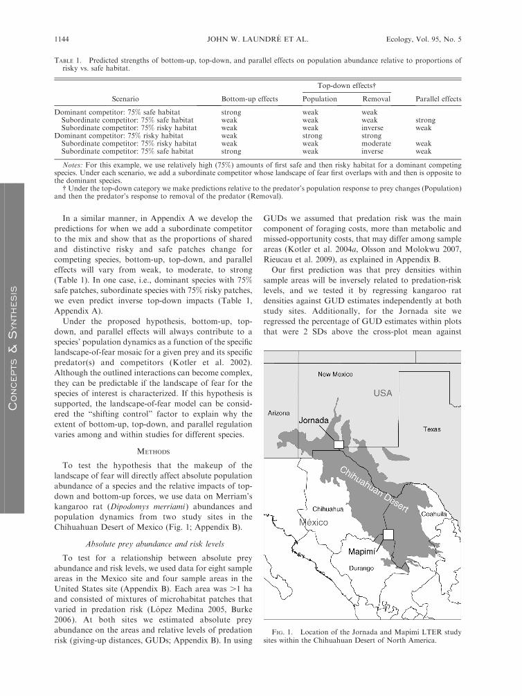
FIG. 1. Location of the Jornada and Mapımı LTER studysites within the Chihuahuan Desert of North America.

JOHN W. LAUNDRE ET AL.1144 Ecology, Vol. 95, No. 5

CONCEPTS&SYNTHESIS

kangaroo rat density (see Appendix B for details). As

food-resource levels affect population density on an

annual basis (Hernandez et al. 2005, 2011a) and can

affect GUDs as a missed-opportunity cost (Brown 1988,

Rieucau et al. 2009), we tested for their possible effects

on our results by regressing the normalized difference

vegetation index (NDVI) from satellite images of the

Jornada plots against kangaroo rat densities (see

Appendix B for method details). We did not have

similar data from Mapimı to do this analysis.

Impact of predation risk on bottom-up, top-down, and

parallel effects

To test for impacts of predation risk on the strength

of bottom-up effects on rodent densities, we used long-

term (12 years) data sets from the Mapimı site on

kangaroo rat densities and plant productivity estimates

(Hernandez et al. 2005, 2011b; Appendix B). These data

came from two distinct areas, shrubland and grassland,

that differed in the proportion of closed shrub and open

sparse grass/bare ground microhabitats (J. Lopez-

Portillo, L. Hernandez, and A. Gonzalez-Romero,

unpublished data). Predation risk for desert rodents is

higher in open microhabitat patches, especially during

the full moon (Kotler et al. 2004b, Lopez Medina 2005,

Burke 2006); thus the grassland area will have higher

overall predation risk (Burke 2006). If the strength of

bottom-up forces is greater in low-risk areas, we predict

that in the area with the lower predation risk, the

shrubland, there will be a stronger relation between

kangaroo rat densities and grass and forb cover when

compared to the high-risk grassland. To test this

prediction, we regressed yearly November estimates of

Merriam’s kangaroo rat densities against annual No-

vember estimates of percent cover of forb and grasses

separately for the grassland and shrubland areas

(Appendix B).

Finally, we also estimated the relative abundance of

kit fox (Vulpes macrotis) and gray fox (Urocyon

cinereoargenteus) in the grassland and shrubland areas

in Mapimı (Appendix B). The main diet of these two fox

species is kangaroo rats (L. Hernandez and M. Delibes,

unpublished data). If the level of predation risk directly

influences the strength of top-down forces, then, as in

Table 1, we predict that fox abundance should be higher

and strongly related to changes in kangaroo rat densities

in the high-risk grassland areas. To test the predictions

regarding fox abundance, we first compared annual fox

track numbers between grassland and shrubland. We

then regressed the annual November number of fox

tracks per 100 scent-station nights (for details see

Appendix B: Estimates of abundance) against corre-

sponding kangaroo rat densities separately for the

shrubland and grassland areas. Though there are

coyotes (Canis latrans) in the area, their main diet is

black-tailed jackrabbits (Lepus californicus) (Hernandez

and Delibes 1994, Martınez Calderas 2005, Laundre et

al. 2009), so we did not consider them in this analysis.

RESULTS

Kangaroo rat densities and GUDs

There was a significant inverse relationship between

GUDs (giving-up densities) and kangaroo rat density

for Mapimı (Fig. 2a) and the Jornada (Fig. 2b) sites. The

linear regression accounted for 75% and 99% of the data

variability for Mapimı and Jornada, respectively. When

we compared the estimate of the percent of GUDs .2

SD from the overall mean to the density of kangaroo

rats at the Jornada site, this relationship was also

significant (Fig. 3a) and accounted for 92% of the data

variability. There was no significant relation between the

density of kangaroo rats and the mean NDVI (normal-

ized difference vegetation index) estimates at the

Jornada site (Fig. 3b).

Bottom-up and predation risk

Over the 12 years of the study in Mapimı, percent

cover of grass and forbs was significantly higher in the

grassland area (12.5% 6 1.8% [mean 6 SE]) compared

to the shrubland area (1.6% 6 0.48%; paired t¼7.5, P ,

FIG. 2. Relationships between rodent density vs. giving-updensities (GUDs) for the (a) Mapimı and (b) Jornada sites.Solid lines are the regression lines. The dashed lines show 95%confidence intervals. (Note: GUD in presented in gramsbecause the millet seed used in the boxes was measured ingrams.)

May 2014 1145LANDSCAPE OF FEAR AND POPULATION CONTROL

CONCEPTS&SYNTHESIS

0.001). Moreover, the slope of the linear regressions,

which indicates the increase of plant cover per millimeterof precipitation, was also significantly greater in thegrassland than in the shrubland (P . 0.01, Fig. 4a).As with other studies (Ernest et al. 2000, Meserve et

al. 2003, Hernandez et al. 2005), when we regressedannual estimates of kangaroo rat densities against thecorresponding plant cover for the same year, there was

no significant relationship for either site. Since a one-year lag response in rodent densities is well established inthe literature (Ernest et al. 2000, Hernandez et al. 2005),

we regressed kangaroo rat densities against the previousyear’s plant cover and found significant relationships(Fig. 4b). However, the coefficient of determination was

higher in the shrubland than in the grassland (R2¼ 0.66vs. 0.45, respectively), indicating, as we predicted,stronger bottom-up effects in the shrubland.

As with precipitation vs. plant cover (Fig. 4a), theslopes of the two regression lines differed significantly (P, 0.001) between communities. However, in this case

the slope was one order of magnitude higher in the

shrubland than in the grassland (1.2 vs. 0.15; Fig. 4b).

Thus, as predicted, the population size of kangaroo rats

increased faster in the shrubland as grass and forb cover

increased, even if plant cover gain in relation to

precipitation was lower in the shrubland than in the

grassland.

Top-down impacts and predation risk

Over the 12-year period there were significantly higher

fox track counts (per 100 scent-station nights) in the

higher risk grassland (17.0 6 3.8 fox tracks) than in the

shrubland (10.0 6 1.8 fox tracks) (signed rank test, P¼0.04), and consistently higher kangaroo rat densities in

the shrubland (7.6 6 0.74 animals/ha vs. 2.6 6 0.4

animals/ha; paired t ¼ 8.2, P , 0.001). In addition to

higher fox abundance in the higher risk grassland, the

regression of the number of fox tracks against kangaroo

rat densities was significant at P ¼ 0.07 (Fig. 5a) in the

higher risk grassland but not significant for the lower

risk shrubland (P ¼ 0.48, Fig. 5a). Likewise, the

coefficient of determination was one order magnitude

greater in the higher risk grassland (R2 ¼ 0.24) than in

the lower risk shrubland (R2¼ 0.01; Fig. 5a). When we

combined the densities of all the rodent species (see

Hernandez et al. 2011a for species list), the regression

was highly significant for grasslands (P ¼ 0.003, R2 ¼0.61) and again, not significant for the shrubland (P ¼0.27, R2 ¼ 0.04; Fig. 5b and c).

DISCUSSION

Our purpose in the present study was to explore the

hypothesis that the proportions of safe and risky

habitats making up a landscape of fear can affect (1)

the absolute abundance of a prey species in an area and

(2) the relative impacts of bottom-up, top-down, and

parallel factors on annual changes in that absolute

abundance in areas. We developed various predictions

associated with this hypothesis and used long-term data

from two sites to test some of these predictions. The

results of our analyses lend support to those predictions,

warranting further investigation.

Implications of the landscape of fear for prey abundance

Our analyses of data from the Jornada and Mapimı

sites were used to test the prediction that predation-risk

levels affect the absolute population of prey in an area,

and the results indicated that further work is in order.

Future studies could include manipulative designs, such

as artificially altering the predation risk or perceived risk

over time on plots. For example, in our system, after

obtaining preliminary estimates of prey density and

GUDs (giving-up densities) in study plots, some plots

could be fenced to exclude terrestrial and aerial

predators. The prediction would be that in the fenced

areas rodent densities would increase and there would be

lower GUDs compared to the open controls. Perceived

predation risk could also be altered in areas as done by

Schmitz et al. (1997) with grasshoppers (Melanoplus

FIG. 3. (a) Relationship between density of kangaroo ratsand the percentage of GUD measurements that were .2 SDsabove the overall mean GUD for the four sample plots at theJornada site. (b) Kangaroo rat densities on the four sampleplots at the Jornada site vs. the normalized differencevegetation index (NDVI) measurements as an estimator ofprimary productivity. Solid lines are the regression lines. Thedashed lines show 95% confidence intervals.

JOHN W. LAUNDRE ET AL.1146 Ecology, Vol. 95, No. 5

CONCEPTS&SYNTHESIS

femurrubrum) and spiders (Pisurina mira) or by Zanette

et al. (2011) with songbirds. In such studies, designs as

used by Rieucau et al. (2009), should be employed to

better identify changes in GUDs due to predation risk

vs. the marginal value of energy (China et al. 2008).

Alternatively, other methods of assessing risk, e.g.,

vigilance, could be employed.

Implications for bottom-up, top-down, and parallel control

Besides possibly explaining differences in prey abso-

lute abundance across landscapes, an additional out-

come of this work is in potentially helping understand

the roles of bottom-up, top-down, and parallel forces on

population dynamics over time. One of the perplexing

aspects of these factors is the high variability in results

(Jaksic et al. 1997, Kittlein 1997, Erlinge et al. 1983,

Hanski et al. 2001, Meserve et al. 2003, Previtali et al.

2009, Gutierrez et al. 2010). These often-conflicting

results make it difficult to discern which factor is more

important. As others have observed, one could find

results to support whatever position is desired (Connolly

1978, Ballard et al. 2001). Our results were similar in

that in two adjacent habitats separated by less than 2

km, top-down forces appear stronger in one site while

bottom-up forces seem to be more prevalent in the

other. Thus, like other studies, we also have the dilemma

of a complex system where apparent ‘‘shifting control’’

occurs over a relatively small spatial scale for seemingly

complex reasons.

FIG. 4. (a) Relationship between percent cover of grass and forbs vs. precipitation levels at the Mapimı study site for thegrassland and shrubland habitats. (b) Fall densities of kangaroo rats over 12 years vs. percent cover of grass and forbs of theprevious year in grassland and shrubland habitats. The dashed lines show 95% confidence intervals.

May 2014 1147LANDSCAPE OF FEAR AND POPULATION CONTROL

CONCEPTS&SYNTHESIS

In this context, the landscape-of-fear model provides

a possible solution since it allows us to predict that as

the proportion of risky patches increases, the lethal and

non-lethal impacts of predators on prey will increase.

This results not only in lower prey abundance but

predictable change in the level of bottom-up, top-down,

and parallel impacts on prey population dynamics.

Specifically, the model predicts, as we found, that

bottom-up forces will be weaker and top-down ones

stronger as the level of predation risk increases, and vice

versa.

In the perusal of the extensive literature on just small-

mammal species, every combination we predicted in

Table 1 was found. For example, data from Chile lent

support to the prediction associated with lower levels of

predation risk because in the predator- exclusion areas

of low risk, Octodon degus, responded more to increased

resources than in the high-risk controls, (Meserve et al.

2003; Fig. 7), suggesting a stronger bottom-up effect.

Conversely, the greater declines of O. degus in controls

compared to exclusions (Meserve et al. 2003; Fig. 7)

indicate a possible stronger top-down effect due to

predation risk. In southern Arizona (USA) J. H. Brown

and his team had several results that could be explained

by the landscape-of-fear model. For example, when they

removed the numerically and competitively dominant

kangaroo rat species (Dipodomys merriami and D.

spectabilis), they did not find the strong response by

subordinate species that they predicted (Ernest et al.

2008). This result fits the prediction of weak parallel

effects, if the dominant species has a high amount of safe

patches while the subordinate ones have mainly higher

amounts of risky patches (Table 1). By collecting data

on levels of predation risk, critical tests of the model

could be done at these sites.

FIG. 5. (a) Number of fox tracks per 100 track nights vs. annual fall kangaroo rat density estimates for grassland and shrublandin the Mapimı study site. (b and c) Number of fox tracks per 100 track nights vs. annual fall total rodent density estimates for the(b) shrubland and (c) grassland and in the Mapimı study site. Solid lines are the regression lines. The dashed lines show 95%confidence intervals. ‘‘Track nights’’ refers to sets of tracks at the scent stations: (no. tracks per station-night)3 100; for details seeAppendix B: Estimates for abundance.

JOHN W. LAUNDRE ET AL.1148 Ecology, Vol. 95, No. 5

CONCEPTS&SYNTHESIS

Application to other ecosystems

Although we used a small-mammal–medium-predator

system to provide preliminary tests of some of our

predictions, the implications of the landscape-of-fear

model extend to larger and smaller predator–prey

systems as well as to terrestrial and aquatic systems.

Our initial study of habitat shifts by elk in response to

wolves (Hernandez and Laundre 2005) demonstrated

that elk under predation risk by wolves had poorer diets

than elk in areas without wolves . We predicted that this

would lead to lower survival and reproductive success.

This prediction has been supported by the fact that

poorer diet and increased stress from fear had direct

effects on reproduction and recruitment (Creel et al.

2007). Ongoing studies of snowshoe hare (Lepus

americanus) extend such stress responses to fear to

medium-sized mammalian systems and potentially help

explain temporal population changes in this species

(Sheriff et al. 2009). The previously cited works with

song birds not only demonstrated that the risk of

predation alone affects nest-site selection and clutch size

in birds (Eggers et al. 2006) but reduced the number of

offspring produced per year by up to 40% (Zanette et al.

2011). Schmitz et al. (1997) and others (Denno et al.

2003) demonstrated that the impact of predation risk

extends the possible application of our predictions to

insect predator–prey systems.

In marine systems, researchers are also investigating

predation risk on a seascape scale, i.e., the ‘‘seascapes of

fear’’ and its impact on habitat use (Wirsing et al. 2008,

Wirsing and Heithaus 2009). Of particular interest are

the developments in foraging-arena models in marine

environments (Walters and Juanes 1993, Walters and

Christensen 2009). Foraging-arena and landscape-of-

fear models are similar in that the landscape or seascape

can be divided into safe (refuges) and risky (foraging

arenas) patches. However, foraging-arena theory em-

phasizes more exchange rates of individuals between

refuges and feeding arenas and the implications of

changing those rates on population stability. As the

proportion of risky and safe patches in our model

directly affects these exchange rates, applying foraging-

arena theory, especially the Ecopath with Ecosim model

(Walters and Christensen 2009), can provide functional

insights as to why the makeup of the landscape of fear

matters. Wirsing and Ripple (2011) noted that the

response to predation risk in aquatic and terrestrial

systems appears to be highly similar and that cross-

exchanging ideas could be beneficial to both. Combining

landscape-of-fear and foraging-arena models is an

example of how just such an interchange could prove

to be highly productive.

Summary and conclusions

We have presented a novel hypothesis that predicts

how the changes in the level of predation risk over the

landscape can influence the population dynamics of a

species. We propose that such changes over space and

time can alter the relative impacts of bottom-up, top-

down, and parallel effects on population abundance. We

offered innovative predictions to test this hypothesis and

present data to support some of the predictions made.

Our results indicate that this hypothesis is worth further

investigation, especially in other predator–prey systems,

where estimating species specific predation risk becomes

as essential as estimating species-specific population

densities. If future research supports our hypothesis,

then the landscape-of-fear model could provide the

‘‘missing link’’ in understanding the population dynam-

ics of species across a wide variety of taxa and

ecosystems.

Additionally, we have noted impacts that the makeup

of the landscape of fear might have on the predators,

e.g., lower absolute predator abundance with high

percentage of safe patches. However, we did not

consider in detail the impact the makeup of the

landscape of opportunity (the flipside of the landscape

of fear; Laundre et al. 2010), has on the population

dynamics of the predator. It is anticipated that similar

predictions can be made regarding predators and could

even further help our understanding of both sides of the

predator–prey relationship.

Last, besides the scientific value of further under-

standing predator–prey relationships, the implications

of a landscape-of-fear model for conservation and

management should be noted. If the absolute population

abundance of the prey, and likely the predator, is

dependent on the physical makeup of the landscape of

fear, microhabitat composition of an area relative to

predation risk becomes an important factor in deter-

mining the baseline population abundance in an area. It

also affects how that population will respond to annual

food-resource changes relative to predation and compe-

tition. Manipulation of the microhabitat patches, the

building blocks of the landscape of fear, could then be a

powerful conservation and management tool for prey

and predator (Yong 2013). For example, the current

standard management practice to reduce the lethal

impact of predators on desired prey species is to lethally

reduce the predator population. Under the landscape-of-

fear model, increasing the proportion of safe patches

within an area would increase prey population levels,

reducing the need for lethal control of the predators.

Conversely, increasing the amount of risky patches for

prey could aid in the conservation of declining predator

populations. Conservation then, could rely on balancing

the proportions of risky and safe patches for the desired

species, which would in turn modify structure and

composition of the community. Further investigating

the magnitude of the landscape of fear on prey and

predator dynamics may hold great potential when

incorporating this ecological process into conservation

and management practices.

May 2014 1149LANDSCAPE OF FEAR AND POPULATION CONTROL

CONCEPTS&SYNTHESIS

ACKNOWLEDGMENTS

This work was conducted in conjunction with the MapimıLong-Term Exclusion Experiment (MLTER) coordinated by L.Hernandez and supported by grants from CONACyT (1843P-N9507) of Mexico to Dr. Hernandez, Earthwatch Institute toDr. Laundre, INECOL 902-16 to J. Lopez-Portillo, SEMAR-NAT of Mexico, and U.S. National Science Foundation (DEB-0004526); New Mexico State University Agricultural Experi-ment Center; T&E Inc. (Grant for Conservation BiologyResearch, 2006, 2007); American Society of Mammalogists(Grant in Aid for Research, 2006, 2008); Ecological Society ofAmerica (Forrest Shreve Grant, 2006) to Andrea Campanella.The Jornada Basin LTER produced the data sets for vegetationcover for the Jornada site. We also had logistical andinfrastructure support from the Instituto de Ecologıa, A.C.,estacion de campo Laboratorio del Desierto, Reserva de laBiosfera Mapimı, and USDA Arid Land Research Program,Jornada Experimental Range. We thank the following persons

who helped us in the field: A.J. Martınez , Institute of Ecologystudents, and the many Earthwatch volunteers.

This paper is heartfully dedicated to our co-author LucinaHernandez, who died shortly before manuscript completion.Lucina devoted her professional career to working and teachingmainly in the southern Chihuahuan Desert. It is through hersteadfast devotion and discipline that the data sets used in thismanuscript were possible. She was considered by her peers asone of the top mammal ecologists in Mexico, and receivedmany accolades for her promotion of desert ecology amongscientists and lay people alike. She worked diligently andtirelessly alongside co-workers and students, and recently wasquite dedicated to the development of the Rice Creek FieldStation at the State University of New York at Oswego. Lucinawas also a loving and caring mother and wife to Cecile andJohn Laundre. We will miss the indomitable spirit that kept hersmiling and happy. We will never forget her enthusiasm,happiness, and joy for life.

PLATE 1. Lucina Hernandez (1960–2013), waiting for a puma (Puma concolor) to wake up after radio tagging it for a study onpuma behavior and ecology . . . a previous research study that helped lead to the ideas explored in the current paper, for which shewas instrumental in conducting the field work. Lucina truly enjoyed working in the field and was as comfortable hiking in snow asunder the intense heat of the Chihuahuan Desert of her native country, Mexico. Her indomitable spirit and joy for life buoyed herthroughout her all too short time with us. She will be fondly remembered by her husband, John Laundre, her daughter Cecile, andthe many colleagues and students she touched in her life. Photo by J. W. Laundre.

JOHN W. LAUNDRE ET AL.1150 Ecology, Vol. 95, No. 5

CONCEPTS&SYNTHESIS

This paper is also dedicated to the memory of our localparataxonomist, tracker, guide, and field assistant, Adalberto‘‘Chuca’’ Herrera, who also passed away a few months beforeLucina. Chuca helped Lucina and her co-workers over manyyears in the Mapimı Biosphere Reserve, which he knew byhand. His stories, natural history knowledge, and wit will bedeeply missed.

LITERATURE CITED

Ale, S. B., and C. J. Whelan. 2008. Reappraisal of the role ofbig, fierce predators. Biodiversity Conservation 17:685–690.

Ballard, W. B., D. Lutz, T. W. Keegan, L. H. Carpenter, andJ. C. deVos, Jr. 2001. Deer–predator relationships: a reviewof recent North American studies with emphasis on mule andblack-tailed deer. Wildlife Society Bulletin 29:99–115.

Bishop, C. J., J. W. Unsworth, and E. O. Garton. 2005. Muledeer survival among adjacent populations in southwestIdaho. Journal of Wildlife Management 69:311–321.

Brown, J. H., and S. K. M. Ernest. 2002. Rain and rodents:Complex dynamics of desert consumers. BioScience 52:979–987.

Brown, J. H., and E. J. Heske. 1990. Temporal changes in aChihuahuan Desert rodent community. Oikos 59:290–302.

Brown, J. S. 1988. Patch use as an indicator of habitatpreference, predation risk, and competition. BehavioralEcology and Sociobiology 22:37–47.

Burke, A. M. 2006. Utilization of optimal foraging theory indesert rodents: a review and a study. M.S. thesis, Universityof Illinois, Chicago, Illinois, USA.

China, V., B. P. Kotler, N. Shefer, J. S. Brown, and Z.Abramsky. 2008. Density-dependent habitat and patch use ingerbils: consequences of safety in numbers? Israel Journal ofEcology and Evolution 54:373–388.

Connolly, G. E. 1978. Predators and predator control. Pages369–394 in J. L. Schmidt and D. L. Gilbert, editors. Big gameof North America. Stackpole, Harrisburg, Pennsylvania,USA.

Creel, S., D. Christianson, S. Liley, and J. A. Winnie, Jr. 2007.Predation risk affects reproductive physiology and demog-raphy of elk. Science 315:960.

Denno, R. F., C. Gratton, H. Dobel, and D. L. Finke. 2003.Predation risk affects relative strength of top-down andbottom-up impacts on insect herbivores. Ecology 84:1032–1044.

Dickman, C. R., P. S. Mahon, P. Masters, and D. F. Gibson.1999. Long-term dynamics of rodent populations in aridAustralia: the influence of rainfall. Wildlife Research 26:389–403.

Eggers, S., M. Griesser, M. Nystrand, and J. Ekman. 2006.Predation risk induces changes in nest-site selection andclutch size in the Siberian jay. Proceedings of the RoyalSociety of London B 273:701–706.

Erlinge, S., G. Goransson, L. Hansson, G. Hogstedt, O. Liberg,I. N. Nilsson, T. Nilsson, T. von Schantz, and M. Sylven.1983. Predation as a regulating factor on small rodentpopulations in Southern Sweden. Oikos 40:36–52.

Ernest, S. K. M., J. H. Brown, and R. R. Parmenter. 2000.Rodents, plants, and precipitation: spatial and temporaldynamics of consumers and resources. Oikos 88:470–482.

Ernest, S. K. M., J. H. Brown, K. M. Thibault, E. P. White, andJ. R. Goheen. 2008. Zero sum, the niche, and metacommun-ities: long-term dynamics of community assembly. AmericanNaturalist 172:257–269.

Estes, J. A. 1996. Predators and ecosystem management.Wildlife Society Bulletin 24:390–396.

Gutierrez, J. R., P. L. Meserve, D. A. Kelt, A. Engilis, Jr.,M. A. Previtalie, W. B. Milstead, and F. M. Jaksic. 2010.Long-term research in Bosque Fray Jorge National Park:twenty years studying the role of biotic and abiotic factors ina Chilean semiarid scrubland. Revista Chilena de HistoriaNatural 83:69–98.

Hanski, I., H. Henttonen, E. Korpinaki, L. Oksanen, and P.Turchin. 2001. Small-rodent dynamics and predation. Ecol-ogy 82:1505–1520.

Hernandez, L., and M. Delibes. 1994. Seasonal food habits ofcoyotes, Canis latrans, in the Bolson de Mapimi, southernChihuahuan Desert, Mexico. Zeitschrift fur Saugetierkunde59:82–86.

Hernandez, L., and J. W. Laundre. 2005. Foraging in the‘‘landscape of fear’’ and its implications for habitat use anddiet quality of elk Cervus elaphus and bison Bison bison.Wildlife Biology 11:215–220.

Hernandez, L., J. W. Laundre, A. Gonzalez-Romero, J. Lopez-Portillo, and K. M. Grajales. 2011a. Tale of two metrics:density and biomass in a desert rodent community. Journalof Mammalogy 92:840–851.

Hernandez, L., J. W. Laundre, K. M. Grajales, G. L. Portales,J. Lopez-Portillo, A. Gonzalez-Romero, A. Garcıa, and J. M.Martınez. 2011b. Plant productivity, predation, and theabundance of black-tailed jackrabbits in the ChihuahuanDesert of Mexico. Journal of Arid Environments 75:1043–1049.

Hernandez, L., A. G. Romero, J. W. Laundre, D. Lightfoot, E.Aragon, and J. Lopez Portillo. 2005. Changes in rodentcommunity structure in the Chihuahuan Desert Mexico:comparisons between two habitats. Journal of Arid Envi-ronments 60:239–257.

Jaksic, F. M., S. I. Silva, P. L. Meserve, and J. R. Gutierrez.1997. A long-term study of vertebrate predator responses toan El Nino (ENSO) disturbance in western South America.Oikos 78:341–354.

Kittlein, M. J. 1997. Assessing the impact of owl predation onthe growth rate of a rodent prey population. EcologicalModelling 103:123–134.

Kotler, B. P. 1984. Risk of predation and the structure of desertrodent communities. Ecology 65:689–701.

Kotler, B. P., J. S. Brown, and A. Bouskila. 2004a. Appre-hension and time allocation in gerbils: The effects ofpredatory risk and energetic state. Ecology 85:917–922.

Kotler, B. P., J. S. Brown, A. Bouskila, S. Mukherjee, and T.Goldberg. 2004b. Foraging games between gerbils and theirpredators: seasonal changes in schedules of activity andapprehension. Israel Journal of Zoology 50:255–271.

Kotler, B. P., J. S. Brown, S. R. X. Dall, S. Gresser, D. Ganey,and A. Bouskila. 2002. Foraging games between gerbils andtheir predators: temporal dynamics of resource depletion andapprehension in gerbils. Evolutionary Ecology Research 4:495–518.

Laundre, J. W. 2010. Behavioral response races, predator–preyshell games, ecology of fear, and patch use of pumas andtheir ungulate prey. Ecology 91:2995–3007.

Laundre, J. W., J. M. M. Calderas, and L. Hernandez. 2009.Foraging in the landscape of fear, the predator’s dilemma:Where should I hunt? The Open Ecology Journal 2:1–6.

Laundre, J. W., L. Hernandez, and K. B. Altendorf. 2001.Wolves, elk, and bison: reestablishing the ‘‘landscape of fear’’in Yellowstone National Park, U.S.A. Canadian Journal ofZoology 79:1401–1409.

Laundre, J. W., L. Hernandez, and S. G. Clark. 2006. Impact ofpuma predation on the decline and recovery of a mule deerpopulation in southeastern Idaho. Canadian Journal ofZoology 84:1555–1565.

Laundre, J. W., L. Hernandez, and S. G. Clark. 2007.Numerical and demographic responses of pumas to changesin prey abundance: Testing current predictions. The Journalof Wildlife Management 71:345–355.

Laundre, J. W., L. Hernandez, and W. J. Ripple. 2010. Thelandscape of fear: ecological implications of being afraid. TheOpen Ecology Journal 3:1–7.

Lightfoot, D. C., A. D. Davidson, D. G. Parker, L. Hernandez,and J. W. Laundre. 2012. Bottom-up regulation of desertgrassland and shrubland rodent communities: implications of

May 2014 1151LANDSCAPE OF FEAR AND POPULATION CONTROL

CONCEPTS&SYNTHESIS

species-specific reproductive potentials. Journal of Mammal-ogy 93:1017–1028.

Lopez Medina, V. P. I. 2005. Frecuencia de capturas deheteromidos: una herramienta para mapear el paisaje delmiedo. B.Sc. thesis. Universidad Autonoma de CiudadJuarez, Ciudad Juarez, Chihuahua, Mexico.

Marın, A. I., L. Hernandez, and J. W. Laundre. 2003.Predation risk and food quantity in the selection of habitatby black-tailed jackrabbit (Lepus californicus): an optimalforaging approach. Journal of Arid Environments 55:101–110.

Martınez Calderas, J. M. 2005. Forrajeo optimo del coyote enla Reserva de la Biosfera de Mapimı. Bachelor’s thesis.Universidad Autonoma de Ciudad Juarez, Ciudad Juarez,Chihuahua, Mexico.

Meserve, P. L., J. R. Gutierrez, and F. M. Jaksic. 1993. Effectsof vertebrate predation on a caviomorph rodent, the Degu(Octodon degus), in a semiarid thorn scrub community inChile. Oecologia 94:153–158.

Meserve, P. L., D. A. Kelt, W. B. Milstead, and J. R. Gutierrez.2003. Thirteen years of shifting top-down and bottom-upcontrol. BioScience 53:633–646.

Meserve, P. L., W. B. Milstead, J. R. Gutierrez, and F. M.Jaksic. 1999. The interplay of biotic and abiotic factors in asemiarid Chilean mammal assemblage: results of a long-termexperiment. Oikos 85:364–372.

Olsson, O., and M. N. Molokwu. 2007. On the missedopportunity cost, GUD, and estimating environmentalquality. Israel Journal of Ecology and Evolution 53:263–278.

Pimm, S. L., M. L. Rosenzweig, and W. Mitchell. 1985.Competition and food selection: field tests of a theory.Ecology 66:798–807.

Previtali, M. A., M. Lima, P. L. Meserve, D. A. Kelt, and J. R.Gutierrez. 2009. Population dynamics of two sympatricrodents in a variable environment: rainfall, resource avail-ability, and predation. Ecology 90:1996–2006.

Rieucau, G., W. L. Vickery, and G. J. Doucet. 2009. A patchuse model to separate effects of foraging costs on giving-updensities: an experiment with white-tailed deer (Odocoileusvirginianus). Behavioral Ecology and Sociobiology 63:891–897.

Rohner, C., and C. J. Krebs. 1996. Owl predation on snowshoehares: consequences of antipredator behavior. Oecologia 108:303–310.

Schmitz, O. J., A. P. Beckerman, and K. M. O’Brien. 1997.Behaviorally mediated trophic cascades: effects of predationrisk on food web interactions. Ecology 78:1388–1399.

Sheriff, M. J., C. J. Krebs, and R. Boonstra. 2009. The sensitivehare: sublethal effects of predator stress on reproduction insnowshoe hares. Journal of Animal Ecology 78:1249–1258.

Shrader, A. M., J. S. Brown, G. I. H. Kerley, and B. P. Kotler.2008. Do free-ranging domestic goats show ‘landscapes offear’? Patch use in response to habitat features and predatorcues. Journal of Arid Environments 72:1811–1819.

Sih, A. 1984. The behavioral response race between predatorand prey. American Naturalist 123:143–150.

Sih, A. 2005. Predator–prey space use as an emergent outcomeof a behavioral response race. Pages 240–255 in P. Barbosaand I. Castellanos, editors. Ecology of predator–preyinteractions. Oxford University Press, Oxford, UK.

Sih, A., P. Crowley, M. McPeek, J. Petranka, and K.Strohmeier. 1985. Predation, competition, and prey commu-nities: a review of field experiments. Annual Review ofEcological Systems 16:269–311.

Terborgh, J., et al. 2001. Ecological meltdown in predator-freeforest fragments. Science 294:1923–1926.

van der Merwe, M., and J. S. Brown. 2008. Mapping thelandscape of fear of the cape ground squirrel (Xerus inauris)Journal of Mammalogy 89:1162–1169.

Vucetich, J. A., and R. O. Peterson. 2004. The influence of top-down, bottom-up and abiotic factors on the moose (Alcesalces) population of Isle Royale. Proceedings of the RoyalSociety of London B 271:183–189.

Walters, C. J., and V. Christensen. 2009. Foraging arenatheory. Working paper Series number 2009-03. FisheriesCentre, University of British Columbia, Vancouver, BritishColumbia, Canada.

Walters, C. J., and F. Juanes. 1993. Recruitment limitation as aconsequence of natural selection for use of restricted feedinghabitats and predation risk taking by juvenile fishes.Canadian Journal of Fisheries and Aquatic Sciences 50:2058–2070.

Wirsing, A. J., and M. R. Heithaus. 2009. Olive-headed seasnakes (Disteria major) shift seagrass microhabitats to avoidshark predators. Marine Ecololgy Progress Series 387:287–293.

Wirsing, A. J., M. R. Heithaus, A. Frid, and L. M. Dill. 2008.Seascapes of fear: evaluating sublethal predator effectsexperienced and generated by marine mammals. MarineMammal Science 24:1–15.

Wirsing, A. J., and W. J. Ripple. 2011. A comparison of sharkand wolf research reveals similar behavioral responses byprey. Frontiers in Ecology and the Environment 9:335–341.

Yong, E. 2013. Scared to death: how predators really kill. NewScientist [1 June] 218 (2919):36–39.

Zanette, L. Y., A. F. White, M. C. Allen, and M. Clinchy. 2011.Perceived predation risk reduces the number of offspringsongbirds produce per year. Science 344:1398–1401.

SUPPLEMENTAL MATERIAL

Appendix A

Development of predictions for the impact of the landscape of fear for parallel effects between competing species (EcologicalArchives E095-098-A1).

Appendix B

Detailed description of study areas and methods used to test predictions (Ecological Archives E095-098-A2).

JOHN W. LAUNDRE ET AL.1152 Ecology, Vol. 95, No. 5

CONCEPTS&SYNTHESIS