Regional Competitiveness in Indonesia: The Incentives of Fiscal Decentralization on State Efficiency and Economic Growth

A dissertation submitted in partial fulfillment of the requirements for the degree of Doctor of Philosophy at George Mason University

By

Darius Tirtosuharto Master of Urban Design

University of Colorado, 1998 Bachelor of Engineering

University of Tarumanagara, 1996

Director: Roger Stough, Professor School of Public Policy

Fall Semester 2009 George Mason University

Fairfax, VA

ii

Copyright 2009 Darius Tirtosuharto All Rights Reserved

iii

DEDICATION

This dissertation is dedicated to my wife Ira and my two wonderful children, Avi and Dhafin who have endlessly loved and supported me.

iv

ACKNOWLEDGEMENTS

This dissertation would not have been completed without the assistance, support and input from numerous people. First, I want to offer my Chair Committee Professor Roger Stough, my sincere appreciation and thanks for his guidance and continuous encouragement to me to complete this dissertation. I have been fortunate to have a chair who has given me trust and freedom to explore on my own, yet has also taught me how to form my thoughts and ideas.

I owe my gratitude to all members of my committee who have made this dissertation possible. My deepest gratitude is to Dr. Ramkishen Rajan and Dr. Naoru Koizumi who have provided insightful remarks and constructive criticism throughout my dissertation process. I want to thank Dr. Carrie Meyer, a committee member from the Department of Economics, for valuable support and direction on how to refine my writing skills. I would also like to thank Professor Iwan Jaya Azis, Director of the Regional Science Program at Cornell University who was willing to be my external reader to help sharpen this manuscript. My appreciation also goes to faculty members at the School of Public Policy and Department of Economics at George Mason University who have been generous in sharing their ideas to support this research.

I also take this opportunity to thank Head of Division Regional Development and Autonomy, the National Development Planning Agency (BAPENAS) Dr. Sumedi Andono Mulyo and Executive Board of the Monitoring Agency of Regional Autonomy (KPPOD) Mr. Agung Pambudhi who have provided valuable information and ideas for this research during a meeting in Jakarta, Indonesia.

Finally, I want to dedicate this dissertation to my wife and best friend, Ira, my sons, Avi and Dhafin, for their continuous support and patience during my pursuit of knowledge. I am especially indebted to my wife who has fully supported me while I completed my research and writing. Her patience, understanding, and encouragement have truly been a light on my path to complete my doctoral journey to the end.

August 2009

v

TABLE OF CONTENTS

Page

LIST OF TABLES ............................................................................................................ vii

LIST OF FIGURES ......................................................................................................... viii

ABSTRACT ....................................................................................................................... ix

1. Introduction ......................................................................................................................1

2. Theoretical Review ..........................................................................................................8

2.1. Competitiveness and Theory of Regional Growth ...................................................8

2.2. Decentralization and the Role of Institution ...........................................................13

2.3. Fiscal Decentralization and Efficiency in the Allocation of Fiscal Resources ......21

2.4. Productivity of Public Capital Expenditure ............................................................26

3. Fiscal Decentralization in Developing Countries ..........................................................29

3.1. Empirical Studies on Fiscal Decentralization ........................................................29

3.2. Case Studies of Fiscal Decentralization in Developing Countries .........................34

4. Regional Development and Decentralization Policy in Indonesia ................................40

4.1. Governance System and Economic Development in a Pre-Decentralized Era ......41

4.2. Financial Crisis and Decentralization Policy .........................................................53

5. Problem Statement and Research Hypotheses ...............................................................67

5.1. Research Questions ................................................................................................72

vi

5.2. Hypotheses .............................................................................................................73

6. Analytical Framework and Empirical Analysis .............................................................77

6.1. State Performance and Efficiency Analysis Using Data Envelopment Analysis ...77

6.1.1. Descriptive Analysis of Input and Output Data ...........................................84

6.1.2. Technical Efficiency Analysis of State Government using DEA ................86

6.1.3. Determinants of State Technical Efficiency in a Tobit Panel Data Model ...95

6.2. Regional Growth Model Using Fixed-Effects Panel Data Analysis ....................104

6.2.1. Descriptive Analysis of the Panel Data Regression ....................................109

6.2.2. Growth Model Using Fixed Effect Panel Data Regression .........................113

6.3. Evaluation of Decentralization and Regional Competitiveness Policies .............130

7. Concluding Remarks ....................................................................................................138

REFERENCES ................................................................................................................157

vii

LIST OF TABLES

Table Page Table 1. Regional Account during the New Order Era in Indonesia ................................ 44 Table 2. Sectoral Contribution to GDP Growth in Indonesia, 1960-2000........................ 47 Table 3. Rank of High-Technology and Manufactured Exports in East Asia .................. 54 Table 4. Rate of Growth of Indonesian States, 1996-2000 ............................................... 56 Table 5. Poverty Rate and Gini Index of Indonesian States, 1996-2002 .......................... 57 Table 6. Revenue Sharing Scheme (in pecent) ................................................................. 61 Table 7. Per capita Income of Indonesian States, 2001-2005 (in Rupiah) ....................... 63 Table 8. Fiscal Decentralization and Growth Rate of Indonesian States, 2001-2005 ...... 64 Table 9. Descriptive Analysis of Input-Output Variables ................................................ 86 Table 10. Technical Efficiency of 26 States in Indonesia between 1996-2005 ................ 88 Table 11. Average Technical Efficiency Scores and Slacks between 1996-2005 ............ 89 Table 12. Average Technical Efficiency Scores, 1996-2000 and 2001-2005 .................. 91 Table 13. 10-Year Average Technical Efficiency and Real GRDP .................................. 93 Table 14. Determinant of State Technical Efficiency in Indonesia, 1996-2005 ............... 99 Table 15. Determinant of State Technical Efficiency in Indonesia, 1996-2000 ............. 101 Table 16. Determinant of State Technical Efficiency in Indonesia, 2000-2005 ............. 102 Table 17. Descriptive Analysis of Growth Panel Data Variables ................................... 111 Table 18. Growth Panel Model with 26 States (1996-2005) .......................................... 116 Table 19. Growth Panel Model in Lagging States (1996-2005) .................................... 122 Table 20. Growth Panel Model in Leading States (1996-2005) ..................................... 123 

viii

LIST OF FIGURES

Figure Page Figure 1. Efficiency and Effectiveness Model .................................................................. 25 Figure 2. States/Provinces in Indonesia ............................................................................ 41 Figure 3. Real Gross Domestic Product (GDP) in Indonesia, 1970-2002 ........................ 45 Figure 4. Distribution of Manufacturing Employment in Indonesia, 1996 ...................... 48 Figure 5. Percentage Growth of Poverty Incidence, 1995–2000 ...................................... 50 Figure 6. Poverty Rate and Unemployment Rate in Indonesia, 1982-2002 ..................... 55 Figure 7. Framework of Regional Competitiveness ......................................................... 67 Figure 8. DEA Research Framework ................................................................................ 79 Figure 9. Measurement of Technical Efficiency ............................................................... 81 Figure 10. Growth Rate in Indonesia during the Period of Financial crisis ................... 155 Figure 11. Growth of Private Investments in Indonesia during the Period of ................ 155 

ix

ABSTRACT

REGIONAL COMPETITIVENESS IN INDONESIA: THE INCENTIVES OF FISCAL DECENTRALIZATION ON STATE EFFICIENCY AND ECONOMIC GROWTH Darius Tirtosuharto, PhD George Mason University, 2009 Dissertation Director: Dr. Roger Stough

This dissertation examines the implementation of decentralization in Indonesia and

measures the incentives of fiscal decentralization on state efficiency and economic

growth. Efficiency of state governments in utilizing fiscal resources to support private

sector development and accelerate economic growth is consistent with the concept of

regional competitiveness. The main goal of this dissertation is to expand existing

empirical and theoretical frameworks on fiscal decentralization and economic growth that

have traditionally excluded efficiency factors of sub national governments. This

dissertation also aims to fill gaps in the way state efficiency is measured as an extension

of institutional quality of public sector.

Following a two-stage empirical methodology, the efficiency of Indonesia’s 26 states

government expenditure over a 10-year period (1996-2005) is constructed using Data

x

Envelopment Analysis (DEA) and a Tobit panel data model is used to analyze the

determinants of state efficiency. In the second stage, panel data analysis is employed to

analyze the impact of fiscal decentralization and state government efficiency on regional

growth.

This dissertation found that the degree of fiscal decentralization has a positive association

with economic growth if there are insignificant imbalances between regions following a

disproportionate growth in labor force and population. To a certain degree, regional

imbalances, which are a crucial issue in many developing countries, are one of the

disincentives in a decentralized system.

Another finding is that although decentralization provides a greater incentive structure for

states to become more efficient, this does not always lead to robust growth due to the

extent of misallocation of fiscal resources and lack of investment in productive spending.

Of several factors that potentially determine state efficiency, the degree of fiscal

decentralization, ratio of productive spending, operating costs and revenue independence

are significant and these factors differ between leading and lagging states.

Keywords: Regional Competitiveness, Economic Growth, Decentralization, Institutional Development, Public Expenditure, Capital Investments, Indonesia

1

1. Introduction

The purpose of this dissertation is to shed light on how to measure the relationship

between fiscal decentralization, allocative efficiency and economic growth within the

framework of regional competitiveness. Those three factors are examined at the state

level where only a few empirical studies have been completed. This dissertation will

contribute to the growing theoretical and methodological literature on fiscal

decentralization and economic growth. Furthermore, the methodology introduced in

measuring and incorporating state efficiency levels in the growth model will fill the gap

in existing empirical studies on fiscal decentralization and economic growth that

traditionally excluded efficiency factors of sub national governments.

There are two differing views on decentralization that influence the discussion on

regional competitiveness. Traditional economic theories focus on the sources of benefits

of decentralization based on Hayek (1945) and Tiebout (1956). Hayek argued that sub-

national governments have better information on the unique conditions and specific needs

of their jurisdiction, that enable them to allocate resources more efficiently than the

central government through a centralized planning system. Tiebout assumed that citizens

are able to sort their preferences of local public goods and have them met because

regional competition exists. Hence, traditionalists fail to recognize the relationship

between institutions and incentive structures in a decentralized system.

2

From institutionalists’ point of view, the relationship between institutions,

markets and firms is crucial. They believe in the importance of incentive structures to

motivate institutions, markets and firms to be more productive and efficient following the

concept of “Market Preserving Federalism” (Qian and Weingast 1997).1 Efficient

markets require institutions, particularly the rule of law, and governments to provide

positive market incentives by rewarding economic successes and punishing economic

failures. Government policies to impose high taxes that can reduce future wealth or to

bail out unproductive programs or projects are an example of some of the problems that

relate to negative incentive structures. These actions discourage firms from taking risks

and making investments, which lead to lower competitiveness and economic growth level

(North 1995).

Regional competitiveness focuses on the capacity of sub-national governments to

stimulate and sustain economic growth and development.2 Sub-national governments

play a key role in supporting the private sector and preserving a market economy, as

active agents of development at the regional level. For this to occur, it is necessary to

have in place a supportive system of governance, which will allow a sub-national

government to have a major role in the process of development. Within the framework of

regional competitiveness, decentralization is an avenue to increase the power and

1 Market Preserving Federalism is an economic concept of a federal system where there is a certain limit on how far the political system of government can intervene the markets. 2 Sub-national government refers to a state or province and district government. The latter consists of local regencies and municipalities. National government refers to the central government.

3

capacity of a sub-national government, sustain economic growth and improve standards

of living.

Predominant amongst the structure of a decentralized system is fiscal

decentralization that expands a state’s fiscal capacity since it allows for the transfer of

fiscal responsibility to sub-national states. Fiscal capacity relates to the size of funding

available in the state budget. A larger fiscal capacity is driven by an argument that state

governments have greater capability to allocate fiscal resources efficiently, generate

revenues, and maintain budget discipline in a decentralized system (Bird and Wallich

1993, Oates 1993). However, being responsible for a larger fiscal capacity offers both

challenges and opportunities for state government in developing countries, which

typically lack transparency and accountability.

Since there is a limit to fiscal resources, the ability of state governments to

allocate fiscal resources efficiently is important. Allocative efficiency is ultimately a

proxy of state government performance as a whole and is often times tied to the quality of

state institutions.3 State governments are the decision-making units responsible for

making choices on how and where to spend fiscal resources based on both short and long

term development goals and strategies. Similar to the idea that rational individuals will

want to maximize their utilities, states will also want to optimize their fiscal resources to

better serve their goals and interests. Thus, state government efficiency eventually

becomes the determinant factor of competitiveness and growth at the regional level.

3 The gap in linking the concepts of public sector efficiency and institutional quality is due to the complexity in quantifying the correlation between efficiency and institutional factors.

4

Although it is widely assumed that the implementation of fiscal decentralization

will increase efficiency and economic growth, the empirical evidence that supports this

idea is still inconclusive (Martinez-Vasquez and McNab 2003). Earlier studies on the

relationship between fiscal decentralization and economic growth have so far shown

inconsistent results even within the same country. Some of the studies found a negative

relationship between fiscal decentralization and economic growth (Davoodi and Zou

1998, Zhang and Zou 1998), while others reported a positive correlation (Lin and Liu

2000, Jin et. al. 2001) or no relationship at all (Woller and Phillips 1998). These

inconclusive outcomes may be caused by several factors, such as unequal wealth

distribution, inconsistent national and sub-national policies, and uncoordinated public

services provided by government institutions (Prud’homme 1995).

This dissertation argues that part of the inconclusive results of previous empirical

studies on the relationship between fiscal decentralization and economic growth are

attributed to the exclusion of a measure of state government efficiency in the growth

model. The problem of including state efficiency factor in the growth equation is the

difficulty in quantifying efficiency factors, specifically efficiency in the allocation of

fiscal resources (Rodriguez-Pose 2007). Fiscal decentralization, measured as the share of

sub-national spending or revenue over total national spending or revenue, does not

merely depict an actual measure of efficiency. To test the hypotheses and prove the key

argument of this dissertation, Indonesia is chosen as a case study.

Indonesia experienced a transition to a full-decentralized system following the

1997 financial crisis. The political turmoil that was triggered by the financial crisis

5

resulted in mounting dissatisfaction towards the central government, potentially leading

to regional disintegration. Regions demanded a fair distribution of revenue and an

expansion of power, which would allow for more participation in determining the

direction of development. A new decentralization law was introduced to change from

decades of a central planning system under Suharto’s rule, which to a large extent was an

adoption of a top-down decentralization process.4 This reform was supported by the IMF

as one of the conditions in the economic rescue package.

After almost eight years since the new law of decentralization was implemented,

several challenges persist despite the astonishing outcomes in such a short time period.

The swift implementation was a response to a mandate by the legislature, resulting in

limited time for extensive policy analysis. Critics have argued that the rapid process of

decentralization in Indonesia, also referred to as the “big-bang decentralization”, had not

been planned to improve the welfare and development at the regional level, but was the

result of political compromise due to the internal and external pressures toward the New

Order authoritarian rule. Consequently, this transformation of the system of governance

has been considered a failure in certain areas.

First, several regions still faced challenges in stimulating their economy despite a

larger fiscal capacity. States spent less in public capital investments than what was

expected to be necessary to accelerate economic growth. In order to increase revenue

4 The central government controls the process of decentralization in the top-down process, while the bottom-up process is mostly driven by regional demands. This process affects the transfer of powers that includes administrative and financial responsibilities (Rodriguez-Pose 2007).

6

and narrow budget deficits, states also introduced additional taxes, fees, and charges that

were not conducive to private sector growth.

Second, the undesired rise of rent seeking and corruption at the regional level has

diminished the ability of states in Indonesia to efficiently allocate resources. Ultimately,

this inefficiency resulted in a drastic decline in Indonesia’s level of competitiveness

compared to neighboring countries, which continued to improve efficiency, by cutting

red-tape bureaucracy and reducing transaction costs (Borner et al. 2004). During the

crisis, Indonesia’s business climate and corruption index was one of the worst in the

South East Asia region and considered as a leading cause for capital flight and further

deterioration in the country’s economic growth rate.

Third, the implementation of decentralization in Indonesia has not lead to

economic convergence, as it was hoped, although there is an indication that relative

inequality has declined slightly. In general, the level of regional disparities in Indonesia

is still significantly high despite many efforts and policies to address the problem through

the process of decentralization. The imbalances in development, economic capacity, and

distribution of population between the western and eastern part of Indonesia is an issue.

Due to the limited role of states under the new decentralization laws, there has

been lack of studies on decentralization at the state level. States no longer have control

over district governments since hierarchically they are the same level. District

governments also receive larger autonomy and revenue sharing under the new

decentralization law. Yet, it is necessary to redefine the role of states, so that they have a

larger responsibility in coordinating and monitoring development at the regional level.

7

States play a central role to set up and integrate agendas, strategies and priorities

of development at the regional level. The ability of states to transform both vision and

strategy into development initiatives can put the respective regions in a better position to

implement decentralization and compete in a global market.5 State policies and

regulations should also be directed to increase the competitiveness of firms by providing

better infrastructure and public services that can help reduce the cost of production. Such

strategies help preserve market efficiencies as well as increase the productivity of firms

and enterprises in their respective regions.

This dissertation is organized as follows. The first chapter is a review of select

literature on competitiveness and regional growth, fiscal decentralization and state

government efficiency. The second chapter presents an overview of the case study,

Indonesia, depicting the development process at the regional level in a pre- and post-

decentralization period. The third chapter provides a literature review of fiscal

decentralization in developing countries. This is followed by the fourth chapter, which

consists of a compilation of problem statements and the research hypothesis. The fifth

chapter discusses an outline of the analytical framework used and a description of the

empirical analysis methodology and model. The last chapter evaluates relevant

decentralization and development policies and provides a conclusion to this dissertation.

5 A growing divergence between states, particularly in developing countries is one of the consequences of regional competition. The potential winner (leading state) and loser (lagging state) is an inevitable phenomenon of development that further raises the level of regional disparities (Rodriguez-Pose 2009)

8

2. Theoretical Review

The literature review covers three main areas: regional competitiveness and

economic growth, decentralization, and fiscal allocative efficiency. The discussion in

this chapter begins with the concepts of regional competitiveness and economic growth to

provide a framework on key development issues that justify the role of states in forming

development strategies.6 Next, the arguments for decentralization and an overview of

institutional factors are reviewed to further support the role of states in regional

development. In the last part of this chapter, public expenditure and allocative efficiency

tied to the concept of fiscal decentralization is discussed.

2.1. Competitiveness and Theory of Regional Growth

Competition between nations or regions is one of the most notable dynamics of an

open economy, which are typically associated with economic growth and development.

Economic growth is defined as output growth from additional input or factors of

production (Kindleberger 1965). This definition of economic growth incorporates the

6 Development strategies adhere to various theoretical approaches and techniques of economic growth and regional economics in formulating concrete policies. Certain types of policies might work in one region but may not work in another region due to different characteristics of a region. In defining development strategies that fit a region but also align with national policy objectives and constraints, it is important to set priorities and assess causal relationships in the regional economy (OECD 2005).

9

importance of efficiency and productivity in the production process. It is also recognizes

that outputs are also influenced by other intangible factors. The term total factor

productivity (TFP) is used to define intangible factors, such as technological growth and

efficiency.7

In general terms, competition is defined as “striving or vying with another or

others for profit, reward, position, or the necessities of life” (American Heritage

Dictionary 1973). This term is linked to the notion of rational individuals maximizing

utilities and firms or industries exploiting scarce resources and market capacity for

profits. In the regional development context, the focus of competition between regions is

associated with accumulation of wealth and sustainable development.

The literature reviewed reveals a lack of consensus in defining competitiveness at

the national and regional level because of the inherent ambiguities in transferring the

concept from a micro to macro scale. Several distinctions have been made on macro

competitiveness; it is referred to as the capability of nations or regions to produce and

distribute goods and services in the international economy, to reach the highest possible

growth of productivity, and to increase income per capita, raise standards of living,

achieve equal distribution and economic sustainability (Boltho 1996, OECD 2005).

7 The main distinction between economic development and growth is that growth strictly refers to additional output, while development refers to not only additional output, but also considers other factors such as technological changes and institutional arrangements. Changes in structural output and allocation of inputs are aimed to reposition the structure and expand the capacity of the economy. What distinguishes these terms is also the sequential process in which growth tends to follow a natural process of market competition, while development typically constitutes an acceleration of growth (Rashid 2000).

10

From a micro perspective, the concept of competitiveness refers to the dynamic of

global market forces and the critical aspects of re-structuring firms and industries in order

to increase productivity and efficiency.8 The capability of firms and industries to

generate goods and services that are able to compete in international markets is affected

by the capacity to exploit available resources at the maximum level with the support of

innovation and technological changes (Conti and Giaccaria 2001). Improving

competitiveness at the micro level is considered the key to enhance both the national and

regional economies at the macro level.

A notable theoretical aspect of competitiveness comes from Porter in 1990

(1996), who defined competitiveness from the concept of competitive advantage.

Competitive advantage focuses on the optimum efficiency and productivity of factors of

production rather than allocating resources according to opportunity cost as argued in the

comparative advantage theory.9 Porter argued that national competitiveness is linked to

productivity and efficiency of firms and industries where capital and resources are

utilized to increase wealth. Government’s role is significant in aiding industrial policies

that support competitive advantage.

The determinants of national (competitive) advantage in Porter’s scheme are

defined in the “Diamond” model, which illustrates key driving forces of competitiveness.

8 The focus of competitiveness from a microeconomic perspective is the success of firms and industries over rivals in terms of growth, market share, costs of production and returns on investment. 9 The shifting from comparative advantage to competitive advantage was derived by the nature of competition and transformation of industries, particularly with the integration among industries, more similarity in levels of factor endowments among nations or regions, and more advanced technology used in the process of production. Transformation of a market economy and geography also affect competitive advantage and market share using both mobile and immobile factor endowments (Myrdal 1957).

11

The model combines factors (supply) and demand conditions with industrial organization

policies. Factor conditions refer to the factor endowments of a nation, which is an

application of supply-side economic theory. Given that certain industries require specific

inputs for production, it is advantageous from an efficiency standpoint to have sufficient

capacity (quantity) and quality of production factors inside the region to support these

industries. Market demand is determined by the consumption level of industrial goods

and services. Specific industries may gain a competitive advantage when surrounding

countries are able to absorb output growth from their production, which is consistent with

the concept of externalities.

Governments have the opportunity to create market conditions that allow firms

and industries to exploit their competitive advantage (Porter 1996).10 Governments may

attempt to stimulate certain types of investments and employment through incentives that

can generate high wages, high rates of return and produce high value added output.

Certain policies to diversify industry sectors are also critical to prevent volatility of

economic cycles.

By consolidating several key definitions of competitiveness from both a macro

and micro standpoint, this dissertation defines regional competitiveness as follows:

“the role of the state government in supporting firms and industries within its territory to

gain success in global market competition through specific development policies or

10 According to Olson (2000), “market-augmenting government” is the type of government that can positively support economic growth, which emphasizes the role of government in securing the legality of market activities.

12

strategies, which lead to greater capacity to sustain growth and improve standards of

living.”

Globalization and global trade competition is the major driver for regional

competitiveness.11 International and interregional trade involves mobile resources of

factors of production, particularly capital investments, skilled labor and information on

new technology (Siebert 1995). Although these mobile resources can move across

borders with relatively low costs and few barriers, lagging or remote regions still have

limited access to essential resources potentially restricting their ability to compete with

larger and integrated global or regional forces.12 These limitations will continue to widen

the gap between lagging and leading states and eventually force states to evaluate their

location advantages to develop appropriate growth strategies that serve in their best

interests. Geographical location of economic activities provides a reason for regions to

compete based on factors in which they have an advantage (Martin 2003).

Both classical and neoclassical models assumed that space is heterogeneous and

growth should be treated as non-spatial in the macroeconomics framework (Richardson

1978). Regional economics emerged because neoclassical theory failed to recognize the

spatial (geographical) dynamics in the growth theory. The theory of regional economics

11 National and regional boundaries matter due to the policies related to trade barriers and factor mobility as it may affect the degree of openness and integration of the economy (Krugman 1991). 12 Per capita income does not necessarily converge over time as argued in the hypothesis of circular and cumulative causation, which states that ‘the play of forces in the market normally tends to increase, rather than to decrease, the inequalities between regions’ (Myrdal 1957 as described in Richardson 1978). This constitutes that catch-up or convergence between nations or regions is likely to be a long process. Economic development policies and strategies play an important role to achieve a more balanced growth by promoting equity between regions.

13

was initially adopted from neoclassical premises following the evolution of economic

geography theory, which focuses on the causes of growth and where it occurs within a

spatial or geographical framework.

Neoclassical theory put a foundation of interregional trade and geographical

distribution of factor endowments as the basis of regional development. State

government policies are geared to support trade and export that can increase a state’s

comparative advantage (Martin 2003). These types of policies stimulate competitive

advantage to overcome any geographical disadvantage. Referring to the theory of new

economic geography, factor mobility could potentially induce spillover effects and

increasing returns to scale because of positive externalities from economic

agglomeration. Positive externalities enable regions to grow and improve the level of

productivity and efficiency. This notion provides a rationale for governments to

internalize both externalities and costs associated with economies of scale (Devarajan

1996).13

2.2. Decentralization and the Role of Institution

The concept of decentralization began to gain recognition in the late 1960s

stemming from criticisms towards central planning systems. One of the major issues

related to centralized power of government is the difficulty to maintain regional equity

13 In the same line of thought, a new approach to competitiveness is introduced through technological changes and innovation that are mainly driven by the human factor. This approach follows the basic premise of endogenous growth theory.

14

and reduce socio-economic problems that are caused by imbalanced development.14

Rapid economic growth because of industrialization in several developing countries has

only benefited a small (typically exclusive) group in the society. Consequently, income

disparities within societies and regions increase as the standards of living of the poorest

groups decline (Cheema and Rondinelli 1983). One of the key objectives of

decentralization policies is to promote income distribution through district or regional

initiatives that would accelerate regional growth.15

In an attempt to balance the role of central or national and state and, local district

governments, decentralization allows for greater administrative power and fiscal

allocation to district governments (Cheema and Rondinelli 1983).16 Local district

governments have an advantage in terms of the planning and execution of policies that

include broader citizen participation (Maddick 1963). The inclusion of citizens

(grassroots participation) in the development of policies is a key to stimulate the potential

capacity of district communities. Another key point of decentralization in supporting

democracy is through transparency and accountability in which citizens have a role in 14 The rational of central planning policy is based on a major economic development theory that focused on capital-intensive industrialization. This theory of economic development believed that central government national policy will be able to allocate public resources to initiate and steer development (Myrdal as noted by Cheema and Rondinelli 1983). Government intervention on investments and production processes is a key requirement. The major criticism towards central planning is derived from the complexity of its implementation and the inability to promote equitable growth. 15 There were a number of studies that confirmed a wider access to resources and institutions of people living in rural regions because of the implementation of decentralization. This has been the case in most developed countries; while in developing countries, decentralization actually increases regional disparities (Rodriguez-Pose and Ezcurra 2009). 16 The formal definition of decentralization by Rondinelli, et. al. (1981) is as follow: “ the transfer of responsibility for planning, management, and resource-raising and allocation from the central government to (a) field units of central government ministries or agencies; (b) subordinate units or levels of government; (c) semi-autonomous public authorities or corporations; (d) area-wide regional or functional authorities”.

15

preserving good governance. In a democratic system, state and local district elections

provide a mean for citizens to give their opinion. The success of state leaders in providing

vision, accommodating aspirations, and delivering public goods will be part of the issues

that voters consider in the public election.

Decentralization is also considered more accommodative to ethnic, racial and

religious diversity. In a centralized system, national unity is the key objective, which

sometime comes at the expense of minority groups of people or even states or regions.

Since people from different parts of a region may have different ethnic, cultural, and

religious backgrounds, social and political tension may be inevitable.17 Decentralization

may help ensure that local politics and cultures are well preserved (Azis 2003).

There are three types of decentralization according to Rondinelli, et al. (1981):

- Deconcentration: the weakest form of decentralization as it only entails a shift of

administrative responsibility to state and local district governments with close

monitoring by central government.

- Delegation: the transfer of decision-making and administrative responsibilities to

semi-autonomous institutions, which can be regional bodies or public corporations.

- Devolution: the strongest form of decentralization since it allows the transfer of a

significant degree of authority for decision-making, finance, and management. State

and district governments can also elect their own leaders, raise their own revenue, and

make their own investment decisions.

17 More diversely populated countries that spread on a large geographic area tend to implement decentralization at various degrees to accommodate the aspirations from all diverse regions.

16

The arguments behind decentralization depart from two bases. The traditional

approach focuses on allocative benefits based on the works of Hayek (1945), Tiebout

(1956), Musgrave (1959) and Oates (1972). The second view is from the institutionalist

perspective that focuses on the market incentive structures (Qian and Weingast 1997).

The traditionalist view, argues that state and local district governments have better access

and knowledge over the needs of their regions, which enable them to deliver public goods

and services more efficiently and innovatively, compared to the central government (Jin,

et al. 2001, Azis 2003). Thus, the efficiency gain from decentralization is influenced by

the ability of states to strategically mobilize and coordinate fiscal resources.

In relation to public sector development, it has been argued that decentralization

increases competitiveness levels among state and local district governments and limits

the size of the public sector (Gill 2002). The fundamental concept of competition at the

district level concerning public services was introduced by Tiebout (1956) through the

“public choice” model. In the Tiebout model, individuals allocate themselves according

to the public goods and services provided by various district governments (Bardhan

2002). Tiebout assumes that mobility is costless and individuals have perfect information.

In addition, district public services are provided at a minimum average cost, financed

with lump-sum taxes and there are no interregional externalities. Public services then

become efficient due to market approach solution (Hoyt 1990).18

18 Some of the empirical work on the Tiebout hypotheses has involved examining the efficiency of local public services (Hoyt 1990), which follow certain rigid assumptions and therefore not so convincing.

17

At the sub-national level, decentralization supports various policy goals, such as

poverty reduction, income equality, job creation and new investments. Related to

investments, an effective decentralized system will reduce transaction costs and

overcome problems of bureaucracy and information sharing (Bardhan 2002, Azis 2003,

Borner et al. 2004). Transaction costs in the form of fees or charges at the state level

affect the costs of doing business and the level of competitiveness. The problem typically

lies on the multiple fees and charges that state and local district government impose on

businesses.

The implementation of decentralization has transformed the state government into

an active agent of development. Thus, supporting the second argument over

decentralization that one of the elements in the framework of decentralization and

development are institutions where state governments are a key participant.

Institutions are defined as sets of rules and standards that are reflected in the laws,

government, economics, and socio-political setting (North 1981 as discussed in Glaeser

2004). Most of the discussion regarding institutions is related to the quality of

institutions that affects growth. Contrary to expectations, institutional and organizational

factors were actually excluded in the theoretical framework of the neoclassical growth

model. Neoclassical economic theory has been merely focused on factors inputs,

productivity and technological changes as the drivers of growth and development. It was

not until numerous economic adversities, particularly the fall of the planned economy,

economic stagnation in many developing countries, and the occurrence of global financial

crises, that institutional issues became the focus of studies on economic growth. The

18

assumption that the market can allocate all resources efficiently should be thoroughly

considered (Hamalainen 2003).

From the institutionalists’ view, decentralization is a key theme in development.

Decentralization in an institutional framework focuses on the dynamics between policy-

making and competing interests, which is a key issue in many developing or transitional

countries due to more conflicts of interests attributed to a weak institutional framework.

From a neo-institutionalist framework, the right balance of decentralization is determined

by policy-making that steers clear from any potential conflict of interests that can harm

the process of development and democratization (Hadiz 2003).

Studies on decentralization and democratization suggest that decentralization

supports the process of democratization (Maddick 1963).19 The failure in the

implementation of decentralization and democratization in a number of developing

countries is considered to be caused by weak institutions, the inappropriate design of

decentralization policies, and the lack of commitment among political elites (Hadiz

2003). Institutions that do not function optimally will affect the system of governance and

potentially spread further risk of rent seeking, corruption, and moral hazard.20

19 Decentralization provides a mechanism for direct public involvement in the political and democratization process through the voting booth. In the decentralized system, heads of state and district and representatives are selected through public election. 20 In general, the issuance of external debt at the regional level is restricted because of the potential moral hazard and the risk associated with potential default. In some cases, the issuance of municipal bond is permitted as long as it levied toward public capital investments.

19

Within the context of decentralization, the quality of institutions at the state level

can be evaluated by the degree of transparency, efficiency, and accountability. These

affect the following three key roles of state government according to Musgrave (1959):

- Allocative Role: correcting market failure through regulation, taxation, subsidies and

providing public goods

- Distributional Role: achieving a just and fair society by regulating, providing access

to the market, progressive taxation and subsidies

- Stabilization Role: controlling growth, unemployment, inflation by demand and

money management

The varying quality of state institutions could explain why both nation and state

grow at different rates and provide a reason for competition between regions (Rodrik, et

al 2002, Easterly 2001, Acemoglu, et al 2004). The above-mentioned roles of states

emphasize the key relationship between the market, the state and the firm. The

Keynesian postulate in particular believes that the government should spend either more,

or less, as a means to preserve market stability by reducing the volatility of business

cycles that influence the demand side of the economy. Justification of this theory can be

observed in both developed and developing countries, which have heavily depended on

government intervention in the market based on the assumption that most government

intervention is necessary, appropriate, and productive.21

21 Many economists are against government intervention in the market economy and specifically in the allocation of public goods since it may cause the crowding-out of private investment. Mainstream market economists argue that markets are efficient and self-sufficient in correcting its deficiencies. On the same token, monetary economists reject government fiscal policy due to possible inflationary in the economy.

20

The New Institutional Economics revisits the relationship between institution,

market, and firm with a focus on the extent to which property rights, transaction costs,

incentives structure and political economy affect the quality of institutions (North 1989,

Clague 1997). It argues that the combination of bounded rationality (neoclassical

economics), opportunism, and institutional flaws may cause an economy to operate far

from its potential (Brock 2003).

Cost efficiency is particularly relevant in the context of decentralization and state

efficiency. The New Institutional Economics argues that cost efficiency in the form of

low transaction costs is one of the key indicators of economic performance (North

1989).22 Rational individuals and firms consider imperfect information and uncertainty in

the market economy will result in cost occurrence (Clague 1997, Furubotn and Richter

1998). Consequently, both high transaction costs from regulated or unregulated charges

and “red tape” bureaucracies are one of the impediments to invest in a certain region.

Decentralization is supposed to reduce costs associated with inefficiency and rent-

seeking activities as it focuses on more transparency and accountability. Along with the

effort to reduce transaction costs, providing sufficient information and fiscal incentives

will also promote a healthier investment climate. Smaller and productive government is

also believed to be an indicator of cost efficiency that potentially reduces waste of

expenditure and raises income growth (Brennan and Buchanan 1980).

22 From the perspective of New Public Management, the concept of cost efficiency focuses on how to make public sector more efficient as the private sector. It is argued that greater cost efficiency for the public sector can be achieved if the government has a market orientation in managing the public sector. In other word, the government should act as an entrepreneur and serve the public as its customer.

21

2.3. Fiscal Decentralization and Efficiency in the Allocation of Fiscal Resources

Fiscal decentralization is associated with the issuance of intergovernmental

finance in the form of expenditure and revenue allocation to accommodate district or

regional economies, particularly to ensure efficient delivery of public service provisions

(Rao 2003). The degree of fiscal decentralization, which is defined as the share of sub-

national spending/revenue over total government spending/revenue, is used in various

studies as one indicator to measure the extent of decentralization (Oates 1993, Woller and

Phillips 1998, Davoodi and Zou 1998, Ebel and Yilmaz 2003)

Most of the early studies conducted on fiscal decentralization based on the

neoclassical theory lead to two frameworks. The first approach was the extent of state

spending levied by taxes and the second approach is the utilization of debt. State fiscal

policies on tax and debt utilization are important to the economy since they influence the

level of state spending on public goods.23

Musgrave (1959) and Oates (1972) emphasized the utilization of fiscal

instruments in particular taxes and expenditures to improve public welfare. Presumably,

both support income distribution and narrow the gap between lagging and leading states.

State fiscal policies are also directed to benefit the society through poverty reduction

23 A weak taxation system and ineffective tax collection in many developing countries has been a major issue, particularly since decentralization limits the extent of central government transfers. Most districts and states in developing countries are also restricted in their capability to issue debts. Thus, states were not able to optimize these fiscal instruments as a mean to meet their needs and goals. Debt liabilities and budget shortfalls are a common problem that states face besides the extent of rent seeking and corruption activities that also affect the implementation of fiscal decentralization.

22

programs (Rao 2002). However, these policies are typically influenced by the political

dynamics within state government institutions.

Studies on tax competition found that fiscal decentralization can harm the

economy by distorting the taxation system (Tanzi 2000, Brueckner 2004).24 States are

known to engage in tax competition by offering tax incentives to firms and enterprises

with the expectation that there will be a boost in investments and job creation. Yet, these

incentives may result in the misallocation of resources of both the public and private

sectors, which is a recipe for market failure.25

Market failure can encourage government intervention in the form of capital

investments or through various regulatory and fiscal incentives. Such actions by state

governments may augment the inefficiency of resource allocation, reduce the

effectiveness of incentive structures and further constrain business enterprises. Many

opponents of government intervention argue that markets can work efficiently without

government involvement. Interestingly, a number of facts indicate that the “invisible

hand” of a market economy has often failed to allocate resources efficiently (Chang

2000). A leading tenet suggests that the private sector is often hesitant to get involved in

public capital investments because of the high risks and low returns on investment, and

therefore government intervention is unavoidable.

24 Tax competition also provides an incentive for states to become strategic and efficient in utilizing tax instrument. State’s tax regulation is part of the development strategies that aim to stimulate aggregate demand and private sector development. 25 The development of fiscal decentralization along with the modern theory of public finance has focused on how governments should intervene in the markets and how to maintain a proper role of governments in a market economy since government interventions are also the ingredient for market failure or economic inefficiency (Chang 2000).

23

Another concern with fiscal decentralization is the potential of higher moral

hazard at the state level (Tanzi 2000). Moral hazard may be more apparent in the cases

where states lack the ability to manage debt, budget deficits exist, and “good” incentives

that encourage the efficient allocation of resources are lacking, offsetting the benefit of

fiscal decentralization and increasing the risk to the fiscal and macroeconomic stability of

both central and state government.

Most of the current work on fiscal decentralization focuses on the relation

between on one hand, fiscal decentralization and the development of the private sector

and on the other hand, the establishment of a market economy (Hamalainen 2003).

Although there are differences in priorities and strategies of resource allocation, there is a

similar goal to support development of firms and enterprises along with a market

economy. In a centralized system, the decision to allocate fiscal resources is

predominantly in the hands of the central government. Lack of consideration by the

central government to address specific needs of a region potentially decreases the

efficiency and effectiveness of state resource allocation.

The role of state institutions and organizations on the allocation of resources and

its effect on economic growth, has been a subject of discussion both at the national and

sub national level. A number of empirical studies have focused on measuring the effect

of fiscal decentralization on economic growth related to fiscal resource allocation (Barro

1990, Davoodi and Zou 1998). The results of these studies were rather inconclusive,

particularly the cross-country studies of developed and developing countries. One of the

earliest cross-country studies by Oates (1972) found that fiscal centralization in a sample

24

of 58 countries was negatively correlated with per capita income. Most of the subsequent

studies found that fiscal decentralization is associated with higher growth in developed

countries (Davoodi and Zou 1998, Woller and Phillips1998).

Based on the competitiveness and allocative efficiency concepts, fiscal

decentralization supports economic efficiency and intergovernmental competition

(Bardhan 2002). An efficient economy is measured by its ability to efficiently allocate or

distribute resources. This implies that states should optimize the use of their limited

fiscal resources to serve the welfares of both individual citizens and firms, which is

consistent with the principles of neoclassical theory.

The theory of efficiency and effectiveness focuses on the relationship between

inputs and outputs. This concept is central in measuring the efficiency of allocating fiscal

resources. Part of the challenge in measuring allocative efficiency of fiscal resources is

attributed to the complex principal agent relationship in economic activities.

Neoclassical theory argues that organizations are not always efficient. The theory of X-

inefficiency (Liebenstein 1996) explains why organizations do not necessarily operate at

the optimum level; or stated differently, why organizations or firms do not utilize their

resources to the maximum efficiency (Hamalainen 2003).

The performance of state governments is also measured based on whether

resources are allocated to deliver effective or productive results. The term efficiency

refers to the minimum resources used to produce the optimum amount, while

effectiveness refers to the extent allocated resources produce a positive effect on

25

economic growth. Both efficiency and effectiveness or productivity of the allocation of

fiscal resources is critical for state governments due to limited sources of financing.

Low

Effi

cien

cy

High Effectiveness

High E

fficiency

Effective But excessively costly

Best, all-around Performers

Problematic, Underperforming

Efficiently managed for insignificant results

Low Effectiveness

Figure 1. Efficiency and Effectiveness Model

As shown in Figure 1, high efficiency and high effectiveness in the right upper

corner is the ideal situation. The lower right box refers to cases where the allocation of

resources is efficient, but the types of resources that are being allocated are not

productive or effective. For example, building an infrastructure project may be an

efficient use of resources, but unproductive if the project is not utilized optimally to

support development. The upper left box describes a situation where the allocation of

resources produces a highly effective outcome but at a very high cost structure that

potentially results in waste spending. The lower left box illustrates circumstances where

a state may inefficiently allocate resources in projects or programs that do not support

development. The preference over certain types of resource allocation and the decision to

limit non-productive allocation ultimately affects competitiveness and economic growth.

26

2.4. Productivity of Public Capital Expenditure

Following the framework of fiscal decentralization, the allocation of fiscal

resources is primarily related to state spending or expenditure. The choices a state

government makes through its expenditure can determine the degree of public capital

accumulation, which is identified as the key factor of growth and development by both

classical and neoclassical theory.

The discussion of public expenditure is part of the modern theory on public

finance that originated from the Samuelson (1954) paper titled “The Pure Theory of

Public Expenditure“. Samuelson presented the idea of common public goods that

focused on optimal public spending rather than taxation. He argued that public

expenditure is a critical element in the economy that put government into a major role.

Tiebout (1956) extended Samuelson’s concept in his paper “A Pure Theory of Local

Expenditures” that linked public expenditure and neoclassical theory of capital stock.

Capital stock is assumed to have a key role in determining output levels, and can

change over time because of additional investments and depreciation of capital stock.

Solow’s (2000) growth model emphasizes capital along with the growth of the labor

force as the main factors of production. The production function in the Solow model is

based on the extent of efficiency or productivity of labor and capital. Despite the lack of

initial discussion on the role of public capital, the neoclassical theory provides a

foundation to understand the key issues of public capital and output growth.

Accumulation of public capital stock provides a rationale for government involvement in

27

the market economy through public investments as an attempt to support private sector

production.26

Public expenditure influences economic growth in mainly three areas: aggregate

demand, resource allocation and income distribution. The main idea is that public inputs

through government expenditure increase production and aggregate demand. The

neoclassical theory views public capital stock as a function of the marginal utility theory

with respect to consumption (Samuelson 1954, Musgrave 1956, Tiebout 1956). An

increase in production is a result of higher productivity as consumers derive utilities from

public capital stock (Arrow and Kurz 1970). Thus, it is critical for state governments to

provide incentives for the private sector to invest and produce (Aschaeur 1989).

Public capital is considered an input to production and a complement of private

capital (Barro 1990). Allocation of state fiscal resources in productive public capital

investment potentially reduces the costs of production and increases output of firms due

to higher productivity. Thereby, regions compete to support higher return on capital

investments to the private sector (Munnel 1992, Siebert 1995).27

26 A new model of public-private partnership has emerged following the premise that the private sector can better manage and finance public capital investments. 27 Despite several empirical studies (Aschaeur 1989, Munnel 1990, Eisner 1991, Holtz-Eakin 1994), the effect of public capital on private capital as it relates to economic growth remains inconclusive. Aschaeur’s (1989) study suggests that public capital investments are highly productive since they pay for themselves in the form of tax revenues during the operation of the assets. The rate of return of public capital investments is high despite the fact that governments may not always be efficient. Yet, many have criticized the validity of the results pointing to the fact that private capital is mostly utilized in production, while some public capital investments are used in government programs that do not count towards aggregate output (Munnell 1990).

28

An important element in evaluating the relation between public capital and

economic growth is to identify certain types of capital investments that are productive

and have a positive impact on growth. The composition of productive and unproductive

public capital investments influences whether states should adjust the types and scale of

public investments to continuously stimulates growth (Devarajan 1996).

The potential negative impact from increased public expenditure is lower

aggregate investment and consumption in the private sector. This condition is typically

referred to as “crowding-out”, where public capital acts as a substitute to private capital

and in doing so hinders incentives for the private sector to invest. Ultimately, the

increase in public expenditure may come at the cost of higher taxes to finance public

investments. Empirical studies suggest that there should be a balance between

investments from public and private capital (Munnell 1992).

Since the government intervention can reduce the optimality of resources

allocation, the questions are whether the share of public spending is significantly large

compared to the national economy and whether the government should be directly

involved in production, which could drive more inefficiencies from waste spending, rent

seeking, and corruption practices. All of these issues are important to the implementation

of fiscal decentralization in particular in developing countries where the extent of

inefficiency is greater than in developed countries, as prior studies have identified.

29

3. Fiscal Decentralization in Developing Countries

Decentralization has emerged as an important factor discussed in theories and

policies on development in the last few decades. The transfer of political, fiscal and

administrative powers to sub-national governments is both a global and regional

phenomenon, which has influenced the process of democratization and development in

developing countries. A study by the World Bank observed that most developing

countries have implemented, to varying degrees, a decentralized system (Bird et. al.

1998).

This chapter provides an overview of the relevant literature and the lessons

learned on the implementation of fiscal decentralization in several developing countries.

Incorporated in this chapter is a discussion of the impact of fiscal decentralization in

Brazil, China, and India to better understand the issues and complexities of decentralized

systems in developing countries.

3.1. Empirical Studies on Fiscal Decentralization

Previous empirical analysis on fiscal decentralization highlights the relationship

between fiscal decentralization and economic growth. These studies gained momentum

after the endogenous growth theory was extended to include the dynamics of public

expenditure and its correlation with economic growth. From the growth accounting

30

perspective, the role of state institutions in relation to fiscal decentralization may explain

the different rates of economic growth observed in developing countries.

Cross-country research on fiscal decentralization and economic growth typically

include case studies of both developed and developing countries. Davoodi and Zou

(1998) found a significant negative correlation between the degree of fiscal federalism

and the average rate of growth of GDP per capita. Yet, the effect was not significant in

the sample of developed countries used.28 The sample included data from 1970 to 1989

for 46 countries. In the same year, Woller and Phillips (1998) studied the same subject

with a sample of 23 developing countries for the period from 1974 to 1991. The results

indicated that there was an absence of a robust significant effect from fiscal

decentralization on economic growth. In contrast, Enikolopov (2006) demonstrated that

fiscal decentralization had a positive relationship on economic growth from the

standpoint of political institutions. This latter study used data from 21 developed

countries and 70 developing countries between 1975 and 2000.

Several explanations were offered to explain the finding that fiscal

decentralization is negatively correlated with economic growth in developing countries.

Generally, it is assumed that if the correlation between fiscal decentralization and

economic growth is negative, then there is an indication of misallocation of resources that

causes lower efficiency. Excessive spending over unproductive activities or a mismatch

28 A panel data study of 64 countries by Letelier (2005) also found that the positive outcome from fiscal decentralization only applied to countries with high income per capita. Although recent study by Thornton (2006) demonstrated that when the measure of fiscal decentralization is limited to the revenues over which sub-national governments have full autonomy, its effect on economic growth is not statistically significant.

31

in revenue assignments may lead to negative economic growth (Davoodi and Zou 1998,

Devarajan 1998).29 Misallocation of fiscal resources is also influenced by the extent of

rent seeking and corruption activities in developing countries.

Second, developing countries face more challenges in optimizing the efficiency

gains from a decentralized system as the role of sub-national governments is still

relatively constrained. 30 Davoodi and Zou (1998) pointed out that some revenue

collection and expenditure decisions are still determined by the central government

hampering states from capitalizing the full benefits of fiscal decentralization. This is a

key disincentive factor of decentralization in many developing countries following the

top-down process of decentralization

Third, insufficient coordination among different levels of government and

inadequate organizational management of governments in developing countries

negatively influence state government performance. Several conditions have to be met in

order to gain the full benefits from fiscal decentralization, such as sound regulations and

tax reforms, sufficient size of regional market and strong macroeconomic coordination

(Tanzi's 1996 as discussed in Rao 2000).

Fourth, a high degree of rent seeking and corruption in developing countries in

decentralized systems negatively influences economic growth. Decentralization could

lead to more corruption (Prud’homme 1995). A study by Treisman (2001) in particular

29 One of the dangers of decentralization is that an increase in the local share of revenue and expenditure may actually slow growth (Prud’homme 1995). In this respects, the composition of public expenditure is important. 30 The assumption about efficiency gains from decentralized is attributed to the rationale that state and district governments will be responsive to local needs.

32

confirmed that there has been an increase in corruption in developing countries after the

implementation of decentralization. Tanzi (2000) believed that decentralization and

corruption is caused by a deficiency in institutional development, where transparency and

accountability (checks and balances) are not practiced.

The last explanation is related to the process of decentralization itself.

Decentralized systems in developing countries were mostly introduced through a top-

down process in the initial stage where the degree and rule of the game of

decentralization was controlled by the central government.31 Although the central

government assigned administrative autonomy to state and district governments, revenue

collection and revenue sharing scheme was still determined by the central government.

Major expenditures were often times also controlled by the central government.

The top-down process of decentralization is argued to be less effective in

providing incentive structures for states and district governments to become more

efficient and independent because of interference from the central government in the

decision making process. State and district governments are discouraged from coming up

with specific initiatives or commitments to develop their respective regions. The desire

of the central government to control regional resources forces states and district

31 A unitary system of government may be more supportive toward the top-down process of decentralization. States in a unitary system may not be as independent as states in a federal system although both systems can still maintain the same rigid government hierarchy to ensure unity within the country. State governments may not be able to fully accommodate the needs of their respective regions since they ought to consider national interests before regional interests.

33

governments to be dependent on fiscal transfers.32 Changes of the regime in power can

also affect the level of control over regional resources.

The top-down process of decentralization is often associated with lower economic

growth as central governments may not be able to match the needs and preferences of

regions. State governments may also be unable to accommodate the needs of their

respective regions because they are often required to consider national interests before

regional interests.

Critics argue that the bottom-up process is more effective in supporting economic

growth because states and district governments receive the support of their constituents.

This will give them the bargaining power and legitimacy to demand adequate fiscal

resources and negotiate fair revenue sharing schemes associated with the exploitation of

natural resources in their respective region. A deepening democracy triggers a bottom-up

process of decentralization that is driven by regional demand. A stronger voice and

weight from local citizens also tends to result in a stronger commitment from state and

district governments, and provides a bigger incentive for states to shape policies that

satisfy the needs of their regions (Rodriguez-Pose et. al. 2007). Not only the interests of

citizens of the state are represented through this bottom-up process of decentralization,

but there should be a mechanism for checks and balances to further support the process of

democratization.33

32 China was more flexible in following the top-down model of decentralization since it allowed some autonomy at the state and district levels in order to stimulate development and reduce regional disparities. 33 In a democratic environment, a multi-party system protects the public’s interests through checks and balances. This encompasses the monitoring over the process of decentralization to ensure the efficient

34

3.2. Case Studies of Fiscal Decentralization in Developing Countries

Developing countries have been the subject of many studies in the areas of fiscal

decentralization, allocative efficiency and economic growth. A major debate in the

context of fiscal decentralization and growth in developing countries is whether the

implementation of fiscal decentralization has a negative or positive effect on economic

growth. A further concern for many developing countries is on how far they should

decentralize to generate incentive structures that support a market economy, and what are

the key factors associated with economic growth.

Several studies have been conducted on the implementation of decentralization in

the following developing countries: Brazil, China, and India. Each of these countries is

considered one of the fastest growing economies in the world; each is following a

different path of development one which is tied to a set of unique characteristics, such as

the dynamics of political institutions, and organizational structure within central and state

governments.34 These countries are also greatly influenced by globalization where the

economic links between regions are not only within the same country, but also with other

allocation of resources. On the other hand, differing interests and ideological views from multiple political parties can also generate competition and increase conflicts of interest between the central and regional governments. This can potentially trigger serious regional conflict and disintegration. Hence, there is a need to balance the interests of the different political parties, levels of government and regions to maintain unity within the country. 34 BRICs (Brazil, Russia, India, and China) refer to the fast-growing developing economies. The four countries, combined, currently account for more than a quarter of the world's land area and more than 40% of the world's population Based on the rank of world’s biggest economy in 2008, China was in the third place, Brazil in the tenth place, and India in the twelfth place. Nevertheless, the degree of fiscal decentralization in Brazil, China, and India was relatively at the same level based on the allocation of tax collection in 2003.

35

countries. As income per capita increases, decentralized systems may become more

desirable and more conducive since regions demand more role.

Brazil

Brazil follows a federal system where the autonomy of the federal government,

states and districts or municipalities on budgetary matters is regulated by the constitution.

The decentralization policy in regard to expenditure and taxation has been inconsistent

following the changes in political regimes (Mora and Varsano 2001). An authoritarian

rule has limited the sub-national government’s role in the decision-making process

affecting provisions assigned to public services. The federal government dictates most of

the decisions on where the private sectors should invest.

As a result of fiscal restrictions and cuts in federal government transfers, states

had to finance most of their expenditure through external borrowing mechanisms that

relied on state banks. The excessive issuance of state loans put the macroeconomic

stability of the country at risk and created a major catastrophe during the recession that

hit Brazil in the 1980s. To avoid a major loan default that would have exacerbated the

crisis, the federal government decided to bailout the states by repaying their debts.

In 1988, the Brazilian government altered the decentralization policy, restricting

the borrowing capacity of states and at the same time attempting to satisfy the demands

of state and district governments to generate more revenue. The tax base of states was

expanded to include taxes on goods and services that were previously only subjected to

36

federal taxes. Yet, this effort was not quite successful since state debts remained large

and continued to pose a risk to the macroeconomic stability of the country.

Another issue with the implementation of decentralization in Brazil was

overestimating the strength of the existing institutional and financial frameworks. The

federal government created a provision to transfer programs and services to the sub-

national governments in order to decrease the national deficit, while simultaneously

shifting the responsibility of funding these programs and services to the sub-national

governments. Unfortunately, the states’ limited financial capacity made it difficult to

fund the additional amount of expenditure to provide the goods and services that were

now the responsibility of each respective state. Limited financial capacity has also been

credited as one of the factors that hampered regional development in Brazil in the 1990s.

China

In 1958, following the end of the first five-year development plan under a rigid

central planning system, China began decentralizing its regions to overcome the growing

imbalance between its industrial and agricultural economies. The central government

achieved decentralization by transferring decision making to the provincial or state and

district levels through several fiscal reforms.35 The reforms also allowed taxes and other

revenues, including profits from State Owned Enterprises (SOE), to be collected by state

governments based on tax rates and bases determined by the central government. 35 To this day, China has kept the unitary system of government with a one-party system. Yet, this considerably rigid institutional arrangement has allowed for larger economic authority at different levels of government to carry out China’s development strategy.

37

As a continuation of the economic reform in the 1980s, a new fiscal

decentralization policy was implemented in 1994, altering the dynamics of the revenue

sharing scheme between the central government and states. Changes in tax collection and

adjustments to the revenue sharing formula were introduced as an attempt to address the

issue of inequality between coastal and inland states. These changes have been viewed

by rich resource regions as a policy that could eventually reduce their wealth and compel

redistribution of wealth to other regions (Singh 2006).

Implementation of the budget reform in 1994 also enhanced the fundamentals of

fiscal operation. State and district governments were not required to first obtain central

government approval on their budgets. However, they did have to maintain a balanced

budget, prohibiting them from financing deficits through local bond issuance, private

sector borrowing, or grants from the central government.

In China, a higher level of state and district fiscal decentralization was considered

as pat of a movement towards a federal structure.36 Based on a 2003 estimate, total

expenditure at the sub national level reached 70 percent, which is very significant for a

country under an authoritarian rule (Martinez-Vazquez and Rider 2005). This increase

in expenditure is believed to be one of the contributing factors that spurred rapid growth

in the regions in the late 1990s and up to now, despite criticism that the implementation

of fiscal decentralization in China is thought to have moved too quickly, where public

investment at the national level has been crowded out by sub-national public spending.

36 Federalism is seen as a larger distribution of power to sub national governments, which include non-fiscal aspects such as the control over public resources.

38

The studies on fiscal decentralization and economic growth in China showed

inconclusive results since there are two opposite opinions on this subject. Studies by

Zhang and Zou (1998) and Zou and Jin (1999) reported a significant negative relationship

between fiscal decentralization and economic growth in Chinese states. While studies by

Lin and Liu (2000) and Jin, et. al. (2001), found a significant positive correlation between

regional decentralization and economic growth.

India

The decentralized system in India goes further back to a period when India was

still under British rule. In 1907, a commission that was assigned to investigate the

existing financial and administrative relationship between the central government and

states, or the provincial governments in India, recommended that some measure of

decentralization should be allowed. India’s wide geographic spread was also a

consideration.

Contrary to China, India is a constitutional democracy with an explicit federal

system. Indian federalism has evolved as a two-tier structure (federal and state

government) as mandated by the constitution. Before the constitutional reform in 1992

that provided more autonomy to district governments, states were tasked to provide

oversight over district budgets. A problem with decentralization in India before the

reform was structural imbalances between states, where one state may have had more

power to raise revenues and allocate expenditures compared to another state (Martinez-

39

Vazquez and Rider 2005). States were highly dependent on fiscal transfers and loans

from the federal government.

The 1992 reform in India provided a stronger legitimacy for district governments

to be more autonomous, allowing state governments to have some control over economic

policies that affected the amount of private investment (Singh and Srinivasan, 2006).

However, a significant transfer of funds did not accompany this higher level of fiscal

decentralization. This unfunded mandate created problems for several district

governments, which then had difficulties in providing adequate public services. Despite

these challenges, India has still managed to increase its economic performance since the

late 1990s until now, mirroring the same period where China experienced similar rapid

growth. In the case of India, the effects of fiscal decentralization on economic growth

remain unclear because of the hidden risk to macroeconomic stability from state

government debt.

To summarize, the process and results of decentralization may differ between

developing countries, but in general, decentralization is seen as one of the development

policies that can expand the role of state and district governments and accelerate

economic growth.37

37 The inconclusive results of the empirical analysis on the relationship between fiscal decentralization and economic growth at the country level could be caused by the dissimilar definitions of fiscal expenditures and revenues among different countries. These differences could also occur as a result of different sources and formulation in determining those expenditures and revenues.

40

4. Regional Development and Decentralization Policy in Indonesia

Just recently, Indonesia experienced one of the most significant institutional

changes in its history following the economic shock of the Asian financial crisis. A

number of studies describe the rapid process of Indonesia’s “Reformation” as

extraordinary due to the timeframe and magnitude of the institutional changes and

structural adjustments in the economy. For more than three decades, the country was

under authoritarian rule with a centralized system of government. State governments

mostly functioned as regional administrators with a limited role in coordinating

development and in the decision making process.

The 1997 financial crisis was a turning point for the central planning system as

regions demanded full autonomy and insisted on being able to fully take advantage of

their own resources.38 The fall of the ruling authoritarian power (Suharto) in Indonesia,

lead to broad institutional reforms, including constitutional amendments, implementation

of good governance policies, and a move from a central planning system to a

decentralized system. From a regional development standpoint, the transfer from a

centralized to a decentralized system was a significant change that affected not only the

38 The 19987 Asian financial crisis provides a new precedent in economic growth. One of the most important lessons is that high economic growth as postulated by neoclassical economics does not guarantee sustainability of the economy. Other fundamental aspects in the economic structure at the macro and micro level are key in determining the strength and vulnerability of the economy.

41

structure of the regional economies but also more importantly the process and outcome of

development at the regional level.

4.1. Governance System and Economic Development in a Pre-Decentralized Era

The Indonesian Constitution establishes the legal foundation of a unitary state

even though the country consists of a large number of islands. The Constitution states

that the central government has the power to determine the regional division and sub-

national system of governance. There are three-tiers of government (central-provinces-

districts) in Indonesia, based on Law 22/1948. This law granted administrative

autonomy to two levels of government in this top-down process of decentralization: the

state or province as Region Level I, and the kabupaten (district) or kotamadya (city) as

Region Level II.

Figure 2. States/Provinces in Indonesia

42

In order to preserve national unity in a fragile country, the New Order (1966-

1997) followed the doctrine of strong nationalism and used the central planning system as

the most feasible system of governance. The central planning system was also used to

coordinate a national development-planning program that aimed to lift Indonesia from

poverty and promote development.39 For a young and inexperienced country, this central

planning model was also intended to ensure political and economic stability, allowing the

country to focus on achieving its development goals via a planned strategy for

development, yet also maintaining equity amongst its people through fair distribution.

During the New Order era, the 26 states and 330 local district governments

managed the administrative tasks of governance and basic public services. However, all

activities were still coordinated by the Ministry of Home Affairs. State and district

leaders were selected by the central government. They were responsible to submit a

budget to justify the transfers from central government, but they had limited influence in

the decision making process over specific programs that were intended to support

development at their respective region.

The concept of a central planning system was implemented through a government

body that was set up to study and establish a foundation for development policies. The

National Development Planning Council (Bappenas) introduced five-year development

plans as part of the strategy to transform the agricultural economy to an industrial

39 At the beginning of the New Order, the government inherited large debt and a weak economic system, which can be attributed to the large number of mega projects, firm nationalization and military build-up. Other issues with the economic system during the New Order were an existing isolation policy and the ineffectiveness of the preceding Sukarno administration in implementing strategic policies for development.

43

economy. Similar to Rostow’s concept on stages of economic development (1960), a

five-year development-phasing plan known as Repelita was created.40

During the implementation of Repelita, the central government focused on basic

infrastructure (water and electricity), transportation, health and education, all essential for

development. The first Repelita occurred in fiscal year (FY) 1969-73 with a focus on the

production of staple foods and the development of key infrastructure. Repelita II (FY

1974-78) emphasized agriculture, employment, and equitable development at the regional

level; Repelita III (FY 1979-83) concentrated on the development of an agriculture-

related industry; Repelita IV (FY 1984-88) targeted basic industries; Repelita V (FY

1989-93) focused on transportation and communications; and Repelita VI (FY 1994-

1999) was considered as the take-off period where the nation embraced advanced

industrialization.

The success of the New Order was attributed in particular to the steady

improvement in the country’s economic condition as the government demonstrated its

capacity to lead. Growth at the regional level was a result of new capital investment as

shown in Table 1. Funding from international donors and development agencies was also

directed towards critical public capital investments, such as infrastructure, energy, and

educational projects both at the national and regional level.

40 Development can be classified into five stages: traditional, transitional, take-off, maturity, and high-mass consumption, in which each of the stage has a set of criteria and requirement that at some extent followed the transition from agriculture economy to industrial economy (Rostow 1960 as discussed in Riedel 1977).

44

Table 1. Regional Account during the New Order Era in Indonesia

Cumulative 1994-1997* Real GRDP (in Billions Rupiah)** (in Millions USD)

States/Provinces Domestic FDI 1971 1983 1996 Investment

DI Aceh 2997.2 3,972.7 56.3 3,470.5 14,636.9 North Sumatra 8266.8 5,014.1 305.7 3,645.7 28,173.1 West Sumatra 11326.5 302.6 72.6 1,251.6 9,514.8 Riau 28492.8 12,924.4 315.6 8,687.9 23,854.8 Jambi 12520.3 72.3 44.0 423.8 4,023.8 South Sumatra 10776.1 3,311.6 212.9 3,189.1 16,986.1 Bengkulu 1222.7 92.6 13.7 236.2 2,206.5 Lampung 3093.4 623.3 74.0 999.2 9,239.2 DKI Jakarta 40565.1 15,701.8 329.0 7,192.5 82,587.3 West Java 91843.4 32,638.4 550.1 9,185.9 89,405.2 Central Java 20347.2 6,264.0 470.4 6,740.9 52,505.4 DI Yogyakarta 920.7 163.2 54.7 713.1 6,393.3 East Java 31923.9 18,861.7 656.8 10,347.8 76,566.6 Bali 4449.2 712.0 62.8 904.9 8,621.5 West Nusa Tenggara 583.8 1,381.1 33.6 525.4 3,986.5 East Nusa Tenggara 1157.5 125.8 31.8 509.7 3,332.8 West Kalimantan 15125.5 748.2 59.5 759.9 8,454.5 Central Kalimantan 6599.8 213.5 23.8 483.6 5,205.7 South Kalimantan 7603.8 2,493.8 54.7 842.1 7,293.6 East Kalimantan 15562.0 4,165.8 58.4 3,880.3 24,118.3 North Sulawesi 2253.5 636.1 61.2 715.3 4,790.7 Central Sulawesi 4902.6 979.9 15.0 341.0 3,023.9 South Sulawesi 5527.2 5,925.3 119.7 1,684.5 11,833.1 Southeast Sulawesi 2091.4 13.0 20.6 315.1 2,101.9 Maluku 3144.6 267.3 33.8 536.1 3,634.4 Papua 9621.7 3,660.4 26.6 892.4 8,264.1

Source: * Bank of Indonesia, data compilation from the Indonesia Investment Coordinating Board (BKPM) ** Central Bureau of Statistics (BPS) Note : Real GRDP (Gross Regional Domestic Product) is a measure of a state’s real income and output for a given state's economy, which accounts for the total value of all final goods and services produced in a particular economy. It represents a measure of economic performance of public and private economic activities at the regional level.

During the first two decades of the New Order, real GDP was relatively flat,

encumbered by high levels of indebtedness that the country had to repay and investments

that the government had to make to provide the necessary infrastructure to support

45

industrialization. A steep rise in real GDP took place in the last 20 years of the New

Order era as strategic industries were established along with a significant improvement in

human capital development.

Figure 3. Real Gross Domestic Product (GDP) in Indonesia, 1970-2002

Source: Central Bureau of Statistics (BPS) as reported by Tambunan (2005)

One of the key aspects that contributed to higher GDP in Indonesia were exports

of energy. Indonesia has an abundance of natural resources including minerals, oil and

gas. During the oil boom in the 1970s, the country received a significant amount of

revenue from gas and oil exports. High oil prices increased fiscal capacity and the ability

of the government to spend on many development projects. Central government revenue

almost double compared to the previous period, which resulted in a larger fiscal capacity

in the national budget. Yet, this also marked the beginning of many rent-seeking

activities by government bureaucrats and private enterprises.

46

As the oil boom faded, the government began to realize the risk of depending on

its energy sector as the main export commodity. Consequently, the government began to

introduce a number of initiatives and policies to support exports from sectors other than

energy. States put more effort into identifying other potential exports in their region. To

help small businesses and home industries expand, states offered a number of

development grants and aid to the regions in the form of micro financing. This was a

starting point for state governments to build a framework that would support strategic

industrialization as planned in the Repelita.

Table 2 provides a picture of the incremental growth and decline in key sectors of

Indonesia’s economy. The contribution of agriculture to real GDP gradually declined at

the beginning of the New Order, although it increased sharply during the 1997 financial

crisis. Rapid urbanization in several regions, particularly in Java, decelerated the growth

and sustainability of the agricultural sector. Nevertheless, the agricultural sector is

important since it employs more labor than other sectors of the economy.

The contribution of the mining sector to real GDP reached the highest level

during the first term of the New Order. Its gradual decline reflects a fall in production

capacity.41 Consequently, states that were dependent on the export of natural resources as

their main revenue were also affected by the declining profit sharing. Revenue from

natural resources has always been a sensitive issue for regions because a large share of

41 Indonesia became a net oil importer in 2004 due to declining production and a lack of new exploration and investment. Consequently, Indonesia did not reap the benefits of high global oil prices and the cost of domestic fuel subsidies went up drastically. This eventually put a stress on both national and state budgets.

47

the revenues was not enjoyed by the producer regions, but instead went to the central

government and a select group of people in power.

Table 2. Sectoral Contribution to GDP Growth in Indonesia, 1960-2000

Sector 1960-1967 1968-1973 1973-1981 1982-1986 1987-1996 1997-2000

Sukarno Era Recovery

Era Oil Boom Recession

Export Growth

Financial Crisis

Agriculture 47.36 31.07 18.05 22.98 8.2 17.88Mining 6.65 18.72 6.53 -23.12 5.74 -2.84Manufacturing 6.77 12.47 21.55 35.06 31.18 59.9Utilities 1.32 0.41 1.08 2.28 1.56 6.09Construction 3.06 6.82 8.52 4.42 10.2 4.91Trade 13.38 16.85 16.86 20 15.16* 8.27Transport 1.64 2.9 7.4 6.72 7.61 5.05Finance 0.34 0.98 2.61 9.34 6.42 -9.69Housing 1.69 3.5 4.23 3.01 1.91 -4.49Public Admin. 10.42 4.86 12.04 12.54 4.22 5.63Other Services 7.37 1.42 1.13 6.77 7.81 9.29 Total Annual 100 100 100 100 100 100% Average Growth 2.02 9.2 7.94 4.37 6.69 -2.48* The contribution of the trade sector to GDP decreased, but inter-regional trade actually increased. Source: Marks (2006)

The manufacturing sector has expanded along with the service sector, which is

typical for developing countries where rapid industrialization has occurred. The strategy

of deregulation and privatization of a number of industries in the 1980s and early 1990s

was designed to spur private capital investment and provide a greater role for the private

sector in development.

48

The transformation from an agricultural to an industrial economy has been the

model for regional development in Indonesia. Consequently, regions compete for

resources or factors of production to accelerate industrialization. States in Java have a

greater economic agglomeration and economies of scale that can facilitate rapid

industrialization. A high concentration of Indonesia’s population on Java affects the

decision to locate manufacturing on this island. The level of infrastructure in Java also

supported the development of various industries in particular industries that required

advanced technology. A survey of economics and industry in 1996 in Indonesia revealed

the significant gap in industrialization between states in Java and states in Indonesia’s

eastern region (Fig.4). An agricultural economy was still dominant in regions outside of

Java.

Figure 4. Distribution of Manufacturing Employment in Indonesia, 1996

Legend: Each dot is randomly placed within a district and represents 500 employees Source: Economic Census and Survey of Industry, 1996 (Lall, et al. 2005)

49

Demography also influences the shape of regional development in Indonesia

where migration and urbanization is the key issue. Low mobility between regions is a

result of high transportation costs and insufficient infrastructure, which has resulted in

low population growth in certain regions. Growth deficiency beyond Java, in particular

in the eastern region, was considered a key barrier for migration. Most urbanization or

migration to Java was motivated by the pursuit of more job opportunities, higher wages

and better standards of living.

In an attempt to overcome the problem of poverty and an uneven population

distribution between Java and other major islands (Sumatra, Kalimantan, Sulawesi, and

Papua), the government launched a transmigration program. The policy was designed to

increase the population of sparsely populated regions and ease the problem of

urbanization in Java. The program was also intended to create more jobs and diversify

the economy outside of Java. Almost 2.5 million people migrated between the early

1980s until the time when the program ended due to lack of government funding.42

Rapid population growth coupled with urbanization was a contributing factor to

increased poverty and inequality during the New Order era (Hill 1989). Despite the

record growth rate and the reduction of poverty rate from 40% of the population in 1976

to 11% in 1996, the poverty rate in the eastern region was by far remain the highest

compared to Sumatra and Java in the western region. It is apparent in Figure 5, that

42 The unprecedented social tension was caused by a demographic shift as transmigration triggered greater ethnic and religious diversity. A lack of clear government policies to address the issues of disintegration and other socio-economic challenges posed a risk to growth and stability both at the national and regional levels.

50

poverty levels in the eastern and western regions (particularly Java and Bali) were not

that much different from they were in 1995. Beginning in 1996, the number of people

living in poverty in the eastern region increased significantly. At the peak of the Asian

financial crisis, the incidence of poverty in all regions increased as a result of negative

GDP growth and employment.

0 10 20 30

1…

1…

1…

1…

1…

2…

Percent G row th

East Region

Java-Ba li

Figure 5. Percentage Growth of Poverty Incidence, 1995–2000

Source: Asian Development Bank

At the regional level, the issue of inequality was a result of decades of imbalanced

development between the eastern and western regions in Indonesia. For many years,

inequality has been a concern, highlighted by the lag in development in Indonesia’s

eastern region. Socio-economic divergence in Indonesia accelerated during the financial

crisis, making the process of catching-up even more challenging.

51

The economy of Indonesia’s eastern region, which consists of Kalimantan,

Sulawesi, Nusa Tenggara, Maluku, and Papua, is dominated by agriculture. Agriculture

employs approximately 18% of Indonesia’s total population. Insufficient infrastructure

and investment characterize the majority of remote areas within the region as well as

small populations. High growth areas in the eastern region are concentrated in states that

have natural resources and commodity products, such as oil, gas, minerals, and agro

business. East Kalimantan has the highest income per capita due to oil and gas

exploitation in that state.

Another obstacle that has limited growth in Indonesia’s eastern region is its

smaller market economy and limitation on access to capital, which has hindered the

expansion of domestic trade and investment except for some modest commodity exports.

Inadequate access to capital and deficiency in economic integration in the eastern region

has affected the feasibility of economic activities to take place. Looking at table 1 above,

almost 80% of both domestic and foreign investments took place in the western region.

The volume of exports accounted for by the eastern and western regions is also far from

balanced. Except for exports of natural resources, the majority of exports is concentrated

in the western region.

Starting in the 1990s, the central government began to support development

initiatives in Indonesia’s eastern region. In order to spur investment and growth in the

eastern region, the central government put together several programs with assistance from

international donors. Nevertheless, lack of commitment from the government to provide

an incentive structure and weak infrastructure in the eastern regions have made these

52

efforts less effective, triggering more dissatisfaction towards the centralized system. This

situation has also been one of the reasons that have hindered private sector investment in

the eastern region.43

To respond to the growing demand for more autonomy and fair resource

allocation, the government launched a two-year pilot project of district autonomy in

1995. In its initial phase, the program transferred the major functions of central and state

levels to 26 selected districts. The program included several transfers of responsibilities

and personnel reassignment. Yet without any substantial adjustments to the financial

condition of state governments, this program did not produce the expected results.

The main criticism towards the New Order in the pre-decentralized era was

nepotism and cronyism within Suharto’s inner circle, which encouraged the spread of

rent-seeking activities and corruption. By centralizing the system of governance, the

regime had ensured the power to control and monitor all economic activities. Despite

economic stability during the New Order, the fundamentals of the economic system were

weakened by illegitimate practices in many economic activities, creating more

inefficiency in the economy, social inequality, and political suppression.

43 Public resentment toward government concessions in exploring natural resources in the eastern region to benefit foreign investors and a crony group in power was growing, in particular since eastern regions felt that they had limited opportunities to prosper and enjoy the outcomes of development.

53

4.2. Financial Crisis and Decentralization Policy

The 1997 financial crisis began when the collapse of the Rupiah triggered a

massive banking rush that eventually bankrupted many local financial institutions. Lack

of trust and oversight were some of the reasons behind the banking crisis that crippled the

financial system. Macroeconomic stability was at risk because of both external and

internal forces in the economy as credits dried up, capital investments flew out of the

country, and the real sector of the economy could not sustain itself. Part of the problem

were the limited resources that the Indonesian government had, which did not allow the

government to intervene in the financial markets and inject sufficient capital. The country

faced strained fiscal conditions that forced the government to accept conditional IMF

loans that were not fully in the interest of the country. These factors together, resulted in

a rapid spiral downturn in the economy and the crisis soon became the worst in

Indonesia’s history since the 1960s.

Competitiveness levels in Indonesia dropped because of the financial crisis, which

delayed most major infrastructure development and investments projects. Dependency

on natural resources and foreign investment without significant advancement in

technology, infrastructure and human capital development were also key factors that

reduced Indonesia’s competitiveness following the financial crisis. Despite the high

growth rates in the 1970s and 1980s, the government did not give much attention to the

advancement of R&D and high value exports, which would have triggered technological

54

change and economic growth. The existing incentive structure did not encourage the

private sector to invest in R&D, which resulted in limited technological changes.44

Table 3. Rank of High-Technology and Manufactured Exports in East Asia

Country High-Technology Exports Share of Manufactured

(Millions of USD) Exports to Total Exports (%)

Indonesia 4,580 14Malaysia 47,042 58Singapore 71,421 59Thailand 18,203 30China 107,543 27

Republic of Korea 57,161 32Source: Wie (2006)

At the peak of the crisis in 1998, the drastic depreciation of the Indonesian

currency caused inflation to skyrocket from about 11% to 77%. National GDP growth

contracted by more than 13 percent compared to the growth rate before the crisis took

place.45 Poverty rate climbed to almost 25 percent in 1999 as high unemployment rates

started to rattle the Indonesian economy.46 The World Bank predicted that there were

about 14-15 million people unemployed in Indonesia in 1999. Yet, many of the

44 FDI in Indonesia has focused on certain types of industries that require skilled workers or more advance technology, such as mining, biochemical, and auto industry. Yet, not all of these industries were given incentives to allow for transfer of technology. Lack of protection of property rights also hinders efforts to invent even to this day. 45 Repelita VI (FY1994–99) expected an annual average GDP growth rate of 6.2. Those goals were met by 1997, which ironically took place right before the financial crisis that hit several Asian countries including Indonesia. 46 Despite the continuing upward trend of poverty and unemployment rate in the coming years following the crisis, the informal sector of the economy was able to absorb some of the unemployed labor force.

55

unemployed moved into low-paying urban or rural informal sectors that could not be

properly identified and measured clearly. Real wages dropped significantly in 1998,

which contributed to lower aggregate demand.

Figure 6. Poverty Rate and Unemployment Rate in Indonesia, 1982-2002

Legend: Poverty Rate Unemployment Source: Central Bureau of Statistics (BPS) as reported by Tambunan (2005)

Table 4 shows growth rates at the regional level during the period of crisis.47 The

process of economic recovery took quite some time due to a lack of trust on the

government and the private sector in Indonesia, which further deteriorated

macroeconomic stability.

47 The graph in Appendix F.1 shows the extent of rapid decline in the growth rates during the peak of the financial crisis. Another key indicator of regional growth is private investment that also drastically declined during the period of the financial crisis as shown in the chart in Appendix F.2.

56

Table 4. Rate of Growth of Indonesian States, 1996-2000

Provinces/States GDP Growth

1996 1998 2000DI Aceh 2.47 -9.3 -8.3North Sumatra 9.01 -10.9 4.8West Sumatra 7.87 -6.8 3.8Riau 5.46 -3.9 6.5Jambi 8.81 -5.4 5.4South Sumatra 8.03 -6.8 3.3Bengkulu 5.72 -6.3 3.9Lampung 7.95 -7.0 3.4DKI Jakarta 9.1 -17.5 4.3West Java 9.21 -17.8 4.2Central Java 7.3 -11.7 3.9DI Yogyakarta 7.79 -11.2 4.0East Java 8.26 -16.1 3.3Bali 8.16 -4.0 3.1West Nusa Tenggara 8.11 -3.1 8.8East Nusa Tenggara 8.22 -2.7 4.2West Kalimantan 10.75 -4.7 3.0Central Kalimantan 11.85 -6.9 1.5South Kalimantan 9.95 -5.5 4.3East Kalimantan 8.29 -0.8 4.0North Sulawesi 9.25 -2.4 6.1Central Sulawesi 8.33 -4.0 4.2South Sulawesi 8.31 -5.3 4.9Southeast Sulawesi 6.01 -5.8 5.3Maluku 7.14 -5.9 -2.9Papua 13.87 12.7 2.2

Source: Central Bureau of Statistics (BPS)

States in Java were hit most by double-digit negative growth. Rich states with

abundant natural resources, such as Riau and East Kalimantan also experienced slower

growth, but the impact of the crisis was less compared to other states. Most states in the

eastern region were also less impacted by the crisis compared to states in the western

57

region. Except for Aceh and Maluku, which were disrupted by conflict and ethnic

tensions, most of the states experienced growth in 2000.48

Table 5. Poverty Rate and Gini Index of Indonesian States, 1996-2002

States/Provinces Poverty Rate* Gini Index** Pop. Growth*

1996 1999 1996 1999 1990 – 2000 DI Aceh 12.72 14.75 0.26 0.27 1.46 North Sumatra 13.22 16.74 0.3 0.27 1.32 West Sumatra 9.84 13.24 0.28 0.25 0.63 Riau 12.62 14 0.3 0.27 4.35 Jambi 14.84 26.64 0.25 0.26 1.84 South Sumatra 15.89 23.53 0.3 0.27 2.39 Bengkulu 16.69 19.79 0.27 0.28 2.97 Lampung 25.59 29.11 0.28 0.29 1.17 DKI Jakarta 2.35 3.99 0.36 0.46 0.17 West Java 11.06 19.78 0.36 0.29 2.03 Central Java 21.61 28.46 0.29 0.27 0.94 DI Yogyakarta 18.43 26.1 0.38 0.34 0.72

East Java 22.13 29.47 0.31 0.29 0.7 Bali 7.81 8.53 0.31 0.28 1.31 West Nusa Tenggara 31.97 32.96 0.29 0.25 1.82 East Nusa Tenggara 38.89 46.73 0.3 0.28 1.64 West Kalimantan 24.21 26.17 0.3 0.27 2.29 Central Kalimantan 13.5 15.06 0.27 0.27 2.99 South Kalimantan 8.53 14.37 0.29 0.27 1.45

East Kalimantan 9.73 20.16 0.32 0.29 2.81

North Sulawesi 17.94 18.19 0.34 0.28 1.33 Central Sulawesi 22.31 28.69 0.3 0.3 2.57 South Sulawesi 16.71 18.32 0.32 0.28 1.49 Southeast Sulawesi 29.23 29.51 0.31 0.28 3.15

Maluku 44.57 46.14 0.27 0.29 0.08 Papua 42.26 54.75 0.39 0.44 3.22 Source: * Central Bureau of Statistics (BPS) ** Figures represent Gini coefficient for household expenditure based on Susenas data.

48 The tsunami disaster in Aceh in 2001 has significantly affected the state’s economy and many public services were not function properly until the recovery task started.

58

Poverty rates at the regional level significantly increased during the peak of the

crisis particularly states in Java that experienced a significant economic decline (see

Table 5 below). To some extent, the epicenter of the crisis was in the urban areas

because of high inflation, food shortage, and a lack of jobs. The crisis also put pressure

on urban areas more than in rural areas because of the vast social issues in particular the

wide gap between the rich and poor.

The ripple effect from the financial crisis was irreversible as high uncertainty and

increased risk both from an economic and political standpoint crippled economic

activities. The political crisis and the accumulation of distrust and dissatisfaction towards

the government have prolonged the crisis and created a negative sentiment towards the

economy. The crisis escalated the degree of tension and unrest indicating that there was a

much larger issue than the crisis in the financial sector. All of these issues finally forced

Suharto to step down and transfer power to Habibie in 1998.49

The end of the New Order was marked by a staggering crisis that had begun as a

financial crisis and spread into an economic and socio-political crisis. Democratization

and reformation were critical elements in fixing the multi-dimensional problems during

the crisis. A free election with multiple parties and freedom of press were the first signs

of a democratization process that went underway during Habibie’s administration. The

regions demanded decentralization in order to gain access to larger shares of revenue in

general, and regional resources in specific. This bottom-up process finally gained 49 The end of the Suharto rul was triggered by bloody demonstration and major riot that took place in May 1998. Pressures from the international community also influenced the decision to transfer power. Yet, this sparked further political fragmentation and friction with the multi party system.

59

momentum with the introduction of two laws that became the foundation and legal

framework of a decentralization policy in Indonesia. Hence as observed, the process of

decentralization in Indonesia was not designed for economic purposes but was rather a

political compromise to prevent regional disintegration.

The Law 22/1999 on District Governance and the Law 25/1999 on the Fiscal

Balance between central and regional governments were the basis for the implementation

of decentralization in Indonesia.50 Law No. 22/1999 transferred functions, personnel and

assets from the central government to the states, local districts and city or municipal

governments. This law corresponds to the devolution of authority, which was a step

forward from deconcentration of government during the New Order era. In the new

scheme, district governments receive full autonomy while central and state governments

maintain a hierarchical relationship with the main responsibility for national defense,

international trade, and the judicial system (Bahl and Alm 1999).

Following the enactment of a law on decentralization, the central government

decided that implementation of decentralization would be effective within two years.

Critics of the implementation of decentralization in Indonesia believe that the policy did

not examine thoroughly the capacity of states and district governments to carry out the

new functions required for successful implementation of decentralization. The

50 The laws of decentralization in Indonesia are based on five principles: (1) democracy, (2) community participation and empowerment, (3) equity and justice, (4) recognition of potential and diversity within regions and (5) the need to strengthen local legislatures.

60

government should have implemented decentralization in phases, so that state

governments had the necessary regulations and directives in place.51

The process of transferring administrative functions, personnel, and assets was

part of the restructuring the institutional framework of state and local district

governments. One of the problems with transferring central government personnel was

the rigidness of existing organizational structures, making it difficult to restructure or

downsize sub-national governments. Consequently, inefficiencies existed in state and

district governments, stemming from unnecessary administrative structures.

In the public finance sector, decentralization of state and district budgetary

systems occurred mainly on the expenditure side based on Law 25/1999. The impact was

less severe on the revenue side since states and districts could not obtain financing

through debt issuance as a way to tap public financing. The central government still has

doubts on how to control sub-national debt and is concerned with potential defaults or

mismanagement at the regional level. Regions were allowed to collect local taxes, fees,

proceeds from public services, and profit sharing from joint ventures with private

enterprises.52 In the case of natural resource exploitation and property taxes, there was a

revenue sharing scheme that regulated the portion for each central, state, and district

government (see Table 6 below).

51 In many situations, state and district governments have lacked the necessary training and tools to develop their institutional frameworks sine only few technical assistance and development aid provided. 52 All new taxes, charges, and fees should follow certain criteria and must obtain approval from the central government to prevent abuse of taxing power by state and district governments. The central government also has the power to negotiate the percentage of profit sharing of large public investments.

61

Table 6. Revenue Sharing Scheme (in percent)

Regional/District Government (%) Revenue Sharing Central State/Provincial District/ Other District/ Collection IntensifyingCategory Government Government Municipal Municipal in Cost Cost Government the Province

Property Tax 10 16.2 64.8 6.5 9 3.5Property Fee 10 16 64 20 Forestry 20 16 32 32 General Mining 20 16 32 32 Fishery 20 80 Oil Mining 85 3 6 6

Gas Mining 70 6 12 12 Source: Pratikno, ‘Local Autonomy and Democracy in Indonesia, 1999-2001’ in Erb (ed) (2005), Regionalism in Post-Suharto Indonesia.

Because of limited funding capacity through revenue generation, most regions

still depend on transfers from the central government through two primary mechanisms.

First, is the discretionary grant or known as DAU (Dana Alokasi Umum), previously

known as INPRES in the New Order, which is a combination of subsidies and direct

transfers. DAU serves as a means to equalize the regions’ fiscal capacity. The second

mechanism is the special allocation fund known as DAK (Dana Alokasi Khusus), which

is considered to be an earmarked fund.

The slow economic recovery has further limited the amount transferred by the

central government and put stress on state and district budgets. With a weak local taxing

power and an inability to propose many alternative taxes, charges or fees, states have to

impose new tax rates, charges, and fees as a medium to generate additional revenue.

These actions had a negative impact on the investment climate in the regions and

encouraged collusion between state officials and the private sector.

62

Corruption and rent-seeking activities at the regional level have been considered

the major impediment to economic growth as they potentially affect state government

efficiency in the implementation of decentralization in Indonesia. These illegal practices

are possible since state and district governments have the power to make decisions on

where and when to invest and to negotiate taxes, charges, and fees that apply to certain

firms.

The issue of fiscal equality was raised with the introduction of the new transfer

mechanism. A fair distribution of DAU and DAK was a challenge for the central

government, particularly with the current allocation method and the presence of political

interventions. Although states with large natural resource endowments should receive a

significant increase in their revenue from an increase in profit sharing, it has not fully

been the case since the central governments have tried to equalize the transfer of funds to

the states.

With larger fiscal capacity, rich states are potentially able to diversify their

economic activities, and provide more infrastructure and public services. These efforts

will eventually raise their income per capita and standard of living. Most of these states

are in the western region except for East Kalimantan. This state has the highest income

per capita in Indonesia, which is attributed to the natural resources revenues.

The per capita income of states in both the western and eastern regions exhibited a

steady increase from 2001 to 2005 as shown in Table 7. This increase is an indication that

decentralization has improved the standards of living of the people in both regions. The

gap in the level of income per capita between the western and eastern regions also

63

decreased from the beginning of decentralization in 2001. Nevertheless, rich states that

reside mainly in the western region still have the advantage over poor states due to higher

public capital spending and larger fiscal capacity.

Table 7. Per capita Income of Indonesian States, 2001-2005 (in Rupiah)

States/Provinces 2001 2003 2005DI Aceh 8,402 9,642 8,649North Sumatra 6,637 7,919 7,047West Sumatra 5,932 7,368 6,619Riau 11,544 13,007 29,308Jambi 4,569 5,971 8,442South Sumatera 6,078 7,303 10,529Bengkulu 3,470 4,398 6,172Lampung 3,708 4,350 5,453DKI Jakarta 26,064 33,118 50,104West Java 4,312 5,027 7,987Central Java 4,338 5,533 7,349DI Yogyakarta 4,618 5,851 7,688East Java 5,602 7,214 11,341Bali 5,925 7,297 10,031West Nusa Tenggara 3,460 3,959 5,898East Nusa Tenggara 1,929 2,398 3,532West Kalimantan 4,746 5,445 7,662Central Kalimantan 6,424 7,810 9,796South Kalimantan 6,014 7,122 8,955East Kalimantan 33,983 36,754 62,024North Sulawesi 3,517 4,301 5,902Central Sulawesi 4,487 5,317 7,091South Sulawesi 3,937 4,807 6,117Southeast Sulawesi 3,647 4,483 6,202Maluku 1,466 1,729 2,115Papua 10,756 11,945 17,275Source: Central Bureau of Statistics (BPS)

64

Table 8. Fiscal Decentralization and Growth Rate of Indonesian States, 2001-2005

States/Provinces Fiscal Decentralization Percent Growth Rate

2001 2003 2005 2001 2003 2005 DI Aceh 1.56 4.66 6.48 1.2 3.4 1.6 North Sumatra 2.90 4.43 5.47 3.7 4.4 5.5 West Sumatra 1.23 1.87 2.23 3.6 4.5 5.7 Riau 3.58 6.28 7.28 4.3 4.7 5.4 Jambi 0.72 1.64 1.92 5.9 4.5 5.6 South Sumatra 1.80 2.85 3.28 2.4 4.5 4.8 Bengkulu 0.56 1.05 1.07 4.0 5.1 5.8 Lampung 1.13 2.16 2.58 3.6 5.7 4.0 DKI Jakarta 21.67 34.05 37.18 3.6 4.4 6.0 West Java 7.01 10.27 12.87 4.8 4.3 5.6 Central Java 4.77 8.55 8.77 3.3 4.2 5.4 DI Yogyakarta 1.04 1.98 2.02 3.4 4.1 4.7 East Java 5.83 11.39 12.08 3.3 4.1 5.8 Bali 1.80 2.22 2.51 3.4 3.7 5.6 West Nusa Tenggara 0.99 1.41 1.55 9.0 3.1 1.7 East Nusa Tenggara 0.68 1.53 1.33 5.1 5.9 3.5 West Kalimantan 1.11 1.64 2.05 1.9 3.0 4.7 Central Kalimantan 1.05 1.44 1.61 2.7 4.9 5.9 South Kalimantan 1.32 2.25 2.38 3.7 4.9 5.1 East Kalimantan 4.32 8.18 6.25 5.1 2.4 3.2 North Sulawesi 0.81 1.35 1.39 4.3 5.2 4.9 Central Sulawesi 0.71 1.20 1.37 5.2 6.3 7.6 South Sulawesi 1.61 2.69 3.48 5.0 5.4 2.3 Southeast Sulawesi 0.56 1.15 1.12 5.6 7.2 7.3 Maluku 0.74 1.26 1.53 -1.6 3.5 5.1 Papua 2.26 7.89 7.95 -1.6 3.0 4.6 Note: States in italics are part of the western region from geographical standpoint. Source: Central Bureau of Statistics (BPS)

Since the implementation of decentralization in 2001, the degree of fiscal

decentralization has increased continuously except in East Kalimantan and East Nusa

65

Tenggara after both reached the highest level of fiscal decentralization in 2003.53 The

degree of fiscal decentralization was relatively high in most states in Java and states that

were endowed with rich natural resources, including Aceh, Riau, East Kalimantan, and

Papua as shown in Table 8 above. DKI Jakarta, West Java and East Java were among the

richest states in Java that also had a higher degree of fiscal decentralization. The spending

of these three states combined represented more than half of total state spending in

Indonesia, which made Java the most prosperous region.

The regional growth rate increased in most states after a 3-year period of negative

growth during the financial crisis (1997-1999). Yet, the growth rate after

decentralization was lower than in the pre-crisis period during the New Order. In

general, most states in the western region except for Aceh experienced a relatively higher

growth rate after the implementation of decentralization. Growth rates in most of the

lagging states in the eastern region also gradually increased with the expansion of the

economy.

Public capital investment is essential for growth and state spending in Indonesia,

supporting job generation and triggering positive externalities. The 1997 financial crisis

significantly affected the fiscal capacity of both central and state governments, which

resulted in a major decrease in public capital expenditure.54 The delay in many critical

53 Following the measurement of fiscal decentralization in other studies that has been discussed in the previous chapter, the degree of fiscal decentralization is defined as the share of sub-national spending and revenue over total government spending. 54 Inability to utilize limited fiscal resources coupled with the instability of the economy encouraged state governments to invest the majority of their funds in government bonds that had marginal yield but were guaranteed by the central government.

66

public investment projects had caused further deterioration of public services in

Indonesia, not only reducing regional competitiveness but also slowing the pace of

economic recovery. Annual infrastructure investment in Indonesia was only around 3.4

percent of GDP during the course of the crisis, which was low compared to most

developing countries that invested between 4 to 7 percent of GDP.55

Other basic public services, such as education and health care are critical to

eradicate poverty and to improve standards of living. The World Bank’s reports on public

expenditure in Indonesia also outlined the critical role of the public sector in Indonesia’s

economic recovery and the importance of catching up with neighboring regions that

continue to be more competitive.56

55The political and economic uncertainty followed the financial crisis in 1997 as Indonesia struggled to restructure its financial sector and economy, resulting in a delay in the infrastructure projects. 56 In 2004, the Indonesia’s government introduced a number of initiatives, regulations, and incentive structure to attract Public Private Partnership (PPP) in key infrastructure projects. PPP scheme has been a critical factor in state finance since it enables state governments to share risks and overcome budgets constraint in large-scale public investment projects.

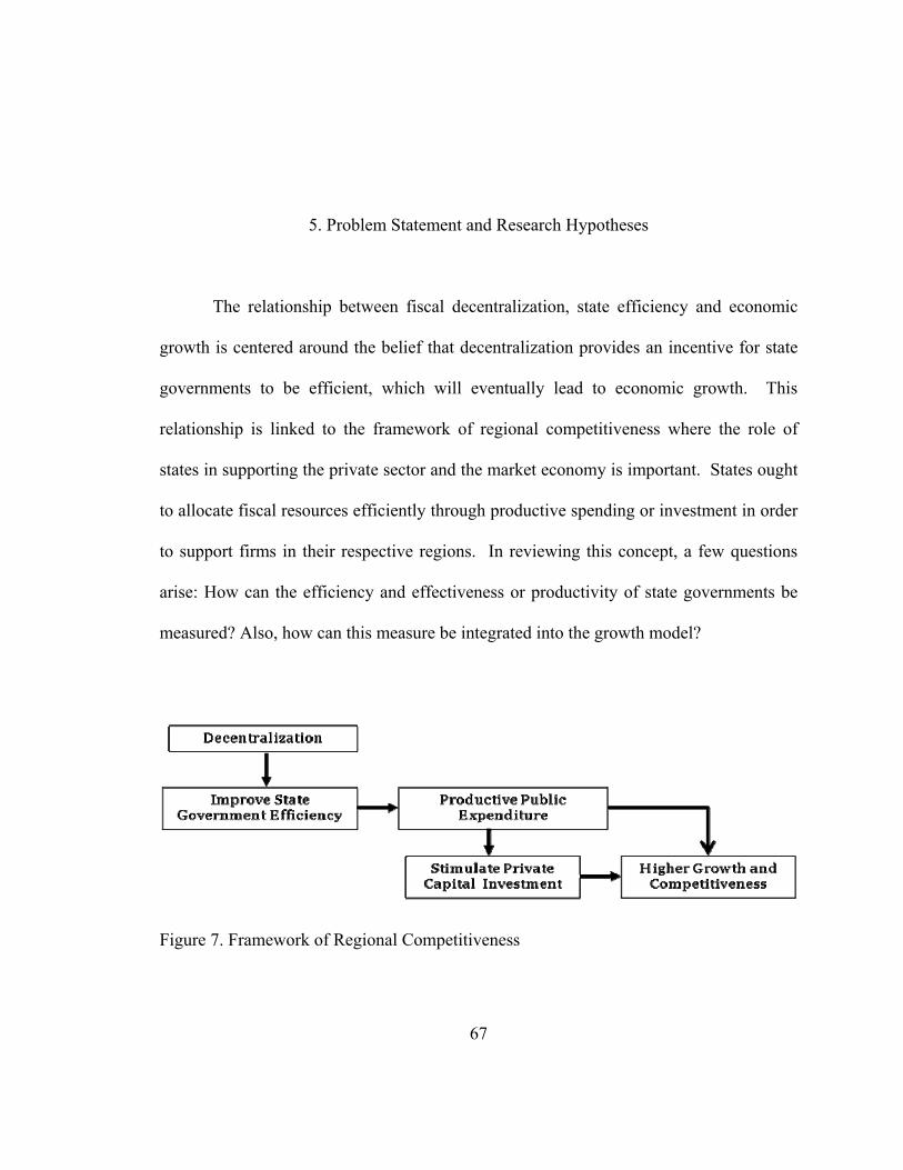
67

5. Problem Statement and Research Hypotheses

The relationship between fiscal decentralization, state efficiency and economic

growth is centered around the belief that decentralization provides an incentive for state

governments to be efficient, which will eventually lead to economic growth. This

relationship is linked to the framework of regional competitiveness where the role of

states in supporting the private sector and the market economy is important. States ought

to allocate fiscal resources efficiently through productive spending or investment in order

to support firms in their respective regions. In reviewing this concept, a few questions

arise: How can the efficiency and effectiveness or productivity of state governments be

measured? Also, how can this measure be integrated into the growth model?

Figure 7. Framework of Regional Competitiveness

68

Brennan and Buchanan (1980) introduced a way to measure the efficiency of state

governments, by correlating efficiency levels with the size of government. They believe

that the bigger the state governments, the less efficient they are. Opponents of “big

government” have used this argument to encourage smaller and efficient government

organizations.

The efficiency of state governments can also be measured by the magnitude of

transaction costs associated with the delivery of public goods. This cost benefit approach

focuses on the quality of services against costs, which to some extent indicates the

choices of state governments in allocating public goods. Following the theory introduced

by Tiebout, people choose where to live based on the net benefits that states offer, in

particular the quality and cost of public services delivered.

Evaluating the effectiveness of laws or regulations that support local and regional

economic development may not fully measure state efficiency, but it can certainly

indicate the performance of state governments. Unfortunately, this evaluation method

has a challenge because of the inconsistencies in political institutions in each state. In

addition, it is difficult to pinpoint which policies contribute to specific results, making it

even more difficult to compare the performance of state governments across the board.

Another way to measure state efficiency is by analyzing the efficiency of states in

allocating fiscal resources. This is reflected in the policies, strategies and decisions on

how to allocate public expenditure. The ability of states to efficiently allocated spending

or expenditure demonstrates their performance levels and to some extent indicates the

quality of state institutions in general (Borner et al. 2004). Here, it is assumed that state

69

governments will optimize the allocation of their scarce fiscal resources to serve the

needs of their state effectively. Decisions and strategies made by the states which

influence how public expenditure is allocated, can affect the efficiency of factors of

production and the market economy, even though state governments are not typically

involved in real production.57

Of the several methods that can be used to measure state efficiency levels, the last

option is the most commonly used in current studies because the choices or preferences

made by state governments in allocating public expenditure depict a measurable role of

states in supporting development and public welfare goals. Measuring state performance

through efficiency of public expenditure is also viable since all states follow the same

standardized structure and assessment method.

Previous empirical studies of fiscal decentralization have excluded an efficiency

measure in the extended growth model with public spending. Most of these studies have

used the level of fiscal decentralization as the key explanatory variable for economic

growth (Davoodi 1998, Woller 1998, Brueckner 2005). Surprisingly, the results from

those studies were inconclusive, although it is generally acknowledged that fiscal

decentralization has a negative relationship with economic growth in developing

countries or regions, contradicting conventional wisdom that a decentralized system

provides incentives for governments to become more efficient. Because of this finding, it

57 In some circumstances, states have a major stake in delivering public goods. It is common for state owned enterprises to run public utilities or energy companies in many developing countries. The question is how should state governments be involved and what should the appropriate role, scope and size of the state government be? A reason to have control of a critical public good rather than relying on a market mechanism is so that the public goods are affordable and all citizens have fair access to them.

70

would be critical for this dissertation to incorporate a measure of state efficiency in the

growth model.

There are four possible outcomes from analyzing the relationship between fiscal

decentralization, state efficiency and regional growth. The first possible result is that the

implementation of fiscal decentralization is expected to have a positive correlation with

state efficiency levels and regional growth. The second possible outcome is the exact

opposite in which fiscal decentralization is actually associated with lower efficiency and

lower growth.

The remaining two potential outcomes are where fiscal decentralization supports

state efficiency, but do not have an impact on regional growth and may even be

associated with lower regional growth. On the contrary, fiscal decentralization does not

increase state efficiency, but has a positive correlation with regional growth. Stated

differently, an efficient allocation of fiscal resources does not always mean higher

economic growth, and a greater degree of fiscal decentralization does not always

correspond to a more efficient state government.

When this analysis is applied to developing countries, it potentially explains a

paradox where a higher degree of fiscal decentralization does not necessarily increase

government efficiency levels, but the country still experiences robust growth. A number

of studies have supported the rationale of why developing countries experienced strong

economic growth over several decades despite deterioration in the performance of their

governments. One explanation is that growth can occur simultaneously with growing

corruption and rent seeking. Another explanation is that growth is particularly influenced

71

by factors that are independent of decentralization policies, such as an expansion of the

global market economy, a growing capital market and private investment, and an increase

in domestic demand due to population growth.

In order to determine whether the effects of fiscal decentralization on economic

growth differ in lagging and leading states, it is important to examine the different

structure and characteristic of each state and how these affect government efficiency and

regional competitiveness. Differences in fiscal and human resources as well as

technology may result in inequalities between these two clusters of states. State

government organizations may have dissimilar preferences, priorities, and strategies on

public expenditure utilization, tax revenue collection, and factor cost determination.58

The effect of these factors, in addition to other factors unique to a region, on regional

growth has been a subject of continuous debate in the regional economics field.

The dynamic relation between institutions, markets and firms in the context of

decentralization and regional competitiveness in developing countries is the key reason to

conduct the current research. As one of the largest and most diverse developing countries

in the world, Indonesia is chosen as the case study. The key challenge in Indonesia’s

decentralization is related to the extent of regional disparities, corruption, rent seeking

and revenue sharing for certain types of resources between the central and state

58 In some developing countries, aids, grants or loans from multilateral agencies are a key source of financing for development. Since revenue collection through taxes is limited in developing countries, states face many obstacles in obtaining financing to fund development. One of the challenges for developing countries is to expand its revenue base by integrating the informal market into the economic system.

72

governments. Yet, the implementation of a decentralized system in Indonesia also opens

a window of opportunity to improve state governments’ performance.

5.1. Research Questions

This dissertation attempts to provide answers to the questions that pertain to the

implementation of decentralization in Indonesia. The key question is whether fiscal

decentralization provides suitable incentive structures to make state governments more

efficient in allocating resources, eventually leading to growth that is more robust. More

specifically, what is the effect of the implementation of fiscal decentralization on

economic growth and what role does the efficiency of state allocation play?

This dissertation attempts to determine whether the implementation of fiscal

decentralization triggers different results in lagging and leading states taking into account

the differences in fiscal capacity. In addition, this study also aims to reveal whether

factors that support state efficiency differ in a pre-decentralization and post-

decentralization period.

The following subset of questions is also relevant when discussing fiscal

decentralization, state government efficiency and regional growth in Indonesia:

(1) What factors influence state fiscal efficiency in the pre-decentralization and post-

decentralization period?

(2) Do capital and current expenditure, tax rates, and cost structure have a significant

effect on regional growth?

73

(3) How different are the effects of allocative efficiencies, public expenditure, and tax

rates on economic growth in the eastern and western regions, lagging and leading

states respectively, in Indonesia?

(4) What are the policy implications on competition between regions as it relates to state

government efficiency, productivity of public capital expenditure, and regional

growth? Does Indonesia’s decentralization policy play an important role in reducing

disparities between regions?

5.2. Hypotheses

The primary hypothesis (H-P) is that the decentralization policies in Indonesia do

provide incentives to support state government efficiency and regional growth.

H-P1: Fiscal Decentralization has a positive relationship with economic growth since

decentralization provides positive incentive structures to improve the level of state

efficiency. Yet, the outcomes from the implementation of fiscal decentralization differ

between lagging and leading states.

The first hypothesis assumes that fiscal decentralization improves the efficiency

of states, which will then lead to higher economic growth. As indicated in previous

studies, the relationship between fiscal decentralization and economic growth differs

74

between developed and developing countries; similar results may occur at a smaller scale

between leading and lagging states in Indonesia.

H-P2: The level of state efficiency is neither determined by the level of a state’s economy

nor its fiscal capacity.

Similar to the first hypothesis, the second hypothesis in this set of primary

hypotheses presumes that the level of state efficiency has a positive relationship with

economic growth. State efficiency implies that states will allocate expenditure and

resources to productive investments, which can contribute to the growth of the private

sector and the market economy at the regional level.

Leading states are assumed to have an advantage over lagging states in utilizing

their fiscal capacity to support regional development for a number of reasons: First,

leading states may have a larger supply of skilled and trained staff and more advanced

technological resources than lagging states. Second, the productivity of public capital

investments is typically higher in leading states because of economies of scale and

positive externalities that are driven by capital investments.

In this context, despite lower fiscal capacity and challenges in managing fiscal

decentralization, it is still possible for lagging states to be more efficient if the state

government is committed to improving its capability to allocate resources efficiently. In

contrast, a larger fiscal capacity in leading states may not guarantee higher inefficiency

levels, because of possible increases in waste spending.

75

The set of secondary hypotheses (H-S) focuses on several factors of fiscal

decentralization that can affect state government efficiency and economic growth.

H-S1: A higher ratio of productive spending and revenue independence indicates a

higher level of state efficiency.

The first secondary hypothesis assumes that the level of state government

efficiency is affected by the ratio of productive spending and revenue independence.

States are supposed to be more efficient if they assign their fiscal resources to productive

spending and can generate sources of revenue independently.

H-S2: Higher state tax rates and factor costs are correlated with lower growth, which

can add to the financial burden of firms.

The next secondary hypothesis assumes that with a higher level of state

efficiency, some other factor costs may decrease.59 A lower cost structure is expected to

promote economic growth and increase the competitiveness level of a state.

A decentralized system also allows states to manage their own sources of revenue.

States may need to raise taxes, increase fees and charges to avoid budget deficits or

revenue shortfalls as transfers from the central government decline. Higher taxes,

59 Operating costs and staff wages and allowances are some of the costs of managing administration and organization of state governments. Those costs are part of the current expenditure in the state budget.

76

charges, and fees are expected to improve public services not support corruption.

Unfortunately, corruption often takes place and can impede the growth and

competitiveness of a region, as firms become more reluctant to invest. With

globalization and growing competition between regions, this can be problematic because

firms can easily move their capital to other regions. However, it can also encourage

regions to be more competitive to retain capital and investments in their respective

regions.60

H-S3: Productive public capital expenditure is correlated with higher growth. Despite a

larger fiscal capacity, capital expenditures in the leading states are not always more

productive, because higher spending may result in more inefficiency.

The third secondary hypothesis assumes that public capital expenditure can

increase the capacity of the private sector to succeed in a market economy in both the

short and long term. Leading states are assumed to have a stronger ability to finance

public capital investments using their own resources as well as external resources. Yet,

this larger financial capacity does not guarantee higher growth if resources are not

allocated in an efficient manner.

60 Higher factor mobility of capital and the existence of alternate locations for production can force states to seriously reconsider any policies that are not conducive to the private sector investments. One exception is in states endowed with a surplus of natural resources where the private sector is more likely to invest. In that situation, the private sector may be more tolerant of government inefficiency and red tape bureaucracy. The private sector is also more willing to provide infrastructure or financial resources to support the investment of a project.

77

6. Analytical Framework and Empirical Analysis

The dissertation employs a two-stage method to determine the relationship

between efficiency factors at the state government level, fiscal decentralization and

economic growth. The first stage is the application of the Data Envelopment Analysis

(DEA) to construct a measure of technical efficiency of state governments. As an

extension to the analysis of state efficiency levels using DEA, this study applies a tobit

panel data regression to reveal factors that influence technical efficiency. The second

stage adopts an extension of the endogenous growth model within a public spending

framework. Panel data analysis is utilized in the growth model to determine the effect of

fiscal decentralization and state efficiency on economic growth.

Despite a number of constraints in this study, the methodology and data analysis

used will be a valuable foundation for future research that aims to validate the

relationship between fiscal decentralization, state efficiency, and economic growth at

either the regional or the national level.

6.1. State Performance and Efficiency Analysis Using Data Envelopment Analysis

Two basic analytical methods are generally used to measure comparative

performance or efficiency: the parametric model and the non-parametric model. The

78

parametric technique with a statistical regression has been used in single input-multiple

outputs or single output-multiple inputs analysis. Ordinary Least Square (OLS)

regression is typically used to estimate performance levels in the parametric models.

The major limitation of the parametric model is the risk of it being inaccurately specified

since it is necessary to hypothesize the type of model before running OLS regression

(Thanassoulis 2001). In addition, there have been unsatisfactory results when confidence

intervals take into account statistical noise. In addition, the parametric method does not

allow inefficiency to be measured.

In response to the limitation of the standard OLS regression in measuring

efficiency, the Stochastic Frontier (SF) model was introduced. Instead of focusing on

central tendency, the SF model is oriented towards the efficiency frontier. Unlike the

parametric method, this model allows for inefficiency. The standard error is composed of

two parts: the normally distributed random error and an inefficiency parameter. The SF

model measures the average efficiency rather than the efficient level of input for a given

output. However, one of the issues with the SF model is the inaccuracy of the efficiency

ratio because of the unknown size of the random error within the observed output.

The non-parametric method of comparative performance measurement has the

ability to run multiple inputs and outputs. This method can also estimate the efficiency

model based on the relationship between inputs and outputs. The model constructs an

efficient production frontier from the observed inputs and outputs. In constructing the

efficient production of the non-parametric method, it is assumed that every input and

output correspondence can be observed based on their interpolation; thus, all observed

79

inputs and outputs essentially operate at the same production function. The efficient

production frontier represents the optimum capacity of the efficiency model rather than

the average profile of the parameters in the regression analysis. All units on the frontier

or “envelope” are assumed to be fully efficient.61

Data Envelopment Analysis is the main category of the non-parametric method

that measures the relative performance of certain Decision Making Units (DMU).

Performance is measured in terms of efficiency when it references a set of units that are

being compared to each other.

Although DEA measures relative efficiency, it is assumed that each DMU

includes a sufficient number of units that have absolute technical efficiency and therefore

the DEA analysis is capable of continuously improving their performance (Thanassoulis

2001).62 The main criterion of a DMU is homogeneity since it uses the same input

61 It is feasible to obtain an inefficient production frontier where the model produces slacks from input excess and output shortfall. The theory of inefficiency by Leibenstein (1966) argued that firms do not always maximize production as postulated by neoclassical economics. 62 DEA was introduced by Charnes, et al. in 1978 and intended to measure the efficiency of an organization unit. The DEA concept is an extension of the linear production function that was initially put together in the economic concept of empirical efficiency by Farrell in 1957 (Thanassoulis 2001). Farrell attempted to measure the efficiency of a unit of production in a single input-single output case, which involved the measurement of price and technical efficiencies and the derivation of the efficient production function.

Input (Resources) State Government

(Decision Making Unit)Output (Goals)

Figure 8. DEA Research Framework

80

resources to produce output. Yet, each unit of assessment has a “decision” control

mechanism to convert inputs into outputs. This decision control instrument is a key

concept that applies to this research as each state government is considered as a DMU

that makes decisions on the allocation of input resources to generate maximum output.

Following Farrell (1957), technical efficiency refers to a condition when, given a

set of inputs, a maximum quantity of outputs are produced or when given a set of outputs,

a minimum quantity of inputs are required.63 The technical efficiency of a DMU is

computed as the ratio of output produced to input consumed as shown below.

Technical Efficiency = Σ weighted outputs / Σ weighted inputs

In measuring efficiency, DEA allows discretion under certain conditions in which

the model should control inputs or outputs in the analysis. The concept of Pareto

efficiency has three orientations based on whether inputs or outputs are controllable. An

input-oriented model (inputs are controllable) is where DMUs are deemed to generate a

given amount of outputs with the smallest possible amount of inputs. Alternatively, for

an output-oriented model, efficiency is measured based on a given amount of inputs to

generate the maximum outputs. The third orientation is the base-oriented model where

DMUs produce the optimal combination of inputs and outputs controlling for both inputs

and outputs. The DEA model in this research is based on input orientation as it pertains to

63 Efficiency is generally an economic terminology. Other fields may refer it to performance, which is a broader term to explain the quality of state government organization.

81

the capability of state governments in maximizing a limited amount of public spending as

input.

The DEA model allows each DMU to maximize the weight multipliers. The

weights of inputs and outputs for each DMU vary until the model reaches the best

possible combination. The resulting efficiency score is relative to the DMU’s sample

observed and the set of weights have to be accounted for other units of assessment in

which none of them have an efficiency score greater than one.

Figure 9 exhibits the graphical representation of the efficiency measurement of

the DEA model with a single-input (x) and single-output (y). The model produces two

frontier efficiency lines: first is a linear line (0ICM) that correlates with constant returns

to scale (CRS); and the other is a convex line (GABCDF) with variable returns to scale

(VRS).

Figure 9. Measurement of Technical Efficiency

82

K represents an inefficient DMU that is located outside of the envelope boundary.

The technical efficiency of K is hi/hk in the CRS and hj/hk in the VRS. The scale

efficiency K refers to the ratio of hi/hj.

The standard DEA model proposed by Charnes, Cooper, and Rhodes (1978) is

expressed by the following ratio:

(1)

j jj

i ii

xv

yMax

0

00

Subject to:

(2)

j jj

i iki

xv

y

0

1 for all DMUs k=1,2,….,n

(3) µi ≥ 0 (4) vj ≥ 0

The parameters used in this input-oriented model are:

0 : the efficiency score of the DMU0 under analysis;

n : number of DMUs under analysis;

i : number of outputs;

j : number of inputs;

Yk y1k, y2k, …yik : vector of outputs for DMU k with yik being the value of output i for

DMU k;

Xk x1k, x2k, ..,xjk : vector of inputs for DMU k with xik being the value of input j for

DMU k;

and vector on multipliers respectively set on Yk and Xk where i, j = the

respective weights for output i and for input j.

The model determines that for each DMU0 the optimal set of input weights 10 iiv and

output weights 10 rr that maximize its efficiency score is 0.

83

Charnes, Cooper and Rhodes define efficiency by referencing the orientation of

inputs and outputs. In the input-oriented model, a DMU is not efficient if it is possible to

decrease any input without augmenting any other input and without decreasing any

output and vice verse for the output-oriented model.

The traditional Charnes, Cooper and Rhodes model is built under the constant

return to scale (CRS) assumption in which an increase in inputs consumed would lead to

a proportional increase in the outputs produced (Cooper et al. 2007). The CRS structure

is more restrictive than the variable return to scale (VRS), which lowers the number of

efficient units and efficiency. The issue with the CRS assumption is that it is required for

all DMUs to operate at an optimal scale. In this research, there are a number of factors

that can prevent DMUs from operating optimally, such as limited resources, imperfect

competition, and institutional issues.

Banker, Charnes, and Cooper (1984) were the first to introduce the VRS structure

that is commonly used. In the BCC model, the outputs produced can increase more or

less than proportionally to the increase in inputs. Parameter w relaxes the constant return

to scale by allowing the frontier set to go through the origin. The Banker, Charnes, and

Cooper input-oriented model is considered more appropriate for this research. The linear

programming of BCC model is written as follows:

(1) wyii

vwMax 000

,,

Subject to: (2)

j jj xv 10

84

(3) i j jkjiki wxvy 1 for all k-1,2,….n

(4) 0i

(5) 0jv

(6) w free 6.1.1. Descriptive Analysis of Input and Output Data

This study includes all the 26 states in Indonesia.64 Table 9 exhibits the

descriptive statistics of the variables used in the input-output analysis. In determining the

input and output variables, a Granger causality test is performed to identify a stronger

causal relationship between the input and output variables. Following a number of

previous studies, the input to measure efficiency of states is the public expenditure

(Afonso et al. 2003, Herrera and Pang 2005). Thus, technical efficiency is an analysis of

spending or expenditure efficiency.

Technical efficiency scores are calculated in the DEA model with state revenue

and private investment as the outputs of the model.65 Appendix B.2 and B.3 show the

result of the Granger causality tests to confirm the causality direction from the level of

state spending on private investment and state revenue.

64 During the course of the study, several new provinces were created. Currently there are 33 states or provinces in Indonesia; however, this study consistently uses data from 26 states in the empirical model by merging the data of the newly created states into their original jurisdiction before the current formation. 65 State spending potentially affects output growth or GRDP from a theoretical standpoint; however, the Granger test in Appendix B.1 shows a significant F-statistic, which means that the assumption that state spending directly affects growth cannot be retained. State spending was a small fraction of GRDP and its effects on regional growth might come through private sector production driven by the multiplier effect of government spending.

85

In this study, the input variables consist of two types of state spending: Capital

Expenditure and Current Expenditure. The first input variable, capital expenditure

includes spending on various public investments, such as infrastructure, public housing,

health and education. Because of the nature of typical public capital investments where

there is a time lag for a project or program to be fully operated, the data used has a one-

year lag.66 The second input variable, state current expenditure is spending that covers all

operating costs of state governments including rent, wages, expenses and subsidies.

The two output variables in the DEA model are state revenue and private

investment.67 State revenue includes taxes, fees, and charges, but it excludes transfers

from the central government. Some of the state revenue also comes from profits

generated by State Owned Enterprises (SOE), such as state local banks and public

utilities. Spending on capital investment projects or services generate revenue for states

either directly though fees or charges, or indirectly through tax collections driven by

private sector development.

The level of private investment is also affected by state decisions to invest

particularly in capital projects in connection to public service deliveries. The availability

of infrastructure, such as transportation networks, telecommunication, and electricity

66 Limitation on data availability has precluded the use of data with more than one-year lag. Yet, a number of studies found that public infrastructure investment affects private sector investment within a year after being implemented (Murty and Soumya 2006). In fact, during the period of economic crisis, public capital investments have been scaled back because of budget constraints. Consequently, states can only invest in a relatively modest scale of programs and services or in capital improvement projects. Thus, a one-year lag is considered sufficient to measure the effects from public capital investments. 67 A number of studies have used a couple different variations of outputs in the efficiency analysis, such as education, health, infrastructure development, income inequality, institutional quality, and growth (Afonso et al. 2003, Herrera and Pang 2005).

86

would be part of the consideration when making a decision to invest in a region. The

expansion of state expenditure will also boost government consumption, expand market

demand, and potentially induce private investment in the region. This resembles the

concept of the multiplier effect from government spending that can lead to higher

economic growth.

Table 9. Descriptive Analysis of Input-Output Variables

Variable Pre-Decentralization (1996-2000), n=130 Post-Decentralization (2001-2005), n=130

Mean St. D. Min Max Mean St. D. Min Max Capital Expenditure 149,159 192,605 36,907 1,229,105 504,412 1,470,387 14,432 15,800,000Current Expenditure 301,708 540,725 27,850 3,826,516 971,035 1,462,443 61,741 9,041,520Revenue 175,441 386,940 9,841 2,668,535 678,847 1,210,385 15,667 7,597,868

Investments 403,230 693,075 100 45,395 217,005 385,942 1,200 2,928,370Note: In Million Rupiah (Indonesian currency)

6.1.2. Technical Efficiency Analysis of State Government using DEA

In this first stage analysis, DEA is used under a dynamic rather than a static

condition. The issue with a dynamic or time dependent setting in DEA is the risk of an

excessive use of resources that are intended to produce future outputs. To overcome this

problem, a time dependent method of DEA known as window analysis is used. Window

analysis is a temporal evolution of efficiency scores that evaluates how consistent these

scores are overtime. Illustrated below are the properties of the window analysis:

87

n : number of Decision Making Unit (DMUs) under analysis. Each state or province in

Indonesia is considered one DMU following the structure of the DEA model;

k : number of periods;

p : length of window (p ≤ k);

w : number of windows

With 26 DMUs (n) and 10 years of observation (k), this study uses a 3 year window

length (p) to examine the consistency of the scores. The numerical illustration that

defines the application of window analysis is:

Formula Application No. of windows w = k – p + 1 w = 10 – 3 +1 = 8

No. of DMUs in each window np/2 26 x 3 / 2 = 39

No. of different DMUs n(k – p + 1)p 26 x 8 x 3 = 624

Table 10 presents a compilation of the results of the window analysis where the

technical efficiency score is calculated as the average efficiency score in each window

year. A higher technical efficiency score represents a higher spending efficiency level or

to some extent also a more efficient allocation of fiscal resources by state governments.

As a whole, technical efficiency levels seem to improve after the implementation

of decentralization, as shown in Table 11. The technical efficiency bounced back

following a rapid decline during the financial crisis. The technical efficiency of states in

the post-decentralization period was lower compared to the pre-crisis period. Prior to

decentralization, most states were dependent on central government transfers as other

sources of revenue were subject to budget constraint. Consequently, state governments

had to manage their expenditures to balance their budget. By default, this would increase

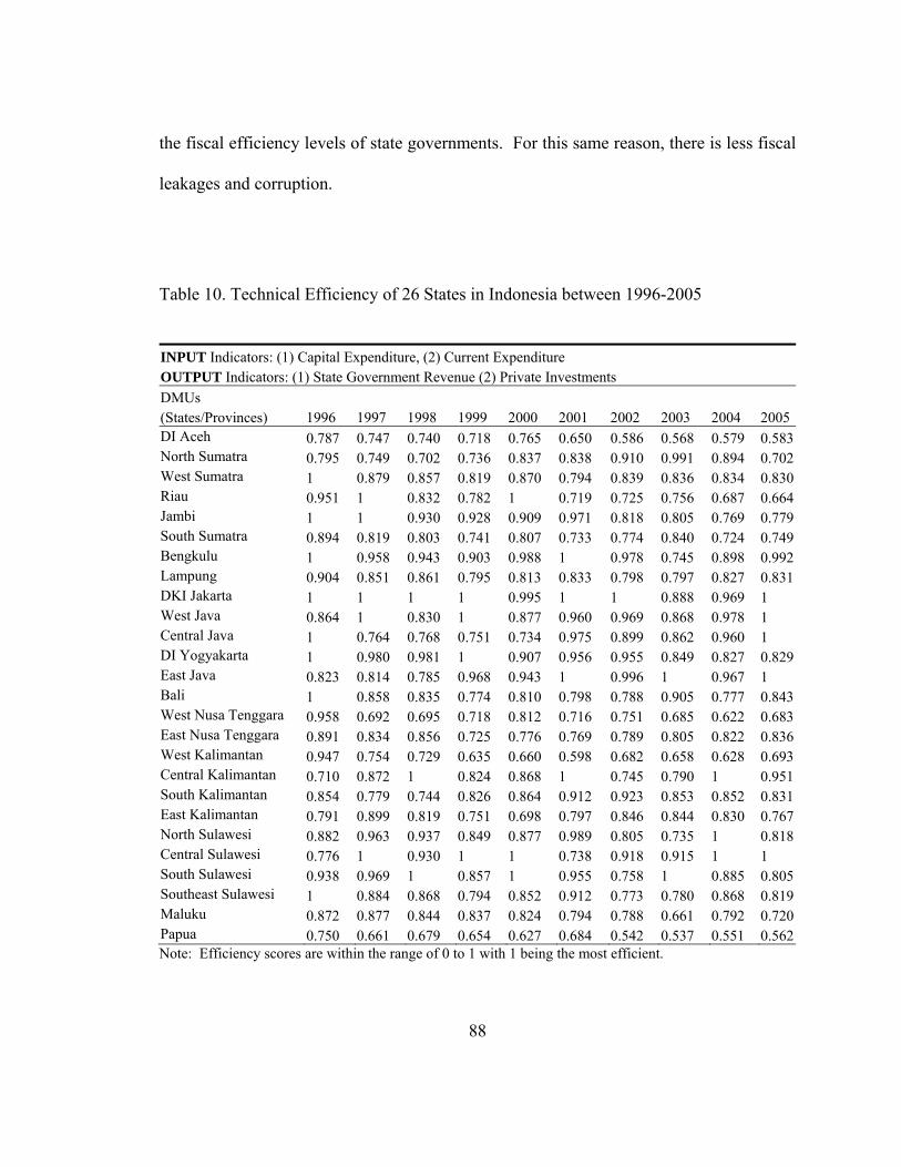
88

the fiscal efficiency levels of state governments. For this same reason, there is less fiscal

leakages and corruption.

Table 10. Technical Efficiency of 26 States in Indonesia between 1996-2005

INPUT Indicators: (1) Capital Expenditure, (2) Current Expenditure OUTPUT Indicators: (1) State Government Revenue (2) Private Investments

DMUs 1996 1997 1998 1999 2000 2001 2002 2003 2004 2005(States/Provinces)

DI Aceh 0.787 0.747 0.740 0.718 0.765 0.650 0.586 0.568 0.579 0.583North Sumatra 0.795 0.749 0.702 0.736 0.837 0.838 0.910 0.991 0.894 0.702West Sumatra 1 0.879 0.857 0.819 0.870 0.794 0.839 0.836 0.834 0.830Riau 0.951 1 0.832 0.782 1 0.719 0.725 0.756 0.687 0.664Jambi 1 1 0.930 0.928 0.909 0.971 0.818 0.805 0.769 0.779South Sumatra 0.894 0.819 0.803 0.741 0.807 0.733 0.774 0.840 0.724 0.749Bengkulu 1 0.958 0.943 0.903 0.988 1 0.978 0.745 0.898 0.992Lampung 0.904 0.851 0.861 0.795 0.813 0.833 0.798 0.797 0.827 0.831DKI Jakarta 1 1 1 1 0.995 1 1 0.888 0.969 1 West Java 0.864 1 0.830 1 0.877 0.960 0.969 0.868 0.978 1 Central Java 1 0.764 0.768 0.751 0.734 0.975 0.899 0.862 0.960 1 DI Yogyakarta 1 0.980 0.981 1 0.907 0.956 0.955 0.849 0.827 0.829East Java 0.823 0.814 0.785 0.968 0.943 1 0.996 1 0.967 1 Bali 1 0.858 0.835 0.774 0.810 0.798 0.788 0.905 0.777 0.843West Nusa Tenggara 0.958 0.692 0.695 0.718 0.812 0.716 0.751 0.685 0.622 0.683East Nusa Tenggara 0.891 0.834 0.856 0.725 0.776 0.769 0.789 0.805 0.822 0.836West Kalimantan 0.947 0.754 0.729 0.635 0.660 0.598 0.682 0.658 0.628 0.693Central Kalimantan 0.710 0.872 1 0.824 0.868 1 0.745 0.790 1 0.951South Kalimantan 0.854 0.779 0.744 0.826 0.864 0.912 0.923 0.853 0.852 0.831East Kalimantan 0.791 0.899 0.819 0.751 0.698 0.797 0.846 0.844 0.830 0.767North Sulawesi 0.882 0.963 0.937 0.849 0.877 0.989 0.805 0.735 1 0.818Central Sulawesi 0.776 1 0.930 1 1 0.738 0.918 0.915 1 1 South Sulawesi 0.938 0.969 1 0.857 1 0.955 0.758 1 0.885 0.805Southeast Sulawesi 1 0.884 0.868 0.794 0.852 0.912 0.773 0.780 0.868 0.819Maluku 0.872 0.877 0.844 0.837 0.824 0.794 0.788 0.661 0.792 0.720Papua 0.750 0.661 0.679 0.654 0.627 0.684 0.542 0.537 0.551 0.562Note: Efficiency scores are within the range of 0 to 1 with 1 being the most efficient.

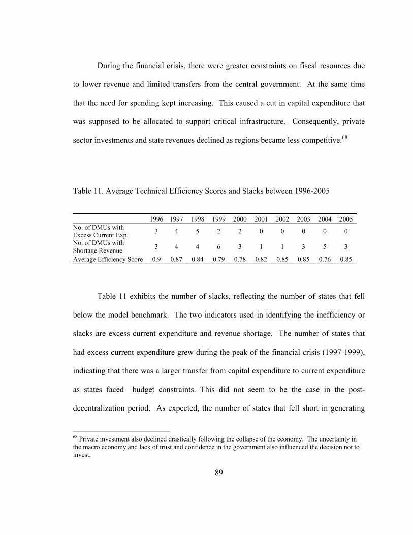
89

During the financial crisis, there were greater constraints on fiscal resources due

to lower revenue and limited transfers from the central government. At the same time

that the need for spending kept increasing. This caused a cut in capital expenditure that

was supposed to be allocated to support critical infrastructure. Consequently, private

sector investments and state revenues declined as regions became less competitive.68

Table 11. Average Technical Efficiency Scores and Slacks between 1996-2005

1996 1997 1998 1999 2000 2001 2002 2003 2004 2005 No. of DMUs with Excess Current Exp.

3 4 5 2 2 0 0 0 0 0

No. of DMUs with Shortage Revenue

3 4 4 6 3 1 1 3 5 3

Average Efficiency Score 0.9 0.87 0.84 0.79 0.78 0.82 0.85 0.85 0.76 0.85

Table 11 exhibits the number of slacks, reflecting the number of states that fell

below the model benchmark. The two indicators used in identifying the inefficiency or

slacks are excess current expenditure and revenue shortage. The number of states that

had excess current expenditure grew during the peak of the financial crisis (1997-1999),

indicating that there was a larger transfer from capital expenditure to current expenditure

as states faced budget constraints. This did not seem to be the case in the post-

decentralization period. As expected, the number of states that fell short in generating

68 Private investment also declined drastically following the collapse of the economy. The uncertainty in the macro economy and lack of trust and confidence in the government also influenced the decision not to invest.

90

their own revenue increased during the financial crisis. Surprisingly, after

decentralization, the number also went up largely due to the persistent deterioration of the

country’s economy as a whole and the slower pace of economic recovery.

To give a snapshot of state technical efficiency levels before and after the

implementation of decentralization, the average technical efficiency score of Indonesia’s

26 states has been calculated for the period of observation between 1996-2000 and 2001-

2005. The results are presented in Table 12. A high and a low technical efficiency score

threshold have been established for purposes of analysis in this dissertation. An upper

bound has been designated for average efficiency scores greater than 0.95, while a lower

bound has been assigned to average efficiency scores lower than 0.75. In general, only

few states fall under the low benchmark category.

One of the findings, as shown in Table 12, is that most states in Java have a

relatively higher degree of technical efficiency after the implementation of

decentralization compared to other states in Indonesia. As the most developed region in

Indonesia, the higher level of technical efficiency of state governments in Java can be

attributed to a higher level of organizational capability in managing fiscal

decentralization. The rapid growth during the central planning era contributed to the

competency of state governments in Java when reforming and restructuring their

organizations and management to better serve the public.

In the western region, only North Sumatra was able to improve its technical

efficiency levels significantly, while Riau, the only major oil exporter state in the western

region, experienced a sharp decline. The contrast between these two states provides

91

evidence that supports the hypothesis that states that are rich in resources are not always

more efficient. This is because these states have a tendency to spend more in proportion

to their large fiscal capacity. Unfortunately, the higher levels of state spending may

actually lead to higher levels of inefficiency.

Table 12. Average Technical Efficiency Scores, 1996-2000 and 2001-2005

DMUs 5-year

Average 5-year

Average (States/Provinces) 1996-2000 2001-2005DI Aceh 0.751 0.593 North Sumatra 0.764 0.843 West Sumatra 0.885 0.827 Riau 0.913 0.710 Jambi 0.953 0.828 South Sumatra 0.813 0.764 Bengkulu 0.958 0.923 Lampung 0.845 0.817 DKI Jakarta 0.999 0.971 West Java 0.914 0.955 Central Java 0.803 0.939 DI Yogyakarta 0.974 0.883 East Java 0.867 0.992 Bali 0.855 0.822 West Nusa Tenggara 0.775 0.691 East Nusa Tenggara 0.816 0.804 West Kalimantan 0.745 0.652 Central Kalimantan 0.855 0.897 South Kalimantan 0.813 0.874 East Kalimantan 0.792 0.817 North Sulawesi 0.902 0.869 Central Sulawesi 0.941 0.914 South Sulawesi 0.953 0.880 Southeast Sulawesi 0.880 0.830 Maluku 0.851 0.751 Papua 0.674 0.575

92

Some states have not been able to improve their technical efficiency levels after

the implementation of decentralization because of endless conflict and instability within

their borders. This is particularly the case of Aceh, Papua, and Maluku, which have been

plagued by separatist and ethnic conflicts that have disrupted the function of state

governments, including the ability to deliver basic public services and maintain state

assets. The tsunami disaster that hit part of Aceh’s coastal area in 2004 was also the

cause for low fiscal efficiency level, following the state government’s inability to

function properly for a period of time. Without a functioning state government coupled

with uncertainties and security concerns, growth has been stagnant as private investment

and employment level declined drastically.

As shown in Table 13 that provides a side-by-side comparison between state

technical efficiency levels and real GRDP over the 10-year period of analysis, certain

states with low real GRDP had high effiiency level, such as Bengkulu and Jambi. On the

other hand, certain rich states had low effciency level, such Papua, North Sumatra and

East Kalimantan. One explanation is the state government’s inability to utilize the state’s

abundant fiscal resources that were previously under the control of the central

government during the New Order. Widespread corruption is also a contributing factor.

This proves that more developed states do not always capable to plan an effective

strategy and priority to utilize their fiscal resources to support development.

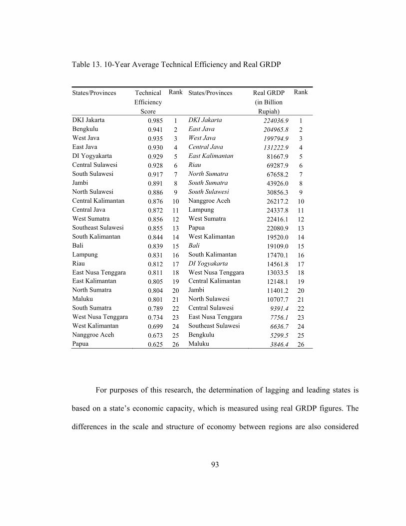
93

Table 13. 10-Year Average Technical Efficiency and Real GRDP

States/Provinces Technical Rank States/Provinces Real GRDP Rank

Efficiency (in Billion

Score Rupiah) DKI Jakarta 0.985 1 DKI Jakarta 224036.9 1 Bengkulu 0.941 2 East Java 204965.8 2 West Java 0.935 3 West Java 199794.9 3 East Java 0.930 4 Central Java 131222.9 4 DI Yogyakarta 0.929 5 East Kalimantan 81667.9 5 Central Sulawesi 0.928 6 Riau 69287.9 6 South Sulawesi 0.917 7 North Sumatra 67658.2 7 Jambi 0.891 8 South Sumatra 43926.0 8 North Sulawesi 0.886 9 South Sulawesi 30856.3 9 Central Kalimantan 0.876 10 Nanggroe Aceh 26217.2 10 Central Java 0.872 11 Lampung 24337.8 11 West Sumatra 0.856 12 West Sumatra 22416.1 12 Southeast Sulawesi 0.855 13 Papua 22080.9 13 South Kalimantan 0.844 14 West Kalimantan 19520.0 14 Bali 0.839 15 Bali 19109.0 15 Lampung 0.831 16 South Kalimantan 17470.1 16 Riau 0.812 17 DI Yogyakarta 14561.8 17 East Nusa Tenggara 0.811 18 West Nusa Tenggara 13033.5 18 East Kalimantan 0.805 19 Central Kalimantan 12148.1 19 North Sumatra 0.804 20 Jambi 11401.2 20 Maluku 0.801 21 North Sulawesi 10707.7 21 South Sumatra 0.789 22 Central Sulawesi 9391.4 22 West Nusa Tenggara 0.734 23 East Nusa Tenggara 7756.1 23 West Kalimantan 0.699 24 Southeast Sulawesi 6636.7 24 Nanggroe Aceh 0.673 25 Bengkulu 5299.5 25 Papua 0.625 26 Maluku 3846.4 26

For purposes of this research, the determination of lagging and leading states is

based on a state’s economic capacity, which is measured using real GRDP figures. The

differences in the scale and structure of economy between regions are also considered

94

since these can affect the allocation of resources and either constrain or stimulate

growth.69

Based on this criterion, the following eleven states are identified as leading states:

DKI Jakarta, East Java, West Java, Central Java, East Kalimantan, Riau, North Sumatra,

South Sumatra, South Sulawesi, Bali, and Yogyakarta.70 Aceh, Papua, Riau and East

Kalimantan are not included as leading states despite large revenue from natural

resources. Yogyakarta and Bali are considered leading states due to geographic

adjacency and economic integration with other states in Java.

Fifteen states are designated as lagging states in this dissertation for purposes of

constructing a separate panel data model. An independent growth model for each lagging

and leading state is constructed to test the hypotheses.

Most states in the eastern region have lower real GRDP compared to states in the

western region, except for East Kalimantan and Papua. This was caused by the lag of

development and the fact that states in Indonesia’s eastern region are geographically

disadvantage. This has resulted in lower factor mobility and higher cost structures

compared to states in the western region. Lower factor mobility in the eastern region has

69 States in Java will have a lower real GRDP per capita due to the higher concentration of population in this region and therefore the rank of state’s economic capacity will be biased since real GRDP per capita does not accurately depict the actual level of economy and development in those states. 70To validate the division between leading and lagging states, a Chow statistical test was performed. The test aims to identify the presence of a threshold or a break in statistical data. The assumption is that the coefficients in two linear regressions of different data sets are equal. In this study, the basic growth model with capital (K) and labor (L) is used to test two subsamples, the leading and lagging states. The result of the Chow test in Stata is included in Appendix C. Referring to the F-significance level, the null hypothesis is rejected and therefore the two data sets are distinct from each other. Using a variation of different subsets assigned to leading and lagging states showed a lower level of significance.

95

contributed to lower production, less private investment and a smaller market economy.71

Although cost of labor is typically lower in the eastern region, it is not low enough to

offset the high costs of other factors of production.72

The imbalance in regional development is evident among states inside and outside

of Java. Most of the development in Indonesia during the New Order was concentrated

in Java and a handful of urban centers on the other major islands. A cluster of economic

activities also developed along major ports and other transportation networks. This

created a situation where resources were not distributed equally and certain regions were

left with less productive resources, making it even more difficult to achieve levels of

efficiency and competitiveness already attained by regions such as Java.

6.1.3. Determinants of State Technical Efficiency in a Tobit Panel Data Model

This section is an extension of the first stage empirical analysis that examines

factors that influence technical efficiency levels of state governments in Indonesia. Some

of the factors that are identified as the possible determinants of state government

efficiency are used to construct a weighted variable that will adjusts technical efficiency

71 Low factor mobility puts a limit on the level of business and industrial integration in the eastern region. This might hamper positive externalities or spillover effects that are the key growth factors in the endogenous growth model. 72 A low labor cost in the eastern region is mainly associated with lower quality of workers. A lack of educational facilities, particularly for higher education, has led many productive workers to leave lagging states to obtain a higher education, better skill sets, and eventually pursue higher paying jobs, which are mostly located in Java.

96

levels in the panel growth model. This adjustment made is instrumental to create a more

appropriate state efficiency factor.

Due to the skewed distribution of technical efficiency scores from the DEA

analysis, a tobit panel data regression is used to reveal these determinants. In a normal

panel data regression, the estimates of the parameter are biased and inconsistent with

scores, causing the estimates to lean towards the higher bound. The tobit panel data

model is essentially a maximum-likelihood random effect model that has the ability to

censor the dependent variable. The tobit model is used because the technical efficiency

scores are constrained within the range of 0 and 1. A right-censored tobit model is

constructed in this study as the observed efficiency scores lean towards 1.

The technical efficiency scores are considered as latent variables because the

efficiency of states is not directly observed but rather inferred through other variables in

the DEA model. The mathematic expression of a tobit censored panel data regression

can be explained as the level of yit (efficiency scores as the dependent variable) in terms

of an underlying latent variable yit*:

yit* = ß0 + ß1 xit + εit (6)

yit = ß0 + ß1 xit + εit if yit* > 0, and (7)

yit = 0 if yit* ≤ 1

The error term (εit) in the efficiency distribution of the tobit panel data model where yit*

is a latent variable is assumed to be normally distributed as a function of N(). εit, xit

97

and ß are vectors of explanatory variables and unknown parameters respectively. Both ß

and are estimated using maximum likelihood estimation (MLE).

The standard estimation using a maximization of likelihood function (L), where F

is the standard normal cumulative distribution function is as follows:

σ

xF1

0yσ2

)βx(y 2(yσ2loglog(2

2

1

0yLlog it

it

ititit

it

)

(8)

The estimated coefficients in the tobit panel data model are represented by the

marginal effect of xit on yit*. In order to achieve the expected rather than desired

marginal effect of xit on yit , the following equation is implemented in the tobit panel data

model:

/)(

/)(0|

10

1010

it

itititit x

xxyyE

(9)

The following factors are analyzed to establish the likelihood that they influence

state technical efficiency levels. These factor are the explanatory variables in the tobit

panel data model:

- Fiscal Decentralization: share of state spending over total government spending; a higher

share of state spending represents a higher degree of fiscal decentralization.

- Ratio of Productive Spending: share of state capital expenditure over total state spending.

Capital expenditures are either existing capital improvements or new capital investment

projects and are considered productive spending.

98

- Ratio of Operating Costs: share of state operating costs over total state spending. It is

also considered a ratio of overhead costs, which are costs associated with the operation

and management of a state government, excluding expenditure that is allocated for

human capital expenses.

- Ratio of Revenue independence: share of taxes, charges and fees generated independently

by states over transfers from the central government. A higher ratio of revenue

independence indicates either an increase in a state’s own revenue or a decrease in central

government transfers.

The results of the tobit panel data regression over the 10-year period of analysis

(1996-2005) are shown in Table 14. The dependent variable is the average efficiency

score of 26 states in Indonesia for each year between 1996 and 2005. In the tobit model,

the magnitude of likelihood for each factor determinant is indicated by the marginal

effect of each factor.

Several factors were identified as determinants of state efficiecy scores based on

the degree of significance (z-ratio). Fiscal decentralization is the factor with the highest

marginal effect. This indicates that fiscal decentralization has the most effect on the

levels of technical efficiency compared to other factors and to some extent, it also

supports the primary hypothesis H-P1 that fiscal decentralization provides incentives for

states to become more efficient in allocating fiscal resources.73

73 Other factors that influence state efficiency should also be considered. In measuring the technical efficiency of states, not all factors are observed and consequently a modification is needed to ensure the appropriate level of state efficiency beyond technical efficiency is observed in the next stage.

99

Table 14. Determinant of State Technical Efficiency in Indonesia, 1996-2005

Dependent Var: State Efficiency n = 260 Obs (26 States)

Independent Var. Coefficients z-ratio Marginal Fiscal Decentralization

0.79

2.94*

0.72

Ratio of Productive Spending

-0.07

-2.64*

-0.06

Ratio of Operating Costs

-0.09

-2.82*

-0.08

Ratio of Revenue Independence

0.04

2.96*

0.04

Lagging states Dummy

0.01

1.00

0.01

Per capita Income Per capita Spending

0.002

-0.20

1.14

-2.77*

0.001

-0.19

Constant 0.86 36.39* Log-Likehood 139.78 R-squared 0.21 Wald chi2 74.20

Note: * The point estimate is significant at the 1% level.

*** The point estimate is significant at the 10% level.

The results from the tobit panel model show that a higher ratio of productive

spending and level of per capita spending are likely to reduce the levels of technical

efficiency. Productive spending that is generally assumed to be an indicator of a state’s

ability to allocate resources efficiently to support public welfare and long-term

development, shows an unexpected inverse correlation than what the hypothesis H-S1 is

assumed. This may be a reflection of inefficiencies in the allocation of capital

expenditure. Along similar lines, an increase in the level of per-capita spending could

more likely result in less efficiency when there is larger waste spending.

100

As expected, the model demonstrates that a higher ratio of state operating costs is

associated with lower technical efficiency levels (H-S2). The ability of states to cut or

limit costs is one of the crucial determinants of technical efficiency. State operations can

be more efficient by implementing cost reduction programs such as increasing energy

efficiency or utilizing technology to automate certain public services. Efficiencies are

more likely to occur under budget constraint, such as in the period of financial crisis.

The tobit model suggests that the degree of states independence to collect own

revenues has a significant positive influence on technical efficiency levels, which is in

agreement with hypothesis H-S1. States that are not dependent on central government

transfers due to their capability to generate their own revenue are also more likely to be

efficient in managing fiscal decentralization.74 A higher revenue independence implies

that state administrators have more responsibility in generating revenues to close fiscal

gap in their budget. Yet, it is also possible that state excessively increase or introduce

new taxes and fees, which will hinder growth through its impact on the private sector.

The lagging state dummy variable is not significant, indicating that technical

efficiency levels do not differ between leading and lagging states. This supports he

primary hypothesis H-P2 that leading or lagging states can be either more or less

efficient, despite variances in the capability and capacity of states to manage fiscal

decentralization and public capital investment. Thus, a separate panel model for lagging

states and one for leading states is not needed in this analysis. 74 Low revenue independence could also be the result of high revenue sharing of profits generated by the exploitation of natural resources. This is typically the case with rich resource states such as Riau, East Kalimantan, Aceh and Papua.

101

Table 15 and 16 show the results of the tobit panel data regression in a pre-

decentralization and post-decentralization period where each period covers a 5-year

observation timeframe. The objective of this analysis is to evaluate the differences in the

determinants of technical efficiency in a pre-decentralization and post-decentralization

period. In addition, the analysis is used to check the robustness of the preceding 10-year

observation model.

Table 15. Determinant of State Technical Efficiency in Indonesia, 1996-2000

Dependent Var: State Efficiency n = 130 Obs (26 States)

Independent Var. Coefficients z-ratio Marginal Fiscal Decentralization

0.35

2.09**

0.22

Ratio of Productive Spending

0.34

3.96*

0.31

Ratio of Operating Cost

-0.09

-0.89

-0.08

Ratio of Revenue Independence

0.06

2.75*

0.05

Lagging states Dummy

-0.03

-1.37

-0.03

Per capita Income Per capita Spending

-0.005

0.06

-1.78***

0.20

-0.005

0.05

Constant 0.71 13.01* Log-Likehood 77.19 R-squared 0.21 Wald chi2 37.79

102

Table 16. Determinant of State Technical Efficiency in Indonesia, 2000-2005

Dependent Var: State Efficiency n = 130 Obs (26 States)

Independent Var. Coefficients z-ratio Marginal Fiscal Decentralization

0.86

2.87*

0.82

Ratio of Productive Spending

-0.10

-3.96*

-0.09

Ratio of Operating Cost

-0.06

-1.83***

-0.05

Ratio of Revenue Independence

0.04

1.95**

0.03

Lagging states Dummy

0.02

0.86

0.02

Per capita Income Per capita Spending

0.004

-0.25

2.85*

-3.24*

0.004

-0.24

Constant 0.74 21.28* Log-Likehood 88.26 R-squared 0.46 Wald chi2 99.93

Note: * The point estimate is significant at 1% level.

** The point estimate is significant at 5% level. *** The point estimate is significant at 10% level.

The post-decentralization tobit panel model results in a better model with a

significantly higher R-square of 0.46 compared to 0.21 in the pre-decentralization model.

All of the independent variables in the post-decentralization model are significant except

for the regional dummy variable. This confirms the robustness of the 10-year observation

model (Table 14) in revealing factors that determine technical efficiency.

Fiscal decentralization, the key determinant of technical efficiency, is significant

in both 5-year observation models. Nevertheless, fiscal decentralization had a bigger

influence on efficiency levels in the post-decentralization period. This again supports the

103

argument that fiscal decentralization provides an incentive for state governments to

become more efficient (H-P1).

The likelihood that the ratio of productive spending is correlated with technical

efficiency is significant in both 5-year observation models. However, the direction and

magnitude of the relationship in the pre-decentralization are the reverse of those in the

post-decentralization period. The ratio of productive spending has a significant positive

association with efficiency in the pre-decentralization period and a negative association

with efficiency in the post-decentralization period. This finding raises a concern over the

negative impact of increased public capital expenditure on efficiency because of larger

fiscal capacity of state governments after the implementation of decentralization.75 This

finding provides the basis to reject the secondary hypothesis H-S1 that states that a higher

ratio of productive spending indicates higher technical efficiency.

The relationship and significance of the operating cost ratio and technical

efficiency in both the pre-decentralization and post-decentralization models are the same

except in terms of marginal effects. The model indicates that an increase in state

operating costs negatively affects efficiency levels, and to a lesser degree in the post-

decentralization period.

The results of the model indicate that the ratio of revenue independence is more

likely to increase technical efficiency, which supports the secondary hypothesis H-S1 that

a higher ratio of revenue independence is associated with higher technical efficiency.

75 Rich states with a higher fiscal capacity for spending tend to have lower efficiency levels if a lack of control results in waste spending, rent seeking and corruption in their regions.

104

The per capita income variable has a negative relationship with technical

efficiency in the pre-decentralization period. However, this association becomes positive

in the post-decentralization model. There is a small probability that per capita income

influences technical efficiency levels in both models as indicated by the low marginal

effects, which again support the primary hypothesis H-P2.

From the empirical analysis, it can be concluded that the implementation of fiscal

decentralization in Indonesia has provided an incentive for state governments to become

more efficient. The level of fiscal decentralization is a key factor that influences state

efficiency.

6.2. Regional Growth Model Using Fixed-Effects Panel Data Analysis

This classic work of Arrow and Kurz in 1970 offers an argument that private

production benefits from the service of public investments. Arrow and Kurz expanded the

standard neoclassical concept by incorporating public investment in the analysis of fiscal

policy and the growth rate of the economy. Their model was based on the assumption

that consumers derive utility from both private consumption and public capital stock. Yet,

public capital investment does not affect the steady-state growth rate in the neo-classical

view and therefore the effects of public capital investment are transitional. The

neoclassical theory in general also assumes that public spending that adds to the stock of

capital is productive; although a number of later studies confirmed that not all public

spending is productive (Landau 1983, Aschaeur 1989, Devarajan 1998).

105

The public expenditure model that was introduced by Aschaeur (1989) in his

seminal paper formally conceptualizes the analytical framework of public investment

productivity. The introduction of endogenous growth theory that focuses on long-term

growth rates has changed the dynamics on the issue of public capital investment.

Targeted public capital investment is considered more effective in sustaining long-term

growth since it supports the process of technological change and encourages higher

productivity levels, eventually generating multiplier and spillover effects.

The basic expression of the neoclassical model that incorporates public capital is:

y = f (k, kg) (1)

where y = private sector output, k = private capital, and kg = public capital (“g” refers to

government). A generation of neoclassical economists both in developed and developing

countries have followed this extension of the Solow model. International institutions that

support economic development, such as the World Bank have been proponents of the

utilization of public capital investment in promoting growth and private sector

development. However, not all public capital investment is productive and effectively

promotes growth, and reduces poverty and income inequality in developing countries.

This has become one of the key puzzles in development economics and it is such a

critical issue considering the increasing gap between lagging and leading states or

developed and developing countries over a period of time.

Modification of the production function to measure the productivity of public

capital in Aschaeur’s model is influenced by the birth of endogenous growth theory that

106

explains long-term growth variables. Barro (1990) introduced the extension of the

endogenous model that incorporates public capital in the production function. He

assumed that all government spending is productive and the utility function maximizes

both private consumption and public capital stock

A basic endogenous model of the production function is written as:

y = A. f(k,g) = k. A(g/k) (2)

where y = real aggregate output of goods and services, k = aggregate stock of private

capital, and variable g represents aggregate stock of public capital, which is a flow of

services from the government sector (Aschaeur 1987). In the endogenous growth model,

A represents a multifactor productivity. It is defined by the neo-classical model as

technological progress that could change over time, exogenous from the production

decision and part of the Solow residual that could not be explained within the model.

It is assumed that government finances its services through a flat rate income tax

(τ). Aggregate government expenditure (g) is equal to aggregate government revenue (t),

which can be expressed by the following relation:76

g = t = τy = τ. k. A(g/k) (3)

The model optimization uses derivatives of the production function in equation

(2) to yield the marginal product of capital as follows:

76 It is also assumed that the government implements a balanced budget policy, which means that the government has to issue debt to cover deficits and does not run a budget surplus (Barro 1990).

107

∂y/∂k = A(g/k).(1 - A’.g/y)

= A(g/k).(1 - η) (4)

Marginal product ∂y/∂k has variable k, while holding g constant. η (0< η <1),

represents the elasticity of y leaving k adjustable and g fixed. This indicates that although

the private sector shifts the amount of capital and output, this does not lead to any

changes in the consumption of public capital (Barro 1990). The endogenous model

assumes a constant marginal product of capital over a return to scale condition where

A>0. However, Barro (1990) also argued that the production function that incorporates

public capital should allow diminishing returns to scale as in the neoclassical concept,

where production experiences a constant return in k and g together and diminishing

returns in k separately. Based on the concept of complementarity between public and

private capital, a decreasing return to private inputs takes place if public capital inputs do

not effectively support private inputs as expected. On the other hand, an increasing

return to scale, one of the most prominent characteristics of the endogenous growth

model, would emerge due to the spillover effect of productive capital investments.

In the public expenditure model, A is a function of productive activities provided

by governments to support long-term growth and development, as indicated in the

concept of regional competitiveness. It is also a representation of the role of state

institutions in providing good incentive structures. In this study, A is considered a

measure of state government efficiency and of the degree of fiscal decentralization.

Higher efficiency scores imply that higher efficiencies in financial allocation of state

108

budgets exist. They are also an indication of state government quality in supporting

growth through its resource strategies. In theory, fiscal decentralization is correlated with

higher efficiency of public service, which also translates into higher productivity in the

private sector. These would affect output growth and the level of competitiveness in the

region.

One of the key issues related to accumulation of public capital is productive and

unproductive public investment. The hypothesis in this dissertation (H-S1) follows the

neoclassical assumption that all public capital investments are productive.77 Yet, the

growth model accounts for two types of government spending, the productive spending

(g1) and non-productive spending (g2). Productive spending is spending that is allocated

to capital investments, while unproductive spending is routine government expenditure

that covers the costs of running the government. Incorporating those aspects in the

production function and expanding the aggregate production function to include

aggregate employment of labor services (L) will result in rewriting the model as follows:

y = A* f(k, l, g1, g2) (5)

Assume the production function is Cobb-Douglass and a panel data structure with

i (=1, …,I) and t (=1, …,N) refer to state i at time t, I denotes the number of states and N

denotes the number of time periods:

77 This dissertation does not further identify which types of public capital investments are productive and support private sector growth. In many cases, several studies have determined that infrastructure and human capital development are crucial. Accordingly, physical infrastructure, such as road, electricity, water and sanitation, along with education are still the priority in development strategies.

109

yit = Aitα.kit

ß. litγ. g1it

ζ1.g2it ζ2 (6)

The production elasticity of each factor in the model holds a constant return to

scale that corresponds to the following rules: 1<α<0, 1<β<0, 1<γ<0, 1<ζ1<0, 1<ζ2<0,

and α + β + γ + ζ1 + ζ2 = 1. In the case where public capital investment exhibits

increasing returns to scale and private capital is estimated based on its marginal product,

the estimation of sum production elasticity is higher than 1.

The empirical analysis of the panel data regression is built based on the

transformation into natural logarithms of equation (6):

lnyit = αlnAit + ßlnkit + γlnlit + ζ1lngit + ζ2lngit (7)

6.2.1. Descriptive Analysis of the Panel Data Regression

The panel data model in this second stage of empirical analysis consists of

aggregate data from 26 states in Indonesia. The time frame of the data spans from 1996 to

2005, which represents a 5-year period before and after the implementation of

decentralization. This provides an opportunity to study the impact of decentralization on

state economic growth and public capital investment. The data were collected from

several Indonesian government agencies among others the Fiscal Balance Directorate of

the Finance Ministry, the Central Bureau of Statistics, and the Central Bank of Indonesia.

Table 17 provides a descriptive analysis of the variables used in the panel data. The

panel data models include a 10-year and 5-year period of observation along with several

110

iterations of the model. Each iteration of the model, adds an additional variable to test the

robustness of the model. In addition, two independent 5-year observation models were

constructed to account for regional differences between lagging and leading states.

The dependent variable is real GRDP, which is a measure of a state’s real income

or output. It accounts for the total value of all final goods and services produced in a

given economy and represents a measure of economic performance of public and private

economic activities at the regional level.

The key explanatory variables are state efficiency and fiscal decentralization.

State efficiency is a variable that is constructed using the technical efficiency score from

the first stage DEA model adjusted by an interaction term of two factors that significantly

influence technical efficiency as identified in the Tobit model: ratio of productive

spending and ratio of operating cost. These two instrumental variables indicate the

preferences or choices of state government in allocating fiscal resources and controlling

costs. To a certain degree, this indicates state institutional quality that influences the

level of performance and competitiveness of a state.

The underlying assumption is that state leaders act rationally to serve the interests

of their respective region by focusing on public welfare, which includes high levels of

employment, income per capita, education and health care. Thus, the decision to

maximize state spending through the allocation of capital expenditure and to minimize

operating or overhead costs is assumed to be driven by the goal to improve public

welfare. In this framework, state efficiency refers to choices and preferences of states to

use minimum fiscal inputs as minimum as possible to gain the maximum productive

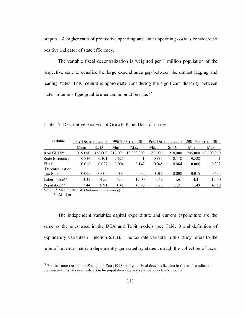
111

outputs. A higher ratio of productive spending and lower operating costs is considered a

positive indicator of state efficiency.

The variable fiscal decentralization is weighted per 1 million population of the

respective state to equalize the large expenditures gap between the utmost lagging and

leading states. This method is appropriate considering the significant disparity between

states in terms of geographic area and population size. 78

Table 17. Descriptive Analysis of Growth Panel Data Variables

Variable Pre-Decentralization (1996-2000), n=130 Post-Decentralization (2001-2005), n=130

Mean St. D. Min Max Mean St. D. Min Max Real GRDP* 319,000 428,000 210,000 18,900,000 683,000 938,000 295,000 43,600,000

State Efficiency 0.856 0.101 0.627 1 0.831 0.118 0.538 1Fiscal 0.018 0.027 0.004 0.147 0.045 0.064 0.006 0.372 Decentralization Tax Rate 0.005 0.005 0.001 0.032 0.010 0.008 0.015 0.435

Labor Force** 3.33 4.53 6.57 17.00 3.40 4.61 4.41 17.40

Population** 7.44 9.91 1.45 43.80 8.23 11.21 1.49 48.50Note: * Million Rupiah (Indonesian currency). ** Million

The independent variables capital expenditure and current expenditure are the

same as the ones used in the DEA and Tobit models (see Table 9 and definition of

explanatory variables in Section 6.1.3). The tax rate variable in this study refers to the

ratio of revenue that is independently generated by states through the collection of taxes

78 For the same reason, the Zhang and Zou (1998) studyon fiscal decentralization in China also adjusted the degree of fiscal decentralization by population size and relative to a state’s income.

112

as a percentage of GRDP. The extension of the endogenous growth model for public

capital expenditure uses a variable tax rate to explain the effects of fiscal decentralization

on economic growth (Barro 1990, Davoodi and Zou 1998).79

The control variables in the panel data model for a robustness test include private

investment, labor force and population. A number of empirical analyses have validated

the positive role of private investment on economic growth. Both domestic and Foreign

Direct Investments (FDI) are argued to have significant effects on growth, supporting the

genesis of the growth theory from a neoclassical perspective. The effect of private

investment has also been proven more significant than that of public investment in

developing countries (Khan and Reinhart 1990). Labor force growth generally

corresponds to population growth, which can be the driver of economic growth in

regions.

In addition, the model also incorporates spatial dummy variables to analyze

particular growth effects in the eastern region and lagging states. Most of the lagging

states are located in the eastern region, except for East Kalimantan and South Sulawesi.

The panel data also controls for time dependency in the model, in particular for the period

during the financial crisis (1997-1999).

79 The Granger test in Appendix B.4 shows that the direction of the causality is from state revenue to real GRDP and there is no indication of reverse causality.

113

6.2.2. Growth Model Using Fixed Effect Panel Data Regression

Panel data analysis encompasses a form of longitudinal data analysis across time

and subjects; and therefore suits the purpose and structure of this study, where multiple

subject data elements are analyzed over a specific time frame. The cross sectional panel

data regression in this model has the following equation:

lnyit = δ1+ δ2lnλit+ δ3lnθit+ δ4tit + δ5lng1it+ δ6lng2it+ + δ9lnXit+ε (8)

All variables except for dummy variables are expressed in the form of percentage

growth rate (log format). The following variables are used in the regression:

λ : Fiscal Efficiency of State Government

θ : Measure of Fiscal Decentralization per Capita

t : Measure of Tax Rate

g1 : Public Capital Expenditure80

g2 : Current Government Expenditure

X : Control Variables

yit is Regional Growth (measured as growth of Real GRDP)

80 Considering the size and scope of the projects that were handled by each state, it is assumed that most of the public capital investments could be fully operated within a year and therefore variable g1 is assigned to use 1-year lag. Mega public investment projects were typically managed by the central government since state financial resources typically could not provide an adequate amount of funding for this type of projects.

114

This study considered using either a fixed effect or a random effect model in the

empirical analysis of the growth model. The fixed effect panel has constant slopes but

different intercept points according to the cross-sectional group. Although it is assumed

that there are no significant temporal effects, major differences among states are allowed

in this type of model. The intercept is based on cross-sectional specific data that are

different between states, and may or may not differ over time. In the fixed effect model,

this unobserved effect is assumed stable (fixed) over time. The random effect panel

model has a random constant term in which the intercept is a random outcome variable.

The random effect model is generally used if unobserved effects, which are not correlated

with independent variables, are expected.

One problem with panel data analysis is autocorrelation, which is when there is a

correlation between variables observed in the model due to the nature of time series

modeling. Another problem with panel data is related to heteroskedasticity where the

biased outliers affect the regression slope. In deciding which type of panel model to use,

the main objective is to minimize these problems. In statistical terms, the analysis should

include a test to estimate the unobserved heterogeneity as a parameter of the model (fixed

effects) or as an outcome of a random variable (random effects).

The Hausman specification test is utilized to verify whether the fixed or random

effects model should be used.81 This test would compare an efficient model against a

consistent model to ensure that the more efficient model also gives consistent results. In 81 If there is no significant correlation between unobserved effects and explanatory variables (regressors), then the random effects model is more appropriate. But, if there is such a correlation, the parameters of the random effects model would be inconsistent and therefore fixed effects model should be used.

115

general, fixed effect models always give consistent results, but may not be the most

efficient models to conduct estimates. The result of the Hausman test in Appendix D

confirms that the coefficients estimated by the efficient random effect estimator are the

same as the coefficients estimated by the consistent fixed effect estimator. Accordingly,

the time fixed effect model should be used.

Panel Data Regression with Observations from 26 States

Table 18 exhibits the outcome of the panel data analysis with all 26 states. The

growth model uses a log function as expressed in equation (8) for the dependent variable

and several of the independent variables. The baseline regression includes the following

explanatory variables: State Efficiency, Fiscal Decentralization, Tax Rate, Capital and

Current Expenditures. For each key explanatory variable, an interaction term with post-

decentralization time dummy is constructed to measure the impact of the respective

variable on regional growth after decentralization.

The sign of the coefficients and their significance levels are mostly consistent as

control variables are added in the model, which supports the robustness of the model.

The variable state efficiency is chosen in lieu of technical efficiency based on the results

of the regression analysis in Appendix E. State efficiency has a lower impact on growth

than technical efficiency, although the coefficients of both variables are insignificant due

to the exclusion of other growth factors. Since state efficiency accounts for adjustments

that are proven to have a lesser impact on growth, this study will use the adjusted value as

a more conservative efficiency measurement of state government.

116

Table 18. Growth Panel Model with 26 States (1996-2005)

Dep. Var (Log GRDP): n = 260 Obs (26 States)

Regional Growth

Indep. Var. (1) (2) (3) Constant

-3.83 (-3.89)*

-1.92 (-2.01)**

-1.31 (-1.65)***

State Efficiency

0.55 (5.15)*

0.41 (4.07)*

0.53 (6.33)*

State Efficiency (D)

-0.61 (-5.44)*

-0.48 (-4.60)*

-0.55 (-6.34)*

Log Fiscal Decentralization

-0.40 (-5.56)*

-0.36 (-5.34)*

0.45 (4.67)*

Log Fiscal Decentralization (D) Log Tax Rate

0.13 (1.38) -0.58

(-8.69)*

0.12 (1.46)

-0.47 (-7.32)*

0.01 (0.16)

-0.51 (-9.60)*

Log Tax Rate (D)

0.03 (0.32)

-0.002 (-0.02)

0.27 (3.45)*

Log Capital Expenditure

0.32 (2.68)*

0.27 (2.48)**

0.04 (0.39)

Log Capital Expenditure (D)

-0.29 (-2.26)**

-0.22 (-1.87)**

-0.58 (-0.57)**

Log Current Expenditure

0.91 (10.37)*

0.81 (9.80)*

0.28 (3.31)*

Log Current Expenditure (D)

0.24 (2.10)**

0.18 (1.69)**

0.05 (0.59)

Eastern Region Dummy

-0.16 (-1.81)**

-0.16 (-2.01)**

-0.13 (-1.99)**

Eastern Region Dummy (D)

-0.16 (-1.35)

-0.18 (-1.63)***

0.03 (0.30)

Crisis Period

-0.59 (-2.68)*

-0.57 (-4.24)*

-0.47 (-5.00)*

Log Investment

0.10 (6.57)*

0.08 (6.35)*

Log Labor Force

0.84 (10.33)*

Adj. R-square 0.88 0.90 0.93 F-value 89.74 102.80 146.87 Prob > F 0.00 0.00 0.00

Note: t-statistics are in parentheses. All regressions are controlled for time specific dummies. * The point estimate is significant at the 1% level. ** The point estimate is significant at the 5% level. *** The point estimate is significant at the 10% level. (D) Interaction Term between selected explanatory variable and the post-decentralization time dummy

117

The first finding from the model is that an increase in state efficiency is associated

with higher regional growth. A 0.1-point increase in the level of state efficiency is

associated with a 0.053 percent higher growth. The result is significant at a one percent

level. However, in the post-decentralization period, state efficiency is associated with

lower regional growth. This is evidence that the implementation of decentralization has

not improved state efficiency in support of growth, which is contrary to the main

hypothesis. Although decentralization may provide incentive structures for states to be

independent in allocating their fiscal resources, it may not necessarily affect the

capability of a state to allocate resources into productive spending, which is one of the

key factors of economic growth at the regional level.

Assuming that there are no significant changes in investment and labor force in

the states, the degree of fiscal decentralization has a positive association with growth.

With a one percent increase in the degree of fiscal decentralization, regional growth is

expected to increase by a 0.45 percent. This finding supports the primary hypothesis H-

P1 where decentralization is argued to provide incentive structures to regions to grow.

Yet if there are greater imbalances within regions following a disproportionate growth in

labor force and population, then a higher degree of fiscal decentralization is associated

with lower economic growth. This proves that regional imbalances, which are a crucial

issue in many developing countries, are one of the disincentives or disadvantages in the

decentralized system.

The coefficients of fiscal decentralization in the post-decentralization period are

not significant. Although the sign of the coefficients are positive, there is an indication

118

that the effect of an increase in the degree of fiscal decentralization on regional growth is

insignificant or marginal. This result is consistent with recent observations of the

implementation of decentralization in Indonesia that determine decentralization is the

cause of increased inefficiency, rent seeking and corruption at the regional level.

State tax rates are associated with lower regional growth rates, where a one

percent increase in tax rates causes a 0.51 percent decline in the growth rate. This

correlation is expected and significant at the one percent level in a one-tail test. In the

post-decentralization period, the tax rate coefficient is positive after controlling for

investment and labor force growth, indicating that the negative impact from higher tax

rates on regional growth is less. This finding provides evidence that decentralization may

actually increase tax competition between regions that aims to spur development.

Furthermore, this finding also confirms the expected outcome from the secondary

hypothesis H-S2 where a higher ratio of state tax revenue hurts regional growth.

Although the negative impact of higher tax rates on growth is significantly less

after the implementation of decentralization, this does not necessarily mean that state

taxes, charges, and fees were lower in the post-decentralization period, as shown in Table

17. This may indicate that states have more control in assigning taxes, charges, and fees

that potentially have less negative impact on economic growth.

Both public capital expenditure and current expenditure have a positive

relationship with regional growth. The coefficients of these two variables are statistically

significant. A one percent increase in capital expenditure boosts regional growth by a

0.04 percent, while a one percent increase in current expenditure is associated with a 0.28

119

percent increase in growth holding the growth of investments and labor force constant

among regions.

The effect of current expenditure on growth is greater than the effect of capital

expenditure on growth although it is generally assumed that current expenditure is less

productive than capital expenditure. Current expenditure is routine or concurrent

expenditure that covers state operating costs and is not directly aimed to improving

public welfare through public capital projects. However, it is also important to put into

perspective the drastic increase in the size of current expenditure that can be attributed to

the transfer in government employees and programs from the central government to the

state level. In the descriptive analysis that is presented in Table 9, the size of spending in

current expenditure is almost twice the spending in capital expenditure, which could be

the cause for a greater effect on growth. A significantly larger current expenditure will

also have an immediate impact on the economy compared to inadequate spending on

capital investments that do not necessarily bear a significant impact on the economy.

The impact of capital expenditure on growth is significantly lower after

decentralization. A one percent increase in capital expenditure is associated with a 0.58

percent decline in growth compared to the period before the implementation of

decentralization. This indicates the possibility of misallocation of resources that is driven

by corruption and rent seeking at the regional level. Laws and regulatory oversight have

not been responsibly implemented to overcome these types of illegal activities. Another

reason for this finding is that capital expenditure actually declined after decentralization

due to budget constraints and increase in risks associated with economic uncertainty. The

120

financial crisis put many public capital investment projects on hold as the costs of the

projects drastically increased. Unfortunately, many of these projects were critical

infrastructure projects that can accelerate growth and development in the regions.

On the contrary, the effect of state current expenditure on growth is higher in the

post-decentralization period compared to the pre-decentralization period. This result is

consistent with a sharp increase in the level of current expenditure in the post-

decentralization period, which may be a factor that boosts regional growth.

The control variable, private investment, is significantly correlated with higher

regional growth where a one percent increase in private investment leads to a 0.08

percent growth controlling for growth of labor force at the regional level. The size of the

labor force is another factor that significantly affects regional growth. To a certain

degree, the population and demographic distribution, as well as factor mobility influence

the growth of the labor force. Thus, regional imbalances are a critical factor for regional

growth particularly in a decentralized system.

Based on the sign and level of significance of the spatial dummy variables, being

in the eastern region decreases growth rates by almost 0.11 percent and being a lagging

state will decrease growth rates further. These results are as expected, considering the

extent of disparities between the eastern and western regions in Indonesia. Looking

further at the coefficient of the dummy variables for the eastern region, lagging states are

actually better off after the implementation of decentralization. Yet, it is not obvious that

121

the implementation of decentralization has helped to reduce the level of inequality

between regions and to support long-term regional convergence.82

The crisis period variable is a time dummy variable that includes the period of the

financial crisis from 1997-1999. In aggregate, during the 3-year period of the financial

crisis the growth rate contracted by about 0.59 percent.83

Panel Data Regression with Observation from Lagging and Leading States

This last section of the empirical analysis examines whether the effects of the

explanatory variables on growth rates differ for lagging and leading states. It can be

determined that regional imbalances are one of the key factors that influence the success

or the net benefits of a decentralization policy. This further emphasizes the need to

determine the extent of the different impacts of state efficiency levels and the degree of

fiscal decentralization in particular on regional growth for lagging and leading states.

Table 19 and 20 present the result of growth panel data regression for lagging

states and leading states independently. As previously identified, lagging states consist of

fifteen states and leading states consist of eleven states

82 One of the expected roles of a decentralized system is to allow more distribution of wealth or opportunity in order to accumulate wealth through better public sector. Yet in many cases, a decentralized system benefits only certain regions due to the imbalanced revenue sharing system. Current studies on regional disparities in Indonesia also argue that decentralization has not been successful in overcoming inequality, although there have been tremendous growth and development in lagging regions (Aritenang 2008). 83 Nationally, the growth rate stood at 8 percent in 1996 before declining to 4.7 percent in 1997. At the peak of the crisis, growth rate declined by more than 13.1 percent compared to the rate of growth in 1996 (see Appendix F.1).

122

Table 19. Growth Panel Model in Lagging States (1996-2005)

Dep. Var (Log GRDP): n = 150 Obs (15 States)

Regional Growth

Indep. Var. (1) (2) (3) Constant

-1.22 (-0.59)

-0.87 (-0.46)

-0.79 (-0.50)

State Efficiency

0.55 (3.83)

0.49 (3.65)*

0.50 (4.51)*

State Efficiency (D)

-0.57 (-3.84)*

-0.52 (-3.82)*

-0.53 (-4.63)*

Log Fiscal Decentralization

-0.52 (-4.53)*

-0.52 (-4.96)*

0.22 (1.68)***

Log Fiscal Decentralization (D) Log Tax Rate

0.09 0.62) -0.51

(-7.42)*

0.12 (0.90)

-0.45 (-7.00)*

-0.07 (-0.57)

-0.45 (-8.42)*

Log Tax Rate (D)

0.07 (0.68)

0.05 (0.53)

0.21 (2.64)*

Log Capital Expenditure

0.06 (0.32)

0.05 (0.27)

-0.13 (-0.82)

Log Capital Expenditure (D)

-0.09 (-0.43)

-0.05 (-0.26)

-0.58 (-0.57)

Log Current Expenditure

0.89 (9.41)*

0.86 (9.73)*

0.39 (4.04)*

Log Current Expenditure (D)

0.04 (0.28)

0.03 (0.24)

0.06 (0.61)

Eastern Region Dummy

-0.10 (-1.04)**

-0.07 (-0.86)

-0.09 (-1.26)

Eastern Region Dummy (D)

-0.17 (-1.36)

-0.23 (-1.97)***

-0.02 (-0.24)

Crisis Period

-0.59 (-2.68)*

-0.57 (-4.24)*

-0.47 (-5.00)*

Log Investment

0.07 (4.71)*

0.07 (5.62)*

Log Labor Force

0.79 (7.60)*

Adj. R-squared 0.81 0.83 0.88 F-value 29.86 34.23 49.89 Prob > F 0.00 0.00 0.00

Note: t-statistics are in parentheses. All regressions are controlled for time specific dummies. * The point estimate is significant at the 1% level. ** The point estimate is significant at the 5% level. *** The point estimate is significant at the 10% level. (D) Interaction Term between selected explanatory variable and the post-decentralization time dummy

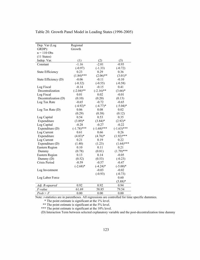
123

Table 20. Growth Panel Model in Leading States (1996-2005)

Dep. Var (Log GRDP): n = 110 Obs (11 States)

Regional Growth

Indep. Var. (1) (2) (3) Constant

-1.16 (-0.97)

-2.01 (-1.33)

-0.93 (-0.72)

State Efficiency

0.23 (1.84)***

0.29 (2.06)**

0.36 (3.01)*

State Efficiency (D)

-0.06 (-0.32)

-0.11 (-0.55)

-0.10 (-0.58)

Log Fiscal Decentralization

-0.14 (-2.04)**

-0.15 (-2.16)**

0.41 (3.66)*

Log Fiscal Decentralization (D) Log Tax Rate

0.01 (0.10) -0.65

(-4.92)*

0.02 (0.20)

-0.72 (-4.77)*

-0.01 (0.13)

-0.65 (-5.04)*

Log Tax Rate (D)

0.06 (0.29)

0.08 (0.38)

0.02 (0.12)

Log Capital Expenditure

0.54 (3.89)*

0.53 (3.84)*

0.35 (2.92)*

Log Capital Expenditure (D)

-0.28 (-1.78)***

-0.27 (-1.68)***

-0.22 (-1.63)***

Log Current Expenditure

0.61 (4.83)*

0.66 (4.76)*

0.26 (1.92)***

Log Current Expenditure (D)

0.21 (1.40)

0.19 (1.23)

0.22 (1.64)***

Eastern Region Dummy

0.10 (0.78)

0.11 (0.81)

0.21 (1.79)***

Eastern Region Dummy (D)

0.13 (0.52)

0.14 (0.53)

-0.05 (-0.23)

Crisis Period

-0.59 (-2.68)*

-0.57 (-4.24)*

-0.47 (-5.00)*

Log Investment

-0.03 (-0.93)

-0.02 (-0.73)

Log Labor Force

0.60 (5.88)*

Adj. R-squared 0.92 0.92 0.94 F-value 61.69 58.85 79.54 Prob > F 0.00 0.00 0.00

Note: t-statistics are in parentheses. All regressions are controlled for time specific dummies. * The point estimate is significant at the 1% level. ** The point estimate is significant at the 5% level. *** The point estimate is significant at the 10% level. (D) Interaction Term between selected explanatory variable and the post-decentralization time dummy

124

The result shows that an increase in the level of state efficiency is associated with

higher regional growth in both lagging and leading states. A 0.1-point increase in the

level of state efficiency is associated with a 0.050 percent growth in lagging states and a

0.036 percent growth in leading states. Both coefficients of state efficiency are

significant at a one percent level.

After the implementation of decentralization, the impact of state efficiency levels

on economic growth was lower since the net effect of the interaction coefficient is

negative. Although this finding is consistent with the previous panel data regression

using 26 state observations, the net effect of the state efficiency levels on regional growth

differs between lagging and leading states. Leading states seem more capable in

efficiently allocating fiscal resources to support growth after decentralization. This result

satisfies the primary hypothesis H-P1, which argues that the impact from decentralization

on economic growth differs for lagging and leading states.

Part of the problem with a declining level of state efficiency is attributed to the

challenges that lagging states faced in managing fiscal decentralization. A rapid rise in

fiscal resources after decentralization meant that state government had a greater capacity

to spend, although some may not have had adequate resources and strategic plans in place

to allocate spending appropriately. In many cases, this also became a cause for

corruption and rent-seeking activities where state leaders allocated resources to benefit

certain group or people that had provided political support. Hence, this study cannot

confirm whether these practices were more common in lagging or in leading states.

125

Consistent with the results in the previous panel data regression with 26 state

observations, the relationship between fiscal decentralization and economic growth turns

positive with the inclusion of control variables population and labor force. A one percent

increase in the degree of fiscal decentralization is associated with a 0.22 percent higher

growth in lagging states and a 0.41 percent in leading states. There is a significant

reverse correlation between fiscal decentralization and regional growth when the model

does not control the growth of investment and labor force.

After the implementation of decentralization, the impact from an increase in the

degree of fiscal decentralization on regional growth is less than in the period prior to

decentralization, holding the control variable constant. The sign of the coefficient for

fiscal decentralization is negative in both lagging and leading states, but the impact is less

for leading states than for lagging states. A one percent increase in the degree of fiscal

decentralization is associated with a 0.07 percent lower growth in lagging states and only

a 0.01 percent lower growth in leading states assuming that there is no significant change

in the growth of investment and labor force among regions. The fact that a larger degree

of fiscal decentralization is associated with lower regional growth provides an indication

of misallocation of fiscal resources. This finding also confirms that the implementation

of decentralization had more detrimental effect on lagging states compared to leading

states.

The panel data regression finds that a one percent increase in tax rates was

associated with a 0.45 percent lower growth rate in lagging states and a 0.65 percent in

leading states. The coefficients are significant at the one percent level, holding the

126

growth of investment and labor force constant. A higher negative impact from tax rates

on growth is more dominant in leading states since they have a higher capability to tax at

a higher rate and increase charges or fees from various sources. Leading states have a

larger size and economies of scale due to the size of their population, capacity and

diversification in their economy. Consequently, leading states have a larger tax base, as

the private sector is more willing to invest. Yet, a higher tax rate can increase the cost

structures in the economy that may negatively affect economic growth.

This outcome further validates one of the consequences of decentralization where

states have the power to set new tax rates, charges and fees, but can run into the risk of

excessive taxation. Although the negative impact from tax rates on growth is lower and

can be assumed to be triggered by tax competition between states after decentralization,

there is still a greater risk of higher tax rates on regional development. To balance the

potential negative impacts from tax rates on economic growth, states should ensure that

revenues from taxes, charges and fees are optimally utilized and distributed to benefit the

public and private sectors. In several cases, new taxes, charges and fees have been

introduced as part of schemes to enrich certain people that hold power in the state

government. This may be due to a lack of accountability and oversight.

The coefficients for public expenditure in the panel data model with lagging states

are for the most part insignificant, except in the case of current expenditure in the pre-

127

decentralization period.84 Yet, the sign of the coefficients indicate that an increase in

capital expenditure is associated with lower regional growth. The sign of the interaction

coefficient in the post-decentralization period is also negative, which indicates that an

increase in capital expenditure further lowers growth due to inefficiency and

ineffectiveness in the allocation of capital spending.

Lagging states were not well prepared to manage a rapid increase in capital

investment projects due to a lack of experience and resources. The less developed

institutions in the lagging states also cause a lack of oversight on the allocation and

management of capital investment projects. This would have an effect on the capability

to limit abuses of power and corruption.

Other factor that affects inefficiency in capital spending is an increase in the scale

and scope of programs that transferred to states by the central government. In some

instances, states choose to cut their capital investment budget and spend a larger

percentage of the budget on current expenditure as they are unable to manage certain

level of capital investment projects. Consequently, these actions would lower the level of

competitiveness and economic growth at the regional level. Furthermore, this can hinder

efforts to reduce regional disparities between lagging and leading states and between

eastern and western regions in Indonesia.85

84 Due to a lack of statistical significance in the model, the effect from public expenditure on growth in lagging states is inconclusive and therefore the coefficients are not interpreted. 85 A number of studies agreed that the decentralized system in Indonesia has not reduced the level of regional inequality. If regional convergence did in fact occur after the 1997 financial crisis, following a significant decline in the growth rates of most leading states, it was more likely temporary convergence.

128

An increase in current expenditure in lagging states is significantly associated

with higher growth in the 10-year period of analysis where a one percent increase in

current expenditure is associated with a 0.39 percent increase in growth. Even though

the current expenditure coefficient in the post-decentralization is not significant, the sign

of the coefficient is positive, which indicates that an increase in current expenditure after

decentralization further boost regional growth in lagging states.

Looking at the sign and statistical significance of the public expenditure

coefficients in leading states, it can be determined that an increase in both capital and

current expenditures is associated with higher growth in the 10-year period of analysis.

A one percent increase in capital expenditure will increase regional growth by 0.35

percent; while a one percent increase in current expenditure is associated with 0.26

percent increase in growth. This result shows that, as expected, the effect of capital

expenditure on economic growth is higher than the effect of current expenditure, which is

opposite to the results in the panel data model for lagging states. Again, it proves that

leading states are more capable in strategically allocating capital spending to productive

activities than lagging states.

The effectiveness of capital expenditure in supporting growth significantly

decreased after decentralization in leading states. Thus, indicating the possibility of

misallocation of capital spending after the implementation of decentralization. This is

similar to what occurred in lagging states. Lower productivity of capital spending after

decentralization is also a major issue in many developing countries.

129

A drastic decrease in capital spending caused by a state’s limited financial

capacity may also contribute to low productivity of capital investment projects. With

limited financial capacity, states may choose to satisfy their current expenditure

obligations first, while delaying spending on capital investment projects. The decision to

grant capital investment needs lower priority may further challenge the level of state

competitiveness and result in lower economic growth. Furthermore, there is also the

possibility that an increase in current expenditure is part of ongoing rent seeking and

corrupt practices, since oversight and accountability over current expenditure are weaker

than over capital expenditure.

The productivity of current expenditure in supporting growth in leading states

significantly increases after decentralization. Part of the reason for this is the sharp

increase in current expenditure to administer the programs and services that were

transferred to the states by the central government. Financing additional current

expenditure may have come at the expense of capital expenditure, yet, it seems that part

of the current expenditures went to the regional economy and supported growth.86

The results of the empirical analysis indicate that decentralization tend to benefit

leading states more compared to lagging states, suggesting that leading states were more

prepared and capable of exploiting the advantages of a larger fiscal capacity. Leading

states are also argued to be more competent in managing fiscal decentralization with the

more adequate support of human resources, management systems and technologies.

86 Several studies have found a similar result associated with lower capital expenditure because of increased in the current expenditure after decentralization (Bose 2003, Rodriguez-Pose et. al. 2007).

130

6.3. Evaluation of Decentralization and Regional Competitiveness Policies

The collaboration between decentralization and regional competitiveness policies

is key to creating robust and sustainable growth in Indonesian states. Yet, a number of

challenges persist in particular since decentralization in Indonesia was not initially

planned within the framework of an economic policy, but was rather the result of political

compromise. Some of these challenges are discussed in an attempt to understand the

complexity of policies that focus on revitalizing regions to become more competitive in a

decentralized system.

First, there has been imbalanced development and a concentration of the market

economy in certain regions. Rapid growth during the New Order was limited to specific

regions, at the expense of other regions. One reason why this occurred was due to

restrictive government regulations and the influence of specific interest groups, which is

a common practice in the market economies of developing countries. Consequently, this

limited the ability of state governments to stimulate and sustain the real sector of the

economy to support local economic development in specific regions. A strong local

economy will help support the national economy and with a strong local market and real

sector of the economy, the impact from future economic crises could potentially be

minimized.

Second, there has been a lack of coordination in the economic policies to support

a strong and diverse regional economy. Strategic economic policies with clear priorities

are needed to develop the real sector of the regional economy, encourage entrepreneurial

131

activities and build industrial integration.87 An example of those sound economic

policy are the assurance of property right, contract law, and non-discriminatory toward

small businesses. Economic policies during the New Order were geared towards

supporting large conglomerations and state owned enterprises, which were influenced by

certain interest groups and the regime in power.

Third, the public sector in Indonesia was impaired by entrenched corruption and

rent seeking, ranking the country as one of the most corrupt in the world. Furthermore,

red-tape bureaucracy has been the primary causes for inefficiency in the public services.

This also affects the competitiveness level of private sector due to higher transaction cost.

In the private sector, the low competitiveness of firms and enterprises is also caused by

protectionist policies, among other policies, issued by the government that created wrong

incentive structures and resulted in negative externalities.

In conclusion, growth in Indonesia has been unsustainable because has been a

lack of policies to strengthen the relationship between institutions, markets and firms. At

a sub-national level, such policies should focus on the development of local institutions

and the market economy. These policies are best to follow the concept of Market

Preserving Federalism, which provides direction on how to create incentive structures in

a decentralized or federal system using a market mechanism.88 Based on this

87 Co-ops (Koperasi) has been used to promote local economic development and to provide a strong foundation for a market economy has not been optimal. In addition, the state government also supports entrepreneurial through a number of policies, such as the non-discriminatory toward small businesses, special loans or credits to small–medium enterprises. 88 The New Institutional Economics aim to depict the relationship between institutions and the market economy. Economic reform in developing countries is intended to reap the benefits of the market

132

framework, it is important for state governments to facilitate the development of the

private sector and market economy through laws, policies and regulations. By pursuing

this path, Indonesia should be able to achieve sustainable growth and better manage

future financial crisis.

One of the key concepts of decentralization is creating incentive structures,

which can increase the efficiency of state governments. Several factors drive state

efficiency levels. Policy analysis should evaluate these factors to understand how to

maximize the benefits from the implementation of decentralization. This dissertation has

identified a number of factors that influence state efficiency levels, which result from the

implementation of fiscal decentralization. One policy that can raise state efficiency

levels is the decision to allow states to generate their own revenues. The centralized

revenue system that was implemented in Indonesia during the New Order has been

proven to be an obstacle to development because it has resulted in an imbalanced

distribution of growth. Another policy to increase efficiency levels is to offer incentives

for states to spend on human capital development utilizing technology.89

The empirical analysis of this dissertation has concluded that policies to support

higher levels of fiscal decentralization and state efficiency are critical for economic

growth. The following fiscal decentralization policies should be further examined to

ensure that state governments promote appropriate incentives.

economy, but in many cases, there has been little attention to and progress on the institutional front. To a certain degree, this was exactly the problem in Indonesia before the 1997 economic crisis. 89 The analysis shows that the organizational management through better administration and increased productivity of state employees influences state efficiency. However, these may not affect growth significantly even if the quality of public service is improved.

133

First, a review should be performed of policies that regulate and monitor the

utilization of public funding and public debt.90 With the expansion of a market economy,

there is a desire by states to finance development through market mechanisms. States can

sell local bonds through domestic financial markets in order to broaden their access to

capital. However, states must also be aware of the moral hazard that can exist if states

borrow excessively, forcing central governments to bail them out, ultimately putting a

country’s macroeconomic stability at risk.91

Second, an analysis of policies that dictate how revenues are generated and how

expenditure is used to ensure that states have the capability and capacity to meet their

goals should be undertaken. Restrictions on the types and sources of revenues will cause

state and district governments to find other ways to balance their budget. So, if state and

district governments are not allowed to introduce new taxes, charges or fees other than

what has been determined by law, they will be forced to increase current tax rates,

charges, and fees in order to raise revenues and close fiscal gaps. Consequently, tax

distortions may raise costs excessively and burden the private sector, limiting its ability to

compete in a market economy.92

90 Regulations that allow state governments in Indonesia to issue debt has been delayed considering the potential risks in regard to the accountability and moral hazard. 91 It is important that state governments recognize the dangers or risks of excessive spending that are financed with debt. This issue becomes more critical when states’ spending on specific capital investments is not efficient or productive. 92 States that are not endowed with many natural resource or that lack economic advantages will have to carefully consider raising taxes, charges, and fees. These actions may have a negative impact on the level of investment and economic growth. The concern is typically on the indirect taxes that hinder productive efficiency. Moreover, this type of taxes can be easily levied in developing countries, for examples fees collected in ports and roads.

134

Third, an assessment should be done of regulations that distinguish between

national and sub-national expenditures, to ensure that central government intervention on

spending decisions in the regions is limited.93 Currently, decentralization policies in

Indonesia have not clearly assigned expenditure responsibilities between the different

levels of government. Under the new decentralization law, state and district governments

do not have spending restrictions but are required to maintain a balanced budget. There

have been debates on whether policy guidelines should be established to specify a

minimum portion that should be allocated to critical sectors. An example of this is the

existence of a minimum percentage that must be allocated to expenditure on education,

health and infrastructure to support the desired level of productivity and development in a

region. This type of policy guideline should correspond with national development

strategies that promote competitiveness. However, the government should be aware that

these types of guidelines are still considered another form of central government

intervention.

Fourth, it is important to ensure that there is sufficient funding for programs and

services that are being transferred to the regions to better overcome unfunded mandates.

With changes in the distribution or allocation of revenue and expenditure, the central

government transfers a number of programs and services that are initially the

responsibility of the central government, to the sub-national level governments without

considering the financial consequences to the states. State governments may suddenly 93 The central government has full control over spending associated with national interests, such as providing national defense, maintaining macroeconomic stability, and funding public utilities that benefit the entire country.

135

find themselves responsible for funding part or all of these programs and services.

Problems can surface when states do not have sufficient funds to cover the costs of these

programs and services because of restrictions on the types and bases of revenue that

states and districts can generate. This may cause an interruption of public services and

can jeopardize production activities of firms and enterprises, risking a region’s

competitiveness. To prevent this to take place, there is a need for a greater policy

coordination between the central and state governments94

Fifth, a review of policies related to the allocation of public capital expenditure at

both the national and regional levels should be conducted. Policies on public capital

investments should aim to increase productivity and reduce the cost of production. It is

important for states to identify the type, scale and scope of capital investments that can

encourage private sector development. States should explore the different types of

incentives that they can offer, such as tax incentives, critical infrastructure, access to

highly trained workers, and low production cost structures. States also need to manage

the challenges of balanced budget policies, whereby they are forced to use all the funds

allocated to specific programs within a certain time frame, even though the spending may

not be necessary.

94 Promoting public-private partnerships (PPP) to finance the development of public services is an alternative for limited state budgets, in the event that states are not allowed to issue debt. Public-private partnerships will not only provide the means for states to access capital, but also reduce the risks associated with certain capital investments. Hence, the issue with allowing the private sector to finance critical public services is related to how much balance exists between the service charged to consumers and the return to investment to private investors.

136

Sixth, it is necessary to manage policies on public capital investment to ensure

that the outcomes of these policies do not “crowd-out” private capital investment. An

excessive investment in public capital projects may cause the private sector to reduce its

investment and consumption, when in fact, the effect from private investment is

potentially larger than public investment when taking into account externalities and

spillovers into the regional economy. Thus, “crowding-out” can indirectly lower state

growth rates.

Seventh, it is important to support policies that promote good governance. These

policies should encourage transparency, accountability and the rule of law. In many

developing countries, one factor that has negatively influenced the efficiency and

productivity of public capital expenditure is corruption and rent-seeking activities.95

These illegal activities increase transaction costs and cause the regions to be less

competitive. The role of institutions is important and cannot be considered as an

exogenous factor anymore since it determines the quality of institutions and development

process as a whole (Borner et al. 2004). Regional institutions should have strong good

governance policies in place, otherwise decentralization will not be effective.96

Besides reviewing fiscal decentralization policies, it is also important to review

policies that aim to reduce disparities at the regional level. This issue is particularly

95 The term “soft money” refers to collusion practices whereby state officials collaborate with the private sectors for personal benefit. The lack of transparency in awarding and supervising contracts, collusion in the permit application, or the use of regulations to benefit certain groups are examples of where “soft money” is being used. This further deteriorates states capacity to allocate resources efficiently. 96 In the democratic system, decentralization should ensure the accountability of state government as demanded by the public.

137

critical for developing countries since it affects imbalances in state revenue and

development levels. Fair and progressive revenue sharing schemes between central and

state governments can help reduce regional disparities. Yet this type of redistributive

policy typically draws dissatisfaction from rich resource regions, because they believe

that it is unfair for the central government to exploit their resources to subsidize other

regions.

Growth policies at the regional level should take into consideration the investment

needs of the private sector. Private capital investment at the regional level is affected by

labor and population growth in addition to public goods and services that are provided by

the state. From the supply side, skilled labor is a key production input for firms and

enterprises. From the demand side, the private sector’s decision to invest is driven by

population growth, which ultimately determines what and where to produce.

In sum, the financial crisis in Indonesia provided a window of opportunity for

policy reform to occur. Hence, many of the policies are only geared towards short-term

solutions and have not been comprehensive enough to respond to more long-term

problems. Part of the reason for this is attributed to the uncertainty that existed at the

time when the policies were introduced. Decentralization policies should evolve over

time where policy reforms are allowed to realign the goals and strategies of development

and mitigate the negative side effects from the implementation of decentralization.

138

7. Concluding Remarks

This dissertation aims to expand previous empirical and theoretical approaches on

fiscal decentralization and economic growth with the inclusion of efficiency factors of

state governments. Past empirical studies on the effect of fiscal decentralization on

regional growth have been robust yet inconclusive in their results. Following the key

premise of decentralization, which provides state governments with incentives to become

more efficient and independent in managing their fiscal resources, it is crucial to also

measure the effect of state efficiency on regional growth.

This dissertation aims to fill gaps in the way state efficiency is measured by

developing a method to adjust technical efficiency scores from the non-parametric DEA

model that merely represents efficiency of expenditures. The adjustment is made using

the interaction between the following two determinants: ratio of productive spending and

operating costs. These two determinants represent state government choices and

preferences in allocating fiscal resources, which are also a reflection of the priorities in

development strategies and an indication of state institutional quality.

The process of decentralization influences state institutional setting where

political dynamics and performance of state administrators as economic agents are among

the key factors. In that regard, the bottom up process of decentralization supposedly has

an effect on state institutional setting as it encourages citizens to be more involved and

139

supportive in the process of decentralization and democratization. At the same time,

state administrators should be more transparent and responsible as the citizens demand

accountability for their action. Hence, the implementation of decentralization in

Indonesia has resulted in a greater unchecked power of state and district governments

that is considered as the cause for inefficiency, rent seeking and corruption.

In theory, regional competition is not a zero sum game since states are motivated

to become more efficient and productive in order to remain competitive. A decentralized

system also encourages states to compete against each other as they become more

independent. In reality, some states are more capable and prepared than others in

managing fiscal decentralization that serves the best interests of their citizens as well as

meeting their development goals. Furthermore, decentralization does not always provide

the same incentive structures; or in other word, a level playing field may not fully exist

between regions. Decentralization potentially assigns different incentive structures and

net fiscal benefits to specific regions, as an example, rich resource regions in Indonesia

may receive significantly larger transfers from revenue sharing schemes with the central

government. Although there is an effort to equalize transfers through General Allocation

Funds (DAU) and Special Allocation Funds (DAK), there are still fiscal imbalances that

give higher net benefits to certain regions.

Another factor can also affect growth at the regional level, such as the differences

in structure and economic capacity of regions. Certain regions may have larger

economies of scale and fiscal capacity that will influence the choices or preferences and

140

priorities in development policies, including the strategies over allocation of fiscal

resources.

One of the lessons learned from the implementation of decentralization in

Indonesia is the need to better plan the transition to a decentralized system. Lack of

consideration on issues surrounding decentralization policies, such as horizontal and

vertical fiscal imbalances, tax distortion and less accountability are recipes for failure that

will cost citizens of the respective states. It is necessary to prepare state governments to

manage both administrative and fiscal decentralization. Providing technical support in

the transition process to a decentralized system and constructing a framework of good

governance, particularly to lagging states, is critical to help states reap the benefits of

decentralization to accelerate growth and development in their region.

A larger policy framework on economic and social equity also needs to be an

integral part of decentralization. The role of the central government in supporting

lagging states may be limited under a decentralized system; however, it is the

responsibility of the central government to implement a fair distribution policy as one of

the fundamentals of regional competitiveness to help reduce regional disparities and

accelerate growth at the regional level.

This chapter provides a conclusion to this dissertation. The first part contains a

summary of the key findings. The second part discusses the limitations of the research

and the third part provides recommendations for future research needed on fiscal

decentralization and economic growth.

141

Summary of Key Findings

From the empirical analysis of the Tobit model it is evident that the degree of

fiscal decentralization in Indonesia influences state efficiency levels. Thus, it can be

concluded that decentralization policies provide a framework for incentive structures to

support higher state efficiency levels. The magnitude of the effect that fiscal

decentralization has on state efficiency levels was significantly higher in the post-

decentralization period in Indonesia.

Second, the ratio of variables productive spending and operating cost have an

inverse relationship with state efficiency levels in the post-decentralization period in

Indonesia. Contrary to this, productive spending had a positive correlation with state

efficiency levels in the pre-decentralization period, and the magnitude of this positive

correlation was significantly higher than in the post-decentralization period. This

indicates that state governments were less efficient in the decentralized system.

Third, the results of the Tobit model indicate that the ratio of state employee

salary and allowances that is part of current expenditure positively influences state

efficiency levels. It is implied that more spending on human capital development and

higher wages of state government employees can potentially improve state efficiency

levels. The rationale is that better welfare and improvement in the quality of state

government employees can increase productivity and potentially reduce rent seeking and

corruption in the states.

Higher revenue independence affects state efficiency levels through an underlying

assumption that state governments can be more efficient as they become more

142

independent in generating revenue from their own sources. Similar to the assumption

that relates productivity of state government employees to state efficiency levels, the

same principle applies to the assumption that principal agents in state organizations act

for the common purpose of the state, which is to improve public welfare and support the

process of development in their respective regions.

The Tobit model also confirms per capita income and per capita spending as

determinants of state efficiency. Still, the probability that per capita income has an effect

on state efficiency levels is very low in both the pre- and post-decentralization periods.

Therefore, it is valid to assume that per capita income is a weak explanatory variable of

state efficiency levels. In contrast, the probability that per capita spending has a negative

impact on state efficiency levels is significantly higher in the post-decentralization

period. One explanation for this is that states with a larger spending capacity following

decentralization are more inclined to be less efficient.

Followings are the results of the growth panel data analysis. First, fiscal

decentralization generally supports higher growth assuming that there are insignificant

imbalances in the growth of labor force. Hence, despite the fact that fiscal

decentralization is one of the stronger determinants of higher state efficiency, there is no

indication that the incentive structures from decentralization are associated with higher

growth. Of concern is whether a higher state efficiency levels following a larger fiscal

capacity cause corruption and rent seeking in the regions if compared to the period prior

to decentralization.

143

Second, when taking into account regional inequalities, the positive effect of

fiscal decentralization on economic growth is more apparent in leading states. Lagging

states often fail to reap the benefits of decentralization due to lower efficiency of state

governments in allocating fiscal resources, lower economic capacity and lack of own

resources. The results of this empirical study are in agreement with the argument that

there are different outcomes from the implementation of fiscal decentralization in lagging

and leading states.

As expected, a third result from the panel data analysis is that higher tax rates are

associated with lower growth because of an increase in the production costs of firms and

enterprises. The impact of high tax rates on growth in leading states is more significant

than in lagging states, reflecting the consequence of the choices made by leading state

governments to raise additional revenue through taxes, charges and fees since they have a

stronger and more stable economic structure.

A fourth outcome is that there is a tendency for state governments to increase

current expenditure at the expense of capital expenditure in a decentralized system,

negatively affecting economic growth. Unfortunately, because states have limited fiscal

resources and are not willing to reduce current expenditure and cut overhead costs,

capital expenditure is minimized. This path is taken even though the action puts the

competitiveness level of each respective state at risk. The results from the growth panel

data analysis support this conclusion, showing that the productivity of current

expenditure is higher than that of capital expenditure in the post-decentralization period.

In lagging states, capital expenditure has a negative relationship with economic growth

144

despite the argument that public capital expenditure is typically more productive in

supporting economic growth than current expenditure.

Contrary to the hypothesis, the negative correlation between public capital

expenditure and economic growth after the implementation of decentralization signifies

that increased capital spending results in higher inefficiencies in resource allocation. Part

of the inefficiencies can be attributed to poor capital expenditure choices by the state

government. It can also be due to increased rent seeking and corruption practices at the

regional level in the post-decentralization period. Since the productivity level of public

capital expenditure was significantly lower in lagging states compared to leading states, it

implies that the extent of rent seeking and corruption practices may be far more

entrenched in lagging states.

Research Limitations

This dissertation acknowledges that a number of constraints could not be fully

controlled, and may have affected the outcomes and interpretations of the empirical

analysis. The first constraint is the period of observation used in the empirical model,

where the process of decentralization coincided with the 1997 financial crisis. The extent

and depth of the economic shock and macroeconomic instability on state expenditure

could not be fully controlled, since the model did not include specific macroeconomic

variables such as interest rates and inflation.

The second constraint is data limitation. There were limited data for the pre-

decentralization period, which did not allow this study to include a lag of more than one

145

year in the model. This may have affected the results of the capital expenditure and

private investment variables in the growth model, since both have a lagging effect on

growth. Furthermore, there are limited data on the composition of public capital

expenditure for each sector of spending as well as inconsistency in data compilation.

The third constraint is related to the finding that fiscal decentralization has

contributed to regional growth in Indonesia, despite the fact that effects of state efficiency

on growth are small due to the extent of rent seeking and corruption at the regional level.

The following aspects can contribute to the contradiction between the findings in this

dissertation and current observations over the implementation of decentralization:

- This dissertation focuses on the efficiency of states in allocating fiscal resources and

it does not necessarily capture other causes of inefficiencies that take place in the

decentralized system in Indonesia, such as corruption, collusion and nepotism. The

difficulty of accounting for these inefficiency factors is related to the availability and

validity of data. An index of corruption or rent seeking has not been fully developed

at the regional level.

- States can be more efficient because of the structure and proportion of revenue

sharing which is relatively more constrained than that of local districts. Lower

revenue at the state level compared to the district level could mean lower spending

and potentially higher efficiency. As discussed in the beginning of this dissertation,

the reason to choose states as the unit of analysis is that studies that focus on states in

146

a decentralized system are lacking, eventhough states play a key role in setting up

priorities and strategies for development.97

- The period of observation in the growth panel data model did not include the period

of New Order prior of the 1997 financial crisis where the growth rate was

significantly high. The reason for this was to remove outliers where low level of

fiscal decentralization during the New Order is associated with high growth rate.

The last constraint in this dissertation is the assumption that state administrators

behave rationally in allocating fiscal resources to improve public welfare. In reality,

many of the state administrators have personal interests and aim to enrich themselves and

their supporter at the expense of the citizens of the states that they represent. Lucrative

contracts and other types of collusion activities are meant to compensate donors who

support candidates during the state election campaign (“soft money politics”). This can

result in inefficiency in fiscal resource allocation as personal interests instead of the

public interest influence state decision-making.

Suggestions on Future Research

Future studies should look at other factors that may influence state allocative

efficiency and the effectiveness of fiscal decentralization policy, such as the institutional

97 There is recently an effort to redefine the role of states as part of the 10-year assessment of the decentralization law in Indonesia. States are supposed to be the representatives of the central government responsible for providing oversight, assistance and coordinating local districts under their jurisdiction. Refer to UNDP (2009), “Ten Years of the Implementation of Indonesia's Decentralization: Reformulating the Role of the Province”, Online access: http://www.undp.or.id/press/view.asp?FileID=20090625-1&lang=en.

147

framework for the development of laws and regulations, politics and the leadership of

state governments. These areas can influence the dynamics between institutions in the

decentralization process, as many of the issues in a decentralized system are the result of

conflicts of interest between central and regional government, groups of people in power

and political parties. The inclusion of other institutional factors can also add to advancing

the literature on the relationship between democracy and decentralization.

Since a corruption index at the regional level does not currently exist, future

studies may want to explore the possibility of constructing a corruption index in order to

improve the growth panel data model presented in this dissertation. One possibility is to

correlate corruption with cost inefficiency in discretionary spending, which is typically

associated with state capital expenditure to finance specific public investments. Cost

inefficiency is also closely connected with the productivity of public capital expenditure.

The productivity of specific sectors of capital expenditure, including health,

education and infrastructure should be integrated in the future state expenditures study.

The inclusion of the composition of capital expenditure in the growth model makes it

possible to compare productivity factors by sector of capital expenditure against

economic growth. Doing so would help create a more robust policy discussion and

enable better decision making on the type, scale and scope of public capital investments.

More in-depth studies on regional imbalances and how they influence state

efficiency and regional growth are also suggested for future research. It is important to

examine the impact not only on growth, but also on state efficiency levels, of poverty,

income inequality and imbalances in the distribution of population and labor, since all of

148

these factors may affect how state governments allocate fiscal resources. Furthermore, in

any future study it is also important to include the spatial characteristics of states that

may influence allocative efficiency and economic growth. Differences in a state’s

jurisdictional area, population density and urban and rural concentration can affect the

process and outcome of decentralization as well. As an example, smaller states may be

more manageable and less bureaucratic, while densely populated states with larger urban

centers may benefit from the efficiency of public service delivery.

149

Appendix A

RECENT PROGRESS OF DECENTRALIZATION IN INDONESIA

Decentralization in Indonesia continues to move forward despite a number of

problems, particularly an increase in corruption and rent-seeking activities at the regional

level. One of the key issues with promoting good governance policy is the ambiguous

process in assessing transparency and accountability of state governments. This also

causes many state and district governments choose not to allocate capital spending in

order to avoid a legal fight when it comes to fiscal audits. Consequently, this stalls the

development in the regions as capital expenditures that are supposed to finance critical

infrastructure, health and educational facilities and transportation decline significantly. It

is important for the central government to resolve this issue to prevent a risk of being less

competitive compared to other East Asian countries.

A recent study by the World Bank has identified specific infrastructure investments

that are critical to strengthen the regional economy and increase competitiveness.98 New

investment initiatives and incentives for financing are the key to spur public-private

partnership and stimulate growth and development in the regions.

98“ Now is the time to build on the achievements of the past few years and to spend Indonesia’s financial resources effectively and efficiently to improve the quality of education, expand healthcare, close critical infrastructure gaps, in order to reduce poverty and build a competitive economy”. Online access: http://web.worldbank.org/WBSITE/EXTERNAL/COUNTRIES/EASTASIAPACIFICEXT/INDONESIA EXTN/0,,contentMDK:21433945~pagePK:141137~piPK:141127~theSitePK:226309,00.html#PER.

150

Appendix B

B.1. Granger Causal Test: (H0) State Spending affects GRDP Source | SS df MS Number of obs = 234 -------------+------------------------------ F( 2, 231) =10332.76 Model | 1.3981e+18 2 6.9907e+17 Prob > F = 0.0000 Residual | 1.5628e+16 231 6.7655e+13 R-squared = 0.9889 -------------+------------------------------ Adj R-squared = 0.9888 Total | 1.4138e+18 233 6.0676e+15 Root MSE = 8.2e+06 ------------------------------------------------------------------------------ GRDP | Coef. Std. Err. t P>|t| [95% Conf. Interval] -------------+---------------------------------------------------------------- GRDP_lag1 | 1.164899 .0148358 78.52 0.000 1.135668 1.19413 Total_Spen~1 | 1.581375 .6892525 2.29 0.023 .22335 2.9394 _cons | -454939.4 655738.1 -0.69 0.489 -1746931 837052.5 ------------------------------------------------------------------------------ ( 1) Total_Spending_lag1 = 0 F( 1, 231) = 5.26 Prob > F = 0.0227 (Significant at the 5% level – Reject H0) B.2. Granger Causal Test: (H0) State Spending affects State Revenue Source | SS df MS Number of obs = 260 -------------+------------------------------ F( 2, 257) = 3058.98 Model | 7.4811e+14 2 3.7406e+14 Prob > F = 0.0000 Residual | 3.1426e+13 257 1.2228e+11 R-squared = 0.9597 -------------+------------------------------ Adj R-squared = 0.9594 Total | 7.7954e+14 259 3.0098e+12 Root MSE = 3.5e+05 ------------------------------------------------------------------------------ Total_Reve~e | Coef. Std. Err. t P>|t| [95% Conf. Interval] -------------+---------------------------------------------------------------- Total_Reve~1 | 1.199314 .0911483 13.16 0.000 1.019821 1.378806 Total_Spen~1 | -.0697105 .1015295 -0.69 0.493 -.2696462 .1302253 _cons | 49449.84 25117.86 1.97 0.050 -13.19901 98912.88 ------------------------------------------------------------------------------ ( 1) Total_Spending_lag1 = 0 F( 1, 257) = 0.47 Prob > F = 0.4930 (Not Significant – Accept H0)

151

Appendix B

B.3. Granger Causal Test: (H0) Total Public Capital Expenditure affects Private Investments Source | SS df MS Number of obs = 234 -------------+------------------------------ F( 2, 231) = 44.75 Model | 2.0306e+09 2 1.0153e+09 Prob > F = 0.0000 Residual | 5.2412e+09 231 22689182.2 R-squared = 0.2792 -------------+------------------------------ Adj R-squared = 0.2730 Total | 7.2718e+09 233 31209403.6 Root MSE = 4763.3 ------------------------------------------------------------------------------ Total_Inve~s | Coef. Std. Err. t P>|t| [95% Conf. Interval] -------------+---------------------------------------------------------------- Total_Inve~1 | .5052403 .0536137 9.42 0.000 .399606 .6108746 Capex_lag1 | -.0001279 .0002823 -0.45 0.651 -.0006841 .0004284 _cons | 1333.895 362.1241 3.68 0.000 620.407 2047.383 ------------------------------------------------------------------------------ ( 1) Capex_lag1 = 0 F( 1, 231) = 0.21 Prob > F = 0.6511 (Not Significant – Accept H0) B.4. Granger Causal Test: (H0) State Revenue affects GRDP Source | SS df MS Number of obs = 234 -------------+------------------------------ F( 2, 231) =10156.94 Model | 1.3979e+18 2 6.9893e+17 Prob > F = 0.0000 Residual | 1.5896e+16 231 6.8813e+13 R-squared = 0.9888 -------------+------------------------------ Adj R-squared = 0.9887 Total | 1.4138e+18 233 6.0676e+15 Root MSE = 8.3e+06 ------------------------------------------------------------------------------ GRDP | Coef. Std. Err. t P>|t| [95% Conf. Interval] -------------+---------------------------------------------------------------- GRDP_lag1 | 1.178994 .0149928 78.64 0.000 1.149454 1.208535 Total_Reve~1 | .7099419 .6255137 1.13 0.258 -.5224995 1.942383 _cons | -441145.3 661382.6 -0.67 0.505 -1744259 861968 ------------------------------------------------------------------------------ ( 1) Total_Revenue_lag1 = 0 F( 1, 231) = 1.29 Prob > F = 0.2576 (Not Significant – Accept H0)

152

Appendix C

Chow Threshold Test: (H0) Coefficients in two linear regressions of different data sets (Lagging States and Leading States) are equal Source | SS df MS Number of obs = 260 -------------+------------------------------ F( 6, 254) =26977.04 Model | 75003.1066 6 12500.5178 Prob > F = 0.0000 Residual | 117.697562 254 .463376229 R-squared = 0.9984 -------------+------------------------------ Adj R-squared = 0.9984 Total | 75120.8042 260 288.92617 Root MSE = .68072 ------------------------------------------------------------------------------ logGRDP | Coef. Std. Err. t P>|t| [95% Conf. Interval] -------------+---------------------------------------------------------------- Lagging_st~s | 2.765 1.781436 1.55 0.122 -.7432657 6.273266 Lagging_K | .0114158 .0283985 0.40 0.688 -.0445108 .0673424 Lagging_L | .9564533 .1270595 7.53 0.000 .706229 1.206678 Leading_st~s | 8.273819 1.048804 7.89 0.000 6.208359 10.33928 Leading_K | .1881685 .0425988 4.42 0.000 .1042767 .2720604 Leading_L | .5410831 .0743392 7.28 0.000 .3946833 .6874829 ------------------------------------------------------------------------------ ( 1) Lagging_K - Leading_K = 0 ( 2) Lagging_L - Leading_L = 0 F( 2, 254) = 8.45 Prob > F = 0.0003 (Significant at the 1% level – Reject H0) ( 1) Lagging_K - Leading_K = 0 ( 2) Lagging_L - Leading_L = 0 ( 3) Lagging_states - Leading_states = 0 F( 3, 254) = 21.06 Prob > F = 0.0000 (Significant at the 1% level – Reject H0)

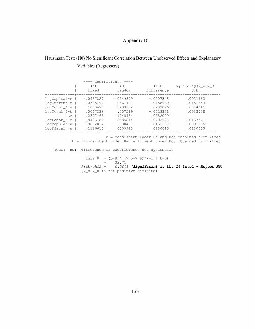
153

Appendix D

Hausmann Test: (H0) No Significant Correlation Between Unobserved Effects and Explanatory

Variables (Regressors)

---- Coefficients ---- | (b) (B) (b-B) sqrt(diag(V_b-V_B)) | fixed random Difference S.E. -------------+---------------------------------------------------------------- logCapital~e | -.0457227 -.0249879 -.0207348 .0031562 logCurrent~e | -.0505497 -.0664467 .0158969 .0151653 logTotal_R~e | .1088678 .0789652 .0299026 .0014041 logTotal_I~t | .0047338 .007569 -.0028351 .0033058 DEA | -.2327463 -.1945454 -.0382009 . logLabor_F~e | .8483187 .8685814 -.0202628 .0137371 logPopulat~n | .8852812 .930497 -.0452158 .0091985 logFiscal_~n | .1116613 .0835998 .0280615 .0180253 ------------------------------------------------------------------------------ b = consistent under Ho and Ha; obtained from xtreg B = inconsistent under Ha, efficient under Ho; obtained from xtreg Test: Ho: difference in coefficients not systematic chi2(8) = (b-B)'[(V_b-V_B)^(-1)](b-B) = 32.71 Prob>chi2 = 0.0001 (Significant at the 1% level – Reject H0) (V_b-V_B is not positive definite)

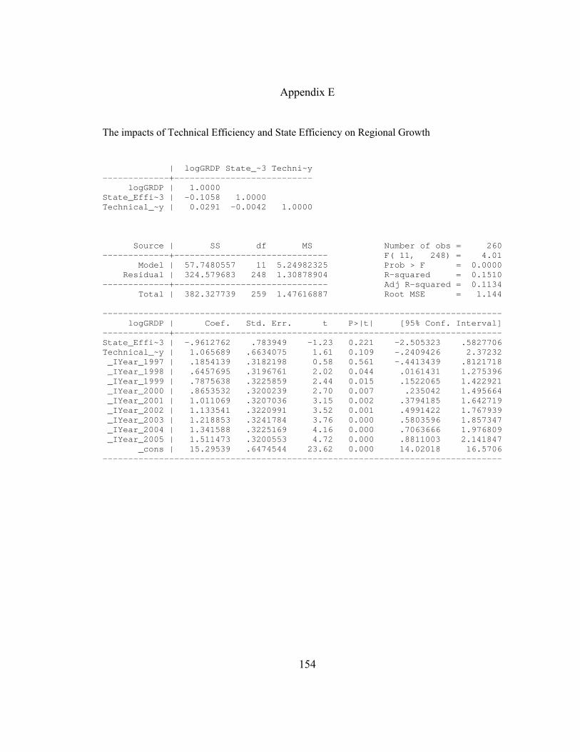
154

Appendix E

The impacts of Technical Efficiency and State Efficiency on Regional Growth

| logGRDP State_~3 Techni~y -------------+--------------------------- logGRDP | 1.0000 State_Effi~3 | -0.1058 1.0000 Technical_~y | 0.0291 -0.0042 1.0000 Source | SS df MS Number of obs = 260 -------------+------------------------------ F( 11, 248) = 4.01 Model | 57.7480557 11 5.24982325 Prob > F = 0.0000 Residual | 324.579683 248 1.30878904 R-squared = 0.1510 -------------+------------------------------ Adj R-squared = 0.1134 Total | 382.327739 259 1.47616887 Root MSE = 1.144 ------------------------------------------------------------------------------ logGRDP | Coef. Std. Err. t P>|t| [95% Conf. Interval] -------------+---------------------------------------------------------------- State_Effi~3 | -.9612762 .783949 -1.23 0.221 -2.505323 .5827706 Technical_~y | 1.065689 .6634075 1.61 0.109 -.2409426 2.37232 _IYear_1997 | .1854139 .3182198 0.58 0.561 -.4413439 .8121718 _IYear_1998 | .6457695 .3196761 2.02 0.044 .0161431 1.275396 _IYear_1999 | .7875638 .3225859 2.44 0.015 .1522065 1.422921 _IYear_2000 | .8653532 .3200239 2.70 0.007 .235042 1.495664 _IYear_2001 | 1.011069 .3207036 3.15 0.002 .3794185 1.642719 _IYear_2002 | 1.133541 .3220991 3.52 0.001 .4991422 1.767939 _IYear_2003 | 1.218853 .3241784 3.76 0.000 .5803596 1.857347 _IYear_2004 | 1.341588 .3225169 4.16 0.000 .7063666 1.976809 _IYear_2005 | 1.511473 .3200553 4.72 0.000 .8811003 2.141847 _cons | 15.29539 .6474544 23.62 0.000 14.02018 16.5706 ------------------------------------------------------------------------------

Appendix F

-6

-4

-2

0

2

4

6

8

1997 1998 1999 2000 2001 2002 2003

Leading Regions National Lagging Regions

0

1

2

3

4

5

1997 1998 1999 2000 2001 2002 2003

Leading Regions National Lagging Regions

Figure 10. Growth Rate in Indonesia during the Period of Financial crisis

Figure 11. Growth of Private Investments in Indonesia during the Period of Financial crisis

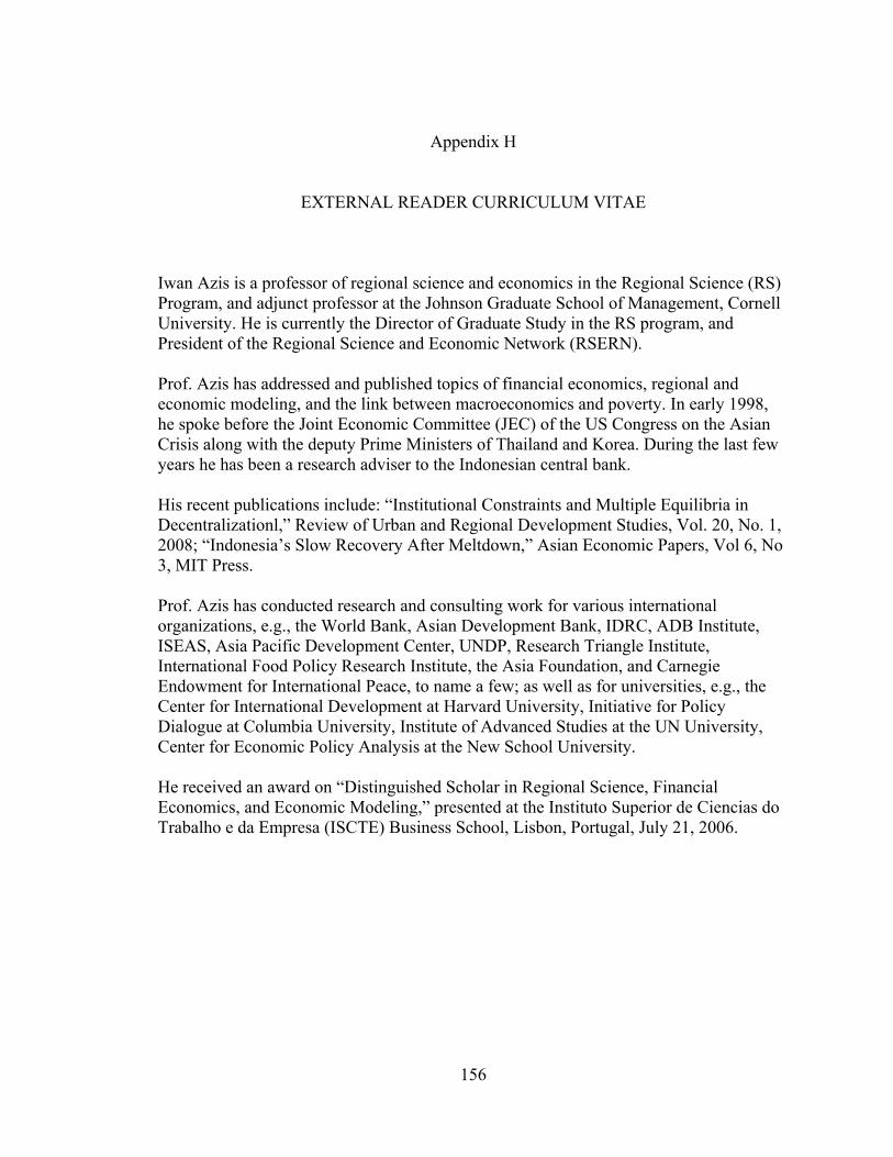
156

Appendix H

EXTERNAL READER CURRICULUM VITAE

Iwan Azis is a professor of regional science and economics in the Regional Science (RS) Program, and adjunct professor at the Johnson Graduate School of Management, Cornell University. He is currently the Director of Graduate Study in the RS program, and President of the Regional Science and Economic Network (RSERN). Prof. Azis has addressed and published topics of financial economics, regional and economic modeling, and the link between macroeconomics and poverty. In early 1998, he spoke before the Joint Economic Committee (JEC) of the US Congress on the Asian Crisis along with the deputy Prime Ministers of Thailand and Korea. During the last few years he has been a research adviser to the Indonesian central bank. His recent publications include: “Institutional Constraints and Multiple Equilibria in Decentralizationl,” Review of Urban and Regional Development Studies, Vol. 20, No. 1, 2008; “Indonesia’s Slow Recovery After Meltdown,” Asian Economic Papers, Vol 6, No 3, MIT Press. Prof. Azis has conducted research and consulting work for various international organizations, e.g., the World Bank, Asian Development Bank, IDRC, ADB Institute, ISEAS, Asia Pacific Development Center, UNDP, Research Triangle Institute, International Food Policy Research Institute, the Asia Foundation, and Carnegie Endowment for International Peace, to name a few; as well as for universities, e.g., the Center for International Development at Harvard University, Initiative for Policy Dialogue at Columbia University, Institute of Advanced Studies at the UN University, Center for Economic Policy Analysis at the New School University. He received an award on “Distinguished Scholar in Regional Science, Financial Economics, and Economic Modeling,” presented at the Instituto Superior de Ciencias do Trabalho e da Empresa (ISCTE) Business School, Lisbon, Portugal, July 21, 2006.

157

REFERENCES

158

REFERENCES

Acemoglu, D. et. Al., (2004), ‘Institutions as the Fundamental Cause of Long-Run Growth’, Paper is part of the Handbook of Economic Growth edited by P. Aghion and S. Durlauf,” North Holland, NJ: Elsevier. Ahmad, E. and V. Tanzi (ed.) (2002), Managing Fiscal Decentralization, London, England: Routledge. Ahmad, E. and A. Mansoor (2000), ‘Indonesia: Managing Decentralization’, Paper was presented at the Conference on Fiscal Decentralization, IMF. Aritenang, A.F. (2008), ‘A Study on Indonesia Regions Disparity: Post Decentralization’, Paper was presented at the N-AERUS Workshop, Edinburgh, Scotland. Arrow and Kurz (1970), Public Investment, the Rate of Return and Optimal Fiscal Policy, Baltimore, MD: John Hopkins Press. Aschaeur, D. (1989), ‘Is Public Investment Productive’, Journal of Monetary Economics, 23 (2): 177-200. Azis, I.J., (2003), ‘Concepts and Practice of Decentralization: Some Notes on the Case of Indonesia’, Paper was presented at the Policy Dialogue on “Empowering Women in Autonomy and Decentralization Processes,” United Nations, New York. Bahl, R. and J. Alm (1999), ‘Decentralization in Indonesia: Prospects and Problems’, The research paper was funded by the United States Agency for International Development.

159

Balassa, B. (1982), Development Strategies in Semi-Industrializing Economies, Baltimore, MD: John Hopkins Press. Bardhan, P. (2002),’Decentralization of Governance and Development’, Journal of Economic Perspectives, 16 (4): 185-205. Barro, R (1990), ‘Government Spending in A Simple Model of Endogenous Growth’, Journal of Political Economy, 98 (5): 103-126 Barro, R. J. and X. Sala-i-Martin (1991), ‘Convergence across States and Regions’ Brookings Papers on Economic Activity, 1: 107-182. Bird R. and C. Wallich (1993), "Fiscal Decentralization and Intergovernmental Relations in Transition Economics: Toward a Systematic Framework of Analysis,", Policy Research Working Paper No. 1122, World Bank. Bird, R. et. al. (1998), Rethinking Decentralization in Developing Countries, Washington, DC: World Bank Publication. Blane, D. (2005), ‘Indonesian District Government Spending, Taxing and Saving: An Explanation of Pre- and Post-decentralization Fiscal Outcomes’, Asian Economic Journal, 19 (3): 291-317 Boltho, M. (1996), "The assessment: International Competitiveness" Oxford Review of Economic Policy, 12 (3): 1-16. Borner, S. et al. (2004), Institutional Efficiency and Its Determinants: The Role of Political Factors in Economic Growth, Development Centre Studies, Paris, France: OECD. Bose, N. et. al. (2003), ‘Public Expenditure and Economic Growth: A Disaggregated Analysis for Developing Countries’, Paper was funded by the Economic and Social Research Council, UK.

160

Brennan G. and J. Buchanan (1980), The Power to Tax: Analytical Foundations of a Fiscal Constitution, Cambridge, England: Cambridge University Press. Brock, G.W. (2003), ‘The New Institutional Economics: Third in a Series on Poverty, Wealth, and Globalization’ Public Justice Report, 1st Quarter. Brueckner, J.K. (2004), "Fiscal Decentralization with Distortionary Taxation: Tiebout vs. Tax Competition " International Tax and Public Finance, 11 (2): 133-153. Camagni, R. (2002), ‘On the Concept of Territorial Competitiveness: Sound or Misleading’, Dortmund, England: ERSA Conference Paper. Chang, H.J., et al (2000), Institutions and the Role of the State, Cheltenham, England: Edward Elgar. Cheema, G.S. and D.A. Rondinelli (ed.) (1983), Decentralization and Development: Policy Implementation in Developing Countries, Beverly Hills, California: Sage Publications. Clague, C., (ed.) (1997), Institutions and Economic Development: Growth and Governance in Less-Developed and Post-Socialist Countries. Baltimore, MD: Johns Hopkins University Press. Conti, S. and P. Giaccaria (2001), District Development and Competitiveness, Dordrecht, Netherland: Kluwer Academic Publisher. Cooper, W.W., et al (2007), Data Envelopment Analysis, New York, NY: Springer. Devarajan, S. et al (1996), ‘The Composition of Public Investment and Economic Growth’, Journal of Monetary Economics, 37: 313-344. Davoodi, H. and H. Zou (1998), ‘Fiscal Decentralization and Growth’, Journal of Urban Economics, 43 (2): 35-58.

161

Easterly, W. (2001), The Elusive Quest for Growth, Cambridge, MA: The MIT Press. Ebel, R. and S. Yilmaz (2003). ‘Fiscal Decentralization in Developing Countries: Is It Happening? How Do We Know?’, World Bank Policy Research Working Paper No. 2809 Eisner, R. (1991), ‘Infrastructure and Regional Economic Performance’, New England Economic Review, Sept/Oct, 47-58 Enikolopov R. and E. Zhuravskaya (12005), ‘Decentralization and Political Institutions’, Center for Economic and Financial Research (CEFIR), Harvard, MA. Facchini, G. and C. Testa (2006), ‘Fiscal decentralization, regional inequality and bailouts: Lessons from Brazil’s Debt Crisis’, University of Illinois at Urbana-Champaign, IL. Farrell, M.J. (1957), “The Measurement of Productive Efficiency”, Journal of the Royal Statistical Society, 120 (3): 253-290. Fishman, R. and R. Gatti (1999), ‘Decentralization and Corruption: Evidence Across Countries’, Policy Research Working Paper No. 28202, World Bank. Furubotn, E.G. and R. Richter (1998), Institutions and Economic Theory: The Contribution of the New Institutional Economics, Ann Arbor, Michigan: University of Michigan Press. Garside, W.R., et al (2007), Institutions and Market Economies, New York, NY: Palgrave MacMillan. Gil, C, et al. (2002), ‘Decentralization and Regional Economic Disparities’, Tyne, England: Center for Urban & Regional Development Studies.

162

Glaeser, E. et al (2004), ‘Do Institutions Cause Growth’, Journal of Economic Growth, 9 (3): 271-303. Gramlich, E (1994), ‘Infrastructure Investment: A Review Essay’, Journal of Economic Literature, 32 (3): 1176-1196. Hadiz, V.R. (2003), ‘Decentralization and Democracy in Indonesia: A Critique of Neo-Institutionalist Perspectives’, Southeast Asia Research Centre Working Paper Series 2003/47. Hamalainen, T. (2003), National Competitiveness and Economic Growth: The Changing Determinants of Economic Performance in the World Economy, Cheltenham, England : Edward Elgar. Hayek, F.A. (1945), ‘The Use of Knowledge in Society’, American Economic Review, 35 (4): 519-530. Herrera, S. and G. Pang (2005), ‘Efficiency of Public Spending in Developing Countries: An Efficiency Frontier Approach’, Working Paper Series No. 3645, World Bank. Hill, H. (ed.) (1989), Unity and Diversity: Regional Development in Indonesia since 1970, New York, NY: Oxford University Press. Hirschman, A. (1958), The Strategy of Economic Development, New Haven, CT: Yale University Press. Holtz-Eakin, D. (1994), ‘Public-Sector Capital and the Productivity Puzzle’, The Review of Economics and Statistics, 76 (1): 12-22. Hoyt, W. (1990), ‘District Government Inefficiency and the Tiebout Hypothesis: Does Competition among Municipalities Limit District Government Inefficiency?’, Southern Economic Journal, 57 (2): 481-496.

163

Jin, et al. (2001), ‘Regional Decentralization and Fiscal Incentives: Federalism, Chinese Style’, The Center for Research on Economic Development and Policy Reform, Stanford, CA. Israel, Arturo (1987), Institutional Development: Incentives to Performance, BalHamalainenre, MD: The Johns Hopkins University Press. Khan, M.S. and C.M. Reinhart (1990), ‘Private Investment and Economic Growth in Developing Countries’, World Development, 18 (1): 19-27. Kindleberger, C. (1983), Economic Development, New York, NY: McGraw-Hill. Krugman, P. (1991), Geography and Trade, Cambridge, MA: The MIT Press. Krugman, P. (1996), ‘Making Sense of Competitiveness Debate’, Oxford Review of Economic Policy, 12: 17-25. Lall, S.V., et al. (2005), ‘Agglomeration, Transport, and Regional Development in Indonesia’, Working Paper Series 3477, World Bank. Leibenstein, H. (1996), ‘Fiscal Allocative Efficiency vs. X-Efficiency’, American Economic Review, 56 (3): 392-415. Lin, J.Y. and Z. Liu (2000), ‘Fiscal Decentralization and Economic Growth in China’, Economic Development and Cultural Change, 49 (1): 1-21. Letelier, L. (2005), ‘Explaining Fiscal Decentralization, Public Finance Review, 33 (2): 155-183. Maddick, H. (1963), Democracy, Decentralization and Development, London, England: Asia Publishing House.

164

Marks, D. (2006), ‘Reconstruction of the Service Sector in the National Accounts of Indonesia, 1900-2000, ASEAN Economic Bulletin, 23 (3): 373-390. Martin, R.L. (2003), ‘A Study of the Factors of Regional Competitiveness’, Final Report to The European Commission Directorate-General Regional Policy, Cambridge, England: Cambridge Econometrics. Martinez-Vazquez, J. and R. McNab (2003), ‘Fiscal Decentralization and Economic Growth’, World Deveopment, 31 (9): 1597-1616. Martinez-Vazquez, J. and M. Rider (2005), ‘Fiscal Decentralization and Economic Growth: A Comparative Study of India and China’, Working Paper Series 05-19, International Studies Program Georgia State University. Mora, M. and R. Varsano (2001), ‘Fiscal Decentralization and Sub National Fiscal Autonomy in Brazil: Some Facts of the Nineties’, IPEA Discussion Paper No.854, Rio de Janeiro, Brazil. Munnell, A. (ed.) (1990), Is There a Shortfall in Public Capital Investment?, Federal Reserve of Boston: Collection of Conference Papers, Harwich Port, MA. Munnell, A. (1992), ‘Infrastructure Investment and Economic Growth’, Journal of Economic Perspectives, 6 (4): 189-198. Murty, K.N. and A. Soumya (2006), “Effects of Public Investment in Infrastructure on Growth and Poverty in India”, Working Paper 2006-006, Indira Gandhi Institute of Development Research, Mumbai. Musgrave, R.A. (1959), The Theory of Public Finance: a Study in Political Economy, New York: Mcgraw-Hill. Myrdal, G. (1957), Economic Theory and Under-Developed Regions. London, England: Gerald Duckworth & Co. Ltd.

165

North, D.C. (1955), ‘Location Theory and Regional Economic Growth’, Journal of Political Economy, 63: 243-58. North, D.C. (1989), "Institutions and economic growth: An historical introduction," World Development, 17 (9): 1319-1332 North, D.C. (1990), Institutions, Institutional Change and Economic Performance, Cambridge, MA: Cambridge University Press. Oates, W.E. (1972), Fiscal Federalism, New York: Harcourt Brace Jovanovich. Oates, W.E. (1993), ‘Fiscal Decentralization and Economic Development’, National Tax Journal, 46 (2): 237-243. OECD (2005), Building Competitive Regions: Strategies and Governance, Paris, France: OECD. Porter, M. (1996), The Competitive Advantage of Nations, New York, NY: The Free Press. Porter, M. (2000), ‘Location, Competition and Economic Development: District Clusters in the Global Economy’, Economic Development Quarterly, 14: 15-31. Porter, M. (2003), ‘The Economic Performance of Regions’, Regional Studies, 37: 549-578. Pratikno (2005), ‘Local Autonomy and Democracy in Indonesia, 1999-2001’ in Regionalism in Post-Suharto Indonesia, M. Erb, et al (ed.), London, England: Routledge. Prud’Homme, R. (1995), ‘The Dangers of Decentralizations’, World Bank Research Observer, 10 (2): 201-220.

166

Qian, Y. and B. Weingast (1997), ‘Federalism as a Commitment to Preserving Market Incentives, Journal of Economic Perspectives, 11 (4): 83-92. Qian, Y. et al. (1999), “Regional Decentralization and Fiscal Incentives: Federalism in Transition Economies”, Paper was presented at the Annual Conference of American Economic Association, Chicago, IL Rao, P.K. (2003), Development Finance, Berlin, Germany: Springer. Rao, M.G. (2000), ‘Fiscal Decentralization in Indian Federalism’, Institute for Social and Economic Change, Bangalore, India. Rao, M.G. (2002), Development, Poverty, and Fiscal Policy: Decentralization of Institutions, New Delhi, India: Oxford University Press. Rajan, R, (ed.) (2003), Sustaining Competitiveness in the New Global Economy: A Case Study of Singapore, Cheltenham, England: Edward Elgar. Rashid, S, (2000), Economic Policy for Growth, Boston, MA: Kluwer Academic Publisher. Richardson, H. (1978), Regional Economics, Urbana, IL: University of Illinois Press. Riedel, J. (1977), ‘Strategies of Economic Development’ in Vol. 4 of Handbook of Comparative Economic Policies, E. Grilli and D. Salvatore (ed.), Westport, CT: Greenwood Press. Rodriguez-Pose, A. and N. Gill. (2005), ‘On the Economic Dividend of Devolution’, Regional Studies, 39 (4): 405-420. Rodriguez-Pose, A., et al. (2007), ‘Fiscal Decentralization, Efficiency, and Growth’, Working Paper Series 2007/11, London School of Economics.

167

Rodriguez-Pose, A. and R. Ezcurra. (2009), ‘Does Decentralization Matter for Regional Disparities? A Cross-country Analysis’, Working Paper Series 2009/04, London School of Economics. Rodrik, D., et al. (2002), ‘Institutions Rule: The Primacy of Institutions over Integration and Geography in Economic Development’, Working Paper 02/189, IMF. Rondinelli, D. et. Al. (1981), ‘Government Decentralization in Comparative Perspective: Developing Countries’, International Review of Administrative Science, 47(2): 133-145. Samuelson, A. (1954), ‘The Pure Theory of Public Expenditure’, Review of Economics and Statistics, (November): 387–389 Shah, A. and H. Zou (2004), ‘The Impact of Decentralization on Service Delivery, corruption, Fiscal Management and Growth in Developing and Emerging Market Economies’, CESifo DICE Report, World Bank. Shankar R. and A. Shah (2001), ‘Bridging the economic divide within nations: A scorecard on the performance of regional development policies in reducing regional income disparities’, Policy Research Working Paper No. 2717, World Bank. Siebert, H. (ed.) (1995), Locational Competition in the World Economy, Kiel, Germany: J.C.B. Mohr (Paul Siebeck) Tubingen. Singh, N. and T.N. Srinivasan (2006), ‘Federalism and Economic Development in India: An Assessment’, Paper was presented at the SCID Conference on Economic Reform in Asia, Stanford, CA. Singh, N. (2006), ‘Fiscal Decentralization in China and India: Competitive, Cooperative or Market Preserving Federalism?’, Center for International Economics, University of California at Santa Cruz, CA. Solow, R. (2000), Growth Theory: An Exposition, New York, NY: Oxford University Press.

168

Stimson, R. J., R. R. Stough and B. H. Roberts (2002), Regional Economic Development, Berlin, Germany: Springer. Tambunan, T. (2005), ‘Economic Growth, Appropriate Policies and Poverty Reduction in a Developing Country’, South Asia Economic Journal, 6 (1): 59-78. Tanzi, V. (1996), ‘Fiscal Federalism and Decentralization: A Review of Some Efficiency and Macroeconomics Aspects’, Annual World Bank Conference on Development Economics 1995, Washington DC Tanzi, V. (2000), ‘On Fiscal Federalism: Issues to Worry About’, Paper was presented at the Conference of Fiscal Decentralization, IMF. Thanassoulis, E. (2001), Introduction to the Theory and Application of Data Envelopment Analysis, Norwell, MA : Kluwer Academic Publishers. Thornton, J. (2006), ‘Fiscal decentralization and economic growth reconsidered’, Journal of Urban Economics, 61 (1): 64-70. Tiebout, C. M. (1956), ‘A Pure Theory of Local Expenditures’, Journal of Political Economy, 64: 160-69. Wie, T.K. (2006), ‘Technology and Indonesia’s Industrial Competitiveness’, Asian Development Bank (ADB) Institute Discussion Paper No. 43. Williamson, O. (1996), ‘The Institutions and Governance of Economic Development and Reform’, The Mechanism of Governance, Ch.13, New York, NY: Oxford University Press. Woller, G.M. and K. Phillips (1998), ‘Fiscal decentralization and LDC growth: An empirical investigation’, Journal of Development Studies, 34: pp. 138–148

169

Zimmermann, H. (1990), ‘Fiscal Federalism and Regional Growth’ in R.J. Bennett (ed.), Decentralization, Local Governments, and Markets: Towards a Post-Welfare Agenda, Oxford, England: Clarendon Press Zou, H. and J. Jin (1999), ‘Fiscal Decentralization and Economic Growth in China’, Preliminary Paper from the Development Research Group, World Bank. Zou H. and T. Zhang (1996), ‘Fiscal Decentralization, Public Spending, and Economic Growth in China’, Policy Research Working Paper No. 16087, World Bank.

170

CURRICULUM VITAE

Darius Tirtosuharto currently works as a researcher for the Institute of National Capacities Studies (Lembaga Studi Kapasitas Nasional/LSKN), a non-profit organization based in Jakarta, Indonesia that focuses on the study of competitiveness and capacity building both at the national and regional levels. He also acts as a liaison for LSKN in the United States. Prior to this appointment in 2003, he has been with the Asian Pacific Economic Consultancy Indonesia (ASPECINDO) as a research assistant for more than three years. From 2007 to 2009, he was working as a program planner for various US government agencies. He received his Bachelor of Engineering with honors from University of Tarumanagara, Jakarta, Indonesia in 1996. He was a teaching assistant at the Department of Architecture and Planning, University of Tarumanagara before continuing his higher education in the United States. He received his Master of Urban Design from University of Colorado in 1998.