the impact of same-sex marriage laws on
303
THE IMPACT OF SAME-SEX MARRIAGE LAWS ON HEALTH INSURANCE COVERAGE IN SAME-SEX HOUSEHOLDS A DISSERTATION SUBMITTED TO THE FACULTY OF THE UNIVERSITY OF MINNESOTA BY GILBERT GONZALES, JR. IN PARTIAL FULFILLMENT OF THE REQUIREMENTS FOR THE DEGREE OF DOCTOR OF PHILOSOPHY LYNN A. BLEWETT OCTOBER 2015
-
Upload
khangminh22 -
Category
Documents
-
view
0 -
download
0
Transcript of the impact of same-sex marriage laws on

1
THE IMPACT OF SAME-SEX MARRIAGE LAWS ON
HEALTH INSURANCE COVERAGE IN SAME-SEX HOUSEHOLDS
A DISSERTATION
SUBMITTED TO THE FACULTY OF THE
UNIVERSITY OF MINNESOTA
BY
GILBERT GONZALES, JR.
IN PARTIAL FULFILLMENT OF THE REQUIREMENTS
FOR THE DEGREE OF
DOCTOR OF PHILOSOPHY
LYNN A. BLEWETT
OCTOBER 2015

2
Copyright by Gilbert Gonzales, 2015

i
Acknowledgments
This project could not have been completed without the many contributions from
my dissertation committee. I am thankful to Bryan Dowd and Kathleen Call for
approaching this project from different disciplinary perspectives. I am also grateful for
having Sharon Long of the Urban Institute serve on my dissertation committee. Sharon’s
prolific and policy-oriented research is a model for junior health services researchers
across the county. I am extremely fortunate for having Lynn Blewett as my dissertation
advisor and chair. Everything I know about the health policy process and how to use
research to inform health policy debates, I owe to her. I am also grateful for having the
opportunity to work with Lynn and her team of researchers at the State Health Access
Data Assistance Center (SHADAC). Working at SHADAC taught me the importance of
using the best available data for answering pressing health policy research questions, a
constant theme throughout this dissertation.
I am thankful for several colleagues, friends and family not serving on my
dissertation committee, but helped me along the way through their friendship, advice and
wisdom. I was lucky to work with and learn from Ezra Golberstein on his research
projects. I’m thankful for my parents, Gilbert and Xochitl Gonzales, who taught me to
enjoy life. During my time at the University of Minnesota, I took advantage of life in the
Twin Cities with members of my cohort, who will undoubtedly go on to lead successful
careers in health services research. I am also thankful to my partner, Andy Hofer, for
without him, life would be more boring and dull. Andy was also my sounding board
through much of this work, and I am grateful for his patience as I ran hypotheses by him.

ii
Dedication
This dissertation is dedicated to my parents, Gilbert and Xochitl Gonzales.

iii
Table of Contents
Acknowledgments .............................................................................................................. i
Dedication .......................................................................................................................... ii
Table of Contents ............................................................................................................. iii
List of Tables ................................................................................................................... vii
List of Figures ................................................................................................................... xi
1. Introduction ....................................................................................................................1
1.1 The Importance of State Policy Environments & Processes .............................1
1.2 A Conceptual Model Bridging the State Policy Process to Health Outcomes ..4
1.2.1 Problem Definition & Saliency ...........................................................7
1.2.2 State Policy Diffusion .......................................................................10
1.2.3 Target Population Benefited or Burdened ........................................12
1.2.4 Short-Term and Long-Term Health Outcomes .................................13
1.2.5 Political Climate................................................................................16
1.2.6 Economic Conditions, Resources & Infrastructure ..........................18
1.2.7 Federal Policy ...................................................................................20
1.2.8 Demographic & Socioeconomic Structures & Health Needs ...........21
1.2.9 Policy Feedback ................................................................................23
1.3 Other Applications of the Conceptual Model in Health Policy .......................24
1.4 Next Chapters in the Dissertation ....................................................................25
2. Causality and Threats to Validity ..............................................................................30
2.1 Requirements for Establishing Causality .........................................................30
2.2 Challenges to Establishing Causality Between Same-Sex Marriage and Health
Insurance Coverage ................................................................................................33
2.3 Threats to Internal and External Validity.........................................................35
2.3.1 Threats to Internal Validity ...............................................................36
2.3.2 Treats to External Validity ................................................................45
2.4 Implications of Limited Internal and External Validity ...................................48

iv
3. The Association Between State Policy Environments and Health Insurance
Coverage for Adults in Cohabiting Same-Sex Couples ................................................54
3.1 Introduction ......................................................................................................54
3.2 Background ......................................................................................................56
3.3 Literature Review.............................................................................................58
3.4 Data and Methodology .....................................................................................61
3.4.1 Data Source .......................................................................................61
3.4.2 Statistical Analyses ...........................................................................63
3.5 Results ..............................................................................................................66
3.5.1 Descriptive Statistics .........................................................................66
3.5.2 National Disparities in ESI ...............................................................68
3.5.3 State-Specific Disparities in ESI .......................................................70
3.5.4 Association Between Same-Sex Marriage, Civil Unions and ESI ...72
3.6 Discussion ........................................................................................................73
3.7 Study Limitations .............................................................................................75
3.8 Conclusion .......................................................................................................78
3.9 Technical Appendix .........................................................................................79
3.9.1 Data Sample ......................................................................................79
3.9.2 Methods.............................................................................................81
3.9.3 Sensitivity Analyses ..........................................................................85
4. The Association Between State Policy Environments and Health Insurance
Coverage For Children of Cohabiting Same-Sex Parents..........................................126
4.1 Introduction ....................................................................................................126
4.2 Background ....................................................................................................129
4.3 Literature Review...........................................................................................130
4.4 Methods..........................................................................................................132
4.4.1 Data Source .....................................................................................132
4.4.2 Primary Outcome ............................................................................133
4.4.3 Independent Variables ....................................................................134
4.4.4 Analyses ..........................................................................................135
4.5 Results ............................................................................................................136

v
4.6 Discussion ......................................................................................................138
4.7 Conclusion .....................................................................................................143
4.8 Technical Appendix .......................................................................................144
4.8.1 Data Sample ....................................................................................144
4.8.2 Methods...........................................................................................145
4.8.3 Sensitivity Analysis ........................................................................146
4.8.4 Additional Limitations ....................................................................147
5. The Impact of New York’s Same-Sex Marriage Law on Health Insurance
Coverage Among Adults in Cohabiting Same-Sex Couples .......................................179
5.1 Introduction ....................................................................................................179
5.2 Background ....................................................................................................181
5.3 Previous Research on Civil Unions and Domestic Partnerships ...................184
5.4 New York’s Marriage Equality Act of 2011..................................................185
5.5 Conceptual Framework ..................................................................................186
5.6 Data and Methods ..........................................................................................188
5.6.1 Data Source and Study Population .................................................188
5.6.2 Outcome Measures..........................................................................190
5.6.3 Statistical Analysis ..........................................................................190
5.7 Results ............................................................................................................194
5.7.1 Descriptive Statistics .......................................................................194
5.7.2 The Effects of New York’s Marriage Equality Act on Health
Insurance Outcomes .................................................................................195
5.8 Sensitivity Analyses .......................................................................................197
5.8.1 Synthetic Control Group .................................................................198
5.8.2 Falsification Tests ...........................................................................199
5.9 Discussion ......................................................................................................200
5.9.1 Limitations ......................................................................................201
5.10 Conclusion ...................................................................................................205
5A. Technical Appendix to Chapter 5: Data and Sample Limitations .....................229
5A.1 Data Source .................................................................................................229
5A.2 Study Sample and Challenges in the ACS ..................................................230

vi
5A.3 Contamination in the Sample of Married Same-Sex Couples ....................232
5A.4 Reducing Contamination in the Sample of Same-Sex Couples ..................235
5A.5 Primary Comparison Group: Opposite-Sex Couples in New York ............240
5A.6 Data and Study Limitations.........................................................................243
5A.6.1 Missing Information on Sexual Orientation and Same-Sex
Couples ....................................................................................................243
5A.6.2 Limited Generalizations from New York to Other States............245
5A.6.3 Changing Economy, Societal Attitudes and Data Collection Over
Time .........................................................................................................247
5A.7 The Comparison Group as a Counterfactual ...............................................254
5A.8 Regression-Adjusted Results ......................................................................258
5A.9 Recommendations for Researchers Interested in Studying Same-Sex
Couples ................................................................................................................262
5A.10 Next Steps for Future Research ................................................................267
6. Conclusion ..................................................................................................................269
6.1 Policy Implications ........................................................................................270
6.2 Next Steps ......................................................................................................272
6.3 Concluding Comments...................................................................................275
7. Bibliography ...............................................................................................................276

vii
List of Tables
Table 2.1 Threats to Internal and External Validity………………………………… 50
Table 3.1 Sample Descriptive Statistics, by Relationship Type……………………. 86
Table 3.2 Multinomial Logistic Regression Analysis of Health Insurance Coverage
by Relationship Type for Men……………………………………………………… 89
Table 3.3 Multinomial Logistic Regression Analysis of Health Insurance Coverage
by Relationship Type for Women…………………………………………………... 90
Table 3.4 Unadjusted and Adjusted Differences in ESI Between Men in Same-Sex
Couples and Men in Married Opposite-Sex Couples……………………………….. 91
Table 3.5 Unadjusted and Adjusted Differences in ESI Between Women in
Cohabiting Same-Sex Couples and Women in Married Cohabiting Opposite-Sex
Couples……………………………………………………………………………… 94
Table 3.6 Differences in ESI Coverage for Same-Sex Couples by State Marriage
Policy…………………………………………………………………………..…… 97
Table 3.7 Multinomial Logistic Regression Analysis of Health Insurance Coverage
for All Men…………………………………………………………..……………… 99
Table 3.8 Multinomial Logistic Regression Analysis of Health Insurance Coverage
for Employed Men………………………………………………………………… 101
Table 3.9 Multinomial Logistic Regression Analysis of Health Insurance Coverage
for All Women……………………………………………………………………… 103
Table 3.10 Multinomial Logistic Regression Analysis of Health Insurance
Coverage for Employed Women……………………………………………………. 105
Table 3.11 Sample Descriptive Statistics, by Relationship Type for the Sensitivity
Sample………………………………………………………………………………. 108
Table 3.12 Multinomial Logistic Regression Analysis of Health Insurance
Coverage for All Men in Sensitivity Sample……………………………………….. 111
Table 3.13 Multinomial Logistic Regression Analysis of Health Insurance
Coverage for Employed Men in Sensitivity Sample………………………………... 113
Table 3.14 Multinomial Logistic Regression Analysis of Health Insurance
Coverage for All Women in Sensitivity Sample……………………………………. 115
Table 3.15 Multinomial Logistic Regression Analysis of Health Insurance

viii
Coverage for Employed Women in Sensitivity Sample……………………………. 117
Table 3.16 Unadjusted and Adjusted Differences in ESI Between Men in
Cohabiting Same-Sex Couples and Men in Married Cohabiting Opposite-Sex
Couples, Restricted to Sensitivity Sample………………………………………….. 119
Table 3.17 Unadjusted and Adjusted Differences in ESI Between Women in
Cohabiting Same-Sex Couples and Women in Married Cohabiting Opposite-Sex
Couples, Restricted to Sensitivity Sample……………………………..…………… 122
Table 3.18 Differences in ESI Coverage for Same-Sex Couples by State Marriage
Policy……………………………………………………………………………….. 125
Table 4.1 Selected Characteristics of Children by Family Type…………………… 150
Table 4.2 Factors Associated with Children's Type of Health Insurance…………... 153
Table 4.3 The Association Between Family Type and Type of Health Insurance
Coverage by State Marriage Policies as if January 1, 2008………………………… 155
Table 4.4 The Association Between Family Type and Type of Health Insurance
Coverage by State Adoption Policies as of January 1, 2008……………………….. 156
Table 4.5 The Association Between Family Type and Children's Health Insurance
Coverage in States with Same-Sex Marriage, Civil Unions or Domestic
Partnerships as of January 1, 2008………………………………………………….. 158
Table 4.6 The Association Between Family Type and Children's Health Insurance
Coverage in States Without Marriage Provisions as of January 1, 2008…………… 160
Table 4.7 The Association Between Family Type and Children's Health Insurance
Coverage in States with Second-Parent Adoption Available Statewide as of
January 1, 2008………………………………………………………...…………… 162
Table 4.8 The Association Between Family Type and Children's Health Insurance
Coverage in States Without Second-Parent Adoption Available Statewide as of
January 1, 2008……………………………………………………………………... 164
Table 4.9 Selected Characteristics of Children by Family Type for the Sensitivity
Sample………………………………………………………………………………. 167
Table 4.10 Factors Associated with Children's Type of Health Insurance in
Sensitivity Sample…………………………………………………………………... 169
Table 4.11 The Association Between Family Type and Children's Health Insurance
Coverage in States with Same-Sex Marriage, Civil Unions or Domestic

ix
Partnerships as of January 1, 2008 in Sensitivity Sample………………………….. 171
Table 4.12 The Association Between Family Type and Children's Health Insurance
Coverage in States Without Marriage Provisions as of January 1, 2008 in
Sensitivity Sample…………………………………………………………………...
173
Table 4.13 The Association Between Family Type and Children's Health Insurance
Coverage in States with Second-Parent Adoption Available Statewide as of
January 1, 2008 in Sensitivity Sample……………………………………………… 175
Table 4.14 The Association Between Family Type and Children's Health Insurance
Coverage in States Without Second-Parent Adoption Available Statewide as of
January 1, 2008 in Sensitivity Sample……………………………………………… 177
Table 5.1 Descriptive Characteristics of Cohabiting Adults in New York, by Sex
and Relationship Type……………………………………………………………… 210
Table 5.2 Descriptive Characteristics of Same-Sex and Opposite-Sex Households
in New York, by Sex and Relationship Type……………………………………….. 212
Table 5.3 Changes in Health Insurance Coverage After the Implementation of New
York's Marriage Equality Act………………………………………………………. 214
Table 5.4 Changes in Household Health Insurance Coverage After the
Implementation of New York's Marriage Equality Act…………………………….. 215
Table 5.5 State Weights Used to Construct Synthetic New York………………….. 216
Table 5.6 Results from the Falsification Test on Each Outcome, By Sex and
Outcome…………………………………………………………………………….. 217
Table 5.7 Complete Regression Results for Difference-in-Differences Estimates in
Table 5.3 Without Propensity Score Weighting……………………………………. 221
Table 5.8 Complete Regression Results for Difference-in-Differences Estimates in
Table 5.3 With Propensity Score Weighting……………………………………….. 223
Table 5.9 Complete Regression Results for Difference-in-Differences Estimates in
Table 5.4 Without Propensity Score Weighting……………………………………. 225
Table 5.10 Complete Regression Results for Difference-in-Differences Estimates
in Table 5.4 With Propensity Score Weighting…………………………………….. 227
Table A1 Characteristics of Male Same-Sex Couples in New York Over the Study
Period……………………………………………………………………………….. 252

x
Table A2 Characteristics of Female Same-Sex Couples in New York Over the
Study Period…………………………………………………………………………
253
Table A3 Changes in Health Insurance Coverage After the Implementation of New
York's Marriage Equality Act……………………………………………………….
260
Table A4 Changes in Household Health Insurance Coverage After the
Implementation of New York's Marriage Equality Act…………………………….. 261

xi
List of Figures
Figure 1.1 The Preliminary Conceptual Model Bridging the Policy Process to
Health Outcomes……………………………………………………………………. 28
Figure 1.2 The S-Shaped Diffusion of Same-Sex Marriage Across the United
States………………………………………………………………………………... 29
Figure 4.1 Same-Sex Marriage and Adoption Laws as of October 2013…………... 149
Figure 5.1 Conceptual Framework………………………………………………….. 206
Figure 5.2 Percent Covered by Employer-Sponsored Insurance (ESI) Before and
After New York’s Marriage Equality Act, by Sex………………………………….. 207
Figure 5.3 Percent Both Members Covered by ESI Before and After New York’s
Marriage Equality Act, by Sex……………………………………………………… 208
Figure 5.4 Trends in ESI Comparing the Treatment Group to the Synthetic Control
Group, by Sex…………………………………………………………………..…… 209
Figure A1 Same-Sex Couples in the ACS by Response Mode and Allocated
Marital Status………………………………………………………………..……… 233
Figure A2 Flow Diagram for the Selection of the Final Sample of Same-Sex
Couples in New York from the 2008-2013 American Community Survey……….... 238
Figure A3 Year Last Married Among Same-Sex Couples in New York When Both
Members Reported the Same Year of Marriage…………………………………..… 240
Figure A4 Flow Diagram for the Selection of a Final Sample of Opposite-Sex
Couples in New York from the 2008-2013 American Community Survey…..…….. 242
Figure A5 Statewide Unemployment Rates in New York……………...…………... 248
Figure A6 Percent Covered by Employer-Sponsored Insurance (ESI) Before and
After New York’s Marriage Equality Act, by Sex………………………………….. 256
Figure A7 Percent Both Members Covered by Employer-Sponsored Insurance
(ESI) Before and After New York’s Marriage Equality Act, by Sex………………. 257

xii
Figure A8 Questions on Sex, Date of Birth and Relationship to the Primary
Householder in the 2005-2007 ACS………...……………………………………… 264
Figure A9 Questions on Sex, Date of Birth and Relationship to the Primary
Householder in the 2008-2013 ACS…...…………………………………………… 264
Figure A10 Revised Relationship Question in the 2013 American Community
Survey Questionnaire Design Test (ACS-QDT)……………………………………. 264

1
1. Introduction
The purpose of this dissertation is to document the impact of state-level same-sex
marriage laws on health insurance coverage in same-sex households. At the start of this
dissertation project in 2012, only six states allowed same-sex couples to marry and, in
accordance with the federal Defense of Marriage Act (DOMA), the federal government
did not recognize any same-sex marriage licenses authorized by those six states. Now, in
October 2015, all 50 states and the federal government recognize same-sex marriages
following the Supreme Court’s ruling in Obergefell v. Hodges, which upheld the right to
marriage for same-sex couples. Additionally, a majority (60 percent) of Americans
surveyed by Gallup believes that marriages between same-sex couples should be
recognized by the law (McCarthy 2015). While the rapid diffusion and support of legal
same-sex marriage across the United States reflects a major shift in attitudes and
acceptance of lesbian, gay, bisexual and transgender (LGBT)1 populations, the policy
“experiments” that occurred one state at a time provided health policy researchers an
opportunity to study how changes in federal and state policies affect health insurance
coverage, among other health outcomes, in LGBT populations and, more specifically,
cohabiting same-sex couples.
1.1 The Importance of State Policy Environments & Processes
This dissertation took advantage of the state-by-state rollout of same-sex marriage
laws to examine how policy environments across the United States shape health
1 This dissertation uses the acronym LGBT as an umbrella term for lesbian, gay, bisexual
and transgender (LGBT) populations, but it is important to note that the LGBT
population is not a single, monolithic group. Each subgroup is unique and may not be
affected the same ways by same-sex marriage laws.

2
outcomes and access to care in vulnerable populations. Although current conceptual
models (Aday & Andersen 1974; Aday & Andersen 1981; Andersen 1995; Phillips et al.
1998; Gelberg, Andersen & Leake 2000) in health services research position policy as a
remote, distant force shaping access to care and the delivery of health care, a growing
body of theoretical models in epidemiology (Krieger 2001; Krieger 2014), community-
based participatory research (Cacari-Stone et al. 2014), and international health (Solar &
Irwin 2010) recognize the importance of policy as a central determinant of health care,
health services utilization and population health outcomes. Meanwhile, recent events in
American policymaking require a reassessment of the relationship between state policy
and health outcomes in the United States, particularly following the rapid ascension of
state governments in health and social policymaking that followed welfare reform in the
mid-1990s. Beginning with the early expansions in Medicaid to low-income families,
children and pregnant women (Currie & Gruber 1996a; Currie & Gruber 1996b), states
have been granted increasing levels of authority and power to determine the delivery of
health care for vulnerable populations. For instance, welfare reform in the mid-1990s—
which decoupled eligibility between Medicaid and cash assistance for low-income
families—allowed states to customize their Medicaid programs through federal waivers.
Following the defeat of comprehensive health care reform under President Bill Clinton,
states were again granted authority in building and managing state-administered health
insurance programs for low- and middle-income children under the Children’s Health
Insurance Program (CHIP). CHIP’s reauthorization in 2009 further allowed the states to
consider covering lawfully residing immigrant children and pregnant women without a 5-
year waiting period required of other immigrants. Finally, and most recently, federal
3
health care reform under President Barack Obama, known as the Affordable Care Act
(ACA), further promotes state health policymaking. Under the ACA, states are permitted
to (1) expand the Medicaid program to families and individuals beneath 138% of the
federal poverty guidelines (FPG), (2) create state-based health insurance exchanges (or
marketplaces) to allow the sale of federally subsidized private health insurance plans for
middle-income families, and (3) design and test new payment and service delivery
models through financial awards and technical assistance from Centers for Medicare and
Medicaid Services (CMS) Innovation Center. Given the growing importance of state
roles in health policymaking, conceptual models in health services research should
refocus the role of state policy environments and state policy processes in explaining
population health outcomes.
Not only is state policymaking increasingly important in health care, but states are
predominant actors in non-health policy arenas that directly and indirectly affect health
outcomes and the social determinants of health. For instance, as this chapter suggests,
more states have adopted policies that recognize LGBT families through laws
establishing same-sex marriage, civil unions or domestic partnerships for LGBT couples.
Meanwhile, states have taken steps to extend other financial and safety protections for
LGBT populations, including the prohibition of discrimination in housing, employment
and education for LGBT people. States are also leading policy actors in creating new
laws that regulate other spheres of the social landscape, including the sale of firearms, the
possession of medicinal and recreational marijuana and limits to abortions—all of which
potentially affects population health.

4
This chapter presents a preliminary2 conceptual model
3 that bridges the important
relationship between state policy environments and health outcomes using themes from
well-established theories of the policy process (Kingdon 2010; Sabatier & Weible 2014).
The purpose of the conceptual model is not to definitively describe why public policies
spread across the country, but rather to identify the contextual factors of state policy
environments and to assess the policy-level determinants of individual and population-
based health outcomes. This preliminary framework will guide ongoing and future
research that acknowledges and highlights the important role of state policy processes in
efforts to improve health and health care in priority populations.
1.2 A Conceptual Model Bridging the State Policy Process to Health Outcomes
Conceptual models (or conceptual frameworks) visually present a “paradigm
though a combination of identified variables” which emerges from the “researcher’s
appreciation of reading, personal experience and reflection upon theoretical positions
towards the phenomenon to be investigated” (Leshem & Trafford 2007, page 99). The
conceptual model presented here was derived from observing, studying and reflecting on
the rollout of same-sex marriage policies across the country. Interestingly, the conceptual
model developed and presented here can be used for studying the rollout of state health
policies (like state Medicaid expansions) or non-health policies that affect health
outcomes across the country.
A simple and generalizable conceptual model is helpful for studying the
relationship between the policy process and health outcomes. Although the predominant
2 This conceptual model is “preliminary” in terms that it is in its initial state and will be
tested, improved upon and retested throughout the next stages in my career. 3 Conceptual model and conceptual framework are used interchangeably.

5
theories and conceptual models in health services research often situate policy as a
remote, upstream factor affecting downstream health behaviors and health outcomes
(Andersen 2008), these models do not take into consideration the dynamic nature of the
policy process, which plays a critical role on access to care and health outcomes among
vulnerable populations. For example, in the most recent version of Ronald Andersen’s
Behavioral Model of Health Services Use (Andersen 2007; Andersen & Davidson 2008),
contextual and environmental factors—like health policy—are included in the conceptual
model that explains access to medical care and health services utilization. Yet, the
discussion of health policy gives the reader a sense that policies are simply accepted as
they are—they are omnipresent, yet unchanging. According to Andersen, “health policies
are authoritative decisions made pertaining to health or influencing the pursuit of
health…in the legislative, executive, or judicial branches of government…[or] in the
private sector by such decision makers as executives” (2007; page 6). From this
perspective, policies are granted by authorities, and there is no discussion of the political
and economic contexts or the impact of changing policies through the policy process and
policy feedback loops.
The reality is that we live in a time where state governments are given significant
responsibility and flexibility in designing and implementing national health policy.
States vary dramatically in terms of their (1) economic conditions and capital resources:
technical expertise, state revenue, available workforce, and infrastructure; (2) political
climate: progressivity, Republican or Democratic control of government, trust in
government; and (3) socioeconomic, demographic and health care needs of the
population : age distribution, health and socioeconomic status. These factors, in addition

6
to federal policy, determine whether states take up certain policy issues and the direction
of their policy choices. Recent examples include reforms in the legalization of medical
marijuana, health insurance expansions, firearm regulation and same-sex marriage. The
preliminary conceptual model presented in this chapter is designed to highlight the role of
state policy contexts and state policy levers in efforts to improve health outcomes in
targeted populations.
The preliminary conceptual model in Figure 1 was developed while observing the
rollout of same-sex marriage across the United States during the writing of this
dissertation, but the straightforward design is generalizable to other state policies
influencing health outcomes. The conceptual framework largely draws on lessons from
theories in the policy process and policy sciences (Sabatier & Weible 2014) with a
special emphasis on policy innovation and policy diffusion at the state-level (Shipan &
Volden 2012; Karch 2007). The conceptual model does not assert a new definition or
conceptual model for the policy process. Rather, the conceptual model links what is
known about the policy process and health outcomes, in order to formally identify the
state policy process as a key factor in shaping and addressing population health outcomes
(including health disparities). What follows next is a discussion of the conceptual model
with examples from the diffusion of same-sex marriage. The examples from same-sex
marriage are not intended to provide a comprehensive or historical account of the
acceptance and dispersion of same-sex marriage policies across the American states, but
to demonstrate the usefulness and applicability of the conceptual model for the study of
policy impacts on health outcomes.

7
1.2.1 Problem Definition & Saliency
The preliminary conceptual model is illustrated in Figure 1.1. Moving from left to
right, the “Preliminary Conceptual Model Bridging the Policy Process to Health
Outcomes” begins with the first stage of the policy process, which is to identify a
problem and to raise saliency, or awareness, of the issue. Problems can originate through
special reports or research sponsored by the government, philanthropic organizations,
academic researchers, think tanks or the media. Problems also elevate to the public
agenda during times of crises, especially during environmental disasters and economic
recessions (Kingdon 2010). Policymakers begin to recognize and frame the public
problem as awareness spreads through the media or through policy entrepreneurs, who
are researchers, interest groups and policy specialists ready to address specific problems
with specific solutions at hand (Mintrom 1997). As the problem is defined and framed in
the public discourse, alternative solutions are recommended. Several policy alternatives
may float in the “primeval soup” of ideas and compete against one another in policy
networks until a single solution is recommended and vetted through the political process
(Kingdon 2010).
In the case of same-sex marriage, most states first adopted state-level same-sex
marriage bans through legislation and amendments to their state constitutions after it was
clear that the Hawaii Supreme Court would allow same-sex couples to marry in 1993
(Haider-Markel 2001). After Hawaii amended its constitution to prevent same-sex
couples from marrying, the United States Congress followed suit and passed the federal
Defense of Marriage Act (DOMA) in 1996, which prevented the recognition of married
same-sex couples by the federal government. More specifically, DOMA defined marriage
8
between one man and one woman for federal purposes and allowed states to refuse the
recognition of same-sex unions granted in other states (Pub. L 104-199). From the
perspective of the federal government, same-sex couples were not eligible for any federal
benefits or rights granted to married opposite-sex couples, including federal tax
exemptions, social security and veteran benefits, citizenship associated with marriage
(U.S. Government Accounting Office 2004). By 2004, 37 states adopted similar measures
preventing same-sex couples from legally marrying within their state borders (Soule
2004).
Two North American court cases in 2003 (Halpern v. Canada in Ontario) and
2004 (Goodridge v. Department of Public Health in Massachusetts) reignited the public
debate on banning same-sex marriages (Smith 2007). While opponents to same-sex
marriage argued against same-sex marriage on moral grounds, proponents in both the
United States and Canada framed same-sex marriage as a human rights issue. Under this
social construct, same-sex couples were discriminated against and treated unfairly though
historical, social and economic policies that affected and devalued the lives of LGBT
individuals, families and same-sex households (Smith 2007). This human rights approach
to framing same-sex marriage worked in 2004, when Massachusetts became the first
American state to legalize same-sex marriage after the Massachusetts Supreme Judicial
Court found the state’s same-sex marriage ban unconstitutional under state law (Figure
1.2).
At the time (in 2004) only 42% of Americans believed same-sex couples should
be recognized by the law (McCarthy 2015), but not allowing same-sex couples to marry
increasingly became a civil rights problem (Warren & Bloch 2014). Over time, the

9
concept of fairness and inequality evolved through the courts, and civil unions and
domestic partnerships (once considered a fair policy for same-sex couples) became
symbols of inequality and second-class citizenry (NeJaime 2013). In 2008, the
Connecticut Supreme Court ruled that civil unions offered to same-sex couples in the
state did not provide equal rights and privileges similar to marriages (Kerrigan v.
Commissioner of Public Health 2008), and the state of Connecticut was required to issue
same-sex marriage licenses to same-sex couples beginning in November 2008. In the
following year, Vermont became the first state to replace civil unions with legal same-sex
marriage through the legislative process rather than through court decisions.
Meanwhile, researchers working in academia, the federal government and non-
profit research centers began reporting on the federal costs associated with not
recognizing same-sex unions (Congressional Budget Office 2004), the barriers to
employment and health care found among LGBT people (Badgett 1995; Ash & Badgett
2006; Heck, Sell & Gorrin 2006), and the unequal tax burdens on LGBT families
(Badgett 2007). For example, as discussed in later chapters, the federal government does
not tax employer contributions to an opposite-sex spouse’s health benefits, but under the
federal Defense of Marriage Act (DOMA), a same-sex partner’s health benefits were
taxed as if the employer contribution was taxable income. LGBT workers were required
to pay $1,069, on average, in federal income taxes when they added their same-sex
spouse to ESI—which may have led some LGBT families to forgo employer-sponsored
health insurance (Badget, 2010).
In terms of disparities in health and health care, the primary recognition of health
disparities as a problem for LGBT people in the United States occurred in 2011, when the

10
Institute of Medicine issued its landmark report on The Health of Lesbian, Gay, Bisexual,
and Transgender People, which noted that LGBT people experience worse physical and
mental health outcomes and more barriers to medical care compared to their heterosexual
and non-transgender counterparts, partially as a result of discrimination and stigma
prevalent in society. In summary, the disparate treatment of LGBT people under federal
and state policies was increasingly framed as a civil rights issue, and for public health
researchers, detrimental and discriminatory public policies led to the development and
persistence of LGBT health disparities (Meyer 1995; Meyer 2003; Hatzenbuehler 2009).
1.2.2 State Policy Diffusion
The preliminary conceptual framework presented here assumes that states are the
primary source driving policy innovation given their resurgence in the policymaking
process. Problems are recognized, which causes early adopters to act. States may act prior
to or in response to federal action,4 but typically, innovative states take action and adopt
new policies to address a growing public problem—even when it is not permitted by the
federal government. As more states recognize the problem, more states may pursue the
same or similar policy objectives while some states lag behind. As states adopt a specific
policy position over time, the adoption of the policy resembles an S-shaped curve, as
depicted in Figure 1.1 (Gray 1973; Berry & Berry 2014). Policy adoptions occur
infrequently in the early stages by leading states, but then the rate of adoption occurs very
quickly until it tapers off again (Rogers 1962; Gray 1973; Boushey 2010).
4 Some health policy research suggests that the states were leaders in expanding health
insurance to children and adopting portability and pre-existing condition exclusions for
people changing jobs before the federal government adopted the Children’s Health
Insurance Program (CHIP) and the Health Insurance Portability and Accountability Act
(HIPAA) [Weissert & Scheller 2008].

11
There are four main reasons that policies diffuse, or spread, across the country
according to political scientists studying the policy process: competition, learning,
imitation and coercion (Shipan & Volden 2008; Shipan & Volden 2012; Berry & Berry
2014). First, interstate competition requires states to compete against each other for
economic advantages, or to be more attractive to potential businesses and residents.
Second, states learn from each other and adopt policies that they perceive as working in
other states. States learn from each other in various ways. Some states learn through
professional networks and technical assistance provided by professional associations and
interstate collaborations, including the National Conference of State Legislatures
(NCSL), the National Governors Association or the National Association of Medicaid
Directors. Another source of policy learning occurs through the professional staff
conducting research in state legislatures and executive agencies. In fact, the maintenance
of research staff to assist state legislatures and executive agencies by providing research
briefs and detailed reports on policy effectiveness is one reason that states have become
more involved with policymaking in the 21st century (Shipan & Volden 2006).
At some point, state policies may be implemented out of coercion or imitation
(Shipan & Volden 2008). The federal government can coerce states to adopt a policy by
legally requiring them to do so or by providing states strong financial incentives to adopt
a policy. For instance, a Supreme Court decision may require states to adopt a policy
despite the state’s unwillingness to do so, or federal matching funds for specific programs
may lead some state leaders to adopt or expand federal-state programs. Finally, some
states may imitate other states. States that lagged in adopting a policy may eventually

12
concede and imitate or copy other state policies, especially the states that are perceived as
leaders in a particular policy area.
The diffusion of same-sex marriage in the United States followed an S-shaped
pattern (Figure 1.2). The adoption of same-sex marriage at the state-level was slow at
first, but more states increasingly learned from early adopters (Massachusetts,
Connecticut, Vermont and Iowa) and adopted same-sex marriage through legislative
action (Vermont, New Hampshire, New York and Washington between 2009-2012) or
through a public referendum (Maine in 2012). Some states with similar political
environments imitated and copied their neighbors (Delaware and Rhode Island in 2013)
or from afar (Minnesota in 2013). Finally, states were coerced to legalize same-sex
marriage beginning in 2014, when several federal district court decisions required states
to recognize same-sex marriage. Finally, the lagging 13 states with same-sex marriage
bans were required to issue same-sex marriage licenses following the landmark decision
in Obergefell v. Hodges on June 26, 2015, in which the U.S. Supreme Court ruled that
same-sex couples were guaranteed the right to marriage under the United States
Constitution. The adoption of same-sex marriage was not smooth (Figure 1.2), or a
perfectly shaped S. Rather, the adoption of same-sex marriage was “chunky.” In other
words, the implementation of same-sex marriage occurred simultaneously among many
states in single flashes of time, especially towards the end of the period when the federal
government intervened.
1.2.3 Target Population Benefited or Burdened
As public policies spread across the country, these policies provide substantial
and immediate benefits or burdens (Schieder, Ingram & Deleon 2014). State policies and

13
policy tools are designed to (a) extend tangible benefits to targeted populations, such as
cash and nutritional assistance, tax relief or health insurance coverage, or (b) extend
incentives to change behaviors of targeted populations (Scneider & Ingram 1990).
Alternatively, state-level policies can also create substantial burdens to target
populations. For instance, states can adopt demanding sanctions, such as strict work
requirements and time limits on public programs, in states where welfare recipients are
perceived to be free-loaders (Soss et al. 2001).
The diffusion of same-sex marriage, provided immediate benefits and incentives
to the targeted LGBT population, particularly after 2013, when the United States repealed
Section 3 of the federal Defense of Marriage Act (DOMA), which restricted federal
benefits to married opposite-sex couples because marriage was defined as a union
between one man and one woman. Same-sex couples living in states that legalized same-
sex marriage were immediately eligible to marry and gain all the rights, benefits and
protections afforded to married opposite-sex couples. For example, after Section 3 of
DOMA was repealed in June 2013, married same-sex couples qualified for roughly 1,138
federal provisions under the U.S. Code in which marital status was used to determine
federal benefits and privileges (Government Accounting Office 2004). Some of these
benefits included tax exemptions for married couples, eligibility for public programs, and
benefits for veterans, government employees and their families.
1.2.4 Short-Term and Long-Term Health Outcomes
State policies extend benefits and burdens to target populations, which in turn,
shape short-term and long-term health outcomes. State policies may extend tangible
benefits, such as health insurance or cash, housing and nutritional assistance. Some

14
benefits (health insurance or immunizations) may directly improve access to medical care
or population health outcomes. State policies aimed at improving access and reducing
health care cost may have far-reaching impacts on the short-term and long-term health
outcomes of targeted populations.
Other benefits may have positive spillover effects on the health of its recipients
and their families (Ploeg 2009), especially if they improve the social determinants of
health which are the conditions we live, learn, work and play (Robert Wood Johnson
Foundation 2010). A growing body of research in this policy area, called “Health in All
Policies,” recommends a “collaborative approach to improving the health of all people
by incorporating health considerations into decision-making across sectors and policy
areas” (Rudolph, Caplan, Ben-Moshe & Dillon 2013, page 6). The Health in All Policies
approach focuses on the intersection of public policy and health outcomes to develop
public policies that promote better health. One example of using Health in All Policies in
a non-health policy area includes the strategic plan by the Department of Housing and
Urban Development (HUD), which emphasizes “housing as a platform for improving the
quality of life” (Bostic, Thornton, Rudd & Stemthal 2012).
Same-sex marriage may be another example of a Health in All Policies practice.
Legalizing same-sex marriage—a non-health related policy—has the potential to impact
short-term and long-term health outcomes in LGBT people (Buffie 2011). First, the short-
term impacts of legalizing same-sex marriage for LGBT people include broader health
insurance coverage, or more specifically, expanded access to employer-sponsored health
insurance for same-sex partners and children of LGBT workers. After states authorize
same-sex marriage, “fully-insured” employers are required to extend employer-sponsored

15
insurance (ESI) to legal dependents. Gaining health insurance improves access to health
care and the maintenance of preventive and primary health services, which may improve
long-term health outcomes (Gallo et al. 2013; Miller & Wherry 2015).
Meanwhile, legalizing same-sex marriage may also have health impacts outside of
the formal health care system and through social processes associated with marriage.
Public health research consistently finds that married people live happier, healthier and
longer lives. Married people are more likely to enjoy better physical and mental health
compared to their unmarried counterparts, and they are less likely to be heavy alcohol
drinkers and cigarette smokers (Wood, Goesling & Avellar 2007), perhaps because they
have spouses to monitor and deter negative health habits (Umberson 1992). Indeed, early
qualitative research on health behaviors among lesbian and gay couples suggests that
members in same-sex relationships cooperatively work to monitor each other’s negative
health habits (Reczek & Umberson 2012).
Finally, legalizing same-sex marriage may improve mental health outcomes
through the reduction of minority stress, or the chronic stress associated with being a
member of a marginalized minority group (Meyer 1995; Meyer 2003; Hatzenbuehler
2009). Early studies conducted in states adopting same-sex marriage have found some
improvements in mental health among LGBT adults. For instance, one study in
Massachusetts followed a group of gay and bisexual men before and after same-sex
marriage was implemented in 2004 and discovered that these men were less likely to
need a mental health or medical care visit after same-sex marriage was legal
(Hatzenbuehler et al. 2012). Another study found lesbian, gay and bisexual (LGB) adults
marrying after the California Supreme Court ruled in favor of same-sex marriage were
16
less likely to report psychological distress (Wight, LeBlanc & Badgett 2013). The
following chapters in this dissertation document the role of same-sex marriage laws on
health insurance coverage in same-sex households.
1.2.5 Political Climate
There are four factors in the preliminary conceptual model that affect the types of
policy choices states pursue and the acceleration of policy diffusion across the country:
(1) the political climate; (2) economic conditions, resources and infrastructure, (3) federal
policy; and (4) demographic and health needs. First, political climate matters, both within
the state and nationally. The policy options states pursue—if policymakers are interested
in addressing problems at all—are customized to fit the state political environment,
which includes the political ideology of the state, the timing of state elections, and the
influence of state interest groups. Not only do state policymakers customize policies that
best fit the political ideology of their state based on how conservative or liberal voters
are, particularly if they intend to win reelection, but state lawmakers also look to other
states with similar political ideologies for ideas and policy recommendations (Grossback,
Nicholson-Crotty & Peterson 2004).
The national political climate may also lead governors and state policymakers to
consider new ideas and policies over time—sometimes unexpectedly. The national mood,
which “refers to the notion that a fairly large number of individuals in a given country
tend to think along common lines” (Zahariadis 2014; page 34), is heavily monitored by
public opinion polls. Policymakers may decide which policy issues to take up and which
policies to consider by whether or not public opinion polls indicate whether voters find a

17
policy position favorable. Based on positive or negative feedback from public opinion
polls, policymakers either promote certain policies or restrain their support for others.
Additionally, state lawmakers support policies that have the support of powerful
interest groups. The role of interest groups is extremely important. Interest groups can
mobilize policy networks and social movements to support the adoption of a policy, or
conversely, interest groups can build a national or state coalition to prevent the adoption
of policy. Finally, state elections influence the policy diffusion process. Not only can
endorsing a policy position improve (or weaken) a policymaker’s prospects of election or
re-election, but national elections can change the tide in Washington and introduce a new
administration with its own policy agenda and policy preferences.
In regards to banning and legalizing same-sex marriage across the country,
interest groups have played a critical role. A strong national collation of interest groups,
led by religious conservative groups, helped diffuse same-sex marriage bans across
country in the 1990s (Haider-Markel 2001). Interest groups were able to coalesce their
financial resources and political networks with citizen ideologies against same-sex
marriage to ban the policy one state at a time through legislative action and voter
referendums (Lewis 2011; Lupia et al. 2010), especially after the passage of the federal
Defense of Marriage Act (DOMA) in 1996 (Soule 2004) and again during the 2004
presidential election when President George W. Bush won reelection based on a family
values campaign (Lewis 2005; Smith, DeSantis & Kassel 2006).
However, national public opinion on same-sex marriage shifted very rapidly. In
2008, only 40% of Americans supported same-sex marriage (McCarthy 2015), and the 11
states with the highest levels of support for same-sex marriage legalized same-sex

18
marriage or marriage-like policies (e.g. civil unions or domestic partnerships) for same-
sex couples (Lewis & Soo Oh 2008). Public opinion continued to grow in support of
same-sex marriage, both nationally (McCarthy 2015) and in Congress (Theriault &
Thomas 2014), and by the time the Supreme Court required all states to recognize same-
sex marriage in 2015, the national mood was leaning towards the adoption of same-sex
marriage. Thirty-seven states had already adopted same-sex marriage, and approximately
60% of Americans supported the legal recognition of same-sex couples (McCarthy 2015).
1.2.6 Economic Conditions, Resources & Infrastructure
State policymaking is also contingent on economic conditions, especially if a
policy requires extensive financial support and resources to implement. Several studies
have demonstrated that economic factors, such as income and wealth per capita, are
strongly associated with policy innovation (Berry & Berry 2014) and the generosity of
public programs extending assistance to targeted populations (Kousser 2002). While the
fiscal health of a state is important for innovating and adopting distributive policies,
people living in wealthier states may demand governmental services, including better
quality schools, public hospitals and public transit (Borcherding & Deacon 1972; Berry
& Lowery 1987). Additionally, economic conditions are also important for setting the
policy agenda. For instance, Americans most often cite economic problems as the most
important problem in public opinion polls (Gallup 2015), leaving less room for social
problems to rise to the agenda.
Another factor that affects whether states are early adopters of highly technical
and complicated policies depends on the professionalization of the state government.
State governments that compensate their legislators higher incomes (and attract qualified

19
and skilled people into government), meet more frequently and in longer legislative
sessions, and maintain a regular staff of researchers in the legislative and executive
branches are better positioned to address technical problems compared to states without
these resources and infrastructure (Shipan & Volden 2006; Shipan & Volden 2012).
One other aspect of economic conditions is the role of the private sector in
addressing public problems. In his book, The Divided Welfare State, Jacob Hacker (2002)
argues that employers in the United States play an important role in providing social
insurance, including health insurance and retirement pensions. Since employers in the
United States receive substantial federal and state tax exemptions for providing health
insurance and retirement pensions to working Americans, state governments have fewer
incentives to provide similar and duplicative public programs. Instead, state and federal
policymakers are more likely to subsidize and incentivize private market actors to fill
gaps in social insurance.
There are some examples in which economic conditions and private market actors
have affected the passage of same-sex marriage laws across the country. First, private
market actors have been important for the expansion of same-sex marriage across the
United States. For instance, as public opinion shifted in favor of same-sex marriage, more
private-sector companies publicly endorsed same-sex marriage and treat their LGBT
workers equally as their heterosexual and non-transgender workers. In the 2015 Supreme
Court (Obergefell v. Hodges) case authorizing same-sex marriage across the country, 379
employers from diverse industries (including Coca-Cola, Google, Target, Nike and The
Walt Disney Company) submitted an amicus brief to the court arguing that same-sex
marriage bans were detrimental to the economy, “impose[d] an added economic burden

20
on American businesses” and impaired “business interests and employer/employee
relations” (Brief of 379 Employers and Organization Representing Employers 2014).
Additionally, a growing number of private-sector companies extended health
benefits to same-sex partners of LGBT workers and adopted non-discrimination polices
protecting LGBT workers. According to the 2014 Employer Health Benefits Survey
conducted by the Kaiser Family Foundation and the Health Research and Educational
Trust, 39% of private-sector firms offered health benefits to same-sex domestic partners
in 2014, which was up from 22% in 2008. Thus, employers have played an important role
in advancing LGBT equality in the workplace and public policy.
1.2.7 Federal Policy
Federal policy influences state policy in two ways. First, federal and state
governments learn from each other and may adopt each other’s policy positions (Weissert
& Scheller 2008). States can adopt other state policy through horizontal policy adoption,
or a state government may adopt a federal policy (or vice versa) through vertical policy
adoption. Therefore, states may look to the federal government for policy ideas and
solutions. When federal policy recommendations are not be politically feasible at the
national level, some states may borrow these ideas and adopt these policy measures. In
other cases, states may replicate or imitate federal policies to reinforce a specific policy at
the state level. When the federal government fails to act on a problem, particularly during
periods of divided government, states may take on issues on their own.
Second, federal policy may accelerate or impede the passage of policies across the
states. When the federal government intervenes, policy diffusion at the state level
accelerates when the federal government (1) provides resources and incentives to
21
overcome the financial and political barriers to adoption or (2) coerces the states to adopt
a policy through executive, legislative or judicial decisions. Meanwhile, national
intervention can impede policy diffusion if federal policy creates additional obstacles and
costs for states to adopt the policy (Karch 2006).
Federal policy was instrumental to the diffusion of both same-sex marriage bans
and same-sex marriage adoptions. For example, the federal Defense of Marriage Act
(DOMA) was adopted by Congress in September 1996. Many states sensed the urgency
to adopt and imitate similar statutes, and by the end of 1997, 27 states adopted state-level
DOMA laws defining marriage between one man and one women. Meanwhile, following
the Supreme Court’s decision to overturn parts of DOMA in United States v. Windsor in
2013, more states rapidly adopted same-sex marriage through legislative action
(Delaware, Hawaii, Minnesota, and Rhode Island) and, in more conservative states,
without challenging court decisions (New Jersey and New Mexico). Finally, the
remaining 13 states without same-sex marriage were coerced to implement the policy
following the 2015 Supreme Court ruling in Obergefell v. Hodges (Figure 1.2). Thus,
federal policy likely accelerated the diffusion of same-sex marriage each time the federal
government intervened.
1.2.8 Demographic & Socioeconomic Structures & Health Needs
State policies are also determined, in part, by the demographic and health needs of
the individual states. That is, states may customize their policies and programs to fit the
demographic needs of their state populations, including the age distribution, racial and
ethnic composition, and the socioeconomic and health status of the state’s residents. For
example, the states most likely to initially expand successful Children’s Health Insurance

22
Programs (CHIP) were states with the highest uninsurance rates among low-income
children (Volden 2006). Meanwhile, state legislatures may consider using budget
surpluses to address the economic, health and social needs of the state population during
healthy fiscal periods. Although most states will save their budget surpluses in “rainy day
funds,” some states may use excess revenue to expand educational opportunities for low-
income children or add specific health care services in the Medicaid program for low-
income families (Kousser 2002).
Not only may the demographic structure and health needs of a state drive state
policymaking, but the impact of state policies on short- and long-term health outcomes
may be limited by the underlying demographic, social and health structures already
present in society. Medical sociologists (Berkman & Kawachi 2000) have well-
documented the social and economic conditions related to the formation and
perseverance of disparities and differentials in health and health care, including (but not
limited to) discrimination, socioeconomic position, social networks, family structures,
and the social construction of race/ethnicity, gender and sexual orientation. Each of these
factors work together to impair health in vulnerable populations.
While legalizing same-sex marriage may improve health outcomes, the
underlying demographic and socioeconomic structures may prevent some subpopulations
within the LGBT population from benefiting from the advantages associated with legal
same-sex marriage. While sexual orientation represents one identity, LGBT people come
from all walks of life and also represent various communities of color, gender identities
and expressions, and the complete spectrum of socioeconomic status. The LGBT
individuals at the intersections of multiple marginalized identities (Bowleg 2008; Bowleg

23
2012), particularly those from disadvantaged populations may lack the resources, social
networks, or power to take advantage of same-sex marriage policies (Phelan, Link &
Tehranifar 2010). For example, wealthy and advantaged LGBT subpopulations may
benefit from same-sex marriage while other subgroups, including LGBT people of color
or low-income LGBT couples, may not be affected by same-sex marriage, be able to take
full advantage of the rights and privileges associated with same-sex marriage, or face
other circumstances that prevent them from acting on same-sex marriage.
1.2.9 Policy Feedback
An important characteristic of the policy diffusion process includes learning from
other states and the federal government through the policy feedback mechanism. The
conceptual model in Figure 1.1 reconnects health outcomes back to the policy and
political process. However, the arrow pointing away from health outcomes to the shaded
box suggests that the health outcomes lead to changes in the state policy process (or
problem definition, economic conditions, political climate and federal and state policy).
In the words of Paul Pierson, the “effect becomes the cause” (1993, page 595), and, thus,
health outcomes may reshape the policy process and how problems are framed and
addressed. For instance, the policy feedback process can rebalance the power of groups
and how health problems are defined over time. The example of national health insurance
reform provides a useful example here. Although the United States never adopted a
compulsory health insurance system, incremental expansions over time to the elderly,
children and pregnant women made the political climate and policy process more difficult
to adopt health insurance expansions for working-age childless adults—who may be
perceived as undeserving of public assistance.

24
Research on the policy feedback mechanisms surrounding same-sex marriage has
not been explored much given the very recent diffusion of same-sex marriage across the
country, but early observations suggests that the debate over adopting same-sex marriage
rather than civil unions or domestic partnerships for same-sex couples may have changed
as more states legalized same-sex marriage, since civil unions and domestic partnerships
were increasingly framed as unequal to the status of same-sex marriage (NeJaime 2013).
Now that same-sex marriage is the law of the land, LGBT advocates and policymakers
may seek to adopt other state policies limiting discrimination in employment, public
accommodations and housing for LGBT people (Jones 2015) or the specific inclusion of
transgender populations in anti-discrimination policies (Allen 2015).
1.3 Other Applications of the Conceptual Model in Health Policy
One value of the preliminary conceptual model presented here is its adaptability
to other public policies at the state level that public health researchers and policymakers
are interested in researching. In other words, the conceptual model can be applied to other
situations and policy innovations spreading across the country, including firearm
regulation, the adoption of medicinal and recreational marijuana and the expansion of
health insurance coverage occurring at the state level. For example, the process in which
Medicaid expansions expand across the country can be studied from the perspective of
the policy diffusion process using the preliminary conceptual model. The Affordable
Care Act (ACA) allows states to expand Medicaid to individuals and families beneath
138% of the federal poverty guidelines (FPG). Health policy researchers interested in
documenting the short- and long-term health outcomes or exploring how and why states

25
adopt the ACA’s Medicaid expansion might consider adopting the preliminary
conceptual model in their research.
Documenting improvements in health outcomes is important, not just for research,
but also for the policy process. If policies operate as expected at the state level, similar
policies may be considered in other states or by the federal government. For instance,
expansions in Medicaid for children (Currie & Gruber 1996a; Lo Sasso & Buchmueller
2004), pregnant women (Currie & Gruber 1996b; Dubay & Kenney 1997), parents (Aizer
& Grogger 2003; Hamersma & Kim 2009) and childless adults (Long, Zuckerman &
Graves 2006; Long & Stockley 2011); requirements for employers to cover young adults
until the age of 26 (Monheit et al. 2011); and insurance mandates for specific screenings
and treatment (Gruber 1994) each occurred at the state level before federal mandates
were adopted.
1.4 Next Chapters in the Dissertation
The following chapters include three papers that analyze different aspects of
same-sex marriage laws at the state level and their association with short-term health
outcomes, specifically employer-sponsored health insurance coverage. Before
introducing the three papers, chapter 2 discusses the challenges to establishing causality
between same-sex marriage and health insurance coverage and the threats to internal and
external validity encountered in this dissertation. Then, given these empirical limitations,
the three papers illustrate how the passage of same sex marriage laws affect access to
employer-sponsored insurance for a subset of targeted LGBT populations: adults in
cohabiting same-sex couples. Using data from the American Community Survey (ACS),
one of the leading data resources for measuring health insurance coverage and same-sex

26
couple households in the United States, this dissertation demonstrates that state policy
environments extending legal protections to LGBT households were associated with
narrower disparities in employer-sponsored health insurance for cohabiting adults in
same-sex couples (chapter 3) and their children (chapter 4). The analysis in chapter 5
takes advantage of the policy “experiment” in New York to measure the potential causal
impacts of legalizing same-sex marriage on employer-sponsored insurance for cohabiting
adults in same-sex couples. Each chapter supports the conclusion that living in a state
with same-sex marriage laws in place is associated with narrower s gaps in employer-
sponsored health insurance for adults in cohabiting same-sex couples and their children.
Each chapter is also tied together by providing key lessons for the policy process.
First, state policies can be customized; they are not monolithic laws that can be adopted
and measured singularly and dichotomously (i.e. whether a state has adopted the policy
or not). Instead, chapter 3 demonstrates that state policies, such as same-sex marriage
laws, can take different forms and share similar outcomes. While some states legalized
same-sex marriage, other states legalized civil unions and domestic partnerships. Results
from chapter 3 illustrate that health insurance disparities for adults in cohabiting same-
sex couples were smallest and similar in magnitude in states that legalized same-sex
marriage or civil unions and domestic partnerships compared to states without these
policies in place.
The policy message in chapter 4 is that targeted policies can have indirect effects.
Not only is living in a state with same-sex marriage associated with reduced disparities
for adults in cohabiting same-sex couples, but living in a state with same-sex marriage is
also associated with reduced disparities for children with cohabiting same-sex parents.

27
Thus, the benefits of same-sex marriage, and potentially other state-level family policies,
may spill over among other family members. Lastly, the policy lesson in chapter 5
demonstrates that state policies can have immediate impacts. Within one year following
the adoption of same-sex marriage in New York, employer-sponsored health insurance
increased for adults in cohabiting same-sex couples relative to adults in cohabiting
opposite-sex couples, suggesting that same-sex couples potentially took advantage of
health benefits very rapidly. Concluding comments and next steps in my research agenda
are reserved for chapter 6.

28
Figure 1.1 The Preliminary Conceptual Model Bridging the Policy Process to Health Outcomes

29
Figure 1.2 The S-Shaped Diffusion of Same-Sex Marriage Across the United States
Source: National Conference of State Legislatures, the Human Rights Campaign and various news sources.
0
5
10
15
20
25
30
35
40
45
50
2000 2001 2002 2003 2004 2005 2006 2007 2008 2009 2010 2011 2012 2013 2014 2015 2016
Nu
mb
er o
f S
tate
s w
ith
Sam
e-S
ex M
arr
iage
Year
MA is first state to legalize
same-sex marriage on May 17, 2004
CT court replaces civil unions with
same-sex marriage
VT legislature replaces civil unions with same-sex marriage;
IA court decision legalizes same-sex
marriage
Obergefell v. Hodges
mandates
same-sex marriage in lagging 13 states on
June 26, 2015
United States v. Windsor
ruled Section 3 of the federal Defense of
Marriage Act (DOMA)
defining marriage between one man and one
woman unconstitutional
on June 26, 2013

30
2. Causality and Threats to Validity
One important goal in research is to establish a causal relationship between two
phenomena in the natural or social domains, such that X causes Y. In health services
research, determining whether a change in an independent variable (X) yields a change in
the dependent variable (Y) allows researchers and policymakers to manipulate the
independent variable in hopes that it will lead to desired individual and population-level
outcomes in the dependent variable (Dowd & Town 2002). Thus, establishing causal
relationships is important for the development and expansion of health policy and clinical
guidelines, which can affect millions of people in a single, sweeping moment. This
chapter discusses the requirements to conceptually and empirically establishing causality
in social science research and the challenges to establishing causality between same-sex
marriage laws and health insurance coverage among same-sex couples and their children.
This chapter goes on to identify the threats to internal and external validity in conducting
research on same-sex marriage laws and what those threats mean for the conclusions
drawn from this dissertation.
2.1 Requirements for Establishing Causality
In order to establish causality, at least three criteria must be met. According to
Shadish, Cook and Campbell (2002), “a causal relationship exists if (1) the cause
preceded the effect, (2) the cause was related to the effect, and (3) we can find no
plausible alternative explanation for the effect other than the cause. These three
characteristics mirror what happens in experiments in which (1) [researchers] manipulate
the presumed cause and observe an outcome afterward; (2) [researchers] see whether

31
variation in the cause is related to variation in the effect; and (3) [researchers] use various
methods during the experiment to reduce the plausibility of other explanations for the
effect” (page 6). In addition to these three primary criteria (temporal precedence,
covariation and non-spuriousness), the discipline of epidemiology has adopted Bradford
Hill’s (1965) criteria for establishing causality, which would add that causality requires
consistency across studies; a plausible mechanism based on the available literature; a
dose-response gradient; a strong association (versus a modest association) between the
cause and the effect; and specificity between one cause and one effect (Lucas &
McMichael 2005; Hofler 2005).5
Bradford Hill also argued that experimental evidence was useful (but not
necessary) to empirically establish causality, since experiments allow researchers to
manipulate potentially independent causal variables while holding alternative
explanations constant or limiting their influence on the dependent outcome. Experiments
are the “gold standard” in the natural and social sciences for a few reasons. First,
experiments, such as randomized control trials (RCTs), allow researchers to randomly
assign participants to control and treatment groups, which prevents selection into
treatment. RCTs also allow researchers to manipulate and measure the impact of a single,
isolated treatment and to rule out alternative explanations for a causal relationship in a
controlled environment.
Unfortunately, some research questions in the natural and social sciences do not
allow researchers to conduct experiments or randomized control trials. For example,
suppose that a researcher were interested in the effects of a biological agent on mortality
5 To the best of my knowledge, no other disciplines in public health have adopted such a
formal set of requirements for establishing causality.

32
outcomes. It is unethical to inject a biological agent, such as a disease, into a random
subset of human hosts and deny them medication (particularly following historic
atrocities like the Tuskegee experiment). In social science research, conducting
experiments can also be financially, administratively and programmatically infeasible.
For example, suppose that a random subset of an assigned community were given health
insurance (i.e. the treatment group) and the remaining random subset were denied health
insurance (i.e. the control group). Not only is denying health insurance from the control
group potentially unethical, but the control group may seek health insurance and medical
care through alternative sources (i.e. employers, charity care or though out-of-pocket
spending). The control group may even obtain medical care without the researcher
learning about their behavior, which will contaminate and bias the results of the study. In
the policy sciences, randomly assigning a state or municipality to a treatment policy is
also difficult. Researchers interested in measuring the effects of a policy change on
social, economic and health outcomes are often unable to formulate a specific policy
treatment and implement it on a specific and isolated population. Not only does policy
formulation and implementation occur through political processes—which are correlated
and endogenous to a region’s demographic needs and political preferences—but study
populations are mobile and may migrate into or out of the jurisdiction experimenting with
a policy change.
Since experimental studies are often difficult to achieve (but not impossible to
successfully conduct [Baicker et al. 2013]), health services researchers typically rely on
quasi-experimental methods to empirically establish causal relationships between X and
Y. Although quasi-experimental methods often share many characteristics of the

33
experiments they seek to mimic, including the identification of a treatment and control
group, measurement before and after an intervention is applied, and the manipulation of
an intervention at varying levels, quasi-experiments lack the random assignment and
environmental regulation found in experimental research. These characteristics of quasi-
experimental techniques make it difficult for establishing causality between X and Y, or
in this dissertation, same-sex marriage laws and changes in health insurance coverage.
2.2 Challenges to Establishing Causality Between Same-Sex Marriage and Health
Insurance Coverage
There are several challenges to conceptually and empirically establishing
causality between same-sex marriage laws and health insurance coverage among same-
sex couples (cohabiting lesbian, gay and bisexual adults). First, not all criteria for
establishing criteria are easily met. Although, the first criteria required for causality (i.e.
the cause precedes the effect) is conceptually simple to demonstrate. I take advantage of
the timing same-sex marriage laws go into effect to establish that same-sex marriage laws
were implemented prior to the measurement of health insurance among same-sex
couples. However, data limitations can blur the ordering of events, especially in data
sources like the American Community Survey (ACS) that do not provide detailed timing
information, such as the day, month, or quarter of interview. When detailed temporal data
are absent (and only the response year is available), demonstrating that changes in health
insurance coverage followed the implementation of same-sex marriage can be difficult.
This dissertation assigns treatment (residing in a state with same-sex marriage) after the
policy change occurred. In chapter 5, this dissertation graphs health insurance coverage
34
among adults in same-sex couples annually to establish that increases in employer-
sponsored health insurance followed the policy change, and thus meeting the first criteria.
The second criterion (i.e. the cause was related to the effect) can also be
demonstrated relatively easily by determining whether same-sex couples are more likely
to have health insurance when they live in states that allow same-sex couples to marry
compared to states that ban same-sex marriage. Measuring the percentage of adults with
health insurance by state policy environment (i.e. the state allows same-sex marriage or
does not) allows researchers to identify an association between same-sex marriage laws
and the health insurance coverage, which is performed in chapters 3 and 4. However,
alternative explanations, such as selection issues, may drive these results—that is why the
third criterion is crucial for establishing causality.
The third requirement for causality (i.e. no plausible alternative explanation for
the effect other than the factor being examined) is difficult to establish in quasi-
experimental studies. The threats to internal validity presented in the next section
describe in more detail an exhaustive set (to the best of my knowledge) of alternative
options that may explain changes in health insurance following the legalization of same-
sex marriage. There are several reasons or threats to internal validity that alternatively
explain an apparent causal relationship between same-sex marriage laws and health
insurance coverage in same-sex couple households, including historical events occurring
simultaneously, selection bias, and omitted variable bias. Each of these alternative
explanations is described in the next section.
Drawing from Bradford Hill’s criteria for causality, establishing that same-sex
marriage laws affect health insurance coverage is limited when findings are not consistent

35
across studies, the literature does not establish a plausible mechanism, and there is
limited evidence of a dose-response gradient or a strong association between same-sex
marriage and health insurance status. Since same-sex marriage is a relatively new and
recent phenomenon, there is very little research available to make comparisons across
studies. However, previous research demonstrates that adults in same-sex couples are less
likely to have employer-sponsored health insurance (Ash & Badgett 2006; Buchmueller
& Carpenter 2010) and laws extending legal civil unions or domestic partnerships to
same-sex couples are associated with increased health insurance coverage (Buchmueller
& Carpenter 2012; Dillender 2014), all of which are consistent with the results in this
dissertation.
Meanwhile, it can also be difficult to empirically demonstrate that same-sex
marriage leads to increased health insurance coverage among same-sex couples. First,
conducting experiments or RCTs is not feasible. Researchers are unable to assign a
random subset of individuals to same-sex marriages, and researchers are unable to expose
a random state or jurisdiction to a same-sex marriage law. These processes occur socially
and politically, and thus, researchers are left with the quasi-experiments that occur when
states take-up same-sex marriage on their own. However, the causal inferences made
from these quasi-experimental studies rely on their ability to overcome threats to internal
and external validity, or at the very least recognize the boundaries these threats place on
the conclusions drawn from quasi-experimental research.
2.3 Threats to Internal and External Validity
Internal validity refers to whether a causal relationship between X and Y is
established in a scientific study, and external validity refers to whether conclusions from

36
the study can be extrapolated to other populations, settings, treatments or outcomes. This
section discusses the threats to internal and external validity that limit the ability to make
causal inferences on the relationship between same-sex marriage laws and health
insurance coverage and the ability to generalize the findings to other populations,
outcomes and settings. Table 2.1 lists the array of threats to internal and external validity
and their relevance to studying the impacts of same-sex marriage laws on health
insurance coverage among same-sex couples in this dissertation. I address each threat to
internal validity and then each threat to external validity below.
2.3.1 Threats to Internal Validity
Threats to internal validity are issues found in a study that prevent the researcher
from making causal inferences, or that there is a causal relationship between X and Y.
According to Shadish, Cook and Campbell (2002), threats to internal validity are the
alternative explanations of a causal relationship, or “reasons to think that the relationship
between [X] and [Y] is not causal, that it could have occurred even in the absence of the
treatment, and that it could have led to the same outcomes that were observed for the
treatment” (page 54). Adapted from Shadish, Cook and Campbell (2002) and Meyer
(1995), an array of common threats to internal validity in experimental and quasi-
experimental research are presented in Table 2.1 Some threats to internal validity provide
limitations to drawing causal inferences in each chapter and should be explored in future
analyses, while other threats to validity are directly addressed or present minimal
concerns for using cross-sectional survey data to study the impacts of same-sex marriage
laws.

37
First, ambiguous temporal precedence may pose a threat to internal validity. More
specifically, the lack of clarity on which variable (X or Y) occur first may yield confusion
about which variable is the cause and which is the effect. The inability of establishing X
as a precedence to Y can lead to other alternative relationships between X and Y, such as
reverse causality—or Y exerts a causal effect on X (Dowd & Town 2002). I take
advantage of the specific date when same-sex marriage goes into effect to determine
whether the policy change occurs prior to the measurement in health insurance status (in
chapters 3-4) and changes in health insurance coverage (in chapter 5). Unfortunately, the
public use American Community Survey (ACS) does not contain detailed information on
when each responding household first received the ACS or submitted the ACS to the U.S.
Census Bureau (note: the ACS does not contain day, month or quarter of response). In
order to prevent any confusion on the timing of the same-sex marriage laws, each chapter
in this dissertation assigns the treatment group as respondents living in states where
same-sex marriage was previously implemented and available during the entire survey
year. Assigning the treatment group as respondents exposed to same-sex marriage during
the entire survey year may misclassify respondents exposed to same-sex marriage part of
the year during implementation periods. For instance, in chapter 5, classifying
respondents in the transition year into pre-reform baseline estimates will underestimate
the impact estimates. This may not present a major concern, since the impacts of
legalizing same-sex marriage may be lagged. Chapter 5 allows time—approximately a 6-
month lag—for same-sex couples to enroll in employer-sponsored health insurance
before measuring health insurance status in the treatment period. Other strategies to avoid
confusion on the timing of same-sex marriage is to exclude respondents exposed to same-

38
sex marriage part of the year in transition or washout periods or to include them as
partially exposed by assigning them to an implementation period in regression models
(i.e. empirically, this is done by interacting treatment with the implementation time
period). Future research should continue to investigate whether and how the timing of
same-sex marriage laws affects health outcomes and whether there are impacts during
implementation period that are different from post-treatment periods.
Second, selection bias—or systemic differences in characteristics found among
the treatment group that may cause the observed effect—poses a major threat to internal
validity. I am only able to identify the subset of same-sex couples that are in the
relationship with the primary householder in the ACS, and this subsample of same-sex
couples may be different from same-sex couples not cohabiting together or outside the
relationship with the primary householder that are missing from this study. Thus,
conclusions drawn from the following chapters can only infer to same-sex couples
measured in the ACS: cohabiting same-sex couples in a relationship with the primary
householder, or in other words, the householder and his or her same-sex partner.
Additionally, the sample of same-sex couples self-reporting their relationships in the
ACS may be systematically different than those not disclosing their relationships for fear
of stigma and discrimination. Indeed, the sample of same-sex couples in the ACS report
relatively high levels of education and income, which may lead to increased levels of
employer-sponsored health insurance compared to same-sex couples not disclosing their
relationship. To address these differences in observable characteristics, this study uses
propensity score weighting methods (in chapter 5) to match the treatment and control
group on observable characteristics, but other solutions to addressing selection may

39
include parametric sample selection models (Dowd & Town 2002; Dowd 2010). One
challenge to using propensity score analyses is that propensity score studies only match
the observable characteristics between the treatment and control groups; differences in
unobservable characteristics may persist that could explain treatment effects.
Another threat to internal validity is history, or in social science research, the
political, social and economic events that occur simultaneously with the treatment that
may cause the observed effect. During the rollout of same-sex marriage laws, there were
other social and economic events occurring simultaneously which may explain the
observed effects. For example, the economic recession (December 2007—June 2009) and
its subsequent economic recovery occurred at the same time several states implemented
same-sex marriage (including Connecticut, Iowa, Vermont, New Hampshire, New York,
Maine and Washington). Improvements in the economy during post-treatment periods
may explain some of the increases in employer-sponsored health insurance over time for
same-sex couples. Also occurring during this study period was the rapid shift in societal
attitudes and opinion on same-sex marriage. For instance, in May 2008, only 40% of
Americans believed that marriages between same-sex couples should be valid with the
same rights as traditional marriages, but that figure increased to 50% by 2012 (McCarthy
2015). Historical changes in attitudes and opinion on same-sex marriage may affect who
cohabitates, who gets married and who reports being part of a same-sex couple in federal
surveys over time. While this dissertation acknowledges historical changes as a
limitation, there are two traits to the studies in this dissertation that may minimize the role
of economic recessions and shifting attitudes on same-sex marriage. First, this study does
not use data with long time trends, which would allow more simultaneous events to
40
explain the findings. Previous studies have pooled data over very long periods of time
from the 1997-2003 National Health Interview Survey (Heck et al. 2006), the 1996-2003
Current Population Survey (Ash & Badgett 2006), the 2000-2007 Behavioral Risk Factor
Surveillance Survey (Buchmueller & Carpenter 2010) and the 2001-2007 California
Health Interview Survey (Buchmueller & Carpenter 2012). Chapters 3 and 4 use data
from the 2008-2010 ACS to measure disparities in employer-sponsored health insurance,
and chapter 5 uses data from the 2008-2012 to measure the impacts of a same-sex
marriage law on changes in health insurance coverage for same-sex couples. While these
studies do not eliminate the role of the economic recession on differences in health
insurance status, pooling fewer years of data may limit how many and how much
historical events explain the findings. Future research should explore whether the
findings in these studies are robust to eliminating the recession period (2007-2009) in the
analyses or the inclusion of local area variables that explain historical changes, such as
county-level unemployment rates and attitudes on same-sex marriage.
A fourth threat to internal validity is maturation, or naturally occurring changes
over time that could be confused with a treatment effect. While this issue often relates to
naturally and biologically occurring changes in individuals (e.g. growing older, wiser or
stronger over time), this threat to internal validity also includes secular trends occurring
in the community at-large and over time. One secular trend that has occurred over time
has been the growing number of employers voluntarily offering health benefits to same-
sex partners without being required to do so by law. According to the Mercer’s National
Survey of Employer-Sponsored Health Plans (2013), approximately 45% of firms with
more than 500 employees offered same-sex domestic partner coverage in 2012, up from

41
32% in 2008. Therefore, increases in ESI among same-sex couples may be attributable to
these secular trends rather than the legalization of same-sex marriage. Secular trends
unique to the comparison group may also explain the results in this dissertation. For
example, attitudes towards marriage among the comparison groups of opposite-sex
couples were changing during the study period, as fewer opposite-sex couples are
marrying and pursuing unmarried cohabitation instead (Pew Research Center 2010).
Although the treatment and comparison groups in this dissertation may be exposed to
similar secular trends, a robustness check to maturation is to test the analyses against
alternative comparison groups, but sample sizes in the ACS may limit this approach.
A fifth threat to internal validity is attrition, or the loss of respondents to
treatment or to changes in measurement over time that may produce artificial effects if
that loss is systematically correlated with study conditions. Attrition is a major challenge
to overcome in RCTs and in longitudinal surveys collecting data from individuals or
households in multiple waves. Attrition is not a relevant concern when using repeated
cross-sectional data like the ACS.
A threat to internal validity, however, involves imprecise instrumentation. The
nature of a measure may change over time in a way that could be confused with treatment
effect. This is especially problematic in this study, since measuring same-sex couples and
sexual orientation is a very recent undertaking in social science. More federal surveys are
adding and revising questions that measure same-sex households and sexual
orientation—which may explain changes in outcomes over time. For example, the ACS
redesigned the mail response questionnaire in 2008, which reduced the likelihood to
misreporting information for each person in the household, including sex and relationship
42
to the primary householder (O’Connell, Lofquist, Simmons and Lugalia 2010). This
dissertation does not pool data over the 2007-2008 ACS when instrument changes went
into place. Meanwhile, there is also a growing body of research suggesting that a
substantial number of same-sex couples are actually opposite-sex couples misreporting
sex on the ACS questionnaire. Although this type of error occurs relatively infrequent
among opposite-sex couples, a small number of miscoded opposite-sex couples can
inundate and contaminate the relatively small sample of same-sex couples. Estimates
vary, but between 20-57% of the national sample of married same-sex couples using the
“husband/wife” designation and approximately 7% of unmarried same-sex couples using
the “unmarried partner” designation may actually represent miscoded opposite-sex
couples in the ACS (Black et al., 2007; Gates and Steinberger 2009; Kreider and Lofquist
2015; Lofquist 2015). To avoid this contamination issue, each chapter conducts
sensitivity analyses restricting the sample to same-sex couples at lowest risk of
contamination error, which includes same-sex couples verifying their sex in follow-up
telephone and personal interviews and same-sex couples not using the “husband/wife”
response category in mail responses.
A seventh threat to internal validity is omitted variable bias, or events and
variables, other than the treatment, that provide alternative explanations for the results.
For example, one omitted variable in each chapter that is important for studying the
relationship between same-sex marriage laws and health insurance coverage is whether
the primary householder or his/her partner was employed and offered ESI by an
employer. Leaving out these omitted variables from regression models may bias
regression-based estimates toward finding larger disparities in ESI (in chapters 3 and 4)

43
or a stronger impact (in chapter 5) of same-sex marriage laws on ESI coverage among
same-sex couples. Potential solutions to omitted variables are to collect additional data on
the unobserved variables and add them to the analysis (Dowd & Town 2002) or to use
alternative data sources that include information on important omitted variables. Future
research will explore how family- and partner-level variables affect health insurance
coverage among same-sex couples using the ACS and other data resources with richer
information, including the Current Population Survey and the National Health Interview
Survey.
The next threat to internal validity includes misspecified variances (Meyer 1995).
Incorrectly specifying the variances (and their corresponding standard errors) can
overstate the significance of statistical tests due to effects such as the omission of group
error terms that indicate that outcomes for individual units are correlated. For example,
individuals in a household or in a family unit are likely to share similar outcomes of
interest, including health insurance status or poverty. To address this correlation within
the household or family, standard errors should be corrected and clustered at the
household or family level, which is a relatively an easy correction in most statistical
packages. This study acknowledges the correlation of health insurance outcomes in the
household and clusters all standard errors at the household level. Furthermore, including
both members in the same-sex couple in regression models may similarly overstate
disparities (chapters 3-4) and impact estimates (chapter 5), so future research should
examine how estimates may vary when studying one member in the same-sex couple.
A ninth threat to internal validity includes omitted interactions. Differential trends
in socioeconomic and demographic characteristics between the treatment and control

44
groups (or omitted variables) can change in different ways for the treatment and control
group over time. For example, household composition can change differently over time
for opposite-sex couples compared to same-sex couples. Since opposite-sex couples are
more likely to have children compared to same-sex couples, their children may be more
likely to remain in the household through early adulthood, particularly during economic
recessions. Therefore, opposite-sex households may grow in size and be more likely to
have young adults living in the household over time and during economic recessions. To
adjust for these varying time trends, interactions between household composition and
time should be included. The “exclusion of such interactions is a common identifying
assumption in the designs of natural experiment” (Meyer 1995, page 153). Meanwhile,
omitted variables may be changing differently for the treatment and control groups. For
instance, eligibility for employer-sponsored insurance—an omitted variable in this
study—may not only be different between same-sex couples and opposite-sex couples,
but differences in eligibility may change over time for same-sex couples. These
interactive relationships between observed and omitted variables may explain causal
relationships. Thus, additional data should be collected and included in regression-based
analyses. Future research should continue to explore whether and how interactions
between characteristics explain disparities in ESI and explain the impacts of same-sex
marriage laws on health insurance coverage in same-sex households.
Finally, threats to internal validity are additive and/or interactive. The previous
threats to internal validity may interact and accumulate to explain the casual relationships
between same-sex marriage laws and health insurance coverage in same-sex couples. For
instance, the selection issues and the omitted variables in this dissertation may work in

45
tandem and overstate the impact of same-sex marriage laws on health insurance coverage
among same-sex couples, or the instrumentation and history issues involved may be
additively explain the findings in each chapter.
2.3.2 Treats to External Validity
According to Shadish, Cook and Campbell (2002), “external validity concerns
inferences about the extent to which a causal relationship holds over variations in
persons, settings, treatment and outcomes” (page 83). Threats to external validity limit
the ability to draw generalizations from a study to other populations, settings, treatments
and outcomes. There are four threats to external validity in social science research in
which Shadish, Cook and Campbell describe as “interactions” between the causal
relationship and alternative units, treatments, outcomes and settings. The term
“interaction” is used not as a statistical interaction per se, but a conceptual interaction in
which the causal relationship varies across populations, treatments, outcomes and
settings.
The first threat to external validity is the interaction of the causal relationship
with units. A causal relationship for one unit (i.e. individuals, populations or
communities) may not hold if other kinds of units are studied. For example, the impacts
of same-sex marriage found in gay men may not be found in lesbian women, or vice
versa. Additionally, the effects of same-sex marriage laws found at the individual level
(the individual is covered by ESI) may not be found at the couple level (dual ESI
coverage). This study acknowledges that the causal relationship may vary by unit and
studies the impact of same-sex marriage laws separately for men and women at the
individual-level in each chapter and at the couple level in chapter 5. Readers are advised

46
not to extrapolate the findings in these chapters to all lesbian, gay and bisexual (LGB)
adults or all same-sex couples. Rather, the following chapters include findings from a
sample of same-sex couples in cohabiting relationships with the primary householder.
The second threat to external validity is the interaction of the causal relationship
over treatment variations, which suggests that an effect found with one treatment type or
variation might not hold with other variations of that treatment, or when that treatment is
combined with other treatments, or when only part of that treatment is used. This type of
challenge limits generalizations from a study when unique treatments are involved or
when the treatment is combined with another treatment. For example, the analyses in
chapters 3-4 examine early same-sex marriage laws and comprehensive domestic
partnership policies. The strength of these policies was limited by the federal Defense of
Marriage Act (DOMA), which only recognized marriages between one man and one
woman. After June 2013, when the U.S. Supreme Court ruled this section of DOMA
unconstitutional, the legalization of same-sex marriage carried additional federal benefits
and incentives. Thus, the pre-DOMA findings in this study may not be generalizable to
states legalizing same-sex marriage after DOMA (or simultaneously implementing
employment anti-discrimination laws protecting LGBT people). Meanwhile, the passage
of same-sex marriage in New York (chapter 5) is a unique case, and its effects may not be
generalizable to other same-sex marriage laws. More specifically, New York was the
only state to recognize out-of-state same-sex marriage licenses while denying same-sex
couples to marry in the state following a state court decision (Martinez v. County of
Monroe) in 2008. In other states, same-sex marriage is implemented after the state
successfully and incrementally adopted civil unions or comprehensive domestic

47
partnerships. Meanwhile, most states adopted same-sex marriage “from scratch” or
without having any laws in place legally recognizing same-sex couples. Therefore, results
from New York are not generalizable to these other treatment variations.
The third threat to external validity is the interaction of the causal relationship
with outcomes, which means that an effect found for one kind of outcome may not hold
when other outcomes are studied. This study only focuses on health insurance status, and
more specifically, employer-sponsored insurance (ESI) status. Any causal relationships
found between legalizing same-sex marriage and ESI among same-sex couples may not
be generalizable to other outcomes, including access to care measures, health services
utilization, and out-of-pocket health care spending. Although health insurance coverage is
an important determinant of access to affordable health care, other barriers to care may
persist, such as provider-based discrimination, which may limit the effect of same-sex
marriage laws on access measures or the extent to which ESI translates into access to care
for same-sex couples versus opposite-sex couples. Readers are reminded to take caution
to not interpret the findings in this dissertation to reflect access to health care.
The fourth threat to external validity is the interaction of the causal relationships
with settings, which suggests that an effect found in one kind of setting may not hold if
other kinds of settings were to be used. This limitation is especially important in state
health policy research, since so few states resemble each other (which also makes it
difficult to identify reliable comparison states for studying same-sex marriage). While
results in one state might be generalizable to other states (in direction, magnitude and
significance), researchers should take into account the political, social and economic
context of the study states prior to making generalizations. For example, the results from

48
chapters 3-4 (in which I examine early adopters of same-sex marriage) or in chapter 5 (in
which I study the policy change in New York) may not be generalized to other states.
Early adopters of same-sex marriage, including New York, are unique in their political
economies that may create policy endogeneity challenges and limit their ability to make
comparisons across states.
2.4 Implications of Limited Internal and External Validity
This dissertation acknowledges and addresses threats to internal and external
validity, including instrumentation issues, misspecified variances, and interactions of the
causal relationship with units, settings and outcomes. Corrections are made throughout
this dissertation that (1) addresses the limitations and errors involved with measuring
same-sex couples in the American Community Survey (ACS), (2) clusters standard errors
around the household, since outcomes in the household are correlated, and (3) uses
propensity score weighting methods to match the treatment and control group on
observable characteristics. While these corrections may absolve some threats to validity,
this dissertation does not address all alternative explanations that may explain the
relationship between same-sex marriage laws and health insurance coverage among
same-sex couples, including the exclusion of omitted variables, omitted interactions and
the occurrence of historical events or maturation over time. These unresolved limitations
and data challenges may bias potential disparities in ESI and impact estimates of same-
sex marriage laws on health insurance coverage for same-sex couples. Therefore, the
reader is reminded to carefully interpret the findings from each chapter in this
dissertation. For example, the following chapters should not be extrapolated to the entire
lesbian, gay and bisexual (LGB) population or to all same-sex couples. Rather, data in the
49
ACS allow researchers to examine cohabiting adults in same-sex couples where the
relationship is between the primary householder and another person in the household.
The characteristics of this sample are likely different from same-sex couples not
disclosing their relationship or missing in the ACS—and these differences may change
over time. Future research should continue to explore how the selection of same-sex
couples in the ACS affects the analysis of health insurance among cohabiting same-sex
couples by adding supplementary data, using alternative data sources and approaching
these research questions alternative methodological approaches. While each data source
maintains unique challenges and limitations, researchers should continue to acknowledge
and address these issues when describing the impact of important policies.

50
Table 2.1 Threats to Internal and External Validity
Threats to Internal Validity
Name Definition Relevance to the Three Papers
1. Ambiguous
temporal
precedence
Ambiguity about which variable occurred
first may yield confusion about which
variable is the cause and which is the
effect.
Confusion around the timing that same-sex marriage goes into effect
in a state may yield confusion on whether same-sex marriage caused
changes in health insurance status. Each chapter assigns “treatment” as
living in a state with same-sex marriage present during the entire
survey year, which assures that marriage was implemented prior to the
contemporaneous measurement of health insurance status.
2. Selection Systematic differences in respondent
characteristics could also cause the
observed effect.
In each chapter, the sample of same-sex couples self-reporting their
relationship is systematically different than same-sex couples choosing
not to disclose their relationship or same-sex couples missing in the
ACS (not cohabiting together or not in a relationship with the primary
householder). Chapter 5 uses propensity score methods to match the
observable characteristics between the treatment and comparison
groups (but differences may remain in unobservable characteristics).
3. History Events occurring simultaneously with
treatment could cause the observed
effect.
A state legalizing same-sex marriage may also implement health
insurance reform or experience an economic recession, which affects
the observed outcome (i.e. health insurance status). For instance, data
for each chapter were collected during the Great Recession (2007-
2009), which also affected access to employer-sponsored health
insurance. The analysis in chapter 5 also occurred during a rapid shift
in public opinion favoring same-sex marriage.
4. Maturation Naturally occurring changes over time
could be confused with a treatment
effect.
For each chapter, there are two maturation threats. First, more
employers voluntarily offered health insurance benefits to same-sex
partners over time without being required to do so by law, which may
be confused as a treatment effect. Second, the marriage rate declined
among opposite-sex couples over time, which reduced their likelihood
of having ESI and their ability to serve as a counterfactual in each

51
Table 2.1 Threats to Internal and External Validity
study.
5. Attrition Loss of respondents to treatment or to
measurement can produce artificial
effects if that loss is systematically
correlated with observed conditions.
Since the American Community Survey (ACS) is not a longitudinal
data source, attrition is not a relevant issue for this study.
6.
Instrumentation
The nature of a measure may change
over time in a way that could be confused
with a treatment effect.
Changes in the ACS (e.g. response mode or questions on household
relationships and sexual orientation) may change the composition of
same-sex couples over time, which may artificially inflate the
outcome. This dissertation does not recommend pooling data when
there are major changes in the ACS questionnaire (see the technical
appendix in chapter 5 for a detailed discussion on this issue).
Meanwhile, in each chapter, a substantial portion of same-sex couples
may actually be opposite-sex couples misreporting sex in the ACS.
Each chapter conducts sensitivity analyses on the sample of same-sex
couples least likely to be exposed to this contamination error.
7. Omitted
variables
Events, other than the treatment, may
provide alternative explanations for the
results.
Omitted characteristics of the partner (e.g. employment status or ESI
eligibility and offerings from an employer) or the individual (e.g.
health status, risk aversion, firm size) may explain disparities in ESI
coverage in adults in cohabiting same-sex couples (chapter 3), their
children (chapter 4) or the impact estimates of legalizing same-sex
marriage (chapter 5).
8. Misspecified
variances
The overstatement of the significance of
statistical tests due to effects, such as the
omission of group error terms that
indicate outcomes for individual units are
correlated.
Treating individual adults in same-sex couples as independently
unrelated units (rather than clustered in the household) will
underestimate the standard errors and overstate the effect. Each
chapter clustered standard errors at the household-level. Chapter 5
conducts analyses that treat the couple as the unit of observation.

52
Table 2.1 Threats to Internal and External Validity
9. Omitted
interactions
Differential trends in treatment and
control groups or omitted variables that
change in different ways for treatment
and control groups.
Eligibility for ESI coverage may change differently for same-sex
couples versus opposite-sex couples over time. Not including
interactions between time and sociodemographic characteristics in
chapters 3-5 may bias the findings away from null findings.
10. Additive and
interactive
effects of threats
to internal
validity
The impact of a threat can be added to
that of another threat or may depend on
the level of another threat.
These threats to internal validity in each chapter may intersect or be
additive.
Threats to External Validity
Name Definition Relevance to the Three Papers
1. Interaction of
the causal
relationship with
units
An effect found with certain kinds of
units might not hold if other kinds of
units had been studied.
In each chapter, the association and impacts of same-sex marriage
laws and health insurance status may not be consistent when observing
the couple as the unit of analysis versus the individual as the unit of
analysis. Chapter 5 conducts analyses that treat the couple as the unit
of analysis.
2. Interaction of
the causal
relationship over
treatment
variations
An effect found with one treatment
variation might not hold with other
variations of that treatment, or when that
treatment is combined with other
treatments, or when only part of that
treatment is used.
The relationship between same-sex marriage laws on health insurance
coverage may be different in states that legalize same-sex marriage
versus comprehensive domestic partnership laws; between states that
legalize same-sex marriage under DOMA and those that legalize
same-sex marriage after DOMA’s repeal; or in states that
simultaneously legalize same-sex marriage and employment anti-
discrimination laws for LGBT people. Each chapter explores early
adopters of same-sex marriage laws. Later adopters may have
variations of the treatment combined with other treatments, including
federal recognition of same-sex marriage.

53
Table 2.1 Threats to Internal and External Validity
3. Interaction of
the causal
relationship with
outcomes
An effect found on one type of outcome
may not hold if other outcomes were
considered.
The effects found on health insurance coverage may not be the same
effects found on access to care measures (e.g. a usual source of care),
health services utilization or out-of-pocket health care spending. None
of the chapters are generalizable to other health care outcomes;
separate studies should be conducted on alternative outcomes,
including access to care, health services utilization and out-of-pocket
medical spending.
4. Interactions of
the causal
relationship with
settings
An effect found in one kind of setting
may not hold if other settings were used.
The association between narrower disparities in employer-sponsored
health insurance and same-sex marriage laws (chapters 3-4) and the
effects found in New York (chapter 5) may not be the same effects
found in other states. Researchers should consider the political,
economic and social context prior to making generalizations to other
states.
Source: Adapted from Shadish, Cook & Campbell (2002) and Meyer (1995).

54
3. The Association Between State Policy Environments and Health
Insurance Coverage for Adults in Cohabiting Same-Sex Couples
3.1 Introduction
This chapter6 examines the association between state-level same-sex marriage
policies and disparities in health insurance coverage, particularly through employers, for
adults in cohabiting same-sex couples. This study makes two contributions, one in public
health and the other in the policy process and policy sciences. Borrowing techniques from
previous public health and demographic research using intra-household information to
identify cohabiting same-sex couples (or the cohabiting relationship between the primary
householder and another person of the same sex in the household) in federal surveys, this
study confirms previous research that men and women in cohabiting same-sex couples
are less likely to have employer-sponsored health insurance.
After comparing health insurance coverage for adults in same-sex couples to
adults in opposite-sex couples nationally, this chapter extends the analysis to the state
level and state policy environments. This study finds geographic disparities in ESI for
adults in cohabiting same-sex couples, with the largest gaps in employer-sponsored
6 A version of this paper was published as Gonzales, G. and L.A. Blewett. 2014.
“National and State-Specific Health Insurance Disparities for Adults in Same-Sex
Relationships.” American Journal of Public Health 104(2):e95-e104. Portions were
reproduced with permission by the Sheridan Press and the American Public Health
Association. This chapter differs from the paper in the American Journal of Public
Health in the following ways: this chapter includes the introduction (section 3.1) required
in the dissertation, adds metropolitan statistical area (MSA) to the statistical analyses,
uses an alternative measure of income, extends the discussion on the data and analytic
limitations, and presents complete regression results and sensitivity analyses in the
technical appendix.

55
insurance (ESI) for men in same-sex couples living in the South and for women in same-
sex couples living in the Midwest. This study also finds support that there is at least an
association between living in a state with same-sex marriage or marriage-like policies and
reduced disparities in ESI for adults in same-sex couples. After controlling for
demographic and socioeconomic factors, differences in ESI coverage between women in
same-sex couples and women in married opposite-sex couples were narrower in states
allowing same-sex marriage, civil unions or domestic partnerships.
These conclusions should be considered in light of the limitations present in the
current study. Alternative explanations common in descriptive studies and using
observational data may drive some of these findings, including selection bias, omitted
variable bias and historical threats to internal validity. First, same-sex couples may be
more likely to cohabitate and report or register their relationships in states legalizing
same-sex marriage, civil unions or domestic partnerships, and those self-reporting their
relationships in federal surveys may be systematically different than those not disclosing
their relationships. This study may also suffer from omitted variables bias that may
explain disparities in ESI, including the firm size of a respondent’s employer, ESI
eligibility and offerings in the household, the health status and risk aversion for each
person, and the employment characteristics of the partner. Finally, data for this study was
collected during the economic recession in 2007-2009, which may also influence the
magnitude of ESI disparities during this study, especially if the recession affected same-
sex couples differently than opposite-sex couples. Another issue to conducting this study
included instrumentation challenges, as a potentially significant number of same-sex
couples may actually represent opposite-sex couples misreporting sex. The sensitivity

56
analyses included in the technical appendix to this chapter edits the data to reduce
potential contamination errors in the sample, and the findings were very similar.
In light of these limitations, this study provides an informative lesson for the
study of the health policy process. As states adopt customized policies that fit their
unique political climates (illustrated in Figure 1.1 by the rollout of state policy over time),
the range of alternative policies can extend similar benefits to the target population and,
in turn, potentially lead to similar health outcomes. The findings in this study suggest that
civil unions and broad domestic partnerships—while called different names and framed
as unequal to same-sex marriage laws (NeJaime 2013)—may lead to similar outcomes in
health insurance coverage. As this chapter describes, unadjusted and observed differences
in ESI were diminished (and even favorable) for men and women in cohabiting same-sex
couples living in states with either same-sex marriage laws or civil union policies. After
controlling demographic and socioeconomic factors, adjusted differences in ESI moved
in similar directions and were narrower in states providing same-sex marriage or civil
unions to same-sex couples.
3.2 Background
There are approximately 646,000 same-sex couple households in the United
States according to the 2010 decennial census (Lofquist 2012).7 Same-sex couples reside
in every state, but each state maintains its own set of laws and regulations regarding the
7 There are major challenges in estimating an accurate number of same-sex couples and
same-sex households in the United States (described in more detail in the technical
appendix to chapter 4). Changes in survey formats and shifting attitudes on LGBT
populations make it difficult to count the number of same-sex couples in the United
States.

57
legal status of same-sex marriage. As of October 2013, thirteen states and the District of
Columbia had recognized legal marriages for same-sex couples; an additional six states
had extended civil unions or comprehensive domestic partnerships to same-sex couples;
and the remaining states had banned same-sex marriage altogether through legislative
action or amendments to their state constitutions (National Conference of State
Legislatures [NCSL] 2013). Differences in same-sex marriage laws can affect access to
health insurance for same-sex couples or a subset of the lesbian, gay, bisexual, and
transgender (LGBT) population. When states adopt same-sex marriage or civil unions
that extend spousal rights and protections to same-sex couples, fully insured private
employers regulated by state insurance laws are often required to treat married same-sex
couples as married opposite-sex couples.
The Employee Retirement Income Security Act (ERISA) of 1974 limits the reach
of state insurance regulation. Although states maintain jurisdiction over fully insured
health plans, employers that self-insure—or assume the risk of health claims out of their
own assets—are regulated under the federal Employee Retirement Income Security Act
(ERISA), as health benefits are treated not as insurance but as an employee benefits
similar to employer-provided pension plans (ERISA 1974; Badgett 2010). In 2010, more
than half of all workers (57.5%) with employer-sponsored insurance (ESI) were covered
by self-insured plans (Crimmel 2011). Because so many workers are covered by self-
insured plans, state-level marriage policies can have a limited effect. Using data from the
2001–2007 California Health Interview Surveys, Buchmueller and Carpenter (2012)
found that insurance mandates that extended health care benefits to same-sex spouses in

58
California had no statistically significant effect on dependent coverage for gay and
bisexual men and only a small positive effect on lesbian and bisexual women.
The federal Defense of Marriage Act (DOMA), passed in 1996, created additional
barriers for LGBT workers interested in adding their spouses to their ESI plan, even
when states acknowledged the legality of same-sex marriage. Section 3 of the Defense of
Marriage Act (ruled unconstitutional by the United States Supreme Court in 2013)
defined marriage as “a legal union between one man and one woman as husband and
wife” for federal purposes (DOMA 1996). The federal government does not tax employer
contributions to an opposite-sex spouse’s health benefits, but under the Defense of
Marriage Act, a same-sex partner’s health benefits were taxed as if the employer
contribution was taxable income. LGBT employees paid, on average, $1,069 in
additional federal income taxes when they added their same-sex spouses to employer
health plans (Badgett 2007). These barriers to ESI may have led LGBT persons to enroll
in public programs or forgo health insurance and access to affordable health care.
3.3 Literature Review
Data on the LGBT population have historically been limited to convenience and
nonprobability samples of gay men and lesbian women through health care providers and
researchers focusing their research on LGBT health (Institute of Medicine 2011).
Although federal surveys do not ascertain sexual orientation, data have been edited to
identify same-sex couples and households. Three previous studies have used intra-
household information from federal population surveys to compare health insurance

59
coverage of individuals in cohabiting same-sex couples with insurance coverage of those
in cohabiting opposite-sex couples.
Heck et al. (2006) used the National Health Interview Survey to compare health
insurance coverage and access to medical care of adults in same-sex couples with that of
married adults in opposite-sex couples. They used multivariate logistic regression models
for men and women and found women in same-sex relationships significantly less likely
to have health insurance, to have seen a medical provider in the previous 12 months, and
to have a usual source of care. Health insurance coverage, unmet medical needs, and
having a usual source of care were not statistically different between men in same-sex
couples and married men in opposite-sex couples. The authors believed the HIV
epidemic motivated gay men to maintain a regular provider. Compared with the other
studies using federal surveys, the National Health Interview Survey accommodates the
smallest sample size (316 men and 298 women in same-sex couples)—even after pooling
data across a wide time frame, 1997–2003.
Ash and Badgett (2006) took advantage of larger samples in the Current
Population Survey. Designed to measure labor force participation and unemployment, the
Annual Social and Economic Supplement to the Current Population Survey (CPS-ASEC)
requires respondents to report health insurance coverage during the previous 16 months
for each person in the household. Pooled data between 1996 and 2003 still produced
relatively small sample sizes (486 men and 478 women in same-sex couples), but their
study found that both men and women in same-sex couples were 2 to 3 times more likely
to be uninsured than were married individuals in opposite-sex couples.

60
Buchmueller and Carpenter (2010) used a national sample of adults aged between
25 and 64 years in the Behavioral Risk Factor Surveillance System to compare health
insurance and utilization of health services of same-sex couples with that of opposite-sex
couples (both married and unmarried).8 Again, both men and women in same-sex
relationships were significantly less likely to be insured. Married people in opposite-sex
couples had the highest rates and odds of insurance coverage, followed by men and
women in same-sex couples, and then by unmarried men and women in opposite-sex
couples. Although it provides the largest sample to date (2,384 men and 2,881 women in
same-sex relationships), their study pooled data across a wide period (2000–2007) of
decline in health insurance coverage, especially for people with ESI (Halahan & Cook
2008).
These three studies were restricted to national-level estimates and surveys with
limited sample size. This research builds on the previous work but extends the analysis to
all states. Only one other study has estimated health insurance disparities for same-sex
couples in a single state using the California Health Interview Study (Ponce et al. 2010).
Because of the variation in state policies and attitudes toward same-sex couples (Lax &
Phillips 2009; Lupia et al. 2010), differential geographic patterns in health insurance may
be expected. This study takes advantage of relatively large samples in the American
Community Survey (ACS) to compare state-specific health insurance disparities,
particularly in ESI coverage. Following recent studies examining the potential for same-
sex marriage to improve the health of the LGBT population (Buffie 2011; Lau & Strohm
8 Buchmueller and Carpenter (2010) identified adults in same-sex relationships when the
randomly sampled adult reported being “a member of an unmarried coupled,” and there
were exactly two men or exactly two women living in the household.
61
2011; Hatzenbuehler et al. 2012; Wight, LeBlanc & Badgett 2012), this study adds early
evidence on the relationship between legal same-sex marriage and health insurance
coverage.
3.4 Data and Methodology9
3.4.1 Data Source
This study uses data from the 2008–2010 ACS 3-year public use microdata
sample. The ACS is a general household survey conducted by the US Census Bureau, and
it is designed to provide states and communities with reliable and timely demographic,
social, economic, and housing information. Replacing the decennial census long-form
questionnaire in 2005, the ACS has an annual sample size of about 3 million housing
units and a monthly sample size of about 250,000 households. The large samples
available in the ACS make it a powerful source for studying relatively small
subpopulations, such as same-sex couples, at the state level (Lofquist 2011).
Like most federal surveys, the ACS does not ascertain sexual orientation. Instead,
same-sex couples were identified on the basis of intra-household relationships and were
assumed to be lesbian, gay, or bisexual persons. Identification strategies cannot ascertain
transgender status because of the binary male–female categories of gender identify
included in the survey. Lesbian, gay, and bisexual persons were identified when the
primary respondent identified another cohabiting person of the same sex as a husband,
wife, or unmarried partner. The Census Bureau edited same-sex spouses as unmarried
9 A detailed discussion of the data and methods is included in the technical appendix at
the end of this chapter.

62
partners using the husband or wife response categories in the public use files regardless
of their legal marriage status (O’Connell & Gooding 2012). Meanwhile, the instruction
guide accompanying the survey defines an unmarried partner as a “domestic partner” or
“person who shares a close and personal relationship with the reference person” (U.S.
Census Bureau 2009, p. 4). A survey of 602 individuals in same-sex relationships
indicated that same-sex couples use both responses depending on the nature and legal
status of their relationship when asked identical relationship questions in the 2010
decennial census (Gates 2010).
A question regarding health insurance coverage was added to the ACS in 2008
and requires the respondent to report current health insurance coverage for all members
of the household. This study used hierarchical assignment to designate a single source of
health insurance coverage for each individual, although respondents were able to report
multiple sources of coverage. If multiple sources of coverage were reported for a
respondent, the primary source of insurance was assigned in the following order:
1. Medicare
2. ESI, Tricare, or other military health care, or Veterans Affairs (including for
those who have ever enrolled in or used Veterans Affairs health care)
3. Medicaid, Medical Assistance, or any kind of government assistance plan for
those with low incomes or a disability
4. Insurance purchased directly from an insurance company
Individuals reporting no source of coverage or only Indian Health Services were
classified as uninsured, in accordance to definitions used by the US Census Bureau

63
(2013). Insurance information was available for both the primary respondent and their
partner, so the unit of analysis was the individual.
3.4.2 Statistical Analyses
This paper first examined ESI disparities at the national level for individuals in
same-sex couples in comparison with married and unmarried individuals in opposite-sex
couples, which was consistent with previous research (Ash & Badgett 2006; Buchmueller
& Carpenter 2010). This study used the following multinomial logistic regression model
on the entire sample to control for factors associated with health insurance coverage:
Insurancei = α + β1Relationshipi + βkXi + ε
where Insurance was one of four primary sources of insurance coverage (ESI, directly
purchased insurance, Medicaid, and Medicare; uninsured was the reference category) and
Relationship indexed the type of relationship (same-sex couple or unmarried opposite-sex
couple; married opposite-sex couple was the reference category) for person i. X was the
vector of control variables that included age group (25–34, 35–44, and 45–54 years; 55–
64 was the reference group), race and ethnicity (Hispanic, non-Hispanic Black, non-
Hispanic Asian, and non-Hispanic other and multiple races; non-Hispanic White was the
reference group), educational attainment (less than high school, high school, and some
college; college degree was the reference group), couple’s combined income in dollars
(0-34999, 35000-49999, 75-99999, 100000-149999, >15000; 50000-74999 was the
reference group), employment status (part-time employment, unemployed, and not in
labor force; full-time employment was the reference group), disability status (whether the
individual had difficulties with any of the following: concentrating, remembering or

64
making decisions because of physical, mental or emotional condition; walking or
climbing stairs; dressing or bathing; doing errands such as visiting a doctor’s office or
shopping; no disabilities was the reference group), residence in a Metropolitan Statistical
Area (MSA), citizenship (naturalized and noncitizen; citizen was the reference group),
the presence of a biological, adopted, or stepchild younger than 18 years in the
household, and state and year fixed effects. Consistent with previous work (Buchmueller
& Carpenter 2010; Ponce et al. 2010), our sample was restricted to adults aged between
25 and 64 years to account for the completion of educational attainment and Medicare
coverage starting at age 65. This paper estimated models separately for men and women,
first for the entire sample and then restricted to employed adults to remove any bias in
estimating public insurance enrollment attributable to disability or unemployment. This
study reported the relative risk ratios (RRRs) for primary source of coverage using
individuals in married opposite-sex couples as the reference group.
The second objective of this study was to estimate state-specific disparities in ESI
coverage and to identify how they differ across regions and state marriage policies. This
paper estimated unadjusted risk (or rate) differences10
in ESI coverage between adults in
same-sex couples and married adults in opposite-sex couples. Rate differences (RDs) in
ESI were then tested for statistical significance using a two-tailed test. Adjusted state-
level estimates were calculated using predictive margins, or recycled probabilities, from
logistic regression models on ESI coverage (Kleinman & Norton 2009). This procedure
10
Rate differences, or “risk” differences, in this context represents the absolute difference
in health insurance coverage in percentage point between adults in same-sex relationships
and adults in opposite-sex relationships (Norton, Miller & Kleinman 2001; Kleinman &
Norton 2009; Bieler, Brown, Williams & Brogan 2009).

65
allows one to compare adjusted differences in ESI coverage across states while
controlling for the noted variables likely to influence insurance coverage. Results are
presented as unadjusted and adjusted rate differences (RDs) in percentage points because
they are more intuitive than odds ratios and are frequently utilized in the health disparities
literature, such as the National Healthcare Disparities Report (2011).
Finally, this study estimated unadjusted and adjusted rate differences between
adults in cohabiting same-sex couples and married cohabiting opposite-sex couples on
the basis of the legal status of same-sex marriage, civil unions, and broad domestic
partnerships available in each respondent’s state according to data from the National
Conference of State Legislatures (2013). This study assigned each individual to one of
three categories:
(1) Same-sex marriage was present in the individual’s state during the entire
survey year: California (2009, 2010),11
Connecticut (2009, 2010), Iowa (2010),
Massachusetts (2008, 2009, 2010), New Hampshire (2010), Vermont (2010);
(2) Civil unions or domestic partnerships extending broad spousal rights were
present in the individual’s state during the entire survey year: California (2008),
Connecticut (2008), New Hampshire (2008, 2009), New Jersey (2008, 2009,
2010), Oregon (2009, 2010), Washington (2010), Vermont (2008, 2009); and
11
Although same-sex marriage was adopted in California on June 16, 2008, and repealed
on November 5, 2008, following the passage of Proposition 8, the state continued to
recognize existing same-sex marriage licenses. Therefore, this study assumes that some
same-sex couples in California were exposed to legal same-sex marriage and had the
opportunity to be legally married in the 2009 and 2010 ACS.
66
(3) Neither same-sex marriage, nor civil unions, nor broad domestic partnerships
were present in the individual’s state during the entire survey year (remaining
state–year combinations).
This last category included states with limited domestic partnerships and registries that
only provided some spousal rights to same-sex couples or explicitly protected private
employers from having to extend health benefits to domestic partners (Maine, Nevada,
Wisconsin, and Washington, DC) [NCSL 2013]. Because the specific date (e.g. week or
month) when the survey was completed was not available in the ACS public use
microdata sample, this study classified individuals on the basis of the marriage policy
present in their state of residence the entire year. If a state implemented same-sex
marriage early in the year or midyear, this study did not consider respondents in that state
to reside in a policy environment with same-sex marriage until the following year.
The final sample size included 15,529 men and 16,418 women in cohabiting
same-sex couples, making this the largest analysis of health insurance coverage among
same-sex couples and the first to compare health insurance disparities across all states.
All regression models and ESI coverage estimates were conducted using Stata, version
12, with survey weights and commands (svy and subpop). Standard errors were clustered
at the household level. Adjusted ESI differences were calculated on the basis of
predictive margins using Stata’s margins command (StataCorp 2011).
3.5 Results
3.5.1 Descriptive Statistics

67
Descriptive statistics are presented in Table 3.1. Men and women in cohabiting
same-sex couples exhibited characteristics that inform predictions of their access to
insurance, especially ESI. Both men and women in cohabiting same-sex couples reported
similar or higher levels of income and education as their married counterparts in
cohabiting opposite-sex couples, whereas adults in unmarried opposite-sex couples
reported the lowest levels of income, education and employment. For example, 48% of
men in same-sex couples had a college degree compared to 34% of married men and 18%
of unmarried men in opposite-sex couples. Men in cohabiting same-sex couples and
married men in cohabiting opposite-sex couples reported the highest levels of full-time
employment (71% and 77%, respectively). Men in same-sex couples also had the highest
income levels of any group; 62% of men in same-sex couples were members of a couple
that earned more than $75,000 combined. Unmarried men in opposite-sex couples tended
to be younger, more racially and ethnically diverse, and more likely to have less than a
high school education.
Women in same-sex couples also reported higher levels of education, income, and
full-time employment. Like their male counterparts, women in same-sex couples reported
high incomes: 54% of women in same-sex couples were part of a couple earning more
than $75,000 combined, compared with 49% of married women and 32% of unmarried
women in opposite-sex couples. Almost 70% of women in same-sex couples were
employed full-time, a much higher figure than the 47% of women in married opposite-
sex couples.
Similar to previous studies (Buchmueller & Carpenter 2010; Ponce et al. 2010),
this study also found that adults in married cohabiting opposite-sex couples reported the

68
highest levels of having a related child in the household, whereas adults in cohabiting
same-sex couples reported the lowest levels. Only 12% of men and 25% of women in
same-sex couples had a related child in the household compared to roughly 50% of adults
in married opposite-sex couples. Although men and women in same-sex couples were
more educated, were more likely to work full-time, and had higher incomes, they were
covered by an employer health plan less frequently than were their married counterparts
but more often than their unmarried counterparts in opposite-sex couples.
3.5.2 National Disparities in ESI
Adjusted RRRs for insurance coverage among men in cohabiting same-sex
couples and unmarried men in cohabiting opposite-sex couples are presented in Table
3.2; married men in cohabiting opposite-sex couples are the reference group. After
controlling for demographic and socioeconomic characteristics, men in same-sex couples
were less likely than were men in married opposite-sex couples to have health insurance
through an employer (RRR = 0.50; 95% confidence interval [CI] = 0.47, 0.54) or directly
purchased from an insurance company (RRR = 0.73; 95% CI = 0.66, 0.80) and more
likely to have insurance through Medicaid (RRR = 1.28; 95% CI = 1.11, 1.49). There
were no significant differences in Medicare coverage (RRR = 0.99; 95% CI = 0.87, 1.14)
between men in same-sex couples and men in married opposite-sex couples. Unmarried
men in opposite-sex couples were far less likely than men in same-sex couples and men
in married opposite-sex couples to have health insurance through an employer (RRR =
0.32; 95% CI = 0.31, 0.33), directly purchased from an insurance company (RRR = 0.45;
95% CI = 0.43, 0.46), Medicaid (RRR = 0.52; 95% CI = 0.50, 0.54) and Medicare (RRR
= 0.47; 95% CI = 0.44, 0.49) [Table 3.2].

69
When the sample was restricted to employed men (Table 3.2), coverage patterns
were similar in magnitude and direction. Notably, even employed men in same-sex
couples were marginally (p<0.10) more likely to maintain coverage through Medicaid
(RRR = 1.23; 95% CI = 0.98, 1.55). It is important to note that Medicaid includes
Medical Assistance and any kind of government assistance plan for those with low
incomes or a disability. Some men in same-sex relationships may be HIV positive and
they may consider the comprehensive primary care received through the Ryan White
HIV/AIDS Program when selecting this category. The complete regression results with
coefficients for all covariates are included in the appendix to this chapter (Tables 3.7-
3.8).
Based on results presented in Table 3.3, women in same-sex couples were also
less likely to have insurance through an employer (RRR = 0.46; 95% CI = 0.43, 0.50) and
directly purchased from an insurance company (RRR = 0.62; 95% CI = 0.56, 0.69). There
were no significant differences between women in same-sex couples and women in
married opposite-sex couples in coverage through Medicaid (RRR = 0.99; 95% CI =
0.88, 1.13) and Medicare (RRR = 1.11; 95% CI = 0.97, 1.26).
Like their unmarried male counterparts, unmarried women in opposite-sex
couples were also less likely to have insurance through an employer (RRR = 0.27; 95%
CI = 0.27, 0.28), directly purchased from an insurer (RRR = 0.43; 95% CI = 0.42, 0.45)
or Medicare (RRR = 0.90; 95% CI = 0.86-0.95). However, unmarried women in
opposite-sex couples were more likely to have coverage through Medicaid (RRR = 1.35;
95% CI = 1.31-1.39) relative to married women in opposite-sex couples.

70
When the sample was restricted to employed women, women in same-sex couples
were significantly less likely to have coverage through Medicaid (RRR = 0.79; 95% CI =
0.66, 0.95) and unmarried women in opposite-sex couples were more likely to have
coverage through Medicaid (RRR = 1.27; 95% CI = 1.22, 1.33) compared to married
women in opposite-sex couples after controlling for demographic and socioeconomic
factors. Again, the complete regression results with coefficients for all covariates are
included in the appendix to this chapter (Tables 3.9-3.10)
3.5.3 State-Specific Disparities in ESI
The state-specific ESI rate differences (RDs) between men in cohabiting same-sex
couples and men in married cohabiting opposite-sex couples are presented in Table 3.4,
which includes differences that are unadjusted (or directly observed) and differences that
are adjusted for demographic and socioeconomic characteristics. According to the
unadjusted RD estimates, men in same-sex couples were less likely to have ESI
compared to married men in opposite-sex couples in almost every state, but these
absolute differences were only statistically significant at the 95% CI level in twelve states
(with ample sample sizes).12
Among these twelve states, ESI coverage rates for men in
same-sex couples were at least 10 percentage points lower compared to ESI coverage
rates for men in married opposite-sex couples in six states, including Vermont,
Wisconsin, Louisiana, South Carolina, Hawaii, and New Mexico. Meanwhile, men in
12
The National Center for Health Statistics (2015) considers an estimate unreliable when
estimates are based on fewer than 30 records or the relative standard error (defined as the
standard error divided by the health insurance estimate and multiplied by 100%) is
greater than 30%. The estimates in this study do not have relative standard errors greater
than 30% (relative standard errors are available upon request). This study considers
sample sizes with fewer than 50 adults in a same-sex relationship unreliable.

71
same-sex couples had significantly higher levels of unadjusted ESI coverage in only one
state—California. ESI coverage for California men in same-sex couples was 3.3
percentage points higher than California men in married opposite-sex couples.
Adjusted rate differences (RDs) between men in same-sex couples and men in
married opposite-sex couples are also presented in Table 3.4. After adjusting for
demographic and socioeconomic characteristics, ESI coverage for men in same-sex
couples was approximately 8.4 percentage points lower than ESI coverage for men in
married opposite-sex couples. Adjusted state-level differences in ESI were wider than
unadjusted differences and were statistically significant at the 95% CI level in 33 states
for men in same-sex couples. Among these states, adjusted differences in ESI were wider
than 10 percentage points in 20 states—many of which were located in the South
(Georgia, Kentucky, Louisiana, Mississippi, Oklahoma, South Carolina, Tennessee and
West Virginia).
Table 3.5 presents the unadjusted and adjusted rate differences (RDs) in ESI
between women in cohabiting same-sex couples and women in married cohabiting
opposite-sex couples. Unadjusted RDs in ESI for women in same-sex couples were
largest in the Midwest. Of the seven states with statistically significant differences in ESI
disadvantaging women in same-sex couples relative to women in married opposite-sex
couples, five were located in the Midwest: Illinois, Indiana, Michigan, Missouri and
Ohio. The other two states where women in same-sex couples were significantly less
likely to have ESI were Alabama and Tennessee. In only one state (California) did
women in same-sex couples have a significantly higher, unadjusted rate of ESI compared
to their married counterparts in opposite-sex couples. The ESI coverage rate for

72
California women in same-sex couples was 8.9 percentage points higher than the ESI
coverage rate for married California women in opposite-sex couples.
Adjusted rate differences (RDs) in ESI coverage between women in cohabiting
same-sex couples and women in married cohabiting opposite-sex relationships are also
presented in Table 3.5. After adjusting for demographic and socioeconomic
characteristics, the ESI coverage rate for women in same-sex couples was 9 percentage
points lower than women in married opposite-sex couples, nationally. Adjusted
differences in ESI for women in same-sex couples were significantly greater than 10
percentage points in 17 states, many of which were located in the Midwest (Michigan,
Illinois, Missouri, Wisconsin, Indiana and Iowa) and the South (Alabama, Georgia,
Louisiana, and Tennessee), but some states with large gaps in ESI were located in other
regions (Maine and Utah, for instance).
3.5.4 Association Between Same-Sex Marriage, Civil Unions and ESI
Table 3.6 presents unadjusted and adjusted rate differences (RDs) between adults
in cohabiting same-sex couples and adults in married cohabiting opposite-sex couples on
the basis of the legal status of same-sex marriage or marriage-like (e.g. civil unions or
broad domestic partnerships) policies. Observed (unadjusted) ESI differences were
negligible for men (RD = 0.0; 95% CI = 2.2, 2.2) and were positive and favorable for
women in same-sex couples (RD = 6.19; 95% CI = 4.2, 8.2) in states that recognized
legal same-sex marriage. Unadjusted differences in ESI were also not significantly
different in states that offered civil unions or broad domestic partnerships to men (RD =
0.3; 95% CI = -2.1, 2.27) or women (RD = 2.3; 95% CI = -0.2, 4.9) in same-sex couples.

73
Meanwhile, ESI coverage was approximately 4 percentage points lower for both men and
women in same-sex couples living in states with same-sex marriage bans or lacking
comprehensive same-sex marriage provisions.
After adjusting for socioeconomic and demographic factors, differences in ESI
coverage between same-sex couples and married opposite-sex couples grew wider, but
the differences were slightly smaller in states that offered legal same-sex marriage, civil
unions or broad domestic partnerships than in states without these provisions. Men in
cohabiting same-sex couples, for example, experienced similarly sized gaps in ESI in
states with same-sex marriage (RD = -7.2; 95% CI = -8.7, -5.6) and states with civil
unions or broad domestic partnerships (RD = -7.2; 95% CI = -9.1, -5.2), and these gaps
were smaller than the disparities in ESI coverage in states banning same-sex marriage
(RD = -8.7; 95% CI = -9.5, -7.8). Meanwhile, adjusted ESI disparities were also narrower
for women in same-sex couples living in states with same-sex marriage (RD = -6.4; 95%
CI = -8.1, -4.8) or states with civil unions or broad domestic partnerships (RD = -6.1;
95% CI = -8.2, -3.9) compared to women in same-sex couples living in states banning
same-sex marriage (RD = -9.6; 95% CI = -10.4, -8.7).
3.6 Discussion
Men and women in cohabiting same-sex couples in the American Community
Survey (ACS) enjoy higher income and education levels. Yet, after controlling for
education and income, among other factors, this study finds that they do not enjoy the
same levels of ESI. Furthermore, there is a significant relationship between access to ESI
and the legality of same-sex marriage. ESI coverage gaps are smaller in states that

74
recognize same-sex marriage—particularly for women in cohabiting same-sex couples.
Without the legal status of same-sex marriage and civil unions, LGBT workers in
cohabiting same-sex couples face barriers to adding their partners to their health plans.
Thus, same-sex marriage remains an imperative health policy issue and part of the public
policy goal of expanding access to health care through employer health plans (Buffie
2011).
Although thirteen states and the District of Columbia have adopted marriage
equality laws at the time of this writing, 35 states continue to limit the rights of same-sex
couples similar to the federal Defense of Marriage Act (NCSL 2013). Yet, many private
firms, typically large and self-insured employers, are ahead of state policies and
voluntarily extend health benefits to same-sex couples. According to the 2012 Employer
Health Benefits Survey sponsored by the Kaiser Family Foundation and the Health
Research and Educational Trust, almost half (42%) of large employers with 200 or more
employees offer health benefits to same-sex domestic partners. Among all employers
surveyed, 31% offered health benefits to same-sex domestic partners in 2012; up from
22% in 2008 (Claxton et al. 2012). Further research should investigate the economic and
health effects of extending employer benefits to same-sex couples.
Interestingly, cohabiting couples who were least likely to have ESI were
unmarried men and women in opposite-sex couples. These couples are less likely than are
their married counterparts and those in same-sex couples to have insurance through an
employer. In this regard, the lower levels of income and education do translate into lower
levels of health insurance coverage, but as the category of people refraining from
marriage grows, so too will the rates of the uninsured among working age adults.

75
3.7 Study Limitations
There were several limitations to using data from the ACS for this study.
Foremost, researchers and demographers are concerned with data quality when using
intra-household and relationship information to identify same-sex couples. Misreporting
gender among married opposite-sex couples, although uncommon, unintentionally
includes heterosexuals as false positives among our same-sex couples (Gates 2009). The
computer-assisted telephone and personal interview versions of the ACS verify the
gender of the husband, wife, and unmarried partner if it matches the primary respondent’s
gender. After restricting our sample to the respondents using the computer-assisted
telephone and personal interview versions of the ACS, sensitivity analyses estimated
RRRs similar in direction, magnitude, and significance to the results presented in Tables
3.2-3.3, and similar RDs to the results presented in Table 3.6.13
Additionally, the
identification strategy employed here may be missing some same-sex couples. This study
only knew each cohabiting person’s relationship to the primary respondent, so this
analysis excluded same-sex couples unrelated to the primary respondent or same-sex
couples that were identified as a roommate, relative, or nonrelative. Excluding this group
from the analysis may underestimate health insurance coverage at the vulnerable
spectrum of same-sex couples, which may overstate the size of ESI disparities.
Some of the results, particularly in Table 3.6, may be affected by composition and
selection bias. State marriage policies may influence how respondents identify their
same-sex partners. This study found smaller ESI disparities in states with same-sex
13
Results from the sensitivity analyses restricting the sample to adults at lower risk of
contamination are included in Tables 3.11-3.18.

76
marriage, but this may not be explained by the policies themselves but as a response to
who reports their same-sex couple status. Additionally, selection into partnership may
explain the sensitivity to covariates in the adjusted results, as partnered LGBT adults
report elevated socioeconomic measures compared with non-partnered LGBT persons
(Carpenter & Gates 2008). Very high levels of income and education may explain why
same-sex couples remain disadvantaged in the adjusted models in Table 3.6 because they
continue to exhibit lower levels of ESI than their high socioeconomic status may predict.
Finally, lesbian women are also more likely to be partnered and report being in state-
sanctioned same-sex couple than are gay men (Carpenter and Gates 2008; Black et al.
2000) which may explain why this study found favorable unadjusted RDs and narrower
adjusted RDs among women living in states with same-sex marriage (Table 3.6).
This study would have benefited from additional information missing in the ACS.
For instance, the method of identifying same-sex couples employed here cannot verify
the sexual orientation or the transgender identity of the sample, so bisexual and
transgender people were missing from the analysis if they were in an opposite-sex couple.
Knowing sexual orientation would have also assisted the analysis and comparison of non-
partnered LGBT adults. Furthermore, the legal status of the same-sex couple’s
relationship remains unknown in this study; researchers cannot decipher whether a same-
sex couple is legally married, in a state-sanctioned civil union or domestic partnership, or
unmarried cohabitating partners in the 2008-2010 ACS. The Census Bureau reassigns
same-sex couples identified as husband or wife to unmarried partners without providing
edit flags in the public use files. Withholding reassignment flags for these edits in the

77
public use files prevents researchers from examining differences between unmarried
same-sex couples and married same-sex spouses.14
This study would have also benefited from additional variables related to ESI
coverage. The size of the firm an individual works for and the individual’s health status
contribute to whether an employee is offered health insurance and eventually enrolls in
an ESI plan. This study attempted to complete the lack of information on health status by
including the respondent’s disability status in the regression models. Other omitted
variables include characteristics of the partner, including the partner’s employment status
and an ESI offer through employment, which are important predictors of ESI coverage.
Future research should continue to explore the mechanisms in which same-sex couples
enroll in ESI plans and how enrollment may vary across demographic characteristics.
With these limitations in mind, the current study contributes by leveraging the large
sample of adults in same-sex couples in the ACS to document disparities in health
insurance coverage for same-sex couples across the country, and this paper does so by
combining relatively few years of data. The ACS is the largest federal survey conducted
in the United States—second to the decennial census—and permits demographers and
researchers to regularly describe same-sex couples and their economic well-being
(Lofquist etl al. 2012). Other studies on this topic have pooled data across long periods of
time, which allows history and maturation issues to bias the results. While data for this
study were collected during the economic recession, relying on just three years of data
14
Following the Supreme Court’s 2013 ruling in U.S. v. Windsor, which found the
section that defined marriage between a man and a women under the Defense of Marriage
Act (DOMA) unconstitutional, the U.S. Census Bureau no longer reclassifies same-sex
couples using the “husband/wife” response options.
78
minimizes the influence of maturation issues, such as the secular trends of more
companies voluntarily offering ESI to same-sex couples. Future research should continue
to explore whether and how economic recessions and cycles affect same-sex couples
differently than opposite-sex couples.
3.8 Conclusion
Same-sex couples reside in every state but face various marriage discrimination
laws at the time of this writing. Although health insurance disparities among same-sex
couples have been well documented, this study used one of the largest national surveys to
estimate differences in health insurance coverage, particularly in ESI, across the United
States. This study found men in the South and women in the Midwest who are in
cohabiting same-sex couples (i.e. the primary householder and his/her partner)
experienced the largest ESI disparities between 2008 and 2010. This study also found that
ESI disparities were narrower for same-sex couples living in states that had adopted legal
same-sex marriage, civil unions, and broad domestic partnerships, but these findings do
not satisfy criteria for a causal relationship and may be due to selection bias and omitted
variable bias—which should guide future research questions. Nonetheless, this finding
contributes to the growing body of evidence that same-sex marriage is potentially
associated with health benefits to cohabiting same-sex couples, including expansions in
employer-sponsored health insurance.
This study also adds important lessons to the conceptual model in chapter 1. State
policies can be customized, including same-sex marriage laws. At the time of this
writing, legalizing same-sex marriage was not politically feasible in every state. While

79
most states continued to ban same-sex marriage, some states implemented marriage-like
policies, such as civil unions and broad domestic partnership laws that extended
equivalent rights to marriage. This study demonstrates that the narrower gaps in ESI
found in states with same-sex marriage laws were also present in states with these
marriage-like policies. Thus, results presented in this paper suggest that alternative
policies advancing through the policy process can have similar health outcomes. In the
next chapter, I extend the analysis to children in same-sex households and examine the
association between state policy environments and health insurance coverage for children
of same-sex parents.
3.9 Technical Appendix
3.9.1 Data Sample
This study uses data from the 2008-2010 American Community Survey (ACS) to
estimate national and state-level disparities in employer-sponsored health insurance for
adults in cohabiting same-sex couples relative to adults in cohabiting opposite-sex
couples. This study followed previous research (Buchmueller & Carpenter 2010; Ash &
Badgett 2006) which divided the analytic sample into three subsamples: (1) married
adults in cohabiting opposite-sex couples, (2) unmarried adults in cohabiting opposite-sex
couples and (3) all adults in cohabiting same-sex couples. Each sample was constructed
based on the relationship with the primary householder. The results presented in this
study are consistent with previous findings; adults in same-sex couples are more likely to
have employer-sponsored health insurance (ESI) compared to adults in unmarried

80
opposite-sex couples but less likely to have ESI compared to adults in married opposite-
sex couples.
At the time this study was conducted, much less research was available on the
accuracy of self-reporting a same-sex relationship with the primary householder in the
ACS. A key concern with using the ACS for same-sex marriage research is that there is
now a large body of research suggesting that married same-sex couples using the
“husband/wife” categories may actually be opposite-sex couples who mistakenly marked
the wrong sex on the survey form (Black et al. 2007; Gates and Steinberger 2009;
O’Connell and Feliz 2011; Kreider and Lofquist 2015; Lewis, Bates and Streeter 2015).
Although this type of error occurs infrequently, a small number of miscoded opposite-sex
couples can inundate and contaminate the relatively small sample of same-sex couples.
Estimates vary, but between 20-57% of the national sample of married same-sex couples
using the “husband/wife” designation may actually represent miscoded opposite-sex
couples (Black et al., 2007; Gates and Steinberger 2009; Kreider and Lofquist 2015;
Lofquist 2015).
To test the sensitivity of the results presented in this analysis, this study followed
the guidance of Gates and Steinberger (2009), and restricted the sample to individuals
using the CATI/CAPI response mode (since the sex of a same-sex husband or wife is
verified by the interviewer) and individuals using the mail response mode and not
allocated marital status (representing same-sex couples using the unmarried partner
response option) in the 2008-2010 ACS. While restricting the analytic sample may not
completely eliminate contamination, this practice reduces the risk of contamination in the
sample of same-sex couples. The sensitivity analyses using the sample of adults at lower

81
risk of contamination does not change the paper’s main findings. Men and women in
cohabiting same-sex couples (and part of the relationship with the primary householder)
are less likely to have employer-sponsored insurance (ESI) compared to their
counterparts in married cohabiting opposite-sex couples (and part of the relationship with
the primary householder). Differences in ESI were widest in the Midwest for women in
same-sex couples and the South for men in same-sex couples. Also, differences in ESI
were narrower for women in same-sex couples living in states with same-sex marriage,
civil unions or broad domestic partnerships for same-sex couples. The sensitivity results
are presented at the end of this technical appendix (Tables 3.11-3.18).
3.9.2 Methods
This study estimated national disparities using the following multinomial logistic
regression equation:
Yi = α + β1Relationshipi + βkXi + ε
where Yi represents one of the four health insurance outcomes (ESI, directly purchased
insurance, Medicaid, and Medicare; uninsured was the reference category) for person i.
Relationshipi indicates the relationship type for person i (cohabiting same-sex couple,
unmarried cohabiting opposite-sex couple; married cohabiting opposite-sex couple was
the reference category). The regression model also controls for the vector of covariates,
Xi, which included age group, race and ethnicity, educational attainment, couple’s
combined income, employment status, disability status, residence in a Metropolitan
Statistical Area (MSA), citizenship, the presence of a biological, adopted, or stepchild
younger than 18 years in the household, state and survey year. The control variables were
selected based on their strong association with predicting health insurance status in the

82
United States (Andersen 2008) and motivated by the synthesis of previous research
measuring disparities in health insurance for adults in same-sex couples (Ash & Badgett
2006; Buchmueller & Carpenter 2006). The multinomial regression was first estimated
on all adults and then restricted to working adults using Stata 12 and survey weights with
the svy and subpop commands. Because cohabiting partners of the same household are
likely to share similar characteristics, their health insurance outcomes may be correlated.
To address this correlation, all standard errors were clustered at the household level.
Results from the multinomial logistic regression models are presented here using relative
risk ratios (RRRs) which are sometimes reported as odds ratios to mimic the
interpretation in logistic regression models (StataCorp 2011; Stata Consulting Group
2015). The abbreviated results from the multinomial logistic regression are presented in
Tables 3.2-2.3, and the complete regression coefficients are presented in Tables 3.7-3.10.
The complete regression results do not include the coefficients for state fixed effects, but
they are available upon request.
After estimating national RRRs in health insurance status, this study then
estimated unadjusted and adjusted differences in employer-sponsored insurance (ESI)
between adults in cohabiting same-sex couples and adults in married cohabiting opposite-
sex couples. Unadjusted estimates were calculated without regression models and
covariates using survey person weights with Stata’s svy and subpop commands; again,
standard errors were clustered at the household level. To calculate adjusted differences in
ESI, this study relied on regression-adjusted estimates predicted from the following
logistic regression model on ESI:
Yi = α + β1Relationshipi + β2State + βkXi + ε

83
where Yi represents a binary variable for whether the individual i has ESI or not.
Relationshipi indicates the relationship type for person i (cohabiting same-sex couple;
cohabiting married opposite-sex couple was the reference category). The regression
model also controlled for the vector of covariates, Xi, which included individual-level
variables for age group, race and ethnicity, educational attainment, couple’s combined
income, employment status, disability status, residence in a Metropolitan Statistical Area
(MSA), citizenship, the presence of a biological, adopted, or stepchild younger than 18
years in the household and survey year. Using the method referred as recycled
predictions, predictive margins, or regression risk analysis (Kleinman & Norton 2009;
Graubard & Korn 2009; Blewett, Davern & Rodin 2004), the predicted probability of
having ESI in each state was estimated from the fully-adjusted logistic regression
coefficients (available by request) separately for adults in same-sex couples and adults in
married opposite-sex couples using Stata’s margins command, survey weights and the
svy and subpop commands.
After estimating predicted probabilities of ESI for the subsamples, adjusted rate
differences (RDs), which calculated the difference in ESI coverage between adults in
same-sex relationships and adults in opposite-sex relationships, were estimated:
Adjusted RD = Pr(ESI | X)same-sex – Pr(ESI | X)opposite-sex
Rate differences, sometimes called “risk” differences, in this context represent the
absolute difference in ESI in percentage point terms (Norton, Miller & Kleinman 2001;
Kleinman & Norton 2009; Bieler, Brown, Williams & Brogan 2009). Rate differences
were then tested using the following t-score in a two-tailed t-test to evaluate the null
hypothesis that the contrast equals zero (Bieler, Brown, Williams & Brogan 2010):

84
t = 𝑅𝑎𝑡𝑒 𝐷𝑖𝑓𝑓𝑒𝑟𝑒𝑛𝑐𝑒 (𝑅𝐷)
√𝑉𝑎𝑟(𝑠𝑎𝑚𝑒𝑠𝑒𝑥)−𝑉𝑎𝑟(𝑜𝑝𝑝𝑜𝑠𝑖𝑡𝑒𝑠𝑒𝑥)
where statistical significance was assigned at 10%, 5% and 1% when the t-score was
above the critical values of 2.54, 1.96 and 1.65 respectively. This study uses rate
differences (RDs) in percentage points because they are more intuitive to the reader than
odds ratios from a logistic regression model. Unadjusted and regression-adjusted
differences in ESI coverage rates and their risk differences are presented in Tables 3.4 for
men and Table 3.5 for women.
Finally, unadjusted and adjusted ESI estimates and risk differences were
estimated by state policy environments using the same techniques described above. Each
observation in the analytic sample was coded into three categories based on the
contemporaneous state policy environment for the entire year: (1) whether same-sex
marriage was present the entire year; (2) whether civil unions or domestic partnership
laws were present the entire year; or (3) whether no marriage provisions for same-sex
couples were available the entire year. The timing of state policies regarding the
implementation of same-sex marriage, civil union and domestic partnership laws was
taken from the National Conference of State Legislature’s website and verified by the
data on the Human Rights Campaign website. This study uses contemporaneous state
policy environments to code observations in this analysis and allows states to be coded
differently from year to year in order to reflect the diffusion of same-sex marriage, civil
unions and domestic partnerships over the study period. Since detailed information on the
exact timing when the survey was completed or mailed (e.g. month or week) is not

85
included in ACS public use files, this study classifies observations based on the policy
environment available in the state during the entire year.
3.9.3 Sensitivity Analyses
Because there is concern about contamination in the sample of adults in same-sex
couples (as described above), all of the analyses were repeated and restricted to the
sample of adults using the CATI/CAPI response modes and the sample of adults using
the mail response mode and not allocated marital status, which should reduce some
contamination (Gates and Steinberger 2009). This sensitivity analysis does not change the
main findings. Adults in cohabiting same-sex couples are less likely to have ESI
compared to adults in married cohabiting opposite-sex couples, and differences in ESI
coverage between adults in same-sex couples and adults in married opposite-sex couples
are narrower in states that have authorized same-sex marriage, civil unions or
comprehensive domestic partnerships. All tables from this sensitivity analysis are
presented in Tables 3.11-3.18.
This study relies on a non-random sample of household heads and their partners.
Future research should continue to investigate whether and how same-sex marriage laws
affect marriage, cohabitation and ESI disparities among other LGBT individuals and
couples, including those couples unrelated to the household head. Specifically, the next
extensions of this work will use data on the universe of LGBT people in a randomly
selected sample of LGBT adults in order to examine whether same-sex marriage laws are
actually associated with narrower disparities in ESI, and that these findings are not driven
by the increased likelihood of cohabiting and changing compositions over time.

86
Table 3.1 Sample Descriptive Statistics, by Relationship Type
Men
Women
Same-Sex, Opposite-Sex
Unmarried,
Opposite-Sex
Married, Same-Sex,
Opposite-Sex
Unmarried,
Opposite-Sex
Married,
Weighted
Mean, %
Weighted Mean,
%
Weighted
Mean, %
Weighted
Mean, %
Weighted Mean,
%
Weighted
Mean, %
Age (years)
25-34 19.7 43.0 17.7
21.7 44.6 20.3
35-44 32.0 26.5 27.0
28.3 25.8 27.1
45-54 31.6 20.0 29.9
31.9 20.3 29.4
55-64 16.8 10.4 25.4
18.2 9.3 23.2
Race/Ethnicity
Non-Hispanic White 76.7 62.6 70.3
77.0 64.5 70.8
Non-Hispanic Black 5.4 13.9 7.7
7.4 11.2 7.1
Non-Hispanic Asian 3.6 1.9 5.7
2.2 2.9 6.6
Non-Hispanic
Other/Multiple Races 2.2 2.9 1.8
2.7 3.1 1.9
Hispanic 12.0 18.6 14.5
10.6 18.3 13.6
Educational Attainment
Less than high school 5.8 17.8 11.8
5.7 14.7 9.8
High school degree or
GED 16.3 34.1 25.9
16.9 28.5 25.1
Some college or
vocational 30.5 29.9 28.8
30.3 34.1 31.4
College degree 47.5 18.2 33.6
47.1 22.7 33.6
Couple's combined income
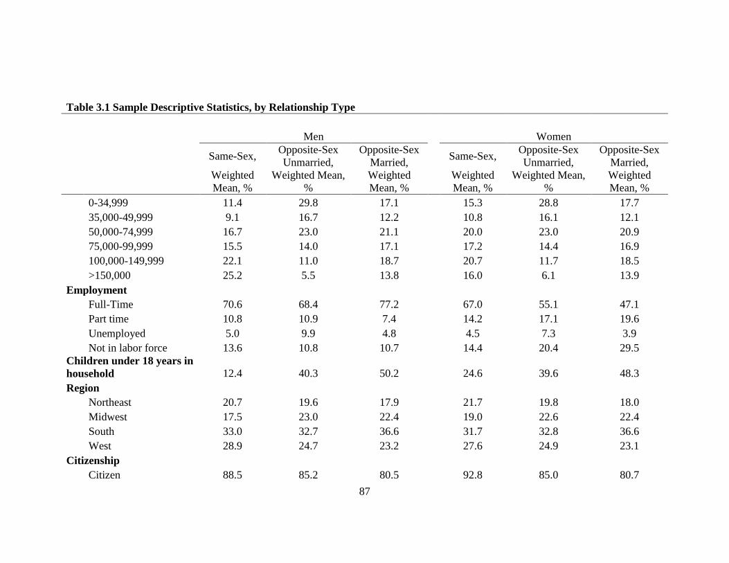
87
Table 3.1 Sample Descriptive Statistics, by Relationship Type
Men
Women
Same-Sex, Opposite-Sex
Unmarried,
Opposite-Sex
Married, Same-Sex,
Opposite-Sex
Unmarried,
Opposite-Sex
Married,
Weighted
Mean, %
Weighted Mean,
%
Weighted
Mean, %
Weighted
Mean, %
Weighted Mean,
%
Weighted
Mean, %
0-34,999 11.4 29.8 17.1
15.3 28.8 17.7
35,000-49,999 9.1 16.7 12.2
10.8 16.1 12.1
50,000-74,999 16.7 23.0 21.1
20.0 23.0 20.9
75,000-99,999 15.5 14.0 17.1
17.2 14.4 16.9
100,000-149,999 22.1 11.0 18.7
20.7 11.7 18.5
>150,000 25.2 5.5 13.8
16.0 6.1 13.9
Employment
Full-Time 70.6 68.4 77.2
67.0 55.1 47.1
Part time 10.8 10.9 7.4
14.2 17.1 19.6
Unemployed 5.0 9.9 4.8
4.5 7.3 3.9
Not in labor force 13.6 10.8 10.7
14.4 20.4 29.5
Children under 18 years in
household 12.4 40.3 50.2
24.6 39.6 48.3
Region
Northeast 20.7 19.6 17.9
21.7 19.8 18.0
Midwest 17.5 23.0 22.4
19.0 22.6 22.4
South 33.0 32.7 36.6
31.7 32.8 36.6
West 28.9 24.7 23.2
27.6 24.9 23.1
Citizenship
Citizen 88.5 85.2 80.5
92.8 85.0 80.7

88
Table 3.1 Sample Descriptive Statistics, by Relationship Type
Men
Women
Same-Sex, Opposite-Sex
Unmarried,
Opposite-Sex
Married, Same-Sex,
Opposite-Sex
Unmarried,
Opposite-Sex
Married,
Weighted
Mean, %
Weighted Mean,
%
Weighted
Mean, %
Weighted
Mean, %
Weighted Mean,
%
Weighted
Mean, %
Naturalized 5.7 3.7 8.8
3.9 4.5 9.0
Non-citizen 5.8 11.2 10.7
3.3 10.4 10.2
Disabled 6.3 6.8 5.7
8.6 8.2 6.2
MSA residence 92.7 84.0 83.7
89.8 84.1 83.5
Primary source of health
insurance
Employer 70.9 51.2 74.5
72.1 50.4 74.1
Direct Purchase 8.3 5.1 6.1
6.7 5.3 6.9
Medicaid 3.5 5.9 3.3
4.4 13.1 4.0
Medicare 3.5 2.5 2.7
3.2 2.9 2.3
Uninsured 13.8 35.3 13.5
13.6 28.4 12.7
Sample Size 15,529 133,347 1,491,384 16,418 125,800 1,569,327
Note: GED = general equivalency diploma. FPG = federal poverty guidelines. Weighted means are for adults aged 25 to 64 years.
Source: 2008-2010 American Community Survey

89
Table 3.2 Multinomial Logistic Regression Analysis of Health Insurance Coverage by Relationship Type for Men
Adjusted RRR (95% CI)
Employer Direct Purchase Medicaid Medicare
vs. Uninsured vs. Uninsured vs. Uninsured vs. Uninsured
All Men
In a married opposite-sex couple 1.00 Reference
1.00 Reference
1.00 Reference
1.00 Reference
In an unmarried opposite-sex couple 0.32 (0.31-0.33) *** 0.45 (0.43-0.46) *** 0.52 (0.50-0.54) *** 0.47 (0.44-0.49) ***
In a same-sex couple 0.50 (0.47-0.54) *** 0.73 (0.66-0.80) *** 1.28 (1.11-1.49) *** 0.99 (0.87-1.14)
Only Employed Men
In a married opposite-sex couple 1.00 Reference
1.00 Reference
1.00 Reference
1.00 Reference
In an unmarried opposite-sex couple 0.36 (0.35-0.36) *** 0.47 (0.45-0.49) *** 0.44 (0.42-0.47) *** 0.48 (0.43- 0.54) ***
In a same-sex couple 0.58 (0.53-0.63) *** 0.79 (0.66- 0.84) *** 1.23 (0.98-1.55) * 1.10 (0.84-1.45)
Note: RRR = Relative risk ratio. CI = confidence interval. All models control for age group, income group, educational attainment, employment status,
citizenship status, disability status, the presence of a related child under 18 years in the household, state of residence, metropolitan status and survey year.
*P<.10; **P<.05; ***P<.01

90
Table 3.3 Multinomial Logistic Regression Analysis of Health Insurance Coverage by Relationship Type for Women
Adjusted RRR (95% CI)
Employer Direct Purchase Medicaid Medicare
vs. Uninsured vs. Uninsured vs. Uninsured vs. Uninsured
All Women
In a married opposite-sex couple 1.00 Reference
1.00 Reference
1.00 Reference
1.00 Reference
In an unmarried opposite-sex couple 0.27 (0.27-0.28) *** 0.43 (0.42-0.45) *** 1.35 (1.31-1.39) *** 0.90 (0.86-0.95) ***
In a same-sex couple 0.46 (0.43-0.50) *** 0.62 (0.56-0.69) *** 0.99 (0.88-1.13)
1.11 (0.97-1.26)
Only Employed Women
In a married, opposite-sex couple 1.00 Reference
1.00 Reference
1.00 Reference
1.00 Reference
In an unmarried, opposite-sex couple 0.35 (0.34-0.36) *** 0.49 (0.45-0.51) *** 1.17 (1.11-1.22) *** 0.67 (0.60-0.76) ***
In a same-sex couple 0.50 (0.46-0.55) *** 0.67 (0.60-0.76) *** 0.79 (0.66-0.95) ** 0.98 (0.75-1.27)
Note: RRR = Relative risk ratio. CI = confidence interval. All models control for age group, income group, educational attainment, employment status,
citizenship status, disability status, the presence of a related child under 18 years in the household, state of residence, metropolitan status and survey year.
*P<.10; **P<.05; ***P<.01

91
Table 3.4 Unadjusted and Adjusted Differences in ESI Between Men in Same-Sex Couples and Men in Married Opposite-Sex
Couples
Unadjusted RD (95% CI)
in percentage points
Adjusted RD (95% CI)
in percentage points
Northeast -3.2 (-5.1,-1.3)***
-7.8 (-9.6,-6)***
Connecticut -0.1 (-7.7,7.4)
-2.2 (-10.4,6.1)
Maine -6.4 (-19,6.3)
-13.7 (-25,-2.4)**
Massachusetts -4.4 (-8.8,0)*
-7.5 (-12.1,-2.9)***
New Hampshire -10.3 (-23,2.5)
-4.8 (-13.4,3.9)
New Jersey -2.8 (-7.2,1.7)
-7.4 (-11.4,-3.4)***
New York 0.4 (-2.6,3.3)
-6.8 (-9.6,-4.1)***
Pennsylvania -5.1 (-10.1,-0.1)*
-9.3 (-13.9,-4.7)***
Rhode Island -11.5 (-25.2,2.2)
-13.2 (-21.1,-5.3)***
Vermont -18.8 (-35.4,-2.2)**
-15.7 (-28.5,-2.8)**
Midwest -6.6 (-8.9,-4.3)***
-8.3 (-10.1,-6.4)***
Illinois -3.1 (-7.1,0.9)
-6.5 (-9.9,-3.1)***
Indiana -9.1 (-16.4,-1.7)**
-11.8 (-18,-5.64)***
Iowa -8.9 (-23.7,5.8)
-8.0 (-15.2,-0.7)*
Kansas -9.4 (-27,8.2)
-10.9 (-20.2,-1.5)**
Michigan -1.7 (-7.1,3.8)
-5.5 (-9.7,-1.3)**
Minnesota -9.6 (-17.4,-1.8)**
-11.5 (-17.9,-5)***
Missouri -7.0 (-15.2,1.2)
-8.3 (-15.3,-1.3)**
Nebraska† -17.6 (-43.5,8.2)
1.4 (-14.7,17.4)
North Dakota† -4.8 (-36.7,27.1)
2.6 (-17.6,22.9)
Ohio -5.7 (-10.4,-1)**
-7.6 (-12,-3.3)***
South Dakota† -0.4 (-30.8,30.1)
1.8 (-16.9,20.6)
Wisconsin -15.6 (-24.7,-6.5)***
-12.9 (-20.2,-5.7)***

92
Table 3.4 Unadjusted and Adjusted Differences in ESI Between Men in Same-Sex Couples and Men in Married Opposite-Sex
Couples
Unadjusted RD (95% CI)
in percentage points
Adjusted RD (95% CI)
in percentage points
South -4.5 (-6.0,-3)***
-9.3 (-10.5,-8)***
Alabama -10.3 (-22.4,1.8)
-7.3 (-14.9,0.2)*
Arkansas 6.1 (-4.3,16.5)
5.6 (-2.1,13.3)
Delaware -10.8 (-22.3,0.8)
-12.1 (-23.4,-0.8)*
District of Columbia -1.7 (-6.8,3.4)
-9.1 (-14.2,-3.9)**
Florida -4.7 (-7.9,-1.5)***
-9.2 (-11.7,-6.7)***
Georgia -4.3 (-8.7,0.0)*
-10.2 (-14.1,-6.2)***
Kentucky -7.0 (-15.1,1.2)
-10.2 (-18.3,-2.2)**
Louisiana -12.0 (-20.9,-3.1)**
-12.4 (-19.2,-5.6)***
Maryland -8.7 (-15.9,-1.6)**
-11.2 (-17.4,-4.9)***
Mississippi -13.8 (-26.6,-1)*
-15.1 (-26.8,-3.4)**
North Carolina -1.4 (-6.9,4.1)
-4.4 (-8.4,-0.4)**
Oklahoma -8.2 (-19.9,3.5)
-13.4 (-22.7,-4.1)***
South Carolina -15.8 (-24.6,-7)***
-13.0 (-21,-4.9)***
Tennessee -5.2 (-11.4,0.9)
-11.1 (-16.4,-5.8)***
Texas 1.2 (-2.2,4.7)
-8.7 (-11.5,-5.9)***
Virginia -8.7 (-15.5,-1.9)**
-7.2 (-11.6,-2.7)***
West Virginia -12.0 (-30,6.1)
-21.4 (-37.5,-5.3)**
West 0.1 (-1.6,1.7)
-7.9 (-9.4,-6.5)***
Alaska† 6.5 (-6.4,19.5)
-0.8 (-14,12.5)
Arizona -6.1 (-12.3,0.1)*
-11.4 (-16.9,-5.9)***
California 3.3 (1.2,5.4)***
-7.5 (-9.3,-5.7)***
Colorado 0.2 (-6.3,6.8)
-6.3 (-12.5,-0.1)*

93
Table 3.4 Unadjusted and Adjusted Differences in ESI Between Men in Same-Sex Couples and Men in Married Opposite-Sex
Couples
Unadjusted RD (95% CI)
in percentage points
Adjusted RD (95% CI)
in percentage points
Hawaii -16.9 (-32.5,-1.3)**
-22.0 (-38.7,-5.4)**
Idaho† 10.6 (-6.7,27.8)
3.0 (-12,18)
Montana† -4.7 (-37,27.5)
-2.6 (-22.4,17.3)
Nevada -8.5 (-16.6,-0.4)*
-13.7 (-20.2,-7.1)***
New Mexico -16.1 (-27.4,-4.8)**
-17.4 (-28.2,-6.5)***
Oregon -0.9 (-7.3,5.6)
-5.9 (-11.8,-0.1)*
Utah 3.9 (-4.9,12.6)
-4.4 (-12.7,3.9)
Washington -0.2 (-5.9,5.5)
-5.3 (-10.5,0)*
Wyoming† -56.0 (-78.5,-33.5)***
-31.7 (-45.4,-18)***
United States -3.5 (-4.4,-2.6)***
-8.4 (-9.2,-7.7)***
Note: RD = Rate difference. CI = Confidence interval. Adjusted models include a control for age group, income group, educational
attainment, employment status, citizenship status, disability status, the presence of related children under 18 years living in the
household, residence in a Metropolitan Statistical Area (MSA) and survey year.
† Indicates sample size fewer than 50 adults in a same-sex relationship, and results are not considered reliable.
*P<.10; **P<.05; ***P<.01

94
Table 3.5 Unadjusted and Adjusted Differences in ESI Between Women in Cohabiting Same-Sex Couples and Women in
Married Cohabiting Opposite-Sex Couples
Unadjusted RD (95% CI)
in percentage points
Adjusted RD (95% CI)
in percentage points
Northeast -1.6 (-3.5,0.3)
-8.5 (-10.3,-6.8)***
Connecticut -5.2 (-12.6,2.2)
-8.6 (-17.4,0.3)*
Maine -7.4 (-18.3,3.6)
-12.5 (-22.8,-2.2)**
Massachusetts -2.5 (-5.8,0.8)
-9.2 (-12.4,-6)***
New Hampshire 3.2 (-3.5,9.9)
1.0 (-6,7.9)
New Jersey -2.0 (-7.5,3.4)
-9.2 (-13.9,-4.5)***
New York 1.1 (-2.2,4.4)
-8.1 (-11.3,-5)***
Pennsylvania -3.7 (-9.2,1.8)
-7.8 (-12.4,-3.3)***
Rhode Island -3.5 (-13.6,6.6)
-9.5 (-19.5,0.5)
Vermont -6.8 (-19.9,6.4)
-13.5 (-27.1,0.1)*
Midwest -9.3 (-11.6,-7.1)***
-12.0 (-13.8,-10.3)***
Illinois -10.4 (-15.8,-5.1)***
-13.8 (-17.6,-10)***
Indiana -10.5 (-16.9,-4.1)***
-12.4 (-17.2,-7.7)***
Iowa -2.4 (-13.4,8.5)
-12.1 (-21.7,-2.6)**
Kansas 1.2 (-6.4,8.8)
-6.0 (-12.9,0.9)
Michigan -16.0 (-22.9,-9.1)***
-14.7 (-20.1,-9.4)***
Minnesota -2.5 (-9.7,4.7)
-7.1 (-13,-1.2)**
Missouri -13.2 (-21.1,-5.2)***
-13.8 (-19.9,-7.7)***
Nebraska -11.4 (-24.4,1.7)
-10.3 (-26.9,6.3)
North Dakota† -11.8 (-36,12.4)
-4.0 (-15.7,7.6)
Ohio -8.6 (-12.9,-4.3)***
-11.7 (-15.6,-7.7)***
South Dakota† 17.0 (5.5,28.4)**
17.2 (6.7,27.8)***
Wisconsin -7.6 (-14.8,-0.4)*
-13.0 (-18.6,-7.5)***
South -2.1 (-3.6,-0.5)**
-8.6 (-9.9,-7.3)***

95
Table 3.5 Unadjusted and Adjusted Differences in ESI Between Women in Cohabiting Same-Sex Couples and Women in
Married Cohabiting Opposite-Sex Couples
Unadjusted RD (95% CI)
in percentage points
Adjusted RD (95% CI)
in percentage points
Alabama -15.4 (-25.5,-5.2)***
-13.9 (-20.4,-7.3)***
Arkansas -6.4 (-18.7,5.9)
-2.8 (-14.6,9.1)
Delaware 4.0 (-6.3,14.3)
1.0 (-11.1,13.2)
District of Columbia -1.7 (-10.4,7.1)
-15.6 (-23.6,-7.7)***
Florida 0.3 (-3.0,3.6)
-8.6 (-11.6,-5.6)***
Georgia -3.7 (-8.5,1.2)
-10.5 (-14.9,-6.1)***
Kentucky -3.0 (-11.2,5.1)
-3.8 (-11,3.4)
Louisiana -9.2 (-18.6,0.3)*
-10.7 (-18.3,-3)**
Maryland 2.8 (-1.4,6.9)
-4.5 (-9.1,0.1)*
Mississippi -5.6 (-18.1,7)
-11.6 (-24.7,1.6)
North Carolina -2.8 (-7.9,2.3)
-8.6 (-13.1,-4)***
Oklahoma -0.9 (-9.8,8)
-3.5 (-10.1,3.1)
South Carolina -7.6 (-16.8,1.6)
-6.0 (-12.5,0.6)
Tennessee -9.3 (-16.1,-2.5)**
-11.2 (-16.3,-6.1)***
Texas 1.7 (-1.6,5)
-9.6 (-12.4,-6.8)***
Virginia -1.6 (-6.6,3.4)
-5.9 (-10.4,-1.4)**
West Virginia -2.5 (-18.9,14)
-6.6 (-18,4.8)
West 3.1 (1.5,4.8)***
-7.4 (-8.9,-5.8)***
Alaska 0.5 (-12.4,13.4)
-7.3 (-21.1,6.5)
Arizona -1.2 (-7.3,4.9)
-9.6 (-15.1,-4.2)***
California 8.9 (6.8,11)***
-4.7 (-6.8,-2.6)***
Colorado -3.6 (-9.5,2.3)
-11.5 (-16.8,-6.3)***
Hawaii -12.2 (-26.9,2.6)
-14.0 (-30.3,2.3)
Idaho 0.7 (-10,11.4)
1.2 (-7.4,9.8)

96
Table 3.5 Unadjusted and Adjusted Differences in ESI Between Women in Cohabiting Same-Sex Couples and Women in
Married Cohabiting Opposite-Sex Couples
Unadjusted RD (95% CI)
in percentage points
Adjusted RD (95% CI)
in percentage points
Montana 10.0 (-1.0,20.9)
-2.0 (-16.1,12.1)
Nevada -5.7 (-17.4,6.1)
-12.0 (-21.2,-2.8)**
New Mexico -6.7 (-16.0,2.7)
-13.9 (-21,-6.8)***
Oregon 0.6 (-5.5,6.7)
-4.8 (-10.5,0.9)
Utah -2.7 (-14.4,9.1)
-12.3 (-22.4,-2.3)**
Washington -2.0 (-6.9,3)
-9.7 (-14.4,-5)***
Wyoming† -2.2 (-25.7,21.2)
-12.4 (-33.4,8.6)
United States -2.0 (-2.9,-1.1)***
-9.0 (-9.8,-8.2)***
Note: RD = Rate difference. CI = Confidence interval. Adjusted models include a control for age group, income group, educational
attainment, employment status, citizenship status, disability status, the presence of related children under 18 years living in the
household, residence in a Metropolitan Statistical Area (MSA) and survey year.
† Indicates sample size fewer than 50 adults in a same-sex relationship, and results are not considered reliable.
*P<.10; **P<.05; ***P<.01
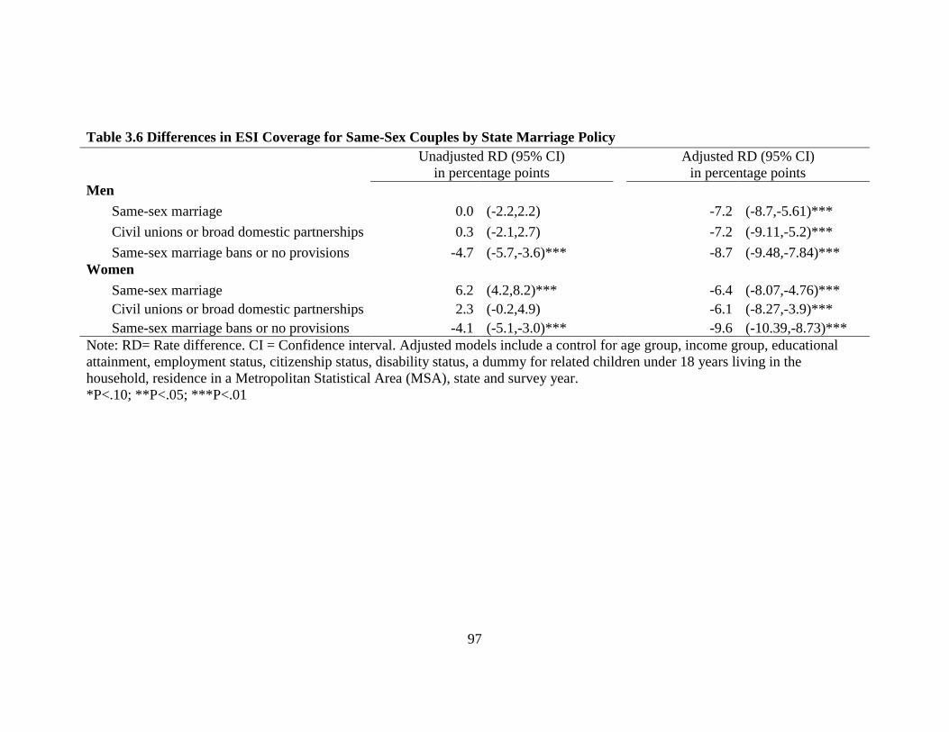
97
Table 3.6 Differences in ESI Coverage for Same-Sex Couples by State Marriage Policy
Unadjusted RD (95% CI)
in percentage points
Adjusted RD (95% CI)
in percentage points
Men
Same-sex marriage 0.0 (-2.2,2.2)
-7.2 (-8.7,-5.61)***
Civil unions or broad domestic partnerships 0.3 (-2.1,2.7)
-7.2 (-9.11,-5.2)***
Same-sex marriage bans or no provisions -4.7 (-5.7,-3.6)***
-8.7 (-9.48,-7.84)***
Women
Same-sex marriage 6.2 (4.2,8.2)***
-6.4 (-8.07,-4.76)***
Civil unions or broad domestic partnerships 2.3 (-0.2,4.9)
-6.1 (-8.27,-3.9)***
Same-sex marriage bans or no provisions -4.1 (-5.1,-3.0)***
-9.6 (-10.39,-8.73)***
Note: RD= Rate difference. CI = Confidence interval. Adjusted models include a control for age group, income group, educational
attainment, employment status, citizenship status, disability status, a dummy for related children under 18 years living in the
household, residence in a Metropolitan Statistical Area (MSA), state and survey year.
*P<.10; **P<.05; ***P<.01

98
Complete Regression Tables
The following tables represent the complete multinomial logistic regression results
presented in Tables 3.2 and 3.3.

99
Table 3.7 Multinomial Logistic Regression Analysis of Health Insurance Coverage for ALL MEN
Adjusted RRR (95% CI)
Employer Direct Purchase Medicaid Medicare
vs. Uninsured vs. Uninsured vs. Uninsured vs. Uninsured
Relationship type
Married opposite-sex couple 1.00 Reference 1.00 Reference 1.00 Reference 1.00 Reference
Same-sex couple 0.50 (0.47-0.54) 0.73 (0.66-0.80) 1.28 (1.11-1.49) 1.00 (0.87-1.14)
Unmarried opposite-sex couple 0.32 (0.31-0.33) 0.45 (0.43-0.46) 0.52 (0.50-0.54) 0.47 (0.44-0.49)
Age (years)
25-34 0.41 (0.40-0.42) 0.30 (0.29-0.31) 1.08 (1.04-1.13) 0.14 (0.13-0.15)
35-44 0.46 (0.45-0.47) 0.39 (0.38-0.41) 0.97 (0.93-1.02) 0.28 (0.27-0.30)
45-54 0.59 (0.58-0.6) 0.59 (0.58-0.61) 0.94 (0.90-0.98) 0.49 (0.47-0.50)
55-64 1.00 Reference 1.00 Reference 1.00 Reference 1.00 Reference
Race/Ethnicity
White 1.00 Reference 1.00 Reference 1.00 Reference 1.00 Reference
Hispanic 0.73 (0.71-0.75) 0.34 (0.32-0.35) 0.71 (0.68-0.74) 0.79 (0.75-0.84)
Black 0.98 (0.95-1.00) 0.39 (0.37-0.41) 1.37 (1.31-1.44) 1.07 (1.01-1.12)
Asian 0.98 (0.94-1.02) 0.83 (0.79-0.87) 1.57 (1.47-1.67) 0.97 (0.88-1.07)
Multiple/Other Races 0.66 (0.63-0.69) 0.45 (0.41-0.48) 1.08 (1.00-1.16) 0.83 (0.76-0.91)
Educational Attainment
Less than high school 0.25 (0.24-0.26) 0.19 (0.18-0.19) 1.30 (1.24-1.37) 0.75 (0.71-0.79)
High school graduate 0.41 (0.40-0.42) 0.32 (0.31-0.32) 1.07 (1.02-1.13) 0.79 (0.75-0.83)
Some college 0.59 (0.58-0.61) 0.47 (0.46-0.49) 1.06 (1.00-1.11) 0.91 (0.87-0.96)
College degree 1.00 Reference 1.00 Reference 1.00 Reference 1.00 Reference

100
Table 3.7 Multinomial Logistic Regression Analysis of Health Insurance Coverage for ALL MEN
Couple's combined income ($)
0-34,999 0.21 (0.21-0.21) 0.43 (0.42-0.45) 2.73 (2.62-2.85) 0.52 (0.50-0.55)
35,000-49,999 0.51 (0.50-0.52) 0.65 (0.63-0.67) 1.39 (1.32-1.46) 0.73 (0.70-0.77)
50,000-74,999 1.00 Reference 1.00 Reference 1.00 Reference 1.00 Reference
75,000-99,999 1.80 (1.75-1.85) 1.40 (1.35-1.45) 0.76 (0.71-0.83) 1.44 (1.36-1.52)
100,000-149,999 2.63 (2.55-2.72) 1.81 (1.74-1.88) 0.77 (0.70-0.85) 1.66 (1.56-1.77)
>150,000 3.09 (2.96-3.23) 2.90 (2.76-3.05) 0.73 (0.64-0.84) 1.64 (1.50-1.79)
Employment
Part-time 0.42 (0.41-0.43) 0.92 (0.89-0.95) 1.25 (1.20-1.29) 2.29 (2.14-2.44)
Unemployed 0.21 (0.20-0.22) 0.40 (0.38-0.42) 1.29 (1.25-1.34) 0.96 (0.88-1.04)
Not in labor force 0.55 (0.53-0.56) 1.01 (0.97-1.04) 2.75 (2.65-2.86) 18.94 (18.04-19.88)
Children under 18 years in household 1.12 (1.10-1.13) 1.14 (1.11-1.16) 3.25 (3.15-3.35) 1.12 (1.07-1.16)
Citizenship
Citizen 1.00 Reference 1.00 Reference 1.00 Reference 1.00 Reference
Naturalized 0.53 (0.52-0.55) 0.85 (0.82-0.89) 0.83 (0.79-0.87) 0.65 (0.61-0.69)
Non-citizen 0.26 (0.25-0.27) 0.41 (0.39-0.42) 0.35 (0.33-0.36) 0.22 (0.20-0.24)
Disabled 1.05 (1.02-1.08) 0.62 (0.59-0.66) 3.13 (3.01-3.26) 6.72 (6.47-6.97)
MSA residence 1.19 (1.17-1.22) 0.97 (0.94-0.99) 0.94 (0.91-0.98) 0.97 (0.94-1.01)
Year
2008 1.00 Reference 1.00 Reference 1.00 Reference 1.00 Reference
2009 0.99 (0.98-1.01) 0.97 (0.95-0.99) 1.07 (1.04-1.1) 0.95 (0.92-0.98)
2010 0.96 (0.95-0.98) 0.92 (0.90-0.95) 1.18 (1.14-1.22) 0.94 (0.90-0.97)
Note: RRR = Relative risk ratio. CI = confidence interval. MSA = Metropolitan Statistical Area. Model contains full set of covariates
listed and state fixed effects. Coefficients for state covariates are not listed due to the large number of coefficients and lack of specific
relevance; the full model results are available on request.
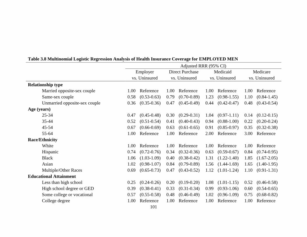
101
Table 3.8 Multinomial Logistic Regression Analysis of Health Insurance Coverage for EMPLOYED MEN
Adjusted RRR (95% CI)
Employer Direct Purchase Medicaid Medicare
vs. Uninsured vs. Uninsured vs. Uninsured vs. Uninsured
Relationship type
Married opposite-sex couple 1.00 Reference 1.00 Reference 1.00 Reference 1.00 Reference
Same-sex couple 0.58 (0.53-0.63) 0.79 (0.70-0.89) 1.23 (0.98-1.55) 1.10 (0.84-1.45)
Unmarried opposite-sex couple 0.36 (0.35-0.36) 0.47 (0.45-0.49) 0.44 (0.42-0.47) 0.48 (0.43-0.54)
Age (years)
25-34 0.47 (0.45-0.48) 0.30 (0.29-0.31) 1.04 (0.97-1.11) 0.14 (0.12-0.15)
35-44 0.52 (0.51-0.54) 0.41 (0.40-0.43) 0.94 (0.88-1.00) 0.22 (0.20-0.24)
45-54 0.67 (0.66-0.69) 0.63 (0.61-0.65) 0.91 (0.85-0.97) 0.35 (0.32-0.38)
55-64 1.00 Reference 1.00 Reference 2.00 Reference 3.00 Reference
Race/Ethnicity
White 1.00 Reference 1.00 Reference 1.00 Reference 1.00 Reference
Hispanic 0.74 (0.72-0.76) 0.34 (0.32-0.36) 0.63 (0.59-0.67) 0.84 (0.74-0.95)
Black 1.06 (1.03-1.09) 0.40 (0.38-0.42) 1.31 (1.22-1.40) 1.85 (1.67-2.05)
Asian 1.02 (0.98-1.07) 0.84 (0.79-0.89) 1.56 (1.44-1.69) 1.65 (1.40-1.95)
Multiple/Other Races 0.69 (0.65-0.73) 0.47 (0.43-0.52) 1.12 (1.01-1.24) 1.10 (0.91-1.31)
Educational Attainment
Less than high school 0.25 (0.24-0.26) 0.20 (0.19-0.20) 1.08 (1.01-1.15) 0.52 (0.46-0.58)
High school degree or GED 0.39 (0.38-0.41) 0.33 (0.31-0.34) 0.99 (0.93-1.06) 0.60 (0.54-0.65)
Some college or vocational 0.57 (0.55-0.58) 0.48 (0.46-0.49) 1.02 (0.96-1.09) 0.75 (0.68-0.82)
College degree 1.00 Reference 1.00 Reference 1.00 Reference 1.00 Reference

102
Table 3.8 Multinomial Logistic Regression Analysis of Health Insurance Coverage for EMPLOYED MEN
Couple's combined income
0-34,999 0.21 (0.21-0.22) 0.42 (0.41-0.44) 2.97 (2.82-3.13) 0.53 (0.49-0.58)
35,000-49,999 0.50 (0.48-0.51) 0.64 (0.61-0.66) 1.51 (1.42-1.60) 0.72 (0.65-0.79)
50,000-74,999 1.00 Reference 1.00 Reference 1.00 Reference 1.00 Reference
75,000-99,999 1.83 (1.78-1.88) 1.42 (1.37-1.48) 0.67 (0.61-0.74) 1.37 (1.24-1.53)
100,000-149,999 2.71 (2.61-2.80) 1.86 (1.78-1.94) 0.66 (0.59-0.74) 1.67 (1.49-1.86)
>150,000 3.20 (3.05-3.36) 2.93 (2.77-3.10) 0.61 (0.52-0.72) 2.10 (1.83-2.41)
Part-time employment 0.43 (0.42-0.44) 0.93 (0.91-0.96) 1.27 (1.22-1.32) 2.13 (1.99-2.27)
Children under 18 years in household 1.12 (1.10-1.14) 1.18 (1.15-1.21) 4.07 (3.89-4.26) 0.85 (0.79-0.93)
Citizenship
Citizen 1.00 Reference 1.00 Reference 1.00 Reference 1.00 Reference
Naturalized 0.54 (0.52-0.56) 0.87 (0.83-0.91) 0.84 (0.79-0.90) 0.57 (0.50-0.65)
Non-citizen 0.26 (0.25-0.26) 0.38 (0.36-0.40) 0.36 (0.33-0.38) 0.29 (0.25-0.34)
Disabled 0.90 (0.86-0.94) 0.65 (0.60-0.70) 2.19 (2.03-2.37) 7.07 (6.51-7.68)
MSA residence 1.18 (1.16-1.21) 0.93 (0.90-0.95) 0.96 (0.91-1.01) 1.06 (0.97-1.15)
Year
2008 1.00 Reference 1.00 Reference 1.00 Reference 1.00 Reference
2009 1.01 (0.99-1.03) 0.99 (0.96-1.01) 1.07 (1.03-1.12) 0.85 (0.79-0.92)
2010 0.97 (0.95-0.99) 0.93 (0.91-0.96) 1.19 (1.14-1.24) 0.80 (0.74-0.87)
Note: RRR = Relative risk ratio. CI = confidence interval. MSA = Metropolitan Statistical Area. Model contains full set of covariates
listed and state fixed effects. Coefficients for state covariates are not listed due to the large number of coefficients and lack of specific
relevance; the full model results are available on request.

103
Table 3.9 Multinomial Logistic Regression Analysis of Health Insurance Coverage for ALL WOMEN
Adjusted RRR (95% CI)
Employer Direct Purchase Medicaid Medicare
vs. Uninsured vs. Uninsured vs. Uninsured vs. Uninsured
Relationship type
Married opposite-sex couple 1.00 Reference 1.00 Reference 1.00 Reference 1.00 Reference
Same-sex couple 0.46 (0.43-0.50) 0.62 (0.56-0.69) 1.00 (0.88-1.13) 1.11 (0.97-1.26)
Unmarried opposite-sex couple 0.27 (0.27-0.28) 0.43 (0.42-0.45) 1.35 (1.31-1.39) 0.90 (0.86-0.95)
Age (years)
25-34 0.46 (0.44-0.47) 0.30 (0.29-0.31) 1.51 (1.45-1.57) 0.15 (0.14-0.16)
35-44 0.51 (0.50-0.52) 0.39 (0.38-0.40) 1.11 (1.07-1.16) 0.29 (0.27-0.30)
45-54 0.65 (0.64-0.66) 0.56 (0.54-0.57) 0.94 (0.91-0.98) 0.45 (0.44-0.47)
55-64 1.00 Reference 1.00 Reference 1.00 Reference 1.00 Reference
Race/Ethnicity
White 1.00 Reference 1.00 Reference 1.00 Reference 1.00 Reference
Hispanic 0.67 (0.65-0.69) 0.37 (0.36-0.39) 0.82 (0.79-0.85) 0.74 (0.70-0.78)
Black 0.96 (0.94-0.99) 0.47 (0.45-0.50) 1.66 (1.59-1.73) 1.49 (1.42-1.57)
Asian 1.01 (0.97-1.05) 0.92 (0.88-0.97) 1.51 (1.43-1.59) 1.05 (0.95-1.15)
Multiple/Other Races 0.67 (0.64-0.70) 0.50 (0.46-0.53) 1.07 (1.00-1.14) 0.90 (0.82-0.98)
Educational Attainment
Less than high school 0.24 (0.23-0.24) 0.19 (0.18-0.20) 1.48 (1.41-1.55) 0.48 (0.46-0.51)
High school graduate 0.40 (0.39-0.41) 0.35 (0.34-0.36) 1.21 (1.16-1.27) 0.60 (0.58-0.63)
Some college 0.54 (0.53-0.55) 0.50 (0.49-0.52) 1.23 (1.18-1.28) 0.81 (0.77-0.85)
College degree 1.00 Reference 1.00 Reference 1.00 Reference 1.00 Reference
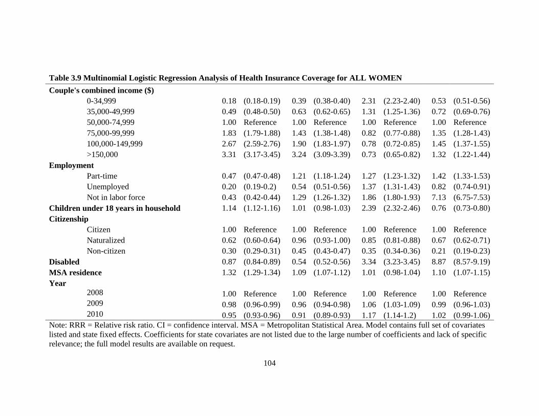
104
Table 3.9 Multinomial Logistic Regression Analysis of Health Insurance Coverage for ALL WOMEN
Couple's combined income ($)
0-34,999 0.18 (0.18-0.19) 0.39 (0.38-0.40) 2.31 (2.23-2.40) 0.53 (0.51-0.56)
35,000-49,999 0.49 (0.48-0.50) 0.63 (0.62-0.65) 1.31 (1.25-1.36) 0.72 (0.69-0.76)
50,000-74,999 1.00 Reference 1.00 Reference 1.00 Reference 1.00 Reference
75,000-99,999 1.83 (1.79-1.88) 1.43 (1.38-1.48) 0.82 (0.77-0.88) 1.35 (1.28-1.43)
100,000-149,999 2.67 (2.59-2.76) 1.90 (1.83-1.97) 0.78 (0.72-0.85) 1.45 (1.37-1.55)
>150,000 3.31 (3.17-3.45) 3.24 (3.09-3.39) 0.73 (0.65-0.82) 1.32 (1.22-1.44)
Employment
Part-time 0.47 (0.47-0.48) 1.21 (1.18-1.24) 1.27 (1.23-1.32) 1.42 (1.33-1.53)
Unemployed 0.20 (0.19-0.2) 0.54 (0.51-0.56) 1.37 (1.31-1.43) 0.82 (0.74-0.91)
Not in labor force 0.43 (0.42-0.44) 1.29 (1.26-1.32) 1.86 (1.80-1.93) 7.13 (6.75-7.53)
Children under 18 years in household 1.14 (1.12-1.16) 1.01 (0.98-1.03) 2.39 (2.32-2.46) 0.76 (0.73-0.80)
Citizenship
Citizen 1.00 Reference 1.00 Reference 1.00 Reference 1.00 Reference
Naturalized 0.62 (0.60-0.64) 0.96 (0.93-1.00) 0.85 (0.81-0.88) 0.67 (0.62-0.71)
Non-citizen 0.30 (0.29-0.31) 0.45 (0.43-0.47) 0.35 (0.34-0.36) 0.21 (0.19-0.23)
Disabled
0.87 (0.84-0.89) 0.54 (0.52-0.56) 3.34 (3.23-3.45) 8.87 (8.57-9.19)
MSA residence 1.32 (1.29-1.34) 1.09 (1.07-1.12) 1.01 (0.98-1.04) 1.10 (1.07-1.15)
Year
2008 1.00 Reference 1.00 Reference 1.00 Reference 1.00 Reference
2009 0.98 (0.96-0.99) 0.96 (0.94-0.98) 1.06 (1.03-1.09) 0.99 (0.96-1.03)
2010 0.95 (0.93-0.96) 0.91 (0.89-0.93) 1.17 (1.14-1.2) 1.02 (0.99-1.06)
Note: RRR = Relative risk ratio. CI = confidence interval. MSA = Metropolitan Statistical Area. Model contains full set of covariates
listed and state fixed effects. Coefficients for state covariates are not listed due to the large number of coefficients and lack of specific
relevance; the full model results are available on request.

105
Table 3.10 Multinomial Logistic Regression Analysis of Health Insurance Coverage for EMPLOYED WOMEN
Adjusted RRR (95% CI)
Employer Direct Purchase Medicaid Medicare
vs. Uninsured vs. Uninsured vs. Uninsured vs. Uninsured
Relationship type
Married opposite-sex couple 1.00 Reference 1.00 Reference 1.00 Reference 1.00 Reference
Same-sex couple 0.50 (0.46-0.55) 0.67 (0.60-0.76) 0.79 (0.66-0.95) 0.98 (0.75-1.27)
Unmarried opposite-sex couple 0.35 (0.34-0.36) 0.49 (0.47-0.51) 1.17 (1.11-1.22) 0.67 (0.60-0.76)
Age (years)
25-34 0.45 (0.44-0.47) 0.29 (0.28-0.31) 1.61 (1.49-1.74) 0.15 (0.13-0.17)
35-44 0.52 (0.50-0.54) 0.39 (0.37-0.41) 1.15 (1.06-1.24) 0.24 (0.22-0.27)
45-54 0.69 (0.67-0.71) 0.58 (0.56-0.61) 0.96 (0.89-1.04) 0.35 (0.32-0.38)
55-64 1.00 Reference 1.00 Reference 1.00 Reference 1.00 Reference
Race/Ethnicity
White 1.00 Reference 1.00 Reference 1.00 Reference 1.00 Reference
Hispanic 0.71 (0.69-0.74) 0.39 (0.37-0.42) 0.90 (0.85-0.96) 0.84 (0.72-0.97)
Black 1.02 (0.98-1.06) 0.48 (0.45-0.51) 1.57 (1.47-1.68) 1.96 (1.75-2.20)
Asian 0.94 (0.9-0.99) 0.93 (0.87-0.99) 1.71 (1.57-1.86) 1.37 (1.13-1.65)
Multiple/Other Races 0.65 (0.61-0.69) 0.50 (0.45-0.55) 0.98 (0.88-1.09) 1.17 (0.95-1.45)
Educational Attainment
Less than high school 0.25 (0.24-0.26) 0.21 (0.2-0.23) 1.24 (1.15-1.34) 0.53 (0.46-0.61)
High school degree or GED 0.40 (0.39-0.41) 0.36 (0.35-0.38) 1.13 (1.06-1.21) 0.57 (0.51-0.63)
Some college or vocational 0.54 (0.52-0.55) 0.51 (0.50-0.53) 1.18 (1.11-1.26) 0.69 (0.63-0.77)
College degree 1.00 Reference 1.00 Reference 1.00 Reference 1.00 Reference

106
Table 3.9 Multinomial Logistic Regression Analysis of Health Insurance Coverage for ALL WOMEN
Couple's combined income
0-34,999 0.20 (0.20-0.21) 0.39 (0.37-0.41) 2.57 (2.43-2.71) 0.63 (0.57-0.69)
35,000-49,999 0.47 (0.46-0.49) 0.62 (0.59-0.64) 1.46 (1.37-1.55) 0.79 (0.71-0.87)
50,000-74,999 1.00 Reference 1.00 Reference 1.00 Reference 1.00 Reference
75,000-99,999 1.93 (1.87-1.99) 1.48 (1.42-1.55) 0.77 (0.70-0.84) 1.43 (1.27-1.61)
100,000-149,999 2.91 (2.80-3.03) 2.02 (1.92-2.12) 0.68 (0.61-0.76) 1.79 (1.57-2.04)
>150,000 3.61 (3.42-3.82) 3.27 (3.07-3.48) 0.68 (0.57-0.81) 1.88 (1.60-2.22)
Part-time employment 0.49 (0.48-0.50) 1.23 (1.20-1.27) 1.25 (1.20-1.29) 1.41 (1.32-1.52)
Children under 18 years in household 1.14 (1.12-1.17) 1.03 (0.99-1.06) 3.24 (3.09-3.39) 0.85 (0.77-0.94)
Citizenship
Citizen 1.00 Reference 1.00 Reference 1.00 Reference 1.00 Reference
Naturalized 0.64 (0.62-0.67) 0.98 (0.93-1.04) 0.87 (0.82-0.94) 0.72 (0.61-0.84)
Non-citizen 0.28 (0.27-0.29) 0.45 (0.43-0.48) 0.41 (0.39-0.44) 0.38 (0.32-0.45)
Disabled
0.82 (0.78-0.86) 0.60 (0.56-0.65) 2.00 (1.86-2.16) 6.42 (5.87-7.01)
MSA residence 1.24 (1.21-1.27) 1.02 (0.99-1.05) 1.01 (0.96-1.07) 1.11 (1.02-1.22)
Year
2008 1.00 Reference 1.00 Reference 1.00 Reference 1.00 Reference
2009 0.99 (0.97-1.01) 0.97 (0.94-1.00) 1.03 (0.99-1.08) 0.84 (0.77-0.91)
2010 0.95 (0.92-0.97) 0.92 (0.9-0.95) 1.12 (1.07-1.16) 0.83 (0.76-0.9)
Note: RRR = Relative risk ratio. CI = confidence interval. MSA = Metropolitan Statistical Area. Model contains full set of covariates
listed and state fixed effects. Coefficients for state covariates are not listed due to the large number of coefficients and lack of specific
relevance; the full model results are available on request.

107
Sensitivity Analyses
The following tables present the results from the sensitivity analysis, which restricts the
sample to respondents using the CATI/CAPI response mode or the mail response mode
and not receiving an allocation flag for marital status (Gates & Steinberger 2009). Results
from the sensitivity analyses do not change the main findings. Individual men and women
in cohabiting same-sex couples are less likely to have employer-sponsored insurance
(ESI) compared to their counterparts in married cohabiting opposite-sex couples.
Differences in ESI were widest in the Midwest (for women) and in the South (for men).
Also, differences in ESI were narrower for women in cohabiting same-sex couples living
in states with same-sex marriage, civil unions or broad domestic partnerships for same-
sex couples.

108
Table 3.11 Sample Descriptive Statistics, by Relationship Type for the Sensitivity Sample
Men
Women
Same-Sex, Opposite-Sex
Unmarried,
Opposite-Sex
Married, Same-Sex,
Opposite-Sex
Unmarried,
Opposite-Sex
Married,
Weighted
Mean, %
Weighted Mean,
%
Weighted
Mean, %
Weighted
Mean, %
Weighted Mean,
%
Weighted
Mean, %
Age (years)
25-34 21.1 43.4 17.6
23.4 45.0 20.2
35-44 32.9 26.5 27.1
29.7 25.8 27.2
45-54 31.1 19.9 30.0
31.5 20.1 29.4
55-64 14.9 10.2 25.4
15.3 9.1 23.2
Race/Ethnicity
Non-Hispanic White 77.1 62.7 70.5
77.3 64.6 70.9
Non-Hispanic Black 5.2 13.8 7.7
7.3 11.1 7.1
Non-Hispanic Asian 3.4 1.9 5.6
1.6 2.9 6.5
Non-Hispanic
Other/Multiple Races 2.2 2.9 1.8
2.8 3.1 1.9
Hispanic 12.1 18.7 14.4
11.0 18.3 13.5
Educational Attainment
Less than high school 4.9 17.8 11.7
4.9 14.6 9.8
High school degree or
GED 15.9 34.1 25.8
16.4 28.5 25.1
Some college or
vocational 31.2 29.9 28.8
31.4 34.2 31.4
College degree 48.0 18.2 33.7
47.3 22.7 33.7
Couple's combined
income

109
Table 3.11 Sample Descriptive Statistics, by Relationship Type for the Sensitivity Sample
Men
Women
Same-Sex, Opposite-Sex
Unmarried,
Opposite-Sex
Married, Same-Sex,
Opposite-Sex
Unmarried,
Opposite-Sex
Married,
Weighted
Mean, %
Weighted Mean,
%
Weighted
Mean, %
Weighted
Mean, %
Weighted Mean,
%
Weighted
Mean, %
0-34,999 11.1 29.8 17.0
15.3 28.8 17.5
35,000-49,999 9.0 16.7 12.1
10.8 16.1 12.1
50,000-74,999 16.5 23.1 21.2
20.3 23.0 21.0
75,000-99,999 15.5 14.0 17.1
17.4 14.4 16.9
100,000-149,999 22.6 11.0 18.7
20.5 11.7 18.6
>150,000 25.4 5.5 13.9
15.7 6.1 13.9
Employment
Full-Time 71.4 68.5 77.3
68.5 55.2 47.1
Part time 10.7 10.9 7.4
13.9 17.1 19.6
Unemployed 5.2 9.9 4.7
4.6 7.3 3.9
Not in labor force 12.8 10.7 10.6
13.0 20.4 29.4
Children under 18 years
in household 9.4 40.5 50.3
23.3 39.8 48.4
Region
Northeast 20.0 19.6 17.9
20.7 19.8 18.0
Midwest 17.5 23.0 22.4
20.0 22.7 22.4
South 33.8 32.6 36.6
32.2 32.7 36.6
West 28.7 24.8 23.1
27.2 24.9 23.0
Citizenship
Citizen 89.1 85.2 80.5
94.1 85.0 80.8
Naturalized 5.4 3.6 8.8
3.0 4.5 9.0

110
Table 3.11 Sample Descriptive Statistics, by Relationship Type for the Sensitivity Sample
Men
Women
Same-Sex, Opposite-Sex
Unmarried,
Opposite-Sex
Married, Same-Sex,
Opposite-Sex
Unmarried,
Opposite-Sex
Married,
Weighted
Mean, %
Weighted Mean,
%
Weighted
Mean, %
Weighted
Mean, %
Weighted Mean,
%
Weighted
Mean, %
Non-citizen 5.5 11.3 10.7
2.9 10.5 10.2
Disabled 5.9 6.7 5.7
8.4 8.1 6.2
MSA residence 93.4 84.0 83.7
90.2 84.1 83.5
Primary source of health
insurance
Employer 70.1 51.1 74.6
71.5 50.3 74.2
Direct Purchase 8.3 5.1 6.1
6.5 5.2 6.9
Medicaid 3.5 5.9 3.2
4.5 13.0 4.0
Medicare 3.4 2.4 2.7
2.8 2.9 2.3
Uninsured 14.7 35.5 13.4
14.7 28.5 12.7
Sample Size 12,219 129,372 1,479,694 12,365 121,873 1,557,611
Note: GED = general equivalency diploma. FPG = federal poverty guidelines. Weighted means are for adults aged 25 to 64 years.
Source: 2008-2010 American Community Survey

111
Table 3.12 Multinomial Logistic Regression Analysis of Health Insurance Coverage for ALL MEN in Sensitivity Sample
Adjusted RRR (95% CI)
Employer Direct Purchase Medicaid Medicare
vs. Uninsured vs. Uninsured vs. Uninsured vs. Uninsured
Relationship type
Married opposite-sex couple 1.00 Reference 1.00 Reference 1.00 Reference 1.00 Reference
Same-sex couple 0.44 (0.41-0.48) 0.66 (0.59-0.74) 1.32 (1.11-1.56) 0.98 (0.84-1.15)
Unmarried opposite-sex couple 0.32 (0.31-0.32) 0.44 (0.43-0.46) 0.52 (0.50-0.54) 0.46 (0.44-0.49)
Age (years)
25-34 0.41 (0.40-0.42) 0.30 (0.29-0.31) 1.07 (1.02-1.12) 0.14 (0.13-0.15)
35-44 0.46 (0.45-0.47) 0.39 (0.38-0.40) 0.96 (0.91-1.00) 0.28 (0.27-0.3)
45-54 0.59 (0.58-0.60) 0.59 (0.57-0.61) 0.93 (0.89-0.97) 0.48 (0.46-0.5)
55-64
Race/Ethnicity
White 1.00 Reference 1.00 Reference 1.00 Reference 1.00 Reference
Hispanic 0.73 (0.71-0.75) 0.33 (0.32-0.35) 0.70 (0.67-0.73) 0.79 (0.75-0.84)
Black 0.98 (0.96-1.01) 0.39 (0.37-0.41) 1.36 (1.30-1.43) 1.07 (1.01-1.12)
Asian 0.99 (0.95-1.03) 0.83 (0.78-0.87) 1.54 (1.44-1.64) 0.99 (0.90-1.10)
Multiple/Other Races 0.66 (0.63-0.69) 0.44 (0.41-0.48) 1.06 (0.98-1.14) 0.82 (0.74-0.89)
Educational Attainment
Less than high school 0.25 (0.24-0.26) 0.19 (0.18-0.19) 1.29 (1.23-1.36) 0.75 (0.71-0.8)
High school graduate 0.41 (0.40-0.42) 0.31 (0.31-0.32) 1.07 (1.02-1.12) 0.80 (0.76-0.83)
Some college 0.59 (0.58-0.61) 0.47 (0.46-0.48) 1.05 (1.00-1.11) 0.92 (0.88-0.96)
College degree 1.00 Reference 1.00 Reference 1.00 Reference 1.00 Reference
Couple's combined income ($)
0-34,999 0.21 (0.20-0.21) 0.43 (0.42-0.45) 2.79 (2.67-2.91) 0.52 (0.50-0.54)

112
Table 3.12 Multinomial Logistic Regression Analysis of Health Insurance Coverage for ALL MEN in Sensitivity Sample
35,000-49,999 0.51 (0.50-0.52) 0.65 (0.63-0.67) 1.40 (1.33-1.47) 0.73 (0.70-0.77)
50,000-74,999 1.00 Reference 1.00 Reference 1.00 Reference 1.00 Reference
75,000-99,999 1.81 (1.76-1.86) 1.41 (1.36-1.46) 0.76 (0.70-0.82) 1.45 (1.37-1.53)
100,000-149,999 2.67 (2.58-2.75) 1.82 (1.75-1.90) 0.75 (0.68-0.83) 1.68 (1.57-1.79)
>150,000 3.13 (2.99-3.28) 2.93 (2.79-3.09) 0.69 (0.60-0.80) 1.66 (1.52-1.82)
Employment
Full-time 1.00 Reference 1.00 Reference 1.00 Reference 1.00 Reference
Part-time 0.42 (0.41-0.43) 0.92 (0.89-0.95) 1.24 (1.20-1.29) 2.31 (2.17-2.47)
Unemployed 0.21 (0.21-0.22) 0.40 (0.38-0.41) 1.29 (1.24-1.34) 0.96 (0.88-1.05)
Not in labor force 0.55 (0.54-0.56) 1.01 (0.98-1.04) 2.75 (2.65-2.86) 19.49 (18.56-20.48)
Children under 18 years in household 1.11 (1.10-1.13) 1.14 (1.11-1.17) 3.38 (3.27-3.49) 1.13 (1.09-1.18)
Citizenship
Citizen 1.00 Reference 1.00 Reference 1.00 Reference 1.00 Reference
Naturalized 0.53 (0.51-0.55) 0.85 (0.82-0.89) 0.83 (0.79-0.88) 0.65 (0.60-0.69)
Non-citizen 0.26 (0.25-0.27) 0.41 (0.39-0.42) 0.35 (0.33-0.36) 0.22 (0.20-0.24)
Disabled 1.05 (1.02-1.09) 0.62 (0.59-0.65) 3.17 (3.04-3.30) 6.79 (6.54-7.05)
MSA residence 1.20 (1.17-1.22) 0.97 (0.94-0.99) 0.94 (0.91-0.98) 0.97 (0.93-1.00)
Year
2008 1.00 Reference 1.00 Reference 1.00 Reference 1.00 Reference
2009 1.00 (0.98-1.01) 0.97 (0.95-1.00) 1.08 (1.04-1.11) 0.95 (0.92-0.98)
2010 0.96 (0.95-0.98) 0.93 (0.9-0.95) 1.18 (1.15-1.22) 0.94 (0.91-0.97)
Note: RRR = Relative risk ratio. CI = confidence interval. MSA = Metropolitan Statistical Area. Model contains full set of covariates
listed and state fixed effects. Coefficients for state covariates are not listed due to the large number of coefficients and lack of specific
relevance; the full model results are available on request.

113
Table 3.13 Multinomial Logistic Regression Analysis of Health Insurance Coverage for EMPLOYED MEN in Sensitivity
Sample
Adjusted RRR (95% CI)
Employer Direct Purchase Medicaid Medicare
vs. Uninsured vs. Uninsured vs. Uninsured vs. Uninsured
Relationship type
Married opposite-sex couple 1.00 Reference 1.00 Reference 1.00 Reference 1.00 Reference
Same-sex couple 0.52 (0.47-0.57) 0.73 (0.64-0.83) 1.21 (0.92-1.58) 1.05 (0.77-1.44)
Unmarried opposite-sex couple 0.35 (0.34-0.36) 0.47 (0.45-0.48) 0.44 (0.42-0.46) 0.46 (0.41-0.52)
Age (years)
25-34 0.47 (0.46-0.48) 0.30 (0.29-0.31) 1.02 (0.96-1.09) 0.14 (0.12-0.15)
35-44 0.52 (0.51-0.54) 0.41 (0.40-0.43) 0.92 (0.86-0.98) 0.22 (0.20-0.24)
45-54 0.67 (0.66-0.69) 0.63 (0.61-0.65) 0.90 (0.84-0.96) 0.34 (0.32-0.37)
55-64 1.00 Reference 1.00 Reference 1.00 Reference 1.00 Reference
Race/Ethnicity
White 1.00 Reference 1.00 Reference 1.00 Reference 1.00 Reference
Hispanic 0.74 (0.72-0.76) 0.34 (0.32-0.35) 0.62 (0.58-0.66) 0.83 (0.72-0.95)
Black 1.06 (1.03-1.10) 0.40 (0.37-0.42) 1.29 (1.20-1.38) 1.84 (1.65-2.04)
Asian 1.03 (0.98-1.07) 0.84 (0.79-0.89) 1.52 (1.41-1.65) 1.67 (1.41-1.98)
Multiple/Other Races 0.69 (0.65-0.73) 0.47 (0.43-0.51) 1.10 (0.99-1.22) 1.05 (0.87-1.27)
Educational Attainment
Less than high school 0.25 (0.24-0.25) 0.19 (0.19-0.20) 1.07 (1.00-1.14) 0.51 (0.46-0.57)
High school degree or GED 0.40 (0.39-0.41) 0.33 (0.31-0.34) 0.99 (0.93-1.06) 0.60 (0.55-0.66)
Some college or vocational 0.57 (0.55-0.58) 0.48 (0.46-0.49) 1.02 (0.96-1.09) 0.76 (0.69-0.83)
College degree 1.00 Reference 1.00 Reference 1.00 Reference 1.00 Reference
Couple's combined income

114
Table 3.13 Multinomial Logistic Regression Analysis of Health Insurance Coverage for EMPLOYED MEN in Sensitivity
Sample
0-34,999 0.21 (0.21-0.22) 0.42 (0.41-0.44) 3.02 (2.86-3.19) 0.53 (0.48-0.58)
35,000-49,999 0.49 (0.48-0.51) 0.63 (0.61-0.66) 1.52 (1.43-1.62) 0.72 (0.65-0.79)
50,000-74,999 1.00 Reference 1.00 Reference 1.00 Reference 1.00 Reference
75,000-99,999 1.83 (1.78-1.88) 1.43 (1.37-1.48) 0.67 (0.61-0.73) 1.38 (1.24-1.54)
100,000-149,999 2.74 (2.64-2.83) 1.88 (1.80-1.96) 0.65 (0.58-0.73) 1.68 (1.50-1.89)
>150,000 3.24 (3.09-3.41) 2.97 (2.80-3.14) 0.58 (0.49-0.69) 2.11 (1.83-2.42)
Part-time employment 0.43 (0.42-0.44) 0.93 (0.91-0.96) 1.27 (1.22-1.32) 2.15 (2.01-2.3)
Children under 18 years in household 1.12 (1.10-1.14) 1.18 (1.15-1.21) 4.26 (4.07-4.47) 0.87 (0.8-0.95)
Citizenship
Citizen 1.00 Reference 1.00 Reference 1.00 Reference 1.00 Reference
Naturalized 0.54 (0.52-0.56) 0.87 (0.83-0.91) 0.85 (0.79-0.90) 0.57 (0.50-0.65)
Non-citizen 0.26 (0.25-0.26) 0.38 (0.36-0.40) 0.36 (0.34-0.38) 0.29 (0.25-0.34)
Disabled
0.90 (0.86-0.95) 0.65 (0.60-0.70) 2.18 (2.02-2.36) 7.24 (6.66-7.87)
MSA residence 1.19 (1.16-1.21) 0.92 (0.9-0.95) 0.96 (0.91-1.01) 1.04 (0.96-1.14)
Year
2008 1.00 Reference 1.00 Reference 1.00 Reference 1.00 Reference
2009 1.02 (1.00-1.04) 0.99 (0.96-1.02) 1.08 (1.04-1.13) 0.85 (0.79-0.92)
2010 0.97 (0.95-0.99) 0.93 (0.91-0.96) 1.19 (1.15-1.24) 0.80 (0.74-0.86)
Note: RRR = Relative risk ratio. CI = confidence interval. MSA = Metropolitan Statistical Area. Model contains full set of covariates
listed and state fixed effects. Coefficients for state covariates are not listed due to the large number of coefficients and lack of specific
relevance; the full model results are available on request.

115
Table 3.14 Multinomial Logistic Regression Analysis of Health Insurance Coverage for ALL WOMEN in Sensitivity Sample
Adjusted RRR (95% CI)
Employer Direct Purchase Medicaid Medicare
vs. Uninsured vs. Uninsured vs. Uninsured vs. Uninsured
Relationship type
Married opposite-sex couple 1.00 Reference 1.00 Reference 1.00 Reference 1.00 Reference
Same-sex couple 0.41 (0.38-0.45) 0.56 (0.50-0.63) 0.97 (0.84-1.11) 1.04 (0.89-1.22)
Unmarried opposite-sex couple 0.27 (0.26-0.28) 0.43 (0.41-0.44) 1.36 (1.32-1.40) 0.90 (0.86-0.95)
Age (years)
25-34 0.46 (0.45-0.47) 0.30 (0.29-0.31) 1.47 (1.41-1.54) 0.15 (0.14-0.16)
35-44 0.51 (0.50-0.52) 0.39 (0.37-0.40) 1.09 (1.05-1.14) 0.29 (0.27-0.30)
45-54 0.65 (0.64-0.66) 0.55 (0.54-0.57) 0.94 (0.90-0.97) 0.45 (0.44-0.47)
55-64
Race/Ethnicity
White 1.00 Reference 1.00 Reference 1.00 Reference 1.00 Reference
Hispanic 0.67 (0.65-0.69) 0.37 (0.36-0.39) 0.81 (0.78-0.85) 0.74 (0.70-0.79)
Black 0.97 (0.94-0.99) 0.48 (0.45-0.50) 1.65 (1.58-1.72) 1.49 (1.42-1.57)
Asian 1.02 (0.98-1.06) 0.93 (0.89-0.97) 1.49 (1.41-1.58) 1.05 (0.95-1.15)
Multiple/Other Races 0.67 (0.64-0.70) 0.50 (0.46-0.53) 1.07 (1.00-1.14) 0.89 (0.82-0.98)
Educational Attainment
Less than high school 0.24 (0.23-0.24) 0.19 (0.18-0.19) 1.46 (1.39-1.53) 0.48 (0.45-0.50)
High school graduate 0.40 (0.39-0.41) 0.35 (0.34-0.36) 1.20 (1.15-1.26) 0.60 (0.57-0.63)
Some college 0.54 (0.53-0.55) 0.50 (0.49-0.52) 1.22 (1.17-1.28) 0.81 (0.77-0.85)
College degree 1.00 Reference 1.00 Reference 1.00 Reference 1.00 Reference
Couple's combined income ($)
0-34,999 0.18 (0.18-0.19) 0.39 (0.38-0.40) 2.34 (2.26-2.43) 0.53 (0.51-0.55)

116
Table 3.14 Multinomial Logistic Regression Analysis of Health Insurance Coverage for ALL WOMEN in Sensitivity Sample
35,000-49,999 0.49 (0.48-0.5) 0.63 (0.62-0.65) 1.31 (1.26-1.37) 0.72 (0.69-0.75)
50,000-74,999 1.00 Reference 1.00 Reference 1.00 Reference 1.00 Reference
75,000-99,999 1.84 (1.79-1.89) 1.44 (1.39-1.49) 0.82 (0.77-0.88) 1.36 (1.29-1.44)
100,000-149,999 2.70 (2.61-2.78) 1.92 (1.84-1.99) 0.76 (0.70-0.83) 1.47 (1.38-1.56)
>150,000 3.33 (3.2-3.48) 3.26 (3.11-3.42) 0.72 (0.64-0.81) 1.33 (1.23-1.45)
Employment
Full-time 1.00 Reference 1.00 Reference 1.00 Reference 1.00 Reference
Part-time 0.47 (0.46-0.48) 1.21 (1.18-1.24) 1.27 (1.23-1.32) 1.44 (1.34-1.54)
Unemployed 0.20 (0.19-0.20) 0.54 (0.51-0.56) 1.37 (1.31-1.43) 0.83 (0.74-0.92)
Not in labor force 0.43 (0.42-0.44) 1.30 (1.27-1.33) 1.86 (1.80-1.92) 7.33 (6.93-7.76)
Children under 18 years in household 1.13 (1.11-1.15) 1.01 (0.98-1.03) 2.46 (2.39-2.53) 0.76 (0.73-0.80)
Citizenship
Citizen 1.00 Reference 1.00 Reference 1.00 Reference 1.00 Reference
Naturalized 0.62 (0.60-0.64) 0.96 (0.93-1.00) 0.85 (0.82-0.89) 0.67 (0.63-0.72)
Non-citizen 0.30 (0.29-0.31) 0.45 (0.43-0.46) 0.35 (0.34-0.37) 0.21 (0.19-0.23)
Disabled
0.87 (0.85-0.89) 0.54 (0.52-0.56) 3.38 (3.27-3.50) 9.04 (8.73-9.36)
MSA residence 1.32 (1.29-1.34) 1.09 (1.07-1.12) 1.01 (0.98-1.04) 1.10 (1.06-1.15)
Year
2008 1.00 Reference 1.00 Reference 1.00 Reference 1.00 Reference
2009 0.98 (0.96-1.00) 0.96 (0.94-0.98) 1.07 (1.04-1.10) 0.99 (0.96-1.03)
2010 0.95 (0.93-0.96) 0.91 (0.89-0.93) 1.18 (1.14-1.21) 1.02 (0.98-1.06)
Note: RRR = Relative risk ratio. CI = confidence interval. MSA = Metropolitan Statistical Area. Model contains full set of covariates
listed and state fixed effects. Coefficients for state covariates are not listed due to the large number of coefficients and lack of specific
relevance; the full model results are available on request.

117
Table 3.15 Multinomial Logistic Regression Analysis of Health Insurance Coverage for EMPLOYED WOMEN in Sensitivity
Sample
Adjusted RRR (95% CI)
Employer Direct Purchase Medicaid Medicare
vs. Uninsured vs. Uninsured vs. Uninsured vs. Uninsured
Relationship type
Married opposite-sex couple 1.00 Reference 1.00 Reference 1.00 Reference 1.00 Reference
Same-sex couple 0.46 (0.42-0.50) 0.61 (0.53-0.70) 0.75 (0.60-0.92) 0.73 (0.52-1.04)
Unmarried opposite-sex couple 0.35 (0.34-0.36) 0.49 (0.46-0.51) 1.17 (1.12-1.23) 0.65 (0.57-0.73)
Age (years)
25-34 0.46 (0.44-0.47) 0.29 (0.28-0.30) 1.58 (1.46-1.70) 0.15 (0.13-0.17)
35-44 0.52 (0.50-0.54) 0.39 (0.37-0.41) 1.12 (1.04-1.21) 0.24 (0.22-0.28)
45-54 0.69 (0.67-0.71) 0.58 (0.56-0.60) 0.95 (0.88-1.02) 0.35 (0.32-0.38)
55-64 1.00 Reference 1.00 Reference 1.00 Reference 1.00 Reference
Race/Ethnicity
White 1.00 Reference 1.00 Reference 1.00 Reference 1.00 Reference
Hispanic 0.72 (0.69-0.74) 0.39 (0.37-0.42) 0.89 (0.84-0.95) 0.84 (0.72-0.97)
Black 1.02 (0.99-1.06) 0.48 (0.45-0.51) 1.57 (1.47-1.68) 1.96 (1.74-2.20)
Asian 0.95 (0.90-1.00) 0.94 (0.88-1.00) 1.70 (1.56-1.85) 1.39 (1.15-1.69)
Multiple/Other Races 0.65 (0.61-0.69) 0.50 (0.45-0.55) 0.98 (0.87-1.09) 1.16 (0.93-1.44)
Educational Attainment
Less than high school 0.25 (0.24-0.26) 0.21 (0.20-0.22) 1.23 (1.15-1.33) 0.51 (0.45-0.59)
High school degree or GED 0.40 (0.39-0.41) 0.36 (0.35-0.38) 1.13 (1.06-1.21) 0.56 (0.51-0.63)
Some college or vocational 0.54 (0.52-0.55) 0.51 (0.50-0.53) 1.18 (1.11-1.26) 0.69 (0.62-0.77)
College degree 1.00 Reference 1.00 Reference 1.00 Reference 1.00 Reference
Couple's combined income

118
Table 3.15 Multinomial Logistic Regression Analysis of Health Insurance Coverage for EMPLOYED WOMEN in Sensitivity
Sample
0-34,999 0.20 (0.20-0.21) 0.39 (0.37-0.40) 2.61 (2.47-2.75) 0.62 (0.56-0.69)
35,000-49,999 0.47 (0.46-0.49) 0.62 (0.59-0.64) 1.47 (1.38-1.56) 0.78 (0.70-0.87)
50,000-74,999 1.00 Reference 1.00 Reference 1.00 Reference 1.00 Reference
75,000-99,999 1.94 (1.87-2.00) 1.49 (1.42-1.55) 0.77 (0.7-0.84) 1.44 (1.27-1.63)
100,000-149,999 2.94 (2.83-3.06) 2.03 (1.94-2.14) 0.66 (0.59-0.75) 1.81 (1.59-2.07)
>150,000 3.66 (3.46-3.87) 3.31 (3.10-3.52) 0.67 (0.56-0.8) 1.90 (1.61-2.24)
Part-time employment 0.48 (0.48-0.49) 1.24 (1.20-1.27) 1.25 (1.20-1.29) 1.42 (1.32-1.53)
Children under 18 years in household 1.14 (1.11-1.17) 1.03 (0.99-1.06) 3.34 (3.19-3.51) 0.85 (0.77-0.94)
Citizenship
Citizen 1.00 Reference 1.00 Reference 1.00 Reference 1.00 Reference
Naturalized 0.64 (0.62-0.67) 0.98 (0.93-1.04) 0.88 (0.82-0.94) 0.72 (0.61-0.85)
Non-citizen 0.28 (0.27-0.29) 0.45 (0.43-0.48) 0.42 (0.39-0.44) 0.38 (0.32-0.46)
Disabled
0.82 (0.79-0.86) 0.60 (0.56-0.65) 2.02 (1.87-2.18) 6.58 (6.01-7.20)
MSA residence 1.24 (1.21-1.27) 1.02 (0.99-1.05) 1.01 (0.96-1.06) 1.11 (1.01-1.22)
Year
2008 1.00 Reference 1.00 Reference 1.00 Reference 1.00 Reference
2009 0.99 (0.97-1.01) 0.97 (0.94-1.00) 1.04 (0.99-1.09) 0.83 (0.77-0.91)
2010 0.95 (0.93-0.97) 0.92 (0.9-0.95) 1.13 (1.08-1.18) 0.82 (0.75-0.89)
Note: RRR = Relative risk ratio. CI = confidence interval. MSA = Metropolitan Statistical Area. Model contains full set of covariates
listed and state fixed effects. Coefficients for state covariates are not listed due to the large number of coefficients and lack of specific
relevance; the full model results are available on request.

119
Table 3.16 Unadjusted and Adjusted Differences in ESI Between Men in Cohabiting Same-Sex Couples and Men in Married
Cohabiting Opposite-Sex Couples, Restricted to Sensitivity Sample
Unadjusted RD (95% CI)
in percentage points
Adjusted RD (95% CI)
in percentage points
Northeast -3.2 (-5.1,-1.3)***
-9.1 (-11.1,-7)***
Connecticut -0.1 (-7.7,7.4)
-2.2 (-12.8,8.5)
Maine -6.4 (-19,6.3)
-15.9 (-28.2,-3.6)**
Massachusetts -4.4 (-8.8,0)*
-9.5 (-15.8,-3.1)***
New Hampshire† -10.3 (-23,2.5)
-6.5 (-17.3,4.4)
New Jersey -2.8 (-7.2,1.7)
-9.5 (-13.9,-5.2)***
New York 0.4 (-2.6,3.3)
-7.6 (-10.7,-4.5)***
Pennsylvania -5.1 (-10.1,-0.1)*
-9.9 (-15,-4.7)***
Rhode Island -11.5 (-25.2,2.2)
-19.0 (-27.7,-10.3)***
Vermont† -18.8 (-35.4,-2.2)**
-16.4 (-28.7,-4)**
Midwest -6.6 (-8.9,-4.3)***
-10.4 (-12.5,-8.3)***
Illinois -3.1 (-7.1,0.9)
-10.1 (-14.1,-6.1)***
Indiana -9.1 (-16.4,-1.7)**
-13.2 (-20.1,-6.35)***
Iowa† -8.9 (-23.7,5.8)
-10.4 (-18.4,-2.4)**
Kansas -9.4 (-27,8.2)
-13.1 (-23.2,-3.1)**
Michigan -1.7 (-7.1,3.8)
-8.1 (-13,-3.3)***
Minnesota -9.6 (-17.4,-1.8)**
-10.8 (-17.8,-3.8)***
Missouri -7.0 (-15.2,1.2)
-8.5 (-16.2,-0.8)**
Nebraska† -17.6 (-43.5,8.2)
0.4 (-16.8,17.7)
North Dakota† -4.8 (-36.7,27.1)
-1.4 (-26.6,23.9)
Ohio -5.7 (-10.4,-1)**
-9.4 (-14.3,-4.4)***
South Dakota† -0.4 (-30.8,30.1)
-11.6 (-34.5,11.3)

120
Table 3.16 Unadjusted and Adjusted Differences in ESI Between Men in Cohabiting Same-Sex Couples and Men in Married
Cohabiting Opposite-Sex Couples, Restricted to Sensitivity Sample
Wisconsin -15.6 (-24.7,-6.5)***
-17.5 (-25.9,-9)***
South -4.5 (-6.0,-3)***
-10.2 (-11.6,-8.8)***
Alabama -10.3 (-22.4,1.8)
-10.5 (-20.2,-0.7)**
Arkansas 6.1 (-4.3,16.5)
4.9 (-3.3,13.1)
Delaware -10.8 (-22.3,0.8)
-20.8 (-33.2,-8.4)***
District of Columbia -1.7 (-6.8,3.4)
-7.7 (-13.1,-2.2)*
Florida -4.7 (-7.9,-1.5)***
-10.3 (-13,-7.6)***
Georgia -4.3 (-8.7,0.0)*
-10.5 (-14.8,-6.2)***
Kentucky -7.0 (-15.1,1.2)
-14.1 (-23.2,-5)***
Louisiana -12.0 (-20.9,-3.1)**
-15.8 (-22.8,-8.7)***
Maryland -8.7 (-15.9,-1.6)**
-11.0 (-18.2,-3.8)***
Mississippi† -13.8 (-26.6,-1)*
-11.4 (-25.3,2.5)
North Carolina -1.4 (-6.9,4.1)
-3.0 (-7.2,1.3)
Oklahoma -8.2 (-19.9,3.5)
-8.9 (-19.3,1.4)
South Carolina -15.8 (-24.6,-7)***
-12.1 (-21.5,-2.7)**
Tennessee -5.2 (-11.4,0.9)
-14.6 (-20.8,-8.5)***
Texas 1.2 (-2.2,4.7)
-9.6 (-12.7,-6.5)***
Virginia -8.7 (-15.5,-1.9)**
-8.7 (-13.7,-3.8)***
West Virginia† -12.0 (-30,6.1)
-25.8 (-43.5,-8.2)***
West 0.1 (-1.6,1.7)
-9.8 (-11.4,-8.1)***
Alaska† 6.5 (-6.4,19.5)
2.3 (-12.3,16.9)
Arizona -6.1 (-12.3,0.1)*
-12.3 (-18.4,-6.3)***
California 3.3 (1.2,5.4)***
-9.5 (-11.7,-7.4)***
Colorado 0.2 (-6.3,6.8)
-6.5 (-13.2,0.3)*

121
Table 3.16 Unadjusted and Adjusted Differences in ESI Between Men in Cohabiting Same-Sex Couples and Men in Married
Cohabiting Opposite-Sex Couples, Restricted to Sensitivity Sample
Hawaii -16.9 (-32.5,-1.3)**
-24.6 (-41.8,-7.5)***
Idaho† 10.6 (-6.7,27.8)
-7.4 (-23.7,8.9)
Montana† -4.7 (-37,27.5)
9.8 (-11.7,31.4)
Nevada -8.5 (-16.6,-0.4)*
-17.3 (-24.5,-10)***
New Mexico -16.1 (-27.4,-4.8)**
-20.7 (-32.2,-9.3)***
Oregon -0.9 (-7.3,5.6)
-6.5 (-13.1,0.1)*
Utah 3.9 (-4.9,12.6)
-1.9 (-10.9,7.1)
Washington -0.2 (-5.9,5.5)
-7.5 (-13.1,-2)**
Wyoming† -56.0 (-78.5,-33.5)***
-42.1 (-70.4,-13.9)***
United States -4.5 (-5.6,-3.5)***
-9.9 (-10.8,-9)***
Note: RD = Rate difference. CI = Confidence interval. Adjusted models include a control for age group, income group, educational
attainment, employment status, citizenship status, disability status, the presence of related children under 18 years living in the
household, residence in a Metropolitan Statistical Area (MSA) and survey year.
† Indicates sample size fewer than 50 adults in a same-sex relationship, and results may not be reliable.
*P<.10; **P<.05; ***P<.01
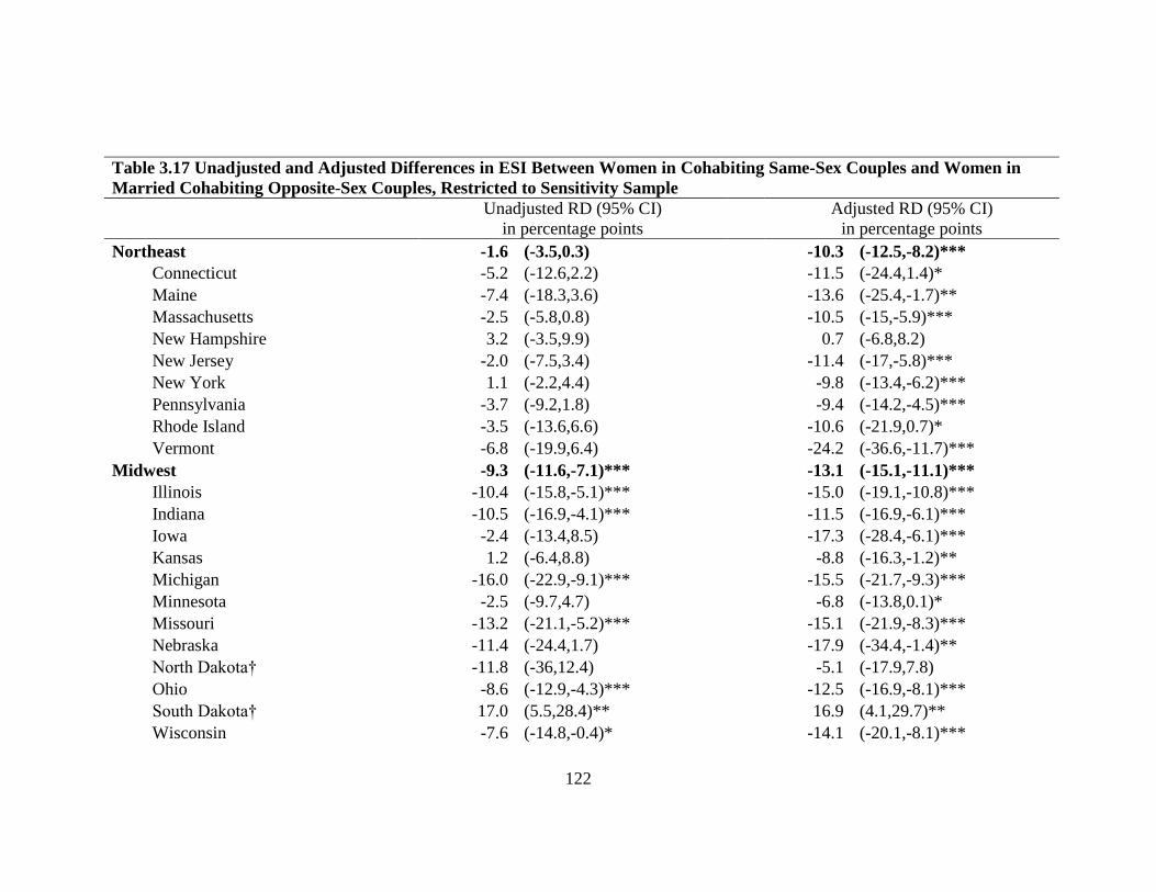
122
Table 3.17 Unadjusted and Adjusted Differences in ESI Between Women in Cohabiting Same-Sex Couples and Women in
Married Cohabiting Opposite-Sex Couples, Restricted to Sensitivity Sample
Unadjusted RD (95% CI)
in percentage points
Adjusted RD (95% CI)
in percentage points
Northeast -1.6 (-3.5,0.3)
-10.3 (-12.5,-8.2)***
Connecticut -5.2 (-12.6,2.2)
-11.5 (-24.4,1.4)*
Maine -7.4 (-18.3,3.6)
-13.6 (-25.4,-1.7)**
Massachusetts -2.5 (-5.8,0.8)
-10.5 (-15,-5.9)***
New Hampshire 3.2 (-3.5,9.9)
0.7 (-6.8,8.2)
New Jersey -2.0 (-7.5,3.4)
-11.4 (-17,-5.8)***
New York 1.1 (-2.2,4.4)
-9.8 (-13.4,-6.2)***
Pennsylvania -3.7 (-9.2,1.8)
-9.4 (-14.2,-4.5)***
Rhode Island -3.5 (-13.6,6.6)
-10.6 (-21.9,0.7)*
Vermont -6.8 (-19.9,6.4)
-24.2 (-36.6,-11.7)***
Midwest -9.3 (-11.6,-7.1)***
-13.1 (-15.1,-11.1)***
Illinois -10.4 (-15.8,-5.1)***
-15.0 (-19.1,-10.8)***
Indiana -10.5 (-16.9,-4.1)***
-11.5 (-16.9,-6.1)***
Iowa -2.4 (-13.4,8.5)
-17.3 (-28.4,-6.1)***
Kansas 1.2 (-6.4,8.8)
-8.8 (-16.3,-1.2)**
Michigan -16.0 (-22.9,-9.1)***
-15.5 (-21.7,-9.3)***
Minnesota -2.5 (-9.7,4.7)
-6.8 (-13.8,0.1)*
Missouri -13.2 (-21.1,-5.2)***
-15.1 (-21.9,-8.3)***
Nebraska -11.4 (-24.4,1.7)
-17.9 (-34.4,-1.4)**
North Dakota† -11.8 (-36,12.4)
-5.1 (-17.9,7.8)
Ohio -8.6 (-12.9,-4.3)***
-12.5 (-16.9,-8.1)***
South Dakota† 17.0 (5.5,28.4)**
16.9 (4.1,29.7)**
Wisconsin -7.6 (-14.8,-0.4)*
-14.1 (-20.1,-8.1)***

123
Table 3.17 Unadjusted and Adjusted Differences in ESI Between Women in Cohabiting Same-Sex Couples and Women in
Married Cohabiting Opposite-Sex Couples, Restricted to Sensitivity Sample
South -2.1 (-3.6,-0.5)** -9.6 (-11.2,-8.1)***
Alabama -15.4 (-25.5,-5.2)***
-15.7 (-24.1,-7.3)***
Arkansas -6.4 (-18.7,5.9)
-5.6 (-20.3,9)
Delaware 4.0 (-6.3,14.3)
0.1 (-13.4,13.7)
District of Columbia -1.7 (-10.4,7.1)
-15.7 (-24.1,-7.2)***
Florida 0.3 (-3.0,3.6)
-8.8 (-12.2,-5.5)***
Georgia -3.7 (-8.5,1.2)
-13.3 (-18.2,-8.3)***
Kentucky -3.0 (-11.2,5.1)
-0.9 (-9.1,7.3)
Louisiana -9.2 (-18.6,0.3)*
-13.9 (-23.2,-4.6)***
Maryland 2.8 (-1.4,6.9)
-5.0 (-9.9,0)*
Mississippi† -5.6 (-18.1,7)
-17.6 (-32.6,-2.6)**
North Carolina -2.8 (-7.9,2.3)
-10.0 (-15.5,-4.5)***
Oklahoma -0.9 (-9.8,8)
-4.3 (-11.3,2.7)
South Carolina -7.6 (-16.8,1.6)
-10.8 (-18.9,-2.8)**
Tennessee -9.3 (-16.1,-2.5)**
-13.1 (-19.1,-7.1)***
Texas 1.7 (-1.6,5)
-10.2 (-13.4,-7)***
Virginia -1.6 (-6.6,3.4)
-6.1 (-11.5,-0.8)**
West Virginia† -2.5 (-18.9,14)
-5.1 (-18.6,8.4)
West 3.1 (1.5,4.8)***
-8.1 (-10,-6.3)***
Alaska† 0.5 (-12.4,13.4)
-2.0 (-16.6,12.6)
Arizona -1.2 (-7.3,4.9)
-10.2 (-16.4,-4)***
California 8.9 (6.8,11)***
-4.8 (-7.4,-2.1)***
Colorado -3.6 (-9.5,2.3)
-12.6 (-18.4,-6.8)***
Hawaii† -12.2 (-26.9,2.6)
-16.5 (-37,4.1)
Idaho† 0.7 (-10,11.4)
0.0 (-11.1,11.1)
Montana† 10.0 (-1.0,20.9)
-6.4 (-26.4,13.6)

124
Table 3.17 Unadjusted and Adjusted Differences in ESI Between Women in Cohabiting Same-Sex Couples and Women in
Married Cohabiting Opposite-Sex Couples, Restricted to Sensitivity Sample
Nevada -5.7 (-17.4,6.1)
-11.5 (-21.9,-1.2)**
New Mexico -6.7 (-16.0,2.7)
-14.9 (-22.7,-7.2)***
Oregon 0.6 (-5.5,6.7)
-4.6 (-10.9,1.8)
Utah -2.7 (-14.4,9.1)
-14.7 (-26.4,-3)**
Washington -2.0 (-6.9,3)
-10.9 (-16,-5.7)***
Wyoming† -2.2 (-25.7,21.2)
-28.5 (-44.8,-12.1)***
United States -2.7 (-3.7, -1.6)***
-10.1 (-11,-9.2)***
Note: RD = Rate difference. CI = Confidence interval. Adjusted models include a control for age group, income group, educational
attainment, employment status, citizenship status, disability status, the presence of related children under 18 years living in the
household, residence in a Metropolitan Statistical Area (MSA) and survey year.
† Indicates sample size fewer than 50 adults in a same-sex relationship, and results may not be reliable.
*P<.10; **P<.05; ***P<.01
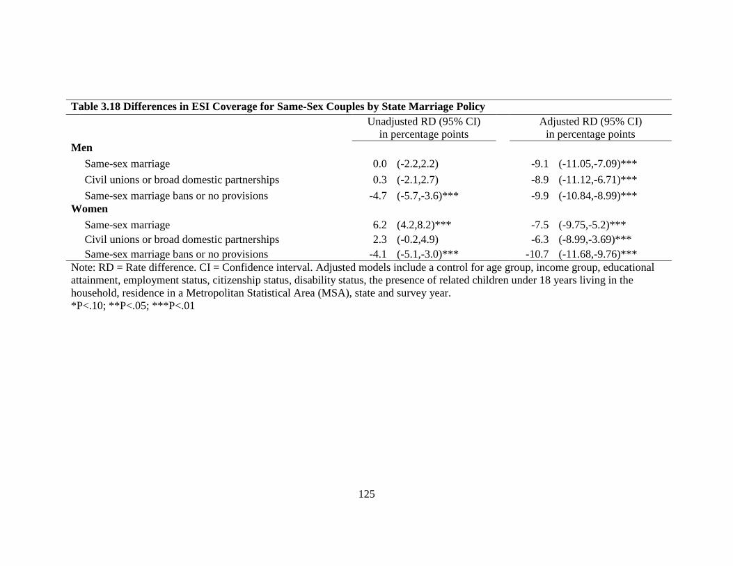
125
Table 3.18 Differences in ESI Coverage for Same-Sex Couples by State Marriage Policy
Unadjusted RD (95% CI)
in percentage points
Adjusted RD (95% CI)
in percentage points
Men
Same-sex marriage 0.0 (-2.2,2.2)
-9.1 (-11.05,-7.09)***
Civil unions or broad domestic partnerships 0.3 (-2.1,2.7)
-8.9 (-11.12,-6.71)***
Same-sex marriage bans or no provisions -4.7 (-5.7,-3.6)***
-9.9 (-10.84,-8.99)***
Women
Same-sex marriage 6.2 (4.2,8.2)***
-7.5 (-9.75,-5.2)***
Civil unions or broad domestic partnerships 2.3 (-0.2,4.9)
-6.3 (-8.99,-3.69)***
Same-sex marriage bans or no provisions -4.1 (-5.1,-3.0)***
-10.7 (-11.68,-9.76)***
Note: RD = Rate difference. CI = Confidence interval. Adjusted models include a control for age group, income group, educational
attainment, employment status, citizenship status, disability status, the presence of related children under 18 years living in the
household, residence in a Metropolitan Statistical Area (MSA), state and survey year.
*P<.10; **P<.05; ***P<.01

126
4. The Association Between State Policy Environments and Health
Insurance Coverage For Children of Cohabiting Same-Sex Parents
4.1 Introduction
This chapter15
examines the association between state policy environments and
health insurance coverage for children of cohabiting same-sex couples. This chapter
makes two contributions to the dissertation. First, this is the first study to examine health
insurance coverage among children of cohabiting same-sex couples using federal
surveys. One previous study uses a similar method to study academic achievement
among children with same-sex parents in the Early Childhood Longitudinal Study—
Kindergarten (ECLS-K) and found children with same-sex parents scored lower than
their peers with married opposite-sex parents on math exams, but these differences
diminished after controlling for demographic characteristics and family structure
transitions (Potter 2012). Other studies have either enumerated the number of children in
same-sex households (Krivickas & Lofquist 2011; Gates 2013); used the presence of
children in same-sex households to predict the likelihood of being a cohabiting same-sex
couple in Census data (Black et. al, 2000); used a convenience sample from a Boston
health center to study access to health care among children in LGBT families (Perrin &
15
A version of this paper was published as Gonzales, G. and L.A. Blewett. 2013.
“Disparities in Health Insurance Among Children With Same-Sex Parents.” Pediatrics
132(4):703-711. This modified version was reproduced with permission by the American
Academy of Pediatrics. This chapter differs from the paper in Pediatrics in the following
ways: this chapter includes the introduction (section 4.1) required in the dissertation, adds
metropolitan statistical area (MSA) to the statistical analysis, extends the discussion on
the data and analytic limitations, clarifies that the sample includes children with
cohabiting parents, presents findings in terms of relative risk ratios, and presents
complete regression results and sensitivity analyses in the technical appendix.
127
Kulkin 1996); or only focused on developmental and psychosocial outcomes among
children with LGBT parents (Patterson 2006).
Using data from the American Community Survey (ACS), this study finds that
children with cohabiting same-sex parents are less likely to have private health insurance
compared to their peers with married cohabiting opposite-sex parents. However, these
disparities in private health insurance are narrower when children with dual mothers live
in states that have implemented same-sex marriage, civil unions or domestic partnerships.
Second, this study contributes to the conceptual framework in chapter 1, by
suggesting that public policies have indirect effects on populations not directly targeted.
For instance, same-sex marriage is an evolving state policy (in Figure 1.1) aimed directly
at lesbian, gay, bisexual and transgender (LGBT) adults wanting to enter unions, but
marriage also affects the health and well-being of all members in the family, including
children of cohabiting same-sex couples who may choose to get married. While policy
debates surrounding same-sex marriage may frame the legalization of same-sex marriage
as harmful for children, this study suggests that the benefits accompanying same-sex
marriage are extended to children in same-sex households.
Additionally, this study examines another related policy affecting same-sex
households: second-parent adoption laws, which allow two adults of the same-sex to
legally adopt the same child. At the time of this writing, not all states with same-sex
marriage policies also allowed second-parent adoptions, and not all states with second-
parent adoptions allowed same-sex couples to marry (but these scenarios are increasingly
being challenged in federal and state courts following the enactment of same-sex
marriage across the country in 2015). In the milieu of alternative polices available to the

128
states, some policy options may be more acceptable by the public compared to other
policies. For example, while a minority (39%) of Americans polled in national public
opinion surveys between 1999 and 2008 supported legalizing same-sex marriage, a
majority of Americans supported laws that would prohibit discrimination against LGBT
populations in housing (75%), hate crimes (70%) and employment (62%) [Lax & Phillips
2009]. Approximately 43% of Americans in these surveys also endorsed second-parent
adoption laws for same-sex couples, which was greater than the support for same-sex
marriage (39%) but less than the support for civil unions (49%) [Lax & Phillips 2009].
Therefore, the key policy contribution towards the conceptual framework in chapter 1 is
that state policies depend on the political climate and the policy alternatives available.
While same-sex marriage may not be a viable option in one state, the state may still
pursue alternative policy options that would extend legal protections to some same-sex
households while placing same-sex marriage on hold in the state or while waiting for the
federal government to act.
The ability to make causal inferences and extrapolations from this chapter is
bounded by the threats to internal and external validity in this study. First, there are
instrumentation issues with measuring cohabiting same-sex couples and their children in
the ACS. Although uncommon, a small number of opposite-sex couples misreporting sex
can inundate and contaminate the sample of cohabiting same-sex couples. The technical
appendix to this chapter addresses these issues. Another instrumentation issue includes
the measurement of children with same-sex parents. This study does not include children
with single parents, children whose same-sex parents are not living together or not in the
relationship with the primary householder, and children unrelated to the primary

129
householder. Selection and omitted variable bias also present threats to internal validity
in this study. Cohabiting same-sex couples (in a relationship with the primary
householder) measured in the ACS and disclosing their relationships in federal surveys
are systematically different from same-sex couples missing in the ACS or not disclosing
their relationships. These differences may overstate disparities in ESI for same-sex
couples and their children. This study may also be missing observed and unobserved
omitted variables important for this analysis, including whether a parent or their partner
was eligible for and offered ESI (this study does control for parental work status).
In terms of external validity, the reader is reminded to not extrapolate the results
from this study to other health outcomes, including access to care measures, health
services utilization and out-of-pocket medical spending. Findings from this chapter may
also not be generalizable to other settings and states, as the state policy environments in
this study represent early adopters of same-sex marriage and second-parent adoptions
under the federal Defense of Marriage Act (DOMA), which did not recognize married
same-sex couples at the federal level. This discriminatory portion of DOMA was
repealed in 2013, and same-sex couples are now eligible for legal and federal recognition
across the country.
4.2 Background
A growing number of children are living with cohabiting same-sex couples and
being raised by gay and lesbian parents. Data from the American Community Survey
indicate that there are approximately 125,000 same-sex couples raising 220,000 children
in the United States (though these estimates do not incorporate children with single gay
or lesbian parents or families not disclosing their same-sex relationship status) [Lofquist

130
et al. 2012; Gates 2013]. As a result, pediatricians and children’s health care providers
should expect to encounter more children from gay and lesbian families in their practices.
4.3 Literature Review
Although disparities in health and health care are well-documented for gay and
lesbian adults (Institute of Medicine 2011; Heck et al. 2006; Ash & Badgett 2006;
Buchmueller & Carpenter 2010; Ponce et al. 2010; Clift & Kirby 2012), very little is
known about the children living within their households. The large number of studies that
do investigate the health and well-being of children with same-sex parents
disproportionately focus on the psychological and social development of children
(Patterson 1992; Lambert 2005; Patterson 2006; Patterson 2009; Biblarz & Savci 2010).
Yet, gay and lesbian families face legal obstacles that directly impact the health of their
children, particularly improvements in health associated with health insurance (Currie &
Gruber 1996; Levy & Meltzer 2008).
More than half (55%) of the United States population receives health insurance
through their own or a family member’s employer-sponsored health plan (Janicki 2013;
DeNavas-Walt, Proctor & Smith 2012), but children with gay and lesbian parents can
face barriers to gaining coverage through a parent’s private health plan. First, not all
employers extend health benefits to same-sex partners of employees and their children
like they do for married heterosexual couples. Approximately 30% of all employers
offering health benefits have extended health insurance to same-sex partners and their
children as of 2012 (Claxton et al. 2012; Bureau of Labor Statistics 2011). Employers
offering health insurance to employees and their dependents often set provisions
requiring qualified children be related to the employee by birth, by legal marriage or by
131
legal adoption so that health insurance is exempted from federal taxes under standards
determined by the Internal Revenue Service (Internal Revenue Service 2010).
Meanwhile, not all states afford children with same-sex parents the opportunity to
be legally related to both parents through legal marriage or legal adoption. At the time of
this writing, thirteen states and the District of Columbia recognized legal marriages for
same-sex couples, and an additional six states recognized civil unions or comprehensive
domestic partnerships that include full spousal and family rights to same-sex couples
(Figure 4.1) [National Conference of State Legislatures 2013]. When states adopt these
provisions, employers that are “fully-insured” and regulated by state insurance laws, are
oftentimes required to extend health benefits to the dependents of gay and lesbian
employees (Badgett 2010). Additionally, not all states allow adoption by same-sex
parents. Eighteen states allowed “second-parent” adoptions statewide, at the time of this
writing, which permitted both parents of a gay or lesbian couple the ability to be legally
adoptive parents (Figure 4.1) [Human Rights Campaign 2013]. State policies like same-
sex marriage and second-parent adoptions secure the child’s eligibility for private health
insurance from both parents.
To the best of my knowledge, researchers know next to nothing on the health
insurance coverage patterns and the disparities that are likely to exist among children
living in same-sex households. This paper examines the distribution of health insurance
coverage for children with cohabiting same-sex parents compared to their counterparts
living with cohabiting opposite-sex parents and investigates how state policies, namely
same-sex marriage, civil unions, domestic partnerships and second-parent adoption affect
the distribution of health insurance coverage.

132
4.4 Methods
4.4.1 Data Source
This study analyzed data from the 2008-2010 American Community Survey
(ACS) three-year public use microdata sample (PUMS) [U.S. Census Bureau 2011]. The
ACS is a general household survey conducted by the U.S. Census Bureau and is designed
to provide states and communities with timely demographic, social, economic, and
housing information. The ACS maintains an annual sample size of about 3 million
housing units and a monthly sample size of about 250,000 households. The large samples
provided by the ACS make it a powerful resource for studying relatively small
subpopulations, like same-sex households (Lofquist 2011).
Like most federal surveys, the ACS does not ascertain sexual orientation. Instead,
cohabiting same-sex couples and their children were identified based on the relationship
to the primary respondent. Adults in cohabiting same-sex couples were identified when
the primary respondent identified another person of the same sex as a husband, wife, or
unmarried partner. Same-sex couples using the husband or wife response categories were
reassigned as unmarried partners in the public use files by the Census Bureau regardless
of the legal status of their marriage (O’Connell and Gooding 2012). Meanwhile, the
instruction guide accompanying the survey defined an unmarried partner “as a domestic
partner” or “a person who shares a close and personal relationship with the reference
person” (U.S. Census Bureau 2009). Consistent with previous research using similar
techniques to identify cohabiting same-sex couples, the present study assumes that these
couples are lesbian, gay or bisexual adults (Heck et al. 2006; Ash & Badgett 2006;
Buchmueller & Carpenter 2010; Gates 2010). This identification strategy cannot

133
ascertain transgender populations given the binary male-female categories on gender
identify included in the survey.
The subjects of this analysis were children aged 0 to 17 years related to the
primary respondent as a biological child, adopted child or stepchild.16
The final sample
sizes included 1,369,789 children in married opposite-sex households; 101,678 children
in unmarried opposite-sex households; 1,649 children in dual father same-sex
households; and 3,432 children in dual mother same-sex households. This study
separated same-sex households by those headed by two men versus those headed by two
women to determine whether state-level policies affect gay and lesbian households
differently as has been detected in prior research (Buchmueller & Carpenter 2012). We
do not include children in single parent households because they do not share similar
economic experiences as two-parent households (Manning & Lamb 2003). Furthermore,
the strategy for identifying same-sex households using relationship information cannot
differentiate children in single parent households headed by gay or lesbian parents.
4.4.2 Primary Outcome
A question regarding health insurance was added to the ACS in 2008 and requires
the respondent to report current type of health insurance coverage for all members of the
household (Davern et al. 2009). This study assigned each child into one of three
insurance categories: (1) private coverage, (2) public coverage, or (3) uninsured. Children
were assigned private health insurance if the respondent indicated that the child was
covered by employer-sponsored insurance, TRICARE or other military health care, or
16
This study does not include foster children or unrelated children, since most employers
do not cover foster and unrelated children, and virtually all foster children are
categorically eligible for Medicaid (Allen & Hendricks 2013).

134
insurance purchased directly from an insurance company.17
Children covered by public
health insurance had insurance through Medicare, Medicaid or the Children’s Health
Insurance Program. Children were assigned uninsured if the respondent reported no type
of insurance coverage or coverage through the Indian Health Service (U.S. Census
Bureau 2013).18
4.4.3 Independent Variables
The primary independent variable of interest was the type of family each child
belonged to: married and cohabiting opposite-sex parents, unmarried and cohabiting
opposite-sex parents, cohabiting dual father parents, or cohabiting dual mother parents.
Children were also grouped into variables previously found to be associated with
children’s health insurance coverage (Aday & Andersen 1974; Blewett, Davern & Rodin
2004). Child demographic variables included age group in years (<1, 1-5, and 6-17
years), race and ethnicity (non-Hispanic white, Hispanic, non-Hispanic black, non-
Hispanic Asian, and non-Hispanic multiple or other races), sex, citizenship status
(citizen, naturalized, and non-citizen), disability status (reporting at least one of six
disability types: deaf or having serious difficulty hearing; blind or having serious
17
If multiple sources of coverage were reported for an observation, a single primary
source of health insurance is assigned in the following order to minimize overestimation
in the individual insurance market (Abraham, Karaca-Mandic, & Boudreaux 2013; Mach
& O’Hara 2011): (1) Medicare; (2) employer-sponsored insurance (ESI), military health
care, or VA; (3) Medicaid, Medical Assistance, or any kind of government-assistance
plan for those with low incomes or a disability; and (4) insurance purchased directly from
an insurance company. TRICARE and military health care is considered as private health
insurance since eligibility is determined by military employment. 18
The U.S. Census Bureau does not consider enrollment in the Indian Health Service
(IHS) as comprehensive health insurance. The IHS is an agency in the Department of
Health and Human Services that provides federal health services to American Indians and
Alaska Natives in IHS facilities.

135
difficulty seeing; physical, mental or emotional problems; serious difficulty walking or
climbing stairs; difficulty bathing or dressing; and because of a physical, mental, or
emotional problem, having difficulty doing errands) and relationship to reference parent
(biological, adopted and step-son or daughter). Household variables included the age
group of the reference parent in years (15-24, 25-34, 35-44, 45-54, 55-64, and 65+ years),
combined parents’ income (<100%, 100 to <200%, 200 to <400%, and ≥400% of the
federal poverty guidelines [FPG] for the corresponding year), work status of parents (any
adult working full-time, only part-time, all unemployed, and all not in labor force),
highest parental educational attainment (less than high school, high school, some college,
and college), total number of children in household (two or less, three or more), and
primary language spoken at home (English, not English).
4.4.4 Analyses
Descriptive statistics, including health insurance coverage, were estimated for
children by family type. Pearson χ2 statistics were used to compare descriptive
characteristics of children across family types. A multinomial logistic regression model
was then used to assess the association between family type and type of health insurance
while controlling for demographic and household characteristics. We report the relative
risk ratios (RRRs) for the regression model which included all independent variables
discussed in the previous section in addition to state and year fixed effects.
This study also tested whether state policies modified disparities in health
insurance coverage by stratifying children based on the presence of same-sex marriage,
civil unions or comprehensive domestic partnerships with spousal rights (California,
District of Columbia, Massachusetts, New Jersey, and Vermont) and second-parent
136
adoptions (California, Colorado, Connecticut, District of Columbia, Illinois, Indiana,
Massachusetts, New Jersey, New York, Pennsylvania, and Vermont) in each child’s state
as of January 1, 2008 (National Conference of State Legislatures 2013; National Gay and
Lesbian Task Force, 2013). This analysis estimated the RRRs by each state policy group
to determine whether state policies qualitatively modified the relationship between a
child’s family type and type of insurance coverage. All regression models were estimated
in Stata 12 using mlogit and svy commands with sampling weights (StataCorp 2011).
This study was exempt from approval by the Institutional Review Board because the data
were obtained from secondary sources. See the technical appendix in section 4.8 for a
detailed discussion of the methods used in this study, sensitivity analyses and complete
regression tables.
4.5 Results
Children in married (cohabiting) opposite-sex households were more likely to
have private insurance (77.5%; Table 4.1) compared to children in same-sex households
with cohabiting dual-fathers (63.3%) and cohabiting dual-mothers (67.5%). Notably,
children in unmarried (cohabiting) opposite-sex households were much less likely to have
private insurance (37.7%), but their public insurance coverage (51.1%) exceeded any
other group. Children of cohabiting same-sex couples were also more likely to be
adopted, which may affect their access to private health insurance when employers
require adopted children be done so legally. Nearly 13% and 16% of the children in dual
father and dual mother households, respectively, were adopted by the primary
respondent. Fewer than 3% of the children in married and unmarried opposite-sex
households were adopted by the primary respondent.

137
Results from the multinomial logistic regression model on the entire sample
indicated significant differences in private health insurance coverage across family types
(Table 4.2). After adjusting for demographic and household characteristics, children with
cohabiting dual fathers (RRR = 0.55; 95% CI = 0.39-0.78) or cohabiting dual mothers
(RRR = 0.60; 95% CI = 0.47- 0.78) were significantly less likely to have private
insurance compared to children with married, cohabiting opposite-sex parents. Children
with unmarried and cohabiting opposite-sex parents were much less likely to have private
insurance (RRR =0.46; 95% CI = 0.44-0.48), but they were significantly more likely to
be covered by public insurance (RRR = 1.42; 95% CI = 1.36-1.48). A similar relationship
with public health insurance was not found for children with cohabiting same-sex
parents. Although not the primary focus of this study, the additional independent
variables predicted patterns and associations with type of health insurance in expected
directions.
The final models examined the association between family type and health
insurance coverage based on state polices that were available to gay and lesbian families
prior to the first survey year. No statistical difference was detected for private insurance
coverage between children with cohabiting dual mothers (RRR = 0.83; 95% CI = 0.48-
1.41) and children with married and cohabiting opposite-sex parents living in states with
same-sex marriage, civil unions or comprehensive domestic partnership laws (Table 4.3).
Differences in private health insurance coverage remained statistically significant for
children with cohabiting dual fathers (RRR = 0.43; 95% CI = 0.20-0.94). When same-sex
marriage, civil unions or domestic partnership laws were absent in the state prior to being
surveyed, children with either cohabiting dual fathers (RRR = 0.61; 95% CI = 0.41-0.92)

138
or cohabiting dual mothers (RRR = 0.59; 95% CI = 0.44-0.78) experienced statistically
lower rates of private health insurance coverage. The rates of having public health
insurance were similar for children with cohabiting same-sex parents and married
cohabiting opposite-sex parents across states with and without same-sex marriage
policies. Differences in private and public health insurance coverage remained
directionally and statistically similar across state policies for children with unmarried
cohabiting opposite-sex parents.
Differences in private health insurance also diminished for children with
cohabiting same-sex parents when these families lived in states that allowed second-
parent adoptions (Table 4.4). Children with dual fathers (RRR = 0.70; 95% CI = 0.40-
1.22) were less likely to have private coverage than children with married opposite-sex
parents, but differences were not statistically significant. Children with cohabiting dual
mothers (RRR = 0.66; 95% CI = 0.41-1.05) were less likely to have private health
insurance. Meanwhile, significant differences in private health insurance coverage
remained for (1) children with cohabiting same-sex parents where second-parent
adoptions were not available statewide and (2) children with unmarried cohabiting
opposite-sex parents (Table 4.4).
4.6 Discussion
To the best of available knowledge, there is very little research on the health and
the provision of health care for children with gay and lesbian parents. One qualitative
study conducted over fifteen years ago found that gay and lesbian parents in Boston were
able to obtain pediatric care that was affirming, supportive, and satisfactory (Perrin &
Kulkin 1996). Rather, most studies on children with same-sex parents have

139
disproportionately focused on their psychological and social development (Patterson
1992; Lambert 2005; Patterson 2006; Patterson 2009; Biblarz & Savci 2010). While
previous studies have examined childhood disparities in health insurance on the basis of
race and ethnicity (Shone et al. 2005; Flores & Olson 2005), socioeconomic status
(Newacheck et al. 1999; Fairbrother et al. 2010), and immigration status (Guendelman,
Schuffler & Pearl 2001; Acevedo-Garcia & Stone 2008), this study is the first to evaluate
health insurance coverage and disparities for children with cohabiting same-sex parents.
This study found that children with cohabiting same-sex parents were less likely
to have private health insurance than their peers with married opposite-sex parents.
Disparities in private health insurance coverage diminished when children were living in
states with legal same-sex marriage, civil unions or second-parent adoptions for gay and
lesbian couples. State policies regarding same-sex marriage and second-parent adoptions
did not affect differences in health insurance coverage for children with unmarried
opposite-sex parents—probably because they were not affected by these provisions.
Interestingly, this study did not find any differences in public health insurance coverage
rates for children living with cohabiting same-sex parents compared to their counterparts
with married cohabiting opposite-sex parents. Public programs such as Medicaid and the
Children’s Health Insurance Program assess children’s eligibility for coverage based on
household income rather than parental marital status.
Since 2002, the American Academy of Pediatrics (AAP) has endorsed legal
adoption by same-sex parents, because “children deserve to know that their relationships
with both of their parents are stable and legally recognized” (p 339) [Committee on
Psychological Aspects of Child and Family Health 2002]. The policy statement and

140
accompanying technical brief (Perrin et al. 2002) suggested that legal adoption for same-
sex parents would ensure a child’s eligibility for health insurance coverage from both
parents. This study adds early evidence in favor of the AAP’s policy statement.
Moreover, this study adds to the growing body of evidence on the health benefits
associated with legal same-sex marriage (Hatzenbuehler et al. 2012; Wight, LeBlanc &
Badgett 2012). Yet, potential gains in health that accompany same-sex marriage are often
discussed in the context of gay and lesbian adult populations and have excluded the
children raised by gay and lesbian parents and the health issues important to children and
pediatricians (Heck et al. 2006; Ash & Badgett 2006; Buchmueller & Carpenter 2010;
Buffie 2011).
In a 2006 analysis commissioned by the AAP Board of Directors (Pawelski et al.
2006), expanded access to employer-based health insurance was listed among the benefits
that are conferred to children when their same-sex parents are allowed to marry. More
recently, pediatricians and the AAP have endorsed marriage equality for same-sex
couples (Garrett & Lantos 2013; Committee on Psychological Aspects of Child and
Family Health 2013; Perrin et al. 2013). While the future of legal same-sex marriage and
the benefits to health remain uncertain, this study suggests that children with cohabiting
same-sex parents experienced increased access to private health insurance coverage when
they lived in states that allowed their parents to marry—especially for children in
cohabiting dual mother households. This finding is consistent with early evidence in
California that found significant gains in health insurance coverage for lesbian couples
rather than gay male couples following health insurance mandates for same-sex couples
(Buchmueller & Carpenter 2012).

141
Studying children with cohabiting same-sex parents or with gay and lesbian
parents remains challenging because of data limitations similar to the ones faced here.
This study relied on a common strategy to identify cohabiting same-sex couples based on
the intra-household relationship to the survey respondent and assuming that same-sex
couples were gay, lesbian or bisexual (Heck et al. 2006; Ash & Badgett 2006;
Buchmueller & Carpenter 2010). Missing from this analysis were same-sex couples
outside of the relationship with the primary respondent or same-sex partners identified as
unrelated adults rather than a husband, wife, or unmarried partner. Also missing were
children of same-sex couples that were living outside of the household, children of same-
sex couples whose parents were not residing together or children who were not reported
as the biological, adopted or step-child of the primary respondent. There is some
substantial concern that the sample of same-sex couples may include opposite-sex
couples that have misreported sex (Gates & Steinberger 2009). The computer assisted
telephone and personal interview (CATI/CAPI) versions of the ACS verified the sex of
the husband, wife, and unmarried partner if it matched the primary respondent’s sex.
After restricting our sample to the same-sex couples confirming their sex in the
CATI/CAPI versions of the ACS and the couples most likely not using the husband/wife
designation based on marital status “allocation flags” in the ACS (as they are prone to
error) [Gates & Steinberger 2009], RRRs were similar in direction and significance to the
results presented here (see Tables 4.9-4.14 in the accompanying technical appendix).
This study would have benefited from knowing the legal status of the same-sex
couple’s relationship. Researchers cannot distinguish whether same-sex couples are
legally married, are in a state-sanctioned civil union or domestic partnership, or are

142
unmarried cohabitating partners. The Census Bureau reassigns same-sex couples
identified as husband or wife to unmarried partners without providing specific
“assignment edit flags” in the public use files (Gates & Steinberger 2009; O’Connell &
Gooding 2012). Making these edits or withholding edit flags in the public use files
prevents researchers from examining differences between unmarried same-sex couples
and married same-sex spouses. Notwithstanding the data limitations here, the ACS is a
predominant resource for studying same-sex households and health insurance coverage
(Lofquist 2011; Lofquist et al. 2012; Davern et al. 2009; U.S. Census Bureau 2013).
Other limitations to this study include selection bias and omitted variable bias.
Cohabiting same-sex couples in the ACS (i.e. the primary householder and his or her
partner) choosing to disclose their relationships and their families are systematically
different from those that choose not to disclose their relationships or missing from the
analysis (i.e. not cohabiting or not in a relationship with the primary householder). The
cohabiting same-sex couples in this study display high levels of socioeconomic status,
and leaving out same-sex couples not included in the ACS may overstate the association
between same-sex marriage laws and disparities in ESI. Meanwhile, not controlling for
observed or unobserved omitted variables in this analysis may also overstate the results.
Future research should continue to explore the mechanisms for enrolling children in ESI
plans using richer data sources or measures not included in this study.
Additionally, the association between state policy environments and disparities in
ESI may not be generalizable to other settings or populations. For instance, the findings
in this study may not be generalizable to other states, which depends in part on their
political, economic and health insurance environments. Moreover, these results may not

143
be extrapolated to other populations, such as children with single lesbian, gay or bisexual
(LGB) parents or children with same-sex parents not cohabiting together or cohabiting as
secondary families in a household.
Finally, conducting health research on gay and lesbian families is difficult when
data are not collected. A first step towards improving our knowledge on children with
gay and lesbian parents is to include questions on sexual orientation in health surveys.
Beginning in 2013, the National Health Interview Survey (NHIS) included for the first
time a question on sexual orientation.19
Pediatricians and children’s health researchers
should take advantage of this improved data collection to build our understanding of the
unique health circumstances facing gay and lesbian families and their children.
Specifically, the health research agenda should move beyond determining how parental
sexual orientation affects childhood psychological and social outcomes and towards
advancing issues in accessing appropriate health care and tracking health behaviors of
children with same-sex parents.
4.7 Conclusion
Findings from this study indicate that children with cohabiting same-sex parents
(and in a relationship to primary householder) face barriers to private health insurance
that translate into significant disparities in insurance coverage. Disparities in private
health insurance, however, can potentially be modified and even reduced when
pediatricians and states support policies that promote the well-being of all children,
including same-sex marriage and second-parent adoptions. Results highlighted in this
19
Researchers interested in using newly collected data on sexual orientation, however,
should take caution with new data resources, as these data are likely to suffer selection
and instrumentation issues.

144
study provide supporting evidence in favor of recent policy statements by the American
Academy of Pediatricians (AAP) endorsing same-sex marriage and second-parent
adoptions.
The contributions this study makes in the dissertation are twofold. First, this is the
first study to measures health insurance coverage and disparities in health insurance for
children with cohabiting same-sex parents. Second, this paper suggests that same-sex
marriage laws are associated with narrower disparities in ESI for children with cohabiting
same-sex parents. Public policies, especially family policies that affect a target
population can also provide benefits or burdens to all members in the family. The next
chapter examines the causal impact of legalizing same-sex marriage in a large state, New
York, on health insurance coverage rates for adults in cohabiting same-sex couples.
4.8 Technical Appendix
4.8.1 Data Sample
This study uses data from the 2008-2010 American Community Survey (ACS) to
estimate disparities in health insurance coverage for children with cohabiting same-sex
parents versus children with cohabiting opposite-sex parents. This technical appendix
provides more information on the selection of the sample, the methods used and complete
regression tables. First, this study restricts the original sample to (1) children between 0-
17 years of age, (2) residing in housing units (not in group quarters), and (3) related to the
primary reference person as a “biological son or daughter”, “adopted son or daughter”, or
“stepson or stepdaughter.” Children indicated as a “foster child” or “other nonrelative”
are not included in this study, because most employers do not cover foster children or

145
unrelated and non-dependent individuals. Additionally, virtually all foster children are
categorically eligible for Medicaid (Allen & Hendricks 2013). Missing from this analysis
are also children related to the primary respondent but not residing in the home, children
residing with a single parent, children living with a grandparent (and the grandparent is
the primary reference person), and children whose same-sex parents may not be residing
together. This study only includes data from 2008-2010, because health insurance was
first added the ACS in 2008, and more recent data were not available at the time this
study was first completed.
4.8.2 Methods
This study uses the following multinomial logistic regression to measure
differences in health insurance status:
Yi = α + β1Familyi + βkXi + ε
where Yi represents one of the two health insurance outcomes (private and public;
uninsured was the reference category) for child i. Familyi indicates the family type
(cohabiting dual fathers, cohabiting dual mothers, unmarried and cohabiting opposite-sex
parents; married and cohabiting opposite-sex parents were the reference category). The
regression model also controls for the vector of covariates, Xi, which included the child’s
age group, the child’s race and ethnicity, the child’s sex, the child’s citizenship status, the
child’s disability status, and the child’s relationship to the reference person. Also
included in the vector of covariates was the age group of the reference person, parent’s
combined income relative to the federal poverty guidelines (FPG), work status of the
parents, highest education attainment of the parents, total number of children in the
household, primary language spoken at home, residence in a Metropolitan Statistical

146
Area (MSA), state of residence and survey year. The control variables were selected
based on their strong association with predicting health insurance status in the United
States (Andersen 2008) and motivated by the synthesis of previous research measuring
disparities in health insurance for children (Blewett, Davern & Rodin 2004).
The multinomial logistic regression was first estimated on all children and then
stratified by state policy environment using Stata 12 and survey weights with the svy and
subpop commands. Because children in the same household are likely to share similar
characteristics, their health insurance outcomes may be correlated. To address this
correlation, all standard errors were clustered at the household level. Results from the
multinomial logistic regression models are presented here using relative risk ratios
(RRRs) which are sometimes reported as odds ratios to mimic the interpretation in
logistic regression models (StataCorp 2011; Stata Consulting Group 2015). The
abbreviated results by state policy environment from the multinomial logistic regression
models are presented in Tables 4.3-4.4, and the complete regression coefficients are
presented in Tables 4.5-4.8.
4.8.3 Sensitivity Analysis
There is some concern about the accuracy to which cohabiting same-sex couples
in the American Community Survey (ACS) are truly same-sex couples (a more detailed
discussion of this issue is included in the technical appendix to chapter 4). Although an
uncommon error, some married opposite-sex couples may mismark the sex of one
spouse, which can inundate the relatively small sample of same-sex couples. The
computer assisted telephone and personal interview (CATI/CAPI) versions of the ACS
verify the sex of the husband or wife if it matches the primary respondent’s sex.

147
Following the guidance of Gates and Steinberger’s (2009) recommendations for
minimizing contamination of opposite-sex couples mismarking sex in the ACS, this study
restricts the sample to same-sex couples confirming their sex in the CATI/CAPI versions
of the ACS and the couples not using the “husband/wife” designation based on marital
status “allocation flags” in the ACS (as they are prone to error). After making these
adjustments in sensitivity tests, RRRs were similar in direction and significance to the
results presented in Tables 4.2 - 4.4. The results from the sensitivity analyses restricting
the sample to cohabiting same-sex couples at lower risk of contamination issues are
presented in Tables 4.9-4.14. The results do not change the main findings. Children with
cohabiting same-sex parents are less likely to have private health insurance, and
differences in private health insurance are narrower in states with same-sex marriage and
second parent adoption available statewide.
4.8.4 Additional Limitations
There are some limitations to this study not already mentioned in the main text.
First, same-sex couples residing in states with same-sex marriage, civil unions, domestic
partnerships or second-parent adoptions may be more likely to self-report their same-sex
relationship. That is, selection bias may be driving some of the results presented here.
Additionally, a householder may be more likely to consider a child of a partner as their
own in states recognizing their families. If this is true, the composition of these
households may be different in states with LGBT-friendly policies compared to states
lacking protections for LGBT families. The selection bias associated with self-reporting a
same-sex relationship in LGBT-friendly states may bias the results presented here
towards the null (or finding no differences in private health insurance coverage in states

148
that recognize same-sex marriage, civil unions, domestic partnerships or second-parent
adoptions). The next extensions of this research should consider using data on the entire
universe of LGBT people to determine how and whether same-sex couples with children
self-report their families and take up cohabitation, marriage and adoption following the
legal recognition of same-sex marriage laws.

149
Figure 4.1 Same-Sex Marriage and Adoption Laws as of October 2013

150
Table 4.1 Selected Characteristics of Children by Family Type
Weighted Percent
Opposite-Sex Opposite-Sex Same-Sex Same-Sex
Married Unmarried Dual Fathers Dual Mothers P
(n=1,369,789) (n=101,678) (n=1,649) (n=3,432)
Health insurance coverage
<.001
Private 77.5 37.7 63.3 67.5
Public 15.9 51.5 26.6 25.4
Uninsured 6.6 10.8 10.1 7.1
Age group, years
<.001
< 1 4.7 9.5 4.9 4.8
1-5 26.3 34.5 28.1 27.0
6-17 69.0 55.9 66.9 68.2
Race/Ethnicity
<.001
White 68.1 48.4 52.6 61.0
Hispanic 17.1 31.0 24.4 17.5
Black 5.4 12.1 11.6 11.9
Asian 5.2 1.4 5.9 3.2
Multiple/Other 4.1 7.1 5.5 6.4
Sex
<.001
Male 51.3 51.2 57.6 49.1
Female 48.7 48.8 42.5 50.9
Citizenship
Citizen 96.3 97.8 93.3 95.3 <.001
Naturalized 1.0 0.2 2.7 3.1
Non-citizen 2.7 2.0 4.0 1.6
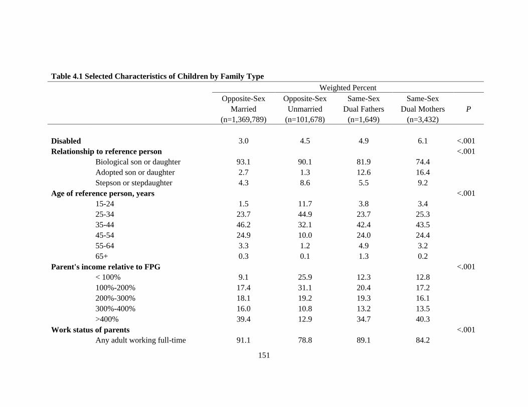
151
Table 4.1 Selected Characteristics of Children by Family Type
Weighted Percent
Opposite-Sex Opposite-Sex Same-Sex Same-Sex
Married Unmarried Dual Fathers Dual Mothers P
(n=1,369,789) (n=101,678) (n=1,649) (n=3,432)
Disabled
3.0 4.5 4.9 6.1 <.001
Relationship to reference person
<.001
Biological son or daughter 93.1 90.1 81.9 74.4
Adopted son or daughter 2.7 1.3 12.6 16.4
Stepson or stepdaughter 4.3 8.6 5.5 9.2
Age of reference person, years
<.001
15-24 1.5 11.7 3.8 3.4
25-34 23.7 44.9 23.7 25.3
35-44 46.2 32.1 42.4 43.5
45-54 24.9 10.0 24.0 24.4
55-64 3.3 1.2 4.9 3.2
65+ 0.3 0.1 1.3 0.2
Parent's income relative to FPG
<.001
< 100% 9.1 25.9 12.3 12.8
100%-200% 17.4 31.1 20.4 17.2
200%-300% 18.1 19.2 19.3 16.1
300%-400% 16.0 10.8 13.2 13.5
>400% 39.4 12.9 34.7 40.3
Work status of parents
<.001
Any adult working full-time 91.1 78.8 89.1 84.2

152
Table 4.1 Selected Characteristics of Children by Family Type
Weighted Percent
Opposite-Sex Opposite-Sex Same-Sex Same-Sex
Married Unmarried Dual Fathers Dual Mothers P
(n=1,369,789) (n=101,678) (n=1,649) (n=3,432)
Only part-time adult workers 5.7 12.1 5.7 10.6
All adults unemployed 1.8 5.9 2.9 2.2
All adults not in labor force 1.5 3.2 2.4 2.9
Highest educational attainment of parents
<.001
Less than high school 5.9 13.2 11.5 4.8
High school graduate 14.2 30.8 16.9 12.1
Some college 30.8 42.1 30.3 32.2
College degree or more 49.1 13.9 41.4 50.9
Total number of children in household
<.001
< 2 62.4 63.6 61.6 70.9
≥ 3 37.6 36.4 38.4 29.1
Primary language spoken at home
<.001
English only 71.0 66.0 61.1 74.6
Not English 29.0 34.0 38.9 25.4
MSA residence 84.6 82.6 88.5 89.0 <.001
FPG indicates federal poverty guidelines defined by the US Department of Health and Human Services. MSA indicates Metropolitan
Statistical Area. Source: 2008-2010 American Community Survey.

153
Table 4.2 Factors Associated with Children's Type of Health Insurance
Private Public
vs. Uninsured vs. Uninsured
RRR 95% CI RRR 95% CI
Family Type
Opposite-Sex, Married 1.00 Reference
1.00 Reference
Opposite-Sex, Unmarried 0.46 (0.44-0.48) ** 1.42 (1.36-1.48) **
Same-Sex, Dual Fathers 0.55 (0.39-0.78) ** 1.13 (0.79-1.62)
Same-Sex, Dual Mothers 0.60 (0.47-0.78) ** 1.05 (0.81-1.36)
Age group, years
< 1 1.00 Reference
1.00 Reference
1-5 0.67 (0.63-0.7) ** 0.62 (0.59-0.66) **
6-17 0.55 (0.52-0.58) ** 0.44 (0.41-0.46) **
Race/Ethnicity
White 1.00 Reference
1.00 Reference
Hispanic 0.81 (0.78-0.85) ** 1.16 (1.1-1.22) **
Black 0.96 (0.91-1.01)
1.40 (1.32-1.48) **
Asian 1.15 (1.07-1.23) ** 1.43 (1.33-1.54) **
Multiple/Other 0.77 (0.73-0.82) ** 0.99 (0.93-1.06)
Sex
Male 1.00 Reference
1.00 Reference
Female 0.99 (0.97-1.01)
0.99 (0.97-1.01)
Citizenship
Citizen 1.00 Reference
1.00 Reference
Naturalized 0.83 (0.75-0.92) ** 0.83 (0.74-0.93) *
Non-citizen 0.28 (0.26-0.29) ** 0.26 (0.25-0.28) **
Disability
No disability 1.00 Reference
1.00 Reference
Any disability 1.24 (1.17-1.31) ** 2.44 (2.3-2.59) **
Relationship to reference person
Biological son or daughter 1.00 Reference
1.00 Reference
Adopted son or daughter 0.96 (0.89-1.04)
1.97 (1.8-2.15) **
Stepson or stepdaughter 0.95 (0.91-1.00)
1.14 (1.08-1.2) **
Age of reference person, years
15-24 0.75 (0.69-0.81) ** 1.60 (1.49-1.71) **
25-34 0.89 (0.86-0.92) ** 1.31 (1.26-1.35) **
35-44 1.00 Reference
1.00 Reference
45-54 1.04 (1-1.07) * 0.85 (0.82-0.88) **
55-64 0.98 (0.91-1.05)
0.84 (0.78-0.9) **
65+ 1.30 (1.07-1.59) * 1.23 (1.01-1.5) *

154
Table 4.2 Factors Associated with Children's Type of Health Insurance
Parents' combined income relative to FPG
< 100% 0.07 (0.07-0.08) ** 4.86 (4.55-5.19) **
100%-200% 0.16 (0.15-0.17) ** 3.29 (3.1-3.49) **
200%-300% 0.33 (0.31-0.34) ** 1.86 (1.75-1.97) **
300%-400% 0.57 (0.54-0.6) ** 1.27 (1.19-1.36) **
>400% 1.00 Reference
1.00 Reference
Work status of parents
Any adult working full-time 1.00 Reference
1.00 Reference
Only part-time adult workers 0.48 (0.46-0.5) ** 1.24 (1.19-1.3) **
All adults unemployed 0.28 (0.25-0.3) ** 1.45 (1.35-1.55) **
All adults not in labor force 0.54 (0.49-0.6) ** 1.61 (1.47-1.76) **
Highest educational attainment of parents
Less than high school 0.16 (0.15-0.17) ** 0.85 (0.8-0.9) **
High school graduate 0.33 (0.32-0.35) ** 1.04 (0.99-1.09)
Some college 0.54 (0.52-0.56) ** 1.10 (1.06-1.15) **
College degree or more 1.00 Reference
1.00 Reference
Total number of children in household
< 2 1.00 Reference
1.00 Reference
≥ 3 1.18 (1.15-1.22) ** 1.25 (1.21-1.29) **
Primary language spoken at home
English only 1.00 Reference
1.00 Reference
Not English 0.51 (0.49-0.53) ** 0.90 (0.86-0.94) **
Urban/Rural
Not MSA residence 1.00 Reference
1.00 Reference
MSA residence 1.33 (1.28-1.38) ** 1.05 (1.01-1.1) *
Survey year
2008 1.00 Reference
1.00 Reference
2009 1.15 (1.12-1.19) ** 1.19 (1.15-1.24) **
2010 1.21 (1.18-1.25) ** 1.41 (1.36-1.46) **
Models are weighted and adjusted for variables listed, state of residence and survey
year. RRR indicates relative risk ratio; CI, confidence interval; FPG, federal poverty
guidelines. Source: 2008-2010 American Community Survey.
** p < .01
* p < .05

155
Table 4.3 The Association Between Family Type and Type of Health Insurance Coverage by State Marriage Policies as if
January 1, 2008
Private Public
vs. Uninsured vs. Uninsured
n RRR 95% CI RRR 95% CI
Same-Sex Marriage, Civil Unions or Domestic Partnerships†
Opposite-Sex, Married 240,957 1.00 Reference
1.00 Reference
Opposite-Sex, Unmarried 18,807 0.50 (0.45-0.55) ** 1.32 (1.2-1.45) **
Same-Sex, Dual Fathers 360 0.43 (0.2-0.94) * 0.89 (0.38-2.06)
Same-Sex, Dual Mothers 744 0.83 (0.48-1.41)
1.24 (0.7-2.22)
No Provisions
Opposite-Sex, Married 1,128,832 1.00 Reference
1.00 Reference
Opposite-Sex, Unmarried 82,871 0.48 (0.45-0.5) ** 1.51 (1.44-1.58) **
Same-Sex, Dual Fathers 1,289 0.61 (0.41-0.92) * 1.24 (0.83-1.85)
Same-Sex, Dual Mothers 2,688 0.59 (0.44-0.78) ** 1.07 (0.82-1.42)
Models are weighted and adjusted for children's age group, race and ethnicity, sex, citizenship, disability, relationship to reference
parent, age of reference parent, parents' combined income relative to FPG, work status of parents, highest educational attainment of
parents, number of children in household, primary language spoken at home, and survey year. RRR indicates relative risk ratio; CI,
confidence interval; FPG, federal poverty guidelines. Source: 2008-2010 American Community Survey. †As of January 1, 2008. States included California, Massachusetts, New Jersey, Vermont and the District of Columbia.
** p < .01
* p < .05

156
Table 4.4 The Association Between Family Type and Type of Health Insurance Coverage by State Adoption Policies as of
January 1, 2008
Private Public
vs. Uninsured vs. Uninsured
RRR 95% CI RRR 95% CI
Second-Parent Adoption Available Statewide†
Opposite-Sex, Married 1.00 Reference
1.00 Reference
Opposite-Sex, Unmarried 0.51 (0.47-0.55) ** 1.47 (1.37-1.58) **
Same-Sex, Dual Fathers 0.70 (0.4-1.22)
1.25 (0.68-2.3)
Same-Sex, Dual Mothers 0.66 (0.41-1.05)
0.89 (0.56-1.43)
No Provisions
Opposite-Sex, Married 1.00 Reference
1.00 Reference
Opposite-Sex, Unmarried 0.46 (0.43-0.48) ** 1.45 (1.38-1.52) **
Same-Sex, Dual Fathers 0.49 (0.31-0.78) * 1.07 (0.69-1.65)
Same-Sex, Dual Mothers 0.60 (0.44-0.81) * 1.23 (0.91-1.65)
Models are weighted and adjusted for children's age group, race and ethnicity, sex, citizenship, disability, relationship to reference
parent, age of reference parent, parents' combined income relative to FPG, work status of parents, highest educational attainment of
parents, total number of children in household, primary language spoken at home and survey year. RRR indicates relative risk ratio;
CI, confidence interval; FPG, federal poverty guidelines. Source: 2008-2010 American Community Survey. †As of January 1, 2008. States included California, Colorado, Connecticut, Illinois, Indiana, Massachusetts, New Jersey, New York,
Pennsylvania, Vermont, and the District of Columbia.
** p < .01
* p < .05

157
Complete Regression Tables
The following tables present complete regression results for the abbreviated results
presented in Tables 4.3 and 4.4.

158
Table 4.5 The Association Between Family Type and Children's Health Insurance
Coverage in States with Same-Sex Marriage, Civil Unions or Domestic
Partnerships as of January 1, 2008
Private Public
vs. Uninsured vs. Uninsured
RRR 95% CI RRR 95% CI
Family Type
Opposite-Sex, Married 1.00 Reference
1.00 Reference
Opposite-Sex, Unmarried 0.50 (0.45-0.55) ** 1.32 (1.2-1.45) **
Same-Sex, Dual Fathers 0.43 (0.2-0.94) * 0.89 (0.38-2.06)
Same-Sex, Dual Mothers 0.83 (0.48-1.41)
1.24 (0.7-2.22)
Age group, years
< 1 1.00 Reference
1.00 Reference
1-5 0.63 (0.55-0.72) ** 0.63 (0.56-0.72) **
6-17 0.48 (0.42-0.55) ** 0.40 (0.35-0.46) **
Race/Ethnicity
White 1.00 Reference
1.00 Reference
Hispanic 0.60 (0.54-0.66) ** 0.74 (0.67-0.82) **
Black 0.86 (0.72-1.02)
1.33 (1.1-1.6) *
Asian 0.94 (0.84-1.07)
1.04 (0.91-1.19)
Multiple/Other 0.87 (0.73-1.04)
0.96 (0.79-1.16)
Sex
Male 1.00 Reference
1.00 Reference
Female 1.00 (0.95-1.04)
1.00 (0.96-1.04)
Citizenship
Citizen 1.00 Reference
1.00 Reference
Naturalized 0.78 (0.64-0.95) * 0.98 (0.8-1.2)
Non-citizen 0.30 (0.27-0.33) ** 0.39 (0.36-0.43) **
Disability
No disability 1.00 Reference
1.00 Reference
Any disability 1.19 (1.02-1.39) * 2.02 (1.74-2.35) **
Relationship to reference person
Biological son or daughter 1.00 Reference
1.00 Reference
Adopted son or daughter 1.13 (0.9-1.43)
1.92 (1.51-2.44) **
Stepson or stepdaughter 0.97 (0.85-1.1)
1.00 (0.87-1.15)
Age of reference person, years
15-24 0.71 (0.57-0.88) * 1.40 (1.15-1.7) *
25-34 0.92 (0.84-1) * 1.27 (1.17-1.38) **
35-44 1.00 Reference
1.00 Reference
45-54 0.95 (0.88-1.02)
0.78 (0.72-0.85) **

159
55-64 0.97 (0.84-1.13)
0.82 (0.71-0.94) *
65+ 0.85 (0.53-1.37)
1.13 (0.68-1.86)
Parents' combined income relative to FPG
< 100% 0.07 (0.06-0.07) ** 3.86 (3.33-4.46) **
100%-200% 0.14 (0.13-0.16) ** 3.02 (2.64-3.45) **
200%-300% 0.29 (0.26-0.32) ** 2.08 (1.81-2.38) **
300%-400% 0.52 (0.46-0.58) ** 1.35 (1.16-1.58) **
>400% 1.00 Reference
1.00 Reference
Work status of parents
Any adult working full-
time 1.00 Reference
1.00 Reference
Only part-time adult
workers 0.52 (0.47-0.58) ** 1.23 (1.12-1.35) **
All adults unemployed 0.31 (0.26-0.37) ** 1.31 (1.13-1.51) **
All adults not in labor
force 0.55 (0.44-0.69) ** 1.46 (1.2-1.77) **
Highest educational attainment of parents
Less than high school 0.27 (0.24-0.3) ** 1.14 (1.02-1.29) *
High school graduate 0.44 (0.4-0.49) ** 1.16 (1.04-1.3) *
Some college 0.64 (0.58-0.7) ** 1.10 (0.99-1.22)
College degree or more 1.00 Reference
1.00 Reference
Total number of children in
household
< 2 1.00 Reference
1.00 Reference
≥ 3 1.28 (1.2-1.38) ** 1.35 (1.26-1.44) **
Primary language spoken at home
English only 1.00 Reference
1.00 Reference
Not English 0.58 (0.53-0.64) ** 1.31 (1.18-1.45) **
Urban/Rural
Not MSA residence
MSA residence 1.79 (1.46-2.2) ** 0.70 (0.56-0.86) *
Survey year
2008 1.00 Reference
1.00 Reference
2009 1.14 (1.06-1.23) * 1.11 (1.02-1.2) *
2010 1.20 (1.11-1.29) ** 1.29 (1.19-1.39) ** Models are weighted and adjusted for variables listed. Analysis restricted to children living in states with
same-sex marriage, civil unions or domestic partnership policies in place as of January 1, 2008, which
includes California, the District of Columbia, Massachusetts, New Jersey and Vermont. RRR indicates
relative risk ratio; CI, confidence interval; FPG, federal poverty guidelines. Source: 2008-2010 American
Community Survey.
** p < .01
* p < .05

160
Table 4.6 The Association Between Family Type and Children's Health Insurance
Coverage in States Without Marriage Provisions as of January 1, 2008
Private Public
vs. Uninsured vs. Uninsured
RRR 95% CI RRR 95% CI
Family Type
Opposite-Sex, Married 1.00 Reference
1.00 Reference
Opposite-Sex, Unmarried 0.48 (0.45-0.5) ** 1.51 (1.44-1.58) **
Same-Sex, Dual Fathers 0.61 (0.41-0.92) * 1.24 (0.83-1.85)
Same-Sex, Dual Mothers 0.59 (0.44-0.78) ** 1.07 (0.82-1.42)
Age group, years
< 1 1.00 Reference
1.00 Reference
1-5 0.67 (0.64-0.71) ** 0.63 (0.59-0.66) **
6-17 0.56 (0.53-0.6) ** 0.45 (0.42-0.47) **
Race/Ethnicity
White 1.00 Reference
1.00 Reference
Hispanic 0.65 (0.62-0.68) ** 0.99 (0.94-1.04)
Black 0.85 (0.8-0.9) ** 1.36 (1.28-1.44) **
Asian 1.23 (1.13-1.33) ** 1.54 (1.41-1.69) **
Multiple/Other 0.71 (0.67-0.76) ** 0.91 (0.85-0.98) *
Sex
Male 1.00 Reference
1.00 Reference
Female 0.99 (0.97-1.01)
0.99 (0.97-1.01)
Citizenship
Citizen 1.00 Reference
1.00 Reference
Naturalized 0.94 (0.84-1.06)
0.87 (0.77-0.99) *
Non-citizen 0.29 (0.27-0.3) ** 0.24 (0.22-0.25) **
Disability
No disability 1.00 Reference
1.00 Reference
Any disability 1.23 (1.16-1.31) ** 2.51 (2.36-2.67) **
Relationship to reference person
Biological son or daughter 1.00 Reference
1.00 Reference
Adopted son or daughter 0.93 (0.85-1.01)
1.94 (1.77-2.13) **
Stepson or stepdaughter 0.91 (0.86-0.96) ** 1.12 (1.06-1.18) **
Age of reference person, years
15-24 0.73 (0.67-0.79) ** 1.55 (1.44-1.67) **
25-34 0.87 (0.84-0.91) ** 1.28 (1.23-1.33) **
35-44 1.00 Reference
1.00 Reference
45-54 1.07 (1.03-1.11) ** 0.89 (0.85-0.92) **
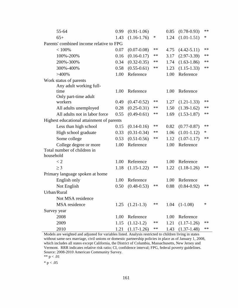
161
55-64 0.99 (0.91-1.06)
0.85 (0.78-0.93) **
65+ 1.43 (1.16-1.76) * 1.24 (1.01-1.51) *
Parents' combined income relative to FPG
< 100% 0.07 (0.07-0.08) ** 4.75 (4.42-5.11) **
100%-200% 0.16 (0.16-0.17) ** 3.17 (2.97-3.39) **
200%-300% 0.34 (0.32-0.35) ** 1.74 (1.63-1.86) **
300%-400% 0.58 (0.55-0.61) ** 1.23 (1.15-1.33) **
>400% 1.00 Reference
1.00 Reference
Work status of parents
Any adult working full-
time 1.00 Reference
1.00 Reference
Only part-time adult
workers 0.49 (0.47-0.52) ** 1.27 (1.21-1.33) **
All adults unemployed 0.28 (0.25-0.31) ** 1.50 (1.39-1.62) **
All adults not in labor force 0.55 (0.49-0.61) ** 1.69 (1.53-1.87) **
Highest educational attainment of parents
Less than high school 0.15 (0.14-0.16) ** 0.82 (0.77-0.87) **
High school graduate 0.33 (0.31-0.34) ** 1.06 (1.01-1.12) *
Some college 0.53 (0.51-0.56) ** 1.12 (1.07-1.17) **
College degree or more 1.00 Reference
1.00 Reference
Total number of children in
household
< 2 1.00 Reference
1.00 Reference
≥ 3 1.18 (1.15-1.22) ** 1.22 (1.18-1.26) **
Primary language spoken at home
English only 1.00 Reference
1.00 Reference
Not English 0.50 (0.48-0.53) ** 0.88 (0.84-0.92) **
Urban/Rural
Not MSA residence
MSA residence 1.25 (1.21-1.3) ** 1.04 (1-1.08) *
Survey year
2008 1.00 Reference
1.00 Reference
2009 1.15 (1.12-1.2) ** 1.21 (1.17-1.26) **
2010 1.21 (1.17-1.26) ** 1.43 (1.37-1.48) ** Models are weighted and adjusted for variables listed. Analysis restricted to children living in states
without same-sex marriage, civil unions or domestic partnership policies in place as of January 1, 2008,
which includes all states except California, the District of Columbia, Massachusetts, New Jersey and
Vermont. RRR indicates relative risk ratio; CI, confidence interval; FPG, federal poverty guidelines.
Source: 2008-2010 American Community Survey.
** p < .01
* p < .05

162
Table 4.7 The Association Between Family Type and Children's Health Insurance
Coverage in States with Second-Parent Adoption Available Statewide as of January
1, 2008
Private Public
vs. Uninsured vs. Uninsured
RRR 95% CI RRR 95% CI
Family Type
Opposite-Sex, Married 1.00 Reference
1.00 Reference
Opposite-Sex, Unmarried 0.51 (0.47-0.55) ** 1.47 (1.37-1.58) **
Same-Sex, Dual Fathers 0.70 (0.4-1.22)
1.25 (0.68-2.3)
Same-Sex, Dual Mothers 0.66 (0.41-1.05)
0.89 (0.56-1.43)
Age group, years
< 1 1.00 Reference
1.00 Reference
1-5 0.74 (0.68-0.81) ** 0.73 (0.67-0.8) **
6-17 0.61 (0.56-0.67) ** 0.51 (0.46-0.56) **
Race/Ethnicity
White 1.00 Reference
1.00 Reference
Hispanic 0.83 (0.77-0.89) ** 1.11 (1.02-1.2) *
Black 0.87 (0.77-0.98) * 1.38 (1.22-1.56) **
Asian 1.10 (1-1.22)
1.44 (1.29-1.6) **
Multiple/Other 0.90 (0.79-1.02)
1.11 (0.96-1.28)
Sex
Male 1.00 Reference
1.00 Reference
Female 1.00 (0.97-1.03)
1.00 (0.97-1.03)
Citizenship
Citizen 1.00 Reference
1.00 Reference
Naturalized 0.86 (0.74-1.01) * 1.04 (0.88-1.23)
Non-citizen 0.30 (0.28-0.33) ** 0.41 (0.39-0.45) **
Disability
No disability 1.00 Reference
1.00 Reference
Any disability 1.11 (1-1.24)
2.07 (1.87-2.31) **
Relationship to reference person
Biological son or daughter 1.00 Reference
1.00 Reference
Adopted son or daughter 0.97 (0.83-1.12)
1.75 (1.49-2.05) **
Stepson or stepdaughter 0.90 (0.82-0.99) * 1.03 (0.93-1.13)
Age of reference person, years
15-24 0.69 (0.59-0.81) ** 1.47 (1.28-1.69) **
25-34 0.82 (0.77-0.88) ** 1.21 (1.14-1.29) **
35-44 1.00 Reference
1.00 Reference

163
45-54 1.03 (0.97-1.09)
0.85 (0.8-0.91) **
55-64 1.02 (0.91-1.14)
0.85 (0.76-0.96) *
65+ 1.07 (0.75-1.55)
1.12 (0.78-1.62)
Parents' combined income relative to FPG
< 100% 0.07 (0.07-0.08) ** 4.51 (4.04-5.03) **
100%-200% 0.16 (0.15-0.18) ** 3.48 (3.15-3.84) **
200%-300% 0.33 (0.31-0.36) ** 2.26 (2.05-2.5) **
300%-400% 0.57 (0.52-0.62) ** 1.55 (1.38-1.73) **
>400% 1.00 Reference
1.00 Reference
Work status of parents
Any adult working full-
time 1.00 Reference
1.00 Reference
Only part-time adult
workers 0.52 (0.49-0.57) ** 1.20 (1.11-1.29) **
All adults unemployed 0.31 (0.27-0.36) ** 1.33 (1.19-1.48) **
All adults not in labor force 0.49 (0.41-0.58) ** 1.40 (1.21-1.62) **
Highest educational attainment of parents
Less than high school 0.18 (0.16-0.2) ** 0.76 (0.7-0.84) **
High school graduate 0.39 (0.36-0.42) ** 1.03 (0.95-1.12)
Some college 0.59 (0.55-0.63) ** 1.05 (0.97-1.13)
College degree or more 1.00 Reference
1.00 Reference
Total number of children in
household
< 2 1.00 Reference
1.00 Reference
≥ 3 1.18 (1.12-1.24) ** 1.19 (1.13-1.25) **
Primary language spoken at home
English only 1.00 Reference
1.00 Reference
Not English 0.48 (0.45-0.51) ** 1.00 (0.93-1.08)
Urban/Rural
Not MSA residence
MSA residence 1.74 (1.6-1.89) ** 1.32 (1.2-1.44) **
Survey year
2008 1.00 Reference
1.00 Reference
2009 1.16 (1.09-1.22) ** 1.22 (1.15-1.29) **
2010 1.16 (1.09-1.23) ** 1.32 (1.24-1.4) ** Models are weighted and adjusted for variables listed. Analysis restricted to children living in states with
second-parent adoption available statewide as of January 1, 2008, which includes California, Colorado,
Connecticut, the District of Columbia, Illinois, Indiana, Massachusetts, New York, New Jersey,
Pennsylvania and Vermont. RRR indicates relative risk ratio; CI, confidence interval; FPG, federal
poverty guidelines. Source: 2008-2010 American Community Survey.
** p < .01
* p < .05

164
Table 4.8 The Association Between Family Type and Children's Health Insurance
Coverage in States Without Second-Parent Adoption Available Statewide as of
January 1, 2008
Private Public
vs. Uninsured vs. Uninsured
RRR 95% CI RRR 95% CI
Family Type
Opposite-Sex, Married 1.00 Reference
1.00 Reference
Opposite-Sex, Unmarried 0.46 (0.43-0.48) ** 1.45 (1.38-1.52) **
Same-Sex, Dual Fathers 0.49 (0.31-0.78) * 1.07 (0.69-1.65)
Same-Sex, Dual Mothers 0.60 (0.44-0.81) * 1.23 (0.91-1.65)
Age group, years
< 1 1.00 Reference
1.00 Reference
1-5 0.64 (0.6-0.68) ** 0.59 (0.55-0.62) **
6-17 0.53 (0.5-0.56) ** 0.41 (0.39-0.44) **
Race/Ethnicity
White 1.00 Reference
1.00 Reference
Hispanic 0.59 (0.56-0.62) ** 0.90 (0.85-0.96) *
Black 0.86 (0.81-0.92) ** 1.38 (1.29-1.48) **
Asian 1.22 (1.11-1.34) ** 1.26 (1.13-1.41) **
Multiple/Other 0.71 (0.66-0.76) ** 0.89 (0.83-0.97) *
Sex
Male 1.00 Reference
1.00 Reference
Female 0.99 (0.97-1.01)
0.99 (0.97-1.01)
Citizenship
Citizen 1.00 Reference
1.00 Reference
Naturalized 0.91 (0.8-1.04)
0.76 (0.65-0.88) **
Non-citizen 0.30 (0.28-0.32) ** 0.19 (0.18-0.21) **
Disability
No disability 1.00 Reference
1.00 Reference
Any disability 1.29 (1.2-1.38) ** 2.65 (2.47-2.84) **
Relationship to reference person
Biological son or daughter 1.00 Reference
1.00 Reference
Adopted son or daughter 0.96 (0.87-1.06)
2.08 (1.87-2.31) **
Stepson or stepdaughter 0.94 (0.89-0.99) * 1.15 (1.08-1.22) **
Age of reference person, years
15-24 0.76 (0.7-0.83) ** 1.59 (1.46-1.72) **
25-34 0.92 (0.88-0.95) ** 1.32 (1.27-1.38) **
35-44 1.00 Reference
1.00 Reference
45-54 1.04 (1-1.09) * 0.85 (0.81-0.9) **

165
55-64 0.95 (0.87-1.03)
0.83 (0.75-0.91) **
65+ 1.41 (1.12-1.76) * 1.26 (1.01-1.57) *
Parents' combined income relative to FPG
< 100% 0.07 (0.07-0.08) ** 4.74 (4.37-5.15) **
100%-200% 0.16 (0.15-0.17) ** 3.04 (2.82-3.27) **
200%-300% 0.33 (0.31-0.35) ** 1.60 (1.49-1.73) **
300%-400% 0.57 (0.54-0.61) ** 1.12 (1.03-1.22) *
>400% 1.00 Reference
1.00 Reference
Work status of parents
Any adult working full-
time 1.00 Reference
1.00 Reference
Only part-time adult
workers 0.47 (0.44-0.5) ** 1.28 (1.21-1.35) **
All adults unemployed 0.26 (0.23-0.29) ** 1.52 (1.39-1.66) **
All adults not in labor force 0.57 (0.5-0.65) ** 1.76 (1.58-1.97) **
Highest educational attainment of parents
Less than high school 0.16 (0.15-0.17) ** 0.94 (0.88-1.01) *
High school graduate 0.32 (0.3-0.33) ** 1.09 (1.03-1.15) *
Some college 0.53 (0.51-0.55) ** 1.16 (1.1-1.22) **
College degree or more 1.00 Reference
1.00 Reference
Total number of children in
household
< 2 1.00 Reference
1.00 Reference
≥ 3 1.21 (1.16-1.25) ** 1.27 (1.22-1.32) **
Primary language spoken at home
English only 1.00 Reference
1.00 Reference
Not English 0.52 (0.49-0.54) ** 0.85 (0.8-0.9) **
Urban/Rural
Not MSA residence
MSA residence 1.14 (1.1-1.19) ** 0.93 (0.89-0.97) **
Survey year
2008 1.00 Reference
1.00 Reference
2009 1.15 (1.11-1.19) ** 1.18 (1.13-1.23) **
2010 1.23 (1.19-1.28) ** 1.44 (1.38-1.5) ** Models are weighted and adjusted for variables listed. Analysis restricted to children living in states
without second-parent adoption available statewide as of January 1, 2008, which includes all states except
California, Colorado, Connecticut, the District of Columbia, Illinois, Indiana, Massachusetts, New York,
New Jersey, Pennsylvania and Vermont. RRR indicates relative risk ratio; CI, confidence interval; FPG,
federal poverty guidelines. Source: 2008-2010 American Community Survey.
** p < .01
* p < .05

166
Sensitivity Analysis
The following tables present the results from the sensitivity analysis, which restricts the
sample to cohabiting same-sex couples at lower risk of contamination issues, or where
opposite-sex parents may have misreported one member’s sex. The sample is restricted to
respondents using the CATI/CAPI versions and respondents using the mail version of the
ACS and not receiving a marital status allocation flag (Gates & Steinberger 2009).

167
Table 4.9 Selected Characteristics of Children by Family Type for the Sensitivity
Sample
Weighted Percent
Opposite-Sex
Opposite-
Sex
Same-
Sex Same-Sex
Married Unmarried
Dual
Fathers
Dual
Mothers P
(n=1,366,214) (n=99,074) (n=827) (n=2,332)
Health insurance coverage
<.001
Private 77.5 37.6 49.7 64.6
Public 15.9 51.6 36.5 27.8
Uninsured 6.6 10.8 13.8 7.6
Age group, years
<.001
< 1 4.7 9.6 5.2 4.3
1-5 26.3 34.7 31.0 27.4
6-17 69.0 55.7 63.8 68.4
Race/Ethnicity
<.001
White 68.1 48.5 45.7 59.9
Hispanic 17.1 31.2 29.9 18.8
Black 5.4 11.9 14.8 11.8
Asian 5.2 1.3 2.9 2.5
Multiple/Other 4.1 7.1 6.8 6.9
Sex
<.001
Male 51.3 51.2 58.6 51.6
Female 48.7 48.8 41.4 48.4
Citizenship
Citizen 96.3 97.8 94.0 95.4 <.001
Naturalized 1.0 0.2 1.9 3.3
Non-citizen 2.7 2.0 4.1 1.4
Disabled 3.0 4.5 5.7 7.1 <.001
Relationship to reference person
<.001
Biological son or
daughter 93.1 90.1 76.7 70.0
Adopted son or
daughter 2.7 1.3 17.2 19.2
Stepson or
stepdaughter 4.3 8.6 6.2 10.8
Age of reference person, years
<.001
15-24 1.5 11.7 6.3 3.8
25-34 23.8 45.2 28.7 26.3

168
35-44 46.2 32.0 39.3 43.4
45-54 24.9 9.8 19.3 23.5
55-64 3.3 1.1 5.1 2.8
65+ 0.3 0.1 1.3 0.2
Parent's income relative to FPG
<.001
< 100% 9.1 25.9 15.1 13.9
100%-200% 17.4 31.2 26.1 17.5
200%-300% 18.1 19.2 18.4 16.3
300%-400% 16.0 10.8 12.2 13.0
>400% 39.5 12.9 28.2 39.5
Work status of parents
<.001
Any adult working full-
time 91.1 78.8 86.0 83.3
Only part-time adult
workers 5.7 12.1 6.4 10.8
All adults unemployed 1.8 5.9 3.9 2.5
All adults not in labor
force 1.5 3.2 3.7 3.4
Highest educational attainment of parents <.001
Less than high school 5.9 13.3 15.6 4.4
High school graduate 14.2 30.7 19.8 12.5
Some college 30.8 42.1 32.6 34.3
College degree or more 49.1 13.8 31.9 48.8
Total number of children in household
<.001
< 2 62.4 63.8 60.3 71.5
≥ 3 37.6 36.2 39.7 28.5
Primary language spoken at home
<.001
English only 71.0 66.1 64.0 75.3
Not English 29.0 33.9 36.0 24.7
MSA residence 81.3 77.8 87.2 87.7 <.001
FPG indicates federal poverty guidelines defined by the US Department of Health and
Human Services. MSA indicates Metropolitan Statistical Area. Source: 2008-2010
American Community Survey.

169
Table 4.10 Factors Associated with Children's Type of Health Insurance in
Sensitivity Sample
Private Public
vs. Uninsured vs. Uninsured
RRR 95% CI RRR 95% CI
Family Type
Opposite-Sex, Married 1.00 Reference
1.00 Reference
Opposite-Sex, Unmarried 0.46 (0.44-0.48) ** 1.42 (1.36-1.48) **
Same-Sex, Dual Fathers 0.38 (0.24-0.6) ** 1.09 (0.71-1.67)
Same-Sex, Dual Mothers 0.54 (0.4-0.74) ** 1.01 (0.75-1.37)
Age group, years
< 1 1.00 Reference
1.00 Reference
1-5 0.67 (0.63-0.7) ** 0.62 (0.59-0.66) **
6-17 0.55 (0.53-0.58) ** 0.44 (0.41-0.46) **
Race/Ethnicity
White 1.00 Reference
1.00 Reference
Hispanic 0.82 (0.78-0.85) ** 1.16 (1.1-1.22) **
Black 0.96 (0.91-1.01)
1.40 (1.32-1.48) **
Asian 1.15 (1.07-1.23) ** 1.44 (1.33-1.55) **
Multiple/Other 0.77 (0.73-0.82) ** 0.99 (0.92-1.06)
Sex
Male 1.00 Reference
1.00 Reference
Female 0.99 (0.97-1.01)
0.99 (0.97-1.01)
Citizenship
Citizen 1.00 Reference
1.00 Reference
Naturalized 0.83 (0.75-0.92) * 0.83 (0.74-0.93) *
Non-citizen 0.28 (0.27-0.29) ** 0.26 (0.25-0.28) **
Disability
No disability 1.00 Reference
1.00 Reference
Any disability 1.24 (1.17-1.31) ** 2.45 (2.31-2.6) **
Relationship to reference person
Biological son or daughter 1.00 Reference
1.00 Reference
Adopted son or daughter 0.96 (0.89-1.04)
1.97 (1.81-2.16) **
Stepson or stepdaughter 0.96 (0.91-1.01)
1.15 (1.09-1.21) **
Age of reference person, years
15-24 0.75 (0.7-0.81) ** 1.60 (1.49-1.71) **
25-34 0.89 (0.86-0.92) ** 1.31 (1.26-1.35) **
35-44 1.00 Reference
1.00 Reference
45-54 1.04 (1-1.07) * 0.85 (0.82-0.89) **
55-64 0.98 (0.91-1.05)
0.84 (0.78-0.9) **

170
65+ 1.31 (1.07-1.6) ** 1.23 (1-1.5) *
Parents' combined income relative to FPG
< 100% 0.07 (0.07-0.08) ** 4.89 (4.58-5.23) **
100%-200% 0.16 (0.15-0.17) ** 3.31 (3.12-3.52) **
200%-300% 0.33 (0.31-0.34) ** 1.86 (1.76-1.98) **
300%-400% 0.57 (0.54-0.59) ** 1.28 (1.19-1.37) **
>400% 1.00 Reference
1.00 Reference
Work status of parents
Any adult working full-
time 1.00 Reference
1.00 Reference
Only part-time adult
workers 0.48 (0.45-0.5) ** 1.24 (1.19-1.3) **
All adults unemployed 0.27 (0.25-0.3) ** 1.45 (1.35-1.55) **
All adults not in labor force 0.54 (0.48-0.59) ** 1.61 (1.47-1.76) **
Highest educational attainment of parents
Less than high school 0.16 (0.15-0.17) ** 0.85 (0.81-0.9) **
High school graduate 0.33 (0.32-0.35) ** 1.04 (0.99-1.09)
Some college 0.54 (0.52-0.56) ** 1.10 (1.06-1.15) **
College degree or more 1.00 Reference
1.00 Reference
Total number of children in household
< 2 1.00 Reference
1.00 Reference
≥ 3 1.18 (1.15-1.22) ** 1.25 (1.21-1.29) **
Primary language spoken at home
English only 1.00 Reference
1.00 Reference
Not English 0.51 (0.49-0.53) ** 0.90 (0.86-0.94) **
Urban/Rural
Not MSA residence 1.00 Reference
1.00 Reference
MSA residence 1.33 (1.28-1.38) ** 1.05 (1.01-1.09) *
Survey year
2008 1.00 Reference
1.00 Reference
2009 1.15 (1.12-1.19) ** 1.20 (1.16-1.24) **
2010 1.22 (1.18-1.26) ** 1.41 (1.36-1.46) ** Models are weighted and adjusted for variables listed, state of residence and survey year. RRR indicates
relative risk ratio; CI, confidence interval; FPG, federal poverty guidelines. Source: 2008-2010 American
Community Survey.
** p < .01
* p < .05

171
Table 4.11 The Association Between Family Type and Children's Health Insurance
Coverage in States with Same-Sex Marriage, Civil Unions or Domestic
Partnerships as of January 1, 2008 in Sensitivity Sample
Private Public
vs. Uninsured vs. Uninsured
RRR 95% CI RRR 95% CI
Family Type
Opposite-Sex, Married 1.00 Reference
1.00 Reference
Opposite-Sex, Unmarried 0.49 (0.45-0.55) ** 1.32 (1.2-1.45) **
Same-Sex, Dual Fathers 0.26 (0.09-0.72) * 0.81 (0.3-2.2)
Same-Sex, Dual Mothers 0.80 (0.41-1.56)
1.13 (0.54-2.37)
Age group, years
< 1 1.00 Reference
1.00 Reference
1-5 0.63 (0.55-0.72) ** 0.64 (0.56-0.73) **
6-17 0.49 (0.43-0.56) ** 0.40 (0.35-0.46) **
Race/Ethnicity
White 1.00 Reference
1.00 Reference
Hispanic 0.59 (0.54-0.65) ** 0.74 (0.66-0.82) **
Black 0.85 (0.71-1.02)
1.32 (1.1-1.6) *
Asian 0.95 (0.84-1.07)
1.04 (0.91-1.2)
Multiple/Other 0.87 (0.73-1.03)
0.96 (0.79-1.16)
Sex
Male 1.00 Reference
1.00 Reference
Female 1.00 (0.96-1.04)
1.00 (0.96-1.04)
Citizenship
Citizen 1.00 Reference
1.00 Reference
Naturalized 0.78 (0.64-0.96) * 0.99 (0.81-1.22)
Non-citizen 0.30 (0.27-0.33) ** 0.39 (0.36-0.43) **
Disability
No disability 1.00 Reference
1.00 Reference
Any disability 1.19 (1.02-1.39) * 2.03 (1.75-2.36) **
Relationship to reference person
Biological son or daughter 1.00 Reference
1.00 Reference
Adopted son or daughter 1.13 (0.9-1.42)
1.92 (1.51-2.45) **
Stepson or stepdaughter 0.97 (0.85-1.1)
1.00 (0.87-1.15)
Age of reference person, years
15-24 0.72 (0.58-0.89) * 1.41 (1.15-1.71) *
25-34 0.92 (0.84-1) * 1.27 (1.17-1.39) **
35-44 1.00 Reference
1.00 Reference
45-54 0.95 (0.88-1.02)
0.78 (0.72-0.85) **

172
55-64 0.97 (0.83-1.12)
0.81 (0.7-0.94) *
65+ 0.85 (0.53-1.37)
1.12 (0.68-1.85)
Parents' combined income relative to FPG
< 100% 0.07 (0.06-0.07) ** 3.88 (3.35-4.49) **
100%-200% 0.14 (0.12-0.15) ** 3.03 (2.65-3.46) **
200%-300% 0.29 (0.26-0.32) ** 2.09 (1.82-2.39) **
300%-400% 0.51 (0.46-0.58) ** 1.35 (1.16-1.58) **
>400% 1.00 Reference
1.00 Reference
Work status of parents
Any adult working full-
time 1.00 Reference
1.00 Reference
Only part-time adult
workers 0.52 (0.47-0.58) ** 1.23 (1.12-1.35) **
All adults unemployed 0.31 (0.26-0.37) ** 1.31 (1.13-1.51) **
All adults not in labor
force 0.55 (0.44-0.68) ** 1.45 (1.19-1.76) **
Highest educational attainment of parents
Less than high school 0.27 (0.24-0.3) ** 1.15 (1.02-1.29) *
High school graduate 0.44 (0.4-0.49) ** 1.16 (1.04-1.3) *
Some college 0.64 (0.58-0.7) ** 1.10 (0.99-1.22)
College degree or more 1.00 Reference
1.00 Reference
Total number of children in
household
< 2 1.00 Reference
1.00 Reference
≥ 3 1.29 (1.2-1.38) ** 1.34 (1.25-1.44) **
Primary language spoken at home
English only 1.00 Reference
1.00 Reference
Not English 0.58 (0.53-0.64) ** 1.31 (1.18-1.45) **
Urban/Rural
Not MSA residence 1.00 Reference
1.00 Reference
MSA residence 1.80 (1.47-2.22) ** 0.70 (0.57-0.87) *
Survey year
2008 1.00 Reference
1.00 Reference
2009 1.14 (1.05-1.22) * 1.11 (1.03-1.2) *
2010 1.20 (1.11-1.3) ** 1.29 (1.2-1.4) ** Models are weighted and adjusted for variables listed. Analysis restricted to children living in states with
same-sex marriage, civil unions or domestic partnership policies in place as of January 1, 2008, which
includes California, the District of Columbia, Massachusetts, New Jersey and Vermont. RRR indicates
relative risk ratio; CI, confidence interval; FPG, federal poverty guidelines. Source: 2008-2010 American
Community Survey.
** p < .01
* p < .05

173
Table 4.12 The Association Between Family Type and Children's Health Insurance
Coverage in States Without Marriage Provisions as of January 1, 2008 in
Sensitivity Sample
Private Public
vs. Uninsured vs. Uninsured
RRR 95% CI RRR 95% CI
Family Type
Opposite-Sex, Married 1.00 Reference
1.00 Reference
Opposite-Sex, Unmarried 0.48 (0.45-0.5) ** 1.51 (1.44-1.58) **
Same-Sex, Dual Fathers 0.43 (0.26-0.72) * 1.20 (0.75-1.92)
Same-Sex, Dual Mothers 0.53 (0.38-0.75) ** 1.06 (0.77-1.45)
Age group, years
< 1 1.00 Reference
1.00 Reference
1-5 0.67 (0.64-0.71) ** 0.62 (0.59-0.66) **
6-17 0.56 (0.53-0.6) ** 0.45 (0.42-0.47) **
Race/Ethnicity
White 1.00 Reference
1.00 Reference
Hispanic 0.65 (0.62-0.68) ** 0.99 (0.94-1.04)
Black 0.85 (0.8-0.9) ** 1.36 (1.28-1.44) **
Asian 1.23 (1.13-1.33) ** 1.55 (1.41-1.69) **
Multiple/Other 0.72 (0.67-0.76) ** 0.91 (0.84-0.97) *
Sex
Male 1.00 Reference
1.00 Reference
Female 0.99 (0.97-1.01)
0.99 (0.97-1.01)
Citizenship
Citizen 1.00 Reference
1.00 Reference
Naturalized 0.94 (0.83-1.06)
0.86 (0.76-0.98) *
Non-citizen 0.29 (0.27-0.3) ** 0.24 (0.22-0.25) **
Disability
No disability 1.00 Reference
1.00 Reference
Any disability 1.23 (1.16-1.31) ** 2.51 (2.36-2.68) **
Relationship to reference person
Biological son or daughter 1.00 Reference
1.00 Reference
Adopted son or daughter 0.93 (0.85-1.01)
1.95 (1.77-2.14) **
Stepson or stepdaughter 0.91 (0.87-0.96) * 1.12 (1.06-1.19) **
Age of reference person, years
15-24 0.73 (0.67-0.79) ** 1.55 (1.44-1.67) **
25-34 0.87 (0.84-0.91) ** 1.28 (1.24-1.33) **
35-44 1.00 Reference
1.00 Reference
45-54 1.07 (1.03-1.11) ** 0.89 (0.85-0.93) **

174
55-64 0.99 (0.92-1.07)
0.85 (0.78-0.93) **
65+ 1.44 (1.16-1.78) * 1.23 (1.01-1.51) *
Parents' combined income relative to
FPG
< 100% 0.07 (0.07-0.08) ** 4.79 (4.45-5.15) **
100%-200% 0.16 (0.16-0.17) ** 3.20 (2.99-3.41) **
200%-300% 0.33 (0.32-0.35) ** 1.75 (1.64-1.87) **
300%-400% 0.58 (0.55-0.61) ** 1.24 (1.15-1.34) **
>400% 1.00 Reference
1.00 Reference
Work status of parents
Any adult working full-time 1.00 Reference
1.00 Reference
Only part-time adult
workers 0.49 (0.46-0.52) ** 1.27 (1.21-1.33) **
All adults unemployed 0.28 (0.25-0.31) ** 1.50 (1.39-1.62) **
All adults not in labor force 0.55 (0.49-0.61) ** 1.69 (1.53-1.87) **
Highest educational attainment of
parents
Less than high school 0.15 (0.14-0.16) ** 0.82 (0.77-0.87) **
High school graduate 0.33 (0.31-0.34) ** 1.06 (1.01-1.12) *
Some college 0.53 (0.51-0.56) ** 1.12 (1.07-1.17) **
College degree or more 1.00 Reference
1.00 Reference
Total number of children in household
< 2 1.00 Reference
1.00 Reference
≥ 3 1.18 (1.14-1.22) ** 1.22 (1.18-1.26) **
Primary language spoken at
home
English only 1.00 Reference
1.00 Reference
Not English 0.50 (0.48-0.53) ** 0.88 (0.84-0.92) **
Urban/Rural
Not MSA residence 1.00 Reference
1.00 Reference
MSA residence 1.25 (1.21-1.3) ** 1.04 (1-1.08)
Survey year
2008 1.00 Reference
1.00 Reference
2009 1.16 (1.12-1.2) ** 1.21 (1.17-1.26) **
2010 1.21 (1.17-1.26) ** 1.43 (1.38-1.48) ** Models are weighted and adjusted for variables listed. Analysis restricted to children living in states
without same-sex marriage, civil unions or domestic partnership policies in place as of January 1, 2008,
which includes all states except California, the District of Columbia, Massachusetts, New Jersey and
Vermont. RRR indicates relative risk ratio; CI, confidence interval; FPG, federal poverty guidelines.
Source: 2008-2010 American Community Survey.
** p < .01
* p < .05

175
Table 4.13 The Association Between Family Type and Children's Health Insurance
Coverage in States with Second-Parent Adoption Available Statewide as of January
1, 2008 in Sensitivity Sample
Private Public
vs. Uninsured vs. Uninsured
RRR 95% CI RRR 95% CI
Family Type
Opposite-Sex, Married 1.00 Reference
1.00 Reference
Opposite-Sex, Unmarried 0.51 (0.47-0.55) ** 1.47 (1.37-1.58) **
Same-Sex, Dual Fathers 0.54 (0.27-1.09)
1.22 (0.59-2.51)
Same-Sex, Dual Mothers 0.62 (0.35-1.12)
0.83 (0.47-1.46)
Age group, years
< 1 1.00 Reference
1.00 Reference
1-5 0.75 (0.68-0.81) ** 0.74 (0.67-0.8) **
6-17 0.61 (0.56-0.67) ** 0.51 (0.47-0.56) **
Race/Ethnicity
White 1.00 Reference
1.00 Reference
Hispanic 0.83 (0.77-0.9) ** 1.11 (1.02-1.21) *
Black 0.87 (0.77-0.98) * 1.38 (1.22-1.56) **
Asian 1.11 (1-1.22) * 1.44 (1.3-1.61) **
Multiple/Other 0.89 (0.78-1.02)
1.11 (0.96-1.28)
Sex
Male 1.00 Reference
1.00 Reference
Female 1.00 (0.97-1.03)
1.00 (0.97-1.03)
Citizenship
Citizen 1.00 Reference
1.00 Reference
Naturalized 0.86 (0.74-1.01)
1.04 (0.88-1.23)
Non-citizen 0.30 (0.28-0.33) ** 0.41 (0.39-0.45) **
Disability
No disability 1.00 Reference
1.00 Reference
Any disability 1.11 (0.99-1.23)
2.08 (1.87-2.32) **
Relationship to reference person
Biological son or daughter 1.00 Reference
1.00 Reference
Adopted son or daughter 0.96 (0.83-1.12)
1.76 (1.5-2.06) **
Stepson or stepdaughter 0.90 (0.82-0.99) * 1.03 (0.93-1.13)
Age of reference person, years
15-24 0.70 (0.6-0.82) ** 1.48 (1.29-1.7) **
25-34 0.82 (0.77-0.88) ** 1.21 (1.14-1.29) **
35-44 1.00 Reference
1.00 Reference
45-54 1.03 (0.97-1.09)
0.85 (0.8-0.91) **

176
55-64 1.02 (0.91-1.14)
0.85 (0.76-0.95) *
65+ 1.07 (0.74-1.54)
1.11 (0.77-1.61)
Parents' combined income relative to
FPG
< 100% 0.07 (0.07-0.08) ** 4.56 (4.08-5.09) **
100%-200% 0.16 (0.15-0.17) ** 3.51 (3.18-3.88) **
200%-300% 0.33 (0.3-0.36) ** 2.28 (2.06-2.52) **
300%-400% 0.57 (0.52-0.62) ** 1.56 (1.39-1.74) **
>400% 1.00 Reference
1.00 Reference
Work status of parents
Any adult working full-time 1.00 Reference
1.00 Reference
Only part-time adult
workers 0.52 (0.48-0.57) ** 1.20 (1.11-1.29) **
All adults unemployed 0.31 (0.27-0.36) ** 1.33 (1.19-1.49) **
All adults not in labor force 0.48 (0.41-0.57) ** 1.40 (1.2-1.62) **
Highest educational attainment of
parents
Less than high school 0.18 (0.16-0.2) ** 0.76 (0.7-0.84) **
High school graduate 0.39 (0.36-0.42) ** 1.03 (0.95-1.12)
Some college 0.59 (0.55-0.63) ** 1.05 (0.97-1.13)
College degree or more 1.00 Reference
1.00 Reference
Total number of children in household
< 2 1.00 Reference
1.00 Reference
≥ 3 1.18 (1.12-1.24) ** 1.19 (1.13-1.25) **
Primary language spoken at
home
English only 1.00 Reference
1.00 Reference
Not English 0.48 (0.45-0.51) ** 1.00 (0.92-1.08)
Urban/Rural
Not MSA residence 1.00 Reference
1.00 Reference
MSA residence 1.74 (1.6-1.89) ** 1.32 (1.2-1.45) **
Survey year
2008 1.00 Reference
1.00 Reference
2009 1.16 (1.09-1.22) ** 1.22 (1.15-1.29) **
2010 1.16 (1.09-1.23) ** 1.32 (1.25-1.4) ** Models are weighted and adjusted for variables listed. Analysis restricted to children living in states with
second-parent adoption available statewide as of January 1, 2008, which includes California, Colorado,
Connecticut, the District of Columbia, Illinois, Indiana, Massachusetts, New York, New Jersey,
Pennsylvania and Vermont. RRR indicates relative risk ratio; CI, confidence interval; FPG, federal
poverty guidelines. Source: 2008-2010 American Community Survey.
** p < .01
* p < .05
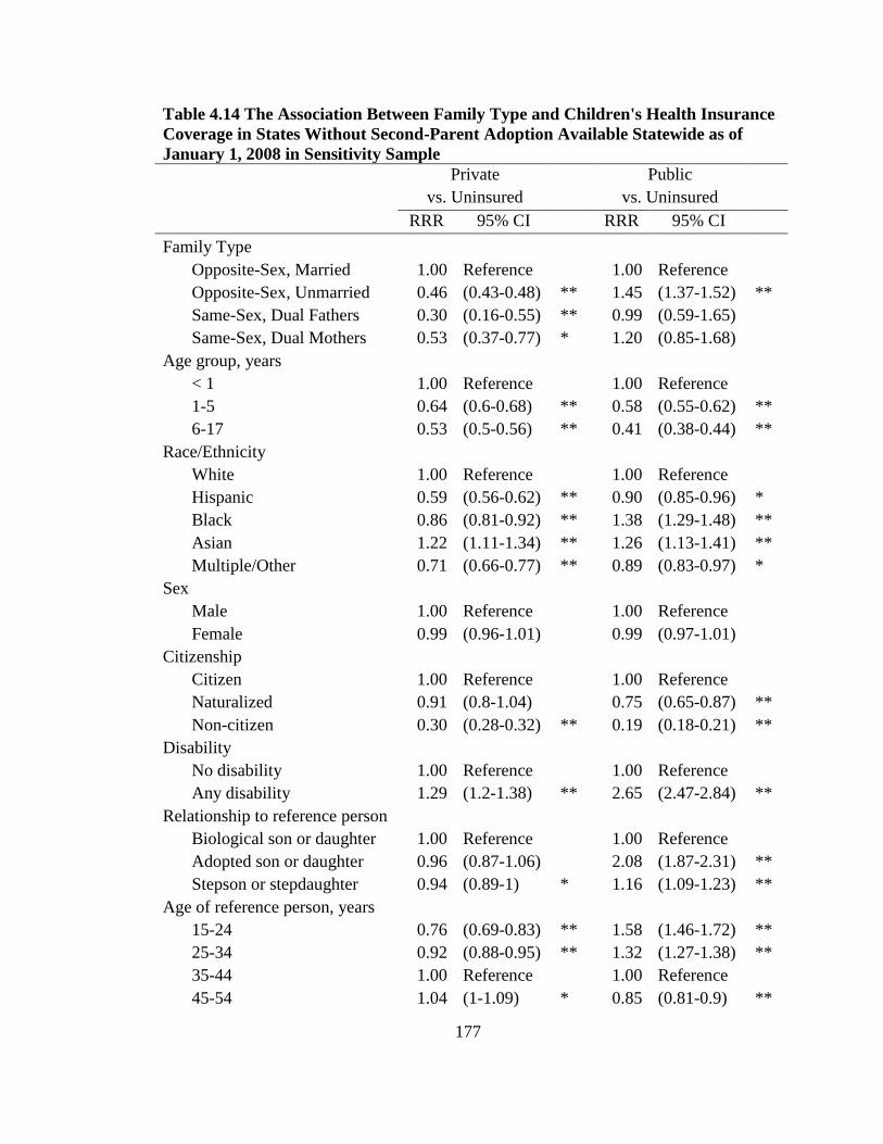
177
Table 4.14 The Association Between Family Type and Children's Health Insurance
Coverage in States Without Second-Parent Adoption Available Statewide as of
January 1, 2008 in Sensitivity Sample
Private Public
vs. Uninsured vs. Uninsured
RRR 95% CI RRR 95% CI
Family Type
Opposite-Sex, Married 1.00 Reference
1.00 Reference
Opposite-Sex, Unmarried 0.46 (0.43-0.48) ** 1.45 (1.37-1.52) **
Same-Sex, Dual Fathers 0.30 (0.16-0.55) ** 0.99 (0.59-1.65)
Same-Sex, Dual Mothers 0.53 (0.37-0.77) * 1.20 (0.85-1.68)
Age group, years
< 1 1.00 Reference
1.00 Reference
1-5 0.64 (0.6-0.68) ** 0.58 (0.55-0.62) **
6-17 0.53 (0.5-0.56) ** 0.41 (0.38-0.44) **
Race/Ethnicity
White 1.00 Reference
1.00 Reference
Hispanic 0.59 (0.56-0.62) ** 0.90 (0.85-0.96) *
Black 0.86 (0.81-0.92) ** 1.38 (1.29-1.48) **
Asian 1.22 (1.11-1.34) ** 1.26 (1.13-1.41) **
Multiple/Other 0.71 (0.66-0.77) ** 0.89 (0.83-0.97) *
Sex
Male 1.00 Reference
1.00 Reference
Female 0.99 (0.96-1.01)
0.99 (0.97-1.01)
Citizenship
Citizen 1.00 Reference
1.00 Reference
Naturalized 0.91 (0.8-1.04)
0.75 (0.65-0.87) **
Non-citizen 0.30 (0.28-0.32) ** 0.19 (0.18-0.21) **
Disability
No disability 1.00 Reference
1.00 Reference
Any disability 1.29 (1.2-1.38) ** 2.65 (2.47-2.84) **
Relationship to reference person
Biological son or daughter 1.00 Reference
1.00 Reference
Adopted son or daughter 0.96 (0.87-1.06)
2.08 (1.87-2.31) **
Stepson or stepdaughter 0.94 (0.89-1) * 1.16 (1.09-1.23) **
Age of reference person, years
15-24 0.76 (0.69-0.83) ** 1.58 (1.46-1.72) **
25-34 0.92 (0.88-0.95) ** 1.32 (1.27-1.38) **
35-44 1.00 Reference
1.00 Reference
45-54 1.04 (1-1.09) * 0.85 (0.81-0.9) **

178
55-64 0.95 (0.87-1.04)
0.83 (0.75-0.91) **
65+ 1.42 (1.13-1.79) * 1.26 (1.01-1.56) *
Parents' combined income relative to
FPG
< 100% 0.07 (0.07-0.08) ** 4.77 (4.39-5.18) **
100%-200% 0.16 (0.15-0.17) ** 3.06 (2.84-3.29) **
200%-300% 0.33 (0.31-0.35) ** 1.61 (1.49-1.73) **
300%-400% 0.57 (0.54-0.61) ** 1.12 (1.03-1.22) *
>400% 1.00 Reference
1.00 Reference
Work status of parents
Any adult working full-time 1.00 Reference
1.00 Reference
Only part-time adult
workers 0.47 (0.44-0.5) ** 1.28 (1.21-1.35) **
All adults unemployed 0.26 (0.23-0.29) ** 1.52 (1.39-1.66) **
All adults not in labor force 0.57 (0.5-0.65) ** 1.76 (1.57-1.97) **
Highest educational attainment of
parents
Less than high school 0.16 (0.14-0.17) ** 0.94 (0.88-1.01)
High school graduate 0.32 (0.3-0.33) ** 1.09 (1.03-1.16) **
Some college 0.53 (0.51-0.55) ** 1.16 (1.1-1.22) **
College degree or more 1.00 Reference
1.00 Reference
Total number of children in household
< 2 1.00 Reference
1.00 Reference
≥ 3 1.20 (1.16-1.25) ** 1.27 (1.22-1.32) **
Primary language spoken at
home
English only 1.00 Reference
1.00 Reference
Not English 0.52 (0.49-0.54) ** 0.85 (0.81-0.9) **
Urban/Rural
Not MSA residence 1.00 Reference
1.00 Reference
MSA residence 1.14 (1.1-1.19) ** 0.92 (0.89-0.96) **
Survey year
2008 1.00 Reference
1.00 Reference
2009 1.15 (1.11-1.2) ** 1.18 (1.13-1.23) **
2010 1.23 (1.19-1.28) ** 1.44 (1.38-1.5) ** Models are weighted and adjusted for variables listed. Analysis restricted to children living in states
without second-parent adoption available statewide as of January 1, 2008, which includes all states except
California, Colorado, Connecticut, the District of Columbia, Illinois, Indiana, Massachusetts, New York,
New Jersey, Pennsylvania and Vermont. RRR indicates relative risk ratio; CI, confidence interval; FPG,
federal poverty guidelines. Source: 2008-2010 American Community Survey.
** p < .01
* p < .05

179
5. The Impact of New York’s Same-Sex Marriage Law on Health
Insurance Coverage Among Adults in Cohabiting Same-Sex Couples
5.1 Introduction
This chapter documents the impact of legalizing same-sex marriage in New York
on employer-sponsored health insurance (ESI) coverage for individual adults in
cohabiting same-sex couples and same-sex households as separate units of observation.
On July 24, 2011, New York began licensing same-sex marriages under the state’s
Marriage Equality Act, and at least 12,280 marriage licenses were issued to same-sex
couples in the 18 months following the implementation of the law (Pew Research Center
2013). Although many LGBT workers in the state were previously able to add same-sex
partners to health insurance, this study measures the additional impact of formally
legalizing same-sex marriage in New York. Data from the 2008-2012 American
Community Survey (ACS) demonstrate that ESI coverage increased among some adults
in cohabiting same-sex couples relative to adults in cohabiting opposite-sex couples
following the implementation of New York’s Marriage Equality Act, making this the first
study to measure the impact of a same-sex marriage law rather than a civil union or
domestic partnership policy.
This study also adds key policy lessons that tie the three papers together. The
short-term health outcomes (described in Figure 1.1) associated with state policies
benefitting target populations may be detected immediately and relatively quickly. This
study demonstrates that ESI coverage for adults in same-sex relationships may have
increased 4-7 percentage points in the year immediately following the implementation of

180
the Marriage Equality Act. Researchers studying same-sex marriage, among other state
policies, may anticipate short-term health outcomes to occur relatively quickly.
Several limitations should be acknowledged prior to making these inferences.
First, threats to internal validity common in quasi-experimental studies also present
challenges to this chapter. Instrumentation issues, selection bias, omitted variable bias,
and historical events may provide alternative explanations for these findings. For
instance, the same-sex couples in the ACS suffer measurement problems, as some same-
sex couples may actually be married opposite-sex couples misreporting sex on the ACS
questionnaire. The technical appendix to this chapter provides one potential solution for
addressing this measurement issue. Additionally, same-sex couples measured in the ACS
may also be systematically different from same-sex couples not disclosing their
relationships or missing in the ACS—and these systematic differences in respondent
characteristics may explain the findings presented here. This chapter uses propensity
score analyses to match the treatment and comparison group on observable
characteristics, but differences in unobservable characteristics may remain. This study
also lacks omitted variables from the analysis, including health status, risk aversion, firm
size of a current employer, and the partner’s employment status and access to ESI, all of
which are predictors or ESI coverage. Moreover, historical events occurring
simultaneously with the treatment policy may explain the results presented here. During
the passage of New York’s Marriage Equality Act, the economy was recovering and
stabilizing following the Great Recession, which may explain changes in ESI in the post-
treatment period.

181
The reader should also be reminded not to over-generalize from this study to other
populations and settings, since there are threats to external validity present in this chapter.
For instance, this study measures changes in health insurance status for cohabiting same-
sex couples, so the reader should not extrapolate to the entire LGBT population or to
other same-sex couples who may be missing from this study. Meanwhile, the results
presented here may not be found in other settings (e.g. states dissimilar to New York in
size and political economic diversity). Future research studies should explore how same-
sex marriage laws affect LGBT populations across different settings.
5.2 Background
There are an estimated 726,600 same-sex households in the United States,
according to the 2013 American Community Survey (US Census Bureau 2015).20
Although same-sex couples reside in every state, each state maintains its own set of laws
and regulations regarding the legal status of same-sex marriage.21
At the start of this
analysis, thirty-seven states and the District of Columbia authorized legal same-sex
marriages (Human Rights Campaign 2015), and the United States Supreme Court was
preparing to determine whether same-sex couples in the remaining 13 states were
guaranteed the right to legal same-sex marriage.
Differences in state-level same-sex marriage laws affect access to employer-
sponsored insurance (ESI) for same-sex couples. When states authorize same-sex
20
Measurement issues described in the technical appendix make it difficult to estimate an
accurate number of same-sex households, but changes to the questionnaire used in the
American Community Survey (ACS) and technological improvements in data collection
after 2008 suggests improved estimates of same-sex households after 2008 (O’Connell,
Lofquist, Simmons and Lugalia 2010). 21
This study was initiated prior to U.S. Supreme Court case, Obergefell v. Hodges
(decided on June 26, 2015), guaranteeing the right to same-sex marriage in every state.

182
marriage, some workplaces offering ESI are required to treat married same-sex couples
like married opposite-sex couples (Badgett 2010). Employers that offer “fully-insured”
health plans through state-licensed insurance companies are regulated under state law and
required to cover same-sex spouses after states legalizes same-sex marriage. In contrast,
“self-insured” employers that manage health benefits in-house and pay for medical
claims out of company funds are regulated under the federal Employee Retirement
Income Security Act (ERISA) of 1974, and are not subject to state insurance mandates
and state same-sex marriage laws. Thus, “self-insured” employers are not required to
provide ESI to same-sex spouses (Roe v. Empire Blue Cross Blue Shield 2015). Because
so many workers are covered by self-insured plans—58% of all workers with ESI were
covered by a self-insured plan in 2011 (Crimmel 2013)—state-level same-sex marriage
laws can have a limited effect.
Additional federal laws prevent some LGBT workers from adding a same-sex
partner to ESI. The federal Defense of Marriage Act (DOMA), signed into law in 1996
and overturned by the U.S. Supreme Court in 2013, created financial barriers for LGBT
workers interested in adding a same-sex partner to an ESI plan. Even when states
authorized same-sex marriage, Section 3 of DOMA defined marriage as “a legal union
between one man and one woman as husband and wife.” While the federal government
does not tax employer contributions to an opposite-sex spouse’s health benefits, under
DOMA, a same-sex spouse’s health benefits were taxed as if the employer contribution
was taxable income. LGBT employees paid $1,069, on average, in federal income taxes
when they added a same-sex partner to an ESI plan (Badgett 2007). Given the federal and

183
state barriers to adding a same-sex partner to ESI, disparities in health insurance were
expected.
Unfortunately, most federal surveys measuring health insurance do not ascertain
sexual orientation, which makes it difficult to study health insurance in LGBT
populations. To overcome data shortages, researchers identify cohabiting same-sex
couples in federal surveys when the primary respondent identifies another person of the
same sex as a husband, wife or unmarried partner. Prior research using data on cohabiting
same-sex couples from the National Health Interview Survey (Heck, Sell, and Gorin
2006; Gonzales, Moltz, and King 2014), the Current Population Survey (Ash and Badgett
2006) and the Behavioral Risk Factor Surveillance System (Buchmueller and Carpenter
2010) found men and women in same-sex couples consistently less likely to have health
insurance, especially through employers, compared to their counterparts in opposite-sex
couples.
Each of these federal surveys has strengths and limitations in the measurement of
same-sex couples. The National Health Interview Survey (NHIS) and the Current
Population Survey (CPS) both ascertain the relationship to the householder for every
person in the household. Starting with the 2006 NHIS and the 2007 CPS, all household
members are allowed to identify someone else in the household as a cohabiting spouse or
unmarried partner, which enables the researcher to measure the complete universe of
same-sex couples residing in households. The Behavioral Risk Factor Surveillance
System (BRFSS), on the other hand, does not collect information from every household
member; only one random adult is surveyed in each household. Buchmueller and
Carpenter (2010) identified adults in same-sex couples when the randomly sampled adult

184
reported being “a member of an unmarried couple” and there were exactly two men or
exactly two women living in the household. Data collection for sexual minorities is
improving, however, as questions related to sexual orientation have been added to the
BRFSS in 25 states (The Fenway Institute 2013) and the NHIS. The technical appendix
to this chapter further discusses the challenges to using federal census surveys to study
same-sex couples and their households over time.
5.3 Previous Research on Civil Unions and Domestic Partnerships
To the best of my knowledge, no studies have measured the causal impacts of
same-sex marriage laws on health insurance among adults in same-sex couples. Rather,
two previous studies measured the impacts of “civil unions” and “domestic partnership”
laws on health insurance outcomes for lesbian, gay and bisexual (LGB) adults. Using
data from the California Health Interview Survey—which includes information on sexual
orientation—Buchmueller and Carpenter (2012) found California’s domestic partnership
law (AB205) associated with a 7.2 percentage point (p<.001) increase in health insurance
coverage for lesbian women relative to heterosexual women. There were no significant
changes in health insurance coverage for gay men. Using data on individual adults in
same-sex relationships from the 1996-2011 Current Population Survey, Dillender (2014)
found various relationship recognition laws (predominantly civil union and domestic
partnership policies) between 1996 and 2011 increased dependent coverage by 6.7
percentage points (p<0.05) for women in cohabiting same-sex couples compared to
women in cohabiting opposite-sex couples. Again, similar findings were not found
among individual men in same-sex relationships.
185
5.4 New York’s Marriage Equality Act of 2011
The purpose of the current study is to measure the impact of New York’s
Marriage Equality Act (AB A08354) on changes in health insurance coverage for adults
in cohabiting same-sex couples. While many states have recently implemented same-sex
marriage, I focus on the policy “experiment” in New York because it was the largest state
to legalize same-sex marriage without repeal and without previously providing civil
unions or domestic partnerships to same-sex couples. Although a prior judicial decision
in New York, Martinez v. County of Monroe (2008), authorized the recognition of out-of-
state same-sex marriage licenses, New York continued to deny same-sex couples the
right to marry within the state. On July 24, 2011, New York began licensing same-sex
marriages under the state’s Marriage Equality Act, and at least 12,280 marriage licenses
were issued to same-sex couples in the eighteen months following the implementation of
the law (DeSilver 2013). Fully-insured employers were required to cover same-sex
partners obtaining a marriage license from the state, but some same-sex couples had to
wait until the next open enrollment period to enroll (Bernard 2012). Additionally,
because the federal government did not recognize married same-sex couples under
DOMA until its repeal in 2013, LGBT workers were required to pay federal income taxes
on employer-sponsored insurance for a same-sex partner.
There are limitations to using New York for this study. First, a previous judicial
decision in New York (Martinez v. County of Monroe) authorized the recognition of out-
of-state same-sex marriages beginning in 2008. Between 2008 and 2011, New York was
the only state to recognize out-of-state same-sex marriages while denying same-sex
couples from obtaining marriage licenses inside New York. Another limitation to
186
studying New York is its limited generalizability. Very few states are similar in size and
economic and cultural diversity as New York, so making generalizations to other states
may be problematic. Finally, since there are so few states similar to New York, finding
another state to make comparisons may be difficult.
5.5 Conceptual Framework
This study adopts the conceptual framework in Figure 5.1 to analyze the
relationship between the passage of New York’s same-sex marriage law and employer-
sponsored insurance (ESI) coverage among individual adults in same-sex couples or
same-sex households. The adoption of same-sex marriage is a function of state
characteristics, such as the state’s culture, political economy, and attitudes towards LGBT
people and same-sex marriage. Adopting same-sex marriage leads to more workplaces
offering ESI to same-sex partners. When states legalize same-sex marriage, fully-insured
employers are required to offer ESI to same-sex partners of LGBT workers (Badgett
2010), but ESI offers for same-sex partners are also a function of employer
characteristics, such as industry of employment, firm size, fully-insured status, whether
employers work full-time and the length of employment (or job tenure).
ESI take-up for each individual and household is a function of individual and
household characteristics. Taking up ESI is not only contingent on an ESI offer, but
explained by Andersen’s Behavioral Model (Andersen 2008), which emphasizes the
predisposing, enabling and need characteristics for each individual and household.
Predisposing demographic characteristics (e.g. age, sex, race/ethnicity and citizenship)
are conditions that make certain populations more likely to enroll in health insurance
(Andersen and Davidson 2007). Enabling conditions (e.g. education, income, and family

187
structure) are circumstances that promote or deter health insurance enrollment. Lastly,
perceived needs (e.g. health care needs, disability status and risk aversion) may also lead
individuals and families to enroll in health insurance.
I use this conceptual framework to inform the specification of my empirical
models that measure the impacts of New York’s Marriage Equality Act on ESI coverage
for individual adults in same-sex couples or same-sex households (Note: this study
examines the impact on individual adults and households as separate units of analysis for
reasons discussed below). The empirical models, discussed next, make some exceptions
to the conceptual framework. I do not include employment-related factors (job tenure,
industry, or full-time employment status) in modeling the impact estimates because they
are endogenous to the policy change and health insurance status. Some LGBT workers
may reduce their working hours or withdraw from the labor force in response to joining a
same-sex partner’s ESI plan after marrying in the state. Moreover, other factors are
unobserved and not measured in the ACS (risk aversion, firm size, self-insured versus
fully-insured status) and are not operationalized in this study (subsequent research will
study these factors when richer data are collected or become available in other federal
surveys).
I hypothesize that ESI coverage will increase among individual adults in same-sex
couples and same-sex households in New York following the implementation of the
Marriage Equality Act in 2011. However, ESI coverage may remain at similar levels or
decline after the legalization of same-sex marriage in New York. First, some LGBT
workers may choose not to enroll a same-sex partner into ESI for fear of employment-
based discrimination or if they were unable or unwilling to pay the federal income taxes

188
associated with ESI coverage for same-sex partners (Bernard 2012). Additionally, some
companies previously covering same-sex partners on a volunteer basis may require same-
sex couples to marry in order to remain covered. Same-sex couples choosing not to marry
or unable to marry within the period allotted by their employers may lose their ESI
coverage (Appleby 2015; Silverman 2015).
5.6 Data and Methods
5.6.1 Data Source and Study Population
This study uses data from the 2008-2012 American Community Survey (ACS) to
measure the impact of New York’s Marriage Equality Act on ESI coverage among
individual adults in cohabiting same-sex couples and same-sex households. The ACS is a
household survey conducted annually by the U.S. Census Bureau and is designed to
provide states and communities with timely demographic, economic and housing
information. Replacing the decennial census long form questionnaire in 2005, the ACS
maintains an annual sample size of about 3 million housing units and a monthly sample
size of about 250,000 households. The large samples available in the ACS make it a
powerful source for studying relatively small populations, like same-sex households,22
at
the state level (Lofquist 2011).
Like most federal surveys, the ACS does not ascertain sexual orientation. Instead,
cohabiting same-sex couples are identified based on relationship information and were
assumed to be lesbian, gay and bisexual (LGB) individuals. Adults in cohabiting same-
sex couples were identified when the primary respondent (i.e. the householder or
household head) identified another cohabiting person of the same sex as a husband, wife,
22
Same-sex households, same-sex couples and same-sex couple households are used
interchangeably.

189
or unmarried partner (Gates and Steinberger 2009; DeMaio, Bates, and O’Conell 2013).
There are some concerns about the measurement of same-sex households in the ACS, and
the technical appendix to this chapter discusses those issues in greater detail and conducts
sensitivity analyses to test the robustness of the findings presented here. Meanwhile,
identification strategies cannot ascertain transgender populations given the binary male-
female categories on gender identity in the ACS. In accordance with DOMA, same-sex
couples using the “husband/wife” response category were edited as unmarried partners by
the Census Bureau regardless of their legal marital status until the 2012 ACS (O’Connell
and Gooding 2012). Additionally, this study could not distinguish legally married same-
sex couples from unmarried same-sex couples in the ACS.
Consistent with previous studies (Buchmueller and Carpenter 2012), the analytic
sample was restricted to adults between 26 and 64 years of age to account for the
completion of education, Medicare coverage starting at 65 years and provisions under the
Affordable Care Act allowing young adults to remain on a parent’s health plan until age
26 (O’Hara & Brault 2013). This study also restricted the analysis to adults partnered to
another cohabiting adult between 26 and 64 years of age. Separate analyses were
conducted at the individual level using person survey weights and at the household level
using household survey weights to measure changes in both individual and household-
level health insurance outcomes. The “treatment group” included 3,524 adults in
cohabiting same-sex couples living in New York (or 1,762 same-sex households in New
York). Changes in health insurance coverage were compared to a group unaffected by
New York’s Marriage Equality Act: 284,872 adults in cohabiting opposite-sex couples
also residing in New York (or 142,436 opposite-sex households in New York). Because
190
legally married and unmarried same-sex couples could not be distinguished in the data,
married and unmarried opposite-sex couples were combined in the comparison sample.
5.6.2 Outcome Measures
A question regarding health insurance was added to the ACS in 2008 and requires the
primary respondent to report current health insurance status for each member in the
household (Davern et al. 2009). Because many respondents misreport public health
insurance programs in the ACS (Boudreaux, Call, Turner & O’Hara 2015), this study
used three health insurance outcomes: ESI coverage, other non-ESI coverage and
uninsured. A person reporting both ESI coverage and public health insurance coverage
was assigned to ESI. Unfortunately, the specific source of ESI coverage—or whether a
person with ESI was the primary policy holder or a dependent on another person’s ESI
plan—was not measured in the ACS. Meanwhile, to determine whether New York’s
Marriage Equality Act affected family coverage in same-sex households, this study relied
on couple-based health insurance outcomes: both members of a couple were insured; and
both members of a couple were insured by ESI. The couple-based measure of ESI
potentially captures take-up of dependent coverage for same-sex couples assuming that
same-sex couples enroll in ESI together after the Marriage Equality Act.
5.6.3 Statistical Analysis
Descriptive statistics were first used to describe the treatment and comparison
groups. Next, trends in ESI were used to assess opposite-sex couples as a reasonable
comparison group (a discussion of counterfactuals is included in the technical appendix).
Then, a quasi-experimental difference-in-differences approach was used to compare the
treatment group (adults in cohabiting same-sex couples) to the comparison group (adults

191
in cohabiting opposite-sex couples). The following linear probability model was
estimated to measure the differential impact of legalizing same-sex marriage on changes
in health insurance for the treatment group relative to the comparison group:
Yi = α + β1TREATi + β2POSTi + β3TREATi x POSTi + β4Xi + ε
where Yi represents a dichotomous variable for each health insurance outcome (ESI, other
coverage, uninsured) for person i. TREAT was an indicator variable equal to 1 for the
treatment group (adults in cohabiting same-sex couples residing in New York) and 0 for
the comparison group (adults in cohabiting opposite-sex couples residing in New York).
POST was an indicator variable equal to 1 for observations in 2012, which allowed a 6-
month lag in implementation that coincided with fall enrollment periods. POST was equal
to 0 for observations in 2008-2011.23
X was the vector of control variables that included
age group (25-34, 35-44, 45-54, 55-64), race and ethnicity (White, Black, Hispanic,
Asian, and other/multiple races), educational attainment (less than high school, high
school, some college, Bachelor’s degree, and graduate degree), the couple’s combined
income in dollars (0-34999; 35000-49999; 50000-74999; 75000-99999; 100000-149999;
and >150000), citizenship (citizen, naturalized and non-citizen), disability status,24
the
presence of a child under 18 years of age in the household, the presence of a person older
than 65 years of age, residence in a Metropolitan Statistical Area (MSA) and
23
Data from 2013 was not included in this study, as the Supreme Court ruled portions of
the federal Defense of Marriage Act unconstitutional—making it easier for LGB workers
to add a same-sex partner to ESI. Additionally, changes to the 2013 ACS may disrupt the
time series of self-reporting a same-sex relationship over time (a more detailed discussion
on this issue is included in the technical appendix to this chapter). 24
Disability status was defined as having difficulties with at least one of the following:
(1) concentrating, remembering or making decisions because of physical, mental or
emotional condition; (2) walking or climbing stairs; (3) dressing or bathing; (4) doing
errands such as visiting a doctor’s office or shopping.

192
homeownership (owned free and clear, owned with mortgage or loan, rented or occupied
without rent).
This study also used propensity score weights to ensure that the comparison group
matched the treatment group on observable characteristics. Propensity scores were
estimated separately for each sex and comparison group using logistic regression and
Stata’s psmatch2 to model the propensity of being part of the treatment group (versus the
comparison group) based on age group, race/ethnicity, educational attainment, the
couple’s combined income, citizenship status, disability status, the presence of a child
under 18 years of age in the household, the presence of a person older than 65 years of
age in the household, residence in a MSA and homeownership. Following guidance from
DuGoff, Schuler & Stuart (2014), propensity scores were estimated using the unweighted
sample and logistic regression, and each logistic regression model included the
individual’s survey weight as a covariate.25
After estimating propensity scores, the survey
weights for the comparison group were adjusted and “weighted by the odds” of the
propensity score, or weighted by e(1 – e), where e is the propensity score (DuGoff,
Schuler & Stuart 2014).
After conducting individual-level analyses, separate models were estimated on
household-level outcomes (both members insured; both members insured by ESI) using
household weights and the sample of household heads. This study estimated similar
linear probability models to the equation above, but covariates controlled for household
characteristics. The vector or household covariates, X, included the age of the oldest
25
Dugoff, Schuler & Stuart (2014) recommends using the survey weight as a predictor in
the propensity score model because survey weights capture relevant information that may
be missing from public use files, such as where individuals live, their demographic
characteristics, and their probability of responding to the survey.

193
member in the couple (25-34, 35-44, 45-54, 55-64), race and ethnicity (both white, one
white, both non-white), the couple’s highest educational attainment (less than high
school, high school, some college, Bachelor’s degree, and graduate degree), the couple’s
combined income in dollars (0-34999; 35000-49999; 50000-74999; 75000-99999;
100000-149999; and >150000), a dummy variable for whether any member in the couple
was a non-citizen, a dummy variable for whether any member in the couple was disabled,
whether there were any children in the household, whether there were any older adults
(≥65 years) in the household, residence in a Metropolitan Statistical Area (MSA) and
homeownership (owned free and clear, owned with mortgage or loan, rented or occupied
without rent).
The coefficient of interest in each of the linear probability models, β3, represents
the relative effect of the Marriage Equality Act on each individual- or household-level
health insurance outcome for the treatment group compared to the comparison group. The
assumption underlying this analytic approach is that the trends over time for the control
group provide the counterfactual for what would have happened in the absence of the
Marriage Equality Act. All models were conducted separately for men and women, first
comparing adults in cohabiting same-sex couples to adults in cohabiting opposite-sex
couples and then comparing same-sex households to opposite-sex households.
Sensitivity analyses considered a synthetic control group and falsification tests
assigning artificial treatment to adults in same-sex couples residing in states never
adopting same-sex marriage. All analyses were conducted in Stata using survey weights
(person weights for individual-level analyses and household weights for household-level
analyses) and the svy command to reflect the complex survey design of the ACS. Because

194
cohabiting partners of the same household are likely to share similar characteristics, their
health insurance outcomes may be correlated. To address this correlation, all standard
errors were clustered at the household level. Abbreviated tables are presented here with
complete regression tables included as an appendix to this chapter.
5.7 Results
5.7.1 Descriptive Statistics
Table 5.1 presents descriptive characteristics of cohabiting adults in New York by
sex and relationship type. Men and women in cohabiting same-sex couples exhibited
characteristics that informed predictions of their access to ESI. Both men and women in
same-sex couples were younger, less racially and ethnically diverse and reported higher
levels of education and income relative to their peers in opposite-sex couples. For
instance, approximately 75% of men and women in same-sex couples were white
compared to 68% of men and women in opposite-sex couples. Additionally, 65% of men
in same-sex couples had a college degree compared to 37% of men in opposite-sex
couples. Over half (60%) of women in same-sex couples received a college degree while
fewer than half (40%) of women in opposite-sex couples received a college degree.
Finally, approximately 64% and 50% of men and women in same-sex couples,
respectively, were part of a couple earning more than $100,000 in income, which was
substantially higher than 40% of adults in opposite-sex couples.
Adults in cohabiting same-sex couples were also less likely to have a child or an
elderly adult in the household. Only 12.9% of men in same-sex couples and 29% of
women in same-sex couples had a child less than 18 years of age living in the household,
whereas 55% of men and women in opposite-sex couples had a child living in the

195
household. Having an older adult living in the household was also more common for
adults in opposite-sex couples: 3.3% of nonelderly men and women in opposite-sex
couples were living with an older person over 65 years of age, whereas only 1.6% of men
and 2.4% of women in same-sex couples were living with an older adult. Finally, adults
in same-sex couples were much more likely to reside in a Metropolitan Statistical Area
(MSA), particularly around the New York City area.
After reweighting the comparison group of men and women in cohabiting
opposite-sex couples with propensity score weights, the characteristics of the comparison
groups aligned to match the treatment group on observable characteristics (also presented
in Table 5.1). Meanwhile, the high socioeconomic measures at the individual-level for
men and women in cohabiting same-sex couples translated to high socioeconomic
measures at the household-level. Descriptive statistics of same-sex and opposite-sex
households are presented in Table 5.2. Both male and female same-sex households
reported higher levels of income and education; they were more likely to living in the
New York City MSA; and they were less likely to be non-white households.
5.7.2 The Effects of New York’s Marriage Equality Act on Health Insurance
Outcomes
Figure 5.2 demonstrates that both the treatment and comparison groups shared
relatively parallel trends in ESI coverage until the implementation of same-sex marriage
in 2011. ESI coverage for men in same-sex couples (Figure 5.2, Panel A) declined from
80% in 2008 to 75% in 2011, and then ESI coverage increased to 85% the year
immediately following the legalization of same-sex marriage in New York. Meanwhile,
ESI coverage steadily declined to74% for men in opposite-sex couples. Similarly, women

196
in same-sex and opposite-sex couples shared similar trends in ESI coverage (Figure 5.2,
Panel B). ESI coverage declined for women in same-sex couples from 79% in 2008 to
78% in 2011. Then, ESI coverage increased to 84% in 2012 for women in same-sex
couples while ESI coverage continued to decline to 75% for women in opposite-sex
couples.
Table 5.3 presents changes in health insurance coverage after the implementation
of New York’s Marriage Equality Act in 2011. The regression adjusted difference-in-
differences estimates indicate that the passage of the Marriage Equality Act was
associated with a 4.4 (p<0.10) to 5.1 (p<0.05) percentage point increase in ESI for men in
same-sex couples and a 5.6 to 7.0 percentage point (p<0.05) increase in ESI for women in
same-sex couples relative to the comparison group of adults in opposite-sex couples
(after controlling for demographic and socioeconomic characteristics). Legalizing same-
sex marriage was also associated with marginally significant declines in other coverage
options (4 to 4.6 percentage points; p<0.10) for women in same-sex couples. Only in
models using propensity score weighting did other types of insurance coverage decline
for men in same-sex couples (4.2 percentage points; p<0.05). Men and women in same-
sex couples also experienced reductions in uninsurance, but these reductions in
uninsurance were not statistically significant.
Figure 5.3 presents the trends in both members having ESI for the treatment and
comparison households. The percentage of both members with ESI in opposite-sex
households declined over time, from approximately 73% in 2008 to 70% in 2012.
Meanwhile, the percentage of same-sex households where both men had ESI declined
rapidly until the passage of the Marriage Equality Act in 2011. The percentage of both

197
men in same-sex households with ESI was lowest in 2010 at 61%, which was
significantly lower than the trend found in opposite-sex households. Meanwhile, female
same-sex households shared similar trends in dual ESI coverage relative to opposite-sex
households over time, but the percentage of female same-sex households with dual ESI
coverage slightly increased to 74% in 2012, up from 70% in 2011.
Table 5.4 presents the changes in couple-based health insurance outcomes for
same-sex and opposite-sex households after the implementation of the Marriage Equality
Act. After controlling for household-level characteristics, the adjusted difference-in-
differences estimates suggest that the Marriage Equality Act was associated with a
marginally significant increase (7.2 percentage points; p<0.10) in the percentage of both
men in same-sex households with ESI, but given the non-parallel trends in ESI between
the treatment and comparison group prior to the Marriage Equality Act, these findings
may not be reliable. Meanwhile, the Marriage Equality Act was associated with increases
in ESI for female same-sex households, but these findings were not statistically
significant (3.3-4.6 percentage points; p>0.10).
5.8 Sensitivity Analyses
This study conducted a series of sensitivity and robustness checks to explore the
consistency of the results. The findings presented here were robust to synthetic control
groups and falsification tests assigning artificial treatment to states never receiving the
actual treatment. The accompanying technical appendix also conducts sensitivity tests to
address instrumentation issues in measuring same-sex households in the ACS.

198
5.8.1 Synthetic Control Group
Finding a reasonable comparison state for New York is difficult to accomplish
given the state’s size and socioeconomic diversity. Recent advancements in comparative
case studies allow me to create “synthetic control groups” that predict health insurance
outcomes in the absence of the treatment policy (Abadie, Diamond & Hainmueller 2010;
2014). Instead of relying on a single comparison state, synthetic control groups average
the pre-treatment aggregate trend for each outcome based on a weighted sample of
representative states, and then it uses this information to predict what would happen in a
“synthetic New York” had the state never passed the Marriage Equality Act.
To create synthetic New York, I first created a panel data set of state-level
measures averaging demographic and socioeconomic characteristics of men and women
(separately) in cohabiting same-sex couples in New York and the 27 largest states26
never
legalizing or amending their same-sex marriage laws. Then, I implemented the synthetic
control method in Stata using the “synth” family of commands developed by Abadie et
al. (2010). I supplemented demographic and socioeconomic data with annual data
associated with state-level ESI rates (union representation rates) [Shen & Zuckerman
2003], the likelihood of legalizing state-level same-sex marriage (measured by the
percent of state residents supporting same-sex marriage in 2008), and the potential for
same-sex marriage laws to affect fully-insured employers (the percent of private
employees covered by fully-insured health plans).
26
AL, AZ, AR, CO, FL, GA, IN, KS, KY, LA, ME, MD, MI, MN, MS, MO, NM, NC,
OH, OK, PA, SC, TN, TX, UT, VA, WV. The 2008-2012 ACS sample size of men and
women in same-sex relationships was greater than 100 in these states.

199
Figure 5.4 compares the trends in ESI coverage for actual New York and
synthetic New York separately for men and women. Had the Marriage Equality Act not
been implemented in 2011—as represented by synthetic New York—ESI coverage would
have increased slightly for men in same-sex couples and decreased for women in same-
sex relationships. Instead, men in same-sex couples in actual New York experienced a 7
percentage point increase in ESI coverage, and women in same-sex couples in actual
New York experienced an 11 percentage point increase in ESI compared to synthetic
New York. Table 5.5 reports the state weights used to construct synthetic New York.
Pennsylvania contributed the most information to construct the synthetic sample of men
in same-sex couples; other states included Maryland and Minnesota. Meanwhile, the
synthetic sample of women in same-sex couples relied on information from Virginia,
Maryland, New Mexico and Pennsylvania. Because Medicaid programs vary
dramatically in terms of eligibility across these 27 states, I do not repeat this analysis for
other health insurance outcomes.
5.8.2 Falsification Tests
In a final sensitivity test, I applied artificial treatment—or placebo tests—to adults
in same-sex relationships living in all 34 states banning and never legalizing civil unions,
domestic partnerships or same-sex marriage prior to or during the study period. In other
words, I applied the same linear probability model used in this analysis to the adults in
cohabiting same-sex couples living in the 34 states never legalizing same-sex marriage
(with state fixed effects added). Health insurance outcomes were compared to adults in
opposite-sex couples living in the same states. Any increases in ESI coverage in this
falsification (or placebo) test would mean that the gains in ESI found in New York were

200
associated with secular trends in ESI offers for same-sex couples, confounding factors or
noise in the data rather than the passage of the Marriage Equality Act itself. However,
results from the placebo tests provide additional support for the main findings. Null
findings were found in each falsification test. There were no statistically significant
increases in ESI coverage for adults in cohabiting same-sex couples relative to adults in
cohabiting opposite-sex couples in the non-treatment states (Table 5.6).
5.9 Discussion
Previous research found laws establishing civil unions or domestic partnerships
for same-sex couples associated with gains (6-7 percentage points) in health insurance for
lesbian women (Buchmueller & Carpenter 2012) and cohabiting women in same-sex
couples (Dillender 2014). This study is the first to demonstrate that New York’s same-sex
marriage law (called the Marriage Equality Act) increased ESI coverage by 4-7
percentage points for New York men and women in cohabiting same-sex couples
compared to New York men and women in cohabiting opposite-sex couples. The gains in
ESI presented in this study were similar in direction and magnitude to previous studies on
civil unions and domestic partnership laws. Additionally, the Marriage Equality Act was
potentially associated with small declines in other sources of coverage for men and
women in cohabiting same-sex couples compared to adults in cohabiting opposite-sex
couples.
Gains in ESI were found in sensitivity analyses when comparing actual New York
to a synthetic New York, which was constructed based on the weighted average of
different states best representing New York prior to the Marriage Equality Act.
Falsification tests also did not find increases in states never implementing the treatment

201
policy when comparing adults in same-sex couples to adults in opposite-sex couples,
which suggests that the gains in ESI coverage in 2012 were unique to New York.
Future research should continue to investigate whether and how same-sex
marriage laws shape health outcomes and confer health benefits to cohabiting same-sex
couples and other LGBT adults. For instance, health services researchers should continue
to examine whether same-sex marriage laws reduce provider discrimination and financial
barriers to medical care. Other research should study whether entering a same-sex
marriage improves health behaviors similar to the reductions in smoking and heavy
drinking commonly found in opposite-sex marriages (Wood, Goesling, and Avella 2007).
Another interesting direction in health services research could examine whether same-sex
couples assist each other with receiving preventive medical services, including
recommended cancer screenings, behavioral health screenings and immunizations. In
summary, this area of research should move beyond health insurance coverage and
explore other measures of access to medical care and health services utilization.
5.9.1 Limitations
There were several limitations to using data from the ACS for this study.
Foremost, demographers are concerned with data quality and instrumentation issues
when using relationship information to identify same-sex couples. Misreporting gender
among opposite-sex couples, although uncommon, unintentionally includes heterosexuals
as false positives among same-sex couples (Gates and Steinberger 2009; DeMaio, Bates,
and O’Conell 2013). The technical appendix to this chapter discusses in greater detail the
contamination issues in the ACS and sensitivity analyses addressing these issues.
Additionally, data on same-sex couples in the ACS are limited to the primary

202
householder and the householder’s partner (husband, wife or unmarried partner). This
study is missing same-sex couples unrelated to the primary respondent and same-sex
couples choosing not to disclose their relationship or using other relationship responses,
such as roommates or unrelated adults. Excluding this group from the analysis may lead
to selection bias among the sample of same-sex couples disclosing their relationships in
the ACS, as they report relatively high socioeconomic measures. This study used
propensity score weighting methods to match the treatment and comparison sample on
observable characteristics, but differences may remain among unobservable factors
between the treatment and comparison groups.
This study would have benefited from additional information and omitted
variables missing in the ACS. For example, the method used to identify same-sex couples
does not validate the sexual orientation of the sample. Although I assumed that people in
same-sex couples were lesbian, gay or bisexual (LGB) adults, bisexual adults were
missing from the analysis if they were in an opposite-sex couple during the survey
period. Knowing sexual orientation would have also facilitated a comparison to single
LGB adults. Specifically, knowing sexual orientation would have allowed me to rule out
whether the Marriage Equality Act increased partnership and cohabitation among LGB
adults, which raises major endogeneity issues for this study. In other words, gains in ESI
found in the treatment group may be an artifact of more same-sex couples with different
demographic and socioeconomic characteristics to partner and report their relationship in
the post-treatment period. Indeed, sample sizes for adults in the treatment group were
higher in 2008 and 2012 compared to the intermediate years of the study period (see the

203
technical appendix). This may bias the results upward to the extent that this pattern was
associated with the Marriage Equality Act in New York.
Additionally, historical events occurring simultaneously during the study period
created additional challenges and burdens for this project. Many aspects of society were
rapidly changing during the study period, which may affect health insurance outcomes
and selection into the treatment group. For example, this study overlaps with the 2007-
2009 economic recession, which represents a period when approximately 5 million
Americans lost employer-sponsored health insurance due to unemployment and declining
incomes (Holahan 2011). However, trends in ESI declined similarly for both the
treatment and comparison groups prior to the implementation of the Marriage Equality
Act. Additionally, attitudes rapidly shifted in support of LGBT people and same-sex
marriage between 2008 and 2012. In May 2008, only 40% of Americans believed that
marriages between same-sex couples should be valid with the same rights as traditional
marriages (Gallup 2015), and only Massachusetts licensed same-sex marriages
(Connecticut and California would issue same-sex marriages later in the year). By
November 2012, 53% of Americans supported same-sex marriage (Gallup 2015), and 8
states would legalize same-sex marriage by the end of the year. This rapid shift in opinion
and attitudes on same-sex marriage may have led more and different types of same-sex
couples to report their relationship over time—which may also bias towards finding a
positive impact in this paper.
This study also uses a single post-treatment year to study the effects of the
Marriage Equality Act on changes in health insurance coverage. A stronger difference-in-
differences framework requires multiple years in the follow-up period, but changes in the
204
2013 ACS and federal policy prevented me from using data from the 2013. First of all,
married same-sex couples using the “husband/wife” response category were maintained
in the 2013 ACS, and cohabiting couples with incomplete responses to sex or relationship
were imputed as same-sex couples based on the likelihood of their first names being a
common male or female first name (Lofquist 2015). Moreover, in June 2013, the U.S.
Supreme Court ruled portions of the Defense of Marriage Act (DOMA) defining
marriage between one man and one woman unconstitutional in United States v. Windsor.
Subsequently, same-sex couples had extra incentives to get married since the federal
government recognized their unions. Indeed, administrative data on same-sex marriages
in Connecticut, New Hampshire, and Vermont suggests that nearly twice as many same-
sex couples married in 2013 than in 2012 (Badgett & Mallory 2014). The Windsor
decision may have led more same-sex couples to get married, cohabitate and report their
relationship in the ACS, which would have caused more composition problems in the
years following the 2012 ACS.
In addition to these threats to internal validity present in quasi-experimental
designs with observational data, this study acknowledges threats to external validity.
Readers should be reminded not to generalize and extrapolate the findings in this study to
other populations and settings. This study examines the impact of New York’s Marriage
Equality Act on adults in cohabiting same-sex couples in the ACS who are either the
primary householder or the householder’s partner. Thus, these results should not be
extrapolated to all same-sex couples—especially those who are not cohabitating—or the
entire LGBT population in New York. The reader should also take caution to extrapolate
205
the findings in this study to other settings, particularly in states that are dissimilar to New
York in social, political and/or economic contexts.
5.10 Conclusion
With respect to the boundaries of these limitations, this study leveraged large
samples in the ACS to document the potential impact of New York’s same-sex marriage
law on ESI coverage among New York adults in cohabiting same-sex couples. This study
found the Marriage Equality Act was associated with increased ESI coverage among men
and women in cohabiting same-sex couples, making marriage equality a potentially
imperative health policy issue and part of the public policy goal of expanding access to
health care through employer health plans. Therefore, the health benefits to same-sex
marriage—including expanded access to ESI—should be considered in ongoing policy
discussions and health services research.
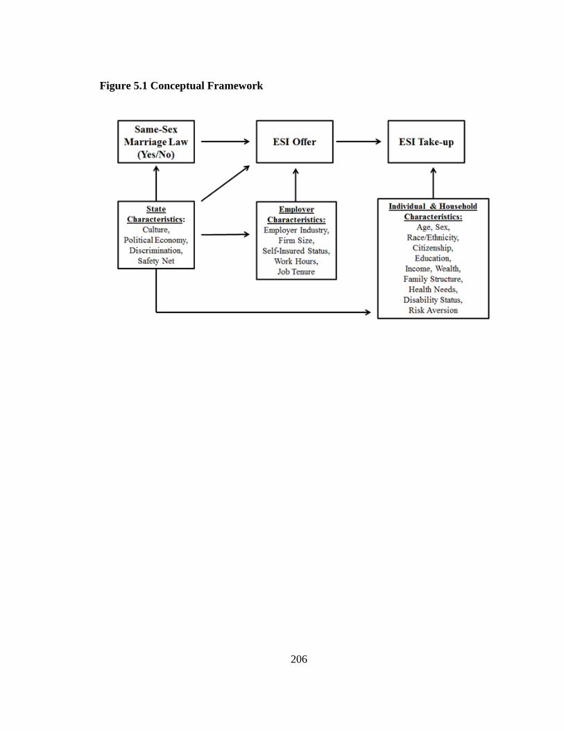
206
Figure 5.1 Conceptual Framework

207
Figure 5.2 Percent Covered by Employer-Sponsored Insurance (ESI) Before and
After New York’s Marriage Equality Act, by Sex
A. Men
B. Women
Data are from an analysis of the 2008-2012 American Community Survey. The vertical line represents the
year during which the Marriage Equality Act was implemented in New York. The reported percentage in
employer-sponsored insurance (ESI) reflects post-stratification weighting and have not been adjusted for
covariates. * indicates that estimates between the treatment group and comparison group are significantly
different (p<0.05) in the same year; otherwise estimates are statistically similar.
80%
78%
74% 75%
85%
78% 77% 75%
74%
65%
70%
75%
80%
85%
2008 2009 2010 2011 2012
Cover
ed b
y E
mp
loyer
Sp
on
sore
d
Insu
ran
ce (
%)
Treatment Group
(NY men in same-sex couples)
Comparison Group
(NY men in opposite-sex couples)
79%
78% 78%
78%
84%
78% 77%
75% 75% 75%
65%
70%
75%
80%
85%
2008 2009 2010 2011 2012
Cover
ed b
y E
mp
loyer
Sp
on
sore
d
Insu
ran
ce (
%)
Treatment Group
(NY women in same-sex couples)
Comparison Group
(NY women in opposite-sex couples)
*
*

208
Figure 5.3 Percent Both Members Covered by ESI Before and After New York’s
Marriage Equality Act, by Sex
A. Men
B. Women
Data are from an analysis of the 2008-2012 American Community Survey. The vertical line represents the
year during which the Marriage Equality Act was implemented in New York. The reported percentage of
both members covered by employer-sponsored insurance (ESI) reflects post-stratification weighting and
have not been adjusted for covariates. * indicates that estimates between the treatment group and
comparison group are significantly different (p<0.05) in the same year; otherwise no significant difference.
73%
67% 61%
65%
77%
74%
73% 70% 70%
70%
45%
50%
55%
60%
65%
70%
75%
80%
85%
2008 2009 2010 2011 2012
Both
Mem
ber
s C
over
ed b
y
Em
plo
yer
Sp
on
sore
d I
nsu
ran
ce (
%)
Treatment Group
(NY male same-sex households)
Comparison Group
(NY opposite-sex households)
74%
70%
74%
74%
73% 70%
70% 70%
45%
50%
55%
60%
65%
70%
75%
80%
85%
2008 2009 2010 2011 2012
Both
Mem
ber
s C
over
ed b
y
Em
plo
yer
Sp
on
sore
d I
nsu
ran
ce (
%)
Treatment Group
(NY female same-sex households)
Comparison Group
(NY opposite-sex households)
*

209
Figure 5.4 Trends in ESI Comparing the Treatment Group to the Synthetic Control
Group, by Sex
A. Men
B. Women
Data are from an analysis of the 2008-2012 American Community Survey. The vertical line represents the
year during which the Marriage Equality Act was implemented in New York. The reported percentage of
both members covered by employer-sponsored insurance (ESI) reflects post-stratification weighting and
have not been adjusted for covariates.
80%
78%
74% 75%
85%
75%
77%
65%
70%
75%
80%
85%
2008 2009 2010 2011 2012
Cover
ed b
y E
mp
loyer
Sp
on
sore
d
Insu
ran
ce (
%)
Treatment Group
(Actual New York)
Comparison Group
(Synthetic New York)
79% 78% 78% 78%
84%
73%
60%
65%
70%
75%
80%
85%
90%
2008 2009 2010 2011 2012
Cover
ed b
y E
mp
loyer
Sp
on
sore
d
Insu
ran
ce (
%)
Treatment Group
(Actual New York)
Comparison Group
(Synthetic New York)

210
Table 5.1 Descriptive Characteristics of Cohabiting Adults in New York, by Sex and Relationship Type
Men
Women
Treatment Group
Comparison Group
Treatment Group
Comparison Group
NY Adults in
Same-Sex Couples
NY Adults in
Opposite-Sex
Couples
without
Propensity Score
Weighting
NY Adults in
Opposite-Sex
Couples
with Propensity
Score
Weighting
NY Adults in
Same-Sex Couples
NY Adults in
Opposite-Sex
Couples
without
Propensity
Score
Weighting
NY Adults in
Opposite-Sex
Couples with
Propensity
Score
Weighting
Sample Size 1,842 142,436 142,436 1,682 142,436 142,436
Age (years)
26-34 18.8
14.3 18.8
19.8
19.7 20.9
35-44 32.4
27.7 34.0
29.4
29.7 30.3
45-54 34.5
32.2 32.8
33.8
31.8 32.6
55-64 14.2
25.8 14.4
16.9
18.7 16.3
Race/Ethnicity
White 75.3
68.0 72.1
75.7
68.3 74.1
Black 5.3
9.0 6.2
7.7
8.1 8.4
Asian 5.0
8.2 5.4
3.1
8.9 3.8
Other/multiple races 1.4
1.6 1.6
2.7
1.5 2.2
Hispanic 13.1
13.2 14.8
10.7
13.2 11.6
Couple's Combined Income
0-34,999 7.6
15.2 8.8
10.6
15.0 10.9
35,000-49,999 4.7
10.3 5.7
6.7
10.2 7.5
50,000-74,999 12.7
18.6 13.8
15.4
18.6 15.8
75,000-99,999 10.6
16.3 10.7
16.7
16.4 16.7
100,000-149,999 23.5
20.5 21.9
25.1
20.6 24.2

211
>150,000 41.0
19.1 39.2
25.5
19.3 25.0
Education
Less than high school 4.0
10.8 4.7
4.1
9.0 4.3
High school degree or GED 10.9
25.9 11.0
11.7
23.7 11.8
Some college or vocational 19.8
25.8 21.1
24.0
27.0 23.9
Bachelor's Degree 33.0
21.0 32.2
26.9
21.7 26.6
Graduate Degree 32.4
16.4 31.0
33.3
18.6 33.3
Citizenship
Citizen 82.4
71.4 79.8
87.7
71.4 86.3
Naturalized 7.6
16.1 8.8
7.5
15.8 8.0
Non-citizen 10.1
12.5 11.4
4.8
12.8 5.7
Children under 18 years 12.9
55.0 12.1
29.2
54.8 29.8
Adults over 65 years 1.6
3.3 1.7
2.4
3.3 2.6
Disabled 4.1
4.8 4.3
7.4
4.7 7.5
Residence in MSA
New York City MSA 78.0
64.5 77.6
61.7
64.1 62.4
Other MSA 17.9
27.1 18.6
30.2
27.5 30.0
Non-MSA 4.1
8.3 3.8
8.1
8.4 7.5
Homeownership
Owned free and clear 51.5
56.6 48.9
56.2
56.9 54.1
Owned with mortgage 8.3
13.0 8.2
11.3
13.1 10.0
Renting or residing without rent 40.3
30.4 43.0
32.5
30.0 36.0
Note: GED = general equivalency diploma. MSA = Metropolitan Statistical Area. Weighted percentages are for adults aged 26 to 64 years.

212
Table 5.2 Descriptive Characteristics of Same-Sex and Opposite-Sex Households in New York, by Sex and Relationship Type
Men
Women
Treatment Group
Comparison Group
Treatment Group
Comparison Group
NY Same-Sex
Households
NY
Opposite-Sex
Households
without
Propensity
Score
Weighting
NY
Opposite-Sex
Households
with
Propensity
Score
Weighting
NY Same-Sex
Households
NY Adults in
Opposite-Sex
Relationships
without
Propensity
Score
Weighting
NY Adults in
Opposite-Sex
Relationships
with
Propensity
Score
Weighting
Sample Size 921 142,436 142,436 841 142,436 142,436
Oldest Age in Couple (years)
26-34 11.1
12.3 10.6
13.8
12.3 14.4
35-44 27.6
26.7 29.8
24.9
26.7 27.0
45-54 40.0
32.7 38.0
36.1
32.7 34.9
55-64 21.4
28.3 21.5
25.2
28.3 23.7
Couple's Race
Both white 64.5
64.5 62.2
69.5
64.5 67.8
One non-white 21.8
7.5 22.4
12.6
7.5 13.3
Both non-white 13.7
28.1 15.4
17.9
28.1 18.9
Couple's Combined Income
0-34,999 7.6
15.1 8.5
10.6
15.1 10.8
35,000-49,999 4.9
10.2 5.5
6.8
10.2 7.5
50,000-74,999 12.8
18.6 13.6
15.4
18.6 15.7
75,000-99,999 10.6
16.4 10.6
16.4
16.4 16.7
100,000-149,999 23.3
20.5 21.9
25.3
20.5 24.2
>150,000 40.8
19.2 39.8
25.5
19.2 25.0
Couple's Highest Educational Attainment
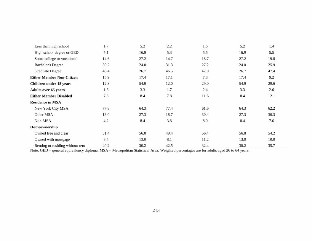
213
Less than high school 1.7
5.2 2.2
1.6
5.2 1.4
High school degree or GED 5.1
16.9 5.3
5.5
16.9 5.5
Some college or vocational 14.6
27.2 14.7
18.7
27.2 19.8
Bachelor's Degree 30.2
24.0 31.3
27.2
24.0 25.9
Graduate Degree 48.4
26.7 46.5
47.0
26.7 47.4
Either Member Non-Citizen 15.9
17.4 17.1
7.8
17.4 9.2
Children under 18 years 12.8
54.9 12.0
29.0
54.9 29.6
Adults over 65 years 1.6
3.3 1.7
2.4
3.3 2.6
Either Member Disabled 7.3
8.4 7.8
11.6
8.4 12.1
Residence in MSA
New York City MSA 77.8
64.3 77.4
61.6
64.3 62.2
Other MSA 18.0
27.3 18.7
30.4
27.3 30.3
Non-MSA 4.2
8.4 3.8
8.0
8.4 7.6
Homeownership
Owned free and clear 51.4
56.8 49.4
56.4
56.8 54.2
Owned with mortgage 8.4
13.0 8.1
11.2
13.0 10.0
Renting or residing without rent 40.2
30.2 42.5
32.4
30.2 35.7
Note: GED = general equivalency diploma. MSA = Metropolitan Statistical Area. Weighted percentages are for adults aged 26 to 64 years.

214
Table 5.3 Changes in Health Insurance Coverage After the Implementation of New York's Marriage Equality Act Treatment Group
Comparison Group
Unadjusted
Difference-in-Differences
Regression Adjusted
Difference-in-Differences
without Propensity Score
Weighting
Regression Adjusted
Difference-in-Differences
with Propensity Score
Weighting
NY Adults in Same-Sex
Couples
NY Adults in Opposite-Sex
Couples
Before After Difference
Before After Difference
Percentage
Points (95% CI)
Percentage
Points (95% CI)
Percentage
Points (95% CI)
Men
ESI Coverage 76.8 84.5 7.7 **
75.8 73.9 -1.9 ***
9.6 (3.8, 15.5)** 5.1 (0.05, 10.2)** 4.4 (-0.5, 9.3)*
Other Coverage 13.8 8.5 -5.3 **
13.5 14.4 0.8 **
-6.1 (-10.6, -1.6)** -3.6 (-7.9, 0.8) -4.2 (-8.4, -0.02)**
Uninsured 9.4 7.0 -2.5
10.6 11.7 1.1 ***
-3.5 (-7.5, 0.4)* -1.5 (-5.0, 1.9) -0.2 (-3.6, 3.2)
Women
ESI Coverage 78.4 84.2 5.7 *
76.4 74.6 -1.8 ***
7.5 (1.7, 13.5)** 7.0 (1.7, 12.2)** 5.6 (0.5, 10.6)**
Other Coverage 14.4 10.6 -3.8
14.7 15.7 1.0 **
-4.8 (-9.9, 0.4)* -4.6 (-9.3, 0.2)* -4.0 (-8.6, 0.5)*
Uninsured 7.2 5.2 -2.0 8.9 9.7 0.8 ** -2.8 (-6.1, 0.6) -2.4 (-5.6, 0.7) -1.5 (-4.3, 1.3)
Note: Regression adjusted difference-in-difference estimates are from linear probability models adjusting for age group, race/ethnicity, educational attainment, the couple's combined
income, the presence of a child in the household, the presence of a person ≥65 in the household, citizenship, disability status, MSA residence and homeownership.
*P<0.10; **P<0.05; ***P<0.001.
Source: 2008-2012 American Community Survey

215
Table 5.4 Changes in Household Health Insurance Coverage After the Implementation of New York's Marriage Equality Act Treatment Group
Comparison Group
Unadjusted
Difference-in-Differences
Regression Adjusted Difference-in-Differences
without Propensity Score
Weighting
Regression Adjusted Difference-in-Differences
with Propensity Score
Weighting
NY Same-Sex Households
NY Opposite-Sex
Households
Before After Difference
Before After Difference Percentage
Points (95% CI)
Percentage
Points (95% CI)
Percentage
Points (95% CI)
Men
Both Members Insured 85.5 88.4 3.1
87.0 85.7 -1.3 *** 4.4 (-1.9, 10.6) 2.0 (-3.7, 7.8) 0.1 (-5.7, 5.9)
Both Members Insured by ESI 66.9 76.8 10.0 **
71.7 69.8 -1.9 *** 11.9 (3.7, 20.0)** 7.2 (-0.3, 14.7)* 5.8 (-1.5, 13.2)
Women
Both Members Insured 87.9 89.4 1.5
87.0 85.7 -1.3 *** 2.8 (-3.5, 9.0) 2.7 (-3.4, 8.7) 0.8 (-5.0, 6.6)
Both Members Insured by ESI 71.1 74.0 2.9
71.7 69.8 -1.9 *** 4.8 (-3.9, 13.5) 4.6 (-3.0, 12.3) 3.3 (-4.2, 10.7)
Note: Regression Adjusted difference-in-difference estimates are from linear probability models adjusting for age group, race/ethnicity, educational attainment, the couple's combined income, the presence of a child in the household, the presence of a person ≥65 in the household, citizenship, disability status, MSA residence and homeownership.
*P<0.10; **P<0.05; ***P<0.001.
Source: 2008-2012 American Community Survey

216
Table 5.5 State Weights Used to Construct Synthetic New York
State Men in Same-Sex Couples Women in Same-Sex Couples
Alabama 0 0
Arizona 0 0
Arkansas 0 0
Colorado 0 0
Florida 0 0
Georgia 0 0
Indiana 0 0
Kansas 0 0
Kentucky 0 0
Louisiana 0 0
Maine 0 0
Maryland 0.17 0.30
Michigan 0.0 0
Minnesota 0.22 0
Mississippi 0 0
Missouri 0 0
New Mexico 0 0.09
North Carolina 0 0
Ohio 0 0
Oklahoma 0 0
Pennsylvania 0.61 0.07
South Carolina 0 0
Tennessee 0 0
Texas 0 0
Utah 0 0
Virginia 0 0.55
Note: State weights were estimated from the synthetic control method and
"synth" program in Stata developed by Abadie et al. (2010; 2014). State weights
are from the synthetic control method used to create synthetic New York and
based on state-level ESI rates and demographic characteristics for adults in
same-sex relationships.

217
Table 5.6 Results from the Falsification Test on Each Outcome, By Sex and Outcome
Men Women
(n = 1,525,768) (n = 1,527,064)
ESI Other Coverage Uninsured ESI Other Coverage Uninsured
Coef. (Std. Error) Coef. (Std. Error) Coef. (Std. Error) Coef. (Std. Error) Coef. (Std. Error) Coef. (Std. Error)
Post -0.014 (0.001)*** 0.008 (0.001)*** 0.005 (0.001)***
-0.017 (0.001)*** 0.010 (0.001)*** 0.007 (0.001)***
Treat -0.066 (0.005)*** 0.037 (0.005)*** 0.029 (0.004)***
-0.042 (0.005)*** 0.015 (0.004)** 0.028 (0.004)***
Post x Treat 0.011 (0.012) -0.014 (0.01) 0.003 (0.01)
-0.002 (0.012) -0.002 (0.01) 0.003 (0.01)
Education
Less than high school -0.129 (0.002)*** -0.015 (0.002)*** 0.144 (0.002)***
-0.169 (0.002)*** 0.011 (0.002)*** 0.158 (0.002)***
High School -0.041 (0.001)*** -0.022 (0.001)*** 0.063 (0.001)***
-0.060 (0.001)*** -0.005 (0.001)*** 0.065 (0.001)***
Some College -0.029 (0.001)*** 0.002 (0.001)** 0.027 (0.001)***
-0.041 (0.001)*** 0.006 (0.001)*** 0.035 (0.001)***
Bachelor's Degree Ref
Ref
Ref
Ref
Ref
Ref
Graduate degree -0.002 (0.001)* 0.015 (0.001)*** -0.012 (0.001)***
0.027 (0.001)*** -0.019 (0.001)*** -0.007 (0.001)***
Race/Ethnicity
White Ref
Ref
Ref
Ref
Ref
Ref
Hispanic -0.020 (0.002)*** -0.045 (0.001)*** 0.065 (0.002)***
-0.023 (0.002)*** -0.047 (0.001)*** 0.070 (0.002)***
Black 0.005 (0.002)** -0.004 (0.001)** -0.001 (0.001)
0.030 (0.002)*** -0.010 (0.001)*** -0.020 (0.001)***
Asian 0.039 (0.003)*** 0.020 (0.002)*** -0.059 (0.003)***
0.030 (0.003)*** 0.033 (0.002)*** -0.063 (0.002)***
Multiple/Other Races -0.043 (0.003)*** -0.003 (0.003) 0.046 (0.003)***
-0.045 (0.003)*** 0.003 (0.003) 0.042 (0.003)***
Age Group
25-34 -0.015 (0.001)*** -0.049 (0.001)*** 0.064 (0.001)***
-0.032 (0.001)*** -0.021 (0.001)*** 0.052 (0.001)***
35-44 -0.012 (0.001)*** -0.045 (0.001)*** 0.058 (0.001)***
-0.018 (0.001)*** -0.032 (0.001)*** 0.050 (0.001)***
45-54 -0.004 (0.001)*** -0.034 (0.001)*** 0.037 (0.001)***
-0.004 (0.001)*** -0.028 (0.001)*** 0.033 (0.001)***
55-64 Ref
Ref
Ref
Ref
Ref
Ref
Citizenship
Citizen Ref
Ref
Ref
Ref
Ref
Ref
Naturalized -0.057 (0.002)*** -0.006 (0.002)** 0.063 (0.002)***
-0.063 (0.002)*** 0.014 (0.002)*** 0.050 (0.002)***
Non-Citizen -0.104 (0.002)*** -0.078 (0.002)*** 0.182 (0.002)***
-0.115 (0.002)*** -0.060 (0.002)*** 0.174 (0.002)***

218
Disabled -0.138 (0.002)*** 0.235 (0.002)** -0.097 (0.002)***
-0.106 (0.002)*** 0.175 (0.002)*** -0.069 (0.002)***
MSA Residence 0.020 (0.001)*** -0.014 (0.001)** -0.007 (0.001)***
0.022 (0.001)*** -0.006 (0.001)*** -0.016 (0.001)***
Homeownership
Own home free and clear Ref
Ref
Ref
Ref
Ref
Ref
Own home with mortgage -0.030 (0.001)*** 0.026 (0.001)*** 0.004 (0.001)***
-0.033 (0.001)*** 0.028 (0.001)*** 0.006 (0.001)***
Renting -0.114 (0.001)*** 0.026 (0.001)*** 0.088 (0.001)***
-0.110 (0.001)*** 0.037 (0.001)*** 0.072 (0.001)***
Any kids -0.009 (0.001)*** 0.019 (0.001)*** -0.011 (0.001)***
-0.022 (0.001)*** 0.028 (0.001)*** -0.006 (0.001)***
Any older adults -0.004 (0.003) -0.001 (0.002) 0.006 (0.002)**
-0.006 (0.003)** -0.002 (0.002) 0.008 (0.002)**
Couple's Combined Income
0-34999 -0.382 (0.002)*** 0.158 (0.001)*** 0.224 (0.002)***
-0.391 (0.002)*** 0.155 (0.001)*** 0.236 (0.001)***
35000-49999 -0.129 (0.002)*** 0.039 (0.001)*** 0.090 (0.001)***
-0.135 (0.002)*** 0.041 (0.001)*** 0.095 (0.001)***
50000-74999 Ref
Ref
Ref
Ref
Ref
Ref
75000-99999 0.064 (0.001)*** -0.024 (0.001)*** -0.040 (0.001)***
0.061 (0.001)*** -0.020 (0.001)*** -0.041 (0.001)***
100000-149999 0.079 (0.001)*** -0.032 (0.001)*** -0.047 (0.001)***
0.068 (0.001)*** -0.021 (0.001)*** -0.046 (0.001)***
>150000 0.051 (0.001)*** -0.014 (0.001)*** -0.037 (0.001)***
0.036 (0.001)*** 0.005 (0.001)*** -0.040 (0.001)***
State
Alabama Ref
Ref
Ref
Ref
Ref
Ref
Alaska -0.112 (0.009)*** 0.048 (0.007)*** 0.063 (0.007)***
-0.096 (0.008)*** 0.030 (0.007)*** 0.066 (0.007)***
Arizona -0.061 (0.004)*** 0.058 (0.003)*** 0.003 (0.003)
-0.051 (0.004)*** 0.059 (0.003)*** -0.008 (0.003)**
Arkansas -0.041 (0.004)*** 0.015 (0.004)*** 0.026 (0.004)***
-0.033 (0.004)*** 0.000 (0.004) 0.033 (0.004)***
Colorado -0.079 (0.004)*** 0.056 (0.003)*** 0.023 (0.003)***
-0.068 (0.004)*** 0.055 (0.003)*** 0.014 (0.003)***
Florida -0.086 (0.003)*** 0.039 (0.003)*** 0.047 (0.002)***
-0.068 (0.003)*** 0.032 (0.003)*** 0.036 (0.002)***
Georgia -0.039 (0.003)*** 0.002 (0.003) 0.038 (0.003)***
-0.030 (0.003)*** -0.003 (0.003) 0.033 (0.003)***
Idaho -0.063 (0.005)*** 0.031 (0.005)*** 0.031 (0.004)***
-0.051 (0.005)*** 0.024 (0.004)*** 0.027 (0.004)***
Indiana 0.006 (0.003)* -0.018 (0.003)*** 0.012 (0.003)***
0.013 (0.003)*** -0.020 (0.003)*** 0.007 (0.003)**
Kansas -0.006 (0.004) 0.004 (0.003) 0.002 (0.003)
-0.003 (0.004) 0.003 (0.003) 0.000 (0.003)
Kentucky -0.010 (0.004)** 0.009 (0.003)** 0.001 (0.003)
0.003 (0.004) -0.006 (0.003)* 0.003 (0.003)
Louisiana -0.054 (0.004)*** 0.013 (0.003)*** 0.040 (0.003)***
-0.058 (0.004)*** 0.010 (0.003)** 0.049 (0.003)***
Maine -0.063 (0.005)*** 0.056 (0.005)*** 0.007 (0.004)
-0.047 (0.005)*** 0.063 (0.005)*** -0.016 (0.004)***

219
Maryland -0.014 (0.003)*** 0.012 (0.003)*** 0.002 (0.003)
-0.009 (0.003)** 0.011 (0.003)*** -0.002 (0.003)
Michigan 0.009 (0.003)** -0.009 (0.003)*** 0.000 (0.002)
0.015 (0.003)*** -0.003 (0.003) -0.012 (0.002)***
Minnesota -0.018 (0.003)*** 0.029 (0.003)*** -0.011 (0.003)***
-0.006 (0.003)* 0.027 (0.003)*** -0.022 (0.003)***
Mississippi -0.045 (0.005)*** 0.010 (0.004)** 0.035 (0.004)***
-0.035 (0.004)*** 0.002 (0.004) 0.033 (0.004)***
Missouri -0.018 (0.003)*** 0.004 (0.003) 0.014 (0.003)***
-0.006 (0.003)* -0.001 (0.003) 0.007 (0.003)
Montana -0.096 (0.007)*** 0.033 (0.006)*** 0.063 (0.006)***
-0.076 (0.007)*** 0.022 (0.005)*** 0.053 (0.006)***
Nebraska -0.026 (0.005)*** 0.035 (0.004)*** -0.010 (0.004)**
-0.021 (0.005)*** 0.032 (0.004)*** -0.011 (0.004)**
New Mexico -0.074 (0.005)*** 0.046 (0.004)*** 0.028 (0.004)***
-0.065 (0.005)*** 0.047 (0.004)*** 0.017 (0.004)***
North Carolina -0.054 (0.003)*** 0.026 (0.003)*** 0.028 (0.003)***
-0.043 (0.003)*** 0.018 (0.003)*** 0.025 (0.003)***
North Dakota -0.031 (0.007)*** 0.043 (0.006)*** -0.012 (0.005)**
-0.026 (0.007)*** 0.039 (0.006)*** -0.013 (0.005)**
Ohio 0.019 (0.003)*** -0.015 (0.003)*** -0.004 (0.002)*
0.023 (0.003)*** -0.014 (0.003)*** -0.010 (0.002)***
Oklahoma -0.042 (0.004)*** 0.002 (0.003) 0.040 (0.003)***
-0.038 (0.004)*** -0.007 (0.003)* 0.044 (0.003)***
Pennsylvania 0.012 (0.003)*** -0.005 (0.003)* -0.007 (0.002)**
0.019 (0.003)*** -0.002 (0.003) -0.017 (0.002)***
South Carolina -0.041 (0.004)*** 0.014 (0.003)*** 0.027 (0.003)***
-0.033 (0.004)*** 0.008 (0.003)** 0.025 (0.003)***
South Dakota -0.063 (0.007)*** 0.062 (0.006)*** 0.001 (0.005)
-0.044 (0.007)*** 0.049 (0.006)*** -0.005 (0.005)
Tennessee -0.025 (0.003)*** 0.018 (0.003)*** 0.007 (0.003)**
-0.015 (0.003)*** 0.017 (0.003)*** -0.002 (0.003)
Texas -0.057 (0.003)*** 0.007 (0.002)** 0.050 (0.002)***
-0.048 (0.003)*** -0.003 (0.002) 0.051 (0.002)***
Utah -0.013 (0.004)** 0.001 (0.003) 0.012 (0.003)***
-0.002 (0.004) -0.002 (0.003) 0.003 (0.003)
Virginia -0.040 (0.003)*** 0.037 (0.003)*** 0.003 (0.002)
-0.033 (0.003)*** 0.033 (0.003)*** 0.000 (0.002)
West Virginia 0.016 (0.005)** -0.028 (0.004)*** 0.012 (0.004)**
0.016 (0.005)** -0.036 (0.004)*** 0.020 (0.004)***
Wyoming -0.065 (0.008)*** 0.030 (0.007)*** 0.035 (0.006)***
-0.061 (0.008)*** 0.017 (0.007)** 0.044 (0.007)***
Source: 2008-2012 American Community Survey
*P<0.10; **P<0.05; ***P<0.001.

220
Complete Regression Tables
The following tables represent the complete regression results presented in Tables 5.3-
5.4.

221
Table 5.7 Complete Regression Results for Difference-in-Differences Estimates in Table 5.3 Without Propensity Score
Weighting Men Women
(n = 144,278) (n = 144,118)
ESI Other Coverage Uninsured ESI Other Coverage Uninsured
Coef. (Std. Error) Coef. (Std. Error) Coef. (Std. Error) Coef. (Std. Error) Coef. (Std. Error) Coef. (Std. Error)
Post -0.014 (0.003)*** 0.006 (0.003)** 0.008 (0.003)**
-0.015 (0.003)*** 0.008 (0.003)** 0.007 (0.002)**
Treatment -0.059 (0.015)*** 0.052 (0.013)*** 0.006 (0.009)
-0.049 (0.014)*** 0.037 (0.013)** 0.012 (0.009)
Post x Treatment 0.051 (0.026)** -0.036 (0.022) -0.015 (0.018)
0.070 (0.027)** -0.046 (0.024)* -0.024 (0.016)
Education
Less than high school -0.122 (0.006)*** 0.048 (0.005)*** 0.073 (0.005)***
-0.147 (0.006)*** 0.081 (0.006)*** 0.066 (0.006)***
High School -0.040 (0.004)*** 0.008 (0.003)** 0.032 (0.003)***
-0.054 (0.004)*** 0.025 (0.003)*** 0.029 (0.003)***
Some College -0.020 (0.003)*** 0.010 (0.003)*** 0.010 (0.003)***
-0.025 (0.003)*** 0.015 (0.003)*** 0.010 (0.002)***
Bachelor's Degree Ref
Ref
Ref
Ref
Ref
Ref
Graduate degree 0.011 (0.003)** 0.002 (0.003) -0.013 (0.002)***
0.021 (0.003)*** -0.013 (0.003)*** -0.008 (0.002)***
Race/Ethnicity
White Ref
Ref
Ref
Ref
Ref
Ref
Hispanic -0.020 (0.005)*** -0.055 (0.004)*** 0.075 (0.004)***
-0.027 (0.005)*** -0.036 (0.004)*** 0.063 (0.004)***
Black 0.021 (0.005)*** -0.024 (0.004)*** 0.002 (0.004)
0.036 (0.005)*** -0.029 (0.005)*** -0.007 (0.004)*
Asian -0.036 (0.006)*** 0.051 (0.005)*** -0.015 (0.005)**
-0.035 (0.006)*** 0.049 (0.005)*** -0.014 (0.005)**
Multiple/Other Races -0.010 (0.01) -0.004 (0.009) 0.015 (0.009)
-0.024 (0.01)** 0.006 (0.01) 0.018 (0.009)**
Age Group
25-34 -0.031 (0.004)*** -0.046 (0.004)*** 0.077 (0.004)***
-0.040 (0.004)*** -0.008 (0.004)** 0.048 (0.003)***
35-44 -0.019 (0.004)*** -0.036 (0.003)*** 0.055 (0.003)***
-0.023 (0.004)*** -0.017 (0.004)*** 0.039 (0.003)***
45-54 -0.010 (0.003)** -0.018 (0.003)*** 0.028 (0.002)***
-0.006 (0.003)* -0.016 (0.003)*** 0.022 (0.002)***
55-64 Ref
Ref
Ref
Ref
Ref
Ref

222
Citizenship
Citizen Ref
Ref
Ref
Ref
Ref
Ref
Naturalized -0.041 (0.004)*** 0.023 (0.004)*** 0.018 (0.003)***
-0.034 (0.004)*** 0.018 (0.004)*** 0.016 (0.003)***
Non-Citizen -0.139 (0.005)*** -0.041 (0.005)*** 0.180 (0.005)***
-0.128 (0.005)*** -0.034 (0.005)*** 0.162 (0.005)***
Disabled -0.103 (0.006)*** 0.179 (0.007)*** -0.077 (0.004)***
-0.100 (0.006)*** 0.148 (0.006)*** -0.048 (0.004)***
MSA residence
New York City MSA Ref
Ref
Ref
Ref
Ref
Ref
Other MSA 0.015 (0.003)*** -0.013 (0.003)*** -0.003 (0.002)
0.020 (0.003)*** -0.016 (0.003)*** -0.005 (0.002)**
Non-MSA 0.013 (0.004)** -0.023 (0.004)*** 0.010 (0.003)**
0.009 (0.004)** -0.022 (0.004)*** 0.013 (0.003)***
Homeownership
Owned free and clear Ref
Ref
Ref
Ref
Ref
Ref
Owned with mortgage -0.016 (0.003)*** 0.017 (0.003)*** -0.001 (0.002)
-0.015 (0.003)*** 0.017 (0.003)*** -0.002 (0.002)
Renting or residing without rent -0.100 (0.004)*** 0.063 (0.003)*** 0.037 (0.003)***
-0.090 (0.004)*** 0.074 (0.003)*** 0.016 (0.003)***
Any children in HH -0.013 (0.003)*** 0.036 (0.002)*** -0.024 (0.002)***
-0.031 (0.003)*** 0.052 (0.002)*** -0.021 (0.002)***
Any older adults in HH -0.005 (0.007) 0.011 (0.006)* -0.006 (0.005)
0.001 (0.006) 0.006 (0.006) -0.007 (0.005)
Couple's Combined Income
0-34,999 -0.411 (0.005)*** 0.290 (0.005)*** 0.122 (0.005)***
-0.413 (0.005)*** 0.301 (0.005)*** 0.112 (0.005)***
35,000-49,999 -0.155 (0.006)*** 0.081 (0.005)*** 0.074 (0.005)***
-0.154 (0.006)*** 0.090 (0.005)*** 0.064 (0.005)***
50,000-74,999 Ref
Ref
Ref
Ref
Ref
Ref
75,000-99,999 0.069 (0.004)*** -0.030 (0.003)*** -0.038 (0.003)***
0.068 (0.004)*** -0.035 (0.003)*** -0.034 (0.003)***
100,000-149,999 0.102 (0.004)*** -0.047 (0.003)*** -0.055 (0.003)***
0.090 (0.004)*** -0.046 (0.003)*** -0.044 (0.003)***
>150,000 0.099 (0.004)*** -0.043 (0.003)*** -0.056 (0.003)*** 0.090 (0.004)*** -0.043 (0.003)*** -0.047 (0.003)***
Source: 2008-2012 American Community Survey
*P<0.10; **P<0.05; ***P<0.001.

223
Table 5.8 Complete Regression Results for Difference-in-Differences Estimates in Table 5.3 With Propensity Score Weighting Men Women
(n = 144,278) (n = 144,118)
ESI Other Coverage Uninsured ESI Other Coverage Uninsured
Coef. (Std. Error) Coef. (Std. Error) Coef. (Std. Error) Coef. (Std. Error) Coef. (Std. Error) Coef. (Std. Error)
Post -0.003 (0.006) 0.006 (0.005) -0.003 (0.004)
-0.005 (0.003) 0.004 (0.003) 0.001 (0.003)
Treatment -0.057 (0.014)*** 0.048 (0.013)*** 0.009 (0.009)
-0.043 (0.013)** 0.033 (0.013)** 0.010 (0.008)
Post x Treatment 0.044 (0.025)* -0.042 (0.021)** -0.002 (0.017)
0.056 (0.026)** -0.040 (0.023)* -0.015 (0.014)
Education
Less than high school -0.091 (0.031)** 0.018 (0.03) 0.073 (0.031)**
-0.132 (0.033)*** 0.057 (0.04) 0.075 (0.033)**
High School -0.056 (0.022)** 0.007 (0.017) 0.050 (0.019)**
-0.019 (0.019) 0.002 (0.016) 0.016 (0.013)
Some College -0.027 (0.014)* 0.000 (0.012) 0.028 (0.011)**
-0.011 (0.015) -0.003 (0.014) 0.014 (0.009)
Bachelor's Degree Ref
Ref
Ref
Ref
Ref
Ref
Graduate degree 0.027 (0.012)** -0.014 (0.01) -0.014 (0.008)*
0.018 (0.013) -0.015 (0.011) -0.003 (0.008)
Race/Ethnicity
White Ref
Ref
Ref
Ref
Ref
Ref
Hispanic -0.014 (0.017) -0.005 (0.014) 0.019 (0.013)
0.004 (0.017) -0.003 (0.018) -0.001 (0.014)
Black -0.008 (0.021) 0.032 (0.023) -0.024 (0.02)
0.011 (0.024) 0.016 (0.023) -0.027 (0.015)*
Asian 0.056 (0.029)* -0.047 (0.017)** -0.009 (0.028)
0.063 (0.026)** -0.012 (0.02) -0.052 (0.021)**
Multiple/Other Races -0.010 (0.032) 0.034 (0.032) -0.024 (0.017)
-0.046 (0.048) -0.007 (0.028) 0.054 (0.044)
Age Group
25-34 0.016 (0.022) -0.063 (0.02)** 0.048 (0.014)**
-0.040 (0.019)** 0.003 (0.018) 0.037 (0.01)***
35-44 0.011 (0.02) -0.042 (0.019)** 0.031 (0.01)**
-0.015 (0.016) -0.027 (0.015)* 0.042 (0.009)***
45-54 -0.010 (0.019) 0.000 (0.017) 0.010 (0.01)
-0.011 (0.015) -0.018 (0.015) 0.029 (0.008)***
55-64 Ref
Ref
Ref
Ref
Ref
Ref
Citizenship

224
Citizen Ref
Ref
Ref
Ref
Ref
Ref
Naturalized -0.044 (0.022)** 0.038 (0.019)** 0.006 (0.013)
-0.038 (0.024) 0.002 (0.019) 0.036 (0.016)**
Non-Citizen -0.116 (0.02)*** 0.003 (0.019) 0.113 (0.018)***
-0.129 (0.025)*** -0.060 (0.026)** 0.189 (0.03)***
Disabled -0.093 (0.031)** 0.203 (0.032)*** -0.110 (0.013)***
-0.199 (0.024)*** 0.232 (0.025)*** -0.033 (0.016)**
MSA residence
New York City MSA Ref
Ref
Ref
Ref
Ref
Ref
Other MSA 0.042 (0.015)** -0.012 (0.014) -0.031 (0.009)**
0.025 (0.014)* -0.014 (0.013) -0.011 (0.008)
Non-MSA 0.055 (0.029)* -0.030 (0.023) -0.025 (0.016)
0.009 (0.029) -0.010 (0.029) 0.000 (0.012)
Homeownership
Owned free and clear Ref
Ref
Ref
Ref
Ref
Ref
Owned with mortgage -0.065 (0.035)* 0.072 (0.035)** -0.008 (0.01)
-0.028 (0.024) 0.026 (0.023) 0.002 (0.011)
Renting or residing without rent -0.062 (0.014)*** 0.022 (0.012)* 0.040 (0.009)***
-0.064 (0.014)*** 0.036 (0.013)** 0.028 (0.008)**
Any children in HH 0.021 (0.014) -0.022 (0.013)* 0.001 (0.014)
-0.003 (0.011) 0.032 (0.011)** -0.029 (0.008)***
Any older adults in HH -0.006 (0.036) 0.021 (0.046) -0.015 (0.027)
-0.058 (0.041) 0.017 (0.033) 0.041 (0.034)
Couple's Combined Income
0-34,999 -0.407 (0.028)*** 0.234 (0.025)*** 0.173 (0.028)***
-0.386 (0.028)*** 0.272 (0.029)*** 0.114 (0.021)***
35,000-49,999 -0.142 (0.032)*** 0.049 (0.025)* 0.093 (0.025)***
-0.129 (0.031)*** 0.097 (0.027)*** 0.032 (0.017)*
50,000-74,999 Ref
Ref
Ref
Ref
Ref
Ref
75,000-99,999 0.063 (0.029)** -0.016 (0.026) -0.047 (0.019)**
0.081 (0.024)** -0.044 (0.022)** -0.037 (0.014)**
100,000-149,999 0.142 (0.021)*** -0.048 (0.017)** -0.093 (0.015)***
0.109 (0.021)*** -0.062 (0.018)** -0.047 (0.013)***
>150,000 0.133 (0.022)*** -0.035 (0.018)* -0.099 (0.015)***
0.123 (0.021)*** -0.062 (0.019)** -0.061 (0.013)***
Source: 2008-2012 American Community Survey
*P<0.10; **P<0.05; ***P<0.001.

225
Table 5.9 Complete Regression Results for Difference-in-Differences Estimates in Table 5.4 Without Propensity Score
Weighting
Men
Women
(n = 143,357)
(n = 143,277)
Both insured Both insured by ESI
Both insured Both insured by ESI
Coef. (Std. Error) Coef. (Std. Error) Coef. (Std. Error) Coef. (Std. Error)
Post -0.011 (0.003)*** -0.015 (0.003)***
-0.011 (0.003)*** -0.015 (0.003)***
Treatment -0.041 (0.014)** -0.118 (0.019)***
-0.028 (0.014)** -0.071 (0.017)***
Post x Treatment 0.020 (0.029) 0.072 (0.038)*
0.027 (0.031) 0.046 (0.039)
Education
Less than high school -0.108 (0.008)*** -0.137 (0.007)***
-0.108 (0.008)*** -0.137 (0.007)***
High School -0.049 (0.004)*** -0.055 (0.005)***
-0.049 (0.004)*** -0.055 (0.005)***
Some College -0.018 (0.003)*** -0.020 (0.004)***
-0.018 (0.003)*** -0.020 (0.004)***
Bachelor's Degree Ref
Ref
Ref
Ref
Graduate degree 0.015 (0.002)*** 0.022 (0.003)***
0.015 (0.002)*** 0.021 (0.003)***
Race/Ethnicity
Both white Ref
Ref
Ref
Ref
One non-white -0.014 (0.004)** -0.013 (0.005)**
-0.014 (0.004)*** -0.013 (0.005)**
Both non-white -0.042 (0.003)*** -0.040 (0.004)***
-0.041 (0.003)*** -0.041 (0.004)***
Age Group
25-34 -0.080 (0.004)*** -0.039 (0.005)***
-0.079 (0.004)*** -0.040 (0.005)***
35-44 -0.065 (0.003)*** -0.026 (0.004)***
-0.065 (0.003)*** -0.027 (0.004)***
45-54 -0.034 (0.003)*** -0.012 (0.003)***
-0.034 (0.003)*** -0.012 (0.003)***
55-64 Ref
Ref
Ref
Ref
Any non-citizen -0.142 (0.004)*** -0.102 (0.005)***
-0.142 (0.004)*** -0.102 (0.005)***
Any disabled 0.023 (0.004)*** -0.086 (0.005)***
0.022 (0.004)*** -0.088 (0.005)***

226
MSA residence
New York City MSA Ref
Ref
Ref
Ref
Other MSA 0.003 (0.002) 0.021 (0.003)***
0.002 (0.002) 0.021 (0.003)***
Non-MSA -0.019 (0.004)*** 0.008 (0.004)*
-0.019 (0.004)*** 0.008 (0.004)*
Homeownership
Owned free and clear Ref
Ref
Ref
Ref
Owned with mortgage 0.004 (0.003) -0.015 (0.004)***
0.004 (0.003) -0.015 (0.004)***
Renting or residing without rent -0.053 (0.003)*** -0.118 (0.004)***
-0.053 (0.003)*** -0.118 (0.004)***
Any children in HH 0.034 (0.003)*** -0.009 (0.003)**
0.035 (0.003)*** -0.009 (0.003)**
Any older adults in HH 0.012 (0.006)** -0.007 (0.007)
0.011 (0.006)* -0.008 (0.007)
Couple's Combined Income
0-34,999 -0.139 (0.005)*** -0.399 (0.005)***
-0.139 (0.005)*** -0.399 (0.005)***
35,000-49,999 -0.089 (0.005)*** -0.171 (0.006)***
-0.089 (0.005)*** -0.171 (0.006)***
50,000-74,999 Ref
Ref
Ref
Ref
75,000-99,999 0.046 (0.004)*** 0.084 (0.004)***
0.046 (0.004)*** 0.084 (0.004)***
100,000-149,999 0.067 (0.003)*** 0.125 (0.004)***
0.066 (0.003)*** 0.125 (0.004)***
>150,000 0.071 (0.003)*** 0.128 (0.005)*** 0.071 (0.003)*** 0.128 (0.005)***
Source: 2008-2012 American Community Survey
*P<0.10; **P<0.05; ***P<0.001.

227
Table 5.10 Complete Regression Results for Difference-in-Differences Estimates in Table 5.4 With Propensity Score Weighting
Men
Women
(n = 143,357)
(n = 143,277)
Both insured Both insured by ESI
Both insured Both insured by ESI
Coef. (Std. Error) Coef. (Std. Error) Coef. (Std. Error) Coef. (Std. Error)
Post
0.004 (0.006) 0.001 (0.007)
0.000 (0.003) -0.005 (0.004)
Treatment -0.038 (0.013)** -0.110 (0.019)***
-0.022 (0.014) -0.065 (0.016)***
Post x Treatment 0.001 (0.03) 0.058 (0.038)
0.008 (0.03) 0.033 (0.038)
Education
Less than high school -0.028 (0.056) -0.072 (0.035)**
-0.131 (0.082) -0.110 (0.054)**
High School -0.073 (0.034)** -0.048 (0.035)
-0.024 (0.042) -0.039 (0.039)
Some College -0.007 (0.02) -0.026 (0.026)
-0.012 (0.019) -0.021 (0.023)
Bachelor's Degree Ref
Ref
Ref
Ref
Graduate degree 0.023 (0.014)* 0.036 (0.019)*
0.015 (0.015) 0.014 (0.019)
Race/Ethnicity
Both white Ref
Ref
Ref
Ref
One non-white 0.000 (0.016) -0.006 (0.021)
-0.003 (0.019) -0.029 (0.024)
Both non-white -0.021 (0.021) -0.011 (0.023)
0.014 (0.019) -0.026 (0.022)
Age Group
25-34 -0.087 (0.026)** 0.019 (0.031)
-0.056 (0.023)** -0.046 (0.029)
35-44 -0.052 (0.015)** 0.042 (0.025)*
-0.052 (0.016)** -0.009 (0.022)
45-54 -0.019 (0.014) 0.013 (0.024)
-0.037 (0.015)** -0.006 (0.021)
55-64 Ref
Ref
Ref
Ref
Any non-citizen -0.100 (0.021)*** -0.102 (0.025)***
-0.145 (0.028)*** -0.083 (0.029)**
Any disabled 0.070 (0.019)*** -0.063 (0.035)*
0.022 (0.022) -0.148 (0.026)***

228
MSA residence
New York City MSA Ref
Ref
Ref
Ref
Other MSA 0.032 (0.014)** 0.051 (0.022)**
0.019 (0.015) 0.032 (0.018)*
Non-MSA 0.015 (0.028) 0.073 (0.038)*
0.000 (0.023) 0.018 (0.03)
Homeownership
Owned free and clear Ref
Ref
Ref
Ref
Owned with mortgage 0.004 (0.017) -0.056 (0.036)
0.005 (0.019) -0.021 (0.029)
Renting or residing without rent -0.055 (0.014)*** -0.068 (0.019)***
-0.057 (0.015)*** -0.094 (0.019)***
Any children in HH 0.016 (0.018) 0.029 (0.021)
0.054 (0.012)*** 0.016 (0.015)
Any older adults in HH 0.008 (0.035) -0.004 (0.044)
-0.096 (0.064) -0.093 (0.063)
Couple's Combined Income
0-34,999 -0.212 (0.037)*** -0.382 (0.032)***
-0.168 (0.033)*** -0.380 (0.032)***
35,000-49,999 -0.129 (0.04)** -0.151 (0.043)***
-0.071 (0.032)** -0.139 (0.039)***
50,000-74,999 Ref
Ref
Ref
Ref
75,000-99,999 0.067 (0.028)** 0.095 (0.038)**
0.047 (0.024)** 0.121 (0.032)***
100,000-149,999 0.127 (0.023)*** 0.198 (0.03)***
0.076 (0.021)*** 0.177 (0.029)***
>150,000 0.140 (0.022)*** 0.202 (0.03)***
0.102 (0.019)*** 0.198 (0.029)***
Source: 2008-2012 American Community Survey
*P<0.10; **P<0.05; ***P<0.001.

229
5A. Technical Appendix to Chapter 5: Data and Sample Limitations
This technical appendix describes the instrumentation challenges to measuring
cohabiting same-sex couples in the American Community Survey (ACS) and how
changes in the ACS have improved the measurement of same-sex couples and disrupted
the measurement of cohabiting same-sex couples over time. After discussing the data
limitations surrounding the measurement of same-sex couples in the ACS, this technical
appendix provides recommendations for using the public use ACS to measure same-sex
couples and demonstrates how measurement can affect regression-based analyses.
5A.1 Data Source
This technical appendix uses cross-sectional data from the 2008-201327
American
Community Survey (ACS) Public Use Microdata Samples (PUMS) [U.S. Census Bureau
2015]. The ACS is a household survey conducted annually over a 12-month calendar
period by the U.S. Census Bureau. Replacing the decennial Census long-form
questionnaire in 2005, the ACS is designed to provide states and communities with
timely demographic, economic and housing information. Many state and local
governments rely on the ACS to plan and monitor programs that affect housing,
transportation, health care and education (Powers, Beede and Telles 2015).
Each year, approximately 3 million housing units are selected from the U.S.
Census Bureau’s Master Address File and sent a mail questionnaire requesting
information on the physical characteristics of the housing structure and information for
27
Data from 2013 are used in this technical appendix to assess the quality and usefulness
of additional data, but my evaluation, included in this chapter, recommends not
combining data on same-sex couples from the 2008-2012 ACS with the 2013 ACS.

230
each person in the household. Although households are asked to return their completed
mail forms promptly, respondents are eligible for Computer-Assisted Telephone
Interviewing (CATI) after one month of non-response. During the third month of non-
response, the U.S. Census Bureau retrieves answers using Computer-Assisted Personal
Interviewing (CAPI) methods (Virgile 2011). Beginning with the 2013 ACS, households
were allowed to submit their responses online using a computer or a handheld tablet
(Horwitz 2015).28
Households are required by federal law (Title 18 U.S.C. Section 3571 and 3559)
to complete the ACS, and the Census Bureau uses a multi-modal survey design, three to
four mailings to encourage housing units to return the questionnaire, CATI methods for
initial non-respondents, and CAPI methods for a subsample of mail and telephone non-
respondents. Therefore, the ACS maintains a relatively high response rate, which is
defined as the ratio of the estimate of units interviewed after data collection is complete
to the estimate of all units that should have been interviewed. According to the U.S.
Census Bureau (2015), the housing unit response rate averages approximately 97% each
year. In 2013, the response rate was 89.9% because the Census Bureau did not conduct
follow-ups in October 2013 due to a federal government shutdown.
5A.2 Study Sample and Challenges in the ACS
Like most federal surveys, the ACS does not directly ascertain sexual orientation.
Previous research using the ACS identifies same-sex couples and same-sex households
when the primary respondent (most often “the person living or staying here in whose
name this house or apartment is owned, being bought, or rented”) identifies another
28
All self-responses (i.e. mail and internet) are treated equally in weighting procedures
(U.S. Census Bureau 2014 Data and Methodology Report).

231
cohabiting person of the same sex as a husband, wife, or unmarried partner (see Figure
A9 on page 264) [Gates and Steinberger 2009; Gates 2010; O’Connell and Feliz 2011;
DeMaio, Bates, and O’Connell 2013]. The current study uses this same approach and
assumes cohabiting same-sex couples are lesbian, gay or bisexual (LGB); transgender
populations are not identifiable given the binary male-female response options for sex.
Same-sex couples are missing in this analysis if they are not in a relationship with the
primary respondent, not cohabiting together in the same house or apartment, or designate
alternative relationship categories, such as a roommate or nonrelative, to conceal their
relationship.
Prior to 2013 and in accordance with the Defense of Marriage Act (DOMA)29
—
which defined marriage between one man and one woman for federal purposes—same-
sex couples using the “husband/wife” response categories were edited and recoded as
“unmarried partners” by the Census Bureau regardless of their legal marital status
(O’Connell and Gooding 2006; Lofquist and Lewis 2015). In the 2012 ACS, the Census
Bureau included “editing flags”30
identifying the sample of same-sex spouses changed to
unmarried partners, and in the 2013 ACS, all same-sex spouses using the “husband/wife”
categories were retained without edits in the public use files for the first time (Lofquist
and Lewis 2015; Lofquist 2015).31
29
Section 3 of the federal Defense of Marriage Act (DOMA)—signed into law in 1996
and overturned by the U.S. Supreme Court in United States v. Windsor in 2013—defined
marriage as “a legal union between one man and one woman as husband and wife” for
federal purposes, including federal data collection, federal income taxes and eligibility
for public programs. 30
The recode editing flag is labeled SSPA in the 2012 ACS PUMS. 31
Allocation flags (labeled SSMC) were also included to indicate whether the
householder or spouse did not report their sex, and sex was assigned, or imputed, based
on their first name (Lofquist 2015).

232
An additional concern with using the ACS for same-sex marriage research is that
there is now a large body of research suggesting that many married same-sex couples
using the “husband/wife” categories may actually be opposite-sex couples who
mistakenly marked the wrong sex on the survey form (Black et al. 2007; Gates and
Steinberger 2009; O’Connell and Feliz 2011; Kreider and Lofquist 2015; Lewis, Bates
and Streeter 2015). Although this type of error occurs relatively infrequent among
opposite-sex couples, a small number of miscoded opposite-sex couples can inundate and
contaminate the relatively small sample of same-sex couples. Estimates vary, but
between 20-57% of the national sample of married same-sex couples using the
“husband/wife” designation and approximately 7% of unmarried same-sex couples using
the “unmarried partner” designation may actually represent miscoded opposite-sex
couples in the ACS (Black et al., 2007; Gates and Steinberger 2009; Kreider and Lofquist
2015; Lofquist 2015). Additionally, for reasons discussed below, the potential rate of
contamination varies by response mode. The percentage of married same-sex couples
likely to be opposite-sex couples misreporting sex is 59.2% in mail responses and 46.3%
in the CATI/CAPI responses (Krieder & Lofquist 2015).
5A.3 Contamination in the Sample of Married Same-Sex Couples
Previous research by Gates and Steinberger (2009) provides guidance for
reducing the contamination problem among married same-sex couples in the ACS. To
illustrate the problem, Figure A1 divides the total sample of same-sex couples by
response mode and allocated marital status. Quadrants (1) & (3) are assumed to represent
the sample of same-sex couples using the “unmarried partner” category and with fewer
contamination issues, (Gates and Steinberger 2009; Klawitter 2011; Badgett and

233
Schneebaum 2015), perhaps because the distal position of “unmarried partner” in the
relationship roster (see Figure A9 on page 264) suggests that the respondent may be
carefully answering the questionnaire. Research from the Census Bureau indicates that
approximately 93% of same-sex couples using this “unmarried partner” designation
(Quadrants 1 & 3) are credible same-sex couples when matching data from the 2010
Census to name directories indicating the state-specific probability of a male first name
(O’Connell and Feliz 2011).32
Similar results were found after merging the 2010 ACS to
Social Security administrative records: 93% of same-sex couples using the “unmarried
partner” response were valid same-sex couples (Krieder and Lofquist 2015).
Figure A1 Same-sex couples in the ACS by response mode and allocated marital
status
Not allocated marital
status
Allocated marital status
(or self-reported same-sex
spouses in the 2013 ACS)
Self-responses
(mail and internet)
(1)
Same-sex couples who used
the “unmarried partner”
designation
(2)
A combination of same-sex
spousal couples who used
the “husband/wife”
designation and opposite-
sex married couples who
miscoded the sex of one
spouse
CATI/CAPI responses (3)
Same-sex couples who used
the “unmarried partner”
designation
(4)
A combination of same-sex
spousal couples who used
the “husband/wife”
designation and opposite-
sex married couples who
miscoded the sex of one
spouse
Source: Adapted from Gates and Steinberger (2009).
32
The sex of a respondent was assumed male if the respondent’s first name was used by
men at least 95% of the time.

234
Quadrants (2) and (4) [shaded in Figure A1] correspond to married same-sex
couples at greatest risk of contamination from miscoding by opposite-sex couples; this
group includes same-sex couples receiving the marital status allocation flag in the 2008-
2012 ACS and same-sex couples using the “husband/wife” response categories in the
2013 ACS. The “marital status allocation flag” (labeled FMARP in the ACS-PUMS)
identifies same-sex spouses where the original marital status response was altered from
“currently married” to something else (never married, separated, divorced, widowed) by
the Census Bureau. Although the Census Bureau did not release the same-sex “editing
flags” (labeled SSPA) for same-sex spouses changed to “unmarried partners” until the
2012 ACS, researchers used the marital status allocation flag to identify married same-
sex couples after the Census Bureau confirmed a very strong correlation between editing
flags for married same-sex couples (SSPA) and the marital status allocation flag
(FMARP) [Black et al., 2007; Gates and Steinberger 2009].
Based on the 2012 ACS sample of 502 same-sex couples in New York (the only
year when both editing and allocation flags are publicly available), receiving a marital
status allocation flag (FMARP) is highly correlated with self-reporting a same-sex
“husband/wife” (SSPA); the correlation coefficient is 95% in the correlation matrix. In
fact, every same-sex couple using the “husband/wife” category received the marital status
allocation flag (in addition to very few [n=16] same-sex couples using the “unmarried
partner” response). This suggests that my method of assigning married same-sex couples
using the “husband/wife” response category to Quadrants (2) and (4) in 2013 is consistent
with previous practices by the U.S. Census Bureau.

235
Returning back to Figure A1, Quadrant (2) represents same-sex couples using the
“husband/wife” designation in the mail/internet survey, and Quadrant (4) represents
same-sex couples using the “husband/wife” designation in the CATI/CAPI surveys. The
CATI/CAPI modules prompt the interviewer to verify the sex of a same-sex husband or
wife, which should eliminate the possibility of miscoding sex. However, very recent
research (Krieder and Lofquist 2015; Lofquist 2015) suggests that Quadrant (4) also
suffers contamination issues. After matching the 2010 ACS to information on sex from
Social Security administrative records, approximately 59% of Quadrant (2) and 46% of
Quadrant (4) represented opposite-sex couples miscoding sex. Using a different method
that matched the 2013 ACS to name directories, contamination error rates were smaller:
26.1% of Quadrant (2) and 16.6% of Quadrant (4) were opposite-sex couples
misreporting sex (Lofquist 2015), but an additional 19.6% of Quadrant (2) and 18.8% of
Quadrant (4) could not be determined since some first names may be ambiguous and
commonly used across genders.33
For added precaution, this technical appendix departs
from Gates and Steinberger’s guidance and does not assume Quadrant (4) is free from
contamination. Instead, this technical appendix assumes that Quadrants (2) and (4)
experience severe contamination issues and treats them similarly.
5A.4 Reducing Contamination in the Sample of Same-Sex Couples
The sample flow diagram in Figure A2 illustrates how I selected a final sample of
married same-sex couples to minimize the potential contamination in Quadrants (2) and
33
Additionally, the contamination issue is potentially minimal in the internet responses.
Only 8% of married same-sex couples using the internet response option in the 2013
ACS were opposite-sex couples miscoding sex after comparing reported sex to probable
sex based on the first name directory, where a name is probably male if it was reported as
male 95% of the time and probably female if it was reported as female 95% of the time
(Lofquist 2015).

236
(4). First, my analytic sample was restricted to same-sex and opposite-sex couples where
both members were between 26 and 64 years of age to account for Medicare coverage
starting at age 65 and provisions in the Affordable Care Act allowing parents to keep
adult children on employer health plans until the age of 26 (Sommers et al. 2013). Next, I
excluded all same-sex and opposite-sex couples where at least one member was allocated
sex or relationship to the householder because of missing or inconsistent information
(Badgett and Schneebaum 2015). Sex and relationship to the householder was assigned
by a Census Bureau algorithm when there was missing or inconsistent information in the
original responses. Therefore, I assumed data were unreliable when one member was
allocated sex or relationship to the householder.
I assume partnership status was reported with fewer contamination errors for the
1,404 same-sex couples using the “unmarried partner” response, which represented same-
sex couples from Quadrants (1) and (3) in Figure A1. Remember, Kreider & Lofquist’s
(2015) comparison of the 2010 ACS to Social Security administrative records on sex
indicates that approximately 93% of this sample is comprised of credible unmarried
same-sex couples. The 758 same-sex couples from Quadrants (2) and (4) represent a
combination of married same-sex couples who used the “husband/wife” designation and
married opposite-sex couples who miscoded the sex of a spouse. Removing this entire
group from the analysis, however, potentially eliminates a substantial portion of the
treatment group affected by New York’s Marriage Equality Act.
To identify a sample of married same-sex couples at lower risk of contamination,
I took advantage of information on when the primary respondent reported the year in
which each member was last married. I used marital history data for each person to check

237
whether members in a married same-sex relationship reported the same marital year. Of
the 758 married same-sex couples, 300 couples were missing marital history data, 26
couples were “allocated” marital history, and 124 couples reported discordant marital
years—all of which potentially represents incomplete or misreported information from
married opposite-sex couples. Without complete and inconsistent marital information, I
cannot decipher whether these are married same-sex couples (n=450), so I do not include
them in the analysis presented here.

238
Figure A2 Flow diagram for the selection of the final sample of same-sex couples in
New York from the 2008-2013 American Community Survey
Note: The sample size, “n”, indicates the number of cohabiting same-sex couples in New York (there are
two adults in a same-sex couple in each same-sex household). Source: 2008-2013 American Community
Survey.
Potential same-sex
couples
(n = 2,948)
Both members of the couple
aged 26-64 years
(n = 2,216)
Sex not allocated
(n = 2,209)
Relationship to householder
not allocated
(n = 2,162)
Quadrants (1) & (3):
Relationships to householder
not allocated
(n = 1,404)
Likely same-sex
couple households
(n = 1,404)
Did not meet age criteria
(n = 732)
Allocated sex
(n = 7)
Allocated relationship to
householder
(n = 47)
Quadrants (2) & (4):
A combination of same-
sex spousal couples who
used the “husband/wife”
designation and opposite-
sex couples who miscoded
the sex of one spouse
(n = 758)
Same-sex spousal couples who
used the “husband/wife”
designation and both members
reported being married
in the same year
(n = 308) Final sample of
same-sex couple households
(n = 1,712)
Opposite-sex
couples
miscoding the
sex of one
spouse
(n = 450)

239
Of the remaining 308 married same-sex couples using the “husband/wife”
category with concordant marital histories, approximately 9% reported getting married in
2008, the year New York recognized out-of-state marriage licenses—and this represented
a major surge to previous years (Figure A3). Similarly, over 15% of the same-sex couples
with concordant marital histories reported getting married in 2011, the year the Marriage
Equality Act was passed in New York. Only 30% reported getting married prior to 2004,
when Massachusetts became the first state to legalize same-sex marriage. This technical
appendix assumes that the 308 same-sex couples with concordant marital histories are
plausible married same-sex couples in New York, or same-sex couples considering
themselves married in the 2008-2013 ACS.34
I also assume 450 of the 758 married same-
sex couples excluded (59% of all same-sex couples using the “husband/wife”
designation) represent inaccurate and miscoded opposite-sex couples from Quadrants (2)
and (4). Therefore, my final sample included 1,712 cohabiting same-sex couples in New
York.
34
The annual sample sizes for the 308 married same-sex couples are as follows: 13 in
2008, 20 in 2009, 14 in 2010, 18 in 2011, 39 in 2012, and 204 in 2013. Changes to the
2013 ACS (edits to married same-sex couples and adding an internet response option)
and the repeal of DOMA in June 2013 may have led more same-sex couples to marry
and/or report their relationships.

240
Figure A3 Year last married among same-sex couples in New York when both
members reported the same year of marriage
Source: 2008-2013 American Community Survey
5A.5 Primary Comparison Group: Opposite-Sex Couples in New York
I compare health insurance outcomes to an in-state comparison group unaffected
by New York’s Marriage Equality Act: cohabiting opposite-sex couples residing in New
York. The sample flow diagram in Figure A4 illustrates how I selected the final sample
of opposite-sex couples. Opposite-sex couples were excluded if they did not meet the age
criteria or one member was allocated sex or relationship to the householder (similar to the
sample of same-sex couples). My sample of opposite-sex couples does not include the
450 “same-sex” couples from Figure A2 who potentially miscoded sex, was missing
marital history data or reported discordant martial history compared to their partner. The
0
.05
.1.1
5.2
De
nsity
1960 1970 1980 1990 2000 2010Year Last Married
Marital Year for Same-Sex Couples in New York
NY begins licensing in-state marriages in 2011
NY recognizes out-of-state marriages in 2008
MA legalizes same-sex marriage in 2004

241
final sample of opposite-sex couples includes married and unmarried couples to be
consistent with the sample of same-sex households. Distinguishing legally married and
unmarried same-sex households is problematic, since same-sex couples use the
“husband/wife” categories based on evolving sociological and legal definitions (Gates
2010) and distinguishing legally married same-sex couples from unmarried same-sex
couples is not possible in the public use files (Krieder and Lofquist 2015). Additionally,
some workplaces voluntarily offer health benefits to unmarried same-sex couples over
the study period (Kaiser 2014). Therefore, for consistency, my sample of opposite-sex
couples includes married and unmarried opposite-sex couples. My final sample included
170,169 opposite-sex households in New York.

242
Figure A4 Flow diagram for the selection of a final sample of opposite-sex couples in
New York from the 2008-2013 American Community Survey
Note: The sample size, “n”, indicates the number of cohabiting opposite-sex couples in
New York (there are two adults in an opposite-sex couple in each opposite-sex
household). Source: 2008-2013 American Community Survey.
Potential opposite-sex
couples
(n = 235,005)
Both members of the couple
aged 26-64 years
(n = 170,648)
Sex not allocated
(n =170,472)
Relationship to householder
not allocated
(n = 170,169)
Did not meet age criteria
(n = 64,357)
Allocated sex
(n = 176)
Allocated relationship to
householder
(n = 302)
Final sample of
opposite-sex couple households
(n = 170,169)

243
5A.6 Data and Study Limitations
5A.6.1 Missing Information on Sexual Orientation and Same-Sex Couples
This study has a number of limitations. My method of identifying same-sex
couples does not verify the sexual orientation of the sample. Although I assume that
people in cohabiting same-sex couples are lesbian, gay and bisexual (LGB), bisexual
adults are missing from this analysis if they were in an opposite-sex couple during the
survey period. Knowing sexual orientation would also facilitate studying single LGB
adults and partnership patterns over time. Specifically, knowing sexual orientation would
allow me to rule out whether the Marriage Equality Act increased cohabitation among
LGB adults, which raises major endogeneity issues for this study. Since marriage
provides substantial financial benefits beyond health insurance, the Marriage Equality
Act may have increased the likelihood of marrying, cohabitating and self-reporting a
same-sex relationship in the post-treatment period, and the changing composition of
same-sex couples in the post-treatment period may be driving the results. Previous
research by Buchmueller & Carpenter (2012) found California’s domestic partnership
law increased partnership by 7.6 percentage points for lesbian women (a similar effect
was not found for gay men).
Additionally, data on same-sex couples in the ACS are limited to the primary
householder (sometimes referred as the household head) and the householder’s partner
(husband, wife or unmarried partner). Although the selection of households in the ACS is
designed to be nationally representative, the identity of the primary respondent is not
random. The primary respondent is most often “the person living or staying here in
whose name this house or apartment is owned, being bought, or rented.” The primary

244
respondent is likely to have different characteristics than other adults living in
households, including higher levels of employment, income and education (all of which
may bias health insurance coverage estimates upward). Not only is the primary
respondent not a randomly selected member of the household, but all members in the
household are only asked of their relationship to the primary householder—and not to
each other. Therefore, not only is this study missing same-sex couples not cohabiting
together, but this study is missing same-sex couples unrelated to the primary respondent.
However, there may not be many missing same-sex couples cohabiting together in
households and not in a relationship with the primary householder. Based on a national
sample of 1,623 (unweighted) same-sex couples in the 2010-2013 CPS-ASEC (which
ascertains the identity of a spouse or unmarried partner for each person in the household),
only 2.5% of all same-sex couples were not partnered with the household head (based on
my calculations).
Finally, this study is missing same-sex couples choosing not to disclose their
relationship or using alternative relationship responses, such as roommates or unrelated
adults. Discrimination and stigma may lead some same-sex couples not to disclose their
relationships in federal surveys or to interviewers in CATI/CAPI surveys, especially in
regions with high levels of stigma and discrimination. People who choose not to disclose
their sexual orientation in surveys (Kim & Fredriksen-Goldsen 2013) or in the workplace
(Badgett 1996) tend to be racial and ethnic minorities and low-income workers.
Therefore, same-sex couples not disclosing their relationship in the ACS may be
socioeconomically disadvantaged, and leaving this group out may underestimate the

245
relationship between sexual orientation and health insurance coverage at the lower end of
the socioeconomic spectrum.
5A.6.2 Limited Generalizations from New York to Other States
This study focuses on New York, which is unique in terms of the size and
representativeness of the general population, the LGBT population and cohabiting same-
sex couples, especially since so much of the state and the LGBT population lives in the
New York City area. According to the 2010 decennial Census, there were approximately
19.4 million people in New York, making it the third most populous state (U.S. Census
2015). Meanwhile, approximately 43% of the state’s population lives in New York City
(NYC Department of City Planning 2015). People in New York also enjoy high levels of
income—the median household income in New York is $55,000 (the 16th highest state in
the U.S.) [U.S. Census Bureau 2015]. The population is also more racially and ethnically
diverse compared to the rest of the country. Only 57% of New York is non-Hispanic
White compared to 62% of the country (U.S. Census 2015). Moreover, the economy and
health care industry in New York is not comparable to most states. New York has the
third largest economy in the United States based on gross state product, after California
and Texas. In terms of health insurance coverage, New York maintained a relatively low
uninsurance rate prior to the passage of the Affordable Care Act. In 2009, only 13% of
people under 65 years of age were uninsured in New York compared to 17% in the
United States (Robert Wood Johnson Foundation DataHub 2015). Given these unique
features of New York, making generalizations and finding an adequate comparison state
is extremely challenging.

246
In regards to health insurance coverage among same-sex couples, employers in
the Northeast are more likely to cover same-sex partners compared to other regions.
According to the 2012 Employer Health Benefits Report sponsored by the Kaiser Family
Foundation, approximately 54% of firms offering health benefits in the Northeast
extended coverage to same-sex partners in 2012 (Claxton et al. 2012). Only 15% of firms
in the South, 34% of firms in the Midwest, and 36% of firms in the West covered same-
sex partners (Claxton et al. 2012). It remains uncertain what percentage of companies in
New York covered same-sex partners prior to the Marriage Equality Act, but it’s likely to
be above the national average. Given varying health insurance industries across the
country, it may be difficult to generalize the findings presented here to other states, but I
would hypothesize that the impacts of same-sex marriage laws on ESI coverage in same-
sex households could be larger in states where more employers would be required to
cover same-sex spouses.
There are other methodological limitations to using New York as the treatment
state for the study of same-sex marriage. First, New York State recognized same-sex
marriage licenses obtained outside the state beginning in 2008, when the New York Court
of Appeals ruling in Martinez v. County of Monroe required the state to recognize same-
sex marriages performed in another state or country. This decision meant that New York
State (and fully-insured employers) had to recognize same-sex marriage licenses obtained
from nearby states (e.g. Connecticut, Massachusetts, New Hampshire and Vermont) or
other countries (e.g. Canada, the Netherlands, Belgium, Spain and South Africa) that
already implemented same-sex marriage. Between 2008 and 2011, New York was the
only state to recognize same-sex marriages conducted outside of New York while

247
denying same-sex marriage licenses inside the state. This method of implementation is
rare. Very few states recognized out-of-state same-sex marriage licenses prior to
authorizing same-sex marriages in-state. To the extent that same-sex couples in New
York traveled to other jurisdictions to obtain marriage licenses, the results in this study
may be biased downward. If many same-sex couples obtained marriage licenses in
Canada or in a nearby state after 2008, the policy change itself would affect fewer same-
sex couples and households.
5A.6.3 Changing Economy, Societal Attitudes and Data Collection Over Time
This technical appendix uses cross-sectional data from the 2008-2013 American
Community Survey (ACS) and a difference-in-differences (DD) framework to measure
the differential impact of New York’s Marriage Equality Act on health insurance
coverage in same-sex households. One risk to relying on a pre-post design, including a
DD framework, is that other factors—beyond the Marriage Equality Act—changed
during the study period which may have affected health insurance outcomes and the
composition of self-reported same-sex couples. For example, the 2007-2009 economic
recession coincided with the period immediately preceding the passage of the Marriage
Equality Act. Between December 2007 and June 2009, approximately 8.7 million jobs
were lost during the economic downturn in the United States, and as many as 5 million
people lost ESI nationally due to unemployment or declining incomes (Holahan 2011).
Figure A5 illustrates the impact of the recession on statewide unemployment rates in
New York during the study period. The unemployment rate in New York increased from
4.9% in 2008 to 8.9% at the beginning of 2010. Given the rapid increase in
unemployment before 2010, many people (and their partners) in New York likely lost

248
their jobs and their access to ESI, and the relatively unstable economy in 2008 and 2009
may explain transitions in ESI during this period. This study includes data from 2008 and
2009, because I assume all households were affected by the economic recession similarly,
but problems arise if the recession affected the treatment group differently than the
comparison groups.
Figure A5 Statewide Unemployment Rates in New York
Source: U.S. Department of Labor, Bureau of Labor Statistics
This study does not include data from 2013 in the analysis for several reasons.
First of all, changes in the ACS data collection break the consistent nature of the ACS.
For example, the ACS implemented an internet response option in 2013, and
approximately 29% (based on my calculations) of all households in New York responded
using the internet response mode in 2013. Cohabiting same-sex couples may be more
likely to report their sexual minority status over the internet compared to CATI/CAPI and
4.0%
5.0%
6.0%
7.0%
8.0%
9.0%
10.0%
2008 2009 2010 2011 2012 2013

249
mail response modes. The anonymity associated with submitting answers online may lead
some same-sex couples to report their relationships. Additionally, respondents using the
internet option may be demographically different from respondents using the CATI/CAPI
and mail response modes in previous surveys.
Changes in editing same-sex households in the 2013 ACS also make it difficult to
compare same-sex households over time. Specifically, the U.S. Census Bureau stopped
editing same-sex households using the “husband/wife” response category to “unmarried
partners.” The Census Bureau now maintains same-sex households using the
“husband/wife” response option and imputes missing information on age and relationship
status as same-sex couples if the respondents’ first names have a high probability of
being the same sex (Lofquist 2015).
Changes in federal law in 2013 may also be associated with more same-sex
couples marrying, cohabitating and reporting their same-sex relationship status. In June
2013, the U.S. Supreme Court ruled section 3 of the Defense of Marriage Act (DOMA),
which defined marriage between one man and one woman, unconstitutional in United
States v. Windsor. Subsequently, same-sex couples gained immediate incentives to marry
since the federal government recognized their unions. Indeed, administrative data on
same-sex marriages in Connecticut, New Hampshire, and Vermont suggests that nearly
twice as many same-sex couples married in 2013 than in 2012; the number of same-sex
marriage licenses in New York was also slightly higher in 2013 than in 2012 (Badgett &
Mallory 2014). Thus, the Windsor decision may have independently led more same-sex
couples to get married, cohabitate and report their relationship status in the ACS, which
would have caused more compositional problems in the 2013 ACS.

250
Finally, changes in attitudes and public opinion on homosexuality, LGBT people
and same-sex marriage dramatically shifted over the study period. For instance, in May
2008, only 40% of Americans believed that marriages between same-sex couples should
be valid with the same rights as traditional marriages (McCarthy 2015), and only
Massachusetts licensed same-sex marriages (Connecticut and California would issue
same-sex marriages later in the year). By 2013, 16 states issued same-sex marriage
licenses; the federal government recognized those marriage licenses following the
Windsor decision; and 54% of Americans believed that same-sex marriages should be
valid. As laws, attitudes and opinions changed over time, LGBT people may be more
likely to report their same-sex relationships in the ACS, and the results in this study may
be driven by changing population compositions, especially if same-sex couples in the
2012-2013 ACS were demographically different from those in the 2008-2010 ACS.
I find mixed evidence that more male and female same-sex couples reported their
same-sex relationship over time. The percentage of male same-sex households in the final
sample remained between 0.76% and 0.98% between 2008 and 2012 (Table A1). In
2013, the percentage of households headed by cohabiting male same-sex couples
increased to 1.43%, which coincided with changes in the ACS data collection and federal
policy. Meanwhile, male same-sex households in 2013 were significantly less likely to be
white and more likely to have children in the household compared to male same-sex
households in 2008. Disregarding 2013, male same-sex households are slightly less likely
to be white (or both white) in 2012, which may bias the impact estimates on ESI
coverage downward, since non-white adults may be less likely to have jobs that offer
health insurance (Zuvekas & Taliaferro 2003).

251
Female same-sex households in New York (Table A2) made up a smaller
percentage of households in 2010 and 2011 (less than 1%) compared to opposite-sex
households (Note: the sample size for female same-sex households was smallest in 2011).
The percentage of female same-sex households was statistically similar in 2012 (1.08%)
relative to the beginning of the period (1.34%), but female same-sex households in 2012
were less likely to be white (or both white), less likely to live in New York City and less
likely to own their home. These compositional changes in the post-treatment period
suggest that more disadvantaged—not advantaged—same-sex couples were more likely
to report their same-sex relationship status following the implementation of the Marriage
Equality Act, which may bias the impacts on ESI coverage downward, since they are less
likely to have access to ESI or are able to afford premiums for ESI.

252
Table A1 Characteristics of male same-sex couples in New York over the study period
2008 2009 2010 2011 2012 2013
Sample size of male same-sex couples 150 144 138 119 135 219
Percent same-sex couples vs opposite-sex couples 0.91% 0.85% 0.76% 0.76% 0.98% 1.43% **
Age of householder 45.6 42.8 ** 44.0 45.8 46.0 45.2
Highest educational attainment: college degree 83.4% 86.0% 84.2% 86.2% 75.3% 86.2%
Couple's combined income ≥ $100,000 73.1% 64.2% 65.5% 63.1% 70.0% 71.4%
Any member working full-time 91.4% 92.6% 92.3% 83.2% 91.7% 91.3%
Both members working part-time 2.3% 3.0% 0.6% 5.0% 5.4% 3.0%
Householder is white 88.1% 82.3% 79.6% * 85.6% 77.9% * 73.1% **
Both members white 75.9% 70.0% 67.1% 61.0% ** 64.5% * 57.2% **
Any member non-citizen 10.3% 10.5% 19.6% * 13.1% 9.8% 13.7%
Any member disabled 5.8% 5.9% 5.9% 14.7% * 4.1% 6.0%
New York City MSA residence 76.6% 77.0% 79.5% 78.1% 75.0% 78.5%
Homeownership: owned free and clear or with mortgage or loan 68.0% 57.5% 53.7% ** 64.1% 62.9% 59.5%
Homeownership: rented 31.8% 41.4% 46.3% ** 35.9% 37.1% 39.6%
Any children in household 6.6% 4.8% 6.4% 6.0% 4.5% 13.0% *
Any adults > 65 years in household 3.3% 0.1% * 2.3% 1.3% 1.4% 1.8%
Migrated from out of state within past year 0.4% 2.8% 0.0% 2.1% 1.4% 2.5% *
Notes: The year-specific sample of same-sex couples is significantly different from the 2008 sample at *p<.10 or **p<.05. Household weights and data on the
primary householder were used in the calculation of these estimates. Source: 2008-2013 American Community Survey.

253
Table A2 Characteristics of female same-sex couples in New York over the study period
2008 2009 2010 2011 2012 2013
Sample size of female same-sex couples 141 125 124 106 124 187
Percent same-sex couples vs opposite-sex couples 1.34% 1.09% 0.99% ** 0.87% ** 1.08% 1.35%
Age of householder 44.2 45.9 45.4 45.9 44.4 45.0
Highest educational attainment: college degree 79.6% 72.5% 75.9% 73.3% 75.6% 67.5% **
Couple's combined income ≥ $100,000 59.6% 46.4% * 45.8% * 50.1% 47.9% 50.0%
Any member working full-time 85.5% 84.3% 82.0% 86.1% 89.9% 82.2%
Both members working part-time 9.3% 0.8% ** 5.3% 3.1% * 2.7% * 5.4%
Householder is white 80.5% 83.6% 83.5% 76.4% 65.3% ** 75.7%
Both members white 72.6% 78.1% 75.7% 67.8% 55.5% ** 70.1%
Any member non-citizen 4.4% 6.9% 5.7% 8.0% 6.5% 8.0%
Any member disabled 8.3% 13.8% 11.2% 9.8% 14.3% 13.0%
New York City MSA residence 67.6% 51.6% ** 56.9% * 62.6% 54.2% * 66.2%
Homeownership: owned free and clear or with mortgage or loan 75.3% 71.7% 65.7% 68.4% 58.4% ** 63.1% *
Homeownership: rented 24.7% 27.7% 34.3% 30.9% 39.6% ** 36.5% *
Any children in household 22.9% 25.0% 29.4% 20.4% 31.2% 32.4%
Any adults > 65 years in household 1.9% 1.7% 4.2% 2.3% 0.3% 3.1%
Migrated from out of state within past year 3.9% 2.3% 1.5% 0.8% 2.7% 2.0%
Notes: The year-specific sample of same-sex couples is significantly different from the 2008 sample at *p<.10 or **p<.05. Household weights and data on the
primary householder were used in the calculation of these estimates. Source: 2008-2013 American Community Survey.

254
5A.7 The Comparison Group as a Counterfactual
The key assumption underlying a difference-in-differences (DD) framework is
that the trends over time for the comparison groups provide the counterfactual for what
would have happened in the absence of the Marriage Equality Act in New York (Angrist
& Pischke 2009). Opposite-sex couples in New York are the preferred comparison group,
since they are exposed to the same economic, political, and social environment over time
(as well as health insurance industry and access to Medicaid) as same-sex couples in New
York.
An important step in using a difference-in-differences framework is to
demonstrate that the treatment and comparison group share parallel trends in the pre-
treatment period. Figure A6 presents trends in ESI coverage for individual adults in
cohabiting same-sex couples, and figure A7 presents trends in both members having ESI.
With the exception of 2008, New York men in same-sex couples shared a similar trend in
ESI coverage to New York men in opposite-sex couples (Figure A6, Panel A). Following
the implementation of the Marriage Equality Act in 2011, ESI coverage increased to 85%
for men in same-sex couples. Meanwhile, New York women in same-sex couples also
experienced parallel trends in ESI coverage over time with New York women in
opposite-sex couples, and there was a slight increase in ESI coverage for women in same-
sex couples in 2011. However, ESI coverage continued to decline for both New York
women in same-sex couples and opposite-sex couples.
Figure A7 presents the trends in both members having ESI between same-sex
households and opposite-sex households. Dual ESI coverage declined for male same-sex
households between 2008 and 2010, but then began to increase after 2011, from 62% to

255
78% (Figure A7, Panel A). Interestingly, dual ESI coverage for both women in same-sex
households was approximately the same over time as ESI coverage for both members in
opposite-sex households (Figure A7, Panel B). So why did the pre-treatment trend in ESI
coverage for male same-sex households fall so quickly and were very different from
female same-sex households and opposite-sex households? One plausible hypothesis is
that the economy affected male same-sex households differently than other households
(i.e. a history issue). For instance, the types of jobs gay and bisexual men in cohabiting
same-sex couples are likely to hold may have been affected by the economic recession
more than the sectors where heterosexual and lesbian workers work. During the
recession, gay and bisexual male workers may have been unable or reluctant to add their
same-sex partners to ESI for fear of losing their job. Either the economic recovery may
have helped increase ESI coverage for gay and bisexual men returning to work, or the
increases in ESI were due to the passage of the Marriage Equality Act. This is one
instance where knowing the specific source of ESI (primary policy holder versus
dependent on another person’s health plan) would be help explain this pattern.

256
Figure A6 Percent Covered by Employer-Sponsored Insurance (ESI) Before and
After New York’s Marriage Equality Act, by Sex
A. Men
B. Women
Data are from an analysis of the 2008-2013 American Community Survey. The vertical line represents the
year during which the Marriage Equality Act was implemented in New York. The reported percentage in
employer-sponsored insurance (ESI) reflects post-stratification weighting and have not been adjusted for
covariates. * indicates that estimates between the treatment group and comparison group are significantly
different (p<0.05) in the same year; otherwise estimates are statistically similar.
87%
77%
71%
84% 85%
78%
75% 75% 74% 73%
65%
70%
75%
80%
85%
90%
2008 2009 2010 2011 2012 2013
Cover
ed b
y E
mp
loyer
Sp
on
sore
d
Insu
ran
ce (
%)
Treatment Group
(Men in same-sex relationships)
Comparison Group
(Men in opposite-sex relationships)
80% 79% 79%
82%
80%
78%
78% 77%
75% 75% 75% 74%
65%
70%
75%
80%
85%
90%
2008 2009 2010 2011 2012 2013
Cover
ed b
y E
mp
loyer
Sp
on
sore
d
Insu
ran
ce (
%)
Treatment Group
(Women in same-sex relationships)
Comparison Group
(Women in opposite-sex relationships)
*
*
* *

257
Figure A7 Percent Both Members Covered by Employer-Sponsored Insurance (ESI)
Before and After New York’s Marriage Equality Act, by Sex
A. Men
B. Women
Data are from an analysis of the 2008-2013 American Community Survey. The vertical line represents the
year during which the Marriage Equality Act was implemented in New York. The reported percentage of
both members covered by employer-sponsored insurance (ESI) reflects post-stratification weighting and
have not been adjusted for covariates. * indicates that estimates between the treatment group and
comparison group are significantly different (p<0.05) in the same year; otherwise no significant difference.
81%
65% 58% 62%
77% 78%
74% 73%
70% 70%
70% 69%
0.45
0.5
0.55
0.6
0.65
0.7
0.75
0.8
0.85
2008 2009 2010 2011 2012 2013
Both
Mem
ber
s C
over
ed b
y
Em
plo
yer
Sp
on
sore
d I
nsu
ran
ce (
%)
Treatment Group
(Male Same-Sex Households)
Comparison Group
(Opposite-Sex Households)
75%
71% 72%
71%
66%
70%
0.45
0.5
0.55
0.6
0.65
0.7
0.75
0.8
0.85
2008 2009 2010 2011 2012 2013
Both
Mem
ber
s C
over
ed b
y
Em
plo
yer
Sp
on
sore
d I
nsu
ran
ce (
%)
Treatment Group
(Female Same-Sex Households)
Comparison Group
(Opposite-Sex Households)
*
*
*

258
5A.8 Regression-Adjusted Results
This section uses the sample defined in this this technical appendix to provide an
alternative set of results estimating the impact of New York’s Marriage Equality Act on
health insurance coverage for individual adults in cohabiting same-sex couples and same-
sex households in New York as separate units of observations (similar to the results
presented in chapter 5). These estimates do not include data from the 2013 ACS given the
changes in data collection and federal policy occurring in 2013. Table A3 presents the
changes in health insurance coverage between New York adults in same-sex couples and
New York adults in opposite-sex couples, and after adjusting for demographic and
socioeconomic characteristics, ESI coverage increased 5.7 percentage points (p<0.10) for
men in same-sex relationships relative to men in opposite-sex couples after the Marriage
Equality Act. Meanwhile, at the household level (Table A4), dual ESI coverage (or both
members having ESI) increased 8.1 percentage points for male same-sex households
relative to opposite-sex households after the Marriage Equality Act (Table A4). These
findings were only marginally significant (p<.10) in linear probability models without
propensity score weighting. Similar results were not found for women in same-sex
couples or female same-sex households in New York.
These results are consistent with the results presented in chapter 5, which found
that the Marriage Equality Act was associated with increased ESI coverage for men and
women in same-sex couples. However, these estimates and the review of compositional
changes in the samples over time provide some important insights to the previous results.
First, there is very little evidence that the composition of male same-sex households in
New York changed in the 2008-2012 ACS. If anything, they were slightly less likely to

259
be white in 2012 (Table A1), which would bias the impact estimates downward, since
racial and ethnic minorities are less likely to have ESI. Results in this technical appendix
also suggest that ESI coverage increased (5.7 percentage points) for New York men in
same-sex couples relative to New York men in opposite-sex couples. These findings
support the results from chapter 5 that ESI coverage increased 4-7 percentage points for
New York men in cohabiting same-sex couples relative to New York men in cohabiting
opposite-sex couples. However, the findings for New York women in same-sex couples
do not hold across samples. When comparing New York women in same-sex couples to
New York women in opposite-sex couples in this technical appendix, I do not find that
the Marriage Equality Act had a significant impact on ESI coverage for New York
women in same-sex couples like I did in chapter 5. Therefore, the results for New York
women in same-sex couples remain mixed and inconclusive at this point.

260
Table A3 Changes in Health Insurance Coverage After the Implementation of New York's Marriage Equality Act
Treatment Group Comparison Group
Unadjusted Difference-in-
Differences
Regression Adjusted
Difference-in-Differences
without Propensity Score
Weighting
Regression Adjusted
Difference-in-
Differences with
Propensity Score
Weighting
NY Adults in Same-Sex
Couples
NY Adults in Opposite-Sex
Couples
Before After Difference Before After Difference Percentage
Points
(95% CI) Percentage
Points
(95% CI) Percentage
Points
(95% CI)
Men
ESI Coverage 77.7 84.4 6.6 *
75.9 74.0 -1.9 ***
8.5 (1.7, 15.4)** 5.7 (-0.3, 11.8)* 4.9 (-0.9, 10.8)
Other Coverage 14.0 8.9 -5.1 *
13.5 14.7 0.9 **
-6.0 (-11.5, -0.5)** -4.3 (-9.4, 0.9) -4.7 (-9.9, 0.4)*
Uninsured 8.3 6.8 -1.5
10.6 11.6 1.1 ***
-2.6 (-6.7, 1.6) -1.5 (-5.4, 2.4) -0.2 (-4.4, 3.6)
Women
ESI Coverage 80.1 79.7 -0.3
76.5 74.7 -1.8 ***
1.5 (-5.9, 8.8) 2.8 (-3.6, 9.1) 1.6 (-4.3, 7.6)
Other Coverage 13.2 13.2 0.0
14.6 15.6 1.0 **
-1.0 (-7.5, 5.5) -1.9 (-7.7, 3.8) -1.6 (-7.1, 3.8)
Uninsured 6.8 7.1 0.3 8.9 9.7 0.8 ** -0.5 (-4.6, 3.6) -0.8 (-4.8, 3.2) 0.0 (-3.6, 3.6)
Note: Regression adjusted difference-in-difference estimates are from linear probability models adjusting for age group, race/ethnicity, educational attainment, the couple's
combined income, the presence of a child in the household, the presence of a person ≥65 in the household, citizenship, disability status, MSA residence and homeownership.
*P<0.10; **P<0.05; ***P<0.001.
Source: 2008-2012 American Community Survey

261
Table A4 Changes in Household Health Insurance Coverage After the Implementation of New York's Marriage Equality Act Treatment Group Comparison Group
Unadjusted Difference-in-
Differences
Regression Adjusted Difference-in-Differences
without Propensity Score
Weighting
Regression Adjusted Difference-in-Differences
with Propensity Score
Weighting
NY Same-Sex Households
NY Opposite-Sex
Households
Before After Difference Before After Difference Percentage
Points (95% CI)
Percentage
Points (95% CI)
Percentage
Points (95% CI)
Men
Both Members Insured 86.2 87.9 1.6
87.1 85.8 -1.3 *** 2.9 (-4.5, 10.4) 1.5 (-5.5, 8.6) -0.7 (7.9, 6.5)
Both Members Insured by ESI 67.5 76.7 9.2
71.7 69.9 -1.9 *** 11.0 (1.4, 20.7)** 8.1 (-1.0, 17.1)* 6.5 (-2.5, 15.5)
Women
Both Members Insured 88.0 85.6 -2.4
87.1 85.8 -1.3 *** -1.1 (-9.3, 7.1) -0.1 (-8.1, 7.9) -2.4 (-9.9, 5.1)
Both Members Insured by ESI 72.5 66.1 -6.3
71.7 69.9 -1.9 *** -4.4 (-15.5, 6.7) -2.3 (-12.0, 7.3) -3.9 (-13.0, 5.3)
Note: Regression Adjusted difference-in-difference estimates are from linear probability models adjusting for age group, race/ethnicity, educational attainment, the couple's
combined income, the presence of a child in the household, the presence of a person ≥65 in the household, citizenship, disability status, MSA residence and homeownership.
*P<0.10; **P<0.05; ***P<0.001.
Source: 2008-2012 American Community Survey

262
5A.9 Recommendations for Researchers Interested in Studying Same-Sex Couples
In the absence of richer data, which includes information on sexual orientation,
the U.S. Census Bureau should continue its efforts to improve the measurement of same-
sex households. For example, changing the design of the survey from horizontal panels
(Figure A8) to vertical panels (Figure A9) in the 2008 ACS reduced the likelihood of
misreporting sex (O’Connell and Lofquist 2009). Respondents were much less likely to
misreport sex or select both sex responses—leaving the Census Bureau to allocate sex—
when the male-female responses were place side-by-side. This change in the
questionnaire design dramatically reduced the number of same-sex couples by 52%
(O’Connell and Feliz 2011), but it’s often credited as a major improvement in the
collection of sex information in Census surveys (O’Connell and Lofquist 2009; Lofquist
and Lewis 2015).
Additionally, the Interagency Working Group on Measuring Relationships in
Federal Household Surveys should continue testing new questions to measure same-sex
couples. A revised question on the relationship to the householder was tested in the 2013
ACS Design Test (Lewis 2014), and it included three changes. The revised question (1)
moved the “unmarried partner” option from the 13th response item to the 2nd response
item, (2) added a gender-neutral “spouse” option, and (3) split up the spouse and partner
options for opposite-sex and same-sex couples. The revised relationship question in
Figure A10 now includes the following options: opposite-sex husband/wife/spouse;
opposite-sex unmarried partner; same-sex husband/wife/spouse; and same-sex unmarried
partner.

263
While there are no current plans to add the revised relationship question to the
ACS, since it requires additional ACS testing, the revised relationship question will be
fully implemented in the 2015 American Housing Survey, the 2015 Annual Social and
Economic Supplement to the Current Population Survey (CPS-ASEC), and the 2020
decennial Census (Lofquist and Lewis 2015). However, early evaluations—albeit with
very small sample sizes—found continued inconsistencies with misreporting sex in the
revised question (Lofquist and Lewis 2015; Lewis, Bates and Streeter 2015).
Approximately 44% of respondents (n=16) reporting a same-sex husband, wife or spouse
reported inconsistent sex information for the corresponding spouse (Lofquist and Lewis
2015).

264
Figure A8 Questions on sex, date of birth and relationship to the primary
householder in the 2005-2007 ACS
Figure A9 Questions on sex, date of birth and relationship to the primary
householder in the 2008-2013 ACS
Figure A10 Revised relationship question in the 2013 American Community Survey
Questionnaire Design Test (ACS-QDT)

265
Researchers using the ACS to study issues affecting cohabiting same-sex couples
should take caution when interpreting their findings. First, researchers should be aware of
the challenges involved with data collection and measurement. Cohabiting same-sex
couples in the ACS may not be generalizable to the entire universe of same-sex couples,
as they represent a subsample of household heads and their same-sex spouses and
partners. Selection of the household head may not be random, since the household head is
the person whose name the house or apartment is owned, being bought, or rented. Same-
sex couples outside the household head may represent socially and economically
disadvantaged populations and may have changed in size and composition through
economic recessions and through evolving legal issues and societal attitudes on LGBT
people. Additionally, same-sex couples reporting their sexual minority status in federal
surveys must be understood in light of stigma and discrimination. The ACS is likely to
measure same-sex couples who feel comfortable reporting their same-sex partners in a
federal survey, and these same-sex couples are more likely to be white and highly
educated compared to those who are single or do not report their sexual orientation
(Carpenter & Gates 2008).
For researchers interested in using the ACS for their research, added precautions
should be taken to address potential contamination issues. Researchers should not use
data on married same-sex couples prior to the 2008 ACS—or at least not combine data
over the 2007 and 2008 ACS given the changes in the 2008 ACS questionnaire (Figure
A9). Moreover, researchers should not include in their sample any same-sex couple
where one member was allocated sex or relationship to the primary householder, since
266
the missing data were imputed by the Census Bureau. For researchers interested in
studying married same-sex couples using the “husband/wife” designation, researchers
should restrict their analysis to couples married in the same year and carefully assess
when they reported getting married. Although qualitative research demonstrates that
same-sex couples who are legally married are more likely to use the “husband/wife”
response categories in Census surveys (Gates 2010; DeMaio, Bates and O’Connell 2013),
researchers should take extra steps to rid the sample of contamination. The method
pursued here recommends confirming that both members in a married same-sex
relationship consistently reported being married in the same year.
Finally, researchers should consider other federal surveys measuring sexual
orientation, including the National Health Interview Survey (NHIS), which added sexual
orientation in 2013 (Ward et al. 2014), and the Behavioral Risk Factor Surveillance
System for some 25 states (Fenway Institute 2013). Although these surveys do a better
job ascertaining sexual orientation for a random adult in the household, data may not be
available at the state level or have the large sample sizes found in the ACS. For example,
region (not state) is the lowest level of geography available in the public use NHIS data
sets. Researchers can obtain approval from the National Center for Health Statistics to
conduct state policy analyses in one of the Census Bureau’s Research Data Centers to
access restricted NHIS files, but researchers should expect to have information on no
more than 23,000-36,000 sample adults across the United States randomly selected for
detailed interviews. Researchers may be able to bypass issues common in the ACS and
other federal surveys by using administrative records or marriage license registries
managed by the states, but obtaining permissions to use these records may be difficult.

267
5A.10 Next Steps for Future Research
Future research will explore alternative research designs and strategies to
overcome the issues and limitations in this project. For example, one problem in this
paper is the issue of changing compositions of same-sex couples over time. As previously
mentioned, the policy change itself—legalizing same-sex marriage—can change the
composition of self-reported same-sex couples in the ACS following the policy
implementation. To bypass this issue, instead of studying the direct effects of legalizing
same-sex marriage on LGBT populations, researchers might study the effects of same-sex
marriage laws on LGBT people indirectly by comparing changes in outcomes in one state
adopting same-sex marriage to changes in outcomes in a similar state not adopting same-
sex marriage—and attributing differential changes in the adoption state to changes in the
LGBT population.
A difference-in-differences framework may still be implemented to detect small,
statewide changes in outcomes of interest in a state implementing same-sex marriage,
such as statewide marriage rates. The underlying assumption in this DD framework is
that a similar comparison state provides the counterfactual for what would happen had
the policy change never occurred in the treatment state. For instance, suppose that a
researcher were interested in whether legalizing same-sex marriage in New York
increased the marriage rate in the state. Using a DD framework, the researcher could
compare marriage rates in New York to surrounding states with similar economies,
demographics and attitudes on LGBT people, and changes in the marriage rate in New
York may be attributed to the passage of the Marriage Equality Act in New York.

268
Another strategy may include using data that includes sexual orientation
information in the National Health Interview Survey (NHIS). Beginning with the 2013
NHIS, one randomly sampled adult in each household was asked whether they were
lesbian or gay, straight, bisexual or something else. I recommend using these data to
explore health insurance disparities in LGB individuals and seeking permission from the
National Center for Health Statistics (NCHS) to measure disparities in ESI by state policy
environments, or whether the sample adult lives in a state recognizing same-sex marriage
or not. One benefit to the NHIS is that the researcher can identify the specific source of
ESI, such as whether the person is the primary policy holder or a dependent on another
person’s ESI plan. Another benefit to the NHIS is that it can be linked to the Medical
Expenditure Panel Survey (MEPS), since the MEPS draws its sample from the NHIS.
The MEPS includes important variables missing in the ACS, including whether a person
works for a fully-insured employer and the firm size of the employer. While the ACS
facilitated early explorations of health insurance disparities in a subset of the LGBT
population, different research designs and new data resources will allow me to build upon
my research agenda in the next stages of my career.

269
6. Conclusion
This dissertation introduced a preliminary conceptual framework to study the
impact of state policies and state policy processes on health outcomes in target
populations, such as health insurance coverage and access to care. Then, using data from
the American Community Survey (ACS), this dissertation used three papers to document
the impact of same-sex marriage laws on health insurance coverage in same-sex
households. These studies were the first to (1) provide state-level estimates in employer-
sponsored health insurance for adults in cohabiting same-sex couples; (2) estimate
disparities in private health insurance coverage for children with cohabiting same-sex
parents; and (3) measure the impact of legalizing same-sex marriage (rather than
legalizing civil union or domestic partnerships laws) on changes in health insurance
coverage for adults in cohabiting same-sex couples. While each study bears data
limitations to making conclusive inferences and generalizations, each of the three
manuscripts presented here consistently supports the finding that same-sex marriage laws
were associated with narrower disparities and potential gains in employer-sponsored
insurance (ESI) coverage.
These studies also illustrate the advantages and challenges to conducting research
in the evolving policy context. Health and social policy is rapidly changing across the
country, and states are major actors in these reforms and initiatives. During the study of
this dissertation, states were implementing various forms of health reform, same-sex
marriage, firearm regulation, and medical marijuana initiatives. As I discussed in chapter
1, the implementation of each state policy varies based on the state’s political and
economic climate, the framing of public programs in the media, the demographic and

270
health needs of the state’s population, and the federal policies in place that set boundaries
or the acceleration for what states can do. This preliminary conceptual model is a
framework for researchers to examine the contextual factors in the policy process that
drive state policies and their consequential population health outcomes.
Meanwhile, during the development of this project, various forms of same-sex
marriage laws (including domestic partnerships, civil unions and legal same-sex
marriage) rolled out across the country. By the start of 2015, 37 states legalized same-sex
marriage—6 months later, every state in the country would be required to provide
marriage licenses to same-sex couples. These policy changes—which extended
substantial marriage benefits and protections to LGBT people—may have potential
impacts on health and access to medical care for LGBT people and cohabiting same-sex
couples. Parallel to the rapid diffusion of same-sex marriage laws was the rapid inclusion
of sexual orientation questions to federal and state surveys and scientific advancements in
measuring sexual orientation and same-sex couples in federal surveys. The three
manuscripts presented in this dissertation illustrate the challenges to studying same-sex
couples and LGBT populations in a rapidly shifting policy and “big data” world.
6.1 Policy Implications
Disparities in health and access to health care for LGBT people have recently
been targeted for elimination by the Institute of Medicine and the Healthy People 2020
initiative. This dissertation adds evidence to the growing body of research that finds
same-sex marriage laws beneficial to a subset of the LGBT population: adults in
cohabiting same-sex couples. While previous public health research found discriminatory
environments and same-sex marriage bans detrimental to LGBT health outcomes

271
(Hatzenbuehler et al. 2010), more research demonstrates that legalizing same-sex
marriage is associated with fewer mental health visits for gay men (Hatzenbuehler et al.
2012), reduced psychological distress among lesbian, gay and bisexual adults (Wight et
al. 2013), and better self-reported health for adults in same-sex relationships (Kail,
Acosta & Wright 2015).
In 2013, the United States Supreme Court ruled Section 3 of the federal Defense
of Marriage Act (DOMA) unconstitutional, or specifically the provisions defining
marriage between a man and a woman. In writing the opinion of the court, Justice
Anthony Kennedy argued that DOMA prevented LGBT families and same-sex couples
from achieving equity in health and health care:
“Under DOMA, same-sex married couples have their lives burdened, by reason
of government decree, in visible and public ways. By its great reach, DOMA
touches many aspects of married and family life, from the mundane to the
profound. It prevents same-sex married couples from obtaining government
healthcare benefits they would otherwise receive… DOMA also brings financial
harm to children of same-sex couples. It raises the cost of health care for families
by taxing health benefits provided by employers to their workers’ same-sex
spouses.”
This summer, the United States Supreme Court ruled that same-sex couples in the
remaining 13 states were guaranteed the right to same-sex marriage under the United
States Constitution in Obergefell v. Hodges. Now, same-sex couples across the country
can enjoy the full rights and privileges to legal marriage. Not only will they be eligible

272
for the legal and financial protections associated with legal marriage, but same-sex
couples may enjoy better health and access to health insurance and medical care.
6.2 Next Steps
The next steps of this research agenda will continue to explore and document how
same-sex marriage laws affect the short- and long-term health outcomes in LGBT people.
As states legalize same-sex marriage following the Obergefell v. Hodges Supreme Court
decision, more data will be available to study these policy “experiments” in various
settings. My future research questions will explore whether the results in New York
(chapter 5) are comparable to legalizing same-sex marriage in states with political
environments promoting discrimination against sexual minorities. For instance, I will
explore whether the same results in New York are found in other states, particularly in
the southern United States. Although some researchers might expect fewer LGBT
workers in southern states to enroll their same-sex partners on employer health plans for
fear of discrimination, many of these states maintain limited safety nets and are not
expanding Medicaid under health reform. LGBT workers in the south may be more likely
to enroll same-sex partners if uninsurance rates are higher among these couples.
Other research questions will explore different health outcomes available in other
federal surveys. For example, I will begin to explore whether same-sex marriage
improves access to medical care for LGBT people. While health insurance is one
important determinant of accessing affordable health care, some LGBT people may
continue to experience financial and social barriers to medical care. For example, the
rising cost of medical care and high cost sharing provisions in some ESI health plans may
prevent some people from obtaining medical care. Future research will examine whether
273
same-sex marriage laws improves access to care measures, including reductions in
delayed or unmet medical care due to cost, maintenance of a usual source of care,
provider discrimination and financial burdens to medical care.
Additional research will explore new data to examine the impacts of same-sex
marriage laws on LGBT health outcomes. For instance, the National Health Interview
Survey (NHIS) added a question on sexual orientation to the sample adult questionnaire
in 2013. One randomly sampled adult in each household is now asked whether they are
lesbian or gay, straight, bisexual or something else. To test whether health outcomes,
including health insurance coverage and access to care, are better for lesbian, gay and
bisexual (LGB) adults living in states recognizing same-sex marriage laws, I will request
restricted access to the NHIS to divide the LGB sample by their state policy environment
(state of residence is not included in the public use files). Meanwhile, I will explore
whether cohabitating and being married affects physical and mental health outcomes for
LGB adults in the NHIS. A large body of research consistently shows that married
heterosexual adults live longer, heathier and happier lives. The new sexual orientation
data included in the NHIS will all me to explore preliminary health patterns in LGB
adults who report being married.
Other research will explore additional dimensions of the preliminary conceptual
model in terms of same-sex marriage research. For example, very little research has
examined how legalizing same-sex marriage affects the policy feedback loop. Now that
same-sex couples can wed across the country, it is likely that LGBT advocates will seek
other benefits and protections, including anti-discrimination laws protecting transgender
populations in health care, employment and education. Meanwhile, it will be interesting

274
to observe how the political climate responds to legal same-sex marriage, particularly in
the 2016 presidential election. As more same-sex couples choose to marry, it is possible
that support for same-sex marriage will continue to grow, making it increasingly difficult
for conservative policymakers and politicians to oppose same-sex marriage.
Finally, future research will apply the preliminary conceptual model to other
examples of state health politics and policy. My research agenda will measure the
impacts of state policies (health and non-health policies) on health outcomes in the
populations targeted by developing state policy. For example, my research will take
advantage of state variation in the rollout of state laws decriminalizing cannabis across
the country. At the time of this writing, over half of the states have passed laws approving
cannabis for medical use or decriminalized the sale and possession of marijuana for
recreational use and retail sale. Understanding the politics and health outcomes associated
with medical marijuana laws is very important, as more states (and the federal
government) may consider decriminalizing marijuana for medical and recreational
purposes in the foreseeable future. While early research shows that state marijuana laws
have had limited effects on adolescent marijuana use (Lynne-Landsman, Livingston &
Wagenaar 2013) and suicides in working age men (Anderson, Rees & Sabia 2014), there
are ample research questions to explore with the state policy “experiments” surrounding
the legalization of marijuana, including asthmatic outcomes associated with cannabis use
in adolescents and substitution effects among adult cannabis users, or whether adults
switch cigarette and alcohol use with marijuana.

275
6.3 Concluding Comments
This dissertation provides supporting evidence that same-sex marriage laws in the
United States are associated with narrower disparities in health insurance coverage,
particularly through employers for adults in cohabiting same-sex couples. During the
writing of the three papers presented here, more states legalized same-sex marriage and
two Supreme Court decisions helped pave the way for LGBT Americans and same-sex
couples to marry in all 50 states and the District of Columbia. It important to note that
this was once a policy objective that was considered politically infeasible in the United
States, but state policymakers (including judges, legislators and governors) took risks and
experimented with various forms of same-sex marriage laws one state at a time until
same-sex marriage cascaded across the country. The risks taken by these state policy
champions will have profound consequences on the policy process and health outcomes
in committed same-sex couples and LGBT populations across the country. This
dissertation demonstrates the importance of the state policy process and argues that we
should focus on state policymaking. State policies not only affect the careers of the state
policymakers who pursue specific policy objectives, but state policies have the potential
to profoundly improve the lives and health of the people they affect.

276
7. Bibliography
Abadie A., Diamond A., Hainmueller J. 2010. “Synthetic Control Methods for
Comparative Case Studies: Estimating the Effect of California’s Tobacco Control
Program.” Journal of the American Statistical Association 105: 493-505.
Abadie A., Diamond A., Hainmuller J. 2014. “Comparative Politics and the Synthetic
Control Methods.” American Journal of Political Science 59: 495-510.
Abraham, J., P. Karaca-Mandic, M. Boudreaux. 2013. “Sizing Up the Individual Market
for Health Insurance: A Comparison of Survey and Administrative Data Sources.”
Medical Care Research and Review 70(4): 418-433.
Acevedo-Garcia, D., L.C. Stone. 2008. “State Variation in Health Insurance Coverage for
U.S. Citizen children of Immigrants.” Health Affairs 27:434-446.
Aday, L.A., R. Andersen. 1974. “A Framework for the Study of Access to Medical
Care.” Health Services Research 9(3): 208-220.
Aday, L.A., R.M. Andersen. 1981. “Equity of Access to Medical Care: A Conceptual and
Empirical Overview.” Medical Care 19(12): 4-27.
Aizer, A. and J. Grogger. 2003. “Parental Medicaid Expansions and Health Insurance
Coverage.” NBER Working Paper No. 9907 [accessed on June 12, 2015].
Available at: http://www.nber.org/papers/w9907
Allen, S. “LGBT Leaders: Gay Marriage is Not Enough.” The Daily Beast, June 26,
2015. Available at: http://www.thedailybeast.com/articles/2015/06/26/same-sex-
marriage-is-legal-now-what.html
Allen, K.D. and T. Hendricks. 2013. Medicaid and Children in Foster Care. Hamilton,
New Jersey: Center for Health Care Strategies, Inc. Available at:
http://www.childwelfaresparc.files.wordpress.com/2013/03/medicaid-and-children-
in-foster-care.pdf
Allen, K.D. and T. Hendricks. 2013. “Medicaid and Children in Foster Care” [accessed
on July 21, 2015]. Trenton, NJ: Center for Health Care Strategies. Available at:
https://childwelfaresparc.files.wordpress.com/2013/03/medicaid-and-children-in-
foster-care.pdf
Andersen, R.M. 1995. “Revisiting the Behavioral Model and Access to Medical Care:
Does it Matter?” Journal of Health and Social Behavior 36(1): 1-10.
Andersen, R.M. 2008. “National Health Surveys and the Behavioral Model of Health
Services Use.” Medical Care 46(7): 647-653.
Andersen, R.M. and P.L. Davidson. 2007. “Improving Access to Care in America:
Individual and Contextual Indicators.” In Changing the U.S. Health Care System,
3rd
Edition, edited by R.M. Andersen, T.H. Rice and G.F. Kominski, pp. 3-31.
Angrist, J.D. and J.S. Pischke. 2009. Mostly Harmless Econometrics: An Empiricist’s
Companion. Princeton, NJ: Princeton University Press.
Appleby J. 2015. “Once, Same-Sex Couples Couldn’t Wed; Now, Some Employers Say
They Must.” Kaiser Health News. Available at:
http://khn.org/news/oncesamesexcouplescouldntwednowsomeemployerssaytheymu
st

277
Ash, M.A. and M.V.L. Badgett. 2006. “Separate and Unequal: The Effect of Unequal
Access to Employment-Based Health Insurance on Same-Sex and Unmarried
Different-Sex Couples.” Contemporary Economic Policy 24: 582-599.
Badgett, M.V.L. 1995. “The Wage Effects of Sexual Orientation Discrimination.”
Industrial and Labor Relations Review 48(4): 726-739.
Badget, M.V.L. 1996. “Employment and Sexual Orientation: Disclosure and
Discrimination in the Workplace.” Journal of Gay & Lesbian Social Services 4(4):
29-52.
Badgett MVL. 2007. Unequal Taxes on Equal Benefits: The Taxation of Domestic
Partner Benefits [accessed January 16, 2013]. Available at:
http://williamsinstitute.law.ucla.edu/wp-content/uploads/Badgett-
UnequalTaxesOnEqualBenefits-Dec-2007.pdf.
Badgett, M.V.L. 2010. “The Economic Value of Marriage for Same-Sex Couples.” Drake
Law Review 102(58): 1081-1116.
Badgett, M.V.L. and C. Mallory. 2014. “The Windsor Effect on Marriages by Same-Sex
Couples.” Los Angeles, CA: The Williams Institute. Available at:
http://williamsinstitute.law.ucla.edu/wp-content/uploads/Badgett-Mallory-Windsor-
Dec-2014.pdf
Badgett, M. V. L. and A. Schneebaum. 2015. “The Impact of Wage Equality on Sexual
Orientation Poverty Gaps.” Los Angeles, CA: The Williams Institute. Available at:
http://williamsinstitute.law.ucla.edu/research/workplace/the-impact-of-wage-
equality-on-sexual-orientation-poverty-gaps
Baicker, K., S.L. Taubman, H.L. Allen, M. Bernstein et al. 2013. “The Oregon
Experiment—Effects of Medicaid on Clinical Outcomes.” The New England
Journal of Medicine 368(18): 1713-1722.
Bieler, G.S., G.G. Brown, R.L. Williams, and D.J. Brogan. 2010. “Estimating Model-
Adjusted Risks, Risk Differences, and Risk Ratios from Complex Survey Data.”
American Journal of Epidemiology 171(5): 618-623.
Bernard, T. S. 2012. “When Gay Employees Can Enroll Spouses for Health Insurance.”
New York Times. Available at: http://bucks.blogs.nytimes.com/2012/02/21/when-
gay-employees-can-enroll-spouses-for-health-insurance/?_r=0
Berry, W.D. and D. Lowery. 1987. “Explaining the Size of the Public Sector: Responsive
and Excessive Government Interpretations.” The Journal of Politics 49(2): 401-
440.
Berry, F. S. and W.D. Berry. 2014. “Innovation and Diffusion Models in Policy
Research.” In Theories of the Policy Process, 3rd
edition, edited by P.A. Sabatier
and C.M. Weible, pp. 307-359. Boulder, CO: Westview Press.
Berkman, L.F. and I. Kawachi. 2000. Social Epidemiology. Oxford: Oxford University
Press.
Besley, T. and A. Case. 2000. “Unnatural Experiments? Estimating the Incidence of
Endogenous Policies.” The Economic Journal 110: F672-F694.
278
Biblarz, T.J. and E. Savci. 2010. “Lesbian, Gay, Bisexual, and Transgender Families.”
Journal of Marriage and Family 72(3): 480-497.
Black, D., G.Gates, S. Sanders, and L. Taylor. 2007. “The Measurement of Same-Sex
Unmarried Partner Couples in the 2000 U.S. Census.” California Center for
Population Research. Working Paper Series CCPR-023-07. Available at:
http://papers.ccpr.ucla.edu/papers/PWP-CCPR-2007-023/PWP-CCPR-2007-
023.pdf
Blewett L.A., M. Davern, H. Rodin. 2004. “Covering Kids: Variation in Health Insurance
Coverage Trends by State, 1996-2002.” Health Affairs23:170-180.
Boehmer, U., D.J. Bowen, and G.R. Bauer. 2007. “Overweight and Obesity in Sexual-
Minority Women: Evidence from Population-Based Data.” American Journal of
Public Health 97: 1134-1140.
Borcherding, T.E. and R.T. Deacon. 1972. “The Demand for the Services of Non-Federal
Governments.” The American Economic Review 62(5): 891-901.
Bostic, R.W., R.L. Thornton, E.C. Rudd and M.J. Sternthal. 2012. “Health in All
Policies: The Role of the US Department of Housing and Urban Development and
Present and Future Challenges.” Health Affairs 31(9): 2130-2137.
Boudreaux, M.H., K.T.Call, J. Turner, B. Fried and B. O’Hara. 2015. “Measurement
Error in Public Health Insurance Reporting in the American Community Survey:
Evidence from Record Linkage.” Health Services Research, published early online.
Boushey, G. 2010. Policy Diffusion in America. Cambridge: Cambridge University Press.
Bowleg, L. 2008. “When Black + Lesbian + Woman ≠ Black Lesbian Woman: The
Methodological Challenges of Qualitative and Quantitative Intersectionality
Research.” Sex Roles 59(5): 312-325.
Bowleg, L. 2012. “The Problem with the Phrase Women and Minorities:
Intersectionality—An Important Theoretical Framework for Public Health.”
American Journal of Public Health 102(7): 1267-1273.
Brief of 379 Employers and Organization Representing Employers as Amici Curiae in
Support of the Petitioners [accessed September 4, 2015]. Available at:
http://www.supremecourt.gov/ObergefellHodges/AmicusBriefs/14-
556_379_Employers_and_Organizations_Representing_Employers.pdf
Brueckner, J. 2000. “Welfare Reform and the Race to the Bottom: Theory and Evidence.”
Southern Economic Journal 66(3): 505-525.
Buchmueller, T. and C.S. Carpenter. 2010. “Disparities in Health insurance Coverage,
Access, and Outcomes for Individuals in Same-Sex Versus Different-Sex
Relationships, 2000-2007.” American Journal of Public Health 100: 489-495.
Buchmueller, T., and C.S. Carpenter. 2012. “The Effect of Requiring Private Employers
to Extend Health Benefit Eligibility to Same-Sex Partners of Employees: Evidence
from California.” Journal of Policy Analysis and Management 31(2): 388-403.
Buffie,W.C. 2011. “Public Health Implications of Same-Sex Marriage.” American
Journal of Public Health 101:986-990.
Bureau of Labor Statistics. 2011. Employee Benefits in the United States: March 2011.
Washington, DC: US Department of Labor [accessed on March 18, 2013]. USDL-
11-1112. Available at:
http://www.bls.gov/news.release/archives/ebs2_07262011.pdf

279
Cacari-Stone, L., N. Wallerstein, A.P. Garcia and M. Winkler. 2014. “The Promise of
Community-Based Participatory Research for Health Equity: A Conceptual Model
for Bridging Evidence with Policy.” American Journal of Public Health
104(9):1615-1623.
Carpenter, C. and G. Gates. 2008. “Gay and Lesbian Partnership: Evidence from
California.” Demography, 45(3): 573-590.
Claxton, G. M. Rae, N. Panchel, A. Damico, J. Lundy, N. Bostick, K. Kenward, and H.
Whitmore. 2012. Employer Health Benefits: 2012 Annual Survey [accessed on
January 23, 2013]. Chicago, IL: Henry J. Kaiser Family Foundation and Health
Research & Educational Trust.
Clift, J.B. and J. Kirby. 2012. “Health Care Access and Perceptions of Provider Care
Among Individuals in Same-Sex Couples: Findings from the Medical Expenditure
Panel Survey.” Journal of Homosexuality 59(6): 839-850.
Committee on Psychological Aspects of Child and Family Health. 2002. “Coparent or
Second-Parent Adoption by Same-Sex Parents.” Pediatrics 109:339-340.
Committee on Psychological Aspects of Child and Family Health. 2013. “Promoting the
Well-Being of Children whose Parents are Gay or Lesbian.” Pediatrics 131:827-
830.
Congressional Budget Office. 2004. “The Potential Budgetary Impact of Recognizing
Same-Sex Marriages” [accessed August 28, 2015]. Available at:
https://www.cbo.gov/sites/default/files/108th-congress-2003-2004/reports/06-21-
samesexmarriage.pdf
Crimmel, B.L. 2011. Self-Insured Coverage in Employer-Sponsored Health Insurance for
the Private Sector, 2000 and 2010. Rockville, MD: Agency for Healthcare
Research and Quality. Statistical Brief 339.
Currie, J. and J. Gruber. 1996a. “Health Insurance Eligibility, Utilization of medical
Care, and Child Health.” Quarterly Journal of Economics 111(2): 431-466.
Currie, J. and J. Gruber. 1996b. “Saving Babies: The Efficacy and Cost of Recent
Expansions of Medicaid Eligibility for Pregnant Women.” Journal of Political
Economy 104(6): 1263-1296.
Davern, M., B.C. Quinn, G.M. Kenney, and L.A. Blewett. 2009. “The American
Community Survey and Health Insurance Coverage Estimates: Possibilities and
Challenges for Health Policy Researchers.” Health Services Research 44(2): 593-
605.
Defense of Marriage Act, Pub. L. 104-199, 1 USC §7 and 28 USC §1738C (1996).
DeMaio, T.J. and N. Bates. 2012. “New Relationship and Marital Status Questions: A
Reflection of Changes to the Social and Legal Recognition of Same-Sex Couples in
the U.S.” Washington, DC: US Census Bureau. Survey Methodology #2012-02.
DeMaio, T.J., N. Bates, and M. O’Connell. 2013. “Exploring Measurement Error Issues
in Reporting of Same-Sex Couples.” Public Opinion Quarterly 77: 145-158.
DeNavas-Walt, C., B.D. Proctor, J.C. Smith. 2012. Income, Poverty, and Health
Insurance Coverage in the United States: 2011. Washington, DC: US Bureau of
Census. P60-243.
DeSilver, D. 2013. “How Many Same-Sex Marriages in the U.S.? At Least 71,165,
Probably More” [accessed August 15, 2015]. Washington, DC: Pew Research

280
Center. Available at: http://www.pewresearch.org/fact-tank/2013/06/26/how-many-
same-sex-marriages-in-the-u-s-at-least-71165-probably-more/
Dillender, M. 2014. “Health Insurance and Labor Force Participation: What Legal
Recognition Does for Same-Sex Couples.” Contemporary Economic Policy Online
First: 1-13.
Dowd, B.E. and R. Town. 2002. Does X Really Cause Y? Washington, DC: Academy
Health.
Dowd, B.E. 2011. “Separated at birth: statisticians, social scientists, and causality in
health services research.” Health Services Research, 46(2): 397-420.
Dubay, L. and G. Kenney. 1997. “Did Medicaid Expansions for Pregnant Women Crowd
Out Private Coverage?” Health Affairs 16(1): 185-193.
DuGoff, E.H., M. Schuler, and E.A. Stuart. 2014. “Generalizing Observational Study
Results: Applying Propensity Score Methods to Complex Surveys.” Health
Services Research 49(1): 284-303.
Employee Retirement Income Security Act, 29 USC §1002 (1974).
Fairbrother G.L., A.C. Carle, A. Cassedy and P.W. Newacheck. 2010. “The Impact of
Parental Job Loss on Children’s Health Insurance Coverage.” Health Affairs
29:1343-1349.
The Fenway Institute. 2013. 25 States Have Included Sexual Orientation Items in the
Behavioral Risk Factor Surveillance System (BRFSS). Available at:
http://lgbtpopulationcenter.org/2013/07/25-states-have-included-sexual-orientation-
items-in-the-brfss/
Flores, G., L. Olson, and S.C. Tomany-Korman. 2005. “Racial and Ethnic Disparities in
Early Childhood Health and Health Care.” Pediatrics 115: e183-e193.
Gallo, J.J., K.H. Morales, H.R. Bogner, P.J. Raue, J. Zee, M.L. Bruce and C.F. Reynolds.
2013. “Long term Effect of Depression Care Management on Mortality in Older
Adults: Follow-up of Cluster Randomized Clinical Trial in Primary Care.” British
Medical Journal 346: 1-10.
Garrett, J.R., J.D. Lantos. 2013. “Marriage and the Well-Being of Children.” Pediatrics
131:559-536.
Gates, G. 2010. “Same-Sex Couples in US Census Bureau Data: Who Gets Counted and
Why” [accessed on September 30, 2014]. Los Angeles, CA: The Williams Institute.
Available at: http://williamsinstitute.law.ucla.edu/wp-content/uploads/Gates-Who-
Gets-Counted-Aug-2010.pdf
Gates, G. 2013. “LGBT Parenting in the United States” [accessed on March 18, 2013].
Los Angeles, CA: The Williams Institute. Available at:
http://williamsinstitute.law.ucla.edu/wp-content/uploads/LGBT-Parenting.pdf
Gates, G. and M.D. Steinberger. 2009. “Same-Sex Unmarried Partner Couples in the
American Community Survey: The Role of Misreporting, Miscoding and
Misallocation.” Paper presented at the Annual Meeting of the Population
Association of America; April 30, 2009; Detroit, MI.
Gelberg L., R.M. Andersen, B.D. Leake. 2000. “The Behavioral Model for Vulnerable
populations: Application to medical Care Use and Outcomes for Homeless People.”
Health Services Research 34(6): 1273-1302.

281
U.S. Government Accounting Office. 2004. “Defense of Marriage Act: Update to Prior
Report. Letter from Dayna Shah to Bill Frist” [accessed on September 4, 2015].
Available at: http://www.gao.gov/new.items/d04353r.pdf
Gonzales, G. and L.A. Blewett. 2014. “National and State-Specific health Insurance
Disparities for Adults in Same-Sex Relationships.” American Journal of Public
Health 104: e95-e104.
Gonzales, G. and L.A. Blewett. 2013. “Disparities in Health Insurance Among Children
with Same-Sex Parents.” Pediatrics 132(4):703-711.
Gonzales, G., R. Moltz, and M. King. 2014. “Health Insurance Coverage for Same-Sex
Couples: Disparities and Trends under DOMA.” In Health Care Disparities and
the LGBT Population. Ed. Harvey, V.L. and T.H. Housel. Lanham, MD: Lexington
Books.
Gonzales, G. and K. Ortiz. 2015. “Health Insurance Disparities among Racial and Ethnic
Minorities in Same-Sex Relationships: An Intersectional Approach.” American
Journal of Public Health.
Goodridge v. Department of Public Health. 2003. 798 N.E.2d 941 (Mass 2003).
Graubard, B.I. and E.L. Korn. 1999. “Predictive Margins with Survey Data.” Biometrics
55: 652-659.
Gray, V. 1973. “Innovation in the States: A Diffusion Study.” The American Political
Science Review 67(4): 1174-1185.
Grossback, L.J, S. Nicholson-Crotty, and D.A.M. Peterson. 2004. “Ideology and
Learning in Policy Diffusion.” American Politics Research 32(5): 521-524.
Gruber J. 1994. “State-Mandated Benefits and Employer-Provided Health Insurance.”
Journal of Public Economics 55:433-463. Guendelman, S., H.H. Schauffler and M. Peal. 2001. “Unfriendly Shores: How
Immigrant Children Fare in the U.S. Health System.” Health Affairs 20:257-266.
Hacker, J. 2002. The Divided Welfare State. Cambridge: Cambridge University Press.
Haider-Markel, D.P. 2001. “Policy Diffusion as a Geographical Expansion of the Scope
of Political Conflict: Same-Sex Marriage Bans in the 1990s.” State Politics &
Policy Quarterly 1(1): 5-26.
Hamersma, S. and M. Kim. 2009. “The Effect of Parental Medicaid Expansions on Job
Mobility.” Journal of Health Economics 28(4): 761-770.
Halperns v Canada. 2003. O.J. No. 2268.
Hatzenbuehler, M.L. 2009. “How Does Sexual Minority Stigma ‘Get Under the Skin’? A
Psychological Mediation Framework.” Psychological Bulletin 135(5): 707-30.
Hatzenbuehler, M.L., K.A. McLaughlin, K.M. Keyes, and D.S. Hasin. 2010. “The Impact
of Institutional Discrimination on Psychological Disorders in Lesbian, Gay and
Bisexual Populations: A Prospective Study.” American Journal of Public Health
100: 452-459.
Hatzenbuehler, M.L., C. O’Cleirigh, C. Grasso, K. Mayer, S. Safren, and J. Bradford.
2012. “Effect of Same-Sex Marriage Laws on Health Care Use and Expenditures in
Sexual Minority Men: A Quasi-Experimental Experiment.” American Journal of
Public Health 102: 285-291.
Heck, J.E., R.L. Sell, S.S. Gorin. 2006. “Health Care Access Among Individuals
Involved in Same-Sex Relationships.” American Journal of Public Health 96:
1111-1118.

282
Hill, A.B. 1965. “The Environment and Disease: Association or Causation?” Proceedings
of the Royal Society of Medicine, 58(5): 295-300.
Hofler, M. 2005.”The Bradford Hill Considerations on Causality: A Counterfactual
Perspective.” Emerging Themes in Epidemiology, 2(11): 1-9.
Holahan, J.C. 2011. “The 2007-09 Recession and Health Insurance Coverage.” Health
Affairs 30(1): 145-152.
Horwitz, R. 2015. “Usability of the American Community Survey Internet Instrument on
Mobile Devices.” Washington, DC: U.S. Census Bureau. ACS15-MP-02.
Available at: https://www.census.gov/library/working-
papers/2015/acs/2015_Horwitz_01.html
Human Rights Campaign. 2013. “Parenting Laws: Second Parent Adoption” [accessed on
March 24, 2013]. Available at:
http://www.hrc.org/files/assets/resources/parenting_laws_2nd.pdf
Human Rights Campaign. 2014. “Marriage Equality and Other Relationship Recognition
Laws.” [accessed on September 30, 2014]. Available at: http://hrc-assets.s3-
website-us-east-1.amazonaws.com//files/assets/resources/marriage-equality_8-
2014.pdf
Institute of Medicine. 1999. Lesbian Health: Current Assessment and Directions for the
Future. Washington, DC: National Academies Press.
Institute of Medicine. 2011. The Health of Lesbian, Gay, Bisexual and Transgender
People. Washington, DC: National Academies Press.
Internal Revenue Service. 2010. “Tax Treatment of Health Care Benefits Provided With
Respect to Children Under Age 27” [accessed on March 18, 2013]. Washington,
DC: Internal Revenue Service. Notice 2010-38. Available at:
http://www.irs.gov/pub/irs-drop/n-10-38.pdf.
Janicki, H. 2013. Employment-Based Health Insurance: 2010. Washington, DC: US
Bureau of Census. P70-134.
Jones, R. 2015. “After Same-Sex Marriage, Then What?” The Atlantic, June 24, 2015.
Kail, B.L., K.L. Acosta, and E.R. Wright. 2015. “State-Level Marriage Equality and the
Health of Same-Sex Couples.” American Journal of Public Health 105(6): 1101-
1105.
Karch, A. 2007. Democratic Laboratories: Policy Diffusion Among the American States.
Ann Arbor, MI: The University of Michigan Press.
Kerrigan v. Commissioner of Public Health. 2008. 289 Conn. 135, 957 A.2d 407.
Kickbusch, I. 2013. “Health in All Policies.” The British Medical Journal 347:1-2.
Kingdon, J. W. 2010. Agendas, Alternatives, and Public Policies, 2nd
Edition. New York:
Pearson Publishing.
Kim, H.J. and K.I. Fredrisken-Goldsen. 2013. “Nonresponse to a Question on Self-
Identified Sexual Orientation in a Public Health Survey and Its Relationship to
Race and Ethnicity.” American Journal of Public Health 103(1): 67-69.
Klawitter, M. 2011. “Multilevel Analysis of the Effects of Antidiscrimination Policies on
Earnings by Sexual Orientation.” Journal of Policy Analysis and Management,
30(2): 334-358.

283
Kleinman, L.C. and E.C. Norton. 2009. “What’s the Risk? A Simple Approach for
Estimating Adjusted Risk Measures from Nonlinear Models Including Logistic
Regression.” Health Services Research 44(1): 288-302.
Kousser, T. 2002. “The Politics of Discretionary Medicaid Spending, 1980-1993.”
Journal of Health Politics, Policy and Law 27(4): 639-672.
Krivickas, K.M. and D. Lofquist. 2011. “Demographics of Same-Sex Households with
Children.” Washington, DC: U.S. Census Bureau. SEHSD Working Paper
Number 2011-11.
Kreider, R. M. and D. A. Lofquist. 2015. “Matching Survey Data with Administrative
Records to Evaluate Reports of Same-Sex Married Couple Households.”
Washington, DC: U.S. Census Bureau. SEHSD Working Paper Number 2014-36.
Krieger N. 2001. “Theories for Social Epidemiology in the 21st Century: An Ecosocial
Perspective.” International Journal of Epidemiology 30:668-677.
Krieger, N. 2014. “Got Theory? On the 21st C. CE Rise of Explicit Use of Epidemiologic
Theories of Disease Distribution: A Review and Ecosocial Analysis.” Current
Epidemiology Reports1: 45-56.
Lambert, S. 2005. “Gay and Lesbian Families: What We Know and Where to Go From
Here.” The Family Journal 13(1): 43-51.
Lax, J.R. and J.H. Phillips. 2009. “Gay Rights in the States: Public Opinion and Policy
Responsiveness.” American Political Science Review 103(3): 367-386.
Leshem, S. and V. Trafford. 2007. “Overlooking the Conceptual Framework.”
Innovations in Education and Teaching International 44(1): 93-105.
Lewis, G.B. 2005. “Same-Sex Marriage and the 2004 Presidential Election.” PSOnline
April: 195-199.
Lewis, G.B. and S. Soo Oh. 2008. “Public Opinion and State Action on Same-Sex
Marriage.” State & Local Government Review 40(1): 42-53.
Lewis, D.C. 2011. “Direct Democracy and Minority Rights: Same-Sex Marriage Bans in
the U.S. States.” Social Science Quarterly 92(2): 364-383.
Lewis, J.M. 2014. “Testing Alternative Relationship and Marital Status Questions on the
2013 American Community Survey-Questionnaire Design Test: Final Report.”
Washington, D.C.: U.S. Census Bureau. Available at:
https://www.census.gov/library/working-papers/2014/acs/2014_Lewis_01.html
Lewis, J. M., N. Bates, and M. Streeter. 2015. “Measuring Same-Sex Couples: The What
and Who of Misreporting of Relationship and Sex.” Washington, D.C.: U.S.
Census Bureau. SEHSD Working Paper Number 2015-12.
Levy, H. and D. Meltzer. 2008. “The Impact of Health Insurance on Health.” Annual
Review of Public Health 29: 399-409.
Lofquist, D. 2011. Same-Sex Couple Households. Washington, DC: US Census Bureau.
Publication ACSBR/10-03. Available at:
https://www.census.gov/prod/2011pubs/acsbr10-03.pdf
Lofquist, D., T. Lugalia, M. O’Conell, and S. Feliz. 2012. Households and Families:
2010. Washington, DC: U.S. Census Bureau. 2010 Census Briefs C2010BR-14.

284
Lofquist, D. A. and J.M. Lewis. 2015. “Improving Measurement of Same-Sex Couples.”
Washington, D.C.: U.S. Census Bureau. SEHSD Working Paper 2015-13.
Presented at the Annual Meeting of the Population Association of America,
Boston, MA, May 1-3, 2014. Available at:
https://www.census.gov/hhes/samesex/files/Lofquist_Lewis_2015-13.pdf
Long, S.K., S. Zuckerman and J.A. Graves. 2006. “Are Adults Benefiting from State
Coverage Expansions?” Health Affairs 25(2):w1-w14.
Long, S.K. and K. Stockley.2011. “The Impacts of State Health Reform Initiatives on
Adults in New York and Massachusetts.” Health Services Research 46(1): 365-
387.
Lo Sasso, A. and T.C. Buchmueller. “The Effect of the State Children’s Health Insurance
Program on Health Insurance Coverage.” Journal of Health Economics 23(5):
1059-1082.
Lucas, R.M. and A.J. McMichael. 2005. “Association or causation: evaluating links
between ‘environment and disease’” Bulletin of the World Health Organization,
83(10): 792-795.
Lupia, A., Y. Krupnikov, A.S. Levine, S. Piston, and A. Von Hagen-Jamar. 2010. “Why
State Constitutions Differ in their Treatment of Same-Sex Marriage.” The Journal
of Politics 72(4): 1222-1235.
Manning, W.D., K.A. Lamb. 2003. “Adolescent Well-Being in Cohabitating, Married,
and Single-Parent Families.” Journal of Marriage and Family 65:876-893.
Martinez v. County of Monroe. 50 A.D.3d 189; 850 N.Y.S.2d 740.
Marriage Equality Act. 2011. New York AB A08354.
McCarthy J. 2015. “Record-High 60% if Americans Support Same-Sex Marriage.”
Gallup. [Accessed on June 12, 2015]. Available at:
http://www.gallup.com/poll/183272/record-high-americans-support-sex-
marriage.aspx
Meyer, B.D. 1995. “Natural and quasi-experiments in economics.” Journal of Business &
Economic Statistics, 13(2): 151-161.
Meyer, I.H. 1995. “Minority Stress and Mental Health in Gay Men.” Journal of Health
and Social Behavior 36: 38-56.
Meyer, I.H. 2003. “Prejudice, Social Stress, and Mental Health in Lesbian, Gay and
Bisexual Populations: Conceptual Issues and Research Evidence. Psychological
Bulletin 129: 674-697.
Miller, S. and L.R. Wherry. 2015. “The Long-Term Health Effects of Early Life
Medicaid Coverage” [accessed September 4, 2015]. Available at:
http://papers.ssrn.com/sol3/papers.cfm?abstract_id=2466691
Mintrom, M. 1997. “Policy Entrepreneurs and the Diffusion of Innovation.” American
Journal of Political Science 41(3): 738-770.
Monheit, A.C., J.C. Cantor, D. DeLia, and D. Belloff. 2011. “How Have State Policies to
Expand Dependent Coverage Affected the Health Insurance Status of Young
Adults?” Health Services Research 46(1): 251-267.
National Conference of State Legislatures. 2013. Defining Marriage: Defense of
Marriage Acts and Same-Sex Marriage Laws [accessed on March 25, 2013].

285
Available at: http://www.ncsl.org/issues-research/human-services/same-sex-
marriage-overview.aspx.
National Gay and Lesbian Task Force. 2013. “Second-Parent Adoption in the United
States” [accessed on March 18, 2013]. Available at:
http://www.outfront.org/files/pg332/Secondparentadoption.pdf.
Newacheck, P.W., C.D. Brindis, C.U. Cart, K. Marchi and C.E. Irwin. 1999. “Adolescent
Health Insurance Coverage: Recent Changes and Access to Care.” Pediatrics
104:195-202
New York City Department of City Planning. 2015. Current Population Estimates.
Available at: http://www.nyc.gov/html/dcp/html/census/popcur.shtml
NeJaime, D. 2013. “Framing (In)Equality for Same-Sex Couples.” UCLA Law Review
Discourse 60: 184-199.
Norton, E.C., M.M. Miller and L.C. Kleinman. 2001. “Computing adjusted risk ratios and
risk differences in Stata.” The Stata Journal 13(3): 492-509.
Obergefell v. Hodges, 576 U.S. (2015).
O’Connell, M. and S. Feliz. 2011. “Same-sex Couple Household Statistics.” Washington,
DC: U.S. Census Bureau. SEHSD Working Paper Number 2011-26. Available at:
http://www.census.gov/hhes/samesex/data/acs.html
O’Connell, M and G. Gooding. 2006. “Editing unmarried couples in Census Bureau
Data.” Paper presented at the Annual Meeting of the Population Association of
America; March 30, 2006; Los Angeles, CA. Available at:
http://www.census.gov/hhes/samesex/data/acs.html
O’Connell, M. and D. Lofquist. “Changes to the American Community Survey Between
2007 and 2008 and their Potential Effect on the Estimates of Same-Sex Couple
Households.” Washington, D.C.: U.S. Census Bureau. Available at:
https://www.census.gov/hhes/samesex/files/changes-to-acs-2007-to-2008.pdf
O’Connell, M., L. Lofquist, T. Simmons, and T. Lugaila. 2010. “New Estimates of the
Same-Sex Couple Households from the American Community Survey.”
Washington, D.C.: U.S. Census Bureau. Available at:
https://www.census.gov/hhes/samesex/files/SS_new-estimates.pdf
O’Hara and M.W. Brault. 2013. “The Disparate Impact of the ACA-Dependent
Expansion Across Population Subgroups.” Health Services Research 48(5): 1581-
1592.
Olson, L.M., S.S. Tang and P.W. Newacheck. 2005. “Children in the United States with
Discontinuous Health Insurance Coverage.” New England Journal of Medicine
353: 382-391.
Mach, A. and B. O’Hara. 2011. “Do People Really Have Multiple Health Insurance
Plans? Estimates of Nongroup Health Insurance in the American Community
Survey.” SEHSD Woking Paper 2011-28. Washington, DC: U.S. Census Bureau.
Mercer. 2013. “Mercer’s National Survey of Employer-Sponsored Health Plans.”
Available at:
http://benefitcommunications.com/upload/downloads/Mercer_Survey_2013.pdf

286
Patterson, C.J. 1992. “Children of Lesbian and Gay Parents.” Child Development
63(5):1025-1042.
Patterson, C.J. 2006. “Children of Lesbian and Gay Parents.” Current Directions in
Psychological Science 15(5): 241-244.
Patterson, C.J. 2009. “Children of Lesbian and Gay Parents: Psychology, Law and
Policy.” American Psychologist 64(8): 727-736.
Pawelski, J.G., E.C. Perrin, J.M. Foy, C.E. Allen, et al. 2006. “The Effects of Marriage,
Civil Union, and Domestic Partnership Laws on the Health and Well-Being of
Children.” Pediatrics 118:349-364.
Phelan, J.C., B.G. Link and P. Tehranifar. 2010. “Social Conditions as Fundamental
Causes of Health Inequalities: Theory, Evidence, and Policy Implications.” Journal
of Health and Social Behavior 51 Supplement: S28-S40.
Perrin, E.C. and Committee on Psychological Aspects of Child and Family Health. 2002.
“Technical Report: Coparent or Second-Parent Adoption by Same-Sex Parents.”
Pediatrics 109:341-344.
Perrin, E.C., B.S. Siegel and the Committee on Psychological Aspects of Child and
Family Health. 2013. “Technical Report: Promoting the Well-Being of Children
Whose Parents are Gay or Lesbian.” Pediatrics 131:e1374-e1383.
Pew Research Center. 2010. “The Decline of Marriage and Rise of New Families”
[accessed September 28, 2015]. Washington, DC: The Pew Research Center for the
People & the Press. Available at:
http://www.pewsocialtrends.org/files/2010/11/pew-social-trends-2010-families.pdf
Pew Research Center. 2013. “In Gay Marriage Debate, Both Supporters and Opponents
See legal Recognition as ‘Inevitable.’” Washington, DC: The Pew Research Center
for the People & the Press.
Phillips, K.A., K.R. Morrison, R. Andersen and L.A. Aday. 1998. “Understanding the
Context of Healthcare Utilization: Assessing Environmental and Provider-Related
Variables in the Behavioral Model of Utilization.” Health Services Research 33(3):
571-596.
Pierson, P. 1993. “When Effect Becomes Cause: Policy Feedback and Political Change.”
World Politics 45(4): 595-628.
Ploeg, M.V. 2009. “Do Benefits of U.S. Food Assistance Programs for Children Spillover
to Older Children in the Same Household?” Journal of Family and Economic Issues
30:412-427.
Ponce, N.A., S.D. Cochran, J.C. Pizer, and V.M. Mays. 2010. “The Effects of Unequal
Access to Health Insurance for Same-Sex Couples in California.” Health Affairs
29(8):1539-1548.
Potter, D. 2012. “Same-Sex Parent Families and Children’s Academic Achievement.”
Journal of Marriage and Family 74(3): 556-571.
Powers, R., D. Beede and R. Telles, Jr. 2015. The Value of the American Community
Survey: Smart Government, Competitive Business, and Informed Citizens.
Washington, DC: Economics and Statistics Administration. Available at:
http://www.esa.gov/sites/default/files/the-value-of-the-acs.pdf

287
Reczek, C. and D. Umberson. 2012. “Gender, Health Behavior, and Intimate
Relationships: Lesbian, Gay and Straight Contexts.” Social Science & Medicine 74:
1783-1790.
Robert Wood Johnson Foundation. 2010. A New Way to Talk About the Social
Determinants of Health [accessed September 4, 2015]. Available at:
http://www.rwjf.org/content/dam/farm/reports/reports/2010/rwjf63023
Robert Wood Johnson Foundation DataHub. 2015. Available at:
http://www.rwjf.org/en/how-we-work/rel/research-features/rwjf-
datahub/national.html
Roe v. Empire Blue Cross Blue Shield. 2015. No. 14-1759-CV.
Rogers, E.M. 1962. Diffusion of Innovations. New York, NY: The Free Press.
Rudolph, L., J. Caplan, K., Ben-Moshe and L. Dillon. 2013. Health in All Policies: A
Guide for State and Local Governments. Washington, DC and Oakland, CA:
American Public Health Association and Public Health Institute.
Sabatier, P. A. and C.M. Weible. 2014. Theories of the Policy Process, 3rd
Edition.
Boulder, CO: Westview Press.
Schneider, A.L., H. Ingram and P. deLeon. 2014. “Democratic Policy Design: Social
Construction of Target Populations.” In Theories of the Policy Process, 3rd
edition,
edited by P.A. Sabatier and C.M. Weible, pp. 105-150. Boulder, CO: Westview
Press.
Schneider, A.K. and H. Ingram. 1990. “Behavioral Assumptions of Policy Tools.” The
Journal of Politics 52(2): 510-529.
Schuster, M.A., R.Collins, W.E. Cunningham, S.C. Morton, S. Zierler, M. Wong, W. Tu,
D. E. Kanouse. 2005. “Perceived Discrimination in Clinical Care in a Nationally
Representative Sample of HIV-Infected Adults Receiving Health Care.” Journal of
General Internal Medicine 20(9): 807-813.
Sexual Minority Assessment Research Team (SMART). 2009. “Best Practices for Asking
Questions about Sexual Orientation on Surveys.” Los Angeles, CA: The Williams
Institute. Available at: http://williamsinstitute.law.ucla.edu/research/census-lgbt-
demographics-studies/best-practices-for-asking-questions-about-sexual-
orientation-on-surveys
Shadish, W.R., T.D. Cook and D.T. Campbell. 2002. Experimental and Quasi-
Experimental Designs for Generalized Causal Inference. New York, NY:
Houghton Mifflin Company.
Shen Y., Zuckerman, S. 2003. “Why is There State Variation in Employer-Sponsored
Insurance?” Health Affairs 22: 241-251.
Shipan, C.R. and C. Volden. 2006. “Bottom-Up Federalism: The Diffusion of
Antismoking Policies from U.S. Cities to States.” American Journal of Political
Science 50(4): 825-843.
Shipan, C.R. and C. Volden. 2008. “The Mechanisms of Policy Diffusion.” American
Journal of Political Science 52(4): 840-857.
Shipan, C.R. and C. Volden. 2012.”Policy Diffusion: Seven Lessons for Scholars and
Practitioners.” Public Administration Review 72(6): 788-796.

288
Shone, L.P., A.W. Dick, J.D. Klein, J. Zwanziger, and P.G. Szilagyi. 2005. “Reduction in
Racial and Ethnic Disparities After Enrollment in the State Children’s Health
Insurance Program.” Pediatrics 115: e697-e705.
Silverman, R.E. 2015. “Firms Tell Gay Couples: Wed or Lose Your Benefits.” The Wall
Street Journal.
Smith, D.A., M. DeSantis, and J. Kassel.2006. “Same-Sex Marriage Ballot Measures and
the 2004 Presidential Election.” State & Local Government Review 38(2): 78-91.
Smith, M. 2007. “Framing Same-Sex Marriage in Canada and the United States:
Goodridge, Halpern and the National Boundaries of Political Discourse.” Social &
Legal Studies 16(1): 5-26.
Solar O. and A. Irwin. 2010. A Conceptual Framework for Action on the Social
Determinants of Health. Social Determinants of Health Discussion Paper 2 (Policy
and Practice).
Sommers, B., T. Buchmueller, S. L. Decker, C. Carey and R. Kronick. 2013. “The
Affordable Care Act has led to Significant Gains in Health Insurance and Access
To Care for Young Adults.” Health Affairs, 32(2): 165-174.
Sommers, B.D., G. M. Kenney and A.M. Epstein. 2014. “New Evidence on the
Affordable Care Act: Coverage Impacts of Early Medicaid Expansions.” Health
Affairs 33(1): 78-87.
Soule, S.A. 2004. “Going to the Chapel? Same-Sex Marriage Bans in the United States,
1973-2000.” Social Problems 51(4): 453-477.
Soss, J., S.F. Schram, T.P. Vartanian, and E. O’Briend. 2001. “Settling the Terms of
Relief: Explaining State Policy Choices in the Devolution Revolution.” American
Journal of Political Science 45(2): 378-395.
State Health Access Data Assistance Center (SHADAC). 2013. “State-Level Trends in
Employer-Sponsored Health Insurance.” SHADAC Report. Minneapolis, MN:
University of Minnesota.
StataCorp. 2011. Stata: Release 12. Statistical Software. College Station, TX: StataCorp
LP.
Stata Consulting Group. 2015. Stata Annotated Output: Multinomial Logistic Regression
[accessed September 1, 2015]. Available at:
http://www.ats.ucla.edu/stat/stata/output/stata_mlogit_output.htm
Theriault, S.M. and H.F. Thomas. 2014. “The Diffusion of Support for Same-Sex
Marriage in the US Senate.” PS: Political Science & Politics 47(4): 824-828.
United States v. Windsor, 133 S. Ct. 2675 (2013).
Umberson, D. 1992. “Gender, Marital Status and the Social Control of Health Behavior.”
Social Science & Medicine 34(8): 907-917.
U.S. Census Bureau. 2009. Your Guide for the American Community Survey.
Washington, DC: US Census Bureau. Publication ACS-30(2009)(8-2008).
U.S. Census Bureau. 2011. American Community Survey Public Use Microdata Sample
(PUMS) 3-year file, 2008-2010. Prepared by the U.S. Census Bureau, 2011.
U.S. Census Bureau. 2013. ACS Health Insurance Definitions [accessed on January 23,
2013]. Available at:
http://www.census.gov/hhes/www/hlthins/methodology/definitions/acs.html

289
U.S. Census Bureau. 2014. Design and Methodology Report. Washington, DC: U.C.
Census Bureau. Available at: http://www.census.gov/programs-
surveys/acs/methodology/design-and-methodology.html
U.S. Census Bureau. 2014. “Same-Sex Married Couples Edit Change in 2013 ACS
PUMS Files.” Washington, DC: U.S. Census Bureau. Available at:
https://www.census.gov/programs-surveys/acs/technical-documentation/user-
notes/2013-03.html
U.S. Census Bureau. 2015. State and Country Quick Facts: New York. Washington, DC:
U.S. Census Bureau. Available at:
http://quickfacts.census.gov/qfd/states/36000.html
U.S. Department of Labor. Local Area Unemployment Statistics. Washington, DC:
Bureau of Labor Statistics. Available at: http://www.bls.gov/lau/
U.S. General Accounting Office. 2004. Defense of Marriage Act: Update to Prior Report
[accessed on August 28, 2015]. Available at:
http://www.gao.gov/new.items/d04353r.pdf
Virgile, M. 2011. “Measurement Error in the Relationship Status of Same-Sex Couples in
the 2009 American Community Survey: Final Report.” Washington, DC: U.S.
Census Bureau. ACS11-RER-10. Available at:
https://www.census.gov/library/working-papers/2011/acs/2011_Virgile_01.html
Volden, C. 2006. States as Policy Laboratories: Emulating Success in the Children’s
Health Insurance Program. American Journal of Political Science 50(2): 294-312.
Ward, B.W., J.M. Dahlhamer, A.M. Galinksy and S. Joestl. 2014. “Sexual Orientation
and Health Among U.S. Adults: National Health Interview Survey, 2013.”
Bethesda, MD: National Center for Health Statistics. Available at:
http://www.cdc.gov/nchs/data/nhsr/nhsr077.pdf
Warren, D.M. and K.R. Bloch. 2014. “Framing same-sex marriage: Media constructions
of California’s Proposition 8.” The Social Science Journal 51:503-513.
Weissert, C.S. and D. Scheller. 2008. “Learning from the States? Federalism and
National Health Policy.” Public Administration Review68(s1): S162-S174.
Wood, R.G., B. Goesling, and S. Avellar. 2007. The Effects of Marriage on Health: A
Synthesis of Recent Research Evidence. Washington, DC: Mathematica Policy
Research, Inc.
Wight, R. G., A.J. Leblanc, M.V.L. Badgett. 2012. “Same-Sex Legal Marriage and
Psychological Well-Being: Findings from the California Health Interview Survey.”
American Journal of Public Health 103: 339-346.
Zahariadis, N. 2014. “Ambiguity and Multiple Streams.” In Theories of the Policy
Process, 3rd edition, edited by P.A. Sabatier and C.M. Weible, pp. 25-58.
Boulder, CO: Westview Press.
Zuvekas, S.H. and G.S. Taliaferro. 2003. “Pathways to Access: Health Insurance, the
Health Care Delivery System, and Racial/Ethnic Disparities, 1996-1999.” Health
Affairs 22(2): 139-53.