This article appeared in a journal published by Elsevier. The attachedcopy is furnished to the author for internal non-commercial researchand education use, including for instruction at the authors institution

and sharing with colleagues.

Other uses, including reproduction and distribution, or selling orlicensing copies, or posting to personal, institutional or third party

websites are prohibited.

In most cases authors are permitted to post their version of thearticle (e.g. in Word or Tex form) to their personal website orinstitutional repository. Authors requiring further information

regarding Elsevier’s archiving and manuscript policies areencouraged to visit:

http://www.elsevier.com/copyright

Author's personal copy

The impact of place and time on the proportion of late-stage diagnosis:The case of prostate cancer in Florida, 1981–2007

Pierre Goovaerts a,⇑, Hong Xiao b

a BioMedware, Inc., 121 W. Washington St., 4th Floor – TBC, Ann Arbor, MI 48104, USAb Florida A&M University, Tallahassee, FL, USA

a r t i c l e i n f o

Article history:Received 29 August 2011Revised 20 February 2012Accepted 2 March 2012Available online 13 March 2012

Keywords:Cluster analysisBoundary analysisBinomial krigingPSA screeningUrbanization

a b s t r a c t

A suite of techniques is introduced for the exploratory spatial data analysis of geographicaldisparities in time series of health outcomes, including 3D display in a combined time andgeography space, binomial kriging for noise filtering, space–time boundary analysis todetect significant differences between adjacent geographical units, and spatially-weightedcluster analysis to group units with similar temporal trends. The approach is used toexplore how time series of annual county-level proportions of late-stage prostate cancerdiagnosis differ across Florida. The state-average proportion of late-stage diagnosisdecreased 50% since 1981. This drop started in the early 1990s when prostate-specific anti-gen (PSA) test became widely available and several parts of Florida underwent fast urban-ization. Boundary analysis revealed geographical disparities in the impact of the screeningprocedure, in particular as it began available. The gap among counties is narrowing withtime, except for the Big Bend region where the decline is much slower.

� 2012 Elsevier Ltd. All rights reserved.

1. Introduction

Interpretation of cancer incidence and mortality rates ina defined population requires an understanding of multiplecomplex factors that likely change through time and space,and interact with the different types and scales of placeswhere people live. These factors include the prevalenceof risk factors in the population, changes in the use of med-ical interventions to screen and treat the disease, andchanges in how data are collected and reported. Analyzingtemporal trends in cancer incidence and mortality ratescan provide a more comprehensive picture of the burdenof the disease and generate new insights about the impactof various interventions (Potosky et al., 2001). The analysisof temporal trends outside a spatial framework is howeverunsatisfactory, since it has long been recognized that thereis significant variation among US counties and states with

regard to the incidence of cancer (Cooper et al., 2001).Visualizing, analyzing and interpreting these geographicaldisparities should bring important information and knowl-edge that will benefit substantially cancer epidemiology,control and surveillance.

Despite the significant work accomplished in healthdata visualization and analysis this last decade, spatialand temporal data are still displayed in separate viewsand so one does not capitalize on the human visual pro-cessing engine to extract knowledge from the spatial inter-connectedness of information over time and geography.For example, Geographic Information System (GIS) prod-ucts, such as GeoDA (Anselin et al., 2006) or ESRI ArcView,show events in the single dimension of space on a map. Ineach case, only a thin slice of a multidimensional picture isrepresented. Recently Goovaerts (2010a) proposed the useof time as a third dimension to display time series of can-cer mortality and incidence data. The 3D view of timeseries of health outcome maps makes it easier to compre-hend spatiotemporal relationships because there is no dis-connect between the temporal and spatial dimensions as

1877-5845/$ - see front matter � 2012 Elsevier Ltd. All rights reserved.http://dx.doi.org/10.1016/j.sste.2012.03.001

⇑ Corresponding author.E-mail addresses: goovaerts@biomedware.com, goovaerts@terraseer.

com (P. Goovaerts), hong.xiao@famu.edu (H. Xiao).

Spatial and Spatio-temporal Epidemiology 3 (2012) 243–253

Contents lists available at SciVerse ScienceDirect

Spatial and Spatio-temporal Epidemiology

journal homepage: www.elsevier .com/locate /sste

Author's personal copy

opposed to a combination of 2D map and linked time lineplots or an animation.

During the analysis of large space–time–attribute data-sets, users may have difficulty perceiving, tracking andcomprehending numerous visual elements that changesimultaneously both in space and time, such as yearly timeseries for 67 counties in Florida. A common solutionadopted in the spatial domain is to group or cluster geo-graphical units with similar properties (Guo, 2008). Includ-ing additional information, such as the geographicallocations of observations, in the classification creates clus-ters that are spatially compact and more easily interpret-able. One popular approach in soil sciences is spatiallyweighted classification that is based on a dissimilarity ma-trix that accounts for distances in both the attribute andgeographical spaces (Caeiro et al., 2003; Simbahan andDobermann, 2006). This approach has however been ap-plied mainly to stratify isopleth maps of interpolated val-ues and it has always been used outside a temporalframework. In this paper, we introduce a dissimilaritymeasure to assess differences between time series ofhealth outcomes in both the geographical and attributespaces. To account for the instability of rates recorded insparsely populated counties (small number problem), thedissimilarity measure is computed after noise-filteringusing binomial kriging (Goovaerts, 2009b). This approachis similar to the practice of computing local Moran’s I onrates that are first noise-filtered using empirical Bayessmoothers (Anselin et al., 2006).

A natural complement to the clustering of geographicalunits is provided by boundary analysis since the edge of acluster necessarily implies a boundary (Jacquez et al.,2008). Yet, boundary detection allows a finer analysis thancluster detection because only two entities are consideredat a time, leading to the detection of significant changes oredges that might go undetected when neighboring ratesare averaged. In recent years, substantial insights and ben-efits have accrued by using geographic boundary analysisto study spatial patterns of cancer health outcomes. Theidentification of zones of rapid change has allowedresearchers to focus scientific and epidemiological inquiryon those areas where mortality and/or incidence arechanging rapidly, and to then evaluate whether these tran-sition zones tend to occur near boundaries in putativeenvironmental exposures (Jacquez and Grieling, 2003).The application of boundary analysis to space–time healthdata poses however two challenges: (1) the need to ac-count for the instability of rates recorded in sparsely pop-ulated counties, and (2) the incorporation of the timedimension in this intrinsically spatial technique. Thesetwo aspects are here tackled by the repetition across timeof the geostatistical boundary analysis introduced byGoovaerts (2010b).

Prostate cancer is the most frequently diagnosed non-skin cancer and the second leading cause of male cancer-related death in the US. Prostate cancer mortality andlate-stage diagnosis started declining after 1991 (Smart,1997; Chu et al., 2002). According to some studies, thisdecline in mortality is due to early detection (prostate-specific antigen (PSA) screening) although screening forprostate cancer is still controversial (Farkas et al., 1998;

McDougall et al., 2000; Coldman et al., 2003; Shaw et al.,2004). Other studies showed that men who are diagnosedwith and treated aggressively for localized prostate cancerhave higher survival rates compared to men diagnosedwith advanced-stage cancer (Wong et al., 2006). Althoughprostate cancer-related incidence and mortality have de-clined recently, striking geographical and racial/ethnic dif-ferences in incidence and mortality persist in the UnitedStates. For example Jemal et al. (2005) showed that non-metro counties generally had higher death rates and inci-dence of late-stage disease and lower prevalence of PSAscreening (53%) than metro areas (58%), despite loweroverall incidence rates. Their analysis was however con-ducted for a single time period (1995–2000) and basedon state-level data.

This paper explores how the county-level proportions ofprostate cancer diagnosed late among patients 65 yearsand older changed yearly over the period 1981–2007 inFlorida. This exploratory spatial data analysis of aggregateddata is a preliminary step toward the quantification of therelative contribution of contextual (neighborhood-level)and compositional (individual-level) factors through mul-ti-level regression. The approach rely on techniques thatare either new or were recently introduced in the field ofhealth geostatistics and medical geography (Goovaerts,2009a). Although a county-level analysis might seemrather crude and limits the interpretation of results be-cause of potentially wide heterogeneity within a county,the present study represents a substantial improvementover most analyses of temporal trends which are usuallyaspatial and conducted at the National level or for a singlecancer registry. In addition, county-level analysis allowedthe use of a fine temporal resolution (i.e. year) whichwould not be possible for finer spatial resolutions becauseof rate instability caused by the small number problem.

2. Data and methods

Number of cases of prostate cancer and associated stageat diagnosis recorded yearly from 1981 through 2007 fornon-Hispanic white males within each county of Floridawere downloaded from the Florida Cancer Data Systemwebsite. Proportions of late-stage diagnosis were com-puted for each year and county using only cases 65 yearsand over to minimize the impact of disparities in age distri-bution across Florida and attenuate the impact of variabil-ity in health coverage since all cases are covered byMedicare. One potential problem associated with the anal-ysis of time series of areal data is temporal changes in thedefinition of administrative units used to report the re-sults. This was not the case in the present study since nocounty has been deleted or created in Florida since 1925.In addition, out of the 144 boundaries that exist betweenadjacent Florida counties, only four slightly changed be-tween 1981 and 2007. Two of these changes consisted ina shift of the boundary over water bodies (e.g. from theeast bank to the middle of a river), so without any impacton the county population.

The rates of late-stage diagnosis were processed usingbinomial kriging (Goovaerts, 2009b) to filter the noise

244 P. Goovaerts, H. Xiao / Spatial and Spatio-temporal Epidemiology 3 (2012) 243–253

Author's personal copy

caused by the small number problem. Geographical andtemporal changes were visualized using three-dimensionalspace–time displays (Goovaerts, 2010a) of the data. Aboundary analysis (Goovaerts, 2010b) was conducted todetect county boundaries where significant changes inrates of late-stage diagnosis occur. Finally, counties thathave similar temporal trends of late-stage incidence rateswere grouped using a hierarchical cluster analysis (Ward’sminimum-variance method in SAS) that was spatiallyweighted. Following Jemal et al. (2005), results were inter-preted on the basis of the US Department of AgricultureRural–Urban Continuum Codes (USDA, 2004) described inTable 1. This nine-part county codification distinguishesmetropolitan (metro) counties by the population size oftheir metro area, and non-metropolitan (non-metro) coun-ties by degree of urbanization and adjacency to a metroarea or areas. This information was available for 1983,1993 and 2003. For 1983 and 1993 codes 0 and 1 werecombined to make these classifications comparable to the2003’s codification. These codes were linearly interpolatedover the periods 1983–1993 and 1993–2003 to explorerelationships between yearly health outcomes andurbanization.

The geostatistical filtering was conducted using thecommercial software SpaceStat (BioMedware, Inc., 2011),while the clustering analysis was performed using theSAS procedures DISTANCE and CLUSTER. Three-dimen-sional displays were created using SGeMS, the StanfordGeostatistical Modeling Software (Remy et al., 2008), 3Dvisualization panel and FORTRAN programs developed toformat the data. Similarly, the boundary analysis was con-ducted using the first author’s programs.

2.1. Binomial kriging

For a given number N of geographical units va (i.e. coun-ties here), denote the observed proportion or rate of late-stage diagnosis as z(va) = d(va)/n(va), where d(va) is thenumber of late-stage cases and n(va) is the total numberof cases. Mapping the rates z(va) might lead to misleading

conclusions since in sparsely populated counties the num-ber of prostate cancer cases recorded in a single year can betoo small to compute reliable estimates of late-stage diag-nosis rates. Smoothing methods have been developed toimprove the reliability of observed rates by borrowinginformation from neighboring entities. These methodsrange from simple deterministic techniques (Wang et al.,2008) to sophisticated full Bayesian models (Matheret al., 2006). Geostatistics provides a model-based ap-proach with intermediate difficulty in terms of implemen-tation and computer requirements. The noise-filtered ratefor a given area va is estimated as a linear combination ofthe kernel rate z(va) and the rates observed in (K � 1)neighboring entities vi:

rðvaÞ ¼PKi¼1

kizðv iÞ ð1Þ

The weights ki assigned to the K rates are computed bysolving the following system of linear equations; known as‘‘binomial kriging’’ system (Webster et al., 1994; Goova-erts, 2009b):

PKj¼1

kj Cðv i;v jÞ þ dija

nðv iÞ

h iþ lðvaÞ ¼ Cðv i; vaÞ i ¼ 1; . . . ;K

PKj¼1

kj ¼ 1:

ð2Þ

where dij = 1 if i = j and 0 otherwise, a ¼ m�ð1�m�Þ�Cðv i;v iÞ, and m⁄ is the population-weighted average ofthe N rates. The addition of the error variance term, a/n(vi), for a zero distance accounts for variability arisingfrom population size, leading to smaller weights for lessreliable late-stage rates based on fewer cases. The terml(va) is a Lagrange parameter that results from the mini-mization of the estimation variance subject to the unbi-asedness constraint on the estimator.

The area-to-area covariance terms Cðv i;v jÞ ¼ CovfZðv iÞ;Zðv jÞg and Cðv i; vaÞ are numerically approximated byaveraging the point-support covariance C(h) computed be-tween any two locations discretizing the areas vi and vj.The point-support covariance C(h), or equivalently thepoint-support semivariogram c(h), cannot be estimated di-rectly from the observed rates, since only areal data areavailable. Thus, only the regularized semivariogram canbe estimated using the following population-weightedestimator (Goovaerts, 2005):

cðhÞ ¼ 1

2PNðhÞ

a;b nðvaÞnðvbÞPNðhÞa;b

nðvaÞnðvbÞ½zðvaÞ � zðvbÞ�2n o

ð3Þ

where N(h) is the number of pairs of areas (va,vb) whosepopulation-weighted centroids are separated by the vectorh. The different spatial increments [z(va) � z(vb)]2 areweighted by the product of their respective populationsizes to assign more importance to the more reliable datapairs. Derivation of a point-support semivariogram fromthe experimental semivariogram cðhÞ computed from arealdata is called ‘‘deconvolution’’, an operation that is con-ducted using an iterative procedure (Goovaerts, 2008a).

Table 1Definition of 2003 Rural–Urban Continuum Codes (from http://www.er-s.usda.gov/data/RuralUrbanContinuumCodes/).

Code Description

Metro counties1 Counties in metro areas of 1 million population or more2 Counties in metro areas of 250,000 to 1 million population3 Counties in metro areas of fewer than 250,000 population

Non-metro counties4 Urban population of 20,000 or more, adjacent to a metro

area5 Urban population of 20,000 or more, not adjacent to a metro

area6 Urban population of 2500–19,999, adjacent to a metro area7 Urban population of 2500–19,999, not adjacent to a metro

area8 Completely rural or less than 2500 urban population,

adjacent to a metro area9 Completely rural or less than 2500 urban population, not

adjacent to a metro area

P. Goovaerts, H. Xiao / Spatial and Spatio-temporal Epidemiology 3 (2012) 243–253 245

Author's personal copy

2.2. Boundary analysis

The objective is to detect for every year any significantchange between neighboring units which are here definedas Florida counties sharing a common border or vertex (1storder queen adjacencies). The dissimilarity between ratesmeasured in any two adjacent entities va and vb was quan-tified as half their absolute difference:

Dab ¼jzðvaÞ � zðvbÞj

2ð4Þ

A change is declared significant either if z(va) is suffi-ciently greater than z(vb) or if z(va) is sufficiently less thanz(vb), which amounts at testing whether the statistic Dab issignificantly different from zero. In order to test the nullhypothesis H0 ðDab ¼ 0Þ, one needs to compare the ob-served boundary statistic to its expected distribution un-der H0, which allows the computation of the probability(p-value) of obtaining a result as extreme as the test statis-tic by chance alone when H0 is true.

Following an approach detailed in a previous issue of thisjournal (Goovaerts, 2010b), the reference distribution wasobtained by conducting the boundary analysis on 999 real-izations of proportions of late-stage cancer diagnosis gener-ated by the sampling of binomial distributions (one for eachcounty) using a set of spatially autocorrelated probabilities(p-field). Each binomial distribution is characterized by twoparameters: population-weighted average of rates acrossthe edge (i.e. the null hypothesis is that the risk does notchange across the county border) and population size of eachcounty. This so-called ‘‘neutral model of type IV’’ accounts forthe fact that rates in adjacent counties are usually spatiallycorrelated and less reliable for sparsely populated counties.

Since each county typically consists of multiple edges,boundary analysis greatly increases the number of tests rel-ative to the other types of analysis (e.g. cluster detection)conducted in the health literature. In the present applica-tion, the test will be repeated for each of the J = 144 edges,increasing the likelihood that some tests will turn out sig-nificant by chance alone (i.e. false positives), even if the nullhypothesis of no change is true in all cases. Multiple testingcorrections reduce the significance level applied to each testso that the overall false positive rate is kept to less than orequal to the user-specified significance level a. We usedthe false discovery rate (FDR) approach which was provento be less restrictive and more powerful than other ap-proaches, such as the simple Bonferroni correction (Castroand Singer, 2006). The first step is to rank all J p-values byascending order (smallest p-value has rank 1) and apply acorrection that increases as the rank r of the p-value de-creases, i.e. the multiplication factor is r/J. The decision ruleis however sequential and involves checking that the p-va-lue of rank r does not exceed the adjusted significance level,starting with the largest p-value (r = J). Once this conditionhas been met for a given rank r0, the adjusted significance le-vel aFDR is set to r0a/J and applied to all tests of hypothesis.

2.3. Spatially weighted cluster analysis

The objective is to group counties va that display similartemporal trends in proportion of late-stage diagnosis and

are close geographically. A common approach is to apply aclustering algorithm (e.g. complete linkage, kth-Nearest-Neighbor) to a matrix of dissimilarities dab that quantifiesthe difference between any two pair of geographical unitsva and vb. We here used the Ward’s minimum variance hier-archical method that is one of the most frequently used(Milligan, 1981) and has been shown to give the best recov-ery of cluster structure. This iterative algorithm aims tominimize the total within-cluster variance. It starts by iden-tifying each observation with a single cluster, then clustersare merged so as to minimize the increase in the error sumof squares.

Dissimilarity in attribute space is generally measuredby metrics such as Euclidean or Mahalanobis distance. Inthe present study, the following squared Euclidian distanceeab that accumulates over T years the differences betweennoise-filtered rates recorded in any two counties wascomputed:

eab ¼PTt¼1½rðva; tÞ � rðvb; tÞ�2 ð5Þ

where rðva; tÞ is the rate recorded for geographical unit vaat year t after filtering using binomial kriging. Although theuncertainty attached to the kriging estimates rðva; tÞ is ig-nored in the computation of the dissimilarity metric (5),simulation studies (Goovaerts, 2008b) have demonstratedthat quantity ½rðva; tÞ � rðvb; tÞ� provides a more accurateassessment of differences between underlying risks rela-tive to differences computed on the basis of local empiricalBayes smoothers or even simulated values. The measure isthus accurate enough to aggregate geographical units dur-ing an exploratory phase.

To increase the spatial continuity of the clusters formed,the dissimilarity measure (5) was weighted by a functionof the geographic separation between the two geographi-cal units, as measured by the Euclidian distance hab be-tween their respective centroids. By analogy with theapproach developed by Oliver and Webster (1989), the fol-lowing weighting scheme was developed:

dab ¼eab

emax� cðhabÞ

Sillð6Þ

where emax is the maximum value taken by the squaredEuclidian distance, and Sill is the sill of the semivariogrammodel c(�) that was fitted to the population-weightedsemivariogram (Eq. (3)) computed from late-stage diagno-sis rates aggregated over the 27 year period. The rescalingof both the Euclidian and the variogram distances ensuresthat the maximum dissimilarity in both the attribute andgeographical spaces is one. The new metric dab tends to en-hance the dissimilarity between counties that are geo-graphically distant from one another, which increases thelikelihood of joining neighboring counties. The use of kri-ging estimates in the metric (5) also helps creating spa-tially compact clusters because of the smoothing effect ofkriging. In absence of any spatial correlation (pure nuggeteffect), the semivariogram value will be constant for anyseparation distance: c(h) = Sill " h, and measure dab willidentify the distance in the attribute space.

246 P. Goovaerts, H. Xiao / Spatial and Spatio-temporal Epidemiology 3 (2012) 243–253

Author's personal copy

3. Results and discussion

3.1. Visualization of space–time trends

Fig. 1 shows how the total number of cases and propor-tion of late-stage diagnosis for white males changed withtime according to the patient age. For all statistics, resultswere averaged over Florida and 3-year time windows to in-crease stability. Both age categories display opposite pat-terns for the total number of diagnosed cases: thenumber of cases 65 years and older has strongly declinedsince the early nineties while the number of younger caseskept increasing during the same period (Fig. 1A). Therefore,the percentage of prostate cancer cases 65 years and over,which peaked at 87.6% in 1989, was only 67.5% in 2006.

Both age categories share a similar trend for the propor-tion of late-stage diagnosis over the period 1981–2007:substantial decline between 1990 and 2000, followed bya plateau and a slight increase in the most recent years(Fig. 1B). For example, the percentage for cases 65 yearsand older decreased from 22.96% in 1982 to a minimumof 7.22% in 2003 and slightly increased since then. Yet,diagnosis at younger ages tends to occur at a later stageand this age disparity has widened with time. In 1990, pa-tients younger than 65 years were 18% more likely to bediagnosed late than older individuals (0.232/0.197 = 1.18). The odd ratio was 1.46 in 2006 (0.120/0.082).

Although differences between age categories are worthstudying, the focus of this paper is on patients 65 years andover. The pattern of the stadewide proportion of late-stagediagnosis encompasses significant geographical disparitiesamong counties, as illustrated by the time-averaged mapof Fig. 2A. On average over the period 1981–2007, the pro-portion of late-stage diagnosis was higher in the Big Bendregion, as well as in Alachua County (Gainesville) andGlades County (Fig. 2A). Results for Glades County are,however, based on only 92 cases and are not very reliable.This spatial pattern reflects to a large extent the spatial dis-tribution of county-level degree of urbanization and popu-lation density as captured by the USDA county Rural–Urban Continuum Codes (Fig. 2C and D). The associationbetween proportion of late-stage diagnosis and residencein non-metro areas was explored using the three-way con-tingency table introduced in Goovaerts (2010c). The twocovariates in the frequency table of Fig. 2B are the Rural–Urban Continuum Codes for 1983 and 2003. Based on thesecodes the 67 counties were assigned to one of the 9 � 9classes and the corresponding proportion of late-stagediagnosis was computed. Many classes are empty and thedegree of urbanization of most counties increased since1983 (i.e. lower rural urban-code in 2003). The only countythat showed a decrease in urbanization over that time per-iod (i.e. non-empty class above the diagonal in the fre-quency table) is Bradford County. Clearly, more caseswere diagnosed at later stages in non-metro counties thatremained completely rural or with urban population lessthan 19,999 (classes 6 through 9).

The impact of urbanization on the proportion of late-stage diagnosis was analyzed at a finer temporal scale by

grouping county-level time-series into non-metro and me-tro subsets based on whether their USDA Rural–UrbanContinuum codes exceed 3 or not. In agreement with Jemalet al. (2005) metro areas had a smaller percentage of late-stage diagnosis than non-metro counties: 7.83% versus9.64% in 2005 (Fig. 1C). Yet, this was not always the caseand in the eighties late-stage diagnosis was more prevalentin metro areas: 23.1% versus 20.77% in 1985. Interestinglythe two curves cross in the early 1990s when PSA becamewidely available, which might suggest that better access tohealth care in urbanized areas did not impact late-stagediagnosis until the introduction of the new screeningprocedure.

Except for the metro versus non-metro analysis ofFig. 1C, the spatial and temporal domains were visualizedand studied separately so far. The three-dimensional rep-resentation of Fig. 3 allows the visualization of fluctuationsat the highest resolutions in both space (county-level) andtime (year). This display highlights in particular the FloridaPanhandle where proportions were consistently high inthe Big Bend region whereas they were much lower inthe adjacent Tallahassee area. The trend is intermediatein Central and South Florida where late-stage diagnosishas been declining since the mid nineties. In Southern Flor-ida, percentages appeared however to remain high for alonger time on the West coast relative to the East Coast.

3.2. Space–time boundary analysis

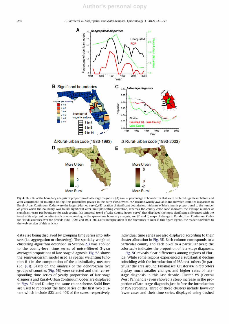
Proportions of late-stage diagnosis were first computedover a 3-year moving window to reduce random fluctua-tions, yielding for each county a times series spanning1982 through 2006. Boundary analysis was then conductedon each of the 25 time periods using the absolute boundarystatistic (rate difference) and the aforementioned Neutralmodel IV as randomization scheme. The percentageof the total number of 144 edges declared significant ata-level = 0.05 was computed every year before and afteradjustment using the False Discovery Rate approach.Fig. 4A shows that the percentage of significant boundariespeaked in the early 1990s when PSA became widely avail-able. This temporal trend, which is even more pronouncedafter multiple testing correction, suggests the existence ofgeographical disparities in the implementation and/or im-pact of the new screening procedure, in particular as it be-gan available. The absolute boundary statistic was alsocomputed on the USDA Rural–Urban Continuum Codes,and interestingly the magnitude of the statistic follows asimilar temporal trend with a peak in the early nineties(Fig. 4A, dashed curve). This result supports the priorhypothesis about possible interactions between urbaniza-tion and efficiency of PSA screening (Fig. 1C).

The geographical location of the most significantboundaries over the 27-year time period was derived bycomputing for each edge the number of years it was foundsignificant. Boundaries that were significant at least onceare depicted in black in Fig. 4B. The larger the thicknessof the black segments the more years that edge tested sta-tistically significant (up to 14 years). The background coloris an index of dissimilarity between each county and its

P. Goovaerts, H. Xiao / Spatial and Spatio-temporal Epidemiology 3 (2012) 243–253 247

Author's personal copy

Fig. 1. Evolution of the number of white males (total and proportion of late-stage diagnosis) diagnosed with prostate cancer annually over the period 1981–2007 for the entire state of Florida. Results, which are averaged over a 3-year window to reduce random fluctuations, are presented for cases younger orolder than 65 years, as well as for metro and non-metro counties (cases older than 65 years).

248 P. Goovaerts, H. Xiao / Spatial and Spatio-temporal Epidemiology 3 (2012) 243–253

Author's personal copy

neighbors which was computed by adding up the numberof significant years over all the county edges and dividing

the total figure by the number of edges. The counties thatdiffered the most frequently from their neighbors weremainly located in Central Florida, an area that underwentlarge urbanization in the eighties (Fig. 4D). The case of LakeCounty (isolated green polygon in Fig. 4C), located justNorth of Orlando area, is particularly striking. This county,which takes one of the largest values of the dissimilarityindex, is also the county that experienced the largest dropin the Urban–Rural Code between 1983 (code 4) and 1993(code 1); see dark brown polygon in Fig. 4D. The time ser-ies for Lake County and the average of adjacent countiesare compared in Fig. 4C. The urbanization of Lake Countycoincided with a decline in the proportion of late-stagediagnosis. Differences were the largest in 1989 and van-ished in the nineties when the adjacent counties, in partic-ular on the Eastern side, started getting more urban(Fig. 4E).

3.3. Spatially weighted cluster analysis

During the analysis of large space–time–attribute data-sets, users may have difficulty perceiving, tracking andcomprehending numerous visual elements that changesimultaneously, such as the 67 time series in Fig. 3. Onesolution (Ward, 2004) illustrated in Fig. 5 is to reduce the

Fig. 2. Proportions of late-stage cases (white males older than 65 years) that were diagnosed over the period 1981–2007 within each county (A), and eachcombination of 1983 and 2003 Rural–Urban Continuum Codes (B). These Rural–Urban County Codes are mapped in (C) and (D).

Fig. 3. Three-dimensional representation of yearly proportions of late-stage prostate cancer for white males 65 years and older. Rates werenoise-filtered at the county level using binomial kriging. The same colorscale is used for all the maps that were aligned along a time axis rotatedso as to minimize slide overlaps and the resulting loss of information.

P. Goovaerts, H. Xiao / Spatial and Spatio-temporal Epidemiology 3 (2012) 243–253 249

Author's personal copy

data size being displayed by grouping time series into sub-sets (i.e. aggregation or clustering). The spatially weightedclustering algorithm described in Section 2.3 was appliedto the county-level time series of noise-filtered 3-yearaveraged proportions of late-stage diagnosis. Fig. 5A showsthe semivariogram model used as spatial weighting func-tion f(�) in the computation of the dissimilarity measure(Eq. (6)). Based on the analysis of the dendrogram fivegroups of counties (Fig. 5B) were selected and their corre-sponding time series of yearly proportions of late-stagediagnosis and Rural–Urban Continuum Codes are displayedin Figs. 5C and D using the same color scheme. Solid linesare used to represent the time series of the first two clus-ters which include 52% and 40% of the cases, respectively.

Individual time series are also displayed according to theircluster allocation in Fig. 5E. Each column corresponds to aparticular county and each pixel to a particular year; thecolor scale indicates the proportion of late-stage diagnosis.

Fig. 5C reveals clear differences among regions of Flor-ida. While some regions experienced a substantial declinecoinciding with the introduction of PSA test, others (in par-ticular the area around Tallahassee, Cluster #4 in red color)display much smaller changes and higher rates of late-stage diagnosis in this last decade. Cluster #5 (CentralWest Panhandle) even showed a steep increase in the pro-portion of late-stage diagnosis just before the introductionof PSA screening. Three of these clusters include howeverfewer cases and their time series, displayed using dashed

Fig. 4. Results of the boundary analysis of proportion of late-stage diagnosis: (A) annual percentage of boundaries that were declared significant before andafter adjustment for multiple testing: this percentage peaked in the early 1990s when PSA became widely available and between-counties disparities inRural–Urban Continuum Codes were the largest (dashed curve), (B) location of significant boundaries: thickness of black lines is proportional to the numberof years when the boundary was found significant after multiple testing correction, whereas the county color code indicates the average number ofsignificant years per boundary for each county, (C) temporal trend of Lake County (green curve) that displayed the most significant differences with thetrend of its adjacent counties (red curve) according to the space–time boundary analysis, and (D and E) maps of change in Rural–Urban Continuum Codesfor Florida counties over the periods 1983–1993 and 1993–2003. (For interpretation of the references to color in this figure legend, the reader is referred tothe web version of this article.)

250 P. Goovaerts, H. Xiao / Spatial and Spatio-temporal Epidemiology 3 (2012) 243–253

Author's personal copy

lines in Fig. 5C, are less smooth than the results obtainedfor the first two clusters. These clusters, located in NorthFlorida and Florida Panhandle, are mainly rural accordingto their Rural–Urban Continuum Codes. Interestingly, thelargest spread of the five time series in Fig. 5C is observedin the late eighties, just before the introduction of PSAscreening.

The two most stable time series correspond to the mostpopulated Cluster #1 (East coast) and Cluster #2 (Westcoast and Keys). These two time series start overlappingwith the Florida State curve (black dashed curve) in themid nineties, following the introduction of PSA screening.Until then, a smaller proportion of cases were diagnosedlate in the North-east coast of Florida compared tothe Western coast of Southern Florida. During thisperiod, Cluster #1 was slightly less urban than Cluster #2

according to the Rural–Urban Code (Fig. 5D), which con-firms the positive relationship between degree of urbani-zation and frequency of late-stage diagnosis found in theeighties (Fig. 1C). Cluster #3, centred on Panama City,stands out from other clusters because it is the only areathat has not seen a decline in percentage of late-stage diag-nosis since the early nineties. Interestingly, it is also theonly area with no substantial change in the Rural–Urbancontinuum code over that time period.

4. Conclusions

A comprehensive picture of the burden of cancer andthe impact of various interventions can only be achievedthrough the simultaneous incorporation of the spatial

Fig. 5. Results of spatially weighted classification of 67 counties in Florida: population-weighted indicator semivariogram model used as weightingfunction in the computation of the dissimilarity measure (A), grouping of counties based on the similarity of their temporal trends in proportions of late-stage diagnosis and their geographically proximity (B), time series of proportion of late-stage diagnosis and population-weighed Rural–Urban Code for eachof the five clusters and Florida (black dashed line) (C and D), individual time series of noise-filtered rates of late-stage diagnosis displayed as horizontalstrings and ordered according to their allocation to one of the five clusters (E). The same color code is used for the counties in the choropleth map B and thecorresponding time series in plots (C) and (D).

P. Goovaerts, H. Xiao / Spatial and Spatio-temporal Epidemiology 3 (2012) 243–253 251

Author's personal copy

and temporal dimensions in the visualization and analysisof health outcomes and putative covariates. Analysis of asingle snapshot can lead one to overlook interesting trends,such as the changing relationships between degree ofurbanization and county-level percentages of prostate can-cer late-stage diagnosis in Florida over the period 1981–2007. Similarly, the analysis of temporal trends outside aspatial framework would lead one to ignore substantialgeographical differences in the speed and nature of the de-cline in the percentage of late-stage diagnosis over a largeState, such as Florida.

The application of spatial cluster and boundary analysisto space–time health data posed two challenges: (1) theneed to account for the instability of rates recorded in spar-sely populated counties and (2) the incorporation of thetime dimension in these intrinsically spatial techniques.The first aspect was addressed using geostatistical filtersthat account for the spatial patterns of data in the process-ing of rates for rare diseases (Poisson kriging) or percent-ages of late-stage diagnosis (binomial kriging). On theother hand, the analysis was extended to the temporaldimension using either a multivariate approach for thecluster analysis or the repetition of the boundary analysisacross time using the geostatistical approach introducedby Goovaerts (2010b).

The 3D display of time series of county-level health out-comes makes it easier to comprehend spatiotemporal rela-tionships because there is no disconnect between thetemporal and spatial dimensions as opposed to a combina-tion of 2D map and linked time line plots or an animation.Boundary analysis, used in conjunction with binomial dis-tributions and the False Discovery rate approach, allowsone to tackle the issues of unstable rates and increased riskof false positives in hypothesis testing. We also proposed anew index that summarizes for each geographical unit(county here) the results obtained over the set of edgesand years. Mapping this index of dissimilarity highlightedsimilitude in the spatial patterns of geographical dispari-ties in percentage of late-stage diagnosis and temporalchanges along the Rural–Urban Continuum. Spatiallyweighted cluster analysis allowed the study of temporaltrends at spatial scales intermediate between the State le-vel and the county or boundary level. Fig. 5 gave an originalexample of space time visual analytics where the map ofcounty clusters is displayed together with individual timeseries, providing the user with a geographical summaryof temporal trends without masking information pertain-ing to each county.

The case-study demonstrated that the 50% decline inthe proportion of late-stage diagnosis observed in Floridabetween 1981 and 2007 encompasses substantial geo-graphical disparities in the temporal patterns of changes.This drop generally started in the early 1990s when pros-tate-specific antigen (PSA) test became widely availableand several parts of Florida underwent a fast urbanization.Geographical disparities were substantial at that time,which suggests disparities in the impact of the new screen-ing procedure, in particular as it began available. The gapamong Florida counties is narrowing with time as thepercentage of late-stage diagnosis is decreasing. One out-lier is the Big Bend region of Florida where the decline in

percentage of late-stage diagnosis has been the slowestin the entire State. In the eighties, a smaller proportion ofcases were diagnosed late in non-metro areas, a trend thathas changed since then.

The present study was mainly exploratory and theinterpretation of the results suffers from limitations typi-cally associated with ecological studies. In particular, theanalysis was conducted at the county level and it is wellknown that different geographic scales can lead to incon-sistent results for health outcomes (Krieger et al., 2002;Meliker et al., 2009). However, the analysis of temporaltrends at a fine resolution (e.g. year) requires some levelof spatial aggregation in order to capture enough casesfor a reliable estimation of percentages of late-stage diag-nosis. In addition, by focusing on the population coveredby Medicare one source of individual-level heterogeneitywas controlled for. Individual-level data available for thesame time period are currently analyzed to explore the im-pact of race, individual characteristics, area-level censusmeasures of education, income, and environmental expo-sure on prostate cancer mortality, incidence and stage atdiagnosis (Xiao et al., 2011). These data will help testhypothesis on the potential influence of urbanization andthe introduction of PSA test that were formulated on thebasis of results of the current exploratory county-levelanalysis.

Acknowledgements

This research was funded by Grants R43CA150496-01and R44CA132347-02 from the National Cancer Institute,as well as Grant # RSGT-10-082-01-CPHPS from the Amer-ican Cancer Society. The views stated in this publicationare those of the authors and do not necessarily representthe official views of the NCI and ACS.

References

Anselin L, Syabri I, Kho Y. GeoDa: an introduction to spatial data analysis.Geogr Anal 2006;38:5–22.

BioMedware, Inc.: SpaceStat user manual version 2.2.; 2011.Caeiro S, Goovaerts P, Painho M, Costa H. Delineation of estuarine

management areas using multivariate geostatistics: the case of SadoEstuary. Environ Sci Technol 2003;37:4052–9.

Castro MC, Singer BH. Controlling the false discovery rate: a newapplication to account for multiple and dependent tests in localstatistics of spatial association. Geogr Anal 2006;38:180–208.

Chu KC, Tarone RE, Freeman HP. Trends in prostate cancer mortalityamong black men and white men in the United States. Cancer2002;97:1507–16.

Coldman AG, Phillips N, Pickles TA. Trends in prostate cancer incidenceand mortality: an analysis of mortality change by screening intensity.Can Med Assoc J 2003;168(1):31–5.

Cooper GS, Yuan Z, Jethva RN, Rimm AA. Determination of county-levelprostate carcinoma incidence and detection rates with Medicareclaims data. Cancer 2001;92:102–9.

Farkas A, Schneider D, Perrotti M, Cummings KB, Ward WS. Nationaltrends in the epidemiology of prostate cancer, 1973 to 1994: evidencefor the effectiveness of prostate-specific antigen screening. Urology1998;1998(52):444–8.

Goovaerts P. Simulation-based assessment of a geostatistical approach forestimation and mapping of the risk of cancer. In: Leuangthong O,Deutsch CV, editors. Geostatistics Banff 2004. Dordrecht: KluwerAcademic Publishers; 2005. p. 787–96.

Goovaerts P. Kriging and semivariogram deconvolution in presence ofirregular geographical units. Math Geosci 2008a;40:101–28.

252 P. Goovaerts, H. Xiao / Spatial and Spatio-temporal Epidemiology 3 (2012) 243–253

Author's personal copy

Goovaerts P. Accounting for rate instability and spatial patterns in theboundary analysis of cancer mortality maps. Environ Ecol Stat2008b;15(4):421–46.

Goovaerts P. Medical geography: a promising field of application forgeostatistics. Math Geosci 2009a;41(3):243–64.

Goovaerts P. Combining area-based and individual-level data in thegeostatistical mapping of late-stage cancer incidence. Spat Spatio-tempor Epidemiol 2009b;1:61–71.

Goovaerts P. Three-dimensional visualization, interactive analysis andcontextual mapping of space-time cancer data. In: Proceedings of13th Agile international conference. Guimarães, Portugal; 2010a.

Goovaerts P. How do multiple testing correction and spatialautocorrelation affect areal boundary analysis? Spat Spatio-temporEpidemiol 2010b;1(4):219–29.

Goovaerts P. Visualizing and testing the impact of place on late-stagebreast cancer incidence: a non-parametric geostatistical approach.Health Place 2010c;16:321–30.

Guo D. Regionalization with dynamically constrained agglomerativeclustering and partitioning (REDCAP). Int J Geogr Inf Sci2008;22:801–23.

Jacquez GM, Grieling D. Geographic boundaries in breast, lung andcolorectal cancers in relation to exposure to air toxics in Long Island,New York. Int J Health Geogr 2003;2:4.

Jacquez GM, Kaufmann A, Goovaerts P. Boundaries, links and clusters: anew paradigm in spatial analysis? Environ Ecol Stat2008;15(4):403–19.

Jemal E, Ward E, Wu X, Martin HJ, McLaughlin CC, Thun MJ. Geographicpatterns of prostate cancer mortality and variations in access tomedical care in the United States. Cancer Epidemiol Biomarkers Prev2005;14:590–5.

Krieger N, Chen JT, Waterman PD, Soobader M-J, Subramanian SV, CarsonR. Geocoding and monitoring of US socio-economic inequalities inmortality and cancer incidence. Does the choice of area-basedmeasure and geographic level matter? – The public healthdisparities geocoding project. Am J Epidemiol 2002;156(5):471–82.

Mather FJ, Chen VW, Morgan LH, Correa CN, Shaffer JG, Srivastav SK, et al.Hierarchical modeling and other spatial analyses in prostate cancerincidence data. Am J Prev Med 2006;30(2S):S88–100.

McDougall Jr GJ, Weber BA, Dziuk TW, Heneghan R. The controversy ofprostate screening. Geriatr Nurs 2000;21(5):245–8.

Meliker JR, Goovaerts P, Jacquez GM, AvRuskin GA, Copeland G. Breast andprostate cancer survival in Michigan: can geographic analyses assistin understanding racial disparities? Cancer 2009;115(10):2212–21.

Milligan GW. A review of Monte Carlo tests of cluster analysis. MultivarBehav Res 1981;16(3):379–407.

Oliver MA, Webster R. A geostatistical basis for spatial weighting inmultivariate classification. Math Geol 1989;21:15–35.

Potosky AL, Feuer EJ, Levin DL. Impact of screening on incidence andmortality of prostate cancer in the United States. Epidemiol Rev2001;23(1):181–6.

Remy N, Boucher A, Wu J. Applied geostatistics with SGeMS: a user’sguide. New-York, USA: Cambridge University Press; 2008.

Shaw PA, Etzioni R, Zeliadt SB, Mariotto A, Karnofski K, Penson DF, WeissNS, Feuer EJ. An ecologic study of prostate-specific antigen screeningand prostate cancer mortality in nine geographic areas of the UnitedStates. Am J Epidemiol 2004;160:1059–69.

Simbahan G, Dobermann A. An algorithm for spatially constrainedclassification of categorical and continuous soil properties.Geoderma 2006;136:504–23.

Smart CR. The results of prostate cancer screening in the U.S. as reflectedin the surveillance, epidemiology, and end results program. Cancer1997;80:1835–44.

USDA. Measuring rurality: rural-urban continuum codes: EconomicResearch Service: US Department of Agriculture; 2004. <http://www.ers.usda.gov/briefing/Rurality/RuralUrbCon/> (accessed01.07.11).

Wang F, McLafferty S, Escamilla V, Luo L. Late-stage breast cancerdiagnosis and health care access in Illinois. Prof Geogr2008;60:54–69.

Ward MO. Finding needles in large-scale multivariate data haystacks.Comput Graph Appl 2004;24(5):16–9.

Webster R, Oliver MA, Muir KR, Mann JR. Kriging the local risk of a raredisease from a register of diagnoses. Geogr Anal 1994;26:168–85.

Wong YN, Mitra N, Hudes G, Localio R, Schwartz JS, Wan F, Montagnet C,Armstrong K. Survival associated with treatment vs observation oflocalized prostate cancer in elderly men. J Am Med Assoc2006;296:2683–93.

Xiao H, Tan F, Goovaerts P. Racial and geographic disparities in late-stageprostate cancer diagnosis in Florida. J Health Care Poor Underserv2011;22(4):187–99.

P. Goovaerts, H. Xiao / Spatial and Spatio-temporal Epidemiology 3 (2012) 243–253 253