Degree project in The Built Environment

Second cycle 30 HP

The Impact of Metro Stations Proximity to Commercial Property Prices in Stockholm A Hedonic Analysis

HANNA OLSSON & MATTEO VERVERIDIS

Stockholm, Sweden 2022

Title The Impact of Metro Stations Proximity to Commercial Property Prices in Stockholm: A Hedonic Analysis

Authors Hanna Olsson & Matteo Ververidis

Department Real Estate and Construction Management

TRITA - number

Supervisor

TRITA – ABE – MBT – 22511

Berndt Lundgren

Keywords Commercial property prices, office buildings, hedonic price model, metro station

Abstract

The impact of geographical choices is crucial for both individuals and businesses to assess. Generally, companies are favored by being in accessible areas, which pushes up the demand and price for space. This phenomenon is referred to as a bid-rent theory. Infrastructure like roads and public transport contributes to accessibility. Earlier studies have shown that property prices are affected by all public means of transport but seems to be mostly affected by the accessibility to metro stations. With a quantitative research method, the aim of this master thesis is to explore how commercial property transaction prices are affected by the proximity to public transport specified on metro stations in Stockholm. Our study is performed on 123 office-buildings, and all observations are within the timeline of 2015 to 2021, in both the inner and outer city. The aim is also to explore the difference between those areas. In this study, a hedonic price model is used, where price/sqm is the dependent variable:

y = m + β1x1 + … + βnxn + ε

10 independent variables are used, all arguably related to determine a price for a commercial office property. The variables Metro and I/O are in focus and considered our main variables to examine, Metro represents the distance to metro stations and I/O is a dummy for inner and outer city. In total, 7 models are presented in the results, with different combinations of independent variables. All models contribute to discussion, however, the model that we consider gives the most relevant results has a degree of explanation R2 of 46,7%. This model gives us significant results on both independent variables in focus, and the model itself. A large factor that interrupted better results was the limitations on observations. The interpretation of the model for offices in the inner city showed that the dependent variable changed 0,667 units when the independent variable I/O changed 1 unit. Moreover, when the distance to metro stations increased with 1 unit the dependent variable decreased with 0,0454 units per km. Furthermore, within the inner city the distance to metro stations tends to have less significance, to clarify the reason why, is yet to be discovered.

Acknowledgement

This master thesis concludes two educational years within the department of Real Estate and Construction Management at the Royal Institute of Technology in Stockholm (KTH). The master thesis includes 30 hp and was carried out during the spring semester 2022.

Our journey at KTH started two years ago with relocating from Malmö to Stockholm to attend the program Real Estate and Construction Management. It has been an interesting experience in whole, and regardless of the circumstances with COVID-19, we believe that KTH has done a good job countering its effect on the educational requirements. During this period with the master thesis, we have been given the privilege to execute what we have learned in earlier courses and have found them useful. We will leave KTH with new and solid knowledge that we believe will nurture a continuous desire to learn more and to contribute to the better.

We would also like to show our appreciation to our supervisor Berndt Lundgren for good support and interesting input throughout the process. In addition, also mention the support we received from Joachim Wallmark, Svefa, who contributed with great insight in the real estate market.

Stockholm, June 2022 Hanna & Matteo

Titel Tunnelbanestationers prispåverkan på kommersiella fastigheter i Stockholm: En hedonisk analys

Författare Hanna Olsson & Matteo Ververidis

Institution Institutionen för Fastigheter och Byggande

TRITA - nummer TRITA – ABE – MBT – 22511

Handledare Berndt Lundgren

Nyckelord Kommersiella fastighetspriser, kontorsfastigheter, hedonisk prismodell, tunnelbanestationer

Sammanfattning

Valet av geografisk placering är något som både privatpersoner och företag påverkas av. Generellt sett är det ekonomiskt fördelaktigt för företag att placera sig i lättillgängliga områden, vilket i sin tur bidrar till en högre efterfrågan och högre hyror i vissa områden. Infrastruktur såsom vägar och kollektivtrafik bidrar till ökad tillgänglighet. Tidigare studier visar att närhet till kollektivtrafik, oavsett trafik-slag, har en effekt på priset. Dock verkar priset påverkas främst av tillgängligheten till tunnelbana. Med en kvantitativ forskningsmetod är syftet med denna masteruppsats att undersöka hur kommersiella fastighetspriser påverkas av närhet till kollektivtrafik, med en inriktning på tunnelbanestationer i Stockholms län. Vår studie grundar sig på 123 kontorsfastigheter och samtliga transaktioner är utförda mellan år 2015–2021, i både innerstad och ytterstad. Syftet är därför också att undersöka vilken skillnad det finns mellan dessa områden. I studien används en hedonisk prismodell, där vår beroende variabel är pris/kvm:

y = m + β1x1 + … + βnxn + ε

10 oberoende variabler, som i någon mån kan förklara priset, har använts i analysen. Bland dessa har vi haft störst fokus på variablerna för avstånd till tunnelbanestation Metro samt dummy-variabeln för innerstad/ytterstad I/O. Totalt sett redovisas 7 modeller med olika kombinationer av oberoende variabler. Samtliga modeller bidrar till diskussion, men den modell vi anser ger oss mest relevant information har en förklaringsgrad R2 på 46,7% och visar signifikans på modellen i sin helhet samt våra oberoende variabler i fokus. Tolkningen av modellen för kontorsfastigheter i innerstaden visade att den beroende variabeln steg 0,667 enheter när den oberoende variabeln I/O ändrades med 1 enhet. Samt visade det sig att när avståndet ökade till tunnelbanestationer med 1 enhet så minskade den beroende variabeln med 0,0454 enheter per kilometer. Dessutom, tenderar avståndet till tunnelbanestationer i innerstad, att ha mindre påverkan på priset. Orsaken till detta, framgår inte i denna studie.

Förord Denna masteruppsats avslutar två lärorika år på institutionen för Fastigheter och Byggande på Kungliga Tekniska Högskolan. Uppsatsen omfattar 30 hp och genomfördes vårterminen 2022. Vår resa på KTH började för två år sedan när vi flyttade från Malmö till Stockholm för att läsa masterprogrammet fastigheter och byggande. Det har varit en intressant erfarenhet, och trots omständigheterna kring COVID-19, så har KTH erhållit en hög kvalitét på utbildningen. Under genomförandet av master-arbetet har vi fått använda nyvunnen kunskap från utbildningen och kommer lämna KTH med en bredare kunskapsbas. Vi vill också passa på att tacka vår handledare Berndt Lundgren som under hela processen bidragit med stöd och intressanta perspektiv. Dessutom vill vi visa vår tacksamhet till Joachim Wallmark, Svefa, som gett oss lärorik insyn och förståelse för den svenska fastighetsmarknaden och dess utmaningar.

Stockholm, juni 2022 Hanna & Matteo

Content 1 Introduction ............................................................................................................... 1

1.1 Background ......................................................................................................... 1

1.2 Aim and Problem Formulation............................................................................... 2

1.3 Research question ................................................................................................ 2

1.4 Delimitations and definitions ................................................................................. 2

2 Literature Review ....................................................................................................... 4

3 Theoretical Framework ............................................................................................... 6

3.1 Urban structure .................................................................................................... 7

3.1.1 Urban models ................................................................................................ 7

3.1.2 Bid-rent theory .............................................................................................. 9

3.2 Hedonic Pricing Model ....................................................................................... 10

4 Methodology ........................................................................................................... 11

4.1 Quantitative research method .............................................................................. 11

4.2 Multiple Regression Analysis .............................................................................. 11

4.2.1 Regression function ...................................................................................... 12

4.2.2 Ordinary Least Square (OLS) ........................................................................ 12

4.2.3 Tools in Regression Analysis ........................................................................ 12

4.3 Data Collection .................................................................................................. 15

4.3.1 Dependent variable ...................................................................................... 15

4.3.2 Independent variables ................................................................................... 15

4.4 Ethical considerations ......................................................................................... 17

5 Results & Analysis ................................................................................................... 17

5.1 Descriptive statistics ........................................................................................... 17

5.2 Simple correlation analysis .................................................................................. 19

5.3 Regression analysis ............................................................................................ 21

6 Discussion ............................................................................................................... 27

7 Conclusion .............................................................................................................. 29

8 Recommendations for Future Research ....................................................................... 30

References .................................................................................................................. 31

Appendix ................................................................................................................... 35

1

1 Introduction

1.1 Background Cities are crucial for economic growth from a national and regional perspective (Laird & Venables, 2017) and it is easy to think that the prosperity of a city only has to do with size and density. However, the author Blumenfeld-Lieberthal (2009) also highlights that a contribution to high productivity levels is the infrastructure networks between different places. Urban economics explores the efficiency of geographical and economical choices for individuals and businesses (O’Sullivan, 2012) and the impact of locations (Debrezion, Pels & Rietveld, 2007). Households and businesses are affected by the availability of infrastructure networks since it is essential for people to have access to daily activities like work and public services. Likewise, it is essential for companies to have access to customers, suppliers and labour. This phenomenon is widely studied and is referred to as agglomeration economies (Melo, Graham & Noland, 2009). Generally, companies are favoured by being located in accessible and visible areas. The demand is high in attractive areas, and thereby also the prices for space. Alonso (1964) explains this phenomenon in a bid-rent theory. In short, the theory suggests that more accessible locations have higher prices than the contrary. The bid-rent function explains the relationship between how much a company or individual is willing to pay for a location, and the distances from the central business district (CBD). Earlier studies have been made on the theme of property value in relation to public transportations. The property prices were, according to several studies, affected by all public means of transport but seems to be mostly affected by the accessibility to metro stations. To stimulate the economy, it is therefore common to invest in roads, railways and other types of infrastructure projects. When expanding the infrastructure, the benefits entailed are weighed against fixed costs. Railways are an example of an arrangement that entails high fixed costs but have for instance a great impact on the accessibility (Debrezion, Pels & Rietveld, 2007). As the availability of infrastructure networks and public transportation systems affects the accessibility, and thus the price of properties and space, it becomes interesting to investigate to what extent the proximity to public transportation affects the valuation of commercial properties. The topic is up to date since it, for a couple of years, has been possible for municipalities to let private property owners co-finance the expansion of new infrastructure. Västra Sicklaön, Hagastaden and Arenastaden are examples of co-financing metro station projects already realised in Stockholm. The investment in new infrastructure must be in

2

reasonable proportion to the increase in value which the expansion entails, which leads us to the aim and contribution of this study.

1.2 Aim and Problem Formulation Aim The aim of this master thesis is to explore how commercial property transaction prices are affected by the proximity to public transport, specified on metro stations in Stockholm. Our study will be performed on office-buildings in Stockholm municipality, in both the inner city and outer areas. The aim is also to explore the difference between those areas. Contribution The findings on how metro stations affect commercial property prices, will contribute to a deeper understanding for private property owners´ future investment strategies, regarding co-financing expansion of metro stations. Since the study will analyse properties in both the inner and outer city, it will also contribute to a deeper understanding about how the location affects prices. The relevancy of making this study in Stockholm is connected to the future plans of the expansion of the metro web and possible investment opportunities for private property owners.

1.3 Research question Does distance to metro stations affect commercial property prices more in outer areas compared to inner city?

1.4 Delimitations and definitions Means of transport The analysis and discussion will focus on the proximity to metro stations and not other municipal means of transport such as buses or commuter trains. However, even though the focus is on metro stations, other public means of transport will be considered in the regression analysis. Building types & Standards The concept of commercial properties is a collective term, generally for buildings, that generates an income. However, in this study we have chosen to focus only on office buildings. Datscha, the provider of real estate data, categories buildings based on which function it has. A building containing both a hotel and offices are in the category hotel-office, while a pure office-building is under a category of itself. To maximise the number of office-buildings, all categories containing offices will be analysed in this study. The building standards have not been taken into consideration due to hard accessible information.

3

Distance measurement In this study, distance will be defined as the Euclidean distance, which will provide a consistent value of distance in a metric unit and avoid influence of human choice of travel patterns and capacity of physique. While computing distances the authors will therefore not consider the time and distance regarding individuals starting point. The reason for this is that the scope and availability of data will be too overwhelming and will not, in the author's consideration, contribute to a significantly better result since the focus is office buildings and their prices. This thesis will be of more concern to property owners rather than individuals working at a particular office building. The authors also argue that a buyer who considers proximity to metro stations as a value-adding factor, assesses distance through a map rather than the actual walking time. Property value The property value in this study is defined as the actual transaction price. The observed transactions are within the timeline of year 2015 to 2021. Geographical definition This study will have the geographical limit of Stockholm´s county, see Appendix A. Geographical location will in this study identify the different observation´s location by extracting their specific coordinates within the Stockholm´s county. Since one important aspect of the study is to explore the difference between inner city and outer areas, this geographical boundary must be defined. In Stockholm, the road tolls are often considered as a boundary between the outer and inner city. The authors consider that as an appropriate boundary for this study as well. The limit for the road tolls is illustrated in Figure 1. To translate the inner and outer city into an area that can be applied to the Dachas database, we will use the Datscha border tools to separate the areas. The observations in the inner city are grouped by districts, a division of the inner city that Datscha can provide. A compilation of all districts is presented in Appendix B. The observations in the outer city are grouped by municipality and a compilation is presented in Appendix C. The general motivation to include the whole region outside the tolls is mainly a question of available observations and thereby to improve the results of the regression analysis.

4

Figure 1 An overview map of all toll stations in Stockholm (Transportstyrelsen, 2020). The

dotted line shows the limit between inner and outer city.

2 Literature Review Urban economics explores the impact of geographical and economical choices made by individuals or companies (O´Sullivan, 2012) and are therefore fundamental in this study. Within urban economics, location choice, accessibility (Debrezion, Pels & Rietveld, 2007) and agglomeration are some main concepts discussed. Agglomeration refers to when similar economic activities are located within the same geographical area (Johansson & Quigley, 2004). This literature review will contain relevant concepts, related earlier studies and elucidate the research gap in the area. The impact of location (Debrezion, Pels & Rietveld, 2007) and agglomeration is of great importance when studying new interactions in urban economics (Johansson & Quigley, 2004) even though the concept of agglomeration has existed for a long time. After World War I, studies were made on agglomerated companies and industries in New York. The outcome of the analysis indicated that local contact between actors in the same industry was not necessary in standardised markets (Haig, 1926). A modern analysis of this study would probably also reflect on that the transaction costs between actors were low enough for the standardised products to cover the economic benefits of being clustered. Un-standardized markets are on the other hand more likely to profit from local networks (Johansson & Quigley, 2004).

5

Johansson and Quigley (2004) explain that agglomeration refers to a point while networks entail nodes. The connection is therefore necessary to entail economic exchange. Therefore, the second important theme to explain in this literature review is accessibility. According to Bohman and Nilsson (2021), studies have shown that the property value increases in relation to the increasing accessibility of goods and services. Rosen (1974) also means that closeness to public transportation stations is seen as a value adding component. The economic benefits of being accessible are today well known among companies, since it is essential to have access to customers, suppliers, and labour (Melo, Graham & Noland, 2009). This awareness has benefited the development of networks (Johansson & Quigley, 2004). In transportation terms, accessibility explains how simple the transportation systems allow travel or how well locations can be reached (Hensher, Li & Mulley, 2012). Improved accessibility leads to lower travel costs and thereby makes it possible for land and property prices to increase. This concept is referred to as land value uplift (Mohammad, Graham, Melo & Anderson, 2013). In the mid-60s the planner and economist William Alonso explained the relationship between property value and accessibility with a monocentric model. This model is mostly based on the distance from the property to the CBD (Alonso, 1964). However, even though all jobs and services are not located in the CBD, the model can be seen as an indicator of a relationship between property value and accessibility. Bohman and Nilsson (2021) argue that an expansion of infrastructure in areas promoted by better accessibility, should lead to an increase in property prices. The article “Borrowed sizes: A hedonic price approach to the value of network structure in public transport systems” by Bohman and Nilsson (2021) explores how railway networks have an impact on regional accessibility and affect local agglomeration economies and perceived value of housing. The findings indicate that the effects of transportation networks increase the value of agglomeration. In China, many land value uplift studies have been performed (Salon, Wu & Shewmake, 2014); (Xu, Zhang & Aditjandra, 2016); (Zhang, Meng, Wang & Xu, 2014); (Zheng, 2018). Zhang, Meng, Wang and Xu (2014) have for instance analysed different impacts of metro, light rail transit and bus transit which showed that metro had the greatest impact of land value. Zheng (2018) did an empirical land value uplift study and used a random effects model to investigate how residential property prices were affected by metro accessibility in Xián in China. The conclusion was that the area closest to the metro station had a low positive impact of the value, while the impact was most distinct within the distance between 0,3 and 1,2 km from the station. The article “The impacts of distance to CBD on housing prices in Shanghai: a hedonic analysis” suggest that the general mean of property prices decrease on average 5% one kilometre outside

6

the city centre. The impact of distance is more distinct outside the “one kilometre-zone”, compared to inside it. The study also shows that accessibility of a metro station increases the property prices sharply (Chen & Hao, 2008) which also Cao et.al., (2020) brings up in their research. The study performed by a hedonic price model which is a widely used approach to analyse factors that affect the price of properties (Rosen, 1974). From a national perspective, we need to consider the fundamental benchmarks of urban planning in line with this study. In modern urban planning and construction projects, the government highlights the importance of accessibility to public transportation systems (Regeringskansliet, 2021). According to the government's proposition about future infrastructure, co-financing for the construction of new public infrastructure networks is possible from different actors including private companies (Regeringens Proposition 2020/21:151). Real estate owners' willingness to co-finance public infrastructure is probably based on an increased property value, but it might also have a connection with the sharp increase of certified green buildings (SGBC, 2021) that require closeness to public transportations to be certified (BREEAM-SE, 2017). To summarise, the main themes of this study is agglomeration, location, accessibility, and value of transportation networks which all goes under the wide concept of urban economics. Earlier studies have been made on the theme of property value in relation to public transportations. The property prices were, according to more than one study, most affected by the accessibility to metro stations, which motivates us to carry out a study on that means of transport. Other studies have analysed for instance the relation between property prices and distance to CBD but as far as we know, there has been no earlier studies made on what impact the distance to metro stations have on commercial property prices in Stockholm.

3 Theoretical Framework There are many factors that influence property prices. For commercial properties, agglomeration and accessibility has contributed to higher demand for space in certain areas, hence also higher prices (Johansson and Quigley, 2004). The theoretical framework contains theories of urban structure, where urban models and rent theory is included, and the hedonic price model. These theories will be the main concepts to describe, predict and understand the relationship between property prices and distance to metro stations in this study.

7

3.1 Urban structure Urban areas are flexible, which even though the locations are fixed, also reflect the economic potentials for properties. The surrounding condition and development of an area, has a direct impact on property prices and use potentials. Properties economic and use potential, is according to Fanning (2014), based on the value concept of the present value of future benefits. Urban structure within a city refers to a complex structure of economic activities within the overall urban system. As the complexity of the economic situations increase, the activities tend to be more specialised, which provides clear boundaries in the patterns of land use. Retailing and manufacturing for example, tend to cluster in a specific area of the city. As urban networks develop, multiple locations can have the function as a centre of economic activities (Fanning, 2014). There are several factors that can affect urban structures. Economic base, market forces, technology, and physical characteristics are some of the factors that in different ways affect a city. Physical characteristics like natural and man-made features widely impact the urban structure. Topography, like water and variations in terrain, affect the direction of development of a city due to the physical boundaries that come with it. Even roads and other utilities put constraints on the development. Prediction of urban growth, therefore, requires an understanding of the interplay between natural and man-made features and urban economy. Generally, cities have a tactically appropriate place for connection with the outer world and grow along transportation networks where the natural features allow it. Willingness to pay for space, are according to many land economists, connected to the accessibility to the central business district (CBD) and other prominent nodes of economic activities (Fanning, 2014).

3.1.1 Urban models Urban models describe and provide guiding insight about patterns of urban growth and land use. The models are used to predict and analyse future economic activities and changes in the urban structure. However, since the complexity of most cities, a combination of models is often necessary to explain the structure and patterns. The most prominents urban growth models are the concentric zone model, the sector wedge model, the radial corridor model and lastly the multiple nuclei model (Fanning, 2014).

8

The concentric zone model 1. Central business district (CBD) 2. Zone of transition 3. Zone for workers home 4. Zone for middle- and high-income units 5. Commuter zone

Figure 2. The concentric zone model (Fanning, 2014). The sector wedge model

1. Central business district (CBD) 2. Wholesale manufacturing 3. Low income residential 4. Middle income residential 5. High income residential

Figure 3. The sector wedge model (Fanning, 2014). The radial corridor model

1. Central business district (CBD) 2. High-intensity corridor (Manufacturing, high-

density housing, retail, office) 3. Moderate-income housing (Moderate-density housing) 4. Middle-income housing (Low-density housing) 5. High-income housing (Very low density) 6. Open space/agriculture

Figure 4. The radial corridor model (Fanning, 2014). The multiple nuclei model

1. Central business district (CBD) 2. Wholesale, light manufacturing 3. Low- income residential 4. Middle-income residential 5. High-income residential 6. Heavy manufacturing 7. Outlying business district 8. Residential suburb 9. Industrial suburb 10. Commuter zone

Figure 5. The multiple nuclei model (Fanning, 2014).

9

3.1.2 Bid-rent theory Rent theory is another angle of urban structure (Fanning, 2014). Bid-rent is the amount of money a company or household is willing to pay for a certain level of utility (Wheaton, 1977). In 1960, the economist William Alonso made a theory based on bid-rent. The aim of the theory is to explain how price and demand for land relate to the distance to CBD. According to Alonso (1964), a buyer who invests in land, purchases both land and location in the same transaction. Thereby according to this theory, the quantity of land can be traded with location. The theory suggests that more accessible locations have higher prices than the contrary. Companies are favoured by accessibility since it attracts more people and affects business opportunities. Therefore, the willingness to pay for space within the city core is highest for commerce. Industries, on the other hand, are less willing to pay for space compared to commerce but still benefit from being close to the CBD due to accessibility and closeness to the marketplace. According to this theory, residents are least willing to pay for space close to the city core.

Figure 6. An illustration of Alonso's model of urban structure (Fanning, 2014).

10

Figure 7. An illustration of bid-rent curves for office and retail demand. Bid-rent curve 1 shows the importance for offices to be located close to the CBD. Bid-rent curve 2 shows that

retail does not have the same willingness to pay for space close to the CBD, compared to offices (Fanning, 2014).

3.2 Hedonic Pricing Model A hedonic price model is a common approach to investigate what impact area characteristics have on prices (Ismail, Warsame & Wilhelmsson, 2021) and is used for analysing data. The hedonic approach is seen as a reliable method among economists since it is based on valuations on the real estate market (Belniak & Wieczorek, 2017). Hedonic pricing of goods and wares have been exercised on several different occasions to determine different prices. The method defines the implicit prices of characteristics and attributes that are related to the product. The hedonic pricing is according to Belniak and Wieczorek (2017) an indirect valuation method. Rosen (1974) evolved this method and in his paper started to focus more on individual characteristics' effect on the total price. Rosen´s model is used today to understand certain attributes of a property and how they affect its total price on the market. The model is explained as an equation of the properties of different attributes structured down into single components:

y = m + β1x1 + … + βnxn + ε

The result of the equation will be the function of a vector that will take its shape depending on its variable data. The equation involves a dependent variable y, which represents the total price of a property. The dependent variable is in turn determined by several independent variables, x. β represents the independent variable coefficient, explaining how much of that particular

11

component affects the dependent variable, y, the total price. The m is the interceptor, where the vector intercepts the y-axis. Lastly, the variable ε explains the error term and shows how imperfect the relationship is between factors and the prediction of the total price.

4 Methodology To fulfil the aim of this study, a quantitative approach is applied. The study is based on 123 sold office properties spread throughout Stockholm municipality. All transactions have been performed between 2015 and 2021. In this chapter we present the basics about a quantitative research method, multiple regression analysis, data collection and finally our ethical considerations.

4.1 Quantitative research method In a quantitative research method, quantifiable data are used with the purpose to find statistical, mathematical generalizable results. A quantitative method is, according to Pathak, Jena and Kalra (2013), more objective compared to a qualitative method. The base of this study is data about where metro stations and properties are located and information about commercial properties and transaction prices in Stockholm city centre, which is typical quantitative data (Saunders, Lewis & Thornhill, 2019). All data analysis will be conducted in Microsoft Excel.

4.2 Multiple Regression Analysis Multiple regression analysis is in general the method to be used to successfully produce a hedonic price model for the intended property. The multiple regression analysis end-result tries to describe the relationship between the dependent variable y and the independent variables xi of the model and how these interact when manipulated. Regression models with a single independent variable are referred to as simple-regressions, while a model with multiple variables is referred to as a multiple-regression model. In general, with more variables comes better descriptive results (Carter, Griffiths & Lim, 2018) and more adoptive to ceteris paribus (Wooldridge, 2012). Multiple regression analysis can consider several factors in the same model and can be explained as:

y = m+ β1x1 + β2x2+ … + βnxn + ε

where m = the intercept β1 = the elasticity parameter associated with the independent variable x1 β3 = the elasticity parameter associated with the independent variable x2 and so on.

12

n = number of independent variables ε = error term that contains other factors that explain the dependent variable (y) All β-values are parameters to be estimated (Wooldridge, 2012).

4.2.1 Regression function

While performing the regression analysis several types of functional forms can be used, some examples of forms can be linear, log-linear and log-log. However, there is no clear evidence on what type of function that is best fit, it is rather up to the specific research question and aim of the study to determine the function that is mostly going to fulfil the purpose (Berawi et. alt. 2020). The authors for this study have determined that the best fit for the price model equation will be the log-linear. The log-linear function transforms the dependent variable into its natural logarithm but keeps the independent variable in its natural state. And since this explains the changes of the dependent variable y, the property value, in percentage when the independent variable xi changes, the authors argue that this is the best fit (Principles of Econometrics, 2018). By applying the ordinary least square method (OLS) the unknown coefficients in the function will be known.

4.2.2 Ordinary Least Square (OLS) Ordinary Least Squares is a widely used method for estimating linear regression equation coefficients. The method will provide a vector with a slope and an interceptor to describe the best fitted line that explains the relationship between the different variables. The OLS tries to minimise the squared residuals for the fitted line. The residuals show the difference between the actual value of the dependent variable and the fitted value of the dependent variable and are assumed to be zero when summarised for any observation. Moreover, the residuals are squared to best present y as a function of xi, the independent variable (Wooldridge, 2012).

4.2.3 Tools in Regression Analysis Residuals, beta coefficients, F-value and t-test When conducting a regression analysis, the automated process will provide a fitted line that shows the best estimated relationship between the dependent variable and the independent variables. The error terms, the difference between the fitted line and the individual observations is called the residuals. These residuals give a preliminary statement if the fitted line and the model in whole is convenient or not. The dependent variable y will be explained by several independent variables. These independent variables will be provided with a coefficient, presenting the magnitude of their specific contribution to the property value. To test the estimated values and conclude if the results are significant or not a t-test can be made. A t-test shows if the mean of two groups is significantly different from each other. It interacts with the critical t-value that is given by calculations including the probability level and the degree of freedom. Moreover, while the t-value is dedicated to the single variable the F-value provides information about the group of variables and if they are jointly significant. A high F-value is accompanied with a low p-value (Wooldridge, 2012).

13

Dummy variable A dummy variable makes it possible for the regression analysis to capture qualitative factors that represent themselves as binary information. The dummy variable contains two possible options, a 0 that could represent that a property is outside the CDB or a 1 that would represent that a property is inside the CDB. The usefulness of a dummy variable becomes relevant when the regression analysis chooses to contain qualitative independent variables attached to those data that are mutually exclusive to one another (Wooldridge, 2012). Interaction term Interaction terms can occur in several regression analysis when there is indication of a possible relationship between different variables. It is an occurrence where an independent variable is explained by the interaction of two explanatory variables. For example, people might value the proximity to metro stations, but the property value differs between the inner city and in the suburbs, which gives us two explanatory variables that interact with each other. In conclusion, the interactional term should be used when the authors making the regressions analysis suspect that there might be a hidden relationship between two variables that, in this study, explains the price of a property (Wooldridge, 2012). Endogeneity When the regressions error terms are correlated with one or more of the explanatory variables within the system, endogeneity has occurred. This creates a malfunction of the OLS method, hindering it from not providing solid results and not fulfilling the assumption that the sum of all residuals is zero. The problem can occur when a variable not included in the regression analysis affects both the independent variables and in turn the dependent variable (Carter, Griffiths & Lim, 2018). Multicollinearity Multicollinearity occurs when independent variables in a multi regression model correlate with each other. When this phenomenon is present it is hard to extinguish from the regression result the independent variables solely effect on the dependent variable, in this case the price of the property. To solve this problem and distinguish the variable causing problem, a correlation matrix can be used to identify (Wooldridge, 2012). Coefficient of determination The coefficient of determination that can be explained as R2, measures the variance of the dependent variable and how much the variance is explained by the independent variables. With a dimension of 0 to 1, a 1 represents a perfect explanation and a 0 no explanation by the independent variables. Moreover, it is favorable for the results to use the adjusted R,2 thus it makes the R2 more reliable and precise and modified so that the variable causing potential

14

problems gets considered and corrected. The results emerge as a better estimate of the observations (Wooldridge, 2012). Heteroskedasticity In the ordinary least square method, it is assumed that the variance of the error term ε is constant, also called residual. When examining the variance of error in a variable, different patterns of the residuals can appear, for example heteroskedasticity. There are some common situations to be aware of, all strongly connected to heteroskedasticity; for example, when the dependent variable is aggregate and also when the dependent variable is asymmetric and has a bell-shaped distribution.

Figure 8. The figure shows heteroskedasticity; the residuals differ in terms of variance, where

some sets of residuals are significantly larger in comparison to the other residuals in the same set of data (Kaufmanm, 2014).

Moreover, heteroskedasticity results in inefficient OLS estimates of the coefficients β and ignoring this problem causes untrustworthy estimates of the OLS standard errors (Kaufmanm, 2014). With detected heteroskedasticity, a way to address heteroskedasticity is to transform the variable to its natural logarithmic (Principles of Econometrics, 2018).

15

4.3 Data Collection

4.3.1 Dependent variable The dependent variable in this analysis is the transaction price and is explained with SEK/sqm.

4.3.2 Independent variables When analysing property prices with this approach, you divide the property into value-adding components like structural, locational and neighbourhood characteristics. The variables can be for instance size, building year or closeness to public transportation (Rosen, 1974). Each property has a unique combination of attributes and value-adding factors. Table 1, 2 and 3 contains the variables that are included in this analysis. The variables are divided into the variable group´s accessibility, building characteristics and neighbourhood characteristics. Accessibility Accessibility and choice of location have an impact on property prices (Debrezion, Pels & Rietveld, 2007). Therefore, we will take distance to metro stations and distance to CBD in consideration. Distance will be defined as the Euclidean distance, which according to Fabbri et. al. (2008) is explained as:

𝑑(𝑝, 𝑞) = (𝑞 − 𝑝 )𝑥2 + (𝑞 − 𝑝 )𝑥2 In this formula q1, q2 represent the coordinates for the metro station or CBD and p1, p2 are the coordinates for the commercial property examined. Sergels torg will represent the centre point of CBD. To identify if distance to metro stations and distance to CBD correlates, we will make a correlation matrix, see Appendix D. The authors argue for using the Euclidean method can be found in chapter 1.4 Delimitations and definitions.

Table 1. The independent variables in the category Accessibility.

16

The variable closeness to other public transportation (OPT) is also important to observe since availability to different means of transport probably will affect the price in a positive direction. The variable will be a dummy-variable, and to be considered close, the property needs to be within 300 m of other public transportation. Building characteristics The price of a building is also reflected in its characteristics, both physical and economical. Regarding physical qualities we will observe the impact of building size. In this category it is relevant to consider building standards as well. However, the standards are complex (Lantmäteriet & Mäklarsamfundet, 2010) and such information is hard to provide without visiting the building on site and will therefore be deselected for this study. From an economical perspective, rent level, yield requirements, vacancy rates will most probably correlate with the price and will therefore be observed in this study. These three variables are represented with their mean value for each observation. All these parameters are also considered during a property valuation (Lantmäteriet & Mäklarsamfundet, 2010) and are therefore relevant to observe as independent variables. The time span for the observations extends from 2015 to 2021 and therefore the general price development needs to be considered. One method is to adjust the price with a property price index (SCB, 2021) or use the sales year as an independent variable. During the test regressions, it turned out that all values in the models were considerably worse using the property price index, therefore sales year is used to explain the price development. Datscha is the information provider for all variables in this variable group. See Table 2 for a variable compilation.

Table 2. The independent variables in the category Building characteristics.

17

Neighbourhood characteristics Neighbourhood characteristics have a clear impact on property prices (Tse, 2002). The physical factors observed in this study are median household income and geographical location regarding inner or outer city. The variable for geographical location is a dummy variable and will most probably correlate with the price.

Table 3. The independent variables in the category Neighbourhood characteristics. The median household income variable may give an indication of the standard of the residential neighbourhood of each area examined. The hypothesis is that higher income has a positive relation to commercial property prices. An attractive area for households is not necessarily a more preferable place for companies, however, it should reflect the desirability (Sherry, 2005).

4.4 Ethical considerations The observed properties will not be presented with names. Hence, the properties, transactions and the individuals connected to these will not be a subject for identification whatsoever.

5 Results & Analysis In this chapter we firstly introduce a summary of the descriptive statistics to see the observations from a larger perspective. Thereafter we present an initial simple correlation analysis, containing controls of collinearity and heteroscedasticity. And finally, seven performed regression models are presented and analysed.

5.1 Descriptive statistics

The data that will be examined in the regression analysis contains a total of 123 observations regarding office buildings. Attempting to explain the property prices in price/sqm, 10 independent variables are used, all arguably related to determine a price for a commercial office property, see chapter 4.4.2 Independent variables. In this data set the variables Metro and I/O

18

are in focus and considered our main variable to examine, the remaining eight will be manipulated in case of regression malfunction. Presented in Table 4 the variables and range of data are shown.

Table 4. A summary of the descriptive statistics

The descriptive statistics exhibit low standard deviation on the dependent variable which indicated a low spread of data. The sales year varies from 2015 to 2021 and with an average sales year of 2017. Our metro variable is giving us a large spread on distance, starting at a low 59 metres up to 22,5 kilometres.

Diagram 1. The diagram shows the price distribution among the 123 observations. The price distribution varies from 6 305 to 215 517.

19

Further, the distance to cbd varies from 387 metres to 46,5 kilometres with a standard deviation of 7,142 km. The rent variable provides information that ranges from 900 SEK/sqm/year to 7,000 SEK/sqm/year. The range can be considered wide, but reasonable since the data covers both inner and outer city transactions and the standard of the property has not been considered. Regarding the dummy variable inner and outer city (I/O), we can see that the whole data set is divided with 57 of the observations in the inner city and 66 in the outer city. This provides a mean of 0,463. The I/O will be the variable providing information that will be examined in direct control of the master thesis research question, “Does distance to metro stations affect commercial property prices more in outer areas compared to inner city?”. Overall, the statistics of the data set being used supports a reasonably good view of the market in whole.

Diagram 2. The diagram shows the variation of distances to metro stations among the 123 observations

5.2 Simple correlation analysis Initially, we discover the relationship between the dependent variable price/sqm and the independent variable distance to metro station in Diagram 3. When considering only these two variables, the trendline shows that the closer the property is to a metro station, the more expensive it gets.

20

Diagram 3. The diagram shows the observations spread, each marker represents an observed property. The price is explained on the y-axis and the distance to metro stations on the x-axis.

In conjunction with the performance of the regression analysis, the collinearity of the independent variables are tested. Appendix D shows the correlation control including all 10 independent variables. The variables Metro and CBD for example, show a high level of collinearity, while I/O and Yield show a relatively high negative collinearity. The individual effects of these variables on the dependent variable are in this model difficult to separate.

For a second initial analysis of the variables a test for heteroskedasticity is made. The results provide information that the variable Metro may have a tendency for heteroskedasticity which is shown in Diagram 4. During the analysis this must be considered due to the skewed variance distribution of the residuals and lost credibility of the model.

Diagram 4. The diagram shows tendencies for heteroskedasticity on the variable Metro.

21

Diagram 5. The diagram demonstrates how the natural logarithm of Metro counteracted the problem with heteroskedasticity. The residuals are shown on the y-axis and the x-axis show

the natural logarithm of the observations distance to metro stations.

Diagram 6. The diagram demonstrates the residual plot without three of the largest outliers. The residuals are shown on the y-axis and the x-axis show the observations distance to metro

stations.

5.3 Regression analysis

The main software used to require a regression and hedonic price have been Microsoft Excel, initially providing results with variables carrying high p-values showing poor significance, which did not deliver manageable results. Continuing, the authors considered it necessary to troubleshoot to identify the malfunction. Following, a correlation matrix was conducted for all independent variables to determine if multicollinearity was a subject of malfunction. The correlation matrix highlighted CBD as highly correlated with multiple variables, especially

22

Metro. Moreover, the Yield variable was shown to correlate highly with I/O. To reduce the multicollinearity within the dataset both CBD and Yield were removed from further participance. For Model 3, 4, 5, 6 and 7, the variable Size was removed in order to analyse if better results could be obtained. To further remove variables that correlate with Metro and I/O, other public transport (OPT) was removed to verify if results were improved, thus showing significant correlation to be withdrawn.

However, all model functions have considerable high adjusted 𝑅 with p-values within 99,9% of significance showing trustworthy explanatory power regarding the level 𝑅 . The independent variables could explain between 61,9% to 62,3% of the dependent variable which is reasonably high regarding the limited observations gained from data sources.

Notes: The Dependent variable is the natural logarithm of the sales price. *0.1, **0.05, ***0.01, ****0.001, ns=not significant.

23

Model 1 In regression model 1 all variables are included to explain the price: 𝐿𝑛(𝑃𝑅𝐼𝐶𝐸) = −222,00657 − 0,0000510 − 0,256 / − 0,0166 − 0,261

+ 0,000000450 + 0,115 _ + 0,340 − 9,785 + 7,165

+ 0,00111

The F-value of the model is high and the p-value for F is significant at 99,9% level. 𝑅 and 𝑅

adjusted have a degree of explanation of 65,0% and 61,9% respectively. The coefficient for Metro is negative which indicates that the price decreases as the distance increases. The coefficient provides a p-value that is not significant on a 90,0% level. Furthermore, the coefficient for the dummy variable I/O is negative, which implies that the prices are lower for office buildings in the inner city compared to the outer city. The p-value for this variable is not considered significant. The variable shows a correlation with Rent (79,2%) and a negative correlation with Yield (-83,0%). The coefficient for the variable CBD is negative, which can be interpreted as the price is lower further away from the central business district. The p-value for this variable is not considered significant. CBD has a high correlation with the variables Yield (60,3%) and Metro (82,1%). Further, the coefficient for the dummy variable OPT is negative, which implies that properties with other public transportation options within a ratio of 300 meters have comparatively lower prices. The p-value for this variable is not considered significant. The variable coefficient for Size is positive but the p-value is not significant. A positive coefficient indicates higher price as the size increases. Moreover, the coefficients for the variables S_Year and Rent are positive, and the values are significant at a 99,9% level. Newer sales have higher prices, and the rent tends to have the same effect on prices. The higher rent the higher prices. The vacancy variable has a negative coefficient meaning that higher vacancy affects the price in a negative way. The p-value shows a significance at a 99,0% level. The Yield and Income variable coefficients are both positive, however only the income shows a significant p-value at a 90% level. The yield is not significant, and the variable shows a negative correlation with the variables Rent (- 93,0%) and I/O (- 83,0%). The yield-variable also shows a correlation with CBD (60,3%) and Vacancy (65,6%).

24

Model 2 Since the variables CBD and Yield were not significant and correlated with many other variables, they are removed from Model 2:

𝐿𝑛(𝑃𝑅𝐼𝐶𝐸) = −224,847 − 0,0247 − 0,246 / − 0,330 + 0,000000117

+ 0,117 _ + 0,318 − 9,815 + 0,00126

The F-value of the model is high and the p-value for F is significant at 99,9% level. 𝑅 adjusted has a degree of explanation of 62,0%. As in Model 1 the coefficient for Metro is negative, but comparatively much higher and significant at a 90,0% level. The coefficient for the dummy variable I/O is unchanged, negative and not significant. The variable shows a correlation with Rent at the same level as in Model 1 (79,2%). Further, the coefficient for the dummy variable OPT is still negative, and still without a significant p-value. The variable coefficient for Size is still positive but with a number very close to 0. However, the p-value is not significant in this model either. The coefficients for the variables S_Year and Rent are positive, and the values are significant at a 99,9% level as in Model 1. Rent is as mentioned correlated with the variable for I/O. The Vacancy variable shows similar values compared to Model 1. The Income variable coefficient is still positive, and the significance is 95% which is higher compared to Model 1. Model 3 In Model 3 the variable Size is removed.

𝐿𝑛(𝑃𝑅𝐼𝐶𝐸) = −224,622 − 0,0247 − 0,246 / − 0,329 + 0,116 _

+ 0,318 − 9,809 + 0,00126 The F-value and p-value for F is still significant at 99,9% level. 𝑅 adjusted has a degree of explanation of 62,3%, which is similar to the levels in Model 1 and 2. The values for Metro are similar to Model 2 and better compared to Model 1. The coefficient for the dummy variable I/O is unchanged, negative, and not significant. The variable shows a correlation with Rent at the same level as in Model 1 (79,17%). The variable Size was removed due to insignificant contribution. The dependant variable is presented with SEK/sqm and is already adjusted depending on the size of the building, making it less likely that the variable Size will add any contribution to the model.

Further, all data for the variable OPT is comparative to Model 2 and 3. The coefficients for the variables S_Year and Rent are positive, and the values are significant at a 99,9% level as in Model 1 and 2. Rent is still correlated with the variable I/O (79,2%). The vacancy variable

25

remains unchanged compared to Model 1 and 2. The income variable coefficient is still positive and the significance at 95,0% has remained compared to Model 2.

Notes: The Dependent variable is the natural logarithm of the sales price. *0.1, **0.05, ***0.01, ****0.001, ns=not significant.

Model 4

𝐿𝑛(𝑃𝑅𝐼𝐶𝐸) = −230,648 − 0,0200 − 0,256 / + 0,119 _ + 0,319

− 9,616 + 0,00136

Within the next model OPT was removed due to shown correlation. Model 4 revealed coefficients with logical polarity, negative numbers decreasing the dependent variable when independently increasing, in more detail, high vacancy affects the price negatively, and furthermore, the larger the distance to the metro the lower the price on the property. However, metro and I/O is not considered significant, although the remaining variables gather within the significance border.

Model 5

𝐿𝑛(𝑃𝑅𝐼𝐶𝐸) = −222,853 − 0,0255 − 0,346 + 0,116 _ + 0,259

− 8,817 + 0,000834

In Model 5, I/O is removed to check if a relationship between metro and I/O could exist. Here Metro becomes significant with 90% and fairly the same value as in Model 4. The OPT remains insignificant as in the other 5 models with a polarity showing negative effect on the price if other public transport is within the set radius.

26

Model 6

𝐿𝑛(𝑃𝑅𝐼𝐶𝐸) = −265,0983 − 0,0454 + 0,667 / − 0,340 + 0,137 _

In Model 6, Vacancy, Rent and Income was removed due to detected high correlation with I/O, which is a variable that the authors are most interested in. The result gave us significant levels on both Metro and I/O and a slightly lower 𝑅 which can be explained by the decrease of explanatory variables. I/O shows low correlation with both S_Year and OPT with 15,5% and 7,8% respectively. This model arguably provides the best significance levels for both the variables that concern this paper.

Model 7

𝐿𝑛(𝑃𝑅𝐼𝐶𝐸) = −260,743 + 0,602 / − 0,217 + 0,135 _ − 0,143 ( )

Continuing the analysis, a last model was conducted. The change here was made on the Metro variable converting it to its logarithmic form to deal with the detected tendency for heteroscedasticity within the dataset. Here the model gives significant results on the I/O variable and shows that prices are positively influenced when within the inner city, at the same time giving us the expected polarity on Ln(Metro) with a p-value of 0,00106 slightly passing the barrier of a 99,9% significance level. All variables, excluding OPT, provide information that is reasonable of how the set could explain the total price of an office property. The coefficients differ substantially little when comparing the models but vary in terms of significance. The significance level changes when we alter the model input, as for Model 5 and 6 for example.

27

6 Discussion The aim for this study was to reveal if the distance to metro stations affects the prices for office buildings and if there was any difference on properties within and outside the city tolls. To begin with, the observed frequency was relatively low. However, since we were looking at transactions, we couldn´t expect to use the whole spectrum of office buildings in Stockholm. The simple reason for this was the frequency of transactions. A most interesting finding during the data collection was that office buildings do not trade as often. The total number of observations of 123, caused a bit of a problem in the beginning during the model testing and regression analysis, resulting in insignificant values that were hard to analyse. Commenting on the choice of variables the authors reflected on what was normally used during valuation processes in property valuation and added additional variables that could explain the price. The real estate market is difficult in interpreting how a price should be set and to later experience that the price differs. An example for this was when the pandemic of COVID-19 emerged and rattled the economic situation for many assets, including properties. This is also the reason why we removed the adjusted prices from our dependent variable and used the sales years instead. Each property is indeed unique, and its surrounding environment. When doing a study in this form, where the overhaul is circling around a broader area, the risk of missing out on these types of explanatory factors is in the authors opinion high. Office buildings does not only necessarily have to fill the needs for space, the property also has to reflect a company's image, values, special requirements i.e. And these potential factors have not been considered in this study due to its great scope of information, time requirement and analysis that come with it. The standard of buildings was not considered in the regression analysis, thus this information was not obtainable from the choice of data sources. The standard of an office is most relevant when deciding the price range of rents and the attractiveness of the building itself. However, although other variables may reflect the standard to some extent, the lack of information about building standards is considered to have an impact on the result. When testing the models with all the chosen variables the authors get an explanatory degree of 65,0%, and with consideration of the observation frequency, higher results would seem too much to ask for. Moreover, half of the variables, including those that were the focus for this study, were not significant and therefore very hard to draw conclusions from. However, when removing high correlated variables, such as the CBD and Yield, better results with significant values, started to emerge. The improved results were most noticeable with the variable Metro and later in Model 6, also the I/O variable. This could be explained since the Metro and CBD act with the same importance and relevance since Stockholm today is not a city with one business centre. The present Stockholms city and the accessibility to different locations submerge the classic concentric zone that the bid-rent theory mostly relates to. With the current

28

metro network individuals and companies have a wider spectrum of opportunities to conduct work and determine an office space which lowers the value of the accessible city core, the CBD. However, the results confirm the theory that more accessible locations have higher prices than the contrary. Commenting on the Vacancy and Rent variable which when removed from the analysis gave clearly better results on the significance level for the two focus variables Metro and I/O. Vacancy and rent do have a relation between them. It is more profitable for an office building to keep the space vacant, rather than to lower the rents, since if rents are lowered the value of the property drops and therefore making it more convenient to keep the vacancy. If the case was different and the vacancies were lower accompanied with the rents the results of the analysis would maybe show significant results of the Metro and I/O variable earlier and with higher explanatory power. A problem comes to light when the authors need to remove those variables suspected of taking too much power, since the decision culminates in the models containing lower explanatory degree. This is what was experienced with Model 6, which also provided this study with the most relevant results. The explanatory degree decreased drastically with 20,0%, giving very significant results but still not explaining more than 46,7% of the price. However, in Model 6 and the understanding of how the prices differ in the inner and outer city with relation to distance to the metro station is shown with a high significance level. The variable OPT, that includes the other public transport are indeed included in this result, however with no significance and therefore not reliable as a source for analysis and discussion in the meaning of explanation of price and contribution to the thesis aim. Moreover, commenting on the OPT variable, individuals going to work will naturally take the metro when distance increases since it saves time. However, this would certainly be a great contribution to the result if an individual's pattern of behaviour towards commuting was examined in more detail and perhaps attempting to borderline in what radius an individual would take the metro in comparison to other public transport. To add, mostly outside the city centre other public transport are often located at the same spot as the metro stations which confuses the result in a manner that both OPT and Metro is considered the same, hence the interesting suggestion to measure an individual's choice for commuting source. Looking at the Model 6, we can see that office properties are more expensive in the inner city with relation to distance to metro stations. The further away an office is located from a metro station the lower the price per sqm, however lowering the effect when distance increases inside the city tolls. An explanation for this could be the higher density of metro stations and that companies with more attractiveness and public knowledge are located inside the core. An explanation that could justify that the majority of commuting workers commute to the city core and not the opposite. An interesting perspective of the inner city is that the sensitivity to distance from a metro station could be larger, rather than outside the city core, where it perhaps is more

29

accepted and expected to be distanced to a metro station due to the significantly lower density. However, the studies statistics do not support a perspective of that kind. Interestingly enough, the authors started this journey to try explaining the effect distance to metro stations have on office buildings and opened up a broader spectre of possible explanatory factors of office prices that surely is intriguing to understand. As mentioned previously the real estate market is complex and everything does not add up in numbers and statistics, the authors would argue that an important part of the explanation lies in the psychological factors and is something that has not been considered in this quantitative study whatsoever.

7 Conclusion This study was set out to investigate the impact of metro stations proximity to office buildings, how it affects prices and if there could be any difference when comparing the inner and outer city of Stockholm. The study was based on the theory of hedonic pricing developed by Rosen (1974), and the bid-rent theory Alonso (1964). There were 123 observations included in this quantitative research with transactions stretching from 2015 to 2021 divided between inner and outer city with the tolls as borders. 10 different variables were used in the regression analysis, the two variables that were in focus were the distance to metro stations (Metro) and the dummy variable for inner and outer city (I/O). Moreover, the complementing variables included information on both classic valuation basics such as rent, vacancy levels and yield levels and also other factors such as income levels i.e.. Multiple models were required to be done to find the best fit for this study. The most relevant results, provided from Model 6, ended up with a model explaining 46,7% of the property prices with significant results on both variables in focus, Metro and I/O, and the model itself. A large factor that interrupted better results was the limitations on observations. The interpretation of the model for offices in the inner city showed that the dependent variable changed 0,667 units when the independent variable I/O changed 1 unit. Moreover, when the distance to metro stations increased with 1 unit the dependent variable decreased with 0,0454 units per km. Furthermore, within the inner city the distance to metro stations tends to have less significance, to determine the reason why this is the case is yet to be discovered. The studies result provide good evidence and ground for further research in regards to, in more detail, study the impact of metro stations and how it relates to other explanatory factors which stretches beyond this master thesis.

30

8 Recommendations for Future Research The infrastructure networks in Stockholm are in constant progress and not least the development of the metro network. Hence, it would be of interest for future studies to analyse what impact metro stations have on commercial properties in areas where metro stations have recently been added. Such a study could compare transaction prices before and after the implementation of a metro station with for instance a “difference in difference” method. The outcome is interesting to compare with the findings from this study and it could also be of interest to see how it affects different property segments. The consequences of Corona can be discovered in the real estate industry due to changes in working and travel patterns, and also improvement in technology. Future offices may not have the same accessibility requirement as earlier, which could be of interest to investigate deeper. Regardless of the design of future studies, the authors want to highlight the importance of considering the number of observations in an early stage.

31

References Ahola, T. 2020. Gränserna för CBD ändras. Fastighetsnytt. 3 december. https://www.fastighetsnytt.se/fastighetsmarknad/forvaltning/granserna-for-cbd-andras/ [2022-02-15] Alonso, W. 2013. Location and Land Use: Toward a General Theory of Land Rent. Cambridge, MA and London, England: Harvard University Press. DOI: https://doi.org/10.4159/harvard.9780674730854 Bellman, L. & Öhman, P. 2016. Authorised property appraisers’ perceptions of commercial property valuation. Journal of Property Investment & Finance, 34(3), 225-248. DOI: 10.1108/JPIF-08-2015-0061 Belniak, S. & Wieczorek, D. 2017. Property valuation using hedonic price method – procedure and its application. Journal of Technical Transactions 6/2017. DOI: 10.4467/2353737XCT.17.087.6563 Berawi et. al. 2020. Impact of rail transit station proximity to commercial property prices: utilizing big data in urban real estate. Journal of Big Data. 7(71), DOI: https://doi.org/10.1186/s40537-020-00348-z Blumenfeld-Lieberthal, E. 2009. The topology of transportation networks: A comparison between different economies. Journal of Networks and Spatial Economics, 9, 427–458. DOI: 10.1007/s11067-008-9067-6 Bohman, H. & Nilsson, D. 2021. Borrowed sizes: A hedonic price approach to the value of network structure in public transport systems. Journal of Transport and Land Use, 14(1), 87-103. DOI: http://dx.doi.org/10.5198/jtlu.2021.1664 Boverket. 2007. Bostadsnära natur - inspiration & vägledning. https://www.boverket.se/globalassets/publikationer/dokument/2007/bostadsnara_natur.pdf [2022-02-16] BREEAM-SE. 2017. Nybyggnad 2017 - Teknisk Manual 1.1. https://www.sgbc.se/certifiering/breeam-se/certifieringsstod-for-breeam-se/manualer-och-verktyg-for-certifiering-i-breeam-se/ [2022-01-27] Chen, J & Hao, Q. 2008. The impacts of distance to CBD on housing prices in Shanghai: a hedonic analysis. Journal of Chinese Economic and Business Studies, 6(3), 291-302, DOI: https://doi.org/10.1080/14765280802283584 Cao, Z., Liu, X., Lei, B., Liu, C. & Jing, L. 2020. Analyzing Indicators Affecting Commercial Property Value in Metro Station Accessible Area Using Walking Time Consumption: Case of Xi’an, China. Journal of Complexity, 2020, Article ID 5975243. https://doi.org/10.1155/2020/5975243

32

Carter Hill, R., Griffiths, E. W., & Lim, C., G. 2018. 5 Edition. Principles of Econometrics. John Wiley & Sons Inc. Debrezion, G., Pels, E. & Rietveld, P. 2007. The impact of railway stations on residential and commercial property value: A meta-analysis. Journal of Real Estate Finance and Economics, 35(2), 161– 180. DOI: https://doi.org/10.1007/s11146-007-9032-z Fabbri, R., Costa, L., Torelli, J. & Bruno, O. 2008. 2D Euclidean Distance Transform Algorithms: A Comparative Survey. ACM Computing Surveys, 40(1), 1-44. DOI: https://doi-org.focus.lib.kth.se/10.1145/1322432.1322434 Fanning, S. 2014. Market analysis for real estate. 2nd Edition. Haig, R.M. 1926. Towards an understanding of the metropolis: II. The Assignment of Activities to Areas in Urban Regions. Quarterly Journal of Economics, 40(3), 402–434. DOI: https://doi.org/10.2307/1885172 Hensher, D.A., Li & Z., Mulley, C., 2012. The impact of high speed rail on land values and property prices: A review of market monitoring evidence from eight countries. Journal of Road and Transport Research, 21(4), 3-14. https://www.researchgate.net/publication/286374640_The_impact_of_high_speed_rail_on_land_and_property_values_A_review_of_market_monitoring_evidence_from_eight_countries [2022-01-27] Ismail, M., Warsame, A., & Wilhelmsson M. 2021. Do segregated housing markets have a spillover effect on housing prices in nearby residential areas? Stockholm, Sweden. Journal of European Real Estate Research. 14(2), 171-188. DOI: 10.1108/JERER-06-2020-0037 Johansson, B. & Quigley, J. M. 2004. Agglomeration and networks in spatial economies. Papers in Regional Science, 83(1), 165–176. DOI: https://doi.org/10.1007/s10110-003-0181-z Kaufmanm R. L. 2014. What is Heteroskedasticity and Why should We Care? In: Heteroskedasticity in Regression: Detection and Correction. SAGE Research Methods. https://dx.doi.org/10.4135/9781452270128 Laird, J. & Venables, A. J. 2017. Transport investment and economic performance: A framework for project appraisal. Journal of Transport Policy, 56, 1–11. DOI: 10.1016/j.tranpol.2017.02.006 Lantmäteriet & Mäklarsamfundet. 2010. Fastighetsvärdering - Grundläggande teori och praktisk värdering. Länsstyrelsen. 2018. Kommuner i Stockholms län. https://www.lansstyrelsen.se/stockholm/om-oss/om-lansstyrelsen-stockholm/om-lanet/kommuner-i-stockholms-lan.html [2022-03-23]

33

Melo, P. C., Graham, D. J. & Noland, R. B. 2009. Regional science and urban economics: A meta-analysis of estimates of urban agglomeration economies. Journal of Regional Science and Urban Economics, 39(3), 332–342. DOI: https://doi.org/10.1016/j.regsciurbeco.2008.12.002 Mohammad, S.I., Graham, D.J., Melo, P.C. & Anderson R.J. 2013. A meta-analysis of the impact of rail projects on land and property values. Journal of Transportation Research Part A, 50(1), 158-170. DOI: https://doi.org/10.1016/j.tra.2013.01.013 O’Sullivan, A. 2012. Urban Economics, 8 Edition. NewYork: McGraw-Hill Education. Pathak, V., Jena, B. & Kalra, S. 2013. Qualitative research. Perspectives in clinical research, 4(3), 192. DOI: 10.4103/2229-3485.115389 Regeringskansliet, 2021. Mål för transportpolitiken https://www.regeringen.se/regeringens-politik/transporter-och-infrastruktur/mal-for-transporter-och-infrastruktur/ [2022-01-27] Regeringens proposition 2020/21:151. Framtidens infrastruktur – hållbara investeringar i hela Sverige. Rosen, S. 1974. Hedonic prices and implicit markets: product differentiation in pure competition, Journal of Political Economy, 82(1), 34-55. DOI: http://dx.doi.org/10.1086/260169 Salon, D., Wu, J. & Shewmake, S. 2014. Impact of bus rapid transit and metro rail on property values in Guangzhou, China. Journal of Transportation Research Record, 2452, 36-45. DOI: https://doi.org/10.3141/2452-05 Saunders, M. N. K., Lewis, P. & Thornhill, A. 2019. 8 Edition. Research methods for business students. Pearson Education SCB. 2021. Fastighetsprisindex. https://www.scb.se/hitta-statistik/statistik-efter-amne/boende-byggande-och-bebyggelse/fastighetspriser-och-lagfarter/fastighetspriser-och-lagfarter/pong/tabell-och-diagram/fastighetsprisindex-ar-1981100/ [2022-04-14] Sherry, R. 2005. The Value of Access to Highways and Light Rail Transit: Evidence for Industrial and Office Firms. Urban Studies, 42(4), 751-764. URL: https://www.jstor.org/stable/43197284 Singhal, S. & Tyagi, Y. 2021. Analyzing the influence of metro stations on commercial property values in delhi: a hedonic approach. Real Estate Management and Valuation, 29(4), 10-22. DOI: https://doi.org/10.2478/remav-2021-0026 Sweden green building council. 2021. Certifierade byggnader. https://www.sgbc.se/statistik/ [2021-12-04]

34

Transportstyrelsen. 2020. Betalstationernas placering i Stockholm. https://transportstyrelsen.se/sv/vagtrafik/Trangselskatt/Trangselskatt-i-stockholm/Betalstationerna/Betalstationernas-placering1/ [2022-02-21] Tse, R. Y. C. 2002. Estimating Neighbourhood Effects in House Prices: Towards a New Hedonic Model Approach. Urban Studies, 39(7), 1165–80. URL: http://www.jstor.org/stable/43196905 Wheaton, W. 1977. A bid rent approach to housing demand, Journal of Urban Economics, 4, 200–17. DOI: 10.1016/0094-1190(77)90023-7. Wooldridge, M., J. 2012. 5 Edition. Introductory Econometrics: A Modern Approach Xu, T., Zhang, M. & Aditjandra, P.T. 2016. The impact of urban rail transit on commercial property value: New evidence from Wuhan, China. Journal of Transportation Research Part A, 91(3), 223-235. DOI: https://doi.org/10.1016/j.tra.2016.06.026 Zhang, M., Meng, X., Wang, L. & Xu, T. 2014. Transit development shaping urbanization: Evidence from the housing market in Beijing. Journal of Habitat International, 44, 545-554 DOI: https://doi.org/10.1016/j.habitatint.2014.10.012 Zheng, L. 2018. The impact of metro accessibility on residential property values: An empirical analysis. Research in Transportation Economics, 70, 52-56. DOI: https://doi.org/10.1016/j.retrec.2018.07.006

35

Appendix Appendix A. Stockholms län (Länsstyrelsen, 2018)

36

Appendix B. A description of the different areas that have been observed regarding office property transactions in the inner city.

County Municipality District

Stockholm Stockholm Adolf Fredrik

Stockholm Stockholm Domkyrkodistrikt

Stockholm Stockholm Engelbrekt

Stockholm Stockholm Gustav Vasa

Stockholm Stockholm Hedvig Eleonora

Stockholm Stockholm Högalid

Stockholm Stockholm Katarina

Stockholm Stockholm Kungsholmen

Stockholm Stockholm Maria Magdalena

Stockholm Stockholm Oscar

Stockholm Stockholm Sankt Göran

Stockholm Stockholm Sankt Johannes

Stockholm Stockholm Sankt Matteus

Stockholm Stockholm Sofia

37

Appendix C. A description of the different areas that have been observed regarding office property transactions in the outer city.

County Municipality District

Stockholm Huddinge Huddinge Sankt Mikael

Stockholm Lidingö Lidingö

Stockholm Nacka Nacka

Stockholm Sollentuna Sollentuna

Stockholm Solna Råsunda

Stockholm Solna Solna

Stockholm Stockholm Brännkyrka

Stockholm Stockholm Enskede

Stockholm Stockholm Farsta

Stockholm Stockholm Kista

Stockholm Stockholm Stockholms Sofia

Stockholm Stockholm Västerled

Stockholm Sundbyberg Sundbyberg

Stockholm Södertälje Södertälje

Stockholm Täby Täby

Stockholm Österåker Österåker-Östra Ryd

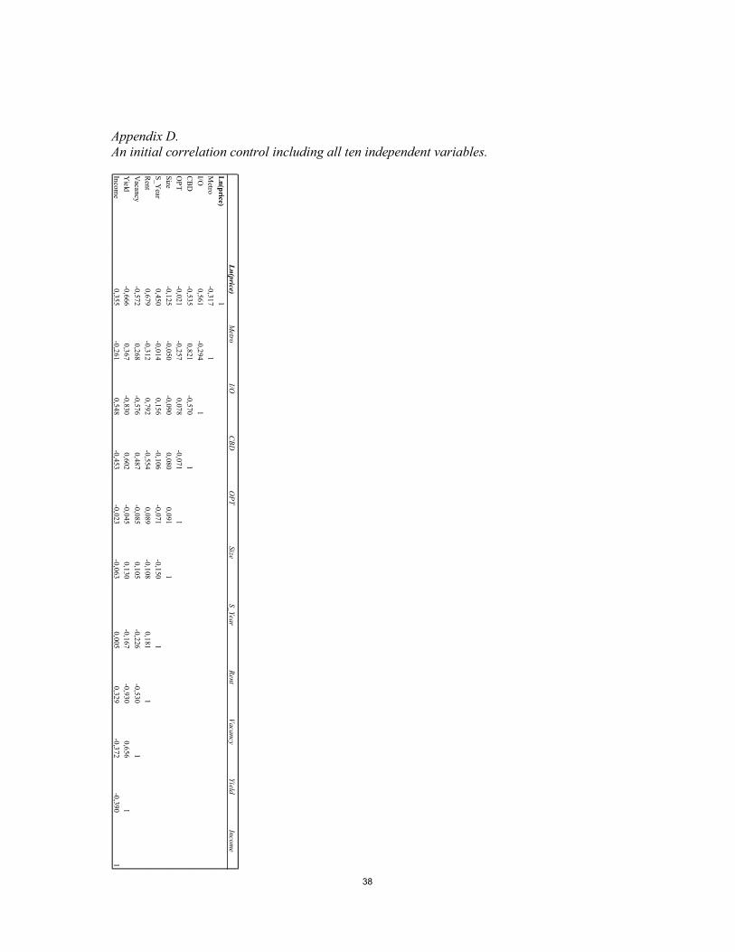
38

Appendix D. An initial correlation control including all ten independent variables.

Ln(price)

Metro

I/OC

BD

OP

TSize

S_YearR

entV

acancyYield

Income

Ln(p

rice)1

Metro

-0,3171

I/O0,561

-0,2941

CB

D-0,535

0,821-0,570

1

OP

T-0,021

-0,2570,078

-0,0711

Size-0,125

-0,050-0,090

0,0800,091

1

S_Year

0,450-0,014

0,156-0,106

-0,071-0,150

1

Rent

0,679-0,312

0,792-0,554

0,089-0,108

0,1811

Vacancy

-0,5720,268

-0,5760,487

-0,0850,105

-0,226-0,530

1

Yield

-0,6660,367

-0,8300,602

-0,0450,130

-0,167-0,930

0,6561

Income

0,355-0,261

0,548-0,453

-0,023-0,063

0,0050,329

-0,372-0,390

1

39 TRITA – ABE – MBT – 22511

www.kth.se