The Impact of Human Capital Endowments on International ...

The Impact of Human Capital Endowments on International

Competitiveness, with Special Reference to Transition

Economies

Arta MULLIQI

A thesis submitted in partial fulfilment of the requirement of Staffordshire University for the

degree of Doctor of Philosophy

October 2016

2

Abstract

The aim of this thesis is to investigate the impact of human capital endowments on international

competitiveness, with special reference to transition economies. This investigation is based on

country, industry and firm level estimations using longitudinal and cross section data for the

period 1995-2010 and 2011-2014, respectively. The theoretical framework informing this

empirical investigation proposes a relationship between human capital and international

competitiveness through the underlying mechanism of labour productivity and innovation. More

educated and higher skilled individuals are more likely to innovate and/or adopt and use

efficiently new sophisticated technologies which, consequently, boosts labour productivity. In

turn, more productive firms and countries are more likely to maintain and/or develop their

international competitiveness. In this investigation, the degree of international competitiveness is

measured by export market share, relative export advantage, the share of medium and high tech

exports, export sophistication, and export intensity. Human capital is represented by educational

attainment, the quality of education, and provision/participation in training programmes. To

empirically test the human capital-international competitiveness nexus, a diversified modelling

strategy has been employed. In line with theoretical underpinnings, human capital endowments

appear to exert a positive and significant impact on export market share at both country and

industry levels, though this effect is not replicated when the relative export advantage index is

taken as the measure of international competitiveness. The share of the population with tertiary

education seems to exert a positive impact on the share of medium and high-tech manufactures

exported by the EU-27, the impact being relatively stronger in the high tech category. No

supporting evidence is found for the influence of the quality of education, irrespective of the

international competiveness measure used. In the export sophistication sub-analysis, the

estimated results suggest that the share of population with tertiary education has a positive

impact only on the level of export sophistication of the EU-17. Consistent with previous

research, the firm level results suggest that having a more educated workforce exerts a positive

and statistically significant impact on the export intensity and export market share of firms in 30

transition economies. Mixed evidence is found for the role of on-the-job training programmes

and years of experience of the top manager. The empirical evidence obtained in this investigation

has potentially useful policy implications for European and Euro-Asian countries seeking to

sustain or increase their international competitiveness.

3

Table of Contents CHAPTER 1

HUMAN CAPITAL AND INTERNATIONAL COMPETITIVENESS: INTRODUCTION AND CONTEXT

1.1 Introduction .......................................................................................................................................... 18

1.2 International competitiveness and the transition process ................................................................... 19

1.3 Human capital development in transition economies .......................................................................... 29

1.4 Research questions and structure of the thesis ................................................................................... 42

CHAPTER 2

ASSESSING THE MULTIDIMENSIONAL CONCEPT OF INTERNATIONAL COMPETITIVENESS

2.1 Introduction .......................................................................................................................................... 46

2.2 The concept of international competitiveness ..................................................................................... 47

2.3 International competitiveness: key measurement approaches ........................................................... 50

2.4 Empirical evidence on international competitiveness: micro and macro perspectives ....................... 64

2.5 Conclusions ........................................................................................................................................... 78

CHAPTER 3

HUMAN CAPITAL AND INTERNATIONAL COMPETITIVENESS: THEORY, MEASUREMENT AND EVIDENCE

3.1 Introduction .......................................................................................................................................... 90

3.2 Theoretical framework ......................................................................................................................... 90

3.2.1 Human capital and economic growth ............................................................................................ 90

3.2.2 Human capital and international competitiveness ........................................................................ 94

3.3 Human capital, productivity, and growth: empirical evidence ............................................................. 98

3.3.1 Human capital and international competitiveness: a review of the macro evidence ................. 101

3.3.2 Human capital and international competitiveness: a review of the micro evidence .................. 106

3.4 Human capital: definition and measurement ..................................................................................... 128

3.5 Conclusions ......................................................................................................................................... 137

CHAPTER 4

HUMAN CAPITAL AND INTERNATIONAL COMPETITIVENESS: COUNTRY AND INDUSTRY LEVEL EVIDENCE

4.1 Introduction ........................................................................................................................................ 141

4

4.2 Data and variable specification ........................................................................................................... 142

4.3 Estimation methodology ..................................................................................................................... 156

4.4 Country level empirical evidence ........................................................................................................ 160

4.5 Industry level empirical evidence ....................................................................................................... 174

4.6 Conclusions ......................................................................................................................................... 179

CHAPTER 5

HUMAN CAPITAL AND TECHNOLOGY INTENSIVE EXPORTS: EMPIRICAL EVIDENCE

5.1. Introduction ....................................................................................................................................... 183


5.3 Model specification and estimation methodology ............................................................................. 201

5.4 Empirical evidence .............................................................................................................................. 204

5.4.1 Export market share and relative export advantage ................................................................... 205

5.4.2 Export sophistication ................................................................................................................... 211

5.5 Conclusions ......................................................................................................................................... 214

CHAPTER 6

HUMAN CAPITAL AND INTERNATIONAL COMPETITIVENESS: A MICRO-LEVEL ANALYSIS

6.1 Introduction ........................................................................................................................................ 218

6.2 Data and model specification ............................................................................................................. 219

6.2.1 Descriptive statistics .................................................................................................................... 230



6.4.1 Export intensity ............................................................................................................................ 244

6.4.2 Export market share .................................................................................................................... 256

6.5 Conclusions ......................................................................................................................................... 260

CHAPTER 7

CONCLUSIONS AND RECOMMENDATIONS

7.1 Introduction ........................................................................................................................................ 264

7.2 Empirical findings ................................................................................................................................ 266

5

7.3 Contributions to knowledge ............................................................................................................... 273

7.4 Policy implications .............................................................................................................................. 275

7.5 Limitations and recommendations for future research ..................................................................... 280

8. References ............................................................................................................................................ 282

FIGURES

Figure 1.1 Export patterns across transition economies (1995-2014) ................................................... 21

Figure 1.2 Export to GDP ratio by country group ................................................................................... 23

Figure 1.3 Merchandise exports by product group (1995-2014) ............................................................ 25

Figure 1.4 High-technology exports by country group (1996-2013) ...................................................... 27

Figure 1.5 High-technology exports (% of manufactured exports) ........................................................ 29

Figure 1.6 Percentage of population aged 15 and over with no completed schooling .......................... 33

Figure 1.7 Percentage of population aged 15 and over who have completed tertiary education ........ 35

Figure 1.8 Average test scores in mathematics and science (1964-2003) ............................................. 38

Figure 1.9 Prevalence of staff training in transition countries - Rankings .............................................. 41

Figure 4.1 Export market share (emsh) functional transformation ...................................................... 153

Figure 5.1 Export market share of European transition economies in medium-high and high tech

industries, percentages (1995-2010) .................................................................................................... 185

Figure 5.2 Export market share of non- transition economies/EU-18 in medium-high and high tech

industries, percentages (1995-2010) .................................................................................................... 186

Figure 5.3 RXAs of non-transition economies/EU-18 in medium-high and high tech industries (1995-

2010) ..................................................................................................................................................... 190

Figure 5.4 The percentage change in the RXA of non-transition economies (1995-2010) .................. 191

Figure 5.5 RXAs of medium-high and high tech in the Czech Republic, by industry ............................ 194

Figure 5.6 RXAs of medium-high and high tech in Slovak Republic, by industry .................................. 194

Figure 5.7 RXAs of medium-high and high tech in Hungary, by industry ............................................. 195

Figure 5.8 RXAs of European transition economies in medium-high and high tech exports (1995-2010)

.............................................................................................................................................................. 196

Figure 5.9 The percentage change in the RXA of European transition economies (1995-2010) ......... 197

Figure 5.10 Export sophistication index (EXPY) .................................................................................... 200

6

TABLES

Table 2.1 International competitiveness: overview of empirical studies ............................................... 77

Table 3.1 Human capital and international competitiveness: overview of empirical studies .............. 113

Table 4.1 Manufacturing industries according to ISIC rev. 3 ................................................................ 144

Table 4.2 Variable descriptions ............................................................................................................. 151

Table 4.3 Export market share (emsh) functional transformation ....................................................... 152

Table 4.4 Descriptive statistics .............................................................................................................. 154

Table 4.5 Collinearity diagnostics ......................................................................................................... 156

Table 4.6 Estimated results with Driscoll-Kraay standard errors ......................................................... 161

Table 4.7 FEVD and HT estimated results ............................................................................................. 164

Table 4.8 IV estimated results .............................................................................................................. 166

Table 4.9 IV estimated results (training included) ................................................................................ 171

Table 4.10 IV estimated industry results .............................................................................................. 178

Table 4.11 FEVD and HT estimated results ........................................................................................... 179

Table 5.1 Manufacturing industries according to ISIC rev. 3 ................................................................ 187

Table 5.2 Medium-high and high tech manufacturing industries according to ISIC rev. 3................... 188

Table 5.3 Relative export advantage (RXA) of non-transition economies/EU-18, by industry (1995-

2010) ..................................................................................................................................................... 188

Table 5.4 RXAs of European transition economies, by industry (1995-2010) ...................................... 193

Table 5.5 Export sophistication index (EXPY), averaged (1995-2010) .................................................. 199

Table 5.6 Descriptive statistics .............................................................................................................. 201

Table 5.7 Driscoll-Kraay and IV estimated results ................................................................................ 209

Table 5.8 FEVD and HT estimated results ............................................................................................. 210

Table 5.9 Driscoll-Kraay and IV estimated results ................................................................................ 212

Table 5.10 FEVD and HT estimated results ........................................................................................... 213

Table 6.1 Variable descriptions ............................................................................................................. 228

Table 6.2 Descriptive statistics by export intensity .............................................................................. 232

Table 6.3 Collinearity diagnostics ......................................................................................................... 236

Table 6.4 Full sample estimated results (marginal effects) .................................................................. 247

Table 6.5 Estimated results (marginal effects) by country group ......................................................... 253

7

Table 6.6 Industry estimated results (marginal effects) by country group .......................................... 256

Table 6.7 Full sample estimated results (marginal effects) .................................................................. 258

APPENDIX

Table A4.1 Model 1 - Fixed effects estimated results........................................................................... 318

Table A4.1.1 Model 1 - Random effects estimated results .................................................................. 319

Table A4.1.2 Model 1 - Fixed effects versus Random effects ............................................................... 319

Table A4.1.3 Model 1- Diagnostic tests ................................................................................................ 320

Table A4.1.4 Model 1 - Driscoll-Kraay estimated results ...................................................................... 321

Table A4.1.4.1 Model 1 - Driscoll-Kraay estimated results ................................................................... 322


Table A4.1.5 Model 1 - FEVD estimated results (STATA ado file) ........................................................ 323

Table A4.1.5.1 Model 1- FEVD estimated results (three stage procedure) ......................................... 324

Table A4.1.6 Model 1 - Hausman and Taylor estimated results ........................................................... 325

Table A4.1.6.1 Model 1 - Fixed effects versus Hausman and Taylor .................................................... 326

Table A4.1.7 Model 1 - Hsiao 2 step procedure ................................................................................... 326

Table A4.1.8 Model 1 - IV estimated results ......................................................................................... 328

Table A4.1.8.1 Model 1 - IV estimated results (ETEs) ........................................................................... 329

Table A4.1.8.2 Model 1 - IV estimated results (N-ETEs) ....................................................................... 330

Table A4.1.8.3 Model 1 - IV estimated results ...................................................................................... 332





Table A4.2.2.1 Models 1& 2 - Fixed effects versus Random effects ..................................................... 337

Table A4.2.3 Model 2 - Diagnostic tests ............................................................................................... 337

Table A4.2.3.1 Models 1&2 - Diagnostic tests ...................................................................................... 338




Table A4.2.5 Model 2 - FEVD estimated results (STATA ado file) ......................................................... 340

8

Table A4.2.5.1 Model 2 - FEVD estimated results (Three stage procedure)........................................ 341









Table A4.3 Descriptive statistics (Variables in levels) ........................................................................... 351

Table A4.3.1 Correlation matrix ............................................................................................................ 352

Figure A4.4 Functional transformations for all explanatory variables ................................................. 352

Figure A4.4.1 Functional transformation for sedut .............................................................................. 353

Figure A4.4.2 Functional transformation for tedut .............................................................................. 353

Figure A4.4.3 Functional transformation for avyrs ............................................................................... 354

Figure A4.4.4 Functional transformation for cskills .............................................................................. 354

Figure A4.4.5 Functional transformation for patappr .......................................................................... 355

Figure A4.4.6 Functional transformation for fdi ................................................................................... 355

Figure A4.4.7 Functional transformation for gdpc ............................................................................... 356

Figure A4.4.8 Functional transformation for unem .............................................................................. 356

Figure A4.4.9 Functional transformation for ecofree ........................................................................... 357

Figure A4.5.1 Functional transformation for rulc ................................................................................. 357

Figure A4.5.2 Functional transformation for serv ................................................................................. 358

Figure A4.5.3 Functional transformation for pop ................................................................................. 358

Figure A4.5.4 Functional transformation for trandinN ......................................................................... 359

Figure A4.5.5 Functional transformation for dist ................................................................................. 359

Figure A4.5.6 Functional transformation for transdummy ................................................................... 360

Figure A4.5.7 Functional transformation for emplcvt .......................................................................... 360

Figure A4.5.8 Functional transformation for trngent ........................................................................... 361




9

Table A4.6.3 Model 1 - FEVD estimated results ................................................................................... 363













Table A4.8 Model 1&2 - IV estimated results – emsh at industry level ................................................ 377

Table A4.9 Model 1& 2 - Estimation results – old version dataset ....................................................... 378

Table A4.9.1 Model 1 - FE standard errors vs FEVD standard errors ................................................... 379

Table A5.1. Relative export advantage (RXA) of ETEs in medium-high and high tech sub-industries . 383

Table A5.1.1 Relative export advantage (RXA) of EU -18 in medium-high and high tech sub-industries

.............................................................................................................................................................. 383

Table A5.1.2 Correlation between Export sophistication and GDP per capita ..................................... 385

Table A5.1.3 Correlation matrix between potential measures of international competitiveness ....... 385

Table A5.1.4 Descriptive statistics for variables in levels ..................................................................... 386

Table A5.2 Model 1 - Fixed effects estimated results (medium-high and high tech) ........................... 387


Table A5.2.2 Model 1 - Driscoll-Kraay estimated results (medium-high and high tech) ...................... 388

Table A5.2.4 Model 1 - FEVD estimated results (medium-high and high tech) ................................... 389

Table A5.2.5 Model 1 - Hausman and Taylor estimated results (medium-high and high tech) ........... 390

Table A5.2.6 Model 1 - IV estimated results (medium-high and high tech) ......................................... 391

Table A5.2.6.1 Model 1 - IV estimated results - ETEs (medium-high and high tech) .......................... 392

Table A5.2.6.2 Model 1 - IV estimated results –N-ETEs (medium-high and high tech) ........................ 394

Table A5.2.6.3 Model 1 - IV estimated results (high tech) ................................................................... 395

Table A5.2.6.3.1 Model 1 - IV estimated results - ETEs (high tech) ...................................................... 396

10

Table A5.2.6.3.2 Model 1 - IV estimated results – N-ETEs (high tech) ................................................. 398

Table A5.2.6.4 Model 1 - IV estimated results (medium-high tech) ..................................................... 399

Table A5.2.6.4.1 Model 1 - IV estimated results – ETEs (medium-high tech) ...................................... 400

Table A5.2.6.4.2 Model 1 - IV estimated results – N-ETEs (medium-high tech) ................................... 402




Table A5.3.4 Model 2 - FEVD estimated results (medium-high and high tech) .................................... 406



Table A5.3.6.1 Model 2 - IV estimated results - ETEs (medium-high and high tech) ........................... 409

Table A5.3.6.2 Model 2 - IV estimated results – N-ETEs (medium-high and high tech) ....................... 410


Table A5.3.6.3.1 Model 2 - IV estimated results – ETEs (high tech) ..................................................... 413

Table A5.3.6.3.2 Model 2 - IV estimated results - N-ETEs (high tech) .................................................. 414


















11






Table A5.5.5 Model 2 - IV estimated results (medium-high and high tech) ........................................ 440

Table A5.5.5.1 Model 2 - IV estimated results –ETEs (medium-high and high tech)............................ 441






Table A5.5.5.4.1 Model 2 - IV estimated results -ETEs (medium-high tech) ........................................ 450

Table A5.5.5.4.2 Model 2 - IV estimated results –N-ETEs (medium-high tech) .................................... 451







Table A5.6.5.1 Model 1 - IV estimated results - ETEs .......................................................................... 458

Table A5.6.5.2 Model 1 - IV estimated results – N-ETEs ....................................................................... 459







Table A5.7.5.1 Model 2 - IV estimated results – ETEs .......................................................................... 466


Table A5.8 Driscoll-Kraay and IV estimated results (export market share) .......................................... 470

Table A5.8.1. Driscoll-Kraay and IV estimated results (relative export advantage, RXA) ..................... 471

12

Table A5.9 IV estimated results (medium-low, medium-high and high tech) ...................................... 472

Table A5.9.1 FEVD & Hausman and Taylor estimated results (medium-low, medium-high and high

tech) ...................................................................................................................................................... 474

Table A6.1 Descriptive statistics ........................................................................................................... 477

Table A6.2 Correlation matrix ............................................................................................................... 477

Table A6.3 Tobit Model - Full sample estimated results ...................................................................... 478

Table A6.3.1 Tobit Model - Industry estimated results ........................................................................ 479

Table A6.3.2 Tobit Model - CEECs estimated results ............................................................................ 480

Table A6.3.3 Tobit Model - CEECs Industry estimated results .............................................................. 482

Table A6.3.4 Tobit Model - CIS estimated results ................................................................................. 483

Table A6.3.5 Tobit Model - CIS Industry estimated results .................................................................. 485

Table A6.3.6 Tobit vs Probit estimated results ..................................................................................... 486

Table A6.3.7 Tobit Model - Full sample (imputed) estimated results .................................................. 487

Table A6.3.8 Tobit (Augumented) Model - Full sample (imputed) estimated results (45) ................... 488


Table A6.4 Fractional Logit Model - Full sample estimated results ...................................................... 490

Table A6.4.1 Fractional Logit Model - Industry estimated results ........................................................ 492

Table A6.4.2 Fractional Logit Model - CEECs Estimated results ........................................................... 493

Table A6.4.3 Fractional Logit Model - CEECs Industry estimated results ............................................. 494

Table A6.4.4 Fractional Logit Model - CIS estimated results ................................................................ 496

Table A6.4.5 Fractional Logit Model - CIS Industry estimated results .................................................. 497

Table A6.4.6 Fractional Logit Model - Full sample (imputed) estimated results .................................. 499

Table A6.4.7 Fractional Logit (Augumented) Model - Full sample (imputed) estimated results (45) .. 500


Table A6.5 Poisson Model - Full sample estimated results .................................................................. 503

Table A6.5.1 Poisson Model - Industry estimated results .................................................................... 504

Table A6.5.2 Poisson Model - CEECs estimated results ........................................................................ 505

Table A6.5.3 Poisson Model - CEECs Industry estimated results .......................................................... 506

Table A6.5.4 Poisson Model - CIS estimated results ............................................................................. 508

Table A6.5.5 Poisson Model - CIS Industry estimated results .............................................................. 509

Table A6.5.6 Poisson Model - Full sample (imputed) estimated results .............................................. 511

Table A6.5.7 Poisson (Augumented) Model - Full sample (imputed) estimated results (45)............... 512

13


Table A6.6 Panel estimated results ...................................................................................................... 514

Table A6.6.1 IVTobit Model - Full sample estimated results ................................................................ 514

Table A6.6.2 IVPoisson Model - Full sample estimated results ............................................................ 516

Table A6.7 Tobit Model - Full sample estimated results (exp_share_industryEU28) .......................... 517

Table A6.7.1 Tobit Model - CEECs estimated results (exp_share_industryEU28) ................................ 518

Table A6.7.2 Tobit Model -CIS estimated results (exp_share_industryEU28) ...................................... 519

Table A6.7.3 Tobit Model - Full sample estimated results (exp_share_industryEA40) ........................ 521

Table A6.7.4 Tobit Model - CEECs estimated results (exp_share_industryEA40) ................................ 522

Table A6.7.5 Tobit Model - CIS estimated results (exp_share_industryEA40) ..................................... 523

Table A6.7.6 Tobit Model - Full sample estimated results (exp_share_totalEU28) ............................. 525

Table A6.7.7 Tobit Model - Full sample estimated results (exp_share_totalEA40) ............................. 526

Table A6.8 Fractional Logit Model - Full sample estimated results (exp_share_industryEU28) .......... 527

Table A6.8.1 Fractional Logit Model - CEECs estimated results (exp_share_industryEU28)................ 528

Table A6.8.3 Fractional Logit Model - Full sample estimated results (exp_share_industryEA40) ....... 530

Table A6.8.4 Fractional Logit Model - CEECs estimated results (exp_share_industryEA40) ................ 531

Table A6.8.5 Fractional Logit Model - CIS estimated results (exp_share_industryEA40)..................... 532

Table A6.8.6 Fractional Logit Model - Full sample estimated results (exp_share_totalEU28) ............. 534

Table A6.8.7 Fractional Logit Model - Full sample estimated results (exp_share_totalEA40) ............ 535

Table A6.9 Poisson Model - Full sample estimated results (exp_share_industryEU28) ...................... 536

Table A6.9.1 Poisson Model - CEECs estimated results (exp_share_industryEU28) ............................ 537

Table A6.9.2 Poisson Model - CIS estimated results (exp_share_industryEU28) ................................. 539

Table A6.9.3 Poisson Model - Full sample estimated results (exp_share_industryEA40) .................... 540

Table A6.9.4 Poisson Model - CEECs estimated results (exp_share_industryEA40) ............................ 541

Table A6.9.5 Poisson Model - CIS estimated results (exp_share_industryEA40) ................................. 542

Table A6.9.6 Poisson Model - Full sample estimated results (exp_share_totalEU28) ......................... 544

Table A6.9.7 Poisson Model - Full sample estimated results (exp_share_totalEA40) ......................... 545

14

Abbreviations

ALL – Adult Literacy and Lifeskills Survey

BEEPS –Business Environment and Enterprise Performance Survey

CEE – Central and Eastern Europe

CEEC – Central and East European Country

CEPII – Centre d'Études Prospectives et d'Informations Internationales

CIS – Commonwealth of Independent States

CVTS – Continuing Vocational Training Survey

EBRD – European Bank for Reconstruction and Development

ETE – European Transition Economy

EU – European Union

FDI – Foreign Direct Investment

FE – Fixed Effects

FEVD - Fixed Effects Vector Decomposition

GDP – Gross Domestic Product

GLS – Generalized Least Squares

GMM – Generalized Method of Moments

HT – Hausman and Taylor

IAEP – International Assessment of Educational Progress

IALS – International Adult Literacy Survey

IEA – International Association for the Evaluation of Educational Achievement

ISIC – International Standard Industrial Classification

IV – Instrumental Variable

LSDV – Least Squares Dummy Variable

MAR – Missing at Random

MCAR – Missing Completely at Random

MICE – Multiple Imputation using Chained Equations

MLE – Maximum Likelihood Estimator

MNAR – Missing not at Random

MNE – Multinational Enterprise

15

MVN – Multivariate Normal Regression

N-ETE – non-Transition Economy

OECD – Organisation for Economic Co-operation and Development

OLS – Ordinary Least Squares

PIAAC – Programme for the International Assessment of Adult Competencies

PIRLS – Progress in International Reading Literacy Study

PISA – Programme for International Student Assessment

R&D – Research & Development

RE – Random Effects

SITC – Standard International Trade Classification

SME – Small and Medium Enterprise

TIMSS –Trends in International Mathematics and Science Study

UNCTAD – United Nations Conference on Trade and Development

UNESCO – United Nations Educational, Scientific and Cultural Organization

VIF – Variance Inflation Factor

WDI – World Development Indicators

16

Acknowledgements

First of all, I would like to express my profound gratitude to my supervisory team, Professor

Nick Adnett, Professor Mehtap Hisarciklilar and Dr. Artane Rizvanolli for their valuable advice,

guidance, and support during the course of this thesis. A special appreciation goes to Professor

Nick Adnett, for leading my academic journey since my Master’s, for believing in me,

encouraging me and sharing his expertise throughout all these years. I am also deeply thankful to

Staffordshire University and the Open Society Foundation for funding this research project and

the kind staff that helped during this course. I owe my deepest gratitude to my beloved family for

their unconditional love, care and constant support. I would like to extend my gratefulness to my

friends and colleagues for their great support and encouragement throughout the time of my

research. Special thanks to my roommate, Arberesha Loxha, for the happy time we spent

together during the past four years. Last but not the least, I wish to express my warm

appreciation to my lovely nephews, Klevis and Levik, whose pure love and beautiful laughter

made this journey less stressful for me.

I dedicate this thesis to my beloved parents, Servete and Ramiz.

17

Chapter 1

HUMAN CAPITAL AND INTERNATIONAL COMPETITVENESS:

INTRODUCTION AND CONTEXT

Contents 1.1. Introduction ......................................................................................................................................... 18

1.2 International competitiveness and the transition process ................................................................... 19

1.3 Human capital development in transition economies .......................................................................... 29

1.4 Research questions and structure of the thesis ................................................................................... 42

18

1.1 Introduction

The aim of this introductory chapter is to provide a discussion on the characteristics and

evolution of international competitiveness and human capital across transition countries since the

beginning of the transformation from centrally planned to market economies. The link between

international competitiveness and the process of transition is analysed in the light of the data

provided by the World Bank and the UNCTAD. Initially, the transformation process has been

covered and its impact on the integration of these countries into the global economy is discussed.

The evolving performance and pattern of exports in European and Central Asian transition

economies since mid-1990s is presented and discussed, followed for comparative purposes by an

overview of the performance of 18 European countries, henceforth refered as EU-181 over the

same time span. The change in the compositional structure of exports in transition economies,

and their convergence towards the structure typical of high income countries is placed at the

centre of our debate. Particular attention is paid to the high technology-intensive exports and

their evolution during the course of transition. This part of the chapter also focuses on the re-

orientation of the export flows from transition countries towards Western Europe since the

beginning of the transformation process.

The following section of this chapter focuses on the development of human capital in the former

socialist countries of Central and Eastern Europe and Central Asia. It provides a discussion on

the evolution of the human capital stock since the beginning of transition by focusing on the

level of education attainment, quality of education and training incidence. Furthermore, it

describes the key characteristics of the educational system of the region before and during the

reform process with particular emphasis on different types of schooling, skill upgrading and

teaching approaches. The remaining gaps with respect to the EU-18, skill and qualification

mismatches and other transition-related subjects are also elaborated in this chapter. The last

section of the chapter outlines the aim of the thesis, the key research questions and the structure

of the thesis.

1 EU18 refers to 17 non-transition member countries of the European Union (Austria, Belgium, Cyprus, Denmark,

Finland, France, Germany, Greece, Ireland, Italy, Luxembourg, Malta, Netherlands, Portugal, Spain, Sweden and the United Kingdom) and Norway. EU-17, on the other hand, refers to all the above mentioned countries excluding Malta.

19

1.2 International competitiveness and the transition process

The transformation of the Central and Eastern Europe and Former Soviet Union from a centrally

planned economic regime to a market oriented system has been associated with a deeper

integration of this region into the global economy. Increased openness and international

integration through trade have been key outcomes of the transition process in the former socialist

countries. Integration into the world economy through trade has also been closely related to

integration via labour and capital flows. Increased movement of capital and labour are regarded

to play a key role in promoting wider integration and in enhancing the performance of transition

economies (EBRD, 2003). During the course of transition, movement of capital was mainly

achieved by increased foreign direct investment and cross-border bank flows (Roaf et al., 2014).

However, in order for this region to be able to realise greater integration, increased policy

cooperation and other adjustments were required to take place. Membership in international

institutions, such as World Trade Organization (WTO) has assisted these countries significantly

in harmonising their legislation and political frameworks (Roaf et al., 2014).

The increased trade liberalisation which started after the fall of the Berlin Wall and the end of the

Soviet Union has been characterized by an improved export performance in the majority of these

countries. In a globalized economy, maintaining and increasing international competitiveness is a

major challenge for most countries, particularly for developing and transition economies. Over

the transition period, the majority of transition countries have managed to increase their

engagement with international markets and in turn enhanced their international competitiveness.

As a complex and multifaceted concept, international competitiveness has been elaborated quite

extensively in the literature; however, its definition and measurement still remain contentious.

Various definitions and measurement approaches at both macro and micro levels of aggregation

have been proposed and used in the literature with no agreement on any single one. Since the

ability to compete in international markets is regarded as an important indication of the economic

performance of countries, this section will focus primarily on export based indicators. Greater

integration into international markets has been followed by faster productivity growth in most of

these countries, thus, narrowing, the previously wide productivity gap with the EU-15 and other

developed countries. As already postulated in the literature, international trade is perceived to

facilitate technological transfer, which in turn plays a key role in increasing productivity,

20

particularly in developing countries (Choudhri and Hakura, 2000). The benefits of fuller

international integration for productivity improvement in transition economies have been more

prevalent in the new EU member states, with their productivity levels being twice as high, in

2005, as those in several CIS economies (Alam et al., 2008). The impact of trade and FDI on

productivity enhancement appears to have been mainly channelled through technological

transfers and innovation promotion. Note that productivity growth in some services industries,

over the period 1997 to 2004 has significantly exceeded the comparable growth rates in the EU-

15 (Broadman, 2005, Alam et al., 2008). However, in spite of the evident convergence, there is

still a significant gap in productivity levels of the region relative to those found in high income

countries. The aim of this section is to assess and discus the evolving performance and pattern of

exports in European and Central Asian transition economies since mid-1990s. A comparative

analysis of this region’s export performance with that of EU-18 is also presented and debated in

this section. Particular attention is paid to the change in the composition of exports, i.e. the

movement towards technology intensive (more sophisticated goods), and the extent to which

these countries have converged in this respect with the EU-18.

Since the start of transition, the region has witnessed a rapid and significant growth of exports,

which has been accompanied by increasing market shares in world markets. In 2014, the total

exports of Central and East European countries (CEECs) and the Commonwealth of Independent

States (CIS) accounted for approximately 1,228 billion (constant) US dollars, which represents

an increase of 235 percent from 1995 (an annual average rate of 6.6 percent). Data on the EU-18,

on the other hand, reveals just a 126 percent increase in total exports of goods and services

during this period (World Bank, 2016a). It is pertinent to note that the transition progress and

consequently the international integration have been uneven among transition countries.

Important discrepancies in the speed and degree of integration and export restructuring have

been observed between countries in Central and Eastern Europe (CEECs) and Former Soviet

Union (CIS). The highest average growth rate in total exports of goods and services among

transition economies was recorded in the region of Central and Eastern Europe. From 1995 to

2014, the exports of the CEECs increased by 351 percent, as compared to 138 percent for the

CIS. It is also worth noting that these high growth rates are partly a result of the lower levels of

international integration of these countries prior to transition. While, the majority of countries

21

from the former group have finalised the transformation process and have joined the European

Union, many countries from the CIS are still lagging behind in terms of their reform and

transformation progress. Many of the CEE countries have had bilateral trade agreements with the

EU since the mid-1990s, whereas, the trade agreements of CIS with the EU are much weaker in

terms of the degree of liberalization (Roaf et al., 2014). Geographical proximity, initial economic

conditions, transformation progress and their prevailing policy regime have been considered as

the main sources of the faster integration of the former region into the EU markets and beyond

(Roaf et al., 2014). Figure 1.1, presented below, shows how the total exports of these transition

economies have evolved from mid-1990s to 2014. It is important to note that the share of

Russia’s exports in total exports of Commonwealth Independent States (CIS) is quite large;

hence, driving the total export figures considerably. After excluding Russia from the

calculations, the export value of CIS drops significantly and the gap between the latter and

CEECs widens further (see Figure 1.1). However, it should be emphasized, that many countries

from the former Soviet Union are highly engaged in exporting primary goods due to their natural

resource abundance, thus making it difficult to compare their export performance with that of the

CEECs.

Figure 1.1 Export patterns across transition economies (1995-2014)

Data Source: World Bank - World Development Indicators (Exports of goods and services, constant 2005 US$)

0

1E+11

2E+11

3E+11

4E+11

5E+11

6E+11

7E+11

8E+11

19

95

19

96

19

97

19

98

19

99

20

00

20

01

20

02

20

03

20

04

20

05

20

06

20

07

20

08

20

09

20

10

20

11

20

12

20

13

20

14

con

stan

t 2

00

5 U

S$

CEECs

CIS

CIS (excl. Russia)

22

In spite of the relatively high average growth rate recorded in the CEECs, diverse exporting

performances have been witnessed across the region. While, Poland, the Czech Republic,

Hungary, the Slovak Republic, and Romania appear to be the top five export performers,

countries from the Western Balkan region seem to lag behind and thus are positioned at the

lower end of the ranking. However, it is worth emphasizing that countries such as Albania and

Serbia have experienced exceptionally high rates of growth in their exports from 1995 to 2014,

i.e. 792.9 and 905.5 percent increase, respectively. The violent dissolution of former Yugoslavia

has been regarded as one of the potential causes for the slower integration of many of the

Western Balkan countries (EBRD, 2003).

Regarding the export performance of the former Soviet Union countries (i.e. CIS), Russia,

Kazakhstan, Ukraine, Azerbaijan and Belarus appear to be the top five exports performers,

whereas, Armenia, Kyrgyz Republic and Tajikistan are ranked amongst the countries with the

weakest export performance. Countries that experienced the highest rate of (positive) change

over the period 1995-2014 were Azerbaijan and Georgia (over 800 percent). It is important to

note that the overall positive trend of transition economies was hampered by the global financial

crisis 2008-09, which affected to a large extent the exporting sector. The entire region suffered

an 8 percent decline in its exports of goods and services in 2009 as compared to a 11.8 percent

fall in the EU-18. However, their overall exports recovered rapidly in 2010, with a rate of

increase of 13.7 percent in CEECs and 7.4 percent in the CIS (World Bank, 2016a).

The overall increase in exports over time has been accompanied by a significant expansion in the

exports to GDP ratio. From the two sets of transition economies, countries from the Central and

Eastern Europe appear to have witnessed the highest growth rates since mid-1990s. On average,

CEECs’ total exports in 2014 accounted for 60 percent of GDP, as compared to about 35 percent

in 1995, reaching the EU-18 level by the end of this period. It is pertinent to note that countries

such as the Slovak Republic, the Czech Republic, Hungary, and Estonia in 2014 recorded

relatively high export ratios, thus, outperforming most of the EU-18 countries. A completely

different story is portrayed when the CIS’ export to GDP figures are assessed. With an initial rate

higher than the average of CEECs, these countries have recorded a decrease of 7 percent on their

export shares in GDP from 1995 to 2014 (World Bank, 2016b). The first two decades of

23

transition for these countries have been followed by high volatility in their export to GDP ratios.

Among the potential causes for the limited degree of integration of many of these countries, their

less favourable geographical position, high transportation and transit costs, and the poor quality

of institutions and policies have been highlighted (EBRD, 2003). The composition and quality of

exports might be another potential reason for their lower rates of participation in western

markets. The change on the export to GDP ratio from 1995 to 2014 across these countries is

presented in Figure 1.2.

Figure 1.2 Export to GDP ratio by country group

Data Source: World Bank- World Development Indicators (Exports of goods and services % of GDP)

A separate assessment of goods and services export data (in current US dollars) during 1995-

2013, reveals an extremely high growth rate in the export of goods (i.e. 618%), followed by an

almost equally impressive growth rate in the services sector (i.e. 507%). The highest average

growth rate, in the export of services, was recorded in the CIS region, i.e. a growth rate of 647%,

as compared to 368% percent in CEECs and 257 percent in the EU-18. While the share of goods

in total exports during the same period increased slightly in CEECs, both the CIS and EU-18

experienced a decline in this ratio by approximately 10.7 percent and 16.6 percent, respectively.

Differences in the contribution of services to total exports (i.e. services as a % of total exports),

on the other hand, has been more evident in the CIS region. While countries from Central and

East Europe have experienced a negligible increase in this share over time, i.e. a 1.4 % increase

0

10

20

30

40

50

60

70

CEECs CIS EU-18

1995

2014

24

from 1995 to 2013; countries from the former Soviet Union, have recorded an average rate of

change as high as 93.7%. The share of services in total exports for EU-18 went up as well. At the

same time, this set of countries has witnessed an average share of 37.8%, representing a change

of 37.7 percent since 1995 (UNCTAD, 2016b).

A further disaggregation of the data extracted from the UNCTAD has helped us to assess the

evolution of the share of manufactured and primary goods in merchandise exports across the

region during the course of transition. The new data show large differences between the two

transition subgroups in terms of their engagement in exporting these particular product groups

over the past twenty years. While, the share of manufactured goods2, in CEECs, in 2014, appears

to be as high as 78.3 percent (exceeding this share in the EU-18), the CIS has recorded a share as

low as 19.5 percent, which represent a decline of approximately 37% since 1995. The EU-18’s

share has slightly declined over the same period of time (i.e.3.8%), though it still remains high

with a current value of around 72.5%. The contribution of primary commodities3 to their export

baskets, on the other hand, has grown in both the CIS and EU-18 countries, by 39.8 percent and

26.3 percent respectively, while it has dropped by 20.3 % in European transition economies. It is

worth noting that the engagement of the latter group of transition countries (i.e. CEECs) together

with the EU-18 in this sector, has not been very substantial, as indicated by their relatively low

shares (19-21%), whereas, the average share of the same product group, in the former Soviet

bloc in 2014 was recorded to be around 77% (UNCTAD, 2016a). Overall, data seem to suggest

that the latter set of countries have experienced in the last two decades a significant shift of

exports away from manufacturing industries and towards primary commodity exports. It is worth

noting that, reliance on primary products tends to be associated with a real appreciation of a

country’s exchange rate, a contraction of other exportable sectors, i.e. the “Dutch disease”

problem, and greater trade volatility. The average shares of merchandise exports by product

group, during 1995-2014, are presented graphically in Figure 1.3.

2 UNCTAD data based on SITC 5 to 8 (less 667 and 68)

3 UNCTAD data based on SITC 0 + 1 + 2 + 3 + 4 + 68

25

Figure 1.3 Merchandise exports by product group (1995-2014)

Data Source: Author’s calculations based on UNCTAD’s Merchandise: Trade matrix by product groups, exports in

thousands of dollars, annual, 1995-2014.

The rapid export growth in transition countries has also been accompanied by re-orientation of

their export flows towards Western Europe. Data on the export direction reveal that the EU-15

has become the main destination for these countries’ exports, particularly for CEECs (UNCTAD,

2016a). Note that, the pre-transition period was characterized by countries exporting

predominately within their own region, particularly for the Soviet Union economies. In 1990,

Russia was the most important destination (approx. 80 percent) for the Baltic and

Commonwealth of Independent States (CIS) exports (Roaf et al., 2014). However, despite the

overall increased diversification of the export destinations, there are still significant differences

in the extent of this reorientation across countries from the Central and Eastern Europe and those

from the CIS. Data on merchandise exports to the EU-15 and EU-28 (% of total merchandise

exports)4 show relatively high rates for CEECs as compared to the CIS bloc (UNCTAD, 2016a).

During 1995-2014, the exports of CEECs to EU-15 accounted for approximately 60.3 percent of

their total exports, while the average share of exports absorbed by the EU-28 was 78.1 %. It is

pertinent to note that this export trend, particularly to the EU-15 has not been very stable during

4Merchandise exports to EU-15 and EU-28 are defined as the value of merchandise exports from CEECs and CIS to

EU-15 and EU-28 as a percentage of total merchandise exports by these countries. These are the author’s own

calculations based on UNCTAD’s Merchandise: Trade matrix by product groups, exports in thousands of dollars,

annual, 1995-2014, database (UNCTAD, 2016a).

0

10

20

30

40

50

60

70

80

90

CEECs CIS EU-18

Manufactured exports (% of merchandise exports)

Primary goods exports (% of merchandise exports)

26

the course of transition. A general positive tendency was witnessed until yearly 2000s, followed

by a 1.73 percent average annual contraction in the subsequent years. The share of CIS’s

merchandise exports to these two markets, on the other hand, has been less impressive. During

the same time span, countries from the former Soviet Union appear to have had relatively lower

shares of merchandise exported to EU countries. CIS’s exports to EU-15 and EU-28, on average,

accounted for 31.4 and 44.3 percent of their total exports, respectively. While, their initial low

shares to EU-15 increased by 4.6 percent, the same was not experienced regarding the EU-28.

Their share of merchandise exports to the latter market fell by 16.7 percent, i.e. from 35.5

percent, in 1995 to 29.6 percent in 2014. It is also worth highlighting that in the last 20 years,

these countries experienced a volatile trend, with the lowest share of exports recorded in 2014

(UNCTAD, 2016a).

Competing successfully in terms of the quality of exports rather than just quantity appears to be

at the centre of many current economic debates. Highly sophisticated and technology-intensive

exports are considered a key source of sustainable economic growth and international

competitiveness given the rapidly increasing global demand for these products. It has been

postulated that what countries export rather than how much is likely to matter more for economic

development and growth. Specializing in certain products might have a stronger impact on

growth than specializing in others (Hausmann et al., 2007). In other words, focusing on products

that rich countries export, keeping everything else unchanged, tends to have a stronger impact on

growth compared to specializing in other (less sophisticated) products (Hausmann et al., 2007).

The authors explain the influencing mechanism by arguing that, the reallocation of resources

from lower productivity products to higher productivity ones tends to yield a positive impact on

economic performance and growth. Hence, amid growing global competition, many transition

countries managed to change their initial export structure and move towards more knowledge

and technology intensive goods and services, which, in turn has increased their relative

competitive positions within these industries. The data extracted from the World Bank, World

Development Indicators, show an overall positive trend towards an increasing specialisation in

high technology goods. Note that, a deeper analysis on the export specialization of selected

transition economies using various measures and indices of the quality and sophistication of

exports will be presented in Chapter 5. In this section, a particular focus will be paid to the

27

evolvement of high technology exports during the process of transition. On average, total high

technology5 exports appear to have increased in most transition economies, though; the rates of

change are not uniform across them. In 2013, countries from Central and Eastern Europe have

experienced growth rates as high as, 1,674 percent, i.e. from around 3.699 billion (current) US

dollars in 1996 to approximately 65.656 billion in 2013. This was followed by a 439 percent

raise in the CIS block, i.e. from 2.748 billion dollars, in 1996 to 14.819 billion in 2013 (World

Bank, 2016c). The overall positive trend of high technology exports is also presented in Figure

1.4.

Figure 1.4 High-technology exports by country group (1996-2013)

Data Source: World Bank - World Development Indicators (High-technology exports, current US$)

These high growth rates of exports have been also followed by an increased share of high-

technology exports in total manufactured exports, particularly in the CEECs. During 1996-2013,

transition countries from the Central and Eastern Europe experienced, on average, an increase of

90 percent in their share of high technology exports (World Bank, 2016d). Countries with the

highest high-tech export shares recorded in 2013 were Hungary (16 %), Czech Republic (14 %),

Latvia (13 %), Estonia (10.5 %), Lithuania (10.3 %) and Slovak Republic (10.1 %), whereas,

countries that displayed the highest growth rates in exporting this product group, over the same

period of time, were Romania, Slovak Republic, Lithuania and Albania. The average rate of

5 According to the World Bank, High-technology exports are products with high R&D intensity, such as in

aerospace, computers, pharmaceuticals, scientific instruments, and electrical machinery.

0

1E+10

2E+10

3E+10

4E+10

5E+10

6E+10

7E+10

8E+10

19

95

19

96

19

97

19

98

19

99

20

00

20

01

20

02

20

03

20

04

20

05

20

06

20

07

20

08

20

09

20

10

20

11

20

12

curr

en

t U

S$

CEECs

CIS

28

change for CIS countries, for the same time span, on the other hand, appears to be relatively

lower (i.e. 35 %) compared to the former group of transition economies. Kazakhstan led the top

performers group, in 2013, with a relatively high share of high technology exports (i.e. 36%),

followed by Azerbaijan (13.4 %), and Russia (10 %). It is worth stressing that, with the

exception of Kazakhstan and Azerbaijan, the remaining set of countries from the former Soviet

Union6 have experienced either small or negative

7 changes over the period 1996-2013. The

actual outcome implies that there are large differences in the structure and level of sophistication

of the export baskets between the countries in this region. Furthermore, the exclusion of

Kazakhstan’s exports, as an outstanding performer, from the total CIS exports, turns the rate of

change to negative, implying a decline on the average share of high technology exports in this

region by around 18%. After excluding Kazakhstan from the total exports of CIS, the average

rate of change in the region becomes negative (i.e. 18 %). Note that, Kazakhstan’s technology

based exports as a share of manufactured exports are the highest in the context of transition

economies and well above the EU-18 export shares (World Bank, 2016d).

Despite its relatively high level of export sophistication, the EU-18 has, on average, experienced

a negative trend in high technology exports since early 2000s, with very few annual exceptions.

However, it is worth emphasising that there are significant variations across the region, with

some of the countries experiencing positive or lower negative rates as compared to others. In

sum, in spite of the positive tendency of transition economies to converge, there are still striking

differences between the export structure of the latter and that of the EU-18. This further

reinforces the importance of assessing the potential determinants of their diverse export baskets,

with special focus on the role of human capital endowments. A regression analysis examining

the impact of human capital endowments on the technology intensive exports of EU-18 and

selected European transition economies will be conducted in Chapter 5. Differences in the share

of high technology exports as a percentage of total manufacturing exports across CEECs, CIS,

and EU-18 are exhibited also graphically in Figure 1.5.

6Data for Tajikistan, Turkmenistan and Uzbekistan are largely missing.

7 Armenia, Kyrgyzstan, and Moldova.

29

Figure 1.5 High-technology exports (% of manufactured exports)

Data Source: World Bank – World Development Indicators

1.3 Human capital development in transition economies

The shift towards knowledge-based economies, greater participation into international markets

and continued transition-related structural changes has increased profoundly the demand for

highly qualified labour in the former socialist countries of Central and East Europe and Central

Asia. Switching to market economies has brought the need for a new set of skills that were not

promoted and developed in the former planned economic system. This section describes the

evolution of the human capital stock in transition economies, since the beginning of the

transformation and reform process. It focuses on three key dimensions of the human capital:

education attainment, quality of education and training incidence. Furthermore, it presents the

key characteristics of the educational system before and during the transition with particular

emphasis on different types of schooling, i.e. vocational versus general, non-cognitive skills

development and the main pedagogical approach adopted. While, there are several approaches to

defining and measuring human capital, a particular focus in the literature has been placed on

education as a key source of human capital accumulation. In accordance with the conventional

human capital theory (see Schultz, 1961, Becker, 1964), education is regarded as a key

component of human capital development, assessed primarily through its role in boosting labour

productivity. In recent years, the potential importance of the quality of education has also

0

2

4

6

8

10

12

14

16

18

20

CEECs CIS EU-18

1996

2013

30

become a subject of considerable debates amongst researchers, particularly in the growth

literature. Another important component, albeit, less frequently assessed in the empirical

literature, is the provision of on- and off-the-job training programmes. It should be

acknowledged that the measurement of these human capital dimensions faces many challenges,

particularly related to data restrictions. Hence, by making use of the available data, this section

provides a comparative assessment of different measures of the stock of human capital since

early 1990s. The transition of the Central and East European countries (CEECs) and the

Commonwealth of Independent States (CIS) towards market economies was accompanied by

numerous changes in their educational systems. The pre-transition period in these countries was

primarily associated with larger shares of resources being invested in heavy industries and

agriculture (Brunello et al., 2010). Intellectual work was valued relatively less than physical

work, whereas, the socialism period was associated with low wage differences between skilled

and unskilled workers (Munich et al., 2005). This encouraged the overwhelming majority of

students to pursue vocational studies and/or leave school after the completion of the secondary

level of education (Brunello et al., 2010). Their educational system was dominated by vocational

schooling as compared to a general type of education. In 1989, countries from the European and

Euro-Asian transition region witnessed a very high proportion of students enrolled in vocational

studies, i.e. an average of 61.3 percent. A particularly high prevalence of vocational secondary

students was found in CEECs, i.e. over 70 percent of total students (Murthi and Sondergaard

2012).

This period was also associated with an authoritarian administration of education institutions –

strictly centralized, old-fashioned curriculum with no emphasis on creative judgment and

problem-solving skills, and restricted monitoring of learning outcomes (OECD, 2011a). A

stronger emphasis was placed on technical skills as compared to business-relevant skills (Kertesi

and Köllő, 2002). According to Radó (2001), a key feature of the communism era was the lack of

interest in the “pedagogical added-value” of teaching, with participation rates and talented

students’ achievement being the main quality indicators assessed. Teaching approaches in

CEECs and CIS before the collapse of the planned economic system were mainly teacher centred

as compared to the student-centred approach in the EU-18. The traditional pedagogy in these

countries discouraged interactive discussion and treated students as strictly passive learners.

31

Students were not encouraged to make their own choices, judgments and problem formulations,

thus were unable to learn from their mistakes (Berryman, 2000).

However, when the restructuring process started in early 1990s, the situation changed

significantly, shifting the focus from vocational upper secondary towards general education.

Student enrolments in the former type of schooling, during the period 1989-1999 decreased

significantly, i.e. from 60 to 40 percent of total enrolments (Arias et al., 2014). The expansion of

the services and the contraction of the agriculture sector were associated with a profound change

in the composition of skills demanded in the market. A shift in the demand towards highly

educated employees has been prevalent in the majority of these countries. In particular, the

structural changes were reflected in a reduction in the demand for agricultural and manual skills

and a growing demand for services and professional skills (Murthi and Sondergaard 2012).

However, it is important to note that the reform process did not evolve evenly in all transition

economies, partly due to their varying initial economic and political conditions (Botezat and

Seiberlich, 2011). The economic transition has posed new challenges regarding the adaptability

of pre-transition educated labour force. There is a large number of studies that have assessed the

issue of skills “obsolesce” in the former socialist countries, with many of them having found

supporting evidence regarding skills devaluation since the beginning of transition (e.g. Vecernik,

1995, Rutkowski, 1996, Burda and Schmidt, 1997, Kertesi and Köllő, 1999).

During socialism, vocational education and training was provided solely by education

institutions or in collaboration with the industry. While, the former was mainly organized in the

school settings, the latter also involved learning in the workplace, i.e. the so called, “a dual-

system” (Kogan et al., 2008). However, the reform and privatization process in the CEECs has

led to a considerable reduction in the provision of apprentice and training programmes by

enterprises, primarily due to the lack of infrastructure and finance. This, in turn, caused chaos in

the education and training systems followed by broken links between schools and the industry

(Kogan et al. 2008). Influenced by the Austro-German tradition, countries such as Hungary,

Slovakia and the Czech Republic have continued to operate their dual education systems-

apprentice practices, though their nature has changed remarkably over time, losing their

similarity with Western European counterparts (Horn, 2013). Poland appears to have a larger

32

apprenticeship sector, followed by less significant provisions in Latvia, Slovenia and Croatia.

Regulation of apprenticeship programmes have been recently introduced in Estonia, Lithuania,

and Romania, albeit their implementation has been very restricted (West, 2013). It is worth

noting that the lack of data on apprenticeships and the lack comparability of these programmes

across countries have made their assessment much more complex.

The transition process appears to have been associated with changes in the duration of

compulsory schooling as well. Across the transition region, the years of compulsory education

range between eight and eleven, with the majority of countries having extended the duration of

this type of education over the course of transition. Compulsory schooling for the EU-18, on the

other hand, lasts from nine to thirteen years, with an average of 10.5, 13 percent higher than the

transition average (UNdata, 2016). The importance of starting to learn at an early age has been

highly emphasised in the literature (see Heckman, 1999). Compulsory schooling in majority of

transition economies starts at primary level, commencing at the age of six or seven (generally

higher than in developed countries), albeit, in countries such as Bulgaria, Latvia, Hungary and

Poland, the pre-primary level of education has become mandatory as well (Eurydice, 2012).

The distribution of educational attainment of the population aged 15 and over across transition

countries is presented using Barro and Lee’s (2014) data. Stock figures extracted from their most

recent dataset show that transition economies8 have managed to successfully reduce their no

schooling rates over the period 1990-20109 (see Figure 1.6). The proportion of population aged

15 and over, with no completed schooling, on average, decreased significantly by 82.8 percent,

i.e. from 4.7 percent in 1990 to 0.8 percent in 2010. With a relatively high proportion of the

population without an education in 1990 compared to the CEECs, the CIS region has witnessed a

sharp decline of 88 percent. For the same period of time, countries from Central and Eastern

Europe have experienced a slightly lower rate of change, though it is worth noting that both sets

of countries, on average, have outperformed the EU-18. In 2010, among the countries with the

lowest no schooling rates, i.e. proportion of population 15 and over without any level of

schooling, were Lithuania, Estonia, Czech Republic, Hungary, Latvia, Kazakhstan and

8 Educational attainment data for Azerbaijan, Belarus, Georgia, Uzbekistan, Bosnia-Herzegovina, Kosovo,

Macedonia, and Montenegro are missing hence are not included in our calculations. 9Data are not available after 2010.

33

Tajikistan. The proportion of population aged 15 and over who have completed primary

education as their highest level of education attainment in transition economies also decreased

significantly from 18.9 percent in 1990 to just 5.0 percent in 2010, on average. However, it is

pertinent to note that a greater reduction in the proportion of the individuals with primary

education (as their highest level completed) was recorded in CEECs as compared to the former

Soviet Union countries, though the latter started from a lower base.

Figure 1.6 Percentage of population aged 15 and over with no completed schooling

Data Source: Barro and Lee (2014)

With initially on average higher rates compared to the EU-18, the transition region experienced a

significant improvement in the proportion of the population who completed secondary education

during the course of transition. A positive trend in the proportion of population who have

attended and completed secondary education has been recorded in the entire region since the

early 1990s, though the magnitude is significantly higher in the CEE region. A rate of

approximately 43 percent was recorded for the percentage of the population 15 and over who

have attended secondary education in European transition economies (CEECs), while the growth

rate for population with completed secondary education (as their highest level attained) was 70

percent whereas, the corresponding rates for the CIS region, on average, were 8.6 percent and

19.2 percent, respectively. In 2010, the average proportion of individuals who have attended (but

not completed) secondary education, in the entire transition region was 70.7 percent, whereas the

0.0

1.0

2.0

3.0

4.0

5.0

6.0

7.0

1990 1995 2000 2005 2010

Pe

rce

nta

ge

CEECs

CIS

EU-18

34

proportion of population who have completed the entire cycle of secondary education was 52.4

percent. The corresponding average rates for EU-18, for the same time span were 55.1 percent

and 33.6 percent respectively. It is worth noting that these figures represent the proportion of

population who have completed secondary education as their highest level attained rather than

total stock of population with secondary education. The latter values are relatively higher for

both sets of countries.

A rapid expansion was also recorded in the attainment of tertiary education of the population

aged 15 and over, albeit, there is considerable variation across the region. Data extracted from

Barro and Lee (2014) reveal positive trends since the beginning of the transformation process in

the majority of transition economies. In 2010, the transition region experienced an increase of

80.5 - 85.5 percent in the stock of population who have attended and completed tertiary

education, the rate being higher for the CEECs. The CEECs’ figures seem to confirm a

converging pattern towards the EU-18 region, though, slight difference are still persistent. While,

the CIS region, on average, appears to have continuously outperformed the EU-18, this has been

mainly driven by the very large rates of Russia and Ukraine. Regarding the transition economies

of Central and Eastern Europe, in spite of their average rapid growth rate, in 2010, a gap of 28

percent was prevalent with respect to the EU-18. In 2010, countries with highest stock of

population with higher education were: Estonia, Hungary, Lithuania, Armenia, Russia and

Ukraine. The improvement in the completion of higher levels of education among the population

aged 15 and over has also contributed to rising the average years of schooling. Barro and Lee’s

stock data show that, since the beginning of transition, the average years of total schooling has

increased by 21 percent, i.e. from 9.2 percent, in 1990 to 11.2 percent, in 2010. The transition

region and CEECs in particular, appears to have persistently recorded high average years of

schooling, overtaking the EU-18. While there are variations across the countries, the Czech

Republic, Estonia and Slovakia have been positioned on top of the ranking list. Figure 1.7

illustrates the evolution of the stock of population with tertiary education across countries during

the transition period.

35

Figure 1.7 Percentage of population aged 15 and over who have completed tertiary education

Data Source: Barro and Lee (2014)

It is pertinent to note that the consistency of the education stock figures available is highly

dependent on the data sources used. A comparison at a glance of educational attainment data

provided by Barro and Lee with the OECD reveals an overall lack of correspondence between

the two. As Barro and Lee (2000, 2013) emphasise, the difference between the two outputs stem

from the different data sources used, i.e. while their figures are constructed primarily based on

UNESCO national censuses, OECD data are extracted from labour force survey on samples of

households/individuals. This is also accompanied by differences in the classification of education

systems used by the two sources. Furthermore, it is important to note that the labour force

surveys utilized by OECD do not cover the population aged 15-24 and over 65, making thus a

comparison inherently difficult. Note that, excluding the percentage of population with generally

lower education attainment (i.e. 65 and over) tends to inflate the overall average attainment

figures (Barro and Lee, 2000).

A complementary discussion regarding the proportion of the labour force with different levels of

educational attainment is presented below. The World Bank’s World Development Indicators

(WDI) provides data on the proportion of the labour force with primary, secondary and tertiary

0.0

2.0

4.0

6.0

8.0

10.0

12.0

14.0

16.0

CEECs CIS EU-18

1990

2000

2010

36

education across the region. In 1995, the percentage of labour force with tertiary education

entering the labour market in transition economies was 18.5, though data coverage was limited to

a handful of countries. The percentage increased to 19.5 in 2002, when additional transition

economies entered the calculations, with the CIS average being relatively higher. In recent years,

the country coverage has improved significantly, albeit, missing data are persistent, particularly

for countries from the former Soviet Union. In 2012, 26.3 percent of labour force had completed

tertiary education. The corresponding values for the EU-18 were 19.9, 23.8 and 32.1 percent,

respectively. In spite of the slight yearly changes, the percentage of labour force that attained or

completed secondary education remained generally unchanged during the course of transition. In

2012, transition economies, on average, recorded a share of 58.3 percent of labour force with

secondary education as the highest level of education completed as compared to 43 percent in

EU-18. The process of structural transformation was also associated with decreasing rates in the

labour force flows with only completed primary education. In 1995, the average labour force

with only primary education (% of total) in eight transition economies was 22 percent, dropping

steadily over time. Data from a more completed set of countries10

collected in 2012 show an

average share of 14.4 percent in the transition region as compared to the 23.4 percent in EU-18

(World Bank, 2016e).

However, in spite of the rapid growth of the higher education sector, the lack of suitable skills to

meet the needs of the market economies appears to be a persistent issue in many transition

economies. Following firm surveys conducted in the transition region, skill mismatches have

been identified as a key impediment to firms’ growth (see World Bank’s reports by Arias et al.,

2014, and Murthi and Sondergaard 2012). The labour force’s lack of adequate skills has been

regarded as an important obstacle to doing business by firms in the majority of transition

economies (EBRD, 2014). In addition to the relevance of cognitive skills, employers in these

countries have also highlighted the importance of hiring employees well endowed with non-

cognitive (soft) skills (Arias et al., 2014). For instance, employee’s behavioural skills (e.g. job

attitudes, teamwork and other related skills) are perceived by firms in Kazakhstan and Poland to

be as important as knowledge and generic cognitive skills (Murthi and Sondergaard 2012).

While, the majority of countries from the region have recognized the importance of developing

10

Excluding Belarus, Tajikistan, Turkmenistan, Ukraine, and Uzbekistan.

37

skills to match the upgraded demand through introducing different reforms to their education

systems, the key focus seems to remain on imparting facts and knowledge, as opposed to critical

thinking and problem-solving skills (Murthi and Sondergaard 2012). In addition, business related

and entrepreneurial skills, previously ignored, started to receive greater attention during the

course of transition, albeit, significant gaps remain with respect to developed countries. Among

CEECs, Slovenia, Estonia and Latvia seem to have started to integrate entrepreneurial and

business start-up skills into their educational programmes (Mojsoska-Blazevski, 2006).

Universities in South Eastern Europe have also started to establish stronger links with the private

sector and to develop relevant partnerships that can assist technological diffusion (Potter and

Proto, 2005).

In addition to skill mismatch, there is evidence of shortages in certain professions in the region.

Occupations that are essential to international competitiveness, particularly in knowledge-

intensive industries, such as those related to science, technology, engineering, and mathematics

appear to be deficient in many transition countries (Arias et al., 2014). A decreasing share of

graduates in science and engineering in transition economies was accompanied by a significant

rise in business, law, social sciences, and service-related ones (Arias et al., 2014). A study

conducted in Croatia by Rutkowski (2008a) revealed that there is a lack of engineers and an

excess of lawyers and art designers among employees with higher education (Murthi and

Sondergaard, 2012).

The discussion presented above has provided evidence that the stock of educated individuals in

transition economies has increased significantly over the last two decades, however, the quality

of education is another key dimension of human capital accumulation that requires a deeper

analysis. Hanushek and Woessmann (2009) provide a quality measure that is constructed by

averaging international mathematics and science test scores over the period 1964-2003 for a

sample of 50 countries. The cognitive skills indicator measured by the average test scores,

primary through to the end of secondary school in the entire transition region11

is 4.71. The

CEECs average is 4.73 as compared to 4.88 in the EU-18, though; countries such as Estonia have

11

It is worth noting that very few countries from the former Soviet Union have been covered (e.g. Armenia,

Moldova and Russia).

38

recorded higher test scores than many OECD developed countries, outperforming Finland and

other highly ranked performers. The Czech Republic, Slovakia and Hungary are also ranked

amongst the high performing countries in the region with international comparable scores.

Countries such as Albania and Macedonia, on the other hand, have been listed in the lower end

of the distribution. Russia appears to be among the best scoring economies from the CIS region,

albeit, the region has largely not been covered in this dataset. More specific measures, such as

the average test score in mathematics and science, only for lower secondary education, reveal an

average of 4.74 in Central and East Europe, which is 2.68 percent lower than the average EU-18.

The share of students reaching basic literacy is 0.81, whereas the share of top-performing

students is 0.066 for CEECs and 0.039 for CIS as compared to 0.076 in EU-18. Best performers

from the transition region in the latter dimension are the Czech Republic, Slovakia, Hungary and

Poland, while, participating countries from the CIS, such as Moldova and Armenia have

recorded relatively low average test scores. The different components of the quality of education

across countries are also illustrated graphically in Figure 1.8.

Figure 1.8 Average test scores in mathematics and science (1964-2003)

Data Source: Hanushek and Woessmann (2009)

Since the above analysed indicators reflect student test scores averaged only up to 2003, the

latest available data provided by PISA, TIMSS and PIRLS are presented below. The results from

the Programme for International Student Assessment (PISA) during 2000-2012 show an

0.000

1.000

2.000

3.000

4.000

5.000

6.000

cognitive lowsec basic top

CEECs

CIS

EU-18

39

improvement in the performance of 15 year old school students in transition economies, though,

not all countries have taken part in all the assessment rounds. In 2012, the CEECs average test

scores in reading, science and mathematics were lower than the average EU-18 by a range of 4.8-

6.0 percent. As previously emphasised, the CIS region has not been highly represented in PISA,

with only Russia and Kazakhstan participating in the most recent round of assessment, (i.e.

2012). Notwithstanding the differences, several countries from the former set of transition

economies have performed above the average EU-18. For instance, Estonia and Poland appear to

lead the ranking list in the three fields, whereas, countries such as, the Czech Republic, Latvia

and Slovenia have higher scores in mathematics and science than the average EU-18. Data from

the Progress in International Reading Literacy Study (PIRLS) in reading achievements of 4th

grade students, in 2011, show negligible differences between the two groups of countries.

Comparable data on mathematics and science achievements of 4th

and 8th

grade students have

been provided by Trends in International Mathematics and Science Study (TIMSS). The results

from the most recent round of assessment (i.e. 2011) show a remaining gap in student scores

between transition economies and EU-18, the gap being slightly wider for the former Soviet

Union countries (with the exception of Russia). In addition, the achievement gap appears to be

wider for the 8th

grade students as compared to their younger cohorts (4th

grade), indicating a

relatively good quality of education at the early – elementary level. However, it is important to

note that number of participants from the CEECs and EU-18 region in TIMSS 8th

grade student

assessment is very low, hence, making this contention more difficult to confirm. In a recent study

on education quality, Lassibille (2015) has questioned the reliability of student achievements in

international tests in developing countries given potential mismatches between the contents of

the tests and curricula. The quality of human capital of the adult labour force, on the other hand,

has started to become part of various International Adult Literacy surveys, however, their time

span and country coverage are still very limited.

The overview of schooling data presented above shows that the process of transition was

associated with decreases in the proportion of population 15 and over with no completed

schooling as well as those with primary education as their highest level attained. A positive trend

was witnessed, on the other hand, in the proportion of population who have attended and

completed secondary education, the magnitude being significantly higher in the CEECs as

40

compared to CIS. The largest growth rate was recorded in the sector of tertiary education, albeit,

considerable variations across the region are observed. In spite of the converging tendency, a

significant gap with respect to the EU-18 still exists. The growth in higher levels of education

was also reflected in increases in the average years of total schooling. However, notwithstanding

the rapid growth of the stock of population with tertiary education, the issue of skill mismatch

appears to be prevalent in the region. The labour force’s lack of suitable skills has been

emphasised as an obstacle to doing business by many firms in transition countries. Furthermore,

skill shortages, particularly, in the fields of science, technology, and engineering are also present

in many transition economies of the Central and East Europe and Central Asia. The quality of

education proxied by average student test scores in reading, mathematics and science (see

Hanushek and Woessmann, PISA, TIMSS and PIRLS) appears to be relatively lower than the

average EU-18, though, there are economies from the region that outrank many high performing

countries. It is important to note that the gap becomes less significant for younger cohorts, i.e.

early grade students, implying a better quality of schooling at the primary level, while

information on the quality of schooling of the actual labour force is very restricted.

Training as an important source of human capital development in transition economies has

increased significantly over time, though; it remains low compared to developed countries

standards (Arias et al., 2014). The assessment of this important dimension has been hindered by

the restricted availability of data, primarily at the macro level. A survey on Continuing

Vocational Training (CVT) made available by Eurostat was launched in 1999, providing

information on training enterprises as a percentage of all enterprises and the percentage of

employees (all enterprises) participating in CVT courses. During 1999-2010, European transition

economies (CEECs12

), on average, seem to have witnessed a significant growth rate in the

former component of vocational training, i.e. an increase of 67.1 percent. With a higher base

rate, the percentage of employees participating in CVT courses in the region, on the other hand,

appear to have grown relatively slowly (i.e. 15.5%). The increased percentage of training

enterprises and participating employees during the period 1999-2010 has contributed to the gap

reduction between transition economies and non-transition economies. The initial gap(s) of 52.3

12

Note that the survey did not cover countries from the Western Balkans, with the exception of Croatia in the latest

round of data (i.e. 2010).

41

percent and 35.2 percent respectively recorded in 1999 had narrowed to 22.5 percent and 29

percent by 2010. Furthermore, countries such as the Czech Republic, Slovakia and Slovenia

appear to be on par with, or higher than, many countries from the EU-18. The Business

Environment and Enterprise Performance Survey (BEEPS) conducted by the EBRD and the

World Bank provides data on the provision of training programmes by firms in CEECs as well as

in CIS. A review of the data on the share of employees trained in the region shows an average of

roughly 34 percent of production employees participating in training in 2008 as compared to

24.5 percent in 2005. The corresponding rates for the share of non-production workers were 24.5

percent in 2008 and 59.3 percent in 2005 (World Bank, 2010). World Economic Forum’s report

on Global Competitiveness also presents data on the extent of staff training, which is defined as

the weighted average of the extent firms invest in training and employee development (i.e. 1- not

at all, 7- to a great extent). Data from the most recent report on competitiveness (2014-15) show

an average value of 3.75 for transition economies as compared to the 4.67 for EU-18, the gap

being wider with the CIS region. Note that countries such as Estonia, Lithuania, Albania and the

Czech Republic occupy the highest rankings in the transition region (see Figure 1.9). However, it

is worth noting that despite the general improvement in the incidence of training programmes in

these countries, data on their quality and appropriateness are not yet available.

Figure 1.9 Prevalence of staff training in transition countries - Rankings

Data Source: World Economic Forum: Global Competitiveness Report 2015-2016

0

20 40 60

80 100 120

140 160

Esto

nia

Lith

uan

ia

Alb

ania

Cze

ch R

epu

blic

Latv

ia

Slo

ven

ia

Po

lan

d

Ukr

ain

e

Kaz

akh

stan

Tajik

ista

n

Slo

vak

Rep

ub

lic

Ru

ssia

Ro

man

ia

Aze

rbai

jan

Mac

edo

nia

Mo

nte

neg

ro

Kyr

gyz

Rep

ub

lic

Hu

nga

ry

Arm

enia

Bu

lgar

ia

Geo

rgia

Mo

ldo

va

Cro

atia

Serb

ia

Bo

snia

an

d …

RANK/140 (2015-2016)

42

In conclusion, it is important to note that, in spite of the ongoing reforms, the differing features

of the educational systems in transition economies compared to the EU-18 make cross country

assessment much more complicated. Variations in the length of compulsory schooling (starting

and leaving ages), national curricula, the provision of vocational versus general/academic

programmes, fields of study, training incidence, skill proficiency levels, relative size of public

and private sectors, expenditure on education, quality of teachers, family background and

parental education and aspirations and other national specific characteristics contribute to

differences in the overall educational output. All these varying features highlight the inherent

difficulties in assessing the effectiveness of the education systems across countries. To the

possible extent, we will try to account for these in our empirical analysis by controlling for the

quality of education.

The aim of this section was to provide a discussion of the human capital development in the

transition economies of Europe and Central Asia. The key characteristics of their educational and

training systems before and during the transformation process have been assessed. A particular

focus has been placed on the evolution of educational attainment, quality of education and

training incidence since the early 1990s. The remaining gaps with respect to the EU-18, skill and

qualification mismatches and other transition-related subjects were also analyzed. The main

research questions on the impact of various dimensions of human capital on international

competitiveness, with special reference to transition economies, will be established and

discussed in the following section.

1.4 Research questions and structure of the thesis

The discussion presented in section 1.2 showed that the increased openness and integration

which began with the process of transition has been associated with an improved international

competiveness in the majority of the European transition countries. Since sustaining and

enhancing international competitiveness in a global knowledge economy is very challenging, the

former socialist countries of Central and Eastern Europe and Central Asia started to reform their

educational systems in order to be able to meet the upgraded labour market’s needs. The shift in

the demand towards more highly educated employees has been accompanied by an expansion of

the higher education sector in the majority of transition economies (see section 1.3). Given the

43

positive trends in international competitiveness and human capital since early 1990s, this thesis

aims to analyse and assess the relationship between the two. In addition to the educational

attainment component, the stock of human capital will be proxied by measures of the quality of

education and training incidence. With the purpose of investigating the impact of human capital

endowments on international competitiveness, with special reference to transition economies,

three key research questions will be addressed in this thesis:

1. Do human capital endowments have an impact on the international competitiveness of

EU countries, with special reference to transition economies?

2. Do human capital endowments have an impact on the relative importance of technology-

intensive exports of EU countries, with special reference to transition economies?

3. Do a firm’s human capital resources have an impact on its export intensity and export

market share in transition economies?

In attempting to answer these research questions, this investigation makes use of macro and

micro level data and adopts various estimations approaches. The remaining parts of the thesis are

organised as follows. Chapter 2 elaborates the complexity of defining and measuring

international competitiveness, followed by a comprehensive review of the related theoretical and

empirical literature. Chapter 3 presents a discussion of the concept of human capital and its

measurement, the mechanisms through which human capital influences productivity, growth and

international competitiveness, and a review of contextualised theoretical and empirical studies.

Chapter 4 develops and estimates empirical models for assessing the impact of human capital

endowments on the international competitiveness of European countries, with special reference

to transition economies. The empirical analyses conducted in this chapter make use of country

and industry level longitudinal data for the period 1995-2010. In this chapter, international

competiveness is measured by export market share and the relative export advantage index,

whereas the human capital dimension is proxied by educational attainment indicators, measures

of the quality of education and the provision of vocational training. A different regression

analysis is performed in Chapter 5 which examines the impact of human capital endowments on

international competitiveness with special focus on technology intensive exports. The latter

component is proxied by the share of medium and high tech exports, an export specialization

index and an export sophistication index.

44

The hypothesized positive impact of human capital endowments on international competitiveness

is also investigated through the analysis of firm level data for 30 transition European and Central

Asian countries. This investigation is presented in Chapter 6 and it focuses on the impact of the

share of employees with higher education, on-the-job training programmes, education and years

of experience of the top manager on firms’ export intensity and export market share. Finally,

Chapter 7 provides a synthesis of the main findings of this research programme, the contribution

of these findings to knowledge and their policy implications, the limitations of the research

programme and recommendations for future work.

45

Chapter 2

ASSESSING THE MULTIDIMENSIONAL CONCEPT OF

INTERNATIONAL COMPETITIVENESS

Contents 2.1. Introduction ......................................................................................................................................... 46

2.2. The concept of international competitiveness .................................................................................... 47

2.3 International competitiveness: key measurement approaches ........................................................... 50

2.4 Empirical evidence on international competitiveness: micro and macro perspectives ....................... 64

2.5 Conclusions ........................................................................................................................................... 78

46

2.1 Introduction

As elaborated in the introductory chapter of the thesis, increased integration of transition

countries into the global economy has been accompanied by an overall improvement in their

relative positions in international markets, highlighting the importance of assessing the

determinants of their international competitiveness. Hence, the aim of this chapter is to provide a

thorough discussion of the complexity and ambiguity of defining and measuring international

competitiveness. To provide a deeper understanding of the notion, a broad range of definitions at

different levels of aggregation accompanied by a variety of proxy measures are reviewed in the

light of the existing theoretical and empirical literature. The remainder of this chapter is

structured as follows: section 2.2 presents an overview of the key definitions of international

competitiveness with particular focus on the dilemmas and criticisms associated with this

concept. In contrast to the micro level perspective, the concept appears to be particularly vague

when assessed at more aggregated levels of investigation. Section 2.3 provides a critical

assessment of the key measures developed and adopted in the international competitiveness

literature and their main limitations. It is pertinent to note that several measurement approaches

have been proposed with no agreement on the superiority of any given one. The following

section, 2.4, provides a comprehensive review of empirical studies dealing with international

competitiveness from two distinct perspectives. The first strand of this literature is particularly

concerned with the conceptualization and measurement of international competiveness,

providing thus, ranking analyses and comparative assessments of the relative competitive

positions of entities. The second set of studies, on the other hand, is mainly focused on the

potential determinants of the competitiveness, with less attention being paid to the measurement

issue per se. The key purpose of this review is to highlight the underlying conceptualization of

competitiveness, its theoretical underpinnings, most frequently employed measures, and to

critically analyse their key strengths and weaknesses. The current debate lays the foundations for

the specification of international competitiveness in the context of our own empirical

investigation. The final section provides a summary of the main findings and general conclusions

of the chapter.

47

2.2 The concept of international competitiveness

The concept of international competitiveness has been widely applied in macro and micro levels

of investigation since the early 1980s. Several definitions of competitiveness have been proposed

with no general agreement on any single one. According to Latruffe (2010), competitiveness can

be defined as the ability to compete, the capacity of ensuring high profitability rates, or the

ability to gain market share. In the literature, competitiveness has been assessed by various

theoretical perspectives, the most prominent being the international trade economics and

strategic management school. One of the most frequently cited definitions in the literature is the

one provided by the Organization for Economic Co-operation and Development (OECD). It

defines competitiveness as “the ability of companies, industries, regions, nations and

supranational regions to generate, while being and remaining exposed to international

competition, relatively high factor income and factor employment levels on a sustainable basis”

(Hatzichronoglou, 1996, p.20).

Whilst the concept might seem simpler to define and measure at the firm level, it is more

difficult at the national level, due to its arguably more complex nature. According to Scott and

Lodge (1985, p.3), competitiveness is defined as: “a country’s ability to create, produce,

distribute and/or service products in international trade while earning rising returns on its

resources”. Whereas, D’Andrea Tyson (1992, p.1) defined a nation’s competitiveness as "the

degree to which it can, under free and fair market conditions, produce goods and services that

meet the test of international markets while simultaneously expanding the real incomes of its

citizens ” According to the EU Commission (2003, p.15), competitiveness implies “high and

rising standards of living of a nation with the lowest possible level of involuntary unemployment

on a sustainable basis”. By emphasising that countries themselves do not directly produce goods,

Storper (1997, p.20) states that: “competitiveness reflects the capability of an economy to attract

and maintain firms with stable or rising shares in activity, while maintaining or increasing

standards of living for those who participate in it” All these definitions appear to agree that

competitiveness of a country reflects its ability to produce goods and services that meet

international market requirements, while, earning increasing returns on resources and increasing

standards of living for its citizens.

48

In spite of its popular nature and attractiveness, the concept of competitiveness at the national

level has been strongly criticised and contested by some scholars. Krugman (1994) as one of the

most critical voices defines the concept as “elusive” and “meaningless”. He rejects the supposed

equivalence between a country’s and a firm’s competitiveness by explaining that, while, firms

that cannot afford to pay their stakeholders due to weak performance go out of the business; the

same does not apply to countries, even when they experience poor economic performance.

While, at the micro level, competitiveness refers to the ability of firms to exist, the concept is

perceived to be much more complicated at the country level. From a micro perspective, a firm’s

gain might come at the expense of others, while, for nations, on the other hand, international

trade is not a zero-sum game (Krugman, 1994). Furthermore, Krugman also questions the widely

used proxy measures of competitiveness (i.e. trade-based performance indicators) by arguing

that, in many cases, a trade deficit might be considered an indication of strength, with a trade

surplus representing a weakness. For instance, Mexico in the 1980s had to run large trade

surpluses in order to be able to pay the interest on its foreign debt, since foreign investors refused

to lend additional funds; while, after 1990, it started to run trade deficits, when it became able to

borrow abroad. However, it should be noted that, in this case, a better indicator of strength is the

ability to sustain trade deficits over time. In an early study, Krugman and Hatsopoulos (1987)

also criticised the export based measures, arguing that the failure of the latter to account for

imports leads to no inference about the balance of trade and the potential economic strength of a

country. Again, given the present floating exchange rates and the large international flows of

capital, we argue that the balance of trade does not seem to represent a very reliable indicator of

economic strength.

Krugman also argues that for a country that is not involved much in trade, international

competitiveness does not make much sense, as it represents just another way of describing

productivity. However, it should be noted that given the hypothesised positive impact of

international trade on economic growth, nations have persistently increased their participations in

international markets, highlighting, thus, the relevance of the concept. As discussed in Chapter 1,

international integration through trade, as one of the key outcomes of the transition process, led

to a significant improvement in the competitive position of countries from CEE and the former

Soviet Union block in the global economy. Krugman considers the concept of competitiveness to

49

be a largely political device used by politicians to defend or avoid hard decisions. He refers to

the concept as a wrong and dangerous “obsession” which might lead to misallocation of sources,

e.g. governments spending considerable amounts of money to improve the nation’s

competitiveness, trade conflicts, and bad economic discussion and policymaking. For instance,

during the 1950s, driven by fear of the Soviet Union, in addition to spending on science and

education activities, the United States have also engaged in non-competitiveness enhancing

activities, e.g. bomb shelters. Furthermore, there has frequently been biasness in government

support towards firms engaged in manufacturing (generally perceived to serve more international

markets) as compared to services, though the latter has been regarded as a key source of

employment and value-added. Krugman also argues that for countries that are not capable of

sustaining their competitive positions in global markets, the competitiveness principle might

suggest a closure of their borders through protection measures, instead of risking high paid jobs

and greater value sectors to be acquired by foreigners. The latter outcome of the competitiveness

“obsession” refers to its influence on the quality of the economic debates and polices. That is to

say, a misguided policymaking in the context of international competitiveness might distort the

quality of other economic policy agendas, even when not closely related to trade Krugman,

1994). Note that the foundation of Krugman’s latter criticisms lies in certain assumptions and

conclusions that may not necessarily be applicable to all countries. Besides, potential misuses by

governments and politicians are not strictly tied to the competitiveness concept per se. The same

applies to the quality of policy agendas argument, hence making the nature of this criticism

somewhat general (i.e. potentially applicable to other economic concepts and theories).

The ambiguity and complex nature of the concept of competitiveness has also been raised by

Porter (1990, 2002). He claims that, despite the widespread acceptance of its importance, the

concept has not yet been well defined or fully understood. He further suggests that the aim of a

nation to reach high and rising standards of living depends on the productivity with which a

nation employs its human and capital resources, rather than on the unclear concept of

competitiveness. High and sustainable levels of productivity require that an economy constantly

upgrades itself (Porter, 1990, 2002).

50

With regard to a firm level definition, competitiveness appears to reflect the ability of firms to

produce and sell goods profitably in an open market. According to the Report from the Select

Committee of the House of Lords on Overseas Trade (1985), “a firm is competitive if it can

produce products and services of superior quality and lower costs than its domestic and

international competitors. Competitiveness is synonymous with a firm‘s long run profit

performance and its ability to compensate its employees and provide superior returns to its

owners” (Buckley et al. p.176). Similarly, the Department of Trade and Industry (1998)

postulates that, “for a firm, competitiveness is the ability to produce the right goods and services,

at the right price, at the right time. It means meeting customers' needs more efficiently and more

effectively than other firms” (Henricsson et al., 2004, p. 338). The diversity of competitiveness

definitions formulated in the literature highlights the multidimensional nature of the concept,

thus, making it more difficult to measure and investigate. Hence, the aim of the remaining

section is to provide a review of indicators being most commonly used to assess competitiveness

at the macroeconomic and microeconomic levels of investigation.

2.3 International competitiveness: key measurement approaches

A review of the existing literature has revealed two approaches to measuring international

competitiveness. The first approach, building off several neoclassical theories and the new trade

theory, relies on trade performance indicators, whereas, the second approach proposed by the

strategic management school, focuses on the structure and strategy of firms (Latruffe, 2010).

According to the Heckscher-Ohlin theory, each country trades goods that are intensive in its

relatively abundant factor input, while the related theory developed earlier by Ricardo suggests

that each country trades goods in the production of which it has comparative advantages. The

new trade theory added the possibility of increasing returns to scale and monopolistic

competition to the traditional models (Krugman, 1979). The alternative measurement approach,

on the other hand, originally proposed by Porter (1990) suggests that there are four country

attributes (the ‘diamond’) that determine the main conditions for the competitive advantages of a

nation. These attributes are: factor endowments, demand conditions, related and support

industries, and firms’ strategy, structure and rivalry. In the trade based approach competitiveness

is commonly measured by the real exchange rate, comparative advantage indices, and export or

51

import indices, while the second approach assesses competitiveness through performance

indicators such as cost superiority, profitability, productivity, and efficiency (Latruffe, 2010).

The broad range of competitiveness indicators and its potential determinants is another

extensively debated issue in the current academic literature. According to Porter (1990), no two

research studies in the competitiveness literature have assessed and investigated the same factors,

and similarly, Belkacem (2002) claims that the vast majority of studies tend to implement their

own concepts and measures of competitiveness. However, in spite of the variety of definitions

proposed in the literature, the above overview highlights a mutual objective, i.e. furthering the

mission of a firm or a nation. While, the mission of a firm refers to its underlying ability to

generate persistently high rates of returns for it owners, the mission of a nation is reaching high

and rising standards of living for its citizens. Thus, in this regard, competitiveness refers to the

ability of firms and nations to fulfil their mission statements (Henricsson et al., 2004).

The real exchange rate index (RER) has been proposed as a potential measure of the

international competitiveness of countries by several economists (Edwards, 1989, Lipschitz and

McDonald, 1991). There are two main categories of RER definitions adopted in the literature.

The first category defines the real exchange rate based on purchasing power parity (rppp) as the

ratio of the foreign price level to the domestic price level, measured in the same currency (Eq.

2.1). While, the second group defines the RER (rr) as the ratio of the price index of tradable

commodities to that of non-tradable ones (see eq. 2.2). Both definitions are extensively employed

in the literature, with the latter being more commonly used to measure the level of a country’s

international competitiveness (Kipici and Kesriyeli, 1997).

(2.1)

Where e denotes nominal exchange rate, Pf represents the foreign price level, while, P is the

domestic price level.

(2.2)

52

represents the domestic price level of tradable commodities, while and denote the price

level of non-tradable commodities and the international price level of tradable commodities,

respectively.

A decrease in the real exchange rate represents an appreciation of the real exchange rate, which

implies a decline in the absolute and relative profitability of tradable commodities, a reallocation

of resources from the tradable to the non-tradable sector, and an increase in the domestic costs of

producing tradable commodities. All these changes are reflected in a deterioration in

international competitiveness (Chowdhury, 2005). Despite this, Di Bella et al. (2007) claim that,

an appreciation of the RER does not always result in a loss of international competitiveness, and

similarly, a depreciation of RER does not always result in increased level of competitiveness. For

illustration, the authors argue that productivity gains in the tradable goods sector might be

reflected in an increasing real exchange rate. Besides, even when the productivity gains are more

prevalent in the non-tradable sector, the real exchange rate might appreciate if there is a fixed

exchange rate system and no adequate government policy (i.e. lack of accommodative monetary

policies to keep interest rates low). A common problem associated with the real exchange rates is

the difficulty of measuring directly the price of tradable and non-tradable commodities. In spite

of the acknowledged limitations, several proxies have been adopted in the literature to measure

the price of tradables and non-tradables, e.g., CPI, Unit Labour Cost (ULC), Producer Price

Index (PPI) and Wholesale Price Index (WPI).

Besides the difficulty of finding a good price proxy, other limitations restrain the use of the real

exchange rate. According to Frohberg and Hartmann (1997), it is not easy to interpret different

movements in the real exchange rate between countries, because it is not clear if these

movements are a consequence or a cause of the actual change in international competitiveness.

Moreover, they suggest that real exchange rates in the short and medium term are mainly

affected by capital movements and their impact on the nominal exchange rate, rather than by

changes in the competitiveness of the economy. Hence, the relationship between the real

exchange rate and international competitiveness cannot be established, if information on the

factors that impact the movement of the former is missing (Frohberg and Hartmann, 1997).

53

Moreover, import and export restrictions, changes in world commodity prices and data

limitations may distort RER movements (Harberger, 2004).

A country’s assessment of competitiveness has also relied on a wide range of trade performance

indicators. The revealed comparative advantage (RCA) index developed by Balassa (1965) is

among the most commonly used measures in the competitiveness literature. This index reveals

the comparative advantage of a country in an industry or in a specific commodity. It is defined as

the ratio of a country’s exports of a commodity or industry relative to its total exports and to the

corresponding exports of the world or a specific set of countries.

RCAij= (Xij / Xit) / (Xnj / Xnt) (2.3)

Where X represents exports, i is a country index, j is a commodity (industry) index, t is a set of

commodities (industries) or total exports and n is a set of countries. If the value of the index (i.e.

RCA) is greater than 1, a given country is considered to exert a revealed comparative advantage

in the export of a specific commodity or industry. Conversely, if the value of the index is lower

than 1, there is a lack of a comparative advantage in the export of the corresponding commodity

or industry. The RCA index can be expressed as: (i) a cardinal measure, i.e. revealing the degree

of comparative advantage of a country in a specific commodity; (ii) an ordinal measure, i.e.

ranking of countries by their degree of competitiveness in a specific commodity and, lastly, (iii)

a dichotomous measure, i.e. differentiating between countries that have comparative advantage

in a specific commodity and those that have not (Ballance et al., 1987). In addition, some studies

have also used the RCA in econometric analysis, e.g. Galtonian13

regression analysis. However,

despite its frequent use, this measure seems to be problematic when it comes to ordinal and

cardinal comparisons of its values (Yeats, 1985, Ballance et al., 1987). To test the consistency

between cardinal, ordinal and dichotomous measures, Ballance et al. (1987) proposed a

comparison approach of the correlation coefficients for pairs of alternative measures of revealed

13

This regression analysis analyzes the structural changes of trade performance between two different time periods

(Sanidas and Shin, 2010).

54

comparative advantage. The results of these consistency tests14

in the majority of cases favoured

the dichotomous use of indices relative to the former versions. Furthermore, the index has also

been been criticised for its incomparability across time and space, which is primarily due to the

asymmetry problem. According to Dalum et al. (1998) the RCA index is asymmetric through the

origin, i.e. not comparable on both sides of unity. It ranges from zero to one, if a country does

not have comparative advantages in a specific commodity or industry, while it ranges from one

to infinity, if a country enjoys a distinct comparative advantage in the corresponding commodity

or industry. However, it is important to note that, Dalum et al. (1998) have come up with a

solution to this problem, i.e. by adjusting the RCA to the ‘Revealed Symmetric Comparative

Advantage’ (RSCA) index.

RSCAij= (RCAij – 1)/(RCAij + 1) (2.4)

An alternative solution to the asymmetry problem has been proposed by Vollrath (1991),

involving a logarithmic transformation of the original RCA, though, it is worth noting that the

latter could be problematic, particularly in a regression analysis, if a country does not export a

given commodity or industry. Another problem associated with RCA and other similar

comparative advantage indices is that the trade pattern may be distorted by government

interventions, e.g. import restrictions, export subsidies and other protectionist policies. In that

case, the revealed comparative advantage would be misrepresenting underlying competitiveness

(Utkulu and Seymen, 2004). Pitts et al. (1995). Mlangeni and Seventer (2000) argued that an

additional problem associated with these indices is that sometimes, certain countries, due to the

specificity of their export structures, tend to generate very large index values, thus distorting

cross-country assessments. For instance, if exports of a certain commodity form a large share of

a country’s total domestic exports, but a very small component of total world exports, then

extremely high indicator values will be recorded.

The relative export advantage (RXA) is a modified version of Balassa’s RCA index developed

by Vollrath (1991) and it has been introduced to overcome the issue of double counting between

14

These tests were conducted to compare alternative RCA indices and assess their consistency in measuring the

comparative advantage of countries. For instance, for the cardinal measures a strong correlation coefficient between

two alternative indices implied perfectly consistent indices and vice versa (Ballance et al. 1987).

55

countries and the asymmetry problem. Alternative measures derived from Balassa’s original

index are, the relative import advantage (RMA) index, and the relative trade advantage (RTA)

which is calculated as the difference between relative export advantage (RXA) and relative

import advantage (RMA) (Vollrath, 1991).

RMA = (Mij / Mit) / (Mnj / Mnt) (2.5)

Where m represents imports

RTA = RXA - RMA = (Xij/ Xit) / (Xnj/ Xnt) - (Mij/ Mit) / (Mnj/ Mnt) (2.6)

In contrast to Balassa’s RCA index, t denotes all commodities other than j; n denotes all

countries other than i, thus avoiding double counting. Moreover, as previously emphasised,

Vollrath used logarithms to overcome the potential asymmetry problem associated with these

indices. Positive values of both, RTA and RXA are an indication of comparative advantage.

Another modified version of Balassa’s standard comparative advantage index (LFI) is proposed

by Lafay (1992). See the equation presented below.

and

represent exports and imports of product j of country i with respect to the rest of the

world. N represents the number of products or industries. The existence of a comparative

advantage is revealed by positive values of the index, whilst, negative values indicate a lack of

comparative advantage in a given product or industry (Baumann and Di Mauro, 2007). The main

difference between the standard index provided by Balassa and Lafay’s index is that the latter

also accounts for imports. It is based on net trade flows and is therefore claimed to overcome

some of Balassa’s index shortcomings in measuring international competitiveness.

These and many other attempts have taken place to measure the comparative advantage of a

country in a specific commodity or industry. As Vollrath (1991) asserts, there can be as many

indices as there are combinations and transformations of trade indicators (Sanidas and Yousun,

56

2010). Furthermore, all these indices seem to have their own advantages and disadvantages, thus

it is essential to take them into account when conducting empirical analyses. However, despite

the criticism, particularly in terms of the specification, the decision on selecting measures of

comparative advantage should not be based only on statistical criteria. It is not possible to fully

specify empirically suitable measures, hence, it is strongly recommended to base the

specification of these measures on established theoretical grounds (Ballance et al., 1987).

Another trade indicator frequently used to assess international competitiveness is the export

market share (EMS). The actual indicators may be presented in terms of volumes or values. The

export market share in volume, is defined as the ratio of a country’s export volumes to the

weighted average of the import volumes of major trade partners, while, the market share in value

terms is defined as the ratio of a country’s exports value to an unweighted measure of the value

of world exports. Moreover, export market share indicators tend to differ with respect to the

measure of world exports used. These indicators can be computed as the share of a country’s

exports in the total market for exports, or as an indicator that weights the export markets

according to their importance in the exports of a given country (ECB, 2005). An alternative share

measure which is more likely to capture the relative competitive position of countries is proposed

by European Commission and it has been used to construct export market share indicators by

Eurostat and OECD. It is defined as the share of a country’s exports over the total exports of the

world or a particular region. As constructed, this specification is expected to reflect the degree of

international competitiveness of a country in relation to a region or the world. That is to say,

sustaining and gaining shares in international markets is an indication of a superior

competitiveness position relative to other countries. Alternative, more disaggregated indicators

used in assessing international competitiveness are the export market share at the industry and

firm levels. A potential limitation of the latter indicator per se is that it does not reveal the truth

behind the maintained market share. It could be a result of price cutting, which could as a result

affect the performance of the firm negatively in the longer term (Buckley, 1988). Another related

trade indicator is the net export index (NX/NEI), which is defined as a country’s exports less its

imports (i.e. net exports) divided by the total value of trade (sum of exports and imports)

(Balassa and Noland, 1989, Banterle and Carraresi, 2007).

57

(2.8)

Where X denotes exports; M represents imports; while j and i denotes industry/product and

country, respectively. The index lies between -1 and 1. If a country imports only, the value of

the index will be -1, while, if it exports only, the index will equal to 1. The index will be equal to

0 in the case of equality of imports and exports. The assessment of the relationship between

exports and imports appears to be the main advantage of this proxy measure, though the adoption

of protective barrier on imports might deteriorate the net export indicators, leading sometimes to

very large values of the latter (i.e. 1) (Balassa and Noland, 1989).

The competitive position of countries in international markets has also been assessed through the

use of a newly introduced Manufactured Export Competitiveness Index (MECI). MECI focuses

on the ability of countries, with special reference to developing ones, to produce manufactures

according to world market standards (Wignaraja and Taylor, 2003). It was proposed as a simpler

alternative measure to the existing measures of competitiveness performance provided by the

World Economic Forum (WEF) and International Institute for Management Development

(IMD). The actual index is constructed through a weighted sum of three components of

manufactured export performance: manufactured exports per capita, manufactured export

growth rate per annum and technology-intensive exports as a percentage of total merchandise

exports. The construction of MECI follows a similar approach to the Human Development Index

(HDI) provided by United Nations Development Programme (see equation 2.9 and 2.10 below).

The sample minimum and maximum have been fixed across the main components (sub-indices),

a logarithmic transformation has been taken to account for the high values of the manufactured

export per capita measure, whereas equal weights of 0.3 have been assigned to the first two

components of the index (i.e. manufactured exports per capita and manufactured export growth).

Given its potential higher relevance to competitiveness, a higher weight (i.e. 0.4) has been

assigned to the third component of the index, i.e. the technology-intensive exports.

Value Minimum - Value Maximum

Value Minimum - Value Actual index -Sub

(2.9)

Where the Actual Value represents the value of a specific country, Minimum and maximum

Values denote the sample minimum and maximum, respectively.

58

MECI = [Sub-index1*weight] + [Sub-index2*weight] + [Sub-index3*weight] (2.10)

MECI covers the current position of a country in export markets, which is measured by the

manufactured export value per capita; the long-term export growth that led to this position,

measured by the average manufactured export growth per annum; and the extent to which a

country’s exports are technology-intensive, measured by technology-intensive manufactures

exports as a percentage of total merchandise exports. Accelerated manufactured export growth,

in combination with technological upgrading and diversification are regarded as the key features

of a competitive economy. The index takes values between 0 and 1 with higher values indicating

greater levels of competitiveness at the macro level (Wignaraja and Taylor, 2003). It important to

note that the aim of this index was to provide a framework of assessment in the context of

developing economies, given the increasing internationalisation and the lack of comprehensive

coverage of these countries in previous analyses.

Alternative measures of competitiveness primarily associated with performance indicators such

as cost, profitability and productivity have been proposed by the strategic management school

(Latruffe, 2010). The domestic resource cost (DRC) ratio compares the opportunity costs of

domestic production, i.e. the cost of using domestic resources (land, labour and capital) non-

traded inputs to the value added it generates, i.e. value of output minus tradable input costs per

unit of output (Tsakok, 1990, Gorton et al., 2001). A DRC ratio less than 1, but greater than 0

indicates an efficient and internationally competitive production; while a DRC greater than 1

shows that the production is not internationally competitive. A DRC ratio lower than 0 (i.e.

negative) indicates an unprofitable, loss-making activity. When used to compare countries, a

lower positive DRC indicates a more competitive country. However, it is pertinent to note that

this measure is sensitive to the choice of domestic prices for non-tradable inputs and changes in

international prices (Gorton et al., 2001).

59

The DRC for the production of output i can therefore be defined as:

k

j

B

jij

B

i

n

kj

D

jij

i

PaP

PaDRC

1

1

(2.11)

Where aij, j =1 to k represents the quantity of traded input j, aij, j = k+1 to n denotes the quantity

of non-traded input, used to produce one unit of output i, PD

j is the domestic (shadow) price of

input j, PB

i is the border/reference price15

of output i, while PB

j represents the border/reference

price of traded input j. This indicator has been frequently used in the agricultural competitiveness

literature for CEECs as well as at the farm level (Latruffe, 2010). Note that there are additional

cost-related measures that are used in the literature to assess competitiveness at different levels

of investigation, e.g. social cost-benefit (SCB) ratio, unit labour cost and costs of production.

A more composite measure of competitiveness, capturing not only the cost dimension but also

the revenue is profitability. Profitability is frequently used at the firm and product level, but

rarely at the country or industry level due to measurement complexities. There are two

distinguishable approaches to measuring profitability, the accounting approach and the economic

approach. While, the former reflects differences between revenues and costs, the latter tends to

also evaluate the opportunity costs of the engaged resources. Considering that opportunity costs

are not easily quantifiable, the accounting approach is more frequently used in the research work

and it is frequently regarded to be a key measure of the competitive success (Schornberg and

Fischer, 2007). Commonly used measures in the profitability literature are: return on assets,

return on sales and value added. However, it worth noting that a few complications tend to arise

when firms of different sizes are compared and assessed. For instance, some firms may decide to

sacrifice short-run profits for long-run ones, which, in the short term would make them look

uncompetitive, even though they are improving their competitive advantages in existing markets

(Buckley et al., 1988). Another limitation stems from the complexity of measuring profitability,

e.g. the value added measure contains labour costs, which tend to differ considerably across

countries, thus making the actual measure imprecise (Schornberg and Fischer, 2007). However,

15

The reference (border) price is: “the world price at fob (free on board) for exports, or at cif (cost, insurance and

freight) for imports, converted into domestic currency at the official exchange rate” (Ellis, 1992, p. 75).

60

in spite of the highlighted limitations, profitability continues to be regarded an important

component of competitiveness.

Of the wide range of competitiveness indicators, according to Porter (1990) productivity

represents the only meaningful concept of competitiveness at the national level, since the

standard of living of a country depends primarily on the productivity of its economy. The latter is

measured by the value of goods and services produced per unit of the country’s labour and

capital. Countries with high levels of productivity, in turn, are able to support high wages, a

strong currency and high returns to capital and, thus, assure a higher standard of living for their

citizens (Porter, 2002). Similarly, Krugman (1994, p.11) claims that competitiveness is just

another way of saying productivity. He also argues that, “Productivity isn’t everything, but in the

long run it is almost everything. A country’s ability to improve its standard of living over time

depends almost entirely on its ability to raise its output per worker” (Krugman, 1994, p.11). A

firm, an industry, or a country with high levels of productivity tends to be more competitive than

its counterparts (McKee and Sessions-Robinson, 1989). However, it is pertinent to note that,

despite the extensive promotion of productivity, it has been rarely utilised or associated with the

concept of competitiveness in empirical studies (Latruffe, 2010). Productivity is commonly

measured by: labour productivity, capital productivity and total factor productivity proxies. The

former measure shows how productively labour is used to generate a unit of output and it is

commonly represented by two main categories: a gross output, effectively measuring ULC and a

value-added proxy (OECD, 2001a). According to Ark (1996), at a country level the value added

approach is more valid, while, at an industry level, gross output is more appropriate. At more

aggregated levels, the value added approach avoids double counting of intermediate inputs and is

easily compared to the domestic product published in national accounts, thus allowing an

integration of both primary and secondary source data. The gross output treats equally all

engaged inputs, i.e. intermediate inputs, capital and labour; hence, it is to be preferred at the

industry level, where the purchases of intermediate inputs from other industries are more

dominant than at the country level.

Labour productivity is defined as follows:

61

Labour inputs are commonly approximated by: hours worked, number of full-time equivalent

employed persons and numbers employed. Hours worked tends to be the most preferred proxy of

the labour input, but also the most difficult in terms of data availability and comparability.

Countries may differ in their practices of computing these particular measures, and as a

consequence their comparison will be inherently more difficult. It is important to note that,

labour productivity does not refer only to the skills of employees or the intensity of their effort,

but, it also depends on a wide range of other inputs, e.g. changes in capital, intermediate inputs,

technical, organizational and efficiency changes, and economies of scale. Hence, it is considered

as a partial productivity measure (OECD, 2001a). The measure of capital productivity is

computed following the same approach as labour productivity, and it depict how productively

capital is used to generate gross-output or value-added. Commonly used measures of capital

input are capital services and gross/net stocks of capital.

A more comprehensive productivity measure is the total factor productivity, also called the

multifactor productivity. It describes how productively a combination of inputs (labour, capital,

energy, services) is used to generate gross output. However, an inherent drawback of this

particular measure relates to the difficulty of computing it since it requires a large amount of data

that are generally not readily available (OECD, 2001a).

As already postulated, no one indicator is sufficient to assess the broad concept of

competitiveness (Henricsson et al., 2004, Latruffe, 2010), hence a joint analysis of its various

components is frequently preferred. Supporting this approach, Fischer and Schornberg (2007)

constructed a composite measure, called the Industrial Competitiveness Index (ICI) based on

62

profitability, productivity, and output growth. Profitability was defined as the share of gross

operating surplus in turnover, whereas productivity and output growth are measured as the value

added per employee and the annual change in the value of production, respectively. They

aggregated the three different components of competitiveness into one index by using the same

methodology used by United Nations to construct the Human Development Index. The above

outlined components were initially transformed into individual indices by using a standardization

procedure that transforms absolute measure values into a scale from 0 to 100. The minimum

value recorded across countries (i) and industries (j) in a period of time (t) has a zero score for a

particular measure (k), while the maximum value will have a score of 100.

Where

represents the individual index values, denotes the maximum values,

iss

the minimum values, while, i–countries; j–industries; t–years; k–measures. The composite index

(ICI) is constructed by combining simple means of individual indices. This assures that all

indices have equal weights, thus reflecting the multidimensional definition of competitiveness

(Fischer and Schornberg, 2007). Similarly, Wijnands et al. (2008) assessed competitiveness

through the use of five individual indicators, i.e. growth in the real value added of a specific

industry in the total food industry, growth of Balassa index (RCA), growth of the export share on

the world market, growth of the real labour productivity and growth of real value added. The

theory of international economics seems to have laid the foundation for this framework, though,

no explicit rationale has been provided for the choice of these sub-indices. The authors, however,

make reference to O’Mahoney and Van Ark (2003), and several EU studies, regarding the set of

indicators adopted. All these (sub) indicators are standardized so they could have the same mean

and the same variance. Standardized indicators can be presented as one single index and their

mean can be used to assess the overall competitiveness of a nation. The authors used equal

weights for each indicator. Note that a key limitation of this index is the strong dependency on

the sample size, i.e. the number of countries and levels of indicators. If any of these features is

likely to change, the position of a country will consequently change.

63

In the same vein, to assess the overall competitiveness of a country, the World Economic Forum

(WEF) and the International Institute of Management Development (IMD) have produced

composite indices based on a large set of independent measures. The World Economic Forum

has introduced a Global Competitiveness Index (GCI), to assess the microeconomic and

macroeconomic foundations of a country’s competitiveness. The GCI comprises of a weighted

average of several different components, each measuring a different aspect of competitiveness.

These components are grouped into 12 pillars of competitiveness: Institutions, Infrastructure,

Macroeconomic environment, Health and primary education, Higher education and training,

Goods market efficiency, Labour market efficiency, Financial market development,

Technological readiness, Market size, Business sophistication, and Innovation. The GCI is

computed based on aggregations of scores from the indicator level to the overall GCI score.

Individual variables are aggregated within a category through an arithmetic mean (WEF, 2012).

Similarly, IMD provides the World Competitiveness Yearbook that focuses on the

competitiveness of economic environment in which firms operate and compete. The report

categorizes 249 measures into eight input factors: domestic economy; internationalisation;

government; finance; infrastructure; management; science and technology; and people. Data are

standardized and equally weighted in order to compute indices of competitiveness environment

for countries analysed (Martin, 2004). The yearbook ranks countries according to their

performance in each of these measures. It identifies 47 macro and micro factors, sub-divided by

8 input factors, which are considered as the most important for a competitive environment.

Although the report provides a comprehensive representation of various measures, the quantity

of variables and the lack of relative weights for the more important ones tends to reduce its

analytical value (Martin, 2004).

Having provided an overview of a wide range of concepts and measures, this section highlights

the complexity of fully capturing the notion of international competitiveness. In spite of the

many indicators developed and/or adopted in the literature, their intended use is not yet clearly

determined. Namely, there are studies that have used indicators such as productivity and

profitability as measures or components of competiveness, with others treat them as potential

determinants. However, in spite of this inconsistency, it is important to note that the international

dimension of competitiveness puts emphasis on competition with other countries, whilst many of

64

the outlined indicators (e.g. productivity, profitability and related measures) do not seem to be

tied strictly to this notion (i.e. its international element). While, the actual proxies might be

regarded as important indicators of a country’s well being and economic success, they do not

reflect its relative competitive position in the global economy.

2.4 Empirical evidence on international competitiveness: micro and

macro perspectives

The complexity of defining and measuring the ambiguous and multifaceted concept of

international competitiveness at different levels of aggregation has been reflected in the

empirical research carried out in this field. Given the variety of theoretical and measurement

approaches used and country and time-specific factors, differing results have been presented in

studies. Taking these into consideration, two broad categories of empirical studies can be

identified. The first category is concentrated on the assessment of international competitiveness

per se with particular focus on ranking analysis. The second category, on the other hand, is

focused on the investigation of the determinants of international competitiveness through the use

of survey analysis, regression analysis and/or simple correlation analysis. The aim of this section

is to provide a comprehensive review of the research work from both strands of literature.

Studies dealing with the assessment of international competitiveness for the purpose of ranking

and comparing the relative competitive positions of firms, industries or countries will be initially

presented, followed by a overview of the empirical literature on the main driving factors of

competitiveness (see Table 2.1). Distinguishing between two broad strands of this literature, the

function of Table 2.1 is to summarize the key features of each empirical research reviewed in

this section. Details on the authors of the study, followed by the research time span, methodology

adopted, level of aggregation, sample size, measures of international competitiveness and their

potential determinants (when available) are presented in this overview table. Furthermore,

important notes regarding the potential impact of the choice of competitiveness measures on the

final results of these studies have also been added.

This section will start with a review of studies employing mainly trade based indicators, to be

followed by a consideration of studies following the strand of research adopting alternative

proxies of international competitiveness (e.g. cost and composite measures). Banterle and

65

Carraresi (2007) used Balassa’s revealed comparative advantage index, Vollrath’s indices, net

export index and the Grubel-Lloyd index16

to assess the competitiveness of the EU countries in

the prepared swine meat sector for the period 1990-2003. With few exceptions, all these indices

seem to reveal a similar competitive performance for countries under analysis. In a later study,

the same authors examined the international competitiveness of food and agricultural sectors of

15 European countries through the use of several trade based indicators (i.e. RCA, RXA, RMA,

EMS, NEI) for the period 1991 – 2006. In addition, they used cluster analysis to classify

countries into categories based on their competitiveness performance. Again, similar results were

obtained, highlighting the validity and consistency of the employed measurement approaches

(Carraresi and Banterle, 2008). Another similar research study assessing the international

competitiveness of nations is conducted by Qineti et al. (2009). To analyse the dynamics of the

agro-food trade of the Slovak Republic and the EU-27 with Russia and Ukraine, the authors

employed a trade dataset made available from the EUROSTAT, for the period 1999 – 2006.

Initially, Balassa’s index was used to examine the export comparative advantage of these

countries. Second, a regression analysis was carried out to check the stability of the index over

time. The results indicated comparative advantage only for some commodities while differences

across markets were identified. The evidence extracted from the regression analysis revealed

declining comparative advantage for both the Slovak Republic and the EU 27, though a few

exceptions were marked. An assessment of the competitive position of the agricultural sector in

Czech Republic and Bulgaria was carried out by Gorton et al. (2000). The analysis adopted the

revealed comparative advantage index (RCA) and the domestic resource cost (DRC) to proxy the

competitiveness of these countries relative to EU and other international markets. The overall

results of the RCA analysis revealed an uncompetitive position in the agricultural production in

both countries, whereas when the domestic resource costs was used as a proxy measure, the

cereal producers appeared to be competitive at international market prices as well as at the EU

prices. This inconsistency of the results seems to be due to trade restrictions. As the authors

explain, limited preferential access to the EU agricultural markets has been given to the selected

countries, thus resulting in a low RCA.

16

The Grubel-Lloyd index reveals the structure of an industry trade flows. When the index equals to 0, it indicates

inter industry trade flows, while, when it equals to 1, it shows pure intra industry trade flows (Grubel and Lloyd,

1975).

66

Havrila and Gunawardana (2003), on the other hand, investigated the competitiveness of

Australian’s textile and clothing sector based on Balassa’s and Vollrath’s indices using Standard

International Trade Classification (SITC) two and three digit level trade data. According to the

findings obtained in the actual analysis, Australia appears to exert a comparative disadvantage in

textiles and clothing, in all commodities at the aggregate level, though some exceptions were

identified. Following the same approach, Fertö and Hubbard (2003) examined the

competitiveness of Hungary in agriculture and food processing in relation to the EU, using both,

Balassa’s and Vollrath’s indices of revealed comparative advantage, for the period 1992 - 1998.

The empirical findings of the latter investigation reveal a comparative advantage of Hungary in a

broad range of agro-food commodities, and furthermore show a stable trend during the course of

the transition. Note that the results of the above outlined studies seem to further reinforce the

consistency of the comparative advantage based indices. The competitive position of Turkey in

the tomato, olive oil, and fruit juice industries in relation to the EU market was investigated by

Serin and Civan (2008). The research was carried out for the period 1995-2005 and made use of

the revealed comparative advantage (RCA) and the comparative export performance (CEP)

indices. It is pertinent to note that the both sets of indicators produced similar evidence in terms

of the comparative advantages/disadvantages of Turkey in specific industries. Drescher and

Maurer (1999) conducted a similar analysis to determine the competitive position of the German

dairy products relative to the corresponding products of other EU countries during the period

1983-1993. In addition to the traditional proxy measures of international competitiveness (i.e.

export shares and Revealed Comparative Advantage), the analysis has also adopted a Revealed

Comparative Advantage Export Indicator (XRCA) and a Revealed Comparative Advantage Net

Export Indicator (NXRCA). The final results obtained from the analysis do not seem to draw

clear conclusions about the competitiveness of Germany in these particular products. That is to

say, while the XRCA showed a competitive disadvantage in certain products, but these findings

were not supported by the NXRCA based analysis. Note that when the period under analysis was

divided into two sub-periods, both indicators seem to tell a consistent story (i.e. a revealed

competitive disadvantage). Another study focusing its research on trade indicators to evaluate

international competiveness is provided by Bojnec and Fertö (2009). The competiveness of the

agro-food industry in eight Central European and Balkan countries relative to the EU-15, for the

period 1995 to 2007 was assessed using Balassa’s and Vollrath’s comparative advantage indices.

67

The ultimate findings of this investigation revealed substantial differences across commodity

groups as well as across countries. Superior export specialization in more competitive and niche

commodities was suggested by the revealed comparative export advantages (RXA) index,

whereas, a relative trade disadvantage in all commodity groups was indicated by the RTA index.

In the same vein, the RMA index revealed an import specialization disadvantage in the majority

of commodities and countries. The mixed results are attributed to some extent to differences in

factor endowments, agricultural structures, barriers to trade, and other potential influencing

factors.

The review of studies outlined above shows how the assessment of international competitiveness

is commonly carried out through the use of trade-based indicators. However, studies adopting

other indicators, mainly of multidimensional nature, are also present in the literature. Fischer and

Schornberg (2007) in their research study, constructed a composite indicator to assess the

international competitiveness of food and drink manufacturing sector in 13 EU countries for the

period 1995-2002. The ‘industrial competitiveness index’ covering profitability, productivity and

output growth enabled competitiveness comparisons across industries and countries over time.

Overall, the empirical results show a slight competitiveness enhancement compared to the EU

average of the period 1995–1998. Following a similar approach, the competitiveness of the food

and beverage manufacturing sector in 18 European countries for the period 2002 – 2007 was

examined by Notta and Vlachvei (2011). According to this study, the beverage manufacturing

sector appears to be the most competitive sector in Europe. In the same vein, Wijnands et al.

(2008) assessed the competitiveness of the EU food industry in relation to Australia, Brazil,

Canada, and the United States for the period 1996-2004. The authors constructed a composite

index based on five individual indicators, i.e. growth in the real value added of a specific

industry in the total food industry, growth of Balassa’s index (RCA), growth of the export share

on the world market, growth of the real labour productivity and growth of real value added. The

findings of this research revealed a weak competitive position of the European food industry vis-

à-vis the United States and Canada, and a comparable degree of competitiveness with Australia

and Brazil.

68

A review of empirical studies adopting the domestic resource cost (DRC) methodology to assess

the international competitiveness of agricultural production of Central and East European

Countries (CEECs) was provided by Gorton and Davidova (2001). Based on their assessment,

the crop production of this group of countries is revealed to be generally more competitive than

livestock farming, some variations being identified across countries. However, the authors warn

that these results should be treated with particular caution given the acknowledged limitations of

DRC ratios (see the discussion presented in section 2.2). Similarly, Bojnec (2003) evaluated the

international competitiveness of livestock production in Central and East European countries

(CEECs) based on an overview of three concepts of competitiveness: Porter’s diamond of

competitive advantage, measures based on accountancy data using the Policy Analysis Matrix

(PAM) approach17

, and trade-based competitiveness measures. An overall decline in the size of

the livestock production in the former socialist countries of CEE was recorded during the course

of transition. Whilst international competitiveness in this sector seemed to have improved over

time, the results of this investigation revealed mixed evidence, with few sub-sectors being more

competitive than others. Kovacic (2008), on the other hand, examined the competitive position of

CEECs in relation to other EU countries by using the WEF of IMD competitiveness indices.

Assessed from the Growth Competitiveness Index perspective, Slovenia was ranked on top of the

group, while the Czech Republic appeared to be the best performing country in the field of

technology. Estonia seemed to have been ranked very high when assessed in the context of

marketing and technology-driven industries, whilst the lowest gap with respect to EU, in the

white-collar high-skilled occupations, was recorded by Hungary. Additional specific rankings

based on the above outlined indices were provided in this study.

The main purpose of this review was to show how research studies have been primarily

concerned with the measurement of international competitiveness, through the development of

new measures or adoption of existing ones. Considering the multidimensional nature of the

concept, there was a tendency to use as many indicators as possible, so, that more supposedly

reliable results could be provided. Regarding the theoretical background, most of the reviewed

studies were grounded in the traditional neoclassical theories. When the comparative advantage

17

It compares revenues, costs of traded and non-traded intermediary inputs, primary domestic resources, and

profitability at private (domestic) and economic (social) prices (Bojnec, 2003).

69

principle was used to explain and assess international competitiveness, Heckscher – Ohlin theory

was predominantly followed, with only few studies adopting Porter’s diamond approach. The

international competitiveness research work presented in this section was mostly conducted at a

country or sector level, using either trade based or composite indices. The main purpose of those

studies was to compare the performance and trends of sectors and/or countries in the global

market. In spite of their limitations and valid criticisms, the revealed comparative advantage

indices developed by Balassa and Vollrath were among the most widely used in the

competitiveness literature. Note that these indicators have been criticized for being based on

assumptions that do not always apply to industries or countries. The ignored role of domestic

demand, domestic market size, and important developments within the market has also been

highlighted as a potential drawback of the index (Drescher and Maurer, 1999). Furthermore, an

economy’s trade patterns are likely to be distorted by government interventions and policies,

thus, leading to potentially false comparative advantageous positions (Fertö and Hubbard, 2003).

However, given the complexity of fully defining and measuring comparative advantage, Balassa

argued that relying on the trade performance of an economy is a sensible indication ofits

comparative advantage as it reflects the relative costs and differences in non-price factors. By

taking this into consideration, the author claims that it is not strictly necessary to account for

other potential components of comparative advantage (Balassa, 1965).With respect to the

composite indices recently used in the literature, the coverage of many dimensions of

competitiveness appears to be their key advantage. However, core shortcomings stem from the

difficulty of comparing their findings with those of other empirical studies, and the lack of a

solid theoretical basis and aggregation methods (Fischer and Schornberg, 2007, Siggel, 2007).

As previously discussed, the focus of this strand of literature was placed on developing or

adopting international competitiveness measures with the purpose of ranking and comparing

trends across sectors or countries. However, this reveals nothing about the sources and potential

determinants of international competitiveness, as well as changes required to enhance the

competitiveness of an entity. To account for these, the remainder of this section will present a

review of the empirical studies on the potential drivers of international competitiveness

conducted at different levels of aggregation. The discussion will be initiated with an overview of

country level studies, followed by sector and firm level research analyses.

70

Fagerberg (1988) was one of the first scholars to investigate the determinants of international

competitiveness at a country level. He developed a model to assess the impact of the ability to

compete in technology, the ability to compete in price and the ability to compete in delivery on

growth in market shares for exports and imports. The model was tested on pooled cross-country

and time-series data for 15 industrial countries for the period 1960-1983. The level of

technological development was captured by a weighted average of an R&D index (%of GDP)

and patent index (i.e. adjusted external patent applications per capita). Growth rates for

technological development were also utilized in the regression analysis. The ability to compete in

delivery has been represented by investment-based factors, such as gross fixed investment (as a

% of GDP), whereas the growth of relative unit labour costs (RULC) was introduced to proxy

the price or cost dimension of competitiveness. The evidence obtained from this study

highlighted the importance of the technological competitiveness and the ability to compete on

delivery as key influencing factors on differences in the growth of markets shares across

countries. Alternatively, Guerrieri and Meliciani (2003) examined the determinants of

international competitiveness and international specialisation in selected groups of producer

services in eleven OECD countries for a period of eight years. Specialisation was measured by

the share of exports in a given sector over the total exports of that country, while competitiveness

was measured by the share of exports of a given country in a given sector over the total exports

of the 11 OECD countries in the same sector. The former reflects comparative advantage, while

the latter is perceived to capture the absolute advantage of the country. In addition to the

traditional cost factors, the impact of intermediate demand and the impact of national technology

advantage were also quantified and assessed in the present study. The share of labour costs in

total production costs was introduced to represent the cost dimension, whereas the technological

advantage was captured by the information and communication expenditure on GDP. The impact

of intermediate demand, on the other hand, was proxied by computing specialisation in

manufacturing weighted by the use of services by manufacturing industries. Supporting evidence

was found for the positive role of the domestic demand from the manufacturing sector and

Information and Communication Technology (ICT) expenditures on international specialisation

and international competitiveness. The results appear to be consistent with the theoretical

considerations and highlight the key importance of technology on trade patterns and

competitiveness (Posner, 1961; Krugman, 1985).

71

Marconi and Rolli (2007) assessed the relationship between the revealed comparative advantages

and competitiveness structure of the domestic manufacturing sector of sixteen developing

countries over the period 1985-2000. The former was measured by a modified version of the

Lafay index, while, the latter was captured by a set of industry and country factors, i.e. costs, the

accumulation of physical capital, the availability of skilled human capital, the acquisition of

foreign technology via imports of capital goods, and other potential driving factors. Note that,

the model specification was derived from the traditional trade theories and the “new economic

geography”18

approach. The main findings of this study show that low unit labour costs in both,

low-tech and medium/high-tech sectors seem to affect positively the revealed comparative

advantages (RCA), while the accumulation of physical capital affects positively the RCA in

medium-or-high tech sectors only. In line with expectations, human capital endowments

appeared to exert a strong and positive impact on the international advantages of countries in the

technology-intensive sectors. No supporting evidence, on the other hand, was found for the

economic geography approach, since the impact of the latter characteristics on revealed

comparative advantage of the manufacturing sector turned out insignificant.

The research paper by Chor (2010) provided a quantitative assessment of the importance of

various sources of comparative advantage for the pattern of trade at an industry level. For a

sample of 83 countries and 20 manufacturing industries, a model that expresses comparative

advantage as function of country and industry characteristics was developed. By applying two

estimation methods, OLS and simulated method of moments (SMM), the author examined the

impact of distance, Ricardian productivity, factor endowments, and institutional conditions on

bilateral trade flows. The Ricardian and Hescksher-Ohlin theories were incorporated in this

empirical investigation, using an extended version of the Eaton and Kortum (2002) empirical

model. The estimated results of this study highlight the importance of all the assessed potential

determinants for a country’s trade pattern, thus confirming the usefulness of the adopted

modelling framework in explaining bilateral trade flows. In the same vein, Van der Marel (2012)

examined the determinants of comparative advantage in the services sector for a group of 23

18

This theory suggests that location characteristics have an important impact on a country’s economic performance

(Venables, 2006).

72

OECD countries. To assess the comparative advantage of the sector, this author also adopted the

extended version of Eaton and Kortum’s (2002) model of comparative advantage developed by

Chor (2010). The actual model specification relied on geographical, Heckscher‐Ohlin,

institutional and regulatory based variables. Moreover, potential variations in the sources of

comparative advantage between goods and services were assessed. The empirical findings of the

research study suggested that the determinants of competitive advantage for services tend to

differ from those of goods. In the former sector, the main sources of comparative advantages

were found to be a high skilled labour force, the level of trust enjoyed by importers, and the

quality of regulatory governance practiced when liberalizing services sectors. The same factors

are also likely to influence the comparative advantage of the goods sector, though, to a lesser

extent. No significant differential effects were found for sharing a common border, a similar

jurisdiction, decreasing entry barrier and lowering FDI restrictions.

Following the same approach, Kowalski (2011) assessed the role of several sources of

comparative advantages on bilateral trade flows, covering a sample of 55 OECD and emerging

economies and 44 manufacturing sectors for the period 1990-2009. Physical capital

accumulation, human capital accumulation, financial development, energy supply, the business

climate, a number of aspects of functioning of labour markets and import tariff policy were

regarded as key determinants of comparative advantage this paper. Supporting evidence was

found for the positive role of the majority of the assessed determinants (i.e. physical and human

capital accumulation, financial development, the business climate, and a number of aspects of

labour market institutions). In addition, the obtained results suggested growing differences

between OECD and non-OECD countries in terms of physical capital, availability of credit or

regulatory quality and more heterogeneity within the non-OECD countries, implying thus high

and increasing potential for North-South and South-South trade. It is pertinent to note that the

estimated results are consistent with the traditional comparative advantage theoretical

framework. Another research analysis assessing the potential sources of comparative advantages,

with particular focus on factor endowments, was conducted by Stone et al. (2011). To carry out

such an analysis, the authors constructed a measure for the factor content of trade based on the

Heckscher-Ohlin-Vanek (HOV) model. Consistent with the neoclassical trade theory, the

evidence acquired from the analysis supported the importance of the relative factor endowment

73

in explaining the pattern of trade. That is to say, countries that possess larger stocks of capital

and skilled labour tend to trade more goods and services requiring intensive use of these factors

(e.g. OECD countries). While for developing countries that are typically endowed with relatively

larger stocks of unskilled labour, the intensive use of these resources in their trade was more

common. However, it is worth noting that some contradicting results in the case of the United

States and Japan were identified. For instance, a surplus in the unskilled labour trade was

recorded in Japan, while a deficit in the capital-intensive trade existed in the United States. When

the actual analysis was extended by also including the intermediate trade component, some of the

seemingly counterintuitive results reversed. The changing nature of trade is perceived to be a

potential explanation for these findings, i.e. trade depending not only on domestic based factors

but also on internationally mobile ones. Additional empirical evidence of a positive relationship

between a country’s factor endowments and its trade pattern is provided by Debaere (2003),

Romalis (2004) amongst others.

Olmeda and Varela (2012) in their research study tried to identify the factors that determine the

level of competitiveness of the pharmaceutical industry using data provided by the Global

Competitiveness Report of the World Economic Forum (WEF). Following Porter’s

competitiveness diamond approach, through a discriminant analysis, the authors examined the

impact of 5 sets of factors, i.e. factor conditions, related and supporting industries, demand

conditions, firm structure, strategy and rivalry, government on the competitiveness level of the

pharmaceutical industry. Note that each factor category consisted of 6 to 16 independent

variables. The empirical findings emerging from this investigation suggested that a country’s

factor conditions are major drivers of competitiveness. Conversely, government-related

determinants, such as property rights, intellectual property protection, burden of government

regulation, inflation, and prevalence of trade barriers were not found to exert a significant impact

on the level of competitiveness of a country. Also following Porter’s diamond model, Shafaei

(2009) employed the same assessment framework to measure and explain the competitive

performance of four major Iranian, synthetic fibre-manufacturing firms. The determinants of

Porter’s diamond model used in the analysis comprise of two to six elements, with each element

consisting of several independent variables. Questionnaires and interviews were utilised to

74

collect firm data for the above outlined elements. The Analytical Hierarchy Process (AHP)19

was

employed to assess the competitive performance of firms, an approach commonly adopted when

following Porter’s competitive advantage diamond. The results emerging from the analysis

suggested a low competitive position of the firms under investigation. Factor conditions, such as

raw materials, human resources, specialized factors, capital, physical and information

infrastructure, administrative and logistical infrastructure, and technology, were found to

contribute highly to the competitive performance of these firms. Whereas, the demand conditions

(i.e. local market, quality of demand, market share export, related industries, and supporting

industries) turned out to exert an insignificant impact on the latter. Note that the actual findings

are consistent with those of the export value and RCA analyses for the same industry in Iran and

other countries, hence supporting the validity of the utilised approach. Nevertheless, it is also

important to note that this approach is regarded as being more useful when identifying potential

driving factors, rather than assessing their quantitative effect on competitiveness (Shafaei, 2009).

Schiefer and Hartmann (2008) assessed the determinants of competitiveness in the German food

processing industry through a nonparametric correlation, and regression analysis. Data used to

carry such an analysis were gathered in an online survey. The competitive performance was

measured by profitability indicators, such as the relative return on assets and sales (ROA, ROS),

relative change in sales (CIS) and a combination of the three. The first two indicators are

commonly used to measure the current profitability of a firm, while the relative change in sales

was introduced to overcome some of the limitations of current profitability, i.e. not capturing the

dynamics of a firm’s performance. Moreover, in order to cover the various dimensions of

performance, the authors constructed a composite measure, integrating the three indicators

together. Technology and production-related variables turned out to exert a stronger impact on

firm’s competitive performance, whereas the influence of staff qualification was significant only

at the management level. Overall, a consistent picture was revealed; few variations in terms of

the level of significance were identified across the performance indicators. In line with the

‘‘resource-based view’’ (RBV), firm-specific factors were found to explain a large share of the

variation in a firm’s competitive performance. Note that the latter theoretical approach highlights

the key contribution of a firm’s resources to its comparative advantage. However, given that the

19

This approach structures multiple-choice criteria into a hierarchy, evaluates the relative importance of these

criteria, compares alternatives and determines an overall ranking of these alternatives.

75

survey response was not satisfactory; the estimated results from this investigation should be

interpreted with caution.

The international competitiveness of the 103 Peruvian SMEs was examined by Peña Vinces and

Róldan (2012) using Partial Least Squares Structural Equation Modelling (PLS-SEM). Global

strategy20

, human resources background21

, firm size, firm age, collaboration of industrial sector,

the environment of the home country and the environment of the host country were quantified

and their potential impact on the competitive performance of firms was assessed. The

investigation was based on questionnaires completed by international operations managers, with

five to seven point scales being used to evaluate the variables of interest. The competitiveness

dimension was represented by the percentage of local profits over total profits and the percentage

of foreign profits over total profits. The results showed that one of the most influential factors on

international competitiveness was the use of a global strategy, with human resources background

playing a crucial role in utilizing this strategy. In conclusion, all the empirical findings of this

study appear to be consistent with the resource based view (RBV) and the industrial economics

approach. Arbache and De Negri (2005) looked into the determinants of the competitive

advantage of Brazilian exporting firms by employing data on employees and firm characteristics.

A probabilistic binomial model was used to examine the impact of education, technology and

scale of production on a firm’s probability of exporting. Significant differences between

exporting and non-exporting firms in terms of their labour force, size, capital ownership and

other specific characteristics were revealed by the actual analysis. Economies of scale and

technology appeared to play a key role in determining a firm’s probability of being an exporter.

The quality and efficiency gains from human capital (i.e., schooling, tenure, experience) appear

to be valued higher in exporting firms as compared to their counterparts22

,while, the impact of

firm characteristics on competitive performance turned out to be stronger than those of the

industry. The results of the study are consistent with the traditional and new trade theories,

20

“The set of activities, actions, plans, policies that a firm makes in order to plan its future in local and international

markets, with the unique aim of improving its international performance”(p. 6). 21

The set of employee characteristics that helps firms improve their competitive position in international markets

(e.g. age, education, fluency in foreign languages, and knowledge and experience of international markets). 22

A more detailed discussion on the link between human capital and international competitiveness, accompanied by

a review of empirical studies will be presented in Chapter 4.

76

suggesting that factor endowments, technology and economies of scale are key influencing

factors on trade and firm’s probability of exporting.

A study by Dosi et al. (2013) investigated the determinants of international competitiveness of

Italian firms with respect to a subset of OECD countries for the period 1989-2006. The focus of

the study was on the impact of costs and technology on a firm's decision to enter foreign

markets, as well as on the level of export market shares and its growth rate. Supporting evidence

was found for the positive role of investment and patents on the probability of being an exporter

as well as on the capacity to gain and increase market share. Wage expenditure, (i.e. the average

labour cost per employee and the firm’s wage over the weighted average of wages across

countries) turned out positive and significant in the majority of sectors. In the growth (market

share) model specification, the relative unit labour cost was used to capture the cost dimension

and it exerted a statistically significant impact only in some sectors. Note that, unit labour cost is

regarded as a more appropriate proxy measure than simple wage measures, since it covers the

full set of labour costs, not just wages and salaries and furthermore, it potentially accounts for

productivity. The present study was also augmented by an analysis focusing on the potential link

between cost-technology and export market share at a macro level, for a sample of 15 OECD

countries. Technology appeared to be a significant determinant of the pattern of international

competitiveness, while costs seemed to matter in specific sectors only. The current empirical

evidence is consistent with the theoretical considerations highlighting the key importance of

technology on comparative advantages.

77

Table 2.1 International competitiveness: overview of empirical studies

Studies assessing international competitiveness for ranking and comparative purposes

Authors Period Methodology Level of

aggregation Sample

Competitiveness

measure (Dependent

variable)

Independent

variables Comments/Notes

Drescher and

Maurer (1999)

1983-

1993 NA Sector Germany

Export shares,

Balassa’s index,

XRCA, & NXRCA

NA

The use of

alternative

competitiveness

measures yielded

mixed results

Gorton et al.

(2000)

1994-

1996,

1997

NA Sector

Bulgaria and

Czech

Republic

Balassa’s index &

Domestic resource

cost (DRC)

NA

The use of

alternative

competitiveness

measures yielded

different results

Gorton and

Davidova (2001)

1992-

1998 NA Sector CEECs

Domestic resource

cost (DRC) NA

78


aggregation Sample

Competitiveness

measure (Dependent

variable)

Independent


Havrila and

Gunawardana

(2003)

1965-

1996 NA Sector Australia

Balassa’s

index,Vollrath’s

indices & Grubel-

Loyd index

NA

The use of

alternative

competitiveness

measures yielded

similar results

Fertö and

Hubbard (2003)

1992-

1998 NA Sector Hungary

Balassa’s index &

Vollrath’s indices NA

The use of

alternative

competitiveness

measures yielded

similar results

Bojnec (2003) 1989-

1998 NA Sector CEECs

Porter’s diamond,

accounting based

measures and Policy

Analysis Matrix

(PAM) approach, &

trade-based measures

NA

Banterle and

Carraresi (2007)

1990-

2003 NA Sector EU countries

Balassa’s index,

Vollrath’s indices, Net

export index, &

Grubel-Lloyd index

NA

The use of

alternative

competitiveness

measures yielded

similar results

79


aggregation Sample

Competitiveness

measure (Dependent

variable)

Independent


Fischer and

Schornberg

(2007)

1995-

2002 NA Sector

13 EU

countries

Industrial

competitiveness index NA

Carraresi and

Banterle (2008)

1991-

2006 NA Sector

15 EU

countries

Balassa’s index,

Vollrath’s indices,

Export market share,

& Net export index

NA

The use of

alternative

competitiveness

measures yielded

similar results

Serin and Civan

(2008)

1995-

2005 NA Sector Turkey

Balassa’s index &

Comparative export

performance (CEP)

NA

The use of

alternative

competitiveness

measures yielded

similar results

Wijnands et al.

(2008)

1996-

2004 NA Sector EU countries

Composite


Kovacic (2008)

2000,

2004-

2005

NA Country CEECs

WEF of IMD

competitiveness

indices

NA

80


aggregation Sample

Competitiveness

measure (Dependent

variable)

Independent


Qineti et al.

(2009)

1999-

2006 NA Sector

Slovak

Republic and

the EU 27

Balassa’s index NA

Bojnec and Fertö

(2009)

1995-

2007 NA Sector

8 Central

European and

Balkan

countries

Balassa’s index &

Vollrath’s indices NA

The use of

alternative

competitiveness

measures yielded

different results

Notta and

Vlachvei (2011)

2002-

2007 NA Sector

18 EU

countries

Industrial


Studies assessing the potential determinants of international competitiveness


aggregation Sample

Competitiveness

measure (Dependent

variable)

Independent


81

Fagerberg (1988) 1960-

1983 2SLS Country

15 OECD

countries

Growth (export and

import) market share

The ability to

compete in

technology, the

ability to compete in

price and the ability

to compete in

delivery

Guerrieri and

Meliciani (2003)

1992-

1999 GLS Sector

11 OECD

countries Export market share

Traditional cost

variables,

intermediate

demand, and

national technology

advantage

The use of

alternative

competitiveness

measures yielded

similar results.

Arbache and De

Negri (2005)

1996-

1998 Logit Firm Brazil

Firm’s probability of

exporting

Education,

technology and

scale of production

Marconi and

Rolli (2007)

1985-

2000

Cross-country

panel Sector

16 developing

countries Lafay index

Costs, physical

capital

accumulation,

skilled human

capital availability,

and foreign

technology

acquisition via

imports of capital

goods

82


aggregation Sample

Competitiveness

measure (Dependent

variable)

Independent


Schiefer and

Hartmann (2008) 2006

Nonparametric

correlation

and OLS

Firm Germany

Relative return on

assets and sales,

relative change in

sales, and a composite

measure combining

the three variables

Technology,

production-related

variables, and staff

qualification

The use of

alternative

competitiveness

measures yielded

similar results.

Shafaei (2009) 2001-

2005

Analytical

Hierarchy

Process (AHP)

Firm Iran Competitive

performance index

Factor conditions,

related and

supporting

industries, demand

conditions, firm

structure, strategy

and rivalry, and

government

Chor (2010) 1990 OLS and

SMM Sector 83 countries Bilateral trade flows

Distance, Ricardian

productivity, factor

endowments, and

institutional

conditions

83


aggregation Sample

Competitiveness

measure (Dependent

variable)

Independent


Kowalski (2011) 1990-

2009

Conditional

Poisson Fixed

Effects

Sector

55 OECD and

emerging

economies

Bilateral trade flows

Physical and human

capital

accumulation,

financial

development,

energy supply,

business climate,

labour markets

aspects and import

tariff policy

Stone et al.

(2011)

1997,

2001,

2004

NA Country

41 OECD and

emerging

economies

Factor content of trade NA

Peña Vinces and

Róldan (2012)

2006-

2009 PLS-SEM Firm Peru

Percentage of local

profits over total

profits and the

percentage of foreign

profits over total

profits

Global strategy,

human resources

background, firm

size, firm age,

collaboration of

industrial sector,

and the environment

of the home country

and host country

The use of

alternative

competitiveness

measures yielded

similar results.

84


aggregation Sample

Competitiveness

measure (Dependent

variable)

Independent


Olmeda and

Varela (2012)

2001,

2004,

2007

Discriminant

analysis Sector 36 countries Competitiveness level

Factor conditions,

related and

supporting

industries, demand

conditions, firm

structure, strategy

and rivalry, and

government

Van der Marel

(2012)

1999-

2005

OLS and

PPML Sector

23 OECD

countries

Services and Goods

trade

Geographical,

Heckscher‐Ohlin,

institutional and

regulatory related

variables

Dosi et al. (2013) 1989-

2006 Pooled OLS

Country and

Firm

15 OECD

countries/Italy

Probability of

exporting, level and

growth of export

shares

Costs and

technology related

variables

The use of

alternative

competitiveness

measures yielded

similar results, with

a few exceptions.

85

The overview of papers presented above has shown how the majority of analyses have been

carried out at sector and firm level, while lesser attention being given to the country level of

aggregation. The ambiguity of the concept of competitiveness at a more aggregated level might

be a potential explanation for this. It is pertinent to note that the majority of the reviewed studies

in this section do explicitly refer to the concept of international competitiveness and its

assessment. There is, on the other hand, a wide range of studies that have tested empirically

various potential proxies of international competitiveness (e.g. productivity, profitability, trade

patterns) without referring to the concept per se. An important implication of this review is that

the measurement approaches adopted in the literature seem to depend highly on the purpose of

the undertaken investigation, i.e. whether it aims to assess the competitiveness of an entity or to

investigate its hypothesized determinants. While the strand of research dealing with the former

tends to provide a thorough discussion of the complexity of defining and measuring

competitiveness, as well as its various measures developed/adopted in the literature, studies

dealing with the potential determinants of competitiveness in general provide a narrower

discussion of the concept. They appear to be mainly focused on the selection of the potential

driving factors, without giving much attention to the measurement of competitiveness itself. In

this strand of literature, the concept of international competitiveness is commonly tied to the

comparative advantage framework and trade patterns. Depending on the theoretical framework

adopted as well as the level of aggregation, the impact of different sets of factors on international

competitiveness has been assessed. The traditional theories of Ricardo and Heckscher-Ohlin

have frequently formed the basis for the underlying analysis, followed by the new trade theory,

Porter’s diamond of competitive advantage, and the new economic geography approach. In spite

of the criticisms outlined above, the findings obtained in the majority of studies provided

sufficient evidence to support the validity of the corresponding theories. Though empirical

results from studies adopting the new economic geography approach, in general, were

inconsistent with the hypothesized role of geographical factors in explaining comparative

advantages. Porter’s diamond model, on the other hand, due to its qualitative nature, was unable

to provide a quantitative assessment of the potential determinants of competitiveness (Shafaei,

2007). In conclusion, considering the variety of traditional and new theories developed in the

literature, the strengths and limitations of each, an integrated theoretical framework, i.e. an

eclectic approach, is recommended for a more reliable investigation.

86

The literature review presented in this chapter has emphasized the strengths and limitations of

each commonly used measure of international competitiveness, while at the same time

acknowledging that there is no single perfect measure. Common shortcomings acknowledged in

the literature relate to the lack of appropriate data, specification problems and the lack of a solid

theoretical basis. However, in spite of the highlighted limitations and the variety of potential

alternative measures, trade based indicators are so far the most widely employed in assessing

international competitiveness. The key rationale for relying on this approach stems primarily

from its intrinsic connection with the concept per se, well established theoretical grounds and the

availability of the required data. The hypothesized link between human capital and international

competitiveness, accompanied by a thorough review of studies dealing with the latter nexus will

be presented in the next chapter (i.e. Chapter 3).

2.5 Conclusions

The purpose of this chapter was to provide a review of the research undertaken in the

international competitiveness literature with particular emphasis on its meaning and

measurement. A comprehensive discussion of its various definitions accompanied by

corresponding measurement approaches has been placed at the centre of the chapter. Given the

diverse conceptualisation, the term ‘international competitiveness’ appears to be inherently

ambiguous and complex, particularly, when being assessed from a macro level perspective. In

spite of the extensive use of the notion in previous research, various scholars have raised doubts

about its relevance and importance at the country level, the most prominent opponent being

Krugman. The latter author contested the underlying concept of international competitiveness on

several grounds. In order to capture the arguably unclear concept of competitiveness, two broad

measurement approaches have been distinguished in the literature. The first approach focuses

primarily on the international trade dimension, whereas, the structure and strategy of firms seems

to have laid the basis for the second approach. The former approach builds off several

conventional trade theories and new trade theory models and it has been commonly proxied by

the real exchange rate, comparative advantage indices, and export or import indicators. Cost

superiority, profitability, and productivity are listed among the key measures of international

competitiveness from the strategic management perspective. A set of multidimensional

87

indicators has also been introduced to the current debate, though; their theoretical basis and

aggregation approaches remain questionable.

The diversity of measures has also contributed to a wide range of empirical studies prevailing in

the competitiveness literature. Depending on the aim of the undertaken investigation, two broad

sets of empirical studies have been identified and presented in this chapter. The first category of

research has been mainly concerned with the measurement of competitiveness, where a large

number of indicators were developed, modified and/or adopted. Conventional trade theories were

used as the theoretical framework, with very few studies relying on alternative frameworks, e.g.

Porter’s diamond approach. The vast majority of studies from this strand of literature were

undertaken at more aggregated levels of investigation, mainly adopting the trade based

measurement approach, Balassa’s and Vollrath’s revealed comparative advantage indices being

the most prominent. Ranking and comparative assessments across sectors and countries were at

the focus of this body of literature. The second category of research studies reviewed in this

chapter placed a key emphasis on the assessment of the potential determinants of international

competitiveness. A core feature of the latter set of studies is their prime focus on the choice of

potential drivers of competitiveness rather than on its measurement per se. The majority of these

studies were conducted at the firm and sector levels, relying mainly on the comparative

advantage framework. In general, the evidence generated by these studies was consistent with

the hypothesised theoretical underpinnings, with few exceptions regarding some of the newer

theoretical approaches.

The overall literature review presented in this chapter has emphasised the lack of agreement on a

single measure of international competitiveness, while at the same time recognising the

advantages and disadvantages of the most commonly used measurement approaches. Among the

main shortcomings surrounding these measures are the lack of solid theoretical basis,

specification problems and the lack of appropriate data. The comprehensive and critical

assessment presented in this chapter will help us understand the broad concept of international

competitiveness, identify and justify the potential proxy measures for our own empirical

investigation presented in the later chapters. The theoretical background behind the potential link

between human capital endowments and international competitiveness, followed by a

88

contextualised review of empirical literature will be presented in Chapter 3. Particular emphasis

will be placed on a critical review of the main approaches to defining and measuring human

capital.

89

CHAPTER 3

HUMAN CAPITAL AND INTERNATIONAL

COMPETITIVENESS: THEORY, MEASUREMENT AND

EVIDENCE

Contents 3.1 Introduction .......................................................................................................................................... 90

3.2 Theoretical framework ......................................................................................................................... 90

3.2.1 Human capital and economic growth ............................................................................................ 90

3.2.2 Human capital and international competitiveness ........................................................................ 94

3.3 Human capital, productivity, and growth: empirical evidence ............................................................. 98

3.3.1 Human capital and international competitiveness: a review of the macro evidence ................. 101

3.3.2 Human capital and international competitiveness: a review of the micro evidence .................. 106

3.4 Human capital: definition and measurement .................................................................................... 128

3.5 Conclusions ......................................................................................................................................... 137

90

3.1 Introduction

In light of the preceding discussions on the link between international competitiveness and the

process of transition, its broad range of definitions and measures, this chapter focuses on human

capital theory, the key measurement approaches and the underlying mechanisms through which

human capital endowments influence international competitiveness. An empirical assessment of

the aforementioned link will be carried out using macro and micro level data in the subsequent

chapters. Section 3.2 of this chapter provides a review of the key contributions to human capital

theory with particular reference to Becker (1964) and Schultz (1961). The central role of human

capital for the economic performance of nations is discussed in the light of different schools of

thought, followed by a critical assessment of the theoretical mechanisms through which human

capital influences innovation, productivity and international competitiveness. The hypothesised

causal channels are explained and their relevance for transition economies is assessed. The

remainder of this chapter provides an overview of empirical research undertaken on the

relationships between human capital, productivity, growth and international competitiveness.

The evidence on the human capital and international competitiveness nexus is reviewed from a

macro and micro perspective. Following the rationale established in the previous chapter, studies

focusing on the export dimension of competitiveness have received a greater attention in the

literature review presented in section 3.3. In particular, the choice of human capital measures

employed in these studies, the estimation approaches utilised, their key limitations and their

relevance to this research investigation are highlighted in this section. Section 3.4 looks at the

main approaches to defining and measuring human capital, with special reference to education as

one of the most important sources of human capital accumulation. Finally, section 3.5

summarises the main findings of the chapter and concludes.

3.2 Theoretical framework

3.2.1 Human capital and economic growth

The central role of human capital in determining the economic performance of nations has been

recognized since the early work of Petty (1690) and Smith (1776). However, with economies

becoming increasingly based on knowledge, it has started to receive even greater attention in

recent decades. Although, the importance of human capital accumulation for productivity and

91

economic growth has been investigated extensively in the literature, different schools of thought

have offered different theoretical explanations for the mechanism through which human capital

influences growth. While, traditional-neoclassical theories of growth stress the importance of

physical capital accumulation, and treat human capital as just another factor input in production

(Mankiw et al., 1992), the new endogenous growth theory consider the role of knowledge and

human capital investment as crucial for the economic performance of nations (Lucas, 1988,

Romer 1990). According to Romer (1990), skilled individuals are more likely to innovate, adopt,

and adapt to more sophisticated technologies, thus leading to higher productivity and economic

growth. Similarly, Nelson and Phelps (1966) argue that better educated individuals make better

innovators and are more likely to successfully adopt new technologies, hence accelerate

technological diffusion. Moreover, these authors postulate that the introduction of education, a

proxy measure for human capital, as another factor of production, as suggested by the

neoclassical theories, may comprise a serious misspecification of its hypothesised relationship

with growth. According to Nelson and Phelps’s theoretical viewpoint, education is perceived to

influence growth through the technology diffusion mechanism, rather than to be treated as just a

simple input in production. This may have been one reason why many empirical studies seem to

have found inconclusive results on the human capital-growth relationship. This view has been

supported by Benhabib and Spiegel (1994), who, following Lucas’s (1990) suggestion that poor

endowments of human capital might be an explanation for the lack of physical capital flows to

less developed countries, argue that human capital may also encourage physical capital

accumulation. From all the outlined theoretical perspectives, innovation and technology diffusion

emerge as the key channels through which human capital increases productivity and generates

growth, thus, making human capital a necessary precondition for these activities to take place

(Nelson and Phelps, 1966, Romer, 1990, Aghion and Howitt, 1992).

The potential link between human capital and labour productivity, with particular focus on the

main sources of human capital accumulation has been assessed by various schools of thought,

one of the most prominent being orthodox human capital theory. Becker as one of its main

contributors considers education and on-the-job-training as the key components of human capital

development, suggesting that investment in the latter activities increases an individual’s labour

productivity and earnings (Becker, 1964). In line with these views, Rosenzweig (1995, 1996)

92

postulates that education develops learning abilities of individuals which in turn, tends to

translate into higher labour productivity. The author emphasises two channels through which

education may boost labour productivity: “by improving access to information sources such as

newspapers or instruction materials, or by improving the ability to decipher new information,

whether from external sources or from own experience” (Rosenzweig, 1995, p.153). Through

better access to information, educated individuals will know better how to use new technologies

and at the same time benefit from their use (Nelson and Phelps, 1966). Furthermore, they will be

able to learn and interpret information more quickly and efficiently. Hence, when engaged in the

production process they are expected to generate a relatively larger output compared to their less

educated counterparts.

In the same vein, Welch (1970) distinguished two key underlying effects of education on labour

productivity: the ‘worker effect’ and the ‘allocative effect’. According to the latter, higher levels

of education allow workers to perform better with resources at hand, increasing, thus, their final

output. Moreover, increased education will improve a worker’s ability to select and distribute

efficiently inputs between different uses. An extension of the ‘allocative effect’ was proposed by

Ram (1980), who claims that education decreases the marginal costs of gaining useful

information for production and increases the marginal benefits of using the current information.

The cost decline might come as a result of more educated individuals having better

communications skills and superior ‘contacts’. Whereas, a rise in marginal benefits tend to come

as a result of more educated individuals being more capable of utilizing the acquired

information. Hence, education is perceived to raise the level of relevant information acquired by

individuals, which, in turn enhances their allocative and productive abilities. A simple

implication of this view is that information is an important intermediary between education and

allocative competences. Furthermore, the relevance of information and education tends to be

more valuable in ‘dynamic’ rather than ‘static’ production settings (Schultz, 1964, Welch, 1970,

Ram, 1980). Referring to the agricultural sector, Welch (1970) postulates that in a static

environment of production, the productive characteristics will be easily understood, and

information will flow from one generation to another, leaving, thus, no place for a role of

education. A dynamic environment, on the other hand, entails much more diverse production

characteristics, primarily related to the changing technology: hence requiring more educated

93

individuals. The transition process in the former socialist countries of CEE and former Soviet

Union23

has been accompanied by several reforms and structural changes in their production

settings, thus, highlighting the need for a more educated labour force.

An important implication of Rosenzweig’s studies discussed above is that education is likely to

have a greater impact on productivity when more learning is required to perform complex tasks,

whereas, the effect will be relatively smaller when simpler tasks are to be performed. The latter

was supported empirically by Acemoglu and Autor (2012) who suggest that the effect of human

capital on growth is subject to the set of tasks in use. Since different types of skills are needed to

perform different tasks, workers with a specific set of skills will have comparative advantage in

performing skill-specific tasks. Other studies have also supported this view by arguing that the

effect of human capital on productivity is determined by the effectiveness of its use. That is to

say, if the knowledge and skills acquired throughout education and other human capital

enhancing activities do not match with the specific job undertaken, the underlying relationship

between the two tends to be insignificant (Australian Workforce and Productivity Agency,

2013). Furthermore, Thurow (1975) argues that productivity is more related to the characteristics

of the job rather than to an employee’s background. Like Nelson and Phelps (1966) and Romer

(1990), Thurow argues that employers hire workers with higher levels of education, because they

tend to adapt more quickly to required changes, and can be trained at a lower cost than those

with lower levels of education. According to Arrow (1973), Spence (1973) and Stiglitz (1975),

education acts as a signalling or screening mechanism for a worker’s individual abilities rather

than as a direct enhancer of labour productivity.

On the relationship between human capital and technological knowledge, Rosenzweig (1995,

1996) postulates that specific types of skills are mostly useful when combined with specific

technologies. Hence, consequently the demand for high skill workers will be in line with the

changes in technology. This appears to confirm the complementary link between formal and

informal education and technological change. The importance of education for skill development

was also supported by Curtin et al. (2011), who argue that more educated individuals are more

able to understand, engage and contribute to the production process. Schultz (1975), on the other

23

This group of countries will be empirically assessed in Chapter 6 adopting a micro level perspective.

94

hand, claims that education improves the ability of individuals to cope with economic

disequilibria. Moreover, in an earlier study, the same author introduced two other categories of

activities that are likely to affect the size and distribution of human capital: health and migration.

Even though the latter has been rarely elaborated in the literature, it is considered as an

investment in human capital since it captures workers’ mobility to exploit superior job

opportunities (Schultz, 1961).

Another important component of human capital expected to influence positively labour

productivity is informal education. Following Hanushek and Woessmann (2007), knowledge and

skills embedded in an individual’s human capital can be developed not only through formal

education, but also through the informal dimension of education, on and off-the job training

programmes, experience, family, peers, and other human capital accumulation sources.

According to Stanwick (2011), vocational education and training enhances the ability of

individuals to learn, solve problems and adapt quickly to changing economic conditions, and it is

also likely to produce spillover effects. That is to say, highly productive workers, as a result of

their superior competencies and skills, are likely to boost the productivity level of other workers

as well (Boarini et al., 2012). According to Becker (1962), workers raise their labour

productivity by learning new skills and upgrading their existing ones while performing different

tasks on the job. The author categorizes the knowledge and skills acquired through training

programmes into: general and specific. General characteristics are usually provided by education

institutions, while investment on specific knowledge and skills is usually provided by firms on

the job. The key difference between these two types lies on the transferability of a worker’s

human capital across different firms. Knowledge acquired on the job at a specific firm increase a

worker’s productivity in performing only firm-specific tasks; while general characteristics can be

utilized in a broader range of firms.

3.2.2 Human capital and international competitiveness

Following the discussion of the key role of human capital and its main sources of accumulation

presented above, this section elaborates the main approaches to modelling empirically the

hypothesised relationship between human capital and international competitiveness, by focusing

on the links between knowledge and skills, technological diffusion and catch-up and labour

productivity. The importance of human capital accumulation for competitiveness and export

95

performance is generally derived from its intrinsic relation with technological progress,

innovation and labour productivity. According to Wakelin (1998a), there are two theoretical

approaches that explain the link between innovation and exports. The “neo-endowment”

approach, which initially focused on the factor endowments, of labour and capital, has been

augmented by including human capital and knowledge as determinants of trade, i.e. the

Heckscher-Ohlin theory. The second approach, on the other hand, refers to the technological

differences as the principal sources of trade, i.e. the technology gap theory (Posner, 1961) and

the product cycle approach (Vernon, 1966). Notwithstanding these differences, most empirical

studies referring to either approach treat human capital and technology as crucial drivers of

international competitiveness. Accordingly, an increasing level of human capital is expected to

play an important role in inducing innovative activities, which, in turn, will impact international

competitiveness and export market share by improving the quality of the existing products and

supporting the creation of new products that are of superior quality to those of competitors

(Grossman and Helpman, 1991, Agénor, 1995). It was Stokey (1991), who argued that an

increase in the stock of human capital in less developed countries raises the proportion of high

quality goods produced and reduces the share of low quality goods. According to Toner (2011),

the skills set required to induce and promote innovation activities tends to depend considerably

on the nature of innovation. There are two types of innovation identified in the literature:

‘radical’ and ‘incremental’. The former type involves ‘elite scientific, engineering and design

occupations, and original management skills’ since it deals with major technological

modifications, whereas the latter refers to minor changes to existing products, therefore lower

level and more generic set of skills are required.

The importance of knowledge and skills for international competitiveness is also supported by

the established link between productivity and knowledge-based activities. According to Porter

(1990), human capital, as a key determining factor of productivity, is regarded as an important

source of the competitive advantage of countries. There is an increasing body of literature that

supports the positive link between productivity and export performance. As Melitz (2003) points

out, the level of productivity of firms is a key determinant of their export propensity. Only the

most productive firms can overcome the additional export-related costs and thus engage in

exporting activities. Similarly, Bernard and Jensen (1999), Wagner (2007), Bernard et al. (2007)

96

have argued that more productive firms are more likely to participate in international markets via

exporting. According to a research undertaken by Cassiman et al. (2010) for a sample Spanish

firms, it is the product innovation that enhances a firm’s productivity, leading, thus to self

selection firms into international markets. Similarly, studies assessing the explicit link between

innovation and exports have suggested that innovative firms are more globally oriented than their

non-innovative counterparts, implying that the innovation level of a firm is positively associated

with its export engagement. Besides, not only do these firms export more, they also likely to

export to more destinations. Damijan and Kostevc (2008) investigated the relationship between

innovation and exporting for Slovenian firms. The results of a bivariate Probit regression

suggested a positive relationship between the two, even though the causation direction was not

clearly established. Overall, engagement in innovation activities appears to be a major

underlying force to exporting, outweighing, thus, the explanatory power of country specific and

traditional driving factors such as price-cost (Wakelin, 1998b, Roper and Love, 2002, European

Commission, 2008).

However, it is pertinent to note that, in the context of transition economies, a different pattern

might prevail given their degree of innovation engagement and level of technological

development. For this set of countries, human capital is more likely to facilitate technological

catch-up rather than stimulate pure innovation. In accordance with Nelson and Phelps’ (1966)

model, Benhabib and Spiegel (1994) and Griffith et al. (2004) suggest that countries that are far

from the technological frontier but are well endowed with human capital tend to catch up faster

with the world leaders. According to Acemoglu et al. (2002) and Vandenbussche et al. (2006),

technological adoption is regarded as a potential source of productivity growth in countries that

are far from the technological frontier, while, innovation activities tend to be closely linked to

productivity in countries closer to the frontier. Similarly, Madsen (2010) suggests that the

interaction between educational attainment and distance to the technological frontier is a key

determining factor of productivity growth. Distinguishing between skilled and unskilled human

capital, Vandenbussche et al. (2006) suggest that a highly skilled labour force is better suited to

innovation activities, with less skilled workers being only able to assist with imitation or

technical adoption. This implies a relatively greater advantage of the former category in

specializing in innovation activities. Similarly, following Toner’s (2011) assessment of the

97

skills-innovation link, we would expect that the current skill formation of transition economies is

more likely to induce ‘incremental’ innovation, i.e. minor changes to the existing products, rather

than ‘radical’ innovation. It should, however, be emphasised that some of the transition

economies who are already members of the European Union have started to engage increasingly

in innovation activities. Based on their innovation performance, the Innovation Union

Scoreboard 2015 ranks Slovenia as among the ‘innovator followers’24

, while, Croatia, the Czech

Republic, Estonia, Slovakia, Hungary, Poland, and Lithuania are classified as ‘moderate

innovators’.25

The innovation performance of Bulgaria, Latvia and Romania appears to be well

below that of the EU average, hence are treated as ‘modest innovators’. No transition economies

have been listed in the top performing category, i.e. ‘innovation leaders’.26

In spite of the improvements, R&D activities in the transition region remain low compared to

those of developed economies. In contrast to the latter set of countries, the R&D expenditure

accounted by firms in transition countries is relatively low compared with that of governments

(EBRD, 2014a). The same applies to the percentage of patents held by firms, the quality of the

latter also differing across countries. According to the Transition Report 2014 which draws from

the latest round of BEEPS data, innovation activities, in many transition economies involve

mainly the adoption of existing products, processes and technologies from advanced countries

and their adaption to the local environment. This implies that there is a tendency among firms in

these countries to ‘buy’ rather than ‘make’ knowledge (EBRD, 2014a). Of the total number of

firms covered in BEEPS, only 12 percent appear to have introduced a new product in the last

three years. Note that the actual percentage dropped significantly when products new to the

market were assessed. A third of firms having introduced new products have also engaged in

new process innovation activities. The share of surveyed firms introducing new processes but not

new products is around 9 percent. The organizational and marketing innovation statistics show

that around 28 percent of firms surveyed by BEEPS have adopted new organisational or

marketing practices over the previous three years (EBRD, 2014a). All in all, the discussion

presented above suggests that, while, for a subset of transition economies, the human capital–

24

This group refers to countries with a performance above to that of the EU average. 25

This group refers to countries with a performance below to that of the EU average. 26

This group refers to countries with a performancewell above to that of the EU average.

98

innovation link might be valid, for the remaining majority of the countries, a more relevant

theoretical explanation seems that of human capital–technological catch-up.

3.3 Human capital, productivity, and growth: empirical evidence

In spite of the vast literature assessing the relationship between human capital, productivity and

growth, empirical studies do not fully agree on the nature and strength of this relationship.

Education based measures appear to have been most frequently used to proxy human capital in

cross-country growth models. Early studies, such as Benhabib and Spiegel (1994), and Barro and

Sala-i-Martin (1995) found a positive and significant impact of the level of schooling on growth,

though; the same was not replicated when changes in schooling were assessed. The lack of

robust evidence has been attributed to some extent to the measurement and misspecification

errors related to education per se (De la Fuente and Doménech, 2000, Woessmann, 2000,

Krueger and Lindahl, 2001). Barro (1991), on the other hand, has found supporting evidence for

the hypothesised positive role of school enrolment rates at the primary and secondary levels on

the growth rate of real GDP per capita, though, no discussion about potential endogeneity in the

latter relationship was provided in the study. In later research studies undertaken by the same

author, a positive relationship between the growth rate and years of school attainment of males at

the secondary and higher levels was established, while the role of the educational background of

females turned out to be statistically insignificant (Barro, 1996, 2001, 2013).

Since neglecting the quality dimension of education is likely to cause a serious specification

error (Woessmann, 2000), Barro (2013) in his panel analysis introduced students’ performance in

international tests as an indicator of the quality of education. In accordance with Hanushek and

Kimko’s (2000) and Hanushek and Woessmann’s (2007) research studies, the impact of the

quality of education on growth turned out to be positive and stronger than that of the quantity of

education. Other macro level studies that have found a positive relationship between education

based measures and growth are: Levin and Renelt (1992), Mankiw et al (1992), Hanushek and

Kimko (1995), Gemmel, (1996), Krueger and Lindahl (1999, 2001), De la Fuente and Domenech

(2006), Cohen and Soto (2001), Bassanini and Scarpetta (2001), Sianesi and Van Reenen (2003).

99

The relationship between education based indicators and productivity has also been gaining

increased attention in the empirical literature. According to Lynch and Black’s (1995) empirical

analysis, everything else constant, firms with a better-educated workforce tend to have relatively

higher levels of labour productivity. In the same vein, Black and Lynch (2001) found that an

increase in the average education level of production employees increases a firm’s labour

productivity significantly. A positive link between education attainment and labour productivity

was also found in Canton (2007). The latter study has also highlighted the importance of human

capital stock on improving a country’s capacity to absorb new technologies. An empirical

investigation carried out by Jones (1999) supported the higher relative productivity of individuals

with completed tertiary education as compared to their secondary educated counterparts. The

latter, on the other hand, in line with expectations, turned out more productive than individuals

with just primary education. However, note that when the development level of countries was

accounted for, differences across countries in the final results were identified. According to

Gemmell (1996) and Sianesi and Van Reenan (2003), tertiary education is more likely to impact

growth in more developed countries, whereas, lower levels of education tend to be more

important for growth in developing economies.

In addition to formal schooling, a variety of other factors are perceived to influence human

capital development and consequently, boost labour productivity and economic growth.

According to Mason et al. (2012), in addition to the hypothesised positive impact of educational

attainment, on-the-job training and experience are additional key drivers of labour productivity

growth. On-the-job training is an important component of human capital, though; it has not been

extensively investigated in this literature, potentially due to restricted availability of adequate

data. Given the latter issue, the research literature seems to have been mainly directed towards

individual and firm level assessments as compared to the country level of aggregation (Bishop,

1994, Bartel, 1994, Conti, 2005, Deardern et al. 2006, Columbo and Stanca 2008, Bernier et al.

2010, Sala and Silva, 2011). Early studies such as Bartel (1994, 1995) highlighted the positive

role of formal training on firm’s productivity, particularly in firms with low initial productivity.

However, it is important to note that these studies seem to have suffered from estimation bias

due to inability to control for unobserved heterogeneity and the potential prevalence of

endogeneity. Note that attempts have been made to account for the latter. For instance, utilizing

100

longitudinal data, Conti (2005) found supporting evidence for the positive hypothesised link

between training and productivity. A similar investigation was carried out by Dearden et al.

(2000, 2005). A positive and significant association between the proportion of workers trained in

an industry and the value added per worker was established in the latter study. According to

Zwick (2006) and Columbo and Stanca (2008), training intensity exerts a positive impact on the

valued added per worker. Similarly, Sala and Silva (2011) suggested that an extra hour of

training per worker is positively associated with productivity growth, and that access to training

helps workers benefit from technology development and consequently raises their labour

productivity.27

It is also worth highlighting that training data being restricted only to specific

countries has made cross-country assessments more difficult. The lack of comprehensive

information on the types and quality of training is another shortcoming evident in the literature.

Although, the majority of empirical studies on the impact of human capital flows on productivity

growth have relied on neoclassical growth models, there are increasing numbers of studies

investigating the relationship between human capital stock and productivity through the

underlying mechanism of innovation. The latter approach, in accordance with the endogenous

growth view, postulates that high skilled individuals are more likely to adopt and develop new

practices and processes than their less skilled counterparts (Australian Workforce and

Productivity Agency, 2013).

Reviewing the literature on the human capital-competitiveness nexus is challenging, primarily

due to the multidimensional nature of the latter concept. As already discussed in Chapter 2, a

variety of measures of international competitiveness have been proposed with no general

agreement on the superiority of any given one. Given the large and diverse pool of developed

measures, this chapter will provide a review of two broad strands of literature. The first category

of empirical research consists of studies that have used performance indicators, such as

profitability and productivity to proxy competitiveness while, the second body of literature

covers studies that have employed trade based indicators (i.e. comparative advantage indices and

other export indicators). It is worth noting that, not all the studies reviewed here have explicitly

focused on international competitiveness in their investigation. Even though, the concept has

27

For an extensive review of training studies see the Australian Workforce and Productivity Agency review paper

(2013).

101

attracted widespread interest in the literature, it has been more frequently used for ranking

analyses and comparative assessments of the relative competitive positions of entities rather than

examining its potential determinants. Hence, the review presented below aims to focus primarily

on studies that have assessed the potential impact of human capital endowments on comparative

advantage and export performance, at different levels of aggregation. Note that, studies adopting

other measurement approaches, i.e. profitability and productivity are also briefly covered in the

sub-sections below. The first sub-section provides a review of studies examining the human

capital-international competitiveness nexus from a macro level perspective, to be followed by an

overview of micro level empirical studies presented in the second sub-section. The overview of

studies is also presented in a tabular format. Table 3.1 summarises the key features of these

studies by providing details about their authors, time span, methodology, level of aggregation,

sample size, measures of international competitiveness and human capital. In addition, it presents

any potential human capital related factor assessed in these studies, e.g. technology and

innovation based, and relevant notes and comments about their key findings.

3.3.1 Human capital and international competitiveness: a review of the macro

evidence

Focusing on labour productivity as a measure of competitiveness, Cörvers (1996) examined the

potential impact of the share of intermediate and highly-skilled workers on the level and growth

of labour productivity in manufacturing sectors in seven EU countries. The empirical results of

this study revealed that highly-skilled workers are more likely to increase the productivity level,

whereas, the intermediate workers tend to exert a stronger impact on productivity growth.

Marconi and Rolli (2007), on the other hand, investigated the link between revealed comparative

advantage and human capital for 16 developing countries, for the period 1985-2000. The results

of their cross country panel analysis supported the positive impact of the average years of

schooling, a proxy for human capital, on the Lafay Index of international trade specialization(for

further details on this index see section 2.3). Similarly, Van der Marel (2012) assessed the

importance of human capital for the comparative advantage in the services sector. The relative

factor endowments for both high‐skilled and mid‐skilled turned out to exert a positive impact on

the export of services, implying that countries with higher levels of skilled workers are more

102

likely to exploit comparative advantages in skill-intensive services. A similar study was

conducted by Chor (2010) for a sample of 83 countries. The latter author examined the potential

impact of factor endowments on bilateral exports at the industry level. The empirical findings

supported the key importance of human capital per worker, proxied by average educational

attainment, for the comparative advantage of a country. Kowalski (2011) assessed the impact of

human capital, distinguishing between secondary, tertiary education attainment and average

years of schooling on bilateral trade flows. A novelty of this study was the introduction of

interaction terms between industry and country characteristics, e.g. human capital stock variables

being interacted with labour skill intensities. The results of this investigation revealed a positive

relationship between human capital endowments and trade, with the interaction terms exerting a

strong and robust influence. Similarly, Cörvers and Grip (1997) analysed the impact of human

capital endowments on the trade performance of 14 industrialized countries. Human capital

endowments were proxied by the share of low-skilled28

, intermediate-skilled29

and highly-

skilled30

labour and the proportion of R & D workers in a country's labour force, whereas, the

revealed comparative advantage in specific sectors31

was employed to measure the trade

performance of a country. The empirical results, in general, suggested that a highly-skilled

labour force and high levels of technological knowledge are likely to have a positive impact on

the revealed comparative advantage of technology intensive sectors and a negative impact on the

revealed comparative advantage of labour-intensive sectors. The labour force with low and

intermediate skills, on the other hand, exerted an insignificant impact on either of the sectors.

Note that the latter outcome is in accordance with the Heckscher-Ohlin-Vanek (HOV) model,

supporting its usefulness in explaining trade flows between developed countries.

Using a cointegration and error correction technique, Chuang (2000) assessed the causal

relationship between human capital accumulation and exports for Taiwan during the period

1952-1995. The Granger causality test carried out in this research revealed bidirectional causality

28

The low skilled workers correspond to workers who completed less than ISCED level 3 or level A in the OECD

classification 29

The intermediate skilled workers correspond to workers who completed an initial education beyond lower

secondary education (ISCED level 2), but without achieving level D or E. 30

The highly-skilled workers correspond to either level D (higher non-university education) or level E (university

education) in the OECD classification. 31

Labour-intensive, capital-intensive and technology-intensive sectors.

103

between exports and higher education attainment. The empirical results suggested that a more

skilled labour force is likely to improve the comparative advantage of countries in exporting

more superior-skilled intensive products, while, at the same time, expanding trade tends to

promote the accumulation of human capital, which in turn impacts a country’s long-run growth.

Carlin et al. (2001) examined the association between the average years of schooling and export

market share in 14 OECD countries during the period 1970-1990. In line with a priori

expectations, the results of the investigation revealed a positive and significant impact of the

average years of schooling on the export market share of countries under analysis. The evidence

appears to be in accordance with theoretical considerations, highlighting the key importance of

education in boosting labour productivity and in turn increasing a country’s export share in

international markets. Gråsjö (2005) examined the impact of human capital endowments on

export performance of Swedish municipalities during the period 1993-1999. The author proxied

human capital by the number of people with at least three years of university studies, whereas

exports were proxied by the value of exports and the number of export products with export price

above 1000 SEK per kg. In addition, access to university R&D and company R&D and its

impact on exports was empirically tested. Human capital and company R&D were shown to have

a significant positive impact on export performance, with the former measure exerting a stronger

impact compared to the latter. However, it is worth noting that due to multicollinearity problems

the separate effects of these factors were not easily determined. Subsequently, Fraga and Bacha

(2011) investigated the impact of the average level of schooling of the employed workforce on

export performance of Brazilian states during 1995-2006. The results of their empirical analysis

suggested a non-linear relationship between human capital and exports. An increase in the level

of schooling was shown to increase exports to certain point, and after that its effect becomes

negative. This implies that increases in lower level of human capital have a stronger effect on

export performance. A possible explanation for this might be that the group of commodities

investigated in this study was not intensive in high skills, e.g. farming, agro-industrial and

mineral commodities. A non-linear relationship was also revealed in Contractor and Mudambi’s

(2008) study. In an assessment of a set of developed and developing countries, the impact of

human capital investment appeared to be stronger for the exports of goods and services in the

latter subset of countries.

104

An important aspect that has started to increasingly attract the interest of researchers is the

potential impact of human capital on the quality of exports of a country. According to Cavallaro

and Mulino (2009), a country’s ability to absorb foreign technological knowledge is translated

into higher quality exports and greater competitiveness. This view has also been supported by an

earlier research conducted by the authors, i.e. Cavallaro and Mulino (2008). The empirical

results of the latter study revealed an improved quality content of the exports of 5 CEECs32

over

time, potentially as a result of the technological catching-up following their integration in the

European Union. This quality upgrading and its potential positive impact on export

competitiveness and market share growth of CEECs has also been discussed in Cavallaro et al.

(2012). Skilled human capital, according to the latter study, is considered a key source of higher

quality and technological catch-up with more advanced economies. In their assessment of export

diversification and sophistication, Cabral and Veiga (2010) found supporting evidence for the

positive role of the educational level of the workforce on both export dimensions, the impact

being relatively stronger on the latter. This view was also supported by Parketa and Tamberi

(2008), who argued that a higher quality human capital is expected to ease the diversification

process and the diffusion of innovative activities. However, this analysis failed to determine the

underlying link empirically. Expenditure on R&D turned out to be statistically significant and

with the expected sign. To capture the "quality" or “sophistication” of a country’s export basket,

Hausmann et al. (2007) developed an export sophistication index. The authors postulate that

countries that specialise in more sophisticated (higher level productivity) export portfolios tend

to have better economic performances. While human capital turned out to be positively

correlated with export sophistication, the causality direction was not well established. According

to Anand et al. (2012), the educational level of the workforce is a key precondition to producing

and exporting higher quality/sophisticated goods and services. The results of their research

revealed a positive association between the years of schooling in tertiary education, total years of

schooling and export sophistication. Similarly, Zhu et al. (2009) found supporting evidence for

the positive impact of human capital on export sophistication. The gross tertiary enrolment rate

turned out significant for low-income countries, whereas, the R&D based measure appeared to

exert a positive and significant impact for high-income economies only. The positive empirical

32

The Czech Republic, Hungary, Poland, Slovakia, and Slovenia.

105

association between human capital stock and export sophistication has also been supported by

Jarreau and Poncet (2009), Weldemicael (2010) and other research studies.

The share of medium and high technology intensive exports is an alternative, more conventional

measure, used frequently to capture the quality/sophistication level of exports. Srholec (2007)

examined the impact of technological capabilities on export specialization in electronics products

for a group of 111 developing countries. The empirical analysis undertaken in this study revealed

supporting evidence for the positive impact of the ICT patents per capita, computers per capita,

and gross tertiary enrolment on a country’s specialization in high-tech products. A positive

association between the stock of human capital, R&D expenditure and export specialization in

ICT products was also found in a study conducted by Vogiatzoglou (2009). Similarly, Ferragina

and Pastore (2007) investigated the impact of human capital on the high technology exports of

84 countries for the period 1994-2003. According to their empirical assessment, human capital

proxied by secondary school enrolments exerted a positive impact on the share of high-tech

exports. Furthermore, the hypothesised role of R&D expenditure on technology intensive exports

was also revealed, confirming the complementary link between the two. It is important to note,

however, that enrolment rate is a proxy of flows rather than the stock of human capital, limiting

thus, the inference drawn from the analysis. Tebaldi (2011) in his panel analysis suggested a

positive effect of the average years of schooling on measures of high-tech exports (i.e. high-tech

exports per worker and high-tech exports as a percentage of manufactured exports). The positive

role of human capital on the high-tech exports of 15 EU countries during 1995-2010 was also

established through a cointegration analysis conducted by Gökmen and Turen (2013). In contrast

to the above outlined studies, Sara et al. (2012) found an insignificant relationship between the

quality of education and training of a country’s labour force and the percentage of high-

technology products as share of manufactured exports. This counterintuitive evidence might be

possibly due to the proxy of human capital by a composite index (i.e. Global Competitiveness

Report, 2008-2009). Note that such indices tend to be subject to many limitations, one of the

main being the lack of solid theoretical grounds. Though Sara et al. (2012) did find evidence on

the importance of a country’s innovative capabilities for their high-tech export performance.

106

3.3.2 Human capital and international competitiveness: a review of the micro

evidence

As previously highlighted, the empirical literature on international competitiveness is quite broad

and diverse and this is primarily due to the wide range of indicators adopted. It is pertinent to

note, however, that when reviewing the research on the potential driving factors of

competitiveness, the tendency to employ export-based indicators was more prevalent. Taking

this into consideration, the section below provides an overview of studies examining the impact

of human capital on export behaviour undertaken at the micro level of aggregation. Schiefer and

Hartmann (2008) assessed the impact of the qualification of staff at the executive and non-

executive levels on international competitiveness, the latter being proxied by profitability

measures such as returns on assets and sales, and relative change in sales. The empirical results

revealed supporting evidence for the positive role of the former, while, the latter level of

qualification (i.e. of non-executive staff) turned out to exert a less significant impact. It is

important to note, however, that due to low survey participation rates, the evidence should be

interpreted with great caution. In a similar study, Peña Vinces and Róldan (2012) investigated

the impact of employee education, fluency in foreign languages, knowledge and experience in

foreign markets and similar human capital characteristics (e.g. experience of other countries and

cultures and proficiency in English) on the local and foreign profits of Peruvian SMEs. No

evidence was found to support the hypothesized relationships, a potential explanation for their

counterintuitive results, according the authors, was the employees’ lack of adequate work-related

competencies and skills, potentially due to the poor quality of education in Latin American

developing countries. However, it is interesting to note that with the exception of the employee

education, the other measures are skills-based hence the given explanation does not seem

appropriate. Following Porter’s diamond model, Shafaei (2009) assessed the competitive

performance of four major Iranian firms using the Analytical Hierarchy Process.33

Factor

conditions34

were revealed to be the main contributors to the performance of firms, i.e. quality of

education, on-the-job training, labour productivity, presence of R&D, cooperation of universities

with industry and level of applied research, and the presence of national research funds. Note

33

“It involves structuring multiple-choice criteria into a hierarchy, assessing the relative importance of these criteria,

comparing alternatives for each and determining an overall ranking of the alternatives” (Shafaei, 2009, p. 24). 34

The interviewees evaluated the importance of each variable by scoring them as highly related, very related, related,

less related and not related to the competitiveness of a firm.

107

that the reliability of the results is subject to the underlying limitations of the methodology

adopted, The Analytical Hierarchy Process faces various shortcomings, e.g. the weights assigned

to the main components for each index being based on ‘expert’s’ perceptions. Furthermore, the

Porter’s framework per se, has not been strongly supported in the empirical research.

Van Dijk (2001) investigated the potential impact of the share of skilled employees35

, the share

of training expenditure in output and R&D expenditure to output ratio on the export propensity

of Indonesian firms. The assessment was conducted separately for 28 industries at three digit

level and it revealed mixed empirical evidence. Employees’ skills turned out to exert a positive

and significant impact on the exports of supplier dominated36

firms and a negative impact on

scale intensive37

firms. The impact of the training dimension was relatively small, whereas, the

results on R&D expenditure and export propensity differed significantly across industries. A

similar relationship was examined empirically by Arbache and De Negri (2005). The authors

found a positive association between the average years of schooling, experience and tenure of

employees and the probability of exporting in Brazilian firms. Günther and Norbert (1999)

examined the impact of employees’ human capital on the probability of German firms exporting.

The former dimension was proxied by the share of employees with university or college degree,

the share of skilled employees without university or college degree and the level of average

wages. Out of the three measures employed in this study, only the level of average wages turned

out to have a positive and significant impact on export probability. The authors argue that

knowledge and skills needed to engage in exporting are mostly acquired through on-the-job

training and other activities, thus explaining the lack of significance of the formal education

proxies. A positive relationship between the average wage per employee and export propensity

and intensity is also found in a study undertaken by Barrios et al. (2001) for a sample of Spanish

firms. Moreover, the human capital dimension was augmented by additional potential measures

of human capital, i.e. the proportion of non-production and technical employee to total

employees, respectively. Overall, the evidence for the latter set of measures turned out positive

and significant when export intensity was assessed, though this result was not replicated when

35

It is defined as the sum of four education levels, i.e. college, bachelor, master, and PhD in total employees. 36

“In supplier dominated firms, new technology is mainly introduced by suppliers of machinery or other capital

goods. Process innovation is relatively more important than product innovation and firms are typically small.

Supplier dominated sectors are mature industries such as the textile and food industry” (Van Dijk, 2001, p.7) 37

“Scale intensive firms produce mainly bulk materials such as cement or steel” (Van Dijk, 2001, p.7).

108

the export propensity of firms was examined. In line with expectations, R&D engagement

appeared to play an important role in driving a firm’s export behaviour. The impact of average

wages, as a proxy for the human capital of the workforce, has also been assessed in studies

conducted by Bernard and Jensen (2001) and Wagner (2012). The latter authors found

supporting evidence for the positive impact of average wages on the export propensity and

intensity of U.S and German firms, respectively. In addition, a positive association between the

share of white collar, medium38

and highly qualified39

employees and export propensity and

intensity was established in both research studies. In line with expectations, the share of highly

qualified employees turned out to have a stronger impact on export performance as compared to

their less qualified counterparts (i.e. employees with a medium qualification). Another wage

based assessment, focusing on the impact of wage expenditure per employee and relative unit

labour costs on export propensity, export market share and its growth rate was conducted by

Dosi et al. (2013). A firm’s decision to engage internationally was positively influenced by wage

expenditure, whereas the (negative) impact of relative unit labour costs was significant only in

some sectors (i.e. food, textile and chemicals). Overall, supporting evidence was found for the

positive role of technology in the export performance of firms.

This review of empirical literature has identified a large set of studies relying primarily on labour

cost measures when controlling for the potential impact of human capital endowments on firms’

export behaviour.Controlling for potential simultaneity, Arnold and Hussinger (2005)

investigated the causal relationship between productivity and the engagement of a sample of

manufacturing German firms in international markets via exporting. Given the hypothesised

positive correlation between the quality of the labour force and wages, the authors decided to

rely on average wages as a proxy measure for the human capital dimension. Employing a Probit

estimation approach, two model specifications were analysed. Initially, the entire sample of firms

was assessed, to be followed by a separate estimation of a subsample of persistently exporting

firms only. In line with the recent firm-level theoretical underpinnings, the results of the analysis

found supporting evidence for the causal impact of productivity on exporting rather than vice

versa. The human capital dimension, as proxied by average wages, was found to exert an

38

The share of employees with either the high-school diploma or with vocational training. 39

The share of employees with a polytechnic or university degree.

109

insignificant impact on the export decision of firms in the former model specification. It is,

however, pertinent to note that the latter model seems to only assess the export probability of

firms, a specific reference to the results for persistent exporters is made. Since the latter

assessment does not seem to be explained the obtained empirical evidences in not reported and

commented in this review. A positive and significant impact was identified for the R&D

intensity on export behaviour, in both specifications, whereas the share of newly introduced

products appeared significant only in the specification for persistent exporters. However, it is

important to note that, in spite of the potential positive correlation between wages and human

capital, the lack of more direct information about the latter dimension reduces the explanatory

power of the model and the inference drawn from the latter. With a particular focus on export

spillovers from MNE’s, Sousa et al. (2000) also explored the potential link between the labour

force skills and the export decision and propensity for a sample of UK firms. The skill

composition of firms was proxied by the average wage, while the innovation dimension was

measured by the domestic and foreign R&D activities, respectively. The latter refers to the R&D

expenditure performed in UK by foreign firms. Adopting a Heckman selection model, the study

revealed supporting evidence for the hypothesised positive role of skills on both the decision to

export and the share of exports over turnover. The effect of foreign R&D activities turned out

positive and robust across the two specifications, while the expenditure on R&D performed by

domestic firms appeared to exert a significant impact only in the former model.

The determinants of the export behaviour of firms were also investigated by Eickelpasch and

Vogel (2009). Using cross-sectional and pooled fractional Probit models, the export behaviour of

a sample of German firms in the services sector was empirically assessed. Following many

previous studies, the human capital dimension was captured by average wages. It is worth noting

that no additional measures potentially related to human capital, such as the technology level or

innovation, were adopted in this research analysis. The impact of human capital appeared

positive and significant when the cross sectional analysis was undertaken, however its

underlying effect disappeared when accounting for the fixed effects (e.g. unobserved

heterogeneity). The latter revealed the potential link between the human capital and unobserved

characteristics. However, it should be noted that, the prime reliance on wages and the lack of

more adequate measures of human capital might have driven the final results. Wages were also

110

used by Cassiman and Martínez-Ros (2007) and Ruane and Sutherland (2004) to proxy the skill

level of the workforce when modelling the export decision and intensity of firms. However, the

hypothesised positive link between the two was not empirically established, i.e. overall

insignificant or counterintuitive results were found. As previously argued, this might, to some

extent, be attributed to remuneration not being an accurate measure of human capital.The

potential link between qualification of the workforce and export intensity was empirically tested

in an earlier study conducted by Wagner (2001). Overall, supporting evidence was found for the

hypothesised role of the percentage of jobs demanding a university or polytechnic degree on the

export intensity of German-based firms. Other variables potentially correlated with human

capital intensity, such as R&D, patents and product innovation appeared to exert a positive and

significant impact on export performance as well. It is worth noting that when an industry

classification is introduced to the assessment, mixed evidence was revealed. Another empirical

analysis focusing on the human capital-export performance nexus is conducted at the firm level

by Alvarez (2007). A novelty of this investigation is the differentiation between non-exporters,

sporadic exporters, and permanent exporters for a sample of Chilean manufacturing firms. The

human capital dimension was proxied by the share of white and blue collar wages, whereas, the

technological innovation level of firms was captured by the expenditure on foreign technical

licenses. The results, in general, supported the hypothesised positive influence of human capital

endowments on a firm’s exports, however the same measures fail to explain the performance

differences between permanent and sporadic exporters. Similar research was carried out by

Johansson and Pettersson (2010) for Swedish food processing firms for the period 1997-2004.

According to their empirical results, the share of employees with at least three years of university

education has a positive and stronger impact on the probability of being a permanent exporter

relative to the probability of exporting occasionally or not exporting at all.

In the same vein, Kagochi and Jolly (2010) assessed the impact of human capital and R&D

expenditure on the export volume of US, Canada, Australia and Brazil’s agricultural

commodities. Overall, contrary to expectations, human capital proxied by the secondary school

enrolment rate turned out to be negative. The arguably inaccurate measurement approach

adopted in the current study might be a potential explanation for the counterintuitive result.

School enrolment rates are regarded as weaker proxies of the current human capital stock;

111

therefore, their use might have distorted the findings of the study. In line with expectations,

supporting empirical evidence is found for the positive role of domestic R&D expenditure on the

exports of agricultural commodities. Employing a multinomial logit approach, Hollenstein

(2005) assessed the determinants of a Swiss firm being engaged in international markets via

exporting (without direct presence abroad), participating in foreign locations with other activities

(in addition to exporting) or serving domestic markets only. This study followed Dunning’s ‘OLI

paradigm’ to explain the engagement of firms in international markets, i.e. ‘O’ representing a

firm’s ownership specific factors, ‘L’ denoting location specific characteristics and ‘I’

representing the internalising advantages. Amongst the three sets of potential determinants, the

O-advantages, captured by a firm’s key characteristics, such as the share of personnel holding a

university degree or similar, R&D activities, the share of firms with high expenditure for product

development and the share of firms with product innovations were found to be the key drivers of

a firm’s level of internationalisation. The impact of the underlying factors appeared to be the

strongest for firms engaged in other foreign activities in addition to exports.

Using the Business Environment and Enterprise Performance Survey (BEEPS) undertaken by the

World Bank and EBRD, Gashi et al. (2014) assessed the potential impact of human capital and

technology-related factors on the export behaviour of SMEs in transition economies. The authors

employed both cross section and panel data for the years 2002, 2005 and 2008/2009. The share

of employees with higher education was found to exert a positive and significant impact on the

export intensity of firms. The empirical evidence on the importance of on-the-job training, the

share of skilled workforce and the education of the top managers was generally weak. The

hypothethised role of on-the-job training turned out insignificant, whereas top manager’s

education was statistically significant in only one of the model specifications (the imputed

sample). The introduction or upgrading of (new) products and technologies, on the other hand,

was revealed to influence positively the export behaviour of firms. To address the issue of

missing data, alternative model specifications were estimated using a multiple imputation

technique. Overall, consistent empirical evidence was found across the specifications. The export

behaviour of firms, with particular focus on the computer services industry was also examined

by Falk and Hagsten (2015). A micro perspective was employed to assess the determinants of the

export engagement of Swedish SMEs. The results indicated that a higher share of workers with

112

tertiary education tends to increase the probability of a firm exporting. However, its size and

significance appears to decrease considerably when the output to employment (a measure of

labour productivity) ratio is added to the explanatory variable list. This might be due to

potentially high correlation between the two. To account for potential endogeneity in the

estimations, the majority of explanatory variables were lagged one year. Again, it is worth noting

that no information about additional sources of human capital accumulation (e.g. on-the-job

training) was included in the analysis, neither did it control for related influencing factors, i.e.

innovation activities.

113

Table 3.1 Human capital and international competitiveness: overview of empirical studies

Macro level empirical evidence


aggregation

Sample International

Competitiveness

measure

Human Capital

measure (result)

Human Capital -

related measures

Comments/Notes

Cörvers

(1996)

1988-1991 OLS Sector 7 EU

Countries

Competitiveness

indicator:

Labour

productivity (level

and growth rate)

The share of intermediate

workers (+, productivity

growth)

The share of highly-

skilled workers (+ ,

productivity level)

NA

Cörvers and

Grip (1997)

1985 OLS Country 14

industrializ

ed

countries

RCA The share of low-skilled

labour in a country's

labour force (insig.)

The share of

intermediate-skilled

labour in a country's

labour force (insig.)

The share of highly-

skilled labour in a

country's labour force

(mixed)

The proportion of

R & D workers in

a country's labour

force (mixed)

Chuang

(2000)

1952-1995 Cointegration

and error

correction

modelling

Country Taiwan Exports Higher education

attainment ratio (+)

NA

114


aggregation


Competitiveness

measure

Human Capital

measure (result)

Human Capital -

related measures

Comments/Notes

Carlin et al.

(2001)

1970-1990 OLS Sector 14 OECD

countries

Export market

shares

Average years of

schooling (+)

R&D expenditure

to GDP (insig.)

Patent applications

(insig.)

R&D scientists

and engineers per

worker (insig.)

Ferragina

and Pastore

(2004)

1994-2003 Panel FE and

RE

Country 84

countries

High-technology

exports (% of

manufactured

exports)

Human capital (%

secondary school

enrolment) (+)

Research and

development

expenditure (% of

GDP) (+)

Gråsjö

(2005)

1997-1999 Quantile

regression

Municipaliti

es

Sweden Export value

Number of high

valued export

products

Average of the number of

people with at least three

years of university studies

(+)

University R&D

(insig.)

Company R&D

(+)

Due to multicollinearity

problems the impact of

each measure is not

easily determined,

when investigated

together.

Marconi and

Rolli (2007)

1985-2000 Cross-country

panel

Sector 16

developing

countries

Lafay index Average years of

schooling (+)

Haussman et

al. (2007)

1992-2003 OLS Country 48-133

countries

Export

sophistication

index - EXPY

Human capital (+) NA The causal direction has

not been tested

empirically in this

analysis

115


aggregation


Competitiveness

measure

Human Capital

measure (result)

Human Capital -

related measures

Comments/Notes

Srholec

(2007)

2003 OLS and

2SLS

Country 111

Developing

countries

Export

specialization,(exp

orts/(exports +

imports))

Technological

capabilities (composite

index): ICT patents per

capita, computers per

capita, and

gross tertiary enrolment

(+)

NA

Contractor

and

Mudambi

(2008)

1989-2003 Hierarchical

OLS

Country 25

developed

and

developing

countries

Exports of goods

and services

Average years of

schooling (+, non-lin)

NA The impact of human

capital investment

appeared stronger for

the exports of goods

and services in the

subset of developing

countries.

Parteka and

Tambieri

(2008)

1985-2004 Pooled OLS

and FE

Country 60

countries

Export

specialization/diver

sification:

The relative Theil

entrophy index

(Cowell, 1995)

The relative Gini

index (Amiti, 1999)

Enrolment in secondary

and tertiary education as

% of population

(insignificant)

Illiteracy rate (%

population aged 15-24)

(insignificant)

Spending on R&D

as % of GDP (-)

Number of

researchers per

mln citizens

(insig.)

Despite having the

expected sign, almost

all human capital

variables turned out

insignificant.

Zhu et al

(2009)

1992-2006 GLS and

GMM

Country 171

countries

Export

sophistication

index - EXPY

Gross tertiary enrolment

rate (+)

The proportion of

R&D expenditure

in GDP (+)

In order to deal with

potential endogeneity,

system GMM and IV

were used

116


aggregation


Competitiveness

measure

Human Capital

measure (result)

Human Capital -

related measures

Comments/Notes

Jarreau and

Poncet

(2009)

1997-2007 FE Panel Country China Export

sophistication

index - EXPY

The share of

medium and high-

tech products in

exports

Stock of university

graduates over population

15+ (+)

Secondary education

stock (mixed)

NA

Vogiatzoglo

u (2009)

2000-2005 FE Panel Country mixed

group of

countries

ICT Export

specialization:

Balassa Index

Human capital stock:

Researchers in R&D per

million people (+)

Research &

development

expenditure as a %

of GDP (+)

Chor (2010) 1990 Simulated

method of

moments

(OLS and

SMM)

Sector 83

countries

Bilateral exports Factor endowments:

Human capital per

worker: average

educational attainment

(+)

NA

Kagochi and

Jolly (2010)

1971-2006 Dynamic

ordinary least

squares

(DOLS)

Commodity US,

Canada,

Australia

and Brazil

Export volume The fraction of secondary

school graduates to the

agricultural labour force

(-)

R&D expenditure

(+)

117


aggregation


Competitiveness

measure

Human Capital

measure (result)

Human Capital -

related measures

Comments/Notes

Cabral and

Veiga

(2010)

1960 to

2005

Pooled OLS

and FE

Country Sub-

Saharan

Africa

Export

diversification

(ED) - Number

equivalent and

Theil index

Export

sophistication (ES)

- EXPY and

PRODY

Labour force with

primary, secondary and

tertiary level of education

(+)

The share of GDP spent

in education (+, ED,

Insignificant, ES)

NA Tertiary education plays

a more important role in

explaining ES, whereas,

primary education is a

more important factor

in explaining ED.

Weldemicae

l (2010)

1980-2000 OLS, 2SLS

and GMM

Country mixed

group of

countries

Export

sophistication

index - EXPY

Average years of

schooling (+)

Kowalski

(2011)

1995, 2005 Conditional

Poisson Fixed

Effects

Sector 55 OECD

and

emerging

economies

Value of exports Secondary

schooling*skilled-labour

intensity (+)

Tertiary


intensity (+)

Years of


intensity (+)

NA The results suggest that

differences in

secondary schooling

had a stronger influence

on trade patterns

118


aggregation


Competitiveness

measure

Human Capital

measure (result)

Human Capital -

related measures

Comments/Notes

Fraga and

Bacha

(2011)

1995-2006 FE Country Brazil Total value of

exports

Average years of

schooling of the

workforce (non-lin.)

NA The findings suggest

that human capital has a

non-linear effect on

exports

Tebaldi

(2011)

1980-2008 Panel FE Country 95

countries

High-technology

exports per worker;

High-technology

exports (% of

manufactured

exports)

Average years of

schooling (+)

NA

Van der

Marel

(2012)

1999-2005 Poission

Pseudo‐Maxi

mum

Likelihood

technique

(OLS and

PPML)

Sector 23 OECD

countries

Export of services The stock of high‐skilled

labour (+)

The stock of mid‐skilled

labour (+)

NA

Anand et al.

(2012)

1990–2008 Fully

Modified

Ordinary

Least Squares

(FMOLS)

Country 100

countries

Sophistication of

goods and services

exports (EXPY)

Total years of schooling,

and years of schooling in

tertiary education (+)

NA

119


aggregation


Competitiveness

measure

Human Capital

measure (result)

Human Capital -

related measures

Comments/Notes

Sara et al.

(2012)

2008 NA Country 120

countries

High-technology

exports (% of

manufactured

exports)

An index of the quality of

training and education of

a country’s labour force

(Insig.)

An index of

innovative

capability of a

country (+)

An index of the

quality of existing

technologies in a

country (insig.)

Gökmen and

Turen

(2013)

1995-2010 Panel unit root

test;

Cointegration

test;

FMOLS panel

long-run

estimators;

Panel Granger

causality test

Country EU-15 High technology

export volume

Human Development

Index Scores (+)

NA

Dosi et al.

(2013)

1989-2006 Pooled OLS Country and

Firm

15 OECD

countries/

Italy

Probability of

exporting

Level of export

shares

Growth of export

shares

Wage Expenditure (+)

Relative Unit labour costs

(mixed)

Investment

intensity (+)

Propensity to

patent (+)

120

Micro level empirical evidence


aggregation


Competitiveness

measure

Human Capital

measure (result)

Human Capital -

related measures

Comments/Notes

Günther and

Norbert

(1999)

1997 Simple and

Simultaneous

Probit

Firm Germany Export probability Employees with univ. or

college degree/number of

employees (Insig.)

Skilled employees

without univ. or college

degree/ number of

employees (Insig.)

Total labour

costs/number of

employees (+)

innovation

expenditures/sales

(+)

Allowing for

simultaneity, the results

do not support the

potential effect of

export activities on

innovation.

Sousa et al.

(2000)

1992-1996 Heckman

selection

model

Firm United

Kingdom

Export decision and

propensity

Average wages (+) Domestic R&D

expenditure

(insig., +)

Foreign R&D

expenditure (+)

The main focus of the

paper was on the links

between MNEs and the

export performance of

domestic firms.

Bernard and

Jensen

(2001)

1984-1992 Linear

probability

and Probit

Firm U.S. Export propensity Workforce quality:

Lagged average wages

(+)

Ratio of white collar to

total employees (+)

NA

121


aggregation


Competitiveness

measure

Human Capital

measure (result)

Human Capital -

related measures

Comments/Notes

Wagner

(2001)

1994-1995 OLS, Tobit,

BETA and

PW

Firm Germany Export/sales ratio Percentage of jobs

demanding a university or

polytech degree (+)

R&D/sales ratio

(+)

Patents (+)

Product

innovation (+)

When firms by industry

were investigated

separately, mixed

results were found.

Van Dijk

(2001)

1995 Tobit and

Papke and

Woolridge

models (PW)

Firm Indonesia Export propensity Share of skilled

employees (educational

level) (mixed)

Share of training

expenditures in output

(mixed)

R&D expenditures

to output ratio

(mixed)

The impact of skilled

labour varies between

sectors

Barrios et al.

(2001)

1990-1998 Probit and

Tobit

Firm Spain Export propensity

Exports/sales ratio

Average wage per

employee (+)

Ratio of non-production

to total employees

(mixed)

Percentage of technical

employees (mixed)

R&D expenditure

/ sales (+)

R&D expenditure

by domestic firms

in sector j / sales

by domestic firms

in j; (mixed)

R&D expenditure

by MNEs in sector

j / sales by MNEs

in j (mixed)

Ruane and

Sutherland

(2004)

1991-1998 Heckman

selection

model

Firm Ireland Export decision and

intensity

Average wages R&D expenditure

per employee (+)

122


aggregation


Competitiveness

measure

Human Capital

measure (result)

Human Capital -

related measures

Comments/Notes

Arbache and

De Negri

(2005)

1998 Logit Firm Brazil The probability of

exporting

Average years of

schooling of the

workforce (+)

Average

experience of

workers in the

firms (+)

Average tenure in

the firm (+)

The probability of

exporting grows until

some point of

schooling, and after that

it decreases.

Arnold and

Hussinger

(2005)

1992-2000 Probit Firm Germany Export probability Average wages (mixed) R&D intensity (+)

The introduction

of new products

(mixed)

The estimated results

appear to suggest that

the direction of

causality runs from

productivity to

exporting, and not vice

versa.

Hollenstein

(2005)

1998 Multinomial

Logit

Firm Switzerlan

d

The probability to

export, engage in

other foreign

activities or serve

the domestic

market.

The share of personnel

holding university or

similar degrees (+)

R&D performing

Share (%) of firms

with high outlays

for product

development (+)

Share (%) of firms

with product

innovations (+)

Overall, the estimates

of the study are in line

with the "OLI

paradigm", a theoretical

framework proposed by

Dunning.

Cassiman

and

Martínez-

Ros (2007)

1990-1999 Pooled Probit

& Random

effects Probit

Firm Spain Export decision Wage intensity (-) Product

innovation (+)

Process innovation

(insig.)

123


aggregation


Competitiveness

measure

Human Capital

measure (result)

Human Capital -

related measures

Comments/Notes

Alvarez

(2007)

1990-1996 Multinomial

Logit

Firm Chile Permanent

exporters

Sporadic exporters

Non-exporters

Labour skills:

White-collar wages

(mixed)

Blue-collar wages

(mixed)

R&D - the

expenditure on

foreign technical

licenses

normalized by

value-added

(mixed)

Labour skills and

technological

innovation are

positively correlated

with exporting, but

these factors cannot

explain why some firms

export permanently.

Schiefer and

Hartmann

(2008)

2006 Nonparametri

c correlation

and OLS

Firm Germany Relative return on

assets and sales,

relative change in

sales, and a

combination of

these variables

Staff qualification at the

executive level (+)

Staff qualification at the

non-executive level

(insig.)

Product

innovation:

Share of

innovative

products in the

product range (+)

Level of

innovation (insig.)

Process innovation

(+)

Shafaei

(2009)

2001-2005 Analytical

Hierarchy

Process (AHP)

Firm Iran Competitive

performance index

- An index based

on Porter's diamond

of competitive

advantage.

Quality of education (+)

On-the-job training (+)

Human resource

productivity (+)

Presence of R & D

(+)

Cooperation of

universities with

industry and level

of applied research

(+)

Presence of

national research

and funds (+)

The CP index reflects

how each component

(diamond) influences

the competitiveness of a

firm/country

124


aggregation


Competitiveness

measure

Human Capital

measure (result)

Human Capital -

related measures

Comments/Notes

Eickelpasch

and Vogel

(2009)

2003-2005 Cross-

sectional

Probit and

pooled

Fractional

Probit

Firm Germany Export probability

and intensity

Average wage (mixed) NA This study adopted a

newly introduced

approach to estimating

the export behaviour,

i.e. the so called

Fractional Probit.

Johansson

and

Pettersson

(2010)

1997 –

2004

Multinomial

Logit

Firm Sweden Permanent

exporters

Occasional

exporters

Non-exporters

The share of employees

that have at least three

years of university

education (mixed)

NA Human capital

increases the

probability of being a

permanent exporter

relative to the

probability of exporting

occasionally or not

exporting

Kagochi and

Jolly (2010)

1971-2006 Dynamic

ordinary least

squares

(DOLS)

Commodity US,

Canada,

Australia

and Brazil

Export volume The fraction of secondary

school graduates to the

agricultural labour force

(-)

R&D expenditure

(+)

125


aggregation


Competitiveness

measure

Human Capital

measure (result)

Human Capital -

related measures

Comments/Notes

Peña Vinces

and Róldan

(2012)

2006-2009 Partial Least

Squares

Structural

Equation

Modelling

(PLS-SEM)

Firm Peru Percentage of local

profits over total

profits and the

percentage of

foreign profits over

total profits

Employees age and

education

Fluency in foreign

languages,

Experience in foreign

markets,

Knowledge of foreign

markets,

Experience in other

countries

Cultures and English as a

means to work in the firm

(insig.)

NA

Wagner

(2012)

2006 OLS, Probit,

Fractional

logit

Firm Germany Export propensity

Exports/total

turnover

The shares of medium

qualified employees (+)

The shares of highly

qualified employees (+)

The average wage in a

firm (+)

R&D intensity (+) The study suggests that

average wage is a

useful proxy for human

capital stock of a firm.

Gashi et al.

(2014)

2002, 2005

&

2008/2009

Generalised

Tobit

Firm Transition

countries

Export intensity The share of the

workforce with some

university or higher

education (+)

On-the job training

(insig.)

The share of skilled

workers (insig.)

Changes in

organizational

structures (insig.)

Spending in R&D

(insig.)

The introduction

of new products

(technologies)/

upgrading of

To handle the issue of

missing data,

alternative model

specifications were

estimated using a

multiple imputation

technique. Overall,

consistent empirical

evidence was found

across the

specifications.

126

The education of the top

manager (insig.)

existing products

(+)

The relative

technological level

(insig.)

Falk and

Hagsten

(2015)

2002-2010 Fixed effects

conditional

Logit

Firm Sweden Export probability The share of workers

with a tertiary education

(+)

Output to employment

ratio (+)

NA

127

As previously argued, international competitiveness has been mainly approximated by

trade/export based indicators; hence this review has covered mainly studies examining the

determinants of the latter, even when no direct reference to the concept has been made. The

determinants of export behaviour (propensity and intensity) of firms have been most frequently

assessed, with most of the studies also controlling for the impact of human capital endowments.

At the country/sector level, studies have mainly relied on export measures, i.e. revealed

comparative advantage indices or export market share indicators. The level of education

attainment, years of schooling, enrolment rates and/or average wages have been amongst the

most commonly employed measures of human capital, with very few studies also controlling for

other specific human capital components (e.g. training incidence). An increasing strand of

literature appears to be focusing on the determinants of the quality of exports and the

hypothesised positive impact of human capital endowments. Quality or the sophistication of

exports has been assessed mainly at the country/sector level and it has been proxied by the

relative size of technology intensive exports and/or a newly introduced export sophistication

index. It is pertinent to note that one of the main shortcomings of the vast majority of studies

reviewed here is the lack of a critical debate regarding potential sources of endogeneity and ways

to account for it. In many cases, potential reverse causation between human capital and

international competitiveness was not discussed and/or no robustness checks were undertaken to

determine the direction of causality. It is well established in the literature that estimating models

in the presence of endogeneity yields biased and inconsistent estimates and invalid causal

inherence. Hence, an important element of our own investigation will be assessing and

addressing, where necessary, potential endogeneity. Another limitation of most of these studies

relates to appropriately capturing the broad dimension of human capital. While, various measures

related to the quantity of education have been employed, the quality of education as a key

dimension of human capital was rarely quantified and tested in any of the above outlined

analyses. Given its hypothesised key relevance, particularly when conducting cross-country

analyses (i.e. differing qualities of schooling), we will account for this dimension in our research

analysis to the greatest possible extent. On-and off-the job training are two other important

dimension of human capital accumulation not frequently assessed in the empirical literature.

128

3.4 Human capital: definition and measurement

The aim of this section is to provide a discussion of the main approaches to defining human

capital and its measurement, with special reference to education as an important source of human

capital accumulation. There is a widespread acceptance that an individual’s human capital is

based on knowledge and skills obtained by various learning activities. In spite of many

definitions of human capital proposed, the one provided by the OECD is currently the most

comprehensive and is frequently cited in the literature. It defines human capital as “the

knowledge, skills, competencies and attributes embodied in individuals that facilitate the creation

of personal, social and economic well-being” (OECD, 2001b, p18). According to Laroche (1999,

p. 89), human capital consists of two main components: the innate abilities and the knowledge

and skills acquired over an individual’s lifetime. Innate abilities are defined as “physical,

intellectual and psychological capacities that individuals possess at the time of birth” whereas,

the latter component refers to competencies, knowledge and skills that are generally built up

throughout education, on-the job training, work experience, and other similar activities. While

human capital might seem simple to define, it is inherently more difficult to measure due to its

multidimensional nature.

Three key approaches to measuring the stock of human capital have been identified in the

literature: the cost-based approach, income-based approach and education-based approach. The

first method measures the stock of human capital by looking at the total costs incurred to produce

an individual’s human capital. This approach was first introduced by Engel (1883) and later

augmented by Kendrick (1976) and Eisner (1995). According to Kendrick, human capital costs

can be divided into tangible and intangible dimensions. The tangible component refers to the

costs needed to produce and rear an individual until a certain age, while the intangible costs are

expected to improve the productivity of labour. The latter component refers to costs on health,

safety, mobility, education and training, and also the opportunity cost of attending school and

training (Oxley et al., 2008). Given the availability of data on public and private costs, the

approach appears easily applicable; though it has also been criticized for unjustifiably assuming

a positive relationship between investment and the quantity and quality of output produced. The

value of human capital does not necessarily depend just on the cost of production, it is more

likely to depend on demand and supply for that human capital (Le et al., 2003, Oxley et al.,

129

2008). This measure tends to become even more problematic under certain circumstances:

specific individuals require additional rearing costs (e.g. such as with children with disabilities

and health issues), leading to an over-estimated human capital (Oxley et al., 2008, Boarini et al.,

2012). Another limitation of this approach stems from the difficulty of precisely distinguishing

between investment and consumption costs in the production of human capital. For instance, the

expenditure incurred for a student’s food and clothes can be considered both consumption and

investment expenditure (Boarini et al., 2012). Frequently, an arbitrary division is proposed,

making sensitive assumptions, which if not valid, can lead to over or under-estimation of the real

value of human capital. An additional drawback relates to the use of different depreciation

methods by researchers. Furthermore, this approach appears to completely neglect the potential

appreciation of human capital (Oxley et al., 2008).

An alternative measurement method which places greater emphasis on the future rather than past

and output as opposed to input, is the income-based approach. The latter focuses on the sum of

the discounted values of future income flows that a person expects to earn throughout her/his

lifetime. This approach, initially introduced by Petty (1690), was later adopted and extended

versions by various researchers. According to Oxley et al. (2008), among the key pioneer

contributors to measuring the value of human capital are: Farr (1853), Wittstein (1867),

Nicholson (1891), De Foville (1905), and Dublin and Lotka (1930). Later, Jorgenson and

Fraumeni (1989) provided an augmented method by simplifying the discounting procedure. Note

that relying on this approach as opposed to the historical costs seems more sensible, when the

future productivity of an economy is assessed (Oxley et al., 2008). Human capital is valued at

market prices, depreciation is implicitly captured, life tables are available and earnings by age

and education level can be acquired from various surveys. However, the approach is also subject

to various limitations. Initially, the assumption that the wage rate captures productivity capacities

does not necessarily hold, since there are other factors highly likely to impact the wages

differences, e.g. minimum wage provisions, market conditions, bargaining power, etc. Besides, a

subjective judgment has to be made about the discount rate, retirement age, and future income

growth rate, which, if not correctly specified, might lead to biased results (Oxley et al., 2008). It

is, however, important to note that, a common limitation of the two measurement approaches

outlined above is the undervaluation of human capital that comes mainly as a result of neglecting

130

completely the non-market benefits of human capital investment e.g. improved health, greater

civic awareness and participation, and improved social inclusion (Boarini et al., 2012).

The final measurement approach, the most commonly used in the economic literature, rests

primarily on education-based indicators. As hypothesised by the conventional human capital

theory, education is regarded as a key source of human capital development. Widespread

accepted theoretical grounds and general availability of data on education participation and

attainment constitute the main rationale behind their frequent use. It is pertinent to note that the

choice of which human capital measurement approach to be adopted should depend primarily on

the purpose of the investigation. Hence, given that education-based indicators are generally

perceived to reflect the knowledge, skills and competences of the potential labour force,

employing this approach seems more sensible when assessing the human capital-international

competiveness nexus. Besides, not being prone to problems associated with the alternative

measures (i.e. valuation, costs) tends to further favour the adoption of this approach. That is to

say, the mechanism through which human capital influences international competitiveness relies

primarily on productivity, the latter being determined by the knowledge and skills of the

individuals/workforce. It important to highlight that, in spite of the widespread use and its

intrinsic relevance to our own empirical investigation, this measurement approach is also subject

to limitations that will be discussed in more details below. As the human capital theory

somewhat reluctantly acknowledges, there are other components of human capital that are of

similar importance to productivity and competitiveness and should be taken into account in order

to obtain reliable results., e.g. informal education, on-the-job training and experience.

The education-based approach typically estimates human capital generally based on output

indicators such as adult literacy rates, and education attainment. One of the commonly used

proxies of education is school enrolment rates. Both, gross and net enrolment rates have been

proposed in the literature, with the former being more frequently used given the general

availability of such data for developing countries. The gross enrolment ratio is defined as “the

ratio of all persons enrolled at a given level of schooling to the population of the age group that

national regulation or custom dictates should be enrolled at that level”. The net enrolment ratio,

on the other hand, is defined as “the ratio of students at a given level of schooling in the

131

designated age group to the total population of that age group” (Barro and Lee, 2001, p.7). These

ratios represent today’s investment in human capital that will be reflected in the accumulated

human capital sometime in the future. However, school enrolment rates are considered to be

weaker proxies of the current human capital stock. As a measure of current flows, these rates

represent the future level of schooling rather than that of present labour force (Oxley et al.,

2008). Another drawback stems from the fact that current level of schooling might not be added

to the future human capital stock, if graduates do not participate in the labour force, e.g. due to

emigration, unemployment, health conditions and/or if there are significant numbers of grade

repetition and dropouts in the current enrolment. While, changes in the stock of human capital

over time are a reflection of the differences between the human capital of those who enter the

labour market and those who retire, the latter component is not captured by enrolment rates at all

(Woessmann, 2003, Oxley et al., 2008). Furthermore, data on enrolment rates sometimes tend to

be of poor quality, particularly for developing countries, due to false reporting or inaccurate data.

For instance, in some countries schools or municipalities deliberately report exaggerated figures

in order to acquire additional resources for their educational institutions (Chapman and

Boothroyd, 1988). Besides, this ratio refers only to the registered number of students at the

beginning of the year, thus ignoring that the number of students attending school during the years

might be significantly lower (Barro and Lee, 1993). It also tends to ignore the differences in the

length of both compulsory and actual schooling. Overall, the above outlined limitations question

the adequacy of this approach in representing accurately either the current or future flows of

human capital.

As opposed to the education flows discussed above, the adult literacy rate is a measurement

method that captures the stock of human capital for the adult population. According to UNESCO

(1993, p.24), the adult literacy rate is defined as “the percentage of population aged 15 years and

over who can both read and write with understanding a short simple statement on his/her

everyday life”. Although it represents a relevant component of the human capital stock, it

focuses only on basic literacy, while neglecting other important fundamentals such as: numeracy,

logical and analytical reasoning and scientific and technological knowledge acquisitions. It is

worth noting that this measure is not as commonly employed in the research work as enrolment

rates, mainly due to censuses and surveys of the adult population being carried out less

132

frequently and the lack of variation of the literacy rates across time or countries (Barro and Lee,

1993). More importantly, reliance on this proxy assumes that advanced levels of education are

irrelevant for the productivity of the labour force. The inappropriateness of this proxy to capture

the human capital stock has also been highlighted by Judson (2002). The latter argues that only

in countries with little education beyond the first level is this proxy valid, it is inadequate when

assessing countries with relatively high levels of education. To overcome some of these

shortcomings, newly designed international comparable literacy tests covering more advanced

dimensions have been introduced and will be discussed later in this section.

Education attainment is another proxy measure of human capital frequently used, particularly

when trying to assess the hypothesised role of the knowledge, skills and competences of the

population/potential labour force. As opposed to the previous measures, this proxy captures the

total amount of formal education acquired by the potential labour force of an economy, rather

than the stock of future labour force (Woessmann, 2003). Education attainment is typically

defined as the percentage of population who have successfully completed different levels of

education; with average years of schooling being one the most commonly used specification in

the research literature (Woessmann, 2003). According to the OECD (1998), education attainment

proxies have been found to be positively correlated with direct skills indicators and earnings.

The lack of readily available data on years of education has led several researchers to construct

their own estimates. Depending on the estimation methodology used, three sets of studies can be

identified, i.e. studies that used census/survey based method, the projection method, and the

perpetual inventory method (Oxley et al., 2008). The survey/census estimation method, which

focuses on the levels of educational attainment extracted from surveys and censuses, was

proposed by Psacharopoulos and Arriagada (1986). Although, the authors collected data on the

educational attainment of the labour force for six different levels of education the limited

coverage in terms of the time span and countries seems to be one of the main drawbacks of their

dataset. In order to overcome some of these limitations, a projection method was developed by

Kyriacou (1991). Years of schooling as provided by Psacharopoulos and Arriagada were

regressed on lagged gross enrolment ratios obtained from UNESCO databases, to predict average

years of schooling in the labour force for additional countries and years. However, in spite of the

133

improvements, the dataset remained associated with significant measurement errors. This method

rests on assumption that lagged enrolment ratios and years of schooling have a stable relationship

over time and across countries, which might not be applicable in many cases (Oxley et al., 2008).

Alternatively, Lau et al. (1991) proposed the perpetual inventory method that measures the stock

of education by computing the sum of enrolment rates at specific grade levels at a specific time

and the probability of survival. A shortcoming related to this approach stems from the

measurement errors related to enrolment and mortality data, given that earlier periods figures

were not available and thus had to be extrapolated. Furthermore, this approach did not take into

account dropouts, grade repetition and migration rates when performing the calculations. To

address the latter limitation, Nehru et al. (1995) offered a modified version, albeit by keeping the

dropouts and repetition rates constant over time and across grade levels. Moreover, the ability to

collect data for earlier periods reduced to a large extent the previous issues associated with

backwards extrapolation. Yet, the authors decided not to use census data on attainment levels,

arguing that the actual data are not necessarily better than those computed using the perpetual

inventory method. This, was, however, strongly criticized by De la Fuente and Domenech

(2006), who argue that the decision to ignore direct information provided by censuses is

irrational.

A composite measurement approach was introduced by Barro and Lee (1993, 1996, 2001, and

2013), who integrated the three methods outlined above to produce education attainment stock

data. Using UNESCO, Eurostat, and national sources survey and census data, they constructed

measures of educational attainment for a large number of countries at 5-year intervals for the

period 1950 to 2010. The dataset presents the distribution of educational attainment of the adult

population aged 15 and 25 over across six different categories of education. The dataset was also

augmented by additional measures of average years of schooling. Since there was a large number

of missing observations on education attainment levels, forward and backward extrapolation

were used to fill the gaps. Data on adult illiteracy rates were used to fill the missing values of the

no–schooling category, considering the high correlation between the two proxies. Initially, to fill

the missing observations for the main categories of education the authors applied a perpetual

inventory method, using the census/survey data on the educational attainment of the adult

population over age 15 or 25 as benchmark stocks. School enrolment rates and population age

134

structures were used to estimate changes from the benchmarks. However, given the criticism

raised against this approach, a new methodology was later adopted by the authors. In their new

dataset, Barro and Lee (2013) used observations in 5-year intervals for the previous or following

5-year periods, thus reducing the measurement error considerably. New estimates, such as

survival/mortality rates by age and education, and completion ratios by educational attainment

and age were also constructed. The updated estimates appear to have overcome to a large extent

the previously acknowledged limitations (Barro and Lee, 2013).

Despite its widespread use and popularity, education attainment proxies have been criticized for

reflecting only the formal education output. As postulated by the human capital theory, training

represents an important component of human capital accumulation that should be taken into

account when quantifying the stock of the human capital. However, in spite of the hypothesised

added value, its role has been researched relatively less compared to that of formal schooling. A

possible reason behind this might be the complexity of measuring investments in training and the

limited availability of data, particularly at more aggregated levels of investigation. Eurostat has

started to address the latter issue by carrying out a survey on the continuing vocational training

(CVTS). This survey is conducted every five years and up to now there are three waves of data

available: 1999, 2005, and 2010. Firm level data on the incidence of on-the job training in the

transition region is also provided by BEEPS survey, a joint initiative of EBRD and the World

Bank.

Another drawback relates to each additional year of schooling being typically perceived to

increase the stock of human capital by an equal amount, regardless of being a person’s first or

tenth year of schooling. This measurement approach also ignores the quality of the education

system, by implicitly assuming that it does not have any significant impact on the human capital

stock (Woessmann, 2003). That is to say, by considering the quality of education the same across

countries, one year of schooling in a Brazilian Amazon village is perceived to make the same

contribution to the stock of human capital as one year of schooling in Belgium. Given that the

latter perception is highly likely to be false a cross-country analysis relying only on the quantity

of education tends to produce biased and inconsistent results (Hanushek and Woessmann, 2007).

By further supporting this view, Hanushek and Woessmann (2009), argue that focusing primarily

135

on cognitive skills as opposed to years of schooling is inherently advantageous, since it reflects

the differences in knowledge that the schooling system aims to produce. In this way, it is likely

to capture skills and competencies acquired from various sources, beyond those related to formal

schooling. In order to capture latter dimension, Barro and Lee (1996, 2001) introduced the real

public educational spending per student, teacher-pupil ratios, estimated real salaries of teachers,

length of the school year, as well as repeaters and dropout rates, as input proxies for the quality

of education. In spite of the attempts, the existing evidence seems to suggest that the majority of

these proxies are weak measures of the quality of education (Hanushek, 1996).

Alternatively, the quality dimension of education across countries has been represented by

students’ achievements on internationally comparable tests. In this context, international tests in

the field of mathematics, science and reading (PISA, TIMSS, PIRLS) have been carried out by

the Organisation for Economic Co-operation and Development (OECD), the International

Assessment of Educational Progress (IAEP), and the International Association for the Evaluation

of Educational Achievement (IEA). By making use of such information Hanushek and Kimko

(2000) constructed a single quality index based on primary or secondary students’ cognitive

achievements on six international tests in mathematics and science for 39 countries. The inability

to directly account for the educational capital of the current workforce represents a key limitation

of this approach. Furthermore, due to data limitations for the latter dimension, it is difficult to

provide an assessment that integrates both the quality and quantity of education. Woessmann

(2003) tried to integrate the above mentioned quality measure into the stock of human capital,

the latter being proxied by the average years of schooling (extracted by Barro and Lee)and

average rates of return to education (Psacharopoulos, 1994). However, given the restricted

availability of the data for the quality and rates of return to education this turned out not to be

very useful. Furthermore, the weighting procedure for the quality measures was determined in an

ad-hoc manner (Woessmann, 2003). In attempt to extend this approach further, Hanushek and

Woessmann (2009) included new international tests, additional countries, and other time and

country specific elements. The latter cognitive skills measure was constructed by integrating and

standardizing mathematics and science test scores for 50 countries, for the period 1964–2003.

136

Unlike the quality measures discussed so far, the International Adult Literacy surveys were

introduced to capture the human capital of the adult labour force. The adult literacy test scores

are comparable across countries and reflect specific skills of the adult population, beyond the

education related skills (Barro and Lee, 2001). Three main adult literacy surveys have been

designed and made available: the International Adult Literacy Survey (IALS), the Adult Literacy

and Lifeskills Survey (ALL), and the OECD’s Programme for the International Assessment of

Adult Competencies (PIAAC) (Thorn, 2009). Statistics Canada in cooperation with OECD and

other institutions introduced the International Adult Literacy Survey (IALS). Data were collected

for three waves (1994, 1996, 1998) for 22 countries, where three domains of literacy were

assessed, prose literacy, document literacy and quantitative literacy. The Adult Literacy and

Lifeskills Survey (ALL) was introduced to measure a wider range of adult population skills,

though, the country coverage remains quite limited. In the first round (2002-2003), seven

countries were covered, while the assessment carried out in 2006introducedanother five

countries. This test focused on prose literacy, document literacy, numeracy, and problem solving.

Other domains, such as teamwork, practical cognition and working with information technology

were initially projected to be part of the survey, but it turned out not to be possible to construct

corresponding reliable measures for the latter (Thorn, 2009). To provide an assessment of an

advanced range of skills the OECD introduced a programme for the International Assessment of

Adult Competencies. The latter survey assessed the skill level of the adult population aged 16

and over, in literacy (combined prose and document), numeracy and problem solving in

technology rich environments in 24 countries. Moreover, information on activities related to

reading and numeracy, the use of information technology, and other basic skills were also

collected. Respondents were also asked if their skills and credentials matched their job

requirements (OECD, 2013a). However, despite the advantage of measuring directly labour force

skills, these datasets remain very limited in terms of the time span and country coverage. It is

pertinent to highlight that, in addition to the skills discussed above; there is another important set

of skills that is likely to influence the performance of individuals. It refers to the “set of attitudes,

behaviours, and strategies that are thought to underpin success in school and at work, such as

motivation, perseverance, and self-control” (Gutman and Schoon, 2013, p.2). These skills are

commonly termed as “non-cognitive skills” or “soft skills” and have been less extensively

researched in the literature. Despite the hypothesized positive link between non-cognitive skills

137

and an individual’s personal and professional success, the causal empirical evidence is still weak.

An important implication is that, in order to obtain more reliable results, non-cognitive skills

should be assessed in combination with each other rather than separately (Gutman and Schoon,

2013).

The discussion presented above indicates that the measurement of human capital is very

challenging and that there are no flawless measures currently available. Data restrictions and

incorrect measurement specifications may be potential reasons why inconsistent results,

particularly on the relationship between human capital and economic growth, have prevailed in

the empirical literature. However, given their established theoretical grounds, popularity, the

general availability of data, and the relationship to be investigated in this research project, the

macro level analyses conducted in Chapters 4 and 5 will be based on an integrated approach,

using both estimates of the educational attainment developed by Barro and Lee (2013) and the

cognitive skills measure proposed by Hanushek and Woessmann (2009). In the micro level

analysis conducted in Chapter 6, the human capital dimension will be proxied by the education

attainment of a firm’s labour force. This analysis will also take into account the training

dimension as an important source of human capital accumulation. The latter will be captured by

a dichotomous measure, i.e. whether a firm has offered formal training programmes for its

permanent, full-time employees or not. In addition, the potential impact of the percentage of

skilled workers and the level of education and years of experience of the top manager will be

also assessed in this research analysis. Note that, the choice of human capital measures to be

employed in this firm-level analysis is ultimately determined by the specificity of data made

availability by BEEPS.

3.5 Conclusions

In this chapter, the importance of human capital endowments for productivity and economic

growth has been elaborated in the light of different schools of thought. It was endogenous growth

theory that emphasised the crucial importance of human capital investment for the economic

performance of nations. Proponents of this view argue that skilled individuals are more likely to

innovate and/or adopt new sophisticated technologies, which consequently increases productivity

and generates growth. According to the conventional human capital theory, education and on-the

138

job training are the main sources of human capital development. Both activities are expected to

develop and enhance learning abilities of individuals, which in turn tend to translate into higher

labour productivity. Regarding the transmission mechanism, the influence of skills and

knowledge on productivity seems to depend on the set of tasks to be performed. The role of

informal sources such as on-and off-the job training, and the importance of the quality dimension

of education have been also reviewed and critically assessed. Furthermore, the chapter provided

a discussion on the main approaches to modelling empirically the relationship between human

capital and international competitiveness. Similar to the human capital – growth mechanisms, the

importance of human capital accumulation for competitiveness and export performance was

generally derived from its relation with technological diffusion and catch up, innovation and

labour productivity. The importance of knowledge and skills for international competitiveness

was supported by the established link between productivity and knowledge and skill based

activities. Human capital, as a key determinant of productivity, is considered an important source

of competitiveness. The research reviewed suggests that more productive firms are more likely to

participate and remain in international markets as compared to their less productive counterparts.

An increasing level of human capital is also expected to play a key role in inducing innovative

activities, which, in turn, is likely to enhance international competitiveness. It is pertinent to note

that the validity of the above outlined link tends to be also subject to the level of development of

countries under analysis. For instance, for many transition economies, given their current degree

of innovation engagement and level of technological development, human capital is more likely

to facilitate technological catch-up and incremental innovation, rather than stimulate radical

innovation. As hypothesised, the skill set required to induce innovation is subject to the nature of

innovation. More advanced skills are needed to promote major changes in technology and

production processes, whilst, more basic skills may be sufficient to deal with minor process

modifications.

In spite of the extensive number of studies having assessed empirically the relationship between

human capital, productivity and growth, the results remain inconclusive. To a large extent, the

lack of conclusive results has been attributed to measurement and misspecification errors

surrounding human capital. Among the three key measurement approaches reviewed in this

chapter, the education-based method has been most commonly employed in the economic

139

literature. Its widespread accepted theoretical basis and the availability of data are the main

reasons behind its frequent use. Furthermore, in the absence of direct information, education

attainment, both formal and informal, is perceived to reflect the knowledge, skills and

competences of individuals more adequately than the alternative proxy measures.

To the complexity of measuring precisely human capital is also added the difficulty of

quantifying the multidimensional concept of international competitiveness. Regarding the latter,

a variety of measures have been proposed in the literature with no agreement on the superiority

of any given one, though, a tendency towards trade/export based measures has been identified.

Taking these into consideration, a review of empirical studies assessing the potential link

between human capital and international competitiveness, the latter being mostly proxied by

export based indicators has been presented in this chapter. Overall, the review of micro and

macro evidence has revealed that, relative human capital endowment tend to have a positive

impact on the international competitiveness of entities. To shed new light on the hypothesised

link between human capital endowments and international competitiveness, with special

reference to transition economies, a country-industry level analysis using longitudinal data for

the period 1995-2010 will be conducted in the following chapter.

140

CHAPTER 4


COMPETITIVENESS: COUNTRY AND INDUSTRY LEVEL

EVIDENCE

Contents 4.1 Introduction ........................................................................................................................................ 141



4.4 Country level empirical evidence ........................................................................................................ 160

4.5 Industry level empirical evidence ....................................................................................................... 174

4.6 Conclusions ......................................................................................................................................... 179

141

4.1 Introduction

The aim of this chapter is to investigate the impact of human capital endowments on the

international competitiveness of a group of European countries, with special reference to

transition economies. This investigation is based on country and industry level estimations using

longitudinal data for the period 1995-2010. The choice of the model specification is derived from

the discussion on the theoretical mechanisms through which human capital influences

international competitiveness presented in Chapter 3. As argued in the previous chapter, the

stock of human capital is likely to impact international competitiveness through the following

underlying channels: technological diffusion, innovation and labour productivity. The new

endogenous growth theory postulates that more educated and higher skilled individuals are more

likely to innovate and/or adopt new sophisticated technologies, which consequently tends to

boost labour productivity. In turn, more productive firms and countries are more likely to

maintain and/or enhance their international competitiveness. In this investigation, following the

discussions in the previous two chapters, international competitiveness is represented by the

export market share and a measure of relative export advantage, whereas, human capital is

proxied by education attainment, quality of education, and participation in vocational training. In

line with the human capital theoretical underpinnings, the education and training are considered

crucial to developing the knowledge, skills and competences of individuals. The remaining parts

of this chapter are organized as follows: section 4.2 discusses variable specification, their

functional transformations, data sources, and presents key descriptive statistics. The following

section (4.3) provides discussions of the main estimation methodologies employed for panel data

analysis, their key advantages and disadvantages, the issue of omitted time invariant variables

and ways to handle it. Section 4.4 and 4.5 present and interpret the country and industry level

empirical findings obtained from the preferred baseline estimation method as well as the

alternative estimators. The issue of endogeneity bias is assessed and accounted for in all the

specified models following an instrumental variable (IV) approach, using lagged values of the

potentially endogenous variables as instruments. Finally, section 4.6 summaries the main

findings and concludes.

142

4.2 Data and variable specification

As elaborated in Chapter 2, international competitiveness is regarded as a complex and

ambiguous notion, and this is reflected in the many measurement approaches proposed in the

literature. That Chapter provided a comprehensive assessment of its main definitions and proxy

measures, accompanied by a review of empirical research; that analysis established the basis for

the specification of international competitiveness in the empirical investigation presented in this

and the following chapters. In spite of the variety of measures being developed/adopted in the

economic literature, there was a distinct tendency among researchers to rely on trade/export

based indicators. Hence, given the widely accepted theoretical basis and data availability,

international competitiveness in this empirical analysis is initially represented by export market

share (emsh). This variable is defined as the ratio of each country’s exports of goods to the total

exports of goods of EU-28. As constructed, it is expected to reflect the degree of competitiveness

of each country relative to this set of countries. Data are taken from UNCTAD’s database: Goods

and services trade openness indicators, annual, 1980-2011. It is important to note that, alternative

specification of this measure has also been considered to proxy international competitiveness, i.e.

exports of goods of country i over the total imports of goods of EU-28.40

Even though, the latter

might be regarded a sensible measure of the export share of a country in a particular market, in

this investigation, we are more interested in measuring the competitiveness of a country by

comparing its exports with the exports of specific group of countries (e.g. potential competitors).

As previously argued, the rationale for using this particular specification of export market share

is to be able to capture the degree of importance/competitiveness of a country within the total

exports of a region (EU-28). That is to say, if exports of a country increase at a higher rate than

the total exports of EU-28, it can be argued that the relative position of that country has

improved compared to EU-28, and vice-versa.

In addition to assessing the export market share of these countries, a modified version of

Balassa’s (1965) revealed comparative advantage index (RCA) has been introduced to capture

the degree of international competitiveness at the industry level. Indices are calculated for ten

manufacturing industries (grouped), using export data from the OECD’s STAN Bilateral Trade

40

For comparison purposes, an alternative regression analysis employing this measure has been conducted in this

chapter and the use of the two alternative measures has yielded very similar empirical evidence.

143

Database by Industry and End-use Category, edition 2012 (OECD, 2013b). As discussed in

Chapter 2, the revealed comparative advantage index (RCA) has been introduced to measure the

comparative advantage of a country in a specific industry or product. Despite its widespread use

in the literature, it has been subject to various criticisms, i.e. the inability to fully capture the

theoretical concept of comparative advantage, as well as its questionable statistical features. The

revealed comparative advantage was initially introduced by Balassa (1965) (see equation 4.1)

and it has since been modified by numerous scholars with the purpose of overcoming some of its

limitations, e.g. inconsistency when compared with alternative comparative advantage measures,

asymmetric41

distribution, and instability across time and countries.

RCAij= (Xij / Xit) / (Xnj / Xnt) (4.1)

Where X represents exports, i denotes countries, j denotes industries t represents a set industries

and n denotes a set of countries. If the value of the index is greater than 1, a given country has a

revealed comparative advantage in the export of that specific product or industry. Conversely, if

the value is less than 1, there is a lack of a comparative advantage in the export of that specific

product or industry. Vollrath (1991) developed a modified specification of the original index, in

order to correct for the industry and country double counting and the asymmetry problem, the

relative export advantage (RXA). This index, henceforth referred as RXA is defined as the ratio

of country i exports of industry/product j relative to its total exports and to the corresponding

exports of EU-28, expressed in logarithmic terms. In contrast to Balassa’s RCA index, t denotes

all products or industries other than j; n denotes all countries other than i. The industry

classification used to construct these indices is presented in Table 4.1 below.

Table 4.1 Manufacturing industries according to ISIC rev. 3

No. Manufacturing industries

ISIC code

Technology intensity

1 Food products, beverages and tobacco (FBT) 15-16 Low 2 Textiles, textile products, leather and footwear (TLF) 17-19 Low 3 Wood and products of wood and cork (PWC) 20 Low

41

The RCA is asymmetric through the origin, i.e. not comparable on both sides of unity. The index ranges from zero

to one, if a country does not have a comparative advantage, while it ranges from one to infinity, if a country has a

comparative advantage in a specific industry/product.

144

4 Pulp, paper, paper products, printing and publishing (PPP) 21-22 Low 5 Chemical, rubber, plastics and fuel products (CRPF) 23-25 M. low/ M. high/ High 6 Other non-metallic mineral products (NMM) 26 M. low 7 Basic metals and fabricated metal products (BMF) 27-28 M. low 8 Machinery and equipment (ME) 29-33 M. high/high 9 Transport equipment (TE) 34-35 M. low/M. high/high

10 Manufacturing n.e.c. and recycling (MR) 36-37 Low Source: STAN Bilateral Trade Database by Industry and End-use category. Ed. 2012 ISIC Revision 3

Human capital as the primary variable of interest in this investigation is proxied by the education

attainment indicators provided by Barro and Lee (2014), and a cognitive skills measure

developed by Hanushek and Woessmann (2009). The choice of these measures is derived from

the human capital measurement discussion provided in the previous chapter. As previously

argued, in the absence of more direct information on the skills and competences of the potential

labour force, we have to primarily rely on the attainment of formal education. The formal

education based indicators used in this investigation are: the percentage of population aged 15

and over who have attained secondary education, the percentage of population aged 15 and over

who have attained tertiary education and the average number of years of schooling for the

population aged 15 and over. The first two variables refer not only to the total stock of

population who have completed the entire cycle of studies, but also to those who have completed

some secondary/tertiary education. That is to say, the first measure reflects the share of

population who have completed secondary education as their highest level attained as well as

those who have attained part of secondary education, whereas, the share of population who have

continued to higher education are reflected in the (total) tertiary education measure. Henceforth,

these variables will be referred as the share of population 15 and over who have attained

secondary/tertiary education as their highest level.42

Since these indicators are constructed at 5-

year intervals, the gaps for the periods in between need to be filled in order to make use of the

highest possible number of observations. According to Rizvanolli (2012), interpolation is

preferred to multiple imputation since the missing values are more likely to be linked to the

existing data values rather than to other variables. By assuming that the education stock changes

slowly over time with a possible increasing trend, the author has used linear interpolation based

42

The share of population with no schooling and the share of population who have attained primary education are

omitted from the estimations as the total shares would add up to one and the model would suffer from

multicollinearity (see Wooldridge (2009) for further explanations).

145

on the time variable. The same approach has been adopted in several other studies (Chen, 2004;

Apergis, 2009; Shirotori et al., 2010, Seck, 2012) and it will be also employed in this empirical

assessment.

As already discussed in the previous chapter, in order to overcome some of the drawbacks of

focusing entirely on the quantity of education, a proxy for the quality dimension of education has

also been introduced to this investigation. To the best of our knowledge, no study so far has

assessed the impact of the quality of education on international competitiveness. Given the lack

of more direct information on the quality of education, this investigation has been restricted to

using students’ achievements on internationally comparable tests. Hanushek and Woessmann

(2009) proposed a single indicator which is constructed by integrating and standardizing

students’ test scores for the period 1964–2003. The cognitive skills measure (cskills) is defined

as the average test score in mathematics and science, primary through end of secondary school,

all years (scaled to the PISA scale divided by 100). According to the authors, the key rationale

for averaging the data over a period of 40 years is to try to capture the education quality of the

labour force rather than that of students. However, its constant nature seems to rely on the

assumption of no or slow changes in the quality of education. To ensure that this assumption

holds, students’ scores of the main tests included in the calculation of the indicator were assessed

and compared. A review of PISA and TIMSS test scores in mathematics and science for the

sample of countries covered in this study did not suggest any significant changes in the quality of

education over the time period covered. Taking this into account, we decided to make use of the

cognitive skills measure beyond its original time span, i.e. until 2010. Note that data on this

index are originally averaged until 2003.

Vocational training is another important component of human capital development expected to

influence international competitiveness through the productivity mechanism, technology and

innovation channels. However, given the data restrictions, this aspect will only be partially

assessed in this investigation. Eurostat conducts a survey on continuing vocational training

(CVTS) at 5-year intervals and up to now there are only three waves of data available: 1999,

2005, and 2010. Using these datasets, one of the models will be assessing the role of the

percentage of employees participating in CVT courses (emplcvt) and training enterprises as a

146

percentage of all enterprises (trngent) on the country’s export market share. In order to be able to

make use of the highest possible number of observations, the same approach as with education

attainment data, i.e. linear interpolation to fill the gaps in between was adopted. We are aware of

the restrictions that this imposes on the analysis and thus we will be very cautious when making

inference about the magnitude and significance of these parameters. Given the theoretical

rationale for assessing the role of human capital endowments, this component is expected to

exert a significant impact on the international competitiveness of countries under investigation.

A related dimension, of special interest to this assessment, given the highlighted theoretical

considerations is the innovation engagement. As argued by many researchers, innovation and

technology diffusion are among the major underlying forces of international competitiveness

(Wakelin, 1998b, Roper and Love, 2002, European Commission, 2008). In line with this,

numerous empirical studies have found a positive correlation between innovation activities and

export share, though the causation direction has not been clearly established (Damijan et al.,

2008, Cassiman et al., 2010). Three potential innovation measures have been considered for this

empirical analysis: research and development expenditure (% GDP), patent grants, and patent

applications. The former two have been excluded from the estimations due to the large

proportion of missing values. Data on patent applications (patappr) are provided by World

Bank’s World Development Indicators (WDI) database, and refer to the number of patent filings

by residents. Consistent with the current empirical evidence, a positive and significant coefficient

is expected to be found for this variable.

Subsequently, the current investigation aims to control for other variables that are also likely to

explain the export market share/relative export advantage of countries. The choice of control

variables is derived from the theoretical framework and literature review presented in the

previous two chapters. The foreign direct investment (FDI) stock is expected to influence the

export performance of host countries through different channels. According to UNCTAD (2002),

transnational corporations (TNCs) play an important role in promoting the export share of host

countries by providing extra capital, technology and managerial practices, better access to their

home markets as well as to other new international markets. Numerous studies have found

supporting evidence for the positive and significant impact of inward FDI on the export

147

performance of different countries (for example: Zhang and Song, 2000, Jensen, 2002, Wang et

al., 2007, Kutan and Vukšic, 2007). Taking this into consideration, the potential impact of FDI

stock on export market share will be assessed in our own sample of countries. Foreign direct

investment (fdi) is represented by the inward foreign direct investment stock (% GDP) and it is

expected to exert a positive and significant impact. Data used for this variable are taken from

UNCTAD.

The level of real GDP per capita (gdpc) is another control variable to be included in the model

specification. This indicator is introduced to capture the level of development of countries, while

their sizes have been proxied by their total population (pop). The values of real GDP per capita

are expressed in US Dollars at constant 2005 prices and are derived from the World Bank’s

World Development Indicators (WDI) database. The population figures come from the Penn

World Table 7.1 (Heston et al., 2012). Following the theoretical argumentations behind these

relationships, both variables are expected to exert positive effects on export market share/relative

export advantage. In accordance with Ricardo’s theory of comparative advantage (1817),

production cost (e.g. labour cost/unit labour cost) is another potential influential determinant of

exporting. Although, the discussion in Chapter 2 revealed that some researchers have used the

cost dimension as a measure of competitiveness rather than a determinant, this does not seem to

be easily justified as a comprehensive measure. Therefore, given that in this investigation, the

degree of international competitiveness is captured by the engagement of countries in

international markets, the unit labour cost is likely to have a significant impact. This variable, in

our estimations, is proxied by a real unit labour cost index (rulc) and is derived from Eurostat’s

database. In line with previous research, Amable and Verspagen (1995), Carlin et al. (2001),

Laursen and Meliciani (2010) and other empirical studies, labour cost is expected to exert a

negative effect on export market share.

The hypothesised importance of the geographical characteristics of a country for its international

competitiveness dates back to Adam Smith’s “Wealth of Nations”, and is has been further

supported by the economic geography approach (Krugman, 1991, Krugman and Venables, 1990,

Venables and Limão, 2002). Distance is highly likely to influence transportation costs and

consequently impact on the international competitiveness of countries. A greater distance to the

148

exporting market implies higher shipping costs and longer transporting procedures (Radelet And

Sachs, 1998, Limao and Venables, 2001, Behar and Venables, 2010). This measure is commonly

used in gravity models since data on the bilateral distance between the country of origin and

destination are needed. In this analysis, however, given the nature of data the distance from each

country’s capital city to Brussels will be used, the latter being a proxy for ease of access to the

main EU markets. The calculations for this measure are done by CEPII (2014) using the great

circle formula and, we expect to find a negative and significant coefficient for the latter. It is

important to note that, numerous studies have already found supporting empirical evidence on

the negative impact of distance on export performance (e.g. Chor, 2010, Kowalski, 2011, Van

der Marel, 2012). Transportation infrastructure and landlocked-ness are additional geographical

features that are likely to impact a country’s international competitiveness. The extent of rail

lines (total route-km) and roads (total network-km) are potential proxies for transport

infrastructure but have not been included in the estimations due to lack of adequate data.

Landlocked countries are also likely to export less due to higher transportation costs (Limao and

Venables, 2001, Clarke et al., 2004, Behar and Venables, 2010). This variable was initially

included in the estimations; however, given its low variation, i.e. the majority of countries not

being landlocked, it did not seem to make a significant contribution to the analysis. The EU-28

being an important exporting destination for our sample of countries, i.e. around 67 %, on

average (1990-2010) (UNCTAD, 2014b) represents another potential reason for not assessing the

latter measure.

Since the competitiveness level of transition economies is of primary interest to this

investigation, a transition indicator and a transition dummy have been also included in the

estimations. The former is defined as an average measure of a set of indicators (large scale

privatisation, small scale privatisation, governance and enterprise restructuring, price

liberalisation, trade and foreign exchange system, and competition policy) provided by the

EBRD (2014b). It represents a country’s progress in transition, and it is scaled from 1 to 4.3.

Following Hall and Jones (1999) and Eicher and Schreiber (2007), this averaged indicator is

normalized to a range from zero to one. Zero denotes the “complete absence of market based

economic institutions”, whereas one refers to “institutional standard similar to OECD

economies” Eicher and Schreiber (2007, p. 4). Note that, since the corresponding data for the

149

Czech Republic are missing from 2006, due to completion of the transition process, the

maximum value, 4.3, which was later normalized to 1.0 has been imputed for the remaining

years. A range of governance indicators provided by World Bank – Control of Corruption,

Government Effectiveness, Political Stability and Absence of Violence/Terrorism, Regulatory

Quality, Rule of Law, Voice and Accountability – were initially included in the analysis, but due

to the large share of missing values, their potential impact could not be quantified. The transition

dummy, on the other hand, represents a dummy variable which equals to 1 if a country has gone

through the transition process and 0 otherwise. It is important to note that, although, the

transition process has been declared to be completed by the World Bank (2008) for all the

Central Eastern European countries analysed in our sample, these are still refered as transition

economies in order to differentiate between countries that have gone through the transformation

process and those that have not.

The potential link between the level of economic freedom of a country and its export market

share and relative export advantage will be also assessed in this investigation. The Heritage

Foundation has constructed an economic freedom index based on a set of 10 different factors

(including property rights, freedom from corruption, fiscal freedom, government spending,

business freedom, labour freedom, and monetary freedom). This is an average measure with

equal weights being given to each factor or category. In line with the existing evidence, this

indicator is expected to exert a positive impact on international competitiveness.

Another important aspect to be accounted for in this investigation is the phenomenon of labour

market mismatch. The initial aim was to introduce a specific measure that captures the degree of

mismatch between the knowledge and skills of employees and market needs. This would have

allowed us to assess the hypothesis that in the presence of a high degree of skill mismatch the

contribution of more educated employees to productivity enhancement and competitiveness

would be have been less significant. However, since the degree of skills mismatch is not easily

measurable due to the lack of appropriate data, a broader mismatch proxy, i.e., the long term

unemployment rate (% of total unemployment) is employed in this investigation. Data for this

variable are made available by the World Development Indicators (WDI) - World Bank, and we

expect this indicator to exert a negative effect on competitiveness.

150

Finally, in order to assess the potential impact of the size of the non-tradable sector on the

exports share of a country, services, etc., 43

value added as a % of GDP is used, though we are

aware that this is not an ideal proxy. This measure represents the value added in wholesale and

retail trade, transport, and government, financial, professional, and personal services such as

education, health care, and real estate services (% of GDP). It also covers the imputed bank

service charges, import duties, and any statistical discrepancies noted by national compilers as

well as discrepancies arising from rescaling. However, given the recent changes in the

information and communication technology, services are becoming increasingly tradable, though

since distinguishing between tradable and non-tradable goods is quite difficult; using the share of

services is the only option readily available. Data for this measure are taken from World Bank’s

World Development Indicators (WDI) database. A higher share of services in a country, holding

other factors constant, is likely to reduce its propensity to export; hence, we expect to find a

negative coefficient for this variable.

Variable descriptions, labels, the expected signs and data sources are also summarized in Table

4.2 below.44

Table 4.2 Variable descriptions

43

This is the World Bank’s definition of this indicator and it consists of the above listed categories. 44

A domestic investment measure and a price measure (REER) were initially included in the analysis as control

variables but were later excluded since they did not seem to add much value to the explanatory power of models.

151

Variable name Description Expected sign Data source

emsh Exports of goods of country i over total

exports of goods of EU-28 (level) Dep. variable

Own calculations based on

UNCTAD

database (2013)

rxa

The ratio of country i exports of industry j relative to its total exports and to the

corresponding exports of EU-28

Dep. variable

Own calculations

based on OECD STAN database

(2012)

sedut The percentage of population aged 15 and

over who have attained secondary education + Own calculations

based on Barro

and Lee’s (2014)

database (version 2.0)

tedut The percentage of population aged 15 and over who have attained tertiary education

+

avyrs The average number of years of schooling of

the population aged 15 and over +

cskills

Average test score in mathematics and science, primary through end of secondary

school, all years (scaled to the PISA scale divided by 100)

+ Hanushek and Woessmann

(2009)

emplcvt

Percentage of employees (all enterprises) participating in CVT courses

+ Eurostat (2014)

trngent Training enterprises (as % of all enterprises) + Eurostat (2014)

patappr Number of patent applications by residents + WDI – World

Bank (2014)

fdi Inward foreign direct investment stock (%

GDP) + UNCTAD (2014)

gdpc GDP per capita (constant 2005 US$) + WDI – World Bank (2014)

pop Total population (in thousands) +

Penn World Table

7.1 (Heston et

al., 2012)

rulc Real unit labour cost index (2005=100) - Eurostat (2014)

dist Distance from capital city to Brussels (in km) - CEPII (2014)

transindN

Transition indicator (average of a set of single indicators - normalized from 0 to 1 )

+ EBRD (2014)

transdummy Transition dummy - going through transition

(1-Yes, 0-No)

- EBRD (2014)

ecofree Index of Economic Freedom (overall score based on a set of 10 factors)

+

The Heritage

Foundation

(2014)

unem Skills mismatch: Long-term unemployment

- WDI – World Bank (2014)

152

For the purpose of linearising and normalising the distribution of the variables, the approach of

ladder of powers proposed by Tukey (1977) was followed. Its output, in general seems to support

the logarithmic transformation of the dependent variable and a number of explanatory

variables.45

For the rest of the variables46

, no functional transformation is needed or is applicable.

The ladder of powers has been computed in Stata by the ladder and gladder commands. The

ladder option reports numeric results for several functional transformations, supporting the one

with the lowest chi-squared value. Similarly, the gladder command produces nine histograms

and it favours the transformation which makes the variable more normally distributed. The

results presented in the table and figure below support the logarithmic transformation of the

export market share variable. The functional transformations (histograms) of other variables are

presented in Figures A4.4.1- A4.5.8, in the appendix section (A4).

Table 4.3 Export market share (emsh) functional transformation

Transformation formula chi2(2) P(chi2)

cubic emsh^3 . 0.000

square emsh^2 . 0.000

identity emsh . 0.000

square root sqrt(emsh) . 0.000

log log(emsh) 27.65 0.000

1/(square root) 1/sqrt(emsh) . 0.000

inverse 1/emsh . 0.000

1/square 1/(emsh^2) . 0.000

1/cubic 1/(emsh^3) . 0.000

. implies high chi-squared values

45

Although there is no functional transformation required for sedut and tedut, a logarithmic transformation has been

taken in order to account for potential outlying observations. Furthermore, the use of logged variables seems to

capture more closely the relationship(s) we are trying to investigate. 46

Avyrs, cskills, transdummy/transind, unem, serv and dist.

(% of total unemployment)

serv Services, etc. , value added (% of GDP) - WDI – World

Bank (2014)

153

Figure 4.1 Export market share (emsh) functional transformation

The summary statistics for variables expressed in levels show very large standard deviations for

patappr, fdi, gdpc, pop and dist, implying that data for these variables are spread widely around

the mean (see Table A4.3 in Appendix A4). Since we are dealing with countries of different sizes

and economic development levels, this level of dispersion is expected. In addition, the means of

these variables are larger than their medians, indicating a positively skewed distribution. The

logarithmic transformation applied to these variables has made their distribution more

symmetrical; thus suggesting that the log based descriptive statistics should be reported rather

than their levels (see Table 4.4). The statistics from the table below also show that we are using

an unbalanced panel due to missing data for some variables in some years. There is no indication

of data missing for a specific reason rather than randomly, therefore this is not expected to

influence the reliability of the results.

01.0

e-0

42.0

e-0

43.0

e-0

44.0

e-0

4

0 1000020000300004000050000

cubic

0

.00

5.0

1.0

15

0 500 1000 1500

square

0.1

.2.3

0 10 20 30 40

identity0

.2.4

.6.8

0 2 4 6

sqrt

0.1

.2.3

-4 -2 0 2 4

log

0.2

.4.6

.8

-6 -4 -2 0

1/sqrt

0.1

.2.3

.4

-40 -30 -20 -10 0

inverse

0

.00

5.0

1.0

15.0

2

-1500 -1000 -500 0

1/square

01.0

e-0

42.0

e-0

43.0

e-0

44.0

e-0

45.0

e-0

4

-40000-30000-20000-10000 0

1/cubic

De

nsity

EmshHistograms by transformation

154

Table 4.4 Descriptive statistics Quantiles

Variable n Mean S.D. Min .25 Mdn .75 Max

lnemsh 464 0.20 1.70 -3.55 -1.02 0.43 1.35 3.60

lnrxa 4570 -0.10 0.89 -5.52 -0.59 -0.09 0.41 3.92

lnsedut 464/4640* 4.05 0.24 3.21 3.89 4.09 4.19 4.49

lntedut 464/4640 2.81 0.36 1.95 2.52 2.87 3.11 3.69

avyrs 464/4640 10.34 1.18 6.69 9.54 10.38 11.22 12.82

Cskills** 432/4320 4.90 0.19 4.54 4.78 4.96 5.05 5.19

lnpatappr 442/4420 6.56 1.97 1.10 5.49 6.67 7.73 10.85

lnfdi 463/4630 3.23 1.75 -9.21 2.83 3.45 3.93 5.78

lngdpc 464/4640 9.83 0.83 7.76 9.19 9.99 10.48 11.38

lnpop 464/4640 8.94 1.38 5.93 8.23 9.01 9.71 11.32

unem 440/4400 39.22 15.35 0.00 27.00 42.35 51.10 73.10

lnecofree 453/4530 4.18 0.12 3.76 4.11 4.19 4.26 4.41

lnrulc 431/4310 4.62 0.04 4.52 4.60 4.61 4.64 4.86

serv 452/4520 66.71 7.47 35.83 62.03 66.66 72.01 86.55

dist 464/4640 1142.02 631.97 68.44 767.16 1129.98 1601.10 2904.98

transdummy 464/4640 0.38 0.49 0.00 0.00 0.00 1.00 1.00

transind 153†/1530 3.62 0.30 2.60 3.40 3.60 3.90 4.10

emplcvt 293††

31.95 12.86 8.00 19.20 33.00 41.00 61.00

trngent 299 60.92 20.43 11.00 44.00 68.00 76.00 96.00

Notes:

(*) The number of observations for the industry level analysis. Note that the descriptive statistics for the independent

variables are the same across the two levels of aggregation.

(**) Data for Croatia and Malta are missing for all years; therefore both countries are excluded from the

estimations. (†)

The number of observations refers to the sub-sample of transition economies since the transition indicator is

applicable only for this group of countries. (††)

The number of observations refers to the training sub-analysis which covers the period 1999-2010. The same

applies for the trngent variable.

The diagnostics presented in the Table 4.5 raise no major concerns regarding the collinearity of

explanatory variables, with the exception of GDP per capita, population, transitional dummy and

patent applications. Their variance inflation factors (VIFs) are 10 or greater than 10, thus

indicating potential problems of multicollinearity. The correlations matrix is another tool that

gives insights about the potential collinearity between explanatory variables. Its results indicate

quite high degrees of correlation between population and patent application, GDP per capita and

transitional indicator, and secondary education attainment and average years of schooling (see

155

Table A4.3.1 in Appendix A4). The share of population who attained secondary education and

average years of schooling are by definition correlated with each other but since these are

included in separate models, multicollinearity is not an issue. Dealing with multicollinearity

usually involves either increasing the sample size or dropping the potentially problematic

variables (Wooldridge, 2009). The former is not always applicable, whereas the latter can lead to

omitted variable bias, if relevant variables are excluded. To investigate this further, models with

and without the potentially problematic variables were estimated. Even though, some slight

changes in the magnitude and significance of some of the estimated coefficients were noticed,

the signs remained unchanged. Both, GDP per capita and population are considered of key

importance to the model specification and their exclusion would distort the estimated results.

Moreover, as Wooldridge (2009) points out, if the degree of correlation between any control

variables does not affect, i.e. is not correlated with the variables of interest, the partial effects of

the latter can be determined without any difficulties. Hence, taking this into account, the

econometric models were estimated with the full set of explanatory variables.

Table 4.5 Collinearity diagnostics SQRT R- Cond

Variable VIF VIF Tolerance Squared Eigenval Index

lnsedut 8.07 2.84 0.1239 0.8761 5.0035 1.0000

lntedut 3.70 1.92 0.2704 0.7296 2.9259 1.3077

avyrs 9.19 3.03 0.1088 0.8912 2.0887 1.5477

cskills 2.66 1.63 0.3765 0.6235 1.1699 2.0680

lnpatappr 11.94 3.46 0.0837 0.9163 1.0741 2.1583

lnfdi 1.30 1.14 0.7683 0.2317 0.8591 2.4134

lngdpc 21.28 4.61 0.0470 0.9530 0.7325 2.6135

lnpop 13.37 3.66 0.0748 0.9252 0.6245 2.8306

unem 2.17 1.47 0.4603 0.5397 0.4985 3.1682

lnecofree 2.86 1.69 0.3492 0.6508 0.3252 3.9223

lnrulc 1.19 1.09 0.8412 0.1588 0.2398 4.5676

serv 2.72 1.65 0.3680 0.6320 0.1995 5.0081

dist 3.42 1.85 0.2928 0.7072 0.1326 6.1424

transdummy 22.96 4.79 0.0436 0.9564 0.0558 9.4660

trngent* 7.81 2.79 0.1280 0.8720 0.0513 9.8752

emplcvt 4.17 2.04 0.2395 0.7605 0.0190 16.2348

Mean VIF 7.43

Condition Number 16.2348

Eigenvalues & Cond Index computed from deviation sscp (no intercept)

Det(correlationmatrix) 0.0000

Notes: (*) Training variables, i.e. trngent and emplcvt are assessed separately therefore multicollinearity is not an

issue.

156

4.3 Estimation methodology

Following the data and variable specification discussion presented in section 4.2, the baseline

model specification for this empirical analysis is presented below.

Yi(k)t = βX′it + αi + εit , (4.2)

i = 1, . . ., 27, t = 1, . . . ,16

Where Yi(k)t represents the natural logarithm of export market share/ relative export advantage

(RXA), Xit is a vector of explanatory variables, αi is the unobserved country specific effect and εit

is the error term, i denotes countries, k denotes industries, and t denotes time. All the models in

this investigation have been augmented by including a set of time dummies. According to Roodman

(2006, p.26), “it is almost always wise to include time dummies in order to remove universal time-

related shocks from the errors”. Two separate models have been estimated: Model 1 focuses on the

impact of the share of population aged 15 and over who have attained secondary and tertiary

education, while, Model 2 assesses the effect of the average years of schooling on the export

market share/ relative export advantage.

In order to investigate the impact of human capital on international competitiveness, a sample of

27 European countries47

(EU-27)48

over the period 1995-2010 will be used. The key focus of this

analysis is placed on transition economies.49

Given the advantages of combining two dimensions

of data, time series and cross-section, panel data modelling is widely adopted in the empirical

research. The advantages of using panel data analysis are, “more information, more variability,

less collinearity among the variables, more degrees of freedom and more efficiency” (Baltagi,

2005, p.5). Moreover, it accounts for heterogeneity across units, and it is better at analyzing the

“dynamics of adjustment” (Baltagi, 2005, p.6). The most commonly used methods to estimate

panel data are fixed effects (FE) and random effects (RE). One of the key features of the fixed

47

Countries included in our sample are members of the EU, excluding Malta and Croatia (i.e. Austria, Belgium,

Bulgaria, Cyprus, Czech Republic, Denmark, Germany, Estonia, Finland, France, Greece, Hungary, Ireland, Italy,

Latvia, Lithuania, Luxembourg, Netherlands, Poland, Portugal, Romania, Slovenia, Slovakia, Spain, Sweden, and

United Kingdom) and Norway. 48

It is important not to confuse this with EU-28 which represents the reference group of countries in constructing

emsh and RXA. 49

Albania, Croatia, Bosnia and Herzegovina, Kosovo, Macedonia, Montenegro and Serbia are excluded from the

investigation due to the lack of available data.

157

effects estimation is that it allows for correlation between the unobserved effect and explanatory

variables in the model. A random effects estimator, on the other hand, is used when the

unobserved individual effect is assumed to be uncorrelated with the included explanatory

variables (Wooldridge, 2002, Greene, 2002, Baltagi, 2005). Choosing the appropriate estimator

does primarily depend on the discussed link between the explanatory variables and unobserved

unit effects. If the explanatory variables are correlated with the unobserved effect, the estimates

of the RE (GLS50

) would be inconsistent and biased. As Greene (2002) argues, the assumption of

no correlation is hardly justifiable and it usually fails. In the same vein, Wooldridge (2009, p.

450) claims that “in many applications, the whole reason for using panel data is to allow the

unobserved effect to be correlated with the explanatory variables”. Hausman (1978) has

contributed to the aforementioned debate by proposing a specification test that checks if there are

systematic differences between the two estimators. A simple interpretation of the results is that

the rejection of the null hypothesis suggests that the fixed effects estimator is needed, while a

non-rejection favours the use of random effects (Wooldridge, 2002, Baltagi, 2005). This

approach was adopted in order to make a decision on choosing the appropriate estimation

method for our own empirical analysis. Despite the noted advantages, a main shortcoming of this

model is the inability to estimate the coefficients of time-invariant variables. The fixed effects

estimator uses a transformation to remove the unobserved specific effect and all the time

invariant explanatory variables before estimation (Wooldridge, 2009). Hence, this restricts the

investigation given that three of the explanatory variables are constant over time. The cognitive

skills measure which is of primary interest to this analysis would be omitted if the standard FE

approach is employed. The same applies to the other time invariant explanatory variables,

distance and the transitional dummy. To overcome this problem, alternative estimation methods

that share similar features with FE but allow for time constant variables have been developed.

Hausman and Taylor (1981) developed an instrumental variable method which is a mixture of

fixed effects and random effects. In contrast to the FE and RE’s strict assumptions of correlation

and no correlation, respectively, this estimator allows for some explanatory variables to be

correlated with unobserved specific effects while others not. Variables that are specified as

exogenous, both time varying and time invariant, are used as instruments for the endogenous

50

Generalized Least Square

158

variables. It is important to note that, all the explanatory variables are assumed to be uncorrelated

with the error term (Baltagi, 2005, Cameron and Trivedi, 2005). Despite its widespread

popularity among researchers, Cameron and Trivedi (2005) and Breusch et al. (2011) argue that

identifying the endogeneity or exogeneity of every explanatory variable is not an easy task.

Similarly, Plumper and Troeger (2007) claim that this method yields reliable estimates only if

the instrumental variables are strongly correlated with the endogenous variables and uncorrelated

with the unobserved specific effects and error term. Given the difficulty of specifying these links,

the authors introduced an alternative estimation method.

The fixed effects vector decomposition, henceforth referred as FEVD, is a three step procedure

that allows for time invariant and rarely changing variables in models estimated with unobserved

specific effects. First, a standard fixed effects model is estimated, excluding time invariant

variables. In stage two, the unit effects, which is extracted from the regression in the previous

stage, is regressed on time invariant and rarely/slowly changing variables. This stage enables the

decomposition of unit effects into the unexplained and explained part. The third stage involves a

pooled OLS model of time varying, time invariant, rarely changing variables and the

unexplained part extracted from step two. The rationale for extending the procedure to the third

step, according to the authors, is to correct for the degrees of freedom and hence, adjust the

standard errors of the estimated parameters. This procedure can be easily implemented in Stata

using the ado file provided by the authors. By conducting a series of Monte Carlo simulations,

the authors have suggested that their estimator outperforms pooled OLS, random effects and

Hausman and Taylor in estimating models with time invariant and/or slowly changing variables.

They argue that FEVD has got better finite sample properties and thus, produces more accurate

estimates when both time invariant and time varying variables are assumed to be correlated with

the unobserved effect. Moreover, they argue that FEVD is more efficient than FE as well, given

that its estimates are based on within as well as between variance (Plumper and Troeger, 2007,

2011). Although, it has attracted the attention of many researchers and has been used in many

empirical analyses, it has also been criticised by some econometricians. Greene (2011) argues

that the new method is the same as the LSDV estimator and that there are no apparent efficiency

gains. Moreover, he has strongly criticised step 3 of the procedure by arguing that it produces

very small standard errors, and therefore, it should not be carried out. He further suggests that,

159

subject to the validity of the orthogonality assumption, researchers should only rely on the

estimates of step 1 and step 2 (with some additional calculations). If the above outlined condition

is not met then the actual estimator, according to Greene (2011), is regarded as inconsistent with

a potentially smaller variance compared to its alternative estimation approaches. However, the

authors of FEVD claim to have addressed the issue of very small standard errors in their updated

Stata ado file. According to Breusch et al. (2011), if there is an indication of potential

endogeneity, i.e. time invariant variables being correlated with the unobserved effects, the FEVD

estimator will be inconsistent. A similar procedure, to the first two steps of FEVD, is the two

stage estimator proposed by Hsiao (2003). It assumes no correlation between the time invariant

variables and the unobserved fixed effects. However, the consistency of this estimator seems to

be subject to the sample size to be investigated. This procedure produces consistent estimates for

time invariant variables only when N approaches infinity.

By assuming that there might be some persistence in countries’ export market shares, the

estimation was further extended by also accounting for the “dynamics of adjustment”. As Bond

(2002) argues, even when we are not primarily interested in its impact, allowing for dynamics

might improve the consistency of the estimates of other coefficients included in the model. A

favourable estimation approach that accounts for the past while at the same time allowing for

time variant variables is the “system” GMM51

developed by Arellano and Bover (1995)/Blundell

and Bond (1998). A great advantage of estimating GMM models is that it allows for endogenous

variables, heteroskedasticity and serial correlation within individuals (Roodman, 2006).

“System” GMM, in particular, is more efficient since it uses more information and it performs

better for variables that are close to a “random walk” (Bond, 2002, Roodman, 2006). The issue

of endogeneity is addressed through the use of internal instruments. However, a main drawback

of this estimation approach is the problem of “too many instruments”. Although, it is not clearly

specified how many instruments are “too many”, the xtabond252

usually gives a warning when it

exceeds the number of cross sections (Roodman, 2006). The same author has suggested limiting

the number of instruments by restricting the lags or applying the “collapse53

” option in xtabond2.

51

Generalized method of moments 52

Xtabond2 is a user written command for STATA that implements both difference and system GMM. 53

“The collapse suboption of gmmstyle() specifies that xtabond2 should create one instrument for each variable and

lag distance, rather than one for each time period, variable, and lag distance” (STATA - xtabond2 help).

160

As predicted, given the small number of cross sections (27) and fairly long time series (16), the

problem of “too many instruments” arose in the estimations. Roodman’s suggestions were

applied to reduce the number of instruments to an “acceptable” figure, however, the specification

tests for instrument validity turned out “too good” (p-value = 1.00). The latter implies that a high

number of instruments tends to weaken the power of the test itself and its ability to detect the

potential invalidity of the instruments (Roodman, 2009). Unless the number of regressors in the

model is reduced, the problem seemed to persist. Excluding relevant explanatory variables is not

an advisable solution, since this would lead to omitted variable bias. Therefore, given all the

above outlined estimation issues, we decided not to proceed further with this particular estimator.

4.4 Country level empirical evidence

Following the discussion on the different estimation methodologies presented in the previous

section, the empirical results and diagnostic tests from the preferred estimator (s) will be reported

in this section. We have started the estimations using the fixed effects (FE) and random effects

(RE) and their estimated results are presented in Tables A4.1 (A4.1.1), A4.2 (A4.2.1) in the

appendix section (A4). To be able to compare the two estimators and consequently decide on the

preferred approach, the Hausman test has been employed. The null hypothesis of no systematic

differences between the estimators has been strongly rejected for all the models (p-value

=0.000), suggesting that the FE estimator is a more appropriate approach (see Tables A4.1.2 and

A4.2.2 or A4.2.2.1, in Appendix A4). Furthermore, given that we are not interested in making

any inference outside the sample, i.e. we are already investigating the population of interest,

using FE does not represent a drawback in this respect. It is important to note that when

comparing these estimators, the default version of Hausman produces a negative chi-square test

statistic. This is likely to happen due to different estimates of the error variance being used for

the FE and RE. The sigmamore option is recommended to overcome this problem since it

specifies that both covariance matrices are based on the estimated disturbance variance from the

efficient estimator (Cameron and Trivedi, 2009).

Once the preferred estimation methodology is established, the next step involves checking the

key diagnostics of the models. Heteroskedasticity is commonly present in panel data analysis

when countries of different sizes and economic development levels are assessed. In the presence

161

of heteroskedasticity estimates are still consistent but not efficient and their standard errors are

biased. This can, however, be easily corrected by using robust standard errors (Baltagi, 2005).

Serial correlation and non-normality are also highly likely to be present in panel data

estimations. The results of several diagnostic statistics show evidence of groupwise

heteroskedasticity, serial correlation and non-normality in the errors in all the econometric

models (see Tables A4.1.3 and A4.2.3 or A4.2.3.1, in Appendix A4). To ensure that the

statistical inference is valid, the aforementioned specification issues need to be addressed. xtscc

is a user written command that accounts for heteroskedasticity, serial correlation and cross

sectional dependence54

by producing Driscoll and Kraay (1998) standard errors (Hoechle, 2007).

Although, the presence of cross sectional dependence was not tested in this investigation, due to

the unbalanced panel, as Hoechle (2007, p.281) argues, “erroneously ignoring possible

correlation of regression disturbances over time and between subjects can lead to biased

statistical inference”.

Table 4.6 Estimated results with Driscoll-Kraay standard errors

Model 1 Model 2

VARIABLES lnemsh lnemsh

lnsedut 0.228**

(0.109)

lntedut 0.592***

(0.117)

avyrs

-1.081***

(0.328)

sqravyrs

0.0495***

(0.0148)

lnpatappr 0.0557** 0.0521**

(0.0254) (0.0218)

lnfdi -0.00428 0.00525**

(0.00469) (0.00223)

lngdpc 1.224*** 1.436***

(0.122) (0.177)

lnpop -1.922*** -1.627***

(0.145) (0.321)

unem 0.00398*** 0.00278***

162

(0.00113) (0.00066)

lnecofree -0.0587 -0.0661

(0.162) (0.134)

lnrulc -0.462 -0.772**

(0.274) (0.292)

serv -0.00702 -0.00236

(0.006) (0.00762)

N 366 366 Notes: (1) Year dummies are included in the estimations but are not reported in the table

(2) ***p<0.01, **p<0.05, *p<0.1; Standard errors in parentheses;

Since within estimators allow for time varying variables only, we had to look for alternative

approaches that share similar features with the standard FE model but also produce consistent

estimates for the coefficients of time invariant variables.

Yi(k)t = βX′it + γZi′ + αi + εit , (4.3)

Where Zi is a vector of time invariant variables

The discussion provided in the previous section revealed that Plumper and Troeger’s FEVD

estimator has been frequently employed in empirical studies. For comparison purposes, both, the

three step procedure and the STATA ado file were applied to estimate the models (see Tables

A4.1.5 (A4.1.5.1) and A4.2.5 (A4.2.5.1) in the appendix section, A4). The former gives smaller

standard errors, hence more significant coefficients, and this has been regarded as the main

drawback of this estimator. Although, the authors claim to have accounted for this in their latest

ado file, the “adjusted” standard errors, in this analysis turned out very high and there is a big

difference between the FEVD and FE standard errors and significance levels for the coefficients

of time varying variables as well. An example reflecting these differences is presented in Table

A4.9.1 in Appendix A4.

The Hausman and Taylor (HT) is an alternative estimator that handles the issue of omitted time

invariant variables. Since it accounts for both within and between variation, it is claimed to be

more efficient that within estimation approaches (Hausman and Taylor, 1981). It requires

distinguishing between the variables (time varying and time invariant) that are correlated with

the unobserved country specific effects and those that are not.

163

Yi(k)t = β1X′1it + β2X′2it + γ1Z1i′ + γ2Z2i′ + αi + εit , (4.4)

X′1it represents the set of variables that are time varying and uncorrelated with αi

X′2itrepresents the set of variables that are time varying and correlated with αi

Z1i′ represents the set of variables that are time invariant and uncorrelated with αi

Z2i′ represents the set of variables that are time invariant and correlated with αi

αi represents the unobserved country specific effect, εit is the error term, while, i denotes

countries, and t denotes time

Although the distinction is not simple given that the country specific effect component is

unobservable, education attainment and cognitive skills measures are perceived to be correlated

with the αi, whereas other variables are assumed to be uncorrelated. The potential correlation

between these variables and αi may be related to countries having different attitudes towards

education; e.g. higher expenditure on education. Variables treated as exogenous are used as

instruments for the potentially endogenous variables (i.e. sedut, tedut, avyrs and ckills). To

check the suitability and validity of these instrumental variables, we were guided by the

correlation matrix, which shows, generally, acceptable levels of correlation between the

instruments and the endogenous variables. The estimated results presented in the table below

(Table 4.7) show some differences across the estimators (FEVD and HT), mostly in terms of the

levels of significance. While the coefficients of the FEVD model are highly insignificant, the

significance of HT estimates corresponds to a large extent to those of FE model (see Tables

A4.1.6 & A4.2.6 in the appendix section). Again, the Hausman test has been used to compare the

FE with HT estimators and its results seem to favour the use of HT (see Tables A4.1.6.1 &

A4.2.6.1 in Appendix A4). Although, the latter model is supposed to be more efficient, the

incorrect specification of variables as correlated or uncorrelated with αi might lead to

inconsistent estimates. Moreover, this approach assumes that the error components are

homoskedastic, which is highly unlikely to be true, and there seems to be no available options to

correct for it.

164

Table 4.7 FEVD and HT estimated results

Model 1 Model 2 Model 1 Model 2

FEVD FEVD HT HT

VARIABLES lnemsh lnemsh lnemsh lnemsh

lnsedut 0.228

0.292**

(7.184)

(0.124)

lntedut 0.592

0.514***

(6.514)

(0.125)

avyrs

-1.081

-1.058***

(7.323)

(0.188)

sqravyrs

0.0495

0.0483***

(0.343)

(0.00875)

cskills 0.432 0.944 -0.0858 0.45

(5.456) (3.991) (5.221) (4.661)

lnpatappr 0.0557 0.0521 0.0631** 0.0623**

(1.45) (0.919) (0.0274) (0.0269)

lnfdi -0.00428 0.00525 -0.00658 0.00205

(0.104) (0.104) (0.00513) (0.00499)

lngdpc 1.224 1.436 1.386*** 1.551***

(10.12) (5.551) (0.128) (0.11)

lnpop -1.922 -1.627 -1.105*** -0.901***

(3.698) (3) (0.316) (0.283)

unem 0.00398 0.00278 0.00429*** 0.00301***

(0.0209) (0.0181) (0.00088) (0.00092)

lnecofree -0.0587 -0.0661 -0.00742 0.00347

(6.537) (5.674) (0.176) (0.172)

lnrulc -0.462 -0.772 -0.495** -0.809***

(4.342) (4.639) (0.194) (0.193)

serv -0.00702 -0.00236 -0.00731* -0.00319

(0.121) (0.104) (0.00383) (0.00384)

dist -0.00117 -0.00106 -0.00139 -0.00125

(0.00433) (0.00284) (0.00147) (0.00131)

transdummy -0.74 -0.274 0.21 0.572

(13.4) (8.456) (1.6) (1.43)

Constant 5.095 7.029 -1.573 1.428

(113.9) (74.89) (26.79) (23.94)

N 366 366 366 366 Notes: (1) Year dummies are included in the estimations but are not reported in the table


165

Finally, as previously argued, both estimators, FEVD and HT make strong assumptions that if

not valid are likely to produce inconsistent estimates. Considering this, the estimated results for

the time invariant variables included in these models should be interpreted with considerable

caution. The estimated results from the Hsiao (2003) procedure have not been reported in this

section given the assumptions of infinite sample properties required for inconsistent estimates,

however they can be found in the appendix section (Tables A4.1.7 and A4.2.7).

Another source of estimate inconsistency is the presence of endogenous variables in the model

due to potential simultaneity i.e. variables being determined within the system. Education

attainment, patent applications and foreign direct investment are suspected to be subject to

simultaneous causality in this empirical investigation. A potential feedback effect from exports

to education attainment is likely to happen if we assume that the increased demand for more

educated workers increases the rate of return from investing in additional schooling and hence

raises the proportion of the workforce with higher levels of educational attainment. In a similar

manner, a feedback effect may also occur from exports to innovation. As hypothesized in the

literature, exporting firms are more likely to engage in innovating activities than their

counterparts. Recently, several empirical studies have found supporting evidence for this

hypothesis, even though, the latter tends to be limited to specific firms, countries and/or

innovation categories (Salomon and Shaver, 2005, Damijan et. al., 2008, Girma et al., 2008, and

Van Beveren and Vandenbussche, 2010). FDI is also likely to be influenced by a country’s

exporting. For instance, a higher degree of openness, commonly measured by export ratios, has

been suggested to encourage foreign investment, though the empirical evidence is mixed

(Charkrabarti, 2001). Whilst, most of these relationships are highly unlikely to occur

simultaneously as it usually takes some time for these feedback effects to take place, it is always

better to be cautious about any form of potential endogeneity and use appropriate estimation

methods to account for it. Schaffer’s (2010) instrumental variable estimation approach (xtivreg2)

is applied to deal with these potential endogenous variables. Since finding suitable instruments is

very difficult, the lagged values (one period) of the potential endogenous variables have been

used as internal instruments in this investigation. The endogeneity test implemented by the

xtivreg2 shows mixed evidence with regard to potential endogeneity for the aforementioned

variables. Nevertheless, it is never safe to draw any inference by just looking at the test results

166

since this is rather a theoretical matter and it presence needs to be assessed on a theoretical basis.

Moreover, the actual test depends highly on the variables chosen as weak instruments might

invalidate the test results. Hence, taking all these issues into account, the estimated results should

interpreted with great caution.

Table 4.8 IV estimated results

Notes: (1) Year dummies are included in the estimations but are not reported in the table

(2) ***p<0.01, **p<0.05, *p<0.1; Robust standard errors in parentheses;

Model 1 Model 2

EU-27 ETEs N-ETEs EU-27 ETEs N-ETEs

VARIABLES lnemsh lnemsh lnemsh lnemsh lnemsh lnemsh

lnsedut 0.342* 1.164*** 0.0542

(0.187) (0.43) (0.177)

lntedut 0.673*** 0.515* 0.290*

(0.218) (0.283) (0.154)

avyrs

-1.032*** -0.305 -0.208

(0.295) (0.885) (0.177)

sqravyrs

0.0482*** 0.0346 0.0095

(0.0137) (0.0353) (0.00871)

lnpatappr 0.061 0.16 0.146** 0.0567 0.0713 0.133**

(0.0533) (0.105) (0.0565) (0.0546) (0.144) (0.0547)

lnfdi -0.00599 0.0553 0.0065 0.00695 0.0395 0.0108**

(0.00592) (0.0831) (0.0047) (0.00503) (0.073) (0.00444)

lngdpc 1.198*** 0.940*** 0.0498 1.461*** 0.645** 0.0974

(0.2) (0.284) (0.244) (0.153) (0.252) (0.237)

lnpop -2.016*** 5.427*** -0.115 -1.771*** 5.147* 0.26

(0.572) (1.67) (0.419) (0.503) (2.783) (0.37)

unem 0.00323** -0.00303 0.000703 0.00272** -0.003 0.000764

(0.0015) (0.00205) (0.00083) (0.00124) (0.002) (0.0008)

lnecofree -0.247 -0.964*** -0.139 -0.168 -0.958** -0.21

(0.241) (0.352) (0.225) (0.226) (0.38) (0.23)

lnrulc -0.565* -0.735* -0.556* -0.798** -0.863** -0.583**

(0.32) (0.407) (0.289) (0.322) (0.432) (0.281)

serv -0.00725 0.0167 -0.0364*** -0.00362 0.0157 -0.0365***

(0.0089) (0.0114) (0.00508) (0.00901) (0.0113) (0.005)

transindN

0.274

0.653

(0.47)

(0.51)

N 349 134 215 349 134 215

167

The interpretation of the estimated results is based on the instrumental variable (IV) fixed effects

estimator for time varying variables and on fixed effects vector decomposition (FEVD) and

Hausman and Taylor (HT) for time invariant variables. Although, due to their specific

econometric properties, different estimators have been chosen for different purposes, it is

important to note that they all seem to provide a consistent story. The overall results suggest that

the impact of education attainment on export market share is subject to the level of education

investigated, thus, highlighting the importance of distinguishing between different levels.

Although, both measures of education attainment seem to have a positive impact on the export

market share of EU-27, the share of population who have attained tertiary education exerts a

relatively stronger impact. Namely, it is estimated on average holding other factors constant, that

an increase of 1 percent in the share of the population aged 15 and over who have attained

secondary education increases the export market share by 0.342 percent (significant at 10 %)55

(see Table 4.8). In economic terms, this effect is not large, as it requires, at least a 10% rise in

sedut (from 58.5 to 64.73) to increase export market share by 3.42%, which at the mean value of

emsh in the sample would be an increase from 4.02 to 4.15. As expected, the effect of tertiary

education is stronger in magnitude and in significance, i.e. an increase of 1 percent in the share

of population with tertiary education increases the share of exports by 0.673 percent, ceteris

paribus. Hence, these findings support the relative importance of tertiary education in explaining

export market share compared to secondary education. However, it is important to note that this

effect, in economic terms, is not very strong either, as it requires an increase of tedut from 17.64

to 19.40 (10%), to increase export market share by 6.73 %, which expressed in terms of the

sample means would be an increase from 4.02 to 4.29.

The relationship between export market share and average years of schooling (Model 2) is of a

non-linear nature. For levels up to 10.70 years of schooling, the marginal effect of this variable

on export market share is negative, while, for higher levels of schooling, it becomes positive (see

Table 4.8). All these results seem to suggest that higher levels of education are relatively more

important for international competitiveness, thus supporting the hypothesis that more qualified

55

The effect is calculated as follows: %Δemsh=β1%Δsedut. i.e. if sedut increases by 1 percent, we would expect the

emsh ratio to increase by β1 percent (e.g. 0.342*1% = 0.342%).

168

workers are more productive than their counterparts and thus contribute more to the international

competitiveness of a country.

A comparison of results between transition economies (ETEs) and non-transition economies (N-

ETEs) suggests that the share of population who have attained secondary and tertiary education,

respectively, has a positive impact on export market share of ETEs, the impact of the former

measure being relatively stronger. It is estimated on average, holding other factors constant, that

an increase of 1 percent on the share of population with secondary (tertiary) education increases

the export market share of ETEs by 1.164 (0.515) percent. When expressing these effects in

terms of our sample means, a rise in sedut (tedut) from 68.62 to 75.48 (15.01 to 16.51)56

,

increases the mean value of export market share from 0.73 to 0.81 (0.73 to 0.76). The relative

importance of less qualified workforce (which is in abundance in these countries) might be due

to the potentially low share of high skill and technologically-intensive goods exported by these

countries. As Rosenzweig (1995, 1996) argues, higher levels of education are likely to have a

greater impact on productivity when more complex tasks are to be performed, whereas the effect

will be relatively smaller for simpler tasks. Since we are not able to make such a distinction

given the nature of the data in the current analysis, we will explore this further in our next

empirical chapter.

When the N-ETEs are investigated separately, the empirical evidence appears to support the

importance of tertiary education in enhancing the international competitiveness of this particular

group of countries. An increase of 1 percent on the share of population with tertiary education,

ceteris paribus, increases the export market share by 0.290 percent. No supporting evidence is

found for the impact of secondary education on the international competitiveness of these

countries. Given their stage of development and their potentially higher level of export

sophistication, this empirical finding is in accordance with a priori expectations. As Gemmell

(1996) and Sianesi and Van Reenan (2003) suggest, tertiary education is more likely to impact

growth in more developed countries, whereas, lower levels of education are more important for

growth in developing countries. Despite the expected positive sign, is worth noting that the

magnitude of the coefficient is not practically large. It requires an increase of 10% in tedut, i.e.

56

A 10 % rise.

169

from 19.25 to 21.18, to increase export market share by 2.90 %, which at the mean value of emsh

be an increase from 6.04 to 6.21. Concerning the average year of schooling, when the two

samples of countries are investigated separately, the estimated coefficient of this variable (level

and squared) becomes statistically insignificant. In the same vein, the quality of education,

proxied by a cognitive skills index is found insignificant but with the expected sign (with the

exception of Model 1 – HT estimates), see Table 4.7. This result might be attributed to the proxy

not being sufficiently strong, its time invariant nature and also the methods (FEVD and HT) used

to estimate its coefficient. Hence, taking all these issues into account, we are not able to draw

any firm conclusions on the effect of this variable.

From the set of control variables, GDP per capita (gdpc), population (pop), long term

unemployment (unem) and unit labour cost (rulc) are significant, while the rest are not

statistically different from zero, though they have, in general, the expected signs. The empirical

results suggest that GDP per capita (gdpc) has a positive impact on the export market share of

countries for the whole sample. When its impact is investigated separately, the coefficient of this

variable remains significant for ETEs only. The coefficient of population (pop) is negative for

the whole sample, while it turns positive for the ETEs when the two subsamples are investigated

separately. Although, country size is generally perceived to exert a positive impact on the share

of exports, as bigger countries are expected to produce more output, and thus are more likely to

export more, our data does not seem to support this hypothesis. For instance, a summary of

shares of exports of countries covered in our sample shows that relatively small countries such as

Belgium, have a an export share of 7.25% (on average), whereas, larger countries such as Spain,

Norway, Poland and Czech Republic appear to have much smaller shares of exports: 5.2%,

2.4%, 2.1% and 1.6% respectively.

Surprisingly, the coefficient of the mismatch proxy exerts a counterintuitive (positive) impact for

the whole sample, while when investigated separately for the two sub-groups of countries, its

sign and significance levels appear mixed. Namely, the long term unemployment (unem) is

negative for ETEs and positive for N-ETEs, however, in both cases it is insignificant. Finally, the

estimated results suggest that, in the line with the theory, real unit labour cost (rulc) exerts a

negative impact on the export market share of total EU-27 when estimated jointly and separately.

170

The effect of inward FDI stock (fdi), patent applications (patappr) and the share of services

(serv) is generally significant and with expected signs for N-ETEs. The estimated coefficient of

economic freedom (ecofree) is negative but insignificant in the total EU-27 and N-ETEs and

significant (negative) in the ETEs subsample. Surprisingly, the transition indicator index

(transindN) was found to be statistically insignificant thus, suggesting that the progress of

countries during transition did not contribute much to their international competitiveness. This

might be a reflection of the transition process being completed by the majority of countries

included in our sample by 2004. Similarly, the estimated coefficients of the transition dummy

(transdummy) and distance (dist) are not statistically different from zero. The sign of the former

differs across the two estimators (FEVD and HT), whereas, the latter exerts the expected sign

(see Table 4.7). As elaborated in the previous chapter, vocational training is another important

component of human capital that is likely to influence the international competitiveness of

countries through boosting labour productivity. Given the data restrictions discussed in section

4.2, we were forced to conduct the empirical analysis for a shorter period of time (1999-2010). In

addition, due to high collinearity between the percentage of employees participating in CVT

courses (emplcvt) and training enterprises as percentage of all enterprises (trngent), the two

indicators have been included separately in the regression analysis.

In line with the conventional human capital theory, the estimated results with Driscoll-Kraay

standard errors suggest highly significant coefficients for both variables (see Table 4.9). In all

models, the percentage of employees participating in CVT courses (emplcvt), and training

enterprises as percentage of all enterprises (trngent) appear to influence positively the

international competitiveness of EU countries, proxied by their export market share (see Tables

A4.1.4.1/A4.1.4.2 and A4.2.4.1/A4.2.4.2 in Appendix A4). However, no conclusive causation

inference can be drawn without checking first for potential endogenity in the hypothesised

relationship. Some reverse causation going from export market share to training activities would

be expected, since exporting firms might invest more in the latter in order to enhance the

productivity of their employees. To correct for potential endogeneity of these variables, the IV

approach previously discussed has been followed. The IV estimated coefficient for emplcvt

remains significance only in Model 2 (at 10% level of significance), whereas, trngent is

statistically significant at 10 % only in Model 1 (see Table 4.9). No distinction between

171

transition economies and non-transition economies has been made given the limited sample size.

Overall, given the data limitations discussed in the previous sections, these empirical findings

should be considered only suggestive. The impact of training activities on international

competitiveness will be investigated further with a more disaggregated set of data in Chapter 6.

Table 4.9 IV estimated results (training included)

Model 1 Model 2

VARIABLES lnemsh lnemsh lnemsh lnemsh

lnsedut 0.00413 0.0389

(0.224) (0.246)

lntedut 0.706*** 0.729***

(0.198) (0.186)

avyrs

0.21 0.14

(0.336) (0.345)

sqravyrs

-0.00973 -0.00581

(0.016) (0.0161)

emplcvt 0.00624

0.00719*

(0.00398)

(0.0038)

trngent

0.00382*

0.00322

(0.00204)

(0.00203)

lnpatappr 0.0649 0.0806 0.0326 0.0689

(0.0634) (0.053) (0.0659) (0.0608)

lnfdi -0.0116 -0.00633 -0.00213 0.00409

(0.00878) (0.00846) (0.00764) (0.00786)

lngdpc 0.872*** 1.015*** 1.262*** 1.482***

-0.218 -0.231 (0.241) (0.254)

lnpop -2.607*** -2.710*** -2.160*** -2.032***

(0.764) (0.618) (0.656) (0.539)

unem -0.0005 -0.00044 0.000266 0.000567

(0.00112) (0.00118) (0.00121) (0.00121)

lnecofree -0.155 -0.406 -0.321 -0.444

(0.286) -0.261 (0.298) (0.292)

lnrulc -0.746* -0.972 -0.699* -1.040*

(0.386) (0.654) (0.381) (0.613)

serv -0.00304 -0.00763 -0.00385 -0.0061

(0.0125) (0.0153) (0.0127) (0.0148)

N 235 245 235 245 Notes: (1) Year dummies are included in the estimations but are not reported in the table


172

Box 4.1 Comparative analysis using two versions of education data

High quality data is an essential requirement for reliable empirical results. Given that

measurement errors in data are quite common, particularly when constructing stock estimates,

the empirical findings should always be interpreted with great caution. As already discussed in

Chapter 3, Barro and Lee have constructed measures of educational attainment based on survey

and census data taken from various sources, at 5-year intervals. Since there was a large number

of missing observations, they used forward and backward extrapolation to fill in the gaps. Even

though they updated their dataset several times since 2010, these changes, in general, were not of

significant magnitude, with the exception of the most recent version. In the most recent version

of data (2.0) that we used in our previous estimations (see above), the authors updated the

estimates of education attainment by using new survey and census data on attainment and also

more recent data on enrolment ratios for many countries. To examine the importance of having

accurate measures for the variables of interest when conducting empirical analyses, two versions

of education attainment data (Versions 1.2 and 2.0)57

have been used to assess the impact of

human capital endowments on the international competitiveness of EU-27. To simplify the

comparison, the estimated results from version 1.2 will be henceforth referred as the old version

results58

, while the results from the updated dataset, 2.0, will be referred as the new version

results.

The interpretation and comparison of the both pairs of results is based on the instrumental

variable fixed effects estimator, which accounts for potential endogeneity in the models. The

empirical findings suggest that the impact of education attainment on export market share tends

to change when different versions of education attainment data are used. The new version results

appear to support the relative importance of tertiary education in explaining export market share

compared to secondary education for the whole sample of countries. Namely, on average, an

increase of 1 percent in the share of population aged 15 and over who have attained tertiary

education, holding other factors constant, increases the export market share by 0.673 percent.

The share of population who have attained secondary education appears to have a weaker

impact, i.e. an increase of 1 percent on sedut, ceteris paribus, increases the share of exports, on

57

There is another updated version of data in between the two, 1.3. However, there are no significant difference

between this and the previous version, 1.2. 58

A summary of the main results using the old version education dataset can be found in Table A4.9 in appendix A4

173

average, by 0.342 (10% level of significance). The old version of education attainment estimates,

on the other hand, appears to tell a different story. In the latter analysis, it is the share of

population who have attained secondary education that appears to be the only education based

determinant of the share of exports of EU-27, i.e. an increase of 1 percent on sedut, ceteris

paribus, increases the export market share by 0.476 percent. In economic terms, the magnitude of

the coefficient is not large, as it requires 10% rise in the mean sedut, i.e. from 57.03 to 62.73, to

increase export market share by 4.76%, which at the mean value of emsh in the sample would be

an increase from 4.02 to 4.21. The stock of population with tertiary education has a statistically

insignificant effect.

The relationship between export market share and average years of schooling is of a non-linear

nature in both analyses. However, the turning point differs slightly between the two. The new

version results suggest that the marginal effect of this variable is negative up 10.70 years of

schooling, and after that point, its effect becomes positive. The turning point for the old version

analysis is slightly lower, 10.13, thus suggesting that the positive effect of years of schooling on

competitiveness begins at a slightly lower level of education.

The differences in the results tend to persist also when the transition economies (ETEs) and non-

transition economies (N-ETEs) are investigated separately. In the old version analysis, both, the

stock of population 15 and over who attained secondary and tertiary education appear to have a

significant impact on the export market share of ETEs. Specifically, an increase of 1 percent in

the share of population who have attained secondary (tertiary) education, ceteris paribus,

increases the export market share of ETEs, on average, by 1.937 (0.813) percent. The obtained

results appear to also be economically significant, particularly for the share of population who

have attained secondary education. Namely, an increase of the mean value of sedut (tedut) by

10%, i.e. from 65.90 to 72.49 (13.58 to 14.93), would increase export market share by 19.37%

(8.13%), which expressed at the mean value of emsh in the sample would be an increase from

0.73 to 0.86 (0.73 to 0.78). No empirical evidence is found for either of the measures when N-

ETEs are estimated separately. The new version analysis finds a similar evidence for ETEs, with

slightly different levels of significance, i.e. an increase of 1 percent in the share of population

who attained secondary (tertiary) education, on average, holding other factors constant, increases

174

the export market share of ETEs by 1.164 (0.515) percent. The economic impact of secondary

education appears to be twice as a higher as of tertiary education. In contrast to the old version

findings, the coefficient of tertiary education is statistically significant in the N-ETEs subsample

(an increase of 1 percent in the share of population who attained tertiary education, ceteris

paribus, increases the export market share by 0.290 percent). For further explanations on the

economic significance of the new version results see the interpretation section presented above.

Concerning the average years of schooling, when both samples of countries are assessed

separately, using the old data set, the average years of schooling appears to have a negative

impact up to 8.64 years for N-ETEs, and a positive impact for higher years of schooling. The

same measure did not seem exert a significant impact on the export market share of the ETEs

subsample. No empirical evidence is found for the role of average years of schooling on

international competitiveness of either set of countries, when the new version of the data is used.

The inconsistency of these two pairs of findings is clearly a result of the differences in the

education attainment estimates used when conducting the empirical analyses.

4.5 Industry level empirical evidence

The determinants of the international competitiveness of the EU-27 are further investigated by

introducing a new dataset of manufacturing industries. In addition to assessing the export market

share of these countries at the country level59

, a modified version of Balassa’s (1965) revealed

comparative advantage index (RCA) has been introduced to capture the degree of international

competitiveness at the industry level. We are employing the RCA/RXA index to represent the

international competitiveness of countries while at the same time assessing its potential

determinants. In this empirical analysis, the RXA is used to proxy the international

competitiveness, namely, the export performance/specialisation of countries in given industries

relative to EU-28. Furthermore, econometric models are established to investigate the potential

59

Note that, in addition to the country level analysis; we have also assessed the export market share at the industry

level, but since this was not of primary interest to us, the results are not reported here but can be found summarized

in Table A4.8 in Appendix A4. The estimated results obtained from this analysis are consistent with the country

level findings, suggesting that a higher level of education attained exerts a stronger impact on export market share of

EU-27. That is to say, the impact of the share of population with tertiary education is more significant compared to

that of secondary educated counterparts. Average years of schooling seem to reinforce further the hypothesized link

between human capital and export market share, when being assessed at the industry level of aggregation.

175

impact of human capital endowments on the export performance of European countries in a set

of ten manufacturing industry groups. These industries contributed 4.64 trillion dollars to the

EU-28 real GDP in 2010, accounting for approximately 32% of their GDP. From 1995 to 2010,

the share of these industries has increased by approximately 78%.

The statistical limitations of the competitiveness index used here, however, are more worrisome

and should be accounted for to ensure the reliability and accuracy of the estimates. One of the

main limitations, when used in econometric analysis, is the violation of the normality assumption

due to its asymmetric distribution. As previously argued, this can be corrected by either taking

the logarithmic of the actual index or using the “Revealed Symmetric Comparative Advantage”

(RSCA) developed by Dalum et al. (1998). The index has also been criticised for generating

extremely high values for some countries in some specific industries or products. In the analysis

undertaken here, the high index values for Albania, Latvia, Cyprus and Malta in some industries

are a result of those industries forming a large share of total domestic exports, but a very small

component of total EU exports (see tables below). Albania and Malta are excluded from the

estimations due to missing data, while the Latvia and Cyprus outliers industries do not seem to

influence the estimated results.60

The problem of inconsistency and instability are more difficult

to deal with and hence are more likely to distort the estimated results.

The variables of interest remain the same given the unavailability of education attainment stock

data at the industry level and so do the control variables. One might assume that since there are

repeated values for the independent variables, this would increase the total number of

observations and in turn might influence the significance levels of the parameter estimates.

However, our comparative analysis assessing export market share, constructed at both, country

and industry levels of aggregation reveals no supporting evidence for this proposition. Both

estimation approaches seem to tell a consistent story and no differences in the level of statistical

significance of the parameter estimates were found. In contrast to other estimation approaches,

fixed effects estimator which represents our main model focuses on within rather than between

variation, indicating thus less important implications for the model specification. Besides, fixed

60

We estimated the models with and without the outliers and the difference in results were negligible, hence we

decided to keep these latter two countries in the analysis.

176

effects models also account for unobserved individual effects, capturing thus some industry-

country specific factors. It is important to note that in this empirical assessment we are not trying

to draw any inference regarding particular sub-industries. While the effect of human capital

endowments might be underestimated or overestimated for specific sub-industries, due to

unavailability of more disaggregated information, the overall results are not likely to be distorted

since those are based on mean values. Classification by technology intensity of these industries

will be introduced in the next chapter where the hypothesised impact of human capital

endowments on medium and high tech manufactures will be empirically assessed.

In order to estimate the two econometric models, the same methodologies as in the previous

section was used: Driscoll-Kraay to correct for heteroskedasticity, serial correlation and cross

sectional dependence (see Tables A4.6.1 & A4.7.1 for diagnostic tests – Appendix A4), the

Fixed Effects Vector Decomposition (FEVD) and Hausman and Taylor (HT) to estimate the

coefficients of time invariant variables, and finally, the country/industry fixed effects

instrumental variable (IV) approach to account for potential endogeneity (for further details see

Tables A4.6-A4.7.5.2 in the appendix section). While, the link between human capital

endowments and export market share remains consistent also at the industry level (see Table

A4.8 in Appendix A4), the introduction of the relative export advantage (RXA) as a measure of

competitiveness seems to tell a different story. As previously argued, to correct for the

asymmetry problem, either the logarithmic transformation of RXA or the RCSA index can be

used. Given that both measures yielded similar results, only the outcomes of the logged RXA are

reported in the Table 4.10.

The estimated results from Model 1 (Table 4.10) suggest that neither the share of population (15

and over) who have attained secondary education nor the share of population who have attained

tertiary education (negative sign) appear to have a significant impact on the relative export

advantage of the EU-27. These finding are not in line with a priori expectations and a potential

reason for this might be the instability of the index over time and across countries. Another

important feature to be noted is that the consistency of the index tends to change when different

levels of aggregation are used. The index has been initially introduced by Balassa (1965) to

177

measure the comparative advantage of countries in specific products but later its use has been

extended to more aggregated dimensions of data: industries.

The marginal effect of average years of schooling is positive up to 11.72 year of schooling, and

after that point it becomes negative. The estimated coefficients of sedut and tedut remain

statistically insignificant even after distinguishing between the two subsamples of countries

(ETEs and N-ETEs), with the exception of secondary education for N-ETEs. The latter appears

to have a positive impact on the relative export advantage of these countries at 5% significance

level. The average years of schooling, level and squared, are insignificant for both sets of

countries, with the exception of the coefficient of the squared term, which is negative and

statistically significant at 10 %, in the ETEs subsample.

178

Table 4.10 IV estimated industry results

Model 1 Model 2


VARIABLES lnrxa lnrxa lnrxa lnrxa lnrxa lnrxa

Lnsedut 0.0942 -0.6 0.262**

(0.108) (0.41) (0.107) Lntedut -0.122 -0.113 0.00831

(0.125) (0.287) (0.143)

Avyrs

0.516*** 0.901 0.0152

(0.185) (0.635) (0.201)

Sqravyrs

-0.0220** -0.0448* 0.00186

(0.00857) (0.0265) (0.00932)

Lnpatappr 0.106*** -0.0283 0.111** 0.106*** 0.11 0.137***

(0.0339) (0.109) (0.0454) (0.0342) (0.112) (0.0478)

Lnfdi 0.0189*** 0.0659 0.0195*** 0.0141*** 0.0801 0.0191***

(0.00561) (0.0856) (0.00589) (0.00547) (0.0814) (0.00593)

Lngdpc -0.0466 0.29 0.0467 -0.136 0.352 0.02

(0.135) (0.247) (0.231) (0.109) (0.278) (0.236)

Lnpop -0.616 -3.026* -1.332*** -0.835** -0.169 -1.712***

(0.377) (1.595) (0.449) (0.338) (2.036) (0.388)

Unem -0.00102 0.00045 -0.0005 -0.00047 0.000563 -0.00054

(0.00062) (0.00136) (0.00067) (0.0006) (0.00136) (0.00068)

Lnecofree 0.000329 0.263 0.104 0.00889 0.0988 0.0896

(0.143) (0.296) (0.169) (0.142) (0.273) (0.168)

Lnrulc 0.0255 0.24 -0.0228 0.096 0.196 -0.0446

(0.176) (0.236) (0.275) (0.173) (0.232) (0.273)

Serv 0.00599* -0.00465 0.0151*** 0.00313 -0.00115 0.0132***

(0.00345) (0.00788) (0.0046) (0.00355) (0.00727) (0.00465)

Transindn

-0.385

-0.46

(0.424)

(0.442)

N 3,450 1,330 2,120 3,450 1,330 2,120 Notes: (1) Year dummies are included in the estimations but are not reported in the table


179

Table 4.11 FEVD and HT estimation results

Model 1 Model 2

FEVD HT FEVD HT

VARIABLES lnrxa lnrxa lnrxa lnrxa

Cskills -0.363 -0.412 -0.668 -0.637

(0.572) (0.452) (0.55) (0.564)

Dist -0.00014 1.49E-05 -0.0003 -4.79E-05

(0.00048) (0.00013) (0.00039) (0.00016)

Transdummy -0.00874 0.399** -0.307 0.312

(1.447) (0.16) (1.132) (0.19)

N 3,600 3,600 3,600 3,600 Notes: (1) Education attainment variables, controls and year dummies are included in the estimations but are not

reported in the table


From the set of other explanatory variables, patent applications (patappr), the share of inward

FDI (fdi) are statistically significant in both models, while the share of services (serv) and total

population (pop) appear to be significant (but with counterintuitive signs) in Model 1 and 2,

respectively. The importance of these particular determinants appears to be mainly influenced by

the domination of non-ETE countries in the sample. When the two sets of countries are estimated

separately, their estimated coefficients remain generally significant only in the N-ETEs

subsample. The cognitive skills index which has been introduced to the analysis to capture the

quality of education turned out to be statistically insignificant. The insignificance of the quality

dimension of education might possibly be due to the lack of a more appropriate measure and

estimation issues related to the actual index. The other two time invariant variables – dist and

transdummy – are also insignificant with the exception of the latter in Model 1 (HT). For further

details see Table 4.11 presented above.

4.6 Conclusions

This empirical chapter has made use of longitudinal data to investigate the impact of human

capital on international competitiveness of EU-27, with particular focus on transition economies,

for the period 1995-2010. When export market share is used to measure international

180

competitiveness, in line with the new endogenous growth theories, the empirical findings suggest

that human capital endowments exert a significant effect on international competitiveness of

countries under investigation. In order to check the robustness of the results, various estimation

methods have been employed, and the issue of potential endogeneity has been accounted for by

following an instrumental variable approach.

The effects of secondary, tertiary education and average years of schooling have been robust in

all models for the whole sample of countries. However, when the two sets of countries, ETEs

and N-ETEs are estimated separately, the significance of education attainment levels tends to

differ across them. The level of secondary education appears to exert a stronger impact in the

ETEs subsample, while the share of population who have attained tertiary education seems to be

the only education based determinant of the export share of N-ETEs. These empirical findings

are in line with a priori expectations, considering the stage of development and the tendency of

the latter group of countries to export more skill and technology intensive goods. The quality of

education proxied by an averaged index of students’ test scores in mathematics and science was

not found to have a significant impact on international competitiveness. This counterintuitive

result may be attributed to cskills not being a very strong proxy of the quality of education and

estimation issues related to the index per se.

The hypothesised positive impact of vocational training on international competitiveness was

initially supported, however after accounting for potential endogeneity, the coefficients of the

two measures assessed lost some degree of significance. However, given the data restrictions, the

latter results should be considered as only suggestive and no conclusive inference can be drawn

in this regard. A more comprehensive analysis regarding the relationship between the training

dimension of human capital and international competitiveness, at a firm level, will be carried out

in Chapter 6. Overall, the obtained findings, when using export market share as a dependent

variable, seem to suggest that investment in education as a key source of human capital

development can have important effects on boosting the international competitiveness of

European countries. However, when the relative export advantage index (RXA) is used to

capture the degree of international competitiveness of our sample of countries, the empirical

evidence fails to support its underlying hypothesised link with human capital endowments. It has

181

been already argued that the reliability of the latter empirical findings might be subject to the

reliability of the index per se, i.e. its various acknowledged statistical limitations.

To highlight the importance of having accurate measures for the variables of interest, a

comparative analysis using two versions of education data has also been conducted. The

estimated results using the most recent version of education data appear to tell a different story

compared to the ones produced using an older version of the dataset, highlighting the importance

of being particularly cautious when interpreting estimation results. To assess the hypothesised

positive impact of human capital endowments on international competitiveness, with particular

focus on technology intensive exports, a cross industry-country panel analysis for the period

1995-2010 will be conducted in Chapter 5.

182

CHAPTER 5

HUMAN CAPITAL AND TECHNOLOGY INTENSIVE

EXPORTS: EMPIRICAL EVIDENCE

Contents 5.1. Introduction ....................................................................................................................................... 183


5.3 Model specification and estimation methodology ............................................................................. 201


5.4.1 Export market share and relative export advantage ................................................................... 205

5.4.2 Export sophistication ................................................................................................................... 211

5.5 Conclusion ........................................................................................................................................... 214

183

5.1. Introduction

The empirical assessment conducted in Chapter 4 indicated that the share of population who

have attained secondary education exerts a positive and significant impact on the share of exports

of the EU-2761

and so does the share of population with tertiary education. However, when

differentiating between non-transition (N-ETEs) and transition economies (ETEs), the impact of

tertiary education turned out to be stronger on the export share of the former set of countries,

with the share of population who attained secondary education having a larger effect on the share

of exports of ETEs. The different stages of economic development of these countries and their

distinct export structures were highlighted as potential reasons for these latter differences. That is

to say, there is a higher tendency among developed countries to export more sophisticated,

technology-intensive goods, with less advanced economies being more involved in exporting less

skill and technology intensive goods. In line with theoretical underpinnings, a higher level of

education attained is more likely to enhance productivity of workers when more advanced

activities are to be performed. This hypothesis is tested empirically in this chapter using OECD

and UNCTAD medium and high tech export data based on ISIC and SITC revision 3

classifications. In addition to proxying international competitiveness by the share of medium and

high tech exports, two alternative measures, i.e. export specialization (RXA) and export

sophistication (EXPY) are introduced into the empirical analysis. Human capital endowments are

captured by the share of population who have attained secondary and tertiary education, the

average years of schooling, and a measure of the quality of education. To assess the relative

importance of different levels of education on the medium and high technology intensive exports

of EU-27, for the period 1995-2010, a range of estimation techniques are employed. The

remainder of this chapter is organized as follows: section 5.2 discusses the specification of the

dependent variables, their data sources and descriptive statistics. Furthermore, it examines the

characteristics and evolution of EU-27’s export share, export specialization and sophistication in

medium and high technology intensive industries over the period 1995-2010. Section 5.3

provides a brief discussion on the model specification and estimation methodologies. The

following section (5.4) reports and interprets the estimated findings extracted from the various

empirical assessments conducted in this chapter. In order to address the potential endogeneity in

61

Austria, Belgium, Bulgaria, Cyprus, Czech Republic, Denmark, Germany, Estonia, Finland, France, Greece, Hungary, Ireland, Italy, Latvia, Lithuania, Luxembourg, Netherlands, Norway, Poland, Portugal, Romania, Slovenia, Slovakia, Spain, Sweden, and the United Kingdom.

184

the estimations, a fixed effects IV estimation approach was employed, instrumenting the

endogenous variables by their lagged values. The last section (5.5) summarizes the main

empirical findings and concludes.

5.2 Data and variable specification

As discussed in Chapter 2, several approaches to measuring international competitiveness have

been proposed in the literature. Among the wide range of indicators, trade/export based measures

appear to have received particular emphasis given their well-established theoretical basis and

data availability. In order to assess the relative competitiveness of 27 EU countries in exporting

medium and high technology intensive manufactures, three distinct measures are adopted in this

empirical assessment: export market share, relative export advantage and export sophistication

index.

Export market share (emshind) is defined as the share of a country’s exports in medium and

high tech industries in the exports of same industries in EU-28 measured as percentages, for the

period 1995-2010. As constructed, it is expected to reflect the degree of competitiveness of each

country relative to this particular set of countries in medium and high tech manufacturing

exports. Data used to construct this measure are taken from the OECD STAN Bilateral Trade

Database by Industry and End-use category, edition 2012, based on 2 digit level, ISIC revision 3

(OECD, 2013b).

Figures below present the trend over the period 1995-2010 for export market share in medium-

high and high tech manufactures for transition and non-transition European economies. There

seem to be large disparity of shares between these two sets of countries, with the average export

market share being 0.63 for ETEs and 6.31 for N-ETEs. Based on their relative performance,

transition economies can be re-grouped in three distinct categories: low share (Bulgaria, Croatia,

Estonia, Latvia, and Lithuania), medium share (Romania, Slovak Republic and Slovenia) and

high share (Czech Republic, Hungary, and Poland). The current classification is determined as

follows: the low category refers to countries with shares of medium-high and high technology

manufactures of less than 0.2%, medium implies shares from 0.2% to 0.8%, whereas, the

countries with shares greater than 0.8% are classified as high share performers. Averaged export

market shares for 11 transition countries are presented in Figure 5.1.

185

Figure 5.1 Export market share of European transition economies in medium-high and high tech

industries, percentages (1995-2010)

Source: Own calculations based on STAN Bilateral Trade Database Ed. 2012 ISIC Revision 3

Figure 5.2 presented below displays the export market share of N-ETEs. Countries with lowest

market shares, on average, are Cyprus, Greece, Luxembourg, Malta, Norway and Portugal).

Austria, Denmark, Finland, Ireland, Spain and Sweden appear to rank higher in terms of their

averaged export market share. Germany is clearly the best performer, followed by France, UK,

Italy, Netherlands, and Belgium. In order to check whether the actual figures are driven by the

size of the country and its economy, a relative export index is computed and presented below.

0

0.2

0.4

0.6

0.8

1

1.2

1.4

1.6

1.8

2

%

186

Figure 5.2 Export market share of non- transition economies/EU-18 in medium-high and high

tech industries, percentages (1995-2010)


The relative export index (RXA) represents the relative export advantage of country i in

industry k. It is defined as the ratio of a country’s exports of industry k relative to its total exports

and to the corresponding exports of EU-28. A more detailed explanation for this measure has

been provided in Chapters 2 and 4. Data used to construct this index are taken from the OECD’s

STAN Bilateral Trade Database by Industry and End-use category, edition 2012, based on the

ISIC62

revision 3 (OECD, 2013b). The OECD has classified the manufacturing industries into

four groups of technological intensity: low, medium-low, medium-high and high tech. This

classification follows Hatzichronoglou’s (1997) approach and it is based on R&D intensity

indicators: R&D expenditures divided by value added, R&D expenditures divided by production

and R&D expenditures plus technology embodied in intermediate and capital goods divided by

production (OECD Science, Technology and Industry Scoreboard 2003, p. 146). While

industries ranked in Table 5.1 as 1, 2, 3, 4, 6, 7 and 10 (i.e. Food products, beverages and

62

“The International Standard Industrial Classification of All Economic Activities (ISIC) is the international

reference classification of productive activities. Its main purpose is to provide a set of activity categories that can be

utilized for the collection and reporting of statistics according to such activities”. United Nations (2008, p.iii).

0

5

10

15

20

25

30

35

40

%

187

tobacco, Textiles, textile products, leather and footwear, Wood and products of wood and cork,

Pulp, paper, paper products, printing and publishing, Other non-metallic mineral products, Basic

metals and fabricated metal products and Manufacturing n.e.c. and recycling) are classified as

low and medium-low tech, the technology intensity of Chemical, rubber, plastics and fuel

products, Machinery and equipment, and Transport equipment (i.e. industries 5, 8, 9) is mixed.

Namely, the majority of manufactures pertaining to industry 5 are medium-low tech (e.g. 23, 25)

with the exception of Chemicals excluding Pharmaceuticals (i.e. ISIC 24 excluding 2423) which

is medium-high tech.63

Industry 8 is a mixture of medium-high and high tech manufactures, with

the share of the latter being relatively higher. Industry 9, on the other hand, covers a mixture of

medium-low, medium-high and high tech manufactures. Motor Vehicles, Trailers and Semi-

Trailers (i.e. Industry 34) are solely medium-high, whereas, industry 35 covers medium-low,

medium-high and high tech manufactures. The share of the medium-high products is relatively

higher than the other two.

Table 5.1 Manufacturing industries according to ISIC rev. 3

No. Manufacturing industries Abb. ISIC code

Technology intensity

1 Food products, beverages and tobacco FBT 15-16 Low

2 Textiles, textile products, leather and footwear TLF 17-19 Low 3 Wood and products of wood and cork PWC 20 Low 4 Pulp, paper, paper products, printing and publishing PPP 21-22 Low 5

Chemical, rubber, plastics and fuel products CRPF

23-25 M. low/ M. high/

high 6 Other non-metallic mineral products NMM 26 M. low 7 Basic metals and fabricated metal products BMF 27-28 M. low 8 Machinery and equipment ME 29-33 M. high/high 9

Transport equipment TE

34-35 M. low/M. high/high

10 Manufacturing n.e.c. and recycling MR 36-37 Low

Source: STAN Bilateral Trade Database by Industry and End-use category. Ed. 2012 ISIC Revision 3

A more disaggregated classification with special focus on medium-high and high tech

manufacturing industries is presented in Table 5.2. Railroad and Transport Equipment, n.e.c

(RTE), Motor Vehicles, Trailers and Semi-Trailers (MVTST), Electrical Machinery and

Apparatus, n.e.c. (EMA), Machinery and Equipment, n.e.c (ME), and Chemicals excluding

63

The manufacture coded 2423 is high tech.

188

Pharmaceuticals (ChePh) represent medium-high tech manufactures, whereas, high tech refers to

the following categories: Pharmaceuticals (Ph), Office, Accounting and Computing Machinery

(OACM), Radio, Television and Communication Equipment (RTCE), Medical, Precision and

Optical Instruments (MPOI), and Aircraft and Spacecraft (AS).

Table 5.2 Medium-high and high tech manufacturing industries according to ISIC rev. 3

Medium-high and high tech manufactures ISIC code Tech intensity Chemicals excluding Pharmaceuticals (ChePh) 24, excluding 2423 Medium-high Pharmaceuticals (Ph) 2423 High Machinery and Equipment, n.e.c (ME) 29 Medium-high Office, Accounting and Computing Machinery (OACM) 30 High Electrical Machinery and Apparatus, n.e.c. (EMA) 31 Medium-high Radio, Television and Communication Equipment (RTCE) 32 High Medical, Precision and Optical Instruments (MPOI) 33 High Motor Vehicles, Trailers and Semi-Trailers (MVTST) 34 Medium-high Aircraft and Spacecraft (AS) 353 High Railroad and Transport Equipment, n.e.c (RTE) 352+359 Medium-high Source: STAN Bilateral Trade Database by Industry and End-use category. Ed. 2012 ISIC Revision 3

The pattern of export specialization of ETEs and N-ETEs economies in ten different

manufacturing industry groups is displayed in the tables below. Their relative export advantage

indices (RXAs) are reported in separate Tables, 5.3 and 5.4. A greater value than 1 implies that a

given country has a relative export advantage in exporting this specific manufacture and is

indicated by a bold font in the table below. The export specialization of these countries in

specific medium-high and high tech industries can be found in Tables A5.1 and A5.1.1 in

Appendix A5.

Table 5.3 Relative export advantage (RXA) of non-transition economies/EU-18, by industry

(1995-2010)

No. Industry Tech intensity Austria Belgium Cyprus Denmark Finland France 1 FBT Low 0.70 1.15 6.30 3.69 0.26 1.44 2 TLF Low 0.89 1.06 1.15 1.17 0.24 0.83 3 PWC Low 3.75 0.80 0.08 1.38 5.43 0.54 4 PPP Low 1.91 0.69 0.51 0.62 7.32 0.72 5 CRPF M. low/M. high/high 0.57 2.10 1.27 0.85 0.52 1.13 6 NMM M. low 1.20 0.98 0.74 0.93 0.65 0.88 7 BMF M. low 1.61 1.14 0.30 0.66 1.37 0.90 8 ME M. high/high 0.94 0.43 0.55 1.09 1.47 0.77

189

9 TE M. low/M. high/high 0.93 0.83 0.66 0.25 0.35 1.41 10 MR Low 1.87 1.57 0.70 1.63 0.28 0.61

No. Industry Tech intensity Germany Greece Ireland Italy Luxembourg

Malta

1 FBT Low 0.51 2.81 1.50 0.76 0.82 0.54 2 TLF Low 0.53 3.77 0.16 3.32 0.92 1.36 3 PWC Low 0.55 0.44 0.31 0.46 1.49 0.02 4 PPP Low 0.84 0.52 1.14 0.58 1.32 1.00 5 CRPF M. low/M. high/high 0.81 1.22 3.11 0.63 0.83 0.56 6 NMM M. low 0.74 1.98 0.27 2.10 2.08 0.13 7 BMF M. low 0.99 1.85 0.15 1.14 5.03 0.13 8 ME M. high/high 1.29 0.31 1.51 1.08 0.63 4.08 9 TE M. low/M. high/high 1.71 0.19 0.06 0.58 0.34 0.16 10 MR Low 0.65 0.39 0.21 2.32 0.45 1.38

No. Industry Tech intensity Netherlands

Norway Portugal Spain Sweden UK

1 FBT Low 2.37 1.73 1.01 1.40 0.36 0.77 2 TLF Low 0.58 0.18 4.78 1.20 0.30 0.58 3 PWC Low 0.29 1.30 4.40 0.72 3.87 0.16 4 PPP Low 0.85 1.15 1.36 0.82 3.50 0.87 5 CRPF M. low/M. high/high 1.60 1.11 0.52 0.83 0.73 1.17 6 NMM M. low 0.42 0.44 2.37 2.03 0.49 0.61 7 BMF M. low 0.70 3.16 0.69 1.09 1.28 0.77 8 ME M. high/high 1.23 0.67 0.57 0.48 1.25 1.23 9 TE M. low/M. high/high 0.32 0.55 0.86 1.99 0.88 1.10 10 MR Low 0.45 0.60 1.01 0.70 0.75 0.97


Note: RXA>1 indicates a relative export advantage in industry j

The table above suggests that for Austria, Greece, Luxembourg and Portugal, the relative export

advantage is revealed to be mainly in low and medium-low tech industries. Belgium’s relative

export advantage is spread across different technology intense industries, i.e. low, medium-low

and medium-high, and high, and so is the comparative advantage of Cyprus, Denmark, Finland,

France, Ireland, Italy, Malta, Netherlands, Norway, Spain and Sweden. Finally, as expected,

Germany and the UK hold relative export advantage in medium-high and high technology

intensive industries mainly. Note that the pattern of relative export advantage has changed

significantly over time, with some of these countries shifting from low tech to more technology

intensive industries. Namely, Austria has gained comparative advantage on numerous medium-

190

high tech manufactures (Machinery and Equipment, Electrical Machinery and Apparatus, Motor

Vehicles, Trailers and Semi-Trailers, Railroad and Transport Equipment). Similarly, Cyprus has

improved its relative position in several medium-high and high tech products (e.g.

Pharmaceuticals, Radio, Television and Communication Equipment, Medical, Precision and

Optical Instruments). Denmark and Finland have also lost their relative advantage on several low

tech industries, while they improved their comparative position in a number of medium-high and

high tech manufactures. On the other hand, France, Greece, Ireland, Italy, Luxembourg, Malta,

Norway, Portugal, and Sweden have lost some degree of their relative comparative advantage in

many manufacturing industries.

Given that our main interest lies in medium-high and high technology rather than low and

medium-low industries, the figures below present the average relative export advantage of N-

ETEs (EU-18) in the former two categories. It is important to note that the RXA indices are

initially calculated for each industry and then are averaged over all medium-high and high tech

industries, respectively. The export advantage of each industry within the medium-high and high

tech groupings can be found in Tables A5.1 and A5.1.1 in Appendix A5.

Figure 5.3 RXAs of non-transition economies/EU-18 in medium-high and high tech industries

(1995-2010)


0.00

0.20

0.40

0.60

0.80

1.00

1.20

1.40

1.60

1.80

2.00

High

M. high

191

The change in the relative export advantage of N-ETEs from 1995 to 2010 is brought out in

Figure 5.4. Some of the industries are excluded from the figure due to extremely high values, e.g.

Belgium, Cyprus, Greece, Ireland and Malta. The actual figure shows that many countries have

witnessed a significant growth rate in medium-high and high tech exports (including Belgium an

outlier), e.g. Austria, Greece, Malta, Norway, Cyprus, Greece, France and Netherlands,

respectively. On the other hand, a decreasing trend is evident in several other countries,

including some high performers, e.g. UK, Spain, Germany and France.

Figure 5.4 The percentage change in the RXA of non-transition economies (1995-2010)


On the other hand, the trend in the relative export advantage of ETEs is displayed in tables and

figures below. The results summarized in Table 5.4 indicate that, Albania, Bulgaria, Croatia,

Estonia, Latvia, Lithuania, Poland, Romania, Slovak Republic and Slovenia, on average, hold

relative export advantage mainly in low and medium-low tech industries. Lithuania and Croatia

hold relative advantage in some medium-high tech products as well (e.g. Railroad and Transport

equipment and Electrical Machinery and Apparatus, respectively), whereas the Slovak Republic

exerts a relative advantage in several medium-high and high tech products: Electrical Machinery

and Apparatus, Radio, Television and Communication Equipment, Motor Vehicles, Trailers and

Semi-Trailers, Railroad and Transport Equipment. The relative export advantage of Czech

-40

-30

-20

-10

0

10

20

30

40

50

M.high

High

192

Republic is mixed. The latter appears to have an advantageous position in numerous

manufacturing industries, i.e. low tech, medium-low and medium-high and high tech. Hungary

exerts an advantageous position in two low tech industries and a number of medium-high and

high tech manufactures (e.g. Office, Accounting and Computing Machinery, Electrical

Machinery and Apparatus, Motor Vehicles, Trailers and Semi-Trailers, Railroad and Transport

Equipment).

193

Table 5.4 RXAs of European transition economies, by industry (1995-2010)


Note: RXA>1 indicates a relative export advantage in industry j

It is important to emphasise that the export structure of some of these countries has shifted away

from low and medium-low industries to medium-high and high tech intensive industries. For

instance, the Czech Republic has lost comparative advantage in exporting many low and

medium-low tech manufactures, while, it has gained relative advantage in several medium-high

and high tech industries. Similarly, the Slovak Republic has lost some of its advantageous

position in exporting low and medium-low tech manufactures, while improving its position in

some medium-high and high tech industries. Hungary has also improved its position in a number

No. Industry Tech intensity Albania Bulgaria Croatia Czech

Republic Estonia Hungary

1 FBT Low 0.85 1.25 1.35 0.46 1.40 0.98 2 TLF Low 33.60 4.39 2.81 0.98 2.19 1.08 3 PWC Low 1.85 1.57 4.33 1.74 9.38 0.97 4 PPP Low 0.55 0.37 0.72 0.91 0.74 0.44 5

CRPF M. low/M. high/high 0.12 1.16 1.09 0.54 0.74 0.56

6 NMM M. low 0.81 1.50 2.23 2.40 1.10 0.87 7 BMF M. low 1.31 2.97 0.70 1.62 1.00 0.69 8 ME M. high/high 0.11 0.40 0.49 1.23 0.86 1.83 9

TE M. low/M. high/high 0.02 0.12 0.82 1.05 0.38 0.99

10 MR Low 0.87 0.71 1.27 1.36 1.71 1.16

No. Industry Tech intensity Latvia Lithuania Poland Romania

Slovak Republic

Slovenia

1 FBT Low 1.69 1.83 1.24 0.29 0.41 0.42 2 TLF Low 2.30 2.75 1.46 6.07 1.11 1.28 3 PWC Low 32.26 4.36 3.13 3.95 1.74 2.90 4 PPP Low 0.66 0.46 0.94 0.20 1.13 1.27 5

CRPF M. low/M. high/high 0.52 1.79 0.58 0.69 0.70 0.83

6 NMM M. low 1.23 0.79 1.47 0.95 1.45 1.45 7 BMF M. low 1.50 0.42 1.70 1.76 1.99 1.55 8 ME M. high/high 0.31 0.39 0.60 0.55 0.84 0.88 9

TE M. low/M. high/high 0.23 0.52 1.09 0.48 1.38 0.84

10 MR Low 1.70 1.48 2.57 1.75 0.94 2.27

194

of medium-high and high tech products, though, it lost its advantageous position in most of the

manufacturing industries (see Figures 5.5, 5.6 and 5.7 below).

Figure 5.5 RXAs of medium-high and high tech in the Czech Republic, by industry


Figure 5.6 RXAs of medium-high and high tech in Slovak Republic, by industry


0

0.5

1

1.5

2

2.5

3

3.5

4

FBT TLF PWC PPP CRPF NMM BMF ME TE MR

1995

2010

0

0.5

1

1.5

2

2.5

3


1997

2010

195

Figure 5.7 RXAs of medium-high and high tech in Hungary, by industry


Additional evidence supporting the relative export advantage of these countries in medium-high

and high tech exports is provided in Figures 5.8 and 5.9. Namely, the Czech Republic, Hungary,

the Slovak Republic and Slovenia appear to hold an advantageous position in exporting medium-

high tech manufactures. Hungary exerts relative export advantage on high tech exports as well.

Note that some countries (e.g. Estonia, Poland, and Romania) hold advantageous positions on

some specific medium-high and high tech industries, but this is not reflected in the actual figure

due to averaging.

0

0.5

1

1.5

2

2.5

3


1995

2010

196

Figure 5.8 RXAs of European transition economies in medium-high and high tech exports (1995-

2010)


The change in the relative export advantage (RXA) of ETEs in medium-high and high tech

manufactures is brought out in Figure 5.9. The percentage change in the relative export

advantage of some countries in some industries has been extremely high, hence a reason for

excluding them from the figures below. Outlier industries- countries are: Estonia’s medium-high

and Czech Republic, Hungary, Poland and Romania’s high tech industries. Namely, the relative

export advantage of Estonia in medium-high tech industries has increased from 1995 to 2010, by

136%. The percentage change in the RXAs of Czech Republic, Hungary, Poland and Romania in

high tech industries is 473%, 258%, 194%, and 541 %, respectively. The actual figure shows that

the majority of transition economies (including outliers) have improved their advantageous

position in both tech categories.

0.00

0.20

0.40

0.60

0.80

1.00

1.20

1.40

1.60

High

M. high

197

Figure 5.9 The percentage change in the RXA of European transition economies (1995-2010)


Export sophistication index (EXPY) is a measure of the sophistication of a country’s export

basket. This index has been introduced by Hausmann et al. (2007) to capture the productivity

level associated with a country’s export portfolio. The index covers 89 product groups64

which

have been classified by the Innovation Union Scoreboard (European Commission, 2011) as

medium and high tech manufactures.65

Data used to construct this measure are taken from

UNCTAD’s database: Merchandise trade matrix - detailed products, exports in thousands of

dollars, annual, 1995-2013, SITC revision 3 (UNCTAD, 2014a). In contrast to the classification

used to construct our alternative measures of international competitiveness (sectoral approach),

i.e. ISIC, the actual measure is calculated using the product approach - three digit export data

according to SITC66

, rev. 3. It is also important to note that there were some missing data for

some product groups for some countries; hence the results should be interpreted with great

caution.

64

SITC: 266, 267, 512, 513, 525, 533, 54, 553, 554, 562, 57, 58, 591, 593, 597, 598, 629, 653, 671, 672, 679, 71,

72, 731, 733, 737, 74, 751, 752, 759, 76, 77, 78, 79, 812, 87, 88 and 891. 65

Note that Innovation Union Scoreboard provides no explanation for this classification but this data has been

widely used by researchers. 66

“SITC is the Standard International Trade Classification which is a statistical classification of the commodities

entering external trade. It is designed to provide the commodity aggregates requited for purposes of economic

analysis and to facilitate the international comparison of trade-by-commodity data” (OECD, 2002, p.226).

-80

-60

-40

-20

0

20

40

60

80

100

120

M.high

High

198

Construction of the export sophistication index (EXPY):

Stage 1:

Initially, an index called PRODY is constructed. It is defined as the weighted average of the per

capita GDPs of countries exporting a product, where the weights reflect the revealed comparative

advantage of each country in that specific product.

jY )/X(x

)/X(xPRODY

j jjkj

jjk k

xjk/Xj is the share of product k in country j’s total exports

∑ xjk/Xj is the sum of the shares across all countries exporting product k

Yj is the per capita GDP of country j.

Stage 2:

Subsequently, the export sophistication index (EXPY) is constructed. It is defined as the

weighted average of PRODY for a country, where the weights reflect the shares of products in

country’s total exports.

l )

i

il( i PRODYX

x EXPY

l

i represents countries, whereas l denotes goods

Source: Hausmann et al. (2007)

The pattern of export sophistication across countries, averaged over 1995-2010 is presented in

Table 5.5. Although, the EXPY index appears to be highly correlated with per capita GDP for

the majority of countries (see Table A5.1.2), there are some slight divergences within the sample.

For instance, Malta67

has higher levels of EXPY relative to its income level, exceeding the

indices of many developed countries. This might be attributed to some extent to the high share of

specific product groups on its total domestic exports, e.g. Articles of rubber, n.e.c., Apparatus for

electrical circuits; board, panels, Cathode valves and tubes, Ships, boats and floating structures,

and Instruments and appliances, n.e.c., for medical, etc. The same seems to apply to some other

67

Malta is excluded from the estimations due to missing data for some of the explanatory variables.

199

countries as well, e.g. the UK, and to a lesser extent to the Netherlands and Sweden. The

opposite holds for Norway, i.e. higher levels of income are not followed by higher levels of

EXPY, thus ranking Norway lowest in export sophistication.

Table 5.5 Export sophistication index (EXPY), averaged (1995-2010)

Source: Own calculations based on UNCTAD Merchandise trade matrix SITC revision 3

Figure 5.10 presented below shows that the export sophistication of EU-27 (excl. Malta) has

risen significantly over time; with extremely high rates for some countries. While, the pattern of

export sophistication appears to be quite stable for more developed countries, it has changed

rapidly for selected transition economies, e.g. Czech Republic, Hungary, Poland, Romania and

Slovak Republic.

Country EXPY Country EXPY

Norway 3916.801

Belgium 12392.16

Latvia 5094.703

Slovenia 12440.93

Bulgaria 5620.625

Spain 12799.93

Greece 6316.746

Austria 13184.91

Lithuania 7052.907

Finland 13192.69

Romania 7146.258

Italy 13203.98

Estonia 8230.534

Czech Republic 13897.19

Croatia 9091.67

Malta 14428.62

Portugal 9309.66

Sweden 14470.44

Cyprus 9632.925

United Kingdom 14960.95

Poland 9960.49

France 15349.67

Luxembourg 10087.11

Hungary 15388.42

Denmark 10823.73

Ireland 15413.5

Netherlands 11661.67

Germany 16673.41

Slovak Republic 11744.59

200

Figure 5.10 Export sophistication index (EXPY)

Source: Own calculations based on UNCTAD Merchandise trade matrix SITC revision 3

The export market share and the relative export advantage measures discussed above have been

also constructed at the country level, using less disaggregated data:

MhstechC/mstechC/hstechC represent the shares of a country’s medium and high skill and

technology-intensive exports over the exports (the same product group) of EU-28, constructed

for each technology category separately and jointly. Data used to construct these measures are

taken from the UNCTAD’s database: Merchandise trade matrix - product groups, exports in

thousands of dollars, annual, 1995-2013 SITC revision 3 (UNCTAD, 2014b).

RXAmidhigh/RXAmid/RXAhigh represent the relative export advantage of country i in the

medium and high-skill and technology-intensive industries, constructed for each tech category

separately and jointly. Data used to construct these measures are taken from the UNCTAD’s

database: Merchandise trade matrix - product groups, exports in thousands of dollars, annual,

1995-2013, SITC revision 3 (UNCTAD, 2014b).

0 2000 4000 6000 8000

10000 12000 14000 16000 18000 20000

Au

stri

a

Bel

giu

m

Bu

lgar

ia

Cro

atia

Cyp

rus

Cze

ch R

epu

blic

Den

mar

k

Esto

nia

Fin

lan

d

Fran

ce

Ger

man

y

Gre

ece

Hu

nga

ry

Irel

and

Ital

y

Latv

ia

Lith

uan

ia

Luxe

mb

ou

rg

Mal

ta

Net

her

lan

ds

No

rway

Po

lan

d

Po

rtu

gal

Ro

man

ia

Slo

vak

Rep

ub

lic

Slo

ven

ia

Spai

n

Swed

en

Un

ited

Kin

gdo

m

EXPY

1995

2010

201

Table 5.6 Descriptive statistics68

Quantiles


lnemshind 1371 -0.13 1.99 -5.35 -1.61 -0.17 1.32 4.01

lnemshmhtech 4570 -0.43 2.29 -9.44 -2.05 -0.39 1.35 4.16

lnemshhtech 2285 -0.61 2.38 -9.44 -2.39 -0.66 1.29 4.14

lnemshmtech 2285 -0.26 2.18 -8.78 -1.69 -0.16 1.40 4.16

lnrxa 1371 -0.34 0.73 -3.58 -0.74 -0.25 0.13 1.73

lnrxamhtech 4570 -0.63 1.10 -6.55 -1.16 -0.49 0.07 3.25

lnrxahtech 2285 -0.79 1.24 -6.55 -1.47 -0.73 -0.03 3.25

lnrxamtech 2285 -0.46 0.91 -6.24 -0.81 -0.35 0.13 1.86

lnEXPY 464 9.24 0.42 7.95 9.01 9.37 9.56 9.84

lnmstechC 464 -0.19 2.02 -4.95 -1.86 -0.08 1.36 3.92

lnhstechC 464 -0.13 1.92 -4.13 -1.72 -0.49 1.26 3.49

lnRXAmid 464 -0.46 0.71 -2.18 -1.04 -0.38 0.19 0.69

lnRXAhigh 464 -0.36 0.75 -1.99 -0.78 -0.49 -0.01 2.18

The correlation coefficients between the potential measures of competitiveness reveal that the

more the disaggregated the data, the more correlated the export market share ratios and relative

export advantage indices become (see Table A5.1.3). For comparison purposes the estimated

results obtained using both, country and industry aggregated data will be discussed although the

main focus of the investigation is placed on the latter dimension.

5.3 Model specification and estimation methodology

The baseline model specification adopted in this analysis is similar to the one used in the

previous chapter, with the exception of the dependent variable(s).

Yikt = βX′it + αi + εit, (5.1)

i = 1, . . . , 27, t = 1, . . . ,16

Where Yikt is the export market share (emsh), relative export advantage (RXA) and export

sophistication (EXPY) of medium and high tech manufactures, Xit is a vector of explanatory

variables, αik is the unobserved industry and country specific effect and εit is the error term, i

68

The descriptive statistics of variables in levels can be found in Table A5.1.4 in appendix A5.

202

denotes countries, t denotes time, and k denotes industries. For reasons already explained in

Chapter 4, all the models are augmented by a set of time dummies.

The variables of interest remain the same as in the previous chapter given the unavailability of

education attainment stock data at more disaggregated levels and so do the control variables. The

education attainment dimension is, as in the previous chapter, represented by the percentage of

population aged 15 and over who have attained secondary education (sedut), the percentage of

population aged 15 and over who have attained tertiary education (tedut) and the average number

of years of schooling for the same group of population (avyrs). A cognitive skills measure

introduced by Hanushek and Woessmann (2009) is employed to assess the hypothesised role of

the quality of education (cskills). To assess the hypothesised role of innovation, the number of

patent filings by residents (patappr) has been introduced to the modelling strategy of this

investigation. In line with the theoretical and empirical considerations discussed previously, this

variable is expected to exert a positive and significant impact. Note that research and

development expenditure (% GDP) and patent grants were left out of the analysis due to large

share of missing data. The foreign direct investment (FDI) represented by the inward foreign

direct investment stock (% GDP) has been introduced to capture the hypothesised role of

transnational corporations (TNCs) on the export engagement of host countries. Additional

control variables entail GDP per capita as a measure of the level of development of a country

(gdpc), and population as a proxy of its size (pop). Another potential driver of export

engagement in tech intensive goods is unit labour cost, which in the present empirical analysis is

proxied by a real unit labour cost index (rulc) derived from Eurostat. In line with the existing

empirical evidence, a negative coefficient for the latter measure is expected to be found. The

hypothesised importance of the geographical characteristics of a country for its international

competitiveness will be also assessed through the use of a distance measure. The ease of access

to the main EU markets is represented by distance from each country’s capital city to Brussels

(dist). Given the focus of our research, a transition indicator (transindN) and a transition dummy

(transdummy) have been introduced to the model specification. The former represents a

country’s progress in transition, covering large scale privatisation, small scale privatisation,

governance and enterprise restructuring, price liberalisation, trade and foreign exchange system,

and competition policy. The transition dummy equals to 1 if a country has gone through the

203

transition process and 0 otherwise. The potential impact of the economic freedom level of a

country (ecofree) is captured by an equal weight index covering property rights, freedom from

corruption, fiscal freedom, government spending, business freedom, labour freedom, and

monetary freedom. To capture the phenomenon of labour market mismatch, an unemployment

measure, i.e. long term unemployment rate (% of total unemployment) has been included in the

estimations (unem). The potential impact of the size of the non-tradable sector is captured by a

World Bank measure, defined as services, etc., value added as a % of GDP (serv). A higher share

of services in a country, holding everything else fixed, is likely to reduce its propensity to export.

A more detailed description of independent variables can be found in Section 4.2.

In principle, employing industry level data for the set of explanatory variables seems more

sensible, however, given the unavailability of more disagregated information, and supported by

international competitiveness/comparative advantage literature, we do not expect this to have

major implications for our model specification. As discussed in Section 4.5, using repeated data

for explanatory variables does not appear to influence the significance of the overall parameter

estimates. In this Chapter, for comparative purposes, the shares of a country’s medium and high

technology intensive exports and the relative export advantage of countries in the medium and

high technology intensive manufactures were constructed using different levels of aggregation.

The final results reveal that irrespective of the level of aggregation used, the link between human

capital endowments and international competitiveness remains unchanged.

Hence, we argue that, in spite of the lack of more disaggregated data, the stock of human capital

at the national level is still expected to play an important role in explaining the international

competitiveness of particular industries. In line with the theoretical consideration discussed in

this thesis, a more highly qualified educated labour force is more likely to enhance a country’s

ability to compete in exporting more technology intensive goods. For instance, building on the

theoretical framework of Heckscher-Ohlin-Vanek, Corvers and Grip (1997) suggest that it is the

factor endowments measured at the country level that are more likely to explain the industry

export patterns. Since countries tend to focus on exporting goods that are produced using their

abundant endowments, country characteristics are expected to play an important role in

explaining their export patterns at a sectoral level. A more highly skilled labour force was found

204

to exert a significant and positive impact on the revealed comparative advantage of technology-

intensive industries. The key reason for focusing on country specific rather than industry specific

determinants, according to the authors is that the national human capital stock tends to depend on

country-specific characteristics, i.e. its educational system. By assessing the importance of

linking macro and micro theories, with particular focus on the field of sociology, Liska (1990)

argues that explanatory variables measured at broader levels are no less significant in testing

micro theoretical hypothesis. The author argues that while they might not explain as much of the

total variance as less aggregated variables (e.g. individual level variables) they play a key role in

linking micro and macro level theories. The argument that aggregated factors have no role in

explaining micro level phenomena according to Gräbner and Kapeller (2015) is a “dogmatic

fallacy”.

Two separate models will be estimated in this Chapter: Model 1 focuses on the impact of the

stock of population (15 and over) with secondary (tertiary) education as their highest level

attained while, Model 2 assesses the effect of average years of schooling on tech intensive goods

exported by EU-27. The empirical methodology employed in this chapter is the same as in the

previous chapter: Driscoll-Kraay approach to correct for heteroskedasticity, serial correlation and

cross sectional dependence, Fixed Effects Vector Decomposition (FEVD) and Hausman and

Taylor (HT) to estimate the coefficients of time invariant variables, and finally, the country and

industry fixed effects instrumental variable (IV) approach to account for potential endogeneity.

As discussed in Section 4.4, reverse causation from international competitiveness to education,

innovation and FDI is likely to occur, hence, instrumenting the potential endogenous variables is

required. Although, we have considered competitiveness measures constructed at both industry

and country levels, for the emsh and RXA analyses, the industry level findings are of primary

interest, given that more disaggregation allows us to make use of a larger number of observations

and to also draw a clearer inference about different tech intensive industries separately.

Estimated results of Driscoll-Kraay and IV are presented in the section below.

5.4 Empirical evidence

Even though considerable research has been dedicated to the construction of indices to measure

international competitiveness, the determinants of their variation across countries and time have

205

not been profoundly investigated. Hence, to fill in this gap, the impact of human capital

endowments on the international competitiveness of EU-27, the latter being proxied by several

indices has been assessed in this chapter. The focus of this investigation is placed on ten

medium-high and high tech industries based on the ISIC classification, revision 3. Given the

variety of model specifications used in the estimations this section is split into two sub-sections.

The first sub-section presents and interprets the results when export market share and relative

export advantage are used to proxy international competitiveness, whereas, in the second sub-

section the findings from the export sophistication index are reported and commented upon.

5.4.1 Export market share and relative export advantage

The empirical findings obtained from the Driscoll-Kraay and IV estimation approaches are

presented in Table 5.7 (for further details see Tables A5.2.2, A5.3.2, A5.2.6 and A5.3.6 in

Appendix A5). In line with expectations, the fixed effects IV estimated results suggest that, the

share of population 15 and over who have attained tertiary education exerts a positive impact on

the share of medium-high and high tech goods exported in the sample of countries relative to

EU-28. It is estimated on average, that an increase of 1 percent in the share of population with

tertiary education increases the export market share of medium-high and high tech manufactures

by 0.60 percent, ceteris paribus. In economic terms, however, this effect is not very large as it

requires a rise of 10 percent in the mean value of tedut (i.e. from 17.64 to 19.40) to increase

export market share by 6.0%, i.e. from 4.22 to 4.47. No empirical evidence is found for the

impact of the share of population with secondary education and average years of schooling (see

columns 2 and 4 in Table 5.7). In addition, the actual analysis has been extended by including

another category of technology intensive exports, i.e. medium-low manufactures. The estimated

results from the extended analysis are generally consistent with the initial analysis with the

exception of the average years of schooling which, in the latter becomes statistically significant.

Its marginal effect is negative up to 12.30 years of schooling, and after that point it turns

positive.69

The latter finding is in line with our expectations as we would not expect low levels of

education - less than 12 year of schooling - to influence positively the productivity of workers

when engaged in producing and exporting medium and high tech intensive manufactures. The

quality of education, proxied by the cognitive skills index, developed by Hanushek and

69

A summary of the main results is presented in Tables A5.9 and A5.9.1.

206

Woessmann (2009), does not appear to exert a significant impact on the share of medium and

high tech exports (see columns 1-4 in Table 5.8, and for further details see Tables A5.2.4/ A5.2.5

and A5.3.4/A5.3.5 in the Appendix section). As previously argued, its lack of variation within

countries and the limitations of the methodologies adopted to estimate its coefficient might have

led to the insignificant effect. From the set of control variables, the GDP per capita (positive

sign) and total population (negative sign)70

are revealed to have a significant impact in both

models, (see columns 2 and 4 in Table 5.7). The estimated results from the Hausman and Taylor

(HT) approach reveal a significant (positive) coefficient for transition dummy in Model 2 only.

No supporting evidence is found in either model when the Fixed Effect Vector Decomposition

(FEVD) method is followed (see columns 1-4 in Table 5.8).

In order to discriminate between transition and non-transition economies, two pairs of

estimations have been conducted. The full set of results from these separate samples can be

found in the Tables A5.2.6.1, A5.2.6.2, A5.3.6.1 and A5.3.6.2. The education attainment

indicators do not seem to have any explanatory power in the ETEs model. When N-ETEs are

investigated separately, the share of population 15 and over who have attained secondary

education exerts a significant impact on the share of medium and high tech exports. Namely, it is

estimated on average, holding other factors constant, that 1 percent increase in the share of

population with secondary education decreases the export market share by 0.32 percent, ceteris

paribus. When expressed in economic terms, an increase of 10 percent in the mean value of sedut

(from 52.87 to 58.15) increases export market share by 3.2%, which at its mean value represents

an increase from 6.40 to 6.60. Neither the share of population with tertiary education nor the

average years of schooling (level and squared) are significant in this particular group of

countries. The coefficient of patent applications is significant in both samples of countries, but

with different signs, i.e. negative for ETEs and positive for N-ETEs. The contribution of control

variables to the explanatory power of model is not very impressive. The unemployment rate

exerts a negative impact on the export market share of ETEs only; while, population (negative)

and unit labour cost (negative) exert a significant impact on the export market share of N-ETEs.

70

A potential explanation for this result might be that bigger countries have larger domestic markets and in turn are

less incentivized to engage in export activities.

207

When discriminating between medium-high and high tech exports, the stock of population who

have attained tertiary education appears to influence the share of both, medium-high and high

tech exports of EU-27, when the two categories are estimated separately (see Tables A5.2.6.3

and A5.2.6.4). It is estimated on average, holding everything else constant that an increase of 1

percent in the share of population who have attained tertiary education increases the share of

medium-high tech manufactures exported by these countries by 0.40 percent and the share of

high tech exports by 0.78. When these effects are applied at the mean values of the measures, the

results reveal that a 10 percent increase in tedut (i.e. from 17.64 to 19.40) is needed to increase

the (mean) share of medium-high (high) tech exports by 4.0% (7.8%), i.e. from 4.20 to 4.37

(4.23 to 4.56). The latter findings indicate that the impact is relatively stronger when more tech

intensive manufactures are exported. This further highlights the relative importance of highly

educated population when more technology intensive goods are to be produced and exported.

The estimated coefficient of the share of population who have attained secondary education, and

average years of schooling are statistically insignificant across all models. For further details see

Tables A5.2.6.3- A5.2.6.4.2 and A5.3.6.3- A5.3.6.4.2.

On the other hand, there is no empirical evidence that supports the hypothesis that education

attainment indicators have a significant impact on international competitiveness when the latter

is proxied by the relative export advantage (RXA) of EU-27 in medium-high and high tech

manufactures. The coefficients of secondary, tertiary education and cognitive skills are

insignificant across all models for the entire sample, while the average years of schooling, level

and squared, are significant but with counterintuitive signs, i.e. its marginal effect is positive

until 9.60 years of schooling, and after that point it becomes negative (see columns 6 and 8 in

Tables 5.7, and for the full set of results see Tables A5.4.2, A5.4.5, A5.5.2 and A5.5.5). The IV

estimation results presented in column 6 and 8 (Table 5.7) show that GDP per capita (GDPc) and

total population (pop) exert a positive and negative impact on the relative export advantage of

EU-27, respectively. The coefficient of patent application (patappr) is negative in Model 2,

while the share of services (serv) is positive (10 % significance level) in Model 1. Being a

transition country appears to have a positive impact on the relative export advantage, when the

analysis is conducted using the Hausman and Taylor (HT) approach. The FEVD estimates show

no significant association between the two, when the latter method is employed (see columns 5-8

208

in Table 5.8). For further details on the latter set of results see Tables A5.4.3/A5.4.4 and

A5.5.3/A5.5.4.

The insignificance of secondary and tertiary levels of education in explaining the relative

advantage in exporting medium-high and high tech manufactures is also evident in the N-ETEs

subsample (see Table A5.4.5.2 in Appendix A5). While, for transition economies, the share of

population who have attained tertiary education turns significant but with a negative sign (see

Table A5.4.5.1 in the appendix section), the estimated coefficients of the level and squared terms

of average years of schooling are insignificant in both subsamples (see Tables A5.5.5.1 and

A5.5.5.2 in Appendix A5). No supporting evidence is found for the role of different levels of

education attainment either in the RXA of medium-high or high tech exports of EU-27, when the

two categories are estimated separately (Tables A5.4.5.3, A5.5.5.3, A5.4.5.4 and A5.5.5.4 in the

appendix section). When distinguishing between N-ETEs and ETE-s, tedut appears to exert a

negative impact on the share of both, medium-high and high tech exports, only in the ETEs

subsample. The marginal effect of average years of schooling on the share of medium-high tech

exports is positive up to 10.48 year of schooling and after that point it becomes negative. No

supporting evidence is found when high tech exports are estimated instead (for further details see

Tables A5.4.5.3.1, A5.4.5.3.2, A5.5.5.3.1, A 5.5.5.3.2, A5.4.5.4.1, A5.4.5.4.2, A5.5.5.4.1 and

A5.5.5.4.2 in Appendix A5).

209

Table 5.7 Driscoll-Kraay and IV estimated results

Estimator Driscoll-Kraay IV (xtivreg2) Driscoll-Kraay IV (xtivreg2) Driscoll-

Kraay IV (xtivreg2) Driscoll-

Kraay IV (xtivreg2) Tech intensity M. high & high M. high & high M. high & high M. high & high

M. high & high

M. high & high

M. high & high

M. high & high

VARIABLES lnemshmhtech Lnemshmhtech lnemshmhtech lnemshmhtech lnrxamhtech lnrxamhtech lnrxamhtech lnrxamhtech

lnsedut 0.00665 0.14

0.0684 0.0995 (0.178) (0.202)

(0.0839) (0.194)

lntedut 0.448*** 0.594**

-0.0492 0.0685 (0.141) (0.238)

(0.0951) (0.228)

avyrs

-0.897*** -0.551

0.329** 0.616*

(0.22) (0.369)

(0.167) (0.351)

sqravyrs

0.0341*** 0.0191

-0.0195*** -0.0321**

(0.0102) (0.0169)

(0.00722) (0.0161)

lnpatappr -0.0673 -0.0771 -0.0886*** -0.109 -0.0870*** -0.0846 -0.103*** -0.111*

(0.0528) (0.0691) (0.030 (0.0703) (0.0233) (0.0668) (0.0231) (0.0672) lnfdi 0.00307 -0.00298 0.0115* 0.00942 0.00875** 0.00723 0.00732** 0.00567 (0.00428) (0.00964) (0.0065) (0.0094) (0.00371) (0.00967) (0.0037) (0.00952) lngdpc 1.542*** 1.572*** 1.867*** 1.983*** 0.529** 0.499** 0.577*** 0.621*** (0.273) (0.24) (0.13) (0.181) (0.233) (0.233) (0.207) (0.18) lnpop -4.393*** -4.431*** -3.764*** -3.764*** -1.742*** -1.995*** -1.726*** -1.821*** (0.47) (0.671) (0.393) (0.586) (0.301) (0.654) (0.299) (0.568) unem 0.00353* 0.00206 0.00246** 0.00204 -3.80E-05 -0.000757 0.000291 9.93E-05 (0.00187) (0.00133) (0.001) (0.0013) (0.00085) (0.00129) (0.00079) (0.00121)

lnecofree 0.216 -0.0612 0.222 0.0641 -0.0297 -0.0937 0.0408 -0.00605 (0.305) (0.272) (0.191) (0.274) (0.206) (0.267) (0.167) (0.271) lnrulc 0.0191 -0.0859 -0.193 0.00844 0.197 0.18 0.25 0.00914 (0.432) (0.303) (0.215) (0.0086) (0.274) (0.298) (0.231) (0.00813) serv 0.00578 0.00713 0.00950** -0.195 0.0132*** 0.0132* 0.0106*** 0.277

210

(0.00664) (0.00845) (0.0043) (0.3) (0.00302) (0.00792) (0.00302) (0.292) N 3,600 3,450 3,600 3,450 3,600 3,450 3,600 3,450




FEVD FEVD HT HT FEVD FEVD HT HT

MODEL 1 Model 2 MODEL 1 Model 2 MODEL 1 Model 2 MODEL 1 Model 2

VARIABLES lnemshmhtech lnemshmhtech Lnemshmhtech lnemshmhtech lnrxamhtech lnrxamhtech lnrxamhtech lnrxamhtech

cskills -0.838 0.0739 0.766 1.559 -0.215 -0.0846 0.533 0.704 (4.035) (2.775) (3.109) (2.782) (1.566) (1.205) (1.194) (1.199) dist -0.00294 -0.00266 -0.00133 -0.00123 -0.00091 -0.00095 0.000126 4.31E-05 (0.00335) (0.00195) (0.00088) (0.00079) (0.0013) (0.00085) (0.00034) (0.00034) transdummy -1.771 -0.908 1.071 1.614* -0.543 -0.391 0.845** 0.970** (10.19) (5.696) (0.967) (0.868) (3.955) (2.477) (0.397) (0.398) N 3,600 3,600 3,600 3,600 3,600 3,600 3,600 3,600

Notes: (1) Education attainment variables, controls and year dummies are included in the estimations but are not reported in the table


211

5.4.2 Export sophistication

In their empirical analysis, Hausmann et al. (2007) introduced human capital as one of the key

determinants of the level of export sophistication. Although, their estimated results appear to

suggest a positive correlation between the two, the causality direction was not clearly defined,

due to potential reverse causation. As the authors themselves claim, there might be a potential

causal effect going from export sophistication to human capital. This issue has already been

elaborated in the previous empirical chapter, where it was argued that the increased demand for

more educated workers increases the rate of return from investing in additional schooling and

hence raises the proportion of the workforce with higher levels of educational attainment.71

Although the feedback effect is highly unlikely to occur simultaneously, it is always advisable to

be cautious about it. Hence, to account for potential endogeneity in this relationship, human

capital variables were instrumented by their lagged values using the fixed effects instrumental

variable approach. As previously discussed in Chapter 3, the positive association between the

two has been supported by numerous empirical studies (e.g. Zhu et al., 2009, Jarreau and Poncet,

2009, Weldemicael, 2010, Anand et al., 2012). In contrast, the current investigation finds no

evidence that supports the positive impact of human capital endowments on export sophistication

when the entire sample of countries is estimated (see columns 2 and 4 in Table 5.9).

Not many of the set of control variables are statistically significant, even though the explanatory

power of the models based on their R square is quite high. The level of GDP per capita exerts a

robust positive impact in both models, while, the unemployment rate and the share of services

appear to have a negative and positive impact on EXPY, in models 1 and 2, respectively

(columns 2 and 4). For further details see Table A5.6.2, A5.7.2, A5.6.5 and A5.7.5 in Appendix

A5. The significance of the transition dummy differs across estimators (FEVD and Hausman and

Taylor). The estimates of the Hausman and Taylor approach suggest that being a transition

economy has, other things being equal, a positive impact on the level of export sophistication.

This is not empirically supported by the alternative estimator, i.e. FEVD (see columns 1-4 in

Table 5.10). When ETEs and N-ETEs are estimated separately, tedut is found to exert a

statistically significant impact in the N-ETEs subsample. Namely, it is estimated on average,

71

A potential reverse effect is also likely to occur from innovation (patent applications) and FDI to export

sophistication.

212

holding other factors constant, that an increase of 1 percent in the stock of population who have

attained tertiary education, increases the export sophistication index by 0.23 percent (10 %

significance level). If this effect is interpreted at the mean value, an increase of 10 percent in

tedut, i.e. from 19.25 to 21.17, increases EXPY by 2.3 percent, i.e. from 12,101 to 12,379. This

supports the hypothesis that investing in higher levels of education may play an important role in

enhancing the export sophistication of this set of countries. The insignificance of the coefficients

of the average years of schooling (level and squared) and cognitive skills is persistent across the

two samples of countries. The statistical significance of control variables appears to diverge

across country groups: the coefficients of GDP per capita (gdpc) and long term unemployment

(unem) rate are statistically significant in the ETEs subsample, while, the share of inward FDI

(fdi), total population (pop), and the share of services (serv) appear to have a significant impact

on EXPY, only for N-ETEs (see Tables A5.6.5.1, A5.6.5.2, A5.7.5.1 and A5.7.5.2 in Appendix

A5).

Table 5.9 Driscoll-Kraay and IV estimated results

Estimator Driscoll-

Kraay IV (xtivreg2) Driscoll-

Kraay IV

(xtivreg2)

VARIABLES lnEXPY lnEXPY lnEXPY lnEXPY

lnsedut -0.239* -0.183 (0.118) (0.166) lntedut 0.028 0.0579 (0.0703) (0.177) avyrs

-0.159 -0.0419

(0.23) (0.247) sqravyrs

0.00344 -0.00129

(0.0103) (0.0111) lnpatappr 0.00129 -0.00874 -0.0074 -0.0201 (0.00951) (0.0494) (0.0111) (0.0481) lnfdi 0.00495* 0.00555 0.00592** 0.00655 (0.00244) (0.00451) (0.00248) (0.00407) lngdpc 0.611*** 0.607*** 0.714*** 0.721*** (0.0898) (0.18) (0.078) (0.134) lnpop -0.641** -0.819* -0.320** -0.498 (0.252) (0.433) (0.135) (0.411) unem 0.000216 -0.00016 -7.76E-05 -0.00017 (0.00068) (0.00086) (0.00036) (0.00086) lnecofree 0.0979 0.0215 0.074 0.0165

213

(0.148) (0.219) (0.119) (0.202) rulc 0.284 0.194 0.00804** 0.00922* (0.228) (0.274) (0.00307) (0.00551) serv 0.00640* 0.00861 0.28 0.227 (0.0032) (0.00589) (0.182) (0.259) N 366 349 366 349




Estimator FEVD FEVD HT HT MODEL 1 MODEL 2 MODEL 1 MODEL 2

VARIABLES lnEXPY lnEXPY lnEXPY lnEXPY

cskills 0.568 0.721 0.243 0.454 (1.68) (0.932) (1.585) (1.063) dist -0.00013 -4.48E-06 0.0001 0.000175 (0.00133) (0.00065) (0.00045) (0.0003) transdummy 0.46 0.774 0.900* 1.056*** (4.129) (1.947) (0.503) (0.347) N 366 366 366 366

Notes: (1) Education attainment variables, controls and year dummies are included in the estimations but are not

reported in the table


As previously emphasized, more aggregated data have been used to construct additional

measures of international competitiveness, i.e. the shares of a country’s medium and high skill

and technology-intensive exports relative to EU-28 (mhstechC/ mstechC/ hstechC), and the

relative export advantage of countries in the medium and high-skill and technology-intensive

sector (RXAmidhigh/RXAmid/RXAhigh). The key motivation for using different aggregation level

measures was to be able to compare the estimated results and see if the aggregation level,

particularly for RXA indices, does influence the final results.

The empirical findings suggest that, overall, both aggregation levels tell a consistent story. Given

that the new measures cover all medium tech intensive manufactures, i.e. medium-low and

medium-high, the estimated results tend to resemble those from the “extended” analysis,

discussed briefly above. The share of population 15 and over who have attained tertiary

214

education appears to have a positive impact on the share of medium and high tech exports of EU-

27. No evidence is found for its impact on the high tech exports, when this category is examined

separately. The coefficient of the average years of schooling is significant across all models (i.e.

medium and high jointly, and medium and high separately). Its marginal effect is negative up to

11.9 for the former two models, and 12.02 for high tech manufactures, and after that point it

becomes positive. None of the variables of interest exerts a significant impact on the relative

export advantage (RXA) of EU-27. The estimated results for these analyses are summarized in

Tables A5.8 and A5.8.1 in Appendix A5.

To summarize, the empirical analyses conducted in this chapter seem to provide sufficient

evidence to support the hypothesised positive link between the share of population who have

attained tertiary education and the share of medium and high tech exports by EU-27. In line with

a priori expectations, the effect is relatively stronger for high tech manufactured exports. No

empirical evidence is found for either the share of population who have attained secondary or

tertiary education when competitiveness is represented by the relative export advantage index

(RXA). The empirical findings from the export sophistication analysis appear to support the

importance of the share of population with tertiary education on the export sophistication of non

transition economies only (EU-17). No supporting evidence is found for the role of the quality

of education, measured by the cognitive skills index, on international competiveness of EU-27 in

neither of the empirical models.

5.5 Conclusions

This chapter examined the impact of human capital endowments on the medium and high tech

exports of EU-27, using a cross industry-country panel dataset over the period 1995-2010. In

addition to the share of medium and high tech intensive exports, two alternative measures of

international competitiveness have been introduced, the relative export advantage index (RXA)

and the export sophistication index (EXPY).

According to many schools of thought, education is regarded as a key determining factor of

labour productivity, which, in turn is expected to enhance the international competitiveness of

countries. In particular, a higher level of education attainment is more likely to enhance the

215

productivity of workers when more advanced activities are to be performed. Hence, this

investigation, aimed to assess the impact of the share of population who have attained tertiary

education on technology intensive manufactures exported by 27 European countries. In addition,

the analysis has made use of another three education based indicators: the share of population

who have attained secondary education, average years of schooling and a cognitive skills index.

In line with a priori expectations, the empirical findings suggest that the share of population 15

and over who have attained tertiary education has a positive impact on the share of medium and

high tech manufactures exported by EU-27. This result is consistent across the two model

specifications, i.e. with and without the medium-low tech category included. As expected, the

impact appears to be relatively stronger when these countries export high tech manufactures.

These findings further reinforce the hypothesis that more educated individuals are more likely to

enhance labour productivity and consequently improve the international competitiveness of

countries engaged in more sophisticated and technology intensive manufactures When transition

(ETEs) and non-transition economies (N-ETEs) are assessed separately, the impact of tertiary

education becomes insignificant in both subsamples. The share of population who have attained

secondary education is found to exert a negative impact on the share of medium and medium and

high tech manufactures exported by N-ETEs.

When international competitiveness is measured by the relative export advantage index (RXA),

the estimated human capital results are generally found to be insignificant, with very few

exceptions. Namely, in the ETEs subsample, the share of population 15 and over who have

attained tertiary education appears to influence negatively the share of medium-high and high

tech manufactures exported by these countries. The marginal effect of average years of schooling

is subject to the competitiveness measure adopted, though, in the majority of models and sub-

samples it appears statistically insignificant or with a counterintuitive sign. No supporting

evidence is found for the hypothesized influence of the quality of education on the technology

intensive exports in any of the model specifications.

The estimated results from the export sophistication analysis are mixed. No supporting evidence

is found for the role of education attainment indicators on the export sophistication of all EU

countries, while, the estimations of the separate samples of countries appear to find some

216

supporting evidence for the underlying link. In accordance with a priori expectations, the

empirical findings suggest that higher levels of export sophistication in non-transition economies

are partly determined by higher levels of education. This implies that the higher the share of

population who have attained tertiary education, the higher the export sophistication of EU-17.

217

CHAPTER 6


COMPETITIVENESS: A MICRO-LEVEL ANALYSIS


6.2 Data and model specification ............................................................................................................. 219

6.2.1 Descriptive statistics .................................................................................................................... 230



6.4.1 Export intensity ............................................................................................................................ 244

6.4.2 Export market share .................................................................................................................... 256

6.5 Conclusion ........................................................................................................................................... 260

218

6.1 Introduction

The aim of this chapter is to investigate the impact of human capital endowments on

international competitiveness by employing firm level data for 30 transition72

European and

Central Asian countries. The theoretical framework informing this empirical analysis has been

developed in Chapter 3 and it focused on explaining the relationship between human capital and

international competitiveness through the underlying mechanism of labour productivity,

innovation and technology adoption. As an extension of the country and industry level empirical

analyses conducted in the previous chapters, this investigation aims to re-examine this

relationship by adopting a micro level perspective. First, the impact of the share of employees

with higher education, on-the-job training and years of experience of the top manager on export

intensity is assessed. Second, the same set of measures is employed to examine the potential

impact of human capital on the export market share of surveyed firms. To empirically test these

relationships, a diversified modelling strategy has been adopted: a Tobit model, a Fractional

Logit approach, and a Poisson regression model. Furthermore, to check the robustness of the

findings, an empirical model using multiple imputation has been estimated. To assess the relative

importance of human capital endowments on the export engagement of firms in the sample, a

distinction between manufacturing, services and primary goods industries has been introduced.

European transition countries as the main group of interest in this investigation are estimated

separately and their results are compared and contrasted with those of other transition economies.

The remaining parts of this chapter are organized as follows: section 6.2 discusses data, variable

specification and descriptive statistics. The subsequent section, 6.3, outlines the empirical

modelling strategy, the advantages and disadvantages of each estimation approach and ways to

handle missing data, with particular focus on multiple imputation. Section 6.4 reports and

interprets the final estimates and marginal effects from the baseline model specification and also

briefly summarizes the augmented model outcomes. Finally, section 6.5 summarizes the main

estimated findings and concludes.

72

Turkey is also included.

219

6.2 Data and model specification

This empirical analysis uses firm level data taken from the Business Environment and Enterprise

Performance Surveys (BEEPS) conducted by the European Bank for Reconstruction and

Development (EBRD) and the World Bank. To the best of our knowledge, there are very few

research studies that have used this large scale dataset to investigate the area of international

competitiveness. The BEEPS enterprise survey was first undertaken in 1999-2000 and since then

there have been five waves of data in total. In this empirical analysis, the latest data survey

which was conducted in 2011-2014 will be employed and it covers approximately 16,000

enterprises in 3073

countries, making it the largest and most comprehensive BEEPS firm-level

dataset available.74

BEEPS provides a wide range of indicators on several business

(environment) areas, such as performance measures, competition, access to finance, corruption

and infrastructure. Although the main interest lies in the human capital dimension, given the

large set of available indicators, this empirical investigation will be able to account for some

other relevant competitiveness-enhancing factors. Note that in addition to the cross section data,

BEEPS has recently introduced a panel dataset covering three rounds of data (2002-2009).

Despite the well-known advantages of undertaking panel analysis, the BEEPS panel component

is very restricted and is less likely to produce efficient estimates. One of the initial objectives of

this research was to assess the potential impact of human capital on a firm’s export persistence

(i.e. distinguishing between permanent, sporadic and non-exporters), however, given the data

limitations, this analysis was postponed for future research. The present empirical analysis is

derived from the theoretical framework and empirical research discussed in Chapter 3. The new

endogenous growth theory has been the main theoretical base used in the previous macro level

empirical analyses: more educated and higher skilled individuals are more likely to innovate

and/or adopt new sophisticated technologies, which consequently boosts labour productivity and

raises an economy’s competitiveness. A similar approach is adopted for the micro level analysis,

where the impact of the quality (human capital) of the labour force on firm’s engagement in

73

17 of these countries belong to Central and Eastern Europe (CEECs) and the remaining 13 are part of the

Commonwealth of Independent States (CIS) (excluding Turkey). 74

Recently, BEEPS has provided a combined dataset covering its latest round of data and the Middle East and North

Africa Enterprise Surveys. However, this is extended country coverage is beyond the scope of the current

investigation.

220

international markets is explained through its enhancing impact on labour productivity and its

close relationship with innovation. More productive firms, in turn, following Melitz’s (2003)

theoretical framework, as one of the most prominent in the micro level literature, self-select

themselves into international markets. A similar contribution to the productivity-export nexus

has been made by Bernard et al. (2003). Their theoretical approach has been further extended in

the literature, by including other firm characteristics that are likely to influence export behaviour.

Two distinct measures have been used to capture the degree of international competitiveness of

firms. The first measure, which is defined as the share of exports in firm’s total sales, reflects the

export intensity of the establishment. The second indicator is constructed using a combined set of

BEEPS firm level data and OECD industry/country data and it represents the export market share

of the firm within the industry that it operates. This measure is defined as the ratio of exports of

firm i in industry k over the total exports of EU-28 and EU-28+/EA4075

in the corresponding

industry. Industry k refers to total manufacturing, services and primary goods, respectively. The

latter indicator, following the previous discussions, is considered to be a more precise measure of

competitiveness, as it reflects the degree of importance of a firm in a specific industry within the

industry exports of EU-28. Note that this definition provided by European Commission, was

originally used at the country level, however, following Dosi et al. (2013), it was also adopted

for the micro level analysis.

As the main component of interest, human capital is represented in this dataset by several proxy

measures: the education level of the workforce, the extent of on-the-job training, the share of

skilled workers, and top manager’s education and experience. The first measure is defined as the

percentage of full-time employees who have completed a university degree. The importance of

on-the-job training will be captured by a dummy variable, which takes the value of one if the

firm has offered formal training programmes for its employees and zero otherwise. The third

proxy measure is defined as the percentage of skilled full-time production workers in a firm’s

total full-time workforce, while the final dimension represents the level of education and years of

experience of the top manager in the sector that the establishment operates in.76

Education of this

75

EA40 refers to EU-28 plus Euro-Asian economies (EA): Albania, Belarus, Georgia, Macedonia FYR, Moldova,

Montenegro, Serbia, Bosnia-Herzegovina, Kazakhstan, Russia, Turkey and Ukraine. 76

In BEEPS, this indicator is defined as: “the years of Top Manager’s managerial experience in the type of sector

that the establishment presently operates. Top Manager refers to the individual who has the highest executive rank.

221

manager in the original dataset has five categorical responses: primary school or less, secondary

school, bachelor, master degree, and doctorate. Since, on theoretical grounds it is expected that a

highly educated manager is more likely to influence a firm’s engagement in export markets; a

dummy variable was constructed, indicating whether the manager had completed higher

education. This takes the values of one if the top manager has completed a bachelor, master

and/or doctorate degree, and zero, if primary school or less and secondary is his/her highest level

of education attained. Due to the very high percentage of missing values, the share of workforce

classified as skilled and top manager’s level of education are left out of the baseline model

specification. These will be taken into account when estimating the imputed model. In line with

the theoretical framework discussed in the previous chapters, all these measures are expected to

exert significant positive effects on the international competitiveness of the surveyed firms.

As previously emphasized, the positive impact of human capital on export intensity is mainly

explained through the mechanism of labour productivity. More skilled and competent employees

are more likely to perform better at work, hence, enhancing the productivity level of the firm.

Furthermore, a highly qualified labour force tends to be better endowed with skills that are

particularly relevant for exporting - foreign languages, intercultural competence - which would

facilitate the process of exporting, through creating and maintaining contacts with clients in

international markets (Van Dijk, 2002, Eickelpasch and Vogel, 2009). A similar explanation can

be adopted for the role of firm’s top manager on its export activities. Even though, according to

Syverson (2011), the impact of managers on firms’ productivity has not been very much

explored, a significant positive result is expected to be found in this analysis. As the author

argues, managers are “conductors of an input orchestra”, as they organize the application of

labour, capital and inputs. Similar to a conductor, poor managerial skills could cause

“discordant” production processes (p. 336). Moreover, as Nazarov and Akhmedjonov (2011)

argue, better managers are more likely to adopt new technologies, employ a more educated

workforce and offer more on-the-job training to their workers.

This person may be the owner if he or she works as a senior company official” (see explanation notes on EBRD and

World Bank, 2012, p.13).

222

To shed more light on the predictive power of human capital on international competitiveness, a

labour cost measure will be also introduced, the latter being defined as the total cost of labour

(including wages, salaries and benefits) divided by the total number of employees. This proxy

variable has been extensively used in the literature, mainly due to the lack of better or more

direct information on the level of skills and competencies of workers, i.e. education, training and

experience. A justification for the use of this measure is that, in competitive markets, the level of

compensation proxied by the average wage tends to be highly correlated with the skill structure

of the labour force. In his research study, Wagner (2012) argues that average wage per worker

can be considered a plausible measure of the intensity of human capital. He estimated export

intensity and propensity models by including, separately, the average wage and the share of

medium and highly qualified employees, and found that irrespective of the measure used, the

results were in line with the expectations. Numerous other studies have used labour cost

measures to capture the human capital intensity when modelling firms’ engagement in

international markets (e.g. Aitken et al., 1997, Wakelin, 1998a, Günther and Nobert, 1999,

Barrios et al., 2001, Ruane and Sutherland, 2004, Arnold and Hussinger, 2004, Cassiman and

Martínez-Ros, 2007, Dosi et al., 2013).

A significant body of literature has argued that engaging in innovative activities tends to boost

firm’s labour productivity, which in turn is reflected in more productive firms entering

international markets. Among the most recent econometric analyses supporting this hypothesis

are Cassiman and Martinez-Ros (2007), Cassiman et al. (2010), Calder (2010), Aw et al. (2011),

Cassiman and Golovko, (2011), Becker and Eagger (2013), and Gashi et al. (2014). This

hypothesis will be tested by employing two distinct sets of innovation related measures: an input

measure represented by R&D spending and several output proxies: introduction of new

products/services, new production/supply methods and new organisational/ management

practices or structures. In line with previous empirical studies, both innovation output and

innovation inputs are expected to exert a positive impact on international competitiveness of

firms. There have been various discussions as to which innovation measure is more likely to

have a stronger impact. Evidence on the appropriateness of these measures is mixed, there are

studies who have found supporting evidence for both approaches. Despite the widespread use of

R&D intensity, product and process innovations have been considered as more appropriate proxy

223

measure by some researchers. For instance, Dosi et al. (2013) argue that R&D can be considered

only a partial measure of innovation as it does not account for additional improvements in

product and processes, especially in SMEs. Furthermore, Harris and Moffat (2011) claim that

R&D activities do not always lead to innovation, and there might be significant time differences

between the two. However, the statistically significant parameter for R&D in their investigation

has been attributed to its enhancing impact on firm’s knowledge assets. In the same vein, Love

and Roper (2013) argue that R&D establishes the foundation for innovation through its potential

ability to generate new knowledge. In addition, skilled and competent R&D employees tend to

enhance firm’s ability to absorb external knowledge. Hence, given the ongoing debate in this

area, and assisted by the richness of the dataset, the effects of each measure on firms’

participation in international markets will be examined in this investigation. A relative measure

of technology77

, i.e. comparing the technology of the firm with its main competitor will be also

used in the analysis. This particular measure is based on firms’ self-assessment of their

technological level by comparing it to that of their main competitor, i.e. less advanced, the same,

or more advanced. For practical reasons, this measure is transformed into a binary variable, by

grouping similar and more advanced technology compared to the main competitor in one

category (i.e. dummy=1), whereas leaving the less advanced technology as the reference

category (dummy=0).

The econometric model has been augmented by a set of control variables, which have been

derived from various strands of research. Firm size is one of the most investigated characteristics

in the literature on firm internationalization. According to Wagner (1995, 2001, 2012), the

positive impact of a firm’s size on its export activities comes from the ability of larger firms to

absorb the fixed costs associated with exporting and efficiency gains from economies of scales in

production. Furthermore, larger firms tend to benefit from more specialized management and

marketing practices, have higher risk-taking capacities due to their greater diversification, face

fewer constraints in accessing finance and have advantages in competing for more qualified

workers. In the same vein, Bernard and Jensen (2001) argue that a larger size is a reflection of

firm being successful in the past, and it also entails lower average or marginal costs which, in

77

Due to the high share of missing values for this measure, we will only be able to check its potential impact on

international competitiveness after imputing the missing data.

224

turn, are likely to have a positive impact on firm’s engagement in international markets.

However, there seem to be limits to these advantages, according to Wagner (2012) organization

costs increase as the operation scale increases and after some threshold point expansion becomes

no longer profitable. Furthermore, as Wakelin (1998a) argues, large firms might have no

incentives to penetrate international markets if they exert monopoly power in their domestic

markets. Similarly, Cassiman and Martinez-Ros (2007) claim that, after some point, firms might

consider foreign direct investment rather than exporting as a way of participating in international

markets. In this empirical investigation, size is measured by the number of employees, and to

avoid potential endogeneity, its lagged values have been used (i.e. the number of employees

three years78

previous). A similar approach has been followed by Gashi et al. (2014). In line with

the arguments above, a squared term of this variable is added to control for potential non-

linearity.

The age of the establishment is another plant characteristic perceived to have some explanatory

power on firm’s engagement in international markets, though it has been less frequently

investigated in the empirical literature (Roberts and Tybot, 1997, Barrios et al., 2001, Van Dijk,

2002, Arnold and Hussinger, 2004 Gashi et al., 2014, Wagner, 2014). By capturing the

experience of the firm, age is expected to have a positive impact on the firm’s international

competitiveness. However, the link between these two does not seem to be very clear according

to Van Dijk (2002), who argues that although older firms might be more likely to engage in

international markets given their business experience, younger firms may be more likely to use

new advanced technologies which enhance productivity and product quality. In his recent study,

Wagner (2014) found empirical evidence supporting the positive link between the age of the firm

and export propensity and intensity. In addition, the number of exporting destinations and

products exported appeared to be positively affected by age. Arnold and Hussinger (2004), on

the other hand, argue that age might be more important for relatively newer firms and experience

gains are likely to be significant only until a certain threshold point. In our analysis, the number

of years of experience of the establishment is constructed by subtracting the year of firm’s

establishment from the year the survey is conducted. Following the discussion above, and in line

78

Given that a certain percentage (4%) of firms had not been in business three years previously, in order to not lose

observations, we decided to fill the “missing” values with the number of employees in the earliest year available/last

fiscal year. The same approach was followed for other missing values.

225

with existing empirical research, we test for non-linearities between firm’s size and age and

export intensity by also introducing these in quadratic terms. Both measures have been

transformed to logarithms given their non-normal, skewed distributions.

The ownership structure, with particular emphasis on foreign ownership is considered as another

important determinant of international competitiveness (Roberts and Tybout, 1997, Aitken et al.,

1997, Bernard and Jensen, 1999, 2001, 2004, Greenaway et al., 2005, Alvarez and Lopez, 2005,

Greenaway and Kneller, 2007, Roper et al., 2006, Engelmann and Fuchs, 2008). Foreign-owned

firms are more likely to engage in international markets through exporting as they are generally

more integrated into international business networks. In addition to having more access to new

and more advanced technologies, human capital, management know-how, marketing expertise

allows them to produce more efficiently (Van Dijk, 2002, Greenaway et al., 2004, Martínez-Ros,

2007). In the present analysis, foreign ownership is represented by a dummy variable which

takes the value of one if more than 50 percent of a firm’s assets are foreign-owned, and zero

otherwise. Given the major firm ownership transformations carried out during the process of

transition in these countries, the presence of state-owned firms is also controlled for. A firm is

considered to be state-owned if more than 50 percent of its assets belong to the state. Although

the percentage of these firms in the dataset is fairly low, in line with previous empirical studies,

the impact of the state ownership dummy is expected to be negative due to underlying

inefficiencies of these types of firms. As argued in the EBRD Transition Report (2005), state-

owned firms in transition economies perform less efficiently than foreign-owned and private

firms.

To consider the influence of access to external finance on international competitiveness, a

dummy for firms that have a line of credit or a loan from a financial institution has been included

into the model specification. As summarized in Manova (2013), financial constraints tend to

have a greater negative impact on export related activities compared to domestic production.

This appears to be in line with previous strands of literature which argue that exporting entities

are more likely to depend on external finance than domestically engaged firms mainly due to

extra fixed and variable costs related to exporting, greater risks, and the larger working capital

required. Among the empirical studies that have investigated the relationship between exporting

226

and firm’s finance access and constraints are: Muûls (2008), Bellone et al. (2010), Bernard et al.

(2010), Berman and Hericourt (2010), Minetti and Zhu (2011), Feenstra et al. (2011), Eck et al.

(2012), Gashi et al. (2014), Alvarez and Lopez (2013). In line with the existing empirical

evidence, a positive coefficient for the access to finance proxy measure is expected to be found

in this analysis.

Location of the establishment is another measure controlled for in the empirical analysis. Being

located in the capital city is expected to exert a positive impact on the firm’s international

competitiveness as it tends to capture the potential economies of agglomeration.79

Marshall

(1920) was the first who discussed the geographic concentration of firms in the same industry

and the underlying benefits of location economies (Fujita et al., 1999). Aitken et al.’s (1997),

Becchetti and Rossi’s (2000) and Koenig’s (2009) studies reveal that co-location, i.e. firms

operating close to each other, has a positive and significant impact on firms’ propensity to

export. Focusing on the innovation-based, agglomeration economies, Dobkins (1996) argued that

co-location is likely to positively influence export performance of firms. In their recent study,

Cainelli et al. (2014) investigated the impact of localisation economies and related variety80

on

the internationalization of Italian manufacturing firms. Their findings suggest that both forms of

agglomeration have a positive influence on firm’s export decision, this being consistent with the

view that firms benefit from co-location through gaining relevant information about international

markets. Different measures of knowledge spillovers linked to agglomeration (e.g. export

spillovers from MNEs and other exporters) have been used in the literature, however due to the

lack of more comprehensive measures in BEEPS, the modelling is restricted to using location in

the capital city as a proxy measure for agglomeration. Following Gashi et al. (2014) a dummy

variable which takes the value of 1 if a firm is located in the capital city and zero otherwise has

been introduced to the hypothesis testing.

In the same vein, this empirical investigation aims to test the potential impact of a firm’s

participation in any business association, and foreign material inputs on its international

79

Agglomeration economies are: “the benefits that come when firms and people locate near one another together in

cities and industrial clusters’’ (Glaeser, 2010, p.1). 80

While the localization effect refers to firms being co-located with other firms that operate in the same industry, the

related variety effect refers to firms operating in related industries.

227

competitiveness. Bennett (1998) and Gashi et al. (2014), referring to SMEs, argue that being a

member of a business association is crucial for networking and as a consequence it is likely to

have a positive influence on competitiveness. The main contribution of being a member of a

business association, according to the former author, is “improvement of collective industry

standards, through codes of conduct, information, collective events, benchmarking and

management seminars” (p. 243).

Another potential determinant investigated in this analysis is the share of imported input

materials. It has already been established in previous research that importing foreign

intermediate inputs is likely to enhance firm’s productivity. Among the studies that have found

supporting evidence for this nexus are Kasahara and Rodrigue (2008), Halpern, Koren and Szeidl

(2009), Smeets and Warzynski (2010), Bas and Strauss-Kahn (2014). As argued by Feng et al.

(2012) the impact of importing intermediate inputs can be even stronger if domestic and foreign

input materials complement each other or if the latter are more technologically advanced.81

Studies that have focused on the relationship between foreign inputs and engaging in exporting

activities are scarcer. Bas and Strauss-Kahn (2014) and Bas (2012) have found evidence

supporting the positive impact of imported materials on exports. The former study shows that

increasing the variety of imported inputs increases the number of exported products, whereas the

latter suggests that a reduction in the foreign input tariffs increases the probability of a firm being

engaged in export activities. In the same vein, Feng et al. (2012) argue that firms’ shares of

imported inputs generally exert a positive impact on their export volume and scope, and similar

results were found in the context of transition economies by Aristei et al. (2013) and Gashi et al.

(2014). Note that due to the issue of missing data, these particular variables will be included only

in the imputed model.

Measures of capital intensity or investment activities have also been extensively used in

empirical models of export propensity and intensity. Investing in physical assets is expected to

be positively associated with a firm’s probability of joining international markets and

maintaining their market power (Wakelin, 1998a, Sterlacchini, 1999, Hollenstein, 2005,

81

Lo Turco and Maggioni (2013), on the other hand, contradict this view by suggesting that importing intermediate

inputs from low income countries exerts a positive impact on firms’ export propensity, however, the same does not

hold when these inputs are imported from more developed countries.

228

Greenaway and Kneller 2007, Gashi et al., 2014, among others). As Dosi et al. (2013) argue, as a

measure of the degree of a firm’s investment in acquiring and renewing machinery, buildings

and other physical assets, investment intensity can represent new technologies and innovative

processes that would reduce the cost of production and consequently influence export propensity

and intensity. The ratio of total capital stock to the number of employees or to total sales could

be used to proxy these effects, however, given that data on stock values are rarely available,

studies sometimes tend to use flow indicators. However, using flow82

rather than stock data when

calculating capital and/or investment intensities does not accurately capture their effects, hence

these are excluded completely from the analysis. It is also worth noting that these flow variables

in the BEEPS dataset have a very high incidence of missing data, which would have prevented

their inclusion in the main econometric model.

In order to account for industry characteristics, the empirical model has been augmented by a set

of industry dummies. Initially, an aggregated industry dummy differentiating between

manufacturing, services and primary goods was considered. To be able to control for the

technology intensity of goods, the former category has been further disaggregated into low tech,

medium-low, medium-high and high-tech intensive goods using ISIC rev. 3 while services and

primary goods are grouped in one category. The low and medium-low technology intensive

goods have been grouped in one single category given the similarities in the estimated

coefficients, whereas, the latter two technology categories (medium-high and high) have been

included separately. Finally, the assessment also controls for time invariant country-specific

characteristics (e.g. economic, political, cultural and institutional influencing factors) by

including country dummies. Variable descriptions are presented in Table 6.1.

Table 6.1 Variable descriptions

Variable descriptions Variable name Expected sign

Direct exports as a % of total annual sales

exp_int Dep. variables

Export market share

exp_share_industryEU28 exp_share_industryEA40

exp_share_totalEU28

Dep. variable

82

The BEEPS dataset offers only flow data on spending on machinery, land and buildings.

229

exp_share_totalEA40

% of full time employees who completed a university degree

emp_edu +

Provision of formal training programs for permanent employees

emp_trng +

The share of skilled production workers in a firm’s total full-time workforce

skilled_emp +

Top manager’s level of formal education completed

manager_edu_dummy +

Top manager's number of years of experience working in this sector

manager_exp +

Labour cost - Average wage*

avrg_tlc +

Spending on R&D (dummy)

RD_exp +

New products/services introduced over the last 3 years (dummy)

new_prod_serv +

New production/supply methods introduced over the last 3 years (dummy)

new_methods +

New organisational/management practices or structures introduced over the last 3 years (dummy)

new_org_str +

Higher/same level of technology compared to the that of the firm's main competitor (dummy)

tech_dummy +

Number of permanent, full-time individuals working 3 fiscal yrs ago Size squared

size

size_sqr

+

Establishment’s age/business experience Age squared

age

age_sqr

+

Foreign ownership (dummy)

foreign

+

230

State ownership (dummy)

state -

Access to finance (dummy)

credit +

Location in the capital city (dummy)

location +

Participation in a business association (dummy)

bus_assoc +

Foreign material inputs or supplies

f_inputs +

Manufacturing/Tech intensity (dummies): Low tech goods Medium-low tech goods Medium-high tech goods High tech goods

low_tech mlow_tech mhigh_tech high_tech

+

Country dummies dcountry1-dcountry30 Note: (*) The variable was initially measured in local currency units and has been converted to Euros.

6.2.1 Descriptive statistics

A summary of descriptive statistics reveals that the percentage of exporting firms in the entire

sample is fairly low. Only 16 percent of the firms have been engaged in exporting activities, with

an average share of exports of approximately 39%. In line with previous empirical studies

(Bernard and Jensen, 1995, 1999, 2001, Bernard and Wagner, 1997, 2001, Girma et al. 2004, etc)

exporters appear to have better performance characteristics than non-exporting firms, i.e.

exporters are larger, more productive, have more educated and experienced managers, are more

inclined to offer training programmes for their employees, are more engaged in innovation

activities, are more likely to be foreign-owned, have better access to finance, pay higher wages,

and are more likely to produce medium and high tech intensive goods compared to non-

exporters. Education of the workforce in our sample is a remarkable exception in this regard.

Surprisingly, the descriptive statistics reveal that exporters have, on average, lower shares of

employees with higher education. On average, the percentage of employees who completed a

university degree is 5.9 percentage points lower for exporting firms compared to non-exporting

firms (see Table 6.2). Note that, in order to account for the size differences across firms these

averages have been weighted by the number of employees.

231

In terms of the size, exporters are, on average, 2.5 times larger than non-exporters. The

age/experience of exporting firms is approximately 36% longer than of their non exporting

counterparts. Concerning on-the-job training, nearly 49.1% of exporting firms seem to have

offered formal training programmes compared to 35.5 % of non-exporting firms. They also seem

to have more experienced top managers, i.e. the years of experience of the top managers are, on

average, 18.6% higher for firms engaged in exporting activities. The share of skilled production

workers is the same across these firms, while, exporters seem to have, on average, more highly

educated top managers than non-exporters. The same applies to input and output measures of

innovation. For instance, about 22.2 % of exporting firms have been engaged in R&D activities,

while this share is much lower for firms that sell only domestically (8.2 %). On average, the

share of exporting firms that have introduced new products/services, production/supply methods

and new organisational/management practices or structures is relatively higher compared to non-

exporting firms (around 30%, 37.3% and 28.4 % of exporting firms, respectively, have been

engaged in these three innovation activities over the three previous years, compared to just

19.4%, 21.5% and 18% of their non-exporting counterparts). Similarly, the share of imported

input materials appears to be, on average, 43% higher for exporting firms. The above outlined

differences between these two groups of firms are also supported by the t-test and Kruskal-

Wallis.

There seem to be negligible differences in terms of whether a firm is located in the capital city or

not, its participation in a business association and its technological progress compared to its main

competitors. The null hypotheses of Kruskal-Wallis and t-test have not been rejected, suggesting

no differences between exporters and non-exporters. In line with previous studies, foreign

ownership seems to be significantly higher for exporters. The share of foreign-owed firms among

exporters is 12%, whereas, it is as low as 2.8% for domestically engaged firms. Whilst, state

ownership is slightly higher amongst non-exporters, an average difference of 7.3%. Although the

average wage at first seem to be higher for non-exporting firms, after accounting for two extreme

outlier observations83

, a reverse relationship is revealed. Consistent with previous studies,

83

Immensely large values.

232

exporting firms in our sample, on average, appear to pay higher wages compared to their

counterparts, i.e. the average wage is 89% higher in the exporting set of firms.84

Table 6.2 Descriptive statistics by export intensity

Exporters Non-exporters t-test K. Wallis

Variable | Obs Mean Obs Mean p.value p. value

emp_edu | 2532 21.73813 12589 27.68514 0.0000 0.0001

emp_trng | 2631 .4918282 13037 .3551431 0.0000 0.0001

manager_exp | 2599 19.09504 12794 16.10489 0.0000 0.0001

manager_edu_d| 499 .59318 800 .38625 0.0000 0.0001

skilled_emp| 1668 58.35299 4212 58.47339 0.9307 0.7072

RD_exp | 2662 .2227648 13090 .0827349 0.0000 0.0001

new_org_str | 2675 .2990654 13120 .1947409 0.0000 0.0001

new_prod_s~v | 2673 .3737374 13124 .2150259 0.0000 0.0001

new_methods | 2670 .2846442 13126 .1797196 0.0000 0.0001

location | 2701 .2188078 13182 .2103626 0.6057 0.6010

size | 2674 125.7214 13121 49.26225 0.0000 0.0001

age | 2671 18.46069 13053 13.56094 0.0000 0.0001

foreign_du~y | 2650 .1196226 13071 .028766 0.0000 0.0001

state_dummy | 2652 .010181 13068 .0094888 0.9569 1.0000

avrg_tlc | 1886 11041.36 9354 5839.983 0.034685 0.0001

credit | 2620 .519084 13004 .3141341 0.0000 0.0001

f_inputs| 1703 37.3810 4330 26.17968 0.0000 0.0001

tech_dummy| 425 .88705 853 .898007 0.5657 0.5595

bus_assoc| 246 .59756 507 .5936884 0.8707 0.8708

CEEC_dummy | 2701 .5386894 13182 .3074647 0.0000 0.0001

tech_int_l~y | 2701 .3054424 13180 .1789074 0.0000 0.0001

te~mlowdummy | 2701 .1780822 13180 .0982549 0.0000 0.0001

t~mhighdummy | 2701 .1480933 13180 .0537936 0.0000 0.0001

tech_int_h~y | 2701 .0303591 13180 .0141882 0.0000 0.0001

nonclass_t~h | 2701 .338023 13180 .6548558 0.0000 0.0001

Notes:

(1) The null hypothesis for the t-test is that there is no difference in the mean values between exporters and non-

exporters.

(2) The null hypothesis for Kruskal-Wallis test is that the two groups of firms (i.e. exporters and non-exporters)

come from the same population.

84

The differences between these groups of firms are even more evident when we look at firms’ total labour costs,

rather than labour costs per employee, i.e. total wages paid by exporting firms are, on average, 632.4% higher than

those of their non-exporting counterparts. However assessing the average wage measure seems more appropriate as

it accounts for the size differences across firms, i.e. it prevents firms with a lower number of employees driving the

final results of the former measure. 85

As the t test assumes normality in the data, we have also compared the mean values of the avrg_tlc in logarithm

terms and its p value is 0.0000.

233

In line with previous findings, a rough measure of productivity86

seems to reveal that exporters

are nearly 33% more productive than their non-exporting counterparts. Access to external

finance appears to be higher among exporters as well: 52% of exporters have had a line of credit

or a loan from a financial institution compared to 31.4% of non-exporters. A comparison

between European transition economies (i.e. CEECs) and non-European transition economies

(CIS, including Turkey) reveals that around 53.8 % of exporters belong to the former group of

countries. The differences in the share of exported output among these groups of countries do not

appear to be significantly large. The summary statistics reveal that Central and East European

countries have exported, on average, 4% more output compared to their counterparts. With

regard to the technology intensity of produced goods, the average share of low tech, medium-

low, medium-high, and high tech producers is 30.8%, 17.5%, 14.8 and 3% among exporting

firms, respectively. The shares of non-exporting firms are much lower, i.e. 17.8%, 9.8%, 5.3%

and 1.4%, respectively. Exporters appear to less likely engage in services and primary goods, as

compared to their non-exporting counterparts. The differences between exporters and non-

exporters are reported in Table 6.2. In addition, the p values of the t-test and Kruskal-Wallis test

are reported in the table to assess if there are any significant differences between these two

groups of firms. Note that the descriptive statistics for the entire sample are presented in Table

A6.1 in the appendix section.

There are some outlier firms that seem to contribute further to the human capital gap between

exporters and non-exporters. For instance, there are a number of firms that have a very high

share of highly educated workforce (up to 100%) but are not engaged in any exporting activities

(services and primary goods mainly). Whereas, on the other hand, there are several firms that

export nearly all of their output but have zero percentage of employees with a higher education

degree. To explore this further, industry characteristics and the technology intensity level of

manufactured goods have also been taken into account. Again, the outcomes are contrary to

expectations, since firms that are engaged in exporting services (mostly) and primary goods

appear to be better endowed with an educated labour force than their manufacturing counterparts.

It is important to note that the majority of firms that are engaged in selling internationally operate

in the manufacturing industry and their average share of exports in sales is around 41%. An

86

This measure is constructed as total sales over total number of employees.

234

additional interesting finding is that even the non-exporting service and primary goods firms

have, on average, a higher share of educated labour force compared to both exporting and non-

exporting manufacturing firms. A further investigation involves assessing manufacturing firms

by their technology intensity level (ISIC rev.3). According to this classification, the majority of

manufacturing firms seem to export low-tech goods (45.8%), followed by medium-low (27.2%),

medium-high (22.5%) and a very small proportion (4.5%) appear to export high tech goods. This

remains true even after distinguishing between European and non-European transition

economies. Firms from both groups of countries appear to be more engaged in exporting

manufacturing goods, and their exports have been mainly concentrated on low and medium-low

tech goods. With regard to their average percentage of highly educated labour force, in line with

expectations, high tech exporters seem to have a better educated workforce, followed by

medium-high, medium-low and low-tech exporters. However, contrary to expectations, their

share of educated workforce remains lower than that of their non-exporting counterparts. With

regard to the export market share variable, the summary statistics show that, on average, firms

with higher shares87

of exports in relation to EU-28 and EU-28+/EA40 have higher shares of

employees with higher education compared to firms with lower shares of exports. The same

applies to on-the-job training, i.e. firms that have higher shares of exports appear to be more

inclined to offer formal training programmes to their employees. Surprisingly, the years of

experience of the top manager appear to be, on average, lower for higher share exporters

compared to their lower share counterparts, although the differences are not very large.

6.3 Estimation methodology

Guided by the theoretical framework discussed earlier in the chapter, an empirical model has

been developed to examine the impact of human capital endowments on firms’ engagement in

international markets through exporting. We make use of a large cross section of firms from 30

European and Euro-Asian transition economies88

(and Turkey). First, the impact of various

dimensions of human capital on firm’s share of international sales - export intensity is assessed.

87

The mean value has been used here as a threshold level, i.e. higher and lower than the average export market

share. 88

Albania, Armenia, Azerbaijan, Belarus, Bosnia-Herzegovina, Bulgaria, Croatia, Czech Republic, Estonia,

Georgia, Hungary, Kazakhstan, Kosovo, Kyrgyzstan, Latvia, Lithuania, FYR Macedonia, Moldova, Mongolia,

Montenegro, Poland, Romania, Russia, Serbia, Slovak Republic, Slovenia, Tajikistan, Turkey, Ukraine, and

Uzbekistan.

235

Second, the impact of the level of education, training and experience on firm’s export market

share is examined. The latter is defined as the share of exports of a firm over the total exports of

EU-28 and EU-28+/EA4089

in the corresponding industry. Firm’s share of exports, as explained

in section 6.2, is introduced to capture relative international competitiveness.

The baseline model specification is presented below:

Yi = β1Xi + β2Zi + ui, i = 1, 2,…, N firms (6.1)

where Yi denotes export intensity and export market share, respectively, Xi is a vector of human

capital endowments, whereas, Zi represents other firm-specific characteristics explained in more

details in the previous section, and ui denotes the error term. The baseline model has also been

augmented by country and industry specific dummies90

to capture country-specific

characteristics (e.g. economic, political, cultural, institutional and other country unobserved

factors) and industry-specific features (for manufacturing, services and primary goods).

Furthermore, to account for the technology level of manufacturing goods, different technology

intensity categories have been introduced into the model. Interaction terms between human

capital and industry/tech intensity dummies have also been included to assess the impact of

different dimensions of human capital on international competitiveness of firms engaged in

different tech intensive activities. The same set of variables are used to predict both export

intensity and export market share, as firm’s human capital endowments and other characteristics

are expected to have a similar impact on these two competitiveness dimensions. In order to

assess any potential collinearity between the predictors in the baseline regression model, the

variance inflation factors and the correlation matrix have been computed. The outcomes from

both approaches appear to show no warning signs of potential multicollinearity in the data (see

Table 6.3). The correlation matrix can be found in Table A6.2.

89

This refers to EU-28 plus Albania, Belarus, Georgia, Macedonia FYR, Moldova, Montenegro, Serbia, Bosnia-

Herzegovina, Kazakhstan, Russia, Turkey, and Ukraine. 90

Given the nature of the data, the model does not control for sunk costs and unobserved heterogeneity.

236

Table 6.3 Collinearity diagnostics Sqrt R- Cond

Variable VIF VIF Tolerance Squared Eigenval Index

emp_edu 1.29 1.14 0.7725 0.2275 8.3050 1.0000

emp_trng 1.18 1.08 0.8505 0.1495 1.4585 2.3863

manager_exp 1.22 1.10 0.8209 0.1791 1.0369 2.8300

lnavrg_tlc 1.10 1.05 0.9061 0.0939 1.0279 2.8424

RD_exp 1.26 1.12 0.7915 0.2085 1.0033 2.8771

new_org_str 1.44 1.20 0.6966 0.3034 0.9472 2.9610

new_prod_serv 1.44 1.20 0.6933 0.3067 0.8209 3.1807

new_methods 1.57 1.25 0.6358 0.3642 0.7540 3.3188

location 1.05 1.02 0.9549 0.0451 0.6464 3.5843

lnsize 1.36 1.17 0.7361 0.2639 0.5987 3.7245

lnage 1.36 1.16 0.7369 0.2631 0.5232 3.9842

foreign_dummy 1.08 1.04 0.9300 0.0700 0.4659 4.2222

state_dummy 1.03 1.02 0.9698 0.0302 0.4489 4.3015

credit 1.11 1.05 0.9035 0.0965 0.3668 4.7581

low_mlow_tech 1.18 1.09 0.8439 0.1561 0.2828 5.4192

mhigh_tech 1.10 1.05 0.9054 0.0946 0.1731 6.9266

high_tech 1.04 1.02 0.9609 0.0391 0.0818 10.0776

CEEC_dummy 1.40 1.18 0.7149 0.2851 0.0473 13.2529

Mean VIF 1.23

Condition Number 27.0919

Eigenvalues & Cond Index computed from scaled raw sscp (w/ intercept)

Det(correlation matrix) 0.1301

To examine the impact of human capital on international competitiveness, a variety of

econometric techniques have been used. From the range of estimation approaches commonly

employed in the literature, some studies have relied on two stage estimators arguing that the

probability of exporting and its intensity are determined by different underlying mechanisms.

The Heckman selection approach has been frequently employed in this context and it involves

two separate regression models. While this method requires at least one different regressor in the

selection equation, there have been cases in the research work that have used the same set of

determinants for both models (Cameron and Trivedi, 2009). According to Wagner (2001), two

stage estimation approaches do not make sense theoretically in this particular context, as firms

do not independently decide on whether to export or not, and how much to export. He argues that

firms decide on exporting the quantity of goods that maximizes their profits and this might be

zero. Hence, by arguing that the same mechanism is expected to determine both, the probability

237

of firms engaging in exporting activities and their export intensity and market share, the

econometric strategy focuses entirely on one stage estimator methods.

Given that in this sample, export intensity and export market share are zero for a significant

number of firms (84%) and positive and roughly continuous for others, a “corner solution

model” has been employed in this econometric analysis. A standard Tobit approach (see

Wooldridge, 2002 for further details on this approach) will be used to estimate the underlying

model. The Tobit estimation relies on the strong assumptions of normality and homoskedasticity,

and any departure from these results in inconsistent estimates. Concerning the specification of

the model, an informal way of assessing the appropriateness of a Tobit model, according to

Wooldridge (2002), is to compare the Tobit estimates with those of Probit after adjusting the

former with the estimated standard error of the regression, σ (i.e. βj/σ). If the estimates produced

by the two estimators are significantly different, this suggests that the model is not well

specified.

Despite its widespread use, Tobit has been criticized for not being an appropriate estimation

approach when the dependent variable is by definition bounded by zero and one. While, in the

sample, the upper bound is not highly represented, there are a very high number of observations

in the lower bound (i.e. non-exporters). To address these criticisms, as a robustness check, we

have implemented another estimation approach, which has been designed to account for the

bounded nature of data. Quasi-likelihood estimation methods for models with fractional

dependent variable have been developed by Papke and Wooldridge (1996). In this analysis a

“fractional logit” model, which is modelled by a generalized linear model (GLM) with Binomial

distribution and Logit link function will be employed. As outlined above, the key rationale for

adopting such an estimator is to account for the bounded nature of the data in our sample.

Furthermore, the actual approach does not rely on the assumption of normality, which is likely to

be violated in our regression model. However, it is important to note that although the GLM

framework has been extensively used in biostatistics, it has not been often employed in

econometric studies. Hence, Cameron and Trivedi (2009, p. 321) hesitate to advocate its use in

econometric modelling. Wagner (2001, 2012), Van Dijk (2002), and Eickelpasch and Vogel

(2009) are among the few studies that have adopted this estimation method when assessing the

238

determinants of firms’ export to sales ratio. It is important to note that, in the first empirical

study the obtained estimates were quite consistent across different estimation approaches (e.g.

Tobit and Fractional Logit), whereas in the second study some differences in the significance

level of the estimated results have been found. Despite some recent applications of this method,

it still remains under explored in empirical research, especially in the field of international

competitiveness.

To assess the consistency of the estimated results, we have additionally employed a third

estimation approach, the Poisson regression model. This model has been designed to model non-

negative, count dependent variables, with its main advantage being its ability to accommodate

zero outcome values. In contrast to the Tobit’s strong assumption of normality, this approach

relies on a Poisson distribution of the dependent variable.91

It is important to note that a Poisson

distribution imposes restrictions on the conditional moments of the dependent variable that are

frequently violated, e.g. the variance-mean equality (Wooldridge, 2002). A situation where the

conditional variance is greater than the mean is very often observed when modelling count data.

This situation is called “overdispersion92

” and is the opposite of “underdispersion” which occurs

when variance is smaller than the mean (Wooldridge, 2002). However, irrespective whether the

assumption of a Poisson distribution is satisfied, Wooldridge (2009) argues that we will still be

able to obtain consistent and asymptotically normal estimates. If the variance assumption is

violated, the produced standard errors are incorrect, thus they should be properly adjusted. In the

same vein, Cameron and Trivedi (2009) argue that if the distribution and variance assumptions

fail, the quasi-maximum likelihood approach can be applied, which is similar to the Poisson

maximum likelihood estimator (MLE) but uses robust variance estimates (p. 560).

Alternative specifications have been adopted in the research literature. For instance, a commonly

used approach to dealing with overdispersed count data is the negative binomial regression

model (Cameron and Trivedi, 2009). In addition, given that excess zero observations might be a

possible cause of overdispersion, zero-inflated Poisson regression models and zero-inflated

91

While, this approach has been primarily designed to model count data, there are research studies that have

estimated Poisson regression models with continuous outcomes, as well. As Gourieroux, Monfort and Trognon (1984) and Santos Silva and Tenreyro (2006) argue, data are not required to be Poisson distributed and furthermore,

the dependent variable does not need to be an integer for the estimator to produce consistent results. 92

Note that overdispersion is likely to be problematic in GLM models as well.

239

negative binomial models have been used in various disciplines. However, a key feature of these

approaches is the tendency to model zeros and positive values separately, as these are perceived

to be determined by different mechanisms. As previously argued, we expect these outcome

values to be generated by the same decision-making process, hence making these estimation

strategies unsuitable for this current analysis. Hence, in this investigation, following Cameron

and Trivedi’s suggestion, a Poisson regression model has been employed with the vce (robust)

option, to account for any distribution departures and overdispersion.

A prevalent issue when conducting survey-based analyses is missing data, which mainly occur

when no responses are given to the survey questions. For the majority of variables in the dataset,

the fraction of missing information93

is fairly low (less than 5%), however, there are some

explanatory variables that have high rates of missing data and due to that we were forced to

exclude them completely from the baseline model specification.94

The most common approach to

dealing with survey non-response observations is listwise deletion, i.e. excluding missing

observations completely from the analysis. If data are perceived to be missing completely at

random (MCAR), listwise deletion would still produce consistent estimates but with large

standard errors due to less information being used. However, this tends to become particularly

problematic when the proportion of explanatory variables with missing data is substantial, as this

would shrink considerably the total number of observations, and as a result, would lead to less

efficient results (Cameron and Trivedi, 2005). The impact of this approach is more severe when

the MCAR assumption does not hold and data are missing at random (MAR) or not at random

(MNAR). In this case, the obtained coefficient estimates will be biased. However, as the authors

argue, listwise deletion might still be suitable if the probability of missing observations for

explanatory variables does not depend on the dependent variable. It also appears to be sensible

when the share of incomplete cases, i.e. missing values, is not very large, e.g. five percent or less

(Schafer, 1997).

93

Note that all responses coded as: don’t know, refused, and does not apply are treated as missing values, given the

difficulty of identifying the underlying reasons for those non-responses. 94

avrg_tlc (29.01%), skilled_emp (62.95%), f_inputs (62.02%), tech_dummy (91.95%), manager_edu_dummy

(91.82%), bus_assoc (95.26%)

240

A more innovative95

strategy, which has become increasingly popular in handling missing data in

survey analysis is the multiple imputation technique introduced by Donald Rubin. In order to

mitigate the risk of making incorrect inferences from our incomplete data, as a robustness check,

the model will be also estimated with imputed data through multiple imputation. According to

Rubin (1987), multiple imputation involves replacing each missing observation with a set of m

plausible values. Each set of imputed values is used to create a complete dataset, resulting in m

complete datasets, which are then analyzed using any standard analyzing technique. The required

number of imputations m appears to be subject to the rate of missingness, with 2-10 values being

sufficient when there are not many missing values (Rubin, 1987). However, when the rate of

missingness is relatively higher, a larger set of imputed values might be required to produce

more reliable results. For instance, Schafer and Graham (2002) used 20 imputations for a share

of nearly 80% of incomplete data. On the other hand, White et al. (2011) argue that number of

imputations should be even higher, e.g. equal to the fraction of missing data. Once the datasets

are analyzed, the results are combined96

in order to produce the final estimates and standard

errors.

The ultimate aim of multiple imputation, according to Rubin (1996), is not to generate

information through simulated values but to address incomplete data in a way that leads to valid

statistical inference. Nonetheless, in order for this approach to produce valid statistical inference,

certain requirements must be satisfied. As emphasized in the imputation literature, the

assumption about the pattern of missingness is one of the key requirements of this technique.

Multiple imputation is generally perceived to produce valid inference when data are missing at

random (MAR). In addition, both the model used for imputation and analysis (based on imputed

data) should be correctly specified and in some sense, relate to each other (Allison, 2000).

However, according to Collins et al. (2001), a slight departure from the MAR assumption, in

many cases, has not proved to exert a significant impact on estimates and standard errors. There

is no clear practical guidance on how much missing information is too much for multiple

imputation to produce valid inference. According to White et al. (2011), subject to the validity of

95

Although, it was introduced in the early 70s, it has received greater attention lately given its easier implementation

in various software packages. 96

The combination of estimates is undertaken using Rubin’s rules, which are based on a Bayesian asymptotic

theory. The combined variance-covariance matrix involves within imputation as well as between imputation

variability (White et al., 2011)

241

MAR and the imputation procedure being applied accurately, any rate of missing data can be

imputed. However, they also note that any departure from these is likely to have a stronger

impact on estimates when the share of imputed data is larger. Hence, particular attention should

be paid when the fraction of missing values is 30 - 50 percent. It is pertinent to note that there are

very few empirical studies in the area of international competitiveness that have discussed or

used multiple imputation in their investigations (Hollenstein, 2005, Gashi et al. 2013).

Concerning the implementation of multiple imputation in Stata, various approaches have been

introduced in recent years. The two main methods supported by this statistical software when the

missing pattern of data is arbitrary are: multiple imputation using the multivariate normal

regression (MVN) and multiple imputation using chained equations (MICE). The first approach

relies on a well-established theoretical basis; however, it has been mainly designed to handle

normally distributed continuous variables (Schafer, 1997). Given that this is highly likely to be

violated in practice, other alternative approaches have been developed. MICE as a more

innovative approach, has introduced more flexibility to the process of multiple imputation. Its

key feature is the ability to address different types of variables (e.g. continuous, categorical,

unordered categorical, ordered categorical) using a broad range of imputation methods (White et

al., 2011, Royston and White 2011). It is worth noting that a drawback of this approach is the

lack of a strong theoretical rationale. A detailed comparison of multivariate normal imputation

(MVN) and multiple imputation using chained equations (MICE) can be found in Lee and Carlin

(2010). Considering the need to impute binary and potentially non-normally distributed variables

in this empirical analysis, the latter approach is adopted.

An important issue that has received particular attention in this literature is the specification of

the imputation model, i.e. which variables to be included in the model. In addition to the

variables to be used in the analysis model97

, Rubin (1996) suggests including as many predictive

variables as possible as these might contain potential information about missing data. In the same

vein, Collins et al. (2001) argue that it is always beneficial to use a larger number of “auxiliary”

variables in the imputation model. According to their assessment, the cost of using more

variables is very small compared to the benefits, i.e. a reduced possibility of omitting a relevant

cause of missing data and an increased chance of having more efficient and unbiased estimates.

97

This refers to the model used for hypothesis testing. This model is specified using the complete (imputed) dataset.

242

Similarly, White et al. (2011) argue that variables that are likely to determine the incomplete

variable and also determine if that particular variable is missing should be part of the imputation

model. Raghunathan et al. (2001) provide some evidence that including more predictor variables

can result in relatively smaller standard errors compared to a model with fewer variables used.

As it is not feasible to include the entire BEEPS dataset (too many variables) into the imputation

model, it was decided to rely on a less extensive set of potentially predictive variables and the

dependent variable. While, the majority of studies seem to emphasize the importance of

including the outcome variable in the imputation model (Schafer and Graham 2002, Allison

2002, White et al., 2011), whether imputed values should be retained for estimation is still

unclear. For instance, von Hippel (2007) proposed a “multiple imputation, then deletion” method

(MID), which excludes the dependent variable imputed values prior to the analysis stage, i.e.

these values are not used to produce the ultimate estimates and standard errors. According to the

author, the imputed values of the outcome variable add nothing but estimation error, hence they

should be excluded from the analysis. Young and Johnson (2010), through the use of an

observed dataset, compared the two techniques: when the imputed values of the dependent

variable were deleted from the analysis model and when those were retained in the model. They

found no major differences in the final results, hence suggesting that it might be sensible to keep

these values in the analysis model if the number of datasets created is sufficient. Schafer and

Graham (2002) argue that missing values of the dependent variable do not essentially differ from

those on independent variables; hence, raising awareness about the potential problems associated

with ignoring this type of missing information. Given that the fraction of missing information in

the dependent variables is fairly low (1.1%), this is not expected to have any particular impact on

the ultimate estimates.

The robustness of the results was also checked by controlling for possible sources of endogeneity

in the baseline model. The direction of causality between education, innovation and a firm’s

engagement in exporting activities might not be very well determined; if it was hypothesized that

there might be some feedback effects from the latter to the former measures. For instance, one

can argue that exporting firms might be more likely to attract/hire highly educated individuals

and are also more likely to engage in innovative activities. However, it is argued that, even if

243

such a feedback effect is likely to exist, it does not occur simultaneously, but it rather takes some

time to materialize. To shed more light on this issue, various robustness checks have been carried

out in this chapter. First, an instrumental variable approach has been adopted, by instrumenting

education by the average share of educated workforce by industry and country.98

Second, by

making use of the BEEPS panel dataset, the share of employees with higher education has been

regressed on lagged values of export intensity. In the former approach, the Wald test99

from

IVTobit fails to reject the null hypothesis of exogeneity of education at 5% and 1% (see Table

A6.6.1), whereas in the second approach no supporting evidence is found for the hypothethised

impact of lagged values of firm’s export intensity on its current share of educated workforce.100

Furthermore, as noted above, the summary statistics reveal that exporting firms have, on average,

lower shares of educated individuals than non-exporters, which suggests that reverse causation is

not likely to be present in the analysis.

The second robustness check has also been applied to on-the-job training and the input measure

of innovation, R&D expenditure101

, i.e. these measures have been regressed on lagged values of

export intensity, and again, no evidence supporting the presence of endogeneity was found.102

With regard to the output measures of innovation, we argue that endogeneity is not likely be of

concern, as these are not measured in the same period as the dependent variable. These binary

values refer to the preceding three year periods and there is no reason to hypothesize that the

current values of export intensity could have influenced previous years’ innovation activities.

Average labour cost, as an alternative measure of human capital, might be thought of being

endogenous, if we assume that exporting firms’ potentially higher wages might be due to their

participation in international markets. However, as Schank et al. (2010) argue, exporting firms

are likely to pay higher wages because they are more productive not due to their engagement in

export activities. Given that the average labour cost is not a key human capital proxy, no other

robustness checks have been conducted to examine the direction of causality.

98

This measure aims to reflect the level of the workforce education required by firms to produce and export. 99

This is also confirmed by a similar test conducted after using IV Poisson (see Table A6.6.2). 100

See Table A6.6 for estimated results. 101

As these are binary variables, it is much harder to detect any potential endogeneity. Furthermore, IV approaches

(e.g. ivtobit) do not handle binary endogeneous variables. 102

See Table A6.6 for a summary of results.

244

6.4 Empirical evidence

This section reports and interprets the results drawn from the various estimation methodologies

explained in the previous section. Given the variety of model specifications used in the

estimations, for practicality, the present section is split into two sub-sections. The first sub-

section presents the results when export intensity is used to capture international competitiveness

of firms, whereas in the second sub-section, we briefly report and comment on the findings from

the export market share model(s).

6.4.1 Export intensity

The results reported in this section are mainly extracted from the baseline model specification

established in section 6.3. In addition, an augmented regression model, which was developed

after applying multiple imputation, will be briefly discussed. The entire sample estimates from

the three estimation methods used in this analysis are initially reported and discussed. To

examine the impact of human capital endowments on the export intensity of firms operating in

different industries, with particular focus on the manufacturing sector, interaction terms between

human capital proxies and three technological intensity dummies103

(i.e. low and medium-low,

medium-high and high-tech goods) have been introduced. A country group distinction has also

been introduced to the modelling strategy. Models for European104

transition economies,

henceforth, referred asCEECs, and Euro-Asian105

transition economies, henceforth, referred as

CIS have been estimated separately and their results are also reported and interpreted in this

section. As highlighted in section 6.3, in order to assess the robustness of the results, three

different estimation approaches have been adopted, though acknowledging the limitations of

each method. Tobit106

, as one of the most extensively used approaches in the literature, is very

sensitive to the violation of non-normality.107

Furthermore, it has also been criticized by some

103

The reference group being services and primary goods 104

Central and East European countries (CEECs) 105

The Commonwealth of Independent States (CIS) and Turkey 106

As a rough check of the appropriateness of the Tobit model, following Wooldridge (2002), we have compared the

adjusted Tobit estimates with those of the Probit. The outcome of this check reveals no significant differences

between the two estimation methods, suggesting that the Tobit estimates are consistent (see Table A6.3.6 in the

appendix section). 107

The tobcm test has been applied to check potential non-normality in our estimations. It is pertinent to note that

this test is applicable only for models with zero lower bounds, and no upper limits. In our empirical analysis, we

have used both lower and upper limits in Tobit, which makes the test unsuitable, however, given the lack of

alternative tests, we had to rely on its outcome. The issue of non-normality in our estimations is likely to be due to

245

researchers for not being able to model the bounded nature of export intensity properly (Wagner,

2001, Van Dijk, 2002, Eickelpasch and Vogel, 2009, Hobdari et al., 2011). Fractional Logit, on

the other hand, has been designed to account for the bounded nature of the data; however, it has

not been very much explored in the related research work. Poisson, as an alternative estimator,

appears to have its own drawbacks, e.g. overdispersion and sensitivity to the presence of too

many zeros in the data. Given that all these methods have their own advantages and

disadvantages, instead of choosing a preferred model for interpretation, the estimates from the

three models are reported and commented upon jointly.108

The estimated results based on the full sample show that, in line with the expectations, and

consistent with previous research studies, a higher share of employees with higher education has

a positive and significant109

impact on firm’s export intensity (see columns 1, 3, and 5 of Table

6.4). The interpretation of results in Tobit and Fractional Logit is commonly undertaken using

marginal or partial effects, while, Poisson estimates can be interpreted as either semi-elasticities

or average marginal effects.110

In Wooldridge (2009, p. 541), two types of partial/marginal

effects for Tobit model are discussed: the ‘conditional partial’ effects for the expected values of

the dependent variable (y), where y is greater than 0, and ‘unconditional marginal’ effect, where

E (y│x). The main difference between the two is that the former option produces the expected

values of y for the sub-population where y is only positive, while the latter covers the zero sub-

population as well. In our estimation strategy, we adopt the latter approach for interpretation

given that we are interested in examining the effects of variables on the whole population of

firms.111

According to the Tobit’s ‘unconditional’112

marginal effects, holding everything else constant, an

increase of 10 percentage points in the share of employees with a university degree (emp_edu)

increases the share of international sales in a firm’s total sales (exp_int) by 0.2 percentage points

the dependent variable being highly skewed (too many zero values). Note that for the positive values, the variable is

normally distributed. 108

A robust estimator of variance (i.e. VCE (robust)) has been used for all estimates 109

The statistical significance of their coefficient estimates is lower in Fractional logit and Poisson (10%) 110

For comparison purposes we have decided to interpret the marginal effects. 111

Current exporting firms and firms that are likely to engage in exporting in the future, i.e. potential exporters. 112

For comparison purposes, the “conditional” marginal effects have been also computed but have not been

reported.

246

(column 1, Table 6.4). If this effect is interpreted at the mean value, an increase of 10 percentage

points on emp_edu, i.e. from 34% to 44%, increase the mean value of exp_int from 6.24% to

6.44%. The average marginal effects of education in Fractional Logit and Poisson reveal that,

ceteris paribus, an increase of 10 percentage points on the share of employees with higher

education (emp_edu) increases export intensity by 0.1 percentage points (see columns 3 and 5

of Table 6.4). While, the effect of the quality of workforce appears to be statistically different

from zero, its economic effect, similar to the Tobit results, is relatively small, i.e. the mean value

of export intensity increases from 6.24% to 6.34%. No supporting empirical evidence is found

for the impact of on-the-job training (emp_trng) and top manager’s years of experience

(manager_exp) on a firm’s extent of exporting. The estimates of these two variables are positive

but statistically insignificant across the three estimation methods. A possible explanation for this

insignificant impact might be that SMEs, which are highly represented in our sample, might be

less inclined to offer training programmes compared to larger firms.113

As Bryan (2006, p. 637)

summarizes, “smaller budgets, shallow hierarchies, the lack of understanding of its benefits,

higher labour turnover, and greater firm instability” are among the key reasons highlighted in the

literature why smaller firms do not engage extensively in on-the-job trainings. As hypothesized,

the summary statistics of our sample of firms reveal that SMEs are less involved in offering

training programmes compared to large firms. On average, 68 % of large firms in our sample

have provided on-the-job training, compared to around 36 % of SMEs. The estimated results

reveal supporting evidence for the impact of this dimension of human capital114

on larger firms’

extent of exporting only.

While the top manager’s level of education and year of experience might be considered as

complementary rather than alternative proxies of his/her human capital, due to very high share of

missing information for the former measure, we were forced to rely primarily on the partial

effect of manager’s years of experience115

in the sector where the firm operates. The potential

113

The lack of more superior measures (e.g. the quality, frequency and duration of training) might be another

potential reason for this insignificant results. 114

The share of educated workforce, on the other hand, appears to have a stronger impact on the export intensity of

SMEs compared to large firms. 115

Note that, as reported, this measure contains very large values, implying highly experienced managers. However,

some of these values do not seem very plausible, e.g. 60 or 65 years of experience, thus, raising doubts about the

accuracy of this measure. Three very large observations (70-100) have been already excluded from the sample

247

impact of his/her level of education is estimated in the augmented model, discussed below, after

using multiple imputation to fill in the missing data. Following previous studies, in an alternative

regression model, the average labour cost (lnavrg_tlc) is used as a proxy measure for human

capital endowments (columns 1, 3 and 5, Table 6.4). Its coefficient exerted a positive and

significant impact on firm’s export intensity in the Tobit model, whereas, the Fractional Logit

and Poisson models did not produce any statistically significant parameters for this measure.

Table 6.4 Full sample estimated results (marginal effects)

Tobit Fractional Logit

Poisson

VARIABLES exp_int exp_int

exp_int

exp_int

exp_int

exp_int

emp_edu 0.000203*** 0.000365*** 0.000136* 0.000466*** 0.000137* 0.000476*** (3.78e-05) (4.89e-05) (7.18e-05) (0.000102) (7.59e-05) (0.000115) emp_trng 0.00269 -0.00230 0.00104 -0.00926 0.00121 -0.00660 (0.00193) (0.00288) (0.00330) (0.00601) (0.00336) (0.00677) manager_exp 6.00e-05 -0.000250* 1.66e-05 -0.000507* 1.97e-05 -0.000599* (8.70e-05) (0.000150) (0.000150) (0.000307) (0.000146) (0.000350) int_edu_lowmlow -0.000500*** -0.000862*** -0.000884***

(7.51e-05) (0.000146) (0.000161) int_edu_mhightech -0.000245** -0.000394** -0.000333*

(9.56e-05) (0.000181) (0.000186) int_edu_hightech -0.000273* -0.000236 -0.000175

(0.000161) (0.000260) (0.000248) int_trng_lowmlow 0.0105** 0.0136* 0.0101

(0.00467) (0.00697) (0.00755) int_trng_mhigh 0.0142** 0.0266*** 0.0202**

(0.00701) (0.00911) (0.00918) int_trng_high -0.00436 -0.00227 -0.00535

(0.00859) (0.0158) (0.0148) int_mngexp_lowmlow 0.000465** 0.000644* 0.000728*

(0.000189) (0.000356) (0.000389) int_mngexp_mhigh 0.000423* 0.000711 0.000783*

(0.000245) (0.000442) (0.000448) int_mngexp_high 0.000758* 0.00114 0.00131*

(0.000458) (0.000815) (0.000763) new_org_str 0.00497** 0.00516** 0.00663* 0.00655* 0.00628 0.00596 (0.00245) (0.00247) (0.00394) (0.00394) (0.00382) (0.00383) new_prod_serv 0.00533** 0.00509** -0.00449 -0.00517 -0.00423 -0.00481

estimations. Values greater than 60 were also initially excluded, but given the negligible differences in the final

results, they were preserved in the final estimations.

248

(0.00226) (0.00227) (0.00376) (0.00377) (0.00370) (0.00370) new_methods 0.00280 0.00287 0.00594 0.00632 0.00563 0.00609 (0.00251) (0.00254) (0.00426) (0.00424) (0.00414) (0.00412) location -0.00484** -0.00443** -0.0151*** -0.0143*** -0.0135*** -0.0128*** (0.00216) (0.00219) (0.00409) (0.00413) (0.00417) (0.00423) lnsize 0.0196*** 0.0200*** 0.0305*** 0.0310*** 0.0348*** 0.0355*** (0.00290) (0.00288) (0.00523) (0.00517) (0.00541) (0.00542) lnsize_sqr -0.000851** -0.000894** -0.00151** -0.00156*** -0.00203*** -0.00210*** (0.000360) (0.000357) (0.000611) (0.000603) (0.000609) (0.000610) lnage 0.00473 0.00596 0.00848 0.00978 0.00751 0.00897 (0.00508) (0.00513) (0.00857) (0.00854) (0.00870) (0.00869) lnage_sqr -0.00155 -0.00173* -0.00325* -0.00335** -0.00307* -0.00319* (0.000985) (0.000991) (0.00166) (0.00165) (0.00164) (0.00163) foreign_dummy 0.0571*** 0.0562*** 0.0513*** 0.0508*** 0.0438*** 0.0434*** (0.00809) (0.00796) (0.00526) (0.00522) (0.00464) (0.00462) state_dummy -0.0104* -0.0108* -0.0378** -0.0378** -0.0396** -0.0397** (0.00592) (0.00576) (0.0157) (0.0155) (0.0177) (0.0174) credit 0.0109*** 0.0111*** 0.00928*** 0.00942*** 0.00996*** 0.0101*** (0.00199) (0.00200) (0.00310) (0.00309) (0.00310) (0.00310) low_mlow_tech 0.0455*** 0.0465*** 0.0582*** 0.0599*** 0.0625*** 0.0649*** (0.00297) (0.00747) (0.00354) (0.00895) (0.00397) (0.00989) mhigh_tech 0.0925*** 0.0802*** 0.0740*** 0.0599*** 0.0765*** 0.0629*** (0.00718) (0.0173) (0.00457) (0.0119) (0.00477) (0.0121) high_tech 0.100*** 0.0967** 0.0821*** 0.0683*** 0.0842*** 0.0679*** (0.0151) (0.0428) (0.00826) (0.0240) (0.00778) (0.0210) RD_exp 0.0156*** 0.0123*** 0.0109*** (0.00316) (0.00396) (0.00379) lnavrg_tlc 0.00282*** 0.00153 0.00171 (0.00101) (0.00163) (0.00164) No. of observations: 14,026

Notes: (1) Country dummies included but not reported

(2) RD_exp and lnavrg_tlc are estimated separately from other innovation and human capital measures,

respectively

(3) *** p<0.01, ** p<0.05, * p<0.1; Robust standard errors in parentheses

Once we distinguish between manufacturing, services and primary good sectors, the following

evidence is revealed: the three estimation approaches suggest that a highly educated workforce

(int_edu_lowmlow, int_edu_mhightech, int_edu_hightech) has a lower impact on export intensity

of manufacturing firms compared to those operating in services and primary goods sectors (see

columns 2, 4, 6 of the table above). A potential explanation for this, seemingly counterintuitive

result, is that manufacturing firms in our sample are mainly engaged in exporting low and

medium-low tech goods, where the qualification of the workforce might not be of primary

249

importance. This explanation is consistent with the interaction terms between medium-high and

high-tech goods and education (int_edu_mhightech, int_edu_hightech), i.e. the effect of

education on the manufacturing sector exports appears to get smaller or insignificant for more

tech intensive goods. The statistics also show that, on average, manufacturing firms in the

sample have lower shares of employees with higher education compared to their counterparts.

Offering formal training programmes to employees (int_trng_lowmlow, int_trng_mhightech,

int_trng_hightech), on the other hand, appears to have a stronger impact on a firm’s extent of

exporting in the manufacturing industry (i.e. medium-low and low and medium-high tech)

compared to services and primary goods. Similarly, a stronger positive impact is found for

manager’s years of experience (int_mngexp_lowmlow, int_mngexp_mhightech, int_mngexp

hightech) in almost all technology intensive goods, although its significance level decreases or

disappears in some cases (e.g. interaction with medium-high and high tech goods in Fractional

Logit).

A firm’s expenditure on R&D (RD_exp) appears to have a positive impact on firm’s export

intensity. The estimated coefficient of new organisational/management practices or structures

introduced over the three previous years (new_org_str) turned out to be positive and significant

across the three models. The introduction of new products and/or services (new_prod_serv) was

found to have a positive and significant impact on the extent of exporting only in the Tobit

model, whereas, new methods introduced over the three previous years (new_methods) did not

seem to have any statistically significant impact on the export intensity of firms in any of the

models. Note that, following previous discussion on whether input or output measures are better

proxies of innovation, and also to avoid for potential correlation between the two, we have

assessed their influences separately. As outlined in section 6.2, while R&D is highly likely to

establish the basis for innovation, it might require some time until an innovation output is

generated. Given that the existing evidence in this regard is mixed, assessing the impact of these

two dimensions separately seems more sensible.

From the set of control variables, location in the capital city (location), which has been

introduced to capture potential economies of agglomeration, turned out to have a negative impact

on firm’s export intensity. Although this result is contrary to expectations, it should be noted that

250

this is not a very comprehensive measure of potential knowledge spillovers or agglomeration.

Furthermore, the data shows a very low concentration of firms in the capital cities. The size of

the firm (lnsize), as hypothesized, appears to have a positive impact on firm’s share of

international sales up to a certain threshold point, and after that it becomes negative (lnsize_sqr).

Weak evidence is found for the potential role of firm’s business experience (lnage) on its export

intensity, its estimated parameter appears to be statistically insignificant (positive sign) up to a

certain point and after that it becomes significant with a negative sign (lnage_sqr). In line with

previous studies, the ownership structure appears to be an important determinant of a firm’s

participation in international markets via exporting. Being foreign-owned (foreign_dummy) tends

to positively influence a firm’s export intensity compared to being domestic-owned. Whereas,

the estimated parameter for state ownership (state_dummy) is significant116

and negative,

suggesting that being owned by the state rather than by a private owner(s) exerts a negative

impact on the extent of a firm’s engagement in exporting activities.

Given the existing discussion in the literature that exporting firms are more likely to depend on

external finance, we have hypothesized a positive coefficient for the access to finance dummy.

The results from the three estimators/models suggest that having a line of credit or a loan from a

financial institution (credit) has a positive impact on firm’s export intensity. To account for

industry characteristics, we have introduced manufacturing dummies117

classified by their

technology intensity (i.e. low_mlow_tech, mhigh_tech, and high_tech). Operating in the

manufacturing sector seems to have positive impact on firm’s share of international sales, with

its impact becoming stronger in magnitude for firms producing and exporting medium-high and

high-tech goods. Country specific conditions, as captured by country dummies118

(dcountry), are

generally found to be statistically significant, implying that economic, institutional, cultural and

other country-specific factors explain a firm’s extent of exporting. The entire sample results are

reported in Tables A6.3, A6.4 and A6.5, whereas, the estimated results from the industry sub-

analysis are presented in Tables A6.3.1, A6.4.1 and A6.5.1.

116

With the exception of the Tobit model. 117

The base group is services and primary goods. 118

Country dummies are not reported in the main text but can be found in the corresponding tables in the appendix

section.

251

Following the discussion presented in section 6.3 on the issue of missing values, as a robustness

check the full sample model has been estimated through the use of multiple imputation.119

The

estimated results from the imputed baseline model are generally consistent with those of non-

imputed model with very few exceptions (see imputed results in Tables A6.3.7

A6.4.6, A6.5.6 in the appendix section). The estimate of the on-the-job training dummy

(emp_trng) becomes significant at 5% in the imputed Tobit model, while the share of educated

workforce in Fractional Logit and Poisson models loses its 10% level of statistical significance.

However, an issue of major concern to our empirical analysis has been the inability to include

some potential determinants of export intensity (such as, the share of skilled employees, the

education level of the top manager, technological progress, etc.) in the main model due to very

high fractions of missing data. In order to be able to examine the impact of these variables on a

firm’s international competitiveness, assisted by the multiple imputation technique, an additional

– augmented120

regression model has been developed.

As discussed in the previous section, there is no strict agreement on the number of imputations to

be used. While, there are studies that have used 20 imputations even for higher fractions of

missing data, other researchers have suggested using higher number of imputations when the

share of missing information is high (e.g. equal to the rate of missingness). Since the rate of

missingness for these additional variables is very high, to assess the consistency of the results,

we have applied different numbers of imputation, i.e. 45 and 95. Overall, the results are

consistent in terms of the sign, while the magnitude and level of statistical significance of

estimates appear to slightly change when the number of imputations is increased. For instance,

from the additional human capital variables, the education level of the top manager

(manager_edu_dummy) appears to have a positive and significant (at 10% significance level)

impact across the three estimators, when 45 imputations are used, while its statistical

significance vanishes in Fractional Logit and Poisson when the number of imputations is

increased to 95. The share of skilled workers in a firm’s total workforce (skilled_emp), the

technological position compared to the main competitor (tech) and participation in a business

119

Given the relatively low share of missing data in the baseline model, the number of imputations used was 22. 120

In addition to the baseline model regressors, it also includes: the share of skilled production employees, the level

of formal education of the top manager, a relative measure of technology, participation in a business association and

the share of foreign material inputs.

252

association (bus_assoc) appear to have no significant impact on a firm’s export intensity. The

parameter estimate of the share of imported input materials (f_inputs), on the other hand, turned

out to be highly significant and with an expected sign. The results from the augmented imputed

model are presented in Tables A6.3.8, A6.3.9, A6.4.7, A6.4.8, A6.5.7 and A6.5.8 in the appendix

section. Acknowledging that multiple imputation when the share of missing data is high is likely

to be more problematic, these results will be interpreted with caution.

Since one of the main objectives of this thesis is to assess the international competitiveness of

European transition economies, the actual sample has been split into two country groups,

European transition economies (CEECs) and Euro-Asian transition economies (CIS and,

Turkey). Again, the estimated results (marginal effects) of Tobit, Fractional Logit and Poisson

will be interpreted jointly in order to assess the robustness of our findings (see Table 6.5). Based

on the estimated results produced by the Tobit model, the share of employees with higher

education appears to have a positive and highly significant impact on the export intensity of

firms from both groups of countries. The unconditional marginal effects reveal that, holding

everything else constant, an increase of 10 percentage points on firm’s share of workforce with

higher education (emp_edu), increases its export intensity by 0.3 percentage points if operating

in CEECs and 0.1 in CIS . It is important to note that these marginal effects, in economic terms,

are not very large. Namely, a 10 percentage points increase in the mean value of emp_edu, in

CEECs (i.e. from 20% to 30%) increases the export intensity mean (exp_int) from 10.01% to

10.31%. When the marginal effect is applied in the latter set of countries (CIS), its economic

impact is slightly smaller, i.e. a 10 percentage point increase in the mean value of emp_edu (from

41% to 51%) raises the mean value of export intensity (exp_int) from 4.25% to 4.35%.

Note that, the significance level of this variable disappears when the other two alternative

estimation methods are adopted. The training dummy, on the other hand, i.e. if a firm has

introduced formal training programmes for its employees (emp_trng), seems to have a positive

impact on CIS firms’ export intensity, while its impact is statistically insignificant for firms

operating in CEECs. The results suggest that a discrete change of this variable from 0 to 1 (i.e.

having provided trainings) increases the export intensity of CIS firms by 0.6-0.8 percentage

points. The years of experience of the top manager in a particular sector (manager_exp) turned

253

out to be insignificant across the three estimators (sign varies). When average labour cost

(lnavrg_tlc) is used to proxy human capital, its estimated coefficient is positive and significant in

both sub-samples, however, this result is supported only by the Tobit estimator.

Table 6.5 Estimated results (marginal effects) by country group

Tobit Fractional logit Poisson CEECs CIS CEECs CIS CEECs CIS VARIABLES exp_int, exp_int, exp_int, exp_int, exp_int, exp_int,

emp_edu 0.000352*** 0.000141*** 0.000136 0.000111 0.000168 0.000101 (0.000113) (3.35e-05) (0.000165) (6.85e-05) (0.000174) (7.27e-05) emp_trng -0.00648 0.00559*** -0.0112 0.00795** -0.0110 0.00770** (0.00524) (0.00193) (0.00703) (0.00341) (0.00716) (0.00350) manager_exp 0.000122 8.20e-06 -1.88e-05 -9.68e-06 -5.61e-05 -8.56e-06 (0.000250) (8.21e-05) (0.000324) (0.000153) (0.000315) (0.000150) new_org_str 0.0183*** 0.00118 0.0142* 0.00345 0.0141* 0.00383 (0.00697) (0.00223) (0.00840) (0.00389) (0.00812) (0.00377) new_prod_serv 0.00626 0.00503** -0.00832 -0.00276 -0.00834 -0.00204 (0.00596) (0.00234) (0.00771) (0.00411) (0.00754) (0.00410) new_methods 0.0137* -0.00118 0.0122 0.00170 0.0117 0.00181 (0.00718) (0.00225) (0.00875) (0.00448) (0.00846) (0.00446) location -0.00112 -0.00551** -0.0154* -0.0142*** -0.0125 -0.0140*** (0.00585) (0.00219) (0.00788) (0.00489) (0.00803) (0.00519) lnsize 0.0558*** 0.0102*** 0.0619*** 0.0163*** 0.0722*** 0.0198*** (0.00864) (0.00266) (0.0115) (0.00535) (0.0125) (0.00551) lnsize_sqr -0.00437*** -9.85e-05 -0.00429*** -0.000458 -0.00553*** -0.000885 (0.00113) (0.000322) (0.00142) (0.000594) (0.00148) (0.000588) lnage 0.00486 0.00188 -0.00637 0.0101 -0.0117 0.0105 (0.0166) (0.00434) (0.0206) (0.00817) (0.0204) (0.00848) lnage_sqr -0.00314 -0.000493 -0.00262 -0.00242 -0.00173 -0.00252 (0.00312) (0.000861) (0.00389) (0.00161) (0.00378) (0.00164) foreign_dummy 0.102*** 0.0420*** 0.0784*** 0.0387*** 0.0670*** 0.0361*** (0.0160) (0.0103) (0.0101) (0.00651) (0.00890) (0.00594) state_dummy -0.0407** -0.00718* -0.192*** -0.0224* -0.230*** -0.0219* (0.0205) (0.00418) (0.0418) (0.0119) (0.0574) (0.0125) credit 0.0200*** 0.00782*** 0.0126* 0.00712** 0.0135** 0.00700** (0.00523) (0.00198) (0.00674) (0.00313) (0.00672) (0.00318) low_mlow_tech 0.117*** 0.0193*** 0.109*** 0.0250*** 0.120*** 0.0277*** (0.00796) (0.00264) (0.00680) (0.00400) (0.00811) (0.00444) mhigh_tech 0.188*** 0.0497*** 0.129*** 0.0377*** 0.136*** 0.0398*** (0.0179) (0.00635) (0.00986) (0.00471) (0.0102) (0.00506) high_tech 0.203*** 0.0551*** 0.152*** 0.0375*** 0.156*** 0.0409*** (0.0421) (0.0122) (0.0182) (0.00789) (0.0160) (0.00824) RD_exp 0.0360*** 0.00900*** 0.0262*** 0.00473 0.0243*** 0.00476 (0.00821) (0.00310) (0.00817) (0.00428) (0.00778) (0.00414) lnavrg_tlc 0.00554* 0.00183** 0.00312 0.000762 0.00351 0.000818

254

(0.00329) (0.000847) (0.00400) (0.00147) (0.00403) (0.00148) Observations 4,836 9,190 4,836 9,190 4,836 9,190



respectively


(4) CIS subsample also covers Turkey

From the set of innovation measures, the introduction of new organisational, management

practices or structures (new_org_str) appears to exert a positive and significant impact on the

export intensity of firms in CEECs only. Little121

empirical evidence is found for the importance

of new products and/or services (new_prod_serv) and new methods ((new_methods) on export

intensity in either set of countries. R&D expenditure (RD_exp), on the hand, as a measure of

input innovation, appears to have a positive and significant impact on the export intensity of

firms located in CEECs, but an insignificant impact for those operating in CIS (with the

exception of the Tobit model).

The sign of the location estimate (location) remains negative, even after splitting the sample in

two, though its significance level is not consistent across the estimators. The coefficient on the

size of firms (lnsize) for both groups of countries remains positive up to a certain threshold point

and after that it becomes negative (lnsize_sqr). This is consistent across the three models, though

the sign of the quadratic term is insignificant for CIS. The parameter estimates of business

experience (lnage) and its squared term (lnage_sqr) are insignificant in both sub-samples. The

hypothesized importance of ownership structure to firms’ participation in international markets,

is also confirmed when CEECs and CIS are estimated separately. As we can see from the results

in Table 6.5, foreign ownership (foreign_dummy) has a highly significant impact on firm’s

export intensity, irrespective of the country group it belongs, while state ownership

(state_dummy) is negative and significant, with the expectation of the Tobit parameter estimate.

The expected positive impact of a firm’s access to external finance (credit) on its exporting

extent is re-established in both sets of countries. Being involved in a manufacturing industry,

other things kept unchanged, has a positive impact on a firm’s export intensity in all transition

countries. Again, the effect is larger for firms that are involved in manufacturing more

121

The coefficient of the former measure of innovation is significant for N-ETEs, only in the Tobit, while the

parameter of the latter measure is again significant in ETEs only in the Tobit model.

255

technology-intensive goods as reflected by the larger parameters of medium-high (mhigh_tech)

and high-tech (high_tech) dummies.

Consistent with the full sample estimations, three interaction terms between human capital

measures of technology intensity industries have been included in the model(s). While the signs

of the interaction parameters are generally consistent, their statistical significance is rather mixed

(see Table 6.6). While, in the CEECs sub-sample, the share of workforce with higher education

appears to exert a lower impact on the manufacturing industries (i.e. int_edu_lowmlow, and

int_edu_mhightech) compared to services and primary goods, the evidence is slightly weaker for

CIS. In the latter set of countries, a highly educated workforce exerts a lower impact on the

export intensity of low and medium-low tech firms (int_edu_lowmlow) only. On the hypothesis

as to whether offering formal training programmes is of more use for manufacturing firm’s

export intensity, across the two country groups, evidence is again mixed. The only significant

interaction term revealed in the CEECs sub-sample is int_trng_mhigh, which suggests that firms

operating in medium-high tech industries benefit more from training programmes compared to

non-manufacturing industries. Insufficient evidence is found for the role of on-the-training across

different industries in the CIS. The evidence for the impact of top manager’s experience on a

firm’s extent of exporting appears to be scarce as well. While the signs of the interaction terms

between manager’s experience and tech intensive industries (int_mngexp_lowmlow,

int_mngexp_mhigh, and int_mngexp_high) are positive, their estimated parameters are

insignificant, with the exception of Tobit estimates in the CIS sub-sample. The final results for

these two groups of countries are also reported in Tables A6.3.2-A6.3.5, A6.4.2-A6.4.5, and

A6.5.2-A6.5.5.

Table 6.6 Industry estimated results (marginal effects) by country group

Tobit Fractional logit Poisson CEECs CIS CEECs CIS CEECs CIS VARIABLES exp_int, exp_int,

exp_int,

exp_int, exp_int,

exp_int,

emp_edu 0.000621*** 0.000225*** 0.000618*** 0.000271** 0.000719*** 0.000277** (0.000132) (4.95e-05) (0.000212) (0.000117) (0.000245) (0.000132) emp_trng -0.0103 0.00132 -0.0212* 0.000791 -0.0174 0.00184 (0.00713) (0.00309) (0.0116) (0.00700) (0.0135) (0.00781)

256

manager_exp -9.50e-05 -0.000293* -0.000467 -0.000447 -0.000761 -0.000471 (0.000365) (0.000166) (0.000569) (0.000377) (0.000676) (0.000422) int_edu_lowmlow -0.00116*** -0.000225*** -0.00158*** -0.000395** -0.00169*** -0.000422** (0.000248) (6.95e-05) (0.000345) (0.000154) (0.000379) (0.000169) int_edu_mhightech -0.000672* -6.49e-05 -0.000947* -3.90e-05 -0.000915* -3.78e-05 (0.000344) (8.35e-05) (0.000492) (0.000172) (0.000482) (0.000185) int_edu_hightech 0.000120 -0.000225 0.000474 -0.000257 0.000336 -0.000258 (0.000577) (0.000141) (0.000567) (0.000249) (0.000473) (0.000271) int_trng_lowmlow 0.00695 0.00856* 0.0126 0.00885 0.00719 0.00723 (0.0110) (0.00491) (0.0140) (0.00785) (0.0153) (0.00857) int_trng_mhigh 0.0412* 0.00451 0.0479** 0.0117 0.0351* 0.00860 (0.0216) (0.00565) (0.0201) (0.00944) (0.0192) (0.0100) int_trng_high -0.0328 0.00442 -0.0284 0.0143 -0.0261 0.0134 (0.0203) (0.00983) (0.0347) (0.0157) (0.0298) (0.0168) int_mngexp_lowmlow 0.000532 0.000378** 0.000774 0.000442 0.00103 0.000466 (0.000519) (0.000193) (0.000708) (0.000412) (0.000779) (0.000450) int_mngexp_mhigh 0.000286 0.000374* 0.000479 0.000657 0.000750 0.000638 (0.000798) (0.000227) (0.00105) (0.000458) (0.000968) (0.000487) int_mngexp_high 7.94e-05 0.000844** 0.000534 0.00123 0.00121 0.00120 (0.00165) (0.000378) (0.00174) (0.000821) (0.00151) (0.000846) Observations 4,836 9,190 4,836 9,190 4,836 9,190

Notes: (1) Control variables and country dummies included but not reported


respectively

(3) *** p<0.01, ** p<0.05, * p<0.1; Robust standard errors in parenthese

(4) CIS subsample also covers Turkey

6.4.2 Export market share

This section reports and comments on the estimated results when an alternative measure of

international competitiveness is adopted. In line with the previous country and industry level

empirical analyses, an export market share measure has been used to capture the international

competitiveness of firms in the sample. In the actual analysis, four different specifications of the

dependent variable have been constructed. The first two specifications refer to the share of a

firm’s exports over the exports of EU-28 and EU-28+/EA40122

in a particular industry123

, while,

the second two specifications constructed use more aggregated data, i.e. the total rather than

industry level exports of EU-28 and EU-28 +. The marginal effects and standard errors from the

former two model specifications (i.e. exp_share_industryEU28 and exp_share_industryEA40)

are reported in Table 6.7 while, the final results from the latter two models (i.e.

122

This refers EU-28 + Albania, Belarus, Georgia, Macedonia FYR, Moldova, Montenegro, Serbia, Bosnia-

Herzegovina, Kazakhstan, Russia, Turkey, and Ukraine. 123

Manufacturing, Services and Primary goods industries.

257

exp_share_totalEU28 and exp_share_totalEA40) are presented in Tables A6.7.6-A6.7.7, A6.8.6-

A6.8.7, and A6.9.6-A6.9.7. While in principle the estimators used in the previous analysis, i.e.

Tobit, Fractional Logit and Poisson, seem to also be econometrically suitable for the new

dependent variables, given that the share values are very small the latter two approaches might

be slightly more sensitive than Tobit. As previously argued, Papke and Wooldride (1996) have

introduced the Fractional Logit approach to model data that are bounded 0 and 1 (100%) . In the

actual analysis, this is less of a problem as we have no higher bounds restrictions - the majority

of the values are close to zero. However, having many zeros and almost zero values seems to

exacerbate the issue of overdispersion in both models (i.e. Fractional logit and Poisson). In this

section, the marginal effects from the three estimation methods will be reported but only the

Tobit results will be commented upon. Note that, partially due to high share of zero and very

small values, non-normality is likely to be violated in the Tobit model. The presence of some

outlier observations124

seems to exacerbate this even further. We are aware of the potential

consequences of these on this estimations; hence the final estimates will be interpreted with great

caution. For complete Tobit estimate results see Tables A6.7, A6.7.3, whereas for the Fractional

Logit and Poisson estimates check Tables, A6.8, A6.8.3, A6.9 and A6.9.3 in the appendix

section.

Table 6.7 Full sample estimated results (marginal effects)

Tobit Fractional logit125 Poisson

VARIABLES

exp_share_industryEU28

exp_share_industryEA40





emp_edu 1.72e-05*** 2.02e-05*** 1.29e-07 2.40e-07 1.29e-07 2.41e-07 (3.63e-06) (4.17e-06) (1.32e-07) (1.47e-07) (1.33e-07) (1.48e-07) emp_trng 0.000293** 0.000298 -2.34e-06 -3.30e-06 -2.35e-06 -3.30e-06 (0.000146) (0.000184) (2.79e-06) (6.01e-06) (2.80e-06) (6.02e-06)

124

Cook (1977) has introduced a tool for detecting influencing observations in linear regression. Cook's distance is

a measure of “the change in the regression coefficients that would occur if this case was omitted, thus revealing

which cases are most influential in affecting the regression equation” (Stevens, 1984, p.341). Note that, if Cook’s

distance is revealed to be greater than 4/sample size (N), the observation is perceived to have a high influence,

whereas, if the distance is greater than 1, the observation is considered to be a big outlier. In our analysis, according

to Cook’s distance measure, there seem to be quite a few influencing observations, but there is just one big outlier

in each model specification. The big outlier observations were initially excluded from the estimations but given that

the changes in the ultimate results were negligible, the full sample estimates are reported in this section. 125

The dependent variable in Tobit is in percentages while, in Fractional Logit and Poisson, we have used

proportion data mainly because the former approach does not support values greater than 1. Note that latter becomes

an issue due to some outlier observations as otherwise, the share values are very small.

258

manager_exp -7.49e-06 -7.81e-06 -3.55e-07 -3.48e-07 -3.56e-07 -3.48e-07 (8.24e-06) (9.29e-06) (3.33e-07) (3.21e-07) (3.36e-07) (3.22e-07) new_org_str 0.000552*** 0.000418 1.06e-05** 5.88e-06 1.07e-05** 5.88e-06 (0.000211) (0.000263) (4.99e-06) (6.71e-06) (5.02e-06) (6.72e-06) new_prod_serv 0.000827*** 0.000925*** -2.86e-06 -5.46e-07 -2.90e-06 -5.59e-07 (0.000221) (0.000235) (4.64e-06) (5.60e-06) (4.67e-06) (5.61e-06) new_methods -0.000144 -1.28e-05 -3.75e-06 1.68e-06 -3.75e-06 1.69e-06 (0.000192) (0.000280) (4.85e-06) (7.47e-06) (4.87e-06) (7.47e-06) location 0.000502** 0.000573** 7.89e-06 1.03e-05 7.93e-06 1.03e-05 (0.000227) (0.000271) (1.06e-05) (7.58e-06) (1.07e-05) (7.59e-06) lnsize 0.000762** 0.00104** -1.84e-06 8.03e-06 -1.84e-06 8.06e-06 (0.000315) (0.000448) (6.74e-06) (8.07e-06) (6.77e-06) (8.09e-06) lnsize_sqr 4.11e-05 2.27e-05 5.85e-07 -2.19e-07 5.86e-07 -2.21e-07 (4.16e-05) (5.75e-05) (6.35e-07) (6.54e-07) (6.37e-07) (6.54e-07) lnage 0.000328 0.000393 4.06e-06 -7.58e-06 4.11e-06 -7.58e-06 (0.000447) (0.000486) (1.06e-05) (1.01e-05) (1.07e-05) (1.01e-05) lnage_sqr -5.15e-05 -6.98e-05 -6.67e-07 1.81e-06 -6.82e-07 1.81e-06 (8.84e-05) (9.82e-05) (1.84e-06) (1.77e-06) (1.85e-06) (1.77e-06) foreign_dummy 0.00191*** 0.00226*** -4.69e-06 -5.89e-06 -4.70e-06 -5.89e-06 (0.000405) (0.000540) (7.17e-06) (6.22e-06) (7.20e-06) (6.22e-06) state_dummy -0.000766 -0.000803 -1.05e-05 -2.11e-05* -1.05e-05 -2.11e-05* (0.000511) (0.000567) (9.11e-06) (1.10e-05) (9.18e-06) (1.10e-05) credit 0.00120*** 0.00132*** 1.22e-05* 1.36e-05** 1.23e-05* 1.36e-05** (0.000184) (0.000203) (6.56e-06) (6.26e-06) (6.58e-06) (6.27e-06) low_mlow_tech 0.00274*** 0.00279*** -2.27e-05*** -3.07e-05*** -2.28e-05*** -3.07e-05*** (0.000213) (0.000246) (5.66e-06) (9.93e-06) (5.71e-06) (9.96e-06) mhigh_tech 0.00584*** 0.00599*** -1.94e-05*** -2.68e-05** -1.95e-05*** -2.68e-05** (0.000527) (0.000571) (5.15e-06) (1.26e-05) (5.19e-06) (1.26e-05) high_tech 0.00612*** 0.00610*** -2.58e-05*** -4.95e-05*** -2.58e-05*** -4.95e-05*** (0.00103) (0.00110) (7.70e-06) (1.64e-05) (7.74e-06) (1.65e-05) RD_exp 0.00141*** 0.00172*** 4.54e-06 9.37e-06 4.54e-06 9.38e-06 (0.000277) (0.000339) (4.40e-06) (6.30e-06) (4.41e-06) (6.31e-06) lnavrg_tlc 0.000363*** 0.000373*** 7.82e-07 1.50e-06 7.89e-07 1.51e-06 (7.75e-05) (7.60e-05) (2.33e-06) (1.05e-06) (2.35e-06) (1.06e-06) No. of observations: 13,711



respectively


The unconditional marginal effects of the Tobit suggest that having a higher share of graduate

employees is likely to have a positive impact on a firm’s export market share. Holding

everything else constant, an increase of 10 percentage points in the share of employees with

higher education, (emp_edu) increases the share of exports of a firm by 0.000172 and 0.000202

259

percentage points, respectively. If these effects are applied at the mean values of the measures,

the results reveal that, a 10 percentage points increases in emp_edu (i.e. from 34% to 44%) is

reflected in a 23.5% (i.e. from 0.00073% to 0.00090%) and 19.3% (i.e. from 0.00104% to

0.00124%) increase in the mean values of exp_share_industryEU28 and

exp_share_industryEA40, respectively. Offering on-the-job training programmes to employees

appears to have a positive and significant impact on a firm’s share of exports in the EU-28, but

not when EA40 is used as a reference group of countries. Ceteris paribus, a discrete change from

0 to 1 in emp_trng increases the export market share of firms with reference to EU-28 by

0.000293. The estimate parameter of manager’s years of experience (manager_exp) is not

statistically different from zero, implying that there is no evidence that export market share of the

firm is determined by the experience of top manager’s experience (see columns 1 and 2 of Table

6.7).

The introduction of new products and/or services over the period of three years (new_prod_serv)

appears to have a highly significant impact on export market share, while, the parameter estimate

of new organisational/ management practices or structures (new_org_str) turned out to be

positive and significant only when the first specification of export market share is used (i.e. EU-

28). While, the introduction of new methods (new_methods) turned out statistically insignificant

across all model specifications. When, R&D expenditure is estimated separately, its coefficient

(RD_exp) seems to have a positive and highly statistically significant on export market share

regardless of the dependent variable specification used. From the set of control variables, in line

with expectations, location (location) in the capital city exerts a positive impact on a firm’s

export market share and so does the size of the firm (lnsize). No empirical evidence is found for

its squared term (lnsize_sqr), though, implying that the absence of non-linearities in the impact

of firm’s size on market share. The hypothesis that a firm’s business experience (lnage and

lnage_sqr) has a significant impact on firm’s export market share is not supported empirically.

As expected, foreign ownership (foreign_dummy) turned out to have a positive and highly

significant impact on a firm’s export market share, while the evidence for state ownership

(state_dummy) is mostly insignificant (negative sign). The parameter estimate for credit suggests

that having a line of credit or a loan from a financial institution has a positive and significant

impact on a firm’s share of exports.

260

Firms engaged in manufacturing industries (low_mlow_tech, mhigh_tech, and high_tech) are

found to have larger export market shares, on average, compared to those in services and primary

goods; and this difference is particularly strong for more technological intensive goods. The

generally significant coefficient estimates of the country dummies show that economic,

institutional, cultural and other specific country conditions are highly likely to influence a firm’s

export market share. After distinguishing between European (CEECs) and Euro-Asian transition

economies (CIS), the parameter estimate of the share of employees with higher education

(emp_edu) remains highly significant in both sub-samples, however, the parameter estimate of

on-the-job training (emp_trng) is positive and significant only in the CIS sub-sample. Top

manager’s years of experience in a particular sector remains statistically insignificant across the

two sub-samples of countries. See Tables A6.7.1, A6.7.2, A6.7.4 and A6.7.5 for Tobit sub-

sample estimates, and A6.8.1/ A6.9.1, A6.8.2/ A6.9.2, A6.8.4/ A6.9.4 and A6.8.5/ A6.9.5 for

Fractional Logit and Poisson.

6.5 Conclusions

In this chapter we have examined the impact of human capital endowments on international

competitiveness, using a large sample of approximately 16,000126

firms from 30 transition

economies (and Turkey). To assess empirically the above outlined relationship, various

estimation methods have been employed: a Tobit model, an innovative approach introduced by

Papke and Woolridge (Fractional Logit), and a Poisson regression model. The international

competitiveness of firms in the present empirical investigation is represented by their export

intensity and export market share.

In line with theoretical underpinnings and existing empirical research, the full sample estimated

results suggest that having a more qualified workforce exerts a positive and statistically

significant impact on export intensity of firms. No supporting evidence is found for the

significance of on-the-job training programmes and years of experience of the top manager.

Once industry groups are distinguished, the share of workforce with higher education is revealed

to have a lower marginal effect on the export engagement of firms in manufacturing industries

126

Note that due to missing data, the number of firms utilized in the baseline model estimations is 14,026.

261

compared to those operating in services and primary goods sectors. However, this difference gets

smaller when the differences between services and primary goods and more technology-intensive

manufacturing goods are considered. On the other hand, on-the-job training programmes and

years of experience of the top manager in the sector where the firm operates tend to have an

overall stronger impact on a firm’s export intensity of manufacturing goods. The country group

differentiation shows that, according to the Tobit’s final estimates, the share of workforce with

higher education has a positive impact on a firm’s share of international sales, in both European

(CEECs) and Euro-Asian (CIS) transition economies (and Turkey). Offering formal training

programmes to employees turned out to have a positive and significant effect on the export

intensity of firms in the CIS sub-sample. Although we have raised the issue of potential

endogeneity in this relationship, the robustness checks conducted in above, have shown little

evidence of its presence in the model. When interaction terms between technological intensity

dummies and human capital measures are introduced to the estimations, the empirical evidence

for the two sub-samples of countries becomes mixed.

To check the robustness of the empirical findings, multiple imputation has been employed to fill

in the gaps in the dataset due to missing information. The overall estimated results from the

imputed models are consistent with those from the non-imputed models with a few exceptions

(i.e. the parameter estimate of on-the-job training becomes significant in Tobit model, while the

share of educated workforce in Fractional Logit and Poisson models loses its 10% level of

statistical significance). Furthermore, the adoption of this approach allowed us to develop an

augmented model, which, in addition to the main set of explanatory variables, has included the

share of skilled employees, the education level of the top manager, the establishment’s

technological level compared to its competitors, and other potential determinants of export

intensity. From the added set of human capital measures, some supporting empirical evidence is

found for the importance of the education level of the top manager on export intensity.

When export market share is used to proxy the international competitiveness of firms, supporting

evidence is found for the positive impact of the share of employees with a university degree. In

the same vein, the positive parameter on the measure of on-the-job training in the model reveals

that having provided formal training programmes tends to exert a positive and statistically

262

significant impact on a firm’s export market share. The impact of the share of employees with

higher education remains positive and significant when CEECs and CIS are estimated separately,

whereas, on-the-job training appears to exert a positive and significant impact only on the CIS

sub-sample.

The main conclusions on the impact of human capital endowments on international

competitiveness from both macro and micro level empirical analyses will be summarized and

synthesised in the next chapter. In addition, the final chapter will identify and discuss the key

contributions to knowledge of this research project, its limitations and assess the policy

implications of the key findings with particular reference to transition economies.

263

Chapter 7

CONCLUSIONS AND RECOMMENDATIONS


7.2 Empirical findings ................................................................................................................................ 266

7.3 Contributions to knowledge ............................................................................................................... 273

7.4 Policy implications .............................................................................................................................. 275

7.5 Limitations and recommendations for future research ..................................................................... 280

264

7.1 Introduction

The effect of human capital endowments on enhancing international competitiveness, with

special reference to transition economies, has been assessed in this thesis using macro and micro

level data. The transformation from centrally planned economies to market economies has

resulted in increased openness and fuller integration of these countries into the global economy.

The importance of fully participating in international markets for a country’s economic

development has become part of a growing economic debate. In a rapidly changing globalized

economy, maintaining and increasing their international competitiveness is a major challenge for

most countries, particularly for developing and transition economies. The overall export

performance of these countries has improved significantly since the beginning of transition,

indicating an increasing level of competitiveness. This transition and integration process has also

involved significant shifts in the composition of exports, with some of these countries having

managed to switch their focus from low skill and technology goods to more a sophisticated

basket of exports.

Once the rationale for assessing international competitiveness, its impact on the transition

process, and the key research questions were established at the start of this thesis, a discussion on

the complex and ambiguous nature of international competitiveness has followed. The

multidimensional concept of international competitiveness has been elaborated from micro and

macro perspectives, and a critical analysis of the main measurement approaches followed by a

comprehensive review of empirical studies was presented in this investigation. Human capital

endowments as the main dimension of interest were also assessed in light of the theoretical and

empirical literature. The key sources of human capital accumulation, with particular focus on

education and training, were thoroughly elaborated followed by a discussion of the underlying

mechanisms through which human capital influences labour productivity, economic growth and

international competitiveness. The pre-estimation stage was further complemented by an

extensive review of empirical studies assessing the link between human capital and international

competitiveness at different levels of aggregation and across various countries. Once the

theoretical framework was developed, various estimation approaches were adopted to address the

three key research questions:

265

1. Do human capital endowments have an impact on the international competitiveness of

EU countries, with special reference to transition economies?

2. Do human capital endowments have an impact on the relative importance of technology

intensive exports of EU countries, with special reference to transition economies?

3. Do a firm’s human capital resources have an impact on its export intensity and export

market share in transition economies?

While the key focus of this thesis is placed on European transition economies, in order to be able

to compare and contrast the findings; the main sample of ETEs has been further extended by

covering an additional 17 European countries and 13 Euro-Asian127

transition economies. To

assess the robustness of our findings, both macro and micro level data extracted from various

sources have been employed. Econometric analyses, at both macro and micro levels, were

undertaken to assess the consistency of our results and thus allow us to draw a more conclusive

inference. To carry out the hypothesis testing various proxy measures of international

competiveness and human capital were adopted, augmented by a number of relevant control

variables. Particular attention has been paid to choosing and applying appropriate econometric

methods, given the sensitivity of the data and other issues faced during the estimations.

The aim of this concluding chapter is to provide a synthesis of the key findings of the research;

establish the contribution to knowledge of these findings; examine their policy implications;

identify the main limitations of the research and provide recommendations for future research

work. The remaining parts of this chapter are organized as follows: section 7.2 summarises and

discusses the main findings of the thesis with particular emphasis on the key research questions.

Section 7.3 provides a discussion of the main contributions to knowledge of this research project.

Section 7.4 develops the main policy implications emerging from this research and suggests a

range of human capital based policy interventions to enhance international competitiveness.

Section 7.5 points out the main limitations that have arisen while conducting the empirical

analyses and provides recommendations for further research in the future.

127

Including Turkey.

266

7.2 Empirical findings

To examine whether human capital endowments have an impact on the international

competitiveness of EU countries with special reference to selected transition economies, a macro

level investigation using both country and industry level panel data for the period 1995-2010 was

conducted in Chapter 4. In order to assess the robustness of our results, two proxy measures of

international competitiveness were used: export market share and a measure of relative export

advantage. The choice of these proxy measures of competiveness was based on their better

established theoretical underpinnings and the availability of data. Human capital as the key

component of interest in this investigation was proxied by measures of the quantity of education

(i.e. education attainment), quality of education, and participation in vocational training. Data on

the share of population 15 and over who have attained secondary and tertiary education as their

highest level, respectively, provided by Barro and Lee (2014), were used in this empirical

analysis. In addition, data on the average years of schooling of the population 15 and over, and

students’ achievements on internationally comparable tests were employed to complement the

initial human capital measures.

The choice of the stock measures for education attainment rather than flow measures stems from

their relative superiority in capturing the actual human capital of the labour force. As previously

discussed in Chapter 3, school enrolment rates, despite being frequently employed in the

research literature, represent the level of schooling and human capital of the future rather than

current workforce and, furthermore, they can be distorted by differences in dropout rates,

emigration, health, unemployment, and so on. The average student test score measure has been

constructed by Hanushek and Woessmann (2009), and although it is not a direct measure of the

quality of education of the labour force, to the best of our knowledge, it represents the best proxy

measure available. Note that International Adult Literacy surveys have been also introduced in

the literature, but that data are limited in terms of both time span and country coverage. Even

though the chosen measure represents the test scores of students in mathematics and science, the

authors have averaged the data over a period of 40 years in order to better capturethe quality of

education of the labour force. Vocational training is another important dimension of human

capital development assessed in Chapter 4, though the lack of more detailed information

precludes a full investigation. Data on the percentage of employees participating in continuing

267

vocational training (CVT) and training enterprises as a percentage of all enterprises were used in

this macro level analysis. The survey was conducted by Eurostat in 1999, 2005, and 2010 and in

order to obtain the values in the years between, a linear interpolation approach has been adopted.

The choice of measures for the stock of human capital in this analysis is derived from the human

capital theories discussed in Chapter 3. According to the conventional human capital theory,

education and on-the-job-training are the key sources of human capital development and

investing in these activities will boost labour productivity and employee earnings (Becker, 1964).

To empirically test the impact of human capital on international competitiveness, several

estimation techniques were adopted, controlling for different sources of potential estimate

inconsistency. Among the wide range of approaches employed in this analysis, an instrumental

variable method was used to account for potential endogeneity, and various techniques (e.g.

fixed effects vector decomposition (FEVD), Hausman and Taylor, and Hsiao’s two stage

estimators) were employed to estimate the coefficients of the time invariant variables. The

empirical evidence obtained from this macro analysis suggests that, in line with theoretical

expectations, the level of education attainment exerts a positive and significant impact on the

export market share, at both country and industry level, though this effect is not replicated when

the relative export advantage index is taken as a measure of international competitiveness.

While both measures of education attainment, i.e. the share of the population with secondary and

tertiary education, are found to have a positive and significant impact on the export market share

of EU-27, the effect of the latter is relatively stronger. The relative importance of highly

educated individuals has been further reinforced by an assessment of the impact of average years

of schooling on export market share. For levels up to 10.7 years of schooling, the marginal effect

of this variable on export market share turned out negative, while, for higher levels of schooling

it exerted a positive impact. The empirical evidence on the importance of vocational training is

limited, whereas no supporting evidence is found for the hypothesised positive role of the quality

of education. While the importance of the quality dimension of education has been strongly

highlighted, particularly in the growth literature, its insignificance in these estimations might be

attributed to the limitations of this measure of education quality. As previously discussed, the

quality of education was represented by a standardised index of students’ test scores. The lack of

variation over time has introduced new challenges to the main estimation methodology. In order

268

to be able to assess the importance of this dimension, alternative approaches that allow for time

invariant variables had to be adopted (e.g. FEVD, Hausman and Taylor, and Hsiao’s two stage

estimator), despite the acknowledged limitations of these methods. However, in spite of the

different assumptions these approaches make, overall they seem to tell a consistent story.

Since measurement errors are quite common when constructing stock estimate data, in order to

assess the accuracy and reliability of our results, comparative analysis using two versions of

education attainment data (i.e. an older and an updated version of Barro and Lee’s dataset) was

conducted. The results obtained for these two datasets differ, highlighting the importance of

being particularly cautious when interpreting estimation results. As discussed above, the results

obtained from the most recent version of the data suggest that the share of population with higher

education has a relatively stronger impact on the export market share of EU-27 compared to the

share of population with secondary education. On the other hand, the older version of the data

suggests that the share of population who have attained secondary education is the only

education based determinant of export market share. Slight differences in the results were also

identified when the average years of schooling was used as a proxy for human capital. To be able

to compare the empirical findings for transition and non-transition economies, the human capital-

international competitiveness nexus was estimated separately for these two sets of countries. In

the former group, both the share of population 15 and over who have attained secondary and

tertiary education as their highest level of education were found to exert a positive and

significant impact, though the effect of secondary education appears to be stronger. The relative

importance of the latter might have been due to the potentially low share of high skill and

technologically-intensive goods exported by these countries. In the non-transition set of

countries, on the other hand, the only education based indictor remaining statistically significant

was the share of population with tertiary education, implying that higher levels of education are

the only human capital based source of international competiveness in the EU-17. Again, this

result is likely to be a reflection of the different levels of economic development and structure of

exports of these countries. In line with several strands of research (e.g. Rosenzweig, 1995, 1996

and Acemoglu and Autor, 2012), it was argued that higher levels of education are more likely to

boost labour productivity when more advanced activities are to be performed and completed.

Furthermore, more skilled and competent individuals are more likely to induce and stimulate

innovation activities compared to their counterparts (see Section 3.2.2 for a more detailed

269

discussion on human capital, innovation and productivity). Hence, a higher proportion of highly

skilled and qualified individuals are required if countries aim to engage in skill and technology

intensive exports.

With the purpose of modelling and testing the relative importance of human capital endowments

on technology intensive exports of EU countries (the second research question), an industry

level analysis using medium and high technology goods export data for the period 1995-2010

was conducted in Chapter 5. This particular dimension of competiveness has been represented by

the share of a country’s exports in medium and high technology industries over the exports of

EU-28 in the corresponding industries, an export specialization measure (RXA) and an export

sophistication index (EXPY). RXA was defined as the ratio of a country’s exports of industry k

relative to its total exports and to the corresponding exports of EU-28, whereas EXPY represents

the sophistication of a country’s export basket and, according to Hausmann et al. (2007), it

captures the productivity level associated with a country’s export portfolio. Constrained by the

lack of more disaggregated data, human capital endowments are captured by the education

attainment and student test scores (i.e. quality of education) measured at the country level. The

results, drawn from the various estimation methods employed, suggest that the share of

population who have attained tertiary education exerts a positive impact on the share of medium

and high tech exports in the exports of the EU-27, the impact being relatively stronger for the

high tech category. This finding further reinforces the importance of highly educated individuals

when countries are involved in exporting more technology-intensive manufacturing goods.

However, no supporting evidence for this link is found when either transition or non-transition

economies are assessed separately or when the export specialization measure (RXA) is used to

capture international competitiveness. The latter results might be attributed to some extent to the

questionable quality of this competitiveness index per se. As discussed in Chapter 2 and Chapter

4, despite its widespread use, the export specialization or relative export advantage index has

been criticised by many researchers on several theoretical and statistical grounds. Its statistical

shortcomings were evident in our analysis (such as asymmetric distribution, some very high

values, inconsistency and instability), though some of these were overcome and/or accounted for

by performing adjustments to correct for non-normality and also estimating the models excluding

the (extremely high) outlier observations.

270

When a more innovative measure of competitiveness was used in the analysis, i.e. the export

sophistication index introduced by Hausmann et al. (2007), the results appeared to be

inconclusive. The full sample estimates reveal no supporting evidence for the key hypothesis,

whereas the separate sample estimations suggest that the share of the population who have

attained tertiary education has a positive impact on the export sophistication of non-transition

economies only (i.e. EU-17). Again, these particular results might be attributed to the more

sophisticated composition of exports in these countries compared to their transition counterparts.

No supporting evidence is found for the influence of the quality of education in this analysis,

irrespective of the international competiveness measure used.

To provide further insights into the link between human capital and international competiveness,

the investigation went one step further by adopting a micro level perspective. Using a micro

approach enabled us to delve deeper into this relationship and assess how the human capital of

their employees influences a firm’s international competitiveness. The link between the two can

be more directly observed and examined when firms are used as units of analysis. The aim of this

investigation is to answer the third research question: whether human capital resources have an

impact on the export intensity and export market share of approximately 16,000 firms in 30

transition economies, with particular focus on European transition countries. The human capital

dimension is represented by the share of a firm’s employees with a university degree, the

provision of on-the-job training programmes by the firm, and the level of education and years of

experience of the firm’s ‘top’ manager. The importance of on-the-job training was captured by a

dummy variable showing whether or not the firm has provided formal training programmes for

its employees. A dummy variable was also used for the education level of the top manager

indicating whether or not they have completed a degree in higher education. For comparison

purposes and as a robustness check, a labour cost measure, defined as the total cost of labour,

including wages, salaries and benefits divided by the total number of employees, was used to

proxy human capital in an alternative model specification. Furthermore, to assess the robustness

of our results several estimation methods were used and the issue of potential endogeneity and

missing values was taken into account. The former issue was addressed by performing various

robustness checks and also providing theoretical explanations on why reverse causation is not

likely to be present in our analysis. The latter involved conducting additional regression analyses

after using multiple imputation to fill in the missing information. Overall, the share of missing

271

observations for the majority of variables used in the estimations is fairly low, though there were

some potentially relevant variables that suffered from a higher rate of missingness. In order to be

able to model and assess the predictive power of these variables, a multiple imputation approach

introduced by Rubin (1987) was employed to fill in the missing observations.

Consistent with the theoretical framework and existing empirical research, the full sample

estimates suggest that having a more educated workforce is associated with higher export

intensity and export market share of firms in all transition economies. The evidence on the

importance of training programmes and year of experience of the top managers was limited.

When multiple imputation was adopted to fill in the gaps in the baseline dataset the results

appeared to be generally consistent. However, the empirical results from the imputed augmented

model revealed some supporting evidence for the role of the education level of the top manager

on export intensity. Note that, due to a very high share of missing data, this dimension of human

capital was not assessed in the baseline model specification.

To examine the relative importance of human capital endowments on the share of firms’

international sales, classification by industry group was introduced into the modelling strategy.

The industry level results reveal that highly educated employees have a stronger impact on the

export intensity of firms engaged in the services and primary goods sectors compared to

manufacturing, though this differences appear to vanish for more technology-intensive goods. As

reflected by the interaction terms between industry dummies and education, the relative

importance of more educated employees for services and primary goods becomes smaller when

compared to more technology-intensive manufacturing goods. A potential explanation for this

counterintuitive finding is that the manufacturing firms in this sample are mainly engaged in

exporting low and medium-low technology goods where the formal qualifications of the

workforce might not be of great importance. In line with theoretical considerations, highly

educated employees are likely to be less productive if they are engaged in performing simpler

tasks, i.e. producing less skilled and technology intensive goods. On-the-job training

programmes and years of experience of the top manager appear to, generally, have stronger

influences on firm’s international sales in the manufacturing industry compared to firms engaged

272

in services and primary goods. Some supporting evidence128

is found for the role of highly

educated employees on the export intensity and export market share of firms in European and

Euro-Asian transition economies, when the two sub-samples are examined separately. It is worth

noting that the economic impact of the share of employees with higher education is slightly

higher in the former group of countries, though the effect is not very large in magnitude in either

set of countries. Firms that offer training programmes to their employees appear to have, on

average, higher international sales and export market shares only in Euro-Asian firms, though the

economic effect is not very large in magnitude. The years of experience of the top manager are

not found to have any economic or statistical impact in any of the country groups.

The overall findings of this research project reveal that, in line with theoretical expectations,

human capital endowments appear to exert a positive and significant impact on export market

share at both country and industry levels, though this effect is not obtained when the relative

export advantage index is used as the measure of international competitiveness. The share of the

population who have attained tertiary education turned out to exert a positive impact on the share

of medium and high tech manufactures exported by EU-27, the impact being relatively stronger

for the high tech category. No supporting evidence is found for the influence of the quality of

education, irrespective of the international competiveness measure used. As previously argued,

this finding might be attributed to the limitations of the proxy itself, i.e. it measures the

performance of current students (up to the age of 15) rather than the quality of education of the

workforce. In the export sophistication sub-analysis, the estimated results suggest that the share

of population who have attained tertiary education has a positive impact on the export

sophistication only of non-transition economies. Consistent with the macro analysis, the firm

level estimated results suggest that having a more educated workforce exerts a positive and

statistically significant impact on the export intensity and export market share of firms in the 30

transition economies.

128

While the tobit estimates seem to support the hypothesized link between the two, this was not found to be the

case in the alternative estimation approaches.

273

7.3 Contributions to knowledge

While the concept of international competitiveness per se has been elaborated quite extensively

in the literature, its potential determinants have received less significant attention, both at a

theoretical and empirical level. The impact of human capital endowments, in particular, has been

under-researched, especially at more aggregated levels of investigation. The vast majority of

research studies investigating the concept of international competitiveness at the macro level

have focused on constructing and developing competitiveness indicators and indices with the

purpose of ranking and comparing trends across sectors or countries. Research papers examining

the determinants of competitiveness, on the other hand, seem to have usually employed only a

limited set of influencing factors. Whilst micro level studies have more frequently assessed the

importance of human capital endowments in their analyses, they rarely make any reference to

international competitiveness and where they do the choice of measures for the latter is usually

very restricted. Hence, through addressing the under-theorised and under-researched link

between human capital endowments and international competitiveness, this research project

aimed at filling these gaps in the research literature, with particular reference to transition

economies.

The contributions of this research range from elaborating the theoretical framework that has

informed and guided the empirical investigation, to developing models that explain the impact of

human capital endowments on international competitiveness and estimating these models using

macro and micro level data. The empirical investigation presented in this thesis makes use of

various human capital and international competitiveness measures which allows the drawing of

more comprehensive inferences. Initially, the discussion on international competitiveness shed

new light on the complexity of defining and measuring this concept by reviewing different

measures of competitiveness and examining how these have been assessed in the research

literature. In this investigation, the choice of measures was determined based on their theoretical

considerations as well as the availability of data. To help establish the basis for the modelling

stage, the underlying mechanisms through which human capital endowments are likely to

influence the international competitiveness of firms and countries have been elaborated in depth.

The main approaches to defining human capital and its measurement approaches have also

received great attention in this research project. A review of the most commonly used measures

274

in the literature; their theoretical rationale and the availability of the data have determined the

choice of measures for this dimension. Furthermore, this empirical investigation has controlled

for a range of potential competitiveness-enhancing factors derived from different macro and

micro strands of literature. To highlight the importance of having accurate measures for the

variables of interest, a comparative analysis using two versions of education stock data was

conducted. The outcome from this particular analysis highlighted the sensitivity of the findings

of research studies when stock estimate data are used. Recent research on human capital

accumulation has highlighted the importance of focusing on the quality as well as the quantity of

education (see Hanushek and Woessmann, 2009); accordingly a measure of the former

dimension was also integrated into the regression analysis. No other research study has assessed

its potential impact in the field of international competitiveness.

While the main focus of this investigation was placed on European transition economies, the

hypothesis testing was expanded by covering additional country groups, i.e. EU-17 and Euro-

Asian transition economies (and Turkey). In the firm level analysis, the large cross-country

dataset (BEEPS) made available by the World Bank and EBRD, rarely utilized in this area of

study, was employed. The extended country coverage has enabled the investigation of the

hypothesized differences between each set of countries. Furthermore, in the micro level analysis,

the relative importance of human capital endowments for different industries was empirically

examined. The human capital dimension was further expanded by including on-the-job training

programmes offered by the firm and years of experience of the top manager. In alternative model

specifications, the level of education of the top manager and average wages of the employees

were also assessed. Note that whilst these potential source of human capital development have

been emphasized in the theoretical literature, they have less frequently been examined in the

empirical research.

To assess the robustness of the empirical results, a diversified modelling strategy was employed.

Furthermore, various estimation approaches to account for potential endogeneity and handle the

issue of missing data were adopted. The use of various estimation methods has helped ensure

that the findings are consistent and unbiased and hence the inference drawn from these results is

more reliable. It is worth noting that very few studies in this field of research have adopted such

a wide range of estimation techniques. By providing empirical evidence on the contribution of

275

the key components of human capital on international competitiveness, this investigation can

assist policy-makers in designing effective policies that facilitate and promote human capital

accumulation and in turn enhance the international competitiveness of this sample of countries.

The policy implications derived from this research project and their relationship to the current

policy agenda in transition economies will be presented and discussed in the following section.

7.4 Policy implications

The empirical evidence obtained in this investigation has potential useful policy implications for

European and Euro-Asian countries seeking to sustain and/or increase their international

competitiveness. Since competitiveness enhancement in international markets is a key objective

of transition economies, the results presented in this thesis can help the policy-making in these

countries with respect to human capital development. The macro level evidence obtained in this

investigation suggests that increasing the stock of highly educated individuals has important

implications for the enhancement of international competitiveness of the EU-27, as proxied by

their export market share. Although, the impact of higher levels of education (i.e. tertiary)

remains significant when transition and non-transition economies are assessed separately, its

effect in the former set of countries is surpassed by that of secondary education. Given the high

and rising share of the population who have attained secondary education in transition countries,

promoting and raising post-secondary attainment129

seems more appropriate as it would assist

them in the process of catching-up with their non-transition counterparts. Policy interventions in

raising the school leaving age in some developed countries were found to have a positive impact

also on post-compulsory education participation (see Meghir and Palme, 2004, and Oreopoulos,

2005). The current school leaving age, in transition economies varies from 14 to 16 years, with

the exception of few countries that have made school attendance mandatory up to the age of 18.

Government action in this regard would, therefore, be likely to increase not only the share of

individuals with secondary education, but also those who complete post-secondary education.

It is worth noting that the empirical findings of this research programme are in accordance with a

priori expectations given the current stage of development and the relatively lower levels of

export sophistication in these countries. Hence, in policy terms, these countries should also try to

129

The tertiary level education attainment appears to be, on average, lower in the European transition economies,

compared to their non-transition counterparts; although, it has grown rapidly in many of these countries.

276

focus on changing their current structure of exports to more knowledge and technology-intensive

based goods. The lack of evidence on the role of the quality of education and vocational training,

on the other hand, makes it more difficult to suggest any policy recommendations, though it can

be argued that the absence of clear findings might have been driven to a large extent by the poor

quality of data. The need to improve the quality of data and, more generally, quality assurance

mechanisms, both internal and external, is part of the current educational policy debates in

transition economies, especially in countries that are struggling to achieve higher quality

schooling. According to a World Bank report, many of transition countries are still focused on

the measurement of inputs into education rather than on the outputs; hence, policy agendas

should try to switch that focus into paying more attention to how much students are learning and

if their acquired knowledge and skills are meeting the labour market’s demands (Murthi and

Sondergaard, 2012).

Since the importance of specializing in high skill and technology intensive goods for economic

growth has been elaborated extensively in the recent literature (see, Rodrik, 2006, Hausmann et

al., 2007, Jarreau and Poncet, 2012, Anand et al., 2012), public policies in these countries should

redirect their focus towards high profile skilled individuals. The positive impact of the share of

population with tertiary education on the share of medium-high and high technology goods

exported by EU-27 emphasizes the relative importance of higher levels of education for these

sectors and in turn, suggests specific policy interventions. Policy makers are advised to place

more emphasis on promoting higher education attainment in subjects relevant to their profile of

exports, particularly if these countries aim at maintaining and enhancing their competitive

positions in more technology-intensive goods. Potential interventions might involve expanding

the expenditure on more technology-related study programmes rather than on generic ones. This

finding might also have implications for attracting highly-qualified employees from other

countries, or in the context of transition economies, attracting back students and emigrants who

have undertaken higher education abroad. The large and increasing student flows from many

European transition economies to more developed countries have also increased the size and

costs of the brain drain. According to Adnett (2010), the provision of educational assistance for

students (e.g. scholarship programmes) has contributed significantly to this problem, hence, the

financial support should be redirected towards domestic higher education institutions rather than

student mobility. Encouraging the mobility of high-quality study programmes and institutions,

277

rather than of students, via franchising and other forms of delivery is another potential way of

minimising the size of the brain drain (OECD and World Bank, 2007). International emigration

rates are relatively high in many transition economies, with a substantial number of the

emigrants being highly-skilled workers (EBRD, 2013, Arias et al., 2014). Hence, to prevent the

loss of actual and potential highly-qualified workers, policy makers in these countries should

place more focus on creating the economic conditions that help retain and/or attract back this

group. Transition countries should therefore continue the process of reforming their public

sectors and labour markets; foster employment through promoting entrepreneurship as key

source of job creation; designing adequate integration programmes for migrants to assist and

facilitate their incorporation into labour markets; and improve the business climate to encourage

returning emigrants to invest.

The absence of supporting evidence for the role of education attainment of the population on the

export sophistication of European transition economies makes it more difficult to give any

suggestions on potential policy actions. Above it was argued that this lack of evidence might be

due to their generally less sophisticated export baskets; hence, policy interventions that

encourage these countries to switch to producing and exporting more sophisticated goods might

be recommended. Potential policy actions involve encouraging entrepreneurs to engage in more

skilled and technology-based goods via subsidizing their investments in the latter activities,

supporting technological transfer and accumulation, and attracting foreign direct investment.

Human capital development and “tax-favoured” high technology zones, according to Wang and

Wei (2008), turned out to be main contributors to the increasing export sophistication of China.

Even though the structure of exports in some transition countries has changed significantly in

recent years, greater investment in human capital accumulation might still be warranted to help

them catch up with their non-transition counterparts.

The micro level evidence provides further evidence in favour of the key sources of human capital

development and their impact on firms’ engagement in international markets. As the focus of the

analysis was placed strictly on transition economies, both European and Euro-Asian, the main

findings aimed to shed new light on how policy makers can intervene to promote international

competitiveness in these particular groups of countries. The empirical findings could help design

human capital development policies which, in turn, would boost labour productivity and drive

278

the international competitiveness of firms in transition economies. Firms’ investments in

enhancing their labour productivity through attracting and hiring more skilled and qualified

employees can be further supported and facilitated by suitable policy interventions.

Implementing policies that encourage and support higher education might have positive

implications for firms that aim to enter, remain and increase their export share in international

markets. Not only would exporting firms become more productive by hiring more skilled and

competent workers, but also raising the supply of tertiary educated individuals would, other

things being equal, lower their relative costs and in turn improve the international

competitiveness of firms. The absence of robust empirical evidence on the role of on-the-job

training programmes and top manager’s level of education and years of experience suggests that

pursuing policies that focus solely on these dimensions might not be sufficient to improve the

international competitiveness of firms. However, it is worth noting that this lack of evidence

might be attributed to the lack of more superior measures (e.g. the quality, frequency and

duration of training) and the high share of missing data on the level of education of the top

manager.

A recent World Bank report on the human capital in transition economies shows that in spite of

the relatively high rates of education attainment and satisfactory quality in the early years of

schooling, in many of these countries employers have continued to complain about workers

lacking suitable skills and competencies (e.g. behavioural skills, socio-emotional skills and

similar) (Arias et al., 2014). The system of education and training in these countries appears to

be lagging behind in delivering appropriate knowledge and skills in accordance with the market

needs (Murthi and Sondergaard, 2012). Hence, the World Bank report emphasizes the need to

manage tertiary education expansion by improving the quality assurance system; improving the

link between tertiary education curricula and labour market needs; creating stronger

harmonization between government, training providers and the business sector; incentivizing

firms into offering high-quality on-the-job training programmes for their employees; paying

attention to the education and training of the adult labour force, particularly in ‘aging countries’;

and finally, investing in lifelong learning development (Arias et al., 2014).

It is worth noting that when the industry dimension was accounted for, the role of workforce

with a university degree turned out to a have a lower impact on the export intensity of

279

manufacturing firms compared to those operating in services and primary goods sectors.

However, as the link between the two appears to vanish when more technology-intensive

manufacture goods are observed and estimated, hence again policy actions directed towards

supporting technology-related goods are recommended. The key roles of the provision of on-the-

job training programmes and top manager’s years of experience on export intensity appear to be

stronger in the manufacturing sector. Nevertheless, this does not preclude the importance of

human capital in raising the export intensity of firms engaged in services. As services are

becoming increasingly tradable, fostering this sector should also be part of the policy making

agendas in transition economies.

Given that the economic impact of human capital endowments revealed in this investigation is

not very large in magnitude in transition economies, policies focusing merely on this source of

competitiveness are unlikely to be sufficient; hence they should be complemented by additional

complementary, competiveness-enhancing interventions). The latter would include improving

the business climate, encouraging entrepreneurship, business start-up, attracting foreign investors

promoting R&D and innovation, facilitating technological diffusion, targeting return migrants,

and exploiting links with diaspora. Note that the above outlined actions have been the subject of

considerable debate amongst researchers and policy-makers. The “behind the border130

” reforms

have been also highlighted as key interventions for transition countries in order to enhance their

international competitiveness. Business environment reforms entailing stronger competition,

improved governance and increased investment in knowledge, skills and infrastructure are

regarded as key requirement to a greater international integration (Mitra, 2008). To induce

deeper integration and stronger international competitiveness, Damijan et al. (2008) suggest that

transition countries should pay particular attention to their supply capacities, whereas for the less

integrated countries (CIS and EU candidate countries), institutional changes, structural reforms

and FDI accumulation should be prioritized in their policy agendas.

7.5 Limitations and recommendations for future research

The aim of this section is to highlight the key limitations of this investigation and how these can

be addressed in future research work. As previously argued, international competiveness is an

130

This term refers to “domestic structural and institutional reforms” (Broadman, 2005, p. 57).

280

ambiguous and multidimensional concept, therefore various measuring approaches have been

proposed in the literature with no agreement on which is superior. While, the focus of this

analysis has been placed on assessing export-based indicators, exploring other competitiveness

indicators is recommended for future research work. Concerning the international

competitiveness measures used in our analysis, a key limitation is their static nature. A dynamic

proxy measure capturing changes over time rather than the current international competitiveness

would be worth assessing in the future.

The scarcity of data on the stock of human capital at the macro level is another shortcoming of

our research project. Data on education attainment provided by Barro and Lee (2014) are the

most comprehensive available, but are still restricted in terms of the time span (no data are

available after 2010) and are constructed at 5-year intervals rather than annually. Furthermore,

the actual dataset does not distinguish between different types of education acquired. The lack of

such information did not allow to control for qualification mismatch, or potential shortages in

high profile professions (e.g. science, engineering) in the sample of countries. Limitations

stemming from measurement errors in data when constructing stock estimates should be also

noted. Given the lack of more direct information on the quality dimension of education, this

investigation has made use of students’ achievements in different international tests. At the time

of the writing, this is the best available proxy measure, though it covers a limited time span and

unchanging nature (i.e. lack of variation over time). The impact of the training dimension at the

macro level of investigation has also not been fully assessed and that is principally due to data

restrictions.

Due to missing information for the main variable of interest, the macro level analyses was

constrained in both time span and country coverage. In terms of the former, data on education

were not available in the most recent years (i.e. after 2010), while with regard to country

coverage some transition economies had to be excluded from the empirical estimations.

Although the potential to overcome these constraints is currently rather limited, this can be listed

in the agenda for future work. Another limitation concerning the variables of interest is the lack

of disaggregated data at the industry level. In the absence of such data, the research question was

addressed using information on human capital measured and reported at more aggregated levels

(i.e. country level). Again, such a limitation opens up opportunities for further research once

281

more disaggregated data become available. The main limitation of the micro level analysis, on

the other hand, is its cross sectional nature. Note that, recently BEEPS has introduced a

longitudinal dataset, but due to the small fraction of participating firms and the short time span,

currently only the cross section component is suitable for analysis of the determinants of

competitiveness. Apart from the data being collected at a single point in time, which does not

allow an assessment of the relationship between human capital and international competitiveness

overtime, it also makes it more difficult to control for potential reverse causation. A dataset

extension, i.e. a panel covering a larger time span, is required to address this limitation and allow

researchers to draw more comprehensive inference from the data. The lack of information on the

type and quality of education and on-the-job training is another shortcoming of the micro level

analysis. While firms in the sample have reported whether they have offered on-the-job training

programmes for their employees, no information on their content/relevance, duration, frequency

or quality has been provided. Information on the level of education of the top manager is missing

for a large share of firms, whereas there is no measure of the quality of education of the

workforce. Although, such information is rarely available in cross country surveys, accounting

for these important components, in the future, could provide further insights into the human

capital – international competiveness nexus.

282

8. References

Acemoglu, D. and Autor, D. (2012). What does human capital do? A review of Goldin

and Katz's the race between education and technology. National Bureau of Economic

Research Working Paper No. 17820.

Acemoglu, D., Aghion, P. and Zilibotti, F. (2002). Distance to Frontier, Selection, and

Economic Growth. National Bureau of Economic Research Working Papers No. 9066.

Adnett, N. (2010). The Growth of International Students and Economic Development:

Friends or Foes? Journal of Education Policy, 25(5) pp. 625-637.

Agénor, P. (1995). Competitiveness and External Trade Performance of the French

Manufacturing Industry. IMF Working Paper No. 95/137.

Aghion, P. and Howitt, P. (1992). A model of growth through creative destruction.

Econometrica, 60 (2), pp. 323-351.

Aitken, B., Hanson, G. and Harrison, A. (1997). Spillovers, foreign investment and

export behaviour. Journal of International Economics, 43 (1-2), pp. 103-132.

Alam, A., Casero, P., Khan, F. and Udomsaph, Ch. (2008). Unleashing Prosperity:

Productivity Growth in Eastern Europe and the Former Soviet Union. Washington, DC:

World Bank.

Aldington Report (1985). Report from the Select Committee of the House of Lords on

Overseas Trade. London: HMSO.

Allison, P. (2000). Multiple imputation for missing data: a cautionary tale. Sociological

Methods and Research, 28 (3), pp. 301-309.

Allison, P. (2002). Missing Data. Thousand Oaks, CA: Sage.

Alvarez, R. (2007). Explaining Export Success: Firm Characteristics and Spillover

Effects. World Development, 35 (3), pp. 377–393.

Alvarez, R. and López, R. (2005). Exporting and Performance: Evidence from Chilean

Plants. The Canadian Journal of Economics, 38 (4), pp. 1384-1400.

Alvarez, R., and López R. (2013). Financial Development and Exporting in Chilean

Plants, Review of World Economics, 149 (1), pp. 183-207.

Amable, B. and Verspagen, B. (1995). The role of technology in market shares. Applied

Economics, 27(2), pp. 197- 204.

283

Anand, R., Mishra, S. and Spatafora, N. (2012). Structural Transformation and the

Sophistication of Production. International Monetary FundWorking Papers No. 12/59.

Apergis, N. (2009). Technology, Human Capital and Growth: Further Evidence from

Threshold Cointegration. The Open Economics Journal, 2, pp. 80-86.

Arbache, J. and De Negri, J. (2005). The determinants of competitive advantage of

Brazilian exporting firms. University of Brasilia Economics Working Paper.

Arellano, M. and Bover, O. (1995). Another look at the instrumental variables estimation

of error components models. Journal of Econometrics, 68, pp. 29–51.

Arias, O., Sánchez-Páramo, C., Dávalos, M., Santos, I., Tiongson, E., Gruen, C., de

Andrade Falcão, N., Saiovici, G. and Cancho, C. (2014). Back to Work: Growing with

Jobs in Europe and Central Asia. Washington, DC: World Bank.

Aristei, D., Castellani, D. and Franco, C. (2013). Firms' exporting and importing

activities: is there a two-way relationship? Review of World Economics. 149 (1), pp. 55-

84.

Ark, Bart van (1996). Issues in Measurement and International Comparison of

Productivity – An overview. Groningen Growth and Development Centre, University of

Groningen. GGDC Research Memorandum No 199628.

Arnold, J. and Hussinger, K. (2004). Export Behavior and Firm Productivity in German

Manufacturing: A Firm-level Analysis. The Centre for European Economic Research

(ZEW) Discussion Papers No. 04-12.

Arrow, K. (1973). Higher education as a filter. Journal of Public Economics, 2(3), pp.

193-216.

Australian Workforce and Productivity Agency (2013). Human capital and productivity.

Literature review. Australian Workforce and Productivity

Agency.Canberra:Commonwealth of Australia.

Aw, B. Y., Roberts, M. J. and Xu D. Y. (2011). R&D investment, exporting, and

productivity dynamics. American Economic Review, 101 (4), pp. 1312-1344.

Balassa, B. (1965). Trade liberalization and revealed comparative advantage. The

Manchester School of Economic and Social Studies, 33(1), pp. 99-123.

Balassa, B. and Noland, M. (1989). Revealed Comparative Advantage in Japan and the

United States. Journal of International Economic Integration. 4(2), pp. 8-22

284

Ballance, R. Forstner, H. and Murray, T. (1987). Consistency tests of alternative

measures of comparative advantage. Review of Economics and Statistics. 69 (1), pp.157-

161.

Baltagi, B. H. (2005). Econometric Analysis of Panel Data. Third Edition. Chichester.

West Sussex: John Wily & Sons Ltd.

Banterle, A. and Carraresi, L. (2007). Competitive performance analysis and European

Union trade: The case of the prepared swine meat sector. Food Economics –

ActaAgriculturaeScandinavica, Section C. 4 (3), pp. 159-172.

Barrios S., Görg H., and Strobl E. (2001). Explaining Firms’ Export Behaviour: The Role

of R&D and Spillovers. Globalisation and Economic Policy (GEP)Research PaperNo.

01/27.

Barro, R. (1991). Economic Growth in a Cross Section of Countries. Quarterly Journal

of Economics, 106 (2), pp. 407-443.

Barro, R. (1996). Determinants of Economic Growth: A Cross-Country Empirical Study.

National Bureau of Economic Research Working Paper No. 5698.

Barro, R. (2001). Human Capital and Growth. American Economic Review. 91(2), pp. 12-

17.

Barro, R. (2013). Education and Economic Growth. Annals of Economics and Finance,

14(2), pp. 301-328.

Barro, R and Lee, J. (2000). International Data on Educational Attainment: Updates and

Implications. Centre for International Development at Harvard University (CID)

Working Paper No. 42.

Barro, R and Lee, J. (2014). Educational Attainment Dataset, Version 2.0.[Online].

Available from Barro and Lee: http://www.barrolee.com/. [Accessed: 1 December 2014].

Barro, R. and Lee, J. (1993). International comparisons of educational attainment. NBER

Working Paper Series, No.4349.

Barro, R. and Lee. J. (1996). International Measures of Schooling Years and Schooling.

American Economic Review, 86 (2), pp. 218–223.

Barro, R. and Lee. J. (2001). International Data on Educational Attainment: Updates and

Implications. Oxford Economic Papers, 53 (3), pp. 541–563.

http://www.barrolee.com/

285

Barro, R. and Lee. J. (2013). A New Data Set of Educational Attainment in the World,

1950–2010. Journal of Development Economics. 104 (September), pp. 184–198.

Barro, R. and Sala-i-Martin, X. (1995). Economic Growth. Cambridge MA: MIT Press.

Bartel, A, (1994). Productivity gains from the implementation of employee training

programs. Industrial Relations: A Journal of Economy and Society, 33(4), pp. 411-425.

Bartel, A. (1995). Training, wage growth and job performance: Evidence from a

company database. Journal of Labour Economics. 13(3), pp. 401–425.

Bas, M. (2012). Input-trade Liberalization and firm export decisions: Evidence from

Argentina. Journal of Development Economics, 97(2), pp. 481-493.

Bas, M. and Strauss-Kahn, V. (2014). Does importing more inputs raise exports? Firm

level evidence from France. Review of World Economics, 150 (2), pp. 241-275.

Bassanini, A. and Scarpetta, S. (2001). Does human capital matter for growth in OECD

countries? Evidence from pooled mean-group estimates. OECD Economics Department

Working Papers, No. 282, OECD Publishing.

Baumann, U. and Di Mauro, F. (2007). Globalisation and euro area trade interactions and

challenges. European Central Bank, Occasional Paper Series No. 55.

Becchetti, L. and Rossi, S. (2000). The positive effect of industrial district on the export

performance of Italian firms. Review of Industrial Organization, 16 (1), pp. 53–68.

Becker, G. (1964). Human Capital. New York: Columbia University Press.

Becker, S. and Egger, P. (2013). Endogenous product versus process innovation and a

firm's propensity to export. Empirical Economics, 44 (1), pp. 329-354.

Behar, A. and Venables, A. (2010).Transport costs and international trade. University of

Oxford, Department of Economics Discussion Paper Series No. 488.

Belkacem, L. (2002). Meaning and Definitions of Competitiveness. Posting at E-

conference on Arab competitiveness. Kuwait: The Arab Planning Institute..

Bellone, F., Musso, P., Nesta, L., and Schiavo, S. (2010). Financial constraints and firm

export behaviour. World Economy, 33(3), pp. 347-373.

Benhabib, J. and Spiegel, M. (1994). The Role of Human Capital in Economic

Development: Evidence from Aggregate Cross-country Data. Journal of Monetary

Economics, 34(2), 143-174.

286

Bennett, R. J. (1998). Business associations and their potential contribution to the

competitiveness of SMEs. Entrepreneurship & Regional Development: An International

Journal, 10(3), pp. 243–260.

Berman, N., and Hericourt, J. (2010). Financial factors and the margins of trade:

Evidence from cross-country firm-level data. Journal of Development Economics, 93(2),

pp. 206-217.

Bernard, A., Eaton, J., Jensen, J., and Kortum, S. (2003). Plants and productivity in

international trade. American Economic Review, 93(4), pp. 1268-1290.

Bernard, A. and Jensen, J. (2001). Why some firms export. National Bureau of Economic


Bernard, A. and Jensen, J. (1999), Exceptional exporter performance: cause, effect, or

both?,Journal of International Economics, 47(1), pp.1-25.

Bernard, A. and Jensen, J. (2004). Why Some Firms Export. Review of Economics &

Statistics, 86(2), pp. 561-569.

Bernard, A., Jensen, J., Redding, S. and Schott, P. (2007). Firms in international trade.

Journal of Economic Perspectives, 21(3), pp. 105–130.

Bernard, A., Stabilito, A., and Yoo, D. J. (2010). Access to Finance and Exporting

Behavior in Transition Countries. Advanced Studies in International Economic Policy

Research, Kiel Institute for the World Economy Working PaperNo.456.

Bernard, A.B. and Wagner, J. (1997). Exports and success in German manufacturing.

WeltwirtschaftlichesArchiv, 133, pp.134-157.

Bernard, A.B. and Wagner, J. (2001). Export Entry and Exit by German Firms.

WeltwirtschaftlichesArchiv, 137, pp. 105-23.

Bernier A. and Cousnieau, J. (2010). The impact of training on productivity in Canadian

firms: estimating distributed lags from the WES 1995-2005. International Journal of

Interdisciplinary Social Sciences, 5(7), pp. 231-239.

Berryman, Sue. (2000). Hidden Challenges to Education Systems in Transition

Economies. A World Free of Poverty series. Washington, D.C.: The World Bank.

Bishop, J. (1994). The Impact of Previous Training on Productivity and Wages, in L.

Lynch, ed., Training and the Private Sector: International comparisons. Chicago:

University of Chicago Press, pp. 161-199.

287

Black, S. and Lynch, L. (2001). How To Compete: The Impact Of Workplace Practices

And Information Technology On Productivity. The Review of Economics and Statistics.

83(3), pp. 434–445.

Blundell, R. and Bond, S. (1998). Initial conditions and moment restrictions in dynamic

panel data models. Journal of Econometrics, 87, pp. 11–143.

Boarini, R., d'Ercole, M and Liu, G. (2012). Approaches to Measuring the Stock of

Human Capital: A Review of Country Practices. OECD Statistics Working Papes,

2012/04, OECD Publishing.

Bojnec, S. (2003). Three concepts of competitiveness measures for livestock production

in Central and Eastern Europe. Agriculturae Conspectus Scientificus, 68 (3), pp. 209-

220.

Bojnec, S. and Fertö, I. (2009). Agro-food trade competitiveness of Central European and

Balkan countries. Food Policy. 34 (5), pp. 417-425.

Bond, S. (2002). Dynamic panel data models: A guide to micro data methods and

practice. Institute for Fiscal StudiesWorking Paper No. 09/02.

Botezat, A. and Seiberlich, R. (2011). How Far is the East? Educational Performance in

Eastern Europe. University of Konstanz Economics Working Paper No. 2011-15.

Breusch, T., Ward, M., Nguyen, H. and Kompas, T. (2011). On the fixed-effects vector

decomposition. Political Analysis, 19, pp. 165–169.

Brinkman, G. (1987). The competitive position of Canadian agriculture. Canadian

Journal of Agricultural Economics. 35 (2), pp. 263-288.

Broadman, H. (2005). From Disintegration to Reintegration: Eastern Europe and the

Former Soviet Union in International Trade. Washington, DC: World Bank.

Brunello, G. Crivellaro, E. and Rocco, L. (2010). Lost in Transition? The Returns to

Education Acquired under Communism 15 years after the fall of the Berlin Wall. Institute

for the Study of Labor (IZA) Discussion Paper No. 5409.

Buckley, P. Pass, C. and Prescott, K. (1988). Measures of International Competitiveness:

A critical survey. Journal of Marketing Management, 4(2), pp. 175-200.

Burda, M. and Schmidt, C. (1997). Getting behind the East-West German wage

differential: Theory and Evidence. The Davidson Institute Working Paper Series No 105.

288

Cabral, M. and Veiga, P. (2010). Determinants of Export Diversification and

Sophistication in Sub-Saharan Africa. Universidade Nova de Lisboa, Faculdade de

Economia, Working Paper No. wp550.

Cainelli, G., Di Maria, E., and Ganau, R. (2014). An explanation of firms’

internationalisation modes, blending firm heterogeneity and spatial agglomeration:

microevidence from Italy. Environment and Planning A, 46(4), pp. 943-962.

Caldera, A. (2010). Innovation and exporting: Evidence from Spanish manufacturing

firms. Review of World Economics, 146(4), pp. 657-689.

Cameron, A. and Trivedi, P. (2005). Microeconometrics: Methods and applications. New

York: Cambridge University Press.

Cameron, A. and Trivedi, P. (2009). Microeconometrics using STATA. Stata Press.

Canton, E. (2007). Social returns to education: macro evidence. De Economist, 155(4),

pp. 449-468.

Carlin, W., Glyn, A. and Reenen, J. (2001). Export market performance of OECD

countries: an empirical examination of the role of cost competitiveness. The Institute for

Fiscal Studies, Working Paper Series No. W99/21.

Carraresi, L. and Banterle, A. (2008). Measuring Competitiveness in the EU Market: A

Comparison Between Food Industry and Agriculture. Paper presented at the 12th EAAE

Congress, Gent, Belgium, 27-30 August.

Cassiman, B. and Golovko, E. (2011). Innovation and internationalization through

exports. Journal of International Business Studies, 42 (1), pp. 56-75.

Cassiman, B., Golovko, E. and Martínez-Ros, E. (2010). Innovation, Exports and

Productivity. International Journal of Industrial Organization, 28 (4), pp. 372-376.

Cassiman, B. and Martinez-Ros, E. (2007). Product innovation and exports. Evidence

from Spanish manufacturing. IESE Working Paper.

Cavallaro, E., Esposito, P., Matano, A. and Mulino, M. (2012). Technological catching

up, quality of exports and competitiveness: a sectoral perspective. University of Rome La

Sapienza, Department of Public Economics, Working Paper No. 158.

Cavallaro, E. and Mulino, M. (2008). Vertical Innovation and Catching-Up: Implications

of EU Integration for CEECs-5.International Advances in Economic Research,14(3),

pp.265–279.

289

Cavallaro, E. and Mulino, M. (2009). Technological catching up, competitiveness and

growth. The Journal of International Trade & Economic Development. 18(4), pp. 505–

525.

CEPII - Centre d’Etudes Prospectivesetd’InformationsInternationales (2014). Bilateral

distance data (dist_cepii) available at http://www.cepii.fr.

Chapman, D. and Roger, B. (1988). Threats to Data Quality in Developing Country

Settings. Comparative Education Review, 32(4), pp. 416-429.

Charkrabarti, A. (2001). The Determinants of Foreign Direct Investment: Sensitivity

Analyses of Cross-Country Regressions. Kyklos-International Review for Social

Sciences, 54(1), pp. 89-114.

Chen, D. (2004). Gender Equality and Economic Development: The Role for Information

and Communication Technologies. The Knowledge for Development Program.

Washington: The World Bank

Chor, D. (2010). Unpacking Sources of Comparative Advantage: A Quantitative

Approach. Journal of International Economics, 82 (2), pp. 152-167.

Choudhri, E. and Hakura, D. (2000). International Trade and Productivity Growth:

Exploring the Sectoring Effects for Developing Countries. IMF Working Paper,

WP/00/17.

Chowdhury, M. (2005). Real Exchange Rates and International Competitiveness of

SAAR Countries, 1960-2000. International Journal of Applied Econometrics and

Quantitative Studies. 2 (4), pp. 5-18.

Chuang, Y. (2000). Human capital, Exports, and Economic Growth: A causality Analysis

for Taiwan, 1952-1995. Review of International Economics, 8(4), pp.712-720.

Clarke, X. Dollar, D. and Micco, A. (2004). Port efficiency, maritime transport costs, and

bilateral trade. Journal of Development Economics. 75, pp. 417– 450.

Cohen, D. and Soto, M. (2001). Growth and Human Capital: Good Data, Good Results.

CEPR Discussion Paper No. 3025.

Collins, L., Schafer J. and Kam, Ch. (2001). A comparison of inclusive and restrictive

strategies in modern missing data procedures. Psychological Methods, 6(4), pp. 330-351.

http://www.cepii.fr/

290

Columbo, L. and Stanca, E. (2008). The impact of training on productivity: evidence

from a large panel of firms. Working Papers No. 134, University of Milano-Bicocca,

Department of Economics.

Conti, G. (2005). Training, productivity and wages in Italy. Labour Economics. 12 (4),

pp. 557–576.

Contractor, F. and Mudambi, S. (2008). The Influence of Human Capital Investment on

the Exports of Services and Goods: An Analysis of the Top 25 Services Outsourcing

Countries. Management International Review, 48(4), pp. 433-446.

Cook, R.D. (1977). Detection of Influential Observation in Linear Regression.

Technometrics, 19 (1), pp. 15-18.

Corvers, F. and Grip, A. (1997). Explaining trade in industrialized countries by country-

specific human capital endowments. Economic Modelling, 14 (3), pp. 395-416.

Curtin, P., Stanwick, J. and Beddie, F. (2011) Fostering enterprise: the innovation and

skills nexus — research readings. Adelaide: National Centre for Vocational Education

Research.

Dalum, B. Laursen, K. and Villumsen, G. (1998). Structural Change in OECD Export

Specialisation Patterns: De-specialisation and 'Stickiness. International Review of

Applied Economics. 12 (3), pp. 447-467.

Damijan, J. and Kostevc, C. (2008). Causal Link between Exporting and Innovation

Activity. Evidence from Slovenian Firms. Economic and Social Research Institute (ESRI)

Working Paper No. DYNREG22.

Damijan, J., Kostevc, C. and Polanec, S. (2008). From innovation to exporting or vice

versa? Causal link between innovation activity and exporting in Slovenian microdata.

LICOS-Centre for Institutions and Economic Performance Discussion Paper No.

202/2008.

Damijan, J., Rojec, M. and Ferjančič, M. (2008). Growing export performance of

transition economies: EU market access versus supply capacity factors. LICOS-Centre

for Institutions and Economic Performance Discussion Paper No. 202/2008.

291

De la Fuente, A. and Doménech, R. (2000). Human capital in growth regressions: how

much difference does data quality make? OECD Economics Department Working Paper

No. 262.

De la Fuente, A. and Domenech, R. (2006). Human capital in growth regressions: how

much difference does data quality make? Journal of the European Economic Association

4(1), pp. 1-36.

Dearden, L., Reed, H. and Van Reenen, J. (2000). Who gains when workers train?

Institute of Fiscal Studies, WP 00/04, UK.

Dearden, L., Reed, H. and Van Reenan, J. (2005). The impact of training on productivity

and wages, Evidence from British Panel Data. Centre for Economic Performance,

Discussion Paper No. 674.

Dearden, L., Reed, H. and Van Reenen, J. (2006). The impact of training on productivity

and wages: Evidence from British Panel Data. Oxford Bulletin of Economics and

Statistics, 68(4), pp. 397-421.

Debaere, P. (2003). Relative Factor Abundance and Trade. Journal of Political

Economy. 111 (3), pp. 589-610.

Department of Trade and Industry (DTI) (1998). The 1998 Competitiveness White Paper.

London: Department of Trade and Industry.

Di Bella, G. Lewis, M. And Martin, A. (2007). Assessing Competitiveness and Real

Exchange Rate Misalignment in Low-Income Countries. IMF Working Papers No.

07/201.

Dijk, M. (2001). The Determinants of Export Performance in Developing Countries: The

Case of Indonesian Manufacturing. Eindhoven Center for Innovation Studies (ECIS),

Working Paper No. 02.01.

Dobkins, L. (1996). Location, innovation and trade: the role of localisation and nation-

based externalities. Regional Science and Urban Economics, 26 (6), pp. 591-612.

Dosi, G. Grazzi, M. and Moschella, D. (2013). The determinants of international

competitiveness: a firm level perspective. 4th

International Conference on “Economics of

Global Interactions: New Perspectives on Trade, Factor Mobility and Development”.

Bari (Italy), 17-18 September.

292

Drescher, K. and Maurer, O. (1999). Competitiveness of the European dairy industries.

Agribusiness. 15 (2), pp. 163-177.

Eaton, J. and Kortum, S. (1996). Trade in ideas: productivity and patenting in the OECD.

Journal of International Economics, 40 (3-4), pp. 251-278.

EBRD (2003). Transition report 2003: Integration and regional cooperation. London:

European Bank for Reconstruction and Development (EBRD).

EBRD (2005). Transition report: Business in transition. London: European Bank for

Reconstruction and Development.

EBRD (2013). Transition report 2013. Stuck in Transition? London: European Bank for


EBRD (2014a). Transition report 2014. Innovation in transition. London: European

Bank for Reconstruction and Development.

EBRD (2014b). Transition indicators database. London: European Bank for


EBRD and World Bank (2012). World Bank’s and EBRD’s Business Environment and

Enterprise Performance Survey (BEEPS): Understanding the Questionnaire. London:

European Bank for Reconstruction and Development and World Bank.

EBRD and WORLD BANK (2014). The Business Environment and Enterprise

Performance Survey (BEEPS): Round five of data (2012-2014).London: European Bank

for Reconstruction and Development and World Bank.

Eck, K., Engemann, M., and Schnitzer, M. (2012). How trade credits foster international

trade. Centre for Economic Policy Research Discussion Paper No. DP8954.

Edwards, S. (1989). Real Exchange Rates in the Developing Countries: Concepts and

Measurement. National Bureau of Economic Research Working Papers No. 2950.

Eicher, T. and Schreiber, T. (2007). Institutions and Growth: Time Series Evidence from

Natural Experiments. University of Washington, Department of Economics, Working

Paper No. UWEC-2007-15.

Eickelpasch, A. and Vogel. (2009). Determinants of the export behaviour of German

business services companies. Deutsches Institut für Wirtschaftsforschung (DIW) Berlin

Discussion Paper No. 876.

293

Ellis, F. (1992) Agricultural Policies in Developing Countries. Wye Studies in

Agricultural and Rural Development. Cambridge: Cambridge University Press.

European Central Bank (2005). Competitiveness and the export performance of the euro

area. ECB Occasional Paper Series No. 30.

European Commission (2003). European Competitiveness Report 2003. Brussels:

European Commission.

European Commission-Enterprise and Industry (2008). European Competitiveness

Report. Luxembourg: Office for Official Publications of the European Communities.

Eurostat (2014). The Continuing vocational training survey (CVTS). [Online]. Data

available from Eurostat.

http://ec.europa.eu/eurostat/data/database?node_code=trng_cvts02. [Accessed: 31 August

2014].

Eurydice (2012). Key Data on Education in Europe 2012. Education, Audiovisual and

Culture Executive Agency (EACEA P9 Eurydice).

Fagerberg, J. (1988). International Competitiveness. The Economic Journal. 98(2), pp.

355–374.

Falk, M. and Hagsten, E. (2015). Export behaviour of SMEs in the Swedish computer

service industry. Kiel Institute for the World Economy (IfW), Economics Discussion

Papers 2015-14.

Feenstra, C. R., Li, Z., and Yu, M. (2011). Exports and credit constraints under

incomplete information: Theory and evidence from China. National Bureau of Economic


Feng, L., Zhiyuan, L., and Deborah, L.S. (2012). The connection between imported

intermediate inputs and exports: evidence from Chinese firms. National Bureau of

Economic Research Working Paper No.18260.

Ferragina, A. and Pastore, F. (2007). High tech export performance: which role for

diversification? Ninth Annual Conference 13-15 September, Athens University of

Economics and Business.

Fertö, I. and Hubbard, L. (2003). Revealed comparative advantage and competitiveness

in Hungarian agri-food sectors. World Economy. 26 (2), pp. 247-259.

http://ec.europa.eu/eurostat/data/database?node_code=trng_cvts02

294

Fischer, C. and Schornberg, S. (2007). Assessing the competitiveness situation of EU

food and drink manufacturing industries: An index-based approach. Agribusiness. 23(4),

pp. 473-495.

Fraga, G. and Bacha, C. (2011). The Non-linearity of the Relationship between Human

Capital and Exports in Brazil – evidences of regional differences. European Regional

Science Association (ERSA) Conference Paper No. ersa11p1016.

Frohberg, K. and Hartmann, M. (1997). Comparing Measures of Competitiveness.

DiscussionPaper No.2, Institute of Agricultural Development in Central and Eastern

Europe (IAMO), Halle(Saale), Germany.

Fujita, M., Krugman, P. R., and Venables, A. J. (1999). The spatial economy: Cities,

regions, and international trade. Cambridge: MIT Press.

Gashi, P., Hashi, I., and Pugh, G. (2014). Export behaviour of SMEs in transition

countries. Small Business Economics, 42(2), pp. 407-435.

Gemmell, N. (1996). Evaluating the Impacts of Human Capital Stocks and Accumulation

on Economic Growth: Some New Evidence. Oxford Bulletin of Economics and Statistics.

Department of Economics, University of Oxford. 58(1), pp. 9-28.

Girma, S., Görg, H. and Hanley, A. (2008). R&D and exporting: a comparison of British

and Irish firms”. Review of World Economics, 144(4), pp. 750-773.

Girma, S., Greenaway, D. and Kneller, R. (2004). Does exporting lead to better

performance? A microeconometric analysis of matched firms. Review of International

Economics, 12 (5), pp. 855-866.

Glaeser, E. (2010). Agglomeration Economics. Chicago and London: National Bureau of

Economic Research/The University of Chicago Press.

Gökmen, Y. and Turen, U. (2013). The Determinants of High Technology Exports

Volume: A Panel Data Analysis of EU-15 Countries. International Journal of

Management, Economics and Social Sciences, 2(3), pp. 217 –232.

Gorton, M. and Davidova, S. (2001). The international competitiveness of CEEC

agriculture. World Economy. 24(2), pp. 185-200.

Gorton, M., Davidova, S. and Ratinger, T. (2000). The competitiveness of agriculture in

Bulgaria and the Czech Republic vis-à-vis the European Union. Comparative Economic

Studies. 42 (1), pp. 59-86.

295

Gourieroux, C., Monfort, A. and Trognon, A. (1984). Pseudo Maximum Likelihood

Methods: Theory. Econometrica, 52 (3), pp. 681-700.

Günther, E. and Norbert, J. (1999). Export and innovation activities in the German

service sector: empirical evidence at the firm level. The Centre for European Economic

Research (ZEW) Discussion Papers No. 99-53.

Gråsjö, U. (2005). Human Capital, R&D and Regional Export Performance. Centre of

Excellence for Science and Innovation Studies (CESIS). Working Paper Series in

Economics and Institutions of Innovation No. 50.

Gräbner, C. and Kapeller, J. (2015). The Micro‐Macro Link in Heterodox Economics.

Institute for comprehensive analysis of economy (ICAE) Working Paper Series No. 37.

Greenaway, D. and Kneller, R. (2004). Firm Heterogeneity, Exporting and Foreign Direct

Investment: A Survey. Globalisation, Productivity and Technology Research Paper

2005/32. The University of Nottingham.

Greenaway, D., Gullstrand, J., and Kneller, R. (2005). Exporting may not always boost

firm productivity. Review of World Economics, 141(4), pp. 561-582.

Greenaway, D. and Kneller, R. (2007). Firm heterogeneity, exporting, and foreign direct

investment. Economic Journal, 117 (517), pp. F134-F161.

Greene, W. (2002). Econometric Analysis. Fifth Edition. Upper Saddle River, New

Jersey: Prentice Hall.

Greene, W. (2011). Fixed Effects Vector Decomposition: A Magical Solution to the

Problem of Time-Invariant Variables in Fixed Effects Models? Political Analysis, 19, pp.

135–146.

Griffith, R. Redding, S. and Van Reenen, J. (2004). Mapping the Two Faces of R&D:

Productivity Growth in a Panel of OECD Industries. The Review of Economics and

Statistics, 86(4), pp. 883–895.

Grossman, G. M. and Helpman, E. (1991).Innovation and growth in the global economy.

Cambridge MA: The MIT Press.

Guerrieri, P. and Meliciani, V. (2003). International competitiveness in producer services.

Paper prepared for the SETI Meeting in Rome, May.

Günther, E. and Norbert, J. (1999). Export and innovation activities in the German

service sector: empirical evidence at the firm level. Zentrum für Europäische

296

Wirtschaftsforschung/ Center for European Economic Research (ZEW) Discussion

Papers, No. 99-53.

Gutman, L. and Schoon, I. (2013). The impact of non-cognitive skills on outcomes for

young people: Literature review. Institute of Education, University of London.

Hall, R. and Jones, Ch. (1999). Why Do Some Countries Produce So Much More Output

Per Worker Than Others? Quarterly Journal of Economics, 114 (1), pp. 83 – 116.

Halpern, L., Koren, M., and Szeidl, A., (2009). Imported Inputs and Productivity. Center

for Firms in the Global Economy (CeFiG)Working Papers No. 8.

Hanushek, E. (1996). Measuring Investment in Education. Journal of Economic

Perspectives, 10 (4), pp. 9–30.

Hanushek, K. and Kim, D. (1995). Schooling, Labor Force Quality, and Economic

Growth. NBER Working Paper No. 5399.

Hanushek, E. and Kimko, D. (2000). Schooling, labour force quality, and the growth of

nations. American Economic Review, 90 (5), pp. 1184–1208.

Hanushek, E. and Woessmann, L. (2007). The role of education quality for economic

growth. World Bank Policy Research Working Paper No.4122.

Hanushek, E. and Woessmann, L. (2009). Do Better Schools Lead to More Growth?

Cognitive Skills, Economic Outcomes, and Causation. NBER Working Paper No. 14633.

Harberger. A. (2004). The Real Exchange Rate: issues of concept and measurement.

Paper Prepared for a Conference In Honour Of Michael Mussa. University of California,

Los Angeles.

Harris, R. and Moffatt, J. (2011). R&D, Innovation and Exporting. Spatial Economics

Research Centre (SERC) Discussion Paper No. 73.

Harrison, R. and Kennedy, L. (1997). A neoclassical economic and strategic management

approach to evaluating global agribusiness competitiveness. Competitiveness Review. 7

(1) pp. 14-25.

Hatzichronoglou, T. (1996). Globalisation and Competitiveness: Relevant Indicators,

OECD Science, Technology and Industry Working Papers, 1996/5, Paris: Organisation

for Economic Co-operation and Development.

297

Hatzichronoglou, T. (1997). Revision of the High-Technology Sector and Product

Classification. OECD Science, Technology and Industry Working Paper, 1997/02, OECD

Publishing.

Hausman. J. (1978). Specification Tests in Econometrics. Econometrica, 46 (6), pp.

1251-1271.

Hausman, J. and Taylor, W. (1981). Panel data and unobservable individual effects.

Econometrica, 49 (6), pp. 1377-1398.

Hausmann, R., Hwang, J. and Rodrik, D. (2007). What You Export Matters. Journal of

Economic Growth. 12(1), pp. 1–25.

Havrila, I. and Gunawardana, P. (2003). Analysing comparative advantage and

competitiveness: an application to Australia’s textile and clothing industries. Australian

Economic Papers. 42 (1), pp. 103-117.

Heckman, J. (1999). Policies to foster human capital. National Bureau of Economic

Research (NBER) Working Paper No. 7288.

Henricsson, J. Ericsson, S. Flanagan, R. and Jewell, C. (2004). Rethinking

competitiveness for the construction industry. In: Khosrowshahi, F (Ed.), 20th Annual

ARCOM Conference, 1-3 September.

Heston, A., Summers, R. and Aten, B. (2012). Penn World Table Version 7.1, Centre for

International Comparisons of Production, Income and Prices at the University of

Pennsylvania.

Hobdari, B., Gregoric, A. and Sinani, E. (2009). The role of firm ownership on

internationalization: Evidence from two transition economies. Journal of Management

and Governance, 15(3), pp. 393-413.

Hoechle, D. (2007). Robust Standard Errors for Panel Regressions with Cross-Sectional

Dependence. The Stata Journal, 7(3), pp. 281-312.

Hollanders, H., Nordine, E. and Kanerva, Minna. (2014). Innovation Union Scoreboard

2015. Maastricht Economic and Social Research Institute on Innovation and Technology

(UNU-MERIT), European Commission.

Hollenstein, H. (2005). Determinants of international activities: Are SME's

different?Small Business Economics, 24 (5), pp. 431-450.

298

Horn, D. (2013). Workplace-Based Vocational Training in Central and Eastern Europe –

Evidence on the School to Work Transition of Hungarian Apprentices. GRINCOH

Working Papers; WP 4.3 P4.8. Centre for Economic and Regional Studies, Hungarian

Academy of Sciences, Budapest.

Hsiao, Ch. (2003). Analysis of panel data. Cambridge: Cambridge University Press.

Jarreau, J. and Poncet, S. (2012). Export sophistication and economic growth: Evidence

from China. Journal of Development Economics. 97 (2012) pp. 281–292.

Jarreau, J. and Poncet, J. (2009). Sophistication of China’s exports and foreign spillovers.

The Centred'EtudesProspectivesetd'InformationsInternationales(CEPII), Working Paper

No. 0917.

Jensen, C. (2002). Foreign Direct Investment, Industrial Restructuring and the Upgrading

of Polish Exports. Applied Economics, 34, pp. 207-217.

Johansson, S. and Pettersson, L. (2010). Export behavior of firms in urban and rural

regions. Nordic Rural Futures: pressures and possibilities, May 3-5 2010, Uppsala,

Sweden.

Jones, P. (1999). Are Educated Really Workers More Productive? Journal of

Development Economics, 64(1), pp. 57-79.

Judson, R. (2002). Measuring human capital like physical capital: what does it tell us?

Bulletin of Economic Research, 54 (3), pp. 209–231.

Kagochi, J. and Jolly, C. (2010). R&D Investments, Human Capital, and the

Competitiveness of Selected U.S. Agricultural Export Commodities. International

Journal of Applied Economics, 7(1), pp. 58-77.

Kasahara, H. and Rodrigue, J. (2008). Does the use of imported intermediates increase

productivity? Plant-level evidence. Journal of Development Economics, 87(1), pp. 106-

118.

Kertesi, G. and Köllö, J. (1999). Economic transformation and the return to human

capital. Budapest Working Papers on the Labour Market, 1999/1996. Institute of

Economics, Budapest University of Economics, Budapest.

Kertesi, G. and Köllö, J. (2002). Economic transformation and the revaluation of human

capital — Hungary, 1986–1999, in Andries de Grip, Jasper van Loo, Ken Mayhew (eds.)

299

The Economics of Skills Obsolescence (Research in Labour Economics, Volume 21)

Bingley:Emerald Group Publishing Limited, pp. 235 – 273.

Kipici, A. and Kesryyeli, M. (1997). The REER definitions and calculations. Central

Bank of Turkey, Research Department, Publication No. 97/1.

Koenig, P. (2009). Agglomeration and the export decisions of French firms. Journal of

Urban Economics, 66 (3), pp. 186-195.

Kogan, I., Gebel, M., and Noelke, C. (2008). Europe Enlarged: A Handbook of

Education, Labour and Welfare Regimes in Central and Eastern Europe. Bristol: Policy

Press at the University of Bristol.

Kovačič, A. (2008). The Competitiveness Evaluation of CEE Countries. Romanian

Economic Journal. 11 (29), pp. 3-26.

Kowalski, P. (2011). Comparative Advantage and Trade Performance: Policy

Implications. OECD Trade Policy Papers, No. 121.

Krueger, A. and Lindahl, M. (1999). Education for Growth in Sweden and the World,

Swedish Economic Policy Review. 6 (2), pp. 289–339.

Krueger, A. and Lindahl, M. (2001). Education for Growth: Why and For Whom?

Journal of Economic Literature, 39, pp. 1101-1136.

Krugman P. and Venables A.J. (1990). Integration and the competitiveness of peripheral

industry. [in:] Bliss, C. and Braga de Macedo, J. (eds.). Unity with diversity in the

Europeaneconomy: the Community's southern frontier. Cambridge: Cambridge

University Press.

Krugman, P. (1979). Increasing returns, monopolistic competition, and international

trade. Journal of International Economics. 9(7) pp. 469-479.

Krugman, P. (1990). The Age of Diminished Expectations. MIT Press: Cambridge, Mass.

Krugman, P. (1991) Increasing returns and economic geography. Journal of Political

Economy, 99 (3), pp. 483–499.

Krugman, P. (1994). Competitiveness: A Dangerous Obsession. Foreign Affairs 73

(Mar./Apr.) pp. 28–44.

Krugman, P. and Hatsopoulus G. (1987). The problem of US competitiveness in

manufacturing. New England Economic Review (Federal Reserve Bank of Boston).

January. pp. 18-29.

300

Kutan, A. and Vukšic, G. (2007). Foreign Direct Investment and Export Performance:

Empirical Evidence. Comparative Economic Studies, 49, pp. 430-445.

Kyriacou, G. (1991). Level and growth effects of human capital: a cross-country study of

the convergence hypothesis. Economic Research Reports, No. 91–26. C.V. Starr Centre

for Applied Economics, New York University.

Laroche, M., Merette, M. and Ruggeri, G. (1999). On the concept and dimensions of

human capital in a knowledge-based economy context. Canadian Public Policy – Analyse

de Politiques, 25 (1), pp. 87–100.

Lassibille, G. (2005). International Assessment Surveys of Educational Achievement in

Developing Countries: Why Education Economists Should Care. Comparative Economic

Studies. 57 (4), pp. 655-668.

Latruffe, L. (2010). Competitiveness, Productivity and Efficiency in the Agricultural and

Agri-Food Sectors. OECD Food, Agriculture and Fisheries Working Papers, No. 30,

OECD Publishing.

Lau, L., Jamison, D. and Louat, F. (1991). Education and productivity in developing

countries: an aggregate production function approach. Policy Research Working Paper

Series, No. 612. Washington, DC: World Bank.

Laursen, K. (1998). Revealed comparative advantage and the alternatives as measures of

international specialisation. DRUID Working PaperNo 98-30.

Laursen, K. and Meliciani, V. (2010). The role of ICT knowledge flows for international

market share dynamics. Research Policy, 39(5), pp. 687–697.

Le, T., Gibson, J. and Oxley, L. (2003), Cost- and income-based measuresof human

capital.Journal of Economic Surveys, 17 (3), pp. 271–307.

Lee, K. and Carlin. J. (2010). Multiple imputation for missing data: Fully conditional

specification versus multivariate normal imputation. American Journal of Epidemiology,

171(5), pp. 624-632.

Levine, R. and Renelt, D. (1992). A sensitivity analysis of cross-country growth

regressions. The American Economic Review. 82 (4), pp. 942-963.

Liefert, W. (2002). Comparative (dis?) advantage in Russian agriculture. American

Journal of Agricultural Economics. 84 (3), pp. 762-767.

301

Limao, N and Venables, A. (2001). Infrastructure, Geographical Disadvantage, Transport

Costs and Trade. World Bank Economic Review, 15 (3), pp. 451-479.

Lipschitz, L. and McDonald, D. (1991). Real Exchange Rates and Competitiveness: a

clarification of concepts and some measurements for Europe. IMF Working Paper No.

91/25.

Liska, A. (1990). The Significance of Aggregate Dependent Variables and Contextual

Independent Variables for Linking Macro and Micro Theories. American Sociological

Association, Social Psychology Quarterly, 53 (4), pp. 292-301.

Lo Turco, A. and Maggioni, D. (2013). On the Role of Imports in Enhancing

Manufacturing Exports. The World Economy, 36(1), pp. 93-120.

Love, J. and Rober, S. (2013). SME innovation, exporting and growth. Enterprise

Research Centre (ERC) White Paper No.5.

Lucas, R. (1988). On the mechanics of economic development. Journal of Monetary

Economics, 22(1), pp. 3-42.

Lucas, R. (1990). Why Doesn't Capital Flow from Rich to Poor Countries? The American

Economic Review, 80(2), pp. 92-96.

Lynch, L. and Black, S. (1995). Beyond the Incidence of Training: Evidence from a

National Employers Survey. NBER Working Papers No. 5231.

Maastricht Economic and Social Research Institute on Innovation and Technology -

UNU-MERIT (2012). Innovation Union Scoreboard 2011. European Commission.

Madsen, J. (2010). The anatomy of growth in the OECD since 1870. Journal of Monetary

Economics. 57 (6), pp. 753–767.

Mankiw, G. Romer, D. and Weil, D. (1992). A contribution to the empirics of economic

Growth. Quarterly Journal of Economics, 107 (2), pp. 407-437.

Manova, K. (2013). Credit Constraints, Heterogeneous Firms, and International Trade.

The Review of Economic Studies, 80, pp.711-744.

Marconi, D and Rolli, V. (2007). Comparative advantage patterns and domestic

determinants in emerging countries: an analysis with a focus on technology. Bank of

Italy, Temi di discussion Working Paper No. 638.

302

Martin, R. (2004). A study on the factors of regional competitiveness – a draft final report

for the European Commission Directorate-General Regional Policy. Cambridge:

Cambridge University Press.

Mason, G. O’Leary, B. and Vecchi, M. (2012). Certified and uncertified skills and

productivity growth performance: Cross-country evidence at industry level. Labour

Economics, 19 (3). pp. 351–360.

McKee, K. And Sessions-Robinson, C. (1989). Manufacturing Productivity and

Competitiveness. Journal of Manufacturing, No.3, pp 35-9.

Meghir, C. and Palme, M. (2004). Educational Reform, Ability and Family Background.

London: Institute for Fiscal Studies.

Melitz, M. (2003). The impact of trade on intra-industry reallocations and aggregate

industry productivity. Econometrica. 71 (6), pp. 1695-1725.

Minetti, R., and Zhu, S. (2011). Credit constraints and firm export: Microeconomic

evidence from Italy. Journal of International Economics, 83(2), pp. 109-125.

Mitra, P. (2008). Innovation, inclusion, and integration: from transition to convergence

in Eastern Europe and the Former Soviet Union. Europe and Central Asia reports.

Washington, DC: World Bank.

Mlangeni, E. and van Seventer, D. (2000). Revealed comparative advantage in SADC

economies, Southern African Update, Vol. 5.

Mojsoska-Blazevski, N. (2006). The Public Employment Service, Education and Labour

Markets in Macedonia. PhD thesis. Staffordshire University.

Munich, D. Svejnar, J. and Terrell, K. (2005). Returns to human capital under the

communist wage grid and during the transition to a market economy. The Review of

Economics and Statistics, 87(1) pp. 100-123.

Murthi, M. and Sondergaard, L. (2012). Skills, Not Just Diplomas: The Path for

Education Reforms in Eastern Europe and Central Asia. Washington, DC: World Bank.

Muûls, M. (2008). Exporters and credit constraints. A firm-level approach. National Bank

of Belgium Working Paper No. 139.

Nazarov, Z and Akhmedjonov, A. (2011). Education, Training and Innovation in

Transition Economies. Is there a Link? RAND Working paper WR-776-1.

303

Nehru, V. Swanson, E. and Dubey, A. (1995). A new database in human capital stock in

developing industrial countries: Sources, methodology and results. Journal of

Development Economics, 46 (2), pp. 379–401.

Nelson, R. and Phelps, E. (1966). Investment in humans, technological diffusion, and

economic growth. The American Economic Review, 56(1/2), pp. 69-75.

Notta, O. and Vlachvei, A. (2011). Competitiveness in food and beverage manufacturing

industries. International Conference on Applied Economics – ICOAE.

OECD (1998). Human Capital Investment: An international comparison. Paris: Centre

for Educational Research and Innovation.

OECD (2001a). Measuring Productivity: Measurement of aggregate and industry-level

productivity growth. OECD Manual. Paris: OECD.

OECD (2001b). The Well-being of Nations: The Role of Human and Social Capital.

Paris: OECD.

OECD (2002). Measuring the Non-Observed Economy: A Handbook. Paris: OECD.

OECD (2003). OECD Science, Technology and Industry Scoreboard 2003. Paris: OECD.

OECD (2011a).Competitiveness and Private Sector Development: Eastern Europe and

South Caucasus 2011: Competitiveness Outlook, Paris: OECD Publishing.

OECD (2011b). Skills for Innovation and Research. Paris: OECD

OECD (2013a). OECD Skills Outlook 2013: First Results from the Survey of Adult Skills.

Paris: OECD

OECD (2013b). STAN Bilateral Trade Database by Industry and End-use category

(BTDIxE), edition 2012, ISIC revision 3.Paris: OECD.

OECD and World Bank. (2007). Cross-border Tertiary Education: A Way towards

Capacity Development. Paris: OECD

Olemda, G. and Varela, J. (2012). Determinants of International Competitiveness in the

Pharmaceutical Industry. Esic Market Economic and Business Journal. 43(2) May-

August pp. 371-385.

Oreopoulos, P. (2005). Stay in school: new lessons on the benefits of raising the legal

school-leaving age. Toronto: C.D. Howe Institute.

304

Oxley, L., Le, T. and Gibson, J. (2008). Measuring human capital: alternative methods

and international evidence. The Korean Economic Review, 24(2), pp. 283-344.

Papke, L. and Wooldridge, J. (1996). Econometric methods for fractional response

variables with an application to 401(k) plan participation rates. Journal of Applied

Econometrics, 11(4), pp. 619-632.

Parteka, A. and Tamberi M. (2008). Determinants of export diversification: an empirical

investigation. Universita' Politecnicadelle Marche (I), Dipartimento di

ScienzeEconomiche e Sociali, Working Paper No. 327.

Peña-Vinces, J. and Róldan, J. (2012). Factors determining of international

competitiveness of the Latin American Peruvians-SMEs. Congreso de la

AsociaciónCientífica de Economía y Dirección de la Empresa (ACEDE), Cádiz(Spain).

Petty, W. (1690). Political Arithmetik, or a Discourse Conceirning the Extent and Value

of Lands, People, Buildings. Reprinted in C.H. Hull (1899) The Economic Writings of Sir

William Petty. Cambridge: Cambridge University Press.

Pitts, E. Viaene, J. Traill, B. and Gellynk, X. (1995). Measuring Food Industry

Competitiveness. Structural Change in the European Food Industries. A Concerted Action

project within the EU AAIR Programme, University of Reading, UK, Discussion Paper

Series, No. 7.

Plumper, T. and Troeger, V. ( 2007). Efficient estimation of time-invariant and rarely

changing variables in finite sample panel analyses with unit fixed effects. Political

Analysis, 15, pp. 124–139.

Plumper, T. and Troeger, V. (2011). Fixed-Effects Vector Decomposition: Properties,

Reliability, and Instruments. Political Analysis 19, pp. 147–164.

Porter, M. (1990). The Competitive Advantage of Nations. London: MacMillan

Porter, M. (2002). Building the Microeconomic Foundations of Prosperity: Findings from

the Microeconomic Competitiveness Index. In: World Economic Forum (WEF). The

Global Competitiveness Report. Geneva: World Economic Forum.

Posner, M. (1961). International trade and technical change. Oxford Economic Papers,

13(3), pp. 323-341.

305

Potter, J. and Proto, A. (2005). Promoting Entrepreneurship in South East Europe:

Policies and Tools. Paris: Organisation for Economic Co-Operation and Development

(OECD).

Programme for International Student Assessment (PISA) database. [Online]. Available

from: OECD. http://www.oecd.org/pisa/pisaproducts/[Accessed: 20 February 2016].

Psacharopoulos, G. and Arriagada, A. M. (1986). The educational composition of the

labour force: An international comparison. International Labour Review, 125(5), pp.

561–574.

Qineti, A. Rajcaniova, M. and Matejkova, E. (2009). The competitiveness and

comparative advantage of the Slovak and the EU agri-food trade with Russia and

Ukraine. Agricultural Economics – Czech. 55 (8), pp. 375-383.

Radelet, S. and Sachs, J. (1998). Shipping costs, manufactured exports, and economic

growth. Harvard Institute for International Development (HIID) Papers. Presented at the

American Economics Association annual meeting.

Radó, P. (2001). Transition in Education. The Open Society Institute. Institute for

Educational Policy.

Raghunathan, T., Lepkowski, J., Hoewyk, J. and Solenberger P. (2001). A multivariate

technique for multiply imputing missing values using a sequence of regression models.

Survey Methodology, 27(1), pp. 85-95.

Ram, R. (1980). Role of Education in Production: A Slightly New Approach. The

Quarterly Journal of Economics, 95(2), pp. 365-373.

Ricardo, David. (1817).On the Principles of Political Economy and Taxation. London:

John Murray.

Rizvanolli, A. (2012). The effect of human capital on FDI in European transition

economies. PhD Thesis, Staffordshire University: UK.

Roaf, J., Atoyan, R., Joshi, B., Krogulski, K. and an IMF Staff Team. (2014). 25 Years of

Transition Post-Communist Europe and the IMF. Washington, DC: International

Monetary Fund.

Roberts, M. and Tybout, J (1997). The decision to export in Colombia: An empirical

model of entry with sunk costs. American Economic Review, 87 (4), pp. 545–64.

http://www.oecd.org/pisa/pisaproducts/

306

Rodrik, D. (2006). What's so special about China's Exports? NBER Working Paper No.

11947.

Romalis, J. (2004). Factor Proportions and the Structure of Commodity Trade. The

American Economic Review. 94 (1), pp. 67-97.

Romer, P. (1990). Endogenous technological change. Journal of Political Economy,

98(5), part 2, pp. S71-S102.

Roodman, D. (2006). How to do xtabond2: An Introduction to “Difference” and

“System” GMM in STATA. Centre for Global Development Working Paper No. 103.

Roodman, D. (2009) How to do xtabond2: An introduction to difference and system

GMM in Stata. The Stata Journal, 9(1) pp.86-136.

Roper, S. and Love, J. (2002). Innovation and export performance: evidence from the UK

and German manufacturing plants. Research Policy, 31 (7), pp. 1087-1102.

Roper, S., Love, J. H., and Higon, D.A. (2006). The Determinants of Export

Performance: Evidence for Manufacturing Plants in Ireland and Northern Ireland.

Scottish Journal of Political Economy, 53(5), pp. 586-615.

Rosenzweig, M. (1995). Why Are There Returns to Schooling? American Economic

Review, 85(2), pp. 153-158.

Rosenzweig, M. (1996). When Investing in Education Matters and When It Does Not.

Challenge. 39 (2), pp. 22-29.

Royston, P. and White, I. (2011). Multiple Imputation by Chained Equations (MICE):

Implementation in Stata. Journal of Statistical Software, 45 (4), pp. 1-20.

Ruane, F. and Sutherland J. (2004). Foreign Direct Investment and Export Spillovers:

How Do Export Platforms Fare?,IIIS Discussion Paper No.58.

Ruane, F. and Sutherland J. (2004). Foreign Direct Investment and Export Spillovers:

How Do Export Platforms Fare? The Institute for International Integration Studies (IIIS)

Discussion Paper No.58.

Rubin, D. (1987). Multiple Imputation for Nonresponse in Surveys. New York: Wiley.

Rubin, D. (1996). Multiple imputation after 18+ years. Journal of the American

Statistical Association, 91(434), pp. 473-489.

Rutkowski, J. (1996). High skills pay off: The changing wage structure during economic

transition in Poland. Economics of Transition, 4(1), pp. 89–112.

307

Sala, H. and Silva, J. (2011). Labour productivity and vocational training: evidence from

Europe. Institute of the Study of Labour (IZA) Discussion Paper 6171.

Salomon, R. and Shaver, J. (2005). Learning by Exporting: New Insights from

Examining Firm Innovation. Journal of Economics and Management Strategy, 14 (2), pp.

431-460.

Sanidas, E. and Yousun, S. (2010). Comparison of Revealed Comparative Advantage

Indices with Application to Trade Tendencies of East Asian Countries. Department of

Economics, Seoul National University.

Santos Silva, J.M.C. and Tenreyro, S. (2006). The Log of Gravity. The Review of

Economics and Statistics, 88(4), pp. 641–658.

Sara, T., Jackson, F. and Upchurch, L. (2012). Role of Innovation in Hi-Tech-Exports of

a Nation, International Journal of Business and Management, 7(7), pp. 85-93.

Schafer, J. (1997). Analysis of Incomplete Multivariate Data. London: Chapman & Hall.

Schafer, J. and Graham, J. (2002). Missing Data: Our View of the State of the Art.

Psychological Methods, 7 (2), pp. 147-177.

Schaffer, M. (2010). xtivreg2: Stata module to perform extended IV/2SLS, GMM and

AC/HAC, LIML and k-class regression for panel data models.

http://ideas.repec.org/c/boc/bocode/s456501.html.

Schiefer, J. and Hartman, M. (2008). Determinants of competitive advantage for German

food processors. Agribusiness. 24(3), pp. 306-319.

Schultz, T. (1961). Investment in Human Capital. American Economic Review, 51(1),

pp. 1-17.

Schultz, T. (1964). Transforming Traditional Agriculture. New Haven, Conn.: Yale

University Press.

Schultz, T. (1975). The value of the ability to deal with disequilibria. Journal of

Economic Literature, 13(3), pp. 827-846.

Schwab, K. (2014). The Global Competitiveness Report 2014–2015. Geneva: World

Economic Forum.

Scott, B. and Lodge, G. (1985). U.S. Competitiveness in the World Economy. Boston:

Harvard Business School Press.

http://ideas.repec.org/c/boc/bocode/s456501.html

308

Seck, A. (2012). International Technology Diffusion and Economic Growth: Explaining

the Spillover Benefits to Developing Countries. Structural Change and Economic

Dynamics, 23 (4), pp. 437-451.

Serin, V. and Civan, A. (2008). Revealed Comparative Advantage and Competitiveness:

A Case Study for Turkey towards the EU. Journal of Economic and Social Research.

10(2), pp. 25-41.

Shafaei, R. (2009). An analytical approach to assessing the competitiveness in the textile

industry. Journal of Fashion Marketing and Management, 13 (1), pp.20 – 36.

Sheard, N. (2014). Learning to Export and the Timing of Entry to Export Markets.

Review of International Economics, 22 (3), pp.536-560.

Shirotori et al. (2010). Revealed factor intensity indices at the product level. UNCTAD,

Policy issues in international trade and commodities study series No. 44.

Sianesi, B. and van Reenen, J. (2003). The returns to education: macroeconomics.

Journal of Economic Surveys. 17 (2), pp. 157-200.

Siggel, E. (2006). International competitiveness and comparative advantage: A survey

and a proposal for measurement. Journal of Industry, Competition and Trade. 6(2), pp.

137-159.

Smeets, V. and Warzynski, F. (2010). Learning by Exporting, Importing or Both?

Estimating productivity with multi-product firms, pricing heterogeneity and the role of

international trade. Aarhus University, Department of Economics Working Papers 10-13.

Smith, A. (1776). An Inquiry into the Nature and Causes of the Wealth of Nations, Vol. I

ed. R. H. Campbell and A. S. Skinner, vol. II of the Glasgow Edition of the Works and

Correspondence of Adam Smith. Indianapolis: Liberty Fund, 1981.

Sousa, N., Greenaway, D. and Wakelin, K. (2000). Multinationals and Export Spillovers.

Centre for research on globalisation and labour markets, Research Paper 2000/14.

Spence, M. (1973). Job Market Signalling. Quarterly Journal of Economics, 87(3), pp.

355-374.

Srholec, M. (2007). High-tech exports from developing countries: A symptom of

technology spurts or statistical illusion? Review of World

Economics/WeltwirtschaftlichesArchiv, 143(2), pp. 227–255.

309

Stanwick, J. (2011). Innovation: its links with productivity and skill development.

Adelaide: National Centre for Vocational Education Research.

Sterlacchini, A. (1999). Do innovative activities matter to small firms in non-

R&Dintensive industries. An application to export performance. Research Policy, 28 (8)

pp.819-832.

Stevens, J.P. (1984). Outliers and Influential Data Points in Regression Analysis,

Psychological Bulletin, 95 (2), pp. 334-344.

Stiglitz, J. (1975). The Theory of ‘Screening,’ Education, and the Distribution of

Income. The American Economic Review, 65 (3), pp. 283–300.

Stokey, N. (1991). The Volume and Composition of Trade between Rich and Poor

Countries. The Review of Economic Studies. 58 (1), pp. 63-80.

Stone, S. Cavazos Cepeda, R. and Jankowska, A. (2011). The Role of Factor Content in

Trade: Have Changes in Factor Endowments Been Reflected in Trade Patterns and on

Relative Wages? OECD Trade Policy Working Papers, No. 109.

Storper, M. (1997). The Regional World: Territorial Development in a Global Economy.

New York: Guilford Press.

Syverson, C. (2011). What determines productivity? Journal of Economic Literature, 49

(2), pp. 326-365.

Tebaldi, E. (2011). The Determinants of High-Technology Exports: A Panel Data

Analysis. Atlantic Economic Journal, 39 (4), pp 343-353.

The Heritage Foundation. (2014). Explore the Data: Index of Economic Freedom.

Washington: The Heritage Foundation.

The International Bank for Reconstruction and Development and World Bank. (2008).

Doing business in landlocked economies 2009. Washington: World Bank.

Thorn, W. (2009). International Adult Literacy and Basic Skills Surveys in the OECD

Region. OECD Education Working Papers, No. 26, OECD Publishing.

Thurow, L. (1975). Generating Inequality. London: The MacMillan Press.

Toner, P. (2011). Tradespeople and technicians in innovation, in fostering enterprise:

The innovation and skills nexus—research readings, Eds Curtin P, Stanwick J and Beddie

F, Adelaide: National Centre for Vocational Education Research.

310

Trends in International Mathematics and Science Study (TIMSS) and Progress in

International Reading Literacy Study (PIRLS) database. [Online]. Available from: IEA

TIMSS and PIRLS – International Study Centre, Boston College’s Lynch School of

Education. http://timssandpirls.bc.edu/#. [Accessed: 19 February 2016].

Tsakok, I. (1990). Agricultural Price Policy: A Practitioner's Guide to Partial-

Equilibrium Analysis, Ithaca and London: Cornell University Press.

Tukey, J. (1977). Exploratory Data Analysis. Reading, MA: Addison–Wesley.

Tyson, L. (1992) Who’s bashing whom? Trade conflicts in High-technologyindustries.

Washington DC: The Institute for International Economics.

UNCTAD (2002). World Investment Report 2002: Transnational Corporations and

Export Competitiveness. New York: United Nations.

UNCTAD. (2013). Goods and services trade openness indicators(1980-2011). New

York: United Nations. Available from UNTACD.

http://unctadstat.unctad.org/wds/ReportFolders/reportFolders.aspx.

UNCTAD (2014a). Merchandise trade matrix database: detailed products, exports in

thousands of dollars, annual, 1995-2013, SITC revision 3. New York: United Nations.

UNCTAD. (2014b). Merchandise trade matrix - product groups, exports in thousands of

dollars, annual, 1995-2013. New York: United Nations. Available from

UNTACD.http://unctadstat.unctad.org/wds/ReportFolders/reportFolders.aspx.

UNCTAD. (2016a). Trade matrix by product groups, exports in thousands of dollars,

annual, 1995-2014.New York: United Nations. Available from UNTACD.

http://unctadstat.unctad.org/wds/TableViewer/tableView.aspx?ReportId=24739.

[Accessed: 25 January 2016].

UNCTAD (2016b). Goods and Services (BPM5): Exports and imports of goods and

services, annual, 1980-2013.New York: United Nations. Available from UNTACD.

http://unctadstat.unctad.org/wds/TableViewer/tableView.aspx?ReportId=25116.


UNdata (2016). Compulsory Education, Duration. [Online]. Available from: The United

Nations Statistics Division (UNSD). New York: United Nations. Available from

http://data.un.org/Data.aspx?d=UNESCO&f=series%3ACEDUR_1. [Accessed: 17

February 2016].

http://timssandpirls.bc.edu/

http://unctadstat.unctad.org/wds/ReportFolders/reportFolders.aspx

http://unctadstat.unctad.org/wds/ReportFolders/reportFolders.aspx

http://unctadstat.unctad.org/wds/TableViewer/tableView.aspx?ReportId=24739

http://unctadstat.unctad.org/wds/TableViewer/tableView.aspx?ReportId=25116

http://data.un.org/Data.aspx?d=UNESCO&f=series%3ACEDUR_1

311

UNESCO (1993). World Education Report. Paris: UNESCO Publishing.

United Nations (2008). The International Standard Industrial Classification of All

Economic Activities (ISIC), Rev. 4. Department of Economic and Social Affairs, Statistics

Division. Statistical papers Series M No. 4/Rev.4. New York.

Utkulu, U. and Seymen, D. (2004). Revealed Comparative Advantage and

Competitiveness: Evidence for Turkey vis-à-vis the EU/15. European Trade Study Group

6th Annual Conference ETSG 2004, Nottingham.

Van Beveren, I. and Vandenbussche, H. (2010). Product and Process Innovation and

Firms' Decision to Export, Journal of Economic Policy Reform, 13, pp. 3-24.

Van Buuren, S., Boshuizen, H. and Knook, D. (1999). Multiple imputation of missing

blood pressure covariates in survival analysis. Statistics in Medicine, 18(6), pp. 681-694.

Van der Marel, E. (2012). Determinants of Comparative Advantage in Services.

ForschungsschwerpunktInternationaleWirtschaft (FIW) Working Paper Series No. 087.

Van Dijk, M. (2001). The Determinants of Export Performance in Developing Countries:

the Case of Indonesian Manufacturing. Eindhoven Centre for Innovation Studies Working

Paper No. 02/01.

Vandenbussche, J., Aghion, P. and Meghir, C. (2006). Growth, distance to frontier and

composition of human capital. Journal of Economic Growth. 11 (2), pp 97-127.

Vecernik, J. (1995). Changing earnings distribution in the Czech Republic: Survey

evidence from 1988–1994. Economics of Transition, 3(3), pp. 355–371.

Venables, A. and Limão, N. (2002). Geographical disadvantage: a Hecksher-Ohlin-von

Thünen model of international specialization. Journal of International Economics, 58(2),

pp. 239–263.

Vernon, V. (1966). International investment and international trade in the product cycle.

The Quarterly Journal of Economics, 80 (2), pp.190-207.

Vogiatzoglou, K. (2009). Determinants of Export Specialization in ICT Products: A

Cross-Country Analysis. International Network for Economic Research, Working Papers

No. 2009.3.

Vollrath, T. (1991). A theoretical evaluation of alternative trade intensity measures of

revealed comparative advantage. WeltwirtschaftlichesArchiv, 127 (2) pp. 265-280.

312

Von Hippel, P. (2007). Regression With Missing Y's: An Improved Strategy for

Analyzing Multiply Imputed Data. Sociological Methodology, 37(1), pp. 83-117.

Wagner, J. (1995). Exports, Firm Size, and Firm Dynamics. Small Business Economics,

7(1), pp. 29-39.

Wagner, J. (2001). A note on the firm size-export relationship. Small Business

Economics. 17(4), pp. 229–237. Institute for the Study of Labor (IZA), Discussion Papers

No. 6274.

Wagner, J. (2007). Exports and Productivity: A Survey of the Evidence from Firm-Level

Data, World Economy, 30 (1), pp. 60-82.

Wagner, J. (2012). Average Wage, Qualification of the Workforce and Export

Performance in German Enterprises: Evidence from KombiFiD Data. Institute for the

Study of Labor (IZA) Discussion Paper No. 6274.

Wagner, J. (2014). A note on firm age and the margins of exports: First evidence from

Germany. University of Lüneburg Working Paper Series in EconomicsNo. 303.

Wakelin, K. (1998a). Innovation and Export Behaviour at the Firm Level. Research

Policy, 26 (7-8), pp. 829-841.

Wakelin, K. (1998b). The role of innovation in bilateral OECD trade performance.

Applied Economics, 30 (10), pp. 1335-1346.

Wang, Ch., Buckley, P., Clegg, J. and Kafouros, M. (2007). The impact of inward foreign

direct investment on the nature and intensity of Chinese manufacturing exports.

Transnational Corporations, 16 (2), pp. 123-140.

Wang, Z. and Wei, S. (2008). What Accounts for the Rising Sophistication of China’s

Exports? NBER Working PaperNo. 13771.

Welch, F. (1970). Education in Production. Journal of Political Economy, 78(1), pp. 35-

59.

Weldemicael, E. (2010). Determinants of Export Sophistication. The University of

Melbourne.

West, J. (2013). Vocational Education and Training in Eastern Europe: Transition and

Influence. Centre for Learning and Life Chances in Knowledge Economies and Societies

(LLAKES). Institute of Education, University of London.

313

White, I., Royston, P. and Wood, A. (2011). Multiple imputation using chained

equations: Issues and guidance for practice. Statistics in Medicine, 30 (4), pp. 377-399.

Wijnands, J. Bremmers, H. van der Meulen, B. and Poppe, K. (2008). An economic and

legal assessment of the EU food industry’s competitiveness. Agribusiness. 24(4), pp. 417-

439.

Woessmann, L. (2000). Specifying Human Capital: A Review, Some Extensions, and

Development Effects. Kiel Institute for the World Economy, Working Paper No. 1007.

Woessmann, L. (2003). Specifying human capital. Journal of Economic Surveys, 17 (3),

pp. 239–270.

Wooldridge, J. (2002). Econometric Analysis of Cross Section and Panel Data. London:

The MIT Press.

Wooldridge, J. (2009). Introductory Econometrics. Fourth Edition. Mason: South

Western Cengage Learning.

World Bank (2008). Unleashing Prosperity: Productivity Growth in Eastern Europe and

the Former Soviet Union. Washington: World Bank.

World Bank (2010). BEEPS At-A-Glance 2008 Cross Country Report. Washington, DC:

World Bank.

World Bank (2014). World Development Indicators Database. Washington: World Bank.

World Bank (2016a). Exports of goods and services, constant 2005 US$ [Online].

Available from World Bank: http://data.worldbank.org/indicator/NE.EXP.GNFS.KD.


World Bank (2016b). Exports of goods and service % of GDP. [Online].Available from

World Bank: http://data.worldbank.org/indicator/NE.EXP.GNFS.ZS. [Accessed: 15

January 2016].

World Bank (2016c). High-technology exports, current US$. [Online].Available from

World Bank: http://data.worldbank.org/indicator/NE.EXP.GNFS.KD. [Accessed: 16

January 2016].

World Bank (2016d). High-technology exports % of manufactured exports.

[Online].Available from World Bank:

http://data.worldbank.org/indicator/TX.VAL.TECH.MF.ZS.[Accessed: 17 January 2016].

http://data.worldbank.org/indicator/NE.EXP.GNFS.KD

http://data.worldbank.org/indicator/NE.EXP.GNFS.ZS

http://data.worldbank.org/indicator/NE.EXP.GNFS.KD

http://data.worldbank.org/indicator/TX.VAL.TECH.MF.ZS

314

World Bank (2016e). Labour force with primary/secondary/tertiary education (% of

total) - database. [Online]. Available fromWorld Development Indicators (WDI), World

Bank. http://data.worldbank.org/indicator/. [Accessed: 15 February 2016].

World Economic Forum (2012). The Global Competitiveness Report2012–2013. Geneva:

World Economic Forum.

Yeats, A. (1985). On the Appropriate Interpretation of the Revealed Comparative

Advantage Index: Implications of a Methodology Based on Industry Sector Analysis.

Weltwirtschaftliches Archives. 121(1) pp. 61-73.

Young, R, and Johnson, D. (2010). Imputing the missing Y’s: implications for survey

producers and survey users. In Proceedings ofAmerican Association for Public Opinion

Research, pp. 6242–6248.

Zhang, K.H. and Song, Sh. (2000). Promoting exports: the role of inward FDI in China.

China Economic Review, 11, pp. 385-396.

Zhu, Sh., Fu, X., Lai, M. and Xuan, J. (2009). What Drives the Export Sophistication of

Countries? University of Oxford, Department of International Development. SLPTMD

Working Paper Series No. 033.

Zwick, T. (2006). The Impact of Training Intensity on Establishment Productivity,

Industrial Relations: A Journal of Economy and Society. 45(1), pp. 26–46.

http://data.worldbank.org/indicator/

315

Appendix - A4

Contents Table A4.1 Model 1 - Fixed effects estimated results........................................................................... 318



Table A4.1.3 Model 1- Diagnostic tests ................................................................................................ 320




Table A4.1.5 Model 1 - FEVD estimated results (STATA ado file) ........................................................ 323

Table A4.1.5.1 Model 1- FEVD estimated results (three stage procedure) ......................................... 324












Table A4.2.2.1 Models 1& 2 - Fixed effects versus Random effects ..................................................... 337


Table A4.2.3.1 Models 1&2 - Diagnostic tests ...................................................................................... 338




316

Table A4.2.5 Model 2 - FEVD estimated results (STATA ado file) ......................................................... 340

Table A4.2.5.1 Model 2 - FEVD estimated results (Three stage procedure)........................................ 341









Table A4.3 Descriptive statistics (Variables in levels) ........................................................................... 351

Table A4.3.1 Correlation matrix ............................................................................................................ 352

Figure A4.4 Functional transformations for all explanatory variables ................................................. 352

Figure A4.4.1 Functional transformation for sedut .............................................................................. 353

Figure A4.4.2 Functional transformation for tedut .............................................................................. 353

Figure A4.4.3 Functional transformation for avyrs ............................................................................... 354

Figure A4.4.4 Functional transformation for cskills .............................................................................. 354

Figure A4.4.5 Functional transformation for patappr .......................................................................... 355

Figure A4.4.6 Functional transformation for fdi ................................................................................... 355

Figure A4.4.7 Functional transformation for gdpc ............................................................................... 356

Figure A4.4.8 Functional transformation for unem .............................................................................. 356

Figure A4.4.9 Functional transformation for ecofree ........................................................................... 357

Figure A4.5.1 Functional transformation for rulc ................................................................................. 357

Figure A4.5.2 Functional transformation for serv ................................................................................. 358

Figure A4.5.3 Functional transformation for pop ................................................................................. 358

Figure A4.5.4 Functional transformation for trandinN ......................................................................... 359

Figure A4.5.5 Functional transformation for dist ................................................................................. 359

Figure A4.5.6 Functional transformation for transdummy ................................................................... 360

Figure A4.5.7 Functional transformation for emplcvt .......................................................................... 360

Figure A4.5.8 Functional transformation for trngent ........................................................................... 361



317















Table A4.8 Model 1&2 - IV estimated results – emsh at industry level ................................................ 377

Table A4.9 Model 1& 2 - Estimation results – old version dataset ....................................................... 378

Table A4.9.1 Model 1 - FE standard errors vs FEVD standard errors ................................................... 379

318

Table A4.1 Model 1 - Fixed effects estimated results xtreg lnemsh lnsedut lntedut cskills lnpatappr lnfdi lngdpc lnpop unem lnecofree

lnrulc serv dist transdummy year1996 year1997 year1998 year1999 year2000 year2001

year2002 year2003 year2004 year2005 year2006 year2007 year2008 year2009 year2010, fe

note: cskills omitted because of collinearity

note: dist omitted because of collinearity

note: transdummy omitted because of collinearity

Fixed-effects (within) regression Number of obs = 366

Group variable: country Number of groups = 27

R-sq: within = 0.7141 Obs per group: min = 5

between = 0.2692 avg = 13.6

overall = 0.2043 max = 16

F(25,314) = 31.38

corr(u_i, Xb) = -0.9233 Prob > F = 0.0000

------------------------------------------------------------------------------

lnemsh | Coef. Std. Err. t P>|t| [95% Conf. Interval]

-------------+----------------------------------------------------------------

lnsedut | .2278381 .1265099 1.80 0.073 -.0210761 .4767523

lntedut | .5918861 .1272115 4.65 0.000 .3415915 .8421807

cskills | (omitted)

lnpatappr | .0557272 .0277064 2.01 0.045 .0012136 .1102408

lnfdi | -.0042827 .0052079 -0.82 0.412 -.0145294 .005964

lngdpc | 1.223514 .1357031 9.02 0.000 .9565112 1.490516

lnpop | -1.921913 .3773957 -5.09 0.000 -2.664457 -1.179369

unem | .0039765 .0008909 4.46 0.000 .0022237 .0057293

lnecofree | -.0586927 .1780905 -0.33 0.742 -.4090943 .2917088

lnrulc | -.4617832 .1959859 -2.36 0.019 -.8473949 -.0761716

serv | -.0070245 .0038653 -1.82 0.070 -.0146297 .0005808

dist | (omitted)

transdummy | (omitted)

year1996 | .0036437 .0460969 0.08 0.937 -.0870542 .0943416

year1997 | -.0374412 .0471993 -0.79 0.428 -.1303081 .0554257

year1998 | -.0658051 .0484716 -1.36 0.176 -.1611753 .0295651

year1999 | -.0985383 .051051 -1.93 0.054 -.1989835 .0019069

year2000 | -.1153523 .051616 -2.23 0.026 -.2169092 -.0137954

year2001 | -.1413013 .0535384 -2.64 0.009 -.2466406 -.035962

year2002 | -.1694559 .0571088 -2.97 0.003 -.2818202 -.0570916

year2003 | -.1953327 .0600268 -3.25 0.001 -.3134383 -.0772271

year2004 | -.2446844 .0630965 -3.88 0.000 -.3688297 -.1205391

year2005 | -.258355 .0675741 -3.82 0.000 -.3913103 -.1253997

year2006 | -.3265143 .0710035 -4.60 0.000 -.466217 -.1868116

year2007 | -.3612019 .0738698 -4.89 0.000 -.5065442 -.2158595

year2008 | -.3272289 .0760833 -4.30 0.000 -.4769265 -.1775312

year2009 | -.2355773 .0777604 -3.03 0.003 -.3885746 -.0825799

year2010 | -.2733546 .0791745 -3.45 0.001 -.4291342 -.1175751

_cons | 5.727365 4.460174 1.28 0.200 -3.048241 14.50297

-------------+----------------------------------------------------------------

sigma_u | 3.7994624

sigma_e | .12173099

rho | .99897455 (fraction of variance due to u_i)

------------------------------------------------------------------------------

F test that all u_i=0: F(26, 314) = 54.68 Prob > F = 0.0000

319

Table A4.1.1 Model 1 - Random effects estimated results xtreg lnemsh lnsedut lntedut cskills lnpatappr lnfdi lngdpc lnpop unem lnecofree


year2002 year2003 year2004 year2005 year2006 year2007 year2008 year2009 year2010, re

Random-effects GLS regression Number of obs = 366



between = 0.9505 avg = 13.6


Wald chi2(28) = 1280.84

corr(u_i, X) = 0 (assumed) Prob > chi2 = 0.0000

------------------------------------------------------------------------------

lnemsh | Coef. Std. Err. z P>|z| [95% Conf. Interval]

-------------+----------------------------------------------------------------

lnsedut | .3441857 .1295316 2.66 0.008 .0903083 .598063

lntedut | .3270771 .1184489 2.76 0.006 .0949216 .5592326

cskills | .3950799 .395629 1.00 0.318 -.3803387 1.170499

lnpatappr | .0749434 .0291072 2.57 0.010 .0178943 .1319925

lnfdi | -.0113765 .0056464 -2.01 0.044 -.0224432 -.0003097

lngdpc | 1.606786 .112462 14.29 0.000 1.386364 1.827208

lnpop | .8760211 .0619248 14.15 0.000 .7546507 .9973915

unem | .0053651 .0009695 5.53 0.000 .003465 .0072653

lnecofree | .276913 .1905637 1.45 0.146 -.0965849 .6504109

lnrulc | -.527893 .2156944 -2.45 0.014 -.9506462 -.1051398

serv | -.0110863 .004056 -2.73 0.006 -.0190359 -.0031368

dist | -.0002422 .0001267 -1.91 0.056 -.0004905 6.01e-06

transdummy | 1.204635 .2045135 5.89 0.000 .8037962 1.605475

year1996 | .0325913 .0513396 0.63 0.526 -.0680325 .1332152

year1997 | -.0201704 .0524968 -0.38 0.701 -.1230622 .0827214

year1998 | -.0426018 .0536586 -0.79 0.427 -.1477708 .0625672

year1999 | -.0828063 .0560612 -1.48 0.140 -.1926842 .0270716

year2000 | -.1178102 .056196 -2.10 0.036 -.2279524 -.0076679

year2001 | -.1606278 .0578137 -2.78 0.005 -.2739406 -.047315

year2002 | -.1963685 .0611303 -3.21 0.001 -.3161816 -.0765553

year2003 | -.2249339 .0639232 -3.52 0.000 -.350221 -.0996467

year2004 | -.2987946 .0661558 -4.52 0.000 -.4284576 -.1691316

year2005 | -.3293725 .0698847 -4.71 0.000 -.466344 -.1924011

year2006 | -.4220311 .0723107 -5.84 0.000 -.5637575 -.2803048

year2007 | -.4697669 .0743196 -6.32 0.000 -.6154306 -.3241031

year2008 | -.4370662 .0762374 -5.73 0.000 -.5864888 -.2876436

year2009 | -.2971298 .0798667 -3.72 0.000 -.4536655 -.140594

year2010 | -.3507957 .0807714 -4.34 0.000 -.5091047 -.1924867

_cons | -26.29119 2.592463 -10.14 0.000 -31.37232 -21.21005

-------------+----------------------------------------------------------------

sigma_u | .27328966

sigma_e | .12173099


------------------------------------------------------------------------------

Table A4.1.2 Model 1 - Fixed effects versus Random effects hausman FE RE, sigmamore

Note: the rank of the differenced variance matrix (17) does not equal the number of

coefficients being tested (25); be sure

this is what you expect, or there may be problems computing the test. Examine

the output of your estimators for

320

anything unexpected and possibly consider scaling your variables so that the

coefficients are on a similar scale.

---- Coefficients ----

| (b) (B) (b-B) sqrt(diag(V_b-V_B))

| FE RE Difference S.E.

-------------+----------------------------------------------------------------

lnsedut | .2278381 .3441857 -.1163476 .0568188

lntedut | .5918861 .3270771 .264809 .0787351

lnpatappr | .0557272 .0749434 -.0192162 .0106003

lnfdi | -.0042827 -.0113765 .0070938 .0014219

lngdpc | 1.223514 1.606786 -.3832724 .1018454

lnpop | -1.921913 .8760211 -2.797934 .4173818

unem | .0039765 .0053651 -.0013886 .0002285

lnecofree | -.0586927 .276913 -.3356057 .057728

lnrulc | -.4617832 -.527893 .0661097 .0386154

serv | -.0070245 -.0110863 .0040619 .001492

year1996 | .0036437 .0325913 -.0289477 .0045296

year1997 | -.0374412 -.0201704 -.0172708 .0053786

year1998 | -.0658051 -.0426018 -.0232034 .0075995

year1999 | -.0985383 -.0828063 -.015732 .0107256

year2000 | -.1153523 -.1178102 .0024579 .0131305

year2001 | -.1413013 -.1606278 .0193265 .0155138

year2002 | -.1694559 -.1963685 .0269126 .0184401

year2003 | -.1953327 -.2249339 .0296012 .0204462

year2004 | -.2446844 -.2987946 .0541102 .0244966

year2005 | -.258355 -.3293725 .0710176 .028709

year2006 | -.3265143 -.4220311 .0955169 .0327614

year2007 | -.3612019 -.4697669 .108565 .0360254

year2008 | -.3272289 -.4370662 .1098373 .0377362

year2009 | -.2355773 -.2971298 .0615525 .0343512

year2010 | -.2733546 -.3507957 .0774411 .0362226

------------------------------------------------------------------------------

b = consistent under Ho and Ha; obtained from xtreg

B = inconsistent under Ha, efficient under Ho; obtained from xtreg

Test: Ho: difference in coefficients not systematic

chi2(17) = (b-B)'[(V_b-V_B)^(-1)](b-B)

= 81.69

Prob>chi2 = 0.0000

(V_b-V_B is not positive definite)

Table A4.1.3 Model 1- Diagnostic tests

Groupwise heteroskedasticity xttest3

Modified Wald test for groupwise heteroskedasticity

in fixed effect regression model

H0: sigma(i)^2 = sigma^2 for all i

chi2 (27) = 1583.88

Prob>chi2 = 0.0000

Autocorrelation in panel data xtserial lnemsh lnsedut lntedut cskills lnpatappr lnfdi lngdpc lnpop unem lnecofree


year2002 year2003 year2004 year2005 year2006 year2007 year2008 year2009 year2010

Wooldridge test for autocorrelation in panel data

H0: no first order autocorrelation

F( 1, 26) = 62.329

Prob > F = 0.0000

321

Normality of residuals pantest2 lnemsh lnsedut lntedut cskills lnpatappr lnfdi lngdpc lnpop unem lnecofree



Test for serial correlation in residuals

Null hypothesis is either that rho=0 if residuals are AR(1)

or that lamda=0 if residuals are MA(1)

Following tests only approximate for unbalanced panels

LM= 66.572906

which is asy. distributed as chisq(1) under null, so:

Probability of value greater than LM is 3.372e-16

LM5= 8.1592221

which is asy. distributed as N(0,1) under null, so:

Probability of value greater than abs(LM5) is 2.220e-16

Test for significance of fixed effects

F= 54.684067

Probability>F= 1.84e-100

Test for normality of residuals

Skewness/Kurtosis tests for Normality

------- joint ------

Variable | Obs Pr(Skewness) Pr(Kurtosis) adj chi2(2) Prob>chi2

-------------+---------------------------------------------------------------

__00000B | 366 0.0001 0.0000 58.08 0.0000

Table A4.1.4 Model 1 - Driscoll-Kraay estimated results xtscc lnemsh lnsedut lntedut cskills lnpatappr lnfdi lngdpc lnpop unem lnecofree



Regression with Driscoll-Kraay standard errors Number of obs = 366

Method: Fixed-effects regression Number of groups = 27

Group variable (i): country F( 28, 26) = 158584.82

maximum lag: 2 Prob > F = 0.0000

within R-squared = 0.7141

------------------------------------------------------------------------------

| Drisc/Kraay


-------------+----------------------------------------------------------------

lnsedut | .2278381 .1088336 2.09 0.046 .0041274 .4515488

lntedut | .5918861 .1166649 5.07 0.000 .352078 .8316942

cskills | (omitted)

lnpatappr | .0557272 .0254298 2.19 0.038 .0034554 .107999

lnfdi | -.0042827 .0046884 -0.91 0.369 -.0139198 .0053544

lngdpc | 1.223514 .1221395 10.02 0.000 .9724522 1.474575

lnpop | -1.921913 .1450437 -13.25 0.000 -2.220055 -1.623771

unem | .0039765 .001135 3.50 0.002 .0016436 .0063094

lnecofree | -.0586927 .1618869 -0.36 0.720 -.3914559 .2740705

lnrulc | -.4617832 .2744321 -1.68 0.104 -1.025886 .1023199

serv | -.0070245 .005997 -1.17 0.252 -.0193515 .0053026

dist | .00553 .0021728 2.55 0.017 .0010638 .0099961


year1996 | .0036437 .0166121 0.22 0.828 -.0305029 .0377902

year1997 | -.0374412 .0145314 -2.58 0.016 -.067311 -.0075714

year1998 | -.0658051 .0217187 -3.03 0.005 -.1104486 -.0211617

year1999 | -.0985383 .0280971 -3.51 0.002 -.1562928 -.0407838

year2000 | -.1153523 .0295056 -3.91 0.001 -.176002 -.0547026

year2001 | -.1413013 .0330164 -4.28 0.000 -.2091675 -.0734351

year2002 | -.1694559 .0380976 -4.45 0.000 -.2477667 -.0911451

322

year2003 | -.1953327 .0432281 -4.52 0.000 -.2841894 -.106476

year2004 | -.2446844 .0473835 -5.16 0.000 -.3420825 -.1472863

year2005 | -.258355 .0525528 -4.92 0.000 -.3663789 -.1503311

year2006 | -.3265143 .0596868 -5.47 0.000 -.4492023 -.2038263

year2007 | -.3612019 .0633378 -5.70 0.000 -.4913946 -.2310091

year2008 | -.3272289 .0647013 -5.06 0.000 -.4602244 -.1942333

year2009 | -.2355773 .063774 -3.69 0.001 -.3666665 -.104488

year2010 | -.2733546 .0681064 -4.01 0.000 -.4133493 -.1333599

_cons | (omitted)

Table A4.1.4.1 Model 1 - Driscoll-Kraay estimated results xtscc lnemsh lnsedut lntedut cskills lnpatappr lnfdi lngdpc lnpop unem lnecofree

lnrulc serv dist transdummy emplcvt year2000 year2001 year2002 year2003 year2004

year2005 year2006 year2007 year2008 year2009 year2010 if year>=1999, fe






------------------------------------------------------------------------------

| Drisc/Kraay


-------------+----------------------------------------------------------------

lnsedut | -.0001417 .1212394 -0.00 0.999 -.2493529 .2490694

lntedut | .4874158 .1448727 3.36 0.002 .1896257 .7852058

cskills | (omitted)

lnpatappr | .0675709 .0246628 2.74 0.011 .0168758 .118266

lnfdi | -.0042138 .0042458 -0.99 0.330 -.0129412 .0045135

lngdpc | 1.052187 .1547232 6.80 0.000 .7341488 1.370225

lnpop | -2.505562 .4119352 -6.08 0.000 -3.352307 -1.658817

unem | .000228 .0005474 0.42 0.680 -.0008973 .0013533

lnecofree | -.2121704 .09718 -2.18 0.038 -.4119267 -.0124141

lnrulc | -.7199074 .3481213 -2.07 0.049 -1.435481 -.0043338

serv | -.0090782 .0098606 -0.92 0.366 -.0293471 .0111906

dist | .014422 .0040647 3.55 0.002 .0060669 .0227771


emplcvt | .0054245 .0017876 3.03 0.005 .0017501 .009099

year2000 | -.0104548 .008113 -1.29 0.209 -.0271314 .0062218

year2001 | -.0213074 .0119484 -1.78 0.086 -.0458678 .0032529

year2002 | -.0339452 .0243696 -1.39 0.175 -.0840377 .0161473

year2003 | -.042481 .0304751 -1.39 0.175 -.1051233 .0201614

year2004 | -.0814902 .0386084 -2.11 0.045 -.1608509 -.0021295

year2005 | -.0888033 .047552 -1.87 0.073 -.1865479 .0089414

year2006 | -.1498734 .0571763 -2.62 0.014 -.2674009 -.0323459

year2007 | -.1877568 .0613344 -3.06 0.005 -.3138314 -.0616822

year2008 | -.165777 .0633924 -2.62 0.015 -.296082 -.0354719

year2009 | -.0989989 .0650548 -1.52 0.140 -.232721 .0347232

year2010 | -.1085966 .068193 -1.59 0.123 -.2487694 .0315762

_cons | (omitted)

------------------------------------------------------------------------------

Table A4.1.4.2 Model 1 - Driscoll-Kraay estimated results xtscc lnemsh lnsedut lntedut cskills lnpatappr lnfdi lngdpc lnpop unem lnecofree

lnrulc serv dist transdummy trngent year2000 year2001 year2002 year2003 year2004

year2005 year2006 year2007 year2008 year2009 year2010, fe



323




------------------------------------------------------------------------------

| Drisc/Kraay


-------------+----------------------------------------------------------------

lnsedut | -.0226812 .1197222 -0.19 0.851 -.2687738 .2234114

lntedut | .4869711 .1511451 3.22 0.003 .176288 .7976542

cskills | (omitted)

lnpatappr | .0771079 .0199564 3.86 0.001 .0360869 .1181289

lnfdi | -.0001828 .0037157 -0.05 0.961 -.0078205 .007455

lngdpc | 1.205036 .1556221 7.74 0.000 .88515 1.524922

lnpop | -2.54841 .4470838 -5.70 0.000 -3.467403 -1.629416

unem | .0003372 .0005965 0.57 0.577 -.000889 .0015634

lnecofree | -.3083823 .0922264 -3.34 0.003 -.4979563 -.1188083

lnrulc | -.9417257 .434806 -2.17 0.040 -1.835482 -.0479693

serv | -.0110808 .0108595 -1.02 0.317 -.0334028 .0112412

dist | .0156204 .0046311 3.37 0.002 .0061011 .0251397


trngent | .0037935 .0009122 4.16 0.000 .0019185 .0056685

year2000 | -.0322841 .0090107 -3.58 0.001 -.0508058 -.0137624

year2001 | -.0405786 .0153211 -2.65 0.014 -.0720715 -.0090858

year2002 | -.0511925 .0236809 -2.16 0.040 -.0998693 -.0025157

year2003 | -.0658759 .0305714 -2.15 0.041 -.1287163 -.0030356

year2004 | -.1094283 .0374161 -2.92 0.007 -.1863382 -.0325184

year2005 | -.1281449 .0467443 -2.74 0.011 -.2242291 -.0320607

year2006 | -.1935653 .0584784 -3.31 0.003 -.3137693 -.0733612

year2007 | -.2361966 .0631359 -3.74 0.001 -.3659742 -.1064189

year2008 | -.2072109 .0637127 -3.25 0.003 -.3381742 -.0762476

year2009 | -.1161116 .0646503 -1.80 0.084 -.2490022 .016779

year2010 | -.1339737 .0715373 -1.87 0.072 -.2810207 .0130733

_cons | (omitted)

------------------------------------------------------------------------------

Table A4.1.5 Model 1 - FEVD estimated results (STATA ado file) xtfevd lnemsh lnsedut lntedut cskills lnpatappr lnfdi lngdpc lnpop unem lnecofree


year2002 year2003 year2004 year2005 year2006 year2007 year2008 year2009 year2010,

invariant (cskills dist transdummy)

panel fixed effects regression with vector decomposition

degrees of freedom fevd = 311 number of obs = 366

mean squared error = .0127131 F( 30, 311) = 3.860252

root mean squared error = .1127523 Prob > F = 1.84e-09

Residual Sum of Squares = 4.652988 R-squared = .9945998

Total Sum of Squares = 861.6282 adj. R-squared = .9936621

Estimation Sum of Squares = 856.9752

------------------------------------------------------------------------------

| fevd


-------------+----------------------------------------------------------------

lnsedut | .227838 7.1843 0.03 0.975 -13.90814 14.36382

lntedut | .5918861 6.513698 0.09 0.928 -12.2246 13.40838

lnpatappr | .0557272 1.449755 0.04 0.969 -2.796841 2.908295

lnfdi | -.0042827 .1037668 -0.04 0.967 -.2084564 .199891

lngdpc | 1.223514 10.12053 0.12 0.904 -18.68985 21.13688

lnpop | -1.921913 3.697784 -0.52 0.604 -9.197751 5.353926

324

unem | .0039765 .0209349 0.19 0.849 -.0372154 .0451684

lnecofree | -.0586931 6.536864 -0.01 0.993 -12.92077 12.80338

lnrulc | -.4617832 4.341907 -0.11 0.915 -9.005011 8.081444

serv | -.0070245 .1210407 -0.06 0.954 -.2451866 .2311377

year1996 | .0036437 .9742373 0.00 0.997 -1.913286 1.920574

year1997 | -.0374412 1.368525 -0.03 0.978 -2.73018 2.655297

year1998 | -.0658051 1.511183 -0.04 0.965 -3.039241 2.907631

year1999 | -.0985383 1.54311 -0.06 0.949 -3.134794 2.937718

year2000 | -.1153523 1.621689 -0.07 0.943 -3.306223 3.075518

year2001 | -.1413013 1.814489 -0.08 0.938 -3.711529 3.428926

year2002 | -.1694559 1.95121 -0.09 0.931 -4.008699 3.669787

year2003 | -.1953327 2.230428 -0.09 0.930 -4.583969 4.193304

year2004 | -.2446844 2.291952 -0.11 0.915 -4.754377 4.265008

year2005 | -.258355 2.506411 -0.10 0.918 -5.190022 4.673312

year2006 | -.3265143 2.427469 -0.13 0.893 -5.102853 4.449824

year2007 | -.3612018 2.86382 -0.13 0.900 -5.996115 5.273712

year2008 | -.3272288 2.945501 -0.11 0.912 -6.122859 5.468401

year2009 | -.2355773 2.74702 -0.09 0.932 -5.640672 5.169518

year2010 | -.2733546 2.72262 -0.10 0.920 -5.630439 5.08373

cskills | .4322903 5.456129 0.08 0.937 -10.3033 11.16789

dist | -.0011707 .0043279 -0.27 0.787 -.0096863 .007345

transdummy | -.7400727 13.40416 -0.06 0.956 -27.11439 25.63425

eta | .9999999 . . . . .

_cons | 5.095233 113.8573 0.04 0.964 -218.9328 229.1233

Table A4.1.5.1 Model 1- FEVD estimated results (three stage procedure) regress lnemsh lnsedut lntedut cskills lnpatappr lnfdi lngdpc lnpop unem lnecofree

lnrulc serv dist transdummy res1 year1996 year1997 year1998 year1999 year2000 year2001


Source | SS df MS Number of obs = 366

-------------+------------------------------ F( 29, 336) = 2118.71

Model | 856.942 29 29.5497241 Prob > F = 0.0000

Residual | 4.68619351 336 .013947004 R-squared = 0.9946

-------------+------------------------------ Adj R-squared = 0.9941

Total | 861.628194 365 2.36062519 Root MSE = .1181

------------------------------------------------------------------------------


-------------+----------------------------------------------------------------

lnsedut | .2071703 .0436335 4.75 0.000 .1213411 .2929995

lntedut | .5554104 .0306641 18.11 0.000 .4950926 .6157281

cskills | .3878305 .0514466 7.54 0.000 .2866325 .4890285

lnpatappr | .0736929 .0104674 7.04 0.000 .0531031 .0942828

lnfdi | -.0030968 .0043417 -0.71 0.476 -.0116373 .0054436

lngdpc | 1.25244 .0345189 36.28 0.000 1.18454 1.320341

lnpop | -1.85638 .0683355 -27.17 0.000 -1.990799 -1.721961

unem | .0035821 .0006194 5.78 0.000 .0023636 .0048006

lnecofree | -.0318772 .0872249 -0.37 0.715 -.2034529 .1396986

lnrulc | -.4294586 .1540345 -2.79 0.006 -.7324521 -.1264652

serv | -.0105273 .0013637 -7.72 0.000 -.0132098 -.0078447

dist | -.0011424 .0000251 -45.44 0.000 -.0011919 -.0010929

transdummy | -.6593765 .0554173 -11.90 0.000 -.7683849 -.550368

res1 | .9980148 .0256981 38.84 0.000 .9474653 1.048564

year1996 | .011923 .0435878 0.27 0.785 -.0738163 .0976622

year1997 | -.0291207 .0441826 -0.66 0.510 -.11603 .0577887

year1998 | -.0544739 .0439682 -1.24 0.216 -.1409615 .0320137

year1999 | -.0832359 .0441412 -1.89 0.060 -.1700638 .0035921

year2000 | -.1022648 .0434881 -2.35 0.019 -.1878081 -.0167215

year2001 | -.1278523 .0440573 -2.90 0.004 -.2145151 -.0411894

year2002 | -.1532446 .0450221 -3.40 0.001 -.2418053 -.0646839

year2003 | -.1753686 .0455765 -3.85 0.000 -.2650198 -.0857174

325

year2004 | -.2249091 .0460832 -4.88 0.000 -.315557 -.1342612

year2005 | -.237147 .0467276 -5.08 0.000 -.3290625 -.1452316

year2006 | -.3066745 .0477151 -6.43 0.000 -.4005324 -.2128166

year2007 | -.3432312 .0479909 -7.15 0.000 -.4376315 -.2488308

year2008 | -.3119111 .0479121 -6.51 0.000 -.4061566 -.2176656

year2009 | -.2138779 .0485361 -4.41 0.000 -.3093509 -.1184049

year2010 | -.2490618 .0486258 -5.12 0.000 -.3447111 -.1534124

_cons | 4.407886 1.116067 3.95 0.000 2.212528 6.603245

------------------------------------------------------------------------------------

Table A4.1.6 Model 1 - Hausman and Taylor estimated results xthtaylor lnemsh lnsedut lntedut cskills lnpatappr lnfdi lngdpc lnpop unem dist

lnecofree lnrulc serv transdummy year1996 year1997 year1998 year1999 year2000 year2001


endog (lnsedut lntedut cskills)

Hausman-Taylor estimation Number of obs = 366


Obs per group: min = 5

avg = 13.6

max = 16

Random effects u_i ~ i.i.d. Wald chi2(28) = 786.95

Prob > chi2 = 0.0000

------------------------------------------------------------------------------


-------------+----------------------------------------------------------------

TVexogenous |

lnpatappr | .0631056 .027384 2.30 0.021 .0094338 .1167773

lnfdi | -.0065782 .0051293 -1.28 0.200 -.0166314 .0034749

lngdpc | 1.385903 .1283267 10.80 0.000 1.134387 1.637418

lnpop | -1.105387 .3164936 -3.49 0.000 -1.725703 -.485071

unem | .0042882 .0008794 4.88 0.000 .0025646 .0060117

lnecofree | -.0074174 .1759922 -0.04 0.966 -.3523558 .3375211

lnrulc | -.4952554 .1939962 -2.55 0.011 -.875481 -.1150299

serv | -.0073103 .0038279 -1.91 0.056 -.0148129 .0001922

year1996 | .0076572 .0456625 0.17 0.867 -.0818397 .0971541

year1997 | -.0385679 .0467632 -0.82 0.410 -.1302221 .0530863

year1998 | -.0675467 .0480213 -1.41 0.160 -.1616666 .0265732

year1999 | -.1057184 .0505448 -2.09 0.036 -.2047844 -.0066525

year2000 | -.1293869 .0510169 -2.54 0.011 -.2293782 -.0293956

year2001 | -.1606703 .0528233 -3.04 0.002 -.2642021 -.0571384

year2002 | -.1930174 .0562756 -3.43 0.001 -.3033155 -.0827194

year2003 | -.2213432 .0591173 -3.74 0.000 -.3372111 -.1054754

year2004 | -.2796166 .0619099 -4.52 0.000 -.4009578 -.1582754

year2005 | -.3007994 .0661188 -4.55 0.000 -.4303899 -.171209

year2006 | -.3777091 .0692003 -5.46 0.000 -.5133391 -.242079

year2007 | -.4184051 .0718101 -5.83 0.000 -.5591503 -.27766

year2008 | -.3856482 .0739841 -5.21 0.000 -.5306544 -.240642

year2009 | -.2787041 .0762871 -3.65 0.000 -.428224 -.1291842

year2010 | -.321286 .0775318 -4.14 0.000 -.4732455 -.1693265

TVendogenous |

lnsedut | .291828 .1243184 2.35 0.019 .0481684 .5354876

lntedut | .5139196 .1245018 4.13 0.000 .2699006 .7579385

TIexogenous |

dist | -.0013921 .0014657 -0.95 0.342 -.0042648 .0014807

transdummy | .2096076 1.600302 0.13 0.896 -2.926926 3.346142

TIendogenous |

cskills | -.085789 5.220704 -0.02 0.987 -10.31818 10.1466

326

|

_cons | -1.573235 26.79117 -0.06 0.953 -54.08297 50.9365

-------------+----------------------------------------------------------------

sigma_u | 3.6341621

sigma_e | .11715643


------------------------------------------------------------------------------

Note: TV refers to time varying; TI refers to time invariant.

Table A4.1.6.1 Model 1 - Fixed effects versus Hausman and Taylor

hausman FE HT



| FE HT Difference S.E.

-------------+----------------------------------------------------------------

lnsedut | .2278381 .291828 -.0639899 .0234452

lntedut | .5918861 .5139196 .0779665 .0261165

lnpatappr | .0557272 .0631056 -.0073784 .0042138

lnfdi | -.0042827 -.0065782 .0022955 .0009015

lngdpc | 1.223514 1.385903 -.162389 .0441316

lnpop | -1.921913 -1.105387 -.8165259 .2055707

unem | .0039765 .0042882 -.0003117 .0001427

lnecofree | -.0586927 -.0074174 -.0512753 .0272572

lnrulc | -.4617832 -.4952554 .0334722 .0278561

serv | -.0070245 -.0073103 .0002859 .0005367

year1996 | .0036437 .0076572 -.0040135 .0063136

year1997 | -.0374412 -.0385679 .0011267 .0064015

year1998 | -.0658051 -.0675467 .0017416 .0065921

year1999 | -.0985383 -.1057184 .0071801 .0071711

year2000 | -.1153523 -.1293869 .0140346 .007841

year2001 | -.1413013 -.1606703 .0193689 .0087208

year2002 | -.1694559 -.1930174 .0235615 .0097198

year2003 | -.1953327 -.2213432 .0260106 .0104095

year2004 | -.2446844 -.2796166 .0349322 .0121789

year2005 | -.258355 -.3007994 .0424445 .0139487

year2006 | -.3265143 -.3777091 .0511948 .0159002

year2007 | -.3612019 -.4184051 .0572033 .0173222

year2008 | -.3272289 -.3856482 .0584194 .017749

year2009 | -.2355773 -.2787041 .0431268 .0150654

year2010 | -.2733546 -.321286 .0479314 .0160443

------------------------------------------------------------------------------


B = inconsistent under Ha, efficient under Ho; obtained from xthtaylor


chi2(25) = (b-B)'[(V_b-V_B)^(-1)](b-B)

= 15.80

Prob>chi2 = 0.9206

Table A4.1.7 Model 1 - Hsiao 2 step procedure Step 1

xtreg lnemsh lnsedut lntedut cskills lnpatappr lnfdi lngdpc lnpop unem lnecofree







327



between = 0.2692 avg = 13.6


F(25,314) = 31.38

corr(u_i, Xb) = -0.9233 Prob > F = 0.0000

------------------------------------------------------------------------------


-------------+----------------------------------------------------------------

lnsedut | .2278381 .1265099 1.80 0.073 -.0210761 .4767523

lntedut | .5918861 .1272115 4.65 0.000 .3415915 .8421807

cskills | (omitted)

lnpatappr | .0557272 .0277064 2.01 0.045 .0012136 .1102408

lnfdi | -.0042827 .0052079 -0.82 0.412 -.0145294 .005964

lngdpc | 1.223514 .1357031 9.02 0.000 .9565112 1.490516

lnpop | -1.921913 .3773957 -5.09 0.000 -2.664457 -1.179369

unem | .0039765 .0008909 4.46 0.000 .0022237 .0057293

lnecofree | -.0586927 .1780905 -0.33 0.742 -.4090943 .2917088

lnrulc | -.4617832 .1959859 -2.36 0.019 -.8473949 -.0761716

serv | -.0070245 .0038653 -1.82 0.070 -.0146297 .0005808

dist | (omitted)


year1996 | .0036437 .0460969 0.08 0.937 -.0870542 .0943416

year1997 | -.0374412 .0471993 -0.79 0.428 -.1303081 .0554257

year1998 | -.0658051 .0484716 -1.36 0.176 -.1611753 .0295651

year1999 | -.0985383 .051051 -1.93 0.054 -.1989835 .0019069

year2000 | -.1153523 .051616 -2.23 0.026 -.2169092 -.0137954

year2001 | -.1413013 .0535384 -2.64 0.009 -.2466406 -.035962

year2002 | -.1694559 .0571088 -2.97 0.003 -.2818202 -.0570916

year2003 | -.1953327 .0600268 -3.25 0.001 -.3134383 -.0772271

year2004 | -.2446844 .0630965 -3.88 0.000 -.3688297 -.1205391

year2005 | -.258355 .0675741 -3.82 0.000 -.3913103 -.1253997

year2006 | -.3265143 .0710035 -4.60 0.000 -.466217 -.1868116

year2007 | -.3612019 .0738698 -4.89 0.000 -.5065442 -.2158595

year2008 | -.3272289 .0760833 -4.30 0.000 -.4769265 -.1775312

year2009 | -.2355773 .0777604 -3.03 0.003 -.3885746 -.0825799

year2010 | -.2733546 .0791745 -3.45 0.001 -.4291342 -.1175751

_cons | 5.727365 4.460174 1.28 0.200 -3.048241 14.50297

-------------+----------------------------------------------------------------

sigma_u | 3.7994624

sigma_e | .12173099


------------------------------------------------------------------------------


Step 2.

. xtreg residfe cskills dist transdummy, be

Between regression (regression on group means) Number of obs = 366


R-sq: within = . Obs per group: min = 5

between = 0.1082 avg = 13.6


F(3,23) = 0.93

sd(u_i + avg(e_i.))= 3.8149 Prob > F = 0.4421

------------------------------------------------------------------------------

residfe | Coef. Std. Err. t P>|t| [95% Conf. Interval]

-------------+----------------------------------------------------------------

328

cskills | .1157208 4.721369 0.02 0.981 -9.651175 9.882616

dist | -.0018337 .0014197 -1.29 0.209 -.0047707 .0011032

transdummy | -.3347728 1.594482 -0.21 0.836 -3.633209 2.963664

_cons | 1.520285 23.93124 0.06 0.950 -47.98525 51.02582

--------------------------------------------------------------------------------------

Table A4.1.8 Model 1 - IV estimated results

xtivreg2 lnemsh cskills lngdpc lnpop unem lnecofree serv lnrulc dist transdummy


year2005 year2006 year2007 year2008 year2009 year2010 (lnsedut lntedut lnpatappr

lnfdi = lnsedutlag1 lntedutlag1 lnpatapprlag1 lnfdilag1), fe endog (lnsedut lntedut

lnpatappr lnfdi) small robust bw(3)

Warning - collinearities detected

Vars dropped: cskills dist transdummy year1997

FIXED EFFECTS ESTIMATION

------------------------

Number of groups = 27 Obs per group: min = 3

avg = 12.9

max = 15

IV (2SLS) estimation

--------------------

Estimates efficient for homoskedasticity only

Statistics robust to heteroskedasticity and autocorrelation

kernel=Bartlett; bandwidth=3

time variable (t): year

group variable (i): country

Number of obs = 349

F( 24, 298) = 20.26

Prob > F = 0.0000

Total (centered) SS = 14.63220443 Centered R2 = 0.7260

Total (uncentered) SS = 14.63220443 Uncentered R2 = 0.7260

Residual SS = 4.009426721 Root MSE = .116

------------------------------------------------------------------------------

| Robust


-------------+----------------------------------------------------------------

lnsedut | .3424256 .1872516 1.83 0.068 -.0260774 .7109286

lntedut | .6733095 .2179679 3.09 0.002 .2443581 1.102261

lnpatappr | .0610218 .0532667 1.15 0.253 -.0438048 .1658485

lnfdi | -.0059936 .0059154 -1.01 0.312 -.0176348 .0056476

lngdpc | 1.197576 .1997254 6.00 0.000 .8045254 1.590627

lnpop | -2.016415 .5715912 -3.53 0.000 -3.141281 -.891548

unem | .0032295 .0015005 2.15 0.032 .0002766 .0061823

lnecofree | -.247174 .2410619 -1.03 0.306 -.7215733 .2272253

serv | -.0072541 .0088983 -0.82 0.416 -.0247656 .0102574

lnrulc | -.5650038 .320498 -1.76 0.079 -1.19573 .0657222

year1996 | .0413185 .0413735 1.00 0.319 -.0401028 .1227398

year1998 | -.0275463 .028259 -0.97 0.330 -.0831588 .0280663

year1999 | -.0637151 .0368149 -1.73 0.085 -.1361653 .008735

year2000 | -.0807552 .0452444 -1.78 0.075 -.1697942 .0082837

year2001 | -.1060222 .0474109 -2.24 0.026 -.1993249 -.0127195

year2002 | -.1346071 .0528127 -2.55 0.011 -.2385403 -.030674

year2003 | -.1565867 .055701 -2.81 0.005 -.2662039 -.0469695

year2004 | -.2146719 .0619406 -3.47 0.001 -.3365683 -.0927756

year2005 | -.2315709 .0666623 -3.47 0.001 -.3627594 -.1003824

year2006 | -.2965732 .0712968 -4.16 0.000 -.4368822 -.1562643

329

year2007 | -.3355562 .07638 -4.39 0.000 -.4858688 -.1852436

year2008 | -.3020992 .0833971 -3.62 0.000 -.466221 -.1379774

year2009 | -.2113287 .0943561 -2.24 0.026 -.3970174 -.0256401

year2010 | -.2487715 .0924033 -2.69 0.007 -.4306171 -.0669258

------------------------------------------------------------------------------

Underidentification test (Kleibergen-Paap rk LM statistic): 15.718

Chi-sq(1) P-val = 0.0001

------------------------------------------------------------------------------

Weak identification test (Cragg-Donald Wald F statistic): 63.507

(Kleibergen-Paap rk Wald F statistic): 15.880

Stock-Yogo weak ID test critical values: <not available>

------------------------------------------------------------------------------

Hansen J statistic (overidentification test of all instruments): 0.000

(equation exactly identified)

-endog- option:

Endogeneity test of endogenous regressors: 5.551

Chi-sq(4) P-val = 0.2353

Regressors tested: lnsedut lntedut lnpatappr lnfdi

------------------------------------------------------------------------------

Instrumented: lnsedut lntedut lnpatappr lnfdi

Included instruments: lngdpc lnpop unem lnecofree serv lnrulc year1996 year1998

year1999 year2000 year2001 year2002 year2003 year2004


Excluded instruments: lnsedutlag1 lntedutlag1 lnpatapprlag1 lnfdilag1

Dropped collinear: cskills dist transdummy year1997

------------------------------------------------------------------------------

Table A4.1.8.1 Model 1 - IV estimated results (ETEs) xtivreg2 lnemsh cskills lngdpc lnpop unem lnecofree serv lnrulc dist transdummy

transindN year1996 year1997 year1998 year1999 year2000 year2001 year2002 year2003

year2004 year2005 year2006 year2007 year2008 year2009 year2010 (lnsedut lntedut

lnpatappr lnfdi = lnsedutlag1 lntedutlag1 lnpatapprlag1 lnfdilag1) if transdummy==1,

fe endog (lnsedut lntedut lnpatappr lnfdi) small robust bw(3)




------------------------


avg = 13.4

max = 15


--------------------






Number of obs = 134

F( 25, 99) = 46.34

Prob > F = 0.0000




------------------------------------------------------------------------------

| Robust


330

-------------+----------------------------------------------------------------

lnsedut | 1.164194 .4304078 2.70 0.008 .3101716 2.018216

lntedut | .5152809 .2828284 1.82 0.071 -.0459121 1.076474

lnpatappr | .1603175 .1053727 1.52 0.131 -.0487648 .3693998

lnfdi | .0553047 .0830858 0.67 0.507 -.1095555 .2201649

lngdpc | .9404404 .2837797 3.31 0.001 .37736 1.503521

lnpop | 5.42684 1.669529 3.25 0.002 2.114132 8.739547

unem | -.0030287 .0020472 -1.48 0.142 -.0070909 .0010334

lnecofree | -.9639629 .3522358 -2.74 0.007 -1.662875 -.2650505

serv | .0167495 .0114201 1.47 0.146 -.0059104 .0394095

lnrulc | -.7353934 .4065713 -1.81 0.074 -1.542119 .0713324

transindN | .2737753 .4697199 0.58 0.561 -.6582508 1.205801

year1996 | -.003413 .0596975 -0.06 0.955 -.1218658 .1150397

year1998 | -.0003758 .054672 -0.01 0.995 -.1088569 .1081053

year1999 | -.1015828 .08178 -1.24 0.217 -.2638521 .0606865

year2000 | -.0531393 .094359 -0.56 0.575 -.2403681 .1340894

year2001 | -.0324937 .1117421 -0.29 0.772 -.2542142 .1892268

year2002 | -.0731176 .1579314 -0.46 0.644 -.3864878 .2402525

year2003 | -.0527558 .1686321 -0.31 0.755 -.3873585 .2818469

year2004 | -.0422034 .1970161 -0.21 0.831 -.433126 .3487193

year2005 | -.018774 .216989 -0.09 0.931 -.4493273 .4117793

year2006 | -.0391536 .2364381 -0.17 0.869 -.508298 .4299909

year2007 | -.0540033 .2546519 -0.21 0.832 -.5592879 .4512813

year2008 | -.0126152 .2614469 -0.05 0.962 -.5313825 .5061521

year2009 | -.0361056 .2709823 -0.13 0.894 -.5737933 .5015821

year2010 | .0936595 .2549561 0.37 0.714 -.4122287 .5995477

------------------------------------------------------------------------------


Chi-sq(1) P-val = 0.0003

------------------------------------------------------------------------------




------------------------------------------------------------------------------



-endog- option:


Chi-sq(4) P-val = 0.0215


------------------------------------------------------------------------------


Included instruments: lngdpc lnpop unem lnecofree serv lnrulc transindN year1996



year2010



------------------------------------------------------------------------------

Table A4.1.8.2 Model 1 - IV estimated results (N-ETEs)

xtivreg2 lnemsh cskills lngdpc lnpop unem lnecofree serv lnrulc dist transdummy



lnfdi = lnsedutlag1 lntedutlag1 lnpatapprlag1 lnfdilag1) if transdummy==0, fe endog

(lnsedut lntedut lnpatappr lnfdi) small robust bw(3)




------------------------

331


avg = 12.6

max = 15


--------------------






Number of obs = 215

F( 24, 174) = 12.74

Prob > F = 0.0000



Residual SS = .6901324152 Root MSE = .06298

------------------------------------------------------------------------------

| Robust


-------------+----------------------------------------------------------------

lnsedut | .0542098 .1768283 0.31 0.760 -.2947946 .4032142

lntedut | .2900513 .153847 1.89 0.061 -.0135952 .5936978

lnpatappr | .1458985 .0565263 2.58 0.011 .0343331 .2574639

lnfdi | .0064967 .0047006 1.38 0.169 -.0027807 .0157742

lngdpc | .0497715 .2443512 0.20 0.839 -.4325025 .5320454

lnpop | -.1153604 .418653 -0.28 0.783 -.9416522 .7109314

unem | .0007031 .0008257 0.85 0.396 -.0009266 .0023329

lnecofree | -.138552 .2254544 -0.61 0.540 -.5835295 .3064255

serv | -.0363652 .005077 -7.16 0.000 -.0463856 -.0263447

lnrulc | -.5557825 .2887582 -1.92 0.056 -1.125702 .014137

year1996 | .0225266 .0223163 1.01 0.314 -.0215189 .0665721

year1998 | -.0119614 .019957 -0.60 0.550 -.0513503 .0274274

year1999 | .0168608 .0295942 0.57 0.570 -.041549 .0752705

year2000 | -.0149168 .0408226 -0.37 0.715 -.0954881 .0656545

year2001 | -.0025398 .0439587 -0.06 0.954 -.0893007 .084221

year2002 | .0113951 .0458121 0.25 0.804 -.0790239 .1018141

year2003 | .0257112 .0471422 0.55 0.586 -.067333 .1187554

year2004 | .0007732 .0544692 0.01 0.989 -.1067322 .1082785

year2005 | -.0009511 .059345 -0.02 0.987 -.1180798 .1161775

year2006 | -.0472057 .067034 -0.70 0.482 -.1795102 .0850988

year2007 | -.0581055 .0704246 -0.83 0.410 -.1971019 .0808908

year2008 | -.0439293 .0744593 -0.59 0.556 -.190889 .1030303

year2009 | .0366275 .0739494 0.50 0.621 -.1093258 .1825808

year2010 | -.0227341 .0751072 -0.30 0.762 -.1709725 .1255044

------------------------------------------------------------------------------


Chi-sq(1) P-val = 0.0015

------------------------------------------------------------------------------




------------------------------------------------------------------------------



-endog- option:


Chi-sq(4) P-val = 0.1527


------------------------------------------------------------------------------

332







------------------------------------------------------------------------------

Table A4.1.8.3 Model 1 - IV estimated results xtivreg2 lnemsh cskills lngdpc lnpop unem lnecofree lnrulc dist transdummy serv


year2009 year2010 (lnsedut lntedut lnpatappr lnfdi emplcvt = lnsedutlag1 lntedutlag1

lnpatapprlag1 lnfdilag1 emplcvtlag1), fe endog (lnsedut lntedut lnpatappr lnfdi

emplcvt) small robust bw(3)

Warning - singleton groups detected. 1 observation(s) not used.




------------------------


avg = 9.8

max = 11


--------------------






Number of obs = 235

F( 21, 190) = 32.26

Prob > F = 0.0000




------------------------------------------------------------------------------

| Robust


-------------+----------------------------------------------------------------

lnsedut | .0041323 .22372 0.02 0.985 -.4371617 .4454264

lntedut | .7064749 .1975416 3.58 0.000 .3168185 1.096131

lnpatappr | .064873 .0633813 1.02 0.307 -.0601483 .1898944

lnfdi | -.0115761 .0087805 -1.32 0.189 -.0288959 .0057437

emplcvt | .0062403 .003979 1.57 0.118 -.0016083 .014089

lngdpc | .8719175 .2177042 4.01 0.000 .4424899 1.301345

lnpop | -2.607213 .764153 -3.41 0.001 -4.114526 -1.0999

unem | -.0004969 .0011179 -0.44 0.657 -.0027019 .0017082

lnecofree | -.1552381 .2861278 -0.54 0.588 -.7196332 .409157

lnrulc | -.7457831 .3855491 -1.93 0.055 -1.50629 .0147234

serv | -.003039 .0125194 -0.24 0.808 -.0277337 .0216558

year2001 | -.0182529 .0244279 -0.75 0.456 -.0664376 .0299318

year2002 | -.0312823 .0439965 -0.71 0.478 -.1180666 .0555019

year2003 | -.0441282 .0497434 -0.89 0.376 -.1422485 .0539921

year2004 | -.0793621 .0650195 -1.22 0.224 -.2076149 .0488907

year2005 | -.0877043 .0753256 -1.16 0.246 -.2362862 .0608775

year2006 | -.1479297 .0820927 -1.80 0.073 -.3098598 .0140004

333

year2007 | -.1847118 .0896442 -2.06 0.041 -.3615374 -.0078861

year2008 | -.1700239 .0935857 -1.82 0.071 -.3546244 .0145766

year2009 | -.1401614 .0968861 -1.45 0.150 -.331272 .0509492

year2010 | -.1422623 .0900442 -1.58 0.116 -.3198771 .0353525

------------------------------------------------------------------------------


Chi-sq(1) P-val = 0.0006

------------------------------------------------------------------------------




------------------------------------------------------------------------------



-endog- option:


Chi-sq(5) P-val = 0.0473

Regressors tested: lnsedut lntedut lnpatappr lnfdi emplcvt

------------------------------------------------------------------------------

Instrumented: lnsedut lntedut lnpatappr lnfdi emplcvt

Included instruments: lngdpc lnpop unem lnecofree lnrulc serv year2001 year2002


year2009 year2010


emplcvtlag1


------------------------------------------------------------------------------



year2009 year2010 (lnsedut lntedut lnpatappr lnfdi trngent = lnsedutlag1 lntedutlag1

lnpatapprlag1 lnfdilag1 trngentlag1), fe endog (lnsedut lntedut lnpatappr lnfdi

trngent) small robust bw(3)





------------------------


avg = 9.4

max = 11


--------------------






Number of obs = 245

F( 21, 198) = 27.22

Prob > F = 0.0000




------------------------------------------------------------------------------

| Robust

334


-------------+----------------------------------------------------------------

lnsedut | .038942 .2458555 0.16 0.874 -.4458894 .5237734

lntedut | .7287337 .1855638 3.93 0.000 .3627987 1.094669

lnpatappr | .0805568 .0529975 1.52 0.130 -.0239552 .1850688

lnfdi | -.0063252 .0084588 -0.75 0.455 -.0230062 .0103558

trngent | .0038247 .0020429 1.87 0.063 -.000204 .0078534

lngdpc | 1.015105 .2310175 4.39 0.000 .5595341 1.470675

lnpop | -2.710436 .6179533 -4.39 0.000 -3.92905 -1.491821

unem | -.0004413 .0011823 -0.37 0.709 -.0027727 .0018902

lnecofree | -.4056694 .2610385 -1.55 0.122 -.9204418 .109103

lnrulc | -.9715607 .653951 -1.49 0.139 -2.261164 .3180422

serv | -.0076349 .0153137 -0.50 0.619 -.0378339 .0225641

year2001 | -.009719 .0255515 -0.38 0.704 -.0601071 .0406691

year2002 | -.0192922 .0396138 -0.49 0.627 -.0974114 .058827

year2003 | -.0374682 .0468478 -0.80 0.425 -.1298529 .0549166

year2004 | -.0792914 .0568401 -1.39 0.165 -.191381 .0327983

year2005 | -.1002742 .0659989 -1.52 0.130 -.2304253 .0298768

year2006 | -.1633208 .0758433 -2.15 0.032 -.312885 -.0137565

year2007 | -.2057542 .0824314 -2.50 0.013 -.3683104 -.043198

year2008 | -.1787355 .0846388 -2.11 0.036 -.3456447 -.0118263

year2009 | -.1212402 .0907268 -1.34 0.183 -.3001551 .0576747

year2010 | -.1361013 .08405 -1.62 0.107 -.3018494 .0296467

------------------------------------------------------------------------------


Chi-sq(1) P-val = 0.0001

------------------------------------------------------------------------------




------------------------------------------------------------------------------



-endog- option:


Chi-sq(5) P-val = 0.6553

Regressors tested: lnsedut lntedut lnpatappr lnfdi trngent

------------------------------------------------------------------------------

Instrumented: lnsedut lntedut lnpatappr lnfdi trngent



year2009 year2010


trngentlag1


------------------------------------------------------------------------------

Table A4.2 Model 2 - Fixed effects estimated results xtreg lnemsh avyrs sqravyrs cskills lnpatappr lnfdi lngdpc lnpop unem lnecofree lnrulc

serv dist transdummy year1996 year1997 year1998 year1999 year2000 year2001 year2002

year2003 year2004 year2005 year2006 year2007 year2008 year2009 year2010, fe







between = 0.1824 avg = 13.6


335

F(25,314) = 32.74

corr(u_i, Xb) = -0.8914 Prob > F = 0.0000

------------------------------------------------------------------------------


-------------+----------------------------------------------------------------

avyrs | -1.080913 .1899696 -5.69 0.000 -1.454688 -.707139

sqravyrs | .049501 .0088414 5.60 0.000 .032105 .0668969

cskills | (omitted)

lnpatappr | .0520743 .0273091 1.91 0.057 -.0016577 .1058062

lnfdi | .0052473 .0051033 1.03 0.305 -.0047936 .0152882

lngdpc | 1.435969 .114614 12.53 0.000 1.21046 1.661477

lnpop | -1.627357 .3371254 -4.83 0.000 -2.290667 -.9640471

unem | .0027774 .0009256 3.00 0.003 .0009563 .0045985

lnecofree | -.0661197 .1742631 -0.38 0.705 -.4089908 .2767513

lnrulc | -.7721936 .1953689 -3.95 0.000 -1.156591 -.3877959

serv | -.0023586 .0038857 -0.61 0.544 -.010004 .0052867

dist | (omitted)


year1996 | .027878 .0451139 0.62 0.537 -.0608857 .1166418

year1997 | .0037678 .0459997 0.08 0.935 -.0867388 .0942745

year1998 | -.0090401 .0466186 -0.19 0.846 -.1007643 .0826842

year1999 | -.0435811 .0485319 -0.90 0.370 -.1390699 .0519077

year2000 | -.0603345 .0485849 -1.24 0.215 -.1559276 .0352586

year2001 | -.0579877 .0499644 -1.16 0.247 -.156295 .0403196

year2002 | -.0755238 .052998 -1.43 0.155 -.1797998 .0287522

year2003 | -.0853357 .0552017 -1.55 0.123 -.1939476 .0232762

year2004 | -.1256662 .0581086 -2.16 0.031 -.2399976 -.0113347

year2005 | -.1277923 .0621234 -2.06 0.041 -.2500231 -.0055616

year2006 | -.1856784 .0658082 -2.82 0.005 -.3151592 -.0561977

year2007 | -.216428 .0682483 -3.17 0.002 -.3507098 -.0821462

year2008 | -.1621321 .0694706 -2.33 0.020 -.2988189 -.0254453

year2009 | -.051436 .0687749 -0.75 0.455 -.186754 .0838819

year2010 | -.0729625 .0711878 -1.02 0.306 -.2130279 .067103

_cons | 10.47527 4.159338 2.52 0.012 2.291572 18.65896

-------------+----------------------------------------------------------------

sigma_u | 3.3868244

sigma_e | .11988634


------------------------------------------------------------------------------

F test that

all u_i=0: F(26, 314) = 54.87 Prob > F = 0.0000

xtreg lnemsh avyrs sqravyrs cskills lnpatappr lnfdi lngdpc lnpop unem lnecofree


year2002 year2003 year2004 year2005 year2006 year2007 year2008 year2009 year2010, re

Random-effects GLS regression Number of obs = 366



between = 0.9552 avg = 13.6


Wald chi2(28) = 1295.23

corr(u_i, X) = 0 (assumed) Prob > chi2 = 0.0000

------------------------------------------------------------------------------


-------------+----------------------------------------------------------------

Table A4.2.1 Model 2 - Random effects estimated results

336

avyrs | -.9914933 .1972637 -5.03 0.000 -1.378123 -.6048635

sqravyrs | .0444612 .0092536 4.80 0.000 .0263245 .0625979

cskills | .7907957 .4022904 1.97 0.049 .002321 1.579271

lnpatappr | .0861025 .0285853 3.01 0.003 .0300764 .1421287

lnfdi | -.0041766 .0053651 -0.78 0.436 -.014692 .0063387

lngdpc | 1.685165 .1050948 16.03 0.000 1.479183 1.891147

lnpop | .8401194 .0627301 13.39 0.000 .7171707 .9630681

unem | .003811 .0010001 3.81 0.000 .0018508 .0057711

lnecofree | .3034713 .183776 1.65 0.099 -.056723 .6636656

lnrulc | -.8209565 .2117368 -3.88 0.000 -1.235953 -.4059599

serv | -.0075803 .0040364 -1.88 0.060 -.0154914 .0003309

dist | -.0002765 .0001276 -2.17 0.030 -.0005265 -.0000264

transdummy | 1.453597 .2040162 7.12 0.000 1.053733 1.853461

year1996 | .0620547 .0496083 1.25 0.211 -.0351759 .1592853

year1997 | .0267563 .050603 0.53 0.597 -.0724237 .1259363

year1998 | .022597 .0511335 0.44 0.659 -.0776229 .1228169

year1999 | -.0143912 .0530314 -0.27 0.786 -.1183308 .0895485

year2000 | -.0431238 .05291 -0.82 0.415 -.1468255 .0605779

year2001 | -.0613037 .0541036 -1.13 0.257 -.1673449 .0447374

year2002 | -.085015 .0570435 -1.49 0.136 -.1968183 .0267882

year2003 | -.0962515 .0591477 -1.63 0.104 -.2121788 .0196758

year2004 | -.1587686 .0614396 -2.58 0.010 -.279188 -.0383491

year2005 | -.1747637 .0648842 -2.69 0.007 -.3019344 -.047593

year2006 | -.25754 .0676374 -3.81 0.000 -.3901069 -.124973

year2007 | -.3011292 .0692934 -4.35 0.000 -.4369418 -.1653166

year2008 | -.2566167 .0700356 -3.66 0.000 -.3938841 -.1193494

year2009 | -.1116414 .0712873 -1.57 0.117 -.2513618 .0280791

year2010 | -.1491276 .073015 -2.04 0.041 -.2922345 -.0060208

_cons | -20.1145 2.8937 -6.95 0.000 -25.78605 -14.44295

-------------+----------------------------------------------------------------

sigma_u | .28379644

sigma_e | .11988634


hausman FE RE, sigmamore

Note: the rank of the differenced variance matrix (17) does not equal the number of

coefficients being tested (25); be sure this is what you expect, or there may be

problems computing the test. Examine the output of your estimators for

anything unexpected and possibly consider scaling your variables so that the

coefficients are on a similar scale.



| FE RE Difference S.E.

-------------+----------------------------------------------------------------

avyrs | -1.080913 -.9914933 -.08942 .0714703

sqravyrs | .049501 .0444612 .0050398 .0031184

lnpatappr | .0520743 .0861025 -.0340283 .0096228

lnfdi | .0052473 -.0041766 .0094239 .0017274

lngdpc | 1.435969 1.685165 -.2491961 .0705616

lnpop | -1.627357 .8401194 -2.467477 .3670156

unem | .0027774 .003811 -.0010335 .0002118

lnecofree | -.0661197 .3034713 -.369591 .057176

lnrulc | -.7721936 -.8209565 .0487629 .04155

serv | -.0023586 -.0075803 .0052216 .0014579

year1996 | .027878 .0620547 -.0341767 .0046524

year1997 | .0037678 .0267563 -.0229885 .0045192

year1998 | -.0090401 .022597 -.0316371 .0060299

year1999 | -.0435811 -.0143912 -.02919 .0077935

year2000 | -.0603345 -.0431238 -.0172107 .0089376

Table A4.2.2 Model 2 - Fixed effects versus Random effects

337

year2001 | -.0579877 -.0613037 .003316 .0108616

year2002 | -.0755238 -.085015 .0094912 .0131231

year2003 | -.0853357 -.0962515 .0109158 .0147845

year2004 | -.1256662 -.1587686 .0331024 .0185469

year2005 | -.1277923 -.1747637 .0469714 .0223085

year2006 | -.1856784 -.25754 .0718615 .0266049

year2007 | -.216428 -.3011292 .0847012 .0296662

year2008 | -.1621321 -.2566167 .0944847 .031337

year2009 | -.051436 -.1116414 .0602054 .0262262

year2010 | -.0729625 -.1491276 .0761652 .0291622

------------------------------------------------------------------------------


B = inconsistent under Ha, efficient under Ho; obtained from xtreg


chi2(17) = (b-B)'[(V_b-V_B)^(-1)](b-B)

= 75.27

Prob>chi2 = 0.0000

(V_b-V_B is not positive definite)

Table A4.2.3 Model 2 - Diagnostic tests





chi2 (27) = 4430.56

Prob>chi2 = 0.0000

Autocorrelation in panel data . xtserial lnemsh avyrs sqravyrs cskills lnpatappr lnfdi lngdpc lnpop unem lnecofree





F( 1, 26) = 74.686

Prob > F = 0.0000

Normality of residuals pantest2 lnemsh avyrs sqravyrs cskills lnpatappr lnfdi lngdpc lnpop unem lnecofree







LM= 71.975981


Table A4.2.2.1 Models 1& 2 - Fixed effects versus Random effects

Hausman

test

χ² p-

value

Null Hypothesis Decision Estimate

Model 1 81.69 0.0000 Difference in coefficients

not systematic

Reject Fixed effects

Model 2 75.27 0.0000 Difference in coefficients

not systematic

Reject Fixed effects

338


LM5= 8.4838659


Probability of value greater than abs(LM5) is 0


F= 54.867683




------- joint ------


-------------+---------------------------------------------------------------

__00000B | 366 0.0000 0.0000 65.01 0.0000

Table A4.2.3.1 Models 1&2 - Diagnostic tests

Table A4.2.4 Model 2 - Driscoll-Kraay estimated results . xtscc lnemsh avyrs sqravyrs cskills lnpatappr lnfdi lngdpc lnpop unem lnecofree








------------------------------------------------------------------------------

| Drisc/Kraay


-------------+----------------------------------------------------------------

avyrs | -1.080913 .3278661 -3.30 0.003 -1.754852 -.4069749

sqravyrs | .049501 .0147577 3.35 0.002 .0191662 .0798358

cskills | (omitted)

lnpatappr | .0520743 .0217595 2.39 0.024 .007347 .0968015

lnfdi | .0052473 .0022308 2.35 0.027 .0006619 .0098327

lngdpc | 1.435969 .1769305 8.12 0.000 1.072283 1.799655

lnpop | -1.627357 .3206984 -5.07 0.000 -2.286562 -.9681523

unem | .0027774 .000661 4.20 0.000 .0014188 .0041361

lnecofree | -.0661197 .1340637 -0.49 0.626 -.3416915 .2094521

lnrulc | -.7721936 .2917213 -2.65 0.014 -1.371835 -.1725519

serv | -.0023586 .0076249 -0.31 0.760 -.0180319 .0133147

dist | .0101142 .0054 1.87 0.072 -.0009857 .0212142


year1996 | .027878 .0134806 2.07 0.049 .0001683 .0555877

year1997 | .0037678 .0133087 0.28 0.779 -.0235887 .0311243

year1998 | -.0090401 .0171144 -0.53 0.602 -.0442193 .0261391

year1999 | -.0435811 .0252326 -1.73 0.096 -.0954474 .0082851

Test statistic (Models 1 & 2)

p-value Null Hypothesis Decision

Groupwise heteroskedasticity

2428.06 & 4430.56

0.0000 Homoskedasticity Reject

Autocorrelation in panel data

68.172 & 74.686

0.0000 No first order autocorrelation

Reject

Normality of residuals

54.23 & 65.01 0.0000 Residuals normally distributed

Reject

339

year2000 | -.0603345 .0312892 -1.93 0.065 -.1246504 .0039814

year2001 | -.0579877 .0324698 -1.79 0.086 -.1247304 .008755

year2002 | -.0755238 .0381843 -1.98 0.059 -.1540128 .0029652

year2003 | -.0853357 .0407983 -2.09 0.046 -.1691978 -.0014737

year2004 | -.1256662 .0471177 -2.67 0.013 -.2225181 -.0288143

year2005 | -.1277923 .0542486 -2.36 0.026 -.2393019 -.0162828

year2006 | -.1856784 .0630953 -2.94 0.007 -.3153727 -.0559842

year2007 | -.216428 .0683356 -3.17 0.004 -.3568939 -.0759621

year2008 | -.1621321 .0692881 -2.34 0.027 -.3045558 -.0197084

year2009 | -.051436 .0592759 -0.87 0.393 -.1732794 .0704074

year2010 | -.0729625 .0619239 -1.18 0.249 -.2002488 .0543239

_cons | (omitted)

------------------------------------------------------------------------------

Table A4.2.4.1 Model 2 - Driscoll-Kraay estimated results xtscc lnemsh avyrs sqravyrs cskills lnpatappr lnfdi lngdpc lnpop unem lnecofree lnrulc

serv dist transdummy emplcvt year2000 year2001 year2002 year2003 year2004 year2005

year2006 year2007 year2008 year2009 year2010, fe






------------------------------------------------------------------------------

| Drisc/Kraay


-------------+----------------------------------------------------------------

avyrs | -.1091938 .1650686 -0.66 0.514 -.4484971 .2301096

sqravyrs | .0043597 .0075474 0.58 0.568 -.0111543 .0198737

cskills | (omitted)

lnpatappr | .0508035 .0376878 1.35 0.189 -.0266649 .1282718

lnfdi | .0010466 .0029138 0.36 0.722 -.0049428 .007036

lngdpc | 1.368132 .1924679 7.11 0.000 .9725087 1.763755

lnpop | -1.920067 .393501 -4.88 0.000 -2.72892 -1.111214

unem | .0005136 .0006747 0.76 0.453 -.0008733 .0019004

lnecofree | -.2914959 .1112297 -2.62 0.014 -.5201318 -.0628599

lnrulc | -.7267018 .3523537 -2.06 0.049 -1.450975 -.0024285

serv | -.0085993 .0111456 -0.77 0.447 -.0315095 .0143109

dist | .0089111 .0046604 1.91 0.067 -.0006684 .0184906


emplcvt | .0053224 .0019968 2.67 0.013 .0012179 .0094269

year2000 | -.0155423 .0114992 -1.35 0.188 -.0391792 .0080947

year2001 | -.0136744 .0128546 -1.06 0.297 -.0400974 .0127485

year2002 | -.0221831 .0290177 -0.76 0.451 -.0818298 .0374636

year2003 | -.0257974 .0348675 -0.74 0.466 -.0974687 .0458739

year2004 | -.0625157 .0444105 -1.41 0.171 -.1538027 .0287714

year2005 | -.0682145 .0557052 -1.22 0.232 -.1827182 .0462891

year2006 | -.1274935 .0633694 -2.01 0.055 -.2577512 .0027641

year2007 | -.1659385 .0689101 -2.41 0.023 -.3075852 -.0242918

year2008 | -.127027 .0713717 -1.78 0.087 -.2737335 .0196796

year2009 | -.0258184 .0724126 -0.36 0.724 -.1746645 .1230277

year2010 | -.0278897 .0734327 -0.38 0.707 -.1788328 .1230534

_cons | (omitted)

------------------------------------------------------------------------------

340

Table A4.2.4.2 Model 2 - Driscoll-Kraay estimated results xtscc lnemsh avyrs sqravyrs cskills lnpatappr lnfdi lngdpc lnpop unem lnecofree

lnrulc serv dist transdummy trngent year2000 year2001 year2002 year2003 year2004

year2005 year2006 year2007 year2008 year2009 year2010 , fe






------------------------------------------------------------------------------

| Drisc/Kraay


-------------+----------------------------------------------------------------

avyrs | -.2194707 .177504 -1.24 0.227 -.5843354 .145394

sqravyrs | .0096823 .0081556 1.19 0.246 -.0070817 .0264464

cskills | (omitted)

lnpatappr | .0648301 .0319264 2.03 0.053 -.0007955 .1304557

lnfdi | .0052982 .0024287 2.18 0.038 .000306 .0102905

lngdpc | 1.541499 .1907944 8.08 0.000 1.149315 1.933682

lnpop | -1.897898 .4483206 -4.23 0.000 -2.819434 -.9763613

unem | .0006527 .0006814 0.96 0.347 -.0007479 .0020533

lnecofree | -.3432416 .0842891 -4.07 0.000 -.5165004 -.1699828

lnrulc | -1.01032 .4184818 -2.41 0.023 -1.870522 -.1501184

serv | -.0090949 .0119118 -0.76 0.452 -.0335799 .0153901

dist | .0094917 .0053851 1.76 0.090 -.0015775 .0205609


trngent | .0035154 .0007499 4.69 0.000 .0019739 .0050568

year2000 | -.0384295 .0117839 -3.26 0.003 -.0626517 -.0142074

year2001 | -.0386158 .0169544 -2.28 0.031 -.0734661 -.0037656

year2002 | -.048629 .0285709 -1.70 0.101 -.1073574 .0100994

year2003 | -.0602386 .0357699 -1.68 0.104 -.1337646 .0132874

year2004 | -.1038608 .0438171 -2.37 0.025 -.1939282 -.0137934

year2005 | -.1210933 .054921 -2.20 0.037 -.2339849 -.0082016

year2006 | -.1860541 .0653044 -2.85 0.008 -.3202893 -.051819

year2007 | -.2304448 .0713404 -3.23 0.003 -.3770872 -.0838025

year2008 | -.1853523 .0722031 -2.57 0.016 -.3337679 -.0369367

year2009 | -.0609674 .0732318 -0.83 0.413 -.2114975 .0895628

year2010 | -.0737697 .0782099 -0.94 0.354 -.2345324 .0869929

_cons | (omitted)

------------------------------------------------------------------------------

Table A4.2.5 Model 2 - FEVD estimated results (STATA ado file)

xtfevd lnemsh avyrs sqravyrs cskills lnpatappr lnfdi lngdpc lnpop unem lnecofree







root mean squared error = .1110437 Prob > F = .0043369




------------------------------------------------------------------------------

| fevd


341

-------------+----------------------------------------------------------------

avyrs | -1.080913 7.32284 -0.15 0.883 -15.48949 13.32766

sqravyrs | .049501 .3433536 0.14 0.885 -.6260888 .7250908

lnpatappr | .0520743 .9192366 0.06 0.955 -1.756635 1.860784

lnfdi | .0052473 .1039506 0.05 0.960 -.199288 .2097826

lngdpc | 1.435969 5.551273 0.26 0.796 -9.486834 12.35877

lnpop | -1.627357 3.000251 -0.54 0.588 -7.530715 4.276

unem | .0027774 .0181445 0.15 0.878 -.0329241 .038479

lnecofree | -.0661196 5.673922 -0.01 0.991 -11.23025 11.09801

lnrulc | -.7721935 4.638977 -0.17 0.868 -9.899943 8.355556

serv | -.0023586 .1043572 -0.02 0.982 -.2076941 .2029768

year1996 | .027878 .946997 0.03 0.977 -1.835453 1.891209

year1997 | .0037678 1.250233 0.00 0.998 -2.456218 2.463753

year1998 | -.0090401 1.267724 -0.01 0.994 -2.503441 2.485361

year1999 | -.0435812 1.133639 -0.04 0.969 -2.274152 2.18699

year2000 | -.0603345 1.085334 -0.06 0.956 -2.19586 2.075191

year2001 | -.0579877 1.215693 -0.05 0.962 -2.45001 2.334035

year2002 | -.0755238 1.237765 -0.06 0.951 -2.510976 2.359929

year2003 | -.0853358 1.451805 -0.06 0.953 -2.941938 2.771266

year2004 | -.1256662 1.542291 -0.08 0.935 -3.16031 2.908977

year2005 | -.1277924 1.759571 -0.07 0.942 -3.589962 3.334377

year2006 | -.1856785 1.795801 -0.10 0.918 -3.719135 3.347778

year2007 | -.2164281 2.118943 -0.10 0.919 -4.385705 3.952849

year2008 | -.1621322 2.149305 -0.08 0.940 -4.391149 4.066885

year2009 | -.0514361 1.898269 -0.03 0.978 -3.78651 3.683637

year2010 | -.0729626 1.923868 -0.04 0.970 -3.858405 3.71248

cskills | .9437148 3.991406 0.24 0.813 -6.909859 8.797289

dist | -.0010556 .0028443 -0.37 0.711 -.0066521 .0045409

transdummy | -.2740663 8.45568 -0.03 0.974 -16.91164 16.36351

eta | 1 . . . . .

_cons | 7.028601 74.89124 0.09 0.925 -140.329 154.3862

------------------------------------------------------------------------------

Table A4.2.5.1 Model 2 - FEVD estimated results (Three stage procedure) . regress lnemsh avyrs sqravyrs cskills lnpatappr lnfdi lngdpc lnpop unem lnecofree

lnrulc serv dist transdummy res1 year1996 year1997 year1998 year1999 year2000 year2001


Source | SS df MS Number of obs = 366

-------------+------------------------------ F( 29, 336) = 2189.62

Model | 857.092946 29 29.5549292 Prob > F = 0.0000

Residual | 4.53524822 336 .013497763 R-squared = 0.9947

-------------+------------------------------ Adj R-squared = 0.9943

Total | 861.628194 365 2.36062519 Root MSE = .11618

------------------------------------------------------------------------------


-------------+----------------------------------------------------------------

avyrs | -1.110924 .0686678 -16.18 0.000 -1.245996 -.9758507

sqravyrs | .0509864 .0034117 14.94 0.000 .0442753 .0576974

cskills | .8907606 .0484429 18.39 0.000 .7954711 .9860502

lnpatappr | .0676452 .0107093 6.32 0.000 .0465794 .088711

lnfdi | .0062892 .0041998 1.50 0.135 -.0019719 .0145504

lngdpc | 1.441092 .0388593 37.08 0.000 1.364654 1.51753

lnpop | -1.59816 .0606314 -26.36 0.000 -1.717425 -1.478895

unem | .0023633 .0006191 3.82 0.000 .0011455 .0035811

lnecofree | -.0504342 .0857356 -0.59 0.557 -.2190802 .1182119

lnrulc | -.7429245 .1522684 -4.88 0.000 -1.042444 -.4434051

serv | -.0051168 .0014251 -3.59 0.000 -.00792 -.0023136

dist | -.0010461 .000023 -45.51 0.000 -.0010913 -.0010009

transdummy | -.2404452 .055581 -4.33 0.000 -.3497758 -.1311146

342

res1 | .9976891 .0256122 38.95 0.000 .9473087 1.04807

year1996 | .033311 .0428003 0.78 0.437 -.0508794 .1175014

year1997 | .0089998 .0433315 0.21 0.836 -.0762354 .094235

year1998 | -.0018857 .0430688 -0.04 0.965 -.0866042 .0828328

year1999 | -.0336484 .0431863 -0.78 0.436 -.118598 .0513012

year2000 | -.0524368 .0424717 -1.23 0.218 -.1359808 .0311072

year2001 | -.0505214 .0428856 -1.18 0.240 -.1348794 .0338366

year2002 | -.0665169 .043755 -1.52 0.129 -.1525852 .0195513

year2003 | -.0740781 .044117 -1.68 0.094 -.1608583 .0127022

year2004 | -.1148623 .0444593 -2.58 0.010 -.2023158 -.0274087

year2005 | -.1164443 .0449142 -2.59 0.010 -.2047926 -.0280959

year2006 | -.1755587 .0457345 -3.84 0.000 -.2655208 -.0855966

year2007 | -.2081536 .0459151 -4.53 0.000 -.2984708 -.1178363

year2008 | -.1574952 .0457141 -3.45 0.001 -.2474171 -.0675732

year2009 | -.0445535 .046506 -0.96 0.339 -.1360331 .0469261

year2010 | -.0639115 .0463097 -1.38 0.168 -.1550049 .027182

_cons | 6.982916 1.219102 5.73 0.000 4.584883 9.380949

--------------------------------------------------------------------------------------

Table A4.2.6 Model 2 - Hausman and Taylor estimated results

xthtaylor lnemsh avyrs sqravyrs cskills lnpatappr lnfdi lngdpc lnpop unem dist

lnecofree lnrulc serv transdummy year1996 year1997 year1998 year1999 year2000 year2001

year2002 year2003 year2004 year2005 year2006 year2007 year2008 year2009 year2010,endog

(avyrs sqravyrs cskills)




avg = 13.6

max = 16


Prob > chi2 = 0.0000

------------------------------------------------------------------------------


-------------+----------------------------------------------------------------

TVexogenous |

lnpatappr | .0622833 .0269314 2.31 0.021 .0094987 .1150679

lnfdi | .0020501 .004994 0.41 0.681 -.007738 .0118382

lngdpc | 1.551464 .1098438 14.12 0.000 1.336174 1.766754

lnpop | -.9008545 .2827201 -3.19 0.001 -1.454976 -.3467332

unem | .0030139 .000915 3.29 0.001 .0012205 .0048074

lnecofree | .003472 .1717828 0.02 0.984 -.3332161 .34016

lnrulc | -.8091059 .1933035 -4.19 0.000 -1.187974 -.4302379

serv | -.0031934 .0038426 -0.83 0.406 -.0107247 .004338

year1996 | .0348935 .0446596 0.78 0.435 -.0526376 .1224247

year1997 | .0061083 .0455654 0.13 0.893 -.0831982 .0954148

year1998 | -.0054072 .0461729 -0.12 0.907 -.0959044 .0850899

year1999 | -.0433342 .0480743 -0.90 0.367 -.1375581 .0508898

year2000 | -.0645864 .0481132 -1.34 0.179 -.1588865 .0297138

year2001 | -.0684398 .0494221 -1.38 0.166 -.1653053 .0284257

year2002 | -.0892914 .0523821 -1.70 0.088 -.1919584 .0133756

year2003 | -.1010051 .054536 -1.85 0.064 -.2078937 .0058834

year2004 | -.1494594 .0572492 -2.61 0.009 -.2616658 -.037253

year2005 | -.157931 .0610715 -2.59 0.010 -.2776289 -.0382331

year2006 | -.2246655 .0644567 -3.49 0.000 -.3509984 -.0983327

year2007 | -.2611275 .066679 -3.92 0.000 -.3918159 -.130439

year2008 | -.2100643 .0677713 -3.10 0.002 -.3428935 -.077235

year2009 | -.0877591 .0675169 -1.30 0.194 -.2200898 .0445716

343

year2010 | -.1147225 .0697404 -1.64 0.100 -.2514112 .0219662

TVendogenous |

avyrs | -1.057891 .1880327 -5.63 0.000 -1.426428 -.6893534

sqravyrs | .0482889 .0087508 5.52 0.000 .0311375 .0654402

TIexogenous |

dist | -.0012541 .0013075 -0.96 0.337 -.0038168 .0013086

transdummy | .5717101 1.429772 0.40 0.689 -2.230592 3.374012

TIendogenous |

cskills | .4497035 4.660743 0.10 0.923 -8.685184 9.584591

|

_cons | 1.427867 23.94151 0.06 0.952 -45.49662 48.35236

-------------+----------------------------------------------------------------

sigma_u | 3.2447554

sigma_e | .1153811


------------------------------------------------------------------------------


Table A4.2.6.1 Model 2 - Fixed effects versus Hausman and Taylor hausman FE HT



| FE HT Difference S.E.

-------------+----------------------------------------------------------------

avyrs | -1.080913 -1.057891 -.0230226 .0270586

sqravyrs | .049501 .0482889 .0012121 .0012624

lnpatappr | .0520743 .0622833 -.010209 .0045261

lnfdi | .0052473 .0020501 .0031972 .0010504

lngdpc | 1.435969 1.551464 -.1154953 .0327219

lnpop | -1.627357 -.9008545 -.7265028 .1836378

unem | .0027774 .0030139 -.0002365 .0001393

lnecofree | -.0661197 .003472 -.0695917 .0292971

lnrulc | -.7721936 -.8091059 .0369123 .028333

serv | -.0023586 -.0031934 .0008348 .0005775

year1996 | .027878 .0348935 -.0070155 .0063865

year1997 | .0037678 .0061083 -.0023405 .0063066

year1998 | -.0090401 -.0054072 -.0036328 .006431

year1999 | -.0435811 -.0433342 -.000247 .0066484

year2000 | -.0603345 -.0645864 .0042519 .0067536

year2001 | -.0579877 -.0684398 .0104521 .0073414

year2002 | -.0755238 -.0892914 .0137676 .0080562

year2003 | -.0853357 -.1010051 .0156694 .008547

year2004 | -.1256662 -.1494594 .0237932 .0099568

year2005 | -.1277923 -.157931 .0301387 .0113838

year2006 | -.1856784 -.2246655 .0389871 .0132683

year2007 | -.216428 -.2611275 .0446995 .0145513

year2008 | -.1621321 -.2100643 .0479322 .0152716

year2009 | -.051436 -.0877591 .0363231 .0130943

year2010 | -.0729625 -.1147225 .04176 .0142822

------------------------------------------------------------------------------


B = inconsistent under Ha, efficient under Ho; obtained from xthtaylor


chi2(25) = (b-B)'[(V_b-V_B)^(-1)](b-B)

= 15.68

Prob>chi2 = 0.9240

344

Table A4.2.7 Model 2 - Hsiao 2 step procedure Step 1

xtreg lnemsh avyrs sqravyrs cskills lnpatappr lnfdi lngdpc lnpop unem lnecofree lnrulc









between = 0.1824 avg = 13.6


F(25,314) = 32.74

corr(u_i, Xb) = -0.8914 Prob > F = 0.0000

------------------------------------------------------------------------------


-------------+----------------------------------------------------------------

avyrs | -1.080913 .1899696 -5.69 0.000 -1.454688 -.707139

sqravyrs | .049501 .0088414 5.60 0.000 .032105 .0668969

cskills | (omitted)

lnpatappr | .0520743 .0273091 1.91 0.057 -.0016577 .1058062

lnfdi | .0052473 .0051033 1.03 0.305 -.0047936 .0152882

lngdpc | 1.435969 .114614 12.53 0.000 1.21046 1.661477

lnpop | -1.627357 .3371254 -4.83 0.000 -2.290667 -.9640471

unem | .0027774 .0009256 3.00 0.003 .0009563 .0045985

lnecofree | -.0661197 .1742631 -0.38 0.705 -.4089908 .2767513

lnrulc | -.7721936 .1953689 -3.95 0.000 -1.156591 -.3877959

serv | -.0023586 .0038857 -0.61 0.544 -.010004 .0052867

dist | (omitted)


year1996 | .027878 .0451139 0.62 0.537 -.0608857 .1166418

year1997 | .0037678 .0459997 0.08 0.935 -.0867388 .0942745

year1998 | -.0090401 .0466186 -0.19 0.846 -.1007643 .0826842

year1999 | -.0435811 .0485319 -0.90 0.370 -.1390699 .0519077

year2000 | -.0603345 .0485849 -1.24 0.215 -.1559276 .0352586

year2001 | -.0579877 .0499644 -1.16 0.247 -.156295 .0403196

year2002 | -.0755238 .052998 -1.43 0.155 -.1797998 .0287522

year2003 | -.0853357 .0552017 -1.55 0.123 -.1939476 .0232762

year2004 | -.1256662 .0581086 -2.16 0.031 -.2399976 -.0113347

year2005 | -.1277923 .0621234 -2.06 0.041 -.2500231 -.0055616

year2006 | -.1856784 .0658082 -2.82 0.005 -.3151592 -.0561977

year2007 | -.216428 .0682483 -3.17 0.002 -.3507098 -.0821462

year2008 | -.1621321 .0694706 -2.33 0.020 -.2988189 -.0254453

year2009 | -.051436 .0687749 -0.75 0.455 -.186754 .0838819

year2010 | -.0729625 .0711878 -1.02 0.306 -.2130279 .067103

_cons | 10.47527 4.159338 2.52 0.012 2.291572 18.65896

-------------+----------------------------------------------------------------

sigma_u | 3.3868244

sigma_e | .11988634


------------------------------------------------------------------------------


Step 2.

. xtreg residfe2 cskills dist transdummy, be

Between regression (regression on group means) Number of obs = 366


345


between = 0.1104 avg = 13.6


F(3,23) = 0.95

sd(u_i + avg(e_i.))= 3.396431 Prob > F = 0.4324

------------------------------------------------------------------------------

residfe2 | Coef. Std. Err. t P>|t| [95% Conf. Interval]

-------------+----------------------------------------------------------------

cskills | .6554133 4.203466 0.16 0.877 -8.040118 9.350945

dist | -.0016271 .001264 -1.29 0.211 -.0042419 .0009877

transdummy | .0847174 1.419577 0.06 0.953 -2.851902 3.021337

_cons | -1.508556 21.30614 -0.07 0.944 -45.58366 42.56654

---------------------------------------------------------------------------------

Table A4.2.8 Model 2 - IV estimated results xtivreg2 lnemsh cskills lngdpc lnpop unem lnecofree serv lnrulc dist transdummy


year2005 year2006 year2007 year2008 year2009 year2010 (avyrs sqravyrs lnpatappr lnfdi

=avyrslag1 sqravyrslag1 lnpatapprlag1 lnfdilag1), fe endog (avyrs sqravyrs lnpatappr

lnfdi) small robust bw(3)




------------------------


avg = 12.9

max = 15


--------------------






Number of obs = 349

F( 24, 298) = 15.72

Prob > F = 0.0000




------------------------------------------------------------------------------

| Robust


-------------+----------------------------------------------------------------

avyrs | -1.031575 .2948954 -3.50 0.001 -1.611916 -.4512335

sqravyrs | .0482362 .013676 3.53 0.000 .0213225 .07515

lnpatappr | .0567323 .0545946 1.04 0.300 -.0507075 .164172

lnfdi | .0069452 .005033 1.38 0.169 -.0029595 .0168499

lngdpc | 1.460736 .1528232 9.56 0.000 1.159987 1.761485

lnpop | -1.771418 .5034151 -3.52 0.001 -2.762118 -.7807194

unem | .002719 .0012378 2.20 0.029 .0002832 .0051549

lnecofree | -.1675852 .2264491 -0.74 0.460 -.6132272 .2780567

serv | -.0036182 .0090052 -0.40 0.688 -.0213402 .0141037

346

lnrulc | -.7975026 .3216266 -2.48 0.014 -1.43045 -.1645554

year1996 | .0295505 .0383195 0.77 0.441 -.0458607 .1049616

year1998 | -.0134661 .0273068 -0.49 0.622 -.0672048 .0402726

year1999 | -.044812 .0355406 -1.26 0.208 -.1147544 .0251304

year2000 | -.0695808 .0472118 -1.47 0.142 -.1624916 .0233299

year2001 | -.066127 .0486055 -1.36 0.175 -.1617805 .0295265

year2002 | -.0863375 .0521045 -1.66 0.099 -.1888769 .016202

year2003 | -.0930256 .0535988 -1.74 0.084 -.1985058 .0124545

year2004 | -.1421195 .0612433 -2.32 0.021 -.2626437 -.0215952

year2005 | -.1480621 .0684107 -2.16 0.031 -.2826914 -.0134328

year2006 | -.2065023 .0753484 -2.74 0.007 -.3547847 -.0582198

year2007 | -.2432144 .0818328 -2.97 0.003 -.4042577 -.082171

year2008 | -.1857263 .0870564 -2.13 0.034 -.3570495 -.014403

year2009 | -.0707786 .0862203 -0.82 0.412 -.2404564 .0988992

year2010 | -.0958456 .0867498 -1.10 0.270 -.2665655 .0748743

------------------------------------------------------------------------------


Chi-sq(1) P-val = 0.0002

------------------------------------------------------------------------------




------------------------------------------------------------------------------



-endog- option:


Chi-sq(4) P-val = 0.3684

Regressors tested: avyrs sqravyrs lnpatappr lnfdi

------------------------------------------------------------------------------

Instrumented: avyrs sqravyrs lnpatappr lnfdi




Excluded instruments: avyrslag1 sqravyrslag1 lnpatapprlag1 lnfdilag1


Table A4.2.8.1 Model 2 - IV estimated results (ETEs) xtivreg2 lnemsh cskills lngdpc lnpop unem lnecofree serv lnrulc dist transindN



= avyrslag1 sqravyrslag1 lnpatapprlag1 lnfdilag1) if transdummy==1, fe endog (avyrs

sqravyrs lnpatappr lnfdi) small robust bw(3)


Vars dropped: cskills dist year1997


------------------------


avg = 13.4

max = 15


--------------------






Number of obs = 134

F( 25, 99) = 57.06

347

Prob > F = 0.0000




------------------------------------------------------------------------------

| Robust


-------------+----------------------------------------------------------------

avyrs | -.3052558 .8846765 -0.35 0.731 -2.060646 1.450134

sqravyrs | .0346494 .0352968 0.98 0.329 -.035387 .1046858

lnpatappr | .0713089 .1435895 0.50 0.621 -.2136038 .3562215

lnfdi | .0395134 .0730237 0.54 0.590 -.1053815 .1844083

lngdpc | .645078 .2519814 2.56 0.012 .1450922 1.145064

lnpop | 5.147192 2.782861 1.85 0.067 -.3746081 10.66899

unem | -.0030045 .0019977 -1.50 0.136 -.0069684 .0009594

lnecofree | -.9577257 .3796993 -2.52 0.013 -1.711131 -.2043199

serv | .0156958 .0112817 1.39 0.167 -.0066896 .0380811

lnrulc | -.862894 .4321943 -2.00 0.049 -1.720461 -.0053267

transindN | .6528614 .5101366 1.28 0.204 -.3593603 1.665083

year1996 | .0176631 .0602031 0.29 0.770 -.1017929 .1371192

year1998 | -.0041615 .0535936 -0.08 0.938 -.1105027 .1021797

year1999 | -.1299999 .0809781 -1.61 0.112 -.2906781 .0306783

year2000 | -.0755349 .092034 -0.82 0.414 -.2581503 .1070806

year2001 | -.0359315 .1050194 -0.34 0.733 -.2443128 .1724498

year2002 | -.0701535 .1506527 -0.47 0.642 -.3690812 .2287743

year2003 | -.0589288 .1520536 -0.39 0.699 -.3606362 .2427785

year2004 | -.0418056 .1747348 -0.24 0.811 -.3885174 .3049061

year2005 | -.029688 .1901875 -0.16 0.876 -.4070612 .3476852

year2006 | -.0421618 .2052132 -0.21 0.838 -.4493493 .3650257

year2007 | -.0415037 .2187794 -0.19 0.850 -.4756095 .3926022

year2008 | .0053018 .2250431 0.02 0.981 -.4412324 .4518361

year2009 | -.0440012 .2413103 -0.18 0.856 -.5228131 .4348107

year2010 | .0716051 .2245842 0.32 0.751 -.3740187 .5172288

------------------------------------------------------------------------------


Chi-sq(1) P-val = 0.0002

------------------------------------------------------------------------------




------------------------------------------------------------------------------



-endog- option:


Chi-sq(4) P-val = 0.0385


------------------------------------------------------------------------------





year2010


Dropped collinear: cskills dist year1997

Table A4.2.8.2 Model 2 - IV estimated results (N-ETEs) xtivreg2 lnemsh cskills lngdpc lnpop unem lnecofree serv lnrulc dist year1996 year1997


year2007 year2008 year2009 year2010 (avyrs sqravyrs lnpatappr lnfdi = avyrslag1

348

sqravyrslag1 lnpatapprlag1 lnfdilag1) if transdummy==0, fe endog (avyrs sqravyrs



Vars dropped: cskills dist year1997


------------------------


avg = 12.6

max = 15


--------------------






Number of obs = 215

F( 24, 174) = 11.89

Prob > F = 0.0000




------------------------------------------------------------------------------

| Robust


-------------+----------------------------------------------------------------

avyrs | -.208023 .1765125 -1.18 0.240 -.5564043 .1403582

sqravyrs | .0094988 .0087071 1.09 0.277 -.0076863 .0266839

lnpatappr | .1328604 .0547323 2.43 0.016 .0248358 .2408851

lnfdi | .0107908 .0044414 2.43 0.016 .0020248 .0195568

lngdpc | .097354 .2373415 0.41 0.682 -.3710848 .5657928

lnpop | .2600111 .3704091 0.70 0.484 -.4710621 .9910843

unem | .0007636 .0007947 0.96 0.338 -.000805 .0023322

lnecofree | -.2097773 .2300386 -0.91 0.363 -.6638025 .2442479

serv | -.0364731 .0049984 -7.30 0.000 -.0463383 -.0266079

lnrulc | -.5832545 .2811184 -2.07 0.039 -1.138096 -.0284136

year1996 | .0160154 .021723 0.74 0.462 -.026859 .0588898

year1998 | -.0042814 .0184336 -0.23 0.817 -.0406636 .0321008

year1999 | .0302899 .0270154 1.12 0.264 -.0230301 .0836099

year2000 | .0032514 .0390915 0.08 0.934 -.0739031 .0804059

year2001 | .02505 .040151 0.62 0.534 -.0541956 .1042956

year2002 | .0407288 .0408543 1.00 0.320 -.039905 .1213627

year2003 | .0581461 .0390808 1.49 0.139 -.0189874 .1352796

year2004 | .0356136 .0452288 0.79 0.432 -.0536542 .1248813

year2005 | .0348479 .0505001 0.69 0.491 -.0648237 .1345195

year2006 | -.0037839 .0572327 -0.07 0.947 -.1167436 .1091759

year2007 | -.0101578 .0598228 -0.17 0.865 -.1282297 .107914

year2008 | .0162896 .0619283 0.26 0.793 -.1059377 .1385168

year2009 | .1058635 .0587101 1.80 0.073 -.0100121 .2217391

year2010 | .0510753 .0601496 0.85 0.397 -.0676414 .169792

------------------------------------------------------------------------------


Chi-sq(1) P-val = 0.0024

------------------------------------------------------------------------------




------------------------------------------------------------------------------

349



-endog- option:


Chi-sq(4) P-val = 0.3488


------------------------------------------------------------------------------






Dropped collinear: cskills dist year1997

------------------------------------------------------------------------------



year2009 year2010 (avyrs sqravyrs lnpatappr lnfdi emplcvt = avyrslag1 sqravyrslag1

lnpatapprlag1 lnfdilag1 emplcvtlag1), fe endog (avyrs sqravyrs lnpatappr lnfdi

emplcvt) small robust bw(3)



Vars dropped: cskills dist transdummy


------------------------


avg = 9.8

max = 11


--------------------






Number of obs = 235

F( 21, 190) = 24.53

Prob > F = 0.0000




------------------------------------------------------------------------------

| Robust


-------------+----------------------------------------------------------------

avyrs | .2100002 .3363832 0.62 0.533 -.4535253 .8735256

sqravyrs | -.0097267 .0159883 -0.61 0.544 -.041264 .0218105

lnpatappr | .0326035 .0658534 0.50 0.621 -.0972942 .1625011

lnfdi | -.0021279 .0076413 -0.28 0.781 -.0172006 .0129449

emplcvt | .0071931 .0037966 1.89 0.060 -.0002959 .0146821

lngdpc | 1.262157 .2413452 5.23 0.000 .7860963 1.738217

lnpop | -2.16032 .6562217 -3.29 0.001 -3.454736 -.8659043

unem | .0002655 .0012139 0.22 0.827 -.002129 .0026601

lnecofree | -.3205598 .2980319 -1.08 0.283 -.9084362 .2673166

lnrulc | -.698581 .3806397 -1.84 0.068 -1.449404 .0522416

350

serv | -.0038473 .0126986 -0.30 0.762 -.0288957 .0212011

year2001 | -.001364 .0237684 -0.06 0.954 -.0482478 .0455197

year2002 | -.0096716 .0390855 -0.25 0.805 -.0867688 .0674255

year2003 | -.0164771 .045483 -0.36 0.718 -.1061937 .0732395

year2004 | -.0477635 .0599382 -0.80 0.427 -.1659932 .0704663

year2005 | -.0533026 .0729129 -0.73 0.466 -.1971253 .0905202

year2006 | -.1110718 .0798245 -1.39 0.166 -.268528 .0463844

year2007 | -.1465777 .0878638 -1.67 0.097 -.3198914 .0267361

year2008 | -.1078058 .0884421 -1.22 0.224 -.2822604 .0666487

year2009 | -.029549 .0879184 -0.34 0.737 -.2029705 .1438725

year2010 | -.0251925 .0790725 -0.32 0.750 -.1811652 .1307803

------------------------------------------------------------------------------


Chi-sq(1) P-val = 0.0006

------------------------------------------------------------------------------




------------------------------------------------------------------------------



-endog- option:


Chi-sq(5) P-val = 0.0090

Regressors tested: avyrs sqravyrs lnpatappr lnfdi emplcvt

------------------------------------------------------------------------------

Instrumented: avyrs sqravyrs lnpatappr lnfdi emplcvt



year2009 year2010

Excluded instruments: avyrslag1 sqravyrslag1 lnpatapprlag1 lnfdilag1 emplcvtlag1

Dropped collinear: cskills dist transdummy

--------------------------------------------------------------------------------------



year2009 year2010 (avyrs sqravyrs lnpatappr lnfdi trngent = avyrslag1 sqravyrslag1

lnpatapprlag1 lnfdilag1 trngentlag1), fe endog (avyrs sqravyrs lnpatappr lnfdi

trngent) small robust bw(3)



Vars dropped: cskills dist transdummy


------------------------


avg = 9.4

max = 11


--------------------






Number of obs = 245

F( 21, 198) = 18.04

351

Prob > F = 0.0000




------------------------------------------------------------------------------

| Robust


-------------+----------------------------------------------------------------

avyrs | .1402249 .3446741 0.41 0.685 -.5394785 .8199284

sqravyrs | -.005806 .016073 -0.36 0.718 -.0375022 .0258902

lnpatappr | .0689269 .0608204 1.13 0.258 -.051012 .1888658

lnfdi | .0040889 .0078644 0.52 0.604 -.0114198 .0195977

trngent | .0032168 .0020315 1.58 0.115 -.0007894 .0072229

lngdpc | 1.482311 .2542142 5.83 0.000 .980996 1.983626

lnpop | -2.032036 .5385296 -3.77 0.000 -3.094026 -.9700463

unem | .0005673 .0012097 0.47 0.640 -.0018182 .0029528

lnecofree | -.4444192 .2923973 -1.52 0.130 -1.021032 .1321933

lnrulc | -1.04007 .6129938 -1.70 0.091 -2.248904 .1687648

serv | -.0061007 .0147592 -0.41 0.680 -.0352061 .0230047

year2001 | -.0010207 .0262829 -0.04 0.969 -.0528511 .0508097

year2002 | -.0139329 .0389911 -0.36 0.721 -.0908241 .0629582

year2003 | -.0280595 .0471727 -0.59 0.553 -.1210848 .0649659

year2004 | -.072281 .0582493 -1.24 0.216 -.1871496 .0425875

year2005 | -.0950734 .0704682 -1.35 0.179 -.2340378 .0438911

year2006 | -.1570947 .0812154 -1.93 0.055 -.317253 .0030635

year2007 | -.2007215 .0893234 -2.25 0.026 -.3768687 -.0245742

year2008 | -.1510465 .0892068 -1.69 0.092 -.3269639 .024871

year2009 | -.0420551 .088853 -0.47 0.637 -.2172748 .1331646

year2010 | -.05491 .0831786 -0.66 0.510 -.2189397 .1091196

------------------------------------------------------------------------------


Chi-sq(1) P-val = 0.0002

------------------------------------------------------------------------------




------------------------------------------------------------------------------



-endog- option:


Chi-sq(5) P-val = 0.4961

Regressors tested: avyrs sqravyrs lnpatappr lnfdi trngent

------------------------------------------------------------------------------

Instrumented: avyrs sqravyrs lnpatappr lnfdi trngent



year2009 year2010

Excluded instruments: avyrslag1 sqravyrslag1 lnpatapprlag1 lnfdilag1 trngentlag1

Dropped collinear: cskills dist transdummy

------------------------------------------------------------------------------

Table A4.3 Descriptive statistics (Variables in levels)

Quantiles


emsh 464 4.02 6.66 0.03 0.36 1.54 3.84 36.60

sedut 464 58.85 12.95 24.67 48.99 59.77 66.10 88.99

352

tedut 464 17.64 6.01 7.05 12.46 17.72 22.40 40.09

avyrs 464 10.34 1.18 6.69 9.54 10.38 11.22 12.82

cskills 432 4.90 0.19 4.54 4.78 4.96 5.05 5.19

patappr 442 3883.05 9421.06 3.00 242.00 788.00 2274.00 51736.00

fdi 463 42.14 40.54 0.00 16.92 31.46 50.84 322.19

gdpc 464 24993.55 17580.37 2353.99 9766.65 21877.45 35600.00 87716.73

pop 464 17208.14 22010.91 376.89 3751.43 8168.71 16531.04 82504.55

unem 440 39.22 15.35 0.00 27.00 42.35 51.10 73.10

ecofree 453 66.00 7.56 42.90 61.20 66.20 70.80 82.60

rulc 431 101.85 4.72 91.90 99.20 100.70 103.80 129.10

serv 452 66.71 7.47 35.83 62.03 66.66 72.01 86.55

dist 464 1142.02 631.97 68.44 767.16 1129.98 1601.10 2904.98

transdummy 464 0.38 0.49 0.00 0.00 0.00 1.00 1.00

transind 153 3.62 0.30 2.60 3.40 3.60 3.90 4.10

emplcvt 293 31.95 12.86 8.00 19.20 33.00 41.00 61.00

trngent 299 60.92 20.43 11.00 44.00 68.00 76.00 96.00

Table A4.3.1 Correlation matrix

| lnsedut lntedut avyrs cskills lnpata~r lnfdi lngdpc lnpop unem lnecof~e lnrulc serv

-------------+------------------------------------------------------------------------------------------------------------

lnsedut | 1.0000

lntedut | -0.1898 1.0000

avyrs | 0.7791 0.2618 1.0000

cskills | 0.3873 0.2768 0.5145 1.0000

lnpatappr | 0.0129 0.0110 0.0814 0.2640 1.0000

lnfdi | 0.1000 0.2076 0.1876 0.2012 -0.0142 1.0000

lngdpc | -0.3071 0.3748 -0.0579 0.1422 0.3725 -0.0887 1.0000

lnpop | -0.0529 -0.1600 -0.0330 0.0578 0.8469 0.0859 0.0445 1.0000

unem | 0.1729 -0.3365 0.0465 -0.0613 -0.1863 0.0534 -0.5836 0.1064 1.0000

lnecofree | -0.0699 0.5145 0.1859 0.3242 0.0295 0.0596 0.5584 -0.1503 -0.4274 1.0000

lnrulc | 0.0232 0.1993 0.0506 0.1189 0.0002 -0.0404 0.0665 -0.1168 -0.2238 0.0900 1.0000

serv | -0.3474 0.3865 -0.2229 -0.1627 -0.0162 -0.0230 0.5457 -0.1276 -0.2590 0.4688 0.0413 1.0000

dist | -0.2377 -0.1341 -0.3058 -0.3781 -0.3444 -0.0031 -0.5491 -0.1562 0.1228 -0.3996 -0.1135 -0.3484

transdummy | 0.6041 -0.3048 0.4061 0.0719 -0.4544 0.0797 -0.8622 -0.2724 0.4846 -0.3987 -0.0275 -0.5735

transindN | 0.6126 -0.2843 0.4374 0.1075 -0.4520 0.0941 -0.8382 -0.2680 0.4818 -0.3497 -0.0287 -0.5616

emplcvt | 0.0029 0.2191 0.2893 0.3706 0.2795 0.0738 0.6576 0.0005 -0.3365 0.3705 0.0504 0.1841

trngent | 0.0707 0.3980 0.2836 0.5694 0.3368 0.0371 0.7259 -0.0454 -0.4934 0.6284 0.1329 0.2670

| dist transd~y transi~N emplcvt trngent

-------------+---------------------------------------------

dist | 1.0000

transdummy | 0.3101 1.0000

transindN | 0.2948 0.9944 1.0000

emplcvt | -0.5515 -0.4186 -0.3912 1.0000

trngent | -0.5781 -0.4991 -0.4742 0.7532 1.0000

Figure A4.4 Functional transformations for all explanatory variables

353

Figure A4.4.1 Functional transformation for sedut

Figure A4.4.2 Functional transformation for tedut

01.0

e-0

62.0

e-0

63.0

e-0

64.0

e-0

6

0 200000400000600000800000

cubic

01.0

e-0

42.0

e-0

43.0

e-0

44.0

e-0

4

0 2000 4000 6000 8000

square

0

.01.

02.

03.

04.

05

20 40 60 80 100

identity

0.2

.4.6

5 6 7 8 9

sqrt

01

23

3 3.5 4 4.5

log

010

20

30

40

-.2 -.18 -.16 -.14 -.12 -.1

1/sqrt

050

10

015

0

-.04 -.03 -.02 -.01

inverse

0

10

0020

0030

0040

00

-.0015 -.001 -.0005 0

1/square

0

5.0

e+

04

1.0

e+

05

1.5

e+

05

-.00006 -.00004 -.00002 0

1/cubic

De

nsity

sedutHistograms by transformation

0

5.0

e-0

51.0

e-0

41.5

e-0

4

0 20000 40000 60000

cubic

0

.00

1.0

02

.00

3

0 500 1000 1500

square

0

.02

.04

.06

.08

10 20 30 40

identity

0.2

.4.6

3 4 5 6 7

sqrt

0.5

11.5

2 2.5 3 3.5 4

log

05

10

15

-.4 -.35 -.3 -.25 -.2 -.15

1/sqrt

010

20

30

-.15 -.1 -.05 0

inverse

0

10

020

030

040

0

-.02 -.015 -.01 -.005 0

1/square

0

10

0020

0030

0040

00

-.003 -.002 -.001 0

1/cubic

De

nsity

tedutHistograms by transformation

354

Figure A4.4.3 Functional transformation for avyrs

Figure A4.4.4 Functional transformation for cskills

02.0

e-0

44.0

e-0

46.0

e-0

48.0

e-0

4

.00

1

0 2000

cubic

0

.00

5.0

1.0

15.0

2

50 100 150 200

square

0.1

.2.3

.4

6 8 10 12 14

identity

0.5

11.5

2

2.6 2.8 3 3.2 3.4 3.6

sqrt

01

23

4

1.8 2 2.2 2.4 2.6

log

05

10

15

20

25

-.38 -.36 -.34 -.32 -.3 -.28

1/sqrt

010

20

30

40

-.16 -.14 -.12 -.1 -.08

inverse

050

10

015

020

0

-.025 -.02 -.015 -.01 -.005

1/square

0

50

010

001

500

-.003 -.002 -.001 0

1/cubic

De

nsity

avyrsHistograms by transformation

0

.02

.04

.06

.08

90 100 110 120 130 140

cubic

0.1

.2.3

.4

20 22 24 26 28

square

01

23

4

4.4 4.6 4.8 5 5.2

identity

05

10

15

20

2.1 2.15 2.2 2.25 2.3

sqrt

05

10

15

20

25

1.5 1.55 1.6 1.65

log

020

40

60

801

00

-.47 -.46 -.45 -.44

1/sqrt

050

10

015

0

-.22 -.21 -.2 -.19

inverse

0

10

020

030

0

-.048-.046-.044-.042 -.04 -.038

1/square

0

20

040

060

080

010

00

-.011 -.01 -.009 -.008 -.007

1/cubic

De

nsity

CskillsHistograms by transformation

355

Figure A4.4.5 Functional transformation for patappr

Figure A4.4.6 Functional transformation for fdi

0

5.0

e-1

41.0

e-1

31.5

e-1

3

0 5.00e+131.00e+141.50e+14

cubic

02.0

e-0

94.0

e-0

96.0

e-0

98.0

e-0

9

0 1.00e+092.00e+093.00e+09

square

0

1.0

e-0

42.0

e-0

43.0

e-0

4

0 1000020000300004000050000

identity

0

.00

5.0

1.0

15.0

2

0 50 100 150 200 250

sqrt

0.1

.2.3

0 2 4 6 8 10

log

05

10

15

20

-.6 -.4 -.2 0

1/sqrt

020

40

60

-.3 -.2 -.1 0

inverse

050

10

015

020

0

-.1 -.05 0

1/square

0

20

040

060

0-.04 -.03 -.02 -.01 0

1/cubic

De

nsity

PatappRHistograms by transformation

0

2.0

e-0

74.0

e-0

76.0

e-0

7

0 1.00e+072.00e+073.00e+074.00e+07

cubic

05.0

e-0

51.0

e-0

41.5

e-0

42.0

e-0

4

0 20000400006000080000100000

square

0

.00

5.0

1.0

15.0

2

0 100 200 300

identity

0

.05

.1.1

5.2

0 5 10 15 20

sqrt

0.1

.2.3

.4

-10 -5 0 5

log

0

.05

.1.1

5.2

-100 -80 -60 -40 -20 0

1/sqrt

05.0

e-0

4

.00

1.00

15 .0

02

-10000-8000-6000-4000-2000 0

inverse

05.0

e-0

81.0

e-0

71.5

e-0

72.0

e-0

7

-1.00e+08-8.00e+07-6.00e+07-4.00e+07-2.00e+070

1/square

05.0

e-1

21.0

e-1

11.5

e-1

12.0

e-1

1

-1.00e+12-8.00e+11-6.00e+11-4.00e+11-2.00e+110

1/cubic

De

nsity

FDI1l(adjusted)Histograms by transformation

356

Figure A4.4.7 Functional transformation for gdpc

Figure A4.4.8 Functional transformation for unem

05.0

e-1

51.0

e-1

41.5

e-1

42.0

e-1

4

0 2.00e+144.00e+146.00e+148.00e+14

cubic

0

5.0

e-1

01.0

e-0

91.5

e-0

9

0 2.00e+094.00e+096.00e+098.00e+09

square

01.0

e-0

52.0

e-0

53.0

e-0

54.0

e-0

5

0 20000 40000 60000 80000

identity

0

.00

2.00

4.00

6.00

8 .01

50 100 150 200 250 300

sqrt

0.2

.4.6

.81

8 9 10 11 12

log

0

10

020

030

0

-.02 -.015 -.01 -.005 0

1/sqrt

0

50

00

1.0

e+

04

1.5

e+

04

2.0

e+

04

-.0004 -.0003 -.0002 -.0001 0

inverse

02.0

e+

07

4.0

e+

07

6.0

e+

07

8.0

e+

07

-2.00e-07-1.50e-07-1.00e-07-5.00e-08 0

1/square

05.0

e+

10

1.0

e+

11

1.5

e+

11

2.0

e+

11

2.5

e+

11

-8.00e-11-6.00e-11-4.00e-11-2.00e-11 0

1/cubic

De

nsity

GDPcrHistograms by transformation

0

5.0

e-0

61.0

e-0

51.5

e-0

5

0 100000 200000 300000 400000

cubic

0

1.0

e-0

42.0

e-0

43.0

e-0

44.0

e-0

4

0 2000 4000 6000

square

0

.01

.02

.03

0 20 40 60 80

identity

0.1

.2.3

.4

0 2 4 6 8

sqrtDe

nsity

UnemHistograms by transformation

357

Figure A4.4.9 Functional transformation for ecofree

Figure A4.5.1 Functional transformation for rulc

01.0

e-0

62.0

e-0

63.0

e-0

64.0

e-0

65.0

e-0

6

100000200000300000400000500000600000

cubic

01.0

e-0

42.0

e-0

43.0

e-0

44.0

e-0

4

2000 3000 4000 5000 6000 7000

square

0

.02

.04

.06

40 50 60 70 80

identity

0.2

.4.6

.81

6.5 7 7.5 8 8.5 9

sqrt

01

23

4

3.8 4 4.2 4.4

log

020

40

60

80

-.15 -.14 -.13 -.12 -.11

1/sqrt

0501

001

502

002

50

-.025 -.02 -.015 -.01

inverse

020

0040

0060

0080

00

1.0

e+

04

-.0006-.0005-.0004-.0003-.0002-.0001

1/square

01.0

e+

05

2.0

e+

05

3.0

e+

05

4.0

e+

05

5.0

e+

05

-.000012-.00001-8.00e-06-6.00e-06-4.00e-06-2.00e-06

1/cubic

De

nsity

EcofreeHistograms by transformation

01.0

e-0

62.0

e-0

63.0

e-0

64.0

e-0

65.0

e-0

6

5000001000000150000020000002500000

cubic

02.0

e-0

44.0

e-0

46.0

e-0

48.0

e-0

4

8000 10000 12000 14000 16000

square

0

.05

.1.1

5

90 100 110 120 130

identity

01

23

9.5 10 10.5 11 11.5

sqrt

05

10

15

20

4.5 4.6 4.7 4.8 4.9

log

0

10

020

030

040

0

-.105 -.1 -.095 -.09 -.085

1/sqrt

0

50

010

0015

0020

00

-.011 -.01 -.009 -.008

inverse

02.0

e+

04

4.0

e+

04

6.0

e+

04

8.0

e+

04

-.00012 -.0001 -.00008 -.00006

1/square

0

2.0

e+

06

4.0

e+

06

6.0

e+

06

-1.40e-06-1.20e-06-1.00e-06-8.00e-07-6.00e-07-4.00e-07

1/cubic

De

nsity

RULCHistograms by transformation

358

Figure A4.5.2 Functional transformation for serv

Figure A4.5.3 Functional transformation for pop

01.0

e-0

62.0

e-0

63.0

e-0

64.0

e-0

65.0

e-0

6

0 200000 400000 600000

cubic

01.0

e-0

42.0

e-0

43.0

e-0

44.0

e-0

45.0

e-0

4

0 2000 4000 6000 8000

square

0

.02

.04

.06

40 50 60 70 80 90

identity

0.2

.4.6

.81

6 7 8 9 10

sqrt

01

23

4

3.6 3.8 4 4.2 4.4

log

020

40

60

-.18 -.16 -.14 -.12 -.1

1/sqrt

0501

001

502

002

50

-.03 -.025 -.02 -.015 -.01

inverse

0

20

0040

0060

0080

00

-.0008 -.0006 -.0004 -.0002 0

1/square

01.0

e+

05

2.0

e+

05

3.0

e+

05

4.0

e+

05

-.00002-.000015-.00001-5.00e-06 0

1/cubic

De

nsity

ServHistograms by transformation

0

1.0

e-1

42.0

e-1

43.0

e-1

4

0 2.00e+144.00e+146.00e+14

cubic

05.0

e-1

01.0

e-0

91.5

e-0

92.0

e-0

92.5

e-0

9

0 2.00e+094.00e+096.00e+098.00e+09

square

02.0

e-0

54.0

e-0

56.0

e-0

58.0

e-0

5

0 20000 40000 60000 80000

identity

0

.00

5.0

1.0

15.0

2

0 100 200 300

sqrt

0.2

.4.6

.8

6 7 8 9 10 11

log

020

40

60

801

00

-.05 -.04 -.03 -.02 -.01 0

1/sqrt

010

0020

0030

0040

0050

00

-.0025-.002-.0015-.001-.0005 0

inverse

0

1.0

e+

06

2.0

e+

06

3.0

e+

06

-8.00e-06-6.00e-06-4.00e-06-2.00e-06 0

1/square

02.0

e+

08

4.0

e+

08

6.0

e+

08

8.0

e+

08

1.0

e+

09

-2.00e-08-1.50e-08-1.00e-08-5.00e-09 0

1/cubic

De

nsity

popHistograms by transformation

359

Figure A4.5.4 Functional transformation for trandinN

Figure A4.5.5 Functional transformation for dist

05

10

15

0 .2 .4 .6 .8 1

cubic

05

10

15

0 .2 .4 .6 .8 1

square

05

10

15

0 .2 .4 .6 .8 1

identity

05

10

15

0 .2 .4 .6 .8 1

sqrtDe

nsity

transindNHistograms by transformation

01.0

e-1

02.0

e-1

03.0

e-1

04.0

e-1

0

0 5.00e+091.00e+101.50e+102.00e+102.50e+10

cubic

01.0

e-0

72.0

e-0

73.0

e-0

74.0

e-0

75.0

e-0

7

0 2000000400000060000008000000

square

02.0

e-0

44.0

e-0

46.0

e-0

48.0

e-0

4

0 1000 2000 3000

identity

0

.02

.04

.06

.08

10 20 30 40 50

sqrt

0.2

.4.6

.8

4 5 6 7 8

log

020

40

60

80

-.12 -.1 -.08 -.06 -.04 -.02

1/sqrt

0

20

040

060

080

010

00

-.015 -.01 -.005 0

inverse

02.0

e+

04

4.0

e+

04

6.0

e+

04

8.0

e+

04

1.0

e+

05

-.0002-.00015-.0001-.00005 0

1/square

02.0

e+

06

4.0

e+

06

6.0

e+

06

-3.00e-06-2.00e-06-1.00e-06 0

1/cubic

De

nsity

dist (km)Histograms by transformation

360

Figure A4.5.6 Functional transformation for transdummy

Figure A4.5.7 Functional transformation for emplcvt

05

10

15

0 .2 .4 .6 .8 1

cubic

05

10

15

0 .2 .4 .6 .8 1

square

05

10

15

0 .2 .4 .6 .8 1

identity

05

10

15

0 .2 .4 .6 .8 1

sqrtDe

nsity

TransdummyHistograms by transformation

0

1.0

e-0

52.0

e-0

53.0

e-0

5

0 50000100000150000200000250000

cubic

02.0

e-0

44.0

e-0

46.0

e-0

48.0

e-0

4

0 1000 2000 3000 4000

square

0

.01

.02

.03

.04

10 20 30 40 50 60

identity

0.1

.2.3

.4

3 4 5 6 7 8

sqrt

0.5

11.5

2 2.5 3 3.5 4

log

05

10

15

-.35 -.3 -.25 -.2 -.15 -.1

1/sqrt

010

20

30

40

50

-.12 -.1 -.08 -.06 -.04 -.02

inverse

0

20

040

060

080

0

-.015 -.01 -.005 0

1/square

0

20

0040

0060

0080

00

-.002 -.0015 -.001 -.0005 0

1/cubic

De

nsity

emplcvtHistograms by transformation

361

Figure A4.5.8 Functional transformation for trngent

Industry level analysis

Table A4.6 Model 1 - Fixed effects estimated results xtreg lnrxa lnsedut lntedut cskills lnpatappr lnfdi lngdpc lnpop unem lnecofree







Group variable: cn_ind Number of groups = 270


between = 0.0000 avg = 13.3


F(25,3305) = 3.72

corr(u_i, Xb) = -0.5586 Prob > F = 0.0000

------------------------------------------------------------------------------

lnrxa | Coef. Std. Err. t P>|t| [95% Conf. Interval]

-------------+----------------------------------------------------------------

lnsedut | .1234209 .0684403 1.80 0.071 -.0107688 .2576106

lntedut | -.1546624 .0690227 -2.24 0.025 -.2899941 -.0193308

cskills | (omitted)

lnpatappr | .0679651 .0150417 4.52 0.000 .0384731 .097457

lnfdi | .0142454 .0032775 4.35 0.000 .0078193 .0206714

lngdpc | .0150208 .076413 0.20 0.844 -.1348007 .1648423

lnpop | -.5476247 .2176893 -2.52 0.012 -.9744442 -.1208051

unem | -.0011066 .0004864 -2.28 0.023 -.0020601 -.000153

lnecofree | -.113683 .0961946 -1.18 0.237 -.30229 .074924

01.0

e-0

62.0

e-0

63.0

e-0

64.0

e-0

6

0 200000400000600000800000

cubic

05.0

e-0

51.0

e-0

41.5

e-0

42.0

e-0

42.5

e-0

40 2000 4000 6000 800010000

square

0

.01

.02

.03

.04

0 20 40 60 80 100

identity

0.1

.2.3

.4.5

2 4 6 8 10

sqrt0

.51

1.5

2

2.5 3 3.5 4 4.5

log

010

20

30

-.3 -.25 -.2 -.15 -.1

1/sqrt

050

10

015

0

-.1 -.08 -.06 -.04 -.02 0

inverse

0

50

010

0015

0020

00

-.008 -.006 -.004 -.002 0

1/square

050

00

1.0

e+

04

1.5

e+

04

2.0

e+

04

2.5

e+

04

-.0008 -.0006 -.0004 -.0002 0

1/cubic

De

nsity

TrngentHistograms by transformation

362

lnrulc | .0473726 .1067171 0.44 0.657 -.1618658 .2566109

serv | .0055433 .0020919 2.65 0.008 .0014418 .0096448

dist | (omitted)


year1996 | .0056938 .0267864 0.21 0.832 -.0468259 .0582135

year1997 | .0015589 .0271223 0.06 0.954 -.0516193 .0547371

year1998 | -.0012644 .0277959 -0.05 0.964 -.0557633 .0532345

year1999 | -.0374796 .0288172 -1.30 0.193 -.0939809 .0190217

year2000 | -.0415794 .0291777 -1.43 0.154 -.0987875 .0156287

year2001 | -.0272956 .0302586 -0.90 0.367 -.0866231 .0320319

year2002 | -.0325108 .0322816 -1.01 0.314 -.0958048 .0307831

year2003 | -.0140008 .0338229 -0.41 0.679 -.0803167 .0523152

year2004 | -.0238826 .0355823 -0.67 0.502 -.0936481 .0458829

year2005 | -.0273414 .0380414 -0.72 0.472 -.1019285 .0472457

year2006 | -.0158675 .0400352 -0.40 0.692 -.0943638 .0626287

year2007 | -.0233036 .0416941 -0.56 0.576 -.1050524 .0584452

year2008 | -.0417289 .0428789 -0.97 0.331 -.1258007 .0423429

year2009 | -.0551752 .0435849 -1.27 0.206 -.1406312 .0302809

year2010 | -.0389955 .0444093 -0.88 0.380 -.126068 .048077

_cons | 4.146145 2.583454 1.60 0.109 -.9191861 9.211477

-------------+----------------------------------------------------------------

sigma_u | .99724611

sigma_e | .20753679


------------------------------------------------------------------------------







chi2 (270) = 3.4e+05

Prob>chi2 = 0.0000

Autocorrelation in panel data xtserial lnrxa lnsedut lntedut cskills lnpatappr lnfdi lngdpc lnpop unem lnecofree





F( 1, 269) = 256.882

Prob > F = 0.0000

Normality of residuals pantest2 lnrxa lnsedut lntedut cskills lnpatappr lnfdi lngdpc lnpop unem lnecofree







LM= 1670.2717


Probability of value greater than LM is 0

LM5= 40.868958




363

F= 185.25419

Probability>F= 0



------- joint ------


-------------+---------------------------------------------------------------

__00000B | 3.6e+03 0.0020 0.0000 . 0.0000

Table A4.6.2 Model 1 - Driscoll-Kraay estimated results xtscc lnrxa lnsedut lntedut cskills lnpatappr lnfdi lngdpc lnpop unem lnecofree lnrulc





Group variable (i): cn_ind F( 28, 269) = 6606.68



------------------------------------------------------------------------------

| Drisc/Kraay


-------------+----------------------------------------------------------------

lnsedut | .1234209 .0398783 3.09 0.002 .0449076 .2019343

lntedut | -.1546624 .0433464 -3.57 0.000 -.2400038 -.0693211

cskills | (omitted)

lnpatappr | .0679651 .0151777 4.48 0.000 .0380828 .0978473

lnfdi | .0142454 .0013518 10.54 0.000 .0115839 .0169069

lngdpc | .0150208 .0819883 0.18 0.855 -.1463995 .1764411

lnpop | -.5476247 .156811 -3.49 0.001 -.8563575 -.2388918

unem | -.0011066 .0003679 -3.01 0.003 -.0018309 -.0003822

lnecofree | -.113683 .0358397 -3.17 0.002 -.184245 -.043121

lnrulc | .0473726 .0727631 0.65 0.516 -.0958851 .1906302

serv | .0055433 .0022764 2.44 0.016 .0010615 .0100251

dist | .0039818 .0018959 2.10 0.037 .0002491 .0077145


year1996 | .0056938 .0062413 0.91 0.362 -.0065943 .0179818

year1997 | .0015589 .0059499 0.26 0.794 -.0101554 .0132731

year1998 | -.0012644 .0072446 -0.17 0.862 -.0155278 .012999

year1999 | -.0374796 .0094535 -3.96 0.000 -.0560919 -.0188674

year2000 | -.0415794 .0097198 -4.28 0.000 -.0607159 -.0224429

year2001 | -.0272956 .0111549 -2.45 0.015 -.0492576 -.0053335

year2002 | -.0325108 .0128895 -2.52 0.012 -.0578881 -.0071336

year2003 | -.0140008 .0156999 -0.89 0.373 -.0449111 .0169096

year2004 | -.0238826 .0179897 -1.33 0.185 -.059301 .0115359

year2005 | -.0273414 .0208688 -1.31 0.191 -.0684284 .0137456

year2006 | -.0158675 .0241009 -0.66 0.511 -.063318 .0315829

year2007 | -.0233036 .0271546 -0.86 0.392 -.0767661 .0301589

year2008 | -.0417289 .0274523 -1.52 0.130 -.0957776 .0123198

year2009 | -.0551752 .0234714 -2.35 0.019 -.1013862 -.0089641

year2010 | -.0389955 .024281 -1.61 0.109 -.0868004 .0088094

_cons | (omitted)

------------------------------------------------------------------------------

Table A4.6.3 Model 1 - FEVD estimated results xtfevd lnrxa lnsedut lntedut cskills lnpatappr lnfdi lngdpc lnpop unem lnecofree


364


invariant(cskills dist transdummy)




root mean squared error = .1988518 Prob > F = .0000113




------------------------------------------------------------------------------

| fevd


-------------+----------------------------------------------------------------

lnsedut | .1234209 .4874045 0.25 0.800 -.8322247 1.079067

lntedut | -.1546624 .7953648 -0.19 0.846 -1.71412 1.404796

lnpatappr | .067965 .1371675 0.50 0.620 -.2009769 .336907

lnfdi | .0142454 .0295928 0.48 0.630 -.0437767 .0722675

lngdpc | .0150208 1.088136 0.01 0.989 -2.118469 2.14851

lnpop | -.5476247 .3725321 -1.47 0.142 -1.278042 .1827927

unem | -.0011066 .001808 -0.61 0.541 -.0046514 .0024383

lnecofree | -.113683 .4776359 -0.24 0.812 -1.050175 .8228095

lnrulc | .0473725 .4302181 0.11 0.912 -.7961486 .8908937

serv | .0055433 .0128854 0.43 0.667 -.0197209 .0308076

year1996 | .0056938 .1110193 0.05 0.959 -.2119799 .2233674

year1997 | .0015589 .1293945 0.01 0.990 -.2521426 .2552604

year1998 | -.0012644 .1412976 -0.01 0.993 -.2783041 .2757753

year1999 | -.0374796 .1186475 -0.32 0.752 -.2701097 .1951505

year2000 | -.0415794 .1258059 -0.33 0.741 -.2882448 .2050859

year2001 | -.0272956 .152776 -0.18 0.858 -.3268409 .2722498

year2002 | -.0325108 .1518988 -0.21 0.831 -.3303362 .2653145

year2003 | -.0140008 .1615578 -0.09 0.931 -.3307643 .3027628

year2004 | -.0238826 .1577766 -0.15 0.880 -.3332325 .2854673

year2005 | -.0273414 .174896 -0.16 0.876 -.3702569 .3155741

year2006 | -.0158676 .1694724 -0.09 0.925 -.3481491 .316414

year2007 | -.0233036 .205376 -0.11 0.910 -.4259807 .3793735

year2008 | -.0417289 .1978709 -0.21 0.833 -.4296909 .3462331

year2009 | -.0551752 .1987421 -0.28 0.781 -.4448454 .3344951

year2010 | -.0389955 .2021095 -0.19 0.847 -.4352682 .3572771

cskills | -.3629372 .5723603 -0.63 0.526 -1.485154 .7592796

dist | -.0001364 .0004756 -0.29 0.774 -.0010688 .0007961

transdummy | -.0087393 1.446683 -0.01 0.995 -2.845226 2.827747

eta | 1 . . . . .

_cons | 6.078501 11.31066 0.54 0.591 -16.09812 28.25512

------------------------------------------------------------------------------

Table A4.6.4 Model 1 - Hausman and Taylor estimated results xthtaylor lnrxa lnsedut lntedut cskills lnpatappr lnfdi lngdpc lnpop unem lnecofree



endog (lnsedut lntedut cskills)




avg = 13.3

max = 16


365

Prob > chi2 = 0.0000

------------------------------------------------------------------------------

lnrxa | Coef. Std. Err. z P>|z| [95% Conf. Interval]

-------------+----------------------------------------------------------------

TVexogenous |

lnpatappr | .0685678 .0145664 4.71 0.000 .0400182 .0971173

lnfdi | .013809 .0032239 4.28 0.000 .0074902 .0201277

lngdpc | .1093974 .0598297 1.83 0.067 -.0078667 .2266615

lnpop | -.0939836 .0527848 -1.78 0.075 -.1974399 .0094727

unem | -.0008941 .00047 -1.90 0.057 -.0018153 .0000271

lnecofree | -.0921139 .0934604 -0.99 0.324 -.2752928 .091065

lnrulc | .0312761 .1048266 0.30 0.765 -.1741803 .2367325

serv | .0055438 .0020324 2.73 0.006 .0015603 .0095273

year1996 | .0046537 .0263899 0.18 0.860 -.0470695 .0563769

year1997 | -.0011457 .0266708 -0.04 0.966 -.0534195 .0511281

year1998 | -.0038903 .0273055 -0.14 0.887 -.0574081 .0496276

year1999 | -.0422605 .0282025 -1.50 0.134 -.0975365 .0130155

year2000 | -.0498774 .0283101 -1.76 0.078 -.1053641 .0056094

year2001 | -.0378999 .0291346 -1.30 0.193 -.0950027 .0192028

year2002 | -.0456874 .030842 -1.48 0.139 -.1061367 .0147618

year2003 | -.0287572 .0322045 -0.89 0.372 -.0918769 .0343625

year2004 | -.0432241 .0333396 -1.30 0.195 -.1085684 .0221203

year2005 | -.0506457 .0352089 -1.44 0.150 -.1196538 .0183624

year2006 | -.0436607 .0364289 -1.20 0.231 -.11506 .0277387

year2007 | -.0544594 .0374901 -1.45 0.146 -.1279386 .0190198

year2008 | -.0724745 .0386098 -1.88 0.061 -.1481484 .0031994

year2009 | -.0770145 .0406726 -1.89 0.058 -.1567313 .0027024

year2010 | -.0633935 .0411285 -1.54 0.123 -.1440038 .0172168

TVendogenous |

lnsedut | .1446695 .0650882 2.22 0.026 .0170989 .2722401

lntedut | -.2070473 .0632375 -3.27 0.001 -.3309905 -.0831041

TIexogenous |

dist | .0000149 .00013 0.11 0.909 -.0002399 .0002696

transdummy | .3989881 .1596994 2.50 0.012 .085983 .7119931

TIendogenous |

cskills | -.4118763 .4520302 -0.91 0.362 -1.297839 .4740867

|

_cons | .9925833 2.485329 0.40 0.690 -3.878573 5.863739

-------------+----------------------------------------------------------------

sigma_u | 1.0202289

sigma_e | .20675628


------------------------------------------------------------------------------


Table A4.6.5 Model 1 - IV estimated results xtivreg2 lnrxa cskills lngdpc lnpop unem lnecofree serv lnrulc dist transdummy








------------------------


avg = 12.8

max = 15

366


--------------------





group variable (i): cn_ind

Number of obs = 3450

F( 24, 3156) = 1.85

Prob > F = 0.0073




------------------------------------------------------------------------------

| Robust


-------------+----------------------------------------------------------------

lnsedut | .0942457 .1083871 0.87 0.385 -.1182707 .306762

lntedut | -.122198 .1254647 -0.97 0.330 -.3681986 .1238027

lnpatappr | .1062714 .03392 3.13 0.002 .039764 .1727789

lnfdi | .018941 .0056111 3.38 0.001 .0079393 .0299428

lngdpc | -.0465591 .1352415 -0.34 0.731 -.3117293 .2186111

lnpop | -.6157787 .3767464 -1.63 0.102 -1.354471 .122914

unem | -.0010206 .0006243 -1.63 0.102 -.0022446 .0002035

lnecofree | .0003291 .143375 0.00 0.998 -.2807886 .2814468

serv | .0059893 .0034451 1.74 0.082 -.0007657 .0127442

lnrulc | .0255151 .1757974 0.15 0.885 -.3191736 .3702038

year1996 | .0808597 .0522539 1.55 0.122 -.0215954 .1833148

year1997 | .0721762 .0481352 1.50 0.134 -.0222033 .1665556

year1998 | .0674149 .0437543 1.54 0.123 -.0183747 .1532046

year1999 | .0345248 .0422973 0.82 0.414 -.0484081 .1174577

year2000 | .029319 .0379832 0.77 0.440 -.0451553 .1037934

year2001 | .0413628 .0335962 1.23 0.218 -.0245097 .1072354

year2002 | .0312739 .0312173 1.00 0.317 -.0299343 .0924822

year2003 | .0479855 .0300909 1.59 0.111 -.0110143 .1069853

year2004 | .0454566 .0291213 1.56 0.119 -.011642 .1025552

year2005 | .0448666 .0276705 1.62 0.105 -.0093873 .0991205

year2006 | .0528517 .028987 1.82 0.068 -.0039837 .109687

year2007 | .0471474 .0283721 1.66 0.097 -.0084823 .1027771

year2008 | .0241729 .020202 1.20 0.232 -.0154376 .0637834

year2010 | .0148231 .0150658 0.98 0.325 -.0147166 .0443629

------------------------------------------------------------------------------


Chi-sq(1) P-val = 0.0000

------------------------------------------------------------------------------




------------------------------------------------------------------------------



-endog- option:


Chi-sq(4) P-val = 0.0267


------------------------------------------------------------------------------





367



--------------------------------------------------------------------------------------

Table A4.6.5.1 Model 1 - IV estimated results (ETEs) xtivreg2 lnrxa cskills lngdpc lnpop unem lnecofree serv lnrulc dist transdummy

transindn year1996 year1997 year1998 year1999 year2000 year2001 year2002 year2003







------------------------


avg = 13.3

max = 15


--------------------







F( 25, 1205) = 1.05

Prob > F = 0.4013




------------------------------------------------------------------------------

| Robust


-------------+----------------------------------------------------------------

lnsedut | -.600155 .4101264 -1.46 0.144 -1.404796 .2044862

lntedut | -.1129637 .2867444 -0.39 0.694 -.6755374 .4496101

lnpatappr | -.0282684 .1086767 -0.26 0.795 -.2414851 .1849483

lnfdi | .0659424 .0855849 0.77 0.441 -.1019696 .2338544

lngdpc | .289886 .2465175 1.18 0.240 -.1937653 .7735373

lnpop | -3.025744 1.594587 -1.90 0.058 -6.15422 .1027313

unem | .0004501 .001359 0.33 0.741 -.0022162 .0031164

lnecofree | .2634736 .2958641 0.89 0.373 -.3169925 .8439396

serv | -.0046543 .0078829 -0.59 0.555 -.02012 .0108115

lnrulc | .2403688 .2364923 1.02 0.310 -.2236138 .7043513

transindn | -.3848616 .4236559 -0.91 0.364 -1.216047 .4463236

year1996 | .2569396 .2772193 0.93 0.354 -.2869465 .8008258

year1997 | .2190671 .2430111 0.90 0.368 -.2577047 .6958389

year1998 | .1904372 .2203951 0.86 0.388 -.2419637 .622838

year1999 | .1141801 .2036971 0.56 0.575 -.2854604 .5138205

year2000 | .1339896 .1800903 0.74 0.457 -.2193358 .4873151

year2001 | .1323446 .1554394 0.85 0.395 -.1726174 .4373066

year2002 | .1408549 .1188407 1.19 0.236 -.0923027 .3740126

year2003 | .0937076 .111793 0.84 0.402 -.1256229 .3130382

year2004 | .061726 .0902432 0.68 0.494 -.1153252 .2387772

year2005 | .0640983 .0768106 0.83 0.404 -.086599 .2147956

year2006 | .0287601 .0675869 0.43 0.671 -.103841 .1613612

year2007 | -.006462 .059547 -0.11 0.914 -.1232894 .1103653

368

year2008 | -.0220229 .0455857 -0.48 0.629 -.1114591 .0674133

year2010 | .0052942 .0369475 0.14 0.886 -.0671944 .0777828

------------------------------------------------------------------------------


Chi-sq(1) P-val = 0.0000

------------------------------------------------------------------------------




------------------------------------------------------------------------------



-endog- option:


Chi-sq(4) P-val = 0.6686


------------------------------------------------------------------------------


Included instruments: lngdpc lnpop unem lnecofree serv lnrulc transindn year1996



year2010



------------------------------------------------------------------------------

Table A4.6.5.2 Model 1 - IV estimated results (N-ETEs) xtivreg2 lnrxa cskills lngdpc lnpop unem lnecofree serv lnrulc dist transdummy








------------------------


avg = 12.5

max = 15


--------------------







F( 24, 1926) = 2.31

Prob > F = 0.0003




------------------------------------------------------------------------------

| Robust


-------------+----------------------------------------------------------------

369

lnsedut | .2617736 .1072878 2.44 0.015 .0513611 .4721861

lntedut | .0083084 .1431877 0.06 0.954 -.2725108 .2891276

lnpatappr | .1107816 .0453566 2.44 0.015 .0218284 .1997348

lnfdi | .0194609 .0058887 3.30 0.001 .007912 .0310098

lngdpc | .0467309 .2310044 0.20 0.840 -.4063141 .4997758

lnpop | -1.331936 .4488725 -2.97 0.003 -2.212263 -.4516084

unem | -.0004952 .0006731 -0.74 0.462 -.0018153 .0008248

lnecofree | .1042241 .1694347 0.62 0.539 -.2280707 .4365189

serv | .0151488 .0046034 3.29 0.001 .0061206 .0241769

lnrulc | -.0227677 .2746152 -0.08 0.934 -.561342 .5158067

year1996 | .1251823 .0743513 1.68 0.092 -.0206352 .2709998

year1997 | .1174659 .0673052 1.75 0.081 -.0145329 .2494647

year1998 | .1083894 .0591354 1.83 0.067 -.0075868 .2243656

year1999 | .0985957 .052567 1.88 0.061 -.0044985 .2016899

year2000 | .0745485 .0442142 1.69 0.092 -.0121641 .1612612

year2001 | .0775124 .0396113 1.96 0.051 -.0001732 .155198

year2002 | .0445962 .0356336 1.25 0.211 -.0252883 .1144806

year2003 | .0662356 .0334325 1.98 0.048 .0006679 .1318033

year2004 | .0598957 .0321401 1.86 0.063 -.0031373 .1229287

year2005 | .0421549 .029088 1.45 0.147 -.0148924 .0992023

year2006 | .0552848 .0265654 2.08 0.038 .0031848 .1073848

year2007 | .0522269 .0261807 1.99 0.046 .0008815 .1035724

year2008 | .0295374 .0201756 1.46 0.143 -.0100309 .0691056

year2010 | .010323 .0159054 0.65 0.516 -.0208705 .0415165

------------------------------------------------------------------------------


Chi-sq(1) P-val = 0.0000

------------------------------------------------------------------------------




------------------------------------------------------------------------------



-endog- option:


Chi-sq(4) P-val = 0.1271


------------------------------------------------------------------------------







------------------------------------------------------------------------------

Table A4.7 Model 2 - Fixed effects estimated results xtreg lnrxa avyrs sqravyrs cskills lnpatappr lnfdi lngdpc lnpop unem lnecofree lnrulc









between = 0.0000 avg = 13.3


370

F(25,3305) = 4.23

corr(u_i, Xb) = -0.7634 Prob > F = 0.0000

------------------------------------------------------------------------------


-------------+----------------------------------------------------------------

avyrs | .4830082 .1100836 4.39 0.000 .2671692 .6988471

sqravyrs | -.0207875 .0050919 -4.08 0.000 -.030771 -.0108039

cskills | (omitted)

lnpatappr | .069517 .0150222 4.63 0.000 .0400633 .0989707

lnfdi | .0106467 .0032345 3.29 0.001 .0043049 .0169886

lngdpc | -.0939363 .0649537 -1.45 0.148 -.2212898 .0334172

lnpop | -.8503491 .1966108 -4.33 0.000 -1.23584 -.4648578

unem | -.0005264 .0005111 -1.03 0.303 -.0015284 .0004757

lnecofree | -.0702104 .0954394 -0.74 0.462 -.2573367 .116916

lnrulc | .1319793 .1078344 1.22 0.221 -.0794497 .3434084

serv | .0025944 .0021369 1.21 0.225 -.0015953 .0067842

dist | (omitted)


year1996 | .0020329 .0266115 0.08 0.939 -.0501438 .0542095

year1997 | -.0095525 .026952 -0.35 0.723 -.0623969 .0432918

year1998 | -.0145711 .0273733 -0.53 0.595 -.0682415 .0390992

year1999 | -.046926 .028096 -1.67 0.095 -.1020133 .0081613

year2000 | -.0448797 .0280785 -1.60 0.110 -.0999327 .0101732

year2001 | -.0389746 .0289264 -1.35 0.178 -.09569 .0177408

year2002 | -.0455315 .0306926 -1.48 0.138 -.1057098 .0146468

year2003 | -.0301498 .0318946 -0.95 0.345 -.0926851 .0323854

year2004 | -.0418106 .0335868 -1.24 0.213 -.1076636 .0240424

year2005 | -.0457036 .0357401 -1.28 0.201 -.1157785 .0243712

year2006 | -.0376922 .0378847 -0.99 0.320 -.1119721 .0365877

year2007 | -.0443865 .0393349 -1.13 0.259 -.1215098 .0327367

year2008 | -.0681821 .0400883 -1.70 0.089 -.1467826 .0104184

year2009 | -.0864546 .0396743 -2.18 0.029 -.1642433 -.0086659

year2010 | -.0778298 .0409272 -1.90 0.057 -.1580751 .0024155

_cons | 4.909063 2.420573 2.03 0.043 .1630882 9.655037

-------------+----------------------------------------------------------------

sigma_u | 1.2867459

sigma_e | .20715126


------------------------------------------------------------------------------







chi2 (270) = 3.0e+05

Prob>chi2 = 0.0000

Autocorrelation in panel data xtserial lnrxa avyrs sqravyrs cskills lnpatappr lnfdi lngdpc lnpop unem lnecofree





F( 1, 269) = 251.294

Prob > F = 0.0000

Normality of residuals Test for serial correlation in residuals

371




LM= 1669.6988



LM5= 40.861948




F= 185.43749

Probability>F= 0



------- joint ------


-------------+---------------------------------------------------------------

__00000B | 3.6e+03 0.0026 0.0000 . 0.0000

Table A4.7.2 Model 2 - Driscoll-Kraay estimated results xtscc lnrxa avyrs sqravyrs cskills lnpatappr lnfdi lngdpc lnpop unem lnecofree lnrulc








------------------------------------------------------------------------------

| Drisc/Kraay


-------------+----------------------------------------------------------------

avyrs | .4830082 .0762068 6.34 0.000 .3329705 .6330458

sqravyrs | -.0207875 .003683 -5.64 0.000 -.0280386 -.0135363

cskills | (omitted)

lnpatappr | .069517 .0133581 5.20 0.000 .0432172 .0958168

lnfdi | .0106467 .0007563 14.08 0.000 .0091577 .0121358

lngdpc | -.0939363 .0665949 -1.41 0.160 -.2250497 .0371772

lnpop | -.8503491 .1638855 -5.19 0.000 -1.17301 -.5276877

unem | -.0005264 .0003013 -1.75 0.082 -.0011195 .0000668

lnecofree | -.0702104 .0276044 -2.54 0.012 -.1245584 -.0158623

lnrulc | .1319793 .053279 2.48 0.014 .0270824 .2368763

serv | .0025944 .0024943 1.04 0.299 -.0023163 .0075052

dist | .0047145 .0021526 2.19 0.029 .0004763 .0089526


year1996 | .0020329 .0074585 0.27 0.785 -.0126515 .0167172

year1997 | -.0095525 .0069163 -1.38 0.168 -.0231695 .0040644

year1998 | -.0145711 .0077955 -1.87 0.063 -.0299191 .0007768

year1999 | -.046926 .010038 -4.67 0.000 -.0666891 -.027163

year2000 | -.0448797 .010839 -4.14 0.000 -.0662199 -.0235396

year2001 | -.0389746 .0115259 -3.38 0.001 -.061667 -.0162822

year2002 | -.0455315 .0133886 -3.40 0.001 -.0718913 -.0191717

year2003 | -.0301498 .0155421 -1.94 0.053 -.0607494 .0004498

year2004 | -.0418106 .0171901 -2.43 0.016 -.0756548 -.0079664

year2005 | -.0457036 .0193466 -2.36 0.019 -.0837935 -.0076137

year2006 | -.0376922 .0213753 -1.76 0.079 -.0797763 .0043919

year2007 | -.0443865 .0234229 -1.90 0.059 -.0905021 .0017291

year2008 | -.0681821 .0234934 -2.90 0.004 -.1144364 -.0219278

year2009 | -.0864546 .0225943 -3.83 0.000 -.1309388 -.0419705

372

year2010 | -.0778298 .0230108 -3.38 0.001 -.123134 -.0325256

_cons | (omitted)

------------------------------------------------------------------------------

Table A4.7.3 Model 2 - FEVD estimated results xtfevd lnrxa avyrs sqravyrs cskills lnpatappr lnfdi lngdpc lnpop unem lnecofree lnrulc


year2003 year2004 year2005 year2006 year2007 year2008 year2009 year2010, invariant

(cskills dist transdummy)








------------------------------------------------------------------------------

| fevd


-------------+----------------------------------------------------------------

avyrs | .4830082 .7908615 0.61 0.541 -1.06762 2.033637

sqravyrs | -.0207875 .0346373 -0.60 0.548 -.0887003 .0471253

lnpatappr | .069517 .1078528 0.64 0.519 -.141948 .2809821

lnfdi | .0106467 .043342 0.25 0.806 -.0743332 .0956267

lngdpc | -.0939363 .7306091 -0.13 0.898 -1.526429 1.338556

lnpop | -.8503491 .3737762 -2.28 0.023 -1.583206 -.1174926

unem | -.0005264 .002196 -0.24 0.811 -.0048321 .0037794

lnecofree | -.0702103 .5734646 -0.12 0.903 -1.194592 1.054172

lnrulc | .1319793 .4715409 0.28 0.780 -.7925627 1.056521

serv | .0025944 .0134111 0.19 0.847 -.0237005 .0288894

year1996 | .0020329 .1077622 0.02 0.985 -.2092546 .2133204

year1997 | -.0095525 .1238833 -0.08 0.939 -.2524484 .2333433

year1998 | -.0145711 .1310643 -0.11 0.911 -.2715467 .2424045

year1999 | -.046926 .14301 -0.33 0.743 -.3273232 .2334712

year2000 | -.0448797 .1339905 -0.33 0.738 -.3075926 .2178331

year2001 | -.0389746 .1401024 -0.28 0.781 -.3136709 .2357217

year2002 | -.0455315 .1469168 -0.31 0.757 -.3335887 .2425256

year2003 | -.0301498 .1805425 -0.17 0.867 -.3841364 .3238367

year2004 | -.0418106 .2060778 -0.20 0.839 -.4458638 .3622426

year2005 | -.0457036 .2353333 -0.19 0.846 -.5071175 .4157103

year2006 | -.0376922 .2428116 -0.16 0.877 -.5137686 .4383842

year2007 | -.0443865 .3021498 -0.15 0.883 -.6368064 .5480334

year2008 | -.0681821 .2949383 -0.23 0.817 -.6464626 .5100984

year2009 | -.0864546 .2650839 -0.33 0.744 -.6062001 .4332908

year2010 | -.0778298 .271283 -0.29 0.774 -.6097296 .4540701

cskills | -.6681441 .5504917 -1.21 0.225 -1.747484 .4111954

dist | -.0003026 .0003875 -0.78 0.435 -.0010623 .0004571

transdummy | -.3068022 1.131639 -0.27 0.786 -2.525587 1.911983

eta | 1 . . . . .

_cons | 8.630719 9.639938 0.90 0.371 -10.27014 27.53158

Table A4.7.4 Model 2 - Hausman and Taylor estimated results xthtaylor lnrxa avyrs sqravyrs cskills lnpatappr lnfdi lngdpc lnpop unem lnecofree



endog (avyrs sqravyrs cskills)

373




avg = 13.3

max = 16


Prob > chi2 = 0.0000

------------------------------------------------------------------------------

lnrxa | Coef. Std. Err. z P>|z| [95% Conf. Interval]

-------------+----------------------------------------------------------------

TVexogenous |

lnpatappr | .0765332 .0144488 5.30 0.000 .048214 .1048523

lnfdi | .0091228 .0031418 2.90 0.004 .002965 .0152807

lngdpc | .0254856 .0550361 0.46 0.643 -.0823833 .1333544

lnpop | -.1443884 .0630392 -2.29 0.022 -.2679429 -.0208339

unem | -.0003334 .0004953 -0.67 0.501 -.0013042 .0006375

lnecofree | -.0197373 .0918539 -0.21 0.830 -.1997677 .1602931

lnrulc | .0983888 .1051942 0.94 0.350 -.107788 .3045656

serv | .0021562 .002065 1.04 0.296 -.001891 .0062035

year1996 | .0023962 .0260568 0.09 0.927 -.0486742 .0534666

year1997 | -.0117681 .0263657 -0.45 0.655 -.0634439 .0399077

year1998 | -.0149471 .0267763 -0.56 0.577 -.0674278 .0375336

year1999 | -.049337 .0274523 -1.80 0.072 -.1031425 .0044685

year2000 | -.0519156 .0273535 -1.90 0.058 -.1055275 .0016963

year2001 | -.0509954 .0280145 -1.82 0.069 -.1059028 .003912

year2002 | -.0613962 .0295791 -2.08 0.038 -.1193702 -.0034222

year2003 | -.0480625 .0306607 -1.57 0.117 -.1081564 .0120314

year2004 | -.0671229 .0319063 -2.10 0.035 -.1296581 -.0045877

year2005 | -.0770967 .0336381 -2.29 0.022 -.1430262 -.0111673

year2006 | -.0771328 .0351335 -2.20 0.028 -.1459933 -.0082723

year2007 | -.0896413 .0360916 -2.48 0.013 -.1603797 -.018903

year2008 | -.1156465 .0366004 -3.16 0.002 -.187382 -.043911

year2009 | -.1230803 .0371509 -3.31 0.001 -.1958948 -.0502657

year2010 | -.1189885 .0380092 -3.13 0.002 -.1934852 -.0444918

TVendogenous |

avyrs | .4629558 .1066994 4.34 0.000 .2538288 .6720828

sqravyrs | -.0202253 .0049407 -4.09 0.000 -.0299088 -.0105418

TIexogenous |

dist | -.0000479 .000161 -0.30 0.766 -.0003635 .0002677

transdummy | .3115623 .1902851 1.64 0.102 -.0613895 .6845142

TIendogenous |

cskills | -.6371477 .5638827 -1.13 0.259 -1.742337 .468042

|

_cons | .4556345 3.1143 0.15 0.884 -5.648281 6.55955

-------------+----------------------------------------------------------------

sigma_u | 1.2877728

sigma_e | .2063722


------------------------------------------------------------------------------


Table A4.7.5 Model 2 - IV estimated results . xtivreg2 lnrxa cskills lngdpc lnpop unem lnecofree serv lnrulc dist transdummy



= avyrslag1 sqravyrslag1 lnpatapprlag1 lnfdilag1), fe endog (avyrs sqravyrs lnpatappr


374




------------------------


avg = 12.8

max = 15


--------------------







F( 24, 3156) = 1.88

Prob > F = 0.0059




------------------------------------------------------------------------------

| Robust


-------------+----------------------------------------------------------------

avyrs | .5160941 .1847943 2.79 0.005 .153765 .8784231

sqravyrs | -.0220156 .0085695 -2.57 0.010 -.038818 -.0052133

lnpatappr | .1061824 .0341583 3.11 0.002 .0392077 .173157

lnfdi | .0141061 .0054714 2.58 0.010 .0033783 .0248339

lngdpc | -.1362473 .1088761 -1.25 0.211 -.3497225 .0772278

lnpop | -.8348867 .3376568 -2.47 0.013 -1.496936 -.1728376

unem | -.0004697 .0006031 -0.78 0.436 -.0016522 .0007128

lnecofree | .0088918 .1421278 0.06 0.950 -.2697804 .2875641

serv | .0031296 .0035489 0.88 0.378 -.0038288 .0100879

lnrulc | .096033 .1732456 0.55 0.579 -.2436524 .4357184

year1996 | .1093559 .0480722 2.27 0.023 .0150999 .2036119

year1997 | .0946754 .0430999 2.20 0.028 .0101687 .1791822

year1998 | .0875996 .0391434 2.24 0.025 .0108504 .1643487

year1999 | .0549852 .0374399 1.47 0.142 -.0184238 .1283942

year2000 | .0576506 .0327564 1.76 0.079 -.0065753 .1218766

year2001 | .060846 .0297057 2.05 0.041 .0026017 .1190904

year2002 | .0496195 .0272101 1.82 0.068 -.0037318 .1029708

year2003 | .0628701 .0267928 2.35 0.019 .0103372 .1154031

year2004 | .057094 .0252483 2.26 0.024 .0075893 .1065987

year2005 | .0548447 .0239234 2.29 0.022 .0079378 .1017517

year2006 | .0595986 .0247215 2.41 0.016 .0111268 .1080704

year2007 | .0549333 .0240283 2.29 0.022 .0078207 .1020459

year2008 | .0263909 .0177325 1.49 0.137 -.0083774 .0611592

year2010 | .007029 .0149147 0.47 0.637 -.0222145 .0362726

------------------------------------------------------------------------------


Chi-sq(1) P-val = 0.0000

------------------------------------------------------------------------------




------------------------------------------------------------------------------



375

-endog- option:


Chi-sq(4) P-val = 0.0211


------------------------------------------------------------------------------







------------------------------------------------------------------------------

Table A4.7.5.1 Model 2 - IV estimated results (ETEs) xtivreg2 lnrxa cskills lngdpc lnpop unem lnecofree serv lnrulc dist transdummy


year2004 year2005 year2006 year2007 year2008 year2009 year2010 (avyrs sqravyrs

lnpatappr lnfdi = avyrslag1 sqravyrslag1 lnpatapprlag1 lnfdilag1) if transdummy==1, fe

endog (avyrs sqravyrs lnpatappr lnfdi) small ro

> bust bw(3)




------------------------


avg = 13.3

max = 15


--------------------







F( 25, 1205) = 1.05

Prob > F = 0.3899




------------------------------------------------------------------------------

| Robust


-------------+----------------------------------------------------------------

avyrs | .901425 .6347637 1.42 0.156 -.34394 2.14679

sqravyrs | -.0448221 .0265018 -1.69 0.091 -.096817 .0071727

lnpatappr | .1103746 .1115165 0.99 0.322 -.1084134 .3291626

lnfdi | .0800574 .0813805 0.98 0.325 -.0796058 .2397207

lngdpc | .352139 .2779699 1.27 0.205 -.1932198 .8974978

lnpop | -.1689262 2.036301 -0.08 0.934 -4.164015 3.826163

unem | .0005633 .0013559 0.42 0.678 -.0020969 .0032235

lnecofree | .0987891 .2731213 0.36 0.718 -.437057 .6346352

serv | -.0011461 .0072724 -0.16 0.875 -.0154141 .0131218

lnrulc | .1961243 .2322245 0.84 0.399 -.259485 .6517335

transindN | -.4598909 .4418534 -1.04 0.298 -1.326778 .4069966

year1996 | .2509804 .2475202 1.01 0.311 -.2346381 .7365989

year1997 | .2244127 .2095868 1.07 0.285 -.1867829 .6356083

376

year1998 | .1999283 .184931 1.08 0.280 -.1628941 .5627508

year1999 | .1295103 .1671737 0.77 0.439 -.1984736 .4574942

year2000 | .1506967 .1420573 1.06 0.289 -.1280105 .4294039

year2001 | .1350756 .1232174 1.10 0.273 -.106669 .3768201

year2002 | .1236459 .0935996 1.32 0.187 -.0599903 .3072822

year2003 | .0984851 .091039 1.08 0.280 -.0801274 .2770977

year2004 | .0611992 .0737223 0.83 0.407 -.0834391 .2058375

year2005 | .077112 .0661004 1.17 0.244 -.0525726 .2067967

year2006 | .0431194 .0600526 0.72 0.473 -.0746999 .1609388

year2007 | .0023187 .0572929 0.04 0.968 -.1100862 .1147236

year2008 | -.0146788 .0467101 -0.31 0.753 -.1063209 .0769633

year2010 | .0062926 .0363223 0.17 0.862 -.0649695 .0775546

------------------------------------------------------------------------------


Chi-sq(1) P-val = 0.0000

------------------------------------------------------------------------------




------------------------------------------------------------------------------



-endog- option:


Chi-sq(4) P-val = 0.3450


------------------------------------------------------------------------------





year2010



------------------------------------------------------------------------------

Table A4.7.5.2 Model 2 - IV estimated results (N-ETEs) xtivreg2 lnrxa cskills lngdpc lnpop unem lnecofree serv lnrulc dist transdummy








------------------------


avg = 12.5

max = 15


--------------------







F( 24, 1926) = 2.33

377

Prob > F = 0.0003




------------------------------------------------------------------------------

| Robust


-------------+----------------------------------------------------------------

avyrs | .0151932 .2013867 0.08 0.940 -.3797656 .410152

sqravyrs | .0018585 .0093226 0.20 0.842 -.016425 .020142

lnpatappr | .137351 .0477676 2.88 0.004 .0436693 .2310327

lnfdi | .019139 .0059339 3.23 0.001 .0075014 .0307766

lngdpc | .0199618 .2355933 0.08 0.932 -.442083 .4820065

lnpop | -1.711842 .3878337 -4.41 0.000 -2.47246 -.951224

unem | -.0005401 .0006767 -0.80 0.425 -.0018673 .000787

lnecofree | .0896178 .1682751 0.53 0.594 -.2404027 .4196383

serv | .0131628 .0046487 2.83 0.005 .0040458 .0222799

lnrulc | -.0445859 .2727608 -0.16 0.870 -.5795235 .4903517

year1996 | .1166062 .062987 1.85 0.064 -.0069236 .2401361

year1997 | .1105163 .0571548 1.93 0.053 -.0015755 .2226081

year1998 | .1029511 .0501197 2.05 0.040 .0046566 .2012456

year1999 | .0956655 .0450105 2.13 0.034 .007391 .18394

year2000 | .0702831 .0365825 1.92 0.055 -.0014623 .1420285

year2001 | .0769893 .0343317 2.24 0.025 .009658 .1443206

year2002 | .0469468 .0303351 1.55 0.122 -.0125462 .1064398

year2003 | .0725437 .0291378 2.49 0.013 .0153987 .1296887

year2004 | .0662835 .0277865 2.39 0.017 .0117887 .1207784

year2005 | .048232 .0251407 1.92 0.055 -.0010738 .0975379

year2006 | .0597444 .0237764 2.51 0.012 .0131142 .1063746

year2007 | .0563859 .024621 2.29 0.022 .0080993 .1046726

year2008 | .0294778 .0202292 1.46 0.145 -.0101956 .0691512

year2010 | .0067744 .0159293 0.43 0.671 -.024466 .0380149

------------------------------------------------------------------------------


Chi-sq(1) P-val = 0.0000

------------------------------------------------------------------------------




------------------------------------------------------------------------------



-endog- option:


Chi-sq(4) P-val = 0.0661


------------------------------------------------------------------------------







------------------------------------------------------------------------------

Table A4.8 Model 1&2 - IV estimated results – emsh at industry level

Model 1 Model 2

IV IV

378

Table A4.9 Model 1& 2 - Estimation results – old version dataset

Model 1 Model 2


VARIABLES lnemsh lnemsh lnemsh lnemsh lnemsh lnemsh

lnsedut 0.476** 1.937*** 0.179

(0.212) (0.595) (0.166)

lntedut 0.116 0.813*** 0.113

(0.194) (0.299) (0.092)

avyrs

-1.060*** -0.0247 -0.325*

(0.25) (0.704) (0.177)

sqravyrs

0.0523*** 0.0194 0.0188**

(0.012) (0.0305) (0.00854)

lnemshind lnemshind

lnsedut 0.178*

(0.105)

lntedut 0.444***

(0.123)

avyrs

-0.725***

(0.186)

sqravyrs

0.0329***

(0.00861)

lnpatappr 0.116*** 0.111***

(0.0328) (0.0332)

lnfdi 0.00726 0.0173***

(0.00552) (0.00537)

lngdpc 0.962*** 1.170***

(0.129) (0.101)

lnpop -3.121*** -2.864***

(0.359) (0.324)

unem 0.00147** 0.00109*

(0.00068) (0.000624)

lnecofree 0.0285 0.0817

(0.141) (0.139)

lnrulc -0.194 -0.350**

(0.166) (0.166)

serv 0.000506 0.00325

(0.00357) (0.00363)

N 3,450 3,450 Year dummies included but not reported

Robust standard errors in parentheses *** p<0.01, ** p<0.05, * p<0.1

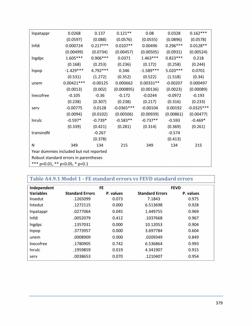
379

lnpatappr 0.0268 0.137 0.121** 0.08 0.0328 0.162***

(0.0597) (0.088) (0.0576) (0.0555) (0.0896) (0.0578)

lnfdi 0.000724 0.217*** 0.0107** 0.00496 0.296*** 0.0128**

(0.00499) (0.0734) (0.00457) (0.00505) (0.0931) (0.00524)

lngdpc 1.605*** 0.906*** 0.0371 1.463*** 0.823*** 0.218

(0.168) (0.253) (0.236) (0.172) (0.258) (0.244)

lnpop -1.429*** 4.792*** 0.346 -1.589*** 5.020*** 0.0701

(0.531) (1.272) (0.352) (0.522) (1.518) (0.34)

unem 0.00421*** -0.00125 0.000662 0.00331** -0.00207 0.000497

(0.0013) (0.002) (0.000895) (0.00136) (0.0023) (0.00089)

lnecofree -0.105 -0.36 -0.172 -0.0244 -0.0972 -0.193

(0.238) (0.307) (0.238) (0.217) (0.316) (0.233)

serv -0.00775 0.0128 -0.0365*** -0.00104 0.00192 -0.0325***

(0.0094) (0.0102) (0.00506) (0.00939) (0.00861) (0.00477)

lnrulc -0.597* -0.739* -0.583** -0.737** -0.593 -0.469*

(0.339) (0.421) (0.281) (0.314) (0.369) (0.261)

transindN

-0.267

-0.574

(0.378)

(0.413)

N 349 134 215 349 134 215

Year dummies included but not reported Robust standard errors in parentheses *** p<0.01, ** p<0.05, * p<0.1

Table A4.9.1 Model 1 - FE standard errors vs FEVD standard errors

Independent Variables

FE Standard Errors P. values

FEVD Standard Errors P. values

lnsedut .1265099 0.073 7.1843 0.975 lntedut .1272115 0.000 6.513698 0.928

lnpatappr .0277064 0.045 1.449755 0.969

lnfdi .0052079 0.412 .1037668 0.967

lngdpc .1357031 0.000 10.12053 0.904 lnpop .3773957 0.000 3.697784 0.604

unem .0008909 0.000 .0209349 0.849

lnecofree .1780905 0.742 6.536864 0.993 lnrulc .1959859 0.019 4.341907 0.915

serv .0038653 0.070 .1210407 0.954

380

Appendix – A5

Contents Table A5.1. Relative export advantage (RXA) of ETEs in medium-high and high tech sub-industries . 383


.............................................................................................................................................................. 383

Table A5.1.2 Correlation between Export sophistication and GDP per capita ..................................... 385

Table A5.1.3 Correlation matrix between potential measures of international competitiveness ....... 385

Table A5.1.4 Descriptive statistics for variables in levels ..................................................................... 386







Table A5.2.6.1 Model 1 - IV estimated results - ETEs (medium-high and high tech) .......................... 392











Table A5.3.4 Model 2 - FEVD estimated results (medium-high and high tech) .................................... 406





381


Table A5.3.6.3.1 Model 2 - IV estimated results – ETEs (high tech) ..................................................... 413

Table A5.3.6.3.2 Model 2 - IV estimated results - N-ETEs (high tech) .................................................. 414























Table A5.5.5 Model 2 - IV estimated results (medium-high and high tech) ........................................ 440

Table A5.5.5.1 Model 2 - IV estimated results –ETEs (medium-high and high tech)............................ 441






382

Table A5.5.5.4.1 Model 2 - IV estimated results -ETEs (medium-high tech) ........................................ 450

Table A5.5.5.4.2 Model 2 - IV estimated results –N-ETEs (medium-high tech) .................................... 451







Table A5.6.5.1 Model 1 - IV estimated results - ETEs .......................................................................... 458








Table A5.7.5.1 Model 2 - IV estimated results – ETEs .......................................................................... 466


Table A5.8 Driscoll-Kraay and IV estimated results (export market share) .......................................... 470

Table A5.8.1. Driscoll-Kraay and IV estimated results (relative export advantage, RXA) ..................... 471

Table A5.9 IV estimated results (medium-low, medium-high and high tech) ...................................... 472

Table A5.9.1 FEVD & Hausman and Taylor estimated results (medium-low, medium-high and high

tech) ...................................................................................................................................................... 474

383

Table A5.1. Relative export advantage (RXA) of ETEs in medium-high and high tech sub-industries

Industry Tech intensity

Bulgaria Croatia Czech Republic

Estonia Hungary Latvia

ChePH High 0.93 0.73 0.53 0.60 0.51 0.43 Ph M. high 0.48 0.87 0.22 0.18 0.53 0.78 ME M. high 0.58 0.48 1.06 0.37 0.61 0.36 OACM High 0.14 0.15 1.63 0.31 1.99 0.29 EMA M. high 0.80 1.20 1.96 1.19 2.12 0.59

RTCE High 0.26 0.60 1.02 2.49 3.62 0.37

MPOI High 0.29 0.31 0.47 0.51 0.58 0.26

MVTST M. high 0.05 0.12 1.26 0.42 1.29 0.21 AS High 0.07 0.09 0.24 0.04 0.02 0.08 RTE M. high 0.81 0.51 2.15 1.00 1.08 1.47


Lithuania Poland Romania Slovak Republic

Slovenia

ChePH High

0.91 0.58 0.58 0.55 0.64 Ph M. high

0.32 0.20 0.10 0.19 1.35

ME M. high

0.37 0.61 0.55 0.70 1.28 OACM High

0.22 0.24 0.20 0.40 0.14

EMA M. high

0.60 1.34 1.54 1.38 1.44 RTCE High

0.70 0.85 0.51 1.79 0.37

MPOI High

0.41 0.24 0.16 0.25 0.75 MVTST M. high

0.44 1.03 0.39 1.73 1.04

AS High

0.24 0.17 0.13 0.06 0.06 RTE M. high

1.30 1.19 1.73 1.89 1.08


Notes: RXA>1 indicates a relative export advantage in industry j



Austria Belgium Cyprus Denmark Finland France

ChePH High 0.42 2.06 0.27 0.51 0.52 1.23

Ph M. high 0.78 2.01 2.01 1.73 0.22 1.06

ME M. high 1.25 0.54 0.37 1.17 1.03 0.72

OACM High 0.36 0.45 0.30 0.54 0.35 0.59

EMA M. high 1.24 0.50 0.37 1.27 1.22 1.03

RTCE High 0.73 0.46 1.30 0.83 3.29 0.90

384

MPOI High 0.71 0.52 1.08 1.44 0.80 0.96

MVTST M. high 1.02 1.06 0.76 0.19 0.25 1.03

AS High 0.40 0.16 0.30 0.18 0.09 3.64

RTE M. high 2.77 0.68 0.10 0.59 0.21 0.82

Industry

Tech intensity

Germany Greece Ireland Italy Luxembour

g Malta

ChePH High 0.94 0.63 2.96 0.51 0.60 0.15

Ph M. high 0.76 0.82 4.44 0.65 0.08 0.61

ME M. high 1.58 0.34 0.18 2.13 0.71 0.23

OACM High 0.68 0.16 6.68 0.25 0.49 0.35

EMA M. high 1.33 0.64 0.49 0.81 0.72 1.18

RTCE High 0.79 0.38 1.37 0.40 0.99 17.03

MPOI High 1.45 0.29 1.87 0.69 0.40 1.11

MVTST M. high 1.92 0.10 0.03 0.54 0.36 0.08

AS High 1.14 0.57 0.26 0.42 0.39 0.57

RTE M. high 0.82 0.22 0.07 2.06 0.71 0.04

Industry

Tech intensity

Netherlands Norway Portugal Spain Sweden UK

ChePH High 1.58 0.42 0.45 0.79 0.43 1.09

Ph M. high 0.87 0.56 0.23 0.63 1.23 1.41

ME M. high 0.55 0.88 0.43 0.57 1.15 0.86

OACM High 4.22 0.37 0.27 0.27 0.37 1.76

EMA M. high 0.59 0.72 1.28 0.89 0.91 0.89

RTCE High 1.31 0.56 1.09 0.52 2.34 1.48

MPOI High 1.52 0.87 0.29 0.37 1.02 1.40

MVTST M. high 0.31 0.17 1.04 2.27 1.01 0.78

AS High 0.28 0.58 0.23 0.56 0.52 3.08

RTE M. high 0.74 0.34 0.83 1.54 0.68 0.72 Source: Own calculations based on STAN Bilateral Trade Database Ed. 2012 ISIC Revision 3

Notes: RXA>1 indicates a relative export advantage in industry j

385

Table A5.1.2 Correlation between Export sophistication and GDP per capita

Country Austria Belgium Bulgaria Croatia Cyprus Czech

Republic Denmark Estonia

Correlation coefficient

0.9783 0.9332 0.8702 0.9189 0.8988 0.8719 0.9237 0.8479

Country Finland France Germany Greece Hungary Ireland Italy


0.9055 0.9741 0.8513 0.9673 0.8455 0.9488 0.9324

Country Latvia Lithuania

Luxembourg

Malta Netherlan

ds Norway Poland


0.8092 0.9192 0.8865 0.2808 0.6448 -0.2094 0.9537

Country Portugal Romania

Slovak Republic

Slovenia Spain Sweden United

Kingdom


0.9181 0.9511 0.8836 0.8743 0.936 0.6995 0.2603

Table A5.1.3 Correlation matrix between potential measures of international competitiveness

Medium-low, medium-high and high tech measures | lnemsh~d lnrxa

-------------+------------------

lnemshind | 1.0000

lnrxa | 0.5624 1.0000

Medium-high and high tech measures | lnemsh~h lnrxam~h

-------------+------------------

lnemshmhtech | 1.0000

lnrxamhtech | 0.7050 1.0000

High tech measures | lnemsh~h lnrxah~t

-------------+------------------

lnemshhtech | 1.0000

lnrxahtech | 0.7241 1.0000

Medium-high tech measures | lnemsh~m lnrxam~t

-------------+------------------

lnemshmtech | 1.0000

lnrxamtech | 0.6838 1.0000

Medium and high tech measures (country level analysis) | lnEXPY lnmste~C lnhste~C lnRXAmid lnRXAh~h

-------------+---------------------------------------------

386

lnEXPY | 1.0000

lnmstechC | 0.5895 1.0000

lnhstechC | 0.6371 0.9291 1.0000

lnRXAmid | 0.6319 0.6577 0.4147 1.0000

lnRXAhigh | 0.6770 0.1849 0.4788 -0.0449 1.0000

Table A5.1.4 Descriptive statistics for variables in levels

Quantiles


emshind 1371 4.17 8.17 0.00 0.20 0.84 3.74 55.39

emshmhtech 4570 4.22 8.70 0.00 0.13 0.68 3.86 63.94

emshhtech 2285 4.23 8.71 0.00 0.09 0.52 3.65 62.75

emshmtech 2285 4.20 8.68 0.00 0.19 0.85 4.04 63.94

rxa 1371 0.90 0.65 0.03 0.48 0.78 1.13 5.66

rxamhtech 4570 0.89 1.30 0.00 0.31 0.61 1.07 25.76

rxahtech 2285 0.93 1.73 0.00 0.23 0.48 0.97 25.76

rxamtech 2285 0.85 0.62 0.00 0.45 0.70 1.14 6.39

EXPY 464 11154.73 3896.00 2848.85 8155.45 11685.00 14117.84 18723.78

mstechC 464 4.17 8.97 0.01 0.16 0.93 3.88 50.49

hstechC 464 3.98 6.80 0.02 0.18 0.61 3.51 32.78

RXAmid 464 0.79 0.48 0.11 0.35 0.69 1.21 1.99

RXAhigh 464 1.01 1.35 0.14 0.46 0.61 0.99 8.82

387


Table A5.2 Model 1 - Fixed effects estimated results (medium-high and high tech) xtreg lnemshmhtech lnsedut lntedut cskills lnpatappr lnfdi lngdpc lnpop unem lnecofree









between = 0.3573 avg = 13.3


F(25,3305) = 53.71

corr(u_i, Xb) = -0.9699 Prob > F = 0.0000

------------------------------------------------------------------------------

lnemshmhtech | Coef. Std. Err. t P>|t| [95% Conf. Interval]

-------------+----------------------------------------------------------------

lnsedut | .0066473 .1371567 0.05 0.961 -.2622733 .2755679

lntedut | .4480713 .1383239 3.24 0.001 .1768622 .7192804

cskills | (omitted)

lnpatappr | -.0673167 .030144 -2.23 0.026 -.1264195 -.0082139

lnfdi | .0030749 .0065681 0.47 0.640 -.0098031 .0159529

lngdpc | 1.541684 .1531341 10.07 0.000 1.241437 1.841932

lnpop | -4.392801 .4362566 -10.07 0.000 -5.248162 -3.537441

unem | .0035325 .0009747 3.62 0.000 .0016215 .0054435

lnecofree | .216126 .1927771 1.12 0.262 -.1618486 .5941006

lnrulc | .0190662 .2138647 0.09 0.929 -.4002544 .4383868

serv | .0057841 .0041922 1.38 0.168 -.0024355 .0140037

dist | (omitted)


year1996 | .1284116 .0536809 2.39 0.017 .0231604 .2336629

year1997 | .0904508 .054354 1.66 0.096 -.0161201 .1970217

year1998 | .0375129 .0557039 0.67 0.501 -.0717048 .1467306

year1999 | -.0272276 .0577506 -0.47 0.637 -.1404581 .0860029

year2000 | -.0653485 .058473 -1.12 0.264 -.1799954 .0492985

year2001 | -.066461 .0606392 -1.10 0.273 -.1853552 .0524333

year2002 | -.1089596 .0646934 -1.68 0.092 -.2358028 .0178835

year2003 | -.1310579 .0677822 -1.93 0.053 -.2639573 .0018415

year2004 | -.1309639 .071308 -1.84 0.066 -.2707763 .0088485

year2005 | -.1544219 .0762363 -2.03 0.043 -.303897 -.0049468

year2006 | -.2081729 .0802318 -2.59 0.010 -.3654819 -.0508639

year2007 | -.204008 .0835563 -2.44 0.015 -.3678353 -.0401807

year2008 | -.1381461 .0859307 -1.61 0.108 -.3066288 .0303366

year2009 | -.0594517 .0873455 -0.68 0.496 -.2307084 .1118051

year2010 | -.1484804 .0889977 -1.67 0.095 -.3229766 .0260159

_cons | 22.33965 5.177327 4.31 0.000 12.18856 32.49074

-------------+----------------------------------------------------------------

sigma_u | 7.4539724

sigma_e | .41591057


------------------------------------------------------------------------------

388


Table A5.2.1 Model 1 - Diagnostic tests Groupwise heteroskedasticity xttest3




chi2 (270) = 3.4e+06

Prob>chi2 = 0.0000

Autocorrelation in panel data . xtserial lnemshmhtech lnsedut lntedut cskills lnpatappr lnfdi lngdpc lnpop unem

lnecofree lnrulc serv dist transdummy year1996 year1997 year1998 year1999 year2000


year2010



F( 1, 269) = 95.964

Prob > F = 0.0000

Normality of residuals pantest2 lnemshmhtech lnsedut lntedut cskills lnpatappr lnfdi lngdpc lnpop unem



year2010, fe





LM= 1147.6511



LM5= 33.876999




F= 64.545133

Probability>F= 0


Skewness/Kurtosis tests for Normality ------- joint ------


-------------+---------------------------------------------------------------

__00000B | 3.6e+03 0.0000 0.0000 . 0.0000

Table A5.2.2 Model 1 - Driscoll-Kraay estimated results (medium-high and high tech) xtscc lnemshmhtech lnsedut lntedut cskills lnpatappr lnfdi lngdpc lnpop unem lnecofree


year2002 year2003 year2004 year2005 year2006 year2007 year2008 year2009 year2010,fe






389

------------------------------------------------------------------------------

| Drisc/Kraay


-------------+----------------------------------------------------------------

lnsedut | .0066473 .1782427 0.04 0.970 -.3442809 .3575755

lntedut | .4480713 .1414963 3.17 0.002 .1694902 .7266524

cskills | (omitted)

lnpatappr | -.0673167 .0527501 -1.28 0.203 -.1711722 .0365388

lnfdi | .0030749 .0042777 0.72 0.473 -.0053472 .011497

lngdpc | 1.541684 .2733236 5.64 0.000 1.003559 2.07981

lnpop | -4.392801 .4697144 -9.35 0.000 -5.317585 -3.468017

unem | .0035325 .0018687 1.89 0.060 -.0001467 .0072117

lnecofree | .216126 .3049482 0.71 0.479 -.3842628 .8165148

lnrulc | .0190662 .4318098 0.04 0.965 -.8310904 .8692229

serv | .0057841 .006645 0.87 0.385 -.0072987 .0188669

dist | .0214541 .00571 3.76 0.000 .0102122 .032696


year1996 | .1284116 .0246588 5.21 0.000 .0798629 .1769603

year1997 | .0904508 .0186104 4.86 0.000 .0538102 .1270914

year1998 | .0375129 .0242462 1.55 0.123 -.0102235 .0852494

year1999 | -.0272276 .029337 -0.93 0.354 -.0849869 .0305317

year2000 | -.0653485 .0296372 -2.20 0.028 -.1236988 -.0069982

year2001 | -.066461 .0361776 -1.84 0.067 -.1376881 .0047662

year2002 | -.1089596 .0427393 -2.55 0.011 -.1931057 -.0248135

year2003 | -.1310579 .0462134 -2.84 0.005 -.222044 -.0400719

year2004 | -.1309639 .0610153 -2.15 0.033 -.2510922 -.0108357

year2005 | -.1544219 .0710363 -2.17 0.031 -.2942797 -.0145641

year2006 | -.2081729 .0901684 -2.31 0.022 -.3856983 -.0306475

year2007 | -.204008 .0992636 -2.06 0.041 -.3994404 -.0085756

year2008 | -.1381461 .1069378 -1.29 0.198 -.3486876 .0723954

year2009 | -.0594517 .089528 -0.66 0.507 -.2357164 .116813

year2010 | -.1484804 .0944648 -1.57 0.117 -.3344647 .037504

_cons | (omitted)

------------------------------------------------------------------------------

Table A5.2.4 Model 1 - FEVD estimated results (medium-high and high tech) xtfevd lnemshmhtech lnsedut lntedut cskills lnpatappr lnfdi lngdpc lnpop unem



year2010, invariant (cskills dist transdummy)








------------------------------------------------------------------------------

| fevd


-------------+----------------------------------------------------------------

lnsedut | .0066473 3.396927 0.00 0.998 -6.653648 6.666942

lntedut | .4480712 5.591645 0.08 0.936 -10.51537 11.41151

lnpatappr | -.0673167 .9623298 -0.07 0.944 -1.95414 1.819507

lnfdi | .0030749 .2075636 0.01 0.988 -.4038915 .4100413

lngdpc | 1.541684 7.661675 0.20 0.841 -13.48043 16.5638

lnpop | -4.392801 2.624321 -1.67 0.094 -9.538261 .7526586

unem | .0035325 .0124319 0.28 0.776 -.0208424 .0279074

lnecofree | .2161257 3.333812 0.06 0.948 -6.320422 6.752673

390

lnrulc | .0190664 2.964983 0.01 0.995 -5.794325 5.832458

serv | .0057841 .0906264 0.06 0.949 -.1719056 .1834738

year1996 | .1284116 .7631332 0.17 0.866 -1.36785 1.624674

year1997 | .0904508 .895325 0.10 0.920 -1.664997 1.845899

year1998 | .0375129 .9795663 0.04 0.969 -1.883106 1.958132

year1999 | -.0272276 .8164943 -0.03 0.973 -1.628114 1.573659

year2000 | -.0653485 .8669077 -0.08 0.940 -1.765079 1.634382

year2001 | -.066461 1.058072 -0.06 0.950 -2.141005 2.008083

year2002 | -.1089596 1.050027 -0.10 0.917 -2.16773 1.94981

year2003 | -.1310579 1.1172 -0.12 0.907 -2.321532 2.059416

year2004 | -.1309639 1.089502 -0.12 0.904 -2.267132 2.005205

year2005 | -.1544219 1.212068 -0.13 0.899 -2.530902 2.222058

year2006 | -.2081729 1.17328 -0.18 0.859 -2.508603 2.092257

year2007 | -.204008 1.430642 -0.14 0.887 -3.009042 2.601026

year2008 | -.1381461 1.375258 -0.10 0.920 -2.83459 2.558298

year2009 | -.0594517 1.376848 -0.04 0.966 -2.759014 2.64011

year2010 | -.1484804 1.399729 -0.11 0.916 -2.892905 2.595944

cskills | -.8379719 4.035411 -0.21 0.836 -8.750132 7.074188

dist | -.0029434 .0033539 -0.88 0.380 -.0095193 .0036325

transdummy | -1.771144 10.18861 -0.17 0.862 -21.74778 18.20549

eta | 1 . . . . .

_cons | 30.20459 79.61571 0.38 0.704 -125.8966 186.3057

------------------------------------------------------------------------------

Table A5.2.5 Model 1 - Hausman and Taylor estimated results (medium-high and high tech) xthtaylor lnemshmhtech lnsedut lntedut cskills lnpatappr lnfdi lngdpc lnpop unem



year2010,endo (lnsedut lntedut cskills)




avg = 13.3

max = 16


Prob > chi2 = 0.0000

------------------------------------------------------------------------------

lnemshmhtech | Coef. Std. Err. z P>|z| [95% Conf. Interval]

-------------+----------------------------------------------------------------

TVexogenous |

lnpatappr | -.0402285 .0293262 -1.37 0.170 -.0977068 .0172499

lnfdi | .0004914 .0064159 0.08 0.939 -.0120835 .0130663

lngdpc | 2.24496 .1328334 16.90 0.000 1.984611 2.505308

lnpop | -.9964431 .2729665 -3.65 0.000 -1.531448 -.4614387

unem | .0049675 .0009426 5.27 0.000 .00312 .006815

lnecofree | .3991721 .1875633 2.13 0.033 .0315548 .7667894

lnrulc | -.0626792 .2088904 -0.30 0.764 -.4720968 .3467385

serv | .0043484 .0040916 1.06 0.288 -.003671 .0123677

year1996 | .1176501 .0524684 2.24 0.025 .0148139 .2204862

year1997 | .0646099 .0530752 1.22 0.223 -.0394156 .1686354

year1998 | .0103687 .0543855 0.19 0.849 -.0962248 .1169622

year1999 | -.0699946 .0562891 -1.24 0.214 -.1803192 .0403301

year2000 | -.1384423 .0567016 -2.44 0.015 -.2495755 -.0273092

year2001 | -.1616747 .0585354 -2.76 0.006 -.2764021 -.0469474

year2002 | -.2265004 .0621804 -3.64 0.000 -.3483717 -.1046291

year2003 | -.2601939 .0650354 -4.00 0.000 -.3876608 -.1327269

year2004 | -.2979283 .0677657 -4.40 0.000 -.4307467 -.1651099

391

year2005 | -.353316 .0719421 -4.91 0.000 -.4943199 -.2123121

year2006 | -.4448567 .074952 -5.94 0.000 -.5917598 -.2979536

year2007 | -.4673665 .0775325 -6.03 0.000 -.6193274 -.3154057

year2008 | -.4054393 .0798445 -5.08 0.000 -.5619316 -.248947

year2009 | -.2635684 .0829911 -3.18 0.001 -.426228 -.1009088

year2010 | -.3726656 .0841737 -4.43 0.000 -.537643 -.2076881

TVendogenous |

lnsedut | .2496374 .1318766 1.89 0.058 -.008836 .5081108

lntedut | .1309138 .1313395 1.00 0.319 -.126507 .3883345

TIexogenous |

dist | -.0013344 .0008806 -1.52 0.130 -.0030603 .0003916

transdummy | 1.071381 .9672452 1.11 0.268 -.8243851 2.967146

TIendogenous |

cskills | .7655087 3.109235 0.25 0.806 -5.328479 6.859496

|

_cons | -18.81571 16.20514 -1.16 0.246 -50.5772 12.94579

-------------+----------------------------------------------------------------

sigma_u | 7.160894

sigma_e | .4143464


------------------------------------------------------------------------------


Table A5.2.6 Model 1 - IV estimated results (medium-high and high tech) xtivreg2 lnemshmhtech cskills lngdpc lnpop unem lnecofree serv lnrulc dist transdummy








------------------------


avg = 12.8

max = 15


--------------------







F( 24, 3156) = 15.66

Prob > F = 0.0000




------------------------------------------------------------------------------

| Robust


-------------+----------------------------------------------------------------

lnsedut | .1399436 .2024388 0.69 0.489 -.2569813 .5368685

lntedut | .5940303 .2378455 2.50 0.013 .1276829 1.060378

lnpatappr | -.0771282 .06909 -1.12 0.264 -.2125939 .0583376

lnfdi | -.0029849 .009637 -0.31 0.757 -.0218803 .0159106

392

lngdpc | 1.571574 .2401647 6.54 0.000 1.100679 2.042469

lnpop | -4.431126 .6706334 -6.61 0.000 -5.746048 -3.116204

unem | .0020621 .0013306 1.55 0.121 -.0005468 .0046709

lnecofree | -.0611914 .2724328 -0.22 0.822 -.5953548 .4729719

serv | .0071299 .0084514 0.84 0.399 -.009441 .0237007

lnrulc | -.0859437 .3031814 -0.28 0.777 -.6803962 .5085088

year1996 | .2401015 .0990599 2.42 0.015 .0458733 .4343298

year1997 | .2021264 .0910967 2.22 0.027 .0235115 .3807412

year1998 | .1480505 .0835859 1.77 0.077 -.0158376 .3119387

year1999 | .0695011 .0782203 0.89 0.374 -.0838666 .2228688

year2000 | .0337942 .0728581 0.46 0.643 -.1090598 .1766482

year2001 | .0309833 .0632898 0.49 0.624 -.09311 .1550765

year2002 | -.0119223 .0579409 -0.21 0.837 -.1255279 .1016833

year2003 | -.0097416 .0553357 -0.18 0.860 -.1182391 .0987559

year2004 | -.0541639 .0533582 -1.02 0.310 -.1587841 .0504563

year2005 | -.0869496 .0515353 -1.69 0.092 -.1879957 .0140966

year2006 | -.1316133 .053001 -2.48 0.013 -.2355333 -.0276934

year2007 | -.1353721 .0517302 -2.62 0.009 -.2368003 -.0339439

year2008 | -.0831214 .0376148 -2.21 0.027 -.1568734 -.0093694

year2010 | -.0848502 .0313313 -2.71 0.007 -.1462819 -.0234184

------------------------------------------------------------------------------


Chi-sq(1) P-val = 0.0000

------------------------------------------------------------------------------




------------------------------------------------------------------------------



-endog- option:


Chi-sq(4) P-val = 0.0008


------------------------------------------------------------------------------







------------------------------------------------------------------------------

Table A5.2.6.1 Model 1 - IV estimated results - ETEs (medium-high and high tech) xtivreg2 lnemshmhtech cskills lngdpc lnpop unem lnecofree serv lnrulc dist transdummy








------------------------


avg = 13.3

max = 15


393

--------------------







F( 24, 1206) = 19.54

Prob > F = 0.0000




------------------------------------------------------------------------------

| Robust


-------------+----------------------------------------------------------------

lnsedut | .1952297 .6618024 0.29 0.768 -1.103182 1.493642

lntedut | -.7948303 .4962951 -1.60 0.110 -1.768528 .1788675

lnpatappr | -.4790029 .1921727 -2.49 0.013 -.8560328 -.101973

lnfdi | -.1334717 .1566632 -0.85 0.394 -.4408344 .173891

lngdpc | .5816821 .4227933 1.38 0.169 -.24781 1.411174

lnpop | 2.372562 2.910227 0.82 0.415 -3.337108 8.082232

unem | -.0086893 .0025283 -3.44 0.001 -.0136498 -.0037289

lnecofree | .1294825 .5211792 0.25 0.804 -.8930362 1.152001

serv | .0005366 .0141007 0.04 0.970 -.0271281 .0282013

lnrulc | .5205598 .4480107 1.16 0.245 -.3584072 1.399527

year1996 | -1.571125 .4189215 -3.75 0.000 -2.393021 -.7492292

year1997 | -1.44155 .3753862 -3.84 0.000 -2.178033 -.7050675

year1998 | -1.391926 .3501737 -3.97 0.000 -2.078944 -.7049088

year1999 | -1.430992 .3247988 -4.41 0.000 -2.068225 -.7937583

year2000 | -1.328463 .2942554 -4.51 0.000 -1.905772 -.7511536

year2001 | -1.096504 .2545619 -4.31 0.000 -1.595937 -.5970707

year2002 | -.9002179 .2024752 -4.45 0.000 -1.297461 -.5029751

year2003 | -.7976994 .1834149 -4.35 0.000 -1.157547 -.4378516

year2004 | -.5931634 .1496387 -3.96 0.000 -.8867444 -.2995823

year2005 | -.5092432 .1390069 -3.66 0.000 -.7819655 -.2365209

year2006 | -.3769978 .1222872 -3.08 0.002 -.616917 -.1370786

year2007 | -.1939025 .1065175 -1.82 0.069 -.4028826 .0150777

year2008 | -.0711946 .0905889 -0.79 0.432 -.248924 .1065349

year2010 | .1303283 .0756506 1.72 0.085 -.0180931 .2787497

------------------------------------------------------------------------------


Chi-sq(1) P-val = 0.0000

------------------------------------------------------------------------------




------------------------------------------------------------------------------



-endog- option:


Chi-sq(4) P-val = 0.0005


------------------------------------------------------------------------------






394


------------------------------------------------------------------------------

Table A5.2.6.2 Model 1 - IV estimated results –N-ETEs (medium-high and high tech) xtivreg2 lnemshmhtech cskills lngdpc lnpop unem lnecofree serv lnrulc dist transdummy








------------------------


avg = 12.5

max = 15


--------------------







F( 24, 1926) = 3.91

Prob > F = 0.0000




------------------------------------------------------------------------------

| Robust


-------------+----------------------------------------------------------------

lnsedut | -.3280825 .1565764 -2.10 0.036 -.6351596 -.0210053

lntedut | .2917022 .2340289 1.25 0.213 -.1672744 .7506788

lnpatappr | .1233427 .066653 1.85 0.064 -.0073769 .2540623

lnfdi | .0115541 .0093632 1.23 0.217 -.006809 .0299172

lngdpc | -.4715698 .3389591 -1.39 0.164 -1.136335 .1931956

lnpop | -2.701889 .6122162 -4.41 0.000 -3.902565 -1.501213

unem | -.0003338 .001271 -0.26 0.793 -.0028264 .0021588

lnecofree | -.0768207 .2653024 -0.29 0.772 -.5971309 .4434895

serv | -.0117376 .0071989 -1.63 0.103 -.025856 .0023809

lnrulc | -.8860703 .4119562 -2.15 0.032 -1.693997 -.0781433

year1996 | -.1153767 .1118698 -1.03 0.303 -.3347753 .1040219

year1997 | -.0993442 .1025621 -0.97 0.333 -.3004887 .1018004

year1998 | -.1163879 .0907828 -1.28 0.200 -.2944308 .0616551

year1999 | -.0987693 .0824043 -1.20 0.231 -.2603804 .0628418

year2000 | -.1002267 .0715184 -1.40 0.161 -.2404884 .0400351

year2001 | -.0585931 .0611852 -0.96 0.338 -.1785892 .061403

year2002 | -.0443178 .0557202 -0.80 0.427 -.1535961 .0649605

year2003 | -.0049112 .0513555 -0.10 0.924 -.1056294 .095807

year2004 | -.0154307 .049206 -0.31 0.754 -.1119333 .081072

year2005 | -.0251745 .044828 -0.56 0.574 -.1130909 .0627419

year2006 | -.0370108 .0406477 -0.91 0.363 -.1167288 .0427073

year2007 | -.0195811 .0401961 -0.49 0.626 -.0984135 .0592513

year2008 | -.0203023 .0312567 -0.65 0.516 -.0816028 .0409983

395

year2010 | -.0611201 .0244465 -2.50 0.012 -.1090644 -.0131758

------------------------------------------------------------------------------


Chi-sq(1) P-val = 0.0000

------------------------------------------------------------------------------




------------------------------------------------------------------------------



-endog- option:


Chi-sq(4) P-val = 0.3323


------------------------------------------------------------------------------







--------------------------------------------------------------------------------------

Table A5.2.6.3 Model 1 - IV estimated results (high tech) xtivreg2 lnemshmhtech cskills lngdpc lnpop unem lnecofree serv lnrulc dist transdummy



lnfdi = lnsedutlag1 lntedutlag1 lnpatapprlag1 lnfdilag1) if mhtechintens==1, fe endog





------------------------


avg = 12.8

max = 15


--------------------







F( 24, 1566) = 6.57

Prob > F = 0.0000




------------------------------------------------------------------------------

| Robust


-------------+----------------------------------------------------------------

lnsedut | .4473376 .3491348 1.28 0.200 -.2374834 1.132159

lntedut | .7832476 .431423 1.82 0.070 -.06298 1.629475

lnpatappr | -.2173787 .1219136 -1.78 0.075 -.4565097 .0217523

396

lnfdi | -.0122058 .0167072 -0.73 0.465 -.0449766 .0205651

lngdpc | 1.793507 .4206616 4.26 0.000 .9683873 2.618626

lnpop | -3.423159 1.123148 -3.05 0.002 -5.626191 -1.220126

unem | .0035996 .0024182 1.49 0.137 -.0011436 .0083427

lnecofree | .0590562 .4855697 0.12 0.903 -.8933791 1.011492

serv | .013172 .0150688 0.87 0.382 -.0163852 .0427292

lnrulc | .2416909 .5202102 0.46 0.642 -.778691 1.262073

year1996 | .3567661 .172619 2.07 0.039 .0181773 .6953549

year1997 | .3349443 .1605689 2.09 0.037 .0199916 .6498969

year1998 | .2483239 .1482803 1.67 0.094 -.0425249 .5391727

year1999 | .1284968 .1401919 0.92 0.360 -.1464868 .4034803

year2000 | .1040232 .1300797 0.80 0.424 -.1511255 .3591719

year2001 | .0751594 .1122336 0.67 0.503 -.1449846 .2953033

year2002 | .0204579 .1027182 0.20 0.842 -.1810219 .2219376

year2003 | .0171007 .0982833 0.17 0.862 -.17568 .2098814

year2004 | -.0468091 .0948619 -0.49 0.622 -.2328789 .1392607

year2005 | -.1050729 .0913715 -1.15 0.250 -.2842963 .0741505

year2006 | -.1660474 .0937589 -1.77 0.077 -.3499535 .0178587

year2007 | -.1625663 .0918048 -1.77 0.077 -.3426396 .0175071

year2008 | -.0878096 .0667486 -1.32 0.189 -.2187356 .0431164

year2010 | -.1183215 .0565171 -2.09 0.036 -.2291787 -.0074644

------------------------------------------------------------------------------


Chi-sq(1) P-val = 0.0000

------------------------------------------------------------------------------




------------------------------------------------------------------------------



-endog- option:


Chi-sq(4) P-val = 0.0085


------------------------------------------------------------------------------







------------------------------------------------------------------------------

Table A5.2.6.3.1 Model 1 - IV estimated results - ETEs (high tech) xtivreg2 lnemshmhtech cskills lngdpc lnpop unem lnecofree serv lnrulc dist transdummy








------------------------


avg = 13.3

max = 15


--------------------

397






Number of obs = 665

F( 25, 590) = 9.42

Prob > F = 0.0000




------------------------------------------------------------------------------

| Robust


-------------+----------------------------------------------------------------

lnsedut | .198904 1.280211 0.16 0.877 -2.315421 2.713229

lntedut | -1.251518 .8483557 -1.48 0.141 -2.917683 .4146463

lnpatappr | -.9870772 .3430659 -2.88 0.004 -1.660856 -.3132982

lnfdi | -.1711796 .2875938 -0.60 0.552 -.7360118 .3936526

lngdpc | -.0285719 .7144161 -0.04 0.968 -1.43168 1.374536

lnpop | 5.02204 5.299476 0.95 0.344 -5.386092 15.43017

unem | -.0123027 .0045496 -2.70 0.007 -.021238 -.0033673

lnecofree | .5824788 .9035067 0.64 0.519 -1.192002 2.35696

serv | -.0138461 .0261494 -0.53 0.597 -.0652033 .0375112

lnrulc | 1.482213 .7813957 1.90 0.058 -.0524425 3.016869

transindn | .104459 1.456044 0.07 0.943 -2.755202 2.96412

year1997 | .19873 .2359112 0.84 0.400 -.264598 .6620579

year1998 | .2495063 .2791831 0.89 0.372 -.2988073 .7978199

year1999 | .2308803 .3071002 0.75 0.452 -.3722624 .834023

year2000 | .3684242 .3485211 1.06 0.291 -.3160688 1.052917

year2001 | .7136917 .3960203 1.80 0.072 -.0640893 1.491473

year2002 | 1.086806 .4918969 2.21 0.028 .1207237 2.052888

year2003 | 1.226051 .5121049 2.39 0.017 .2202803 2.231821

year2004 | 1.532979 .5730116 2.68 0.008 .4075884 2.65837

year2005 | 1.623036 .6135215 2.65 0.008 .4180838 2.827988

year2006 | 1.85954 .6783466 2.74 0.006 .5272725 3.191808

year2007 | 2.180718 .724708 3.01 0.003 .7573966 3.604039

year2008 | 2.415822 .7339488 3.29 0.001 .9743517 3.857292

year2009 | 2.507309 .7820675 3.21 0.001 .9713335 4.043284

year2010 | 2.68994 .8245002 3.26 0.001 1.070628 4.309252

------------------------------------------------------------------------------


Chi-sq(1) P-val = 0.0000

------------------------------------------------------------------------------




------------------------------------------------------------------------------



-endog- option:


Chi-sq(4) P-val = 0.0017


------------------------------------------------------------------------------





year2010


398


------------------------------------------------------------------------------

Table A5.2.6.3.2 Model 1 - IV estimated results – N-ETEs (high tech) xtivreg2 lnemshmhtech cskills lngdpc lnpop unem lnecofree serv lnrulc dist transdummy






Vars dropped: cskills dist transdummy transindn year2009


------------------------


avg = 12.5

max = 15


--------------------







F( 24, 951) = 1.46

Prob > F = 0.0727




------------------------------------------------------------------------------

| Robust


-------------+----------------------------------------------------------------

lnsedut | -.3375307 .273709 -1.23 0.218 -.8746741 .1996128

lntedut | .3103843 .4258358 0.73 0.466 -.525302 1.146071

lnpatappr | .1504939 .1167502 1.29 0.198 -.0786238 .3796117

lnfdi | .0091923 .0160264 0.57 0.566 -.0222588 .0406435

lngdpc | -.3710433 .5602907 -0.66 0.508 -1.470592 .7285056

lnpop | -1.437164 .965156 -1.49 0.137 -3.331245 .4569179

unem | .0015189 .0020722 0.73 0.464 -.0025477 .0055856

lnecofree | -.027151 .4676405 -0.06 0.954 -.9448776 .8905757

serv | -.0077963 .0119496 -0.65 0.514 -.0312469 .0156544

lnrulc | -.9998117 .69037 -1.45 0.148 -2.354636 .3550129

year1996 | -.0263008 .1874509 -0.14 0.888 -.394166 .3415643

year1997 | .0089463 .1721086 0.05 0.959 -.3288103 .3467029

year1998 | -.0280909 .1544092 -0.18 0.856 -.3311131 .2749313

year1999 | -.0354209 .1415122 -0.25 0.802 -.3131332 .2422913

year2000 | -.0152459 .1232223 -0.12 0.902 -.2570648 .226573

year2001 | .0226422 .1043773 0.22 0.828 -.1821942 .2274787

year2002 | .0308054 .0949041 0.32 0.746 -.1554402 .2170511

year2003 | .0765164 .0873999 0.88 0.382 -.0950026 .2480355

year2004 | .0541268 .0844058 0.64 0.522 -.1115164 .21977

year2005 | .0403186 .0744287 0.54 0.588 -.1057448 .186382

year2006 | -.0031439 .0684843 -0.05 0.963 -.1375418 .1312539

year2007 | .0020158 .0681561 0.03 0.976 -.1317378 .1357694

year2008 | -.0191508 .0533456 -0.36 0.720 -.1238396 .085538

399

year2010 | -.0773921 .0413598 -1.87 0.062 -.1585591 .003775

------------------------------------------------------------------------------


Chi-sq(1) P-val = 0.0000

------------------------------------------------------------------------------




------------------------------------------------------------------------------



-endog- option:


Chi-sq(4) P-val = 0.1171


------------------------------------------------------------------------------






Dropped collinear: cskills dist transdummy transindn year2009

------------------------------------------------------------------------------

Table A5.2.6.4 Model 1 - IV estimated results (medium-high tech) xtivreg2 lnemshmhtech cskills lngdpc lnpop unem lnecofree serv lnrulc dist transdummy



lnfdi = lnsedutlag1 lntedutlag1 lnpatapprlag1 lnfdilag1) if mhtechintens==0, fe endog





------------------------


avg = 12.8

max = 15


--------------------







F( 24, 1566) = 17.01

Prob > F = 0.0000




------------------------------------------------------------------------------

| Robust


-------------+----------------------------------------------------------------

lnsedut | -.1674505 .1984741 -0.84 0.399 -.5567534 .2218525

lntedut | .4048131 .194179 2.08 0.037 .0239348 .7856913

lnpatappr | .0631224 .0583133 1.08 0.279 -.051258 .1775028

400

lnfdi | .006236 .0093863 0.66 0.507 -.0121749 .024647

lngdpc | 1.349641 .2203114 6.13 0.000 .9175047 1.781778

lnpop | -5.439093 .6492838 -8.38 0.000 -6.71265 -4.165536

unem | .0005246 .0010658 0.49 0.623 -.0015659 .0026151

lnecofree | -.1814391 .2438059 -0.74 0.457 -.6596594 .2967812

serv | .0010877 .0072886 0.15 0.881 -.0132087 .0153841

lnrulc | -.4135783 .3000781 -1.38 0.168 -1.002176 .175019

year1996 | .1234369 .0948049 1.30 0.193 -.062521 .3093949

year1997 | .0693084 .08228 0.84 0.400 -.0920821 .230699

year1998 | .0477772 .07472 0.64 0.523 -.0987846 .194339

year1999 | .0105054 .0680696 0.15 0.877 -.1230118 .1440227

year2000 | -.0364348 .0644958 -0.56 0.572 -.162942 .0900723

year2001 | -.0131928 .0574562 -0.23 0.818 -.125892 .0995065

year2002 | -.0443024 .0526282 -0.84 0.400 -.1475316 .0589267

year2003 | -.0365839 .0503018 -0.73 0.467 -.1352499 .0620821

year2004 | -.0615187 .0487717 -1.26 0.207 -.1571835 .0341461

year2005 | -.0688262 .0478742 -1.44 0.151 -.1627306 .0250781

year2006 | -.0971792 .0488335 -1.99 0.047 -.1929651 -.0013933

year2007 | -.1081779 .0471089 -2.30 0.022 -.2005811 -.0157747

year2008 | -.0784331 .0340115 -2.31 0.021 -.1451459 -.0117203

year2010 | -.0513788 .0261566 -1.96 0.050 -.1026845 -.0000731

------------------------------------------------------------------------------


Chi-sq(1) P-val = 0.0000

------------------------------------------------------------------------------




------------------------------------------------------------------------------



-endog- option:


Chi-sq(4) P-val = 0.1292


------------------------------------------------------------------------------







--------------------------------------------------------------------------------------

Table A5.2.6.4.1 Model 1 - IV estimated results – ETEs (medium-high tech) xtivreg2 lnemshmhtech cskills lngdpc lnpop unem lnecofree serv lnrulc dist transdummy




fe endog (lnsedut lntedut lnpatappr lnfd

> i) small robust bw(3)




------------------------


avg = 13.3

max = 15


--------------------

401






Number of obs = 665

F( 25, 590) = 18.47

Prob > F = 0.0000




------------------------------------------------------------------------------

| Robust


-------------+----------------------------------------------------------------

lnsedut | .0111428 .6243905 0.02 0.986 -1.215156 1.237441

lntedut | -.4679169 .4650778 -1.01 0.315 -1.381326 .4454926

lnpatappr | -.011925 .1867436 -0.06 0.949 -.3786882 .3548381

lnfdi | -.0453126 .1348395 -0.34 0.737 -.3101363 .2195111

lngdpc | 1.201673 .3836031 3.13 0.002 .4482793 1.955067

lnpop | -.7327731 2.822518 -0.26 0.795 -6.276178 4.810631

unem | -.0054929 .002273 -2.42 0.016 -.009957 -.0010288

lnecofree | -.2989488 .483659 -0.62 0.537 -1.248852 .6509541

serv | .0119407 .0140464 0.85 0.396 -.0156462 .0395276

lnrulc | -.3595579 .422086 -0.85 0.395 -1.188532 .469416

transindn | -.8155096 .6574322 -1.24 0.215 -2.106702 .4756825

year1997 | .0846869 .1111557 0.76 0.446 -.1336221 .3029959

year1998 | .1333968 .1281721 1.04 0.298 -.1183323 .3851259

year1999 | .0818291 .1463964 0.56 0.576 -.2056925 .3693506

year2000 | .1487755 .1649361 0.90 0.367 -.1751578 .4727088

year2001 | .285964 .1909751 1.50 0.135 -.0891097 .6610378

year2002 | .3305668 .2389493 1.38 0.167 -.1387278 .7998615

year2003 | .3958062 .2473209 1.60 0.110 -.0899302 .8815426

year2004 | .5069215 .2779604 1.82 0.069 -.0389908 1.052834

year2005 | .603016 .2979247 2.02 0.043 .0178939 1.188138

year2006 | .6390865 .3279505 1.95 0.052 -.005006 1.283179

year2007 | .6839278 .3522095 1.94 0.053 -.0078091 1.375665

year2008 | .7064335 .3614573 1.95 0.051 -.0034661 1.416333

year2009 | .7575518 .3858116 1.96 0.050 -.0001794 1.515283

year2010 | .8530488 .4119988 2.07 0.039 .0438862 1.662212

------------------------------------------------------------------------------


Chi-sq(1) P-val = 0.0000

------------------------------------------------------------------------------




------------------------------------------------------------------------------



-endog- option:


Chi-sq(4) P-val = 0.2387


------------------------------------------------------------------------------





year2010

402



------------------------------------------------------------------------------

Table A5.2.6.4.2 Model 1 - IV estimated results – N-ETEs (medium-high tech) xtivreg2 lnemshmhtech cskills lngdpc lnpop unem lnecofree serv lnrulc dist transdummy








------------------------


avg = 12.5

max = 15


--------------------







F( 24, 951) = 4.36

Prob > F = 0.0000




------------------------------------------------------------------------------

| Robust


-------------+----------------------------------------------------------------

lnsedut | -.318634 .1566759 -2.03 0.042 -.6261044 -.0111636

lntedut | .2730445 .194708 1.40 0.161 -.1090624 .6551514

lnpatappr | .0961931 .0671562 1.43 0.152 -.0355984 .2279847

lnfdi | .0139154 .0092796 1.50 0.134 -.0042955 .0321263

lngdpc | -.5721201 .367021 -1.56 0.119 -1.292385 .1481445

lnpop | -3.966668 .7008103 -5.66 0.000 -5.341981 -2.591354

unem | -.0021867 .0013669 -1.60 0.110 -.0048691 .0004957

lnecofree | -.126508 .2490801 -0.51 0.612 -.6153181 .3623022

serv | -.0156783 .0081918 -1.91 0.056 -.0317544 .0003979

lnrulc | -.7723529 .4490001 -1.72 0.086 -1.653498 .1087926

year1996 | -.2044467 .1179135 -1.73 0.083 -.4358474 .0269539

year1997 | -.2076314 .1080195 -1.92 0.055 -.4196155 .0043527

year1998 | -.2046822 .0913745 -2.24 0.025 -.3840012 -.0253631

year1999 | -.1621109 .0825139 -1.96 0.050 -.3240412 -.0001805

year2000 | -.1852075 .0706913 -2.62 0.009 -.3239366 -.0464785

year2001 | -.139823 .0617644 -2.26 0.024 -.2610332 -.0186127

year2002 | -.1194326 .0564736 -2.11 0.035 -.2302599 -.0086052

year2003 | -.0863312 .0526675 -1.64 0.102 -.189689 .0170267

year2004 | -.0849828 .0499536 -1.70 0.089 -.1830149 .0130492

year2005 | -.0906651 .0499837 -1.81 0.070 -.1887563 .0074261

year2006 | -.0708732 .0436872 -1.62 0.105 -.1566076 .0148612

year2007 | -.0411719 .0422376 -0.97 0.330 -.1240616 .0417179

year2008 | -.0214471 .032233 -0.67 0.506 -.0847031 .0418089

403

year2010 | -.0448439 .0263458 -1.70 0.089 -.0965465 .0068587

------------------------------------------------------------------------------


Chi-sq(1) P-val = 0.0000

------------------------------------------------------------------------------




------------------------------------------------------------------------------



-endog- option:


Chi-sq(4) P-val = 0.6432


------------------------------------------------------------------------------







------------------------------------------------------------------------------

Table A5.3 Model 2 - Fixed effects estimated results (medium-high and high tech)

xtreg lnemshmhtech avyrs sqravyrs cskills lnpatappr lnfdi lngdpc lnpop unem lnecofree









between = 0.3106 avg = 13.3


F(25,3305) = 55.57

corr(u_i, Xb) = -0.9590 Prob > F = 0.0000

------------------------------------------------------------------------------


-------------+----------------------------------------------------------------

avyrs | -.8968393 .2199295 -4.08 0.000 -1.328051 -.4656276

sqravyrs | .0341225 .0101728 3.35 0.001 .014177 .0540681

cskills | (omitted)

lnpatappr | -.0885896 .0300119 -2.95 0.003 -.1474334 -.0297458

lnfdi | .0115371 .0064621 1.79 0.074 -.001133 .0242071

lngdpc | 1.867017 .1297671 14.39 0.000 1.612585 2.121449

lnpop | -3.763733 .392797 -9.58 0.000 -4.533882 -2.993583

unem | .0024554 .001021 2.40 0.016 .0004535 .0044573

lnecofree | .2223198 .1906727 1.17 0.244 -.1515288 .5961684

lnrulc | -.1933507 .215436 -0.90 0.370 -.6157522 .2290507

serv | .0094993 .0042691 2.23 0.026 .001129 .0178697

dist | (omitted)


404

year1996 | .166084 .0531655 3.12 0.002 .0618433 .2703247

year1997 | .1517407 .0538459 2.82 0.005 .0461661 .2573154

year1998 | .117544 .0546875 2.15 0.032 .0103192 .2247689

year1999 | .0568837 .0561313 1.01 0.311 -.0531718 .1669393

year2000 | .0146843 .0560963 0.26 0.794 -.0953026 .1246713

year2001 | .0434266 .0577902 0.75 0.452 -.0698817 .1567349

year2002 | .0185194 .0613188 0.30 0.763 -.1017073 .1387461

year2003 | .0169961 .0637204 0.27 0.790 -.1079393 .1419314

year2004 | .0321439 .067101 0.48 0.632 -.0994199 .1637076

year2005 | .0238619 .0714029 0.33 0.738 -.1161365 .1638603

year2006 | -.0170238 .0756877 -0.22 0.822 -.1654232 .1313756

year2007 | -.0077467 .0785849 -0.10 0.921 -.1618267 .1463332

year2008 | .085773 .0800901 1.07 0.284 -.0712583 .2428042

year2009 | .1981758 .0792629 2.50 0.012 .0427664 .3535853

year2010 | .1323395 .0817661 1.62 0.106 -.0279778 .2926568

_cons | 21.02575 4.835919 4.35 0.000 11.54405 30.50744

-------------+----------------------------------------------------------------

sigma_u | 6.6546768

sigma_e | .41385514


------------------------------------------------------------------------------


Table A5.3.1 Model 2 - Diagnostic tests Groupwise heteroskedasticity Modified Wald test for groupwise heteroskedasticity



chi2 (270) = 6.6e+05

Prob>chi2 = 0.0000

Autocorrelation in panel data xtserial lnemshmhtech avyrs sqravyrs cskills lnpatappr lnfdi lngdpc lnpop unem



year2010



F( 1, 269) = 95.579

Prob > F = 0.0000

Normality of residuals pantest2 lnemshmhtech avyrs sqravyrs cskills lnpatappr lnfdi lngdpc lnpop unem



year2010





LM= 1118.6225



LM5= 33.445814




F= 64.865809

Probability>F= 0



405

------- joint ------


-------------+---------------------------------------------------------------

__00000B | 3.6e+03 0.0000 0.0000 . 0.0000

Table A5.3.2 Model 2 - Driscoll-Kraay estimated results (medium-high and high tech) xtscc lnemshmhtech avyrs sqravyrs cskills lnpatappr lnfdi lngdpc lnpop unem lnecofree








------------------------------------------------------------------------------

| Drisc/Kraay


-------------+----------------------------------------------------------------

avyrs | -.8968393 .501026 -1.79 0.075 -1.88327 .0895917

sqravyrs | .0341225 .0223712 1.53 0.128 -.0099223 .0781674

cskills | (omitted)

lnpatappr | -.0885896 .0418109 -2.12 0.035 -.1709078 -.0062715

lnfdi | .0115371 .0051818 2.23 0.027 .0013351 .0217391

lngdpc | 1.867017 .3607054 5.18 0.000 1.156853 2.577182

lnpop | -3.763733 .6856884 -5.49 0.000 -5.113731 -2.413734

unem | .0024554 .0011102 2.21 0.028 .0002697 .0046412

lnecofree | .2223198 .2454636 0.91 0.366 -.2609543 .7055939

lnrulc | -.1933507 .3777967 -0.51 0.609 -.9371652 .5504638

serv | .0094993 .007884 1.20 0.229 -.0060229 .0250216

dist | .0201923 .011184 1.81 0.072 -.001827 .0422115


year1996 | .166084 .0168978 9.83 0.000 .1328152 .1993528

year1997 | .1517407 .0192261 7.89 0.000 .1138879 .1895936

year1998 | .117544 .0227153 5.17 0.000 .0728216 .1622664

year1999 | .0568837 .0313853 1.81 0.071 -.0049082 .1186757

year2000 | .0146843 .0418711 0.35 0.726 -.0677524 .097121

year2001 | .0434266 .0557711 0.78 0.437 -.0663768 .15323

year2002 | .0185194 .0672279 0.28 0.783 -.1138404 .1508793

year2003 | .0169961 .073638 0.23 0.818 -.127984 .1619761

year2004 | .0321439 .0946313 0.34 0.734 -.1541684 .2184561

year2005 | .0238619 .1104838 0.22 0.829 -.1936611 .2413848

year2006 | -.0170238 .1351754 -0.13 0.900 -.2831601 .2491124

year2007 | -.0077467 .1477067 -0.05 0.958 -.298555 .2830615

year2008 | .085773 .1545156 0.56 0.579 -.2184407 .3899866

year2009 | .1981758 .1191961 1.66 0.098 -.0365001 .4328517

year2010 | .1323395 .127525 1.04 0.300 -.1187345 .3834135

_cons | (omitted)

------------------------------------------------------------------------------

406

Table A5.3.4 Model 2 - FEVD estimated results (medium-high and high tech) . xtfevd lnemshmhtech avyrs sqravyrs cskills lnpatappr lnfdi lngdpc lnpop unem



year2010,invariant (cskills dist transdummy)








------------------------------------------------------------------------------

| fevd


-------------+----------------------------------------------------------------

avyrs | -.8968394 3.979761 -0.23 0.822 -8.699888 6.906209

sqravyrs | .0341225 .1741807 0.20 0.845 -.3073906 .3756357

lnpatappr | -.0885897 .5392303 -0.16 0.870 -1.145849 .9686697

lnfdi | .0115371 .2175439 0.05 0.958 -.4149974 .4380716

lngdpc | 1.867017 3.675641 0.51 0.612 -5.339749 9.073784

lnpop | -3.763732 1.880162 -2.00 0.045 -7.450134 -.0773306

unem | .0024554 .0108626 0.23 0.821 -.0188427 .0237535

lnecofree | .2223195 2.868015 0.08 0.938 -5.400948 5.845587

lnrulc | -.1933509 2.3315 -0.08 0.934 -4.764683 4.377981

serv | .0094993 .0672242 0.14 0.888 -.1223061 .1413047

year1996 | .1660841 .5306033 0.31 0.754 -.8742606 1.206429

year1997 | .1517408 .6135297 0.25 0.805 -1.051196 1.354678

year1998 | .1175441 .650426 0.18 0.857 -1.157735 1.392823

year1999 | .0568838 .7107923 0.08 0.936 -1.336754 1.450522

year2000 | .0146844 .6649677 0.02 0.982 -1.289106 1.318475

year2001 | .0434267 .6957611 0.06 0.950 -1.32074 1.407593

year2002 | .0185195 .7299116 0.03 0.980 -1.412606 1.449645

year2003 | .0169961 .9005044 0.02 0.985 -1.748607 1.782599

year2004 | .032144 1.029664 0.03 0.975 -1.986701 2.050989

year2005 | .023862 1.177211 0.02 0.984 -2.284276 2.332

year2006 | -.0170237 1.214297 -0.01 0.989 -2.397876 2.363828

year2007 | -.0077467 1.51455 -0.01 0.996 -2.977298 2.961805

year2008 | .085773 1.478059 0.06 0.954 -2.812231 2.983778

year2009 | .1981759 1.326524 0.15 0.881 -2.402717 2.799069

year2010 | .1323396 1.357495 0.10 0.922 -2.529277 2.793956

cskills | .0738706 2.774635 0.03 0.979 -5.366308 5.514049

dist | -.0026613 .0019516 -1.36 0.173 -.0064877 .0011651

transdummy | -.9081958 5.696299 -0.16 0.873 -12.07683 10.26044

eta | 1 . . . . .

_cons | 23.77879 48.47387 0.49 0.624 -71.26309 118.8207

--------------------------------------------------------------------------------------

Table A5.3.5 Model 2 - Hausman and Taylor estimated results (medium-high and high tech) xthtaylor lnemshmhtech avyrs sqravyrs cskills lnpatappr lnfdi lngdpc lnpop unem



year2010, endo (avyrs sqravyrs cskills)



407


avg = 13.3

max = 16


Prob > chi2 = 0.0000

------------------------------------------------------------------------------

lnemshmhtech | Coef. Std. Err. z P>|z| [95% Conf. Interval]

-------------+----------------------------------------------------------------

TVexogenous |

lnpatappr | -.0493255 .0290654 -1.70 0.090 -.1062926 .0076416

lnfdi | .0049894 .0062839 0.79 0.427 -.0073269 .0173057

lngdpc | 2.378784 .1162905 20.46 0.000 2.150859 2.606709

lnpop | -.7213987 .2451031 -2.94 0.003 -1.201792 -.2410054

unem | .0035239 .0009924 3.55 0.000 .0015789 .0054688

lnecofree | .4774073 .1846688 2.59 0.010 .1154632 .8393514

lnrulc | -.2947224 .2102893 -1.40 0.161 -.7068819 .1174371

serv | .0060939 .0041544 1.47 0.142 -.0020486 .0142363

year1996 | .1655502 .0519701 3.19 0.001 .0636907 .2674097

year1997 | .1369552 .0526115 2.60 0.009 .0338385 .240072

year1998 | .1090316 .0534438 2.04 0.041 .0042837 .2137796

year1999 | .0406922 .0548316 0.74 0.458 -.0667757 .14816

year2000 | -.0223529 .0546961 -0.41 0.683 -.1295553 .0848494

year2001 | -.0189106 .0561376 -0.34 0.736 -.1289383 .0911172

year2002 | -.0622019 .0593877 -1.05 0.295 -.1785996 .0541958

year2003 | -.0728442 .0616268 -1.18 0.237 -.1936305 .0479421

year2004 | -.0919865 .0644124 -1.43 0.153 -.2182324 .0342595

year2005 | -.1274186 .0681524 -1.87 0.062 -.2609948 .0061577

year2006 | -.2059943 .0715737 -2.88 0.004 -.3462762 -.0657124

year2007 | -.2220334 .0738266 -3.01 0.003 -.3667309 -.077336

year2008 | -.1407378 .0750102 -1.88 0.061 -.2877552 .0062795

year2009 | .0193886 .0754159 0.26 0.797 -.1284239 .1672011

year2010 | -.0685817 .0774025 -0.89 0.376 -.2202877 .0831244

TVendogenous |

avyrs | -.8301021 .2145482 -3.87 0.000 -1.250609 -.4095955

sqravyrs | .0302623 .0099237 3.05 0.002 .0108123 .0497123

TIexogenous |

dist | -.0012344 .0007867 -1.57 0.117 -.0027764 .0003075

transdummy | 1.613994 .8678819 1.86 0.063 -.0870229 3.315012

TIendogenous |

cskills | 1.559119 2.781989 0.56 0.575 -3.89348 7.011718

|

_cons | -19.57817 14.55544 -1.35 0.179 -48.10631 8.94997

-------------+----------------------------------------------------------------

sigma_u | 6.406808

sigma_e | .4122987


------------------------------------------------------------------------------


Table A5.3.6 Model 2 - IV estimated results (medium-high and high tech) xtivreg2 lnemshmhtech cskills lngdpc lnpop unem lnecofree serv lnrulc dist transdummy


year2005 year2006 year2007 year2008 year2009 year2010 (avyrs sqravyrs lnpatappr ln

fdi = avyrslag1 sqravyrslag1 lnpatapprlag1 lnfdilag1), fe endog (avyrs sqravyrs





408

------------------------


avg = 12.8

max = 15


--------------------







F( 24, 3156) = 15.88

Prob > F = 0.0000




------------------------------------------------------------------------------

| Robust


-------------+----------------------------------------------------------------

avyrs | -.5513998 .3693506 -1.49 0.136 -1.275591 .1727919

sqravyrs | .0191196 .0169249 1.13 0.259 -.0140654 .0523046

lnpatappr | -.1093611 .0702809 -1.56 0.120 -.247162 .0284398

lnfdi | .0094212 .0094038 1.00 0.316 -.009017 .0278594

lngdpc | 1.98332 .1811352 10.95 0.000 1.628166 2.338475

lnpop | -3.763867 .5857229 -6.43 0.000 -4.912303 -2.615431

unem | .0020355 .0012573 1.62 0.106 -.0004297 .0045008

lnecofree | .0640747 .2740392 0.23 0.815 -.4732383 .6013877

serv | .0084355 .0085902 0.98 0.326 -.0084074 .0252785

lnrulc | -.1946806 .3003077 -0.65 0.517 -.7834986 .3941374

year1996 | .0110139 .0896577 0.12 0.902 -.1647795 .1868073

year1997 | -.01032 .0790476 -0.13 0.896 -.16531 .1446699

year1998 | -.0480895 .0732496 -0.66 0.512 -.1917112 .0955322

year1999 | -.1141843 .0694111 -1.65 0.100 -.2502798 .0219112

year2000 | -.1576835 .0623588 -2.53 0.011 -.2799515 -.0354155

year2001 | -.132196 .055883 -2.37 0.018 -.2417666 -.0226253

year2002 | -.1594589 .0499899 -3.19 0.001 -.2574748 -.061443

year2003 | -.1382347 .0492049 -2.81 0.005 -.2347115 -.0417579

year2004 | -.1665539 .046023 -3.62 0.000 -.256792 -.0763158

year2005 | -.1830104 .0444594 -4.12 0.000 -.2701828 -.0958381

year2006 | -.2198448 .0458408 -4.80 0.000 -.3097257 -.129964

year2007 | -.2178072 .0433901 -5.02 0.000 -.3028828 -.1327316

year2008 | -.1310017 .0327538 -4.00 0.000 -.1952227 -.0667808

year2010 | -.0658645 .0313051 -2.10 0.035 -.1272449 -.0044841

------------------------------------------------------------------------------


Chi-sq(1) P-val = 0.0000

------------------------------------------------------------------------------




------------------------------------------------------------------------------



-endog- option:


Chi-sq(4) P-val = 0.2086


409

------------------------------------------------------------------------------







------------------------------------------------------------------------------

Table A5.3.6.1 Model 2 - IV estimated results - ETEs (medium-high and high tech) xtivreg2 lnemshmhtech cskills lngdpc lnpop unem lnecofree serv lnrulc dist transdummy




endog (avyrs sqravyrs lnpatappr lnfdi) small robust bw(3)




------------------------


avg = 13.3

max = 15


--------------------







F( 25, 1205) = 18.34

Prob > F = 0.0000




------------------------------------------------------------------------------

| Robust


-------------+----------------------------------------------------------------

avyrs | .4527492 1.270887 0.36 0.722 -2.040648 2.946147

sqravyrs | -.0290877 .0535775 -0.54 0.587 -.1342033 .0760279

lnpatappr | -.5195308 .2167962 -2.40 0.017 -.9448707 -.0941908

lnfdi | -.0372701 .1522718 -0.24 0.807 -.3360174 .2614772

lngdpc | .5357723 .4654535 1.15 0.250 -.3774171 1.448962

lnpop | .1910367 4.084891 0.05 0.963 -7.823253 8.205327

unem | -.0086146 .0026244 -3.28 0.001 -.0137635 -.0034656

lnecofree | .2067589 .4994755 0.41 0.679 -.7731794 1.186697

serv | -.009727 .0151936 -0.64 0.522 -.0395359 .0200819

lnrulc | .7819756 .4635162 1.69 0.092 -.1274129 1.691364

transindn | -.6665467 .873526 -0.76 0.446 -2.380347 1.047254

year1996 | -1.454255 .3906169 -3.72 0.000 -2.22062 -.68789

year1997 | -1.318902 .3289437 -4.01 0.000 -1.964268 -.6735361

year1998 | -1.272431 .3008235 -4.23 0.000 -1.862627 -.6822349

year1999 | -1.289788 .2707054 -4.76 0.000 -1.820894 -.7586818

year2000 | -1.175839 .2398671 -4.90 0.000 -1.646442 -.705235

410

year2001 | -.9742668 .2085044 -4.67 0.000 -1.383339 -.5651949

year2002 | -.788085 .1609791 -4.90 0.000 -1.103915 -.4722545

year2003 | -.7216679 .1551313 -4.65 0.000 -1.026025 -.4173104

year2004 | -.5444631 .1303149 -4.18 0.000 -.8001324 -.2887938

year2005 | -.4641797 .1229394 -3.78 0.000 -.7053789 -.2229806

year2006 | -.3498172 .1118385 -3.13 0.002 -.569237 -.1303975

year2007 | -.184907 .1056377 -1.75 0.080 -.3921613 .0223472

year2008 | -.0574928 .0896721 -0.64 0.522 -.2334237 .118438

year2010 | .130977 .0788465 1.66 0.097 -.0237146 .2856686

------------------------------------------------------------------------------


Chi-sq(1) P-val = 0.0000

------------------------------------------------------------------------------




------------------------------------------------------------------------------



-endog- option:


Chi-sq(4) P-val = 0.0764


------------------------------------------------------------------------------





year2010



------------------------------------------------------------------------------

Table A5.3.6.2 Model 2 - IV estimated results – N-ETEs (medium-high and high tech) . xtivreg2 lnemshmhtech cskills lngdpc lnpop unem lnecofree serv lnrulc dist transdummy year1996 year1997 year1998 year1999 year2000 year2001 year2002 year2003 year2004







------------------------


avg = 12.5

max = 15


--------------------







F( 24, 1926) = 4.22

Prob > F = 0.0000

411




------------------------------------------------------------------------------

| Robust


-------------+----------------------------------------------------------------

avyrs | .1791761 .3253691 0.55 0.582 -.4589365 .8172888

sqravyrs | -.0118769 .0148419 -0.80 0.424 -.0409848 .017231

lnpatappr | .0542478 .0688315 0.79 0.431 -.0807444 .18924

lnfdi | .0150009 .0094609 1.59 0.113 -.0035538 .0335556

lngdpc | -.3967788 .3437401 -1.15 0.249 -1.070921 .277363

lnpop | -1.677714 .5350033 -3.14 0.002 -2.726961 -.6284679

unem | .0001508 .0012881 0.12 0.907 -.0023754 .002677

lnecofree | -.1003462 .2607965 -0.38 0.700 -.6118193 .411127

serv | -.0105956 .0072412 -1.46 0.144 -.0247969 .0036058

lnrulc | -.8250945 .4063667 -2.03 0.042 -1.622059 -.0281296

year1996 | -.1682992 .0910078 -1.85 0.065 -.3467833 .010185

year1997 | -.151271 .0824313 -1.84 0.067 -.312935 .010393

year1998 | -.1654227 .0722505 -2.29 0.022 -.3071202 -.0237252

year1999 | -.1470391 .0665014 -2.21 0.027 -.2774615 -.0166168

year2000 | -.1393508 .0556556 -2.50 0.012 -.2485023 -.0301993

year2001 | -.0993544 .049457 -2.01 0.045 -.1963492 -.0023596

year2002 | -.0876053 .0452004 -1.94 0.053 -.1762523 .0010417

year2003 | -.0528619 .0416987 -1.27 0.205 -.1346413 .0289175

year2004 | -.060854 .0405322 -1.50 0.133 -.1403456 .0186375

year2005 | -.0682429 .0378177 -1.80 0.071 -.142411 .0059251

year2006 | -.0733571 .0370786 -1.98 0.048 -.1460755 -.0006387

year2007 | -.0498415 .0381405 -1.31 0.191 -.1246426 .0249596

year2008 | -.0325552 .0312694 -1.04 0.298 -.0938806 .0287701

year2010 | -.0535569 .0242903 -2.20 0.028 -.101195 -.0059187

------------------------------------------------------------------------------


Chi-sq(1) P-val = 0.0000

------------------------------------------------------------------------------




------------------------------------------------------------------------------



-endog- option:


Chi-sq(4) P-val = 0.4600


------------------------------------------------------------------------------







------------------------------------------------------------------------------

412

Table A5.3.6.3 Model 2 - IV estimated results (high tech) xtivreg2 lnemshmhtech cskills lngdpc lnpop unem lnecofree serv lnrulc dist transdummy



= avyrslag1 sqravyrslag1 lnpatapprlag1 lnfdilag1) if mhtechintens==1, fe endog (avyrs





------------------------


avg = 12.8

max = 15


--------------------







F( 24, 1566) = 6.59

Prob > F = 0.0000




------------------------------------------------------------------------------

| Robust


-------------+----------------------------------------------------------------

avyrs | -.6015589 .6357493 -0.95 0.344 -1.848568 .6454506

sqravyrs | .0187715 .0291777 0.64 0.520 -.0384599 .076003

lnpatappr | -.2651346 .1230322 -2.16 0.031 -.5064598 -.0238094

lnfdi | .0035589 .0164395 0.22 0.829 -.0286868 .0358047

lngdpc | 2.298096 .3140217 7.32 0.000 1.682149 2.914043

lnpop | -2.793913 .9366174 -2.98 0.003 -4.631069 -.9567563

unem | .0036252 .0022633 1.60 0.109 -.0008143 .0080647

lnecofree | .2991396 .4870772 0.61 0.539 -.6562526 1.254532

serv | .013142 .0152987 0.86 0.390 -.016866 .0431501

lnrulc | .0679941 .520302 0.13 0.896 -.9525678 1.088556

year1996 | -.0190269 .1572416 -0.12 0.904 -.3274531 .2893993

year1997 | -.0153783 .1398175 -0.11 0.912 -.2896276 .258871

year1998 | -.0724438 .1297551 -0.56 0.577 -.3269558 .1820682

year1999 | -.1686438 .1243151 -1.36 0.175 -.4124855 .0751978

year2000 | -.1950861 .1104167 -1.77 0.077 -.4116663 .0214941

year2001 | -.1825698 .0982752 -1.86 0.063 -.3753346 .0101949

year2002 | -.2096583 .0876661 -2.39 0.017 -.3816136 -.0377031

year2003 | -.18154 .0863826 -2.10 0.036 -.3509778 -.0121022

year2004 | -.2185546 .0805262 -2.71 0.007 -.3765052 -.060604

year2005 | -.2475542 .0773957 -3.20 0.001 -.3993643 -.0957442

year2006 | -.2959518 .0804449 -3.68 0.000 -.4537428 -.1381608

year2007 | -.2804218 .0763812 -3.67 0.000 -.430242 -.1306017

year2008 | -.1553569 .058051 -2.68 0.008 -.2692229 -.0414909

year2010 | -.0924394 .0563037 -1.64 0.101 -.2028779 .0179991

------------------------------------------------------------------------------


Chi-sq(1) P-val = 0.0000

413

------------------------------------------------------------------------------




------------------------------------------------------------------------------



-endog- option:


Chi-sq(4) P-val = 0.1135


------------------------------------------------------------------------------







------------------------------------------------------------------------------

Table A5.3.6.3.1 Model 2 - IV estimated results – ETEs (high tech) xtivreg2 lnemshmhtech cskills lngdpc lnpop unem lnecofree serv lnrulc dist transdummy








------------------------


avg = 13.3

max = 15


--------------------






Number of obs = 665

F( 25, 590) = 9.09

Prob > F = 0.0000




------------------------------------------------------------------------------

| Robust


-------------+----------------------------------------------------------------

avyrs | 1.129014 2.216558 0.51 0.611 -3.224291 5.482319

sqravyrs | -.0620255 .0932789 -0.66 0.506 -.2452246 .1211736

lnpatappr | -.9785358 .3695272 -2.65 0.008 -1.704285 -.2527871

lnfdi | -.052484 .2646422 -0.20 0.843 -.5722393 .4672714

lngdpc | -.1494802 .7714283 -0.19 0.846 -1.66456 1.365599

lnpop | 3.200568 7.111602 0.45 0.653 -10.76657 17.1677

unem | -.0117958 .0045927 -2.57 0.010 -.0208157 -.0027758

414

lnecofree | .6488538 .8748078 0.74 0.459 -1.069262 2.36697

serv | -.0272943 .0264002 -1.03 0.302 -.079144 .0245555

lnrulc | 1.800013 .7748469 2.32 0.021 .2782194 3.321807

transindn | -.3797262 1.523892 -0.25 0.803 -3.37264 2.613187

year1997 | .1879103 .2364596 0.79 0.427 -.2764947 .6523152

year1998 | .2362427 .2801832 0.84 0.399 -.314035 .7865205

year1999 | .2469435 .3132865 0.79 0.431 -.3683489 .862236

year2000 | .4068803 .3544942 1.15 0.252 -.2893438 1.103104

year2001 | .6894817 .3871635 1.78 0.075 -.0709047 1.449868

year2002 | 1.024315 .468258 2.19 0.029 .1046595 1.94397

year2003 | 1.117352 .4743128 2.36 0.019 .1858046 2.048898

year2004 | 1.375276 .5190807 2.65 0.008 .3558054 2.394747

year2005 | 1.452851 .5503804 2.64 0.009 .3719083 2.533794

year2006 | 1.658479 .6070084 2.73 0.006 .4663184 2.850639

year2007 | 1.953835 .643251 3.04 0.002 .6904947 3.217176

year2008 | 2.189779 .6442083 3.40 0.001 .9245588 3.455

year2009 | 2.253332 .6764657 3.33 0.001 .9247582 3.581906

year2010 | 2.422991 .7138113 3.39 0.001 1.021071 3.824911

------------------------------------------------------------------------------


Chi-sq(1) P-val = 0.0000

------------------------------------------------------------------------------




------------------------------------------------------------------------------



-endog- option:


Chi-sq(4) P-val = 0.1407


------------------------------------------------------------------------------





year2010



------------------------------------------------------------------------------

Table A5.3.6.3.2 Model 2 - IV estimated results - N-ETEs (high tech) . xtivreg2 lnemshmhtech cskills lngdpc lnpop unem lnecofree serv lnrulc dist transdummy year1996 year1997 year1998 year1999 year2000 year2001 year2002 year2003 year2004







------------------------


avg = 12.5

max = 15


--------------------



415





F( 24, 951) = 1.64

Prob > F = 0.0279




------------------------------------------------------------------------------

| Robust


-------------+----------------------------------------------------------------

avyrs | -.0578471 .5632155 -0.10 0.918 -1.163136 1.047442

sqravyrs | -.0018724 .0256329 -0.07 0.942 -.0521759 .0484311

lnpatappr | .0840967 .1199154 0.70 0.483 -.1512327 .319426

lnfdi | .0139996 .0163698 0.86 0.393 -.0181256 .0461247

lngdpc | -.2629225 .5618005 -0.47 0.640 -1.365434 .8395895

lnpop | -.3542781 .8256291 -0.43 0.668 -1.974543 1.265987

unem | .0018903 .00211 0.90 0.371 -.0022505 .0060311

lnecofree | -.0776557 .4541934 -0.17 0.864 -.9689928 .8136815

serv | -.0055884 .0121497 -0.46 0.646 -.0294318 .018255

lnrulc | -.9847564 .6867501 -1.43 0.152 -2.332477 .3629643

year1996 | -.1027469 .1467757 -0.70 0.484 -.3907885 .1852947

year1997 | -.0636419 .1318912 -0.48 0.630 -.3224733 .1951895

year1998 | -.0941684 .1175163 -0.80 0.423 -.3247896 .1364528

year1999 | -.0986003 .1100095 -0.90 0.370 -.3144898 .1172892

year2000 | -.0708602 .0923614 -0.77 0.443 -.2521159 .1103955

year2001 | -.029749 .0809767 -0.37 0.713 -.1886625 .1291646

year2002 | -.0232007 .0748113 -0.31 0.757 -.1700151 .1236137

year2003 | .0196011 .0682753 0.29 0.774 -.1143867 .1535888

year2004 | .000375 .067864 0.01 0.996 -.1328056 .1335555

year2005 | -.0111933 .061194 -0.18 0.855 -.1312841 .1088976

year2006 | -.0450525 .062826 -0.72 0.473 -.1683461 .078241

year2007 | -.033667 .0649322 -0.52 0.604 -.1610939 .0937599

year2008 | -.0330199 .0534914 -0.62 0.537 -.1379948 .071955

year2010 | -.0683688 .0410737 -1.66 0.096 -.1489743 .0122367

------------------------------------------------------------------------------


Chi-sq(1) P-val = 0.0000

------------------------------------------------------------------------------




------------------------------------------------------------------------------



-endog- option:


Chi-sq(4) P-val = 0.2857


------------------------------------------------------------------------------







------------------------------------------------------------------------------

416

Table A5.3.6.4 Model 2 - IV estimated results (medium-high tech) xtivreg2 lnemshmhtech cskills lngdpc lnpop unem lnecofree serv lnrulc dist transdummy



lnpatappr lnfdi = avyrslag1 sqravyrslag1 lnpatapprlag1 lnfdilag1) if mhtechintens==0,

fe endog (avyrs sqravyrs lnpatappr lnfdi)small robust bw(3)




------------------------


avg = 12.8

max = 15


--------------------







F( 25, 1565) = 16.87

Prob > F = 0.0000




------------------------------------------------------------------------------

| Robust


-------------+----------------------------------------------------------------

avyrs | -.4703411 .3599745 -1.31 0.192 -1.176424 .235742

sqravyrs | .0183234 .0162563 1.13 0.260 -.013563 .0502098

lnpatappr | .0538441 .0589889 0.91 0.361 -.0618615 .1695497

lnfdi | .0141475 .0089763 1.58 0.115 -.0034593 .0317543

lngdpc | 1.520824 .2084777 7.29 0.000 1.111899 1.929749

lnpop | -4.414756 .608897 -7.25 0.000 -5.609096 -3.220416

unem | -.0000428 .001014 -0.04 0.966 -.0020317 .0019461

lnecofree | -.1810885 .2431714 -0.74 0.457 -.6580646 .2958876

serv | .0011216 .0066672 0.17 0.866 -.0119561 .0141992

lnrulc | -.4482164 .2960928 -1.51 0.130 -1.028997 .132564

transindn | .7603205 .5564915 1.37 0.172 -.3312271 1.851868

year1996 | .0493583 .0870452 0.57 0.571 -.1213792 .2200959

year1997 | -.0078561 .0729116 -0.11 0.914 -.1508708 .1351586

year1998 | -.0238817 .0673898 -0.35 0.723 -.1560654 .108302

year1999 | -.0588756 .0616001 -0.96 0.339 -.1797031 .0619519

year2000 | -.1177411 .0575765 -2.04 0.041 -.2306763 -.0048058

year2001 | -.0803646 .0521212 -1.54 0.123 -.1825994 .0218702

year2002 | -.1074748 .0470664 -2.28 0.023 -.1997946 -.0151551

year2003 | -.0903472 .046266 -1.95 0.051 -.181097 .0004026

year2004 | -.1073362 .0437641 -2.45 0.014 -.1931786 -.0214938

year2005 | -.1117752 .0429089 -2.60 0.009 -.1959402 -.0276103

year2006 | -.1381458 .0422628 -3.27 0.001 -.2210435 -.0552481

year2007 | -.1447722 .0407304 -3.55 0.000 -.224664 -.0648803

year2008 | -.0991623 .0302698 -3.28 0.001 -.1585359 -.0397888

year2010 | -.0377955 .0259266 -1.46 0.145 -.0886501 .0130591

------------------------------------------------------------------------------


417

Chi-sq(1) P-val = 0.0000

------------------------------------------------------------------------------




------------------------------------------------------------------------------



-endog- option:


Chi-sq(4) P-val = 0.8317


------------------------------------------------------------------------------





year2010



------------------------------------------------------------------------------

Table A5.3.6.4.1 Model 2 - IV estimated results – ETEs (medium-high tech) xtivreg2 lnemshmhtech cskills lngdpc lnpop unem lnecofree serv lnrulc dist transdummy








------------------------


avg = 13.3

max = 15


--------------------






Number of obs = 665

F( 25, 590) = 18.68

Prob > F = 0.0000




------------------------------------------------------------------------------

| Robust


-------------+----------------------------------------------------------------

avyrs | -.2235932 1.11725 -0.20 0.841 -2.417864 1.970678

sqravyrs | .003853 .0460376 0.08 0.933 -.0865644 .0942705

lnpatappr | -.060539 .1991369 -0.30 0.761 -.4516425 .3305644

lnfdi | -.0220598 .1250471 -0.18 0.860 -.2676514 .2235318

lngdpc | 1.221033 .440937 2.77 0.006 .3550356 2.08703

418

lnpop | -2.818836 3.876492 -0.73 0.467 -10.43224 4.794566

unem | -.0054334 .0022646 -2.40 0.017 -.009881 -.0009858

lnecofree | -.2353136 .4510029 -0.52 0.602 -1.12108 .6504528

serv | .0078397 .0132287 0.59 0.554 -.0181415 .0338208

lnrulc | -.2360412 .4332825 -0.54 0.586 -1.087005 .6149226

transindn | -.9533868 .6922261 -1.38 0.169 -2.312914 .4061404

year1997 | .0827963 .111923 0.74 0.460 -.1370196 .3026122

year1998 | .1274064 .1288699 0.99 0.323 -.1256932 .3805059

year1999 | .0819929 .148972 0.55 0.582 -.210587 .3745729

year2000 | .1499552 .1680655 0.89 0.373 -.1801243 .4800346

year2001 | .2704991 .1876543 1.44 0.150 -.0980527 .6390509

year2002 | .3080321 .2267256 1.36 0.175 -.1372553 .7533195

year2003 | .3478283 .2296858 1.51 0.130 -.103273 .7989295

year2004 | .4443146 .2524795 1.76 0.079 -.0515533 .9401826

year2005 | .5273062 .2667497 1.98 0.049 .0034117 1.051201

year2006 | .5504036 .2953291 1.86 0.063 -.0296207 1.130428

year2007 | .5848678 .3149429 1.86 0.064 -.0336778 1.203413

year2008 | .603752 .3184632 1.90 0.058 -.0217074 1.229211

year2009 | .6551889 .3315656 1.98 0.049 .0039965 1.306381

year2010 | .7474848 .3524502 2.12 0.034 .0552751 1.439695

------------------------------------------------------------------------------


Chi-sq(1) P-val = 0.0000

------------------------------------------------------------------------------




------------------------------------------------------------------------------



-endog- option:


Chi-sq(4) P-val = 0.4289


------------------------------------------------------------------------------





year2010



------------------------------------------------------------------------------

Table A5.3.6.4.2 Model 2 - IV estimated results – N-ETEs (medium-high tech) . xtivreg2 lnemshmhtech cskills lngdpc lnpop unem lnecofree serv lnrulc dist transdummy transindn year1996 year1997 year1998 year1999 year2000 year2001 year2002 year2003







------------------------


avg = 12.5

max = 15


--------------------

419







F( 24, 951) = 4.45

Prob > F = 0.0000




------------------------------------------------------------------------------

| Robust


-------------+----------------------------------------------------------------

avyrs | .4162129 .3230949 1.29 0.198 -.2178484 1.050274

sqravyrs | -.021882 .0148667 -1.47 0.141 -.0510573 .0072933

lnpatappr | .0243997 .0704304 0.35 0.729 -.1138172 .1626167

lnfdi | .0160023 .0092417 1.73 0.084 -.0021342 .0341387

lngdpc | -.5306194 .3799658 -1.40 0.163 -1.276288 .2150489

lnpop | -3.001187 .6135748 -4.89 0.000 -4.205304 -1.79707

unem | -.0015886 .0013692 -1.16 0.246 -.0042756 .0010983

lnecofree | -.123056 .2528611 -0.49 0.627 -.6192862 .3731742

serv | -.0156024 .0079552 -1.96 0.050 -.0312142 9.29e-06

lnrulc | -.6654343 .4317375 -1.54 0.124 -1.512703 .181834

year1996 | -.2338446 .1028531 -2.27 0.023 -.4356898 -.0319994

year1997 | -.2388962 .0949609 -2.52 0.012 -.4252534 -.052539

year1998 | -.2366741 .0793285 -2.98 0.003 -.3923532 -.080995

year1999 | -.1954731 .072383 -2.70 0.007 -.3375219 -.0534243

year2000 | -.2078419 .0597177 -3.48 0.001 -.3250356 -.0906482

year2001 | -.1689569 .0541564 -3.12 0.002 -.2752368 -.0626769

year2002 | -.1520052 .0483146 -3.15 0.002 -.2468208 -.0571897

year2003 | -.1253205 .0460571 -2.72 0.007 -.2157058 -.0349353

year2004 | -.1220811 .043061 -2.84 0.005 -.2065867 -.0375755

year2005 | -.1252929 .0437517 -2.86 0.004 -.2111539 -.0394319

year2006 | -.1016604 .0391893 -2.59 0.010 -.1785679 -.0247529

year2007 | -.0660142 .0395378 -1.67 0.095 -.1436057 .0115772

year2008 | -.032088 .0318407 -1.01 0.314 -.0945742 .0303981

year2010 | -.0387423 .0262428 -1.48 0.140 -.0902428 .0127582

------------------------------------------------------------------------------


Chi-sq(1) P-val = 0.0000

------------------------------------------------------------------------------




------------------------------------------------------------------------------



-endog- option:


Chi-sq(4) P-val = 0.6140


------------------------------------------------------------------------------







420

------------------------------------------------------------------------------

Table A5.4 Model 1 - Fixed effects estimated results (medium-high and high tech) xtreg lnrxamhtech lnsedut lntedut cskills lnpatappr lnfdi lngdpc lnpop unem lnecofree









between = 0.0326 avg = 13.3


F(25,3305) = 8.41

corr(u_i, Xb) = -0.9350 Prob > F = 0.0000

------------------------------------------------------------------------------

lnrxamhtech | Coef. Std. Err. t P>|t| [95% Conf. Interval]

-------------+----------------------------------------------------------------

lnsedut | .0684092 .1310535 0.52 0.602 -.188545 .3253634

lntedut | -.0491646 .1321687 -0.37 0.710 -.3083054 .2099763

cskills | (omitted)

lnpatappr | -.0870021 .0288026 -3.02 0.003 -.1434749 -.0305292

lnfdi | .0087483 .0062759 1.39 0.163 -.0035567 .0210533

lngdpc | .529116 .1463199 3.62 0.000 .2422292 .8160029

lnpop | -1.742003 .416844 -4.18 0.000 -2.559302 -.9247047

unem | -.000038 .0009313 -0.04 0.967 -.0018639 .001788

lnecofree | -.0297467 .1841989 -0.16 0.872 -.3909022 .3314087

lnrulc | .196702 .2043481 0.96 0.336 -.2039597 .5973636

serv | .0132255 .0040057 3.30 0.001 .0053716 .0210793

dist | (omitted)


year1996 | .0587531 .0512922 1.15 0.252 -.0418147 .1593208

year1997 | .0485495 .0519354 0.93 0.350 -.0532792 .1503782

year1998 | .0257366 .0532252 0.48 0.629 -.0786211 .1300943

year1999 | -.0114175 .0551808 -0.21 0.836 -.1196094 .0967744

year2000 | -.0416281 .0558711 -0.75 0.456 -.1511735 .0679173

year2001 | -.0243133 .0579409 -0.42 0.675 -.137917 .0892904

year2002 | -.0518795 .0618147 -0.84 0.401 -.1730784 .0693194

year2003 | -.0716304 .064766 -1.11 0.269 -.198616 .0553552

year2004 | -.0326971 .068135 -0.48 0.631 -.1662881 .1008939

year2005 | -.0563684 .0728439 -0.77 0.439 -.1991921 .0864553

year2006 | -.0596159 .0766616 -0.78 0.437 -.209925 .0906931

year2007 | -.0318939 .0798382 -0.40 0.690 -.1884313 .1246434

year2008 | .0091779 .0821069 0.11 0.911 -.1518076 .1701635

year2009 | .0124326 .0834588 0.15 0.882 -.1512036 .1760688

year2010 | -.0260488 .0850375 -0.31 0.759 -.1927803 .1406827

_cons | 8.829708 4.946946 1.78 0.074 -.8696791 18.5291

-------------+----------------------------------------------------------------

sigma_u | 2.7889395

sigma_e | .39740336


------------------------------------------------------------------------------


421




chi2 (270) = 2.6e+06

Prob>chi2 = 0.0000

Autocorrelation in panel data xtserial lnrxamhtech lnsedut lntedut cskills lnpatappr lnfdi lngdpc lnpop unem



year2010



F( 1, 269) = 85.147

Prob > F = 0.0000

Normality of residuals pantest2 lnrxamhtech lnsedut lntedut cskills lnpatappr lnfdi lngdpc lnpop unem



year201

> 0, fe





LM= 1581.0459



LM5= 39.762368




F= 67.240915

Probability>F= 0


Skewness/Kurtosis tests for Normality ------- joint ------


-------------+---------------------------------------------------------------

__00000B | 3.6e+03 0.0000 0.0000 . 0.0000

Table A5.4.2 Model 1 - Driscoll-Kraay estimated results (medium-high and high tech) xtscc lnrxamhtech lnsedut lntedut cskills lnpatappr lnfdi lngdpc lnpop unem lnecofree








422

------------------------------------------------------------------------------

| Drisc/Kraay


-------------+----------------------------------------------------------------

lnsedut | .0684092 .083937 0.82 0.416 -.0968477 .2336662

lntedut | -.0491646 .0951096 -0.52 0.606 -.2364185 .1380893

cskills | (omitted)

lnpatappr | -.0870021 .0233325 -3.73 0.000 -.1329396 -.0410645

lnfdi | .0087483 .0037076 2.36 0.019 .0014487 .0160479

lngdpc | .529116 .2333677 2.27 0.024 .0696565 .9885755

lnpop | -1.742003 .3014533 -5.78 0.000 -2.335511 -1.148495

unem | -.000038 .0008504 -0.04 0.964 -.0017122 .0016363

lnecofree | -.0297467 .2064144 -0.14 0.886 -.4361399 .3766464

lnrulc | .196702 .2736492 0.72 0.473 -.3420646 .7354685

serv | .0132255 .0030248 4.37 0.000 .0072702 .0191808

dist | .0084797 .0043825 1.93 0.054 -.0001486 .017108


year1996 | .0587531 .0108313 5.42 0.000 .0374283 .0800779

year1997 | .0485495 .0112585 4.31 0.000 .0263836 .0707154

year1998 | .0257366 .0161208 1.60 0.112 -.0060024 .0574755

year1999 | -.0114175 .0224486 -0.51 0.611 -.0556148 .0327798

year2000 | -.0416281 .0265766 -1.57 0.118 -.0939528 .0106966

year2001 | -.0243133 .030679 -0.79 0.429 -.0847147 .0360881

year2002 | -.0518795 .0362151 -1.43 0.153 -.1231806 .0194217

year2003 | -.0716304 .0413304 -1.73 0.084 -.1530027 .0097418

year2004 | -.0326971 .0504501 -0.65 0.517 -.1320244 .0666302

year2005 | -.0563684 .0590427 -0.95 0.341 -.172613 .0598761

year2006 | -.0596159 .0693482 -0.86 0.391 -.1961502 .0769183

year2007 | -.0318939 .0764777 -0.42 0.677 -.1824649 .118677

year2008 | .0091779 .0781229 0.12 0.907 -.1446321 .1629879

year2009 | .0124326 .0622809 0.20 0.842 -.1101874 .1350526

year2010 | -.0260488 .0644465 -0.40 0.686 -.1529326 .100835

_cons | (omitted)

------------------------------------------------------------------------------

Table A5.4.3 Model 1 - FEVD estimated results (medium-high and high tech) xtfevd lnrxamhtech lnsedut lntedut cskills lnpatappr lnfdi lngdpc lnpop unem lnecofree


year2002 year2003 year2004 year2005 year2006 year2007 year2008 year2009

year2010,invariant (cskills dist transdummy)








------------------------------------------------------------------------------

| fevd


-------------+----------------------------------------------------------------

lnsedut | .0684092 1.324926 0.05 0.959 -2.52935 2.666169

lntedut | -.0491646 2.172454 -0.02 0.982 -4.308658 4.210329

lnpatappr | -.087002 .3742291 -0.23 0.816 -.8207465 .6467425

lnfdi | .0087483 .0807259 0.11 0.914 -.1495296 .1670262

lngdpc | .529116 2.974658 0.18 0.859 -5.303245 6.361477

lnpop | -1.742003 1.018675 -1.71 0.087 -3.739301 .2552944

unem | -.000038 .0048786 -0.01 0.994 -.0096034 .0095275

423

lnecofree | -.0297465 1.299436 -0.02 0.982 -2.577528 2.518035

lnrulc | .196702 1.162341 0.17 0.866 -2.082279 2.475683

serv | .0132255 .0352034 0.38 0.707 -.0557972 .0822481

year1996 | .0587531 .299522 0.20 0.845 -.5285146 .6460207

year1997 | .0485495 .3503511 0.14 0.890 -.6383778 .7354769

year1998 | .0257366 .3829817 0.07 0.946 -.725169 .7766421

year1999 | -.0114175 .3202995 -0.04 0.972 -.6394232 .6165882

year2000 | -.0416281 .3398695 -0.12 0.903 -.7080043 .6247481

year2001 | -.0243133 .413865 -0.06 0.953 -.8357711 .7871446

year2002 | -.0518795 .411068 -0.13 0.900 -.8578535 .7540945

year2003 | -.0716304 .4372932 -0.16 0.870 -.9290236 .7857627

year2004 | -.0326972 .4267279 -0.08 0.939 -.8693752 .8039809

year2005 | -.0563684 .4739582 -0.12 0.905 -.9856501 .8729132

year2006 | -.0596159 .459004 -0.13 0.897 -.9595772 .8403453

year2007 | -.0318939 .5581275 -0.06 0.954 -1.126205 1.062417

year2008 | .0091779 .5370674 0.02 0.986 -1.043841 1.062197

year2009 | .0124326 .5384776 0.02 0.982 -1.043351 1.068216

year2010 | -.0260488 .5475057 -0.05 0.962 -1.099534 1.047436

cskills | -.21452 1.565827 -0.14 0.891 -3.28461 2.85557

dist | -.0009117 .0013012 -0.70 0.484 -.003463 .0016396

transdummy | -.5432119 3.955336 -0.14 0.891 -8.298371 7.211947

eta | 1 . . . . .

_cons | 11.042 30.91505 0.36 0.721 -49.57261 71.65661

------------------------------------------------------------------------------

Table A5.4.4 Model 1 - Hausman and Taylor estimated results (medium-high and high tech) xthtaylor lnrxamhtech lnsedut lntedut cskills lnpatappr lnfdi lngdpc lnpop unem lnecofree lnrulc serv dist transdummy year1996 year1997 year1998 year1999 year2000


year2010, endo (lnsedut lntedut cskills)




avg = 13.3

max = 16


Prob > chi2 = 0.0000

------------------------------------------------------------------------------

lnrxamhtech | Coef. Std. Err. z P>|z| [95% Conf. Interval]

-------------+----------------------------------------------------------------

TVexogenous |

lnpatappr | -.0713658 .0275886 -2.59 0.010 -.1254384 -.0172931

lnfdi | .0072799 .0060729 1.20 0.231 -.0046227 .0191825

lngdpc | .903275 .1156017 7.81 0.000 .6766999 1.12985

lnpop | .1224206 .132223 0.93 0.355 -.1367318 .381573

unem | .0007312 .0008869 0.82 0.410 -.0010071 .0024695

lnecofree | .0798291 .1766995 0.45 0.651 -.2664955 .4261537

lnrulc | .1508803 .1976039 0.76 0.445 -.2364163 .5381769

serv | .0124967 .0038525 3.24 0.001 .004946 .0200475

year1996 | .0527059 .0496916 1.06 0.289 -.044688 .1500997

year1997 | .0342405 .050234 0.68 0.495 -.0642163 .1326973

year1998 | .0106676 .0514525 0.21 0.836 -.0901774 .1115126

year1999 | -.0349863 .053182 -0.66 0.511 -.1392211 .0692486

year2000 | -.0817057 .0534192 -1.53 0.126 -.1864054 .0229939

year2001 | -.0768772 .0550061 -1.40 0.162 -.1846872 .0309327

year2002 | -.1168202 .0582764 -2.00 0.045 -.2310398 -.0026006

424

year2003 | -.1428977 .0608794 -2.35 0.019 -.262219 -.0235763

year2004 | -.1246676 .0630912 -1.98 0.048 -.2483242 -.0010111

year2005 | -.1657058 .0666955 -2.48 0.013 -.2964266 -.034985

year2006 | -.1897018 .0690768 -2.75 0.006 -.3250899 -.0543138

year2007 | -.1764892 .0711542 -2.48 0.013 -.3159489 -.0370295

year2008 | -.1381005 .0733068 -1.88 0.060 -.2817793 .0055783

year2009 | -.1014571 .0771307 -1.32 0.188 -.2526305 .0497163

year2010 | -.1508886 .0780279 -1.93 0.053 -.3038204 .0020432

TVendogenous |

lnsedut | .2037041 .1233412 1.65 0.099 -.0380402 .4454483

lntedut | -.2134415 .1210888 -1.76 0.078 -.4507712 .0238881

TIexogenous |

dist | .0001264 .000342 0.37 0.712 -.0005439 .0007967

transdummy | .8448319 .3972765 2.13 0.033 .0661843 1.62348

TIendogenous |

cskills | .5334601 1.193932 0.45 0.655 -1.806604 2.873524

|

_cons | -15.26586 6.418311 -2.38 0.017 -27.84552 -2.686204

-------------+----------------------------------------------------------------

sigma_u | 2.758089

sigma_e | .3959088


------------------------------------------------------------------------------


Table A5.4.5 Model 1 - IV estimated results (medium-high and high tech) xtivreg2 lnrxamhtech cskills lngdpc lnpop unem lnecofree serv lnrulc dist transdummy



lnfdi= lnsedutlag1 lntedutlag1 lnpatapprlag1 lnfdilag1), fe endog (lnsedut lntedut





------------------------


avg = 12.8

max = 15


--------------------







F( 24, 3156) = 2.53

Prob > F = 0.0001




------------------------------------------------------------------------------

| Robust


-------------+----------------------------------------------------------------

lnsedut | .0995346 .1939387 0.51 0.608 -.2807241 .4797932

lntedut | .0684942 .2280949 0.30 0.764 -.378735 .5157235

425

lnpatappr | -.0845821 .0667826 -1.27 0.205 -.2155237 .0463596

lnfdi | .007232 .009672 0.75 0.455 -.0117319 .026196

lngdpc | .4993471 .2329709 2.14 0.032 .0425574 .9561368

lnpop | -1.995353 .6539367 -3.05 0.002 -3.277537 -.7131687

unem | -.0007574 .0012856 -0.59 0.556 -.0032782 .0017634

lnecofree | -.0936801 .2668952 -0.35 0.726 -.6169857 .4296256

serv | .0132192 .0079244 1.67 0.095 -.0023182 .0287567

lnrulc | .1802852 .2980351 0.60 0.545 -.4040769 .7646473

year1996 | .0733332 .0944003 0.78 0.437 -.111759 .2584253

year1997 | .0632403 .0880788 0.72 0.473 -.1094571 .2359377

year1998 | .0388113 .0803739 0.48 0.629 -.1187792 .1964018

year1999 | -.0033112 .075303 -0.04 0.965 -.1509591 .1443366

year2000 | -.030571 .0697098 -0.44 0.661 -.1672521 .1061102

year2001 | -.0156013 .060508 -0.26 0.797 -.1342403 .1030376

year2002 | -.0437111 .0554716 -0.79 0.431 -.1524752 .0650531

year2003 | -.0399871 .0525468 -0.76 0.447 -.1430165 .0630423

year2004 | -.0348189 .0506626 -0.69 0.492 -.1341538 .064516

year2005 | -.0608427 .0489231 -1.24 0.214 -.156767 .0350817

year2006 | -.0575511 .0504597 -1.14 0.254 -.1564883 .0413862

year2007 | -.0338404 .0492986 -0.69 0.492 -.130501 .0628201

year2008 | -.0029349 .0360492 -0.08 0.935 -.0736173 .0677474

year2010 | -.0359769 .0309577 -1.16 0.245 -.0966761 .0247223

------------------------------------------------------------------------------


Chi-sq(1) P-val = 0.0000

------------------------------------------------------------------------------




------------------------------------------------------------------------------



-endog- option:


Chi-sq(4) P-val = 0.8629


------------------------------------------------------------------------------







------------------------------------------------------------------------------

Table A5.4.5.1 Model 1 - IV estimated results - ETEs (medium-high and high tech) xtivreg2 lnrxamhtech cskills lngdpc lnpop unem lnecofree serv lnrulc dist transdummy



lnfdi= lnsedutlag1 lntedutlag1 lnpatapprlag1 lnfdilag1) if transdummy==1, fe endog





------------------------


avg = 13.3

max = 15


426

--------------------







F( 24, 1206) = 3.29

Prob > F = 0.0000




------------------------------------------------------------------------------

| Robust


-------------+----------------------------------------------------------------

lnsedut | -.9442801 .6713344 -1.41 0.160 -2.261393 .3728331

lntedut | -1.011508 .5081643 -1.99 0.047 -2.008492 -.0145233

lnpatappr | -.5215919 .193792 -2.69 0.007 -.9017988 -.1413851

lnfdi | -.1287024 .1579845 -0.81 0.415 -.4386574 .1812525

lngdpc | -.0166063 .4281068 -0.04 0.969 -.8565231 .8233105

lnpop | -2.954911 2.920887 -1.01 0.312 -8.685495 2.775672

unem | -.0031771 .0024949 -1.27 0.203 -.0080721 .0017178

lnecofree | .8890269 .5217102 1.70 0.089 -.1345336 1.912587

serv | -.0022495 .0140327 -0.16 0.873 -.0297806 .0252817

lnrulc | .8550871 .4519132 1.89 0.059 -.0315363 1.74171

year1996 | -1.061463 .4281761 -2.48 0.013 -1.901516 -.2214103

year1997 | -1.025364 .386043 -2.66 0.008 -1.782754 -.267973

year1998 | -1.004534 .3590958 -2.80 0.005 -1.709056 -.3000126

year1999 | -.971986 .333672 -2.91 0.004 -1.626628 -.3173438

year2000 | -.9732826 .302517 -3.22 0.001 -1.566801 -.3797646

year2001 | -.8207132 .2609725 -3.14 0.002 -1.332724 -.3087027

year2002 | -.6655833 .2075007 -3.21 0.001 -1.072686 -.2584809

year2003 | -.6232196 .1879879 -3.32 0.001 -.9920393 -.2543999

year2004 | -.4732842 .1530197 -3.09 0.002 -.7734985 -.1730699

year2005 | -.4482208 .141531 -3.17 0.002 -.7258952 -.1705464

year2006 | -.3484128 .1236612 -2.82 0.005 -.5910278 -.1057978

year2007 | -.1761372 .1073942 -1.64 0.101 -.3868374 .0345631

year2008 | -.0838068 .0915862 -0.92 0.360 -.2634928 .0958791

year2010 | .0393881 .0763687 0.52 0.606 -.1104422 .1892183

------------------------------------------------------------------------------


Chi-sq(1) P-val = 0.0000

------------------------------------------------------------------------------




------------------------------------------------------------------------------



-endog- option:


Chi-sq(4) P-val = 0.0353


------------------------------------------------------------------------------






427


--------------------------------------------------------------------------------------

Table A5.4.5.2 Model 1 - IV estimated results – N-ETEs (medium-high and high tech) xtivreg2 lnrxamhtech cskills lngdpc lnpop unem lnecofree serv lnrulc dist transdummy



lnfdi= lnsedutlag1 lntedutlag1 lnpatapprlag1 lnfdilag1) if transdummy==0, fe endog

(lnsedut lntedut lnpatappr lnfdi) small robu

> st bw(3)




------------------------


avg = 12.5

max = 15


--------------------







F( 24, 1926) = 0.80

Prob > F = 0.7351




------------------------------------------------------------------------------

| Robust


-------------+----------------------------------------------------------------

lnsedut | .102369 .1474384 0.69 0.488 -.1867866 .3915246

lntedut | .0646693 .2341571 0.28 0.782 -.3945587 .5238974

lnpatappr | .0306843 .0670471 0.46 0.647 -.1008083 .1621769

lnfdi | .0138864 .0095354 1.46 0.145 -.0048145 .0325872

lngdpc | -.0994538 .3351943 -0.30 0.767 -.7568357 .5579282

lnpop | -1.364503 .624744 -2.18 0.029 -2.589749 -.1392572

unem | -.000348 .0012546 -0.28 0.782 -.0028085 .0021125

lnecofree | -.2451217 .2607663 -0.94 0.347 -.7565358 .2662923

serv | .0047392 .0070925 0.67 0.504 -.0091706 .018649

lnrulc | .0289567 .4112271 0.07 0.944 -.7775405 .8354538

year1996 | -.01204 .111394 -0.11 0.914 -.2305054 .2064254

year1997 | .0046242 .1022433 0.05 0.964 -.195895 .2051435

year1998 | -.0098131 .0902728 -0.11 0.913 -.1868559 .1672297

year1999 | -.0212849 .0818904 -0.26 0.795 -.181888 .1393183

year2000 | -.0093495 .0708415 -0.13 0.895 -.1482835 .1295845

year2001 | .0150988 .0603106 0.25 0.802 -.1031823 .1333798

year2002 | .0055897 .0551598 0.10 0.919 -.1025895 .113769

year2003 | .0184432 .0508563 0.36 0.717 -.081296 .1181823

year2004 | .0246136 .0489273 0.50 0.615 -.0713424 .1205696

year2005 | -.0011153 .0444314 -0.03 0.980 -.0882539 .0860234

year2006 | .0104431 .0394004 0.27 0.791 -.0668288 .087715

year2007 | .0195957 .038946 0.50 0.615 -.0567851 .0959765

428

year2008 | .0197894 .030343 0.65 0.514 -.0397192 .079298

year2010 | -.0209648 .0236926 -0.88 0.376 -.0674307 .0255012

------------------------------------------------------------------------------


Chi-sq(1) P-val = 0.0000

------------------------------------------------------------------------------




------------------------------------------------------------------------------



-endog- option:


Chi-sq(4) P-val = 0.7809


------------------------------------------------------------------------------







------------------------------------------------------------------------------

Table A5.4.5.3 Model 1 - IV estimated results (high tech) xtivreg2 lnrxamhtech cskills lngdpc lnpop unem lnecofree serv lnrulc dist transdummy



lnfdi= lnsedutlag1 lntedutlag1 lnpatapprlag1 lnfdilag1) if mhtechintens==1, fe endog





------------------------


avg = 12.8

max = 15


--------------------







F( 24, 1566) = 1.67

Prob > F = 0.0227




------------------------------------------------------------------------------

| Robust


-------------+----------------------------------------------------------------

lnsedut | .4315659 .3292442 1.31 0.190 -.21424 1.077372

lntedut | .2716371 .4108917 0.66 0.509 -.5343188 1.077593

429

lnpatappr | -.2278271 .1166354 -1.95 0.051 -.4566051 .000951

lnfdi | -.0024775 .0167996 -0.15 0.883 -.0354295 .0304745

lngdpc | .7124172 .4020616 1.77 0.077 -.0762185 1.501053

lnpop | -.9800767 1.093072 -0.90 0.370 -3.124116 1.163963

unem | .0008052 .0023212 0.35 0.729 -.0037478 .0053583

lnecofree | .0253038 .4704199 0.05 0.957 -.8974154 .948023

serv | .0191616 .0140748 1.36 0.174 -.0084459 .0467691

lnrulc | .499033 .5009676 1.00 0.319 -.4836049 1.481671

year1996 | .1953418 .1634296 1.20 0.232 -.1252221 .5159057

year1997 | .2015073 .1537035 1.31 0.190 -.0999791 .5029937

year1998 | .1443397 .1412327 1.02 0.307 -.1326854 .4213649

year1999 | .0598277 .1338985 0.45 0.655 -.2028116 .322467

year2000 | .0441437 .1228898 0.36 0.719 -.1969021 .2851895

year2001 | .0324847 .1062159 0.31 0.760 -.1758557 .2408252

year2002 | -.0075433 .0975658 -0.08 0.938 -.1989166 .18383

year2003 | -.009853 .0925776 -0.11 0.915 -.1914422 .1717362

year2004 | -.0248771 .0891546 -0.28 0.780 -.1997521 .149998

year2005 | -.0762697 .0855921 -0.89 0.373 -.2441569 .0916175

year2006 | -.0903387 .0881716 -1.02 0.306 -.2632857 .0826082

year2007 | -.0596381 .0864154 -0.69 0.490 -.2291402 .109864

year2008 | -.0054124 .0632003 -0.09 0.932 -.1293786 .1185538

year2010 | -.069109 .0555997 -1.24 0.214 -.1781667 .0399487

------------------------------------------------------------------------------


Chi-sq(1) P-val = 0.0000

------------------------------------------------------------------------------




------------------------------------------------------------------------------



-endog- option:


Chi-sq(4) P-val = 0.3711


------------------------------------------------------------------------------







------------------------------------------------------------------------------

Table A5.4.5.3.1 Model 1 - IV estimated results - ETEs (high tech) xtivreg2 lnrxamhtech cskills lngdpc lnpop unem lnecofree serv lnrulc dist transdummy








------------------------


avg = 13.3

max = 15


--------------------

430






Number of obs = 665

F( 24, 591) = 3.05

Prob > F = 0.0000




------------------------------------------------------------------------------

| Robust


-------------+----------------------------------------------------------------

lnsedut | -.9053043 1.158915 -0.78 0.435 -3.181398 1.37079

lntedut | -1.465818 .8562761 -1.71 0.087 -3.147532 .2158961

lnpatappr | -1.047901 .3118148 -3.36 0.001 -1.660301 -.4355007

lnfdi | -.166202 .2749374 -0.60 0.546 -.7061751 .3737712

lngdpc | -.6320686 .7243768 -0.87 0.383 -2.054735 .7905972

lnpop | -.338424 5.024181 -0.07 0.946 -10.20585 9.528998

unem | -.0068298 .0043817 -1.56 0.120 -.0154355 .0017759

lnecofree | 1.317612 .8932248 1.48 0.141 -.4366695 3.071893

serv | -.0176323 .0241093 -0.73 0.465 -.0649827 .029718

lnrulc | 1.844057 .7537059 2.45 0.015 .3637888 3.324325

year1997 | .1128854 .2234507 0.51 0.614 -.3259687 .5517396

year1998 | .1354787 .2665477 0.51 0.611 -.3880174 .6589747

year1999 | .1893637 .2898101 0.65 0.514 -.3798192 .7585466

year2000 | .2250237 .3325099 0.68 0.499 -.4280212 .8780686

year2001 | .494073 .3717945 1.33 0.184 -.2361263 1.224272

year2002 | .8307532 .4505583 1.84 0.066 -.054137 1.715643

year2003 | .9090783 .4813095 1.89 0.059 -.0362068 1.854364

year2004 | 1.164843 .5414713 2.15 0.032 .1014008 2.228285

year2005 | 1.195251 .5732441 2.09 0.037 .0694075 2.321094

year2006 | 1.401981 .6372919 2.20 0.028 .1503486 2.653613

year2007 | 1.712912 .6895902 2.48 0.013 .3585663 3.067258

year2008 | 1.920144 .6878454 2.79 0.005 .5692252 3.271063

year2009 | 2.025174 .734997 2.76 0.006 .58165 3.468698

year2010 | 2.121111 .7657313 2.77 0.006 .6172259 3.624997

------------------------------------------------------------------------------


Chi-sq(1) P-val = 0.0000

------------------------------------------------------------------------------




------------------------------------------------------------------------------



-endog- option:


Chi-sq(4) P-val = 0.0141


------------------------------------------------------------------------------







431

------------------------------------------------------------------------------

Table A5.4.5.3.2 Model 1 - IV estimated results – N-ETEs (high tech) xtivreg2 lnrxamhtech cskills lngdpc lnpop unem lnecofree serv lnrulc dist transdummy








------------------------


avg = 12.5

max = 15


--------------------







F( 24, 951) = 0.42

Prob > F = 0.9942




------------------------------------------------------------------------------

| Robust


-------------+----------------------------------------------------------------

lnsedut | .083057 .2503893 0.33 0.740 -.4083224 .5744365

lntedut | .0823298 .4238164 0.19 0.846 -.7493936 .9140533

lnpatappr | .0577876 .1153689 0.50 0.617 -.1686195 .2841946

lnfdi | .0112644 .0163094 0.69 0.490 -.0207422 .043271

lngdpc | -.0698795 .5519502 -0.13 0.899 -1.153061 1.013302

lnpop | -.0924936 .9888848 -0.09 0.925 -2.033142 1.848155

unem | .0014315 .0020534 0.70 0.486 -.0025983 .0054613

lnecofree | -.1765668 .4591603 -0.38 0.701 -1.077651 .7245177

serv | .0096166 .0116731 0.82 0.410 -.0132914 .0325245

lnrulc | -.194223 .6803324 -0.29 0.775 -1.529349 1.140903

year1996 | .0694312 .1850715 0.38 0.708 -.2937645 .4326269

year1997 | .1071826 .1700884 0.63 0.529 -.2266093 .4409746

year1998 | .0751715 .1524247 0.49 0.622 -.2239561 .3742991

year1999 | .0394048 .1401805 0.28 0.779 -.235694 .3145036

year2000 | .0747285 .1217028 0.61 0.539 -.1641085 .3135655

year2001 | .0971287 .1022445 0.95 0.342 -.1035222 .2977797

year2002 | .0817046 .0935852 0.87 0.383 -.1019529 .265362

year2003 | .1001245 .0861008 1.16 0.245 -.0688451 .2690941

year2004 | .0940485 .083194 1.13 0.259 -.0692166 .2573135

year2005 | .0667097 .0725384 0.92 0.358 -.0756442 .2090635

year2006 | .0460772 .0656163 0.70 0.483 -.0826922 .1748466

year2007 | .0440435 .0652328 0.68 0.500 -.0839734 .1720605

year2008 | .0247016 .051506 0.48 0.632 -.0763771 .1257802

year2010 | -.0375521 .0400841 -0.94 0.349 -.1162157 .0411114

------------------------------------------------------------------------------

432


Chi-sq(1) P-val = 0.0000

------------------------------------------------------------------------------




------------------------------------------------------------------------------



-endog- option:


Chi-sq(4) P-val = 0.3629


------------------------------------------------------------------------------







------------------------------------------------------------------------------

Table A5.4.5.4 Model 1 - IV estimated results (medium-high tech) xtivreg2 lnrxamhtech cskills lngdpc lnpop unem lnecofree serv lnrulc dist transdummy



lnfdi= lnsedutlag1 lntedutlag1 lnpatapprlag1 lnfdilag1) if mhtechintens==0, fe endog

(lnsedut lntedut lnpatappr lnfdi) small r

> obust bw(3)




------------------------


avg = 12.8

max = 15


--------------------







F( 24, 1566) = 2.37

Prob > F = 0.0002




------------------------------------------------------------------------------

| Robust


-------------+----------------------------------------------------------------

lnsedut | -.2324968 .1973697 -1.18 0.239 -.6196335 .1546399

lntedut | -.1346487 .1914078 -0.70 0.482 -.5100913 .2407939

lnpatappr | .0586629 .0576525 1.02 0.309 -.0544214 .1717472

lnfdi | .0169415 .0094068 1.80 0.072 -.0015096 .0353927

433

lngdpc | .286277 .2236042 1.28 0.201 -.1523181 .7248721

lnpop | -3.010629 .6309527 -4.77 0.000 -4.24823 -1.773028

unem | -.00232 .0010579 -2.19 0.028 -.004395 -.000245

lnecofree | -.2126639 .2485274 -0.86 0.392 -.7001455 .2748176

serv | .0072769 .0068847 1.06 0.291 -.0062274 .0207811

lnrulc | -.1384627 .311796 -0.44 0.657 -.7500443 .473119

year1996 | -.0486755 .0918292 -0.53 0.596 -.2287967 .1314457

year1997 | -.0750267 .0821374 -0.91 0.361 -.2361376 .0860842

year1998 | -.0667171 .0741512 -0.90 0.368 -.2121633 .078729

year1999 | -.0664502 .0675804 -0.98 0.326 -.1990078 .0661075

year2000 | -.1052856 .0647496 -1.63 0.104 -.2322906 .0217194

year2001 | -.0636874 .0569227 -1.12 0.263 -.1753402 .0479654

year2002 | -.0798788 .0518504 -1.54 0.124 -.1815823 .0218246

year2003 | -.0701213 .0492302 -1.42 0.155 -.1666854 .0264428

year2004 | -.0447607 .0481483 -0.93 0.353 -.1392027 .0496813

year2005 | -.0454157 .0476932 -0.95 0.341 -.138965 .0481337

year2006 | -.0247634 .0485351 -0.51 0.610 -.119964 .0704372

year2007 | -.0080427 .0469255 -0.17 0.864 -.1000862 .0840008

year2008 | -.0004574 .0340192 -0.01 0.989 -.0671854 .0662706

year2010 | -.0028447 .0262951 -0.11 0.914 -.054422 .0487326

------------------------------------------------------------------------------


Chi-sq(1) P-val = 0.0000

------------------------------------------------------------------------------




------------------------------------------------------------------------------



-endog- option:


Chi-sq(4) P-val = 0.5757


------------------------------------------------------------------------------







Table A5.4.5.4.1 Model 1 - IV estimated results – ETEs (medium-high tech) xtivreg2 lnrxamhtech cskills lngdpc lnpop unem lnecofree serv lnrulc dist transdummy



lnpatappr lnfdi= lnsedutlag1 lntedutlag1 lnpatapprlag1 lnfdilag1) if transdummy==1, fe

endog (lnsedut lntedut lnpatappr lnfdi) small robust bw(3)




------------------------


avg = 13.3

max = 15


--------------------



434




Number of obs = 665

F( 25, 590) = 2.26

Prob > F = 0.0005




------------------------------------------------------------------------------

| Robust


-------------+----------------------------------------------------------------

lnsedut | -1.377799 .6284355 -2.19 0.029 -2.612042 -.1435563

lntedut | -.8409825 .4808385 -1.75 0.081 -1.785346 .103381

lnpatappr | -.0849494 .1863563 -0.46 0.649 -.4509518 .281053

lnfdi | .0191531 .1375068 0.14 0.889 -.2509093 .2892154

lngdpc | .6201053 .3831024 1.62 0.106 -.1323052 1.372516

lnpop | -6.56837 2.799506 -2.35 0.019 -12.06658 -1.07016

unem | -.0004365 .0022346 -0.20 0.845 -.0048252 .0039522

lnecofree | .5141365 .4936524 1.04 0.298 -.4553934 1.483666

serv | .0066182 .0139699 0.47 0.636 -.0208186 .034055

lnrulc | .0445731 .4357808 0.10 0.919 -.8112972 .9004435

transindn | -1.555182 .6575679 -2.37 0.018 -2.846641 -.2637235

year1997 | .0123838 .1126383 0.11 0.912 -.2088371 .2336047

year1998 | .0319799 .1279063 0.25 0.803 -.2192272 .2831869

year1999 | .0605549 .1451777 0.42 0.677 -.224573 .3456828

year2000 | .0210509 .1648376 0.13 0.898 -.3026889 .3447907

year2001 | .0976884 .1912737 0.51 0.610 -.2779718 .4733486

year2002 | .1262712 .2395391 0.53 0.598 -.344182 .5967244

year2003 | .1314531 .2489519 0.53 0.598 -.3574867 .6203929

year2004 | .1951793 .2806788 0.70 0.487 -.3560718 .7464304

year2005 | .2549542 .3015144 0.85 0.398 -.3372179 .8471264

year2006 | .2655105 .3319789 0.80 0.424 -.3864937 .9175146

year2007 | .2987661 .356843 0.84 0.403 -.402071 .9996031

year2008 | .3028585 .3656184 0.83 0.408 -.4152135 1.020931

year2009 | .3659084 .3912617 0.94 0.350 -.4025267 1.134344

year2010 | .3869613 .4188367 0.92 0.356 -.435631 1.209554

------------------------------------------------------------------------------


Chi-sq(1) P-val = 0.0000

------------------------------------------------------------------------------




------------------------------------------------------------------------------



-endog- option:


Chi-sq(4) P-val = 0.4653


------------------------------------------------------------------------------





year2010



------------------------------------------------------------------------------

435

Table A5.4.5.4.2 Model 1 - IV estimated results – N-ETEs (medium-high tech) xtivreg2 lnrxamhtech cskills lngdpc lnpop unem lnecofree serv lnrulc dist transdummy



lnpatappr lnfdi= lnsedutlag1 lntedutlag1 lnpatapprlag1 lnfdilag1) if transdummy==0, fe

endog (lnsedut lntedut lnpatappr lnfdi) small robust bw(3)




------------------------


avg = 12.5

max = 15


--------------------







F( 24, 951) = 1.32

Prob > F = 0.1395




------------------------------------------------------------------------------

| Robust


-------------+----------------------------------------------------------------

lnsedut | .1216814 .1593933 0.76 0.445 -.1911217 .4344845

lntedut | .0470201 .1989672 0.24 0.813 -.3434454 .4374856

lnpatappr | .0035823 .0711223 0.05 0.960 -.1359925 .1431571

lnfdi | .0165081 .0095334 1.73 0.084 -.0022009 .035217

lngdpc | -.1290177 .3658555 -0.35 0.724 -.8469952 .5889597

lnpop | -2.636544 .7146087 -3.69 0.000 -4.038936 -1.234152

unem | -.0021275 .0013329 -1.60 0.111 -.0047433 .0004883

lnecofree | -.313683 .2446967 -1.28 0.200 -.793891 .1665249

serv | -.0001379 .0082115 -0.02 0.987 -.0162527 .0159768

lnrulc | .2521338 .4630926 0.54 0.586 -.6566676 1.160935

year1996 | -.0935057 .1199258 -0.78 0.436 -.3288556 .1418441

year1997 | -.0979297 .1100192 -0.89 0.374 -.3138381 .1179788

year1998 | -.0947945 .0926153 -1.02 0.306 -.2765485 .0869595

year1999 | -.0819705 .0827093 -0.99 0.322 -.2442843 .0803432

year2000 | -.0934271 .0705763 -1.32 0.186 -.2319305 .0450763

year2001 | -.0669281 .0617954 -1.08 0.279 -.1881993 .0543431

year2002 | -.0705208 .0564374 -1.25 0.212 -.1812771 .0402354

year2003 | -.0632339 .0528139 -1.20 0.231 -.1668791 .0404113

year2004 | -.044818 .0508175 -0.88 0.378 -.1445455 .0549094

year2005 | -.0689388 .0513617 -1.34 0.180 -.1697341 .0318566

year2006 | -.0251902 .043472 -0.58 0.562 -.1105024 .060122

year2007 | -.0048507 .0421044 -0.12 0.908 -.0874789 .0777776

year2008 | .0148792 .0317029 0.47 0.639 -.0473365 .0770948

year2010 | -.0043756 .0255327 -0.17 0.864 -.0544826 .0457315

------------------------------------------------------------------------------


436

Chi-sq(1) P-val = 0.0000

------------------------------------------------------------------------------




------------------------------------------------------------------------------



-endog- option:


Chi-sq(4) P-val = 0.1275


------------------------------------------------------------------------------







------------------------------------------------------------------------------

Table A5.5 Model 2 - Fixed effects estimated results (medium-high and high tech) xtreg lnrxamhtech avyrs sqravyrs cskills lnpatappr lnfdi lngdpc lnpop unem lnecofree









between = 0.0328 avg = 13.3


F(25,3305) = 8.98

corr(u_i, Xb) = -0.9354 Prob > F = 0.0000

------------------------------------------------------------------------------


-------------+----------------------------------------------------------------

avyrs | .3294195 .2107553 1.56 0.118 -.0838047 .7426437

sqravyrs | -.0194701 .0097484 -2.00 0.046 -.0385837 -.0003566

cskills | (omitted)

lnpatappr | -.1027553 .02876 -3.57 0.000 -.1591445 -.0463661

lnfdi | .0073231 .0061925 1.18 0.237 -.0048184 .0194647

lngdpc | .5774677 .124354 4.64 0.000 .3336491 .8212863

lnpop | -1.725759 .3764118 -4.58 0.000 -2.463783 -.9877351

unem | .0002908 .0009784 0.30 0.766 -.0016275 .0022092

lnecofree | .0408001 .182719 0.22 0.823 -.3174537 .399054

lnrulc | .2498943 .2064493 1.21 0.226 -.1548871 .6546756

serv | .0106243 .004091 2.60 0.009 .0026031 .0186455

dist | (omitted)


year1996 | .0765638 .0509478 1.50 0.133 -.0233285 .1764562

year1997 | .0681594 .0515997 1.32 0.187 -.0330113 .1693301

year1998 | .0515029 .0524063 0.98 0.326 -.0512491 .154255

year1999 | .023538 .0537898 0.44 0.662 -.0819267 .1290027

year2000 | .0006101 .0537563 0.01 0.991 -.1047889 .106009

437

year2001 | .0212656 .0553796 0.38 0.701 -.0873161 .1298474

year2002 | .0031826 .058761 0.05 0.957 -.1120289 .1183942

year2003 | -.0091338 .0610623 -0.15 0.881 -.1288576 .11059

year2004 | .0372318 .064302 0.58 0.563 -.0888439 .1633075

year2005 | .0225801 .0684244 0.33 0.741 -.1115784 .1567386

year2006 | .0220509 .0725304 0.30 0.761 -.1201582 .16426

year2007 | .0539607 .0753068 0.72 0.474 -.093692 .2016134

year2008 | .1041141 .0767492 1.36 0.175 -.0463667 .254595

year2009 | .1227964 .0759566 1.62 0.106 -.0261303 .2717231

year2010 | .0886447 .0783553 1.13 0.258 -.0649851 .2422745

_cons | 6.725036 4.634193 1.45 0.147 -2.361143 15.81122

-------------+----------------------------------------------------------------

sigma_u | 2.80004

sigma_e | .39659157


------------------------------------------------------------------------------





chi2 (270) = 3.0e+06

Prob>chi2 = 0.0000

Autocorrelation in panel data xtserial lnrxamhtech avyrs sqravyrs cskills lnpatappr lnfdi lngdpc lnpop unem



year2010



F( 1, 269) = 85.213

Prob > F = 0.0000

Normality of residuals pantest2 lnrxamhtech avyrs sqravyrs cskills lnpatappr lnfdi lngdpc lnpop unem



year2010, fe





LM= 1565.6363



LM5= 39.568122




F= 67.676565

Probability>F= 0



------- joint ------


-------------+---------------------------------------------------------------

__00000B | 3.6e+03 0.0000 0.0000 . 0.0000

438

Table A5.5.2 Model 2 - Driscoll-Kraay estimated results (medium-high and high tech) xtscc lnrxamhtech avyrs sqravyrs cskills lnpatappr lnfdi lngdpc lnpop unem lnecofree








------------------------------------------------------------------------------

| Drisc/Kraay


-------------+----------------------------------------------------------------

avyrs | .3294195 .1672355 1.97 0.050 .0001626 .6586763

sqravyrs | -.0194701 .0072196 -2.70 0.007 -.0336842 -.005256

cskills | (omitted)

lnpatappr | -.1027553 .0231275 -4.44 0.000 -.1482892 -.0572214

lnfdi | .0073231 .003697 1.98 0.049 .0000443 .014602

lngdpc | .5774677 .2065258 2.80 0.006 .1708551 .9840803

lnpop | -1.725759 .2990008 -5.77 0.000 -2.314438 -1.13708

unem | .0002908 .0007878 0.37 0.712 -.0012602 .0018419

lnecofree | .0408001 .1673327 0.24 0.808 -.2886482 .3702485

lnrulc | .2498943 .23119 1.08 0.281 -.2052778 .7050663

serv | .0106243 .0030153 3.52 0.001 .0046878 .0165608

dist | .0064585 .0048509 1.33 0.184 -.003092 .0160089


year1996 | .0765638 .0092841 8.25 0.000 .0582852 .0948425

year1997 | .0681594 .0159262 4.28 0.000 .0368036 .0995152

year1998 | .0515029 .0202091 2.55 0.011 .0117147 .0912911

year1999 | .023538 .0276046 0.85 0.395 -.0308107 .0778866

year2000 | .0006101 .0334239 0.02 0.985 -.0651957 .0664159

year2001 | .0212656 .0425818 0.50 0.618 -.0625704 .1051017

year2002 | .0031826 .0514488 0.06 0.951 -.0981109 .1044762

year2003 | -.0091338 .0585142 -0.16 0.876 -.1243379 .1060703

year2004 | .0372318 .0711204 0.52 0.601 -.1027916 .1772552

year2005 | .0225801 .0815052 0.28 0.782 -.1378892 .1830494

year2006 | .0220509 .0949559 0.23 0.817 -.1649003 .2090021

year2007 | .0539607 .10238 0.53 0.599 -.1476072 .2555286

year2008 | .1041141 .1056155 0.99 0.325 -.1038241 .3120523

year2009 | .1227964 .0881548 1.39 0.165 -.0507646 .2963575

year2010 | .0886447 .0938972 0.94 0.346 -.0962222 .2735116

_cons | (omitted)

------------------------------------------------------------------------------

Table A5.5.3 Model 2 - FEVD estimated results (medium-high and high tech)

xtfevd lnrxamhtech avyrs sqravyrs cskills lnpatappr lnfdi lngdpc lnpop unem lnecofree











439

------------------------------------------------------------------------------

| fevd


-------------+----------------------------------------------------------------

avyrs | .3294195 1.730964 0.19 0.849 -3.064452 3.723291

sqravyrs | -.0194701 .0757963 -0.26 0.797 -.1680826 .1291424

lnpatappr | -.1027553 .2356341 -0.44 0.663 -.5647589 .3592483

lnfdi | .0073231 .094795 0.08 0.938 -.1785398 .193186

lngdpc | .5774678 1.598978 0.36 0.718 -2.55762 3.712556

lnpop | -1.725759 .8179957 -2.11 0.035 -3.329589 -.1219289

unem | .0002908 .0047838 0.06 0.952 -.0090887 .0096704

lnecofree | .0407999 1.252996 0.03 0.974 -2.415928 2.497528

lnrulc | .2498942 1.027078 0.24 0.808 -1.76388 2.263669

serv | .0106243 .0293211 0.36 0.717 -.0468652 .0681138

year1996 | .0765638 .234455 0.33 0.744 -.383128 .5362557

year1997 | .0681594 .2699537 0.25 0.801 -.4611342 .5974529

year1998 | .0515029 .2857617 0.18 0.857 -.5087851 .611791

year1999 | .023538 .3119372 0.08 0.940 -.588072 .6351479

year2000 | .0006101 .2921441 0.00 0.998 -.5721917 .5734119

year2001 | .0212656 .3055254 0.07 0.945 -.5777728 .620304

year2002 | .0031826 .3204229 0.01 0.992 -.6250651 .6314303

year2003 | -.0091338 .3941853 -0.02 0.982 -.782006 .7637384

year2004 | .0372318 .450154 0.08 0.934 -.8453773 .9198408

year2005 | .0225801 .514225 0.04 0.965 -.9856519 1.030812

year2006 | .0220509 .5305267 0.04 0.967 -1.018144 1.062245

year2007 | .0539607 .6606 0.08 0.935 -1.241266 1.349188

year2008 | .1041141 .6447918 0.16 0.872 -1.160118 1.368346

year2009 | .1227964 .5792921 0.21 0.832 -1.013012 1.258604

year2010 | .0886447 .5928329 0.15 0.881 -1.073713 1.251002

cskills | -.0846318 1.205406 -0.07 0.944 -2.44805 2.278787

dist | -.0009524 .0008483 -1.12 0.262 -.0026156 .0007108

transdummy | -.3914323 2.47703 -0.16 0.874 -5.248102 4.465238

eta | 1 . . . . .

_cons | 8.282433 21.09462 0.39 0.695 -33.07743 49.6423

------------------------------------------------------------------------------

Table A5.5.4 Model 1 - Hausman and Taylor estimated results (medium-high and high tech) xthtaylor lnrxamhtech avyrs sqravyrs cskills lnpatappr lnfdi lngdpc lnpop unem



year2010, endo (avyrs sqravyrs cskills)




avg = 13.3

max = 16


Prob > chi2 = 0.0000

------------------------------------------------------------------------------

lnrxamhtech | Coef. Std. Err. z P>|z| [95% Conf. Interval]

-------------+----------------------------------------------------------------

TVexogenous |

lnpatappr | -.0789832 .0274345 -2.88 0.004 -.1327538 -.0252127

lnfdi | .0034393 .0059588 0.58 0.564 -.0082398 .0151183

lngdpc | .8812029 .104968 8.39 0.000 .6754695 1.086936

lnpop | .1003167 .1313037 0.76 0.445 -.1570337 .3576671

440

unem | .0009143 .0009398 0.97 0.331 -.0009277 .0027563

lnecofree | .1973001 .1743803 1.13 0.258 -.1444789 .5390792

lnrulc | .1856409 .1995586 0.93 0.352 -.2054868 .5767685

serv | .0086736 .0039228 2.21 0.027 .0009851 .0163622

year1996 | .0760551 .0494082 1.54 0.124 -.0207832 .1728933

year1997 | .0591605 .049998 1.18 0.237 -.0388338 .1571549

year1998 | .0462499 .0507809 0.91 0.362 -.0532788 .1457785

year1999 | .0135529 .0520703 0.26 0.795 -.088503 .1156089

year2000 | -.0219144 .0518891 -0.42 0.673 -.1236153 .0797864

year2001 | -.0164564 .0531536 -0.31 0.757 -.1206355 .0877227

year2002 | -.0456664 .0561344 -0.81 0.416 -.1556878 .0643549

year2003 | -.0634069 .0581957 -1.09 0.276 -.1774684 .0506547

year2004 | -.0376252 .0605847 -0.62 0.535 -.156369 .0811187

year2005 | -.0685413 .0638965 -1.07 0.283 -.1937761 .0566934

year2006 | -.0917173 .0667693 -1.37 0.170 -.2225828 .0391482

year2007 | -.0749394 .0686163 -1.09 0.275 -.2094249 .0595461

year2008 | -.0322409 .0695957 -0.46 0.643 -.1686459 .1041642

year2009 | .0145622 .0705825 0.21 0.837 -.1237769 .1529013

year2010 | -.0327808 .0722351 -0.45 0.650 -.174359 .1087973

TVendogenous |

avyrs | .3637942 .202713 1.79 0.073 -.0335159 .7611043

sqravyrs | -.0214986 .0093838 -2.29 0.022 -.0398904 -.0031067

TIexogenous |

dist | .0000431 .000342 0.13 0.900 -.0006272 .0007133

transdummy | .9700191 .3978296 2.44 0.015 .1902874 1.749751

TIendogenous |

cskills | .7038131 1.198758 0.59 0.557 -1.64571 3.053337

|

_cons | -17.26372 6.548996 -2.64 0.008 -30.09951 -4.427918

-------------+----------------------------------------------------------------

sigma_u | 2.7686119

sigma_e | .39510006


------------------------------------------------------------------------------


Table A5.5.5 Model 2 - IV estimated results (medium-high and high tech) . xtivreg2 lnrxamhtech cskills lngdpc lnpop unem lnecofree serv lnrulc dist transdummy








------------------------


avg = 12.8

max = 15


--------------------







F( 24, 3156) = 2.82

441

Prob > F = 0.0000




------------------------------------------------------------------------------

| Robust


-------------+----------------------------------------------------------------

avyrs | .6159592 .3514508 1.75 0.080 -.073136 1.305054

sqravyrs | -.0320945 .0161425 -1.99 0.047 -.0637454 -.0004436

lnpatappr | -.1110618 .067202 -1.65 0.099 -.2428258 .0207021

lnfdi | .0056667 .0095171 0.60 0.552 -.0129936 .024327

lngdpc | .6206497 .180374 3.44 0.001 .2669875 .9743119

lnpop | -1.82075 .567507 -3.21 0.001 -2.93347 -.70803

unem | .0000993 .0012134 0.08 0.935 -.0022799 .0024785

lnecofree | -.0060476 .2710259 -0.02 0.982 -.5374524 .5253572

serv | .0091416 .0081272 1.12 0.261 -.0067935 .0250768

lnrulc | .2765848 .2923818 0.95 0.344 -.2966928 .8498624

year1996 | -.0313309 .0835702 -0.37 0.708 -.1951883 .1325266

year1997 | -.0404453 .0752436 -0.54 0.591 -.1879767 .1070861

year1998 | -.0596778 .0692807 -0.86 0.389 -.1955176 .076162

year1999 | -.0932591 .0659026 -1.42 0.157 -.2224753 .0359571

year2000 | -.1108519 .059109 -1.88 0.061 -.2267477 .005044

year2001 | -.0943692 .0526779 -1.79 0.073 -.1976556 .0089172

year2002 | -.1127343 .04722 -2.39 0.017 -.2053194 -.0201492

year2003 | -.1027388 .0462073 -2.22 0.026 -.1933381 -.0121395

year2004 | -.0906912 .0437397 -2.07 0.038 -.1764524 -.0049301

year2005 | -.1080765 .0427354 -2.53 0.011 -.1918684 -.0242846

year2006 | -.1040941 .0442674 -2.35 0.019 -.1908898 -.0172984

year2007 | -.0744521 .0421562 -1.77 0.077 -.1571083 .0082042

year2008 | -.0308625 .0319414 -0.97 0.334 -.0934906 .0317656

year2010 | -.0336965 .030762 -1.10 0.273 -.0940122 .0266191

------------------------------------------------------------------------------


Chi-sq(1) P-val = 0.0000

------------------------------------------------------------------------------




------------------------------------------------------------------------------



-endog- option:


Chi-sq(4) P-val = 0.3217


------------------------------------------------------------------------------







------------------------------------------------------------------------------

Table A5.5.5.1 Model 2 - IV estimated results –ETEs (medium-high and high tech) . xtivreg2 lnrxamhtech cskills lngdpc lnpop unem lnecofree serv lnrulc dist transdummy



442






------------------------


avg = 13.3

max = 15


--------------------







F( 25, 1205) = 3.31

Prob > F = 0.0000




------------------------------------------------------------------------------

| Robust


-------------+----------------------------------------------------------------

avyrs | 1.184516 1.276105 0.93 0.353 -1.319119 3.688151

sqravyrs | -.077475 .0538763 -1.44 0.151 -.1831768 .0282267

lnpatappr | -.4264457 .2162005 -1.97 0.049 -.8506169 -.0022745

lnfdi | .0255854 .1540183 0.17 0.868 -.2765883 .3277592

lngdpc | .2117617 .4666915 0.45 0.650 -.7038564 1.12738

lnpop | -2.807272 4.094409 -0.69 0.493 -10.84023 5.22569

unem | -.0035036 .0025682 -1.36 0.173 -.0085422 .0015351

lnecofree | .7922318 .4972095 1.59 0.111 -.1832608 1.767724

serv | -.0091833 .0151252 -0.61 0.544 -.0388581 .0204914

lnrulc | 1.188467 .4647462 2.56 0.011 .276665 2.100268

transindn | -1.564774 .876834 -1.78 0.075 -3.285065 .1555168

year1996 | -1.073142 .3927075 -2.73 0.006 -1.843608 -.3026752

year1997 | -.978278 .3338388 -2.93 0.003 -1.633248 -.3233081

year1998 | -.9574495 .3041693 -3.15 0.002 -1.55421 -.3606893

year1999 | -.8836847 .2742248 -3.22 0.001 -1.421696 -.3456735

year2000 | -.8826555 .2421566 -3.64 0.000 -1.357751 -.4075601

year2001 | -.7622384 .210336 -3.62 0.000 -1.174904 -.3495729

year2002 | -.616273 .1618144 -3.81 0.000 -.9337421 -.2988038

year2003 | -.5850459 .1558562 -3.75 0.000 -.8908254 -.2792663

year2004 | -.4604133 .1310225 -3.51 0.000 -.7174708 -.2033558

year2005 | -.4064333 .1238253 -3.28 0.001 -.6493704 -.1634961

year2006 | -.3199922 .1122759 -2.85 0.004 -.5402701 -.0997142

year2007 | -.1809783 .1055074 -1.72 0.087 -.3879769 .0260204

year2008 | -.0795048 .0905541 -0.88 0.380 -.257166 .0981564

year2010 | .065579 .078614 0.83 0.404 -.0886566 .2198145

------------------------------------------------------------------------------


Chi-sq(1) P-val = 0.0000

------------------------------------------------------------------------------




443

------------------------------------------------------------------------------



-endog- option:


Chi-sq(4) P-val = 0.5256


------------------------------------------------------------------------------





year2010



------------------------------------------------------------------------------

Table A5.5.5.2 Model 2 - IV estimated results –N-ETEs (medium-high and high tech) xtivreg2 lnrxamhtech cskills lngdpc lnpop unem lnecofree serv lnrulc dist transdummy transindn year1996 year1997 year1998 year1999 year2000 year2001 year2002 year2003







------------------------


avg = 12.5

max = 15


--------------------







F( 24, 1926) = 0.83

Prob > F = 0.7023




------------------------------------------------------------------------------

| Robust


-------------+----------------------------------------------------------------

avyrs | .4303903 .3236645 1.33 0.184 -.2043794 1.06516

sqravyrs | -.0202541 .0147481 -1.37 0.170 -.0491779 .0086698

lnpatappr | .00581 .0689973 0.08 0.933 -.1295074 .1411273

lnfdi | .011767 .0096788 1.22 0.224 -.007215 .030749

lngdpc | -.1473983 .3392192 -0.43 0.664 -.8126738 .5178771

lnpop | -1.265435 .5443551 -2.32 0.020 -2.333022 -.1978479

unem | .0000795 .0012682 0.06 0.950 -.0024077 .0025667

lnecofree | -.2872237 .2566781 -1.12 0.263 -.79062 .2161726

serv | .002368 .0071802 0.33 0.742 -.0117138 .0164498

444

lnrulc | .0771994 .4073377 0.19 0.850 -.7216699 .8760686

year1996 | -.0612756 .0904411 -0.68 0.498 -.2386484 .1160972

year1997 | -.0445163 .0819084 -0.54 0.587 -.2051547 .1161221

year1998 | -.0574464 .0716329 -0.80 0.423 -.1979325 .0830398

year1999 | -.0670378 .0660696 -1.01 0.310 -.1966132 .0625376

year2000 | -.0443333 .0552805 -0.80 0.423 -.1527492 .0640826

year2001 | -.0196898 .0489348 -0.40 0.687 -.1156605 .076281

year2002 | -.0223705 .044885 -0.50 0.618 -.1103988 .0656579

year2003 | -.0075825 .0414177 -0.18 0.855 -.0888108 .0736458

year2004 | .0031439 .0403963 0.08 0.938 -.0760812 .082369

year2005 | -.0181479 .0375506 -0.48 0.629 -.091792 .0554961

year2006 | -.004773 .036056 -0.13 0.895 -.0754858 .0659398

year2007 | .0093744 .0371233 0.25 0.801 -.0634318 .0821806

year2008 | .0139197 .0306009 0.45 0.649 -.0460947 .0739341

year2010 | -.0216593 .0234713 -0.92 0.356 -.0676912 .0243725

------------------------------------------------------------------------------


Chi-sq(1) P-val = 0.0000

------------------------------------------------------------------------------




------------------------------------------------------------------------------



-endog- option:


Chi-sq(4) P-val = 0.4242


------------------------------------------------------------------------------







------------------------------------------------------------------------------

Table A5.5.5.3 Model 2 - IV estimated results (high tech) xtivreg2 lnrxamhtech cskills lngdpc lnpop unem lnecofree serv lnrulc dist transdummy








------------------------


avg = 12.8

max = 15


--------------------






445


F( 24, 1566) = 1.74

Prob > F = 0.0150




------------------------------------------------------------------------------

| Robust


-------------+----------------------------------------------------------------

avyrs | .5613475 .6042551 0.93 0.353 -.6238869 1.746582

sqravyrs | -.0321423 .0277834 -1.16 0.247 -.0866389 .0223543

lnpatappr | -.2700577 .1163328 -2.32 0.020 -.4982421 -.0418733

lnfdi | -.0004972 .0165979 -0.03 0.976 -.0330536 .0320592

lngdpc | .9286508 .3099063 3.00 0.003 .3207757 1.536526

lnpop | -.8562444 .9074494 -0.94 0.346 -2.636188 .9236995

unem | .0017244 .0021667 0.80 0.426 -.0025256 .0059744

lnecofree | .2331856 .4764538 0.49 0.625 -.7013691 1.16774

serv | .013672 .0144741 0.94 0.345 -.0147186 .0420627

lnrulc | .5248821 .4947889 1.06 0.289 -.4456365 1.495401

year1996 | -.0614847 .1458157 -0.42 0.673 -.3474993 .2245298

year1997 | -.0452241 .1323431 -0.34 0.733 -.3048124 .2143642

year1998 | -.0833105 .1221668 -0.68 0.495 -.3229382 .1563171

year1999 | -.1476402 .1178398 -1.25 0.210 -.3787806 .0835002

year2000 | -.1476025 .1040251 -1.42 0.156 -.3516456 .0564406

year2001 | -.1440819 .0919649 -1.57 0.117 -.3244691 .0363054

year2002 | -.162017 .0824456 -1.97 0.050 -.3237324 -.0003017

year2003 | -.1451262 .0807204 -1.80 0.072 -.3034577 .0132053

year2004 | -.1421972 .0760157 -1.87 0.062 -.2913005 .0069061

year2005 | -.1715544 .0738213 -2.32 0.020 -.3163534 -.0267555

year2006 | -.1800938 .0770602 -2.34 0.020 -.3312458 -.0289418

year2007 | -.1369672 .0736159 -1.86 0.063 -.2813633 .007429

year2008 | -.0537049 .0562481 -0.95 0.340 -.1640344 .0566246

year2010 | -.0599489 .055138 -1.09 0.277 -.1681011 .0482033

------------------------------------------------------------------------------


Chi-sq(1) P-val = 0.0000

------------------------------------------------------------------------------




------------------------------------------------------------------------------



-endog- option:


Chi-sq(4) P-val = 0.1409


------------------------------------------------------------------------------







------------------------------------------------------------------------------

Table A5.5.5.3.1 Model 2 - IV estimated results - ETEs (high tech) xtivreg2 lnrxamhtech cskills lngdpc lnpop unem lnecofree serv lnrulc dist transdummy



446






------------------------


avg = 13.3

max = 15


--------------------






Number of obs = 665

F( 25, 590) = 2.96

Prob > F = 0.0000




------------------------------------------------------------------------------

| Robust


-------------+----------------------------------------------------------------

avyrs | 1.795148 2.221732 0.81 0.419 -2.568317 6.158614

sqravyrs | -.1067643 .0936947 -1.14 0.255 -.29078 .0772515

lnpatappr | -.9073153 .3670101 -2.47 0.014 -1.628121 -.1865101

lnfdi | -.0018009 .2673199 -0.01 0.995 -.5268153 .5232135

lngdpc | -.490308 .7731682 -0.63 0.526 -2.008805 1.028189

lnpop | .0629572 7.091814 0.01 0.993 -13.86531 13.99123

unem | -.0066389 .0044954 -1.48 0.140 -.0154678 .0021901

lnecofree | 1.225125 .8662458 1.41 0.158 -.4761757 2.926426

serv | -.0275081 .0262343 -1.05 0.295 -.079032 .0240158

lnrulc | 2.219255 .7701008 2.88 0.004 .7067821 3.731727

transindn | -1.21322 1.529209 -0.79 0.428 -4.216576 1.790135

year1997 | .14829 .2331958 0.64 0.525 -.3097049 .6062849

year1998 | .1714269 .2746495 0.62 0.533 -.3679828 .7108366

year1999 | .2721834 .3101252 0.88 0.380 -.3369002 .881267

year2000 | .3215077 .3525748 0.91 0.362 -.3709467 1.013962

year2001 | .5239688 .3868793 1.35 0.176 -.2358594 1.283797

year2002 | .8204322 .4697386 1.75 0.081 -.1021311 1.742995

year2003 | .8764355 .4768753 1.84 0.067 -.0601442 1.813015

year2004 | 1.084319 .5230016 2.07 0.039 .0571479 2.111491

year2005 | 1.13025 .5549959 2.04 0.042 .0402416 2.220258

year2006 | 1.309115 .6134261 2.13 0.033 .1043505 2.51388

year2007 | 1.580336 .6502661 2.43 0.015 .3032176 2.857454

year2008 | 1.790807 .6500331 2.75 0.006 .5141465 3.067467

year2009 | 1.87815 .6804121 2.76 0.006 .541825 3.214474

year2010 | 1.982936 .7172382 2.76 0.006 .5742853 3.391587

------------------------------------------------------------------------------


Chi-sq(1) P-val = 0.0000

------------------------------------------------------------------------------




447

------------------------------------------------------------------------------



-endog- option:


Chi-sq(4) P-val = 0.4535


------------------------------------------------------------------------------





year2010



------------------------------------------------------------------------------

Table A5.5.5.3.2 Model 2 - IV estimated results – N-ETEs (high tech) xtivreg2 lnrxamhtech cskills lngdpc lnpop unem lnecofree serv lnrulc dist transdummy year1996 year1997 year1998 year1999 year2000 year2001 year2002 year2003 year2004



sqravyrs lnpatappr lnfdi) small robus

> t bw(3)




------------------------


avg = 12.5

max = 15


--------------------







F( 24, 951) = 0.47

Prob > F = 0.9857




------------------------------------------------------------------------------

| Robust


-------------+----------------------------------------------------------------

avyrs | .1971484 .5592138 0.35 0.725 -.9002872 1.294584

sqravyrs | -.0104402 .0253952 -0.41 0.681 -.0602774 .0393969

lnpatappr | .0350449 .1178183 0.30 0.766 -.196169 .2662588

lnfdi | .0105083 .0166483 0.63 0.528 -.0221634 .04318

lngdpc | -.0841741 .5538802 -0.15 0.879 -1.171143 1.002795

lnpop | .0743456 .8460375 0.09 0.930 -1.585971 1.734662

unem | .0017456 .0020813 0.84 0.402 -.0023389 .0058302

lnecofree | -.2428827 .4489965 -0.54 0.589 -1.124021 .6382556

serv | .0083599 .0120321 0.69 0.487 -.0152526 .0319724

448

lnrulc | -.1895933 .6810409 -0.28 0.781 -1.52611 1.146923

year1996 | -.0009039 .1454393 -0.01 0.995 -.2863229 .2845151

year1997 | .0396082 .1308747 0.30 0.762 -.2172285 .2964449

year1998 | .0124627 .1163774 0.11 0.915 -.2159235 .2408488

year1999 | -.0195095 .109807 -0.18 0.859 -.2350014 .1959825

year2000 | .0249141 .0922713 0.27 0.787 -.1561648 .2059929

year2001 | .0519933 .0801289 0.65 0.517 -.1052566 .2092432

year2002 | .0440085 .0744488 0.59 0.555 -.1020943 .1901113

year2003 | .0658509 .067785 0.97 0.332 -.0671745 .1988763

year2004 | .064832 .0672654 0.96 0.335 -.0671737 .1968377

year2005 | .0417338 .0599803 0.70 0.487 -.0759753 .1594429

year2006 | .0256672 .060707 0.42 0.673 -.093468 .1448024

year2007 | .0286823 .0627534 0.46 0.648 -.0944688 .1518335

year2008 | .0173791 .0522454 0.33 0.739 -.0851505 .1199088

year2010 | -.0367263 .039584 -0.93 0.354 -.1144085 .0409559

------------------------------------------------------------------------------


Chi-sq(1) P-val = 0.0000

------------------------------------------------------------------------------




------------------------------------------------------------------------------



-endog- option:


Chi-sq(4) P-val = 0.2795


------------------------------------------------------------------------------







------------------------------------------------------------------------------

Table A5.5.5.4 Model 2 - IV estimated results (medium-high tech) xtivreg2 lnrxamhtech cskills lngdpc lnpop unem lnecofree serv lnrulc dist transdummy



= avyrslag1 sqravyrslag1 lnpatapprlag1 lnfdilag1) if mhtechintens==0, fe endog (avyrs





------------------------


avg = 12.8

max = 15


--------------------






449


F( 24, 1566) = 2.35

Prob > F = 0.0002




------------------------------------------------------------------------------

| Robust


-------------+----------------------------------------------------------------

avyrs | .6705759 .3349812 2.00 0.045 .0135171 1.327635

sqravyrs | -.032047 .0152247 -2.10 0.035 -.0619098 -.0021841

lnpatappr | .0479333 .0587323 0.82 0.415 -.0672689 .1631355

lnfdi | .0118303 .0092269 1.28 0.200 -.0062681 .0299287

lngdpc | .3126517 .1795705 1.74 0.082 -.0395722 .6648757

lnpop | -2.785229 .6105743 -4.56 0.000 -3.982858 -1.5876

unem | -.0015258 .0010255 -1.49 0.137 -.0035373 .0004856

lnecofree | -.245275 .2508757 -0.98 0.328 -.7373625 .2468126

serv | .004611 .0067586 0.68 0.495 -.0086458 .0178678

lnrulc | .0283002 .3103313 0.09 0.927 -.5804084 .6370087

year1996 | -.0011775 .0830825 -0.01 0.989 -.1641422 .1617872

year1997 | -.0356663 .0714933 -0.50 0.618 -.175899 .1045664

year1998 | -.0360451 .065377 -0.55 0.581 -.1642808 .0921907

year1999 | -.0388773 .0594487 -0.65 0.513 -.1554847 .0777302

year2000 | -.0741012 .0561496 -1.32 0.187 -.1842375 .0360351

year2001 | -.0446555 .0506023 -0.88 0.378 -.1439109 .0545999

year2002 | -.0634503 .0453695 -1.40 0.162 -.1524416 .025541

year2003 | -.0603509 .0443154 -1.36 0.173 -.1472747 .0265728

year2004 | -.0391839 .0425734 -0.92 0.358 -.1226909 .0443231

year2005 | -.0445979 .0423795 -1.05 0.293 -.1277245 .0385287

year2006 | -.0280953 .04201 -0.67 0.504 -.1104971 .0543064

year2007 | -.0119371 .0403549 -0.30 0.767 -.0910924 .0672182

year2008 | -.0080204 .0298074 -0.27 0.788 -.0664869 .0504462

year2010 | -.0074437 .0260065 -0.29 0.775 -.0584549 .0435675

------------------------------------------------------------------------------


Chi-sq(1) P-val = 0.0000

------------------------------------------------------------------------------




------------------------------------------------------------------------------



-endog- option:


Chi-sq(4) P-val = 0.9229


------------------------------------------------------------------------------







------------------------------------------------------------------------------

450

Table A5.5.5.4.1 Model 2 - IV estimated results -ETEs (medium-high tech) xtivreg2 lnrxamhtech cskills lngdpc lnpop unem lnecofree serv lnrulc dist transdummy








------------------------


avg = 13.3

max = 15


--------------------






Number of obs = 665

F( 25, 590) = 2.47

Prob > F = 0.0001




------------------------------------------------------------------------------

| Robust


-------------+----------------------------------------------------------------

avyrs | .5739272 1.119495 0.51 0.608 -1.624754 2.772608

sqravyrs | -.0481873 .0459766 -1.05 0.295 -.1384849 .0421104

lnpatappr | .0544242 .1985917 0.27 0.784 -.3356086 .4444569

lnfdi | .0529761 .1272308 0.42 0.677 -.1969042 .3028565

lngdpc | .9138058 .4411921 2.07 0.039 .0473077 1.780304

lnpop | -5.6774 3.935366 -1.44 0.150 -13.40643 2.051631

unem | -.0003683 .0021876 -0.17 0.866 -.0046647 .0039281

lnecofree | .35933 .4573645 0.79 0.432 -.5389306 1.257591

serv | .0091407 .0132122 0.69 0.489 -.016808 .0350895

lnrulc | .1577376 .4447999 0.35 0.723 -.7158463 1.031321

transindn | -1.916339 .6909908 -2.77 0.006 -3.273441 -.5592384

year1997 | .0414342 .1128028 0.37 0.714 -.1801097 .262978

year1998 | .0599588 .1271188 0.47 0.637 -.1897017 .3096193

year1999 | .1067351 .1456314 0.73 0.464 -.179284 .3927542

year2000 | .0594654 .1654179 0.36 0.719 -.265414 .3843449

year2001 | .0978408 .1854172 0.53 0.598 -.2663172 .4619989

year2002 | .0933107 .2241518 0.42 0.677 -.3469219 .5335433

year2003 | .0997584 .2276736 0.44 0.661 -.347391 .5469078

year2004 | .1411394 .2505483 0.56 0.573 -.3509358 .6332145

year2005 | .2031741 .2650198 0.77 0.444 -.317323 .7236711

year2006 | .1971858 .2936986 0.67 0.502 -.3796362 .7740079

year2007 | .2039972 .3135133 0.65 0.516 -.4117407 .819735

year2008 | .196471 .3157511 0.62 0.534 -.4236619 .816604

year2009 | .2681362 .3287433 0.82 0.415 -.3775132 .9137857

year2010 | .2945089 .3503868 0.84 0.401 -.3936483 .9826661

------------------------------------------------------------------------------


451

Chi-sq(1) P-val = 0.0000

------------------------------------------------------------------------------




------------------------------------------------------------------------------



-endog- option:


Chi-sq(4) P-val = 0.2748


------------------------------------------------------------------------------





year2010



------------------------------------------------------------------------------

Table A5.5.5.4.2 Model 2 - IV estimated results –N-ETEs (medium-high tech) xtivreg2 lnrxamhtech cskills lngdpc lnpop unem lnecofree serv lnrulc dist transdummy








------------------------


avg = 12.5

max = 15


--------------------







F( 24, 951) = 1.36

Prob > F = 0.1186




------------------------------------------------------------------------------

| Robust


-------------+----------------------------------------------------------------

avyrs | .6636438 .3228711 2.06 0.040 .0300217 1.297266

sqravyrs | -.0300684 .0148948 -2.02 0.044 -.0592988 -.0008379

lnpatappr | -.0234247 .0747644 -0.31 0.754 -.1701469 .1232975

lnfdi | .0130256 .0096888 1.34 0.179 -.0059884 .0320395

lngdpc | -.2106046 .3757369 -0.56 0.575 -.9479738 .5267646

452

lnpop | -2.605247 .6224117 -4.19 0.000 -3.826706 -1.383788

unem | -.0015867 .0013386 -1.19 0.236 -.0042137 .0010403

lnecofree | -.331575 .2443302 -1.36 0.175 -.8110635 .1479136

serv | -.0036238 .0079074 -0.46 0.647 -.0191417 .0118942

lnrulc | .3439934 .4457957 0.77 0.441 -.5308635 1.21885

year1996 | -.1216424 .102819 -1.18 0.237 -.3234206 .0801359

year1997 | -.1286369 .0946173 -1.36 0.174 -.3143198 .0570459

year1998 | -.1273531 .0787292 -1.62 0.106 -.2818561 .02715

year1999 | -.1145631 .0711191 -1.61 0.108 -.2541315 .0250053

year2000 | -.1135813 .0584138 -1.94 0.052 -.2282161 .0010534

year2001 | -.0913708 .0534216 -1.71 0.088 -.1962086 .013467

year2002 | -.0887464 .0476817 -1.86 0.063 -.1823199 .0048271

year2003 | -.0810128 .0457396 -1.77 0.077 -.170775 .0087494

year2004 | -.0585424 .04345 -1.35 0.178 -.1438113 .0267266

year2005 | -.0780295 .044533 -1.75 0.080 -.1654238 .0093649

year2006 | -.0352134 .0386812 -0.91 0.363 -.1111237 .040697

year2007 | -.0099331 .0391212 -0.25 0.800 -.086707 .0668407

year2008 | .0104613 .0312978 0.33 0.738 -.0509593 .071882

year2010 | -.0065907 .0255264 -0.26 0.796 -.0566852 .0435039

------------------------------------------------------------------------------


Chi-sq(1) P-val = 0.0000

------------------------------------------------------------------------------




------------------------------------------------------------------------------



-endog- option:


Chi-sq(4) P-val = 0.6127


------------------------------------------------------------------------------







------------------------------------------------------------------------------

Country level analysis

Table A5.6 Model 1 - Fixed effects estimated results xtreg lnEXPY lnsedut lntedut cskills lnpatappr lnfdi lngdpc lnpop unem lnecofree









between = 0.0063 avg = 13.6


F(25,314) = 27.42

453

corr(u_i, Xb) = -0.9314 Prob > F = 0.0000

------------------------------------------------------------------------------

lnEXPY | Coef. Std. Err. t P>|t| [95% Conf. Interval]

-------------+----------------------------------------------------------------

lnsedut | -.2386216 .1009995 -2.36 0.019 -.437343 -.0399002

lntedut | .0279932 .1015597 0.28 0.783 -.1718303 .2278167

cskills | (omitted)

lnpatappr | .0012863 .0221195 0.06 0.954 -.0422348 .0448074

lnfdi | .0049525 .0041577 1.19 0.234 -.003228 .013133

lngdpc | .6109679 .108339 5.64 0.000 .3978057 .82413

lnpop | -.6414952 .301295 -2.13 0.034 -1.234307 -.048683

unem | .0002162 .0007112 0.30 0.761 -.0011832 .0016156

lnecofree | .0979272 .1421791 0.69 0.491 -.1818169 .3776714

lnrulc | .2836756 .1564659 1.81 0.071 -.0241786 .5915297

serv | .0063964 .0030859 2.07 0.039 .0003248 .0124681

dist | (omitted)


year1996 | .0607501 .0368016 1.65 0.100 -.0116589 .133159

year1997 | .1381549 .0376817 3.67 0.000 .0640143 .2122955

year1998 | .1817794 .0386975 4.70 0.000 .1056404 .2579185

year1999 | .2103717 .0407567 5.16 0.000 .130181 .2905624

year2000 | .1934972 .0412078 4.70 0.000 .112419 .2745754

year2001 | .2275407 .0427425 5.32 0.000 .1434427 .3116386

year2002 | .2354343 .045593 5.16 0.000 .1457279 .3251406

year2003 | .2323779 .0479226 4.85 0.000 .1380879 .3266678

year2004 | .2338066 .0503733 4.64 0.000 .1346948 .3329184

year2005 | .2462277 .053948 4.56 0.000 .1400824 .3523729

year2006 | .2521093 .0566858 4.45 0.000 .1405773 .3636414

year2007 | .2499677 .0589742 4.24 0.000 .1339332 .3660021

year2008 | .2156327 .0607414 3.55 0.000 .0961212 .3351443

year2009 | .2034776 .0620803 3.28 0.001 .0813317 .3256235

year2010 | .1876792 .0632092 2.97 0.003 .0633122 .3120463

_cons | 7.55294 3.560794 2.12 0.035 .5469093 14.55897

-------------+----------------------------------------------------------------

sigma_u | 1.1144565

sigma_e | .0971843


------------------------------------------------------------------------------






chi2 (27) = 6292.83

Prob>chi2 = 0.0000

Autocorrelation in panel data xtserial lnEXPY lnsedut lntedut cskills lnpatappr lnfdi lngdpc lnpop unem lnecofree





F( 1, 26) = 97.769

Prob > F = 0.0000

Normality of residuals

454

pantest2 lnEXPY lnsedut lntedut cskills lnpatappr lnfdi lngdpc lnpop unem lnecofree







LM= 64.388648



LM5= 8.0242538




F= 75.012361




------- joint ------


-------------+---------------------------------------------------------------

__00000B | 366 0.0365 0.0000 29.11 0.0000

Table A5.6.2 Model 1 - Driscoll-Kraay estimated results xtscc lnEXPY lnsedut lntedut cskills lnpatappr lnfdi lngdpc lnpop unem lnecofree








------------------------------------------------------------------------------

| Drisc/Kraay


-------------+----------------------------------------------------------------

lnsedut | -.2386216 .117998 -2.02 0.054 -.4811699 .0039267

lntedut | .0279932 .0703227 0.40 0.694 -.1165571 .1725435

cskills | (omitted)

lnpatappr | .0012863 .0095113 0.14 0.893 -.0182645 .0208371

lnfdi | .0049525 .0024424 2.03 0.053 -.000068 .009973

lngdpc | .6109679 .089773 6.81 0.000 .4264369 .7954989

lnpop | -.6414952 .2521325 -2.54 0.017 -1.159761 -.1232294

unem | .0002162 .0006746 0.32 0.751 -.0011706 .0016029

lnecofree | .0979272 .147756 0.66 0.513 -.2057896 .401644

lnrulc | .2836756 .2282301 1.24 0.225 -.1854581 .7528092

serv | .0063964 .0031992 2.00 0.056 -.0001796 .0129725

dist | .0072926 .0032385 2.25 0.033 .0006358 .0139494


year1996 | .0607501 .0088558 6.86 0.000 .0425468 .0789533

year1997 | .1381549 .0116641 11.84 0.000 .114179 .1621307

year1998 | .1817794 .0158447 11.47 0.000 .1492101 .2143488

year1999 | .2103717 .0204183 10.30 0.000 .1684014 .252342

year2000 | .1934972 .0211542 9.15 0.000 .1500141 .2369803

year2001 | .2275407 .0222052 10.25 0.000 .1818973 .273184

year2002 | .2354343 .0253591 9.28 0.000 .1833079 .2875607

year2003 | .2323779 .0287601 8.08 0.000 .1732606 .2914952

year2004 | .2338066 .0317073 7.37 0.000 .1686312 .298982

year2005 | .2462277 .0360672 6.83 0.000 .1720905 .3203649

455

year2006 | .2521093 .0381714 6.60 0.000 .1736469 .3305718

year2007 | .2499677 .0407531 6.13 0.000 .1661985 .3337368

year2008 | .2156327 .040466 5.33 0.000 .1324538 .2988117

year2009 | .2034776 .0404388 5.03 0.000 .1203544 .2866007

year2010 | .1876792 .0416063 4.51 0.000 .1021563 .2732022

_cons | (omitted)

------------------------------------------------------------------------------

Table A5.6.3 Model 1 - FEVD estimated results xtfevd lnEXPY lnsedut lntedut cskills lnpatappr lnfdi lngdpc lnpop unem lnecofree











------------------------------------------------------------------------------

| fevd


-------------+----------------------------------------------------------------

lnsedut | -.2386216 2.21275 -0.11 0.914 -4.592476 4.115233

lntedut | .0279932 2.008215 0.01 0.989 -3.923413 3.9794

lnpatappr | .0012863 .4467247 0.00 0.998 -.8776986 .8802712

lnfdi | .0049525 .032149 0.15 0.878 -.0583045 .0682096

lngdpc | .6109679 3.117605 0.20 0.845 -5.523298 6.745233

lnpop | -.6414952 1.138808 -0.56 0.574 -2.882239 1.599248

unem | .0002162 .0064695 0.03 0.973 -.0125133 .0129457

lnecofree | .0979272 2.014234 0.05 0.961 -3.865322 4.061177

lnrulc | .2836755 1.342552 0.21 0.833 -2.357957 2.925308

serv | .0063964 .0373047 0.17 0.864 -.067005 .0797979

year1996 | .0607501 .3019041 0.20 0.841 -.5332828 .6547829

year1997 | .1381549 .4227108 0.33 0.744 -.6935797 .9698895

year1998 | .1817794 .4665564 0.39 0.697 -.7362268 1.099786

year1999 | .2103717 .4763786 0.44 0.659 -.726961 1.147704

year2000 | .1934972 .5005347 0.39 0.699 -.7913655 1.17836

year2001 | .2275407 .5598575 0.41 0.685 -.8740468 1.329128

year2002 | .2354343 .6019378 0.39 0.696 -.9489513 1.41982

year2003 | .2323779 .6878947 0.34 0.736 -1.121138 1.585894

year2004 | .2338066 .7068029 0.33 0.741 -1.156914 1.624527

year2005 | .2462277 .7727858 0.32 0.750 -1.274322 1.766777

year2006 | .2521093 .7485354 0.34 0.736 -1.220725 1.724943

year2007 | .2499676 .8827054 0.28 0.777 -1.486862 1.986797

year2008 | .2156327 .9077494 0.24 0.812 -1.570474 2.00174

year2009 | .2034776 .8469324 0.24 0.810 -1.462965 1.86992

year2010 | .1876792 .8395349 0.22 0.823 -1.464207 1.839566

cskills | .5675052 1.680204 0.34 0.736 -2.738501 3.873511

dist | -.0001257 .0013328 -0.09 0.925 -.0027482 .0024969

transdummy | .4596955 4.129105 0.11 0.911 -7.664818 8.584209

eta | 1 . . . . .

_cons | 4.714104 35.07336 0.13 0.893 -64.29699 73.72519

-----------------------------------------------------------------------------

Table A5.6.4 Model 1 - Hausman and Taylor estimated results xthtaylor lnEXPY lnsedut lntedut cskills lnpatappr lnfdi lngdpc lnpop unem lnecofree


456

year2002 year2003 year2004 year2005 year2006 year2007 year2008 year2009 year2010, endo

(lnsedut lntedut cskills)




avg = 13.6

max = 16


Prob > chi2 = 0.0000

------------------------------------------------------------------------------

lnEXPY | Coef. Std. Err. z P>|z| [95% Conf. Interval]

-------------+----------------------------------------------------------------

TVexogenous |

lnpatappr | .0064612 .0214357 0.30 0.763 -.035552 .0484743

lnfdi | .0032765 .0039971 0.82 0.412 -.0045577 .0111107

lngdpc | .7287862 .0927469 7.86 0.000 .5470055 .9105668

lnpop | -.0423171 .1548225 -0.27 0.785 -.3457637 .2611295

unem | .000453 .0006876 0.66 0.510 -.0008946 .0018006

lnecofree | .1372826 .1377823 1.00 0.319 -.1327658 .407331

lnrulc | .2566149 .152358 1.68 0.092 -.0420012 .555231

serv | .0062612 .0030049 2.08 0.037 .0003716 .0121507

year1996 | .0636566 .0359109 1.77 0.076 -.0067275 .1340406

year1997 | .1373336 .0367853 3.73 0.000 .0652357 .2094315

year1998 | .1805362 .037768 4.78 0.000 .1065123 .25456

year1999 | .2050968 .0397081 5.17 0.000 .1272703 .2829233

year2000 | .183248 .0399699 4.58 0.000 .1049084 .2615875

year2001 | .2134243 .0412683 5.17 0.000 .13254 .2943085

year2002 | .2182175 .0438736 4.97 0.000 .1322267 .3042082

year2003 | .2134154 .046044 4.64 0.000 .1231707 .3036601

year2004 | .2083411 .0479286 4.35 0.000 .1144029 .3022793

year2005 | .2153065 .0509492 4.23 0.000 .115448 .3151651

year2006 | .2147976 .0529722 4.05 0.000 .110974 .3186212

year2007 | .2083794 .0547287 3.81 0.000 .101113 .3156457

year2008 | .1732754 .0564084 3.07 0.002 .062717 .2838338

year2009 | .1722207 .0590177 2.92 0.004 .0565481 .2878933

year2010 | .1528609 .0598007 2.56 0.011 .0356537 .2700681

TVendogenous |

lnsedut | -.1927718 .0964358 -2.00 0.046 -.3817825 -.0037611

lntedut | -.0303265 .0957492 -0.32 0.751 -.2179915 .1573384

TIexogenous |

dist | .0001004 .0004513 0.22 0.824 -.0007842 .0009849

transdummy | .9004043 .5025249 1.79 0.073 -.0845263 1.885335

TIendogenous |

cskills | .2431767 1.585119 0.15 0.878 -2.8636 3.349953

|

_cons | -.7570688 8.334575 -0.09 0.928 -17.09254 15.5784

-------------+----------------------------------------------------------------

sigma_u | 1.1175008

sigma_e | .09353218


------------------------------------------------------------------------------


457

Table A5.6.5 Model 1 - IV estimated results xtivreg2 lnEXPY cskills lngdpc lnpop unem lnecofree serv lnrulc dist transdummy








------------------------


avg = 12.9

max = 15


--------------------






Number of obs = 349

F( 24, 298) = 11.71

Prob > F = 0.0000




------------------------------------------------------------------------------

| Robust


-------------+----------------------------------------------------------------

lnsedut | -.1834326 .1658806 -1.11 0.270 -.5098785 .1430132

lntedut | .0578985 .1766735 0.33 0.743 -.2897871 .4055842

lnpatappr | -.0087444 .0493608 -0.18 0.860 -.1058843 .0883954

lnfdi | .0055529 .0045059 1.23 0.219 -.0033146 .0144204

lngdpc | .6070447 .1795567 3.38 0.001 .2536848 .9604045

lnpop | -.8190879 .4326585 -1.89 0.059 -1.670541 .0323652

unem | -.0001631 .000864 -0.19 0.850 -.0018634 .0015372

lnecofree | .0214996 .2188513 0.10 0.922 -.4091902 .4521894

serv | .0086074 .0058938 1.46 0.145 -.0029914 .0202062

lnrulc | .1935282 .2736938 0.71 0.480 -.3450892 .7321456

year1996 | -.074001 .0321089 -2.30 0.022 -.1371899 -.010812

year1998 | .0410134 .0210914 1.94 0.053 -.0004935 .0825203

year1999 | .0670403 .0255149 2.63 0.009 .0168281 .1172525

year2000 | .0459142 .0323732 1.42 0.157 -.0177949 .1096233

year2001 | .0816322 .0304448 2.68 0.008 .0217182 .1415463

year2002 | .0865316 .0343926 2.52 0.012 .0188485 .1542147

year2003 | .0840866 .0360165 2.33 0.020 .0132077 .1549655

year2004 | .0791254 .0386172 2.05 0.041 .0031284 .1551223

year2005 | .0894012 .0425711 2.10 0.037 .005623 .1731793

year2006 | .0978549 .0452075 2.16 0.031 .0088885 .1868213

year2007 | .0967708 .0479233 2.02 0.044 .0024598 .1910818

year2008 | .0590172 .050452 1.17 0.243 -.0402701 .1583045

year2009 | .044976 .0643205 0.70 0.485 -.0816038 .1715559

year2010 | .0301227 .0647847 0.46 0.642 -.0973709 .1576162

------------------------------------------------------------------------------


Chi-sq(1) P-val = 0.0001

458

------------------------------------------------------------------------------




------------------------------------------------------------------------------



-endog- option:


Chi-sq(4) P-val = 0.0135


------------------------------------------------------------------------------







------------------------------------------------------------------------------

Table A5.6.5.1 Model 1 - IV estimated results - ETEs xtivreg2 lnEXPY cskills lngdpc lnpop unem lnecofree serv lnrulc dist transdummy








------------------------


avg = 13.4

max = 15


--------------------






Number of obs = 134

F( 25, 99) = 11.74

Prob > F = 0.0000




------------------------------------------------------------------------------

| Robust


-------------+----------------------------------------------------------------

lnsedut | -.3273341 .5054781 -0.65 0.519 -1.330312 .6756442

lntedut | -.4143736 .4251237 -0.97 0.332 -1.257911 .429164

lnpatappr | -.164355 .134384 -1.22 0.224 -.4310021 .102292

lnfdi | .012986 .0961767 0.14 0.893 -.1778493 .2038214

lngdpc | .8445394 .3331686 2.53 0.013 .1834607 1.505618

lnpop | 2.071803 2.179402 0.95 0.344 -2.252604 6.396209

unem | -.0038394 .0021456 -1.79 0.077 -.0080967 .0004179

459

lnecofree | -.1440598 .4019605 -0.36 0.721 -.9416366 .653517

serv | -.0010653 .0107022 -0.10 0.921 -.0223008 .0201701

lnrulc | .2369057 .3116118 0.76 0.449 -.3813998 .8552112

transindN | -.5813905 .5496779 -1.06 0.293 -1.672071 .5092897

year1996 | -.1664378 .0767019 -2.17 0.032 -.3186311 -.0142446

year1998 | .0706213 .0494032 1.43 0.156 -.0274053 .168648

year1999 | .1120747 .0585709 1.91 0.059 -.0041426 .2282921

year2000 | .1616826 .0828292 1.95 0.054 -.0026685 .3260337

year2001 | .2342649 .099801 2.35 0.021 .036238 .4322918

year2002 | .3029415 .1451083 2.09 0.039 .0150151 .5908679

year2003 | .3004843 .1461273 2.06 0.042 .0105361 .5904325

year2004 | .3339416 .1676208 1.99 0.049 .0013457 .6665376

year2005 | .3621091 .1910513 1.90 0.061 -.0169781 .7411964

year2006 | .398762 .2083771 1.91 0.059 -.0147034 .8122275

year2007 | .4234231 .2238723 1.89 0.061 -.0207881 .8676342

year2008 | .3987454 .2367982 1.68 0.095 -.0711136 .8686043

year2009 | .436553 .2495723 1.75 0.083 -.0586525 .9317585

year2010 | .5066901 .2825293 1.79 0.076 -.0539093 1.06729

------------------------------------------------------------------------------


Chi-sq(1) P-val = 0.0003

------------------------------------------------------------------------------




------------------------------------------------------------------------------



-endog- option:


Chi-sq(4) P-val = 0.0251


------------------------------------------------------------------------------





year2010



------------------------------------------------------------------------------

Table A5.6.5.2 Model 1 - IV estimated results – N-ETEs xtivreg2 lnEXPY cskills lngdpc lnpop unem lnecofree serv lnrulc dist transdummy








------------------------


avg = 12.6

max = 15


--------------------



460




Number of obs = 215

F( 24, 174) = 15.00

Prob > F = 0.0000




------------------------------------------------------------------------------

| Robust


-------------+----------------------------------------------------------------

lnsedut | -.150169 .1205378 -1.25 0.215 -.3880735 .0877354

lntedut | .2399896 .1416539 1.69 0.092 -.0395915 .5195706

lnpatappr | .0845948 .0556865 1.52 0.131 -.0253131 .1945027

lnfdi | .0121554 .0050995 2.38 0.018 .0020905 .0222203

lngdpc | .0682884 .2588819 0.26 0.792 -.4426645 .5792414

lnpop | -1.52655 .4518352 -3.38 0.001 -2.418333 -.6347664

unem | -.0001901 .0007424 -0.26 0.798 -.0016554 .0012751

lnecofree | .3183276 .2227207 1.43 0.155 -.1212544 .7579096

serv | .0147342 .0071871 2.05 0.042 .0005491 .0289194

lnrulc | .1292573 .3356432 0.39 0.701 -.5331988 .7917134

year1996 | -.0565254 .019889 -2.84 0.005 -.0957801 -.0172707

year1998 | .0435167 .0214233 2.03 0.044 .0012338 .0857996

year1999 | .0904089 .0290204 3.12 0.002 .0331315 .1476863

year2000 | .05529 .0437456 1.26 0.208 -.0310504 .1416304

year2001 | .108466 .0444577 2.44 0.016 .0207203 .1962118

year2002 | .1123234 .0507265 2.21 0.028 .0122049 .2124418

year2003 | .1162226 .0520748 2.23 0.027 .0134431 .2190022

year2004 | .1242324 .0590455 2.10 0.037 .0076949 .24077

year2005 | .1506392 .0634745 2.37 0.019 .0253602 .2759182

year2006 | .1619086 .071519 2.26 0.025 .0207521 .3030651

year2007 | .1567471 .0773712 2.03 0.044 .0040402 .3094541

year2008 | .0975383 .0867873 1.12 0.263 -.073753 .2688296

year2009 | .0321895 .0922286 0.35 0.727 -.1498413 .2142204

year2010 | .0127991 .0873142 0.15 0.884 -.1595322 .1851304

------------------------------------------------------------------------------


Chi-sq(1) P-val = 0.0015

------------------------------------------------------------------------------




------------------------------------------------------------------------------



-endog- option:


Chi-sq(4) P-val = 0.0023


------------------------------------------------------------------------------







461

Table A5.7 Model 2 - Fixed effects estimated results xtreg lnEXPY avyrs sqravyrs cskills lnpatappr lnfdi lngdpc lnpop unem lnecofree lnrulc









between = 0.0114 avg = 13.6


F(25,314) = 28.73

corr(u_i, Xb) = -0.8772 Prob > F = 0.0000

------------------------------------------------------------------------------


-------------+----------------------------------------------------------------

avyrs | -.1593657 .1580386 -1.01 0.314 -.4703142 .1515829

sqravyrs | .0034403 .0073173 0.47 0.639 -.0109568 .0178374

cskills | (omitted)

lnpatappr | -.0074042 .0217919 -0.34 0.734 -.0502809 .0354724

lnfdi | .0059188 .0040845 1.45 0.148 -.0021176 .0139552

lngdpc | .7137505 .091344 7.81 0.000 .5340268 .8934743

lnpop | -.3204504 .2690468 -1.19 0.235 -.8498127 .208912

unem | -.0000776 .0007428 -0.10 0.917 -.001539 .0013839

lnecofree | .0740471 .1390409 0.53 0.595 -.1995226 .3476167

lnrulc | .2804745 .1563722 1.79 0.074 -.0271954 .5881443

serv | .0080429 .0031063 2.59 0.010 .0019311 .0141547

dist | (omitted)


year1996 | .065825 .0360379 1.83 0.069 -.0050813 .1367314

year1997 | .1457527 .0368188 3.96 0.000 .0733099 .2181954

year1998 | .1888673 .03741 5.05 0.000 .1152613 .2624733

year1999 | .2157788 .0389693 5.54 0.000 .1391049 .2924527

year2000 | .1954816 .0388442 5.03 0.000 .1190537 .2719095

year2001 | .2339885 .0400052 5.85 0.000 .1552764 .3127006

year2002 | .245107 .0424619 5.77 0.000 .1615611 .3286528

year2003 | .2449533 .0442748 5.53 0.000 .1578405 .332066

year2004 | .2498072 .0466433 5.36 0.000 .1580343 .34158

year2005 | .2642048 .0497699 5.31 0.000 .1662802 .3621294

year2006 | .2735693 .0527573 5.19 0.000 .1697668 .3773718

year2007 | .2716757 .0547426 4.96 0.000 .1639671 .3793843

year2008 | .2430929 .0557881 4.36 0.000 .1333271 .3528587

year2009 | .2388271 .055284 4.32 0.000 .1300531 .347601

year2010 | .2313475 .0570877 4.05 0.000 .1190247 .3436704

_cons | 4.07845 3.33775 1.22 0.223 -2.488732 10.64563

-------------+----------------------------------------------------------------

sigma_u | .818763

sigma_e | .09563513


------------------------------------------------------------------------------


462





chi2 (27) = 3569.86

Prob>chi2 = 0.0000

Autocorrelation in panel data xtserial lnEXPY avyrs sqravyrs cskills lnpatappr lnfdi lngdpc lnpop unem lnecofree





F( 1, 26) = 92.816

Prob > F = 0.0000

Normality of residuals pantest2 lnEXPY avyrs sqravyrs cskills lnpatappr lnfdi lngdpc lnpop unem lnecofree







LM= 59.305243



LM5= 7.7009898




F= 91.295041




------- joint ------


-------------+---------------------------------------------------------------

__00000B | 366 0.0292 0.0000 30.23 0.0000

Table A5.7.2 Model 2 - Driscoll-Kraay estimated results xtscc lnEXPY avyrs sqravyrs cskills lnpatappr lnfdi lngdpc lnpop unem lnecofree lnrulc








------------------------------------------------------------------------------

| Drisc/Kraay


-------------+----------------------------------------------------------------

avyrs | -.1593657 .2301521 -0.69 0.495 -.63245 .3137187

463

sqravyrs | .0034403 .0103278 0.33 0.742 -.0177887 .0246693

cskills | (omitted)

lnpatappr | -.0074042 .0110645 -0.67 0.509 -.0301476 .0153392

lnfdi | .0059188 .0024847 2.38 0.025 .0008114 .0110262

lngdpc | .7137505 .0780245 9.15 0.000 .5533688 .8741322

lnpop | -.3204504 .1351481 -2.37 0.025 -.5982513 -.0426495

unem | -.0000776 .000361 -0.21 0.832 -.0008196 .0006645

lnecofree | .0740471 .1186551 0.62 0.538 -.169852 .3179461

lnrulc | .2804745 .1819007 1.54 0.135 -.0934277 .6543766

serv | .0080429 .0030664 2.62 0.014 .0017397 .014346

dist | .0039379 .002177 1.81 0.082 -.000537 .0084128


year1996 | .065825 .0068459 9.62 0.000 .0517531 .079897

year1997 | .1457527 .0129128 11.29 0.000 .1192101 .1722953

year1998 | .1888673 .0151907 12.43 0.000 .1576424 .2200922

year1999 | .2157788 .0204726 10.54 0.000 .1736968 .2578607

year2000 | .1954816 .0204438 9.56 0.000 .1534587 .2375045

year2001 | .2339885 .023402 10.00 0.000 .1858851 .2820919

year2002 | .245107 .0276482 8.87 0.000 .1882753 .3019386

year2003 | .2449533 .0313624 7.81 0.000 .1804869 .3094197

year2004 | .2498072 .0360429 6.93 0.000 .17572 .3238943

year2005 | .2642048 .0405768 6.51 0.000 .1807979 .3476117

year2006 | .2735693 .0465467 5.88 0.000 .1778911 .3692474

year2007 | .2716757 .0500357 5.43 0.000 .1688258 .3745256

year2008 | .2430929 .0490614 4.95 0.000 .1422458 .34394

year2009 | .2388271 .0423963 5.63 0.000 .1516802 .3259739

year2010 | .2313475 .0457946 5.05 0.000 .1372153 .3254797

_cons | (omitted)

------------------------------------------------------------------------------

Table A5.7.3 Model 2 - FEVD estimated results . xtfevd lnEXPY avyrs sqravyrs cskills lnpatappr lnfdi lngdpc lnpop unem lnecofree











------------------------------------------------------------------------------

| fevd


-------------+----------------------------------------------------------------

avyrs | -.1593657 1.735442 -0.09 0.927 -3.574058 3.255327

sqravyrs | .0034403 .0806881 0.04 0.966 -.1553233 .1622039

lnpatappr | -.0074042 .2121188 -0.03 0.972 -.4247737 .4099653

lnfdi | .0059188 .0245688 0.24 0.810 -.0424233 .0542609

lngdpc | .7137505 1.279509 0.56 0.577 -1.803838 3.231339

lnpop | -.3204504 .6807283 -0.47 0.638 -1.659866 1.018965

unem | -.0000776 .0042562 -0.02 0.985 -.0084522 .0082971

lnecofree | .074047 1.313449 0.06 0.955 -2.510322 2.658417

lnrulc | .2804744 1.081762 0.26 0.796 -1.848023 2.408972

serv | .0080429 .0240002 0.34 0.738 -.0391804 .0552662

year1996 | .065825 .221578 0.30 0.767 -.3701566 .5018067

year1997 | .1457527 .2927798 0.50 0.619 -.4303271 .7218324

year1998 | .1888673 .2999011 0.63 0.529 -.4012244 .778959

year1999 | .2157788 .2722041 0.79 0.429 -.3198158 .7513733

464

year2000 | .1954816 .2553564 0.77 0.445 -.306963 .6979262

year2001 | .2339885 .2860368 0.82 0.414 -.3288235 .7968005

year2002 | .245107 .2928377 0.84 0.403 -.3310868 .8213007

year2003 | .2449533 .3445339 0.71 0.478 -.4329589 .9228655

year2004 | .2498072 .3665422 0.68 0.496 -.4714089 .9710233

year2005 | .2642048 .4154607 0.64 0.525 -.5532645 1.081674

year2006 | .2735693 .4234358 0.65 0.519 -.5595919 1.10673

year2007 | .2716757 .498568 0.54 0.586 -.7093173 1.252669

year2008 | .2430929 .5062922 0.48 0.631 -.7530982 1.239284

year2009 | .2388271 .4486424 0.53 0.595 -.6439312 1.121585

year2010 | .2313475 .4537286 0.51 0.610 -.6614184 1.124113

cskills | .7207232 .9315926 0.77 0.440 -1.112298 2.553744

dist | -4.48e-06 .0006538 -0.01 0.995 -.0012909 .0012819

transdummy | .7744078 1.946938 0.40 0.691 -3.056428 4.605244

eta | 1 . . . . .

_cons | .239579 17.27828 0.01 0.989 -33.75754 34.2367

------------------------------------------------------------------------------

Table A5.7.4 Model 2 - Hausman and Taylor estimated results . xthtaylor lnEXPY avyrs sqravyrs cskills lnpatappr lnfdi lngdpc lnpop unem lnecofree


year2002 year2003 year2004 year2005 year2006 year2007 year2008 year2009 year2010, endo

(avyrs sqravyrs cskills)




avg = 13.6

max = 16


Prob > chi2 = 0.0000

------------------------------------------------------------------------------

lnEXPY | Coef. Std. Err. z P>|z| [95% Conf. Interval]

-------------+----------------------------------------------------------------

TVexogenous |

lnpatappr | -.0017438 .0209434 -0.08 0.934 -.0427922 .0393045

lnfdi | .0040817 .0038424 1.06 0.288 -.0034492 .0116126

lngdpc | .7765969 .0800993 9.70 0.000 .6196052 .9335887

lnpop | .1020146 .1119708 0.91 0.362 -.1174442 .3214734

unem | .0000693 .0007197 0.10 0.923 -.0013413 .0014798

lnecofree | .1177496 .1334748 0.88 0.378 -.1438562 .3793553

lnrulc | .2539865 .151917 1.67 0.095 -.0437654 .5517384

serv | .0077129 .0030039 2.57 0.010 .0018254 .0136004

year1996 | .0696941 .0350917 1.99 0.047 .0009157 .1384726

year1997 | .1469793 .0359113 4.09 0.000 .0765945 .2173641

year1998 | .190874 .0364675 5.23 0.000 .119399 .262349

year1999 | .2156843 .0379891 5.68 0.000 .1412269 .2901417

year2000 | .19282 .0378319 5.10 0.000 .1186708 .2669693

year2001 | .2277534 .0388266 5.87 0.000 .1516546 .3038521

year2002 | .2368221 .0411094 5.76 0.000 .1562491 .3173951

year2003 | .235601 .0428002 5.50 0.000 .1517141 .3194879

year2004 | .2357648 .0447177 5.27 0.000 .1481197 .3234099

year2005 | .2465096 .0473928 5.20 0.000 .1536213 .3393978

year2006 | .2507714 .0496836 5.05 0.000 .1533932 .3481495

year2007 | .2457914 .0511581 4.80 0.000 .1455235 .3460594

year2008 | .2154358 .0519015 4.15 0.000 .1137107 .317161

year2009 | .2174269 .052439 4.15 0.000 .1146483 .3202056

year2010 | .2066705 .0537941 3.84 0.000 .1012361 .3121049

TVendogenous |

465

avyrs | -.1509265 .1531854 -0.99 0.324 -.4511643 .1493113

sqravyrs | .0029791 .0070961 0.42 0.675 -.0109291 .0168873

TIexogenous |

dist | .0001749 .000303 0.58 0.564 -.0004189 .0007687

transdummy | 1.055614 .3468638 3.04 0.002 .3757733 1.735454

TIendogenous |

cskills | .4541542 1.062774 0.43 0.669 -1.628845 2.537154

|

_cons | -3.296869 5.739779 -0.57 0.566 -14.54663 7.95289

-------------+----------------------------------------------------------------

sigma_u | .74799655

sigma_e | .09204123


------------------------------------------------------------------------------


Table A5.7.5 Model 2 - IV estimated results xtivreg2 lnEXPY cskills lngdpc lnpop unem lnecofree serv lnrulc dist transdummy








------------------------


avg = 12.9

max = 15


--------------------






Number of obs = 349

F( 24, 298) = 12.16

Prob > F = 0.0000




------------------------------------------------------------------------------

| Robust


-------------+----------------------------------------------------------------

avyrs | -.0418507 .2471238 -0.17 0.866 -.5281795 .4444781

sqravyrs | -.0012947 .0111172 -0.12 0.907 -.0231728 .0205835

lnpatappr | -.0201088 .0480746 -0.42 0.676 -.1147175 .0744998

lnfdi | .0065521 .0040659 1.61 0.108 -.0014494 .0145537

lngdpc | .7213378 .1335569 5.40 0.000 .4585037 .9841719

lnpop | -.498095 .4108821 -1.21 0.226 -1.306693 .3105032

unem | -.0001646 .0008626 -0.19 0.849 -.0018621 .0015329

lnecofree | .0165212 .2016106 0.08 0.935 -.3802396 .4132821

serv | .009224 .0055068 1.68 0.095 -.0016132 .0200611

lnrulc | .2271092 .2592658 0.88 0.382 -.2831145 .7373329

year1996 | -.0753466 .032655 -2.31 0.022 -.1396101 -.011083

466

year1998 | .0401857 .0218062 1.84 0.066 -.002728 .0830995

year1999 | .06586 .0266568 2.47 0.014 .0134006 .1183193

year2000 | .0418237 .0341921 1.22 0.222 -.0254648 .1091122

year2001 | .0808706 .0319424 2.53 0.012 .0180093 .1437319

year2002 | .0888471 .0353844 2.51 0.013 .0192122 .158482

year2003 | .0883282 .0361139 2.45 0.015 .0172576 .1593988

year2004 | .0867001 .039354 2.20 0.028 .0092531 .164147

year2005 | .098741 .0431323 2.29 0.023 .0138584 .1836235

year2006 | .1092549 .0468223 2.33 0.020 .0171107 .2013991

year2007 | .1087399 .0487433 2.23 0.026 .0128152 .2046645

year2008 | .0772435 .0509642 1.52 0.131 -.0230518 .1775388

year2009 | .074311 .0577254 1.29 0.199 -.03929 .1879121

year2010 | .0657972 .0599347 1.10 0.273 -.0521518 .1837461

------------------------------------------------------------------------------


Chi-sq(1) P-val = 0.0002

------------------------------------------------------------------------------




------------------------------------------------------------------------------



-endog- option:


Chi-sq(4) P-val = 0.0117


------------------------------------------------------------------------------







------------------------------------------------------------------------------

Table A5.7.5.1 Model 2 - IV estimated results – ETEs xtivreg2 lnEXPY cskills lngdpc lnpop unem lnecofree serv lnrulc dist transdummy



lnpatappr lnfdi =avyrslag1 sqravyrslag1 lnpatapprlag1 lnfdilag1) if transdummy==1, fe





------------------------


avg = 13.4

max = 15


--------------------






Number of obs = 134

F( 25, 99) = 11.96

467

Prob > F = 0.0000




------------------------------------------------------------------------------

| Robust


-------------+----------------------------------------------------------------

avyrs | .89595 1.170925 0.77 0.446 -1.427419 3.219319

sqravyrs | -.0454034 .0470891 -0.96 0.337 -.1388384 .0480316

lnpatappr | -.0715456 .1726313 -0.41 0.679 -.4140836 .2709924

lnfdi | .0438141 .0794747 0.55 0.583 -.1138808 .2015091

lngdpc | .8266677 .3754223 2.20 0.030 .0817484 1.571587

lnpop | 3.376687 2.972462 1.14 0.259 -2.521322 9.274695

unem | -.0035758 .0021383 -1.67 0.098 -.0078187 .0006671

lnecofree | -.2375639 .4168535 -0.57 0.570 -1.064692 .5895639

serv | -.0022184 .0098867 -0.22 0.823 -.0218356 .0173989

lnrulc | .2757247 .3062217 0.90 0.370 -.3318857 .883335

transindN | -.7009442 .5627996 -1.25 0.216 -1.817661 .4157723

year1996 | -.1623414 .0774778 -2.10 0.039 -.3160741 -.0086086

year1998 | .0742967 .0489493 1.52 0.132 -.0228294 .1714228

year1999 | .1266062 .0641011 1.98 0.051 -.0005843 .2537967

year2000 | .1851674 .0863715 2.14 0.034 .0137876 .3565473

year2001 | .2309543 .0963277 2.40 0.018 .0398191 .4220894

year2002 | .2748553 .1320831 2.08 0.040 .0127739 .5369368

year2003 | .2745178 .1258726 2.18 0.032 .0247593 .5242763

year2004 | .2914265 .1420164 2.05 0.043 .0096352 .5732178

year2005 | .3232388 .1574958 2.05 0.043 .010733 .6357446

year2006 | .3538498 .1777324 1.99 0.049 .0011901 .7065095

year2007 | .369433 .1903758 1.94 0.055 -.008314 .7471799

year2008 | .3425418 .1981646 1.73 0.087 -.0506597 .7357434

year2009 | .3668717 .2110077 1.74 0.085 -.0518133 .7855567

year2010 | .4315914 .2296205 1.88 0.063 -.0240255 .8872082

------------------------------------------------------------------------------


Chi-sq(1) P-val = 0.0002

------------------------------------------------------------------------------




------------------------------------------------------------------------------



-endog- option:


Chi-sq(4) P-val = 0.4320


------------------------------------------------------------------------------





year2010



468

Table A5.7.5.2 Model 2 - IV estimated results – N-ETEs . xtivreg2 lnEXPY cskills lngdpc lnpop unem lnecofree serv lnrulc dist transdummy



=avyrslag1 sqravyrslag1 lnpatapprlag1 lnfdilag1) if transdummy==0, fe endog (avyrs





------------------------


avg = 12.6

max = 15


--------------------






Number of obs = 215

F( 24, 174) = 16.50

Prob > F = 0.0000




------------------------------------------------------------------------------

| Robust


-------------+----------------------------------------------------------------

avyrs | .2431545 .2060535 1.18 0.240 -.1635315 .6498405

sqravyrs | -.0126002 .009729 -1.30 0.197 -.0318022 .0066018

lnpatappr | .0375926 .0612589 0.61 0.540 -.0833135 .1584988

lnfdi | .0135888 .0045313 3.00 0.003 .0046454 .0225321

lngdpc | .0728258 .2870376 0.25 0.800 -.493698 .6393495

lnpop | -.9096391 .4321604 -2.10 0.037 -1.76259 -.0566878

unem | .0001249 .0007321 0.17 0.865 -.00132 .0015698

lnecofree | .2917025 .2301851 1.27 0.207 -.1626119 .7460169

serv | .0143883 .0069 2.09 0.039 .0007699 .0280067

lnrulc | .1946795 .3245619 0.60 0.549 -.4459056 .8352646

year1996 | -.0568894 .0192467 -2.96 0.004 -.0948764 -.0189025

year1998 | .0447257 .02176 2.06 0.041 .0017782 .0876731

year1999 | .0922679 .0293749 3.14 0.002 .0342909 .1502449

year2000 | .0662428 .0434924 1.52 0.130 -.0195978 .1520835

year2001 | .1180845 .0421644 2.80 0.006 .0348649 .2013041

year2002 | .1221263 .0489428 2.50 0.014 .0255283 .2187243

year2003 | .1236744 .0493053 2.51 0.013 .0263609 .2209879

year2004 | .1346271 .057246 2.35 0.020 .0216412 .2476131

year2005 | .163514 .0623864 2.62 0.010 .0403825 .2866455

year2006 | .1800764 .0707645 2.54 0.012 .0404091 .3197436

year2007 | .1806632 .0773433 2.34 0.021 .0280113 .3333151

year2008 | .132503 .0841958 1.57 0.117 -.0336735 .2986794

year2009 | .0746472 .0848309 0.88 0.380 -.0927829 .2420772

year2010 | .0604838 .0820159 0.74 0.462 -.1013902 .2223578

------------------------------------------------------------------------------


Chi-sq(1) P-val = 0.0024

469

------------------------------------------------------------------------------




------------------------------------------------------------------------------



-endog- option:


Chi-sq(4) P-val = 0.0368


------------------------------------------------------------------------------







----------------------------------------------------------------------------

470

Country level analysis

Table A5.8 Driscoll-Kraay and IV estimated results (export market share)

Driscoll-Kraay

IV (xtivreg2)

Driscoll-Kraay

IV (xtivreg2)

Driscoll-Kraay

IV (xtivreg2)

Driscoll-Kraay

IV (xtivreg2)

Driscoll-Kraay

IV (xtivreg2)

Driscoll-Kraay

IV (xtivreg2)

Tech intensity medium medium medium medium high high high high Mid &high Mid &high Mid &high Mid &high

Variables lnmstechC lnmstechC lnmstechC lnmstechC lnhstechC lnhstechC lnhstechC lnhstechC lnmhstechC lnmhstechC lnmhstech

C lnmhstech

C

lnSedut -0.145 -0.0804

-0.177 0.0854

-0.227 -0.0918

(0.225) (0.299)

(0.207) (0.412)

(0.196) (0.313) Lntedut 0.466*** 0.530*

0.588** 0.714

0.536*** 0.608*

(0.142) (0.302)

(0.281) (0.471)

(0.132) (0.342) Avyrs

-1.155* -1.010**

-1.827*** -1.660**

-1.542** -1.376***

(0.586) (0.48)

(0.525) (0.726)

(0.572) (0.523)

Sqravyrs

0.0476* 0.0424*

0.0757*** 0.0690**

0.0643** 0.0576**

(0.0268) (0.0217)

(0.0232) (0.0335)

(0.026) (0.0238)

Lnpatappr 0.0389 0.0762 0.0271 0.0628 0.00391 -0.0608 -0.00846 -0.079 0.016 -0.00215 0.00532 -0.0161

(0.05) (0.0892) (0.0472) (0.092) (0.0312) (0.137) (0.0367) (0.142) (0.0327) (0.0961) (0.0309) (0.0993)

Lnfdi 0.0201*** 0.0257*** 0.0293*** 0.0375*** 0.00623 0.00551 0.0196** 0.0234** 0.00993* 0.0115 0.0215*** 0.0263***

(0.00319) (0.00748) (0.0069) (0.0082) (0.0104) (0.0139) (0.00884) (0.0115) (0.00527) (0.00873) (0.0054) (0.0073)

Lngdpc 1.829*** 1.759*** 2.111*** 2.092*** 1.721*** 1.650*** 2.062*** 2.063*** 1.809*** 1.742*** 2.129*** 2.122***

(0.131) (0.335) (0.18) (0.248) (0.263) (0.391) (0.315) (0.269) (0.145) (0.32) (0.212) (0.216)

lnpop -4.143*** -4.455*** -3.532*** -3.833*** -1.153** -1.67 -0.41 -1.038 -2.251*** -2.659*** -1.512*** -1.956**

(0.453) (0.892) (0.473) (0.812) (0.536) (1.109) (0.49) (1.038) (0.414) (0.858) (0.369) (0.81)

Unem 0.00500*** 0.00400** 0.00345*** 0.00329* 0.00491*** 0.00365 0.00226 0.00213 0.00454*** 0.00333 0.00239**

* 0.00216

(0.00154) (0.00201) (0.0005) (0.00183) (0.00155) (0.00242) (0.0016) (0.00229) (0.00155) (0.00204) (0.0008) (0.0018)

Lnecofree 0.238 0.0963 0.192 0.127 -0.0209 -0.385 -0.0903 -0.28 0.16 -0.089 0.0836 -0.046

(0.404) (0.39) (0.31) (0.344) (0.281) (0.459) (0.254) (0.412) (0.328) (0.384) (0.251) (0.331)

Lnrulc 0.236 -0.0354 -0.0349 -0.186 0.17 0.0937 -0.254 -0.203 0.0544 -0.149 -0.293 -0.362

471

(0.387) (0.436) (0.236) (0.381) (0.432) (0.493) (0.436) (0.49) (0.381) (0.388) (0.278) (0.349)

Serv -0.00231 -0.00148 0.00401 0.00338 -0.0224*** -0.0184 -0.0127* -0.0112 -0.00787 -0.00528 0.00078 0.00135

(0.0094) (0.0125) (0.0106) (0.0126) (0.0073) (0.0116) (0.00716) (0.00926) (0.00706) (0.0112) (0.0081) (0.0101)

N 366 349 366 349 366 349 366 349 366 349 366 349

Year dummies included but not reported (Robust) standard errors in parentheses

*** p<0.01, ** p<0.05, * p<0.1

Estimator Driscoll-

Kraay IV

(xtivreg2) Driscoll-

Kraay IV


Kraay IV


Kraay IV


Kraay IV


Kraay IV

(xtivreg2) Tech intensity medium medum medum medum high high high high mid&high mid&high mid&high mid&high lnRXA lnRXA lnRXA lnRXA lnRXA lnRXA lnRXA lnRXA lnRXA lnRXA lnRXA lnRXA

Lnsedut -0.193 -0.217

-0.278 -0.0317

-0.376*** -0.306 (0.163) (0.247)

(0.187) (0.332)

(0.134) (0.23)

lntedut -0.124 -0.0214

0.0788 0.259

-0.0274 0.075 (0.231) (0.257)

(0.255) (0.36)

(0.097) (0.227)

avyrs

-0.118 0.00927

-0.825*** -0.696

-0.597** -0.437

(0.269) (0.346)

(0.262) (0.576)

(0.282) (0.343)

sqravyrs

0.00205 -0.00235

0.0307*** 0.0259

0.0214 0.015

(0.0123) (0.0157)

(0.011) (0.0265)

(0.0126) (0.0154)

lnpatappr 0.0234 0.0899 0.0208 0.085 -0.0111 -0.063 -0.0193 -0.0785 0.00206 -0.00768 -0.00279 -0.0169 (0.0334) (0.0733) (0.0351) (0.0763) (0.0417) (0.115) (0.0467) (0.116) (0.0185) (0.0624) (0.0184) (0.0608) lnfdi 0.00562 0.00927 0.00522 0.00899 -0.00926 -0.0131 -0.00466 -0.00579 -0.00452 -0.00537 -0.00191 -0.00183 (0.00516) (0.00684) (0.00407) (0.00754) (0.00973) (0.0127) (0.0083) (0.0111) (0.00505) (0.00641) (0.00326) (0.00585) lngdpc 0.921*** 0.840*** 0.920*** 0.897*** 0.667*** 0.587** 0.795*** 0.790*** 0.821*** 0.743*** 0.907*** 0.890*** (0.186) (0.311) (0.103) (0.256) (0.225) (0.293) (0.204) (0.223) (0.123) (0.242) (0.0986) (0.185)

lnpop -2.434*** -

2.661*** -

2.330*** -

2.415*** 0.839 0.385 1.230*** 0.74 -0.394 -0.795 -0.0162 -0.346 (0.463) (0.652) (0.296) (0.58) (0.51) (0.901) (0.351) (0.822) (0.402) (0.583) (0.241) (0.585)

Table A5.8.1. Driscoll-Kraay and IV estimated results (relative export advantage, RXA)

472

unem 0.00177* 0.00129 0.00135 0.00129 0.000804 6.40E-05 -0.00069 -0.00071 0.00109 0.000276 -6.99E-05 -0.0003 (0.00104) (0.00135) (0.00091) (0.00137) (0.00096) (0.00159) (0.00137) (0.00175) (0.00117) (0.00123) (0.00078) (0.00128) lnecofree 0.219 0.289 0.198 0.258 -0.0871 -0.293 -0.134 -0.232 0.182 0.104 0.118 0.083 (0.331) (0.349) (0.306) (0.344) (0.155) (0.35) (0.162) (0.319) (0.227) (0.294) (0.192) (0.269) lnrulc 0.586 0.313 0.596* 0.0109 0.394 0.398 0.244 -0.00788 0.245 0.0582 0.172 0.00704 (0.387) (0.501) (0.338) (0.00858) (0.337) (0.397) (0.33) (0.00918) (0.338) (0.352) (0.268) (0.00673)

serv 0.00838* 0.0102 0.00958* 0.359 -

0.0163** -0.0109 -0.0113 0.288 -0.00017 0.00404 0.00421 0.0452 (0.00476) (0.00827) (0.00489) (0.483) (0.00728) (0.0105) (0.00666) (0.383) (0.00404) (0.00767) (0.00382) (0.319) N 366 349 366 349 366 349 366 349 366 349 366 349 Year dummies included but not reported

(Robust) standard errors in parentheses

*** p<0.01, ** p<0.05, * p<0.1


Table A5.9 IV estimated results (medium-low, medium-high and high tech) Estimator IV (xtivreg2) IV (xtivreg2) IV (xtivreg2) IV (xtivreg2)

Tech intensity

M. low/ M. high/

high

M. low/ M. high/ high

M. low/ M. high/

high

M. low/ M. high/

high

Variables lnemshind lnemshind lnrxa lnrxa

lnsedut -0.0446

-0.187

(0.222)

(0.222)

lntedut 0.524**

-0.0614

(0.242)

(0.238)

avyrs 0.0564 -0.874** 0.0403 0.296

(0.0681) (0.385) (0.065) (0.37)

sqravyrs -0.00292 0.0355** -0.00035 -0.0171

(0.0128) (0.0176) (0.0131) (0.0171)

473

lnpatappr 1.608*** 0.0383 0.720*** 0.0267

(0.248) (0.069) (0.261) (0.0639)

lnfdi -3.477*** 0.00998 -0.988 -0.00197 (0.722) (0.0124) (0.789) (0.0128)

lngdpc 0.00228* 1.969*** -0.00013 0.791***

(0.00133) (0.183) (0.0012) (0.209)

lnpop 0.0493 -2.786*** 0.0425 -0.721

(0.272) (0.683) (0.275) (0.744)

unem 0.0889 0.00178 0.295 0.000165 (0.322) (0.00118) (0.338) (0.00112)

lnecofree -0.00516 0.1 -0.00041 0.0431

(0.0084) (0.266) (0.00756) (0.278)

lnrulc -0.0446 -0.00121 -0.187 -0.00153

(0.222) (0.0083) (0.222) (0.00772)

serv 0.524** -0.044 -0.0614 0.388 (0.242) (0.309) (0.238) (0.324)

N 1,035 1035 1,035 1,035

Year dummies included but not reported Robust standard errors in parentheses *** p<0.01, ** p<0.05, * p<0.1

474

Table A5.9.1 FEVD & Hausman and Taylor estimated results (medium-low, medium-high and high tech)

Estimator FEVD FEVD HT HT FEVD FEVD HT HT

MODEL 1 Model 2 MODEL 1 Model 2 MODEL 1 Model 2 MODEL 1 Model 2

Variables lnemshind lnemshind lnemshind lnemshind lnrxa lnrxa lnrxa lnrxa

cskills -0.882 0.00264 0.156 0.909 -0.154 -0.0275 0.16 0.252

(6.255) (3.982) (4.834) (4.076) (1.621) (1.06) (1.238) (1.077)

dist -0.00246 -0.00206 -0.00168 -0.00134 -0.00037 -0.00028 0.000246 0.000239

(0.00527) (0.00302) (0.00136) (0.00115) (0.00137) (0.00081) (0.000355) (0.00031)

transdummy -1.055 -0.187 0.71 1.354 0.409 0.604 1.108*** 1.178***

(16.41) (8.824) (1.485) (1.256) (4.255) (2.35) (0.413) (0.366)

N 1080 1080 1080 1080 1080 1080 1080 1080

Education attainment variables, controls and year dummies are included but not reported Standard errors in parentheses

*** p<0.01, ** p<0.05, * p<0.1

475

Appendix – A6

Contents Table A6.1 Descriptive statistics ........................................................................................................... 477

Table A6.2 Correlation matrix ............................................................................................................... 477

Table A6.3 Tobit Model - Full sample estimated results ...................................................................... 478

Table A6.3.1 Tobit Model - Industry estimated results ........................................................................ 479

Table A6.3.2 Tobit Model - CEECs estimated results ............................................................................ 480

Table A6.3.3 Tobit Model - CEECs Industry estimated results .............................................................. 482

Table A6.3.4 Tobit Model - CIS estimated results ................................................................................. 483

Table A6.3.5 Tobit Model - CIS Industry estimated results .................................................................. 485

Table A6.3.6 Tobit vs Probit estimated results ..................................................................................... 486

Table A6.3.7 Tobit Model - Full sample (imputed) estimated results .................................................. 487



Table A6.4 Fractional Logit Model - Full sample estimated results ...................................................... 490

Table A6.4.1 Fractional Logit Model - Industry estimated results ........................................................ 492

Table A6.4.2 Fractional Logit Model - CEECs Estimated results ........................................................... 493

Table A6.4.3 Fractional Logit Model - CEECs Industry estimated results ............................................. 494

Table A6.4.4 Fractional Logit Model - CIS estimated results ................................................................ 496

Table A6.4.5 Fractional Logit Model - CIS Industry estimated results .................................................. 497

Table A6.4.6 Fractional Logit Model - Full sample (imputed) estimated results .................................. 499



Table A6.5 Poisson Model - Full sample estimated results .................................................................. 503

Table A6.5.1 Poisson Model - Industry estimated results .................................................................... 504

Table A6.5.2 Poisson Model - CEECs estimated results ........................................................................ 505

Table A6.5.3 Poisson Model - CEECs Industry estimated results .......................................................... 506

Table A6.5.4 Poisson Model - CIS estimated results ............................................................................. 508

Table A6.5.5 Poisson Model - CIS Industry estimated results .............................................................. 509

Table A6.5.6 Poisson Model - Full sample (imputed) estimated results .............................................. 511

476



Table A6.6 Panel estimated results ...................................................................................................... 514

Table A6.6.1 IVTobit Model - Full sample estimated results ................................................................ 514

Table A6.6.2 IVPoisson Model - Full sample estimated results ............................................................ 516

Table A6.7 Tobit Model - Full sample estimated results (exp_share_industryEU28) .......................... 517

Table A6.7.1 Tobit Model - CEECs estimated results (exp_share_industryEU28) ................................ 518

Table A6.7.2 Tobit Model -CIS estimated results (exp_share_industryEU28) ...................................... 519

Table A6.7.3 Tobit Model - Full sample estimated results (exp_share_industryEA40) ........................ 521

Table A6.7.4 Tobit Model - CEECs estimated results (exp_share_industryEA40) ................................ 522

Table A6.7.5 Tobit Model - CIS estimated results (exp_share_industryEA40) ..................................... 523

Table A6.7.6 Tobit Model - Full sample estimated results (exp_share_totalEU28) ............................. 525

Table A6.7.7 Tobit Model - Full sample estimated results (exp_share_totalEA40) ............................. 526

Table A6.8 Fractional Logit Model - Full sample estimated results (exp_share_industryEU28) .......... 527

Table A6.8.1 Fractional Logit Model - CEECs estimated results (exp_share_industryEU28)................ 528

Table A6.8.3 Fractional Logit Model - Full sample estimated results (exp_share_industryEA40) ....... 530

Table A6.8.4 Fractional Logit Model - CEECs estimated results (exp_share_industryEA40) ................ 531

Table A6.8.5 Fractional Logit Model - CIS estimated results (exp_share_industryEA40)..................... 532

Table A6.8.6 Fractional Logit Model - Full sample estimated results (exp_share_totalEU28) ............. 534

Table A6.8.7 Fractional Logit Model - Full sample estimated results (exp_share_totalEA40) ............ 535

Table A6.9 Poisson Model - Full sample estimated results (exp_share_industryEU28) ...................... 536

Table A6.9.1 Poisson Model - CEECs estimated results (exp_share_industryEU28) ............................ 537

Table A6.9.2 Poisson Model - CIS estimated results (exp_share_industryEU28) ................................. 539

Table A6.9.3 Poisson Model - Full sample estimated results (exp_share_industryEA40) .................... 540

Table A6.9.4 Poisson Model - CEECs estimated results (exp_share_industryEA40) ............................ 541

Table A6.9.5 Poisson Model - CIS estimated results (exp_share_industryEA40) ................................. 542

Table A6.9.6 Poisson Model - Full sample estimated results (exp_share_totalEU28) ......................... 544

Table A6.9.7 Poisson Model - Full sample estimated results (exp_share_totalEA40) ......................... 545

477

Table A6.1 Descriptive statistics

Variable n Mean S.D. Min Mdn Max

exp_int 15708 0.06 0.20 0.00 0.00 1.00

emp_edu 15121 34.03 31.36 0.00 25.00 100.00

emp_trng 15668 0.38 0.48 0.00 0.00 1.00

manager_exp 15393 16.61 10.05 1.00 15.00 65.00

manager_edu_dummy 1299 0.47 0.50 0.00 0.00 1.00

skilled_emp 5880 58.44 24.36 0.00 61.54 100.00

lnavrg_tlc 11229 8.01 1.35 -6.18 8.11 21.33

RD_exp 15752 0.11 0.31 0.00 0.00 1.00

new_org_str 15795 0.21 0.41 0.00 0.00 1.00

new_prod_serv 15797 0.24 0.43 0.00 0.00 1.00

new_methods 15796 0.20 0.40 0.00 0.00 1.00

location 15883 0.21 0.41 0.00 0.00 1.00

lnsize 15795 2.96 1.28 0.00 2.71 9.35

lnsize_sqr 15795 10.42 9.33 0.00 7.33 87.42

lnage 15724 2.42 0.73 -0.69 2.56 5.16

lnage_sqr 15724 6.37 3.42 0.00 6.58 26.62

foreign_dummy 15721 0.04 0.21 0.00 0.00 1.00

state_dummy 15720 0.01 0.10 0.00 0.00 1.00

credit 15624 0.35 0.48 0.00 0.00 1.00

CEEC_dummy 15883 0.35 0.48 0.00 0.00 1.00

low_mlow_tech 15881 0.31 0.46 0.00 0.00 1.00

mhigh_tech 15881 0.07 0.25 0.00 0.00 1.00

high_tech 15881 0.02 0.13 0.00 0.00 1.00

f_inputs 6033 29.34 35.19 0.00 10.00 100.00

tech_dummy 1278 0.89 0.31 0.00 1.00 1.00

bus_assoc 753 0.59 0.49 0.00 1.00 1.00

Table A6.2 Correlation matrix

| emp_edu emp_trng manage~p lnavrg~c RD_exp new_or~r new_pr~v new_me~s location lnsize lnage foreig~y state_~y

-------------+---------------------------------------------------------------------------------------------------------------------

emp_edu | 1.0000

emp_trng | 0.0357 1.0000

manager_exp | -0.1456 0.0771 1.0000

lnavrg_tlc | -0.0289 0.1171 0.0862 1.0000

RD_exp | 0.0105 0.1977 0.0655 0.1059 1.0000

new_org_str | 0.0321 0.2650 0.0367 0.0863 0.3250 1.0000

new_prod_s~v | 0.0106 0.1910 0.0690 0.1124 0.3345 0.3745 1.0000

new_methods | 0.0140 0.2112 0.0450 0.0777 0.3483 0.4791 0.4888 1.0000

location | 0.1234 0.0034 -0.0238 -0.0227 0.0142 0.0414 0.0190 0.0110 1.0000

lnsize | -0.1543 0.2280 0.1538 0.0287 0.1553 0.1393 0.1123 0.1184 -0.0134 1.0000

lnage | -0.2151 0.0651 0.3955 0.0786 0.0643 0.0446 0.0711 0.0549 -0.0162 0.3133 1.0000

foreign_du~y | 0.0082 0.0919 -0.0349 0.0972 0.0692 0.0652 0.0718 0.0508 0.1157 0.1427 0.0083 1.0000

state_dummy | -0.0263 0.0236 -0.0198 -0.0137 -0.0019 0.0021 -0.0076 0.0004 -0.0320 0.1359 0.0738 -0.0188 1.0000

credit | -0.1382 0.1179 0.0550 0.0773 0.1072 0.1326 0.1296 0.1228 -0.0008 0.1711 0.1148 -0.0023 0.0130

low_mlow_t~h | -0.1979 -0.0595 0.0303 -0.0506 0.0319 -0.0185 0.0740 0.0868 -0.0743 0.1714 0.0820 0.0140 -0.0097

mhigh_tech | -0.0069 0.0108 0.0802 0.0465 0.1182 0.0345 0.0950 0.0555 -0.0380 0.0951 0.0507 0.0272 -0.0055

high_tech | 0.0622 0.0345 0.0463 0.0334 0.1067 0.0373 0.0780 0.0592 0.0128 0.0486 0.0349 0.0233 0.0063

CEEC_dummy | -0.3378 0.0531 0.1496 0.2502 0.0696 0.0838 0.1191 0.0560 0.0551 -0.0649 0.2091 0.1103 -0.0545

| credit low_ml~h mhigh~ch high_t~h CEEC_d~y

-------------+---------------------------------------------

credit | 1.0000

478

low_mlow_t~h | 0.0623 1.0000

mhigh_tech | -0.0169 -0.1849 1.0000

high_tech | -0.0215 -0.0887 -0.0362 1.0000

CEEC_dummy | 0.1952 -0.0457 -0.0462 -0.0233 1.0000

Estimated results: Export intensity

Table A6.3 Tobit Model - Full sample estimated results tobit exp_int emp_edu emp_trng manager_exp new_org_str new_prod_serv new_methods

location lnsize lnsize_sqr lnage lnage_sqr foreign_dummy state_dummy credit

low_mlow_tech mhigh_tech high_tech dcountry1-dcountry7 dcountry9-dcountry30, ll ul

vce(robust) nolog

Tobit regression Number of obs = 14026

F( 46, 13980) = 44.73

Prob > F = 0.0000

Log pseudolikelihood = -4907.2106 Pseudo R2 = 0.2348

------------------------------------------------------------------------------

| Robust

exp_int | Coef. Std. Err. t P>|t| [95% Conf. Interval]

-------------+----------------------------------------------------------------

emp_edu | .0021013 .0003853 5.45 0.000 .0013461 .0028565

emp_trng | .0275278 .0196298 1.40 0.161 -.0109491 .0660047

manager_exp | .0006197 .0008994 0.69 0.491 -.0011433 .0023827

new_org_str | .0493851 .0234472 2.11 0.035 .0034253 .0953448

new_prod_s~v | .0530538 .0217337 2.44 0.015 .0104529 .0956547

new_methods | .0282516 .0248198 1.14 0.255 -.0203985 .0769017

location | -.0520632 .024132 -2.16 0.031 -.0993651 -.0047613

lnsize | .2028949 .0306217 6.63 0.000 .1428723 .2629174

lnsize_sqr | -.0087889 .003756 -2.34 0.019 -.0161511 -.0014266

lnage | .0488579 .0525003 0.93 0.352 -.0540498 .1517656

lnage_sqr | -.0159944 .0101772 -1.57 0.116 -.035943 .0039542

foreign_du~y | .375237 .0368696 10.18 0.000 .3029677 .4475063

state_dummy | -.1267879 .0868611 -1.46 0.144 -.2970472 .0434714

credit | .1078399 .0186855 5.77 0.000 .0712138 .144466

low_mlow_t~h | .3787365 .0208511 18.16 0.000 .3378655 .4196074

mhigh_tech | .5289483 .0279517 18.92 0.000 .4741592 .5837374

high_tech | .5360094 .0516404 10.38 0.000 .4347873 .6372315

dcountry1 | .5516418 .0808891 6.82 0.000 .3930883 .7101952

dcountry2 | .508845 .0591863 8.60 0.000 .3928319 .624858

dcountry3 | .1856281 .0825016 2.25 0.024 .023914 .3473423

dcountry4 | .113816 .0879959 1.29 0.196 -.0586678 .2862997

dcountry5 | .7083855 .0385319 18.38 0.000 .6328579 .7839131

dcountry6 | .1478636 .0433947 3.41 0.001 .0628041 .2329231

dcountry7 | .0581609 .0846692 0.69 0.492 -.1078021 .2241238

dcountry9 | .4978848 .0531995 9.36 0.000 .3936066 .602163

dcountry10 | .5780022 .0504647 11.45 0.000 .4790847 .6769198

dcountry11 | .7394862 .0511557 14.46 0.000 .6392142 .8397581

dcountry12 | -.2787244 .082873 -3.36 0.001 -.4411666 -.1162823

dcountry13 | .3263076 .0667645 4.89 0.000 .1954401 .457175

dcountry14 | .6569483 .0548182 11.98 0.000 .5494972 .7643994

dcountry15 | -.1992676 .1212336 -1.64 0.100 -.4369017 .0383665

dcountry16 | .6596434 .0570845 11.56 0.000 .5477501 .7715367

dcountry17 | .2483821 .0669597 3.71 0.000 .1171321 .379632

dcountry18 | .2087097 .0797429 2.62 0.009 .0524029 .3650165

dcountry19 | .0261929 .0959764 0.27 0.785 -.1619337 .2143195

dcountry20 | .8825653 .0595676 14.82 0.000 .765805 .9993257

dcountry21 | .4884932 .0722076 6.77 0.000 .3469565 .6300298

dcountry22 | .8361702 .0559255 14.95 0.000 .7265487 .9457916

dcountry23 | .4776285 .066304 7.20 0.000 .3476639 .6075931

479

dcountry24 | .8511971 .0614703 13.85 0.000 .7307071 .9716871

dcountry25 | .77429 .0623311 12.42 0.000 .6521128 .8964673

dcountry26 | .6929248 .0606978 11.42 0.000 .573949 .8119006

dcountry27 | 1.038998 .0526759 19.72 0.000 .9357462 1.14225

dcountry28 | .6040559 .0661302 9.13 0.000 .4744318 .73368

dcountry29 | .7177246 .0528375 13.58 0.000 .614156 .8212931

dcountry30 | .4060361 .1067239 3.80 0.000 .1968429 .6152293

_cons | -1.989816 .0914924 -21.75 0.000 -2.169153 -1.810479

-------------+----------------------------------------------------------------

/sigma | .6385366 .0139726 .6111485 .6659248

------------------------------------------------------------------------------

Obs. summary: 11804 left-censored observations at exp_int<=0

2047 uncensored observations

175 right-censored observations at exp_int>=1

Table A6.3.1 Tobit Model - Industry estimated results

tobit exp_int emp_edu emp_trng manager_exp int_edu_lowmlow int_edu_mhightech

int_edu_hightech int_trng_lowmlow int_trng_mhigh int_trng_high int_mngexp_lowmlow

int_mngexp_mhigh int_mngexp_high new_org_str new_prod_serv new_methods location

lnsize lnsize_sqr lnage lnage_sqr foreign_dummy state_dummy credit low_mlow_tech

mhigh_tech high_tech dcountry1-dcountry7 dcountry9-dcountry30, ll ul vce(robust)

nolog


F( 55, 13971) = 39.53

Prob > F = 0.0000


------------------------------------------------------------------------------

| Robust


-------------+----------------------------------------------------------------

emp_edu | .0037382 .0004948 7.56 0.000 .0027684 .004708

emp_trng | -.0236993 .0298756 -0.79 0.428 -.0822595 .034861

manager_exp | -.0025531 .0015303 -1.67 0.095 -.0055527 .0004464

int_edu_lo~w | -.0051116 .0007549 -6.77 0.000 -.0065913 -.0036318

int_edu_mh~h | -.0025071 .0009734 -2.58 0.010 -.0044151 -.0005992

int_edu_h~ch | -.0027965 .0016481 -1.70 0.090 -.0060271 .0004341

int_trng_l~w | .0966031 .0389386 2.48 0.013 .0202782 .1729279

int_trng_m~h | .1239344 .0527396 2.35 0.019 .0205578 .227311

int_trng_h~h | -.0475329 .1000348 -0.48 0.635 -.2436144 .1485486

int_mngexp~w | .0047606 .0019292 2.47 0.014 .0009791 .0085421

int_mn~mhigh | .0043273 .0024969 1.73 0.083 -.0005669 .0092215

int_mn~_high | .0077553 .0046792 1.66 0.097 -.0014165 .0169272

new_org_str | .0507253 .0233213 2.18 0.030 .0050125 .0964382

new_prod_s~v | .0502781 .0217099 2.32 0.021 .0077238 .0928325

new_methods | .0286649 .0247615 1.16 0.247 -.0198709 .0772007

location | -.0470848 .0240704 -1.96 0.050 -.094266 .0000964

lnsize | .2047927 .030088 6.81 0.000 .1458162 .2637692

lnsize_sqr | -.0091499 .0036874 -2.48 0.013 -.0163777 -.0019221

lnage | .0609824 .0524259 1.16 0.245 -.0417793 .1637441

lnage_sqr | -.0177186 .0101368 -1.75 0.080 -.0375881 .0021509

foreign_du~y | .3673346 .0363508 10.11 0.000 .2960822 .4385869

state_dummy | -.1319121 .0851242 -1.55 0.121 -.2987669 .0349427

credit | .1085244 .0185764 5.84 0.000 .0721122 .1449366

low_mlow_t~h | .3816502 .0500812 7.62 0.000 .2834843 .4798161

mhigh_tech | .4770969 .068962 6.92 0.000 .3419221 .6122716

high_tech | .5193047 .1459421 3.56 0.000 .2332387 .8053707

dcountry1 | .5267486 .0795448 6.62 0.000 .3708302 .682667

dcountry2 | .5112482 .058327 8.77 0.000 .3969194 .625577

dcountry3 | .1865928 .08105 2.30 0.021 .027724 .3454615

480

dcountry4 | .1075846 .086338 1.25 0.213 -.0616494 .2768186

dcountry5 | .6687978 .0391281 17.09 0.000 .5921013 .7454942

dcountry6 | .1819951 .0427638 4.26 0.000 .0981724 .2658178

dcountry7 | .0545007 .0836193 0.65 0.515 -.1094044 .2184058

dcountry9 | .4856703 .052598 9.23 0.000 .3825712 .5887694

dcountry10 | .5703959 .0502734 11.35 0.000 .4718533 .6689386

dcountry11 | .7351974 .0508586 14.46 0.000 .6355077 .8348871

dcountry12 | -.2515079 .0815089 -3.09 0.002 -.4112762 -.0917396

dcountry13 | .3253493 .0667289 4.88 0.000 .1945516 .4561469

dcountry14 | .6559665 .0546442 12.00 0.000 .5488565 .7630766

dcountry15 | -.1979079 .1194173 -1.66 0.097 -.4319818 .0361659

dcountry16 | .6516843 .0572208 11.39 0.000 .5395239 .7638448

dcountry17 | .2407466 .0655432 3.67 0.000 .1122732 .36922

dcountry18 | .2170668 .0786896 2.76 0.006 .0628246 .3713091

dcountry19 | .0352353 .0945262 0.37 0.709 -.1500488 .2205193

dcountry20 | .8816456 .0588458 14.98 0.000 .7663 .9969912

dcountry21 | .4827525 .0723739 6.67 0.000 .34089 .624615

dcountry22 | .8169733 .0561188 14.56 0.000 .706973 .9269737

dcountry23 | .4827292 .0667805 7.23 0.000 .3518306 .6136279

dcountry24 | .8528684 .0606487 14.06 0.000 .7339888 .971748

dcountry25 | .7707249 .061112 12.61 0.000 .6509372 .8905126

dcountry26 | .6816106 .0608902 11.19 0.000 .5622575 .8009636

dcountry27 | 1.048517 .0526152 19.93 0.000 .9453843 1.15165

dcountry28 | .6057215 .0661272 9.16 0.000 .4761034 .7353396

dcountry29 | .7215941 .0530843 13.59 0.000 .6175417 .8256465

dcountry30 | .4139284 .1062674 3.90 0.000 .2056301 .6222268

_cons | -1.979507 .0942939 -20.99 0.000 -2.164336 -1.794679

-------------+----------------------------------------------------------------

/sigma | .6326716 .0138427 .6055381 .6598051

------------------------------------------------------------------------------




Table A6.3.2 Tobit Model - CEECs estimated results

tobit exp_int emp_edu emp_trng manager_exp new_org_str new_prod_serv new_methods


low_mlow_tech mhigh_tech high_tech dcountry1-dcountry7 dcountry9-dcountry30 if

CEEC_dummy==1, ll ul vce(robust) nolog

note: dcountry2 omitted because of collinearity














F( 33, 4803) = 29.62

Prob > F = 0.0000


------------------------------------------------------------------------------

| Robust

481


-------------+----------------------------------------------------------------

emp_edu | .0017532 .0005636 3.11 0.002 .0006483 .0028581

emp_trng | -.0324971 .0264824 -1.23 0.220 -.0844146 .0194205

manager_exp | .0006082 .0012479 0.49 0.626 -.0018383 .0030546

new_org_str | .0869656 .0316345 2.75 0.006 .0249475 .1489837

new_prod_s~v | .0307974 .0289979 1.06 0.288 -.0260517 .0876465

new_methods | .0655199 .0330533 1.98 0.048 .0007203 .1303194

location | -.0056078 .0293388 -0.19 0.848 -.0631252 .0519096

lnsize | .2777998 .0440798 6.30 0.000 .1913833 .3642163

lnsize_sqr | -.0217803 .0056854 -3.83 0.000 -.0329263 -.0106343

lnage | .0242115 .0829176 0.29 0.770 -.1383449 .186768

lnage_sqr | -.0156681 .0155338 -1.01 0.313 -.0461216 .0147853

foreign_du~y | .3668555 .0443757 8.27 0.000 .2798589 .4538522

state_dummy | -.2778723 .2056122 -1.35 0.177 -.6809664 .1252219

credit | .0987307 .0256243 3.85 0.000 .0484954 .148966

low_mlow_t~h | .4625178 .0269567 17.16 0.000 .4096704 .5153652

mhigh_tech | .5715936 .0402903 14.19 0.000 .4926062 .6505811

high_tech | .5886531 .0865465 6.80 0.000 .4189823 .758324

dcountry1 | .1145976 .1244912 0.92 0.357 -.1294621 .3586573

dcountry2 | (omitted)






dcountry9 | .0996991 .110211 0.90 0.366 -.116365 .3157632

dcountry10 | .1617454 .1087357 1.49 0.137 -.0514263 .3749172

dcountry11 | .3164807 .1082036 2.92 0.003 .104352 .5286093



dcountry14 | .2459439 .1103192 2.23 0.026 .0296678 .46222


dcountry16 | .2305278 .110866 2.08 0.038 .0131797 .4478759




dcountry20 | .454691 .1119281 4.06 0.000 .2352606 .6741214

dcountry21 | .0487459 .1207189 0.40 0.686 -.1879183 .2854102

dcountry22 | .4192487 .1114068 3.76 0.000 .2008404 .637657

dcountry23 | .0632755 .1152812 0.55 0.583 -.1627284 .2892793

dcountry24 | .4175321 .1132598 3.69 0.000 .1954909 .6395732

dcountry25 | .3438159 .1148107 2.99 0.003 .1187344 .5688974

dcountry26 | .2725167 .1136215 2.40 0.017 .0497666 .4952668

dcountry27 | .6374784 .108886 5.85 0.000 .424012 .8509448

dcountry28 | .1960315 .1157607 1.69 0.090 -.0309125 .4229754

dcountry29 | .3016044 .1092903 2.76 0.006 .0873454 .5158634


_cons | -1.582997 .1613637 -9.81 0.000 -1.899344 -1.266651

-------------+----------------------------------------------------------------

/sigma | .6016749 .0160044 .5702989 .6330508

------------------------------------------------------------------------------




482

Table A6.3.3 Tobit Model - CEECs Industry estimated results

tobit exp_int emp_edu emp_trng manager_exp int_edu_lowmlow int_edu_mhightech




mhigh_tech high_tech dcountry1-dcountry7 dcountry9-dcountry30 if CEEC_dummy==1, ll ul

vce(robust) nolog















F( 42, 4794) = 24.27

Prob > F = 0.0000


------------------------------------------------------------------------------

| Robust


-------------+----------------------------------------------------------------

emp_edu | .0030961 .000664 4.66 0.000 .0017944 .0043977

emp_trng | -.0517673 .0363012 -1.43 0.154 -.1229343 .0193996

manager_exp | -.0004739 .0018206 -0.26 0.795 -.004043 .0030953

int_edu_lo~w | -.0057615 .0012334 -4.67 0.000 -.0081795 -.0033435

int_edu_mh~h | -.0033485 .0017132 -1.95 0.051 -.0067071 .0000101

int_edu_h~ch | .000596 .0028763 0.21 0.836 -.0050429 .0062349

int_trng_l~w | .0336226 .0516199 0.65 0.515 -.0675761 .1348213

int_trng_m~h | .1720853 .0769356 2.24 0.025 .0212563 .3229143

int_trng_h~h | -.2061601 .1675195 -1.23 0.219 -.5345752 .1222551

int_mngexp~w | .0026528 .0025853 1.03 0.305 -.0024155 .0077211

int_mn~mhigh | .0014242 .0039814 0.36 0.721 -.0063812 .0092296

int_mn~_high | .0003958 .0082459 0.05 0.962 -.0157699 .0165616

new_org_str | .0866242 .0314509 2.75 0.006 .024966 .1482824

new_prod_s~v | .0289286 .0289009 1.00 0.317 -.0277304 .0855877

new_methods | .0638984 .032838 1.95 0.052 -.0004792 .1282761

location | -.0032534 .0291908 -0.11 0.911 -.0604807 .053974

lnsize | .2760793 .0435128 6.34 0.000 .1907742 .3613845

lnsize_sqr | -.021612 .0056071 -3.85 0.000 -.0326045 -.0106194

lnage | .0240818 .0820082 0.29 0.769 -.136692 .1848555

lnage_sqr | -.0142432 .0153273 -0.93 0.353 -.0442917 .0158054

foreign_du~y | .362505 .0440274 8.23 0.000 .276191 .4488189

state_dummy | -.2639488 .1912399 -1.38 0.168 -.6388668 .1109692

credit | .0978067 .0254898 3.84 0.000 .047835 .1477785

low_mlow_t~h | .4863728 .0629876 7.72 0.000 .3628881 .6098575

mhigh_tech | .5384897 .1037077 5.19 0.000 .3351749 .7418044

high_tech | .658685 .2350555 2.80 0.005 .1978683 1.119502

dcountry1 | .0987869 .122517 0.81 0.420 -.1414027 .3389764






483


dcountry9 | .0837101 .1090209 0.77 0.443 -.1300209 .297441

dcountry10 | .1480052 .1075934 1.38 0.169 -.0629272 .3589376

dcountry11 | .3062276 .1070172 2.86 0.004 .0964248 .5160305



dcountry14 | .2345306 .1092702 2.15 0.032 .0203108 .4487504


dcountry16 | .216188 .1098373 1.97 0.049 .0008564 .4315196




dcountry20 | .443386 .1106004 4.01 0.000 .2265585 .6602135

dcountry21 | .0424388 .1197613 0.35 0.723 -.1923483 .2772259

dcountry22 | .387212 .1105545 3.50 0.000 .1704745 .6039496

dcountry23 | .0545317 .114598 0.48 0.634 -.1701329 .2791964

dcountry24 | .4195784 .1117518 3.75 0.000 .2004936 .6386632

dcountry25 | .3428672 .1131645 3.03 0.002 .1210127 .5647216

dcountry26 | .2579753 .11263 2.29 0.022 .0371688 .4787818

dcountry27 | .6257372 .1078801 5.80 0.000 .4142427 .8372317

dcountry28 | .1949825 .1146544 1.70 0.089 -.0297928 .4197578

dcountry29 | .287412 .1082906 2.65 0.008 .0751128 .4997113


_cons | -1.574651 .1624217 -9.69 0.000 -1.893072 -1.25623

-------------+----------------------------------------------------------------

/sigma | .5971412 .0159697 .5658334 .6284491

------------------------------------------------------------------------------




Table A6.3.4 Tobit Model - CIS estimated results

. tobit exp_int emp_edu emp_trng manager_exp new_org_str new_prod_serv new_methods



CEEC_dummy==0, ll ul vce(robust) nolog



















F( 29, 9161) = 33.47

Prob > F = 0.0000


------------------------------------------------------------------------------

484

| Robust


-------------+----------------------------------------------------------------

emp_edu | .002264 .0005278 4.29 0.000 .0012295 .0032985

emp_trng | .0868053 .0288929 3.00 0.003 .0301688 .1434418

manager_exp | .0001315 .001317 0.10 0.920 -.0024501 .0027131

new_org_str | .0186881 .0345545 0.54 0.589 -.0490464 .0864227

new_prod_s~v | .0756455 .0331704 2.28 0.023 .0106242 .1406668

new_methods | -.0193022 .0373934 -0.52 0.606 -.0926017 .0539972

location | -.0962103 .0415826 -2.31 0.021 -.1777214 -.0146991

lnsize | .1630033 .0439795 3.71 0.000 .0767936 .249213

lnsize_sqr | -.0015801 .0051825 -0.30 0.760 -.011739 .0085788

lnage | .0300916 .0696886 0.43 0.666 -.1065136 .1666968

lnage_sqr | -.007915 .0138183 -0.57 0.567 -.035002 .019172

foreign_du~y | .3959685 .0646083 6.13 0.000 .2693218 .5226152

state_dummy | -.1398187 .1003519 -1.39 0.164 -.3365308 .0568934

credit | .1168068 .0273406 4.27 0.000 .0632131 .1704005

low_mlow_t~h | .2666887 .0321517 8.29 0.000 .2036642 .3297133

mhigh_tech | .4582887 .0397428 11.53 0.000 .380384 .5361934

high_tech | .4696618 .0661209 7.10 0.000 .3400501 .5992735


dcountry2 | .5451942 .0636002 8.57 0.000 .4205235 .6698648

dcountry3 | .216083 .0864483 2.50 0.012 .046625 .385541

dcountry4 | .1326098 .0911185 1.46 0.146 -.0460027 .3112224

dcountry5 | .7746827 .0468922 16.52 0.000 .6827637 .8666018

dcountry6 | .2007343 .0460324 4.36 0.000 .1105004 .2909681

dcountry7 | .0558818 .0925564 0.60 0.546 -.1255494 .2373131




dcountry12 | -.2872015 .0857447 -3.35 0.001 -.4552803 -.1191227

dcountry13 | .3571798 .0698053 5.12 0.000 .2203459 .4940137


dcountry15 | -.1807628 .1284495 -1.41 0.159 -.4325524 .0710268


dcountry17 | .2849493 .0746472 3.82 0.000 .1386241 .4312745

dcountry18 | .2383258 .0844307 2.82 0.005 .0728227 .4038288

dcountry19 | .0566913 .100041 0.57 0.571 -.1394112 .2527939












_cons | -1.978844 .1278762 -15.47 0.000 -2.22951 -1.728178

-------------+----------------------------------------------------------------

/sigma | .6741665 .0239597 .6272001 .7211328

------------------------------------------------------------------------------




485

Table A6.3.5 Tobit Model - CIS Industry estimated results

. tobit exp_int emp_edu emp_trng manager_exp int_edu_lowmlow int_edu_mhightech




mhigh_tech high_tech dcountry1-dcountry7 dcountry9-dcountry30 if CEEC_dummy==0, ll ul

vce(robust) nolog



















F( 38, 9152) = 26.29

Prob > F = 0.0000


------------------------------------------------------------------------------

| Robust


-------------+----------------------------------------------------------------

emp_edu | .0036068 .0007903 4.56 0.000 .0020575 .005156

emp_trng | .0211054 .0488556 0.43 0.666 -.0746624 .1168732

manager_exp | -.0047118 .0026653 -1.77 0.077 -.0099363 .0005128

int_edu_lo~w | -.0036204 .0011114 -3.26 0.001 -.005799 -.0014418

int_edu_mh~h | -.0010421 .0013411 -0.78 0.437 -.0036709 .0015868

int_edu_h~ch | -.0036096 .0022663 -1.59 0.111 -.0080521 .0008329

int_trng_l~w | .1198955 .0601901 1.99 0.046 .0019094 .2378816

int_trng_m~h | .066289 .0759698 0.87 0.383 -.0826289 .2152068

int_trng_h~h | .0647576 .131885 0.49 0.623 -.1937665 .3232817

int_mngexp~w | .0060724 .003089 1.97 0.049 .0000173 .0121275

int_mn~mhigh | .006007 .0036299 1.65 0.098 -.0011084 .0131223

int_mn~_high | .0135548 .0060454 2.24 0.025 .0017045 .0254051

new_org_str | .0200867 .0346497 0.58 0.562 -.0478343 .0880078

new_prod_s~v | .0766234 .0333005 2.30 0.021 .011347 .1418999

new_methods | -.0177255 .0376234 -0.47 0.638 -.0914758 .0560247

location | -.0976433 .0413402 -2.36 0.018 -.1786792 -.0166073

lnsize | .1677534 .0435283 3.85 0.000 .0824282 .2530786

lnsize_sqr | -.0023124 .0051261 -0.45 0.652 -.0123607 .007736

lnage | .0541005 .0705999 0.77 0.444 -.0842909 .192492

lnage_sqr | -.0126955 .0139814 -0.91 0.364 -.0401021 .0147112

foreign_du~y | .3899163 .0638249 6.11 0.000 .2648052 .5150274

state_dummy | -.144939 .0996023 -1.46 0.146 -.3401817 .0503037

credit | .1197153 .02731 4.38 0.000 .0661817 .173249

low_mlow_t~h | .249212 .0846175 2.95 0.003 .0833429 .4150811

mhigh_tech | .3929996 .1030005 3.82 0.000 .1910957 .5949036

high_tech | .370748 .1896847 1.95 0.051 -.0010764 .7425725


dcountry2 | .5521004 .0633028 8.72 0.000 .4280128 .676188

486

dcountry3 | .2113035 .0865815 2.44 0.015 .0415843 .3810226

dcountry4 | .1289907 .090453 1.43 0.154 -.0483174 .3062989

dcountry5 | .7445066 .0480242 15.50 0.000 .6503683 .8386448

dcountry6 | .2160649 .0459677 4.70 0.000 .125958 .3061718

dcountry7 | .0606255 .0919718 0.66 0.510 -.1196598 .2409108




dcountry12 | -.272473 .0856229 -3.18 0.001 -.440313 -.1046331

dcountry13 | .3634396 .0702093 5.18 0.000 .2258136 .5010656


dcountry15 | -.1743992 .127219 -1.37 0.170 -.4237769 .0749785


dcountry17 | .2838327 .0742112 3.82 0.000 .1383622 .4293032

dcountry18 | .255614 .0843552 3.03 0.002 .0902589 .4209692

dcountry19 | .0701405 .0996781 0.70 0.482 -.1252507 .2655317












_cons | -1.974351 .1389474 -14.21 0.000 -2.246719 -1.701984

-------------+----------------------------------------------------------------

/sigma | .6708007 .0238161 .6241159 .7174855

------------------------------------------------------------------------------




Table A6.3.6 Tobit vs Probit estimated results

VARIABLES Tobit Probit Adjusted Tobit emp_edu 0.00210*** 0.00458*** 0.00329*** emp_trng 0.0275 0.0790** 0.04304 manager_exp 0.00062 0.00154 0.00097 new_org_str 0.0494** 0.0847** 0.07731** new_prod_serv 0.0531** 0.183*** 0.08310 new_methods 0.0283 0.0403 0.04429 location -0.0521** -0.0328 -0.08153** lnsize 0.203*** 0.317*** 0.31768*** lnsize_sqr -0.00879** -0.0111* -0.01376** lnage 0.0489 0.027 0.07653 lnage_sqr -0.016 -0.00734 -0.02504 foreign_dummy 0.375*** 0.552*** 0.58685*** state_dummy -0.127 -0.15 -0.19875 credit 0.108*** 0.231*** 0.16901***

487

low_mlow_tech 0.379*** 0.630*** 0.59311*** mhigh_tech 0.529*** 0.959*** 0.82786*** high_tech 0.536*** 0.862*** 0.83881*** Constant -1.990*** -3.308*** -3.11424*** Sigma 0.639

Observations 14,026 14,026 14,026

Table A6.3.7 Tobit Model - Full sample (imputed) estimated results

. mi estimate, cmdok: tobit exp_int emp_edu emp_trng manager_exp new_org_str

new_prod_serv new_methods location lnsize lnsize_sqr lnage lnage_sqr foreign_dummy

state_dummy credit low_mlow_tech mhigh_tech high_tech dcountry1-dcountry7

dcountry9-dcountry30, ll ul nolog vce(robust)

Multiple-imputation estimates Imputations = 22


Average RVI = 0.0224

Largest FMI = 0.0951

Complete DF = 15837

DF adjustment: Small sample DF: min = 2027.65

avg = 11216.04

max = 15792.24

Model F test: Equal FMI F( 46,15704.8) = 48.16

Within VCE type: Robust Prob > F = 0.0000

-------------------------------------------------------------------------------


--------------+----------------------------------------------------------------

emp_edu | .0018743 .0003827 4.90 0.000 .0011238 .0026248

emp_trng | .0388138 .0189589 2.05 0.041 .0016507 .0759769

manager_exp | .00014 .0008882 0.16 0.875 -.0016011 .0018812

new_org_str | .0367388 .022871 1.61 0.108 -.0080931 .0815708

new_prod_serv | .0596503 .0210565 2.83 0.005 .0183767 .1009239

new_methods | .0288211 .0239593 1.20 0.229 -.0181424 .0757846

location | -.0351879 .0230811 -1.52 0.127 -.0804308 .0100549

lnsize | .1888744 .0284834 6.63 0.000 .1330429 .244706

lnsize_sqr | -.0080106 .0034718 -2.31 0.021 -.0148158 -.0012054

lnage | .0390085 .0514638 0.76 0.449 -.0618848 .1399017

lnage_sqr | -.0127993 .0099519 -1.29 0.198 -.0323098 .0067112

foreign_dummy | .3941954 .0352308 11.19 0.000 .3251318 .463259

state_dummy | -.1246663 .0832323 -1.50 0.134 -.2878513 .0385187

credit | .1136705 .0182035 6.24 0.000 .0779851 .1493559

low_mlow_tech | .3799313 .020178 18.83 0.000 .3403792 .4194833

mhigh_tech | .5348684 .0272644 19.62 0.000 .4814238 .588313

high_tech | .5351004 .0506824 10.56 0.000 .4357552 .6344457

dcountry1 | .4952345 .0723977 6.84 0.000 .3533115 .6371576

dcountry2 | .5119383 .056802 9.01 0.000 .4005997 .6232769

dcountry3 | .1462722 .0798665 1.83 0.067 -.0102752 .3028197

dcountry4 | .1363244 .08065 1.69 0.091 -.0217652 .2944141

dcountry5 | .7411219 .0373842 19.82 0.000 .6678435 .8144002

dcountry6 | .1519668 .0411646 3.69 0.000 .071278 .2326555

dcountry7 | .0537628 .0814327 0.66 0.509 -.1058547 .2133804

dcountry9 | .5326979 .0463803 11.49 0.000 .4417867 .623609

dcountry10 | .5864193 .0500643 11.71 0.000 .4882855 .684553

dcountry11 | .7269466 .0508215 14.30 0.000 .6273295 .8265636

dcountry12 | -.2479117 .0773326 -3.21 0.001 -.3994929 -.0963305

dcountry13 | .3574175 .0651646 5.48 0.000 .2296862 .4851488

dcountry14 | .6452783 .0545528 11.83 0.000 .5383467 .7522098

488

dcountry15 | -.2267146 .1056325 -2.15 0.032 -.4337665 -.0196628

dcountry16 | .6572503 .0569215 11.55 0.000 .5456762 .7688244

dcountry17 | .2497219 .0679295 3.68 0.000 .1165707 .382873

dcountry18 | .2042922 .079573 2.57 0.010 .04832 .3602643

dcountry19 | .0024389 .0963588 0.03 0.980 -.1864358 .1913136

dcountry20 | .8370378 .0575274 14.55 0.000 .7242764 .9497993

dcountry21 | .471005 .0727031 6.48 0.000 .3284982 .6135119

dcountry22 | .8198813 .0555642 14.76 0.000 .7109651 .9287975

dcountry23 | .5127301 .0627963 8.16 0.000 .3896298 .6358304

dcountry24 | .838501 .0556438 15.07 0.000 .7294276 .9475744

dcountry25 | .7903505 .0591082 13.37 0.000 .6744536 .9062473

dcountry26 | .6988788 .0579195 12.07 0.000 .5853485 .812409

dcountry27 | 1.040239 .0519735 20.01 0.000 .9383615 1.142117

dcountry28 | .5931009 .0652869 9.08 0.000 .4651307 .7210711

dcountry29 | .7020224 .0523976 13.40 0.000 .5993144 .8047304

dcountry30 | .4140387 .0969025 4.27 0.000 .2240833 .6039942

_cons | -1.961091 .0877973 -22.34 0.000 -2.133202 -1.788979

--------------+----------------------------------------------------------------

/sigma | .6516277 .0133161 48.94 0.000 .6255264 .6777291

-------------------------------------------------------------------------------

Table A6.3.8 Tobit (Augumented) Model - Full sample (imputed) estimated

results (45)

mi estimate, cmdok: tobit exp_int emp_edu emp_trng manager_exp skilled_emp

manager_edu_dummy new_org_str new_prod_serv new_methods location lnsize lnsize_sqr

lnage lnage_sqr foreign_dummy state_dummy credit f_inputs tech_dummy bus_assoc


nolog vce(robust)





Complete DF = 15832


avg = 5095.66

max = 15138.39

Model F test: Equal FMI F( 51, 9197.7) = 30.80


-----------------------------------------------------------------------------------


------------------+----------------------------------------------------------------

emp_edu | .0013039 .000436 2.99 0.003 .0004474 .0021604

emp_trng | .0291583 .0196185 1.49 0.137 -.0093084 .067625

manager_exp | .0003093 .0009264 0.33 0.739 -.0015073 .0021259

skilled_emp | .0001035 .0005071 0.20 0.838 -.0008971 .0011041

manager_edu_dummy | .0717926 .0395616 1.81 0.073 -.0069939 .1505791

new_org_str | .0245275 .0240417 1.02 0.308 -.0226228 .0716778

new_prod_serv | .0436343 .0221706 1.97 0.049 .0001598 .0871088

new_methods | .0236805 .0243734 0.97 0.331 -.0241009 .0714619

location | -.0718337 .0241826 -2.97 0.003 -.1192488 -.0244185

lnsize | .1765423 .0293479 6.02 0.000 .1190041 .2340805

lnsize_sqr | -.0072172 .0035479 -2.03 0.042 -.0141725 -.0002618

lnage | .0300557 .0522163 0.58 0.565 -.0723267 .132438

lnage_sqr | -.0106467 .010101 -1.05 0.292 -.0304523 .009159

foreign_dummy | .3467769 .0363961 9.53 0.000 .2754031 .4181508

state_dummy | -.1051221 .0859617 -1.22 0.221 -.2736936 .0634494

credit | .1129136 .0185274 6.09 0.000 .0765889 .1492382

489

f_inputs | .0025762 .0003617 7.12 0.000 .0018628 .0032895

tech_dummy | .071626 .066849 1.07 0.288 -.062175 .205427

bus_assoc | -.0103811 .0574783 -0.18 0.857 -.1257501 .1049878

low_mlow_tech | .3771432 .0225195 16.75 0.000 .3329402 .4213463

mhigh_tech | .5102526 .0294463 17.33 0.000 .4524869 .5680183

high_tech | .4800699 .0520593 9.22 0.000 .3780038 .582136

dcountry1 | .4163387 .0747353 5.57 0.000 .2697837 .5628937

dcountry2 | .4511667 .0570368 7.91 0.000 .3393632 .5629702

dcountry3 | .1340331 .0807391 1.66 0.097 -.0242279 .2922942

dcountry4 | .1144456 .081774 1.40 0.162 -.045854 .2747452

dcountry5 | .7608336 .0382279 19.90 0.000 .6858936 .8357736

dcountry6 | .1600155 .041442 3.86 0.000 .0787801 .241251

dcountry7 | .0690198 .0816451 0.85 0.398 -.0910143 .229054

dcountry9 | .5462459 .0491306 11.12 0.000 .4498997 .6425922

dcountry10 | .5202572 .0504891 10.30 0.000 .4212802 .6192341

dcountry11 | .6982728 .0531515 13.14 0.000 .5940557 .8024898

dcountry12 | -.2767649 .0777356 -3.56 0.000 -.429138 -.1243919

dcountry13 | .356757 .0695001 5.13 0.000 .2204671 .493047

dcountry14 | .6126186 .0554604 11.05 0.000 .5038961 .7213411

dcountry15 | -.1773314 .1052613 -1.68 0.092 -.3836568 .028994

dcountry16 | .5890826 .0579765 10.16 0.000 .4754268 .7027385

dcountry17 | .1777972 .0683959 2.60 0.009 .0437248 .3118696

dcountry18 | .1753051 .0802618 2.18 0.029 .0179795 .3326308

dcountry19 | .0207517 .0955541 0.22 0.828 -.166547 .2080504

dcountry20 | .7271144 .0590511 12.31 0.000 .6113435 .8428854

dcountry21 | .3736768 .0751623 4.97 0.000 .2263382 .5210153

dcountry22 | .8003856 .0563109 14.21 0.000 .6899898 .9107814

dcountry23 | .5115324 .063782 8.02 0.000 .3864787 .636586

dcountry24 | .7828465 .0572188 13.68 0.000 .670662 .8950311

dcountry25 | .7318888 .0597808 12.24 0.000 .614676 .8491016

dcountry26 | .6706151 .0583667 11.49 0.000 .5562024 .7850278

dcountry27 | .9868168 .0534313 18.47 0.000 .8820563 1.091577

dcountry28 | .5556229 .0648087 8.57 0.000 .4285878 .6826581

dcountry29 | .6377109 .0535658 11.91 0.000 .5326918 .74273

dcountry30 | .3192309 .0994143 3.21 0.001 .1243205 .5141413

_cons | -2.044423 .1171574 -17.45 0.000 -2.27506 -1.813786

------------------+----------------------------------------------------------------

/sigma | .6405016 .0131529 48.70 0.000 .6147196 .6662837

-----------------------------------------------------------------------------------

Table A6.3.9 Tobit (Augumented) Model - Full sample (imputed) estimated

results (95)

mi estimate, cmdok: tobit exp_int emp_edu emp_trng manager_exp skilled_emp




nolog vce(robust)





Complete DF = 15832


avg = 7025.30

max = 15231.48



-----------------------------------------------------------------------------------

490


------------------+----------------------------------------------------------------

emp_edu | .0013529 .0004277 3.16 0.002 .0005139 .0021919

emp_trng | .0300917 .0196805 1.53 0.126 -.0084906 .0686741

manager_exp | .000279 .0009182 0.30 0.761 -.001521 .0020791

skilled_emp | .0001141 .0004929 0.23 0.817 -.0008546 .0010828


new_org_str | .0245475 .0237026 1.04 0.300 -.0219204 .0710154

new_prod_serv | .0445758 .0218747 2.04 0.042 .0016936 .0874579

new_methods | .0236225 .0241406 0.98 0.328 -.0236977 .0709427

location | -.0713619 .0242238 -2.95 0.003 -.1188503 -.0238735

lnsize | .1785022 .0294024 6.07 0.000 .1208636 .2361408

lnsize_sqr | -.0073971 .0035623 -2.08 0.038 -.0143801 -.000414

lnage | .0307843 .0524358 0.59 0.557 -.0720137 .1335822

lnage_sqr | -.0108988 .0101226 -1.08 0.282 -.0307437 .008946

foreign_dummy | .3493532 .0362819 9.63 0.000 .2782229 .4204835

state_dummy | -.1077213 .084483 -1.28 0.202 -.2733395 .057897

credit | .1116801 .0186757 5.98 0.000 .0750679 .1482923

f_inputs | .0025567 .0003433 7.45 0.000 .0018822 .0032311

tech_dummy | .0628288 .0689401 0.91 0.364 -.0736983 .1993559

bus_assoc | -.0050476 .0537317 -0.09 0.925 -.1115365 .1014412

low_mlow_tech | .3786675 .0222972 16.98 0.000 .3349374 .4223975

mhigh_tech | .5109162 .0291844 17.51 0.000 .4536924 .56814

high_tech | .4802331 .0521153 9.21 0.000 .3780699 .5823963

dcountry1 | .0944623 .1150777 0.82 0.412 -.1311215 .320046

dcountry2 | .4533777 .0573382 7.91 0.000 .3409851 .5657704

dcountry3 | .134024 .0807019 1.66 0.097 -.0241623 .2922103

dcountry4 | .1140778 .0817645 1.40 0.163 -.0461966 .2743522

dcountry5 | .7614621 .0381033 19.98 0.000 .6867718 .8361524

dcountry6 | .159687 .0414252 3.85 0.000 .0784869 .2408871

dcountry7 | .0693905 .0818233 0.85 0.396 -.090993 .229774

dcountry9 | .2240659 .1038621 2.16 0.031 .0204579 .4276739

dcountry10 | .1976396 .1033451 1.91 0.056 -.0049451 .4002243

dcountry11 | .377671 .1040231 3.63 0.000 .1737542 .5815878

dcountry12 | -.2764786 .0777414 -3.56 0.000 -.428862 -.1240952

dcountry13 | .357973 .0695393 5.15 0.000 .2216381 .4943078

dcountry14 | .2909514 .1054908 2.76 0.006 .084161 .4977417

dcountry15 | -.1770782 .1053685 -1.68 0.093 -.3836133 .0294569

dcountry16 | .2676142 .106143 2.52 0.012 .0595444 .4756839

dcountry17 | .1802221 .0691716 2.61 0.009 .0446295 .3158147

dcountry18 | .1738891 .0804654 2.16 0.031 .0161655 .3316126

dcountry19 | .0218422 .0956661 0.23 0.819 -.1656753 .2093596

dcountry20 | .4055503 .1061522 3.82 0.000 .1974645 .6136362

dcountry21 | .0539928 .1166684 0.46 0.644 -.1747035 .2826891

dcountry22 | .4771416 .1063156 4.49 0.000 .268733 .6855502

dcountry23 | .1876846 .1104138 1.70 0.089 -.0287641 .4041332

dcountry24 | .4605867 .1060946 4.34 0.000 .2526096 .6685639

dcountry25 | .4089338 .1079628 3.79 0.000 .1972953 .6205724

dcountry26 | .3498415 .1078076 3.25 0.001 .1385098 .5611732

dcountry27 | .6667387 .1026775 6.49 0.000 .4654663 .8680111

dcountry28 | .2352166 .111652 2.11 0.035 .0163497 .4540835

dcountry29 | .3167577 .1044087 3.03 0.002 .1120846 .5214309

dcountry30 | 0 (omitted)

_cons | -2.044163 .1175773 -17.39 0.000 -2.275111 -1.813214

------------------+----------------------------------------------------------------

/sigma | .6411101 .0131891 48.61 0.000 .6152574 .6669629

Table A6.4 Fractional Logit Model - Full sample estimated results glm exp_int emp_edu emp_trng manager_exp new_org_str new_prod_serv new_methods


491

low_mlow_tech mhigh_tech high_tech dcountry1-dcountry7 dcountry9-dcountry30, family

(binomial) link (logit) vce(robust) nolog

note: exp_int has noninteger values

Generalized linear models No. of obs = 14026

Optimization : ML Residual df = 13979

Scale parameter = 1

Deviance = 3404.399884 (1/df) Deviance = .2435367

Pearson = 11111.60402 (1/df) Pearson = .7948783

Variance function: V(u) = u*(1-u/1) [Binomial]

Link function : g(u) = ln(u/(1-u)) [Logit]

AIC = .3340025

Log pseudolikelihood = -2295.359377 BIC = -130076.4

------------------------------------------------------------------------------

| Robust

exp_int | Coef. Std. Err. z P>|z| [95% Conf. Interval]

-------------+----------------------------------------------------------------

emp_edu | .0027438 .0014501 1.89 0.058 -.0000982 .0055859

emp_trng | .021027 .0667267 0.32 0.753 -.1097549 .1518089

manager_exp | .0003349 .0030266 0.11 0.912 -.0055972 .006267

new_org_str | .134112 .0795538 1.69 0.092 -.0218105 .2900345

new_prod_s~v | -.0908554 .0759251 -1.20 0.231 -.2396659 .0579552

new_methods | .1201731 .0861926 1.39 0.163 -.0487613 .2891076

location | -.306382 .0827391 -3.70 0.000 -.4685477 -.1442163

lnsize | .617263 .1068392 5.78 0.000 .4078621 .826664

lnsize_sqr | -.0306409 .0124116 -2.47 0.014 -.0549672 -.0063147

lnage | .1715372 .1730864 0.99 0.322 -.1677059 .5107802

lnage_sqr | -.0658054 .033514 -1.96 0.050 -.1314917 -.0001191

foreign_du~y | 1.037427 .1052409 9.86 0.000 .8311583 1.243695

state_dummy | -.7643528 .3174622 -2.41 0.016 -1.386567 -.1421383

credit | .1877893 .0626682 3.00 0.003 .0649619 .3106167

low_mlow_t~h | 1.176837 .0730739 16.10 0.000 1.033614 1.320059

mhigh_tech | 1.497412 .0953806 15.70 0.000 1.310469 1.684354

high_tech | 1.659743 .1687179 9.84 0.000 1.329062 1.990424

dcountry1 | 2.128335 .2466171 8.63 0.000 1.644974 2.611695

dcountry2 | 1.623519 .2184044 7.43 0.000 1.195454 2.051583

dcountry3 | 1.013827 .320547 3.16 0.002 .3855664 1.642088

dcountry4 | .9823349 .303404 3.24 0.001 .3876741 1.576996

dcountry5 | 2.141768 .1362351 15.72 0.000 1.874753 2.408784

dcountry6 | .7999487 .1610737 4.97 0.000 .4842501 1.115647

dcountry7 | .6793582 .3091109 2.20 0.028 .0735119 1.285204

dcountry9 | 1.531628 .1982625 7.73 0.000 1.143041 1.920216

dcountry10 | 2.106969 .1712329 12.30 0.000 1.771359 2.44258

dcountry11 | 2.068155 .1940215 10.66 0.000 1.687879 2.44843

dcountry12 | -.5166834 .3774891 -1.37 0.171 -1.256549 .2231817

dcountry13 | 1.03157 .2619943 3.94 0.000 .5180703 1.545069

dcountry14 | 2.139024 .1945291 11.00 0.000 1.757754 2.520294

dcountry15 | -.4684652 .4926297 -0.95 0.342 -1.434002 .4970712

dcountry16 | 2.13868 .2040712 10.48 0.000 1.738708 2.538653

dcountry17 | 1.13357 .2618898 4.33 0.000 .6202758 1.646865

dcountry18 | 1.188024 .2556076 4.65 0.000 .687042 1.689005

dcountry19 | .887503 .3245708 2.73 0.006 .2513559 1.52365

dcountry20 | 2.794963 .1946146 14.36 0.000 2.413525 3.176401

dcountry21 | 1.453751 .2882177 5.04 0.000 .8888543 2.018647

dcountry22 | 2.546862 .1852243 13.75 0.000 2.183829 2.909895

dcountry23 | 1.650954 .2368168 6.97 0.000 1.186802 2.115107

dcountry24 | 2.784576 .199835 13.93 0.000 2.392907 3.176245

dcountry25 | 2.560467 .2038771 12.56 0.000 2.160875 2.960059

dcountry26 | 2.096936 .2110445 9.94 0.000 1.683296 2.510575

dcountry27 | 2.91726 .187338 15.57 0.000 2.550085 3.284436

492

dcountry28 | 2.219339 .2089809 10.62 0.000 1.809744 2.628934

dcountry29 | 2.225024 .1943692 11.45 0.000 1.844067 2.605981

dcountry30 | 1.385678 .3761382 3.68 0.000 .6484604 2.122895

_cons | -6.813577 .3095658 -22.01 0.000 -7.420315 -6.206839

------------------------------------------------------------------------------

Table A6.4.1 Fractional Logit Model - Industry estimated results

glm exp_int emp_edu emp_trng manager_exp int_edu_lowmlow int_edu_mhightech




mhigh_tech high_tech dcountry1-dcountry7 dcountry9-dcountry30, family (binomial)

link (logit) vce(robust) nolog




Scale parameter = 1





AIC = .332848


------------------------------------------------------------------------------

| Robust


-------------+----------------------------------------------------------------

emp_edu | .0095017 .0020769 4.57 0.000 .0054311 .0135723

emp_trng | -.1888204 .1225146 -1.54 0.123 -.4289446 .0513039

manager_exp | -.0103258 .006261 -1.65 0.099 -.022597 .0019455

int_edu_lo~w | -.0175806 .0029578 -5.94 0.000 -.0233778 -.0117835

int_edu_mh~h | -.0080311 .0036907 -2.18 0.030 -.0152648 -.0007975

int_edu_h~ch | -.004813 .0053015 -0.91 0.364 -.0152038 .0055777

int_trng_l~w | .2779296 .1422523 1.95 0.051 -.0008798 .5567391

int_trng_m~h | .5432421 .1859965 2.92 0.003 .1786957 .9077885

int_trng_h~h | -.046364 .321518 -0.14 0.885 -.6765278 .5837997

int_mngexp~w | .0131328 .0072534 1.81 0.070 -.0010837 .0273492

int_mn~mhigh | .014489 .0090142 1.61 0.108 -.0031786 .0321566

int_mn~_high | .0231996 .0166104 1.40 0.163 -.0093562 .0557554

new_org_str | .1334841 .0801744 1.66 0.096 -.0236549 .2906231

new_prod_s~v | -.1054844 .076692 -1.38 0.169 -.2557981 .0448292

new_methods | .1288655 .0864763 1.49 0.136 -.040625 .298356

location | -.2920239 .0840998 -3.47 0.001 -.4568565 -.1271914

lnsize | .6311244 .1064993 5.93 0.000 .4223895 .8398593

lnsize_sqr | -.0317669 .0123398 -2.57 0.010 -.0559525 -.0075813

lnage | .199283 .1738829 1.15 0.252 -.1415212 .5400873

lnage_sqr | -.0683855 .0335623 -2.04 0.042 -.1341665 -.0026045

foreign_du~y | 1.036498 .1054705 9.83 0.000 .8297799 1.243217

state_dummy | -.7701926 .3147594 -2.45 0.014 -1.38711 -.1532755

credit | .1921232 .0629388 3.05 0.002 .0687655 .315481

low_mlow_t~h | 1.221717 .1821611 6.71 0.000 .8646881 1.578747

mhigh_tech | 1.220163 .2423213 5.04 0.000 .7452215 1.695104

high_tech | 1.391615 .4899842 2.84 0.005 .4312636 2.351966

dcountry1 | 2.06457 .2458516 8.40 0.000 1.58271 2.546431

dcountry2 | 1.644286 .2192695 7.50 0.000 1.214526 2.074046

dcountry3 | 1.013096 .3233735 3.13 0.002 .3792953 1.646896

dcountry4 | .9823708 .3053495 3.22 0.001 .3838967 1.580845

493

dcountry5 | 2.060892 .1408951 14.63 0.000 1.784743 2.337042

dcountry6 | .9057214 .1604495 5.64 0.000 .5912461 1.220197

dcountry7 | .6683748 .3114712 2.15 0.032 .0579025 1.278847

dcountry9 | 1.492964 .1993947 7.49 0.000 1.102157 1.88377

dcountry10 | 2.097426 .174082 12.05 0.000 1.756232 2.438621

dcountry11 | 2.055384 .1953647 10.52 0.000 1.672476 2.438292

dcountry12 | -.4861534 .3765782 -1.29 0.197 -1.224233 .2519263

dcountry13 | 1.020487 .263717 3.87 0.000 .5036107 1.537362

dcountry14 | 2.135978 .1954581 10.93 0.000 1.752887 2.519069

dcountry15 | -.4832532 .494399 -0.98 0.328 -1.452257 .485751

dcountry16 | 2.108962 .2056481 10.26 0.000 1.7059 2.512025

dcountry17 | 1.108913 .2628147 4.22 0.000 .5938061 1.624021

dcountry18 | 1.211718 .2562351 4.73 0.000 .7095062 1.713929

dcountry19 | .9173762 .3235677 2.84 0.005 .2831952 1.551557

dcountry20 | 2.808926 .1953003 14.38 0.000 2.426144 3.191707

dcountry21 | 1.463194 .2902215 5.04 0.000 .8943706 2.032018

dcountry22 | 2.505846 .1883239 13.31 0.000 2.136738 2.874954

dcountry23 | 1.657912 .2384759 6.95 0.000 1.190508 2.125316

dcountry24 | 2.812505 .1993731 14.11 0.000 2.421741 3.203269

dcountry25 | 2.571521 .2004568 12.83 0.000 2.178633 2.964409

dcountry26 | 2.072395 .2133858 9.71 0.000 1.654167 2.490623

dcountry27 | 2.958151 .1882912 15.71 0.000 2.589107 3.327195

dcountry28 | 2.233142 .2119681 10.54 0.000 1.817692 2.648591

dcountry29 | 2.232131 .1958595 11.40 0.000 1.848254 2.616009

dcountry30 | 1.413336 .3730124 3.79 0.000 .6822451 2.144427

_cons | -6.829475 .3277246 -20.84 0.000 -7.471804 -6.187147

------------------------------------------------------------------------------

Table A6.4.2 Fractional Logit Model - CEECs Estimated results

. glm exp_int emp_edu emp_trng manager_exp new_org_str new_prod_serv new_methods



CEEC_dummy==1, family(binomial) link (logit) vce(robust) nolog

















Scale parameter = 1





AIC = .4927415


------------------------------------------------------------------------------

494

| Robust


-------------+----------------------------------------------------------------

emp_edu | .0017613 .0021458 0.82 0.412 -.0024444 .0059669

emp_trng | -.1454 .0913475 -1.59 0.111 -.3244379 .0336379

manager_exp | -.000244 .0042074 -0.06 0.954 -.0084903 .0080023

new_org_str | .1846964 .1087626 1.70 0.089 -.0284744 .3978672

new_prod_s~v | -.1080164 .1000092 -1.08 0.280 -.3040309 .0879981

new_methods | .1590174 .1136494 1.40 0.162 -.0637314 .3817662

location | -.2001939 .1024986 -1.95 0.051 -.4010875 .0006998

lnsize | .8039626 .1514248 5.31 0.000 .5071754 1.10075

lnsize_sqr | -.0557085 .0184896 -3.01 0.003 -.0919475 -.0194694

lnage | -.0827023 .267509 -0.31 0.757 -.6070103 .4416057

lnage_sqr | -.0340269 .0504671 -0.67 0.500 -.1329407 .0648869

foreign_du~y | 1.01841 .1303709 7.81 0.000 .7628877 1.273932

state_dummy | -2.490272 .5356572 -4.65 0.000 -3.54014 -1.440403

credit | .163795 .0875514 1.87 0.061 -.0078026 .3353927

low_mlow_t~h | 1.410814 .0907471 15.55 0.000 1.232953 1.588675

mhigh_tech | 1.670082 .1317273 12.68 0.000 1.411902 1.928263

high_tech | 1.973209 .2382896 8.28 0.000 1.50617 2.440248

dcountry1 | .6655137 .4174767 1.59 0.111 -.1527255 1.483753







dcountry9 | .1997442 .3950651 0.51 0.613 -.5745692 .9740576

dcountry10 | .7344388 .3807748 1.93 0.054 -.0118661 1.480744

dcountry11 | .6805161 .3876536 1.76 0.079 -.079271 1.440303



dcountry14 | .7855378 .3895881 2.02 0.044 .0219591 1.549116


dcountry16 | .7393048 .3913658 1.89 0.059 -.027758 1.506368




dcountry20 | 1.421622 .3867192 3.68 0.000 .6636664 2.179578

dcountry21 | .0092621 .4499003 0.02 0.984 -.8725263 .8910505

dcountry22 | 1.20316 .3883132 3.10 0.002 .4420805 1.96424

dcountry23 | .24344 .4096864 0.59 0.552 -.5595305 1.046411

dcountry24 | 1.385502 .3919257 3.54 0.000 .617342 2.153663

dcountry25 | 1.163118 .3994276 2.91 0.004 .3802546 1.945982

dcountry26 | .730379 .4022521 1.82 0.069 -.0580206 1.518779

dcountry27 | 1.619657 .3840092 4.22 0.000 .867013 2.372301

dcountry28 | .8665313 .3974431 2.18 0.029 .0875571 1.645505

dcountry29 | .8696635 .3878155 2.24 0.025 .1095591 1.629768


_cons | -5.366953 .5525822 -9.71 0.000 -6.449994 -4.283912

------------------------------------------------------------------------------

Table A6.4.3 Fractional Logit Model - CEECs Industry estimated results

. glm exp_int emp_edu emp_trng manager_exp int_edu_lowmlow int_edu_mhightech




mhigh_tech high_tech dcountry1-dcountry7 dcountry9-dcountry30 if CEEC_dummy==1,

family (binomial) link (logit) vce(robust) nolog


495
















Scale parameter = 1





AIC = .4924631


------------------------------------------------------------------------------

| Robust


-------------+----------------------------------------------------------------

emp_edu | .0080857 .0027859 2.90 0.004 .0026255 .0135459

emp_trng | -.2775184 .1517203 -1.83 0.067 -.5748848 .0198481

manager_exp | -.0061076 .0074423 -0.82 0.412 -.0206943 .0084791

int_edu_lo~w | -.0206273 .0045226 -4.56 0.000 -.0294914 -.0117631

int_edu_mh~h | -.0123853 .0064416 -1.92 0.055 -.0250106 .00024

int_edu_h~ch | .0061983 .0074179 0.84 0.403 -.0083405 .020737

int_trng_l~w | .1646195 .1835664 0.90 0.370 -.1951641 .524403

int_trng_m~h | .6271344 .2638085 2.38 0.017 .1100793 1.14419

int_trng_h~h | -.3712553 .4546001 -0.82 0.414 -1.262255 .5197446

int_mngexp~w | .0101251 .0092473 1.09 0.274 -.0079993 .0282494

int_mn~mhigh | .0062718 .0137404 0.46 0.648 -.0206589 .0332026

int_mn~_high | .0069807 .0227764 0.31 0.759 -.0376603 .0516216

new_org_str | .1811958 .1093046 1.66 0.097 -.0330373 .3954289

new_prod_s~v | -.1152542 .1004567 -1.15 0.251 -.3121456 .0816372

new_methods | .1615438 .1137789 1.42 0.156 -.0614588 .3845464

location | -.1859622 .1029417 -1.81 0.071 -.3877242 .0157998

lnsize | .8121207 .1516285 5.36 0.000 .5149343 1.109307

lnsize_sqr | -.0562215 .0185138 -3.04 0.002 -.0925078 -.0199351

lnage | -.0860112 .2654075 -0.32 0.746 -.6062004 .434178

lnage_sqr | -.0288862 .050031 -0.58 0.564 -.1269452 .0691727

foreign_du~y | 1.020921 .1304144 7.83 0.000 .7653131 1.276528

state_dummy | -2.346172 .5238666 -4.48 0.000 -3.372932 -1.319413

credit | .16647 .0879022 1.89 0.058 -.0058151 .3387552

low_mlow_t~h | 1.474692 .222257 6.64 0.000 1.039077 1.910308

mhigh_tech | 1.5305 .3468738 4.41 0.000 .8506394 2.21036

high_tech | 1.810751 .642195 2.82 0.005 .5520717 3.06943

dcountry1 | .620355 .4100339 1.51 0.130 -.1832966 1.424007







496

dcountry9 | .1371329 .3905636 0.35 0.726 -.6283576 .9026234

dcountry10 | .7054218 .3747196 1.88 0.060 -.0290153 1.439859

dcountry11 | .6512207 .3810676 1.71 0.087 -.095658 1.398099



dcountry14 | .7471212 .3840393 1.95 0.052 -.0055821 1.499824


dcountry16 | .6913543 .3864028 1.79 0.074 -.0659812 1.44869




dcountry20 | 1.402797 .3801983 3.69 0.000 .657622 2.147972

dcountry21 | .0053183 .4460561 0.01 0.990 -.8689355 .8795722

dcountry22 | 1.105441 .3830959 2.89 0.004 .3545871 1.856295

dcountry23 | .2132465 .4043682 0.53 0.598 -.5793006 1.005794

dcountry24 | 1.407361 .3845353 3.66 0.000 .6536858 2.161036

dcountry25 | 1.171204 .3910023 3.00 0.003 .4048539 1.937555

dcountry26 | .6863615 .3966408 1.73 0.084 -.0910403 1.463763

dcountry27 | 1.596139 .3782593 4.22 0.000 .8547644 2.337514

dcountry28 | .8720452 .3923906 2.22 0.026 .1029737 1.641117

dcountry29 | .8254672 .3817831 2.16 0.031 .0771861 1.573748


_cons | -5.370946 .5652269 -9.50 0.000 -6.47877 -4.263121

------------------------------------------------------------------------------

Table A6.4.4 Fractional Logit Model - CIS estimated results

. glm exp_int emp_edu emp_trng manager_exp new_org_str new_prod_serv new_methods



CEEC_dummy==0, family(binomial) link (logit) vce(robust) nolog





















Scale parameter = 1





AIC = .2511013


497

------------------------------------------------------------------------------

| Robust


-------------+----------------------------------------------------------------

emp_edu | .0032442 .0019962 1.63 0.104 -.0006683 .0071568

emp_trng | .2317898 .100039 2.32 0.021 .035717 .4278625

manager_exp | -.0002822 .0044592 -0.06 0.950 -.009022 .0084576

new_org_str | .1007015 .1133162 0.89 0.374 -.1213943 .3227972

new_prod_s~v | -.0804533 .119782 -0.67 0.502 -.3152218 .1543152

new_methods | .0496682 .1304808 0.38 0.703 -.2060694 .3054058

location | -.4150873 .1423359 -2.92 0.004 -.6940606 -.1361139

lnsize | .4741469 .1572272 3.02 0.003 .1659872 .7823067

lnsize_sqr | -.0133453 .017351 -0.77 0.442 -.0473526 .020662

lnage | .2946307 .2374599 1.24 0.215 -.1707821 .7600435

lnage_sqr | -.070574 .0468087 -1.51 0.132 -.1623173 .0211692

foreign_du~y | 1.128523 .1870261 6.03 0.000 .761959 1.495088

state_dummy | -.6516135 .3448879 -1.89 0.059 -1.327581 .0243545

credit | .2076685 .0911697 2.28 0.023 .0289793 .3863578

low_mlow_t~h | .728679 .1172268 6.22 0.000 .4989187 .9584393

mhigh_tech | 1.097688 .1396414 7.86 0.000 .8239963 1.37138

high_tech | 1.09276 .2327222 4.70 0.000 .6366328 1.548887


dcountry2 | 1.608128 .2259552 7.12 0.000 1.165264 2.050993

dcountry3 | 1.084192 .325146 3.33 0.001 .4469171 1.721466

dcountry4 | 1.009798 .3052487 3.31 0.001 .4115212 1.608074

dcountry5 | 2.235528 .1488395 15.02 0.000 1.943808 2.527248

dcountry6 | .9379206 .1634239 5.74 0.000 .6176155 1.258226

dcountry7 | .677846 .3311272 2.05 0.041 .0288487 1.326843




dcountry12 | -.5145481 .3736964 -1.38 0.169 -1.24698 .2178835

dcountry13 | 1.048227 .2657146 3.94 0.000 .5274361 1.569018


dcountry15 | -.4185436 .5027121 -0.83 0.405 -1.403841 .5667541


dcountry17 | 1.174831 .2783516 4.22 0.000 .6292719 1.72039

dcountry18 | 1.191434 .2663903 4.47 0.000 .6693181 1.713549

dcountry19 | .894545 .3241381 2.76 0.006 .2592459 1.529844












_cons | -6.634003 .4166082 -15.92 0.000 -7.45054 -5.817466

Table A6.4.5 Fractional Logit Model - CIS Industry estimated results

. glm exp_int emp_edu emp_trng manager_exp int_edu_lowmlow int_edu_mhightech



498



family (binomial) link (logit) vce(robust) nolog





















Scale parameter = 1





AIC = .2520531


------------------------------------------------------------------------------

| Robust


-------------+----------------------------------------------------------------

emp_edu | .0079324 .0034204 2.32 0.020 .0012285 .0146362

emp_trng | .0231223 .2047002 0.11 0.910 -.3780827 .4243273

manager_exp | -.0130852 .0110485 -1.18 0.236 -.0347398 .0085695

int_edu_lo~w | -.0115447 .0044516 -2.59 0.010 -.0202696 -.0028197

int_edu_mh~h | -.001142 .0050357 -0.23 0.821 -.0110117 .0087278

int_edu_h~ch | -.0075098 .0072776 -1.03 0.302 -.0217735 .006754

int_trng_l~w | .2587803 .2295431 1.13 0.260 -.191116 .7086765

int_trng_m~h | .3416354 .2759935 1.24 0.216 -.1993019 .8825726

int_trng_h~h | .4195331 .4591534 0.91 0.361 -.4803909 1.319457

int_mngexp~w | .012931 .0120724 1.07 0.284 -.0107304 .0365925

int_mn~mhigh | .019221 .0134074 1.43 0.152 -.007057 .045499

int_mn~_high | .0360097 .0240141 1.50 0.134 -.0110569 .0830764

new_org_str | .0961799 .1147002 0.84 0.402 -.1286283 .3209882

new_prod_s~v | -.0852325 .1216713 -0.70 0.484 -.3237038 .1532388

new_methods | .0628691 .1318728 0.48 0.634 -.1955969 .3213351

location | -.4167678 .1447772 -2.88 0.004 -.7005259 -.1330098

lnsize | .4885961 .1576886 3.10 0.002 .1795321 .7976601

lnsize_sqr | -.01482 .017396 -0.85 0.394 -.0489154 .0192755

lnage | .3528084 .2417289 1.46 0.144 -.1209716 .8265884

lnage_sqr | -.0812144 .047601 -1.71 0.088 -.1745107 .0120819

foreign_du~y | 1.129043 .1873205 6.03 0.000 .7619017 1.496185

state_dummy | -.6689112 .330178 -2.03 0.043 -1.316048 -.0217743

credit | .2149451 .0911951 2.36 0.018 .0362059 .3936843

low_mlow_t~h | .7854361 .328387 2.39 0.017 .1418095 1.429063

mhigh_tech | .7184119 .375598 1.91 0.056 -.0177467 1.45457

499

high_tech | .5499959 .7122304 0.77 0.440 -.84595 1.945942


dcountry2 | 1.634832 .2272724 7.19 0.000 1.189386 2.080277

dcountry3 | 1.064561 .3322871 3.20 0.001 .4132905 1.715832

dcountry4 | 1.020354 .306811 3.33 0.001 .4190159 1.621693

dcountry5 | 2.191189 .1582912 13.84 0.000 1.880944 2.501434

dcountry6 | .9861395 .1638762 6.02 0.000 .6649481 1.307331

dcountry7 | .7023536 .3344004 2.10 0.036 .0469408 1.357766




dcountry12 | -.4955244 .3753842 -1.32 0.187 -1.231264 .2402152

dcountry13 | 1.071351 .268342 3.99 0.000 .5454099 1.597291


dcountry15 | -.398823 .5030811 -0.79 0.428 -1.384844 .5871979


dcountry17 | 1.169319 .2821149 4.14 0.000 .6163839 1.722254

dcountry18 | 1.245564 .2684347 4.64 0.000 .7194413 1.771686

dcountry19 | .9456964 .3245551 2.91 0.004 .30958 1.581813












_cons | -6.672655 .474817 -14.05 0.000 -7.603279 -5.74203

------------------------------------------------------------------------------

Table A6.4.6 Fractional Logit Model - Full sample (imputed) estimated results

. mi estimate, cmdok: glm exp_int emp_edu emp_trng manager_exp new_org_str



dcountry9-dcountry30, family(binomial) link (logit) nolog vce(robust)


Generalized linear models Number of obs = 15883



DF adjustment: Large sample DF: min = 1509.34

avg = 1030911.15

max = 1.74e+07

Model F test: Equal FMI F( 46, 1.4e+06)= 36.91


-------------------------------------------------------------------------------


--------------+----------------------------------------------------------------

emp_edu | .0020798 .0014111 1.47 0.141 -.0006879 .0048475

emp_trng | .0404873 .0635058 0.64 0.524 -.0839947 .1649693

manager_exp | -.0011939 .0029071 -0.41 0.681 -.0068922 .0045045

new_org_str | .0966521 .0759569 1.27 0.203 -.0522319 .2455361

new_prod_serv | -.0794244 .0721101 -1.10 0.271 -.2207599 .0619112

new_methods | .1549107 .0806776 1.92 0.055 -.003216 .3130374

location | -.2510777 .0773108 -3.25 0.001 -.4026096 -.0995458

lnsize | .5475406 .0968486 5.65 0.000 .3577174 .7373637

lnsize_sqr | -.0259259 .0112198 -2.31 0.021 -.0479168 -.0039351

500

lnage | .1541692 .1722761 0.89 0.371 -.1836192 .4919577

lnage_sqr | -.0563979 .0332776 -1.69 0.090 -.1216512 .0088553

foreign_dummy | 1.060789 .0989622 10.72 0.000 .8668 1.254778

state_dummy | -.567039 .2896199 -1.96 0.050 -1.135139 .001061

credit | .1961067 .0596436 3.29 0.001 .0791911 .3130223

low_mlow_tech | 1.133575 .0687367 16.49 0.000 .9988523 1.268298

mhigh_tech | 1.468065 .0907017 16.19 0.000 1.290281 1.645849

high_tech | 1.588617 .1612006 9.85 0.000 1.272661 1.904573

dcountry1 | 1.89705 .2286038 8.30 0.000 1.448948 2.345152

dcountry2 | 1.627445 .2040755 7.97 0.000 1.227464 2.027427

dcountry3 | .8788474 .3072469 2.86 0.004 .2766545 1.48104

dcountry4 | .9798362 .2746442 3.57 0.000 .4415386 1.518134

dcountry5 | 2.203165 .1273016 17.31 0.000 1.953655 2.452675

dcountry6 | .7610562 .1513907 5.03 0.000 .4643295 1.057783

dcountry7 | .6171069 .2907582 2.12 0.034 .0472305 1.186983

dcountry9 | 1.575112 .1702452 9.25 0.000 1.241437 1.908787

dcountry10 | 2.096529 .1642024 12.77 0.000 1.774692 2.418366

dcountry11 | 1.969772 .1878215 10.49 0.000 1.601646 2.337897

dcountry12 | -.4563859 .3426784 -1.33 0.183 -1.128024 .2152524

dcountry13 | 1.159093 .247312 4.69 0.000 .6743686 1.643818

dcountry14 | 2.05887 .188863 10.90 0.000 1.688702 2.429037

dcountry15 | -.7296794 .4521907 -1.61 0.107 -1.615957 .1565982

dcountry16 | 2.095919 .1961995 10.68 0.000 1.711373 2.480464

dcountry17 | 1.136797 .2559109 4.44 0.000 .6352195 1.638375

dcountry18 | 1.166341 .2495385 4.67 0.000 .6772544 1.655428

dcountry19 | .8005791 .320607 2.50 0.013 .1722002 1.428958

dcountry20 | 2.587127 .1846981 14.01 0.000 2.225124 2.949131

dcountry21 | 1.361159 .2853935 4.77 0.000 .8017974 1.92052

dcountry22 | 2.44943 .1800125 13.61 0.000 2.096595 2.802264

dcountry23 | 1.680224 .2173976 7.73 0.000 1.254102 2.106345

dcountry24 | 2.64075 .1803224 14.64 0.000 2.287316 2.994183

dcountry25 | 2.57224 .1855756 13.86 0.000 2.208436 2.936044

dcountry26 | 2.091844 .1945615 10.75 0.000 1.710508 2.47318

dcountry27 | 2.855409 .1802659 15.84 0.000 2.502085 3.208732

dcountry28 | 2.151636 .2017708 10.66 0.000 1.75617 2.547101

dcountry29 | 2.12955 .1877747 11.34 0.000 1.761512 2.497588

dcountry30 | 1.409625 .3167513 4.45 0.000 .788755 2.030496

_cons | -6.573009 .2934331 -22.40 0.000 -7.148183 -5.997836

-------------------------------------------------------------------------------

Table A6.4.7 Fractional Logit (Augumented) Model - Full sample (imputed)

estimated results (45)

mi estimate, cmdok: glm exp_int emp_edu emp_trng manager_exp skilled_emp



low_mlow_tech mhigh_tech high_tech dcountry1-dcountry7 dcountry9-dcountry30,

family(binomial) link (logit) nolog vce(robust)






avg = 52034.33

max = 1032614.00



-----------------------------------------------------------------------------------

501


------------------+----------------------------------------------------------------

emp_edu | .0003259 .001604 0.20 0.839 -.0028242 .0034761

emp_trng | .0091563 .0670405 0.14 0.891 -.1222953 .140608

manager_exp | -.0011576 .0030837 -0.38 0.707 -.0072036 .0048884

skilled_emp | .0014431 .0016479 0.88 0.382 -.0018056 .0046919


new_org_str | .0630101 .0813389 0.77 0.439 -.0965113 .2225314

new_prod_serv | -.133034 .0770572 -1.73 0.084 -.2841287 .0180608

new_methods | .1366219 .0840243 1.63 0.104 -.0280918 .3013356

location | -.3672119 .0822358 -4.47 0.000 -.5284476 -.2059763

lnsize | .5027445 .1023061 4.91 0.000 .3021746 .7033143

lnsize_sqr | -.023026 .0118585 -1.94 0.052 -.0462738 .0002217

lnage | .1130181 .1772855 0.64 0.524 -.234588 .4606241

lnage_sqr | -.0463032 .0343195 -1.35 0.177 -.1135996 .0209931

foreign_dummy | .9216534 .1078802 8.54 0.000 .7100359 1.133271

state_dummy | -.513116 .2989287 -1.72 0.086 -1.099422 .0731895

credit | .2054526 .0621142 3.31 0.001 .0836712 .3272339

f_inputs | .0089324 .0011624 7.68 0.000 .0066416 .0112233

tech_dummy | .2706979 .255887 1.06 0.295 -.2419962 .783392

bus_assoc | -.0322826 .2124458 -0.15 0.880 -.4587403 .3941752

low_mlow_tech | 1.135919 .0778912 14.58 0.000 .9830445 1.288794

mhigh_tech | 1.405501 .1014561 13.85 0.000 1.206434 1.604568

high_tech | 1.40841 .1714351 8.22 0.000 1.07227 1.744549

dcountry1 | 1.624611 .24174 6.72 0.000 1.150547 2.098674

dcountry2 | 1.424195 .2071967 6.87 0.000 1.018088 1.830302

dcountry3 | .8120408 .3121394 2.60 0.009 .2002497 1.423832

dcountry4 | .9005636 .283028 3.18 0.001 .3458128 1.455314

dcountry5 | 2.314496 .1321697 17.51 0.000 2.055411 2.573581

dcountry6 | .7819036 .1542417 5.07 0.000 .4795831 1.084224

dcountry7 | .660658 .2973905 2.22 0.026 .077782 1.243534

dcountry9 | 1.632481 .1823785 8.95 0.000 1.274899 1.990063

dcountry10 | 1.867783 .1683486 11.09 0.000 1.537799 2.197767

dcountry11 | 1.882319 .1990202 9.46 0.000 1.492137 2.272502

dcountry12 | -.5921861 .345023 -1.72 0.086 -1.268422 .0840494

dcountry13 | 1.145231 .2633692 4.35 0.000 .6288613 1.6616

dcountry14 | 1.956453 .1943081 10.07 0.000 1.57558 2.337326

dcountry15 | -.5459727 .456211 -1.20 0.231 -1.440131 .3481855

dcountry16 | 1.854229 .2039785 9.09 0.000 1.454392 2.254066

dcountry17 | .9080919 .2611775 3.48 0.001 .396168 1.420016

dcountry18 | 1.049974 .2556707 4.11 0.000 .5488577 1.551091

dcountry19 | .8667762 .3221062 2.69 0.007 .2354567 1.498096

dcountry20 | 2.226989 .1930905 11.53 0.000 1.84848 2.605499

dcountry21 | 1.021743 .2949117 3.46 0.001 .4437103 1.599775

dcountry22 | 2.415833 .1849648 13.06 0.000 2.053262 2.778404

dcountry23 | 1.678916 .2255597 7.44 0.000 1.236726 2.121106

dcountry24 | 2.462324 .1906101 12.92 0.000 2.088649 2.835998

dcountry25 | 2.384563 .1925896 12.38 0.000 2.007026 2.762101

dcountry26 | 2.020744 .1982717 10.19 0.000 1.632125 2.409362

dcountry27 | 2.704158 .1883631 14.36 0.000 2.334917 3.073399

dcountry28 | 2.015692 .2060533 9.78 0.000 1.611825 2.419558

dcountry29 | 1.920396 .1930582 9.95 0.000 1.541961 2.298831

dcountry30 | 1.076325 .3243124 3.32 0.001 .4405513 1.712098

_cons | -7.021303 .4172112 -16.83 0.000 -7.843822 -6.198784

Table A6.4.8 Fractional Logit (Augumented) Model - Full sample (imputed)

estimated results (95)

mi estimate, cmdok: glm exp_int emp_edu emp_trng manager_exp skilled_emp



502


family (binomial) link (logit) nolog vce(robust)






avg = 103225.22

max = 2458802.26



-----------------------------------------------------------------------------------


------------------+----------------------------------------------------------------

emp_edu | .0005228 .0015764 0.33 0.740 -.0025693 .0036149

emp_trng | .0131093 .0670161 0.20 0.845 -.1182654 .1444839

manager_exp | -.0012655 .0030715 -0.41 0.680 -.0072864 .0047554

skilled_emp | .0014472 .0015883 0.91 0.363 -.001673 .0045674


new_org_str | .0628981 .0798622 0.79 0.431 -.0936579 .2194542

new_prod_serv | -.1294353 .0760857 -1.70 0.089 -.2785811 .0197104

new_methods | .13745 .0830609 1.65 0.098 -.0253538 .3002538

location | -.3650313 .0818787 -4.46 0.000 -.5255325 -.2045302

lnsize | .5105788 .1024652 4.98 0.000 .3097243 .7114332

lnsize_sqr | -.0237944 .0119055 -2.00 0.046 -.0471317 -.0004571

lnage | .1115427 .1764023 0.63 0.527 -.2342511 .4573364

lnage_sqr | -.0462473 .0340073 -1.36 0.174 -.1129113 .0204168

foreign_dummy | .9292855 .1067536 8.70 0.000 .7199863 1.138585

state_dummy | -.5181344 .2945668 -1.76 0.079 -1.095608 .0593397

credit | .2012658 .0627031 3.21 0.001 .0783448 .3241868

f_inputs | .0088463 .0011317 7.82 0.000 .0066233 .0110693

tech_dummy | .2314016 .2653128 0.87 0.385 -.2940856 .7568888

bus_assoc | -.0141266 .1962359 -0.07 0.943 -.4029271 .3746739

low_mlow_tech | 1.140571 .0773177 14.75 0.000 .9889428 1.292198

mhigh_tech | 1.406691 .0995752 14.13 0.000 1.211454 1.601927

high_tech | 1.409251 .1700093 8.29 0.000 1.075992 1.742511

dcountry1 | .5374147 .360438 1.49 0.136 -.169103 1.243932

dcountry2 | 1.428276 .208482 6.85 0.000 1.019651 1.8369

dcountry3 | .8110591 .3117195 2.60 0.009 .2000974 1.422021

dcountry4 | .8980107 .2824347 3.18 0.001 .344438 1.451583

dcountry5 | 2.313015 .1314167 17.60 0.000 2.055431 2.5706

dcountry6 | .7833607 .1542984 5.08 0.000 .4809357 1.085786

dcountry7 | .660983 .2979097 2.22 0.027 .07709 1.244876

dcountry9 | .541371 .3368982 1.61 0.108 -.119034 1.201776

dcountry10 | .7804516 .3259212 2.39 0.017 .1415958 1.419307

dcountry11 | .7978413 .3391758 2.35 0.019 .1329931 1.46269

dcountry12 | -.5911176 .3452225 -1.71 0.087 -1.267743 .0855077

dcountry13 | 1.144793 .2630451 4.35 0.000 .6291541 1.660433

dcountry14 | .8694505 .3381875 2.57 0.010 .2065567 1.532344

dcountry15 | -.5425223 .4561759 -1.19 0.234 -1.436611 .3515665

dcountry16 | .7714738 .3394643 2.27 0.023 .1060741 1.436874

dcountry17 | .9170582 .2618486 3.50 0.000 .403829 1.430287

dcountry18 | 1.045305 .2563339 4.08 0.000 .5428925 1.547717

dcountry19 | .8687564 .3220858 2.70 0.007 .2374786 1.500034

dcountry20 | 1.142503 .331376 3.45 0.001 .4929635 1.792042

dcountry21 | -.0590934 .4029231 -0.15 0.883 -.8488387 .7306518

dcountry22 | 1.321655 .3360691 3.93 0.000 .6628984 1.980411

dcountry23 | .5919069 .3547446 1.67 0.095 -.1034505 1.287264

dcountry24 | 1.375574 .3334762 4.12 0.000 .7219038 2.029245

dcountry25 | 1.29594 .3366948 3.85 0.000 .6359773 1.955902

dcountry26 | .9375237 .3433481 2.73 0.006 .264519 1.610528

503

dcountry27 | 1.622274 .3277321 4.95 0.000 .9798894 2.264659

dcountry28 | .9338835 .3471928 2.69 0.007 .2533414 1.614426

dcountry29 | .838123 .3356191 2.50 0.013 .1802568 1.495989


_cons | -7.00068 .4201557 -16.66 0.000 -7.826486 -6.174874

-----------------------------------------------------------------------------------

Table A6.5 Poisson Model - Full sample estimated results

poisson exp_int emp_edu emp_trng manager_exp new_org_str new_prod_serv new_methods



vce(robust) nolog

note: you are responsible for interpretation of noncount dep. variable

Poisson regression Number of obs = 14026

Wald chi2(46) = 2245.61

Prob > chi2 = 0.0000


------------------------------------------------------------------------------

| Robust


-------------+----------------------------------------------------------------

emp_edu | .0022557 .0012522 1.80 0.072 -.0001986 .0047101

emp_trng | .0200165 .0554383 0.36 0.718 -.0886406 .1286736

manager_exp | .000325 .0024152 0.13 0.893 -.0044087 .0050588

new_org_str | .1035377 .0628404 1.65 0.099 -.0196272 .2267027

new_prod_s~v | -.0697833 .0609258 -1.15 0.252 -.1891956 .0496291

new_methods | .0928956 .0682412 1.36 0.173 -.0408548 .2266459

location | -.2228706 .0685636 -3.25 0.001 -.3572528 -.0884884

lnsize | .5746026 .0893675 6.43 0.000 .3994455 .7497597

lnsize_sqr | -.0334998 .0100783 -3.32 0.001 -.0532529 -.0137466

lnage | .1238847 .1434186 0.86 0.388 -.1572106 .40498

lnage_sqr | -.050618 .026992 -1.88 0.061 -.1035213 .0022853

foreign_du~y | .7219829 .0741866 9.73 0.000 .5765798 .8673861

state_dummy | -.6529478 .2914121 -2.24 0.025 -1.224105 -.0817906

credit | .1643412 .0512472 3.21 0.001 .0638985 .2647839

low_mlow_t~h | 1.031297 .0636236 16.21 0.000 .9065971 1.155997

mhigh_tech | 1.26174 .0775021 16.28 0.000 1.109838 1.413641

high_tech | 1.3885 .1270123 10.93 0.000 1.139561 1.63744

dcountry1 | 1.900665 .2121627 8.96 0.000 1.484834 2.316496

dcountry2 | 1.503755 .1891083 7.95 0.000 1.13311 1.8744

dcountry3 | .9060238 .3002131 3.02 0.003 .317617 1.494431

dcountry4 | .888473 .2850545 3.12 0.002 .3297765 1.447169

dcountry5 | 1.930256 .1220996 15.81 0.000 1.690946 2.169567

dcountry6 | .7659179 .1508674 5.08 0.000 .4702232 1.061613

dcountry7 | .6697388 .2790293 2.40 0.016 .1228514 1.216626

dcountry9 | 1.410234 .1732337 8.14 0.000 1.070702 1.749766

dcountry10 | 1.907169 .146021 13.06 0.000 1.620973 2.193365

dcountry11 | 1.86365 .1680357 11.09 0.000 1.534306 2.192993

dcountry12 | -.4929315 .3726762 -1.32 0.186 -1.223363 .2375003

dcountry13 | .9193422 .2455131 3.74 0.000 .4381453 1.400539

dcountry14 | 1.928763 .1674806 11.52 0.000 1.600507 2.257019

dcountry15 | -.5932531 .4878533 -1.22 0.224 -1.549428 .3629218

dcountry16 | 1.923718 .177526 10.84 0.000 1.575774 2.271663

dcountry17 | 1.027864 .2410654 4.26 0.000 .5553847 1.500344

dcountry18 | 1.122011 .2318627 4.84 0.000 .6675687 1.576454

dcountry19 | .7900767 .3063391 2.58 0.010 .1896631 1.39049

dcountry20 | 2.401858 .1552764 15.47 0.000 2.097522 2.706194

dcountry21 | 1.311741 .2655366 4.94 0.000 .7912989 1.832183

dcountry22 | 2.226036 .14894 14.95 0.000 1.934119 2.517953

504

dcountry23 | 1.498437 .2044936 7.33 0.000 1.097637 1.899237

dcountry24 | 2.432801 .161816 15.03 0.000 2.115647 2.749954

dcountry25 | 2.239727 .1642114 13.64 0.000 1.917879 2.561576

dcountry26 | 1.881865 .1763963 10.67 0.000 1.536135 2.227595

dcountry27 | 2.515855 .1511786 16.64 0.000 2.21955 2.81216

dcountry28 | 1.97308 .1751758 11.26 0.000 1.629742 2.316419

dcountry29 | 1.999796 .1657355 12.07 0.000 1.67496 2.324631

dcountry30 | 1.245418 .3495428 3.56 0.000 .5603264 1.930509

_cons | -6.434522 .2633506 -24.43 0.000 -6.95068 -5.918365

------------------------------------------------------------------------------

Table A6.5.1 Poisson Model - Industry estimated results

. poisson exp_int emp_edu emp_trng manager_exp int_edu_lowmlow int_edu_mhightech




mhigh_tech high_tech dcountry1-dcountry7 dcountry9-dcountry30, vce(robust) nolog



Wald chi2(55) = 2472.40

Prob > chi2 = 0.0000


------------------------------------------------------------------------------

| Robust


-------------+----------------------------------------------------------------

emp_edu | .007844 .0019007 4.13 0.000 .0041187 .0115693

emp_trng | -.1089038 .111664 -0.98 0.329 -.3277613 .1099537

manager_exp | -.0098884 .0057702 -1.71 0.087 -.0211979 .0014211

int_edu_lo~w | -.0145793 .0026266 -5.55 0.000 -.0197273 -.0094312

int_edu_mh~h | -.0054911 .0030626 -1.79 0.073 -.0114937 .0005115

int_edu_h~ch | -.0028801 .0040848 -0.71 0.481 -.0108862 .005126

int_trng_l~w | .1663245 .1244386 1.34 0.181 -.0775706 .4102196

int_trng_m~h | .3334159 .1512503 2.20 0.027 .0369708 .629861

int_trng_h~h | -.0882541 .2439875 -0.36 0.718 -.5664609 .3899527

int_mngexp~w | .0120067 .0064188 1.87 0.061 -.000574 .0245874

int_mn~mhigh | .0129095 .0073939 1.75 0.081 -.0015822 .0274012

int_mn~_high | .0216382 .0125821 1.72 0.085 -.0030223 .0462988

new_org_str | .0983088 .0630382 1.56 0.119 -.0252438 .2218615

new_prod_s~v | -.0793509 .0609867 -1.30 0.193 -.1988827 .0401808

new_methods | .1005003 .0678776 1.48 0.139 -.0325373 .2335379

location | -.210965 .0695293 -3.03 0.002 -.3472399 -.0746901

lnsize | .5860219 .0895574 6.54 0.000 .4104926 .7615513

lnsize_sqr | -.0346137 .0100931 -3.43 0.001 -.0543959 -.0148315

lnage | .1479117 .1432446 1.03 0.302 -.1328425 .4286658

lnage_sqr | -.0526226 .0268082 -1.96 0.050 -.1051658 -.0000794

foreign_du~y | .7155492 .0740367 9.66 0.000 .5704399 .8606585

state_dummy | -.6542472 .2862839 -2.29 0.022 -1.215353 -.0931411

credit | .1664977 .0511469 3.26 0.001 .0662516 .2667439

low_mlow_t~h | 1.069818 .1617745 6.61 0.000 .7527461 1.386891

mhigh_tech | 1.038118 .1987595 5.22 0.000 .6485563 1.427679

high_tech | 1.120333 .3461387 3.24 0.001 .4419139 1.798753

dcountry1 | 1.856101 .2116594 8.77 0.000 1.441256 2.270946

dcountry2 | 1.531102 .1901322 8.05 0.000 1.158449 1.903754

dcountry3 | .9151854 .3049194 3.00 0.003 .3175543 1.512816

dcountry4 | .8987536 .2898743 3.10 0.002 .3306105 1.466897

dcountry5 | 1.881748 .1256473 14.98 0.000 1.635484 2.128012

dcountry6 | .8597568 .1502727 5.72 0.000 .5652278 1.154286

505

dcountry7 | .6737894 .2797342 2.41 0.016 .1255204 1.222058

dcountry9 | 1.39127 .1731621 8.03 0.000 1.051878 1.730661

dcountry10 | 1.907891 .1480021 12.89 0.000 1.617812 2.19797

dcountry11 | 1.862868 .1683553 11.07 0.000 1.532898 2.192838

dcountry12 | -.4651766 .372915 -1.25 0.212 -1.196077 .2657233

dcountry13 | .9223874 .2454305 3.76 0.000 .4413524 1.403422

dcountry14 | 1.932646 .1669737 11.57 0.000 1.605384 2.259908

dcountry15 | -.6035314 .4893711 -1.23 0.217 -1.562681 .3556183

dcountry16 | 1.908992 .1776927 10.74 0.000 1.560721 2.257263

dcountry17 | 1.01553 .2435208 4.17 0.000 .538238 1.492822

dcountry18 | 1.156053 .2312632 5.00 0.000 .7027851 1.60932

dcountry19 | .8257436 .3061708 2.70 0.007 .22566 1.425827

dcountry20 | 2.414408 .1560004 15.48 0.000 2.108652 2.720163

dcountry21 | 1.334278 .2656812 5.02 0.000 .8135524 1.855004

dcountry22 | 2.194241 .1509099 14.54 0.000 1.898463 2.490019

dcountry23 | 1.522761 .2051236 7.42 0.000 1.120726 1.924796

dcountry24 | 2.463621 .1617888 15.23 0.000 2.14652 2.780721

dcountry25 | 2.256666 .160697 14.04 0.000 1.941706 2.571626

dcountry26 | 1.873583 .1766953 10.60 0.000 1.527266 2.219899

dcountry27 | 2.53846 .1512369 16.78 0.000 2.242041 2.834879

dcountry28 | 1.989098 .1767126 11.26 0.000 1.642747 2.335448

dcountry29 | 2.008075 .1658121 12.11 0.000 1.68309 2.333061

dcountry30 | 1.281656 .3472755 3.69 0.000 .601009 1.962304

_cons | -6.451327 .2826711 -22.82 0.000 -7.005352 -5.897301

Table A6.5.2 Poisson Model - CEECs estimated results

poisson exp_int emp_edu emp_trng manager_exp new_org_str new_prod_serv new_methods



CEEC_dummy==1, vce(robust) nolog
















Wald chi2(33) = 1102.33

Prob > chi2 = 0.0000


------------------------------------------------------------------------------

| Robust


-------------+----------------------------------------------------------------

emp_edu | .0016805 .0017393 0.97 0.334 -.0017284 .0050894

emp_trng | -.1097097 .0715902 -1.53 0.125 -.250024 .0306046

manager_exp | -.0005614 .0031547 -0.18 0.859 -.0067445 .0056217

new_org_str | .1407952 .0809603 1.74 0.082 -.0178841 .2994746

new_prod_s~v | -.08345 .0752786 -1.11 0.268 -.2309934 .0640934

new_methods | .1171414 .084548 1.39 0.166 -.0485697 .2828525

506

location | -.1250314 .0802236 -1.56 0.119 -.2822667 .0322039

lnsize | .7221791 .1245767 5.80 0.000 .4780133 .9663448

lnsize_sqr | -.0552931 .0148142 -3.73 0.000 -.0843285 -.0262578

lnage | -.1168433 .2044778 -0.57 0.568 -.5176123 .2839258

lnage_sqr | -.0173422 .0377782 -0.46 0.646 -.0913861 .0567018

foreign_du~y | .6702817 .0869567 7.71 0.000 .4998498 .8407137

state_dummy | -2.29632 .5665298 -4.05 0.000 -3.406698 -1.185942

credit | .1353399 .067375 2.01 0.045 .0032874 .2673924

low_mlow_t~h | 1.203199 .0764156 15.75 0.000 1.053428 1.352971

mhigh_tech | 1.356341 .0990139 13.70 0.000 1.162278 1.550405

high_tech | 1.558707 .1561768 9.98 0.000 1.252606 1.864808

dcountry1 | .5803262 .3773428 1.54 0.124 -.1592522 1.319905







dcountry9 | .2302949 .3596632 0.64 0.522 -.4746321 .9352218

dcountry10 | .6806555 .3464065 1.96 0.049 .0017113 1.3596

dcountry11 | .627615 .3534245 1.78 0.076 -.0650842 1.320314



dcountry14 | .7111577 .3546729 2.01 0.045 .0160116 1.406304


dcountry16 | .6656907 .3576374 1.86 0.063 -.0352657 1.366647




dcountry20 | 1.164718 .3479246 3.35 0.001 .4827985 1.846638

dcountry21 | .0183054 .4137382 0.04 0.965 -.7926067 .8292174

dcountry22 | 1.043901 .3494717 2.99 0.003 .3589486 1.728852

dcountry23 | .2603178 .3717199 0.70 0.484 -.4682398 .9888754

dcountry24 | 1.157457 .3510538 3.30 0.001 .4694046 1.84551

dcountry25 | .9841151 .358568 2.74 0.006 .2813348 1.686895

dcountry26 | .6760311 .3622513 1.87 0.062 -.0339683 1.38603

dcountry27 | 1.354629 .3464829 3.91 0.000 .6755345 2.033723

dcountry28 | .775736 .3586035 2.16 0.031 .0728861 1.478586

dcountry29 | .7920154 .3532429 2.24 0.025 .099672 1.484359


_cons | -5.050132 .4728837 -10.68 0.000 -5.976967 -4.123297

------------------------------------------------------------------------------

Table A6.5.3 Poisson Model - CEECs Industry estimated results






vce(robust) nolog












507





Wald chi2(42) = 1164.39

Prob > chi2 = 0.0000


------------------------------------------------------------------------------

| Robust


-------------+----------------------------------------------------------------

emp_edu | .0071885 .0024529 2.93 0.003 .0023809 .011996

emp_trng | -.1741951 .1351431 -1.29 0.197 -.4390708 .0906806

manager_exp | -.0076104 .0067573 -1.13 0.260 -.0208544 .0056336

int_edu_lo~w | -.0168966 .0037719 -4.48 0.000 -.0242895 -.0095038

int_edu_mh~h | -.0091531 .0048213 -1.90 0.058 -.0186025 .0002964

int_edu_h~ch | .0033565 .0047299 0.71 0.478 -.005914 .012627

int_trng_l~w | .0718842 .1532624 0.47 0.639 -.2285046 .372273

int_trng_m~h | .3513763 .191555 1.83 0.067 -.0240647 .7268173

int_trng_h~h | -.2605988 .298056 -0.87 0.382 -.8447779 .3235802

int_mngexp~w | .0102561 .0077849 1.32 0.188 -.0050019 .0255141

int_mn~mhigh | .0075034 .0096856 0.77 0.439 -.0114801 .0264869

int_mn~_high | .0121209 .0150946 0.80 0.422 -.017464 .0417059

new_org_str | .1364723 .0813894 1.68 0.094 -.0230481 .2959927

new_prod_s~v | -.0876064 .0749638 -1.17 0.243 -.2345329 .05932

new_methods | .1172158 .0838928 1.40 0.162 -.0472111 .2816427

location | -.1134712 .0804678 -1.41 0.158 -.2711851 .0442427

lnsize | .7332622 .1251804 5.86 0.000 .4879131 .9786114

lnsize_sqr | -.0565909 .0148573 -3.81 0.000 -.0857106 -.0274712

lnage | -.1137501 .2005242 -0.57 0.571 -.5067702 .2792701

lnage_sqr | -.0136267 .0368971 -0.37 0.712 -.0859438 .0586903

foreign_du~y | .6720874 .0870551 7.72 0.000 .5014625 .8427123

state_dummy | -2.187547 .550569 -3.97 0.000 -3.266642 -1.108451

credit | .1357401 .0671234 2.02 0.043 .0041806 .2672995

low_mlow_t~h | 1.25123 .1884041 6.64 0.000 .8819646 1.620495

mhigh_tech | 1.245299 .2508095 4.97 0.000 .7537211 1.736876

high_tech | 1.334011 .388559 3.43 0.001 .5724499 2.095573

dcountry1 | .5297683 .3726816 1.42 0.155 -.2006741 1.260211







dcountry9 | .1821998 .3562734 0.51 0.609 -.5160831 .8804828

dcountry10 | .6543813 .3429352 1.91 0.056 -.0177594 1.326522

dcountry11 | .6013315 .3490099 1.72 0.085 -.0827153 1.285378



dcountry14 | .6788751 .3508555 1.93 0.053 -.008789 1.366539


dcountry16 | .6221663 .3541508 1.76 0.079 -.0719566 1.316289




dcountry20 | 1.139447 .3439825 3.31 0.001 .4652538 1.81364

dcountry21 | .015766 .4109439 0.04 0.969 -.7896692 .8212013

dcountry22 | .9611045 .3454285 2.78 0.005 .284077 1.638132

dcountry23 | .2432928 .36831 0.66 0.509 -.4785815 .9651671

dcountry24 | 1.16792 .3463411 3.37 0.001 .489104 1.846736

dcountry25 | .985349 .3536538 2.79 0.005 .2922003 1.678498

508

dcountry26 | .6399381 .3580621 1.79 0.074 -.0618507 1.341727

dcountry27 | 1.323129 .3425999 3.86 0.000 .6516452 1.994612

dcountry28 | .772785 .3553616 2.17 0.030 .076289 1.469281

dcountry29 | .751812 .3492106 2.15 0.031 .0673717 1.436252


_cons | -5.051748 .4861889 -10.39 0.000 -6.004661 -4.098835

------------------------------------------------------------------------------

Table A6.5.4 Poisson Model - CIS estimated results

. poisson exp_int emp_edu emp_trng manager_exp new_org_str new_prod_serv new_methods



CEEC_dummy==0, vce(robust) nolog




















Wald chi2(29) = 1160.45

Prob > chi2 = 0.0000


------------------------------------------------------------------------------

| Robust


-------------+----------------------------------------------------------------

emp_edu | .0025299 .0018221 1.39 0.165 -.0010414 .0061012

emp_trng | .1930226 .088115 2.19 0.028 .0203204 .3657247

manager_exp | -.0002144 .0037651 -0.06 0.955 -.0075939 .0071652

new_org_str | .0960034 .094437 1.02 0.309 -.0890897 .2810965

new_prod_s~v | -.0512139 .1027241 -0.50 0.618 -.2525494 .1501216

new_methods | .0452454 .1116593 0.41 0.685 -.1736027 .2640935

location | -.3497714 .129555 -2.70 0.007 -.6036944 -.0958483

lnsize | .4956735 .1386699 3.57 0.000 .2238855 .7674616

lnsize_sqr | -.0221618 .0147887 -1.50 0.134 -.051147 .0068235

lnage | .2628063 .211962 1.24 0.215 -.1526317 .6782443

lnage_sqr | -.0632003 .0409742 -1.54 0.123 -.1435083 .0171078

foreign_du~y | .9034801 .1436941 6.29 0.000 .621845 1.185115

state_dummy | -.5489228 .3117908 -1.76 0.078 -1.160022 .062176

credit | .175415 .0793095 2.21 0.027 .0199712 .3308587

low_mlow_t~h | .6948214 .110604 6.28 0.000 .4780417 .9116012

mhigh_tech | .9970857 .126728 7.87 0.000 .7487034 1.245468

high_tech | 1.024487 .2072717 4.94 0.000 .6182421 1.430732


dcountry2 | 1.480617 .2010523 7.36 0.000 1.086562 1.874673

509

dcountry3 | 1.00195 .3063613 3.27 0.001 .4014926 1.602407

dcountry4 | .9278343 .2841272 3.27 0.001 .3709553 1.484713

dcountry5 | 1.99836 .1342458 14.89 0.000 1.735243 2.261477

dcountry6 | .8765905 .1522136 5.76 0.000 .5782573 1.174924

dcountry7 | .6610218 .3013357 2.19 0.028 .0704146 1.251629




dcountry12 | -.4927885 .3689626 -1.34 0.182 -1.215942 .2303649

dcountry13 | .9535532 .2502498 3.81 0.000 .4630725 1.444034


dcountry15 | -.5049491 .4968254 -1.02 0.309 -1.478709 .4688107


dcountry17 | 1.099709 .2573667 4.27 0.000 .5952801 1.604139

dcountry18 | 1.125935 .2419551 4.65 0.000 .6517121 1.600159

dcountry19 | .824473 .3092019 2.67 0.008 .2184484 1.430498












_cons | -6.464829 .3770373 -17.15 0.000 -7.203808 -5.725849

Table A6.5.5 Poisson Model - CIS Industry estimated results





mhigh_tech high_tech dcountry1-dcountry7 dcountry9-dcountry30if CEEC_dummy==0,

vce(robust) nolog




















Wald chi2(38) = 1229.10

Prob > chi2 = 0.0000


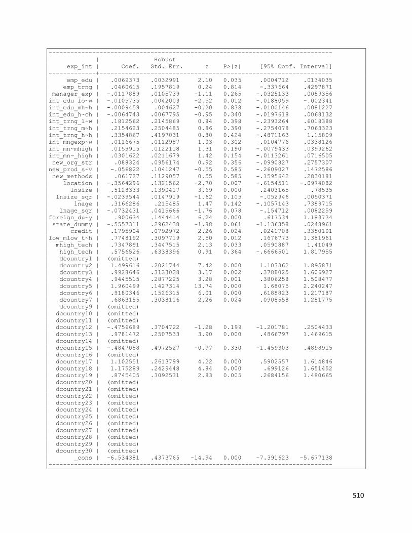
510

------------------------------------------------------------------------------

| Robust


-------------+----------------------------------------------------------------

emp_edu | .0069373 .0032991 2.10 0.035 .0004712 .0134035

emp_trng | .0460615 .1957819 0.24 0.814 -.337664 .4297871

manager_exp | -.0117889 .0105739 -1.11 0.265 -.0325133 .0089356

int_edu_lo~w | -.0105735 .0042003 -2.52 0.012 -.0188059 -.002341

int_edu_mh~h | -.0009459 .004627 -0.20 0.838 -.0100146 .0081227

int_edu_h~ch | -.0064743 .0067795 -0.95 0.340 -.0197618 .0068132

int_trng_l~w | .1812562 .2145869 0.84 0.398 -.2393264 .6018388

int_trng_m~h | .2154623 .2504485 0.86 0.390 -.2754078 .7063323

int_trng_h~h | .3354867 .4197031 0.80 0.424 -.4871163 1.15809

int_mngexp~w | .0116675 .0112987 1.03 0.302 -.0104776 .0338126

int_mn~mhigh | .0159915 .0122118 1.31 0.190 -.0079433 .0399262

int_mn~_high | .0301622 .0211679 1.42 0.154 -.0113261 .0716505

new_org_str | .088324 .0956174 0.92 0.356 -.0990827 .2757307

new_prod_s~v | -.056822 .1041247 -0.55 0.585 -.2609027 .1472586

new_methods | .061727 .1129057 0.55 0.585 -.1595642 .2830181

location | -.3564296 .1321562 -2.70 0.007 -.6154511 -.0974082

lnsize | .5128333 .1390417 3.69 0.000 .2403165 .78535

lnsize_sqr | -.0239544 .0147919 -1.62 0.105 -.052946 .0050371

lnage | .3166286 .215485 1.47 0.142 -.1057143 .7389715

lnage_sqr | -.0732431 .0415666 -1.76 0.078 -.154712 .0082259

foreign_du~y | .900634 .1444414 6.24 0.000 .617534 1.183734

state_dummy | -.5557311 .2962438 -1.88 0.061 -1.136358 .0248961

credit | .1795904 .0792972 2.26 0.024 .0241708 .3350101

low_mlow_t~h | .7748192 .3097719 2.50 0.012 .1676773 1.381961

mhigh_tech | .7347891 .3447515 2.13 0.033 .0590887 1.41049

high_tech | .5756526 .6338396 0.91 0.364 -.6666501 1.817955


dcountry2 | 1.499616 .2021744 7.42 0.000 1.103362 1.895871

dcountry3 | .9928646 .3133028 3.17 0.002 .3788025 1.606927

dcountry4 | .9445515 .2877225 3.28 0.001 .3806258 1.508477

dcountry5 | 1.960499 .1427314 13.74 0.000 1.68075 2.240247

dcountry6 | .9180346 .1526315 6.01 0.000 .6188823 1.217187

dcountry7 | .6863155 .3038116 2.26 0.024 .0908558 1.281775




dcountry12 | -.4756689 .3704722 -1.28 0.199 -1.201781 .2504433

dcountry13 | .9781472 .2507533 3.90 0.000 .4866797 1.469615


dcountry15 | -.4847058 .4972527 -0.97 0.330 -1.459303 .4898915


dcountry17 | 1.102551 .2613799 4.22 0.000 .5902557 1.614846

dcountry18 | 1.175289 .2429448 4.84 0.000 .699126 1.651452

dcountry19 | .8745405 .3092531 2.83 0.005 .2684156 1.480665












_cons | -6.534381 .4373765 -14.94 0.000 -7.391623 -5.677138

------------------------------------------------------------------------------

511

Table A6.5.6 Poisson Model - Full sample (imputed) estimated results

. mi estimate, cmdok: poisson exp_int emp_edu emp_trng manager_exp new_org_str



dcountry9-dcountry30, nolog vce(robust)






avg = 1423112.95

max = 2.93e+07

Model F test: Equal FMI F( 46, 1.4e+06)= 52.42


-------------------------------------------------------------------------------


--------------+----------------------------------------------------------------

emp_edu | .0017187 .0012191 1.41 0.159 -.0006725 .0041099

emp_trng | .035797 .0526923 0.68 0.497 -.0674883 .1390824

manager_exp | -.0009699 .0023278 -0.42 0.677 -.0055327 .003593

new_org_str | .0723633 .0603587 1.20 0.231 -.0459473 .1906738

new_prod_serv | -.0644544 .0582472 -1.11 0.268 -.1786191 .0497102

new_methods | .1240578 .0639861 1.94 0.053 -.0013538 .2494693

location | -.1774292 .064346 -2.76 0.006 -.3035503 -.0513081

lnsize | .5099841 .0811112 6.29 0.000 .3510063 .6689618

lnsize_sqr | -.0286046 .0091101 -3.14 0.002 -.0464603 -.0107489

lnage | .1128158 .1430506 0.79 0.430 -.1676642 .3932959

lnage_sqr | -.0436149 .0268989 -1.62 0.105 -.0963602 .0091304

foreign_dummy | .7596171 .070731 10.74 0.000 .6209691 .8982651

state_dummy | -.4668128 .2568423 -1.82 0.069 -.9705838 .0369581

credit | .170163 .0489299 3.48 0.001 .0742496 .2660764

low_mlow_tech | .9948193 .059964 16.59 0.000 .8772905 1.112348

mhigh_tech | 1.239652 .0738812 16.78 0.000 1.094838 1.384466

high_tech | 1.336185 .1222436 10.93 0.000 1.096585 1.575784

dcountry1 | 1.699997 .2024048 8.40 0.000 1.303251 2.096743

dcountry2 | 1.501744 .1774134 8.46 0.000 1.15402 1.849469

dcountry3 | .7810713 .2896676 2.70 0.007 .2133331 1.348809

dcountry4 | .888987 .2583615 3.44 0.001 .3826036 1.39537

dcountry5 | 1.981301 .1144111 17.32 0.000 1.757057 2.205545

dcountry6 | .7290559 .1420952 5.13 0.000 .4505493 1.007562

dcountry7 | .6199537 .2621269 2.37 0.018 .1061937 1.133714

dcountry9 | 1.453421 .1497578 9.71 0.000 1.1599 1.746941

dcountry10 | 1.902104 .1401916 13.57 0.000 1.627328 2.17688

dcountry11 | 1.785512 .1630505 10.95 0.000 1.465937 2.105086

dcountry12 | -.4435209 .3373211 -1.31 0.189 -1.104659 .217617

dcountry13 | 1.046383 .2280622 4.59 0.000 .5993873 1.493378

dcountry14 | 1.863451 .1633568 11.41 0.000 1.543275 2.183627

dcountry15 | -.8299464 .4473852 -1.86 0.064 -1.706805 .0469126

dcountry16 | 1.882872 .1694689 11.11 0.000 1.550717 2.215026

dcountry17 | 1.033143 .2357746 4.38 0.000 .5710322 1.495254

dcountry18 | 1.100151 .2264616 4.86 0.000 .6562946 1.544008

dcountry19 | .7111046 .3038758 2.34 0.019 .1155185 1.306691

dcountry20 | 2.254018 .1489871 15.13 0.000 1.962006 2.546031

dcountry21 | 1.234355 .2639579 4.68 0.000 .7170073 1.751704

dcountry22 | 2.155231 .145249 14.84 0.000 1.870533 2.439928

dcountry23 | 1.525414 .1883448 8.10 0.000 1.156242 1.894586

dcountry24 | 2.326546 .1494995 15.56 0.000 2.033526 2.619565

dcountry25 | 2.256049 .1509018 14.95 0.000 1.960233 2.551865

dcountry26 | 1.878101 .1632465 11.50 0.000 1.558142 2.198061

dcountry27 | 2.468056 .1460089 16.90 0.000 2.181876 2.754236

512

dcountry28 | 1.923775 .1704594 11.29 0.000 1.58968 2.257871

dcountry29 | 1.925713 .1608249 11.97 0.000 1.610497 2.240929

dcountry30 | 1.284545 .2915923 4.41 0.000 .7129915 1.856098

_cons | -6.226869 .2503661 -24.87 0.000 -6.717624 -5.736114

Table A6.5.7 Poisson (Augumented) Model - Full sample (imputed) estimated

results (45)

mi estimate, cmdok: poisson exp_int emp_edu emp_trng manager_exp skilled_emp



low_mlow_tech mhigh_tech high_tech dcountry1-dcountry7 dcountry9-dcountry30, nolog

vce(robust)






avg = 87411.20

max = 2301286.32



-----------------------------------------------------------------------------------


------------------+----------------------------------------------------------------

emp_edu | .0003327 .0013654 0.24 0.808 -.0023482 .0030136

emp_trng | .0091567 .0550444 0.17 0.868 -.0987744 .1170879

manager_exp | -.0008135 .0024383 -0.33 0.739 -.0055942 .0039673

skilled_emp | .0010561 .0013286 0.79 0.428 -.0015634 .0036755


new_org_str | .0467524 .0636466 0.73 0.463 -.0780771 .1715819

new_prod_serv | -.104475 .061091 -1.71 0.087 -.2242563 .0153064

new_methods | .105921 .0662846 1.60 0.110 -.0240241 .2358661

location | -.2608486 .0672377 -3.88 0.000 -.3926724 -.1290248

lnsize | .4712838 .0853843 5.52 0.000 .3038872 .6386803

lnsize_sqr | -.0265732 .0096103 -2.77 0.006 -.0454139 -.0077326

lnage | .0805252 .1458252 0.55 0.581 -.205383 .3664334

lnage_sqr | -.0355568 .0274696 -1.29 0.196 -.0894191 .0183055

foreign_dummy | .6281294 .0785724 7.99 0.000 .4739307 .7823281

state_dummy | -.4134897 .2601356 -1.59 0.112 -.9236647 .0966853

credit | .1768635 .0501788 3.52 0.000 .078484 .275243

f_inputs | .0072679 .0009485 7.66 0.000 .0053989 .009137

tech_dummy | .2180284 .2109932 1.03 0.306 -.2046262 .6406829

bus_assoc | -.0295667 .1694599 -0.17 0.862 -.369688 .3105547

low_mlow_tech | .9867354 .0664718 14.84 0.000 .8563095 1.117161

mhigh_tech | 1.176714 .0818997 14.37 0.000 1.016032 1.337396

high_tech | 1.165316 .1309253 8.90 0.000 .9085787 1.422054

dcountry1 | 1.46528 .2103528 6.97 0.000 1.052824 1.877736

dcountry2 | 1.332581 .1785774 7.46 0.000 .9825688 1.682592

dcountry3 | .7240589 .2910414 2.49 0.013 .1536235 1.294494

dcountry4 | .8234397 .2644583 3.11 0.002 .3050951 1.341784

dcountry5 | 2.057475 .1174744 17.51 0.000 1.827208 2.287742

dcountry6 | .7470446 .1437524 5.20 0.000 .4652873 1.028802

dcountry7 | .6584635 .2644258 2.49 0.013 .1401975 1.176729

dcountry9 | 1.490373 .1578676 9.44 0.000 1.180869 1.799877

dcountry10 | 1.702227 .142735 11.93 0.000 1.42245 1.982004

dcountry11 | 1.708107 .1712216 9.98 0.000 1.372439 2.043776

dcountry12 | -.5475335 .3383725 -1.62 0.106 -1.210733 .1156664

dcountry13 | 1.028412 .2377376 4.33 0.000 .5623394 1.494484

dcountry14 | 1.77128 .1665673 10.63 0.000 1.444786 2.097774

513

dcountry15 | -.6930696 .4498764 -1.54 0.123 -1.574812 .1886725

dcountry16 | 1.669211 .1744446 9.57 0.000 1.327269 2.011153

dcountry17 | .8369386 .2400562 3.49 0.000 .3664213 1.307456

dcountry18 | .999069 .2285224 4.37 0.000 .5511665 1.446971

dcountry19 | .7553061 .3046446 2.48 0.013 .1582119 1.3524

dcountry20 | 1.942658 .1552903 12.51 0.000 1.638246 2.247069

dcountry21 | .9523006 .2696072 3.53 0.000 .4238699 1.480731

dcountry22 | 2.10677 .1480781 14.23 0.000 1.816506 2.397034

dcountry23 | 1.492417 .190628 7.83 0.000 1.118726 1.866108

dcountry24 | 2.168516 .1556687 13.93 0.000 1.86336 2.473672

dcountry25 | 2.078605 .1546502 13.44 0.000 1.775445 2.381765

dcountry26 | 1.807857 .1652014 10.94 0.000 1.48406 2.131655

dcountry27 | 2.337375 .1512016 15.46 0.000 2.040993 2.633757

dcountry28 | 1.792403 .171914 10.43 0.000 1.45545 2.129357

dcountry29 | 1.749476 .164106 10.66 0.000 1.427801 2.07115

dcountry30 | 1.009952 .2948445 3.43 0.001 .4319694 1.587934

_cons | -6.562049 .3434025 -19.11 0.000 -7.238619 -5.88548

Table A6.5.8 Poisson (Augumented) Model - Full sample (imputed) estimated

results (95)

. mi estimate, cmdok: poisson exp_int emp_edu emp_trng manager_exp skilled_emp




nolog vce(robust)






avg = 188254.38

max = 5714940.38



-----------------------------------------------------------------------------------


------------------+----------------------------------------------------------------

emp_edu | .0004966 .0013415 0.37 0.711 -.0021345 .0031276

emp_trng | .0126721 .0550033 0.23 0.818 -.0951534 .1204976

manager_exp | -.0009069 .0024306 -0.37 0.709 -.0056714 .0038577

skilled_emp | .0010734 .0012753 0.84 0.400 -.0014317 .0035785


new_org_str | .0466102 .0623997 0.75 0.455 -.0757143 .1689347

new_prod_serv | -.1018773 .0605082 -1.68 0.092 -.2204861 .0167315

new_methods | .1069029 .0654323 1.63 0.102 -.0213494 .2351552

location | -.2594634 .0668686 -3.88 0.000 -.3905381 -.1283887

lnsize | .4782467 .0853251 5.60 0.000 .3109913 .6455022

lnsize_sqr | -.0272544 .009623 -2.83 0.005 -.0461176 -.0083912

lnage | .0796817 .1454084 0.55 0.584 -.2053524 .3647158

lnage_sqr | -.0356045 .0272906 -1.30 0.192 -.0891014 .0178923

foreign_dummy | .6357183 .0773848 8.22 0.000 .4839745 .7874621

state_dummy | -.418028 .2565798 -1.63 0.103 -.9210179 .084962

credit | .1739868 .050697 3.43 0.001 .0746026 .273371

f_inputs | .0072047 .0009254 7.79 0.000 .0053869 .0090225

tech_dummy | .1868809 .2185731 0.86 0.394 -.2459935 .6197553

bus_assoc | -.0143893 .1566631 -0.09 0.927 -.3247621 .2959835

low_mlow_tech | .9908668 .0660148 15.01 0.000 .8614208 1.120313

mhigh_tech | 1.178649 .0807755 14.59 0.000 1.020274 1.337025

514

high_tech | 1.167 .1293035 9.03 0.000 .9135281 1.420472

dcountry1 | .4477958 .3222047 1.39 0.165 -.1837646 1.079356

dcountry2 | 1.336052 .1796071 7.44 0.000 .9840232 1.688081

dcountry3 | .7233699 .2908391 2.49 0.013 .1533343 1.293406

dcountry4 | .8217176 .26405 3.11 0.002 .3041822 1.339253

dcountry5 | 2.05745 .1169983 17.59 0.000 1.82813 2.286769

dcountry6 | .7486835 .1438582 5.20 0.000 .4667228 1.030644

dcountry7 | .6586189 .2647689 2.49 0.013 .1396809 1.177557

dcountry9 | .4698627 .3003745 1.56 0.118 -.118931 1.058656

dcountry10 | .6855991 .2895978 2.37 0.018 .1179534 1.253245

dcountry11 | .6925458 .3021943 2.29 0.022 .1002014 1.28489

dcountry12 | -.5469734 .3385602 -1.62 0.106 -1.21054 .1165935

dcountry13 | 1.028903 .2375374 4.33 0.000 .5632858 1.494519

dcountry14 | .753523 .3010611 2.50 0.012 .1634114 1.343635

dcountry15 | -.6893085 .449873 -1.53 0.125 -1.571044 .1924266

dcountry16 | .6567295 .302244 2.17 0.030 .0642973 1.249162

dcountry17 | .8444971 .2408003 3.51 0.000 .372527 1.316467

dcountry18 | .9956669 .2292019 4.34 0.000 .546435 1.444899

dcountry19 | .7577015 .3046862 2.49 0.013 .1605268 1.354876

dcountry20 | .9285693 .290425 3.20 0.001 .3593077 1.497831

dcountry21 | -.0601063 .3670069 -0.16 0.870 -.7794484 .6592358

dcountry22 | 1.083895 .293591 3.69 0.000 .5084154 1.659374

dcountry23 | .4768277 .3134004 1.52 0.128 -.137474 1.091129

dcountry24 | 1.151396 .2934955 3.92 0.000 .5761071 1.726685

dcountry25 | 1.061367 .2950064 3.60 0.000 .4831284 1.639606

dcountry26 | .7925103 .3028468 2.62 0.009 .198902 1.386119

dcountry27 | 1.324417 .2883237 4.59 0.000 .7592831 1.88955

dcountry28 | .7788371 .3052719 2.55 0.011 .180472 1.377202

dcountry29 | .7356585 .2988643 2.46 0.014 .1498487 1.321468


_cons | -6.549236 .3466009 -18.90 0.000 -7.23028 -5.868192

-----------------------------------------------------------------------------------

Endogeneity Testing

Table A6.6 Panel estimated results

Tobit/ Poisson

Probit Logit

VARIABLES emp_edu RD emp_trng

exp_int_lag1 0.00684 0.00349 -0.00181

(0.0935) (5.053) (0.00902) exp_int_lag2 0.00968 0.00450 0.0127 (0.0977) (6.501) (0.00932) Constant 26.85*** -0.731 -0.326

(1.658) (1,057) (0.246)

Observations 359 371 107 Number of panelid 359 371 107

Table A6.6.1 IVTobit Model - Full sample estimated results

ivtobit exp_int emp_edu emp_trng manager_exp new_org_str new_prod_serv new_methods


515

low_mlow_tech mhigh_tech high_tech dcountry1-dcountry7 dcountry9-dcountry30 (emp_edu

= avrg_edu), ll ul vce(robust) nolog

Tobit model with endogenous regressors Number of obs = 14026

Wald chi2(46) = 2051.88

Log pseudolikelihood = -67964.267 Prob > chi2 = 0.0000

------------------------------------------------------------------------------

| Robust

| Coef. Std. Err. z P>|z| [95% Conf. Interval]

-------------+----------------------------------------------------------------

emp_edu | .0030349 .0006511 4.66 0.000 .0017588 .004311

emp_trng | .0233102 .019635 1.19 0.235 -.0151737 .0617941

manager_exp | .0006865 .0009006 0.76 0.446 -.0010786 .0024516

new_org_str | .0478622 .0235079 2.04 0.042 .0017875 .0939369

new_prod_s~v | .0502309 .0217283 2.31 0.021 .0076443 .0928176

new_methods | .0279108 .0248207 1.12 0.261 -.0207368 .0765583

location | -.0631634 .0248912 -2.54 0.011 -.1119492 -.0143776

lnsize | .2097713 .0309238 6.78 0.000 .1491618 .2703807

lnsize_sqr | -.0093375 .0037745 -2.47 0.013 -.0167353 -.0019398

lnage | .0502857 .0525272 0.96 0.338 -.0526657 .1532371

lnage_sqr | -.0160888 .0101906 -1.58 0.114 -.0360621 .0038845

foreign_du~y | .3710641 .0370439 10.02 0.000 .2984594 .4436689

state_dummy | -.1267409 .0867172 -1.46 0.144 -.2967036 .0432218

credit | .1092822 .0187219 5.84 0.000 .0725881 .1459764

low_mlow_t~h | .3861055 .0211696 18.24 0.000 .3446138 .4275972

mhigh_tech | .5308491 .0279609 18.99 0.000 .4760468 .5856514

high_tech | .5303366 .0518326 10.23 0.000 .4287467 .6319265

dcountry1 | .5748757 .0819884 7.01 0.000 .4141815 .73557

dcountry2 | .5239227 .0595124 8.80 0.000 .4072805 .640565

dcountry3 | .1880388 .0826261 2.28 0.023 .0260945 .349983

dcountry4 | .1259382 .0878208 1.43 0.152 -.0461874 .2980637

dcountry5 | .7394131 .0413961 17.86 0.000 .6582783 .8205479

dcountry6 | .1570664 .0434989 3.61 0.000 .0718101 .2423226

dcountry7 | .0821061 .0856085 0.96 0.338 -.0856835 .2498957

dcountry9 | .5168578 .0538431 9.60 0.000 .4113272 .6223884

dcountry10 | .6056033 .0519121 11.67 0.000 .5038575 .7073491

dcountry11 | .771549 .0536279 14.39 0.000 .6664402 .8766578

dcountry12 | -.2731645 .0828506 -3.30 0.001 -.4355486 -.1107804

dcountry13 | .3530267 .0682913 5.17 0.000 .2191783 .4868752

dcountry14 | .6908276 .0573385 12.05 0.000 .5784463 .803209

dcountry15 | -.1776069 .1213011 -1.46 0.143 -.4153526 .0601389

dcountry16 | .6945648 .0597983 11.62 0.000 .5773623 .8117673

dcountry17 | .2487297 .0669108 3.72 0.000 .117587 .3798724

dcountry18 | .2215957 .0800976 2.77 0.006 .0646074 .3785841

dcountry19 | .0466119 .0953723 0.49 0.625 -.1403144 .2335382

dcountry20 | .9149798 .0621433 14.72 0.000 .7931812 1.036778

dcountry21 | .5226681 .0738144 7.08 0.000 .3779944 .6673418

dcountry22 | .8737956 .0587567 14.87 0.000 .7586345 .9889567

dcountry23 | .5123111 .0687615 7.45 0.000 .377541 .6470812

dcountry24 | .87781 .0632946 13.87 0.000 .7537549 1.001865

dcountry25 | .799218 .0635102 12.58 0.000 .6747404 .9236957

dcountry26 | .724402 .0625515 11.58 0.000 .6018033 .8470007

dcountry27 | 1.078401 .0560024 19.26 0.000 .9686388 1.188164

dcountry28 | .6305303 .0677809 9.30 0.000 .4976822 .7633784

dcountry29 | .7570319 .0559026 13.54 0.000 .6474648 .8665991

dcountry30 | .4407176 .1081846 4.07 0.000 .2286797 .6527556

_cons | -2.054761 .0970069 -21.18 0.000 -2.244891 -1.864631

-------------+----------------------------------------------------------------

/alpha | -.0013847 .0007949 -1.74 0.082 -.0029427 .0001733

/lns | -.4485776 .0218916 -20.49 0.000 -.4914844 -.4056708

/lnv | 3.076893 .0070579 435.95 0.000 3.06306 3.090726

-------------+----------------------------------------------------------------

516

s | .6385358 .0139786 .6117177 .6665296

v | 21.69091 .1530915 21.39292 21.99305

------------------------------------------------------------------------------

Instrumented: emp_edu

Instruments: emp_trng manager_exp new_org_str new_prod_serv new_methods

location lnsize lnsize_sqr lnage lnage_sqr foreign_dummy

state_dummy credit low_mlow_tech mhigh_tech high_tech

dcountry1 dcountry2 dcountry3 dcountry4 dcountry5 dcountry6

dcountry7 dcountry9 dcountry10 dcountry11 dcountry12




dcountry28 dcountry29 dcountry30 avrg_edu

------------------------------------------------------------------------------

Wald test of exogeneity (/alpha = 0): chi2(1) = 3.03 Prob > chi2 = 0.0815




Table A6.6.2 IVPoisson Model - Full sample estimated results

ivpois exp_int emp_trng manager_exp new_org_str new_prod_serv new_methods location


mhigh_tech high_tech dcountry1-dcountry7 dcountry9-dcountry30, endog (emp_edu) exog

(avrg_edu)

------------------------------------------------------------------------------


-------------+----------------------------------------------------------------

exp_int |

emp_trng | .062747 .1133685 0.55 0.580 -.1594512 .2849452

manager_exp | -.0011441 .0052881 -0.22 0.829 -.0115085 .0092204

new_org_str | .2238703 .1222223 1.83 0.067 -.0156809 .4634215

new_prod_s~v | -.1630698 .1004821 -1.62 0.105 -.3600111 .0338716

new_methods | -.0160448 .1204989 -0.13 0.894 -.2522182 .2201286

location | -.1219598 .1450168 -0.84 0.400 -.4061874 .1622678

lnsize | .1150871 .1791664 0.64 0.521 -.2360726 .4662469

lnsize_sqr | .0349075 .0234666 1.49 0.137 -.0110862 .0809012

lnage | .6709593 .2785625 2.41 0.016 .1249868 1.216932

lnage_sqr | -.1345367 .0552741 -2.43 0.015 -.242872 -.0262014

foreign_du~y | 1.16245 .1611901 7.21 0.000 .8465234 1.478377

state_dummy | -1.05899 .3829486 -2.77 0.006 -1.809556 -.3084249

credit | .2957289 .0940167 3.15 0.002 .1114596 .4799982

low_mlow_t~h | 1.04483 .1346551 7.76 0.000 .7809111 1.30875

mhigh_tech | 1.159101 .137246 8.45 0.000 .8901037 1.428098

high_tech | .9623794 .1725175 5.58 0.000 .6242513 1.300508

dcountry1 | 1.370243 .3845505 3.56 0.000 .6165381 2.123948

dcountry2 | 1.551772 .2755951 5.63 0.000 1.011616 2.091928

dcountry3 | .0496556 .3921467 0.13 0.899 -.7189378 .818249

dcountry4 | .3743034 .5021244 0.75 0.456 -.6098424 1.358449

dcountry5 | 1.970393 .2256271 8.73 0.000 1.528172 2.412614

dcountry6 | .2897692 .2359993 1.23 0.220 -.1727809 .7523193

dcountry7 | -.0877651 .3388342 -0.26 0.796 -.751868 .5763378

dcountry9 | 1.275979 .2503044 5.10 0.000 .7853915 1.766567

dcountry10 | 1.482666 .2686756 5.52 0.000 .9560717 2.009261

dcountry11 | 1.945149 .2475908 7.86 0.000 1.45988 2.430418

dcountry12 | -1.51006 .5524494 -2.73 0.006 -2.592841 -.4272788

dcountry13 | .7277961 .3402045 2.14 0.032 .0610076 1.394585

dcountry14 | 1.759181 .2728604 6.45 0.000 1.224384 2.293977

dcountry15 | -1.504858 .5510251 -2.73 0.006 -2.584848 -.424869

dcountry16 | 1.608904 .2782674 5.78 0.000 1.06351 2.154298

517

dcountry17 | .214065 .319889 0.67 0.503 -.4129059 .841036

dcountry18 | .8560062 .3137112 2.73 0.006 .2411435 1.470869

dcountry19 | .2544534 .4179528 0.61 0.543 -.564719 1.073626

dcountry20 | 2.179724 .2815575 7.74 0.000 1.627882 2.731567

dcountry21 | 1.272565 .3723713 3.42 0.001 .5427309 2.0024

dcountry22 | 2.224038 .2683873 8.29 0.000 1.698008 2.750067

dcountry23 | 1.091835 .4062451 2.69 0.007 .2956091 1.888061

dcountry24 | 2.038851 .2493496 8.18 0.000 1.550135 2.527568

dcountry25 | 2.114519 .2929466 7.22 0.000 1.540354 2.688684

dcountry26 | 1.930147 .3124204 6.18 0.000 1.317814 2.542479

dcountry27 | 2.596931 .269874 9.62 0.000 2.067988 3.125874

dcountry28 | 1.646363 .2886067 5.70 0.000 1.080704 2.212022

dcountry29 | 1.970595 .2679974 7.35 0.000 1.44533 2.495861

dcountry30 | 1.307789 .4939628 2.65 0.008 .3396398 2.275939

emp_edu | .0095658 .0034846 2.75 0.006 .0027362 .0163954

_cons | -6.645289 .4948344 -13.43 0.000 -7.615146 -5.675431

------------------------------------------------------------------------------

test vhat

( 1) [exp_int]vhat = 0

chi2( 1) = 0.09

Prob > chi2 = 0.7699

Estimated results: Export market share

Table A6.7 Tobit Model - Full sample estimated results (exp_share_industryEU28)

tobit exp_share_industryEU28 emp_edu emp_trng manager_exp new_org_str new_prod_serv

new_methods location lnsize lnsize_sqr lnage lnage_sqr foreign_dummy state_dummy

credit low_mlow_tech mhigh_tech high_tech dcountry1-dcountry7 dcountry9-dcountry30,

ll ul vce(robust) nolog


F( 46, 13665) = 63.64

Prob > F = 0.0000


------------------------------------------------------------------------------

| Robust

exp_sh~yEU28 | Coef. Std. Err. t P>|t| [95% Conf. Interval]

-------------+----------------------------------------------------------------

emp_edu | .0002785 .0000576 4.84 0.000 .0001656 .0003913

emp_trng | .0046764 .0023054 2.03 0.043 .0001574 .0091954

manager_exp | -.0001211 .0001337 -0.91 0.365 -.0003833 .000141

new_org_str | .0084459 .0030529 2.77 0.006 .0024618 .01443

new_prod_s~v | .0124381 .0031884 3.90 0.000 .0061884 .0186879

new_methods | -.002366 .0032113 -0.74 0.461 -.0086605 .0039285

location | .0077128 .0033136 2.33 0.020 .0012177 .0142078

lnsize | .012319 .0050038 2.46 0.014 .0025108 .0221272

lnsize_sqr | .0006653 .0006783 0.98 0.327 -.0006642 .0019948

lnage | .0053059 .0072127 0.74 0.462 -.0088321 .0194438

lnage_sqr | -.0008334 .001425 -0.58 0.559 -.0036266 .0019598

foreign_du~y | .0240689 .0039764 6.05 0.000 .0162745 .0318632

state_dummy | -.0145448 .0115853 -1.26 0.209 -.0372535 .0081639

credit | .0181319 .0024646 7.36 0.000 .0133009 .0229629

low_mlow_t~h | .0369272 .0024484 15.08 0.000 .0321279 .0417264

mhigh_tech | .055048 .0033143 16.61 0.000 .0485515 .0615445

high_tech | .0547239 .0059026 9.27 0.000 .043154 .0662938

dcountry1 | .0501961 .0091248 5.50 0.000 .0323102 .068082

dcountry2 | .052439 .0069409 7.56 0.000 .0388339 .0660442

dcountry3 | .0127452 .0096406 1.32 0.186 -.0061517 .031642

518

dcountry4 | -.0069418 .0111724 -0.62 0.534 -.0288412 .0149576

dcountry5 | .0692111 .004351 15.91 0.000 .0606824 .0777397

dcountry6 | .0092747 .0057667 1.61 0.108 -.0020288 .0205781

dcountry7 | -.000978 .0097482 -0.10 0.920 -.0200858 .0181298

dcountry9 | .0499927 .0066478 7.52 0.000 .0369621 .0630233

dcountry10 | .0562414 .0055702 10.10 0.000 .0453231 .0671597

dcountry11 | .0836858 .0058706 14.26 0.000 .0721786 .095193

dcountry12 | -.0384346 .0107297 -3.58 0.000 -.0594663 -.0174029

dcountry13 | .0293762 .0085859 3.42 0.001 .0125467 .0462058

dcountry14 | .0657518 .0064192 10.24 0.000 .0531693 .0783344

dcountry15 | -.04169 .0165476 -2.52 0.012 -.0741257 -.0092544

dcountry16 | .0698868 .0065039 10.75 0.000 .0571382 .0826354

dcountry17 | .0060696 .0088648 0.68 0.494 -.0113066 .0234457

dcountry18 | .0173181 .0102645 1.69 0.092 -.0028018 .0374381

dcountry19 | -.0194869 .011515 -1.69 0.091 -.042058 .0030841

dcountry20 | .0908044 .0065366 13.89 0.000 .0779917 .103617

dcountry21 | .0554939 .0088478 6.27 0.000 .038151 .0728368

dcountry22 | .0890129 .0061014 14.59 0.000 .0770534 .1009725

dcountry23 | .0475131 .0083615 5.68 0.000 .0311233 .0639029

dcountry24 | .0863787 .0065863 13.11 0.000 .0734687 .0992888

dcountry25 | .0791589 .0068167 11.61 0.000 .0657972 .0925205

dcountry26 | .0593752 .0079956 7.43 0.000 .0437028 .0750477

dcountry27 | .1411126 .00809 17.44 0.000 .1252552 .15697

dcountry28 | .056652 .006851 8.27 0.000 .0432231 .0700808

dcountry29 | .0813099 .0058302 13.95 0.000 .0698818 .092738

dcountry30 | .0395044 .0134887 2.93 0.003 .0130646 .0659442

_cons | -.2523495 .013594 -18.56 0.000 -.2789955 -.2257035

-------------+----------------------------------------------------------------

/sigma | .0872653 .0005487 .0861898 .0883409

------------------------------------------------------------------------------

Obs. summary: 11804 left-censored observations at exp_sh~yEU28<=0


1 right-censored observation at exp_sh~yEU28>=3.0019033

Table A6.7.1 Tobit Model - CEECs estimated results (exp_share_industryEU28)



credit low_mlow_tech mhigh_tech high_tech dcountry1-dcountry7 dcountry9-dcountry30

if CEEC_dummy==1, ll ul vce(robust) nolog















F( 33, 4687) = 41.03

Prob > F = 0.0000

Log pseudolikelihood = 4.3134043 Pseudo R2 = 1.0137

------------------------------------------------------------------------------

| Robust

519


-------------+----------------------------------------------------------------

emp_edu | .0002922 .0000795 3.67 0.000 .0001363 .0004481

emp_trng | -.003174 .0036952 -0.86 0.390 -.0104183 .0040704

manager_exp | -.0001631 .0002034 -0.80 0.423 -.0005618 .0002356

new_org_str | .0141863 .0042216 3.36 0.001 .0059099 .0224627

new_prod_s~v | .0138191 .0045483 3.04 0.002 .0049021 .022736

new_methods | .004811 .0048268 1.00 0.319 -.0046519 .0142738

location | .0180786 .0046667 3.87 0.000 .0089296 .0272276

lnsize | .0067783 .0096957 0.70 0.485 -.0122298 .0257864

lnsize_sqr | .0014803 .0014777 1.00 0.316 -.0014166 .0043773

lnage | .002001 .0116854 0.17 0.864 -.0209078 .0249097

lnage_sqr | -.0005761 .0021232 -0.27 0.786 -.0047386 .0035864

foreign_du~y | .0270814 .005646 4.80 0.000 .0160127 .0381502

state_dummy | -.0238731 .0333706 -0.72 0.474 -.0892951 .0415489

credit | .0213471 .0039891 5.35 0.000 .0135267 .0291676

low_mlow_t~h | .0525781 .0037502 14.02 0.000 .0452258 .0599303

mhigh_tech | .064769 .0052956 12.23 0.000 .0543871 .0751509

high_tech | .0511486 .0091986 5.56 0.000 .033115 .0691822

dcountry1 | .007669 .0183852 0.42 0.677 -.0283746 .0437126







dcountry9 | .0151736 .0172438 0.88 0.379 -.0186324 .0489796

dcountry10 | .0208448 .0164145 1.27 0.204 -.0113353 .0530249

dcountry11 | .0531184 .0165298 3.21 0.001 .0207122 .0855247



dcountry14 | .0339859 .0168634 2.02 0.044 .0009258 .067046


dcountry16 | .0343723 .0168448 2.04 0.041 .0013486 .067396




dcountry20 | .0607032 .0168168 3.61 0.000 .0277344 .093672

dcountry21 | .0156619 .0183267 0.85 0.393 -.0202671 .0515908

dcountry22 | .0623033 .016783 3.71 0.000 .0294007 .0952059

dcountry23 | .0092041 .017826 0.52 0.606 -.0257431 .0441514

dcountry24 | .0534687 .0168704 3.17 0.002 .0203949 .0865426

dcountry25 | .0470039 .0171096 2.75 0.006 .013461 .0805469

dcountry26 | .0271532 .0176557 1.54 0.124 -.0074603 .0617667

dcountry27 | .1199547 .0178153 6.73 0.000 .0850284 .1548809

dcountry28 | .0228983 .0171489 1.34 0.182 -.0107216 .0565182

dcountry29 | .0511304 .016561 3.09 0.002 .0186631 .0835976


_cons | -.2324305 .0239362 -9.71 0.000 -.2793567 -.1855042

-------------+----------------------------------------------------------------

/sigma | .1042454 .0014172 .101467 .1070239

------------------------------------------------------------------------------




Table A6.7.2 Tobit Model - CIS estimated results (exp_share_industryEU28)





520



















F( 29, 8962) = 53.47

Prob > F = 0.0000


------------------------------------------------------------------------------

| Robust


-------------+----------------------------------------------------------------

emp_edu | .000221 .000038 5.82 0.000 .0001466 .0002954

emp_trng | .0072423 .0021007 3.45 0.001 .0031245 .0113601

manager_exp | -.0001029 .000093 -1.11 0.269 -.0002853 .0000795

new_org_str | .0050947 .0024693 2.06 0.039 .0002544 .0099351

new_prod_s~v | .0063879 .0026494 2.41 0.016 .0011944 .0115813

new_methods | -.0055112 .0030758 -1.79 0.073 -.0115405 .0005181

location | -.0042943 .0030821 -1.39 0.164 -.0103358 .0017473

lnsize | .0171191 .0031425 5.45 0.000 .0109592 .0232791

lnsize_sqr | -.0005797 .000362 -1.60 0.109 -.0012893 .0001298

lnage | .003887 .0055263 0.70 0.482 -.0069458 .0147198

lnage_sqr | -.0004679 .0010646 -0.44 0.660 -.0025547 .0016189

foreign_du~y | .0215052 .0048489 4.44 0.000 .0120002 .0310102

state_dummy | -.0099315 .007506 -1.32 0.186 -.024645 .004782

credit | .0123648 .0019832 6.23 0.000 .0084773 .0162522

low_mlow_t~h | .0172432 .002516 6.85 0.000 .0123113 .0221752

mhigh_tech | .0324257 .0030779 10.53 0.000 .0263922 .0384592

high_tech | .0359641 .0049604 7.25 0.000 .0262407 .0456875


dcountry2 | .0346854 .0044971 7.71 0.000 .02587 .0435007

dcountry3 | .0114056 .006052 1.88 0.060 -.0004577 .023269

dcountry4 | -.0021565 .0069388 -0.31 0.756 -.0157581 .011445

dcountry5 | .045137 .002999 15.05 0.000 .0392583 .0510157

dcountry6 | .0077278 .0035224 2.19 0.028 .0008231 .0146325

dcountry7 | .0003348 .0064011 0.05 0.958 -.0122128 .0128825




dcountry12 | -.0257626 .0064879 -3.97 0.000 -.0384804 -.0130448

dcountry13 | .0223276 .005404 4.13 0.000 .0117346 .0329206


dcountry15 | -.0214014 .0104137 -2.06 0.040 -.0418146 -.0009883


dcountry17 | .0083219 .005861 1.42 0.156 -.0031671 .0198108

dcountry18 | .0145756 .0067513 2.16 0.031 .0013416 .0278097

dcountry19 | -.0071331 .0072234 -0.99 0.323 -.0212927 .0070265


521











_cons | -.1771081 .0092592 -19.13 0.000 -.1952582 -.1589579

-------------+----------------------------------------------------------------

/sigma | .0542187 .0001715 .0538825 .0545549

------------------------------------------------------------------------------




Table A6.7.3 Tobit Model - Full sample estimated results (exp_share_industryEA40)

. tobit exp_share_industryEA40 emp_edu emp_trng manager_exp new_org_str new_prod_serv





F( 46, 13665) = 65.98

Prob > F = 0.0000


------------------------------------------------------------------------------

| Robust

exp_sh~yEA40 | Coef. Std. Err. t P>|t| [95% Conf. Interval]

-------------+----------------------------------------------------------------

emp_edu | .000323 .0000655 4.93 0.000 .0001947 .0004514

emp_trng | .00472 .0028911 1.63 0.103 -.000947 .0103869

manager_exp | -.0001252 .0001493 -0.84 0.402 -.0004178 .0001675

new_org_str | .0064416 .003915 1.65 0.100 -.0012323 .0141154

new_prod_s~v | .0137579 .0033398 4.12 0.000 .0072114 .0203044

new_methods | -.0002046 .0045059 -0.05 0.964 -.0090369 .0086276

location | .0087067 .0039093 2.23 0.026 .0010439 .0163696

lnsize | .0167209 .0070617 2.37 0.018 .0028789 .0305629

lnsize_sqr | .0003631 .0009235 0.39 0.694 -.001447 .0021733

lnage | .0063011 .0077683 0.81 0.417 -.0089259 .0215281

lnage_sqr | -.0011189 .0015678 -0.71 0.475 -.0041921 .0019543

foreign_du~y | .02776 .0051452 5.40 0.000 .0176747 .0378453

state_dummy | -.0149761 .0124883 -1.20 0.230 -.0394548 .0095026

credit | .0198087 .0027135 7.30 0.000 .0144898 .0251276

low_mlow_t~h | .0377807 .0028846 13.10 0.000 .0321264 .043435

mhigh_tech | .0572824 .0037056 15.46 0.000 .0500189 .0645458

high_tech | .0560235 .0066013 8.49 0.000 .043084 .068963

dcountry1 | .0550678 .0098534 5.59 0.000 .0357539 .0743818

dcountry2 | .0576934 .0075439 7.65 0.000 .0429063 .0724806

dcountry3 | .0142544 .0104463 1.36 0.172 -.0062218 .0347305

dcountry4 | -.0071566 .012118 -0.59 0.555 -.0309096 .0165965

dcountry5 | .0789219 .0049983 15.79 0.000 .0691246 .0887192

dcountry6 | .0114172 .0062127 1.84 0.066 -.0007605 .0235949

dcountry7 | -.0002774 .010622 -0.03 0.979 -.0210979 .0205431

dcountry9 | .0556046 .0072578 7.66 0.000 .0413783 .069831

dcountry10 | .0620182 .0060168 10.31 0.000 .0502244 .073812

dcountry11 | .0919824 .0064792 14.20 0.000 .0792823 .1046826

dcountry12 | -.0410226 .0115548 -3.55 0.000 -.0636716 -.0183736

522

dcountry13 | .0326192 .0093465 3.49 0.000 .0142988 .0509396

dcountry14 | .0727057 .0070219 10.35 0.000 .0589417 .0864696

dcountry15 | -.0447997 .0180034 -2.49 0.013 -.0800889 -.0095105

dcountry16 | .0779943 .0072555 10.75 0.000 .0637724 .0922161

dcountry17 | .0064922 .0096569 0.67 0.501 -.0124367 .0254212

dcountry18 | .0184553 .0110264 1.67 0.094 -.003158 .0400686

dcountry19 | -.020591 .0125199 -1.64 0.100 -.0451316 .0039497

dcountry20 | .0999315 .007164 13.95 0.000 .0858891 .1139739

dcountry21 | .0617405 .0096412 6.40 0.000 .0428423 .0806386

dcountry22 | .122823 .0148885 8.25 0.000 .0936394 .1520065

dcountry23 | .0522269 .0090813 5.75 0.000 .0344263 .0700275

dcountry24 | .0953119 .0072961 13.06 0.000 .0810106 .1096132

dcountry25 | .0871616 .0074867 11.64 0.000 .0724866 .1018366

dcountry26 | .0767276 .0123598 6.21 0.000 .0525007 .1009545

dcountry27 | .1505079 .0089821 16.76 0.000 .1329017 .168114

dcountry28 | .0631225 .007491 8.43 0.000 .0484392 .0778058

dcountry29 | .0897366 .0064394 13.94 0.000 .0771145 .1023588

dcountry30 | .0441381 .0146761 3.01 0.003 .015371 .0729052

_cons | -.2813399 .0177532 -15.85 0.000 -.3161386 -.2465411

-------------+----------------------------------------------------------------

/sigma | .0950012 .0010073 .0930268 .0969756

------------------------------------------------------------------------------

Obs. summary: 11804 left-censored observations at exp_sh~yEA40<=0


1 right-censored observation at exp_sh~yEA40>=2.7831056

Table A6.7.4 Tobit Model - CEECs estimated results (exp_share_industryEA40)

tobit exp_share_industryEA40 emp_edu emp_trng manager_exp new_org_str new_prod_serv


















F( 33, 4687) = 41.10

Prob > F = 0.0000


------------------------------------------------------------------------------

| Robust


-------------+----------------------------------------------------------------

emp_edu | .0003865 .0001096 3.53 0.000 .0001716 .0006014

emp_trng | -.0044988 .0050389 -0.89 0.372 -.0143774 .0053798

manager_exp | -.0002216 .0002363 -0.94 0.348 -.0006849 .0002417

new_org_str | .011477 .0057928 1.98 0.048 .0001204 .0228336

new_prod_s~v | .015488 .0050095 3.09 0.002 .0056671 .0253089

new_methods | .0094421 .0071799 1.32 0.189 -.004634 .0235182

523

location | .0203201 .0057138 3.56 0.000 .0091184 .0315218

lnsize | .0174494 .0147568 1.18 0.237 -.0114808 .0463796

lnsize_sqr | .0004086 .0020835 0.20 0.845 -.0036761 .0044934

lnage | .0042691 .013069 0.33 0.744 -.0213522 .0298904

lnage_sqr | -.0012806 .0024841 -0.52 0.606 -.0061507 .0035894

foreign_du~y | .0330351 .0075269 4.39 0.000 .0182788 .0477915

state_dummy | -.0266572 .0363078 -0.73 0.463 -.0978375 .0445232

credit | .0245357 .0045865 5.35 0.000 .015544 .0335273

low_mlow_t~h | .0549707 .0046199 11.90 0.000 .0459136 .0640278

mhigh_tech | .0664297 .006139 10.82 0.000 .0543945 .078465

high_tech | .0493743 .0106922 4.62 0.000 .0284126 .070336

dcountry1 | .0069257 .0205598 0.34 0.736 -.0333812 .0472326







dcountry9 | .0172215 .0192197 0.90 0.370 -.0204581 .0549011

dcountry10 | .0227597 .0183313 1.24 0.214 -.0131783 .0586976

dcountry11 | .0591845 .0184425 3.21 0.001 .0230285 .0953404



dcountry14 | .0378957 .0187988 2.02 0.044 .0010413 .0747502


dcountry16 | .0400203 .0188493 2.12 0.034 .0030668 .0769738




dcountry20 | .0677503 .0187805 3.61 0.000 .0309316 .1045689

dcountry21 | .0174913 .0204371 0.86 0.392 -.022575 .0575577

dcountry22 | .0953556 .0229127 4.16 0.000 .0504359 .1402752

dcountry23 | .0099697 .0199053 0.50 0.616 -.0290541 .0489935

dcountry24 | .0602668 .0189231 3.18 0.001 .0231688 .0973649

dcountry25 | .0520565 .0191285 2.72 0.007 .0145556 .0895574

dcountry26 | .0414101 .0219355 1.89 0.059 -.0015938 .0844141

dcountry27 | .1301859 .0196953 6.61 0.000 .0915738 .1687979

dcountry28 | .0263816 .0191253 1.38 0.168 -.011113 .0638762

dcountry29 | .0579011 .0184792 3.13 0.002 .0216731 .0941291


_cons | -.2761549 .0336041 -8.22 0.000 -.3420348 -.210275

-------------+----------------------------------------------------------------

/sigma | .1169155 .0024827 .1120482 .1217829

------------------------------------------------------------------------------




Table A6.7.5 Tobit Model - CIS estimated results (exp_share_industryEA40)

. tobit exp_share_industryEA40 emp_edu emp_trng manager_exp new_org_str new_prod_serv








524















F( 29, 8962) = 53.44

Prob > F = 0.0000


------------------------------------------------------------------------------

| Robust


-------------+----------------------------------------------------------------

emp_edu | .000207 .0000355 5.84 0.000 .0001374 .0002765

emp_trng | .0070926 .0019616 3.62 0.000 .0032475 .0109377

manager_exp | -.0000864 .0000871 -0.99 0.321 -.0002572 .0000843

new_org_str | .0051088 .002322 2.20 0.028 .0005573 .0096604

new_prod_s~v | .0057646 .0024728 2.33 0.020 .0009174 .0106117

new_methods | -.0055633 .0028732 -1.94 0.053 -.0111955 .0000688

location | -.0042069 .002877 -1.46 0.144 -.0098464 .0014326

lnsize | .0146043 .0029593 4.93 0.000 .0088033 .0204053

lnsize_sqr | -.0003244 .000344 -0.94 0.346 -.0009986 .0003498

lnage | .0037247 .0051718 0.72 0.471 -.0064132 .0138627

lnage_sqr | -.0004679 .0009956 -0.47 0.638 -.0024195 .0014837

foreign_du~y | .0194927 .0045422 4.29 0.000 .010589 .0283964

state_dummy | -.0103103 .0070993 -1.45 0.146 -.0242266 .0036059

credit | .011547 .0018516 6.24 0.000 .0079175 .0151766

low_mlow_t~h | .0156464 .0023885 6.55 0.000 .0109643 .0203284

mhigh_tech | .0304303 .0028799 10.57 0.000 .024785 .0360756

high_tech | .0333908 .004644 7.19 0.000 .0242875 .042494


dcountry2 | .0326498 .0042014 7.77 0.000 .0244141 .0408855

dcountry3 | .0110373 .005651 1.95 0.051 -.0000401 .0221146

dcountry4 | -.0016969 .0064703 -0.26 0.793 -.0143802 .0109863

dcountry5 | .0433702 .0028348 15.30 0.000 .0378133 .0489272

dcountry6 | .0075572 .0032952 2.29 0.022 .0010979 .0140165

dcountry7 | .0003472 .0060022 0.06 0.954 -.0114185 .0121129




dcountry12 | -.0240828 .0060788 -3.96 0.000 -.0359987 -.012167

dcountry13 | .0212507 .0050353 4.22 0.000 .0113803 .031121


dcountry15 | -.0195634 .0097196 -2.01 0.044 -.0386162 -.0005107


dcountry17 | .0081085 .0054688 1.48 0.138 -.0026115 .0188285

dcountry18 | .0139034 .0062969 2.21 0.027 .0015601 .0262468

dcountry19 | -.0062268 .0067415 -0.92 0.356 -.0194417 .0069882






525







_cons | -.1636361 .0086392 -18.94 0.000 -.1805708 -.1467014

-------------+----------------------------------------------------------------

/sigma | .0504779 .0001625 .0501592 .0507965

------------------------------------------------------------------------------




Table A6.7.6 Tobit Model - Full sample estimated results (exp_share_totalEU28)

. tobit exp_share_totalEU28 emp_edu emp_trng manager_exp new_org_str new_prod_serv





F( 46, 13665) = 71.53

Prob > F = 0.0000

Log pseudolikelihood = 9126.4716 Pseudo R2 = -0.1528

------------------------------------------------------------------------------

| Robust

exp_sh~lEU28 | Coef. Std. Err. t P>|t| [95% Conf. Interval]

-------------+----------------------------------------------------------------

emp_edu | 2.45e-06 4.27e-07 5.74 0.000 1.61e-06 3.29e-06

emp_trng | .0000439 .0000208 2.11 0.035 3.11e-06 .0000848

manager_exp | 1.30e-06 1.62e-06 0.80 0.423 -1.88e-06 4.47e-06

new_org_str | .0000901 .0000273 3.30 0.001 .0000366 .0001436

new_prod_s~v | .0000724 .0000334 2.17 0.030 6.90e-06 .0001379

new_methods | -.0000121 .000034 -0.36 0.722 -.0000787 .0000546

location | .0000309 .0000306 1.01 0.313 -.0000291 .0000908

lnsize | -.0000169 .0000666 -0.25 0.800 -.0001474 .0001137

lnsize_sqr | .0000256 9.03e-06 2.83 0.005 7.86e-06 .0000433

lnage | .0000692 .0000668 1.04 0.300 -.0000616 .0002001

lnage_sqr | -.0000146 .0000143 -1.02 0.309 -.0000427 .0000135

foreign_du~y | .0002607 .0000557 4.68 0.000 .0001516 .0003699

state_dummy | -.0001531 .0001201 -1.28 0.202 -.0003885 .0000822

credit | .0001441 .0000229 6.29 0.000 .0000992 .0001889

low_mlow_t~h | .000354 .0000284 12.47 0.000 .0002983 .0004096

mhigh_tech | .0005351 .0000355 15.08 0.000 .0004656 .0006046

high_tech | .0004906 .0000523 9.38 0.000 .000388 .0005931

dcountry1 | .0004479 .000075 5.97 0.000 .0003008 .0005949

dcountry2 | .0004484 .0000611 7.34 0.000 .0003286 .0005681

dcountry3 | .0001403 .0000808 1.74 0.082 -.000018 .0002986

dcountry4 | -.0000316 .0000943 -0.33 0.738 -.0002164 .0001533

dcountry5 | .0006438 .0000433 14.86 0.000 .0005589 .0007287

dcountry6 | .0000707 .0000483 1.46 0.144 -.0000241 .0001655

dcountry7 | .0000192 .0000903 0.21 0.832 -.0001579 .0001963

dcountry9 | .000436 .0000589 7.40 0.000 .0003205 .0005515

dcountry10 | .000582 .0000858 6.78 0.000 .0004139 .0007502

dcountry11 | .0007218 .0000538 13.42 0.000 .0006164 .0008272

dcountry12 | -.0002976 .000096 -3.10 0.002 -.0004856 -.0001095

dcountry13 | .000283 .000073 3.88 0.000 .00014 .000426

dcountry14 | .0005757 .0000554 10.39 0.000 .000467 .0006843

dcountry15 | -.0003087 .0001367 -2.26 0.024 -.0005767 -.0000407

526

dcountry16 | .0006046 .0000568 10.64 0.000 .0004932 .0007159

dcountry17 | .0000786 .0000759 1.04 0.300 -.0000701 .0002273

dcountry18 | .0001469 .0000851 1.73 0.084 -.00002 .0003137

dcountry19 | -.0001323 .0000962 -1.38 0.169 -.000321 .0000563

dcountry20 | .0007937 .0000565 14.04 0.000 .0006829 .0009046

dcountry21 | .0004915 .0000737 6.67 0.000 .0003471 .000636

dcountry22 | .0007798 .0000554 14.08 0.000 .0006712 .0008884

dcountry23 | .0004338 .0000721 6.01 0.000 .0002924 .0005751

dcountry24 | .0007331 .0000582 12.60 0.000 .0006191 .0008471

dcountry25 | .0007008 .0000587 11.94 0.000 .0005858 .0008159

dcountry26 | .0005231 .0000689 7.59 0.000 .000388 .0006582

dcountry27 | .0011446 .000071 16.12 0.000 .0010054 .0012837

dcountry28 | .000482 .0000594 8.12 0.000 .0003656 .0005984

dcountry29 | .0007179 .0000528 13.60 0.000 .0006145 .0008214

dcountry30 | .0003621 .000114 3.18 0.001 .0001386 .0005856

_cons | -.00202 .0001644 -12.29 0.000 -.0023422 -.0016978

-------------+----------------------------------------------------------------

/sigma | .0007084 .0000135 .000682 .0007348

------------------------------------------------------------------------------

Obs. summary: 11804 left-censored observations at exp_sh~lEU28<=0


1 right-censored observation at exp_sh~lEU28>=.01620722

Table A6.7.7 Tobit Model - Full sample estimated results (exp_share_totalEA40)

tobit exp_share_totalEA40 emp_edu emp_trng manager_exp new_org_str new_prod_serv





F( 46, 13665) = 68.70

Prob > F = 0.0000

Log pseudolikelihood = 7169.7945 Pseudo R2 = -0.2072

------------------------------------------------------------------------------

| Robust

exp_sh~lEA40 | Coef. Std. Err. t P>|t| [95% Conf. Interval]

-------------+----------------------------------------------------------------

emp_edu | 7.16e-06 1.09e-06 6.55 0.000 5.02e-06 9.31e-06

emp_trng | .0001927 .0000569 3.39 0.001 .0000813 .0003042

manager_exp | 8.40e-06 4.26e-06 1.97 0.049 3.75e-08 .0000168

new_org_str | .0002786 .0000906 3.08 0.002 .000101 .0004561

new_prod_s~v | .0001945 .0000833 2.34 0.020 .0000312 .0003578

new_methods | -.0000677 .0000734 -0.92 0.357 -.0002116 .0000763

location | -.0000123 .0000698 -0.18 0.860 -.0001492 .0001245

lnsize | -.0000993 .0001242 -0.80 0.424 -.0003428 .0001441

lnsize_sqr | .0000785 .0000164 4.78 0.000 .0000463 .0001107

lnage | .0002099 .0001759 1.19 0.233 -.0001349 .0005547

lnage_sqr | -.0000436 .0000365 -1.19 0.232 -.0001151 .000028

foreign_du~y | .0006105 .0001052 5.80 0.000 .0004042 .0008168

state_dummy | -.0006144 .0003046 -2.02 0.044 -.0012116 -.0000173

credit | .0003727 .0000659 5.65 0.000 .0002435 .0005019

low_mlow_t~h | .0009572 .0000658 14.55 0.000 .0008283 .0010862

mhigh_tech | .0016089 .0001343 11.98 0.000 .0013457 .001872

high_tech | .0013558 .0001384 9.79 0.000 .0010844 .0016271

dcountry1 | .0014232 .0002009 7.08 0.000 .0010293 .0018171

dcountry2 | .001413 .0001679 8.42 0.000 .001084 .0017421

dcountry3 | .0005487 .0002278 2.41 0.016 .000102 .0009953

dcountry4 | .0000439 .0002658 0.17 0.869 -.000477 .0005649

dcountry5 | .0021829 .0001352 16.15 0.000 .001918 .0024478

527

dcountry6 | .0003125 .0001324 2.36 0.018 .000053 .0005721

dcountry7 | .0001102 .0002467 0.45 0.655 -.0003733 .0005938

dcountry9 | .0012788 .000161 7.94 0.000 .0009632 .0015944

dcountry10 | .0015237 .0001509 10.09 0.000 .0012278 .0018196

dcountry11 | .0021604 .0001434 15.06 0.000 .0018793 .0024416

dcountry12 | -.0008531 .0002615 -3.26 0.001 -.0013656 -.0003406

dcountry13 | .0009613 .0002008 4.79 0.000 .0005676 .0013549

dcountry14 | .0017207 .0001544 11.14 0.000 .001418 .0020234

dcountry15 | -.0007299 .0003837 -1.90 0.057 -.001482 .0000222

dcountry16 | .0018049 .0001611 11.21 0.000 .0014892 .0021206

dcountry17 | .0004057 .0002091 1.94 0.052 -4.19e-06 .0008156

dcountry18 | .0005146 .0002343 2.20 0.028 .0000553 .0009738

dcountry19 | -.0002001 .0002707 -0.74 0.460 -.0007307 .0003305

dcountry20 | .0023383 .0001558 15.01 0.000 .0020329 .0026437

dcountry21 | .0014902 .0002089 7.13 0.000 .0010807 .0018996

dcountry22 | .0025249 .0001767 14.29 0.000 .0021784 .0028713

dcountry23 | .0012415 .0002021 6.14 0.000 .0008454 .0016376

dcountry24 | .0021852 .0001611 13.56 0.000 .0018694 .0025009

dcountry25 | .0020638 .0001621 12.73 0.000 .001746 .0023816

dcountry26 | .0017114 .0002041 8.38 0.000 .0013112 .0021116

dcountry27 | .0029164 .0001619 18.01 0.000 .002599 .0032338

dcountry28 | .0014042 .0001662 8.45 0.000 .0010785 .00173

dcountry29 | .0020566 .0001433 14.35 0.000 .0017757 .0023375

dcountry30 | .0011452 .0003207 3.57 0.000 .0005167 .0017738

_cons | -.0058208 .0003132 -18.59 0.000 -.0064346 -.005207

-------------+----------------------------------------------------------------

/sigma | .0020043 .000019 .0019671 .0020415

------------------------------------------------------------------------------

Obs. summary: 11804 left-censored observations at exp_sh~lEA40<=0


1 right-censored observation at exp_sh~lEA40>=.04731133

Fractional Logit Model

Table A6.8 Fractional Logit Model - Full sample estimated results (exp_share_industryEU28)

glm exp_share_industryEU28prp emp_edu emp_trng manager_exp new_org_str new_prod_serv



family(binomial) link (logit) vce(robust) nolog

note: exp_share_industryEU28prp has noninteger values



Scale parameter = 1

Deviance = .5364689611 (1/df) Deviance = .0000393




AIC = .0069758

Log pseudolikelihood = -.8225242229 BIC = -130162.1

------------------------------------------------------------------------------

| Robust

exp~yEU28prp | Coef. Std. Err. z P>|z| [95% Conf. Interval]

-------------+----------------------------------------------------------------

emp_edu | .017534 .0175228 1.00 0.317 -.01681 .051878

emp_trng | -.3187703 .3563888 -0.89 0.371 -1.01728 .3797389

528

manager_exp | -.0482272 .0448921 -1.07 0.283 -.1362141 .0397596

new_org_str | 1.446875 .5674272 2.55 0.011 .3347382 2.559012

new_prod_s~v | -.3886401 .5733063 -0.68 0.498 -1.5123 .7350197

new_methods | -.510409 .6171066 -0.83 0.408 -1.719916 .6990977

location | 1.073224 1.311746 0.82 0.413 -1.49775 3.644199

lnsize | -.2507469 .8899208 -0.28 0.778 -1.99496 1.493466

lnsize_sqr | .0796062 .0758359 1.05 0.294 -.0690294 .2282418

lnage | .5516593 1.408667 0.39 0.695 -2.209278 3.312597

lnage_sqr | -.0907862 .2384432 -0.38 0.703 -.5581261 .3765538

foreign_du~y | -.6375387 .8631402 -0.74 0.460 -2.329262 1.054185

state_dummy | -1.429663 1.319222 -1.08 0.278 -4.01529 1.155964

credit | 1.663272 .5425054 3.07 0.002 .599981 2.726563

low_mlow_t~h | -3.09368 .4109512 -7.53 0.000 -3.899129 -2.28823

mhigh_tech | -2.637556 .5586788 -4.72 0.000 -3.732546 -1.542566

high_tech | -3.50437 .5930157 -5.91 0.000 -4.66666 -2.342081

dcountry1 | .1376496 1.726574 0.08 0.936 -3.246373 3.521672

dcountry2 | -2.119254 .8862206 -2.39 0.017 -3.856214 -.3822931

dcountry3 | -3.95886 1.242407 -3.19 0.001 -6.393934 -1.523786

dcountry4 | -3.564329 1.179221 -3.02 0.003 -5.87556 -1.253099

dcountry5 | .4310945 .9543721 0.45 0.651 -1.439441 2.301629

dcountry6 | -4.558481 .5658257 -8.06 0.000 -5.667479 -3.449483

dcountry7 | -2.269972 1.163166 -1.95 0.051 -4.549736 .0097919

dcountry9 | -1.198536 .7359417 -1.63 0.103 -2.640955 .2438834

dcountry10 | -1.091361 .6897482 -1.58 0.114 -2.443243 .2605205

dcountry11 | -.9941827 .8846769 -1.12 0.261 -2.728118 .7397521

dcountry12 | -4.069419 1.049649 -3.88 0.000 -6.126694 -2.012144

dcountry13 | -2.415779 1.303752 -1.85 0.064 -4.971086 .1395282

dcountry14 | -1.609517 .7509327 -2.14 0.032 -3.081318 -.1377163

dcountry15 | -9.35746 1.209284 -7.74 0.000 -11.72761 -6.987307

dcountry16 | -1.379869 1.259945 -1.10 0.273 -3.849316 1.089578

dcountry17 | -5.731202 1.2006 -4.77 0.000 -8.084335 -3.378069

dcountry18 | -.3544237 .9195549 -0.39 0.700 -2.156718 1.447871

dcountry19 | -5.304807 1.1761 -4.51 0.000 -7.60992 -2.999694

dcountry20 | -.4740049 .9174568 -0.52 0.605 -2.272187 1.324177

dcountry21 | -.545601 1.369012 -0.40 0.690 -3.228815 2.137613

dcountry22 | .8372287 1.122799 0.75 0.456 -1.363417 3.037874

dcountry23 | -.2332559 1.49919 -0.16 0.876 -3.171614 2.705102

dcountry24 | -.5960164 1.644138 -0.36 0.717 -3.818468 2.626436

dcountry25 | -1.097629 .8965445 -1.22 0.221 -2.854824 .6595656

dcountry26 | .0199386 1.199998 0.02 0.987 -2.332015 2.371892

dcountry27 | 2.446124 .4750827 5.15 0.000 1.514979 3.377269

dcountry28 | -1.031715 .7723546 -1.34 0.182 -2.545502 .4820725

dcountry29 | -.2735006 .6565029 -0.42 0.677 -1.560223 1.013222

dcountry30 | -.8331052 1.491635 -0.56 0.576 -3.756656 2.090445

_cons | -13.84364 4.094587 -3.38 0.001 -21.86889 -5.8184

Table A6.8.1 Fractional Logit Model - CEECs estimated results (exp_share_industryEU28)

glm exp_share_industryEU28prp emp_edu emp_trng manager_exp new_org_str new_prod_serv



if CEEC_dummy==1, family (binomial) link (logit) vce(robust) nolog






529









note: exp_share_industryEU28prp has noninteger values



Scale parameter = 1





AIC = .0146219


------------------------------------------------------------------------------

| Robust


-------------+----------------------------------------------------------------

emp_edu | .0021494 .0085893 0.25 0.802 -.0146852 .0189841

emp_trng | -.5936601 .464368 -1.28 0.201 -1.503805 .3164844

manager_exp | -.0218334 .0288327 -0.76 0.449 -.0783446 .0346777

new_org_str | .9065984 .3642762 2.49 0.013 .1926301 1.620567

new_prod_s~v | .5247244 .3576392 1.47 0.142 -.1762355 1.225684

new_methods | -.5948629 .6073991 -0.98 0.327 -1.785343 .5956173

location | 1.799245 1.010638 1.78 0.075 -.181569 3.78006

lnsize | -1.339983 .8513932 -1.57 0.116 -3.008683 .3287165

lnsize_sqr | .1739963 .0898802 1.94 0.053 -.0021657 .3501582

lnage | -.7400989 .9860152 -0.75 0.453 -2.672653 1.192455

lnage_sqr | .0938882 .2808892 0.33 0.738 -.4566446 .6444209

foreign_du~y | -.83657 1.046452 -0.80 0.424 -2.887579 1.214439

state_dummy | -2.17678 1.589821 -1.37 0.171 -5.292772 .9392114

credit | .9742668 .5098582 1.91 0.056 -.025037 1.973571

low_mlow_t~h | -2.775479 .3658784 -7.59 0.000 -3.492587 -2.05837

mhigh_tech | -2.645133 .5346479 -4.95 0.000 -3.693023 -1.597242

high_tech | -3.162293 .8367406 -3.78 0.000 -4.802274 -1.522311

dcountry1 | .3638626 1.153309 0.32 0.752 -1.896581 2.624306







dcountry9 | .0135349 1.216595 0.01 0.991 -2.370948 2.398018

dcountry10 | -.3365125 .8980292 -0.37 0.708 -2.096617 1.423592

dcountry11 | -.2237898 .8589291 -0.26 0.794 -1.90726 1.45968



dcountry14 | -.7275774 1.038369 -0.70 0.483 -2.762743 1.307588


dcountry16 | -.9967144 .8633925 -1.15 0.248 -2.688933 .6955039




dcountry20 | .3325825 1.126556 0.30 0.768 -1.875427 2.540592

dcountry21 | -.1489474 1.077526 -0.14 0.890 -2.26086 1.962965

530

dcountry22 | 1.359818 1.013161 1.34 0.180 -.6259404 3.345577

dcountry23 | .078199 1.063097 0.07 0.941 -2.005433 2.161831

dcountry24 | -.7802287 1.293745 -0.60 0.546 -3.315922 1.755465

dcountry25 | -.2978322 .9542082 -0.31 0.755 -2.168046 1.572382

dcountry26 | .7283198 1.064967 0.68 0.494 -1.358976 2.815616

dcountry27 | 3.59483 1.343665 2.68 0.007 .9612957 6.228364

dcountry28 | -.0609036 .9308233 -0.07 0.948 -1.885284 1.763476

dcountry29 | .5316472 .8874161 0.60 0.549 -1.207656 2.270951


_cons | -10.24436 1.15669 -8.86 0.000 -12.51143 -7.97729

Table A6.8.3 Fractional Logit Model - Full sample estimated results

(exp_share_industryEA40)

. glm exp_share_industryEA40prp emp_edu emp_trng manager_exp new_org_str



dcountry9-dcountry30, family(binomial) link (logit) vce(robust) nolog

note: exp_share_industryEA40prp has noninteger values



Scale parameter = 1





AIC = .0070351


------------------------------------------------------------------------------

| Robust

exp~yEA40prp | Coef. Std. Err. z P>|z| [95% Conf. Interval]

-------------+----------------------------------------------------------------

emp_edu | .02218 .0127918 1.73 0.083 -.0028914 .0472514

emp_trng | -.3040897 .5314622 -0.57 0.567 -1.345737 .7375571

manager_exp | -.0320983 .029282 -1.10 0.273 -.08949 .0252934

new_org_str | .5422974 .624063 0.87 0.385 -.6808436 1.765438

new_prod_s~v | -.0503573 .5168732 -0.10 0.922 -1.06341 .9626957

new_methods | .1548825 .6840044 0.23 0.821 -1.185741 1.495506

location | .9515567 .6242008 1.52 0.127 -.2718544 2.174968

lnsize | .7408058 .7406584 1.00 0.317 -.7108579 2.19247

lnsize_sqr | -.0201794 .0607604 -0.33 0.740 -.1392676 .0989088

lnage | -.6990683 .9059487 -0.77 0.440 -2.474695 1.076558

lnage_sqr | .1668978 .1586455 1.05 0.293 -.1440416 .4778372

foreign_du~y | -.543913 .5206579 -1.04 0.296 -1.564384 .4765576

state_dummy | -1.947326 .9140737 -2.13 0.033 -3.738877 -.1557741

credit | 1.257123 .3829603 3.28 0.001 .5065343 2.007711

low_mlow_t~h | -2.830179 .5018247 -5.64 0.000 -3.813738 -1.846621

mhigh_tech | -2.474282 .8912344 -2.78 0.005 -4.221069 -.7274942

high_tech | -4.568333 .7325935 -6.24 0.000 -6.00419 -3.132476

dcountry1 | .4650324 1.205571 0.39 0.700 -1.897843 2.827908

dcountry2 | -1.935166 .7459083 -2.59 0.009 -3.39712 -.4732127

dcountry3 | -3.810794 .9397904 -4.05 0.000 -5.65275 -1.968839

dcountry4 | -3.425192 .9943813 -3.44 0.001 -5.374143 -1.47624

dcountry5 | 2.084767 .6535781 3.19 0.001 .8037776 3.365757

dcountry6 | -4.953387 .5222625 -9.48 0.000 -5.977003 -3.929771

dcountry7 | -2.39841 .9111104 -2.63 0.008 -4.184154 -.6126664

531

dcountry9 | -1.09333 .799111 -1.37 0.171 -2.659559 .4728989

dcountry10 | -.9007014 .5807212 -1.55 0.121 -2.038894 .2374912

dcountry11 | -.8602172 .6215399 -1.38 0.166 -2.078413 .3579786

dcountry12 | -3.942818 .8848224 -4.46 0.000 -5.677038 -2.208598

dcountry13 | -2.219384 1.044372 -2.13 0.034 -4.266315 -.1724522

dcountry14 | -1.343078 .6974981 -1.93 0.054 -2.710149 .0239934

dcountry15 | -9.569105 .7062365 -13.55 0.000 -10.9533 -8.184907

dcountry16 | -.8863265 .7178081 -1.23 0.217 -2.293205 .5205516

dcountry17 | -5.680102 .7985987 -7.11 0.000 -7.245326 -4.114877

dcountry18 | -.242302 .8887209 -0.27 0.785 -1.984163 1.499559

dcountry19 | -5.223791 .979745 -5.33 0.000 -7.144056 -3.303526

dcountry20 | -.3174275 .79925 -0.40 0.691 -1.883929 1.249074

dcountry21 | -.2183173 .9853834 -0.22 0.825 -2.149633 1.712999

dcountry22 | 4.018228 .6903704 5.82 0.000 2.665127 5.371329

dcountry23 | -.2196033 1.043453 -0.21 0.833 -2.264733 1.825526

dcountry24 | -.1963268 .9301564 -0.21 0.833 -2.0194 1.626746

dcountry25 | -.8711851 .7165748 -1.22 0.224 -2.275646 .5332756

dcountry26 | 2.919595 .8322313 3.51 0.000 1.288452 4.550739

dcountry27 | 3.005801 .7095557 4.24 0.000 1.615098 4.396505

dcountry28 | -.8164421 .7319124 -1.12 0.265 -2.250964 .6180797

dcountry29 | .0180945 .6133464 0.03 0.976 -1.184042 1.220231

dcountry30 | -.4706032 1.034093 -0.46 0.649 -2.497388 1.556181

_cons | -14.6819 2.688824 -5.46 0.000 -19.9519 -9.411904

------------------------------------------------------------------------------

------------------------------------------------------------------------------

Table A6.8.4 Fractional Logit Model - CEECs estimated results (exp_share_industryEA40)

glm exp_share_industryEA40prp emp_edu emp_trng manager_exp new_org_str new_prod_serv




















Scale parameter = 1





AIC = .0147736


------------------------------------------------------------------------------

532

| Robust


-------------+----------------------------------------------------------------

emp_edu | .0146112 .0115953 1.26 0.208 -.0081153 .0373376

emp_trng | -.5505861 .7242207 -0.76 0.447 -1.970032 .8688603

manager_exp | -.0258946 .0227011 -1.14 0.254 -.0703879 .0185988

new_org_str | -.0555505 .5540278 -0.10 0.920 -1.141425 1.030324

new_prod_s~v | .4980572 .5499598 0.91 0.365 -.5798442 1.575959

new_methods | .4868794 .6418652 0.76 0.448 -.7711534 1.744912

location | 1.228414 .6104021 2.01 0.044 .0320479 2.42478

lnsize | .301671 .7796611 0.39 0.699 -1.226437 1.829779

lnsize_sqr | .0135456 .0634167 0.21 0.831 -.1107489 .1378401

lnage | -1.935664 .7371804 -2.63 0.009 -3.380511 -.4908172

lnage_sqr | .3778139 .1779189 2.12 0.034 .0290992 .7265286

foreign_du~y | -.4203342 .5178233 -0.81 0.417 -1.435249 .5945808

state_dummy | -3.918893 1.390037 -2.82 0.005 -6.643316 -1.194469

credit | .9583705 .4450475 2.15 0.031 .0860934 1.830648

low_mlow_t~h | -3.487 .7755941 -4.50 0.000 -5.007137 -1.966864

mhigh_tech | -4.012746 1.188074 -3.38 0.001 -6.341328 -1.684164

high_tech | -4.719881 .9271386 -5.09 0.000 -6.537039 -2.902722

dcountry1 | .3695341 1.419664 0.26 0.795 -2.412956 3.152024







dcountry9 | -.5692175 1.105551 -0.51 0.607 -2.736058 1.597623

dcountry10 | -.5416597 .8758209 -0.62 0.536 -2.258237 1.174918

dcountry11 | -.5702165 .8782973 -0.65 0.516 -2.291648 1.151215



dcountry14 | -.9914775 .9004713 -1.10 0.271 -2.756369 .7734139


dcountry16 | -.5276866 .8952854 -0.59 0.556 -2.282414 1.227041




dcountry20 | -.1795567 1.090953 -0.16 0.869 -2.317785 1.958672

dcountry21 | -.2615439 1.141564 -0.23 0.819 -2.498969 1.975881

dcountry22 | 4.199747 .8925361 4.71 0.000 2.450409 5.949086

dcountry23 | -.1006133 1.068607 -0.09 0.925 -2.195045 1.993818

dcountry24 | -.0761112 1.119367 -0.07 0.946 -2.270031 2.117808

dcountry25 | -.5033778 1.036709 -0.49 0.627 -2.535291 1.528535

dcountry26 | 3.202038 1.181476 2.71 0.007 .8863865 5.517689

dcountry27 | 3.45576 1.048642 3.30 0.001 1.40046 5.511061

dcountry28 | -.3037091 .8926908 -0.34 0.734 -2.053351 1.445933

dcountry29 | .3385258 .8060203 0.42 0.674 -1.241245 1.918297


_cons | -11.99623 1.771698 -6.77 0.000 -15.4687 -8.523767

Table A6.8.5 Fractional Logit Model - CIS estimated results (exp_share_industryEA40)

. glm exp_share_industryEA40prp emp_edu emp_trng manager_exp new_org_str new_prod_serv







533


















Scale parameter = 1





AIC = .0067405


------------------------------------------------------------------------------

| Robust


-------------+----------------------------------------------------------------

emp_edu | .0319399 .0075902 4.21 0.000 .0170635 .0468164

emp_trng | .4981691 .3630256 1.37 0.170 -.213348 1.209686

manager_exp | -.0549823 .0242832 -2.26 0.024 -.1025765 -.007388

new_org_str | 1.652994 .3270995 5.05 0.000 1.01189 2.294097

new_prod_s~v | -2.146064 .6128006 -3.50 0.000 -3.347131 -.9449965

new_methods | -.142293 .5479538 -0.26 0.795 -1.216263 .9316767

location | -.7343858 .4985229 -1.47 0.141 -1.711473 .2427011

lnsize | 1.701615 .7011476 2.43 0.015 .3273907 3.075839

lnsize_sqr | -.0469013 .0722454 -0.65 0.516 -.1884996 .0946971

lnage | 1.059444 1.796578 0.59 0.555 -2.461784 4.580672

lnage_sqr | -.0993743 .2946603 -0.34 0.736 -.6768979 .4781493

foreign_du~y | .7195405 .6319416 1.14 0.255 -.5190422 1.958123

state_dummy | -3.29492 1.222911 -2.69 0.007 -5.691781 -.8980596

credit | 1.746161 .3249532 5.37 0.000 1.109264 2.383057

low_mlow_t~h | -3.457221 .5623153 -6.15 0.000 -4.559339 -2.355104

mhigh_tech | -1.952341 .5820663 -3.35 0.001 -3.09317 -.8115117

high_tech | -5.957144 .8816754 -6.76 0.000 -7.685196 -4.229092


dcountry2 | -1.526329 .8436152 -1.81 0.070 -3.179785 .1271261

dcountry3 | -1.664297 .7705986 -2.16 0.031 -3.174642 -.153951

dcountry4 | -1.594665 .8649672 -1.84 0.065 -3.289969 .1006397

dcountry5 | 2.631386 .4551825 5.78 0.000 1.739245 3.523528

dcountry6 | -4.371962 .5200416 -8.41 0.000 -5.391225 -3.3527

dcountry7 | -1.533996 .9967898 -1.54 0.124 -3.487668 .4196764




dcountry12 | -5.042725 1.153433 -4.37 0.000 -7.303412 -2.782038

dcountry13 | -1.29342 .632941 -2.04 0.041 -2.533961 -.0528783


dcountry15 | -8.670242 .752831 -11.52 0.000 -10.14576 -7.194721

534


dcountry17 | -4.482531 .8390482 -5.34 0.000 -6.127035 -2.838027

dcountry18 | 1.169928 .7270204 1.61 0.108 -.2550061 2.594861

dcountry19 | -3.848503 .9963971 -3.86 0.000 -5.801406 -1.895601












_cons | -22.47224 2.636972 -8.52 0.000 -27.64061 -17.30387

------------------------------------------------------------------------------

------------------------------------------------------------------------------

Table A6.8.6 Fractional Logit Model - Full sample estimated results (exp_share_totalEU28)

glm exp_share_totalEU28prp emp_edu emp_trng manager_exp new_org_str new_prod_serv




note: exp_share_totalEU28prp has noninteger values



Scale parameter = 1

Deviance = .0091922294 (1/df) Deviance = 6.73e-07

Pearson = .1703993822 (1/df) Pearson = .0000125



AIC = .0068602


------------------------------------------------------------------------------

| Robust

exp~lEU28prp | Coef. Std. Err. z P>|z| [95% Conf. Interval]

-------------+----------------------------------------------------------------

emp_edu | .0102515 .0060585 1.69 0.091 -.0016229 .022126

emp_trng | .0700893 .2789193 0.25 0.802 -.4765825 .6167611

manager_exp | .0048763 .0139782 0.35 0.727 -.0225204 .032273

new_org_str | .7777995 .2879819 2.70 0.007 .2133653 1.342234

new_prod_s~v | -.4420262 .3771592 -1.17 0.241 -1.181245 .2971922

new_methods | -.067679 .3862816 -0.18 0.861 -.8247771 .6894191

location | .2570956 .3267371 0.79 0.431 -.3832973 .8974885

lnsize | .6211288 .4082763 1.52 0.128 -.179078 1.421336

lnsize_sqr | .0270868 .0343838 0.79 0.431 -.0403043 .0944779

lnage | .2946242 .7681426 0.38 0.701 -1.210908 1.800156

lnage_sqr | -.06568 .1221753 -0.54 0.591 -.3051392 .1737791

foreign_du~y | .482825 .4411376 1.09 0.274 -.3817889 1.347439

state_dummy | -.1425061 .7060533 -0.20 0.840 -1.526345 1.241333

credit | .4370012 .3261994 1.34 0.180 -.2023379 1.07634

low_mlow_t~h | 1.238472 .2961691 4.18 0.000 .6579912 1.818953

mhigh_tech | 1.776708 .3189587 5.57 0.000 1.15156 2.401855

high_tech | 1.053778 .3854378 2.73 0.006 .2983336 1.809222

535

dcountry1 | 1.021708 .8679125 1.18 0.239 -.6793691 2.722785

dcountry2 | -.7518966 .458067 -1.64 0.101 -1.649691 .1458983

dcountry3 | -.9397037 .7283145 -1.29 0.197 -2.367174 .4877665

dcountry4 | -1.938677 .7127912 -2.72 0.007 -3.335722 -.5416319

dcountry5 | 1.778889 .3244577 5.48 0.000 1.142964 2.414815

dcountry6 | -3.063079 .4255294 -7.20 0.000 -3.897101 -2.229057

dcountry7 | .2739103 .5437428 0.50 0.614 -.7918059 1.339627

dcountry9 | .3495438 .6589019 0.53 0.596 -.9418802 1.640968

dcountry10 | 2.348841 .6204801 3.79 0.000 1.132722 3.56496

dcountry11 | .5160964 .619495 0.83 0.405 -.6980915 1.730284

dcountry12 | -.6444332 .7993744 -0.81 0.420 -2.211178 .9223118

dcountry13 | -1.979101 .5911746 -3.35 0.001 -3.137782 -.8204204

dcountry14 | .3723623 .4715742 0.79 0.430 -.551906 1.296631

dcountry15 | -6.064252 .4950893 -12.25 0.000 -7.034609 -5.093895

dcountry16 | .4509819 .4212662 1.07 0.284 -.3746847 1.276649

dcountry17 | -2.418578 .5898173 -4.10 0.000 -3.574599 -1.262557

dcountry18 | .0786339 .6652044 0.12 0.906 -1.225143 1.38241

dcountry19 | -5.454489 .5452115 -10.00 0.000 -6.523083 -4.385894

dcountry20 | 1.651259 .3989213 4.14 0.000 .8693876 2.43313

dcountry21 | .4076505 .5758895 0.71 0.479 -.7210722 1.536373

dcountry22 | 1.410104 .4639114 3.04 0.002 .5008544 2.319354

dcountry23 | 1.570908 .4771399 3.29 0.001 .6357309 2.506085

dcountry24 | .7273101 .4036736 1.80 0.072 -.0638757 1.518496

dcountry25 | 1.215988 .4391765 2.77 0.006 .3552174 2.076758

dcountry26 | 1.2518 .5281965 2.37 0.018 .2165535 2.287046

dcountry27 | 3.092886 .5108193 6.05 0.000 2.091698 4.094073

dcountry28 | .6088115 .5032109 1.21 0.226 -.3774638 1.595087

dcountry29 | 1.349164 .3590623 3.76 0.000 .6454144 2.052913

dcountry30 | .2018115 .6612708 0.31 0.760 -1.094255 1.497878

_cons | -21.63777 1.79468 -12.06 0.000 -25.15527 -18.12026

Table A6.8.7 Fractional Logit Model - Full sample estimated results (exp_share_totalEA40)

. glm exp_share_totalEA40prp emp_edu emp_trng manager_exp new_org_str new_prod_serv




note: exp_share_totalEA40prp has noninteger values



Scale parameter = 1

Deviance = .0166336684 (1/df) Deviance = 1.22e-06

Pearson = .4415905945 (1/df) Pearson = .0000323



AIC = .0068651


------------------------------------------------------------------------------

| Robust

exp~lEA40prp | Coef. Std. Err. z P>|z| [95% Conf. Interval]

-------------+----------------------------------------------------------------

emp_edu | .0054549 .0058363 0.93 0.350 -.005984 .0168939

emp_trng | .901092 .2624347 3.43 0.001 .3867295 1.415454

manager_exp | .0166454 .0073567 2.26 0.024 .0022265 .0310642

new_org_str | .5731831 .2969992 1.93 0.054 -.0089246 1.155291

new_prod_s~v | -.6330994 .4258754 -1.49 0.137 -1.4678 .201601

536

new_methods | -.047523 .2708151 -0.18 0.861 -.5783109 .4832649

location | -.2170851 .3472616 -0.63 0.532 -.8977053 .4635351

lnsize | .7706998 .3759321 2.05 0.040 .0338864 1.507513

lnsize_sqr | .0129779 .0307303 0.42 0.673 -.0472525 .0732082

lnage | .9841441 .7947112 1.24 0.216 -.5734613 2.541749

lnage_sqr | -.1637291 .1296311 -1.26 0.207 -.4178014 .0903432

foreign_du~y | .3908583 .3543054 1.10 0.270 -.3035676 1.085284

state_dummy | -.9691404 .823058 -1.18 0.239 -2.582305 .6440237

credit | .2750194 .2274376 1.21 0.227 -.1707501 .7207889

low_mlow_t~h | 1.264254 .3399928 3.72 0.000 .59788 1.930627

mhigh_tech | 2.294051 .3412392 6.72 0.000 1.625234 2.962867

high_tech | 1.111373 .3805405 2.92 0.003 .3655278 1.857219

dcountry1 | 1.474325 .8914759 1.65 0.098 -.2729355 3.221586

dcountry2 | -.5880718 .536527 -1.10 0.273 -1.639645 .4635019

dcountry3 | -.9519023 .837041 -1.14 0.255 -2.592473 .688668

dcountry4 | -1.898963 .7202937 -2.64 0.008 -3.310713 -.4872135

dcountry5 | 3.094383 .3451714 8.96 0.000 2.41786 3.770907

dcountry6 | -3.150119 .448991 -7.02 0.000 -4.030125 -2.270113

dcountry7 | .3239171 .6549143 0.49 0.621 -.9596913 1.607525

dcountry9 | .1738141 .6561895 0.26 0.791 -1.112294 1.459922

dcountry10 | 2.285596 .6910942 3.31 0.001 .9310761 3.640116

dcountry11 | .7506649 .6133723 1.22 0.221 -.4515227 1.952852

dcountry12 | -1.176597 .792636 -1.48 0.138 -2.730135 .3769406

dcountry13 | -1.853847 .6377847 -2.91 0.004 -3.103882 -.6038121

dcountry14 | .2646183 .5081369 0.52 0.603 -.7313118 1.260548

dcountry15 | -4.994691 .5256045 -9.50 0.000 -6.024857 -3.964525

dcountry16 | .5170856 .4819567 1.07 0.283 -.427532 1.461703

dcountry17 | -2.730187 .6591965 -4.14 0.000 -4.022189 -1.438186

dcountry18 | .328765 .708211 0.46 0.642 -1.059303 1.716833

dcountry19 | -4.898316 .5806934 -8.44 0.000 -6.036454 -3.760178

dcountry20 | 1.652069 .4635676 3.56 0.000 .7434928 2.560645

dcountry21 | .5294193 .6094317 0.87 0.385 -.665045 1.723884

dcountry22 | 3.104803 .5370916 5.78 0.000 2.052123 4.157483

dcountry23 | 1.683344 .4602161 3.66 0.000 .7813374 2.585351

dcountry24 | .8713315 .4557407 1.91 0.056 -.0219039 1.764567

dcountry25 | 1.261629 .4733356 2.67 0.008 .333908 2.18935

dcountry26 | 2.949672 .5509885 5.35 0.000 1.869755 4.02959

dcountry27 | 3.104954 .5472837 5.67 0.000 2.032298 4.177611

dcountry28 | .5064138 .5147812 0.98 0.325 -.5025387 1.515366

dcountry29 | 1.336378 .4392146 3.04 0.002 .475533 2.197222

dcountry30 | .4201972 .5908106 0.71 0.477 -.7377704 1.578165

_cons | -23.68668 1.573381 -15.05 0.000 -26.77045 -20.60291

------------------------------------------------------------------------------

Table A6.9 Poisson Model - Full sample estimated results (exp_share_industryEU28)

poisson exp_share_industryEU28prp emp_edu emp_trng manager_exp new_org_str



dcountry9-dcountry30, vce(robust) nolog



Wald chi2(46) = 1608.46

Prob > chi2 = 0.0000

Log pseudolikelihood = -.8652023 Pseudo R2 = 0.3030

------------------------------------------------------------------------------

537

| Robust


-------------+----------------------------------------------------------------

emp_edu | .0175217 .017522 1.00 0.317 -.0168207 .0518642

emp_trng | -.3182489 .356142 -0.89 0.372 -1.016274 .3797766

manager_exp | -.0481057 .0448708 -1.07 0.284 -.1360509 .0398395

new_org_str | 1.443274 .5659382 2.55 0.011 .3340552 2.552492

new_prod_s~v | -.3926597 .573382 -0.68 0.493 -1.516468 .7311484

new_methods | -.5072611 .6164095 -0.82 0.411 -1.715402 .7008794

location | 1.073021 1.312009 0.82 0.413 -1.498469 3.644511

lnsize | -.2487213 .8903692 -0.28 0.780 -1.993813 1.49637

lnsize_sqr | .0793339 .0758616 1.05 0.296 -.0693521 .2280198

lnage | .5565657 1.41119 0.39 0.693 -2.209316 3.322447

lnage_sqr | -.0922579 .2387426 -0.39 0.699 -.5601848 .375669

foreign_du~y | -.6359173 .8630315 -0.74 0.461 -2.327428 1.055593

state_dummy | -1.426318 1.320056 -1.08 0.280 -4.01358 1.160943

credit | 1.662478 .5428318 3.06 0.002 .5985476 2.726409

low_mlow_t~h | -3.084923 .41034 -7.52 0.000 -3.889174 -2.280671

mhigh_tech | -2.632357 .5563125 -4.73 0.000 -3.722709 -1.542004

high_tech | -3.495734 .5926329 -5.90 0.000 -4.657273 -2.334195

dcountry1 | .1367592 1.72595 0.08 0.937 -3.246041 3.51956

dcountry2 | -2.117755 .8867232 -2.39 0.017 -3.8557 -.3798092

dcountry3 | -3.953979 1.243604 -3.18 0.001 -6.391399 -1.516559

dcountry4 | -3.556465 1.180016 -3.01 0.003 -5.869255 -1.243676

dcountry5 | .4291207 .953555 0.45 0.653 -1.439813 2.298054

dcountry6 | -4.330924 .5931863 -7.30 0.000 -5.493548 -3.1683

dcountry7 | -2.26955 1.16334 -1.95 0.051 -4.549654 .010554

dcountry9 | -1.196507 .7359718 -1.63 0.104 -2.638985 .2459711

dcountry10 | -1.090408 .689615 -1.58 0.114 -2.442029 .2612126

dcountry11 | -.9921035 .8850517 -1.12 0.262 -2.726773 .742566

dcountry12 | -4.049519 1.070333 -3.78 0.000 -6.147333 -1.951704

dcountry13 | -2.415605 1.303604 -1.85 0.064 -4.970623 .1394125

dcountry14 | -1.607433 .7510194 -2.14 0.032 -3.079404 -.135462

dcountry15 | -8.010586 1.313704 -6.10 0.000 -10.5854 -5.435773

dcountry16 | -1.378312 1.260318 -1.09 0.274 -3.84849 1.091866

dcountry17 | -5.700994 1.203667 -4.74 0.000 -8.060138 -3.34185

dcountry18 | -.3522332 .9195707 -0.38 0.702 -2.154559 1.450092

dcountry19 | -5.27154 1.173256 -4.49 0.000 -7.571079 -2.972001

dcountry20 | -.472635 .91814 -0.51 0.607 -2.272156 1.326886

dcountry21 | -.5437408 1.368768 -0.40 0.691 -3.226477 2.138995

dcountry22 | .8393761 1.122078 0.75 0.454 -1.359856 3.038608

dcountry23 | -.2346261 1.498266 -0.16 0.876 -3.171173 2.701921

dcountry24 | -.5960227 1.642907 -0.36 0.717 -3.816062 2.624017

dcountry25 | -1.097016 .8964227 -1.22 0.221 -2.853972 .6599398

dcountry26 | .0189777 1.199523 0.02 0.987 -2.332044 2.369999

dcountry27 | 2.446203 .4752102 5.15 0.000 1.514808 3.377598

dcountry28 | -1.031537 .772092 -1.34 0.182 -2.54481 .4817352

dcountry29 | -.2727613 .6567384 -0.42 0.678 -1.559945 1.014422

dcountry30 | -.8334488 1.490686 -0.56 0.576 -3.75514 2.088242

_cons | -13.84848 4.096646 -3.38 0.001 -21.87776 -5.819207

------------------------------------------------------------------------------

Table A6.9.1 Poisson Model - CEECs estimated results (exp_share_industryEU28)

poisson exp_share_industryEU28prp emp_edu emp_trng manager_exp new_org_str



dcountry9-dcountry30 if CEEC_dummy==1, vce(robust) nolog




538













Wald chi2(33) = 611.47

Prob > chi2 = 0.0000


------------------------------------------------------------------------------

| Robust


-------------+----------------------------------------------------------------

emp_edu | .0021483 .0085839 0.25 0.802 -.0146759 .0189724

emp_trng | -.5924456 .4639944 -1.28 0.202 -1.501858 .3169667

manager_exp | -.0217597 .0288215 -0.75 0.450 -.0782489 .0347294

new_org_str | .9027606 .3626251 2.49 0.013 .1920286 1.613493

new_prod_s~v | .5205504 .3557462 1.46 0.143 -.1766993 1.2178

new_methods | -.5912779 .6066225 -0.97 0.330 -1.780236 .5976803

location | 1.798224 1.009794 1.78 0.075 -.1809356 3.777384

lnsize | -1.336846 .8513076 -1.57 0.116 -3.005378 .3316861

lnsize_sqr | .173619 .0898673 1.93 0.053 -.0025176 .3497556

lnage | -.7349665 .9857974 -0.75 0.456 -2.667094 1.197161

lnage_sqr | .0924379 .2806892 0.33 0.742 -.4577029 .6425787

foreign_du~y | -.834275 1.046501 -0.80 0.425 -2.885379 1.216829

state_dummy | -2.117961 1.578885 -1.34 0.180 -5.212519 .9765981

credit | .9729354 .5098884 1.91 0.056 -.0264274 1.972298

low_mlow_t~h | -2.75424 .3615661 -7.62 0.000 -3.462897 -2.045584

mhigh_tech | -2.636845 .5323749 -4.95 0.000 -3.68028 -1.593409

high_tech | -3.146735 .8313446 -3.79 0.000 -4.776141 -1.51733

dcountry1 | .3637252 1.15408 0.32 0.753 -1.89823 2.625681







dcountry9 | .0153078 1.216168 0.01 0.990 -2.368338 2.398953

dcountry10 | -.3348006 .8982593 -0.37 0.709 -2.095356 1.425755

dcountry11 | -.2216 .8589885 -0.26 0.796 -1.905187 1.461987



dcountry14 | -.7255515 1.037914 -0.70 0.485 -2.759826 1.308723


dcountry16 | -.993721 .8635924 -1.15 0.250 -2.686331 .6988889




dcountry20 | .3329976 1.126079 0.30 0.767 -1.874077 2.540072

dcountry21 | -.1461052 1.07741 -0.14 0.892 -2.257791 1.96558

dcountry22 | 1.362587 1.012806 1.35 0.179 -.6224759 3.347649

dcountry23 | .0779196 1.063812 0.07 0.942 -2.007113 2.162952

dcountry24 | -.7771511 1.292621 -0.60 0.548 -3.310642 1.756339

dcountry25 | -.2976731 .9544044 -0.31 0.755 -2.168271 1.572925

dcountry26 | .7272345 1.065521 0.68 0.495 -1.361148 2.815617

539

dcountry27 | 3.59522 1.342897 2.68 0.007 .9631911 6.227249

dcountry28 | -.0599341 .9310988 -0.06 0.949 -1.884854 1.764986

dcountry29 | .5324982 .8875605 0.60 0.549 -1.207088 2.272085


_cons | -10.252 1.156294 -8.87 0.000 -12.5183 -7.985711

------------------------------------------------------------------------------

------------------------------------------------------------------------------

Table A6.9.2 Poisson Model - CIS estimated results (exp_share_industryEU28)

. poisson exp_share_industryEU28prp emp_edu emp_trng manager_exp new_org_str























Wald chi2(29) = 425.10

Prob > chi2 = 0.0000


------------------------------------------------------------------------------

| Robust


-------------+----------------------------------------------------------------

emp_edu | .034106 .0070087 4.87 0.000 .0203693 .0478427

emp_trng | .2091224 .3590888 0.58 0.560 -.4946788 .9129235

manager_exp | -.089064 .0289513 -3.08 0.002 -.1458075 -.0323206

new_org_str | 1.713789 .364673 4.70 0.000 .9990436 2.428535

new_prod_s~v | -2.273326 .6771504 -3.36 0.001 -3.600517 -.9461359

new_methods | .2632507 .5371872 0.49 0.624 -.7896168 1.316118

location | -.467589 .5043197 -0.93 0.354 -1.456037 .5208595

lnsize | 1.972689 .9456444 2.09 0.037 .1192604 3.826118

lnsize_sqr | -.0801803 .096454 -0.83 0.406 -.2692267 .1088662

lnage | -.1879532 1.128218 -0.17 0.868 -2.399219 2.023313

lnage_sqr | .1990336 .1842611 1.08 0.280 -.1621115 .5601787

foreign_du~y | .7783336 .6640019 1.17 0.241 -.5230862 2.079753

state_dummy | -3.214218 1.309254 -2.45 0.014 -5.78031 -.648127

credit | 1.908541 .3306639 5.77 0.000 1.260451 2.55663

low_mlow_t~h | -4.875421 .6389063 -7.63 0.000 -6.127655 -3.623188

mhigh_tech | -3.93907 .7580581 -5.20 0.000 -5.424837 -2.453304

high_tech | -6.779495 1.102624 -6.15 0.000 -8.940598 -4.618392


dcountry2 | -1.657398 .8689316 -1.91 0.056 -3.360473 .0456766

540

dcountry3 | -1.969288 .8156223 -2.41 0.016 -3.567878 -.3706976

dcountry4 | -1.46852 .8747824 -1.68 0.093 -3.183062 .2460222

dcountry5 | 2.030572 .6256453 3.25 0.001 .8043294 3.256814

dcountry6 | -3.710827 .8146247 -4.56 0.000 -5.307463 -2.114192

dcountry7 | -1.948801 1.116938 -1.74 0.081 -4.137958 .240357




dcountry12 | -4.816259 1.204046 -4.00 0.000 -7.176146 -2.456372

dcountry13 | -1.285902 .5756045 -2.23 0.025 -2.414066 -.157738


dcountry15 | -5.680603 .7810926 -7.27 0.000 -7.211516 -4.14969


dcountry17 | -4.446033 .913891 -4.86 0.000 -6.237226 -2.654839

dcountry18 | 1.132469 .7338074 1.54 0.123 -.3057673 2.570705

dcountry19 | -4.406149 1.103898 -3.99 0.000 -6.569749 -2.242549












_cons | -21.59618 2.336213 -9.24 0.000 -26.17507 -17.01728

------------------------------------------------------------------------------

------------------------------------------------------------------------------

Table A6.9.3 Poisson Model - Full sample estimated results (exp_share_industryEA40)

. poisson exp_share_industryEA40prp emp_edu emp_trng manager_exp new_org_str






Wald chi2(46) = 1318.74

Prob > chi2 = 0.0000


------------------------------------------------------------------------------

| Robust


-------------+----------------------------------------------------------------

emp_edu | .0221619 .0127867 1.73 0.083 -.0028996 .0472233

emp_trng | -.3039322 .5312178 -0.57 0.567 -1.3451 .7372355

manager_exp | -.0320317 .0292552 -1.09 0.274 -.0893708 .0253073

new_org_str | .5412611 .6227751 0.87 0.385 -.6793556 1.761878

new_prod_s~v | -.0515158 .5162262 -0.10 0.921 -1.063301 .960269

new_methods | .1557045 .6826453 0.23 0.820 -1.182256 1.493665

location | .9509035 .623996 1.52 0.128 -.2721061 2.173913

lnsize | .7418989 .7403693 1.00 0.316 -.7091983 2.192996

lnsize_sqr | -.0203508 .0606938 -0.34 0.737 -.1393085 .0986069

lnage | -.6977005 .906076 -0.77 0.441 -2.473577 1.078176

lnage_sqr | .1664409 .1584822 1.05 0.294 -.1441785 .4770602

foreign_du~y | -.5424565 .5195858 -1.04 0.296 -1.560826 .475913

541

state_dummy | -1.943954 .9138698 -2.13 0.033 -3.735106 -.1528025

credit | 1.256227 .3828722 3.28 0.001 .5058115 2.006643

low_mlow_t~h | -2.82755 .5014865 -5.64 0.000 -3.810446 -1.844655

mhigh_tech | -2.471032 .8894515 -2.78 0.005 -4.214325 -.7277389

high_tech | -4.560517 .7344577 -6.21 0.000 -6.000028 -3.121006

dcountry1 | .4647464 1.205428 0.39 0.700 -1.89785 2.827343

dcountry2 | -1.934634 .745958 -2.59 0.010 -3.396685 -.4725837

dcountry3 | -3.805435 .9401197 -4.05 0.000 -5.648036 -1.962835

dcountry4 | -3.417542 .9953005 -3.43 0.001 -5.368295 -1.466789

dcountry5 | 2.083389 .653191 3.19 0.001 .8031578 3.363619

dcountry6 | -4.63878 .5773772 -8.03 0.000 -5.770419 -3.507142

dcountry7 | -2.396475 .9104789 -2.63 0.008 -4.180981 -.6119696

dcountry9 | -1.092777 .7990222 -1.37 0.171 -2.658831 .4732779

dcountry10 | -.900682 .5806996 -1.55 0.121 -2.038832 .2374682

dcountry11 | -.8594387 .6213168 -1.38 0.167 -2.077197 .3583198

dcountry12 | -3.928331 .8923679 -4.40 0.000 -5.67734 -2.179322

dcountry13 | -2.219275 1.044452 -2.12 0.034 -4.266364 -.1721857

dcountry14 | -1.342873 .6973306 -1.93 0.054 -2.709616 .0238695

dcountry15 | -7.997091 .8431727 -9.48 0.000 -9.649679 -6.344503

dcountry16 | -.8862838 .7175653 -1.24 0.217 -2.292686 .5201184

dcountry17 | -5.649666 .8045027 -7.02 0.000 -7.226463 -4.07287

dcountry18 | -.2413759 .888531 -0.27 0.786 -1.982865 1.500113

dcountry19 | -5.189666 .9857868 -5.26 0.000 -7.121773 -3.25756

dcountry20 | -.3165251 .7988829 -0.40 0.692 -1.882307 1.249257

dcountry21 | -.2175514 .9849749 -0.22 0.825 -2.148067 1.712964

dcountry22 | 4.017109 .6897742 5.82 0.000 2.665177 5.369042

dcountry23 | -.220021 1.04306 -0.21 0.833 -2.264381 1.824339

dcountry24 | -.1966323 .9298007 -0.21 0.833 -2.019008 1.625744

dcountry25 | -.870918 .716325 -1.22 0.224 -2.274889 .5330533

dcountry26 | 2.91881 .8318231 3.51 0.000 1.288467 4.549154

dcountry27 | 3.004641 .7097399 4.23 0.000 1.613576 4.395706

dcountry28 | -.8166461 .7318304 -1.12 0.264 -2.251007 .617715

dcountry29 | .0180602 .6132572 0.03 0.977 -1.183902 1.220022

dcountry30 | -.4704636 1.033718 -0.46 0.649 -2.496513 1.555586

_cons | -14.68261 2.688558 -5.46 0.000 -19.95209 -9.413132

Table A6.9.4 Poisson Model - CEECs estimated results (exp_share_industryEA40)

poisson exp_share_industryEA40prp emp_edu emp_trng manager_exp new_org_str



















Wald chi2(33) = 348.23

Prob > chi2 = 0.0000


542

------------------------------------------------------------------------------

| Robust


-------------+----------------------------------------------------------------

emp_edu | .0145974 .0115843 1.26 0.208 -.0081075 .0373023

emp_trng | -.5502243 .7237719 -0.76 0.447 -1.968791 .8683425

manager_exp | -.0258448 .0226756 -1.14 0.254 -.0702882 .0185986

new_org_str | -.0565038 .5519827 -0.10 0.918 -1.13837 1.025362

new_prod_s~v | .4968261 .5483305 0.91 0.365 -.5778819 1.571534

new_methods | .487259 .6403344 0.76 0.447 -.7677734 1.742291

location | 1.227756 .6100784 2.01 0.044 .0320239 2.423487

lnsize | .3028665 .7788546 0.39 0.697 -1.22366 1.829393

lnsize_sqr | .013362 .0633087 0.21 0.833 -.1107208 .1374448

lnage | -1.933777 .7358687 -2.63 0.009 -3.376053 -.491501

lnage_sqr | .3772753 .1774244 2.13 0.033 .0295299 .7250208

foreign_du~y | -.4185746 .51628 -0.81 0.418 -1.430465 .5933155

state_dummy | -3.90557 1.419225 -2.75 0.006 -6.687201 -1.12394

credit | .9579925 .444707 2.15 0.031 .0863828 1.829602

low_mlow_t~h | -3.485509 .7738985 -4.50 0.000 -5.002322 -1.968696

mhigh_tech | -4.009195 1.184979 -3.38 0.001 -6.331712 -1.686679

high_tech | -4.718269 .926986 -5.09 0.000 -6.535128 -2.90141

dcountry1 | .3697997 1.419282 0.26 0.794 -2.411941 3.151541







dcountry9 | -.5684763 1.104911 -0.51 0.607 -2.734061 1.597109

dcountry10 | -.5413261 .8753336 -0.62 0.536 -2.256948 1.174296

dcountry11 | -.5695273 .8778355 -0.65 0.516 -2.290053 1.150999



dcountry14 | -.990641 .8997323 -1.10 0.271 -2.754084 .772802


dcountry16 | -.5273536 .8947928 -0.59 0.556 -2.281115 1.226408




dcountry20 | -.1783885 1.089683 -0.16 0.870 -2.314128 1.957351

dcountry21 | -.260213 1.140249 -0.23 0.819 -2.495059 1.974634

dcountry22 | 4.199158 .8919348 4.71 0.000 2.450998 5.947318

dcountry23 | -.1007962 1.068547 -0.09 0.925 -2.19511 1.993517

dcountry24 | -.0760822 1.119122 -0.07 0.946 -2.269521 2.117357

dcountry25 | -.5030489 1.036236 -0.49 0.627 -2.534035 1.527937

dcountry26 | 3.201248 1.181037 2.71 0.007 .8864584 5.516038

dcountry27 | 3.455027 1.048171 3.30 0.001 1.400651 5.509404

dcountry28 | -.3035958 .8925141 -0.34 0.734 -2.052891 1.4457

dcountry29 | .3384355 .8058824 0.42 0.675 -1.241065 1.917936


_cons | -11.99834 1.769576 -6.78 0.000 -15.46665 -8.530036

------------------------------------------------------------------------------

Table A6.9.5 Poisson Model - CIS estimated results (exp_share_industryEA40)

poisson exp_share_industryEA40prp emp_edu emp_trng manager_exp new_org_str






543


















Wald chi2(29) = 487.65

Prob > chi2 = 0.0000


------------------------------------------------------------------------------

| Robust


-------------+----------------------------------------------------------------

emp_edu | .0318802 .0075825 4.20 0.000 .0170187 .0467416

emp_trng | .4961126 .3627561 1.37 0.171 -.2148763 1.207102

manager_exp | -.0549361 .0242314 -2.27 0.023 -.1024287 -.0074434

new_org_str | 1.650973 .3267274 5.05 0.000 1.010599 2.291347

new_prod_s~v | -2.140977 .6138924 -3.49 0.000 -3.344184 -.9377703

new_methods | -.1428894 .5476765 -0.26 0.794 -1.216316 .9305368

location | -.7325041 .4986771 -1.47 0.142 -1.709893 .244885

lnsize | 1.693417 .7025441 2.41 0.016 .3164558 3.070378

lnsize_sqr | -.0463455 .0722587 -0.64 0.521 -.18797 .0952789

lnage | 1.069617 1.802861 0.59 0.553 -2.463926 4.603159

lnage_sqr | -.1017781 .295853 -0.34 0.731 -.6816393 .4780832

foreign_du~y | .7183406 .6315192 1.14 0.255 -.5194143 1.956095

state_dummy | -3.275065 1.233467 -2.66 0.008 -5.692616 -.8575145

credit | 1.742353 .3255057 5.35 0.000 1.104373 2.380332

low_mlow_t~h | -3.443858 .5673961 -6.07 0.000 -4.555934 -2.331782

mhigh_tech | -1.942997 .5833356 -3.33 0.001 -3.086313 -.7996798

high_tech | -5.747872 1.06863 -5.38 0.000 -7.842348 -3.653397


dcountry2 | -1.522664 .8440355 -1.80 0.071 -3.176943 .1316154

dcountry3 | -1.656701 .7708022 -2.15 0.032 -3.167446 -.1459564

dcountry4 | -1.582934 .864106 -1.83 0.067 -3.27655 .1106828

dcountry5 | 2.625628 .4558962 5.76 0.000 1.732088 3.519168

dcountry6 | -3.86353 .5577855 -6.93 0.000 -4.95677 -2.770291

dcountry7 | -1.523398 .9991095 -1.52 0.127 -3.481617 .4348207




dcountry12 | -4.961042 1.233776 -4.02 0.000 -7.379198 -2.542886

dcountry13 | -1.289844 .6341868 -2.03 0.042 -2.532827 -.0468605


dcountry15 | -5.847681 .746863 -7.83 0.000 -7.311506 -4.383856


dcountry17 | -4.395329 .8805871 -4.99 0.000 -6.121248 -2.66941

dcountry18 | 1.166364 .7266482 1.61 0.108 -.2578406 2.590568

dcountry19 | -3.772683 1.024891 -3.68 0.000 -5.781432 -1.763933



544










_cons | -22.44692 2.648634 -8.47 0.000 -27.63815 -17.25569

------------------------------------------------------------------------------

Table A6.9.6 Poisson Model - Full sample estimated results (exp_share_totalEU28)

. poisson exp_share_totalEU28prp emp_edu emp_trng manager_exp new_org_str






Wald chi2(46) = 1759.82

Prob > chi2 = 0.0000


------------------------------------------------------------------------------

| Robust

exp~lEU28prp | Coef. Std. Err. z P>|z| [95% Conf. Interval]

-------------+----------------------------------------------------------------

emp_edu | .0100404 .006051 1.66 0.097 -.0018194 .0219002

emp_trng | .0702823 .2789468 0.25 0.801 -.4764433 .6170079

manager_exp | .0048596 .0139876 0.35 0.728 -.0225555 .0322748

new_org_str | .7707679 .2858967 2.70 0.007 .2104208 1.331115

new_prod_s~v | -.4330558 .3776612 -1.15 0.252 -1.173258 .3071466

new_methods | -.0679126 .38477 -0.18 0.860 -.8220479 .6862227

location | .227633 .3223101 0.71 0.480 -.4040831 .8593491

lnsize | .5287786 .4125092 1.28 0.200 -.2797246 1.337282

lnsize_sqr | .0343524 .0346963 0.99 0.322 -.0336512 .102356

lnage | .2616217 .7761464 0.34 0.736 -1.259597 1.782841

lnage_sqr | -.0594659 .1233747 -0.48 0.630 -.3012759 .1823442

foreign_du~y | .4845468 .4382284 1.11 0.269 -.3743651 1.343459

state_dummy | -.1600998 .702718 -0.23 0.820 -1.537402 1.217202

credit | .4212511 .3218278 1.31 0.191 -.2095198 1.052022

low_mlow_t~h | 1.186597 .2965647 4.00 0.000 .6053413 1.767854

mhigh_tech | 1.725534 .3123225 5.52 0.000 1.113393 2.337674

high_tech | 1.014679 .383037 2.65 0.008 .2639405 1.765418

dcountry1 | .989301 .8689865 1.14 0.255 -.7138812 2.692483

dcountry2 | -.682078 .4654282 -1.47 0.143 -1.5943 .2301445

dcountry3 | -.7040331 .7039054 -1.00 0.317 -2.083662 .6755961

dcountry4 | -.9733255 .5751973 -1.69 0.091 -2.100692 .1540406

dcountry5 | 1.766162 .3220005 5.48 0.000 1.135053 2.397271

dcountry6 | -1.711952 .4071846 -4.20 0.000 -2.510019 -.9138848

dcountry7 | .2820555 .5444483 0.52 0.604 -.7850435 1.349155

dcountry9 | .3426717 .6602582 0.52 0.604 -.9514106 1.636754

dcountry10 | 2.323361 .621257 3.74 0.000 1.10572 3.541002

dcountry11 | .5074145 .6212864 0.82 0.414 -.7102846 1.725114

dcountry12 | -.588677 .8036515 -0.73 0.464 -2.163805 .9864509

dcountry13 | -1.05679 .5104595 -2.07 0.038 -2.057272 -.0563078

dcountry14 | .3717775 .4725986 0.79 0.431 -.5544986 1.298054

dcountry15 | -2.582157 .654558 -3.94 0.000 -3.865067 -1.299247

545

dcountry16 | .4472461 .4210591 1.06 0.288 -.3780145 1.272507

dcountry17 | -1.792246 .5660236 -3.17 0.002 -2.901631 -.6828597

dcountry18 | .0746035 .6655872 0.11 0.911 -1.229923 1.379131

dcountry19 | -2.541342 .6672606 -3.81 0.000 -3.849148 -1.233535

dcountry20 | 1.605439 .4002101 4.01 0.000 .8210413 2.389836

dcountry21 | .3804562 .580648 0.66 0.512 -.757593 1.518505

dcountry22 | 1.375905 .467441 2.94 0.003 .4597375 2.292073

dcountry23 | 1.536192 .4795086 3.20 0.001 .5963729 2.476012

dcountry24 | .7112189 .4068171 1.75 0.080 -.086128 1.508566

dcountry25 | 1.199219 .4380915 2.74 0.006 .3405759 2.057863

dcountry26 | 1.224436 .5194551 2.36 0.018 .2063227 2.242549

dcountry27 | 3.058407 .4991836 6.13 0.000 2.080025 4.036789

dcountry28 | .5978256 .5025516 1.19 0.234 -.3871575 1.582809

dcountry29 | 1.334293 .3580481 3.73 0.000 .6325315 2.036054

dcountry30 | .2436769 .6636875 0.37 0.714 -1.057127 1.54448

_cons | -21.24642 1.84394 -11.52 0.000 -24.86048 -17.63236

-----------------------------------------------------------------------------

Table A6.9.7 Poisson Model - Full sample estimated results

(exp_share_totalEA40)

. poisson exp_share_totalEA40prp emp_edu emp_trng manager_exp new_org_str






Wald chi2(46) = 3763.94

Prob > chi2 = 0.0000


------------------------------------------------------------------------------

| Robust

exp~lEA40prp | Coef. Std. Err. z P>|z| [95% Conf. Interval]

-------------+----------------------------------------------------------------

emp_edu | .0059321 .0058581 1.01 0.311 -.0055496 .0174138

emp_trng | .8750509 .2613405 3.35 0.001 .3628328 1.387269

manager_exp | .0163114 .0074067 2.20 0.028 .0017944 .0308283

new_org_str | .5790581 .2998275 1.93 0.053 -.008593 1.166709

new_prod_s~v | -.6228184 .4298712 -1.45 0.147 -1.46535 .2197136

new_methods | -.054552 .2733968 -0.20 0.842 -.5903999 .4812959

location | -.254674 .3499118 -0.73 0.467 -.9404884 .4311405

lnsize | .6756345 .3837244 1.76 0.078 -.0764516 1.427721

lnsize_sqr | .0207536 .0314108 0.66 0.509 -.0408103 .0823176

lnage | .8660204 .8121589 1.07 0.286 -.7257817 2.457823

lnage_sqr | -.1436285 .1325474 -1.08 0.279 -.4034167 .1161597

foreign_du~y | .3868643 .3568749 1.08 0.278 -.3125975 1.086326

state_dummy | -.9889176 .8230773 -1.20 0.230 -2.60212 .6242843

credit | .2593445 .2276345 1.14 0.255 -.1868109 .7054999

low_mlow_t~h | 1.199576 .3400873 3.53 0.000 .533017 1.866135

mhigh_tech | 2.232993 .3432713 6.51 0.000 1.560194 2.905793

high_tech | 1.042705 .385026 2.71 0.007 .2880676 1.797342

dcountry1 | 1.493041 .8752269 1.71 0.088 -.2223721 3.208454

dcountry2 | -.4677378 .5459816 -0.86 0.392 -1.537842 .6023664

dcountry3 | -.454178 .8348611 -0.54 0.586 -2.090476 1.18212

dcountry4 | -.7038546 .5968227 -1.18 0.238 -1.873606 .4658964

dcountry5 | 3.079482 .3430454 8.98 0.000 2.407125 3.751838

dcountry6 | -1.644677 .3867327 -4.25 0.000 -2.402659 -.8866948

dcountry7 | .3408239 .6596907 0.52 0.605 -.9521461 1.633794

dcountry9 | .1695376 .6651785 0.25 0.799 -1.134188 1.473264

dcountry10 | 2.260662 .6898386 3.28 0.001 .9086029 3.61272

546

dcountry11 | .7455973 .6175648 1.21 0.227 -.4648075 1.956002

dcountry12 | -1.04631 .8016546 -1.31 0.192 -2.617524 .524904

dcountry13 | -.6061474 .570315 -1.06 0.288 -1.723944 .5116495

dcountry14 | .2873672 .5134423 0.56 0.576 -.7189612 1.293696

dcountry15 | -2.170382 .6818526 -3.18 0.001 -3.506789 -.833976

dcountry16 | .5531146 .4834834 1.14 0.253 -.3944955 1.500725

dcountry17 | -1.11941 .5735505 -1.95 0.051 -2.243548 .0047283

dcountry18 | .3401161 .7057499 0.48 0.630 -1.043128 1.72336

dcountry19 | -2.234719 .7420034 -3.01 0.003 -3.689019 -.7804194

dcountry20 | 1.629529 .4655006 3.50 0.000 .7171649 2.541894

dcountry21 | .5437955 .6184428 0.88 0.379 -.6683301 1.755921

dcountry22 | 3.059873 .5436131 5.63 0.000 1.99441 4.125335

dcountry23 | 1.641501 .4668644 3.52 0.000 .7264631 2.556538

dcountry24 | .8873558 .4573573 1.94 0.052 -.009048 1.78376

dcountry25 | 1.238822 .4804654 2.58 0.010 .2971276 2.180517

dcountry26 | 2.918679 .5456414 5.35 0.000 1.849241 3.988116

dcountry27 | 3.051306 .5388569 5.66 0.000 1.995166 4.107446

dcountry28 | .4964355 .5173633 0.96 0.337 -.5175779 1.510449

dcountry29 | 1.306438 .4432935 2.95 0.003 .4375986 2.175277

dcountry30 | .4874052 .5965659 0.82 0.414 -.6818425 1.656653

_cons | -23.144 1.689192 -13.70 0.000 -26.45476 -19.83325

------------------------------------------------------------------------------

The Impact of Human Capital Endowments on International ...

Documents

Transcript of The Impact of Human Capital Endowments on International ...