The Haplotyping Problem: An Overview of Computational

Models and Solutions

Paola Bonizzoni∗ Gianluca Della Vedova† Riccardo Dondi‡ Jing Li§

June 16, 2008

Abstract

The investigation of genetic differences among humans has given evidence thatmutations in DNA sequences are responsible for some genetic diseases. The mostcommon mutation is the one that involves only a single nucleotide of the DNA se-quence, which is called a single nucleotide polymorphism (SNP). As a consequence,computing a complete map of all SNPs occurring in the human populations is one ofthe primary goals of recent studies in human genomics. The construction of such amap requires to determine the DNA sequences that from all chromosomes. In diploidorganisms like humans, each chromosome consists of two sequences called haplotypes.Distinguishing the information contained in both haplotypes when analyzing chromo-some sequences poses several new computational issues which collectively form a newemerging topic of Computational Biology known as Haplotyping.

This paper is a comprehensive study of some new combinatorial approaches pro-posed in this research area and it mainly focuses on the formulations and algorithmicsolutions of some basic biological problems. Three statistical approaches are brieflydiscussed at the end of the paper.

1 Introduction

The completion of the Human Genome project [1, 2] has resulted in a draft map of theDNA sequence (which may be thought of as a string over the alphabet {A,C,G,T}) presentin each human being. At this point one of the main topics of research in Genomics isdetermining the relevance of all mutations as causes of some genetic diseases.

Mutation in DNA is the principle factor that is responsible for the phenotypic dif-ferences among human beings, and SNPs (single nucleotide polymorphisms) are the mostcommon mutations, hence it is fundamental to complete a map of all SNPs in the humanpopulation. For this purpose a SNP is defined as a position in a chromosome where eachone of two (or more) specific nucleotides are observed in at least 10% of the population

∗DISCo, via Bicocca degli Arcimboldi 8, Univ. Milano-Bicocca, 20135 - Milano, Italy, boniz-

zoni@disco.unimib.it†Dip. Statistica, via Bicocca degli Arcimboldi 8, Univ. Milano-Bicocca, 20135 - Milano, Italy, gian-

luca.dellavedova@unimib.it‡DISCo, via Bicocca degli Arcimboldi 8, Univ. Milano-Bicocca, 20135 - Milano, Italy, ric-

cardo.dondi@unimib.it§Dept. Computer Science, Univ. of California at Riverside, Riverside CA, USA, jili@cs.ucr.edu

1

[3]. The nucleotides involved in a SNP are called alleles. It has been observed that foralmost all SNPs only two different alleles are present, in such case the SNP is said biallelic,otherwise the SNP is said multiallelic. In this survey we will consider exclusively biallelicSNPs.

In diploid organisms, such as humans, each chromosome is made of two distinct copiesand each copy is called a haplotype. It is known that exactly one haplotype is inheritedfrom the father and the other is from the mother. More precisely, in the absence ofrecombinations events, each haplotype in a child is identical to one of the two haplotypesof each parent. Whenever recombinations occur, a haplotype of the child may consists ofportions of both haplotypes of a parent. Recent studies [4, 5] show the block structurein human chromosomes which implies that it is possible to partition a chromosome intoblocks where no (or only a few) recombinations have occurred within each block. Thisobservation justifies the fact that different formulations, with or without recombinations,of the biological problem of completing SNP haplotype maps make sense. Furthermore,results in [4, 5] also show that the SNPs within each block induce only a few distinctcommon haplotypes in the majority of the population, even though the theoretical numberof different haplotypes for a block containing n SNPs is exponential in n. The abovefacts make it interesting to build a SNP haplotype map that consists of the informationof haplotype block structure, common haplotypes and their frequencies which, hopefully,could be used to correlate the common haplotypes with common diseases in gene mapping.

Computing a haplotype map requires to determine the possible SNPs combinationsthat are common in a population, hence it is necessary to analyze data derived by alarge scale SNPs screening of single haplotypes in a population. Unfortunately even themost recent technologies are too expensive for large scale analysis or cannot provide goodhaplotype data from diploid organisms of a large population. Indeed, experimental dataonly provide the genotype for each individual at each SNP site on the chromosome, whichis the combined information of the two alleles. For example we are able to know that aSNP occurs at a certain site, and that the two alleles occurring are A and T, but we arenot able to determine to which haplotype the A belongs.

This paper focuses on presenting, in a computational framework, some combinatorialproblems arising from the following two basic biological issues:

1. to infer haplotypes from genotypes,

2. to infer haplotypes from DNA sequence fragments.

The first problem basically consists of examining the genotypes from an entire popu-lation in order to derive the correct haplotypes. Different computational problems maybe defined depending on the fact that recombinations are allowed or forbidden and on thefact that some parental relations among the individuals are known or not.

The second biological problem arises in DNA sequencing, where some fragments oftwo haplotypes are known, and it is desired to compute both haplotypes in their completeform (i.e. the whole sequences).

This paper is organized as follows. In Section 2, some preliminary definitions andnotations used in haplotype inference are given. In Section 3 we introduce the problemof inferring haplotypes in a population, firstly by discussing such problem in a generalframework in Section 3.1 and then exploiting a natural biological property in Section 3.2.

2

The problem of haplotype inference given a pedigree is treated in Section 4. In Section 5some of the recent results regarding the reconstruction of haplotypes from DNA fragmentsare presented. Finally, Section 6 aims to give the reader some references regarding the useof statistical methods for the haplotyping problem.

2 Preliminary Definitions

We have already pointed out in the introduction that we will restrict ourselves to biallelicSNPs. Without loss of generality we can assume that the values of the two involved allelesof each SNP are always 0 or 1. Since the SNPs are located sequentially on a chromosome,a haplotype of length m is a vector 〈a1, · · · , am〉 over {0, 1}m, where each position i is alsocalled a site or a locus. A genotype vector, or simply genotype, represents two haplotypesas a sequence of unordered pairs over the set {0, 1}. Each pair represents the nucleotidesin a given site, and since the pairs are unordered we are not able to determine the twohaplotypes from the genotype alone. For example two haplotypes of length 3 are 〈0, 1, 1〉and 〈1, 0, 1〉 which are combined into the genotype 〈(0, 1), (0, 1), (1, 1)〉.

Whenever a pair is made of two identical values, then the SNP site is homozygous,otherwise it is heterozygous. Clearly, by the assumption on the values of the alleles,the pair for a homozygous site is (0, 0) or (1, 1), while the pair for an heterozygous siteis (0, 1). Hence a compact representation of the genotype consists of a vector over thealphabet {1, 0, ?}, where the first two symbols are used if the site is homozygous, and a? encodes a heterozygous site. For example, the compact representation of the genotype〈(0, 1), (1, 0), (1, 1)〉 is therefore 〈?, ?, 1〉.

Given a genotype g = 〈g1, g2, . . . , gm〉, then a resolution of g is a pair 〈h,k〉 of haplo-types, where h = 〈h1, h2, . . . , hm〉 and k = 〈k1, k2, . . . , km〉, such that hi = ki = gi if gi 6=?and hi, ki ∈ {0, 1}, hi 6= ki if gi =?. When the above conditions hold we also say that〈h,k〉 resolves g. Given a genotype g and a haplotype h, h is said compatible with g ifand only if there exists a haplotype h′ such that 〈h,h

′〉 is a resolution of g; in such casethe haplotype h′ is called the realization of g by h, and is denoted by R(g, h). Given agenotype g (a haplotype h, respectively), let us denote by g[i] (h[i]) the element of g atsite i.

Please notice that, given a genotype g and a haplotype h, there exists exactly onehaplotype R(g, h) such that 〈h,R(g, h)〉 resolves g. Computing R(g, h) is straightforward;in fact for each position i, where g[i] 6=?, R(g, h)[i] = h[i], otherwise R(g, h)[i] = 1 − h[i].The general problem of inferring haplotypes from genotypes can be stated as follows.

Problem 1 (HI). (Haplotype Inference problem)Input: a set G = {g1, · · · , gn} of genotypes.Output: for each genotype g ∈ G, a pair 〈h,k〉 of haplotypes resolving g.

The HI problem stated before is actually a metaproblem, in the next sections wewill analyze some of the formulations of the general problem that have been proposed inliterature.

3

3 Inferring Haplotype in a Population

Recombination events make a number of problems harder, but experimental data showthat human chromosomes can be partitioned into large regions (usually called blocks),where no or few recombinations could occur within each block. By definition of a blockas a portion of the chromosome where there are few SNPs that account for the differencesin the individuals, when we restrict ourselves to the analysis of a specific block in thepopulation, only a relatively small number of distinct haplotypes can be found. Theabove observations justify some simplifying assumptions that are present in a number ofmodels for inferring haplotypes from genotypes:

• haplotypes consist only of certain portions of the chromosomes or SNP sites [6].

• only a block is considered, consequently no recombinations are allowed [7, 8].

The approaches described in Sections 3.1 and 3.2 make use of these two assumptions.Clearly, exploiting those assumptions depends on a feasible solution to the computationalproblem of partitioning chromosomes into blocks. The approach proposed in [8] and in[9] faces the problem by computing a partition of the chromosome minimizing the totalnumber of regions or blocks, where each block induces at most a fixed number of distincthaplotypes in the population. This computational problem and other related issues arediscussed in [10, 9], where efficient algorithms have been proposed.

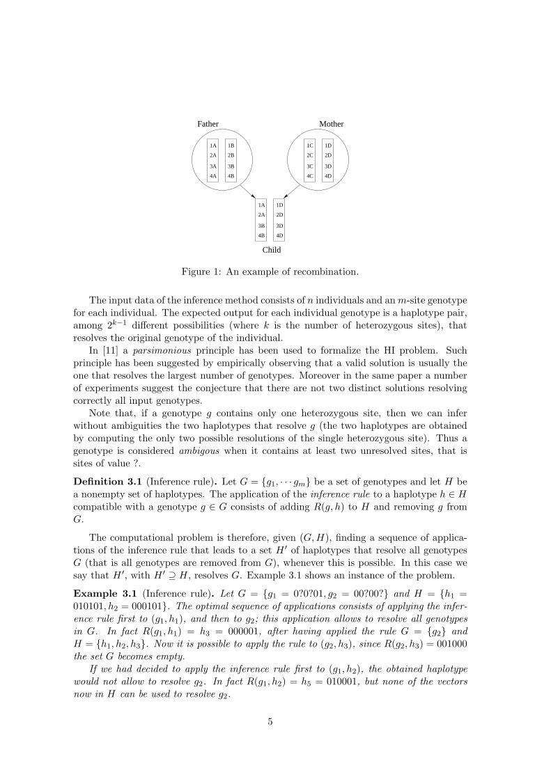
When we consider the haplotype inference problem, the alleles at each site i of anindividual consist of exactly one allele from each of his parents in the corresponding sites:this behavior is known as Mendelian Law, see Fig. 1. When no recombination occurs, eachof the two haplotype copies is equal to one of the haplotype copies of its parents, that isall alleles of a haplotype derives from the same haplotype copy of a parent.

If, on the contrary, recombinations occur, then a haplotype can consist of alleles comingfrom two haplotypes of the same parent. By Mendelian law, the consequence is that thegiven haplotype derives from two grandparents of the individual. Thus, the parental andgrandparental sources of a allele are the basic information to be used to determine andmeasure recombinations.

Fig. 1 shows a recombination event. A recombination occurs between the second locusand the third locus in the left (paternal) haplotype (the haplotype 1A, 2A, 3B, 4B) of thechild, since under Mendelian Law, the alleles at the first two loci are inherited from the left(paternal) haplotype of the father while the alleles at the last two loci are inherited fromthe right (maternal) haplotype of the father. Note that no recombination occurs in theright (maternal) haplotype (the haplotype 1D, 2D, 3D, 4D) of the child, since it is equalto the right (maternal) haplotype of the mother. The number of recombination events inan individual is the total number of such switches of the grandparent source occurring inits haplotypes. In the example of Fig. 1, the number of recombinations is one.

3.1 The Inference Problem: A General Rule

Various methods to infer haplotypes from genotype data have been proposed. Amongthem the inference method proposed in [11] and later largely discussed in [12] deservesour interest since it is the first approach that points out some basic computational issuesrelated to the haplotype inference problem under a general inference rule.

4

1D

2D

3D

4D

1D

2D

3D

4D

1A

1A

Father Mother

2A

3A

4A

1B

2B

3B

4B

1C

2C

4C

3C

2A

3B

4B

Child

Figure 1: An example of recombination.

The input data of the inference method consists of n individuals and an m-site genotypefor each individual. The expected output for each individual genotype is a haplotype pair,among 2k−1 different possibilities (where k is the number of heterozygous sites), thatresolves the original genotype of the individual.

In [11] a parsimonious principle has been used to formalize the HI problem. Suchprinciple has been suggested by empirically observing that a valid solution is usually theone that resolves the largest number of genotypes. Moreover in the same paper a numberof experiments suggest the conjecture that there are not two distinct solutions resolvingcorrectly all input genotypes.

Note that, if a genotype g contains only one heterozygous site, then we can inferwithout ambiguities the two haplotypes that resolve g (the two haplotypes are obtainedby computing the only two possible resolutions of the single heterozygous site). Thus agenotype is considered ambigous when it contains at least two unresolved sites, that issites of value ?.

Definition 3.1 (Inference rule). Let G = {g1, · · · gm} be a set of genotypes and let H bea nonempty set of haplotypes. The application of the inference rule to a haplotype h ∈ H

compatible with a genotype g ∈ G consists of adding R(g, h) to H and removing g fromG.

The computational problem is therefore, given (G, H), finding a sequence of applica-tions of the inference rule that leads to a set H ′ of haplotypes that resolve all genotypesG (that is all genotypes are removed from G), whenever this is possible. In this case wesay that H ′, with H ′ ⊇ H, resolves G. Example 3.1 shows an instance of the problem.

Example 3.1 (Inference rule). Let G = {g1 = 0?0?01, g2 = 00?00?} and H = {h1 =010101, h2 = 000101}. The optimal sequence of applications consists of applying the infer-ence rule first to (g1, h1), and then to g2; this application allows to resolve all genotypesin G. In fact R(g1, h1) = h3 = 000001, after having applied the rule G = {g2} andH = {h1, h2, h3}. Now it is possible to apply the rule to (g2, h3), since R(g2, h3) = 001000the set G becomes empty.

If we had decided to apply the inference rule first to (g1, h2), the obtained haplotypewould not allow to resolve g2. In fact R(g1, h2) = h5 = 010001, but none of the vectorsnow in H can be used to resolve g2.

5

In [12] a formal framework to analyze and investigate the computational complexity ofsuch problem has been proposed, by stating an optimization problem, whose correspondingdecision version is NP-hard. The optimization problem follows:

Problem 2 (MR). (Maximum Resolution problem)Input: a set G of genotypes and a set H of haplotypes.Output: a maximum cardinality subset G′ of G of genotypes that are removed from G

by a sequence of applications of the inference rule starting from G and H.

The computational complexity of some restricted versions of the MR problem is inves-tigated in [12]. Given a set of genotypes G and a set H of haplotypes, H has the uniqueexpression property w.r.t. G, in short UE property, if for every g ∈ G, there exists at mosta pair h1, h2 in H such that R(g, h1) = h2. The consequent problem follows:

Problem 3 (UEMR). (Unique Expression Maximum Resolution problem)Input: a set G of genotypes and a set H of haplotypes with the UE property.Output: a maximum-cardinality subset G′ of G of genotypes that are removed from G

by a sequence of applications of the inference rule starting from G and H that leaves a setH ′ of haplotypes having the UE property w.r.t. G′.

The proof in [12] that the MR problem is NP-hard makes use of a set H of haplotypeswith the UE property, thus proving that also the restricted UEMR problem is NP-hard.

In [12] a heuristic for the MR problem is proposed. In particular, the MR problem isreduced through a worst-case exponential time reduction to a new graph problem, whichconsists of finding some induced subtrees in a graph [12]. A heuristic for this last problemby using integer linear programming is presented.

Some questions related to the MR problem remain open. Mainly, the computationalcomplexity of solving a single genotype from a set containing both genotypes and haplo-types, by iteratively using the inference rule is unknown. Problem 4 is the formalization ofthe above question which is of fundamental importance, as determining if Problem 4 canbe solved in polynomial time, would give some insights on the feasibility of some possibleapplications of the inference rule that are different from the one suggested in the MRproblem.

Problem 4 (SGR). (Single Genotype Resolution problem)Input: a non empty set H of haplotypes and a distinguished genotype g ∈ G in a set G

of genotypes.Output: a sequence of applications of the inference rule that resolves a subset of G

including g

3.2 The Inference Problem by the Coalescent Model

One of the main drawbacks of the approach presented previously is that no biologicalassumption has been made, and sometimes biological assumptions allow to restrict theproblem so that efficient and more realistic solutions are obtained. Consequently somespecific biological models have been introduced recently in the framework of haplotyping.An interesting model has been proposed in [7]: the coalescent model, which assumes thatthe evolutionary history is represented by a rooted tree, where each given sequence labels

6

one of the leaves of the tree. The infinite site model is also assumed, that is at mostone mutation can occur in a given site in the whole tree. This last assumption, whichforbids recurrent mutations, is suitable to represent the evolutionary history in absenceof recombinations and when the basic evolutionary event is changing the value of a SNPsite, from 0 to 1. Consequently mutations are directed, that is descendants of individualsin which a mutation has occurred still own the given mutation [13].

The following definition introduces the main combinatorial tool for describing somecomputational problems related to the coalescent model.

Definition 3.2. Let B be a n×m {0, 1}-matrix, where each row in B is a binary haplotypeand each column i is the n vector of the SNP sites i for the m haplotypes. A haplotypeperfect phylogeny for B, in short hpp, is a rooted tree T with n leaves such that thefollowing properties hold:

1. each leaf of the tree is labeled by a distinct haplotype from B, that is a distinct rowof B,

2. each internal edge of T is labeled by at least a SNP site j changing from 0 to 1,while each site labels at most one edge,

3. for each haplotype leaf h, the unique path from the root of T to h specifies exactlyall SNP sites that are 1 in h.

Without loss of generality, the root of the phylogeny is assumed to be labelled by(0, 0, ..., 0). Consider now a matrix A, where each row is a genotype, that is A is a{0, 1, ?}-matrix. Analogously to the case of genotypes vectors, it is possible to give thedefinition of realization of matrix A by a matrix B, that is a matrix B such that eachrow of A is resolved by a pair of rows of B.

Definition 3.3. A {0, 1}-matrix B is a realization of a {0, 1, ?}-matrix A if each row Aj

of A is resolved by a pair of rows of B.

The third point of Def. 3.2 implies that each path in the perfect phylogeny T from theroot to a haplotype leaf h is a compact representation of the row of matrix B correspondingto h, since it represents all the sites of that row with value 1. Moreover let v be an internalvertex of T , let u be the parent of v and let Hv be the set of all haplotype leaves of thesubtree of T that have root in v; then Hv consists of exactly all haplotypes that have value1 in the SNP sites labeling (u, v). Hence Hv provides a compact representation of columnj of matrix B.

In [7, 8] the haplotype inference problem is then stated using the notion of haplotypeperfect phylogeny. The basic idea of the common approach in [7, 8] is that n genotypesmust be resolved by haplotypes that can be related by a haplotype perfect phylogeny as inDef. 3.2. Formally, the approach described above leads to the following problem as statedin [8].

Problem 5 (PPH). (Perfect Phylogeny Haplotyping problem)Input: an n × m matrix A over alphabet {0, 1, ?}.Output: a matrix B which is a realization of matrix A and a haplotype perfect phylogenyfor B, or decide that such a matrix does not exist.

7

In [7] the PPH problem is stated by requiring that a realization B of matrix A mustbe obtained by doubling each row rj of matrix A, in such a way that rows r2j and r2j+1

of B solve row rj in A. We will call such a realization a full realization of matrix A. Thedefinition given above is more general and allows us to define an optimization version of theproblem, that derives by applying a parsimonious criterion in inferring the haplotypes: theMPPH problem stated below. Indeed, it seems reasonable to require that the inferenceprocess from genotypes should produce a minimum number of distinct haplotypes, aspointed out by the empirical results in [11].

Problem 6 (MPPH). (Minimum Perfect Phylogeny Haplotyping problem)Input: an n × m matrix A over alphabet {0, 1, ?}.Output: a matrix B which is a realization of matrix A with the smallest number of rowsand a haplotype perfect phylogeny for B or decide that such a matrix does not exist.

Given an instance of the PPH problem, a first algorithmic issue concerns the existenceof a solution for that instance. Indeed, a haplotype perfect phylogeny induces two relationsbetween pairs of SNP sites labeling edges in the tree, one between siblings and one betweenan ancestor and a descendant. Those relations do not always allow to find a solution toevery instance of the PPH problem. Two sites i, j of an individual haplotype h are relatedby the ancestor-descendant relation whenever changes 0 to 1 hold in both sites i and j

of h: indeed, in the hpp, the path from the root to the leaf labeled by h contains twoedges labeled i and j. Moreover i and j are 1-0 siblings (0-1 siblings) in an individualhaplotype h, whenever the change 0 to 1 occurs in position i of h and not in j (or viceversa, respectively). It is easy to verify that in a hpp the two sites i and j that arerelated in a haplotype by the parenthood relation cannot be 0-1 siblings in a haplotypeand 1-0 siblings in another haplotype (see Fig. 3). Formally, this situation is describedby the existence of three rows h1, h2, h3 and two columns i, j of a matrix B such thatB[h1, i] = B[h1, j] = 1, while B[h2, i] = 1 and B[h2, j] = 0, B[h3, i] = 1 and B[h3, j] = 0.The submatrix of B induced by i, j and h1, h2, h3 is used [13] to characterize matrices thatcannot be represented by a hpp: we call such submatrix the forbidden matrix, see Fig. 2.

i j

h1 1 1h2 1 0h3 0 1

Figure 2: Example of a forbidden matrix M

Lemma 3.1. Let A be a n × m matrix over alphabet {0, 1}. Then, A admits a hpp iffevery submatrix of A induced by three rows and a pair of columns is not the forbiddenmatrix of Fig. 2.

An analogous of Lemma 3.1 holds for matrices over alphabet {0, 1, ?}. In a first paperon the PPH problem, a polynomial solution to the problem of computing a full realizationof a matrix A based on a reduction to the Graph Realization Problem is proposed [7],while direct algorithms of O(nm2) time complexity are proposed in [14] and [8]. The

8

h2 h1

i

j i

j

h3

(a) (b)

h1

00 00

Figure 3: The forbidden matrix M cannot be represented using a perfect phylogeny. Inthe tree (a) is represented the relation between sites i and j due to the haplotypes h1 andh2 of matrix M . In the tree (b) is represented the relation between sites i and j due tothe haplotypes h1 and h3 of matrix M . Note that in tree (a) i must be an ancestor of j,while in tree (b) j must be an ancestor of i.

complexity of the MPPH problem is still open. An experimental study of the biologicalvalidity and relevance of the Coalescent model in haplotype inference is largely discussedin a recent paper [9].

4 Inferring Haplotypes in Pedigrees

In this section, we investigate the HI problem in a pedigree. The difference betweenpopulation data and pedigree data lies in the relations among the individuals which areregarded independent if taken from a population, while the individuals are related by aparenthood relation if a pedigree is specified. The dependency relationships in pedigreedata have implications in two different aspects: 1) a structure (called pedigree graph)is imposed over pedigree data, whereas for population data to build such a structure(corresponding to recovering the evolutionary history of the involved haplotypes) mightbe one of the goals; 2) Mendelian Law is assumed, that is each child receives one allelefrom the father and one from the mother at each site, thus no mutations occur in thepedigree. Consequently Mendelian law can be used to partially resolve some genotypes.

Although the parental information gives some constraints on the reconstruction ofhaplotypes, there are still too many solutions that are consistent with the genotype dataand Mendelian law, especially for biallelic data like SNPs, where in general the probabilitythat more individuals have the same heterozygous genotypes is higher than that on multi-allelic data. Based on the fact that genetic recombinations are rare in human data [4,5, 15], people believe that haplotypes with fewer recombinations should be preferred in a

9

haplotype reconstruction [16, 17, 18].As already pointed out in this paper, the parsimonious principle naturally leads to

optimization problems. In this case the computational problem is finding a haplotypeconfiguration with minimum number of recombinants. Again, recombinations make theproblem hard; in fact a first formal proof of the NP-hardness of this problem is given in[19] for the general case of pedigree graphs. A heuristic algorithm for this problem anda polynomial exact algorithm for the 0-recombination situation are also presented in thatpaper. We will discuss those results later, but first we need to formally define the notionof a pedigree graph and several models for the HI problem on pedigree data.

Let us first define the general notion of a pedigree graph, without genotype informationthat has become widespread in biology.

Definition 4.1. A pedigree graph is a weakly connected directed acyclic graph G = 〈V, E〉,where V = M ∪ F ∪ N , M stands for the male nodes, F stands for the female nodes, N

stands for the mating nodes, and E = {e = (u, v): u ∈ M ∪ F and v ∈ N or u ∈ N andv ∈ M ∪F}. M ∪F are called the individual nodes. The indegree of each individual nodeis at most 1. The indegree of a mating node must be 2, with one edge starting from amale node (called father) and the other edge from a female node (called mother), and theoutdegree of a mating node must be larger than zero.

In a pedigree, the individual nodes adjacent to a mating node (i.e. they have edgesfrom the mating node) are called the children of the two individual nodes adjacent fromthe mating node (i.e. the father and mother nodes, which have edges to the mating node).The individual nodes that have no parents (indegree is zero) are called founders. For eachmating node, the induced subgraph containing the father, mother, mating, and childrennodes is called a nuclear family. A parents-offspring trio (or simply trio) consists of twoparents and one of their children. A mating loop is a cycle in the graph obtained from G

when the directions of edges are ignored.An equivalent definition of pedigree graph that points out the combinatorial nature of

the representation is the following:

Definition 4.2. A pedigree graph G is a weakly connected directed acyclic graph 〈V, E〉,where each vertex has indegree 2 or 0.

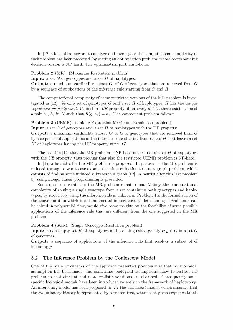
In Def. 4.2 only individual nodes are represented and their gender information areoutfitted. The founders are the vertices without incoming edges and a trio is any subgraphof G with 3 vertices u, v, w where (u, v) (here (u, v) stands for an arc from u to v sincewe are talking about the direct graph) and (w, v) are the only arcs of the pedigree graph;a trio is denoted by the triple < u, v, w >. In the following we will mean Def. 4.2 whenwe refer to the notion of pedigree graph. The only substantial difference with Def. 4.1regards the definition of mating loops; when Def. 4.2 is considered, a mating loop consistsof two distinct paths from a vertex x to a vertex y. Figure 4 shows side by side an examplepedigree according to the two definitions of pedigree graph, in particular to the left thecommon representation of pedigree graphs is reported.

The above pedigree graph definition is very general and there are several restrictedversions defined as follows.

Definition 4.3. A pedigree tree T is a pedigree graph without mating loops.

10

3−2

3−3 3−4 3−5 3−6 3−7 3−8

3−11 3−12 3−13 3−14 3−15 3−9 3−10

3−1

Figure 4: A pedigree with 15 members. (Left) A square represents a male node and acircle represents a female node, and a solid (round) node represents a mating node. Thechildren (e.g. 3-3, 3-5 and 3-7) are placed under their parents (e.g. 3-1 and 3-2). (Right)The representation of the same pedigree according to Def. 4.2

.

1-1 1-2

1-3 1-4 1-5 1-6

1-9

1-7 1-8

1-13 1-14 1-15

1-10 1-11 1-12

1-16 1-17

Figure 5: A pedigree with 17 members and a mating loop without showing the matingnodes.

11

We further distinguish pedigree trees by restricting the number of mating partnerseach individual node of the tree can have. Given a pedigree tree T , for any vertex v letP(v) be the set of vertices x such that (x, v) is an arc of T . Then T is a single-matingpedigree tree, if for any two vertices v, w, the two sets P(v) and P(w) are disjoint or thesame set; otherwise the pedigree tree is called multi-mating.

The definition of pedigree graph introduced so far allows us to describe the structure ofthe parental relations. We still need a notion that allow us to relate the actual genotypesto the structure of a pedigree graph.

Definition 4.4. A genotyped pedigree graph is a pedigree graph G where each individualvertex is labeled by a m-site genotype vector.

With a slight abuse of language by pedigree graph we will denote both a labeled(genotyped) and an unlabeled pedigree graph and in the case of labeled pedigree, we usethe node itself to denote the genotype vector associated to the node itself. Recall thatfor any node u, given the genotype vector < u[1], u[2], . . . , u[m] >, then u[i] ∈ {0, 1, ?}.If u[i] 6=?, then we say that u[i] is defined. Similarly a haplotyped pedigree graph is apedigree graph where each individual vertex is labeled with two haplotypes.

Definition 4.5. A genotyped pedigree graph G is g-valid if the following consistency ruleshold. Given a trio 〈u, v, w〉, then for each i, 1 ≤ i ≤ m:

• if u[i] 6= w[i] are both defined, then v[i] =?,

• if u[i] 6= w[i] and only one of u[i] or w[i] is defined, then v[i] = w[i] or v[i] = u[i],

• if u[i] = w[i] =?, then v[i] can be 0, 1 or ?,

• u[i] = v[i] = w[i], otherwise.

Then, given a g-valid genotyped pedigree graph G, we are interested in a haplotypedpedigree graph with same sets of vertices and edges, such that the haplotypes labeling avertex v resolve the genotype of v in G and each haplotype (paternal/maternal) in a childis inherited from each parent (father/mother) with/without recombinations. In such casewe will say that the haplotyped graph is a realization of G.

Problem 7 (PHI). (Pedigree Graph Haplotype Inference problem)Input: a g-valid genotyped pedigree graph G.Output: a haplotyped pedigree graph which is a realization of G.

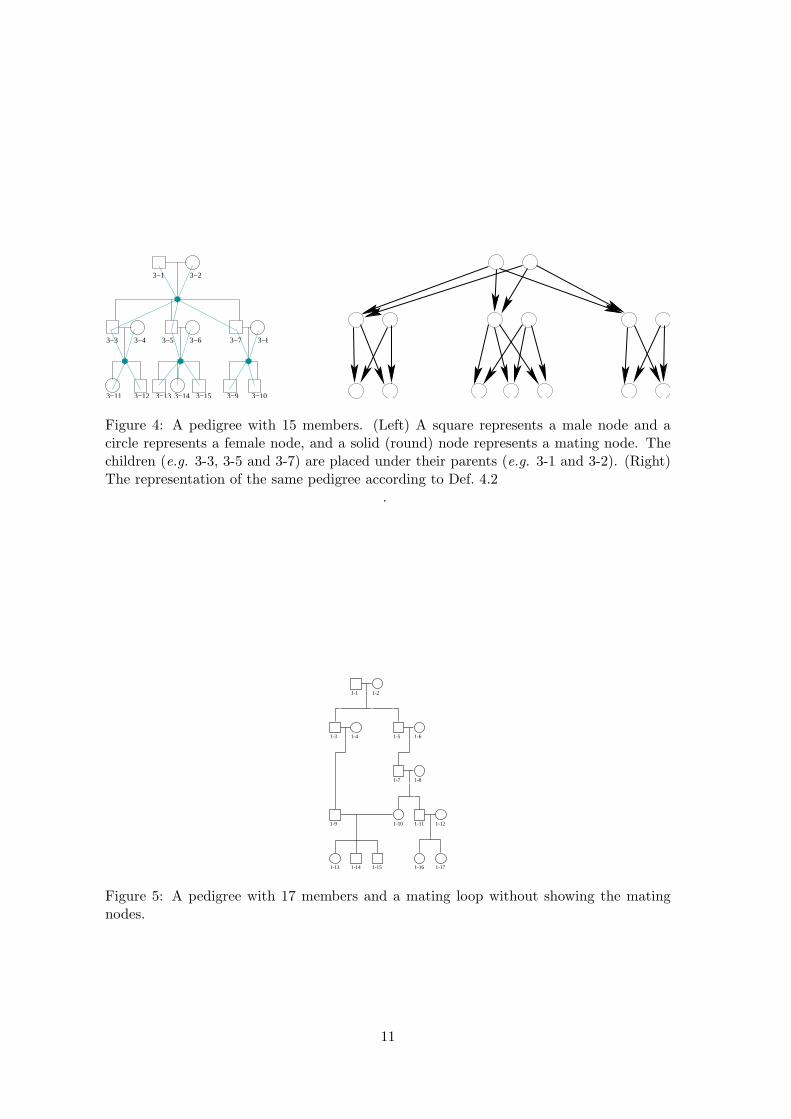
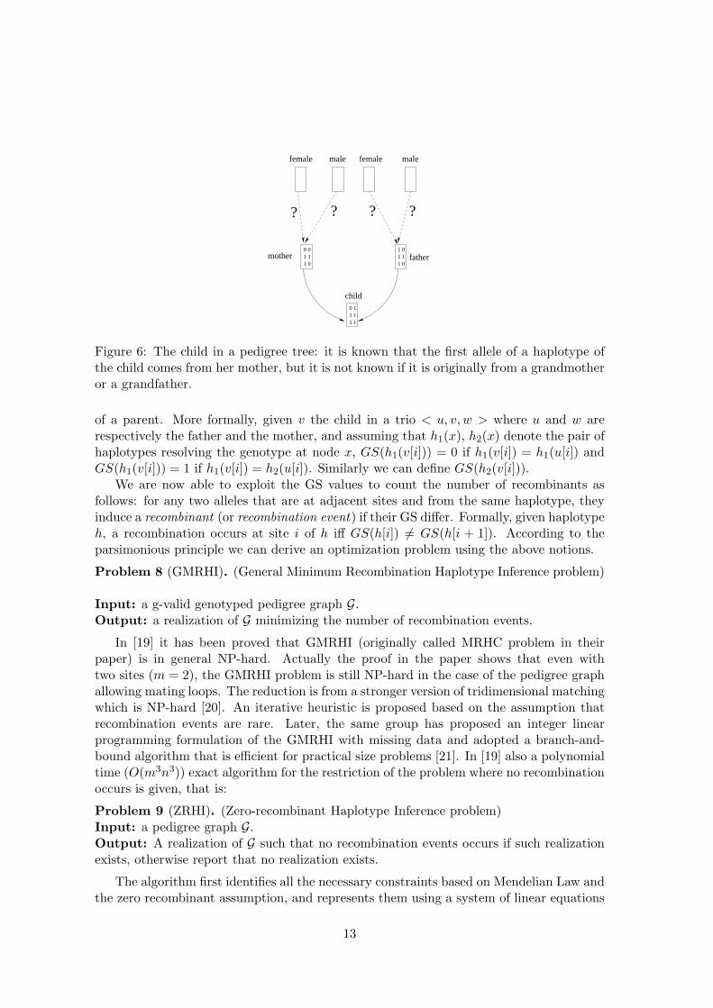
Even though a realization of the genotyped graph explicitly associates the two hap-lotypes of each child to the ones of its parents, a realization might not unambiguouslydetermine for each allele on a given haplotype what is the haplotype of its correspondingparent from which it derives. For instance let us consider Fig. 6, we know that the firstallele of a haplotype of the child comes from her mother, but does it come originally froma grandmother or a grandfather? In order to disambiguate those situations we introducethe notion of GS value of each allele which states if it is inherited from parent’s paternalhaplotype or maternal haplotype.

The introduction of a GS value for each allele is necessary due to the presence ofrecombinations, because in this case each haplotype is not the exact copy of one haplotype

12

0 11 11 1

1 11 0

0 01 11 0

1 0fathermother

male femalefemale male

child

? ? ? ?

Figure 6: The child in a pedigree tree: it is known that the first allele of a haplotype ofthe child comes from her mother, but it is not known if it is originally from a grandmotheror a grandfather.

of a parent. More formally, given v the child in a trio < u, v, w > where u and w arerespectively the father and the mother, and assuming that h1(x), h2(x) denote the pair ofhaplotypes resolving the genotype at node x, GS(h1(v[i])) = 0 if h1(v[i]) = h1(u[i]) andGS(h1(v[i])) = 1 if h1(v[i]) = h2(u[i]). Similarly we can define GS(h2(v[i])).

We are now able to exploit the GS values to count the number of recombinants asfollows: for any two alleles that are at adjacent sites and from the same haplotype, theyinduce a recombinant (or recombination event) if their GS differ. Formally, given haplotypeh, a recombination occurs at site i of h iff GS(h[i]) 6= GS(h[i + 1]). According to theparsimonious principle we can derive an optimization problem using the above notions.

Problem 8 (GMRHI). (General Minimum Recombination Haplotype Inference problem)

Input: a g-valid genotyped pedigree graph G.Output: a realization of G minimizing the number of recombination events.

In [19] it has been proved that GMRHI (originally called MRHC problem in theirpaper) is in general NP-hard. Actually the proof in the paper shows that even withtwo sites (m = 2), the GMRHI problem is still NP-hard in the case of the pedigree graphallowing mating loops. The reduction is from a stronger version of tridimensional matchingwhich is NP-hard [20]. An iterative heuristic is proposed based on the assumption thatrecombination events are rare. Later, the same group has proposed an integer linearprogramming formulation of the GMRHI with missing data and adopted a branch-and-bound algorithm that is efficient for practical size problems [21]. In [19] also a polynomialtime (O(m3n3)) exact algorithm for the restriction of the problem where no recombinationoccurs is given, that is:

Problem 9 (ZRHI). (Zero-recombinant Haplotype Inference problem)Input: a pedigree graph G.Output: A realization of G such that no recombination events occurs if such realizationexists, otherwise report that no realization exists.

The algorithm first identifies all the necessary constraints based on Mendelian Law andthe zero recombinant assumption, and represents them using a system of linear equations

13

over the cyclic group Z2. By using a simple method based on Gaussian elimination,all possible feasible haplotype configurations could be obtained. The running time forZRHI has been further improved to O(mn2 + n3 log n log log n) by Xiao et al. [22]. Theiralgorithm can efficiently eliminate redundant equations in a system of linear equationscollected based on some spanning tree of the pedigree graph. Chan et al. [23] claimeda linear algorithm for ZRHI when a pedigree has no mating loops. Since in the case ofhuman pedigrees, mating loops are very rare, it becomes interesting to give the followingmore restricted formulations of the general problem.

Problem 10 (MPT-MRHI). (Multi-mating Pedigree Tree Minimum Recombination Hap-lotype Inference problem)Input: a multi-mating g-valid genotyped pedigree tree T .Output: a realization of T minimizing the number of recombination events.

Problem 11 (SPT-MRHI). (Single-mating Pedigree Tree Minimum Recombination Hap-lotype Inference problem)Input: a single-mating g-valid genotyped pedigree tree T .Output: a realization of T minimizing the number of recombination events.

It has been proved in [24] that even SPT-MRHI is NP-hard by a reduction fromMAX-CUT [20]. Unlike the NP-hardness proof of GMRHI in [19], where only two sitesare needed, the proof of SPT-MRHI does require an unbounded number of sites. Morerecently, Liu et al. [25] have shown that the SPT-MRHI problem is NP-hard even whenan individual node has at most one mate and at most one child (binary-tree pedigrees) bya reduction from 6=3SAT [26]. In the same paper, the authors have also shown that, withmissing data, GMRHI on pedigrees with two loci and SPT-MRHI on binary-tree pedigreescannot be approximated unless P=NP.

5 Inferring Haplotypes from Fragments

The Human Genome project has successfully produced a draft version of the DNA presentin human beings, through a sequencing process. A different kind of problem arises when thesequencing process aims also to reconstruct haplotypes. Roughly speaking, the sequencingprocess is made of two phases: in the first phase a number of fragments are obtained,where each fragment is a small piece (a few hundreds of bases long) of the examinedDNA. Afterwards all such fragments are merged into a chromosome, for example viashotgun sequencing [2]. In its original formulation the sequencing problem assumes thatall fragments come from only one copy of the chromosomes of a DNA strand. But thisassumption is too weak, in fact not only the fragments come from both copies, but it isnot possible to associate the fragments to the copy of the chromosome from which theyoriginate. Thus computing the two sequences that form the haplotypes becomes morechallenging. Moreover, the presence of errors in the fragments that need to be assembledmakes harder the problem of reconstructing the original sequence from fragments whenSNPs are considered.

In [6], the problem of reconstructing the pair of haplotype sequences from fragments ofa human chromosome is investigated by introducing some formulations. First of all, eachlocation of a SNP over a fragment is assumed to be known, that is the genomic sequence

14

is thought of as a sequence of positions with one (not a SNP site) or two (a SNP biallelicsite) symbols associated to each position. The sequence of SNPs sites along a fragment isdescribed by a vector over a binary alphabet {0, 1} that is used to denote the two distinctalleles of SNP sites contained in the fragment.

The formal definitions of the problems introduced in [6] share the fact that the instanceis always a n × m matrix M where each entry M [i, j] is 0 or 1 or -, and where the i-th row corresponds to the i-th fragment, conversely the j-th column corresponds to thej-th SNP. When M [i, j] = - then the i-th fragment does not cover the j-th SNP, whichmeans that the allele of the fragment in position j is unknown: the entry - of matrix M

is called a hole. Moreover we will say that two fragments conflict with each other if theydisagree on a SNP covered by both fragments, that is fragments i and j of matrix M arein conflict whenever there exists a SNP site k such that M [i, k] 6= M [j, k] and both M [i, k]and M [j, k] are not holes. A conflict occurring at a given SNP site denotes the fact thatthe two fragments come from two distinct haplotypes, or more precisely, the SNP site isheterozygous and has two distinct alleles on the two chromosome copies.

If the matrix M represents m fragments obtained from one pair of haplotypes andfragments do not contain errors in the alleles reported in the matrix, conflicts among thefragments can be used to derive a partition of fragments into two sets, each one containingthe non conflicting fragments from the same haplotype.

Thus, we define a matrix M error free iff there exists a partition of rows of M into twomatrices M1 and M2 such that both M1 and M2 do not contain conflicting fragments.

In [6], the following biological problem is investigated: the reconstruction of the twodifferent haplotypes of a chromosome from SNP values of fragments represented by aninstance matrix that is not necessarily error free. It must be pointed out that, even whenthe matrix is error free, there may be more than one pair of haplotypes whose fragmentsgive the same instance matrix: in this case the reconstruction of the original haplotypesfor the chromosome from a SNP matrix is not solvable, as the instance matrix does notcontain enough information to disambiguate among all possible haplotypes.

Hence, we restrict ourselves to the problem of finding a pair of haplotypes whosefragments are represented by a given matrix. Then the problem consists of assigning eachfragments to a copy of the chromosome.

When the matrix is error free, this problem can be solved easily by computing thefragment conflict graph, whose vertices are the fragments and the pair (i, j) is an edge iffthe two fragments i and j conflict. Indeed, the graph must be bipartite, with each shorerepresenting all the fragments that are in one of the two copies of the chromosome.

Please notice that the solution to the problem of inferring haplotypes from fragmentsobtained from the fragment conflict graph is unique iff the graph is connected, in whichcase the solution consists of a unique pair of haplotypes.

In the presence of errors the problem becomes more complex; in fact we look for theminimum number of modifications to the instance matrix to make it error free. Differentoperations on the matrix may be defined and each of such operations leads to a specificcomputational problem, as pointed out in [6] where the following problems have beenintroduced:

Problem 12 (MFR). (Minimum Fragment Removal)Compute the minimum set of rows to remove from the matrix so that the matrix is error

15

1 2 3 4 5 6

1 0 1 - 0 - 02 0 - 1 - - 03 1 0 - - 1 14 - 1 1 - 0 -5 1 - - 1 - 1

1

2

3

4

5

Figure 7: An error-free matrix and its associated fragment conflict graph

1 2 3 4 5 6

1 0 1 - 0 - 02 0 - 1 - - 03 1 0 - - 1 14 - 1 1 - 0 -5 1 1 - 1 - 1

1

2

3

45

Figure 8: A matrix with errors and its associated fragment conflict graph

free.

Problem 13 (MSR). (Minimum SNP Removal)Compute the minimum set of columns to remove from the matrix so that the matrix iserror free.

Problem 14 (LHR). (Longest Haplotype Reconstruction)Compute a set of rows to remove from the matrix so that the matrix is error free and thesum of the lengths of the inferred haplotypes is maximized.

Problem 15 (MEC). (Minimum Error Correction)Compute the minimum number of corrections on the entries of the matrix so that theresulting matrix is error free.

A single fragment may (but not must) cover SNP sites that are consecutive on thefragment: in such case the fragment is gapless. A fragment has k gaps if it covers k + 1blocks of consecutive SNPs.

Of particular interests are the cases of 0 or 1 gaps, as these cases are common whensequencing. The classical shotgun sequencing procedure deals with probes that are con-secutive nucleotides from a DNA strand. Recent advances of the sequencing technologyhas made the production of mate pairs feasible, where a mate pair is made of two probesfrom the same copy of a chromosome and with a distance between the two probes that isapproximately known. Representing a mate pair with a 1-gap fragment is immediate. InTable 1 are summarized some results described in [6, 27].

The presence of gaps in fragments and also the number of holes is strictly related to thecomputational complexity of the above problems (Table 1 reports all known results about

16

Problems Gaps Exact Approximation

MFR ≤ 1 NP-hard APX-hard1

0 Solvable in time O(m2n + m3)k holes Solvable in time O(22knm2 + 23km3)

MSR ≤ 2 NP-hard APX-hard2

0 Solvable in time O(mn2)k holes Solvable in time O(mn2k+2),

LHR k holes ? ?0 Polynomial time

MEC n NP-hard ?0 ?

Table 1: Known results for some problem on fragments

the complexity of such problems). Indeed, whenever fragments are gapless the problem isin general polynomial. The 1-gap case is relevant since the presence of at most one gap ineach fragment is a sufficient condition to make hard the MFR problem. It is an interestingquestion to investigate the 1-gap case for the MSR and the other problems.

In the following we describe a graph based method to solve the MSR problem forgapless instance matrices. This method uses the notion of conflict among SNP sites.Given a SNP matrix M , two SNP sites i and j are in conflict in M iff i and j assumesboth 0, 1 values in M and there exist two fragments x and y such that the submatrixinduced by rows x and y and columns i and j has three symbols of one type and one ofthe opposite. SNP conflicts of a SNP matrix M are represented by the SNP conflict graphhaving vertices the SNPs and an edge for each pair (i, j) of conflicting SNPs.

An interesting property relates the SNP matrices without gaps to error free matrices.

Lemma 5.1. A matrix without gaps is error free iff it has no SNP conflicts.

By using the above property, that can be easily verified, the problem MSR reduces tosolve the Min Vertex Cover problem over the SNP conflict graph, as making a matrix errorfree means to remove from such graph the minimum number of vertices (matrix columns)so that the graph has no edges. In [6] it is proved that whenever a matrix is withoutgaps then the SNP conflict graph is perfect [28]. Being the Min Vertex Cover problemon perfect graphs polynomial-time solvable, MSR can be solved efficiently via the abovereduction.

On the other hand, when the fragments contain some gaps the reduction does not workas illustrated in the following example.

Example 5.1. Assume that M is the matrix of Fig. 9 and G the corresponding SNPconflict graph. Then the vertex 4 is a minimum vertex cover, but the matrix M ′ obtainedfrom M by removing the column 4 is not error free.

All algorithms for the gapless cases are via dynamic programming; the main idea isthat it is possible to infer the optimal solution from the optimal solution on a submatrixobtained by removing a SNP column (MSR) or a fragment row (MFR). Let M be a SNPmatrix, we denote with M [1...k] the submatrix of M formed by the first k rows of M .

17

1 2 3 41 0 - 0 02 1 1 - 03 - 0 1 1

1 3

24

Figure 9: A matrix with gaps and the corresponding SNP conflict graph

Let us consider the MFR problem. Since the matrix M is gapless, each row of M ,consists of a sequence of defined values encoding the actual fragment, preceded or followedby some (possibly zero) holes. For each row f of M we denote by l(f) and r(f) respectivelythe leftmost and the rightmost positions (SNP) of f that are not holes. The algorithmwill exploit the fact that all positions between l(f) and r(f) must be defined. A firstpreprocessing step of the algorithm is to sort the rows of M in increasing order of l(f),that is l(i) ≤ l(j), whenever i < j.

A dynamic programming algorithm mainly consists of showing that an optimal solutionof an instance can be computed from an optimal solution of some induced subinstance,in our case we will compute the optimal solution over the matrix M by exploiting theoptimal solution where the “rightmost” fragment is removed from M . Consequently wewill show how to solve the instance M [1..k] from an optimal solution of M [1..k − 1] (werecall here that an optimal solution is a minimum-size set of rows that must be removedto obtain an error-free matrix).

The algorithm computes the value D[i, j, k] that is the optimum over instance M [1...k]with the additional restriction that fragment i (respectively j) has the maximum value ofr(i) (resp. r(j)) among all r(f) for all fragments placed on the first (resp. the second)haplotype. See Fig. 10 for an illustrative example.

Haplotype 1

Haplotype 2fragment j

fragment i

l(i) r(i)

Figure 10: Example of fragments placed on the haplotypes by the algorithm in [27]

Moreover for each row f considered we denote with OK(f) the set of rows with indexg < f that agree with row f , that is rows representing fragments that may be on thesame haplotype copy. Now we can explicitly show the recurrence that allows to solve theproblem. The following possible cases must be considered:

18

1. D[i, j, 0] := 0

2. k > i, k > j; D[i, j, k] :=

D[i, j, k − 1] if r(k) ≤ r(j) and rows k and j agreeD[i, j, k − 1] if r(k) ≤ r(i) and rows k and i agreeD[i, j, k − 1] + 1 otherwise;

3. k = i; D[k, j, k] := minh∈OK(k),r(h)≤r(k){D[h, j, k − 1]}

4. k = j; D[i, k, k] := minh∈OK(k),r(h)≤r(k){D[i, h, k − 1]}

The optimal solution will be minh,k{D[h, k; m]}. In [27] the dynamic programmingalgorithm described has also been extended as a fixed-parameter algorithm for the sameproblem, where the parameter is the number of holes contained in the fragments, that isthe number of unresolved symbols between the leftmost and the rightmost resolved symbolof each fragment. The algorithm can also be extended to the class of matrices where thecolumns can be permuted so that in each row the (0/1) symbols appear consecutively. Thelast problem is also a version of the consecutive ones problem, for which a polynomial-timealgorithm has been described in [29].

6 A Glimpse over Statistical Methods

In this section we present some basic aspects of the application of statistical methodsto tackle the haplotype inference problem. These methods are among the most used bybiologists. Indeed, a certain number of results on haplotype inference from real data havebeen produced based on some statistical models. Anyway here we will only briefly reviewsome of these algorithms, since this survey mainly focuses on combinatorial approaches forhaplotype inference. Moreover, some combinatorial problems discussed here aim to addresssome biological issues that are different from the ones attacked using the algorithms basedon statistical models.

The introduction of statistical models is mainly due to the presence of some shortcom-ings of the method introduced in [11]. In fact, the method in [11] requires an initial setof resolved haplotypes and it also highly depends upon the order by which haplotypes areresolved. The approach of [12, 30] lowers the relevance of the dependency on the order,hence making the whole procedure more reliable. The main idea of statistical modelsis that haplotypes have an unknown distribution in the target population and the ob-served genotypes of each individual are simply combination of two haplotypes randomlydrawn from the population. The goal of statistical haplotype inference is thus to estimatethe haplotype frequencies and the haplotypes of each individual can be easily inferredbased on the haplotype frequencies under some biological assumptions (like random mat-ing assumption). Two different formulations of the haplotype inference problem, namely,Maximum-Likelihood inference [31] and Bayesian inference [32, 33] have been investigatedand will be briefly discussed here.

Problem 16 (FHI). (Frequencies Haplotype Inference problem)Input: a sample G of genotypes.

19

Output: the set of haplotype frequencies {h1, h2, ..., hn} (where n is the number of all pos-sible haplotypes) that maximize the likelihood function of observing the genotype sampleG.

Problem 17 (BFHI). (Bayesian Frequencies Haplotype Inference problem)Input: a sample G of genotypes and a priori distribution of the frequencies of haplotypes.Output: the posterior distribution of the haplotype frequencies given the sample G.

The FHI problem is tackled in [31], where an Expectation-Maximization algorithm(EM) has been proposed to estimate the haplotype frequencies that maximize the likeli-hood function of genotype sample. It is well known that the general framework of EMalgorithm [34] is to find the maximum-likelihood estimator(s) by iteratively executing theE-step and M-step until convergence in the presence of missing data. Let Ht denote theset of haplotype frequencies and Gt denote the set of probabilities of all the genotypes attime t. The EM algorithm works by arbitrarily assigning an initial value of H0 (a possibleinitial set of frequency values is the one corresponding to the assumption that all possiblehaplotypes are equiprobable). Based on H0, the expectation of an observing genotype canbe easily calculated, which is one of the elements in G1. The expected genotype frequen-cies in G1 are used in turn to estimate the haplotype frequencies at the M-step resultingin a new H1. Iterate the two steps until convergence (i.e., the difference between Ht+1

and Ht is smaller than a predefined value.). At each iteration, the solution Ht is improvedin the M-step by maximizing the likelihood function of the genotype sample. Differentinitial values can be taken in order to increase the possibility to obtain a global optimalsolution.

The BFHI problem is tackled by an iterative stochastic-sampling strategy, the pseudoGibbs sampler (PGS) [32], that makes use of the Markov chain Monte Carlo methodwith the assumption of a coalescent model. A Gibbs sampler iteratively samples a pairof compatible haplotypes for each genotype conditional on the genotypes G and on otherhaplotypes, and uses these values to update the frequencies of haplotype distribution. Thisiterative algorithm produces haplotype frequencies h1, ..., hm as they were sampled fromthe desired posterior distribution of the haplotype frequencies given the sample genotypesG.

The two methods described above cannot handle satisfactorily a large number of SNPs,or missing data. These issues are addressed by the method proposed in [33], where a robustBayesian procedure has been introduced. The method in [33] makes use of the biologicalmodel also used in [31], but imposes no assumptions on the population history (comparingto the coalescent model used in [32]). In particular the method introduces a divide-and-conquer technique so that a larger number of haplotypes can be studied. This algorithmpartitions the genotypes into units, where each unit has maximum length of 8 loci. Themethod first constructs a set of most probable partial haplotypes compatible with eachunit using the Gibbs sampler. Two adjacent units are then combined to construct a set ofthe most probable partial haplotypes that are compatible with the genotypes of the twounits. The algorithm recursively combines the partial haplotypes until the whole haplotypeis created. A detailed comparison of different statistical methods and the combinatorialmethod in [11] can be found in [33], which is based on an experimental study.

We conclude this section by observing that, since there is an exponential number ofpossible haplotype solutions for a given set of genotypes, the statistical methods may

20

have to analyze an exponential number of haplotypes in order to generate the solutionof the FHI and BFHI problems. Even equipped with advanced numerical methods likeEM algorithm and Gibbs sampler, such statistical methods are still very time consuming.Thus, the application of these methods is restricted to a small number of individualsin a population; moreover the maximum number of individuals tractable decreases as thenumber of SNPs increases. This limitation is not present in other combinatorial approachesbased on polynomial algorithmic solutions.

7 Acknowledgements

J.L. is supported in part by NIH/NLM grant R01 LM008991 and a start-up fund fromCase Western Reserve University.

References

[1] International Human Genome Sequencing Consortium. Initial sequencing and analysisof the human genome. Nature, 409(6822):860–921, February 2001.

[2] J. C. Venter, M. D. Adams, E. W. Myers, and et al. The sequence of the humangenome. Science, 291(5507):1304–1351, 2001.

[3] N. Patil, A.J. Berno, and et al. Blocks of limited haplotype diversity revealed byhigh-resolution scanning of human chromosome 21. Science, 294(5547):1669–1670,2001.

[4] M. Daly, J. Roux, S. Schaffer, T. Hudson, and E. Lander. Fine-structure haplotypemap of 5q31: implicatins for gene-based studies and genomic ld mapping. 2001.

[5] S. B. Gabriel, S. F. Schaffner, H. Nguyen, J. M. Moore, J. Roy, B. Blumenstiel,J. Higgins, M. DeFelice, A. Lochner, M. Faggart, S. N. Liu-Cordero, C. Rotimi,A. Adeyemo, R. Cooper, R. Ward, E. S. Lander, M. J. Daly, and D. Altshuler. Thestructure of haplotype blocks in the human genome. Science, 296(5576):2225–2229,2002.

[6] G. Lancia, V. Bafna, S. Istrail, R. Lippert, and R. Schwartz. SNPs problems, com-plexity and algorithms. In Proc. 9th European Symp. on Algorithms (ESA), pages182–193, 2001.

[7] D. Gusfield. Haplotyping as perfect phylogeny: Conceptual framework and efficientsolutions. In Proc. 6th Annual Conference on Research in Computational MolecularBiology (RECOMB), pages 166–175, 2002.

[8] E. Halperin, E. Eskin, and R. M. Karp. Efficient reconstruction of haplotype struc-ture via perfect phylogeny. Journal of Bioinformatics and Computational Biology, toappear.

21

[9] E. Halperin, E. Eskin, and R. M. Karp. Large scale reconstruction of haplotypesfrom genotype data. In Proc. 7th Annual Conference on Research in ComputationalMolecular Biology (RECOMB), pages 104–113, 2003.

[10] K. Zhang, M. Deng, T. Chen, Michael S. Waterman, and F. Sun. A dynamic pro-gramming algorithm for haplotype block partitioning. Proceedings of the NationalAcademy of Sciences USA, 99(11):7335–7339, 2002.

[11] A. Clark. Inference of haplotypes from pcr-amplified samples of diploid populations.Molecular Biology and Evolution, 7(2):111–122, 1990.

[12] D. Gusfield. Inference of haplotypes from samples of diploid populations: Complexityand algorithms. Journal Of Computational Biology, 8(3):305–323, 2001.

[13] D. Gusfield. Algorithms on Strings, Trees and Sequences: Computer Science andComputational Biology. Cambridge University Press, Cambridge, 1997.

[14] V. Bafna, D. Gusfield, G. Lancia, and S. Yooseph. Haplotyping as perfect phylogeny:A direct approach. Journal of Computational Biology, to appear.

[15] L. Helmuth. Genome research: Map of human genome 3.0. Science, 5530(293):583–585, 2001.

[16] J. R. O’Connell. Zero-recombinant haplotyping: applications to fine mapping usingsnps. Genet. Epidemiol., 19(Suppl. 1):S64–70, 2000.

[17] D. Qian and L. Beckmann. Minimum-recombinant haplotyping in pedigrees. Am. J.Hum. Genet., 70(6):1434–1445, 2002.

[18] P. Tapadar, S. Ghosh, and P. P. Majumder. Haplotyping in pedigrees via a geneticalgorithm. Hum. Hered., 50(1):43–56, 2000.

[19] J. Li and T. Jiang. Efficient inference of haplotypes from genotypes on a pedigree.J Bioinfo Comp Biol, 1(1):41–69, 2003. (an earlier version appeared in RECOMB03,197-206.)

[20] M.R. Garey and D.S. Johnson. Computer and Intractability: A Guide to the Theoryof NP-completeness. W. H. Freeman, 1979.

[21] J. Li and T. Jiang. Computing the minimum recombinant haplotype configurationfrom incomplete genotype data on a pedigree by integer linear programming. J CompBiol, 12:719-739, 2005. (an earlier version appeared in RECOMB04, 101-110.)

[22] J. Xiao, L. Liu, L. Xia and T. Jiang. Fast elimination of redundant linear equa-tions and reconstruction of recombination-free mendelian inheritance on a pedigree.Menuscript, 2006.

[23] M.Y. Chan, W.T. Chan, F.Y.L. Chin, S.P.Y. Fung and M.Y. Kao. Linear-timehaplotype inference on pedigrees without recombinantions. Accepted by the 6th in-ternational Workshop on Algorithms in Bioinformatics (WABI), 2006.

22

[24] K. Doi, J. Li and T. Jiang. Minimum recombinant haplotype configuration on treepedigrees. In Proc. 3rd international Workshop on Algorithms in Bioinformatics(WABI), pages 339-353, Hungary, 2003.

[25] L. Liu, x. Chen, J. Xiao and T. Jiang. Complexity and approximation of the minimumrecombinant haplotype configuration problem. ISAAC, page 370-379, 2005.

[26] T.J. Schaefer. The complexity of satisfiability problems. Proc. of the 10th STOC,page 216-226, 1978.

[27] R. Rizzi, V. Bafna, S. Istrail, and G. Lancia. Pratical algorithms and fixed-parametertractability for the single individual snp haplotyping problem. In Proceedings ofAlgorithms in Bioinformatics, Second International Workshop (WABI 2002), pages29–43, 2002.

[28] M. Grotschel, L. Lovasz, and A. Schrijver. A polynomial algorithm for perfect graphs.Annals of Discrete Mathematics, 21:325–356, 1984.

[29] K. S. Booth and G. S. Lueker. Testing for the consecutive ones property, intervalgraphs, and graph planarity using pq-tree algorithms. Journal of Computer andSystem Sciences, 13(3):335–379, 1976.

[30] S. Orzack, D. Gusfield, and V.P. Stanton. The absolute and relative accuracy ofhaplotype inferral methods and a consensus approach to haplotype inferral. In 51stAnnual Meeting of the American Society of Human Genetics, 2001.

[31] L. Excoffier and M. Slatkin. Maximum-likelihood estimation of molecular haplotypefrequencies in a diploid population. Molecular Biology and Evolution, 12(5):921–927,1995.

[32] M. Stephens, N.J. Smith, and P. Donnelly. A new statistical method for haplotypereconstruction from population data. American Journal of Human Genetics, 68:978–989, 2001.

[33] T. Niu, Z.S. Qin, X. Xu, and J.S. Liu. Bayesian haplotype inference for multiple linkedsingle-nucleotide polymorphisms. American Journal of Human Genetics, 710:157–169, 2002.

[34] T. M. Mitchell. Machine Learning. McGraw Hill, New York, 1987.

Authors’ Biographies

Paola Bonizzoni is Associate Professor of Computer Science at the Universita di Milano-Bicocca in Milan. She received her Master Degree in Computer Science from the Univer-sita’ di Milano in 1988 and her Ph. D in Computer Science from the Universita di Milano-Torino in 1993. She has been Assistant Professor in Computer Science at the Universitadi Milano from 1993 to 1999. She has been Visiting Research Associate at the Universityof Colorado at Boulder (USA).

23

Gianluca Della Vedova has been appointed as an assistant professor at the Departmentof Statistics, Universita di Milano-Bicocca in 2001. He holds a Ph.D. and a M.Sc. inComputer Science (Universita di Milano). His research interests focus on the design ofcombinatorial algorithms in Bioinformatics and Graph theory. He has published severalpapers in Bioinformatics and Theoretical Computer Science international journals.Riccardo Dondi is a Ph.D candidate in Computer Science, at Universita di Milano-Bicocca. In 1999 he has received his M.Sc. in Computer Science at Universita di Milano.His research area is Computational Biology, in particular the design of algorithms and thestudy of the computational complexity of some biological problems, mainly the construc-tion and comparison of evolutionary trees. His more recent focus is on haplotype inferenceproblems.Jing Li currently is a Ph.D candidate in the Department of Computer Science and En-gineering at University of California - Riverside. He received a B.S. in Statistics fromPeking University, Beijing, P.R.China in July 1995 and a M.S., in Statistical Genetics,from Creighton University in Aug. 2000.

His recent research interest includes Bioinformatics and computational molecular biol-ogy, algorithms and statistical genetics. He has published several papers in Bioinformaticsand statistical genetics conferences and journals.

24