Torque Enhancement Principle of Stator PM Vernier Machine ...
Upload
khangminh22Category
view
0download
0
University of Zagreb
Faculty of Mechanical Engineering and Naval
Architecture
master’s thesis
Luka Balatinec
Zagreb, 2019

University of Zagreb
Faculty of Mechanical Engineering and Naval
Architecture
master’s thesis
An Overview of Rotor-Stator Interfaces for
Computational Fluid Dynamics Simulations in
Turbomachinery
Mentor:
prof. dr. sc. Hrvoje Jasak
Student:
Luka Balatinec
Zagreb, 2019

I would like to express my sincere gratitude to professor Jasak for the mentorship
he provided, offering invaluable advice and sharing his immense knowledge and
expertise.
Furthermore, I would like to wholeheartedly thank Tessa Uroic and Vanja
Skuric for the guidance, support and friendship they so kindly offered.
I would also like to thank the rest of the 8th floor CFD ”crew” for making
the time I spent there both interesting and fun.
Finally, I would like to thank my family, friends and my girlfriend for the
support and understanding they provided.

Statement | Izjava
I hereby declare that I have made this thesis independently using the knowledge acquired
during my studies and the cited references.
Izjavljujem da sam ovaj rad radio samostalno koristeci znanja stecena tijekom studija i
navedenu literaturu.
Zagreb, March 2019 Luka Balatinec

Contents
Contents v
List of Figures ix
List of Tables xii
Nomenclature xiii
Sazetak xviii
Abstract xix
Prosireni sazetak xx
Metode povezivanja mreze . . . . . . . . . . . . . . . . . . . . . . . . . . xxi
Kontra-rotirajuci propeleri . . . . . . . . . . . . . . . . . . . . . . . . . . xxii
Numericka mreza . . . . . . . . . . . . . . . . . . . . . . . . . . . . . . . xxiii
Rezultati simulacija . . . . . . . . . . . . . . . . . . . . . . . . . . . . . . xxv
Zakljucak . . . . . . . . . . . . . . . . . . . . . . . . . . . . . . . . . . . xxix
1. Introduction 1
1.1. CFD in Turbomachinery . . . . . . . . . . . . . . . . . . . . . . . . . . . 2
1.2. Scope of Thesis . . . . . . . . . . . . . . . . . . . . . . . . . . . . . . . . 4
1.3. Thesis Outline . . . . . . . . . . . . . . . . . . . . . . . . . . . . . . . . . 4
v

vi
2. Finite Volume Method 5
2.1. Introduction . . . . . . . . . . . . . . . . . . . . . . . . . . . . . . . . . . 5
2.2. The Scalar Transport Equation . . . . . . . . . . . . . . . . . . . . . . . 5
2.2.1. Governing Equations . . . . . . . . . . . . . . . . . . . . . . . . . 7
2.3. Discretisation . . . . . . . . . . . . . . . . . . . . . . . . . . . . . . . . . 9
2.3.1. Temporal Derivative Discretisation . . . . . . . . . . . . . . . . . 12
2.3.2. Convection Term Discretisation . . . . . . . . . . . . . . . . . . . 14
2.3.3. Diffusion Term Discretisation . . . . . . . . . . . . . . . . . . . . 15
2.3.4. Source/Sink Term Discretisation . . . . . . . . . . . . . . . . . . . 15
2.3.5. Linear System of Equations . . . . . . . . . . . . . . . . . . . . . 16
2.4. Boundary Conditions . . . . . . . . . . . . . . . . . . . . . . . . . . . . . 16
2.5. Pressure-Velocity Coupling Algorithms . . . . . . . . . . . . . . . . . . . 17
2.5.1. SIMPLE Algorithm . . . . . . . . . . . . . . . . . . . . . . . . . . 18
2.5.2. PISO Algorithm . . . . . . . . . . . . . . . . . . . . . . . . . . . . 19
2.5.3. PIMPLE Algorithm . . . . . . . . . . . . . . . . . . . . . . . . . . 20
2.6. Turbulence Modelling . . . . . . . . . . . . . . . . . . . . . . . . . . . . . 21
2.6.1. The k − ε Model . . . . . . . . . . . . . . . . . . . . . . . . . . . 22
2.6.2. The k − ω SST Model . . . . . . . . . . . . . . . . . . . . . . . . 23
2.7. Closure . . . . . . . . . . . . . . . . . . . . . . . . . . . . . . . . . . . . . 24
3. Extensions of the Flow Model for Turbomachinery Applications 25
3.1. Introduction . . . . . . . . . . . . . . . . . . . . . . . . . . . . . . . . . . 25
3.2. Domain Handling . . . . . . . . . . . . . . . . . . . . . . . . . . . . . . . 25
3.2.1. Moving Reference Frame . . . . . . . . . . . . . . . . . . . . . . . 26
3.2.2. Moving Mesh . . . . . . . . . . . . . . . . . . . . . . . . . . . . . 33
3.3. Interface Handling . . . . . . . . . . . . . . . . . . . . . . . . . . . . . . 35
3.3.1. General Grid Interface . . . . . . . . . . . . . . . . . . . . . . . . 35
3.3.2. overlapGgi . . . . . . . . . . . . . . . . . . . . . . . . . . . . . . 39
3.3.3. cyclicGgi . . . . . . . . . . . . . . . . . . . . . . . . . . . . . . . 40
3.3.4. Mixing Plane Interface . . . . . . . . . . . . . . . . . . . . . . . . 41
3.4. Closure . . . . . . . . . . . . . . . . . . . . . . . . . . . . . . . . . . . . . 43

vii
4. Contra-Rotating Propellers 44
4.1. Introduction . . . . . . . . . . . . . . . . . . . . . . . . . . . . . . . . . . 44
4.2. Design, Development and Benefits . . . . . . . . . . . . . . . . . . . . . . 44
4.3. Previous Studies . . . . . . . . . . . . . . . . . . . . . . . . . . . . . . . 46
4.4. Characteristics of CRP . . . . . . . . . . . . . . . . . . . . . . . . . . . . 47
4.4.1. Hydrodynamic Coefficients . . . . . . . . . . . . . . . . . . . . . . 48
4.4.2. Q-Criterion . . . . . . . . . . . . . . . . . . . . . . . . . . . . . . 51
4.5. Closure . . . . . . . . . . . . . . . . . . . . . . . . . . . . . . . . . . . . . 51
5. Geometry and Computational Domain 53
5.1. Introduction . . . . . . . . . . . . . . . . . . . . . . . . . . . . . . . . . . 53
5.2. Model Geometry . . . . . . . . . . . . . . . . . . . . . . . . . . . . . . . 53
5.3. Computational Domain . . . . . . . . . . . . . . . . . . . . . . . . . . . . 56
5.3.1. Full Propeller Domain . . . . . . . . . . . . . . . . . . . . . . . . 56
5.3.2. Quarter Propeller Domain . . . . . . . . . . . . . . . . . . . . . . 58
5.4. Boundary Definition . . . . . . . . . . . . . . . . . . . . . . . . . . . . . 61
5.5. Boundary Conditions . . . . . . . . . . . . . . . . . . . . . . . . . . . . . 63
5.6. Closure . . . . . . . . . . . . . . . . . . . . . . . . . . . . . . . . . . . . . 67
6. Results 68
6.1. Introduction . . . . . . . . . . . . . . . . . . . . . . . . . . . . . . . . . . 68
6.2. Full CRP Geometry . . . . . . . . . . . . . . . . . . . . . . . . . . . . . . 68
6.2.1. Steady-State Simulation, J = 0.5 . . . . . . . . . . . . . . . . . . 69
6.2.2. Hydrodynamic Performance . . . . . . . . . . . . . . . . . . . . . 75
6.3. Quarter CRP Geometry . . . . . . . . . . . . . . . . . . . . . . . . . . . 78
6.3.1. Steady-State Simulation, J = 0.5 . . . . . . . . . . . . . . . . . . 79
6.3.2. Steady-State Simulation, J = 1.1 . . . . . . . . . . . . . . . . . . 84
6.3.3. Hydrodynamic Performance . . . . . . . . . . . . . . . . . . . . . 89
6.3.4. Quarter CRP Hydrodynamic Performance Validation . . . . . . . 92
6.4. Effects of Initial Propeller Position . . . . . . . . . . . . . . . . . . . . . 94
6.5. Mixing Plane Simulation . . . . . . . . . . . . . . . . . . . . . . . . . . . 96
6.5.1. Simulation Results . . . . . . . . . . . . . . . . . . . . . . . . . . 96
6.5.2. Hydrodynamic Performance . . . . . . . . . . . . . . . . . . . . . 102
6.6. Transient Simulation . . . . . . . . . . . . . . . . . . . . . . . . . . . . . 105

viii
6.6.1. Simulation Results . . . . . . . . . . . . . . . . . . . . . . . . . . 107
6.6.2. Hydrodynamic Performance . . . . . . . . . . . . . . . . . . . . . 116
6.7. Closure . . . . . . . . . . . . . . . . . . . . . . . . . . . . . . . . . . . . . 121
7. Conclusion 122
7.1. Conclusion . . . . . . . . . . . . . . . . . . . . . . . . . . . . . . . . . . . 122
7.2. Future Work . . . . . . . . . . . . . . . . . . . . . . . . . . . . . . . . . . 125
Appendices 127
A. Interface Set-up Examples 127
A.1. ggi . . . . . . . . . . . . . . . . . . . . . . . . . . . . . . . . . . . . . . . 127
A.2. overlapGgi . . . . . . . . . . . . . . . . . . . . . . . . . . . . . . . . . . 128
A.3. cyclicGgi . . . . . . . . . . . . . . . . . . . . . . . . . . . . . . . . . . . 129
A.4. mixingPlane . . . . . . . . . . . . . . . . . . . . . . . . . . . . . . . . . 130
Bibliography 133
List of Figures
2.1 Closed system or Control Volume (CV). . . . . . . . . . . . . . . . . . . 6
2.2 Surface and Volume sources of a CV. . . . . . . . . . . . . . . . . . . . . 6
2.3 Polyhedral finite volume. . . . . . . . . . . . . . . . . . . . . . . . . . . . 11
3.1 Example of a SRF model. . . . . . . . . . . . . . . . . . . . . . . . . . . 27
3.2 Example of a MRF model. . . . . . . . . . . . . . . . . . . . . . . . . . . 27
3.3 Exmaple of usage of GGI. . . . . . . . . . . . . . . . . . . . . . . . . . . 36
3.4 Example of partially overlapping meshes. . . . . . . . . . . . . . . . . . . 39
3.5 Rotor-stator interaction with overlap. . . . . . . . . . . . . . . . . . . . . 39
3.6 Rotor-stator interaction with cyclicGGI. . . . . . . . . . . . . . . . . . . 41
3.7 Axial turbine stage with cyclicGGI. . . . . . . . . . . . . . . . . . . . . . 41
3.8 Upstream (U) and downstream (D) domains with ribbon patchs (R). . . 42
3.9 Upstream (U), downstream (U) and ribbon (R) patches. . . . . . . . . . 42
4.1 Podded CRP design [1]. . . . . . . . . . . . . . . . . . . . . . . . . . . . 45
4.2 Single shaft CRP design [2]. . . . . . . . . . . . . . . . . . . . . . . . . . 45
5.1 Whole (left) and quarter (right) propeller geometry. . . . . . . . . . . . . 55
5.2 Overlay of the quarter over the whole geometry. . . . . . . . . . . . . . . 55
5.3 Whole geometry: FarField patch identification. . . . . . . . . . . . . . . . 57
5.4 Whole geometry: FarField interfaces near propeller region. . . . . . . . . 57
5.5 Whole geometry: Propeller region interfaces. . . . . . . . . . . . . . . . . 58
5.6 Quarter geometry: FarField patch identification. . . . . . . . . . . . . . . 59
ix

LIST OF FIGURES x
5.7 Quarter geometry: FarField interfaces near propeller region. . . . . . . . 60
5.8 Quarter geometry: Propeller region interfaces. . . . . . . . . . . . . . . . 60
6.1 Full CRP: Pressure field in z = const. plane. . . . . . . . . . . . . . . . . 69
6.2 Full CRP: Mid-propeller slice. . . . . . . . . . . . . . . . . . . . . . . . . 70
6.3 Full CRP: Pressure (left) and suction (right) side of FORE propeller. . . 71
6.4 Full CRP: Pressure (left) and suction (right) side of AFT propeller. . . . 71
6.5 Full CRP: Velocity field in z = const. plane. . . . . . . . . . . . . . . . . 72
6.6 Full CRP: Velocity field at x/R = 0 and x/R = 0.334. . . . . . . . . . . . 73
6.7 Full CRP: TKE in z = const. plane. . . . . . . . . . . . . . . . . . . . . . 73
6.8 Full CRP: Distribution of TKE on propeller blades. . . . . . . . . . . . . 74
6.9 Full CRP: Vortices matching Q-criterion Q > 3 · 103 . . . . . . . . . . . . 74
6.10 Full CRP: Fore propeller steady hydrodynamic coefficients. . . . . . . . . 76
6.11 Full CRP: Aft propeller steady hydrodynamic coefficients. . . . . . . . . 77
6.12 Full CRP: Total propeller set steady hydrodynamic coefficients. . . . . . 77
6.13 Quarter CRP: Pressure field in z = const. plane. . . . . . . . . . . . . . . 79
6.14 Quarter CRP: Pressure (left) and suction (right) side of FORE propeller. 80
6.15 Quarter CRP: Pressure (left) and suction (right) side of AFT propeller. . 80
6.16 Quarter CRP: Velocity field in z = const. plane. . . . . . . . . . . . . . . 81
6.17 Quarter CRP: Velocity field at x/R = 0 and x/R = 0.334. . . . . . . . . 81
6.18 QuarterCRP: TKE in z = const. plane. . . . . . . . . . . . . . . . . . . . 82
6.19 Quarter CRP: Distribution of TKE on propeller blades. . . . . . . . . . . 83
6.20 Quarter CRP: Vortices matching Q-criterion Q > 3 · 103 . . . . . . . . . . 83
6.21 Quarter CRP: Pressure field in z = const. plane, J = 1.1. . . . . . . . . . 84
6.22 Quarter CRP: Pressure (left) and suction (right) side of FORE propeller,
J = 1.1. . . . . . . . . . . . . . . . . . . . . . . . . . . . . . . . . . . . . 85
6.23 Quarter CRP: Pressure (left) and suction (right) side of AFT propeller,
J = 1.1. . . . . . . . . . . . . . . . . . . . . . . . . . . . . . . . . . . . . 85
6.24 Quarter CRP: Velocity field in z = const. plane, J = 1.1. . . . . . . . . . 86
6.25 Quarter CRP: Velocity field at x/R = 0 and x/R = 0.334, J = 1.1. . . . 86
6.26 QuarterCRP: TKE in z = const. plane, J = 1.1. . . . . . . . . . . . . . . 87
6.27 Quarter CRP: Distribution of TKE on propeller blades, J = 1.1. . . . . . 87
6.28 Quarter CRP: Vortices matching Q-criterion Q > 3 · 103, J = 1.1. . . . . 88

LIST OF FIGURES xi
6.29 Quarter CRP: Fore and aft propeller steady hydrodynamic coefficients. . 90
6.30 Quarter CRP: Total propeller set steady hydrodynamic coefficients. . . . 90
6.31 FORE prop. hydrodynamic coeff. comparison: quarter vs. full CRP. . . . 92
6.32 AFT prop. hydrodynamic coeff. comparison: quarter vs. full CRP. . . . . 93
6.33 Total CRP set. hydrodynamic coeff. comparison: quarter vs. full CRP. . 93
6.34 Initial propeller placement. . . . . . . . . . . . . . . . . . . . . . . . . . . 95
6.35 mixingPlane: Pressure field in z = const. plane. . . . . . . . . . . . . . . 97
6.36 mixingPlane: Mid-propeller slice. . . . . . . . . . . . . . . . . . . . . . . 97
6.37 mixingPlane: Pressure (left) and suction (right) side of FORE propeller. 98
6.38 mixingPlane: Pressure (left) and suction (right) side of AFT propeller. . 98
6.39 mixingPlane: Velocity field in z = const. plane. . . . . . . . . . . . . . . 99
6.40 mixingPlane: Velocity field at x/R = 0 and x/R = 0.334. . . . . . . . . 99
6.41 mixingPlane: TKE in z = const. plane. . . . . . . . . . . . . . . . . . . 100
6.42 mixingPlane: Distribution of TKE on propeller blades. . . . . . . . . . . 101
6.43 mixingPlane: Vortices matching Q-criterion Q > 3 · 103 . . . . . . . . . . 101
6.44 mixingPlane: Fore propeller steady hydrodynamic coefficients. . . . . . . 103
6.45 mixingPlane: Aft propeller steady hydrodynamic coefficients. . . . . . . 103
6.46 mixingPlane: Total propeller set steady hydrodynamic coefficients. . . . 104
6.47 mixingPlane: Total propeller set steady hydrodynamic coefficients. . . . 105
6.48 Pressure field in z = const. plane for transient simulation of CRP. . . . . 109
6.49 Pressure distribution on propeller surfaces for transient simulation of CRP.110
6.50 Velocity field in z = const. plane for transient simulation of CRP. . . . . 111
6.51 Axial and tangential velocity at x/R = 0.334 for trans. sim. of CRP. . . . 112
6.52 TKE in z = const. plane for transient simulation of CRP. . . . . . . . . . 113
6.53 Distribution of TKE on prop. blades for transient simulation of CRP. . . 114
6.54 Vortices matching Q-criterion Q > 5 · 104, transient CRP. . . . . . . . . . 115
6.55 Fore propeller unsteady hydrodynamic performance for J = 0.5 . . . . . 118
6.56 Aft propeller unsteady hydrodynamic performance for J = 0.5 . . . . . . 119
6.57 Total CRP unsteady hydrodynamic performance for J = 0.5 . . . . . . . 120
A.1 Use of mixingPlane with θ as sweep axis and R as stack axis. . . . . . . 132
A.2 Use of mixingPlane with θ as sweep axis and Z as stack axis. . . . . . . 132

List of Tables
5.1 Propeller geometry specification. . . . . . . . . . . . . . . . . . . . . . . . 54
5.2 Overview of full geometry mesh regions. . . . . . . . . . . . . . . . . . . 56
5.3 Overview of quarter geometry mesh regions. . . . . . . . . . . . . . . . . 59
5.4 Farfield boundary patches. . . . . . . . . . . . . . . . . . . . . . . . . . . 61
5.5 FORE propeller boundary patches. . . . . . . . . . . . . . . . . . . . . . 62
5.6 AFT propeller boundary patches. . . . . . . . . . . . . . . . . . . . . . . 62
5.7 Overview of Farfield propeller boundary conditions. . . . . . . . . . . . . 64
5.8 Overview of FORE propeller boundary conditions. . . . . . . . . . . . . . 65
5.9 Overview of AFT propeller boundary conditions. . . . . . . . . . . . . . 66
6.1 Full CRP: Hydrodynamic performance coefficients. . . . . . . . . . . . . 75
6.2 Quarter CRP: Hydrodynamic performance coefficients. . . . . . . . . . . 89
6.3 Steady hydrodynamic performance coefficients. . . . . . . . . . . . . . . . 91
6.4 Unsteady hydrodynamic performance coefficients. . . . . . . . . . . . . . 95
6.5 mixingPlane: Hydrodynamic performance coefficients. . . . . . . . . . . 102
6.6 Unsteady hydrodynamic performance coefficients. . . . . . . . . . . . . . 116
xii

Nomenclature
Acronyms
BEP Best efficiency point . . . . . . . . . . . . . . . . . . . . . . 78
CCW Counter-clockwise . . . . . . . . . . . . . . . . . . . . . . . 54
CFD Computational Fluid Dynamics . . . . . . . . . . . . . . . . 2
CRP Contra-Rotating Propellers . . . . . . . . . . . . . . . . . . 44
CV Control Volume . . . . . . . . . . . . . . . . . . . . . . . . . 5
CW Clockwise . . . . . . . . . . . . . . . . . . . . . . . . . . . 54
DFT Direct Fourier Transform . . . . . . . . . . . . . . . . . . . 50
DNS Direct Numerical Simulation . . . . . . . . . . . . . . . . . 21
FVM Finite Volume Method . . . . . . . . . . . . . . . . . . . . . 4
GGI General Grid Interface . . . . . . . . . . . . . . . . . . . . 36
HVAC Heating, Ventilation and Air Conditioning . . . . . . . . . . 2
LES Large Eddy Simulation . . . . . . . . . . . . . . . . . . . . 21
MRF Multiple Reference Frame . . . . . . . . . . . . . . . . . . 27
RANS Reynolds-Averaged Navier-Stokes Equations . . . . . . . . 21
rps Revolutions per second . . . . . . . . . . . . . . . . . . . . 69
RTT Reynolds Transport Theorem . . . . . . . . . . . . . . . . . 5
SRF Single Reference Frame . . . . . . . . . . . . . . . . . . . . 27
TKE Turbulent kinetic energy . . . . . . . . . . . . . . . . . . . 74
Greek Symbols
α [-] Under-relaxation factor . . . . . . . . . . . . . . . . . . . . 17
αP [-] Pressure under-relaxation factor . . . . . . . . . . . . . . . 19
xiii

Nomenclature xiv
αU [-] Velocity under-relaxation factor . . . . . . . . . . . . . . . 19
∆ [m] Length-scale . . . . . . . . . . . . . . . . . . . . . . . . . . 22
ε [m2/s3] Turbulent dissipation . . . . . . . . . . . . . . . . . . . . . 22
ηa [-] Aft propeller efficiency . . . . . . . . . . . . . . . . . . . . 50
ηf [-] Fore propeller efficiency . . . . . . . . . . . . . . . . . . . . 50
η [-] Total set efficiency . . . . . . . . . . . . . . . . . . . . . . 50
φ [-] General scalar property . . . . . . . . . . . . . . . . . . . . 5
γ [-] Diffusivity . . . . . . . . . . . . . . . . . . . . . . . . . . . . 7
ν [m/s2] Kinematic viscosity . . . . . . . . . . . . . . . . . . . . . . 21
νeff [m/s] Effective kinematic viscosity . . . . . . . . . . . . . . . . . . 8
νt [m/s2] Turbulent kinematic viscosity . . . . . . . . . . . . . . . . 22
ω [1/s] Specific dissipation rate . . . . . . . . . . . . . . . . . . . . 23
ω [1/s] Angular velocity . . . . . . . . . . . . . . . . . . . . . . . . 28
θ [rad] Phase angle . . . . . . . . . . . . . . . . . . . . . . . . . . 50
ρ [kg/m3] Fluid density . . . . . . . . . . . . . . . . . . . . . . . . . . 8
ρ [kg/m3] Water density . . . . . . . . . . . . . . . . . . . . . . . . . 50
σ [N/m2] Cauchy stress tensor . . . . . . . . . . . . . . . . . . . . . . 8
S [-] second rank symmetric mean velocity gradient . . . . . . . 21
Roman Symbols
a [-] General vector property . . . . . . . . . . . . . . . . . . . . 6
A [-] Square matrix . . . . . . . . . . . . . . . . . . . . . . . . . 16
A [-] Dimensionless constant . . . . . . . . . . . . . . . . . . . . 22
aN [-] Matrix coefficient corresponding to the neighbour N . . . . 16
aP [-] Central coefficient . . . . . . . . . . . . . . . . . . . . . . . 16
Da [m] Aft propeller diameter . . . . . . . . . . . . . . . . . . . . 50
df [m] Delta vector . . . . . . . . . . . . . . . . . . . . . . . . . . 10
Df [m] Fore propeller diameter . . . . . . . . . . . . . . . . . . . . 50
e [J/m3] Total specific energy . . . . . . . . . . . . . . . . . . . . . . 9
F [-] Face flux . . . . . . . . . . . . . . . . . . . . . . . . . . . . 13
Fb [-] Boundary flux . . . . . . . . . . . . . . . . . . . . . . . . . 33
Fr [-] Relative flux . . . . . . . . . . . . . . . . . . . . . . . . . . 33
g [m/s2] Gravitational acceleration . . . . . . . . . . . . . . . . . . . 8

Nomenclature xv
H [-] Transport part of matrix . . . . . . . . . . . . . . . . . . . 18
J [-] Advance coefficient . . . . . . . . . . . . . . . . . . . . . . 50
k [m2/s2] Turbulent kinetic energy . . . . . . . . . . . . . . . . . . . 22
KQa [-] Aft propeller torque coefficient . . . . . . . . . . . . . . . . 50
KQf [-] Fore propeller torque coefficient . . . . . . . . . . . . . . . 50
KTa [-] Aft propeller thrust coefficient . . . . . . . . . . . . . . . . 50
KTf [-] Fore propeller thrust coefficient . . . . . . . . . . . . . . . 50
KQa,N [-] Aft unsteady torque coefficient . . . . . . . . . . . . . . . . 50
KQf,N [-] Fore unsteady torque coefficient . . . . . . . . . . . . . . . 50
KQ,prop,N [-] Unsteady torque coefficient of a single propeller . . . . . . . 50
KQ,N [-] Total unsteady torque coefficient . . . . . . . . . . . . . . . 50
KTa,N [-] Aft unsteady thrust coefficient . . . . . . . . . . . . . . . . 50
KTf,N [-] Fore unsteady thrust coefficient . . . . . . . . . . . . . . . 50
KT,prop,N [-] Unsteady thrust coefficient of a single propeller . . . . . . . 50
KT,N [-] Total unsteady thrust coefficient . . . . . . . . . . . . . . . 50
n [-] Surface normal vector . . . . . . . . . . . . . . . . . . . . . 5
N [-] Nth harmonic . . . . . . . . . . . . . . . . . . . . . . . . . 50
n [s−1] Rotational speed . . . . . . . . . . . . . . . . . . . . . . . 50
p [Pa] Pressure . . . . . . . . . . . . . . . . . . . . . . . . . . . . 16
qs [-] Surface source . . . . . . . . . . . . . . . . . . . . . . . . . 6
q [W/m2] Specific heat flux . . . . . . . . . . . . . . . . . . . . . . . . 9
qv [-] Volume source . . . . . . . . . . . . . . . . . . . . . . . . . 6
Q [N/m3] Volumetric heat source . . . . . . . . . . . . . . . . . . . . . 9
R [m2/s2] Reynolds stress tensor . . . . . . . . . . . . . . . . . . . . 21
r [-] Right-hand side vector . . . . . . . . . . . . . . . . . . . . 17
rP [m] Centroid position vector . . . . . . . . . . . . . . . . . . . 10
S [-] Complex variable . . . . . . . . . . . . . . . . . . . . . . . 15
Sf [m2] Face surface area . . . . . . . . . . . . . . . . . . . . . . . 10
Sm [m2] Surface area of Vm . . . . . . . . . . . . . . . . . . . . . . . 5
sf [m2] Surface normal vector . . . . . . . . . . . . . . . . . . . . . 10
Sp [-] Constant part of the source term . . . . . . . . . . . . . . . 15
Su [-] Linear part of the source term . . . . . . . . . . . . . . . . 15

Nomenclature xvi
Ta [N] Aft propeller thrust . . . . . . . . . . . . . . . . . . . . . . 50
T1,N [N] Cosine amplitude component of unsteady thrust . . . . . . 50
T2,N [N] Sine amplitude component of unsteady thrust . . . . . . . . 50
Tf [N] Fore propeller thrust . . . . . . . . . . . . . . . . . . . . . 50
Qa [Nm] Aft propeller torque . . . . . . . . . . . . . . . . . . . . . . 50
Q1,N [Nm] Cosine amplitude component of unsteady torque . . . . . . 50
Q2,N [Nm] Sine amplitude component of unsteady torque . . . . . . . 50
Qf [Nm] Fore propeller torque . . . . . . . . . . . . . . . . . . . . . 50
Q [Nm] Unsteady torque . . . . . . . . . . . . . . . . . . . . . . . . 50
T [N] Unsteady thrust . . . . . . . . . . . . . . . . . . . . . . . . 50
u [m/s] velocity vector . . . . . . . . . . . . . . . . . . . . . . . . . 5
U [m/s] Velocity scale . . . . . . . . . . . . . . . . . . . . . . . . . 22
U [m/s] Axial velocity . . . . . . . . . . . . . . . . . . . . . . . . . 50
ub [m/s] Velocity of moving the boundary . . . . . . . . . . . . . . . 33
Ui [m/s] Inlet velocity . . . . . . . . . . . . . . . . . . . . . . . . . 72
ur [m/s] Relative velocity . . . . . . . . . . . . . . . . . . . . . . . . 33
Ux [m/s] Axial velocity . . . . . . . . . . . . . . . . . . . . . . . . . 72
V [m3] Material volume . . . . . . . . . . . . . . . . . . . . . . . . 6
Vm [m3] Material volume . . . . . . . . . . . . . . . . . . . . . . . . 5
VP [m3] Volume of the cell . . . . . . . . . . . . . . . . . . . . . . . 6
x [m] Position vector . . . . . . . . . . . . . . . . . . . . . . . . 10
Superscripts′ Fluctuation around the mean value . . . . . . . . . . . . . 21
Mean value . . . . . . . . . . . . . . . . . . . . . . . . . . 21n Value at new time-step . . . . . . . . . . . . . . . . . . . . 12o Value at old time-step . . . . . . . . . . . . . . . . . . . . 12oo Value at “second old” time-step . . . . . . . . . . . . . . . 14T Transpose . . . . . . . . . . . . . . . . . . . . . . . . . . . 21t Instance of time . . . . . . . . . . . . . . . . . . . . . . . . 11** New value . . . . . . . . . . . . . . . . . . . . . . . . . . . 19* Initial value . . . . . . . . . . . . . . . . . . . . . . . . . . 19
Subscripts

Nomenclature xvii
b Value at the boundary . . . . . . . . . . . . . . . . . . . . 33
f Value at cell face . . . . . . . . . . . . . . . . . . . . . . . 10
I Inertial frame of reference . . . . . . . . . . . . . . . . . . 28
N Value for neighbour cell . . . . . . . . . . . . . . . . . . . . 14
P Value at cell centroid . . . . . . . . . . . . . . . . . . . . . 10
R Relative frame of reference . . . . . . . . . . . . . . . . . . 28
r Value in the relative frame . . . . . . . . . . . . . . . . . . 33
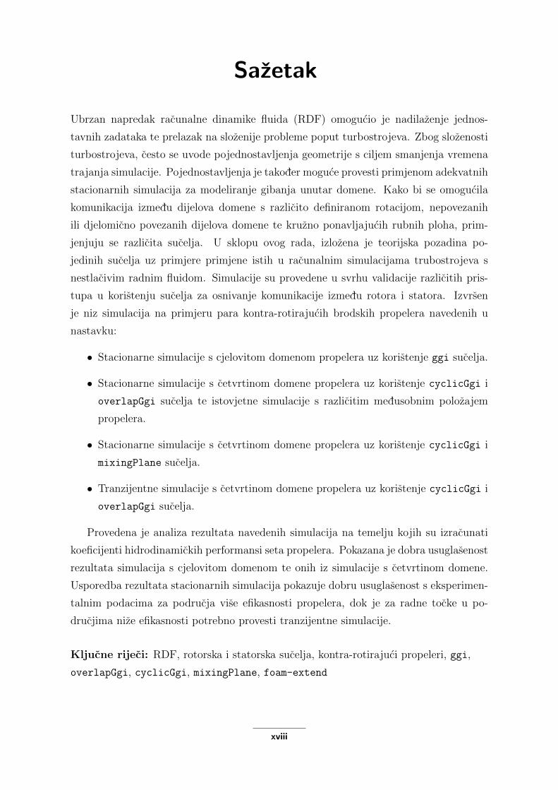
Sazetak
Ubrzan napredak racunalne dinamike fluida (RDF) omogucio je nadilazenje jednos-
tavnih zadataka te prelazak na slozenije probleme poput turbostrojeva. Zbog slozenosti
turbostrojeva, cesto se uvode pojednostavljenja geometrije s ciljem smanjenja vremena
trajanja simulacije. Pojednostavljenja je takoder moguce provesti primjenom adekvatnih
stacionarnih simulacija za modeliranje gibanja unutar domene. Kako bi se omogucila
komunikacija izmedu dijelova domene s razlicito definiranom rotacijom, nepovezanih
ili djelomicno povezanih dijelova domene te kruzno ponavljajucih rubnih ploha, prim-
jenjuju se razlicita sucelja. U sklopu ovog rada, izlozena je teorijska pozadina po-
jedinih sucelja uz primjere primjene istih u racunalnim simulacijama trubostrojeva s
nestlacivim radnim fluidom. Simulacije su provedene u svrhu validacije razlicitih pris-
tupa u koristenju sucelja za osnivanje komunikacije izmedu rotora i statora. Izvrsen
je niz simulacija na primjeru para kontra-rotirajucih brodskih propelera navedenih u
nastavku:
• Stacionarne simulacije s cjelovitom domenom propelera uz koristenje ggi sucelja.
• Stacionarne simulacije s cetvrtinom domene propelera uz koristenje cyclicGgi i
overlapGgi sucelja te istovjetne simulacije s razlicitim medusobnim polozajem
propelera.
• Stacionarne simulacije s cetvrtinom domene propelera uz koristenje cyclicGgi i
mixingPlane sucelja.
• Tranzijentne simulacije s cetvrtinom domene propelera uz koristenje cyclicGgi i
overlapGgi sucelja.
Provedena je analiza rezultata navedenih simulacija na temelju kojih su izracunati
koeficijenti hidrodinamickih performansi seta propelera. Pokazana je dobra usuglasenost
rezultata simulacija s cjelovitom domenom te onih iz simulacije s cetvrtinom domene.
Usporedba rezultata stacionarnih simulacija pokazuje dobru usuglasenost s eksperimen-
talnim podacima za podrucja vise efikasnosti propelera, dok je za radne tocke u po-
drucjima nize efikasnosti potrebno provesti tranzijentne simulacije.
Kljucne rijeci: RDF, rotorska i statorska sucelja, kontra-rotirajuci propeleri, ggi,
overlapGgi, cyclicGgi, mixingPlane, foam-extend
xviii

Abstract
Rapid progress of Computational Fluid Dynamics (CFD) allowed CFD to move past sim-
ple tasks and become a viable tool for the analysis of complex problems, such as turbo-
machines. Nevertheless, due to the complexity of turbomachinery, some simplifications
regarding interface and domain handling are sought in order to allow for reasonable sim-
ulation execution times. Most often, only a part of the whole turbomachine geometry is
simulated, which decreases computational demands. To enable communication between
domain regions wherein different rotation (or other movement) is modelled, between ill-
connected or overlapping regions, or between cyclic patches bounding partial geometry
domains, various interfaces are used. Moreover, steady-state ”frozen rotor” methods
are frequently used to approximate transient problems but avoid computationally de-
manding transient simulations. This Thesis offers an overview of several rotor-stator
interfaces available in foam-extend, with both theoretical background and numerical
simulations. A series of numerical simulations is performed on a Contra-Rotating Pro-
peller set (CRP), investigating different rotor-stator interface handling methods:
• Steady-state simulations using the Multiple Reference Frame (MRF) approach and
the whole CRP geometry with General Grid Interface (ggi).
• Steady-state MRF simulations of a quarter CRP geometry using overlapGgi and
cyclicGgi interfaces across periodic boundaries. Additional simulations are per-
formed to investigate the effects of initial propeller position.
• Quarter CRP geometry steady-state MRF simulations using cyclicGgi and mixingPlane
interfaces.
• Transient simulation of a quarter CRP geometry with the cyclicGgi and overlapGgi
interfaces.
The results were analysed in terms of hydrodynamic performance coefficients, showing
good agreement between quarter and full CRP simulations and validating the interfaces
used. Comparison to experimental data revealed good agreement with steady-state
results for high-efficiency conditions and good agreement with transient simulations for
lower-efficiency conditions.
Keywords: CFD, rotor-stator interfaces, Contra-rotating propellers, ggi,
overlapGgi, cyclicGgi, mixingPlane, foam-extend
xix

Prosireni sazetak
Turbostrojevi predstavljaju skupinu slozenih strojeva koje je moguce klasificirati u
velik broj razlicitih kategorija uzimajuci u obzir znacajke odredene njihovom konstrukci-
jom te strujanjem fluida kroz radni volumen stroja. Primjena racunalne dinamike fluida
za proucavanje strujanja fluida u radu turbostrojeva otvara nove spoznaje rada, kons-
trukcije i poboljsanja turbostrojeva. Istovremeno, kompleksna konstrukcija turbostro-
jeva zahtijeva koristenje odredenih pojednostavljenja prilikom postavljanja racunalnih
simulacija. Ta se pojednostavljenja najcesce svode na razlicite pristupe modeliranja gi-
banja (rotacije) u domeni (racunalnoj mrezi) te povezanosti dijelova domene. U slucaju
kada je numericka mreza stacionarna, a samo dio mreze rotira, relativni polozaja izmedu
stacionarnog i rotirajuceg dijela mreze varira izmedu vremenskih koraka simulacije.
Kako bi se proveo RDF proracun, mrezu je potrebno povezati u jednu domenu. S
obzirom na to da jedan dio mreze rotira, dok je drugi stacionaran, racunalna mreza
ne moze biti izvedena cjelovito, vec se sastoji od dvije povezane domene. Povezanost
dijelova domene ostvaruje se koristenjem razlicitih sucelja koja ostvaruju komunikaciju
izmedu mirujucih i rotirajucih dijelova domene.
Kontra-rotirajuci propeleri predstavljaju primjer turbostroja bez kucista, koji zah-
tijevaju modeliranje dvije rotacijske zone unutar jedne proracunske domene. Upravo su
iz tog razloga ovi propeleri izvrstan odabir za pregled metoda povezivanja rotirajucih i
stacionarnih dijelova racunalne mreze.
xx
Prosireni sazetak xxi
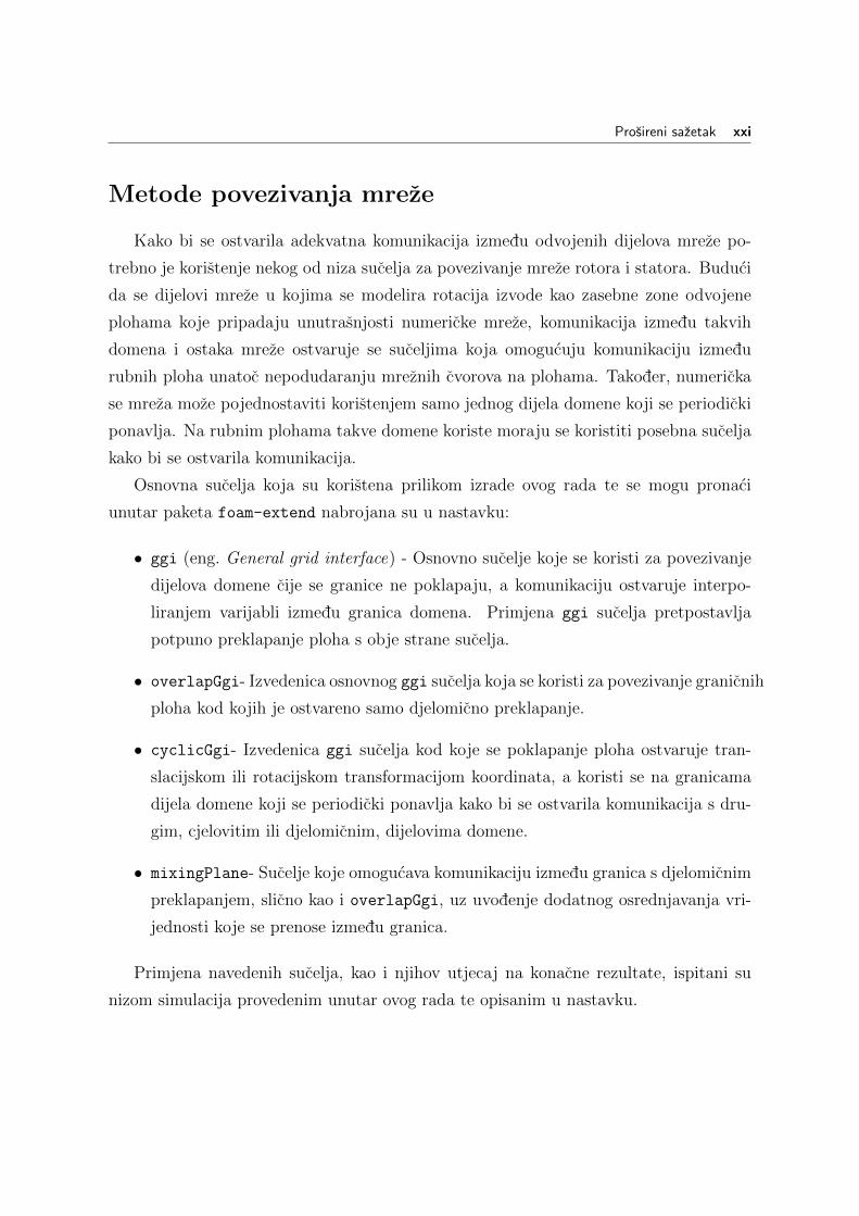
Metode povezivanja mreze
Kako bi se ostvarila adekvatna komunikacija izmedu odvojenih dijelova mreze po-
trebno je koristenje nekog od niza sucelja za povezivanje mreze rotora i statora. Buduci
da se dijelovi mreze u kojima se modelira rotacija izvode kao zasebne zone odvojene
plohama koje pripadaju unutrasnjosti numericke mreze, komunikacija izmedu takvih
domena i ostaka mreze ostvaruje se suceljima koja omogucuju komunikaciju izmedu
rubnih ploha unatoc nepodudaranju mreznih cvorova na plohama. Takoder, numericka
se mreza moze pojednostaviti koristenjem samo jednog dijela domene koji se periodicki
ponavlja. Na rubnim plohama takve domene koriste moraju se koristiti posebna sucelja
kako bi se ostvarila komunikacija.
Osnovna sucelja koja su koristena prilikom izrade ovog rada te se mogu pronaci
unutar paketa foam-extend nabrojana su u nastavku:
• ggi (eng. General grid interface) - Osnovno sucelje koje se koristi za povezivanje
dijelova domene cije se granice ne poklapaju, a komunikaciju ostvaruje interpo-
liranjem varijabli izmedu granica domena. Primjena ggi sucelja pretpostavlja
potpuno preklapanje ploha s obje strane sucelja.
• overlapGgi- Izvedenica osnovnog ggi sucelja koja se koristi za povezivanje granicnih
ploha kod kojih je ostvareno samo djelomicno preklapanje.
• cyclicGgi- Izvedenica ggi sucelja kod koje se poklapanje ploha ostvaruje tran-
slacijskom ili rotacijskom transformacijom koordinata, a koristi se na granicama
dijela domene koji se periodicki ponavlja kako bi se ostvarila komunikacija s dru-
gim, cjelovitim ili djelomicnim, dijelovima domene.
• mixingPlane- Sucelje koje omogucava komunikaciju izmedu granica s djelomicnim
preklapanjem, slicno kao i overlapGgi, uz uvodenje dodatnog osrednjavanja vri-
jednosti koje se prenose izmedu granica.
Primjena navedenih sucelja, kao i njihov utjecaj na konacne rezultate, ispitani su
nizom simulacija provedenim unutar ovog rada te opisanim u nastavku.

Prosireni sazetak xxii
Kontra-rotirajuci propeleri
Ovakav se tip brodskog pogona sastoji od para propelera sa zajednickom osi vrtnje,
koji rotiraju u suprotnim smjerovima te se nalaze na istom ili dva odvojena vratila.
Njihovom se primjenom ostvaruju prednosti u odnosu na koristenje samo jednog pro-
pelera, kao sto su: bolja razdioba opterecenja izmedu propelera, povecanje efikasnosti
pogona, smanjenje mogucnosti pojave kavitacije, produzen zivotni vijek pojedinog pro-
pelera, itd. Jedna od osnovnih prednosti kod primjene kontra-rotirajucih propelera je
smanjenje momenta koji izaziva zakretanje (izboj) broda. Primjena seta propelera s
jednakim i parnim brojem lopatica izaziva pojavu fluktuacije potiska. S druge strane,
koristi li se set s neparnim brojem lopatica, fluktuacija potiska ce biti manja, ali dolazi
do pojave bocnih sila.
Iako je ovaj tip brodskih propelera odavno poznat u brodogradnji, prve su izvedbe
ovih propelera koristile jedno vratilo (Slika 1), sto je dovodilo do velikih problema s
trenjem izmedu unutarnjeg i vanjskog dijela vratila. Upravo je zbog tog razloga dalj-
nji razvoj kontra-rotirajucih propelera zaustavljen. Do ponovnog jacanja interesa za
ovakvim propelerima dolazi tek naglim razvojem elektromagnetskih motora te pojave
moderne inacice ovog sustava. Kod modernih izvedbi jedan se propeler nalazi na vra-
tilu glavnog pogonskog stroja broda, a drugi je pogonjen elektromotorom u pomicnoj
gondoli iz glavnog propelera (Slika 2).
Slika 1: Izvedba s gondolom [1]. Slika 2: Izvedba s jednim vratilom [2].

Prosireni sazetak xxiii
Hidrodinamicke karakteristike propelera
Rad propelera moze se kvantificirati pomocu hidrodinamickih karakteristika na te-
melju kojih se formira dijagram slobodne voznje brodskih propelera. Dijagram se temelji
na koeficijentima poriva i momenta te efikasnosti propelera koji se racunaju za radne
tocke definirane koeficijentom napredovanja J :
J =U
nDf
.
Pomocu vrijednosti J izracunate temeljem promjera prednjeg propelera (Df ), moguce
je izracunati vrijednosti koeficijenta poriva, momenta te efikasnosti za prednji i straznji
propeler:
KTf =Tf
n2D4fρ, KQf =
Qf
n2D5fρ,
KTa =Ta
n2D4aρ, KQa =
Qa
n2D5aρ,
ηf =KTf
KQf
J
2π, ηa =
KTa
KQa
J
2π.
Ukupne se vrijednosti koeficijenata potiska i momenta dobivaju zbrajanjem vrijednosti
za pojedinacne propelere, dok se ukupna efikasnost racuna prema izrazu:
η =KT
KQ
J
2π.
Konacne se vrijednosti navedenih koeficijenta i efikasnosti unose u dijagram u ovisnosti
o koeficijentu napredovanja, sto se naziva dijagramom slobodne voznje propelera.
Numericka mreza
Numericka mreza izradena je na temelju modela kontra-rotirajucih propelera koji je
opisan u tablici (Tablica 1). Model sa sastoji od dva propelera s jednakim brojem lopa-
tica koji rotiraju sinkronizirano brzinom od 12 okretaja u sekundi oko iste osi rotacije.

Prosireni sazetak xxiv
Koristene su dvije numericke mreze, od koji je jedna temeljna na punoj geometriji
(Slika 3, lijevo) propelera, dok se druga temelji na cetvrtini geometrije (Slika 3, desno).
Obje se numericke mreze sastoje od tri regije (odvojne domene) povezane adekvatnim
suceljima. Uz svaki je propeler definirana zona rotacije, koje su okruzene stacionarnom
mrezom koja predstavlja podrucje neporemecenog strujanja fluida.
Tablica 1: Karakteristike propelera.
Propeller type 3686 3687A
Position in set FORE AFT
Blades 4 4
Diameter [ m ] 0.2991 0.3052
Rotation CW CCW
Expanded area ratio 0.303 0.324
Section Meanline NACA a = 0.8 NACA a = 0.8
Thickness Distribution NACA 66 NACA 66
Slika 3: Puna geometrija (lijevo) i cetvrtina geometrije propelera (desno).
Prosireni sazetak xxv
U numerickoj mrezi cjelovite geometrije, komunikacija izmedu domena propelera i
ostatka mreze ostvarena je pomocu ggi sucelja. Mreza djelomicne geometrije zahti-
jeva koristenje cyclicGgi sucelja za ostvarivanje komunikacije na periodickim grani-
cama te overlapGgi za povezivanje domena cetvrtina propelera s ostatkom mreze. Za
testiranje mixingPlane sucelja, koristena je mreza temeljena na cetvrtini propelera s
cyclicGgi suceljem te mixingPlane suceljem na granici domena cetvrtina propelera i
ostatka mreze.
Rezultati simulacija
Za potrebe rada proveden je niz simulacija koristeci prethodno predstavljene nu-
mericke mreze kontra-rotirajucih brodskih propelera:
• Stacionarne simulacije s cjelovitom domenom propelera uz koristenje ggi sucelja.
• Stacionarne simulacije s cetvrtinom domene propelera uz koristenje cyclicGgi i
overlapGgi sucelja te istovjetne simulacije s razlicitim medusobnim polozajem
propelera.
• Stacionarne simulacije s cetvrtinom domene propelera uz koristenje cyclicGgi i
mixingPlane sucelja.
• Tranzijentne simulacije s cetvrtinom domene propelera uz koristenje cyclicGgi i
overlapGgi sucelja.
Rezultati svake simulacije analizirani su grafickim prikazom relevantnih polja, te su
izracunati koeficijenti hidrodinamickih znacajki svakog od propelera i cijelog seta. Na
temelju rezultata formirani su dijagrami slobodne voznje propelera.
Prosireni sazetak xxvi
Simulacija pune geometrije
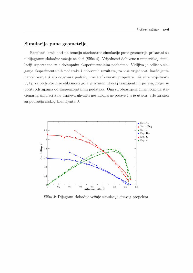
Rezultati izracunati na temelju stacionarne simulacije pune geometrije prikazani su
u dijagramu slobodne voznje na slici (Slika 4). Vrijednosti dobivene u numerickoj simu-
laciji usporedene su s dostupnim eksperimentalnim podacima. Vidljivo je odlicno sla-
ganje eksperimentalnih podataka i dobivenih rezultata, za vise vrijednosti koeficijenta
napredovanja J sto odgovara podrucju vece efikasnosti propelera. Za nize vrijednosti
J , tj. za podrucje nize efikasnosti gdje je izrazen utjecaj tranzijentnih pojava, mogu se
uociti odstupanja od eksperimentalnih podataka. Ona su objasnjena cinjenicom da sta-
cionarna simulacija ne uspijeva uhvatiti nestacionarne pojave ciji je utjecaj vrlo izrazen
za podrucja niskog koeficijenta J .
0 0.2 0.4 0.6 0.8 1 1.2 1.4 1.6Advance ratio, J
0
0.2
0.4
0.6
0.8
1
1.2
KT
,10K
Q,η
Sim. KT
Sim. 10KQ
Sim. ηExp. KT
Exp. K
Exp. η
Slika 4: Dijagram slobodne voznje simulacije citavog propelera.

Prosireni sazetak xxvii
Simulacija cetvrtine geometrije
Rezultati simulacija provedenih s cetvrtinom geometrije usporedeni su s rezultatima
cjelovite geometrije, kako bi se validirala upotreba cyclicGgi i overlapGgi sucelja. Na
slici (Slika 5) vidljivo je vrlo dobro poklapanje rezultata dviju navedenih geometrija,
cime je opravdano daljnje koristenje mreze temeljene na cetvrtini propelera. Ta mreza
sadrzi manji broj kontrolnih volumena sto smanjuje vrijeme potrebno za postizanje
zadane razine konvergencije.
0 0.2 0.4 0.6 0.8 1 1.2 1.4 1.6Advance ratio, J
0
0.2
0.4
0.6
0.8
1
1.2
KT
,10K
Q,η
Quarter KT
Quarter 10KQ
Quarter ηFull KT
Full 10KQ
Full η
Slika 5: Dijagram slobodne voznje simulacije cetvrtine propelera.
mixingPlane simulacija
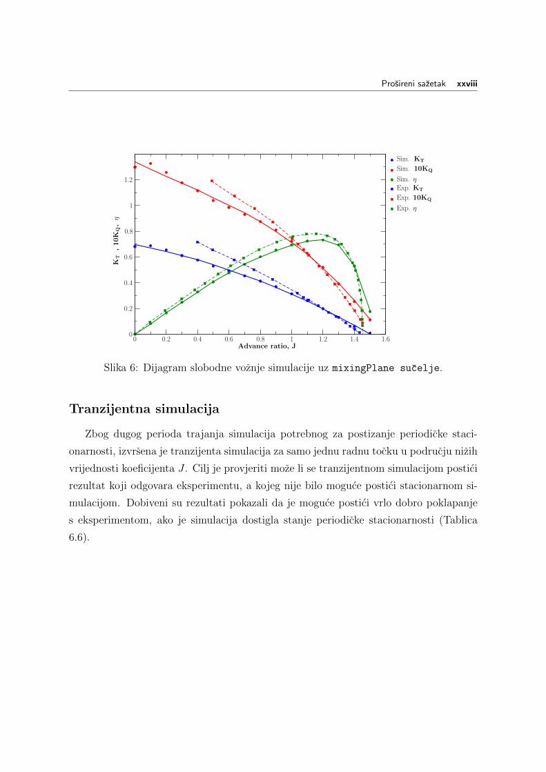
Primjena mixingPlane sucelja ispitana je koristenjem mreze cetvrtine geometrije
uz primjenu cyclicGgi sucelja. Rezultati prikazani na slici (Slika 6) pokazuju bo-
lje podudaranje simulacije s eksperimentalnim podatcima za niza podrucja koeficijenta
J . Takoder, koristenjem mixingPlane sucelja uvedeno je osrednjavanje vrijednosti na
granici. Upravo iz toga razloga ovo sucelje nije smisleno primijeniti u tranzijentnim
simulacijama.
Prosireni sazetak xxviii
0 0.2 0.4 0.6 0.8 1 1.2 1.4 1.6Advance ratio, J
0
0.2
0.4
0.6
0.8
1
1.2
KT
,10K
Q,η
Sim. KT
Sim. 10KQ
Sim. ηExp. KT
Exp. 10KQ
Exp. η
Slika 6: Dijagram slobodne voznje simulacije uz mixingPlane sucelje.
Tranzijentna simulacija
Zbog dugog perioda trajanja simulacija potrebnog za postizanje periodicke staci-
onarnosti, izvrsena je tranzijenta simulacija za samo jednu radnu tocku u podrucju nizih
vrijednosti koeficijenta J . Cilj je provjeriti moze li se tranzijentnom simulacijom postici
rezultat koji odgovara eksperimentu, a kojeg nije bilo moguce postici stacionarnom si-
mulacijom. Dobiveni su rezultati pokazali da je moguce postici vrlo dobro poklapanje
s eksperimentom, ako je simulacija dostigla stanje periodicke stacionarnosti (Tablica
6.6).

Prosireni sazetak xxix
Utjecaj pocetnog polozaja propelera
Posljednji niz simulacija proveden je na cetvrtini geometrije te koristeci cyclicGgi
i overlapGgi sucelja. U simulacijama je variran pocetni polozaj prednjeg propelera u
odnosu na straznji, te je promatran utjecaj na rezultate stacionarne simulacije (Tablica
6.4). Utvrdeno je kako razliciti kutevi zakrenutosti izmedu propelera znatno utjecu
na konacan rezultat, sto je pripisano prirodnim varijacijama u iznosu sile i momenta
tijekom rotacija propelera, vidljivim iz rezultata tranzijentne simulacije.
Zakljucak
Na temelju simulacija provedenih prilikom izrade ovog rada, istrazena su pojednos-
tavljenja geometrije te pristupi modeliranju rotacije koje je moguce koristiti u racunalnim
simulacijama turbostrojeva. Vecina metoda koristenih za modeliranje rotacije, kao i si-
muliranje dijela geometrije, zahtjeva koristenje sucelja, a ciji odabir ovisi o promatranim
pojavama.
Za racunalne simulacije turbostrojeva poput kontra-rotirajucih propelera, moguce je
koristiti samo dio geometrije uz periodicne rubne uvjete. Koristenjem dijela geometrije
nisu uocena znacajna odstupanja u odnosu na primjenu citavog modela. Takoder, za
simulacije radnih tocaka blizu projektne radne tocke, tj. radne tocke u podrucju vi-
soke efikasnosti, stacionarne simulacije daju zadovoljavajuce rezultate. Ako je potrebno
simulirati tocke za podrucja nize efikasnosti, potrebno je koristiti tranzijentne simulacije.

1 Introduction
In general, the term turbomachinery describes a series of different machines oper-
ating on the principle of exchanging energy with a fluid which is continuously flowing
around rotating and/or stationary elements of the machine. The presented definition
of turbomachinery includes a wide range of machines operating on the same principle,
yet involving different functions, operating environments and characteristics. Thus, a
general classification of turbomachines is presented.
The simplest categorisation of turbomachines would be according to type of flow
through the machine. Turbomachines are grouped into three categories depending on the
direction of flow in regards to rotational axis of the machine: radial, axial and mixed flow
machines [3]. The fluid flow in radial machines is perpendicular to the rotational axis,
while fluids in axial machines flow parallel to the axis of rotation. Machines with mixed
flow, represent a category of turbomachinery where the flow does not show dominantly
axial or dominantly radial nature, having both radial and axial components of velocity
instead. The difference between radial and axial flow machines is made evident by the
mechanism of energy transfer between the machine and the fluid, that is, by the change
in the velocity entering and exiting the rotor. While radial machines transfer energy
by changes in the velocity angle and changes in radius, radial flow machines usually
transfer work solely by changes in the velocity angle [4].
Further classification can be performed by examining the streamlines around the
rotor. If the rotor of the machine is enclosed in a casing or shrouded in such a way that
the streamlines cannot diverge to flow around the side of the rotor, the turbomachine can
be considered a closed-type or enclosed machine (e.g. centrifugal pumps, turbopumps,
1

Chapter 1. Introduction 2
compressors). If streamlines are allowed to diverge around an unshrouded rotor, i.e.
the machine operates without a stationary shroud, it can be considered an open-type or
extended turbomachine (e.g. ship propellers or wind turbines) [3].
Closed-type turbomachines are usually sub-categorized depending on the type of
fluid used. Hydraulic machines, such as centrifugal pumps or fans, work with fluids
which can be considered incompressible for normal operating conditions. On the other
hand, in thermal machines, such as steam and gas turbines or jet engines, work with
compressible fluids.
If the energy exchange between the turbomachine and the working fluid is considered,
turbomachines can be categorised as machines that use energy to increase the pressure
of the working fluid (e.g. fans, pumps, compressors) or those that expand the fluid to
generate energy (turbines).
The large number of turbomachines covered by the classification above are used
for different applications in multiple industries. Turbomachines had an important part
in energy generation, transportation and manufacturing since the Industrial revolution
and continue to do so today, proving that further study of such devices and connected
phenomena continues to have a vital role in modern science.
1.1. CFD in Turbomachinery
With various industries shifting towards greater fuel efficiency, cost reduction and
lower emissions, new requirements are imposed on the construction and operation of
turbomachinery. Older plants, vehicle and processes using turbomachines are also being
retrofitted for greater efficiency and lower emissions. The need for improvement over the
existing design and modelling processes calls for a modern approach to the prediction
and verification of turbomachinery designs, such as Computational Fluid Dynamics.
Computational Fluid Dynamics (CFD) is a branch of fluid dynamics which uses
numerical analysis to investigate fluid flow in various circumstances. The use of CFD
for standard external aerodynamics such as heating, ventilation and air conditioning
(HVAC) simulations and simple wall-bounded turbulent flows has been standard prac-
tice for years [5]. On the other hand, using CFD in turbomachinery brings far greater
challenges concerning the geometry used, mesh resolution, simulation of rotating com-
ponents, etc.

Chapter 1. Introduction 3
Complex geometry of most turbomachines supersedes simple geometries of most CFD
simulations. Large numbers of rotating and stationary parts found in turbomachines
further complicate the transient flows which are to be modelled. Interactions between
rotating and stationary elements of such machines bring forth the occurrence of com-
plex phenomena not usually found in external flow. Furthermore, turbulent boundary
layers and wake-to-rotor interactions become of great importance in the CFD study of
turbomachinery which, combined with complex multi-part geometry, demands very fine
resolution of the computational mesh. This makes the simulations more demanding in
terms of computational effort and CPU time. To deal with rotational effects of flow
in single or multi-rotor turbomachines, relative motion needs to be taken into account.
This is usually achieved either by introducing non-inertial rotational frames of reference
or by topological changes of the computational mesh [5].
Taking into account the complex geometries and consequent phenomena connected
with turbomachinery, the difficulties of CFD simulations of turbomachines become ap-
parent. Complex flows, occurrence of transients, geometry optimisation, both design
and off-design conditions are to be investigated and taken into account. Furthermore,
the simulations need to produce quasi-stationary data applicable for machine design pur-
poses and need to be acceptable in respect to both turnaround time and computational
demands.
The need to deal with such high demands brought about the idea of simplifying the
computational mesh by using only part of the whole geometry and introducing cyclic
boundary conditions. To make such simplification possible, the problem of connecting
different regions or geometries (e.g. rotor, stator) of the computational mesh was ad-
dressed by introducing various interfaces as means of enabling communication between
disjoint or partially connected sections.
A good example of an extended turbomachine with complex rotor interaction is a
set of Contra-Rotating Propellers (CRP). A CRP set consists of two unshrouded co-
axial rotors, rotating in opposite directions. Having an increasingly important role in
maritime propulsion, the CRP set presents an ideal choice of turbomachiery to be used
for study of various interfaces in available turbomachinery CFD.

Chapter 1. Introduction 4
1.2. Scope of Thesis
This Thesis investigates different mesh-to-mesh interfaces used to connect stationary
and rotational mesh components in turbomachinery CFD simulations. The theoretical
background needed to understand the basic principles of the Finite Volume Method
(FVM) and different approaches to domain and interface modelling is covered. Different
approaches to turbomachinery simulation are presented on a CRP set, with an analysis of
results gathered from both transient and steady-state simulations run in foam-extend.
1.3. Thesis Outline
This thesis is organised in seven Chapters, as follows: Chapter 1 offers an overview of
turbomachinery and serves as an introduction to the Thesis. Chapter 2 introduces the
basic notions of FVM used for CFD simulations. Chapter 3 gives a detailed overview of
different approaches to interface and domain handling. Chapter 4 introduces the concept
of CRP with details on the characteristics of CRP sets and offering an overview of re-
lated studies. Chapter 5 defines the different geometries used, listing the corresponding
boundary conditions. Chapter 6 presents the results of CFD simulations both graphi-
cally and numerically, offering appropriate comments and explanations where needed.
Chapter 7 serves as the Conclusion of the Thesis, followed by an Appendix offering
examples of interface-setup in foam-extend.
2 Finite Volume Method
2.1. Introduction
The previous chapter served as a short introduction describing the intricacies of
turbomachinery and the use of CFD to analyse the characteristics and performance of
turbomachines. The following chapter shall introduce the Finite Volume Method and
overview some of the theoretical background required to understand the implementation
of the method in turbomachinery CFD.
2.2. The Scalar Transport Equation
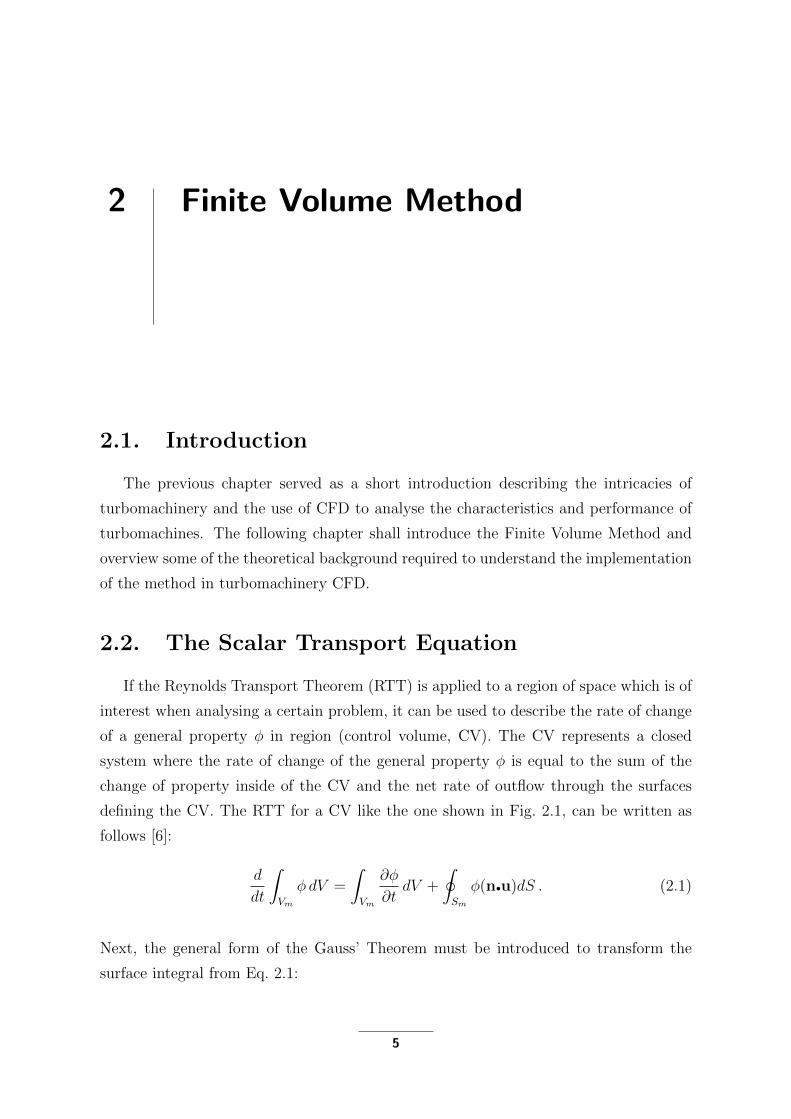
If the Reynolds Transport Theorem (RTT) is applied to a region of space which is of
interest when analysing a certain problem, it can be used to describe the rate of change
of a general property φ in region (control volume, CV). The CV represents a closed
system where the rate of change of the general property φ is equal to the sum of the
change of property inside of the CV and the net rate of outflow through the surfaces
defining the CV. The RTT for a CV like the one shown in Fig. 2.1, can be written as
follows [6]:
d
dt
∫Vm
φ dV =
∫Vm
∂φ
∂tdV +
∮Sm
φ(n•u)dS . (2.1)
Next, the general form of the Gauss’ Theorem must be introduced to transform the
surface integral from Eq. 2.1:
5

Chapter 2. Finite Volume Method 6
∫VP
∇ · a dV =
∮∂VP
ds•a =
∮∂VP
dn•a dS . (2.2)
By applying Eq. 2.2 to Eq. 2.1, a volume integral form of the RTT is shown:
d
dt
∫V
φ dV =
∫V
[∂φ
∂t+∇ · (φu)
]dV , (2.3)
which is used to model the convective transport of a general property φ facilitated by
the convective velocity u. The inflow of the general property φ is given by (u · n) < 0
and the outflow by (u · n) > 0.
u
dSn
CV
INFLOW
OUTFLOW
Figure 2.1: Closed system or Control
Volume (CV).
u
dSn
CV
INFLOW
OUTFLOW
qs
Qv
Figure 2.2: Surface and Volume sources
of a CV.
As well as the convective transport, surface and volume sources also add to the change
of a general property inside the CV. The contribution of surface and volume sources,
shown in Fig. 2.2, is represented by:
d
dt
∫V
φ dV =
∫V
qv dV −∮S
(n•qs)dS . (2.4)
By applying the Gauss’ Theorem to the source term in Eq. 2.4, matching the left-hand
side of the resulting equation with Eq. 2.3 and integrating over the volume of the CV
(V = const.), the following equation is obtained:

Chapter 2. Finite Volume Method 7
∂φ
∂t+∇ · (φu) = qv −∇ · qs . (2.5)
The terms representing surface sources, which act on the surface S of the CV, are
modelled using Diffusive Transport. In physical terms, a general property φ in a closed
domain (CV) will be transported from regions of greater concentration to regions of
lower concentration until uniformity of concentration is achieved. The diffusion model
is based on the fact that ∇φ points in the direction of greater concentration of the
property φ and the fact that the diffusive transport occurs in the opposite direction
governed by the diffusivity γ [6]:
qs = −γ∇φ . (2.6)
By inserting Eq. 2.6 into Eq. 2.5 and rearranging, the general form of the Scalar Trans-
port Equation may be presented:
∂φ
∂t︸︷︷︸temporal derivative
+ ∇ · (φu)︸ ︷︷ ︸convection term
−∇ · (γ∇φ)︸ ︷︷ ︸diffusion term
= qv︸︷︷︸source term
. (2.7)
The temporal derivative from Eq. 2.7 represents the inertia of the system, i.e. the ability
of the system (CV) to accumulate a general property. The convection term represents
a coordinate transform of the property, i.e. the amount of property φ transported into
or out of the system, by the velocity u. The diffusion term represents the gradient
transport of property φ, defining the amount of φ transported by diffusive transport.
Finally, source (or sink) terms define local production and/or destruction of the general
property φ.
2.2.1. Governing Equations
The Scalar Transport Equation 2.7 represents one of the constitutional equations
of Continuum Mechanics. It is the core equation describing how a scalar quantity is
transported in a defined space. By replacing the general property φ with different
properties, other governing equations of Continuum Mechanics can be derived:

Chapter 2. Finite Volume Method 8
Conservation of Mass
By substituting the general property φ in the Scalar Transport Equation 2.7 with
fluid density denoted by ρ and defining a zero value source term, the equation describing
the Conservation of Mass is derived:
∂ρ
∂t+∇ · (ρu) = 0 . (2.8)
For incompressible flow, the density of the fluid can be defined as constant ρ = const.,
further simplifying Eq. 2.8:
∇ · u = 0 . (2.9)
The form of the Conservation of Mass equation presented above (Eq. 2.9) is called the
continuity Equation.
Conservation of Linear Momentum
The equation describing the Conservation of Linear Momentum can be derived from
Eq. 2.7 by replacing the general variable φ with the linear momentum vector ρu:
∂(ρu)
∂t+∇ · (ρuu) = ρg︸︷︷︸
gravitational force
+ ∇ · σ︸︷︷︸surface forces
. (2.10)
For incompressible flow and usually ignoring gravitational forces for turbomachinery
CFD, Eq. 2.10 can be transformed as follows:
∂u
∂t︸︷︷︸local production
+∇ · (uu)︸ ︷︷ ︸convection
−∇ · (νeff∇u)︸ ︷︷ ︸diffusion
= − ∇pρ︸︷︷︸
pressure gradinet
, (2.11)
where the Cauchy stress tensor is given as the sum of the pressure gradient ∇p and
viscous stress tensor represented in the diffusion term. It should be noted that the fluid
velocity u occurs in Eq. 2.11 both as the transporting and the transported variable,
making the convection term non-linear [6].
Chapter 2. Finite Volume Method 9
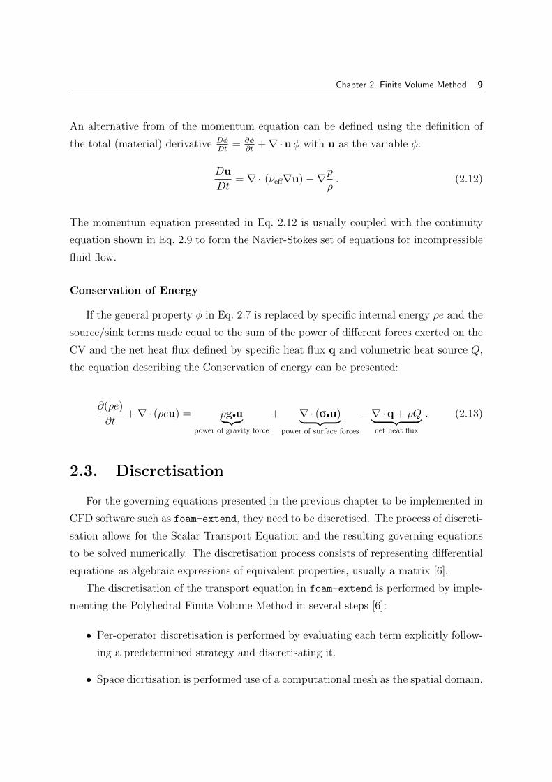
An alternative from of the momentum equation can be defined using the definition of
the total (material) derivative DφDt
= ∂φ∂t
+∇ · uφ with u as the variable φ:
Du
Dt= ∇ · (νeff∇u)−∇p
ρ. (2.12)
The momentum equation presented in Eq. 2.12 is usually coupled with the continuity
equation shown in Eq. 2.9 to form the Navier-Stokes set of equations for incompressible
fluid flow.
Conservation of Energy
If the general property φ in Eq. 2.7 is replaced by specific internal energy ρe and the
source/sink terms made equal to the sum of the power of different forces exerted on the
CV and the net heat flux defined by specific heat flux q and volumetric heat source Q,
the equation describing the Conservation of energy can be presented:
∂(ρe)
∂t+∇ · (ρeu) = ρg•u︸︷︷︸
power of gravity force
+ ∇ · (σ•u)︸ ︷︷ ︸power of surface forces
−∇ · q + ρQ︸ ︷︷ ︸net heat flux
. (2.13)
2.3. Discretisation
For the governing equations presented in the previous chapter to be implemented in
CFD software such as foam-extend, they need to be discretised. The process of discreti-
sation allows for the Scalar Transport Equation and the resulting governing equations
to be solved numerically. The discretisation process consists of representing differential
equations as algebraic expressions of equivalent properties, usually a matrix [6].
The discretisation of the transport equation in foam-extend is performed by imple-
menting the Polyhedral Finite Volume Method in several steps [6]:
• Per-operator discretisation is performed by evaluating each term explicitly follow-
ing a predetermined strategy and discretisating it.
• Space dicrtisation is performed use of a computational mesh as the spatial domain.

Chapter 2. Finite Volume Method 10
• Time is discretised by a series of time-steps adding up to the observed time interval.
• Spatial and temporal variations of a property φ are used to discretely represent
field data.
• Integration over a cell (CV) is preformed.
• Spatial and temporal variations are use for discrete interpretation of operator
terms.
The basis of the discretisation process is the definition of the space and time domains
to be used. The temporal domain is defined by observing the chosen time interval as a
series of consecutive time-steps. The spatial domain is represented by a finite number
of control volumes (cells). A representation of one CV is given by a convex polyhedron
shown in Fig. 2.3.
A polyhedral cell of volume VP is defined with the cell centroid P and the centroid
position vector rP in regard to the origin of the global coordinate system. For a selected
cell face f a surface normal vector sf is defined with a magnitude equal to the area of
the selected face Sf . Any neighbouring cell has a centroid N connected to the centroid
of the main cell P by the delta vector df = PN [6].
The definition of the cell centroid P as the main computational point is given by:∫VP
(x− xP ) dV = 0 , (2.14)
with the face centre f defined in the same manner:∫Sf
(x− xf ) dS = 0 . (2.15)
In practice, faces of the polyhedral cell are not flat surfaces, meaning that the surface
normal vector sf must be calculated from the given integral:
sf =
∫Sf
n dS . (2.16)

Chapter 2. Finite Volume Method 11
Solutions to discretised equations are stored in the cell centroid whereas the boundary
data is stored in face centres of the boundary faces. Depending on situation and purpose
of the data required, it may be necessary to access data stored in face centres of the
finite volume cell. To access such data face interpolation schemes are used.
P
x
z
y
N
rP
sfdf
f
VP
Figure 2.3: Polyhedral finite volume.
The second order discretisation of spatial variation for a general property φ is denoted
by the following expression:
φ(x) = φP + (x− xP )•(∇φ)P , (2.17)
while second order temporal discretisation is given by:
φ(t+ ∆t) = φt + ∆t
(∂φ
∂t
)t. (2.18)
Where the value of φ at the centroid is given by φP = φ(xP ) and the value of φ at time
t by φt = φ(t).
Chapter 2. Finite Volume Method 12
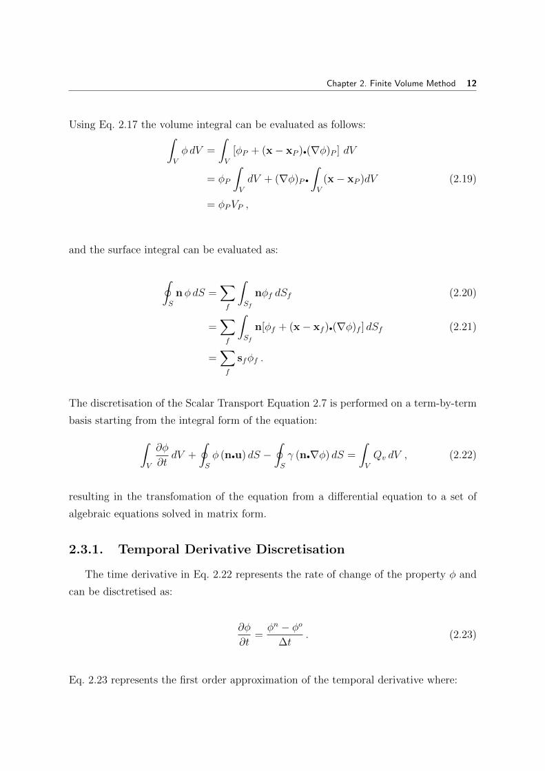
Using Eq. 2.17 the volume integral can be evaluated as follows:∫V
φ dV =
∫V
[φP + (x− xP )•(∇φ)P ] dV
= φP
∫V
dV + (∇φ)P •
∫V
(x− xP )dV (2.19)
= φPVP ,
and the surface integral can be evaluated as:
∮S
nφ dS =∑f
∫Sf
nφf dSf (2.20)
=∑f
∫Sf
n[φf + (x− xf )•(∇φ)f ] dSf (2.21)
=∑f
sfφf .
The discretisation of the Scalar Transport Equation 2.7 is performed on a term-by-term
basis starting from the integral form of the equation:∫V
∂φ
∂tdV +
∮S
φ (n•u) dS −∮S
γ (n•∇φ) dS =
∫V
Qv dV , (2.22)
resulting in the transfomation of the equation from a differential equation to a set of
algebraic equations solved in matrix form.
2.3.1. Temporal Derivative Discretisation
The time derivative in Eq. 2.22 represents the rate of change of the property φ and
can be disctretised as:
∂φ
∂t=φn − φo
∆t. (2.23)
Eq. 2.23 represents the first order approximation of the temporal derivative where:

Chapter 2. Finite Volume Method 13
• The field value of variable φ calculated for the new time-step tnew is defined as:
φn = φ(t = tnew) . (2.24)
• The field value of variable φ calculated for the previous time-step told is defined as
follows:
φo = φ(t = told) . (2.25)
• The time-step size ∆t can be expressed as:
∆t = tnew − told . (2.26)
Backward differencing can be applied to express the second order approximation of the
temporal derivative:
32φn − 2φo + 1
2φoo
∆t, (2.27)
where the term φoo is expressed as φoo = φ(tnew − 2∆t) and the time-step is assumed to
remain constant. Integrating Eq. 2.26 and Eq. 2.27 over the volume of the cell produces
yields: ∫V
∂φ
∂tdV =
φn − φo
∆tVP , (2.28)∫
V
∂φ
∂tdV =
32φn − 2φo + 1
2φoo
∆tVP . (2.29)

Chapter 2. Finite Volume Method 14
2.3.2. Convection Term Discretisation
The dicretisation of the convection term from Eq. 2.22 is accomplished by using the
Gauss’ Theorem 2.2 to transform the volume integral to a surface integral. The same
process is applied for the discretisation of any terms consisting of either the gradient or
the divergence operator. The convection term can now be expressed as:∫V
∇ · (φu) dV =
∮S
φ(n•u)dS . (2.30)
The surface integral can now be expressed as a sum of face integrals:∮S
φ(n•u)dS =∑f
φf (sf •uf ) =∑f
F φf , (2.31)
where φf represents the value of φ at the face of the cell face and the flux F can be
expressed as a product of the surface normal vector and the convective velocity uf :
F = sf •uf . (2.32)
Discretising the convection term as a sum of the products of all face-centred values of
the property φf and the corresponding face flux F . The value of φf need to be evaluated
by using φP and φN which can be achieved by using one of many existing interpolation
schemes, e.g.:
• Central differencing - second order accuracy, but causing oscillation:
φf = fxφP + (1− fx)φN , (2.33)
where fx = fN/PN .
• Upwind differencing - which takes into account the upstream information, produc-
ing no oscillations but smearing the solution:
φf = max(F, 0)φP +max(−F, 0)φN . (2.34)

Chapter 2. Finite Volume Method 15
2.3.3. Diffusion Term Discretisation
The diffusion term from the Scalar Transport Equation 2.22 can be discretizied by
implementing the same method as the one used for the discretization of the convection
term:
∫V
∇ · (γ∇φ) dV =
∮S
γ(n•∇φ)dS
=∑f
∫Sf
γ(n•∇φ) dS (2.35)
=∑f
γf sf •(∇φ)f .
The term describing the face-normal gradient sf •(∇φ)f can be expressed as the difference
of property φ across the face:
sf •(∇φ)f = |sf |φN − φP|df |
. (2.36)
Eq. 2.36 is valid for orthogonal meshes, while for large non-orthogonality, correction
terms must be applied.
2.3.4. Source/Sink Term Discretisation
Sources and sinks describe local effects and may be modelled by a function of space
and time or any complex variable S. Thus, the discretisation produces:∫V
S dV = SVP , (2.37)
where S may be linearised with respect to the general property φ as:
S(φ) = Su − Spφ . (2.38)

Chapter 2. Finite Volume Method 16
2.3.5. Linear System of Equations
A system of linear equations is developed by discretisation of the Scalar Transport
Equation 2.7. A linear equation is solved for every computational point (cell centroid P ),
where the solution of the equation depends on the values of neighbouring cell centroids
N . A general form of the linear equation for a cell centroid P is given by:
aPxP +∑N
aNxN = b . (2.39)
For every time xP depends on itself, contribution is added into aP and for every
time xN depends on itself, contribution is added into aN . Other contributions are added
to b. If equation Eq. 2.39 is developed for each cell of the domain, a system of linear
equations is constructed. It is usually written in matrix form:
[A][x] = [b] . (2.40)
The matrix [A] contains the coefficients aP and aN , the vector [x] contains values of
xP for all cells in the domain and the vector [b] represents the right-hand side. As the
domain contains a large number of cells, each described by a separate linear equation,
the matrix [A] has a dimension of N × N cells, making it a square matrix. This can
make the matrix large, however many coefficients are equal to zero and the matrix is
sparse with the number of non-zero terms in each row being equal to the number of cell
faces.
2.4. Boundary Conditions
As described in [6], boundary conditions are used to isolate the studied system
from the rest of the environment and to limit what is to be modelled. The type and
position of the boundary conditions to be applied depend on the physics governing the
observed phenomena and good engineering practice. Numerical boundary conditions
are frequently used in CFD to prescribe boundary behaviour. Most frequently used
numerical boundary conditions include:
• The Dirichlet boundary condition, which prescribes a fixed value of φ at the

Chapter 2. Finite Volume Method 17
boundary:
φ = const. (2.41)
• The Neumann boundary condition, prescribing a zero gradient or no flux condition:
n · qs = 0 . (2.42)
• A generalised Neumann boundary condition, which prescribes a fixed gradient or
fixed flux at the boundary:
n · qs = qb . (2.43)
• Mixed conditions can be used as a linear combination of Neumann and Dirichlet
conditions:
αφ+ (1− α) n · qs . (2.44)
• Geometric and Coupled boundary conditions such as symmetry plane, cyclic or
periodic boundary conditions.
2.5. Pressure-Velocity Coupling Algorithms
The set of equations shown in Eq. 2.12 and 2.9 represents the Navier-stokes equations
for incompressible flow. This set of equations represents one vector field governed by one
vector equation and one scalar field governed by a scalar equation. These two equations
are linearly coupled as the velocity governed by the momentum equation also appears as
a velocity divergence in the continuity equation. As the pressure gradient is also present
in the momentum equation, linear coupling between the pressure and the velocity is
present.
As the pressure field is a scalar field and velocity represents a vector field, the two
cannot be put in direct relation without the derivation of the pressure equation. The
pressure equation can be derived by discretisation of the momentum equation as follows:
auPuP +∑N
auNuN = r−∇p . (2.45)

Chapter 2. Finite Volume Method 18
All the right-hand-side contributions and the off-diagonal part of the matrix describing
the momentum equation are combined in the newly introduced H(u) operator:
H(u) = r−∑N
auNuN . (2.46)
By using Eq. 2.46, Eq. 2.45 can be transformed:
auPuP = H(u)−∇p , (2.47)
which can be rearranged as:
uP = (auP )−1(H(u)−∇p) . (2.48)
The resulting expression for up can now be substituted into the continuity expression
for incompressible flow 2.9, producing the expression:
∇ ·[(auP )−1∇p
]= ∇ · ((auP )−1H(u)) . (2.49)
Eq. 2.49 represents the pressure equation for incompressible flow and can be used to
establish a direct coupling between pressure and velocity. To deal with solving the
pressure-velocity coupling several coupling methods are used (e.g. SIMPLE, PIMPLE,
PISO, block-coupled solvers, etc.). For the purpose of this Thesis, the SIMPLE and
PIMPLE algorithms are used. The two algorithms are explained in the following sec-
tions with an addition of the PISO algorithm, as it its necessary for understanding the
PIMPLE algorithm.
2.5.1. SIMPLE Algorithm
The Semi-Implicit Algorithm for Pressure-Linked Equations (SIMPLE) is the earli-
est pressure-velocity coupling algorithms used [7].
The SIMPLE algorithm as described in [6] follows the following sequence:
1. Initial guess of the pressure field p∗
Chapter 2. Finite Volume Method 19
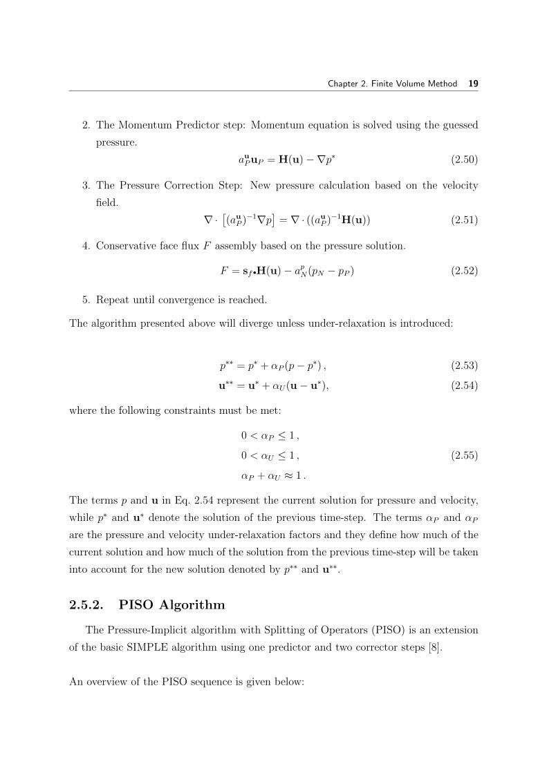
2. The Momentum Predictor step: Momentum equation is solved using the guessed
pressure.
auPuP = H(u)−∇p∗ (2.50)
3. The Pressure Correction Step: New pressure calculation based on the velocity
field.
∇ ·[(auP )−1∇p
]= ∇ · ((auP )−1H(u)) (2.51)
4. Conservative face flux F assembly based on the pressure solution.
F = sf •H(u)− apN(pN − pP ) (2.52)
5. Repeat until convergence is reached.
The algorithm presented above will diverge unless under-relaxation is introduced:
p∗∗ = p∗ + αP (p− p∗) , (2.53)
u∗∗ = u∗ + αU(u− u∗), (2.54)
where the following constraints must be met:
0 < αP ≤ 1 ,
0 < αU ≤ 1 , (2.55)
αP + αU ≈ 1 .
The terms p and u in Eq. 2.54 represent the current solution for pressure and velocity,
while p∗ and u∗ denote the solution of the previous time-step. The terms αP and αP
are the pressure and velocity under-relaxation factors and they define how much of the
current solution and how much of the solution from the previous time-step will be taken
into account for the new solution denoted by p∗∗ and u∗∗.
2.5.2. PISO Algorithm
The Pressure-Implicit algorithm with Splitting of Operators (PISO) is an extension
of the basic SIMPLE algorithm using one predictor and two corrector steps [8].
An overview of the PISO sequence is given below:
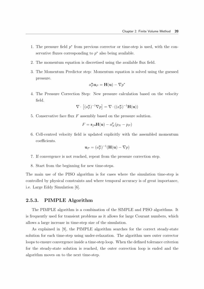
Chapter 2. Finite Volume Method 20
1. The pressure field p∗ from previous corrector or time-step is used, with the con-
servative fluxes corresponding to p∗ also being available.
2. The momentum equation is discretised using the available flux field.
3. The Momentum Predictor step: Momentum equation is solved using the guessed
pressure.
auPuP = H(u)−∇p∗
4. The Pressure Correction Step: New pressure calculation based on the velocity
field.
∇ ·[(auP )−1∇p
]= ∇ · ((auP )−1H(u))
5. Conservative face flux F assembly based on the pressure solution.
F = sf •H(u)− apN(pN − pP )
6. Cell-centred velocity field is updated explicitly with the assembled momentum
coefficients.
uP = (auP )−1(H(u)−∇p)
7. If convergence is not reached, repeat from the pressure correction step.
8. Start from the beginning for new time-steps.
The main use of the PISO algorithm is for cases where the simulation time-step is
controlled by physical constraints and where temporal accuracy is of great importance,
i.e. Large Eddy Simulation [6].
2.5.3. PIMPLE Algorithm
The PIMPLE algorithm is a combination of the SIMPLE and PISO algorithms. It
is frequently used for transient problems as it allows for large Courant numbers, which
allows a large increase in time-step size of the simulation.
As explained in [9], the PIMPLE algorithm searches for the correct steady-state
solution for each time-step using under-relaxation. The algorithm uses outer corrector
loops to ensure convergence inside a time-step loop. When the defined tolerance criterion
for the steady-state solution is reached, the outer correction loop is ended and the
algorithm moves on to the next time-step.
Chapter 2. Finite Volume Method 21
2.6. Turbulence Modelling
Turbulence plays an important part in CFD simulations of turbomachines as its
influence on the operation of turbomachinery can be significant. The stochastic nature
of turbulent flows makes the task of modelling turbulence demanding field of study. The
task of turbulence modelling is to create models and manipulate equations to be able
to simulate turbulence interaction for specific conditions [6].
There exist several different approaches to turbulence modelling such as: Direct
Numerical Simulation (DNS), Reynolds-Averaged Navier-Stokes Equations (RANS) and
Large Eddy Simulation (LES).
The RANS model is frequently used in most turbomachinery CFD simulations. The
basic idea of this model is to describe the variables of interest into fluctuating and mean
values reducing the cost of simulation.
Reynolds-Averaged Navier-Stokes may be assembled by decomposing the values of
pressure and velocity into a sum of mean (u, p) and fluctuating values (u′, p’) as follows:
u = u + u′ , (2.56)
p = p+ p′ . (2.57)
By inserting Eq. 2.56 and 2.57 into Eq. 2.11 and eliminating products of mean and
fluctuating values, the following expression is given:
∂u
∂t+∇ · (u u)−∇ · (ν∇u) = −∇p+∇ · (u′u′) , (2.58)
∇ · u = 0 ,
where the term u′u′ is a second rank symmetric tensor called the Reynolds stress tensor
R:
R = u′u′ . (2.59)
Chapter 2. Finite Volume Method 22
The Reynolds Stress tensor can be assembled by using the second rank symmetric mean
velocity gradient S and turbulent viscosity νt:
R = νt︸︷︷︸turbulent viscosity
1
2
[∇u + (∇u)T
]︸ ︷︷ ︸tensor S
, (2.60)
where the turbulent viscosity νt is modelled using the velocity scale U, the length-scale
∆ and a dimensionless constant A, which allows the model to be tuned to actual physical
phenomena:
νt = AU∆ . (2.61)
The velocity scale can be approximated using turbulent kinetic energy U ≈ |u′|, where
the turbulent kinetic energy is given by:
k =3
2u′
2. (2.62)
Two frequently used two-equation models were used for turbulence modelling in the
scope of this Thesis. The first was the k − ε model and the second was the modified
version of the k − ω model, the k − ω SST model.
2.6.1. The k − ε Model
This model is a popular, yet simple, two-equation model consisting of two partial dif-
ferential equations used to describe turbulence. The first of the two equations describes
the turbulence kinetic energy k:
∂k
∂t+∇ · (uk)−∇ · [(νeff )∇k] = G− ε . (2.63)
The second equation of the k − ε model is the equation for the turbulent dissipation ε,
i.e. the dissipation of the turbulent kinetic energy:

Chapter 2. Finite Volume Method 23
∂ε
∂t+∇ · (uε)−∇ · [(νeff )∇ε] = C1G
ε
k− C2
ε2
k. (2.64)
Where the terms for G used in Eq. 2.63 and 2.64 and for νt are given by:
G = νt
[1
2(∇u +∇uT )
]2
, (2.65)
νt = Cµk2
ε. (2.66)
A detailed overview of the model, its implementation and the various constants used, is
given by Launder et al. in [10, 11].
2.6.2. The k − ω SST Model
The k−ω SST model is the result of combining the k−ε model with the k−ω model
developed by Wilcox [12]. The adaptation of the k− ε model is used in the free-stream
where the k−ω model shows sensitivity. For the inner boundary layer close to the wall,
the k − ω model is used. The fundamental two-equation model is described by:
∂k
∂t+∇ · (uk)−∇ · [(νeff )∇k] = min (G,C1, β
∗kω)− β∗kω , (2.67)
describing the turbulent kinetic energy k, and the following equation describing the
specific dissipation rate ω:
∂ω
∂t+∇ · (uω)− ω∇ · u−∇ · [νeff∇ω] = γ min
[S2,
c1
a1
β∗ωmax(a1ω, b1F23
√S2
)]− βω2 + (1− F1)CDkω . (2.68)
Where the terms for G used in Eq. 2.67 are given by:
Chapter 2. Finite Volume Method 24
G = νtS2 , (2.69)
S2 = 2
[1
2(∇u +∇uT )
]2
, (2.70)
and the turbulent viscosity νt is described by:
νt =a1k
max[a1ω, b1F23
√2∣∣1
2(∇u +∇uT )
∣∣] . (2.71)
Eq. 2.67 and 2.68 describe the k−ω SST model according to Menter and Esch [13] with
updated coefficients from [14]. The consistent production term from [13] and [14] were
updated according to [15], while the optional F3 term was added according to [16].
2.7. Closure
In this chapter an overview of the Finite Volume Method was given, as well as the
fundamental equations of fluid flow and their discretisation, so that they may be used
for CFD simulations. A basic overview of the pressure-velocity coupling algorithms and
turbulence models used in the scope of this thesis was also presented.
The next chapter deals with the theoretical background needed to develop a mathe-
matical model used for turbomachinery CFD. In this chapter, various methods of domain
and interface handling are presented and discussed.

3 Extensions of the
Flow Model for
Turbomachinery
Applications
3.1. Introduction
The previous chapter gave a brief overview of the Finite Volume Method, which
is an important basis for any CFD simulation. The present chapter deals with the
theoretical background needed to extend the flow model for use in various approaches
to CFD simulations of turbomachines. It also offers an overview of different interfaces
that are at disposal for turbomachinery CFD. Methods used for domain and interface
handling are presented. Domain handling deals with the way the rotation of moving
components is handled in the computational domain, i.e. the computational mesh.
Interface handling manages the way mesh regions are interconnected.
3.2. Domain Handling
The decision on how to approach domain handling in turbomachinery CFD depends
on the way the domain is modelled. This, on the other hand, depends on whether the
considered problem and connected phenomena need to be simulated using a steady-state
or a transient approach.
The steady-state approach in turbomachinery CFD is also known as the ”frozen
rotor” approach. This is due to the fact that no actual movement of the mesh occurs
and that movement is modelled by inclusion of additional terms into the equations of
motion for the rotating region [17]. The ”frozen rotor” approach is used when transient
25

Chapter 3. Extensions of the Flow Model for Turbomachinery Applications 26
phenomena are not dominant in the flow or are of no major significance to the analysis
of the observed problem. The absence of actual mesh movement makes the frozen rotor
model very robust and computationally less demanding, which makes it suitable for
steady-state analysis of geometries with rotating and/or stationary parts.
If transient phenomena are to be modelled, the frozen rotor approach must be aban-
doned and the transient Moving (Dynamic) Mesh Model must be used instead. The use
of a Moving Mesh Model makes the simulation require more computational resources,
mainly because of the requirements of the transient simulation used with this model.
The fact that any rotation of the mesh needs to be resolved by additional sets of equa-
tions compensating for topological changes of the computational domain, increases the
computational effort only slightly. The actual cost of a dynamic mesh transient CFD
simulation, when compared to a static mesh transient simulation, is lower than 5% of the
computational effort per time-step [6]. Furthermore, interfaces are required to enable
communication between the stationary and moving (rotating) portion of the mesh.
3.2.1. Moving Reference Frame
The use of Moving Reference Frame modelling in turbomachinery CFD simulations
constitutes a way of representing the flow around moving parts of turbomachines as a
steady-state problem. This is achieved by imposing a moving frame of reference created
by selecting cells of the computational mesh (cell zones) with added inertia. The set of
equations used to describe the motion of the mesh is modified by addition of acceleration
terms occurring due to the transformation from the stationary reference frame to the
moving reference frame [17].
If the entire domain (computational mesh) rotates as a single rotating frame, i.e.
the whole domain can be modelled as a single moving zone, the Single Reference Frame
(SRF) approach is used. An example of a geometry that is modelled as a single rotating
zone is shown in Figure 3.1. As most turbomachines contain not only rotating, but also
stationary parts, a single rotating zone cannot encompass the whole domain. In such
cases the Multiple Reference Frame (MRF) approach is applied. The computational
mesh is divided into different zones depending on the motion of the geometry, which are
assigned either to the rotating or stationary frames of reference. Usually a part of the
computational mesh close to the rotating part of the machine is selected as a zone in
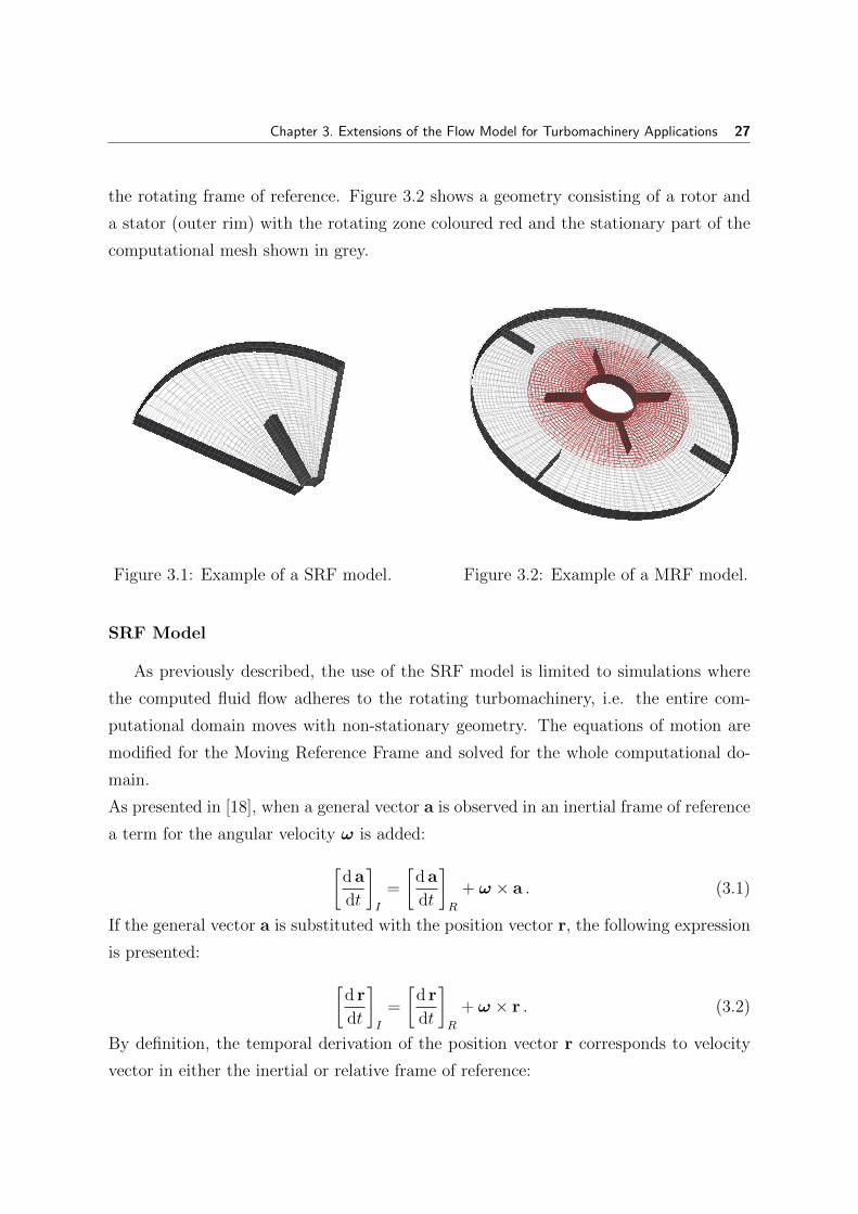
Chapter 3. Extensions of the Flow Model for Turbomachinery Applications 27
the rotating frame of reference. Figure 3.2 shows a geometry consisting of a rotor and
a stator (outer rim) with the rotating zone coloured red and the stationary part of the
computational mesh shown in grey.
Figure 3.1: Example of a SRF model. Figure 3.2: Example of a MRF model.
SRF Model
As previously described, the use of the SRF model is limited to simulations where
the computed fluid flow adheres to the rotating turbomachinery, i.e. the entire com-
putational domain moves with non-stationary geometry. The equations of motion are
modified for the Moving Reference Frame and solved for the whole computational do-
main.
As presented in [18], when a general vector a is observed in an inertial frame of reference
a term for the angular velocity ω is added:[d a
dt
]I
=
[d a
dt
]R
+ ω × a . (3.1)
If the general vector a is substituted with the position vector r, the following expression
is presented: [d r
dt
]I
=
[d r
dt
]R
+ ω × r . (3.2)
By definition, the temporal derivation of the position vector r corresponds to velocity
vector in either the inertial or relative frame of reference:

Chapter 3. Extensions of the Flow Model for Turbomachinery Applications 28
uI = uR + ω × r . (3.3)
The term uI in Eq. 3.3 represents the absolute velocity, i.e. the velocity as viewed from
the stationary (inertial) frame of reference. On the other hand the term uR represents
the relative velocity as viewed from the rotating frame of reference. By substitution of
the general vector r in Eq. 3.1 further derivation of Eq. 3.3 is performed:[d uIdt
]I
=
[d uIdt
]R
+ ω × uI . (3.4)
The term uI on the right-hand side of Eq. 3.4 may be replaced by Eq. 3.3 forming:[d uIdt
]I
=
[d [uR + ω × r]
dt
]R
+ ω × [uR + ω × r] , (3.5)
after sorting, the standard form for the acceleration in the inertial frame of reference
becomes:
[d uIdt
]I
=
[d uRdt
]R
+dω
dt× r︸ ︷︷ ︸
Tangential acceleration
+ 2ω × uR︸ ︷︷ ︸Coriolis acceleration
+ ω × ω × r︸ ︷︷ ︸Centrifugal acceleration
. (3.6)
Equations 2.9 and 2.10 can be easily observed in the inertial frame forming the incom-
pressible Navier-Stokes equations for the inertial frame of reference:DuIDt
= ∇ · (νeff∇uI)−∇p
ρ,
∇ · uI = 0 .(3.7)
The Material Derivative in Eq. 3.7 can be expressed as a sum of local and convective
rates of change:
Dφ
Dt=∂φ
∂t+∇ · v φ −→ DuI
Dt=∂uI∂t
+∇ · (uIuI) . (3.8)
Using Eq. 3.8 and the continuity equation ∇ · uI = 0 the incompressible Navier-Stokes
equation for the inertial frame becomes:∂uI∂t
+∇ · (uIuI)−∇ · (νeff∇uI) = −∇pρ,
∇ · uI = 0 .
(3.9)
Chapter 3. Extensions of the Flow Model for Turbomachinery Applications 29
The left-hand side of the momentum equation from Eq. 3.7 can be expanded by using
the expression presented in Eq. 3.6:
DuIDt
=DuRDt
+dω
dt× r + 2ω × uR + ω × ω × r . (3.10)
Taking note of the fact that the continuity equation must be satisfied, i.e. ∇ · uR =
∇ · uI = 0 the following can be derived:
∇ · uR = ∇ · uI = 0
= ∇ · uR︸ ︷︷ ︸= 0
+∇ · [ω × r]︸ ︷︷ ︸= 0
= 0 , (3.11)
resulting in the equivalence: ∇ · [ω × r] = 0. This can be used to transform the diffusion
term Eq. 3.9 to a form suitable for the rotating frame of reference by taking notice of
the relation shown in Eq. 3.3:
∇ ·∇(uI) = ∇ ·∇ [uR + ω × r] = 0
= ∇ ·∇(uR) +∇ · ∇(ω × r)︸ ︷︷ ︸= 0
. (3.12)
By replacing the term DuI
Dtin Eq. 3.7 with the expression shown in Eq. 3.10 and taking
notice of Eq. 3.12, the following equation can be constructed:
∂uR∂t
+dω
dt× r + 2ω × uR + ω × ω × r +∇ · (uRuR) = ∇ · (νeff∇uR)−∇p
ρ,
∇ · uR = 0 .
(3.13)
For steady-state simulations, usually used with Moving Reference Frame methods, the
temporal derivatives are disregarded and the expression can be written as follows:
∇ · (uRuR) + 2ω × uR︸ ︷︷ ︸
Coriolis force
+ ω × ω × r︸ ︷︷ ︸Centrifugal force
= ∇ · (νeff∇uR)−∇pρ,
∇ · uR = 0 .
(3.14)
The Equations 3.14 constitute the steady-state incompressible Navier-Stokes equa-
tions in the rotating frame of reference. This equation is the governing equation used

Chapter 3. Extensions of the Flow Model for Turbomachinery Applications 30
to solve steady fluid flow in the SRF method. As stated in [17], feasible steady-state
solutions using this method are possible, provided the correct boundary conditions are
applied and that the following requirements are met:
• Walls defining the boundary can assume any shape as long as they move with the
rotating reference frame.
• Walls can be defined as stationary with respect to the inertial reference frame only
if they correspond to surfaces of revolution about the axis of rotation.
• In case of the wall rotating with the frame of reference, a no slip boundary con-
dition must be applied in the rotating frame, making the relative velocity of the
walls zero. In case of the walls defined as stationary with respect to the inertial
frame, the no slip boundary condition in the inertial frame of reference is applied
making the absolute velocity zero on the stationary walls.
• The use of cyclic boundaries is possible as long as the surface defining the boundary
is rotationally periodic about the axis of rotation.
• 3D geometries are defined taking notice of the origin and axis of rotation for the
rotating frame (cell zone). Using the origin of the global coordinate system as
the reference frame origin and either the x, y or z axis as the axis of rotation is
recommended.
Due to a high degree of coupling between the momentum equations when solving
for fluid flow in the moving reference frame, instabilities may arise. Large rotational
terms lead to a large radial pressure gradient, inducing flow in both the axial and
radial direction. Some techniques are offered [17] to help reach convergence if such
instabilities arise: gradually increasing the rotational speed starting from lower values,
fine mesh resolution allowing for resolution of large pressure gradients, lowering the
under-relaxation factors for the velocity, etc.
Geometry found in most turbomachinery rarely meets the previously stated prereq-
uisites without considerable simplification. If stationary parts of the geometry do not
correspond to surfaces of rotation, the model needs to be broken up into rotating and
stationary zones. In such cases use of the MRF model is required.
Chapter 3. Extensions of the Flow Model for Turbomachinery Applications 31
MRF Model
The basis of the Multiple Reference Frame (MRF) model is the idea that the compu-
tational domain can be broken up into zones, each assigned with different motion. The
flow for each zone is solved using equations of motion modified for the moving reference
frame and with terms describing different rotation or translation [17].
The MRF approach models fluid flow using both the stationary and the rotating
frames of reference. The rotating part of the domain (rotating zone) is solved using
equations of motion in the rotating (relative) frame, while the stationary part (zone) is
solved in the stationary frame. For stationary zones the equations of motion are reduced
to their stationary forms. In both the rotating and stationary zones, vectors are defined
for the global Cartesian coordinate system. The equations can also be solved for the
locally defined velocity in the relative frame of reference, but this would require the use
of jump conditions for the velocity at the rotor-stator interface.
The governing equations of the MRF method can be derived using the equations
presented in the previous section. The term representing the convected velocity in
Eq. 3.14 may be further developed [18]:
∇ · (uRuR) = ∇ · (uR [uI − ω × r)]
= ∇ · (uRuI)−∇ · uR︸ ︷︷ ︸= 0
(ω × r)− uR ·∇(ω × r)︸ ︷︷ ︸ω×uR
= ∇ · (uRuI)− ω × uR .
(3.15)
The final form of Eq. 3.15 can be inserted into the left-hand side of the momentum
equation from Eq. 3.14 transforming the left-hand side as follows:
∇ · (uRuR) + 2ω × uR + ω × ω × r = ∇ · (uRuI)− ω × uR + 2ω × uR + ω × ω × r
= ∇ · (uRuI) + ω × uR + ω × ω × r
= ∇ · (uRuI) + ω × (uR + ω × r)︸ ︷︷ ︸=uI
= ∇ · (uRuI) + ω × uI .
(3.16)
With the final form of Eq. 3.16 replacing the left-hand side of the momentum equation
Eq. 3.14 and by taking notice of Eq. 3.12, the governing equation used in the MRF
Chapter 3. Extensions of the Flow Model for Turbomachinery Applications 32
method may be presented:∇ · (uRuI) + ω × uR = ∇ · (νeff∇uI)−∇
p
ρ,
∇ · uR = 0 .(3.17)
The equations presented above form the steady-state incompressible Navier-Stokes equa-
tion for the rotating frame of reference with absolute convected velocity. To resolve fluid
flow of rotating zones in the MRF model, Eq. 3.17 is used. To resolve fluid flow in sta-
tionary zones, the steady-state equation in the inertial (stationary) frame is used, which
follows from Eq 3.9: ∇ · (uIuI)−∇ · (νeff∇uI) = −∇p
ρ,
∇ · uI = 0 .(3.18)
The MRF approach combines the use of stationary and rotating zones. The interac-
tion of neighbouring cell zones is performed by transformation in a local reference frame
allowing flow variables in one zone to be used to calculate fluxes at the boundary of the
adjacent zone [17]. Same as with SRF, several limitations are imposed on the use the
MRF model [17]:
• The interface separating a moving frame must be oriented in a way that the
rotational velocity normal to the interface is zero. This means that interfaces
should be parallel to the translational velocity for a translational frame or, in case
of a rotating frame, should be surfaces of revolution around a rotational axis.
• The MRF method is not suitable for accurate modelling of axisymmetric swirl.
• Translational and rotational velocities are assumed to be constant through time.
• MRF is applicable only for steady-state flow.
The MRF model is a good option when modelling turbomachinery with one or more
rotating parts. This method produces good results when modelling cases without strong
influence of transients or for when transient phenomena are not the object of study.
The results of MRF simulations may be used to initialize transient simulations when
transient flow at the beginning of the simulation is of no interest. When a case with
strong influence of transients is studied, the Moving Mesh model should be used.

Chapter 3. Extensions of the Flow Model for Turbomachinery Applications 33
3.2.2. Moving Mesh
When simulating time-varying geometry without the use of Moving Reference Frame
methods, the computational domain is modelled in such a way that it changes during
the simulation. Such motion can either be prescribed as a pre-defined sequence or
can be solution-dependent. Solution-dependent mesh motion means that solution pa-
rameters influence the shape of the computational mesh [19]. As most turbomachines
operate in such a way that a control volume with fixed boundaries can be determined,
solution-dependent mesh motion is not common practice in tubomachinery CFD. When
simulating turbomachines, non-deforming meshes with a fixed topology and prescribed
mesh motion are generally used.
For simulation of mesh movement using the FVM, the governing conservation laws
need to be rewritten as to take into account the movement of the computational mesh.
The General Transport Equation 2.7 for a static mesh is used assuming V = const.
and as such is used in its differential form. For a moving mesh the integral form of the
General Transport Equation is used:∫V
∂φ
∂tdV +
∮S
φ [n · (u− ub)] dS −∮S
γ(n ·∇φ) dS =
∫V
qv dV . (3.19)
Further modification of Eq. 3.19 is needed[20]. The term describing the rate of change
should be changed to account for the changing volume:∫V
∂φ
∂tdV ≈ φnV n − φoV o
∆t, (3.20)
and the convection term should incorporate the relative velocity ur = u− ub resulting
from the movement of the mesh:∮S
φ [n · (u− ub)] dS =∑f
∫S
φf [n · (u− ub)] dSf =∑f
φfFr . (3.21)
The term Fr from Eq. 3.21 denotes the relative flux and is expressed as:
Fr = sf · (u− ub) = F − Fb ,
Fb = sf · ub .(3.22)
As stated in [20], an auxiliary law is derived to aid in resolving problems concerning
mesh motion. Describing the Conservation of Space, it checks for numerical consistency

Chapter 3. Extensions of the Flow Model for Turbomachinery Applications 34
during the discretisation of a moving mesh:∫V
∂V
∂t−∮S
(n · ub) dS = 0 . (3.23)
The flux through the moving boundary surface Fb from Eq. 3.22 cannot be calculated
using the velocity of the moving boundary ub, as it would not satisfy the Space Con-
servation Equation 3.23. Instead, the discrete form of the Space Conservation Law is
used:
V n − V o
∆t−∑f
Fb = 0 . (3.24)
Knowing old and new point positions in a moving mesh enables direct calculation of
volumes for new (V n) and old (V o) point positions for a certain time-step. The resulting
volume swept by a face in motion V f can be used to determine the flux Fb:
Fb = Vf/∆t . (3.25)
Boundary conditions used in static mesh simulations are defined using absolute ve-
locity. This means that all velocity boundary condition used in moving mesh models
need to be modified to account for velocity of the moving walls. To resolve this, a Moving
Wall Velocity boundary condition is introduced [20]. This special boundary condition
is used on moving walls to specify a boundary velocity in a local (moving) coordinate
system and adjusting the normal component of velocity by using the calculated mesh
motion flux.
For transient simulation of turbomachines, motion (rotation) is added to certain
parts of the computational mesh. The definition and details of the desired motion are
defined using Dynamic Mesh Motion, found in foam-extend. Dynamic Mesh Motion
combines topology modifiers with user-prescribed definitions of moving surfaces, based
on turbomachine geometry, to actuate motion in pre-defined regions (zones) of the
computational domain. The coupling between the mesh regions with defined mesh
motion and the rest of the computational mesh is handled by interfaces facilitating
communication.
Chapter 3. Extensions of the Flow Model for Turbomachinery Applications 35
3.3. Interface Handling
Depending on the choice of domain handling, i.e. choice of the type of simulation
used for turbomachinery CFD, the computational domain may consist of several regions.
Multi-region domains are necessary when simulating motion in the domain, both using
steady-state (MRF) and transient (Dynamic Mesh) approaches. To facilitate communi-
cation between disconnected domains consisting of several regions, interfaces connecting
the domains are introduced.
A discontiguous computational mesh may also be a product of combining different
domains in order to create a single mesh for later use in the simulation. The process
of merging meshes that do not connect ideally requires the use of interfaces to enable
adequate communication between connected domains.
Furthermore, special interfaces are also used when only part of a circumferentially
periodic geometry is simulated. In such cases, only that part of the domain which
encapsulates the repetitive portion of geometry is chosen. A great example would be
using only a quarter of the domain when simulating flow around a four-bladed propeller.
A number of interfaces are available for establishing communication between mesh
regions depending on domain-handling, expected results, phenomena under investiga-
tion, geometry used and temporal discretisation. The following interfaces, which are
available in foam-extend, are of interest to the subject of this Thesis and shall be de-
scribed in detail: General Grid Interface (ggi), overlapGgi, cyclicGgi and the mixing
plane interface (mixingPlane).
3.3.1. General Grid Interface
Typical operation of turbomachines involves a number of components in relative mo-
tion which needs to be taken into account when performing CFD simulations. Typical
methods of handling relative motion (rotation) in CFD involve the creation of different
zones inside the computational domain, making the domain discontiguous. To join mul-
tiple regions of a computational domain (mesh) into a single contiguous mesh, coupling
interfaces are introduced.
Implicit coupling interfaces, such as the cyclic or processor found in foam-extend,
are used for establishing communication between conformal mesh regions. A mesh
region is described as conformal when patch nodes on each side of a connecting interface

Chapter 3. Extensions of the Flow Model for Turbomachinery Applications 36
correspond one-to-one [21]. When dealing with turbomachinery CFD, conformal mesh
regions are rarely found, prompting the use of the General Grid Interface (GGI). The
GGI is a coupling interface designed to connect mesh regions with non-matching patch
nodes on different sides of the interface, i.e. non-conformal meshes.
The use of GGI resolves a number of problems in both steady-state and transient
CFD simulations of turbomachines. It provides communication between non-conformal
mesh regions with different levels of discretisation. Different levels of discretisation are
used for complex geometries as a way of ensuring numerical stability without compro-
mising the geometry [21]. Furthermore, GGI can be used to establish communication
between mesh zones with assigned relative rotation making them non-conformal, and
the rest of the domain, Fig. 3.3.
Figure 3.3: Exmaple of usage of GGI.
The idea behind GGI is to enable coupling between non-conformal mesh regions at
the level of discretisation, without the need to use topological changes and re-meshing
of cells next to the interface, as is the case when using Sliding Interface models [22].
Chapter 3. Extensions of the Flow Model for Turbomachinery Applications 37
Governing Equations
As presented in [21] the governing equations of GGI are based on weighted inter-
polation as a way of evaluating and transmitting variables (flow values) across a pair
of patches, either conformal or non-conformal in nature. The objective of the GGI al-
gorithm is to establish coupling at the matrix level, which directly corresponds to the
discretised form of the interface equations where a topological change with face cutting
would occur. As foam-extend offers support for arbitrary polyhedral cells at matrix
level, both the Sliding Interface approach and GGI can be applied. To achieve this, a
special from of interface discretisation, which relies on GGI interpolation, is used. A
master patch and a slave patch are defined on a pair of coupled patches with the flow
values between the two patches controlled by equations derived from FVM discretisation:
ΦSi=∑n
WMn to SiΦMn , (3.26)
ΦMj=∑m
WSm to MjΦSm . (3.27)
Equation 3.26 controls the variables from the master patch to the slave patch by using
a master facet to shadow facet weighting factor WMn to Si. On the other hand, Eq. 3.27
controls the variables from the slave patch to the master patch using a shadow to master
facet weighting factor WSm to Mj.
For the FVM reasoning to be valid and the interface discretisation to remain con-
servative, constraints must be applied to the weighting factors:
∑n
WMn to Si= 1 , (3.28)
∑m
WSm to Mj= 1 . (3.29)
Additionally the product of the facet surface area and the corresponding weighting
factor for shadow and master facets must be equal to the surface area of the intersection
between master and shadow facets:
WMn to Si|SMn| = WSm to Mj
|SSm| = |S∩M to S| . (3.30)

Chapter 3. Extensions of the Flow Model for Turbomachinery Applications 38
Furthermore, symmetry constraints need to be applied:
if WMn to Si> 0 ⇒ WSm to Mj
> 0 ,
WMn to Si6= WSm to Mj
.(3.31)
The presented constraints help in assuring the computation of correct weighting factors
and, as such, assure correct distribution of flow values across the interface. Their im-
portance is made clear by the fact that even minimal errors in weighting factors lead to
significant errors in the discretisation process.
Eq. 3.30 can be used to determine the values of necessary weighting factors:
• Master to shadow patch weighting factor:
WSm to Mj=|S∩M to S||SMn|
, WSm to Mj∈ [ 0, 1 ] . (3.32)
• Master to shadow patch weighting factor:
WMn to Si=|S∩M to S||SSm|
, WMn to Si∈ [ 0, 1 ] . (3.33)
Other Considerations
The GGI weighting factors calculated from Eq. 3.32 and 3.33 represent percentages
of surface interaction between a pair of overlapping faces. By using the aforementioned
equations, weighting factor values are produced solely by using values of facet area
and polygonal intersection [21]. As shown by Eq. 3.31 the weighting factors must be
greater than zero, which is made obvious by the fact that a zero value weighting factor
would mean that the two faces in a patch pair do not intersect. The surface area of
the master/shadow patch intersection used in Eq. 3.32 and 3.33 is determined by the
Sutherland-Hodgman algorithm [23]. The algorithm is designed as a simple and fast
algorithm, robust enough to handle convex n-sided polygon.
The occurrence of non-overlapped facets produces weighting factors with zero value
and is specially handled by the GGI interface. Non-overlapped faces are treated as an
error in the geometry and are reassigned to a symmetry plane boundary condition. On
the other hand, the GGI interface can also be used when the weighting factor equals 1,
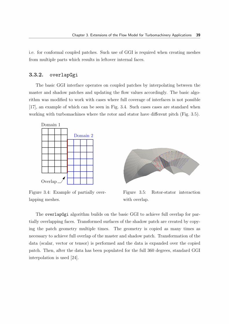
Chapter 3. Extensions of the Flow Model for Turbomachinery Applications 39
i.e. for conformal coupled patches. Such use of GGI is required when creating meshes
from multiple parts which results in leftover internal faces.
3.3.2. overlapGgi
The basic GGI interface operates on coupled patches by interpolating between the
master and shadow patches and updating the flow values accordingly. The basic algo-
rithm was modified to work with cases where full coverage of interfaces is not possible
[17], an example of which can be seen in Fig. 3.4. Such cases cases are standard when
working with turbomachines where the rotor and stator have different pitch (Fig. 3.5).
Domain 1
Domain 2
Overlap
Figure 3.4: Example of partially over-
lapping meshes.
Figure 3.5: Rotor-stator interaction
with overlap.
The overlapGgi algorithm builds on the basic GGI to achieve full overlap for par-
tially overlapping faces. Transformed surfaces of the shadow patch are created by copy-
ing the patch geometry multiple times. The geometry is copied as many times as
necessary to achieve full overlap of the master and shadow patch. Transformation of the
data (scalar, vector or tensor) is performed and the data is expanded over the copied
patch. Then, after the data has been populated for the full 360 degrees, standard GGI
interpolation is used [24].
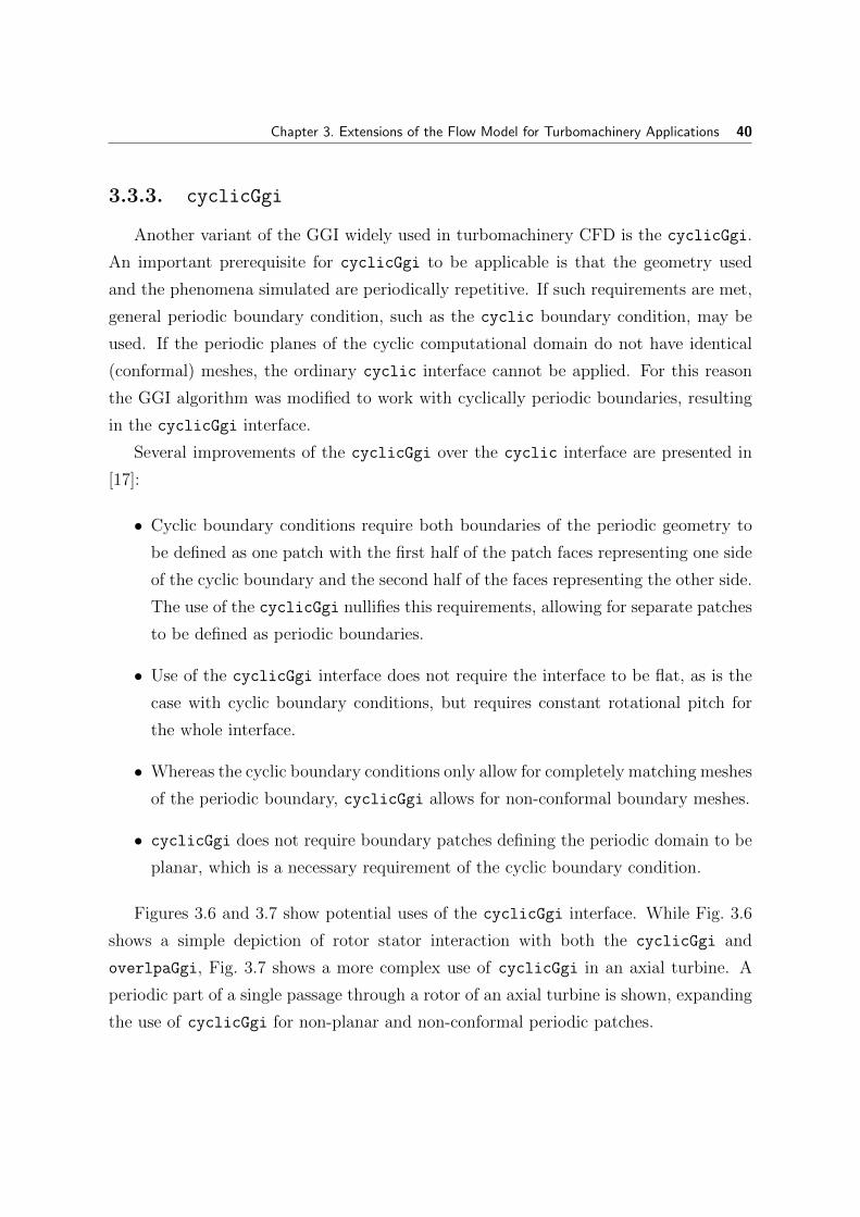
Chapter 3. Extensions of the Flow Model for Turbomachinery Applications 40
3.3.3. cyclicGgi
Another variant of the GGI widely used in turbomachinery CFD is the cyclicGgi.
An important prerequisite for cyclicGgi to be applicable is that the geometry used
and the phenomena simulated are periodically repetitive. If such requirements are met,
general periodic boundary condition, such as the cyclic boundary condition, may be
used. If the periodic planes of the cyclic computational domain do not have identical
(conformal) meshes, the ordinary cyclic interface cannot be applied. For this reason
the GGI algorithm was modified to work with cyclically periodic boundaries, resulting
in the cyclicGgi interface.
Several improvements of the cyclicGgi over the cyclic interface are presented in
[17]:
• Cyclic boundary conditions require both boundaries of the periodic geometry to
be defined as one patch with the first half of the patch faces representing one side
of the cyclic boundary and the second half of the faces representing the other side.
The use of the cyclicGgi nullifies this requirements, allowing for separate patches
to be defined as periodic boundaries.
• Use of the cyclicGgi interface does not require the interface to be flat, as is the
case with cyclic boundary conditions, but requires constant rotational pitch for
the whole interface.
• Whereas the cyclic boundary conditions only allow for completely matching meshes
of the periodic boundary, cyclicGgi allows for non-conformal boundary meshes.
• cyclicGgi does not require boundary patches defining the periodic domain to be
planar, which is a necessary requirement of the cyclic boundary condition.
Figures 3.6 and 3.7 show potential uses of the cyclicGgi interface. While Fig. 3.6
shows a simple depiction of rotor stator interaction with both the cyclicGgi and
overlpaGgi, Fig. 3.7 shows a more complex use of cyclicGgi in an axial turbine. A
periodic part of a single passage through a rotor of an axial turbine is shown, expanding
the use of cyclicGgi for non-planar and non-conformal periodic patches.
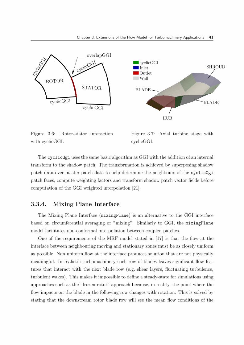
Chapter 3. Extensions of the Flow Model for Turbomachinery Applications 41
cyclicGGI
overlapGGI
ROTOR
STATOR
cyclicGGI
cyclicGGI
cycl
icG
GI
Figure 3.6: Rotor-stator interaction
with cyclicGGI.
BLADE
BLADE
HUB
SHROUD
Wall
cyclicGGIInletOutlet
Figure 3.7: Axial turbine stage with
cyclicGGI.
The cyclicGgi uses the same basic algorithm as GGI with the addition of an internal
transform to the shadow patch. The transformation is achieved by superposing shadow
patch data over master patch data to help determine the neighbours of the cyclicGgi
patch faces, compute weighting factors and transform shadow patch vector fields before
computation of the GGI weighted interpolation [21].
3.3.4. Mixing Plane Interface
The Mixing Plane Interface (mixingPlane) is an alternative to the GGI interface
based on circumferential averaging or ”mixing”. Similarly to GGI, the mixingPlane
model facilitates non-conformal interpolation between coupled patches.
One of the requirements of the MRF model stated in [17] is that the flow at the
interface between neighbouring moving and stationary zones must be as closely uniform
as possible. Non-uniform flow at the interface produces solution that are not physically
meaningful. In realistic turbomachinery each row of blades leaves significant flow fea-
tures that interact with the next blade row (e.g. shear layers, fluctuating turbulence,
turbulent wakes). This makes it impossible to define a steady-state for simulations using
approaches such as the ”frozen rotor” approach because, in reality, the point where the
flow impacts on the blade in the following row changes with rotation. This is solved by
stating that the downstream rotor blade row will see the mean flow conditions of the

Chapter 3. Extensions of the Flow Model for Turbomachinery Applications 42
upstream flow. To achieve this, it is necessary to perform averaging in the sweeping di-
rection. The mixingPlane model, which uses averaging to ”mix out” the flow, makes the
flow uniform. Furthermore, the mixingPlane model provides a great alternative when
simulating simplified turbomachinery components that connect to full-geometry compo-
nents. This is because for complex geometries, such as multi-stage turbomachinery with
varying number of blades in each row, which require large meshes consisting of several
blade passages to maintain circumferential periodicity, the use of unsteady models is
highly impractical [17]. Using the mixingPlane model for such cases produces steady-
state results reducing the computational time required and boosting cost-effectiveness,
while providing averaged data.
U
D
R
Figure 3.8: Upstream (U) and down-
stream (D) domains with ribbon patchs
(R).
U
D R
Figure 3.9: Upstream (U), downstream
(U) and ribbon (R) patches.
The mixingPlane interface builds upon the GGI algorithm by using an intermedi-
ate patch surface to handle interpolation between two modified GGI interfaces. The
intermediate patch surface is cylindrical or radial and consists of a stack of 360° ribbons
shared by the GGI interfaces on both sides. The 2D profiles of the upstream and down-
stream GGI interfaces are used as basis for discretisation generating the intermediate
ribbon patch. The mixingPlane averaging factors are computed based on the GGI
weighting factors and the shape of the intermediate patch ribbons [25]. The aforemen-
tioned upstream (U) and downstream (D) interfaces and the mixingPlane ribbon patch
(R) can be seen in Figures 3.8 and 3.9.
The mixingPlane model deals with each fluid zone (region of the computational
domain) as a separate steady-state problem. Communication between adjacent zones is
established by passing flow-field data as partially averaged boundary conditions through
the mixingPlane interface. The data is averaged at prescribed iteration intervals by

Chapter 3. Extensions of the Flow Model for Turbomachinery Applications 43
either area-weighted averaging, mass averaging or mixed-out averaging, as a combination
of the previous two averaging methods. Circumferential averaging along the ribbons of
the intermediate patch is used to compute flow values which are then used to update
boundary condition along the interface. The use of such averaging removes potential
unsteadiness due to variations in passage-to-passage flow fields, producing a steady-state
result that provides a good approximation of the time-averaged flow field [17].
3.4. Closure
This chapter presented the theoretical background needed for understanding the
various approaches to domain handling and interface handling used in turbomachinery
CFD. The basis of the Moving Reference Frame steady-state models (SRF and MRF)
was presented alongside the Moving Mesh transient model. The available interpolation
interfaces used for coupling of non-conformal meshes, such as the GGI (ggi) and Mixing
Plane (mixingPlane) interfaces, were presented. Finally, variants of the GGI model
used with partially overlapping patches (overlapGgi) and cyclically periodic domains
(cyclicGgi) were discussed.
The next chapter introduces the Contra-Rotating Propeller set as a good example
of an unshrouded turbomachine, which can be simulated by using various domain and
interface handling techniques described above. Benefits of contra-rotating propellers
and their implementation are discussed, with an overview of previous and connected
research also presented.

4 Contra-Rotating
Propellers
4.1. Introduction
The previous chapter gives an overview of various methods of domain and interface
handling and their implementation in turbomachinery CFD.
The following chapter includes a description of the Contra-Rotating Propellers set
(CRP), its operation, benefits and implementation. An overview of previous studies
regarding CRP sets is made, focusing on the experimental studies used, which are later
used for comparison with data produced by numerical simulations in this thesis. Further-
more, an overview of CRP characteristics is given in form of hydrodynamic coefficients
and the Q-criterion, as a mean of visualising vorticity.
4.2. Design, Development and Benefits
Conventional single-blade propellers have been used as predominant means of propul-
sion for ships and submarines since the late 19th century. With an increasing complexity
of maritime propulsion and a continued need to design faster, more reliable and quieter
means of propulsion with greater manoeuvrability, the focus shifted towards Contra-
Rotating Propellers [26].
The Contra-Rotating Propeller set (CRP) usually consists of two propellers with
collinear axes rotating in opposite directions. The main reason for employing such a
design is the idea that positioning a secondary propeller behind the main propeller
and having it rotate in the opposite direction positively affects the performance of the
propulsion system and removes the bulk of the torque transferred from the propeller to
44
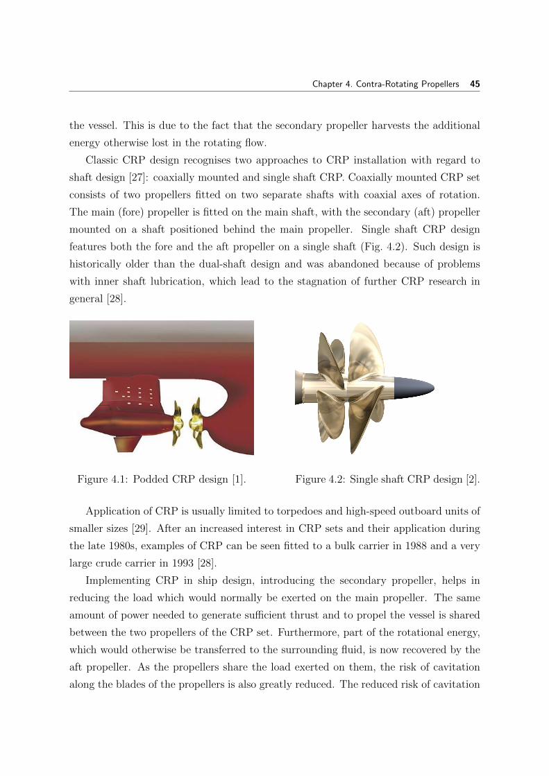
Chapter 4. Contra-Rotating Propellers 45
the vessel. This is due to the fact that the secondary propeller harvests the additional
energy otherwise lost in the rotating flow.
Classic CRP design recognises two approaches to CRP installation with regard to
shaft design [27]: coaxially mounted and single shaft CRP. Coaxially mounted CRP set
consists of two propellers fitted on two separate shafts with coaxial axes of rotation.
The main (fore) propeller is fitted on the main shaft, with the secondary (aft) propeller
mounted on a shaft positioned behind the main propeller. Single shaft CRP design
features both the fore and the aft propeller on a single shaft (Fig. 4.2). Such design is
historically older than the dual-shaft design and was abandoned because of problems
with inner shaft lubrication, which lead to the stagnation of further CRP research in
general [28].
Figure 4.1: Podded CRP design [1]. Figure 4.2: Single shaft CRP design [2].
Application of CRP is usually limited to torpedoes and high-speed outboard units of
smaller sizes [29]. After an increased interest in CRP sets and their application during
the late 1980s, examples of CRP can be seen fitted to a bulk carrier in 1988 and a very
large crude carrier in 1993 [28].
Implementing CRP in ship design, introducing the secondary propeller, helps in
reducing the load which would normally be exerted on the main propeller. The same
amount of power needed to generate sufficient thrust and to propel the vessel is shared
between the two propellers of the CRP set. Furthermore, part of the rotational energy,
which would otherwise be transferred to the surrounding fluid, is now recovered by the
aft propeller. As the propellers share the load exerted on them, the risk of cavitation
along the blades of the propellers is also greatly reduced. The reduced risk of cavitation
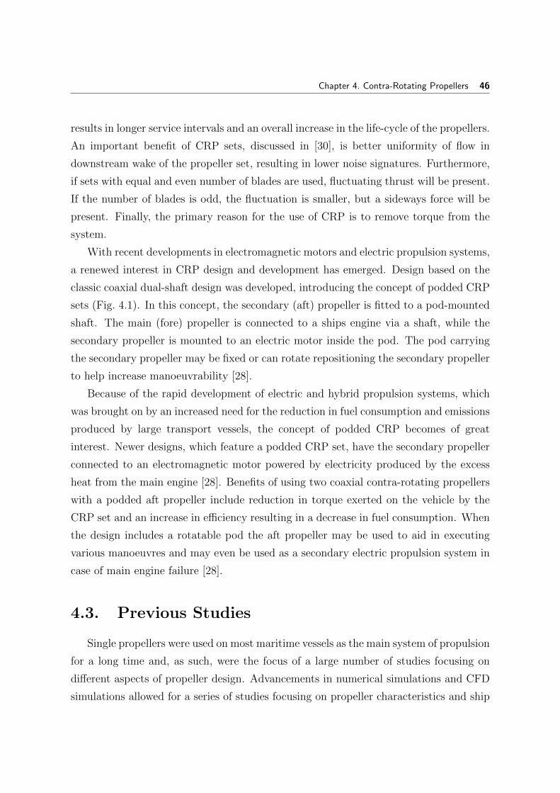
Chapter 4. Contra-Rotating Propellers 46
results in longer service intervals and an overall increase in the life-cycle of the propellers.
An important benefit of CRP sets, discussed in [30], is better uniformity of flow in
downstream wake of the propeller set, resulting in lower noise signatures. Furthermore,
if sets with equal and even number of blades are used, fluctuating thrust will be present.
If the number of blades is odd, the fluctuation is smaller, but a sideways force will be
present. Finally, the primary reason for the use of CRP is to remove torque from the
system.
With recent developments in electromagnetic motors and electric propulsion systems,
a renewed interest in CRP design and development has emerged. Design based on the
classic coaxial dual-shaft design was developed, introducing the concept of podded CRP
sets (Fig. 4.1). In this concept, the secondary (aft) propeller is fitted to a pod-mounted
shaft. The main (fore) propeller is connected to a ships engine via a shaft, while the
secondary propeller is mounted to an electric motor inside the pod. The pod carrying
the secondary propeller may be fixed or can rotate repositioning the secondary propeller
to help increase manoeuvrability [28].
Because of the rapid development of electric and hybrid propulsion systems, which
was brought on by an increased need for the reduction in fuel consumption and emissions
produced by large transport vessels, the concept of podded CRP becomes of great
interest. Newer designs, which feature a podded CRP set, have the secondary propeller
connected to an electromagnetic motor powered by electricity produced by the excess
heat from the main engine [28]. Benefits of using two coaxial contra-rotating propellers
with a podded aft propeller include reduction in torque exerted on the vehicle by the
CRP set and an increase in efficiency resulting in a decrease in fuel consumption. When
the design includes a rotatable pod the aft propeller may be used to aid in executing
various manoeuvres and may even be used as a secondary electric propulsion system in
case of main engine failure [28].
4.3. Previous Studies
Single propellers were used on most maritime vessels as the main system of propulsion
for a long time and, as such, were the focus of a large number of studies focusing on
different aspects of propeller design. Advancements in numerical simulations and CFD
simulations allowed for a series of studies focusing on propeller characteristics and ship

Chapter 4. Contra-Rotating Propellers 47
manoeuvring simulations [31, 32, 33].
With the rising interest in CRP and their use for ship propulsion, a growing number
of numerical and experimental studies focusing on CRP sets can be found. Some of the
first experiments were performed using a scaled CRP model and focused on defining
the open-water characteristics [34] and the effects of axial displacements of such sets
[35]. More recent studies were performed by Miller in 1976 [36] and again in 1981 [37].
These experiments were aimed at determining the unsteady forces on a CRP set in
uniform flow and are of great interest to the subject of this Thesis, as they were used
for comparison with the data produced by CFD simulations run for the purpose of this
thesis.
A number of numerical simulations dealing with CRP was performed by numerous
authors, which will be outlined briefly. Hoshino [38] expanded experimental research on
CRP model and used the experimental data to validate numerical simulations performed
using Lifting Surface Theory. The same theory was used by Tsakonas et al. [39] and
Yang et al. [40] to calculate the hydrodynamic coefficients of CRP. On the other hand,
Ghassemi and Taherinasab [30] implemented the Boundary Element Method to model
steady hydrodynamic performance of CRP, while Gu and Kinnas used a combination of
FVM and the Vortex-Lattice Method. Use of CFD for investigation of CRP blade inter-
action and performance surfaced only recently with Wang and Xiong [41] using RANS
modelling to determine the effects time-step size and turbulence on CRP performance
and with Nouri et al. [42] using CFD for CRP optimisation.
4.4. Characteristics of CRP
This section is dedicated to describing how the performance of CRP is to be evalu-
ated. Besides examining the pressure and velocity fields of propellers, it is common to
define propeller open-water characteristics. Open-water characteristics of CRP sets are
defined by calculating hydrodynamic performance coefficients for each propeller sepa-
rately and for the whole set.
Another interesting phenomena examined as part of this thesis, are vortices. The
Q-criterion is used as a method of vortex identification. It is used to define structures
of different vorticity and examine the influence of propeller interaction in CRP sets on
interacting vortices.
Chapter 4. Contra-Rotating Propellers 48
4.4.1. Hydrodynamic Coefficients
Hydrodynamic coefficients are calculated to determine the open-water characteristics
of the CRP set. The calculated coefficients include the thrust coefficient KT , the torque
coefficient KQ and propeller efficiency η. The aforementioned coefficients are calculated
for each propeller and for the whole CRP set. If values for each of these coefficients are
given in relation to the advance coefficient J , determined for different operating points,
a diagram showing the open-water characteristics of the CRP set can be drawn.
Depending on the type of simulation used, two different types of hydrodynamic
coefficients may be determined: steady coefficients may be expressed from data collected
from both steady state and transient simulations, while the unsteady coefficients may
be determined from transient data only.
It should be noted that the procedure for determining steady and unsteady CRP
hydrodynamic coefficients was defined as to adhere to the procedure used by Miller
[36, 37] in his experimental studies. This was done to allow for comparison between the
experimental data acquired by Miller and the numerical data simulated for the purpose
of this thesis.
Steady Coefficients
The propeller advance ratio J is a non-dimensional coefficient which defines the
ratio of the free-stream fluid velocity compared to propeller rotation speed. It can be
calculated by using the following expression:
J =U
nDf
, (4.1)
where U defines the free-stream velocity of the fluid, n defines the rotational speed of
the propeller and Df is the propeller diameter. The advance ratio J for both propellers
and the whole CRP set is calculated using the diameter of the fore (forward) propeller,
Df . By using the corresponding values of thrust for each propeller, thrust coefficients
may be calculated using the following expressions:

Chapter 4. Contra-Rotating Propellers 49
KTf =Tf
n2D4fρ, (4.2)
KTa =Ta
n2D4aρ. (4.3)
Eq. 4.2 nad 4.3 produce values of aft/fore thrust coefficients for given values of thrust
T , rotational speed n, water density ρ and the corresponding propeller diameter Df , Da.
The same value of the propeller rotation speed n is used for both propellers as their
movement is synchronised in both the experiments and simulations used in the thesis.
By using the same assumptions as above and the corresponding values of torque, the
propeller torque coefficients can be determined using:
KQf =Qf
n2D5fρ, (4.4)
KQa =Qa
n2D5aρ. (4.5)
The values of the torque and thrust coefficients are used to calculate propeller efficiency
for the corresponding advance ratio J :
ηf =KTf
KQf
J
2π, (4.6)
ηa =KTa
KQa
J
2π. (4.7)
Once the steady thrust and torque coefficients are calculated for each of the two pro-
pellers forming the CRP set, the total hydrodynamic coefficients of the CRP set may
be determined using:
KT = KTf +KTa , (4.8)
KQ = KQf +KQa , (4.9)
with the total set efficiency determined by the following expression:

Chapter 4. Contra-Rotating Propellers 50
η =KT
KQ
J
2π. (4.10)
Unsteady Coefficients
Time-varying data gathered from transient simulations is analysed as a part of this
thesis. The values of unsteady thrust and torque are calculated in a way that makes
them comparable to corresponding experimental values from studies performed by Miller
[36, 37]. The Direct Fourier Transform (DFT) was used to transform the transient
data and analyse the resulting amplitudes as functions of frequency. The amplitudes of
unsteady torque and thrust at certain frequencies (or harmonics) were used to determine
unsteady thrust and torque coefficients.
Values of unsteady thrust and torque may be presented as a sum of sine and cosine
amplitudes for any harmonic N :
TN = T1,N cos(Nθ) + T2,N sin(Nθ) , (4.11)
QN = Q1,N cos(Nθ) +Q2,N sin(Nθ) . (4.12)
Eq. 4.11 and 4.12 allow the unsteady coefficients for each propeller to be defined for a
certain harmonic N as:
KT,prop,N =(T 2
1,N + T 22,N)
12
n2D4ρ, (4.13)
KQ,prop,N =(Q2
1,N +Q22,N)
12
n2D5ρ. (4.14)
The total coefficients of unsteady thrust and torque for the complete CRP set may be
calculated from the following equations:
KT,N = KTf,N + KTa,N , (4.15)
KQ,N = KQf,N + KQa,N . (4.16)

Chapter 4. Contra-Rotating Propellers 51
4.4.2. Q-Criterion
An interesting aspect of turbomachinery CFD is the possibility of investigating vor-
ticity of the flow. This becomes of special interest when dealing with multi-blade multi-
rotor machines, such as the CRP set. Rotor interactions of the two propellers result in
interesting vortex interaction.
The vortices in the flow-field around and after the propeller set shall be defined
using the Q-criterion. Historically, one of the first three-dimensional vortex criteria, the
Q-criterion was developed by Hunt, Wray and Moin in 1988 [43].
As shown in [44] the velocity gradient ∇u of a three-dimensional velocity field u may
be decomposed as follows:
∇u = S︸︷︷︸rate-of-strain
tensor
+ Ω︸︷︷︸vortricity
tensor
. (4.17)
Eq. 4.17 represents the decomposition of the velocity gradient into the rate-of-strain
tensor S and the vorticity tensor Ω, both given below:
S =1
2
[∇u + (∇u)T
], (4.18)
Ω =1
2
[∇u− (∇u)T
]. (4.19)
The Q-criterion defines a vortex as a region in space where by the Euclidean norm of the
vorticity tensor dominates over the Euclidean norm of the rate-of-strain tensor. Thus
described as:
Q =1
2
[|Ω|2 − |S|2
]> 0 . (4.20)
4.5. Closure
The concluded chapter gave an examination of the design of CRP, its implemen-
tation and development. The most important benefits of CRP implementation were
discussed, as well as some of the disadvantages of older designs. Moreover, an overview

Chapter 4. Contra-Rotating Propellers 52
of experimental and numerical studies was given. The basic equations used to describe
the characteristics of CRP in terms of open-water characteristics and vorticity were also
presented.
The next chapter deals with geometries used for CFD simulations of CRP and the
resulting computational domains. An overview of patches, regions, domain interfaces
and the necessary boundary conditions is given as an introduction to the numerical
simulations made using the CRP computational model.

5 Geometry and
Computational Domain
5.1. Introduction
The previous chapter dealt with CRP sets in general, their design, application and
improvements over single-propeller designs. Moreover, an overview of previous experi-
mental and numerical studies was given.
The forthcoming chapter deals with the CRP geometry and the resulting computa-
tional domain. An overview of domain characteristics of both the whole geometry and
quarter geometry meshes is presented. An description of domain boundary patches and
interfaces is given with an overview of boundary conditions imposed on the patches.
5.2. Model Geometry
The geometry used as a starting point for creating a computational domain (mesh)
is the model used in experimental studies performed by Miller [36, 37]. The propeller set
geometry closely mimics the CRP set described by Miller, which is a necessary condition
for the numerical results to be comparable to experimental data.
The CRP set consists of two four-bladed propellers mounted on hubs with co-linear
rotational axes. The two propellers are mounted as to face one another and to rotate
in opposite directions at identical rotational speed. The specifications defining the
individual propellers are given in Table 5.1.
53
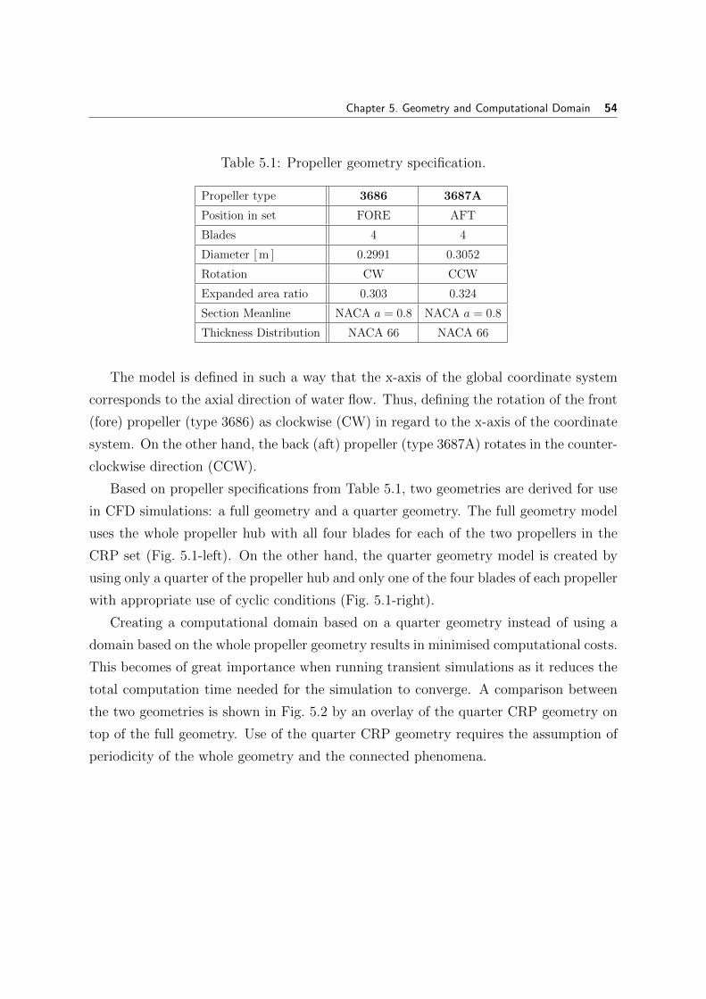
Chapter 5. Geometry and Computational Domain 54
Table 5.1: Propeller geometry specification.
Propeller type 3686 3687A
Position in set FORE AFT
Blades 4 4
Diameter [ m ] 0.2991 0.3052
Rotation CW CCW
Expanded area ratio 0.303 0.324
Section Meanline NACA a = 0.8 NACA a = 0.8
Thickness Distribution NACA 66 NACA 66
The model is defined in such a way that the x-axis of the global coordinate system
corresponds to the axial direction of water flow. Thus, defining the rotation of the front
(fore) propeller (type 3686) as clockwise (CW) in regard to the x-axis of the coordinate
system. On the other hand, the back (aft) propeller (type 3687A) rotates in the counter-
clockwise direction (CCW).
Based on propeller specifications from Table 5.1, two geometries are derived for use
in CFD simulations: a full geometry and a quarter geometry. The full geometry model
uses the whole propeller hub with all four blades for each of the two propellers in the
CRP set (Fig. 5.1-left). On the other hand, the quarter geometry model is created by
using only a quarter of the propeller hub and only one of the four blades of each propeller
with appropriate use of cyclic conditions (Fig. 5.1-right).
Creating a computational domain based on a quarter geometry instead of using a
domain based on the whole propeller geometry results in minimised computational costs.
This becomes of great importance when running transient simulations as it reduces the
total computation time needed for the simulation to converge. A comparison between
the two geometries is shown in Fig. 5.2 by an overlay of the quarter CRP geometry on
top of the full geometry. Use of the quarter CRP geometry requires the assumption of
periodicity of the whole geometry and the connected phenomena.
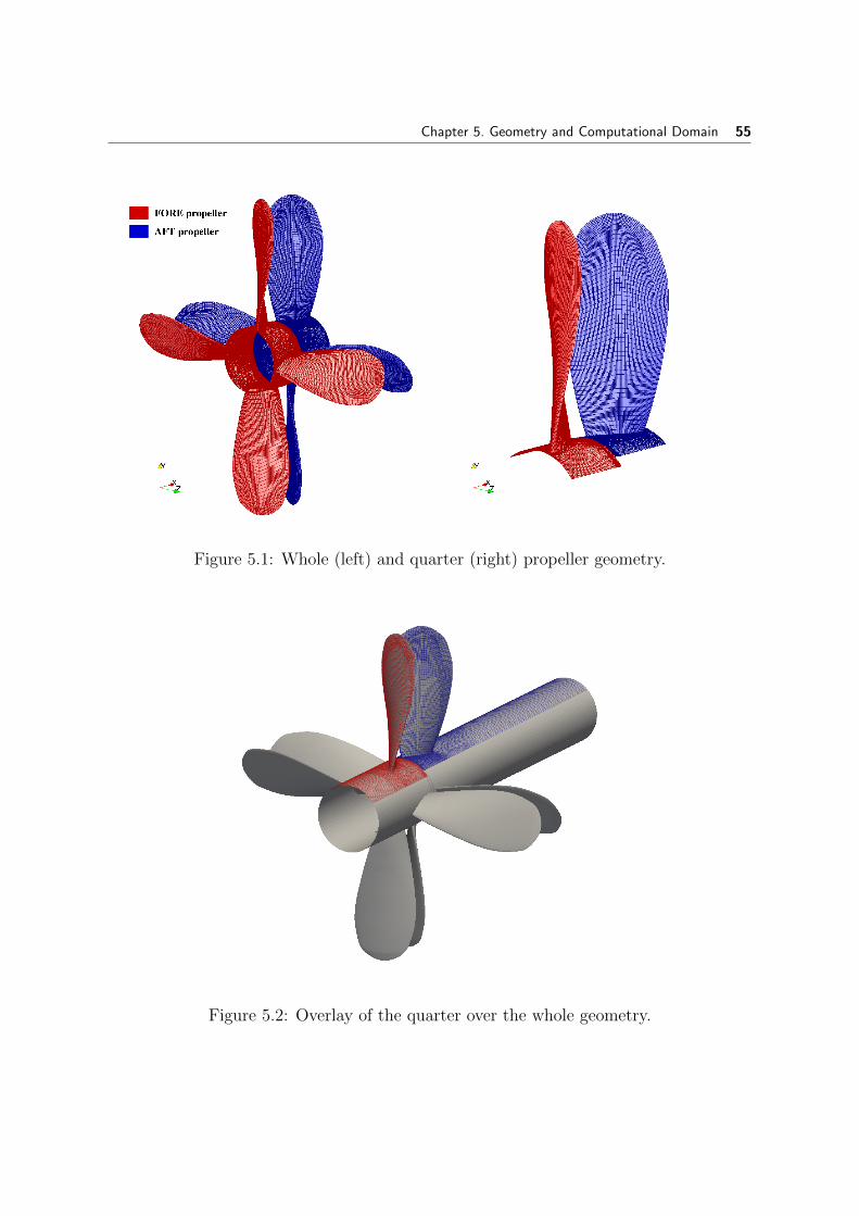
Chapter 5. Geometry and Computational Domain 55
Figure 5.1: Whole (left) and quarter (right) propeller geometry.
Figure 5.2: Overlay of the quarter over the whole geometry.
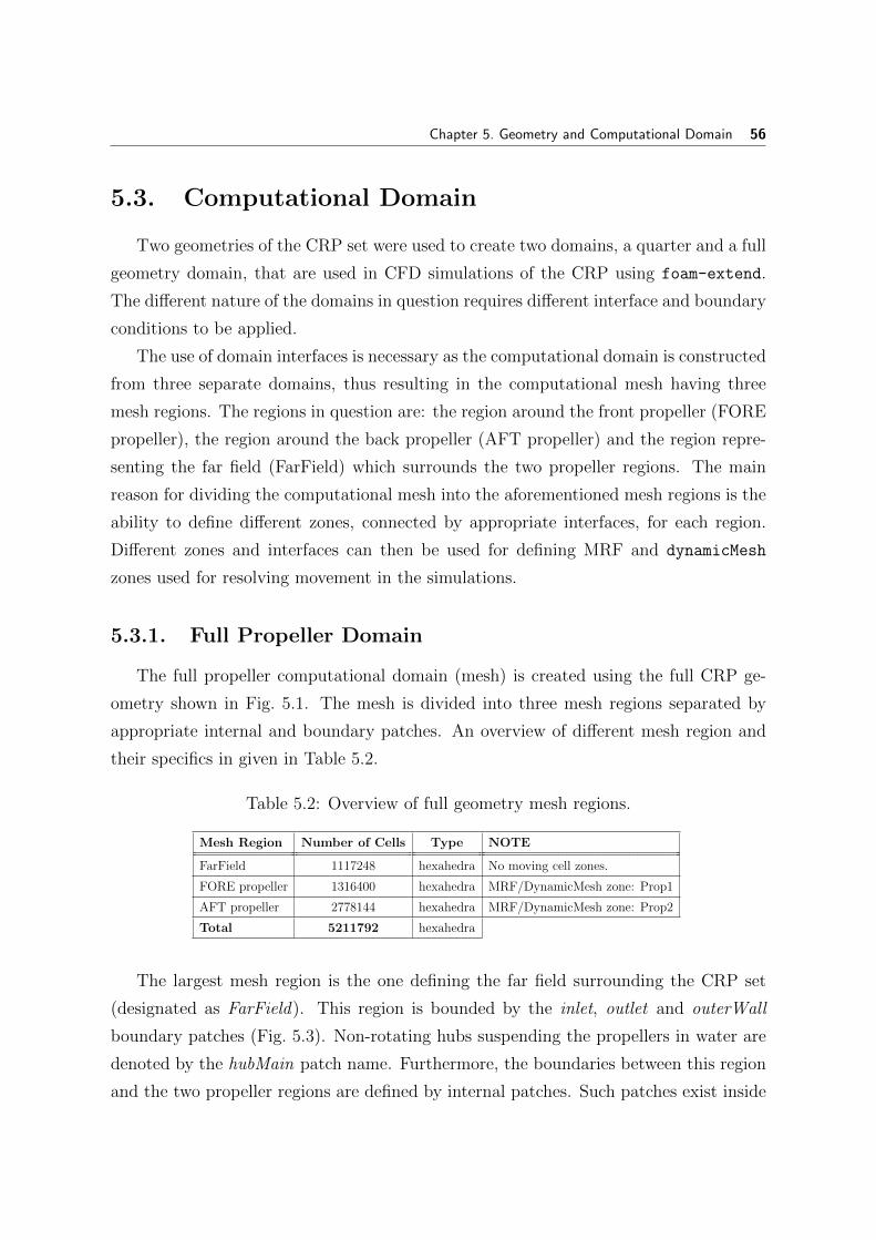
Chapter 5. Geometry and Computational Domain 56
5.3. Computational Domain
Two geometries of the CRP set were used to create two domains, a quarter and a full
geometry domain, that are used in CFD simulations of the CRP using foam-extend.
The different nature of the domains in question requires different interface and boundary
conditions to be applied.
The use of domain interfaces is necessary as the computational domain is constructed
from three separate domains, thus resulting in the computational mesh having three
mesh regions. The regions in question are: the region around the front propeller (FORE
propeller), the region around the back propeller (AFT propeller) and the region repre-
senting the far field (FarField) which surrounds the two propeller regions. The main
reason for dividing the computational mesh into the aforementioned mesh regions is the
ability to define different zones, connected by appropriate interfaces, for each region.
Different zones and interfaces can then be used for defining MRF and dynamicMesh
zones used for resolving movement in the simulations.
5.3.1. Full Propeller Domain
The full propeller computational domain (mesh) is created using the full CRP ge-
ometry shown in Fig. 5.1. The mesh is divided into three mesh regions separated by
appropriate internal and boundary patches. An overview of different mesh region and
their specifics in given in Table 5.2.
Table 5.2: Overview of full geometry mesh regions.
Mesh Region Number of Cells Type NOTE
FarField 1117248 hexahedra No moving cell zones.
FORE propeller 1316400 hexahedra MRF/DynamicMesh zone: Prop1
AFT propeller 2778144 hexahedra MRF/DynamicMesh zone: Prop2
Total 5211792 hexahedra
The largest mesh region is the one defining the far field surrounding the CRP set
(designated as FarField). This region is bounded by the inlet, outlet and outerWall
boundary patches (Fig. 5.3). Non-rotating hubs suspending the propellers in water are
denoted by the hubMain patch name. Furthermore, the boundaries between this region
and the two propeller regions are defined by internal patches. Such patches exist inside

Chapter 5. Geometry and Computational Domain 57
the computational domain separating different regions, unlike boundary patches that
separate the domain from the ”outside world”.
Figure 5.3: Whole geometry: FarField patch identification.
Internal patches of the FarField mesh region are shown in Figure 5.4 and are used as
interfaces enabling communication between propeller mesh regions.
Figure 5.4: Whole geometry: FarField interfaces near propeller region.
All interfaces belonging to the FarField region are denoted by including the prefix
”MAIN” in their name. Similarly, all patches (interfaces) belonging to the FORE pro-
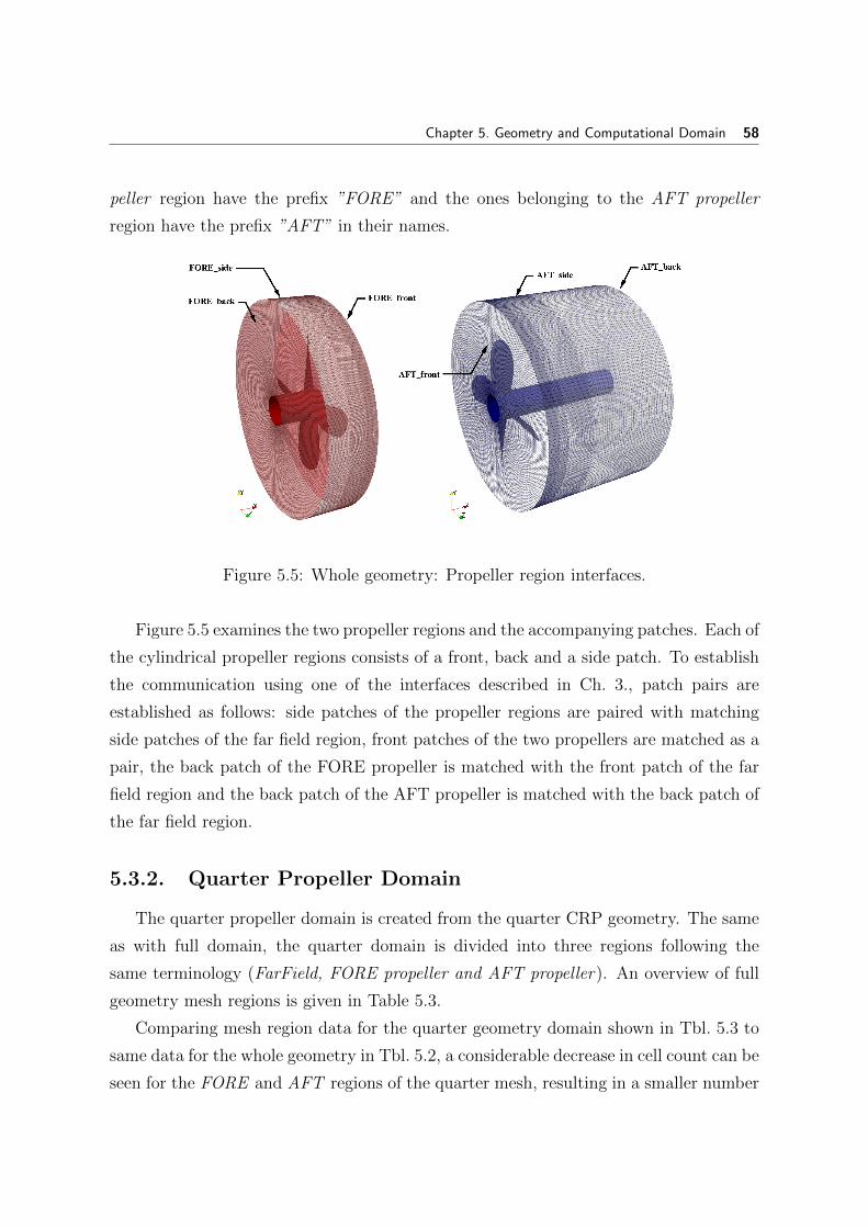
Chapter 5. Geometry and Computational Domain 58
peller region have the prefix ”FORE” and the ones belonging to the AFT propeller
region have the prefix ”AFT” in their names.
Figure 5.5: Whole geometry: Propeller region interfaces.
Figure 5.5 examines the two propeller regions and the accompanying patches. Each of
the cylindrical propeller regions consists of a front, back and a side patch. To establish
the communication using one of the interfaces described in Ch. 3., patch pairs are
established as follows: side patches of the propeller regions are paired with matching
side patches of the far field region, front patches of the two propellers are matched as a
pair, the back patch of the FORE propeller is matched with the front patch of the far
field region and the back patch of the AFT propeller is matched with the back patch of
the far field region.
5.3.2. Quarter Propeller Domain
The quarter propeller domain is created from the quarter CRP geometry. The same
as with full domain, the quarter domain is divided into three regions following the
same terminology (FarField, FORE propeller and AFT propeller). An overview of full
geometry mesh regions is given in Table 5.3.
Comparing mesh region data for the quarter geometry domain shown in Tbl. 5.3 to
same data for the whole geometry in Tbl. 5.2, a considerable decrease in cell count can be
seen for the FORE and AFT regions of the quarter mesh, resulting in a smaller number

Chapter 5. Geometry and Computational Domain 59
of cells for the total computational domain. This was achieved by reducing propeller
regions to a quarter of the original, which was possible by using only one propeller blade
and quarter of the hub geometry. On the other hand, the cell count for the FarField
is the same as for the whole domain, as this region is used in its entirety for both the
quarter and the whole propeller domains.
Table 5.3: Overview of quarter geometry mesh regions.
Mesh Region Number of Cells Type NOTE
FarField 1117248 hexahedra No moving cell zones.
FORE propeller 329100 hexahedra MRF/DynamicMesh zone: Prop1
AFT propeller 694536 hexahedra MRF/DynamicMesh zone: Prop2
Total 5211792 hexahedra
Figure 5.6 shows how the quarter propeller regions connect to the FarField region.
As this mesh region is the same as the one used for the whole propeller domain, the
boundary patches (inlet, outlet, outerWall, hubMain) and internal patches defining the
region have not changed.
Figure 5.6: Quarter geometry: FarField patch identification.
The geometric definition of internal patches belonging to the FarField region shown in
Fig. 5.7 have not changed when compared to the whole geometry mesh. Nevertheless,
they are paired with patches bounding the quarter propeller regions, which is why they
require different patch (interface) definition and a different set of boundary conditions.

Chapter 5. Geometry and Computational Domain 60
Figure 5.7: Quarter geometry: FarField interfaces near propeller region.
Figure 5.8 shows the quarter propeller mesh regions with corresponding boundary patches.
The positions of the front, back and side patches is analogous to those of their whole
geometry counterparts, but they are reduced to a quarter of their original geometry.
New patches defining the boundaries where the quarter regions would expand into the
full geometry region are present (cyclic and cyclic shadow). These patches bound the
cyclically periodic boundary of the propeller regions and are defined as cyclicGgi in-
terfaces.
Figure 5.8: Quarter geometry: Propeller region interfaces.
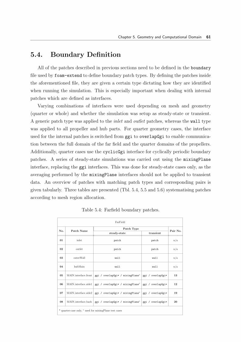
Chapter 5. Geometry and Computational Domain 61
5.4. Boundary Definition
All of the patches described in previous sections need to be defined in the boundary
file used by foam-extend to define boundary patch types. By defining the patches inside
the aforementioned file, they are given a certain type dictating how they are identified
when running the simulation. This is especially important when dealing with internal
patches which are defined as interfaces.
Varying combinations of interfaces were used depending on mesh and geometry
(quarter or whole) and whether the simulation was setup as steady-state or transient.
A generic patch type was applied to the inlet and outlet patches, whereas the wall type
was applied to all propeller and hub parts. For quarter geometry cases, the interface
used for the internal patches is switched from ggi to overlapGgi to enable communica-
tion between the full domain of the far field and the quarter domains of the propellers.
Additionally, quarter cases use the cyclicGgi interface for cyclically periodic boundary
patches. A series of steady-state simulations was carried out using the mixingPlane
interface, replacing the ggi interfaces. This was done for steady-state cases only, as the
averaging performed by the mixingPlane interfaces should not be applied to transient
data. An overview of patches with matching patch types and corresponding pairs is
given tabularly. Three tables are presented (Tbl. 5.4, 5.5 and 5.6) systematising patches
according to mesh region allocation.
Table 5.4: Farfield boundary patches.
FarField
No. Patch NamePatch Type
Pair No.steady-state transient
01 inlet patch patch n/a
02 outlet patch patch n/a
03 outerWall wall wall n/a
04 hubMain wall wall n/a
05 MAIN interface front ggi / overlapGgi* / mixingPlane ggi / overlapGgi* 13
06 MAIN interface side1 ggi / overlapGgi* / mixingPlane ggi / overlapGgi* 12
07 MAIN interface side2 ggi / overlapGgi* / mixingPlane ggi / overlapGgi* 19
08 MAIN interface back ggi / overlapGgi* / mixingPlane ggi / overlapGgi* 20
* quarter-case only, used for mixingPlane test cases

Chapter 5. Geometry and Computational Domain 62
Table 5.5: FORE propeller boundary patches.
FORE propeller
No. Patch NamePatch Type
Pair No.steady-state transient
09 FORE prop wall wall n/a
10 FORE hub wall wall n/a
11 FORE interface front ggi / overlapGgi* / mixingPlane ggi / overlapGgi* 18
12 FORE interface side ggi / overlapGgi* / mixingPlane ggi / overlapGgi* 06
13 FORE interface back ggi / overlapGgi* / mixingPlane ggi / overlapGgi* 05
14 FORE cyclic* cyclicGgi cyclicGgi 15
15 FORE cyclic shadow* cyclicGgi cyclicGgi 14
* quarter-case only, used for mixingPlane test cases
Table 5.6: AFT propeller boundary patches.
AFT propeller
No. Patch NamePatch Type
Pair No.steady-state transient
16 AFT prop wall wall n/a
17 AFT hub wall wall n/a
18 AFT interface front ggi / overlapGgi* / mixingPlane ggi / overlapGgi* 11
19 AFT interface side ggi / overlapGgi* / mixingPlane ggi / overlapGgi* 07
20 AFT interface back ggi / overlapGgi* / mixingPlane ggi / overlapGgi* 08
21 AFT cyclic* cyclicGgi cyclicGgi 22
22 AFT cyclic shadow* cyclicGgi cyclicGgi 21
* quarter-case only, used for mixingPlane test cases
While the quarter cases require the use of both cyclicGgi and overlapGgi interfaces
to resolve cyclically periodic and non-overlapping patch communication brought on by
the use of a quarter domain, the whole cases allowed for the use of the basic ggi
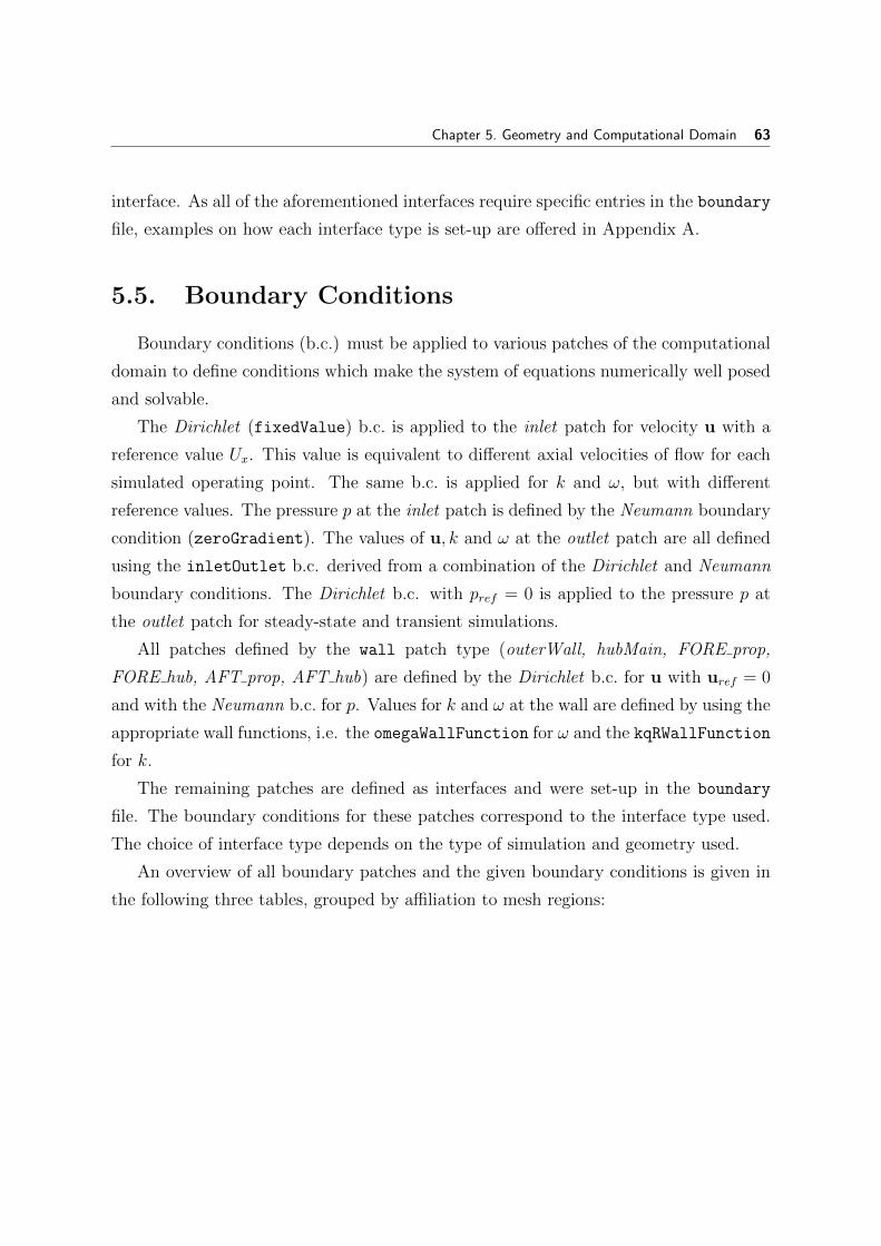
Chapter 5. Geometry and Computational Domain 63
interface. As all of the aforementioned interfaces require specific entries in the boundary
file, examples on how each interface type is set-up are offered in Appendix A.
5.5. Boundary Conditions
Boundary conditions (b.c.) must be applied to various patches of the computational
domain to define conditions which make the system of equations numerically well posed
and solvable.
The Dirichlet (fixedValue) b.c. is applied to the inlet patch for velocity u with a
reference value Ux. This value is equivalent to different axial velocities of flow for each
simulated operating point. The same b.c. is applied for k and ω, but with different
reference values. The pressure p at the inlet patch is defined by the Neumann boundary
condition (zeroGradient). The values of u, k and ω at the outlet patch are all defined
using the inletOutlet b.c. derived from a combination of the Dirichlet and Neumann
boundary conditions. The Dirichlet b.c. with pref = 0 is applied to the pressure p at
the outlet patch for steady-state and transient simulations.
All patches defined by the wall patch type (outerWall, hubMain, FORE prop,
FORE hub, AFT prop, AFT hub) are defined by the Dirichlet b.c. for u with uref = 0
and with the Neumann b.c. for p. Values for k and ω at the wall are defined by using the
appropriate wall functions, i.e. the omegaWallFunction for ω and the kqRWallFunction
for k.
The remaining patches are defined as interfaces and were set-up in the boundary
file. The boundary conditions for these patches correspond to the interface type used.
The choice of interface type depends on the type of simulation and geometry used.
An overview of all boundary patches and the given boundary conditions is given in
the following three tables, grouped by affiliation to mesh regions:

Chapter 5. Geometry and Computational Domain 64
Tab
le5.
7:O
verv
iew
ofF
arfiel
dpro
pel
ler
bou
ndar
yco
ndit
ions.
FA
RF
IEL
DB
oundar
yC
ondit
ions
(B.C
)
No.
Patc
hN
am
e
Ste
ad
y-s
tate
B.C
.T
ran
sient
B.C
.
U[m/s
]p
[m2/s
2]
k[m
2/s
2]
ω[1/s
]U
[m/s
]p
[m2/s
2]
k[m
2/s
2]
ω[1/s
]
01
inle
tfixedValue;
uniform(Ux0
0);
zeroGradient;
fixedValue;
uniformkref;
fixedValue;
uniformωref;
fixedValue;
uniform(Ux0
0);
zeroGradient;
fixedValue;
uniformkref;
fixedValue;
uniformωref;
02
outl
et
inletOutlet;
uniform(0
00);
uniform(Ux0
0);
fixedValue;
uniform0;
inletOutlet;
uniformkx;
uniformkx;
inletOutlet;
uniformωref;
uniformωref;
inletOutlet;
uniform(0
00);
uniform(Ux0
0);
fixedValue;
uniform0;
inletOutlet;
uniformkx;
uniformkx;
inletOutlet;
uniformωref;
uniformωref;
03
oute
rWal
lfixedValue;
uniform(0
00);
zeroGradient;
kqRWallFunction;
omegaWallFunction;
fixedValue;
uniform(0
00);
zeroGradient;
kqRWallFunction;
omegaWallFunction;
04
hubM
ain
fixedValue;
uniform(0
00);
zeroGradient;
kqRWallFunction;
omegaWallFunction;
fixedValue;
uniform(0
00);
zeroGradient;
kqRWallFunction;
omegaWallFunction;
05
MA
INin
terf
ace
fron
tggi
/overlapGgi*;
ggi
/overlapGgi*;
ggi
/overlapGgi*;
ggi/
overlapGgi*;
ggi
/overlapGgi*;
ggi
/overlapGgi*;
ggi
/overlapGgi*;
ggi
/overlapGgi*;
06
MA
INin
terf
ace
side1
ggi
/overlapGgi*;
ggi
/overlapGgi*;
ggi
/overlapGgi*;
ggi/
overlapGgi*;
ggi
/overlapGgi*;
ggi
/overlapGgi*;
ggi
/overlapGgi*;
ggi
/overlapGgi*;
07
MA
INin
terf
ace
side2
ggi
/overlapGgi*;
ggi
/overlapGgi*;
ggi
/overlapGgi*;
ggi/
overlapGgi*;
ggi
/overlapGgi*;
ggi
/overlapGgi*;
ggi
/overlapGgi*;
ggi
/overlapGgi*;
08
MA
INin
terf
ace
bac
kggi
/overlapGgi*;
ggi
/overlapGgi*;
ggi
/overlapGgi*;
ggi/
overlapGgi*;
ggi
/overlapGgi*;
ggi
/overlapGgi*;
ggi
/overlapGgi*;
ggi
/overlapGgi*;
*quar
ter-
case
only
NO
TE
:G
gian
dov
erla
pG
gire
pla
ced
by
mix
ingP
lane
for
mix
ingP
lane
validat
ion
case
s.

Chapter 5. Geometry and Computational Domain 65
Tab
le5.
8:O
verv
iew
ofF
OR
Epro
pel
ler
bou
ndar
yco
ndit
ions.
FO
RE
pro
pel
ler
Bou
nd
ary
Con
dit
ion
s(B
.C.)
No.
Patc
hN
am
e
Ste
ady-s
tate
B.C
.T
ransi
ent
B.C
.
U[m/s
]p
[m2/s
2]
k[m
2/s
2]
ω[1/s
]U
[m/s
]p
[m2/s
2]
k[m
2/s
2]
ω[1/s
]
09
FO
RE
pro
pfixedValue;
uniform
(0
00);
zeroGradient;
kqRWallFunction;
omegaWallFunction;
movingWallVelocity;
uniform(0
00);
zeroGradient;
kqRWallFunction;
omegaWallFunction;
10
FO
RE
hu
bfixedValue;
uniform
(0
00);
zeroGradient;
kqRWallFunction;
omegaWallFunction;
fixedValue;
uniform(0
00);
zeroGradient;
kqRWallFunction;
omegaWallFunction;
11
FO
RE
inte
rfac
efr
ont
ggi
/overlapGgi*;
ggi
/overlapGgi*;
ggi
/overlapGgi*;
ggi
/overlapGgi*;
ggi
/overlapGgi*;
ggi
/overlapGgi*;
ggi
/overlapGgi*;
ggi
/overlapGgi*;
12
FO
RE
inte
rfac
esi
de
ggi
/overlapGgi*;
ggi
/overlapGgi*;
ggi
/overlapGgi*;
ggi
/overlapGgi*;
ggi
/overlapGgi*;
ggi
/overlapGgi*;
ggi
/overlapGgi*;
ggi
/overlapGgi*;
13
FO
RE
inte
rfac
eb
ack
ggi
/overlapGgi*;
ggi
/overlapGgi*;
ggi
/overlapGgi*;
ggi
/overlapGgi*;
ggi
/overlapGgi*;
ggi
/overlapGgi*;
ggi
/overlapGgi*;
ggi
/overlapGgi*;
14
FO
RE
cycl
ic*
cyclicGgi;
cyclicGgi;
cyclicGgi;
cyclicGgi;
cyclicGgi;
cyclicGgi;
cyclicGgi;
cyclicGgi;
15
FO
RE
cycl
icsh
adow
*cyclicGgi;
cyclicGgi;
cyclicGgi;
cyclicGgi;
cyclicGgi;
cyclicGgi;
cyclicGgi;
cyclicGgi;
*qu
arte
r-ca
seon
ly
NO
TE
:G
gian
dov
erla
pG
gire
pla
ced
by
mix
ingP
lan
efo
rm
ixin
gPla
ne
vali
dat
ion
case
s.
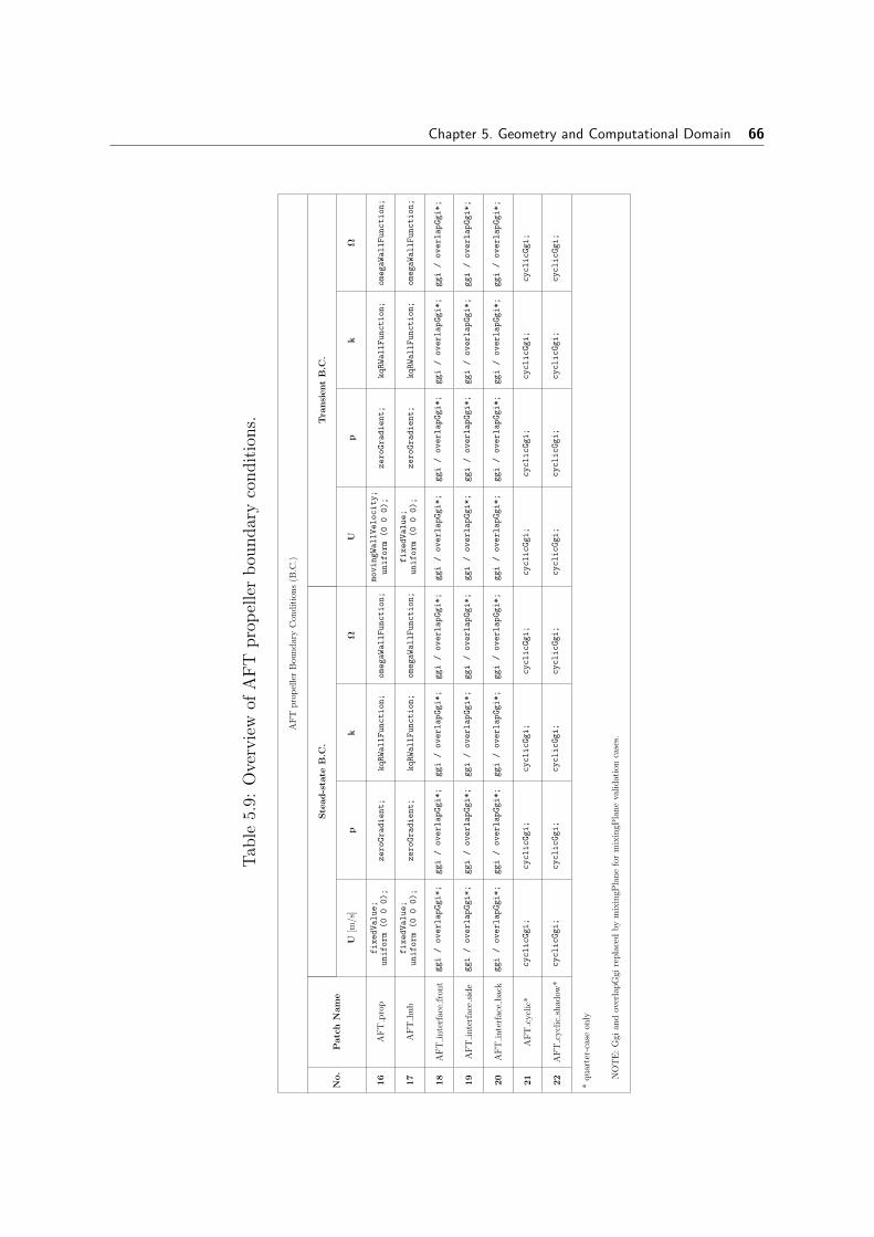
Chapter 5. Geometry and Computational Domain 66
Tab
le5.
9:O
verv
iew
ofA
FT
pro
pel
ler
bou
ndar
yco
ndit
ions.
AF
Tp
rop
elle
rB
oun
dar
yC
ond
itio
ns
(B.C
.)
No.
Patc
hN
am
e
Ste
ad
-sta
teB
.C.
Tra
nsi
ent
B.C
.
U[m
/s]
pk
ΩU
pk
Ω
16
AF
Tp
rop
fixedValue;
uniform(0
00);
zeroGradient;
kqRWallFunction;
omegaWallFunction;
movingWallVelocity;
uniform(0
00);
zeroGradient;
kqRWallFunction;
omegaWallFunction;
17
AF
Thu
bfixedValue;
uniform(0
00);
zeroGradient;
kqRWallFunction;
omegaWallFunction;
fixedValue;
uniform(0
00);
zeroGradient;
kqRWallFunction;
omegaWallFunction;
18
AF
Tin
terf
ace
fron
tggi
/overlapGgi*;
ggi
/overlapGgi*;
ggi/
overlapGgi*;
ggi
/overlapGgi*;
ggi
/overlapGgi*;
ggi/
overlapGgi*;
ggi
/overlapGgi*;
ggi
/overlapGgi*;
19
AF
Tin
terf
ace
sid
eggi
/overlapGgi*;
ggi
/overlapGgi*;
ggi/
overlapGgi*;
ggi
/overlapGgi*;
ggi
/overlapGgi*;
ggi/
overlapGgi*;
ggi
/overlapGgi*;
ggi
/overlapGgi*;
20
AF
Tin
terf
ace
bac
kggi
/overlapGgi*;
ggi
/overlapGgi*;
ggi/
overlapGgi*;
ggi
/overlapGgi*;
ggi
/overlapGgi*;
ggi/
overlapGgi*;
ggi
/overlapGgi*;
ggi
/overlapGgi*;
21
AF
Tcy
clic
*cyclicGgi;
cyclicGgi;
cyclicGgi;
cyclicGgi;
cyclicGgi;
cyclicGgi;
cyclicGgi;
cyclicGgi;
22
AF
Tcy
clic
shad
ow*
cyclicGgi;
cyclicGgi;
cyclicGgi;
cyclicGgi;
cyclicGgi;
cyclicGgi;
cyclicGgi;
cyclicGgi;
*qu
arte
r-ca
seon
ly
NO
TE
:G
gian
dov
erla
pG
gire
pla
ced
by
mix
ingP
lan
efo
rm
ixin
gPla
ne
vali
dat
ion
case
s.

Chapter 5. Geometry and Computational Domain 67
5.6. Closure
This chapter introduced the two geometries used as basis for CRP simulations: the
quarter and the whole (full) geometry. The resulting computational domains were dis-
cussed and the regions which form the domains analysed. An overview of boundary
patches and interface was given. The boundary conditions necessary for running the
CFD simulations of CRP were defined and discussed.
The next chapter presents the results of various numerical simulations of the CRP set
made using foam-extend. A comparison of quarter and whole computational domains
is presented as verification of the quarter domain. The data acquired from transient
and steady-state simulations is assessed and compared to available experimental data.

6 Results
6.1. Introduction
The previous chapter described the full propeller and quarter propeller geometries,
which were the basis for the two CRP computational domains used in numerical simu-
lations. An overview of various mesh regions forming the computational domains was
given with a detailed overview of interface and patch types used. Boundary conditions
applied to patches for simulations using different approaches to interface and domain
handling were given tabularly.
This chapter presents the data acquired from a series of numerical simulations con-
ducted on both the quarter and full CRP domains. Both steady-state and transient
simulation results are offered, taking notice of how the use of different interfaces effects
the resulting data.
The results are presented in form of graphical representations of pressure, velocity
and other significant flow fields, with an analysis of open-water characteristics using
hydrodynamic coefficients.
6.2. Full CRP Geometry
Results presented in this section are of simulations performed using the full CRP
geometry and the resulting domain. Rotating motion of the propellers was handled by
employing the MRF method with two rotational zones, one for each propeller of the
CRP set.
68

Chapter 6. Results 69
The use of MRF for modelling of rotational zones resulted demanded separate mesh
regions in the domain, thus requiring ggi interfaces to enable patch communication.
The interface were set-up as presented in Chapter 5.
The rotational speed for both propellers was set as at a constant value of 12 rps
with the propeller rotation modelled as synchronous to match the conditions of the
experiments used as reference [36, 37].
6.2.1. Steady-State Simulation, J = 0.5
A series of full CRP geometry steady-state simulations using the MRF method was
performed for different operating points defined by the propeller advance coefficient J .
The results presented in continuation are those of an arbitrary CRP operating point
denoted by advance coefficient J = 0.5.
Pressure Field
The graphical representation of the pressure field is given by values of kinematic
pressure, i.e. the value of pressure divided by fluid density ρ. Figure 6.1 shows the
pressure field around the propeller set in the z = const. plane and direction of fluid flow
corresponding to the x+ axis. The occurrence of low-pressure and high-pressure areas
along the propeller blades, attributed to propeller rotation, can be seen clearly. (The
pressure field for the quarter CRP simulation is given in Fig. 6.13.)
Figure 6.1: Full CRP: Pressure field in z = const. plane.
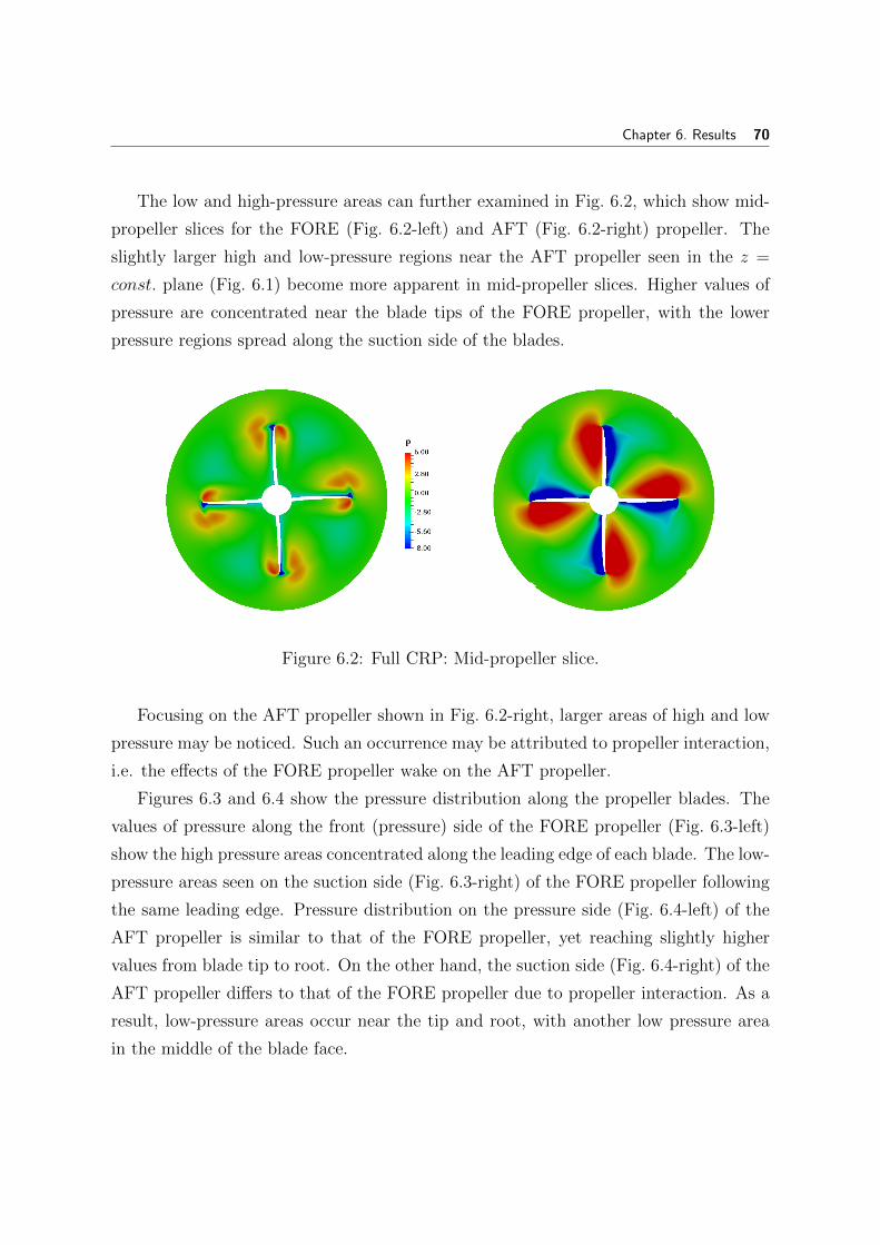
Chapter 6. Results 70
The low and high-pressure areas can further examined in Fig. 6.2, which show mid-
propeller slices for the FORE (Fig. 6.2-left) and AFT (Fig. 6.2-right) propeller. The
slightly larger high and low-pressure regions near the AFT propeller seen in the z =
const. plane (Fig. 6.1) become more apparent in mid-propeller slices. Higher values of
pressure are concentrated near the blade tips of the FORE propeller, with the lower
pressure regions spread along the suction side of the blades.
Figure 6.2: Full CRP: Mid-propeller slice.
Focusing on the AFT propeller shown in Fig. 6.2-right, larger areas of high and low
pressure may be noticed. Such an occurrence may be attributed to propeller interaction,
i.e. the effects of the FORE propeller wake on the AFT propeller.
Figures 6.3 and 6.4 show the pressure distribution along the propeller blades. The
values of pressure along the front (pressure) side of the FORE propeller (Fig. 6.3-left)
show the high pressure areas concentrated along the leading edge of each blade. The low-
pressure areas seen on the suction side (Fig. 6.3-right) of the FORE propeller following
the same leading edge. Pressure distribution on the pressure side (Fig. 6.4-left) of the
AFT propeller is similar to that of the FORE propeller, yet reaching slightly higher
values from blade tip to root. On the other hand, the suction side (Fig. 6.4-right) of the
AFT propeller differs to that of the FORE propeller due to propeller interaction. As a
result, low-pressure areas occur near the tip and root, with another low pressure area
in the middle of the blade face.
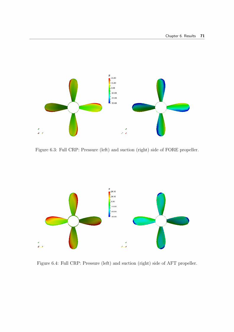
Chapter 6. Results 71
Figure 6.3: Full CRP: Pressure (left) and suction (right) side of FORE propeller.
Figure 6.4: Full CRP: Pressure (left) and suction (right) side of AFT propeller.

Chapter 6. Results 72
Velocity Field
A graphical representation of the velocity field around the propeller set is shown
below. Figure 6.5 depicts the axial velocity field in the z = const. plane. The velocity
field is presented as a ratio of the axial velocity Ux and the inlet velocity Ui, which
depends on the operating point. For J = 0.5 the corresponding inlet velocity equals
Ui = 1.8312 m/s. The highest values of axial velocity may be seen along the blades of
the AFT propeller and wake of the CRP set. (Equivalent quarter CRP simulation data
is given in Fig. 6.16.)
Figure 6.5: Full CRP: Velocity field in z = const. plane.
Propeller interaction can be studied further by assessing the axial velocity in x =
const. planes positioned behind each of the propellers. Both cutting-planes are po-
sitioned at the same distance behind the corresponding propeller. The velocity field
behind the FORE propeller (Fig. 6.5-left) peaks at Ux/Ui values of around 3 m/s, while
the same values at an axial slice behind the AFT propeller rise to about 4 m/s.
Higher values of the axial velocity after the second propeller may be attributed to
the contra-rotating motion of the AFT propeller. The second propeller of the CRP set
”rectifies” the flow, reducing the tangential component of the velocity and increasing
axial velocity. (Equivalent quarter CRP simulation data is given in Fig. 6.17.)
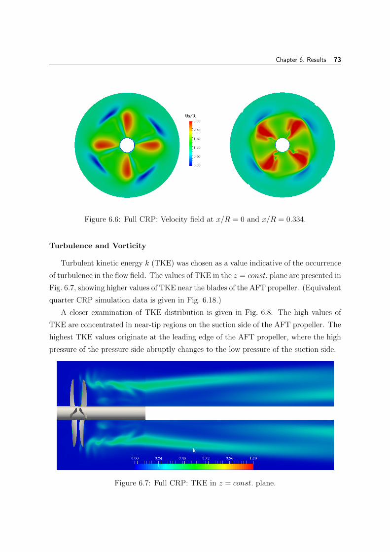
Chapter 6. Results 73
Figure 6.6: Full CRP: Velocity field at x/R = 0 and x/R = 0.334.
Turbulence and Vorticity
Turbulent kinetic energy k (TKE) was chosen as a value indicative of the occurrence
of turbulence in the flow field. The values of TKE in the z = const. plane are presented in
Fig. 6.7, showing higher values of TKE near the blades of the AFT propeller. (Equivalent
quarter CRP simulation data is given in Fig. 6.18.)
A closer examination of TKE distribution is given in Fig. 6.8. The high values of
TKE are concentrated in near-tip regions on the suction side of the AFT propeller. The
highest TKE values originate at the leading edge of the AFT propeller, where the high
pressure of the pressure side abruptly changes to the low pressure of the suction side.
Figure 6.7: Full CRP: TKE in z = const. plane.

Chapter 6. Results 74
Figure 6.8: Full CRP: Distribution of TKE on propeller blades.
The Q-criterion was used as a measure of vorticity. Q was described in subsection
4.4.2. An arbitrary value of Q defines areas where vortices with an energy rate higher
than the value set by Q can form. Q-contours depicting vortices with Q > 3 · 103 and
coloured by values of the velocity magnitude are shown in Fig. 6.9. Tip vortices are
clearly seen and captured by the simulation, they disappear further downstream as they
enter the far field mesh, which does not have sufficient resolution to preserve them.
(Equivalent quarter CRP simulation data is given in Fig. 6.20.)
Figure 6.9: Full CRP: Vortices matching Q-criterion Q > 3 · 103

Chapter 6. Results 75
6.2.2. Hydrodynamic Performance
Open-water characteristics are offered as a way of determining propeller performance
throughout various operating points. A steady-state simulation using the MRF approach
was carried out for each operating point determined by a different value of the advance
coefficient J .
For each of the simulations, representing a single operating point of the CRP set,
the resulting values of propeller thrust T and torque Q were used to determine the
appropriate hydrodynamic performance coefficients. The equations and the supporting
theory used to determine the hydrodynamic coefficients were introduced in subsection
4.4.1. Values of the coefficients describing the hydrodynamic performance were calcu-
lated separately for each propeller and summed to produce the total values of the set.
The coefficients given tabularly:
Table 6.1: Full CRP: Hydrodynamic performance coefficients.
FORE AFT TOTAL
J KT KQ η KT KQ η KT KQ η
1.5 0.0022 0.0062 8.40 0.0053 0.0059 21.13 0.0075 0.0122 14.61
1.4 0.0281 0.0117 53.58 0.0369 0.0146 56.26 0.0650 0.0263 55.07
1.3 0.0565 0.0167 69.85 0.0786 0.0232 70.11 0.1351 0.0399 70.01
1.2 0.0838 0.0215 74.51 0.1184 0.0311 72.61 0.2023 0.0526 73.39
1.1 0.1102 0.0259 74.48 0.1520 0.0377 70.61 0.2622 0.0636 72.19
1 0.1351 0.0297 72.35 0.1869 0.0442 67.31 0.3220 0.0739 69.34
0.9 0.1585 0.0330 68.78 0.2182 0.0498 62.74 0.3768 0.0828 65.15
0.8 0.1789 0.0355 64.09 0.2437 0.0542 57.24 0.4227 0.0898 59.96
0.75 0.1864 0.0362 61.52 0.2564 0.0564 54.27 0.4428 0.0926 57.10
0.7 0.1903 0.0361 58.79 0.2687 0.0584 51.23 0.4589 0.0945 54.12
0.6 0.2066 0.0377 52.36 0.2947 0.0626 44.92 0.5013 0.1003 47.71
0.5 0.2158 0.0379 45.26 0.3168 0.0660 38.22 0.5326 0.1039 40.79
0.4 0.2258 0.0388 37.00 0.3286 0.0674 31.02 0.5543 0.1063 33.20
0.3 0.2267 0.0382 28.37 0.3202 0.0657 23.25 0.5469 0.1039 25.13
0.25 0.2308 0.0388 23.69 0.3324 0.0684 19.34 0.5632 0.1071 20.91
0 0.2422 0.0407 0.00 0.3456 0.0707 0.00 0.5878 0.1113 0.00
The data shown in Table 6.1 presents the thrust coefficient KT , torque coefficient KQ
and propeller efficiency for the FORE and AFT propellers separately and the CRP set as
a whole. The same data is offered graphically with addition of comparable experimental

Chapter 6. Results 76
data from Miller [36, 37] in Figures 6.10, 6.11 and 6.12:
0 0.2 0.4 0.6 0.8 1 1.2 1.4 1.6Advance ratio, J
0
0.1
0.2
0.3
0.4
0.5
0.6
0.7
0.8
KT
,10K
Q,η
Sim. KT
Sim. 10KQ
Sim. ηExp. KT
Exp. K
Exp. η
Figure 6.10: Full CRP: Fore propeller steady hydrodynamic coefficients.
Figure 6.10 shows the open-water characteristic of the FORE propeller based on
data from full CRP numerical simulations and experimental data. The data based on
simulation results shows good agreement with experimental data in higher efficiency,
i.e. higher J , regions. The data deviates as the values of J decrease and the operating
points move to regions of lower efficiency. This is explained by the fact that as the
advance coefficient J decreases so does the axial velocity, thus moving into region with
increasingly transient flow that cannot be accurately represented by the MRF method.
Open-water characteristics of the AFT propeller are presented in Fig. 6.11. As
with the FORE propeller, the results of the AFT simulations show good agreement
with experimental data for higher values of J with some deviation as the values of
J decrease. Furthermore, the values of KT follow the experimental data curve well,
whereas the values of KQ follow the trend of the experimental data but appear to be of
equally lower value for each data point.
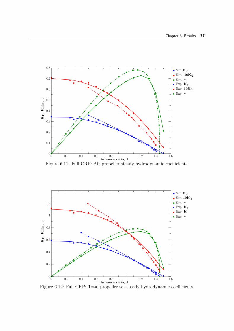
Chapter 6. Results 77
0 0.2 0.4 0.6 0.8 1 1.2 1.4 1.6Advance ratio, J
0
0.1
0.2
0.3
0.4
0.5
0.6
0.7
0.8
KT
,10K
Q,η
Sim. KT
Sim. 10KQ
Sim. ηExp. KT
Exp. 10KQ
Exp. η
Figure 6.11: Full CRP: Aft propeller steady hydrodynamic coefficients.
0 0.2 0.4 0.6 0.8 1 1.2 1.4 1.6Advance ratio, J
0
0.2
0.4
0.6
0.8
1
1.2
KT
,10K
Q,η
Sim. KT
Sim. 10KQ
Sim. ηExp. KT
Exp. K
Exp. η
Figure 6.12: Full CRP: Total propeller set steady hydrodynamic coefficients.

Chapter 6. Results 78
By comparing the results for the FORE (Fig. 6.10) and the AFT (Fig. 6.11) propeller,
it can be noted that the AFT propeller has generally higher values of thrust and torque
coefficients throughout the simulated span of advance coefficients. This would mean
that the secondary propeller of the set bears higher loads, which can be attributed to
the wake of the first propeller affecting the secondary propeller.
The total open-water characteristics of the full propeller set is shown in Figure 6.12.
The numerical data shows good agreement with the experimental values for regions of
higher axial velocity, i.e. higher J , as the transient phenomena have little effect on the
flow in such regions. As the the transient effects increase and the values of J decrease,
the results deviate from the experimental curve. The deviation from experimental data
is attributed to the inability of the steady-state MRF approach to capture transient
phenomena.
The steady-state approach may not be accurate for operating points in the lower
regions of the advance coefficient J , yet it provide satisfactory data for regions of near
the best efficiency point (BEP) of the propeller. As most propellers are designed to work
at BEP, data from steady-state MRF simulations becomes of great interest for propeller
design.
6.3. Quarter CRP Geometry
In the previous section, an overview of data and flow fields from full domain simula-
tions of the CRP set was given. The simulations served as an analysis of the fundamental
behaviour of the CRP set, thus becoming a reference for further simulations where vari-
ants of the basic ggi interface will be used.
In this section, a quarter-geometry based computational domain is used for the
simulation of a CRP set. This requires the use of the cyclicGgi and overlapGgi
interfaces available in foam-extend, which are validated by comparison of quarter and
full CRP simulation data. Both propellers are given a constant rotation of 12 rps and
varying values of the advance coefficient J , depending on the simulated operating point.
By using the quarter-geometry domain, the simulation time needed to reach satisfy-
ing convergence may be greatly reduced as the quarter CRP simulation is less resource-
intensive.

Chapter 6. Results 79
6.3.1. Steady-State Simulation, J = 0.5
For the full CRP simulation and the quarter CRP simulation to be comparable,
using the cyclicGgi and the overlpaGgi interfaces, the same operating point J = 0.5
was chosen for both simulations. Moreover, the steady-state MRF method was used to
handle modelling of the propeller rotation. Again, a rotational MRF zone was set-up
around each propeller with the designated rotational speed.
The details of the geometry, boundary conditions and interfaces used are given in 5.
Detailed examples on how the overlapGgi and cyclicGgi need to be set-up are given
in Appendix A.
It should be noted that the post-processing software used for creation of graphical
representation of numerical data, allows for transformation of the domain. The quarter
domain is copied until the full domain is assembled, thus making the visualised data
seem as if it were created from a complete domain.
Pressure Field
The kinematic pressure field from the quarter CRP simulation is given in Fig 6.13.
The same as with the full CRP simulation (Fig. 6.1), the pressure field in the z =
const. plane shows higher and lower pressure areas near the propeller blades. These
areas correspond to the suction and pressure sides of the propeller blades, depicted in
detail in Fig. 6.14 and Fig. 6.14.
Figure 6.13: Quarter CRP: Pressure field in z = const. plane.

Chapter 6. Results 80
Closer examination of the pressure distribution over the blade surfaces of the FORE
and AFT propellers, reveals nearly identical distribution on both the pressure and suc-
tion sides of the blades as seen for the full CRP geometry. This would point to the fact
that the use of cyclicGgi and overlapGgi interfaces has no apparent effect on pressure
distribution over propeller surfaces.
Figure 6.14: Quarter CRP: Pressure (left) and suction (right) side of FORE propeller.
Figure 6.15: Quarter CRP: Pressure (left) and suction (right) side of AFT propeller.
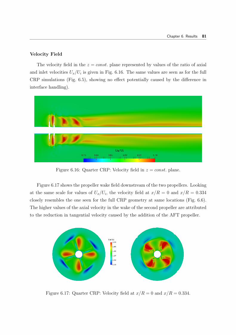
Chapter 6. Results 81
Velocity Field
The velocity field in the z = const. plane represented by values of the ratio of axial
and inlet velocities Ux/Ui is given in Fig. 6.16. The same values are seen as for the full
CRP simulations (Fig. 6.5), showing no effect potentially caused by the difference in
interface handling).
Figure 6.16: Quarter CRP: Velocity field in z = const. plane.
Figure 6.17 shows the propeller wake field downstream of the two propellers. Looking
at the same scale for values of Ux/Ui, the velocity field at x/R = 0 and x/R = 0.334
closely resembles the one seen for the full CRP geometry at same locations (Fig. 6.6).
The higher values of the axial velocity in the wake of the second propeller are attributed
to the reduction in tangential velocity caused by the addition of the AFT propeller.
Figure 6.17: Quarter CRP: Velocity field at x/R = 0 and x/R = 0.334.
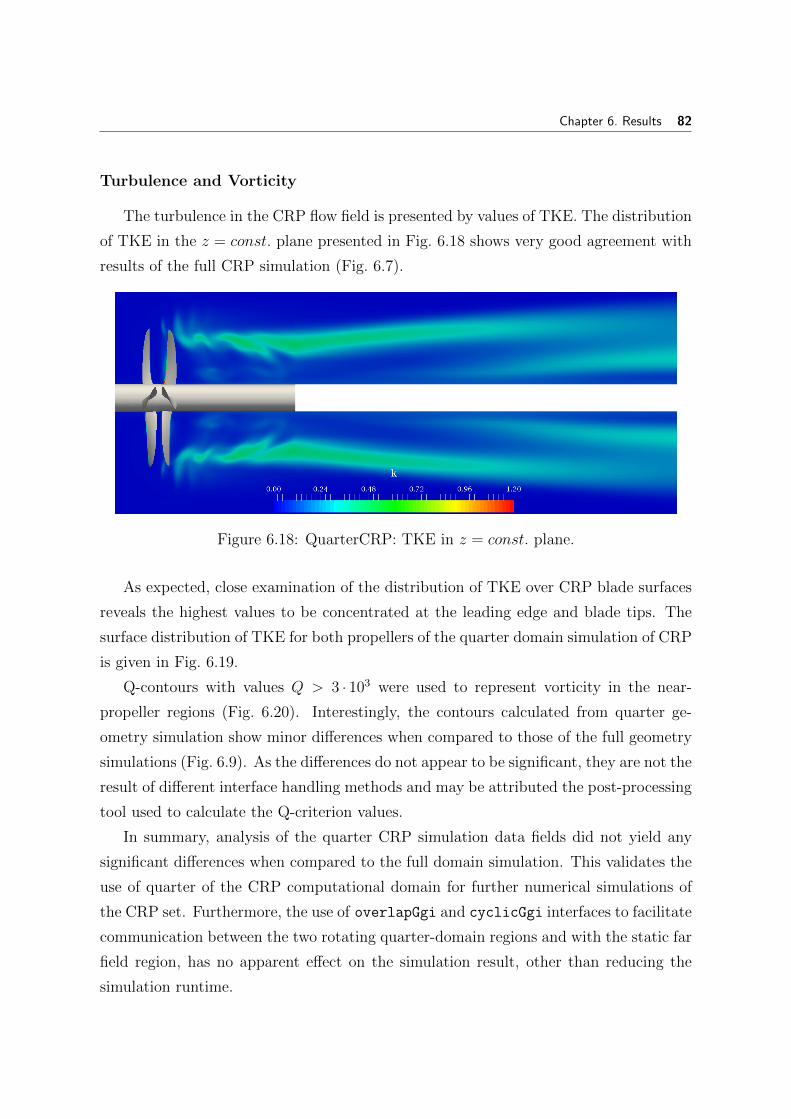
Chapter 6. Results 82
Turbulence and Vorticity
The turbulence in the CRP flow field is presented by values of TKE. The distribution
of TKE in the z = const. plane presented in Fig. 6.18 shows very good agreement with
results of the full CRP simulation (Fig. 6.7).
Figure 6.18: QuarterCRP: TKE in z = const. plane.
As expected, close examination of the distribution of TKE over CRP blade surfaces
reveals the highest values to be concentrated at the leading edge and blade tips. The
surface distribution of TKE for both propellers of the quarter domain simulation of CRP
is given in Fig. 6.19.
Q-contours with values Q > 3 · 103 were used to represent vorticity in the near-
propeller regions (Fig. 6.20). Interestingly, the contours calculated from quarter ge-
ometry simulation show minor differences when compared to those of the full geometry
simulations (Fig. 6.9). As the differences do not appear to be significant, they are not the
result of different interface handling methods and may be attributed the post-processing
tool used to calculate the Q-criterion values.
In summary, analysis of the quarter CRP simulation data fields did not yield any
significant differences when compared to the full domain simulation. This validates the
use of quarter of the CRP computational domain for further numerical simulations of
the CRP set. Furthermore, the use of overlapGgi and cyclicGgi interfaces to facilitate
communication between the two rotating quarter-domain regions and with the static far
field region, has no apparent effect on the simulation result, other than reducing the
simulation runtime.
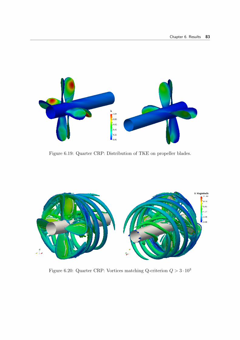
Chapter 6. Results 83
Figure 6.19: Quarter CRP: Distribution of TKE on propeller blades.
Figure 6.20: Quarter CRP: Vortices matching Q-criterion Q > 3 · 103
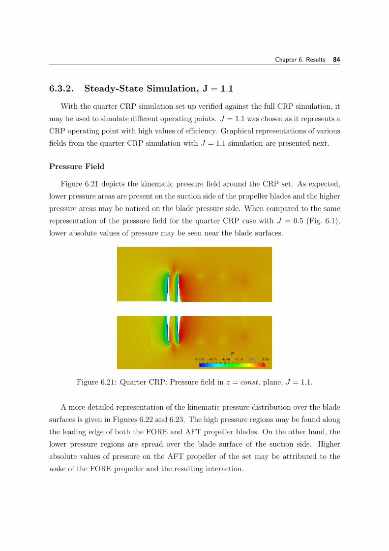
Chapter 6. Results 84
6.3.2. Steady-State Simulation, J = 1.1
With the quarter CRP simulation set-up verified against the full CRP simulation, it
may be used to simulate different operating points. J = 1.1 was chosen as it represents a
CRP operating point with high values of efficiency. Graphical representations of various
fields from the quarter CRP simulation with J = 1.1 simulation are presented next.
Pressure Field
Figure 6.21 depicts the kinematic pressure field around the CRP set. As expected,
lower pressure areas are present on the suction side of the propeller blades and the higher
pressure areas may be noticed on the blade pressure side. When compared to the same
representation of the pressure field for the quarter CRP case with J = 0.5 (Fig. 6.1),
lower absolute values of pressure may be seen near the blade surfaces.
Figure 6.21: Quarter CRP: Pressure field in z = const. plane, J = 1.1.
A more detailed representation of the kinematic pressure distribution over the blade
surfaces is given in Figures 6.22 and 6.23. The high pressure regions may be found along
the leading edge of both the FORE and AFT propeller blades. On the other hand, the
lower pressure regions are spread over the blade surface of the suction side. Higher
absolute values of pressure on the AFT propeller of the set may be attributed to the
wake of the FORE propeller and the resulting interaction.
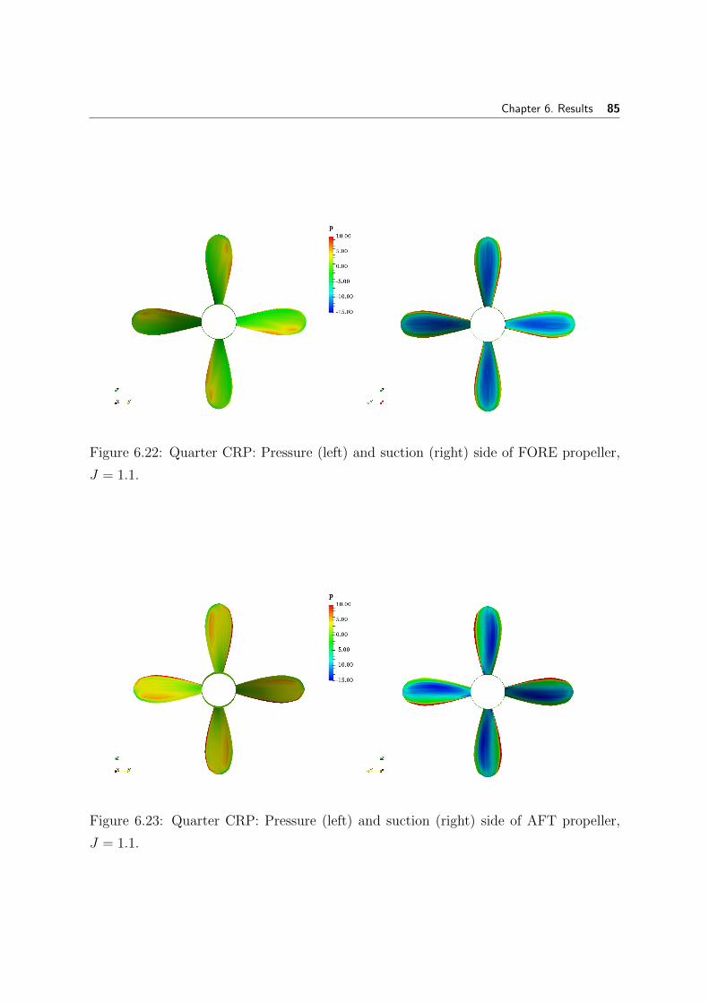
Chapter 6. Results 85
Figure 6.22: Quarter CRP: Pressure (left) and suction (right) side of FORE propeller,
J = 1.1.
Figure 6.23: Quarter CRP: Pressure (left) and suction (right) side of AFT propeller,
J = 1.1.

Chapter 6. Results 86
Velocity Field
The velocity field is presented as values of the axial and inlet velocity ratio Ux/Ui.
The value of the inlet velocity corresponding to the advance coefficient J = 1.1 equals
Ui = 4.0286. As the values of the inlet velocity of J = 1.1 and J = 0.5 differ, the
two fields may not be compared directly. Fig. 6.24 represents the velocity field in the
z = const. plane, with a representation of velocity at two x = const. planes is given
in Fig. 6.17. As expected, the axial velocity downstream of the AFT (x/R = 0.334)
propeller shows higher values than downstream of the FORE propeller (x/R = 0).
Figure 6.24: Quarter CRP: Velocity field in z = const. plane, J = 1.1.
Figure 6.25: Quarter CRP: Velocity field at x/R = 0 and x/R = 0.334, J = 1.1.

Chapter 6. Results 87
Turbulence and Vorticity
The values of TKE, as a chosen measure of turbulence, in the z = const. plane are
shown in Figure 6.26 and the surface distribution of TKE over the propeller blades is
presented in Fig. 6.27. TKE values in the downstream wake of the CRP set appear to
be low with highest values concentrated at the propellers. The distribution of TKE over
the blade surfaces shows the highest values to be concentrated near the leading edge of
each blade. Moreover, values of TKE appear to be higher at the blade pressure side.
Figure 6.26: QuarterCRP: TKE in z = const. plane, J = 1.1.
Figure 6.27: Quarter CRP: Distribution of TKE on propeller blades, J = 1.1.
Q-contours are used to represent vorticity around the CRP set. A Q-criterion value
of Q > 3 · 103 was chosen as a threshold for the contours presented in Figure 6.28.

Chapter 6. Results 88
Figure 6.28: Quarter CRP: Vortices matching Q-criterion Q > 3 · 103, J = 1.1.
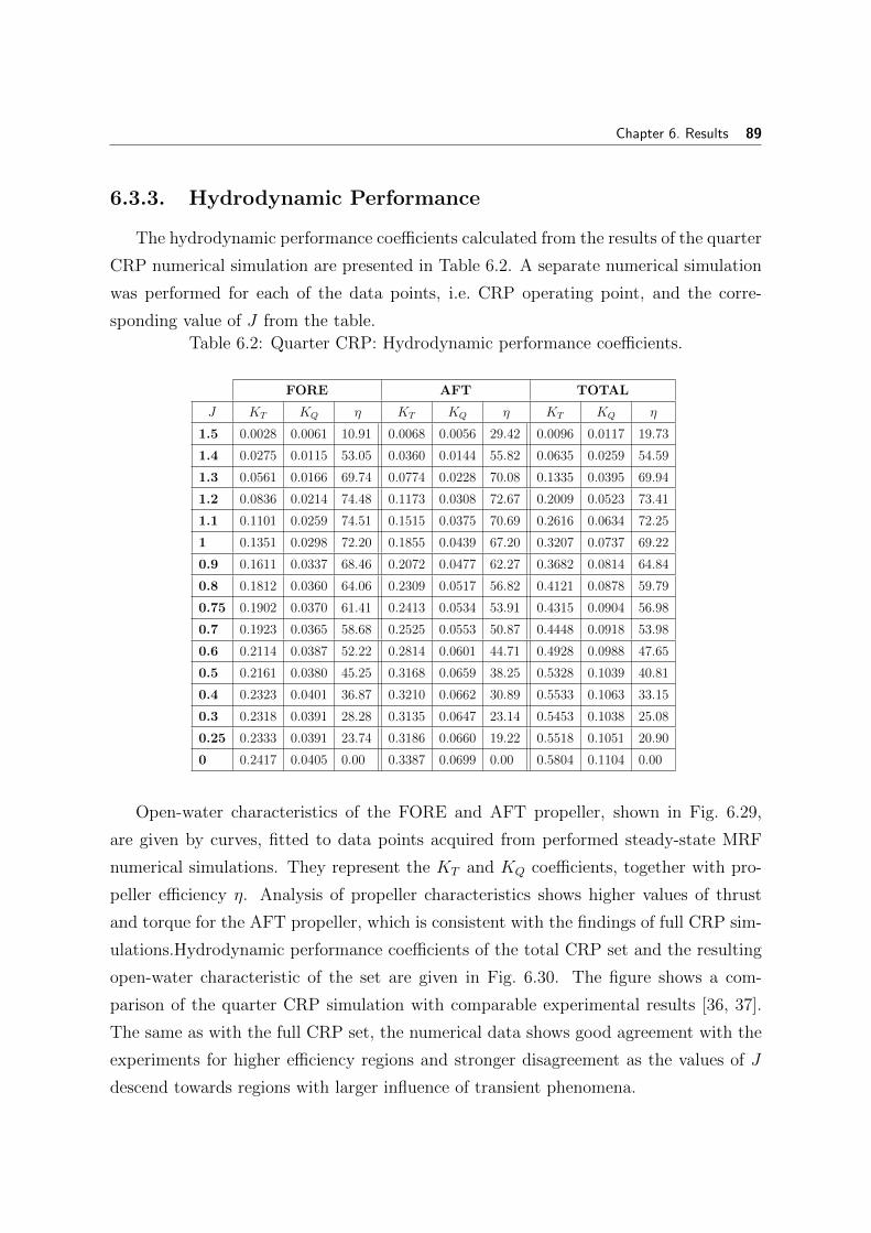
Chapter 6. Results 89
6.3.3. Hydrodynamic Performance
The hydrodynamic performance coefficients calculated from the results of the quarter
CRP numerical simulation are presented in Table 6.2. A separate numerical simulation
was performed for each of the data points, i.e. CRP operating point, and the corre-
sponding value of J from the table.
Table 6.2: Quarter CRP: Hydrodynamic performance coefficients.
FORE AFT TOTAL
J KT KQ η KT KQ η KT KQ η
1.5 0.0028 0.0061 10.91 0.0068 0.0056 29.42 0.0096 0.0117 19.73
1.4 0.0275 0.0115 53.05 0.0360 0.0144 55.82 0.0635 0.0259 54.59
1.3 0.0561 0.0166 69.74 0.0774 0.0228 70.08 0.1335 0.0395 69.94
1.2 0.0836 0.0214 74.48 0.1173 0.0308 72.67 0.2009 0.0523 73.41
1.1 0.1101 0.0259 74.51 0.1515 0.0375 70.69 0.2616 0.0634 72.25
1 0.1351 0.0298 72.20 0.1855 0.0439 67.20 0.3207 0.0737 69.22
0.9 0.1611 0.0337 68.46 0.2072 0.0477 62.27 0.3682 0.0814 64.84
0.8 0.1812 0.0360 64.06 0.2309 0.0517 56.82 0.4121 0.0878 59.79
0.75 0.1902 0.0370 61.41 0.2413 0.0534 53.91 0.4315 0.0904 56.98
0.7 0.1923 0.0365 58.68 0.2525 0.0553 50.87 0.4448 0.0918 53.98
0.6 0.2114 0.0387 52.22 0.2814 0.0601 44.71 0.4928 0.0988 47.65
0.5 0.2161 0.0380 45.25 0.3168 0.0659 38.25 0.5328 0.1039 40.81
0.4 0.2323 0.0401 36.87 0.3210 0.0662 30.89 0.5533 0.1063 33.15
0.3 0.2318 0.0391 28.28 0.3135 0.0647 23.14 0.5453 0.1038 25.08
0.25 0.2333 0.0391 23.74 0.3186 0.0660 19.22 0.5518 0.1051 20.90
0 0.2417 0.0405 0.00 0.3387 0.0699 0.00 0.5804 0.1104 0.00
Open-water characteristics of the FORE and AFT propeller, shown in Fig. 6.29,
are given by curves, fitted to data points acquired from performed steady-state MRF
numerical simulations. They represent the KT and KQ coefficients, together with pro-
peller efficiency η. Analysis of propeller characteristics shows higher values of thrust
and torque for the AFT propeller, which is consistent with the findings of full CRP sim-
ulations.Hydrodynamic performance coefficients of the total CRP set and the resulting
open-water characteristic of the set are given in Fig. 6.30. The figure shows a com-
parison of the quarter CRP simulation with comparable experimental results [36, 37].
The same as with the full CRP set, the numerical data shows good agreement with the
experiments for higher efficiency regions and stronger disagreement as the values of J
descend towards regions with larger influence of transient phenomena.

Chapter 6. Results 90
0 0.2 0.4 0.6 0.8 1 1.2 1.4 1.6Advance ratio, J
0
0.2
0.4
0.6
0.8
1
KT
,10K
Q,η
Fore KT
Fore 10KQ
Fore ηAft KT
Aft 10KQ
Aft η
Figure 6.29: Quarter CRP: Fore and aft propeller steady hydrodynamic coefficients.
0 0.2 0.4 0.6 0.8 1 1.2 1.4 1.6Advance ratio, J
0
0.2
0.4
0.6
0.8
1
1.2
KT
,10K
Q,η
Sim. KT
Sim. 10KQ
Sim. ηExp. KT
Exp. 10KQ
Exp. η
Figure 6.30: Quarter CRP: Total propeller set steady hydrodynamic coefficients.
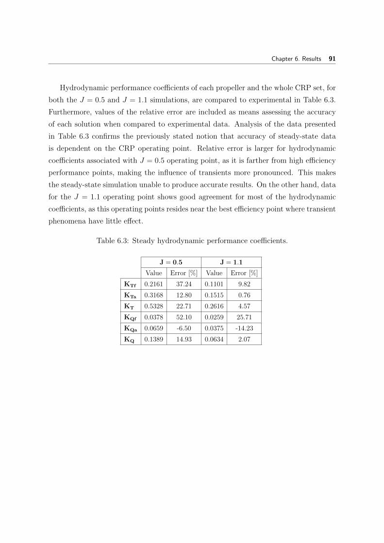
Chapter 6. Results 91
Hydrodynamic performance coefficients of each propeller and the whole CRP set, for
both the J = 0.5 and J = 1.1 simulations, are compared to experimental in Table 6.3.
Furthermore, values of the relative error are included as means assessing the accuracy
of each solution when compared to experimental data. Analysis of the data presented
in Table 6.3 confirms the previously stated notion that accuracy of steady-state data
is dependent on the CRP operating point. Relative error is larger for hydrodynamic
coefficients associated with J = 0.5 operating point, as it is farther from high efficiency
performance points, making the influence of transients more pronounced. This makes
the steady-state simulation unable to produce accurate results. On the other hand, data
for the J = 1.1 operating point shows good agreement for most of the hydrodynamic
coefficients, as this operating points resides near the best efficiency point where transient
phenomena have little effect.
Table 6.3: Steady hydrodynamic performance coefficients.
J = 0.5 J = 1.1
Value Error [%] Value Error [%]
KTf 0.2161 37.24 0.1101 9.82
KTa 0.3168 12.80 0.1515 0.76
KT 0.5328 22.71 0.2616 4.57
KQf 0.0378 52.10 0.0259 25.71
KQa 0.0659 -6.50 0.0375 -14.23
KQ 0.1389 14.93 0.0634 2.07

Chapter 6. Results 92
6.3.4. Quarter CRP Hydrodynamic Performance Validation
The comparison of field data from quarter CRP and full CRP numerical simulation
did not show any significant differences, which validated the use of quarter geometry
simulations from the aspect of field data analysis. As the open-water characteristics of
CRP are to be studied in further simulations based on the quarter CRP domain, the
validity of these characteristics must be examined.
A comparison of the hydrodynamic performance coefficients KT , KQ and resulting
propeller efficiency calculated from quarter and full domain CRP simulations is given
in Fig. 6.31 and 6.32. Data for the FORE propeller is shown in Fig. 6.31 and the data
for the AFT propeller is given in Fig. 6.32.
0 0.2 0.4 0.6 0.8 1 1.2 1.4 1.6Advance ratio, J
0
0.1
0.2
0.3
0.4
0.5
0.6
0.7
0.8
KT
,10K
Q,η
Quarter KT
Quarter 10KQ
Quarter ηFull KT
Full 10KQ
Full η
Figure 6.31: FORE prop. hydrodynamic coeff. comparison: quarter vs. full CRP.
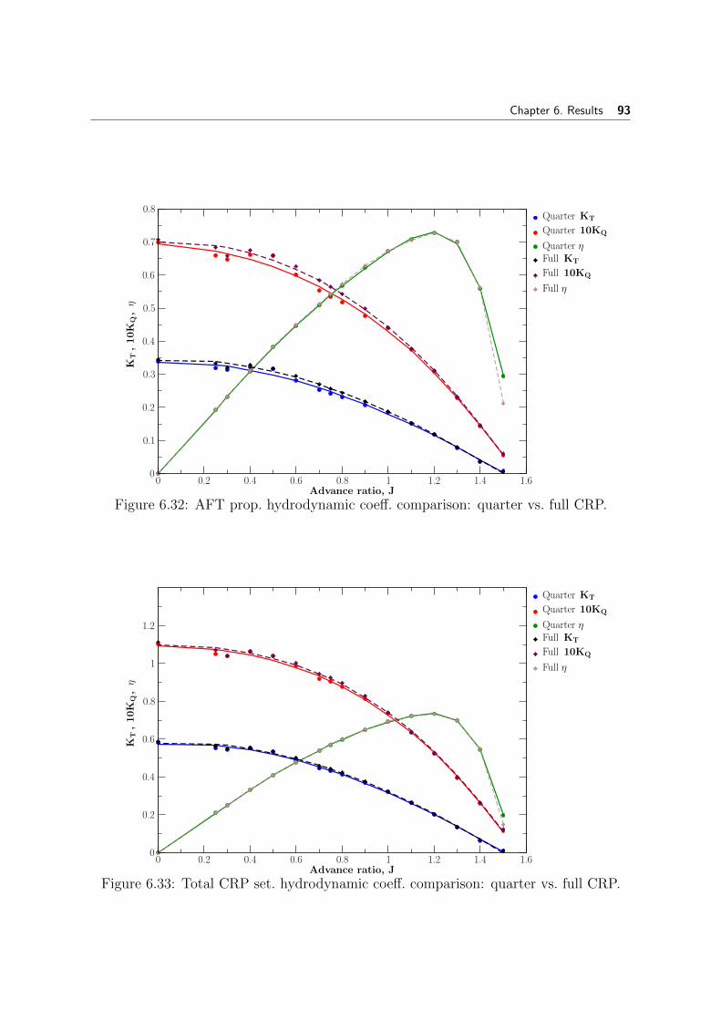
Chapter 6. Results 93
0 0.2 0.4 0.6 0.8 1 1.2 1.4 1.6Advance ratio, J
0
0.1
0.2
0.3
0.4
0.5
0.6
0.7
0.8
KT
,10K
Q,η
Quarter KT
Quarter 10KQ
Quarter ηFull KT
Full 10KQ
Full η
Figure 6.32: AFT prop. hydrodynamic coeff. comparison: quarter vs. full CRP.
0 0.2 0.4 0.6 0.8 1 1.2 1.4 1.6Advance ratio, J
0
0.2
0.4
0.6
0.8
1
1.2
KT
,10K
Q,η
Quarter KT
Quarter 10KQ
Quarter ηFull KT
Full 10KQ
Full η
Figure 6.33: Total CRP set. hydrodynamic coeff. comparison: quarter vs. full CRP.
Chapter 6. Results 94
Hydrodynamic performance of FORE propeller shown in Fig. 6.31 shows nearly ideal
agreement between quarter and full CRP results. On the other hand, some differences
between the full and quarter simulation data for the AFT propeller shown in Fig. 6.32
are present. These minor discrepancies may be considered as having no effect on the
total open-water characteristic of CRP.
Comparison of the total CRP hydrodynamic performance coefficients is shown in
Fig. 6.33. The full and quarter CRP simulation data shows nearly identical characteris-
tics with some minor disagreement which may be considered negligible. With the results
of the two simulated domains showing no major differences in regard to hydrodynamic
performance, the quarter domain approach may be considered valid for use in further
simulations with the purpose of determining propeller open-water characteristics.
6.4. Effects of Initial Propeller Position
This section investigates the idea that different starting positions of one of the pro-
pellers, relative to the other propeller, may affect the results of steady-state simulations.
It is suspected that a transient component of propeller-to-propeller interaction may
be significant. For MRF simulations, all relative positions of ”frozen rotor” blades should
be equally representative. It is suspected that this is not the case and will be further
investigated. As a computationally undemanding way of determining the influence of
relative blade positions to ”frozen rotor” results, the simulation is repeated for various
propeller blade positions. For the ”frozen rotor” approach to be valid for this case,
results for all blade positions should the be the same.
Four new simulations based on the steady-state quarter CRP simulation were con-
ducted. Variations of the quarter propeller geometry presented in Chapter 5. were used
with addition of varying propeller displacement. The geometry was varied by keeping
the AFT propeller at a fixed starting position and changing the angular displacement
of the FORE propeller, as shown in Figure 6.34.
Different values of the relative rotation angle θ were chosen to determine the initial
propeller position for the steady-state simulation. The baseline values were determined
by the MRF quarter-case with J = 0.5 and θ = 0. The same value of the displacement
angle θ = 0 was used for all simulations analysed preceding this section. New steady-
state simulations were performed with a fixed value of the advance coefficient J = 0.5
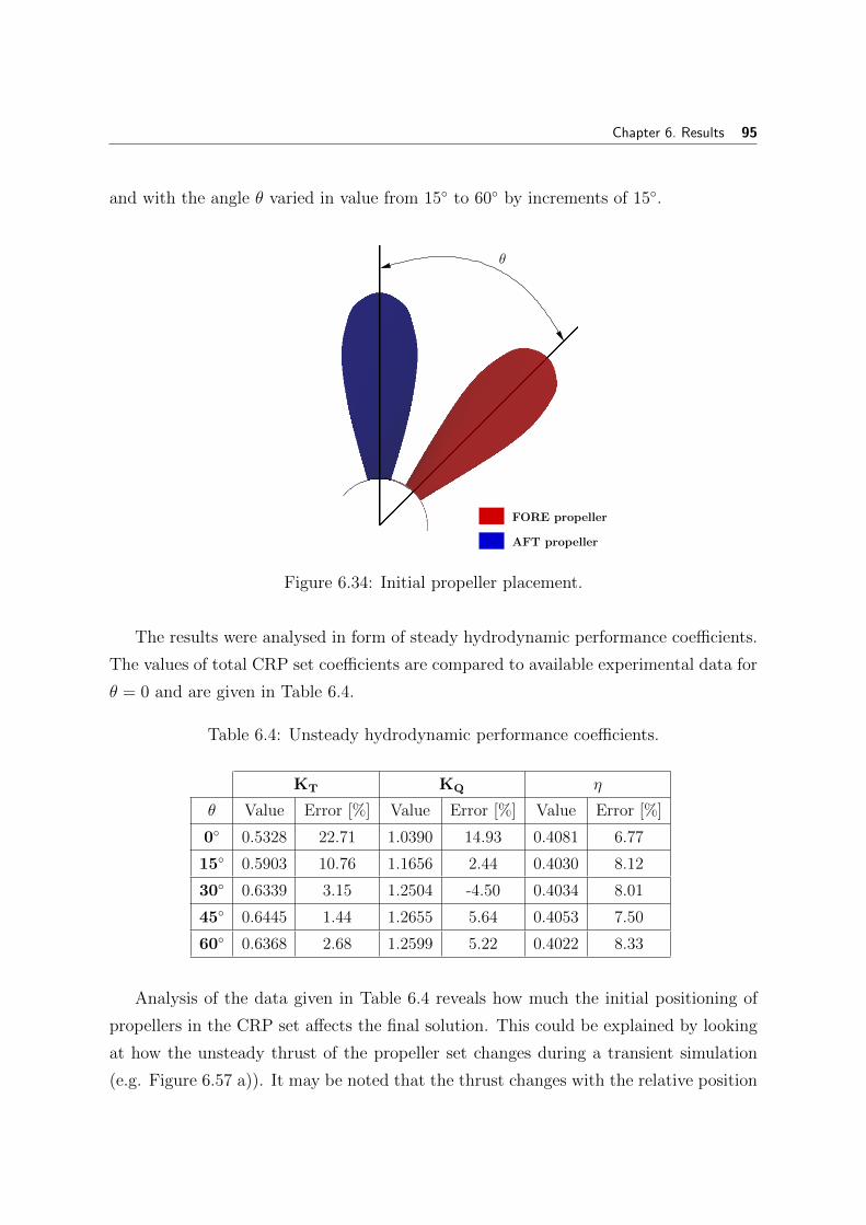
Chapter 6. Results 95
and with the angle θ varied in value from 15 to 60 by increments of 15.
AFT propeller
FORE propeller
θ
Figure 6.34: Initial propeller placement.
The results were analysed in form of steady hydrodynamic performance coefficients.
The values of total CRP set coefficients are compared to available experimental data for
θ = 0 and are given in Table 6.4.
Table 6.4: Unsteady hydrodynamic performance coefficients.
KT KQ η
θ Value Error [%] Value Error [%] Value Error [%]
0 0.5328 22.71 1.0390 14.93 0.4081 6.77
15 0.5903 10.76 1.1656 2.44 0.4030 8.12
30 0.6339 3.15 1.2504 -4.50 0.4034 8.01
45 0.6445 1.44 1.2655 5.64 0.4053 7.50
60 0.6368 2.68 1.2599 5.22 0.4022 8.33
Analysis of the data given in Table 6.4 reveals how much the initial positioning of
propellers in the CRP set affects the final solution. This could be explained by looking
at how the unsteady thrust of the propeller set changes during a transient simulation
(e.g. Figure 6.57 a)). It may be noted that the thrust changes with the relative position

Chapter 6. Results 96
of the propeller, meaning that if the propeller is ”frozen” in a different position, different
values of thrust would be measured. In the same way, if steady-state simulations were
conducted with the propellers ”frozen” in different relative position, different results
could be expected, which is supported by data from the Table 6.4.
6.5. Mixing Plane Simulation
With the overlapGgi and cyclicGgi interfaces used in quarter CRP simulations
successfully validated, a quarter domain simulation using the mixingPlane interface is
conducted. CyclicGgi interfaces are used to establish communication with periodically
rotating patches with the mixingPlane interface facilitating communication between
mesh region. Detailed explanation of the geometry, interfaces and domain used was
presented in Chapter 5. with examples of interface set-up given in appendix A.
6.5.1. Simulation Results
Results of a steady-state simulation using the mixingPlane interface for a propeller
operating point with a corresponding value of the advance coefficient of J = 0.5 are
presented, thus making them comparable to previously presented simulations.
Pressure Field
The kinematic pressure field in the z = const. plane is presented in Fig 6.35. The
expected high- and low- pressure areas can be seen near the blades of each propeller.
Additional relatively high pressure areas may be seen downstream of the CRP set. These
areas occur at the exact position of the interface separating the AFT propeller region
from the far field region and may be attributed to the way the mixingPlane interface
handles communication.
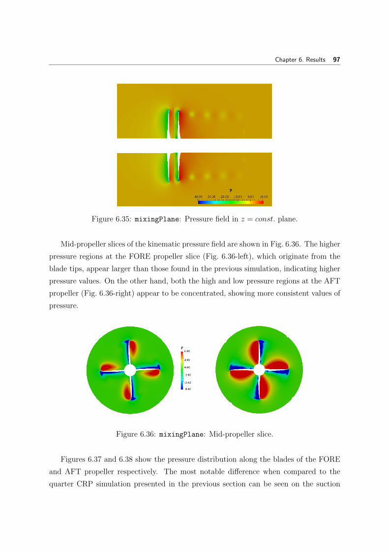
Chapter 6. Results 97
Figure 6.35: mixingPlane: Pressure field in z = const. plane.
Mid-propeller slices of the kinematic pressure field are shown in Fig. 6.36. The higher
pressure regions at the FORE propeller slice (Fig. 6.36-left), which originate from the
blade tips, appear larger than those found in the previous simulation, indicating higher
pressure values. On the other hand, both the high and low pressure regions at the AFT
propeller (Fig. 6.36-right) appear to be concentrated, showing more consistent values of
pressure.
Figure 6.36: mixingPlane: Mid-propeller slice.
Figures 6.37 and 6.38 show the pressure distribution along the blades of the FORE
and AFT propeller respectively. The most notable difference when compared to the
quarter CRP simulation presented in the previous section can be seen on the suction

Chapter 6. Results 98
side of both propellers. Lower values of pressure may be observed on the suction side of
the propellers, without the discontinuity of the low pressure region at the leading edge
of AFT propeller seen in the previously presented simulations.
Figure 6.37: mixingPlane: Pressure (left) and suction (right) side of FORE propeller.
Figure 6.38: mixingPlane: Pressure (left) and suction (right) side of AFT propeller.

Chapter 6. Results 99
Velocity Field
The velocity field, represented by the ratio of the axial velocity Ux and the inlet
velocity Ui, is shown in Fig. 6.39. The value of the inlet velocity corresponding to the
advance coefficient is Ui = 1.8312. The velocity field shows an abrupt discontinuity at
the mixingPlane, which is the result of averaging performed at the interface. After the
interface, the flow continues to show consistent values of the axial/inlet velocity ratio.
Figure 6.39: mixingPlane: Velocity field in z = const. plane.
Figure 6.40 shows the velocity field at two cutting planes positioned behind the
FORE (x/R = 0) and AFT (x/R = 0.334) propeller. By using the same scale and
comparing to Fig. 6.17 lower values of axial velocity may be noticed. Moreover, the
distribution of velocity over the cutting planes more averaged values, which is an effect
of the mixing performed at the interface.
Figure 6.40: mixingPlane: Velocity field at x/R = 0 and x/R = 0.334.
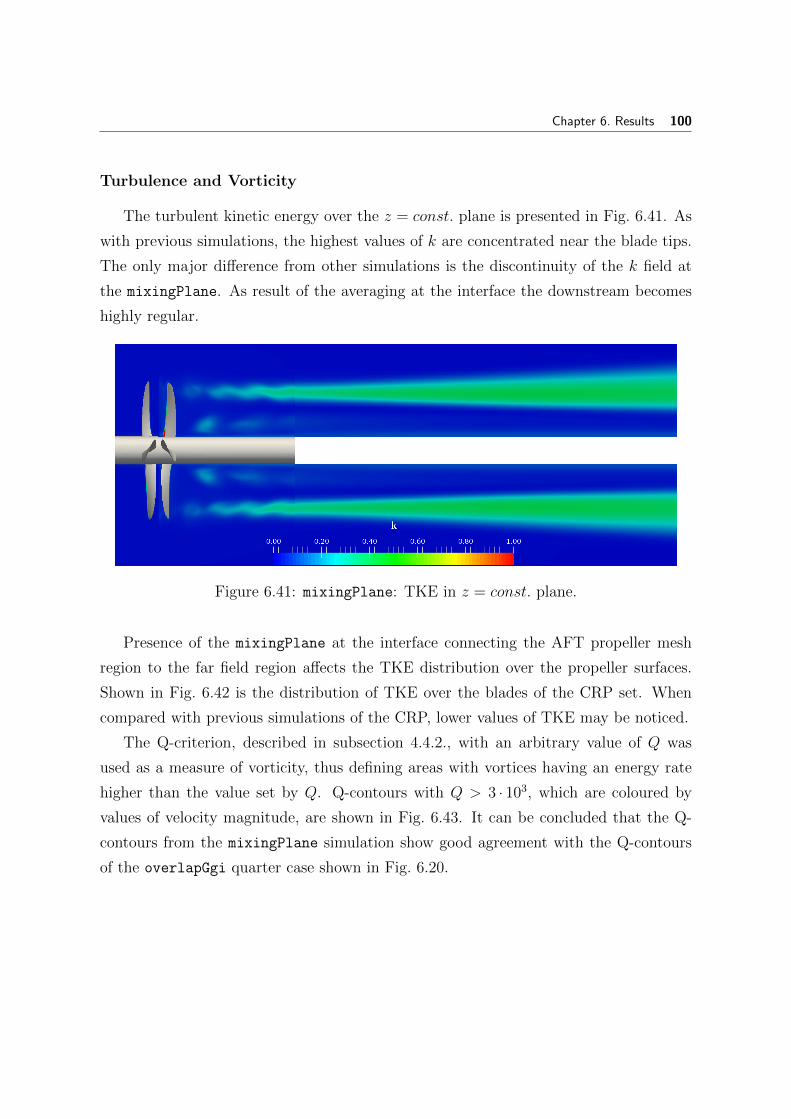
Chapter 6. Results 100
Turbulence and Vorticity
The turbulent kinetic energy over the z = const. plane is presented in Fig. 6.41. As
with previous simulations, the highest values of k are concentrated near the blade tips.
The only major difference from other simulations is the discontinuity of the k field at
the mixingPlane. As result of the averaging at the interface the downstream becomes
highly regular.
Figure 6.41: mixingPlane: TKE in z = const. plane.
Presence of the mixingPlane at the interface connecting the AFT propeller mesh
region to the far field region affects the TKE distribution over the propeller surfaces.
Shown in Fig. 6.42 is the distribution of TKE over the blades of the CRP set. When
compared with previous simulations of the CRP, lower values of TKE may be noticed.
The Q-criterion, described in subsection 4.4.2., with an arbitrary value of Q was
used as a measure of vorticity, thus defining areas with vortices having an energy rate
higher than the value set by Q. Q-contours with Q > 3 · 103, which are coloured by
values of velocity magnitude, are shown in Fig. 6.43. It can be concluded that the Q-
contours from the mixingPlane simulation show good agreement with the Q-contours
of the overlapGgi quarter case shown in Fig. 6.20.

Chapter 6. Results 101
Figure 6.42: mixingPlane: Distribution of TKE on propeller blades.
Figure 6.43: mixingPlane: Vortices matching Q-criterion Q > 3 · 103
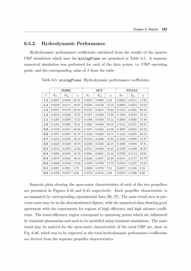
Chapter 6. Results 102
6.5.2. Hydrodynamic Performance
Hydrodynamic performance coefficients calculated from the results of the quarter
CRP simulation which uses the mixingPlane are presented in Table 6.5. A separate
numerical simulation was performed for each of the data points, i.e. CRP operating
point, and the corresponding value of J from the table.
Table 6.5: mixingPlane: Hydrodynamic performance coefficients.
FORE AFT TOTAL
J KT KQ η KT KQ η KT KQ η
1.5 0.0057 0.0048 28.31 0.0025 0.0063 9.43 0.0082 0.0111 17.62
1.4 0.0249 0.0115 48.07 0.0356 0.0139 57.16 0.0605 0.0254 53.04
1.3 0.0587 0.0178 68.10 0.0727 0.0213 70.63 0.1314 0.0391 69.48
1.2 0.0910 0.0238 72.97 0.1077 0.0280 73.36 0.1988 0.0519 73.18
1.1 0.1205 0.0290 72.72 0.1398 0.0339 72.12 0.2603 0.0630 72.40
1.0 0.1484 0.0336 70.31 0.1661 0.0386 68.55 0.3145 0.0721 69.37
0.9 0.1740 0.0374 66.56 0.1947 0.0435 64.08 0.3687 0.0810 65.23
0.8 0.1975 0.0407 61.77 0.2163 0.0469 58.75 0.4138 0.0876 60.15
0.7 0.2184 0.0433 56.14 0.2354 0.0496 52.82 0.4538 0.0930 54.37
0.6 0.2340 0.0449 49.75 0.2590 0.0536 46.18 0.4930 0.0985 47.81
0.5 0.2516 0.0470 42.62 0.2781 0.0569 38.91 0.5298 0.1039 40.59
0.4 0.2698 0.0494 34.78 0.3064 0.0621 31.42 0.5762 0.1114 32.91
0.3 0.2879 0.0520 26.43 0.3232 0.0657 23.50 0.6111 0.1177 24.79
0.2 0.3046 0.0548 17.69 0.3504 0.0709 15.73 0.6550 0.1257 16.59
0.1 0.3267 0.0591 8.79 0.3608 0.0735 7.81 0.6875 0.1326 8.24
0.0 0.3106 0.0557 0.00 0.3713 0.0741 0.00 0.6819 0.1298 0.00
Separate plots showing the open-water characteristics of each of the two propellers
are presented in Figures 6.44 and 6.45 respectively. Each propeller characteristic is
accompanied by corresponding experimental data [36, 37]. The same trend seen in pre-
vious cases may be in the aforementioned figures, with the numerical data showing good
agreement with the experiments for regions of high efficiency and high advance coeffi-
cient. The lower-efficiency region correspond to operating points which are influenced
by transient phenomena and need to be modelled using transient simulations. The same
trend may be noticed for the open-water characteristic of the total CRP set, show in
Fig. 6.46, which was to be expected as the total hydrodynamic performance coefficients
are derived from the separate propeller characteristics.

Chapter 6. Results 103
0 0.2 0.4 0.6 0.8 1 1.2 1.4 1.6Advance ratio, J
0
0.1
0.2
0.3
0.4
0.5
0.6
0.7
0.8
KT
,10K
Q,η
Sim. KT
Sim. 10KQ
Sim. ηExp. KT
Exp. 10KQ
Exp. η
Figure 6.44: mixingPlane: Fore propeller steady hydrodynamic coefficients.
0 0.2 0.4 0.6 0.8 1 1.2 1.4 1.6Advance ratio, J
0
0.1
0.2
0.3
0.4
0.5
0.6
0.7
0.8
KT
,10K
Q,η
Sim. KT
Sim. 10KQ
Sim. ηExp. KT
Exp. 10KQ
Exp. η
Figure 6.45: mixingPlane: Aft propeller steady hydrodynamic coefficients.

Chapter 6. Results 104
0 0.2 0.4 0.6 0.8 1 1.2 1.4 1.6Advance ratio, J
0
0.2
0.4
0.6
0.8
1
1.2
KT
,10K
Q,η
Sim. KT
Sim. 10KQ
Sim. ηExp. KT
Exp. 10KQ
Exp. η
Figure 6.46: mixingPlane: Total propeller set steady hydrodynamic coefficients.
Comparison to the overlapGgi Interface
A comparison of the hydrodynamic performance coefficients for the same quarter
CRP case with the overlapGgi and mixingPlane interfaces is given next. A plot
comparing the two cases with experimental data is given in Figure 6.47. Analysis of the
plot reveals that both the mixingPlane and the overlapGgi cases show good agreement
with the experimental data for operating points near the advance coefficient of J =
1 − 1.2. For values lower than that, the results of the mixingPlane case show better
adherence to experimental data. For values of the advance coefficient smaller than
1, the axial velocity diminishes with rising influence of transients on the flow. This
is the reason why steady-state numerical data shows poor adherence to experimental
values. While both the mixingPlane and the overlapGgi cases show disagreement with
experiments for lower values of J , data from the mixingPlane cases follows the trend
of the experimental data better.

Chapter 6. Results 105
0 0.2 0.4 0.6 0.8 1 1.2 1.4 1.6Advance ratio, J
0
0.2
0.4
0.6
0.8
1
1.2
KT
,10K
Q,η
GGI KT
GGI 10KQ
GGI ηmix. P. KT
mix. P. 10KQ
mix. P.ηexp. KT
exp. 10KQ
exp. η
Figure 6.47: mixingPlane: Total propeller set steady hydrodynamic coefficients.
6.6. Transient Simulation
The simulations presented in the previous sections handled the CRP domain as a
steady-state method. The ”frozen rotor” MRF approach is used to specify a rotational
zone without actual motion of the mesh. Such results proved satisfactory for higher effi-
ciency operating points residing in regions with weak influence of transient phenomena.
For operating points at lower efficiency, transient phenomena have increasingly pro-
nounced influence on the flow, thus rendering steady-state simulations ineffective, i.e. pro-
ducing data with increasing deviation from experimental values. This makes it necessary
for lower advance coefficient (efficiency) to be modelled using transient simulations.
In this section, data produced from a transient simulation of the CRP set is presented
as graphical visualisation of field data and as hydrodynamic performance of the set. As
the previous sections, and therein discussed results, validate the use of the quarter CRP
domain, thus reducing the computational costs of the simulation. This becomes of great
importance for transient simulations, reducing the already high computational time.

Chapter 6. Results 106
The geometry used is the quarter CRP geometry with accompanying domain and
necessary boundary conditions, as presented in Chapter 5. Interface are handled by the
cyclicGgi and overlapGgi interfaces. The propeller rotation was modelled by actually
rotating the computational mesh in the moving regions. The DyMesh dynamic mesh
model implemented in foam-extend is used. By employment of the aforementioned
model rotation is assigned to two mesh regions surrounding the propellers of the CRP
set: the FORE propeller region and the AFT propeller region. A constant rotational
speed of 12 rps is assigned, taking note that the axis of rotation is aligned with the
x-axis of the global coordinate system.
A variant of the PIMPLE algorithm, which supports mesh motion (pimpleDyMFoam),
available in foam-extend was used for the transient simulation. A fixed time-step size
was chosen and set to a low value to avoid fluctuations of time-varying results which may
produce errors in the Fourier Analysis of the numerical data. The chosen time-step ∆t =
5e− 5 resulted in high computational time and maximum Courant numbers of Co ≈ 5.
As the PIMPLE algorithm allows for larger values of the Co number, the maximum Co
values occurring in the simulation were of no concern. It is important to properly resolve
transient interaction between propeller blades, that is why approximately 100 time-step
per repeating pitch period (one quarter of a full rotation) should be used. Using the
chosen time-step size (∆t = 5e − 5) and set rotational speed (12 rps), approximately
1667 time-steps are needed for the transient simulation to complete one full rotation
and 417 time-steps for a quarter of a rotation.
Despite the fact that the quarter CRP domain is used, the transient simulation
requires considerable computational resources to reach a state of periodic convergence
in a reasonable amount of time. For that reason, only one simulation is analysed as a
part of this Thesis. The operating point chosen for the transient simulation corresponds
to a value of the advance coefficient equal to J = 0.5, making the transient results
comparable to both the steady-state and the experimental data.
It should be noted that at the time of writing, the transient simulation had run for
approximately 0.15 seconds, i.e. 3000 time-steps, with the chosen ∆t. As the CRP
set rotates at 12 rps, the simulation run-time allowed for only one full rotation of the
set which was not enough to reach full periodic convergence. That is why the result
presented in continuation, although indicative of the final solution, are susceptible to
change as the simulation continues to converge.

Chapter 6. Results 107
6.6.1. Simulation Results
In this section, numerical data from a transient CRP simulation based on the quarter
propeller domain is presented. Although the quarter CRP domain was used, the post-
processing software enables transformation and copying of the periodically repeating
part of the domain, allowing for the full CRP domain to be presented.
The transient simulation spans over a large number of simulated time-steps, making
it impossible to present all of the results for each time-step. That is why the results for
three distinct time steps are presented, spaced around the point in which the blades of
the two propellers pass each other. The first time-step t = 0.1 s represents the moment
the blades are about to meet, in time-step t = 0.1025 s the blade have just met and in
time-step t = 0.1075 s the propeller blades have already parted.
Pressure Field
Figure 6.48 offers an overview of the kinematic pressure field in the z = constant. plane
for three different time-steps. The pressure near the propeller blades shows higher values
as the blades move closer (Fig. 6.48 a) ) and lower values as the propellers part (Fig. 6.48
b) ). As both the higher and the lower pressure areas are situated near the propeller
surfaces, a closer look at the pressure distribution on the propeller blades is given in
Fig. 6.49. As expected, higher values of pressure over blade surfaces may be seen as the
propellers move closer with the average pressure at the blade surfaces dropping after as
they separate. Overall, the highest values of pressure are present at the pressure side
of the AFT propeller for all time-steps. This is because the AFT propeller suction side
suffers most from the wake of the FORE propeller.
Velocity Field
The velocity field is presented as a ratio of axial velocity Ux and the inlet velocity
Ui = 1.8312 m/s. Fig. 6.50 shows the velocity field for the three time-steps, showing
consistent values of velocity in the CRP wake and with the only fluctuations happening
as blades cut through the z = const. plane used for post-processing. Another analysis of
the CRP set wake is offered in form of graphical representation of axial and tangential
velocities at x/R = 0.334. Distribution of the axial velocity in the wake, presented
in Fig. 6.51 shows only small changes throughout the presented time-steps, while more

Chapter 6. Results 108
considerable changes may be noticed for the distribution of tangential velocity. In figures
showing axial velocity in the wake, areas of back-flow represented by negative values of
the Ux/Ui ratio may be seen. Back-flow may be noticed at blade tips (Fig 6.51) and at
the suction side of the AFT propeller (Fig. 6.50).
Turbulence and Vorticity
The distribution of TKE in the CRP wake for the three selected time-steps is shown
in figure 6.52. Similarly to the velocity field, the TKE field in the z = const. plane shows
only slight temporal variations which are concentrated at the propeller blades, thus
requiring examination of TKE distribution over the blade surfaces. Such distribution
is offered in Fig. 6.53. The highest values of TKE may be noticed at the leading edges
just before and at the moment the propellers meet.
The same as for the steady-state simulations, the Q-criterion is used to visualise vor-
ticity in the region surrounding the propeller set for transient simulations. Q-contours
corresponding to the value of Q > 5 · 105 were used to provide better visibility of pro-
peller interaction. The contours coloured by values of the velocity magnitude are pre-
sented in Figure 6.54. Areas of increased vorticity may be noticed in the region between
the two propellers just as the propeller move past each other 6.54 b).
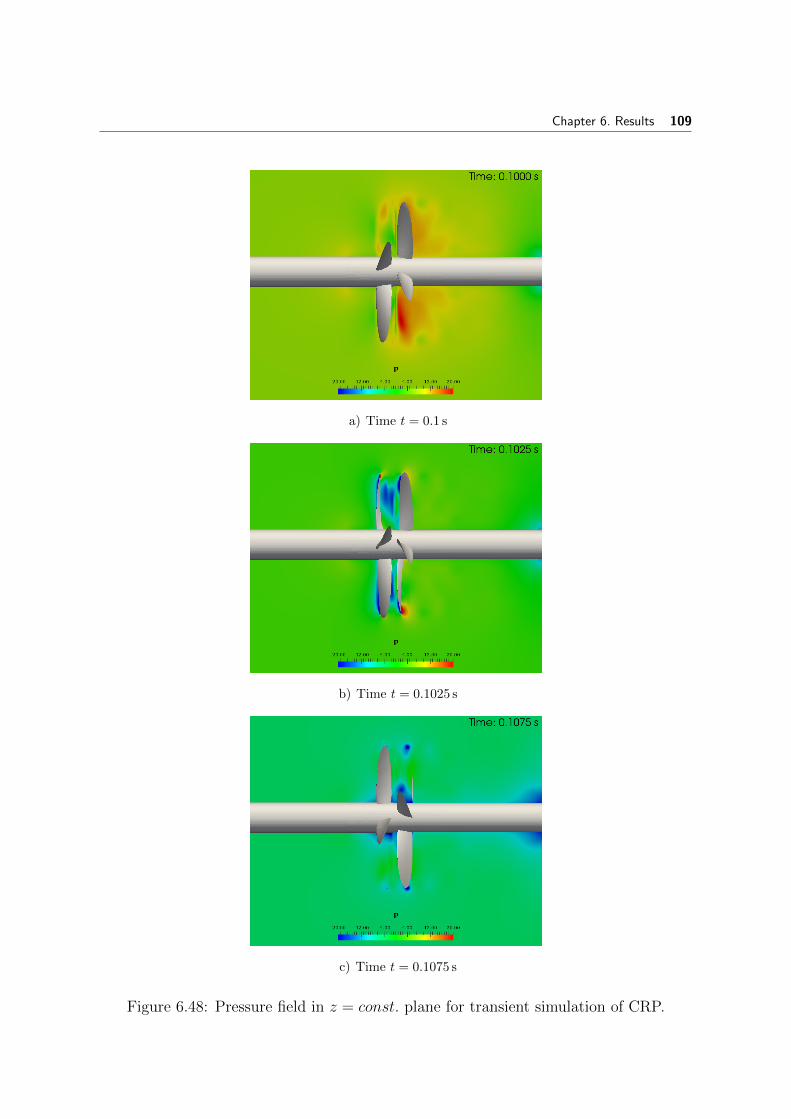
Chapter 6. Results 109
a) Time t = 0.1 s
b) Time t = 0.1025 s
c) Time t = 0.1075 s
Figure 6.48: Pressure field in z = const. plane for transient simulation of CRP.

Chapter 6. Results 110
a) Time t = 0.1 s
b) Time t = 0.1025 s
c) Time t = 0.1075 s
Figure 6.49: Pressure distribution on propeller surfaces for transient simulation of CRP.

Chapter 6. Results 111
a) Time t = 0.1 s
b) Time t = 0.1025 s
c) Time t = 0.1075 s
Figure 6.50: Velocity field in z = const. plane for transient simulation of CRP.
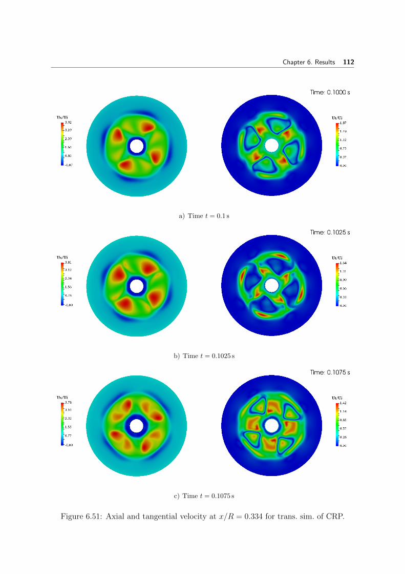
Chapter 6. Results 112
a) Time t = 0.1 s
b) Time t = 0.1025 s
c) Time t = 0.1075 s
Figure 6.51: Axial and tangential velocity at x/R = 0.334 for trans. sim. of CRP.

Chapter 6. Results 113
a) Time t = 0.1 s
b) Time t = 0.1025 s
c) Time t = 0.1075 s
Figure 6.52: TKE in z = const. plane for transient simulation of CRP.

Chapter 6. Results 114
a) Pressure and suction side at time t = 0.1 s
b) Pressure and suction side at time t = 0.1025 s
c) Pressure and suction side at time t = 0.1075 s
Figure 6.53: Distribution of TKE on prop. blades for transient simulation of CRP.

Chapter 6. Results 115
a) Time t = 0.1 s
b) Time t = 0.1025 s
c) Time t = 0.1075 s
Figure 6.54: Vortices matching Q-criterion Q > 5 · 104, transient CRP.

Chapter 6. Results 116
6.6.2. Hydrodynamic Performance
Comparison of the hydrodynamic performance data for operating points J = 0.5 and
J = 1.1, presented in Table 6.3, leads to the conclusion that transient simulations are
necessary to accurately calculate hydrodynamic performance coefficients for operating
points with lower values of the advance coefficients J . As transient simulation are
computationally more demanding than steady-state MRF simulation, performance for
only one operating point shall be analysed (J = 0.5).
The transient solver produces new solutions for each time-step, resulting in time-
varying data. The Direct Fourier Transform (DFT) based on equally spaced time in-
tervals was used to analyse time dependent values of force and torque produced by the
simulation. Time-varying values of thrust and torque of each propeller and the whole
CRP set for one complete rotation, with data transformed by using DFT, are shown in
Figures 6.55, 6.56 and 6.57.
By transferring time dependent data to the frequency domain using DFT, values of
thrust and torque may be analysed more easily. The base amplitudes in the frequency
domain represent mean values of thrust/torque and may be use to calculate steady
hydrodynamic coefficients. Such values may be compared results from steady-state
simulations. As expected, the appearance of unsteady components of thrust and torque
may be seen at eight times shaft frequency (N = 8). The frequency at which unsteady
components occur is equal to the product of the number of propeller blades, number of
propellers in the set and the propeller rotation speed in rps: 4 · 2 · 12 = 96Hz. Values
of unsteady thrust and torque may be used with equations presented in Chapter 4.
to calculate the unsteady hydrodynamic performance coefficients. Both steady and
unsteady coefficients for the whole CRP set are given tabularly:
Table 6.6: Unsteady hydrodynamic performance coefficients.
Transient Transient∗ Experimental
Value Error [%] Value Error [%] data
KT 0.8456 -22.71 0.6891 -5.12 0.6538
KQ 0.1461 -18.24 0.1170 2.10 0.1194
η 0.4609 -5.46 0.4689 -7.07 0.4357
KT 0.1902 - 0.1655 - -
KQ 0.0328 - 0.0284 - -∗ Unrevised, near periodic convergence.

Chapter 6. Results 117
Table 6.6 presents the data for two transient simulations. The first simulation is the
final variation with revised setting and boundary conditions showing consistent values
for the analysed data fields. The other simulation, which is denoted by the superscript ∗,
showed some inconsistencies in the pressure distribution prompting revision of boundary
conditions for pressure at the outlet. The transient simulation with revised boundary
conditions shows large errors when compared to experimental data. This is due to the
fact that the revised simulation did not achieve periodic convergence because of insuffi-
cient runtime, with the simulated CRP set managing to complete only one full rotation.
It is believed that as the simulation continues and better convergence is achieved, the
relative error will diminish greatly. This is supported by the fact that the unrevised
simulation, which was allowed more runtime and managed to achieve several full pro-
peller rotations, shows good agreement with experimental data. The revised simulation
is expected to achieve the same or even better agreement with experimental data.
It should also be noted that no error estimation of unsteady thrust and torque
coefficients was given in Table 6.6. The reason why the comparison of numerical and
experimental values of unsteady coefficients could not be presented is lack of experimen-
tal data for these coefficients at J = 0.5. It should also be noted that both experimental
studies performed by Miller Miller76, Miller81 suffer from high measuring errors.
The author predicts the error to be as high as 20% for total CRP set values and 10%
for individual thrust and torque values.
Furthermore, the converged results of the unrevised simulation point to the fact that
the transient simulation for J = 0.5 produces hydrodynamic coefficients which are closer
to the experimental values than those of the steady-state MRF simulation, as they are
able to encompass the transient effects influencing the solution.

Chapter 6. Results 118
0 90 180 270 360
θ [ ° ]
-240
-160
-80
0
80
Unst
eady
Fx
273
7.49
84.8
2.4930.9
1.07 7.08 0.909 2.06 0.605 1.92
0 4 8 12 16 20 24 28 32 36 40
N-th harmonic
0
100
200
300
Am
plitu
de
of
Fx
273
7.49
84.8
2.4930.9
1.07 7.08
0 24 48 72 96 120 144 168 192 216 240 264 288 312
f [Hz]
0
100
200
300
Am
plitu
de
of
Fx
a) Unsteady thrust, Fx
0 90 180 270 360
θ [ ° ]
-15
-10
-5
0
5
10
Unst
eady
Mx
13.1
0.318
4.6
0.1491.93
0.0613 0.5 0.0536 0.134 0.0303 0.111
0 4 8 12 16 20 24 28 32 36 40
N-th harmonic
0
5
10
15
Am
plitu
de
of
Mx
13.1
0.318
4.6
0.1491.93
0.0613 0.5
0 24 48 72 96 120 144 168 192 216 240 264 288 312
f [Hz]
0
5
10
15
Am
plitu
de
of
Mx
b) Unsteady torque, Mx
Figure 6.55: Fore propeller unsteady hydrodynamic performance for J = 0.5
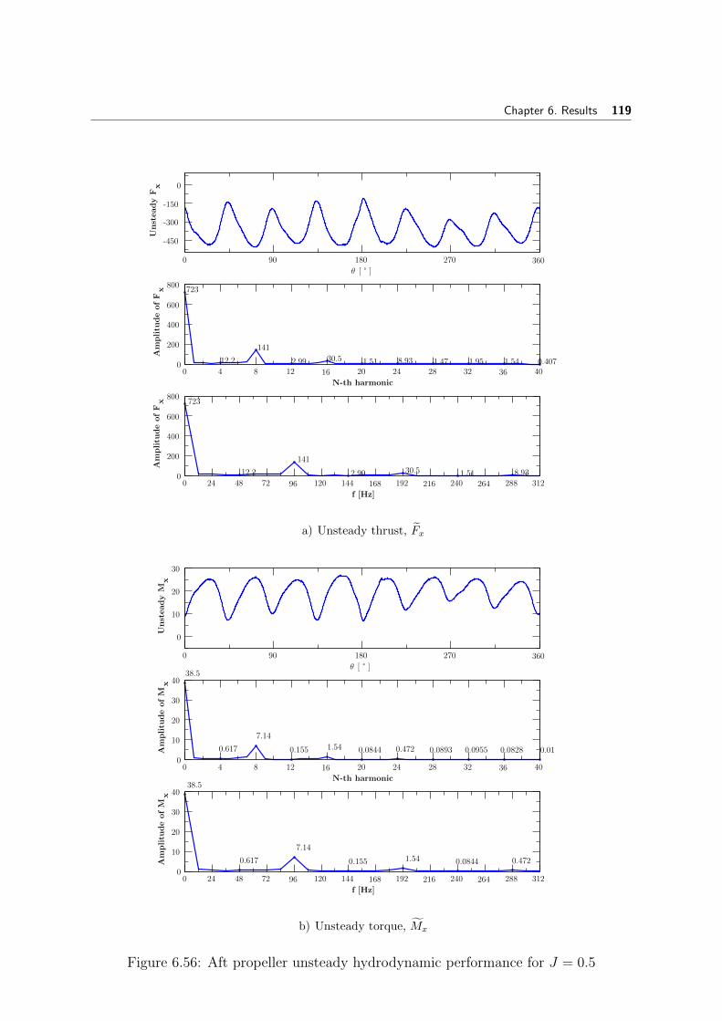
Chapter 6. Results 119
0 90 180 270 360
θ [ ° ]
-450
-300
-150
0
Unst
eady
Fx
723
12.2
141
2.99 30.5 1.51 8.93 1.47 1.95 1.54 0.4070 4 8 12 16 20 24 28 32 36 40
N-th harmonic
0
200
400
600
800
Am
plitu
de
of
Fx
723
12.2
141
2.99 30.5 1.51 8.93
0 24 48 72 96 120 144 168 192 216 240 264 288 312
f [Hz]
0
200
400
600
800
Am
plitu
de
of
Fx
a) Unsteady thrust, Fx
0 90 180 270 360
θ [ ° ]
0
10
20
30
Unst
eady
Mx
38.5
0.617
7.14
0.155 1.54 0.0844 0.472 0.0893 0.0955 0.0828 0.01
0 4 8 12 16 20 24 28 32 36 40
N-th harmonic
0
10
20
30
40
Am
plitu
de
of
Mx
38.5
0.617
7.14
0.155 1.54 0.0844 0.472
0 24 48 72 96 120 144 168 192 216 240 264 288 312
f [Hz]
0
10
20
30
40
Am
plitu
de
of
Mx
b) Unsteady torque, Mx
Figure 6.56: Aft propeller unsteady hydrodynamic performance for J = 0.5

Chapter 6. Results 120
0 90 180 270 360
θ [ ° ]
-600
-400
-200
0
Unst
eady
Fx
996
9.88
225
4.69 59.3 2.49 14.7 2.38 3.87 1.99 2.320 4 8 12 16 20 24 28 32 36 40
N-th harmonic
0
250
500
750
1000
Am
plitu
de
of
Fx
996
9.88
225
4.69 59.3 2.49 14.7
0 24 48 72 96 120 144 168 192 216 240 264 288 312
f [Hz]
0
250
500
750
1000
Am
plitu
de
of
Fx
a) Unsteady thrust, Fx
0 90 180 270 360
θ [ ° ]
0
10
20
30
Unst
eady
Mx
41
0.597
7.99
0.174 1.9 0.0715 0.5 0.0592 0.0342 0.054 0.0262
0 4 8 12 16 20 24 28 32 36 40
N-th harmonic
0
10
20
30
40
Am
plitu
de
of
Mx
41
0.597
7.99
0.174 1.9 0.0715 0.5
0 24 48 72 96 120 144 168 192 216 240 264 288 312
f [Hz]
0
10
20
30
40
Am
plitu
de
of
Mx
b) Unsteady torque, Mx
Figure 6.57: Total CRP unsteady hydrodynamic performance for J = 0.5

Chapter 6. Results 121
6.7. Closure
In this chapter the results of several different simulations of CRP were presented in
hope of analysing the different choices in regard to interface and domain handling. First,
the results of quarter and full CRP domain simulations were analysed showing no major
differences. This validated the overlapGgi and cyclicGgi interfaces, thus allowing
for further use of the smaller quarter CRP case and positively affecting simulation
runtime. Secondly, an overview of the differences between the mixingPlane and the
overlapGgi interfaces was investigated and presented both graphically and in term of
numerical values. Thirdly, a comparison between transient and steady-state simulation
of the CRP set was offered, commenting on the results. Lastly, steady-state simulations
were conducted to analyse the influence of different initial propeller positions on steady
hydrodynamic coefficients.
The next chapter serves as conclusion of the Thesis, offering an overview of completed
task, the resulting findings and possible future work on the subject of CRP.

7 Conclusion
7.1. Conclusion
This Thesis covered an overview of interface handling methods used to establish
rotor-stator interaction in CFD simulations. An introduction was given explaining the
complexity of various turbomachines, acknowledging the need to simplify their geometry
when performing CFD simulations. The mixingPlane and ggi interfaces were intro-
duced, with additional explanation of two ggi variants: the overlapGgi and cyclicGgi
interfaces. The interfaces were established as means of providing communication be-
tween partially connected or disconnected mesh regions, thus enabling the use of sim-
plified, partial geometry, computational domains. The theoretical part of the thesis was
expanded to include practical examples of these interfaces using numerical simulations
of a CRP set, performed in foam-extend.
A series of CRP steady-state simulations was performed for an operating point de-
termined by the propeller advance ratio J = 0.5. First, baseline results were established
using a full CRP geometry with the Ggi interface. Secondly, a quarter CRP simula-
tion using a combination of the cyclicGgi and overlapGgi interfaces was performed,
with the results validated against those of the full geometry simulation. Thus, fur-
ther use of the quarter CRP simulation was made possible, saving on computational
runtime needed to reach convergence of results. Several steady-state simulations were
performed to study the effects of different initial propeller position on resulting hydrody-
namic performance data. Once the quarter simulation was validated, the next series of
steady-state simulations, aimed at comparing the use of mixingPlane and overlapGgi
interfaces, was performed. As the mixingPlane introduces averaging at the interface,
122

Chapter 7. Conclusion 123
overlapGgi was adopted for ensuing transient simulations, performed for the same op-
erating point J = 0.5. The resulting unsteady data was analysed by using DFT and
compared to results from previous simulations. The data gathered from both the steady-
state and transient simulations was presented graphically and by studying the resulting
hydrodynamic performance coefficients, i.e. open-water characteristics of the CRP set.
Conclusions made possible by analysis of numerical data from various simulations
performed on the CRP set are presented next. Firstly, the open-water characteristic
resulting from the full CRP simulations shows the best efficiency point (BEP) of the set
to be around the advance coefficient values of J = 1.2−1.3. The data showed higher val-
ues of torque and thrust on the AFT propeller of the set, which was expected because
the second propeller is influenced by the wake of the FORE propeller. Steady-state
hydrodynamic coefficients show good agreement with experimental data for operating
points near the BEP, with some disagreement for both lower and higher values of J . The
explanation being that, as the CRP operating point moves farther away from the BEP,
transient effects become more pronounced making the steady-state approach unable to
produce fully accurate data. For accurate results of such operating points, transient
simulations should be performed. Nevertheless, steady-state simulations provide accu-
rate data for higher efficiency operating points, which are generally used for propeller
design.
The second series of simulations focused on verifying the validity of quarter geom-
etry CRP simulations. Both the data field analysis and hydrodynamic performance
coefficients showed no major deviations when compared to full CRP simulation results.
This lead to the conclusion that the overlapGGi and cyclicGgi interfaces, used in the
quarter simulation, function as expected and described in the theoretical part of the
Thesis. This fact has a highly positive impact on simulation runtime and computa-
tional demands, allowing for a smaller number of cells in the computational domain by
replacing the full propeller domains with quarter domains. Cases based on the quarter
domain and the mixingPlane interface produce hydrodynamic performance data with
similar behaviour in the higher and lower efficiency regions as the simulations based on
the overlapGgi and Ggi interfaces, with some differences for low values of J . More
specifically, the mixingPlane cases seem to follow the experimental data curve slightly
better, but no difference high enough to justify further use of the mixingPlane interface
over ggi was noticed. As the mixingPlane performs averaging of data at the interface,

Chapter 7. Conclusion 124
which can be seen in graphical representations of various data fields, it is not suitable
for use in transient simulations, as it would average out the unsteady data affecting the
validity of the simulations. The other two interfaces may be used for both steady-state
and transient simulations.
Transient simulation of the CRP set offered several insights into propeller behaviour.
Analysis of resulting transient data fields and unsteady values of force and thrust showed
the values to be time-dependant and influenced by propeller interaction. Considering
the values of unsteady thrust, changes in thrust may be noticed as the propeller rotates
and the blades pass each other. Furthermore, the appearance of unsteady component of
thrust and torque was noticed at eight times shaft frequency (N = 8). As the propellers
rotate synchronous to each other and have the same number of blades, the unsteady
components may be attributed to propeller interaction. Fourier transformation of tran-
sient data allowed for calculation of steady and unsteady hydrodynamic performance
coefficients, which were compared to both steady-state simulation results and experi-
mental data. The previously postulated theory explaining how the steady-state results
disagree with experimental data for lower values of J because of the inability of steady
simulations to capture transient phenomena, was validated by transient data. The data
showed very good agreement with the experiments even for a lower efficiency operating
point J = 0.5, when enough time is allowed for the transient simulation to reach a
periodic steady state.
Finally, it is concluded that steady state simulations provide sufficiently accurate
results for high efficiency operating points. If low efficiency regions are to be modelled,
transient simulations should be performed. A major issue regarding transient simu-
lations is high turnaround time in combination with high computational costs. This
makes transient simulations of little use for practical application when modelling CRP
sets, even with quarter domain simulations, and makes steady-state methods such as
MRF viable alternative for certain operating points.
All things considered, turbomachines prove to be complex machines which require
various simplifications for practically usable CFD simulations. These simplifications may
be offered in form of different interface and domain handling methods which depend on
the problem and the geometry that is to be analysed. A contra-rotating propeller set
proved a good example of a turbomacine on which various approaches to interface and
domain handling could be studied.

Chapter 7. Conclusion 125
7.2. Future Work
A possible continuation of the work in this Thesis would consist of running more
transient simulations on both lower and higher efficiency operating points and repeating
the analysis of the existing transient simulation after a satisfactory periodic steady state
had been achieved.
Furthermore, a study of the effects of different axial spacing of propellers form-
ing the CRP set would provide interesting data from both steady-state and transient
simulations. The data would be comparable to experimental values, as the required
experimental data already exists for the same CRP set as the one used in this Thesis.
Similar research could be conducted on CRP sets with different rotational speed and/or
different number of blades for each propeller in the set.
Lastly, the insights on propeller interaction, case set-up and data analysis gathered
while working on simulations of a maritime CRP set could be used to further the research
to include CRP used in aviation.

Appendices
126

A Interface Set-up
Examples
Appendix A offers several examples of boundary file entries for different interface
types. All entries are based on set-up files used in working CRP simulations and with
existing patches described in Ch. 5.
A.1. ggi
An example of the code used to define an Ggi patch in the boundary file found in
case dir/constant/polymesh, with accompanying explanation.
AFT inter face back
type gg i ;
nFaces 3712 ;
s ta r tFace 6401114;
shadowPatch MAIN interface back ;
zone AFT back zone ;
br idgeOver lap true ;
• type - Defines type of boundary patch.
• nFaces, startFace - Internally defined with mesh.
• shadowPatch - GGI patch pair should be defined.
• zone - Name of the faceZone analogous to the GGI patch being defined.
• bridgeOverlap - If set to false completely and partially uncovered faces are
disallowed. When set to true for cases with non-overlapping cases, a slip boundary
condition is defined (preferably use overlapGgi).
127

Chapter A. Interface Set-up Examples 128
A.2. overlapGgi
An example of the code used to define an overlapGgi patch in the boundary file
found in case dir/constant/polymesh, with accompanying explanation.
FORE inter face f ront
type over lapGgi ;
nFaces 2320 ;
s ta r tFace 6358544;
shadowPatch FT in t e r f a c e f r on t ;
zone FORE front zone ;
br idgeOver lap fa l se ;
r o ta t i onAx i s (1 0 0 ) ;
nCopies 4 ;
• type - Defines type of boundary patch.
• nFaces, startFace - Internally defined with mesh.
• shadowPatch - GGI patch pair should be defined.
• zone - Name of the faceZone analogous to the GGI patch being defined.
• bridgeOverlap - Should be set to false for overlapGgi.
• rotationAxis - Defines the axis of rotation.
• nCopies - Set exact number of patch copies needed for defining a full geometry
(360) .
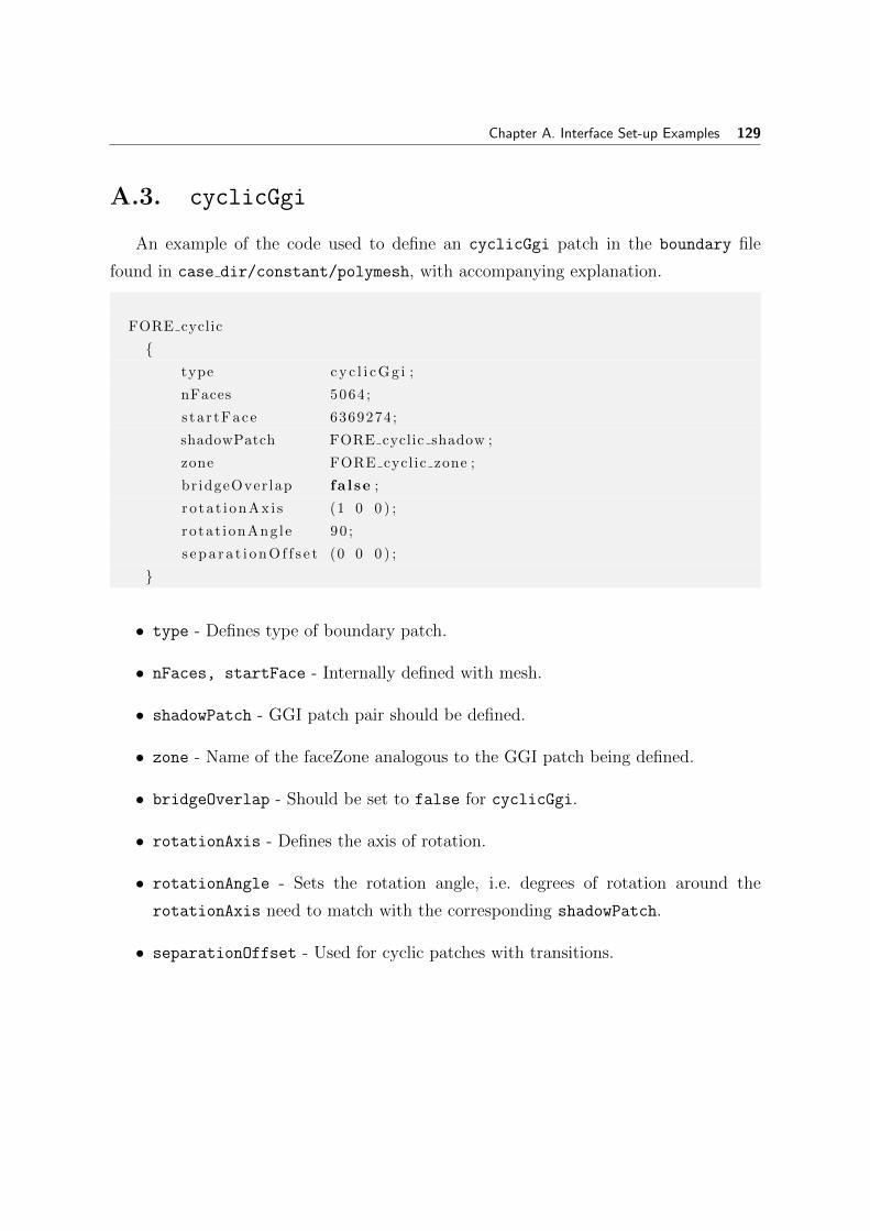
Chapter A. Interface Set-up Examples 129
A.3. cyclicGgi
An example of the code used to define an cyclicGgi patch in the boundary file
found in case dir/constant/polymesh, with accompanying explanation.
FORE cyclic
type cy c l i cGg i ;
nFaces 5064 ;
s ta r tFace 6369274;
shadowPatch FORE cyclic shadow ;
zone FORE cyclic zone ;
br idgeOver lap fa l se ;
r o ta t i onAx i s (1 0 0 ) ;
ro ta t ionAng le 90 ;
s epa r a t i onO f f s e t (0 0 0 ) ;
• type - Defines type of boundary patch.
• nFaces, startFace - Internally defined with mesh.
• shadowPatch - GGI patch pair should be defined.
• zone - Name of the faceZone analogous to the GGI patch being defined.
• bridgeOverlap - Should be set to false for cyclicGgi.
• rotationAxis - Defines the axis of rotation.
• rotationAngle - Sets the rotation angle, i.e. degrees of rotation around the
rotationAxis need to match with the corresponding shadowPatch.
• separationOffset - Used for cyclic patches with transitions.

Chapter A. Interface Set-up Examples 130
A.4. mixingPlane
An example of the code used to define mixingPlane patches in the boundary file
found in case dir/constant/polymesh, with accompanying explanation.
FORE inter face s ide
type mixingPlane ;
nFaces 6090 ;
s ta r tFace 6363184;
shadowPatch MAIN inter face s ide1 ;
zone FORE side1 zone ;
coordinateSystem
type c y l i n d r i c a l ;
name mixingCS ;
o r i g i n (0 0 0 ) ;
ax i s (1 0 0 ) ;
d i r e c t i o n (0 1 0 ) ;
inDegrees fa l se ; // rad ians
ribbonPatch
sweepAxis Theta ;
s tackAxis Z ;
d i s c r e t i s a t i o n bothPatches ;
• type - Defines type of boundary patch.
• nFaces, startFace - Internally defined with mesh.
• shadowPatch - mixingPlane patch pair should be defined.
• zone - Name of the faceZone analogous to the mixingPlane patch being defined.

Chapter A. Interface Set-up Examples 131
coordinateSystem
• type - Defines the coordinate system used for defining mixingPlane ribbon patches.
Available types are: cylindrical, ellipticCylindrical, parabolicCylindrical,
spherical and toroidal.
• name - Defines the name of the coordinate system.
• origin - Defines the origin of the mixingPlane coordinate system in relation to
global coordinates.
• axis - Set the axis of rotation used.
• direction - Sets the direction in which the averaging will be performed.
• inDegrees - Set to true for degrees or to false for radians.
ribbonPatch
• sweepAxis - Defines the sweeping axis for averaging in chosen the mixingPlane
coordinate system. In the example above, Theta is used as the sweep axis in the
cylindrical coordinate system.
• stackAxis - Defines the stacking axis in the chosen mixingPlane coordinate sys-
tem. This example uses Z as the stack axis and for defining the manner in which
the ribbon patches of the mixingPlane interface are stacked. If, for example, the
FORE interface front patch is used, the stack axis should be set to R. Examples
of different stack axes are given in Fig. A.1 and A.2.
• discretisation - Defines the type of discretisation used. Availabe options are:
bothPatches, uniform, slavePatch, masterPatch and userDefined.

Chapter A. Interface Set-up Examples 132
Direction of FlowZ
SW
EE
P
STACK
R
θ
Figure A.1: Use of mixingPlane with θ as sweep axis and R as stack axis.
Direction of Flow
ST
AC
K
Z
R
Z
θ
SW
EE
P
Figure A.2: Use of mixingPlane with θ as sweep axis and Z as stack axis.

Bibliography
[1] NauticEXPO. Ship pod drive.
http://www.nauticexpo.com/prod/abb-marine/product-30709-461731.html.
[Online; accessed March 10, 2019].
[2] Volvo Penta. Multiple ways to create different types of propeller solutions.
http://nordicblog.volvopenta.com. [Online; accessed March 10, 2019].
[3] A. T. Sayers. Hydraulic and compressible flow turbomachines. Department of Me-
chanical Engineering, University of Capetown, 1990.
[4] E. Logan Jr. Handbook of Turbomachinery. Marcel Dekker, 2003.
[5] H. Jasak and M. Beaudoin. Openfoam trubo tools: From general purpose cfd to
turbomachinery simulations. In Proceedings of ASME-JSME-KSME Joint Fluids
Engineering Conference, Hamamatsu, Shizuoka, Japan, 2011.
[6] H. Jasak. Course materials for Numerical Methods in Continuum Mechanics
Method, February 2018.
[7] S. V. Patankar and D.B. Spalding. A calculation procedure for heat, mass and
momentum transfer in three-dimensional parabolic flows. International Journal of
Heat and Mass Transfer, 15:1787–1806, 1972.
[8] R. I. Issa. Solution of the implicit discretized fluid flow equations by operator
splitting. In Mechanical Engineering Report, Imperial College, London, UK, 1982.
133

BIBLIOGRAPHY 134
[9] T. Holzmann. Mathematics, Numerics, Derivations and OpenFOAM, December
2016.
[10] B.E. Launder and D.B. Spalding. The numerical computation of turbulent flows.
Computer Methods in Applied Mechanics and Engineering, 3:269–289, 1974.
[11] B.E. Launder and B.I. Sharma. Application of the energy-dissipation model of
turbulence to the calculation of flow near a spinning disc. Letters in Heat and Mass
Transfer, 1:131–137, 1974.
[12] David C. Wilcox. Turbulence Modeling for CFD. DCW Industries, 1993.
[13] F. Menter and T. Esch. Elements of industrial heat transfer prediction. In 16th
Brazilian Congress of Mechanical Engineering (COBEM), Uberlandia, Brazil, 2001.
[14] F.R. Menter, M. Kuntz, and R. Langtry. Ten years of industrial experience with
the sst turbulence model. Turbulence, Heat and Mass Transfer, 4:625–632, 2003.
[15] Nasa turbulence modeling resource.
http://turbmodels.larc.nasa.gov/sst.html. Accessed: 12-02-2019.
[16] A. Hellsten. Some improvements in menter’s k-omega-sst turbulence model. In
29th AIAA Fluid Dynamics Conference, Albuquerque,NM,USA, 1998.
[17] Gregor Cvijetic. Steady State Methods for Turbomachinery. Faculty of Mechanical
Engineering and Naval Architecture, University of Zagreb, 2014.
[18] The MRF development.
http://openfoamwiki.net/index.php/See_the_MRF_development. Accessed:
10-02-2019.
[19] H. Jasak and H. Rusche. Dynamic mesh handling in openfoam. In Advanced
Training at the OpenFOAM Workshop, Gothenborg, Sweden, 2010.
[20] H. Jasak. Course materials for The Practical Finite Volume Method, February
2018.
BIBLIOGRAPHY 135
[21] H. Jasak and M. Beaudoin. Development of a generalized grid interface for turboma-
chinery simulations with openfoam. In Open Source CFD International Conference,
Berlin, Germany, 2008.
[22] H. Jasak. Dynamic mesh handling in OpenFOAM. In 47th AIAA Aerospace Sci-
ences Meeting including The New Horizons Forum and Aerospace Exposition. Amer-
ican Institute of Aeronautics and Astronautics, jan 2009.
[23] I. E. Sutherland and G. W. Hodgman. Hidden surface removal using polygon area
sorting. In SIGGRAPH ’77: Proceedings of the 4th annual conference on Computer
graphics and interactive techniques, New York, USA, 1977.
[24] H. Jasak. General grid interface - theoretical basis and implementation. In NUMAP-
FOAM Summer School, Zagreb, Croatia, 2009.
[25] M. Beaudoin et al. Evaluation of an improved mixing plane interface for openfoam.
IOP Conference Series: Earth and Environmental Science, 22:022004, 2014.
[26] H. Jasak and L. Balatinec. CFD Evaluation of Hydrodynamic Performance of
Contra-Rotating Propellers (CRP) using OpenFOAM. In press, RINA, 2019.
[27] J. S. Carlton. Marine Propellers and Propulsion, 3rd ed. Elsevier, 2012.
[28] P. C. Van Klujiven et. al. Contra-rotating propellers. Rotterdam Mainport Univer-
sity of Applied Sciences RMU.
[29] S. Brizzolara et al. Design of contra-rotating propellers for high-speed stern
thrusters. Ships and Offshore Structures, 2:169–182, 2007.
[30] H. Ghassemi and M. Taherinasab. Numerical calculations of the hydrodynamic
performance of the contrarotating propeller (crp) for high speed vehicle. Polish
Maritime Research, 20:13–20, 2013.
[31] Borna Seb. Numerical characterisation of a ship propellers. Master’s thesis, Uni-
versity of Zagreb, 2017.
[32] H. Jasak, V. Vukcevic, I. Gatin, and I. Lalovic. CFD validation and grid sensitivity
studies of full scale ship self propulsion. International Journal of Naval Architecture
and Ocean Engineering, 11(1):33–43, 2019.
BIBLIOGRAPHY 136
[33] I. Gatin, V. Vukcevic, H. Jasak, and I. Lalovic. Manoeuvring simulations using
the overset grid technology in foam-extend. In 32nd Symposium on Naval Hydro-
dynamics, 2018.
[34] J. D. Van Manen and M. W. C. Oostervald. Model Tests On Contra-Rotating
Propellers. NSMB Wageningen, Netherlands, 1969.
[35] R. Hecker and N. A. McDonald. The Effect of Axial Spacing and Diameter on The
Powering Performance of Counterrotating Propellers. David W. Taylor Naval Ship
R & D Center, Bethesda Md., 1960.
[36] M. L. Miller. Experimental Determination of Unsteady Forces on Contrarotating
Propellers in Uniform Flow. David W. Taylor Naval Ship R & D Center, Bethesda
Md., 1976.
[37] M. L. Miller. Experimental Determination of Unsteady Forces on Contrarotating
Propellers for Application to Torpedoes. David W. Taylor Naval Ship R & D Center,
Bethesda Md., 1981.
[38] T. Hoshino. Experimental and Theoretical analysis of propeller shaft forces of
contra-rotating propellers and correction with full scale data. Propeller/Shafting’94
Symposium, Society of Naval Architects and Marine Engineers, Virginia Beach,
1994.
[39] S. Tsakonas, W.R. Jacobs, and P. Liao. Prediction of steady and unsteady loads
and hydrodynamic forces on counterrotating propellers. Journal of Ship Research,
27:197–214, 09 1983.
[40] C. J. Yang et al. Prediction of the steady performance of contra-rotating propellers
by lifting surface theory. Transactions of the West-Japan Society of Naval Architects
No. 82, 1991.
[41] Z. Wang and Y. Xiong. Effect of time step size and turbulence model on the open
water hydrodynamic performance prediction of contra-rotating propellers. China
Ocean Engineering, 27, 2013.
[42] N. M. Nouri, S. Mohammadi, and M. Zarezadeh. Optimization of a marine contra-
rotating propellers set. Ocean Engineering, 167:397–404, 2018.

BIBLIOGRAPHY 137
[43] J. C. R. Hunt, A. A. Wray, and P. Moin. Eddies, streams, and convergence zones
in turbulent flows. Studying Turbulence Using Numerical Simulation Databases,
-1:193–208, 11 1988.
[44] G. HALLER. An objective definition of a vortex. Journal of Fluid Mechanics,
525:1–26, feb 2005.
Copyright © 2022 FDOKUMEN