The graPHIGS Programming Interface: Understanding Concepts

The graPHIGS Programming Interface:Understanding Concepts

SC23-6626-00

��

NoteBefore using this information and the product it supports, read the information in Appendix D, “Notices,” on page 325.

First Edition (November 2007)

This edition applies to the graPHIGS API and to all subsequent releases of this product until otherwise indicated innew editions.

© Copyright IBM Corporation 1994, 2007.US Government Users Restricted Rights – Use, duplication or disclosure restricted by GSA ADP Schedule Contractwith IBM Corp.

Contents

About This Book . . . . . . . . . . . . . . . . . . . . . . . . . . . . . . . . viiWho Should Use This Book . . . . . . . . . . . . . . . . . . . . . . . . . . . . . viiHighlighting . . . . . . . . . . . . . . . . . . . . . . . . . . . . . . . . . . . viiISO 9000 . . . . . . . . . . . . . . . . . . . . . . . . . . . . . . . . . . . viiRelated Publications . . . . . . . . . . . . . . . . . . . . . . . . . . . . . . . vii

Part 1. Basic . . . . . . . . . . . . . . . . . . . . . . . . . . . . . . . . . 1

Chapter 1. Introduction to the graPHIGS Programming Interface . . . . . . . . . . . . . . 3What is the graPHIGS API? . . . . . . . . . . . . . . . . . . . . . . . . . . . . . 3Basic Concepts and Terminology . . . . . . . . . . . . . . . . . . . . . . . . . . . 3Getting Started . . . . . . . . . . . . . . . . . . . . . . . . . . . . . . . . . . 6

Chapter 2. Accessing the System . . . . . . . . . . . . . . . . . . . . . . . . . . 11Open Subroutines . . . . . . . . . . . . . . . . . . . . . . . . . . . . . . . . 11Close Subroutines . . . . . . . . . . . . . . . . . . . . . . . . . . . . . . . . 12

Chapter 3. Structures . . . . . . . . . . . . . . . . . . . . . . . . . . . . . . 13Creating Structures . . . . . . . . . . . . . . . . . . . . . . . . . . . . . . . . 13Structure Hierarchies . . . . . . . . . . . . . . . . . . . . . . . . . . . . . . . 16

Chapter 4. Structure Elements . . . . . . . . . . . . . . . . . . . . . . . . . . . 21Output Primitive Attributes . . . . . . . . . . . . . . . . . . . . . . . . . . . . . 21Basic Output Primitives . . . . . . . . . . . . . . . . . . . . . . . . . . . . . . 27

Chapter 5. Viewing Capabilities . . . . . . . . . . . . . . . . . . . . . . . . . . 35View Orientation Information . . . . . . . . . . . . . . . . . . . . . . . . . . . . 35Window and Viewport Definition . . . . . . . . . . . . . . . . . . . . . . . . . . . 37View Priority . . . . . . . . . . . . . . . . . . . . . . . . . . . . . . . . . . 48View Characteristics . . . . . . . . . . . . . . . . . . . . . . . . . . . . . . . 48Mapping of NPC to Output Devices . . . . . . . . . . . . . . . . . . . . . . . . . . 50

Chapter 6. Displaying Structures . . . . . . . . . . . . . . . . . . . . . . . . . . 55Associating Structure Networks with Views and Workstations . . . . . . . . . . . . . . . . 55Disassociating Structure Networks from Views and Workstations . . . . . . . . . . . . . . . 57Structure Traversal . . . . . . . . . . . . . . . . . . . . . . . . . . . . . . . . 57Updating the Workstation . . . . . . . . . . . . . . . . . . . . . . . . . . . . . 65

Chapter 7. Input Devices . . . . . . . . . . . . . . . . . . . . . . . . . . . . . 69Modes of Interaction . . . . . . . . . . . . . . . . . . . . . . . . . . . . . . . 69Device Classes . . . . . . . . . . . . . . . . . . . . . . . . . . . . . . . . . 71

Chapter 8. Structure Editing . . . . . . . . . . . . . . . . . . . . . . . . . . . . 87Structure Content Editing . . . . . . . . . . . . . . . . . . . . . . . . . . . . . 87Operations on Entire Structures . . . . . . . . . . . . . . . . . . . . . . . . . . . 95

Chapter 9. Inquiry Subroutines . . . . . . . . . . . . . . . . . . . . . . . . . . . 99System Related Inquiries. . . . . . . . . . . . . . . . . . . . . . . . . . . . . . 99Workstation Related Inquiries . . . . . . . . . . . . . . . . . . . . . . . . . . . . 99Structure Related Inquiries . . . . . . . . . . . . . . . . . . . . . . . . . . . . 100

Part 2. Advanced . . . . . . . . . . . . . . . . . . . . . . . . . . . . . . 101

© Copyright IBM Corp. 1994, 2007 iii

Chapter 10. Advanced Concepts . . . . . . . . . . . . . . . . . . . . . . . . . . 103The graPHIGS API Environment . . . . . . . . . . . . . . . . . . . . . . . . . . 104Distributed Application Processes (DAPs) . . . . . . . . . . . . . . . . . . . . . . . 113

Chapter 11. Structure Elements . . . . . . . . . . . . . . . . . . . . . . . . . . 119Structure Element Classifications . . . . . . . . . . . . . . . . . . . . . . . . . . 119Output Primitive Elements . . . . . . . . . . . . . . . . . . . . . . . . . . . . . 120Primitive Attribute Elements . . . . . . . . . . . . . . . . . . . . . . . . . . . . 150

Chapter 12. Structure Concepts . . . . . . . . . . . . . . . . . . . . . . . . . . 175Conditional Structure Execution . . . . . . . . . . . . . . . . . . . . . . . . . . . 175Structure Manipulation . . . . . . . . . . . . . . . . . . . . . . . . . . . . . . 176Structure Store Overflow Prevention . . . . . . . . . . . . . . . . . . . . . . . . . 181

Chapter 13. Archiving Structures . . . . . . . . . . . . . . . . . . . . . . . . . 183Archive Functions . . . . . . . . . . . . . . . . . . . . . . . . . . . . . . . . 183Conflicts . . . . . . . . . . . . . . . . . . . . . . . . . . . . . . . . . . . 184The Archive File Format . . . . . . . . . . . . . . . . . . . . . . . . . . . . . 185

Chapter 14. Explicit Traversal Control . . . . . . . . . . . . . . . . . . . . . . . 189Overview . . . . . . . . . . . . . . . . . . . . . . . . . . . . . . . . . . . 189Explicit Traversal Capabilities . . . . . . . . . . . . . . . . . . . . . . . . . . . 190Control of Workstation Resources . . . . . . . . . . . . . . . . . . . . . . . . . . 193Explicit Traversal Control Examples . . . . . . . . . . . . . . . . . . . . . . . . . 196

Chapter 15. Advanced Viewing Capabilities . . . . . . . . . . . . . . . . . . . . . 201View Priority . . . . . . . . . . . . . . . . . . . . . . . . . . . . . . . . . . 201View Table Entry . . . . . . . . . . . . . . . . . . . . . . . . . . . . . . . . 202

Chapter 16. Rendering Pipeline . . . . . . . . . . . . . . . . . . . . . . . . . . 207Morphing . . . . . . . . . . . . . . . . . . . . . . . . . . . . . . . . . . . 209Geometry Generation . . . . . . . . . . . . . . . . . . . . . . . . . . . . . . 215Modeling Clipping . . . . . . . . . . . . . . . . . . . . . . . . . . . . . . . . 219Face and Edge Culling . . . . . . . . . . . . . . . . . . . . . . . . . . . . . . 221Lighting, Shading, and Color Selection . . . . . . . . . . . . . . . . . . . . . . . . 223Hidden Line/Hidden Surface Removal (HLHSR) . . . . . . . . . . . . . . . . . . . . . 232

Chapter 17. Manipulating Color and Frame Buffers . . . . . . . . . . . . . . . . . . 237Color Definition . . . . . . . . . . . . . . . . . . . . . . . . . . . . . . . . . 237Rendering. . . . . . . . . . . . . . . . . . . . . . . . . . . . . . . . . . . 238Color Quantization . . . . . . . . . . . . . . . . . . . . . . . . . . . . . . . 239Default Color Processing Configurations . . . . . . . . . . . . . . . . . . . . . . . 243Color Processing Examples . . . . . . . . . . . . . . . . . . . . . . . . . . . . 245Frame Buffer Manipulation. . . . . . . . . . . . . . . . . . . . . . . . . . . . . 253

Chapter 18. Advanced Input and Event Handling . . . . . . . . . . . . . . . . . . . 257The PHIGS Input Model . . . . . . . . . . . . . . . . . . . . . . . . . . . . . 257Input Model Extensions . . . . . . . . . . . . . . . . . . . . . . . . . . . . . . 259

Chapter 19. Fonts . . . . . . . . . . . . . . . . . . . . . . . . . . . . . . . 271Font Files . . . . . . . . . . . . . . . . . . . . . . . . . . . . . . . . . . . 271Font Directory . . . . . . . . . . . . . . . . . . . . . . . . . . . . . . . . . 271Font Inquiries . . . . . . . . . . . . . . . . . . . . . . . . . . . . . . . . . 272

Chapter 20. Images . . . . . . . . . . . . . . . . . . . . . . . . . . . . . . . 275Image Model. . . . . . . . . . . . . . . . . . . . . . . . . . . . . . . . . . 275

iv The graPHIGS Programming Interface: Understanding Concepts

Image Board . . . . . . . . . . . . . . . . . . . . . . . . . . . . . . . . . . 277Manipulation of Image Board Content . . . . . . . . . . . . . . . . . . . . . . . . 278Image Color Table Connection . . . . . . . . . . . . . . . . . . . . . . . . . . . 279Image Display . . . . . . . . . . . . . . . . . . . . . . . . . . . . . . . . . 281

Chapter 21. Error Handling . . . . . . . . . . . . . . . . . . . . . . . . . . . . 283Error Detection . . . . . . . . . . . . . . . . . . . . . . . . . . . . . . . . . 287Error Handling Mode and the Error Queue . . . . . . . . . . . . . . . . . . . . . . . 287

Part 3. Appendixes . . . . . . . . . . . . . . . . . . . . . . . . . . . . . 291

Appendix A. House Sample Program . . . . . . . . . . . . . . . . . . . . . . . . 293

Appendix B. Compatibility . . . . . . . . . . . . . . . . . . . . . . . . . . . . 297Compatibility with Version 1 of the graPHIGS API . . . . . . . . . . . . . . . . . . . . 297Compatibility Subroutines . . . . . . . . . . . . . . . . . . . . . . . . . . . . . 297Application Control of Compatibility Using ADIB/EDF . . . . . . . . . . . . . . . . . . . 299Color Compatibility . . . . . . . . . . . . . . . . . . . . . . . . . . . . . . . 299Input Compatibility. . . . . . . . . . . . . . . . . . . . . . . . . . . . . . . . 299Error Messages . . . . . . . . . . . . . . . . . . . . . . . . . . . . . . . . 300Workstation Compatibility . . . . . . . . . . . . . . . . . . . . . . . . . . . . . 300Structure Element Compatibility . . . . . . . . . . . . . . . . . . . . . . . . . . . 300Error Handling . . . . . . . . . . . . . . . . . . . . . . . . . . . . . . . . . 300

Appendix C. graPHIGS Glossary. . . . . . . . . . . . . . . . . . . . . . . . . . 303

Appendix D. Notices . . . . . . . . . . . . . . . . . . . . . . . . . . . . . . 325Trademarks . . . . . . . . . . . . . . . . . . . . . . . . . . . . . . . . . . 326

Contents v

vi The graPHIGS Programming Interface: Understanding Concepts

About This Book

This guide helps you understand the use of the graPHIGS API functions in your application to create,display, and interact with graphics data. It contains two parts: basic and advanced. Part 1 describes thebasics of using the graPHIGS API and is especially suited for a first time user of the graPHIGS API.Included in every chapter of the Basic section are sample FORTRAN subroutines to give you hands-onexperience with the graPHIGS API applications. For the experienced graPHIGS API programmer, Part 2offers advanced functions and capabilities to further enhance your application program. It also expandsupon some of the concepts introduced in Part 1. Used in conjunction with other graPHIGS APIpublications, this guide will help you create complete graphics application programs.

Who Should Use This BookThe graPHIGS Programming Interface: Understanding Concepts is useful to anyone who needs tounderstand the how the graPHIGS API functions in applications to create, display, and interact withgraphics data. This book is useful to any graPHIGS API user—from new developers who need to learnbasic graPHIGS concepts to experienced developers who want to learn about advanced functions andcapabilities to enhance their existing application programs.

HighlightingThe following highlighting conventions are used in this book:

Bold Identifies commands, subroutines, keywords, files, structures, directories, andother items whose names are predefined by the system. Also identifiesgraphical objects such as buttons, labels, and icons that the user selects.

Italics Identifies parameters whose actual names or values are to be supplied by theuser.

Monospace Identifies examples of specific data values, examples of text similar to whatyou might see displayed, examples of portions of program code similar to whatyou might write as a programmer, messages from the system, or informationyou should actually type.

ISO 9000ISO 9000 registered quality systems were used in the development and manufacturing of this product.

Related PublicationsPublications that relate to this product include:

v The graPHIGS Programming Interface: Subroutine Reference

v The graPHIGS Programming Interface: Technical Reference

v in AIX® Version 6.1 AIXwindows Programming Guide

v Installation and migration

v AIX® Version 6.1 Commands Reference

v AIX Version 6.1 General Programming Concepts: Writing and Debugging Programs

© Copyright IBM Corp. 1994, 2007 vii

viii The graPHIGS Programming Interface: Understanding Concepts

Part 1. Basic

© Copyright IBM Corp. 1994, 2007 1

2 The graPHIGS Programming Interface: Understanding Concepts

Chapter 1. Introduction to the graPHIGS ProgrammingInterface

What is the graPHIGS API?The graPHIGS API(*) is a programming interface (subroutine package) used in the development ofgraphics applications. The graPHIGS API is based on the International Standards Organization (ISO)standard for Programmer's Hierarchical Interactive Graphics System (PHIGS). The graPHIGS API is apowerful graphics system that supports the definition, modification, and display of hierarchically organizedgraphics data.

It provides graphics application developers with a significant amount of additional function beyond theCORE, GKS, and PHIGS systems. The system adds new, more powerful concepts to provide a highlyinteractive, three-dimensional system that enhances the design and visualization process. The ability toorganize graphic primitives into hierarchical structures makes it easy to edit, modify, and transform graphicentities.

The graPHIGS API provides programmers with the capability to design and code graphics applications thattake advantage of high-function graphics devices. Using over 500 high-level graphic subroutine calls,programmers can develop applications in various programming languages.

The graPHIGS API also supports applications written to the ISO PHIGS standard interface. Applicationsmay use calls (and the syntax) from both the graPHIGS API and ISO PHIGS interfaces, enabling accessto the graPHIGS API functions, thus allowing expanded capabilities to ISO PHIGS applications.

The graPHIGS API system offers a powerful set of device-independent programming tools. The graPHIGSAPI decides whether to use local device capabilities or to have your central processing unit do theprocessing for your less intelligent workstations. The API makes the identical PHIGS function available inboth mainframe and workstation environments.

Suitable application areas for graPHIGS include mechanical design, robotics, electronic design, textiledesign, process control, simulation, and a wide range of engineering and scientific uses.

Basic Concepts and Terminology

Graphical ResourcesThe graPHIGS API system consists of graphical resources with subroutines to control and utilize them.Graphical resources available to your application include:

v Structure Stores - collections of graphical elements (lines, text, etc) that help to create displayableobjects

v Workstations - devices used to display the objects created by structure store elements. Workstationsdisplay the objects to a raster display or to data files, such as CGM or GDF format plot files.Workstations have input devices, such as keyboards and tablets, to provide input to your application.

v Font Directories - collections of displayable characters, typically used for different languages,appearances, or special-purpose user-defined symbols.

v Image boards - data collections for displaying images.

SubroutinesTypes of subroutines available to your application include:

v Control subroutines - provide the basic control functions. These allow your application to open and closethe graPHIGS API and allocate, share, control, and free graphical resources.


v Structure subroutines - provide control of structures, which are groupings of graphical elements. Youcan create, delete and modify structures. Modifications include changes to the whole structure content(such as emptying a structure), as well as changes to the elements in the structures (such as deletingor adding a single element in a structure).

v Element subroutines - provide the basic drawing facilities. These include primitives (such as lines, text,filled areas, curves, and surfaces) and their attributes (color, size, and linetype).

v Workstation subroutines - provide control of a workstation's facilities, such as setting a color table orview table entries.

v Display subroutines - provide the controls to display structure content on a workstation.

v Input subroutines - provide control of a workstation's input devices so that users may provide input tothe application. For example, a user may want to pick a displayed object, provide text from a keyboard,or provide point or stroke (multiple points) input.

v Image subroutines - define image content and controls, such as color mappings and image display.

v Inquiry subroutines - provide your application information about the capabilities, state of resources andthe system.

Resources and CapabilitiesA typical use of the resources and capabilities of the graPHIGS API by your application might include thefollowing:

v Create graphical data

This involves creating structures containing elements and attributes that define displayed objects.Objects include:

– Figures formed by lines and filled areas (such as a robot arm created by lines in different locationsand colors)

– Text such as labels, menus of options, and status information

– Images.

v Open and control a workstation

This involves identifying the current workstation and setting its values, (such as the color table), to thoserequired for your application. This includes viewing information, which controls the parts of visiblegraphical data and their appearance on the display.

v Define the displayed content

This entails associating structures of graphical data with a workstation, so that the workstation can drawthe objects. The display content is modified by editing structures or changing the view tables used todisplay the graphical data.

v Accept user input

This allows you to provide input to the application, typically to change the displayed objects. Forexample, to change an object a user might pick the object, select a choice provided by the functionkeys, or indicate a point or position using a tablet.

The graPHIGS API resources and facilities let you create a graphics application to display objects that auser can modify interactively. Your application can run in numerous environments, and inquiry subroutinesprovide information that enable your application to adapt to different hardware capabilities.

Common TermsFollowing is a brief summary of common terms and their definitions used repeatedly throughout thismanual.

Primitives:The graPHIGS API defines a graphic system architecture that enables you to create, modify and displaygraphical objects. A sequence of elements define an object, including output primitives, attributes, andtransformations. Basic output primitive elements include lines, markers, polygons, and text definitions.


Attributes:Attributes define the characteristics of an output primitive. An attribute, for example, may define the coloror size of a polymarker primitive.

Structures:Graphical primitives and attributes group together to form structures. A structure may represent thegeometry of an object, as well as information regarding the appearance of that object. Elements may beinserted into, or deleted from, structures at any time, in an operation called structure editing. This editingcapability minimizes the need to redefine data in order to modify it. Structures may be related in a numberof ways including geometrically, hierarchically, or characteristically, according to your application needs.

Input:The graPHIGS API supports a wide range of input devices and provides the essential tools for applicationinteraction. Input devices operating synchronously or asynchronously, relay information to the application,which in turn responds by defining, editing, or displaying the graphical data. The graPHIGS API supportssix classes of input devices. These classes represent generic physical devices that differ from one anotherby the type of data they return to the application. Input device classes include the following:

1. Locator

2. Stroke

3. Valuator

4. Choice

5. Pick

6. String

The graPHIGS API supports three modes of interaction that allow you to request and obtain data from alogical input device. In Request mode, your application prompts for input and then waits until the operatoreither enters the requested input or performs a break action which terminates interaction. In Samplemode, your application obtains the current values of the input device by explicitly sampling it. In the Eventmode, an asynchronous environment is established between your application and a chosen device. In thismode, both your application and any corresponding device operate independently of each other with thehelp of a centralized input queue.

Operating Modes:The graPHIGS API supports three modes of interaction (Operating Modes) that allow you to request andobtain data from a logical input device.

1=REQUEST

Your application prompts for input and then waits until the operator either enters the requestedinput or performs a break action which terminates interaction.

2=SAMPLE

Your application obtains the current values of the input device by explicitly sampling it.

3=EVENT

An asynchronous environment is established between your application and a chosen device. Inthis mode, both your application and any corresponding device operate independently of eachother with the help of a centralized input queue.

Workstations:The term "workstation" refers to an abstraction of a physical graphics device. It provides the logicalinterface through which your application program controls physical devices.

The graPHIGS API provides an environment that supports multiple workstations. How your applicationinteracts with a particular workstation depends on the interactive capabilities of that workstation and thedesign of your application.

Chapter 1. Introduction to the graPHIGS Programming Interface 5

The graPHIGS API supports three categories of workstations: INPUT, OUTPUT, and OUTIN. Thecapabilities of a workstation determine its category. For example, a INPUT workstation such as a digitizerprovides only input, while an OUTPUT workstation, such as a plotter, generates only output. The OUTINworkstation, on the other hand, is an interactive design station that offers the capability of providing bothinput and output.

Inquiry Subroutines:Inquiry subroutines allow the application programmer to access the program data contained in state lists,description tables, or structures. They are useful for determining both error conditions and devicecharacteristics.

States:The system state defines whether the graPHIGS API has been activated or deactivated, using the OpengraPHIGS (GPOPPH) or Close graPHIGS (GPCLPH) subroutines respectively. No other subroutine callscan be accessed until the system is "open".

The workstation state defines whether a workstation has been activated or de-activated, using the OpenWorkstation (GPOPPH) or Close Workstation (GPCLPH) subroutines respectively. The graPHIGS APIstructure display subroutines can only be used if a workstation is "open".

The structure state defines whether the graPHIGS API display structure is "open" and able to be modified,or closed and unavailable for modification. A structure is opened and closed with the Open Structure(GPOPST) and Close Structure (GPCLST) subroutines. Graphics primitives and attributes can only becreated if the structure state is "open".

Getting StartedThe following is a sample graPHIGS API program to display an image of a house. It is coded using theFORTRAN language to run under VM or MVS using either a 5080 or 6090 workstation.

Accompanying the program is a sample of the output it will produce, as well as an explanation of its parts.In the chapters to follow you will be asked to modify this program and add more API functions to it, inaddition to creating other assorted programs. At the end you will have a complete graPHIGS API sampleprogram. Building the program step-by-step and then compiling, loading and running it, will help youunderstand the graPHIGS API.


Sample Program

* DECLARE VARIABLESINTEGER*4 STATUS,CHOICEINTEGER*4 WSID,STRID(5),VIEW1REAL*4 WINDOW(4),VIEWPT(4)REAL*4 HOUSE(12)DATA WSID /1/DATA STRID /1,2,3,4,5/DATA VIEW1 /1/DATA WINDOW /-100.0,100.0,-100.0,100.0/DATA VIEWPT /0.0,1.0,0.0,1.0/ *DATA HOUSE/0.0,0.0,0.0,40.0,30.0,70.0,

* 60.0,40.0,60.0,0.0,0.0,0.0/************************************************************************ OPEN FUNCTIONS

CALL GPOPPH(’SYSPRINT’,0)CALL GPCRWS(WSID,1,7,’IBM5080’,’5080 ’,0)

************************************************************************ VIEW DEFINITION CALL

GPXVR(WSID,VIEW1,14,VIEWPT)CALL GPXVR(WSID,VIEW1,16,WINDOW)CALL GPXVCH(WSID,VIEW1,1,8,2)

************************************************************************ DATA CREATION

CALL GPOPST(STRID(1))CALL GPPL2(6,2,HOUSE)CALL GPCLST

************************************************************************* DATA DISPLAY

CALL GPASSW(WSID,1)CALL GPARV(WSID,VIEW1,STRID(1),1.0)CALL GPUPWS(WSID,2)

************************************************************************ INPUT FUNCTIONS

CALL GPRQCH(WSID,1,STATUS,CHOICE)************************************************************************ CLOSE FUNCTIONS

CALL GPCLWS(WSID)CALL GPCLPHSTOPEND

The following figure shows the drawing displayed when the sample program is executed:


To simplify the explanation, we have divided it into several parts. Following is a description of the variousparts and their functions:

1. DECLARE VARIABLES is closely related to the language you are using to code your sample program.Depending on the language, you will probably need to declare the type and initialize the differentvariables of your application program before using them. In this section some of the parameters of thegraPHIGS API subroutines are defined, as well a the coordinates of the drawing displayed by theprogram.

2. OPEN FUNCTIONS enable you to access all the available graPHIGS API application subroutine calls aswell as define the workstation that will display the image. The sample program defines a 5080 typeworkstation and assigns it an identifier (wsid) of 1, which will be used when referring back to theworkstation. If you are using a 6090 type workstation, your application will automatically access it as a5080 type workstation.

If you are using a workstation other than a 5080 or 6090, then replace the GPCRWS statement withone of the following:

v If you are using a GDDM type workstation, then use:CALL GPCRWS(WSID,1,1,’*’,’GDDM ’,0)

v If you are using an AIX® type workstation, use:CALL GPCRWS(WSID,1,1,’*’,’X ’,0)

3. VIEW DEFINITION CALL is the part of the program where your application defines where on the displayscreen the drawing will be shown (viewpt), and what portion of the image will be displayed (window).The sample program uses all of the screen for display. Also, the drawing has been defined in acoordinate system from -100.0 to 100.0 in both the X and Y directions. These coordinates define aview window in the Workstation State List (WSL). Your application also needs to activate this view,(GPXVCH), in order for its content to be displayed.

Figure 1. House Created by Sample Program. This illustration uses a solid line to represent the basic shape of ahouse with a pitched roof.


4. DATA CREATION is the section of your program that creates the drawing. Drawings, or graphical models,are created using structures, the heart of the graPHIGS API data organization. Each structure isassigned an identifier. The sample program assigns the structure an identifier (strid(1)) of 1, which isused whenever referring to the structure.

5. DATA DISPLAY routes the drawing to the appropriate workstation for display. Before displaying yourdrawing, a structure store must first be associated to all views on a workstation (GPASSW) After thisassociation is done, the structure from the structure store that has your drawing (strid(1)) is thenassociated to view 1 (view1) on the workstation (wsid). Finally, to display your drawing, you mustupdate the workstation (GPUPWS)

6. INPUT FUNCTIONS allow you to interact with your application program. The example program simplydisplays the house and waits for a function key to be pressed before proceeding.

7. CLOSE FUNCTIONS enable your application to free the workstation and other resources used whilerunning your application, or close the graPHIGS API system upon completing your application. The lasttwo instructions in the sample program close the workstation and the system.

For additional information and detailed coding of specific subroutine calls, refer to The graPHIGSProgramming Interface: Subroutine Reference, SC33-8194.


Chapter 2. Accessing the System

The graPHIGS API is a powerful set of device-independent programming tools that allows you to designand code graphics applications that take advantage of high-function graphics devices. This chapterreviews how to access these programming tools.

Open SubroutinesThe graPHIGS API is divided into two distinct parts: the graPHIGS API shell and the graPHIGS APInucleus. The graPHIGS API shell is tightly coupled to your application and does the syntax checking andbuilding of the graphics datastream. The graPHIGS API nucleus, on the other hand, may be tightly coupledto your application also, or may run separately. The nucleus manages resources such as the structurestore and the workstations. You will learn more about the relationship of the graPHIGS API shell andnucleus in the second part of this manual.

As shown in the previous sample program, to access the graPHIGS API subroutines, your application must"open" the system.

Opening the SystemAfter issuing the Open graPHIGS (GPOPPH) subroutine call, all the graPHIGS API subroutines areavailable to your application. This subroutine also makes various stored information, maintained in internaldescription tables and state lists, available to your application. Due to the centralized storage for graphicsdata, your application can create and modify graphics data at this point without needing to open aworkstation.

At the time your application issues the Open graPHIGS subroutine, a graPHIGS API shell is created. Bydefault, the graPHIGS API will also perform the following functions:

v connect to a nucleus with nucleus identifier of 1

v create a structure store with identifier of 1 on nucleus 1

v select structure store 1 as the current structure store

Default creation of a nucleus and structure store is provided so that applications written for Version 1 ofthe graPHIGS API will continue to run without modification. The default processing of the nucleus andstructure store can be changed through an External Defaults File (EDF), or through the second parameterof the GPOPPH subroutine.

In the sample program, the statement:CALL GPOPPH(’SYSPRINT’,0)

opened the system and defined the environment explained above. Through this subroutine call you canalso define the name of a file that will be used by the graPHIGS API as an error log. In the sampleprogram we are naming this file 'SYSPRINT' This file will help with debugging the application.

For more information concerning the use of external defaults files and the use of the second parameter ofthe GPOPPH subroutine, refer to the The graPHIGS Programming Interface: Technical Reference

Opening the WorkstationTo display a picture that is generated from your application's graphics data, a workstation must be open.Workstations are resources owned by the nucleus. When your application issues the Create Workstation(GPCRWS) subroutine, it opens a workstation in a graPHIGS API nucleus and attaches it to a graPHIGSAPI shell. The following activities also take place:


v a Workstation State List (WSL) and actual Workstation Description Table (WDT) are created andinitialized for that workstation

v a physical connection is established with a physical device

v the display surface is cleared

In the sample program, the statement:CALL GPCRWS(WSID,1,7,’IBM5080’,’5080 ’,0)

opens a 5080 type workstation and establishes a connection between the workstation and the sampleprogram. The workstation is given the workstation identifier WSID, which is used later in the program toidentify the workstation.

When a workstation is opened the graPHIGS API creates and initializes an Actual Workstation DescriptionTable (WDT) based on the workstation type parameter of the Create Workstation (GPCRWS) subroutineand the actual capabilities of the workstation. The graPHIGS API also creates a generic WDT whichdescribes the capabilities of a generic workstation of the specified type.

An example of the values inserted into the actual WDT that may differ from the generic WDT include:

v the workstation's color capabilities

v the available input devices

v the display size

To make your application device independent, you must access the actual WDT to determine thecharacteristics and capabilities of the workstation your application is using. To do this, first open theworkstation, then determine the name of the actual WDT by using the Inquire Realized Connection andType (GPQRCT) subroutine. Then use the workstation type parameter returned by GPQRCT to inquire theactual workstation capabilities. Inquiry subroutines are discussed in more detail in subsequent chapters.

Close SubroutinesThe close subroutines enable your application to end its use of a particular workstation, the system, orboth.

In the sample program the following two statements closed the workstation and the system:CALL GPCLWS(WSID)CALL GPCLPH

Closing the WorkstationWhen your application issues the Close Workstation (GPCLWS) subroutine, the graPHIGS APIdisconnects the target workstation and releases memory and other resources allocated for the workstation.GPCLWS also clears the input queue of any events from the given workstation.

Closing the SystemWhen your application issues the Close graPHIGS (GPCLPH) subroutine, each resource, such as an openworkstation, is closed. GPCLPH also invokes a set of routines that close the system. This frees all of thestate lists, description tables, and associated system resources.


Chapter 3. Structures

The graPHIGS API stores its graphical data into structures. In some cases, where the complexity of thedrawing or application demands it, the structures can be linked together in a hierarchical type of network.

Although structures can be useful for organizing the graphical data, they are not required in order todisplay a picture. Graphical data can be sent directly to a workstation for display without storing the data instructures. See Chapter 14. Explicit Traversal Control for a description of this processing.

Creating StructuresYour application uses structures to establish relationships between the basic elements of your graphicsdata. This relationship is based on a hierarchical network, which enables structures to reference orexecute other structures. Once a structure has been created, it can easily be modified by inserting ordeleting structure elements.

All structures are defined in a structure store. At the time your application issued the Open graPHIGSsubroutine, a structure store was created and selected as the current structure store. All structures createdafter this subroutine call will be defined in this structure store.

In the Sample Program, you created the following structure to draw the house:CALL GPOPST(STRID(1))CALL GPPL2(6,2, HOUSE)CALL GPCLST

Each data item within the structure is called a structure element. The sample program structure has onlyone element, called an output primitive, which allows you to draw the house. Structure elements varygreatly in their content and organization, enabling your application to define, organize, and control all partsof a graphical model. The following is a list of element types that may be contained in a structure:

v Output primitives

v Attribute settings

v Modeling transformations

v Invocation of a sub-structure

v Labels that delineate specific elements

v Application specific data

v Pick information

v Class name elements


Sample Program

Now, refer back to the sample program and modify it according to the following statements:

1. Add the following statements to the DECLARE VARIABLES section:

REALx4 MATRIX(9)INTEGERx4 POSTDATA MATRIX /1.0, 0.0, 0.0,

0.0, 1.0, 0.0,-30.0,-35.0, 1.0/

DATA POST /2/

2. Replace the statements of the DATA CREATION section with the following:

CALL GPOPST(STRID(1))CALL GPMLX2(MATRIX, POST)CALL GPLT(2)CALL GPPL2(6,2,HOUSE)CALL GPCLST

Recompile, load and run the program after you have input these modifications. The following figure showsthe picture you will get when the modified sample program is executed:

As you can see, some new elements have been added to the structure. The line type and position of thehouse have been modified. One structure element modified the line type attribute setting of the outputprimitive and another applied a modeling transformation to it. In the chapters that follow, you will learn inmore detail how to define each structure element. In the previous structure you were using default values.Information on default settings can be found in The graPHIGS Programming Interface: TechnicalReference.

Figure 2. Modified Sample Program Picture. This illustration uses a dashed line to represent the basic shape of ahouse with a pitched roof.


Opening a StructureIf your application needs to create a structure or access the content of an existing structure, it issues anOpen Structure (GPOPST) subroutine. Your application can assign each structure a unique structureidentifier to aid in the differentiation between structures. To open an existing structure, your applicationspecifies the existing structure's identifier in the GPOPST subroutine.

When your application tries to open a non-existent structure by specifying an unused structure identifier,the API creates a new empty structure. Other ways in which the system implicitly creates a structure are:

v by inserting a reference to a non-existent structure into an open structure

v by associating a non-existent structure with a workstation or by adding the non-existent structure to aview (discussed in Chapter 6. Displaying Structures)

When a structure is open, it has a conceptual current element pointer. The element pointer is amechanism that lets your application locate a position within the open structure.

When an application program opens a structure, the element pointer points to the end of the structure. Inan empty structure, the element pointer points to the conceptual element zero, which is null.

As elements are added, the system increments the element pointer to the most recently added element.The system also assigns a sequence number to each element. The first element is always 1, the secondis always 2, and so on. The following figure shows how your application adds elements to a structure andhow the system increments the current element pointer:

Figure 3. Inserting Elements Into an Empty Structure. This diagram shows the element pointer, represented by anarrow, in three different scenarios: empty structure, structure with element A inserted, and structure with element Binserted. In the first scenario, the arrow points to nothing. In the second scenario, the arrow points to the letter A,which is the only element in the structure (element 1). In the third scenario, the arrow points to the letter B (element2), which has been added after the letter A in the structure.

Chapter 3. Structures 15

Structure HierarchiesAs previously discussed, the graPHIGS API gives your application the ability to group graphic elementswithin structures. It also enables your application to organize structures into hierarchical structurenetworks.

In many instances, a hierarchy can effectively represent the relationships among the parts of a model. Thiscapability provides a way for your application to functionally attach (assemble) individually definedprimitives. For example, your application can functionally attach a table's legs to its top. The followingfigure shows the assembly of a graphics model from individually defined primitives:

In order to establish hierarchies, the graPHIGS API provides a structure element that invokes otherstructures. To create a structure element that invokes another structure, use the Execute Structure(GPEXST) subroutine.

Figure 4. Using Modeling Transformations to Assemble Graphics Models. This illustration depicts the assembly of ascene from its parts: a table top, a table leg, and a box in Modeling Coordinates. The scene consists of one top andfour legs transformed into a table in World Coordinates, with the box resting on top.


One way to organize the table's graphics data is to imbed a structure reference in the tabletop structurethat invokes the leg's structure. The following figure depicts one of many ways to organize the table's topand legs hierarchically:

Note: The depicted organization is only intended to illustrate hierarchies. Other structure organizationsmay perform better in such cases.

Hierarchically organized structures also provide efficient use of storage. Your application needs to definecommon parts only once, then reference them as many times as necessary. Rather than defining duplicateleg structures, your application invokes the same leg structure many times.

The boxes shown in the figure, Hierarchical Structure Relationships, represent structures. Theirorganization enables your application to define the position of each leg relative to the tabletop's position. Ifyour application repositions the top, the legs inherit that new position. The attached legs are automaticallyrepositioned relative to the new position of the top.

At this point, you are ready to modify the sample program and create another structure. This new structurewill add a door to the house.

Figure 5. Hierarchical Structure Relationships. This diagram depicts a hierarchical organization of the table modeldescribed in figure above. The root structure positions, orients, and draws the table top, with links to the Legs andCube structures. The Cube structure positions, orients, and draws the cube. The Legs structure positions and orientseach leg, with links to the (individual) Leg structure. The Leg structure draws a single table leg.


Sample Program

Modify your house sample program according to the following statements to create a new structure:

1. Add the following to the DECLARE VARIABLES section:

REALx4 DOOR(10),TRANSD(9)DATA DOOR /0.0,0.0,0.0,20.0,10.0,20.0,x 10.0,0.0,0.0,0.0/DATA TRANSD / 1.0,0.0,0.0,x 0.0,1.0,0.0,x 10.0,0.0,1.0/

2. Add a new stucture to the DATA CREATION section using structure identifier 2. Code these statements after theGPCLST of the polygon structure.

CALL GPOPST(STRID(2))CALL GPMLX2(TRANSD,POST)CALL GPPL2(5,2,DOOR)CALL GPCLST

At this point you need to relate the door structure with the house structure. In order to indicate this, add an invokestructure statement in structure 1.

3. Add the following statement after the CALL GPPL2 statement of structure 1:

CALL GPEXST(STRID(2))

Now run the sample program. Note that although no line type was specified for the door, it is also adashed line. Being a child structure of structure 1, the door has inherited its linetype attribute. To assemblethe door with the house, your application program makes use of modeling transformation (TRANSD) whichmoves the door to the correct position within the house drawing. The house modeling transformation(matrix) is also inherited by the door and allows it to move with the house to the center of the screen. Seethe following figure:


Hierarchies impose the passing of attributes from parent to child structure. If there was another childstructure which drew a polyline, it would inherit the style and color attributes of its parent structure, in thiscase structure 1.

The ability to inherit attributes and transformations reduces the need for editing every related structure in acomplex model. It also enables your application to easily alter the relationships among models andbetween parts of models.

Since there are many ways to establish hierarchical structure networks, the actual organization dependson the needs of your application.

Closing StructuresOperations on the currently opened structure end when your application closes the structure with theClose Structure (GPCLST) subroutine.

The graPHIGS API provides operations that affect entire structures, and permit your application to inquireand modify the content of structures. Those topics are discussed in Chapter 8. Structure Editing.

Figure 6. Modified Sample Program Output. This illustration uses a dashed line to show the basic shape of a housewith a pitched roof and a door.


Chapter 4. Structure Elements

This chapter reviews the basic data elements that form structures. It presents output primitive elementssuch as lines, markers, polygons, and text. Along with a discussion of how to define each primitive, thischapter describes how to control their appearance through attribute settings and how to use modelingtransformations to affect the size, shape, location, and orientation of primitives.

Output Primitive AttributesThe appearance of graphical data is controlled through output primitive attributes. Color, interior style, linetype, are some of these attributes. For example, in Chapter 3, the line type of the house in the sampleprogram was defined using an attribute-setting subroutine.

This section provides a general discussion of output primitive attributes. Later on, there will be discussionsof specific attributes associated with each primitive.

When a primitive subroutine or an attribute-setting subroutine is called, a structure element is created. Theeffect of the element on the graphical model is not seen immediately. The data to perform the requestedoperation is placed in the graPHIGS API storage area, but the effect of the element is seen only after thestructure containing the element is processed and displayed. This processing of a structure at display time(called structure traversal) is discussed further in Chapter 6. Displaying Structures.

The graPHIGS API provides two ways for your application to assign an attribute to an output primitive:

v directly from an individual setting

v by way of an index into an attribute table called a bundle table

For your application to control where a primitive obtains its attributes, the graPHIGS API provides AttributeSource Flags (ASFs). ASFs can be thought of as switches within a structure that indicate whether theprimitive obtains an attribute directly from a conceptual register or from an entry in a workstation bundletable.

Each workstation maintains internally a set of conceptual registers that contain the current values of eachattribute at display time. Your application can set the ASF of each attribute at any location within astructure to

1=BUNDLED2=INDIVIDUAL

through the Attribute Source Flag Setting (GPASF) subroutine. Initially, all ASFs are set to INDIVIDUAL inorder to obtain attributes directly from the conceptual attribute registers.

The system provides an ASF for each non-geometric primitive attribute. Some attributes, like geometriccharacter height, are expressed in Modeling Coordinates (MC) and are affected when transformations areapplied to the Modeling Coordinate System (MCS). Others, like color, have no effect on the outputprimitive orientation. The first type of attribute is a geometric attribute and cannot be included in a bundletable. The second is a non-geometric primitive attribute and can be bundled.

Special types of attributes that control detectability, highlighting, and visibility of all primitives areintroduced in Highlighting, Detectability, and Invisibility Class Specification.


Individual AttributesThe graPHIGS API provides attribute setting structure elements that enable your application to specify thevalue of each attribute individually. This method of attribute specification is workstation-independent. Byusing the proper structure elements, your application might change, for example, text color from red togreen by specifying a color index.

In the Sample Program, the line type used to draw the house is 1=DASHED. This attribute is set by usingthe Set Linetype (GPLT) subroutine with a line type index of 2. Try changing this index to different values.

Internally, each workstation maintains a set of conceptual registers that contain the current values of eachattribute during display traversal. The graPHIGS API lets your application change the conceptual attributesettings through attribute setting structure elements. When an output primitive is encountered duringdisplay traversal, the API uses the current values in the registers to draw that primitive.

When beginning the traversal of a structure, the conceptual attribute registers contain default values. If theapplication has defined no attributes, as is the case of the Sample Program, these default values are thenused to display the graphical data. Also, in hierarchical structure networks, if the child structure has noattribute settings, the current values of the attributes (either default or defined by its parent structure) areused.

Bundled AttributesThe graPHIGS API gives your application the ability to group attribute settings into tables of outputprimitive attributes called bundle tables. Each workstation has its own bundle tables. This lets yourapplication use a common index across workstations to specify attribute settings that are defined inworkstation-dependent tables.

For each type of bundle table, there is a Set Representation subroutine call to set or change the bundletable contents. Please note that this subroutine call does not create a structure element.

The information in bundle tables exists independently of your application's graphics data. In order toestablish a connection between an output primitive and an entry in the bundle table, your applicationspecifies an index that points to that entry through a set bundle table index structure element.

Each output primitive uses one or more bundle tables. For example, polygons use the edge and interiorbundle tables, while polylines use only the polyline bundle table.

Refer back to the modified Sample Program and modify it again as follows:


Sample Program

Refer to your house sample program and modify it as follows:


INTEGERx4 ATLIST(3),ATFLAG(3),COLOR(2)DATA ATLIST /1,2,3/DATA ATFLAG /1,1,1/DATA COLOR /1,2/

2. In the DATA CREATION section, add the following before the GPOPST(STRID(1)) statement:

CALL GPXPLR(WSID,1,1,1)CALL GPXPLR(WSID,1,2,2.0)CALL GPXPLR(WSID,1,3,COLOR)

3. In the same section, replace the lines which created structure 1 with the following statements:

CALL GPOPST(STRID(1))CALL GPMLX2(MATRIX, POST)CALL GPASF(3,ATLIST,ATFLAG)CALL GPPLI(1)CALL GPPL2(6,2,HOUSE)CALL GPEXST(STRID(2))CALL GPCLST

Recompile, load and run the program after making these modifications. The image displayed should bered with a solid line type.

Instead of defining the attributes individually, you are now using bundle table definitions. In the firststatement of the DATA CREATION section, you have stored attribute settings in the first table index entry ofthe polyline bundle table of the workstation (GPXPLR) Then, in the structure, using the Attribute SourceFlag Setting (GPASF) subroutine, you have set the line typ e, width and color of the polyline to BUNDLED.Use the Set Polyline Index (GPPLI) subroutine to set the attribute for the polyline.

By specifying attribute settings through table entries, your application can associate all of the values in aparticular entry with an output primitive by simply specifying the index to that entry. This saves yourapplication from redefining every attribute of commonly used output primitives. If your application sets theindex such that it points beyond the last table entry, the system, during traversal, uses table entry 1.

Using an index to obtain attribute values has an additional value. You can set the bundle tables of differentworkstations such that the same index entry compensates for the workstation's differences. For example,line types can be used to differentiate between lines on a workstation with a monochrome display, andcolor can be used to do the same on a workstation with color display.

Bundling also provides a simple method of standardizing multiple instances of a model's appearance. Forexample, an application program modeling a bolt may put the structure in many locations. In eachinstance, the application program provides an index to a predefined entry in the polyline bundle table justprior to invoking the bolt structure.

The following table depicts a sample polyline bundle table:

Table 1. Sample Polyline Bundle Table

Index Linetype Linewidth Color Index

1 1 1.00 2

2 2 0.50 8

3 2 2.00 5

4 1 1.50 3

Chapter 4. Structure Elements 23

Table 1. Sample Polyline Bundle Table (continued)

Index Linetype Linewidth Color Index

5 3 1.00 4

6 1 1.00 9

7 1 1.00 10

Mixing Individual and Bundled Attribute SpecificationsFor each attribute, the ASF specifies whether a primitive obtains an attribute directly from an individualsetting or through an entry in a workstation bundle table. The graPHIGS API permits your application tochange many ASFs at once by specifying multiple attributes and their corresponding ASF values in thesame GPASF subroutine.

Sample Program

Refer back to the Sample Program as you have it after adding the previous modifications. Do the following:

1. Change the following statement in the DECLARE VARIABLES section:

DATA ATFLAG /2,1,1/

2. Modify the structure 1 statements of the DATA CREATION section so they look like the following:

CALL GPOPST(STRID(1))CALL GPMLX2(MATRIX, POST)CALL GPASF(3,ATLIST,ATFLAG)CALL GPPLI(1)CALL GPLT(3)CALL GPPL2(6,2, HOUSE)CALL GPEXST(STRID(2))CALL GPCLST

Recompile, load, and run the program after you have input these modifications. You will notice the houseand door are no longer dashed; they now appear dotted.

You are using mixed attribute specifications. Your application has the ASF individual flag on for the linetype (attribute identifier 1). Although the polyline bundle entry you have created specifies line type of2=DASHED, due to the ASF flag setting for line type, the application obtains its line type attribute setting fromthe GPLT(3) subroutine call instead, which is set to 3=DOTTED.

In the case of the sample program we are using one bundle table; the polyline bundle table. In the case ofpolygons, two bundle tables are used; the interior bundle table and the edge bundle table. For example,your application might use the GPASF subroutine to set the polygon output primitive's:

v Edge line type to bundled

v Interior style to bundled

v Interior color index to individual

After using GPASF to set the edge line type and interior style to 1=BUNDLED, your application can specifywhich entry to use in the edge bundle table and interior bundle table using the Set Edge Index (GPEI) andSet Interior Index (GPII) subroutines respectively.

In the above example, the system obtains the edge line type from the edge bundle table and the interiorstyle from the interior bundle table. The system ignores the color value entry from the interior bundle tableand obtains it directly from its conceptual register, as specified by the interior color ASF.


Please note that if a parent structure exists, indexes to bundle table entries and individual (2=INDIVIDUAL)settings are both inherited.

How Workstation Capabilities Affect Realized Attribute ValuesBecause the graPHIGS API provides the tools necessary to develop workstation-independent programs,you may not need to change the attribute specifications in your application program to accommodate thedifferences between workstations. The graPHIGS API automatically maps workstation-independentattribute specifications to the closest workstation-dependent attribute specifications that can be realized atthe target workstation. This section addresses the way in which workstation capabilities affect realizedattribute values for scale factors and indexed tables.

Scale Factor SpecificationAt draw time, the system maps all application-specified, scale-factor attribute values to the closest scalefactor value supported by the workstation. Then it multiplies that scale factor by the workstation's nominalvalue to obtain the primitive's size in Device Coordinates (DC). Your application can inquire the systemdefaults for these values. It can also inquire the workstation's supported values while the workstation isopen.

The following table shows a case in which the workstation supports four scale factor values (0.5, 1.0, 2.0,and 3.0) with a nominal size of 2 Device Coordinates (DCs):

Table 2. Example of Workstation Support of Four Scale Factor Values

Application-Specified

Scale Factor

Closest Scale FactorThat is Available

on This Device (DSF)

Output DeviceNominal Size

of Primitive (N)

Size ofPrimitive(DSF x N)

1.0 1.0 2 2

0.2 0.5 2 1

0.7 0.5 2 1

1.5 2.0 2 4

7.0 3.0 2 6

Indexed-Table SpecificationEach workstation has its own bundle and color tables. In order to remain workstation-independent, yourapplication uses indexes to specify entries into these tables. The workstation simply applies the specifiedindex value to its own table. For example, the same workstation-independent index value that indicatesblue on a color display can indicate a corresponding greyshade on a monochrome display.

The system provides default values for all workstation table entries when it opens the workstation. Thesedefaults can be found in The graPHIGS Programming Interface: Technical Reference, or by using theappropriate inquire subroutines.

Color Specification TablesColors in the graPHIGS API are assigned using tables of color specifications. A color table has entries thatspecify the values of the red, green and blue intensities defining a particular color. Each color table isworkstation-dependent. A color is assigned to a primitive or a view by specifying an index into aworkstation's color table.

The Set Color Representation (GPCR) subroutine can be used to load entries into the default workstationcolor table. The entries are loaded using the (GPCR) subroutine and are interpreted in the currentworkstation color model (discussed below). All workstations supported by the graPHIGS API have a defaultcolor model of RGB. Color table entries can be inquired using the Inquire Color Representation (GPQCR)subroutine. Notice that values returned by GPQCR are returned in the current workstation color model.


The graPHIGS API supports four methods for specifying color values. The four supported color modelsare:

1=RGB(Red, Green, Blue)

2=HSV(Hue, Saturation, Value)

3=CMY(Cyan, Magenta, Yellow)

4=CIELUV(Commission Internationale de l'Eclairage system based on luminance and chromaticitycoordinates)

The color model is a specification of a three-dimensional color coordinate system within which eachdisplayable color is represented by a point. A workstation's color capabilities including whether color issupported, the default color model and the color palette size can be inquired using the Inquire Actual ColorFacilities (GPQACF) subroutine. The current color model can be inquired using the Inquire Color Model(GPQCML) subroutine.

Each workstation has a preferred color model. For example, the IBM 5080 graphics system uses an RGBmodel. The initial table definition and subsequent entries are stored in this preferred model. If theapplication changes the current color model, all subsequent entries are converted from the new colormodel to the preferred model. Changes to the color model are not retroactive. In other words, all entriesloaded before the color model change are not affected.

For each application defined color value, a workstation uses the available color which most closelymatches the application defined values.

Sample Program

Look back at the previous version of the Sample Program and do the following.


REALx4 CTABLE(3)DATA CTABLE /0.40,0.25,0.25/

2. Change the following statement in the DECLARE VARIABLES section:

DATA ATFLAG /1,1,2/

3. Add the following statement to the DATA CREATION section, before the CALL GPOPST(STRID(1)) subroutine call:

CALL GPCR(WSID,6,1,CTABLE)

4. Modify the statements of the DATA CREATION section for structure number 1, so they look like the following:

CALL GPOPST(STRID (1))CALL GPMLX2(MATRIX,POST)CALL GPASF(3,ATLIST,ATFLAG)CALL GPPLI(1)CALL GPPLCI(5)CALL GPPL2(6,2,HOUSE)CALL GPEXT(STRID(2))CALL GPCLST

5. In the same section, after the CALL GPMLX2(TRANSD,POST) of structure number 2, add the following statement:

CALL GPPLCI(6)

Recompile, load and run the program after you have input these modifications. The color of the house isyellow, but now the door is brown.


By issuing the Set Color Representation (GPCR) subroutine, your application has redefined the color tableof your workstation. Index six of your table now contains the color brown. Structure 2, the child structure,uses index six to set the color attribute of the door polyline. By setting its own color attribute, the childstructure does not inherit its parent structure color setting. Try creating your own color table by specifyingdifferent values of red, green and blue intensities.

Basic Output PrimitivesThe graPHIGS API provides five basic output primitives that your application can use to define the parts ofa graphics model. The graPHIGS API discusses advanced output primitives in Part Two of this book. Basicprimitives include:

v Polylines

v Polymarkers

v Polygons

v Geometric Text

v Annotation Text

These output primitives and their attributes are discussed in the following sections.

PolylinePolylines provide a means for drawing lines of various types, widths, and colors. Drawing a polyline is likeusing a pen to draw a line on a piece of paper without lifting the pen from the page. If you need or want tobreak the line, you simply create a new polyline, or use the advanced disjoint polyline output primitivediscussed in Disjoint Polyline Primitive.

Polyline Output PrimitiveThe polyline output primitive lets your application construct connected line segments in two or threedimensions.

For each polyline, your application provides a series of points in order to define its line segments. ThegraPHIGS API accepts, as input, one array into which your application has specified the X, Y, and Zmodeling coordinate values for each point. The array is of a list of points that might look like:1x,1y,1z,2x,2y,2z,...Nx,Ny,Nz.

The Polyline (GPPL2 and GPPL3) subroutines are used to create two- and three-dimensional polylinestructure elements, respectively. At draw time, the system interprets the first X, Y, (and Z with the GPPL3subroutine) coordinates as the starting point for the first line segment. The system then draws a line fromthe first coordinate point to the next coordinate point, then to the next, and the next, and so on.

With each of these subroutines, your application specifies:

v the total number of points in the polyline

v a width that specifies the interval between X coordinates in the point list (number of fullwords)

v the list of coordinates

The width parameter lets your application associate a variable number of array elements to eachcoordinate point. This allows application specific information to be included within the point list. The systemignores this information when constructing the polyline structure element.

Suppose your application uses the GPPL2 subroutine, and the array contains X, Y, Z, and T coordinates,where T can be the temperature at location (x,y,z), and the elements arranged1x,1y,1z,1t,2x,2y,2z,2t,...Nx,Ny,Nz,Nt. This presents no problem. Your application specifies the number ofpoints, a width of four, and the name of the array.


By specifying a width of four, your application knows that the interval between X coordinates is four arrayelements. By virtue of specifying a two-dimensional subroutine, such as GPPL2, the system automaticallyreads only the first two coordinates (X and Y values) in each interval. In a two-dimensional case such asthis one, the effect of this width specification causes the system to skip the third and fourth elements ofeach interval. For all two-dimensional subroutine calls, the Z value automatically defaults to 0.

A two-dimensional specification is simply a shorthand way of specifying that Z=0. The system treats allgraphics data as three-dimensional. (In reality, many devices will optimize on two-dimensional data. Forthe purposes of understanding how the graPHIGS API operates, you should think of 2D data as 3D withZ=0.).

The following figure depicts one way to use the polyline output primitive to construct the parts of a cube. Ateach stage, the application adds another polyline to the model. Each new polyline is highlighted by a boldline.

The sample program you have coded so far to draw the house uses the polyline output primitive. Thefollowing is a completely different program. It also uses the polyline output primitive and will display a star.The coordinates of the star are coded in the variable STAR the program is coded using the FORTRANlanguage and will use the 6090 workstation for display.

Figure 7. Sample Polyline. This image depicts six stages to construct the parts of a cube using the polyline outputprimitive. The first stage uses four polylines to draw a square that will be the front face of the cube. The second stagedepicts a square, drawn with 4 polylines, pictured to the right and higher than the front face, to represent the backface of the cube. In third stage, a polyline is drawn connecting the lower left hand corner of the front face to thecorresponding corner on the back face. In fourth stage, a polyline connecting the top left hand corner of front face tothe corresponding corner on the back face is drawn. In the fifth stage, a polyline connecting the top right hand cornerof the front face to the corresponding corner of the back face is drawn. In the final stage, a polyline is drawn from thebottom left hand corner of the front face to the corresponding corner of the back face to complete the cube.


Sample Program 2

Create this new sample program to learn how the graPHIGS API uses workstation default attribute values.

* DECLARE VARIABLESINTEGERx4 STATUS,CHOICEINTEGERx4 WSID,STRID,VIEW1REALx4 WINDOW(4),VIEWPT(4)REALx4 STAR(12)DATA WSID /1/DATA STRID /1/DATA VIEW1 /1/DATA WINDOW /-10.0,10.0,-10.0,10.0/DATA VIEWPT /0.0,1.0,0.0,1.0/DATA STAR /-6.0,2.0,6.0,2.0,-4.0,-6.0,* 0.0,6.0,4.0,-6.0,-6.0,2.0/

********************************************************************* OPEN FUNCTIONS


********************************************************************* VIEW DEFINITION

CALL GPXVR(WSID,VIEW1,14,VIEWPT)CALL GPXVR(WSID,VIEW1,16,WINDOW)CALL GPXVCH(WSID,VIEW1,1,8,2)

********************************************************************* DATA CREATION

CALL GPOPST(STRID)CALL GPPL2(6,2,STAR)CALL GPCLST

********************************************************************* DATA DISPLAY

CALL GPASSW(WSID,1)CALL GPARV(WSID,VIEW1,STRID,1.0)CALL GPUPWS(WSID,2)

********************************************************************* INPUT FUNCTIONS

CALL GPRQCH(WSID,1,STATUS,CHOICE)********************************************************************* CLOSE FUNCTIONS

CALL GPCLWS(WSID)CALL GPCLPHSTOPEND

The following figure shows the graphic display you should get when you run the program:


Your drawing is a two-dimensional five point star. To draw a complete star the first and last coordinatesmust be the same. The total number of XY coordinates in the array is six. To display the star structure 1contains only one element, a two-dimensional polyline structure element. No attribute elements areincluded in the structure, so the graPHIGS API uses workstation default attribute values. The star willappear white with solid lines.

Polyline AttributesThe graPHIGS API lets your application control the attributes of the polyline output primitive from individualsettings, a bundle table, or a mixture of both.

Individual Polyline Attributes: The individually set polyline attributes include:

v Linetype

v Line Width Scale Factor

v Polyline Color

v Polyline End Type.

The Set Linetype (GPLT) subroutine lets the application program specify an index into the workstation'sline type table. The default line type table contains the following entries:

v 1=SOLID_LINE (system initialized value)

v 2=DASHED

v 3=DOTTED

v 4=DASH_DOT

v 5=LONG_DASH

v 6=DOUBLE_DOT

v 7=DASH_DOUBLE_DOT

v 8-n=SOLID_LINE

Figure 8. Output from Star Sample Program. This illustration shows a two-dimensional five point star.


The Set Linewidth Scale Factor (GPLWSC) subroutine lets the application program specify how wide tomake the polyline. The application program specifies the width as a fraction of the workstation's nominallinewidth. For example, a value of 2 yields a line twice as thick, within the capabilities of the device.

The Set Polyline Color Index (GPLCI) subroutine lets your application specify a color by providing an indexvalue that points to an entry in a workstation's color table.

The Set Polyline End Type (GPPLET) subroutine controls the appearance of line ends. Line ends mayeither be flat (default), round or square. Flat ends are the default and are placed at the endpoints of lines.Round ends are semicircles centered at the line end, having a diameter equal to the linewidth. Squareends are identical to flat ends except they extend one half linewidth past the line's endpoint.

Bundled Polyline Attributes: The API lets your application specify and use bundled polyline attributes.

The Set Extended Polyline Representation (GPXPLR) subroutine enables your application to load apolyline bundle entry, on a specified workstation, consisting of polyline line type, linewidth scale factor, andcolor values. These values are discussed above, individually.

Your application specifies which table entry to load through a parameter of the GPXPLR subroutine. Thisprocedure is used to modify the workstation's polyline bundle table.

The Set Polyline Index (GPPLI) subroutine creates a structure element that points to an entry in theworkstation's polyline bundle table. That entry contains a set of polyline attributes either set by theGPXPLR subroutine or set by default.

When encountering a polyline primitive at draw time, the system applies only those bundled attributes thatare in effect at that time, as specified by the polyline ASFs.

Modified Sample Program 2

Refer back to the star Sample Program. Modify it according to the following:


INTEGERx4 ASFID(2),ASFLAG(2),COLOR(2)DATA ATLIST /1,3/DATA ATFLAG /1,1/DATA COLOR /1,2/

2. In the DATA CREATION section, add the following statement before the GPOPST(STRID) statement:

CALL GPXPLR(WSID,4,1,2)CALL GPXPLR(WSID,4,2,1.0)CALL GPXPLR(WSID,4,3,COLOR)

3. In the same section, replace structure 1 with the following statements:

CALL GPOPST(STRID)CALL GPASF(2,ASFID,ASFLAG)CALL GPPLI(4)CALL GPLWSC(2.0)CALL GPPL2(6,2,STAR)CALL GPCLST

Recompile, load, and run the program after inputting these modifications. The following figure shows theimage displayed:


The changes explained above will allow your application to use mixed attribute specifications. By usingGPXPLR you have changed polyline bundle table index four. In the structure, the GPASF structureelement specifies that only the line type and color attributes are bundled. Then, the GPPLI indicates thebundle table index for these attributes. The GPLWSC specifies the line width scale factor individualattribute. The star is drawn with red dashed lines.

PolymarkerPolymarkers give your application the ability to specify transformable point locations using various types,sizes, and colors of markers.

A single polymarker output primitive can mark several points. The following figure depicts variouspolymarker output primitives. The squares are not part of the polymarker output primitive; they areincluded in the drawing for explanation purposes only.

Figure 9. Polyline Star with New Attributes. This illustration shows a two-dimensional five point star with adash-dot-dash line type.


Polymarker Output PrimitiveIf you need to mark points, use the Polymarker (GPPM2 and GPPM3) subroutines. These subroutine callscreate structure elements that are used to specify markers in either two- or three-dimensional ModelingCoordinate Systems (MCS).

As with the polyline and polygon primitives, your application provides a series of modeling coordinatepoints. Your application must declare a pointlist with X, Y, and optionally Z coordinates to locate thedesired number of polymarkers.

Only the position of markers is fully transformable. In order to change a marker's size, the API provides ascale factor that operates independently of any scaling done to the model.

Figure 10. Marker Type Illustrations. This illustration shows five two-dimensional squares. Each square is marked witha different polymarker output primitive: plus sign, solid circle, open circle, the letter x, and asterisk.


Chapter 5. Viewing Capabilities

Using the graPHIGS API programming tools enables your application to assemble a graphics model. Theassembled graphics model is defined in a system of coordinates known as the World Coordinate System(WCS). The viewing subroutine calls provided by the graPHIGS API enable your application to define whatpart of the WCS is visible. They also help to simulate various camera-like operations such as flyingthrough space, panning, and zooming.

In order to establish what part of the WCS is visible, your application must define a view. Defining a viewinvolves specifying its:

v Orientation through a view matrix

v Clipping volume (window and near/far extents that specify what is within the viewer's field of vision)

v Priority relative to other views

v Characteristics

v Mapping to an output device

The graPHIGS API lets your application define and modify viewing parameters. Calling a viewingsubroutine sets the requested viewing entries in a workstation's view table. When a workstation isupdated, the requested values become the current values. Updating the workstation is discussed inChapter 6. Displaying Structures.

Views are stored in a view table as part of the WSL. The number of entries in the view table may vary foreach workstation and is defined in the WDT. All the view table entries of the WSL are initialized to defaultvalues. These values are explained in the The graPHIGS Programming Interface: Technical Reference.Your application may modify any entry in a view table except view zero.

In the sample program introduced in Chapter 1, the following statements defined the viewing parametersfor view index 1 of the workstation view table:

CALL GPXVR(WSID,VIEW1,14,VIEWPT)CALL GPXVR(WSID,VIEW1,16,WINDOW)CALL GPXVCH(WSID,VIEW1,1,8,2)

The first two statements define the window and viewport and the next statement the view characteristics.The view matrix used is the default matrix. The priority of this view is not modified.

The following sections discuss ways to modify viewing parameters and the effects of modifying entries in aworkstation's view table.

View Orientation InformationIn order to establish a view, other than the system's predefined view, you must specify a viewingtransformation matrix. This matrix establishes a Viewing Coordinate System (VCS).

Initially, the system's predefined view places the VCS coincident with the WCS. The following figuredepicts the relationship between the World Coordinate System and the Viewing Coordinate System:


The Viewing Coordinate System serves as a frame of reference for the viewer. With this frame ofreference, your application can define the viewer's field of vision as discussed in Window and ViewportDefinition.

Your application can use the default viewing transformation matrix. The default establishes the origin of theVCS at the origin of the WCS, and aligns the N and V axes in the VCS with the Z and Y axes in the WCS,respectively.

The following figure depicts how the viewer's field of vision follows changes made to the VCS:

Figure 11. Relationship between the WCS and the VCS. This illustration shows an eye looking at a box. The eye is inviewing coordinates (u,v,n); the box is in world coordinates (x,y,z).


The Set Extended View Representation (GPXVR) subroutine enables your application to set different fieldsin the workstation view table entry.

By setting specific parameters of the GPXVR subroutine, your application can assign two- orthree-dimensional transformation matrixes to entries in a workstation's view table. The definition of theviewing matrix is applied when the API displays the root structures associated with that view.

Other aspects of defining a view are discussed in the following sections of this chapter. Displaying a viewand its contents is discussed in Chapter 6. Displaying Structures.

Window and Viewport DefinitionThis section discusses the programming subroutine calls that enable your application to define:

v what is visible to a virtual viewer, that is, what part of the World Coordinate System is within the clippingboundaries that define the viewer's field of vision

v whether the type of viewing projection is parallel or perspective

v how a virtual viewer's field of vision is mapped to a logical viewport

The Set Extended View Representation (GPXVR) subroutine will also give your application the ability toprovide the above viewport and window definitions for two- or three-dimensional viewing.

The following sections discuss how each aspect of the window and viewport definition contributes to theviewing environment.

Notice that your application has the option of using the system's default values for window boundary, typeof viewing, and viewport mapping specifications. Refer to The graPHIGS Programming Interface:Subroutine Reference for further details.

Figure 12. How the Viewer's Field of Vision Follows the Changes Made to the VCS. Four illustrations depict cumulativechanges in the VCS against a static WCS. The first illustration shows the VCS axes equivalent to the WCS (default);the second shows them offset from the WCS; the third shows them rotated about the v-axis; and the fourth showsthem tilted around the n-axis.

Chapter 5. Viewing Capabilities 37

Clipping BoundariesThe graPHIGS API provides parameters in the GPXVR subroutine that let your application define theclipping boundaries of a two- or three-dimensional field of vision. In order to define clipping boundaries,your application specifies, within the VCS:

v The distance of the view plane relative to the view reference point

v The boundaries of the window (defined on the view plane)

v The near and far clipping planes

These parameters let your application define what part of the WCS is visible to the viewer. Typically,anything that is not within this viewing volume is not seen. Models or parts of models that are outside theviewing volume may be optionally clipped (excluded from view), and therefore not displayed.

The following figures depict how changes to the viewing volume can zoom in on and clip the front or backof the model. Notice that the projection type in these figures is parallel and that the viewport remainsconsistent throughout.


Figure 13. Modifying the Viewing Volume (Part 1 of 4). Initial Viewing Volume Specification. This illustration shows theinitial viewing volume surrounding an object. The near clipping plane lies between the eye and the object, with the farclipping plane behind. An inset shows the final display screen image; it is unclipped.


Figure 14. Modifying the Viewing Volume (Part 2 of 4). Change the Size of the Window for Zoom Effect. Thisillustration shows a smaller window size; the view volume is now too small to contain the entire object. The finaldisplay shows the object zoomed and clipped to the window.


Figure 15. Modifying the Viewing Volume (Part 3 of 4). Enlarge Window and Move Near Clipping Plane. Thisillustration restores the initial window size, but moves the near clipping plane back until it clips the front of the object.The final display shows the object with the front edge trimmed away.


Parallel and Perspective ViewingFor three-dimensional viewing the graPHIGS API provides a parameter in the GPXVR subroutine thatenables your application to request two viewing orientations:

v 1=PARALLEL

v 2=PERSPECTIVE

The following figure depicts how parallel and perspective viewing affect the viewing volume and the imageof a cube.

Figure 16. Modifying the Viewing Volume (Part 4 of 4). Move Far Clipping Plane. This illustration continues by movingthe far clipping plane forward until it clips the back of the object. The final display shows the object with both the frontand back edges trimmed away.


The following figures depict three side-views of typical window, view reference point, and projectionreference point placements. The projection reference point is used in conjunction with the center of thewindow to define the direction of projection. For PARALLEL projection, all projectors are parallel to the linedefined by the projection reference point and the center of the window. For PERSPECTIVE projection, allprojectors converge on the projection reference point. The viewer's field of vision is defined by thoseconverging lines that pass through the window and are within the near and far clipping planes. The firstpart shows PARALLEL projection. The second part shows PERSPECTIVE projection. Each part also shows theresulting display screen image.

Figure 17. How Parallel and Perspective Viewing Affects Viewing Volumes and Images. Two illustrations show thedifference between parallel and perspective views. The parallel illustration shows a cubic view volume and a displayscreen image that looks "squashed," as though the object were flattened into the screen. The perspective illustrationshows a view frustum that is narrower towards the eye and wider away from the eye; the resulting display screenimage has a more natural appearance.


Figure 18. Sample Placements of View Mapping Parameters (Part 1 of 3). Side View of Normal Parallel Projection.This illustration is similar to the first half of figure above, but shown from the side. The Projection Reference Point isshown behind the eye, in the "+n" direction. The Near Clipping Plane is shown next, still behind the eye, followed bythe View Reference Point (the eye itself). The View Plane, World Coordinate object, and Far Clipping plane follow inthe "-n" direction. The Viewing Volume is rectangular and the display screen image looks squashed into the screen.


Figure 19. Sample Placements of View Mapping Parameters (Part 2 of 3). Side View of Oblique Parallel Projection.This illustration is identical to the previous, but the Viewing Volume is sheared into a rectangular prism with the farplane lower than the near plane. The resulting display screen image looks like the normal parallel projection, but isalso squashed vertically.


Viewport MappingThe graPHIGS API provides a parameter in the GPXVR subroutine that lets your application control whereto position the view. The system maps the view to a viewport in a logical workstation space callednormalized projection coordinates (NPC). NPC is defined as a cubic space ranging from zero to one alongeach axis.

Your application specifies the boundaries of a two- or three-dimensional viewport in NPC. This viewportserves as a destination for the view in NPC.

Figure 20. Sample Placements of View Mapping Parameters (Part 3 of 3). Side View of Perspective Projection. Thistime the Projection Reference Point is used to squash the near plane, turning the Viewing Volume into a frustum. Thisillustration and its resulting display screen image are similar to the second half of the previous figure, How Parallel andPerspective Viewing Affects Viewing Volumes and Images, but shown from the side.


NPC is a workstation-dependent, device-independent space in which to specify a logical viewport. Creatinga logical viewport gives different devices a common set of values from which to base a mapping to theiractual screen.

The next mapping, by default, maps all of NPC onto the entire workstation viewport. This mapping may bemodified and is discussed in Mapping of NPC to Output Devices. The following figure depicts the stagesinvolved in the viewing process from the creation of a VCS in the WCS to the viewport mapping into NPC:

A one-to-one correspondence exists between a view and a viewport. The following two sections: ViewPriority and View Characteristics show you how to control the appearance of viewports and their relation toother viewports on a display surface.

Figure 21. Staged Representation of Viewing Process. This illustration depicts a viewing volume and how it getsmapped into a viewport. The viewing volume is specified in WCS as a cubic space. This volume gets mapped into aviewport within the application designated NPC, which ranges from zero to one along each axis.


View PriorityThe Set View Output Priority (GPVOP) subroutine lets your application specify a view's output priorityrelative to another view. This determines the order in which the system presents each view on the outputdevice. Higher priority views are drawn last so they overlay the lower priority views.

The Set View Input Priority (GPVIP) subroutine is similar to GPVOP, but sets a view's relative input priorityfor LOCATOR, STROKE, and extended PICK input. To set the view input and view output priorities at the sametime, your application should issue a Set View Priority (GPVP ) subroutine. Mixing different view input andoutput priorities is discussed in detail in Chapter 15. Advanced Viewing Capabilities in Part Two of thisbook.

When a workstation is opened, its view zero has the highest input and output priority. Notice that thisordering is not static. The graPHIGS API supports dynamic modification of view priorities.

The following figure depicts various changes to the view output priorities of fifteen viewports. In the figure,the application gave view 3 a higher priority than view 1 (which has a higher output priority than view 2).Also, the application gave view 9 a lower output priority than view 10.

View CharacteristicsThe graPHIGS API gives your application control over a viewport's appearance on a display. The SetExtended View Characteristics (GPXVCH) subroutine lets your application:

v activate and deactivate views

v activate and deactivate the clipping boundaries

Figure 22. Controlling View Priorities. This illustration fifteen viewports, each depicted as squares, with priority thatcorresponds to the view number; view 1 has a higher priority than view 15. Two exceptions to the priority list aredepicted in this illustration: view 3 has a higher priority than views 1 and 2, and view 10 has a higher priority that view9 but lower than view 8. Therefore, view 3 overlays views 1 and 2 and has the highest priority. View 10 overlays view9, but both view 9 and 10 are overlayed by view 8.


v control the shielding and shielding color of each view

v control the visibility and color of each view's border

v set temporary view indicator

You should know that the graPHIGS API does not process the content associated with inactive views,although the view's content is still defined to the workstation. The shielding characteristic controls thetransparency of the view. When the Shielding Indicator is ON the view background is filled and it shields thecontent of all lower priority views behind the extents of that viewport. The following figure depicts howthese controls affect the appearance of views:

Window clipping, near clipping, and far clipping may each individually be turned ON or OFF. When yourapplication disables any of these clipping boundaries, the API performs clipping to the workstation which isdescribed in the next section. This remains in effect unless your application modifies the relationshipbetween NPC space and the display surface as part of the workstation transformation discussed inMapping of NPC to Output Devices. Also, if window clipping is turned OFF, the data in that view mayextend beyond its corresponding viewport boundaries, and may overlap data in other views. Nevertheless,in this case, the same viewport shielding remains in effect.

When set to ON, the temporary view indicator identifies to the workstation support software that thecorresponding view will have its view activity changed frequently. When the corresponding temporary viewis activated the image of the underlying screen is saved by the device. When it is deactivated theunderlying screen image is restored without requiring structure traversal. A typical application of thetemporary view capability is the “pop-up-menu”.

Figure 23. Controlling View Characteristics. This illustration depicts fifteen views as in the previous figure. View 1 hasthe highest priority and view 15 has the lowest with no exceptions. This illustration depicts various view characteristicsto show the effect on vies. View 1 has shielding on so the view background is displayed and all lower priority viewsare occluded behind the extents of this view. Views 2 and 3 have shielding off and visible borders, therefore view 4 isvisible through views 2 and 3. Views 5 through 8 have been deactivated so they are not displayed. View 10 isdisplayed with shielding off and an invisible border so view 11 is visible and not occluded by view 10. View 14 has theborder on, so the view has an outline outside of the view background (shielding).


Extended view characteristics associated with advanced viewing concepts are discussed in detail inChapter 15. Advanced Viewing Capabilities.

Mapping of NPC to Output DevicesThe previous sections explained how to create logical viewports in NPC space. This section explains howto control the mapping of NPC space to the physical device.

The process of mapping NPC space to a device is called the workstation transformation. The SetWorkstation Transformation (GPWSX2 and GPWSX3) subroutine enable your application to specify theworkstation transformation. This isotropic mapping is device-dependent and results in a representation ofthe model in Device Coordinate (DC) space.

By default, the system provides the most trivial and useful mapping. It maps the entire NPC space ontothe largest usable portion of the workstation's DC space.

For example, your application might choose to map the entire NPC space (0,0,0 to 1,1,1 in the windowparameter of the GPWSX3 subroutine) to the entire display screen of an output device such as in the IBM5080 Graphics System with a DC space from 0 meters to .28448 meters.

For devices with a square screen, this results in the mapping of all NPC onto the entire display surface.Typically, applications do not need to modify this relationship. One reason to modify the workstationtransformation is to utilize the entire display surface of a workstation with a rectangular display surface,such as an IBM GDDM device.

Your application can determine the extents of a workstation's DC space using the Inquire MaximumDisplay Surface Size (GPQDS) subroutine. See the discussion of workstation related inquiries in Chapter9. Inquiry Subroutines for more information on the use of inquiries.

The graPHIGS API also supports more advanced uses of the workstation transformation. Your applicationcan choose to map any part of the NPC space (GPWSX2 or GPWSX3 workstation window parameter) toany supported part of DC space (workstation viewport) on the particular output device. Notice that during aworkstation transformation the API maintains the same aspect ratio in the workstation viewport that existedin the workstation window, as shown in the following figure:


Figure 24. The Result of Various Workstation Transformations. This illustration demonstrates that the application canmap all or part of the NPC space onto part or all of the device (workstation viewport).



Make the following changes to the house program for a better understanding of view mapping. (See Sample Programand Sample Program 2.) You will add a new view definition and modify the old one.

v In the DECLARE VARIABLES section:

– Add the following statements:

INTEGER*4 CHARID(2),VALUE(2)REAL*4 WNDOW2(4),VIEWPA(4)INTEGER*4 VIEW2

– Modify the VIEWPT DATA statement to the following:

DATA VIEWPT /0.0,0.5,0.0,0.5/


DATA CHARID /6,8/DATA VALUE /2,2/DATA VIEW2 /2/DATA WNDOW2 /-50.0,50.0,-50.0,50.0/DATA VIEWPA /0.5,1.0,0.5,1.0/

v In the VIEW DEFINITION section:


GPXVR(WSID,VIEW2,14,VIEWPA)GPXVR(WSID,VIEW2,16,WNDOW2)GPXVCH(WSID,VIEW2,2,CHARID,VALUE)

v In the DATA DISPLAY section:

– Add the following statement:

GPARV(WSID,VIEW2,STRID(1),1.0)

Make the changes in your sample program, compile it, and run it. The display should show two views ofthe house, as shown in the following figure. By introducing the changes explained, you have modified theview parameters for view index 1 and 2 of the workstation view table.


View 2 is located in the top right-hand corner, and view 1 in the lower left-hand corner. The same structureis associated to both views. You will learn about association of structures to views in the next chapter.

The difference in size of the houses in each view is due to the window size used. This is a zoom effect.View 1 has a larger window size than view 2, therefore the house in view 1 is smaller. Other methods forzoom effects use the view transformation matrix.

View 2 has the border indicator on, and the border color is white, no shielding is in effect. View 1 has noborder and no shielding. Priorities have not been modified. The view matrix used is the default view matrix.

Figure 25. Two views of the house. This illustration shows two views of a house. View 1 has a larger window size thanview 2, therefore the house in view 1 is smaller. View 2 has the border indicator on while view 1 has no border orshielding.


Chapter 6. Displaying Structures

Structures are defined in the centralized structure store, independent of any workstation. Your applicationhas the following two types of facilities to display the graphical data in structures:

v Your application can associate a structure store to a workstation, and then associate structure networks,contained in the structure store, to views of the workstation. Your application can then update theworkstation to initiate the process of generating the picture on the display.

v Your application can use Explicit Traversal Controls to cause direct generation of the picture by theworkstation, bypassing the associating of structures with view and the update process. See Chapter 14.Explicit Traversal Control for details of the explicit traversal process.

This chapter discusses the functions that give your application control over whether its graphic data isassociated with or disassociated from views and workstations and the way the graPHIGS API processes aroot's structure network. It is essential that you understand this process in order to conceptualize how toachieve desired results on a display device.

Associating Structure Networks with Views and WorkstationsThis section discusses how to associate portions of graphics data with a workstation or workstations, andmake it eligible for display. When your application associates a structure with a workstation or a view, thatstructure becomes known as a root structure.

In the sample program introduced in Chapter 1, the statements:CALL GPASSW(WSID,1)CALL GPARV(WSID,VIEW1,STRID(1),1.0)

first associates structure store 1 to all views of the workstation, then structure 1 (the root structure) isassociated with view 1 of the workstation enabling your application to display the house on your graphicsterminal. A detailed discussion of structure stores is contained in Part Two of this manual.

The graPHIGS API splits the process of associating roots into two program subroutine calls that let yourapplication separately associate a root with a workstation and with a view. This lets your application takeadvantage of intelligent workstations that can store graphics data even when it is not needed for display.For example, your application may choose to store many menus at a workstation of which only one isdisplayed at a time. Another menu can then be displayed quickly by associating the structure to a view, inwhich case only the association data (and not the entire menu structure) needs to be sent to theworkstation. The following figure depicts a workstation's storage in which stored structures are bothassociated and not associated with views:


Associate Root with a WorkstationThe Associate Root with a Workstation (GPARW) subroutine lets your application associate a structurenetwork with a workstation. This lets your application pre-load structures that may be required later.

When the data resides at the workstation, your application only needs to associate these structures to aview for display. This reduces communication time, and provides better response time, since at the displaytime, only the root identification information is sent, not the graphics data.

Associate Root with a ViewThe Associate Root With View (GPARV) subroutine lets your application associate a structure network,with a view and, implicitly, a workstation. It also lets your application specify the priority of the rootstructures within that view.

Similar to the priority of views, the graPHIGS API processes root structures within each view in reversepriority order. This results in higher priority networks overlaying lower priority networks on the displaysurface. This gives your application the following three ways of controlling display priority:

1. The priority of views within a workstation

2. The priority of structure networks within a view

3. The sequence of primitives within a structure network

Figure 26. Workstation Capable of Storing Associated and Non-Associated Structures. This illustration shows that rootstructures can be associated to both a workstation and a view or to just a workstation. In this way, the workstationdata is available to the workstation even if the data is not currently being displayed. Once the data is associated to theview as well as the workstation, then the graphics data will be displayed.


Disassociating Structure Networks from Views and WorkstationsThe graPHIGS API provides program subroutine calls that let your application alter the relationshipsbetween structure networks, views, and workstations. None of the subroutine calls in this section delete aroot structure network from the centralized structure storage. They only modify the relationship betweenthe root and the specified workstation.

Disassociate Root from WorkstationThe Disassociate Root from Workstation (GPDRW) subroutine lets your application remove a specifiedstructure from a specified workstation. The GPDRW subroutine is the logical reverse of the Associate RootWith Workstation (GPARW) subroutine. If the structure is no longer referenced by any other structure onthis workstation, the API removes that structure from the workstation. It also removes all of itssub-structures if those sub-structures do not belong to another root's network. The GPDRW also removesthat structure from all views.

Disassociate All Roots from WorkstationThe Disassociate All Roots from Workstation (GPDARW) subroutine lets your application remove allstructures from a specified workstation. Upon completion of the GPDARW subroutine, the workstation's listof associated roots is empty. Thus, it also empties all views.

Disassociate Root from ViewThe Disassociate Root from View (GPDRV) subroutine lets your application remove a specified root from aview on a specified workstation. The root remains associated with the workstation. The GPDRV is thelogical reverse of the associate root with view (GPARV) subroutine.

Disassociate Root from All ViewsThe Disassociate Root from All Views (GPDRAV) subroutine lets your application remove a specified rootfrom all views on a given workstation.

Empty ViewThe Empty View ( GPEV) subroutine lets your application remove all the roots from a specified view. Uponcompletion of the GPEV subroutine, the specified view exists but displays no graphics data.

Empty All ViewsThe Empty All Views (GPEAV) subroutine lets your application remove all the roots from all the views at aspecified workstation.

Structure TraversalAfter associating structure networks with views and workstations, your application can initiate the processof displaying an image on an output device. This process involves a sequential traversal of the structureelements.

In the sample program introduced in Chapter 1, after associating the structure to the workstation and view,the statement:

CALL GPUPWS(WSID,2)

initiates the structure traversal process and generates the house drawing on the workstation display.

Chapter 6. Displaying Structures 57

Structure Traversal ProcessingAs shown in the following figure, each view is traversed in the order of its assigned priority, from lowest tohighest. Within each view, root structures and their corresponding networks are likewise processed inreverse priority order. Therefore, structure traversal begins by processing the lowest priority root structurein the lowest priority view.

Each time the traversal of a root's structure network is initiated, a default set of attribute andtransformation values exists in a conceptual set of traversal-time registers. For example, the defaultcomposite modeling transformation matrix is the identity matrix, and the default line type is 1=SOLID_LINE.The complete set of traversal-time default values can be found in The graPHIGS Programming Interface:Technical Reference.

Structure elements which set attributes or define modeling transformations may modify these conceptualregisters. Other structure elements of the same structure, or of another structure invoked by this samestructure, may use the values in these conceptual registers.

The traversal of a root's structure network begins at element one of the root structure. Elements are thenprocessed sequentially, ending with the last element of the root structure. After completing the processingof a root structure, the API proceeds to traverse either the root with the next highest priority, or if this wasthe last root in the current view, it continues to the next highest priority view. The traversal process endswhen the highest priority view is completely traversed.

Figure 27. Structure Traversal Processing. This illustration shows how each view is traversed in the order of itsassigned priority, from lowest to highest.


As the graPHIGS API processes the structure networks, it encounters elements sequentially. As itencounters these elements, the effect of processing a given element results in one of the following fouractions:

No ActionThe label and application data structure elements have no traversal-time effect.

Modification of Traversal-Time RegistersStructure elements that modify traversal-time registers include attribute setting elements andmodeling transformation elements.

Drawing a Graphics PrimitiveOutput primitive structure elements, when encountered cause the API to draw the primitive usingthe current attribute and transformation settings.

Invocation of Another StructureThe structure element, GPEXST, causes the API to traverse the identified structure at that point.

Each time the graPHIGS API encounters an output primitive, it applies the current attribute andtransformation values to that primitive. The current values reflect changes that are due to structureelement assignments or inheritance. This is called traversal-time attribute binding

Barring any local attribute assignments, when a primitive is referenced by multiple structures, theappearance of that primitive is determined, in each instance, by the inherited attributes.

When encountering a GPEXST element within a structure, the system suspends traversal of that structure.It also saves the current transformation and attribute values. Then it completely traverses the invokedstructure. On return to the structure, the API restores the state of the transformation and attribute values,then resumes structure traversal.

Resolving Attribute Specification During Structure TraversalDuring structure traversal, the system keeps track of the current attribute values in the traversal-timeregisters. When encountering an output primitive, the system checks the ASF setting of each attribute todetermine whether it obtains that attribute from the system's conceptual attribute registers, or from aworkstation's bundle table. These conceptual registers contain either an attribute specification or an indexinto a bundle table.

The current values can consist of default values, inherited values, and assigned values as a result of anyattribute assignment element.

The graPHIGS API Transformation Pipeline and Coordinate SystemsEach time the system encounters an output primitive, it passes that primitive's coordinate data through aseries of transformations before displaying output on a device. This series of transformations is called thetransformation pipeline depicted in the following figure:


Figure 28. Transformation Pipeline With Relation to the Various Coordinate Systems. This illustration shows thevarious stages that the primitive's coordinate data must pass through before being displayed as output on a device.The Modeling Coordinate System must go through Modeling Transformation. The coordinates will now be in the WorldCoordinate System. These coordinates go through a Viewing transformation to get the coordinates in the ViewingCoordinate System. The coordinates then go through clipping operation and view mapping to get into NormalizedProjection Coordinates. Finally, these coordinates go through Workstation Transformation to be in Device Coordinates.The stages beginning with the Modeling Coordinate System to the Viewing Transformation are all WorkstationIndependent while the stages beginning with the Viewing Coordinate System and ending with Device Coordinates areWorkstation Dependent. The various stages between the Modeling Coordinate System to the WorkstationTransformation are Device Independent while Workstation Transformation and Device Coordinates are DeviceDependent. The values used to compute the transformations can be set. Modeling Transformation can be altered bysetting the Global Transformation and the Modeling Transformation(s). The Viewing Transformation can be altered bysetting the Viewing Transformation. The Clipping Operation and View Mapping can be altered by setting the ViewMapping and View Characteristics. The Workstation Transformation can be altered by setting the WorkstationTransformation.60 The graPHIGS Programming Interface: Understanding Concepts

The treatment of this subject is done here at a conceptual level. How the implementation actually realizesthe capabilities described here may be significantly different from the conceptual, stepwise processdescribed here. For example, an intelligent workstation may be able to collapse consecutivetransformations into only one transformation. Most important to the application programmer is that thesystem always functions identical to this conceptual description.

Data does not pass through the pipeline until it is time to display the data.

The transformation pipeline begins with the coordinate system within which your application defines itsgraphics data, the Modeling Coordinate System (MCS). The pipeline ends with the Device CoordinateSystem (DCS), which provides the coordinates used by the output workstation hardware.

The pipeline consists of five distinct coordinate systems with four transformation processes whichtransform that data from the MCS to the DCS.

In the trivial case, a step in the pipeline is equal to an identity transformation. An identity transformation isthe system's default for both modeling and viewing transformations. In this case, the transform does notaffect the data in any way.

Only the modeling transformations can be modified by structure elements during structure traversal. Allother transformations are set by way of control subroutines that are contained in tables. With the exceptionof the modeling transformation value, all transformation values are established when structure displaytraversal is initiated. The following sections discuss the function of each step in the transformation pipeline.

Modeling Coordinates and TransformationsThe graPHIGS API defines all primitives in the Modeling Coordinate System (MCS). Your application mayuse any portion of modeling space. Modeling space is only bounded by the range representable by a32-bit real number.

A typical usage is to define primitives in different portions of modeling space and then “assemble” them tocreate the final model. The “assembling” of parts of the model is done using modeling transformations.They transform the primitive's coordinates into a common coordinate system called the World CoordinateSystem (WCS).

Modeling transformations modify the coordinates of a primitive in an application-defined manner. Themodeling transformation (like all transformations) is represented by a 4 [default] 4 matrix. Modelingtransformations may translate the data, scale the data, rotate the data, or any other operation possible bythe multiplication of a coordinate by a 4 [default] 4 matrix. The default modeling transformation is anidentity transformation.

World Coordinates and the Viewing TransformationAfter the modeling transformation is applied, all data is in the World Coordinate System (WCS). Likemodeling space, world coordinate space is only bounded by the range representable by single precisionfloating-point numbers.

When your application defines a view it indicates to the system what portion of the World CoordinateSystem it wants to display.

By means of the viewing transformation, world coordinate data is transformed into the ViewingCoordinate System. Your application can use the viewing transform to rotate, scale, or in some way modifythe world coordinate data and transform it into the Viewing Coordinate System.

Viewing Coordinates and the Clipping and View Mapping OperationsAny combination of structures may be viewed using the same view definition. Your application can use astructure in many views. More than one view may exist for each workstation and their definitions arecontained in the view table. There is one view table for each workstation.


It is from the viewing coordinate system that the projection operation takes place. The type of projection(or view) of the data may be parallel or perspective. The region to be projected is defined by two clipplanes, a window, a projection reference point (eye point), a view plane position (for projecting onto) and aprojection type.

After the data is projected it is mapped, by way of the defined view mapping, into the NormalizedProjection Coordinate (NPC) system. The view mapping consists of a window on the view plane near/farclip planes and a viewport in NPC space.

NPC Coordinates and the Workstation TransformationAs the name implies, NPC space is a normalized coordinate system. NPC extends from 0.0 to 1.0 in theX, Y and Z directions. A viewport, in this space, is defined as minimum and maximum X, Y and Z valueswhich define a viewport volume in NPC space.

The final step in the transformation of the data to the display takes the data from NPC space to thecoordinate system of the device. The workstation transformation takes the data from NPC to DeviceCoordinates (DC). There is one workstation transformation per workstation. The workstation transformpositions the logical workstation's display surface on the physical display. In the default case, all of NPC ismapped onto all of DC. Most applications do not modify this relationship.

Device CoordinatesDevice Coordinates (DC) are typically defined in meters and express the actual size of the physicaldisplay. Another means of describing the display characteristics is address units (rasters) which measurethe actual addressability of the display. Both the address units and device coordinates used by aworkstation may be determined by inquiries.

Direct Window MappingThere are two methods the graPHIGS API uses to display data in an X-Window: 1=MAPPED and 2=DIRECTUse the Set Device Coordinate Mapping Method (GPDCMM) subroutine to choose the method that bestsuits your application.

By default, the graPHIGS API uses the 1=MAPPED display method. This method displays data in anX-Window by scaling the graPHIGS API device coordinate (DC) range to fit the X-Window. When youchange the X-Window size, the graPHIGS API scales the contents to fit the new window. In this way theaspect ratio of the data is preserved, the same amount of data is displayed regardless of scale, and thewindow can be said to behave like a "rubber sheet."

When using the DIRECT method, the graPHIGS API displays the DC range directly in the X-Window withno scaling. The lower-left corner of the DC volume is aligned with the lower-left corner of the window. Ifthe window is smaller than the DC range addressed in the data, then the window clips the data. If thewindow is larger than the display data, the area of the window beyond the DC range of the data is unused.This window behavior can be likened to that of a "porthole."

Refer to The graPHIGS Programming Interface: Technical Reference for more information on the 2=DIRECTmethod of display in an X-Window.

Resolving Modeling Transformations During Structure TraversalDuring structure traversal, the system keeps track of the current global and local modeling transformationmatrixes in conceptual registers. When root structure traversal begins, the default matrix for both theglobal and local matrixes is the identity matrix.

During structure traversal, each substructure inherits only one composite transformation matrix. Thecomposite matrix is the concatenation of the local modeling transformation and the global transformation atthe time the GPEXST element is encountered. The graPHIGS API refers to the composite matrix in the


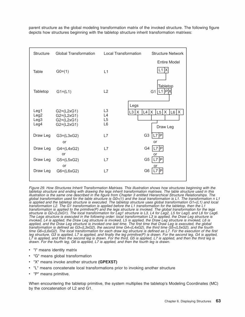
parent structure as the global modeling transformation matrix of the invoked structure. The following figuredepicts how structures beginning with the tabletop structure inherit transformation matrixes:

v "I" means identity matrix

v "G" means global transformation

v "X" means invoke another structure (GPEXST)

v "L" means concatenate local transformations prior to invoking another structure

v "P" means primitive.

When encountering the tabletop primitive, the system multiplies the tabletop's Modeling Coordinates (MC)by the concatenation of L2 and G1.

Figure 29. How Structures Inherit Transformation Matrixes. This illustration shows how structures beginning with thetabletop structure and ending with drawing the legs inherit transformation matrixes. The table structure used in thisillustration is the same one described in the figure from Chapter 3 entitled Hierarchical Structure Relationships. Theglobal transformation used for the table structure is G0=(1) and the local transformation is L1. The transformation n L1is applied and the tabletop structure is executed. The tabletop structure uses global transformation G1=(L1) and localtransformation L2. The G1 transformation is applied before the L1 transformation for the tabletop, then the L1transformation is applied to the primitive(P) and the legs structure is invoked. The global transformation for the legsstructure is G2=(L2xG1). The local transformation for Leg1 structure is L3, L4 for Leg2, L5 for Leg3, and L6 for Leg6.The Legs structure is executed in the following order: local transformation L3 is applied, the Draw Leg structure isinvoked, L4 is applied, the Draw Leg structure is invoked, L5 is applied, the Draw Leg structure is invoked, L6 isapplied, and the Draw Leg structure is invoked one last time. The first time that Draw Leg is executed, the globaltransformation is defined as G3=(L3xG2), the second time G4=(L4xG2), the third time G5=(L5xG2), and the fourthtime G6=(L6xG2). The local transformation for each draw leg structure is defined as L7. For the execution of the firstleg structure, G3 is applied, L7 is applied, and finally the leg primitive(P) is drawn. For the second leg, G4 is applied,L7 is applied, and then the second leg is drawn. For the third, G5 is applied, L7 is applied, and then the third leg isdrawn. For the fourth leg, G6 is applied, L7 is applied, and then the fourth leg is drawn.


When encountering the leg primitive, the system multiplies the leg's coordinates by the concatenation ofthe appropriate inherited matrix and the leg's local modeling transformations. Notice that L3 through L6 alluse the replace concatenation type option. As discussed in Chapter 3. Structures, the concatenation typeoption specifies how the modeling transformation element operates on the current modeling transformationvalues.

Drawing the first leg entails multiplying the leg's coordinates by a concatenation of L7 and G3.

Drawing the second leg entails multiplying the leg's coordinates by a concatenation of L7 and G4.

Drawing the third leg entails multiplying the leg's coordinates by a concatenation of L7 and G5.

Drawing the fourth leg entails multiplying the leg's coordinates by a concatenation of L7 and G6.

Your application may override the inherited global transformation by using the Set Global Transformation(GPGLX2 and GPGLX3) subroutine. The new global transformation matrix replaces the previous globalmatrix.

Resolving Detectability, Highlighting, and InvisibilityPrimitives may be grouped by your application into application-defined classes. By using filters, providedby the graPHIGS API, your application may control the detectability, highlighting and invisibility of theseprimitives. During structure traversal, the system manages the current class name values and resolveswhich primitives are detectable, highlighted, or visible, based on the primitive's class specification.

To this end, the system supports the following three inclusion and exclusion filters:

v pick filter (one pair per pick device)

v highlighting filter (one pair per workstation)

v invisibility filter (one pair per workstation)

These filters operate independently of each other. Making a particular class of primitives detectable, forexample, does not affect whether that class is highlighted or visible.

To provide dynamic control over which classes are detectable, highlighted, and visible, each filter containsan inclusion filter and an exclusion filter.

These filters control the detectability, highlighting, and invisibility of entire classes of output primitives.

The system provides a consistent set of rules that govern the interrelationships between classes assignedto inclusion and exclusion filters. An output primitive is detectable, highlighted, or invisible if and only ifboth of the following are true:

v It is a member of a class that is specified in a corresponding inclusion filter.

v None of its classes are contained in a corresponding exclusion filter.

When all of the filters are empty, for example, at initialization time:

v primitives are not detectable.

v primitives are not highlighted.

v primitives are not invisible (they are visible).

Inclusion and exclusion filter designations are control subroutine calls that modify the workstation state.The following figure depicts a root structure with class designations:


By proper organization of structure content, your application can modify these characteristics of primitiveswithout structure editing. In the figure, Root structure with class designations, polyline 1 can not be madedetectable, highlighted, or invisible. Polyline 2 is affected by how your application assigns classes 1 and 2to inclusion and exclusion filters. Polyline 3 is affected only by how your application assigns class 1 toinclusion and exclusion filters.

Pick Filter: The Set Pick Filter (GPPKF) subroutine enables your application to specify which classesbelong to a pick device's inclusion and exclusion filters. Using the information in the figure, Root structurewith class designations, an assignment of class 1 to only the pick inclusion filter, makes both polyline 2and polyline 3 detectable.

Highlighting Filter: The graPHIGS API enables your application to control the highlighting of primitives.The Set Highlighting Filter (GPHLF) subroutine enables your application to specify which classes belong tohighlighting inclusion and exclusion filters. Using the information in the figure, Root structure with classdesignations, if your application only assigns class 2 to the highlighting inclusion filter, then only polyline 2is highlighted. Because polyline 3 only belongs to class 1, it is affected only by those changes that affectclass 1 because class 2 is removed before polyline 3 is drawn.

Invisibility Filter: The graPHIGS API lets your application specify whether a primitive or set of primitivesare visible. The Set Invisibility Filter (GPIVF) subroutine lets your application control which classes are in aworkstation's inclusion and exclusion filters. Remember that the default is the absence of classes in eitherfilter. This means that all primitives are initially visible. Using the information in the figure, Root structurewith class designations, if your application assigns class 1 to the invisibility inclusion filter and class 2 tothe invisibility exclusion filter, then polyline 3 becomes invisible. In order to analyze why polyline 2 remainsvisible remember the rules that govern how filters affect primitives. Polyline 2 remains visible because atleast one class (number 2) is in the invisibility exclusion filter. This excludes polyline 2 from becominginvisible.

Updating the WorkstationThe graPHIGS API provides two methods for your application to assure that the display imagecorresponds exactly to the state of the system.

The Redraw All Structures (GPRAST) subroutine forces a new frame action on the specified workstation,and then rebuilds the display based on the current state of the system. A new frame action involvesclearing the screen on the display or feeding a new sheet of paper on a plotter-type device.

The Update Workstation (GPUPWS) subroutine assures that the display exactly matches the state of thesystem. A new frame action occurs only if necessary.

When GPUPWS is called, all deferred actions for the specified workstation are executed without anintermediate clearing of the display surface. If the regeneration flag is set to PERFORM and a new frameaction is necessary the following actions are taken on the specified workstation:

1. If the display surface is not empty the display is cleared.

Figure 30. Root structure with class designations. This illustration shows the root structure containing polyline 1, addclass 1 and class 2 to set, polyline 2, remove class 2 from set, and polyline 3.


2. If the workstation window, viewport, view matrix, view mapping, or view characteristics have changedfor any view, the current entries in the Workstation State List (WSL) are assigned the correspondingvalues from the requested WSL entries.

3. All structures associated with views on the workstation are re-displayed.

With the Update Workstation Asynchronous (GPUPWA) subroutine, transactions with the specifiedworkstation do not wait for an on-going traversal to complete. This means that a traversal may beinterrupted before completion, causing intermediate screen changes to go unseen. (It may be important,for example in animation sequences, to see all updates to the workstation in a sequential fashion. In thiscase, the synchronous Update Workstation (GPUPWS) subroutine should be used. Use GPUPWA when itis necessary to see the most up-to-date screen as soon as possible).

When there are no changes pending at the workstation, and GPUPWS is called, no action occurs. On theother hand, if your application invoked GPRAST in this situation, the workstation clears the display surfaceand re-displays the same image. On a plotter-type device, this can be used to generate many identicalplots.

Deferral ModesDeferral modes let your application control when the graPHIGS API traverses the structure networks andgenerates an image on a particular workstation. The following deferral modes let your application controlthe deferral state of the system:

1=ASAPAs soon as possible

2=BNIGBefore the next interaction globally

3=BNILBefore the next interaction locally

4=ASTIAt some time

5=WAITWhen the application requests it (default).

These modes do not affect when structure editing occurs, rather they affect when structure modificationsare seen on the display surface. Since your application can edit structure networks without changing theoutput image, the image may not reflect the current graphics data within the structure networks. Thesedeferral modes let your application control when to resolve the differences between the structuredefinitions and the image.

When the deferral mode is satisfied, the API traverses the structures and generates an image thatcorresponds to the graphics data in the structure networks and the current settings in the workstation'stables, that is, a GPUPWS is performed.

Your application may choose to defer changes to an image when a lot of editing occurs, in order to bufferthe changes and optimize the transfer of data.

Remember that the GPUPWS subroutine causes an immediate traversal of the structure networks andgeneration of an image on an output device, no matter what deferral mode is in effect.

Deferral modes have many application-defined uses. For example, your application may choose to preventan image change until a particular condition is satisfied.


1=ASAP Deferral Mode: When a workstation is in ASAP deferral state, the API re-traverses all data afterevery program subroutine call and updates the output image. This state introduces the maximum systemoverhead per subroutine call.

2=BNIG Deferral Mode: A workstation in BNIG mode is updated immediately before an interaction occursat any open workstation. For example, suppose workstation one is in ASAP mode and workstation two is inBNIG mode. If an output display operator interacts with workstation one, the system updates workstationtwo before the interaction takes place.

Notice that when your application uses BNIG and it places an input device in Sample or Event mode, thesystem always re-traverses the structure networks, since on every subroutine call an interaction is alwaysunderway. Until the input device mode is changed, the BNIG mode simulates the ASAP mode. This mayadversely affect performance.

3=BNIL Deferral Mode: A workstation in BNIL mode is updated immediately before an interaction occursat that workstation.

For example, suppose that workstation one is in ASAP mode, workstation two is in BNIG mode, andworkstation three is in BNIL mode. If an output display operator interacts with workstation two, then thesystem updates workstation one and two, but not three. However, if the display operator interacts inworkstation three, then the API updates all three workstations.

Notice that when your application uses BNIL and it places an input device in sample or event mode, thesystem re-traverses the structure networks, since on every subroutine an interaction is always underway.Until the input device mode is changed, the BNIL state simulates the ASAP mode. This may adverselyaffect performance.

4=ASTI Deferral Mode: Changes to the image of a workstation in ASTI mode occur in animplementation-dependent way. This implementation treats ASTI the same as BNIL.

5=WAIT Deferral Mode: The WAIT deferral mode is the default mode. In this mode, all changes to aworkstation are deferred until your application explicitly requests them. Your application can causechanges to a workstation in WAIT state by:

v changing the deferral mode to one that necessitates a re-traversal such as ASAP

v issuing a GPUPWS subroutine

Notice that, in this mode, your application defers all changes to a workstation until the GPUPWSsubroutine is issued.

Modification ModesThe graPHIGS API supports three Modification Modes selectable through the Set Deferral State (GPDF)subroutine.

1=NO_IMMEDIATE_VISUAL_EFFECT (NIVE)Establishes an environment in which changes to the image depend on the deferral mode only.

2=UPDATE_WITHOUT_REGENERATIONAllows modifications to the display that require no retraversal.

3=QUICK_UPDATEUseful for trivial updates to large models. (See discussion below.)

For information on the use of these modes, see the The graPHIGS Programming Interface: WritingApplications.


QUICK_UPDATEQUICK_UPDATE mode allows the graPHIGS API, running with XLIB and XDWA device drivers, to show theresults of structure editing functions by direct screen modification, eliminating the need for a completescreen redraw. Use of QUICK_UPDATE should be weighed against the need for thoroughly accurate screencontents, since the results of a QUICK_UPDATE may not be perfectly displayed.

When operating in QUICK-UPDATE mode, the application performs as many structure editing operations aspossible without redrawing the screen. The success of a QUICK_UPDATE depends on the target structureelement and the editing operation. Class name, for example, cannot be changed using QUICK_UPDATE.When the graPHIGS API finds that an operation leaves the display too inaccurate, it terminates theQUICK_UPDATE operation and redraws the screen.

Refer to The graPHIGS Programming Interface: Technical Reference for more information onQUICK_UPDATE.


Chapter 7. Input Devices

Up to now you have seen how to display your graphic model, you will now learn how to make yourapplication interactive. To handle interactive input, the graPHIGS API supports various input devices, givingyour application a great deal of flexibility with regard to how your application interacts with an input deviceoperator.

Advanced topics related to input processing are discussed in Chapter 18. Advanced Input and EventHandling in Part Two. This section describes the basic input device concepts provided by the graPHIGSAPI.

Modes of InteractionThe graPHIGS API supports three modes (Operating Modes) of interaction:

v 1=REQUEST

v 2=SAMPLE

v 3=EVENT

REQUEST Mode InputThis mode establishes a synchronous environment between your application and a chosen device. It is thedefault mode for all devices. In this mode, your application must explicitly request input from a particulardevice. In REQUEST mode, the device is inactive until your application explicitly requests input from thatdevice.

After the request is made the device is activated and your application waits until the operator either entersthe requested input or performs a break action. Pressing a reset-type key is an example of a break action.The break action depends on the logical input device and on the particular workstation. If a break occurs,the logical input value is not valid.

There can be only one outstanding request at a time. A value returns when the operator triggers the inputdevice.

In the sample program introduced in Chapter 1, you have used the REQUEST mode of interaction. Thestatement:

CALL GPRQCH(WSID,1,STATUS,CHOICE)

causes the program execution to halt and wait for the operator to trigger a choice device. Your programwill terminate if the variable Status contains a 1, that is, if the operator performs a break action.

SAMPLE Mode InputWhen your application puts a device in SAMPLE mode, it is immediately activated for manipulation by aworkstation operator. Your application obtains the current values of the input device by explicitly samplingit. For example, your application can obtain the location of the screen cursor at any point in time, throughthe use of SAMPLE mode input.

EVENT Mode InputThis mode establishes an asynchronous environment between your application and a chosen device. Inthis mode, both your application and any corresponding device operate independently of each other. Aninput queue exists which accumulates events from all devices that are in EVENT mode, on all workstations.Any device in EVENT mode can supply data to the input queue. Your application can retrieve input from thequeue without affecting input device operation. Notice that the input queue is centralized and collectsevents from all open workstations.


The graPHIGS API maintains one queue containing the input of all devices. The input is queued, first in,first out, in an event report form. The event report contains the input data and an identification of whichdevice sent the input.

An event is generated each time an input device is triggered by an operator. For example, the trigger of alocator device might be the tip switch on a stylus. Notice that one trigger may cause event reports frommultiple devices to be queued. This means that a single operator action can cause multiple events. Theseare called simultaneous events For example, the pick device and locator device may share the sametrigger. If both devices are in EVENT mode and their common trigger is fired, it generates simultaneous PICKand LOCATOR events, which are placed on the event queue.

Before your application can get queued input, it must first transfer the next item on the queue to a currentevent report area. The Await Event (GPAWEV) subroutine transfers the next item on the queue, if oneexists, to the current event report area.

If no events are queued, the API waits for a time interval specified by your application in the GPAWEVsubroutine. Control returns to your application at the end of the time interval, or when an event arrives onthe queue. After issuing a GPAWEV subroutine, your application can examine the input data contained inthe current event report. This gives your application the opportunity to either process the input data ordiscard it by issuing another GPAWEV subroutine.

To retrieve the data, your application issues a get data programming subroutine call. There is a differentGet subroutine call for each type of queued input data. Getting data is discussed in each “DeviceOperation” section.

Your application can flush the queue of all event reports that belong to a specified device on a specificworkstation using the Flush Device Events (GPFLEV) subroutine.

Your application can also flush all event reports for all devices on a specified workstation using the FlushWorkstation Events (GPFWEV) subroutine.

As discussed in Part Two of this book, the event queue is also used in the processing of asynchronousevents other than those generated by input devices.



Modify your sample program according to the following instructions:

1. In the DECLARE VARIABLES section, please add the following statements:

REALx4 AREA(6),CSIZE(3)INTEGERx4 DATAL,DATA(4),ERRIND,UNITS,ASIZE(3)CHARACTERx8 ACONID, AWSTYPINTEGERx4 IWSID,CLASS,DEVICE,ILEN,OLENDATA DATAL /16/DATA DATA /1,0,0,2/DATA ILEN /8/

2. Replace all the INPUT SUBROUTINES statements with the following:

1 CALL GPQRCT(WSID, ILEN , ERRIND, OLEN, ACONID, AWSTYP)CALL GPQDS(AWSTYP, ERRIND, UNITS, CSIZE, ASIZE)IF(ERRIND.NE.0) GOTO 200AREA(1) = 0.AREA(2) = CSIZE(1)AREA(3) = 0.AREA(4) = CSIZE(2)AREA(5) = 0.AREA(6) = CSIZE(3)CALL GPINCH(WSID,1,1,2,AREA,DATAL,DATA)CALL GPCHMO(WSID,1,3,2)TIME = 10.

100 CALL GPAWEV(TIME,IWSID,CLASS,DEVICE)IF(CLASS.EQ.4) THEN

IF(DEVICE.EQ.1) THENCALL GPGTCH(CHOICE)IF(CHOICE.EQ.1) GOTO 200

ENDIFENDIFGOTO 100

Once you have done the modifications, compile and run your program.

You will notice that the first button of the Lighted Program Function Keyboard (LPFK) is lighted. Press it.The program should terminate. The break action procedure is of no use now, your program will onlyterminate if the LPFK button is pressed.

The modifications you added initialized the LPFK CHOICE device by using the GPINCH subroutine. Then,the GPCHMO defined the EVENT mode as the interaction mode for this device.

The GPAWEV subroutine allows your application to examine the event queue. Pressing the LPFK buttongenerates an event of class 4. Your application then checks to determine if the first button (CHOICE.EQ.1)was pressed. If so, the program terminates. If not, the event queue is examined again.

Device ClassesThe graPHIGS API supports six classes of input devices. Each device class represents a generic physicalinput device.

v 1=CHOICE

v 2=LOCATOR

v 3=PICK

v 4=STROKE

v 5=STRING

Chapter 7. Input Devices 71

v 6=VALUATOR

Because these device classes represent generic physical devices, the API must provide a way for yourapplication to determine the actual capabilities of a specific physical device. Your application can use theappropriate inquiry programming subroutine calls to determine these specific capabilities. Which devicesare supported, their supported prompt echo types, and the maximum workstation supported buffer sizesare all examples of input device characteristics that can be determined using the appropriate inquirysubroutine calls.

These capabilities are summarized for each workstation type in The graPHIGS Programming Interface:Technical Reference. The triggers used by each input device for each workstation type can also be foundthere. Nevertheless, keep in mind that those capabilities may vary, depending on the workstation'sconfiguration. To be sure of a workstation's actual capabilities, use the inquiry subroutines.

CHOICE DeviceThis section discusses how your application manages a CHOICE device in the graPHIGS API environment.A CHOICE device provides a positive integer that represents a selection from a number of choices. Zeroindicates no choice.

The Lighted Program Function Keyboard (LPFK) on the IBM 5080 is an example of a CHOICE input device.The CHOICE prompts on this device are the keys' lights. A lit key typically indicates that the applicationprogram uses this key. The CHOICE device is triggered when an operator presses any key.

Establishing the Operating Mode of a CHOICE DeviceYour application selects an operating mode using the Set Choice Mode (GPCHMO) subroutine. GPCHMOlets your application specify whether the CHOICE device is in REQUEST, SAMPLE, or EVENT mode. Yourapplication defines the operating mode of each CHOICE device, independently. For example, yourapplication might put one CHOICE device, such as a lighted program keyboard in REQUEST mode, and asecond CHOICE device, such as the buttons on a cursor controller in EVENT mode. The default mode isREQUEST.

Providing Initial Values for a CHOICE DeviceYour application initializes the device through the Initialize Choice (GPINCH) subroutine. For example,GPINCH lets your application specify which LPFKs to light. Your application can use this subroutine onlywhen the device is in REQUEST mode, that is, when the device is not active.

In the sample program, the statement:CALL GPINCH(WSID,1,1,2,AREA,DATAL,DATA)

initialized the CHOICE device. The second parameter in this statement indicates to the system that we wantto initialize the Lighted Program Function Keyboard (LPFK). The last two parameters indicate whichbuttons we want to use, thus, the DATA /1,0,0,2/ indicates that we want to light (2=ON) the first button ofthe 32 available in the LPFK.

Some CHOICE devices provide echo types which utilize portions of the display screen. For example, thecurrent CHOICE number can be displayed on the screen. The region of the display surface used for thisecho is specified by the echo area parameter of the GPINCH subroutine. The input device echo is clippedto the application specified echo area.

In the GPINCH statement of the sample program, the parameter AREA indicates the part of the screen wewant to use as the echo area, using Device Coordinates (DCs). The LPFK does not produce any echo onthe screen; nevertheless, the parameter must be present.

In the sample program you are making use of the inquiry facility of the graPHIGS API The statements:


CALL GPQRCT(WSID,ILEN,ERRIND,OLEN,ACONID,AWSTYP)CALL GPQDS(AWSTYP,ERRIND,UNITS,CSIZE,ASIZE)

allow your application to inquire the size, in Device Coordinates (DCs), of the display screen available onyour workstation. The size is returned in the parameter CSIZE Your application then uses this information toinitialize the variable Area needed in the GPINCH subroutine. This facilitates the programming of deviceindependent applications.

Input device initialization subroutine calls may be called only when the device is in REQUEST mode, that is,when the device is not activated.

Obtaining Input from a CHOICE DeviceThe program subroutine call needed to obtain input from a CHOICE device depends on the Operating Modeof that device.

Obtaining Input from a CHOICE Device in REQUEST Mode: In REQUEST mode, your application isresponsible for initiating all interactions with the CHOICE device operator. If your application needs choiceinput from an operator before it can proceed, it asks the operator for input by issuing a Request Choice(GPRQCH) subroutine call.

After issuing the request, the graPHIGS API waits for the operator to satisfy the request. The returnedinformation indicates the status of the input and number of the button that was pushed.

After the requested information is obtained, the system returns control to your application so it can resumeprocessing and determine how to use the returned information.

Obtaining Input from a CHOICE Device in SAMPLE Mode: Setting a CHOICE device in SAMPLE modeactivates the CHOICE device. When your application needs the current value, it issues a Sample Choice(GPSMCH) subroutine. When there is no input, the system continues to report that there is no input.

When your application issues a GPSMCH subroutine, it receives the current CHOICE value as fast as thesystem can supply it. However, lacking synchronization, the use of a CHOICE device in this mode haslimited utility.

Obtaining Input from a CHOICE Device in EVENT Mode: Setting a CHOICE device in EVENT modeactivates the device and establishes an indirect relationship between your application and a CHOICE devicethat is mediated by the event queue.

An operator triggers CHOICE events which are placed on the event queue. Your application can then getthat input from the event queue. This lets operator input and application processing occur asynchronously.

Upon issuing the GPAWEV subroutine, the API gives your application the identification of the devicecorresponding to the current event report. If the input came from a CHOICE device and your applicationwants to use that input, your application issues a Get Choice (GPGTCH) subroutine. GPGTCH returns thevalue of the CHOICE input.

In the sample program, the statement:CALL GPGTCH(CHOICE)

gets input from the current event report. The CHOICE parameter then has a numeric value which identifiesthe CHOICE device key pressed by the operator. Your application can then proceed to use this value withinthe program logic.

LOCATOR DeviceA LOCATOR device provides a position in World Coordinates (WC). Also returned with the LOCATOR input isidentification of the view whose matrix was used to convert the screen position indicated back to World


Coordinates. For a given screen location, the active view of highest priority is used for this conversion.Generally, all LOCATOR input occurs from View 0, the default highest priority view, unless this relationship ischanged using the Set View Input Priority (GPVIP) or Set View Priority (GPVP) subroutine. The tablet andcursor controller are an example of a LOCATOR input mechanism.

Typically, a LOCATOR is a 2D device from which a 3D coordinate is derived. This is done as follows:

The LOCATOR device conceptually fires a ray along the direction of projection into the display surface. Theintersection of this ray with the front of the effective clipping volume is the location returned. The front ofthe clipping volume is typically the near clip plane. By modifying the workstation transform, an applicationmay position the front of the workstation clip volume closer to the View Coordinate System (VCS) originthan the near clip plane. In this case the point is returned from the front of the workstation clip volume.This mechanism guarantees that the locator point returned is always in the current clip volume (that is, it isa displayable point).

Since LOCATOR input is returned in World Coordinates (WC), the Device Coordinate (DC) obtained from theabove method must be converted to WC. This is done by applying the inverse of the viewingtransformation to the DC point to transform it to WC.

Because of the reverse transform required, the view matrix must be invertible (non-singular). If the viewmatrix is not invertible (singular), all locator points from the view are returned as (0,0,0) and an error isgenerated. For a matrix to be invertible, its determinant must be non-zero. Most matrixes typically used forview transformations are non-singular. Therefore, if your application generates a matrix which is notinvertible (singular), you should check the application carefully to be sure that the intended matrix is beingused.

Establishing the Operating Mode of a LOCATOR DeviceYour application selects an Operating Mode using the Set Locator Mode (GPLCMO) subroutine. GPCHMOlets your application specify whether the LOCATOR device is in REQUEST, SAMPLE, or EVENT mode. It also letsyour application define the Operating Mode of each LOCATOR device, independently. For example, yourapplication might put one LOCATOR device in EVENT mode and another in SAMPLE mode. The default mode isREQUEST.

Providing Initial Values for a LOCATOR DeviceYour application initializes the LOCATOR device through the Initialize Locator (GPINLC) subroutine. Forexample, your application can initialize such things as the type of prompt and the location of the prompt onthe display.

The locator echo types include:

v Workstation-dependent Prompts and Echoes

v Small Cross Hair

v Cross Hair

v Rubber Band Line

v Rubber Band Rectangle

v Structure Drag

The locator echo area defines both the region of the display within which the device is active and to whichthe echo is clipped. This can be used as an effective means of feedback to the operator. When theLOCATOR is activated, the echo is displayed at the initial position specified in the GPINLC subroutine.

The LOCATOR device is active only in this echo area. For example, when using the drag structure echo typeon the IBM 5080 workstation, the operator may not drag the structure outside the echo area.

Input device initialization subroutine calls may be called only when the device is in REQUEST mode, that is,when the device is not activated.


Obtaining Input From a LOCATOR DeviceThe subroutine call needed to obtain input from a locator device depends on the operating mode of thatdevice.

Obtaining Input from a LOCATOR Device in REQUEST Mode: In REQUEST mode, your application isresponsible for initiating all interactions with the LOCATOR device operator. If your application needs LOCATORinput from an operator before it can proceed, it asks the operator for input by issuing a Request Locator(GPRQLC) subroutine.

After issuing the request, the graPHIGS API waits for the operator to satisfy the request. As with all locatorinput, the returned information indicates the position of the locator prompt in World Coordinates (WC) andthe view which was used to transform the screen position back to World Coordinates.


Obtaining Input From a LOCATOR Device in SAMPLE Mode: Setting a LOCATOR service in SAMPLEmode activates the locator device.

In order to sample a LOCATOR device, your application issues a Sample Locator (GPSMLC) subroutine.After issuing a GPSMLC subroutine, your application receives the current value of the LOCATOR as fast asthe system can supply it.

Obtaining Input From a LOCATOR Device in EVENT Mode: Setting a LOCATOR device in EVENT modeactivates the device and establishes an indirect relationship between your application and a LOCATORdevice that is mediated by the event queue.

An operator triggers LOCATOR events which are placed on the event queue. Your application can then getthat input from the event queue. This lets operator input and application processing occur asynchronously.

An operator can, by triggering the LOCATOR device, send the cursor's location to the event queue.

When the LOCATOR event becomes the next event on the queue, your application issues a GPAWEVsubroutine. The graPHIGS API gives your application the identification of the device corresponding to thecurrent event report. If the input came from a LOCATOR device and your application wants to use that input,your application issues a Get Locator (GPGTLC) subroutine. GPGTLC returns the value of the LOCATORinput.

PICK DeviceA PICK device provides a pick status, a pick path, and a pick path depth. The pick path uniquely identifiesthe picked primitive and its location in the structure network. The cursor controller is an example of a PICKmechanism.

An example of a pick echo is intensification of an individual primitive using the current input echo color.The default echo color is white.

For polygons with the Edge Flag is OFF, a boundary (solid line) is drawn using the echo color. If the EdgeFlag is ON, the edge of the polygon is drawn.

DetectabilityIn order to pick a primitive, that primitive must have visibility and detectability attribute values of “on” Recallthat the detectability of each primitive is controlled in a manner like highlighting and visibility. For detailsrefer to Highlighting, Detectability, and Invisibility.

Due to your application's ability to construct a hierarchy with multiple instances of structures, one primitivemay appear several times on the view surface. In order to uniquely identify which instance of a primitive is


picked, the system returns a list with PICK identifiers, structure names, and element pointer values. This listrepresents a path through the structure network. With this information, your application can determineexactly which instance of a structure element was picked.

Suppose an operator needs to pick the right-front wheel on a car. Your application defines each part of thecar as detectable. In this scenario, the operator picks the right-front wheel. The system supplies yourapplication with a pick path representing the right-wheel's position in the hierarchy. The following figuredepicts the pick path from the Wheel structure up to the Car structure:

In this case, the system reports that the path from the right-front wheel structure to the root structurepasses through the following structures:

v Wheel

v Right Wheels

v Front Wheels

v Wheels

v Drivetrain

v Car

Notice that the pick path contains six entries, making its depth equal to six. Also, the returned informationis in a bottom-up fashion, as specified in the Initialize Pick (GPINPK) subroutine discussed in ProvidingInitial Values for a PICK Device. A top-down pick path would have returned the identical pick pathinformation in reverse order.

Figure 31. Sample Pick Path for Right-Front Wheel. This illustration shows how a hierarchy is used to determine thepick path. At the top level the Car structure links to the Drivetrain structure. This structure in turn links to the Wheelsstructure. The Wheels structure has a link to the front wheels structure and a link to the rear wheels structure. TheFront Wheels structure has a link to the Right Wheels structure and another link to the Left Wheels structure. TheRear Wheels structure has the same links the Front Wheels structure has. The Right Wheels structure contains a linkto the Wheel structure. The Left Wheels Structure similarly links to the Wheels structure.


The graPHIGS API also provides a means of grouping primitives or several primitives with a type of labelcalled a PICK identifier. This enables the application program to keep track of primitives without needing toknow their element number.

The following figure depicts the returned pick path information:


This information includes the:

v structure identifier of each structure in the pick path

Figure 32. Sample Pick Path Information. This illustration shows the returned pick path information given various casesand a defined structure. Structure 1 is defined as a set Pick ID=1, execute structure 2, set Pick ID=2 and anotherexecute structure 2. Structure 2 is defined as a Polyline 1 primitive, set Pick ID=3, Polyline 2 primitive, and an executestructure 3 call. Structure 3 is defined as a Text 1 primitive, set Pick ID=5, and a Text 2 primitive. In Case A, a pick ofPolyline 1 occurs. The results are as follows starting from the bottom of the structure up and through the first executestructure 2 call. The first result is a structure ID of 2, a pick ID of 1, and a structure element number of 1. The nextresult is a structure ID of 1, a pick ID of 1, and a structure element number of 2. In Case B, a pick of Polyline 2occurs. The results are as follows beginning with the bottom of the structure up and through the first execute structure.The first result gives a structure ID of 2, a pick ID of 3, and a structure element number of 3. The second resultprovides a structure ID of 1, a pick ID of 1, and a structure element of 2. In Case 3, a pick of Text 1 occurs. Theresults are as follows starting from the bottom up and through the second execute structure 2 call. The first resultreturns a structure ID of 3, a pick ID of 3, and a structure element number of 1. The second result provides a structureID of 2, a pick ID of 3, and a structure element number of 4. The third result returns a structure ID of 1, a pick ID of 2,and a structure element number of 4.


v pick identifier active for each structure in the pick path at the specified element in that structure

v structure element number at each level in the pick path

The Request Pick (GPRQPK) subroutine enables your application to request pick input.

Establishing the Operating Mode of a PICK DeviceYour application selects an operating mode using the Set Pick Mode (GPPKMO) subroutine. GPPKMOlets your application specify whether the PICK device is in REQUEST, SAMPLE, or EVENT mode. The OperatingMode of each PICK device is set independently. For example, your application might put one PICK device inEVENT mode and another in SAMPLE mode.

Providing Initial Values for a PICK DeviceYour application initializes the PICK device through the Initialize Pick (GPINPK) subroutine. For example,your application can initialize such things as the pick echo area and the direction in which the pick path isconstructed (top-down or bottom-up).

The pick echo area defines the region of the screen within which the PICK device is active. As with otherinput devices, the pick prompt and echo are clipped to the pick echo area.

A primitive is picked when it intersects a PICK device's pick aperture. In the graPHIGS API, a pick apertureis a rectangular area defined in Device Coordinates (DC) which is attached to the screen cursor.

Input device initialization subroutines may be called only when the device is in REQUEST mode, that is,when the device is not activated.

Obtaining Input From a PICK DeviceThe subroutine call needed to obtain input from a PICK device depends on the Operating Mode of thatdevice.

Obtaining Input from a PICK Device in REQUEST Mode: In REQUEST mode, your application isresponsible for initiating all interactions with the PICK device operator. If your application needs PICK inputfrom an operator before it can proceed, it asks the operator for input by issuing a Request Pick (GPRQPK)subroutine.

After issuing the request, the graPHIGS API waits for the operator to satisfy the request.

As with all PICK input, the returned information contains the status of the pick, the depth of the pick path,and the pick path itself.

After the requested information is obtained, the system returns control to your application so it can resumeprocessing and determine how to use the pick path information.

Obtaining Input from a PICK Device in SAMPLE Mode: Setting a PICK device in SAMPLE modeactivates the PICK device.

In order to sample a PICK device, your application issues a Sample Pick (GPSMPK) subroutine. Afterissuing a GPSMPK subroutine, your application receives the input information as fast as the system cansupply it. Lacking synchronization, the use of a PICK device in this mode has limited utility.

Obtaining Input from a PICK Device in EVENT Mode: Setting a PICK device in EVENT mode activatesthe device and establishes an indirect relationship between your application and a PICK device that ismediated by the event queue.

An operator triggers PICK events which are placed on the event queue. Your application can then get thatinput from the event queue. This lets operator input and application processing occur asynchronously.


Upon triggering the PICK device, the depth of the pick and pick path data are added to the event queue.

When the PICK event becomes the next event on the queue, your application issues a GPAWEVsubroutine call. The graPHIGS API gives your application the identification of the device corresponding tothe current event report. If the input came from a PICK device and your application wants to use that input,your application issues a Get Pick (GPGTPK) subroutine call. GPGTPK returns the value of the PICKinput.

The graPHIGS API also supports extended pick subroutine calls which are discussed in Part Two of thisbook.

STROKE DeviceA STROKE input device provides a sequence of positions in World Coordinate (WC), and the view indexwhose matrix was used to convert the positions from Device Coordinates (DC) to the World CoordinateSystem (WCS). For a given sequence of points, the active view of highest priority containing all of thosepoints is used for this conversion. Generally, all STROKE input occurs from View 0, the default highestpriority view, unless this relationship is changed. The tablet with stylus is an example of a STROKE inputdevice. A STROKE input value is simply a sequence of location values.

Establishing the Operating Mode of a STROKE DeviceYour application selects an Operating Mode of a STROKE device using the Set Stroke Mode (GPSKMO)subroutine. GPSKMO lets your application specify whether the STROKE device is in REQUEST, SAMPLE, orEVENT mode. It also lets your application define the Operating Mode of each STROKE device, independently.For example, your application might put one STROKE device in EVENT mode and another in SAMPLE mode.

Providing Initial Values for a STROKE DeviceYour application initializes the STROKE device through the Initialize Stroke (GPINSK) subroutine. Forexample, your application can specify such things as the number of points in the initial stroke, thecoordinates of each point in the initial stroke, the type of prompt and echo, and the length of the STROKEinput buffer.

The stroke echo area defines the region of the screen within which the STROKE device is active. As withother input devices, the stroke prompt and echo are clipped to the stroke echo area.

GPINSK lets your application provide an initial sequence of STROKE locations. STROKE input values areadded to the STROKE buffer beginning at a location specified in the GPINSK subroutine. This location isreferred to as the editing position within the STROKE buffer. For example, an editing position of one causesthe replacement of the initialized STROKE values beginning at the first point. An editing position of onegreater than the number of initial points appends the STROKE input to the initialized values.

The graPHIGS API enables your application to specify the size of the STROKE buffer, which is the maximumnumber of points allowable for STROKE input. Notice that this may be limited by the maximum buffer size ona given workstation.

STROKE devices have different echo types including:

v Polyline with its attributes

v Polymarker with its attributes

Input device initialization subroutines may be called only when the device is in REQUEST mode, that is,when the device is not activated.

Obtaining Input from a STROKE DeviceThe subroutine call needed to obtain input from a STROKE device depends on the Operating Mode of thatdevice.


Obtaining Input from a STROKE Device in REQUEST Mode: In REQUEST mode, your application isresponsible for initiating all interactions with the STROKE device operator. If your application needs STROKEinput from an operator before it can proceed, it asks the operator for input by issuing a Request Stroke(GPRQSK) subroutine call.


When the operator triggers the STROKE device, the system sends your application the number of coordinatepoints in the array, the array containing the points, and the view in which the stroke occurred.


Obtaining Input from a STROKE Device in SAMPLE Mode: Setting a STROKE device in SAMPLE modeactivates the STROKE device.

In order to sample a STROKE device, your application issues a Sample Stroke (GPSMSK) subroutine call.After issuing a GPSMSK subroutine, your application receives, from the API, the input information as fastas the system can supply it. Lacking synchronization, the use of a STROKE device in this mode has limitedutility.

Obtaining Input from a STROKE Device in EVENT Mode: Setting a STROKE device in EVENT modeactivates the device and establishes an indirect relationship between your application and a STROKE devicethat is mediated by the event queue.

An operator triggers STROKE events which are placed on the event queue. Your application can then getthat input from the event queue. This lets operator input and application processing occur asynchronously.

When the STROKE event becomes the next event on the queue, your application issues a GPAWEVsubroutine call. The graPHIGS API gives your application the identification of the device corresponding tothe current event report. If the input came from a STROKE device and your application wants to use thatinput, your application issues a Get Stroke (GPGTSK) subroutine. GPGTSK returns the value of theSTROKE input.

STRING DeviceA STRING device allows an operator to input text. The keyboard is an example of a STRING inputmechanism. To input a string of characters, the operator presses alphanumeric keys. To trigger a typicalSTRING device, the operator presses the ENTER key.

Establishing the Operating Mode of a STRING DeviceYour application selects an Operating Mode using the Set String Mode (GPSTMO) subroutine. GPSTMOlets your application specify whether the STRING device is in REQUEST, SAMPLE, or EVENT mode. It also letsyour application define the Operating Mode of each STRING device, independently. For example, yourapplication might put one STRING device in EVENT mode and another in SAMPLE mode.

Providing Initial Values for a STRING DeviceYour application initializes the STRING device through the Initialize String (GPINST) subroutine. Forexample, your application can specify such things as the length of an initial string, the text of the initialstring and the maximum length of the STRING input buffer.

The string echo is positioned in the lower left corner of the echo area specified in the GPINST subroutine.String echo is clipped to this area.

GPINST lets your application provide an initial string which is placed in the STRING buffer. String inputvalues are added to the string buffer beginning at a location specified in the GPINST subroutine. Thisposition is referred to as the initial cursor position. For example, a cursor position of one causes


replacement of the initialized string values, beginning at the first character. A cursor position of one greaterthan the number of initial characters appends string input to the initialized values.

The graPHIGS API enables your application to specify the size for the STRING input buffer, which is themaximum number of characters allowable for string input. This may be limited by the maximum supportedbuffer size on a given workstation.

The STRING device echo typically is a string of displayed characters. Notice that your application canprevent the characters from displaying by turning echo OFF.

String Echo Type 2 allows your application to pass a protected prompt string to a STRING device on theInitialize String (GPINST) subroutine. This prompt string is passed in via the data record and is displayedin the lower left corner of the echo area, and is followed by the input buffer echo. The prompt may not betyped over and is not returned with the STRING device input. The initial cursor position is given as an offsetin the input buffer. The specified STRING input buffer size, plus the prompt length, must be less than orequal to the maximum STRING input buffer size as defined in the actual WDT.

Input device initialization functions may be called only when the device is in REQUEST mode, that is, whenthe device is not activated.

Obtaining Input from a STRING DeviceThe subroutine call needed to obtain input from a STRING device depends on the Operating Mode of thatdevice.

Obtaining Input from a STRING Device in REQUEST Mode: In REQUEST mode, your application isresponsible for initiating all interactions with the STRING device operator. If your application needs STRINGinput from an operator before it can proceed, it asks the operator for input by issuing a Request String(GPRQST) subroutine call.

After issuing the request, the graPHIGS API waits for the operator to satisfy the request. When theoperator triggers the STRING device, the system sends your application the length of the string in bytes andthe text string. After the requested information is obtained, the system returns control to your application soit can resume processing and determine how to use the returned information.

Obtaining Input from a STRING Device in SAMPLE Mode: Setting a STRING device in SAMPLE modeactivates the STRING device.

In order to sample a STRING device, your application issues a Sample String (GPSMST) subroutine call.After issuing a GPSMST subroutine, your application receives the string data as fast as the system cansupply it. Lacking synchronization, the use of a STRING device in this mode has limited utility.

Obtaining Input from a STRING Device in EVENT Mode: Setting a STRING device in EVENT modeactivates the device and establishes an indirect relationship between your application and a STRING devicethat is mediated by the event queue.

An operator triggers STRING events which are placed on the event queue. Your application can then getthat input from the event queue. This lets operator input and application processing occur asynchronously.

When the STRING event becomes the next event on the queue, your application issues a GPAWEVsubroutine. The graPHIGS API gives your application the identification of the device corresponding to thecurrent event report. If the input came from a STRING device and your application wants to use that input,your application issues a Get String (GPGTST) subroutine call. GPGTST returns the value of the STRINGinput.


VALUATOR DeviceA VALUATOR device provides a real number. A dial is an example of a VALUATOR input mechanism. Each dialon the workstation is a separate VALUATOR device. For example, the IBM 5080 can have eight VALUATORdevices.


You can now add a VALUATOR device to the sample program. The VALUATOR will allow you to modify the view matrix ofone of the views and provide a zooming effect on the house. Modify the sample program as follows:

1. In the DECLARE VARIABLES section add the following statements:

INTEGERx4 VDATAL,VDATA(4)REALx4 VVALUE,LOW,HIGH,SCALE(2),VMATRX(9)DATA VDATAL /16/DATA VDATA /1,0,0,10/DATA LOW /0.5/DATA HIGH /2.0/

2. In the INPUT SUBROUTINES section, add the following statement before the CALL GPAWEV statement:

CALL GPINVL(WSID,1,1.,4,AREA,LOW,HIGH,VDATAL,VDATA)CALL GPVLMO(WSID,1,3,2)

3. Also in the INPUT SUBROUTINES section, add the following statements between the second ENDIF and GOTO 100statements:

IF(CLASS.EQ.3) THENIF(DEVICE.EQ.1) THEN

CALL GPGTVL(VVALUE)SCALE(1) = VVALUESCALE(2) = VVALUECALL GPSC2(SCALE,VMATRX)CALL GPXVR(WSID,VIEW1,18,VMATRX)CALL GPUPWS(WSID,2)

ENDIFENDIF

Modify your sample program, compile it and run it. Try turning dial 1 of the VALUATOR, there should be azooming effect on the house on the lower left view. Also, the echo of the VALUATOR should be displayed onthe lower left corner of the screen.

Establishing the Operating Mode of a VALUATOR DeviceYour application selects an Operating Mode using the Set Valuator Mode (GPVLMO) subroutine call.GPVLMO lets your application specify whether the VALUATOR device is in REQUEST, SAMPLE, or EVENT mode.It also lets your application define the Operating Mode of each VALUATOR device, independently. If, forexample, your application is interacting with a set of dials, the system defines each dial separately. Thislets your application set one dial in EVENT mode and another in SAMPLE mode.

In the sample program, the statement:CALL GPVLMO(WSID,1,3,2)

sets dial 1 to EVENT mode.

Providing Initial Values for a VALUATOR DeviceYour application initializes the VALUATOR device through the Initialize Valuator (GPINVL) subroutine. Forexample, your application can specify such things as the VALUATOR's initial value, its minimum andmaximum values, and where the VALUATOR's echo is placed.

In the sample program, the statement:CALL GPINVL(WSID,1,1.,4,AREA,LOW,HIGH,VDATAL,VDATA)


initializes dial 1 of the VALUATOR device.

One valuator echo type is a digital display. The digital display changes as the operator moves the valuator.If the VALUATOR device is a dial, your application can specify that one rotation of the dial covers the entirerange, or that a number of rotations covers the range. In the sample, the VDATA parameter establishes 10turns between the LOW and HIGH values. The initial value of the dial is 1.0.

The valuator echo is positioned in the lower left corner of the echo area specified in the GPINVLsubroutine call. The valuator echo is clipped to this area.

Input device initialization functions may be called only when the device is in REQUEST mode, that is, whenthe device is not activated.

Obtaining Input from a VALUATOR DeviceThe subroutine call needed to obtain input from a VALUATOR device depends on the Operating Mode of thatdevice.

Obtaining Input from a VALUATOR Device in REQUEST Mode: In REQUEST mode, your application isresponsible for initiating all interactions with the VALUATOR device operator. If your application needsVALUATOR input from an operator before it can proceed, it asks the operator for input by issuing a RequestValuator (GPRQVL) subroutine.


When the operator triggers the VALUATOR device, the system sends that value to your application.


Obtaining Input from a VALUATOR Device in SAMPLE Mode: Setting a VALUATOR device in SAMPLEmode activates the valuator device.

In order to sample a VALUATOR device, your application issues a Sample Valuator (GPSMVL) subroutine.After issuing a GPSMVL subroutine, your application receives, from the graPHIGS API, the VALUATOR dataas fast as the system can supply it.

Note: VALUATORS in EVENT mode typically provide a more efficient communication mechanism with yourapplication.

Obtaining Input from a VALUATOR Device in EVENT Mode: Setting a VALUATOR device in EVENT modeactivates the device and establishes an indirect relationship between your application and a VALUATORdevice that is mediated by the event queue.

An operator triggers VALUATOR events which are placed on the event queue. On the IBM 5080 workstation,a VALUATOR event is triggered by dial movement. This means that the application is notified of dial valuesonly when they change. Your application can then get that input from the event queue. This lets operatorinput and application processing occur asynchronously.

When the VALUATOR event becomes the next event on the queue, your application issues a GPAWEVsubroutine call. The graPHIGS API gives your application the identification of the device corresponding tothe current event report. If the input came from a VALUATOR device and your application wants to use thatinput, your application issues a Get Valuator (GPGTVL) subroutine call. GPGTVL returns the value of theVALUATOR input.

In the sample program, the statement:CALL GPGTVL(VVALUE)


gets the value of dial 1 from the event queue. This value is then used to initialize the scaling vector whichin turn is used to determine the view matrix VMATRX for the zooming effect. The matrix is calculated usingthe utility function GPSC2 The GPXVR subroutine is then used to assign VMATRX to view 1 of the WSIDworkstation. An update workstation operation is then needed.


Chapter 8. Structure Editing

In Chapter 3. Structures you learned how to define structure content. The graPHIGS API also providespowerful subroutine calls that enable your application to edit the content (elements) of those structures. Inaddition to discussing those subroutines, this chapter discusses the operations that affect entire structures.

As you read this chapter, keep in mind that structure content editing operations require an open structure.Operations that affect entire structures do not require an open structure.

Structure Content EditingWhen an application program opens a structure, the element pointer points to the last element of thestructure. In an empty structure, the element pointer points to the null element, conceptually element zero.

Your application can add elements one after another, because the graPHIGS API automatically incrementsthe element pointer to each new element.

Inserting Structure ElementsIn order to edit an element within a structure, your application must position the element pointer. Whenprocessing a subroutine call that creates an element, the system either inserts that element into thestructure after the current element pointer or replaces the element pointed to by the element pointer. TheSet Edit Mode (GPEDMO) subroutine controls whether the elements are inserted or replaced. The defaultEdit Mode is 1=INSERT_MODE Therefore, to insert an element, your application must position the elementpointer at the element immediately before the insertion location.

The graPHIGS API provides the Set Element Pointer GPEP subroutine to position the element pointer atany element position within a structure.

If your application specifies a negative number or a zero, in the GPEP subroutine, the system sets theelement pointer at conceptual element zero.

If your application specifies a number in the GPEP subroutine that is greater than the last element'snumber, the system sets the element pointer at the last element.

The following figure depicts a scenario in which your application inserts two label elements into an existingstructure. Notice that your application could have chosen to insert any other valid structure elementinstead.


The graPHIGS API provides the Insert Label (GPINLB) subroutine in order to create a label element withina structure. Your application assigns an integer identifier to each label. These integer identifiers do notneed to be unique.

A label is a type of structure element. It may be used for anything. It has no graphical effect. ThegraPHIGS API provides labels so your application can more easily edit structure content.

With labels, your application can delineate an element or group of elements, then later find that element orelement group by advancing the element pointer to a specified label.

In the figure, Inserting Elements, your application opens the structure with the GPOPST subroutine. Afteropening the structure, the current element pointer points to the last element in the structure.

Figure 33. Inserting Elements. This illustration shows a scenario in which your application inserts two label elementsinto an existing structure.


In this scenario, your application uses the GPEP subroutine to position the element pointer immediatelybefore the desired insertion point.

Your application then inserts a label “d”, using the GPINLB subroutine. After the insertion, the systempositions the current element pointer at the inserted element, and renumbers the following elements.

Next, your application uses the Offset Element Pointer (GPOEP) subroutine to position the element pointerforward or backward in the structure. The system adds the positive or negative offset value specified in theGPOEP subroutine to the current element pointer value. If the resulting value would move the elementpointer outside of the structure, the system moves the element pointer to the nearest end of the structure,and issues a warning.

After your application uses the GPINLB subroutine to insert another label “g”, the system renumbers thefollowing elements.

Another way to position the element pointer is by using one of the following subroutines:

v Set Element Pointer at Label (GPEPLB)

v Set Element Pointer at Pick Identifier (GPEPPK)

v Locate Element Pointer at Element Code (GPEPCD)

GPEPLB lets your application position the element pointer at any label element within an open structure.GPEPPK does the same for PICK identifier elements. GPEPCD positions the element pointer for anystructure element based on the element's identifier code.

Your application locates a label, PICK identifier, or element code by specifying its integer identifier. Thesystem searches for the next label that has the specified integer identifier, starting at the elementimmediately after the current element pointer. When it finds the identifier, it moves the element pointer tothat position in the structure.

If the system encounters the end of a structure, it resets the element pointer to the first element andcontinues searching for the integer identifier until it finds it or reaches the start element.

Structures can contain more than one label with the same integer identifier. When they do, invokingGPEPLB advances the element pointer to the next label containing the specified integer identifier.GPEPPK operates in an identical fashion.

Deleting Structure ElementsThe graPHIGS API lets your application program delete elements or groups of elements in the followingways:

v by deleting an individual element

v by deleting the elements within a specified range

v by deleting the elements between two labels

Whenever your application deletes an element, or group of elements, the system sets the element pointerto the element before the deleted element or group of elements using method one or two. This lets yourapplication add new elements into the deleted location without moving the element pointer. When usingmethod three, your application can leave the element pointer at either label.

Deleting Individual ElementsTo delete an individual element, your application sets the element pointer to the desired element, thendeletes that element using the Delete Element (GPDLE) subroutine. After deletion, the API sets theelement pointer to the element preceding the deleted element. The following figure depicts the results ofdeleting one element:

Chapter 8. Structure Editing 89

Deleting Elements within a Specified RangeTo delete a range of elements, your application specifies a range of element numbers with the DeleteRange (GPDLER) subroutine. The system deletes all elements within the range, including the specifiedrange elements.

If either number specified in the GPDLER subroutine is outside of the structure's range, the system mapsthat number to the closest end of the structure. For example, if the structure has 20 elements and yourapplication tries to delete the elements between 12 and 30, the system deletes the elements between 12and 20.

In addition, your application program can specify the numbers in either order. Deleting elements between12 and 30 has the same effect as deleting elements between 30 and 12.

After deleting the elements, the system moves the element pointer to the element immediately before thedeleted range, regardless of element pointer's previous position.

The following figure depicts the results of deleting a range of elements:

Figure 34. Deleting One Element. This illustration shows the process to delete an individual element.


Deleting Elements between LabelsTo delete elements between two labels, your application specifies two labels by using a Delete ElementBetween Labels (GPDELB) or Delete Element Group (GPDLEG) subroutines.

When your application issues a GPDELB subroutine, the system initiates a search for the first occurrenceof label one, starting at the element pointer's current position. If the search reaches the end of thestructure, it continues from the beginning of the structure. After finding the first label, the system searchesfor label two in the same manner, including starting at the same original element pointer position. Thesame label structure element will not match both labels if the same label id is specified.

When the system finds both labels, it deletes all elements between, but not including the labels. Noticethat the order in which your application specifies the labels affects the position of the element pointer afterthe deletion. The system resets the element pointer to the first label specified in the GPDELB subroutine.This allows your application to delete the same range and leave the element pointer in either location.

If the system does not find either label, it reports an error.

The function of the GPDLEG subroutine is similar to the GPDELB subroutine in that two labels arespecified to delineate a group of elements to be deleted. GPDLEG differs from GPDELB in the followingways:

v The system does not find either label from the start of the search to the end of the structure, an error isgenerated and the search is discontinued.

v The search for the second label starts at the position of the first label.

v Either, both, or neither of the search labels can optionally be deleted as part of the element group.

The following figure depicts the results of deleting elements between specified labels using the GPDELBsubroutine. In the figure, elements “j” and “m” are labels.

Figure 35. Results of Deleting a Range of Elements. This illustration shows the results of deleting a range of elements.


The graPHIGS API lets your application specify duplicate labels within structures. However, you shouldexercise caution when deleting elements between duplicate labels.

Copying and Moving Structure ElementsThe Copy Structure (GPCPST) subroutine lets your application copy the entire contents of one structureinto another. The system copies all of the elements of a specified structure into the currently openstructure at the location immediately following the current element pointer. The API then moves the currentelement pointer to the last inserted element. The following figure depicts how a copy structure instructionfrom your application is handled. Note that the copied elements are inserted into the structure even if thestructure Edit Mode is set to 2=REPLACE_MODE.

Figure 36. Deleting Elements Between Labels. This illustration shows the results of deleting elements betweenspecified labels using the GPDELB subroutine.


The Copy Element Range (GPCPER) subroutine copies a range of elements from the specified structure,into the open structure following the current element pointer. The API then moves the current elementpointer to the last inserted element.

Using the current element pointer, the Move Element Range (GPMVER) subroutine lets your applicationmove a range of elements to the the location following the element pointer. The API then moves thecurrent element pointer to the last element that was moved.

Closing StructuresThe graPHIGS API lets your application close an open structure. When your application finishes editing theopen structure, it must close the structure before opening another structure. It closes the currently openstructure by using the Close Structure (GPCLST) subroutine.

Figure 37. Copying a Structure. This illustration shows how a copy structure instruction from your application ishandled.



Modifying the sample program according to the following statements will enable you to interactively edit the housestructure.

1. In the DECLARE VARIABLES section, add the following statements:

INTEGERx4 ACTNUM,ACTLEN,CDATA(2),TERM

2. In this same section, modify the data length and data of the choice input device initialization parameters. First,modify the dimension of the variable Data You should have DATA(4) Change it to DATA(7) Then modify the DATAstatements as follows:

DATA DATA /28/DATA DATA /4,0,0,2,1,1,2/

These changes will light the first and fourth Lighted Program Function Key (LPFK).

3. In this same section, change the DATA statement to indicate that the linetype attribute is set to INDIVIDUAL:

DATA ATFLAG /1,1,2/to

DATA ATFLAG /2,1,2/

4. In the DATA CREATION section, modify the the code which creates the second structure as follows:

CALL GPOPST(STRID(2))CALL GPMLX2(TRANSD,POST)CALL GPINLB(1)CALL GPLT(6)CALL GPPLCI(6)CALL GPPL2(5,2,DOOR)CALL GPCLST

5. In the INPUT SUBROUTINES section, after the statement:

IF(CHOICE.EQ.1) GOTO 200

add the following statements:

IF(CHOICE.EQ.4) THENCALL GPOPST(STRID(2))CALL GPEDMO(2)CALL GPEPLB(1)CALL GPOEP(1)CALL GPQED(1,32,ERRIND,ACTNUM,ACTLEN,CDATA,TERM)IF(ERRIND.NE.0) GOTO 200IF(CDATA(2).EQ.6) CALL GPLT(1)IF(CDATA(2).EQ.1) CALL GPLT(6)CALL GPCLSTCALL GPUPWS(WSID,2)

ENDIF

After modifying your sample program, compile and run it. The fourth LPFK should be lit. Press it. The LineType of the door should change from dashed to solid. Press it again. It should change back to dashed.

The instructions you have added modify the door structure by inquiring the structure element type. Theapplication first opens the structure, then editing mode is set to replace, and then the pointer is located atthe label. The pointer is then moved one element down and placed where the Line Type element is. Nowthe application inquires the element type, SOLID_LINE or DASHED, and replaces the element according to theresult of the inquire. The structure is then closed and the workstation updated.


Operations on Entire StructuresThis section discusses operations that affect entire structures. These operations do not require an openstructure. In fact, only the empty structure operation can be done in either the structure open or closedstate. For your application to delete structures, the system must be in the structure closed state.

The following figure depicts a structure network:

The following figure depicts the results of an empty operation applied to the structure network in the figure,Sample Structure Network Before Empty and Delete Operations:

Figure 38. Sample Structure Network Before Empty and Delete Operations. This diagram shows a network of sixstructures.


The following figure depicts the results of a delete operation applied to the structure network in the figure,Sample Structure Network Before Empty and Delete Operations:

Figure 39. Results of an Empty Structure (GPEST) subroutine. This illustration shows the results of an emptyoperation applied to the structure network.

Figure 40. Results of a Delete Structure (GPDLST) subroutine. This illustration shows the results of a delete operationapplied to the structure network.


Emptying a StructureYour application can delete a structure's content by issuing the Empty Structure (GPEST) subroutine. Thislets your application empty open or non-opened structures. If the emptied structure is open, the graPHIGSAPI resets the element pointer to the conceptual element zero.

The figure, Results of an Empty Structure (GPEST) subroutine, depicts the results of emptying structure 4.Notice that this does not remove the reference to structure 4 from structures 2 and 3. However, it doesdisconnect structures 5 and 6 from structures 1, 2, 3, and 4.

Deleting StructuresThe graPHIGS API enables your application to delete an individual structure, a group of structures, or allstructures.

The Delete Structure (GPDLST) subroutine removes all references to the identified structure, since astructure exists by reference. The figure, Results of a Delete Structure (GPDLST) subroutine, depicts theresults of a Delete Structure subroutine call. Notice that the deletion of structure 4 also implies removingall references to structure 4. Notice also that although structures 5 and 6 still exist, they are no longerconnected to structures 1, 2, and 3. Conceptually, deleting an individually identified structure involvesdeleting “upward” in the hierarchy and also deleting the elements that reference the identified structure.

The Delete Structure Network (GPDLNT) subroutine deletes a specified structure and all structures itreferences. These include:

v all structures referenced directly in the element list of the specified structure

v all structures referenced indirectly as part of the network emanating from the specified structure

The following figure shows the results of deleting a structure network—again structure number 4 from thefigure, Sample Structure Network Before Empty and Delete Operations. Notice that the deletion ofstructure 4 removes not only the references to structure 4, but also the network of all structures thatcomprise structure 4, including structures 5 and 6.

The Delete Structure Network Conditionally (GPDLNC) subroutine deletes a specified root structure andconditionally deletes all of the structures referenced, both directly and indirectly, by the root structure. Onlythose structures which are not referenced directly or indirectly by other root structures will be deleted. Forexample, suppose your application creates the following structure network:

v structure A is the root structure which executes structure B

v structure B executes structure D

v structure C is a root structure which also executes structure D

Figure 41. Results of a Delete Structure Network (GPDLNT) subroutine. This illustration shows the results of deleting astructure network.


If your application invokes GPDLNC to conditionally delete the structure network originating at structure A,only structures A and B will be deleted. Structure D will not be deleted because structure C, which is notpart of structure A's network, also references structure D.

The Delete All Structures (GPDAST) subroutine causes the system to delete all structures, their identifiers,and their contents.


Chapter 9. Inquiry Subroutines

A device-independent Application Programming Interface (API) does not guarantee that all programs runidentically on all supported devices. A device-independent API provides the tools that allow properly writtenapplication programs to run identically on all supported devices.

In order for your applications to run on other workstations in the future, your application should adapt to aworkstation's capabilities. That is why the key to creating device-independent programs involves the properuse of inquiries to determine the specific capabilities of a system and its workstations.

Device-independent applications need not perform any differently than device-specific applications. Youmust initially invest more effort in program development. The payback is the reduction of effort in migratingthe application to other supported graphics devices. If programmed properly, your application can rununmodified on other than the original target workstation.

Inquiries enable your application to determine:

v the capabilities of the system

v the state of the system

v information about a workstation's capabilities

v information about a workstation's state

v information about structures and their content

This chapter discusses categories of inquiries. It does not cover every inquiry subroutine call. It presentssome important, commonly used inquiries. Refer to The graPHIGS Programming Interface: SubroutineReference for more information about each inquiry subroutine. Refer to The graPHIGS ProgrammingInterface: Technical Reference for the content of state lists and description tables.

System Related InquiriesSystem related inquiries let your application inquire into the system's operating states, state lists, anddescription table. System related inquiries can be used to inquire information such as:

v the maximum number of simultaneously open workstations

v the current operating states of the system such as the workstation state and the structure state

v the currently open structure's identifier

v the current element pointer value

v whether there are more simultaneous events on the input queue

v supported text fonts and their characteristics

v information about the workstation and views to which a structure is associated

Workstation Related InquiriesThe purpose of workstation inquiries is to enable your application to inquire the state of a workstation, andadapt to its capabilities, such as differing screen sizes, number of supported colors, and supported inputdevices.

In order to determine such workstation-dependent capabilities, your application queries a workstation'sdescription table (WDT) and a workstation's state list (WSL).


Workstation Description TableAll inquiries whose first parameter is a workstation type inquire information from the WDT corresponding tothat workstation type. The values in the WDT are provided by and initialized by the system. It contains allof the workstation's defaults. It also contains all of the general characteristics of that workstation's type.

Certain values in the WDT are configuration variable. These values depend on the type and configurationof each workstation. When the graPHIGS API opens a particular workstation, it obtains the necessarydevice-specific information, then inserts that information and creates an actual WDT for that workstation.

Each actual WDT is identified by a unique system generated workstation type which can be inquired usingthe Inquire Realized Connection and Type (GPQRCT) subroutine. GPQRCT takes a workstation identifieras its' first parameter and returns both the actual connection identifier and workstation type for theworkstation. The actual workstation type can then be used in any WDT inquiry to determine the actualcapabilities of the workstation.

WDT inquiries can be used to inquire information such as:

v default bundle table definitions

v the extent of support for the graPHIGS API output primitive attributes

v default input device support

In the sample program, the statements:CALL GPQRCT (WSID, ILEN, ERRIND, OLEN, ACONID, AWSTYP)CALL GPQDS (AWSTYP, ERRIND, UNITS, CSIZE, ASIZE)

inquire the actual maximum display surface size of the workstation whose identifier is WSID These inquiriesallow the sample program to run on all supported workstations.

Workstation State ListAll inquiries whose first parameter is a workstation identifier, inquire information from the WSLcorresponding to that open workstation. The values in the WSL reflect the current state of the workstationwhen the workstation is open.

For example, the Inquire Highlighting Filter (GPQHLF) subroutine will return the current highlighting filterlists for a specified workstation identifier.

Structure Related InquiriesStructure related inquiries let your application inquire the existence and content of structures.

To inquire the contents of an element within a structure, the structure must be open. Your application mustfirst set the current element pointer at the target element, then issue the appropriate inquiry.

The graPHIGS API provides a rich variety of inquire element subroutine calls. For example, to inquire thelength (in bytes) and element code for a set of structure elements, use the Inquire List of Element Headers(GPQEHD) subroutine.

Next, to obtain the contents of a set of structure elements, use the Inquire List of Element Data (GPQED)subroutine. Both GPQEHD and GPQED return structure element information starting at the structureelement pointed to by the current element pointer. The format of a structure element is described in ThegraPHIGS Programming Interface: Technical Reference.


Part 2. Advanced


Chapter 10. Advanced Concepts

This chapter introduces advanced concepts that are part of the graPHIGS API Version 2. These topics arebased on proposed extensions to the PHIGS standard called "PHIGS+" concepts presented in this part ofthe book involve an organizational change that divides the graPHIGS API into two distinct parts; thegraPHIGS API shell and the graPHIGS API nucleus. The shell is tightly coupled to the user application andperforms syntax checking and building of the graphics data stream. The nucleus, on the other hand, istightly coupled to the resources used by a graPHIGS API application such as structure stores andworkstations. A nucleus manages the resources that may be shared simultaneously by a number ofapplication processes. Each application process is a separate thread of execution with its own shell butattached to the same nucleus. By dividing your application into multiple processes, you can distribute partsof the application to the workstation as a Distributed Application Process (DAP).

Applications written to run under Version 1 of the graPHIGS API should still run under Version 2. For afurther discussion of Version 1 and Version 2 compatibility, please see Appendix B. Compatibility.

Some of the advanced graPHIGS API capabilities include:

v Image display functions

v Advanced event handling; including update complete events and application defined event handlers

v Non-Uniform Rational B-Spline (NURBS) for curve and surface primitives

v Advanced rendering for complex designs

v Control over frame buffer operations

v Advanced input device operations and control

v Advanced structure editing functions

v Additional methods for controlling structure traversal

v Functions to set the line style pattern, marker shape, and hatch

v Advanced text control including filled characters, proportionally spaced characters, and shearing ofcharacters

This chapter describes the basic concepts for controlling the various new components of the graPHIGSAPI products. These components are supported to satisfy the following requirements:

v Avoid duplicate graphical data on a host and a workstation

v Perform part of a host application within a workstation

v Provide multi-application access to a workstation

The following section explains how to create and manipulate graphical data on a remote workstation. It willalso point out the best mechanism to support such remote data manipulation. Access to the sameworkstation from multiple application processes is described as well, and you will learn how to maintain theintegrity and security of each resource and application process.

Following is a list of the major differences between Version 1 and Version 2 of the graPHIGS API:

v The graPHIGS API Version 2 is divided into two major components, a graPHIGS API shell and agraPHIGS API nucleus. An application process has only one shell, but it may be connected to one ormore nuclei.

v The concept of central structure store is extended to multiple structure stores in a graPHIGS APInucleus. Structure stores are completely independent of each other. For example, an Execute Structureelement within a structure store can only reference a structure within the same structure store. Eachstructure store can be shared by multiple application processes through multiple shells, and can bedisplayed on any workstation within the same nucleus.


v A workstation is not considered to be a resource directly owned by an application process but isconsidered to be a resource owned by a graPHIGS API nucleus which may be accessed by multipleapplication processes.

v All releases of the graPHIGS API on all levels of the operating system on the RS/6000 follow theVersion 2 architecture.

The graPHIGS API EnvironmentThe following is a typical example of the graPHIGS API environment:

Components of the graPHIGS API EnvironmentWithin this picture, the boxes roughly represent the following components:

Node A system consisting of a set of hardware and an operating system on which one or more taskscan run simultaneously.

Transport LayerThe transport layer provides communication between the shell and nucleus whether it is network

Figure 42. The graPHIGS API Environment. This illustration shows three application processes and their interactionwith the graPHIGS nucleus. Each application process contains the application code, the graPHIGS shell, andOS/Communications. The graPHIGS nucleus consists of OS/Communications, structure stores, and workstations. ThegraPHIGS Nucleus directly interfaces with the display unit. The transport layer is formed by the OS/Communicationsportion of each application process and the graPHIGS nucleus. Network communication or inter-processcommunication takes place within this layer.


communication or inter-process communication. The communication methods used by thetransport layer include SOCKETS, GAM, and direct subroutine calls.

ApplicationA unit of software that can be individually executed on a node. Each unit may be an entireapplication or may be one of several cooperative processes that comprise the application.

The graPHIGS API ShellA component of the graPHIGS API products that controls communication between an applicationprocess and one or more nuclei.

The graPHIGS API NucleusThe main component of the graPHIGS API products that performs most of the graPHIGS APIfunctions. One graPHIGS API nucleus can handle multiple workstations, structure stores, imageboards, and font directories. A nucleus can accept requests from multiple application processesthrough multiple graPHIGS API shells.

The graPHIGS API WorkstationA unit consisting of one logical display surface and a set of logical input devices which maycorrespond to a physical terminal, a virtual terminal or a window on a physical/virtual terminal.

Structure StoreA storage unit corresponding to the central structure store in the Version 1 graPHIGS APIproducts. There may be multiple structure stores in a graPHIGS API nucleus. Structures in astructure store within a given nucleus can be displayed on any of the graPHIGS API workstationsthat are controlled by the same nucleus.

Font DirectoryA font directory is a repository for application fonts that reside in the memory accessible to anucleus.

Image BoardAn image board is a nucleus resource that allows your application to store and display image data.

Resources of the NucleusAs described above, structure stores, workstations, image boards, and font directories reside in agraPHIGS API nucleus and can be shared by multiple application processes, through multiple shells.Therefore, they are called resources of the graPHIGS API nucleus.

Within a nucleus, each resource is identified and referenced by a tag called a resource identifier Aresource identifier is not the same as the identifier used in the graPHIGS API subroutine calls, such as theworkstation identifier of the Open Workstation (GPOPWS) subroutine. To be able to use any of theadvanced graPHIGS API functions, the workstation identifier is assigned by the application while theresource identifier is assigned to a resource by the nucleus when the resource is created. Regardless ofhow many application processes connect to the nucleus or what identifiers the processes use for theresource, each resource identifier is always unique within a specific nucleus. Nucleus resources which anapplication process can access are considered attached to the application.

When a resource is created at the request of your application process, it is implicitly attached to yourapplication. A resource can also be attached to the application explicitly via the Attach Resource (GPATR)subroutine. In either case, your application process can assign its own identifier to the resource. Once aresource is attached to your application and has been assigned an application identifier, it is alwaysreferred to by the application identifier. Mapping between the application identifier and a resource identifieron the nucleus is automatically performed by the graPHIGS API shell.

The graPHIGS API ShellAn application process must have a graPHIGS API shell. Issuing the Open graPHIGS (GPOPPH)subroutine creates a graPHIGS API shell.

Chapter 10. Advanced Concepts 105

The graPHIGS API shell is responsible for receiving the parameters of the application's subroutine calls,validating them for correct syntax and for ensuring that calls are made in the correct sequence. The shellalso builds the request in a form that is expected by the nucleus. This may involve data conversion suchas IBM floating-point format to IEEE floating-point formats, ASCII-to-EBCDIC, and byte-swapping. Theshell is also responsible for receiving responses and events from a nucleus and performing any necessaryconversions. A nucleus response is the return of information to the shell that was directly requested by theshell through a previous request to the nucleus. Events are generated independently by the nucleus for avariety of reasons and sent to the shell asynchronously. Typical types of events include input device dataand errors. The shell also provides trace facilities and error logging.

To perform these functions, each shell maintains the following information:

v For each connected nucleus:

– A nucleus identifier

– A communication path to the nucleus.

v For each resource which is currently attached to the shell:

– An application identifier of the resource

– A nucleus identifier which owns the resource

– A nucleus identifier of the resource

Note that each resource has two identifiers, an identifier assigned by the application and a resourceidentifier assigned by a nucleus. By keeping this information, the shell can always perform mapping froman application identifier to a resource identifier assigned by a nucleus and vice versa. For almost allgraPHIGS API subroutines, a resource (workstation, structure store, etc.) is referred to by its applicationidentifier. However, when your application attaches to a resource that currently exists in a nucleus, it mustuse the resource's nucleus resource identifier. Use the Inquire Nucleus Resource Identifier (GPQNCR)subroutine to find the resource identifier of a resource assigned by the nucleus.

The graPHIGS API shell is terminated by the Close graPHIGS (GPCLPH) subroutine. If there are anynuclei connected to the shell, the Close graPHIGS subroutine call removes all of these connections.

Conceptually, a shell can access any nucleus on any node if there is a physical communication pathbetween them. However, a given shell may have limitations as to which nuclei can be accessed, andwhich graPHIGS API subroutines are supported. Within each shell there is a graPHIGS API shelldescription table (PDT) and a graPHIGS API shell state list (PSL). By issuing the supported PDT and PSLinquiries, you may determine the capabilities, limitations, and state of a shell.

The graPHIGS API NucleusGenerally speaking, a graPHIGS API nucleus exists and works independently of any graPHIGS API shellor application. A nucleus may run in a S/370, AIX®, or 6090 environment and is created either through anenvironment-dependent mechanism outside of the graPHIGS API or when an application process tries toconnect its shell to a nucleus.

A nucleus that exists in the same process is called a private nucleus. Only the shell that initiated theprivate nucleus may communicate with that nucleus. If a nucleus exists in a different process than theapplication, then that nucleus is called a remote nucleus (whether or not the nucleus resides on the samenode as the application). A remote nucleus can communicate with any shell that is allowed to connect to it.

A special type of remote nucleus can exist on AIX®: a child nucleus. A child nucleus is created when anapplication wants to connect to a private nucleus, but the nucleus has special requirements that it cannotfulfill inside the application's process (for example, not being threadable when running on amultiprocessing system or when the X Asynchronous Event Handling extension does not exist — forexample, X11R6). Only the shell that parented the child nucleus may communicate with the child nucleus.


A connection between a graPHIGS API shell and a graPHIGS API nucleus is established by the Connectto Nucleus (GPCNC) subroutine with the following parameters:

v A nucleus identifier

v A nucleus connection method to be used in exchanging data with the nucleus

v A nucleus connection specification

The nucleus connection methods currently supported are listed below:

1=CALLUse the call method when you want your application to use a private nucleus. For applications thatrun on S/390 or AIX®, this is the default method (for applications that do not call the Connect toNucleus subroutine).

2=GAMUse the GAM method (Graphics Access Method) when your application is in a S/390 environmentand the application wants to communicate with on of the following:

v 6090 nuclues

v remote nucleus on AIX® using the graPHIGS API Gateway daemon

v remote nucleus on AIX® using the 6098 with FDDI feature

3=SOCKETSUse a TCP/IP sockets connection to communicate between an application running in a S/390 oran AIX® environment and a remote nucleus on AIX®. If both the application process and thenucleus are on the same node, then local sockets are used. If each process is on a differentmode, remote sockets are used.

The figures below describe the connection methods and corresponding connection specificationssupported by the different combinations of shell/nucleus environments:

Supported Connection Methods

Shell Environment

VM MVS AIX® 6090---------------------------------| | | | |

VM | CALL | N/A | N/A | N/A |Nucleus |-------------------------------|Environment | | | | |

MVS | N/A | CALL | N/A | N/A ||-------------------------------|| GAM or| GAM or|CALL or| |

AIX® |SOCKETS|SOCKETS|SOCKETS| N/A ||-------------------------------|| | | | |

6090 | GAM | GAM | N/A |SOCKETS|---------------------------------

Connection Specifications

Connection Method

1=CALL 2=GAM 3=SOCKETS-----------------------------------------| Null | Filedef | Nucspecx |

VM | (length=0) | (length<=8)| (length>=2)||---------------------------------------|| Null | DDNAME | Nucspecx |

Application MVS | (length=0) | (length<=8)| (length>=2)|Environment |---------------------------------------|

| Null | N/A | Nucspecx |AIX® | (length=0) | | (length>=2)|

|---------------------------------------|


| N/A | N/A | :0 |6090 | | | (length=2) |

-----------------------------------------

N/A Not a valid combinationx Nucspec is set to the following specification:

hostname: nucleus connection number

Where:- hostname specifies the node id of an AIX®

system.- nucleus connection number specifies a

a nucleus on the named system and is a numberin the range of 0-255.

You may choose to have your application call the Connect to Nucleus (GPCNC) subroutine or have thegraPHIGS API make the connect as part of the defaults processing performed by the Open graPHIGS(GPOPPH) subroutine. This may be done as follows if:

v Your application will be using a workstation resource supported in Version 1 and you want thegraPHIGS API to perform the nucleus connection processing, then you do not need to do anythingadditional. When you execute your application, the graPHIGS API automatically connects to a nucleuswith identifier=1 using the CALL connection method.

v Your application will be using a 6090 workstation resource, and you want the graPHIGS API to performnucleus connection processing, then you must specify the default option (DEFNUC) in the ExternalDefaults file (EDF) or Application Defaults Interface Block (ADIB) to indicate this.

v You want to explicitly connect your application to a nucleus, then you must specify the default option(DEFNUC) in the EDF or ADIB to prevent the graPHIGS API from doing the nucleus connectionprocessing. See the The graPHIGS Programming Interface: Technical Reference for the correct syntaxfor specifying the DEFNUC default.

The most important role of the graPHIGS API nucleus is to distribute requests from graPHIGS API shellsto nucleus resource handlers, and to distribute events or errors generated by nucleus resource handlers tograPHIGS API shells. For this purpose, the nucleus maintains the following information for each applicationprocess (shell) connected to the nucleus and each resource existing in the nucleus:

v For each application process (shell) connected to the nucleus:

– A shell identifier

– A message password

v For each resource existing in the nucleus:

– A resource identifier

– An identifier of the shell that created the resource

– A resource password

– A list of shell identifiers to which the resource is currently attached

Similar to the resource identifier, the identifier of each shell is unique within the nucleus and assigned bythe nucleus when the shell is connected to the nucleus. This shell identifier is mainly used to validate anapplication's access to a resource. The application does not need to know the shell identifier except whenthe application wants to communicate with other applications through the graPHIGS API applicationmessage facility. To determine your shell identifier assigned by the nucleus, use the Inquire Shell Identifier(GPQSH) subroutine.

The connection between a shell and nucleus is terminated explicitly by the Disconnect Nucleus (GPDNC)subroutine and implicitly by the Close graPHIGS (GPCLPH) subroutine. When the connection is destroyed,all resources in the nucleus that are attached to the shell are automatically detached from it.


As with shells, some nuclei may have limitations such as the number or type of shells to which the nucleuscan be connected, the number and type of resources that can be created, and the set of functions actuallysupported.

Within each nucleus there is a Nucleus Description Table (NDT) and a Nucleus State List (NSL). Byissuing the supported NDT and NSL inquiries, your application may determine the capabilities, limitations,and state of a nucleus.

The following two sections describe workstation and structure store resources.

Structure StoreA structure store is a repository for structures. Once a connection between your shell and nucleus isestablished, your application can create a number of structure stores in the nucleus, limited only by theamount of memory available to the nucleus and its maximum supported number. The graPHIGS API shellassociates one or more structure stores within the same nucleus to a workstation in order to produceoutput on the workstation. However, only one structure store may be associated with a workstation at anyone time. Associating a structure store to a workstation implicitly disassociates a structure store previouslyassociated. Several workstations within a nucleus may be associated to the same structure store. Yourapplication program is responsible for managing structure names among the structure stores that it owns.

The Create Structure Store (GPCRSS) subroutine creates a structure store resource in the specifiednucleus, and attaches it to the graPHIGS API shell. All structure stores are mutually independent. Forexample, a structure within a structure store can reference only structures within that structure store.Subroutines applied to a structure store affect only that structure store and have no side effects on otherstructure stores. The same structure identifier can be used in more than one structure store withoutconflict.

Your application can access multiple structure stores, therefore, it is important to select the desiredstructure store before editing. Selecting a structure store may be done implicitly when the graPHIGS APIdoes nucleus connection processing or explicitly by your application calling the Select Structure Store(GPSSS) subroutine.

Structure stores can be created and manipulated using one of two methods. The default method, whichprovides compatibility between Version 1 and Version 2 of the graPHIGS API, relies on the automaticconnection of a nucleus and the creation of a structure store. The structure store is also automaticallyselected to be the current structure store so that the following Version 1 code will continue to work:Open graPHIGS (GPOPPH)Open Structure (GPOPST)

.

.

.Edit

.

.

.Close Structure (GPCLST)

To suppress the default creation of both a nucleus and structure store or to allow an existing application torun on a 6090, your application must specify either an Application Defaults Interface Block (ADIB) or usean External Defaults File (EDF). ADIBs and EDFs are discussed in detail in The graPHIGS ProgrammingInterface: Technical Reference When default nucleus and structure store processing creation issuppressed, your application will take the following form:Open graPHIGS (GPOPPH)

(specifying DEFNUC in ADIB or EDF)Connect Nucleus (GPCNC)Create Workstation (GPCRWS)


Create Structure Store (GPCRSS) or Attach Structure Store (GPATR)Associate Structure Store to Workstation (GPASSW)Select Structure Store (GPSSS)Open Structure (GPOPST)

.

.

.(Edit Structure)

.

.

.Close Structure (GPCLST)Close Workstation (GPCLWS)Close graPHIGS (GPCLPH)

In order to display the contents of a structure store on a workstation, the structure store must beassociated to a workstation using the Associate Structure Store to Workstation (GPASSW) subroutine.

A structure store is automatically associated with a workstation when your application issues the OpenWorkstation (GPOPWS) subroutine, and a structure store is currently selected.

If your application has not selected the structure store or uses GPCRWS to create a workstation, then thestructure store will not be automatically associated with the workstation. Using the Detach Resource(GPDTR) enables your application to detach a structure store from its shell. If GPDTR removes the finalreference to the structure store, either through an attachment to a shell or association to a workstation, thestructure store itself is released.

For each structure store within the nucleus, there is a Structure Store State List (SSL). By issuing thesupported SSL inquiries, your application may determine the state of a structure store.

WorkstationsThe Create Workstation (GPCRWS) subroutine creates a workstation resource owned by a graPHIGS APInucleus and attaches the workstation to the graPHIGS API shell. GPCRWS requires the followingparameters:

v A workstation identifier


v Length of the connection identifier

v A connection identifier

v A workstation type

v Zero or more PROCOPT descriptions

The GPCRWS subroutine replaces the Open Workstation (GPOPWS) subroutine and enables yourapplication to specify on which nucleus the workstation is to be opened. It also enables your application tospecify options for the workstation that were previously specified through the External Default File (EDF) orApplication Default Interface Block (ADIB).

Using the GPOPWS subroutine creates a workstation resource on a nucleus with identifier 1.

A workstation can display graphical data from any structure store existing in the nucleus where theworkstation resides. In order to specify which structure store is used for display, use the AssociateStructure Store with Workstation (GPASSW) subroutine. A workstation can display graphical data withinone structure store only. All display subroutines, such as Associate Root with View (GPARV) subroutine,are treated as referring to a structure within the structure store associated with a particular workstation.


Your application can detach a workstation from the graPHIGS API shell using the Detach Resource(GPDTR) or Close Workstation (GPCLWS) subroutine. GPCLWS detaches the workstation resource on anucleus with nucleus identifier 1. If this subroutine removes the final reference to the workstation, theworkstation and all its resources are removed from the nucleus.

For each workstation within the nucleus, there are two Workstation Description Tables (WDT) and aWorkstation State List (WSL). By issuing the supported WDT and WSL inquiries, you may determine thecapabilities, limitations, and state of a workstation.

The two WDTs for each workstation are:

v Generic Workstation Description Table - defines the maximum capabilities of the workstation.

v Actual (or Realized) Workstation Description Table - defines the actual capabilities of the workstation.This description table exists only after the workstation is opened.

To obtain the most accurate information about a workstation, you should inquire its capabilities from theactual workstation description table. In order to do this you must specify the actual workstation type on theinquiry. The actual workstation type is returned by the Inquire Realized Connection and Type (GPQRCT)subroutine.

Communication between a Shell and NucleusTypically, you won't need to know the details of the communication mechanism used between a graPHIGSAPI shell and nucleus. However, to achieve the maximum performance and to fully understand topicsdiscussed in subsequent sections, you must have a general understanding of the communicationmechanism.

Data BufferingData transmitted between a shell and a nucleus consists of a sequence of buffered data structures calledprocedures Most procedures correspond to a subroutine call in the graPHIGS API and are used by thegraPHIGS API to pass information between a shell and nucleus. The length of a procedure is limited bythe I/O buffer size that has a maximum value of 64K bytes. The most important consequence of thislimitation is that the definition data of each output primitive cannot exceed 64K bytes. For example, thenumber of vertices specified in a Polyline 3 primitive must be less than approximately 5,000.

A graPHIGS API shell normally allocates two 64K I/O buffers, one outbound and one inbound, for eachnucleus connection. However, when you want to minimize the amount of storage used by the shell, yourapplication can override the default I/O buffer sizes through the COMBSZ default of an ApplicationDefaults Interface Block (ADIB) or an External Defaults File (EDF).

By default, the data created by a shell is sent to a nucleus when one of the following situations occur:

1. When a graPHIGS API subroutine call requires modification of the content on the display surface of aworkstation. The following subroutines are included in this category:

v Set Deferral State (GPDF)

v Update Workstation (GPUPWS)

v Update Workstation Asynchronous (GPUPWA)

v Redraw All Structures (GPRAST)

2. When a graPHIGS API subroutine call requires data to be retrieved from the nucleus. The data may berequired for the shell but not for the application itself. The following subroutines belong to this group:

v Set Password (GPPW)

v Set Message Password (GPMSPW)

v Request input device subroutine calls

v Sample input device subroutine calls

v Await Event


v Create Workstation (or Open Workstation) (GPCRWS)

v Create Structure Store (GPCRSS)

v Create Image Board (GPCRIB)

v Create Font Directory (GPCRFD)

v Attach Resource (GPATR)

v Detach Resource (GPDTR)

v Activate Font (GPACFO)

v Initiate Application Process (GPINAP)

v Send Private or Broadcast Message (GPSPMS,GPSBMS)

v Synch Request (GPSYNC) state list

v Inquire Requests for information contained in the nucleus (i.e., structure store, workstation andnucleus state list information)

3. When the buffer becomes full.

Two mechanisms are supplied for the application to change the default action for some of these situations.One is the Set Shell Deferral State (GPSHDF) subroutine that enables the application to suppressautomatic data sending caused by the subroutines within the first group of this list. This enables theapplication to realize an animation sequence without causing unnecessary I/O operations between theshell and nucleus. For example, a series of alternating invocations of Set View Matrix and UpdateWorkstation can be accumulated into the I/O buffer and sent to a nucleus with a single I/O operation. Thenucleus would then generate multiple frames on the display surface without I/O overhead between eachframe. Another mechanism to change the default action is provided by the Synchronize (GPSYNC)subroutine that enables the application to force data transmission directly. When the application issuesSynch, any buffered requests are sent to the nucleus immediately.

Data is sent from a nucleus to a shell in the following situations:

1. When a request from a shell requires a response

2. When a request from a shell cannot be processed for some reason (an error will be generated)

3. When another application process requests an application message to be sent to a target application(shell)

4. When a component of the nucleus encounters an asynchronous error related to a resource attached tothe shell

5. When an input device which has been activated by the shell generates an input device event

6. When certain situations generate events (that is, storage threshold has been reached or synchronousworkstation updates have completed)

Unlike the data sent from a shell to a nucleus, the data from a nucleus to a shell will conceptually betransmitted as it is created. When more than one request from a shell is sent in a single I/O operation andthere is more than one response or error related to these requests, the latter may also be buffered toincrease I/O performance. However, such buffering is not visible to the application.

Resource Access SerializationA nucleus can receive requests from multiple shells at any time and is only required to guarantee thefollowing:

v Requests from any given shell are processed sequentially

v An individual request is processed completely before any other request is processed

There is no assurance that requests coming from multiple shells are processed in the global order of theircreation. Therefore, when multiple shells share the same nucleus resource, special care must be taken toprevent the shells from ending up in a deadlock situation where both shells are waiting for the other shellto free up a resource.


Workstation Serialization: When a workstation is shared by multiple shells, usage of the workstation'sinput devices is serialized as follows:

1. When an input device is activated by an application process the device is dedicated to that processuntil the device is deactivated by the process or by an operator's action. An input device dedicated to aprocess cannot be accessed by any other process.

2. When an input device is set to Event or Request mode, only the application process that activated thedevice is given the input data.

Likewise, when an input device is set to Request mode, only the application process that activated thedevice is notified when a break action occurs.

3. When the device is set to Sample mode, any application process can sample the device.

Structure Store Serialization: When a structure store is shared by multiple application processes,access to the structure store is also treated in a special manner. When an application process calls theOpen Structure (GPOPST) subroutine, the currently selected structure store is dedicated to that applicationprocess. All subsequent structure modification requests from other application processes are notprocessed and are blocked by the nucleus, until the 'owning' application process calls the Close Structure(GPCLST) subroutine.

Notice that the structure store state described here is different from the structure state of the graPHIGSAPI shell. The structure state of the shell is mainly used to check whether an application process issuesgraPHIGS API calls in the correct sequence or not. For example, any output primitive subroutines will onlybe processed if the structure is opened to make sure these primitives are correctly stored in a structure.The purpose of the structure store state in the nucleus is not for validity checking but for ensuring thatstructure editing operations are consistent between application processes. For example, the DeleteStructure (GPDLST) subroutine deletes not only the specified structure but also all references to thestructure. If your application issues this subroutine call while another application process has a structureopen, this automatic deletion of structure references (Execute Structure elements) can cause manyproblems.

All requests to a structure store that are blocked by this mechanism are not discarded but processed at alater time. There is no assurance that these blocked requests are processed immediately after the currentowner issues a Close Structure. If the previous owner issues another Open Structure request, thestructure store may be dedicated to the same application process again. Switching between requests fromdifferent application processes is not guaranteed to be performed in any particular order.

Font Directory Serialization: When a font directory is shared by multiple application processes, accessto the font directory is treated in a special manner. When an application process calls the Load Font(GPLDFO) subroutine to load a font into the directory, the specified font directory is dedicated to thatapplication process. All subsequent requests from other processes to access the font directory are blockedby the nucleus until the the load of the font completes. When the load of the font completes, the fontdirectory may then be accessed by other application processes.

Serialization of Image Boards: When an image board is shared by multiple application processes,access to the image board is also treated in a special manner. When an application process calls theWrite Rectangle (GPWRCT) subroutine, requests from other processes to access the image board areblocked by the nucleus until the write to the image board completes. When the write to the imagecompletes, the image board may be accessed by other application processes.

Distributed Application Processes (DAPs)The graPHIGS API gives you the ability to divide your application into multiple Distributed ApplicationProcesses (DAPs). Each DAP is a separate executable graPHIGS API process with its own graPHIGS APIshell. These DAPS are downloaded to the remote nucleus by a connected shell process, using the InitiateApplication Process (GPINAP) subroutine or the Execute Application Process (GPEXAP) subroutine. A


DAP that already exists on the node containing the remote nucleus can be executed by using GPINAP orGPEXAP. The use of DAPS allows you to offload some functions that cannot be performed efficientlyacross a network.

A DAP can perform many diverse functions, including:

v using a valuator to change a view or modeling transformation matrix.

v communicating with a device such as a digitizer that is attached to the node containing the remotenucleus

v performing animation

On a 6090, DAPs are limited by the amount of memory available and the fact that disk files are notavailable. The memory in a 6090 is shared by other components, such as the graPHIGS API nucleus,operating system, and other DAPS. Therefore, only those functions that can be performed faster in the6090 Graphics System by eliminating the communications overhead with the host, should be performedwith DAPS that run on a 6090.

On an AIX® system, a DAP has the same privileges and restrictions as any other application on thesystem, as shown in the following figure:

For a discussion of compiling, starting, and terminating DAPs, see The graPHIGS Programming Interface:Writing Applications.

One method for two application processes to communicate is through the application message facilitiesprovided by the graPHIGS API as discussed in the following section.

Communication between Multiple Application ProcessesIn order for multiple application processes to communicate, the graPHIGS API provides a message facilityused to send application defined messages from one application process to the event queue of anotherprocess. The messages are sent using the Send Broadcast Message (GPSBMS) and Send PrivateMessage (GPSPMS) subroutines and can be retrieved from the event queue by the target process usingthe Get Message (GPGTMS) subroutine.

The format of the message event is defined by the graPHIGS API, but there is no restriction on thecontents of the application message. The graPHIGS API shell and nucleus do not perform any validity

Figure 43. Dap Organization. This illustration shows how a DAP is like any other process on the system. In thisillustration, system 1 is running a parent application process and the graPHIGS API shell. System two is running agraPHIGS nucleus and 4 DAPs. Each DAP runs its own shell and this shell interfaces with the nucleus. The nucleus insystem 2 interfaces with the graPHIGS API shell and the parent application process.


checking or implicit conversion on the message data and no additional information, such as the originatorof the message, is supplied in the message event. The graPHIGS APIthat performs the followingconversions:

v EBCDIC to ASCII character encoding

v ASCII to EBCDIC character encoding

v IBM single precision floating point to IEEE single precision floating point

v IEEE single precision floating point to IBM single precision floating point

v Byte order swapping

GPCVD performs the conversions based on the environment your application is running in and the targetenvironment specified as a parameter to GPCVD With GPCVD, one application process can convert datato a form recognized by the target environment or by its own environment. The data can be in the form ofeither a character string, integer array, floating-point array, or data record.

In order to prevent an application process from receiving unexpected messages sent by unknownapplications, the following two levels of protection are provided:

1. When a shell is connected to a nucleus, the nucleus assigns the shell an identifier known only to theapplication which owns the shell. The identifier is called a shell identifier and can be retrieved throughthe Inquire Shell Identifier (GPQSH) subroutine.

2. Each application process can set a message password for its shell using the Set Message Password(GPMSPW) subroutine. As with passwords of resources, the message password can take one of thefollowing values:

0=NONENo application messages are received.

-1=ALLAll application messages are received.

UNIQUE INTEGEROnly the application message sent with the matching password are received.

The message password of a shell is set to 0=NONE when a shell and nucleus are connected and can be setto another value using the GPMSPW subroutine.

The Send Private Message (GPSPMS) subroutine has the following parameters:

v A nucleus identifier to which the target shell is connected

v A shell identifier of the target shell

v A message password of the target shell

v A major code

v A minor code

v Length of the message

v A variable length byte string (the message)

This message is sent to the target shell only when the shell has message password ALL, or when thespecified message password matches with that of the target shell.

Because the broadcast message has no specific target, the application need not specify any shell identifieror message password. The broadcast message is sent to all shells attached to the specified nucleus whichhave their shell password ALL. The Send Broadcast Message (GPSBMS) subroutine has the followingparameters:


v A major code


v A minor code

v Length of the message

v A variable length byte string (the message)

A typical scenario for two applications processes to share a resource by using the application messages ispresented below. The resource being shared is a structure store created by the first application process.

v Application Process 1:

1. Opens graPHIGS (GPOPPH)

2. Connects to the nucleus (GPCNC)

3. Obtains its own shell identifier from the nucleus (GPQSH)

4. Creates a structure store resource (GPCRSS)

5. Obtains the structure store resource identifier as it is known on the nucleus (GPQNCR)

6. Assigns a password to the structure store resource (GPPW)

7. Sets its own shell message password to ALL (GPMSPW) so it can receive broadcast messages

8. Waits for broadcast messages from an application (GPAWEV)



2. Connects to the same nucleus (GPCNC) as application process 1

3. Obtains its own shell identifier from the nucleus (GPQSH)

4. Sets its own shell message password so it will receive messages only from processes that know themessage password (GPMSPW)

5. Sends a broadcast message to any application process connected to the same nucleus (GPSBMS)

Note: The message contains the shell identifier and message password of application 2.

6. Waits for a private message from an application (GPAWEV)


1. Receives notification that an event has arrived (GPAWEV)

2. Gets the data contained in the message event (GPGTMS)

3. Uses GPCVD to convert the data to a form recognizable by the receiving environment.

4. Sets its own shell message password to some unique value so it will not receive other broadcastmessages (GPMSPW)

5. Sends a private message to the application process 2 containing its own shell identifier, messagepassword, the nucleus resource identifiers and passwords of the resources to be shared (GPSPMS)

Note: A private message is used because application process 1 now has the shell identifier andmessage password of application process 2 from the data passed in the broadcast message.


1. Receives notification that a message event has arrived (GPAWEV)

2. Obtains data contained in the message event (GPGTMS)

3. Uses GPCVD to convert the data to a form recognizable by the receiving environment.

4. Attaches to the structure store resource created by application process 1 (GPATR)

Each process can now edit structures within the same structure store.

Resource SharingOne application process can attach a nucleus resource (a workstation, structure store, image board, orfont directory) created by another application process to its process by using the Attach Resource(GPATR) subroutine with the following parameters:

v Resource type


v An application identifier to be assigned to the resource

v A nucleus identifier which owns the resource

v A nucleus resource identifier of the resource

v A password assigned to the resource.

The resource type parameter must indicate one of the following resources:

v Workstation

v Structure store

v Image Board

v Font directory.

To be able to attach a resource, your application must know the resource's nucleus resource identifier andpassword. Initially, this information is known only to the application process that created the resource. Thenucleus resource identifier is assigned by the nucleus when the resource is created and can be retrievedusing the Inquire Nucleus Resource Identifier (GPQNCR) subroutine.

The password of each resource can have one of the following values:

0=NONEOnly the application that created the resource can access it

-1=ALLAny application can access (attach) the resource

UNIQUE INTEGERAny application with the correct password can access(attach) the resource.

Each time a resource is created in a nucleus, the resource's password is set to 0=NONE so it cannot beshared by any other application process. Therefore, when two or more application processes want toshare a resource, its password must be explicitly set to some value other than zero by the Set Password(GPPW) subroutine. For security reasons, this subroutine allows only the application process that createdthe resource to change its password.

A scenario for two application processes to share a resource follows:



2. Connects to the Nucleus (GPCNC)

3. Creates a workstation resource (GPCRWS)

4. Inquires the workstation resource identifier as it is known on the nucleus (GPQNCR)

5. Assigns a password to the resource (GPPW)

6. Passes the nucleus resource identifier and its password to application process 2.



2. Connects to the Nucleus (GPCNC)

3. Attaches to the resource after receiving the resource identifier and password from Application 1(GPATR)

The resource is being shared by the 2 application processes.

User Exits and ConferencingThe graPHIGS API supports user exits and provides subroutines that can work in conjunction with aconference utility. Although the software required in a conference utility is considerable in size, the benefits


can be great. Designers collaborating from remote sites can view the same model simultaneously, witheach workstation able to interact with the application. New users of the graPHIGS API also benefit whengetting assistance from the help desk through a conference utility. The following graPHIGS APIsubroutines are available for use with a conference utility.

v Inquire Nucleus Specification (GPQNS) returns the hostname for conference utility connection.

v Inquire Workstation Type and Options (GPQWTO) returns the workstation type and options for themaster workstation where the application runs.

v Create Workstation (GPCRWS) opens participating workstations using the same type and options usedfor the master workstation.

v Inquire Input Device State (GPQID) returns the details of an input device's operating mode.

v Inquire device state subroutines return the state of input devices attached to participating workstations.

– Inquire Choice Device State (GPQCH)

– Inquire Locator Device State (GPQLC)

– Inquire Pick Device State (GPQPK)

– Inquire Stroke Device State (GPQSK)

– Inquire String Device State (GPQST)

– Inquire Valuator Device State (GPQVL)

v Set Input Device Mode (GPIDMO) sets the input device mode in order to request input from a specificdevice without locking out another participating workstation from input focus.

Refer to The graPHIGS Programming Interface: Technical Reference for more information about user exitsand a description of a typical conference utility.


Chapter 11. Structure Elements

While preserving the hierarchical modelling capabilities found in PHIGS, the PHIGS PLUS standardprovides a number of new functions which enable your application program to take advantage of theadvanced features found in modern graphics workstations. These functions include support for:

v Lighting and shading (local lighting)

v Hidden line/hidden surface removal (HLHSR)

v Transparency

v Depth cueing

v Advanced primitives such as:

– Triangle strip

– Line and marker grids

– Polyhedron edge

– Parametric curves and surfaces

v Direct color

This chapter will help you understand the advanced graPHIGS API structure elements many of which arebased on basic structure elements presented in the first part of this manual. Included is a discussion ofadvanced graPHIGS API primitives and attributes.

If you are already familiar with the graPHIGS API, you may wish to skip the section discussing structureelement classifications. If you have a basic understanding of the graPHIGS API but would like a review ofthe basic structure elements, then read all of this chapter.

Structure Element ClassificationsThe graPHIGS API structure elements are grouped into the following classes:

v Output Primitive Elements

v Primitive Attribute Elements

v Transformation Elements

v Structure Execution Elements

v Generalized Drawing Primitives (GDPs)

v Generalized Structure Elements (GSEs)

v Application Data Elements

Each structure element class is defined briefly below:

Output Primitive ElementsStructure elements which generate visible output on a workstation are classified as output primitivestructure elements. Polylines, polygons, surfaces, and curves are examples of output primitive elementssupported by the graPHIGS API A large portion of this chapter is devoted to explaining advancedprimitives such as curves and surfaces.

Primitive Attribute ElementsThe appearance of an output primitive is controlled by attributes applied to the primitive when the primitiveis drawn. Primitive attribute structure elements define attributes such as color, line type, pick identifiers,and rendering quality. Default values are used for attributes which are not specified by your application.Some of the advanced output primitives discussed in this chapter also contain attribute data as part oftheir definition.


Attributes are specified either individually or through an index into an attribute bundle table. For moreinformation on bundled attributes, see Chapter 4. Structure Elements in Part 1 of this manual.

Transformation ElementsTransformation elements are used to position and orient output primitive elements in 2D and 3D space. Atransformation element consists of a 2D or 3D transformation matrix which is inserted into the openstructure. All primitives following the transformation matrix are transformed to a new position andorientation in 2D or 3D space.

Structure Execution ElementsThe graPHIGS API gives you the ability to organize your graphics data into hierarchical structure networksmuch like applications are organized into modules. For example, the geometry of a car can be representedby a network of structures. The first structure, called the root structure, would contain the geometry of thecar body. The second structure, called a sub-structure, could contain the geometry of one wheel. Throughthe use of four transformation structure elements and four structure execution elements, the body structurecan position and execute the wheel structure to draw a car with four wheels. Two extensions to theconcept of structure execution are conditional structure execution and conditional structure return. Bothextensions are discussed in detail in Chapter 12. Structure Concepts.

Generalized Drawing PrimitivesGeneralized Drawing Primitives (GDPs) are structure elements optionally supported on specific hardware.For example, the circle primitive is not supported on 5080 Model 1 devices but is supported on 5080Model 2 devices. Therefore, the circle primitive is defined as a GDP. The list of GDPs supported on aspecified device can be inquired using the Inquire List of Generalized Drawing Primitives (GPQGD)subroutine. The list of attributes used by a GDP can be inquired using the Inquire Generalized DrawingPrimitive (GPQGDP) subroutine. Many of the advanced primitives discussed in this chapter are defined asGDPs. Therefore, before using a GDP primitive, your application should inquire whether or not the GDP issupported on the workstation you are using.

Generalized Structure ElementsTypically, Generalized Structure Elements (GSEs) represent attributes or control subroutines that areoptionally supported on specific hardware. For example, the conditional execute structure element isdefined as a GSE because it is not supported on all hardware platforms. The list of GSEs supported on aspecified device can be inquired using the Inquire List of Available GSEs (GPQGSE) subroutine.

Application Data ElementsYour applications can use the graPHIGS API structure storage facilities to store application specific datainside a structure using the Insert Application Data (GPINAD) subroutine. The data is stored in the form ofa data record and can be retrieved using the Inquire List of Element Headers (GPQEHD) and Inquire Listof Element Data (GPQED) subroutines. Using the graPHIGS API structure store to store large amounts ofdata, data which will change frequently, or data which will be retrieved frequently is not recommended dueto the overhead associated with storing and retrieving data to and from a structure store.

Output Primitive ElementsThe next sections discuss the following output primitive structure elements:

v Output Primitive Classifications

v Reference Vectors

v Composite Primitives

v Geometric Normals

v Advanced Output Primitives


Basic structure elements are discussed in Chapter 4, Structure Elements in Part 1 of this book.

Output Primitive ClassificationsThe graPHIGS API primitives can be grouped into the following geometry classes:

Class Example PrimitivesPoint Polymarkers, Annotation TextCurve Polyline, Circle, ArcSurface Polygon

Each primitive class has a measure (for example, length, area) corresponding to its dimensionality. Pointshave no dimension and therefore have no measure. The measure of a curve is the length of the curve andis therefore one-dimensional. A surface has area as its measure and is therefore two-dimensional.

Geometrical entities other than points are conceptually infinite in their dimensions. With a primitive,however, bounds are placed on the geometry so that only a subset of the entity is displayed. For example,a line segment generated by the graPHIGS API polyline primitive is a subset of a line and is defined bytwo points. The two points define the infinite line as well as the limits of the line segment. We cangeneralize this concept to say that each graPHIGS primitive is based on a geometrical entity that is limitedby entities within the next lower geometrical class. Another example of this concept is the polygon primitivewhich is comprised of a plane that has been limited by a set of line segments.

The PHIGS standard defines only a few primitives within each geometry class. Most other commonprimitives can be approximated using this basic set. For some primitives such as arcs and curves, thequality of the approximation deteriorates as the primitive is scaled due to modeling or viewingtransformations. Another negative side effect of approximating all entities with a basic set is that complexentities require large amounts of space, thus impacting performance and memory utilization. ThegraPHIGS API includes a broader set of primitives to alleviate these problems. The supported primitivesare summarized in the following table which is organized by geometry class and boundary specificationtype.

Class No Limits Required

Point PolymarkerPixel WriteAnnotation TextAnnotation Text RelativeMarker Grid

Class CoordinateSpace Limits

ParameterSpace Limits

Curve PolylineDisjoint PolylinePolyline Set with DataGeometric Text[default]Character LinePolyhedron Edge

Non-Uniform B-Spline CurveCircular ArcElliptical ArcLine Grid

Surface PolygonPolygon with DataGeometric Text[default]Triangular StripQuadrilateral MeshComposite Fill[default]

Non-Uniform B-Spline SurfaceTrimmed Non-Uniform B-Spline Surface


Notes:

1. When character definition indicates NO FILL

2. When character definition indicates FILL

3. The elements of this primitive include both coordinate space and parameter space limits.

Advanced Output PrimitivesThe graPHIGS API supports a wide variety of advanced output primitives. Many of the advanced primitivesare not supported on some hardware platforms. Those primitives that are supported are listed in ThegraPHIGS Programming Interface: Technical Reference and can be inquired using the Inquire List ofGeneralized Drawing Primitives (GPQGD) subroutine. GPQGD'(wstype). To obtain the "realized"workstation type for a specific workstation, use the Inquire Realized Connection and Type (GPQRCT)subroutine. A realized workstation type is a unique workstation type generated when a workstation isopened and provides a means of inquiring the actual configuration of a workstation. In combination withGPQRCT, the GPQGD subroutine will return the actual output primitive capabilities of the workstation yourapplication is using.

Reference VectorsThe definition of some advanced primitives require reference vectors to be specified. In order to minimizetraversal time and data stream size, the graPHIGS API stores only the normalized form of these vectors. Anormalized vector is defined as follows:

vx vy vzN=( —- , —- , —- )

L L L

where:

L = sqrt (vx² + vy² + vz²)

Therefore the length of the resulting vector (N) is 1.

When your application inquires the content of some primitive structure elements, the vector may not beexactly the same as when it was originally given to the graPHIGS API Note that there is no loss ofinformation since the same visual result would be achieved if your application placed the vector returnedby Inquire Element Data (GPQED) subroutine back into the structure element.

Composite PrimitivesFor the basic polygon primitive, the boundary for a filled polygon can only contain line segments. There isno way to define a boundary made up of circles, arcs, and parametric curves. Also, with the introduction ofparametric surfaces, there is a requirement to define an arbitrary boundary in the parameter space of thesurface that identifies the parameter range of the surface to be rendered. This type of primitive is termed atrimmed surface.

Therefore, to permit your application to define primitives with a mixture of boundary element types, thefollowing two composite primitives have been defined for the graPHIGS API:

v Composite Fill Area

v Trimmed Non-Uniform B-Spline Surface

These primitives simplify the definition of complex objects and the processing of the primitives when theyare drawn. Both primitives are discussed in detail later in this chapter.


Geometric NormalsSurface primitives such as polygons and NURBS surfaces have a front side and a back side defined bythe geometric normal of the surface. The normal is used when processing the surface for such operationsas shading and culling.

Given a surface normal, the API uses the following rule to determine which side of the surface is the front:

If the tail of the geometric normal is placed on the surface, the front side is the one which is seenwhen sitting on the head of the normal looking toward the tail.

The following figure illustrates the above rule:

The geometric normal may be specified by your application for some primitives or will be calculated by thegraPHIGS API The geometric normal is usually the normal to the surface but your application can specifyit otherwise. For planar primitives, the geometric normal is used in place of vertex normals when the vertexnormals are not specified by your application. The method used by the graPHIGS API to calculate thenormal will be described for each surface primitive, so that you will be able to predict which side of aprimitive will be the front.

Disjoint Polyline PrimitiveWhen you need or want to store, as one element, many related but unconnected line segments, use theDisjoint Polyline (GPDPL2 and GPDPL3) subroutines to create disjoint polyline structure elements. Disjointpolylines are similar to polylines in all respects except that they let your application store unconnectedlines within a single primitive structure element.

Both GPDPL2 and GPDPL3 enable your application to draw a line segment, move to the next pointwithout drawing, then draw a line segment within the same primitive. To accomplish this, the graPHIGSAPI accepts as input a move and draw array that specifies whether to draw a line segment from thecurrent point to the next point or to move to the next point without drawing.

Figure 44. Determining the front and back faces of a surface. This illustration shows how graPHIGS uses geometricnormals to determine the front and back faces of a surface. The front of the surface is the surface that allows thegeometric normal to point towards your eye.


The following figure shows the arrays used to draw the pictured cube with a single disjoint polyline outputprimitive:

Polyline with DataLike the Disjoint Polyline Primitive, Polyline Set 3 with Data (GPPLD3) allows you to store as one element,many related but unconnected line segments. During traversal, these elements generate a sequence ofpolylines from the specified list of points. Polyline Set 3 with Data also allows you to specify color pervertex.

You can control the color of a line segment three ways: 1) through use of the current polyline color, 2)through the color of the associated vertex, and 3) by interpolating between the colors of the vertices at theendpoints of the line.

Figure 45. Disjoint Polyline Data and Cube. This illustration defines the arrays used to draw a cube with a singledisjoint polyline output primitive. Two arrays are described: the disjoint polygon array, and the move and draw array.Vertices A, B, C, and D (clockwise from the lower left-hand corner) make up the front face of the cube; E, F, G and H(clockwise from the lower left-hand corner) create the back face of the cube. The disjoint polygon array is defined asfollows: Ax, Ay, Az, Bx, By, Bz, Cx, Cy, Cz, Dx, Dy, Dz, Ax, Ay, Az, Ex, Ey, Ez, Fx, Fy, Fz, Gx, Gy, Gz, Hx, Hy, Hz, Ex,Ey, Ez, Bx, By, Bz, Fx, Fy, Fz, Cx, Cy, Cz, Gx, Gy, GZ, Dx, Dy, Dz, Hx, Hy, Hz. The move and draw array is definedas follows: D, D, D, D, D, D, D, D, D, M, D, M, D, M, D, ignored. The last value of ignored means that either a D or Mmay be specified but this value will be ignored since no vertex follows vertex H. The resulting three-dimensional cubeis shown.


The first method requires no color definition beyond that which you specify for the polylines. For thesecond and third methods, you must specify vertex colors with the primitive. The third method alsorequires you to insert a Set Polyline Shading Method attribute. See Set Polyline Shading Method for moreinformation.

Set Polyline Shading MethodUse Set Polyline Shading Method (GPPLSM) when you want a gradual change in color (interpolation)across polyline segments spanning vertices of different colors. If you are specifying that polyline shadingcolor be used with GPPLSM, you must be sure to define vertex colors in the Polyline Set 3 with Dataprimitive.

Pixel PrimitiveWith the graPHIGS API, your application can control the color of individual pixels on a workstation displaythrough the Pixel (GPPXL2 and GPPXL3) subroutines. Your application defines the color of each pixel asin index into the workstation's default color table. The default color table for most workstations is thedisplay color table which implies that the content of this primitive is copied directly to the frame buffer. Formore information on color tables, see Chapter 17. Manipulating Color and Frame Buffers.

In addition to the array of pixel values, your application specifies a point in Modeling Coordinates (MC) atwhich to position the array of colors. That specified point corresponds to the top left corner of the pixelrectangle.

The following figure shows how transformations affect only the location of the pixel data. Note that not alldevices support clipping of the pixel primitive.


When a pixel primitive is encountered during structure traversal, each pixel index is written to the framebuffer in a workstation-dependent way depending upon the size of the workstation's frame buffer. Forexample, for an 8-bit frame buffer, the lower order 8-bits of each pixel index are written to the frame buffer.For a 24-bit frame buffer, the lower order 8-bits of each pixel value are duplicated in each component ofthe frame buffer. For more information on colors, frame buffers, and the color pipeline, see Chapter 17.Manipulating Color and Frame Buffers.

Circle and Circular Arc PrimitiveThe Circle 2 (GPCR2) subroutine lets your application create structure elements which define circles byspecifying a circle's center point and a radius. The center point is specified in X and Y ModelingCoordinates and the Z coordinate is assumed to be zero. Your application can create a 3D circle using theellipse subroutine. Circle primitives are drawn as polylines and are not filled.

The Circular Arc 2 (GPCRA2) subroutine lets your application creates a structure element which defines acircular arc (that is, a portion of a circle's perimeter). In addition to the arc's center point and radius, twoangles are specified that define the portion of the circle's perimeter to be displayed. The arc is drawn inthe counter-clockwise direction from the starting angle position to the ending angle position in the Z=0plane.

Ellipse and Elliptical Arc PrimitiveThe ellipse structure element defines an ellipses in either 2D or 3D Modeling Coordinates (MC) and canbe created using the Ellipse 2 (GPEL2) or Ellipse 3 (GPEL3) subroutines. Ellipses are drawn as polylinesand are not filled.

Figure 46. The Pixel Output Primitive. This illustration shows how transformations affect only the location of the pixeldata. Four cases are shown in this illustration: normal, rotation, scaling down, and enlarging and clipping. In all fourcases, none of the pixel data itself is modified, only the location of the pixel changes relative to the transformationbeing performed.


An ellipse is defined by a center point and two vectors originating from the center point. The magnitudeand direction of the first vector define the major axis of the ellipse. The second vector defines a point onthe perimeter of the ellipse. For GPEL2, the ellipse is drawn through the two points in the Z=0 plane. ForGPEL3, the ellipse is drawn through the two points in the plane specified by the two vectors.

The elliptical arc GDPs (GPELA2 and GPELA3) let your application display a portion of the perimeter ofan ellipse. The arc is defined by two parameter values that define the start and the end of the arc. The arcis drawn in the direction of increasing parameter values.

The following is the basic form of the parametric ellipse:

P(t) = A x cos (t) + B x sin (t) + C

where:

A is the vector defining a point on the ellipse relative to the center

B is the vector defining another point on the ellipse relative to the center

C is the vector defining the center of the ellipse

t is the parametric variable.

Note that A and B are not required to be orthogonal.

The drawing direction of an ellipse can be changed using one of the following methods:

v Interchanging vectors A and B

v Interchanging the parameter limits t1 and t2v Adjusting the parameter limits by pi/2 (ti = pi/2 - ti ).

The following table summarizes the parameters of this equation for each of the graPHIGS API primitives:

Full (closed) Arc

Ellipse C = (Cx, Cy, Cz)A = (Ax, Ay, Az)B = (Bx, By, Bz)t1 = 0t2 = 2 pi

C = (Cx, Cy, Cz)A = (Ax, Ay, Az)B = (Bx, By, Bz)t1 = specifiedt2 = specified

Ellipse 2 C = (Cx, Cy, 0)A = (Ax, Ay, 0)B = (Bx, By, 0)t1 = 0t2 = 2 pi

C = (Cx, Cy, 0)A = (Ax, Ay, 0)B = (Bx, By, 0)t1 = specifiedt2 = specified

Circle 2 C = (Cx, Cy, 0)A = (r, 0, 0)B = (0, r, 0)t1 = 0t2 = 2 pi

C = (Cx, Cy, 0)A = (r, 0, 0)B = (0, r, 0)t1 = specifiedt2 = specified

Polygon with Data PrimitiveA polygon with data primitive is an extension of the polygon primitive that defines a polygon from a set ofcontours which can be rendered with one of several interior styles. In addition to the vertex coordinatesand sub-area definitions, this primitive definition can include additional information to control the renderingprocess. For the two- and three-dimensional forms of this primitive, vertex colors, convexity flags, andboundary flags may be specified. The geometric normal of the polygon and/or a normal for each vertex


may be specified for the three-dimensional form only. The specified colors and normals are used inrendering the primitive. For example, the normals may be used in the lighting calculations to produce morerealistic effects.

The convexity flag indicates that the application has determined the convexity of the polygon to be eitherCONCAVE or CONVEX. As a result, the graPHIGS API does not have to determine the convexity of eachpolygon every time the primitive is rendered, and rendering performance is improved. Sample Csubroutines for determining the convexity of a set of polygons is provided in The graPHIGS ProgrammingInterface; under the following directory:

/usr/lpp/graPHIGS/samples/convexcheck

Provided with the sample subroutines is a README file which explains their use.

A polygon with data primitive is created by calling the Polygon with Data (GPPGD2 and GPPGD3)subroutines. The following figure shows a polygon with vertex normals and a geometric normal:

Note that the normals do not have to actually be orthogonal (normal) to the polygon.

The edges of this primitive are the same as for polygon except when the boundary flags are specified. Inthis case, only a subset of the polygon's perimeter will comprise the edge. The Edge Flag attribute still hasthe same meaning for this primitive as for polygon, which is to control whether the defined edges arerendered or not. Notice that when the Edge Flag attribute is set to 1=OFF, the boundary flags have noeffect. When it is set to 2=ON, only those parts of the polygon's perimeter defined by the boundary flags willbe rendered as part of the edge.

As for polygon 3, it is the responsibility of your application to ensure that all vertices of thethree-dimensional form of this primitive are co-planar. The effect produced by non-planar polygons isundefined.

Figure 47. Five-sided polygon showing vertex normals and geometric normal. This illustration shows that each vertexin the polygon has a vertex normal specified. The polygon also has a geometric normal specified, and this normal isorthogonal to the surface of the polygon.


Triangle Strip PrimitiveTo create a triangle strip such as the one shown in the following figure, your application can call theTriangle Strip(GPTS3) subroutine. The triangle strip primitive generates a sequence of n-2 triangles from nvertices. The kth triangle is defined by vertices k, k+1 and k+2

As with polygon with data primitive, additional information may be specified to control the rendering of theprimitive more precisely. Colors and normals may be specified for each triangle vertex as well as ageometric normal for each triangle.

The edges of this primitive are the line segments forming the boundaries of all triangles in the strip.

Note: Unexpected results may be produced on some workstations when a line type other than solid isselected.

Quadrilateral Mesh PrimitiveTo create a quadrilateral mesh primitive such as the one shown in the following figure, use theQuadrilateral Mesh 3(GPQM3) subroutine.

Figure 48. Triangle strip primitive. This illustration shows a series of triangles strung together to form a triangle strip.This triangle strip contains 14 vertices; therefore, the triangle strip is composed of 12 triangles. All the even verticesare on the top of the primitive, and all the odd vertices are on the bottom. The first triangle is formed by vertices 1, 2,and 3; the second is formed by 2, 3, and 4, and so on.


Note: This figure shows numbering of vertices for a 4 by 3 primitive.

The quadrilateral mesh primitive generates a sequence of m-1 by n-1 quadrilateral facets from m by nvertices. Each set of four neighboring vertices defines a quadrilateral. Thus, each vertex you specify,except those at the ends, is used by four different facets. In this way, the application makes more efficientuse of your vertices than it does when generating triangle strips.

You are not required to specify that the vertices of each quadrilateral lie in the same plane, however, themethod of rendering such a quadrilateral depends on the workstation used.

If you specify fewer than two vertices in either direction, then the primitive is not visible.

You may specify additional data to control such aspects of rendering as color and edges.

Character Line PrimitiveA character line primitive is created using the Character Line 2 (GPCHL2) subroutine. An integral numberof a specific character is generated along a line between two end points by this primitive. It is classified asa text primitive and therefore uses most of the text attributes. The specification of this primitive includesthe two end points, a nominal height in Modeling Coordinates and a single byte character code of thecharacter to be used. Note that double byte characters cannot be used.

The current character set is bound to this primitive at definition time. The combination of text font,character set and character code at traversal time determine the actual set of strokes that are generatedat each character position along the line. The actual height of the characters for a specific character lineprimitive will be the product of the nominal height from the primitive specification and a new attribute calledcharacter line scale factor. The character height attribute is ignored. As stated before, an integral numberof characters is used to represent the line. As the character line primitive is scaled, the number ofcharacters along the line will change but the height remains constant. The expansion factor is modified toensure that an integral number of characters is produced and that there is no space at either end of theline segment. Text alignment and character spacing are not applied to this primitive. See Character LineAttributes for details.

Figure 49. Quadrilateral Mesh Primitive. This illustration shows a quadrilateral mesh primitive made up of sixquadrilaterals (two rows of three). The vertices are organized into 3 rows of 4 vertices. The top row contains vertices(listed from left to right) V₁,₁, V₁,₂, V₁,₃, and V₁,₄. The middle row contains V₂,₁, V₂,₂, V₂,₃, and V₂,₄. The last rowcontains V₃,₁, V₃,₂, V₃,₃, and V₃,₄. The first quadrilateral is created by connecting vertices V₁,₁, V₂,₁, V₂,₂, and V₁,₂;the second is created by connecting V₁,₂, V₂,₂, V₂,₃, V₁,₃; the third connects V₁,₃, V₂,₃, V₂,₄ and V₁,₄; the fourthconnects V₂,₁, V₃,₁, V₃,₂, and V₂,₂, and so on.


Marker Grid PrimitiveA marker grid primitive defines a planar grid of markers. The two-dimensional form of this primitive createsthe grid in the XY plane (Z=0.0) of Modeling Coordinate space. The three-dimensional form specifies anarbitrary plane in three space in which the markers will be positioned. To create a two-dimensional orthree-dimensional marker grid, your application should call the Marker Grid 2 (GPMG2) or Marker Grid 3(GPMG3) subroutines respectively.

Each position on the grid is defined by the following parametric vector equation:

Pi, j = P0 + iV1 + jV2

imin <= i <= imax

jmin <= j <= jmax

where:

+-

Pi, j is the position of the marker at grid location i, j

P0 is a 2D or 3D modeling coordinate which defines the origin of the grid

V1 is a 2D or 3D vector that defines the location of grid location i+1, j relative to grid location i, j

V2 is a 2D or 3D vector that defines the location of grid location i, j+1 relative to grid location i, j

imin , imax are the limits for parameter i. Can be any integer (positive, negative or zero).

jmin , jmax are the limits for parameter j. Can be any integer (positive, negative or zero).

The parameters required to define a grid are then P0, V1, V2 and the limits on i and j (imin , imax , jmin , jmax).

Be aware that marker grid primitives are subject to all transformations and can result in a large number ofmarkers generated for a grid that is defined or transformed in three dimensions so it becomes parallel ornear parallel to the direction of projection.

Line Grid PrimitiveA line grid primitive is created using either the Line Grid 2 (GPLG2) or Line Grid 3 (GPLG3) subroutinesand defines a planer grid of 2 groups of crossing line segments. The two-dimensional form of this primitivecreates the grid in the XY plane (Z=0.0) of modeling coordinate space. The three-dimensional formspecifies an arbitrary plane in three space in which the lines will be positioned.

A line segment is generated for each pair of endpoints (P1 , P2 ) for each value of i and j as shown in thefollowing equations:

Line segments parallel to V1:

P1(j) = P0 + iminV1 + jV2

P2(j) = P0 + imaxV1 + jV2

Line segments parallel to V2:

P1(i) = P0 + iV1 + jminV2


P2(i) = P0 + iV1 + jmaxV2

where:

jmin <= j <= jmax

imin <= i <= imax

P1 , P2 = Endpoints of lines inthe grid.

P0 = a 2D or 3D modelling coordinate which defines the origin of the grid.

V1 = a 2D or 3D vector that defines the direction of the i grid lines and the relative spacing of the jgrid lines.

V2 = a 2D or 3D vector that defines the direction of the j grid lines and the relative spacing of the igrid lines.

imin , imax = limits forparameter i. They can be any integer, positive, negative or zero.

jmin , jmax = limits forparameter j. They can be any integer, positive, negative or zero.

The parameters required to define a grid are then P0 , V1 , V2 and the limits on iand j (i(sub min), i(submax), j(sub min), j(sub max)). This primitive is subject to all transformation and clipping and all polylineattributes are used in rendering it.

Be aware that a large number of lines may be generated for a grid that is defined or transformed in threespace so that it becomes parallel or near parallel to the direction of projection.

Annotation Text Relative PrimitiveThe Annotation Text Relative primitive (GPANR2 and GPANR3) define annotation text associated with aspecified reference point. Using this primitive with the Set Annotation Style (GPAS) attribute, a line can bedrawn from the reference point to the annotation text origin.

The transformation pipeline transforms the specified reference point to NPC coordinates. If the resultingpoint is clipped, then no annotation text is displayed. If the reference point is not clipped, then theannotation text is positioned relative to the reference point, as specified by the text vector. The renderingconsists of the specified annotation text and an annotation style. Text is drawn using the offset specified bythe text vector as the origin of the text coordinate system, and is drawn as normal annotation text usingthe current annotation traversal attribute values. Annotation style is controlled by the Set Annotation Styleattribute. If the attribute is set to LEAD_LINE, a line is drawn from the reference point to the text origin,using the current polyline traversal attribute values. When drawn, the text string and the annotation stylerendering are subject to the normal clipping rules (as long as the reference point is not clipped.)

Composite Fill Area PrimitiveA composite fill area primitive is created by calling the Composite Fill Area 2 (GPCFA2) subroutine and isdefined by the following line geometry forms:

v Line Segments

v Parametric Elliptical Arcs

Note: Circular Arcs are a subset of these.

v Non-Uniform B-Spline Curves


The specified geometry segments define the contours of the fill area as shown in the following figure. Thecurves of each contour must be explicitly connected and each contour must be explicitly closed byconnecting the last curve to the first. However, any gaps due to floating point inaccuracies will be closedimplicitly.

The polygon attributes including lighting and shading are used to render this primitive.

The composite fill area primitive may contain multiple loops in its boundary definition, similar to a polygonprimitive.

The parameters your application must supply to the GPCFA2 routine are:

v The number of contours

v A list of the number of curves in each contour

v An array containing the following information for each curve:

– The type of curve (line, elliptical arc, NURBS curve, etc.)

– A set of options for the curve. One option specifies whether the curve should be processed as anedge of the surface. Other options specify whether weights are specified with each control point andwhether tessellation values are present.

– The order of the basis function.

– The number of points in the point list array to be used for this curve.

– The parameter limits for the curve if the curve type requires them.

v A list of knots from which the knot vectors for non-uniform curves will be taken. The knot vectors mustbe placed in this list in the order that their curve definitions appeared in the previous array.

v The list of tessellation values for parametric curves whose options indicate they are present.

v The width of the point list array.

v The point list containing the coordinates and vectors for each of the curves.

Figure 50. Composite fill area definition. This illustration shows a combination of various line geometry forms used tocreate a closed geometrical shape. The specific forms used in this illustration are line segments, elliptical arcs, andNURBS curves.


The edge of a composite fill area consists of the set of boundary curves that define the region to be filled.Line styles applied to the edge are continuous over an entire contour.

The drawing direction of each segment of the primitive is important in order for the geometry segments tomeet properly. For example, a NURBS curve is drawn from the minimum parameter value to the maximumparameter value. The geometry segments drawn before and after a NURBS curve must meet the curve atits start and end points respectively. In order to reverse the drawing direction of a NURBS curve yourapplication must reverse the order of the control points and adjust the knot vector accordingly. To reversethe direction of an elliptical arc, see the definition of the elliptical arc primitive presented earlier in thischapter.

Polyhedron Edge PrimitiveA polyhedron edge primitive is created by calling the Polyhedron Edge (GPPHE) subroutine and is used torepresent the intersection of two planes or faces of a polyhedron type object. Multiple intersections may bespecified within the same structure element. The definition of each edge segment requires the two endpoints of the edge and the two normals of the faces or planes whose intersection has created the edge.

The normals are used to control whether or not the line segment is actually rendered. When it is rendered,the polyline attributes are used.

A polyhedron primitive is used to model polyhedron objects in which some of the edges are consideredsharp and others are only construction lines. This primitive can be used to produce various effects whenmodeling polyhedron objects as discussed in the Chapter 16. Rendering Pipeline.

Polysphere PrimitiveA polysphere structure element is created using the Polysphere (GPSPH) subroutine. When drawn, apolysphere structure element will generate a set of spheres each defined by a center point and a radius.The polysphere primitive is an area defining primitive, therefore, polygon attributes and surface attributesapply to the interior of the polysphere. In addition, polyline attributes and surface attributes apply to thetesselation curves of the polysphere.

Because a sphere has no edges, polygon edge attributes do not apply to this primitive, and boundariesare not drawn. A sphere with Interior Style of HOLLOW does not have a direct effect on the display, exceptwhen HLHSR processing is active. During HLHSR processing, such a sphere is rendered into the Z-buffer,so a hollow sphere hides parts of other primitives that are farther away in their Z extent.Workstation-dependent techniques are used to perform highlighting color and pick echo for hollow andempty interior styles.

The polysphere primitive is ideal for such applications as molecular modeling and provide betterperformance than a NURBS surface shaped as a sphere.

Non-Uniform Relational B-Spline (NURBS) PrimitiveThe PHIGS PLUS standard and the associated graPHIGS API extensions allow curves and surfaces to bedefined in terms of Non-Uniform Rational B-Splines (NURBS). With the appropriate choice of hardwarearchitecture and software algorithms, rendering curved surfaces defined as NURBS is faster and moreaccurate than rendering the same surfaces defined by polygons.

There are a number of characteristics which must be understood in order to use NURBS curves andsurfaces effectively. These include specification of the data representing curves and surfaces, as well astransformation, tessellation, and evaluation of NURBS curves and surfaces.

This section focuses on the characteristics and generation of NURBS entities from the graPHIGS API pointof view. These entities consist of 2D parametric curves, 3D parametric curves, simple (untrimmed)parametric surfaces, and trimmed parametric surfaces. The following figure provides a simple example of a2D NURBS curve:


A NURBS surface consists of a 2D rectangle which may be bent, stretched, and twisted to form a 3-Dshape. A simple or untrimmed NURBS surface, as shown in the following figure, consists of the entirerectangular surface which has been formed into a 3D shape.

A trimmed NURBS surface, as shown in the following figure, is similar to a dress pattern where thetrimming curves define the pattern to be cut out of the surface.

Figure 51. A 2D NURBS curve. This illustration depicts a sine curve as an example of a two-dimensional NURBScurve.

Figure 52. A NURBS Surface. This illustration shows two views of a rectangular grid. The first view shows atwo-dimensional illustration of the grid. The second view shows the same grid bent, stretched, and twisted to form athree-dimensional shape.


One or more NURBS curves may be specified within the rectangular area which defines the surface. Anyportions of this surface outside these curves are discarded. Anything bounded by an even number ofcurves, such as the interior of the hole shown in the figure, A NURBS Surface, is also discarded. Theresulting 3D surface includes everything bounded by an odd number of curves.

Note: In the figure, "A Trimmed NURBS Surface," the upper diagram represents trimming curves definedin the surface coordinates. The lower diagram represents the resulting 3D trimmed surface.

The following section reviews the essential characteristics of NURBS curves and surfaces. This will befollowed by a discussion of tessellation, the process which controls the accuracy with which a curve orsurface is rendered. Finally, we will examine how NURBS have been implemented as graPHIGS APIprimitives.

NURBS as Parametric Functions: In addition to the geometric coordinates (x,y,z), NURBS depend onone or two parametric coordinates (t, or u and v) which increase monotonically from the start of a curve tothe end, or from one edge of a surface to the opposite edge. Thus, for 3D curves, we have:

x = X(t)

y = Y(t) for tmin<= t <= tmax .

z = Z(t)

where: X(t), Y(t), and Z(t) are functions of the parametric coordinate t. Likewise for surfaces, we have:

x = X(u,v)

y = Y(u,v) for umin <= u <= umax ,

z = Z(u,v) and vmin <= v <= vmax .

Figure 53. A Trimmed NURBS Surface. This illustration is similar to the one described in the previous figure. In thisillustration, there is an enclosed, curved surface with an interior hole on the grid in both views. This surface is thetrimmed NURBS surface.


In addition, for trimmed surfaces, the boundary curves are defined as:

u = U(t)

v = V(t) for tmin <= t <= tmax .

NURBS are closely related to other types of parametric functions, such as Bezier functions, which areactually a special case of NURBS. Parametric curves and surfaces may also be defined in terms of simplepolynomials, and any such parametric polynomial function may be represented exactly by a correspondingNURBS function.

NURBS as Piecewise Representation by Polynomials: NURBS curves and NURBS surfaces may bedefined in either rational (hence the R in NURBS) or non-rational forms. In the simpler non-rational form,each component (x, y, or z) of a NURBS curve, for example, may be determined by evaluating apolynomial function of the parametric coordinate:

mX(t) = cxi ti

i=0

mY(t) = cyi ti

i=0

mZ(t) = czi ti

i=0

The rational case is similar, except that there is an additional function called the weight, which is definedas follows:

mW(t) = cwi ti .

i=0

In this case, the geometric coordinates are determined by ratios of polynomials:

X(t) = WX(t) / W(t),Y(t) = WY(t) / W(t),Z(t) = WZ(t) / W(t),

where: WX(t), WY(t), and WZ(t) are polynomials similar those which specify X(t), Y(t), and Z(t) for thenon-rational case.

Each NURBS function, like any polynomial, may be characterized by the degree (m) corresponding to thehighest power of the parametric coordinate. Equivalently, a NURBS function may be characterized by theorder (k=m+1) corresponding to the number of linearly independent terms in a polynomial of degree mThus a linear function has degree 1 and order 2, a quadratic function has degree 2 and order 3, and soforth.


Unlike a simple polynomial function, for which a single set of coefficients (ci , i = 0 to m) characterizes theentire function, a NURBS function may be represented by multiple sets of coefficients, each of which isvalid only for a limited range of the parametric coordinate. Thus, a curve may be divided into a sequenceof spans, each represented by different polynomials. This is illustrated by the curve in the following figurewhich consists of three spans.

Note: This curve is determined by the six polynomials x1, y1, x2, y2, x3, and y3.

The first span is defined by parameter values t running from t0 to t1. The coordinates of this portion of thecurve are determined by the following polynomials:

kX1(t) = cx1i ti, and

i=0

kY1(t) = cy1it

i.

i=0

The second span, defined by parameter values running from t1 to t2 , is determined by the followingpolynomials:


i=0

kY2(t) = cy2i ti.

i=0

Figure 54. The piecewise polynomial representation of a curve. This illustration shows a curve made up of threespans. The first span of the curve uses x(t)=x₁(t) and y(t)=y₁(t) as its equations when t is between t₀ to t₁. The secondspan of the curve (between t₁ and t₂) uses x(t)=x₂(t) and y(t)=y₂(t). The third span (between t₂ and t₃) uses x(t)=x₃and y(t)=y₃. The aforementioned equations are defined in the text that follows.


Likewise, the third span, with parameter values running from t2 to t3 , is determined by the followingpolynomials:


i=0

kY3(t) = cy3i ti.

i=0

The parametric polynomials that describe adjacent spans of a NURBS curve are defined so as to providea specific degree of continuity, where degree 0 means the values are continuous, degree 1 means thevalue and first derivative are continuous, and so forth. The maximum degree of continuity is k-2 where k isthe order of the functions. For example, a cubic curve (with degree m=3 and order k=4) may have spansjoining with continuity of degree 2 (continuous second derivatives). A lower degree of continuity may beobtained by constructing the knot vector as discussed in the next section.

NURBS Control Points, Weights, and Knot Vectors: NURBS are defined by control points, weights,and knot vectors. The control points provide the primary control over the geometry of a curve or surface. Acurve may have n control points, where n must be greater than or equal to the order k of the curve. Asurface has an nu by nv matrix of control points where nu >= ku and nv >= kv , and ku and kv are the ordersof the u and v parameters.

A NURBS curve or surface does not pass through (interpolate) the control points, except in certain specialcases. Instead, the curve or surface merely passes near these points, as shown in the following figure inwhich the curve passes near the control points, but not through them. If needed, it is possible to constructa NURBS curve which interpolates a set of n points, and the resulting curve is determined by a set of ncontrol points which is related to the n interpolated points by a simple nxn matrix.

The weight values are optional and are used to define the rational form of the NURBS curves andsurfaces. In this form, there is a weight value (w) associated with each of the control points (x,y,z). The

Figure 55. A NURBS curve and its control points. This illustration shows a curve that passes near six control points butdoes not go through them.


weights and coordinates are combined to form the homogeneous coordinates (WX, WY, WZ, W), which formthe control points for a set of four parametric polynomial functions WX(t), WY(t), WZ(t), and W(t). Theresulting geometric coordinates are determined by the following ratios:

x(t) = WX(t) / W(t)y(t) = WY(t) / W(t)z(t) = WZ(t) / W(t)

Similar expressions can be defined for surfaces. Consequently, each point is determined by a ratio ofpolynomials. In order to maintain a well behaved set of operations, the weights are required to be positivedefinite (must be greater than zero). The values of the weights are usually close to unity, and the rationalform reduces to the non-rational form if the weights are all equal.

The knot vectors define a partitioning of the parameter space for the parametric coordinates t (for a curve),or u and v (for a surface). The knot vector for a curve of order k with n control points will have (n+k)components, of which the first and last are never used. Each span in the curve depends on 2 * msuccessive knot values, where m=k-1 and k is the order of the curve.

For a surface, there is a knot vector and a sequence of spans for each of two parametric coordinates. Theportion of a surface determined by one span for each parameter is called a patch

If the values of the knots are spaced uniformly (for example, 0, 1, 2, 3, ...), then the result is called auniform B-spline. For a non-uniform B-spline, the knot values may be separated by irregular intervals, andknot values may be repeated, as in the knot vector (0.0, 1.2, 1.5, 1.5, 2.7, 9.0).

As indicated previously, a curve of order k may be continuous up to degree k-2. A lower degree ofcontinuity may be obtained by using repeated knot values in the knot vector. For example, a NURBS curveof order 4 (cubic) with no repeated knot values will be continuous first and second derivatives (degree 2continuity). If a knot value is repeated so that the same value appears twice in a row in the knot vector,then the second derivatives will be discontinuous at the point where the parametric coordinate has therepeated value.

In this case, the function and first derivative would still be continuous. If a knot value is repeated twice(same knot value three times), then the first derivatives may be discontinuous, and the curve could have asharp corner at this point. If a knot value occurs four times (or more), then the curve itself may bediscontinuous.

The ability to match successive spans with a specified degree of continuity makes it possible to constructa complex curve passing through many points using low order NURBS. This property is extremely valuablebecause it makes it possible to avoid high order functions. High order functions, whether NURBS, simplepolynomials, or any other type tend to be costly to evaluate and prone to numerical instabilities. High orderpolynomials often require double precision (64-bit) floating point operations for reliable evaluation, whereaslow order NURBS may be evaluated with single precision (32-bit) arithmetic without loss of accuracy.

Characteristics of NURBS: NURBS curves and NURBS surfaces all share certain fundamental features.These features are responsible for the selection of NURBS as the means of representing curved lines andcurved surfaces in the graPHIGS API As a tool for geometric modeling, NURBS provide the following:

v Local Shape Control

v Conic Sections and Quadric Surfaces

v Efficient Trivial Rejection Testing

v Efficient Evaluation Algorithms

v Invariance with Respect to Coordinate Transformations

v Efficient data compression


The following paragraphs provide a closer look at each of these characteristics. These paragraphs will use2D curves to provide simple examples of each property. In most cases, the generalization to 3D curvesand surfaces is very simple.

Local Shape Control: The local shape control means that each control point and each knot valueinfluences or controls the shape of only a limited portion of a curve or surface. Each control point of acurve affects up to k spans, and each knot value affects up to 2 * m spans, where k is the order of thecurve and m = k - 1 is the degree of the curve. Each control point for a surface with orders ku and kv

affects a set of up to ku x kv patches.

For example, if the first control point for the curves is moved, then the first span (t2 < t < t3) will change,but the second span (t3 < t < t4) and the third span (t4 < t < t5) will not change.

The local shape control property may be compared to the global control found when fitting a single highorder polynomial to a number of points. For example, consider a polynomial of order 12 that passesthrough a a set of 12 data points. If any point is altered, the entire curve changes. Changing the startingpoint will change the way the curve approaches the ending point. If a cubic NURBS curve is determinedby a set of 12 control points, then the first control point will influence only a short section of the curve nearthe first point. The remainder of the curve does not depend on the location of the first point.

Conic Sections and Quadric Surfaces: NURBS can provide exact representations of the conic sectionsand quadric surfaces. The conic sections include circles and ellipses, as well as parabolas andhyperbolas. The quadric surfaces include the cylinder, cone, sphere, ellipsoids, hyperbolic paraboloid, andso forth. This class of curves and surfaces, especially the circle, cylinder, cone, and sphere, are essentialfor geometric modelling, especially in CAD/CAM applications. The exact representations of these shapesrequire the rational form of the NURBS with the associated weight values. This is the principal reason forgeneralizing parametric curves and surfaces to the rational form, and the principal reason for the supportof these rational forms as part of the graPHIGS API.

The tables on Supported Primitives indicate how to specify the control points and weights for a circle. Thegeometry of these points is shown in the following figure. This is only one of an infinite number of ways todefine a circle with NURBS. Similar sets of points and weights may be used to construct spheres,cylinders, and so forth.


Note: In the figure, The control points for a circle, nine control points, along with the weight valuesspecified in Table 1, are used to define a circle with radius R centered at (Xc, Yc). The knot vectorfor this curve is (0,0,0,1,1,2,2,3,3,4,4,4).

Table 5. The 2D circle as a NURBS curve. The following nine sets of control points and weightsmay be used to generate a circle with radius R centered at (Xc,Yc).

point X-ctrl Y-ctrl weight

1 Xc + R Yc 1

2 Xc + R Yc + R 1/sqrt(2)

3 Xc Yc + R 1

4 Xc - R Yc + R 1/sqrt(2)

5 Xc - R Yc 1

6 Xc - R Yc - R 1/sqrt(2)

7 Xc Yc - R 1

8 Xc + R Yc - R 1/sqrt(2)

9 Xc + R Yc 1

Efficient Trivial Rejection Testing: NURBS curves and NURBS surfaces are contained within theconvex hull of their control points. The convex hull is the smallest convex polygon (2D case) or smallestconvex polyhedron (3D case) which contains a given set of points.

This property applies to each span of a curve and each patch of a surface, as well as to a complete curveor surface. That is, each span of a curve must lie within the convex hull of the k control points which

Figure 56. The control points for a circle. This illustration shows a circle drawn within a grid of four squares. Eachintersection of the grid on the outer perimeter of the four squares is a control point. The points are given the weights 1through 9 starting with the middle intersection on the far right side and traveling clockwise on the perimeter of the grid.


define that span, where k is the order of the curve. Likewise, each patch of a surface is contained withinthe convex hull of a set of ku by kv points, where ku is the order of the u parameter and kv is the order ofthe v parameter.

This property makes it possible to make estimates of and place bounds on the size and location of aNURBS curve or surface without evaluating a single point. An important application of this property isfound in trivial rejection testing. If the convex hull does not overlap with the current screen or window, thenthe surface is not evaluated. This has a large effect on the performance of a system when a user zoomsin for a detailed view of a small portion of a complex scene or object. In this case, most of the surfacescan be rejected, allowing the display to be updated rapidly. Similar advantages are obtained whenprocessing a NURBS curve or surface for pick input.

Efficient Evaluation Algorithms: There are several efficient algorithms for evaluating NURBS functions.In principle, the control points and knot values for a NURBS function may be used to determine thecoefficients of the corresponding polynomials for each span. These may then be evaluated using Horner'sRule:

mf(t) = cit

i

i=0

= C0 + t(C1 + t(C2 + ...))

This requires only m multiplications and m additions per point. Calculation of the coefficients, however,may cost more than evaluating a number of points. In addition, the coefficients in this sum frequently havelarge magnitudes with opposing signs. Consequently, the result may be very sensitive to round-off andtruncation errors in the floating-point operations. In this case, the intrinsic numerical stability characteristicof NURBS has been destroyed by converting to the polynomial representation. Thus, even though NURBSmay be formally equivalent to certain polynomials, it is usually best to avoid any explicit reference to thesepolynomials when processing a NURBS function.

An alternative to Horner's Rule is provided by the forward difference method. This is frequently used forBezier curves which are a special case of NURBS. In this case, the control points are used to determine aset of forward difference components, di, which are related to successive derivatives of the curve. Eachpoint is evaluated by adding each component to its lower order neighbor:

di = di + di+1, for i = m-1, m-2, ..., 0.

The resulting values of d0 form successive values of the function. This requires only m additions, and nomultiplications, making this a very efficient algorithm on a point-by-point basis. This efficiency is partlyoffset by the cost of computing the first set of forward difference components, di. In addition, each point isbased on the value of the previous point, and is subject to the cumulative effects of the limited precision ofthe floating-point operations in all preceding points within a span. Although these errors will usually besmall, they may lead to gaps between successive spans of a curve, or rips between patches of a surface.

A third algorithm, called the DeCasteljau or Cox-DeBoor algorithm, is based on recursively interpolating thecontrol points, as shown in the following figure. Intermediate points A, B, and C are interpolated betweencontrol points 1, 2, 3, and 4 based on the parameter value and the knot vector. Intermediate points D andE are interpolated between points A, B, and C in a similar manner. Point F on the curve is interpolatedbetween points D and E. Segment DE is tangent to the curve.


One point on a cubic curve (order 4) would be given by the following operations:

f1 = ((a1 - t) Q1 + (t - b3) Q2) / (a1 - b3)f2 = ((a2 - t) Q2 + (t - b2) Q3) / (a2 - b2)f3 = ((a3 - t) Q3 + (t - b1) Q4) / (a3 - b1)

f1 = ((a1 - t) f1 + (t - b2) f2) / (a1 - b2)f2 = ((a2 - t) f2 + (t - b1) f3) / (a2 - b1)

f(t) = ((a1 - t) f1 + (t - b1) f2) / (a1 - b1)

where Q1 ... Q4 are four control point values, a1, a2, and a3 are the three knots following the parameter t,b1, b 2 , and b3, are the three knots preceding the parameter t, and f(t) is the result. The denominators areindependent of t and the value of 1/(a1 - b1), for example, needs to be computed only once for each span.

This method requires on the order of m2 floating-point operations, compared to order m operations forHorner's Rule and forward differences. This penalty is not severe for small m (e.g. m = 3 or cubicfunctions), and is largely offset by reduced set-up cost (the control points are used directly). Theinterpolation formulas preserve the numerical stability of the NURBS functions, and each point is computedindependently, so there are no cumulative errors as the calculations progress across a span. Consequentlythe last point on a curve will be just as accurate as the first, and each span will match the next withmaximum accuracy.

Invariance with Respect to Coordinate Transformations: A critical step in the processing of ordinaryvectors and polygons is the transformation (rotation, translation, scaling, etc.) from Modelling Coordinates(MC) to screen coordinates or Device Coordinates (DC). Much attention has been devoted to developingspecialized hardware for performing this process as efficiently as possible. With NURBS, such

Figure 57. The Cox-DeBoor (DeCasteljau) algorithm for a cubic curve. This illustration shows four control points (1, 2,3, and 4) and 6 intermediate points. The control points are displayed on a squared off curve created by three linesegments. The first line segment is drawn from point 1 (lower left) to point 2 (upper left) to form a line that slantsinward. The line segment from point 2 to point 3 forms a straight horizontal line. The last line segment is drawn frompoint 3 (upper right) to point 4 (lower right). This segment forms a lines that slants outward. Point A is on the linesegment between points 1 and 2; B is between 3 and 3; and C is between 3 and 4. Two line segments connect pointsA, B, and C in the following way: one connects A and B, and the other connects B and C. Point D is on the linesegment between A and B. Similarly, E is on the line segment between B and C. Another line segment connectspoints D and E. Point F is on this line segment and on part of the curve that line segment DE is tangent to.


transformations may be applied to either the points (vertices) generated by evaluation of the NURBSfunctions, or to the control points which define a NURBS curve or surface. In both cases the results areexactly the same. The number of control points, however, is usually much less than the number of verticesgenerated by the evaluation of the NURBS. Consequently, it is much more economical to transform thecontrol points than to transform the resulting vertices.

Transforming the control points instead of the vertices has two additional advantages. First, thetransformed control points may be used for trivial rejection based on the convex hull property. In addition,if the curve or surface is not rejected, then the number of vertices generated to represent a curve orsurface will usually be much greater than the number of control points. Consequently, the processing ofvertices, including evaluation of the NURBS, is more critical for performance than the transformation of thecontrol points. In this case, the transformation of the control points may be pulled away from specializedtransformation hardware and performed on a slower general purpose processor. The specializedprocessors normally used for transformations of vertices may then be used to accelerate the evaluation ofthe NURBS. This assumes that the specialized transformation hardware is not so highly specialized that itcannot be used for anything else.

Efficient data compression: NURBS curves and NURBS surfaces form very compact data structures forrepresenting complex shapes. A typical NURBS surface may be determined by roughly 10 to 100 controlpoints with 12 to 16 bytes of data for each control point depending on whether or not the rational form isbeing used. Thus, the total amount of data needed to define a NURBS surface may be in the range of 1kto 2k bytes.

If a graphics workstation (or display station) does not support NURBS, then the same surface may beapproximated with a grid of polygons. The number of polygons required to represent a given surfacedepends on the accuracy or quality expected for the resulting images. This number must be sufficientlylarge to produce a satisfactory image at the largest scale at which the surface is to be displayed. Theseconditions may usually be satisfied with 100 to 1000 four-sided polygons. To support smooth shading, thecoordinates (x, y, z) for each vertex must be accompanied by the corresponding surface normal (Nx, Ny,Nz), yielding a total of 24 bytes per vertex or roughly 100 bytes per polygon. As a result, it may require 10kto 100k bytes to approximate the same surface defined exactly by only 1k to 2k bytes of NURBS data.

As an example, a set of 17 NURBS surfaces can be used to closely approximate a jet aircraft. All together,these 17 surfaces require less than 18k bytes of data. When represented with polygons at a medium levelof quality, the same surfaces require roughly 5000 4-sided polygons occupying over 500k bytes, or morethan 25 times as much data as required by the NURBS surfaces.

The amount of data required to represent a surface as polygons may be reduced by a factor of from 2 to 4by combining the polygons into more efficient data structures such as triangle strips or a quadrilateralmesh. On the other hand, the amount of data required for the polygons may also be increased by similaror larger factors by tightening the requirements for how well the polygons must approximate the truecurved surfaces. Consequently, we see that the amount of data required to represent a object with NURBSis 10 to 100 times smaller than that required to represent the same object with polygons.

Because of the data compression inherent in NURBS, it is clear that NURBS are of great value as a datacommunications tool, as well as a graphics tool. Using NURBS instead of polygons is equivalent toincreasing the host to workstation data transfer rate by a factor of 10 to 100. In addition, this same datacompression factor means NURBS make much better use of system resources such as real memory andmass storage than the corresponding polygon data. This can translate into the ability to support morecomplex graphics, such as a comparison of ten different airplanes. In addition, this can influenceperformance by controlling whether a complex model resides mainly in cache, real memory, local massstorage, or even on a remote host.

Tessellation of Curves and Surfaces: Tessellation is the process by which a curved line is divided intosegments that may be approximated with straight lines, or a curved surface is divided into areas that maybe approximated with flat polygons. Ideally, tessellation would not be needed. A curved line, for example,


would be drawn as a sequence of points or pixels determined directly by the control points and/or otherdata defining the curved line. Lacking this capability, the workstation may divide a curved line into straightvectors (or anything else it can draw) in any manner as long as any resulting errors are negligible, such asless than one pixel.

Currently, however, there are several obstacles to this ideal. First, the judgement of what constitutes anegligible error is not uniquely defined. Secondly, even when a measure of error has been selected, aswell as the size of this error which is considered to be negligible, the problem of determining how to satisfythese conditions can be more complex than the problem of evaluating the curve (or surface) at theselected points. Finally, the performance of current workstations tends to be strongly influenced by the sizeof the acceptable errors and the resulting number of points at which a curve or surface is evaluated.

The graPHIGS API permits the quality/performance trade-off to be controlled by allowing your applicationprogram to select how the error will be measured and the size of the acceptable error. In the case ofNURBS curves, the measure of error is determined by the "curve approximation criterion", and the errortolerance is determined by a curve approximation control value. The recognized approximation criteriainclude:

v constant parametric division between knots

v metric (distance along a curve)

v chordal deviation

In the first case, the control value specifies the number of steps into which each span is to be divided. Inthe case of the metric criterion, the control value may indicate the maximum length of any segment inpixels. The chordal deviation is based on the distance between the true curve and the straight segmentsused to approximate the curve.

A similar set of criteria are defined for curved surfaces, except that there are two control values, one foreach parametric coordinate. In addition, there is a set of corresponding criteria for the trimming curves fortrimmed surfaces. These criteria are all defined as attributes, analogous to colors, line styles, polygoninterior styles, and so forth.

The graPHIGS API supports the following three criteria for tessellation of curves and surfaces:

v 1=WORKSTATION_DEPENDENT

v 3=CONSTANT_SUBDIVISION_BETWEEN_KNOTS

v 8=VARIABLE_SUBDIVISION_BETWEEN_KNOTS

The numbers (1, 3, and 8) were selected for consistency with PHIGS+.

Criterion 1 is based on the chordal deviation in Device Coordinates (DC). This method automaticallyadjusts the number of intervals in each span based on the curvature of the span and the scale of thefigure. Criterion 1 is the criterion to use for all but a few unusual situations.

Criterion 3 specifies that each span (or each edge of each patch) is to be divided into a fixed number ofintervals without regard to the curvature or scale of the figure. This criterion is provided for compatibilitywith PHIGS+.

Criterion 8 is an extension to the criteria defined in PHIGS+. This method permits an application to supplya tessellation vector which may represent any criterion an application may choose to define. Eachcomponent of the tessellation vector (specified as part of the data for a curve or surface) is proportional tothe number of intervals for one span of a curve or one edge of a surface patch. This permits thetessellation to be custom-tailored by any application requiring exceptional treatment of curves or surfaces.This is the advanced option which would enable skilled programmers to substitute their own algorithm forthe built-in algorithm used by the graPHIGS API for criterion 1.


In order to obtain the maximum performance, a tessellation algorithm will seek to evaluate a curve orsurface at the minimum number of points required to satisfy the corresponding approximation criterion. Instriving to meet this objective, however, a tessellation algorithm must also avoid the creation of "artifacts"such as pinholes (isolated missing pixels) or rips (sequences of missing pixels) in a surface. Such artifactswill occur, for example, if a surface is first divided into patches, and then each patch is tessellatedindependently. In this case, the vertices of the polygons which approximate the surface on one side of apatch boundary will not coincide with those on the other side. This creates small triangular holes along theboundaries between adjacent patches. The resulting artifacts can be very distracting when they permit abackground of one color to show through holes in a surface of a sharply contrasting color. The APIeliminates these artifacts by systematically tessellating each surface as a single entity.

Curve and Surface Primitives: The following paragraphs describe the support for NURBS curve andsurface primitives within the graPHIGS API These structure elements are defined as Generalized DrawingPrimitives (GDPs), and therefore may not be supported on all hardware platforms. To determine if thehardware your application is using supports NURBS curves and surfaces, use the Inquire List ofGeneralized Drawing Primitives (GPQGD) subroutine. The actual parameter limits of the subroutine callsdiscussed below should be inquired using the subroutines Inquire Curve Display Facilities (GPQCDF),Inquire Surface Display Facilities (GPQSDF), and Inquire Trimming Curve Display Facilities (GPQTDF).

Non-Uniform Relational B-spline Curve 2/3: Two-dimensional and three-dimensional NURBS curvestructure elements can be generated with the Non-uniform B-spline Relational Curve 2 (GPNBC2) andNon-uniform B-spline Curve 3 (GPNBC3) subroutines respectively. The parameters for both subroutinesare discussed below:

order the order (2 <= k <= max) of the B-spline basis function where 2 = linear, 3 = quadratic, 4 = cubic,etc. The maximum order (max) supported by a workstation can inquired using the Inquire CurveDisplay Facilities (GPQCDF) subroutine.

npoint number of control points (n) that must be greater than or equal to the order (k) of the curve. Themaximum number of control points is limited by the maximum structure element size.

knot knot vector with n + k values = (t1, t2, ..., t(n + k)) The knot vector is subject to the followingrestrictions:

v the values must form a non-decreasing sequence:

ti >=t(i - 1)

v the first and last values are not used but must still be non-decreasing.

The knot vector has the following properties:

v results unaffected by shifting: ti > ti + x for any x

v results unaffected by scaling: ti > ti x s for any s

Typically, you should choose the following values for the first two and last two knots:

v t1 = t2 = 0.0

v t(n + k) = t(n + k - 1) = 1.0 or the number of non-degenerate spans.

tflag tessellation data flag where:

0 indicates that no tessellation data is supplied

1 indicates that tessellation data is supplied for curve approximation criterion 8

tdata tessellation data vector of n - k + 1 values equal to (f1, f2, ...) If the curve approximation criteria is8 then the ith span will be divided in to Q x fi intervals where Q is the control value supplied withthe curve approximation criterion.

Note: If the curve approximation criteria is 1 and tessellation data is supplied, performance will behindered due to the storage overhead of the tessellation data.


cflag control point flag which indicates whether or not the NURBS curve is non-rational (cflag = 0) orrational (cflag = 1). For the non-rational case, no weight information will be supplied in the cltptsarray.

cwidth the number of values between subsequent x values in the ctlpts array. For GPNBC2 cwidth mustbe greater than or equal to cflag + 2. For GPNBC3 cwidth must be greater than or equal to cflag +3.

ctlpts a npoint by cwidth control point array which contains the principal geometric data for the curve.For the rational form of the curve (cflag = 1) each control point is defined as (xi, yi, wi) forGPNBC2 and (xi, yi, zi, wi) for GPNBC3

tmin minimum parameter value

tmax maximum parameter value

The parameters tmin and tmax are subject to the following restrictions:

tmin >= tk and tmin <tmax

tmax <= t(n + 1) and tmax >tmin

To obtain a complete curve set tmin = tk and tmax = t(n + 1).

The number of spans generated by GPNBC2 and GPNBC3 will be n - k. If fewer than k + 1 control pointsare specified, no curve will be generated.

Non-Uniform Relational B-Spline Surface: A NURBS surface can be defined using the Non-UniformB-Spline Surface (GPNBS) subroutine. The parameters for GPNBS are defined as follows:

uorder the order (2 <= ku <= max) of the B-spline basis function for the surface in the u direction where 2= linear, 3 = quadratic, 4 = cubic.

vorder the order (2 <= kv <= max) of the B-spline basis function for the surface in the v direction where 2= linear, 3 = quadratic, 4 = cubic.

The maximum surface order (max) supported can be inquired using the Inquire Surface DisplayFacilities (GPQSDF) subroutine.

unum number of control points in the u direction (nu)

vnum number of control points in the v direction (nv)

uknots vector of nu + ku knot values = (u1, u2, ..., u(nu + ku))

vknots vector of nv + kv knot values = (v1, v2, ..., v(nv + kv))

A knot vector is subject to the following restrictions:

v the values must form a non-decreasing sequence: ui >= u(i - 1) and vi >= v(i - 1)

v the first and last values are not used but must still be non-decreasing.

The knot vector has the following properties:

v results unaffected by shifting: ui —> ui + x and vi —> vi + x for any x

v results unaffected by scaling: ui —> ui x s and vi —> vi x s for any s

Typically, you should choose the following values for the first two and last two knots:

v u1 = u2 = v1 = v2 = 0.0

v u(nu + ku) = u(nu + ku - 1)= v(nv + kv) = v(nv + kv- 1)

= 1.0

tflag tessellation data flag where:

0 indicates that no tessellation data is supplied

1 indicates that tessellation data is supplied for surface approximation criterion 8.


utdata tessellation data vector in the u direction containing nu - ku + 1 values equal to fu1, fu2, ..., fu(nu - ku + 1).

vtdata tessellation data vector in the u direction containing nv - kv + 1 values equal to fv1, fv2, ..., fv(nv - kv + 1).

If the surface approximation criteria is 8 then the ith u span will be divided into Qu x fui intervals andthe v span will be divided into Qv x fvi intervals where Qu and Qv are the control values suppliedwith the surface approximation criterion.

Note: If the surface approximation criteria is 1 and tessellation data is supplied, the performancewill be hindered due to the storage overhead of the tessellation data.

cflag control point flag that indicates whether or not the NURBS surface is non-rational (cflag = 0) orrational (cflag = 1). For the non-rational case, no weight information will be supplied in the cltptsarray.

cwidth the number of values between subsequent x values in the ctlpts array. Note that cwidth must begreater than or equal to cflag + 3.

ctlpts a unum by vnum by cwidth control point array which contains the principal geometric data for thesurface. For the rational form of the surface (cflag = 1) each control point is defined as (xi, yi, zi,wi)

umin minimum u parameter value

umax maximum u parameter value

vmin minimum v parameter value

vmax maximum v parameter value.

The parameters umin, umax, vmin, and vmax are subject to the following restrictions:

v umin>= uku and umin < umax

v umax<= u(nu + 1)and umax > umin

v vmin>= vkv and vmin < vmax

v vmax<= v(nv + 1)and vmax > vmin

To obtain the complete surface, set umin = uku, umax = u(nu + 1)

, vmin = vkv, and vmax = v(nv + 1).. The number

of surface patches generated by GPNBS will be unum - uorder by vnum - vorder. If unum or vnum is lessthan or equal to the order for the corresponding direction, no patches will be generated.

The edge for this primitive consists of the lines ofconstant parameter at the boundary of the surface.

Trimmed Non-Uniform Relational B-Spline Surface: Trimmed Non-Uniform Relational B-Spline surfaceprimitives are generated using the Trimmed Non-Uniform Relational B-Spline Surface (GPTNBS)subroutine. The parameters for GPTNBS includes all the parameters of the Non-Uniform RelationalB-Spline Surface primitive except the u and v parameter limits are specified as a set of curves comprisingmultiple contours called trimming curves The contours can be disjoint and can be contained inside oneanother to produce surfaces with holes. Trimming curves are similar to the edges of a polygon except thatpolygon edges are defined in three-dimensional modeling space while trimming curves are defined in thetwo-dimensional parameter space (u, v coordinates) of the surface.

Trimming curves may be any two dimensional non-uniform realational B-spline curve which adheres to thefollowing guidelines:

v a mix of rational and non-rational curves may be used on the same surface

v the trimming curves may form multiple closed loops

v each loop must be explicitly closed

v each curve is parameterized independently


v trimming curves must not go outside the parameter limits of the surface

v the trimming curves within a loop must be connected in a head to tail fashion and they may not berandomly specified

v the trimming curves may not cross other trimming curves in the same or different loop

If these guidelines are violated, the resulting display will be indeterminate.

The interior or "rendered" part of the surface is defined by the applying the odd winding rule within the itsparameter space. This is the same rule used by the graPHIGS API to determine the interior of polygons.

In addition to the parameters specified for the GPNBS subroutine, the following information is required tospecify trimming curves:

ncontournumber of trimming curves (0)

ncurve array of ncontour entries specifying the number of curves in each contour (nc1, nc2, ..., ncontour)where each nci <0

curve-dataarray of curve data defined as follows:

v one data record for each curve

v number of data records = sum of ncurve values, nci

v each record has 6 values:

1. type of curve (always 3, NURBS curve)

2. options (flags for tessellation, rational, and boundary conditions)

3. curve order (integer, kt = 2...max)

4. number of control points (npoint)

5. starting parameter value (tmin)

6. ending parameter value (tmax)

tknot knot vectors of all trimming curves concatenated into one vector with npoint + kt values per curve

ttess tessellation data for of all trimming curves with the optional tessellation flag turned ON. The data isconcatenated into one vector with npoint - kt - 1 values per curve. If the optional tessellation flag isOFF for all curves then this parameter is treated as a place holder in the GPTNBS subroutine call.Tessellation data should not be specified if the trimming curve approximation criteria is set to 1.

cdwidthnumber of words of data supplied with each control point

cddata array of control point data records for each trimming curve. The number of records equals the sumof all npoint values and each record has cdwidth data values (ui, vi, wi, ...) where the wi terms arepresent only for rational trimming curves. All trimming curves which are specified to be part of theedge will be rendered using edge attributes after the interior has been processed.

Primitive Attribute ElementsThis section contains a discussion of the attributes applied to various primitives. The attributes arediscussed according to the primitive group to which they apply. These groups are:

v Attributes Applied to All Primitives

v Polyline Attributes

v Polymarker Attributes

v Geometric and Annotation Text Attributes

v Polygon Attributes


Each group is further divided into basic and advanced attributes. The basic attributes will only bedescribed briefly as they are fully explained in Chapter 4. Structure Elements.

Many of the attributes affect the color of primitives. There are two ways to define attribute colors; by anindex into a color table or directly by specifying a color vector. A color vector consists of three color valuesthat are interpreted based on the current direct color model. Your application can set the direct color modelusing the Set Direct Color Model (GPDCM) subroutine. For a complete discussion of the color pipeline,see Chapter 17. Manipulating Color and Frame Buffers.

Attributes Applied to All Primitives

Basic Primitive AttributesThe following attributes are discussed in detail in Chapter 4. Structure Elements.

Highlighting Color Index: The Set Highlighting Color Index (GPHCI) subroutine creates a structureelement which sets the highlighting color for all subsequent primitives by specifying an index into theworkstation's rendering color table.

Add Class Name to Set: The Add Class Name to Set (GPADCN) subroutine creates a structure elementwhich adds the specified class names to the current class name set. All primitives in the structure createdafter a call to GPADCN will have the class name set as an attribute. Class names are integer identifiersused to make primitives invisible, highlighted, and pickable.

Remove Class Name from Set: The Remove Class Name from Set (GPRCN) subroutine creates astructure element which removes the specified class names from the current class name set.

Pick Identifier: The Set Pick Identifier (GPPKID) subroutine creates a structure element which sets thecurrent pick identifier for all subsequent primitives. Pick identifiers are part of the pick path informationreturned by a pick input device. For more information on pick devices and pick paths, see Chapter 7. InputDevices and Chapter 18. Advanced Input and Event Handling.

Advanced Primitive Attributes

Highlighting Color Direct: The Set Highlighting Color Direct (GPHLCD) subroutine creates a structureelement which sets the highlighting color for all primitives. (See Frame Buffer Comparison Options for adiscussion of line-on-line highlighting used as a special rendering effect.) This attribute element is similarto the Highlighting Color Index element except that the color is specified with a color vector instead of anindex into the rendering color table.

Color Processing Index: The Set Color Processing Index (GPCPI) subroutine creates a structureelement which sets the current color processing method by specifying an index in the workstation's colorprocessing table. (See Frame Buffer Comparison Options for a discussion of line-on-line highlighting usedas a special rendering effect.) An application can use the Inquire Color Processing Facilities (GPQCPF)subroutine to determine the number of color processing method table entries available. For a completedescription of color processing, refer to Chapter 17. Manipulating Color and Frame Buffers and Chapter16. Rendering Pipeline.

Depth Cue Index: The Set Depth Cue Index (GPDCI) subroutine creates a structure element which setsthe current depth cue information by specifying an index into the workstation's depth cue table. Anapplication can use the Inquire Depth Cue Facilities (GPQDCF) subroutine to determine the number ofentries in the depth cue table. For a complete description of depth cueing, refer to Chapter 16. RenderingPipeline.

HLHSR Identifier: The Set HLHSR Identifier (GPHID) subroutine creates a structure element which setsthe current Hidden Line / Hidden Surface Removal (HLHSR) mode. The valid HLHSR identifiers are:


1=VISUALIZE_IF_NOT_HIDDEN2=VISUALIZE_IF_HIDDEN3=VISUALIZE_ALWAYS4=NOT_VISUALIZE5=FACE_DEPENDENT_VISUALIZATION6=NO_UPDATE7=GREATER_THAN8=EQUAL_TO9=LESS_THAN10=NOT_EQUAL11=LESS_THAN_OR_EQUAL_TO

For a complete description of Hidden Line/Hidden Surface Removal, refer to Chapter 16. RenderingPipeline.

Antialiasing Identifier: The Set Antialiasing Identifier (GPAID) subroutine creates a structure elementthat indicates whether antialiasing is to be performed by the workstation. Antialiasing reduces the jaggedappearance of objects drawn on raster displays by using techniques that "blur" the pixels to a moreuniform appearance. Antialiasing techniques are workstation dependent, and not all workstations provideantialiasing capability. Refer to the workstation description information in The graPHIGS ProgrammingInterface: Technical Reference for a description of available antialiasing methods and restrictions. Use theInquire Available Antialiasing Mode (GPQAMO) to determine the antialiasing capabilities of yourworkstation. The application may control the antialiasing identifier attribute using the Set Extended ViewRepresentation (GPXVR) subroutine. This subroutine lets you specify that the antialiasing identifier beignored (1=OFF) or applied (2=SUBPIXEL_ON_THE_FLY) or (3= NON_SUBPIXEL_ON_THE_FLY) in the specified view.

Set View Index: The Set View Index (GPVWI) subroutine creates a structure element which changescertain current traversal values to those specified in the view table entry. This function providescompatibility with the ISO PHIGS standard. For best results, use this subroutine only if your application isalready written to the ISO PHIGS standard, and avoid it if your application uses the graPHIGS subroutinesfor viewing (e.g. Associate Root To View (GPARV) and Set View Priority (GPVP).

Polyline AttributesThe polyline attributes apply to the following primitives:

Polyline 2/3Disjoint Polyline 2/3Polyhedron EdgeLine Grid 2/3Circle 2Circular Arc 2Ellipse 2/3Elliptical Arc 2/3Non-Uniform B-Spline Curve 2/3

Basic Polyline AttributesThe basic polyline attributes, defined in detail in the first part of this guide, are reviewed in the followingparagraphs.

Polyline End Type: The Polyline End Type (GPPLET) subroutine creates a structure element which setsthe polyline end type to either flat, round, or square.

Polyline Index: The Set Polyline Index (GPPLI) subroutine creates a structure element which is an indexinto a workstation polyline bundle table.


Polyline Linetype: The Set Linetype (GPLT) subroutine creates a structure element which sets thepolyline line type by specifying an index in the workstation's line type table.

Linewidth Scale Factor: The Set Linewidth Scale Factor (GPLWSC) subroutine creates a structureelement which sets the polyline line width scale factor. The line width scale factor attribute is used todefine the width of polyline primitives as a fraction of the workstation's nominal line width.

Polyline Color Index: The Set Polyline Color Index (GPPLCI) subroutine creates a structure elementwhich sets the polyline color by specifying an index in the workstation's rendering color table. For moreinformation on the processing of colors, see Chapter 17. Manipulating Color and Frame Buffers.

Attribute Source Flags: The Attribute Source Flag Setting (GPASF) subroutine creates a structureelement which sets the attribute source flags for polyline line type, line width scale factor, and colorattributes. Each attribute source flag controls whether a specified polyline attribute will be selected fromindividual attribute elements or through the workstation's polyline bundle table.

Advanced Polyline AttributesThe advanced attributes applied to polyline primitives include the following:

Polyline Color Direct: Set Polyline Color Direct (GPPLCD) creates a structure element which sets theline color for all polyline primitives. This attribute element is similar to Set Polyline Color Index (GPPLCI)except that the color is specified with a color vector instead of an index into the rendering color table.

Polyhedron Edge Culling Mode: The Set Polyhedron Edge Culling Mode (GPPHEC) subroutine createsa structure element which controls the display of polyhedron edges. (This attribute applies only to thePolyhedron Edge (GPPHE) primitive.) Polyhedron edges are either front-facing or back-facing, dependingon the transformed normals specified in the Polyhedron Edge primitive. You can control culled (notdisplayed) edges, using different settings of the culling mode attribute. You can specify culled edges if bothnormals are back-facing (2=BOTH_BACK), front-facing (3=BOTH_FRONT), facing the same direction(4=BOTH_BACK_OR_FRONT), face different directions (5=BACK_AND_FRONT), or if one normal is back-facing(6=LEAST_ONE_BACK) or front-facing (7=LEAST_ONE_FRONT). The Inquire Advanced Attributes Facilities(GPQAAF) subroutine returns which polyhedron edge culling modes are supported on a specifiedworkstation.

Vertex Morphing: Morphing modifies the geometry and/or data (texture) mapping data of a primitive.There are two types of morphing, one using vertex coordinates and the other using data mapping datavalues. These functions are called vertex morphing and data morphing, respectively. Because datamorphing applies to area primitives only, data morphing cannot be used for polylines. Vertex morphingtakes place in modeling coordinates. You define the changes using morphing values at each vertex of theaffected primitives along with scale factors that define how the vertex morphing values affect the primitive.Use the Set Vertex Morphing Factors (GPVMF) subroutine to specify the scale factors. For more detailedinformation on vertex morphing, see Morphing. Use the Inquire Workstation Description (GPQWDT) call todetermine whether your workstation supports the graPHIGS API morphing facilities.

Modeling Clipping: The modeling clipping function provides a way to clip geometric entities in worldcoordinates. The clipping volume in world coordinates is set by the Set Modeling Clipping Volume 2/3(GPMCV2) and (GPMCV3) elements. Modeling clipping is activated or deactivated by the Set ModelingClipping Indicator (GPMCI) element. Use the Inquire Workstation Description (GPQWDT) subroutine todetermine whether modeling clipping is supported on your workstation. See Modeling Clipping for moreinformation.

Curve Approximation Criteria: The Set Curve Approximation Criteria (GPCAC) subroutine creates astructure element which sets the curve approximation criteria for subsequent NURBS curves. GPCACcontrols the tessellation of curves and applies only to the Non-Uniform B-Spline Curve 2/3 primitives.Tessellation is the division of each span into intervals which can be drawn as straight lines. The number ofintervals used to represent each span is determined by the criterion and control value as summarizedbelow:


(Criterion 1) WORKSTATION_DEPENDENT: The workstation-dependent curve approximation criterion relies on acontrol value Q which represents the quality of the curve approximation where 1.0 is nominal quality. Avalue of Q greater than or less than 1.0 produces a higher or lower quality curve respectively. Q is used todetermine the number of tessellation intervals (n). The 6090 workstation uses a technique called chordaldeviation to determine how close to approximate the curve. Chordal deviation is the perpendicular distancebetween the actual curve and the approximating line segment as shown in the following figure. Chordaldeviation is independent of modeling transformation.

(Criterion 3) CONSTANT_SUBDIVISION_BETWEEN_KNOTS: The simplest curve approximation criterion involvesspecifying a the number of subdivisions between knots as a constant N

(Criterion 8) VARIABLE_SUBDIVSION_BETWEEN_KNOTS: In the case of criterion 8, the number of tessellationintervals (n) is equal to the following: n = Q x fi

where:

Q is the tessellation control value

fi is the ith tessellation data value supplied with the definition of the NURBS curve.

Bundle TablesIn addition to individual attributes structure elements, polyline attributes may also be controlled by bundletables. The Set Extended Polyline Representation (GPXPLR) subroutine is an advanced version of the SetPolyline Representation (GPPLR) subroutine. Both subroutines allow your application to define bundletable entries for polyline attributes. Specifically, with GPXPLR your application can define polyline bundletable colors directly as color vectors as well as with a color index. To determine the number of entries inthe bundle table, your application may use the Inquire Actual Length of Workstation State Tables(GPQALW) subroutine.

Figure 58. Definition of chordal deviation. This illustration depicts a curve and a chord; that is, a line segment thatconnects two points on the curve. The chord is referred to as the approximating line segment in this illustration andthe curve is called the actual curve. The chordal deviation is the perpendicular distance between the curve(approximating line segment) and the actual curve.


Application Defined Line TypesThe Set Line Type Representation (GPLTR) subroutine allows your application to define line type entries inthe workstation's line type table. To determine the number of entries in the line type table, your applicationcan use the Inquire Polyline Facilities (GPQPLF) subroutine.

Note: Entry number one, SOLID_LINE, cannot be changed.

Your application controls the way a line representation renders a line by using the Set Linetype Rendering(GPLNR) subroutine. Currently, the graPHIGS API supports two rendering styles:

1=WORKSTATION_DEPENDENT_RENDERING

Typically, this line pattern is used to render the line, regardless of whether the end of the pattern fallson the endpoint of the line.

2=SCALED_TO_FIT_RENDERING

The SCALED_TO_FIT_RENDERING line rendering style renders a line using an integral number ofrepetitions of the line pattern. This is achieved by slightly scaling the pattern with each repetition.This scaling occurs in Device Coordinates, therefore, the line pattern is applied after transformationand clipping. In addition, you can specify a minimum line size for display. For example, if the resultingline is less than the minimum size, then the line is rendered as a solid line. The line pattern is appliedfrom point to point in the line, and for disjoint polylines the pattern applies to each draw section of thedisjoint polyline.

There are some restrictions for applying patterns using the SCALED_TO_FIT_RENDERING rendering style. First,it applies only to line primitives using Polyline attributes (except for the ISOPARAMETRIC_LINES of surfaces),and does not apply to polygon edges. Also, the SCALED_TO_FIT_RENDERING style does not apply to shadedlines, or take HLHSR into account. In addition, note that linewidth scale factor is ignored (only the nominallinewidth is used).

Line rendering styles are workstation dependent. To determine your workstion's supported styles, use theInquire List of Line Rendering Styles (GPQLNR) subroutine to determine the supported rendering styles.

Polymarker AttributesThe polymarker attributes apply to the following primitives:

Polymarker 2/3Marker Grid 2/3

Basic Polymarker AttributesThe basic polymarker attributes defined in the first part of this guide include the following:

Polymarker Index: The Set Polymarker Index (GPPMI) subroutine creates a structure element whichrepresents and index into a workstation's polymarker bundle table.

Marker Type: The Set Marker Type (GPMT) subroutine creates a structure element which sets thepolymarker marker type by specifying an index in the workstation's marker type table.

Marker Size Scale Factor: The Set Marker Size Scale Factor (GPMSSC) subroutine creates a structureelement which sets the polymarker marker size scale factor during structure traversal. The actual size of apolymarker is the product of the nominal marker size and the marker size scale factor.


Polymarker Color Index: The Set Polymarker Color Index (GPPMCI) subroutine creates a structureelement which sets the polymarker color by specifying an index in the workstation's rendering color table.For more information on color tables and the processing of color indexes, see Chapter 17. ManipulatingColor and Frame Buffers.

Attribute Source Flags: The Attribute Source Flag Setting (GPASF) subroutine creates a structureelement which sets the attribute source flags for polymarker marker type, marker size scale factor, andcolor attributes. Each attribute source flag indicates whether the attribute will be control by individualattribute structure elements or bundle table entries.

Advanced Polymarker AttributesThe following advanced attribute is defined for polymarkers:

Polymarker Color Direct: The Set Polymarker Color Direct (GPPMCD) creates a structure elementwhich sets the color for all polymarker primitives. This attribute element is similar to Set Polymarker ColorIndex (GPPMCI) subroutine except that the color is specified with a color vector instead of an index intothe rendering color table. For more information on direct colors, see Chapter 17. Manipulating Color andFrame Buffers.

Bundle TablesIn addition to individual attributes structure elements, polymarker attributes may also be controlled bybundle tables. The Set Extended Polymarker Representation (GPXPMR) is an advanced version of the SetPolymarker Representation (GPPMR) subroutine. Both subroutines allow your application to define bundletable entries for polymarker attributes. GPXPMR allows your application to define polymarker colorsdirectly as well as with a color index. To determine the number of entries in the bundle table, yourapplication may use the Inquire Actual Length of Workstation State Tables (GPQALW) subroutine.

Application Defined Marker TypesThe Set Marker Type Representation (GPMTR) subroutine allows your application to define marker typeentries in the workstations marker type table. The marker type representation is specified as a set of moveand draw commands defined in the marker's coordinate system. To determine the number of entries in themarker type table, your application can use the Inquire Polymarker Facilities (GPQPMF) subroutine.

Note: Entry number three, ASTERISK, cannot be changed.

Geometric and Annotation Text AttributesThe text attributes discussed in this section apply to the following primitives:

Geometric Text 2/3Annotation Text 2/3

Basic Geometric and Annotation Text AttributesThe following basic attributes are discussed in detail in Chapter 4. Structure Elements.

Text Alignment: The Set Text Alignment (GPTXAL) subroutine creates a structure element which definesthe alignment point for all subsequent geometric text primitives relatives to the primitive's extent rectangle.

Text Precision: The Set Text Precision (GPTXPR) subroutine creates a structure element which controlsthe rendering detail of geometric and annotation text primitives. The maximum text precision supported ona workstation can be obtained using the Inquire Geometric Font Characteristics (GPQGFC) and InquireExtended Annotation Font Characteristics (GPQXAF) subroutines. The support of specific text attributesbased on text precision is documented in the The graPHIGS Programming Interface: SubroutineReference, under the GPTXPR subroutine.


Character Height: The Set Character Height (GPCHH) subroutine creates a structure element that setsthe height of the nominal character box (hn) for geometric text primitives. Character box height ismeasured from the baseline to the capline along the character up vector as shown in the following figure:

Annotation Height Scale Factor: The Set Annotation Height Scale Factor (GPAHSC) subroutine createsa structure element that controls the actual character height (ha) of annotation text by multiplying theworkstation's nominal annotation character height (hn), by the annotation height scale factor (s). Yourapplication program can obtain the nominal annotation height and the permitted range of values for thisattribute from the Inquire Extended Annotation Font Characteristics (GPQXAF) subroutine.

The actual width (wa) of an annotation character can be calculated as follows:

wa = ha x e x arn

where:

e is the character expansion factor

arn is the nominal character aspect ratio.

Both the character expansion factor and nominal aspect ratio are discussed further in the followingparagraphs.

Character Expansion Factor: The Set Character Expansion Factor (GPCHXP) subroutine sets theactual character aspect ratio (ara) relative to the nominal aspect ratio (arn) for all subsequent geometric orannotation text primitives. The nominal aspect ratio is defined as follows:

Figure 59. Example of measuring character height. This illustration shows a lower case letter g inside the nominalcharacter box. This box consists of the up vector (pointing north in this case), the base vector (pointing east), and thetop line. The base line is located above the base vector. The cap line is located below the top line. The bottom of thelower case g (tail) touches the base vector. The bottom of the circular part of the g touches the base line. Thecharacter height (h) is defined as the distance between the cap line and the base line. The width (w) defines how widethe character box should be.


wn

arn = —hn

Where:

wn is the nominal character width in font coordinates and

hn is the nominal character height (capline to baseline) in font coordinates.

The actual character aspect ratio (actual width divided by actual height) is defined below:

wa

ara = — = e x arn

ha

where:

wa is the actual character width in font coordinates and

ha is the actual character height (capline to base line) in font coordinates

e is the character expansion factor

So, the actual character width (wa) is the product of the actual aspect ratio (ara) and the actual characterheight (ha).

The nominal aspect ratio (arn) for geometric and annotation text characters can be obtained using theInquire Font Characteristics (GPQFCH) and Inquire Extended Annotation Font Characteristics (GPQXAF)subroutines. The aspect ratios of proportionally displayed geometric text can be obtained from the InquireFont Aspect Ratios (GPQFAR) subroutine. Whether or not a font is proportional can be determined fromGPQFCH or GPQXAF, and workstation support for proportional fonts can be inquired using the InquireExtended Text Facilities (GPQXTX) subroutine. Also, the Inquire Geometric Font Characteristics(GPQGFC) subroutine returns the range of expansion factors that a workstation supports.

Character Up Vector: The Set Character Up Vector (GPCHUP) subroutine creates a structure elementwhich defines the character up vector for geometric text primitives with respect to the text referencecoordinate system. The character up vector attribute can be used to rotate geometric text within the textreference plane as shown in the following figure:


The character base vector is equal to the character up vector rotated 90 degrees clockwise in the textreference plane. If you wish to also specify the character base vector then your application should call theSet Character Up and Base Vector (GPCHUB) subroutine defined in the advanced attributes section.

Character Spacing: The Set Character Spacing (GPCHSP) subroutine creates a structure element thatsets the amount of space between character boxes for both geometric and annotation text primitives. Thecharacter spacing is specified as a fraction of the nominal character height (hn) so the actual space isequal to the following:

sa = sf x hn

where:

sa is the actual character spacing

sf is the fractional character spacing set using GPCHSP

hn is the nominal character height.

The actual height (a) for geometric text is set using the Set Character Height (GPCHH) subroutine. Theactual height (ha) for annotation text is set with either the Set Annotation Height Scale Factor (GPAHSC)subroutine or the Set Annotation Height (GPAH) subroutines.

Figure 60. Rotating a character using the character up vector. This illustration shows the same character box asdescribed in the previous figure. In this case, the up vector is pointing in the northeast direction, and the base vector ispointing in the southeast direction. This causes the lower case g and the character box to appear angled.


Text Color Index: The Set Text Color Index (GPTXCI) subroutine creates a structure element whichspecifies the color of geometric text as an index into the workstation's rendering color table.

If the font is defined as "filled", each character will be solid filled using the Text Color attribute.

Text Font: The Set Text Font (GPTXFO) subroutine creates a structure element which sets the font inwhich subsequent text primitives will be rendered. The actual font used to render the text primitivesdepends upon the current character set defined using the Set Character Set (GPTXCS) subroutine.GPTXCS does not create a structure element but specifies which character set will be used when a textprimitive is defined. The Inquire Character Set Identifier (GPQCS) subroutine returns the current TextCharacter Set to your application program.

For more information concerning character sets and fonts see Chapter 4. Structure Elements and Chapter19. Fonts.

Text Index: The Set Text Index (GPTXI) subroutine creates a structure element which is an index intothe workstation's text bundle table. Depending upon the setting of the text Attribute Source Flags (ASFs),text primitives will be rendered with either bundled or individual attributes.

For more information on the use of bundled text attributes, see Chapter 4. Structure Elements.

Text Path: The Set Text Path (GPTXPT) subroutine creates a structure element which specifies thedirection in which character boxes, containing successive characters from the text string in the primitive,are concatenated to obtain the text primitive's extent rectangle. The text path attribute is discussed indetail in Chapter 4. Structure Elements.

Advanced Geometric and Annotation Text Attributes

Geometric Text Culling: The Set Geometric Text Culling (GPGTXC) subroutine is an escape whichdefines the geometric text culling height, in Device Coordinates (DC), for all subsequent geometric textprimitives being displayed on the workstation. If the height of transformed geometric text is less than thespecified culling height, the text is displayed using one of the following text culling methods:

1=TEXT_DISPLAY displays each stroke of each character (default method)

2=BOX_DISPLAY draws a text-colored polyline around the text extant rectangle

3=NO_DISPLAY causes the character text not be displayed

The use of the Set Geometric Text Culling attribute can increase the performance of your application byreducing the amount of processing required to display text smaller than the specified culling height.

Character Positioning Mode: The Set Character Positioning Mode (GPCHPM) creates a structureelement which controls whether or not characters are drawn with the same width character box(1=CONSTANT) or with the character box of each individual character (2=PROPORTIONAL). Each font has awidth to be used for CONSTANT positioning mode. In addition to this, proportional fonts have individualwidths defined for each character. Information on the calculation of actual character widths is in thediscussion of the Set Character Expansion Factor attribute earlier in this chapter. A discussion on fonts isfound in Chapter 19. Fonts.

Use the Inquire Extended Text Facilities (GPQXTX) subroutine to determine if a workstation supportsproportionally spaced fonts.

Character Up and Base Vectors: The Set Character Up and Base Vectors (GPCHUB) subroutinecreates a structure element which rotates and shears the text extent rectangle in the local font coordinatesystem as shown in the following figure:


The base vector defines the rotation of the text string and the up vector defines the shear of the textextent rectangle. The Set Character Up and Base Vectors attribute is an extended form of the SetCharacter Up Vector attribute which explicitly sets the up vector and implicitly sets the base vector to beperpendicular to the up vector.

When using the Character Up and Base Vector attribute to shear text you should note that the characterheight is the length of the edge of the character box along the character up vector from the baseline to thecapline. The height is not the perpendicular distance between the capline and baseline unless the anglebetween the up and base vectors is 90 degrees (i.e. no shear). The width of a character is always thelength of the character extent box along the character base vector.

The text parallelogram is constructed by concatenating rotated and sheared character boxes side to sideor top to bottom according to the text path attribute. The parallelogram is aligned with respect to thecharacter up and base vectors as shown in the following figure:

Figure 61. Shearing text using the character up and base vectors. This illustration shows two views of the characterbox containing the lower case letter g. The first view is the same as the figure above entitled Example of measuringcharacter height. The second view shows the up vector rotated clockwise (in the northeast direction) by a value oftheta. The base vector, character height (h), and width (w) remain unchanged. Hence, the character box and letterappear rotated and sheared.


Text Color Direct: The Set Text Color Direct (GPTXCD) subroutine creates a structure element whichspecifies the color of geometric and annotation text as a color vector. For more information on colors andhow they are specified and processed, see Chapter 17. Manipulating Color and Frame Buffers.

Annotation Alignment: The Set Annotation Alignment (GPAAL) subroutine creates a structure elementwhich defines the alignment point for all subsequent annotation text primitives relatives to the primitive'sextent rectangle.

Annotation Height: The Set Annotation Height (GPAH) subroutine creates a structure element whichspecifies annotation character height in Normalized Projection Coordinates (NPC). The annotation heightattribute is equivalent to the Annotation Height Scale Factor attribute and yields the same annotationcharacter height in Device Coordinates (DC). At structure traversal time the annotation character height, inDC, is obtained by multiplying the Annotation Height by the scale of the workstation transformation. Anequivalent Annotation Scale Factor is then obtained by dividing the annotation character height in DC bythe nominal annotation character height in DC. Your application can get the nominal height and permittedannotation height expansion factors using the Inquire Extended Annotation Font Characteristics (GPQXAF)subroutine. The locations of the capline and baseline in the character box for the nominal height are alsoreturned.

Annotation Path: The Set Annotation Path (GPAPT) subroutine creates a structure element whichspecifies the direction that successive characters from a text primitive are concatenated to obtain the textextent rectangle. The Annotation Path attribute is similar to the Text Path attribute applied to geometric textwhich is described fully in Chapter 4. Structure Elements.

Annotation Style: The Set Annotation Style (GPAS) subroutine creates a structure element that specifiesthe drawing style used for subsequent Annotation Text Relative (GPANR3/GPANR2) primitives. TheAnnotation Text Relative primitives specify a reference point and an offset from the point of where the textis drawn. The Set Annotation Style attribute specifies a method for connecting the reference point to the

Figure 62. Rotating and shearing the text extent rectangle. This illustration depicts a series of letters in characterboxes concatenated to form a parallelogram The series of letters form the word graphics. In this case, the up vector ispointing in a northeastern direction (rotated about 80 degrees from north), and the base vector points in asoutheastern direction (rotated about 160 degrees from north). This causes the text to appear angled and sheared in adiagonal direction.


point specified by the offset parameter. By using the 2=LEAD_LINE style, the two points are connected by apolyline drawn using the current polyline attributes. A style of 1=UNCONNECTED can also be specified. Whenthe reference point specified in the Annotation Text Relative primitive is clipped, the text and anyconnecting line are not displayed. If the reference point is not clipped, then the text and connecting lineare displayed and are subject to the normal clipping rules.

Annotation Up Vector: The Set Annotation Up Vector (GPAUP) subroutine creates a structure elementwhich rotates annotation text within the text reference plane by setting the annotation character up vectorwith respect to the text reference coordinate system. The character base vector is set to the character upvector rotated 90 degrees clockwise in the text reference plane. The effect of this attribute is similar to theCharacter Up Vector attribute applied to geometric text which is illustrated in the following figure:

Bundle TablesEach workstation has a text attribute bundle table which contains multiple entries that each define a set oftext attributes. An entry in a text attribute bundle table can be set by Set Extended Text Representation(GPXTXR) subroutine. To select an entry in a text attribute bundle table your application can create a SetText Index structure element which selects a text bundle table entry during structure traversal. A Set TextIndex element is generated using the Set Text Index (GPTXI) subroutine. The attributes in the selectedbundle table entry will only take effect if the appropriate text Attribute Source Flags (ASFs) are set to1=BUNDLED using the Set Attribute Source Flags (GPASF) subroutine.

The number of entries in a text attribute bundle table can be inquired using the Inquire Extended TextFacilities (GPQXTX) subroutine. Also, the Inquire Predefined Text Representation (GPQPTR) subroutinereturns the predefined values for text bundle table entries. The Inquire Extended Text Representation(GPQXTR) subroutine returns the current text bundle table contents.

Figure 63. Font coordinate system for character line primitives. Font coordinate system for character line primitives.This illustration shows a series of character boxes strung together to form a rectangle. Each character box contains anasterisk. The up vector is pointing in a northeastern direction (rotated about -20 degrees from north), and the basevector is pointing in the northwestern direction (rotated 90 degrees from the up vector). The characters, along with thecharacter boxes, are pictured at an angle going upward.


The following text attributes can be specified as either 1=BUNDLED or 2=INDIVIDUAL:

v Character expansion factor

v Character spacing

v Text color

v Text font

v Text precision.

For more information on the use of bundled text attributes, please see Chapter 4. Structure Elements.

Character Line AttributesSome of the attributes applied to geometric text are also applied to the Character Line 2 primitive.

Due to the definition of the character line primitive, the following geometric text attributes do not apply tothe primitive or are derived directly from the primitive's definition:

v Character expansion factor

v Character up and base vectors

v Character height

v Character spacing

v Text alignment

v Text path

v Text precision

The following attribute descriptions list each text attribute and how the attribute is actually applied tocharacter line primitives.

Character Line Scale Factor: The Set Character Line Scale Factor (GPCHLS) subroutine creates astructure element which controls the actual character height of all subsequent character line primitives.The actual character height is the product of the nominal character height and the character line scalefactor. The nominal character height is supplied as a parameter when the character line primitive iscreated.

Character Positioning Mode: Fonts used by the graPHIGS API can be defined as either proportional offixed. Using the character positioning mode attribute, the use of the proportional information can be eitherturned on or off. Proportionally defined fonts will be displayed as fixed spaced fonts when the characterpositioning mode is set to 1=CONSTANT using the Set Character Positioning Mode (GPCHPM) subroutine.When the character positioning mode is set to 2=PROPORTIONAL as opposed to 1=CONSTANT, the repeatedcharacters of a character line primitive will generally be more tightly spaced.

Character Expansion Factor: The character expansion factor attribute is ignored for character lineprimitives. Instead, a character line primitive is drawn in an integral number of character boxes betweenthe end points of the character line. The width of the character box is the nominal width scaled by theCharacter Line Scale Factor. The nominal width is determined by the Character Positioning Mode and thefont definition. This width is compressed as little as possible to fit in an exact number of characters.

Character Height: The actual height (ha) is the product of the character height contained in the characterline definition and the character line scale factor (s).

Character Spacing: The character spacing attribute is ignored for character line primitives. A spacing ofzero is used instead.

Text Alignment: By definition, a character line primitive is always aligned at the left base of theprimitive's text extent rectangle.

Text Path: The text path attribute is ignored for character line primitives.


Text Precision: Character line primitives are always rendered with STROKE precision.

Text Color Index: The Set Text Color Index (GPTXCI) subroutine creates a structure element whichcontrols the color of subsequent character line primitives. The specified color is an index into theworkstation's rendering color table.

Text Font: The Set Text Font (GPTXFO) subroutine creates a structure element which sets the font inwhich subsequent character line primitives are rendered. The font is taken from the current character setwhich your application can change using the Set Text Character Set (GPTXCS) subroutine. The InquireCharacter Set Identifier (GPQCS) subroutine returns the current Text Character Set to your applicationprogram.

Text Index: The Set Text Index (GPTXI) subroutine creates a structure element which is an index intothe workstation's text bundle table.

Character Up and Base Vectors: The Character Up and Base Vectors are always (0,1) and (1,0) in thelocal font coordinate system. As shown in the figure, Font coordinate system for character line primitives,the x-reference vector in the font coordinate systems lies along the line from the character line's startingpoint toward the end point. The y-reference vector is the x-reference rotated counterclockwise 90 degrees.

Text Color Direct: The Set Text Color Direct (GPTXCD) subroutine creates a structure element whichsets the Text Color attribute for all subsequent character line primitives.

If the character used in the character line primitive is marked as filled in the font definition, the characterwill be solid filled using the current Text Color attribute.

Bundle Tables: The only text bundle table attributes which apply to character line primitives are thefollowing:

v text color

v text font.

Polygon AttributesPolygon attributes apply to the following primitives:

v Polygon 2/3

v Polygon with Data 2/3

v Composite Fill Area 2

v Triangle Strip 3

v Non-Uniform B-Spline Surface

v Trimmed Non-Uniform B-Spline Surface

v Polysphere.

Basic Polygon AttributesThe following basic polygon attributes are discussed in detail in Chapter 4. Structure Elements.

Interior Index: The Set Interior Index (GPII) subroutine creates a structure element which is an indexinto the workstation's interior bundle table. The index is used to select an entry in the interior bundle tablewhich contains interior attributes such as interior style and color.

Interior Style: The Set Interior Style (GPIS) subroutine creates a structure element which sets theinterior style of all subsequent area defining primitives. The style can be one of the following:

v 1=HOLLOW

v 2=SOLID

v 3=PATTERN


v 4=HATCH

v 5=EMPTY

Each of the interior styles listed above are discussed in Chapter 4. Structure Elements.

Interior Style Index: The Set Interior Style Index (GPISI) subroutine creates a structure element which isan index into the workstation's pattern or hatch table depending on the setting of the interior style attribute.

Interior Color Index: The Set Interior Color Index (GPICI) subroutine creates a structure element whichsets the interior color by specifying an index in the workstation's rendering color table. For moreinformation on color tables and color processing, see Chapter 17. Manipulating Color and Frame Buffers.

Edge Index: The Set Edge Index (GPEI) subroutine creates a structure element which is an index intothe workstation's edge bundle table. Depending on the settings of the edge attribute source flags, the edgebundle table entry selected by the index will control the line type, scale factor, and color of polygon edges.

Edge Line Type: The Set Edge Line Type (GPELT) subroutine creates a structure element which setsthe line type of polygon edges by specifying an index in the workstation's line type table.

Edge Scale Factor: The Set Edge Scale Factor (GPESC) subroutine creates a structure element whichsets the edge scale factor for polygon edges. The edge scale factor specifies the width of a polygon edgeas a fraction of the nominal edge width.

Edge Color Index: The Set Edge Color Index (GPECI) subroutine creates a structure element whichsets the color of polygon edges by specifying an index in the workstation's rendering color table. For moreinformation on color tables, see Chapter 17. Manipulating Color and Frame Buffers.

Attribute Source Flags: The Set Attribute Source Flag (GPASF) subroutine creates a structure elementwhich sets the attribute source flag for the interior style, interior style index, interior color, edge flag, edgeline type, edge scale factor, and edge color attributes. Each attribute source flag specifies that the attributeis defined either as an individual structure element or in an entry in a workstation bundle table. For moreinformation on attribute source flags and the use of bundle tables, see Chapter 4. Structure Elements.

Advanced Polygon AttributesMost of the advanced attributes affect all area defining primitives, including surfaces. However, some ofthe attributes, such as the Surface Approximation Criteria, affect surface primitives only.

An advanced property of all polygon primitives is that they are defined to be front or back facing. Apolygon is front facing if its surface normal is pointing toward the viewer and is back facing if its surfacenormal is facing away from the viewer. The surface normals can be specified for some primitives, such asthe Polygon with Data and Triangle Strip primitives, but for others, normals are calculated based on theprimitive's definition. By default all polygons are treated as front facing.

To enable back face differentiation, your application must use the 2=COLOR_AND_SURFACE_PROPERTIES modeusing the Set Face Distinguish Mode (GPFDMO) subroutine. Your application is given the ability with someof the subroutines presented in this section to assign different properties to the front and back faces ofpolygon primitives. The following polygon attributes are affected by the Face Distinguish mode:

v Interior Color

v Specular Color

v Surface Properties

Note that surface primitives, such as polyspheres, are actually rendered using polygons. Each polygon hasan associated surface normal and is independently processed when front and back face attributes areapplied.


Many of the polygon attributes in the following paragraphs are related to lighting and shading. For a fulldiscussion of lights, specular color, and surface properties, refer to Chapter 16. Rendering Pipeline.

Interior Color Direct: The Set Interior Color Direct (GPICD) subroutine creates a structure elementwhich sets the interior color for all polygon primitives. This attribute element is similar to the Set InteriorColor Index (GPICI) subroutine except that the color is specified with a color vector instead of an indexinto the workstation's rendering color table. If the Face Distinguishing Mode is2=COLOR_AND_SURFACE_PROPERTIES, then the interior color direct attribute only effects front facing polygons.

Edge Color Direct: The Set Edge Color Direct (GPECD) subroutine creates a structure element whichsets the edge color for all polygon primitives. This attribute element is similar to the Set Edge Color Index(GPECI) subroutine except that the color is specified with a color vector instead of an index into therendering color table.

Back Interior Color Index: The Set Back Interior Color Index (GPBICI) subroutine creates a structureelement which sets the interior color for back facing polygons by specifying an index in the rendering colortable. The back interior color index attribute only takes effect if the Face Distinguish Mode is set to2=COLOR_AND_SURFACE_PROPERTIES.

Edge Flag: The Set Edge Flag (GPEF) subroutine creates a structure element which controls whether ornot the edges of an area defining primitives are drawn. The available Edge Flag values are 1=OFF, 2=ON,and 3=GEOMETRY_ONLY When the Edge Flag is set to 3=GEOMETRY_ONLY, the graPHIGS API renders (fordisplay) the polygon in the same manner as when the Edge Flag is 1=OFF of the polygon is written to theZ-buffer (used during HLHSR processing) using a line method rather than an area-fill method. Thisguarantees that a line drawn around the boundary of the polygon will be coincident with the boundary ofthe polygon preventing artifacts due to the difference in drawing algorithms.

Back Interior Color Direct: The Set Back Interior Color Direct (GPBICD) subroutine creates a structureelement which sets the interior color for all back facing polygon primitives. This structure element is similarto Back Interior Color Index structure element except that the color is defined by a color vector instead ofan index into a workstation's rendering color table. The back interior color direct attribute only takes effectif the Face Distinguishing Mode is set to 2=COLOR_AND_SURFACE_PROPERTIES.

Polygon Culling: The Set Polygon Culling (GPPGC) subroutine creates a structure element which setsthe polygon culling mode. The available culling modes are: no polygons are culled (1=NONE), back facingpolygons are culled (2=BACK), and front facing polygons are culled (3=FRONT). If a polygon is 'culled', it istaken out of the rendering pipeline and not displayed. This subroutine call may be used to increaseperformance, when displaying polyspheres for example. The Inquire Advanced Attribute Facilities(GPQAAF) subroutine can be used by your application to determine which polygon culling modes aresupported.

Face Distinguish Mode: Set Face Distinguish Mode (GPFDMO) subroutine creates a structure elementwhich sets the Face Distinguish Mode to 1=NONE or 2=COLOR_AND_SURFACE_PROPERTIES When the FaceDistinguish Mode is 1=NONE, all polygons are treated like front facing polygons. When Face DistinguishMode is set to 2=COLOR_AND_SURFACE_PROPERTIES, back facing polygons inherit back facing attributes only.The default mode is 1=NONE.

Light Source State: The Set Light Source State (GPLSS) subroutine creates a structure element whichsets the light source state. The light source state is a list of active light source indexes, each of whichpoints to an entry in the light source table. The Light Source State structure element has two lists of lightsource indexes; an activate and deactivate list. These two lists are applied to the light source state duringtraversal. The default light source state has no entries.

Lighting Calculation Mode: The Set Lighting Calculation Mode (GPLMO) subroutine creates a structureelement which sets the Lighting Calculation Mode. Lighting calculations are done once per polygon(2=PER_AREA) on the facet normal (flat shading), or at each vertex (3=PER_VERTEX) of every polygon if the


data is available (Gouraud shading). The Inquire Advanced Attribute Facilities (GPQAAF) subroutine canbe used by your application to determine which Lighting Calculation Modes are supported. The defaultLighting Calculation Mode is 1=NONE.

Reflectance Model: The lighting process involves the calculation of color values from the light sourcevalues and the primitive attribute values, such as the surface properties and specular color. The SetReflectance Model (GPRMO) and the Set Back Reflectance Model (GPBRMO) subroutines specify whichterms of the calculation are performed. The calculation can include the ambient, diffuse, and specularterms (4=AMB_DIFF_SPEC), or the ambient and diffuse terms (3=AMB_DIFF), or the ambient term only (2=AMB).The reflectance calculations are conceptually performed at each position of the interior of the primitive.However, this calculation at every pixel may not be performed depending on the Interior Shading Methodselected. (See Step Two: Reflectance Calculations and Shading for more information.)

Shading: The Set Interior Shading Method (GPISM and GPBISM) subroutines define how to fill theinterior of area primitives. Except for 1=SHADING_NONE, the shading methods use interpolation to perform thefill process. Interpolation is the process of calculating data at intermediate points along a primitive'sgeometry from data defined at the primitive's vertices. It results in averaging the data across a primitive.(See Shading).

Specular Color Index: The Set Specular Color Index (GPSCI) subroutine creates a structure elementwhich sets the specular color for all polygon primitives by specifying an index in the workstation'srendering color table. If the Face Distinguish Mode is 2=COLOR_AND_SURFACE_PROPERTIES, then the specularcolor attribute only effects front facing polygons.

Specular Color Direct: The Set Specular Color Direct (GPSCD) subroutine creates a structure elementwhich sets the specular color for all polygon primitives. This attribute element is similar to Set SpecularColor Index (GPSCI) except that the color is specified with a color vector instead of an index into therendering color table. If the Face Distinguishing Mode is 2=COLOR_AND_SURFACE_PROPERTIES, then thespecular color attribute only effects front facing polygons.

Back Specular Color Index: The Set Back Specular Color Index (GPBSCI) subroutine creates astructure element which sets the specular color for all back facing polygon primitives by specifying anindex in the rendering color table. A back specular color attribute only takes effect if the Face DistinguishMode is set to 2=COLOR_AND_SURFACE_PROPERTIES.

Back Specular Color Direct: The Set Back Specular Color Direct (GPBSCD) subroutine creates astructure element which sets the specular color for all back facing polygon primitives. This attributeelement is similar to Back Specular Color Index attribute except that the color is defined as a color vectorinstead of an index into a workstation's rendering color table. As with the back specular color indexattribute, this attribute takes effect only if the Face Distinguishing Mode is set to2=COLOR_AND_SURFACE_PROPERTIES.

Surface Properties: The Set Surface Properties (GPSPR) subroutine creates a structure element whichsets the surface properties for all polygon primitives. These surface properties are:

v Ambient Reflection Coefficient

v Diffuse Reflection Coefficient

v Specular Reflection Coefficient

v Specular Reflection Exponent

v Transparency Coefficient

The surface properties effect both front and back facing surfaces unless the Face Distinguishing Mode isset to 2=COLOR_AND_SURFACE_PROPERTIES.


Back Surface Properties: The Set Back Surface Properties (GPBSPR) subroutine creates a structureelement which sets the surface properties for all back facing polygon primitives but only if the FaceDistinguish Mode is set to 2=COLOR_AND_SURFACE_PROPERTIES.

Data Mapping (Texture Mapping): Data mapping uses data values from the vertices of primitives todetermine the colors to be used to render the primitives. (See Color Selection for a description of the colorselection process and how it relates to data mapping.) The Set Data Mapping Representation (GPDMR)subroutine provides the values that specify how the data mapping entry is accessed from the data valuesin the primitive, and how the data mapping entry is organized. The Set Data Mapping Index (GPDMI) orSet Back Data Mapping Index (GPBDMI) specifies the entry in the data mapping representation table usedto perform the mapping. Use the Inquire Workstation Description (GPQWDT) subroutine to determinewhether data mapping is supported on your workstation. Refer to Texture/Data Mapping for informationabout using data mapping to implement texture mapping, and an explanation of the overall data mappingprocess.

Data Morphing and Vertex Morphing: Morphing modifies the geometry and/or data (texture) mappingdata of a primitive. There are two types of morphing, one using vertex coordinates and the other usingdata mapping data values, called vertex morphing and data morphing, respectively. Vertex morphingallows you to modify the rendered geometry of the primitive without changing the structure element. Youdefine the changes using morphing values at each vertex of the affected primitives along with scale factorsthat define how the vertex morphing values affect the primitive. Use the Set Vertex Morphing Factors(GPVMF) subroutine to specify the scale factors. You can only specify Data morphing values ifcorresponding data mapping data values exist in the primitive definition. Data morphing occurs in dataspace before all transformations are applied to the data values. Data morphing changes the vertex datamapping values, before the data matrix is applied. You use the Set Data Morphing Factors (GPDMF andGPBDMF) subroutines to specify the data morphing scale factors. Use the Inquire Workstation Description(GPQWDT) call to determine whether your workstation supports the graPHIGS API morphing facilities. Formore detailed information, see Morphing.

Modeling Clipping: The modeling clipping function provides a way to clip geometric entities in worldcoordinates. The clipping volume in world coordinates is set by the Set Modeling Clipping Volume 2/3(GPMCV2) and (GPMCV3) elements. Modeling clipping is activated or deactivated by the Set ModelingClipping Indicator (GPMCI) element. Use the Inquire Workstation Description (GPQWDT) subroutine todetermine whether modeling clipping is supported on your workstation. See Modeling Clipping for moreinformation.

Transparency (Alpha Blending): You can assign an amount of transparency to objects by specifying thevalue of the transparency coefficient parameter (0.0, 1.0) using the Set Transparency Coefficient(GPTCO), the Set Back Transparency Coefficient (GPBTCO) or the Set Surface Properties (GPSPR)subroutines. The source and destination blending functions specify the methods used to blend the sourceand destination colors. These are specified using the Set Blending Function (GPBLF) and Set BackBlending Function (GPBBLF) subroutines. The 3=BLEND processing mode of the Set Extended ViewRepresentation (GPXVR) subroutine blends area primitives such as polygons; to blend all primitives, use4=BLEND_ALL Use GPQTMO to inquire this and other transparency mode facilities for your workstation, andGPQWDT to inquire the number and availability of source and destination blending functions on yourworkstation. For more detailed information, see Transparency.

Parametric Surface Characteristics: The Set Parametric Surface Characteristics (GPPSC) subroutinecreates a structure element which defines the type of line geometry used to render the interior ofparametric surfaces. When your application specifies 1=NONE, no line geometry is generated for subsequentparametric surfaces. 1=NONE is the default if the Set Parametric Surface Characteristics attribute is notspecified. When your application specifies 2=ISOPARAMETRIC_LINES, lines of constant u and v are drawn inthe u and v parameter space of the surface. To control the spacing of the lines, your application must alsosupply the following information:

v The number of isoparametric lines in the u direction

v The number of isoparametric lines in the v direction


v The scope of the two isoparametric numbers indicating whether the numbers refer to the entire surface(SURFACE scope) or the patches between surface knots (BETWEEN_KNOTS scope).

When the scope is set to SURFACE, the specified number of isoparametric lines are drawn between theminimum and maximum parameter limits of the surface. A value of one results in two isoparametric lines,one in the u direction and one in the v direction at (vmin + vmax)/2 and (umin + umax)/2 respectively. When thescope is set to BETWEEN_KNOTS, the specified number isoparametric lines are drawn between each pair ofknots in addition to the isoparametric lines. drawn at each knot value. So, a value of zero results in anisoparametric line drawn at each knot value within the parameter limits of the surface, and a value of oneresults in an additional isoparametric line midway between each knot pair.

For trimmed surfaces, isoparametric lines are only displayed in the active region of the trimmed surface.This means that the isoparametric lines are clipped by the trimming curves.

Since isoparametric lines are line geometry, polyline attributes are applied when the isoparametrics aredisplayed.

The echoing of a surface by the logical PICK device consists of the edges of the surface in addition to thefollowing:

v The tessellation lines when the Set Parametric Surface Characteristics type is set to 1=NONE

v The isoparametric lines when the Set Parametric Surface Characteristics type is set to2=ISOPARAMETRIC_LINES

Your application can combine the use of interior styles, edge attributes, and parametric surfacecharacteristics. When drawn, the edges of a surface have priority over the ISOPARAMETRIC_LINES, whichhave priority over the area rendering of the surface interior.

Surface Approximation Criteria: The Set Surface Approximation Criteria (GPSAC) subroutine creates astructure element which sets the surface approximation criteria for Non-Uniform Rational B-Spline(NURBS) Surfaces, Trimmed NURBS Surfaces, and Polyspheres. The Set Surface Approximation Criteriastructure element controls the process of dividing each surface into pieces which can be drawn as flatpolygons. This process, called "tessellation" is accomplished by dividing each span of each surfaceparameter into intervals. The following figure illustrates the results of tessellating a NURBS surface into acoarse polygon grid:


The number of intervals used to represent each span is determined by the criterion and control values assummarized below:

(Criterion 1) WORKSTATION_DEPENDENT: This criterion relies on control values Qu and Qv which represent thequality of the surface approximation where 1.0 is nominal quality. A value of Qu or Qv greater than or lessthan 1.0 produces a higher or lower quality surface respectively. Qu and Qv are used to determine thenumber of tessellation intervals in the u (nu) and v (nv) directions using the following formulas:

nu = Qu x dui x sqrt (s)nv = Qv x dvi x sqrt (s)

where:

dui and dvi are values determined by taking the chordal deviation for each interval.

s represents the current scale or ratio of world coordinates to screen coordinates.

(Criterion 3) CONSTANT_SUBDIVISION_BETWEEN_KNOTS: The simplest Surface Approximation Criterion involvesspecifying the number of subdivisions between knots in both the u and v directions as Nu and Nv

respectively.

(Criterion 8) VARIABLE_SUBDIVISION_BETWEEN_KNOTS: In this case, the number of tessellation intervals in theu and v directions is equal to the following:

nu = Qu x fui

nv = Qv x fvi

Figure 64. Tessellation of a NURBS surface into triangles. This illustration shows a surface divided into many flat,triangular polygons to approximate the surface. The polygons are called triangular tessellation polygons in theillustration.


where:

Qu and Qv are the tessellation control values

fui and fvi are the ith tessellation data values supplied with the definition of the NURBS surface.

Note: Only criterion 1 applies to the polysphere primitive.

Trimming Curve Approximation Criteria: The Set Trimming Curve Approximation Criteria (GPTCAC)subroutine creates a structure element which sets the trimming curve approximation criteria applied only toTrimmed Non-Uniform B-Spline (NURBS) Surfaces. The trimming curve approximation criteria structureelement controls the representation of trimming curves. Two of the parameters to GPTCAC are Qtu and Qtv

which control the resolution of the surface near the trimming curves and are independent of the trimmingcurve approximation criterion. Large values of Qtu and Qtv(> 1.0) produce smooth surface edges near thetrimming curves. Small values (< 1.0) produce jagged edges, but can improve the performance of TrimmedNURBS surfaces. The number of intervals used to represent each span of the trimming curve isdetermined by a criterion and the control value as defined below:

(Criterion 1) WORKSTATION_DEPENDENT: The workstation-dependent trimming curve approximation criterionrelies on the control value Qt that represents the quality of the trimming curve approximation where 1.0 isnominal quality. Values greater than or less than 1.0 produce a higher or lower quality trimming curvesrespectively. Qt for criterion 1 is used as follows to calculate the number of tessellation intervals in used torender the trimming curve:

nt = Qt x dti x sqrt (s)

where:

dti is a value determined by taking the chordal deviation of the trimming curve for each interval.

s represents the current scale or ratio of world coordinates to screen coordinates.

(Criterion 3) 3=CONSTANT_SUBDIVISION_BETWEEN_KNOTS: As with regular NURBS curve primitives, thesimplest surface approximation criterion involves specifying a the number of subdivisions between knots asa constant

(Criterion 8) 8=VARIABLE_SUBDIVISION_BETWEEN_KNOTS: In this case, the number of tessellation intervals isequal to the following:

nt = Qt x fui

where:

Qt is the tessellation control value

fti is the ith tessellation data value supplied with the definition of the trimming curve.

Bundle TablesIn addition to the individual attributes discussed previously, polygon attributes can also controlled bybundle tables. The Set Extended Edge Representation (GPXER) subroutine is an advanced version of theSet Edge Representation (GPER) subroutine. Both allow your application to define bundle table entries forpolygon edge attributes. GPXER extends the capabilities of GPER by allowing your application to definepolygon edge colors directly as well as with a color index.

Set Extended Interior Representation (GPXIR) is the advanced version of the Set Interior Representation(GPIR) subroutine. Both subroutines allow your application to define bundle table entries for polygon


interior attributes. Like GPXER, GPXIR allows your application to define polygon interior colors directly aswell as with a color index. To determine the number of entries in a workstation's bundle table, yourapplication may use the Inquire Actual Length of Workstation State Tables (GPQALW) subroutine.

Application Defined Hatch PatternsThe Set Hatch Representation (GPHR) subroutine allows your application to define a hatch pattern entry ina workstation's hatch table. The hatch entry is specified via a data format supported by the workstation.Currently, only one format, the BIT ARRAY is defined. With this format, each hatch is defined by atwo-dimensional array of bits. Similar to the pattern interior style, this array is repeated in both x and ydirections and mapped to the interior of the polygon primitive. The pixels which have 1s at thecorresponding positions are filled with the current interior color.

To determine the number of entries in the hatch table, your application can use the Inquire Hatch Facilities(GPQHF) subroutine. The current contents of the hatch table entry can be determined by using the InquireHatch Representation (GPQHR) subroutine.


Chapter 12. Structure Concepts

This chapter describes advanced functions that control the general organization of graphical data.

Conditional Structure ExecutionThe conditional structure execution capabilities of the graPHIGS API allow your application to createconditional executes and returns in a structure. These facilities can be used to increase performance byeliminating unnecessary traversal and provide your application with a way to control traversal.

Conditional executes and returns are based on tests performed against a condition flag The condition flagis a 32-bit string where bits 0 to 15 are reserved for use by the graPHIGS API application, and bits 16 to31 are reserved for use by the graPHIGS API The traversal default of the condition flag is all 0s.

In order to set the bits in the condition flag, three condition setting structure elements have been defined.First, the Test Extent 2 (GPTEX2) and the Test Extent 3 (GPTEX3) subroutines create structure elementswhich set bits 30 and 31 of the condition flag. Bit 30 is called the cull flag, and bit 31 is called the pruneflag The parameters to GPTEX2 and GPTEX3 are defined as follows:

extent Two diagonal points of an extent box in Modeling Coordinates (MC). The edges of the box areparallel to the axes of the MC system.

cull size indexAn index specifying an entry in the workstation dependent cull size table. Each entry of the table isset by the Set Cull Size Representation (GPCSR) subroutine and includes a culling threshold inDevice Coordinates (DC).

During structure traversal, the following actions are taken:

1. The specified extent box is transformed by the current modeling and viewing transformation andz-clipping applied based on the view specification. The modeling clip of the window and workstationclipping are not applied.

2. The smallest box whose edges are parallel to the Normalized Projection Coordinate (NPC) axes andwhich surrounds the remaining extent box after z-clipping is found.

3. If the box is completely outside the viewport of the view or completely outside of the workstationwindow, bit 31 (prune flag) is set to 1; otherwise it is set to 0.

4. The box is transformed by the workstation transformation and mapped onto 2D-DC by parallelprojection.

5. If the diagonal of the mapped rectangle is shorter than the cull size specified by the cull size index,then bit 30 (cull flag) is set to 1; otherwise it is set to 0.

Through the Set Condition structure element, your application can directly set any condition flag. Theelement consists of two 32-bit bit strings: one on-flag and one off-flag. The bits of the current condition flagspecified in the on-flag and off-flag are set to 1 and 0, respectively. More precisely, the resulting conditionbits after this structure element is traversed becomes:

(current-flag OR on-flag) AND (NOT off-flag)

Two conditional structure execution elements can be created using the Conditional Execute Structure(GPCEXS) and Conditional Return (GPCRET) subroutines. The element created by the GPCEXSsubroutine provides the following construct:

if the specified condition is satisfiedthen execute the specified structure

else do nothing


The GPCRET subroutine provides the following construct:

if the specified condition is satisfiedthen terminate execution of this structure

else continue execution of this structure

For both elements, the conditions are specified as follows:

flag maska 32-bit bit string specifying which bits in the condition flag will be tested.

criteriaan integer specifying how the condition flag bits will be tested.

(1: all 1s, 2: all 0s, 3: not all 1s, 4: not all 0s)

When the bits specified by the flag mask satisfy the specified condition, the operation in the then clause isexecuted, otherwise the else clause is executed.

Structure ManipulationThis section contains a discussion of structure manipulation in terms of editing modes, element pointermanipulation, element deletion, and structure inquiry.

Edit ModeYour application program can edit structures using one of two editing modes - the Insert edit mode or theReplace edit mode. Using the INSERT_MODE, structure elements are inserted to the current open structureimmediately after the element pointed to by the current element pointer. Then the current element pointeris moved to the element that was inserted.

In REPLACE_MODE, structure elements are not inserted, but replace the current element. If the currentelement pointer points to element 0, then the new element is inserted immediately before element 1. Ineither case, the current element pointer is set to point to the new element.

You may select either of the two edit modes by using the Set Edit Mode (GPEDMO) subroutine. When youissue the Open graPHIGS (GPOPPH) subroutine, the editing mode defaults to INSERT_MODE

Using the REPLACE_MODE is equivalent to calling the Delete Element (GPDLE) subroutine, followed by asubroutine call to an element generation function in INSERT_MODE For example, to replace a Polyline inREPLACE_MODE is equivalent to the following calling sequence in the INSERT_MODE:CALL DELETE ELEMENT (GPDLE)

CALL POLYLINE (GPPL2)

As another example, if you want to replace elements 8 through 10 with polylines, then use the followingcalling sequence:

CALL SET EDIT MODE (INSERT_MODE)CALL DELETE ELEMENT RANGE (8,10)CALL POLYLINE (XXXX)CALL POLYLINE (XXXX)CALL POLYLINE (XXXX)

or the calling sequence:CALL SET EDIT MODE (REPLACE_MODE)CALL SET ELEMENT POINTER (8)CALL POLYLINE (XXXX)


CALL OFFSET ELEMENT POINTER (1)CALL POLYLINE (XXXX)CALL OFFSET ELEMENT POINTER (1)CALL POLYLINE (XXXX)

Element Pointer ManipulationThe following element pointer manipulation subroutines are supported by the graPHIGS API:

v Set Element Pointer (GPEP)

v Offset Element Pointer (GPOEP)



v Locate Element Pointer at Element Code (GPEPCD)

v Generalized Set Element Pointer at Label (GPEPLG)

v Generalized Set Element Pointer at Pick Identifier (GPEPPG)

The Locate Element Pointer at Element Code (GPEPCD) subroutine enables your application to locate theelement pointer at the next occurrence of an element with any element code specified by your application.GPEPCD searches for the first occurrence of an element with the specified code starting at the currentelement. If the element is found before reaching the end of the structure, the current element pointer is setto point to the element. If no element with the specified element code has been found before reaching theend of the structure, an error is generated and the current element pointer is left unchanged.

Use the Generalized Set Element Pointer subroutines, (Generalized Set Element Pointer At Label(GPEPLG) and Generalized Set Element Pointer At Pick Identifier (GPEPPG)), to specify whether or notthe search operation should wrap to the beginning of the structure if the label or pick identifier element isnot found before the end of the structure is reached.

Element DeletionThe following element deletion subroutines are supported by the graPHIGS API:

v Delete Element (GPDLE)

v Delete Element Range (GPDLER)

v Delete Element Between Labels (GPDELB)

v Delete Element Group (GPDLEG)

The Delete Element Group (GPDLEG) subroutine will delete all the elements between the two specifiedlabel identifier elements and, depending on the option set by the application, may also delete the first labelelement and/or the second label element. The option also specifies how the subroutine searches for thelabels (i.e., whether the search starts at the current element or whether it starts at the element followingthe current element).

After the element deletions, the element pointer moves to the element immediately preceding the deletedelements. If the search reaches the end of the structure without finding both of the label identifierelements, an error is generated and the current element pointer is left unchanged.

Structure Inquiry and SearchingBecause structure contents are maintained by the graPHIGS API nucleus, each time the application issuesa structure inquire subroutine call, communication between the shell and nucleus is required. When thenucleus is at another location (a remote nucleus), structure inquire subroutine calls may require a relativelylarge amount of I/O involving one round trip communication between the graPHIGS API shell and nucleus.Frequent use of these inquire functions is therefore not a good technique when using a remote nucleus.

Chapter 12. Structure Concepts 177

Inquire List of Element HeadersThe Inquire List of Element Headers (GPQEHD) subroutine, has been introduced as a way of minimizingI/O overhead. This subroutine has the following parameters:

v Number of entries requested

v Error indicator (return value)

v Number of entries actually returned (return value)

v A list of element headers (return value)

The element header returned by this subroutine has the following data format:-----------------------| length | code |-----------------------

The length field contains a 16-bit unsigned integer representing the length of the structure elementincluding the header itself and the code field containing a 16-bit unsigned integer representing thestructure element type.

The subroutine Inquire List Of Element Headers For Any Structure (GPQEHA) is a generalized form ofGPQEHD. Using GPQEHA, your application can specify the structure identifier from which the data isobtained and a starting position in the structure from where to obtain the headers.

Note that the GPQEHD and GPQEHA subroutines return the element information in a different format andwith different values than the Inquire Element Type And Size (GPQETS) subroutine. Although the lattersubroutine is still supported, GPQEHD and GPQEHA are recommended for obtaining element headersfrom structures. Also, if your application is obtaining element headers in order to search for a particularelement type, then you may be able to search more efficiently using the Element Search subroutinediscussed in the Element Pointer Manipulation section on Element Pointer Manipulation. Although the lattersubroutine is still supported, GPQEHD is recommended when searching a structure for a particularelement.

Inquire List of Element DataAnother subroutine, Inquire List of Element Data (GPQED) subroutine, enables your application to inquirethe content of one or more structure elements. The data returned by GPQED for each structure element isin the same order as the element headers returned by the Inquire List of Element Headers. GPQEDrequires the following parameters:

v The number of elements to be returned.

v The size of the buffer that the structure elements are to be placed in.

v An error indicator for returning any errors that are detected.

v An output parameter to receive the total number of elements that are returned. (This may be less thanthe number requested.)

v An output parameter to receive the sum of the lengths of all the elements that are returned.

v The buffer in which the elements are to be placed.

v An output parameter to receive the reason why the list of elements was terminated.

The termination reason parameter may indicate one of the following:

v The requested number of elements were returned. This is the usual case. The actual number returnedequals the requested number.

v All the elements would not fit in the buffer provided by your application. The actual number indicateshow many have been returned and may be zero.

v The end of the structure was encountered. The actual number indicates how many elements have beenreturned which may be equal to the requested number.


v One of the elements would not fit into the buffer between the shell and nucleus. The actual numberindicates how many elements have been returned and that precede the one that would not fit.

The end of structure indication is important when the number returned equals the number requested. Ifyour application tries to increment the element pointer by the number returned, the element pointer will beleft at the last element of the structure since it cannot point beyond the end of the structure. If theapplication then issues another call to this subroutine, the last element that was returned on the previoussubroutine call will be returned again. Your application may not be able to determine from the data contentthat duplicate elements have been returned. Therefore, your application should check the terminationcondition before offsetting the element pointer.

The elements are packed into the buffer provided by the application. The length in the header of eachelement will indicate the offset to the next structure element in the buffer.

Inquire List of Element Data for Any StructureThe subroutine, Inquire List Of Element Data For Any Structure (GPQEDA), is a more generalized form ofGPQED. Using GPQEDA, your application can specify the structure identifier from which the data isobtained, and a starting position in the structure from where to obtain the element data.

Inquire Ancestors/Descendants of StructureYour application can use two inquiry subroutines to determine the structure relations created usingExecute Structure subroutine. These relationships are returned as paths, which are lists of ordered pairs ofinformation. Each element of the pair consists of:

v A structure identifier

The identifier of a structure in the hierarchy related to the specified structure identifier

v An element number

The element number of an EXECUTE STRUCTURE element in the structure

For example, if a path is returned as:(101,10),(102,5),(103,0)

then the path is interpreted as follows:

v In structure 101, element 10 is an EXECUTE STRUCTURE of structure 102


v Structure 103 is the last structure of the path.

The returned data defines the path from structure 101 to structure 103. You can control the order of thepath returned, so the top of the path is returned first or the bottom of the path is returned first. In addition,you can control the depth of the path returned (that is, the number of pairs of data returned).

The Inquire Ancestors Of Structure (GPQPAS) subroutine returns the paths that lead to the specifiedstructure. These paths are those created by other structures that reference the specified structure by useof Execute Structure elements. The Inquire Descendants Of Structure (GPQPDS) subroutine returns thepaths that lead from the specified structure. The paths are those created by the Execute Structureelements in the specified structure.

In addition to the inquiry subroutines that return structure content, the Inquire Structure Status (GPQSTS)subroutine returns to your application an indicator as to whether or not the specified structure exists, andthe number of elements in the structure if it does exist.

Element SearchThe Element Search (GPELS) subroutine is a generalized search facility that operates according toparameters supplied by your application. These included the identifier of the structure to be searched, thesearch direction (forward or backward), and a list of element types to satisfy the search. By using the


element search facility, your application can efficiently locate structure elements for editing. For example,rather than performing a loop that sets the element point and continues to inquire each succeedingelement type in search of a particular one, the element search subroutine could perform the search.

Structure TransferTwo transfer functions allow your application to copy structures from a specified structure store to thecurrently selected structure store. The source and the target structure stores may reside on the samenucleus or on different nuclei.

To copy one or more structures from a specified structure store, use the Transfer Structures (GPTST)subroutine. If you wish to copy all structures from one structure store to the currently selected structurestore, use the Transfer All Structures (GPTAST) subroutine.

Changing Structure Identifiers and ReferencesAt times, applications may find it convenient to give a structure a new identifier. Also, it may be convenientto change any execute structure-type elements (Execute Structure (GPEXST) or Conditional ExecuteStructure (GPCEXS)) that reference a structure so that they reference another structure instead. Thefollowing subroutines perform these tasks:

v Change Structure Identifier (GPCSI)

v Change Structure References (GPCSRS)

v Change Structure Identifier and References (GPCSIR)

GPCSI changes the specified structure identifier to a new identifier but does not change any references toeither the original or the new structure identifiers. The results of using this subroutine are:

v If the two identifiers are the same:

1. If the structure exists, the call is ignored

2. If the structure does not exist, a new, empty structure is created.

v If the new structure identifier already exists, then that structure is deleted.

v If the original structure does not exist, then an empty structure is created with the new structureidentifier. If the original structure does exist, then its structure identifier is changed to the new structureidentifier value.

v If the original structure was the open structure, was associated with a view or workstation, or wasreferenced by an execute structure-type element then a new, empty structure is created with the originalstructure identifier value (any execute structure-type elements now reference an empty structure).

Note that any execute structure-type elements that reference the original structure will remain unchanged.If changing a structure identifier results in a structure that references itself (it contains an executestructure-type element that specifies its own structure identifier), then an error occurs and the change isnot performed.

GPCSRS changes reference to the original structure identifier so that they reference the new structureidentifier, but it does not change any structure identifier. This has the same effect as if your applicationdeleted all execute structure-type elements that refer to the original structure identifier and inserted newexecute structure-type elements that refer to the new structure identifier. The results of using thissubroutine are:

v If the original structure identifier and the new structure identifier are the same, the call is ignored.

v If the original structure identifier does not exist, the call is ignored.

v If the new structure identifier does not exist then an empty structure is created with the new structureidentifier.

v If any structure contains an execute structure-type element that references the original structureidentifier, the elements are changed to reference the new structure identifier.


v If changing a structure reference results in a structure that now references itself (it contains an executestructure-type element that specifies its own structure identifier) then an error is issued and the changeis not performed.

GPCSIR changes both the original structure identifier to a new structure identifier value and references tothe original structure identifier to now reference the new structure identifier value. The result of using thissubroutine is as if GPCSRS was called followed by a call to GPCSI results in a structure that nowreferences itself (it contains an execute structure-type element that specifies its own structure identifier)then an error is issued and the change is not performed.

Conditional EditingThe Conditional Editing (GPCEDT) subroutine lets your application improve the efficiency of structureediting by defining a group of editing operations to perform until an error occurs. This eliminates the needto check for operational errors (such as a label not found error when using the Set Element Pointer atLabel (GPEPLB) subroutine the graPHIGS API will check for the errors and only complete the structureoperations if no error occurs.

When Conditional Editing is active, structure editing operations continue to be processed until:

v Conditional editing is ended

v The currently open structure is closed

v An error occurs during an editing operation

Syntax errors do not affect conditional editing and only the operational errors from the following functionsterminate conditional editing:

v Copying elements

v Deleting elements

v Moving elements

v Moving the element pointer

When such an error is found, all structure editing functions that require an open structure are ignored untila close structure operation or end conditional editing is encountered.

Structure Store Overflow PreventionAn error which may result in a fatal situation is nucleus storage overflow caused by structure editing. Forexample, if the storage overflow occurs while defining a sequence of output primitives, recovery from theoverflow situation is very difficult because it is difficult for your application to find out how many outputprimitives have been lost. The Synchronize (GPSYNC) subroutine is not suitable for preventing anoverflow situation because inserting the GPSYNC subroutine between each call to an output primitiveroutine results in very poor performance due to the many small I/O operations. To solve this problem, astructure store threshold concept is supported by the graPHIGS API Your application can set a thresholdvalue for each structure store and when the structure contents exceeds this value, an event is reported toyour application. By setting the threshold to a value smaller than the available storage, your application willbe informed of a possible storage overflow situation.

To manage this threshold the graPHIGS API supports the following two subroutines:

v Inquire Available Nucleus Storage (GPQNCS)

v Set Structure Store Threshold (GPSSTH)

The former returns an estimation of the current free storage on a nucleus and the latter sets the thresholdvalue for each structure store. Note that the storage amount returned by GPQNCS is not necessarily exactbut will be an estimation within an implementation dependent accuracy. According to the memorymanagement scheme of the nucleus, the value may be greater or less than the exact size of free storage.


You must also be aware that the nucleus storage value returned by GPQNCS represents the amount ofstorage available to all application processes connected to the nucleus and therefore does not mean thatthe entire amount can be used by the application. The amount of storage available to an applicationstrongly depends on storage usage of other applications. Note that when the value of zero (0) is returnedby the GPQNCS subroutine, the nucleus storage is unlimited (i.e.a virtual storage system), and noestimation is meaningful.

Also note that only one structure store threshold event is generated, even if your application continues toadd or delete data to the structure store. If you want additional structure store threshold events, yourapplication must reset the threshold, using the GPSSTH subroutine.


Chapter 13. Archiving Structures

Structure archiving allows your application to store structure information in a file for retrieval at a later time.Upon retrieval, this information is read directly into the structure store in the graPHIGS API nucleus,bypassing the shell. This can result in increased performance and less storage capacity used.

Structure store information is archived in a unique binary format (3) called an archive file. An archive file isa graPHIGS API nucleus resource. It must be accessible by the nucleus that is specified on the OpenArchive File (GPOPAR) subroutine. If the nucleus cannot find the desired archive file (defined by the filedescriptor parameter in the GPOPAR subroutine), then a new archive file is created by the nucleus.Archive file accessibility is only a potential problem when the nucleus has a GAM or SOCKETS connectiontype. No workstation specific information is included in archive files.

Note: On VM, archive files must have a fixed record format with a logical length of 256. On MVS, archivefile datasets must have a fixed-blocked record format, a logical record length of 256, and ablocksize of 4096. Any archive files not formatted in this way will cause the message 1205 FILE ISNOT A VALID ARCHIVE FILE to be sent to the application.

Archive FunctionsThe archive functions allow your application to store archive files, retrieve, and delete them, as well asmake inquiries regarding resource identifiers and potential conflicts. These functions can operate on allcurrent structures or archive files, those associated with a list of root structures, or those listed byidentifier.

Opening Archive FilesYour application can open an archive file by using the Open Archive File (GPOPAR) subroutine. GPOPARsets the current archive state to Archive Open (AROP), making all archiving functions available. The AttachResource (GPATR) subroutine, used with Resource Type 5=ARCHIVE FILE, allows one application toaccess an archive file opened by another application running in a different graPHIGS API shell.

Archiving FilesArchiving transfers an entire structure from the currently selected structure store to a specified archive file.To archive one or more structures, use the Archive Structure (GPARST) subroutine to specify individualstructures in a list of structure identifiers. The Archive Structure Networks (GPARSN) subroutine allowsyou to specify structures for archiving by root identifier, and the Archive All Structures (GPARAS)subroutine archives all structures in the current structure store.

Closing an Archive FileUse the Close Archive File (GPCLAR) subroutine to close an open archive file. If no other archive files areopen, then the current state becomes archive closed (ARCL) and archiving functions are no longeravailable.

Retrieving Archive FilesTo move one or more structures from a specified archive file to the current structure store, use theRetrieve Structures (GPRVST) subroutine. Use the Retrieve Structure Networks (GPRVSN) subroutine forall archive files associated with a specified root structure. To move all structures into the current structurestore, use the Retrieve All Structures (GPRVAS) subroutine.

Deleting Archive FilesUse the Delete Structure from Archive (GPDSAR) subroutine to remove one or more structures from anopen archive file. Use the Delete Structure Networks from Archive (GPDSNA) when you want to remove


all archived structures associated with a root structure. To remove all archived structures from an openarchive file, use the Delete All Structures from Archive (GPDASA) subroutine.

Inquiring for Archive FilesTo determine whether any attached resources contain archive files, use the Inquire List of AttachedResources (GPQATR) subroutine, specifying a resource type of 5=ARCHIVE_FILE.

If an archive file exists in a nucleus, use the Inquire Nucleus Resource Identifier (GPQNCR) subroutine tofind the resource identifier assigned by the nucleus.

To determine the archive state of the graPHIGS API, use the Inquire Archive State Value (GPQASV)subroutine. GPQASV returns a value indicating whether or not any archive files are open based on thecurrent archive state (AROP or ARCL).

The Inquire Archive Files (GPQARF) subroutine returns a list of open archive file identifiers and associateddescriptor information.

Use the Retrieve Structure Identifiers (GPRSTI) subroutine to obtain a list of structure identifiers in aspecified archive file. Use the Retrieve Identifiers of Structures in Network (GPRISN) subroutine to obtaina list of structure identifiers in a specified structure network in an open archive file.

Warning: Temporary Level 4 Header

Ancestors and Descendants of Structures in Archive File: Your application can use two inquiries todetermine the structure relationships that precede and follow a particular structure in an archive file. Theserelationships are expressed as structure identifiers paired with element numbers. For example, the path:

(101,10),(102,5),(103,0)

is interpreted as follows:



v Structure 103 is the last structure of the path.

The returned data defines the path from structure 101 to structure 103. You can control the order of thepath returned, so the top of the path is returned first or the bottom of the path is returned first. In addition,you can control the depth of the path returned (that is, the number of pairs of data returned).

Use the Retrieve Ancestors to Structures (GPRAS) subroutine to retrieve the ancestral paths that lead tothe specified structure in an archive file. These paths are those created by other structures that referencethe specified structure by use of Execute Structure elements. Use the Retrieve Descendants to Structure(GPRDS) subroutine to return paths that lead from the specified structure. These paths are those createdby the Execute Structure elements in the specified structure in an archive file.

ConflictsA conflict exists when both the specified archive file and the currently selected structure store contain thesame structure identifier. The way in which your application resolves this conflict is determined by theconflict resolution flags in the archive and retrieve subroutines. These flags allow your application tocontrol conflicts by providing three different courses of action:

1=ABANDONIf a conflict is encountered, then the graPHIGS API exits the function without retrieving or archivingany structure data.


2=MAINTAINIf a conflict is encountered, then the graPHIGS API does not archive or retrieve the conflictingstructure but continues archiving or retrieving all specified structures not in conflict.

3=UPDATEArchive or retrieve the specified structures regardless of whether a conflict is encountered.

The default for all archiving subroutines is 3=UPDATE subroutines is 1=ABANDON To change the conflictresolution flag from the default value, use the Set Conflict Resolution (GPCNRS) subroutine. To determinethe current value of the flag, use the Inquire Conflict Resolution (GPQCNR) subroutine.

Conflict InquiriesYour application can inquire information regarding potential conflicts by structure or root identifier. TheInquire All Conflicting Structures in Archive (GPQACA) subroutine lists conflicting identifiers in the currentstructure. Inquire Conflicting Structures in Network in Archive (GPQCNA) lists conflicting identifiers in thecurrent structure network.

Table 6 shows how the setting of the conflict resolution flag affects archive and retrieve functions undervarious conditions.

Table 6. Archive and Retrieve Functions and Conflict Resolution

Conditions Function Conflict Resolution Flag Values

Abandon Maintain Update

Identifier in Source;Identifier not in

Destination

Archive Structure Changed Structure Changed Structure Changed

Retrieve Structure Changed Structure Changed Structure Changed

Identifier in Source;Identifier inDestination

Archive Error 128 No Change Structure Changed

Retrieve Error 128 No Change Structure Changed

Identifier not inSource; Identifier not

in Destination

ArchiveWarning 120No Change

Warning 120No Change


RetrieveWarning 120 EmptyStructure Created

Warning 120 EmptyStructure Created


Identifier not inSource; Identifier in

Destination

ArchiveWarning 120No Change



RetrieveWarning 120

Error 128Warning 120No Change


Error 128Structure conflict occurs when resolution flag is abandon.

Warning 120One or more structures do not exist.

The Archive File FormatThe graPHIGS API uses it own binary file format for archive files (ISO PHIGS does not have a standardbinary format for archive files). On VM, archive files must have a fixed record format with a logical lengthof 256. On MVS, archive file datasets must have a fixed-blocked record format, a logical record length of256, and a blocksize of 4096.

For VM and AIX®, if an archive file does not exist, then one is created by the Open Archive File subroutine(GPOPAR) For MVS, however, the dataset for the archive file must be allocated before GPOPAR is called.

Chapter 13. Archiving Structures 185

Estimating Storage Requirements for Archive FilesFor MVS, the following can be used as a guide to calculate how much space will be required for anarchive file:

v The file header is one record in size.

v For every ten (or fewer) structures in an archive file, one record is allocated for internal control. Forexample, if there are eleven structures in an archive file, there will be two control records (one to handlethe first ten structures and one for the last one, with space for nine more structures).

v An empty structure takes no space in the file other than as an entry in a control record.

v A non-empty structure starts on a record boundary and its space requirements can be calculated in thefollowing manner:

1. Add up the size of each element in the structure.

2. Add 12 extra bytes for each grouping of elements that adds up to 65524 or less. Elements aregrouped in their order of appearance in the structure and will be grouped together until the nextelement would cause the element group to be greater than 65524 bytes in size.

3. Add 8 bytes for every execute structure element or conditional execute structure element. Addanother 8 bytes if at least one execute structure-type element exists.

4. Add 12 bytes for structure information.

5. Divide the total number of bytes for the structure by 256. The result is the number of records thatthe structure data uses. If the remainder of the division is not 0, add 1 to the number of records.

The figure, Calculating Space for an Archive File, shows an example calculation of space for an archivefile. It assumes that the archive file will hold the following:

v Structure 1 with 16 elements with the following sizes (in bytes):

8, 8, 8, 10000, 16, 16, 16, 8, 8, 25000, 8, 8, 8, 40000, 16, 16

Note: The 16-byte elements are execute structure elements.

v Structure 2 with 15 elements with the following sizes:

12, 8, 8, 8, 15000, 12, 8, 8, 8, 2000, 12, 8, 8, 8, 45000

v Empty Structures 10, 11, 12, ..., 19, 20

Calculating Space for an Archive File

Data Item | Number of Records-------------------------------------------|-------------------File header | 1-------------------------------------------|-------------------13 structures exist: 2 control records |

needed (1 for first 10, 1 for next 3) | 2-------------------------------------------|-------------------Structure 1: (Bytes) |

|Structure information: 12 |Element group 1: |

Group information: 12 |Element data |(13 elements): 35112 |---------------------- |Total: 35124 |

Element group 2: |Group information 12 |Element data |(3 elements): 40032 |---------------------- |Total: 40044 |

Execute Structure Data: |


Ex.Str. information 8 |Ex.Str. data |(3 elements): 24 |---------------------- |Total: 32 |

---------------------------------- |Total for structure: 75212 |

|75212 / 256 = 293, Remainder = 204 | 294

-------------------------------------------|-------------------Structure 2: (Bytes) |

|Structure information: 12 |Element group 1: |

Group information: 12 |Element data |(13 elements): 62108 |---------------------- |Total: 62120 |

---------------------------------- |Total for structure: 62132 |

|62132 / 256 = 242, Remainder = 180 | 243

-------------------------------------------|-------------------Total records needed in file: | 540

|

File requires 540 / 16 = 34 blocks of storage

Chapter 13. Archiving Structures 187

Chapter 14. Explicit Traversal Control

OverviewThe default processing of the graPHIGS API is to collect primitives and attributes into groups calledstructures. This grouping allows data to be defined hierarchically and permits easy modification throughstructure editing operations. In addition, to draw the picture that is defined by the structure content, thegraPHIGS API traverses the structures. This traversal makes the displayed picture correct, but requiresthat all the affected contents be redrawn.

There may be reasons that the structures are not a benefit to some applications; such as, the data is nothierarchical or the structure changes are extensive enough as to require complete replacement of allstructure content. In addition, you may want to perform your own traversal in your application rather thaninvoking the graPHIGS API to perform the traversal. (By doing your own traversal, you can realize yourown optimizations and "short-cuts" that the graPHIGS API does not provide, thus improving end-userresponsiveness).

To allow an application to directly control the traversal and drawing process, the graPHIGS API providessubroutine calls that access the very basic rendering controls of the workstation. These controls suspendthe normal (implicit) processing of the graPHIGS API rendering and allow your application to provide itsown (explicit) processing. These controls provide your application explicit traversal control in the followingways:

v Immediate Elements

Your application can display output primitives on a workstation without requiring the use of structures.Your application sends primitives and attributes directly to a workstation rather than storing them in astructure. Note that immediate refers to this bypass of structures: it does not mean that your workstationdisplays elements immediately in time (although your application can force that result, if desired). Anapplication's use of immediate elements for traversal is often called Immediate Mode Your applicationcan use immediate mode in place of the graPHIGS traversal processing of data in structures, or yourapplication can combine immediate mode traversal with traversal of elements in structures (see below).

v Direct Traversal Processing

Your application can create pictures by directly rendering graphical data in structures. This is similar toimmediate mode traversal (in that the application does the traversal operation rather than using thenormal graPHIGS traversal processing) but differs in that the application does the traversal of elementsstored in structures rather than providing the elements directly. (The application can create a picture byusing both immediate mode processing and explicit traversal processing together).

v Workstation Resource Control

Your application can control the resources used by the workstation during the interpretation of elementsfor display. These workstation resources are typically frame buffers and Z-buffers used by HLHSRprocessing. Your application can direct the rendering into the currently displayed frame buffer or to abackground frame buffer, it can cause a background frame buffer to be displayed, and it can clear aframe buffer or Z-buffer. These controls allow your application to create pictures, display them, andupdate the displayed result directly, according to the application's requirements.

Together, these three facilities, Immediate Elements, Direct Traversal Processing, and WorkstationResource Control, are called Explicit Traversal Control, since they suspend the default graPHIGS traversaland allow the application to perform the traversal directly (i.e. explicitly). By using these facilities, agraPHIGS application can implement update techniques that are optimized for the application'srequirements, and can use data organizations other than the hierarchical, centralized structure store. Forexample, an application could:

v add data directly to the display without a complete retraversal

v retraverse only part of a structure to display elements defined by a new attribute element setting (e.g.attribute color)


v render successive steps of an animation into a non-displayed workstation resource, then display theresults.

Explicit Traversal CapabilitiesExisting graPHIGS applications operate without change and still obtain all the internal optimizationsimplicitly performed. When using the explicit traversal functions, the application defines its own traversaland can provide its own optimizations in place of those of the graPHIGS API If the workstation is in WAITdeferral state and NO_IMMEDIATE_VISUAL_EFFECT (NIVE) modification mode, changes are processed only atthe application's request. Other combinations of deferral states and modification modes are ignored andthe explicit processing forces the workstation into a "conceptual" mode of WAIT/NO_IMMEDIATE_VISUAL_EFFECT.

Explicit TraversalAll explicit traversals are initiated by the application by calling the Begin Traversal (GPBGTR) subroutine,which specifies the workstation to receive the elements produced by the application's traversal. Thefunction parameters include a workstation identifier, a processing type, and processing-type-specificinformation. This function sets a new workstation state Workstation Selected (WSSL) and can only becalled from state Workstation Open (WSOP), which implies GPBGTR can not be nested. The selectedworkstation receives subsequent explicit traversal commands. The workstation becomes dedicated to thetraversal processing, and is conceptually put in WAIT deferral state and NO_IMMEDIATE_VISUAL_EFFECTmodification mode, since the application explicitly directs the traversal and rendering processing. (Thisprocessing state is similar to the Update Workstation (GPUPWS) and Redraw All Structures (GPRAST)subroutines, where a traversal is performed on the contents of the structure store. However, GPBGTRidentifies the workstation to interpret the elements: the application is performing the traversal).

Upon receiving the Begin Traversal (GPBGTR) subroutine, the workstation:

v moves the requested WSL fields to the current fields and ensures any changes made to WSL becomeeffective

v initializes the traversal defaults for subsequent traversals.

The application process that issues GPBGTR cannot change the contents of the WSL until after an EndTraversal (GPENTR) subroutine is called. This restriction is to ensure consistency of the rendering ofprimitives during explicit traversal processing.

GPENTR completes an explicit traversal sequence and requires the structure state Structure Open (STOP)or Structure Close (STCL) and the workstation state Workstation Selected (WSSL). The structure state cannot be the newly defined state Non-Retained Structure Open (NROP). Upon receiving this command, theworkstation completes any processing of the scene. Notice that this function does not delete the scene orclear the Rendering Resources. The scene can be appended to if the application invokes anotherGPBGTR - GPENTR sequence. The effect of appending to an existing scene is Renderer dependent. Inaddition, the results of appending to a scene are indeterminate if the WSL is changed between GPENTRand the next GPBGTR.

Immediate ElementsIn order for an application to send structure elements directly to a workstation or explicitly traversestructures in the Centralized Structure Store, an application must first call the Begin Structure (GPBGST)subroutine. GPBGST changes the structure state to Non-Retained Structure Open (NROP) and directs allsubsequent elements to the workstation. The End Structure (GPENST) subroutine completes the explicittraversal sequence started by GPBGST and returns the structure state to Structure Closed (STCL).

GPBGST precedes immediate structure elements that are to be interpreted by a workstation. It is part ofthe application's traversal processing, and is analogous to the graPHIGS API processing performed by aworkstation when traversing a root structure, where the Traversal State List (TSL) is initialized. (Refer to


The graPHIGS Programming Interface: Technical Reference for details on the Travers al State List.) TheBegin Structure (GPBGST) subroutine does not reference any retained structures nor does it causeelements to be retained. Rather, it indicates that the application is sending elements for interpretation anddisplay by the workstation.

Upon receiving a Begin Structure (GPBGST) subroutine call, the workstation:

v moves the requested WSL fields to the current fields and ensures any outstanding changes to the WSLbecome effective

v initializes the TSL to the traversal defaults assigned by a previous call to the Begin Traversal (GPBGTR)subroutine.

A GPBGST - GPENST sequence is only permitted in workstation state Workstation Selected (WSSL)which implies that they must be bracketed by Begin Traversal (GPBGTR) and End Traversal (GPENTR)subroutine calls.

Following the GPBGTR and GPBGST subroutine calls, output primitives and attributes (e.g., Polyline 3[GPPL3]) are passed to the traversing workstation for interpretation. Your application can use any API callthat, in the default processing, would create a structure element. (These are the subroutine calls in theOutput Primitives and Attributes chapters of The graPHIGS Programming Interface: Subroutine Referencemanual.) In immediate mode, the same element is sent to the workstation for interpretation rather thanbeing stored in a structure. This includes the Execute Structure element, which results in the traversal ofthe identified structure. Thus, an application can use immediate mode processing to also traversestructures and their contents. The End Traversal (GPENTR) and End Structure (GPENST) subroutinesindicate completion of the corresponding GPBGTR and GPBGST subroutines.

The following immediate elements are valid only in state NROP (these are not valid elements to insert intoa structure):

v Push Set TSL (GPPSTS) subroutine

This structure element has a similar effect on the TSL as the Execute Structure (GPEXST) subroutine.Unlike the Execute Structure (GPEXST) subroutine, GPPSTS does not traverse the specified structure.GPPSTS allows an application to perform its own hierarchical traversal. Specifically, this elementperforms the following:

– Increments the element counter

– Pushes the current TSL onto the TSL stack

– Sets the global modelling transformation to the product of the current global and local modellingtransformation matrices

– Sets the local modelling transformation matrix to the identity matrix

– Sets the structure identifier entry in the TSL to the one specified by the Push Set TSL structureelement

– Sets the element counter to 0

If a GPPSTS subroutine is encountered when the TSL stack is full, it is treated as a NULL element.However, the workstation maintains a logical stack depth and ignores all structure elements except aPop TSL (GPPTS) subroutine until the stack depth becomes less than or equal to the maximumhierarchy depth. This has the effect of skipping the part of the hierarchy below the maximum hierarchydepth. A warning message is generated each time the logical stack depth is incremented beyond themaximum depth.

v Pop TSL (GPPTS) subroutine

This structure element removes the top of the stack TSL and copies it to the current TSL. The effect isthe same as returning from an Execute Structure (GPEXST) subroutine. If the TSL stack is empty whena Pop TSL (GPPTS) subroutine is encountered, GPPTS is treated as a NULL element and a warning isissued.

Chapter 14. Explicit Traversal Control 191

Direct Traversal ProcessingIn the default graPHIGS API processing, traversal is the process of stepping through a structure network,and is performed on the structures associated to a view. The result of traversal is the set of elements(primitives and attributes) to be interpreted by the workstation.

Your application can replace the graPHIGS API default traversal processing with its own traversal. Bydoing this, your application determines the primitives and attributes to be processed by the workstationand directs the rendering of these elements by the workstation. This processing is called direct traversal.

Your application has two methods to provide the elements to the workstation during direct traversal:

v elements can be sent directly to the workstation using the immediate traversal processing, describedabove

v elements retained in the currently-associated structure store can be explicitly traversed.

The application can use these methods either independently or together to perform the traversal. Thus,direct traversal can be performed using both elements in structures and immediate elements.

Two functions are defined to allow an application to traverse a subset of an entire structure. These twofunction are the Traversal Elements (GPTE) and Accumulate Traversal State (GPATS) subroutines. Bothfunctions are only valid in structure state Non-Retained Structure Open (NROP).

The Traversal Elements (GPTE) subroutine function causes the traversal of a group of structure elementsfound in a structure in the associated structure store. Start and end criteria can be specified, allowing theapplication to render a subset of a structure (for example, traversing the elements between two labels in astructure).

GPATS causes traversal of a group of structure elements found in a structure in the associated structurestore. The elements are interpreted only to update the Traversal State List (TSL). No drawing of anyprimitive elements is performed. Execute Structure elements are ignored, but do increment the elementcounter. Accumulating the traversal state can be used, for example, to set the TSL before renderingimmediate mode primitives. The effect of Accumulate Traversal State is to modify the current TSL which issometimes called "Pseudo Traversal".

Both functions accept a flexible specification for the location in the structure to start and end traversal.These locations may be specified as pick identifier, label, element number, element type, orend-of-structure. An error is generated if the start location does not exist. If the end condition does notexist, traversal stops when the end of the structure is reached.

The element counter in the current TSL is incremented for each element that is traversed by these twofunctions.

In addition, to the direct traversal subroutines, two other subroutine calls are available for directprocessing.

v Draw View (GPDRVW) subroutine

This subroutine draws all the roots associated with a view. If the border and the shield of the view areactive, then these are also drawn. The specified view is updated as follows:

– the view table entry is updated by moving the requested entries to the current entries

– if HLHSR mode is not OFF, then the region of any rendering resource (such as a Z-buffer) thatcorresponds to the view extents is cleared

– if the shielding indicator is ON, then the region of any rendering target (such as a frame buffer) thatcorresponds to the view extents is cleared to the shielding color

– elements in the structures associated with the view are traversed.

v Draw Image 2 (GPDRI2) subroutine


This subroutine draws the specified image in a view. The image must be previously defined. Yourapplication specifies the extent of the image and the location, in World Coordinates (WC), where theimage is to be drawn.

Control of Workstation ResourcesThe workstation is responsible for interpreting elements for display on the display surface. The process ofconverting the elements to displayable data is called rendering Each workstation has certain resourcesthat are used during rendering, such as frame buffers, Z-buffers, and memory. The workstation's resourcesare grouped according to purpose:

v Rendering Targets are the repository for the output of a traversal. A rendering target receives the outputgenerated by rendering primitives with their attributes. Common rendering targets include a frame bufferon a raster display and a file on a CGM or GDF workstation.

v Rendering Resources are resources used by the workstation to assist in the rendering process. Themost common rendering resource is a Z-buffer used during HLHSR processing.

A workstation has only one type of rendering target (for example, a frame buffer), although the workstationcan have several of them (for example, a double buffered device.) The application can select which of theresources are used during the traversal process. In addition, the application can perform operations suchas clearing the resource.

Control of Rendering TargetsExplicit control of the rendering target allows the application to control which target is updated by renderingand when pictures are displayed. There are several functions in this category. All require workstation stateWorkstation Open (WSOP). These functions include:

v Select Rendering Target (GPSRT) subroutine

This function selects a Rendering Target on the specified workstation to receive the results of renderingprimitives and their bound attributes. For a double-buffered device, this allows rendering to beperformed without affecting the current display, or allows rendering to be performed directly to thedisplay surface. This function is only applicable to workstations with two or more Rendering Targets(Implicit updates also change the currently Selected Rendering Target).

Note: When a workstation is opened, the Selected Rendering Target is the same as the DisplayedRendering Target.

v Display Rendering Target (GPDRT) subroutine

This function selects a Rendering Target on the specified workstation to be displayed. This function isonly applicable to workstations with two or more Rendering Targets and is ignored on workstations withnon-displayable Rendering Targets such as a CGM or GDF workstations.

v Clear Rendering Target (GPCRT) subroutine

This function resets the entire contents of the specified Rendering Targets. For a frame bufferworkstation, the pixels are set to the value zero. On devices with a page/frame concept, this functionforces a page eject or new frame even if the page/frame is already empty. Clearing a rendering target istypically performed before a traversal to remove any previously rendered output.

Any Rendering Target can be chosen for modification and/or for display. The Rendering Target chosen formodification is called the Selected Rendering Target and the Rendering Target chosen for display iscalled the Displayed Rendering Target

For ease in specifying Rendering Targets, they are conceptually organized in a ring as shown in thefollowing figure. To specify a Rendering Target, an application must specify an offset from either theSelected Rendering Target or the Displayed Rendering Target. The offset must be an integer number;positive, negative, or zero. For example, for a double-buffered workstation, an application could select the


displayed buffer plus one for the next update. Upon completion of the update, the displayed buffer is set tothe one just drawn (0 relative to the currently Selected Rendering Target).

Additional resource control subroutines allow your application to control the areas that are defined by theextents of a view:

v Copy Viewport (GPCPVP) subroutine

This subroutine copies a region from one rendering target to another rendering target. The region isdefined by the viewport of the specified view.

v Clear View (GPCVW) subroutine

This subroutine fills a region of a rendering target. The region is defined by the viewport of the specifiedview. By performing the fill, the previous picture is replaced, thus clearing the area. If the view shieldingindicator is ON, then the shield color is used to clear the view; otherwise, the view is not cleared.Additionally, if HLHSR mode is OFF for the view, then the Z-buffer is not cleared; otherwise, the Z-bufferis cleared.

Figure 65. Rendering Target Ring. This illustration shows six squares connected by a circle to form a ring. Thesquares are labeled A, B, C, D, E, and F starting from the top left side and moving counterclockwise around to the topright side. Square C is the selected rendering target and square E is the displayed rendering target. Square B islabeled as the selected rendering target -1. Square D is labeled as the selected rendering target +1 and the displayedrendering target -1. Square F is the displayed rendering target +1. Square A is labeled as the selected rendering target-2 and the displayed rendering target +2.


Control of Rendering ResourcesThe Clear All Rendering Resources (GPCARR) subroutine resets all Rendering Resources for thespecified workstation. The function requires workstation state Workstation Open (WSOP) which means thatGPCARR is not allowed between the Begin Traversal (GPBGTR) subroutine and the End Traversal(GPENTR) subroutine. This reset occurs in a workstation-dependent manner, depending on the type ofresources. For example, if a workstation has a Z-buffer, then GPCARR causes the Z-buffer to be cleared.

Inquiry FunctionsThe Inquire Rendering Targets (GPQART) subroutine returns the number of Rendering Targets availableon a workstation for explicit use by an application. If the number returned is zero, explicit traversal controlis not supported on the workstation.

Effect of Explicit Traversal Functions on Display Surface StatesPHIGS defines the following two fields in the WSL to describe the state of the display surface:

v State of Visual Representation,

v Display Surface Empty.

The state of the currently Displayed Rendering Target defines the state of the display surface of thegraPHIGS API workstation. In addition, these fields are maintained for every Rendering Target of theworkstation.

If a change is made to the WSL or any of the structure networks posted to the workstation, the State ofVisual Representation for the currently Selected Rendering Target is set appropriately depending onwhether the change was simulated or deferred. The State of Visual Representation is a flag that is setwhen you post structures to a workstation. Instead of displaying the change to a structure when it isposted, you can make a group of changes and then update the display once. The State of VisualRepresentation keeps track of whether the display is correct (shows all the changes that have beenposted.) (Refer to Frame Buffer Manipulation for an explanation of the State of Visual Representationvalues.) The State of Visual Representation for the other Rendering Targets is set to DEFERRED but theircontent is not modified.

A Redraw All Structures (GPRAST) subroutine results in a CORRECT State of Visual Representation for thecurrently displayed Rendering Target (after completion). That is, the GPRAST causes the workstation to becleared and to redisplay all the posted structures. The Clear Rendering Target (GPCRT) subroutine resetsthe Display Surface Empty status of the specified Rendering Target to EMPTY The effect of UpdateWorkstation with control flag set to PERFORM is conditional:

v If the State of Visual Representation is SIMULATED and the modification mode is UQUM, then no update isperformed.

v Otherwise, the update is performed and results in a CORRECT State of Visual Representation for thecurrently displayed Rendering Target (after completion).

All explicit traversal control functions set the state of the Selected Rendering Target to SIMULATED.

Notice that the display of a different Rendering Target could cause the State of Visual Representation andDisplay Surface Empty status of the PHIGS workstation to change.

Interactions with Implicit UpdatesAll of the explicit traversal functions can be used with any combination of deferral states and modificationmodes. If a change is made to the WSL while in workstation state Workstation Selected (WSSL) and thatchange requires a modification be made to the display surface, the modification is postponed until theworkstation state changes from WSSL to Workstation Open (WSOP). When the workstation state changesto WSOP, then the display is updated if required by the current deferral state and modification mode.


Implicit traversals performed by a workstation are affected by the explicit traversal processing of theapplication. Implicit regenerations and simulations of updates are not performed while in state WSSL.Implicit correlations and input device echoes are not performed while in state NROP.

When an implicit update traversal is performed, the graPHIGS API changes the contents of the currentdisplayed and selected Rendering Target. The value of the display status is set to CORRECT for thedisplayed Rendering Target, and is unchanged for any other Rendering Targets. After completion of animplicit update, the selected rendering target is the same as the display rendering target.

Considerations When Using Explicit TraversalThere are several important considerations when using the explicit traversal functions. Theseconsiderations must be addressed to ensure that your use of explicit traversal does not cause problemswith other parts of the graPHIGS API

v Explicit Traversal

For the most efficient use of the workstation's resources, your application must issue the End Structure(GPENST) and End Traversal (GPENTR) subroutine calls at reasonable intervals. This allows otherprocesses to use the workstation's resources.

v Input Echo

Input device echoes cannot be drawn while in state Non-Retained Structure Open (NROP). Yourapplication must issue GPENST at reasonable intervals to allow the echo processing to be performed.

v Await Event

There is a potential for a processing interlock if your application issues an Await Event (GPAWEV)subroutine for pick device events while also doing explicit traversal processing. The potential problemsoccur if the Await Event is issued after a Begin Structure (GPBGST) subroutine but before thecorresponding End Structure (GPENST) subroutine. The interlock occurs because the workstationfacilities required to do the (implicit) correlation for the pick device are dedicated to the application's useby GPBGST If a pick device is active in EVENT mode and is triggered by the user pressing a button,then the workstation queues the pick processing until GPENST occurs. However, GPENST does notoccur while your application is waiting in the Await Event. Note also that input events from other inputdevices are also queued if a pick event is queued under these circumstances. (This is to preserve theorder of input events to the application). Only when the time interval expires does your applicationreceive control again. Since this wait is for the time specified on GPAWEV, the workstation's resourcesare unavailable for other processing.

It is the responsibility of your application to ensure that such an interlock does not occur. This can beprevented by a variety of methods:

– do not issue GPAWEV while in state NROP when a pick device is in EVENT mode. Another way toaccomplish the same result is to issue GPENST or GPENTR as soon as possible. Your applicationshould try to issue these functions as soon as reasonable: this ensures that other parts of thesystem have access to the resources in order to perform other functions.

– avoid use of the pick device during explicit traversal processing that dedicates the workstation'sresources. Other input devices do not use these resources and they can be used to signal eventsfrom the user to the application (as long as the pick device is not used also).

– use a time value of zero, so that your application never waits if the event queue is empty.

Explicit Traversal Control ExamplesThis section contains a set of example pseudocode fragments which illustrate the use of Explicit TraversalControl.

Trivial UpdatesThis example shows the changing of the color of a polyline without forcing a redraw of the entire screen.Through use of the explicit traversal controls, the application can be written to modify the polyline's color


attribute and then retraverse just the attribute and polyline primitive. The code fragment listed belowillustrates this type of trivial update, with the following assumptions:

v a structure is posted to the workstation containing a set of Set Polyline Color Index (GPPLCI) andPolyline 2 (GPPL2) structure element pairs,

v the pseudo variable structure_id contains the structure identifier of the structure containing the polylinesand color attributes,

v the pseudo variable element_number contains the element number within the structure of the polylinethat's color is to be changed.

.

.

.CALL GPOPST(structure_id)

CALL GPEP(element_number-1)CALL GPDLE

CALL GPPLCI(HIGHLIGHT_COLOR)CALL GPCLST

CALL GPBGTR(WORKSTATION_ID, DRAWING, NULL)CALL GPBGST(ANY_INTEGER)

CALL GPTE(structure_id, START(element_number-1), END(element_number))CALL GPENST

CALL GPENTR...

Accumulate State and Traversal State List ManipulationThe trivial update example can be generalized to use a pick path of any depth by taking advantage of theAccumulate Traversal State (GPATS) subroutine. The pseudo code below also illustrates the use of thePush Set TSL (GPPSTS) subroutine and the Pop TSL (GPPTS) subroutine although, in this particularexample, neither are required. The pseudo code was written with the following assumptions:

v a structure exists within a network of structures containing a set of the Set Polyline Color Index(GPPLCI) and the Polyline 2 (GPPL2) structure element pairs,

v all other polyline attributes are contained in the ancestor structures,

v the pseudo variable pick_path contains the pick path to the polyline primitive which is to be highlighted,

v the pseudo variable depth contains the depth of the pick_path

.

.

.CALL GPOPST(pick_path[depth]

CALL GPEP(pick_path[depth]CALL GPDLECALL GPPLCI(HIGHLIGHT_COLOR)

CALL GPCLST

CALL GPBGTR(WORKSTATION_ID, DRAWING, NULL)CALL GPBGST(ANY_INTEGER)

DO 100 i = 1, depthCALL GPPSTS(ANY_INTEGER)structure_id = pick_path[i]element_number = pick_path[i]CALL GPATS(structure_id, START(ELEMENT1), END(element_number-1))

100 CONTINUE

CALL GPTE(structure_id, START(element_number), END(element_number))

DO 200 i = 1, depthCALL GPPTS

200 CONTINUECALL GPENST


CALL GPENTR...

Animation and Double BufferingThe example code fragment below illustrates the animation of a line rotating about the origin. Theanimation is made "smooth" through the use of double buffering. The assumptions are as follows:

v the pseudo variable line contains the end points of a single polyline segment

v the pseudo variable angle contains the current angle of the rotating line measured from the x-axis.

Note: The Inquire Available Rendering Targets (GPQART) subroutine function is called to ensure theworkstation has at least two Rendering Targets.

.

.

.CALL GPQART(WORKSTATION_TYPE, error_indicator, number_of_rts)

if (number_of_rts.GE> 2) THENline[POINT1]line[POINT1]loop i = 1 to 360

CALL GPSRT(WORKSTATION_ID, DISPLAYED_RENDERING_TARGET+1)CALL GPCRT(WORKSTATION_ID, SELECTED_RENDERING_TARGET+0)CALL GPBGTR(WORKSTATION_ID, DRAWING, NULL)

CALL GPBGST(ANY_INTEGER)angle = angle + DELTA_ANGLE x iline[POINT2]line[POINT2]CALL GPPL2(TWO, line)CALL GPENST

CALL GPENTRCALL GPDRT(WORKSTATION_ID, SELECTED_RENDERING_TARGET+0)

.

.

.

Redraw All StructuresThe Redraw All Structures (GPRAST) subroutine function can be defined using the explicit traversalfunctions as shown in the following pseudo code:

CALL GPRAST( workstation_id, flag )CALL GPSRT( workstation_id, DISPLAYED_RENDERING_TARGET+1 )

if ( not_empty(selected_rt) or (flag.EQ.ALWAYS )) THENCALL GPCRT(WORKSTATION_ID, SELECTED_RENDERING_TARGET+0)

CALL GPBGTRfor each root

CALL GPBGST(ANY_INTEGER)CALL GPTE(root, ELEMENT_1, END_OF_STRUCTURE)

CALL GPENSTCALL GPENTR

CALL GPDRT(WORKSTATION_ID, SELECTED_RENDERING_TARGET+0)

Note: After a call to Redraw All Structures, both the Selected Rendering Target and Displayed RenderingTarget are the same.


Update WorkstationThe differences between the pseudo code for the Update Workstation (GPUPWS) and Redraw AllStructures (GPRAST) subroutines are as follows:

v the update is performed only if the State of Visual Representation (SVR) of the currently DisplayedRendering Target is DEFERRED or SIMULATED and the control flag parameter is set to PERFORM,

v the Rendering Target is cleared only if it is not already EMPTY

CALL GPUPWS( workstation_id, flag )IF ( ( state_of_visual_rep(displayed_rt).EQ. DEFERRED or

state_of_visual_rep(displayed_rt).EQ.SIMULATED ) &flag.EQ.PERFORM ) THEN

CALL GPSRT( workstation_id, DISPLAYED_RENDERING_TARGET+1 )

IF ( note_empty(selected_rt) ) THENCALL GPCRT(WORKSTATION_ID, SELECTED_RENDERING_TARGET+0)

for each rootCALL GPBGST(ANY_INTEGER)

CALL GPTE(root, ELEMENT_1, END_OF_STRUCTURE)CALL GPENST

CALL GPDRT(WORKSTATION_ID, SELECTED_RENDERING_TARGET+0)

Note: If the control flag parameter is set to PERFORM, the State of Visual Representation for the currentlydisplayed Rendering Target upon completion of this function is always CORRECT and the sameRendering Target is both selected and displayed.


Chapter 15. Advanced Viewing Capabilities

The viewing functions provided by graPHIGS API enable you to define or modify views on the WorldCoordinate System (WCS). Your application must define a view. This involves specifying:

v Orientation through a view matrix

v Clipping volume

v Priority relative to other views

v Characteristics

v Mapping to an output device

These viewing parameters are stored in a view table entry and maintained by the designated workstation.There is one entry per view in this table. If you need to define multiple views, priorities of these views withrespect to each other can also be controlled by viewing functions.

The first part of this book (Basic), offered examples and illustrations for many viewing functions. Thischapter gives you additional viewing functions that will enable you to increase the application's capabilitiesand improve performance.

View PriorityViews in the graPHIGS API are related by their input and output priority. View input priority is used todetermine which view specification is used to transform LOCATOR and STROKE input from Device Coordinates(DC) to World Coordinates (WC). The decision is made based on the view with the highest relative inputpriority of all the overlapping views which contain the LOCATOR point or STROKE points. View output prioritydetermines which views are drawn on an output device first. In this case, views with lower priority aredrawn first so that higher priority views are drawn on top when overlapping views.

The Set View Priority (GPVP) subroutine sets view output and input priorities. This may create problemsfor some applications. For example, you may wish to display an icon in one corner of a viewport torepresent the view orientation within the viewport. The orientation of the icon should change as the viewtransformation changes, but it should not scale or translate. The icon will always be visible regardless ofthe content of the view. The easiest way to accomplish this is by using two viewports. The first viewportcorresponds to the actual application view. The second overlays the first with higher output priority, andhas shielding turned off. Your application would then change the transformation matrix of the second viewwhenever the first changes, after removing translations and scaling.

Although using two viewports satisfies the output requirements, it may create a problem for input. If youtrigger the LOCATOR near the icon (within the icon viewport), the LOCATOR position will be returned with theinverse transform of the icon view, not the actual view of interest. Ultimately, the best solution is to use twounique subroutines for control of input priority and output priority. The first subroutine, Set View OutputPriority (GPVOP), controls the relative output priority generated for each view on the display surface. Thesecond, Set View Input Priority (GPVIP) subroutine, controls the relative input priority of the viewports fordetermining which view to use in transforming LOCATOR and STROKE input.

Two inquiry subroutines, Inquire Current View Table Entries (GPQCVE) and Inquire Requested View TableEntries (GPQRVE), return the view indexes in the order of decreasing input priority. The Inquire CurrentView Table Entries Output (GPQCVO) and Inquire Requested View Table Entries Output (GPQRVO)subroutines return the view indexes in the order of decreasing output priority. The current view tableentries will equal the requested entries after a workstation is updated.


View Table EntryThe Set Extended View Representation (GPXVR) subroutine enables you to set a view table entry thatincludes the following items:

v Window clipping indicator

v Near plane clipping indicator

v Far plane clipping indicator

v View shielding indicator

v View border indicator

v View shielding color

v View border color

v Temporary view indicator

v Hidden line/hidden surface removal (HLHSR) mode

v Transparency processing mode

v Initial color processing mode index

v Initial frame buffer protect mask

v Viewport settings

v View volume settings

v View matrix

v View input activity flag

v View output activity flag

v View mapping matrix

v Antialiasing mode

v Shield alpha value

Following is a discussion of each of the items listed above:

Window Clipping IndicatorThe window clipping indicator for a view can be either ON or OFF and specifies whether or not primitives areclipped to the window boundary of a view.

Near and Far Plane Clipping IndicatorIn addition to the clipping which can occur at the window boundary, clipping can also be performed at thenear and far clipping plane of a view under the control of the Near and Far Clipping Plane Indicator. Nearand far clipping planes are discussed in detail in Chapter 5. Viewing Capabilities.

View Shielding Indicator and ColorThe background or "shield" of a view can be turned ON or OFF with the View Shielding Indicator. Whenturned ON, a view's background is filled with the View Shielding Color which can be specified as an indexinto the workstation's rendering color table or as a direct color vector. A view's background shield providesa means for your application to block the contents of overlapping lower priority views. The use of viewshielding can also improve the performance of your application when views overlap due to the use of viewoptimization by the graPHIGS API.

View Border Indicator and ColorThe border of a view can be turned ON or OFF using the View Border Indicator. When ON, the border isdrawn in the color specified by the View Border Color.


Temporary View IndicatorIn some applications, pop-up areas, such as pop-up menus, are used to interact with the user. Theseareas are typically active for a relatively short period of time and usually have the highest or near highestdisplay priority. Also, these areas usually have the user's attention so there will be few changes to otherregions of the display.

The content of these pop-up areas is usually simple, yet they may be comprised of any combination ofprimitives and attributes. Through the graPHIGS API, pop-up areas are best simulated through the use ofviews where each pop-up area corresponds to a graPHIGS API view with shielding turned on. The initialdisplay performance of these areas is typically quite good due to the redraw optimization techniquesprovided by the graPHIGS API However, the deactivation or removal of a pop-up area may take a longtime depending on the complexity of the underlying views.

To improve the performance of deactiviating a pop-up area, a view can be marked as "temporary" throughthe Temporary View Indicator. Views marked as temporary can then be processed in aworkstation-dependent way to optimize the deactivation of the view.

Hidden Line/Hidden Surface RemovalThe use of Hidden Line/Hidden Surface Removal (HLHSR) in each view can be controlled by yourapplication through the Hidden Line/Hidden Surface Removal mode. To determine which HLHSR modesare supported on a particular workstation, use the Inquire Available HLHSR Modes (GPQHMO) subroutine.A complete discussion of HLHSR is contained in Chapter 16. Rendering Pipeline.

Transparency ProcessingLike HLHSR, the transparency processing of a view may be controlled by your application. To determinewhich transparency modes are supported on a particular workstation, use the Inquire AvailableTransparency Modes (GPQTMO) subroutine. A complete discussion of transparency processing iscontained in Transparency. See also Shield Alpha Value.

Color ProcessingYou can control the Initial Color Processing Model of a view through the Initial Color Processing Index,which is an index into the workstation's color processing model table. This control determines the modeused for the display of images mapped to the view, as well as the traversal default for structuresassociated to the view. The support for color processing on a particular workstation can be inquired usingthe Inquire Color Processing Facilities (GPQCPF) subroutine. For more information on color processing,see Chapter 17. Manipulating Color and Frame Buffers.

Note: The Initial Color Processing Model does not affect the view's shielding or border colors. Thesecolors are always quantized using color processing table entry zero.

Frame Buffer Protect MaskA frame buffer mask may be used to protect individual frame buffer bit planes within the specified view.For more information on frame buffers and frame buffer masks, see Chapter 17. Manipulating Color andFrame Buffers.

Viewport SettingsYour application can set the 2D or 3D viewport of a view which controls where the view will be displayedin Normalized Projection Coordinates (NPC). For more information concerning viewport setting, seeChapter 5. Viewing Capabilities.

Chapter 15. Advanced Viewing Capabilities 203

View Volume SettingsA viewing volume specifies the region of World Coordinate (WC) space which will be visible through agraPHIGS API view. The volume indicates the following information:

v the limits on the view window

v the position of the view near and far clipping planes

v the viewing plane distance

v the location of the projection reference point relative to the Viewing Coordinate System (VCS)

v the view projection type (parallel or perspective)

For more information concerning viewing volumes, see Chapter 5. Viewing Capabilities.

View MatrixYour application can use a 2D or 3D view matrix to transform an object's coordinates from the WorldCoordinate System (WCS) to the Viewing Coordinate System (VCS). A 2D matrix is specified as a 3[default] 3 homogeneous matrix, and the graPHIGS API expands it to a 4 [default] 4 matrix.

View ActivityA view can be defined as active or inactive for both input or output. When active for input, a view can beused to transform locator and stroke data from Device Coordinates (DC) to World Coordinates (WC). Thecontents of a view which is active for output will be drawn on the display surface when the workstation isupdated.

The view icon problem discussed at the beginning of this chapter in the view priority section can also besolved using view activity. In this case, the view containing the view orientation icon would be activated foroutput only, and the other view would be activated for both input and output. By activating the icon view foroutput only, the view will not be considered for transforming locator or stroke input.

View Mapping MatrixTo transform an object's coordinates from Viewing Coordinates to Normalized Projection Coordinates(NPC), a view mapping matrix is used. This transformation can also be specified using the view volumesettings, as discussed previously. The view mapping matrix is simply an alternative method.

In the viewing process, transforming from WCS to VCS is processed by a view matrix. The view mappingmatrix is then used to transform the coordinates from VCS to NPC coordinates. Your application cancreate a view mapping matrix using the Evaluate View Mapping Matrix subroutines (GPEVM3 andGPEVM2).

Antialiasing ModeThe view's Antialiasing Mode controls the effect of a structure's antialiasing identifier attribute. If the view'smode is OFF, then no antialiasing is performed, otherwise, antialiasing is performed as specified by theantialiasing attribute. Two modes of antialiasing are available. Antialiasing Mode 2=SUBPIXEL_ON_THE_FLYresults in the highest quality rendering. 3=NON_SUBPIXEL_ON_THE_FLY provides better performance.Antialiasing techniques are workstation dependent and may not be available on all workstations. Refer tothe workstation description information in The graPHIGS Programming Interface: Subroutine Reference fora description of available antialiasing methods and restrictions. Use the Inquire Available AntialiasingModes (GPQAMO) to determine the antialiasing capabilities available on your workstation.

Shield Alpha ValueThe shield alpha value is used in the transparency blending operation and is expressed as an integer inthe range of 0 to 255. You use this value to initialize the destination alpha values (alphadest ) when alphaplanes are present and the shielding indicator is on. The initial shield alpha value does not effect the initial


shield color, but is used to blend subsequent primitives with the view shield when blending is in effect. Ifno value is specified, then the value of 255 is used for the initial alpha value. See Transparency for adiscussion of the blending function.

Chapter 15. Advanced Viewing Capabilities 205

Chapter 16. Rendering Pipeline

This chapter provides an overview of the graPHIGS API processing performed on primitives in order togenerate output on a display surface. The sequence of processes applied to primitives in a graphicspackage is called its rendering pipeline. The figure below shows each step in the graPHIGS API renderingpipeline process. This chapter explains the basic operation performed by each of these steps.

The graPHIGS API Rendering Pipeline

Primitive Definition < —- Modeling Coordinates|

Geometry Generation|

Modeling Transformation < —- World Coordinates|

Face/Edge Culling|

Lighting Calculations|

View Matrix Transformation < —- View Reference Coordinates|

View Mapping and Clipping < —-Normalized Projection Coordinates|

HLHSR|

Depth Cueing|

Workstation Transformation < —- Device Coordinates|

Rasterization|

Color Quantization|

Writing to Frame Buffer

Following is a brief definition of each of the rendering steps. The advanced rendering concepts arediscussed in detail in the remainder of this chapter and the next.

Rendering step: Definition:See this section for additionalinformation:

Primitive Definition Geometric primitives are definedwhen your application createsprimitive structure elements, such aspolylines, polygons, NURBS curvesand surface. Primitive definition isdiscussed in detail in the Chapter 4.Structure Elements and Chapter 11.Structure Elements.

Morphing Modifies the geometry and/or data(texture) mapping data of a primitive.

Morphing



Geometry Generation From a given primitive definition, aset of geometric entities aregenerated. The types of entities thatare generated and theircharacteristics are determined by thegeometric attributes of the primitive.For some entities, such as curvesand surfaces, this step may bedeferred to later in the pipeline aftertransformations have been performedon control points. This is done only ifno distortion to lighting calculation isintroduced by the transformation.

Geometry Generation

Modeling Transformation Transforms the geometric entities bythe matrix resulting from theconcatenation of the current local andglobal modeling transformationmatrixes.

Modeling Clipping Provides a way to clip geometricentities in world coordinates.

Modeling Clipping

Face/Edge Culling Determines whether a given geometryshould be further processed or notbased on its geometric information. Inmost cases, the geometry examinedin this step will be the normals ofplanar surfaces. This step can, forexample, reject a primitive based onits normal.

Face and Edge Culling

Lighting Calculations Simulates the effects of light sourcesilluminating the primitives. Thisprocess is performed only on areageometries.

Data (Texture) Mapping Uses data values from the vertices ofprimitives to determine the colors tobe used to render the primitives.Texture Mapping is a method of fillingthe interior of area primitives from acollection of colors.

View Matrix Transformation Transforms the resulting geometry toview reference coordinates by usingthe current view orientation matrix.

View Mapping and Clipping Performs the window to viewportmapping and perspective projection ifspecified. Primitives are also clippedto the view volume.

Hidden Line/Hidden Surface Removal(HLHSR)

Determines the geometric relationshipbetween geometries within the scene.Based on the relation, it is decidedwhether a given geometry should befurther processed or not.

Hidden Line/Hidden Surface Removal(HLHSR)



Depth Cueing Changes the color of geometriesbased on their z-location withinNormalized Projection Coordinate(NPC) space. This helps give thegenerated picture an illusion of depth.

Workstation Transformation Transforms the geometry of theprimitive to device coordinates afterbeing clipped to the workstationwindow.

Rasterization Determines final shape of a givengeometry by using its renderingattributes, such as line style, etc. Thegeometric shape is digitized to a setof pixel coordinates.

Transparency Allows you to control the degree towhich you can "see through" aprimitive.

Color Quantization Maps colors generated by theprevious stages to those available onthe workstation based on applicationspecified controls. For detailedinformation on color quantization, seeChapter 17. Manipulating Color andFrame Buffers.

Writing to Frame Buffer Places the rendered output into theframe buffer, possibly using a framebuffer operation and/or a maskingoperation. For detailed information onframe buffer operations, see Chapter17. Manipulating Color and FrameBuffers.

Morphing

OverviewMorphing lets you transform an object from one shape to another where the start and end shapes havethe same number of vertices. The term itself is derived from the words metamorphosis or metamorphose,which mean changed or to change in form. You define the changes using morphing values at each vertexof the affected primitives along with scale factors that define how the vertex morphing values affect theprimitive.

There are two types of morphing, one using vertex coordinates and the other using data mapping datavalues. These functions are called vertex morphing and data morphing, respectively.

You can use vertex morphing with the following primitives:

v Polyline Set 3 with Data (GPPLD3)

v Polygon 2 with Data (GPPGD2)


v Triangle Strip 3 (GPTS3)

v Quadrilateral Mesh 3 (GPQM3)

Chapter 16. Rendering Pipeline 209

You can use data morphing with the following primitives:



v Triangle Strip 3 (GPTS3)

v Quadrilateral Mesh 3 (GPQM3)

Because data morphing applies to area primitives only, data morphing cannot be used for polylines.

Note: Use the Inquire Workstation Description (GPQWDT) call to determine whether your workstationsupports the graPHIGS API morphing facilities.

Vertex MorphingVertex morphing allows you to modify the rendered geometry of the primitive without changing thestructure element. To achieve the effects of morphing, your application must provide morphing vectorswith each vertex in the primitive definition. These act together with the morphing scale factors to modifythe rendered primitive. You use the Set Vertex Morphing Factors (GPVMF) subroutine to specify the scalefactors. Vertex morphing vectors and scale factors affect only the vertex coordinates, while data morphingvectors and scale factors affect only the data mapping data values at each vertex.

Vertex morphing takes place in modeling coordinates. The modeling coordinate values specified in theprimitives are modified by the vertex morphing process to produce new modeling coordinate values. Thesemodified coordinate values are then used in the graPHIGS API pipeline processing to render the primitive.The values are used only during traversal and do not update any element content.

v Polygons: Polygon primitives are planar primitives, and the rendering results are undefined if all thepoints do not lie in the same plane. With vertex morphing you could cause polygons that are defined asplanar in Modeling Coordinates to become non-planar (after the addition of the vertex morphing terms).To avoid undesirable rendering results when using vertex morphing with polygon and quadrilateral meshprimitives, your application should ensure that all vertex morphing operations result in planar polygons,or that all affected polygons define only triangles which by definition are always planar.

v Normal Vectors: Normals and other vertex values remain unchanged even if you modify the vertexcoordinates through vertex morphing. If you specify normals with a primitive, they will be used asspecified regardless of the change in geometry. This could cause unexpected lighting results. However,if you do not specify normals with a primitive and lighting is enabled, graPHIGS API automaticallycalculates a geometric normal for each primitive facet. (See Geometry Generation. These normals arecalculated after morphing, and reflect the modified geometry.

Data MorphingData morphing occurs in data space and results in morphed data values. That is, data morphing occursbefore all transformations are applied to the data values in the graPHIGS API rendering pipeline. You usethe Set Data Morphing Factors (GPDMF) subroutine to specify the data morphing scale factors.

Data morphing changes the vertex data mapping values, before the data matrix is applied. See Set DataMatrix 2 (GPDM2) and Set Back Data Matrix 2 (GPBDM2) procedures in The graPHIGS ProgrammingInterface: Subroutine Reference for more information on the data matrix specification. You can only specifyData morphing values if corresponding data mapping data values exist in the primitive definition.

Data morphing can be interpreted in different ways, depending on the data mapping method being used.See Texture/Data Mapping. If you use data mapping for contouring to represent application-specific valuessuch as temperature, then data morphing reflects temperature changes that may change the interior colorof the primitive. If data mapping is used for texture mapping, then data morphing provides a means tostretch the texture image across the primitive.


The Morphing EquationIn vertex morphing, the vertex coordinate values (x, y, z) combine with the vertex morphing scale factors(s1, s2, ..., snscale) and the vertex morphing vectors ((dx1, dy1, dz1), (dx2, dy2, dz2), ..., (dxnvector, dynvector,dznvector)) to create the new vertex coordinate values (x', y', z') as follows:

x' = s1x + s2dx1 + s3dx2 +...+ snscaledxnvector

y' = s1y + s2dy1 + s3dy2 +...+ snscaledynvector

z' = s1z + s2dz1 + s3dz2 +...+ snscaledznvector

In data morphing, the data mapping data values (x1, x2, ..., xndata) combine with data morphing scalefactors (s1, s2, ..., snscale) and data morphing vectors ((d1,1, 1,2, ..., d1,ndata), (d2,1, 2,2, ..., d2,ndata), ..., (dnvector,1,dnvector,2, ..., dnvector,ndata)) to create the new data mapping data values (x'1, x'2, ..., x'ndata). This combination isof the form:

x'1 = s1x1 + s2d1,1 + s3d2,1 +...+ snscalednvector,1

x'2 = s1x2 + s2d1,2 + s3d2,2 +...+ snscalednvector,2

...

x'ndata = s1xndata + s2d1,ndata + s3d2,ndata +...+ snscalednvector,ndata

Number of Scale Factors: These equations show that the number of morphing scale factors should beone more than the number of morphing vectors in the affected primitive (nscale = nvector + 1) if thenumber of morphing vectors and scale factors disagree at traversal time, then zero-value vectors or scalefactors are assumed wherever necessary. That is, if you supply too many scale factors for a givenprimitive (nscale > nvector + 1), then the graPHIGS API ignores the extra scale factors as if there wereadditional zero-valued morphing vectors in the primitive definition. And, if too few scale factors are supplied(nscale < nvector + 1), the extra morphing vectors are ignored, as if there were additional scale factorssupplied with value 0.

Scale Factor Constants: You supply data morphing scale factors as a list of parameters using Set DataMorphing Factors (GPDMF) and Set Back Data Morphing Factors (GPBDMF) subroutines.

You supply vertex morphing scale factors as a list of parameters using the Set Vertex Morphing Factors(GPVMF) subroutines.

You can query the maximum number of morphing vectors (and parameters) a particular workstationsupports by using the Inquire Workstation Description (GPQWDT) subroutine.

Morphing ExamplesYou can use morphing to perform several different types of modifications to the rendered primitive values.This section contains a few examples.

Metamorphosis - Linear over TimeMorphing transforms one object's geometry into another, provided the same number of vertices are usedto define both objects. The metamorphosis outlined in this section causes each vertex in the initial objectto follow a linear path to the corresponding vertex in the final object.

1. Specify both object locations with each vertex. Let (xinitial, yinitial, zinitial) represent the location of a vertexat the initial time (tinitial), and (xfinal, yfinal, zfinal) represent the same vertex at the final time (tfinal). Then setthe vertex coordinates and a single vertex morphing value:

(x, y, z) = (xinitial, yinitial, zinitial)


(dx1, dy1, dz1) = (xfinal, yfinal, zfinal)

2. For each time (t) between the initial and final times (tinitial <= t <= tfinal), define u to represent thenormalized time (0.0 <= u <= 1.0):

Then set the vertex morphing factors:

(s1, s2) = ((1 - u), u)

so that:

(s1, s2) = (1.0, 0.0) at time tinitial

(s1, s2) = (0.0, 1.0) at time tfinal

Substituting these values in the vertex morphing equations, you see that (x, y, z) = (xinitial, yinitial, zinitial) attime tinitial and (x, y, z) = (xfinal, yfinal, zfinal) at time tfinal, as shown in the following figure:

Metamorphosis - Second Order Curve over TimeThe metamorphosis outlined in this section causes each vertex in the initial object to follow the path of asecond order Bezier curve to the corresponding vertex in the final object.

1. Specify both object locations and an additional control point with each vertex. Let (xinitial, yinitial, zinitial)represent the location of a vertex at the initial time (tinitial), (xfinal, yfinal, zfinal) represent the same vertex atthe final time (tfinal), and (xcontrol, ycontrol, zcontrol) represent the vertex control point. Then set the vertexcoordinates and two vertex morphing vectors:


(dx1, dy1, dz1) = (xcontrol, ycontrol, zcontrol)


2. For each time (t) between the initial and final times (tinitial <= t <= tfinal ), define u to represent thenormalized time (0.0 <= u <= 1.0):

=u( - )t tinitia l

( - )t tfina l initia l

Figure 66. .

Figure 67. First Order Linear Over Time. This illustration shows two points with a diagonal, straight line connectingthem. This diagonal goes from the lower left to the upper right. The point on the lower left is labeled Initial and thepoint on the upper right is labeled Final.



(s1 , s2 , s3 ) = ((1 - u)2 , 2u(1 - u), u2)

so that:

(s1 , s2 , s3 ) = (1.0, 0.0, 0.0) at time tinitial

(s1 , s2 , s3 ) = (0.0, 0.0, 1.0) at time tfinal

Substituting these values in the vertex morphing equations, you see that (x, y, z) = (xinitial, yinitial, zinitial)at time tinitial, and (x, y, z) = (xfinal, yfinal, zfinal) at time tfinal, as shown in the following figure:

Metamorphosis - Third Order Curve over TimeThe metamorphosis outlined in this section causes each vertex in the initial object to follow the path of athird order Bezier curve to the corresponding vertex in the final object.

1. Specify both object locations and two additional control points with each vertex. Let (xinitial, yinitial, zinitial)represent the location of a vertex at the initial time (tinitial), (xfinal, yfinal, zfinal) represent the same vertex atthe final time (tfinal), and (xc1, yc1, zc1) and (xc2, yc2, zc2) represent the two control points. Then set thevertex coordinates and three vertex morphing vectors:


(dx1, dy1, dz1) = (xc1, yc1, zc1)

(dx2, dy2, dz2) = (xc2, yc2, zc2)




(s1, s2, s3, s4) = ((1 - u)3, 3u(1 - u)2, 3u2(1 - u), u3)

so that:

=u( - )t tinitia l


Figure 68. .

Figure 69. Second Order Bezier Curve Over Time. This illustration shows a curved line connecting two points and thecontrol point for the curve. The first point on the curve is labeled Initial and the second point is labeled Final. Thecontrol point, labeled Control, is located outside of the middle of the curve.

=u( - )t tinitia l


Figure 70. .


(s1, s2, s3, s4) = (1.0, 0.0, 0.0, 0.0) at time tinitial

(s1, s2, s3, s4) = (0.0, 0.0, 0.0, 1.0) at time tfinal

Substituting these values in the vertex morphing equations, you see that (x, y, z) = (xinitial, yinitial, zinitial)at time tinitial, and (x, y, z) = (xfinal, yfinal, zfinal) at time tfinal, as shown in the following figure:

Data Contour ModificationMorphing also provides a means to represent changes in application-specific data, which causes variationsin a primitive's data mapping contour bands the contouring changes outlined in this section allow asingle data value, namely temperature, to vary from one set of readings to another. These temperaturechanges are linear over time; however, non-linear data changes may also be accomplished in a mannersimilar to the vertex morphing examples above.

1. Specify both temperature readings with each vertex. Let temperatureinitial represent the temperature ofa vertex at the initial time (tinitial), and temperaturefinal represent its temperature at the final time (tfinal).Then set the vertex data mapping value and one data morphing vector:

x1 = temperatureinitial

d1 = temperaturefinal


Then set the data morphing factors:

(s1, s2) = ((1 - u), u)

so that:

(s1, s2 ) = (1.0, 0.0) at time tinitial

(s1, s2) = (0.0, 1.0) at time tfinal

Substituting these values in the data morphing equations, you see that x1 = temperatureinitial at time tinitial,and x1 = temperaturefinal at time tfinal.

Figure 71. Third Order Bezier Curve Over Time. This illustration shows a curved line connecting two end points withtwo defined control points, C₁ and C₂. The first end point is labeled Initial and the second end point is labeled Final.The control points are located outside the curve, and each one is evenly spaced between the two end points.

=u( - )t tinitia l


Figure 72. .


Geometry GenerationThe graPHIGS API includes many functions to process primitives based on their geometric data. In otherwords, assume that all geometric data is conceptually treated as one of the following:

1. Glyph

This geometric entity is mathematically a point and so it has no spatial measure. However on theactual display surface, it is displayed as a set of pixels with a fixed relationship. Therefore on mostworkstations, it is treated as a planar object on a plane parallel to the display surface. This geometry isgenerated by the following primitives. Note that many of the listed primitives may generate more thanone glyph.

Polymarker 2/3Marker Grid 2/3Annotation Text 2/3Annotation Text Relative 2/3Pixel 2/3

2. Line

A straight line connecting two endpoints. Like the glyph, it has no spatial measure but is displayed as aset of pixels approximating the mathematical line. Therefore, on most workstations it is treated as aplanar object on a plane which includes the mathematical line. The plane will be a plane parallel to thedisplay when the line itself is parallel to the display. Otherwise, the plane is a plane which intersectswith the display surface on a horizontal or vertical line. This geometry is generated from the followingprimitives:

Polyline 2/3Disjoint Polyline 2/3Polyline Set 3 With DataPolyhedron EdgeLine Grid 2/3Circle 2Circular Arc 2Ellipse 2/3Elliptical Arc 2/3Non-Uniform B-Spline Curve 2/3

and by the following primitives when they have the edge flag attribute on:

Polygon 2/3Polygon With Data 2/3Composite Fill Area 2Triangle Strip 3Quadrilateral Mesh 3Non-Uniform B-Spline SurfaceTrimmed Non-Uniform B-Spline Surface

For the quadrilateral mesh or the polygon with data primitive, the application can individually controlwhether a given edge generates a line entity or not by the boundary flags in the primitive definition.

3. Area

A semi planar region surrounded by a closed sequence of lines. The term “semi” means that the regionmay not be exactly planar in some cases but is treated as planar. This geometric entity is generated bythe following primitives:

Polygon 2/3Polygon With Data 2/3Composite Fill Area 2Quadrilateral Mesh 3


Triangle Strip 3Non-Uniform B-Spline SurfaceTrimmed Non-Uniform B-Spline Surface

4. Text

A set of co-planar geometries which represent a sequence of character shapes. On some workstations,these geometries may be processed as if they are line or area geometries. Geometries of this categoryare generated only by the following primitives:

Text 2/3Character Line 2

Geometric AttributesEach primitive has many attributes. Some of them are used to generate geometric entities described in theprevious section and affect the geometric processing described in this chapter. Others are bound to theentities and will be used for purposes other than geometric processing. We call attributes in the first groupgeometric attributes.

As described in the previous section, geometric entities generated by a given primitive may be different foreach workstation. Therefore, a set of geometric attributes may also be workstation-dependent. Forexample, on a workstation which treats a line geometry as a planar object with some width, the line widthscale factor attribute may affect the geometric processing and so it may be considered to be a geometricattribute.

To minimize such workstation dependencies, we define a set of attributes which are always treated asgeometric attributes and another set of attributes which may be treated as geometric attributes or notdepending on the workstation. Any workstation supported by the graPHIGS API products will never useother attributes as geometric attributes and so they will not affect the geometric processing described here.

Table 7. Workstation-dependent geometric attributes.

PRIMITIVE GROUP ATTRIBUTE WORKSTATION DEPENDENT?

Polymarker Marker TypeMarker Size Scale Factor

YesYes

Polyline Line Width Scale Factor Yes

Polygon Edge FlagEdge Line Width Scale Factor

NoYes

Geometric Text Character HeightCharacter Up VectorText PathText AlignmentText FontText PrecisionCharacter Expansion FactorCharacter SpacingCharacter Positioning Mode

NoNoNoNoNoNoNoNoNo


PRIMITIVE GROUP ATTRIBUTE WORKSTATION DEPENDENT?

Annotation Text Annotation Height Scale FactorAnnotation HeightAnnotation Up VectorAnnotation PathAnnotation AlignmentAnnotation StyleText FontText PrecisionCharacter Expansion FactorCharacter SpacingCharacter Positioning Mode

YesYesYesYesYesYesYesYesYesYes

Note: The name set attribute is not considered as a geometric attribute but it will affect whether a given primitivegenerates geometric entities or not through the invisibility filter of a workstation. When a given primitive becomesinvisible by the name set and filter mechanism, it does not generate any geometric entity and is treated as notexisting for all geometric processing.

Curve TessellationOn some workstations curves are divided into sets of line geometries before they are processed by therendering pipeline. Such a process is called curve tessellation The application can control the process bythe curve approximation criteria attribute in conjunction with its associated approximation value andpossibly the tessellation vector specified in a curve definition itself.

The curve approximation criteria are defined in Chapter 11. Structure Elements.

Note: The curve approximation criteria attribute is applied to the non-uniform curve primitives but is notapplied to the circle, ellipse and arcs.

Surface TessellationAs with curves, your application can control the tessellation of surfaces using the Set SurfaceApproximation Criteria attribute. The Set Surface Approximation Criteria (GPSAC) structure elementdefines two approximation values, one for the u and one for the v directions of the surface. The meaningof the approximation values are conceptually the same for curves and surfaces.

From the definition of the surface approximation criteria, a surface is tessellated into a set of areageometries each of which has a rectangular shape in the topological sense. However, a workstation mayfurther divide the rectangle into a set of smaller pieces, typically into two triangles.

In addition to the surface approximation criteria, the tessellation of a trimmed NURBS surface near a set oftrimming curves is also controlled by the Set Trimming Curve Approximation Criteria (GPTCAC) structureelement.

When creating curves, you can control the tessellation process of a surface into a set of area geometrieswith the surface approximation criteria attribute. The same set of approximation criteria for curves isdefined for surfaces. However, the Set Surface Approximation Criteria (GPSAC) structure element has twoassociated approximation values each of which specifies an approximation value to be applied to one oftwo parameters of the curve definition. The first and second values are used for the first u and second vparameters, respectively.

Geometric NormalEach area geometry has a geometric normal defined in modeling coordinates. It is defined according toeach area defining primitive as follows:


2D PrimitivesAny area geometry generated by 2D primitives has a geometric normal (0,0,1).

Polygon 3This primitive generates one or more area geometries and all of them have the same geometricnormal. It is calculated from coordinates (MC) of the first three vertices of the primitive definition byusing the following equation:

N = (V2 - V1) x (V3 - V2)

When this normal has zero length, a workstation-dependent geometric normal will be used.

Polygon With Data 3This primitive is essentially the same as polygon 3. However, the application can explicitly specifyits geometric normal in the primitive definition. If it is not specified, the normal is calculated as forpolygon 3.

Triangle Strip 3This primitive generates area geometries, each of which is a triangle defined by three consecutivevertices. When the primitive has n vertices, it generates n - 2 triangles and the i sup th triangle isdefined by vertices Vi, Vi + 1 and Vi + 2. If fewer than three vertices are specified, no geometriesare generated. The application can specify a geometric normal for each area of the primitivedefinition. When the geometric normals are not defined, the geometric normal of each triangle iscalculated as follows:

1. for the odd numbered triangleN = (Vi + 1 - Vi) x (Vi + 2 - Vi+ 1)

2. for the even numbered triangleN = (Vi - Vi + 1) x (Vi + 2 - Vi)

When a normal has zero length, a workstation-dependent geometric normal will be used.

Quadrilateral mesh 3This primitive generates area geometries, each of which is a quadrilateral defined by four vertices.When the primitive has m x n vertices, it generates (m-1) x (n-1) quadrilaterals. A quadrilateralwithin the mesh is defined by vertices Vi, j, Vi, j + 1, Vi + 1, j, and Vi + 1, j + 1. The application can specifya geometric normal for each area of the primitive definition. When the geometric normals are notdefined, the geometric normal of each quadrilateral is calculated as the normalized cross productof its diagonals as follows:

where

1 <= i <= m - 1; 1 <= j <= n - 1; Ni, j is the normal, Vi, j are the vertex coordinates, and m and n arethe dimensions of the two-dimensional array of vertex data (m x n).

When a normal has zero length, a workstation-dependent geometric normal is used.

(Trimmed) Non-Uniform B-Spline SurfaceIn the mathematical sense, the geometric normal at a given point on a surface is defined as thecross product of two partial derivatives of the surface at the point as follows:

| (V - V ) x (V - V ) |i + 1 , j + 1 i , j i , j + 1 i + 1 , j

Ni j, =( - ) x ( - )V V V Vi j i , j i , j + 1 i + 1 , j+ 1 , + 1

Figure 73. .


When the surface is tessellated, a geometric normal of each area geometry will be determined as if thearea is explicitly defined by a Polygon 3 primitive with vertices resulting from the tessellation or taken fromthe mathematical normal at some point within a corresponding parameter range. When the resultingnormal has zero length, a workstation dependent geometric normal will be used.

The geometric normals defined above are transformed into World Coordinates (WC) as vertex coordinatesare.

Reflectance NormalEach point of a given area geometry has its own normal vector named a reflectance normal which is usedin the lighting calculation described later.

For area geometries generated by the following primitives, reflectance normals of all points on a givenarea are always the same as the area's geometric normal.

Polygon 2/3Rectangle 2Composite Fill Area 2Polygon Text 2/3

When the following primitives have vertex normals specified as optional vertex data, a reflectance normalof a given point is determined by interpolating vertex normals in a workstation-dependent way.

Polygon With Data 2/3Triangle Strip 3Quadrilateral Mesh 3

When these primitives do not have vertex normals, the reflectance normal is taken from its geometricnormal and so all points on a given area geometry have the same reflectance normal.

For the following surface primitives, the reflectance normal of a given point is determined from theirsurface equations:

Non-Uniform B-Spline SurfaceTrimmed Non-Uniform B-Spline Surface

When these primitives are tessellated, mathematical normals at vertices resulting from the tessellationprocess are calculated precisely from their surface equations. A reflectance normal at other points will beobtained by interpolating these normals.

In the graPHIGS API, all reflectance normals are transformed using the same method that is used forgeometric normals.

Modeling Clipping

OverviewThe modeling clipping function provides a way to clip geometric entities in world coordinates, just after themodeling transformation and before any other rendering pipeline operations.

Figure 74. .


The graPHIGS API maintains current model clipping volume used to "clip" geometric entities duringtraversal. Any portion of element geometry outside the clipping volume is discarded. Modeling clippingoperates only on primitive elements and has no effect on other elements, such as Test Extent 2/3(GPTEX2 and GPTEX3).

Modeling Clipping is supported by the following subroutines:

Set Modeling Clipping Volume 2 (GPMCV2)Set Modeling Clipping Volume 3 (GPMCV3)Restore Modeling Clipping Volume (GPRMCV)Set Modeling Clipping Indicator (GPMCI)

Use the Inquire Workstation Description (GPQWDT) subroutine to determine whether modelingclipping is supported on your workstation. On workstations that do not support modeling clipping, themaximum number of half-spaces (maxhs) and the number of available clipping operators (loper) areset to zero.

Setting the Clipping VolumeThe clipping volume in world coordinates is set by the Set Modeling Clipping Volume 2/3 (GPMCV2) and(GPMCV3) elements with the following parameters:

OperatorThis parameter is an integer specifying an operation to be performed between the current clippingvolume and that which is specified in this element. The Modeling Clipping Operator is defined as:

1= REPLACE_VOLUMESet the current clipping volume to that specified in this element.

2= INTERSECT_VOLUMESet the current clipping volume to the intersection (logical AND) of the current clippingvolume and that specified in this element.

The resulting clipping volume becomes the current modeling clipping volume and is not affected bysubsequent modeling transformation elements encountered during traversal.

List of Half SpacesThis parameter specifies a clipping volume in modeling coordinates. Each entry of this list contains apoint and a direction vector (normal). The point and normal are transformed by the current modelingtransformation into world coordinates, where the transformed point is on a clipping plane and thetransformed normal points into the adjoining unbound region called half-space Each of the halfspaces in the list are intersected to form an acceptance region Element geometries outside of theacceptance region are rejected or "clipped".

Number of Clipping PlanesThis parameter specifies the number of clipping planes (half spaces). Theoretically the graPHIGS APIplaces no limit on the number of clipping planes that can be specified in the Set Modeling ClippingVolume 2 and 3 elements, and no limit to what can be implemented in any particular workstation.However, it may not be necessary or practical to specify an extremely large number. Generallyoptimum results are achieved with six or fewer clipping planes specified at a time. The mostcommonly discussed uses of clipping planes involve 1 plane (slicing), 2 planes (limiting) or 6 planes(bounding).

Therefore, the limit of the number of clipping planes available is workstation dependent; yourapplication should inquire the number of available clipping planes using GPQWDT.


Restoring the Current Clipping Volume to the Inherited SettingThe Restore Modeling Clipping Volume (GPRMCV) subroutine is also available to change the currentmodeling clipping volume. It takes no parameters and restores the current clipping volume to the oneinherited by that structure, i.e., the clipping volume when the current structure was invoked.

Turning Modeling Clipping On and OffModeling clipping (with the current clipping volume) is activated or deactivated by the Set ModelingClipping Indicator (GPMCI) element which takes 1=CLIP or 2=NOCLIP as its parameter.

Note: Traversal defaults for the modeling clipping indicator and modeling clipping volume are 2=NOCLIPand all world coordinate space (i.e., 0 half spaces), respectively. This means that even if the currentmodeling clipping indicator is 1=CLIP, no geometric entities are clipped if the modeling clippingvolume is all of world coordinate space.

Modeling Clipping of Point, Curve, and Surface PrimitivesConceptually, the modeling clip for primitives should be performed by using their mathematical definition.The graPHIGS API defines three classes of geometry for the supported primitives:

v Point primitives

These include the primitives for annotation text, markers, and the pixel primitives. A point primitive isclipped only if its associated point is clipped. If the point is not clipped, then the primitive is expanded toco-planar geometries parallel to the xy-plane of NPC. It then may be clipped by the view clip and/orworkstation clip.

v Curve primitives

These include the primitives for lines, arcs, geometric text, and curves. A curve primitive is clipped usingits mathematical definition without considering its width.

v Surface primitives

These include the area-defining primitives for polygons, surfaces, triangle strip, quadrilateral mesh, andcomposite fill area. Clipping of a surface primitive is achieved by performing a modeling clip of theboundary of the primitive.

Modeling clipping generates new vertices of output primitives at the intersection of the clipping planes andthe primitive's boundary. If color, data, alpha (transparency coefficient), or vertex normals are associatedwith the original vertices, then new values are created for the new vertices by interpolation.

Face and Edge Culling

Polygon CullingPolygon culling is a process to determine whether a given area geometry should be visualized or notbased on its relation to its viewer. In the graPHIGS API, polygon culling is performed in World Coordinates(WC) based on its geometric normal and direction vector from the area to the viewer.

Let PRP and COW be the Projection Reference Point and the Center of Window in VRC. Transforming thesepoints by the inverse of the view matrix, you get PRP' and COW' in WC. The direction vector in a parallelprojection is a vector from COW' to PRP'. The direction vector in a perspective view is a vector from a pointon the area geometry to PRP'. Note that this assumes the view matrix is a normal 3D transformation, thatis, represented by a 4 x 4 matrix with (0,0,0,1) elements in it the fourth column. Unless such a matrix isirregular, the inverse transformation of the PRP and COW are well defined. When the matrix has no inverse,polygon culling and polygon edge culling (see later) are not performed at all.

Let Ed be a unit direction vector to the viewer and Nbe the geometric normal of the area geometry. Whena dot product


has a negative value, the area is back facing to the viewer. Otherwise, it is front facing to the viewer.

The application can control whether each area geometry (including its boundaries/edges) should bevisualized or not by the Polygon Culling Mode attribute set by the Set Polygon Culling Mode (GPPGC)structure element. The element takes one of the following values:

1=NONE (default)No polygon culling is performed. All area geometries are visualized independent of their relation tothe viewer.

2=BACKArea geometries which are back facing are not visualized.

3=FRONTArea geometries which are front facing are not visualized.

Polygon Culling of Edges

By this definition, polygon culling is applied to area geometries, which include both interiors and edges.When an edge is shared by two area geometries there is an ambiguity whether the edge should bevisualized or not if one area is back facing and another is front facing. Polygon culling of edges is definedconceptually as follows:

v A shared edge is visualized when either of the two adjacent areas is determined to be visualized.

v When both areas are visualized, the shared edge is drawn only once. However, the actual processing ofthe shared edge is workstation-dependent.

Polyhedron Edge CullingThe polyhedron edge primitive generates a line geometry. Its primary use is to define a line segment whichis an edge of a polyhedron, or the intersection of two planar area geometries. Each polyhedron edge hastwo normals representing geometric normals of the adjacent areas. Each area will be front facing or backfacing as defined for area geometries. The application can control whether the polyhedron edge should bevisualized or not by the Polyhedron Edge Culling Mode attribute. The Set Polyhedron Edge Culling Mode(GPPHEC) structure element takes one of the following values:

1=NONE (default)All polyhedron edges are always visualized independent of their normals.

2=BOTH_BACKA polyhedron edge with two areas both back facing is not visualized.

3=BOTH_FRONTA polyhedron edge with two areas both front facing is not visualized.

4=BOTH_BACK_OR_BOTH_FRONTA polyhedron edge with two areas facing the same direction is not visualized (edges are displayedif the areas face different directions)

5=BACK_AND_FRONTA polyhedron edge with two areas facing opposite directions is not visualized.

6=LEAST_ONE_BACKA polyhedron edge with any area back facing is not visualized.

7=LEAST_ONE_FRONTA polyhedron edge with any area front facing is not visualized.

E Nd ·

Figure 75. .


Other combinations are meaningful but are not currently supported.

Lighting, Shading, and Color Selection

OverviewLighting and shading simulates the effect of light sources shining on area primitives.

Color SelectionPrior to lighting or shading, a color selection process determines the source of color used with areaprimitives. Depending on the attributes applied to the primitives, the selected colors may be the highlightedcolor, a pattern of colors, or the color values determined by data mapping. The color selection process isdescribed below.

LightingThe lighting calculations modify the colors of area primitives based on values assigned to light sources(illumination) and their interaction with the primitive (reflection). (See Lighting.)

ShadingThe shading calculation (interpolation) defines how the interior of the primitive is filled. For example, theresult of lighting calculations performed at each vertex is interpolated across the interior of the primitive.(See Shading.)

Color Selectionv If you specified highlighting for an area primitive using a Set Highlight Color subroutine (GPHLCD or

GPHLCI), the highlight color is used as the color of the primitive, and no further color selection is done.

v If you specified the Interior Style as 3=PATTERN using the Set Interior Style (GPIS) subroutine, the interioris filled with the pattern.

v If you specified the Interior Style as 1=HOLLOW, 2=SOLID, or 4=HATCH, the Data Mapping Methoddetermines the color as follows:

– If the Data Mapping Method is 1=DM_METHOD_COLOR, then one of the color attributes of the primitive isused:

If vertex colors are present, then the vertex color is used.

If no vertex colors are present, then the facet color is used, if present. (This applies only tothose primitives that support a facet color.)

If neither vertex nor facet colors are present, then the current interior color is used. The currentcolor is determined by resolving the interior color Attribute Source Flag (ASF) to select theappropriate (back) interior color from the current attribute or the current interior bundle tableentry.

– If the Data Mapping Method is -1=IMAGE_ARRAY, 2=SINGLE_VALUE_UNIFORM, or 4=BI_VALUE_UNIFORM,then the Data Mapping Method determines the color used.

The Data Mapping Method uses data values specified at the vertices of certain primitives to determine thecolors to be used with the primitives. These advanced primitives include:

Polygon 2 with Data (GPPGD2)Polygon 3 with Data (GPPGD3)Triangle Strip 3 (GPTS3)Quadrilateral Mesh 3 (GPQM3)

Refer to Texture/Data Mapping for information about using data mapping.


Lighting

In the graPHIGS API, lighting is treated as an individual attribute for specifying or modifying the color of anarea geometry. Lighting calculations simulate the effects of light sources illuminating an object, and areperformed only on area geometries.

Lighting effects on a given point are calculated in two steps.

Step One: Light Source CalculationThis step involves calculating the intensity of the light reaching the surface which is dependent onthe Light Source Type parameter.

Step Two: Reflectance CalculationThis step involves determining the amount of light reflected from the surface which is simulated bycomputing three types of reflection: ambient, diffuse, and specular.

You can control the lighting calculation and the resulting quality of the displayed color by using the SetLighting Calculation Mode (GPLMO) subroutine (See Set Lighting Calculation Mode) as well as the SetReflectance Model (GPRMO) and the Set Back Reflectance Model (GPBRMO) subroutines. (See StepTwo: Reflectance Calculations.) In addition, you can control shadow effects by using the Set Face LightingMethod (GPFLM) attribute subroutine. (See Face-dependent Lighting Effects.)

All lighting calculations in the graPHIGS API are performed using World Coordinates (WC). All vertices andnormal vectors are transformed by the modeling transformation and clipped to the modeling volume. Lightsource information specified in the light source table contains only World Coordinate values and are nottransformed by modeling transformations.

Step One: Light Source CalculationLight source characteristics are stored in a workstation table. These characteristics can be changed withthe Set Light Source Representation (GPLSR) subroutine. The four Light Source Types currently definedare

1=AMBIENT2=DIRECTIONAL3=POSITIONAL4=SPOT

Light sources can be activated and deactivated through the Set Light Source State structure elementcreated with the Set Light Source State (GPLSS) subroutine.

The Light Source EquationFor each active light source, the intensity vector (I = (I1, I2, I3)) of the incoming ray is calculated based onthe light source type and color (L = (L1, L2, L3)) as illustrated the following figures:

AMBIENT light

The following figure shows an ambient light:


The intensity of the incident light (I) is equal to the light source color (L) as defined below:

DIRECTIONAL light

With a directional light source, all rays are parallel and the intensity of the light is assumed to not diminishwith distance as shown in the following figure:

Therefore, the intensity vector I of the light reaching a point on a surface is given by the followingexpression:

POSITIONAL light

Figure 76. Ambient Light Source Definition. This illustration depicts ambient light. Ambient light comes from alldirections to light the surface; there is no one-source.

Figure 77. Ambient Light Equation. This illustration shows the following equation: [I₁ I₂ I₃] = [L₁ L₂ L₃]

Figure 78. Directional Light Source Definition. This illustration shows how directional light effects a surface. Directionallight comes from a source, and the light rays from this source are parallel. In this illustration the rays are traveling fromthe top right corner to the surface. The light source direction is labeled as Ld, and a point on the surface is labeled asOp.

Figure 79. Directional Light Equation. This illustration shows the following equation: [I₁ I₂ I₃] = [L₁ L₂ L₃]


A positional light source illuminates a point on a surface as shown in the following figure:

The illumination is calculated based on two light source attenuation coefficents (a1 and a2) and thedistance of the point (Op) relative to the location of the light source (Lp) as follows:

SPOT light

A spot light illuminates a surface point as shown in the following figure:

Figure 80. Positional Light Source Definition. This illustration depicts a positional light located in the upper right handcorner. The location of the light source is labeled as Lp and the light rays emitting from this source travel outward in alldirections, much like the rays from the sun. A point on the surface is labeled as Op.

Figure 81. Positional Light Equation. This illustration shows the following equation: [I₁ I₂ I₃] = [L₁ L₂ L₃] (1 / ((a₁ + a₂)(|Op – Lp|))


The calculation of the illuminance is based on two light source attenuation coefficents (a1 and a2), alight source concentration exponent (ca), the distance from the point (Op) to the light (Lp), the lightsource direction (Ld ), and the spread angle (theta) of the light rays. The spread angle is the anglebetween the light source direction and the edge of the light cone; it defines the radius of the cone oflight. If the illuminated point falls within the cone defined by the spread angle theta then theillumination is calculated as follows:

If the illuminated point falls outside of the cone defined by theta then the components of the

illumination vector I are all set to zero.

Step Two: Reflectance CalculationsStep two in the lighting process involves the calculation of color values from the light source values andthe primitive attribute values, such as the surface properties and specular color. The Set ReflectanceModel (GPRMO) and the Set Back Reflectance Model (GPBRMO) subroutines specify which terms of thecalculation are performed.

The reflectance calculations are conceptually performed at each position of the interior of the primitive(except when the Interior Style is 5=EMPTY, which displays no interior.) However, this calculation at everypixel may not be performed due to the Interior Shading Method selected; see Shading.

The defined reflectance models are:

1=REFLECTANCE_NONEThis is the traversal default. No reflectance calculation is performed. (The same effect can beachieved also by setting appropriate reflection coefficients to 0.0, causing the terms to provide noeffect.)

Figure 82. Spot Light Source Definition. This illustration depicts the various components of a spot light definition. Thelocation of the spot light is denoted by Lp, and its source direction is denoted as Ld. A point on the surface which fallswithin the light cone is labeled as Op. This point is illuminated; the illumination direction is depicted as an arrowpointing back to the spot light source and is denoted by Id.

Figure 83. Spot Light Equation. This illustration shows the equation for calculating the illuminance of spot light is asfollows: [I₁ I₂ I₃] = ([L₁ L₂ L₃]((|(ld dot product (Op - Lp))/(|Op – Lp|)|ce)/(a₁ + a₂|Op - Lp|)).


2=AMBOnly the ambient term of the reflectance calculation is computed.

3=AMB_DIFFThe ambient and diffuse terms of the reflectance calculation are computed.

4=AMB_DIFF_SPECAll terms (ambient, diffuse, and specular) of the reflectance calculation are computed.

Notes:

1. Typically, an application uses the models 1=REFLECTANCE_NONEand 4=AMB_DIFF_SPEC

2. Lighting and shading do not apply to edges.

3. A specular exponent of 0.0 (the default) will result in no specular effect.

The following figure illustrates the second step in the lighting calculation process:

The Reflectance EquationThe light reflected from an area geometry is the summation of the light reflected from each individual lightsource. For ambient light sources, the jth component of the reflected light is equal to the summation of thefollowing quantity over all active ambient light sources:

ac Ij Dj for j = 1,2,3

where:

ac is the ambient reflection coefficient of the surface

Ij is the jth component of the incident light

Figure 84. Reflected Light Definition. This illustration depicts the second step in the lighting calculation process. Thereis a light source defined in the upper right hand corner that appears as a postional light. Id denotes the direction of theincoming light. The unit reflectance normal of the illuminated point is denoted by Sn. In this illustration, this normal isreflecting upwards from the surface in a northern direction. An eye (observer) is depicted in the upper left corner andthe direction vector from the illuminated point to the eye is denoted by Ed. The ray of light that is emitted from the lightsource causes a reflection off of the surface. The unit direction vector of this reflected ray of light is denoted as Rd. Ina diffuse reflection, light is scattered in all directions from a point on the surface. In a specular reflection, light isconcentrated around the mirror direction Rd.


Dj is the jth component of the surface's diffuse color.

For all other light source types, the reflected light is equal to the sum of the diffuse and specular terms.

The diffuse term is defined to be the summation of the following quantity over all active light sources (otherthan ambient):

where:

dc is the diffuse reflection coefficient of the surface

Dj is the jth diffuse color component of the surface

Ij is the intensity of the incoming ray of light

Id is the direction of the incoming ray of light

Sn is the unit reflectance normal of the illuminated point.

When the dot product

( · )S In d

is less than zero, it is treated as zero and so the light source does not contribute to this term.

The specular term is defined to be the summation of the following quantity over all active light sources(other than ambient):

S S I e jc j j d d( · ) for = 1,2,3E Rs

where:

sc is the specular reflection coefficient of the surface

se is the specular reflection exponent of the surface

Sj is the jth specular color component of the surface

Ij is the jth intensity component of the incoming ray of light

Ed is the unit direction vector from the illuminated point to the observer

Rd is the unit direction vector of the reflected ray of light calculated as follows:

R S I S Id n d n d= 2 ( · ) -

When either the dot product

( · )E Rd d

or the dot product

d D jc j j n dI ( · ) for = 1,2,3S I

Figure 85.


( · )S In d

is less than zero, it is treated as zero and so the light source does not contribute to this term.

Face-dependent Lighting EffectsThe face-dependent lighting method is based on the real-world effect that causes shadows. If a light is onone side of an opaque object and the viewer is on the other side, then the viewer would not see anyillumination from the light. The viewer's side would be dark, or in the shadows, or at least not as bright asthe side facing the light.

The lighting process creates this effect by first determining where the lights and viewer are, then changingsome of the values in the lighting calculation if viewer and lights are on opposite sides.

Use the Set Face Lighting Method (GPFLM) attribute subroutine to enable this effect through2=FACE_DEPENDENT. (By default, the effect is off; i.e., lighting is 1=FACE_INDEPENDENT since the relationshipof lights and viewer to the area is ignored).

When the Face Lighting Method is 2=FACE_DEPENDENT, then:

v Position Relationships

The relationships of the positions of the viewer and the lights to the area is determined by calculationsof various vector cross-products; the results define the orientation of the position to the face.

– Viewer Position

The position of the viewer is used with the geometric normal to determine the viewer orientation tothe front face of the area. An object is front-facing if the geometric normal is pointing to the viewer.

– Light Position

The Light Source Representation table defines a position for each light that enters into the lightingcalculations. You use this light position with the geometric normal to determine the orientation of thelight to the front face of the area. The light is then determined to be on the front or back side.

Note: The use of the geometric normal to determine the orientation of the light relative to the frontface of the area may have a performance impact. For this reason, an approximation may beperformed using the vertex normal rather than the geometric normal. The two normals areclose in value for most situations, so this approximation yields good results without degradingperformance.

v Lighting Calculations

From the above processing, the position relationships of the viewer and light to the area aredetermined. If the light and the viewer are on opposite sides of the area, then the diffuse and specularterms of the lighting processing are suppressed (i.e. the values are set to 0). Only these two terms ofthe lighting calculations are affected since they are the only terms whose reflection is dependent on theposition of the light source.

The effects of face-dependent lighting can be summarized based on the relationships of the light and theviewer to the front and back faces of the area.

v Light and viewer both on front side

All lighting calculations proceed as defined.

v Light on front side, viewer on back side

Diffuse and specular terms are both set to 0. All other lighting calculations proceed as defined.

v Light on back side, viewer on front side

Diffuse and specular terms are both set to 0. All other lighting calculations proceed as defined.

v Light and viewer both on back side

Back-side vertex normals are calculated by inverting the vertex normals. These back-side vertexnormals are then used in the lighting calculations.


Performance Impact of Implicit Normals

The geometric normal can explicitly be provided in some primitives or can be implicitly generated bycalculations performed by the graPHIGS API. Because implicit normals must be generated on everytraversal, a performance impact may result. Therefore, your application programs should provideexplicit normals for lighting and Hidden Line/Hidden Surface Removal (HLHSR) processing.

ShadingThe Set Interior Shading Method (GPISM and GPBISM) subroutines define how to fill the interior of areaprimitives. Except for 1=SHADING_NONE, the shading methods use interpolation to perform the fill process.Interpolation is the process of calculating data at intermediate points along at primitive's geometry fromdata at the primitive's vertices. It results in averaging the data across a primitive, typically from datadefined at each vertex.

The Interior Shading Method options are:

1=SHADING_NONEThis method specifies that no shading is to be done.

This shading method is traditionally known as "flat" shading because the same color is usedeverywhere on the facet.

A single color value is used everywhere for the interior color of the primitive. The method fordetermining the color used is described in Color Selection. If lighting calculations are enabled, thena lighting calculation is performed on the color value.

2=SHADING_COLORThis method is the default. It specifies that shading is done by the interpolation of color valuesacross the interior of the primitive.

This shading method is traditionally known as "Gouraud" shading, and appears as colors thatblend from one vertex to another.

If lighting calculations are enabled, then a lighting calculation is performed on the color value ateach vertex. The method for determining the colors used is described in Color Selection. Theresulting colors are linearly interpolated across the primitive.

If 2=SHADING_COLOR is used but no vertex color values are specified, the Interior Shading Methoddefaults to 1=SHADING_NONE.

3=SHADING_DATAThis method specifies that shading is done by the interpolation of the data mapping data valuesbefore they are converted into colors.

If lighting is enabled, then a lighting calculation is performed on each vertex, independent of thedata and colors. The data values are then linearly interpolated across the primitive along withthese independent lighting calculations. Next, the interpolated data values are used to determinethe color values of the interior of the primitive. Finally, these interior colors are combined with theinterpolated lighting calculations to produce a lit, texture mapped interior.

If 3=SHADING_DATA is used with the data (texture) mapping method (1=DM_METHOD_COLOR) and novertex colors are specified, the method defaults to 1=SHADING_NONE

When Color Values Are Used As Data ValuesThere are instances when data values may not be used during Color Selection. Specifically, thehighlighting color or pattern may be used, or the data mapping index may select 1=DM_METHOD_COLOR (SeeColor Selection.) In such instances, the colors themselves are used as data mapping data values.Processing occurs as follows:

If lighting is enabled, then:


v the lighting calculations are performed independently from the colors

v the colors and lighting calculations are interpolated independently

v the interpolated values are combined at the very end to determine the interior color values

v the resulting appearance is very similar to that of 2=SHADING_COLOR

Set Lighting Calculation ModeThe Set Reflectance Model (GPRMO) and Set Interior Shading Method (GPISM and GPBISM) subroutinesgive you more flexibility over the graPHIGS API lighting and shading controls. However, for compatibility,the Set Lighting Calculation Mode (GPLMO) is also available.

Conceptually, the lighting calculations described here are performed for every point on an area geometry.However, to utilize workstation capabilities and obtain the required performance, your application can

control the lighting process through the Set Lighting Calculation Mode (GPLMO) subroutine which createsa structure element with one of the following values:

1=NONENo lighting calculation is performed in this mode. Colors determined by the color selection stageare passed to the depth cueing stage with no modification. This mode is the traversal default ofthe graPHIGS API.

Note: This mode does not necessarily mean that area geometries are displayed with a constantcolor. Depending on your workstation, interpolation of vertex colors and depth cueing maystill be applied to the primitive.

2=PER_AREA (at least one for an area geometry)At least one lighting calculation is performed for each area. The resultant color is assigned to allpoints of the area. The point where the lighting is performed is workstation dependent. Possiblealternatives are:

v the first vertex

v the center of gravity

v an arbitrary vertex.

This mode does not necessarily mean the area geometry is displayed with a constant color anddoes not inhibit performing more lighting calculations. For polygons with vertex colors, lightingcalculations may be performed for every vertex even in this mode.

3=PER_VERTEX (at least for every vertex)Lighting calculations should be performed at least for all vertices of the area geometry. Colors ofother points will be obtained by interpolating resultant colors at vertices.

Hidden Line/Hidden Surface Removal (HLHSR)Hidden Line / Hidden Surface Removal (HLHSR) is a process used to enhance the display of3-dimensional objects: by controlling how objects that are closer to the viewer are rendered with objectsthat are farther from the viewer, the application can achieve certain desired effects. For example, theapplication can cause hidden parts to not appear on the display, or it can display the hidden parts in aspecial way that indicates to the user that the parts are hidden.

HLHSR is typically implemented using a Z-buffer. A Z-buffer is storage that holds the Z-value of a pixel:this value is used to compare with other pixel Z-values that are generated during the rendering process.The comparison determines whether the frame buffer and/or the Z-buffer are to be updated with the newpixel or are to remain unchanged.

For example, consider a common HLHSR process of removing hidden surfaces. As each pixel of a surfaceprimitive is generated, its Z-coordinate value is compared to the Z-coordinate value in the Z-buffer (if aZ-value already exists). If the new Z-value is closer to the viewer, then the new pixel value replaces the


current pixel value in the frame buffer and the Z-buffer is updated with the Z-value of the new pixel. If thenew Z-value is farther from the viewer, then the new pixel value does not replace the current pixel value.The effect is that closer objects overwrite objects that are farther away, hiding them. Note that both theframe buffer and the Z-buffer are updated if the comparison indicates that the new pixel should replace theexisting pixel.

The Set HLHSR Identifier element is used to specify how each geometric entity is to be processed in theHLHSR process. The following table lists the HLHSR identifiers and summarizes the effect of the framebuffer and Z-buffer.

Table 3. HLHSR Processing

Frame buffer Z-buffer

1: VISUALIZE_IF_NOT_HIDDEN Zprim >= Zbuf Zprim >= Zbuf

2: VISUALIZE_IF_HIDDEN Zprim < Zbuf Never

3: VISUALIZE_ALWAYS Always Always

4: NOT_VISUALIZE Never Zprim >= Zbuf

5: FACE_DEPENDENT_VISUALIZATION

Front-facing Areas Zprim >= Zbuf Zprim >= Zbuf

Back-facing Areas Zprim > Zbuf Zprim > Zbuf

6: NO_UPDATE Never Never

7: GREATER_THAN Zprim > Zbuf Zprim > Zbuf

8: EQUAL_TO Zprim = Zbuf Zprim = Zbuf

9: LESS_THAN Zprim < Zbuf Zprim < Zbuf

10: NOT_EQUAL Zprim <> Zbuf Zprim <> Zbuf

11: LESS_THAN_OR_EQUAL_TO Zprim <= Zbuf Zprim <= Zbuf

Identifiers 1-5 define special HLHSR effects:

1=VISUALIZE_IF_NOT_HIDDENIf the Z-value of the generated pixel is closer to the viewer or the same distance as the Z-buffervalue, then both the Z-buffer and the frame buffer are updated with the generated pixel value. Thiscauses closer objects to overwrite farther objects.

2=VISUALIZE_IF_HIDDENIf the Z-value of the generated pixel is farther from the viewer than the Z-buffer value, then onlythe frame buffer is updated with the generated pixel value, and the Z-buffer is not updated. Thiscauses hidden objects to be displayed, but they do not update the Z-buffer since they are notcloser to the viewer.

3=VISUALIZE_ALWAYSThe frame buffer is updated with the generated pixel value. In addition, if the Z-value of thegenerated pixel is closer to the viewer or the same distance as the Z-buffer value, then theZ-buffer is updated with the generated Z-value. This causes all objects to be displayed, but theydo not update the Z-buffer unless they are closer to the viewer.

4=NOT_VISUALIZEIf the Z-value of the pixel is closer to the viewer or the same distance as the generated Z-buffervalue, then the Z-buffer is updated with the generated pixel Z-value. The frame buffer is notupdated. This causes no objects to be written to the frame buffer, and objects do not update theZ-buffer unless they are closer to the viewer.

5=FACE_DEPENDENT_VISUALIZATIONFor back-facing areas, the frame buffer and Z-buffer are updated if Zprim > Zbuf.


For all other entities (front-facing areas and non-area defining entities), the frame buffer and Z-buffer areupdated if Zprim >= Zbuf.

This definition is useful for the processing of coincident geometries. Consider the silhouette edges of solidobjects, where the front-facing geometry meets the back-facing geometry, and assume that a front-facingarea is already rendered in the frame buffer and Z-buffer and a back-facing area is then processed. Wherethe two areas have equal Z-values (for example, at the shared edge), then the front-facing pixels are notreplaced by the back-facing pixels, (even though the back-facing area is at equal Z-value and renderedlater). Otherwise, back-facing colors would "pop" out onto the front-facing area at the shared edge. Theeffect of this definition is to give preference to front-facing primitives over back-facing primitives when theZ-values are equal.

The front face of an area is defined by the geometric normal. If the geometric normal is pointing to theviewer, then the object is front-facing. The geometric normal can be explicitly provided in some primitives,or can be implicitly generated by calculations. Since implicit normals must be generated on every traversal,a performance impact may result. Therefore, your application programs should provide explicit normals forlighting and HLHSR processing.

The overall effect of HLHSR processing is that, except for VISUALIZE_IF_HIDDEN processing, closer objectsare in the Z-buffer, and the HLHSR processing controls whether these are the objects in the frame buffer(i.e. whether these objects are displayed).

Generation of the Z-value of a pixel is a process that depends on the primitive rendered, its transformationstate, and the hardware that is used by the workstation. Conceptually, each unique pixel represents asingle value out of a range of potential Z-values that the primitive can generate. This value is dependenton the method of generation that the hardware uses. For example, line primitives may generate differentZ-values than a polygon primitive at the same pixel, even though the primitives use the same coordinatesand transformations (and thus the pixel is conceptually the same). In large part, these differences are dueto the way that the workstation hardware implements the transformation facilities and how the calculatedfloating-point values are converted to integer values that the hardware may use. Due to these differences,inaccuracies are possible that may give unpredictable results in some situations.

HLHSR processing of surfaces has an additional consideration. In general, a surface is tesselated intopolygons for processing. This tessellation is an approximation of the conceptual surface, and the resultingpolygons will not correspond at each pixel as the theoretical surface would. Thus, it is unpredictable howtwo close surfaces will display during HLHSR processing as a result of tesselation.

Since the hardware that implements HLHSR may be different on different workstations, see The graPHIGSProgramming Interface: Technical Reference for any restrictions on HLHSR processing.

In the graPHIGS API products, the term “hidden or not hidden” is defined in the NPC of each view. Ageometric entity in one view does not affect the HLHSR process of other views. Whether a givengeometric entity is hidden or not is determined by whether there is any other geometric entity that has thesame Normalized Projection Coordinates (NPC) X and Y values, but larger NPC Z coordinates. If there issuch an entity, then the given entity is hidden. Otherwise it is not hidden.

Whether the HLHSR process should be performed or not and/or how the HLHSR checking should beperformed is controlled by the HLHSR Mode of a view. The HLHSR Mode is controlled using the SetExtended View Representation (GPXVR) subroutine, which takes one of the following values:

1=OFFIn this mode, no HLHSR processing is performed. The HLHSR identifier attribute is ignored and allgeometric entities are always visualized.

2=ON_THE_FLYIn this mode, the HLHSR checking is performed on the fly, i.e. when a geometric entity is


processed. Whether part of the geometry is hidden or not is determined by geometric entities thathave already been processed within the view. This mode corresponds to the Z-buffer technique.

HLHSR of Glyphs, Lines and EdgesConceptually, HLHSR for these geometric entities should be performed by treating them in theirmathematical sense. For example, whether an annotation text primitive is hidden should be determinedonly by whether the annotated reference point is hidden. When the point is hidden, the entire annotationtext will be considered as hidden. However, the effects of HLHSR on these geometric entities isworkstation-dependent.

Annotation Text and Marker HLHSR ProcoptIf you desire not to have annotation text or markers hidden even if the reference point is hidden, use theHLHSR coordinate system processing option (PNTHLHSR). This procopt gives you the option of specifyingHLHSR processing in Device Coordinates (DC) or Viewing Coordinates (VC) for annotation text andmarkers. Specify 2=DEVICE_COORDINATES in PNTHLHSR when you want annotation text or markerprimitives processed on a per-pixel basis in DC with the effect that text and marker strokes are z-buffered,not their reference point. Specify 1=VIEWING_COORDINATES when you want HLHSR processing of annotationtext or marker primitives based on their reference point only. For a general description of the format of thisprocopt, see The graPHIGS Programming Interface: Technical Reference.

HLHSR of Coincident GeometriesSeveral objects can occupy (or be intended to occupy) the same coordinate space during HLHSRprocessing. The resulting display depends on the types of primitives, the transformation of the primitives,and on the HLHSR implementation in the workstation.

Although two different objects may conceptually occupy the same coordinates (in the mathematical sense),the effects of floating-point inaccuracies may make the display unpredicatable in some cases. A Z-buffer ina workstation may be implemented in hardware using integer values. The floating-point Z-coordinatevalues must be converted to this integer format. Two floating-point coordinates that differ slightly in valuemay be represented by the same integer in the Z-buffer. These primitives are coincident during the HLSHRprocessing, and certain situations may cause unintended results to appear on the display. Likewise, twoprimitives that are intended to be coincident may not be when the transformed floating-point coordinatesare used for HLHSR processing as they may be represented by slightly different integer values in theZ-buffer. In addition to the floating-point-to-integer conversions, different primitives may generate differingZ-values for the same pixel due to the method of generation of the pixel values from the input coordinates.For example, area-fill methods.


Chapter 17. Manipulating Color and Frame Buffers

This chapter contains the following sections:

v Color Definition

v Rendering

v Color Quantization

v Default Color Processing Configurations

v Color Processing Examples

v Frame Buffer Manipulations

Certain capabilities are available only on specific workstations. Therefore, your application should use theinquiry subroutines discussed throughout this chapter to make your application portable to other hardwareplatforms.

Color DefinitionThere are two ways to specify colors in the graPHIGS API: indexed and direct. When using indexed color,your application defines colors as indexes into a workstation's rendering color table. Each entry in arendering color table is a color vector which can be set using the Set Extended Color Representation(GPXCR) subroutine. A color vector is defined as three floating-point numbers ranging from zero (0.0) toone (1.0), representing color components in the current workstation color model. Use the Set Color Model(GPCML) subroutine to set the workstation's color model. The supported color models are:

v 1=RGB (Red, Green, Blue)

v 2=HSV (Hue, Saturation, Value)

v 3=CMY (Cyan, Magenta, Yellow)

v 4=CIELUV (Commission Internationale de l'Eclairage system based on luminance and chromaticitycoordinates)

By setting the color model, your application can specify color values relative to the desired color model.Since most workstations use only one color model (usually the RGB color model), colors are automaticallyconverted from the values of the color model, specified in the GPCML call, to the workstation's real colormodel.

When converting CIELUV color components to another color model (typically RGB), the CIELUV values areclipped at a constant luminence to create valid RGB values. If your application specifies CIELUV values thatare clipped, inquiring the color value will return the CIELUV values of the RGB color created by theconversion clipping.

The second way to define colors is to bypass the rendering color table by specifying colors directly ascolor vectors. Direct color vectors are interpreted according to the current Direct Color Model and can beset using the Set Direct Color Model (GPDCM) subroutine. The direct color model can be RGB, HSV, CMY, orCIELUV, and only effects direct color setting structure elements such as Set Polyline Color Direct.

The color definition phase is summarized in the following figure. The result of this phase is a color vectorwhich is passed to the rendering pipeline.


RenderingThe input to the rendering pipeline is a color vector. This vector is processed by the rendering pipeline asdescribed in Chapter 16. Rendering Pipeline. The rendering pipeline processes color according to therendering color model in the current color processing table entry. The Rendering Color Model can be1=RGB_NORMAL or 2=RGB_B_ONLY. In the 1=RGB_NORMAL model, all three components of the color aremanipulated by the rendering pipeline. In the 2=RGB_B_ONLY model, only the blue component is manipulatedby the rendering pipeline. The red and green components pass through the rendering pipeline unchanged.An example of how 2=RGB_B_ONLY model is used is presented in Color Processing Examples.

A color processing table entry can be selected using the Set Color Processing Index (GPCPI) subroutine.A color processing table entry contains the color processing model (1=RGB_NORMAL or 2=RGB_B_ONLY),quantization method, and quantization parameters. Color quantization is discussed in the next section.

All workstations have a color processing table with at least one entry, entry zero, which contains thedefault color processing information and cannot be changed. To set a color processing table entry yourapplication can call the Set Color Processing Representation (GPCPR) subroutine. To determine the colorprocessing capabilities of a workstation, your application should use the Inquire Color Processing Facilities(GPQCPF) subroutine.

See the following figure:

Figure 86. Color Definition Phase. This diagram shows how a color vector is derived from the rendering color table. Acolor index is supplied that references into the rendering color table. In this diagram, each entry in the rendering colortable contains RGB values. The color index corresponds to one of these entries. Once the entry is selected by thecolor index, the RGB values are determined. These RGB values compose the color vector which is passed to therendering pipeline.


Color QuantizationColor quantization is defined as the process or method of mapping a specified color to a displayable coloron the target workstation. For the graPHIGS API, the Quantization Method currently defined is BITWISEquantization.

Note: Some workstations have limited color resolution. That is, they are limited in the number of colorsthey can display at any one time. Shaded images, for example, can appear faceted on aworkstation with limited resolution. An alternative is the use of a technique called dithering toimprove the image output quality. For some workstations with limited color resolution, dithering isalways on.

BITWISE quantization involves the following set of color quantization parameters:

Nr the number of bits of red to be used in the final color value

Ng the number of bits of green to be used in the final color value

Nb the number of bits of blue to be used in the final color value

Np is an illegal DCF control word for a 32-bit string which defines the padding bits to be used in thefinal color value.

The use of these parameters depends on the type of frame buffer used by the workstation. There are twotypes of frame buffers: component and indexed. A component frame buffer consists of three conceptuallyseparate color component buffers; one each for red, green, and blue as shown in the following figure.Each component of the buffer contains a color value for each pixel on the display surface. The color valuerepresents an index into the workstation's display color table as shown in the following figure:

Figure 87. Rendering Color Models. This diagram shows the two possible rendering color models that can be in thecolor processing table entry. The RGB Normal color model performs color processing on each of the color components(R, G, and B) before going through the rendering pipeline. The RGB B-Only color model only processes the intensityof the B component. The R and G components are passed to the rendering pipeline without any change.

Chapter 17. Manipulating Color and Frame Buffers 239

An indexed frame buffer contains only one display color table index for each pixel on the display surfaceas shown in the following figure, as opposed to the three color indexes provided by a component buffer.

Figure 88. 24-Bit Component Frame Buffer. This diagram shows the configuration of a 24-Bit component frame buffer.There are three separate color component buffers. The component display color table contains 256 (0-255) colorvalues for each component; that is, three tables, one for each component. This value can then be used by the display.


Component frame buffers provide millions more simultaneously displayable colors than do indexed framebuffers due to the separate indexing of the red, green, and blue components. For example, a workstationwith a display color table of 256 entries and a component frame buffer with a bit depth of 24 bits (8 bits foreach color component) will be capable of displaying from a palette of 16.7 million colors simultaneously.The same workstation would only be able to display 256 colors simultaneously using an index framebuffer.

Note that not all workstations support a display color table with 256 entries and some do not haveuser-definable display color tables. Therefore, to determine whether or not a workstation's display colortable is modifiable, your application should call the Inquire Extended Color Facilities (GPQXCF) subroutine.For workstations which do have a modifiable display color table, your application can inquire the size ofthe table using the Inquire Color Table Characteristics (GPQCCH) subroutine. Your application candetermine a workstation's frame buffer type and depth by calling the Inquire Frame Buffer Characteristics(GPQFBC) subroutine.

If the workstation has a component frame buffer, color quantization is performed on each red, green, andblue color component independently. Each color component is converted from a floating-point numberbetween 0.0 and 1.0 to an N bit unsigned integer in the range 0 to 2Nx - 1 where Nx is the number of red,green, and blue bits (Nr, Ng, Nb) to be used in the final color value. The remainder of the bits are filled withthe corresponding padding bits as shown in the following figure:

Figure 89. 8-Bit Indexed Frame Buffer. This diagram shows the configuration of an indexed frame buffer. In this case,there is only one index provided. The values provided in the display color table at this index are used by the display.


If the workstation has an indexed frame buffer, the BITWISE Quantization Method is used to reduce the RGBcolor vector down to a N bit integer where N is the bit depth of the frame buffer. Your application candetermine the bit depth of an indexed frame buffer using the GPQFBC subroutine.

Color quantization for an indexed frame buffer is performed as follows:

v First, the red, green, and blue color components are converted from floating-point values between 0.0and 1.0 to an N bit unsigned integer in the range 0 to 2Nx - 1 where Nx is the number of red, green, andblue bits (Nr, Ng, Nb) to be used in the final color value.

v Next, an N bit unsigned integer is formed using Nb bits of blue data, Ng bits of green data, and Nr bits ofred data as shown in the following figure. Any bits that are left over are filled with the correspondinghigh-order bits from the padding bit data.

Figure 90. Color Quantization for a Component Frame Buffer. This diagram shows that padding bits are added to thefront of each unsigned integer to be used in each final frame buffer component.


The N bits of data are then written to the frame buffer as an integer index into the workstation's displaycolor table.

Note: On some workstations, the ordering of the Nr and Nb bits within the quantized color value isreversed, resulting in BGR color quantization instead of RGB color quantization. The reversing of thered and blue bits affects how colors are quantized, including colors taken from the rendering colortable. Initializing the default color table with a BGR color ramp illustrates how to set up a BGRrendering color table ramp for the 8-bit 3D Color Graphics Processor available for the RS/6000®.Your application can determine whether a workstation performs BGR or RGB quantization through theInquire List of Color Facilities (GPQLCF) subroutine.

Default Color Processing ConfigurationsTo maintain upward compatibility with Version 1 of the graPHIGS API, all workstations by default processcolors in a way similar to an IBM 5080. This means that to perform lighting, shading, depth cueing anddirect color processing correctly, a workstation's color tables and color processing modes will have to bemodified. Modifying the way a workstation processes colors is discussed in Color Processing Examples.The following sections discuss how individual workstation configurations process color by default.

To improve performance and speed in processing direct colors, a workstation PROCOPT can be set thatcauses a workstation to initialize the display color table differently. If the DIRCOLOR PROCOPT isspecified, the workstation will initialize the color table components using values that range uniformly fromthe minimum component value to the maximum component value (linear ramps of the color components).

GDDM DevicesAll of the various GDDM devices have a predefined display color table with either 8 or 16 entries. Becausethe entries in the display color table are fixed, your application can only change the contents of therendering color table using either the Set Color Representation (GPCR) or the Set Extended ColorRepresentation (GPXCR) subroutines. The colors entered into the rendering color table and direct colorsspecified by your application are mapped automatically to the closest approximation in the display color

Figure 91. Color Quantization for an Indexed Frame Buffer. This diagram shows how padding bits are added to thefront of the formed unsigned integer to create the value for the frame buffer.


table using a 1=WORKSTATION_DEPENDENT Quantization Method. This means that the use of direct color willwork without having to change the default configuration.

5080 WorkstationsAll of the various 5080 models have an indexed frame buffer that is up to 8 bits deep. One of the bits isreserved by the graPHIGS API for input device echoes and prompts, leaving up to 7 available bits for useby your application. The actual number of available bits can be inquired using the Inquire Frame BufferCharacteristics (GPQFBC) subroutine.

By default, a 5080 workstation with 7 available frame buffer bit planes has a display color table with 128entries and a rendering color table with 256 entries. The default Color Quantization Method is BITWISE2-3-2-0 which means that 2 bits of red, 3 of green, 2 of blue, and no padding bits are used to quantizecolor vectors into 7 bit color indexes.

By default, the display color table is loaded as follows:

Index Color (R,G,B)0 Black (0.0, 0.0, 0.0)1 White (1.0, 1.0, 1.0)2 Red (1.0, 0.0, 0.0)3 Green (0.0, 1.0, 0.0)4 Blue (0.0, 0.0, 1.0)5 Yellow (1.0, 1.0, 0.0)6 Magenta (1.0, 0.0, 1.0)7 Cyan (0.0, 1.0, 1.0)8-127 White (1.0, 1.0, 1.0)

The rendering color table is loaded to produce a one-to-one mapping between the rendering color tableand display color table. For example, entry 5 in the rendering color table contains the color vector (0.000,0.143, 0.333) which when quantized using 2-3-2-0 quantization will produce the integer index 5. So, a2-3-2-0 color table in combination with 2-3-2-0 color quantization produces the indexes 0 thru 127 for therendering color table entries 0 thru 127. By default, entries 128 through 255 in the rendering color tablemap to index 1 in the display color table.

The default Rendering Color Model for a 5080 workstation is 1=RGB_NORMAL.

6090 without the EPM FeatureThe Base 6090 without the Extended Pixel Memory (EPM) feature, has an indexed frame buffer that is 8bits deep and therefore has a display color table with 256 entries. The default Color Quantization Methodis BITWISE 3-3-2-0. 3-3-2-0 quantization means that 3 bits of red, 3 of green, 2 of blue, and no padding bitsare used to quantize color vectors into 8-bit color indexes.

By default the display color table is loaded as follows:

Index Color (R,G,B)0 Black (0.0, 0.0, 0.0)1 White (1.0, 1.0, 1.0)2 Red (1.0, 0.0, 0.0)3 Green (0.0, 1.0, 0.0)4 Blue (0.0, 0.0, 1.0)5 Yellow (1.0, 1.0, 0.0)6 Magenta (1.0, 0.0, 1.0)7 Cyan (0.0, 1.0, 1.0)8-255 White (1.0, 1.0, 1.0)


The default color processing model is RGB_NORMAL and the input color table by default is loaded such thateach input color table entry maps to the corresponding output color table entry. This is accomplished byloading entries 0 thru 255 with a 3-3-2-0 color table. A 3-3-2-0 color table in combination with 3-3-2-0 colorquantization produces the indexes 0 thru 255 for rendering color table entries 0 thru 255.

6090 with the EPM FeatureWhen equipped with the Extended Pixel Memory (EPM) feature, the 6090 has a component frame bufferthat is 24 bits deep. Like the base 6090, a 6090 with EPM has a display color table with 256 entries butthe default Color Quantization Method set to BITWISE 8-8-8-0. 8-8-8-0 quantization means that color valuesare quantized such that each component of the frame buffer will receive an index into the display colortable. By default, the display color table is loaded with the same values as a base 6090.

As with the base 6090, the default color processing model is RGB_NORMAL and the input color table bydefault is loaded such that each input color table entry maps to the corresponding output color table entry.

Color Processing ExamplesIn some cases you may wish to modify the way a workstation processes colors. For example, you maywish to define a range of colors for shading objects and another range to be used for the display of menusand other screen colors. In general, the default color processing configuration of a workstation will not besufficient to handle shading and the use of direct color. The remainder of this chapter addresses a few ofthe typical color processing scenarios you may face when developing a graPHIGS API application. Thescenarios are organized based on the following hardware configurations the graPHIGS API currentlysupports:

v GDDM devices with up to 16 available colors

v 5080 with an indexed frame buffer

v 6090 with an indexed frame buffer

v 6090 with a component frame buffer

v 8-bit 3D Color Graphics Processor

GDDM DevicesAs discussed in the previous section, a GDDM device, such as a 3279 terminal, is limited to a maximumof 16 predefined colors in the display color table. To provide direct color support on a GDDM type device,the graPHIGS API maps color vectors to the closest available color using a 1=WORKSTATION_DEPENDENTColor Quantization Method. No other quantization methods are supported. The color vectors are takeneither from the rendering color table when color indexes are used or directly when direct color vectors aresupplied by your application. Therefore, your application does not need to perform any special processingin order to use the direct color support provided by the graPHIGS API on GDDM type devices.

5080 WorkstationsThe various models of the 5080 support only indexed frame buffers of up to 8 bits per pixel. The actualnumber of bits can be inquired using the Inquire Frame Buffer Characteristics (GPQFBC) subroutine. ThegraPHIGS API reserves one of the bit planes for input device echoing and prompts leaving up to 7 bits foryour use. To use direct color on a 5080 your application must redefine the 5080's display color table tomatch the default color quantization method used for the workstation. For example, the default colorquantization method used for a 5080 with 7 available bit planes is 2-3-2-0 quantization. 2-3-2-0quantization means that 2 bits of red, 3 of green, 2 of blue, and no padding bits are used to quantize adirect color vector into a 7 bit display color table index. The FORTRAN subroutines shown in the figures,Initializing a display color table for direct color processing, Calculating color table entries for an indexframe buffer, and Calculating color table entries for a component frame buffer, show how a display colortable can be initialized to make use of direct color. The subroutines perform the necessary inquires todetermine the type and size of the workstation's frame buffer in order to initialize the display color tablecorrectly.


Figure: Initializing a display color table for direct color processing.

Example Subroutine

*********************************************************************** S E T C T*********************************************************************** FUNCTION: INITIALIZES A WORKSTATION’S DISPLAY COLOR TABLE* BASED ON THE NUMBER OF AVAILABLE BIT PLANES IN* THE WORKSTATION’S FRAME BUFFER.*********************************************************************** CALLED BY: APPLICATION PROGRAM*********************************************************************** PARAMETERS: (INPUT)* INTEGER WSID - WORKSTATION IDENTIFIER*********************************************************************** PARAMETERS: (OUTPUT)* NONE**********************************************************************

SUBROUTINE SETCT(WSID)

INTEGER WSIDREAL COLOR(3, 256)INTEGER ERRIND, ORG, N, DEPTH(3), CIDLENCHARACTER*8 CONNID, WSTYPEINTEGER CTID, START, CTSIZEPARAMETER (CTID = -1, START = 0)

C INQUIRE REALIZE CONNECTION AND TYPECALL GPQRCT(WSID, LEN(CONNID), ERRIND, CIDLEN, CONNID, WSTYPE)

IF (ERRIND .EQ. 0) THENC INQUIRE FRAME BUFFER CHARACTERISTICS

CALL GPQFBC(WSTYPE, ERRIND, ORG, N, DEPTH)IF (ERRIND .EQ. 0) THEN

IF (N .EQ. 1) THENC CALCULATE COLOR TABLE VALUES FOR INDEXED FRAME BUFFER

CALL GETCTI(DEPTH, CTSIZE, COLOR)ELSE IF (N .EQ. 3) THEN

C CALCULATE COLOR TABLE VALUES FOR COMPONENT FRAME BUFFERCALL GETCTC(DEPTH, CTSIZE, COLOR)

ELSEC SOMETHING IS WRONG

WRITE(*,*)’NUMBER OF FRAME BUFFER COMPONENTS NOT 1 OR 3’RETURN

ENDIFELSE

C GPQFBC FAILED SO ISSUE ERRORWRITE(*,*)’ERROR RETURNED BY GPQFBC (ERRIND = ’,ERRIND,’)’RETURN

ENDIFELSE

C GPQRCT FAILED SO ISSUE ERRORWRITE(*,*)’ERROR RETURNED BY GPQRCT (ERRIND = ’,ERRIND,’)’RETURN

ENDIF

C SET COLOR TABLECALL GPXCR(WSID, CTID, START, CTSIZE, COLOR)

RETURNEND


Figure: Calculating color table entries for an index frame buffer.

Example Subroutine

*********************************************************************** G E T C T I*********************************************************************** FUNCTION: CALCULATES COLOR TABLE VALUES BASED ON THE NUMBER OF* AVAILABLE BIT PLANES IN A WORKSTATION’S INDEXED FRAME* BUFFER.*********************************************************************** CALLED BY: SETCT - SET COLOR TABLE*********************************************************************** PARAMETERS: (INPUT)* INTEGER DEPTH - BIT DEPTH OF INDEXED FRAME BUFFER*********************************************************************** PARAMETERS: (OUTPUT)* INTEGER CTSIZE - SIZE OF THE COLOR TABLE* REAL COLOR(3,*) - COLOR TABLE VALUES**********************************************************************


SUBROUTINE GETCTI(DEPTH, CTSIZE, COLOR)

INTEGER DEPTH, CTSIZEREAL COLOR(3,*)INTEGER BITS(3,8)INTEGER R, G, B, REND, GEND, BEND

C QUANTIZATION DATADATA BITS / 0, 1, 0, 1, 1, 0, 1, 1, 1, 1, 2, 1,> 2, 2, 1, 2, 2, 2, 2, 3, 2, 3, 3, 2 /

C CALCULATE NUMBER OF LOOPS FOR EACH COLOR COMPONENTREND = 2**BITS(1,DEPTH) - 1GEND = 2**BITS(2,DEPTH) - 1BEND = 2**BITS(3,DEPTH) - 1

C INITIALIZE COLOR TABLE INDEXI = 0

C LOOP TO CALCULATE COLOR VECTORSDO 300 R = 0, REND

DO 200 G = 0, GENDDO 100 B = 0, BEND

I = I + 1IF (REND.EQ.0) THEN

COLOR (1,I) = 0.0ELSE

COLOR (1,I) = FLOAT(R) / FLOAT(REND)ENDIFIF (GEND.EQ.0) THEN


COLOR (2,I) = FLOAT(G) / FLOAT(GEND)ENDIFIF (BEND.EQ.0) THEN


COLOR (3,I) = FLOAT(B) / FLOAT (BEND)ENDIF

100 CONTINUE200 CONTINUE300 CONTINUE

C RETURN SIZE OF COLOR TABLECTSIZE = I

RETURNEND

Figure: Calculating color table entries for a component frame buffer.

Example Subroutine


*********************************************************************** G E T C T C*********************************************************************** FUNCTION: CALCULATES COLOR TABLE VALUES BASED ON THE NUMBER OF* AVAILABLE BIT PLANES IN A WORKSTATION’S COMPONENT FRAME* BUFFER.*********************************************************************** CALLED BY: SETCT - SET COLOR TABLE*********************************************************************** PARAMETERS: (INPUT)* INTEGER DEPTH(3) - FRAME BUFFER BIT DEPTHS*********************************************************************** PARAMETERS: (OUTPUT)* INTEGER CTSIZE - SIZE OF THE COLOR TABLE* REAL COLOR(3,*) - COLOR TABLE VALUES**********************************************************************

SUBROUTINE GETCTC(DEPTH, CTSIZE, COLOR)

INTEGER DEPTH(3), CTSIZEREAL COLOR(3,*)REAL VALUE

C INITIALIZE COLOR TABLE SIZECTSIZE = 2xxDEPTH(1)

C LOOP TO CALCULATE COLOR TABLE VALUESDO 100 I = 1, CTSIZE

C CALCULATE ITH COLOR VALUEVALUE = FLOAT(I-1) / FLOAT(CTSIZE - 1)

C COPY ITH COLOR VALUE TO COLOR ARRAYCOLOR(1,I) = VALUECOLOR(2,I) = VALUECOLOR(3,I) = VALUE

100 CONTINUE

RETURNEND

6090 with the EPM FeatureThe 6090 with the Extended Pixel Memory (EPM) feature is very easy to use for true color shading,lighting, depth cueing, and direct color. With true color, your application can display any color by choosingfrom 256 shades of red, 256 shades of green, and 256 shades of blue. This is still an approximation, butthe error is not detectable by the human eye. To use true color your application must first, load the displaycolor table with a ramp from 0.0 to 1.0 as shown in the figure, Initializing a display color table with a colorramp.

Next, your application should load the rendering color table with any indexed colors that the applicationneeds. The 6090 will then be ready for your application to use true color.

6090 without the EPM FeatureA 6090 equipped with a shading card but not the EPM feature is still capable of lighting, shading, anddepth cueing. Without the shading card, the only advanced color functionally available to your applicationis direct color in which case your application can treat the 6090 as a 5080 with an 8-bit frame buffer. Tosetup a 6090 without the EPM or shading card features read the section titled 5080 Workstations.

If the 6090 available to your application does have a shading card but not the EPM feature, yourapplication can produce shaded images, but not true color images because the total number of colors on


the screen at one time is limited to 256. Therefore, you must choose between the number of colors andnumber of shades of each color your application will use. That means the application can have a whiteshaded image with 256 shades of grey, or a two color shaded image with 128 shades of each color, etc..As the number of colors goes up, the accuracy of shading goes down, which results in Mach BandingMach bands are noticeable bands of constant color caused by the low number of colors available to shadethe object. The number of colors available for shading is also reduced by the need for indexed colors formenus, views, etc. The following scenarios present some of the ways your application can maximize theuse of the limited number of simultaneous colors.

Scenario 1 - One ColorFor the first scenario assume your application is designed to display a shaded image in one base colorusing all 256 color table entries. To do this your application can define an entry in the color processingtable using the Set Color Processing Representation (GPCPR) subroutine. The entry to be defined willspecify bitwise color quantization using 8 bits of red, 0 bits of both green and blue and no padding bits(8-0-0-0 quantization). Note that 8-0-0-0 quantization simply means that the red component of a color is ineffect the only component that is quantized into an index. The index is then used to select the actual colorto be displayed from the display color table. So, the display color table must be loaded with a ramp fromblack (0.0, 0.0, 0.0) at entry 0 to the desired color at entry 255. If the desired color is Ri, Gi, Bi, then thesubroutine shown in the figure, Initializing a display color table with a color ramp, will initialize the displaycolor table correctly.

Figure: Initializing a display color table with a color ramp.

Example Subroutine

*********************************************************************** C L R R M P*********************************************************************** FUNCTION: INITIALIZES A WORKSTATION’S DISPLAY COLOR TABLE WITH* A RAMP FROM (0.0, 0.0, 0.0) TO (R, G, B). THE* WORKSTATION IS ASSUMED TO HAVE A COLOR TABLE WITH 256* ENTRIES.*********************************************************************** CALLED BY: APPLICATION PROGRAM*********************************************************************** PARAMETERS: (INPUT)* INTEGER WSID - WORKSTATION IDENTIFIER* REAL R, G, B - RED, GREEN, AND BLUE COMPONENTS OF THE TARGET* COLOR*********************************************************************** PARAMETERS: (OUTPUT)* NONE**********************************************************************


SUBROUTINE CLRRMP(WSID, R, G, B)

INTEGER WSIDREAL R, G, BINTEGER CTID, CTSIZE, STARTPARAMETER (CTID = -1, CTSIZE = 256, START = 0)REAL COLOR(3, CTSIZE)

DO 100 I = 1, CTSIZECOLOR(1,I) = R * (I - 1) / FLOAT(CTSIZE - 1)COLOR(2,I) = G * (I - 1) / FLOAT(CTSIZE - 1)COLOR(3,I) = B * (I - 1) / FLOAT(CTSIZE - 1)

100 CONTINUE

CALL GPXCR(WSID, CTID, START, CTSIZE, COLOR)

RETURNEND

Next, your application should call the Set Color Processing Index (GPCPI) subroutine to insert a ColorProcessing Index attribute into the structure to be rendered. The index should select the color processingtable entry defined using the GPCPR subroutine. Your application must also define the light, surface, anddepth cue colors as white (1.0, 1.0, 1.0).

If you need the use of indexed colors, your application can load the output color table with a color rampthat goes from entry 20 thru 255 instead of 0 thru 255. This gives your application 20 indexed colors(entries 0 through 19) that can be used for menus and other screen colors. To prevent these twenty colorsfrom showing up at the darker parts of the shaded image, give the shaded surface an ambient reflectioncoefficient greater than 0.1 using the Set Surface Properties (GPSPR) and Set Back Surface Properties(GPBSPR) subroutines. Also make sure there is an ambient light defined with a color of white using theSet Light Source Representation (GPLSR) subroutine. This means that the darkest part of the surface willproduce an intensity that maps to entry 25 in the display color table.

The structures that make use of the indexed colors must also contain a color Processing Index of 0 to getdefault color processing. This assumes that the rendering color table is still loaded with default 3-3-2-0color table values.

Note: In this case, indexed color will only work for primitives that have not had lighting, shading, or depthcueing applied to them.

Scenario 2 - Two ColorsTo use two colors your application can make use of the RGB_B_ONLY color processing method with 1-0-7-0color quantization. With RGB_B_ONLY, only the blue component of a color is processed by the renderingpipeline. The red and green components pass through the pipeline untouched. By using 1-0-7-0quantization, the blue component will control the intensity of a color and the red component will select oneof the two colors. The green component of the color vector is ignored. For example, suppose yourapplication defines the color of a polyline to be (0.0, 0.5, 0.25). After depth queueing using RGB_B_ONLYprocessing one of the pixels defined by the polyline might have a color of (0.0, 0.5, 0.2). Note that only theblue component of the color changed. Using 1-0-7-0 quantization, the color vector (0.0, 0.5, 0.2) will bemapped to the integer 26 which represents an index in the display color table. If the red component hadbeen set to 1.0 instead of 0.0 the integer index would have been 154 instead of 26, a difference of 128 orhalf of the size of the display color table. So, the red component can be used to switch between the twohalves of the display color table. If a primitive's color attribute is defined with the red component equal to1.0 then the upper half of the display color table will be used to render the primitive. If the red componentis 0.0 then the lower half of the display color table will be used. By defining the two halves of the displaycolor table with two color ramps, one from 0 thru 127 and one from 128 thru 255, primitives can beshaded with two different base colors.


To control which color ramp will be used to render a surface, your application can set the interior color ofthe surface with one of two color vectors. To get the first ramp, your application should specify a directinterior color of (0.0, 1.0, 1.0), and to get the second ramp, your application should specify a direct color of(1.0, 1.0, 1.0). All other colors associated with rendering should remain white as in scenario 1.

To mix indexed colors simultaneously with shading, your application should use the same method outlinedin scenario 1 except the indexed colors will be in the range 0 through 9 and 128 through 137 instead of 0through 19.

Scenario 3 - Four ColorsThe four color scenario is similar to the two color scenario except that 1-1-6-0 color quantization should beused instead of 1-0-7-0 quantization. Your application can then define four color ramps: 0 through 63, 64through 127, 128 through 191, and 192 through 255 in the display color table of the workstation.

To control which color ramp will be used for shaded surfaces, use the following direct interior colors: 0.00.0 1.0 for ramp 1, 0.0 1.0 1.0 for ramp 2, 1.0 0.0 1.0 for ramp 3, and 1.0 1.0 1.0 for ramp 4. Again, themethod for using both indexed colors and shading simultaneously as outlined in scenario 1 will allow yourapplication to use the following color indexes for indexed colors: 0 through 4, 64 through 68, 128 through132, and 192 through 196.

8-Bit 3D Color Graphics ProcessorA RS/6000® 3D Color Graphics Processor with dual 8-bit frame buffers is capable of lighting, shading, anddepth cueing. The quantization phase assumes the color components are ordered blue, green, red (BGR).One way to initialize the input color table is with a BGR BITWISE 3-3-2-0 color ramp as shown in the figure,Initializing the default color table with a BGR color ramp.

Table 4. Initializing the default color table with a BGR color ramp.

Example Subroutine

*********************************************************************** B G R R M P*********************************************************************** FUNCTION: INITIALIZES A WORKSTATION’S DISPLAY COLOR TABLE WITH* A RAMP FROM (0.0, 0.0, 0.0) TO (B, G, R). THE* WORKSTATION IS ASSUMED TO HAVE A COLOR TABLE WITH 256* ENTRIES WITH PIXEL COLOR COMPONENTS ORDERED BGR*********************************************************************** CALLED BY: APPLICATION PROGRAM*********************************************************************** PARAMETERS: (INPUT)* INTEGER WSID - WORKSTATION IDENTIFIER* REAL B, G, R - BLUE, GREEN, AND RED COMPONENTS OF THE TARGET* COLOR*********************************************************************** PARAMETERS: (OUTPUT)* NONE**********************************************************************


Table 4. Initializing the default color table with a BGR color ramp. (continued)

SUBROUTINE BGRRMP(WSID, B, G, R)

INTEGER WSIDREAL B, G, RINTEGER INDEX, I, J, KINTEGER START, CTSIZEPARAMETER (START = 0, CTSIZE = 256)REAL COLOR(3, CTSIZE)

INDEX = 1

DO 300 I = 0, 3DO 200 J = 0, 7

DO 100 K = 0, 7COLOR(1,INDEX) = B * FLOAT(K) / 7.0COLOR(2,INDEX) = G * FLOAT(J) / 7.0COLOR(3,INDEX) = R * FLOAT(I) / 3.0INDEX = INDEX + 1

100 CONTINUE200 CONTINUE300 CONTINUE

CALL GPCR(WSID, START, CTSIZE, COLOR)

RETURNEND

Frame Buffer ManipulationMany workstations use frame buffers to perform the rendering of a picture which is to be displayed. ThegraPHIGS API has controls that allow the application to control the frame buffer to achieve certain effectsduring rendering. The following section describes controls available during the graPHIGS traversal andrendering process.

Your application has additional controls available when doing explicit traversal processing. These explicitcontrols allow your application to select frame buffers for display or for rendering processing. See Chapter14. Explicit Traversal Control for more details of the frame buffer controls available when doing explicittraversal processing.

Frame Buffer Write Protect MaskSome workstations are able to inhibit writing to selected frame buffer bit planes. This capability is usefulwhen you need to control display priorities at the primitive level. By writing primitives with lower prioritiesand those with higher priorities into a lower and higher portion of the frame buffer respectively, and settingthe display color table appropriately, your application can control display priorities of primitives independentof their traversal order.

To support this capability the Generalized Structure Element (GSE) Frame Buffer Protect Mask issupported on some workstations. A Frame Buffer Protect Mask structure element is created by the SetFrame Buffer Protect Mask (GPFBM) subroutine which takes a 32-bit bit string parameter specifying aframe buffer mask.

For an indexed frame buffer workstation, the least significant M bits are used for the actual mask where Mis the bit depth of the frame buffer. For a component frame buffer, the least significant M1 bits, the nextleast significant M2 bits, and the next least significant M3 bits are used for each component of the framebuffer, where M1, M2, and M3 are the bit depths of the three frame buffer components.


When a frame buffer mask bit is set to 1, writing to the corresponding bit plane is inhibited. Therefore, themask '00000000'X means that writing to all bit planes is permitted and the mask 'FFFFFFFF'X means thatwriting to all bit planes is inhibited.

The Frame Buffer Mask structure element is defined as a GSE and is not supported on all workstations.Even when the GSE is supported, the contents (mask bits) should be set in a WORKSTATION_DEPENDENT waybecause two workstations may have different frame buffer organizations. This means that if yourapplication uses frame buffer masks it may not be portable between different workstations. Use of thiscapability should therefore be considered very carefully to prevent loss of application portability.

The initial frame protect buffer mask for a specific view can be set using the Set Extended ViewRepresentation (GPXVR) subroutine. The initial frame buffer protect mask is the traversal default for allimages and structures displayed in the view. The mask does not affect the view shielding or border.

Direct Access to Frame BufferIn the graPHIGS API, a frame buffer is accessed as a two-dimensional array of pixels, as shown in thefollowing figure:

Ix and Iy are the Device Coordinates (DC) in raster units of the workstation. For every operation addressedto the frame buffer directly, the target area is defined as a rectangle by specifying its origin (position of thelower left pixel) and size. Let (Ox, Oy) and (Sx, Sy) be the origin and the size of the rectangle, respectively.The following relations must be satisfied:

0 <= Ox <= Ox + Sx - 1 <= Ix - 10 <= Oy <= Oy + Sy - 1 <= Iy - 1

A component frame buffer actually has multiple frame buffer components and each component must beaccessed by a separate operation.

Figure 92. Accessing a frame buffer as an array of pixels. This diagram shows the configuration of a frame bufferaccessed as a two-dimensional array of pixels. The array is of size IX by Iy. The indices are from 0 to Ix - 1 and 0 to Iy- 1 respectively.


The only direct access that is currently provided allows your application to retrieve a frame buffer'scontents. This is accomplished through the Read Frame Buffer (GPRDFB) subroutine. The parameters forthis subroutine are:

v Workstation identifier.

v Frame buffer component number. This must be a valid frame buffer number which is in the range 1 tothe number of frame buffer components available on the workstation. The number of frame buffercomponents can be determined by invoking the Inquire Frame Buffer Characteristics (GPQFBC)subroutine.

v Source rectangle origin (Ox, Oy) as described above.

v Rectangle size (Sx, Sy) as described above.

v Format of the application area in which the data is to be placed.

v Format dependent parameters.

v Target area in which the frame buffer data is to be placed.

v The location within the target area where the data is to be placed.

This subroutine call will return the content of the frame buffer from the target workstation after all updatescurrently in process have completed. This subroutine call will not initiate an update but will wait for apreviously initiated one to complete. This means that the pixel data that is returned will correspond to theDisplay Status field in the workstation state list as follows:

1=CORRECTThe returned pixel data exactly corresponds to the graphical state of the workstation.

2=DEFERREDThe returned pixel data will be different from the graphical state of the workstation.

3=SIMULATEDThe returned pixel data will contain a reasonable simulation of the graphical state of theworkstation.

Note: This subroutine call does not initiate a new update process. It is your application's responsibility toserialize access to the workstation during the read frame buffer operation. This means that otherapplication processes should not attempt to modify the workstation while the read frame buffer isbeing performed. To guarantee the state of the frame buffer, your application should call the UpdateWorkstation (GPUPWS) subroutine, before calling the Read Frame Buffer subroutine.

Frame Buffer Comparison OptionsYou can use the Set Frame Buffer Comparison (GPFBC) subroutine to control the update of the framebuffer during traversal. Such controls allow your application to achieve certain special rendering effectssuch as underpaint and line-on-line highlighting.

The GPFBC subroutine allows specification of a mask value. This value selects certain bit planes of theframe buffer for testing. The contents of the selected bit planes are compared to a color value (alsospecified with the GPFBC subroutine). There are three comparison options.

1=NO_OPERATIONspecifies no comparison.

2=WRITE_WHEN_EQUALreplaces the pixel value currently in the frame buffer with the new pixel value being rendered. Thisoperation performs an underpaint when the comparison value is the background color. New pixelsreplace background pixels, but do not replace the pixels of other primitives. Objects appear to bebehind other objects, independent of their drawing priority and HLHSR processing.


3=WRITE_WHEN_NOT_EQUALreplaces the pixel value in the frame buffer with the highlighting color value. Use this frame buffercomparison option to highlight the intersection of geometry on the screen.

The WRITE_WHEN_NOT_EQUAL option uses the color attribute you specified for processing in the SetLine-On-Line Color Direct (GPLLCD) or Set Line-On-Line Color Index (GPLLCI) subroutines. The resultingdirect or index color overrides any color specified by the attribute color for the primitive or specified in itsdefinition.


Chapter 18. Advanced Input and Event Handling

This chapter provides information to help you take advantage of the graPHIGS API's advanced input andevent handling capabilities. It contains a discussion of logical and physical input devices, input devicetriggers, cursor shape control, and extensions to the PHIGS input model. A short review of the PHIGSinput model will be presented followed by a discussion of the advanced graPHIGS API functions. If you areunfamiliar with using the graPHIGS API to obtain input, see Chapter 7. Input Devices located in the firstpart of this book.

The PHIGS Input ModelThis section contains a short overview of the PHIGS input device model. Later portions of this chapter willdiscuss the graPHIGS API extensions to the model that provide you with greater control over inputprocessing.

Logical Input DevicesIn order to promote application portability, the PHIGS standard adopted the concept of logical inputdevices. The logical input device model shields your application programs from differences in hardwareinput capabilities by providing a consistent method of acquiring input.

Each logical input device has the concept of a measure The measure is a value determined by one ormore physical input devices together with a measure mapping The measure reflects the current state ofthe logical input value and is continuously updated while the logical input device is active.

The PHIGS standard defines six logical input device classes. A class is defined by the measure returnedby the device as described below:

DeviceDescription

1=LOCATORUsually implemented as a cursor controlled by a mouse, stylus, or puck, the measure of a locatordevice is a view identifier and the position of the screen cursor in World Coordinates (WC).

2=STROKEA stroke device generates a measure which consists of a view identifier and a set of points inWorld Coordinates (WC) defined by a screen cursor.

3=VALUATORA valuator device provides scalar values within a specified range and is typically implemented witha dial.

4=CHOICEA choice device generates integer input based on a selection made from a button type devicesuch as the function keys on a computer keyboard.

5=PICKA pick device is used to select graphical elements and, like the locator and stroke devices, isusually implemented with a screen cursor controlled by a mouse, stylus, or puck.

6=STRINGA computer keyboard is typically used to implement a string device which supplies character datato an application program in the form of a character string.


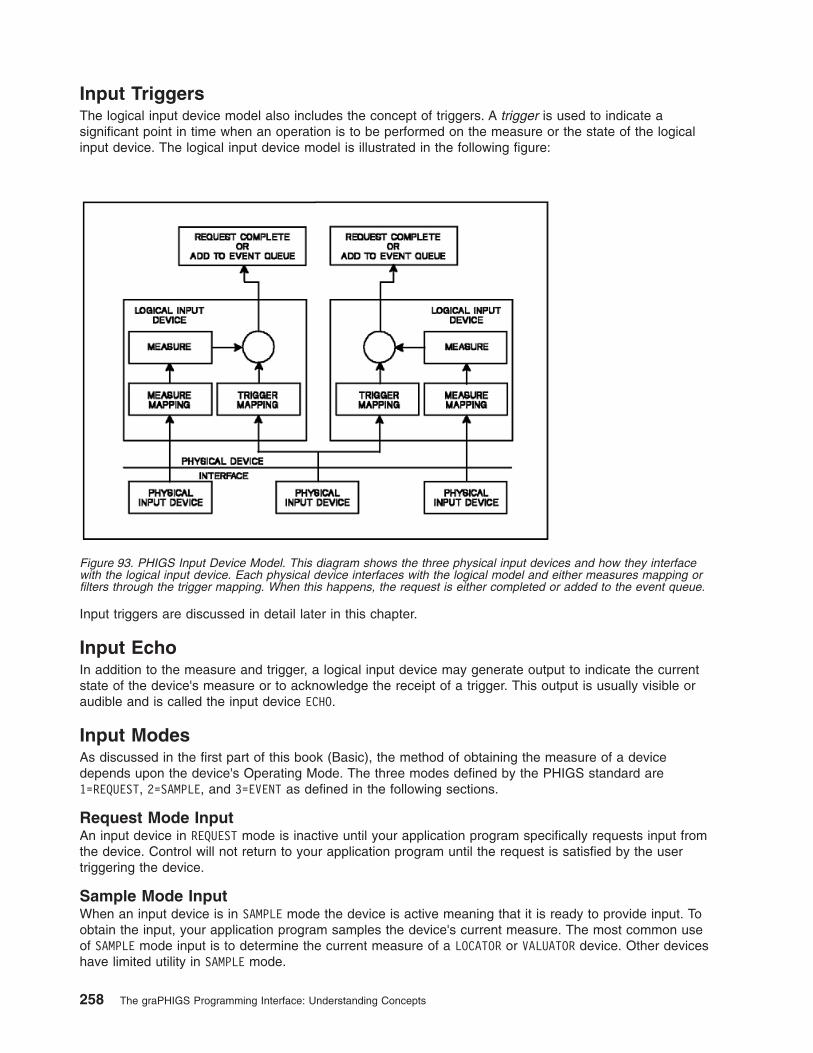
Input TriggersThe logical input device model also includes the concept of triggers. A trigger is used to indicate asignificant point in time when an operation is to be performed on the measure or the state of the logicalinput device. The logical input device model is illustrated in the following figure:

Input triggers are discussed in detail later in this chapter.

Input EchoIn addition to the measure and trigger, a logical input device may generate output to indicate the currentstate of the device's measure or to acknowledge the receipt of a trigger. This output is usually visible oraudible and is called the input device ECHO.

Input ModesAs discussed in the first part of this book (Basic), the method of obtaining the measure of a devicedepends upon the device's Operating Mode. The three modes defined by the PHIGS standard are1=REQUEST, 2=SAMPLE, and 3=EVENT as defined in the following sections.

Request Mode InputAn input device in REQUEST mode is inactive until your application program specifically requests input fromthe device. Control will not return to your application program until the request is satisfied by the usertriggering the device.

Sample Mode InputWhen an input device is in SAMPLE mode the device is active meaning that it is ready to provide input. Toobtain the input, your application program samples the device's current measure. The most common useof SAMPLE mode input is to determine the current measure of a LOCATOR or VALUATOR device. Other deviceshave limited utility in SAMPLE mode.

Figure 93. PHIGS Input Device Model. This diagram shows the three physical input devices and how they interfacewith the logical input device. Each physical device interfaces with the logical model and either measures mapping orfilters through the trigger mapping. When this happens, the request is either completed or added to the event queue.


Event Mode InputLike a device in SAMPLE mode, a device in EVENT mode is active but, instead of your application programsampling the device for input, the user triggers the device to generate the input. Because you can triggerthe device at any time, the input is placed in an event queue to be processed when your applicationprogram is ready. EVENT mode input allows you to input data even if your application is busy doingsomething else.

To determine if an event has occurred your application calls the Await Event (GPAWEV) subroutine. If theevent queue is empty, GPAWEV will wait for a specified number of seconds for an event to occur. If anevent occurs during the wait or there is an event on the queue when GPAWEV is called, GPAWEV willreturn the following information:

Major code -an integer defined by the class of the event

Event class -an integer defining the type of event

Minor code -an integer defined by the class of the event.

If the wait time elapses, the event class will be 0=NONE

In the PHIGS standard, only input devices can generate events. Therefore, the major code is defined asthe workstation identifier, the event class is the input device class, and the minor code is the input devicenumber. If the event class is not 0=NONE, your application can retrieve the event information from thecurrent event report, using one of the graPHIGS API get event subroutine calls. For example, if the eventclass returned by GPAWEV indicates that the event was generated by a choice device (class = 4), yourapplication would call the Get Choice (GPGTCH) subroutine to get the choice information from the eventqueue.

The concept of events has been extended in the graPHIGS API to define events that are not related toinput devices as discussed in the following section.

Input Model Extensions

Event ExtensionsIn addition to input device events, the graPHIGS API can also generate and process events which are notrelated to input devices. This section describes each of those events, how they are generated, and howyour application can use them. All events are categorized by the event class parameter of the Await Event(GPAWEV) subroutine as listed below:

<0=Not UsedNegative values are not used for the event class.

0=NoneZero is used to indicate that no events are in the event queue. When the event class is zero, themajor code and minor code parameters are not set. This value may be returned in two cases,when a time out occurs, or when one or more asynchronous errors are reported by a nucleus tothe graPHIGS API shell.

1-100=Input Device EventsThis value range is used for normal input device events. When the event class is in this range, themajor and minor codes contain a workstation identifier and a device number, respectively, and thecurrent event report will contain an appropriate input device measure. The following classes aredefined:

v 1=LOCATOR

Chapter 18. Advanced Input and Event Handling 259

v 2=STROKE

v 3=VALUATOR

v 4=CHOICE

v 5=PICK

v 6=STRING

101-200=Workstation EventsThis value range is used for events related to the general status of a workstation. When the eventclass is in this range, the major code contains the workstation identifier of the workstation whichgenerated the event. The minor code may or may not be set according to the individual eventclass. The following event classes are defined:

v 101: Link Switch Out

This class is currently used to notify your application that the 5080 link switch is switched awayfrom your application and therefore no graPHIGS API subroutines should be directed to that5080. This event also indicates that a workstation which is realized as a virtual workstation isdisconnected from the actual hardware workstation. The major code contains the workstation'sidentifier but the minor code is not set.

v 102: Link Switch In

This class is currently used to notify your application that the 5080 link switch is switched backto the application but, since the state of the 5080 is not known, the workstation should beclosed, reopened, and reinitialized. The event is also used to indicate that a workstation realizedas a virtual workstation has been reconnected to the actual hardware workstation. The majorcode contains the workstation's identifier but the minor code is not set.

v 103: Update Completion

High function workstations can update their display surface without forcing your application towait for the update to complete. When your application calls an Update Workstation (GPUPWS)or Redraw All Structures (GPRAST) subroutine, the graPHIGS APIwill initiate the update andreturn control to your application. Some time later the update will be complete.

An event of this class is generated when an update completion notification has been requestedusing the Set Shell Deferral State (GPSHDF) subroutine and the graPHIGS APInucleus hascompleted the processing of a previously invoked GPUPWS or GPRAST The major codecontains the workstation identifier and the minor code contains the display status.

v 104: Lost Input Events

This event class is returned when the size of a group of simultaneous events exceeds the inputbuffer size that is being used by the nucleus for sending events from the nucleus to the shell.The major code will contain the workstation identifier and the minor code is undefined.

v 105: Window Resize Notification

This class is returned when the user changes the size of an X-Window containing the output ofa X-Window-type workstation. The major code contains the workstation identifier and the minorcode is undefined. In order to receive this event, you must enable notification using the escape(GPES) subroutine with function 1009. After receiving a resize notification event, yourapplication can use the Inquire Mapped Display Surface Size (GPQMDS) subroutine to obtainthe size of the mapped display surface. (The mapped display surface is the subarea of theX-Window that the workstation uses as the display surface for graphics output.) Note that thedisplay surface size returned by Inquire Maximum Display Surface Size (GPQDS) and InquireMaximum Display Surface Size (GPQADS), does not change as the window is resized. You canspecify the aspect ratio of the display surface in the X-Window by using the XWINDASPPROCOPT.

201-300=Application Communication EventsAs discussed in Chapter 10. Advanced Concepts, your application can be divided into multipleDistributed Application Processes (DAPs) which can communicate through the applicationmessage facility supported by the graPHIGS API.


The following class values are defined for application messages:

v 201: Broadcast message

This class shows that an application message event was generated by another applicationprocess using the Send Broadcast Message (GPSBMS) subroutine. The major and minor codesand event data are set to the values specified by the other application process.

v 202: Private message

This class shows that an application message event was generated by another applicationprocess using the Send Private Message (GPSPMS) subroutine. The major and minor codesand event data are set to the values specified by the other application process.

With the introduction of application message events, the maximum size of events and the numberof events that the queue should hold will be more application specific. Therefore, your applicationmay now define the size of the event queue through the External Defaults File (EDF) or throughthe Application Defaults Interface Block (ADIB) parameter of the Open graPHIGS subroutine.ADIBs and EDFs are discussed in detail in The graPHIGS Programming Interface: TechnicalReference.

For more information on the use of application messages, see Chapter 10. Advanced Concepts.

301-400=Structure Store EventsThis value range is used for events generated by a structure store. The following event class isdefined:

v 301: Structure store threshold value exceeded

In order to prevent loss of data due to out-of-memory errors on a graPHIGS API nucleus, a"threshold exceeded" event is supported. The event is generated whenever the storageallocated to a structure store exceeds a specified threshold value. The structure store thresholdvalue is set using the Set Structure Store Threshold (GPSSTH) subroutine. The event will onlybe generated once per setting.

The event major code contains the structure store identifier that caused the event and the minorcode contains the threshold value that was exceeded.

>400=ReservedThis range is reserved for future extensions.

Event HandlingSome applications require greater control over how events are processed. To accommodate that need, thegraPHIGS API permits your application to specify an event handling function through the Define EventHandling Function (GPEVHN) subroutine. GPEVHN takes the following two parameters:

Parameter Descriptionhandler the address of your application defined event handleranchor a pointer to an anchor block defined by yourapplication.

Whenever an event occurs, your event handler will be called by the graPHIGS API and passed thefollowing parameters by reference using the operating system's standard calling convention:

Parameter Descriptionanchor your application anchor block specified in the call to

GPEVHNmajor the major code of the eventclass the class of the eventminor the minor code of the eventlength the length of the event datadata the event data


Parameter Descriptionsflag an event status flag indicating the following:

v whether or not the event queue is about to overflow

v whether or not the event queue has already overflowed

v whether or not the event data is part of a simultaneousevent.

rflag a return flag which your event handler should set toindicate whether or not the event should be queued ordiscarded.

Event handlers are subject to the following restrictions:

v Must be written in a programming language which can run without any specific run time environment

v Must follow the standard linkage convention of the operating system on which the graPHIGS API shell isrunning

v Must not issue any graPHIGS API subroutine calls

v Must not issue any system calls or should not invoke any system function which may require the normalrun time environment

v Must return to the graPHIGS API event handler.

The restrictions listed above are intended to prevent an event handler from destroying the normal run timeenvironment. For example, if an event occurs and interrupts the graPHIGS API while processing an APIsubroutine call, your event handler will get control. If your event handler then calls a graPHIGS APIsubroutine, the results would be unpredictable.

With the stated restrictions, the function of most event handlers should be limited to the following:

v deciding whether or not the event should be queued based on the data supplied to the event handler

v manipulating the data in the anchor block to communicate with the rest of your application.

Physical Device SupportThe phrase "physical input device" refers to the actual hardware device used to implement a logical inputdevice as shown in the figure, PHIGS Input Device Model. For example, a computer keyboard is aphysical input device used to implement a logical string input device.

In order to meet the needs of application programmers, the graPHIGS API extends the PHIGS input modelto allow your application program to map additional physical input devices to the PHIGS logical inputdevices as described in the following sections.

Device CategoriesEach physical device is categorized by the type of input it provides. The currently defined categories are1=BUTTON, 2=SCALAR, and 3=2D_VECTOR as discussed below:

BUTTON Devices: A device in the BUTTON category will provide a discrete integer value when sometransition of the physical device takes place such as when a key on a keyboard is depressed. The set ofinteger values that a device may return are not required to lie within one contiguous range. This device isfurther characterized by the list of all possible integers that it may return. This would correspond to thekeys on a keyboard for example. If a device can detect make and break transitions, then distinct integervalues are provided for each.

SCALAR Devices: A SCALAR device will provide an integer within a single range. A specific SCALARphysical device may return either absolute or relative values. For an absolute device, the limits of therange are the devices' physical limits (minimum and maximum value that the device can input). For arelative device, there is no minimum value so a value of zero is used. The maximum value of the rangerepresents the number of increments of physical motion. A unit of physical motion is different for different


physical devices. For example, for a dial device, one unit of physical motion equals one turn of the dial.These values will in reality be related to the operation of the corresponding logical input device. Thephysical input is mapped to the range of input values that the logical device can input as specified by theapplication on the initialize device subroutine call.

2D_VECTOR Devices: A 2D_VECTOR device is similar to a SCALAR device except that two integer valuesare generated by the device instead of one. It is often used to control the cursor displayed on the screen.The device can provide either relative or absolute values. A mouse is an example of a 2D_VECTOR devicethat would return relative values, while a tablet is a 2D_VECTOR device that would return absolute values.For an absolute device, the limits of the range are the devices' physical limits. The minimum and maximumvalues generally correspond to the edges of the screen in the case of a device connected to the graphicscursor. For a relative device, there is no minimum limit so a value of zero is used. The maximum value ofthe range represents the number of increments of one unit of physical motion. For a mouse physicaldevice, one unit of physical motion equals the amount of motion necessary to move the cursor from oneedge of the screen to its opposite edge. The limits of the range, as with SCALAR devices, are mapped tothe range that the corresponding logical device can input as specified by the application on the initializedevice subroutine call.

Note:

1. To determine the range for the physical input device, use the Inquire Physical Device(GPQPDC) subroutine.

2. An integer identifier is associated with each physical device to differentiate the devices withineach category.

Physical Device EmulationSome applications require the use of physical input devices other than those defined and explicitlysupported by the graPHIGS API In order to meet that requirement and still isolate your application from thecharacteristics of a physical device and provide the measure mapping operations of logical input devices,the graPHIGS API allows your application to logically and physically detach the default set of physicaldevices and emulate them instead.

For example, the IBM digitizer is a physical device which may be accessed directly by your application.Tailoring this device to the task the end user is performing will give you desirable results. One possibility isto use a section of the digitizer to emulate the normal operation of the tablet by providing the user with away to switch between using the tablet or a section of the digitizer as the physical device that is driving thePICK, LOCATOR, and STROKE logical devices. This would allow the user the convenience of using theselogical devices from either the tablet or digitizer.

The graPHIGS API cannot provide the same level of functions that your application can by accessing thedigitizer directly. Even if the graPHIGS API were to perform the tablet emulation described above, mostapplications would still require access to the unique characteristics of the digitizer such as control overgranularity, access to puck keys, lights, and audible alarms.

This same argument applies to other IBM and non-IBM devices which you may choose to use. Eachphysical device has many different characteristics and it would be impractical for the graPHIGS API tosupport every one.

To allow your application to replace and emulate a physical device, the graPHIGS API provides the SetPhysical Device Mode (GPPDMO) subroutine. The parameters for this subroutine include the physicaldevice category, identifier, and mode. The mode may be specified as either 1=DISABLED or 2=ENABLEDWhen DISABLED, the physical device will not generate any input to the logical input devices to which it isnormally connected. ENABLED is the default mode that permits the physical device to drive the logicaldevices. When a physical device is disabled, your application may emulate it using the Emulate PhysicalDevice (GPEPD) subroutine. The parameters of GPEPD are defined as follows:


Parameter Descriptionwsid workstation identifier of the device to be emulatedcategory physical device category (1=BUTTON, 2=SCALAR, or 3=2D_VECTOR)device physical device identifiervalue emulated input value(s) to be passed to the logical input device(s).

The simulated input will be passed to the set of logical input devices that are connected to the specifiedphysical device. If the specified input values do not fall within the range normally generated by the physicaldevice or the physical device does not exist, an error will be generated. The normal operation of thelogical input device is unchanged.

The characteristics of a physical input device can be determined with the Inquire Physical DeviceCharacteristics (GPQPDC) subroutine. The input parameters to GPQPDC are the physical device categoryand a physical device identifier. GPQPDC returns information which is dependent on the category of thephysical device.

In Version 1 of the graPHIGS API, logical input devices were not available to your application if therequired physical input devices were not present. With the introduction of physical input device emulation,there are cases where your application may require emulation of physical devices that are not reallypresent. Therefore, a new defaults option has been defined that allows your application to control whetheror not logical input devices are created even if the corresponding physical devices are not present. Thisoption is specified as a 'procopt' in either an External Defaults File (EDF) or through a parameter of theCreate Workstation (GPCRWS) subroutine. When logical devices are specified unconditional uponcreation, your application must use the Inquire Physical Device Characteristics (GPQPDC) subroutine todetermine if the physical device is actually present.

Input Trigger ExtensionsEach logical input device may have one or more trigger levels with one trigger each. Each trigger levelcorresponds to an atomic operation on the measure or state of an input device.

The first or primarytrigger level causes the logical input device to pass its current measure value back toyour application or to add the measure to the event queue depending on the mode of the logical inputdevice. Every logical input device has a primary trigger.

Trigger levels greater than the first (secondary) are used to change the measure or the state of the logicalinput device. As an example, the following table summarizes the secondary triggers for the STROKE andPICK logical input devices supported by the 5080 workstation type:

Table: 5080 Secondary Trigger Levels

Device Trigger Levels

STROKE #11 - Ends the accumulation of points into the stroke

buffer.

2 - Initiates the accumulation of stroke points intothe stroke buffer.


Device Trigger Levels

STROKE #21 - Moves the editing position in the stroke buffer

backward one point.

2 - Moves the editing position in the stroke bufferforward one point.

3 - Inserts a point into the stroke buffer.

4 - Deletes the current point from the stroke buffer.

PICK #11 - Suppresses the pick correlation process.

2 - Activates the pick correlation process.

A trigger for any level can be generated by one or more physical input devices in conjunction with a triggermapping A trigger only affects a logical input device that is in EVENT mode or has a REQUEST pending.Triggers at any other time have no effect on the logical input device.

The relationship between the physical and logical input devices is determined by the workstation developerand cannot be altered. For example, the following table lists the physical input devices and the logicalinput device measure and trigger processes which use them:

Table: 5080 Physical/Logical Device Correspondence

Physical Device Logical DeviceMeasure

Logical DeviceTrigger

VALIGN="TOP">Tablet LOCATOR 1,2STROKE 1,2PICK 1

Puck or Stylus CHOICE 2 LOCATOR 1,2STROKE 1,2VALUATOR 1-8PICK 1STRING 1-16

LPFK CHOICE 1 LOCATOR 1,2STROKE 1,2VALUATOR 1-8PICK 1STRING 1-16

Keyboard CHOICE 3CHOICE 4STRING 1-16

LOCATOR 1,2STROKE 1,2VALUATOR 1-8PICK 1STRING 1-16

Dial 1 VALUATOR 1 VALUATOR 1







Physical Device Logical DeviceMeasure

Logical DeviceTrigger



Each logical input device has a set of BUTTON physical devices which are used to trigger any of the logicaldevice's trigger levels. Since a BUTTON physical device can generate many values, the trigger mapping foreach logical input device acts as a filter on these values so that only a subset will actually trigger thelogical device.

The programmable trigger concept allows your application to modify the trigger mapping by selectingwhich buttons on a physical BUTTON device will trigger each of the trigger levels of the logical device. Atrigger mapping includes the following information:

Trigger Type A trigger type value greater than zero represents a physical device identifier fromthe BUTTON category that is to be used to generate the trigger. Values less than zeroare reserved for triggers not generated by physical devices.

Trigger Qualifier A trigger qualifier defines which values from the physical BUTTON device will triggerthe specified trigger level. These values may be specified as ranges forconvenience.

The list of BUTTON type physical devices that may be used for triggering a specific logical input device canbe determined using the Inquire Input Trigger Capabilities (GPQIT) subroutine. This subroutine defines thecorrespondence between the physical devices and the triggers of the logical input devices.

Warning: Temporary Level 4 Header

National Language Pre-editing Mode Effect on Triggers: Some national languages such as Japaneseallow the user to enter a pre-editing mode or to view pop-up translation menus (auxiliary windows) whiletyping in a string device. In these modes, characters are interpreted by a special language processor (theInput Method), before they are entered into the graPHIGS string device.

Triggers behave as follows during pre-editing mode and when auxiliary windows are present:

v BUTTON physical device 4 (the keyboard) does not provide input to any measure process nor to anytrigger process. For example, during pre-editing mode, your application will not receive any choicedevice 4 input events.

v A STRING device in pre-editing mode or with auxiliary windows present cannot be triggered by anytrigger. For example, a Kanji string device in pre-editing mode cannot be triggered by a mouse button.

Change in Measure TriggerProgrammable triggers have been extended to include the notion of firing the primary trigger when thephysical measure changes. The change in measure trigger allows your application to follow the motion themouse or tablet puck as it moves. This is a very common mode of operation. For example, yourapplication may use the cursor to input values for a transformation matrix based on cursor's XY screenlocation. This type of trigger has always been used for the VALUATOR devices in EVENT mode but was notexposed since the VALUATOR does not have programmable triggers.

The change in measure trigger is set by the Set Input Device Trigger (GPIT) subroutine where the triggertype parameter is -1 and is only valid for the primary trigger level of a logical input device.

The low trigger threshold qualifier specifies the minimum change, in 2D_VECTOR physical device units,needed for triggering. Use GPQPDC to determine the valid ranges for the 2D_VECTOR devices. The hightrigger qualifier is not used for this trigger type and must be set to 0.


For PICK devices, the graPHIGS API accumulates the distance from one event to the next and correlatesonly when the low qualifier threshold is exceeded, except for the last event occurring in a chain of events.The last in a chain of events is always correlated, regardless of the low qualifier. Events accumulated priorto the last event are also correlated when they exceed the low qualifier threshold.

This trigger type can be interpreted as an option for the trigger mapping process of the logical inputdevice. When this trigger type is used, the trigger mapping process monitors the physical measure forchange and when the cumulative change is more than the value contained in the low trigger qualifier, theprimary trigger is fired.

Use the Inquire Input Trigger Capabilities (GPQIT) subroutine to determine whether an input devicesupports this trigger type.

Note: The graPHIGS API does not limit the change in measure trigger type to use by DistributedApplication Processes (DAPs) but the communications overhead will be high if the programreceiving the events does not reside in the same node as the one to which the user's display isdirectly attached.

Trigger When Primary FiresThe trigger when primary fires mode allows the secondary trigger to correspond to the same event as theprimary trigger. Trigger when primary fires is set by the Set Input Device Trigger (GPIT) subroutine wherethe trigger type parameter is -2 and is only valid for the secondary trigger level of a logical input device.The low and high trigger qualifiers have no meaning and must be set to 0.

When used in combination, trigger by measure (trigger type -1), and trigger when primary fires (triggertype -2), implement a sliding pick device that returns an event for the first primitive crossed if correlation isset to ON trigger by measure should be set to a small value to avoid skipping primitives.

Input Device Dependent TriggersInput Device Dependent Triggers are used by some logical input devices as a default trigger type becausethe input device uses a special type of trigger or one which is mode dependent. A VALUATOR input deviceon the 5080 workstation is a good example of this. On a 5080 workstation the enter key is the primarytrigger for VALUATOR devices in REQUEST mode but movement is the primary trigger in EVENT mode. Thedefault trigger for a VALUATOR is "logical input device dependent" to allow workstations to supportprogrammable triggers without returning ambiguous or incorrect information on inquiry subroutines. TheInput Device Dependent Trigger type is only returned from inquiry subroutine and is never valid as aparameter to a trigger setting subroutine call.

Input Device Enhancements

Cursor Shape DefinitionOn several of the workstations supported by the graPHIGS API, the graphics cursor is used as the promptfor LOCATOR, STROKE, and PICK input devices. Each one of the logical input devices has a different promptshape. The LOCATOR uses a "+" shape, the STROKE uses an "X" and the PICK device uses a box whose sizecorresponds to the current pick aperture. The prompt is only displayed when the device is active and thecursor is in the input device's ECHO area. Since ECHO areas may partially overlay each other, the shape ofthe cursor may change as it is moved around the screen passing through different combinations of activeECHO areas.

The cursor is drawn by display adapter hardware in some configurations. This produces cursor movementperformance that is independent of screen content. Many application developers like to define their owncursor shapes. Two workstation subroutines are provided to accomplish this. The Set Cursor Shape(GPCUS) subroutine selects the cursor shape for a specified workstation. The second parameter ofGPCUS is an index which selects either a specific type of cursor, such as a cross hair, or an entry in theworkstation's cursor shape table. GPCUS also allows the selection of a two-color (XOR echo)representation of any of the workstation cursors, as well as an option to disable the graPHIGS API cursors


and allow the application to use the default cursor facilities native to a window system such as thoseprovided by X-Windows. (See HWCURS PROCOPT for information on using the hardware crosshaircursor.) Use the Set Cursor Representation (GPCUR) subroutine to redefine an entry in the workstation'scursor shape table. When an entry is selected, that cursor shape is used for all logical input devices thatrequire a graphics cursor. The cursor shape, therefore, is not unique to the logical input device nor does itchange as the cursor moves around the screen unless it moves outside the echo area or the applicationchanges it. GPCUR takes the following parameters:

Workstation IdentifierSpecifies the workstation containing the cursor shape table that is to be set.

Cursor Shape Table IndexSpecifies the entry of the table to be set.

Cursor FormatSpecifies the format of the cursor definition.

Cursor DefinitionContains the data to define the cursor.

The size of the cursor shape table and the cursor formats that are supported by a workstation can bedetermined through the Inquire Cursor Facilities (GPQCUF) subroutine. The only cursor format currentlydefined requires a two-dimensional array of pixel values with 1 bit per pixel. For this format, the cursordefinition must contain the following:

v The size of the pixel array (number of rows and columns)

Note: For this format, the specified array sizes must match the maximum size pixel array which can beinquired using GPQCUF

v The pixel array which is stored in row major order with 8 pixels packed per byte

v Each row must start a 32-bit boundary.

The hot point of the cursor is always the center of the pixel array.

PICK Device Enhancements

Pick Selection Criteria: Based on the organization of your graphics data and performanceconsiderations, you may choose to have the graPHIGS API return the FIRST or LAST primitive which isdetected by a PICK device. In addition, some application programmers would like their applications toreceive every primitive that passes through the PICK aperture. This allows your application or the user tomake the decision as to which primitive of those passing through the PICK aperture is the actual target ofthe operation. You may also choose to perform some operations on every primitive which passes throughthe PICK aperture.

The pick selection criteria controls whether the FIRST, LAST or ALL primitives passing through the PICKaperture are returned to your application. This characteristic of a PICK device can be initialized through theSet Pick Selection Criteria (GPPKSC) escape subroutine. One of the parameters passed to GPPKSCcontrols whether or not the pick selection criteria is FIRST, LAST, or ALL For selection criteria ALL, everyprimitive which intersects the PICK aperture will be echoed when pick echoing is ON.

If the Pick Selection Criteria is set to ALL and a REQUEST or SAMPLE function is invoked for the PICK device,only information about the FIRST pick primitive will be returned. When the PICK device is in EVENT mode,the list of picked primitives will be returned as simultaneous events. Each event will only contain theinformation for a single primitive. Several locations on the same curve or surface may lie within the PICKaperture. Each primitive will be returned only once, even if the selection criteria is set to ALL.

In addition to controlling the picked primitive using the FIRST, LAST, and ALL order of processing, yourapplication can control the picking of primitives effected by HLHSR processing. The criteria FIRST_VISIBLE,LAST_VISIBLE, and ALL_VISIBLE refer to those primitives that are in the PICK aperture and are visible


based on the HLHSR processing. The criteria FIRST, LAST, and ALL refer to those primitives that are in thePICK aperture but not necessarily visible based on HLHSR processing. Any effect due to HLHSRprocessing does not change which object is picked (i.e., the selected object may not be displayed whenHLHSR is active). If a workstation does not support HLHSR processing, then the visible PICK modesoperate the same as normal PICK modes.

Initial Correlation State: PICK correlation is the process of determining which graphical elements areintersected by a PICK device's aperture. Typically, correlation is turned on when the user causes asecondary trigger to fire by pressing and holding down a mouse, stylus, or puck button. Releasing thebutton causes the PICK device's primary trigger to fire and the PICK measure to be sent to your application.Some applications developers however, always want PICK correlation turned ON.

By default, the graPHIGS API defines PICK correlation to be OFF when a PICK device is activated. If youwant correlation always ON then the PICK device triggers must be set so that correlation is turned ON by anytrigger and only turned OFF if the device is put in REQUEST mode (deactivated). This is not convenient sincethe user must fire a trigger (press a button) to start the correlation process each time the PICK device isactivated.

To alleviate this inconvenience the Set Initial Pick Correlation State (GPIPKC) escape subroutine isdefined. GPIPKC takes the following three parameters:

Parameter Descriptionwsid the workstation identifier of the PICK device whose correlation state is to be changeddevice the PICK device identifier of the PICK device whose correlation state is to be changedstate the Pick Correlation State (1=OFF or 2=ON)

A Pick Correlation State of ON specifies that when the device is activated, correlation will be turned onimmediately. The default value of OFF specifies that correlation will start when the PICK device's secondarytrigger is fired.

Extended Pick Input Data: Some applications require more information about a picked primitive than astandard PICK device will return. For example, an application may require the view identifier of the pickedprimitive. Therefore, the PICK device measure has been extended in the graPHIGS API to include thefollowing information:

Label IdentifiersEach level of the pick path hierarchy includes the following:

v Structure identifier

v Pick identifier

v Label identifier

v Element number

View IndexSpecifies the view table index that was used to render the picked primitive.

Composite Modeling MatrixSpecifies the concatenation of the local and global modeling transformation matrices that wereused to render the primitive.

Aperture LocationSpecifies the location of the center of the PICK aperture in Normalized Projection Coordinates(NPC).

The extended PICK information is returned by the Get Extended Pick (GPGTXP), Request Extended Pick(GPRQXP), and Sample Extended Pick (GPSMXP) subroutines. If any of the existing pick inputsubroutines (Get Pick (GPGTPK), Request Pick (GPRQPK), and Sample Pick (GPSMPK)) are issued to aPICK device which returns extended information, only the current pick path without labels will be returned.


Some workstation platforms do not support the extended PICK class. Therefore, to determine if aworkstation supports extended PICK, use the Inquire Pick Measure Type (GPQPKT) subroutine. If one ofthe extended PICK input subroutines is called for a device which does not return extended PICKinformation, the subroutine call will be rejected with an error.


Chapter 19. Fonts

This chapter describes the treatment of fonts by the graPHIGS API It includes a discussion of font files,font directories, and font inquiry subroutines.

Font FilesIn the graPHIGS API, the shell and nucleus may be running as two different processes. In some cases,they may be running on two different machines with two completely different disk systems. The fontdefinition is read from the disk system which the nucleus can access. When the shell receives a call to theActivate Font (GPACFO) subroutine, it sends a corresponding request to a nucleus which owns thespecified workstation. The nucleus searches its own disk system for the specified character set/font pairand loads it into the specified workstation.

The font file is taken from the nucleus's disk to:

v Minimize the data transmission (I/O) for the font activation. Because workstations are nucleusresources, the font data is taken from the resources belonging to the nucleus.

v Enable multiple application processes to share the same font definition. Even when a nucleus isused by multiple applications which are running on different nodes, the font definition is taken from thesame place and is shared by all applications processes.

v Keep the meaning of the character set identifier and font number consistent. A given character setand font pair is always mapped to the same file independent of where and in what environment yourapplication is running. The mapping is determined only by the environment where the nucleus isrunning.

Font DirectoryThough the font files available to a nucleus will be enough for many applications, there are some caseswhere you may want to load a font definition to a workstation from the shell's disk. Following are threeexamples:

1. The font is an application defined font and you do not want to install the font definition onto thenucleus's disk. If all font definitions must reside on the nucleus's disk, there is no way to avoidexposing your font definition to other applications.

2. If your application uses multiple nuclei, either simultaneously or one at a time, you may not want toinstall a font definition to each nucleus. Especially if the font definition may be changed or re-defined,then you might want to keep the font definition file on your application's disk to make it easy tomaintain.

3. The nucleus does not have enough disk space to install all font definitions that your applicationrequires. This will occur when the nucleus is implemented on a workstation with a small disk system oror one without any disk system such as the IBM 6090.

As a result of these requirements, the graPHIGS API supports the concept of a font directory. The fontdirectory can be viewed as a run time disk system for fonts, which is dynamically created and attached tothe shell by the Create Font Directory (GPCRFD) subroutine. A font directory is a nucleus resource andcan be shared by multiple application processes using the Attach Resource (GPATR) subroutine.

When a font directory is created, it is empty. Your application can load any character set/font pair to thefont directory using the Load Font (GPLDFO) subroutine. When the shell receives this call, it searches itsown disk system for the specified font definition. When the shell finds the font file, it reads the file andsends it to the specified font directory. If the specified character set/font pair is already in the font directory,the font is replaced.


A given workstation can have only one font directory associated to the workstation at any given time. Thisassociation is set using the Associate Font Directory with Workstation (GPAFDW) subroutine. If theworkstation already has a font directory associated with it, the subroutine call replaces the currentlyassociated font directory.

When Activate Font (GPACFO) subroutine is called, the following actions are performed by the nucleus:

1. The nucleus checks the workstation to see if it has an associated font directory. If so, it then searchesfor the specified font definition. If the font definition is found, it is activated on the workstation.

2. If the specified font definition does not exist in the font directory, or the workstation has no associatedfont directory, the nucleus' disk system is searched, and if the font exists, the font is activated.

3. The nucleus generates an error if the specified font definition does not exist in an associated fontdirectory or in the nucleus' disk system.

As described above, the search of a font directory associated to a workstation supersedes the normal fontfile search order in the nucleus. Note that the contents of an associated font directory affects onlysubsequent Activate Font subroutines. The contents of a font directory does not affect any characterset/font pairs already active on the workstation. Conceptually, each font definition is copied from the fontdirectory to the workstation's font pool when it is activated and becomes independent of the font directory.Even if the font directory is disassociated from the workstation, character set/font pairs which are currentlyactive on the workstation remain active.

Font InquiriesIn Version 1 of the graPHIGS API, the Inquire Annotation Font Characteristics (GPQAFC) returned thefollowing information about how a workstation would process a specific character set and font pair:

v The highest text precision available

v The nominal character height

v The number of character height scale factors supported

v A list of the height scale factors supported

v For each height scale factor, the number of expansion factors and the minimum and maximumexpansion factors.

The expansion factor information was returned as a deviation from the nominal aspect ratio of thecorresponding geometric text font.

The meaning of the GPQAFC inquiry has been changed slightly in Version 2 but will still producecompatible results for Version 1 applications. The expansion factor information has been redefined to berelative to the annotation nominal font aspect ratio instead of the geometric font aspect ratio. To providecompatibility, all the annotation fonts will have the same aspect ratio as the geometric font with the samecharacter set and font identifiers.

The Inquire Extended Annotation Font Characteristics (GPQXAF) subroutine will return the followinginformation in addition to the information returned by GPQAFC:

v Whether the font definition includes proportional character information

v The amount of space between the capline and topline as a fraction of the character height

v The amount of space between the base and bottom lines as a fraction of the character height

v The nominal aspect ratio of the font.

Unlike geometric text fonts, annotation text fonts are workstation specific.

With the introduction of the shell-nucleus concept and the associated nucleus resources, a font may residein many places. These repositories for fonts include the shell font storage, the nucleus font storage, font


directories, and workstations. A given character set and font number could have a different definition ineach location. To inquire information about a font in the shell's font storage, use the following inquirysubroutines:

v Inquire Font Characteristics (GPQFCH)

v Inquire Font Aspect Ratios (GPQFAR)

The primary use of GPQFCH and GPQFAR is to compute the length of a text string. GPQFCH returnswhether the font has character box definitions for each character (proportional positioning), the amount ofspace between the capline and top line, the amount of space between the base and bottom lines and theaspect ratio of the nominal character box. GPQFAR returns the aspect ratio of each character within aspecified string. This is only useful for a font which has proportional positioning information.

Chapter 19. Fonts 273

Chapter 20. Images

This chapter describes the basic concepts related to the display of image data by the graPHIGS API.

An image is defined by an image board, which is a two-dimensional (2D) array of data values treated as aresource of the graPHIGS API nucleus. Note that an image board is not a physical piece of hardware, buta conceptual place to store image data. An image can be displayed on the workstation by mapping adefined image to a workstation view.

Image ModelIn the most general sense, an image is a mapping function from a 2D surface into a color space. Torepresent the function in a digital form, the image is sampled both within its definition domain and valuedomain. We assume that the definition domain is a planar rectangle and the function is sampled at gridpoints with regular intervals. Therefore, the image is represented by a 2D array of color values.

Color values can be represented by a vector within a normalized three-dimensional color space, so theimage can be represented by a two-dimensional array of three-dimensional vectors. However, such arepresentation requires a large amount of storage when each color value is represented by a triplet of realvalues. To reduce the amount of data, color values are quantized. Two quantization methods arecommonly used in many image applications.

One method is to quantize three color primaries independently and is called scalar quantization, as shownin the following figure. The normal RGB representation of images is a typical example of this method.Each pixel is represented by three indexes each of which specifies one representative value of a colorcomponent. Note that the quantizations of three primaries need not be equal interval sampling (forexample, r-corrected RGB) nor to be identical depth (for example, the broadcast TV color system, digitalYIQ, with different bit length).

Figure 94. Scalar Quantization. This diagram shows the quantization method in which three color primaries arequantized independently.


Another method is to quantize color values as three-dimensional vectors and is called vector quantization,as shown in the following figure. An image handled by the Pixel (GPPXL2 and GPPXL3) subroutines ofthe API is a typical example of this method. Each pixel is represented by an index specifying onerepresentative color selected from a three-dimensional color space. Note that this method of quantizationincludes binary and grey scale images as special cases in which the color representatives are selectedfrom monochrome colors.

Notice that in both cases, an image is represented by a 2D array of color table indexes. The onlydifference between them is the connection between the array and color table. In the scalar quantizedimage, the color table is indexed by three indexes separately for each color component but in the vectorquantized image, it is indexed as a whole by a single index.

Defining, manipulating and displaying an image is similar to that of geometric objects. In addition, thedisplay of an image merges into the rendering pipeline of geometric objects, resulting in both the imageand geometric data showing on the display surface. You may display an image using of the followinggraPHIGS API facilities:

v Image Board - An area of storage that holds the quantized image data

v Image Board Manipulation - graPHIGS subroutines that allow you to create and modify the contents ofthe image board

v Image Color Tables - Color tables associated with image boards that are used to obtain the color valueof a pixel

v Image Display - Subroutines that define the location of the image in World Coordinates

These facilities are discussed below.

Figure 95. Vector Quantization. This diagram shows the quantization method in which color values are quantized asthree-dimensional vectors.


Image BoardTo store the 2D arrays of indexes described above, the graPHIGS API supports a nucleus resource calledan image board. Each pixel is referred to by two indexes where the pixel at the lower-left corner has anindex pair (0,0). Pixels at the lower-right, top-left and top-right corner are referred to by index pairs(SX-1,0), (0,SY-1) and (SX-1,SY-1), respectively, where SX and SY are the horizontal and vertical size ofthe image board.

Conceptually, the image board is an abstraction of a frame buffer for raster type displays. However, imageboards are not necessarily realized by special memory such as a physical frame buffer. A nucleusimplementation can utilize any storage for an image board and your application can create and deleteimage boards independent of the physical frame buffer.

An image board is created using the Create Image Board (GPCRIB) subroutine. GPCRIB takes thefollowing parameters:

v Image board identifier

v Nucleus identifier

v Bit depth

v Horizontal and vertical size

v Image board type

v Type dependent image board description

The bit depth parameter must be one of those supported on the target nucleus. The graPHIGS APIgenerally supports bit depth of 1,2,4,8 and 12, but the application should inquire the actual list of bitdepths available on a given nucleus using the Inquire Image Board Facilities (GPQIBF) subroutine.

The conceptual size of the image board is determined by three size parameters, bit length of each pixel,and the horizontal and vertical dimensions of the image board array. However, the actual amount ofstorage used for an image board may differ between nucleus implementations because of the differencesin their storage organization. A nucleus implementation can use any storage mechanism (for example, itcan use any compressed format) to realize image boards.

You can attach an image board created by another application process to your application using the AttachResource (GPATR) subroutine with the following parameters:

v Resource type (3=IMAGE_BOARD)

v Image board identifier

v Nucleus identifier

v Resource identifier

v Password

After the image board is attached to your application's shell, you application can access it as though itcreated the image board itself.

As for other nucleus resources like structure stores or workstations, the resource identifier of the imageboard and its password is known only to the application process which created the image board.Therefore, your application process which uses the Attach Resource (GPATR) subroutine, for an imageboard, must get the information from the application process which created the image board.

An image board is detached from the shell using the Detach Resource (GPDTR) subroutine which takeswith an image board identifier as a parameter.

Chapter 20. Images 277

Manipulation of Image Board ContentThe graPHIGS API provides functions that enable you to manipulate image board data content.

The Fill Rectangle (GPFRCT) subroutine is used to fill a portion of an image board with a constant value.Note that the contents of an image board are undefined when the image board is created. If theapplication wants to initialize all pixels of the image board to a constant value (clear the image board), theapplication must explicitly fill the entire image board with the value by using this subroutine.

Write Rectangle (GPWRCT) and Read Rectangle (GPRRCT) subroutines are used to move image data toand from an image board. Both subroutines take the following parameters:

v An identifier of an image board to which pixel data is written

v Two integers specifying the location of the low-left corner of a rectangle in the image board

v Two integers specifying the size of pixel data to be moved

v An integer specifying the type of image format and additional parameters which depend on the type

v An application's storage area which contains the image data

v Two integers specifying the location of the low-left corner of a rectangle in the application storage area

The graPHIGS API supports one type of image format: the pixel array. This type of image formatdescription requires the following information:

v An integer specifying the bit length of each pixel passed in the image data parameter. The graPHIGSAPI supports bit depth of 1,2,4,8 and 16.

v An integer specifying the number of pixels in a row (horizontal size).

v An integer specifying the number of rows.

v An integer specifying the order of pixels in the pixel buffer.

– 1=LEFT_TO_RIGHT_BOTTOM_TO_TOP

– 2=LEFT_TO_RIGHT_TOP_TO_BOTTOM

The table below lists the minimum and recommended horizontal size based on the image format depth.

Bit Depth Required MinimumHorizontal Size

RecommendedHorizontal Size

1 Multiple of 8 Multiple of 32



8 No Restriction Multiple of 4

16 No Restriction Multiple of 2

Your application can also transfer image data from one image board to another using the TransferRectangle (GPTRCT) subroutine.

In addition, your application can perform operations on one or two image boards and place the result intoanother image board using the following two subroutines:

v Two Operand Pixel Operation (GPTWPO)

v Three Operand Pixel Operation (GPTHPO)

GPTWPO processes a rectangular area of the source image board and places the result into anotherrectangular area of the target image board. The operation type parameter specifies the process to beperformed on the source rectangle. The following operation is defined:

v Reflection (change pixel order)


GPTHPO performs a binary operation on the two source image boards and stores the result into the targetimage board. The following two operations are currently defined:

v Logical operations

v Arithmetic operations

Image boards which are the target of this subroutine call must reside on the same nucleus and theactually supported pixel operations may depend on the nucleus where these image boards reside. Yourapplication can inquire a list of operations supported by a given nucleus with the Inquire Available PixelOperations (GPQPO) subroutine.

All source and target rectangles must always have the same horizontal and vertical size and be entirelywithin the source image data. If the target rectangle is not entirely within the target image data, pixelsfalling outside of the target are discarded. Also, the bit lengths of the image boards need not be the same.When the bit length of the target pixel is less than that of the source, the source bit string is truncated bydiscarding the most significant part. When the bit length of the target pixel is larger than that of the source,the source bit string is expanded by adding 0-bits to the most significant part. Note too, that the targetimage board for GPTRCT, GPTWPO, and GPTHPO can be the same functions as the source rectangles.

Image Color Table ConnectionTo display the contents of an image board, your application must call the Define Image (GPDFI) subroutinewith the following parameters:

v Workstation identifier

v Image index

v Image connection type

v Number of image boards

v A list of image board identifiers

An image definition is stored in the specified entry of the workstation's image table. Each workstation hasan image table with a predefined number of entries and all entries are initialized as undefined when theworkstation is opened.

The image connection type specifies the relationship ("connection") between the image board contents andthe color table. This defines the colors of pixels. (These colors are then quantized and written to the framebuffer.) There are 3 types of connections supported:

v COMPONENT

The component connection is used for scalar color quantization. Three image board identifiers arespecified. To obtain a pixel color, three indices are used, one from each of the three image boards atthe same pixel location. The three indices are used independently to select a color component from thespecified color table. The first index selects the first color component, the second index selects thesecond color component, and the third index selects the third color component. The resulting colorvalue is the color of the pixel, as shown in the following figure:


v INDEXED

The indexed connection is used for vector color quantization. One image board identifier is specified. Apixel color is obtained by using the index at the pixel location. The index is used to select the threecolor components from the specified color table. The color value obtained is the color of the pixel.

v FRAME-BUFFER-COMPATIBLE

The frame-buffer-compatible connection is used for a color connection that uses the workstation's colorfacilities. The number of image board identifiers specified is the same as the number of frame buffercomponents of the workstation. (Obtain this value using the Inquire Frame Buffer Characteristics(GPQFBC) subroutine.) In addition, the color table used will always be the default color table. If theframe buffer has 1 component, then frame-buffer-compatible is similar to an indexed connection usingthe default color table. If the frame buffer has 3 components, then frame-buffer-compatible is similar to acomponent connection using the default color table.

The actual meaning of the Frame Buffer Compatible connection type is that operations on the image dataare performed in pixel space, not in a color space. In many cases, this will be the preferred connectiontype for workstations with a component frame buffer since the pixels values themselves can be treated asa color space. No additional color mapping is necessary.

An entry of the image table becomes undefined when the Cancel Image (GPCAI) subroutine is called witha specified image index.

Your application can inquire the image capabilities of a workstation and the current status of an imagedefinition using the subroutines:

v Inquire Image Definition Facilities (GPQIDF)

v Inquire Image Board Characteristic (GPQIBC)

Figure 96. Component Image Board Connection. This diagram shows that the resulting color value is the color of thepixel.


Your application can create color tables that are used during the image color processing using the CreateColor Table (GPCRC) subroutine. These image color tables are identified by a color table identifier, whichmust be a positive integer. (A workstation has two color tables: a DISPLAY color table, whose color tableidentifier is the value -1 and a RENDERING color table, whose color table identifier is the value 0.) The SetExtended Color Representation (GPXCR) subroutine sets the image color table entries. When using aCOMPONENT or INDEXED image connection type, you must pass the color table identifier of the image colortable to be used to obtain the color value of each pixel.

To delete an image color table, use the the Delete Color Table (GPDLC) subroutine, which takes an imagecolor table identifier as a parameter. If an image is currently defined on the workstation using this colortable, then the image is undefined (cancelled), before the color table is deleted.

Image DisplayYou can display any defined image by mapping a rectangular part of the image onto a parallelogram in theWorld Coordinates (WC) using the following subroutines:

v Create Image Mapping 2 (GPCIM2)

v Create Image Mapping 3 (GPCIM3)

The mapped image is identified by an image mapping identifier specified by the application. The GPCIM2and GPCIM3 subroutines require a workstation identifier, view index, image mapping identifier, imageindex, image rectangle, three points in WC, mapping type and a display priority.

The parallelogram in the WC space onto which the image rectangle is mapped is defined as follows. Let P,Q, and R be three points specified throughout either GPCIM2 or GPCIM3 The parallelogram has its fourvertices on P,Q,R and Q+(R-P). Image data within the image rectangle is mapped to this parallelogramsuch that the bottom-left corner is on P, bottom-right corner is on Q and top-left corner is on R.

The actual appearance of an image when it is displayed on a display surface is controlled by the mappingtype parameter of GPCIM2 and GPCIM3. Currently only one mapping type, PIXEL_BY_PIXEL, is defined. InPIXEL_BY_PIXEL mapping, only the first point P the image mapping is transformed by the viewingtransformation and workstation transformation. Pixel data within the image rectangle is displayed withoutany transformation. The view clip and workstation clip may be applied to the image in aworkstation-dependent way. This display method corresponds to the pixel primitives supported by thegraPHIGS API.

Although images are mapped in 3D World Coordinates as are graphical primitives, images are not treatedas graphical entities. All images within a view are always rendered as a background picture of the viewand no hidden line or hidden surface process (HLHSR) is applied to the images. The priority parameter ofGPCIM2 and GPCIM3 controls only the priorities of images and has no relation to those of graphical rootstructures. Also, image data is not pick detectable. An image mapping can be performed in a view inPARALLEL projection only. If the view is in PERSPECTIVE projection, an error is generated. If a PARALLELprojection is changed to PERSPECTIVE projection, then the image mapping is deleted.

When GPCIM2 or GPCIM3 is applied to an already existing image mapping, it is treated as a modificationof the image mapping parameters. When an image definition which is already used for any image mappingis re-defined, the newly defined image is displayed at the next update.

An image mapping is deleted from the view by the Delete Image Mapping (GPDIM) subroutine or whenthe image definition referred to by the image mapping becomes undefined. Any modification of the imagedefinition other than cancelling the image, does not affect any image mappings. Such modification will bevisualized at the next update.

Inquire the workstation capabilities related to the image mapping and current status of the image mappingusing the following graPHIGS API subroutines:


v Inquire Image Definition Facilities (GPQIDF)

v Inquire Image Mapping On Workstation (GPQIMW)

v Inquire Image Mapping On View (GPQIMV)

v Inquire Image Mapping of Image (GPQIMI)

v Inquire Image Mapping Characteristic (GPQIMC)


Chapter 21. Error Handling

This chapter describes the error handling facilities of the graPHIGS API These facilities give yourapplication the ability to perform the following:

v Let the graPHIGS API log errors to a specified file as they are detected (the default)

v Turn off parameter checking performed by the graPHIGS API shell

v Turn on and off the processing of errors

v Set up a first-level error handler to receive control each time an error is processed

v Set up a second-level error handler to receive control based on the severity of the error as assessed bythe first level error handler

The following two figures depict the sequence of events that occur when the graPHIGS API detects anerror. Error detection and the processing of errors is discussed in detail in the following sections.


Figure 97. Error Handling Flow of Control (Part 1 of 2). This flow chart shows the sequence of events that occur whenthe graPHIGS API detects an error. If there is no error-free processing and error mode is not off, then the error isadded to the queue. The API checks to see if this is an error that stops processing. If it is not, then the API continuesto point A. If it is, then the API backs out. If the error mode is off, then the API goes on to check if this is an error thatstops processing as described above.


Chapter 21. Error Handling 285

Figure 98. Error Handling Flow of Control (Part 2 of 2). After point A (as described in the previous figure), the APIchecks if the error queue is empty. If it is, the error state gets set to off. The API now compares the call's most severeerror (denoted as C) and the application-defined severity (defined as A). If A is less than C, then the API returns to theapplication program. If A is greater than or equal to C, then an application-defined second-level error handler isinvoked and the exit routine is called. If the error queue is empty, then the error state is set to on. The API checks ifthere is an application error handler. If there is, a first level error handler is invoked and the severity of the error is set.If there is not, the system logs the error and sets the severity of this error to zero. In both cases, the error severity iscompared with the call's most severe error. The highest error is stored and the API goes back to Point A.286 The graPHIGS Programming Interface: Understanding Concepts

Error DetectionDuring the processing of a subroutine call, there are two categories of errors: (1) validation errors, and (2)processing errors.

Validation ErrorsBefore processing any subroutine call, the graPHIGS API shell checks the validity of the subroutine callbased on the current state of the graPHIGS API system. For example, when a first-level error handler isgiven control the graPHIGS API system is put into an error state which prohibits most non-inquirysubroutines from being called. Therefore, if you write a first-level error handler that calls a non-inquirysubroutine such as Open Structure (GPOPST), the graPHIGS API.

Validating a subroutine call includes checking the validity of the parameters supplied by your application.For example, if your application calls the Set Polyline Color Index (GPPLCI) subroutine with a color indexwhich is less than zero, the graPHIGS API shell will generate an error because color index values must begreater than or equal to zero.

Processing ErrorsAfter a subroutine call to the graPHIGS API is validated, the information generated by the subroutine callmay be further processed by a graPHIGS API nucleus. Due to the buffering of data between a shell andnucleus, the actual processing of the information generated by a subroutine call to the graPHIGS API mayoccur at any time before or after the graPHIGS API shell has returned control to your application. Whileattempting to process the information, the nucleus may detect errors which are sent back to the graPHIGSAPI shell to be processed after the next subroutine call to the graPHIGS API.

Error Handling Mode and the Error QueueDuring the processing of a graPHIGS API subroutine call, all errors detected by the graPHIGS API shelland nucleus are put onto the shell's error queue to be processed before control is returned to yourapplication. Asynchronous errors generated by the graPHIGS API nucleus are also put on the shell's errorqueue but will not be processed until the next API call has been completed. The graPHIGS API systemcan detect and queue multiple errors, each of which are processed in the order they are queued.

In order to prevent the graPHIGS API from queueing errors, your application can turn off the API's errorhandling mode using the Set Error Handling Mode (GPEMO) subroutine. With the error handling mode setto OFF, errors are still detected and processed internally but are not queued and therefore not reported inany way. By default, the error handling mode is set to ON meaning that all errors are put on the errorqueue to be processed.

To boost the performance of a stable application, you can disable some of the parameter checkingperformed by the graPHIGS API shell. Parameter checking is disabled through the External Defaults File(EDF) or the Application Defaults Interface Block (ADIB) parameter of the Open graPHIGS (GPOPPH)subroutine. The use of EDF and ADIB options are discussed in detail in The graPHIGS ProgrammingInterface: Technical Reference. When parameter checking is disabled, the graPHIGS API shell will onlycheck the validity of the parameters necessary to build the data stream between the shell and the nucleus.The data stream itself will not be validated and could potentially cause the nucleus to abend if the datastream does contain an error. Therefore, turning off parameter checking will boost the performance of yourapplication but also increases the risk that your application will cause an abend.

Error Queue ProcessingThe graPHIGS API does not explicitly notify your application of errors by way of parameters or returncodes. Instead, after processing a subroutine call to the graPHIGS API, the shell will check the error


queue. If the queue is empty, the shell returns control to your application. If the queue is not empty, theshell invokes the error processing facility of the graPHIGS API By default, the error processing facility willlog each error in the error file specified by the first parameter of the Open graPHIGS (GPOPPH)subroutine. For example, if your application calls the Set Interior Color Direct (GPICD) subroutine with acolor parameter which is invalid, the following error will be logged in the error file:

GPICD AFM0096 COLOR PARAMETER OUT OF RANGE FOR CURRENT COLOR MODEL

Your application can change the way errors are processed by specifying first- and second-level errorhandlers as discussed in the following sections.

First-Level Error HandlingTo override the default handling of errors your application must define a first-level error handler using theDefine Error Handler (GPEHND) subroutine. GPEHND takes one parameter which is the address of yourapplication's first-level error handler. To restore default error handling, your application must call theGPEHND subroutine with a parameter of zero.

With a first-level error handler defined, the graPHIGS API will perform the following actions for each erroron the error queue:

1. Set the graPHIGS API system error state to ON

2. Invoke your application's first-level error handler, which is passed the following parameters:

v a unique error identification number

v the name of the graPHIGS API subroutine which detected the error

v the name of the error log file specified when the graPHIGS API was opened

v a flag that specifies whether the error was generated by a graPHIGS API subroutine that takes aworkstation identifier (wsid) as a parameter

v if the above flag is set, the wsid is also passed. Otherwise, the wsid parameter should be ignored

3. returns to 2 if more errors are on the queue

4. sets the graPHIGS API system error state to OFF.

To determine the cause of an error, your application's first-level error handler may call any inquirysubroutine to obtain information from state lists and description tables. For example, the error messagetext associated with the error being processed may be obtained through the Inquire Error Message(GPQEMS) subroutine. Inquiry subroutines do not generate errors; rather, they return error indicatorsdescribing the success or failure of the inquiry.

A first-level error handler may log the current error and its associated message text using the ErrorLogging (GPELOG) subroutine. GPELOG lets your application specify the name of the file into which theerror is logged. Note that GPELOG is the only valid non-inquiry subroutine that can be called by thefirst-level error handler. Any other non-inquiry subroutine called by a first-level error handler will cause theerror handler to be removed (undefined) resulting in the default processing of subsequent errors.

The major purpose of a first-level error handler is to assign a severity value between 0 and 16. Theseverity value controls whether the API calls the second-level error handler which has more freedom tomodify the state of the graPHIGS API system as discussed in the following section.

Second-Level Error HandlingThe graPHIGS API provides a default second-level error handler which displays an informational messageonly. You may choose to have your application provide a more sophisticated second-level error handlerwhich can call non-inquiry subroutines unlike a first-level error handler.

For your second-level error handler to be called, it must have been previously defined by a call to theSpecify Error Exit and Error Threshold (GPEXIT) subroutine and your first-level error handler must haveset an error severity value greater than or equal to the severity threshold set using GPEXIT Calls that


complete normally are assigned a severity of zero by the API. If you want your second-level error handlerto receive control after every API call then you must set the severity threshold level to zero.

Using a second-level error handler which calls the Synchronize (GPSYNC) subroutine can be helpful whiledebugging a program. GPSYNC forces the contents of the shell'communication buffer to be sent to thenucleus to be processes and will optionally wait for the nucleus to finish processing the buffer beforereturning control to your application. By waiting for the nucleus to finish processing, all errors contained inthe buffered data will be detected by the nucleus and put on the shell's error queue before GPSYNCreturns control to your application. With the severity threshold set to zero, your second-level error handlercan call GPSYNC to force the contents of the shell to nucleus buffer to be sent and processed before yourapplication receives control to make the next call to the graPHIGS API This technique is recommended fordebugging purposes, only because it will greatly degrade the performance of your application.


Part 3. Appendixes


Appendix A. House Sample Program

The following pages contain a listing of the completed house sample program.* DECLARE VARIABLES

INTEGERx4 STATUS,CHOICEINTEGERx4 WSID,STRID(5),VIEW1REALx4 WINDOW(4),VIEWPT(4)REALx4 HOUSE(12)INTEGERx4 CHARID(2),VALUE(2)REALx4 MATRIX(9)INTEGERx4 POSTREALx4 DOOR(10),TRANSD(9)INTEGERx4 ATLIST(3),ATFLAG(3)INTEGERx4 COLOR(2)REALx4 CTABLE(3)REALx4 TRANSW(9), HWNDW1(10),HWNDW2(4),HWNDW3(4)REALx4 WNDOW2(4),VIEWPA(4)INTEGERx4 VIEW2REALx4 AREA(6),CSIZE(3)INTEGERx4 DATAL,DATA(7),ERRIND,UNITS,ASIZE(3)CHARACTERx8 ACONID,AWSTYPINTEGERx4 IWSID,CLASS,DEVICE,ILEN,OLENINTEGERx4 VDATAL,VDATA(4)REALx4 VVALUE,LOW,HIGH,SCALE(2),VMATRX(9)INTEGERx4 ACTNUM,ACTLEN,CDATA(2),TERM

* INITIALIZE VARIABLESDATA WSID /1/DATA STRID /1,2,3,4,5/DATA VIEW1 /1/DATA WINDOW /-100.0,100.0,-100.0,100.0/DATA VIEWPT /0.0,0.5,0.0,0.5/DATA CHARID /6,8/DATA VALUE /2,2/DATA VIEW2 /2/DATA WNDOW2 /-50.0,50.0,-50.0,50.0/DATA VIEWPA /0.5,1.0,0.5,1.0/DATA HOUSE/0.0,0.0,0.0,40.0,30.0,70.0,* 60.0,40.0,60.0,0.0,0.0,0.0/DATA MATRIX /1.0,0.0,0.0,* 0.0,1.0,0.0,* -30.0,-35.0,1.0/DATA DOOR /0.0,0.0,0.0,20.0,10.0,20.0,* 10.0,0.0,0.0,0.0/DATA TRANSD /1.0,0.0,0.0,* 0.0,1.0,0.0,* 10.0,0.0,1.0/DATA POST /2/DATA ATLIST /1,2,3/DATA ATFLAG /2,1,2/DATA COLOR /1,2/DATA CTABLE /0.40,0.25,0.25/DATA HWNDW1 /0.0,0.0,0.0,10.0,16.0,10.0,16.0,0.0,0.0,0.0/DATA HWNDW2 /0.0,5.0,16.0,5.0/DATA HWNDW3 /8.0,0.0,8.0,10.0/DATA TRANSW / 1.0, 0.0,0.0,* 0.0, 1.0,0.0,* 37.0,25.0,1.0/DATA DATAL /28/DATA DATA /4,0,0,2,1,1,2/DATA ILEN /8/DATA VDATAL /16/DATA VDATA /1,0,0,10/DATA LOW /0.5/DATA HIGH /2.0/

* OPEN FUNCTIONS



* VIEW DEFINITIONCALL GPXVR(WSID,VIEW1,14,VIEWPT)CALL GPXVR(WSID,VIEW1,16,WINDOW)CALL GPXVCH(WSID,VIEW1,1,8,2)CALL GPXVR(WSID,VIEW2,14,VIEWPA)CALL GPXVR(WSID,VIEW2,16,WNDOW2)CALL GPXVCH(WSID,VIEW2,2,CHARID,VALUE)

* DATA CREATIONCALL GPCR(WSID,6,1,CTABLE)CALL GPXPLR(WSID,1,1,1)CALL GPXPLR(WSID,1,2,2.0)CALL GPXPLR(WSID,1,3,COLOR)

*CALL GPOPST(STRID(1))CALL GPMLX2(MATRIX,POST)CALL GPASF(3,ATLIST,ATFLAG)CALL GPPLI(1)CALL GPPLCI(5)CALL GPPL2(6,2,HOUSE)CALL GPEXST(STRID(2))CALL GPEXST(STRID(3))CALL GPCLST

*CALL GPOPST(STRID(2))CALL GPMLX2(TRANSD,POST)CALL GPINLB(1)CALL GPLT(6)CALL GPPLCI(6)CALL GPPL2(5,2,DOOR)CALL GPCLST

*CALL GPOPST(STRID(3))CALL GPMLX2(TRANSW,POST)CALL GPPLCI(4)CALL GPPL2(5,2,HWNDW1)CALL GPPL2(2,2,HWNDW2)CALL GPPL2(2,2,HWNDW3)CALL GPCLST

* DATA DISPLAYCALL GPASSW(WSID,1)CALL GPARV(WSID,VIEW1,STRID(1),1.0)CALL GPARV(WSID,VIEW2,STRID(1),1.0)CALL GPUPWS(WSID,2)

* INPUT FUNCTIONSCALL GPQRCT(WSID,ILEN,ERRIND,OLEN,ACONID,AWSTYP)CALL GPQDS(AWSTYP,ERRIND,UNITS,CSIZE,ASIZE)IF(ERRIND.NE.0) GOTO 200AREA(1) = 0.AREA(2) = CSIZE(1)AREA(3) = 0.AREA(4) = CSIZE(2)AREA(5) = 0.AREA(6) = CSIZE(3)CALL GPINCH(WSID,1,1,2,AREA,DATAL,DATA)CALL GPCHMO(WSID,1,3,2)CALL GPINVL(WSID,1,1.,4,AREA,LOW,HIGH,VDATAL,VDATA)CALL GPVLMO(WSID,1,3,2)TIME = 10.

100 CALL GPAWEV(TIME,IWSID,CLASS,DEVICE)IF(CLASS.EQ.4) THEN

IF(DEVICE.EQ.1) THENCALL GPGTCH(CHOICE)IF(CHOICE.EQ.1) GOTO 200IF(CHOICE.EQ.4) THEN

CALL GPOPST(STRID(2))


CALL GPEDMO(2)CALL GPEPLB(1)CALL GPOEP(1)CALL GPQED(1,32,ERRIND,ACTNUM,ACTLEN,CDATA,TERM)IF(CDATA(2).EQ.6) CALL GPLT(1)IF(CDATA(2).EQ.1) CALL GPLT(6)CALL GPCLSTCALL GPUPWS(WSID,2)

ENDIFENDIF

ENDIFIF(CLASS.EQ.3) THEN

IF(DEVICE.EQ.1) THENCALL GPGTVL(VVALUE)SCALE(1) = VVALUESCALE(2) = VVALUECALL GPSC2(SCALE,VMATRX)CALL GPXVR(WSID,VIEW1,18,VMATRX)CALL GPUPWS(WSID,2)

ENDIFENDIFGOTO 100

* CLOSE FUNCTIONS200 CALL GPCLWS(WSID)

CALL GPCLPHSTOPEND

Appendix A. House Sample Program 295

Appendix B. Compatibility

Compatibility with Version 1 of the graPHIGS APIAs new functions have been added to the graPHIGS API products, every effort has been made to makechanges transparent to existing applications. The objective has been for a Version 1 application to run in aVersion 2 environment, using Version 2 defaults. If you look at The graPHIGS Programming Interface:Subroutine Reference, you will notice that there are a number of subroutines with overlapping functions.An example of this is the Open Workstation (GPOPWS) and Create Workstation (GPCRWS) subroutines.The GPCRWS subroutine is new for Version 2, and adds the parameters needed for the advancedfunctionality. On the other hand, the older subroutine, GPOPWS, continues to work with a set of assumeddefaults. This lets older applications work in the new environment, while new functions and capabilities canbe added at your discretion.

Compatibility SubroutinesThe following table lists all of the graPHIGS API Version 1 subroutines which are now considered“compatibility” subroutines, and Version 2 subroutines that should be used instead.

Table 5. Subroutines

Compatibility Subroutines Version 1 Version 2

Inquire Actual Break Capabilities GPQABK GPQBK1

Inquire Actual Color Facilities GPQACF GPQCF1

Inquire Actual Maximum Display Surface Size GPQADS GPQDS1

Inquire Actual Edge Facilities GPQAEF GPQEF1

Inquire Actual Available Escape Functions GPQAES GPQES1

Inquire Actual Font Pool Size GPQAFP GPQFP1

Inquire List of Actual GDPs GPQAGD GPQGDP1

Inquire Actual Interior Facilities GPQAIF GPQIF1

Inquire Actual Input Character Set Facilities GPQAIS GPQISF1

Inquire Actual Trigger Capabilities GPQAIT GPQIT1

Inquire Actual Polyline Facilities GPQALF GQPLF1

Inquire List of Actual Logical Input Devices GPQALI GPQLI1

Inquire Actual Length of Workstation Tables GPQALW GPQLW1

Inquire Actual Polymarker Facilities GPQAMF GPQPMF1

Inquire Actual Number of Definable Views GPQANV GPQNV1

Inquire Actual Pattern Facilities GPQAPF GPQPAF1

Inquire Actual Primary Character Set GPQAPS GPQPCS

Inquire Actual View Facilities GPQAVF GPQVF1

Inquire Actual Workstation Category GPQAWC GPQWC1

Inquire Actual Workstation Display Class GPQAWD GPQWD1

Inquire Color Representation GPQCR GPQXCR

Inquire Current Viewing Transformation GPQCVX GPQCVR

Inquire Edge Representation GPQER GPQXER1

Inquire Element Content GPQE GPQED4

Inquire Element Type and Size GPQETS5 GPQEHD


Table 5. Subroutines (continued)

Compatibility Subroutines Version 1 Version 2

Inquire Interior Representation GPQIR GPQXIR1

Inquire Polyline Representation GPQLR GPQXLR1

Inquire Polymarker Representation GPQMR GPQXMR1

Inquire Requested Viewing Transformation GPQRVX GPQCVR

Inquire Text Representation GPQTR GPQPTR1

Inquire Text Facilities GPQTXF GPQXTX1

Inquire Workstation Connection and Type GPQWCT GPQRCT

Open Workstation GPOPWS GPCRW 3

Set View Characteristics GPVCH GPXVR

Set View Mapping 2 GPVMP2 GPXVR2

Set View Mapping 3 GPVMP3 GPXVR2

Set View Matrix 2 GPVMT2 GPXVR2

Set View Matrix 3 GPVMT3 GPXVR2

Set Color Representation GPCR GPXCR

Set Edge Representation GPER GPXER

Set Interior Representation GPIR GPXIR

Set Polyline Representation GPPLR GPXPLR

Set Polymarker Rep GPPMR GPXPMR

Set Text Rep GPTXR GPXTXR

Notes

1. Actual WDTActual workstation characteristics are now contained in the actual Workstation Description Table (WDT),instead of the Workstation State List (WSL), although WSL inquiries continue to work for compatibility. Thischange was made to be consistent with the PHIGS standard. Inquiries directed at the generic WDT are(as before), likely to be inaccurate. To make inquiries to the actual WDT, the application must first obtainthe “realized” workstation type based on the workstation's identifier (wsid) using the Inquire RealizedConnection and Type (GPQRCT) subroutine. The workstation type returned by GPQRCT can then be usedin any WDT inquiry to obtain the actual capabilities of the workstation.

2. GPXVRSupersedes existing view characteristics subroutines (GPXVCH) and (GPVCH), and adds thosecharacteristics required to support viewing extensions such as HLHSR mode.

3. GPCRWSThe Create Workstation (GPCRWS) subroutine supercedes the Open Workstation (GPOPWS) subroutine.It adds additional parameters needed to specify resources other than those taken by default withGPOPWS For example, in compatibility mode, on GPOPWS, a nucleus of 1 is assumed, yet if usingGPCRWS you can specify the nucleus id.

4. GPQEDThe Inquire Element Data (GPQED) subroutine returns the structure element information that currentlyresides in Version 2 structure store. The Inquire Element Type and Size (GPQETS) and Inquire ElementContent (GPQE) subroutines still work, and return element data in the Version 1 format, but work only forVersion 1 structure elements.


The output from the Inquire Structure Element (GPQE) subroutine is not always exactly the same as inVersion 1. For example, for Pixel structure elements, the Pixel Packing Factor is always 1 (8 bits/pixel).

5. GPQETS:The element size returned by Inquire Element Type and Size (GPQETS) is that of the Version 2 element.In some cases, this is not the same size as in Version 1, and it may not be the size returned by theInquire Element Content (GPQE) subroutine. For example, Insert Application Data (GPINAD) structureelement lengths are rounded to a multiple of 4 bytes. This size is different from that returned in Version 1,and is different from the value of the number of bytes parameter returned when the Inquire ElementContent compatibility subroutine is called for the same structure element.

Application Control of Compatibility Using ADIB/EDFExisting applications can run with no changes by using defaults supplied by the graPHIGS API Thefollowing options have been defined to override the defaults:

COMBSZ Size of I/O Buffers (Default 64K).DEFACTF If compatibility is requested (default) fonts are sent to the

workstation, similar to Version 1.DEFNUC Default = Call Communication method. This is essentially

the same as Version 1.IQSIZE Event queue size in bytes (default is 16K).HCHECK Shell syntax (parameter list) checking (default = yes).

Color CompatibilityApplications written to the Version 1 interface will continue to display color correctly. However, if you wishto use direct color, set the appropriate value in the color tables to ensure that reasonable colors aredisplayed. See Chapter 17. Manipulating Color and Frame Buffers for more information.

Input CompatibilitySeveral input changes have been introduced into the graPHIGS API which may effect current Version 1applications.

Data records used to initialize input devices are checked for errors more thoroughly in Version 2 than inVersion 1. For example, in Version 1 your application could initialize a choice device which has only 12buttons with a data recorded assuming the device has 32 buttons. Since the data record was not checkedagainst the actual number of available buttons, no error was generated. In version 2 an error is generatedand the data record is ignored.

In Version 1 of the graPHIGS API, the buffer length parameter of the Initialize String (GPINST) subroutineincluded the length of the prompt string. In Version 2 the buffer length parameter is defined to beindependent of the prompt string length.

In Version 1 of the graPHIGS API, the Set Device Mode subroutines were sent immediately to theworkstation. In Version 2, these commands are buffered until an event causes the buffer to be sent to thenucleus. In most cases, this change should not be a problem as the buffers are sent when the applicationuses a subroutine to obtain input device data. Any of the following graPHIGS API subroutine calls willcause the buffer to be sent to the workstation:

v REQUEST xxx DEVICE (GPRQxx)

v SAMPLE xxx DEVICE (GPSMxx)

v AWAIT EVENT (GPAWEV) when the event queue is empty

The buffer can also be forced to the nucleus by use of the Synchronixe (GPSYNC) subroutine.

Appendix B. Compatibility 299

Error MessagesNew message numbers have been assigned for Version 2. Note that all error numbers are the same forcompatibility. The new message numbers are in the following ranges:

v 1300 - 1399 DAP Messages

v 2000 - 2100 Device Driver Messages.

Error messages for asynchronous errors now contain asterisks in the API subroutine name field. Inaddition, some subroutines generate the same shell-to-nucleus datastream (Open Workstation and CreateWorkstation for example). An error message may contain a "*" after the API subroutine name. The "*"indicates that the actual name of the subroutine which caused the error could not be determined. See ThegraPHIGS Programming Interface: Messages and Codes for a detailed explanation of error messages.

Workstation CompatibilityThe Message (GPMSG) subroutine text is not sent immediately to the workstation. If you require theGPMSG text to be displayed immediately, use the Synchronize (GPSYNC) to force the message text besent.

In Version 1, a workstation in ASAP deferral mode received and processed each subroutine callimmediately. In Version 2, a workstation's deferral mode is affected by the buffering done by the shell.Subroutine calls are buffered until sent by the shell, and once received by the workstation, they areprocessed according to the deferral mode. This buffering may impact the operation of your application.

In Version 1, unsupported class names defaulted to the highest available class name on the workstation.In Version 2, unsupported class names are ignored.

Structure Element Compatibility(GPTXPT) subroutine applies to both geometric and annotation text. Version 2 provides the Set AnnotationPath (GPAPT) attribute, which sets the path for annotation text. The Set Text Path attribute applies only togeometric text in Version 2.

Error HandlingAlthough the error handling mechanism of Version 1 of and Version 2 of the graPHIGS API is the same,the timing of when errors are reported to your application may differ. The timing difference is due to thebuffering of data between the shell and the nucleus of the Version 2 product. In Version 2 some errors arenot detected by the shell but are detected when a request is actually processed by a graPHIGS APInucleus. Because the request may be kept in a buffer for some period of time, predicting when a requestwill be processed is generally impossible. An error detected by a nucleus is reported to the shellasynchronously and queued on the shell's error queue. The shell will report the error before returningcontrol to your application on the current or next call to the API.

The following is a list of subroutines and related errors which can only be detected by a graPHIGS APInucleus and therefore may not be generated during the call which caused the error.

v Initialize Input Device (GPINxx)

Error 141: INPUT DEVICE NOT IN CORRECT MODE

The validity of these functions depends on the current operating mode of the device which may bechanged by other application processes sharing a workstation.

v Set Input Device Mode (GPxxMO)

Error 168: INPUT DEVICE IS CURRENTLY OWNED BY ANOTHER APPLICATION

If the device was activated and therefore currently owned by another application process, theapplication process which received error 168 cannot change the device's operating mode.


v Delete Element Between Labels (GPDELB)

Error 130: LABEL IDENTIFIER CANNOT BE FOUND IN THE OPEN STRUCTURE

Because structure contents exist only within a nucleus, a shell cannot check for the existence of labels.

v Delete Element Group (GPDLEG)







Error 566: PICK IDENTIFIER CANNOT BE FOUND IN THE OPEN STRUCTURE.

Because structure contents exist only within a nucleus, a shell cannot check for the existence of pickidentifiers.

v Copy Element Group (GPCPER)

Error 125: ATTEMPTING TO EXECUTE THE OPEN STRUCTURE

Because structure contents exist only within a nucleus, a shell cannot check for the existence of anexecute structure-type element that references the open structure in the elements to be copied.

v Copy Structure (GPCPST)

Error 125: ATTEMPTING TO EXECUTE THE OPEN STRUCTURE

Because structure contents exist only within a nucleus, a shell cannot check for the existence of anexecute structure-type element that references the open structure in the elements to be copied.

v Change Structure Identifier (GPCSI)

Error 129: ATTEMPTING TO HAVE THE RESULTING STRUCTURE EXECUTE ITSELF

Because structure contents exist only within a nucleus, a shell cannot check for the existence of anexecute structure-type element in the original structure that references the resulting structure.

v Change Structure References (GPCSRS)


Because structure contents exist only within a nucleus, a shell cannot check for the existence of anexecute structure-type element in the resulting structure that references the original structure.

v Change Structure Identifier and References (GPCSIR)


Because structure contents exist only within a nucleus, a shell cannot check for the existence of anexecute structure-type element in the original structure that references the resulting structure.

v Set Element Pointer at Code (GPEPCD)

Error 132: ELEMENT CODE DOES NOT EXIST BEFORE END OF STRUCTURE

Because structure contents exist only within a nucleus, a shell cannot check for the existence of anelement with the specified code.

v Any workstation related subroutines.

Workstation related errors have error numbers larger than 900.

Because these errors are detected during processing within a nucleus, they may occur at any time aftera request is sent to the nucleus.

The possibility of the asynchronous errors occurring for the Set Input Device Mode (GPxxMO) subroutinescould cause problems for you when using the Await Event (GPAWEV) subroutine. For example, if yourapplication calls the Set Choice Mode (GPCHMO) subroutine to put a choice device in EVENT mode andthe device is already in use by another application process, the request will fail and the nucleus will sendan asynchronous error back to the shell. But, since the Set Choice Mode request is buffered and not sentto the nucleus until the GPAWEV subroutine is called, your application will not know that the Set Choice

Appendix B. Compatibility 301

Mode request failed and the GPAWEV subroutine would wait until a timeout occurs. A shell cannot detectthis situation at the time the GPCHMO subroutine is called but will be informed via an asynchronous errorwhen it is waiting for the actual device event. Therefore, the graPHIGS shell resolves the outstanding waitcondition of the GPAWEV subroutine when it receives asynchronous errors. In this case, the event classreturned by GPAWEV will be 0=NONE which it does not necessarily mean that the timeout interval hasexpired, but does mean that the event queue is empty.

Delayed error reports for structure editing subroutines like the Set Element Pointer at Label (GPEPLB)subroutine may cause more serious problems for applications written to Version 1 of the graPHIGS APIConsider a case where the application wants to change the colors of all polylines in a structure. Assumingthat each polyline is preceded by a label element with sequential numbers and a set polyline color indexelement, the following calling sequence could then be used to change all of the polyline color indexeselements:

i = the_first_numberSet Element Pointer at Label (i)do while no error

Offset Element Pointer (1)Delete ElementSet Polyline Color Index (new_color)i = i + 1Set Element Pointer at Label (i)

end

This sequence works in the Version 1 graPHIGS API, but in the Version 2 environment, it will cause aproblem. Because the error "130: LABEL IDENTIFIER CANNOT BE FOUND IN THE OPEN STRUCTURE" will bereported asynchronously, there is no assurance that the loop terminates at the correct place. Before theerror is reported to the shell, some delete requests have been already generated in the shell's I/O bufferand will be eventually sent to the nucleus to be executed, resulting in more errors.

To solve this problem a synchronization mode is introduced as a parameter of the Synchronize (GPSYNC)subroutine. The synchronization mode has one of the following two values and specifies how thecommunication between the shell and nucleus should be performed when the GPSYNC subroutine iscalled.

1=NOWAITNo synchronization is performed. Each time GPSYNC is called, any buffered data is sent to thenucleus and control is immediately returned to the application. The nucleus does not generate anysynchronization information.

2=SYNC_WAITSynchronization is performed. Each time GPSYNC is invoked, any buffered data is sent to thenucleus and the shell enters a wait state until the nucleus responds that all outstanding requestsfrom that connection have been processed.

The wait parameter ensures that all requests created by previous graPHIGS API subroutine calls havebeen sent to the target nucleus and their processing has been completed before control is returned to yourapplication. Therefore, for the example case, the following calling sequence ensures the correct result:

i = the_first_numberSet Element Pointer at Label (i)Synchronize (WAIT)do while no error

Offset Element Pointer (1)Delete ElementSet Polyline Color Index (new_color)i = i + 1Set Element Pointer at Label (i)Synchronize (WAIT)

end

The above pseudo code will work but is not recommended for performance critical applications.


Appendix C. graPHIGS Glossary

4 x 4 matrix. A logical device used in all transformations to modify the coordinates of a primitive.

A

address space. The set of addressable points, often in a specific coordinate direction; usually limited bythe data path width in a physical device. Some addressable points may not be visible if they fall outsidethe display surface boundaries.

addressable point. Any point in the device coordinate space, whether displayable or not.

ambient light. A type of light source that enters into the reflectance calculation independent of the areabeing illuminated or the location of the eye.

ambient reflection coefficient. The fraction of light from ambient light sources that are reflected from anarea.

anisotropic mapping. A transformation which need not preserve aspect ratio.

annotation text. An output primitive for text display for which only the text position is transformed. This isused for annotating drawing when the application wants the text always facing the display screen operator.The graPHIGS API uses hardware character generators where possible when generating annotation textoutput.

antialiasing. A technique used to "smooth" the jagged-edged appearance of graphical elements (e.g.,lines, polygons) caused by scan conversion into component pixels on a raster grid. Techniques mayinclude varying the intensity of pixels near the "jagged" primitive or the pixels associated with the primitiveitself.

application data. Non-graphical data used by an application program. Application specific data may beinserted into a structure in the form of the application data structure element.

application message. A message passing facility provided by the graPHIGS API to allow applicationprocesses to communicate.

application program. A program used to generate graphics output and/or receive graphics input.

area defining primitive. Any primitive whose attributes may be derived from the interior representationtable. Fill area, fill area set, triangle strip, and non-uniform B-spline surface are considered to be areadefining primitives.

area properties. An attribute that defines the set of reflectance coefficients and other aspects whichprovide information about an area defining primitive to the rendering pipeline. Area properties includeambient reflection coefficient, diffuse reflection coefficient, specular reflection coefficient, specular exponentand transparency coefficient.

aspect ratio. The ratio of an object's width to its height. In graphics it usually pertains either to the displaysurface, to a window or view port, or to the shape of characters.

attenuation coefficient. A parameter that models the fading of light over a distance from one point toanother. This phenomenon is referred to as the attenuation of light.


attribute source flag (ASF). A flag indicating whether a primitive's attribute is selected from a particularworkstation-dependent attribute bundle table, or by way of an individual attribute specification. By default,ASFs are set for individual specification.

attribute. A particular property that applies to an output primitive. Attribute values are modal.

attribute binding. The application of attributes to the output primitives that they affect. In the graPHIGSAPI, this occurs at structure traversal time, not when output primitive elements are inserted into astructure.

attribute bundling. See Bundle, Bundle Table.

attribute definition. The process of declaring the set of possible values for an attribute. Attribute definitionfor workstation-dependent attributes is achieved through definition of the contents of the workstationattribute tables in the Set Extended Representation functions. Attribute definition functions are controlfunctions, not structure elements.

attribute index. Some attributes are organized into workstation-dependent tables, which are accessed byway of workstation-independent attribute indexes.

attribute selection. The means by which the user specifies attribute values from a set of possiblealternatives. For workstation attribute tables, the possible alternatives are the table entries. Attributeselection functions are structure elements. See also ASF.

attribute specification. The processes of attribute definition and attribute selection.

attributes of primitives. Ways in which the characteristics of an output primitive can vary. Some aspectsare controlled directly by workstation-independent attributes; some can be controlled indirectly through abundle table. Transformation and viewing matrices, as well as highlighting and visibility, are treated asattributes in the graPHIGS API.

axis. One of the reference lines of a coordinate system.

B

back face. Any portion of an area defining primitive which has a negative scalar product of its geometricnormal as the vector connecting the positive area to the eyepoint. Back facing portions of primitives can besubjected to special attributes or made invisible.

binding. See Attribute Binding, Language Binding.

break action. An implementation-dependent and workstation-dependent means for the operator tointerrupt an input operation.

bundle. A group of related attributes which may be selected and modified as a unit.

bundle attribute selection. Selection of all attributes applying to an output primitive by selecting a singlebundle table index.

bundle table. A workstation-dependent table associated with particular output primitives. Each entry in abundle table contains information specifying all the workstation-dependent aspects of a primitive. In thegraPHIGS API, bundle tables exist for polylines, polymarkers, texts, interiors, and edges. The informationin bundle tables is accessed via a bundle table index, one for each bundle table.


bundle table entry. A single entry in a bundle table. Each entry contains one value for each attributeaspect which applies to the corresponding output primitive. This set is workstation-dependent, meaningthat a bundle table entry on different workstations may contain different values (although the format isalways the same).

bundle table index. A number (value) used to access a particular bundle table entry. (Index is amechanism for selection, attributes!) The index is workstation-independent. There is one bundle tableindex for each bundle table, e.g., TEXT INDEX for the text bundle table.

C

cartesian coordinates. Two-dimensional (X, Y) or three-dimensional (X, Y, Z) coordinates used indetermining the position of a point in relation to a set of orthogonal axes.

center of projection. See Projection Reference Point (PRP).

character expansion factor. An attribute of text which specifies the multiplicative deviation of characteraspect ratio from the defined nominal value. (A character expansion factor value of 1.0 specifies that thenominal character aspect ratio defined for the text font to be used).

character height. An attribute of text which specifies the height of a capital character in modelingcoordinates (from Base Line to Cap Line).

character plane. The plane on which text appears. See Text Plane.

character set. Character set is an attribute of text. The text character set identifies the language of thetext. Depending on the language, character codes may either be one or two bytes and their interpretationvaries.

character spacing. An attribute of text which specifies the fraction of character height to be addedbetween adjacent character boxes in a string. (A value of 0.0 specifies that no additional spacing be used.)

character up vector. An attribute of text which indicates the up direction of the text characters. Thecharacter up vector is a two-dimensional vector on the text plane.

child structure. A structure which is invoked by an "execute structure" element in another structure. Seealso parent structure.

choice. An input class which returns a positive integer representing an enumeration of alternatives.

choice device. (1) A logical input device that provides one value from a set of alternatives; a choicelogical input device can be implemented as a physical input device such as the Lighted Program FunctionKeyboard (LPFK) or the function keys on a keyboard. (2) See also pick device, locator device, valuatordevice.

chordal deviation. Chordal deviation is the perpendicular distance between the actual curve and theapproximating line segment.

class. An element of the class set; a classification of output primitives which is meaningful to applicationprograms. A primitive will be detectable, highlighted, or invisible if one of the classes which are membersof the set associated with the primitive is also contained in the inclusion filter for that attribute and none ofthe classes are in the exclusion filter.

class set. The traversal state which is comprised of classes which are added and removed duringtraversal. See Class.

Appendix C. graPHIGS Glossary 305

clipping. Removing those parts of output primitives which lie outside a given boundary, usually a window,viewport, or view volume.

clipping volume. A volume in the viewing coordinate system. The clipping volume is defined by thewindow, near and far clipping planes, and projectors of the corners of the window. Graphics data withinthis volume will not be clipped. Data on the planes forming the edges for this volume are considered to bewithin the volume.

color approximation. See color quantization.

color index. An index used to access an entry of a color table in the graPHIGS API Each type of outputprimitive has its own color index, e.g., "polyline color index."

color mapping. See color quantization.

color mapping method. A method for quantizing colors.

color model. The method by which the user describes a color to the graphics system. The color model isa specification of a three-dimensional color coordinate system and a three-dimensional subspace in thecoordinate system where each color is represented by a point. The RGB, CMY and HSV color models aresupported by graPHIGS API.

color processing. See color Quantization.

color quantization. The process of mapping a arbitrary color vector to a color which can be displayed ona workstation.

color table. A workstation-dependent table, in which the entries specify the values defining a particularcolor.

color vector. Three values representing a three dimensional vector in normalized color space whichdefine a specific color.

component frame buffer. A type of frame buffer consisting of three parts. Each part holds a display colortable index for the red, green, and blue component of each screen pixel. Also see Frame Buffer andIndexed Frame Buffer.

composite primitives. Primitive which can be defined by intermixing different types of geometry such aslines, curves, surfaces, and arcs.

composite transformation. During structure traversal, the matrix resulting from the concatenation of thelocal modeling and the global modeling transformations.

concentration exponent. A measure of the concentration of light emanating from a spot light sourcerelative to the direction of that source. This measure is used as an exponent to the cosine of the angle ofdeviation from the spot light direction, to produce a concentration scale factor for that deviation.

conceptual registers. storage device maintained at each workstation containing the current values ofoutput primitive attributes; during display traversal, the API uses the current values in the registers to draweach primitive. See workstation attribute registers.

condition flags. An indexed state of boolean condition indicators that is part of the traversal state list.Some structure elements set or reset these indicators, other structure elements refer to the condition flagsto determine their effects.


conditional traversal. The process of selectively traversing structures or portions of structures based on acondition determined at traversal time. Condition flags can be used to control traversal.

cone of influence. A cone that represents the influence of a spot light source. Only primitives (or portionsof them) inside this cone are influenced by the lighting effect of the corresponding spot light source. Thecone of influence is determined by the position, direction, and spread angle of the spot light source.

connection identifier. An implementation specific means of identifying a physical device, or a collection ofthese comprising a single workstation.

contour. A polygonal line that is closed and planar. Unlike a trimming loop, a contour may cross itself.

coordinate. A numerical value designating a position on an axis.

cull. To replace the representation of one or more primitives by another, typically similar, representation.The graPHIGS API defines two types of culling, face culling and extent culling.

D

DAP. See Distributed Application Process.

data storage. A conceptually centralized collection of structures. graPHIGS API structure editing andmanipulation functions act on the contents of the data storage.

deferral mode. Part of the deferral state. The deferral mode specifies when changes to the workstationstate must be reflected in the displayed image. Values of deferral mode are (ASAP, BNIL, BNIG, ASTI,WAIT).

deferral state. A control state which determines how long actions requested by the application programmay be delayed.

default attribute value. The attribute value inherited by a root structure.

degenerate primitive. An output primitive whose definition reduces the dimensionality of the primitive. Forexample, if the vertices of a polygon are all co-linear, the polygon is degenerate.

depth cue. Colors of primitives are combined with a specific depth cue color to create an effect thatdistinguishes portions or primitives further from the viewer from those that are closer to the viewer.

depth cue mode. A field within a depth cue table entry that indicates whether or not depth cueing shouldbe performed.

depth cue planes. Two reference planes in NPC parallel to the XY plane at which depth cue scalingfactors are specified.

depth cue scale factors. Weights that determine how the primitive's color is combined with the depth cuecolor to produce the depth cue effect. One scale factor is specified for each depth cue plane.

depth cue table. A workstation dependent table, similar to the view table, which contains informationnecessary to control depth cueing.

depth queuing. The process of changing a primitive's color based on it's distance from the viewer to givethe viewer a feeling of depth.

descendant. see child structure.


description table. A conceptually defined data structure containing static (fixed) information. Applicationprograms can obtain description table contents through inquiry. See Description Table, WorkstationDescription Table.

device coordinates (DC). The coordinates used by workstation hardware. The coordinate units may bemeters for devices such as a plotter, or an arbitrary sub-range of the integers for devices such as rasterCRT's.

device space. The space defined by the addressable points of a display device.

diffuse reflection. An approximation of the light reflected equally in all directions from a surface. Diffuselyreflected light gives a surface a dull matte appearance from all viewing angles.

diffuse reflection coefficient. The fraction of light from non-ambient light sources diffusely reflecting froma surface.

dimensionality. The number of coordinates needed to specify a point in any coordinate space. ThegraPHIGS API uses both two and three dimensional coordinate spaces.

direct color. A non-indexed method of specifying color where the components of the color are specifiedtogether with the color model in which these components are expressed.

directional light. A type of light source that enters into the reflectance calculation dependent on the areabeing illuminated, yet independent of the relative position of the area being illuminated.

disjoint polyline. An output primitive which allows a set of unconnected lines to be defined andmanipulated one one structure element.

display color table. A display color table that typically corresponds to a workstation's hardware color tableand contains the color vectors which are actually to be used to drive the display device such as a colormonitor. A Display Color Table is sometimes referred to as an output color table because the output of therendering pipeline is used to select colors from the display color table.

display device. A graphics device (for example, refresh display, storage tube display, plotter) on whichpictures can be represented. A display device is one possible component of a workstation.

display space. That portion of the device space corresponding to the area available for displayingpictures. The display space may be all or part of the display surface.

display surface. The physical area on a display device onto which a graphics picture is generated (forexample, the screen of a display or a computer printout). Also called "view surface."

distributed application process (DAP). Part of an application program which can run as a separateprocess either on the same node as the main application or on a separate node.

E

echo. The immediate notification of the current value, or measure of a logical input device, provided to theoperator, usually at the display console.

echo type. A parameter of device initialization which selects the echoing technique for a particular logicalinput device.

edge flag. An indicator that is part of the specification for some output primitives that controls whether anindividual edge is visible when the EDGE FLAG attribute is set to ON. If the EDGE FLAG attribute is set toOFF, edge visibility flags are not used.


editing. The modification of a structure, including its initial creation.

edit Mode. A mode controlling whether or not new structure elements are inserted between alreadyexisting structure (INSERT mode) elements or in place of them (REPLACE mode).

element pointer. A pointer used during structure editing which points to the structure element which iscurrently subject to modification.

element record. The inquirable contents of a structure element.

element type. A structure element's identifying classification, for example, POLYGON, LABEL,APPLICATION DATA, LINEWIDTH SCALE FACTOR, etc.

empty structure. A structure containing no structure elements.

error condition. An abnormal situation detectable by the graphics system.

error detection. The realization of the presence of an error condition.

error logging. Recording information of the occurrence of an error condition.

error reaction. A predefined action taken after error detection.

error reporting. The communication of the error condition to the application program.

escape. A function used to access implementation or device dependent features, other than for thegeneration of graphical output, that are not otherwise addressed by the GKS or PHIGS models.

event input. One of three input modes. In event input mode, asynchronous input is placed on the eventqueue when a trigger fires.

event queue. A time-ordered collection of input events.

event Report. A logical input value saved on an event queue.

exclusion highlighting set. Those highlighting classes whose primitives are declared ineligible forhighlighting.

exclusion invisibility set. Those invisibility classes whose primitives are declared ineligible for invisibility.

exclusion pick set. Those pick classes whose primitives are declared ineligible for picking.

extended pixel memory (EPM). A feature available on an IBM 6090 which provides a 6090 withComponent Frame Buffer capabilities.

eye point. See projection reference point.

F

face culling. The process of making back facing (or front facing) primitives or portions of primitivesinvisible.

facet. A planar portion of an area defining primitive. Facets may be defined by vertices that constitute asubset of the primitive's set of vertices. The following primitives consist of one or more facets: fill area, fillarea set, and triangle strip. Facets may also result from the tessellation of parametric surface primitives.


facet normal. A vector supplied with an area defining primitive and which is associated with a facet ofsuch a primitive. A facet normal is typically used for determining the geometric normal of a facet, and fordetermining the reflectance normal, in case vertex normals are not supplied with the primitive.

far clipping plane. A plane parallel to the view plane whose location is specified by a viewing coordinatespace distance along the view plane normal from the view reference point. When far plane clipping isenabled, portions of objects behind the far clipping plane are discarded. Clipping against the far clippingplane is controlled separately from all other clipping.

far plane clipping. Clipping against the far clipping plane. If far plane clipping is enabled, only that part ofthe object which lies in front of and on the far clipping plane will be projected onto the viewport. Far planeclipping is enabled by default.

far distance. The distance from the far clipping plane to the origin of the VRC coordinate system.

fill area. An output primitive used to draw polygonal areas. The graPHIGS API supports the more generalpolygon primitive.

fill area with data. An output primitive consisting of a single contour, similar to the polygon primitive in thegraPHIGS API element may include other information such as colors or normals that may be used to lightand shade the primitive.

front face. Any portion of an area defining primitive whose geometric normal when transformed to NPChas a non-negative Z component. Front facing portions of primitives can be made invisible.

fixed size font. A text font in which every character has the same character body boundaries.

font designer. The person who designs text fonts for a graPHIGS API implementation. The font designeris responsible for choosing the font's aspects, including the justification points, using aesthetic criteria.

font directory. A resource of a graPHIGS API nucleus used to store font definitions supplied by agraPHIGS API shell.

frame buffer. An array of memory defining the color or intensity of each pixel on a workstation's displaysurface. Also see Indexed Frame Buffer and Component Frame Buffer.

frame buffer write protect mask. Consists of a set of bits defining which frame buffer bit planes are writeprotected.

G

generalized drawing primitive (GDP). A primitive structure element which is not supported on allworkstation platforms.

generalized structure element (GSE). A structure element (typically a primitive attribute) which is notsupported on all workstation platforms.

geometric normal. A vector that is perpendicular to the plane containing a primitive, facet, orsub-primitive. The geometric normal may be used in lighting calculations, and to determine whetherprimitives or portions of primitives are back facing.

geometric text. An output primitive for text display for which all text attributes are fully transformable. Thisis used for drawing text where the application requires explicit control over all aspects of the text'spresentation.

graphics data. The collection of data required to produce a picture.


graPHIGS API description table. The data structure which gives the static (fixed) workstation-independent parameters and defaults of the graPHIGS API system.

graPHIGS APIstate list. The data structure which gives the dynamic (variable) workstation-independentcontrol parameters of the graPHIGS API system.

global modeling transformation. During structure traversal, the composite modeling transformation of theparent structure, composed with the local modeling transformation to form the current composite modelingtransformation.

H

hatch. One possible representation of the interior of a POLYGON primitive. The interior of the polygon isfilled with a pattern of parallel and/or crossing hatch lines, selected from the workstation's hatch table.

hatch table. The workstation-dependent collection of possible hatches.

Hidden Line and Hidden Surface Removal (HLHSR). The process of displaying only those primitiveswhich are not obscured by other primitives in the user's field of view. Also see Z-Buffer.

HLHSR. See Hidden Line and Hidden Surface Removal and Z-Buffer.

hierarchical. A relationship between structures resulting from the ability of structures to invoke otherstructures.

highlighting. An attribute indicating whether subsequent output primitives encountered during structuretraversal are to be distinguished in some workstation-dependent manner. The current color used tohighlight primitives is indicated by the highlight color index.

highlighting filter. A collection of highlighting classes (the Inclusion Highlighting Filter and the ExclusionHighlighting Filter) used to identify primitives which are eligible or ineligible for highlighting.

hollow. One possible representation of the interior of a POLYGON primitive. A boundary line only isdisplayed (the interior itself is empty).

HSV. The Hue, Saturation, Value color model.

I

intrinsic color. The color of an area defining primitive that is independent of light sources. This color isused as the diffuse color in reflectance calculations. In case lighting is disabled, the intrinsic color is usedfor rendering the primitive.

isoparametric curve. The parametric curve that is produced from a parametric surface by holding one ofthe independent variables constant.

image. A collection of image boards and possibly a color table that can be mapped to a view for display.

image board. A resource of a graPHIGS API nucleus which consists of an array of data used to store anddisplay an image.

implementation-dependent. Some aspect of the system which cannot be completely specified, but willvary from implementation to implementation.


implicit regeneration. Regeneration of the picture on a display surface, which may occur when changesto the picture definition invalidate the displayed image. The application program did not explicitly requestthe regeneration.

inclusion highlighting set. Those highlighting classes whose primitives are declared eligible forhighlighting.

inclusion invisibility set. Those invisibility classes whose primitives are declared eligible for invisibility.

inclusion pick set. Those pick classes whose primitives are declared eligible for picking.

indexed frame buffer. A type of frame buffer which contains one display color table index for each pixelon the display surface. Also see Frame Buffer and Component Frame Buffer.

individual attribute selection. Selection of one particular attribute value by a structure element.

infinite light. A type of light source that enters into the lighting calculation dependent on the orientation ofsurface being illuminated, but independent of the relative position of the surface being illuminated. This isused to simulate light sources relatively far from the surface being shaded. Same as directional lightsource.

inherit. The automatic passing of attribute selections from a parent structure to a child structure. The childstructure need not specify all attributes explicitly, since the inherited values act as local defaults.

input class. A set of input devices that are logically equivalent with respect to their function. In graPHIGSAPI, the input classes are: Locator, Stroke, Valuator, Choice, Pick, and String.

input data record. A data structure containing detailed information about the measure and echo type of alogical input device. Provided by the application program when the device is initialized.

input device. A hardware capability used for input. A physical input device is either part of a displaydevice or a separate part of the workstation.

input mode. One of the three possible means of requesting and obtaining data from a logical input device:REQUEST, SAMPLE, or EVENT.

input priority. One characteristic of a view; it helps determine the particular view whose inversetransformation is applied to locator input.

instancing. A method of defining an object to appear once in a data base and replicating it (withoutcopying) multiple times with what may be different positions, sizes, orientations, and other attributes asinherited by the instance. (See also hierarchical and inheritance.)

interactive device. Any graphics device that supports both graphics output and input.

inquiry. The communication of data contained in a state list or description table to the applicationprogram. Can also be applied to other data structures such as structures (also called "query").

invisibility filter. A collection of invisibility classes (the Inclusion Invisibility Filter and the ExclusionInvisibility Filter) used to identify primitives which are eligible or ineligible for invisibility.

isotropic mapping. A transformation which preserves aspect ratio.

K


knot vector. A non-decreasing sequence of real numbers that is part of the definition of non-uniformB-splines. This vector consists of values for the independent variable of the parametric primitive, and isused in computing the B-spline basis polynomials.

L

label. A structure element consisting of an identifier which can be used to facilitate structure editing.

language binding. The binding of a functional specification to the syntax of a particular programminglanguage.

lighting. The effect of light sources upon an area defining primitive.

lighting equation. A general formula through which the effect of lights illuminating area defining primitivesis modelled.

light source. An entry in a workstation light source table. Four types of light sources are defined: ambient,infinite, positional and spot. All light sources have a color. Some light source types have a position,direction, concentration exponent, spread angle, and/or attenuation coefficients.

light source direction. A unit vector that defines the orientation of directional and spot light sources.

light source state. An attribute that selects which light sources in a workstation light source table are ON.

lighting. The effect of light sources upon an area defining primitive.

linetype. An attribute which indicates the style of the image of certain visible lines (e.g., solid, dashed).Values of this attribute apply only to primitives which create visible line segments (for example,POLYLINE). The default line type is SOLID.

linewidth scale factor. An attribute which indicates the relative width of the image of a visible line. Thelinewidth scale factor is applied to a workstation-dependent nominal value. Values of this attribute applyonly to primitives which create visible line segments (for example, POLYLINE).

local modeling transformation. During structure traversal, the modeling transformation of the currentstructure. Composed with the global modeling transformation, possibly inherited from the parent structure,to form the current composite modeling transformation. Initialized to the identity transformation uponentering a structure.

locator. An input class providing world coordinate positioning information.

locator device. (1) A logical input device that provides a position in World Coordinates (WC); a locatorlogical input device can be implemented as a physical input device such as a mouse, a tablet, or a puck.(2) See also choice device, pick device, valuator device.

logical input device. An abstraction of one or more physical input devices which delivers logical inputvalues to the application program. Logical input devices in graPHIGS API can be of class locator, stroke,valuator, choice, pick, or string.

logical input value. A value delivered by a logical input device.

M

marker. A glyph with a specified appearance which is used to identify a particular location. Markers are ameans by which two-dimensional and three-dimensional points manifest themselves on the output displaysurface. Marker size is not subject to transformations, but position is.


marker size scale factor. An attribute controlling the size of a marker. The size is specified as a multipleof the nominal marker size, a workstation-dependent constant.

marker type. An attribute which defines the glyph used to denote the position of a visible POLYMARKERprimitive.

measure. A value (associated with a logical input device) which is determined by one or more physicalinput devices and a mapping from the values delivered by the physical devices. The logical input valuedelivered by a logical input device is the current value of the measure.

measure process. A process in existence whenever a logical input device has been enabled forinteraction. The current state of a measure process is the measure.

modal. A type of change mechanism which extends its effect until further notice, that is, until anotherchange specification supersedes it. Attribute settings and control functions behave modally in graPHIGSAPI.

modal attribute settings. The specification of attributes during structure traversal in graPHIGS API usinga current value which applies to subsequent output primitives until changed.

model. Refers to a computer's internal representation of an object in the form of an application programinterleaved with graphics data. Your application uses the graphics data to build models that representsobjects in the real world.

modeling coordinates. A local coordinate system in which graphical objects are defined by the applicationprogram using the graPHIGS API output primitives.

modeling coordinate system. A high-level system for defining (constructing) and manipulating objects. Amodeling system describes objects to the graPHIGS API using modeling coordinates. Modeling coordinateobjects are mapped into world coordinates using the modeling transformation.

modeling transformation. A transformation applied to all primitives (which are defined in modelingcoordinate space), to position them in world coordinate space.

N

near clipping plane. A plane parallel to the view plane which is specified by a distance in viewingcoordinate space from the origin along the N axis. When near plane clipping is enabled, portions of objectsin front of the near clipping plane are discarded. Clipping against the near clipping plane is controlledseparately from window clipping.

near distance. The distance from the near clipping plane to the origin of VRC.

near plane clipping. Near plane clipping is clipping against that part of the object which lies within and onthe view volume, behind and on the near clipping plane. Near plane clipping is enabled by default. Nearplane clipping is independent of far plane clipping.

new frame action. See Regeneration.

NIL. A value returned for some parameters of type "enumeration" (E) to indicate non-existence, forexample, Inquire Open Structure returns NIL when no structure is open.

nominal value. The default, workstation-dependent value for an attribute such as linewidth, to which otherpossible values on that workstation are relative.


non-rigid transformation. Any transformation that doesn't preserve angles, and distorts the shape ofobjects, for example; perspective, shearing, and non-uniform scaling.

Non-Uniform Rational B-Splines (NURBS). A mathematically flexible means of defining parametriccurves and surfaces.

normal. A vector that is perpendicular to a surface at a specific location. The normal is used to specify theorientation of a surface for use in the light calculation. Using the graPHIGS API, an application canapproximate a surface by polygon with data primitives. In this case, the application could supply surfacenormals at each vertex to obtain a better visual representation. When this occurs, the normals are notnecessarily perpendicular to the plane of the polygon.

nucleus. The part of the graPHIGS API which manages workstation, structure store, image board, andfont directory resources. The nucleus is responsible for processing requests from attached graPHIGS APIshells.

NURBS. See Non-Uniform Rational B-Spline.

O

object. Refers to both things and abstractions in the real world such as tangible substances, andintangible ideas and processes.

object-centered viewing. A viewing situation in which the object is considered fixed and the most likelydynamic behavior is for the viewer to move around the object. See viewer-centered viewing.

oblique view. A parallel projection whose projectors are not perpendicular to the view plane.

operator. User of an (interactive) application program which is implemented using the graPHIGS API Theoperator interacts with the application program through workstation input and output capabilities.

origin. A reference point whose coordinates are all zero.

output primitive. A basic graphical element (e.g., a line or a text string) used to construct an object. Thevalues of attributes determine certain aspects of the appearance of an output primitive.

P

panning. The process of translating all elements of a picture to give the appearance of sidewaysmovement to a point or object of interest. See zooming.

parallel projection. The image of a three-dimensional object in which lines that are parallel in the objectappear parallel in the image without regard to relative distance or depth.

parent structure. A structure which invokes another structure, the child structure.

pattern. One possible representation of the interior of a POLYGON primitive. The interior of the polygon isfilled with a two-dimensional array of color indexes, selected from the workstation's pattern table.

pattern table. The workstation-dependent table of possible pattern values.

perspective projection. The image of a three-dimensional object in which parallel lines appear toconverge in the image as a function of relative distance or depth of the object from the position of theviewer.

PHIGS. The Programmer's Hierarchical Interactive Graphics System, a standard (ISO and ANSI).


physical input device. The actual hardware input device used to generate input to an applicationprogram. Physical input devices supply input data to logical input devices to generate the actual input toan application program. Also see logical input device.

pick. An input class providing identifying information (e.g., structure identifier, pick identifier, etc.) for aselected output primitive.

pick aperture. An implementation-dependent and workstation-dependent area for testing objects during apick input operation. To be picked, at least some portion of the object must be within the pick aperture.The coordinate system used to define the pick aperture is implementation-dependent andworkstation-dependent.

pick device. (1) A logical input device to select a graphical display element or segment; a pick logicalinput device can be implemented as a physical input device such as a screen cursor controlled by amouse, a stylus, or a puck. (2) See also choice device, locator device, valuator device.

pick filter. A collection of pick classes (the Inclusion Pick Filter and the Exclusion Pick Filter) associatedwith a pick interaction, used to identify primitives which are eligible or ineligible for picking.

pick identifier. A "name" returned by the pick logical input device.

pick path. The traversal path to a picked primitive from its root structure, represented as a series ofstructure elements, pick ids, and structure ids.

pick path depth. The number of levels of the pick path returned on a pick, as specified when the pickdevice is initialized.

picture. The collection of information that is visible at any moment on a display surface.

pipeline. See transformation pipeline.

pixel. The smallest element of a raster display surface that can be independently assigned a color orintensity.

polygon. An output primitive consisting of a collection of polygonal areas which are considered as onearea. Attributes are provided in the graPHIGS API to control the appearance of both the interior and/or theedges of the polygon.

polygonal area. A closed planar figure defined by the vertices of its linear boundary (or edge). Theboundary may cross itself. Polygonal areas are defined using the POLYGON primitive.

polygon edge. The boundary of a polygon. Contained in the POLYGON primitive.

polyline. An output primitive consisting of a set of connected lines.

polyline set with data. An output primitive consisting of an unconnected set of polylines. Thecorresponding structure element may include other information such as colors that may be used to shadethe primitive.

polymarker. An output primitive consisting of a set of markers.

positional Light. A type of light source that enters into the lighting calculation dependent on theorientation and relative position of the surface being illuminated.

priority. The priority used in displaying primitives, structures, and views.


primary trigger. The input trigger which terminates the measure process and causes the input to bereturned to the application.

primitive. See Output Primitive.

projector. Lines which pass through each point of an object and intersect the view plane.

projection. A transformation function used to map three-dimensional coordinates to a constrainedthree-dimensional coordinate space. In particular, the intersections of all of the projectors with the viewplane is called the projection of that object on the view plane. See also parallel projection and perspectiveprojection.

projection plane. See View Plane.

projection reference point (PRP). A VRC point which determines the direction of all projectors in aparallel projection (i.e., all of the projectors are parallel to the vector defined by the projection referencepoint and the center of the window) or from which all projectors in a perspective projection emanate.

projection type. The type of projection to be used in view mapping. i.e., parallel projection or perspectiveprojection.

prompt. Output to the operator indicating that a specific logical input device is available. Used to requestinput.

proportionally sized font. A text font in which each character's body boundaries vary as a function of thatcharacter's visible representation.

prune. To replace or bypass traversal of a portion of a structure network when a particular extent iscompletely clipped by either the modelling clipping limits, or the workstation transformation.

R

raster cell. See cell, pixel.

raster graphics. Computer graphics in which a picture is composed of an array of pixels arranged in rowsand columns.

rational parametric polynomial primitives. Curves and surfaces that are defined via a vector polynomialthat maps from parameter space to 4D homogeneous coordinates, and by a projection to 3D modellingcoordinates.

realized value. An actual value used by a workstation depending on its capabilities. See SET Value.

reference. See Structure Reference.

reflectance equation. The equation that models the light reflected by an illuminated area definingprimitive.

reflectance normal. A vector used in the reflectance calculation, typically derived from vertex normals orfrom the geometry of the primitive.

regeneration. The redrawing of the display. May be explicit or implicit. On some devices, it may also beautomatic.

rendering. The process of generating the image of a geometric primitive based on the primitive's definitionand attributes.


rendering color table. The workstation color table used to convert color index values into color vectors tobe processed by the rendering pipeline. A rendering color table is sometimes referred to as an input colortable because the values taken from the color table are used as input to the rendering pipeline. Also seedisplay color table.

rendering pipeline. The sequential set of processes performed on a primitive to generate the primitive'simage.

request input. One of three input modes. In request mode, the application program requests graphicalinput and then waits for an input value to be returned.

resolution. The number of visible distinguishable units in the device coordinate space. Contrast withaddressable point.

RGB. The Red, Green, Blue color model.

right-handed system. A three-dimensional coordinate system in which, if the positive X-axis points up,then the positive Z-axis points toward the viewer. In mathematical terms, the cross product of the X unitvector with the Y unit vector produces the Z unit vector (Z = X x Y).

rigid transformations. Any transformation that preserves angles, so as to preserve the constant shape ofobjects and, more importantly, preserves normals; for example rotations, translations, and uniform scales.

root structure. A structure which has been associated to a workstation and view or both.

rotation. Turning an object about an arbitrary axis in a two-dimensional or three-dimensional coordinatespace.

S

sample input. One of three input modes. In sample mode, the application program retrieves the measureof a logical input device without waiting for any external operator action.

scaling. Enlarging or reducing the size of an object by multiplying the coordinates of its output primitivesby a constant value.

secondary trigger. An input trigger which performs some intermediate function in the accumulation ofinput during the measure process. For example, this may involve adding, deleting, or modifying the currentdata in the input device buffer.

set value. A value as provided by the application program to a workstation. The workstation may not beable to render the SET value exactly.

shading. The interpolation portion of the rendering pipeline. Shading is applicable to area definingprimitives.

shell. The part of the graPHIGS API which interfaces with an application program. The shell performsparameter checking, error handling, event handling, and the building of data buffers containing nucleusrequests.

silhouette edge. A curve on a surface that exhibits a special relation to an observer of the surface. A pointon the surface belongs to the silhouette edge if the surface normal at that point is perpendicular to thevector emanating from the point to the eye point.

solid. One possible representation of the interior or a polygon primitive. The interior of the image is filledwith the solid color specified by the interior color index attribute.


specular color. The color of specular highlights of an area.

specular exponent. A number representing the shininess of a surface. The higher the specular exponent,the shinier the surface. Negative exponents are not permitted.

specular reflection. An approximation of the light reflected from a surface which causes highlights onshiny objects. The intensity of specular reflections, unlike diffuse reflections, is highly dependent on theviewing angle of the observer.

specular reflection coefficient. The fraction of light from non-ambient sources specularly reflecting froman area.

spot light. A type of light source like a positional light, but that also restricts the zone of illumination to asemi-infinite cone and/or concentrates the brightness of the light along a ray emanating from the lightsource position.

spread angle. An angle that determines the cone of influence of a spot light source. Only points insidethis cone are affected by the corresponding light source.

state list. A data structure containing current values of system variables. Application programs can obtainstate list contents through inquiry. See graPHIGS API State List, Workstation State List, Structure StateList, Error State List, Utility Function State List, Traversal State List.

string. An input class which returns a character string.

string device. A logical input device of input class string.

stroke. An input class which returns a sequence of positions in world coordinates.

stroke device. A logical input device of input class stroke.

structure. A grouping of elements which provides the necessary information to describe all or part of anobject, excluding workstation state and control information.

structure element. A unit of data which comprises a structure. Structure elements include outputprimitives, attribute selections, labels, application data, pick set specifications, transformation selections,and structure invocations.

structure identifier. The identifier by which a structure can be referenced. An integer in the graPHIGSAPI.

structure invocation. The process of executing another structure.

structure network. A hierarchical family of related structures.

structure reference. A reference to a structure; created by executing a structure or by posting it as a root.

structure state list. A data structure containing information for all structures defined during the executionof a graPHIGS API program.

structure store. A resource of a graPHIGS API nucleus used to store structures.

structure traversal. The processing of structures to produce an image.

structure query. Communication of information in the current structure element to the applicationprogram, at the request of the application program.


sub-primitive. An implementation dependent fragment that may be generated by the tessellation of acurve or surface primitive that is rendered in much the same way a polyline or polygon is rendered.

surface properties. An attribute that defines the set of reflectance coefficients and other aspects whichprovide information about an area defining primitive to the lighting and shading stage of the renderingpipeline. Surface properties include ambient reflection coefficient, diffuse reflection coefficient, specularexponent and transparency coefficient.

T

tessellation. The process of subdividing a curve or surface primitive into lines or polygons respectively.

text. An output primitive consisting of a character string.

text alignment. An attribute of text which specifies the mode of justification. This attribute has twocomponents, one for horizontal justification (LEFT, LEFT BODY, CENTER, RIGHT BODY, RIGHT) and onefor vertical justification (TOP, CAP, HALF, BASE, BOTTOM).

text font. A workstation-dependent attribute of text which indicates certain aspects of a visible character(such as style, typeface, boldface, italic, polygonal vs. outline, etc.). Text font in graPHIGS API is aninteger, selecting a font encompassing these aspects, as defined by the font designer. Text font is one ofthe components of text bundle entry.

text path. An attribute of text which indicates the direction, relative to the character up vector, in which thetext is drawn within the text plane.

text plane. The plane on which text appears.

text position. A point defined within the text primitive which (together with the text reference points)defines the text plane. The text position also determines (together with text alignment), the location of thetext string.

text precision. A workstation-dependent attribute of text which indicates the accuracy of interpretation ofpositioning and clipping the text primitive.

text reference points. Two points in the text function which (together with the text position) determine thetext plane.

transformation. A mathematical operation which converts the coordinates of one representational systeminto another; for example, modeling coordinates to world coordinates.

transformation pipeline. The series of mathematical operations which act on output primitives andgeometric attributes to convert them from modeling coordinates to device coordinates.

translation. The application of a displacement to the position of an object without rotation or scaling.

transparency. An attribute applied to surface primitives which permits primitives behind the surface to bevisible through the surface.

transparency coefficient. The fraction of light transmitted through an area.

traversal. See structure traversal.

traversal state list. A data structure containing information for all structures traversed during the executionof a graPHIGS API program.


trimmed surface. A primitive that is defined by a parametric surface and a set of contours in parameterspace. The contours specify the portions of parameter space over which the surface is rendered.

trimming curve. A parametric curve defined in the parameter space of the surface to which it applies.Trim curves are combined to form contours which limit the parameter range over which the correspondingsurface is rendered.

trigger. A physical input device or set of devices which an operator can use to indicate completion of ameasure process.

trigger process. A process which notifies a recipient logical input device when a trigger is fired. Thetrigger process only exists when a device is in EVENT mode, or is in REQUEST mode with a requestpending.

U

utility function. One of a group of functions provided to create a graPHIGS API matrix from theparameters which are natural to the application program. Functions are provided to assist with the creationof both modeling and viewing matrices. Viewing parameters are used which support a commonly usedviewing approach. Application programs may choose to use another approach to viewing, or compose thematrices directly for other reasons.

utility function state list. The data structure which contains the parameters used by the utility functionswhich support the creation of viewing matrices.

UVN Coordinate System. See Viewing Coordinates.

V

valuator device. (1) A logical input device that provides a scalar value; a valuator logical input device istypically implemented as a physical input device such as a dial. The 5080/6090 dials unit with eight dials isan example; each of the eight dials is a valuator input mechanism. (2) See also choice device, locatordevice, pick device.

vector. A straight line segment which has both magnitude and direction. Vectors are used in the graPHIGSAPI to specify certain parameters. In some cases, only the direction of the vector (not its magnitude) isactually used by the graphics system (e.g., character up direction).

vertex color. A Color associated with each vertex of some primitives such as polyline set with data, fillarea with data, fill area set with data, polyhedron with data, or triangle strip with data. The color iscontained within the primitive definition and may be used as input to the rendering pipeline.

vertex normal. A vector supplied with an area defining primitive and associated with a vertex of such aprimitive. Vertex normals are typically used for determining reflectance normals. For example, anapplication can approximate a surface using polygon 3 with data primitives, and supply vertex normals toobtain a better visual representation. In this case, the normals are not necessarily perpendicular to theplane of the polygon, but might be normal to the surface being approximated.

view. The description of a viewing operation which produces a displayable picture from world coordinates.Each workstation has a table of views which is accessed in a workstation-independent manner.

view distance. See view plane distance.

viewer-centered viewing. A viewing situation in which the viewer's position is considered fixed and themost likely dynamic behavior is for the viewer to "look around" at the world.


viewing coordinates. A three-dimensional coordinate system used for defining windows and projectionparameters. It is defined by its view orientation matrix. The axes of the viewing coordinate system arelabeled U, V, N.

viewing parameters. The parameters which may be used to define the viewing coordinate system andother aspects of a view.

viewing pipeline. See transformation pipeline.

viewing transformation. A normalization operation which maps positions in world coordinates to positionsin viewing coordinates. In addition, a viewing operation specifies the portion of world coordinate space thatis to be displayed.

view mapping. The transformation from viewing coordinates to logical device coordinates. Thistransformation includes a projection mapping and optional clipping. Also called the window or viewporttransformation.

view matrix. A matrix used to specify the viewing transformation. The view matrix may be composed usingutility functions.

view plane. A two-dimensional plane onto which three-dimensional objects are projected.

view plane distance. The distance of the view plane from the origin of VRC. Used by the viewing utilities.

view plane normal. A vector normal to the view plane used to orient the plane. Used by the viewingutilities.

viewport. An application program specified part of normalized projection coordinates. The contents of theview volume are mapped to the viewport.

view reference point. A convenient world coordinate point on or near the object being viewed. All of theviewing parameters are specified relative to the view reference point. The view reference point becomesthe origin of the viewing coordinate system. Used by the viewing utilities.

view surface. See display surface.

view table. The workstation-dependent table of views found on each workstation.

view up vector. A vector in world coordinates relative to the view reference point which, if it were withinthe window, would appear upright on the display surface. The view up vector is projected onto the viewplane, in the direction of the view plane normal; this projection (which is the U axis in the viewingcoordinate system) orients the world coordinate "up" direction for the view. The default view up vector is(0,1,0) which causes the Y axis to be "up" Note that this default will not work if the view plane normal isparallel to the Y axis. Used by the viewing utilities.

view volume. The view volume is either a (possibly truncated) pyramid for perspective projection or avolume with sides parallel to the direction of projection for parallel projection. The boundaries of the viewvolume are determined by the window defined in the view plane, the near and far clipping planes, andprojections from the projection reference point through the window corners (for perspective projection) orprojectors in the direction of projection through the window corners (for parallel projection). If the projectionreference point is not on the view plane normal, a sheared projection will result. In strictly two-dimensionalapplications, the view volume reduces to an area on the view plane.

visibility. An attribute which indicates whether output primitives are actually visible on the display surface.In the graPHIGS API, visibility is controlled using class names and filters.


W

Ward. A section of a Double-Byte Character Set where the first byte of all the codes belonging to it are thesame. A Ward has a unique number which represents the first byte of the code belonging to that Ward.

window. A rectangle on the view plane which defines the XY limits of the view volume.

window clipping. Clipping against the sides of the view volume defined by the window.

window or viewport transformation. See view mapping.

wire frame. A three-dimensional object represented as a series of line segments outlining its surface.

workstation. An abstraction of physical graphics devices providing the logical interface through which theapplication program controls physical devices.

workstation attribute. Those attributes which have values that are specific to a workstation. Workstationattribute values are workstation-dependent.

workstation attribute tables. A conceptually upper boundless table of all workstation attribute tableentries for a given table-driven workstation attribute, including, but not limited to, the bundled attributes.The attribute tables are referenced indirectly through an index, which may be either workstation-independent (e.g., Text Index) or workstation-dependent (e.g., Text Color Index). Not all workstationattributes are table-driven. The workstation tables are workstation-dependent since they exist for eachworkstation.

workstation attribute table entry. One of a set of specifications for a particular workstation attribute. Forexample, a color table entry is a workstation attribute table entry since it is a specification of one of a setof colors. Format is of no concern to the user.

workstation attribute table index. A reference to a workstation attribute table entry. The workstationattribute table index is a global-modal attribute. The index can be either workstation-independent (e.g.,Text Index) or workstation-dependent (e.g., Text Color Index).

workstation attribute registers. Conceptual registers in which the current value of each workstationattribute is kept during structure traversal. These values determine the actual appearance of the image.See conceptual registers.

workstation category. Determines whether a particular workstation type can process graphics input only,graphics output only, or both output and input.

Workstation Configuration Variable (WCV). Items describing the capabilities of a workstation which mayvary depending on its physical configuration are identified as WCV's.

workstation-dependent. Entities that can vary from workstation to workstation.

workstation description table. The data structure which gives static (fixed) information for a particularworkstation type.

workstation identifier. Uniquely identifies a particular workstation.

workstation-independent. Entities which are the same across all workstations.

workstation state list. The data structure which gives dynamic (variable) information for a particularworkstation.


workstation transformation. An isotropic transformation which maps the boundary and interior of aworkstation window into the boundary and interior of a workstation viewport, performing translation andscaling. This transformation maps normalized projection coordinates (NPC) to device coordinates. Theeffect of preserving aspect ratio is that the interior of the workstation window might not map to the wholeof the workstation viewport.

workstation type. A type or class of actual workstation, sharing common characteristics and a singleworkstation description table.

workstation viewport. A portion of display space currently selected for output of graphics.

workstation window. The area in NPC space which is represented on a display surface and is mapped tothe workstation viewport.

World Coordinates (WC). Device-independent Cartesian coordinates used by the application program toorganize modelled two-dimensional or three-dimensional objects for display. The effect of applying thecomposite modeling transformation to modeling coordinates is to produce world coordinates.

Z

Z-Buffer. A hardware feature that permits a workstation to perform Hidden Line and Hidden SurfaceRemoval (HLHSR).

zooming. The process of scaling all elements of a picture to give the appearance of having movedtowards or away from a point or object of interest.


Appendix D. Notices

This information was developed for products and services offered in the U.S.A.

IBM may not offer the products, services, or features discussed in this document in other countries.Consult your local IBM representative for information on the products and services currently available inyour area. Any reference to an IBM product, program, or service is not intended to state or imply that onlythat IBM product, program, or service may be used. Any functionally equivalent product, program, orservice that does not infringe any IBM intellectual property right may be used instead. However, it is theuser's responsibility to evaluate and verify the operation of any non-IBM product, program, or service.

IBM may have patents or pending patent applications covering subject matter described in this document.The furnishing of this document does not give you any license to these patents. You can send licenseinquiries, in writing, to:

IBM Director of LicensingIBM CorporationNorth Castle DriveArmonk, NY 10504-1785U.S.A.

The following paragraph does not apply to the United Kingdom or any other country where suchprovisions are inconsistent with local law: INTERNATIONAL BUSINESS MACHINES CORPORATIONPROVIDES THIS PUBLICATION "AS IS" WITHOUT WARRANTY OF ANY KIND, EITHER EXPRESS ORIMPLIED, INCLUDING, BUT NOT LIMITED TO, THE IMPLIED WARRANTIES OF NON-INFRINGEMENT,MERCHANTABILITY OR FITNESS FOR A PARTICULAR PURPOSE. Some states do not allow disclaimerof express or implied warranties in certain transactions, therefore, this statement may not apply to you.

This information could include technical inaccuracies or typographical errors. Changes are periodicallymade to the information herein; these changes will be incorporated in new editions of the publication. IBMmay make improvements and/or changes in the product(s) and/or the program(s) described in thispublication at any time without notice.

Licensees of this program who wish to have information about it for the purpose of enabling: (i) theexchange of information between independently created programs and other programs (including this one)and (ii) the mutual use of the information which has been exchanged, should contact:

IBM CorporationDept. LRAS/Bldg. 00311400 Burnet RoadAustin, TX 78758-3498U.S.A.

Such information may be available, subject to appropriate terms and conditions, including in some cases,payment of a fee.

The licensed program described in this document and all licensed material available for it are provided byIBM under terms of the IBM Customer Agreement, IBM International Program License Agreement or anyequivalent agreement between us.

For license inquiries regarding double-byte (DBCS) information, contact the IBM Intellectual PropertyDepartment in your country or send inquiries, in writing, to:


IBM World Trade Asia CorporationLicensing2-31 Roppongi 3-chome, Minato-kuTokyo 106, Japan

IBM may use or distribute any of the information you supply in any way it believes appropriate withoutincurring any obligation to you.

Information concerning non-IBM products was obtained from the suppliers of those products, theirpublished announcements or other publicly available sources. IBM has not tested those products andcannot confirm the accuracy of performance, compatibility or any other claims related to non-IBM products.Questions on the capabilities of non-IBM products should be addressed to the suppliers of those products.

Any references in this information to non-IBM Web sites are provided for convenience only and do not inany manner serve as an endorsement of those Web sites. The materials at those Web sites are not part ofthe materials for this IBM product and use of those Web sites is at your own risk.

This information contains examples of data and reports used in daily business operations. To illustratethem as completely as possible, the examples include the names of individuals, companies, brands, andproducts. All of these names are fictitious and any similarity to the names and addresses used by anactual business enterprise is entirely coincidental.

COPYRIGHT LICENSE:

This information contains sample application programs in source language, which illustrates programmingtechniques on various operating platforms. You may copy, modify, and distribute these sample programs inany form without payment to IBM, for the purposes of developing, using, marketing or distributingapplication programs conforming to the application programming interface for the operating platform forwhich the sample programs are written. These examples have not been thoroughly tested under allconditions. IBM, therefore, cannot guarantee or imply reliability, serviceability, or function of theseprograms. You may copy, modify, and distribute these sample programs in any form without payment toIBM for the purposes of developing, using, marketing, or distributing application programs conforming toIBM's application programming interfaces.

Each copy or any portion of these sample programs or any derivative work, must include a copyrightnotice as follows:(c) (your company name) (year). Portions of this code are derived from IBM Corp. Sample Programs. (c)Copyright IBM Corp. _enter the year or years_. All rights reserved.

TrademarksThe following terms are trademarks of International Business Machines Corporation in the United States,other countries, or both:

AIX®

AIXwindows

GDDM®

IBM®

RS/6000

UNIX is a registered trademark of The Open Group in the United States and other countries.

Other company, product, or service names may be the trademarks or service marks of others.


��

Printed in U.S.A.

SC23-6626-00

The graPHIGS Programming Interface: Understanding Concepts

Documents

Transcript of The graPHIGS Programming Interface: Understanding Concepts